pre-1919 suspended timber ground floors in the uk - ucl
TRANSCRIPT
Pre-1919 suspended timber ground
floors in the UK: estimating in-situ
U-values and heat loss reduction
potential of interventions
Sofie Liesbet Jan Pelsmakers
A dissertation submitted in partial fulfillment
of the requirements for the degree of
Doctor of Philosophy
of University of London
UCL Energy Institute,
University College London
29th March 2016
(Corrections submitted and approved July 2016)
PhD Thesis Pelsmakers, S. 2016
2
Declaration
I, Sofie Liesbet Jan Pelsmakers, confirm that the work presented in this thesis is my own.
When information has been derived from other sources, I confirm that this has been
indicated
in the thesis.
Sofie Pelsmakers
July 15th 2016
PhD Thesis Pelsmakers, S. 2016
3
Abstract
Space heating demand in dwellings accounts for around 13% of the UK's CO2 emissions. In
support of the UK's carbon emission reduction targets, the UK's existing housing stock would
benefit from its thermal performance being characterised. This would facilitate decision-
making in the reduction of space-heating energy demand through retrofit. Approximately
25% of the UK's 26 million dwellings pre-date 1919 and are predominantly of suspended
timber ground floor construction, the performance of which has not been extensively
investigated at present. While under-floor insulation uptake may increase under future
government policies, the actual thermal performance of suspended timber ground floors
and the implications of insulating them are poorly characterised at present.
This PhD research used in-situ heat-flow measuring techniques and the research improved
and added knowledge and understanding to the methodological approaches of in-situ
estimation of floor U-values, the in-situ estimated U-value of a small number of suspended
timber ground floors and the effect of some insulation interventions.
Findings highlighted a significant variation in 'point' U-values across the floor with increased
thermal transmittance observed along the exposed perimeter and near airbrick locations.
This additionally highlighted that obtaining 'whole' floor U-values from a limited number of
measured point locations on a floor with large heat-flow variations is challenging.
Furthermore, insulation interventions significantly reduced floor U-values and generally a
significant disparity was found between modelled and measured U-values. Current models
appeared to underestimate the 'whole' floor measured U-value for the floors monitored and
this disparity reduced the better insulated the floor.
Using current floor U-value models might result in misguided retrofit strategies due to the
observed disparity between in-situ estimated and modelled floor U-values as found in a
small sample in this study. If these observations are more broadly confirmed in the pre-
1919 housing stock, it could have significant implications for policy and retrofit
decision-making.

PhD Thesis Pelsmakers, S. 2016
4

PhD Thesis Pelsmakers, S. 2016
5
Acknowledgements
This research was made possible by EPSRC funding for the London-Loughborough Centre for
Doctoral Research in Energy Demand, grant number EP/H009612/1. The author is especially
grateful to the University of Salford and Richard Fitton and William Swan for providing access
to the Salford Energy House environmental chamber. Geoffrey Stevens at the Energy Savings
Trust (EST), Dominic Miles Shenton and David Farmer at Leeds Beckett University and
Jonathan Garlick and Caroline Rye from SPAB lent invaluable additional equipment for which
I am very thankful. The author is extremely grateful to the owners of the pilot and field study
houses, who generously granted access to their property for several weeks. I would also like
to thank all the other home owners, the Peabody Trust and Salford City West Housing who
granted me access to their properties' floor surfaces and floor voids for initial investigations.
I also have a debt of gratitude to Neil May at NBT and Stephen Wise at Knauf for providing
industry sponsorship by donation of insulation materials and to Paul MacKinnon at Downs
Energy for the same alongside insulation installations in the field study. I would also like to
thank Richard, Virginia, Sam and Jenny for helping with field work.
I would like to especially acknowledge my supervisory team at UCL: Dr Cliff Elwell, Dr Ben
Croxford and Dr David Shipworth who were instrumental in supporting me throughout this
PhD research. Many others have encouraged and supported my work and provided
feedback, encouragement and inspirational discussions over the years: Alison Parker,
Dr Andrew Smith, Prof Bob Lowe, Dr David Kroll, Dr Federico Calboli, Harper Robertson,
Dr Hector Altamirano, Dr Jenny Love, Dr Jez Wingfield, Dr Kayla Friedman, Lisa Iszatt, Dr Nigel
Isaacs, Paula Morgenstern, Dr Phill Biddulph, Robin Perry (Eltek), Dr Samuel Stamp, Dr
Stephanie Gauthier, Valentina Marincioni, Virginia Gori, Weili Sheng, Dr William Astle. Also
thank you to Andy Simmonds and Tim Martel at the AECB and Prof Miimu Airaksinen at VTT
in Finland alongside individuals at Historic England and Historic Scotland, STBA, SPAB and
DECC. I would also like to thank everyone else at the UCL Energy Institute and the UCL
Institute for Environmental Design and Engineering for making studying and working with
them such an inspirational experience. To all of you: thank you.
Finally, this journey would not have been possible without support from my friends and
family; a big thank you to my Belgian and Italian family, Paula, Mike, Joel, Carrie, Jenny, Kayla,
Peter and Regina. Last but not least, a very special thanks goes to Fede: thank you for always
believing in me, encouraging me and keeping me company during many late nights of
writing.

PhD Thesis Pelsmakers, S. 2016
6
PhD Thesis Pelsmakers, S. 2016
7
Contents
page
Abstract 3
Acknowledgements 5
Contents 7
List of Figures 15
List of Tables 21
Nomenclature 25
Chapter 1 - Introduction 29
1.1 - Introduction 29
1.2 - Context 29
1.2.1 - Carbon reduction policies 30
1.2.2 - Pre-1919 housing stock profile 30
1.2.3 - Suspended timber ground floors 31
1.2.4 - Disparities between predicted and measured performance 33
1.3 - Research Motivation 34
1.4 - Research aim, scope and significance 35
1.5 - Thesis overview 36
Chapter 2 - Literature review 39
2.1 - Introduction 39
2.2 - Floor heat loss: physical theory 39
2.2.1 - Solid ground floors 41
2.2.2 - Suspended ground floors 43
2.2.2.1 - Floor void air flow and stack-effect 45
2.2.2.2 - Impact of void airflow on floor U-values 47
2.2.2.3 - Floor finish 48
2.3 - Suspended ground floor U-value models 49
PhD Thesis Pelsmakers, S. 2016
8
2.3.1 - CIBSE 1986 model 55
2.4 - Published suspended timber ground floor U-values 58
2.4.1 - Literature floor U-values 58
2.4.2 - In-situ measured U-values 61
2.5 - Floors and thermal comfort 65
2.6 - Floor insulation 69
2.6.1 - Typical floor insulation methods 71
2.7 - Unintended consequences of insulating floors 74
2.7.1 - Causes of moisture build-up in suspended ground floors 74
2.7.2 - The role of airbricks and ventilation in the void 76
2.7.3 - Implications of moisture build-up in the floor void 79
2.7.4 - Mould growth thresholds 81
2.7.5 - Insulating floors and moisture build-up risk 83
2.8 - Summary 87
2.9 - Research questions and objectives 89
2.10 - Definitions 90
Chapter 3 - Research design and methodology 93
3.1 - Introduction 93
3.2 - Part 1: Research methods to investigate suspended timber ground floor heat-loss 94
3.2.1 - In-situ heat-flux measurements 94
3.2.2 - Infrared thermography 95
3.2.3 - Co-heating 96
3.2.4 - Blower door tests 96
3.2.5 - Tracer gas techniques 97
3.2.6 - Justification for selected research method 98
3.2.6.1 - Overcoming limitations 99
3.2.7 - Other research methods used 101
3.2.7.1 - Literature review 101
3.2.7.2 - Modelling software 101
PhD Thesis Pelsmakers, S. 2016
9
3.3 - Part 2: In-situ measurement methods 103
3.3.1 - 'Valid' U-values 107
3.3.2 - Heat-flux sensor placement, whole element U-values and model
comparisons
108
3.3.3 - Temperature measurements 110
3.3.3.1 - Air temperatures as a proxy for ambient temperatures 110
3.3.3.2 - Use of surface temperatures in U-value estimation 112
3.3.3.3 - Use of external air temperatures or void air temperatures for
estimation of floor U-values?
114
3.3.4 - Uncertainty and error estimation 115
3.3.4.1 - Sources of error and uncertainty 115
3.3.4.2 - Different error propagation methods 118
3.3.4.3 - Applied error estimation and propagation method 124
3.3.4.4 - Presentation of results and errors 129
3.3.5 - Instrument calibration 130
3.4 - Part 3: Data collection 131
3.4.1 - Research areas and hypotheses 131
3.4.2 - Sampling case studies 133
3.4.2.1 - Primary data collection sampling 134
3.4.2.2 - Exploratory studies 135
3.4.3 - Ethical concerns 136
3.4.4 - Generalisability of research findings 137
3.5 – Summary 139
Chapter 4 - Initial uninsulated floor heat-flow studies 141
4.1 - Introduction 141
4.2 - Re-analysis of the 2012 Pilot Study (STUDY 1) 142
4.2.1 - Research Design 142
4.2.2 - Temperature measurements & data collection 143
4.2.3 - Pilot study results 145
PhD Thesis Pelsmakers, S. 2016
10
4.2.4 - Summary, further research and hypotheses testing 147
4.3 - The Salford Environmental Chamber: research design (STUDY 2) 149
4.3.1 - Description and research design 150
4.3.2 - Instrumentation, fixings and location of instruments on the floor 152
4.3.3 - Side by side 'calibration' checks in the UCL thermal lab 155
4.3.4 - Error propagation and data analysis procedures 156
4.3.5 - Data checks, outliers and Chauvenet's Criterion 157
4.4 - Analysis, results and discussion 163
4.4.1 - Large spread of observed U-values and perimeter effects 163
4.4.2 - Whole floor U-values: different estimation techniques 172
4.4.2.1 - Estimated mean U-value of all 14 estimated point U-values 172
4.4.2.2 - Grouping estimated point U-values 172
4.4.2.3 - Area-weighted summation 173
4.4.2.4 - Comparison between estimated whole floor U-values 177
4.4.2.5 - Estimating a whole floor U-value with fewer point
measurements
178
4.4.3 - Whole floor U-values and comparison to models and other sources 180
4.4.3.1 - Sensitivity analysis 185
4.4.3.2 - Comparison to Building regulations 189
4.4.3.3 - Comparison to literature and other in-situ monitoring studies 189
4.4.4 - Impact of closing of air bricks on U-values 191
4.4.5 - Impact of using air temperatures versus surface temperatures for the
determination of U-values
197
4.5 - Insights for in-situ heat loss measurements in the field 201
4.6 - Discussion and summary
203
PhD Thesis Pelsmakers, S. 2016
11
Chapter 5 - Measuring in-situ floor U-values in the field 205
5.1 - Introduction 205
5.2 - Field study: Research design (Study 4A) 206
5.2.1 - Case study description 206
5.2.2 - Case study sampling & hypotheses testing 209
5.2.3 - Instrumentation 210
5.2.3.1 - Heat-flux sensors and other instruments 210
5.2.3.2 - Floor void field data collection and evaluation methods 214
5.2.3.3 - Heating strategy 215
5.2.3.4 - Sealing airbricks 216
5.2.3.5 - Field study limitations 217
5.2.4 - Error propagation and data analysis procedures 219
5.2.4.1 - Data analysis and measurement uncertainty 219
5.2.4.2 - Removal of outliers 220
5.3 - Analysis, results and discussion 221
5.3.1 - Spread of point U-values and perimeter effect 221
5.3.2 - Whole floor U-value 225
5.3.3 - Impact of using air temperatures versus surface temperatures for U-
value estimation
227
5.3.4 - Estimating a whole floor U-value with fewer point measurements 229
5.3.5 - Comparison to literature and other in-situ studies 230
5.3.6 - Comparison to modelled U-values 231
5.3.7 - Void airflow and effect of sealing airbricks 235
5.3.7.1 - Void air flow 235
5.3.7.2 - Sealing of airbricks and impact on U-values 236
5.3.7.3 - Floor void conditions: short-term monitoring results 238
5.4 - Implications for policy and retrofit decision-making 241
5.5 - Discussion and summary
242
PhD Thesis Pelsmakers, S. 2016
12
Chapter 6 - Measuring heat loss reduction potential of insulation interventions
in the field and other considerations
245
6.1 - Introduction 245
6.2 - Exploratory intervention study (STUDY 3) 247
6.3 - Insulation intervention study: research design (STUDY 4B) 248
6.3.1 - Description of insulation interventions 250
6.3.2 - Error propagation and data analysis procedures 254
6.3.2.1 - U-value determination and removal of outliers 255
6.3.2.2 - Changing environmental conditions over time 256
6.3.3 - Thermal comfort field data collection 261
6.3.4 - Intervention study limitations 262
6.4 - Impact of interventions on floor heat-flow 265
6.4.1 - General assessment of intervention impact 265
6.4.2 - Impact of interventions on whole floor U-values 267
6.4.2.1 - Impact of using air temperatures versus surface temperatures
for U-value estimation
269
6.4.2.2 - Void airflow and sealing airbricks during the woodfibre
intervention
270
6.4.2.3 - Estimating a whole floor U-value with fewer point
measurements
272
6.4.3 - Spread of point U-values and perimeter effect 275
6.4.3.1 - Impact of installation quality on intervention efficacy 280
6.4.4 - Comparisons to modelled U-values 282
6.4.5 - Other in-situ studies and U-value reductions from insulation 286
6.4.6 - Comparison to Building regulation recommendations 287
6.4.7 - Proportional heat-flow 290
6.5 - Thermal comfort and airtightness implications of insulating floors 293
6.5.1 - Airtightness after floor insulation 298
6.5.1.1 - SAP and airtightness assumptions 299
6.5.1.2 - Blower door tests: findings and discussion 300
PhD Thesis Pelsmakers, S. 2016
13
6.6 - Implications for policy and retrofit decision-making 305
6.7 - Discussion and summary 307
Chapter 7 - Conclusions, reflections and further research 311
7.1 - Introduction 311
7.2 - Summary findings 313
7.2.1 - Floor U-values 315
7.2.2 - In-situ heat-flux measuring techniques 316
7.2.3 - Predicted versus measured U-values 317
7.2.4 - Insulating floors: impact on floor heat loss and thermal comfort 319
7.3 - Research limitations and further research 321
7.4 - Policy implications 323
7.5 - Conclusion 325
References 327
Appendices 341
Appendix 2.A: Summary table model assumption inputs 342
Appendix 2.B: Floor insulation materials - summary table 344
Appendix 2.C: Summary of the main fungi found in buildings 345
Appendix 2.D: Floor void moisture management solutions 347
Appendix 3.A: Literature sources 348
Appendix 3.B: Theory testing & theory building 349
Appendix 3.C: In-situ measuring protocols summary table 350
Appendix 3.D: In-situ measuring protocols uncertainty summary table 352
Appendix 3.E: Summary of (dis)advantages of thermal chamber versus
(un)occupied dwelling studies
354
Appendix 3.F: Information sheets and informed consent STUDY 1 355
Appendix 4.A.: Pairing of U-values 359
Appendix 5.A: Research management and ethical considerations - STUDY
4A/B
360
Appendix 5.B. Additional field study limitations 371
PhD Thesis Pelsmakers, S. 2016
14
Appendix 5.C: Chauvenet's Criterion for outlier removal 372
Appendix 5.D: Changing environmental conditions for sealing of airbricks. 374
Appendix 5.E: Comparison of estimated U-value reduction in each point
location for the uninsulated floor compared to airbrick sealing.
375
Appendix 6.A: Intervention pilot study (STUDY 3) 376
Appendix 6.B: bead-insulated floor and U-values over different monitoring
periods
377
Appendix 6.C: Changing environmental conditions during woodfibre
intervention - sealed airbricks
378
Appendix 6.D: Histogram plots of changing external variables during
interventions
379
Appendix 6.E: Field study surface temperatures 380
PhD Thesis Pelsmakers, S. 2016
15
List of Figures
page
Figure 1. a and b. Typical suspended ground floor construction with floorboards removed to
reveal joists and void below (a) and with floorboards down after insulation between joists (b).
33
Figure 2. Flow diagram giving an overview of the main thesis components and studies. 38
Figure 3. Suspended ground floor heat loss factors 44
Figure 4. Diagram of heat-flow model of suspended floors after ISO-13370 51
Figure 5. ISO 13370 : summary of model variables (inputs, assumptions and exclusions) 53
Figure 6. after CIBSE (1986) and adapted from Williamson (2006a) resistance to heat is in series
from the internal space to the floor and in two parallel paths from the void to the outside. Re
includes a foundation wall resistance.
56
Figure 7. Typical floor insulation methods identified 72
Figure 8. illustrates possible causes of moisture in pre-1919 suspended timber ground floors;
letters refer to letters in text above.
76
Figure 9. Sources of mould and microbial growth could transfer to internal spaces 80
Figure 10. Summary diagram of possible unintended consequences associated with insulating
floors.
87
Figure 11. Schematic of typical in-situ U-value experimental set-up for walls and floors. 103
Figure 12. Compares fictive estimated U-values plotted according to the mean of ratios (in grey)
and ratios of means (in red) to illustrate the difference in final estimated U-value.
106
Figure 13.a. and b. are diagrammatic representations of Baker's (2011) moving average U-values
to calculate the standard deviation.
122
Figure 14. Diagram of instruments and measuring locations 144
Figure 15. Presents estimated in-situ U-values in 2 locations for the 2012 pilot study (round data
points) and compared to modelled (square datapoint) and literature average U-values for
terraced houses (cross bar data point)
146
Figure 16. a., b., c. and d. highlight that a floor U-value model is for the whole (a.), while in-situ
floor U-value measurements can be at low-resolution (b.), leading to an area representative
weighting (c.), or at high-resolution (d.), covering a greater area of the floor, though with
significant practical and resource constraints.
147
PhD Thesis Pelsmakers, S. 2016
16
Figure 17. Shows the Salford EH on its concrete plinth in its external environmental chamber. 151
Figure 18. Salford EH living room plan and in-situ point measurement locations 153
Figure 19. shows the instruments on the floor surface in the living room area and the suspended
HOBO U12 air temperature sensors in the middle of the room.
154
Figure 20. Hourly surface temperature (ºC, grey line) and heat-flux data (q, W/m2, black line) in
location 9 over time (5 days).
158
Figure 21. Hourly surface temperature (ºC, dark grey line) and heat-flux data (q, W/m2, black line)
in location 9 over time, with data treated with Chauvenet's Criterion (removed data visible in
light grey line).
159
Figure 22. Estimated hourly U-value in location 9 over time, data treated with Chauvenet's
Criterion.
161
Figure 23. Infrared image of a section of the Salford Energy House 164
Figure 24. In-situ estimated Salford EH suspended floor U-values as a function of nearest distance
to exposed wall measured from the nearest internal surface of the external wall to the middle of
the heat-flux sensor
166
Figure 25. a and b. show the limited space under the deep joists and location of the airbricks
within the deep joist zone.
167
Figure 26. In-situ estimated Salford EH suspended ground floor U-values as a function of external
bay wall distance; red data points are within 1000mm of the exposed perimeter; black data
points are located in the non-perimeter zone.
168
Figure 27. Plots the U-values in location 1, 2, 3 and 4, all aligned with the airbrick in location 1 in
the gable wall.
169
Figure 28. In-situ estimated Salford EH suspended ground floor U-values as a function of external
gable wall distances
169
Figure 29. In-situ estimated Salford EH suspended ground floor U-values as a function of
combined wall distances
170
Figure 30. Individual point location U-values (marked in red) and linear interpolated U-values (in
between the known point U-values) as a function of both bay (X-axis) and gable (Y-axis) wall
distances.
171
Figure 31. Infrared images can be useful to understand how representative each measurement
location is prior to interpolation of each point to a larger area. The image shows a region around
an individual sensor.
174
PhD Thesis Pelsmakers, S. 2016
17
Figure 32. Simplified and approximate representation of the area grid used for weighted
summation, whereby each U-value point location is considered representative of the identified
area.
176
Figure 33. Histogram of the 91 paired U-values 178
Figure 34. Comparison between differently estimated U-values for the Salford EH: differently in-
situ estimated whole floor U-values and mean literature and mean modelled U-values
estimated.
183
Figure 35. Sensitivity analysis of the ISO-13370 model variables, changed one at a time 186
Figure 36. Sensitivity analysis of the CIBSE 1986 model variables, changed one at a time 188
Figure 37. Sealing of the airbricks of the Salford Energy House. 191
Figure 38. Comparison of all 14 point locations with airbricks open (red data points) or closed
(black data points and as a function of the distance to the bay wall.
192
Figure 39. Individual point location U-values with airbricks closed and linear interpolated U-
values as a function of both bay (X-axis) and gable (Y-axis) wall distances with airbricks closed.
194
Figure 40. presents individual point location U-value differences and linear interpolated U-value
differences in % between airbricks open and closed as a function of both bay (X-axis) and gable
(Y-axis).
195
Figure 41. Location 9: hourly instantaneous heat-flux q (W/m2; in black) and observed surface
temperatures (grey, solid line) with airbricks closed and after opening up of the airbricks.
196
Figure 42. Estimated in-situ U-values in location 7 (middle of the floor) at the Salford EH, with
differently estimated U-values (black data points) when derived with different internal
temperatures (grey data points) at different heights in the room (x-axis).
198
Figure 43. a, b, c, d : The Brentham case study house: front facade (a), back facade with glass lean-
to (b), two of three front-facade airbricks (c.) (the weeds died off over winter and were maintained
low during the monitoring study), one of the back facade airbricks with services in front (d.)
207
Figure 44. Case study floor plan with heat-flux sensor locations (marked in red); airbrick locations
(blue); and sleeper walls (grey). Approximate joist locations are marked with a faint grey line and
annotated with J1, J2 etc.
211
Figure 45. a and b. Images illustrate the instrument set up on the bare floorboard surface, which
remained similar after interventions. The tripod held the internal air temperature sensors at
different heights in the middle of the room.
212

PhD Thesis Pelsmakers, S. 2016
18
Figure 46.a and b. Photographs of typical sleeper wall (left, a) and sealing of the openings in the
foundation wall between living area and the kitchen area void with bubble wrap and newspaper
to isolate the living room floor void from the kitchen void for later floor intervention studies
taking place in the living room.
212
Figure 47. a,b,c,. Shows the location of the external windspeed sensor at a height of 2.8m above
the ground (a) and low-level and high-level airflow sensors in the void (b) and high-level airflow
sensor in front of the airbrick in location 6 (c.)
214
Figure 48.a, b, c: sealing of front facade airbricks; from left to right: external taping over the metal
airbrick (a); covered with boxes filled with weights (b) and sealing from the inside with bubble
wrap (c)
216
Figure 49. a. and b. Sealing of back facade airbricks by taping over the metal surface. 217
Figure 50. Presents 26 estimated point U-values on the floor (excluding joist location); the red
data points were located in the 1000 mm perimeter zone.
222
Figure 51. Presents linearly interpolated Up-values as a heat map between observed point U-
value locations for the uninsulated floor; point locations are marked with a red dot.
223
Figure 52. illustrates the living room floor plan with each of the 26 measured locations assigned a
representative area A (m2) and differentiated by different colours on the plan.
226
Figure 53. Estimated in-situ U-values in location 10 with differently estimated U-values (black
data points) when derived with different internal temperatures (grey data points) at different
heights in the room (x-axis).
228
Figure 54. Histogram of the 325 paired U-values; the red line indicates the whole floor estimated
U-value, while the red zone indicates the U-value distribution within the error margins of the
whole floor U-value (97 pairs (or 30% of all combinations).
229
Figure 58. Plots the uninsulated void airflow (m/s) over time in front of the airbrick under location
6 at high level (red line) and low level (pink) and under location 13 at high and low level (dark
grey and light grey respectively).
235
Figure 56. Plots the point U-values on the uninsulated floor with airbricks open (solid data points)
and closed airbricks (outline data points) as a function of wall distance.
238
Figure 57. highlights that the RH and void temperature profiles show less variation after sealing
the airbricks in the uninsulated floor and highlights the increased temperatures (light grey line),
and reduced RH further away from the airbricks (pink line) compared to near the airbricks for a
short period in winter.
240
Figure 58. a., b. and c. the bead filled floor (a.) along the exposed perimeter wall, (b.) post-bead
insulation with monitoring instruments in place and (c.) just before removal of beads.
251
PhD Thesis Pelsmakers, S. 2016
19
Figure 59. a., b., c., d., e., clockwise from left to right: insulation of the void services and
installation of 'lap vents' in front of the airbricks between the joists (a.); close-up of the chamfered
woodfibre insulation to fit against the lap vent to enable airbrick airflow (b.); close-up of the lap
vent prior to installation of chamfered insulation (c.); installation of wood fibre insulation in
between the joists, held in a breather membrane over and under joists (d.) and (e.) overview of the
floor surface after woodfibre insulation with monitoring instruments in place.
253
Figure 60. distinguishes the impact of interventions in the field study on in-situ measured mean
daily heat-flux density (q, W/m2) in the perimeter area (location 6, dark grey line) and in the
centre of the floor (location 10, light grey line) and in the control house (in red, perimeter zone)
over the entire monitoring period.
266
Figure 61. illustrates for the field study the estimated proportion of RSi of the total R-value in
location 10 on the floor when uninsulated, woodfibre and bead insulated.
269
Figure 62. Plots the void airflow (m/s) in the front of airbrick under location 1 (light grey), location
6 (red, high level and pink, low level) and under location 22 (dark grey) during the woodfibre
intervention.
270
Figure 63. illustrates the 13 sensor locations in red which made up the 17 paired locations for
which mean paired U-values were within the margins of error of the whole floor estimated U-
value for all of floor interventions and the uninsulated floor.
274
Figure 64. (top) Figure 65. (bottom) present for the bead insulated floor and the woodfibre
insulated floor respectively, linearly interpolated Up-values as a heat map between observed
point U-value locations; point locations are marked with a red dot.
276
Figure 66. Plots the uninsulated Up-values (solid data points) compared to bead-insulated Up-
values (outline data points) as a function of distance to the exposed wall. Red data points are
located in the perimeter zone; black-data points in the non-perimeter zone.
277
Figure 67. Plots the uninsulated Up-values (solid data points) compared to woodfibre insulated
Up-values (outline data points) as a function of distance to the exposed wall. Red data points are
located in the perimeter zone; black-data points in the non-perimeter zone.
278
Figure 68. a., b. and c.: (a.) shows woodfibre insulated floor with airbricks open and the ineffective
fitting of insulation in location 6; (b.) illustrates the gap underneath the floorboard and the top of
the insulation in location 21 and (c.) shows the leads and airtight taping of the floorboard
opening next to location 3.
281
Figure 69. Compares the in-situ measured whole floor U-values (solid data points) with model
estimates (outline data points) for all three interventions: uninsulated (red data points), wood
fibre insulated (light grey data points) and bead insulated (dark grey data points).
284
Figure 70. Proportional heat loss comparison of different dwelling typologies in a dwelling where
all elements are upgraded to Part L1B 2015, but the floor is left uninsulated.
291
PhD Thesis Pelsmakers, S. 2016
20
Figure 71. Proportional heat loss comparison of terraced house with ground floor flat where all
elements are upgraded to Part L1B 2015, with floor in-situ performance of 1.04 Wm-2K-1as per
Chapter 5. 3.2.
292
Figure 72. Proportional heat-loss comparison of terraced house with ground floor flat where all
elements are upgraded to Part L1B 2015, and the floor is assumed to be insulated according to
the whole floor estimated U-value of the field case when woodfibre insulated (i.e. 0.36±0.07 Wm-
2K-1).
292
Figure 73. Mean floor surface temperatures during heating-on periods when uninsulated (black
data points), or wood fibre insulated (WF, grey data points), (both with open airbricks) or when
bead filled (red data points, sealed airbricks). The light pink shaded zone indicates the expected
10% PPD thermal discomfort zone with floor surface temperatures <19ºC and the darker pink
zone indicates 20% PPD with floor surface temperatures <15ºC.
296
Figure 74. Illustrates the author in the process of installing the blower door in the field 301
Figure 75. In-situ air leakage test results for all interventions and with airbricks open (outline data
points) or sealed airbricks (solid data points) for the field case study; ±10% error margins.
301
Appendix
Figure 76. a., b., c. and d. Histograms with continuous distribution comparing hourly distribution
of external temperatures (a.), ground temperature (b.), external wind speeds (c.) and void airflow
under sensor location 6 (d.) for each of the monitored intervention periods.
379
Figure 77. presents linearly interpolated surface temperatures for the uninsulated floor as a heat
map between observed locations
381
Figure 78. as previous figure but for bead insulated floor 382
Figure 79. as previous figure but for woodfibre insulated floor 383
PhD Thesis Pelsmakers, S. 2016
21
List of Tables
page
Table 1. Published U-values of un-insulated suspended timber ground floors for typical mid-
terraced houses with P/A 0.30
59
Table 2. Published U-values of un-insulated suspended timber ground floors for typical semi-
detached houses with P/A 0.60.
60
Table 3. Published in-situ measured U-values of un-insulated suspended timber ground floors. 62
Table 4. Summary table of different estimated mould growth thresholds for less hazardous moulds
on timber substrates. Time to mould growth depends on source and combination of temperature
and RH threshold and extent of mould growth (i.e. whether microscopic or visually present).
82
Table 5. Summary table of different sources for measured floor void conditions; all based on
Scandinavian climate and usually over several seasons; most are based on insulated floor voids.
Depending on the combination and duration of void RH and void temperatures, mould growth risk
may occur in voids.
85
Table 6. Fictive data used to plot Figure 13. and to illustrate the difference between the 'Average
Method' or mean of ratios and the mean U-value (or ratio of means).
106
Table 7. Typical assumed surface resistances for surfaces in contact with air - adapted from BSI
(2007); downward heat-transfer experiences the greatest internal surface resistance and upward
heat-flow the lowest resistance.
113
Table 8. Summary of ISO-9869 estimated measurement uncertainties; categorisation by author. 118
Table 9. Summary of proposed estimated measurement uncertainties 125
Table 10. Summary table of the different studies undertaken. 131
Table 11. Summary table of testable hypotheses in main field study 132
Table 12. Sampling strategies and considerations for the main studies. 135
Table 13. Summary table of research ethics and how to address these 136
Table 14. Summary table of general concerns and how to address these 138
Table 15. Summary table highlighting the studies subject of this chapter. 142
Table 16. Highlights the similarities and differences between U-values estimated from Chauvenet's
Criterion treated and original data without outliers removed, alongside their standard deviations
and total hours removed per observed location.
160
PhD Thesis Pelsmakers, S. 2016
22
Table 17. Estimated U-values for location 1 and 9, depending on resolution of data (daily, hourly, 3
days, 15 minutes and 1 minute data) used for analysis; including the use of Chauvenet's Criterion,
highlighted in italics.
162
Table 18. The table above shows the area dimensions and area grid for each of the point U-values -
approximately represented by areas in Figure 33.
175
Table 19. Summary table with estimated whole floor U-values obtained from estimated
point-U-values for the Salford Energy house, with and without joist presence adjustment
177
Table 20. presents different Salford EH models and different model input assumptions, alongside
modelled outputs.
181
Table 21. Salford EH and 2012 pilot case study house characteristics and model assumptions. 184
Table 22. Summary table showing estimated point U-values with airbricks open and closed, and
percentage drop in U-value when closed (final column).
193
Table 23. Summary table highlighting the subject of this chapter in red. 206
Table 24. Case study house characteristics from site survey and typical model assumptions. 208
Table 25. Instrument specification and brief field notes. 213
Table 26. Identified errors and applicability 220
Table 27. Estimated point U-values for the uninsulated floor, alongside their estimated absolute
and fractional uncertainties (in grey).
224
Table 28. Whole floor modelled outputs for the field study . 232
Table 29. Mean RH and temperature for the uninsulated field study floor void. 239
Table 30. Summary table highlighting the subject of this chapter. 246
Table 31. Field study monitoring and intervention study timeframe 249
Table 32. Identified errors and applicability 254
Table 33. Summary of monitoring period for U-value estimation for the point-locations on the
bead-insulated floor - based on meeting the ISO-9869 convergence tests.
255
Table 34. presents the different mean environmental variables during exam monitored intervention
period. Mean data are based on daily data unless otherwise stated
259
Table 35. comparison of whole floor U-values and proportional U-value reduction based on in-situ
measured values; excludes joist presence.
268
Table 36. Lists the mean U-values from the 17 matching U-value pairs (from 13 locations on the
floor) where the mean paired U-value was within the whole floor U-value error margins for each
intervention.
273
PhD Thesis Pelsmakers, S. 2016
23
Table 37. Presents the estimated point U-values with the total estimated uncertainty and
percentage reduction after woodfibre insulation and bead-insulation compared to the pre-
insulated floor.
279
Table 38. Different modelled outputs; based on site-survey and actual interventions taken place.; 5
m/s windspeed at 10 meters high; with no airbrick ventilation for the EPS bead insulated floor.
282
Table 39. Limiting design U-values in the UK regions according to the regional building regulations
for ground floors compared to modelled and in-situ measured floor U-values when woodfibre
insulated (100mm in between joists) and bead insulated.
288
Table 40. presents the mean surface temperatures in the middle of the floor, the !T between feet
and head when seated (0.1m-1.1m) and standing (0.1m-1.7m) and % of time that these thresholds
were "3ºC threshold.
294
Table 41. Air leakage test results for each of the field study interventions, including opening and
closing of the airbricks and % differences (final column).
302
Table 42. Research hypotheses 312
Table 43. Summary table of the different studies undertaken. 314
Appendix
Table 44. Identified assumptions and excluded inputs in the ISO-13370 model 342
Table 45. Floor insulation materials summary table 344
Table 46. Summary of the main fungi found in buildings. 346
Table 47. Main literature review sources 348
Table 48. Summary of dimension of the problem and case study selection 349
Table 49. In-situ measuring protocols summary table 350
Table 50. In-situ measuring protocols uncertainty summary table 352
Table 51. Summary of (dis)advantages of thermal chamber versus (un)occupied dwelling studies 354
Table 52. Pairing of U-values: table lists 32 mean U-value pairs within the error margin of the
estimated whole floor U-value
359
Table 53. Comparison of U-value and sd estimation with and without outliers removed for the
uninsulated floor (open airbricks) with % differences.
372
Table 54. Comparison of U-value and sd estimation with and without outliers removed for the
uninsulated floor with airbricks sealed.
373
Table 55. presents the environmental conditions for each monitoring interval pre-post airbrick
sealing.
374

PhD Thesis Pelsmakers, S. 2016
24
Table 56. Comparison of estimated U-value reduction in each point location for the uninsulated
floor compared to airbrick sealing.
375
Table 57. Insights gained from the exploratory pre-post intervention study - summary table 376
Table 58. bead-insulated floor and U-values over different monitoring periods. 377
Table 59. Changing environmental conditions during woodfibre intervention - sealed airbricks 378

PhD Thesis Pelsmakers, S. 2016
25
Nomenclature
Abbreviations
AIVC Air Infiltration and Ventilation Centre
ASHRAE American Society of Heating, Refrigerating and Air-Conditioning Engineers
ASTM American Society for Testing and Materials
ATTMA Air Tightness Testing & Measurement Association
BSI British Standards Institution
BRE Building Research Establishment
BREDEM BRE Domestic Energy Model
BREVENT BRE Ventilation model– now no longer in use
CCC Committee for Climate Change
CEN European Standardisation Committee
CERT Carbon Emissions Reduction Target
CESP Community Energy Saving Programme
CIBSE Chartered Institution of Building Services Engineers
DCLG Department of Communities and Local Government
DECC Department of Energy and Climate Change
DIY 'Do It Yourself', i.e. without expert input
ECO Energy Companies Obligation
EH, Salford EH English Heritage, now renamed to Historic England; also refers to the Salford Energy House (EH)
EST Energy Savings Trust
EPS Expanded Polystyrene
HTT Hard To Treat
IEA International Energy Agency
IR Infrared
ISO International Organisation for Standardisation
JCGM Joint Committee for Guides in Metrology
LEB Low Energy Buildings database
MVOCs Microbial Volatile Organic Compounds
NDA Non-disclosure agreement
NBT Natural Building Technologies
NBS National Building Standards
OAT One Variable at a Time
PHPP PassivHaus Planning Package
PIR Polyisocyanurate
PMV Predicted mean vote
PPD Predicted Percentage of Dissatisfied
PUR Polyurethane
PhD Thesis Pelsmakers, S. 2016
26
RBKC Royal Borough of Kensington and Chelsea
RdSAP Reduced SAP
RH Relative Humidity ( %)
SAP Standard Assessment Procedure
SBSA Scottish Building Standards Agency
SDOM Standard Deviation of the mean, or also SE or standard error
TSB Technology Strategy Board – now renamed to Innovate UK
VTT The Finnish Technical Research Centre
UCL University College London
Up-value
Point U-value: is the term used as a generic description of the small area-based in-situ U-value measurement on a certain location on the floor
WF Woodfibre
WMC Wood Moisture Content
WUFI-BIO® A biohygrothermal model developed by Fraunhofer
WUN World University Network
XPS Extruded Polystyrene
ZCH Zero Carbon Homes
PhD Thesis Pelsmakers, S. 2016
27
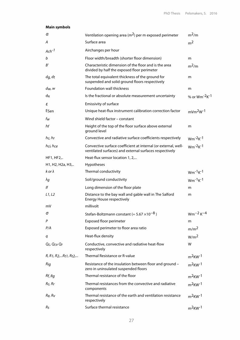
Main symbols
Ventilation opening area (m2) per m exposed perimeter m2/m
A Surface area m2
Ach-1 Airchanges per hour
b Floor width/breadth (shorter floor dimension) m
B' Characteristic dimension of the floor and is the area divided by half the exposed floor perimeter
m2/m
dg, dt The total equivalent thickness of the ground for suspended and solid ground floors respectively
m
dw, w Foundation wall thickness m
dx Is the fractional or absolute measurement uncertainty % or Wm-2K-1
Emissivity of surface
ESen Unique heat-flux instrument calibration correction factor mVm2W-1
fw Wind shield factor – constant
hf Height of the top of the floor surface above external ground level
m
hc, hr Convective and radiative surface coefficients respectively Wm-2K-1
hci, hce Convective surface coefficient at internal (or external, well-ventilated surfaces) and external surfaces respectively
Wm-2K-1
HF1, HF2,.. Heat-flux sensor location 1, 2,...
H1, H2, H2a, H3,.. Hypotheses
k or # Thermal conductivity Wm-1K-1
#g Soil/ground conductivity Wm-1K-1
lf Long dimension of the floor plate m
L1, L2 Distance to the bay wall and gable wall in The Salford Energy House respectively
m
mV millivolt
Stefan-Boltzmann constant (= 5.67 !10"8 ) Wm"2 K"4
P Exposed floor perimeter m
P/A Exposed perimeter to floor area ratio m/m2
q Heat-flux density W/m2
Qc, Qcv Qr Conductive, convective and radiative heat-flow respectively
W
R, R1, R2,...Rt1, Rt2,... Thermal Resistance or R-value m2KW-1
Rig Resistance of the insulation between floor and ground – zero in uninsulated suspended floors
m2KW-1
Rf, Rg Thermal resistance of the floor m2KW-1
Rc, Rr Thermal resistances from the convective and radiative components
m2KW-1
Re, Rv Thermal resistance of the earth and ventilation resistance respectively
m2KW-1
Rs Surface thermal resistance m2KW-1
α
ε
σ
PhD Thesis Pelsmakers, S. 2016
28
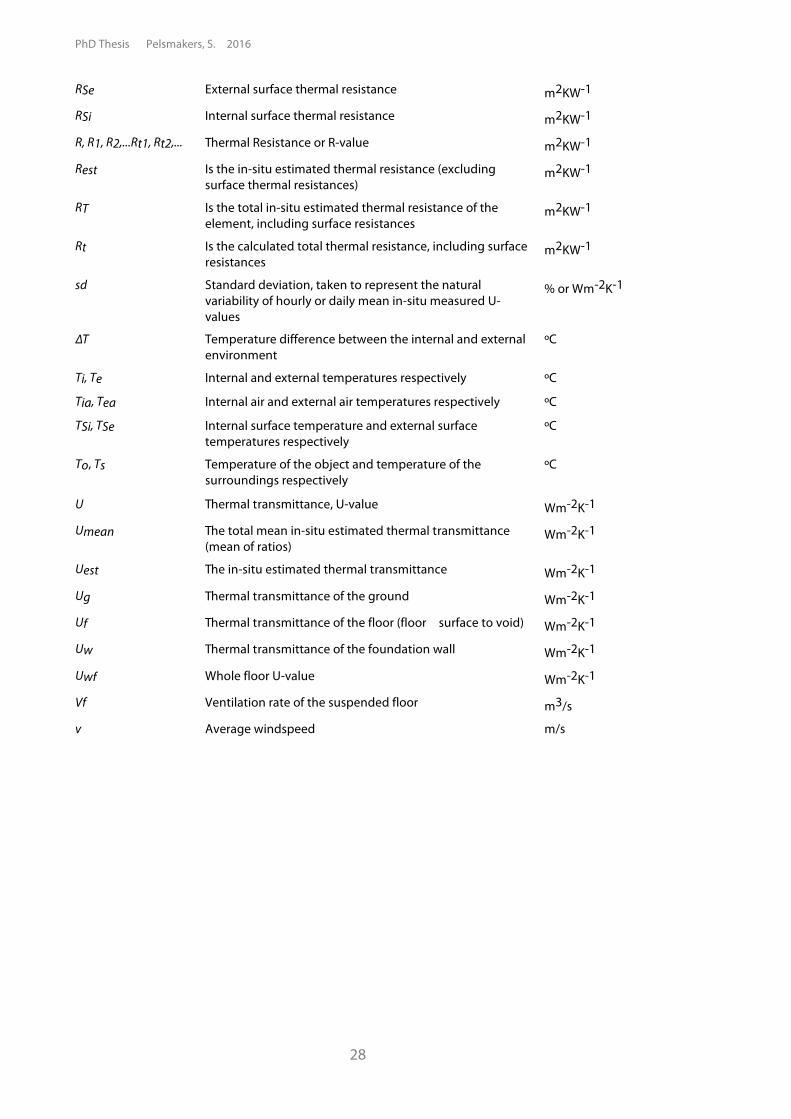
RSe External surface thermal resistance m2KW-1
RSi Internal surface thermal resistance m2KW-1
R, R1, R2,...Rt1, Rt2,... Thermal Resistance or R-value m2KW-1
Rest Is the in-situ estimated thermal resistance (excluding surface thermal resistances)
m2KW-1
RT Is the total in-situ estimated thermal resistance of the element, including surface resistances
m2KW-1
Rt Is the calculated total thermal resistance, including surface resistances
m2KW-1
sd Standard deviation, taken to represent the natural variability of hourly or daily mean in-situ measured U-values
% or Wm-2K-1
!T Temperature difference between the internal and external environment
ºC
Ti, Te Internal and external temperatures respectively ºC
Tia, Tea Internal air and external air temperatures respectively ºC
TSi, TSe Internal surface temperature and external surface temperatures respectively
ºC
To, Ts
Temperature of the object and temperature of the surroundings respectively
ºC
U Thermal transmittance, U-value Wm-2K-1
Umean The total mean in-situ estimated thermal transmittance (mean of ratios)
Wm-2K-1
Uest The in-situ estimated thermal transmittance Wm-2K-1
Ug Thermal transmittance of the ground Wm-2K-1
Uf Thermal transmittance of the floor (floor surface to void) Wm-2K-1
Uw Thermal transmittance of the foundation wall Wm-2K-1
Uwf Whole floor U-value Wm-2K-1
Vf Ventilation rate of the suspended floor m3/s
v
Average windspeed m/s
Chapter 1: Introduction
29
Chapter 1: Introduction
1.1. Introduction This chapter sets out the background and context of the research and motivation and also
details the aims and scope of the study and provides an overview of the thesis structure.
1.2. Context The burning of fossil fuels releases carbon dioxide which significantly contributes to global
warming (IPCC, 2013, Stott, 2010). To curb global warming, the UK has committed to
ambitious carbon reduction targets of 80% by 2050 (from 1990 levels) in the Climate Change
Act 2008 (DECC, 2009). However, to meet overall emission reduction targets of 80%, it has
been argued that the residential sector will have to meet higher carbon reduction standards
of 88-91% (EC, 2011).
Around 50% of the UK's total CO2 emissions are attributed to the construction and operation
of buildings (Mackenzie, 2010). While ~27% of the UK's carbon emissions is attributed to the
domestic sector alone (DECC, 2015d), between 50-65% of this is from dwelling space heating
(DCLG, 2006, Palmer, 2011). Reducing carbon emissions associated with domestic space
heating is a key aspect of the UK's planned transition to a low carbon economy (DECC, 2009,
DECC, 2011a, DECC, 2012a).
Significantly, the UK has one of the oldest and least efficient housing stocks in the developed
world. Approximately one third (Boardman, 2005, Cook, 2009, Stafford, 2011) of its ~ 26.9
million dwelling stock was built before 1940 (ONS, 2011). Seventy to 85% of existing UK
housing is expected to still be in use in 2050 (SDC, 2006, Power, 2008, Killip, 2008), with an
estimated 4.9 million dwellings built pre-1919 in England alone (DCLG, 2012) and 6.6 million
in the UK (Thorpe, 2010). Generally, pre-1919 dwellings are of solid walled construction and
tend to have larger floor areas (DCLG, 2012) and are estimated to have - per m2 floor area per
year - a mean space heat demand of about 14% greater than un-insulated cavity-walled
dwellings and ~ 40% more than post-1990 constructed dwellings (DCLG, 2009).
PhD Thesis Pelsmakers, S. 2016
30
1.2.1. Carbon reduction policies Increasing energy efficiency in existing dwellings is one of the key strategies to meeting the
UK's carbon reduction targets (DECC, 2012a, Mackenzie, 2010, Lowe, 2007a) and strategies to
do this includes upgrading pre-1919 dwellings to low carbon standards by 2050 (DECC,
2009), which includes insulating ground floors (Power, 2008). Carbon reductions of 50-70%
have been obtained in dwellings after insulating floors, walls, windows and lofts and
installing new efficient boilers (Gentry, 2010), while Lowe (2007a) suggests that a
combination of different fabric insulation and more efficient heat-supply could achieve
similar carbon reductions. Additional benefits to upgrading the housing stock may include
reduced fuel poverty and increased occupant thermal comfort (Hamilton, 2011, Bernier et al.,
2010, Rock, 2013, Thorpe, 2010).
In the UK, carbon reduction targets have been underpinned by previous government policies
such as 'Zero Carbon Homes' for new dwellings (ZCH, 2011) and the Green Deal and
ECO-policy for existing buildings and their predecessors CERT, CESP and Warm Front (DECC,
2011b, Ofgem, 2013). The current ECO-policy is an obligation on large energy companies to
install energy efficiency measures for certain consumers and communities, fully or
part-subsidised by the companies (Ofgem, 2015). These policies aim to increase the rate of
retrofit (DECC, 2011b, Mallaburn and Eyre, 2013) by improving the cost-benefit of
interventions (Clinch, 2001). The Green Deal for example allowed building occupants to take
out a pay-as-you-save loan to finance certain energy efficiency improvements, assuming the
loan could be paid back from the predicted energy savings (DECC, 2011c, CCC, 2011).
However, the actual carbon reductions and cost-effectiveness of retrofit interventions is
contingent upon the delivered improvement in thermal performance.
1.2.2. Pre-1919 housing stock profile Pre-1919 dwellings were predominately constructed with solid brick walls (Rock, 2005, Baker,
2011b, DCLG, 2009) and suspended timber ground floors were the prevalent ground floor
construction method (Rock, 2005) (p20, p138) until 1940 (BRE, 1998). The majority of the
pre-1919 housing stock are likely to have insulated lofts (on average 100-199mm) and ~75%
of the pre-1919 dwellings have double glazing (Gentry, 2010). In 2015 DECC (2015e) reported
that just 4% of solid walls in the UK's pre-1919 properties are insulated.
Chapter 1: Introduction
31
At present the proportion of insulated floors is unknown (Boardman, 2005), though floor
insulation uptake might have recently increased as this was a Green Deal and ECO approved1
intervention measure and funding was available under several government funding schemes
under certain conditions (DECC, 2015f, DECC, 2014).
A large proportion of the pre-1919 dwelling typology is classified as hard to treat (HTT)
(Thorpe, 2010, DCLG, 2012), due to its lack of cost-effective retrofit options, disruption and
difficulty to upgrade (Beaumont, 2007, Wetherill M., Dowson et al., 2012). Given that pre-
1919 houses are considered at greater risk of damp and mould problems with about 18%
requiring remedial measures of some kind (DCLG, 2010) (p79), thermal improvement to such
dwellings need to be undertaken with care.
1.2.3. Suspended timber ground floors There might be as many as many as 10 million uninsulated suspended timber ground floors
in the UK (Dowson et al., 2012, Shorrock, 2005), though not all would be dated pre-1919. Yet
the thermal performance of this element is not well characterised at present. Furthermore
there is also no robust data available on the thermal upgrade potential of such floors. It is
estimated that a large proportion of dwelling space heating is lost through un-insulated
walls and insufficiently insulated roofs (50% and 20% respectively, (NEF, 2011)). The
proportion of total dwelling heat loss from un-insulated ground floors depends on the
overall dwelling fabric efficiency standard and the proportional exposed floor area. Hence
there are a variety of estimates in the literature: NEF (2011), WCC (2012) and Rock (2013)
estimate a typical proportional heat loss of 10% to 15% through the ground. Rickaby (2014a)
estimates that for an uninsulated semi-detached 1930's house, proportional floor heat loss
could be as low as 4%, due to its large proportion of uninsulated exposed wall surfaces.
This assumed small proportion of floor heat loss of the total building heat loss might clarify
why floor insulation has not been of much importance in energy policies, which have been in
favour of wall and loft improvements first. However, energy and carbon reductions are not
the only reasons to consider upgrading such floors: a potential benefit of insulating ground
floors might be associated with increased occupant thermal comfort - see Chapter 6.5.
1 For explanation of Green Deal and Eco-policy, see Section 1.2.1.
PhD Thesis Pelsmakers, S. 2016
32
The potential to decrease energy use and reduce CO2 emissions through floor improvements
was indicated by Green Deal assessments, where around 200,000 suspended ground floor
insulation measures were recommended between January 2013 and June 2015, which was
nearly 12% of all recommended measures (DECC, 2015b). Despite this, just over 8,000 floors
had reportedly been insulated under the ECO-policy (or just 0.5% of all installed ECO
measures between January 2013 and September 2015). Around 400 floors were insulated
with Green Deal finance until September 2015 (DECC, 2015c); which is just 2% of all Green
Deal financed installed measures and only about 300 under-floor insulations were installed
with incentives under the Green Deal Home Improvement fund (DECC, 2015c).
As illustrated above and noted by DCLG (2009), the uptake of floor insulation is slow in both
social and privately owned dwellings. The small estimated proportional heat loss from floors,
and the disruptive nature of installing floor insulation (discussed further in Chapter 6) as well
as long payback depending on insulation method might explain this slow uptake (Rickaby,
2014a, Dowson et al., 2012, Killip, 2011). Furthermore, given the small estimated proportional
ground floor heat loss, retrofit strategies might exclude ground floor insulation installations
and in doing so, significantly increase proportional floor heat loss - see Chapter 6.4.7. Harris
(1997) estimates the proportion of floor heat loss up to 25% in well insulated dwellings
where the ground floor remains uninsulated. Some recent Technology Strategy Board (TSB
(2012)) Retrofit for the Future projects adopted this strategy and instead off-set the assumed
ground floor heat loss with increased insulation elsewhere, reducing the disruption of taking
up floor boards. However off-setting assumed heat loss might be problematic if this is
underestimated, and might lead to missed opportunities for energy, cost and carbon savings.
Despite the recent withdrawal of the Green Deal and its incentives, the ECO-policy is in place
until at least 2017 (DECC, 2015a). While only a small proportion of installed ECO measures
were floor insulations, thousands of floors were still insulated. However the actual impact of
doing so on heat loss reduction, thermal comfort and floor void conditions remains
unknown, alongside the unknown benefits and consequences of any of the other efficiency
measures. Insulating the millions of uninsulated floors in the UK housing stock might lead to
potential large carbon savings (Shorrock, 2005, Power, 2008), supporting carbon reduction
policies. It is therefore important to have a better understanding of the thermal
characteristics of these floors and the effect of insulation interventions. Specifically, to make
informed decisions both in terms of government policies and in terms of home-owner
choices, more research is required into the thermal performance of existing floors, heat loss
reduction potential of insulating floors and other possible benefits or unintended
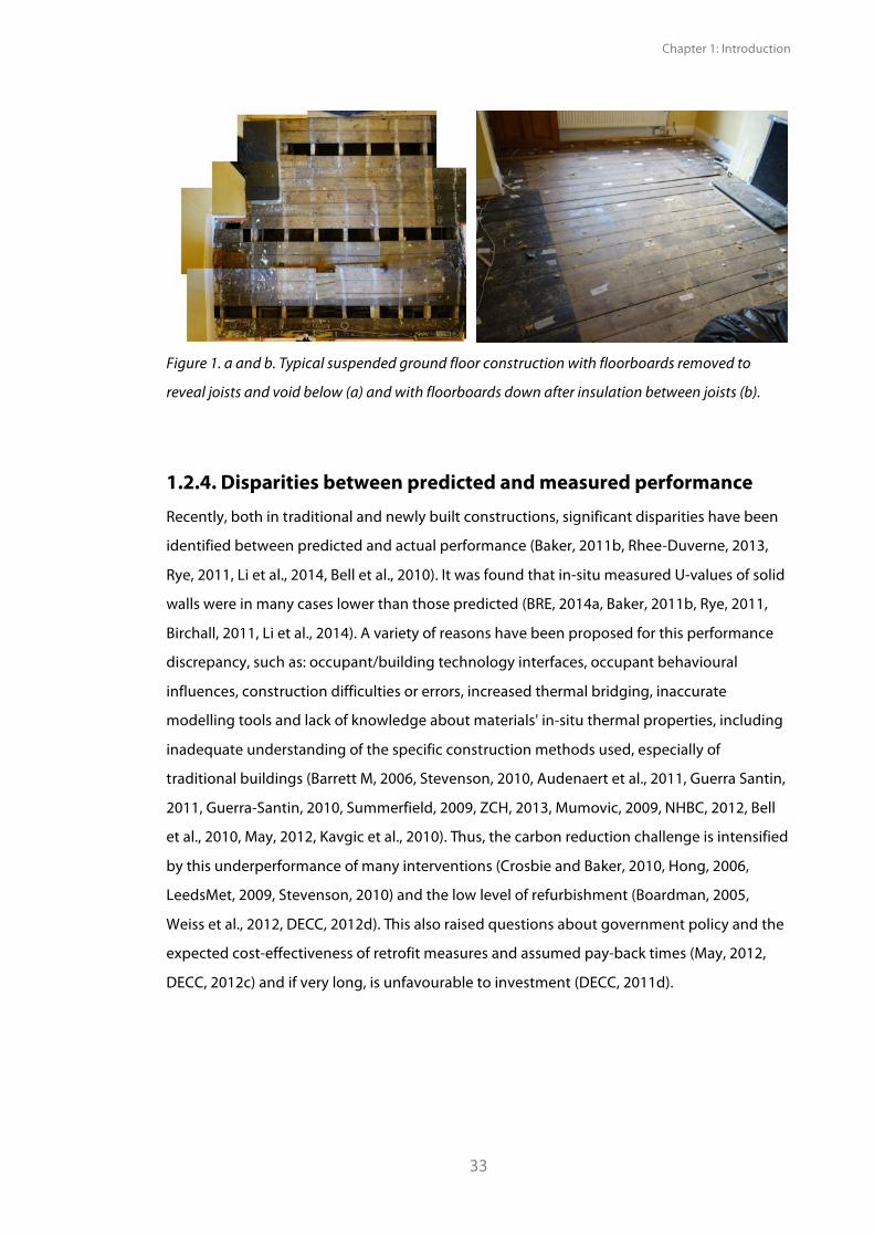
consequences. For an image of a suspended ground floor, see Figure 1.
Chapter 1: Introduction
33
Figure 1. a and b. Typical suspended ground floor construction with floorboards removed to
reveal joists and void below (a) and with floorboards down after insulation between joists (b).
1.2.4. Disparities between predicted and measured performance Recently, both in traditional and newly built constructions, significant disparities have been
identified between predicted and actual performance (Baker, 2011b, Rhee-Duverne, 2013,
Rye, 2011, Li et al., 2014, Bell et al., 2010). It was found that in-situ measured U-values of solid
walls were in many cases lower than those predicted (BRE, 2014a, Baker, 2011b, Rye, 2011,
Birchall, 2011, Li et al., 2014). A variety of reasons have been proposed for this performance
discrepancy, such as: occupant/building technology interfaces, occupant behavioural
influences, construction difficulties or errors, increased thermal bridging, inaccurate
modelling tools and lack of knowledge about materials' in-situ thermal properties, including
inadequate understanding of the specific construction methods used, especially of
traditional buildings (Barrett M, 2006, Stevenson, 2010, Audenaert et al., 2011, Guerra Santin,
2011, Guerra-Santin, 2010, Summerfield, 2009, ZCH, 2013, Mumovic, 2009, NHBC, 2012, Bell
et al., 2010, May, 2012, Kavgic et al., 2010). Thus, the carbon reduction challenge is intensified
by this underperformance of many interventions (Crosbie and Baker, 2010, Hong, 2006,
LeedsMet, 2009, Stevenson, 2010) and the low level of refurbishment (Boardman, 2005,
Weiss et al., 2012, DECC, 2012d). This also raised questions about government policy and the
expected cost-effectiveness of retrofit measures and assumed pay-back times (May, 2012,
DECC, 2012c) and if very long, is unfavourable to investment (DECC, 2011d).
PhD Thesis Pelsmakers, S. 2016
34
This further highlights the necessity of research in this area, as also noted by Shrubsole
(2014) and this also raises questions about the actual thermal performance of suspended
timber ground floors and the efficacy of retrofit measures. While an initial comparison
between the few published in-situ measured U-values and calculated U-values for
suspended timber ground floors suggests a large divergence between the two, it is unclear
how robust direct comparisons are due to a combination of factors - see Chapter 2.4.
1.3. Research Motivation While floor insulation uptake may increase under the ECO-policy, the actual thermal
performance of suspended ground floors and the impact and the implications of insulating
them are poorly characterised. The importance of understanding the actual versus the
predicted performance of a construction element is crucial to ensure that carbon reduction
measures are effective and achieve their intended carbon reductions (May, 2012, ZCH, 2013)
and to ensure appropriate retrofit decision-making and intervention choices. For example, if
predicted floor U-values overestimate the actual values, carbon reduction goals and financial
pay-back of interventions would be jeopardised. Alternatively, if actual floor U-values are
underestimated, insulating such floors might be inappropriately discouraged due to
assumed low carbon reductions and financial payback, while the opposite may be true. In
that case there would be a significant additional potential to reduce energy and carbon
emissions from insulating such floors.
Alignment of predicted versus actual thermal performance is also important for stock models
and energy-reduction scenarios, as illustrated by Li (2014). Different assumptions about
fabric U-values leads to different assumptions about carbon reduction potential and cost-
benefits of retrofit measures. Given the large number of properties with suspended timber
ground floors, such assumptions might have a significant impact on building stock model
outputs, which are used to inform carbon reduction policy and to inform funding for carbon
reduction measures. Yet at present it is unclear what the actual U-values are of suspended
timber ground floors. This PhD thesis aims to contribute to this area of research, as set out in
more detail in the following section.
Chapter 1: Introduction
35
1.4. Research aim, scope and significance The purpose of this PhD research is to investigate the thermal performance of suspended
timber ground floors and how to estimate in-situ floor U-values; specific research questions
and objectives are presented in Chapter 2.9. The research aims to gain and add to the
understanding of the actual performance of uninsulated suspended timber ground floors
and the heat loss reduction potential of interventions and what the benefits and drawbacks
of insulating such floors might be.
In doing so, this research builds on existing knowledge and research, while also contributing
additional and original knowledge to the field with regards to:
• Testing and development of in-situ floor heat-flux measuring methods (Chapters 3, 4,
5, 6);
• Supplementing in-situ heat-flux measurements of floors (Chapters 4, 5 and 6);
• Investigation into the efficacy of some heat loss reduction interventions (Chapter 6);
• Supplementing data on floor void and on thermal comfort conditions of
(un)insulated floors (Chapter 6), however a detailed floor void and thermal comfort
study and the impact of thermal discomfort on compensating energy-use are
outside the scope of this PhD research.
As previously identified, little research is undertaken in this area and Salisbury at DECC (2013)
identified floor heat loss reduction measures and their implications as one of four areas
requiring urgent research as part of existing housing stock retrofit for UK Government. In
support of retrofit decision-making at policy, industry and consumer level, the primary
significance of this study is in contributing knowledge of in-situ measured floor U-values and
robust measurement and analysis techniques, which are poorly characterised at present.
In-situ U-value estimations of floor case-studies advance knowledge and insight, enable a
critical review of comparison to present models and draw out practical monitoring and
insulation installation issues. Furthermore, this research draws together a literature review of
heat loss, thermal comfort and mould growth research specifically related to suspended
timber ground floors. While this study has only undertaken a limited number of in-situ
U-value measurements this is - as far as the author is aware at the time of writing - one of the
most in-depth studies of suspended timber ground floors in the UK. However, given the
limited time-scale and seasonality of the research, undertaking a large-scale survey of
suspended timber ground floors and the investigation of many different insulation
interventions are outside the scope of this PhD research and are highlighted for further
research investigations.
PhD Thesis Pelsmakers, S. 2016
36
Current research paper under review at the time of writing:
Pelsmakers, S., Fitton, R. , Biddulph, P., Swan, W., Croxford, B., Shipworth, D., Stamp, S., Calboli,
F. , Lowe, R., Elwell, C.A., Heat-loss from suspended timber ground floors: in-situ measurement,
variability and uncertainty, Energy & Buildings.
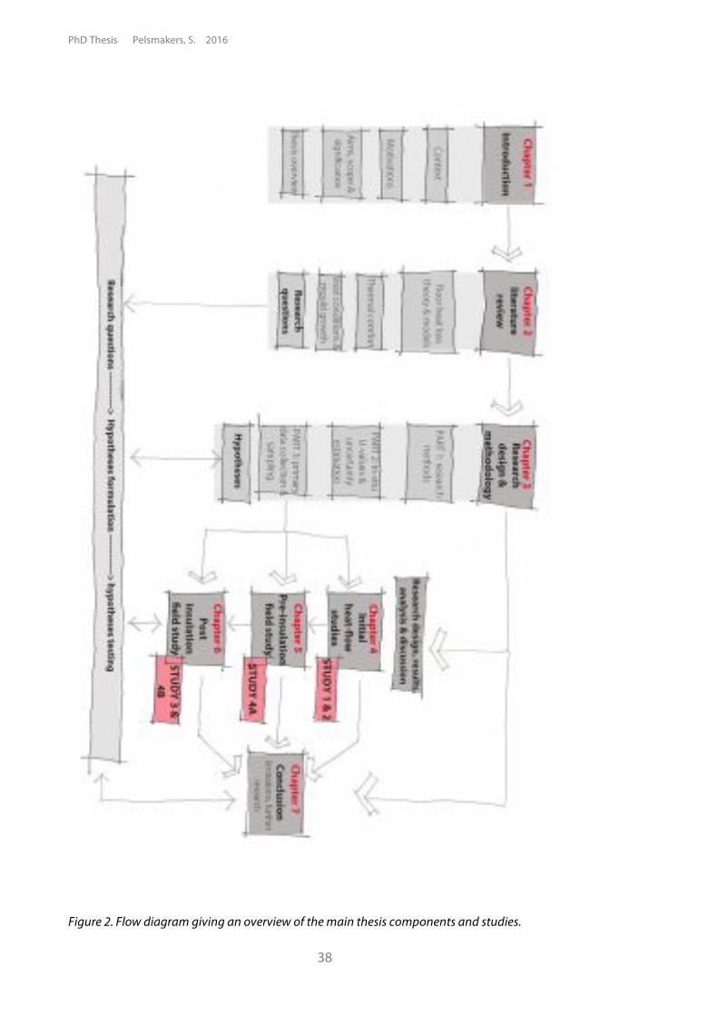
1.5. Thesis overview This PhD thesis is presented in 7 chapters, as illustrated in Figure 2.: Chapter 2 presents a
literature review of physical theory, theoretical models of ground floor U-values and a critical
review of model assumptions and in-situ measurements of suspended timber ground floors.
Additionally, thermal comfort theory specifically related to ground floor surfaces; insulation
of floors and floor void conditions and mould growth risk are reviewed. Finally, the PhD
research questions are presented.
Chapter 3 presents the research design and methodology divided into three distinct parts:
Part 1 reviews available research methods to answer the research questions identified in the
preceding chapter and justifies methods chosen. Part 2 presents and critically reviews in-situ
U-value measurement protocols and uncertainty procedures in detail and presents the
applied in-situ U-value estimation and uncertainty estimation techniques for this study.
Finally, Part 3 gives a brief overview of the formulated research hypotheses and the primary
data collected for the four studies undertaken and includes a discussion about sampling and
research generalisability and ethics.
Chapters 4, 5 and 6 each set out the primary fieldwork undertaken, with each chapter
presenting detailed research design followed by results and analysis and discussion of the
analysis and results, including comparison to models and reference to physical theory and
literature presented earlier.
The subject of Chapter 4 is a low-resolution pilot study in an occupied house (STUDY 1) which
directly leads to high-resolution floor heat-flow measurements in an environmental
chamber, the Salford Energy House (EH, STUDY 2). Knowledge and techniques gained from
this high resolution floor study were then taken forward in an unoccupied and uninsulated
field case-study dwelling (STUDY 4A), subject of Chapter 5. This chapter also gives a snap-
shot of the case-study's floor void conditions pre-insulation.

Chapter 1: Introduction
37
Chapter 6 presents a pre-and post insulation pilot study (STUDY 3), followed by two
insulation interventions of the field case-study house (STUDY 4B). This chapter also gives an
overview of the thermal comfort and airtightness implications of insulating the case-study
floor.
Finally, Chapter 7 briefly summarises the key research findings and draws the findings
together through a discussion of the policy and practical implications of the findings and
reflections on further research. Note that the work is presented in a logical rather than
chronological order.
PhD Thesis Pelsmakers, S. 2016
38
Figure 2. Flow diagram giving an overview of the main thesis components and studies.
Chapter 2: Literature Review
39
Chapter 2: Literature review
2.1. Introduction This chapter outlines the physical theory of ground floor heat-flow and how this is reflected
in models, literature and published empirical results. First is presented a brief overview of
solid ground floor heat-flow, followed by suspended timber ground floor heat loss theory,
void air-flow and comparisons between published theoretical and in-situ heat-flow
measured U-values. The chapter also explores current literature and research on the benefits
of insulating floors, thermal comfort related to ground floors and the possible unintended
consequences of floor insulation, in particular mould growth. The chapter concludes with the
PhD research questions and objectives and definitions.
2.2. Floor heat loss: physical theory Heat-flow through building elements depends on the temperature difference between the
inside and outside environment of a construction and occurs by conduction, convection and
radiation; mechanisms which are dependent on material properties such as material
thickness, conductivity and surface colour but also moisture content and exposure to
climatic conditions. The conductive component is expressed as the thermal resistance or
R-value and is the element's resistance to heat-flow through the materials' given thickness
and can be estimated by dividing the depth of the material (d, in metre) by the material's
conductivity (k, W/mK). For a construction element with several layers, the individual
component's thermal resistances need to be summed. The thermal transmittance or a
U-value is the reciprocal of the total thermal resistance (Rt) and is calculated from the thermal
resistances of each part of the construction element and is expressed as "the rate of heat-flow
in Watts through 1m2 of a structure when there is a temperature difference across the structure of
1 degree K or ºC" (McMullan, 2002) and includes surface resistances of the boundary layers (RSi
and RSe, m2KW-1) - see Equation 1. Surface resistances take into account radiative and
convective processes which "bring heat from the room interior to the inner surface of the
construction and remove it at the exterior surface" (Davies, 1993). Hence a floor U-value
expresses convective and radiative heat-flows from the room air and room surfaces to the
floor surface and conductive heat-flow from the floor surface to the ground and outside.
PhD Thesis Pelsmakers, S. 2016
40
- Equation 1. , where R1, R2, R3 are the individual
material's thermal resistances in a multi-layered construction and where RSi and RSe are the
internal and external surface thermal resistances respectively and where in each case the
surface thermal resistance,
- Equation 2. , where hc is the convective surface coefficient and hr (Wm-2K-1) is
the radiative surface coefficient (Wm-2K-1 (Szokolay, 2008) and are defined as equations
below:
hc = hci = 0.7 Wm-2K-1 for downward heat flow, where internal surfaces or external surfaces
which are next to a well-ventilated layer; at external surfaces: (Equation
3.), where v is the windspeed (m/s) next to the external surface (BSI, 2007).
- Equation 4. , where is the emissivity and is typically 0.9 for internal and
external surfaces (BSI, 2007); and hr0 is the radiative coefficient for a black body and
- Equation 5., where is the Stefan-Boltzmann constant (= 5.67
!10"8 Wm"2 K"4) and Tm is the "mean thermodynamic temperature of the surface and its
surroundings" (BSI, 2007).
Ground floor U-values are mainly influenced by the floor's exposed perimeter to the whole
floor area ratio (CIBSE, 2015), the ground conductivity and characteristics, foundation and
floor wall thickness (and conductivity), surface resistances and any insulation. Heat loss in
suspended ground floors additionally depends on a fluctuating void ventilation rate
(Anderson, 1991a, Harris, 1997).
Conductive heat-flow (Qc) occurs within a body or bodies in direct contact and energy flows
from the warmer to the colder side,1 proportional to the temperature difference and the
cross-sectional area of the body (Fourier's Law), see Equation 6. Natural convective heat-flows
(Qcv) occur between a solid body and liquids or gases due to thermal buoyancy (Szokolay,
2008, Hagentoft, 2001)(see Equation 7. to Equation 8.); for example when warm air rises to
replace cold air and in turn cooler air replaces the displaced warmer air.
1 Second law of Thermodynamics governs that heat transfers from warm to cold.
hr� = �σT �m
Chapter 2: Literature Review
41
- Equation 6., where Qc is the conductive heat-flow (W), U is the U-value
(Wm-2K-1), A is the surface area (m) and !T is the temperature difference between inside and
outside.
- Equation 7., where Qcv is the convective heat-flow (W) and where hc is the
convection coefficient and depends on air velocity, direction of heat flow and surfaces;
typically hc= 1.5 Wm-2K-1 for down-ward flowing heat (Szokolay, 2008). Where air movement
exists, (Equation 8.) where v is the air velocity in m/s (Szokolay, 2008).
Forced convection is caused by wind patterns and pressure differences creating a stack effect
(Hagentoft, 2001), which is likely to contribute to suspended ground floor heat loss. Both
conduction and natural convection heat-flows are directly proportional to !T, i.e. the
temperature difference between inside and outside. Radiation heat transfer occurs between
surfaces not in contact with each other but heat is transferred by infrared radiation and is
proportional to the difference between the 4th power of the object's temperature and the 4th
power of the object's surrounding temperature (To4 - Ts4) and depends on surface
reflectances, emittances and absorptance (Szokolay, 2008) - see Equation 9. :
- Equation 9., where Qr is the radiative heat-flow (W) between two surfaces
and where is the emissivity and is typically 0.9 for internal and external surfaces (SI, 2007)
and is the Stefan-Boltzmann constant (= 5.67!10"8 Wm"2 K"4) (see also previous
definitions) and To is the temperature of the object and Ts the temperature of the
surroundings.2
2.2.1. Solid ground floors Heat-flow to and from a solid ground floor slab, which is in direct contact with the ground,
depends on the temperature difference between the internal and external environment (BSI,
2009b, Hagentoft, 2001, Hagentoft and Blomberg, 2000), and also on seasonal external and
ground temperature changes, dwelling heating regime and presence of insulation on the
floor and foundation walls. External temperatures influence the ground temperature and this
depends on the ground's characteristics, which can have wide-ranging moisture content,
thermal capacity and thermal conductivities (Davies, 1993, Rees, 2001) and hence leads to a
wide range of ground floor U-values (Harris, 1997). Solid ground floor heat-flow is also a
function of exposed floor perimeter (P) to floor area ratio (A).
2 For q (heat-flux density, Wm
-2), divide Q (heat-flux, W) by A (i.e. area, m
2)
PhD Thesis Pelsmakers, S. 2016
42
This is because a location on the floor further away from the external environment will have
increased thermal resistance: in the centre of the floor, "the ground itself adds to the
insulation" while at the building edge "the path of the heat flow has to curve through the
ground back to the outside air" (McMullan, 2002) due to the geometry of the slab/wall
junction. Thus solid ground floor heat-flow is generally increased along the edges and
smaller in the centre of the floor (Davies, 1993, CIBSE, 2015), although Spooner's (1982)
in-situ heat-flux measurements on solid ground floors did not verify this. Furthermore, the
range of heat-flow reduces as floors are insulated (Anderson, 1991b), while the edge effect
reduces as external (foundation) walls are insulated (Harris, 1997). A warm ground region sits
underneath perimeter foundations, though it is affected by ground surface temperatures
further away (Hagentoft, 2001), whereas under the ground slab, temperatures are relatively
warm and stable in winter and summer (Thomas, 1999). As such (Spooner, 1982) suggests the
use of ground temperatures at 1 metre deep for in-situ U-value estimation for solid ground
floors, though this is usually impractical.
The solid ground floor U-value model is set out in ISO-13370 (BSI, 2009b) and in equations
below and indicates inclusion of radiative and convective heat-flow components through
surface thermal resistances.
- Equation 10., where U is the U-value of the uninsulated or
slightly insulated solid ground floor (see ISO-13370 for well insulated ground floor slabs),
where "g is the soil conductivity (which for clay equals to 1.5Wm-1K-1); B' is the 'characteristic
dimension of the floor' and is the floor area (A) divided by half the exposed floor perimeter (P)
(B'=A/0.5P). dt is 'the total equivalent thickness of the ground' (m) (BSI, 2009b) of the solid
ground slab and is as per Equation 11.:
- Equation 11., where dw is the foundation wall thickness; RSi is
the internal surface resistance of the floor and RSe is the external surface resistance of the
external ground surface (see Section 2.2.); typical values as per (BSI, 2007); Rf is the resistance
of floor slab itself, including the insulation.
Chapter 2: Literature Review
43
2.2.2. Suspended ground floors Suspended ground floors are not in contact with the ground but have a sub-floor void which
is an additional thermal resistance, though this might be offset by the sub-floor ventilation
(forced convection), which is an additional heat loss path (Anderson, 1991a). Increased void
ventilation leads to increased heat-flow (Harris, 1997), however Anderson (1991a) estimates
that U-values do not differ much from solid ground floors with "typical ventilation rates" for
suspended ground floors (based on void ventilation area opening assumptions between
0.0030 and 0.0015 m/m2 and 1 to 2 m/s ground windspeed). But it is unknown how
representative these assumptions are in actual houses. Furthermore, natural convective heat-
flow is considered to be of minimal influence due to "thermal buoyancy effects favouring
upward flow of air and heat" (Harris, 1997), though it is unknown if this would be the case
throughout the void as it is likely to depend on positioning of airbricks for example. Similar
to solid ground floors, suspended ground floor thermal transmittances are influenced by
heat-flow through the exposed floor perimeter (P) as a proportion of the floor area
(A)(McMullan, 2002); Chapman (1985b) confirmed the presence of an edge-heat loss effect
based on a thermographic survey. For suspended ground floors the main heat-transfer
mechanisms are illustrated by Figure 3. and are:
a., b. & c. conductive heat-flow from floor surface, foundation walls and sleeper
walls3 to the void: dependent on floor finish, joist and wall depths and material
conductivities and presence of insulation. Foundation wall heat-flow contributes to
edge effects with increased heat-transfer along the perimeter compared to the non-
perimeter zone. Also associated convective and radiant heat-flows to surrounding
surfaces.
d. natural convection from the void floor surface to the void air; this is
temperature difference driven but this component is likely to be small (Harris, 1997).
e. radiation heat-flows to colder void surfaces and the soil/ground surface:
radiation heat-flow from warmer floor and wall surfaces to colder void surfaces,
including the ground surface (and vice versa).
f. Heat-flow from the ground to the outside: dependent on soil characteristics and
soil thermal mass; can be reverse depending on season.
g. cross ventilation (forced convection) in the sub-floor void: forced convection
(i.e. wind driven airflow in the void) leads to increased heat-flow from surfaces to the
void and external environment. Likely to depend on vicinity to the airbricks, external
wind-speeds and void obstructions to void airflow - see Chapter 4 and Chapter 5.
3 Also called dwarf walls
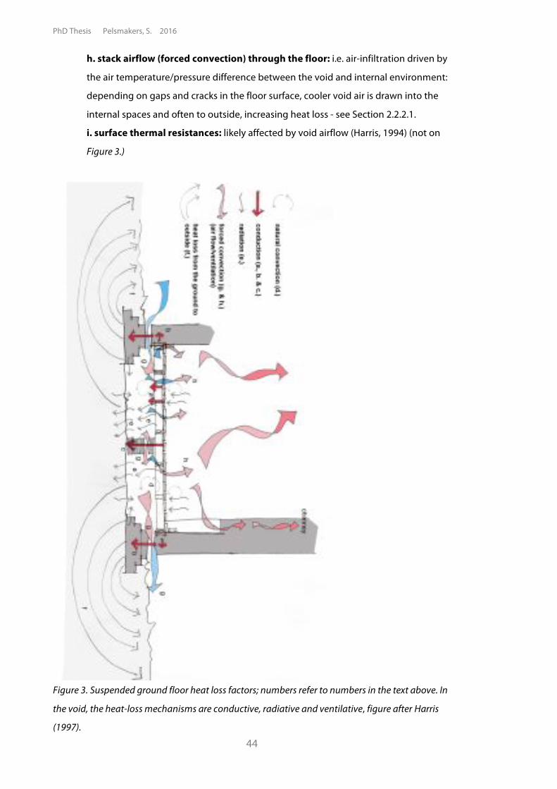
PhD Thesis Pelsmakers, S. 2016
44
h. stack airflow (forced convection) through the floor: i.e. air-infiltration driven by
the air temperature/pressure difference between the void and internal environment:
depending on gaps and cracks in the floor surface, cooler void air is drawn into the
internal spaces and often to outside, increasing heat loss - see Section 2.2.2.1.
i. surface thermal resistances: likely affected by void airflow (Harris, 1994) (not on
Figure 3.)
Figure 3. Suspended ground floor heat loss factors; numbers refer to numbers in the text above. In
the void, the heat-loss mechanisms are conductive, radiative and ventilative, figure after Harris
(1997).
Chapter 2: Literature Review
45
All of the above mechanisms interact; e.g. increased forced convection (g. and h.) in the void
might lead to increased heat-flow (Harris, 1994) and there might be colder floor, wall and
ground surfaces (affecting radiative heat-flow) and additional heat-flow from thermal
bridges (e.g. joists in foundation walls) depending on the detail.
Air-infiltration from the floor void into the internal spaces (h.) has been described as a form
of 'heat-recovery' (Miles-Shenton, 2011); i.e. heat lost to the void would to some extent 'pre-
heat' the floor-void air before it infiltrates the living spaces above through gaps and cracks in
the floor. This 'heat-recovery' mechanism will depend on the total dwelling airtightness and
floor airtightness as well as exposure of the void air to the external environment and is likely
to vary with fluctuating external conditions, void ventilation rate and in different floor
locations. In addition, any recovered air will still be colder than internal room temperature
and depending on the airflow velocity and temperature, may contribute to occupant thermal
discomfort, with possible associated energy compensating behaviour by occupants.
Any such 'heat-recovery' will depend on ventilation rate and where the void air is being
dissipated to and might not lead to any direct heat-recovery into habitable spaces when void
air is dissipated to for example floor or wall gaps which are connected to the roof, as
observed by Hartless (1994) and Hartless (1996) - see Section 2.2.2. Void air infiltrating in
habitable spaces can also affect occupant health - see Section 2.7.
Any uninsulated hot water or heating radiator pipes in the void would act as an additional
heat source and would locally condition the void (and might change radiative heat transfer),
affecting heat-transfer. Both the presence of such services and the heat recovery effect were
excluded in this thesis research but have been highlighted for future research.
2.2.2.1. Floor void air flow and stack-effect
It is unknown what the seasonal pressure differential ranges are between the external
environment and indoor spaces and crawl spaces in the UK and how weather and the size,
number and location of ventilation openings and other variables affect the pressure
differences of the dwelling itself and the floor void. However, according to Hill (2005), in
winter, due to internal and external temperature differences, there is likely a slight negative
(lower) pressure at the bottom of the dwelling and slight positive (higher) pressure at the top
compared to outside. This drives warm air out at the top through construction openings and
cracks and pulls cold air in from the bottom through for example gaps and cracks in the floor,
creating a stack effect (Hill, 2005, Persily, 2009).
PhD Thesis Pelsmakers, S. 2016
46
"While the pressures are relatively small (1 to 5 Pascals), they operate twenty-four hours a day, all
winter long, and thus can move a lot of air over the course of a winter" (Hill, 2005). This stack-
effect airflow from the sub-floor void into the rest of the dwelling has been observed in
research primarily driven by occupant health concerns arising from moisture problems in the
floor void (see Section 2.7.) and the presence of hazardous soil gases such as radon, see e.g.
Welsh (1995).
Void airflow is affected by external weather conditions, wind-speed and wind direction and
whether the airbricks are located in windward or leeward walls. The greater the sub-floor
ventilation, the greater the heat-loss from the floor as observed by Harris (1997, 1993) in a
test-cell. This effect is caused by void ventilation replacing warmer void air with colder
external air and by decreasing the surface thermal resistances and hence increasing heat-
flow from the floor and from exposed foundation walls (Harris, 1993).
Furthermore, Hartless (1999, 1994) found that floor void airflow in a BRE test-house was stack
dominated and driven by sub-floor and external temperature differences rather than the
wind-speed; this was especially the case at night-time. Additionally, air moved via wall
cavities to the ceiling and roof. Under certain environmental conditions Hartless (1999, 1994)
also observed that the stack-induced sub-floor airflow converted into sub-floor cross-
ventilation, for example with an internal/external temperature difference of more than 6ºC,
when airbricks were located in windward walls or if the wind-speed was significantly greater
than 3.5 m/s on the windward side. It is unknown whether the findings of this single test-
house transfer to other dwellings; it is also unclear where the wind-speed was measured; this
might be at the 15m high weather station mention in Hartless (1994) (rather than at airbrick
height) or at 10m high as used by models - see Section 2.3.
Similar airflow through floorboard gaps and cracks and stack-effect findings were observed
by e.g. Lilly (1988), Oldengarm (1988), McGrath (1999, 1996), Basset (1988) and Williamson
(2000), though the study variables are significantly different between studies hence direct
comparisons are not possible.
Even with filled floorboard gaps and where floors are carpeted or linoleum finished, air
leakage is still likely to occur caused by construction and refurbishment practices, occurrence
of service penetrations such as electrical wires, radiator pipes and chimneys as well as non-
permanent gap filling and seasonal floor movement (Lilly, 1988, Basset, 1988, McGrath et al.,
1999, Thorpe, 2010).
Chapter 2: Literature Review
47
The UK Government's Standard Assessment Procedure (SAP), used for building regulation
compliance, assumes that buildings built with suspended timber ground floors pre-1975 in
England, Wales and Scotland and pre-1977 in Northern Ireland have unsealed suspended
timber ground floors (i.e. with gaps and cracks, assumed 0.2 ach-1) and sealed floors after this
period with 0.1 ach-1 (BRE, 2014). It is unclear whether this reflects actual air leakage into the
dwelling and overall contribution to dwelling airtightness. This stack-effect component is
difficult to measure in actual dwellings and floors (see Chapter 3.2.) and is also excluded from
floor U-value models - see Section 2.3.
2.2.2.2. Impact of void airflow on floor U-values
Harris' (1997) research in a ~9m2 test-cell found that floor U-values increased by 40% from
0.62 Wm-2K-1 to 0.87 Wm-2K-1 with increased sub-floor ventilation rates from 0 to 1.5 ach-1.
The test-cell was located in a controlled thermal chamber: temperatures were kept constant
at 20ºC in the test-cell, air-mixed with a fan, and 10ºC ±0.5ºC in the cold thermal chamber
(Harris, 1993, Harris, 1997). The floor surface to the room above was made air-tight,
minimising stack-effect airflow into the space above. Several locations on the floor were
monitored and an average U-value obtained (Harris, 2013). Ventilation was provided by fans
at the airbricks and altered between 0 ach-1 to 1.5 ach-1 (equivalent to up to 4m/s wind-
speed at airbrick height (Harris, 1994)). The upper limit of 4m/s wind-speed at airbrick height
appears to be high compared to the average 5m/s suggested UK heating season wind-speed
at 10m height (Anderson, 2006, METOFFICE, 2015, RRR, 2015). Hartless (1994) reported sub-
floor airflow rates in a test house to be 2 to 8.5 times greater than documented by Harris
(1994), while Lilly (1988) observed in another test house around 5 ach-1 and Basset (1988)
noted air-change rates of 2 to 8 ach-1 in New Zealand floors. Comparison between sources
and findings is however difficult as the sub-floor voids are different alongside several other
different variables (different climate, terrain obstructions as well as different measurement
methods). Detailed characterisation of the void-ventilation rates and typical wind-speeds at
airbrick height and in floor voids are unknown and might be highly variable due to the
factors mentioned above. It is also unclear how representative Harris' test-cell proportions,
distance between airbricks, replicated air-change rates, ground conditions and airflows are
compared to actual dwellings. The test-cell walls were also insulated and this was the reason
why no significant edge-effect was observed (Harris, 1997). However of interest are not the
exact U-values estimated or airflows replicated, but Harris' research highlighted that with
increased airflow an increased thermal transmittance trend was observed.
PhD Thesis Pelsmakers, S. 2016
48
In summary, suspended timber ground floor systems are likely to have fluctuating U-values,
which are related to the varying airflow through airbricks and other sources of ventilation;
increased sub-floor ventilation is expected to lead to increased floor U-values. Airflow was
found to fluctuate with external weather conditions, in particular with wind-speed and wind
direction and whether the airbricks were located in windward or leeward walls. Heat-flow
might also be influenced by stack driven airflow up through the floor, which is affected by
the extent of gaps and cracks in the floor and house-cavities connecting to the floor as well
as temperature differences between void and outside. Wind-driven void airflow is likely to
displace warm void air with colder air, and to reduce both surface temperatures and thermal
resistances in the void (thereby changing radiative and conductive heat transfer); stack-effect
airflow might also have similar influences on void conditions and associated heat-flow,
however this is not characterised at present.
2.2.2.3. Floor finish
Original pre-1919 floors tend to be of pine softwood floorboard construction (Rock, 2013)
and were usually (partially) covered; for example with rugs or animal skin; or with natural
hessian, linoleum and sometimes thin parquet floor finish (Rock, 2013, Collings, 2008).
Floorboards were usually of not very high quality or finish; though sometimes the floor edges
in a room were painted dark, or fitted with more expensive parquet floor finish, using easily
removable rugs in the middle of the floor (Collings, 2008). A 1981 survey of almost 400
dwellings in Cambridge, which included similar proportions of dwelling age and typology
representative of the UK housing stock at the time, found that around 50% of dwellings had
suspended timber ground floors, with 70% carpeted finish and just 16% timber floor finish
(Hawkes, 1981). No literature was found that identifies the proportion of different floor
finishes in the UK's pre-1919 housing stock. Floor finish will effect floor heat loss and has
associated thermal comfort implications - see Section 2.5.
Chapter 2: Literature Review
49
2.3. Suspended ground floor U-value models Thermal resistances are usually calculated in a perpendicular straight line between surfaces
of a building construction. In reality however construction build-ups are not homogenous
and junctions between elements occur and the heat may not travel in straight lines as a
result of this (BSI, 2009b, Anderson, 2006). This 3-dimensionality affects overall heat-flow, yet
in most U-value calculations, this effect is considered to be negligible and calculation
methods are simplified to 2-dimensional effects.
Several models exist to calculate suspended ground floor U-values and BS-EN-ISO-13370 (BSI,
2009b) sets out internationally agreed procedures for the U-value calculation methods of
both solid as well as suspended ground floors and is used as a basis for floor U-value
calculations in CIBSE (2015), RdSAP (BRE, 2011) and software models, e.g. PHPP (PHI, 2007)
and BuildDesk U (BuildDesk, 2012). Models estimate the U-value of the whole floor and not
for specific locations on the floor. ISO-13370 is a simplified example (BSI, 2009b) and does
not include some of the heat-loss mechanisms as identified in Section 2.2.2.; the model and
issues with excluded and assumed inputs are discussed below.
The ISO-13370 U-value model for suspended floors with void depths <500mm is based on
the combined floor U-value 'U' being determined by heat-flow from the internal to the
external environment as set out below in Equations 12 to 20 and as illustrated by Figure 4.:
• Heat is transferred from the floor surface to the sub-floor void (Uf , see Equation 14),
and should include point and repeated thermal bridging separately calculated.
• Heat from the sub-floor void is then transferred to the external environment in the
following way:
⁃ through the ground underneath (Ug , see Equation 15 )
⁃ through the foundation walls (Uw)
⁃ and through ventilation of the sub-floor void (Uv, , see Equation 18); Uw and Uv
are combined in Ux, (see Equation 17 )(BSI, 2009b, Williamson, 2006a).
For void depths greater than 500mm, the increased void area adds additional thermal
resistance to heat-flow (SBSA, 2010) and for the heat-flow component to the ground,
additional parameters are included related to perimeter and depth of the basement below
external ground level; different calculations apply if heated or unheated basements; such
constructions have been excluded in this thesis.
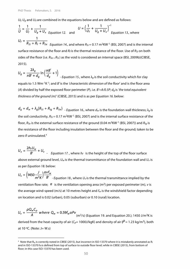
PhD Thesis Pelsmakers, S. 2016
50
Uf, Ug and UX are combined in the equations below and are defined as follows:
Equation 12. and Equation 13., where
Equation 14., and where RSi = 0.17 m2KW-1 (BSI, 2007) and is the internal
surface resistance of the floor and Rf is the thermal resistance of the floor. Use of RSi on both
sides of the floor (i.e. RSe = RSi ) as the void is considered an internal space (BSI, 2009b)(CIBSE,
2015).
- Equation 15., where "g is the soil conductivity which for clay
equals to 1.5 Wm-1K-1; and B' is the 'characteristic dimension of the floor' and is the floor area
(A) divided by half the exposed floor perimeter (P), i.e. B'=A/0.5P; dg is 'the total equivalent
thickness of the ground (m)' (CIBSE, 2015) and is as per Equation 16. below:
- Equation 16., where dw is the foundation wall thickness; "g is
the soil conductivity, RSi = 0.17 m2KW-1 (BSI, 2007) and is the internal surface resistance of the
floor, RSe is the external surface resistance of the ground (0.04 m2KW-1 (BSI, 2007)) and Rig is
the resistance of the floor including insulation between the floor and the ground; taken to be
zero if uninsulated.4
- Equation 17. , where hf is the height of the top of the floor surface
above external ground level, Uw is the thermal transmittance of the foundation wall and Uv is
as per Equation 18. below:
- Equation 18., where Uv is the thermal transmittance implied by the
ventilation flow rate; is the ventilation opening area (m2) per exposed perimeter (m), v is
the average wind-speed (m/s) at 10 metres height and fw is the windshield factor depending
on location and is 0.02 (urban), 0.05 (suburban) or 0.10 (rural) location.
(m3/s) (Equation 19. and Equation 20.); 1450 J/m3K is
derived from the heat capacity of air (Cp= 1000J/kgK) and density of air ( = 1.23 kg/m3), both
at 10 ºC. (Note: J= W.s)
4 Note that Rig is correctly noted in CIBSE (2015), but incorrect in ISO-13370 where it is mistakenly annotated as Rf and in ISO-13370 hf is defined from top of surface to outside floor level; while in CIBSE (2015), from bottom of floor; in this case ISO-13370 has been used.
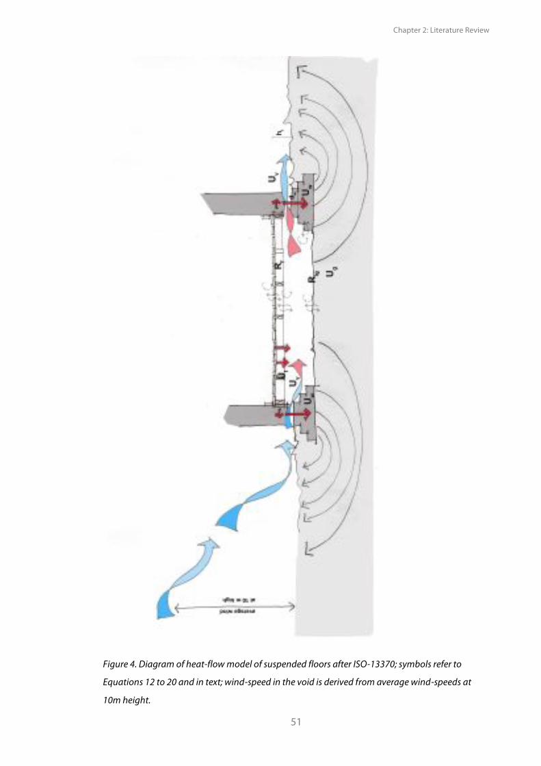
Chapter 2: Literature Review
51
Figure 4. Diagram of heat-flow model of suspended floors after ISO-13370; symbols refer to
Equations 12 to 20 and in text; wind-speed in the void is derived from average wind-speeds at
10m height.
PhD Thesis Pelsmakers, S. 2016
52
The inclusion of surface thermal resistances for the floor structure and the ground in
Equation 14. and Equation 16. respectively includes assumed radiant and natural convection
influences at the surfaces in the floor U-value model (as a U-value is air-to-air, not surface-to
surface heat-transfer). Likewise for inclusion of Uw in Equation 17. as a U-value includes
surface resistances. However based on these assumed values, it is unknown whether this
accurately represents the convective and radiant heat-flows from air to surface and how
accurate these assumptions reflect dynamic conditions even in the same room or floor.
Figure 5. sets out the model's identified assumptions and excluded inputs. Variables excluded
from the model include sleeper wall presence, stack-effect forced convection, wind direction
and airbrick orientation (windward/leeward sides) and uninsulated service pipes in the void
(radiator/hot water pipes). Also excluded is reduced floor void ventilation impact of void
obstructions, such as joists and sleeper walls. The model also assumes that the average
annual heat-flow, using average annual external and internal temperature differences, is
similar to the seasonal heat-flow (CIBSE, 1996, BSI, 2009b); i.e. by considering the heat-
transfer over a full year, the impact of thermal mass of the ground is considered negligible
(and hence excluded in models). It is not characterised at present whether these exclusions
and assumptions might lead to significant inaccurate model outputs or not, nor how this
might effect comparison with in-situ measured results - this is subject of discussion in
Chapter 5.3.6. Repeated thermal bridges such as joists are not separately accounted for in the
ISO-13370 model (BSI, 2009b, BSI, 2009a) and should be included by calculating the
proportion of timber joist presence (Anderson, 2006). Linear thermal bridging (such as the
wall/floor junctions) are excluded in floor U-value models as they should be included in the
whole building's heat loss calculation and not in the separate building element U-value
(Anderson, 2006, BSI, 2009b). These can be calculated separately as for example set out in
ISO-10211 (BSI, 2009a) or ISO-14683 (BSI, 2008) and as per guidance in Ward (2007).
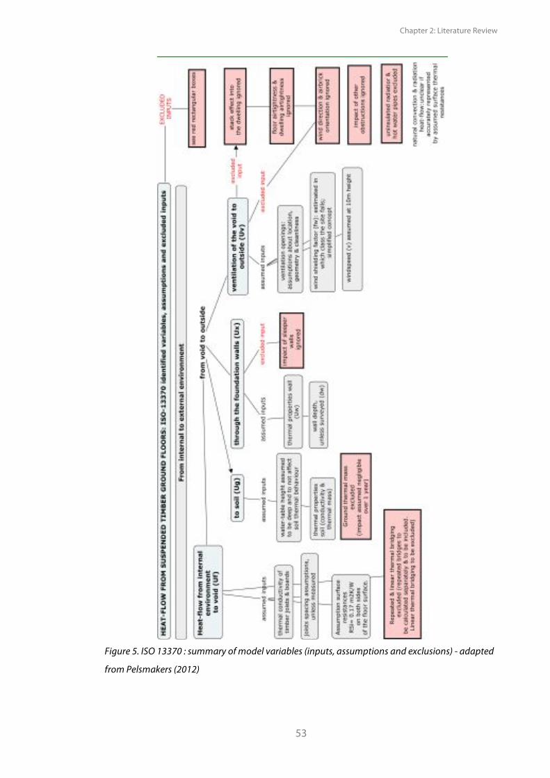
Chapter 2: Literature Review
53
Figure 5. ISO 13370 : summary of model variables (inputs, assumptions and exclusions) - adapted
from Pelsmakers (2012)
PhD Thesis Pelsmakers, S. 2016
54
Reliance on general input assumptions (for example for material conductivities, construction
build-up depths, average wind-speeds, airbrick characteristics etc.) might lead to model
output uncertainty. For instance Harris (1997, 1993) notes that wrong assumptions about
ground conductivity can lead to significantly differently estimated solid ground floor U-
values. Other uncertainties include assumptions of a constant ventilation rate through the
airbricks (Harris, 1993), assumed wind-shielding factors, assumptions about the effective
ventilation area of airbricks (Williamson, 2006a) and assumption of association between 10m
high average wind-speeds and those at airbrick height. Furthermore, the model makes no
distinction between suspended concrete or suspended timber ground floors and the
former's increased floor airtightness. Without a stack-effect component, the model might be
more representative of a more airtight concrete suspended floor. This stack-effect airflow
might also affect the surface thermal resistances but this is not characterised at present.
Williamson (2006a) critiqued the oversimplification of the model, while Rees (2001), Adjali
(2004) and Thomas (1999) have made similar observations for the solid concrete ground floor
model. Williamson (2006a) proposed adjustments to Uv to better reflect that (a.) airbricks will
block over time (and suggests a 70% effective area), (b.) adjusted wind shielding factors (fw)
and (c.) better averaging of pressure coefficients of the wall to low level airbricks.
Williamson's (2006) adjustments are expressed in Equation 21. and overall slightly increases
the wind driven component (Uv), especially in suburban and in rural locations from increased
wind shielding factors (fw), but it has a small overall impact on the final derived U-value.
Williamson's formula is based on a 3 metre building roof height, in itself a limitation.
- Equation 21., where Uv is according to Williamson (2006a) as per
Equation 18. but fw' is the adjusted wind shielding factor 0.03 (urban) 0.10 (suburban) or 0.18
(rural) for a building with roof at 3m height.
For additional detail on assumptions and excluded inputs, see Appendix 2.A. It is unknown if
(and by how much) the model U-value outputs are affected by the individual or cumulative
effect of assumptions and exclusions, nor what their contributory extent to the floor U-value
is, all of which are poorly characterised at present.
Chapter 2: Literature Review
55
2.3.1. CIBSE 1986 model The CIBSE (1986) suspended ground floor U-value model is briefly presented here, even
though it is superseded by the ISO-13370 model which is now the basis for the models in
CIBSE (2015) and its previous version (CIBSE, 2006). While the CIBSE-1986 model is no longer
in use, it is included here for comparison to current models - see Chapters 4 and 5. The model
is graphically presented in Figure 6. and is described by Equations 22 to 35.
The CIBSE-1986 model describes the suspended ground floor heat-transfer as resistances in
series and in parallel (see Figure 6., diagram b), and includes thermal resistances for the floor,
the ground and a ventilative component alongside radiant and convective components.
However some of its limitations include assumptions of ground thermal properties and of the
convective (hc) and radiant coefficients (hr); a smaller heat capacity of air and RSi of 0.14
m2KW-1 compared to 0.17 m2KW-1 in ISO-13370. For RSi and hc, the assumed values are based
on <0.1 m/s airflow at the surface but this is uncharacterised for the ventilated void.
Additionally, it is unknown at which height wind-speeds are to be derived; 1m/s is
recommended in CIBSE (1986) which might imply a low-level wind-speed near the building,
however this is unspecified. Furthermore, the use of breadth (b) and length (lf) is limiting for
more complex floor plates which are not square or rectangular; there is also an assumption
that the free airbrick ventilation area is associated with the longer wall dimension (lf) rather
than the exposed building perimeter. Foundation wall thickness is assumed to be 0.3m with
the thermal resistance of the floor (Rg) assumed to be 0.2 m2KW-1 - though a more complex
equation (Equation 34) can be used to adjust for specific cases. A brief sensitivity analysis and
comparison between the current ISO-13370 and superseded CIBSE-1986 model outputs is
presented and discussed in Chapter 4.4.3.1.
- Equation 22., where Rt is as per Equation 23. below:
- Equation 23., after CIBSE (1986), where RSi is
the internal surface thermal resistance, to be taken as 0.14 m2KW-1; Rg is the resistance of the
floor slab (to be taken as 0.2 m2KW-1 (CIBSE, 1986) or (Equation 24. ); Rt1
and Rt2 are derived from Equation 25. and Equation 26.; Re is the thermal resistance of the
earth and as per Equation 29.; Rv is the ventilation resistance and as per Equation 30.
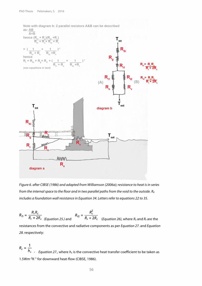
PhD Thesis Pelsmakers, S. 2016
56
Figure 6. after CIBSE (1986) and adapted from Williamson (2006a); resistance to heat is in series
from the internal space to the floor and in two parallel paths from the void to the outside. Re
includes a foundation wall resistance in Equation 34. Letters refer to equations 22 to 35.
(Equation 25.) and (Equation 26), where Rc and Rr are the
resistances from the convective and radiative components as per Equation 27. and Equation
28. respectively:
- Equation 27., where hc is the convective heat transfer coefficient to be taken as
1.5Wm-2K-1 for downward heat-flow (CIBSE, 1986).
Chapter 2: Literature Review
57
- Equation 28., where is the emissivity factor to be taken as 0.9 and hr is the
radiative heat transfer coefficient, to be taken as 5.7Wm-2K-1 (CIBSE, 1986).
- Equation 29., where Ug is derived from a table in CIBSE (1986) and assumes
that the earth has the same conductivity as a solid ground floor slab with limited prescribed
proportions (lf and b). Alternatively for more specific cases, Ug can be derived as per Equation
34.
- Equation 30., where Rv is the ventilation resistance in the suspended floor; Af is
the floor area (m2), cv is the heat capacity of air (to be taken as 1200 J/m3K (CIBSE, 1986) and
Vf is the ventilation rate in m3/s of the suspended floor, and as per Equation 31.
- Equation 31., where is the airbrick ventilation free opening area
per metre length lf (assumed 0.002 m2/m (CIBSE, 1986) and v is the wind velocity in m/s; lf is
the long dimension. Hence (Equation 32., where b is the breadth or shorter floor
dimension; assuming the above inputs with a wind velocity of 1m/s (CIBSE, 1986),
(Equation 33).
- Equation 34., where w is the wall thickness (assumed to
be 0.3m (CIBSE, 1986), b is the floor width; B is a floor dimension and derived as per Equation
35.; artanh is the inverse hyperbolic tangent and where - Equation
35., where lf is the floor length.
PhD Thesis Pelsmakers, S. 2016
58
2.4. Published suspended timber ground floor U-values This section gives an overview of published U-values, both calculated and in-situ measured
and compares the different sources and highlights issues associated with such comparisons.
2.4.1. Literature floor U-values
The majority of published suspended ground floor U-values are based on industry literature
and on an exposed perimeter to floor area ratio (P/A). This P/A ratio differs depending on
building geometry; hence Table 1. and Table 2. present results separately for terraced houses
(assumed P/A=0.3) and semi-detached houses (assumed P/A =0.6, (Thorpe, 2010))
respectively. Un-insulated suspended ground floor published U-values range from
0.45 Wm-2K-1 to 0.70 Wm-2K-1 for mid-terraced houses and 0.45 Wm-2K-1 to 1.30 Wm-2K-1 for
semi-detached dwellings; though insufficient information about the variables were provided
to establish the cause of the difference between the sources. The average literature U-value
for terraced houses is 0.55 Wm-2K-1 based on the range of sources in Table 1. and
0.77 Wm-2K-1 for semi-detached dwellings based on the sources in Table 2. Rickaby (2014b)
questioned the applicability of P/A in a floor with a ventilated void and suggested a doubling
of the U-value for uninsulated suspended ground floors from a calculated 0.65 Wm-2K-1 to
1.30 Wm-2K-1 for a semi-detached dwelling (Rickaby, 2014a, Rickaby, 2014b). The validity of
this is unknown and this is likely to depend on the number of airbricks per P/A for each
dwelling.
There is a difference of 56% between the lowest and highest literature floor U-values for
terraced houses and 188% for semi-detached dwellings. While these divergences suggest
large differences in literature U-values, these sources are likely to have each used different
underlying assumptions and each assumed different dwelling and floor characteristics,
which affect the final value. While in some of the literature sources some of the assumed
variables are stated, not all literature sources disclose detail of embedded assumptions, such
as:
- which calculation model used;
- whether thermal bridging is included;
- material properties and assumptions; (including perimeter wall characteristics,
timber conductivities etc.);
- assumed ventilation/airbrick openings;
- exposed perimeter to floor area (P/A), which is different between each house
typology and also within the same typology;
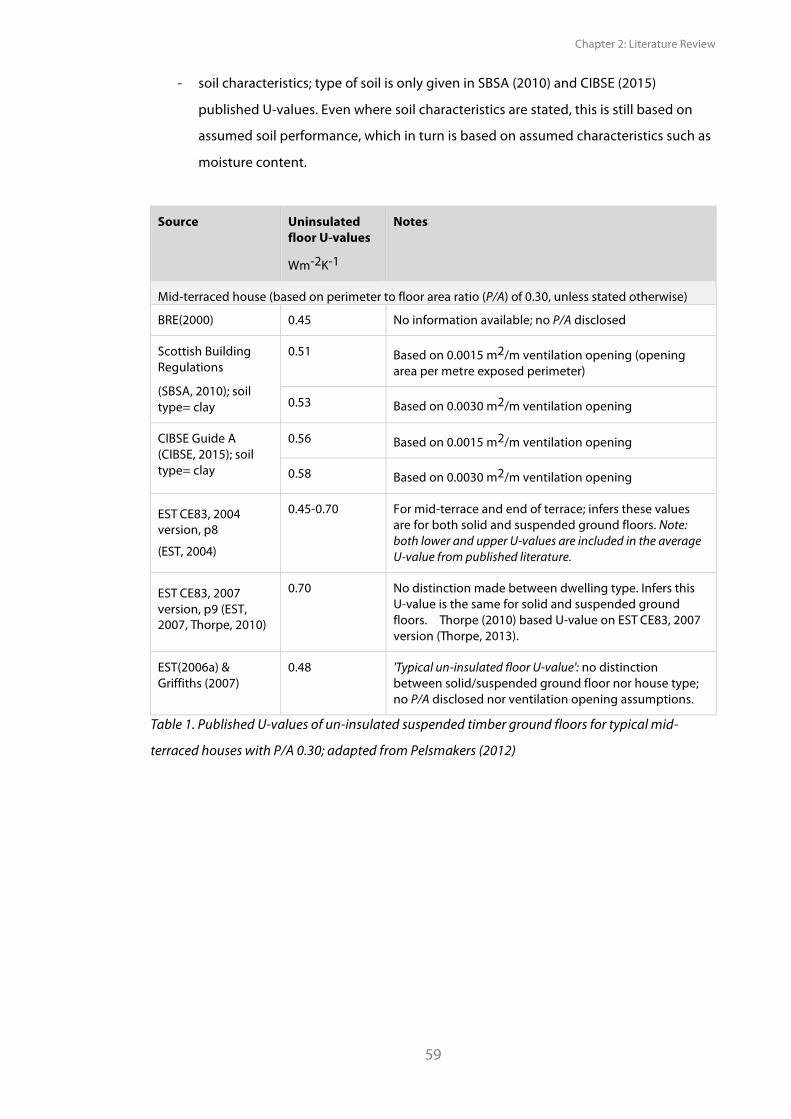
Chapter 2: Literature Review
59
- soil characteristics; type of soil is only given in SBSA (2010) and CIBSE (2015)
published U-values. Even where soil characteristics are stated, this is still based on
assumed soil performance, which in turn is based on assumed characteristics such as
moisture content.
Source Uninsulated floor U-values
Wm-2K-1
Notes
Mid-terraced house (based on perimeter to floor area ratio (P/A) of 0.30, unless stated otherwise)
BRE(2000) 0.45 No information available; no P/A disclosed
Scottish Building Regulations
(SBSA, 2010); soil type= clay
0.51 Based on 0.0015 m2/m ventilation opening (opening area per metre exposed perimeter)
0.53 Based on 0.0030 m2/m ventilation opening
CIBSE Guide A (CIBSE, 2015); soil type= clay
0.56 Based on 0.0015 m2/m ventilation opening
0.58 Based on 0.0030 m2/m ventilation opening
EST CE83, 2004 version, p8
(EST, 2004)
0.45-0.70 For mid-terrace and end of terrace; infers these values are for both solid and suspended ground floors. Note: both lower and upper U-values are included in the average U-value from published literature.
EST CE83, 2007 version, p9 (EST, 2007, Thorpe, 2010)
0.70 No distinction made between dwelling type. Infers this U-value is the same for solid and suspended ground floors. Thorpe (2010) based U-value on EST CE83, 2007 version (Thorpe, 2013).
EST(2006a) & Griffiths (2007)
0.48 'Typical un-insulated floor U-value': no distinction between solid/suspended ground floor nor house type; no P/A disclosed nor ventilation opening assumptions.
Table 1. Published U-values of un-insulated suspended timber ground floors for typical mid-
terraced houses with P/A 0.30; adapted from Pelsmakers (2012)
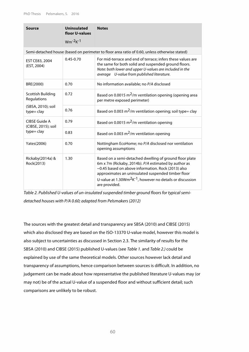
PhD Thesis Pelsmakers, S. 2016
60
Source Uninsulated floor U-values
Wm-2K-1
Notes
Semi-detached house (based on perimeter to floor area ratio of 0.60, unless otherwise stated)
EST CE83, 2004 (EST, 2004)
0.45-0.70 For mid-terrace and end of terrace; infers these values are the same for both solid and suspended ground floors. Note: both lower and upper U-values are included in the average U-value from published literature.
BRE(2000) 0.70 No information available; no P/A disclosed
Scottish Building Regulations
(SBSA, 2010); soil type= clay
0.72 Based on 0.0015 m2/m ventilation opening (opening area per metre exposed perimeter)
0.76 Based on 0.003 m2/m ventilation opening; soil type= clay
CIBSE Guide A (CIBSE, 2015); soil type= clay
0.79 Based on 0.0015 m2/m ventilation opening
0.83 Based on 0.003 m2/m ventilation opening
Yates(2006) 0.70 Nottingham EcoHome; no P/A disclosed nor ventilation opening assumptions
Rickaby(2014a) & Rock(2013)
1.30 Based on a semi-detached dwelling of ground floor plate 6m x 7m (Rickaby, 2014b). P/A estimated by author as ~0.45 based on above information. Rock (2013) also approximates an uninsulated suspended timber floor U-value at 1.30Wm2K-1, however no details or discussion are provided.
Table 2. Published U-values of un-insulated suspended timber ground floors for typical semi-
detached houses with P/A 0.60; adapted from Pelsmakers (2012)
The sources with the greatest detail and transparency are SBSA (2010) and CIBSE (2015)
which also disclosed they are based on the ISO-13370 U-value model, however this model is
also subject to uncertainties as discussed in Section 2.3. The similarity of results for the
SBSA (2010) and CIBSE (2015) published U-values (see Table 1. and Table 2.) could be
explained by use of the same theoretical models. Other sources however lack detail and
transparency of assumptions, hence comparison between sources is difficult. In addition, no
judgement can be made about how representative the published literature U-values may (or
may not) be of the actual U-value of a suspended floor and without sufficient detail; such
comparisons are unlikely to be robust.
Chapter 2: Literature Review
61
2.4.2. In-situ measured U-values There are not many in-situ measured U-values for either uninsulated or insulated suspended
timber ground floors as also noted by Doran (2008), and not all are recent or for UK floor
constructions or climate. A brief consideration of available sources accessible at the time of
writing follows below and are listed in Table 3. for UK sources.
The largest in-situ heat-flux measuring campaign of suspended ground floors appears to
have been undertaken by Isaacs (1985) in New Zealand, who monitored 44 foil insulated
suspended ground floors. Some floors were on stilts and thus lacked perimeter walls and
were exposed to the external environment, hence internal floor surface to external sub-floor
surface temperatures were used in in-situ measurements for practical reasons (without
surface resistance adjustments - see Chapter 3.3.). This is unlike other studies and models
which measure from the internal to the external environment. Excluding part of the heat-
flow path by measuring to the void (such as exclusion of the additional layers of air and the
foundation wall and exclusion of the surface thermal resistances) means that the estimated
thermal resistances from internal space to void in Isaacs' (1985) study are expected to be
lower than if the floor resistances had been estimated to the external environment and if
surface thermal resistances had been included, as acknowledged by Isaacs (1985). However,
these neglected additional thermal resistances might be small in the exposed floors (i.e. the
floors without perimeter walls) (Isaacs, 1985). Measurements were undertaken in single floor
locations with large 600mm x 450mm heat-flux sensors so that joist effects could be
included; an internal surface temperature sensor was embedded in the heat-flux sensor.
Analysis was undertaken by using a cumulative sum to estimate thermal resistances- see
Chapter 3.3. Comparison with UK floor constructions is difficult; however Isaacs (1985) found
that the mean R-value of the foil insulated sheltered floors - estimated as described above -
was 1.1 m2KW-1, while just 0.55 m2KW-1 for the exposed floors; and the latter generally did
not meet prescribed regulations.
Harris (1994, 1997) estimated U-values of a test-cell floor in a controlled environment (as
discussed in Section 2.2.2.) Harris' U-value results of 0.62 Wm-2K-1 to 0.87 Wm-2K-1are within
ranges as those discussed from literature sources in the previous Section 2.4.1., though these
values are not directly comparable with the published estimated values. Firstly, the main
purpose of Harris' (1993, 1997) work was to compare different insulation methods and their
performance in certain conditions (Harris, 2013), not to compare measured versus published
U-values or other in-situ measured sources.
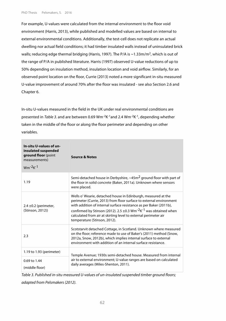
PhD Thesis Pelsmakers, S. 2016
62
For example, U-values were calculated from the internal environment to the floor void
environment (Harris, 2013), while published and modelled values are based on internal to
external environmental conditions. Additionally, the test-cell does not replicate an actual
dwelling nor actual field conditions; it had timber insulated walls instead of uninsulated brick
walls; reducing edge thermal bridging (Harris, 1997). The P/A is ~1.33m/m2, which is out of
the range of P/A in published literature. Harris (1997) observed U-value reductions of up to
50% depending on insulation method, insulation location and void airflow. Similarly, for an
observed point location on the floor, Currie (2013) noted a more significant in-situ measured
U-value improvement of around 70% after the floor was insulated - see also Section 2.6 and
Chapter 6.
In-situ U-values measured in the field in the UK under real environmental conditions are
presented in Table 3. and are between 0.69 Wm-2K-1and 2.4 Wm-2K-1, depending whether
taken in the middle of the floor or along the floor perimeter and depending on other
variables.
In-situ U-values of un-insulated suspended ground floor (point measurements)
Wm-2K-1
Source & Notes
1.19 Semi-detached house in Derbyshire, ~45m2 ground floor with part of the floor in solid concrete (Baker, 2011a). Unknown where sensors were placed.
2.4 ±0.2 (perimeter, (Stinson, 2012))
Wells o' Wearie, detached house in Edinburgh, measured at the perimeter (Currie, 2013) from floor surface to external environment with addition of internal surface resistance as per Baker (2011b), confirmed by Stinson (2012). 2.5 ±0.3 Wm-2K-1 was obtained when calculated from air at skirting level to external perimeter air temperature (Stinson, 2012).
2.3
Scotstarvit detached Cottage, in Scotland. Unknown where measured on the floor; reference made to use of Baker's (2011) method (Snow, 2012a, Snow, 2012b), which implies internal surface to external environment with addition of an internal surface resistance.
1.19 to 1.93 (perimeter) Temple Avenue; 1930s semi-detached house. Measured from internal air to external environment; U-value ranges are based on calculated daily averages (Miles-Shenton, 2011).
0.69 to 1.44
(middle floor)
Table 3. Published in-situ measured U-values of un-insulated suspended timber ground floors;
adapted from Pelsmakers (2012).
Chapter 2: Literature Review
63
Comparing the U-values in Table 3. with the literature U-values for semi-detached dwellings
in Table 2., Section 2.4.1., there appears to be a large divergence between measured and
published U-values. Similar divergences were also found by e.g. Baker (2011b), Rye (2010)
and Li (2014) for solid walls, where theoretical U-values appeared to over-estimate actual
measured U-values. Contrary to this, for the in-situ measured floors listed in Table 3., in-situ
measured U-values appear significantly higher than the published sources and those based
on theoretical models such as SBSA (2010) and CIBSE (2015). Chapman (1985a) also
suggested that floor U-values were significantly higher than predicted. However, direct
comparison between these in-situ measured case studies and literature, as well as between
the different in-situ sources, is difficult for the following reasons:
• each of the above case studies are subject to different variables: different dwellings
of different construction and different terrain obstructions (affecting wind-speeds);
• the in-situ measurements were undertaken on different locations on the floor and
were subject to different environmental conditions;
• different sources use different measurement and data analysis methods or did not
disclose it; for example U-values were estimated from different internal to external
(or void) temperature locations;
• the ISO-13370 model is a whole floor U-value model and not for points on the floor
(CIBSE, 2015, Anderson, 2006), while in-situ U-values are spot measurements or point
locations on the floor.
PhD Thesis Pelsmakers, S. 2016
64
Moreover, from physical theory and as noted by Harris (1993), heat-flow is expected to vary
across the floor. Increased heat-flow is expected along the edges (perimeter) compared to
the non-perimeter zone. This is illustrated to some extent by Miles-Shenton's (2011) in-situ
measurements in two point locations, with measurements in one location in the middle of
the floor generally lower than those observed in the perimeter location. However, apart from
Miles-Shenton (2011), the measurements presented in Table 3. are based on single in-situ
'point' U-value estimates. In some sources the in-situ U-value was measured in the perimeter
zone, a location of the floor which is unlikely to be representative of the whole floor U-value,
and which is expected to be subject to increased heat-flow - see Section 2.2.
This spatial variation of heat-flow might explain large model/literature U-value divergences
with in-situ measurements, depending on the floor location where such in-situ
measurements were undertaken. Equally, it is unknown whether literature U-values and
outputs from ISO-13370 models accurately reflect the actual floor U-value. While the
simplification of models allows for quick floor U-value estimates (and generic assumptions
negate the need for a detailed survey), model outputs may hence not reflect the actual
construction and heat-flow paths due to the previously listed simplifications, assumptions
and omissions (see also Section 2.3.). This could lead to over or under-estimation of the
actual floor U-value, however the extent of this remains uncharacterised. While some
divergence is expected between modelled and in-situ measured values due to input
assumptions (BSI, 2014, McMullan, 2002), there are also uncertainties associated with in-situ
measurements - see Chapter 3.3.
Chapter 2: Literature Review
65
2.5. Floors and thermal comfort
This section focuses and brings together current research and theory associated with thermal
comfort and ground floors specifically. Thermal discomfort is an important factor in dwelling
energy use because it might lead to increased energy use to compensate (Rock, 2013) by for
example increasing room air temperatures (Olesen, 1979).
Thermal comfort may be defined as "that condition of mind that expresses satisfaction with the
thermal environment" (ASHRAE, 2013a) and is dependent on the level of personal activity and
clothing alongside physiology and psychology and the surrounding environmental
conditions (such as humidity, air velocity, air, surface and radiant temperatures) (Olesen,
2000, CIBSE, 2015). Generally thermal comfort theory considers certain local thermal
differences of the body to lead to discomforts, such as large differences between head and
feet, cold floor surfaces and draughts (Olesen, 1977, CIBSE, 2015, Olesen, 2004, Olesen, 1980).
In many thermal comfort studies, use is made of the Predicted Mean Vote (PMV)(Parsons,
2003), which expresses thermal satisfaction based on the average satisfaction of a large
group of individuals, using the ASHRAE thermal sensation scale with 7 values from hot (+3)
to cold (-3)(Olesen, 2004). Another index, Predicted Percentage Dissatisfied (PPD) expresses a
percentage of thermal dissatisfaction and is derived from people's PMV votes of
dissatisfaction with the thermal environment (i.e. votes of ±2 and ±3), assuming a neutral
comfort level of PMV = 0 (Olesen, 2004). A PPD of no more than 20% is generally aimed for
but often buildings do not provide this for their occupants (Brager et al., 2015). Both indexes
relate to the general or whole body thermal (dis)comfort experienced (Olesen, 2004), and not
to local thermal discomfort, the latter has particular relevance to uninsulated ground floors.
Limitations of present thermal comfort models are discussed by e.g. de Dear (2011),
Parkinson and de Dear (2014) and Arens (2010) and they note that current thermal comfort
standards focus on narrow ranges in mostly steady-state environments and are based on the
minimisation or elimination of thermal discomfort (negative alliesthesia) rather than on the
maximisation of thermal pleasure (positive alliesthesia). Generally predictive thermal comfort
theory is developed in controlled environmental thermal labs considering a uniform (steady-
state) laboratory environment on whole body thermal comfort.
PhD Thesis Pelsmakers, S. 2016
66
Less research has been undertaken with transient conditions, changing indoor air-flow, non-
uniform environments and impact of cold (or hot) sensations in body parts on overall
thermal comfort (and thermal pleasure), when thermal comfort responses become more
complex (Zhang, 2009b, Zhang, 2009a, Olesen, 2004, Parkinson and de Dear, 2014). Much
research is also based on theoretical behaviour of people, for example the undertaking of
light or sedentary activity, wearing of certain clothing at different seasons, when in reality
these situations may not occur, or in combination with other factors thermal comfort
sensations may significantly differ. For example, an individual might theoretically be
considered in whole body thermal discomfort, yet in transient conditions or where
occupants have control over their environment or where local heat or cold stimuli are
applied, actual overall thermal comfort might be closer to the neutral thermal sensation
(Zhang, 2009c) or they might even experience thermal pleasure (positive alliesthesia) (de
Dear, 2011, Parkinson and de Dear, 2014).
Main identified thermal comfort theory related to ground floors are mostly local thermal
(dis)comfort issues, i.e. where a particular part of a person's body in sedentary or light activity
is affected (Olesen, 2000), in this case, the feet. Current thermal comfort theory considers that
when someone is exposed to colder conditions, the extremities (head and feet) are also
generally colder while the rest of the body is less affected (Munro, 1948). ASHRAE (2013a)
Standard 55 considers a 10% PPD margin acceptable for whole body comfort or 5% to 20%
depending on different local discomfort factors such as local draughts, vertical temperature
differences and cold floor surfaces (Olesen, 2004). ASHRAE (2013a) Standard 55 and BSI
(2006) also set out local thermal discomfort thresholds, which, where relevant to ground
floors, are discussed below. Thermal comfort theory related to ground floors associates local
thermal discomfort with cold/warm floor surface temperatures and air temperature
differences between head and feet. According to theory, these local thermal discomfort
sensations might also depend on overall room air temperatures; for example when the core
body is cold, introducing warmth to a local body part might increase comfort. The reverse
might happen when introducing cold to warm body parts, though warming the core body
(instead of warming local body parts) might be more effective, as reported by Zhang (2009b).
First, an overview of current thermal discomfort theory from cold floor surfaces is presented,
followed by theory on discomfort from vertical air temperature differences in occupied
spaces and finally thermal comfort theories related to other local discomfort thresholds are
discussed.
Chapter 2: Literature Review
67
Possible discomfort from too cold (or too warm) floor surface temperatures
According to ASHRAE (2013b), when occupants are wearing shoes, it is the floor surface
temperature rather than the floor finish which largely determines thermal comfort. Olesen
(1977) also found that, over a short period of time and for people with bare feet, the floor
temperatures affected local thermal discomfort, which are dependent on the floor's thermal
characteristics. Theory recommends floor surface temperatures are between 19ºC and 29ºC
(ASHRAE, 2013a, BSI, 2006) and depends on floor finish (Olesen, 1977, CIBSE, 2015), for
example on the thermal mass and conductivity of the floor finish. Billington (1948) found
that the warmest feeling of a floor is a combination of low thermal capacity and low
conductivity (such as cork).
Contrary to this, Munro (1948) claims that overall room temperatures are the main factor in
thermal discomfort and that uninsulated floors (or cold floors) in themselves are not the
main cause of 'cold' feet. Munro (1948) notes that for individuals with shoes on over a 60
minute period, low air temperatures (< 18ºC) combined with local discomfort caused by a
concrete surface (but also linoleum and rubber covered concrete and wood) lead to
discomfort. Less discomfort was experienced on cork surfaces, where comfort sensation and
feet temperatures were higher than with other surfaces as also found by Billington (1948).
As expected, this discomfort is further pronounced with bare feet (Munro, 1948). Nevins
(1967) argues that with shoes on, the conducting layer of the floor surface is less important
(as the shoe material adds thermal resistance); cold feet might be experienced at floor
surfaces #15ºC. Heat discomfort was noted by Michaels (1964) at +35ºC floor surface
temperatures and with ~24ºC air temperatures. Parkinson (2014) suggests that warm floors
might lead to subjects feeling thermal pleasure (positive spatial alliesthesia) despite slightly
"cooler-than-preferred ambient temperatures". Brager (2015) describes use of localised foot
warmers providing increased thermal comfort at lower room temperatures, reducing overall
energy use for space-heating.
Given the many different variables which affect thermal comfort, it is unsurprising that there
is little consensus in different sources on the minimum and maximum floor and room air
temperature combinations that might lead to thermal (dis)comfort. In summary, suggested
comfort floor surface temperature values go as low as 17ºC to 19ºC (ASHRAE, 2013a, BSI,
2006) to as high as 37.8ºC for heated floors (Song, 2008). Likewise, suggested ideal air
temperatures range from 20ºC to 24ºC, depending on source (Chrenko, 1957, Olesen, 1977,
CIBSE, 2015, ASHRAE, 2013a, BSI, 2006).
PhD Thesis Pelsmakers, S. 2016
68
Possible discomfort from vertical temperature differences
Olesen's (1979) work was the basis for ASHRAE Standard 55 and BSI-7730 local thermal
comfort standards. Discomfort might be experienced when there is a 3ºC to 4ºC temperature
difference between feet (0.1m height) and head (1.1m head height when seated or 1.7 m
head height when standing)(ASHRAE, 2013a, BSI, 2006, Olesen, 1979, Parsons, 2003). For
standing active people this range might be up to 7ºC (Zhang, 2005), but this was based on
simulation only. As noted by Parkinson (2014), cooling the head and warming the feet might
lead to thermal pleasure.
Other possible local discomfort thresholds
• Possible discomfort from mean radiant temperature differences between
ceiling and floor5 might arise if the ceiling is 5ºC warmer than the floor, or if the
ceiling is 14ºC colder than the floor (with room temperatures of 22.5ºC), according to
ASHRAE (2013a) and BSI (2006). Olesen (1980) suggested that this mean radiant
floor/ceiling temperature difference should ideally be less than 4ºC to minimise
thermal discomfort sensations (for 5% PPD).
• Possible discomfort from increased airflow/draughts: according to ASHRAE
(2013a) draughts might cause "unwanted local cooling of the body caused by air
movement" and might particularly affect head/neck/shoulder region and leg region,
including feet and ankles. Thermal discomfort from draughts might be most
pronounced where room air temperatures are low: ASHRAE (2013a) suggests that
draughts should not be greater than 0.15 m/s below 22.5ºC to minimise discomfort.
CIBSE (2015) suggests a draught airflow increase from 0.1m/s to 0.6m/s might raise
the thermal comfort temperature value by 2 degrees.
In the different sources, there is little consensus on the minimum and maximum thermal
comfort thresholds; this is unsurprising given the differences of the impacting variables, i.e.
differences in physiology, activity and practices (such as clothing levels) and the difficulty in
undertaking such studies. However, an in-depth thermal comfort study and impact of
discomfort on compensating energy use or on occupant thermal comfort is not within the
remit of this research; instead preliminary data is presented and compared with the
theoretical ASHRAE and BSI-7730 thresholds in Chapter 6.5.
5 Also referred to as 'asymmetric thermal radiation'.
Chapter 2: Literature Review
69
2.6. Floor insulation Shorrock (2005) estimated that there are nearly 10 million uninsulated suspended ground
floors in the UK and Power (2008) argues that floor insulation is essential alongside other
fabric intervention measures to achieve significant overall dwelling energy reductions. About
8000 floors were recently insulated under the ECO and the Green Deal policies, though this
represents only a small proportion of overall measures - see Chapter 1.2.3. However, no
literature was found that identifies the proportion of insulated floors in the UK's pre-1919
housing stock.
Insulating floors might provide many benefits, including reduced energy use and energy bills
with reduced associated carbon emissions (Power, 2008), though this depends on
space-heating fuels used. An additional benefit of floor insulation might be increased
dwelling airtightness as well as better occupant thermal comfort - see Chapter 6.5. EST
(2006b) suggests that up to 60% heat loss reductions might be achieved by insulating
suspended timber ground floors. Floor insulation was also highlighted as a cost-effective
carbon reduction measure by Shorrock (2005), Rickaby (2014a) and Mackenzie (2010), with
estimated carbon reductions of 1.82 million tonnes of CO2 per year for the UK housing stock,
excluding any compensating occupant behaviour such as 'take back'6(Mackenzie, 2010). It is
unclear what these estimates are based on and estimated carbon reductions will be lower
when low carbon space-heating supply increases.
However, some dwelling retrofits estimated significant energy reductions without insulating
floors by using higher fabric standards elsewhere, for example 'Cottage Retrofit' at the Isle of
Wight (TSB, 2012). Furthermore, Friedman (2014) found that floor insulation was, together
with doors, one of the least considered energy efficiency upgrades to conservation
properties from a sample of 116 industry respondents. Forty one percent said improving
floors was not a major objective; while only 9% to 18% said it was considered in most if not
all projects respectively (Friedman, 2014).
6 The 'temperature take back factor' is "the degree to which fabric and ventilation changes could result in increases in indoor temperature as opposed to lower energy consumption." (Hamilton et al, 2011)
PhD Thesis Pelsmakers, S. 2016
70
The upgrade of existing ground floor structures is regulated by Building Regulations Part L1B,
which recommends insulated floor U-values of maximum 0.25 Wm-2K-1 for the entire floor
when at least 50% of the floor surface is upgraded or replaced or where 25% of the entire
building envelope is renovated (NBS, 2015). Exceptions exist for listed buildings and other
relaxations exist to take account of practical and technical constraints (such as maximum 15
year payback, difficult floor level differences between parts, structural issues). In these cases a
maximum U-value of 0.70 Wm-2K-1 is allowed (NBS, 2015). New ground floors are to be built
to the same maximum U-value of 0.25 Wm-2K-1 in England and Northern Ireland and
maximum 0.18 Wm-2K-1 in Scotland and Wales. These are improvements from 0.45 Wm-2K-1
in 1990, prior to which no recommendations were specified for floors (Dowson et al., 2012).
Other sources also recommend upgrade of floors with maximum U-values of 0.20 to 0.25
Wm-2K-1 (for example EST (2004, 2007)); Rickaby (2014a) recommends 0.25 Wm-2K-1 as good
practice and 0.15 Wm-2K-1 for advanced practice. Such advanced U-values of 0.16 Wm-2K-1
and 0.13 Wm-2K-1 are reported by Baeli (2013) for the Shaftesbury Park Terrace with
fully-filled floor void with EPS beads (p37) and for Midmoor Road (p 41-42) respectively. The
latter design value was achieved with a combination of 100 mm rigid insulation on top of
joists and 100 mm mineral wool insulation between the joists. In another case study in Brent,
spray foam floor insulation was predicted to lead to a U-value of 0.12 Wm-2K-1 but no further
information was provided regarding the material or application depth (Baeli, 2013, p 65-66).
Large thermal improvements were also predicted for replacement of suspended timber
ground floors with an insulated concrete ground floor: for example in Hawthorn Road, a
U-value of 0.12 Wm-2K-1 was predicted with 200 mm EPS on top of a new concrete floor
(Baeli, 2013, p 46), and 0.13 Wm-2K-1 in Greenwich (LEB, 2011a). In Liverpool, a U-value of
0.12 Wm-2K-1 was estimated by rebuilding a suspended ground floor with a proprietary
product called Supafloor (LEB, 2011b).
Chapter 2: Literature Review
71
The above floor U-values are based on modelled design predictions, not on actual in-situ
measured performance, of which there are only a few published. Currie (2013) reported a
70% U-value reduction from 2.4 to 0.7 Wm-2K-1 in one pre-post measured point U-value; the
floor was insulated with 80 mm woodfibre between joists. Harris (1997, 1994) observed up to
50% heat-flow reduction by insulating a test-cell floor and by stapling a radiant barrier under
the joists of a test-cell; increased void airflow reduced the U-value reduction achieved. In
New Zealand, Cox-Smith (2008) investigated the performance of foil insulation over time and
observed that newer reflective foil draped over joists performed slightly better than when
draped under joists and when soiled after several years. Isaacs (1985) conducted large-scale
in-situ heat-flux monitoring of 63 houses in New Zealand and observed that foil-insulated
floors with enclosed floor voids generally met the (then) stipulated building standards, while
floors with no perimeter walls (i.e. exposed to the outside) and foil insulation did not meet
those standards.
While insulation of floors should lead to reduced heat loss and increased space-heating
energy savings, it might also lead to increased moisture build-up as found by Airaksinen
(2003) in Finland. Airaksinen (2003) observed that floors with a typical U-value of 0.2 Wm-2K-1
had average void relative humidity (RH) almost 10% higher than floors with U-values of
0.4 Wm-2K-1; the latter floors lead to 2ºC warmer void air temperatures on average - see
Section 2.7. Despite slow uptake of floor insulation, thousands of floors have already been
insulated - see Chapter 1.2.3.; yet the impact on heat loss reductions, occupant thermal
comfort and on floor void conditions are unknown, which hinders informed retrofit decision-
making.
2.6.1. Typical floor insulation methods In the UK typically a fibrous insulation is installed in between joists (Figure 7. option a) (BRE,
2000, EST, 2005, EH, 2010, Rock, 2013). Insulating floors with limited void access, such as the
floors subject of this thesis, usually requires lifting of the floorboards, which is a disruptive
process (Rickaby, 2014a). Access to floors from below is less disruptive (Roberts, 2008)
though not always possible due to health and safety concerns. Despite potential large
carbon savings (Shorrock, 2005), the disruptive potential of full floor insulation might lead to
little uptake according to Dowson (2012), Shorrock (2005) and Killip (2011), who argue that
full floor insulation in between joists makes only sense when taking up the floorboards
anyway.
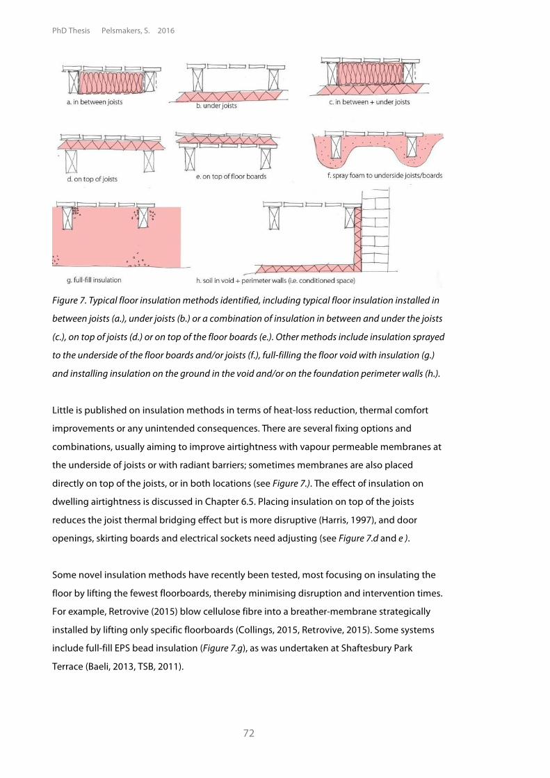
PhD Thesis Pelsmakers, S. 2016
72
Figure 7. Typical floor insulation methods identified, including typical floor insulation installed in
between joists (a.), under joists (b.) or a combination of insulation in between and under the joists
(c.), on top of joists (d.) or on top of the floor boards (e.). Other methods include insulation sprayed
to the underside of the floor boards and/or joists (f.), full-filling the floor void with insulation (g.)
and installing insulation on the ground in the void and/or on the foundation perimeter walls (h.).
Little is published on insulation methods in terms of heat-loss reduction, thermal comfort
improvements or any unintended consequences. There are several fixing options and
combinations, usually aiming to improve airtightness with vapour permeable membranes at
the underside of joists or with radiant barriers; sometimes membranes are also placed
directly on top of the joists, or in both locations (see Figure 7.). The effect of insulation on
dwelling airtightness is discussed in Chapter 6.5. Placing insulation on top of the joists
reduces the joist thermal bridging effect but is more disruptive (Harris, 1997), and door
openings, skirting boards and electrical sockets need adjusting (see Figure 7.d and e ).
Some novel insulation methods have recently been tested, most focusing on insulating the
floor by lifting the fewest floorboards, thereby minimising disruption and intervention times.
For example, Retrovive (2015) blow cellulose fibre into a breather-membrane strategically
installed by lifting only specific floorboards (Collings, 2015, Retrovive, 2015). Some systems
include full-fill EPS bead insulation (Figure 7.g), as was undertaken at Shaftesbury Park
Terrace (Baeli, 2013, TSB, 2011).
Chapter 2: Literature Review
73
To avoid beads spilling out and to reduce moisture being brought in from the outside,
airbricks are permanently sealed, though this is considered controversial as it is assumed
airbricks regulate moisture in the void (see Douglas (1998c), BRE (1991) and Singh (1998))
and as discussed in Section 2.7.2.). The long-term impact of sealing airbricks in general or of
these EPS bead-filled floor voids are however unknown.
Other innovative methods include remote spraying of insulation in floor voids (Baeli, 2013, p
65-66) (Figure 7. f), allowing simultaneous encapsulation of the joists, which otherwise tend
to remain uninsulated and become a thermal bridge after insulating between the joists.
Q-bot (2015) are trialling robotics to survey the floor and apply insulation in this manner7
(Lipinski, 2015) while U-Floor Technologies, developed by Sustainable Venture Development
in London, is a new innovative device deployed through the airbricks and using a natural,
sprayable insulation material (Czako, 2015).8
The different installation options can be achieved with different insulation materials, some of
which are listed in Appendix 2.B. Insulating timber floors is likely to increase the floor's
thermal mass: typically the thermal mass of an uninsulated suspended floor is between
5-7 kJ/m2K (carpet/vinyl floor finish on floorboards respectively; excluding foundation walls
and the ground); which can increase to 17-19 kJ/m2K with 100 mm mineral wool in between
the joists (CIBSE, 2015, table 3.53). This is however, still a relatively small thermal mass
compared to solid concrete floors (38-58 kJ/m2K carpet/vinyl, uninsulated)(CIBSE, 2015) and
the presence of the soil underneath the floor (1285 kJ/m2K based on 1 metre depth of
common earth (CIBSE, 2015, table 3.37). Thermal mass is important in moderating
temperature fluctuations and shifts temperature variations. Hence material conductivity,
thermal mass and time constant (i.e. the time it takes to respond after a change) are
important material characteristics to consider in relation to heat-loss reduction interventions.
Generally, insulating floors reduces the heat-flow from the internally heated spaces to the
floor void (and hence to the external environment) and the sub-floor void air and surfaces
will become colder and closer in temperature to the external environment. This in turn
affects the thermal mass equilibrium of the ground and foundation walls and the moisture
content of the sub-floor void might increase to critical moisture levels for mould growth in
summer - see the following Section 2.7.
7 The author was involved with q-bot for early research design in 2013/2014, based on the research design tested and developed in this PhD research to support q-bot in thermal performance monitoring, however no pre-post data was shared for analysis to be included in the thesis at the time of writing. 8 The author and the innovators signed a mutual NDA and confidentiality agreement.
PhD Thesis Pelsmakers, S. 2016
74
2.7. Unintended consequences of insulating floors Insulating floors might lead to unintended consequences, such as moisture build-up in floor
voids as found in some other countries. This can lead to fungal growth and timber rot,
affecting occupant health in the spaces above and leading to possible structural damage.
However, there is absence of UK evidence at present. Other consequences might be
increased fire risk if old electrical wires are embedded, risk of burst water pipes (EH, 2010)
and radon build-up (Lugg, 1997) - see Figure 10, page 87. However these latter issues are not
subject of this PhD research. This section gives a brief overview of possible causes of moisture
build-up in the floor void, the role of airbrick ventilation and regulatory requirements and
why moisture build-up might be a problem and what the identified issues are with insulating
floors. Little UK research exists in this area, hence research is drawn together from non-UK
sources, though it is unknown to which extent overseas findings transfer to pre-1919
suspended timber ground floor constructions in the UK climate.
2.7.1. Causes of moisture build-up in suspended ground floors There is an increased risk of damp and mould problems in pre-1919 dwellings (DCLG, 2010)
with around 5.8% of floors requiring repair of some kind (DCLG, 2010). Moisture problems
have also been reported in suspended floors since the 1940s in the USA (Rose, 1994b).
Moisture build-up in pre-1919 suspended floors can be caused by several different variables;
the main identified causes are summarised below and illustrated by Figure 8. (letters below
relate to Figure 8.).
Moisture from the ground (A): wet soil (because of high ground water level) or standing
water in the floor void could cause high evaporation rates and high RH in the void, which can
transfer to the indoor spaces above (Harris, 1995). Where no ground cover exists, as likely the
case in most existing old suspended floors (Douglas, 1998c), evaporation from damp soil is
considered a major source of moisture (Harris, 1995, Moses, 1954). Evaporation depends on
differences in moisture content between crawl space air and ground, void ventilation and
the thermal behaviour of the ground (Kurnitski, 2001); Building Regulations require ground-
covers (NBS, 2013), which were also found to be effective in avoiding moisture build-up in
existing floors (Harris, 1995, Rose, 1994a, Flynn, 1994, Brook, 1994, Stiles, 1994). Joists
supported by brick walls can become damp where timber joists are in contact with soil
(Tsongas, 1994) or due to rising damp (or driving rain or 'splash back'), especially a risk
without damp proof membranes (Harris, 1995, Oliver, 1997, Douglas, 1998b, Ridout, 2001,
Tsongas, 1994).
Chapter 2: Literature Review
75
Lack of external site drainage and/or if the external ground level is above the floor (B)
so that water can enter floor voids (Rose, 1994b, Brook, 1994, Oliver, 1997, Singh, 1998).
Leaks from services (C) above/below the floor or leaks from rainwater runoff pipes nearby
(Brook, 1994, Tsongas, 1994, Morton, 2013), though spillage from living spaces above is
probably rare (Harris, 1995) and as with leaks are likely to be localised (Douglas, 1998b).
Impermeable floor finishes (D): BRE (1991) notes some risk from impermeable floor finishes
preventing moisture evaporation to the spaces above where previously this was possible and
may tip wood moisture content above what is desirable. Insulation material characteristics
are also important - see Appendix 2.B.
Ventilation: moisture brought in from the outside through airbricks and other non-
airtight paths (E): see discussion in following Section 2.7.2.
Increased floor insulation (F) leads to colder void air and surface temperatures, impacting
on void moisture conditions (Samuelson, 1994, Airaksinen, 2003). In Finland, Airaksinen
(2003) observed that floors with a typical U-value of 0.2 Wm-2K-1 had average void RH almost
10% higher than floors with 0.4 Wm-2K-1 U-value; the latter floors lead to 2ºC warmer void air
temperatures on average. Section 2.7.5. sets out a separate discussion of the risk of insulating
floors. See also Appendix 2.D.
Surface condensation (G) can occur when the void air reaches its moisture vapour
saturation point at a given temperature and condenses against surfaces in the void which are
below the dew point temperature9 (Moses, 1954). This is likely to be rare in insulated floors
in winter (Harris, 1995); but this might occur especially in summer when warm, humid air
meets for example cold, uninsulated metal pipes or other cold surfaces as found by Lstiburek
(2008) and Hill (2005) in the USA. No UK evidence for this was found as part of this research.
Some possible solutions to floor void moisture management include: ground covers, ground
insulation, mechanical void ventilation when void conditions reach critical levels and
reduced floor insulation to increase downward heat-flow, leading to reduced void RH
(Airaksinen, 2003, Samuelson, 1994) - see more detail in Appendix 2.D.
9 dew point is the saturation temperature at which the air is 100% RH
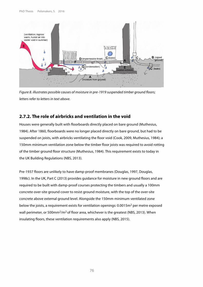
PhD Thesis Pelsmakers, S. 2016
76
Figure 8. illustrates possible causes of moisture in pre-1919 suspended timber ground floors;
letters refer to letters in text above.
2.7.2. The role of airbricks and ventilation in the void Houses were generally built with floorboards directly placed on bare ground (Muthesius,
1984). After 1860, floorboards were no longer placed directly on bare ground, but had to be
suspended on joists, with airbricks ventilating the floor void (Cook, 2009, Muthesius, 1984); a
150mm minimum ventilation zone below the timber floor joists was required to avoid rotting
of the timber ground floor structure (Muthesius, 1984). This requirement exists to today in
the UK Building Regulations (NBS, 2013).
Pre-1937 floors are unlikely to have damp-proof membranes (Douglas, 1997, Douglas,
1998c). In the UK, Part C (2013) provides guidance for moisture in new ground floors and are
required to be built with damp-proof courses protecting the timbers and usually a 100mm
concrete over-site ground cover to resist ground moisture, with the top of the over-site
concrete above external ground level. Alongside the 150mm minimum ventilated zone
below the joists, a requirement exists for ventilation openings: 0.0015m2 per metre exposed
wall perimeter, or 500mm2/m2 of floor area, whichever is the greatest (NBS, 2013). When
insulating floors, these ventilation requirements also apply (NBS, 2015).
Chapter 2: Literature Review
77
However BRE (1998) notes that existing floors often have less than the current minimum
recommended ventilation areas. Yet existing floors with no over-site concrete might need
0.0030m2/m ventilation opening area10 (BRE, 1998, Douglas and Singh, 1995); this is also the
default assumption in the (Rd)SAP floor U-value model (BRE, 2014) and was until the early
1970s also the requirement in Scotland (Douglas, 1998a). It is however unclear what these
standards are based on and if indeed such standards are sufficient to prevent timber rot, or
whether they are overly cautious. Suspended floor void ventilation requirements appear to
have been developed ad-hoc (Harris, 1995) rather than evidence based, as also noted by
Williamson (2006b) for floor ventilation requirements in other countries.
According to Hill (2005), winter void ventilation is generally via stack-effect up through the
floor into the internal spaces (see Section 2.2.2.1.), hence the void might be kept dry.
Furthermore, in winter, due to heat-flow from the spaces above, the uninsulated floor void is
generally warmer than external conditions and incoming external cold air is warmed up and
the relative humidity (RH) reduces (Kurnitski, 2001). Typically in summer, warm, humid air
enters the generally cooler floor void thereby increasing RH, exacerbated by the high thermal
mass of the ground and walls: the warm summer air might be insufficient to increase the air
and surface temperatures of the floor (and hence reduce void RH) (Kurnitski, 2001,
Airaksinen, 2003, Rose, 1994b, Hill, 2005, Samuelson, 1994). This might lead to summer
surface condensation in the void or to moisture build-up (high RH), leading to optimal
mould-growth conditions.
Hill, (2005) suggests that ventilation on its own might be insufficient to deal with significant
amounts of moisture build-up in floor voids and Douglas (1995) acknowledges that even
when voids are well ventilated, humidity can build up in void recesses. While increased void
ventilation might also increase the swift dispersal of moisture build-up (Kurnitski, 2001)
especially in winter (Hill, 2005), this may not always be effective (Harris, 1995). Furthermore,
increased void ventilation leads to an increased evaporation rate from damp soil/surfaces
which might increase moisture build-up in the floor void (Harris, 1995). Increased void
ventilation also leads to increased floor heat-flow as described in Section 2.2.2.2. A balance
between floor void 'health' and heat loss is hence important.
10 Typically 0.0030 m2/m is one airbrick per exposed perimeter and 0.0015 is one airbrick per 2 metres perimeter , according to Anderson (1991a).
PhD Thesis Pelsmakers, S. 2016
78
Sealing airbricks
Clearly, outdoor air cannot dry the floor void if it infiltrates at a higher moisture content than
the floor void itself and instead will bring moisture in; hence Kurnitski (2001) argues that if
there is no moisture source in the void (i.e. if the void is 'moisture insulated') there is no need
to ventilate but acknowledges that "any leakage in the moisture insulation can bring about
high relative humidity" (Kurnitski, 2001). However, Part C of the Building Regulations (NBS,
2013) and industry guidance for the insulation of suspended timber ground floors suggest
that obstructing or reducing floor void ventilation can lead to build-up of moisture in the
floor void (Rickaby, 2014a, EST, 2006a, BRE, 2000). Lack of void ventilation and/or sealing of
airbricks is considered by many to be the cause of moisture build-up in floor voids (Oliver,
1997, Burke, n.d., Douglas, 1998c, Douglas, 1998a, BRE, 1991, Singh, 1998).
Contrary to this, a sealed void is reported by others to prevent moisture build-up risk in
summer (Rose, 1994b, Samuelson, 1994, Lstiburek, 2004), though Kurnitski (2001) points out
the difficulty associated with sealing airbricks to control summer moisture ingress because
air can enter via other ventilation paths.
These latter observations are based on non-UK climates and constructions; while in the UK,
Oliver (1997) notes the importance of unblocking any sealed airbricks in summer. Reduced
void ventilation can occur when (partially) blocking airbricks with insulating material,
whether intentionally (such as when filling the floor void with insulation - see Chapter 6.3.1),
or unintentionally. Note that sealing of airbricks is considered undesirable when radon is
present (Welsh, 1995, Lugg, 1997), however this discussion is excluded for the purpose of this
PhD research.
Chapter 2: Literature Review
79
2.7.3. Implications of moisture build-up in the floor void The main danger of moisture build-up in floor voids is that it can lead to fungal growth and
timber decay (Moses, 1954, Singh, 1998, Oliver, 1997). However, there is little information
about the prevalence of mould growth and timber rot in existing pre-1919 UK dwellings. Few
records of such manifestations appear to exist; though it was reported that from 1945 to
1949, 12.3% of housing repairs around Paddington were primarily for dry rot, affecting
around 2,400 properties (Frankland, 1951). It is unknown whether this occurred in floors or
other construction elements. Most occupants do not realise the presence of fungal growth or
timber decay until some incident indicates its presence (Frankland, 1951), such as fine red
dust (caused by dry rot spores) on floor surfaces (Morton, 2013, Ridout, 2001) or springy
floors (Singh, 1998) or failure of floorboards or floor joists (BRE, 1998).
However, occupant health might be affected prior to any visual manifestation of a problem
as contaminants (such as fungal spores, microbes and bacteria which can thrive in moist
environments) can be transferred from the floor void air flowing into living spaces above as
noted by Frankland (1951), Kroger (2007), Airaksinen (2004, 2003) and (Coulter, n.d.).
Dampness and mould exacerbate asthmatic conditions (Frankland, 1951, WHO, 2009) and
fungal spores are associated with respiratory problems (Park et al., 2004, Verdier et al., 2014).
Moist environments can also give rise to the production of MVOCs (Microbial Volatile Organic
Compounds) by fungal and microbic organisms (Paavilainen, n.d.) which can also effect
human health (Korpi et al., 2009, Fiedler et al., 2001). As such the transfer of air from
contaminated floor voids into internal spaces is a significant concern for occupant health
(Airaksinen, 2007). All airborne spores can be a health hazard but in all cases remedy and
prevention of moisture build-up and water penetration eventually kills the fungus (Ridout,
2001, Oliver, 1997) and reduces occupant exposure.
Much work on contaminant transfer from floor voids into internal spaces above is based on
Finnish apartments which are continuously mechanically ventilated, creating an airflow from
the floor void into the de-pressurised indoor spaces above (Airaksinen, 2003). In the UK,
Victorian houses typically do not have continuous mechanical ventilation and this
phenomena might be less prevalent but is uncharacterised at present. Nevertheless, stack-
effect driven airflow from void to internal spaces and cavities above was observed in
naturally ventilated dwellings (see Section 2.2.2.). This winter stack-effect acts as a drying
mechanism of the floor void (Hill, 2005) and is less pronounced in summer and if buildings
are air-conditioned, the opposite effect can occur in summer, with indoor air infiltrating in
the void spaces (Hill, 2005).
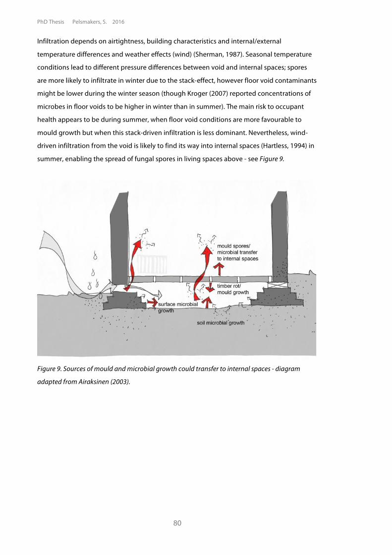
PhD Thesis Pelsmakers, S. 2016
80
Infiltration depends on airtightness, building characteristics and internal/external
temperature differences and weather effects (wind) (Sherman, 1987). Seasonal temperature
conditions lead to different pressure differences between void and internal spaces; spores
are more likely to infiltrate in winter due to the stack-effect, however floor void contaminants
might be lower during the winter season (though Kroger (2007) reported concentrations of
microbes in floor voids to be higher in winter than in summer). The main risk to occupant
health appears to be during summer, when floor void conditions are more favourable to
mould growth but when this stack-driven infiltration is less dominant. Nevertheless, wind-
driven infiltration from the void is likely to find its way into internal spaces (Hartless, 1994) in
summer, enabling the spread of fungal spores in living spaces above - see Figure 9.
Figure 9. Sources of mould and microbial growth could transfer to internal spaces - diagram
adapted from Airaksinen (2003).
Chapter 2: Literature Review
81
2.7.4. Mould growth thresholds
The main occurring organisms in floor voids are wood rotting fungi (such as dry rot and wet
rot) and non-wood rotting fungi, which either grow on timber or on other materials and can
lead to mould growth (Oliver, 1997). Mould growth tends to occur at lower moisture
thresholds (see Appendix 2.C.) and is a precursor of wood-rotting fungi, which require higher
moisture requirements. Hence setting the thresholds for floor void conditions based on
mould growth contamination has the benefit of reduced moisture build-up risk and
therefore also reduced risk from structural damage from timber decay. Mould growth risk
has also been used by most research in this area to evaluate a construction's condition, such
as seminal work by Airaksinen (2003) for Finnish floor voids and Hukka (1999), Viitanen
(2010), Sedlbauer (n.d.) and Johansson (2012) for other internal construction elements.
The strongest drivers for mould growth are a combination of relative humidity, temperature
and exposure time (Sedlbauer, n.d., Paavilainen, n.d.). Of minor importance are other factors
such as PH-value, oxygen and light availability (Sedlbauer, n.d.). Material substrate also plays
a role; timber is the building substrate with the lowest threshold for mould and fungal
growth. Hence conditions inhibiting mould and fungal growth on wood should inhibit it on
other substrates.
Wood can have a high Wood Moisture Content (WMC) if directly in touch with wet surfaces,
but also if in floor voids with high RH: timber as a hygroscopic material will absorb moisture
from the atmosphere until in equilibrium with the surrounding air (Ridout, 2001). Generally
timber decay fungi (such as wet and dry rot ) require $95% RH (or 28-30% WMC, (EH, 2010))
and temperatures of 0ºC to 45ºC; while mould growth can occur with RH of $75% in a similar
temperature range - see Appendix 2.C. Timber decay does not generally occur below 22-24%
WMC, often lowered to 20% as a safety measure (Ridout, 2001) (or equivalent to around 90%
RH (EH, 2010)) and is ideally below 15% WMC (Ridout, 2001) (or <75% RH (EH, 2010)). At very
high RH (> 97% RH or wet materials) bacteria also cause smell and health problems similar to
mould fungi (Viitanen et al., 2010). Fungi usually require stable, unchanging environments to
thrive in and are therefore often limited to the damp zone (Ridout, 2001).
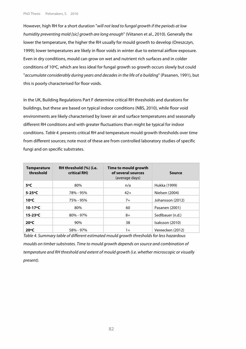
PhD Thesis Pelsmakers, S. 2016
82
However, high RH for a short duration "will not lead to fungal growth if the periods at low
humidity preventing mold [sic] growth are long enough" (Viitanen et al., 2010). Generally the
lower the temperature, the higher the RH usually for mould growth to develop (Oreszczyn,
1999); lower temperatures are likely in floor voids in winter due to external airflow exposure.
Even in dry conditions, mould can grow on wet and nutrient rich surfaces and in colder
conditions of 10ºC, which are less ideal for fungal growth so growth occurs slowly but could
"accumulate considerably during years and decades in the life of a building" (Pasanen, 1991), but
this is poorly characterised for floor voids.
In the UK, Building Regulations Part F determine critical RH thresholds and durations for
buildings, but these are based on typical indoor conditions (NBS, 2010), while floor void
environments are likely characterised by lower air and surface temperatures and seasonally
different RH conditions and with greater fluctuations than might be typical for indoor
conditions. Table 4. presents critical RH and temperature mould growth thresholds over time
from different sources; note most of these are from controlled laboratory studies of specific
fungi and on specific substrates.
Temperature threshold
RH threshold (%) (i.e. critical RH)
Time to mould growth of several sources
(average days) Source
5ºC 80% n/a Hukka (1999)
5-25ºC 78% - 95% 42+ Nielsen (2004)
10ºC 75% - 95% 7+ Johansson (2012)
10-17ºC 80% 60 Pasanen (2001)
15-23ºC 80% - 97% 8+ Sedlbauer (n.d.)
20ºC 90% 38 Isaksson (2010)
20ºC 58% - 97% 1+ Vereecken (2012) Table 4. Summary table of different estimated mould growth thresholds for less hazardous
moulds on timber substrates. Time to mould growth depends on source and combination of
temperature and RH threshold and extent of mould growth (i.e. whether microscopic or visually
present).
Chapter 2: Literature Review
83
Predicting mould growth is complicated by the fact that the in-situ factors affecting growth
fluctuate with the weather and the season and localised effects may not be representative of
the rest of the construction (Oreszczyn, 1999). The need for longitudinal measurements of
temperature and RH to assess risk of fungal growth is emphasised by Pasanen (2001) and
Airaksinen (2013). As such most mould growth research has been conducted in laboratories
to determine the likelihood and extent of different fungal growth under different
environmental conditions with different exposure times (Oreszczyn, 1999) and sometimes
also under fluctuating conditions. These laboratory studies are also the basis for mould
growth prediction models and 'post-processor'11models (H. Altamirano-Medina, 2009).
However, the big differences between lab and in-situ conditions can make mould growth
predictions unreliable and depending on which source or model used, different mould
growth risks could be diagnosed (Vereecken and Roels, 2012, Vereecken et al., 2015, H.
Altamirano-Medina, 2009). Different models exist, but most are only suitable for interior
surfaces, such as ESP-r model, Condensation Targeter II and WUFI-BIO 3.2. (H. Altamirano-
Medina, 2009, Oreszczyn, 1999, Fraunhofer, 2015). VTT (The Finnish Technical Research
Centre) developed a mathematical research mould growth model, which was used for
evaluating Finnish floor voids by Airaksinen (2003) for Scandinavian timbers (Vereecken and
Roels, 2012). This model was recently updated and validated with Finnish floor void data
(Airaksinen, 2013) but the model was not publicly available at the time of writing and ideally
requires year-long seasonal data to evaluate the mould growth risk12(Airaksinen, 2013,
Pasanen, 2001).
2.7.5. Insulating floors and moisture build-up risk In uninsulated floors in winter, when the void air is warmer than the external air, the external
air entering the void is warmed up and its relative humidity (RH) decreases, keeping void
spaces dry. In summer, when warmer, humid external air can enter the void mainly through
airbricks, this increases the risk of surface condensation as the void air and surfaces are cooler
than outside and the void' s thermal mass draws heat from the warm incoming air, further
reducing the void air temperature and increasing the void RH. This might lead to more
optimal void RH and temperature conditions for mould growth.
11 'Post-processor' models are models which evaluate mould growth risk based on actual RH and temperatures collected rather than predictive models which asses a structure's mould growth risk based on modelled temperatures and RH. 12 Hence this model could therefore not be used for the data collected here. Other research models exist such as BREVENT (Edwards, 1990) and CFD software MOISTURE-EXPERT, developed for a Southern USA climate and floor construction (Karagiozis, 2005). However these were not procurable and required unavailable site-data as input parameters.
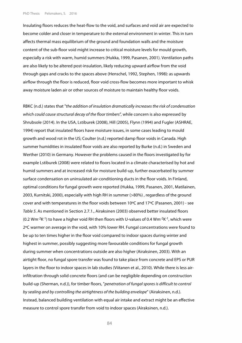
PhD Thesis Pelsmakers, S. 2016
84
Insulating floors reduces the heat-flow to the void, and surfaces and void air are expected to
become colder and closer in temperature to the external environment in winter. This in turn
affects thermal mass equilibrium of the ground and foundation walls and the moisture
content of the sub-floor void might increase to critical moisture levels for mould growth,
especially a risk with warm, humid summers (Hukka, 1999, Pasanen, 2001). Ventilation paths
are also likely to be altered post-insulation, likely reducing upward airflow from the void
through gaps and cracks to the spaces above (Henschel, 1992, Stephen, 1998): as upwards
airflow through the floor is reduced, floor void cross-flow becomes more important to whisk
away moisture laden air or other sources of moisture to maintain healthy floor voids.
RBKC (n.d.) states that "the addition of insulation dramatically increases the risk of condensation
which could cause structural decay of the floor timbers", while concern is also expressed by
Shrubsole (2014). In the USA, Lstiburek (2008), Hill (2005), Flynn (1994) and Fugler (ASHRAE,
1994) report that insulated floors have moisture issues, in some cases leading to mould
growth and wood rot in the US; Coulter (n.d.) reported damp floor voids in Canada. High
summer humidities in insulated floor voids are also reported by Burke (n.d.) in Sweden and
Werther (2010) in Germany. However the problems caused in the floors investigated by for
example Lstiburek (2008) were related to floors located in a climate characterised by hot and
humid summers and at increased risk for moisture build-up, further exacerbated by summer
surface condensation on uninsulated air-conditioning ducts in the floor voids. In Finland,
optimal conditions for fungal growth were reported (Hukka, 1999, Pasanen, 2001, Matilainen,
2003, Kurnitski, 2000), especially with high RH in summer (>80%) , regardless of the ground
cover and with temperatures in the floor voids between 10ºC and 17ºC (Pasanen, 2001) - see
Table 5. As mentioned in Section 2.7.1., Airaksinen (2003) observed better insulated floors
(0.2 Wm-2K-1) to have a higher void RH then floors with U-values of 0.4 Wm-2K-1, which were
2ºC warmer on average in the void, with 10% lower RH. Fungal concentrations were found to
be up to ten times higher in the floor void compared to indoor spaces during winter and
highest in summer, possibly suggesting more favourable conditions for fungal growth
during summer when concentrations outside are also higher (Airaksinen, 2003). With an
airtight floor, no fungal spore transfer was found to take place from concrete and EPS or PUR
layers in the floor to indoor spaces in lab studies (Viitanen et al., 2010). While there is less air-
infiltration through solid concrete floors (and can be negligible depending on construction
build-up (Sherman, n.d.)), for timber floors, "penetration of fungal spores is difficult to control
by sealing and by controlling the airtightness of the building envelope" (Airaksinen, n.d.).
Instead, balanced building ventilation with equal air intake and extract might be an effective
measure to control spore transfer from void to indoor spaces (Airaksinen, n.d.).
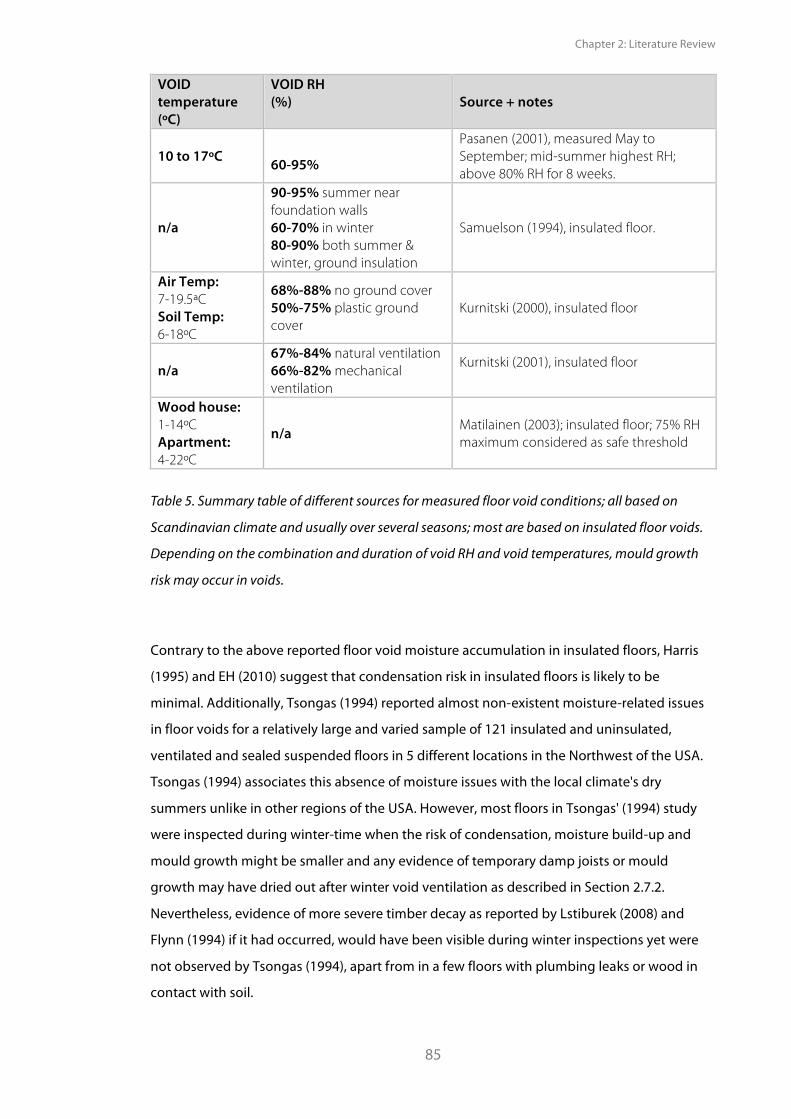
Chapter 2: Literature Review
85
VOID temperature (ºC)
VOID RH (%) Source + notes
10 to 17ºC 60-95%
Pasanen (2001), measured May to September; mid-summer highest RH; above 80% RH for 8 weeks.
n/a
90-95% summer near foundation walls 60-70% in winter 80-90% both summer & winter, ground insulation
Samuelson (1994), insulated floor.
Air Temp: 7-19.5ªC Soil Temp: 6-18ºC
68%-88% no ground cover 50%-75% plastic ground cover
Kurnitski (2000), insulated floor
n/a 67%-84% natural ventilation 66%-82% mechanical ventilation
Kurnitski (2001), insulated floor
Wood house: 1-14ºC Apartment: 4-22ºC
n/a Matilainen (2003); insulated floor; 75% RH maximum considered as safe threshold
Table 5. Summary table of different sources for measured floor void conditions; all based on
Scandinavian climate and usually over several seasons; most are based on insulated floor voids.
Depending on the combination and duration of void RH and void temperatures, mould growth
risk may occur in voids.
Contrary to the above reported floor void moisture accumulation in insulated floors, Harris
(1995) and EH (2010) suggest that condensation risk in insulated floors is likely to be
minimal. Additionally, Tsongas (1994) reported almost non-existent moisture-related issues
in floor voids for a relatively large and varied sample of 121 insulated and uninsulated,
ventilated and sealed suspended floors in 5 different locations in the Northwest of the USA.
Tsongas (1994) associates this absence of moisture issues with the local climate's dry
summers unlike in other regions of the USA. However, most floors in Tsongas' (1994) study
were inspected during winter-time when the risk of condensation, moisture build-up and
mould growth might be smaller and any evidence of temporary damp joists or mould
growth may have dried out after winter void ventilation as described in Section 2.7.2.
Nevertheless, evidence of more severe timber decay as reported by Lstiburek (2008) and
Flynn (1994) if it had occurred, would have been visible during winter inspections yet were
not observed by Tsongas (1994), apart from in a few floors with plumbing leaks or wood in
contact with soil.
PhD Thesis Pelsmakers, S. 2016
86
Whether the floor void conditions reach or exceed critical mould growth thresholds will
depend on many variables, including climate, extent and characteristics of floor insulation
and dwelling construction, alongside the presence of moisture sources, causes of moisture
build-up (Section 2.7.1.) and moisture management solutions (see Appendix 2.D.). The dry rot
timber decaying fungi require a food source such as timber and calcium, which are present in
brick and cement/lime mortar but also in rock or glass wool insulation (Douglas and Singh,
1995), commonly used in buildings (EH, 2010), including floors. EST (2006a) recommends
that the floor void is to be inspected for damp and timber rot and should be rectified prior to
insulating the floor. Nevertheless, there is little conclusive evidence that insulating
suspended floors on its own increases mould growth risk. Given the many variables that
influence moisture accumulation, it is unsurprising that several studies reported high
moisture build-up in insulated floors, while others reported no issues. Figure 10. summarises
the possible unintended consequences associated with insulating floors based on
international case study evidence.
Furthermore, while physical principles remain the same, it is unclear to which extent these
findings transfer to pre-1919 suspended timber ground floor constructions in the UK: the
cases described have significantly different climate, floor construction methods/materials
and building ventilation/heating and cooling systems. In addition, some condensation risks
in the void were associated with cooling ducts in the void, but air-conditioned dwellings in
the UK are rare, though could increase in the future (He, 2005, Pathan, 2008).13 Without
characterisation of existing floor void conditions and in the absence of evidence of insulated
floor void conditions and increased moisture build-up in the UK, no clear conclusions can be
drawn whether similar issues occur in the UK. Similar to suspended timber ground floor heat-
flow not being well characterised in-situ, neither are existing hygrothermal floor void
conditions, even less so once insulated. While it is beyond the scope of this thesis research to
define floor void ventilation requirements and safe moisture thresholds, initial empirical floor
void data was collected; the research design of which is set out in Chapter 5.2.3.2. The data
collection was restricted in time and other limitations (as described in Chapter 5 and 6) and
no pre/post insulation floor void comparisons could be made; significant further research is
required.
13 Cooling ducts in the UK might also be differently designed and installed, such as avoiding running uninsulated cooling ducts through the void.
Chapter 2: Literature Review
87
Figure 10. Summary diagram of possible unintended consequences associated with insulating
floors, based on international case study evidence; in the absence of UK evidence, it is unclear how
this transfers to the UK. Adapted from Pelsmakers (2013).
2.8. Summary The literature review highlighted several research gaps in the characterisation of floors and
floor thermal performance, and highlighted uncertainties and limitations of current research.
Of particular note was the lack of in-situ floor heat-flux measurements and difficulty to
compare in-situ with published and modelled U-values; different recommendations in policy
and in industry could result in different retrofit decision-making, depending on which values
are used.
Despite the availability of some interesting results related to floor heat-flow and sub-floor
airflow, many of these findings were difficult to directly transfer to the larger UK housing
stock due to the fact that the work was either undertaken in test-cells or conducted for
different purposes than to estimate and compare floor U-values. Likewise, the overseas
research findings have probably limited applicability to pre-1919 UK dwellings due to the
differences in climate and building design.
PhD Thesis Pelsmakers, S. 2016
88
Despite these limitations, certain principles can be transferred more generally, including the
complexity of both measuring and modelling floor U-values and the possible factors
influencing floor heat loss in pre-1919 UK dwellings. We can expect that suspended timber
ground floors are likely to have increased heat-flow along the perimeter and have varying U-
values, related to the varying airflow through airbricks. The greater the sub-floor ventilation,
the greater the floor heat loss is expected.
The insulation of suspended timber ground floors could potentially provide significant heat-
flow reductions as highlighted by Harris (1997) and Currie's (2013) work; this would likely
lead to associated energy savings and carbon emission reductions. Multiple options are
available in terms of floor insulation (Section 2.6), however the relative merits and limitations
of these floor insulation approaches in actual pre-1919 UK dwellings is poorly characterised.
Most importantly, the lack of pre/post intervention studies create uncertainty about the
actual performance and efficacy of interventions.
While an apparent divergence between in-situ measured and published U-values was found
for suspended ground floors, robust comparison between sources was not possible, partly
due to the lack of sufficient detail and transparency of both published models but also in-situ
measured sources. In addition, where measurements are taken is expected to significantly
affect estimated U-values.
Current U-value conventions and tools might be ill-suited to accurately predict the actual U-
values of pre-1919 traditional solid walls (Baker, 2011b, Rye, 2010, Gentry, 2010, Zero Carbon
Hub, 2010) and this also raises questions about the actual U-values of suspended timber
ground floors and the cost-effectiveness and benefits of retrofit measures and highlights the
importance of research in this area.
Finally, aside from providing U-value reductions, floor insulation might have other benefits,
such as impacting positively on occupant thermal comfort. However, insulating floors might
also potentially have a number of unintended consequences, such as changing floor void
conditions to become ideal for mould growth, which can impact on occupant health. While
some research exists on the effects of void conditions on mould growth and humidity levels,
this work has been carried out in constructions and climates outside the UK, and the extent
of their generalisibility and transferability to the UK is unknown - see Section 2.7.
Chapter 2: Literature Review
89
2.9. Research questions and objectives Given the premises outlined above, the work presented in this PhD thesis focuses on testing
floor heat-flow theory and testing and refining measuring methods, practices and analysis
techniques for uninsulated and insulated floors. Additionally, this research adds original
knowledge about uninsulated suspended timber ground floor heat-flow and what the
impact of insulating such floors might be, leading to research outcomes that are relevant to
industry practice, policy and academia. In particular it aims to answer the following research
questions:
1. How should in-situ suspended timber ground floor U-values be estimated?
2. What is the in-situ measured thermal transmittance of floors and how does it
compare to model predictions?
3. How does the in-situ thermal performance of a case study floor change after
intervention measures?
⁃ 3.1 What are the thermal comfort implications of insulated and uninsulated
floors?
The purpose of this PhD research is to test and construct knowledge and understanding of
suspended timber ground floor heat-flow and how to measure this heat-flow. The research
objectives are three-fold:
• To test, refine and develop research design and analysis methods to estimate the
in-situ measured U-value of floors.
• To quantify the in-situ thermal transmittance of some existing floor constructions.
• To quantify the in-situ heat loss reduction potential and thermal comfort
implications of some floor interventions.
To meet the above research objectives, the research design takes a multi-method approach
for case studies research with some experimental testing, using primarily quantitative
methods supported by some qualitative methods such as building and thermographic
surveying and visual observations. These methods are discussed, together with research
limitations, in Chapter 3 and in more detail in the relevant chapters.
PhD Thesis Pelsmakers, S. 2016
90
2.10. Definitions Terms and definitions used in this PhD research are outlined below to clarify how a number
of technical terms and definitions are used in the following chapters. Additionally, to allow
for comparison purposes between floor model outputs (U-values) and most literature
sources (U-values), in-situ measurement results are presented as U-values rather than R-
values. Where R-values are stated in literature, R-values will be used.
'Pre-1919 dwellings' and 'pre-1919 floors' are studied and for the purpose of this thesis
research include those constructed between 1860 and 1919, excluding the pre-1870 floors
without ventilated void spaces, while also excluding basement floors. More recent
suspended timber ground floors constructed with cavity walls instead of solid brick walls are
excluded, though aspects of this PhD research might be relevant to these constructions.
'Floors' always refers to 'suspended ground floors' unless specifically defined otherwise and
by this is meant the whole floor system, i.e. the floor surface including the void, its
substructure and the foundation walls and ground to the outside.
Heat loss is used when describing all heat loss mechanisms of the floor, including air-
leakage.
'Floor thermal performance' is used as a generic description of all of the heat loss
characteristics.
'Floor characterisation' is a generic term used when describing the floor's characteristics,
such as void condition, dimensions, heat-flow, thermal comfort etc.
Heat-transfer is the movement of heat by conduction, convection or radiation.
Heat-flux is the rate of heat-transfer (W- Js-1)
Heat-flow is the heat-flux density, q (Wm-2)
U-value is the thermal transmittance (Wm-2K-1) and 'point U-value' , also abbreviated by
Up-value, is the term used as a generic description of the small area-based in-situ U-value
measurement on a certain location on the floor.
Chapter 2: Literature Review
91
'Whole floor U-values' refers to the area-weighted summation of several in-situ point
Up-value measurements (see Chapter 4.4.2.) to allow for comparison with models; models are
based on whole floor U-values.
'Floor U-value model' is used primarily to denote mathematical calculations, which attempt
to describe steady-state suspended ground floor U-values, and are generally simplified
models of the floor system's thermal characteristics. Software models tend to use these
mathematical models and calculate a whole floor's U-value.
'Low-resolution' and 'high-resolution' refers to in-situ monitoring in just a few locations on
a floor or to many locations on a floor respectively. Given that estimated in-situ U-values are
based on small area, or 'point' measurements of a construction element, this differentiation
is important: averaging a few 'point' measurements to estimate a whole floor's U-value leads
to much greater uncertainty compared to many points being averaged to determine a whole
floor U-value - see Chapter 3.3.2 and Chapter 4.4.2

PhD Thesis Pelsmakers, S. 2016
92
Chapter 3: Research design and methodology
93
Chapter 3: Research design and
methodology
3.1. Introduction The purpose of this chapter is to give an overview of the research design and research
methodology supporting the research questions and objectives identified at the end of the
previous chapter (Section 2.9.).
This chapter is split in three parts: the first part presents an overview of the available
research methods, with a brief discussion of the benefits and limitations of each method,
to give a rationale for the methodological choices in this work. Part 2 presents and
critically evaluates measurement protocols available for in-situ U-value data collection,
data and error propagation analysis and examining theoretical and practical issues
affecting in-situ measuring of floors, which are further described and tested in Chapter
4. The third part presents the testable hypotheses and primary data collected for this
thesis and the sampling approach used, discussing the generalisability and the relevant
research ethics.
For ease of reference, detailed research design for specific case-studies are set out in the
appropriate individual field-work chapters prior to presentation, analysis and discussion
of results.
PhD Thesis Pelsmakers, S. 2016
94
3.2. Part 1: Research methods to investigate suspended
timber ground floor heat loss There are several research methods used to characterise in-situ floor heat loss. These
methods include in-situ heat-flux measurements, infrared thermography, co-heating tests,
blower door tests and tracer gas techniques. Their advantages and limitations are briefly
discussed in the following sections.
3.2.1. In-situ heat-flux measurements In-situ heat-flux measurements provide an estimated U-value (thus often referred to as in-
situ U-value measurements) and this is detailed in Section 3.2.6 and 3.3.
In-situ heat-flux measurements are increasingly used in industry and in academia to evaluate
a building element's actual performance, in both new and existing buildings, and to compare
in-situ measured to predicted performance, e.g. Li (2014), Rye (2010), Baker (2011b) and Ficco
(2015). In-situ heat-flux measurements have been used for suspended timber ground floors
only in a limited number of studies. As described in Chapter 2.4., Harris (1997) used multiple
heat-flux sensors in a test-cell study; while Currie (2013), Snow (2012) and Baker (2011a)
measured single points on a suspended timber ground floor and Miles-Shenton (2011)
measured in a few floor locations. In New Zealand, Isaacs (1985b) measured heat-flow at
single area locations on suspended ground floors. This research method was also used by
several others for solid ground floors, e.g. Trethowen , Delsante (1990) and Thomas (1999,
2009).
These studies however present results from single point-measurements (i.e. at low
resolution), with the exception of Harris (1997) and Miles-Shenton (2011); the latter indicated
that there is a large variation of floor heat-flow depending on measurement location, based
on only a few measuring locations. Similar variation in heat-flow has been observed by a few
in-situ studies for solid ground floors, e.g. Delsante (1990). In-situ heat-flux measurements
have also been successfully used with one or a few point measurements in pre/post
insulation interventions, e.g. Byrne (2013) and Stevens (2013) for walls and by Currie (2013)
for pre/post monitoring of one point measurement on a suspended timber ground floor.
Chapter 3: Research design and methodology
95
Because of how in-situ measurements are taken, they only provide a 'point' measurement of
the heat-flux on that location on a given surface under certain conditions over a certain
amount of time. Because of the expected variation in heat-flow on a floor, important
considerations include sensor placement on surfaces, sensor number and how to devise the
best set up to compare to models such as where to measure temperatures. However none of
this is well characterised and this is further discussed in Section 3.3. Another limitation is that
in-situ measurements on the floor surface in occupied dwellings are disruptive and limit
sensor location choice, quantity and monitoring duration. In occupied dwellings, there is also
a risk of occupant interference and lack of control over heating patterns, affecting the
variables being measured. A sufficient temperature difference between the internal and
external environment is generally also required to reduce the relative measurement error,
which means that any monitoring using this method should be undertaken during the
winter season1- see Section 3.3.3.
While in-situ heat-flux measurements measure conductive heat-flow, radiative and
convective components influence the observed conductive rate of heat-transfer but these
mechanisms cannot be isolated with in-situ heat-flux sensors alone. This research method
also excludes other heat loss mechanisms at play, as identified in Chapter 2.2.2., such as heat
loss from forced convection and ventilative stack effects.
3.2.2. Infrared thermography Infrared (IR) thermography helps the understanding of heat loss through construction
elements by visually representing surface temperatures (from which heat loss might be
inferred) caused by for example construction irregularities or air leakage paths (BSI, 1998)
and moisture spots (Grinzato, 1998). While a detailed heat-flow estimate cannot be obtained
from a thermographic survey, it can provide insights into the spatial distribution of heat loss
and features that may be of interest to study using heat-flux sensors. For this reason, this
qualitative method is useful in heat-flux sensor placement (ASTM, 2007a) to help identify any
areas of interest for investigation (or exclusion). Given that IR thermography cannot
accurately estimate floor heat-flow, it cannot be compared to model outputs.
Similarly to in-situ heat-flux measurements, generally a sufficient temperature difference
between the internal and the external environment is required (usually about 10ºC (BSI,
1998, EST, 2006), though might depend on camera specification) and observations are
dependent on changing internal and external environmental conditions (Fox, 2012).
1 This seasonal limitation might be overcome by using Biddulph's (2014) analysis method, though this has not yet been tested widely, including for floors.
PhD Thesis Pelsmakers, S. 2016
96
3.2.3. Co-heating Co-heating is a whole building heat loss measurement method, where a space or a building
are kept at a constant internal temperature (usually for 1 to 3 weeks in winter) and the
energy required to maintain this temperature is measured (Wingfield, 2010b). Co-heating
gives a whole building Heat Loss Coefficient, which could be useful to identify relative
changes between pre/post retrofit.
This method might be combined with simultaneous in-situ heat-flux measurements
(Wingfield, 2010b). If in-situ floor heat-flux measurements are taken, they will contribute to a
better understanding of the proportional and absolute floor heat-transfer as measured
during the co-heating measurement conditions.
Given the extent of control required over the internal conditions to reach and be kept at
steady-state, co-heating is usually undertaken in unoccupied houses, and actual occupancy
patterns are not reflected in the co-heating outputs. Air-mixing fans are used to mechanically
mix the air, affecting the rate of heat-flow through different mechanisms; this also does not
reflect real occupancy patterns. Co-heating accuracy is strongly associated with external
environmental conditions (Stamp, 2015).
3.2.4. Blower door tests Air infiltration measurements by pressure testing can be used to understand the whole
building air infiltration and ventilative heat loss through gaps and cracks. Air leakage can be
quantified by the air-flow rate and is the leakage of air (m3/hr) into and out of the building
per metre square (m2) of the building fabric at a 50Pa pressure difference between in-side
and outside (ATTMA, 2010, CIBSE, 2015). This is undertaken with fan pressurisation –
commonly known as 'blower door tests' (Sherman). Air leakage can also be defined by an air
change rate: air changes per hour (ach-1) express the air leakage by the volume of the space
(CIBSE, 2015). As both are used in literature, for comparison purposes, both are referred to
when communicating results in this thesis.
A blower door test result however cannot separate the ground floor's air leakage from the
whole building leakage, unless the floor is separately pressurised. Some researchers have
attempted to measure the air leakage of the floor void itself by placing the blower door fan
in a large airbrick opening, e.g. DeWitt (1994). However, in the UK the airbricks are typically
the size of one brick, i.e. 215 x 65mm, which is too small for the typical blower door fan used
for air leakage tests.
Chapter 3: Research design and methodology
97
This method also does not directly capture heat loss and the estimated air leakage rates are
under test conditions, including taping up of ventilation openings and under
(de)pressurisation situations and not actual building pressure differences. Furthermore
external environmental conditions need to be sufficiently stable to undertake a blower door
test (ATTMA, 2010, ISO, 2006), though blower door tests are not seasonally bound.
Nevertheless, blower door tests could give an estimate of the airtightness improvement of
the floor pre/post intervention measures if no other interventions take place and if tests are
undertaken in similar conditions pre/post intervention. This was done by Saint-Gobain (2014)
in a lab to investigate the effect of interventions on building airtightness, including a floor
intervention, and is further described in Section 6.5.1.
3.2.5. Tracer gas techniques Suspended floor air leakage rates and paths can also be measured with tracer gas techniques
as discussed in e.g. Hartless (1994), Edwards (1990), Basset (1988) and Williamson (2000).
Typically, tracer gases are released and mixed in the floor void and their decay and release
into the internal spaces above is measured over time. Tracer gases could be used to
investigate the relative improvement in air-infiltration of the floor post-intervention. This
technique also allows for the understanding of the flow of air between internal spaces (Riffat,
1988), and to understand the flow of air from void to other internal spaces under different
environmental conditions.
However, this technique requires repeated testing to understand variability in different
external conditions; it is expensive and tracer gases are difficult to mix in the generally tight
in-situ sub-floor voids as noted by for example Edwards (1990) and Williamson (2000). While
electrical fans in the airbricks can be used to mix the tracer gases in the void (Hartless, 1994)
this changes the natural ventilation paths and hence changes exactly what is being
measured. Given that fan-mixing is likely to affect in-situ U-value measurements, use of
tracer gas techniques should be undertaken sequentially rather than simultaneously with in-
situ heat-flux measurements.
PhD Thesis Pelsmakers, S. 2016
98
3.2.6. Justification for selected research method
The research questions as set out in Chapter 2.9. focus this study on a single building
element in in-situ conditions. The use of air-mixing fans in both co-heating tests and tracer-
gas studies, preclude the study (or replication) of occupied dwelling conditions. Further,
given the difficulty of isolating a single building element in most measuring methods, in-situ
heat-flux measurements were considered to be the most suitable research method for the
proposed research. Additional reasons in favour of in-situ U-value measurements are listed
overleaf:
⁃ In-situ heat-flux measurements have been used extensively for the investigation of
the thermal performance of a variety of construction elements, including a limited
number of suspended timber ground floors - see Chapter 2.4.2. In this thesis, in-situ
heat -flux measurements of floors will add to the other in-situ results, investigate
comparison with models and increase knowledge about the thermal performance of
floors.
⁃ In-situ heat-flux measurements have been used for some pre/post intervention
studies, including for floors - e.g. Currie (2013) observed one point measurement on
a floor pre/post insulation and Harris (1997) measured pre/post insulation floor
performance in a test-cell - see Chapter 2.4.
Furthermore, a thermographic survey can support in-situ heat-flux measurement placement,
while blower door tests will be used as a secondary research method where pre/post
interventions take place to investigate the effect of the floor intervention on the overall
dwelling's air leakage - see Chapter 6.5.1. Given the previously described limitations of
pressurising the floor void itself as well as the difficulty of mixing tracer gases in confined
floor void spaces, the investigation of sub-floor air change rates is considered beyond the
scope of this research and is noted for future research purposes.
Chapter 3: Research design and methodology
99
3.2.6.1. Overcoming limitations
There are however several limitations of in-situ heat-flux measurements in general and more
specifically in relation to suspended timber ground floors, including issues raised previously
in Section 3.2.1. and Chapter 2.4., such as practical aspects of measuring in occupied houses;
limited floor measurements undertaken so far; measurement resolution issues and
comparability to models and other sources. Other potential issues are resource limitations,
inability to capture all heat loss mechanisms and confounding variables. However, with
careful research design, the impact of these disadvantages might be minimised. A summary
of the main limitations are listed below and overleaf, alongside how these limitations might
be controlled for or minimised.
1. Practical issues with measuring floors in occupied dwellings: daily usage of floor
surfaces limits where and how many sensors can be placed as well as the monitoring
duration. This could be minimised by monitoring in an unoccupied dwelling, a
thermal chamber or test-cell, however close replication of a typical floor
construction, its junctions and a realistic approach to space-heating would be
required to reflect typical construction and occupation - see Section 3.4 and research
design in Chapters 4.3 and 5.2.
2. Point measurements on a large surface area and difficulty to compare to
models: one point U-value is unlikely to be representative of the total element
U-value (ASTM, 2007a) - see Section 3.3.2., Chapter 4.4.2.5, 4.4.3. and 5.3. for further
discussion. Undertaking multi-point (i.e. high resolution) measurements will aid the
understanding of the spread of floor heat-flow. Doing so will also support the
understanding of the applicability of point measurements in pre/post comparisons,
and support the testing of point U-value averaging techniques to obtain whole floor
U-values to compare to models. Use of infrared thermography can help with sensor
placement and with estimation of whole-floor U-values - see Chapter 4.4.2.
3. Not all heat-loss may be captured, such as the impact of air leakage of the floor on
dwelling heat loss, which is also excluded in floor U-value models. For pre/post
retrofit measures, blower door tests might give an indication of the floor's air leakage
and any impacts arising from interventions. Monitoring heat loss with open and
sealed airbricks might indicate the impact of floor void ventilation on observed heat-
flow - see Chapters 4.4.4. and 5.3.7.
4. Different measurement and analysis conventions and methods exist which
could affect U-value determination - this will be further investigated; full discussion
in Section 3.3. and in Chapter 4.4.5 and 5.3.3.
PhD Thesis Pelsmakers, S. 2016
100
5. Time consuming to undertake and limited to the heating season: field studies
are limited to the winter heating season, limiting the number of studies that can be
undertaken as well as limiting the time-scale of pre/post intervention monitoring -
see Section 3.4. Access to an environmental chamber would disconnect
measurements from the winter period, however this is subject to other limitations -
see Chapter 4.3.
6. Short-term and seasonally changing variables as confounders in pre/post
intervention field studies: changing external environmental conditions and
seasonal changes of the ground will affect in-situ U-value estimates; there are
potential confounding effects when undertaking pre/post intervention studies. This
can be minimised by:
⁃ access to a thermal chamber with a replicated floor construction, such as the Salford
Energy House; limitations of a thermal chamber are discussed in Section 3.4. and in
Chapter 4.3.
⁃ analysing field data with dynamic methods instead of the more commonly used
steady-state analysis techniques. Given that dynamic methods are not well
characterised for suspended ground floors, steady state analysis was applied in this
thesis.
⁃ measuring other external variables such as solar radiation, wind-speed as well as void
airflow, and ground temperatures and heat-fluxes might give additional useful
insights to support understanding of possible confounding variables; see Chapter
6.3.2.
⁃ Access to an unoccupied control house over the same period of the study might be
useful; an occupied control house may introduce other variables such as occupant
behaviour and different heating patterns, affecting the observed heat-flow - see
Chapter 6.
⁃ monitoring heat-flow over a whole year or longer might provide a year-average
U-value and other useful insights into the different mechanisms affecting heat
transfer; this would also be aligned to current model assumptions. However in
practice access to case-study dwellings is normally short-term, making long term
longitudinal studies highly unlikely, especially if also monitored at high-resolution.
Chapter 3: Research design and methodology
101
3.2.7. Other research methods used The sampling of field studies and exploratory studies are described in Part 3 of this chapter
(Section 3.4.) In addition to in-situ heat-flux monitoring, other in-situ studies were
conducted: (a.) floor void conditions of a field study were monitored pre/post intervention
over a short period only, as described in Chapter 5.2.3. and (b.) a brief thermal comfort study
and the potential impact of air leakage on thermal comfort, as presented in Chapter 6.5. This
study was also supported by visual observations and building surveying as described in the
appropriate chapters. Additionally, literature reviews and software modelling tools were also
used and are described in the following sections.
3.2.7.1. Literature review
This PhD thesis builds on existing research along seven key themes: (1.) Victorian dwellings
and their construction (2.) physics of ground floor heat-transfer (3). in-situ heat-flux
measurements and protocols (4.) floor void ventilation (5.) insulation of suspended timber
ground floors (6.) mould growth and timber rot and (7.) thermal comfort. Other topics
included statistical analysis techniques and experimental research design. Based on the
literature review above and as set out in Chapter 2, it appears that only a limited amount of
research is available specifically related to suspended ground floors and some of it spans
different climates and construction methods and is often sparse on research and analysis
methods used. Most literature was found via regular Web of Knowledge, library and Google
Scholar searches as well as construction and industry databases. More detail of the key
sources are listed in Appendix 3.A.
3.2.7.2. Modelling software
Floor U-value models as described in Chapter 2.3. were used to compare in-situ measured
with modelled floor U-values. Separately, airtightness was investigated by estimating the
impact of air leakage through floors on the whole dwelling with the Reduced Standard
Assesment Procedure (RdSAP) - see Chapter 6.5.1. and below.
Floor U-value models are useful to give insights into estimated U-values of different floors
modelled and to compare to in-situ measured U-values. As discussed in Chapter 2.3., it is
unknown whether model simplifications and input assumptions have a significant effect on
the accuracy of outputs and how this compares to in-situ measured floor U-values.
PhD Thesis Pelsmakers, S. 2016
102
Certain interventions (airtightness measures) cannot be modelled with these U-value
models, though this is also not taken into account when undertaking in-situ heat-flux
measurements. An excel spread-sheet was set up to model the suspended ground floor
U-value in accordance with RdSAP (BRE, 2011), CIBSE Guide A (CIBSE, 2015) and ISO-13370
(BSI, 2009) on which the former two models are based.
The superseded CIBSE-1986 model (CIBSE, 1986) was also included for comparison purposes.
Default model input assumptions for material properties were used to model case-study
floors, unless actual field data was available, for example from a building survey. Initial
spreadsheet validation of the ISO-13370 model was achieved by comparing outputs with a
commercially available floor U-value software calculator, BuildDesk U, which is based on
ISO-13370 (BuildDesk, 2012). The CIBSE-1986 model was validated by use of a sample U-
value floor calculation provided in CIBSE (1986). The use of the spreadsheet allowed the
benefit of input and output transparency of the different variables, unlike commercial
software. The same ISO-13370 and CIBSE-1986 equations were also scripted in R-software to
undertake a brief sensitivity analysis of the different variables - see Section 4.4.3. As explained
in Chapter 2.3 and as undertaken in this research, floor U-value models include adjustments
for joist presence (after BSI 6946) unless stated otherwise but exclude linear thermal
bridging; research of the latter has been noted for further research.
For whole dwelling air leakage (see Chapter 6.5.1.), measured results were also compared to
models. BREVENT, a simplified model developed decades ago by the BRE to model building
ventilation, was used to model stack-effect by e.g. Edwards (1990) but is no longer in use
(Hartless, 2012). The software EnergyPlus was recently used by Gauthier (2014) to investigate
the impact of ventilation through a suspended timber ground floor on thermal stratification.
To do so, the entire building needs to be modelled in a complex dynamic model based on
many input assumptions, e.g. assumed floor surface gaps and cracks, ground temperatures
and airbrick openings and assumed void ventilation rate, often unknown and hence
assumed inputs. Due to the assumed inputs and lack of validation of use of the model for this
purpose, its accuracy is unknown and unverified. Finally, (Rd)SAP (also a whole building heat
loss and airtightness model) also has a floor air leakage component - as discussed in Chapter
6.5.1. (Rd)SAP is a steady-state simplified model and the source of its floor air leakage
assumptions are unknown. However, given that it is used for regulatory compliance in the UK
(BRE, 2011), RdSAP was used in this research for brief comparison purposes.
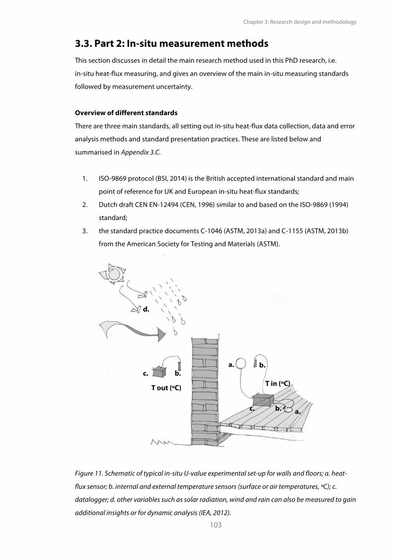
Chapter 3: Research design and methodology
103
3.3. Part 2: In-situ measurement methods This section discusses in detail the main research method used in this PhD research, i.e.
in-situ heat-flux measuring, and gives an overview of the main in-situ measuring standards
followed by measurement uncertainty.
Overview of different standards
There are three main standards, all setting out in-situ heat-flux data collection, data and error
analysis methods and standard presentation practices. These are listed below and
summarised in Appendix 3.C.
1. ISO-9869 protocol (BSI, 2014) is the British accepted international standard and main
point of reference for UK and European in-situ heat-flux standards;
2. Dutch draft CEN EN-12494 (CEN, 1996) similar to and based on the ISO-9869 (1994)
standard;
3. the standard practice documents C-1046 (ASTM, 2013a) and C-1155 (ASTM, 2013b)
from the American Society for Testing and Materials (ASTM).
!Figure 11. Schematic of typical in-situ U-value experimental set-up for walls and floors; a. heat-
flux sensor; b. internal and external temperature sensors (surface or air temperatures, ºC); c.
datalogger; d. other variables such as solar radiation, wind and rain can also be measured to gain
additional insights or for dynamic analysis (IEA, 2012).
PhD Thesis Pelsmakers, S. 2016
104
In-situ heat-flux measurements are not direct measurements of thermal resistances or
thermal transmittances but are undertaken by usually measuring heat-flux on one side and
temperatures on both sides of a construction (Ti and Te, ºC)- as illustrated by Figure 11.
The heat-flux sensor is usually temporarily fixed to the inside, warm face of the element,
protected from heat-sources such as solar gain. Heat-flux sensors measure differential
temperature across the heat-flux plate, generating a mV output (QDL), from which the
conductive heat-flow rate (q, Wm-2) is inferred using each sensor's unique sensitivity
(or calibration factor, ESen in mVm2W-1, see Equation 39.). The internal and external
temperatures (Ti and Te, ºC) and heat-flow rate (q, Wm-2) are then combined in a
measurement model to estimate the element's thermal resistance (R-value, Equation 36.) or
the transmittance (U-value, Equation 38.). The element under observation, and hence the
heat-flux sensor, will be subject to convective and radiative influences in real monitoring
campaigns, which in turn influence the measured rate of conductive heat-flow, but the
different heat-flow influences cannot be isolated (D'Amelio, 2012a).
Equation 37. is referred to as the ‘Average Method’ in ISO-9869 (BSI, 2014) and CEN (1996) or
‘Summation Technique’ by ASTM (2007b). It is also referred to as "the ratio of means" in this
thesis.
- Equation 36., where RT is the total in-situ estimated construction
element thermal resistance (m2KW-1); if surface temperatures are used to compute the in-situ
estimated thermal resistance (Equation 37.), the assumed external and internal surface
thermal resistances (RSe, RSi respectively) have to be added. Conversely, RSe and RSi are set to
zero when utilising air temperatures (Baker, 2011b). RSe and RSi depend on the direction of
heat-flow and can be obtained from BSI (2007).
- Equation 37., where Rest is the in-situ estimated R-value. Tij is the
internal temperature; Tej is the external temperature and q is the heat-flux density (Wm-2),
derived from Equation 39. Index j identifies individual measurements and n is the number of
measurements.
And Equation 38., where U is the final or total estimated in-situ U-value (Wm-2K-1)
and is the reciprocal of the total thermal resistance RT.
- Equation 39., where ESen is each heat-flux sensor's
unique sensitivity or calibration factor in mVm2W-1 and QDL is the data logger acquisition
component in mV, generated from the differential temperature across the heat-flux plate.
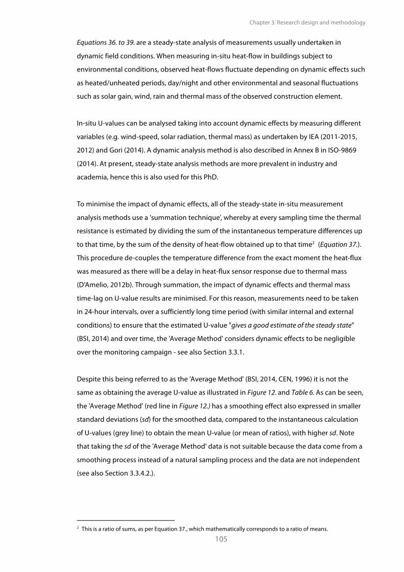
Chapter 3: Research design and methodology
105
Equations 36. to 39. are a steady-state analysis of measurements usually undertaken in
dynamic field conditions. When measuring in-situ heat-flow in buildings subject to
environmental conditions, observed heat-flows fluctuate depending on dynamic effects such
as heated/unheated periods, day/night and other environmental and seasonal fluctuations
such as solar gain, wind, rain and thermal mass of the observed construction element.
In-situ U-values can be analysed taking into account dynamic effects by measuring different
variables (e.g. wind-speed, solar radiation, thermal mass) as undertaken by IEA (2011-2015,
2012) and Gori (2014). A dynamic analysis method is also described in Annex B in ISO-9869
(2014). At present, steady-state analysis methods are more prevalent in industry and
academia, hence this is also used for this PhD.
To minimise the impact of dynamic effects, all of the steady-state in-situ measurement
analysis methods use a 'summation technique', whereby at every sampling time the thermal
resistance is estimated by dividing the sum of the instantaneous temperature differences up
to that time, by the sum of the density of heat-flow obtained up to that time2 (Equation 37.).
This procedure de-couples the temperature difference from the exact moment the heat-flux
was measured as there will be a delay in heat-flux sensor response due to thermal mass
(D'Amelio, 2012b). Through summation, the impact of dynamic effects and thermal mass
time-lag on U-value results are minimised. For this reason, measurements need to be taken
in 24-hour intervals, over a sufficiently long time period (with similar internal and external
conditions) to ensure that the estimated U-value "gives a good estimate of the steady state"
(BSI, 2014) and over time, the 'Average Method' considers dynamic effects to be negligible
over the monitoring campaign - see also Section 3.3.1.
Despite this being referred to as the 'Average Method' (BSI, 2014, CEN, 1996) it is not the
same as obtaining the average U-value as illustrated in Figure 12. and Table 6. As can be seen,
the 'Average Method' (red line in Figure 12.) has a smoothing effect also expressed in smaller
standard deviations (sd) for the smoothed data, compared to the instantaneous calculation
of U-values (grey line) to obtain the mean U-value (or mean of ratios), with higher sd. Note
that taking the sd of the 'Average Method' data is not suitable because the data come from a
smoothing process instead of a natural sampling process and the data are not independent
(see also Section 3.3.4.2.).
2 This is a ratio of sums, as per Equation 37., which mathematically corresponds to a ratio of means.
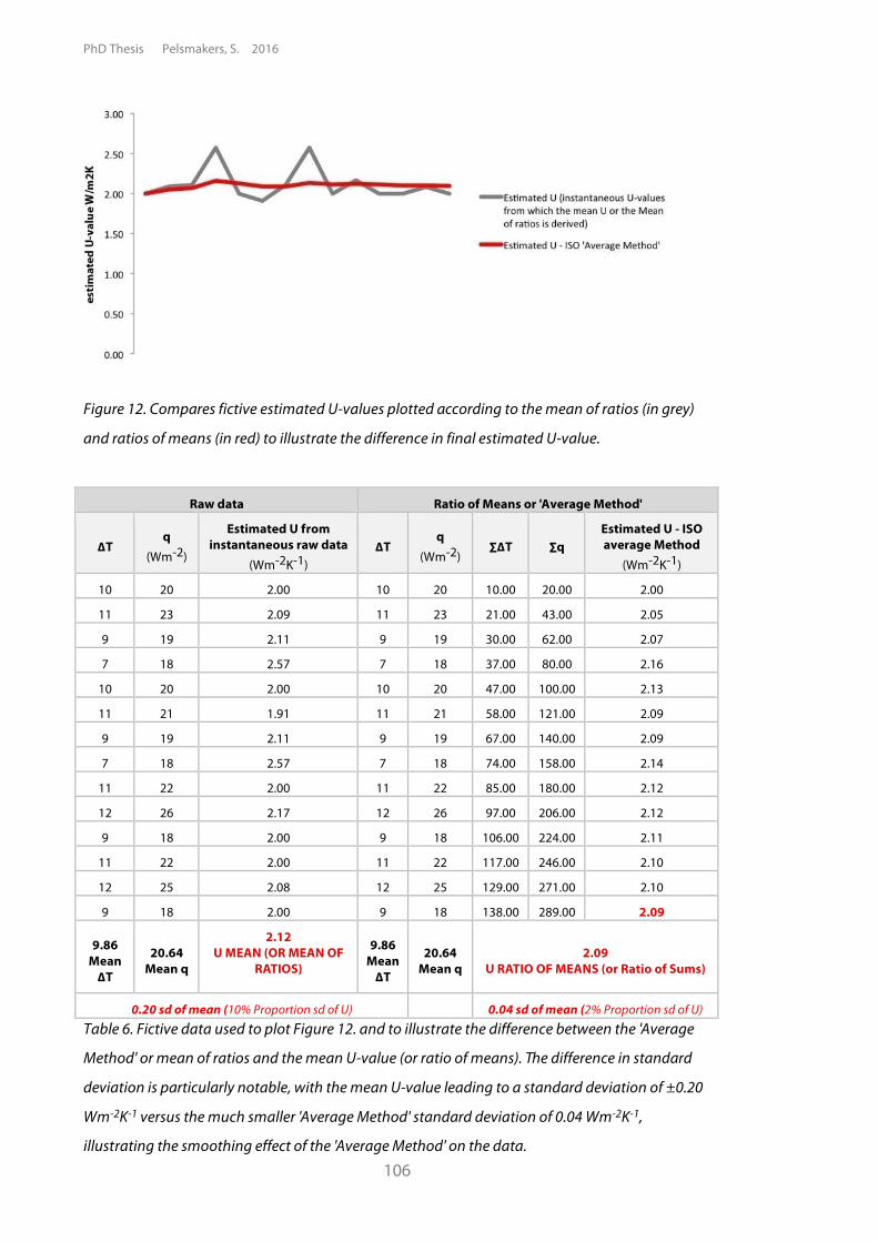
PhD Thesis Pelsmakers, S. 2016
106
Figure 12. Compares fictive estimated U-values plotted according to the mean of ratios (in grey)
and ratios of means (in red) to illustrate the difference in final estimated U-value.
Raw data Ratio of Means or 'Average Method'
!T q
(Wm-2)
Estimated U from instantaneous raw data
(Wm-2K-1) !T
q (Wm-2)
"!T "q Estimated U - ISO average Method
(Wm-2K-1)
10 20 2.00 10 20 10.00 20.00 2.00
11 23 2.09 11 23 21.00 43.00 2.05
9 19 2.11 9 19 30.00 62.00 2.07
7 18 2.57 7 18 37.00 80.00 2.16
10 20 2.00 10 20 47.00 100.00 2.13
11 21 1.91 11 21 58.00 121.00 2.09
9 19 2.11 9 19 67.00 140.00 2.09
7 18 2.57 7 18 74.00 158.00 2.14
11 22 2.00 11 22 85.00 180.00 2.12
12 26 2.17 12 26 97.00 206.00 2.12
9 18 2.00 9 18 106.00 224.00 2.11
11 22 2.00 11 22 117.00 246.00 2.10
12 25 2.08 12 25 129.00 271.00 2.10
9 18 2.00 9 18 138.00 289.00 2.09
9.86 Mean !T
20.64 Mean q
2.12 U MEAN (OR MEAN OF
RATIOS)
9.86 Mean !T
20.64 Mean q
2.09 U RATIO OF MEANS (or Ratio of Sums)
0.20 sd of mean (10% Proportion sd of U) 0.04 sd of mean (2% Proportion sd of U) Table 6. Fictive data used to plot Figure 12. and to illustrate the difference between the 'Average
Method' or mean of ratios and the mean U-value (or ratio of means). The difference in standard
deviation is particularly notable, with the mean U-value leading to a standard deviation of ±0.20
Wm-2K-1 versus the much smaller 'Average Method' standard deviation of 0.04 Wm-2K-1,
illustrating the smoothing effect of the 'Average Method' on the data.
Chapter 3: Research design and methodology
107
3.3.1. 'Valid' U-values Equation 37. is applied at each measurement time; thus as more data is added, this
'summation technique' will converge to a steady U or R-value, the value of which is
considered to be the best estimate of the thermal transmittance or resistance, as long as the
sensor was not subject to direct solar gain and the element's thermal properties remained
the same throughout the measurement (or the change of heat stored in the element is a
small proportion of total heat flow) (BSI, 2014). This convergency to a final U-value can be
seen by the red line in Figure 12. in Section 3.3., which also highlights the smoothing impact
of this technique on the data; implications for this are also discussed in Section 3.3.4.2.
Different convergence criteria are set in the different standards to define the 'valid'
U-(or R)-value. In ISO 9869 (BSI, 2014) and CEN (1996) there are 3 test criteria:
(1.) the monitoring period must be minimum 72 hrs long and always taken over a full 24
hour period;
(2.) the final U-value must be within ±5% (ISO 9869) or ±2% (CEN, 1996) of the value
obtained a complete 24hrs prior and,
(3.) the final U-value obtained in the first 2/3rds of the data (based on full 24-hour
periods only) should be within ±5% (ISO 9869) or ±2% (CEN, 1996) of the U-value
obtained after analysing the last 2/3rds of the data, again based on complete days.
It is considered that the element's thermal mass is accounted for by measuring over a long
enough period, depending on measuring conditions and the observed construction
element. For solid brick walls, monitoring campaigns can be as long as 14 days (Gori, 2014)
especially in occupied houses (BRE, 2014b) and sometimes longer (Baker, 2011b) to meet
criteria (2.) described above. It is unclear what the measuring time frame of suspended
timber ground floor structures might be; Isaacs (1985b) suggested a 24 hr periodic day/night
cycle and a three to four day measuring period (though a longer term seasonal cycle would
also exist).
PhD Thesis Pelsmakers, S. 2016
108
While longer measuring campaigns with summation technique analysis increase the
likelihood of meeting criteria (2.), it might decrease the likelihood of meeting criteria (3.). This
is because, in general, the longer the measuring period, the more likely that the
environmental conditions, such as solar gain and wind-speed, are dissimilar between the
start (the first 2/3rds of data) and the end of the monitoring period (i.e. the last 2/3rds) and
the more likely that seasonal effects, including seasonal thermal mass effects, influence the
observed heat-flow. In practice, the above criteria might not be used; particularly criteria (3.)
is often not reported, and instead valid U (or R)-values are inferred by visually assessing if the
value converges to a constant value, e.g. Cox-Smith (2008).
3.3.2. Heat-flux sensor placement, whole element U-values and
model comparisons In-situ measuring campaigns are often limited by access to equipment and the available
measurement locations in occupied dwellings, due to placement of furniture and occupant
activities. Resource costs and such practical issues might be the reasons why generally just
one or a few heat-flux sensors are mounted on a construction element, as illustrated by
low-resolution floor monitoring studies in Chapter 2.4. However, in-situ measured U-values
are point-measurements on a construction element, which measure the heat-flow through a
sensor area of about 30mm diameter within an 80mm diameter heat-flux plate (and surface
temperature sensors typically have a smaller sensor area). Clearly, estimating heat-flow of an
entire element based on a single or a few point-measurements is unlikely to be
representative of the whole construction element (ASTM, 2007a), though this is likely to
depend on the construction element and might make comparison with modelled U-values
difficult. Hence, depending where sensors are placed, whole element U-values can be
over- or under-estimated when based on single or few point-measurements.
It is therefore important that sensors are placed to either be representative of the observed
construction surface and to avoid (or purposively investigate) specific unrepresentative
areas, such as local inhomogeneities or thermal bridging (BSI, 2014) - depending on the
monitoring purpose. For example heat-flow is likely to be influenced by thermal bridging
when measuring heat-flow within 200-400mm of window/door openings and floor/wall and
wall/wall junctions (Doran, 2008), hence these areas are unlikely to be representative of the
whole fabric element but could still be of interest to investigate or characterise.
Chapter 3: Research design and methodology
109
Combining point U-values into a 'whole element U-value' is hence useful to understand total
estimated thermal transmittance and to compare with models; the latter usually predict
average U-values of whole fabric elements in steady state conditions - see Chapter 2.3. A
whole element in-situ U-value may be estimated by "averaging the results of several heat-flow
meter measurements" (BSI, 2014) or from area-weighted averages "using appropriate
groupings of sensors in representative subsections" (ASTM, 2007b) - different techniques are
explored, tested and refined in Chapter 4.4.2.
Models will however "not always agree exactly with measured U-values measured on site"
(McMullan, 2002); ISO-9869 (BSI, 2014) and CEN (1996) state that differences between
measured and modelled U-value estimates are significant [only] if >20% and this is due to a
number of reasons which should be taken into account in such comparisons. Divergence
from predictive models might in some cases be explained by model input assumptions that
do not reflect actual variables due to difficulty in determining existing fabric characteristics
(e.g. material conductivities, thickness, assumed surface resistances, see e.g. May (2012) and
Gentry (2010)); but might also be explained by in-situ measurement issues such as lack of
representative surface under investigation and measurement issues such as determination of
representative environmental temperatures (BSI, 2014) - as discussed in Section 3.3.3. Sensor
placement on seemingly homogenous construction elements (such as mortar joints, air-gaps
and hidden services) may not be homogenous and contribute to different heat-flow patterns
than modelled (Byrne et al., 2013, Siviour, 1994, Cesaratto et al., 2011, Cesaratto and De Carli,
2012).
The use of infrared thermography can be useful to identify such (un)representative areas to
investigate for in-situ monitoring (ASTM, 2007a, BSI, 2014). If a large spread of temperatures
is observed from infrared images, strategic placement of several sensors will be necessary to
understand the entire element's in-situ heat-flow (ASTM, 2007a) and to be representative of
the heat-flow of the entire element - this approach was used throughout this thesis. Infrared
thermography can also be useful to check if the greater region surrounding the sensor site is
similar to interpolate to a larger area (ASTM, 2007a) and to estimate whole element U-values
- see Section 4.4.2. However interpolated values will be less accurate than the observed
values (ASTM, 2007a). Evidently, the larger the purposeful coverage of heat-flux sensors on
the surface, the greater the certainty of the whole surface thermal transmittance under those
measuring conditions - see Section 3.3.4., Chapter 4.4.2 and 5.3.
PhD Thesis Pelsmakers, S. 2016
110
3.3.3. Temperature measurements The standards do not stipulate minimum temperature differences (!T) between both sides of
the observed construction element, although ideally in-situ measurements are undertaken
when there is a sufficient !T in order to observe a sufficiently large heat-flux outside the
instrument accuracies. Optimal !T are depending on sources: >4ºC and ideally >10ºC (Cox-
Smith, 2008) or between "7ºC and "10ºC (IEA, 2011-2015, Siviour, 1982, Doran, 2008, Baker,
2011b, McIntyre, 1985, Desogus et al., 2011). However lower temperature differences can still
give valid, albeit less accurate in-situ results (Desogus et al., 2011, Byrne et al., 2013, CEN,
1996, Trethowen, 1986) because, proportionally, the instrument error increases with smaller
!T. Hence the increased importance of both temperature sensor accuracy and precision with
a small !T to avoid large proportional measurement errors.
Another issue to take into account is where these temperatures are actually measured, as
discussed in the following sections.
3.3.3.1. Air temperatures as a proxy for ambient temperatures
Environmental (ambient) temperatures are required for U-value determination, however air
temperatures are often used to substitute ambient temperatures (BSI, 2014, IEA, 2012) as
ambient temperatures cannot be directly measured and are not constant in a room (BSI,
2014). Ambient temperatures are a combination of radiation and convection transfer
coefficients, space emittance (which includes the emissivity and view factor of all the
surrounding surfaces), air temperature and the radiant temperature 'seen' by the observed
surface.
Only air temperature and radiation transfer coefficients can be more easily determined (BSI,
2014). However due to the inhomogeneity of air temperatures in rooms caused by a complex
interplay of convective currents in the room from heating elements and from ventilation
(and surfaces at different temperatures that create these currents), vertical (and horizontal)
temperature gradients exist (BSI, 2014, Gauthier, 2014, MING XU, 2001). As such, it is unclear
where to measure air temperatures in the room for U-value determination - this is explored in
Chapter 4.4.5. Given the above, depending on the location and condition of measurement, a
U-value estimated from air temperatures will vary across the fabric element, even if the
thermal resistance (R-value) of the element is homogenous (BSI, 2014).
Chapter 3: Research design and methodology
111
As such, significant disparities might arise between modelled values and measured U-values
depending on the reference temperatures used and "a U-value measured in situ may not be
the appropriate U-value for use in heat loss calculations if different temperatures are involved in
the two cases" (BSI, 2014). ISO-9869 assumes a ±5% random error associated with U-value
"temperature variations within the space and differences between air and radiant temperatures"
(BSI, 2014) - as discussed in Section 3.3.4.
The question where to measure the air temperature is further complicated by the
practicalities of placing sensors, especially in occupied houses. Siviour (1982) suggests
internal air temperatures to be measured within 500mm from the heat-flux sensor for in-situ
wall measurements while Doran (2001) placed air temperature sensors 10mm away from the
heat-flux sensor on the wall (as also suggested by EST (2006)) and "a few centimetres from the
centre of the heat flux plate" by BRE (2014a); though it is unclear how such sensor locations
were determined while their applicability for floors is unknown. For solid ground floors,
Trethowen (n.d.) observed internal room temperatures at the floor surface and at 300mm
and 2000mm high. However no standard heights and locations are used (if specified),
making comparisons between studies problematic.
While a U-value is typically estimated from 'air to air' environments (BSI, 2014) (which is
usually also the model assumption (IEA, 2012)), surface to air temperatures are often used
instead as this can be more practical to determine - as discussed in the following Section
3.3.3.2.
PhD Thesis Pelsmakers, S. 2016
112
3.3.3.2. Use of surface temperatures in U-value estimation
Typically, surface temperatures are used for R-value estimates of a building element; the
addition of assumed surface thermal resistances is required for the determination of a
U-value or the total thermal resistance (RT) of the element when surface temperatures are
used (CEN, 1996, Baker, 2011b). Where internal surface temperatures and external air
temperatures are used for the estimation of U-values, as done here in this study, the addition
of an internal surface thermal resistance as per - Equation 40. is required - see e.g. Baker
(2011a), Rye (2011), Rhee-Duverne (2013), Currie (2013).
- Equation 40., where TSi is the surface temperature
of the floor in the room and RSi is the internal surface thermal resistance, taken to be
0.17 m2KW-1 in accordance with BSI (2007) while RSe is set to zero if external air temperatures
(Tae) are used instead of external surface temperatures (TSe).
Surface temperature sensors are to be placed under or near the heat-flux sensor, and both
should be of the same colour and emissivity as the observed surface as recommended by
ASTM (2007a) and ISO-9869 (BSI, 2014); some studies place surface temperature sensors on
the heat flux sensor - see e.g. Rye (2010) and Baker (2011b).
When using surface temperatures instead of air temperatures, the addition of constant
surface thermal resistances may not be suitable in all situations (BSI, 2007, Mirsadeghi et al.,
2013). Surface resistances are influenced by the radiative and convective transfer coefficients
(Wm-2K-1) and surface emissivity (BSI, 2007, BSI, 2014), which are unlikely to be constant over
an entire element's surface area or a range of conditions (BSI, 2014) or as assumed by
standards. For instance, external surface resistances vary in accordance with external
environmental conditions and are inversely proportional to wind-speeds; for example a
wall's external surface resistance RSe decreases from 0.08 m2KW-1 to 0.02 m2KW-1 when wind-
speeds increased from 1m/s to 10m/s respectively (BSI, 2007) - see Table 7. Convective
airflows are likely altered by furniture placement, air infiltration and heating sources so the
assumption that an element's surface is subject to constant wind-speed, airflow and
constant radiative heat-flow throughout an enclosure is unlikely to be the case as observed
by Emery (2007).
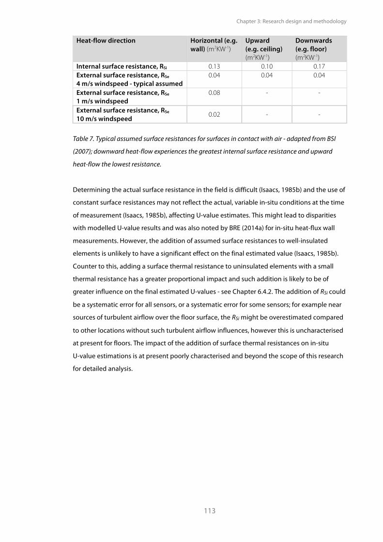
Chapter 3: Research design and methodology
113
Heat-flow direction Horizontal (e.g. wall) (m2KW-1)
Upward (e.g. ceiling) (m2KW-1)
Downwards (e.g. floor) (m2KW-1)
Internal surface resistance, RSi 0.13 0.10 0.17 External surface resistance, RSe 4 m/s windspeed - typical assumed
0.04 0.04 0.04
External surface resistance, RSe
1 m/s windspeed 0.08 - -
External surface resistance, RSe
10 m/s windspeed 0.02 - -
Table 7. Typical assumed surface resistances for surfaces in contact with air - adapted from BSI
(2007); downward heat-flow experiences the greatest internal surface resistance and upward
heat-flow the lowest resistance.
Determining the actual surface resistance in the field is difficult (Isaacs, 1985b) and the use of
constant surface resistances may not reflect the actual, variable in-situ conditions at the time
of measurement (Isaacs, 1985b), affecting U-value estimates. This might lead to disparities
with modelled U-value results and was also noted by BRE (2014a) for in-situ heat-flux wall
measurements. However, the addition of assumed surface resistances to well-insulated
elements is unlikely to have a significant effect on the final estimated value (Isaacs, 1985b).
Counter to this, adding a surface thermal resistance to uninsulated elements with a small
thermal resistance has a greater proportional impact and such addition is likely to be of
greater influence on the final estimated U-values - see Chapter 6.4.2. The addition of RSi could
be a systematic error for all sensors, or a systematic error for some sensors; for example near
sources of turbulent airflow over the floor surface, the RSi might be overestimated compared
to other locations without such turbulent airflow influences, however this is uncharacterised
at present for floors. The impact of the addition of surface thermal resistances on in-situ
U-value estimations is at present poorly characterised and beyond the scope of this research
for detailed analysis.
PhD Thesis Pelsmakers, S. 2016
114
3.3.3.3. Use of external air temperatures or void air temperatures for estimation
of floor U-values?
As discussed in Chapter 2.4.2, different in-situ floor heat-flux data collection techniques are
used, including measurements from the internal environment (surface or air) to the void or
to the external environment. For example, Miles-Shenton (2011) uses internal air to external
air for estimation of floor U-values, while Isaacs (1985b) uses internal surface to void air
temperatures to estimate R-values (though this includes floors with open foundation walls
exposed to the external environment) and Currie (2013) uses the same to estimate a U-value;
though the authors also estimate U-values from skirting air temperature to external air
temperature (Stinson, 2012). Harris (1997) estimates thermal resistances and U-values from
internal air to void air temperatures, specifically to investigate heat-flow reduction to the
floor void after insulation interventions (Harris, 2013), while no detail is provided by Baker
(2011a).
As U-values are calculated or modelled from the internal to the external environment
((Szokolay, 2008) and given that the floor U-value model ISO-13370 uses the external
environment (BSI, 2009), the external environment will be used in this study to enable
comparison of in-situ estimated U-values with models and to understand the actual thermal
performance of the floor system. Thus, throughout the research hereby presented, all
U-values are calculated using external temperatures, rather than floor void temperatures.
Chapter 3: Research design and methodology
115
3.3.4. Uncertainty and error estimation This section gives an overview of measurement uncertainty and errors and critically reviews
different existing in-situ measurement error propagation techniques, prior to presenting the
error propagation method developed and proposed for this thesis.
3.3.4.1. Sources of error and uncertainty
Uncertainty in in-situ heat-flux measurements can be associated with measurement
techniques used (for example, where air temperatures are measured), as well as the addition
of constant surface thermal resistances where surface temperatures are used - see Section
3.3.3. In addition, uncertainty in obtaining a whole element U-value is associated with the
number of point-values used to estimate this whole element U-value and how representative
the observed point-values are of the entire fabric element (Section 3.3.2). Uncertainty with
in-situ field measurements is also associated with seasonal influences and the natural
variability of heat-flow through a construction element (and is affected by timing of the
monitoring campaign) - this is further discussed below.
Moreover, like all field measurements using instruments, in-situ heat-flux measurements are
affected by the conditions of measurement and instruments used, which have errors
associated with them. It is for these reasons that, even when measuring over sufficiently long
periods, the in-situ method in non-steady state conditions is not a high precision method
(BSI, 2014). The act of measuring affects what is being measured: for instance, placing a heat-
flux sensor on a surface inherently affects the characteristics of what is being attempted to
be measured (Childs, 1999), leading, for example, to random or systematic deflection and
reflection errors. This means that measurement results can only ever be an estimate of the
true value rather than the actual true value. It is therefore important that these errors are as
best as possible accounted for as this affects the measurement results, confidence in findings
and comparability between different sources, published literature, specifications, standards,
models (JCGM, 2008, Czichos, 2011) and comparison of the heat-flow reduction potential of
intervention measures. For example, it is generally accepted that the difference between
measurements (and hence also the efficacy of interventions) is only 'demonstrated' if
measurement uncertainties do not overlap (Taylor, 1997).
PhD Thesis Pelsmakers, S. 2016
116
However, the exact number of errors and of possible confounders, and the magnitude of
their effect is not known, despite influencing the estimated result. These errors can be
systematic or random. Systematic errors usually relate to accuracy and spread the readings
around some displaced, but not true value (Squires, 2001) and cannot be controlled for by
repeated measurements (Taylor, 1997). Systematic errors include instrument accuracy (how
close it is certified to a known value), instrument erroneous calibration, research practice and
design (e.g. differences in sensor fixings), and their exact influence is usually unknown but
should instead be minimised for by careful research design and practice. Though small, the
systematic additional influence of the thermal resistance of the heat-flux sensor itself of
6.25 x 10⁻³ m2K/W (Hukseflux, 2012) can be accounted for by adjusting for (i.e. deducting this
factor) in R- and U-value estimations, as has been done in this research. Systematic errors
could be only present (or absent) in certain conditions and could be systematic for each
sensor but random between sensors or for a collection of sensors, making error estimation
difficult. Random errors, usually associated with the precision (or repeatability) of
measurements, are equally likely to be positive or negative and are always present in an
experiment and causes "successive readings to spread about the true value of the quantity"
(Squires, 2001). Random errors can be reduced by repeated measurements and might be
revealed statistically from the spread/variation of repeated measurements (Taylor, 1997).
Random error sources include equipment set-up and researcher and occupant influence,
though these might also be systematic errors or have systematic components. Usually results
are accurate if they are "relatively free from systematic errors, and precise if the random error is
small" (Squires, 2001) - clearly both are important.
Slightly different errors are estimated in different standards and are summarised in Appendix
3.D., adapted from Pelsmakers (2012). Given that ISO-9869 (BSI, 2014) is the UK and EU
accepted protocol, its identified errors are summarised below, and was used in this thesis as
a basis for uncertainty estimation.
Chapter 3: Research design and methodology
117
As described in Section 3.3.3. there is difficulty to measure accurate temperatures which
reflect the heat-flow path and this will create uncertainty, estimated at ±5% by ISO-9869 for
"temperature variations within the space and differences between air and radiant
temperatures"(BSI, 2014). In addition, there will be instrument errors (±5%, (BSI, 2014)) and
contact errors (±5%, (BSI, 2014)) could arise if leaving a small gap between the sensor and the
surface and (or) changing the airspeed around the sensor; contact error was found to be #2%
with airspeeds up to 1m/s (Bales, 1985). It should also be noted that airflow through the floor
board gaps could create turbulence around the sensors and also affect any airflow between
the sensors and the surface, though the airspeed around the sensors is unknown and this
uncertainty is uncharacterised.
The mounting of the sensor on the surface changes the heat-flow that goes through the
undisturbed surface, which can lead to operational deflection errors (Cesaratto et al., 2011,
Childs, 1999, Trethowen, 1986); it is estimated by ISO-9869 (BSI, 2014) at ±2 to ±3% error
though a slightly larger deflection error of ±4% is suggested by Doran (2008). Furthermore,
masking tape smoothed over the sensor's edges can minimise "the differences in turbulent
flow over the sensor compared to the adjacent wall." (Bales, 1985). Similar fixing strategies are
likely to be relevant for floor sensor fixings. Additionally, ISO-9869 (BSI, 2014) estimates a
±10% error for "errors caused by the variations over time of the temperatures and heat-flow", i.e.
natural variability.
However, the natural variability of a U-value is not a measurement error but a real
characteristic of an element's actual thermal transmittance in dynamic situations; i.e.
U-values are not constant but change when subject to e.g. changes in radiation and airflow
over time. To discuss this conceptual difference, it can be helpful to think of the identified
errors as 'intrinsic' and 'extrinsic errors' (Bales, 1985) and separate these from the natural
variability of U-values - as categorised in Table 8. Intrinsic errors are those related to
instrument accuracy, while extrinsic properties are associated and contingent on the
measurement application and technique used (Bales, 1985), i.e. related to measuring
conditions. For example extrinsic errors come from how ambient temperatures are
determined and from sensor fixing methods such as deflection and contact errors.
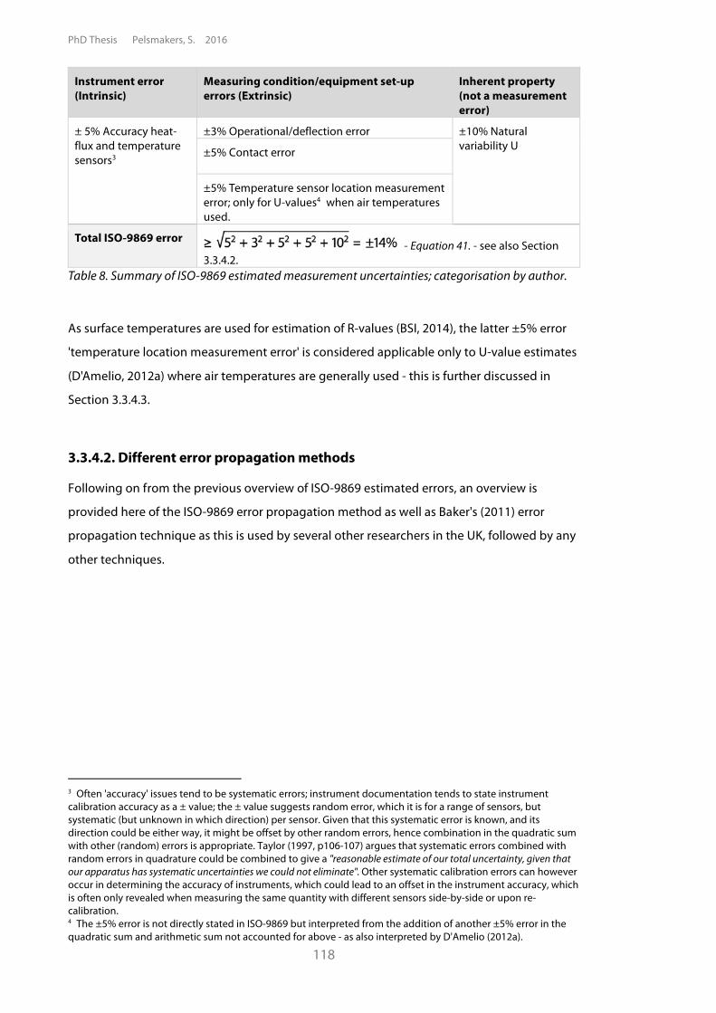
PhD Thesis Pelsmakers, S. 2016
118
Instrument error (Intrinsic)
Measuring condition/equipment set-up errors (Extrinsic)
Inherent property (not a measurement error)
± 5% Accuracy heat-flux and temperature sensors3
±3% Operational/deflection error ±10% Natural variability U ±5% Contact error
±5% Temperature sensor location measurement error; only for U-values4 when air temperatures used.
Total ISO-9869 error - Equation 41. - see also Section
3.3.4.2. Table 8. Summary of ISO-9869 estimated measurement uncertainties; categorisation by author.
As surface temperatures are used for estimation of R-values (BSI, 2014), the latter ±5% error
'temperature location measurement error' is considered applicable only to U-value estimates
(D'Amelio, 2012a) where air temperatures are generally used - this is further discussed in
Section 3.3.4.3.
3.3.4.2. Different error propagation methods
Following on from the previous overview of ISO-9869 estimated errors, an overview is
provided here of the ISO-9869 error propagation method as well as Baker's (2011) error
propagation technique as this is used by several other researchers in the UK, followed by any
other techniques.
3 Often 'accuracy' issues tend to be systematic errors; instrument documentation tends to state instrument calibration accuracy as a ± value; the ± value suggests random error, which it is for a range of sensors, but systematic (but unknown in which direction) per sensor. Given that this systematic error is known, and its direction could be either way, it might be offset by other random errors, hence combination in the quadratic sum with other (random) errors is appropriate. Taylor (1997, p106-107) argues that systematic errors combined with random errors in quadrature could be combined to give a "reasonable estimate of our total uncertainty, given that our apparatus has systematic uncertainties we could not eliminate". Other systematic calibration errors can however occur in determining the accuracy of instruments, which could lead to an offset in the instrument accuracy, which is often only revealed when measuring the same quantity with different sensors side-by-side or upon re-calibration. 4 The ±5% error is not directly stated in ISO-9869 but interpreted from the addition of another ±5% error in the quadratic sum and arithmetic sum not accounted for above - as also interpreted by D'Amelio (2012a).
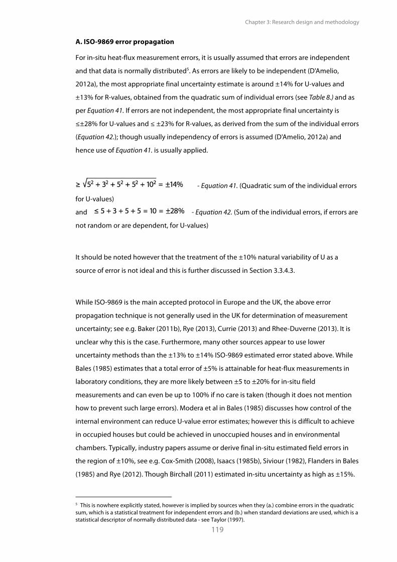
Chapter 3: Research design and methodology
119
A. ISO-9869 error propagation
For in-situ heat-flux measurement errors, it is usually assumed that errors are independent
and that data is normally distributed5. As errors are likely to be independent (D'Amelio,
2012a), the most appropriate final uncertainty estimate is around ±14% for U-values and
±13% for R-values, obtained from the quadratic sum of individual errors (see Table 8.) and as
per Equation 41. If errors are not independent, the most appropriate final uncertainty is
#±28% for U-values and # ±23% for R-values, as derived from the sum of the individual errors
(Equation 42.); though usually independency of errors is assumed (D'Amelio, 2012a) and
hence use of Equation 41. is usually applied.
- Equation 41. (Quadratic sum of the individual errors
for U-values)
and - Equation 42. (Sum of the individual errors, if errors are
not random or are dependent, for U-values)
It should be noted however that the treatment of the ±10% natural variability of U as a
source of error is not ideal and this is further discussed in Section 3.3.4.3.
While ISO-9869 is the main accepted protocol in Europe and the UK, the above error
propagation technique is not generally used in the UK for determination of measurement
uncertainty; see e.g. Baker (2011b), Rye (2013), Currie (2013) and Rhee-Duverne (2013). It is
unclear why this is the case. Furthermore, many other sources appear to use lower
uncertainty methods than the ±13% to ±14% ISO-9869 estimated error stated above. While
Bales (1985) estimates that a total error of ±5% is attainable for heat-flux measurements in
laboratory conditions, they are more likely between ±5 to ±20% for in-situ field
measurements and can even be up to 100% if no care is taken (though it does not mention
how to prevent such large errors). Modera et al in Bales (1985) discusses how control of the
internal environment can reduce U-value error estimates; however this is difficult to achieve
in occupied houses but could be achieved in unoccupied houses and in environmental
chambers. Typically, industry papers assume or derive final in-situ estimated field errors in
the region of ±10%, see e.g. Cox-Smith (2008), Isaacs (1985b), Siviour (1982), Flanders in Bales
(1985) and Rye (2012). Though Birchall (2011) estimated in-situ uncertainty as high as ±15%.
5 This is nowhere explicitly stated, however is implied by sources when they (a.) combine errors in the quadratic sum, which is a statistical treatment for independent errors and (b.) when standard deviations are used, which is a statistical descriptor of normally distributed data - see Taylor (1997).
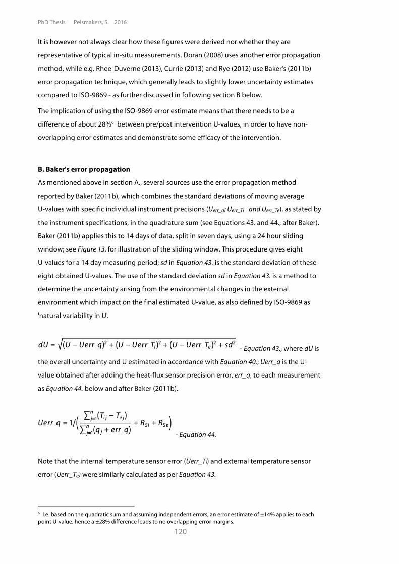
PhD Thesis Pelsmakers, S. 2016
120
It is however not always clear how these figures were derived nor whether they are
representative of typical in-situ measurements. Doran (2008) uses another error propagation
method, while e.g. Rhee-Duverne (2013), Currie (2013) and Rye (2012) use Baker's (2011b)
error propagation technique, which generally leads to slightly lower uncertainty estimates
compared to ISO-9869 - as further discussed in following section B below.
The implication of using the ISO-9869 error estimate means that there needs to be a
difference of about 28%6 between pre/post intervention U-values, in order to have non-
overlapping error estimates and demonstrate some efficacy of the intervention.
B. Baker's error propagation
As mentioned above in section A., several sources use the error propagation method
reported by Baker (2011b), which combines the standard deviations of moving average
U-values with specific individual instrument precisions (Uerr_q; Uerr_Ti and Uerr_Te), as stated by
the instrument specifications, in the quadrature sum (see Equations 43. and 44., after Baker).
Baker (2011b) applies this to 14 days of data, split in seven days, using a 24 hour sliding
window; see Figure 13. for illustration of the sliding window. This procedure gives eight
U-values for a 14 day measuring period; sd in Equation 43. is the standard deviation of these
eight obtained U-values. The use of the standard deviation sd in Equation 43. is a method to
determine the uncertainty arising from the environmental changes in the external
environment which impact on the final estimated U-value, as also defined by ISO-9869 as
'natural variability in U'.
- Equation 43., where dU is
the overall uncertainty and U estimated in accordance with Equation 40.; Uerr_q is the U-
value obtained after adding the heat-flux sensor precision error, err_q, to each measurement
as Equation 44. below and after Baker (2011b).
- Equation 44.
Note that the internal temperature sensor error (Uerr_Ti) and external temperature sensor
error (Uerr_Te) were similarly calculated as per Equation 43.
6 I.e. based on the quadratic sum and assuming independent errors; an error estimate of ±14% applies to each point U-value, hence a ±28% difference leads to no overlapping error margins.
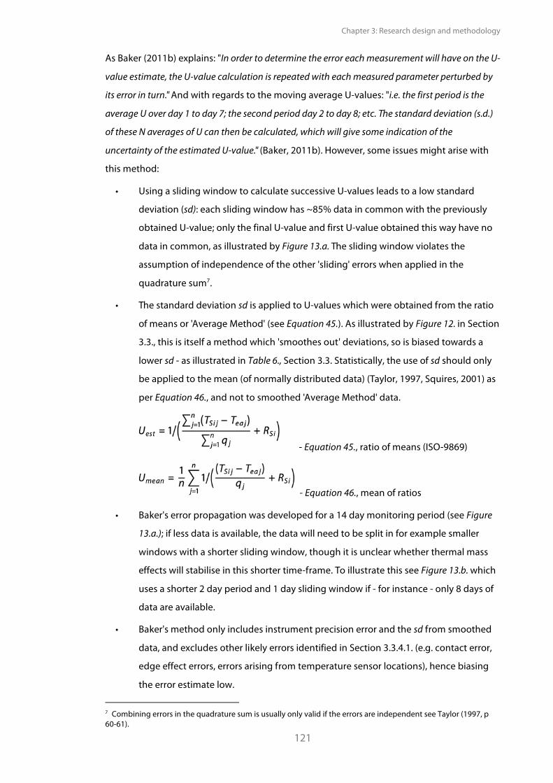
Chapter 3: Research design and methodology
121
As Baker (2011b) explains: "In order to determine the error each measurement will have on the U-
value estimate, the U-value calculation is repeated with each measured parameter perturbed by
its error in turn." And with regards to the moving average U-values: "i.e. the first period is the
average U over day 1 to day 7; the second period day 2 to day 8; etc. The standard deviation (s.d.)
of these N averages of U can then be calculated, which will give some indication of the
uncertainty of the estimated U-value." (Baker, 2011b). However, some issues might arise with
this method:
• Using a sliding window to calculate successive U-values leads to a low standard
deviation (sd): each sliding window has ~85% data in common with the previously
obtained U-value; only the final U-value and first U-value obtained this way have no
data in common, as illustrated by Figure 13.a. The sliding window violates the
assumption of independence of the other 'sliding' errors when applied in the
quadrature sum7.
• The standard deviation sd is applied to U-values which were obtained from the ratio
of means or 'Average Method' (see Equation 45.). As illustrated by Figure 12. in Section
3.3., this is itself a method which 'smoothes out' deviations, so is biased towards a
lower sd - as illustrated in Table 6., Section 3.3. Statistically, the use of sd should only
be applied to the mean (of normally distributed data) (Taylor, 1997, Squires, 2001) as
per Equation 46., and not to smoothed 'Average Method' data.
- Equation 45., ratio of means (ISO-9869)
- Equation 46., mean of ratios
• Baker's error propagation was developed for a 14 day monitoring period (see Figure
13.a.); if less data is available, the data will need to be split in for example smaller
windows with a shorter sliding window, though it is unclear whether thermal mass
effects will stabilise in this shorter time-frame. To illustrate this see Figure 13.b. which
uses a shorter 2 day period and 1 day sliding window if - for instance - only 8 days of
data are available.
• Baker's method only includes instrument precision error and the sd from smoothed
data, and excludes other likely errors identified in Section 3.3.4.1. (e.g. contact error,
edge effect errors, errors arising from temperature sensor locations), hence biasing
the error estimate low.
7 Combining errors in the quadrature sum is usually only valid if the errors are independent see Taylor (1997, p 60-61).
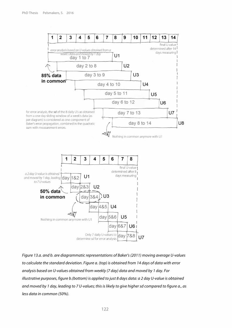
PhD Thesis Pelsmakers, S. 2016
122
Figure 13.a. and b. are diagrammatic representations of Baker's (2011) moving average U-values
to calculate the standard deviation. Figure a. (top) is obtained from 14 days of data with error
analysis based on U-values obtained from weekly (7 day) data and moved by 1 day. For
illustrative purposes, figure b.(bottom) is applied to just 8 days data: a 2 day U-value is obtained
and moved by 1 day, leading to 7 U-values; this is likely to give higher sd compared to figure a., as
less data in common (50%).
Chapter 3: Research design and methodology
123
C. Other techniques
Some research, e.g. Byrne (2013) reports small total error estimates and mentions the use of
'standard deviations' with no further detail whether this is the standard deviation or the
standard deviation of the mean (SDOM, also standard error) nor whether this is applied to the
'Average Method' or to the mean U-values. Following on from previous discussion, statistical
techniques such as sd and SDOM should only be applied to mean values (and where
normally distributed).
In the field, sd of the mean is expected to be large if taken on instantaneous measured values
at short intervals, as there will be large deviations between day/night; heated/unheated
patterns and other changing external conditions - these are not errors however but expected
variations in differently measured U-values as discussed further below in Section 3.3.4.3.
Conversely, in an environmental chamber, sd is expected to be significantly smaller as the
environmental conditions are kept at (near) steady-state.
Even if appropriately applied to the mean U-value distribution, use of sd and SDOM on its
own might not be suitable as an expression of final uncertainty: sd (and SDOM) include the
initial settling time and environmental conditions and (random) researcher error which
affected that sensor, but excludes uncertainties associated with fixing methods
(contact/defection) and the uncertainty associated with ambient temperature
determination.8 In addition, use of SDOM, which takes into account both the spread of the
data (the sd) and the sample size, is unlikely to be suitable as it is based on the assumption
that the measurements are independent repeated measurements. For each point U-value,
heat-flow is being measured in the same location over time at certain intervals for a specific
duration, but in-situ measurements in the field are subject to changing environmental
conditions so measurements are never repeated under the same conditions.9 Moreover, field
data is sampled in given measurement intervals, which exacerbates the autocorrelation
effects associated with the fact that environmental conditions do not vary at random but in a
gradual and correlated way through time. Even in an environmental chamber there are small
differences in the steady-state conditions (so no repeated measurements). Given that (as per
above discussion), other errors are also excluded, SDOM is hence also unlikely to be a
representative error estimate of lab U-value estimates.
8 Such errors are important to include, especially also where comparing between sensors as each sensor will have been subject to different environmental conditions compared to another. 9 E.g. different temperatures during day/night and heated/unheated periods.
PhD Thesis Pelsmakers, S. 2016
124
3.3.4.3. Applied error estimation and propagation method
The error propagation method proposed for in-situ U-value measurements in this thesis
research builds on the ISO-9869 standard and Baker's error propagation method as discussed
in the previous Section 3.3.4.2. The same ISO-9869 estimated intrinsic and extrinsic errors
were accepted for this thesis research - see Table 8. As previously discussed, the natural
variability of in-situ heat flux measurements under changing, dynamic environmental
conditions are listed in ISO-9869 as a ±10% uncertainty, while Baker (2011b) uses the sd of
moving average U-values obtained from the ratio of means, as an attempt to capture this
natural variability 'swing' (Section 3.3.4.2.).
Instead of either of these methods, the natural variability during the monitoring period could
be estimated by using a statistical approach of one of the properties of the data distribution,
such as the sd around the mean, obtained from the mean of ratios. As per - Equation 47. or
Equation 48., depending on use of internal surface or air temperatures respectively.
- Equation 47., mean of ratios where
internal surface temperatures are used or,
- Equation 48., mean of ratios where internal air
temperatures are used, where Umean_surface and Umean_air are the U-values obtained from
internal surface and internal air temperatures respectively; TSi is the surface temperature of
the floor in the room; RSi is the internal surface thermal resistance, taken to be 0.17 m2KW-1
in accordance with BSI (2007), while RSe is set to zero if external air temperatures (Tea) are
used, as is the case in this study. Tia is the internal air temperature and q (Wm-2) is the heat-
flux density, derived from Equation 39. Index j identifies individual measurements and n is the
number of measurements.
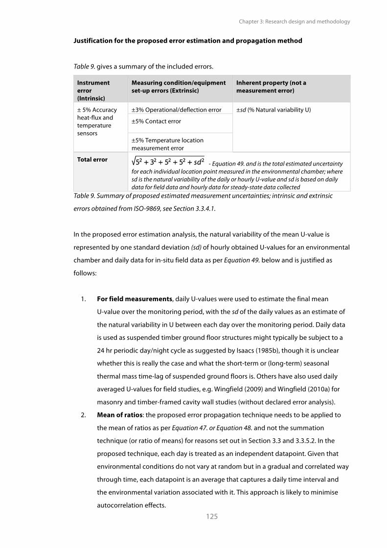
Chapter 3: Research design and methodology
125
Justification for the proposed error estimation and propagation method
Table 9. gives a summary of the included errors.
Instrument error (Intrinsic)
Measuring condition/equipment set-up errors (Extrinsic)
Inherent property (not a measurement error)
± 5% Accuracy heat-flux and temperature sensors
±3% Operational/deflection error ±sd (% Natural variability U)
±5% Contact error
±5% Temperature location measurement error
Total error - Equation 49. and is the total estimated uncertainty
for each individual location point measured in the environmental chamber; where sd is the natural variability of the daily or hourly U-value and sd is based on daily data for field data and hourly data for steady-state data collected
Table 9. Summary of proposed estimated measurement uncertainties; intrinsic and extrinsic
errors obtained from ISO-9869, see Section 3.3.4.1.
In the proposed error estimation analysis, the natural variability of the mean U-value is
represented by one standard deviation (sd) of hourly obtained U-values for an environmental
chamber and daily data for in-situ field data as per Equation 49. below and is justified as
follows:
1. For field measurements, daily U-values were used to estimate the final mean
U-value over the monitoring period, with the sd of the daily values as an estimate of
the natural variability in U between each day over the monitoring period. Daily data
is used as suspended timber ground floor structures might typically be subject to a
24 hr periodic day/night cycle as suggested by Isaacs (1985b), though it is unclear
whether this is really the case and what the short-term or (long-term) seasonal
thermal mass time-lag of suspended ground floors is. Others have also used daily
averaged U-values for field studies, e.g. Wingfield (2009) and Wingfield (2010a) for
masonry and timber-framed cavity wall studies (without declared error analysis).
2. Mean of ratios: the proposed error propagation technique needs to be applied to
the mean of ratios as per Equation 47. or Equation 48. and not the summation
technique (or ratio of means) for reasons set out in Section 3.3 and 3.3.5.2. In the
proposed technique, each day is treated as an independent datapoint. Given that
environmental conditions do not vary at random but in a gradual and correlated way
through time, each datapoint is an average that captures a daily time interval and
the environmental variation associated with it. This approach is likely to minimise
autocorrelation effects.
PhD Thesis Pelsmakers, S. 2016
126
3. For thermal chambers, in the absence of 24-hour day/night or heating pattern
cycles, smaller than 24hr time intervals could be used. However, time intervals which
are too small may contain a lot of noise caused by researcher influence (e.g.
opening/closing doors, touching of sensors during data collection) and might also
show the cycling of the thermostat to provide the required heat input (Isaacs, 1985a).
Hence some kind of averaging of the raw data (collected usually at 1- 5 minute
intervals) over a longer time period may be useful to get a better estimate of the
natural variability with other influences averaged out over a longer time period; for
this reason a one-hour interval was used. Chapters 4.3.5. and 5.2.4. compare the
mean U-value estimated from raw data (at 1 to 5 minute intervals) with the mean
U-value of the hourly or daily data, which were very close and hence were good
approximations of the estimated mean U-values for the case-studies used.
4. Moving average techniques were excluded here due to lack of independence of
data and due to biasing the natural variation component low - as discussed in
Section 3.3.4.2., section B.
5. The sd is a property of the distribution of the in-situ measured U-values, which
reflects the spread of the data around the mean. Because the monitoring period is
over a snapshot in time, using the sd provides a good estimate of the intrinsic
variability observed in the observed data over the monitoring period, and would not
need any further adjustment.
6. Where surface temperatures are used for U-value estimation, it could be argued
that the ±5% temperature sensor location error (see Table 8.) does not apply.
However in this research, external air temperatures were used, as discussed in
Section 3.3.3.3. Additionally, where surface temperature are used, uncertainty is
created by the addition of a constant RSi in the final U-value estimates (see 3.3.3.2.).
Hence some allowance for uncertainty around temperature measurements seems
appropriate and this temperature location measurement error has been retained,
though it's actual effect is unknown.
7. Like the other error propagation methods, the method proposed here also does not
account for any variation in U due to longer-term seasonal changes unless measured
over a longer time period including different seasons. The same assumptions about
independent errors and normally distributed data is applied here as in all other
methods, though further research would be required to investigate these
assumptions; these issues are beyond the scope of this thesis research.
Chapter 3: Research design and methodology
127
Error propagation: Combining intrinsic and extrinsic errors with natural variability of U
in the quadratic sum
Given that buildings exist in a changing environment, it could be argued that the natural
variation in in-situ measured U-values is a property of a dynamic U-value and should not be
combined with true sources of error such as instrument and measurement condition errors.
However, the natural variability of U over time as a result of changing environmental
conditions is treated as an 'error' by ISO-9869 and Baker (2011b) in the estimation of a static
U-value and by combining the natural variability with the other errors in the quadratic sum -
see Equation 41. and Equation 43. respectively. The natural variability is not ideally combined
with the true sources of error in the quadratic sum10 as it is not a true source of error. While
all intrinsic and extrinsic sources of error could be combined in the quadratic sum and the
natural variability estimate could be reported separately alongside, this would make
comparisons between U-values difficult (e.g. Umean ±dx(intrinsic & extrinsic errors) ±natural variability).
Hence for the purpose of this thesis and after ISO-9869 and Baker (2011), the true sources of
error were combined in the quadratic sum with the natural variability as per Equation 49.
Doing so allowed the presentation of a final estimate of uncertainty around the mean
estimated U-value which better enabled comparison between different point U-values on
the floor, pre/post intervention comparisons and estimating whole floor U-values from
point-U-values.
A limitation of this technique is that underestimations of the uncertainty in U might occur
due to use of the quadratic sum. There might be some compensation for this as some ISO-
9869 assumed errors appear conservatively estimated compared to other estimates - see
Appendix 3.D.; there might also be some double-counting as some errors cannot be
separated from the sd - though whether this is the case and the actual extent of the errors
remains unknown. Implications of this proposed error propagation technique are that for all
the data, the errors will be minimum ±9%, based on the inherent instrument and
measurement errors in Table 9., with an addition of the sd as a representation of the natural
variation of the daily or hourly U-values as per Equation 49. With some exceptions,
uncertainty estimates in this thesis generally fell between Bales' (1985, p4.) error estimate
range of ±5% to ±20% for in-situ field measurements - see Chapters 4, 5 and 6.
10 Nor should the natural variability of U be combined in the simple addition of the individual errors as this would bias the uncertainty high because these are independent phenomena.
PhD Thesis Pelsmakers, S. 2016
128
There are also situations where not all of the above individual estimated error components
are required, for example when estimating differences or the impact of changes for the same
sensor locations and these conditions are set out below and in Equation 50.
Point U-value comparisons between interventions
For comparison between U-value points on a floor (in the same intervention and between
different floors), all of the above errors set out in Equation 49. and in Table 9. apply. However
where identical instruments and measurement conditions occur (such as a sensor with the
same fixing and location and use of the same sensors in the same location when pre/post
intervention), contact, deflection and instrument errors need not be included to facilitate
comparison of relative differences between the same locations on the floor – see Equation
50. The temperature location measurement error has been retained in all cases: even where
temperature sensors remained in the same place: the intervention in itself might have had
an effect on observed temperatures.
- Equation 50. is the total estimated uncertainty where a relative comparison is
made for the same point location; the first term is the error estimated from temperature
location measurement errors; sd is based on daily data for field data and hourly data for
steady-state data collected
Whole floor U-value comparisons
Obtaining whole floor U-value estimates from observed point U-values leads to uncertainties
and these are identified below:
(1.) Errors in each point measurement will influence the whole floor estimated value
and can be accounted for by summing the 'average' or 'weighted' individual errors
according to the adopted 'whole floor' U-value estimation technique - see Chapter
4.4.2.
(2.) Natural variation of U in each point can be accounted for by inclusion of sd for
each U-value point in the final uncertainty estimate and adjusted as described in (1.)
but with the same limitations as noted prior.
(3.) Spatial uncertainties:
⁃ Spatial variation with regards to the location and number of sensors (i.e.
resolution) are an unknown but expected uncertainty arising from the spatial
variation of heat-flow across the floor.
Chapter 3: Research design and methodology
129
These can be minimised for by taking as many point measurements as
possible and use of thermal images in sensor placement as noted in Sections
3.3.2., 3.2.6.1. and Chapter 4.4.2.
⁃ There will be an unknown uncertainty in estimating techniques of the whole
floor U-value; this can be minimised with use of thermal imaging to ensure
appropriate point U-value averaging or weighting techniques - see Chapter
4.4.2.
For comparison between whole floor U-values, only the first 2 sources of uncertainty (error in
each point measurement and variability in U) can be included and can be weighted for each
individual point U-value in the final estimated uncertainty of the whole floor U-value, as
illustrated in Chapter 4.4.2. The spatial uncertainties cannot be quantified and can only be
minimised for by careful research design. Unknown uncertainties will be associated with the
above error estimates and assumptions, use of surface temperature sensors (and RSi addition)
and spatial and natural variations and whole floor averaging techniques, which would affect
confidence in final estimated whole floor U-values. Transparency is required in
communication of results and where comparisons are undertaken, as discussed in the
following section.
3.3.4.4. Presentation of results and errors
Great care is required to avoid erroneous conclusions from comparisons between different
in-situ measurement sources and with in-situ measured and modelled U-values, hence
presentation of results alongside their estimated error is important.
The main in-situ U-value standards (see Section 3.3.) set out in-situ data U-value
measurement reporting recommendations, including: transparency about sensor locations
and specifications, environmental conditions and analysis technique and discussion of likely
sources of uncertainty and error estimation methods. In-situ estimated U-values should be
presented as U± dx where dx is the fractional or absolute measurement uncertainty,
reflecting that an uncertainty remains present in the final result (JCGM, 2009). Doing so
allows for a more robust comparison to other measurements, published literature,
specifications and standards JCGM (2009, Taylor, 1997) and models and pre/post
intervention studies. However, erroneous judgments of divergence between different
sources could be made because of the uncertainties surrounding the U-value, which might
have been obtained in different ways.
PhD Thesis Pelsmakers, S. 2016
130
Hence (JCGM, 2008) advocates an entirely transparent approach in the expression of
uncertainties with a detailed presentation of how the uncertainty was obtained so as to allow
for comparison of results and judge reliability of the final estimated values.
At present, many reported U-values estimated from in-situ measurements lack uncertainty
contextualisation and research design and analysis transparency, see e.g. Rye (2012), Byrne
(2013) and Cox-Smith (2008), limiting the wider value of the reported results. The significance
of results can only be appreciated when presenting U-values with error margins and this
supports appropriate policy and decision-making. For example if policies or decision-making
are based on a range of estimated U-values (U± dx), this allows the policy-maker, assessor
and building owner to assess the uncertainty associated with the intervention and to
consider worst-case and best-case payback scenarios based on these ranges, which is not
possible when only a U-value is reported without error margins.
3.3.5. Instrument calibration Heat-flux sensors should be re-calibrated every two years according to specific criteria (BSI,
2014, Hukseflux, 2006). Calibration of all measuring instruments should be undertaken to
test whether any of the measuring instruments used have drifted outside their stated
accuracies. Normally calibration involves testing instruments in a hot-box controlled
environment where they measure a known quantity and each instrument is then compared
to how close the measurement matches this known quantity. When calibrating sensors,
measuring conditions should be as close as possible to the actual measuring conditions
(Bales, 1985).
Instead of a hot-box calibration, side by side 'calibration' testing of sensors could also be
undertaken as described by Doran (2008); re-calibration could also be done by placing
sensors on top of each other as described by Hukseflux (2006). For this PhD study, most
sensors were <2 years old, but where possible, side-by side checking of some of the sensors
was carried out for research undertaken in Chapter 4, though limited time and resources
prevented heat-flux instrument calibration used in Chapter 5 and 6. Several of the sensors
used for the studies reported in Chapters 5 and 6 were <2 years old or previously checked
'side by side', however some older sensors were used without checks - this research
limitation means that sensor drift cannot be excluded.
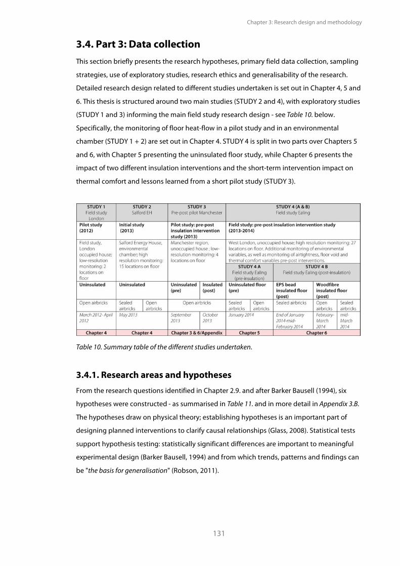
Chapter 3: Research design and methodology
131
3.4. Part 3: Data collection This section briefly presents the research hypotheses, primary field data collection, sampling
strategies, use of exploratory studies, research ethics and generalisability of the research.
Detailed research design related to different studies undertaken is set out in Chapter 4, 5 and
6. This thesis is structured around two main studies (STUDY 2 and 4), with exploratory studies
(STUDY 1 and 3) informing the main field study research design - see Table 10. below.
Specifically, the monitoring of floor heat-flow in a pilot study and in an environmental
chamber (STUDY 1 + 2) are set out in Chapter 4. STUDY 4 is split in two parts over Chapters 5
and 6, with Chapter 5 presenting the uninsulated floor study, while Chapter 6 presents the
impact of two different insulation interventions and the short-term intervention impact on
thermal comfort and lessons learned from a short pilot study (STUDY 3).
Table 10. Summary table of the different studies undertaken.
3.4.1. Research areas and hypotheses From the research questions identified in Chapter 2.9. and after Barker Bausell (1994), six
hypotheses were constructed - as summarised in Table 11. and in more detail in Appendix 3.B.
The hypotheses draw on physical theory; establishing hypotheses is an important part of
designing planned interventions to clarify causal relationships (Glass, 2008). Statistical tests
support hypothesis testing: statistically significant differences are important to meaningful
experimental design (Barker Bausell, 1994) and from which trends, patterns and findings can
be "the basis for generalisation" (Robson, 2011).
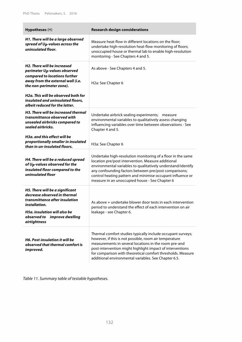
PhD Thesis Pelsmakers, S. 2016
132
Hypotheses (H) Research design considerations
H1. There will be a large observed spread of Up-values across the uninsulated floor.
Measure heat-flow in different locations on the floor; undertake high-resolution heat-flow monitoring of floors; unoccupied house or thermal lab to enable high-resolution monitoring - See Chapters 4 and 5.
H2. There will be increased perimeter Up-values observed compared to locations further away from the external wall (i.e. the non-perimeter zone). H2a. This will be observed both for insulated and uninsulated floors, albeit reduced for the latter.
As above - See Chapters 4 and 5.
H2a: See Chapter 6
H3. There will be increased thermal transmittance observed with unsealed airbricks compared to sealed airbricks. H3a. and this effect will be proportionally smaller in insulated than in un-insulated floors.
Undertake airbrick sealing experiments; measure environmental variables to qualitatively assess changing influencing variables over time between observations - See Chapter 4 and 5.
H3a: See Chapter 6
H4. There will be a reduced spread of Up-values observed for the insulated floor compared to the uninsulated floor
Undertake high-resolution monitoring of a floor in the same location pre/post intervention. Measure additional environmental variables to qualitatively understand/identify any confounding factors between pre/post comparisons; control heating pattern and minimise occupant influence or measure in an unoccupied house - See Chapter 6
H5. There will be a significant decrease observed in thermal transmittance after insulation installation.
H5a. insulation will also be observed to improve dwelling airtightness
As above + undertake blower door tests in each intervention period to understand the effect of each intervention on air leakage - see Chapter 6.
H6. Post-insulation it will be observed that thermal comfort is improved.
Thermal comfort studies typically include occupant surveys; however, if this is not possible, room air temperature measurements in several locations in the room pre-and post-intervention might highlight impact of interventions for comparison with theoretical comfort thresholds. Measure additional environmental variables. See Chapter 6.5.
Table 11. Summary table of testable hypotheses.
Chapter 3: Research design and methodology
133
A thermal chamber and an unoccupied house were identified as the best strategy to test
these hypotheses, enabling high resolution floor heat-flow measurement and undertaking of
interventions with internally controlled conditions which would not be possible in occupied
houses. A summary table of the pro's and cons of (un)occupied houses and use of a thermal
lab are set out in Appendix 3.E. To test hypotheses H2a and H3 to H6, an 'interrupted time
series design' was undertaken (Robson, 2011): floor heat-flow was measured prior to floor
interventions, with continued floor heat-flow measurements after intervention, "offering a
unique perspective on the evaluation of intervention (or "treatment") effects." (Glass, 2008).
3.4.2. Sampling case studies Following on from the research questions, objectives and hypotheses, five distinct primary
data collection areas were identified:
1. High resolution heat-flow measurements in a thermal chamber under controlled
conditions to characterise floor heat-flow and test floor heat transfer theory such as
increased heat-flow in the perimeter versus the non-perimeter zone; with airbricks open or
closed and to test how representative single (or a few) point measurements are of the whole
floor. Research design and limitations are discussed in Chapter 4; discussion about
generalisability in Section 3.4.4.
2. High resolution heat-flow measurements in the field to characterise in-situ heat-flow in
an actual case-study to test and compare theory from the thermal chamber and to build
theory with a pre/post insulation study. Measurement of environmental variables will be
important to understand pre/post comparison studies due to confounding factors. Research
design and limitations are discussed in Chapter 5 and 6; generalisability is discussed in
Section 3.4.4.
3. Monitoring of floor void conditions in the field to compare floor void conditions with
literature values; research design and limitations are discussed in Chapter 5.
4. Data collection for thermal comfort evaluation in order to test thermal comfort theory
and to build theory with regards to the conditions of insulated and uninsulated floors.
Research design and limitations are discussed in Chapter 6.
5. Blower door tests to evaluate air leakage of pre- and post intervention measures.
PhD Thesis Pelsmakers, S. 2016
134
3.4.2.1. Primary data collection sampling
Primary data for all five data collection areas were collected by taking a multiple case-study
approach. Prior to undertaking the main research data collection, exploratory studies were
first undertaken to inform the main studies - these are described in Section 3.4.2.2.
Due to the disruptive and seasonal nature of the data collection and the limited timescale
and resources of this PhD research, random sampling of a large number of floors - whether
for monitoring floor heat-flow, thermal comfort or floor void conditions - was not possible.
Purposive sampling to generate additional or new observations (Robson, 2011), i.e. to
maximise understanding and learning (Stake, 1995), was instead undertaken as a sampling
strategy for all of the main primary data collection case-study sampling strategies.
Convenience sampling is a typical sampling strategy for exploratory studies (Robson, 2011),
as also undertaken in this thesis research for both exploratory studies (STUDY 1 and 3), i.e.
measurements were taken where the author had access to an available house.
For floor heat-flux monitoring, purposive sampling allowed the selection of cases which
fulfilled the needs and objectives of the research purpose (Robson, 2011, Saunders, 2009).
For example, STUDY 2, (Chapter 4) was an environmental chamber replicating an actual
dwelling and floor construction and allowed the study of floor heat-flow in controlled
conditions and at high-resolution. Additionally, heat-flow monitoring in STUDY 4 (Chapter 5
and 6) took place in an unoccupied house over an entire winter season and allowed high-
resolution heat-flow monitoring pre/post intervention studies with homeowner approval -
see summary in Table 12. The implications of these non-random case-study sampling
techniques on generalisability of results is discussed in Section 3.4.4.
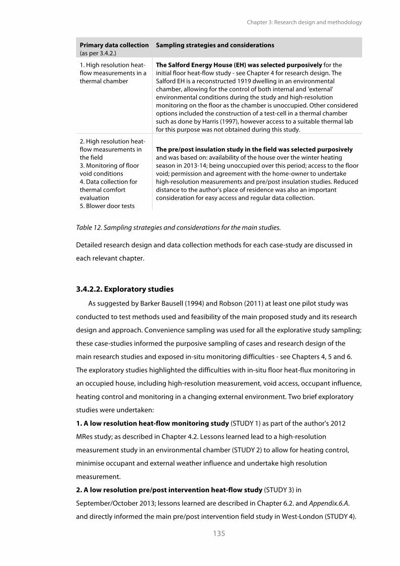
Chapter 3: Research design and methodology
135
Primary data collection (as per 3.4.2.)
Sampling strategies and considerations
1. High resolution heat-flow measurements in a thermal chamber
The Salford Energy House (EH) was selected purposively for the initial floor heat-flow study - see Chapter 4 for research design. The Salford EH is a reconstructed 1919 dwelling in an environmental chamber, allowing for the control of both internal and 'external' environmental conditions during the study and high-resolution monitoring on the floor as the chamber is unoccupied. Other considered options included the construction of a test-cell in a thermal chamber such as done by Harris (1997), however access to a suitable thermal lab for this purpose was not obtained during this study.
2. High resolution heat-flow measurements in the field 3. Monitoring of floor void conditions 4. Data collection for thermal comfort evaluation 5. Blower door tests
The pre/post insulation study in the field was selected purposively and was based on: availability of the house over the winter heating season in 2013-14; being unoccupied over this period; access to the floor void; permission and agreement with the home-owner to undertake high-resolution measurements and pre/post insulation studies. Reduced distance to the author's place of residence was also an important consideration for easy access and regular data collection.
Table 12. Sampling strategies and considerations for the main studies.
Detailed research design and data collection methods for each case-study are discussed in
each relevant chapter.
3.4.2.2. Exploratory studies
As suggested by Barker Bausell (1994) and Robson (2011) at least one pilot study was
conducted to test methods used and feasibility of the main proposed study and its research
design and approach. Convenience sampling was used for all the explorative study sampling;
these case-studies informed the purposive sampling of cases and research design of the
main research studies and exposed in-situ monitoring difficulties - see Chapters 4, 5 and 6.
The exploratory studies highlighted the difficulties with in-situ floor heat-flux monitoring in
an occupied house, including high-resolution measurement, void access, occupant influence,
heating control and monitoring in a changing external environment. Two brief exploratory
studies were undertaken:
1. A low resolution heat-flow monitoring study (STUDY 1) as part of the author's 2012
MRes study; as described in Chapter 4.2. Lessons learned lead to a high-resolution
measurement study in an environmental chamber (STUDY 2) to allow for heating control,
minimise occupant and external weather influence and undertake high resolution
measurement.
2. A low resolution pre/post intervention heat-flow study (STUDY 3) in
September/October 2013; lessons learned are described in Chapter 6.2. and Appendix.6.A.
and directly informed the main pre/post intervention field study in West-London (STUDY 4).
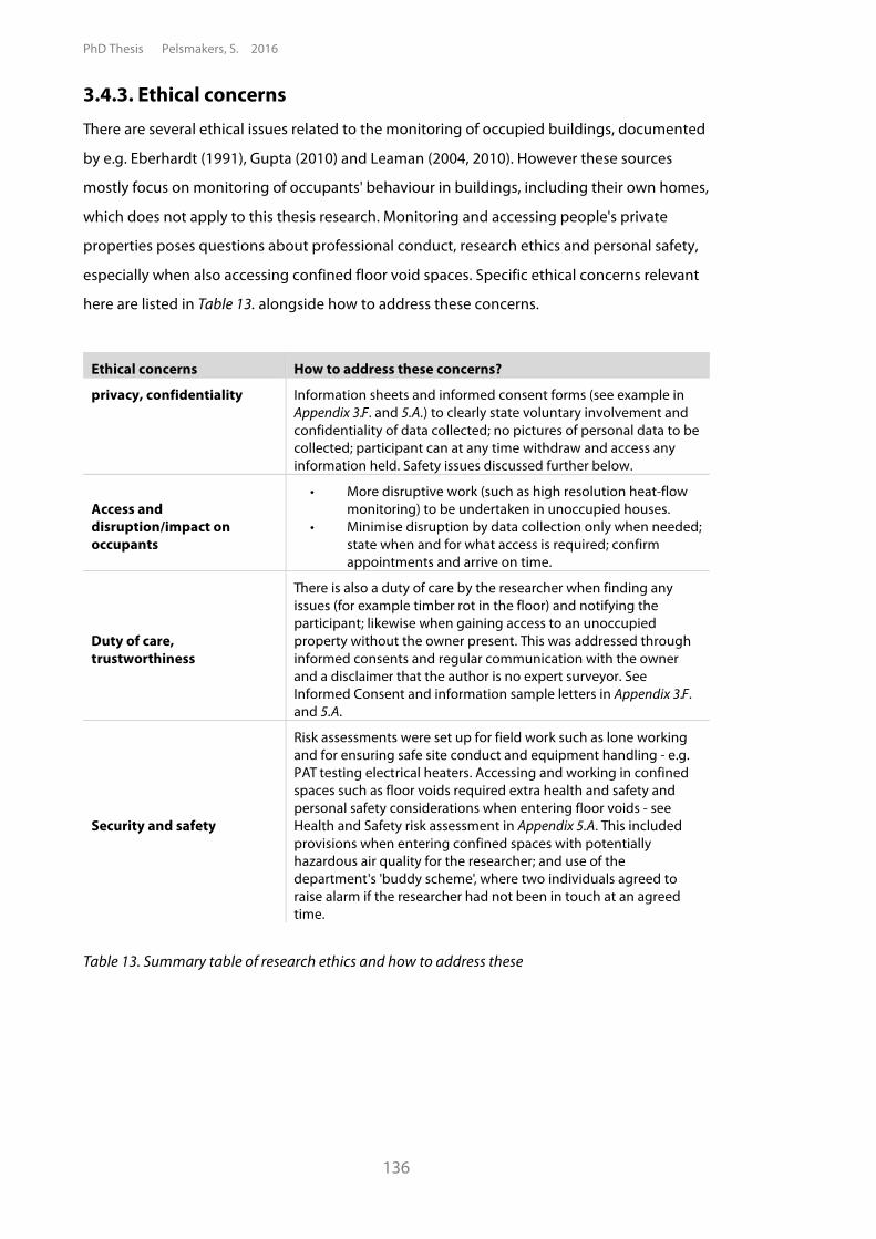
PhD Thesis Pelsmakers, S. 2016
136
3.4.3. Ethical concerns There are several ethical issues related to the monitoring of occupied buildings, documented
by e.g. Eberhardt (1991), Gupta (2010) and Leaman (2004, 2010). However these sources
mostly focus on monitoring of occupants' behaviour in buildings, including their own homes,
which does not apply to this thesis research. Monitoring and accessing people's private
properties poses questions about professional conduct, research ethics and personal safety,
especially when also accessing confined floor void spaces. Specific ethical concerns relevant
here are listed in Table 13. alongside how to address these concerns.
Ethical concerns How to address these concerns?
privacy, confidentiality Information sheets and informed consent forms (see example in Appendix 3.F. and 5.A.) to clearly state voluntary involvement and confidentiality of data collected; no pictures of personal data to be collected; participant can at any time withdraw and access any information held. Safety issues discussed further below.
Access and disruption/impact on occupants
• More disruptive work (such as high resolution heat-flow monitoring) to be undertaken in unoccupied houses.
• Minimise disruption by data collection only when needed; state when and for what access is required; confirm appointments and arrive on time.
Duty of care, trustworthiness
There is also a duty of care by the researcher when finding any issues (for example timber rot in the floor) and notifying the participant; likewise when gaining access to an unoccupied property without the owner present. This was addressed through informed consents and regular communication with the owner and a disclaimer that the author is no expert surveyor. See Informed Consent and information sample letters in Appendix 3.F. and 5.A.
Security and safety
Risk assessments were set up for field work such as lone working and for ensuring safe site conduct and equipment handling - e.g. PAT testing electrical heaters. Accessing and working in confined spaces such as floor voids required extra health and safety and personal safety considerations when entering floor voids - see Health and Safety risk assessment in Appendix 5.A. This included provisions when entering confined spaces with potentially hazardous air quality for the researcher; and use of the department's 'buddy scheme', where two individuals agreed to raise alarm if the researcher had not been in touch at an agreed time.
Table 13. Summary table of research ethics and how to address these
Chapter 3: Research design and methodology
137
3.4.4. Generalisability of research findings
External validity or generalisability of research outcomes
As described in the previous section, for this thesis research, cases were non-randomly
sampled, hence seeking statistical significance of results in the wider population, obtained
from a small sample and non-randomly sampled case-studies, is not possible (Silverman,
2010, Robson, 2011, Saunders, 2009, Flyvbjerg, 2006) neither a purpose of this thesis
research. However, purposively selected case-studies were selected based on maximising
understanding and learning and can give meaningful and detailed insights and refinements
for the testing and building of methodology and theory, which can be transferable and
useful to the wider population where applied in similar conditions and with similar purpose
(Silverman, 2010, Flyvbjerg, 2006, Stake, 1995). Generalisability beyond the case studied does
not need to be based on statistical inferences (Robson, 2011) and "may be thought of as the
development of theory which helps in understanding other cases or situations" (Robson, 2011)
and any trends, patterns and findings "are the basis for generalisation" (Robson, 2011). Case-
studies can also highlight observed phenomena and lead to refinement or modification of
pre-existing generalisations (Stake, 1995). This was done by for example Lowe (2007) who
demonstrated the presence of a thermal bypass in millions of cavity-walls based on a single
case-study. Indeed, findings based on purposive case-study data collection may lead to
generalisations to inform more about typical case-studies (Saunders, 2009) and may support
the refinement and modification of models and theories (Stake, 1995), which might also
apply in other cases with similar characteristics. Case-studies could also highlight interesting
findings about research methods and efficacy of proposed interventions (Silverman, 2010),
which may be applicable elsewhere and support future research. Finally, case-studies can
also be useful to highlight certain trends in the data collected (Robson, 2011) and to
generate and test hypotheses (Flyvbjerg, 2006), as undertaken in this thesis. Hence while
findings are specific to the particular case-studies and not representative of the wider
population, they may highlight methodological and theory implications as well as highlight
generalisable trends and patterns and will inform future research and support future studies.
The high-resolution heat-flow measurements undertaken in the Salford Energy House
environmental chamber (STUDY 2, Chapter 4), are not representative of the wider pre-1919
housing population. Additionally, and as discussed in Section 4.3., the Salford EH has been
reconstructed in an environmental chamber and there are several variables which are not
replicated from an actual house.
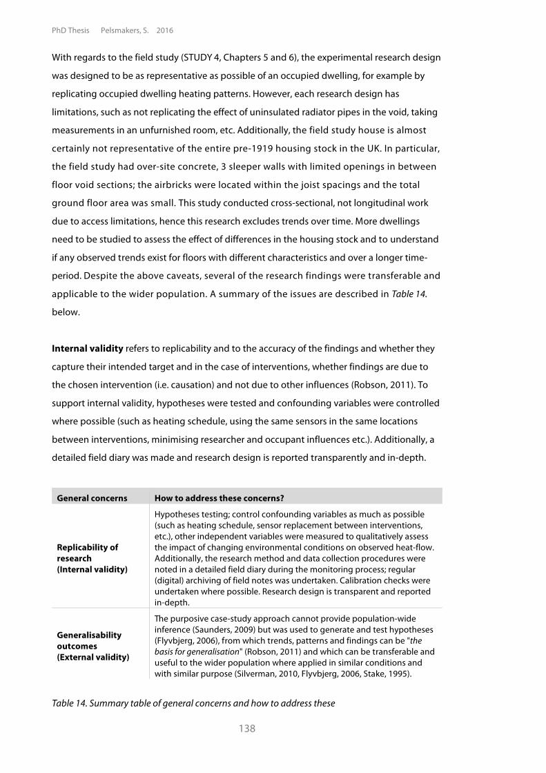
PhD Thesis Pelsmakers, S. 2016
138
With regards to the field study (STUDY 4, Chapters 5 and 6), the experimental research design
was designed to be as representative as possible of an occupied dwelling, for example by
replicating occupied dwelling heating patterns. However, each research design has
limitations, such as not replicating the effect of uninsulated radiator pipes in the void, taking
measurements in an unfurnished room, etc. Additionally, the field study house is almost
certainly not representative of the entire pre-1919 housing stock in the UK. In particular,
the field study had over-site concrete, 3 sleeper walls with limited openings in between
floor void sections; the airbricks were located within the joist spacings and the total
ground floor area was small. This study conducted cross-sectional, not longitudinal work
due to access limitations, hence this research excludes trends over time. More dwellings
need to be studied to assess the effect of differences in the housing stock and to understand
if any observed trends exist for floors with different characteristics and over a longer time-
period. Despite the above caveats, several of the research findings were transferable and
applicable to the wider population. A summary of the issues are described in Table 14.
below.
Internal validity refers to replicability and to the accuracy of the findings and whether they
capture their intended target and in the case of interventions, whether findings are due to
the chosen intervention (i.e. causation) and not due to other influences (Robson, 2011). To
support internal validity, hypotheses were tested and confounding variables were controlled
where possible (such as heating schedule, using the same sensors in the same locations
between interventions, minimising researcher and occupant influences etc.). Additionally, a
detailed field diary was made and research design is reported transparently and in-depth.
General concerns How to address these concerns?
Replicability of research (Internal validity)
Hypotheses testing; control confounding variables as much as possible (such as heating schedule, sensor replacement between interventions, etc.), other independent variables were measured to qualitatively assess the impact of changing environmental conditions on observed heat-flow. Additionally, the research method and data collection procedures were noted in a detailed field diary during the monitoring process; regular (digital) archiving of field notes was undertaken. Calibration checks were undertaken where possible. Research design is transparent and reported in-depth.
Generalisability outcomes (External validity)
The purposive case-study approach cannot provide population-wide inference (Saunders, 2009) but was used to generate and test hypotheses (Flyvbjerg, 2006), from which trends, patterns and findings can be "the basis for generalisation" (Robson, 2011) and which can be transferable and useful to the wider population where applied in similar conditions and with similar purpose (Silverman, 2010, Flyvbjerg, 2006, Stake, 1995).
Table 14. Summary table of general concerns and how to address these
Chapter 3: Research design and methodology
139
3.5. Summary This chapter introduced in-situ U-value measuring and analysis techniques and associated
uncertainties in detail, alongside raising conceptual issues of measurement location and
difficulties of low resolution heat-flux point measurements as a comparison to whole floor U-
value models. These issues are further explored in the following chapter, based on in-situ
measurements in the Salford Energy House. This chapter also set out the main studies and
sampling strategies conducted in this thesis research and associated ethical and general
concerns, including generalisability of findings based on case-study research.

PhD Thesis Pelsmakers, S. 2016
140
Chapter 4: Initial uninsulated floor heat-flow studies
141
Chapter 4: Initial uninsulated floor
heat-flow studies
4.1. Introduction This chapter aims to clarify and develop the identified conceptual floor heat-flow measuring
issues as identified in the previous chapter, while also contributing to a better understanding
of the actual U-value of floors and comparison with models - all of these areas were
identified as being poorly characterised at present. This chapter primarily addresses research
question 1 ("How should in-situ suspended timber ground floor U-values be estimated? ), while
also addressing research question 2 ("What is the in-situ measured thermal transmittance of
floors and how does it compare to model predictions?").
Primarily, this chapter presents and discusses the high-resolution in-situ measured U-values
of 15 point locations on the floor in the Salford Energy House (EH), (STUDY 2). Given the
issues surrounding measurement uncertainty and research design as set out in Chapter 3.3,
a section in this chapter is also devoted to these issues. The Salford EH research design was
informed by results from additional data analysis of the author's 2012 in-situ floor U-value
monitoring pilot study in the field (STUDY 1). Hence the 2012 pilot study data and its re-
analysis for this PhD research is the opening section of this chapter, followed by the main
Salford EH floor U-value study under controlled conditions.
The Salford EH high-resolution study1 enabled testing of whole floor U-value averaging
techniques to enable comparison to predicted values and are described in Section 4.4.2 and
4.4.3 respectively. Additionally, the impact of sensor locations on estimated results is
discussed alongside the impact of closing of airbricks on U-values in Section 4.4.5. and 4.4.4.
respectively.
The diagram below gives an overview of the studies subject to this chapter's analysis and
discussion, STUDY 1 and 2 are highlighted in red.
1 I.e. many points on the floor surface observed.
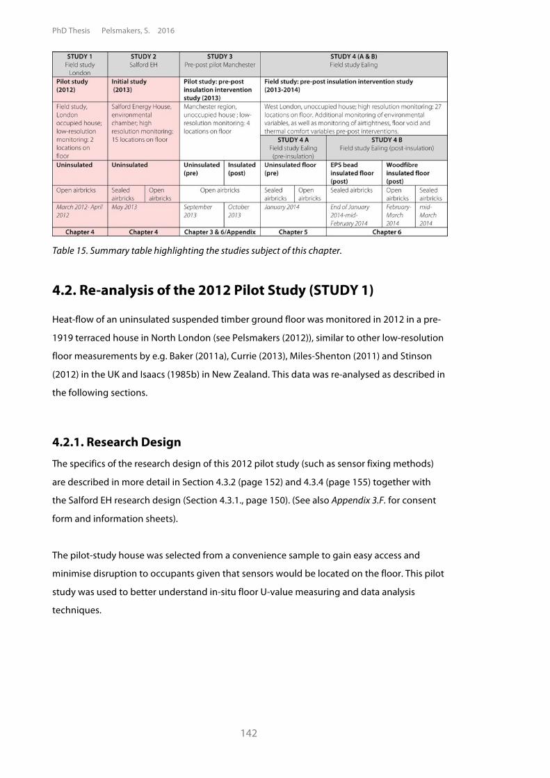
PhD Thesis Pelsmakers, S. 2016
142
Table 15. Summary table highlighting the studies subject of this chapter.
4.2. Re-analysis of the 2012 Pilot Study (STUDY 1)
Heat-flow of an uninsulated suspended timber ground floor was monitored in 2012 in a pre-
1919 terraced house in North London (see Pelsmakers (2012)), similar to other low-resolution
floor measurements by e.g. Baker (2011a), Currie (2013), Miles-Shenton (2011) and Stinson
(2012) in the UK and Isaacs (1985b) in New Zealand. This data was re-analysed as described in
the following sections.
4.2.1. Research Design The specifics of the research design of this 2012 pilot study (such as sensor fixing methods)
are described in more detail in Section 4.3.2 (page 152) and 4.3.4 (page 155) together with
the Salford EH research design (Section 4.3.1., page 150). (See also Appendix 3.F. for consent
form and information sheets).
The pilot-study house was selected from a convenience sample to gain easy access and
minimise disruption to occupants given that sensors would be located on the floor. This pilot
study was used to better understand in-situ floor U-value measuring and data analysis
techniques.
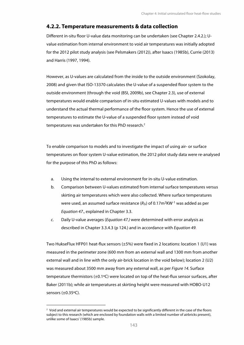
Chapter 4: Initial uninsulated floor heat-flow studies
143
4.2.2. Temperature measurements & data collection Different in-situ floor U-value data monitoring can be undertaken (see Chapter 2.4.2.); U-
value estimation from internal environment to void air temperatures was initially adopted
for the 2012 pilot study analysis (see Pelsmakers (2012)), after Isaacs (1985b), Currie (2013)
and Harris (1997, 1994).
However, as U-values are calculated from the inside to the outside environment (Szokolay,
2008) and given that ISO-13370 calculates the U-value of a suspended floor system to the
outside environment (through the void (BSI, 2009b), see Chapter 2.3), use of external
temperatures would enable comparison of in-situ estimated U-values with models and to
understand the actual thermal performance of the floor system. Hence the use of external
temperatures to estimate the U-value of a suspended floor system instead of void
temperatures was undertaken for this PhD research.2
To enable comparison to models and to investigate the impact of using air- or surface
temperatures on floor system U-value estimation, the 2012 pilot study data were re-analysed
for the purpose of this PhD as follows:
a. Using the internal to external environment for in-situ U-value estimation.
b. Comparison between U-values estimated from internal surface temperatures versus
skirting air temperatures which were also collected. Where surface temperatures
were used, an assumed surface resistance (RSi) of 0.17m2KW-1 was added as per
Equation 47., explained in Chapter 3.3.
c. Daily U-value averages (Equation 47.) were determined with error analysis as
described in Chapter 3.3.4.3 (p 124.) and in accordance with Equation 49.
Two HukseFlux HFP01 heat-flux sensors (±5%) were fixed in 2 locations: location 1 (U1) was
measured in the perimeter zone (600 mm from an external wall and 1300 mm from another
external wall and in line with the only air-brick location in the void below); location 2 (U2)
was measured about 3500 mm away from any external wall, as per Figure 14. Surface
temperature thermistors (±0.1ºC) were located on top of the heat-flux sensor surfaces, after
Baker (2011b); while air temperatures at skirting height were measured with HOBO-U12
sensors (±0.35ºC).
2 Void and external air temperatures would be expected to be significantly different in the case of the floors subject to this research (which are enclosed by foundation walls with a limited number of airbricks present), unlike some of Isaacs' (1985b) sample.
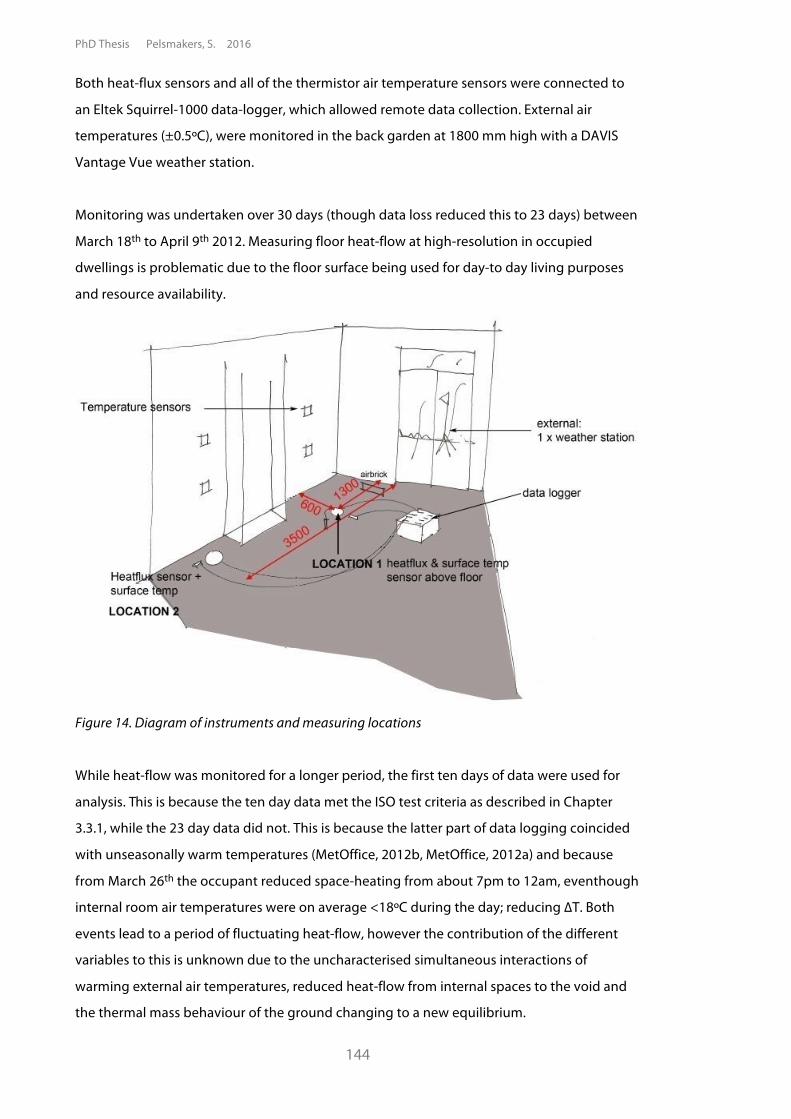
PhD Thesis Pelsmakers, S. 2016
144
Both heat-flux sensors and all of the thermistor air temperature sensors were connected to
an Eltek Squirrel-1000 data-logger, which allowed remote data collection. External air
temperatures (±0.5ºC), were monitored in the back garden at 1800 mm high with a DAVIS
Vantage Vue weather station.
Monitoring was undertaken over 30 days (though data loss reduced this to 23 days) between
March 18th to April 9th 2012. Measuring floor heat-flow at high-resolution in occupied
dwellings is problematic due to the floor surface being used for day-to day living purposes
and resource availability.
Figure 14. Diagram of instruments and measuring locations
While heat-flow was monitored for a longer period, the first ten days of data were used for
analysis. This is because the ten day data met the ISO test criteria as described in Chapter
3.3.1, while the 23 day data did not. This is because the latter part of data logging coincided
with unseasonally warm temperatures (MetOffice, 2012b, MetOffice, 2012a) and because
from March 26th the occupant reduced space-heating from about 7pm to 12am, eventhough
internal room air temperatures were on average <18ºC during the day; reducing !T. Both
events lead to a period of fluctuating heat-flow, however the contribution of the different
variables to this is unknown due to the uncharacterised simultaneous interactions of
warming external air temperatures, reduced heat-flow from internal spaces to the void and
the thermal mass behaviour of the ground changing to a new equilibrium.
Chapter 4: Initial uninsulated floor heat-flow studies
145
4.2.3. Pilot study results Depending on the location of the temperature measurements (surface or skirting air
temperatures), the estimated U-value in the perimeter location (U1) ranged from
1.72 ±0.31 Wm-2K-1 to 2.08 ± 0.44 Wm-2K-1; which is about twice that of location U2 which
ranged between 0.88 ±0.14 Wm-2K-1 to 1.02 ± 0.18 Wm-2K-1; these values were outside the
margins of measurement errors. U-values estimated from surface to external air temperature
(see Figure 15. ) were lower than those estimated from internal air temperatures measured at
skirting height, although the U-values in the same locations (but determined with different
temperatures) were within the estimated margins of error (error margins estimated as per
Equation 49.).
Averaging the two surface to external air temperature point U-values gave an estimated
U-value of 1.30 ±0.22 Wm-2K-1. However, given that one point was located in the perimeter
zone,3 which was only around 30% of the entire floor (see Figure 14.), using the average as
the whole floor U-value is likely to lead to an overestimation of the whole floor U-value by
giving both observed locations equal weighting. Deriving the whole floor U-value from a
weighted average based on a 30/70 perimeter/non-perimeter weighting, reduced the
average floor U-value to 1.13 ±0.19 Wm-2K-1. Note that this excludes the presence of joists,
which would lower the estimated in-situ U-value slightly for the uninsulated floor.
The ISO-13370 floor U-value model (BSI, 2009b) estimated a floor system U-value of 0.43 Wm-
2K-1, based on the pilot study's house and floor characteristics, excluding joist presence (see
Table 21. Page 183). This modelled U-value is below the 0.55 Wm-2K-1 mean published U-
value presented in Chapter 2.4. and just outside the literature range of 0.45 Wm-2K-1 to
0.70 Wm-2K-1 - see Table 1. This disparity might be due to the limited void ventilation
(0.0011 m2/m) and the small perimeter to floor area ratio (P/A = 0.24m/m2) due to the deep
plan of the pilot study house compared to the assumptions in the sources (typically P/A 0.30
m/m2 and ventilation area 0.0015 to 0.0030 m2/m).
From the results above, the average in-situ estimated floor U-value (1.30 ±0.22 Wm-2K-1) was
more than twice as high as the modelled U-value, see Figure 15. However, the model might
be an inaccurate representation of the actual U-value due to the input assumptions (see
Chapter 2.3.).
3 The perimeter zone was defined as within 1000mm from an external wall after Delsante (1989) see discussion in Section 4.4.1, page 162.
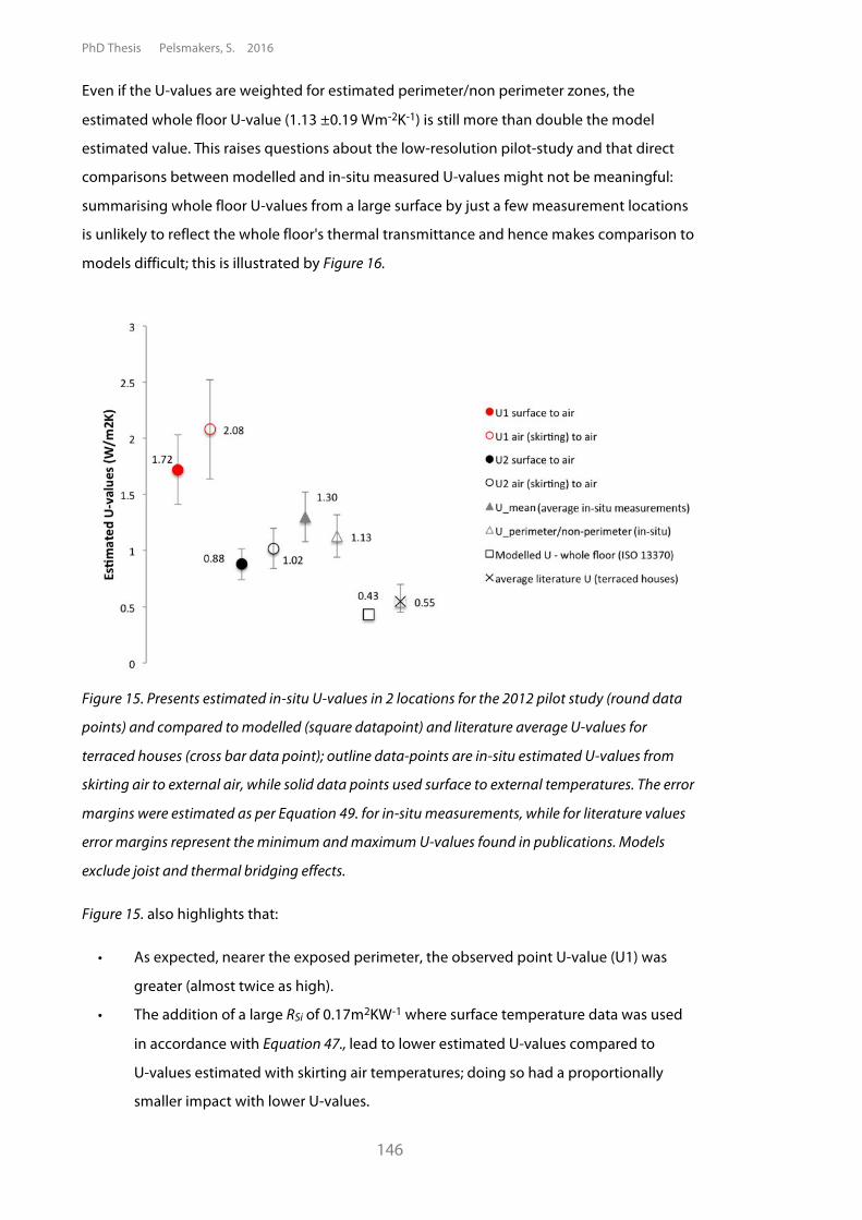
PhD Thesis Pelsmakers, S. 2016
146
Even if the U-values are weighted for estimated perimeter/non perimeter zones, the
estimated whole floor U-value (1.13 ±0.19 Wm-2K-1) is still more than double the model
estimated value. This raises questions about the low-resolution pilot-study and that direct
comparisons between modelled and in-situ measured U-values might not be meaningful:
summarising whole floor U-values from a large surface by just a few measurement locations
is unlikely to reflect the whole floor's thermal transmittance and hence makes comparison to
models difficult; this is illustrated by Figure 16.
Figure 15. Presents estimated in-situ U-values in 2 locations for the 2012 pilot study (round data
points) and compared to modelled (square datapoint) and literature average U-values for
terraced houses (cross bar data point); outline data-points are in-situ estimated U-values from
skirting air to external air, while solid data points used surface to external temperatures. The error
margins were estimated as per Equation 49. for in-situ measurements, while for literature values
error margins represent the minimum and maximum U-values found in publications. Models
exclude joist and thermal bridging effects.
Figure 15. also highlights that:
• As expected, nearer the exposed perimeter, the observed point U-value (U1) was
greater (almost twice as high).
• The addition of a large RSi of 0.17m2KW-1 where surface temperature data was used
in accordance with Equation 47., lead to lower estimated U-values compared to
U-values estimated with skirting air temperatures; doing so had a proportionally
smaller impact with lower U-values.
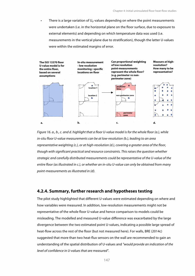
Chapter 4: Initial uninsulated floor heat-flow studies
147
• There is a large variation of Up-values depending on where the point measurements
were undertaken (i.e. in the horizontal plane on the floor surface, due to exposure to
external elements) and depending on which temperature data was used (i.e.
measurements in the vertical plane due to stratification), though the latter U-values
were within the estimated margins of error.
Figure 16. a., b., c. and d. highlight that a floor U-value model is for the whole floor (a.), while
in-situ floor U-value measurements can be at low-resolution (b.), leading to an area
representative weighting (c.), or at high-resolution (d.), covering a greater area of the floor,
though with significant practical and resource constraints. This raises the question whether
strategic and carefully distributed measurements could be representative of the U-value of the
entire floor (as illustrated in c.), or whether an in-situ U-value can only be obtained from many
point-measurements as illustrated in (d).
4.2.4. Summary, further research and hypotheses testing The pilot study highlighted that different U-values were estimated depending on where and
how variables were measured. In addition, low-resolution measurements might not be
representative of the whole floor U-value and hence comparison to models could be
misleading. The modelled and measured U-value difference was exacerbated by the large
divergence between the two estimated point U-values, indicating a possible large spread of
heat-flow across the rest of the floor (but not measured here). For walls, BRE (2014c)
suggested that more than two heat-flux sensors on the wall are recommended to gain an
understanding of the spatial distribution of U-values and "would provide an indication of the
level of confidence in U-values that are measured".
PhD Thesis Pelsmakers, S. 2016
148
Finally, ten days of data collection appeared sufficient to obtain valid U-values4 from the
field, though short-term monitoring cannot isolate the impact of seasonal effects.
Questions that arise from this pilot study are:
• In which internal/external vertical plane do we measure 'representative'
temperatures used for U-value determination?
• How to derive whole floor U-values from point U-value measurements?
These questions were further investigated in the Salford EH to further refine and develop in-
situ floor measuring methods, and specifically to:
• investigate the impact of temperature sensor location on U-value estimation by
measurement of both internal surface temperatures and internal air temperatures;
• control the internal and external environments and diminished occupant influence -
this should lead to reduced measurement uncertainties;
• undertake measurements on a joist to adjust whole floor U-value estimates to take
account of the joist presence;
• undertake high-resolution heat-flow monitoring to understand the spread of
Up-values across the floor; this will enable investigation of sensor placement location
and measurement techniques as well as to investigate whole floor averaging
techniques to enable a more robust comparison between models and in-situ
estimated U-values;
• to test the following hypotheses (H) as set out in Chapter 3.4.1.:
⁃ H1. "There will be a large observed spread of Up-values across the uninsulated
floor."
⁃ H2. "There will be increased perimeter Up-values observed compared to locations
further away from the external wall (i.e. the non-perimeter zone)."
⁃ H3. "There will be increased thermal transmittance observed with unsealed
airbricks compared to sealed airbricks."
4 "valid' U-values as defined in Chapter 3.3.1. by the data meeting the three ISO-9869 test criteria; though for further analysis, ISO-9869 was not used - see Chapter 3.3.
Chapter 4: Initial uninsulated floor heat-flow studies
149
4.3. The Salford Environmental Chamber: research design
(STUDY 2)
The Salford EH is a semi-detached, two-bedroom reconstructed house in an environmental
chamber at the University of Salford and was available for 10 days in May 2013 to measure
floor heat-flow at high resolution (i.e. on 15 locations on the floor, one of which was a joist
location) in a controlled environment. The purpose of this high-resolution study was to test
hypotheses (see Section 4.2.4.) and generate new knowledge. In particular, this study aimed
to:
• understand the spread of heat-flow across the floor and test whether a perimeter
effect was present as per solid ground floor theory (see Chapter 2.2.).
• test and understand the impact of different temperature location measurements on
estimated U-values.
• investigate and test different techniques to determine whole floor system U-values
from many point measurements and to compare to modelled floor U-values.
• understand the extent of reduced heat-flow through a joist to account for this in
whole floor U-value estimates and in comparison with models.
• understand the impact of all of the above on in-situ floor U-value data collection
techniques and to lead to refinement and further development of floor U-value
measuring methods.
• to understand the influence of floor void ventilation on observed Up-values by
closing the airbricks in a controlled experiment.
This study enabled the characterisation of the Salford EH floor U-value with sealed and
unsealed airbricks as well as the testing and refinement of in-situ measuring techniques and
analysis methods in a controlled environment without the problems associated with field
measurements in occupied houses, such as changing environmental conditions and
occupant space heating patterns, as noted in Section 4.2.2. A survey revealed that
uninsulated central heating pipes ran across the entire floor void perimeter. Hence the
internal chamber was heated electrically to enable investigation of the floor heat-flow
perimeter effect. It was also agreed to minimise other studies taking place at the same time
in the Salford EH, including undertaking of blower door tests, to avoid affecting data
collection and analysis.
PhD Thesis Pelsmakers, S. 2016
150
4.3.1. Description and research design
The Salford EH is separated on one side from an adjoining smaller house in the
environmental chamber by a solid brick party wall. This neighbouring property was heated
continuously to 18ºC throughout this study. The suspended timber ground floor was just
28.46m2, with timber floorboards in the living area and tiled floor finish in the kitchen on top
of plywood and floorboards. The externally measured exposed perimeter was 16.34m with
seven airbricks, totalling 0.00077m2/m ventilation area per metre of exposed perimeter.
While the reconstructed construction elements and imposed climatic conditions were a
simulation of the actual environment, there were several variables which were not replicated
from an actual house:
• the construction of the environmental chamber in which the Energy House is located
is built to newer construction standards than pre-1919 houses: the chamber stands
on a 280mm thick concrete slab, which in turn stands on top of an insulated ground
floor slab, collectively referred to as the concrete substructure; see Figure 17.
• floor void ventilation occurred in between both houses with no airbricks on the back
facade (see Figure 18.); the above mentioned void ventilation area excluded this
opening area.
• solar gain cannot be replicated in the EH, while wind-speed was excluded but the
house was subject to air-circulation from the external chamber air conditioning
system.
• there was only a 50-70mm gap under the 190 mm joists and the concrete oversite
slab which was likely to have reduced free airflow in the void. Note that joists run
from gable wall to party wall as indicated on Figure 18.
• the floor finish was tongued and grooved floorboards apart from ten floorboards,
which had gaps between them; as shown on Figure 18. This hybrid is atypical of
floors of this kind.
• the Salford EH was an unoccupied and controlled environment at all times which
was held near-constant for most of the year at winter temperatures in the external
chamber (~5-6ºC) and internal temperatures of 18-20ºC in the living spaces, as was
the case during this study. This means that the thermal behaviour of the concrete
substructure was in equilibrium, while in an actual house, the ground's thermal mass
below the floor is unlikely to be in equilibrium throughout the day and
interseasonally. It is unknown what the effect of this was on the study.
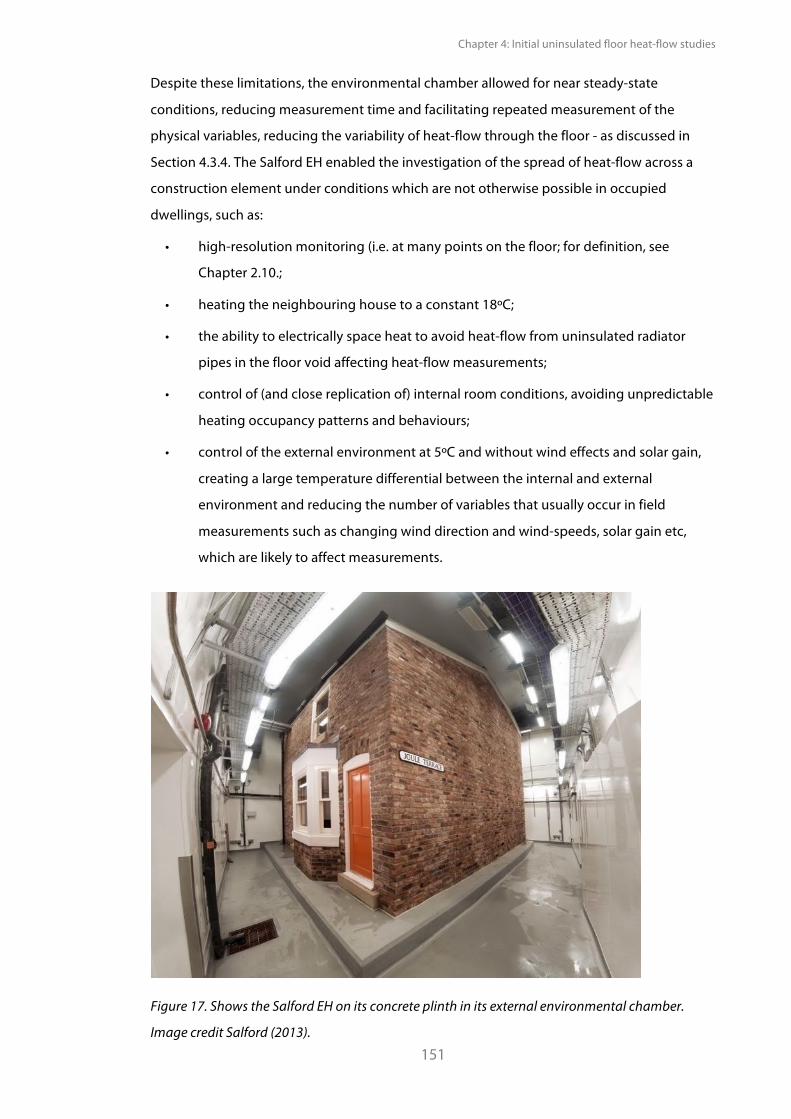
Chapter 4: Initial uninsulated floor heat-flow studies
151
Despite these limitations, the environmental chamber allowed for near steady-state
conditions, reducing measurement time and facilitating repeated measurement of the
physical variables, reducing the variability of heat-flow through the floor - as discussed in
Section 4.3.4. The Salford EH enabled the investigation of the spread of heat-flow across a
construction element under conditions which are not otherwise possible in occupied
dwellings, such as:
• high-resolution monitoring (i.e. at many points on the floor; for definition, see
Chapter 2.10.;
• heating the neighbouring house to a constant 18ºC;
• the ability to electrically space heat to avoid heat-flow from uninsulated radiator
pipes in the floor void affecting heat-flow measurements;
• control of (and close replication of) internal room conditions, avoiding unpredictable
heating occupancy patterns and behaviours;
• control of the external environment at 5ºC and without wind effects and solar gain,
creating a large temperature differential between the internal and external
environment and reducing the number of variables that usually occur in field
measurements such as changing wind direction and wind-speeds, solar gain etc,
which are likely to affect measurements.
Figure 17. Shows the Salford EH on its concrete plinth in its external environmental chamber.
Image credit Salford (2013).
PhD Thesis Pelsmakers, S. 2016
152
Note that the total floor void ventilation area was about 50% of the current UK Building
Regulations minimum requirement of 0.0015 m2/m (NBS, 2013) for timber floor ventilation,
considered sufficient to avoid high relative humidity in floor voids which could lead to
timber rot. The pilot case study house also had ventilation openings significantly below the
current recommendations (see Table 21., page 183). This might reflect that dwellings built
around this time might have lower than current ventilation requirements, however a larger
scale survey of the UK housing stock would be required to confirm this.
4.3.2. Instrumentation, fixings and location of instruments on the
floor
Measured variables included external environmental chamber air temperature (Tea, ºC), heat-
flux (q, mV) and internal surface temperatures (TSi, ºC) in 15 locations on the bare floorboards
of the uninsulated floor of the living room, as shown in Figure 18. For the Salford EH,
Hukseflux HFP01 heat-flux sensors were used with an instrument accuracy of ± 5%; and
110PV surface temperature thermistors, with an accuracy of ±0.2°C, alongside type K
thermocouples (±1.0ºC). A mix of data loggers were used: two Eltek Squirrel-851L, one
Campbell CR-10X, 1000 and 3000. To ensure good surface contact, all heat-flux and surface
temperature sensors were surface-fixed with a thin layer of servisol heat-sink compound
(thermal conductivity = 0.9 Wm-1K-1, (Farnell, 2014)) and were secured with masking tape in
the middle of a floorboard to measure floor board surface temperatures, directly adjacent to
the heat-flux sensors (unlike on top of the heat-flux sensors in the 2012 pilot case-study
house). Areas of floor were sought which broadly represented the conditions and structure
of the floor, with minimal influence from local heat gains and other influences (CEN, 1996,
BSI, 2014); floorboard gaps and joist locations were avoided, apart from location 11 in the
Salford EH study, which was purposively measured on a joist location. An infrared camera
was used in both monitoring studies to aid sensor placement as recommended by BSI (2014),
ASTM (2007a, 2007b) and McIntyre (1985).
Masking tape of similar colour and emissivity to the floorboards was used to create similar
radiant and reflective surfaces, though the middle of the sensor, i.e. the active sensing part,
was kept free from any tape or instruments in the Salford EH (and was hence of different
colour and emissivity). Contrary to this, in the pilot study the surface temperature sensors
were located and taped onto the sensing part after Baker (2011b). In both studies, sensor
edges were smoothed with the same masking tape to minimise turbulent flow over the
sensors as advised by Bales (1985) and as described in Chapter 3.3.
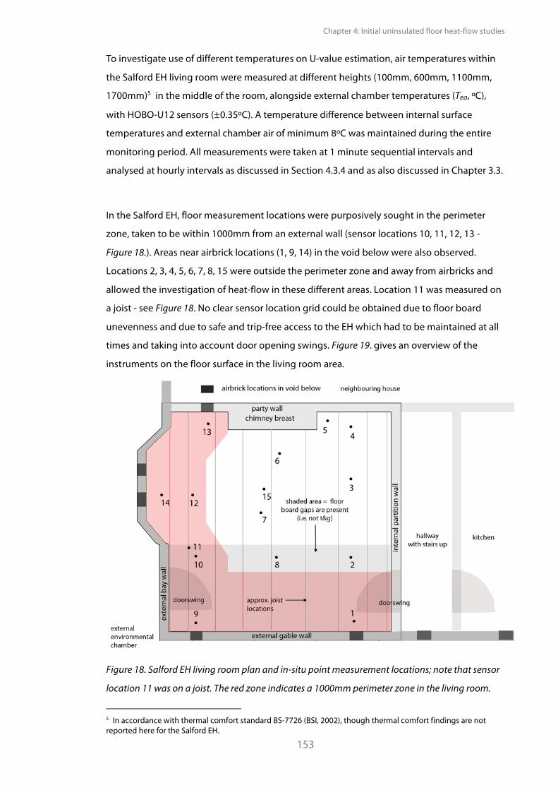
Chapter 4: Initial uninsulated floor heat-flow studies
153
To investigate use of different temperatures on U-value estimation, air temperatures within
the Salford EH living room were measured at different heights (100mm, 600mm, 1100mm,
1700mm)5 in the middle of the room, alongside external chamber temperatures (Tea, ºC),
with HOBO-U12 sensors (±0.35ºC). A temperature difference between internal surface
temperatures and external chamber air of minimum 8ºC was maintained during the entire
monitoring period. All measurements were taken at 1 minute sequential intervals and
analysed at hourly intervals as discussed in Section 4.3.4 and as also discussed in Chapter 3.3.
In the Salford EH, floor measurement locations were purposively sought in the perimeter
zone, taken to be within 1000mm from an external wall (sensor locations 10, 11, 12, 13 -
Figure 18.). Areas near airbrick locations (1, 9, 14) in the void below were also observed.
Locations 2, 3, 4, 5, 6, 7, 8, 15 were outside the perimeter zone and away from airbricks and
allowed the investigation of heat-flow in these different areas. Location 11 was measured on
a joist - see Figure 18. No clear sensor location grid could be obtained due to floor board
unevenness and due to safe and trip-free access to the EH which had to be maintained at all
times and taking into account door opening swings. Figure 19. gives an overview of the
instruments on the floor surface in the living room area.
!Figure 18. Salford EH living room plan and in-situ point measurement locations; note that sensor
location 11 was on a joist. The red zone indicates a 1000mm perimeter zone in the living room.
5 In accordance with thermal comfort standard BS-7726 (BSI, 2002), though thermal comfort findings are not reported here for the Salford EH.
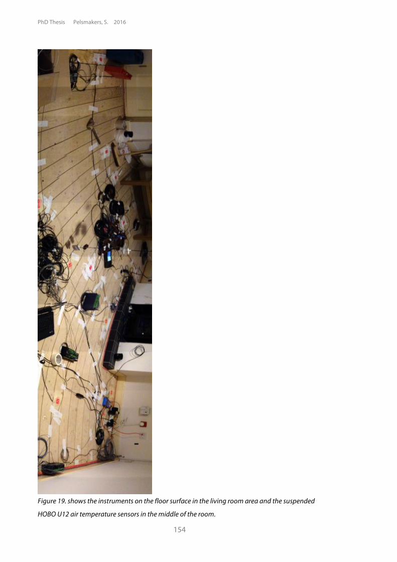
PhD Thesis Pelsmakers, S. 2016
154
Figure 19. shows the instruments on the floor surface in the living room area and the suspended
HOBO U12 air temperature sensors in the middle of the room.
Chapter 4: Initial uninsulated floor heat-flow studies
155
4.3.3. Side by side 'calibration' checks in the UCL thermal lab A 'side by side' calibration check of the UCL heat-flux sensors was undertaken similarly to the
method deployed by Doran (2008), alongside side by side calibration of the HOBO-U12
sensors and two available thermistors. Equipment that had been borrowed had to be
returned before being able to perform the same checks. The purpose of the side by side
calibration was to establish if there was any drift by any of the sensors when measuring the
same quantity in a thermal lab under steady-state conditions. A side by side calibration is
best supported by one heat-flux sensor being re-calibrated in a hot box, against which all
others sensors in the side by side experiment can then be compared, as undertaken by
Doran (2008), however due to limited resources this could not be achieved for this study.
Sensors could also only be tested at one temperature setting, due to another experiment
taking place at the same time in the UCL thermal chamber; the chamber temperatures were
higher than those at the Salford EH: 20-23ºC on the warm side and 12-13ºC on the cold side.
Temperature sensors could be tested at the two chamber conditions by swapping them half
way through from one chamber to another, but could not be checked at the lower Salford
EH temperatures (5-6ºC).
The UCL thermal lab was not designed with the purpose for calibration;6 despite this, good
agreement was indicated between all sensors and their own accuracies, suggesting that a
bias was unlikely. U-value results indicated that the heat-flux sensors were within ±5% of the
mean of the group of sensors and also between each other. Furthermore, no drift was
expected as most of the heat-flux sensors were <2 years old, below the time-period where
re-calibration is recommended (BSI, 2014).
No individual instrument or data adjustments were undertaken as exact measuring
conditions could not be repeated in the chamber and accuracies were all within those stated
by the manufacturer; assumed instrument errors were included in the final error propagation
- as described in Chapter 3.3 and Section 4.3.4.
6 For example the separating wall between the internal and external environmental chamber is made up out of different insulation materials in small sections with timber joists inserted, requiring the careful placement of sensors to ensure that the measured heat-flow is comparable between sensors. Additionally, hot and cold chamber temperatures are measured close to the fan outlet and hence are unreliable for calibration with temperature sensors; this may also create uncertainty in the calibration itself due to different air-flow patterns over sensors.
PhD Thesis Pelsmakers, S. 2016
156
4.3.4. Error propagation and data analysis procedures As discussed in Chapter 3.3.4., in-situ measuring is affected by instrument and measuring
condition errors; additionally the natural variability of U-values in changing environmental
conditions affects the U-value estimation. For the Salford EH, the natural variability of U was
derived from one standard deviation (sd) between hourly obtained U-values as in Equation
49. For the 2012 pilot study, daily data was used for the estimation of U-values and their
natural variability component - as explained in Chapter 3.3.4.3.
The natural variability component of U is estimated in the field as ±10% by BSI (2014) and as
expected this was significantly reduced for the Salford EH: ±1% to ±4% with sealed airbricks
and ±2% to ±5% with open airbricks depending on observed point location (and after
research influence outlier removal - see Section 4.3.5.). Overall this constituted a small
component of the total measurement uncertainty, resulting from undertaking
measurements in a near steady-state chamber. However, for the pilot study, the natural
variability of U was estimated between ±13% to ±19%,7 reflecting the changing
environmental conditions in the field.
A summary of the errors allowed for in the final error estimate is provided in Table 9. in
Chapter 3.3.4.3. As the conditions in the Salford EH were near-steady state, the natural
variability constituted a small component of the total uncertainty, which was ±9 to ±11%
depending on point location and whether airbricks were open or closed.
During the monitoring period, there was some researcher influence when data was collected
or activities took place in the external chamber; outliers were removed by Chauvenet's
Criterion as described in Section 4.3.5. Results are presented rounded to two decimal places
and in accordance with Equation 47. or Equation 48. (see Chapter 3.3.4.3), depending on use
of surface or air temperatures respectively.8 Total measurement uncertainty was derived as
per Equation 49. or Equation 50. in comparative studies - see Chapter 3.3.4.3.
The thermal resistance of the heat-flux sensor itself (~ 6.25 x 10⁻³ m2K/W, (Hukseflux)) was
accounted for by adjusting collected data; while sensor placement errors were minimised by
careful sensor placement with use of an infra-red camera as described in Chapter 3 and
Section 4.3.2.
7 Depending on location on the floor and height of the air temperature measurement used. 8 Where surface temperatures were used to estimate the point U-values, estimates require adjusting with assumed surface resistances to account for airflow and radiative effects at the surface as also undertaken by Baker (2011b), Rye (2010) and Doran (2008) for solid wall research - see Chapter 3.3.4.
Chapter 4: Initial uninsulated floor heat-flow studies
157
4.3.5. Data checks, outliers and Chauvenet's Criterion Outliers caused by researchers' influence during airbrick-open data collection were removed
using Chauvenet's Criterion. Chauvenet's Criterion is a statistical and objective test which
identifies outliers in normally distributed data. The test determines a 'distribution band' to
identify outliers, assuming a normal distribution with mean and standard deviation
corresponding to those of the data (Bayless., n.d., Taylor, 1997). The normality assumption is
used to calculate the probability that each data point would be observed if it did belong to
the data. This probability is then multiplied for the number of observations in the data; if for
any observation point the result of this calculation is "0.5, the data point is considered as an
outlier that is highly unlikely to have been produced by the same process that produced the
rest of the data (Lin, 2007, Bayless., n.d., Taylor, 1997).
Removal of outliers should always be treated with caution (so as to not bias the data and/or
to discard evidence of significance) and is ideally only removed if it is known why this outlier
occurred and can be identified as an error (Taylor, 1997), as was done here. Chauvenet's
Criterion has been criticised by for example Ross (2003), arguing that the "0.5 requirement
described above is arbitrary; however applying Chauvenet's Criterion is widely accepted
(Taylor, 1997, Bayless., n.d.); and it might be less arbitrary than manual outlier removal.
Manual outlier removal based on identified researcher influence gave similar U-values and
standard deviations as outlier removal with Chauvenet's Criterion. As such, in this PhD
research, Chauvenet's Criterion was only used for removal of outliers which were known to
be errors caused by researcher's influence as was the case for the Salford EH airbricks-open
data. No significant research interference took place during the airbrick-closed monitoring
period, thus no Chauvenet's Criterion adjustments were made for that data set.
Chauvenet's Criterion reduced the 120 hour airbrick-open data by between four to eleven
hours (max. 9% removal) depending on sensor location - see Table 16. Outlier removal did
not significantly change mean U-values; it was however undertaken as there were some clear
outliers which affected the estimation of the natural variability of U significantly and hence
the final uncertainty estimates - as can be noted from Table 16. Using Chauvenet's Criterion
lead to slightly higher (0-3%) estimated U-values compared to U-values estimated from the
data including the outliers (see Table 16.).
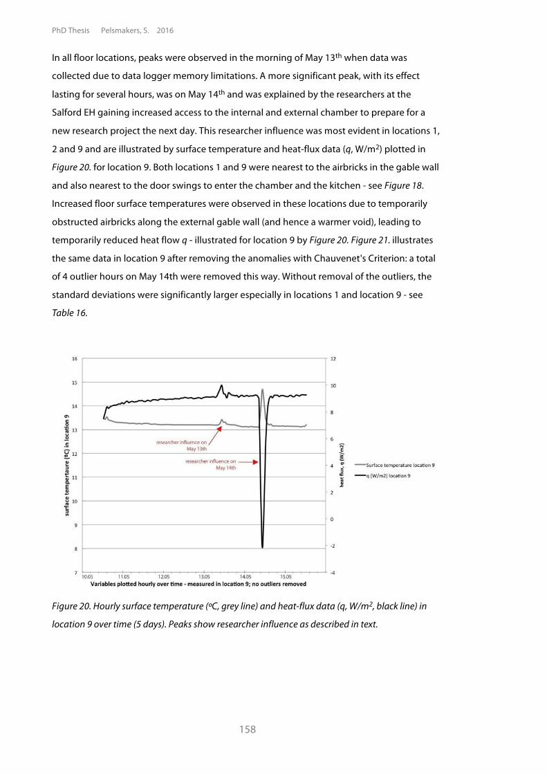
PhD Thesis Pelsmakers, S. 2016
158
In all floor locations, peaks were observed in the morning of May 13th when data was
collected due to data logger memory limitations. A more significant peak, with its effect
lasting for several hours, was on May 14th and was explained by the researchers at the
Salford EH gaining increased access to the internal and external chamber to prepare for a
new research project the next day. This researcher influence was most evident in locations 1,
2 and 9 and are illustrated by surface temperature and heat-flux data (q, W/m2) plotted in
Figure 20. for location 9. Both locations 1 and 9 were nearest to the airbricks in the gable wall
and also nearest to the door swings to enter the chamber and the kitchen - see Figure 18.
Increased floor surface temperatures were observed in these locations due to temporarily
obstructed airbricks along the external gable wall (and hence a warmer void), leading to
temporarily reduced heat flow q - illustrated for location 9 by Figure 20. Figure 21. illustrates
the same data in location 9 after removing the anomalies with Chauvenet's Criterion: a total
of 4 outlier hours on May 14th were removed this way. Without removal of the outliers, the
standard deviations were significantly larger especially in locations 1 and location 9 - see
Table 16.
Figure 20. Hourly surface temperature (ºC, grey line) and heat-flux data (q, W/m2, black line) in
location 9 over time (5 days). Peaks show researcher influence as described in text.
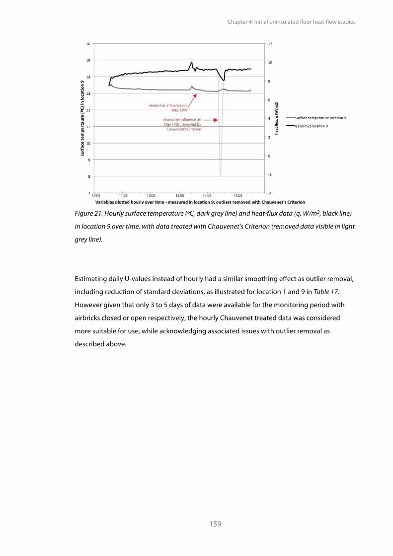
Chapter 4: Initial uninsulated floor heat-flow studies
159
Figure 21. Hourly surface temperature (ºC, dark grey line) and heat-flux data (q, W/m2, black line)
in location 9 over time, with data treated with Chauvenet's Criterion (removed data visible in light
grey line).
Estimating daily U-values instead of hourly had a similar smoothing effect as outlier removal,
including reduction of standard deviations, as illustrated for location 1 and 9 in Table 17.
However given that only 3 to 5 days of data were available for the monitoring period with
airbricks closed or open respectively, the hourly Chauvenet treated data was considered
more suitable for use, while acknowledging associated issues with outlier removal as
described above.
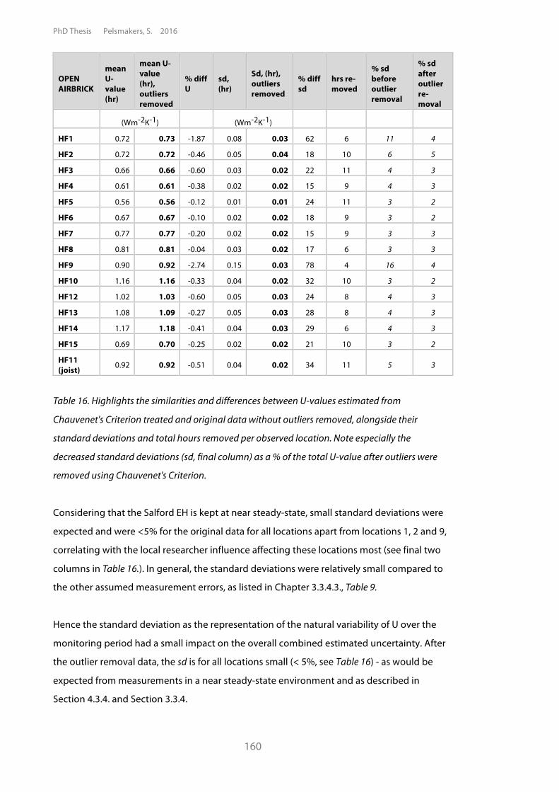
PhD Thesis Pelsmakers, S. 2016
160
OPEN AIRBRICK
mean U-value (hr)
mean U-value (hr), outliers removed
% diff U
sd, (hr)
Sd, (hr), outliers removed
% diff sd
hrs re-moved
% sd before outlier removal
% sd after outlier re-moval
(Wm-2K-1) (Wm-2K-1)
HF1 0.72 0.73 -1.87 0.08 0.03 62 6 11 4
HF2 0.72 0.72 -0.46 0.05 0.04 18 10 6 5
HF3 0.66 0.66 -0.60 0.03 0.02 22 11 4 3
HF4 0.61 0.61 -0.38 0.02 0.02 15 9 4 3
HF5 0.56 0.56 -0.12 0.01 0.01 24 11 3 2
HF6 0.67 0.67 -0.10 0.02 0.02 18 9 3 2
HF7 0.77 0.77 -0.20 0.02 0.02 15 9 3 3
HF8 0.81 0.81 -0.04 0.03 0.02 17 6 3 3
HF9 0.90 0.92 -2.74 0.15 0.03 78 4 16 4
HF10 1.16 1.16 -0.33 0.04 0.02 32 10 3 2
HF12 1.02 1.03 -0.60 0.05 0.03 24 8 4 3
HF13 1.08 1.09 -0.27 0.05 0.03 28 8 4 3
HF14 1.17 1.18 -0.41 0.04 0.03 29 6 4 3
HF15 0.69 0.70 -0.25 0.02 0.02 21 10 3 2
HF11 (joist) 0.92 0.92 -0.51 0.04 0.02 34 11 5 3
Table 16. Highlights the similarities and differences between U-values estimated from
Chauvenet's Criterion treated and original data without outliers removed, alongside their
standard deviations and total hours removed per observed location. Note especially the
decreased standard deviations (sd, final column) as a % of the total U-value after outliers were
removed using Chauvenet's Criterion.
Considering that the Salford EH is kept at near steady-state, small standard deviations were
expected and were <5% for the original data for all locations apart from locations 1, 2 and 9,
correlating with the local researcher influence affecting these locations most (see final two
columns in Table 16.). In general, the standard deviations were relatively small compared to
the other assumed measurement errors, as listed in Chapter 3.3.4.3., Table 9.
Hence the standard deviation as the representation of the natural variability of U over the
monitoring period had a small impact on the overall combined estimated uncertainty. After
the outlier removal data, the sd is for all locations small (< 5%, see Table 16) - as would be
expected from measurements in a near steady-state environment and as described in
Section 4.3.4. and Section 3.3.4.
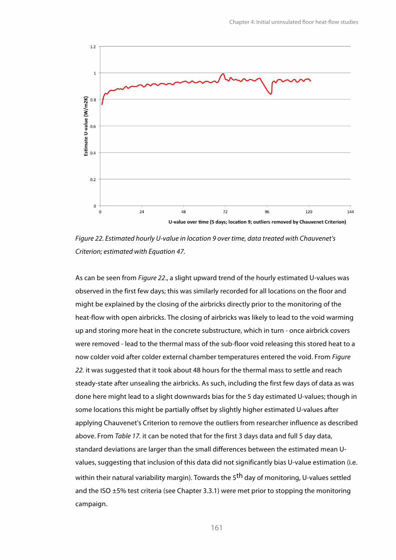
Chapter 4: Initial uninsulated floor heat-flow studies
161
Figure 22. Estimated hourly U-value in location 9 over time, data treated with Chauvenet's
Criterion; estimated with Equation 47.
As can be seen from Figure 22., a slight upward trend of the hourly estimated U-values was
observed in the first few days; this was similarly recorded for all locations on the floor and
might be explained by the closing of the airbricks directly prior to the monitoring of the
heat-flow with open airbricks. The closing of airbricks was likely to lead to the void warming
up and storing more heat in the concrete substructure, which in turn - once airbrick covers
were removed - lead to the thermal mass of the sub-floor void releasing this stored heat to a
now colder void after colder external chamber temperatures entered the void. From Figure
22. it was suggested that it took about 48 hours for the thermal mass to settle and reach
steady-state after unsealing the airbricks. As such, including the first few days of data as was
done here might lead to a slight downwards bias for the 5 day estimated U-values; though in
some locations this might be partially offset by slightly higher estimated U-values after
applying Chauvenet's Criterion to remove the outliers from researcher influence as described
above. From Table 17. it can be noted that for the first 3 days data and full 5 day data,
standard deviations are larger than the small differences between the estimated mean U-
values, suggesting that inclusion of this data did not significantly bias U-value estimation (i.e.
within their natural variability margin). Towards the 5th day of monitoring, U-values settled
and the ISO ±5% test criteria (see Chapter 3.3.1) were met prior to stopping the monitoring
campaign.
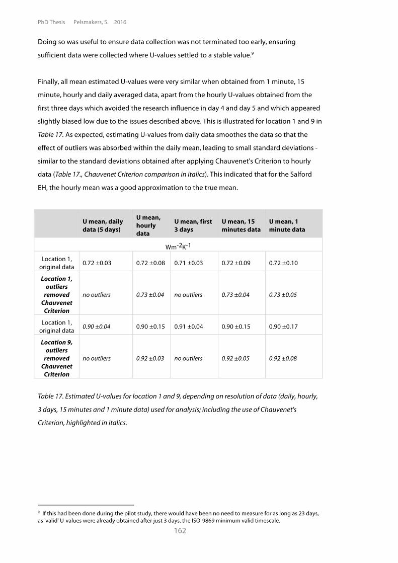
PhD Thesis Pelsmakers, S. 2016
162
Doing so was useful to ensure data collection was not terminated too early, ensuring
sufficient data were collected where U-values settled to a stable value.9
Finally, all mean estimated U-values were very similar when obtained from 1 minute, 15
minute, hourly and daily averaged data, apart from the hourly U-values obtained from the
first three days which avoided the research influence in day 4 and day 5 and which appeared
slightly biased low due to the issues described above. This is illustrated for location 1 and 9 in
Table 17. As expected, estimating U-values from daily data smoothes the data so that the
effect of outliers was absorbed within the daily mean, leading to small standard deviations -
similar to the standard deviations obtained after applying Chauvenet's Criterion to hourly
data (Table 17., Chauvenet Criterion comparison in italics). This indicated that for the Salford
EH, the hourly mean was a good approximation to the true mean.
U mean, daily data (5 days)
U mean, hourly data
U mean, first 3 days
U mean, 15 minutes data
U mean, 1 minute data
Wm-2K-1!
Location 1, original data 0.72 ±0.03 0.72 ±0.08 0.71 ±0.03 0.72 ±0.09 0.72 ±0.10
Location 1, outliers
removed Chauvenet
Criterion
no outliers 0.73 ±0.04 no outliers 0.73 ±0.04 0.73 ±0.05
Location 1, original data 0.90 ±0.04 0.90 ±0.15 0.91 ±0.04 0.90 ±0.15 0.90 ±0.17
Location 9, outliers
removed Chauvenet
Criterion
no outliers 0.92 ±0.03 no outliers 0.92 ±0.05 0.92 ±0.08
Table 17. Estimated U-values for location 1 and 9, depending on resolution of data (daily, hourly,
3 days, 15 minutes and 1 minute data) used for analysis; including the use of Chauvenet's
Criterion, highlighted in italics.
9 If this had been done during the pilot study, there would have been no need to measure for as long as 23 days, as 'valid' U-values were already obtained after just 3 days, the ISO-9869 minimum valid timescale.
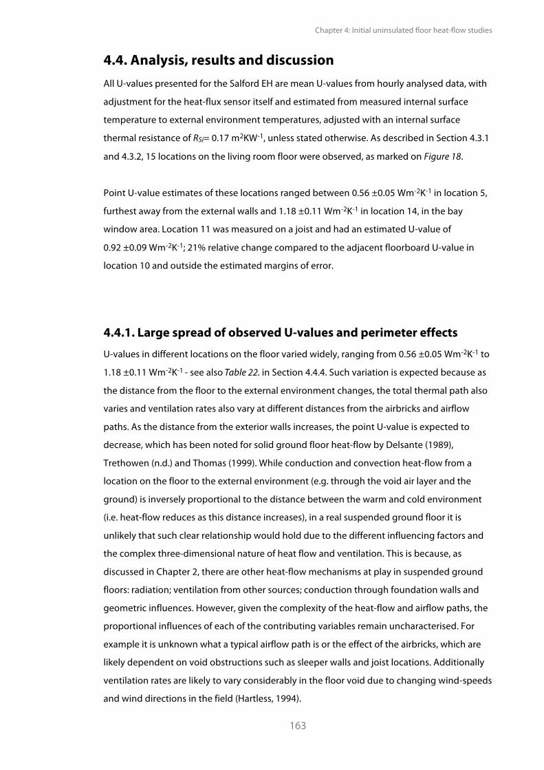
Chapter 4: Initial uninsulated floor heat-flow studies
163
4.4. Analysis, results and discussion All U-values presented for the Salford EH are mean U-values from hourly analysed data, with
adjustment for the heat-flux sensor itself and estimated from measured internal surface
temperature to external environment temperatures, adjusted with an internal surface
thermal resistance of RSi= 0.17 m2KW-1, unless stated otherwise. As described in Section 4.3.1
and 4.3.2, 15 locations on the living room floor were observed, as marked on Figure 18.
Point U-value estimates of these locations ranged between 0.56 ±0.05 Wm-2K-1 in location 5,
furthest away from the external walls and 1.18 ±0.11 Wm-2K-1 in location 14, in the bay
window area. Location 11 was measured on a joist and had an estimated U-value of
0.92 ±0.09 Wm-2K-1; 21% relative change compared to the adjacent floorboard U-value in
location 10 and outside the estimated margins of error.
4.4.1. Large spread of observed U-values and perimeter effects U-values in different locations on the floor varied widely, ranging from 0.56 ±0.05 Wm-2K-1 to
1.18 ±0.11 Wm-2K-1 - see also Table 22. in Section 4.4.4. Such variation is expected because as
the distance from the floor to the external environment changes, the total thermal path also
varies and ventilation rates also vary at different distances from the airbricks and airflow
paths. As the distance from the exterior walls increases, the point U-value is expected to
decrease, which has been noted for solid ground floor heat-flow by Delsante (1989),
Trethowen (n.d.) and Thomas (1999). While conduction and convection heat-flow from a
location on the floor to the external environment (e.g. through the void air layer and the
ground) is inversely proportional to the distance between the warm and cold environment
(i.e. heat-flow reduces as this distance increases), in a real suspended ground floor it is
unlikely that such clear relationship would hold due to the different influencing factors and
the complex three-dimensional nature of heat flow and ventilation. This is because, as
discussed in Chapter 2, there are other heat-flow mechanisms at play in suspended ground
floors: radiation; ventilation from other sources; conduction through foundation walls and
geometric influences. However, given the complexity of the heat-flow and airflow paths, the
proportional influences of each of the contributing variables remain uncharacterised. For
example it is unknown what a typical airflow path is or the effect of the airbricks, which are
likely dependent on void obstructions such as sleeper walls and joist locations. Additionally
ventilation rates are likely to vary considerably in the floor void due to changing wind-speeds
and wind directions in the field (Hartless, 1994).
PhD Thesis Pelsmakers, S. 2016
164
Because airbricks are located at the edges of a building, the main effect of airflow on the
heat-flow rate is generally expected in the floor perimeter area; however it was not possible
to isolate the effect of the airbricks in the perimeter walls. Generally increased void
ventilation leads to an increased rate of heat-flow, because:
• the void air layer is not a still air layer, hence creating mass-transfer heat-flow;
• in winter, colder external air displaces warmer void air, creating a greater !T between
internal spaces and the void, increasing the rate of conductive heat-flow to the void.
A large temperature variation across the floor can be inferred from the below
infrared image Figure 23.;
• surface thermal resistances in the void are likely to be lowered, reducing resistance to
heat-flow - as described by Harris (1993).
Figure 23. Infrared image of a section of the Salford Energy House floor surface, illustrating the
spread of surface temperatures across the floor with airbricks open. In-situ measured surface,
temperatures ranged between 16ºC near the back of the room (illustrated here in yellow),
compared to just 13ºC near airbrick s(illustrated here in blue).
Each estimated point U-value was investigated as a function of its nearest distance to an
exposed wall - see Figure 24. Figure 24. supports a relationship between heat-flow and
distance to nearest external walls; and this was in support of hypothesis H2 ("There will be
increased perimeter Up-values observed compared to locations further away from the external
wall (i.e. the non-perimeter zone)"). To test this hypothesis, simplified categorisation of
estimated Up-values in perimeter and non-perimeter zones was undertaken: Delsante (1989)
described a narrow strip of a 1000mm perimeter zone for solid ground floors where most of
the heat loss occurred, though for larger floor areas. Thomas (1999) describes a 1500mm
perimeter zone also for a large solid ground floor.
Chapter 4: Initial uninsulated floor heat-flow studies
165
For the Salford EH, a 1000mm perimeter zone categorisation would include six measurement
locations in the perimeter zone and eight in the non-perimeter zone; while a 1500mm
perimeter zone would reverse this. Given the small floor plate of the Salford EH and other
floors studied in this PhD research, the categorisation of the 1000mm perimeter zone was
used as it allowed sufficient points to be included in the perimeter zone, while maintaining
the definition of perimeter as not the majority of the floor area. However, it should be
highlighted that this perimeter categorisation and grouping is for the purpose of hypotheses
testing and to allow graphical representation of Up-values within 1000mm from an exposed
wall.
Hypotheses can be tested by undertaking statistical tests of the data. The Wilcoxon or Mann-
Whitney U test is a hypothesis or significance test (Spiegel, 1999) and was used here instead
of the more common t-test. Unlike the t-test, the Wilcoxon test does not assume normal
distribution nor equal standard deviations between the two comparison groups and is
therefore often preferred (Dytham, 2011). Additionally, the Wilcoxon test is less likely to
return a result of significance when there is no real difference (Dytham, 2011); statistical
hypothesis testing excludes error margins.
To test hypothesis H2, the U-values within a 1000mm perimeter zone (i.e. locations 1, 9, 10
and 12 to 14; Figure 24., in red) were compared with the non-perimeter zone of the floor
(points in black) by an unpaired Mann-Whitney U (Wilcoxcon rank sum) test, suggesting that
the observed U-values in the perimeter and non-perimeter floor zone differed significantly
(Mann–Whitney W = 46, n2 = 6; n2 = 8,P < 0.05 (0.002664), unpaired). The probability that
there was a zero difference in heat-flow between the perimeter zone and the non-perimeter
zone of the floor was negligible (0.002664, or about three in 1000). The estimated mean
U-value of the 6 perimeter located points was 1.02 ±0.10 Wm-2K-1 which is about a third
greater than the estimated mean U-value of the non-perimeter zone (0.69 ±0.07 Wm-2K-1).
Increased Up-values nearest the external environment also follows physical principles as
described prior; though it should be noted that there is no clearly defined extent of the
perimeter effect as there is no abrupt change after 1000mm, but a gradual reduction in
Up-values the further away from the external environment - see Figures 24 to 29.

PhD Thesis Pelsmakers, S. 2016
166
Figure 24. In-situ estimated Salford EH suspended floor U-values as a function of nearest distance
to exposed wall measured from the nearest internal surface of the external wall to the middle of
the heat-flux sensor; red data points are within 1000mm of the exposed perimeter; black data
points are located in the non-perimeter zone.
After the monitoring period, builder's debris in the void blocking the airbrick nearest to
location 14, was discovered. This is likely to have affected perimeter heat-flow in location 14
and other nearby locations, possibly resulting in reduced heat-flow than if the airbrick had
been clear. It can also be noted from Figure 24., that the estimated Up-values in the perimeter
zone of the bay-wall (locations 10, 12, 13, 14) were within each other's margins of error, but
were outside the margins of error of the non-perimeter zone Up-values, confirming that the
bay-wall effect especially was large and significant. This is also confirmed by Figure 26. which
plots point U-values as a function of bay-wall distances and highlights that in general there
was increased heat-flow in locations nearest to the external bay-wall (10, 12 to 14) compared
to perimeter locations near the gable-wall (locations 1, 9). This observation might be
explained by the bay wall's two airbricks and its large exposed perimeter. Furthermore, the
190mm deep joists ran from gable to party wall (see Figure 18.) and allowed only about
50-70mm clearance for free airflow underneath, partially obstructing air-flow from the bay-
wall floor void area into the rest of the floor void - see Figure 25. This might lead to an
isolated area of low void temperatures in the bay-wall floor void and hence increased heat-
flow in this bay perimeter area, emphasising increased Up-values in this area. These increased
Up-values in the bay wall perimeter area emphasise the observed low heat-flow away from
the bay-wall, i.e. in the gable perimeter locations 1 and 9.
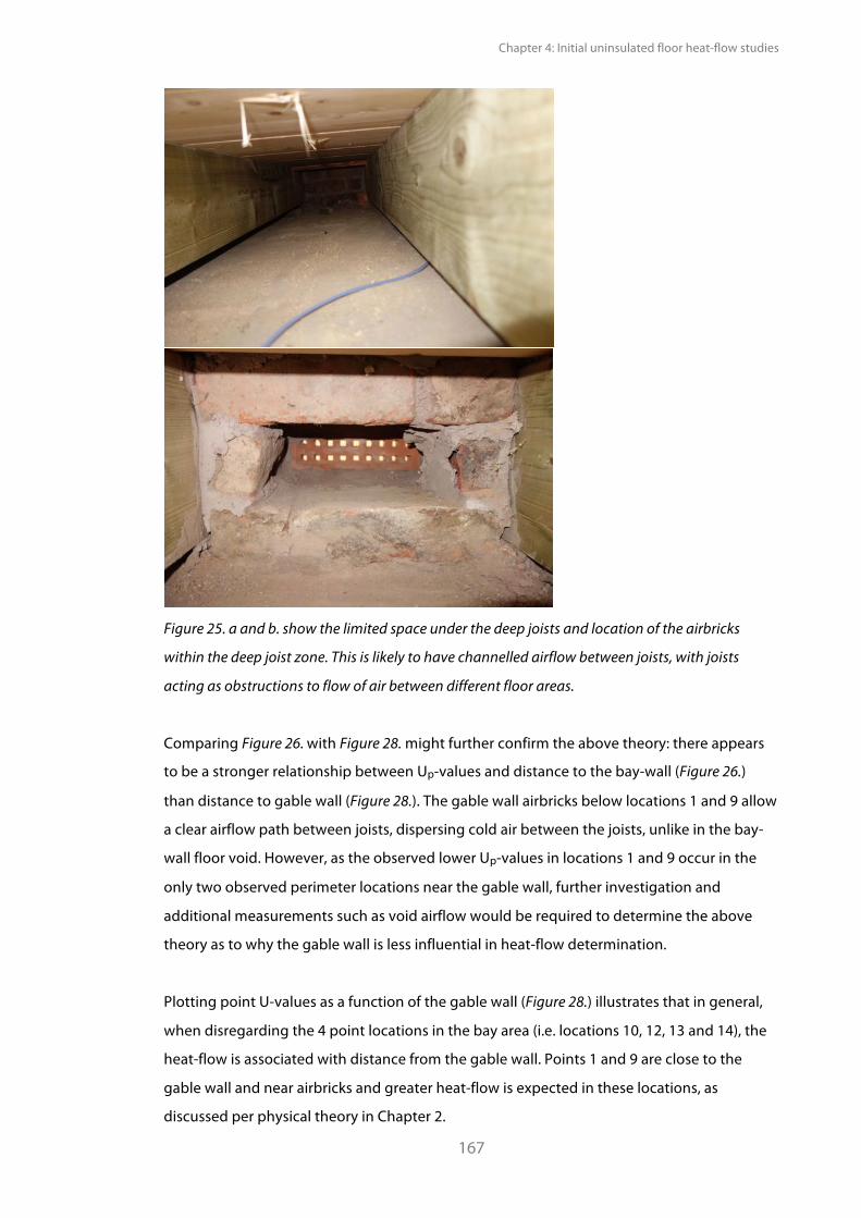
Chapter 4: Initial uninsulated floor heat-flow studies
167
Figure 25. a and b. show the limited space under the deep joists and location of the airbricks
within the deep joist zone. This is likely to have channelled airflow between joists, with joists
acting as obstructions to flow of air between different floor areas.
Comparing Figure 26. with Figure 28. might further confirm the above theory: there appears
to be a stronger relationship between Up-values and distance to the bay-wall (Figure 26.)
than distance to gable wall (Figure 28.). The gable wall airbricks below locations 1 and 9 allow
a clear airflow path between joists, dispersing cold air between the joists, unlike in the bay-
wall floor void. However, as the observed lower Up-values in locations 1 and 9 occur in the
only two observed perimeter locations near the gable wall, further investigation and
additional measurements such as void airflow would be required to determine the above
theory as to why the gable wall is less influential in heat-flow determination.
Plotting point U-values as a function of the gable wall (Figure 28.) illustrates that in general,
when disregarding the 4 point locations in the bay area (i.e. locations 10, 12, 13 and 14), the
heat-flow is associated with distance from the gable wall. Points 1 and 9 are close to the
gable wall and near airbricks and greater heat-flow is expected in these locations, as
discussed per physical theory in Chapter 2.
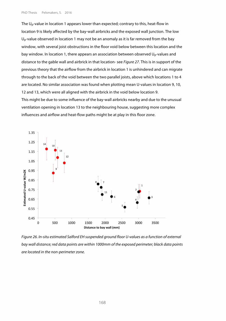
PhD Thesis Pelsmakers, S. 2016
168
The Up-value in location 1 appears lower than expected; contrary to this, heat-flow in
location 9 is likely affected by the bay-wall airbricks and the exposed wall junction. The low
Up-value observed in location 1 may not be an anomaly as it is far removed from the bay
window, with several joist obstructions in the floor void below between this location and the
bay window. In location 1, there appears an association between observed Up-values and
distance to the gable wall and airbrick in that location- see Figure 27. This is in support of the
previous theory that the airflow from the airbrick in location 1 is unhindered and can migrate
through to the back of the void between the two parallel joists, above which locations 1 to 4
are located. No similar association was found when plotting mean U-values in location 9, 10,
12 and 13, which were all aligned with the airbrick in the void below location 9.
This might be due to some influence of the bay-wall airbricks nearby and due to the unusual
ventilation opening in location 13 to the neighbouring house, suggesting more complex
influences and airflow and heat-flow paths might be at play in this floor zone.
Figure 26. In-situ estimated Salford EH suspended ground floor U-values as a function of external
bay wall distance; red data points are within 1000mm of the exposed perimeter; black data points
are located in the non-perimeter zone.
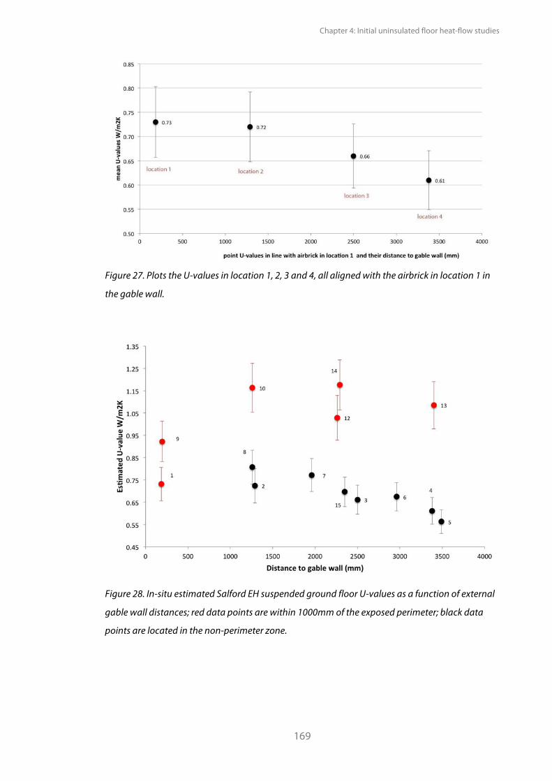
Chapter 4: Initial uninsulated floor heat-flow studies
169
Figure 27. Plots the U-values in location 1, 2, 3 and 4, all aligned with the airbrick in location 1 in
the gable wall.
Figure 28. In-situ estimated Salford EH suspended ground floor U-values as a function of external
gable wall distances; red data points are within 1000mm of the exposed perimeter; black data
points are located in the non-perimeter zone.
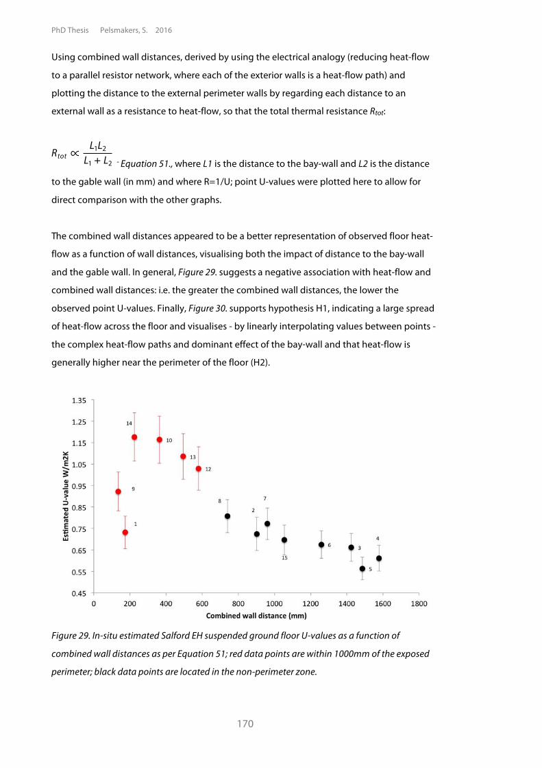
PhD Thesis Pelsmakers, S. 2016
170
Using combined wall distances, derived by using the electrical analogy (reducing heat-flow
to a parallel resistor network, where each of the exterior walls is a heat-flow path) and
plotting the distance to the external perimeter walls by regarding each distance to an
external wall as a resistance to heat-flow, so that the total thermal resistance Rtot:
- Equation 51., where L1 is the distance to the bay-wall and L2 is the distance
to the gable wall (in mm) and where R=1/U; point U-values were plotted here to allow for
direct comparison with the other graphs.
The combined wall distances appeared to be a better representation of observed floor heat-
flow as a function of wall distances, visualising both the impact of distance to the bay-wall
and the gable wall. In general, Figure 29. suggests a negative association with heat-flow and
combined wall distances: i.e. the greater the combined wall distances, the lower the
observed point U-values. Finally, Figure 30. supports hypothesis H1, indicating a large spread
of heat-flow across the floor and visualises - by linearly interpolating values between points -
the complex heat-flow paths and dominant effect of the bay-wall and that heat-flow is
generally higher near the perimeter of the floor (H2).
Figure 29. In-situ estimated Salford EH suspended ground floor U-values as a function of
combined wall distances as per Equation 51; red data points are within 1000mm of the exposed
perimeter; black data points are located in the non-perimeter zone.
Rtot öL�L�
L� + L�
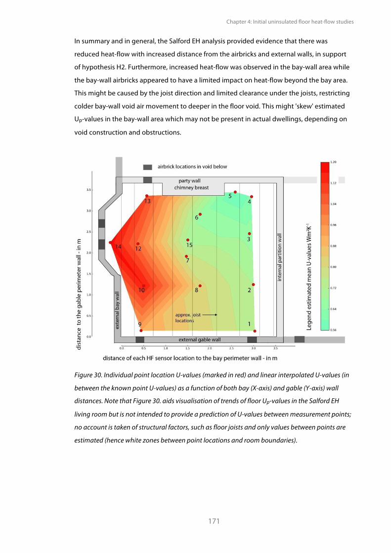
Chapter 4: Initial uninsulated floor heat-flow studies
171
In summary and in general, the Salford EH analysis provided evidence that there was
reduced heat-flow with increased distance from the airbricks and external walls, in support
of hypothesis H2. Furthermore, increased heat-flow was observed in the bay-wall area while
the bay-wall airbricks appeared to have a limited impact on heat-flow beyond the bay area.
This might be caused by the joist direction and limited clearance under the joists, restricting
colder bay-wall void air movement to deeper in the floor void. This might 'skew' estimated
Up-values in the bay-wall area which may not be present in actual dwellings, depending on
void construction and obstructions.
Figure 30. Individual point location U-values (marked in red) and linear interpolated U-values (in
between the known point U-values) as a function of both bay (X-axis) and gable (Y-axis) wall
distances. Note that Figure 30. aids visualisation of trends of floor Up-values in the Salford EH
living room but is not intended to provide a prediction of U-values between measurement points;
no account is taken of structural factors, such as floor joists and only values between points are
estimated (hence white zones between point locations and room boundaries).
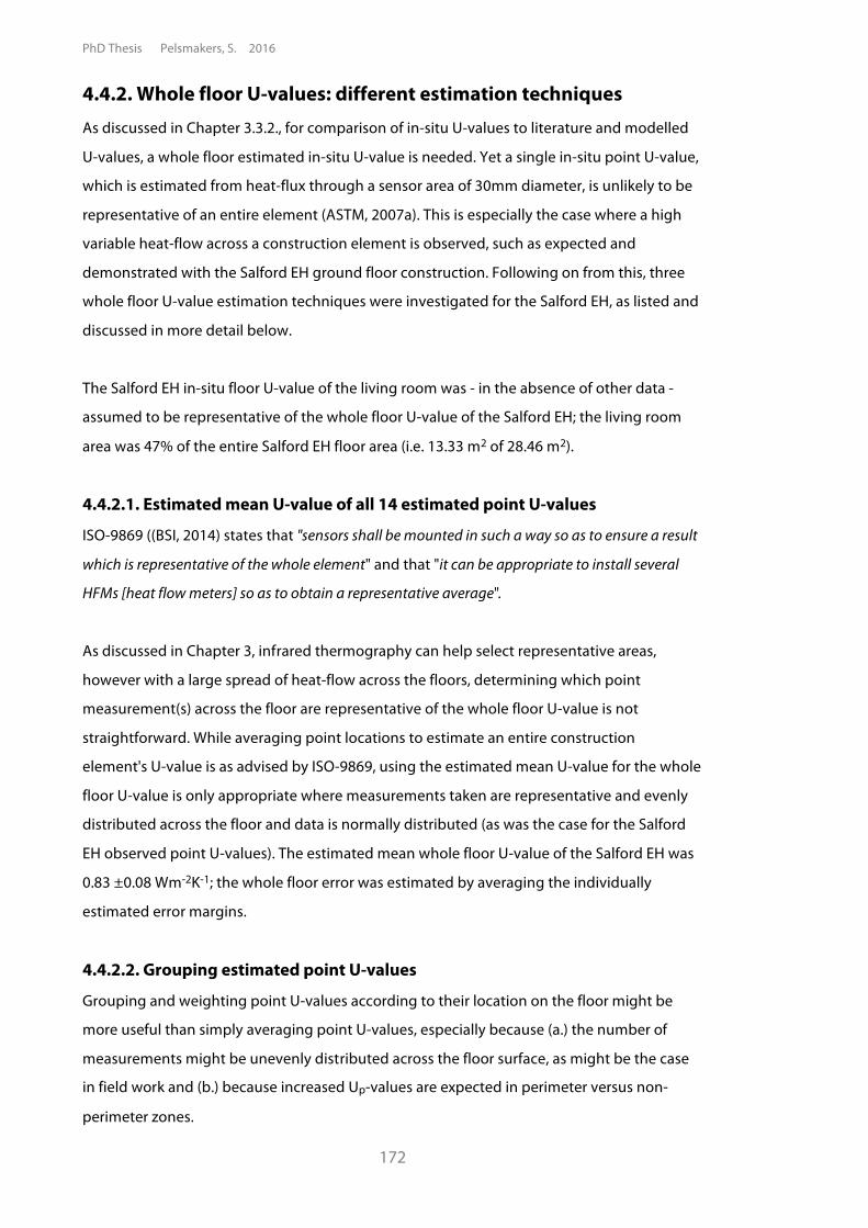
PhD Thesis Pelsmakers, S. 2016
172
4.4.2. Whole floor U-values: different estimation techniques As discussed in Chapter 3.3.2., for comparison of in-situ U-values to literature and modelled
U-values, a whole floor estimated in-situ U-value is needed. Yet a single in-situ point U-value,
which is estimated from heat-flux through a sensor area of 30mm diameter, is unlikely to be
representative of an entire element (ASTM, 2007a). This is especially the case where a high
variable heat-flow across a construction element is observed, such as expected and
demonstrated with the Salford EH ground floor construction. Following on from this, three
whole floor U-value estimation techniques were investigated for the Salford EH, as listed and
discussed in more detail below.
The Salford EH in-situ floor U-value of the living room was - in the absence of other data -
assumed to be representative of the whole floor U-value of the Salford EH; the living room
area was 47% of the entire Salford EH floor area (i.e. 13.33 m2 of 28.46 m2).
4.4.2.1. Estimated mean U-value of all 14 estimated point U-values
ISO-9869 ((BSI, 2014) states that "sensors shall be mounted in such a way so as to ensure a result
which is representative of the whole element" and that "it can be appropriate to install several
HFMs [heat flow meters] so as to obtain a representative average".
As discussed in Chapter 3, infrared thermography can help select representative areas,
however with a large spread of heat-flow across the floors, determining which point
measurement(s) across the floor are representative of the whole floor U-value is not
straightforward. While averaging point locations to estimate an entire construction
element's U-value is as advised by ISO-9869, using the estimated mean U-value for the whole
floor U-value is only appropriate where measurements taken are representative and evenly
distributed across the floor and data is normally distributed (as was the case for the Salford
EH observed point U-values). The estimated mean whole floor U-value of the Salford EH was
0.83 ±0.08 Wm-2K-1; the whole floor error was estimated by averaging the individually
estimated error margins.
4.4.2.2. Grouping estimated point U-values
Grouping and weighting point U-values according to their location on the floor might be
more useful than simply averaging point U-values, especially because (a.) the number of
measurements might be unevenly distributed across the floor surface, as might be the case
in field work and (b.) because increased Up-values are expected in perimeter versus non-
perimeter zones.
Chapter 4: Initial uninsulated floor heat-flow studies
173
For example, a group of Up-values could be taken as representative of a floor zone with a
certain area. Each group of Up-values is averaged and given a weight proportional to the
floor area these points represent; the whole floor U-value can then be estimated by summing
the weighted mean of the different floor zones. However, this method also requires that a
few point measurements are sufficient to characterise these different floor zones as
representative of the whole floor.
Delsante (1989) observed a perimeter effect up to 1 metre from the external walls in solid
ground floors, though such zoning is not well characterised for suspended ground floors.
Using this 1 metre perimeter zone characterisation for the Salford EH, the estimated U-value
of the perimeter zone was 1.02 Wm-2K-1 (mean of estimated Up-values in location 1, 9 and 10
to 14); while the mean U-value of the remaining non-perimeter points was 0.69 Wm-2K-1,
assumed to be representative of the non-perimeter zone. This lead to a weighted whole floor
U-value estimate of 0.88 ±0.08 Wm-2K-1. The error margin was based on the weighted
average of the uncertainty estimates of the point U-values.
4.4.2.3. Area-weighted summation
The total heat-flow through an element can be regarded as the summation of the heat-flow
through a number of areas, which can be represented by a 'grid', see Figure 32. It is assumed
that each point measurement taken is representative of heat-flow through the surrounding
area defined by the grid. Weighting for each zone is simply calculated by dividing each
zone's area by the whole area of the element. Summing all of these weighted point U-values
gives an area-weighted whole floor U-value estimate (Uwf), as per Equation 52. and shown as
derived in Table 18. and illustrated in Figure 32.
The whole floor estimated U-value error can be estimated in the same way.
- Equation 52. , where Uwf (Wm-2K-1) is the whole floor U-value; is the
weighting factor where Aj in m2 is the representative floor area assigned to each U-value
point (Uj) and Awf is the whole floor area. Index j identifies individual point locations on the
floor measured simultaneously and n is the number of point locations observed.
The whole floor error is obtained in the same way, by multiplying the individual point error
by the weighting factor .
Uwf =n
9j=�
U jA j
Awf
PhD Thesis Pelsmakers, S. 2016
174
ASTM (2007a) advises the use of infrared thermography to establish whether the area around
each sensor location is similar in order to interpolate to a larger area; as expected
"interpolated values away from sensors are less accurate than measurements obtained at sensor
sites" (ASTM, 2007a). The use of infrared images (see Figure 31.) supported the qualitative
estimation of areas (Aj) around each sensor as representative of that sensor's U-value (Uj).
This procedure lead to the floor area being divided in a grid formation - see Figure 32.
However, even with many U-value point measurements, dividing the floor area still required
a choice between several possible area grid configurations, increasing uncertainty (as noted
in Chapter 3.3.4.3.). Different configurations were tested for the Salford EH, especially along
the perimeter and for the larger zones around sensors 1, 7, 8, and 9, however this did not
affect the estimated whole floor U-values within the two decimals presented here.
Figure 31. Infrared images can be useful to understand how representative each measurement
location is prior to interpolation of each point to a larger area. The image shows a region around
an individual sensor.
For the Salford EH, the whole floor U-value estimated by weighted summation is equal to the
mean estimated whole floor U-value of 0.83 ± 0.08 Wm-2K-1; however this excludes reduced
heat-flow through the joists. Accounting for 12% joists and assuming that the heat-flow
through all the joists was 21% less than through floorboards, as was found for location 11 in
this study, for illustrative purposes this would give an adjusted whole floor U-value of 0.81
±0.08 Wm-2K-1.
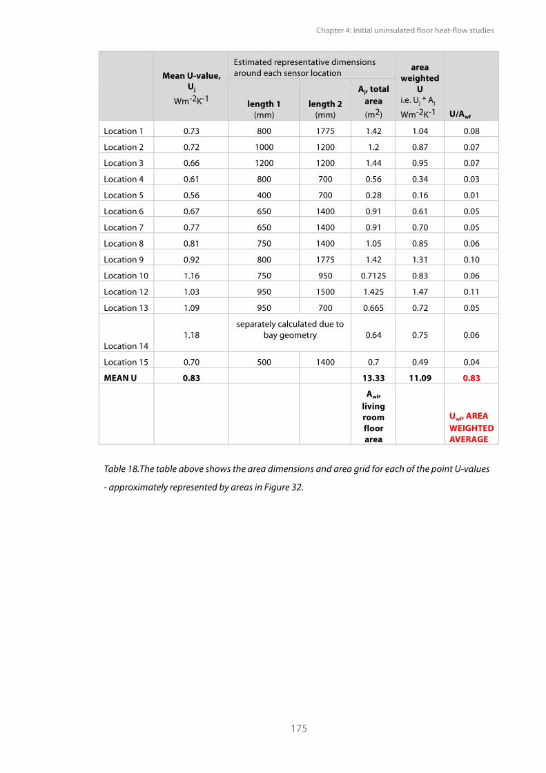
Chapter 4: Initial uninsulated floor heat-flow studies
175
Mean U-value, Uj
Wm-2K-1
Estimated representative dimensions around each sensor location
area weighted
U i.e. Uj * Aj
Wm-2K-1 U/Awf length 1
(mm) length 2
(mm)
Aj, total area (m2)
Location 1 0.73 800 1775 1.42 1.04 0.08
Location 2 0.72 1000 1200 1.2 0.87 0.07
Location 3 0.66 1200 1200 1.44 0.95 0.07
Location 4 0.61 800 700 0.56 0.34 0.03
Location 5 0.56 400 700 0.28 0.16 0.01
Location 6 0.67 650 1400 0.91 0.61 0.05
Location 7 0.77 650 1400 0.91 0.70 0.05
Location 8 0.81 750 1400 1.05 0.85 0.06
Location 9 0.92 800 1775 1.42 1.31 0.10
Location 10 1.16 750 950 0.7125 0.83 0.06
Location 12 1.03 950 1500 1.425 1.47 0.11
Location 13 1.09 950 700 0.665 0.72 0.05
Location 14 1.18
separately calculated due to bay geometry
0.64 0.75 0.06
Location 15 0.70 500 1400 0.7 0.49 0.04
MEAN U 0.83 13.33 11.09 0.83
Awf, living room floor area
Uwf, AREA WEIGHTED AVERAGE
Table 18.The table above shows the area dimensions and area grid for each of the point U-values
- approximately represented by areas in Figure 32.
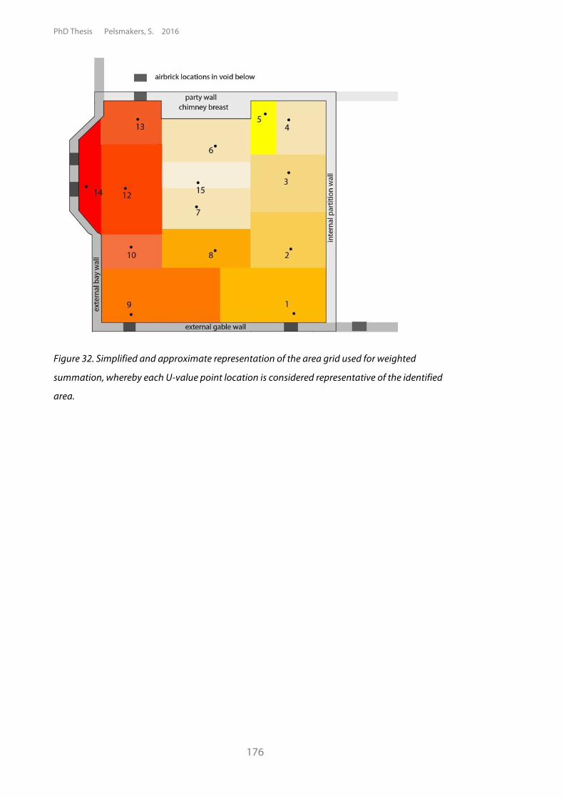
PhD Thesis Pelsmakers, S. 2016
176
Figure 32. Simplified and approximate representation of the area grid used for weighted
summation, whereby each U-value point location is considered representative of the identified
area.
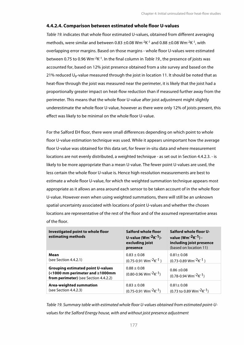
Chapter 4: Initial uninsulated floor heat-flow studies
177
4.4.2.4. Comparison between estimated whole floor U-values
Table 19. indicates that whole floor estimated U-values, obtained from different averaging
methods, were similar and between 0.83 ±0.08 Wm-2K-1 and 0.88 ±0.08 Wm-2K-1, with
overlapping error margins. Based on those margins - whole floor U-values were estimated
between 0.75 to 0.96 Wm-2K-1. In the final column in Table 19., the presence of joists was
accounted for, based on 12% joist presence obtained from a site survey and based on the
21% reduced Up-value measured through the joist in location 11. It should be noted that as
heat-flow through the joist was measured near the perimeter, it is likely that the joist had a
proportionally greater impact on heat-flow reduction than if measured further away from the
perimeter. This means that the whole floor U-value after joist adjustment might slightly
underestimate the whole floor U-value, however as there were only 12% of joists present, this
effect was likely to be minimal on the whole floor U-value.
For the Salford EH floor, there were small differences depending on which point to whole
floor U-value estimation technique was used. While it appears unimportant how the average
floor U-value was obtained for this data set, for fewer in-situ data and where measurement
locations are not evenly distributed, a weighted technique - as set out in Section 4.4.2.3. - is
likely to be more appropriate than a mean U-value. The fewer point U-values are used, the
less certain the whole floor U-value is. Hence high-resolution measurements are best to
estimate a whole floor U-value, for which the weighted summation technique appears most
appropriate as it allows an area around each sensor to be taken account of in the whole floor
U-value. However even when using weighted summations, there will still be an unknown
spatial uncertainty associated with locations of point U-values and whether the chosen
locations are representative of the rest of the floor and of the assumed representative areas
of the floor.
Investigated point to whole floor estimating methods
Salford whole floor U-value (Wm-2K-1)- excluding joist presence
Salford whole floor U-value (Wm-2K-1) - including joist presence (based on location 11)
Mean (see Section 4.4.2.1)
0.83 ± 0.08 (0.75-0.91 Wm-2K-1 )
0.81± 0.08 (0.73-0.89 Wm-2K-1 )
Grouping estimated point U-values (<1000 mm perimeter and !1000mm from perimeter) (see Section 4.4.2.2)
0.88 ± 0.08 (0.80-0.96 Wm-2K-1)
0.86 ±0.08 (0.78-0.94 Wm-2K-1)
Area-weighted summation (see Section 4.4.2.3)
0.83 ± 0.08 (0.75-0.91 Wm-2K-1)
0.81± 0.08 (0.73 to 0.89 Wm-2K-1)
Table 19. Summary table with estimated whole floor U-values obtained from estimated point-U-
values for the Salford Energy house, with and without joist presence adjustment
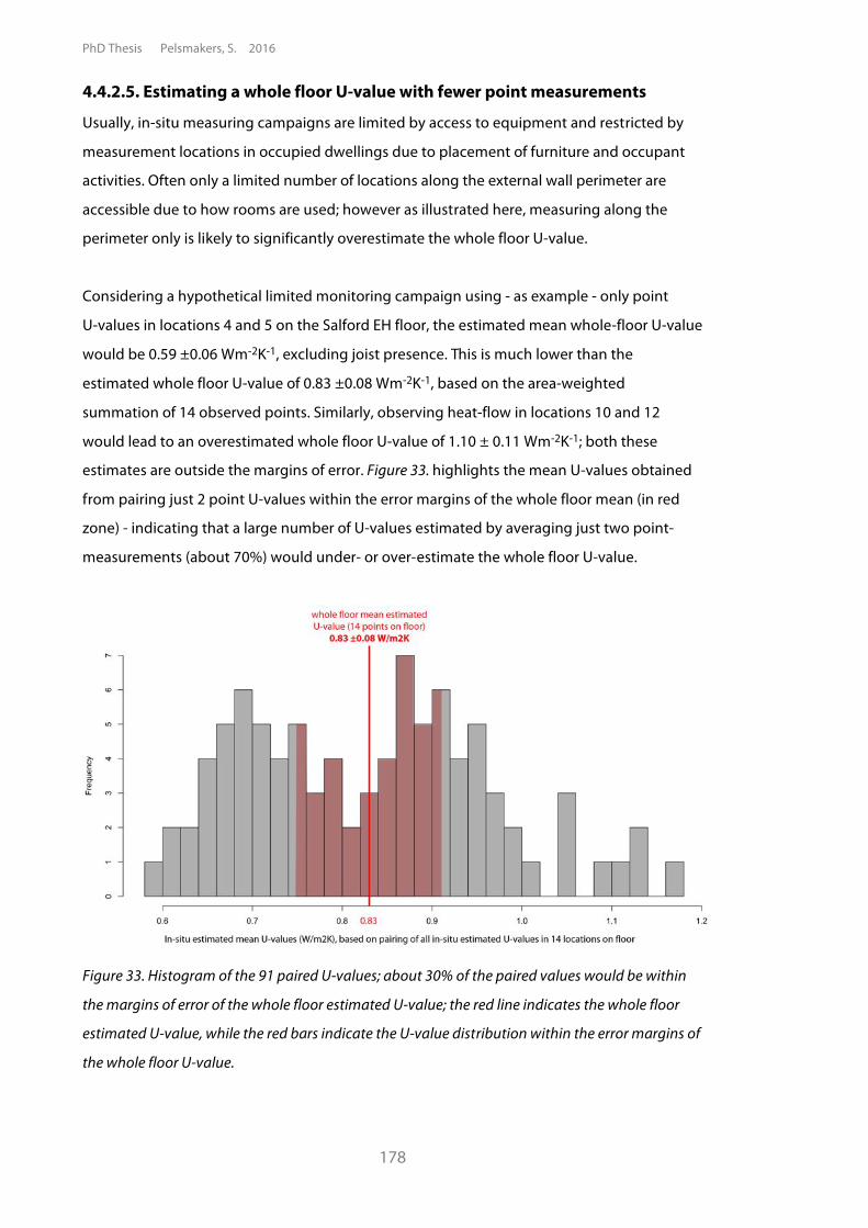
PhD Thesis Pelsmakers, S. 2016
178
4.4.2.5. Estimating a whole floor U-value with fewer point measurements
Usually, in-situ measuring campaigns are limited by access to equipment and restricted by
measurement locations in occupied dwellings due to placement of furniture and occupant
activities. Often only a limited number of locations along the external wall perimeter are
accessible due to how rooms are used; however as illustrated here, measuring along the
perimeter only is likely to significantly overestimate the whole floor U-value.
Considering a hypothetical limited monitoring campaign using - as example - only point
U-values in locations 4 and 5 on the Salford EH floor, the estimated mean whole-floor U-value
would be 0.59 ±0.06 Wm-2K-1, excluding joist presence. This is much lower than the
estimated whole floor U-value of 0.83 ±0.08 Wm-2K-1, based on the area-weighted
summation of 14 observed points. Similarly, observing heat-flow in locations 10 and 12
would lead to an overestimated whole floor U-value of 1.10 ± 0.11 Wm-2K-1; both these
estimates are outside the margins of error. Figure 33. highlights the mean U-values obtained
from pairing just 2 point U-values within the error margins of the whole floor mean (in red
zone) - indicating that a large number of U-values estimated by averaging just two point-
measurements (about 70%) would under- or over-estimate the whole floor U-value.
Figure 33. Histogram of the 91 paired U-values; about 30% of the paired values would be within
the margins of error of the whole floor estimated U-value; the red line indicates the whole floor
estimated U-value, while the red bars indicate the U-value distribution within the error margins of
the whole floor U-value.
Chapter 4: Initial uninsulated floor heat-flow studies
179
Appendix 4.A. lists the 32 paired locations (or 30% of the pairs) where the mean paired U-
value overlapped with the overlapping error margin of the whole floor U-value, i.e. between
0.75 and 0.91Wm-2K-1. Only one pairing combination (location 1 and 9 along the perimeter
(and above airbricks)) lead to an exact match with the whole floor U-value. Generally, for the
semi-detached Salford EH, it appeared that one perimeter location and an internal floor
location were more likely to give a better estimate of the whole floor U-value. Note that
location 13 was an anomaly due to the airbrick to the neighbouring house. Some
combinations of middle of the floor with gable perimeter wall locations might also provide
close whole floor U-value matches for this study, as do two middle of the floor locations
combined; though note that measuring in the middle of the floor is not a practical location in
occupied dwellings.
Clearly, observing just one or two point locations on a construction element such as a floor -
which is subject to a large spread of heat-flow as illustrated by the Salford EH findings -
means that the estimated whole floor U-values might be over- or under-estimated
depending on where those point U-values were measured. Random selection of measuring
locations is highly likely to lead to a poor representation of the whole floor U-value. When a
large spread of heat-flow across a building element is present it is challenging to define a
'representative' or 'typical' area where to undertake these few point measurements. While
several locations combined could construct an average U-value that is within the whole floor
U-value margin, this was only possible by measuring at high-resolution to give a sufficient
number of measured locations to combine. As such, deriving a whole floor U-value based on
a single or few point measurements has unknown and possibly significant uncertainties
associated with it. Increased purposeful monitoring of many points across the surface will
reduce uncertainty of estimating the whole floor U-value under those measuring conditions.
The spread of Up-values across a floor needs to be represented by a sufficient number of
in-situ point measurements, and comparison of low-resolution with high-resolution data is
likely to be problematic.
PhD Thesis Pelsmakers, S. 2016
180
4.4.3. Whole floor U-values and comparison to models and other
sources As discussed in Section 4.4.2, obtaining an estimated whole floor U-value is useful for
comparison with U-values estimated from models; comparisons between the two are
presented in this section, taking the living room bare floorboarded floor as being
representative of the entire Salford EH floor.
For the Salford EH, the floor U-value from models was estimated between 0.59 and
0.68 Wm-2K-1using the ISO-13370 model (BSI, 2009b) as described in Chapter 2 with joist
presence of 12% and depending on assumed wind-speeds (between 1-5 m/s) and concrete
ground conductivity between 1.3 and 1.9 Wm-1K-1 (as per CIBSE (2006)); and as described by
five models in Table 20. Other characteristics and inputs required for the models are listed in
Table 21. for both the Salford EH and the 2012 pilot study. The model values are based on
data that could be recorded while other inputs, such as assumed material conductivities of
floorboards, foundation walls and the characteristic of the concrete subfloor as well as wind-
speeds were based on assumptions. In the Salford EH no wind-speed was simulated, hence
the wind-speed was expected to be small, but there might still be air movement effects from
the chiller plant for example. Hence standard wind-speed model assumptions were tested
alongside lowered wind-speeds to 1m/s. Using RdSAP (BRE, 2011) and CIBSE (2006)
assumptions (instead of using surveyed Salford EH characteristics as typical inputs),
estimated model outputs were between 0.60 and 0.73 Wm-2K-1(Models 1 to 3); this excluded
joist presence as the assumed models' default thermal resistance input for floor deck was
used. When the RdSAP and CIBSE models were adapted for 1m/s wind-speed and actual
surveyed airbrick openings and other surveyed inputs and including joist presence, the
modelled outputs dropped to between 0.58 Wm-2K-1 and 0.71 Wm-2K-1 - see Table 20.,
Models 4 and 5. The superseded CIBSE-1986 model lead to higher U-value estimates than the
current models; with a mean U-value of 1.11 Wm-2K-1 and especially model 4 was more
similar to the whole floor in-situ measured U-value. Note that wind-speed input assumptions
have a significant influence on CIBSE-1986 model outputs - see in Section 4.4.3.1. Yet at
present it is unclear what the wind-speed is at airbrick height and whether models accurately
reflect this.
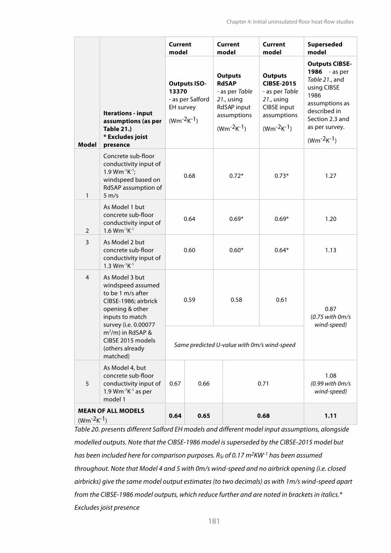
Chapter 4: Initial uninsulated floor heat-flow studies
181
Model
Iterations - input assumptions (as per Table 21.) * Excludes joist presence
Current model
Current model
Current model
Superseded model
Outputs ISO-13370 - as per Salford EH survey
(Wm-2K-1)
Outputs RdSAP - as per Table 21., using RdSAP input assumptions
(Wm-2K-1)
Outputs CIBSE-2015 - as per Table 21., using CIBSE input assumptions
(Wm-2K-1)
Outputs CIBSE-1986 - as per Table 21., and using CIBSE 1986 assumptions as described in Section 2.3 and as per survey.
(Wm-2K-1)
1
Concrete sub-floor conductivity input of 1.9 Wm-1K-1; windspeed based on RdSAP assumption of 5 m/s
0.68 0.72*
0.73*
1.27
2
As Model 1 but concrete sub-floor conductivity input of 1.6 Wm-1K-1
0.64
0.69*
0.69*
1.20
3 As Model 2 but concrete sub-floor conductivity input of 1.3 Wm-1K-1
0.60
0.60*
0.64*
1.13
4 As Model 3 but windspeed assumed to be 1 m/s after CIBSE-1986; airbrick opening & other inputs to match survey (i.e. 0.00077 m2/m) in RdSAP & CIBSE 2015 models (others already matched)
0.59 0.58 0.61 0.87
(0.75 with 0m/s wind-speed)
Same predicted U-value with 0m/s wind-speed
5
As Model 4, but concrete sub-floor conductivity input of 1.9 Wm-1K-1 as per model 1
0.67 0.66 0.71 1.08
(0.99 with 0m/s wind-speed)
MEAN OF ALL MODELS (Wm-2K-1)
0.64 0.65 0.68 1.11
Table 20. presents different Salford EH models and different model input assumptions, alongside
modelled outputs. Note that the CIBSE-1986 model is superseded by the CIBSE-2015 model but
has been included here for comparison purposes. RSi of 0.17 m2KW-1 has been assumed
throughout. Note that Model 4 and 5 with 0m/s wind-speed and no airbrick opening (i.e. closed
airbricks) give the same model output estimates (to two decimals) as with 1m/s wind-speed apart
from the CIBSE-1986 model outputs, which reduce further and are noted in brackets in italics.*
Excludes joist presence
PhD Thesis Pelsmakers, S. 2016
182
Figure 34. plots the mean modelled U-values outputs described in Table 20. and U-values
derived from literature alongside the in-situ estimated whole floor U-values (derived from
area-weighted summation - see Section 4.4.2.). Overall, the divergence between the Salford
EH in-situ estimated whole floor U-value and the U-value estimates from current models was
between 10% and 28%, depending on model used and input assumptions. Given the
uncertainties in in-situ measurements and model input assumptions, both CEN (1996) and
ISO-9869 (BSI, 2014) only regard significant disparities to be greater than 20% between
measured and modelled U-values. In reality, because of error margins around the in-situ
U-values, and depending on which assumptions were used in models, potential disparities
might be small or almost non-existent (i.e. < 20%). Figure 34. illustrates that in general, the
current models appear to underestimate the in-situ estimated whole floor U-value of the
Salford EH and error margins do not overlap. Contrary to this, the superseded CIBSE-1986
model gave U-value estimates 7% to 36% above the in-situ measured whole floor U-value.
Overall for the current models, Model 1 is closer aligned with the in-situ estimated whole
floor U-value, however Models 1, 2 and 3 assumed 5m/s wind-speed (RdSAP recommended
(BRE, 2011)); yet this is unlikely to be reflective of the low windspeed encountered in the
Salford EH (though this was not measured). Nor do these three models account for the actual
airbrick openings and other surveyed variables of the Salford EH in the CIBSE-2015 and
RdSAP models. Model 4 and 5 were adjusted for these differences to better reflect the Salford
EH conditions, but as expected, adjusting the wind-speed (1m/s) and airbrick openings
widens the disparity between modelled and measured U-values for the current models.
However, the superseded CIBSE-1986 Model 4 output is closer to the in-situ measured value
of 0.81±0.08Wm-2K-1, taking joist presence into account. However as with the other models
there is uncertainty around the input assumptions and it is unknown whether this close
alignment is accidental or due to accurate input assumptions and a better model fit.
As discussed in Section 4.2.3., the estimated modelled U-value of the pilot study floor also
appeared to underestimate in-situ U-values, however the latter was based on just two point
locations and lead to significant uncertainty with regards to estimating the whole floor
U-value for comparison with models. As discussed in Chapter 3 and in Chapter 2.4., care must
be taken with comparisons and generalisations between models, literature and in-situ
estimated U-values. Furthermore, the pilot study whole floor U-value is also unlikely to be
comparable to the in-situ estimated whole floor U-value of the Salford EH due to the low-
resolution monitoring and the many different variables between both studies, including P/A
and to what extent the Salford EH floor heat-flow reflects that of real houses in real situations
due to different variables - as described previously in Section 4.3.1.
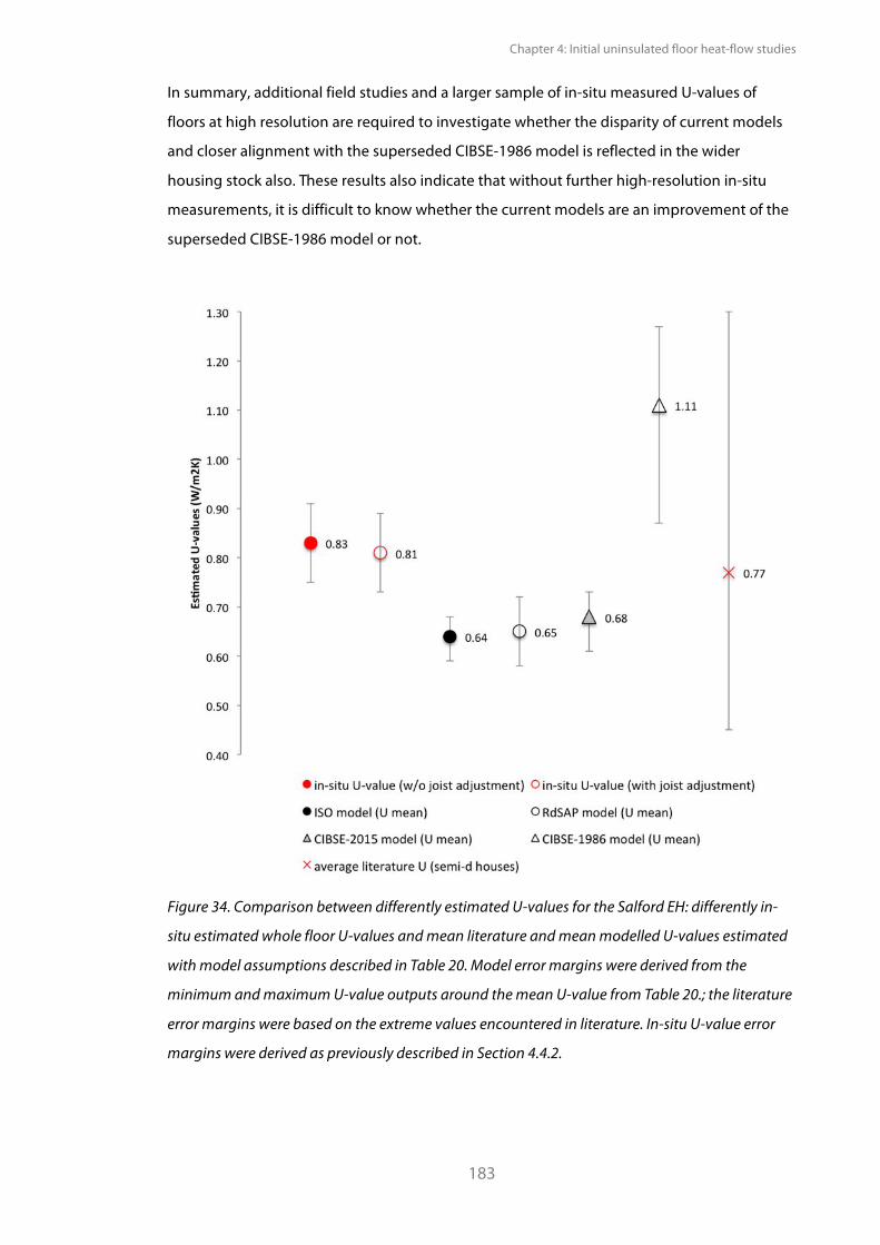
Chapter 4: Initial uninsulated floor heat-flow studies
183
In summary, additional field studies and a larger sample of in-situ measured U-values of
floors at high resolution are required to investigate whether the disparity of current models
and closer alignment with the superseded CIBSE-1986 model is reflected in the wider
housing stock also. These results also indicate that without further high-resolution in-situ
measurements, it is difficult to know whether the current models are an improvement of the
superseded CIBSE-1986 model or not.
Figure 34. Comparison between differently estimated U-values for the Salford EH: differently in-
situ estimated whole floor U-values and mean literature and mean modelled U-values estimated
with model assumptions described in Table 20. Model error margins were derived from the
minimum and maximum U-value outputs around the mean U-value from Table 20.; the literature
error margins were based on the extreme values encountered in literature. In-situ U-value error
margins were derived as previously described in Section 4.4.2.
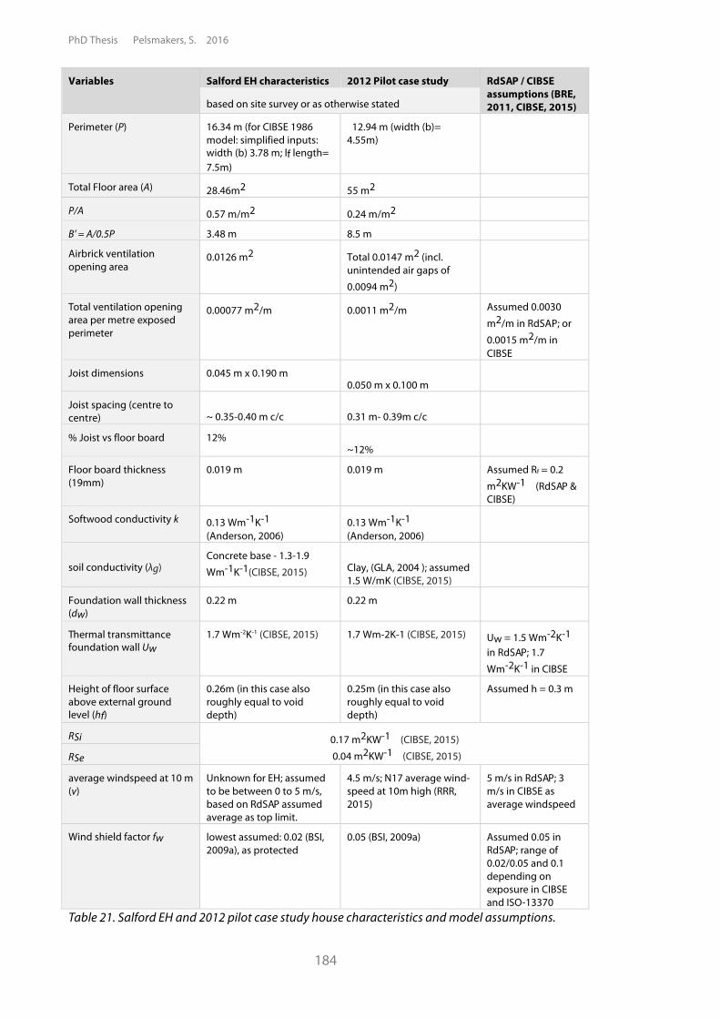
PhD Thesis Pelsmakers, S. 2016
184
Variables Salford EH characteristics 2012 Pilot case study RdSAP / CIBSE assumptions (BRE, 2011, CIBSE, 2015) based on site survey or as otherwise stated
Perimeter (P) 16.34 m (for CIBSE 1986 model: simplified inputs: width (b) 3.78 m; lf length= 7.5m)
12.94 m (width (b)= 4.55m)
Total Floor area (A) 28.46m2 55 m2
P/A 0.57 m/m2 0.24 m/m2
B' = A/0.5P 3.48 m 8.5 m
Airbrick ventilation opening area
0.0126 m2 Total 0.0147 m2 (incl. unintended air gaps of 0.0094 m2)
Total ventilation opening area per metre exposed perimeter
0.00077 m2/m 0.0011 m2/m Assumed 0.0030 m2/m in RdSAP; or 0.0015 m2/m in CIBSE
Joist dimensions 0.045 m x 0.190 m 0.050 m x 0.100 m
Joist spacing (centre to centre) ~ 0.35-0.40 m c/c 0.31 m- 0.39m c/c
% Joist vs floor board 12% ~12%
Floor board thickness (19mm)
0.019 m 0.019 m Assumed Rf = 0.2 m2KW-1 (RdSAP & CIBSE)
Softwood conductivity k 0.13 Wm-1K-1 (Anderson, 2006)
0.13 Wm-1K-1 (Anderson, 2006)
soil conductivity (!g) Concrete base - 1.3-1.9 Wm-1K-1(CIBSE, 2015) Clay, (GLA, 2004 ); assumed
1.5 W/mK (CIBSE, 2015)
Foundation wall thickness (dw)
0.22 m 0.22 m
Thermal transmittance foundation wall Uw
1.7 Wm-2K-1 (CIBSE, 2015) 1.7 Wm-2K-1 (CIBSE, 2015) Uw = 1.5 Wm-2K-1 in RdSAP; 1.7 Wm-2K-1 in CIBSE
Height of floor surface above external ground level (hf)
0.26m (in this case also roughly equal to void depth)
0.25m (in this case also roughly equal to void depth)
Assumed h = 0.3 m
RSi 0.17 m2KW-1 (CIBSE, 2015) 0.04 m2KW-1 (CIBSE, 2015) RSe
average windspeed at 10 m (v)
Unknown for EH; assumed to be between 0 to 5 m/s, based on RdSAP assumed average as top limit.
4.5 m/s; N17 average wind-speed at 10m high (RRR, 2015)
5 m/s in RdSAP; 3 m/s in CIBSE as average windspeed
Wind shield factor fw lowest assumed: 0.02 (BSI, 2009a), as protected
0.05 (BSI, 2009a) Assumed 0.05 in RdSAP; range of 0.02/0.05 and 0.1 depending on exposure in CIBSE and ISO-13370
Table 21. Salford EH and 2012 pilot case study house characteristics and model assumptions.
Chapter 4: Initial uninsulated floor heat-flow studies
185
4.4.3.1. Sensitivity analysis
A limited and simplified sensitivity analysis was undertaken of the ISO-13370 suspended
floor U-value model10 and the CIBSE-1986 model, using the floor characteristics of the Salford
EH for illustrative purposes. A sensitivity analysis is a study of the variation of input variables
and their effects on the model output variation (Saltelli, 2008), in this case floor U-values.
Different sensitivity analyses can be conducted, each with their advantages and limitations.
In this research, a screening sensitivity analysis was conducted (Saltelli, 2008), which enabled
the qualitative evaluation and understanding of the impact of changing input parameters on
output variability. This allowed the isolation of the most significant variables affecting the
model U-value outputs (Saltelli, 2008). Only one variable at a time (OAT) was changed with all
the other variables constant to test the impact of each variable on the estimated modelled U-
value output in turn. Minimum and maximum inputs were used to give value ranges (control
experiment (Saltelli, 2008)) and these were obtained from literature with - where applicable -
sources noted on Figures 35 and 36; values in between were modelled at regular intervals. A
limitation of screening is that no quantitative ranking of the variables is obtained nor a
probability distribution of the range of the variables as for example in local sensitivity analysis
(e.g. differential analysis) and global sensitivity analysis (e.g. Monte Carlo analysis) (Saltelli,
2008). A limitation of OAT sensitivity analysis is that it relies on standard values per variable
and simultaneous interactions of changing variables and evaluation of the impact on model
outputs are excluded (Saltelli, 2008). Screening only allows the evaluation of the main effects
and is considered an effective way to do so (Saltelli, 2008). OAT screening was considered
appropriate given the purpose of the sensitivity analysis was the understanding and
comparison of the important variables in both models.
The graphs in Figure 35. and Figure 36. illustrate the impact of the ISO-13370 and CIBSE-1986
models' assumed inputs and their effect on modelled floor U-values. For model inputs and
floor characteristics, see Table 21.
10 The ISO-13370 model was used here for a simple sensitivity model given that ISO-13370 is the basis of the current RdSAP and CIBSE 2015 models.
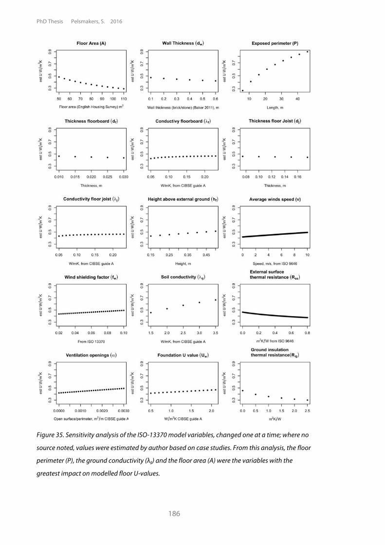
PhD Thesis Pelsmakers, S. 2016
186
Figure 35. Sensitivity analysis of the ISO-13370 model variables, changed one at a time; where no
source noted, values were estimated by author based on case studies. From this analysis, the floor
perimeter (P), the ground conductivity (!g) and the floor area (A) were the variables with the
greatest impact on modelled floor U-values.
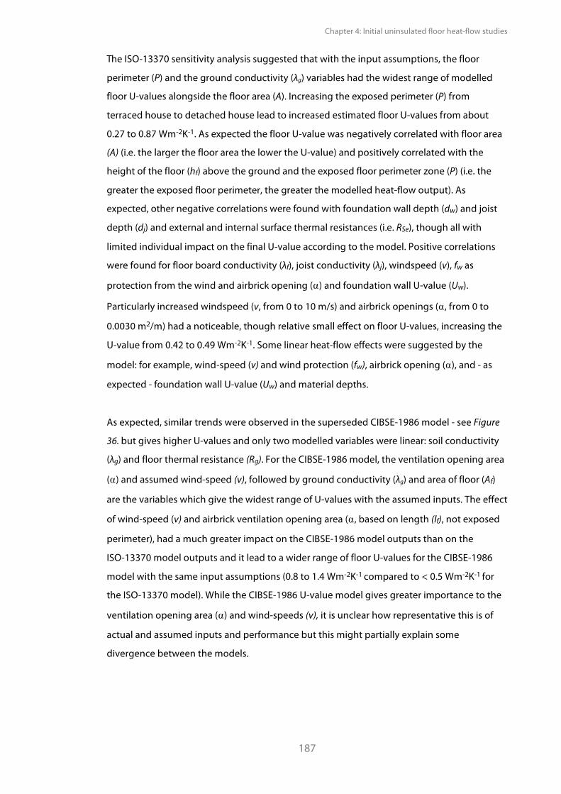
Chapter 4: Initial uninsulated floor heat-flow studies
187
The ISO-13370 sensitivity analysis suggested that with the input assumptions, the floor
perimeter (P) and the ground conductivity (!g) variables had the widest range of modelled
floor U-values alongside the floor area (A). Increasing the exposed perimeter (P) from
terraced house to detached house lead to increased estimated floor U-values from about
0.27 to 0.87 Wm-2K-1. As expected the floor U-value was negatively correlated with floor area
(A) (i.e. the larger the floor area the lower the U-value) and positively correlated with the
height of the floor (hf) above the ground and the exposed floor perimeter zone (P) (i.e. the
greater the exposed floor perimeter, the greater the modelled heat-flow output). As
expected, other negative correlations were found with foundation wall depth (dw) and joist
depth (dj) and external and internal surface thermal resistances (i.e. RSe), though all with
limited individual impact on the final U-value according to the model. Positive correlations
were found for floor board conductivity (!f), joist conductivity (!j), windspeed (v), fw as
protection from the wind and airbrick opening (�) and foundation wall U-value (Uw).
Particularly increased windspeed (v, from 0 to 10 m/s) and airbrick openings (�, from 0 to
0.0030 m2/m) had a noticeable, though relative small effect on floor U-values, increasing the
U-value from 0.42 to 0.49 Wm-2K-1. Some linear heat-flow effects were suggested by the
model: for example, wind-speed (v) and wind protection (fw), airbrick opening (�), and - as
expected - foundation wall U-value (Uw) and material depths.
As expected, similar trends were observed in the superseded CIBSE-1986 model - see Figure
36. but gives higher U-values and only two modelled variables were linear: soil conductivity
(!g) and floor thermal resistance (Rg). For the CIBSE-1986 model, the ventilation opening area
(�) and assumed wind-speed (v), followed by ground conductivity (!g) and area of floor (Af)
are the variables which give the widest range of U-values with the assumed inputs. The effect
of wind-speed (v) and airbrick ventilation opening area (�, based on length (lf), not exposed
perimeter), had a much greater impact on the CIBSE-1986 model outputs than on the
ISO-13370 model outputs and it lead to a wider range of floor U-values for the CIBSE-1986
model with the same input assumptions (0.8 to 1.4 Wm-2K-1 compared to < 0.5 Wm-2K-1 for
the ISO-13370 model). While the CIBSE-1986 U-value model gives greater importance to the
ventilation opening area (�) and wind-speeds (v), it is unclear how representative this is of
actual and assumed inputs and performance but this might partially explain some
divergence between the models.
PhD Thesis Pelsmakers, S. 2016
188
Figure 36. Sensitivity analysis of the CIBSE 1986 model variables, changed one at a time; where no
source noted, values were estimated by author based on case studies. For the CIBSE-1986
analysis, the ventilation opening area (�), assumed wind-speed (v) and ground conductivity (!g)
were the variables with the greatest impact on modelled floor U-values.
Chapter 4: Initial uninsulated floor heat-flow studies
189
4.4.3.2. Comparison to Building regulations
For the renovation of ground floors, current building regulations approved document Part
L1B, 'Conservation of fuel and Power in Existing dwellings' applies in England, with similar
regulations in Scotland, Wales and Northern Ireland. This means that for the restoration or
upgrade of ground floors, minimum standards are recommended: regulations require the
design U-values in the upgraded ground floor in dwellings to be no greater than
0.25 Wm-2K-1 in all UK regions (NBS, 2015, SBSA, 2015, Government, 2014, DFPNI, 2012). As
expected, the recommended insulation standard is significantly better performing than the
Salford estimated in-situ whole floor U-value of the uninsulated floor and at least twice as
good as the Salford EH modelled U-values of the uninsulated floor.
4.4.3.3. Comparison to literature and other in-situ monitoring studies
Table 2. in Chapter 2.4.1. presents literature U-values for semi-detached dwellings, which
range between 0.70 Wm-2K-1 and 1.30 Wm-2K-1 and the average of the sources was
0.77 Wm-2K-1 as plotted in Figure 34. in Section 4.4.3. This mean literature U-value is similar to
the estimated in-situ measured whole floor U-value for the Salford EH of 0.81±0.08 Wm-2K-1
(taking into account presence of joists - as per discussion in Section 4.4.2.).
As discussed in Section 2.4.2., only a few in-situ measured U-values could be traced for
suspended timber ground floors in the UK; for semi-detached dwellings U-values estimated
from in-situ measurements ranged from 0.69 to 2.4 Wm-2K-1, based on one or two point
measurement locations only and indicating some overlap with the Salford EH in-situ
measured point U-values. Miles-Shenton (2011) measured one point U-value location in the
perimeter zone and one in the middle of the floor and - as also observed here - found that
the Up-value in the bay was greater than in the middle of the floor. The few in-situ point
measurements available (Chapter 2.4.2, Table 3.) highlight the wide variation of U-values
estimated in different locations in different dwellings in the field. It also appears that the
point U-values observed in the perimeter in other studies were generally higher than those
observed along the perimeter zone in the Salford EH.
PhD Thesis Pelsmakers, S. 2016
190
This might be caused by a combination of the following:
• Differences in environmental conditions or physical form and materials between the
Salford EH and other studies. For example, the lack of replicated wind in the Salford
EH, which is likely to reduce the rate of heat-flow, in addition to other Salford EH
constraints as discussed in Section 4.3.1. Differences between the case-study
buildings include the sub-floor characteristics, ventilation rates, floor finishes, void
depths, wall thermal performance and environmental and site conditions. These
variables affect measured floor U-values differently hence comparison between
findings from different studies is challenging.
• The large spread of in-situ point U-values observed across the floor in the Salford EH
study, highlighted that a few point measurements were unlikely to lead to valid
U-value comparisons between studies as each point location is specific to that
dwelling and study. Using low-resolution point measurements on the floor to
compare to a whole floor U-value from high-resolution measurement in another
study makes comparisons challenging.
• Differences in measurement and analysis methods further challenge the comparison
between estimated floor U-values presented by different sources. For example,
placement of temperature sensors is not the same in each study; often it is
undisclosed exactly at which height temperatures are measured. If air temperatures
in rooms are inhomogeneous this leads to vertical temperature gradients, affecting
U-value estimates as they depend on the temperatures measured, as discussed in
Section 4.4.5.
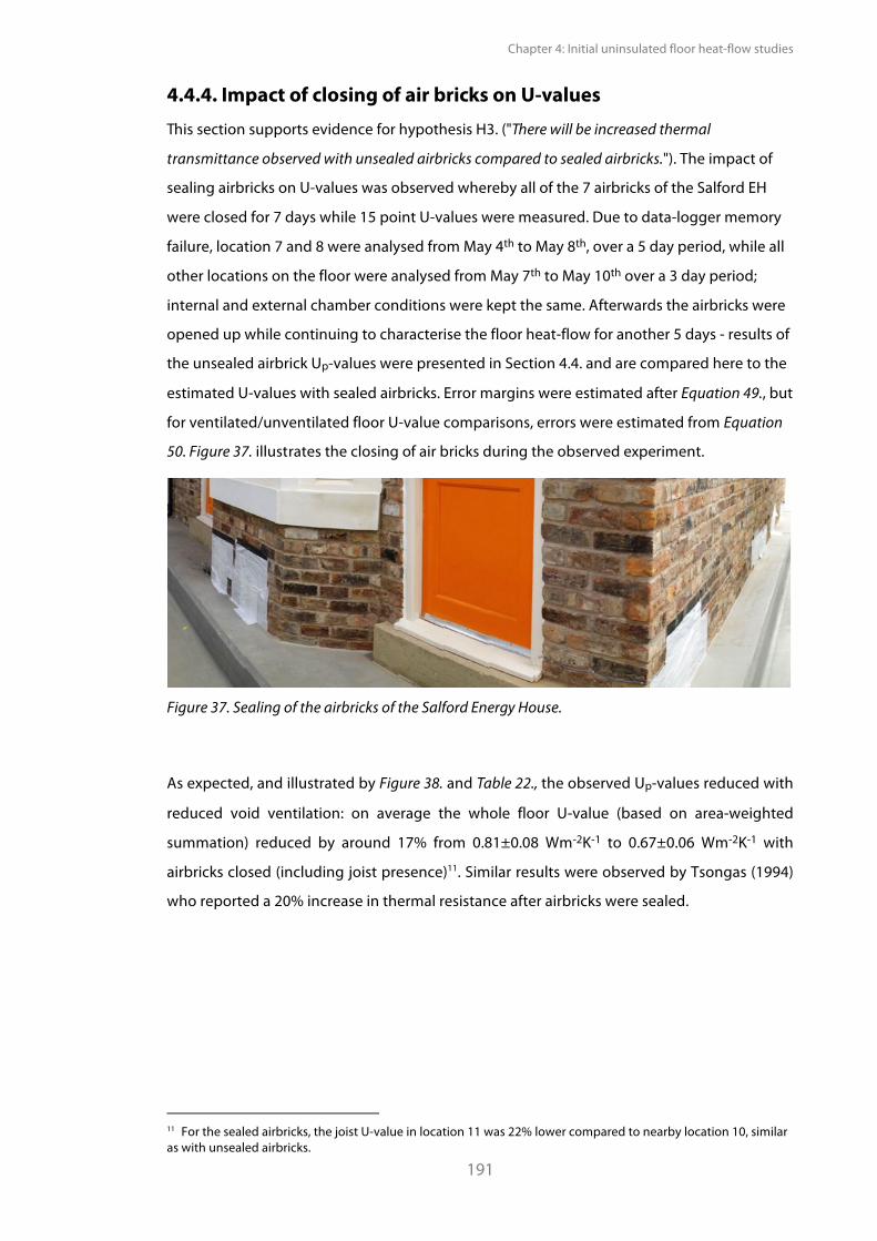
Chapter 4: Initial uninsulated floor heat-flow studies
191
4.4.4. Impact of closing of air bricks on U-values This section supports evidence for hypothesis H3. ("There will be increased thermal
transmittance observed with unsealed airbricks compared to sealed airbricks."). The impact of
sealing airbricks on U-values was observed whereby all of the 7 airbricks of the Salford EH
were closed for 7 days while 15 point U-values were measured. Due to data-logger memory
failure, location 7 and 8 were analysed from May 4th to May 8th, over a 5 day period, while all
other locations on the floor were analysed from May 7th to May 10th over a 3 day period;
internal and external chamber conditions were kept the same. Afterwards the airbricks were
opened up while continuing to characterise the floor heat-flow for another 5 days - results of
the unsealed airbrick Up-values were presented in Section 4.4. and are compared here to the
estimated U-values with sealed airbricks. Error margins were estimated after Equation 49., but
for ventilated/unventilated floor U-value comparisons, errors were estimated from Equation
50. Figure 37. illustrates the closing of air bricks during the observed experiment.
Figure 37. Sealing of the airbricks of the Salford Energy House.
As expected, and illustrated by Figure 38. and Table 22., the observed Up-values reduced with
reduced void ventilation: on average the whole floor U-value (based on area-weighted
summation) reduced by around 17% from 0.81±0.08 Wm-2K-1 to 0.67±0.06 Wm-2K-1 with
airbricks closed (including joist presence)11. Similar results were observed by Tsongas (1994)
who reported a 20% increase in thermal resistance after airbricks were sealed.
11 For the sealed airbricks, the joist U-value in location 11 was 22% lower compared to nearby location 10, similar as with unsealed airbricks.
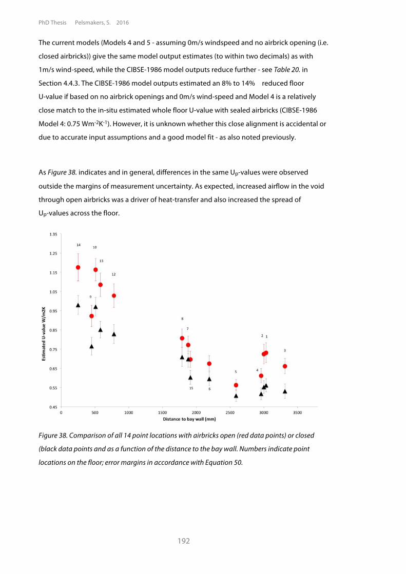
PhD Thesis Pelsmakers, S. 2016
192
The current models (Models 4 and 5 - assuming 0m/s windspeed and no airbrick opening (i.e.
closed airbricks)) give the same model output estimates (to within two decimals) as with
1m/s wind-speed, while the CIBSE-1986 model outputs reduce further - see Table 20. in
Section 4.4.3. The CIBSE-1986 model outputs estimated an 8% to 14% reduced floor
U-value if based on no airbrick openings and 0m/s wind-speed and Model 4 is a relatively
close match to the in-situ estimated whole floor U-value with sealed airbricks (CIBSE-1986
Model 4: 0.75 Wm-2K-1). However, it is unknown whether this close alignment is accidental or
due to accurate input assumptions and a good model fit - as also noted previously.
As Figure 38. indicates and in general, differences in the same Up-values were observed
outside the margins of measurement uncertainty. As expected, increased airflow in the void
through open airbricks was a driver of heat-transfer and also increased the spread of
Up-values across the floor.
Figure 38. Comparison of all 14 point locations with airbricks open (red data points) or closed
(black data points and as a function of the distance to the bay wall. Numbers indicate point
locations on the floor; error margins in accordance with Equation 50.
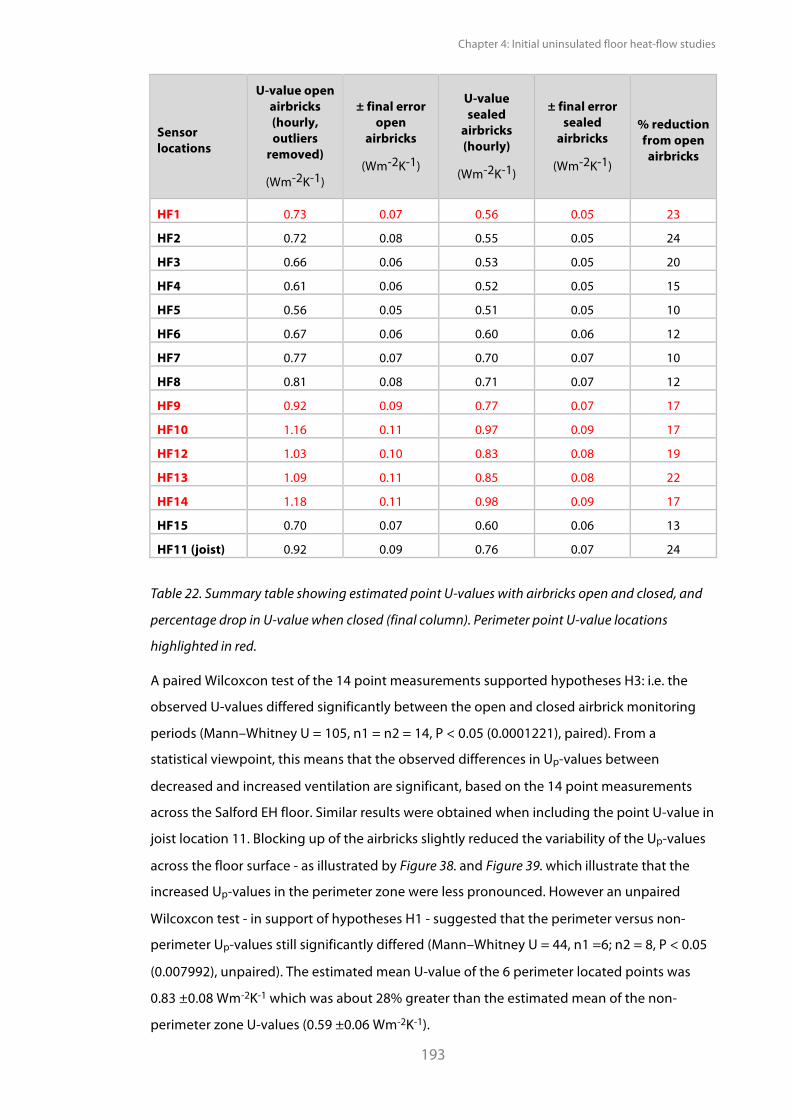
Chapter 4: Initial uninsulated floor heat-flow studies
193
Sensor locations
U-value open airbricks (hourly, outliers
removed)
(Wm-2K-1)
± final error open
airbricks
(Wm-2K-1)
U-value sealed
airbricks (hourly)
(Wm-2K-1)
± final error sealed
airbricks
(Wm-2K-1)
% reduction from open
airbricks
HF1 0.73 0.07 0.56 0.05 23
HF2 0.72 0.08 0.55 0.05 24
HF3 0.66 0.06 0.53 0.05 20
HF4 0.61 0.06 0.52 0.05 15
HF5 0.56 0.05 0.51 0.05 10
HF6 0.67 0.06 0.60 0.06 12
HF7 0.77 0.07 0.70 0.07 10
HF8 0.81 0.08 0.71 0.07 12
HF9 0.92 0.09 0.77 0.07 17
HF10 1.16 0.11 0.97 0.09 17
HF12 1.03 0.10 0.83 0.08 19
HF13 1.09 0.11 0.85 0.08 22
HF14 1.18 0.11 0.98 0.09 17
HF15 0.70 0.07 0.60 0.06 13
HF11 (joist) 0.92 0.09 0.76 0.07 24
Table 22. Summary table showing estimated point U-values with airbricks open and closed, and
percentage drop in U-value when closed (final column). Perimeter point U-value locations
highlighted in red.
A paired Wilcoxcon test of the 14 point measurements supported hypotheses H3: i.e. the
observed U-values differed significantly between the open and closed airbrick monitoring
periods (Mann–Whitney U = 105, n1 = n2 = 14, P < 0.05 (0.0001221), paired). From a
statistical viewpoint, this means that the observed differences in Up-values between
decreased and increased ventilation are significant, based on the 14 point measurements
across the Salford EH floor. Similar results were obtained when including the point U-value in
joist location 11. Blocking up of the airbricks slightly reduced the variability of the Up-values
across the floor surface - as illustrated by Figure 38. and Figure 39. which illustrate that the
increased Up-values in the perimeter zone were less pronounced. However an unpaired
Wilcoxcon test - in support of hypotheses H1 - suggested that the perimeter versus non-
perimeter Up-values still significantly differed (Mann–Whitney U = 44, n1 =6; n2 = 8, P < 0.05
(0.007992), unpaired). The estimated mean U-value of the 6 perimeter located points was
0.83 ±0.08 Wm-2K-1 which was about 28% greater than the estimated mean of the non-
perimeter zone U-values (0.59 ±0.06 Wm-2K-1).
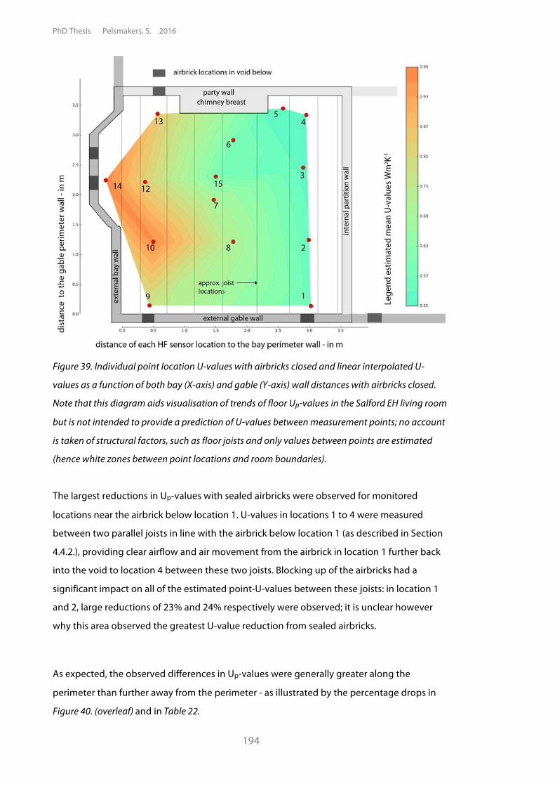
PhD Thesis Pelsmakers, S. 2016
194
Figure 39. Individual point location U-values with airbricks closed and linear interpolated U-
values as a function of both bay (X-axis) and gable (Y-axis) wall distances with airbricks closed.
Note that this diagram aids visualisation of trends of floor Up-values in the Salford EH living room
but is not intended to provide a prediction of U-values between measurement points; no account
is taken of structural factors, such as floor joists and only values between points are estimated
(hence white zones between point locations and room boundaries).
The largest reductions in Up-values with sealed airbricks were observed for monitored
locations near the airbrick below location 1. U-values in locations 1 to 4 were measured
between two parallel joists in line with the airbrick below location 1 (as described in Section
4.4.2.), providing clear airflow and air movement from the airbrick in location 1 further back
into the void to location 4 between these two joists. Blocking up of the airbricks had a
significant impact on all of the estimated point-U-values between these joists: in location 1
and 2, large reductions of 23% and 24% respectively were observed; it is unclear however
why this area observed the greatest U-value reduction from sealed airbricks.
As expected, the observed differences in Up-values were generally greater along the
perimeter than further away from the perimeter - as illustrated by the percentage drops in
Figure 40. (overleaf) and in Table 22.
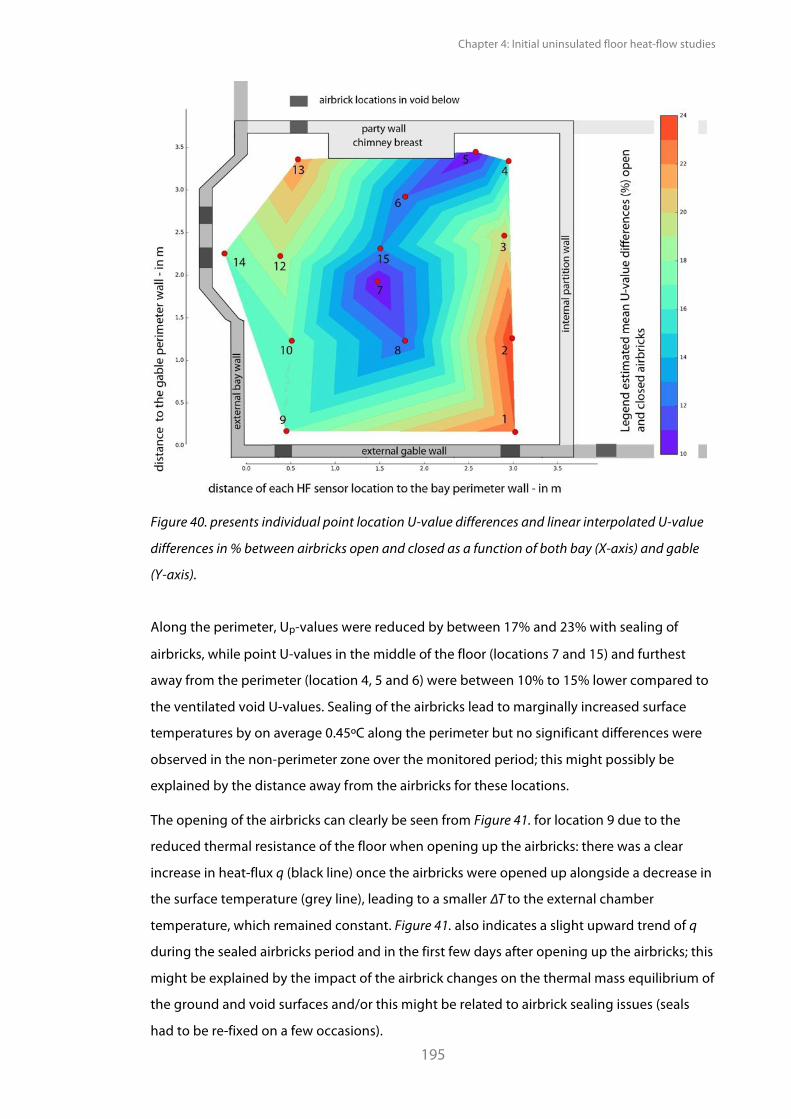
Chapter 4: Initial uninsulated floor heat-flow studies
195
Figure 40. presents individual point location U-value differences and linear interpolated U-value
differences in % between airbricks open and closed as a function of both bay (X-axis) and gable
(Y-axis).
Along the perimeter, Up-values were reduced by between 17% and 23% with sealing of
airbricks, while point U-values in the middle of the floor (locations 7 and 15) and furthest
away from the perimeter (location 4, 5 and 6) were between 10% to 15% lower compared to
the ventilated void U-values. Sealing of the airbricks lead to marginally increased surface
temperatures by on average 0.45ºC along the perimeter but no significant differences were
observed in the non-perimeter zone over the monitored period; this might possibly be
explained by the distance away from the airbricks for these locations.
The opening of the airbricks can clearly be seen from Figure 41. for location 9 due to the
reduced thermal resistance of the floor when opening up the airbricks: there was a clear
increase in heat-flux q (black line) once the airbricks were opened up alongside a decrease in
the surface temperature (grey line), leading to a smaller "T to the external chamber
temperature, which remained constant. Figure 41. also indicates a slight upward trend of q
during the sealed airbricks period and in the first few days after opening up the airbricks; this
might be explained by the impact of the airbrick changes on the thermal mass equilibrium of
the ground and void surfaces and/or this might be related to airbrick sealing issues (seals
had to be re-fixed on a few occasions).
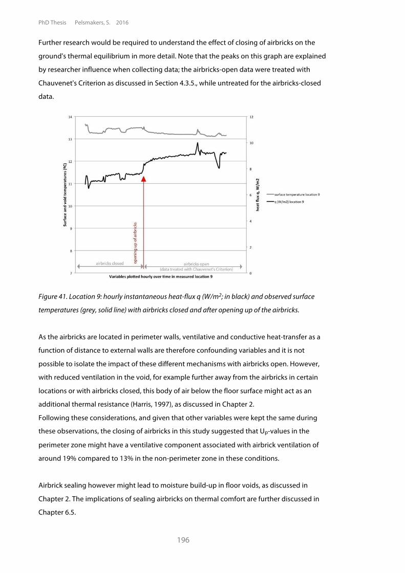
PhD Thesis Pelsmakers, S. 2016
196
Further research would be required to understand the effect of closing of airbricks on the
ground's thermal equilibrium in more detail. Note that the peaks on this graph are explained
by researcher influence when collecting data; the airbricks-open data were treated with
Chauvenet's Criterion as discussed in Section 4.3.5., while untreated for the airbricks-closed
data.
Figure 41. Location 9: hourly instantaneous heat-flux q (W/m2; in black) and observed surface
temperatures (grey, solid line) with airbricks closed and after opening up of the airbricks.
As the airbricks are located in perimeter walls, ventilative and conductive heat-transfer as a
function of distance to external walls are therefore confounding variables and it is not
possible to isolate the impact of these different mechanisms with airbricks open. However,
with reduced ventilation in the void, for example further away from the airbricks in certain
locations or with airbricks closed, this body of air below the floor surface might act as an
additional thermal resistance (Harris, 1997), as discussed in Chapter 2.
Following these considerations, and given that other variables were kept the same during
these observations, the closing of airbricks in this study suggested that Up-values in the
perimeter zone might have a ventilative component associated with airbrick ventilation of
around 19% compared to 13% in the non-perimeter zone in these conditions.
Airbrick sealing however might lead to moisture build-up in floor voids, as discussed in
Chapter 2. The implications of sealing airbricks on thermal comfort are further discussed in
Chapter 6.5.
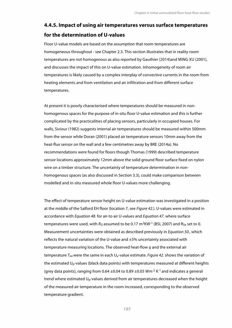
Chapter 4: Initial uninsulated floor heat-flow studies
197
4.4.5. Impact of using air temperatures versus surface temperatures
for the determination of U-values Floor U-value models are based on the assumption that room temperatures are
homogeneous throughout - see Chapter 2.3. This section illustrates that in reality room
temperatures are not homogenous as also reported by Gauthier (2014)and MING XU (2001),
and discusses the impact of this on U-value estimation. Inhomogeneity of room air
temperatures is likely caused by a complex interplay of convective currents in the room from
heating elements and from ventilation and air infiltration and from different surface
temperatures.
At present it is poorly characterised where temperatures should be measured in non-
homogenous spaces for the purpose of in-situ floor U-value estimation and this is further
complicated by the practicalities of placing sensors, particularly in occupied houses. For
walls, Siviour (1982) suggests internal air temperatures should be measured within 500mm
from the sensor while Doran (2001) placed air temperature sensors 10mm away from the
heat-flux sensor on the wall and a few centimetres away by BRE (2014a). No
recommendations were found for floors though Thomas (1999) described temperature
sensor locations approximately 12mm above the solid ground floor surface fixed on nylon
wire on a timber structure. The uncertainty of temperature determination in non-
homogenous spaces (as also discussed in Section 3.3), could make comparison between
modelled and in-situ measured whole floor U-values more challenging.
The effect of temperature sensor height on U-value estimation was investigated in a position
at the middle of the Salford EH floor (location 7, see Figure 42.). U-values were estimated in
accordance with Equation 48. for air-to air U-values and Equation 47. where surface
temperatures were used, with RSi assumed to be 0.17 m2KW-1 (BSI, 2007) and RSe set to 0.
Measurement uncertainties were obtained as described previously in Equation 50., which
reflects the natural variation of the U-value and ±5% uncertainty associated with
temperature measuring locations. The observed heat-flow q and the external air
temperature Tea were the same in each Up-value estimate. Figure 42. shows the variation of
the estimated Up-values (black data points) with temperatures measured at different heights
(grey data points), ranging from 0.64 ±0.04 to 0.89 ±0.05 Wm-2 K-1 and indicates a general
trend where estimated Up-values derived from air temperatures decreased when the height
of the measured air temperature in the room increased, corresponding to the observed
temperature gradient.
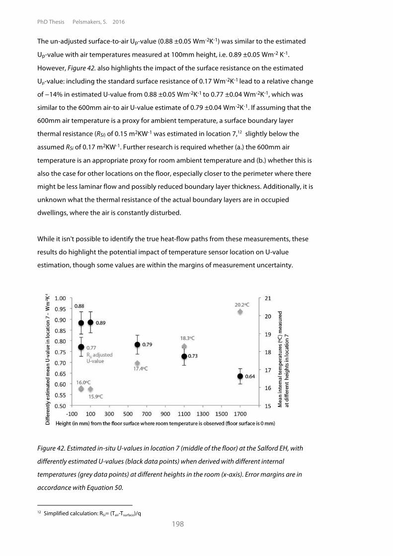
PhD Thesis Pelsmakers, S. 2016
198
The un-adjusted surface-to-air Up-value (0.88 ±0.05 Wm-2K-1) was similar to the estimated
Up-value with air temperatures measured at 100mm height, i.e. 0.89 ±0.05 Wm-2 K-1.
However, Figure 42. also highlights the impact of the surface resistance on the estimated
Up-value: including the standard surface resistance of 0.17 Wm-2K-1 lead to a relative change
of #14% in estimated U-value from 0.88 ±0.05 Wm-2K-1 to 0.77 ±0.04 Wm-2K-1, which was
similar to the 600mm air-to air U-value estimate of 0.79 ±0.04 Wm-2K-1. If assuming that the
600mm air temperature is a proxy for ambient temperature, a surface boundary layer
thermal resistance (RSi) of 0.15 m2KW-1 was estimated in location 7,12 slightly below the
assumed RSi of 0.17 m2KW-1. Further research is required whether (a.) the 600mm air
temperature is an appropriate proxy for room ambient temperature and (b.) whether this is
also the case for other locations on the floor, especially closer to the perimeter where there
might be less laminar flow and possibly reduced boundary layer thickness. Additionally, it is
unknown what the thermal resistance of the actual boundary layers are in occupied
dwellings, where the air is constantly disturbed.
While it isn't possible to identify the true heat-flow paths from these measurements, these
results do highlight the potential impact of temperature sensor location on U-value
estimation, though some values are within the margins of measurement uncertainty.
Figure 42. Estimated in-situ U-values in location 7 (middle of the floor) at the Salford EH, with
differently estimated U-values (black data points) when derived with different internal
temperatures (grey data points) at different heights in the room (x-axis). Error margins are in
accordance with Equation 50.
12 Simplified calculation: RSi= (Tair-Tsurface)/q
Chapter 4: Initial uninsulated floor heat-flow studies
199
Buoyancy effects tend to increase internal room temperatures as the height from the floor
increases: temperatures at 100mm height were 2.4ºC to 4.3ºC lower than those observed at
1100mm and 1700mm height respectively13 in the Salford EH study. In general, using higher
measured temperatures increased the apparent internal-external temperature difference
("T), resulting in lower U-value estimates. However, U-values estimated from temperatures
measured at the surface - before adjustment- and at just 100mm height do not appear
significantly different; though diverge once the former is adjusted with the surface
resistance. This is contrary to observations by Stinson (2012) who did not find significant
differences in U-value when low-level skirting air temperature was used (2.5± 0.3Wm-2K-1,
analysed in accordance with Equation 48.), compared to the U-value derived from internal
surface temperatures (2.4± 0.2 Wm-2K-1, analysed in accordance with Equation 47. with RSi
adjustment). It is unknown which space heating method was used in this study; it is expected
that heating method might influence U-value estimation. For instance in co-heating tests,
space heating is usually provided by electrical fan heaters and circulation fans are used to
mix the internal air (Wingfield, 2010b) to create less of a vertical temperature gradient.
However such heating method is not representative of occupied spaces and is likely to
change the heat-flow paths being measured.
The surface resistance adjustment used in surface-to-air U-value estimations assumes
constant radiation and laminar (non turbulent) airflow across a sealed building element, but
for example in reality external surface thermal resistances are likely to change with changing
wind-speeds (see Chapter 3). Studies reported stack airflow through gaps and cracks of floors
into the internal spaces (see discussion Chapter 2.2); such infiltration through gaps between
floorboards is likely to disrupt the laminar flow, changing the effective surface resistance of
the floor, in addition to contributing to mass-transfer heat-flow. However the impact of stack
airflow on heat-transfer and floor surface resistances is unknown and difficult to characterise.
It might be argued that a variable surface resistance (in different floors and for different
locations on the floor) might be more appropriate than a constant value, depending on air
infiltration through the floor, but this may be difficult to define and apply. Any
overestimation of this surface thermal resistance would lead to underestimated U-values
when U-values are adjusted for with RSi. As illustrated, the significant differences in
suspended timber ground floor U-values estimated via methods with and without the
inclusion of a large surface thermal resistance, and possible variations in the actual surface
resistances, could lead to the inaccurate estimation of U-values.
13 This also has associated thermal comfort implications as discussed in Chapter 2.5.
PhD Thesis Pelsmakers, S. 2016
200
This also makes comparison of estimated U-values between models and in-situ measured
sources as well as between different sources which use different methods with different floor
characteristics (e.g. different floor infiltration rates) more challenging. As variation in surface
resistances can impact on estimated U-values, a better understanding of this factor, and how
it is affected by different floor system variables, would enhance estimation of in-situ floor
U-values. Additionally, there is also an uncertainty associated with characterising in-situ
heat-flow via internal air temperature measurements in non-homogenous spaces, however
further study of both these issues is beyond the scope of this PhD study.
On the basis of this work, estimating U-values from surface temperature to external air
temperature with RSi adjustment was considered preferable for the following reasons:
• Regardless of where temperatures are measured, all of the obtained U-values are
'valid' U-values though not necessarily all are representative of the heat-flow path
through floors, which remains undefined at present. Measuring closer to the floor's
surface might be more representative of the floor's heat-flow path compared to high
up in the room and further away from the floor surface. However measuring on the
floor surface requires adjustment with RSi, with associated uncertainties.
• Having undertaken different temperature measurements, it is more practical and
convenient to monitor surface temperatures than internal air temperatures; air
temperature sensors need to be suspended from the ceiling or tripods which is not
practical in the middle of the room and disruptive in occupied dwellings. Suspended
temperature sensors are prone to sagging/falling of or more exposed to
occupant/researcher influence while in the room.
• The use of floor surface temperatures might be more replicable as the floor surface is
clearly defined.
Given the uncertainty around temperature measurements, for the purpose of this PhD and
its U-value estimates, the ISO-9869 estimated ±5% air temperature error was therefore
included in all U-value estimates and comparisons, including where surface temperatures
were used (when this should not apply according to the ISO-9869 standard). This is to reflect
some uncertainty arising from the addition of the surface thermal resistance and its impact
on the estimation of U-values. It is however acknowledged that the actual effect could be
much greater or smaller than the ±5% error allowed for; further research would be required
to investigate this.
Chapter 4: Initial uninsulated floor heat-flow studies
201
4.5. Insights for in-situ heat loss measurements in the field
Reflecting on both the 2012 low-resolution study and the Salford EH high-resolution study
supported the understanding, development and refinement of further in-situ floor U-value
measurement and analysis methods and techniques. Insights useful for future in-situ U-value
measuring studies are listed below:
• Estimation of U-values from surface temperatures to external air temperatures were
considered most practical. Air temperature measurements for some point locations
would still be desirable to understand room temperature stratification to compare
against thermal comfort theory and to compare U-values estimated with different
temperatures.
• The use of an infrared camera was helpful to enable identification of areas with
differing surface temperature patterns prior to placing sensors to help representative
and/or purposive selection of point locations on the floor and to aid with whole floor
U-value estimation at the analysis stage.
• Use of thermostatically controlled electrical heaters was useful to achieve near-
constant internal temperatures in unoccupied dwellings and to avoid influence from
uninsulated radiator pipes in the void. This could also allow isolation of electrical
space heating energy use in the field.
• In terms of data analysis, the ISO-9869 tests were found useful as initial checks during
the monitoring campaign to determine the duration of the monitoring period and to
determine data inclusion for analysis. Data analysis was undertaken from U-values
which met the ISO test criteria, as described in Chapter 3.3.1. However, instead of
using the ISO-9869 'Average Method' for U-value estimation and error analysis, it was
found more useful to treat the data statistically, by determining the mean U-value
and standard deviation between daily or hourly U-values as an estimate of natural
variability of the U-values, combined with ISO-9869 estimated instrument and
measurement uncertainties - all as described in Chapter 3.3.4.3.
• Careful consideration is required about conducting measurements with airbricks
open and with airbricks closed as this affects thermal mass equilibrium of the ground
and void surfaces; additional data collection as described below might help isolate
and understand such phenomena better. (This also applies to measuring in and
across different seasons, addition of insulation etc.)
PhD Thesis Pelsmakers, S. 2016
202
• It might be of interest to monitor additional variables such as void airflow, ground
and void temperatures and ground heat-fluxes to obtain information about ground
behaviour. Ideally they are monitored over different seasons to understand
confounding variables and how they affect the rate of heat-flow (or are affected by
it).
• Possible influences from lateral heat-flow and stack ventilation through gaps and
cracks in the floor might affect the estimated U-values. However its impact on
environmental conditions, surface resistances and instrumentation is not well
characterised and was not investigated in this study and beyond the scope of this
PhD research, while acknowledging that this could influence estimation of in-situ
U-values.
• High resolution heat-flow measurements are anticipated to lead to decreased
uncertainty in whole floor U-value estimations and might allow for comparisons with
modelled and published U-values and other high-resolution studies, as long as
sufficient information is provided to allow for such comparisons.
Additionally, this study highlighted that few or single point U-value measurements are
unlikely to be representative of the entire construction element but are representative of the
location under observation. A good spread of point U-values at high-resolution in this study
was aimed for to (a.) understand the spread of Up-values across the Salford EH floor and (b.)
estimate whole floor U-values to allow for comparison with models and comparison with
other sources. Despite its advantages, high-resolution monitoring is challenging to
undertake, because:
• in an occupied house there is a limit to sensors that can be placed practically;
• it requires access to a large number of instruments for an extended period of time;
• installing and dismantling a high-resolution set-up is significantly more time
consuming with so many sensors in place; and
• the practicalities of data checking/processing and analyses of large datasets also
commands increased resources.
The following chapters will build on the methodological findings and implications of this
chapter for the in-situ heat-flow measurements of a field study floor before and after some
insulation interventions.
Chapter 4: Initial uninsulated floor heat-flow studies
203
4.6. Discussion and summary This study tested and refined in-situ heat-flux measuring methods and techniques for
suspended ground floor systems; high resolution measurements were undertaken. In doing
so, physical theory was tested, informing further the refinement of techniques, while the
work also provided some novel observations about the influence of Salford EH
characteristics on observed Up-values. A summary of these findings is described below.
Using internal surface to external air temperatures, measurements in 14 locations produced
a wide variation of Up-values between 0.56 ±0.05 Wm-2K-1 and 1.18 ±0.11 Wm-2K-1,
depending on location, supporting hypothesis H1 ("There will be a large observed spread of
Up-values across the uninsulated floor"). For the Salford EH, the whole floor system in-situ
estimated U-value, taking into account joist presence, was 0.81 ± 0.08 Wm-2 K-1, and found to
be higher than the current modelled U-values of 0.58 to 0.73 Wm-2K-1, depending on input
assumptions and model used. This suggested a potential disparity between in-situ measured
and modelled U-values, however given that the Salford EH is an environmental chamber, it is
unknown whether such disparities will remain for a field study and the wider housing stock.
The superseded CIBSE-1986 model appeared to overestimate the whole floor U-value
compared to in-situ measured, though depending on model input assumptions, provided a
closer match between modelled and in-situ measured whole floor U-values (Model 4). The
CIBSE-1986 model gave greater importance to the ventilation opening area and wind-
speeds; it is unclear how representative this is of actual and assumed inputs and
performance but this might explain the divergence between the models.
In general, it was found that the observed floor Up-values were greatest along the exposed
perimeter, which reflected physical theory and solid ground floor research and supported
hypothesis H2 (" There will be increased perimeter Up-values observed compared to locations
further away from the external wall (i.e. the non-perimeter zone"); this perimeter effect was also
found to be statistically significant. Sealing the airbricks reduced the estimated Up-values
between 10% to 24% depending on location on the floor; this was also found to be
statistically significant and supported hypothesis H3 ("There will be increased thermal
transmittance observed with unsealed airbricks compared to sealed airbricks"). There was a
more pronounced Up-value reduction effect along the perimeter from sealing airbricks and
there was a slightly reduced spread of Up-values across the floor.
Additionally, this study observed increased estimated Up-values in the bay-wall compared to
the gable wall; this effect was also retained after airbrick-sealing.
PhD Thesis Pelsmakers, S. 2016
204
This might be explained by the joist direction and large joist depths which provided little
clearance underneath and potentially acted as an obstruction to airflow movement through
to the rest of the void. This might exacerbate increased thermal transmittance along the
perimeter, while buffering other floor areas from colder chamber temperatures, leading to
lower observed Up-values elsewhere - as described in Section 4.4.2.
The study findings have implications for future research design and measuring techniques;
in summary:
• Measuring in just a few point locations on the floor is problematic due to the large spread of
Up-values, especially when few U-value point measurements are used to estimate whole floor
system U-values as representative of the entire floor. This makes comparison with modelled
floor U-values, literature U-values or other in-situ studies challenging. The floor U-value
models are for the whole floor; no individual points on the floor can be derived from the
model.
• If fewer Up-values are used to estimate the whole floor U-value, the greater the uncertainty
associated with this whole floor U-value estimate. Depending where point measurements are
observed, the whole floor U-value can be over-or under-estimated.
• Different point U-value to whole floor U-value estimation techniques can lead to different
whole floor U-value estimates; an area weighted summation approach might be more robust
than other explored averaging techniques in this study. It entails determining a
representative and proportional floor area for each estimated Up-values, aided by infrared
images of the floor, and weighting each point location and its associated uncertainty
accordingly.
• The location of temperature sensors for the determination of U-values can significantly affect
the in-situ estimated U-values due to the observed vertical stratification in actual spaces. This
in turn affects confidence in comparisons between in-situ measured studies and with
modelled U-values.
• The inhomogeneity of room temperatures makes the use of air temperatures for the
determination of floor U-values challenging. Internal surface temperatures were found to be
more practical to measure and replicate, though might under-or over-estimate Up-values due
to the addition of a large constant surface thermal resistance (RSi) for floors. This surface
thermal resistance is based on laminar airflow which is unlikely to be the case in the field,
especially given the upwards airflow from the floor void through floorboard gaps and cracks,
which might change the surface thermal resistance.
This chapter highlighted the complexity of estimating in-situ U-values for suspended timber
ground floor systems and comparing these results with models and other studies. Further
research is required whether the above findings and measuring techniques remain valid in
actual dwellings exposed to the external environment, which is investigated in the following
Chapter. For a discussion on generalisability of case-study findings see Chapter 3.4.4.
Chapter 5: Measuring in-situ floor U-values in the field
205
Chapter 5: Measuring in-situ floor
U-values in the field
5.1. Introduction This chapter presents and discusses the analysis and results from an in-situ heat-flow
field study undertaken during the winter of 2013-2014 in an unoccupied house in West
London, England (STUDY 4A). Following on from the study at the Salford Energy House
(STUDY 2), the heat-flow of an uninsulated suspended timber ground floor system was
monitored at high resolution (27 locations) on a living room floor. Similarly to STUDY 2,
airbricks were closed for a short duration to understand the airbrick ventilation effect on
the observed thermal transmittance. The heat-flow in the same locations was also
monitored during two floor insulation interventions, which is discussed separately in
Chapter 6.
This chapter specifically addresses research question 2 ("What is the in-situ measured
thermal transmittance of floors and how does it compare to model predictions?", supplementing
in-situ heat-flux measurements of floors, while also testing research question 1 in the field
(i.e. "How should in-situ suspended timber ground floor U-values be estimated?"), building and
reflecting on the research methods and techniques developed in STUDY 2. Following
hypotheses were tested (as described in Chapter 3.4.1.)
Hypothesis 1: "There will be a large observed spread of Up-values across the uninsulated
floor."
Hypothesis 2: "There will be increased perimeter Up-values observed compared to
locations further away from the external wall (i.e. the non-perimeter zone)."
Hypothesis 3: "There will be increased thermal transmittance observed with unsealed
airbricks compared to sealed airbricks."
This chapter firstly introduces the field study and the research design prior to presenting and
discussing the analysis and results of the field measurements. Implications for policy and
retrofit-decision-making are briefly discussed prior to the chapter summary and summary
discussion of findings.
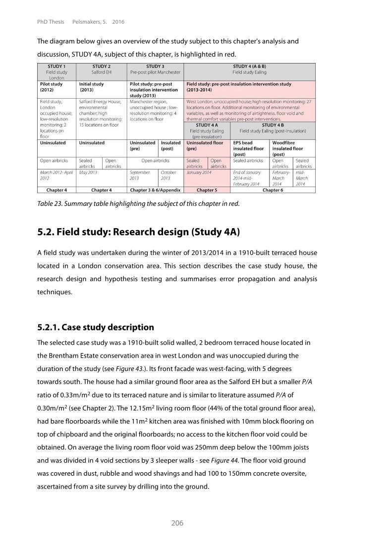
PhD Thesis Pelsmakers, S. 2016
206
The diagram below gives an overview of the study subject to this chapter's analysis and
discussion, STUDY 4A, subject of this chapter, is highlighted in red.
Table 23. Summary table highlighting the subject of this chapter in red.
5.2. Field study: Research design (Study 4A)
A field study was undertaken during the winter of 2013/2014 in a 1910-built terraced house
located in a London conservation area. This section describes the case study house, the
research design and hypothesis testing and summarises error propagation and analysis
techniques.
5.2.1. Case study description The selected case study was a 1910-built solid walled, 2 bedroom terraced house located in
the Brentham Estate conservation area in west London and was unoccupied during the
duration of the study (see Figure 43.). Its front facade was west-facing, with 5 degrees
towards south. The house had a similar ground floor area as the Salford EH but a smaller P/A
ratio of 0.33m/m2 due to its terraced nature and is similar to literature assumed P/A of
0.30m/m2 (see Chapter 2). The 12.15m2 living room floor (44% of the total ground floor area),
had bare floorboards while the 11m2 kitchen area was finished with 10mm block flooring on
top of chipboard and the original floorboards; no access to the kitchen floor void could be
obtained. On average the living room floor void was 250mm deep below the 100mm joists
and was divided in 4 void sections by 3 sleeper walls - see Figure 44. The floor void ground
was covered in dust, rubble and wood shavings and had 100 to 150mm concrete oversite,
ascertained from a site survey by drilling into the ground.
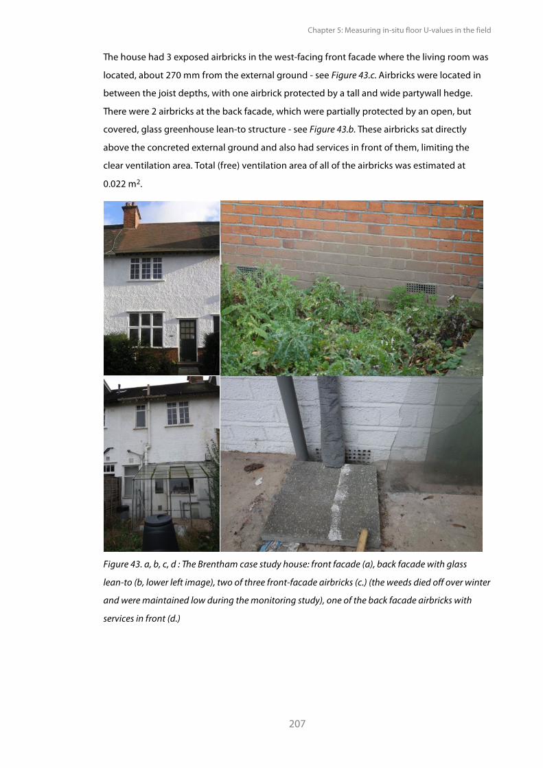
Chapter 5: Measuring in-situ floor U-values in the field
207
The house had 3 exposed airbricks in the west-facing front facade where the living room was
located, about 270 mm from the external ground - see Figure 43.c. Airbricks were located in
between the joist depths, with one airbrick protected by a tall and wide partywall hedge.
There were 2 airbricks at the back facade, which were partially protected by an open, but
covered, glass greenhouse lean-to structure - see Figure 43.b. These airbricks sat directly
above the concreted external ground and also had services in front of them, limiting the
clear ventilation area. Total (free) ventilation area of all of the airbricks was estimated at
0.022 m2.
Figure 43. a, b, c, d : The Brentham case study house: front facade (a), back facade with glass
lean-to (b, lower left image), two of three front-facade airbricks (c.) (the weeds died off over winter
and were maintained low during the monitoring study), one of the back facade airbricks with
services in front (d.)
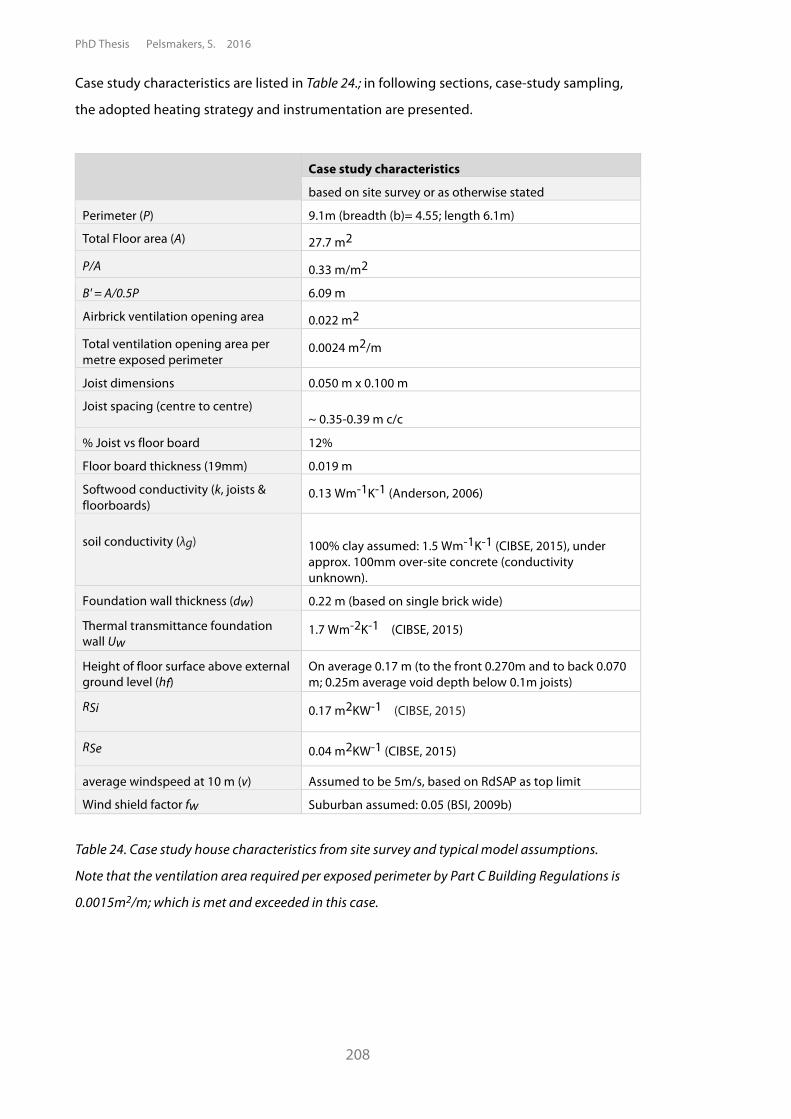
PhD Thesis Pelsmakers, S. 2016
208
Case study characteristics are listed in Table 24.; in following sections, case-study sampling,
the adopted heating strategy and instrumentation are presented.
Case study characteristics
based on site survey or as otherwise stated
Perimeter (P) 9.1m (breadth (b)= 4.55; length 6.1m)
Total Floor area (A) 27.7 m2
P/A 0.33 m/m2
B' = A/0.5P 6.09 m
Airbrick ventilation opening area 0.022 m2
Total ventilation opening area per metre exposed perimeter
0.0024 m2/m
Joist dimensions 0.050 m x 0.100 m
Joist spacing (centre to centre) ~ 0.35-0.39 m c/c
% Joist vs floor board 12%
Floor board thickness (19mm) 0.019 m
Softwood conductivity (k, joists & floorboards)
0.13 Wm-1K-1 (Anderson, 2006)
soil conductivity (!g) 100% clay assumed: 1.5 Wm-1K-1 (CIBSE, 2015), under approx. 100mm over-site concrete (conductivity unknown).
Foundation wall thickness (dw) 0.22 m (based on single brick wide)
Thermal transmittance foundation wall Uw
1.7 Wm-2K-1 (CIBSE, 2015)
Height of floor surface above external ground level (hf)
On average 0.17 m (to the front 0.270m and to back 0.070 m; 0.25m average void depth below 0.1m joists)
RSi
0.17 m2KW-1 (CIBSE, 2015)
RSe 0.04 m2KW-1 (CIBSE, 2015)
average windspeed at 10 m (v) Assumed to be 5m/s, based on RdSAP as top limit
Wind shield factor fw Suburban assumed: 0.05 (BSI, 2009b)
Table 24. Case study house characteristics from site survey and typical model assumptions.
Note that the ventilation area required per exposed perimeter by Part C Building Regulations is
0.0015m2/m; which is met and exceeded in this case.
Chapter 5: Measuring in-situ floor U-values in the field
209
5.2.2. Case study sampling & hypotheses testing
The case-study house was sampled purposively to enable the answering of the research
questions set out in Chapter 2.9. and testing of hypotheses (Chapter 3.4.1.). Case-studies
provide context-dependent knowledge and might lead to generalisability of findings
(Flyvbjerg, 2006) and can highlight observed phenomena and can question pre-existing
generalisations (Stake, 1995) - as also discussed in Chapter 3.4.4.
Six hypotheses based on the research questions were developed (see Table 11., Chapter
3.4.1.); the first three of which were tested in the previous chapter and for which some
statistical significance was found. These hypotheses are further tested in this field study,
while the remaining four hypothesis are subject of the following chapter. As mentioned in
Chapter 3.4, an unoccupied house was identified as the best strategy to test these
hypotheses; an unoccupied case-study house was purposively sampled based on the
following criteria (see also Chapter 3.4.2.):
• Solid walled house with suspended timber ground floors - i.e. built pre-1919.
• Preferably a terraced house, which is the profile of over 50% of pre-1919 dwellings
(Gentry, 2010), to simplify airbrick ventilation investigation.
• Unoccupied and available for minimum one winter season in 2013/14.
• Agreement from the owner to undertake disruptive and invasive monitoring,
entailing the opening up of the floor to the void and later installation of insulation
interventions (subject of Chapter 6).
• Near to the researcher's location to enable regular data collection and analysis and
flexibility in research design adaptations.
Potential case-studies were identified from the author's stakeholder network and social
media contacts, leading to two possible case-studies meeting the above criteria; the west
London located case-study was favoured over a Birmingham located case-study due to travel
distances; insufficient resources were available to undertake two field studies. For research
ethics see Section 3.4.3.
Research management
Several research management and ethical considerations were taken into account for this
field study (and the intervention study described in Chapter 6) and include risk assessments,
instrument and third party insurance, informed consents and agreements about accessing
the property and minimising disruption to neighbours. See Appendix 5.A.
PhD Thesis Pelsmakers, S. 2016
210
5.2.3. Instrumentation
5.2.3.1. Heat-flux sensors and other instruments
As illustrated on Figure 44. , in-situ heat-flux sensors were placed in 27 locations on the living
room floor, 18 of which were in line with the three airbricks below and 8 sensor locations
offset from airbrick locations; only one location was measured on a joist. All of the sensors
were attempted to be fixed in accordance with a grid, aligning sensors in both directions.
However, some grid location offsets occurred due to contact errors caused by uneven
floorboards or presence of nails or staples; a nearest suitable sensor location was then sought
instead. Nail locations also limited sensor placement on joists. For sensor fixing details, see
Table 25.; for instrument error see Section 5.2.4. and Chapter 3.3.4.3.
Joists were supported by three sleeper walls, dividing the void in four sections (marked by
S1, S2, S3 and S4 in light-grey in Figure 44., while sleeper walls are shaded in grey. The space
between the joists was always clear, allowing free airflow movement between floor sections
- see Figure 46.a. The void foundation wall between living room and hallway had no
interconnected openings, though the foundation wall between the living and kitchen floor
void had some limited openings. In this wall, all openings were blocked with tightly packed
bubble wrap and newspaper to isolate the living room floor void from the kitchen void - see
Figure 46.b. The reason for doing so was because the kitchen floor void had to be isolated
from the living-room floor void for later floor intervention studies taking place in the living
room floor only - as described in Chapter 6. Floor voids were not connected to the
neighbouring houses, however there is no knowledge of the heating pattern or condition of
those houses and how this may have affected the field study.
External air temperatures at the front and back of the house were monitored below the first
floor window height. Heat-flux sensors on the floor were monitored with nearby floor surface
temperature sensors, while air temperatures were monitored in the middle of the room at
different heights (100mm, 600mm, 1100mm, 1700mm) in accordance with BS-7726 (BSI,
2002) to understand air temperature stratification and implications for thermal comfort
theory and U-value determination - see Chapter 6.5. and Section 5.3.3. respectively. Void air
temperatures and RH were also monitored to understand floor void conditions - see Chapter
5.3.7.3.
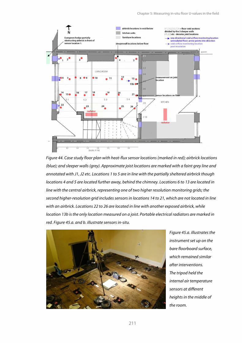
Chapter 5: Measuring in-situ floor U-values in the field
211
Figure 44. Case study floor plan with heat-flux sensor locations (marked in red); airbrick locations
(blue); and sleeper walls (grey). Approximate joist locations are marked with a faint grey line and
annotated with J1, J2 etc. Locations 1 to 5 are in line with the partially sheltered airbrick though
locations 4 and 5 are located further away, behind the chimney. Locations 6 to 13 are located in
line with the central airbrick, representing one of two higher resolution monitoring grids; the
second higher-resolution grid includes sensors in locations 14 to 21, which are not located in line
with an airbrick. Locations 22 to 26 are located in line with another exposed airbrick, while
location 13b is the only location measured on a joist. Portable electrical radiators are marked in
red. Figure 45.a. and b. illustrate sensors in-situ.
Figure 45.a. illustrates the
instrument set up on the
bare floorboard surface,
which remained similar
after interventions.
The tripod held the
internal air temperature
sensors at different
heights in the middle of
the room.
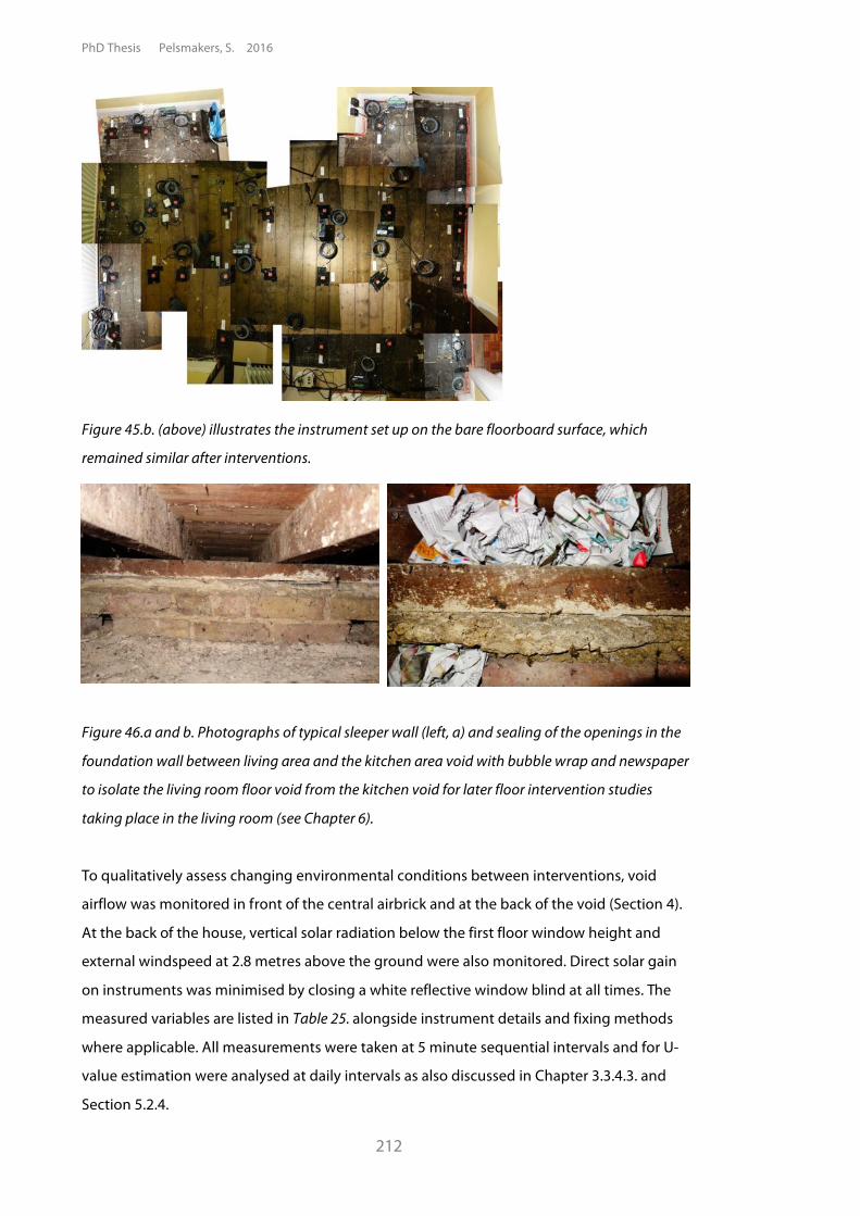
PhD Thesis Pelsmakers, S. 2016
212
Figure 45.b. (above) illustrates the instrument set up on the bare floorboard surface, which
remained similar after interventions.
Figure 46.a and b. Photographs of typical sleeper wall (left, a) and sealing of the openings in the
foundation wall between living area and the kitchen area void with bubble wrap and newspaper
to isolate the living room floor void from the kitchen void for later floor intervention studies
taking place in the living room (see Chapter 6).
To qualitatively assess changing environmental conditions between interventions, void
airflow was monitored in front of the central airbrick and at the back of the void (Section 4).
At the back of the house, vertical solar radiation below the first floor window height and
external windspeed at 2.8 metres above the ground were also monitored. Direct solar gain
on instruments was minimised by closing a white reflective window blind at all times. The
measured variables are listed in Table 25. alongside instrument details and fixing methods
where applicable. All measurements were taken at 5 minute sequential intervals and for U-
value estimation were analysed at daily intervals as also discussed in Chapter 3.3.4.3. and
Section 5.2.4.
Chapter 5: Measuring in-situ floor U-values in the field
213
Instruments (Associated variables/units in brackets)
Specification and field notes
Heat-flux sensors
(q, mV)
Hukseflux HFP01 with ±5% accuracy; the active sensing part, was kept free from any tape or instruments. Notes: sensor placement confirmed with infrared images and fixed with a thin layer of servisol heat-sink compound (thermal conductivity = 0.9 Wm-1K-1, (Farnell, 2014)) and black* duct tape along the edges and the first 100 mm of the lead. Sensors were connected to Eltek Remote Sensor GENII data loggers or Squirrel 451L or 851L data loggers and were downloaded at regular intervals to avoid data-loss. The 451L loggers were borrowed from EST, some of which failed during the monitoring period for unknown reasons, leading to some data loss in locations 17 and 18. To investigate direction of heat-flow in the void, three heat-fluxes were placed on the over site concrete (buried in the rubble and dust) in the void; two under location 22 near the external perimeter and airbrick and one under location 4; use of HFP01 in ground conditions can have accuracies of ±15%, hence two HFP01 outputs are ideally paired and averaged (Bos, 2012).
* Tape colour availability limited matching floor board colour; closest match used.
Surface temperatures (TSi, ºC)
Eltek thermistors with ±0.1ºC accuracy; located next to the heat-flux sensors; notes as above.
Internal air temperatures
(Tea, ºC)
Measured at different heights (100mm, 600mm, 1100mm, 1700mm in accordance with BS-7726 (BSI, 2002)) in the middle of the room with Eltek thermistors (±0.1ºC) connected to Eltek Remote sensor.
External air temperatures & ground temperatures
(Tea, ºC)
Measured at the back and front of the house below the first floor window heights with Stephenson screen shielded; Eltek Remote sensor GENII (±0.4°C). Front-of house external air temperatures were used for living room floor U-value determination. Ground temperatures were measured 1000 mm away at the front of the house, and at 300mm depth.
Floor void air temperatures (T, ºC) and relative humidity (%, RH)
Measured with Eltek Remote sensor GENII (±0.4°C, ±4% RH, up to 100% RH) in line with the central airbrick, in the middle of void section 1, 2 and 4, which enabled the checking of void conditions without lifting of floorboards. Sensors were located in open plastic boxes on the void ground.
Void Airflow (m/s)
Sontay Single-point Air Velocity Sensor AV-DSP set 0-4 m/s with accuracy of ±3% of the range, or ±0.12m/s; continuously measured and averaged over 5 minutes. Notes: Measured in front of the central airbrick in the void, both at high and low level (see Figure 47. b and c.) and also in void section 4 at high and low level, in line with the same central airbrick at the front of the void. Sensors were removed during bead-insulated intervention and after the woodfibre insulation the sensors had to all be placed in void section 1 and closer to the airbrick in front of lap vents, changing the sensor position pre/post insulation - see Chapter 6.4.2.2. These sensors were cowled one-directional sensors, facing the expected airflow (i.e. coming from the airbricks) - for limitations, see Section 5.3.2.5.
Wind-speed (v, m/s)
Measured with A100R Vector Instrument at 2.8 m above the ground at the back of the house to avoid theft risk; however due to its location, the windspeed may not reflect wind-speeds at the front of the house where airbrick airflow exposure was monitored in the void. Minimum wind-speed threshold is 0.2m/s; accuracy: 0.1m/s for 0.3 to 10m/s (Vector_Instruments, n.d.).
Solar radiation
(W/m2)
Averaged over 5 minutes, measured at the front of the house facing west below the first floor window; measured with CMP3 by Kipp & Zonen; uncertainty <10% of daily total (Kipp&Zonen, n.d.).
Table 25. Instrument specification and brief field notes.
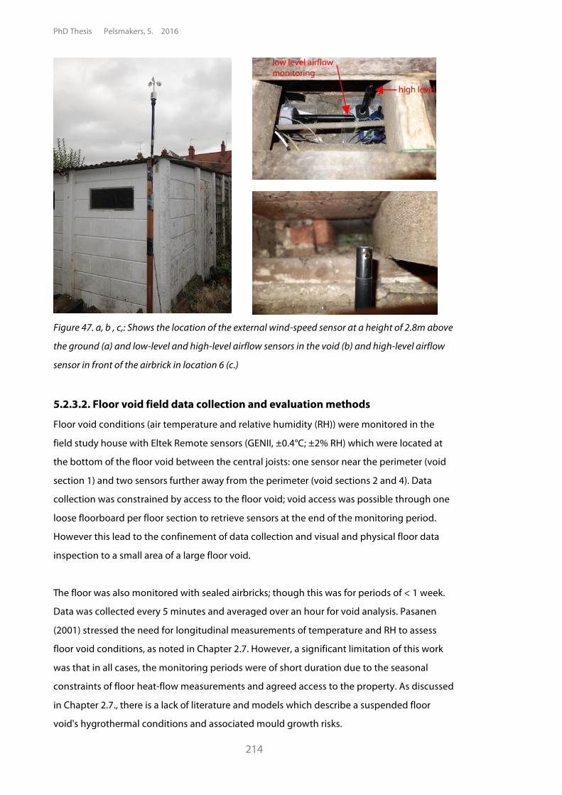
PhD Thesis Pelsmakers, S. 2016
214
Figure 47. a, b , c,: Shows the location of the external wind-speed sensor at a height of 2.8m above
the ground (a) and low-level and high-level airflow sensors in the void (b) and high-level airflow
sensor in front of the airbrick in location 6 (c.)
5.2.3.2. Floor void field data collection and evaluation methods
Floor void conditions (air temperature and relative humidity (RH)) were monitored in the
field study house with Eltek Remote sensors (GENII, ±0.4°C; ±2% RH) which were located at
the bottom of the floor void between the central joists: one sensor near the perimeter (void
section 1) and two sensors further away from the perimeter (void sections 2 and 4). Data
collection was constrained by access to the floor void; void access was possible through one
loose floorboard per floor section to retrieve sensors at the end of the monitoring period.
However this lead to the confinement of data collection and visual and physical floor data
inspection to a small area of a large floor void.
The floor was also monitored with sealed airbricks; though this was for periods of < 1 week.
Data was collected every 5 minutes and averaged over an hour for void analysis. Pasanen
(2001) stressed the need for longitudinal measurements of temperature and RH to assess
floor void conditions, as noted in Chapter 2.7. However, a significant limitation of this work
was that in all cases, the monitoring periods were of short duration due to the seasonal
constraints of floor heat-flow measurements and agreed access to the property. As discussed
in Chapter 2.7., there is a lack of literature and models which describe a suspended floor
void's hygrothermal conditions and associated mould growth risks.
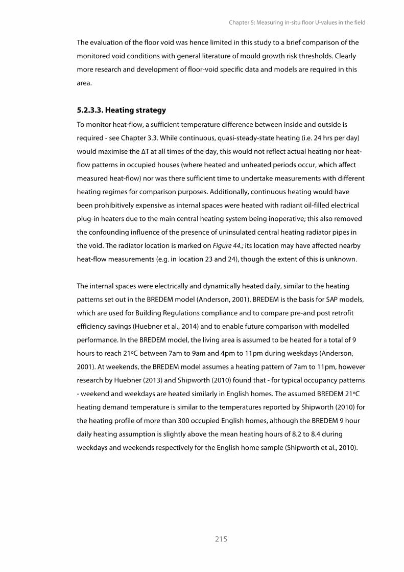
Chapter 5: Measuring in-situ floor U-values in the field
215
The evaluation of the floor void was hence limited in this study to a brief comparison of the
monitored void conditions with general literature of mould growth risk thresholds. Clearly
more research and development of floor-void specific data and models are required in this
area.
5.2.3.3. Heating strategy
To monitor heat-flow, a sufficient temperature difference between inside and outside is
required - see Chapter 3.3. While continuous, quasi-steady-state heating (i.e. 24 hrs per day)
would maximise the !T at all times of the day, this would not reflect actual heating nor heat-
flow patterns in occupied houses (where heated and unheated periods occur, which affect
measured heat-flow) nor was there sufficient time to undertake measurements with different
heating regimes for comparison purposes. Additionally, continuous heating would have
been prohibitively expensive as internal spaces were heated with radiant oil-filled electrical
plug-in heaters due to the main central heating system being inoperative; this also removed
the confounding influence of the presence of uninsulated central heating radiator pipes in
the void. The radiator location is marked on Figure 44.; its location may have affected nearby
heat-flow measurements (e.g. in location 23 and 24), though the extent of this is unknown.
The internal spaces were electrically and dynamically heated daily, similar to the heating
patterns set out in the BREDEM model (Anderson, 2001). BREDEM is the basis for SAP models,
which are used for Building Regulations compliance and to compare pre-and post retrofit
efficiency savings (Huebner et al., 2014) and to enable future comparison with modelled
performance. In the BREDEM model, the living area is assumed to be heated for a total of 9
hours to reach 21ºC between 7am to 9am and 4pm to 11pm during weekdays (Anderson,
2001). At weekends, the BREDEM model assumes a heating pattern of 7am to 11pm, however
research by Huebner (2013) and Shipworth (2010) found that - for typical occupancy patterns
- weekend and weekdays are heated similarly in English homes. The assumed BREDEM 21ºC
heating demand temperature is similar to the temperatures reported by Shipworth (2010) for
the heating profile of more than 300 occupied English homes, although the BREDEM 9 hour
daily heating assumption is slightly above the mean heating hours of 8.2 to 8.4 during
weekdays and weekends respectively for the English home sample (Shipworth et al., 2010).
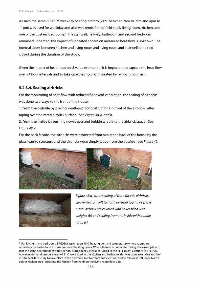
PhD Thesis Pelsmakers, S. 2016
216
As such the same BREDEM weekday heating pattern (21ºC between 7am to 9am and 4pm to
11pm) was used for weekday and also weekends for the field study living room, kitchen, and
one of the upstairs bedrooms.1 The stairwell, hallway, bathroom and second bedroom
remained unheated; the impact of unheated spaces on measured heat-flow is unknown. The
internal doors between kitchen and living room and living room and stairwell remained
closed during the duration of the study.
Given the impact of heat input on U-value estimation, it is important to capture the heat-flow
over 24 hour intervals and to take care that no bias is created by removing outliers.
5.2.3.4. Sealing airbricks
For the monitoring of heat-flow with reduced floor void ventilation, the sealing of airbricks
was done two-ways to the front of the house:
1. from the outside by placing weather-proof obstructions in front of the airbricks, after
taping over the metal airbrick surface - See Figure 48. a. and b.
2. from the inside by pushing newspaper and bubble wrap into the airbrick space - See
Figure 48. c.
For the back facade, the airbricks were protected from rain at the back of the house by the
glass lean-to structure and the airbricks were simply taped from the outside - see Figure 49.
Figure 48.a., b., c.: sealing of front facade airbricks;
clockwise from left to right: external taping over the
metal airbrick (a); covered with boxes filled with
weights (b) and sealing from the inside with bubble
wrap (c)
1 For kitchens and bedrooms, BREDEM assumes an 18ºC heating demand temperature where rooms are separately controlled and assumes reduced heating hours. Where there is no separate zoning, the assumption is that the same heating times apply in non-living spaces, as was assumed in the field study. Contrary to BREDEM however, demand temperatures of 21ºC were used in the kitchen and bedroom; this was done to enable another in-situ heat-flux study to take place in the bedroom (i.e. to create sufficient !T) and to minimise influence from a colder kitchen area (including the kitchen floor void) on the living room floor void.
Chapter 5: Measuring in-situ floor U-values in the field
217
Figure 49.a., b.: Sealing of back facade airbricks by taping over the metal surface.
5.2.3.5. Field study limitations
The main field study limitations and issues are identified below; all of which require future
research.
• Limited calibration checks: All the temperature sensors were checked 'side by side'
in both a cold and warm UCL chamber while some other experiments were taking
place in the thermal lab. All temperature and RH sensors measured within their
stated instrument accuracy under the lab conditions (~10ºC in cold chamber and
~20ºC in the warm chamber), which are similar conditions to those encountered in
the internal room or floor void conditions - see Chapter 6.5.and Section 5.3.7.
However no calibration checks (as described in Chapter 3.3.5.) were undertaken for
the heat-flux sensors: there were no suitable wall surfaces available in the thermal lab
due to other studies taking place.
• The whole floor U-value is derived from living room floor only: the whole floor
U-value is derived from the living room floor only, which represents 44% of the entire
ground floor. It is assumed that similar heat-transfer applied across the rest of the
floor, creating uncertainty around the whole floor estimated U-value. The impact of
unheated spaces on measured living-room floor heat-flow is unknown.
• Only one joist location measured: due to joist locations having nail or holes in
boards, measuring joist heat-flux is limited to suitable locations where surface
contact is sufficient. The lack of several measured joist locations and the exclusion of
a perimeter joist location measurement is a limitation of this field study (and likely
future field studies). Implications of this for whole floor U-value estimation are
discussed in Section 5.3.2.
PhD Thesis Pelsmakers, S. 2016
218
• Missing data: the study started late due to electrical supply failure to the external
temperature data logger and to the electrical heater in the living room (due to an
electrical fault with the kWh readers). Some data loggers failed, leading to missing
data of a few days (in between site visits) in sensor locations 17 and 18 and a few
hours for locations 6 to 9. The late start of the study meant that the uninsulated floor
study with sealed airbricks had to be cut short to 4 days, leading to less robust results
- see Section 5.3.7.
• Sealing of airbricks: In the field study, airbricks in the living room were taped both
from the outside as well as sealed with bubble wrap from the inside; but the
foundation walls might not be airtight so that closing of airbricks on its own may
have no or limited effect on heat loss as observed by Hill (2005).
• Measuring void airflow: void airflow was measured with one-directional sensors -
see Section 5.2.3. In front of the airbricks, the airflow direction is more likely to be in
the direction of the sensor; however, other patterns of air movement and from
different directions were excluded.
• Exclusion of uninsulated, heated central heating pipes in the floor void: radiator
heating pipes typically run through floor voids (often in localised areas) and
condition the void and floor surfaces. This is expected to significantly affect observed
heat-flow (and possibly thermal comfort thresholds). This study was undertaken
without the effect of heated radiator pipes in the void; and this is also excluded in
floor U-value models. While this would have added complexity to the study, the
effect of heat-flow from radiator pipes is outside the scope of this research. The
spaces were electrically heated and given the non-functioning central heating-
system in the case-study, no comparative study could be undertaken and this has
been noted for future research.
• Short-term monitoring only of floor void conditions: due to access arrangements,
the floor void could only be monitored over a short period, hence limiting
comparison with both literature and post-insulation monitored data - see Section
5.3.7.
• Limitations with other measured variables are provided in Appendix 5.B.
Chapter 5: Measuring in-situ floor U-values in the field
219
5.2.4. Error propagation and data analysis procedures This section gives a brief summary reminder of the error propagation and data analysis
procedures as set out in Chapter 3.3.4.3. and comparable to the techniques applied for the
Salford EH, see Chapter 4.3.4.
5.2.4.1. Data analysis and measurement uncertainty
The mean U-values were estimated in accordance with Equation 47. , including adjustment
with surface thermal resistance RSi of 0.17 m2KW-1 where internal surface temperatures were
used; all estimates include adjustment for the thermal resistance of the heat-flux sensor itself
(see Chapter 3.3.).
The measurement uncertainty for the in-situ estimated U-values is estimated from Equation
49. (page 125) and as repeated in Table 26., where the standard deviation is a measure of the
natural variability of U over the monitored period. At the Salford EH, an hourly mean and its
sd was calculated however for the field data a clear day/night cycle exists and a daily mean
and daily sd are estimated instead - justification for this was set out in Chapter 3.3.4.3, page
124.
Contrary to the Salford EH, the natural variability of the uninsulated floor constitutes a large
component of the total uncertainty; this is caused by the changing external environmental
conditions alongside a changing space-heating pattern, which is absent at the Salford EH.
To illustrate: the intrinsic instrument error and the (extrinsic) measuring condition error make
up approximately ±9% of the overall error - see Chapter 3.3.4. Added to this is the natural
variability component of U and in the field-study was found to be between ±4 to ±13%. In
the Salford EH this was found to be " ±5% (after research influence outlier removal - see
Chapter 4.3.4 and 4.3.5.). For the field-study this lead to total measurement uncertainties
between ±10 to ±16% depending on point location on the floor (see Table 27.), while for
Salford total measurement uncertainty was estimated between ±9 to ±11%.
For comparisons between open and sealed airbricks and comparisons for the same point
location with different temperature data, contact, edge heat loss and instrument errors need
not be included as these sensors remained in place – see Equation 50. (in Table 26.) and as
discussed in Chapter 3.3.4.3.
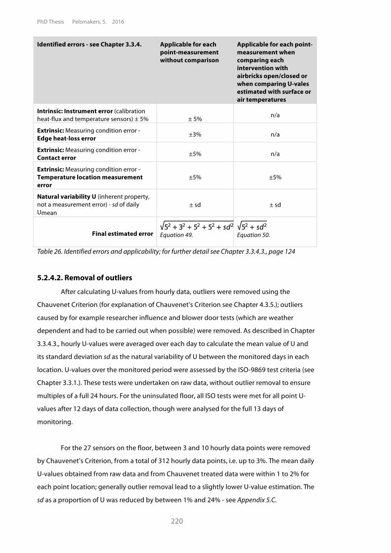
PhD Thesis Pelsmakers, S. 2016
220
Identified errors - see Chapter 3.3.4. Applicable for each point-measurement without comparison
Applicable for each point-measurement when comparing each intervention with airbricks open/closed or when comparing U-vales estimated with surface or air temperatures
Intrinsic: Instrument error (calibration heat-flux and temperature sensors) ± 5%
± 5% n/a
Extrinsic: Measuring condition error - Edge heat-loss error ±3% n/a
Extrinsic: Measuring condition error - Contact error ±5% n/a
Extrinsic: Measuring condition error - Temperature location measurement error
±5% ±5%
Natural variability U (inherent property, not a measurement error) - sd of daily Umean
± sd ± sd
Final estimated error
Equation 49.
Equation 50.
Table 26. Identified errors and applicability; for further detail see Chapter 3.3.4.3., page 124
5.2.4.2. Removal of outliers
After calculating U-values from hourly data, outliers were removed using the
Chauvenet Criterion (for explanation of Chauvenet's Criterion see Chapter 4.3.5.); outliers
caused by for example researcher influence and blower door tests (which are weather
dependent and had to be carried out when possible) were removed. As described in Chapter
3.3.4.3., hourly U-values were averaged over each day to calculate the mean value of U and
its standard deviation sd as the natural variability of U between the monitored days in each
location. U-values over the monitored period were assessed by the ISO-9869 test criteria (see
Chapter 3.3.1.). These tests were undertaken on raw data, without outlier removal to ensure
multiples of a full 24 hours. For the uninsulated floor, all ISO tests were met for all point U-
values after 12 days of data collection, though were analysed for the full 13 days of
monitoring.
For the 27 sensors on the floor, between 3 and 10 hourly data points were removed
by Chauvenet's Criterion, from a total of 312 hourly data points, i.e. up to 3%. The mean daily
U-values obtained from raw data and from Chauvenet treated data were within 1 to 2% for
each point location; generally outlier removal lead to a slightly lower U-value estimation. The
sd as a proportion of U was reduced by between 1% and 24% - see Appendix 5.C.
Chapter 5: Measuring in-situ floor U-values in the field
221
5.3. Analysis, results and discussion
This section presents the estimated uninsulated floor system point U-values and discusses
the spread of the Up-values, followed by an estimated whole floor system U-value and
comparison to literature and models.
5.3.1. Spread of point U-values and perimeter effect Based on the aforementioned data and error analysis protocols and using internal surface to
external air temperatures, estimated Up-values ranged from 2.04 ±0.21 Wm-2K-1 above the
central airbrick along the perimeter (location 6) to values a quarter of this furthest away from
the perimeter (0.54 ±0.09 Wm-2K-1, location 5). All estimated point-U-values are listed in Table
27. The greatest Up-values were observed in locations 6 and 22 (1.99±0.21 Wm-2K-1), near the
central and third airbrick. The first airbrick (below location 1) was protected by a large hedge
and might be the reason why there is still significant, but slightly reduced heat-flow in this
location (1.74 ±0.18 Wm-2K-1).
As expected and as also observed in the Salford EH, the uninsulated living room floor system
in the field study house had a large spread of Up-values across the floor. In general, a clear
negative association exists between the measured Up-value in a location and its distance
from the external perimeter wall. As illustrated by Figure 50., estimated Up-values
progressively reduce with the distance from the perimeter wall. As discussed in Chapter
4.4.1., a 1000mm perimeter zone was used for graphical representation and hypothesis
testing and was also used here for the same purpose. The second hypothesis H2 ("There will
be increased perimeter Up-values observed compared to locations further away from the external
wall (i.e. the non-perimeter zone)") was supported by an unpaired Mann-Whitney U (Wilcoxcon
rank sum): Mann–Whitney W = 147, n1 = 9; n2 = 17,P < 0.05 (0.00002 or about 2 tests in
100,000, unpaired): i.e. the difference in Up-values between the perimeter zone (locations
within 1000mmm from an external wall) and the non-perimeter zone of the floor (sensor
locations further away than 1000mm) was statistically significant. The estimated mean of the
9 perimeter located point U-values was 1.54 ±0.17 Wm-2K-1, 1.8 times greater than the
estimated mean of the 17 point U-values located in the non-perimeter zone
(0.85 ±0.11 Wm-2K-1). As also discussed in Chapter 4.4.1, the extent of the perimeter effect is
less clear as there was no abrupt change after 1000mm, but instead a gradual reduction in
Up-values the further away from the external environment was observed - see Figure 50.
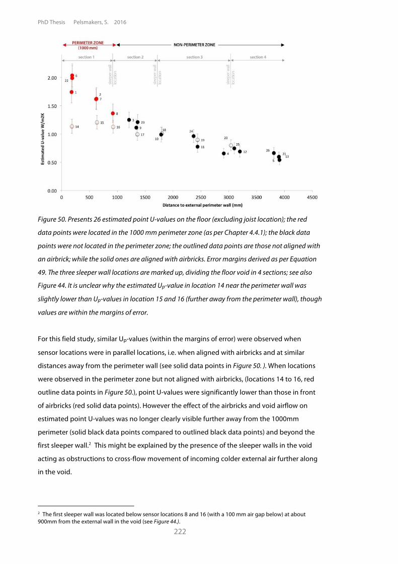
PhD Thesis Pelsmakers, S. 2016
222
Figure 50. Presents 26 estimated point U-values on the floor (excluding joist location); the red
data points were located in the 1000 mm perimeter zone (as per Chapter 4.4.1); the black data
points were not located in the perimeter zone; the outlined data points are those not aligned with
an airbrick; while the solid ones are aligned with airbricks. Error margins derived as per Equation
49. The three sleeper wall locations are marked up, dividing the floor void in 4 sections; see also
Figure 44. It is unclear why the estimated Up-value in location 14 near the perimeter wall was
slightly lower than Up-values in location 15 and 16 (further away from the perimeter wall), though
values are within the margins of error.
For this field study, similar Up-values (within the margins of error) were observed when
sensor locations were in parallel locations, i.e. when aligned with airbricks and at similar
distances away from the perimeter wall (see solid data points in Figure 50. ). When locations
were observed in the perimeter zone but not aligned with airbricks, (locations 14 to 16, red
outline data points in Figure 50.), point U-values were significantly lower than those in front
of airbricks (red solid data points). However the effect of the airbricks and void airflow on
estimated point U-values was no longer clearly visible further away from the 1000mm
perimeter (solid black data points compared to outlined black data points) and beyond the
first sleeper wall.2 This might be explained by the presence of the sleeper walls in the void
acting as obstructions to cross-flow movement of incoming colder external air further along
in the void.
2 The first sleeper wall was located below sensor locations 8 and 16 (with a 100 mm air gap below) at about 900mm from the external wall in the void (see Figure 44.).
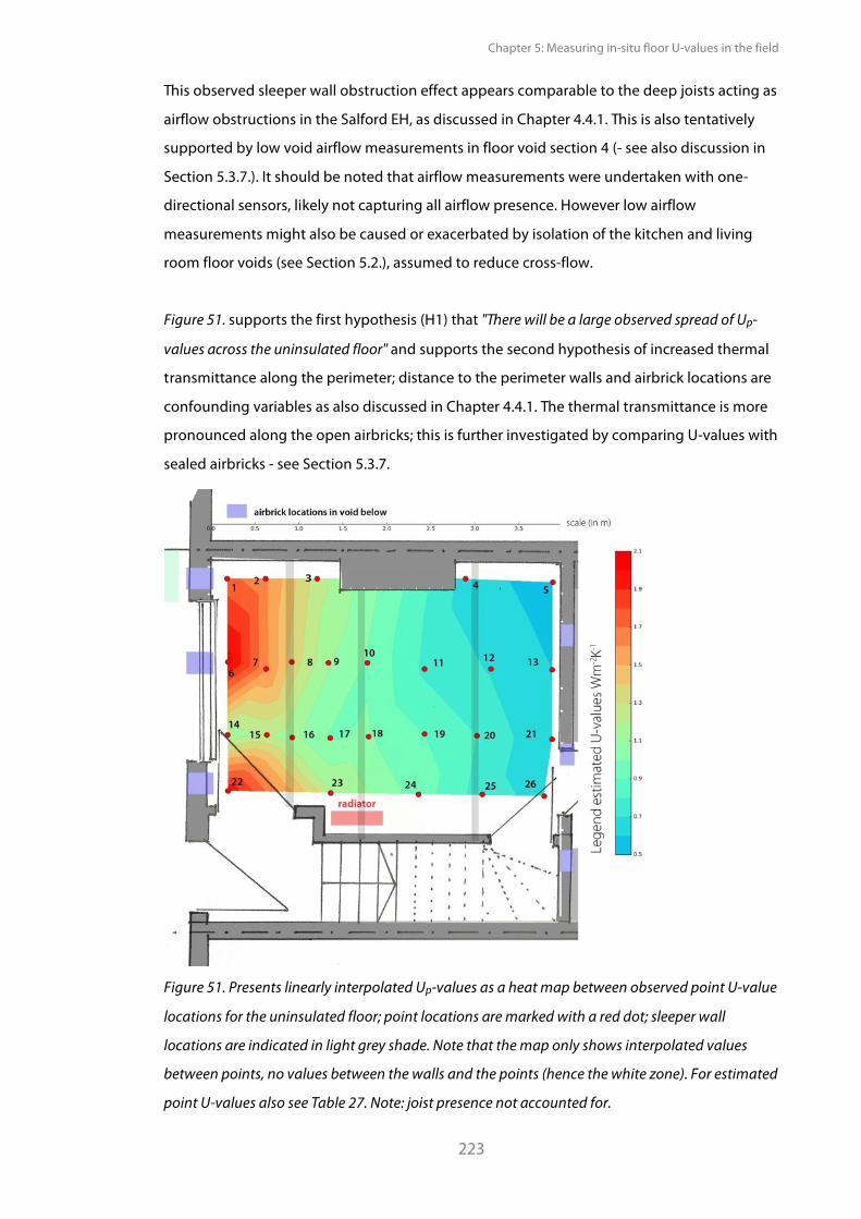
Chapter 5: Measuring in-situ floor U-values in the field
223
This observed sleeper wall obstruction effect appears comparable to the deep joists acting as
airflow obstructions in the Salford EH, as discussed in Chapter 4.4.1. This is also tentatively
supported by low void airflow measurements in floor void section 4 (- see also discussion in
Section 5.3.7.). It should be noted that airflow measurements were undertaken with one-
directional sensors, likely not capturing all airflow presence. However low airflow
measurements might also be caused or exacerbated by isolation of the kitchen and living
room floor voids (see Section 5.2.), assumed to reduce cross-flow.
Figure 51. supports the first hypothesis (H1) that "There will be a large observed spread of Up-
values across the uninsulated floor" and supports the second hypothesis of increased thermal
transmittance along the perimeter; distance to the perimeter walls and airbrick locations are
confounding variables as also discussed in Chapter 4.4.1. The thermal transmittance is more
pronounced along the open airbricks; this is further investigated by comparing U-values with
sealed airbricks - see Section 5.3.7.
Figure 51. Presents linearly interpolated Up-values as a heat map between observed point U-value
locations for the uninsulated floor; point locations are marked with a red dot; sleeper wall
locations are indicated in light grey shade. Note that the map only shows interpolated values
between points, no values between the walls and the points (hence the white zone). For estimated
point U-values also see Table 27. Note: joist presence not accounted for.
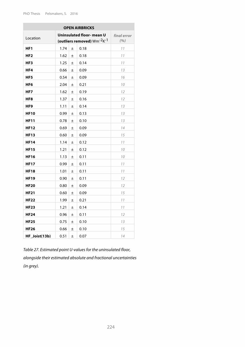
PhD Thesis Pelsmakers, S. 2016
224
OPEN AIRBRICKS
Location Uninsulated floor- mean U (outliers removed) Wm-2K-1
final error (%)
HF1 1.74 ± 0.18 11
HF2 1.62 ± 0.18 11
HF3 1.25 ± 0.14 11
HF4 0.66 ± 0.09 13
HF5 0.54 ± 0.09 16
HF6 2.04 ± 0.21 10
HF7 1.62 ± 0.19 12
HF8 1.37 ± 0.16 12
HF9 1.11 ± 0.14 13
HF10 0.99 ± 0.13 13
HF11 0.78 ± 0.10 13
HF12 0.69 ± 0.09 14
HF13 0.60 ± 0.09 15
HF14 1.14 ± 0.12 11
HF15 1.21 ± 0.12 10
HF16 1.13 ± 0.11 10
HF17 0.99 ± 0.11 11
HF18 1.01 ± 0.11 11
HF19 0.90 ± 0.11 12
HF20 0.80 ± 0.09 12
HF21 0.60 ± 0.09 15
HF22 1.99 ± 0.21 11
HF23 1.21 ± 0.14 11
HF24 0.96 ± 0.11 12
HF25 0.75 ± 0.10 13
HF26 0.66 ± 0.10 15
HF_Joist(13b) 0.51 ± 0.07 14
Table 27. Estimated point U-values for the uninsulated floor,
alongside their estimated absolute and fractional uncertainties
(in grey).
Chapter 5: Measuring in-situ floor U-values in the field
225
5.3.2. Whole floor U-value The whole floor U-value was derived from the living room floor only which represented 44%
of the entire ground floor. This created unknown uncertainty around the whole floor U-value,
but it allowed for comparison with models (where the same characteristics of the living room
floor were used).
As defined earlier in Chapter 4.4.2., the whole floor U-value estimation was calculated as an
area-weighted summation in accordance with Equation 52. Figure 52. illustrates the 12.15 m2
living room floor plan and a representative area grid derived from sensor locations and with
support from infrared images.
The whole floor U-value was estimated as 1.04 ±0.12 Wm-2K-1.3 As discussed in Chapter
3.3.2., uncertainty arises from representative area estimations; different area configurations
were tested along the perimeter, however this did not lead to any differences past the third
significant digit of the whole floor obtained U-value.
Only one joist location was measured near sensor location 13 away from the perimeter, as
marked on Figure 52. and as discussed in Section 5.2.3. The estimated point U-value on the
joist was 0.51 ±0.07 Wm-2K-1, just 15% below the point U-value of 0.60 ±0.09 Wm-2K-1 in
location 13 and within the margins of error. This thermal transmittance reduction is
significantly less than the 21% U-value reduction of a Salford EH joist, however this difference
is likely explained by (a.) joists were 190mm in the Salford EH and just 100mm in the field
study and (b.) the location specificity of observed thermal transmittance reduction; in the
Salford EH, joist measurement was along the exposed perimeter: addition of an increased
thermal resistance (i.e. the joist) will have a greater proportional heat-transfer reduction
impact where heat-flow is higher (i.e. along the perimeter). For the reasons above and given
that the difference was within the margins of error, no joist adjustments were made for the
field study4 and is a limitation of this study as noted in Section 5.2.3.5.
3 This was similar to but slightly below the simple whole floor U mean estimate of 1.09 ±0.13 W/m2K. 4 Joist adjustment would lead to a whole floor U-value of 1.02 ±0.12 Wm-2K-1, close to the unadjusted whole floor U-value.
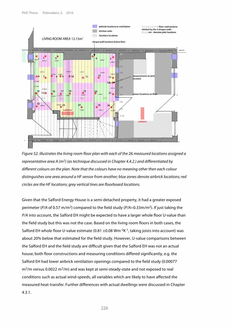
PhD Thesis Pelsmakers, S. 2016
226
Figure 52. illustrates the living room floor plan with each of the 26 measured locations assigned a
representative area A (m2) (as technique discussed in Chapter 4.4.2.) and differentiated by
different colours on the plan. Note that the colours have no meaning other then each colour
distinguishes one area around a HF sensor from another; blue zones denote airbrick locations; red
circles are the HF locations; grey vertical lines are floorboard locations.
Given that the Salford Energy House is a semi-detached property, it had a greater exposed
perimeter (P/A of 0.57 m/m2) compared to the field study (P/A=0.33m/m2). If just taking the
P/A into account, the Salford EH might be expected to have a larger whole floor U-value than
the field study but this was not the case. Based on the living room floors in both cases, the
Salford EH whole floor U-value estimate (0.81 ±0.08 Wm-2K-1, taking joists into account) was
about 20% below that estimated for the field study. However, U-value comparisons between
the Salford EH and the field study are difficult given that the Salford EH was not an actual
house; both floor constructions and measuring conditions differed significantly, e.g. the
Salford EH had lower airbrick ventilation openings compared to the field study (0.00077
m2/m versus 0.0022 m2/m) and was kept at semi-steady-state and not exposed to real
conditions such as actual wind-speeds, all variables which are likely to have affected the
measured heat-transfer. Further differences with actual dwellings were discussed in Chapter
4.3.1.
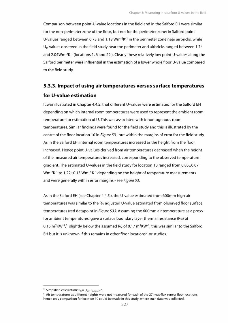
Chapter 5: Measuring in-situ floor U-values in the field
227
Comparison between point-U-value locations in the field and in the Salford EH were similar
for the non-perimeter zone of the floor, but not for the perimeter zone: in Salford point
U-values ranged between 0.73 and 1.18 Wm-2K-1 in the perimeter zone near airbricks, while
Up-values observed in the field study near the perimeter and airbricks ranged between 1.74
and 2.04Wm-2K-1 (locations 1, 6 and 22 ). Clearly these relatively low point U-values along the
Salford perimeter were influential in the estimation of a lower whole floor U-value compared
to the field study.
5.3.3. Impact of using air temperatures versus surface temperatures
for U-value estimation It was illustrated in Chapter 4.4.5. that different U-values were estimated for the Salford EH
depending on which internal room temperatures were used to represent the ambient room
temperature for estimation of U. This was associated with inhomogenous room
temperatures. Similar findings were found for the field study and this is illustrated by the
centre of the floor location 10 in Figure 53., but within the margins of error for the field study.
As in the Salford EH, internal room temperatures increased as the height from the floor
increased. Hence point U-values derived from air temperatures decreased when the height
of the measured air temperatures increased, corresponding to the observed temperature
gradient. The estimated U-values in the field study for location 10 ranged from 0.85±0.07
Wm-2K-1 to 1.22±0.13 Wm-2 K-1 depending on the height of temperature measurements
and were generally within error margins - see Figure 53.
As in the Salford EH (see Chapter 4.4.5.), the U-value estimated from 600mm high air
temperatures was similar to the RSi adjusted U-value estimated from observed floor surface
temperatures (red datapoint in Figure 53.). Assuming the 600mm air temperature as a proxy
for ambient temperatures, gave a surface boundary layer thermal resistance (RSi) of
0.15 m2KW-1,5 slightly below the assumed RSi of 0.17 m2KW-1; this was similar to the Salford
EH but it is unknown if this remains in other floor locations6 or studies.
5 Simplified calculation: RSi= (Tair-Tsurface)/q 6 Air temperatures at different heights were not measured for each of the 27 heat-flux sensor floor locations, hence only comparison for location 10 could be made in this study, where such data was collected.
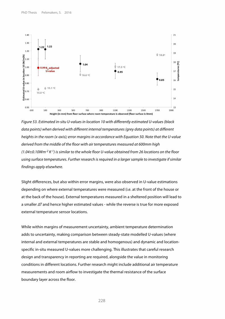
PhD Thesis Pelsmakers, S. 2016
228
Figure 53. Estimated in-situ U-values in location 10 with differently estimated U-values (black
data points) when derived with different internal temperatures (grey data points) at different
heights in the room (x-axis); error margins in accordance with Equation 50. Note that the U-value
derived from the middle of the floor with air temperatures measured at 600mm high
(1.04±0.10Wm-2 K-1) is similar to the whole floor U-value obtained from 26 locations on the floor
using surface temperatures. Further research is required in a larger sample to investigate if similar
findings apply elsewhere.
Slight differences, but also within error margins, were also observed in U-value estimations
depending on where external temperatures were measured (i.e. at the front of the house or
at the back of the house). External temperatures measured in a sheltered position will lead to
a smaller "T and hence higher estimated values - while the reverse is true for more exposed
external temperature sensor locations.
While within margins of measurement uncertainty, ambient temperature determination
adds to uncertainty, making comparison between steady-state modelled U-values (where
internal and external temperatures are stable and homogenous) and dynamic and location-
specific in-situ measured U-values more challenging. This illustrates that careful research
design and transparency in reporting are required, alongside the value in monitoring
conditions in different locations. Further research might include additional air temperature
measurements and room airflow to investigate the thermal resistance of the surface
boundary layer across the floor.
Chapter 5: Measuring in-situ floor U-values in the field
229
5.3.4. Estimating a whole floor U-value with fewer point
measurements As discussed in Chapter 4.4.2.5., measuring in just a few point locations is highly likely to
significantly over-or underestimate the whole floor U-value; this was also confirmed for the
field study: 70% of values estimated by averaging just two point-measurements would
under- or over-estimate the whole floor U-value - this is illustrated by Figure 54.; 30% of the
paired U-values had overlapping error margins which fell within the error margins of the
whole floor U-value. Only 21 paired U-values (or 6.5%) matched the estimated mean U-value
closely (i.e. where the mean U-value overlapped with the whole floor U-value error margins,
i.e. between 0.92 to 1.16 Wm-2 K-1). Just 1 paired location matched the uninsulated whole
floor U-value exactly (pairing of locations 9 and 24).
Figure 54. Histogram of the 325 paired U-values; the red line indicates the whole floor estimated
U-value, while the red zone indicates the U-value distribution within the error margins of the
whole floor U-value (97 pairs (or 30% of all combinations); the grey bars are mean U-values from
two locations on the floor which fall outside the whole floor U-value uncertainty margins. Note no
joist presence is accounted for.
PhD Thesis Pelsmakers, S. 2016
230
In summary, only a small proportion of paired U-values gave a similar whole floor U-value as
obtained from high-resolution measurements and indicated the limited use of low-
resolution measurements to obtain a whole floor U-value. This is in support of the discussion
in Chapter 4.4.2.5., reiterating that random selection of measuring locations is highly likely to
lead to a poor representation of the whole floor U-value due to the large spread of heat-flow
across the floor surface. Only by measuring at high-resolution can insights be gained of the
combined sensor locations which would give a U-value estimate close to the whole floor
U-value. In this field study, there is no real pattern, though locations near the airbricks and
<800mm from the perimeter were generally excluded to obtain a close whole floor U-value.
This is likely to differ depending on floor and dwelling characteristics - further discussion in
Chapter 6.4.2.3.
5.3.5. Comparison to literature and other in-situ studies
Literature - theoretical values
The average published U-value of a terraced house was found to be 0.55 Wm-2K-1 and was
between 0.45 Wm-2K-1 to 0.70 Wm-2K-1 - see Chapter 2.4.1. This is clearly significantly below
and outside the margins of error of the estimated whole floor U-value of 1.04 ±0.12 Wm-2K-1
(i.e. 0.92 to 1.16 Wm-2 K-1) for the field study.
Literature - in-situ reported values
The estimated in-situ Up-values located in the perimeter zone in this field study ranged
between 1.14 ±0.12 Wm-2K-1 (location 14) and 2.04 ±0.21 Wm-2K-1(location 6) and are similar
(though slightly below) the perimeter point U-values of 1.19 Wm-2K-1and 2.4 Wm-2K-1 as
reported by others (see Chapter 2.4.2.). Given that the latter in-situ point floor measurements
are from different housing typologies and were generally single spot measurements in
specific locations, comparison between these in-situ reported measurements and Up-values
as well as the whole floor U-value obtained from 26 point locations across the floor in this
field study is uncertain and challenging.
Chapter 5: Measuring in-situ floor U-values in the field
231
5.3.6. Comparison to modelled U-values The modelled floor U-value was estimated using the ISO-13370 model as described in
Chapter 2.3 and with CIBSE-2015 and RdSAP and the superseded CIBSE-1986 model. Where
available, input data was adapted after the site survey to calibrate model inputs to increase
the accuracy of the model (as recommended by Park (2013) and Lee (2013)). Inputs which
could not be obtained from a survey were assumed based on typical assumptions - as listed
in Table 24. Measured external wind-speeds were excluded in the model as they were taken
at 2.8m instead of the 10m assumed in the model. The models were based on living room
area characteristics to allow for comparison to the in-situ estimated whole floor U-value,
limitations of doing so were noted in Section 5.2.3.5.
U-values were modelled with and without joist presence, but this made no significant
difference to the resulting U-values (see Table 28.); joists were excluded in the in-situ
measurements as discussed in Section 5.3.2. Depending on which current model is used, the
whole floor U-value was estimated between 0.51 and 0.57 Wm-2 K-1, as set out in Table 28.
These modelled values are within the ranges of published U-values for terraced houses of
0.45 to 0.70Wm-2 K-1(see Section 5.3.5.), but significantly below this field study's in-situ
measured whole floor U-value of 1.04 ±0.12 Wm-2 K-1. The in-situ estimated whole floor
U-value was about twice as high than the current U-value model estimates and outside the
margins of in-situ measurement uncertainty; > 20% disparity is considered significant by
ISO-9869 (BSI, 2014).
The superseded CIBSE-1986 model estimated significantly higher floor U-values than the
current models, providing an estimate nearly 30% higher than the whole floor estimated
U-value. Possible reasons for the disparity between the old CIBSE-1986 and current floor
U-value models were discussed in Chapter 4.4.3 and included greater influence by the
CIBSE-1986 model of ventilation opening area and assumed wind-speeds. Changing wind-
speed from 5m/s (as suggested by RdSAP) to 1m/s (as recommended by the CIBSE-1986
model - Chapter 2.3.1.) lead to the (current) model outputs diverging even further from the
in-situ measured whole floor U-value, whereas the CIBSE-1986 model reduced to
1.04 Wm-2 K-1 , aligning with the in-situ estimated whole floor U-value for this field study.
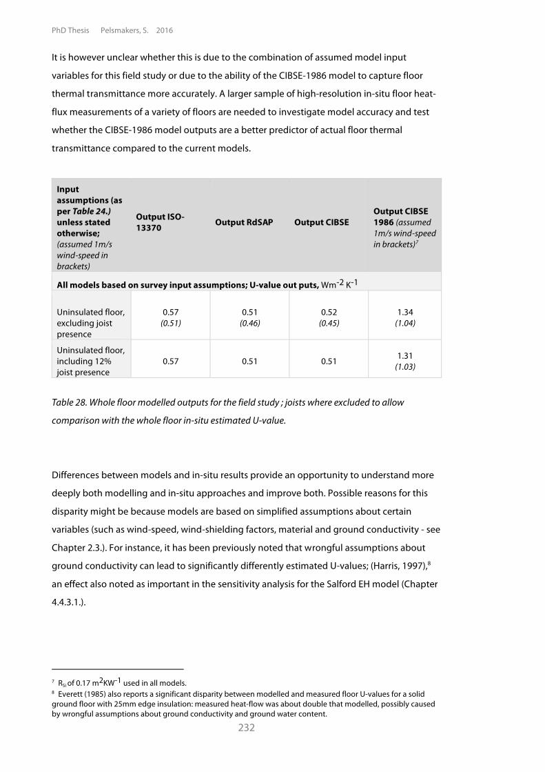
PhD Thesis Pelsmakers, S. 2016
232
It is however unclear whether this is due to the combination of assumed model input
variables for this field study or due to the ability of the CIBSE-1986 model to capture floor
thermal transmittance more accurately. A larger sample of high-resolution in-situ floor heat-
flux measurements of a variety of floors are needed to investigate model accuracy and test
whether the CIBSE-1986 model outputs are a better predictor of actual floor thermal
transmittance compared to the current models.
Input assumptions (as per Table 24.) unless stated otherwise; (assumed 1m/s wind-speed in brackets)
Output ISO-13370
Output RdSAP
Output CIBSE
Output CIBSE 1986 (assumed 1m/s wind-speed in brackets)7
All models based on survey input assumptions; U-value out puts, Wm-2 K-1
Uninsulated floor, excluding joist presence
0.57 (0.51)
0.51 (0.46)
0.52
(0.45)
1.34 (1.04)
Uninsulated floor, including 12% joist presence
0.57 0.51 0.51 1.31 (1.03)
Table 28. Whole floor modelled outputs for the field study ; joists where excluded to allow
comparison with the whole floor in-situ estimated U-value.
Differences between models and in-situ results provide an opportunity to understand more
deeply both modelling and in-situ approaches and improve both. Possible reasons for this
disparity might be because models are based on simplified assumptions about certain
variables (such as wind-speed, wind-shielding factors, material and ground conductivity - see
Chapter 2.3.). For instance, it has been previously noted that wrongful assumptions about
ground conductivity can lead to significantly differently estimated U-values; (Harris, 1997),8
an effect also noted as important in the sensitivity analysis for the Salford EH model (Chapter
4.4.3.1.).
7 RSi of 0.17 m2KW-1 used in all models. 8 Everett (1985) also reports a significant disparity between modelled and measured floor U-values for a solid ground floor with 25mm edge insulation: measured heat-flow was about double that modelled, possibly caused by wrongful assumptions about ground conductivity and ground water content.
Chapter 5: Measuring in-situ floor U-values in the field
233
Overall, the cause of the disparity between the current models and the in-situ measured
estimated whole floor U-value is unclear. The disparity is also more pronounced in the field-
study than in the Salford EH. This might be because the Salford EH conditions were steady-
state and might reflect the steady-state model assumptions (BSI, 2009b), including thermal
mass equilibrium. As discussed in Chapter 2.3., floor U-value models have been created
according to a theoretical and physical framework based on steady-state conditions and
certain input assumptions. However the field-study - unlike the Salford EH - was subject to
dynamic conditions and practical in-situ measuring issues, and alongside the input
assumptions used, the ability of theoretical models to deal with this level of complexity is yet
unknown. A conceptual difference between models and in-situ measurements might be a
reason for such disparities. For instance, linear thermal bridging of the wall-floor junction is
excluded in models, though in-situ measurements might be affected by the wall-floor
junction heat-transfer. Another example is that theoretical floor U-value models consider the
heat-transfer and temperature difference over a full year and that the thermal mass of the
ground is negligible (and is hence excluded in models) (CIBSE, 1996, BSI, 2009b). BSI (2009b)
considers the annual heat-transfer a good approximation of the average heat-flow in the
heating-season (the period in which field-study measurements were undertaken) however it
is unknown if this is indeed the case for suspended floors. CIBSE (1996) suggests the same for
ground floors with 'an appreciable' thermal mass delay but suggests that where there is a
smaller thermal mass delay, seasonal temperatures should be used instead9. It is undefined if
this applies to suspended ground floors.
To investigate the ground's thermal behaviour, the outputs of three heat-flux sensors placed
on the ground in the void (two under sensor location 22 and one in location 5 - see Section
5.2.3.1.) were investigated. For each sensor on the ground in the void it was observed that
the heat-flow (q, W/m2) going into the ground did not equal the heat-flow coming from the
ground10 over the winter floor monitoring period of 13 days. As expected and in general near
the airbricks, more heat was released from the ground over the monitoring period than
transferred to the ground.11 This is unsurprising given the exposure of the void to external
temperatures through nearby airbricks and colder void surfaces, so the void temperatures
are expected to be below the ground temperatures in this area in winter. Further away from
airbricks, the direction of heat-flow was always from void to ground each day; though it is
unknown (how much) of this heat was stored or transferred. 9 CIBSE (1996) does not define what an appreciable or small thermal mass delay is. According to ISO-13370 (BSI, 2009b), the thermal lag for suspended ground floors are less "because the ventilation heat flow has no time lag" (p30) and suggests that suspended floors have a thermal mass delay of 0 months (though this could still include several days or weeks). 10 This was observed outside the HFP01 instrument error margins of ±15% for ground heat-flux measurements. 11 This depended from day to day, but overall heat-flow was from ground to void.
PhD Thesis Pelsmakers, S. 2016
234
This suggests that in the observed locations, the ground thermal mass was not in equilibrium
over the monitored winter period. However, these ground heat-flows were a small
proportion of the overall room to void heat-flows when compared to the nearby sensor
locations on the floor above: the total 13-day observed ground heat-flow near airbricks was
just 2% to 4% of the heat-flow observed in location 22 above; and about 16% further away in
location 5. This might indicate that the thermal mass effect in this suspended floor over the
monitored period was a proportionally small driver in floor heat-transfer, and especially near
airbricks. However further research and high-resolution long-term monitoring of both floor
and ground heat-fluxes are required to reveal longer-term seasonal changes of the ground
and to investigate whether annual heat-flow and temperature assumptions are a good proxy
for the seasonal heat-flow for suspended ground floors as measured here in the field study.
Overall, it is clear that further research is required to understand which parameters and
assumptions create a discrepancy between models and in-situ measurements, and how this
gap can be bridged to create more robust models and more informative in-situ monitoring.
This work is particularly important because significant differences between modelled and
measured U-value estimates have implications for policy and retrofit-decision making as
discussed in Section 5.4 and Chapter 7.4. Hence high-resolution and longitudinal sampling of
a larger number of floors, including different dwelling types and orientation, different void
depths and ventilation and those with different floor areas and with different P/A, are
required to assess if these disparities are specific to the cases studied and/or the different
models used and if they remain in a larger sample.
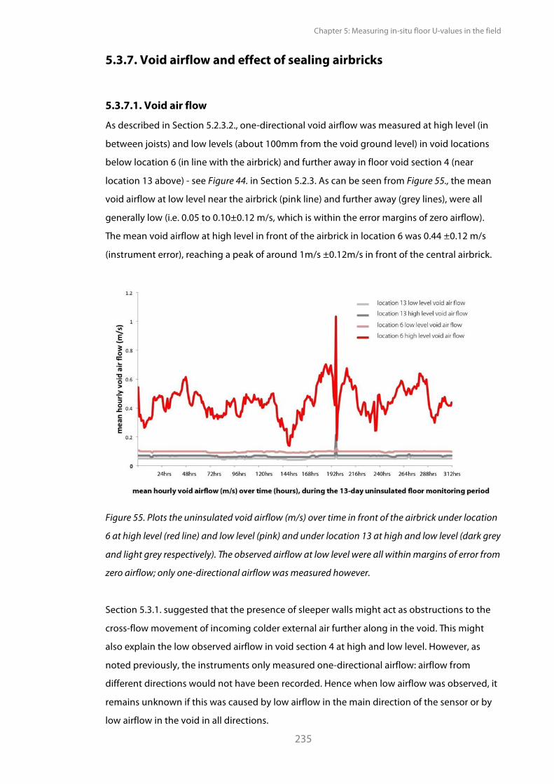
Chapter 5: Measuring in-situ floor U-values in the field
235
5.3.7. Void airflow and effect of sealing airbricks
5.3.7.1. Void air flow
As described in Section 5.2.3.2., one-directional void airflow was measured at high level (in
between joists) and low levels (about 100mm from the void ground level) in void locations
below location 6 (in line with the airbrick) and further away in floor void section 4 (near
location 13 above) - see Figure 44. in Section 5.2.3. As can be seen from Figure 55., the mean
void airflow at low level near the airbrick (pink line) and further away (grey lines), were all
generally low (i.e. 0.05 to 0.10±0.12 m/s, which is within the error margins of zero airflow).
The mean void airflow at high level in front of the airbrick in location 6 was 0.44 ±0.12 m/s
(instrument error), reaching a peak of around 1m/s ±0.12m/s in front of the central airbrick.
Figure 55. Plots the uninsulated void airflow (m/s) over time in front of the airbrick under location
6 at high level (red line) and low level (pink) and under location 13 at high and low level (dark grey
and light grey respectively). The observed airflow at low level were all within margins of error from
zero airflow; only one-directional airflow was measured however.
Section 5.3.1. suggested that the presence of sleeper walls might act as obstructions to the
cross-flow movement of incoming colder external air further along in the void. This might
also explain the low observed airflow in void section 4 at high and low level. However, as
noted previously, the instruments only measured one-directional airflow: airflow from
different directions would not have been recorded. Hence when low airflow was observed, it
remains unknown if this was caused by low airflow in the main direction of the sensor or by
low airflow in the void in all directions.
PhD Thesis Pelsmakers, S. 2016
236
While reduced airflow velocity beyond a sleeper wall in a test cell was also observed by Harris
(1994), airflow extent remains uncharacterised for the field study. Additionally, airflow might
have been reduced by the isolation of the living room and kitchen floor void (by temporarily
sealing the connecting openings), preventing cross-flow of air through the floor void
sections.
Additionally, no positive correlation was observed between measured external wind-speeds
at the back of the house and observed void airflow at the front of the house. This illustrates
the complex relationship between void airflow, wind-driven pressure differences within the
void and their distribution around the dwelling and the wind-speed measurement location.
Sealing of the airbricks seemed successful in the pre-insulated floor void with all sensors
recording low one-directional airflow in the void (i.e. 0.04 to 0.09±0.12 m/s, i.e. within the
error margins of zero airflow); not illustrated here. The effect of airbrick sealing on estimated
U-values is discussed in the following section.
5.3.7.2. Sealing of airbricks and impact on U-values
This section tentatively supports hypothesis 3 ("There will be increased thermal transmittance
observed with unsealed airbricks compared to sealed airbricks."). In general, similar findings
were observed as for the Salford EH as discussed in Chapter 4.4.4. and included a drop in
Up-values, especially pronounced near the airbricks, and a more even spread of Up-values
across the floor with airbrick sealing. Further away from the airbricks error margins overlap
between sealed and open airbrick Up-values - see Figure 56. A paired Mann-Whitney U
(Wilcoxcon rank sum) test supported the third hypothesis when comparing the 26 point
U-values with open airbricks and with sealed airbricks: Mann–Whitney W = 351, n1=n2= 26,
P < 0.05 (0.00000003, paired); error margins are not taken into account in statistical tests.
Chapter 5: Measuring in-situ floor U-values in the field
237
The whole floor U-value of the airbrick sealed floor was 0.72 ±0.15 Wm-2 K-1 (i.e. 0.57 to
0.87 Wm-2 K-1, without joist adjustment).12 This was a 31% whole floor U-value reduction with
sealed airbricks and this reduction was about twice as much compared to the Salford EH (see
Chapter 4.4.4). This disparity might perhaps be explained by exclusion of wind from the
Salford EH though might also be over-or underestimated in the field study: the U-values had
not settled at the end of the airbrick monitoring period (see below).
There is considerable uncertainty around each of the field study point U-values to be able to
draw confident conclusions, this is because:
• only a 4 day period with sealed airbricks was measured due to time constraints - see
Section 5.2.3.5.
• While ISO-9869 test criteria 2 was met (i.e. U-values settled within ±5% from the
U-values obtained 24hrs prior), ISO-9869 test criteria 3 was not met, meaning that
U-values did not settle within ±5% of the first 2/3rds of the data and the last 2/3rds of
the data (whole days), meaning that according to the ISO-13370 no 'valid' U-values
were obtained as they did not settle to within ±5% between the beginning and the
end of the monitoring period- see Chapter 3.3.1.
• The not settling of U-values as described above might have been caused by the
monitoring period being subject to different environmental conditions during
pre/post sealing of airbricks, especially warmer external temperatures during the
airbrick sealing monitoring period and this might have affected the above
comparisons by affecting the thermal mass equilibrium of the ground- see Appendix
5.D. for variables pre/post airbrick sealing and discussion in Chapter 6.3.2.2.
• A larger variability in daily U-values affected overall larger uncertainties (18% to 23%
depending on location on the floor) - see Appendix 5.C.
12 Chauvenet's Criterion removed 2 to 6 hourly data points of a total of 96 hourly data points; this did not significantly affect estimated point U-values (0-6%) but reduced the sd of the daily Up-value by 6% to 27% depending on point location on the floor - see Appendix 5.C.
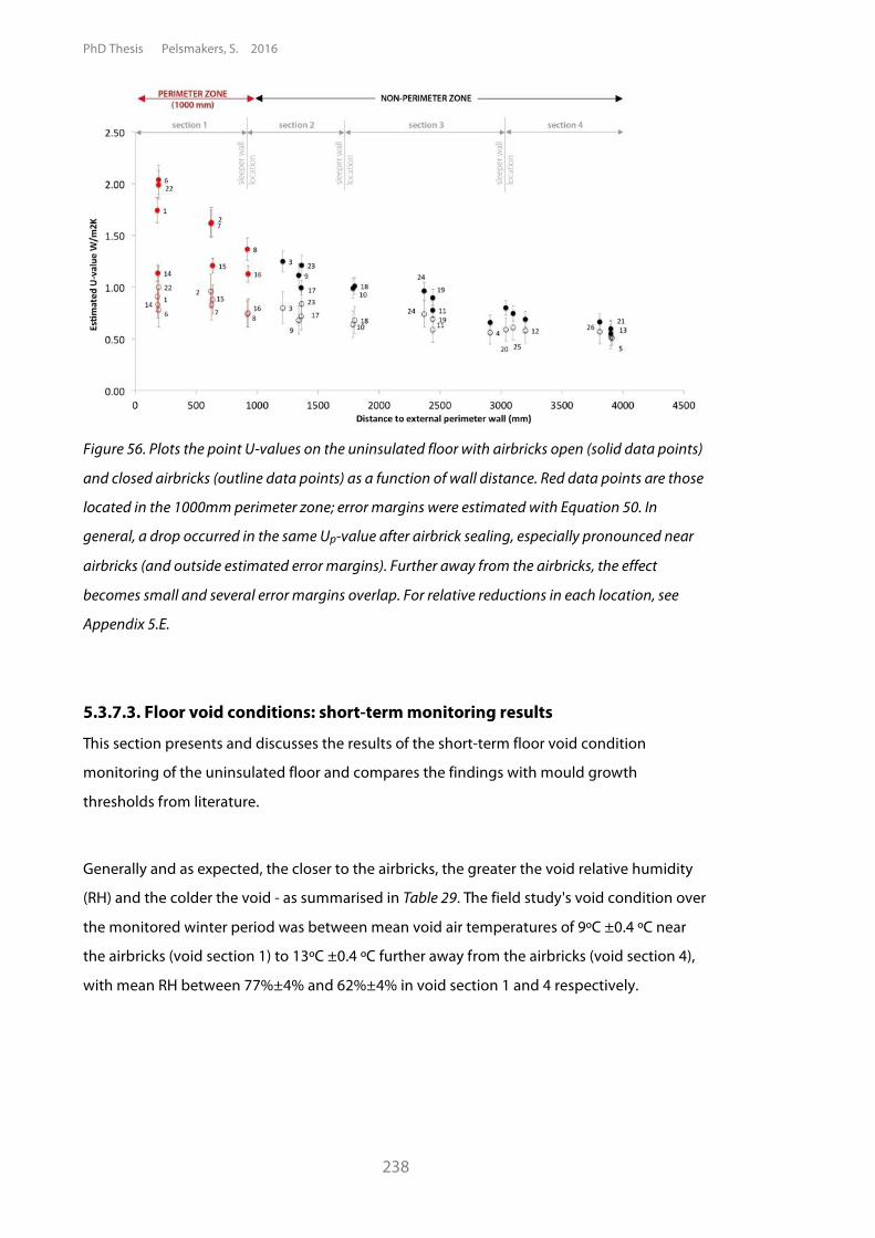
PhD Thesis Pelsmakers, S. 2016
238
Figure 56. Plots the point U-values on the uninsulated floor with airbricks open (solid data points)
and closed airbricks (outline data points) as a function of wall distance. Red data points are those
located in the 1000mm perimeter zone; error margins were estimated with Equation 50. In
general, a drop occurred in the same Up-value after airbrick sealing, especially pronounced near
airbricks (and outside estimated error margins). Further away from the airbricks, the effect
becomes small and several error margins overlap. For relative reductions in each location, see
Appendix 5.E.
5.3.7.3. Floor void conditions: short-term monitoring results
This section presents and discusses the results of the short-term floor void condition
monitoring of the uninsulated floor and compares the findings with mould growth
thresholds from literature.
Generally and as expected, the closer to the airbricks, the greater the void relative humidity
(RH) and the colder the void - as summarised in Table 29. The field study's void condition over
the monitored winter period was between mean void air temperatures of 9ºC ±0.4 ºC near
the airbricks (void section 1) to 13ºC ±0.4 ºC further away from the airbricks (void section 4),
with mean RH between 77%±4% and 62%±4% in void section 1 and 4 respectively.
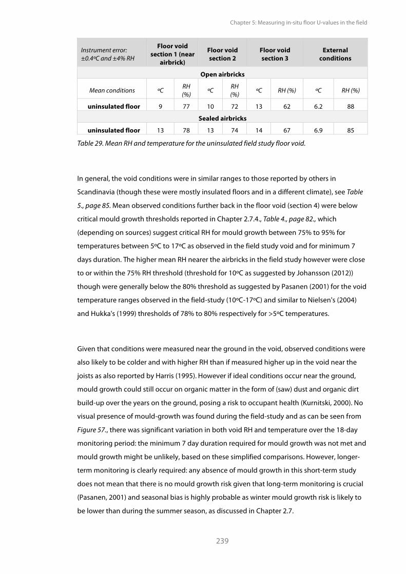
Chapter 5: Measuring in-situ floor U-values in the field
239
Instrument error: ±0.4ºC and ±4% RH
Floor void section 1 (near
airbrick)
Floor void section 2
Floor void section 3
External conditions
Open airbricks
Mean conditions ºC RH (%) ºC RH
(%) ºC RH (%) ºC RH (%)
uninsulated floor 9 77 10 72 13 62 6.2 88
Sealed airbricks
uninsulated floor 13 78 13 74 14 67 6.9 85
Table 29. Mean RH and temperature for the uninsulated field study floor void.
In general, the void conditions were in similar ranges to those reported by others in
Scandinavia (though these were mostly insulated floors and in a different climate), see Table
5., page 85. Mean observed conditions further back in the floor void (section 4) were below
critical mould growth thresholds reported in Chapter 2.7.4., Table 4., page 82., which
(depending on sources) suggest critical RH for mould growth between 75% to 95% for
temperatures between 5ºC to 17ºC as observed in the field study void and for minimum 7
days duration. The higher mean RH nearer the airbricks in the field study however were close
to or within the 75% RH threshold (threshold for 10ºC as suggested by Johansson (2012))
though were generally below the 80% threshold as suggested by Pasanen (2001) for the void
temperature ranges observed in the field-study (10ºC-17ºC) and similar to Nielsen's (2004)
and Hukka's (1999) thresholds of 78% to 80% respectively for >5ºC temperatures.
Given that conditions were measured near the ground in the void, observed conditions were
also likely to be colder and with higher RH than if measured higher up in the void near the
joists as also reported by Harris (1995). However if ideal conditions occur near the ground,
mould growth could still occur on organic matter in the form of (saw) dust and organic dirt
build-up over the years on the ground, posing a risk to occupant health (Kurnitski, 2000). No
visual presence of mould-growth was found during the field-study and as can be seen from
Figure 57., there was significant variation in both void RH and temperature over the 18-day
monitoring period: the minimum 7 day duration required for mould growth was not met and
mould growth might be unlikely, based on these simplified comparisons. However, longer-
term monitoring is clearly required: any absence of mould growth in this short-term study
does not mean that there is no mould growth risk given that long-term monitoring is crucial
(Pasanen, 2001) and seasonal bias is highly probable as winter mould growth risk is likely to
be lower than during the summer season, as discussed in Chapter 2.7.
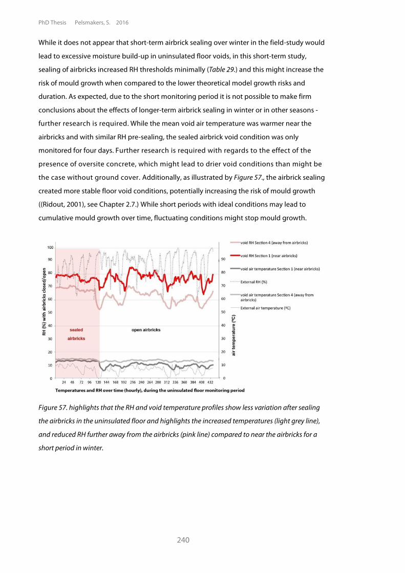
PhD Thesis Pelsmakers, S. 2016
240
While it does not appear that short-term airbrick sealing over winter in the field-study would
lead to excessive moisture build-up in uninsulated floor voids, in this short-term study,
sealing of airbricks increased RH thresholds minimally (Table 29.) and this might increase the
risk of mould growth when compared to the lower theoretical model growth risks and
duration. As expected, due to the short monitoring period it is not possible to make firm
conclusions about the effects of longer-term airbrick sealing in winter or in other seasons -
further research is required. While the mean void air temperature was warmer near the
airbricks and with similar RH pre-sealing, the sealed airbrick void condition was only
monitored for four days. Further research is required with regards to the effect of the
presence of oversite concrete, which might lead to drier void conditions than might be
the case without ground cover. Additionally, as illustrated by Figure 57., the airbrick sealing
created more stable floor void conditions, potentially increasing the risk of mould growth
((Ridout, 2001), see Chapter 2.7.) While short periods with ideal conditions may lead to
cumulative mould growth over time, fluctuating conditions might stop mould growth.
Figure 57. highlights that the RH and void temperature profiles show less variation after sealing
the airbricks in the uninsulated floor and highlights the increased temperatures (light grey line),
and reduced RH further away from the airbricks (pink line) compared to near the airbricks for a
short period in winter.
Chapter 5: Measuring in-situ floor U-values in the field
241
In summary, since this study was undertaken over a short time-period it was unable to
capture longer term seasonal trends, hence caution is especially recommended for short-
term monitoring, because this could over-or underestimate mould growth risk depending on
when data was collected. If short void monitoring periods are taken to be representative of
the yearly floor void conditions, monitoring over winter - as was done here - might
underestimate the mould growth risk, while only monitoring over summer might
overestimate the risk. These observations demonstrated and verified the importance of
monitoring long-term, including summer periods and monitoring void areas away from the
airbricks as these areas are likely to have more stable conditions due to reduced ventilation
and might become susceptible for mould growth. As such - and as expected - any findings
remain inconclusive, and this includes the impact of the sealing of airbricks on the floor void
conditions. For this reason the data also does not support comparison between floor void
conditions pre/post insulation and is not reported in this thesis.
5.4. Implications for policy and retrofit decision-making The field case-study illustrated that the estimated in-situ floor U-value might be
significantly greater than assumed and modelled at present. As a consequence, the
benefits of insulating the ground floor might be underestimated, as also noted by
Everett (1985) for solid ground floor heat loss. For this field study, the superseded
CIBSE-1986 model seemed to give a floor U-value estimate closer to the in situ
measured whole floor U-value, compared to the current models. However, to test
whether the CIBSE-1986 model outputs are a better predictor of actual floor thermal
transmittance, further research and a larger sample of high-resolution in-situ floor heat-flux
measurements of a variety of floors are needed to investigate model accuracy.
However, if the disparity between modelled versus measured U-values are more broadly
confirmed in the pre-1919 housing stock, it would have significant implications for
policy and retrofit decision-making: ground floors might be left uninsulated if the
thermal transmittance and the benefit from insulating floors are underestimated,
especially given the disruption to insulate these floors for a seemingly small benefit.
Doing so might then bypass a significant reduction potential in space-heating energy.
Finally, there might be a significant U-value reduction potential associated with the
temporary sealing of airbricks in winter. However, further research is required into the
efficacy of doing so in a larger sample of floors and the impact on floor void conditions
from airbrick sealing to avoid potentially increased mould growth risks and associated
occupant health impacts.
PhD Thesis Pelsmakers, S. 2016
242
5.5. Discussion and summary In-situ heat-flow measurements were undertaken in an unoccupied field study house at high
resolution in 26 locations on the floor and one location on a joist. Airbricks were sealed to
investigate the effect of airbrick ventilation on observed Up-values. This chapter addressed
research question 2 ("What is the in-situ measured thermal transmittance of floors and how
does it compare to model predictions?", while also testing research question 1 in the field (i.e.
"How should in-situ suspended timber ground floor U-values be estimated?"), building and
reflecting on the research methods and techniques developed at the Salford EH.
As in the Salford EH, several hypotheses were tested and were supported by the field study
analysis and findings, including that there was a large spread of Up-values across the
uninsulated floor (H1) and that perimeter Up-values were greater compared to the non-
perimeter zone (H2). While the whole floor U-value was decreased significantly with sealed
airbricks (H3), though there were data quality issues which created considerable uncertainty
around each of the field study point U-values for the sealed airbrick study - further research is
required.
Furthermore, the presence of sleeper walls might act as obstructions to the cross-flow
movement of incoming colder external air further along in the void. This was tentatively
support by low recorded void airflow away from the airbricks in the present study. However,
more research is required to determine whether this was a general phenomenon, or whether
it was inherent to the instruments used (one-directional air flow only was measured) or to
the study house (which also had temporary obstructed cross ventilation in the void). This
might have implications for the installation of floor insulation, where perimeter insulation
might be most effective; further research is required.
Similarly to the Salford EH, the field study reiterated that the use of only a few in-situ point
measurements would highly likely under-or over estimate the whole floor U-value,
depending on sensor placement. Additionally, comparing U-values estimated from models
with the whole floor U-value estimated from in-situ measurements highlighted that current
models might significantly underestimate the whole floor U-value. For the field study the in-
situ measured whole floor U-value was twice the modelled values; similar disparities were
found by Everett (1985) for a solid concrete ground floor with 25mm edge insulation. It is
unclear what caused this divergence, however the superseded CIBSE-1986 model appeared
to be a better predictor of the actual whole floor U-value of the field study; further research is
required to investigate if this is the case for other studies.
Chapter 5: Measuring in-situ floor U-values in the field
243
It should also be noted that over-estimation of modelled values (some of the CIBSE-1986
outputs, depending on variables used) would overestimate the benefit of floor insulation
and its payback. The generalisability of findings of case-studies is discussed in Section 3.4.4.
The field study also lead to practical insights, useful for future in-situ measuring studies.
Those listed below are in addition to those already reported above or in Chapter 4.5.:
• Where ambient internal and external temperatures are measured and when
adjustments are made for surface resistances, can influence U-value estimation.
However in the field study these differences were within the margin of error.
Additional air temperature and room airflow measurements might be helpful to
investigate the thermal resistance of the surface boundary layer across the floor.
• In this field study, 12-13 days were sufficient for determination of uninsulated floor
U-values. For the sealing of airbricks, a longer monitoring period than the 4 days
allowed for in the field study is required to enable robust U-value comparisons and
to allow for possible thermal mass equilibrium settling. However, the above
monitoring periods may not apply to other measuring studies due to different
environmental conditions etc. - further research is required.
• Multi-directional airflow equipment would be required for more robust analysis of
void airflow.
• Monitoring floor heat-flux at high-resolution over a full year might aid understanding
of theoretical model assumptions and concepts and to investigate the disparity
between modelled and measured floor U-values.

PhD Thesis Pelsmakers, S. 2016
244
Chapter 6: Measuring heat loss reduction potential of insulation interventions in the field & other considerations
245
Chapter 6: Measuring heat loss
reduction potential of insulation
interventions in the field and other
considerations
6.1. Introduction This chapter presents STUDY 4B and discusses the analysis and results of insulation
interventions undertaken in the unoccupied field study house as described in previous
Chapter 5. After measuring the heat-flow of the uninsulated floor, the floor was subject
to two insulation interventions and was monitored at the same 27 locations on the floor
pre/post interventions. The first intervention was EPS bead-filling of the entire floor void
which - after removal- was followed by woodfibre insulation installation in between
joists. In-situ U-value results are compared to the uninsulated floor, modelled outputs,
other in-situ studies and building regulation requirements. A short intervention pilot
study (STUDY 3) was undertaken prior to this study and is briefly described in this
chapter with more information in Appendix 6.A.
Similarly to the uninsulated floor, airbricks were closed for a short duration to
understand the airbrick ventilation effect on the observed Up-values. In addition to
in-situ heat-flux monitoring of the interventions, the field study's room air temperatures
at different heights were also monitored for thermal comfort comparisons with
theoretical thresholds. Blower door tests were also undertaken to investigate the impact
of the interventions on the air leakage of the floor pre-and post intervention.
This chapter specifically addresses research question 3 ("How does the in-situ thermal
performance of a case study floor change after intervention measures?"), while also testing
ancillary research question 3.1 ("What are the thermal comfort implications of insulated and
uninsulated floors?) and thereby contributes to supplementing knowledge of floor
interventions and the impact on in-situ heat-flux measurements, floor airtightness and
thermal comfort while also reflecting on the research methods and techniques developed in
the previous chapters.
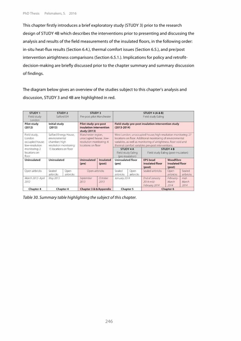
PhD Thesis Pelsmakers, S. 2016
246
This chapter firstly introduces a brief exploratory study (STUDY 3) prior to the research
design of STUDY 4B which describes the interventions prior to presenting and discussing the
analysis and results of the field measurements of the insulated floors, in the following order:
in-situ heat-flux results (Section 6.4.), thermal comfort issues (Section 6.5.), and pre/post
intervention airtightness comparisons (Section 6.5.1.). Implications for policy and retrofit-
decision-making are briefly discussed prior to the chapter summary and summary discussion
of findings.
The diagram below gives an overview of the studies subject to this chapter's analysis and
discussion, STUDY 3 and 4B are highlighted in red.
Table 30. Summary table highlighting the subject of this chapter.
Chapter 6: Measuring heat loss reduction potential of insulation interventions in the field & other considerations
247
6.2. Exploratory intervention study (STUDY 3)
After in-situ heat-flux monitoring of the uninsulated floor as described in Chapter 5, two
insulation interventions were installed and monitored in the case-study house. This main
intervention study was supported by practical insights gained from a brief intervention pilot
study (STUDY 3) as recommended by Robson (2011) and Barker Bausell (1994) and is briefly
described below.
The exploratory pilot study was located in the Manchester region and took place between
early to late September 2013 for the pre-insulation study (and early to late October 2013 for
the post-insulation study). Floor insulation was donated by Knauf and the intervention was
undertaken by owner Salford City West Housing Association and its subsidiaries. A 15 m2
unoccupied living room floor was monitored at low-resolution with four in-situ heat-flux
point measurements, four surface temperature sensors and external air temperatures. For
the purposes of the exploratory study this resolution was sufficient. Given the season in
which the study was undertaken, the purpose of the exploratory study was not to derive
valid pre/post U-values but to test and reflect on research design and techniques to
characterise floor interventions. An electrical radiator was set to keep internal temperatures
at 21ºC internally, however internal temperatures were only a few degrees above external
temperatures during this monitoring period (especially in the pre-insulation study); there
was also loss of external temperature data and no valid U-values could be determined.
Insights gained from this exploratory study, which were carried forward in the main
intervention study, included:
• the need for regular access and frequent data collection;
• sufficient blocking of direct solar gain onto the floor surface;
• importance of robust sensor location replication procedures to enable fixing sensors
in the same location pre/post insulation;
• Presence during insulation installation to record installation quality issues, useful for
later analysis;
• ensuring no other building works interfere with the intervention study;
• possible benefit of measuring other external environmental variables such as solar
gain and wind-speed to understand pre/post changing environmental conditions
and possible effect on pre-post results.
• For more detail and further insights, see Appendix 6.A.; for typical information sheet
and informed consent sheets, see Appendix 5.A.
PhD Thesis Pelsmakers, S. 2016
248
6.3. Insulation intervention study: research design (STUDY
4B)
The intervention study was an 'interrupted time series design' (Robson, 2011): in this case,
floor Up-values were characterised prior to floor interventions (see Chapter 5), with
continued floor heat-flow measurements post-intervention, "offering a unique perspective on
the evaluation of intervention (or "treatment") effects" (Glass, 2008). Establishing hypotheses is
an important part of designing planned interventions to clarify causal relationships (Glass,
2008); six hypotheses, based on the research questions were developed; this study tested
hypotheses 2 to 6, as set out in Chapter 3.4.1.
The number of interventions and the duration of the monitoring was limited by the winter
heating season duration to ensure optimal external environmental conditions for
monitoring. The research design centred around measuring (a.) the effect of insulation
interventions on floor Up-values (and their spread) and (b.) the effect of reduced airflow
through the airbricks on observed heat-loss, by sealing of the airbricks.
Different methodologies were considered how to best undertake an intervention study (such
as test-cell, occupied or unoccupied house) – as summarised in Appendix 3.E., with
advantages and limitations listed. The selection of floor interventions was based on the
following criteria:
• A typical in between joist insulation intervention (see Figure 7. option a) and a least
disruption method, without the need to remove all the floorboards, for example
Figure 7. option f or g.
• Ability to attract industry sponsorship in the form of donated materials and
workmanship to undertake the installation of interventions.
• Agreement with the home owner of the interventions.
The interventions which met the above criteria were (1.) filling of the floor void with EPS
graphite coated beads and (2.) 100mm woodfibre insulation between the joists; findings are
presented and discussed in this order. Only the living room floor was insulated due to access
issues and presence of more extensive service pipes in the rest of the floor - see Chapter 5.2.
The time-scale of the monitoring and intervention studies are listed in the gantt chart
overleaf.
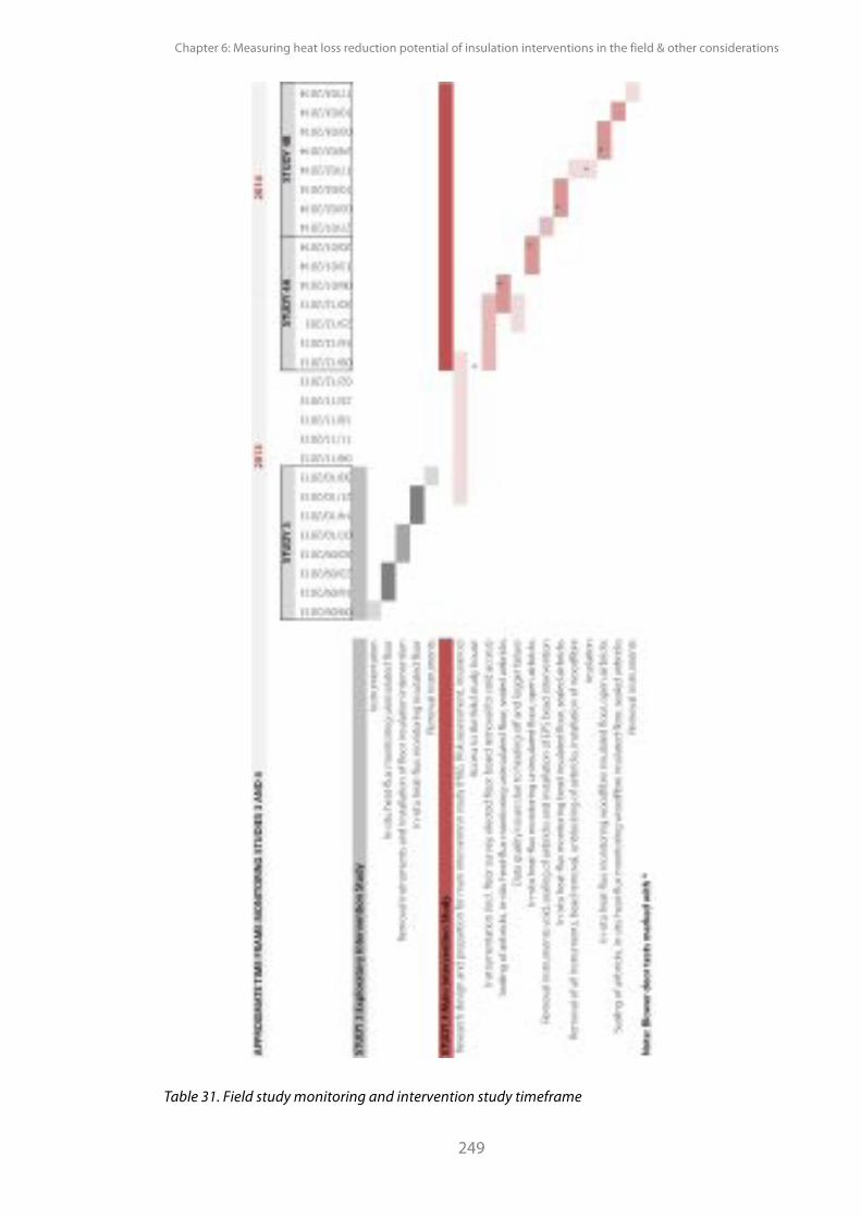
Chapter 6: Measuring heat loss reduction potential of insulation interventions in the field & other considerations
249
Table 31. Field study monitoring and intervention study timeframe

PhD Thesis Pelsmakers, S. 2016
250
6.3.1. Description of insulation interventions A brief description follows of the two insulation interventions undertaken. Between
interventions, sensors either remained in place (bead insulation) or were removed and put
back in the same location after installation (woodfibre intervention) - for sensor details and
locations on top and below the floor, see Chapter 5.2.3, page 210. The case-study description
can be found in Chapter 5.2.1, page 206. A control study house was obtained which was of
limited use due to an unpredictable heating pattern, as described in Chapter 6.3.4.
As described in Chapter 5, isolation of the kitchen and living room floor voids was
undertaken during the entire monitoring period to minimise the effect of the untreated
kitchen floor on the living room floor intervention. This was because the kitchen floor void
could not be accessed and the kitchen units and services could not be removed in order to
insulate the kitchen floor void. As such the whole floor U-value pre/post intervention is
determined from the living room floor only; as discussed in Chapter 5.2.
Industry sponsorship was obtained in kind from NBT and Downs Energy who both donated
insulation materials and Downs Energy also undertook both interventions (and removal of
the first intervention) on site under the author's observation. For associated research ethics
and research management issues see Section 3.4.
Intervention 1: Full-filling of the void with EPS beads is an innovative solution intended
to insulate floors without the disruption of lifting and re-fitting all of the floorboards. This
insulation technique was used in a TSB Retrofit for the Future project as described by Baeli
(2013, p37). The living room floor void was filled entirely with loose graphite coated EPS
beads, after closing of the living room airbricks to avoid the EPS beads spilling out. Four
floorboards - one in each section - were lifted to fill the 250 mm floor void (excluding 100mm
joist height) using the same equipment as cavity blown EPS beaded insulation, without the
binding agent/adhesive to allow for removal of the beads by hoovering them out. The beads
were filled to the top of the joists - as shown in Figure 58. - and they easily filled gaps
between services in the void and small spaces as well as between void sections due to
openings in the sleeper walls. The EPS beads were donated and installed by Downs Energy;
its BBA (2014) certificate states conductivity of 0.033Wm-1K-1. It is unknown however if the
absence of glue increases the thermal conductivity due to possibly an increased number of
air gaps remaining. After mechanical filling, manual smoothing of the beads between joists
and manual top-up filling needed to happen to ensure filling to the top of the joists; this was
visually assessed.
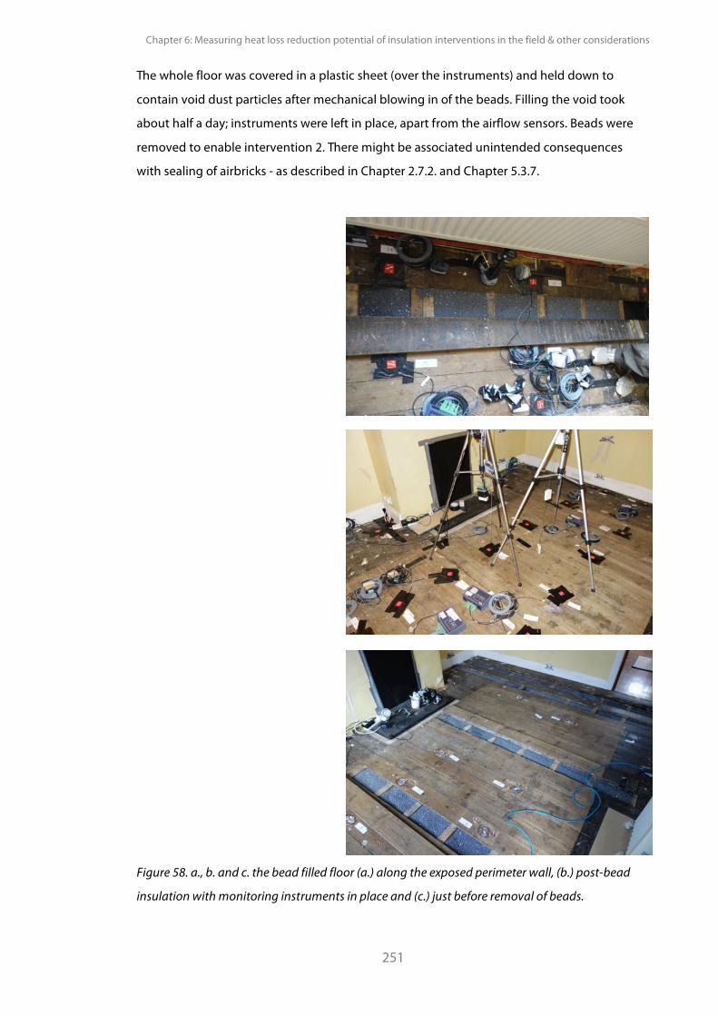
Chapter 6: Measuring heat loss reduction potential of insulation interventions in the field & other considerations
251
The whole floor was covered in a plastic sheet (over the instruments) and held down to
contain void dust particles after mechanical blowing in of the beads. Filling the void took
about half a day; instruments were left in place, apart from the airflow sensors. Beads were
removed to enable intervention 2. There might be associated unintended consequences
with sealing of airbricks - as described in Chapter 2.7.2. and Chapter 5.3.7.
Figure 58. a., b. and c. the bead filled floor (a.) along the exposed perimeter wall, (b.) post-bead
insulation with monitoring instruments in place and (c.) just before removal of beads.
PhD Thesis Pelsmakers, S. 2016
252
Intervention 2: wood fibre insulation installation between joists: After bead removal, all
instruments and floorboards were removed; the void radiator heating pipes were insulated*
and 100mm woodfibre batts were installed between the joists, held by a tightly stretched
and stapled breather membrane suspended over and under the joists. This is a typical
insulation solution but generally the insulation is a flexible insulation such as mineral wool,
which can be more easily inserted between unevenly spaced floor joists and often installed
DIY (BRE, 2000, EST, 2005b).
However, mineral wool is not the recommended best practice insulation material choice by
English Heritage (EH, 2010), and the home owner requested a natural material such as
woodfibre or sheepswool; woodfibre was donated by NBT (Natural Building Technologies)
with conductivity of 0.038 Wm-1K-1 (Pavatex, 2013) and installed by Downs Energy.
Membrane sections were overlapped and taped with airtightness tape; insulation was fitted
tightly between the joists to minimise any air gaps which could lead to increased convective
heat loss (EST, 2006). Near the airbricks, the insulation was chamfered and installed against a
roof ventilation 'lap vent' to allow airflow underneath (see Figure 59.). Reduced insulation was
also fitted where services encroached in the space between joists, as was the case near
sensor locations 23 to 26 and in other unmonitored locations. Airflow between sleeper wall
sections was likely significantly reduced due to the insulation being installed between joists,
which were the largest openings between floor void sections prior to insulation. However, as
discussed in Section 5.3.7., measured airflow in floor section 4 was low compared to the first
section near the perimeter; as such both airflow sensors were moved from void section 4 to
void section 1 and placed in front of the remaining airbricks - see Figure 44. in Chapter 5.2.3.
After insulation installation, all sensors were replaced on top of the floor in the same position
as the uninsulated and bead insulated floor monitoring design.
This final intervention was intended to be left in place permanently, hence it was the final
intervention undertaken. See Chapter 3.4.3 and 3.4.4. regarding research ethics and
generalisability. Information sheets, informed consents and risk assessment are provided in
Appendix 5.A.
* While the central heating system was not being used in this study and out of order, as the insulation would remain in place, the water and heating pipes in the void were insulated to prevent risk of frost and undue lost heat from pipes in winter and to reduce risk of summer surface condensation.
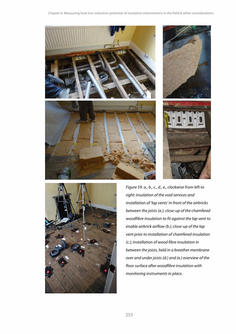
Chapter 6: Measuring heat loss reduction potential of insulation interventions in the field & other considerations
253
Figure 59. a., b., c., d., e., clockwise from left to
right: insulation of the void services and
installation of 'lap vents' in front of the airbricks
between the joists (a.); close-up of the chamfered
woodfibre insulation to fit against the lap vent to
enable airbrick airflow (b.); close-up of the lap
vent prior to installation of chamfered insulation
(c.); installation of wood fibre insulation in
between the joists, held in a breather membrane
over and under joists (d.) and (e.) overview of the
floor surface after woodfibre insulation with
monitoring instruments in place.
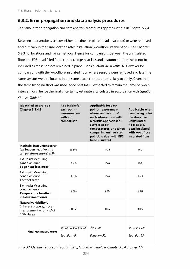
PhD Thesis Pelsmakers, S. 2016
254
6.3.2. Error propagation and data analysis procedures The same error propagation and data analysis procedures apply as set out in Chapter 5.2.4.
Between interventions, sensors either remained in place (bead insulation) or were removed
and put back in the same location after installation (woodfibre intervention) - see Chapter
5.2.3. for locations and fixing methods. Hence for comparisons between the uninsulated
floor and EPS-bead filled floor, contact, edge heat loss and instrument errors need not be
included as these sensors remained in place – see Equation 50. in Table 32. However for
comparisons with the woodfibre insulated floor, where sensors were removed and later the
same sensors were re-located in the same place, contact error is likely to apply. Given that
the same fixing method was used, edge heat loss is expected to remain the same between
interventions; hence the final uncertainty estimate is calculated in accordance with Equation
53. - see Table 32.
Identified errors - see Chapter 3.3.4.3.
Applicable for each point-measurement without comparison
Applicable for each point-measurement when comparison of each intervention with airbricks open/closed; surface or air temperatures; and when comparing uninsulated point U-values with EPS bead insulated
Applicable when comparing point U-values from uninsulated floor or EPS bead insulated with woodfibre insulated floor
Intrinsic: Instrument error (calibration heat-flux and temperature sensors) ± 5%
± 5% n/a n/a
Extrinsic: Measuring condition error - Edge heat-loss error
±3% n/a n/a
Extrinsic: Measuring condition error - Contact error
±5% n/a ±5%
Extrinsic: Measuring condition error - Temperature location measurement error
±5% ±5% ±5%
Natural variability U (inherent property, not a measurement error) - sd of daily Umean
± sd ± sd ± sd
Final estimated error
Equation 49.
Equation 50.
Equation 53.
Table 32. Identified errors and applicability; for further detail see Chapter 3.3.4.3., page 124
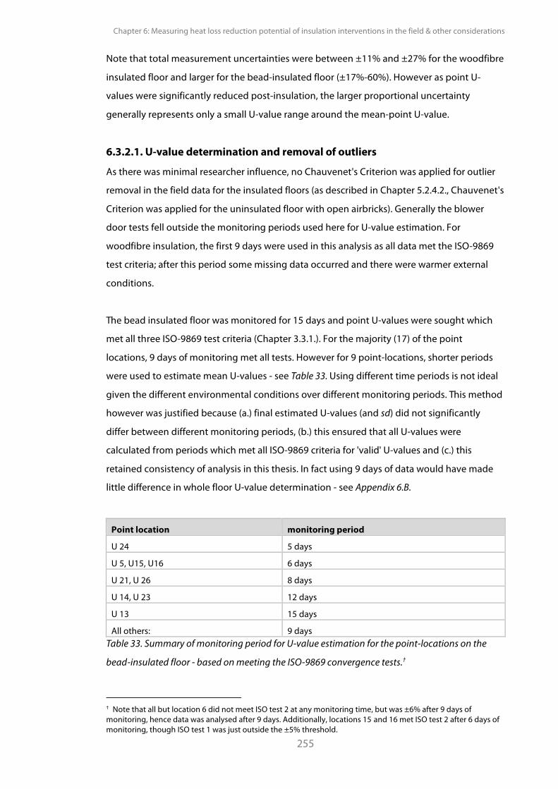
Chapter 6: Measuring heat loss reduction potential of insulation interventions in the field & other considerations
255
Note that total measurement uncertainties were between ±11% and ±27% for the woodfibre
insulated floor and larger for the bead-insulated floor (±17%-60%). However as point U-
values were significantly reduced post-insulation, the larger proportional uncertainty
generally represents only a small U-value range around the mean-point U-value.
6.3.2.1. U-value determination and removal of outliers
As there was minimal researcher influence, no Chauvenet's Criterion was applied for outlier
removal in the field data for the insulated floors (as described in Chapter 5.2.4.2., Chauvenet's
Criterion was applied for the uninsulated floor with open airbricks). Generally the blower
door tests fell outside the monitoring periods used here for U-value estimation. For
woodfibre insulation, the first 9 days were used in this analysis as all data met the ISO-9869
test criteria; after this period some missing data occurred and there were warmer external
conditions.
The bead insulated floor was monitored for 15 days and point U-values were sought which
met all three ISO-9869 test criteria (Chapter 3.3.1.). For the majority (17) of the point
locations, 9 days of monitoring met all tests. However for 9 point-locations, shorter periods
were used to estimate mean U-values - see Table 33. Using different time periods is not ideal
given the different environmental conditions over different monitoring periods. This method
however was justified because (a.) final estimated U-values (and sd) did not significantly
differ between different monitoring periods, (b.) this ensured that all U-values were
calculated from periods which met all ISO-9869 criteria for 'valid' U-values and (c.) this
retained consistency of analysis in this thesis. In fact using 9 days of data would have made
little difference in whole floor U-value determination - see Appendix 6.B.
Point location monitoring period
U 24 5 days
U 5, U15, U16 6 days
U 21, U 26 8 days
U 14, U 23 12 days
U 13 15 days
All others: 9 days Table 33. Summary of monitoring period for U-value estimation for the point-locations on the
bead-insulated floor - based on meeting the ISO-9869 convergence tests.†
† Note that all but location 6 did not meet ISO test 2 at any monitoring time, but was ±6% after 9 days of monitoring, hence data was analysed after 9 days. Additionally, locations 15 and 16 met ISO test 2 after 6 days of monitoring, though ISO test 1 was just outside the ±5% threshold.
PhD Thesis Pelsmakers, S. 2016
256
6.3.2.2. Changing environmental conditions over time
In field studies, it is not possible to have a perfect comparison between interventions
because the monitoring campaign is limited in time (and heating-season bound) and the
environmental conditions are unpredictable and not the same over time. For this reason,
the interventions were undertaken in sequence and as close as possible together, as
also done by other studies, see Byrne (2013) for example.
Environmental variables are inevitable confounding variables which influence the observed
heat-flow, leading to issues of comparison and robust estimations of the actual effect of
interventions (Anderson, 2003, Park et al., 2013): i.e. is the observed effect significant and is it
due to the intervention taking place or are there are other confounding variables affecting
the measured change?
Some studies compare pre/post intervention predicted versus actual energy use and noted
that significant under-or over-estimations may occur due to actual occupant behaviour
versus modelled assumptions (see for example Rosenow (2013) and Sunikka-Blank (2012).
Other studies compare actual pre/post intervention building energy use over longer time
periods to gain an idea of the efficacy of interventions; energy use might be adjusted for
external temperature, energy prices and other variables (such as changes in household
income and members), see for example Hirst (1986). Such studies are also affected by
compensating behaviour such as for example changing occupant behaviour (Rosenow and
Galvin, 2013). However as the field case-study was unoccupied and only accessible for one
winter heating period, no long-term actual pre/post energy use data was available for
comparison purposes.
Stevens (2013) and Byrne (2013) monitored in-situ wall U-values before and after
interventions; Stevens (2013) makes no mention of any adjustments or presence of
confounding variables which may have affected pre/post U-values, though heating degree
day adjustments for heating energy use were made. Byrne (2013) undertook pre/post
monitoring in close succession as was the case in this study and qualitatively assessed
external air temperature differences to gauge how this may have affected heating energy-
use.
Chapter 6: Measuring heat loss reduction potential of insulation interventions in the field & other considerations
257
In this study, long-term pre/post monitoring was not possible and the use of a control house
was not very successful (as described in Section 6.3.4.). External variables (see Section
5.2.3.) were measured and were described qualitatively by average values for each
variable and the distribution of values over the monitoring period (see histogram plots
in Appendix 6.D.). This enabled a qualitative comparison of the monitored environmental
conditions pre/post interventions to evaluate the impact of possible confounders on the
overall U-value changes as different interventions took place.
Table 34. gives an overview of the mean environmental variables during each intervention
period and how they may have affected the estimated U-values pre/post intervention. The
pre-insulation mean external air temperature was slightly warmer (0.8ºC±0.14ºC) than the
mean external temperature during bead-intervention. While the rate of conductive heat-flow
is proportional to ΔT, the reason for possible impacts of changing external temperature (and
hence on ∆T) on estimated U-values is because of thermal mass time lag, which - if all the
ISO-9869 tests are met - is likely to be negligible. Note that thermal conductivities also "show
some variation with temperature" though this is very small for most materials (Winterton,
1997). Radiant heat transfer also varies with changing temperatures and colder surfaces
(largest impact likely near the external environment), though radiant heat-flow quantities are
unknown. Higher mean wind-speed was also observed during the bead-intervention, which
might have under-estimated the efficacy of the intervention, especially along the perimeter.
However, this is likely to have had a minimal effect as the bead intervention relied on sealed
airbricks, though colder air may have infiltrated through gaps and cracks in the foundation
wall. The exact influences of these changing variables in U-value estimation are unknown
and remain unquantified.
The pre-intervention period was significantly colder (6.2±0.1ºC) than the mean external
temperature during the woodfibre intervention (7.9±0.1ºC); the effect on U-value
determination is unknown. There was also significantly increased mean external wind-speed
and observed perimeter void airflow‡ compared to the pre-insulation period and this might
lead to under-estimation of the woodfibre efficacy due to over-estimation of Up-value
estimates along the perimeter, however the exact quantity is unknown.
‡ The void airflow was however measured closer to the external airbrick as a direct result of the woodfibre insulation intervention, compared to the pre-intervention void airflow sensor location.
PhD Thesis Pelsmakers, S. 2016
258
The external ground temperature, likely affected by rainfall (not measured), air temperatures
and solar radiation, followed the external temperature and was slightly warmer on average
for the uninsulated and bead-filled floor; but was similar in temperature to the external
temperature during the woodfibre insulation monitoring period - see Table 34. Solar
radiation was also similar between the pre-intervention period and the bead-insulated floor
but - as expected with longer days - was significantly higher during the woodfibre
intervention. It is unclear - if- and how increased ground and external temperatures and solar
radiation over the pre/post intervention periods might have affected U-value estimation. In
all cases, the actual magnitude of the effect remains difficult to quantify. In addition, there
might be increased heat-transfer to the ground from the floor during spring, as discussed
further on page 260.
In summary, it has not been possible to ascertain how the pre/post intervention
measurements might have been affected by other external changing variables; given that
the magnitude of these effects cannot be quantified, it is unknown if these variables would
(partially or fully) offset each other or not and how this may have biased the final estimated
U-values for each of the intervention periods. In this qualitative assessment the influence of
dynamic diurnal effects was excluded, as are seasonal thermal mass changes of the ground
because no long-term monitoring could be undertaken. However, some hypotheses of
possible seasonal thermal mass effect are presented on page 260.
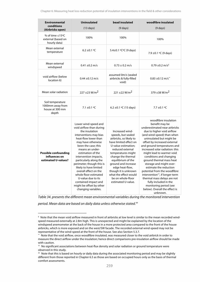
Chapter 6: Measuring heat loss reduction potential of insulation interventions in the field & other considerations
259
Environmental conditions
(Airbricks open)
Uninsulated
(13 days)
bead insulated
(9 days)
woodfibre insulated
(9 days)
% of time ≤15ºC external (based on
hourly data)
100% 100% 100%
Mean external temperature 6.2 ±0.1 ºC
5.4±0.1 ºCºC (9 days)
7.9 ±0.1 ºC (9 days)
Mean external windspeed 0.41 ±0.2 m/s 0.73 ± 0.2 m/s 0.79 ±0.2 m/s§
void airflow (below location 6) 0.44 ±0.12 m/s
assumed 0m/s (sealed airbricks & fully-filled
void) 0.83 ±0.12 m/s**
Mean solar radiation 227 ±23 W/m2 221 ±22 W/m2 379 ±38 W/m2
Soil temperature 1000mm away from
house at 300 mm depth
7.1 ±0.1 ºC 6.2 ±0.1 ºC (15 days) 7.7 ±0.1 ºC
Possible confounding influences on
estimated U-values?
Lower wind-speed and void airflow than during
the insulation interventions may bias heat-flow lower than may have otherwise been the case; this means an under-estimation of the
intervention impacts, particularly along the
perimeter; though this is likely to have limited overall effect on the
whole floor estimated U-value due to its
contained impact and might be offset by other
changing variables.
Increased wind-speeds, but sealed
airbricks, so likely to have limited effect on
U-value estimation; reduced external
temperatures might change the thermal equilibrium of the
ground and increase edge heat-flow,
though it is unknown what the effect would
be on whole-floor estimated U-value.
woodfibre insulation benefit may be
underestimated near airbricks due to higher void airflow
(and wind-speed) than when uninsulated but might be
offset by increased external and ground temperatures and increased solar radiation: this
might lead to warmer void conditions and changing
ground thermal mass heat storage and might over-estimate the reduction
potential from the woodfibre intervention††, if longer-term thermal mass delays are not
fully included in the monitoring period (see
below). Overall the effect is unknown.
Table 34. presents the different mean environmental variables during the monitored intervention
period. Mean data are based on daily data unless otherwise stated.‡‡
§ Note that the mean void airflow measured in front of airbricks at low level is similar to the mean recorded wind-speed measured externally at 2.8m high. This is unexpected and might be explained by the location of the windspeed anemometer at the back of the house in a more protected area compared to the front of the house airbricks, which is more exposed and on the west/SW facade. The recorded external wind-speed may not be representative of the wind-speed at the front of the house. See also Section 5.3.7. ** Note that the void airflow, once woodfibre insulated, was measured closer to the void airbrick in order to measure the direct airflow under the insulation; hence direct comparisons pre-insulation airflow should be made with caution. †† No significant associations between heat-flux density and solar radiation or ground temperature were observed in this study. ‡‡ Note that this is based on hourly or daily data during the associated monitoring period and may be slightly different from those reported in Chapter 6.5 as those are based on occupied hours only as the basis of thermal comfort assessments.
PhD Thesis Pelsmakers, S. 2016
260
Seasonal thermal mass effects
There are short-term daily thermal mass effects of the ground and foundations walls as well
as slow-response seasonal effects as noted by Emery (2007) for solid ground floors. The
day/night thermal mass effects as well as thermal storage changes after interventions were
likely captured by the relatively long monitoring times (as attested by data meeting the
ISO-9869 tests, with exception of the sealed airbrick interventions).
However, slow-response dynamic seasonal thermal mass effects remain uncharacterised as
heat-flow was monitored over one heating season only and over short periods. Yet, it is
highly likely that such seasonal effects influenced the observed heat-flow, especially towards
the end of the monitoring period.
Both Shipp (1985) for a basement floor and Delsante (1990) for a solid ground floor observed
that heat-flow to the ground was generally reduced during summer and autumn, with
increasing heat-flow during winter and peaking in spring. This might be explained by the
thermal capacity of the ground, which is warm after summer, releasing some stored heat to
the slab and buffering heat-flow from the floor slab in autumn. Gradually as the ground's
thermal store is diminished, this might lead to increased heat-flow from the floor to the
ground during winter and into spring. This might mean that monitoring periods during
autumn might lead to lower estimated solid ground floor U-values compared to mid-winter,
while spring monitoring might lead to higher solid ground floor U-value estimates compared
to mid-winter monitoring.
Based on the above, generally, it might be expected that:
• During spring and summer the warm external air brought in via airbricks warms up
the void, and where the ground temperature is less than the void air temperature;
the ground thermal mass stores heat which will be released when the conditions
reverse (e.g. at night or during changing seasons). This process might also lead to
increased humidity in voids - see Chapter 2.7.
• During early autumn, when cold external air is brought into (sections of) the floor
void; the void temperature is likely to drop below the ground temperature and the
ground thermal mass will generally 'release' stored heat to the void. This will also be
influenced by heat-flow from above, depending on the internal conditions and
dynamic diurnal patterns.
However, further longitudinal heat-flux monitoring of the floor and ground are required to
investigate if these trends are similar for suspended ground floors (and in different locations
under the suspended floors).
Chapter 6: Measuring heat loss reduction potential of insulation interventions in the field & other considerations
261
6.3.3. Thermal comfort field data collection As discussed in Chapter 2.5., avoiding thermal discomfort is important because it might lead
to increased energy use to compensate local thermal discomfort (Rock, 2013) by increasing
room air temperatures (Olesen, 1979). An in-depth thermal comfort study and impact of
discomfort on compensating energy-use was not within the remit of this research.
Additionally, as the field study house was unoccupied, people's thermal comfort responses
were also excluded from this study. Instead floor surface and room air temperatures were
monitored during the pre/post intervention studies and during sealing of the airbricks to
enable comparison of these interventions to different theoretical metrics for thermal
comfort. In this study, the ASHRAE (2013), BSI (2006) and CIBSE (2015) 19ºC floor surface
temperature threshold and the 3ºC head-feet temperature difference threshold when seated
(0.1m-1.1m) and standing (0.1m-1.7m) were used as thermal comfort thresholds - see
Chapter 2.5, page 65. A higher 7ºC head-feet temperature difference threshold was not
applicable as monitored air temperatures were all below 23.5ºC (Olesen, 1980).
CIBSE (2015) sets out room 'operative temperatures' in winter of 22ºC to 23ºC for general
thermal comfort in living rooms and as low as 17ºC in kitchens and bedrooms. The term
'operative temperature' (to) refers to a combination of room air temperature and the mean
radiant temperature and is related to the radiant and convective heat transfer coefficients
- see Equation 54.:
-Equation 54. (see BSI (2002) 7726) , where ta is air temperature; tr is mean
radiant temperature; hc and hr are the heat-transfer coefficients by convection and radiation
respectively (see Chapter 2).
Operative temperature is most practically estimated as the average of air and mean radiation
temperatures, where airflow and the difference between air and radiant temperatures is
small (<0.2m/s and <4ºC respectively) (BSI, 2002). Additionally, air temperature can be close
to operative temperature, especially in well-insulated spaces and away from radiant heat
sources (solar gain, radiators) (CIBSE, 2015, BSI, 2002). Despite operative and air temperatures
not being the same, for the purpose of this PhD air temperatures were used due to air
temperature sensor availability, leading to approximate comparisons with theory only.
PhD Thesis Pelsmakers, S. 2016
262
Much of the earlier research by Olesen (1977, 1979), Munro (1948) and Billington (1948) also
use air temperatures instead of operative temperatures. Eltek Type U thermistors (±0.1ºC)
were placed in the middle of the living room at 0.1m, 0.6m, 1.1m and 1.7m in accordance
with BS-7726 (BSI, 2002) and after Gauthier (2014). Surface temperatures were also
monitored across the floor for the purpose of U-value estimation (see Chapter 5.2.3.); middle
of the floor surface temperatures were used for theoretical thermal comfort threshold
comparisons. For practical and resource reasons, the associated thermal comfort
implications of room airflow and draughts were excluded.
The living room was heated to reach 21ºC, just below the CIBSE (2015) benchmark of 22-23ºC
for living rooms, however the lower thermostat settings in this study resembled those
reported by Shipworth (2011) and Huebner (2013) in larger studies, as discussed in Chapter
5.2.3. For thermal comfort comparisons, all data were analysed at hourly intervals during
'occupied' time (i.e. excluding data when the heating was off).
6.3.4. Intervention study limitations Intervention study limitations and issues are identified below. These are in addition to the
limitations discussed in Chapter 5.2.3.5. for the uninsulated field study.
• Changing environmental conditions: Monitoring interventions in field studies are
subject to changing environmental conditions over time. Some environmental
variables were measured and a qualitative evaluation was undertaken of how the
pre/post intervention measurements might have been affected by other external
changing variables. However, it was not possible to ascertain the magnitude of these
single or combined effects, while dynamic diurnal effects and seasonal thermal mass
ground effects were excluded. Use of a control property was not very successful - see
below. There was also some loss of external wind-speed data due to battery leaks in
March, limiting comparisons further.
• Unsuccessful use of a control property: a nearby control floor was considered
useful to enable the understanding and interpretation of the interventions in
changing environmental conditions. As such, two heat-flux sensors were located on
the floor perimeter of a property in the same street with the same orientation as the
field case-study.
Chapter 6: Measuring heat loss reduction potential of insulation interventions in the field & other considerations
263
However the monitoring of heat-flow in the control property to determine valid U-
values was problematic for several reasons: (a.) unpredictable heating pattern by the
occupant (b.) this lead to average room air temperatures of just 14.1±0.35 ºC and low
surface temperatures of around 12±0.1 ºC (c.) only two floor locations could be
observed due to furniture placement, one of which was near an uninsulated radiator
pipe. These influences lead to fluctuating heat-flow and Up-values not meeting the
ISO-9869 test criteria (and hence no valid Up-values could be derived during the
short intervention time frames for comparative purposes). These confounding
variables inhibited isolation of the influences of the external environment on
observed heat-flow which also influenced the main intervention study. This
highlighted the importance to 'control' the heating pattern; and ideally more than
one control site to account for spatial occupancy and temporal issues (Anderson,
2003). However, a general comparison of heat-flow trends in the control house and
field-study house was still useful (see Section 6.4.1.).
The field-study kitchen area was also not considered suitable as a control:
measurements in the kitchen were limited by room access and kitchen cupboards
(see Figure 44. in Chapter 5.2.3.) and the lack of airtightness of the room (e.g. gaps
around single glazed windows and the external door, a room airbrick vent and a cat
flap) lead to difficult to control space-heating. In addition, the kitchen would likely
have been affected from the interventions taking place in the living room.
• Void airflow was not measured in the same locations pre/post interventions:
The airflow sensors were removed prior to bead filling the void due to their fragility
and given that airbricks would be closed and the void fully bead-filled, no or low
airflow was expected in the void. Secondly, the observed airflow at the back of the
floor in void section 4 was low (see Chapter 5.3.7.); as such the two airflow sensors in
floor void section 4 were re-located in front of the airbricks at high level below sensor
locations 1 and 22 for the woodfibre intervention (see Figure 44. in Chapter 5.2.3.);
the airflow sensors in location 6 were placed in similar high and low positions as the
pre-intervention monitoring period. However, due to the airbrick locations in
between joists, insulation installation was chamfered to allow airbrick airflow, and
this was aided by installation of lap vents (see Figure 59.); this is likely to have affected
airflow coming into the void and created differences between pre/post woodfibre
intervention study comparisons.
PhD Thesis Pelsmakers, S. 2016
264
• Short-term floor void monitoring only could be undertaken: the literature review
in Chapter 2.7. highlighted the seasonal impact on floor void conditions, with
typically an increased moisture risk during summer than in winter. Hence ideally
voids are monitored for at least one year. However, due to limited access, no
longitudinal floor void study pre/post insulation could be undertaken - as described
in Chapter 5.2.3.5. If short void monitoring periods are taken to be representative of
the yearly floor void condition, monitoring over winter - as was done here- may
underestimate the mould growth risk, while only monitoring over summer may
overestimate the risk. In summary, short-term measurements were not a good
indicator of floor void conditions: variables are influenced by the seasons and hence
longer term monitoring is required. As such, general conclusions from short-term
observations for the field study could not be drawn with regards to the impact of
interventions on void conditions and mould growth risk and as such no results are
reported.
• Limited thermal comfort study: due to undertaking interventions in an unoccupied
house, no occupant thermal comfort surveys could be undertaken to assess the
thermal comfort impact of the uninsulated floor and post-insulation. Instead, room
air temperatures were monitored to allow for comparison with theoretical thresholds
- as described in Section 6.3.3.
Chapter 6: Measuring heat loss reduction potential of insulation interventions in the field & other considerations
265
6.4. Impact of interventions on floor heat-flow This section presents and discusses the general impact of the interventions and the in-situ
estimated whole floor U-values, prior to model and literature comparisons. This is followed
by discussion of the spread of U-values, void airflow measurements and airbrick sealing
alongside other considerations of interest.
6.4.1. General assessment of intervention impact Despite the control house being subject to low internal temperatures and an erratic heating
pattern over the monitoring period (see Section 6.3.4.), in general several trends of the
intervention impact in the field study can be observed and are illustrated by Figure 60., which
plots daily heat-flux density q (W/m2) for the control house and for two locations in the field
study over the 2 month intervention monitoring period; both control and field study house
were subject to similar environmental conditions.§§ The main trends observed were:
1) When comparing the variability of the daily heat-flux density q (W/m2) in the field study (grey
lines) compared to the control (red line), the control shows significantly less heat-flow
variability at the same time as insulation interventions occur. Overall, this means that the
variability of the heat-flow is highly likely associated with the floor interventions, to which the
control house was not subject.
2) In general, all three lines show a similar daily pattern in peaks and troughs, suggesting that
these are associated with external environmental conditions influencing the heat-flux density
in these different locations in similar ways (including air temperatures, which were the same
for the field study and the control property).
3) Despite differences in environmental conditions during the interventions, the insulation
interventions seem to have a significant impact on the observed heat-flux density.
4) Sealing up of the airbricks also had a significant effect on heat-flow reduction of the
uninsulated floor (and was inherent to the EPS bead insulated floor to the front of the house)
- see discussion in Chapter 5.3.7. Figure 60. also indicates a significant impact for the
woodfibre insulated and airbrick sealed floor in location 6 near the airbrick, but not in
location 10, away from the airbricks. Overall, no significant difference was observed for the
whole floor U-value of the woodfibre insulated floor pre/post airbrick sealing (see Section
6.4.2.2.)
5) Poor insulation and low space heating in the control house as observed here, meant that a
floor could have similarly low heat-flow comparable to an insulated floor, but this is likely to
have significant thermal comfort implications.
§§ Some localised wind-speed effects may have been different between the two dwellings given their slightly different external obstructions and position in the same street (though both had the same orientation).
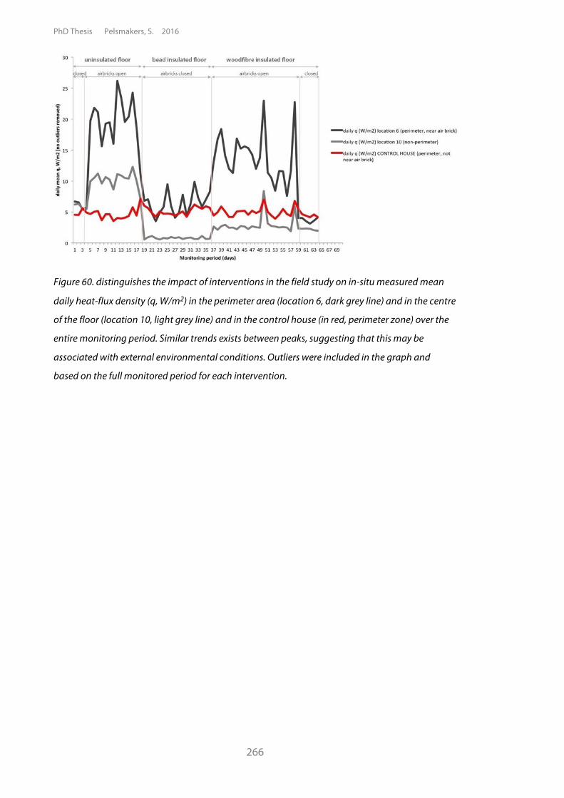
PhD Thesis Pelsmakers, S. 2016
266
Figure 60. distinguishes the impact of interventions in the field study on in-situ measured mean
daily heat-flux density (q, W/m2) in the perimeter area (location 6, dark grey line) and in the centre
of the floor (location 10, light grey line) and in the control house (in red, perimeter zone) over the
entire monitoring period. Similar trends exists between peaks, suggesting that this may be
associated with external environmental conditions. Outliers were included in the graph and
based on the full monitored period for each intervention.
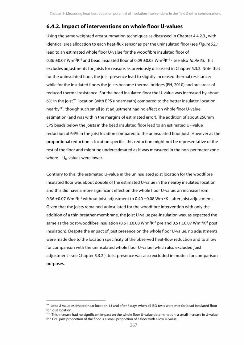
Chapter 6: Measuring heat loss reduction potential of insulation interventions in the field & other considerations
267
6.4.2. Impact of interventions on whole floor U-values Using the same weighted area summation techniques as discussed in Chapter 4.4.2.3., with
identical area allocation to each heat-flux sensor as per the uninsulated floor (see Figure 52.)
lead to an estimated whole floor U-value for the woodfibre insulated floor of
0.36 ±0.07 Wm-2K-1 and bead insulated floor of 0.09 ±0.03 Wm-2K-1 - see also Table 35. This
excludes adjustments for joists for reasons as previously discussed in Chapter 5.3.2. Note that
for the uninsulated floor, the joist presence lead to slightly increased thermal resistance;
while for the insulated floors the joists become thermal bridges (EH, 2010) and are areas of
reduced thermal resistance. For the bead insulated floor the U-value was increased by about
6% in the joist*** location (with EPS underneath) compared to the better insulated location
nearby†††, though such small joist adjustment had no effect on whole floor U-value
estimation (and was within the margins of estimated error). The addition of about 250mm
EPS beads below the joists in the bead insulated floor lead to an estimated Up-value
reduction of 64% in the joist location compared to the uninsulated floor joist. However as the
proportional reduction is location specific, this reduction might not be representative of the
rest of the floor and might be underestimated as it was measured in the non-perimeter zone
where Up-values were lower.
Contrary to this, the estimated U-value in the uninsulated joist location for the woodfibre
insulated floor was about double of the estimated U-value in the nearby insulated location
and this did have a more significant effect on the whole floor U-value: an increase from
0.36 ±0.07 Wm-2K-1 without joist adjustment to 0.40 ±0.08 Wm-2K-1 after joist adjustment.
Given that the joists remained uninsulated for the woodfibre intervention with only the
addition of a thin breather-membrane, the joist U-value pre-insulation was, as expected the
same as the post-woodfibre insulation (0.51 ±0.08 Wm-2K-1 pre and 0.51 ±0.07 Wm-2K-1 post
insulation). Despite the impact of joist presence on the whole floor U-value, no adjustments
were made due to the location specificity of the observed heat-flow reduction and to allow
for comparison with the uninsulated whole floor U-value (which also excluded joist
adjustment - see Chapter 5.3.2.). Joist presence was also excluded in models for comparison
purposes.
*** Joist U-value estimated near location 13 and after 8 days when all ISO tests were met for bead insulated floor for joist location. ††† This increase had no significant impact on the whole floor U-value determination: a small increase in U-value for 12% joist proportion of the floor is a small proportion of a floor with a low U-value.
PhD Thesis Pelsmakers, S. 2016
268
Compared to the uninsulated in-situ estimated whole floor U-value, this field study observed
a 65% mean floor U-value reduction after woodfibre insulation and a 92% mean reduction
after bead filling the void -see Table 35. The insulated Up-values differed significantly from
the uninsulated Up-values in support of the first part of hypotheses 5 ("There will be a
significant decrease observed in thermal transmittance after insulation installation"): Mann–
Whitney W = 351, n1 = n2 = 26,P < 0.05 (0.00000003, paired) for the bead insulated floor and
Mann–Whitney W = 349, n1 = n2 = 26,P < 0.05 (0.00000009, paired) for the woodfibre
insulated floor.
uninsulated
floor
woodfibre
insulated floor
bead insulated
floor
whole floor U-value
(Wm-2K-1) 1.04 ±0.12 0.36 ±0.07 0.09 ±0.03
% uncertainty 12 18 31
% reduction
compared to
uninsulated
-
65 %
92 %
% Reduction when
taking Min and Max U
into account
54-75% 88-95%
Min U (Wm-2K-1) 0.92 0.29 0.06
Max U (Wm-2K-1) 1.16 0.43 0.12
Table 35. comparison of whole floor U-values and proportional U-value reduction based on in-situ
measured values; excludes joist presence.
Uncertainty values listed in Table 35. illustrate that as the floor's U-value decreased, the error
margins increased: from ±12% for the uninsulated floor to ±18% for the woodfibre insulated
floor and ±31% for the bead-insulated floor. While an overall ±31% uncertainty is large, this
larger proportional uncertainty generally represents only a small U-value range around the
mean-point U-value - as also illustrated by Figure 66. in Section 6.4.3., page 277.
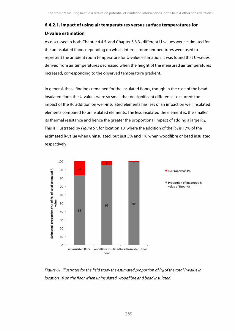
Chapter 6: Measuring heat loss reduction potential of insulation interventions in the field & other considerations
269
6.4.2.1. Impact of using air temperatures versus surface temperatures for
U-value estimation
As discussed in both Chapter 4.4.5. and Chapter 5.3.3., different U-values were estimated for
the uninsulated floors depending on which internal room temperatures were used to
represent the ambient room temperature for U-value estimation. It was found that U-values
derived from air temperatures decreased when the height of the measured air temperatures
increased, corresponding to the observed temperature gradient.
In general, these findings remained for the insulated floors, though in the case of the bead
insulated floor, the U-values were so small that no significant differences occurred: the
impact of the RSi addition on well-insulated elements has less of an impact on well insulated
elements compared to uninsulated elements. The less insulated the element is, the smaller
its thermal resistance and hence the greater the proportional impact of adding a large RSi.
This is illustrated by Figure 61. for location 10, where the addition of the RSi is 17% of the
estimated R-value when uninsulated, but just 5% and 1% when woodfibre or bead insulated
respectively.
Figure 61. illustrates for the field study the estimated proportion of RSi of the total R-value in
location 10 on the floor when uninsulated, woodfibre and bead insulated.
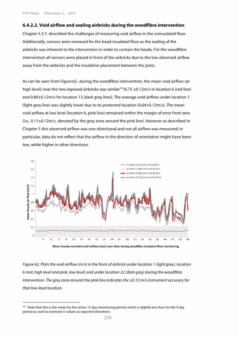
PhD Thesis Pelsmakers, S. 2016
270
6.4.2.2. Void airflow and sealing airbricks during the woodfibre intervention
Chapter 5.3.7. described the challenges of measuring void airflow in the uninsulated floor.
Additionally, sensors were removed for the bead-insulated floor as the sealing of the
airbricks was inherent to the intervention in order to contain the beads. For the woodfibre
intervention all sensors were placed in front of the airbricks due to the low observed airflow
away from the airbricks and the insulation placement between the joists.
As can be seen from Figure 62., during the woodfibre intervention, the mean void airflow (at
high level) near the two exposed airbricks was similar‡‡‡(0.75 ±0.12m/s in location 6 (red line)
and 0.80±0.12m/s for location 13 (dark grey line)). The average void airflow under location 1
(light grey line) was slightly lower due to its protected location (0.64±0.12m/s). The mean
void airflow at low level (location 6, pink line) remained within the margin of error from zero
(i.e., 0.11±0.12m/s, denoted by the grey zone around the pink line). However as described in
Chapter 5 this observed airflow was one-directional and not all airflow was measured; in
particular, data do not reflect that the airflow in the direction of orientation might have been
low, while higher in other directions.
Figure 62. Plots the void airflow (m/s) in the front of airbrick under location 1 (light grey), location
6 (red, high level and pink, low level) and under location 22 (dark grey) during the woodfibre
intervention. The grey zone around the pink line indicates the ±0.12 m/s instrument accuracy for
that low-level location.
‡‡‡ Note that this is the mean for the entire 15 day monitoring period; which is slightly less than for the 9 day period as used to estimate U-values as reported elsewhere.
Chapter 6: Measuring heat loss reduction potential of insulation interventions in the field & other considerations
271
The sealing of the airbricks during the woodfibre insulated floor was slightly less successful
than for the uninsulated floor with mean void airflow of 0.13±0.12m/s in location 6 (high
level). This might have affected the observed heat-flow during the sealed airbrick monitoring
period - as discussed below. Airflow was <0.09±0.12 m/s in the other void locations. Heat-
flow monitoring of the woodfibre intervention with sealed airbricks was undertaken for 6
days towards the end of the winter season and data quality was compromised due to a
limited monitoring period and by changing environmental conditions over this period.
Different environmental conditions pre/post sealing of airbricks included doubling of solar
radiation and increased external ground temperature post-sealing; this is likely to have
affected the comparisons and actual measurements, though its exact effect and quantity is
unknown - see Appendix 6.C. The ISO-9869 test criteria were generally met after 3 days near
the perimeter and 5 days elsewhere. Of 5 days data (120 hours), the sealed airbrick woodfibre
data had between 1 to 7 hourly data points removed caused by researcher influence with
Chauvenet's Criterion. However, there were large uncertainties around the estimated point
U-values caused by large daily variations in U. This lead to large estimated measurement
uncertainties in U-value estimations: the whole floor estimated U-value of the woodfibre
insulated floor with sealed airbricks was estimated at 0.33 ±0.24 Wm-2K-1 (so 0.09 to 0.57
Wm-2K-1) and while this is 8% below the pre-sealed whole floor U-value of 0.36±0.07 Wm-2K-1,
the large post-sealing uncertainty means that this difference falls within the margins of
measurement uncertainty. These results are likely associated with less ideal environmental
monitoring conditions associated with changing external variables towards the end of the
heating-season. As such hypothesis H3 and H3a could not be tested for the woodfibre
insulated floor. ("There will be increased thermal transmittance observed with unsealed airbricks
compared to sealed airbricks' and H3a: "this effect will be proportionally smaller in insulated than
in un-insulated floors".). The impact of the airbrick sealing is likely to mainly affect the
perimeter zone Up-values due to insulation installation between joists, sleeper wall presence
and previously observed low airflow away from the airbricks (see Chapter 5.3.7.).
PhD Thesis Pelsmakers, S. 2016
272
6.4.2.3. Estimating a whole floor U-value with fewer point measurements
Similarly to the Salford EH and the uninsulated field study floor (Chapter 4.4.2.5. and Chapter
5.3.4.), measuring in just a few point locations would also highly likely lead to significant
over-or underestimation of the whole floor U-value of insulated floors. This was especially
pronounced for the woodfibre insulated floor due to the still significant spread of Up-values
across the floor (see Section 6.4.3.): just 79 pairs or 25% of the 325 possible pairing of
Up-values had overlapping error margins with the whole floor U-value estimated error
margins. However, due to the reduced spread of Up-values for the bead insulated floor, 50%
(or 162) of paired locations would overlap with the whole floor U-value estimated error
margins; the uncertainty of the estimated U-value associated with low-resolution
measurements would be slightly reduced in this case.
There were 15 paired U-values where their average was the same as the bead insulated
whole floor U-value; compared to just three for the woodfibre insulated floor. No single
sensor location was found to be representative of the whole floor U-value across pre/post
interventions. However, pairing of sensor locations gave 17 combinations (from a possible
325) which gave estimated mean U-values within uncertainty estimates for each of the
interventions and the uninsulated floor - see Table 36.
Furthermore, slightly different estimates of the efficacy of interventions could be obtained
depending on where paired measurements were observed - as illustrated by the
proportional U-value reductions in Table 36.: U-value reductions were between 67% to 73%
and 91% to 95% for the woodfibre and the bead interventions respectively, which is slightly
above the 65% mean U-value reduction achieved from the area-weighted summation of 26
Up-values for the woodfibre insulated floor, but similar to the 92% for bead-insulated floor.
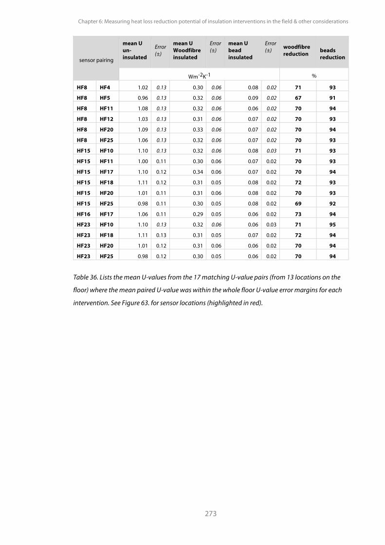
Chapter 6: Measuring heat loss reduction potential of insulation interventions in the field & other considerations
273
sensor pairing
mean U un-insulated
Error (±)
mean U Woodfibre insulated
Error (±)
mean U bead insulated
Error (±)
woodfibre reduction
beads reduction
Wm-2K-1 %
HF8 HF4 1.02 0.13 0.30 0.06 0.08 0.02 71 93
HF8 HF5 0.96 0.13 0.32 0.06 0.09 0.02 67 91
HF8 HF11 1.08 0.13 0.32 0.06 0.06 0.02 70 94
HF8 HF12 1.03 0.13 0.31 0.06 0.07 0.02 70 93
HF8 HF20 1.09 0.13 0.33 0.06 0.07 0.02 70 94
HF8 HF25 1.06 0.13 0.32 0.06 0.07 0.02 70 93
HF15 HF10 1.10 0.13 0.32 0.06 0.08 0.03 71 93
HF15 HF11 1.00 0.11 0.30 0.06 0.07 0.02 70 93
HF15 HF17 1.10 0.12 0.34 0.06 0.07 0.02 70 94
HF15 HF18 1.11 0.12 0.31 0.05 0.08 0.02 72 93
HF15 HF20 1.01 0.11 0.31 0.06 0.08 0.02 70 93
HF15 HF25 0.98 0.11 0.30 0.05 0.08 0.02 69 92
HF16 HF17 1.06 0.11 0.29 0.05 0.06 0.02 73 94
HF23 HF10 1.10 0.13 0.32 0.06 0.06 0.03 71 95
HF23 HF18 1.11 0.13 0.31 0.05 0.07 0.02 72 94
HF23 HF20 1.01 0.12 0.31 0.06 0.06 0.02 70 94
HF23 HF25 0.98 0.12 0.30 0.05 0.06 0.02 70 94
Table 36. Lists the mean U-values from the 17 matching U-value pairs (from 13 locations on the
floor) where the mean paired U-value was within the whole floor U-value error margins for each
intervention. See Figure 63. for sensor locations (highlighted in red).
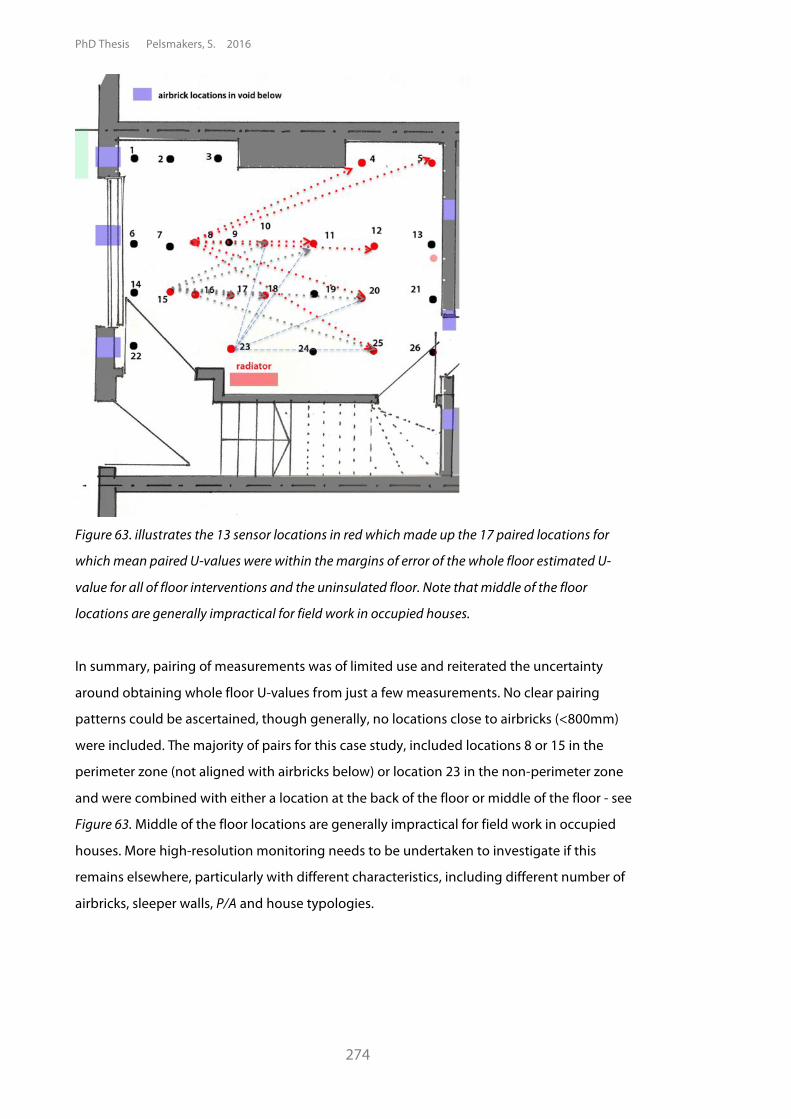
PhD Thesis Pelsmakers, S. 2016
274
Figure 63. illustrates the 13 sensor locations in red which made up the 17 paired locations for
which mean paired U-values were within the margins of error of the whole floor estimated U-
value for all of floor interventions and the uninsulated floor. Note that middle of the floor
locations are generally impractical for field work in occupied houses.
In summary, pairing of measurements was of limited use and reiterated the uncertainty
around obtaining whole floor U-values from just a few measurements. No clear pairing
patterns could be ascertained, though generally, no locations close to airbricks (<800mm)
were included. The majority of pairs for this case study, included locations 8 or 15 in the
perimeter zone (not aligned with airbricks below) or location 23 in the non-perimeter zone
and were combined with either a location at the back of the floor or middle of the floor - see
Figure 63. Middle of the floor locations are generally impractical for field work in occupied
houses. More high-resolution monitoring needs to be undertaken to investigate if this
remains elsewhere, particularly with different characteristics, including different number of
airbricks, sleeper walls, P/A and house typologies.
Chapter 6: Measuring heat loss reduction potential of insulation interventions in the field & other considerations
275
6.4.3. Spread of point U-values and perimeter effect As discussed in Section 5.3.1, (Figure 51.), the uninsulated floor U-values ranged between
0.54 ±0.09 Wm-2K-1 to 2.04 ±0.21 Wm-2K-1. For the bead-insulated floor, there was a
significantly reduced spread of U-values in support of hypotheses H2a, ranging between
0.02 ±0.01 Wm-2K-1 (location 19) to 0.58 ±0.24 Wm-2K-1 (location 6, see Figure 64. and Table
37.). For the woodfibre insulated floor (see Figure 65. and Table 37.) there was still a large
spread of U-values: point U-values ranged between 0.18 ±0.04 Wm-2K-1 (location 4) to
1.89 ±0.22 Wm-2K-1 in location 6.
In both insulated floors, there were increased Up-values in the perimeter zone in support of
hypothesis (H2) but the perimeter effect, or the effect of the distance from the exposed wall,
was significantly reduced once insulated, especially for the bead-insulated floor, when
compared to the uninsulated floor. Despite observing reduced Up-values in the perimeter
zone, this perimeter effect was still considered statistically significant and hence supported
hypothesis 2: Mann–Whitney W = 127, n1 = 9; n2 = 17, P < 0.05 (0.005, unpaired) for the bead
insulated floor and Mann–Whitney W = 130, n1 = 9; n2 = 17, P < 0.05 (0.003, unpaired) for the
woodfibre insulated floor. For the bead insulated floor the estimated mean of the perimeter
U-values was 0.18 ±0.08 Wm-2K-1compared to 0.08 ±0.02 Wm-2K-1 for locations further away
from the perimeter wall. For the woodfibre insulated floor the mean perimeter zone
U-value was 0.64 ±0.11 Wm-2K-1 compared to 0.33±0.06 Wm-2K-1in the non-perimeter zone.
In both cases, locations near the airbricks (sealed for the bead intervention) were generally
outside the margins of error of other estimated point U-values and the pre/post Up-values
were also generally outside the estimated margins of error (see Figure 66. and Figure 67.). For
both floors, a significant drop in Up-values seemed to occur >500mm away from the external
wall.
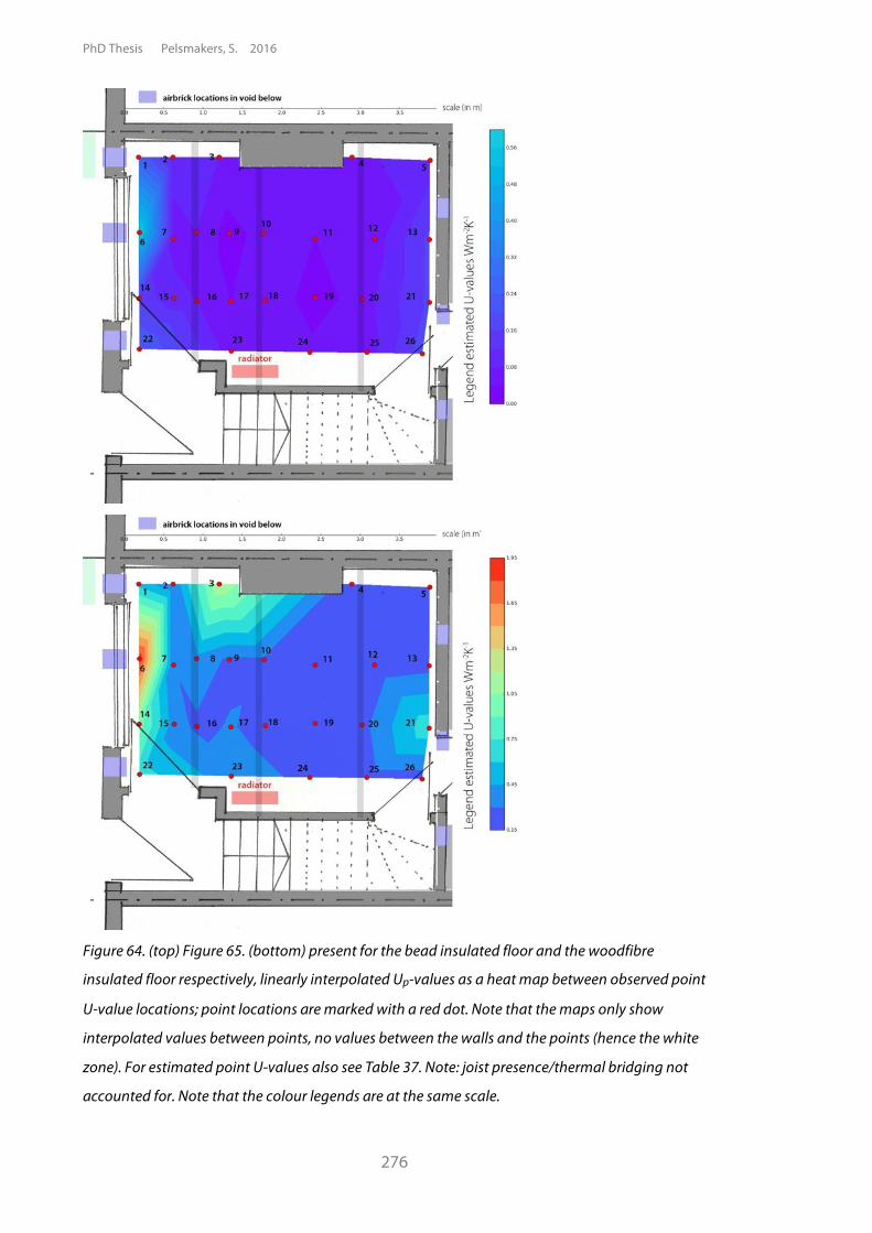
PhD Thesis Pelsmakers, S. 2016
276
Figure 64. (top) Figure 65. (bottom) present for the bead insulated floor and the woodfibre
insulated floor respectively, linearly interpolated Up-values as a heat map between observed point
U-value locations; point locations are marked with a red dot. Note that the maps only show
interpolated values between points, no values between the walls and the points (hence the white
zone). For estimated point U-values also see Table 37. Note: joist presence/thermal bridging not
accounted for. Note that the colour legends are at the same scale.
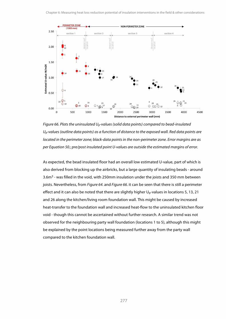
Chapter 6: Measuring heat loss reduction potential of insulation interventions in the field & other considerations
277
Figure 66. Plots the uninsulated Up-values (solid data points) compared to bead-insulated
Up-values (outline data points) as a function of distance to the exposed wall. Red data points are
located in the perimeter zone; black-data points in the non-perimeter zone. Error margins are as
per Equation 50.; pre/post insulated point U-values are outside the estimated margins of error.
As expected, the bead insulated floor had an overall low estimated U-value, part of which is
also derived from blocking up the airbricks, but a large quantity of insulating beads - around
3.6m3 - was filled in the void, with 250mm insulation under the joists and 350 mm between
joists. Nevertheless, from Figure 64. and Figure 66. it can be seen that there is still a perimeter
effect and it can also be noted that there are slightly higher Up-values in locations 5, 13, 21
and 26 along the kitchen/living room foundation wall. This might be caused by increased
heat-transfer to the foundation wall and increased heat-flow to the uninsulated kitchen floor
void - though this cannot be ascertained without further research. A similar trend was not
observed for the neighbouring party wall foundation (locations 1 to 5), although this might
be explained by the point locations being measured further away from the party wall
compared to the kitchen foundation wall.
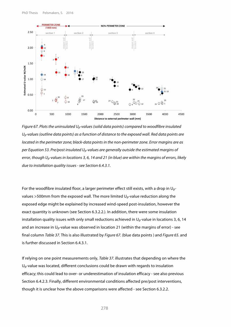
PhD Thesis Pelsmakers, S. 2016
278
Figure 67. Plots the uninsulated Up-values (solid data points) compared to woodfibre insulated
Up-values (outline data points) as a function of distance to the exposed wall. Red data points are
located in the perimeter zone; black-data points in the non-perimeter zone. Error margins are as
per Equation 53. Pre/post insulated Up-values are generally outside the estimated margins of
error, though Up-values in locations 3, 6, 14 and 21 (in blue) are within the margins of errors, likely
due to installation quality issues - see Section 6.4.3.1.
For the woodfibre insulated floor, a larger perimeter effect still exists, with a drop in Up-
values >500mm from the exposed wall. The more limited Up-value reduction along the
exposed edge might be explained by increased wind-speed post-insulation, however the
exact quantity is unknown (see Section 6.3.2.2.). In addition, there were some insulation
installation quality issues with only small reductions achieved in Up-value in locations 3, 6, 14
and an increase in Up-value was observed in location 21 (within the margins of error) - see
final column Table 37. This is also illustrated by Figure 67. (blue data points ) and Figure 65. and
is further discussed in Section 6.4.3.1.
If relying on one point measurements only, Table 37. illustrates that depending on where the
Up-value was located, different conclusions could be drawn with regards to insulation
efficacy; this could lead to over- or underestimation of insulation efficacy - see also previous
Section 6.4.2.3. Finally, different environmental conditions affected pre/post interventions,
though it is unclear how the above comparisons were affected - see Section 6.3.2.2.
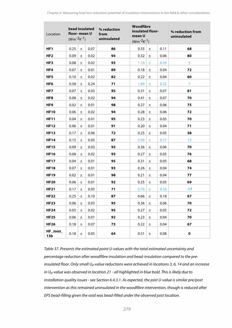
Chapter 6: Measuring heat loss reduction potential of insulation interventions in the field & other considerations
279
Location bead insulated floor- mean U (Wm-2K-1)
% reduction from uninsulated
Woodfibre insulated floor- mean U (Wm-2K-1)
% reduction from uninsulated
HF1 0.25 ± 0.07 86 0.55 ± 0.11 68
HF2 0.09 ± 0.02 94 0.32 ± 0.06 80
HF3 0.08 ± 0.02 93 1.19 ± 0.16 5
HF4 0.07 ± 0.01 89 0.18 ± 0.04 72
HF5 0.10 ± 0.02 82 0.22 ± 0.04 60
HF6 0.58 ± 0.24 71 1.89 ± 0.22 7
HF7 0.07 ± 0.03 95 0.31 ± 0.07 81
HF8 0.08 ± 0.02 94 0.41 ± 0.07 70
HF9 0.02 ± 0.01 98 0.27 ± 0.06 75
HF10 0.06 ± 0.02 94 0.28 ± 0.06 72
HF11 0.04 ± 0.01 95 0.23 ± 0.05 70
HF12 0.06 ± 0.01 91 0.20 ± 0.04 71
HF13 0.17 ± 0.06 72 0.25 ± 0.05 58
HF14 0.15 ± 0.05 87 0.99 ± 0.17 13
HF15 0.09 ± 0.03 93 0.36 ± 0.06 70
HF16 0.08 ± 0.02 93 0.27 ± 0.05 76
HF17 0.04 ± 0.01 95 0.31 ± 0.05 68
HF18 0.07 ± 0.01 93 0.26 ± 0.04 74
HF19 0.02 ± 0.01 98 0.21 ± 0.04 77
HF20 0.06 ± 0.01 92 0.25 ± 0.05 69
HF21 0.17 ± 0.05 71 0.70 ± 0.10 -17
HF22 0.25 ± 0.10 87 0.66 ± 0.18 67
HF23 0.06 ± 0.03 95 0.36 ± 0.06 70
HF24 0.05 ± 0.02 95 0.27 ± 0.05 72
HF25 0.06 ± 0.01 92 0.23 ± 0.04 70
HF26 0.18 ± 0.07 73 0.22 ± 0.04 67
HF_Joist_13b 0.18 ± 0.05 64 0.51 ± 0.08 0
Table 37. Presents the estimated point U-values with the total estimated uncertainty and
percentage reduction after woodfibre insulation and bead-insulation compared to the pre-
insulated floor. Only small Up-value reductions were achieved in locations 3, 6, 14 and an increase
in Up-value was observed in location 21 - all highlighted in blue bold. This is likely due to
installation quality issues - see Section 6.4.3.1. As expected, the joist U-value is similar pre/post
intervention as this remained uninsulated in the woodfibre intervention, though is reduced after
EPS bead-filling given the void was bead-filled under the observed joist location.
PhD Thesis Pelsmakers, S. 2016
280
6.4.3.1. Impact of installation quality on intervention efficacy
Generally, Up-value reductions after woodfibre insulation were between 58% to 80%,
depending where pre/post measurements were taken (see Table 37.). However, in some
locations, thermal transmittance was still significant post-insulation, likely due to installation
quality issues, as described below. Main installation issues included lack of tight-fitting of
insulation with the underside of the floorboards (and nearby foundation walls) to "prevent
cold draughts getting behind the insulation" (BRE, 2000), its importance also noted by EST
(2005a). This was specifically pronounced in location 21 due to a bent floorboard which
created a 15-20 mm gap between floorboard and insulation (see Figure 68.b.). In addition, the
breather membrane was cut in this location to retrieve void sensors, allowing a lead down
into the void - this may not have been sufficiently taped. These issues might have created a
thermal bypass, reducing the effective U-values - as illustrated in Figure 67. in Section 6.4.3. In
Location 21 this lead to a 17% increased Up-value after woodfibre insulation, though within
the margins of measurement uncertainty - see Figure 67. Wingfield (2009) and Wingfield
(2010) observed significant thermal bypass effects in masonry and timber-framed cavity
walls.
Near the airbricks, insulation installation quality was also compromised by chamfering the
insulation to allow for airflow through the airbrick in between joists as recommended by
best-practice guidance- see Figure 59., as discussed in Section 6.3.1. This reduced insulation
quantity is likely to have affected all of the Up-value estimates near the airbrick locations,
likely leading to a more significant perimeter effect as illustrated in Figure 65. However,
location 6 was particularly affected (see Figure 68. a.): later investigation revealed that the
chamfered insulation was slightly too short and did not fit tightly to the external wall.
Additionally, the breather membrane did not fit well over and under the joists along the
external perimeter wall (and kitchen foundation wall), as the edge floorboards were not
taken up to avoid skirting damage. This meant that cold air might be able to flow up along
the edges and create a thermal bypass, reducing the efficacy of the insulation along both
walls. Such installation issues are likely to have contributed to an increased perimeter effect.
Finally, due to services in the void it was difficult to provide full insulation between joists in
some locations; additionally, electrical power leads powering the airflow sensors in the void
(which were absent in the bead insulated floor) were pulled through a large floorboard gap
next to location 3; this affected insulation fit, likely leading to thermal bypass effects - see
Figure 68.(c.). and as visible on Figure 65.
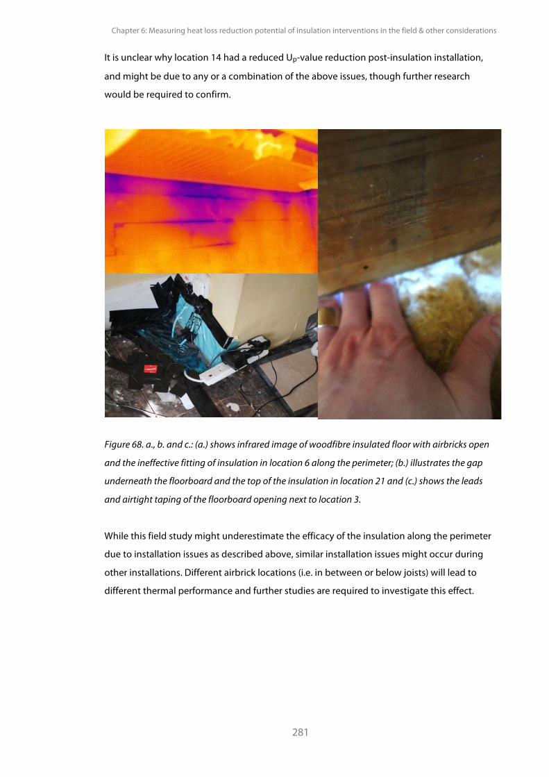
Chapter 6: Measuring heat loss reduction potential of insulation interventions in the field & other considerations
281
It is unclear why location 14 had a reduced Up-value reduction post-insulation installation,
and might be due to any or a combination of the above issues, though further research
would be required to confirm.
Figure 68. a., b. and c.: (a.) shows infrared image of woodfibre insulated floor with airbricks open
and the ineffective fitting of insulation in location 6 along the perimeter; (b.) illustrates the gap
underneath the floorboard and the top of the insulation in location 21 and (c.) shows the leads
and airtight taping of the floorboard opening next to location 3.
While this field study might underestimate the efficacy of the insulation along the perimeter
due to installation issues as described above, similar installation issues might occur during
other installations. Different airbrick locations (i.e. in between or below joists) will lead to
different thermal performance and further studies are required to investigate this effect.
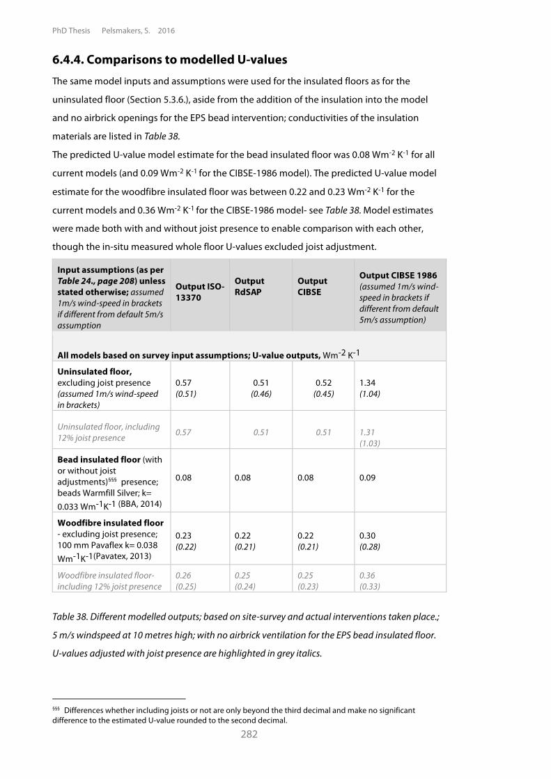
PhD Thesis Pelsmakers, S. 2016
282
6.4.4. Comparisons to modelled U-values The same model inputs and assumptions were used for the insulated floors as for the
uninsulated floor (Section 5.3.6.), aside from the addition of the insulation into the model
and no airbrick openings for the EPS bead intervention; conductivities of the insulation
materials are listed in Table 38.
The predicted U-value model estimate for the bead insulated floor was 0.08 Wm-2 K-1 for all
current models (and 0.09 Wm-2 K-1 for the CIBSE-1986 model). The predicted U-value model
estimate for the woodfibre insulated floor was between 0.22 and 0.23 Wm-2 K-1 for the
current models and 0.36 Wm-2 K-1 for the CIBSE-1986 model- see Table 38. Model estimates
were made both with and without joist presence to enable comparison with each other,
though the in-situ measured whole floor U-values excluded joist adjustment.
Input assumptions (as per Table 24., page 208) unless stated otherwise; assumed 1m/s wind-speed in brackets if different from default 5m/s assumption
Output ISO-13370
Output RdSAP
Output CIBSE
Output CIBSE 1986 (assumed 1m/s wind-speed in brackets if different from default 5m/s assumption)
All models based on survey input assumptions; U-value outputs, Wm-2 K-1
Uninsulated floor, excluding joist presence (assumed 1m/s wind-speed in brackets)
0.57 (0.51)
0.51 (0.46)
0.52
(0.45)
1.34 (1.04)
Uninsulated floor, including 12% joist presence 0.57 0.51 0.51
1.31 (1.03)
Bead insulated floor (with or without joist adjustments)§§§ presence; beads Warmfill Silver; k= 0.033 Wm-1K-1 (BBA, 2014)
0.08
0.08
0.08
0.09
Woodfibre insulated floor - excluding joist presence; 100 mm Pavaflex k= 0.038 Wm-1K-1(Pavatex, 2013)
0.23 (0.22)
0.22 (0.21)
0.22 (0.21)
0.30 (0.28)
Woodfibre insulated floor- including 12% joist presence
0.26 (0.25)
0.25 (0.24)
0.25 (0.23)
0.36 (0.33)
Table 38. Different modelled outputs; based on site-survey and actual interventions taken place.;
5 m/s windspeed at 10 metres high; with no airbrick ventilation for the EPS bead insulated floor.
U-values adjusted with joist presence are highlighted in grey italics.
§§§ Differences whether including joists or not are only beyond the third decimal and make no significant difference to the estimated U-value rounded to the second decimal.
Chapter 6: Measuring heat loss reduction potential of insulation interventions in the field & other considerations
283
Comparing the ISO-13370 modelled uninsulated floor U-value (without joists) with the
interventions, bead-insulating the floor would reduce the floor U-value by 86% and by 60%
when woodfibre insulated. These are slightly underestimated improvements compared to
the actual average measured reductions achieved: 92% (88% to 95%) for the bead insulated
floor and 65% (54% to 75%) for the woodfibre insulated floor. This slight underestimation
might be mostly due to the initial underestimation of the uninsulated floor (see 5.3.6.)
Figure 69. highlights that for this field study, the observed divergence between modelled and
in-situ measured U-values reduced the better insulated the floor was. Cox-Smith (2008) also
reported that a better insulated floor was closer to modelled thermal performance when
investigating radiant foil insulation in newer floors in New Zealand. The increased
convergence between in-situ measured and modelled U-values when better insulated might
be due to the addition of increased insulation increasing the thermal resistance (which is
fairly well known) and as the amount of insulation increases, it starts to dominate the total
thermal resistance. In addition, for the bead-insulated floor, there might be fewer
confounding (or assumed) variables: sealed airbricks removed ventilation both in in-situ
measurements and the model. The bead insulated floor had a similar floor U-value whether
in-situ measured (0.09 ±0.03 Wm-2 K-1) or modelled (0.08 to 0.09 Wm-2 K-1) for current and
superseded models. Contrary to this, the uninsulated and woodfibre insulated modelled and
in-situ measured U-values were outside the margins of error for the current models: the
in-situ measured uninsulated floor U-value was about twice as high compared to current
models (see also Section 5.3.6.), while for woodfibre insulation, the in-situ measured whole
floor U-value estimate (0.36±0.07Wm-2 K-1) was about a third higher than current model
outputs. While the superseded CIBSE-1986 model appeared to overestimate the whole floor
U-value by about 30% for the uninsulated floor, the modelled woodfibre insulated floor was
within the margins of error of the in-situ measured floor U-value (underestimated by about
16%). Furthermore, if assuming 1 m/s wind-speed, the CIBSE-1986 model output of 1.04
Wm-2 K-1 matched the in-situ measured whole floor U-value.
As for the all the modelled floors, it appears that the superseded CIBSE-1986 model outputs
lead to smaller divergences with in-situ measured values, though further research is required
to investigate if this would be the case for other in-situ measured case-studies. Similar issues
apply about the conceptual differences between what is modelled and in-situ measured as
discussed in Chapter 5.3.6. However, given the increased thermal resistance post-insulation,
the impact of certain variables is likely to be proportionally smaller in the modelled U-values.
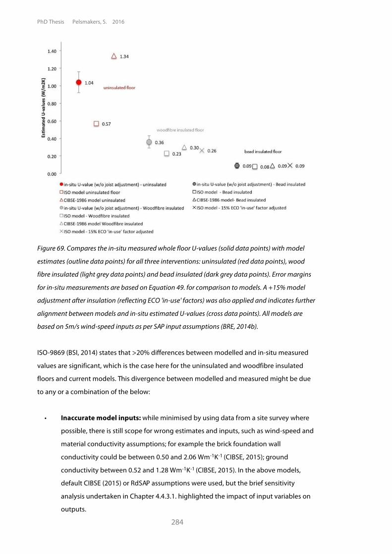
PhD Thesis Pelsmakers, S. 2016
284
Figure 69. Compares the in-situ measured whole floor U-values (solid data points) with model
estimates (outline data points) for all three interventions: uninsulated (red data points), wood
fibre insulated (light grey data points) and bead insulated (dark grey data points). Error margins
for in-situ measurements are based on Equation 49. for comparison to models. A +15% model
adjustment after insulation (reflecting ECO 'in-use' factors) was also applied and indicates further
alignment between models and in-situ estimated U-values (cross data points). All models are
based on 5m/s wind-speed inputs as per SAP input assumptions (BRE, 2014b).
ISO-9869 (BSI, 2014) states that >20% differences between modelled and in-situ measured
values are significant, which is the case here for the uninsulated and woodfibre insulated
floors and current models. This divergence between modelled and measured might be due
to any or a combination of the below:
• Inaccurate model inputs: while minimised by using data from a site survey where
possible, there is still scope for wrong estimates and inputs, such as wind-speed and
material conductivity assumptions; for example the brick foundation wall
conductivity could be between 0.50 and 2.06 Wm-1K-1 (CIBSE, 2015); ground
conductivity between 0.52 and 1.28 Wm-1K-1 (CIBSE, 2015). In the above models,
default CIBSE (2015) or RdSAP assumptions were used, but the brief sensitivity
analysis undertaken in Chapter 4.4.3.1. highlighted the impact of input variables on
outputs.
Chapter 6: Measuring heat loss reduction potential of insulation interventions in the field & other considerations
285
• Installation quality issues are not reflected in the models: for the woodfibre
insulated floor, the models above took no account of the chamfering of insulation
near airbrick locations. While no in-situ point measurements were directly above
these areas, this might have affected nearby perimeter locations - as discussed in
Section 6.4.3. Adjusting models for installation quality issues can only be undertaken
due to in-situ measurement and researcher's presence at insulation installation; for
the field study only small adjustments to the models were made - see further below.
Finally, the presence of service pipes and reduced insulation fit were excluded from
in-situ measurements in this study (though might have affected nearby
measurement locations) and are also excluded in models: generally perfect
insulation fit is assumed, but this might be difficult to achieve in reality as discussed
in Section 6.4.3.
• Measured results might not be directly comparable to modelled results: As
discussed in Chapter 5.3.6., there are some conceptual differences between
modelled and in-situ measured floor U-values: for instance inhomogenous room
temperatures, short-term thermal mass effects and dynamic external conditions
occur in reality while floor U-value models assume annual steady-state heat-flow as a
proxy for seasonal heat-transfer. Furthermore, floor U-value models exclude linear
floor/wall thermal bridge junctions; but in-situ measurements might have been
affected by such junctions. Likewise, surface thermal resistances might be affected
by airbrick airflow but this is excluded from models. Measuring conditions (internal
and environmental conditions), assumptions and analysis methods also affect in-situ
measurements as discussed elsewhere. It remains unclear however what the
individual or combined impact is of these variables on the modelled outputs and
how this affects comparison with in-situ measurements- further research is required.
Including actual installation quality issues in the model
Allowing for localised chamfered insulation installation in locations 1, 6 and 22 and a 10%
air-gap correction factor (both as per ISO-9646 (BSI, 2007)), lead to slightly increased
U-values: 0.25 Wm-2K-1 for the ISO-13370 model and 0.33 Wm-2K-1 for the superseded
CIBSE-1986 model, slightly closer to the in-situ measured value of 0.36±0.07Wm-2K-1. The air-
gap correction was only possible from in-situ observations, though it is still unclear if this also
affected other locations than those observed - hence assumption of 10% occurrence was
assumed. At present, ECO-policy uses a 15% 'in-use' factor for floor insulation for ECO-funded
insulation installations (DECC, 2012) but it is unknown if this reflects different floor
characteristics and installation quality. Figure 69. indicates further alignment of insulated
floor U-value models adjusted with +15% to in-situ estimated U-values.
PhD Thesis Pelsmakers, S. 2016
286
6.4.5. Other in-situ studies and U-value reductions from insulation Only few in-situ measurements exist for insulated floors and for pre/post floor insulation
studies. Direct comparison between floor insulation studies is challenging given previously
noted different variables and - in the case of insulated floors - different insulation materials,
insulation depth and material conductivities. Harris (1997) reported around 50% floor
U-value reduction in a test cell after introduction of 30mm EPS insulation (with similar
thermal conductivity as woodfibre insulation). This is a significant U-value reduction given
the small depth of insulation, however due to the test-cell nature, comparison with in-situ
field study results are difficult.
Currie (2013) reported a 71% point U-value reduction (from 2.4 Wm-2K-1 to 0.70 Wm-2K-1)
after 80 mm woodfibre insulation installation in a detached cottage in Scotland. This is a
slightly better improvement than the mean 65% reduction observed in this field study after
100mm woodfibre insulation installation, though within the experimental error estimate of
reductions between 54% to 75% for the field study. The field study reduction is based on the
whole floor U-value reduction of 26 points pre/post insulation; while the Currie (2013) study
was based on observation of one point measurement located in the exposed perimeter zone
(and unknown how close to airbricks). Given the initial high point U-value of 2.4 Wm-2K-1 in
the Currie (2013) perimeter monitoring study means that the introduction of a large thermal
resistance (i.e. the insulation) is likely to lead to a greater proportional Up-value reduction in
the perimeter compared to non-perimeter locations.**** However this was not observed in
the woodfibre intervention study here due to installation quality issues (see Section 6.4.3.1.).
This again reiterates that estimating floor U-value reductions from one point measurement
might over or under-estimate the insulation efficacy of the whole floor, depending on
measurement locations and installation quality issues - see also Section 6.4.2.3.
**** For example for the bead-insulated floor, largest U-value reductions were observed in the perimeter floor zone, with exception of locations nearest to airbricks and directly adjacent to the external wall - see Table 37.
Chapter 6: Measuring heat loss reduction potential of insulation interventions in the field & other considerations
287
6.4.6. Comparison to Building regulation recommendations As discussed in Chapter 2.6., Building Regulations Part L1B recommend maximum design
floor U-values of 0.25 Wm-2K-1 with a maximum allowable design U-value of 0.70 Wm-2K-1 for
exceptions to listed buildings or where other regulatory relaxations apply (NBS, 2015, SBSA,
2015, Government, 2014, DFPNI, 2012).
The bead-filled floor void meets these regulatory requirements when both modelled (0.08
Wm-2K-1) and measured in-situ (0.09 ±0.03 Wm-2K-1); however it is unclear whether it would
meet Building Regulations Part C (NBS, 2013), which stipulates a ventilated floor void.††††
Part L1B (NBS, 2010) recommends that to obtain a ground floor U-value of 0.25 Wm-2K-1 for a
floor with P/A of 0.3, 97mm to 107mm insulation with thermal conductivity of 0.035 to 0.040
Wm-1K-1 between the joists is required‡‡‡‡. This specification is similar to the woodfibre
insulated study and the U-values modelled with current models, which all met the building
regulations upgrade requirements (see Table 39. ). However the superseded CIBSE-1986
model output does not meet the Part L1B U-value recommendation and when adjusting for
joist presence, the ISO-13370 model also exceeds the recommendations. Further adjusting
the modelled values with the +15% 'in-use' factor further increases modelled values,
exceeding the recommended values.
Furthermore, the woodfibre insulated in-situ measured whole floor U-value fails to meet the
building regulation requirement by about 30%. Without the perimeter airbricks in between
the joists, greater in-situ heat-flow reductions might have been achieved, though it is unclear
if this would have brought in-situ measured closer to modelled values and regulatory
requirements. The presence of services and installation quality issues associated with airbrick
locations and ill-fitting floorboards are excluded from models yet are likely to be practical
issues present in other dwellings, preventing 'perfect insulation' installation. This raises
questions about the practicalities of achieving the Building Regulations recommended
design floor U-values of 0.18 to 0.25 Wm-2K-1, depending in which UK region.
†††† Shaftesbury Park Terrace which implemented EPS void-filling and permanently sealed airbricks was approved by local building control (Baeli, 2013, TSB, 2011). ‡‡‡‡ No information is provided with regards to ventilation area assumptions; 12% joist presence is assumed.
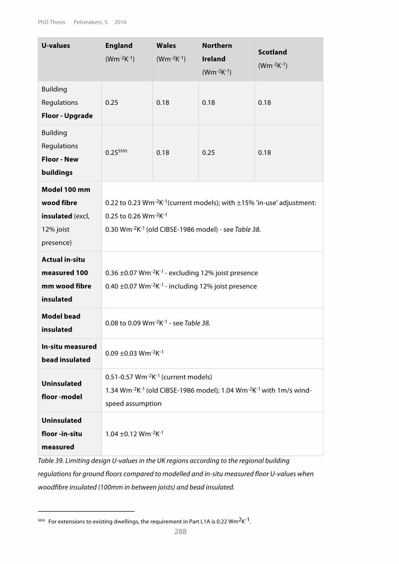
PhD Thesis Pelsmakers, S. 2016
288
U-values England
(Wm-2K-1)
Wales
(Wm-2K-1)
Northern
Ireland
(Wm-2K-1)
Scotland
(Wm-2K-1)
Building
Regulations
Floor - Upgrade
0.25
0.18 0.18 0.18
Building
Regulations
Floor - New
buildings
0.25§§§§ 0.18 0.25 0.18
Model 100 mm
wood fibre
insulated (excl,
12% joist
presence)
0.22 to 0.23 Wm-2K-1(current models); with ±15% 'in-use' adjustment:
0.25 to 0.26 Wm-2K-1
0.30 Wm-2K-1 (old CIBSE-1986 model) - see Table 38.
Actual in-situ
measured 100
mm wood fibre
insulated
0.36 ±0.07 Wm-2K-1 - excluding 12% joist presence
0.40 ±0.07 Wm-2K-1 - including 12% joist presence
Model bead
insulated 0.08 to 0.09 Wm-2K-1 - see Table 38.
In-situ measured
bead insulated 0.09 ±0.03 Wm-2K-1
Uninsulated
floor -model
0.51-0.57 Wm-2K-1 (current models)
1.34 Wm-2K-1 (old CIBSE-1986 model); 1.04 Wm-2K-1 with 1m/s wind-
speed assumption
Uninsulated
floor -in-situ
measured
1.04 ±0.12 Wm-2K-1
Table 39. Limiting design U-values in the UK regions according to the regional building
regulations for ground floors compared to modelled and in-situ measured floor U-values when
woodfibre insulated (100mm in between joists) and bead insulated.
§§§§ For extensions to existing dwellings, the requirement in Part L1A is 0.22 Wm2K-1.
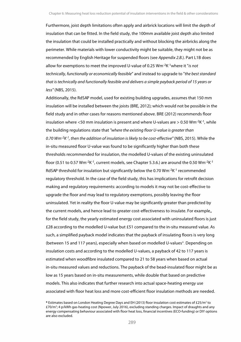
Chapter 6: Measuring heat loss reduction potential of insulation interventions in the field & other considerations
289
Furthermore, joist depth limitations often apply and airbrick locations will limit the depth of
insulation that can be fitted. In the field study, the 100mm available joist depth also limited
the insulation that could be installed practically and without blocking the airbricks along the
perimeter. While materials with lower conductivity might be suitable, they might not be as
recommended by English Heritage for suspended floors (see Appendix 2.B.). Part L1B does
allow for exemptions to meet the improved U-value of 0.25 Wm-2K-1where it "is not
technically, functionally or economically feasible" and instead to upgrade to "the best standard
that is technically and functionally feasible and delivers a simple payback period of 15 years or
less" (NBS, 2015).
Additionally, the RdSAP model, used for existing building upgrades, assumes that 150 mm
insulation will be installed between the joists (BRE, 2012); which would not be possible in the
field study and in other cases for reasons mentioned above. BRE (2012) recommends floor
insulation where <50 mm insulation is present and where U-values are > 0.50 Wm-2K-1, while
the building regulations state that "where the existing floor U-value is greater than
0.70 Wm-2K-1, then the addition of insulation is likely to be cost-effective" (NBS, 2015). While the
in-situ measured floor U-value was found to be significantly higher than both these
thresholds recommended for insulation, the modelled U-values of the existing uninsulated
floor (0.51 to 0.57 Wm-2K-1, current models, see Chapter 5.3.6.) are around the 0.50 Wm-2K-1
RdSAP threshold for insulation but significantly below the 0.70 Wm-2K-1 recommended
regulatory threshold. In the case of the field study, this has implications for retrofit decision
making and regulatory requirements: according to models it may not be cost-effective to
upgrade the floor and may lead to regulatory exemptions, possibly leaving the floor
uninsulated. Yet in reality the floor U-value may be significantly greater than predicted by
the current models, and hence lead to greater cost-effectiveness to insulate. For example,,
for the field study, the yearly estimated energy cost associated with uninsulated floors is just
£28 according to the modelled U-value but £51 compared to the in-situ measured value. As
such, a simplified payback model indicates that the payback of insulating floors is very long
(between 15 and 117 years), especially when based on modelled U-values*. Depending on
insulation costs and according to the modelled U-values, a payback of 42 to 117 years is
estimated when woodfibre insulated compared to 21 to 58 years when based on actual
in-situ measured values and reductions. The payback of the bead-insulated floor might be as
low as 15 years based on in-situ measurements, while double that based on predictive
models. This also indicates that further research into actual space-heating energy use
associated with floor heat loss and more cost-efficient floor insulation methods are needed.
* Estimates based on London Heating Degree Days and EH (2013) floor insulation cost estimates of £25/m2 to £70/m2; 4 p/kWh gas-heating cost (Npower, July 2016), excluding standing charges. Impact of draughts and any energy compensating behaviour associated with floor heat loss, financial incentives (ECO-funding) or DIY options are also excluded.
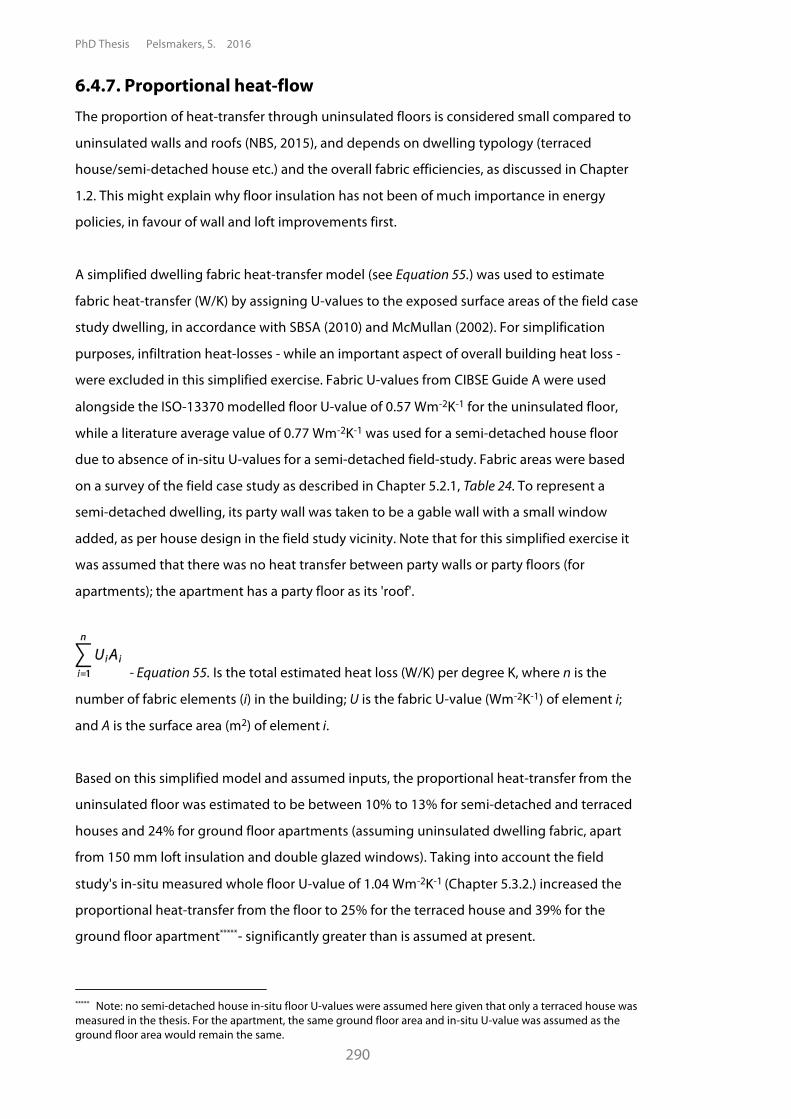
PhD Thesis Pelsmakers, S. 2016
290
6.4.7. Proportional heat-flow The proportion of heat-transfer through uninsulated floors is considered small compared to
uninsulated walls and roofs (NBS, 2015), and depends on dwelling typology (terraced
house/semi-detached house etc.) and the overall fabric efficiencies, as discussed in Chapter
1.2. This might explain why floor insulation has not been of much importance in energy
policies, in favour of wall and loft improvements first.
A simplified dwelling fabric heat-transfer model (see Equation 55.) was used to estimate
fabric heat-transfer (W/K) by assigning U-values to the exposed surface areas of the field case
study dwelling, in accordance with SBSA (2010) and McMullan (2002). For simplification
purposes, infiltration heat-losses - while an important aspect of overall building heat loss -
were excluded in this simplified exercise. Fabric U-values from CIBSE Guide A were used
alongside the ISO-13370 modelled floor U-value of 0.57 Wm-2K-1 for the uninsulated floor,
while a literature average value of 0.77 Wm-2K-1 was used for a semi-detached house floor
due to absence of in-situ U-values for a semi-detached field-study. Fabric areas were based
on a survey of the field case study as described in Chapter 5.2.1, Table 24. To represent a
semi-detached dwelling, its party wall was taken to be a gable wall with a small window
added, as per house design in the field study vicinity. Note that for this simplified exercise it
was assumed that there was no heat transfer between party walls or party floors (for
apartments); the apartment has a party floor as its 'roof'.
- Equation 55. Is the total estimated heat loss (W/K) per degree K, where n is the
number of fabric elements (i) in the building; U is the fabric U-value (Wm-2K-1) of element i;
and A is the surface area (m2) of element i.
Based on this simplified model and assumed inputs, the proportional heat-transfer from the
uninsulated floor was estimated to be between 10% to 13% for semi-detached and terraced
houses and 24% for ground floor apartments (assuming uninsulated dwelling fabric, apart
from 150 mm loft insulation and double glazed windows). Taking into account the field
study's in-situ measured whole floor U-value of 1.04 Wm-2K-1 (Chapter 5.3.2.) increased the
proportional heat-transfer from the floor to 25% for the terraced house and 39% for the
ground floor apartment*****- significantly greater than is assumed at present.
***** Note: no semi-detached house in-situ floor U-values were assumed here given that only a terraced house was measured in the thesis. For the apartment, the same ground floor area and in-situ U-value was assumed as the ground floor area would remain the same.
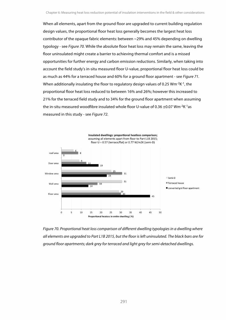
Chapter 6: Measuring heat loss reduction potential of insulation interventions in the field & other considerations
291
When all elements, apart from the ground floor are upgraded to current building regulation
design values, the proportional floor heat loss generally becomes the largest heat loss
contributor of the opaque fabric elements: between ~29% and 45% depending on dwelling
typology - see Figure 70. While the absolute floor heat loss may remain the same, leaving the
floor uninsulated might create a barrier to achieving thermal comfort and is a missed
opportunities for further energy and carbon emission reductions. Similarly, when taking into
account the field study's in-situ measured floor U-value, proportional floor heat loss could be
as much as 44% for a terraced house and 60% for a ground floor apartment - see Figure 71.
When additionally insulating the floor to regulatory design values of 0.25 Wm-2K-1, the
proportional floor heat loss reduced to between 16% and 26%; however this increased to
21% for the terraced field study and to 34% for the ground floor apartment when assuming
the in-situ measured woodfibre insulated whole floor U-value of 0.36 ±0.07 Wm-2K-1as
measured in this study - see Figure 72.
Figure 70. Proportional heat loss comparison of different dwelling typologies in a dwelling where
all elements are upgraded to Part L1B 2015, but the floor is left uninsulated. The black bars are for
ground floor apartments; dark grey for terraced and light grey for semi-detached dwellings.
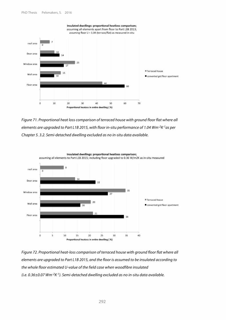
PhD Thesis Pelsmakers, S. 2016
292
Figure 71. Proportional heat loss comparison of terraced house with ground floor flat where all
elements are upgraded to Part L1B 2015, with floor in-situ performance of 1.04 Wm-2K-1as per
Chapter 5. 3.2. Semi-detached dwelling excluded as no in-situ data available.
Figure 72. Proportional heat-loss comparison of terraced house with ground floor flat where all
elements are upgraded to Part L1B 2015, and the floor is assumed to be insulated according to
the whole floor estimated U-value of the field case when woodfibre insulated
(i.e. 0.36±0.07 Wm-2K-1). Semi-detached dwelling excluded as no in-situ data available.
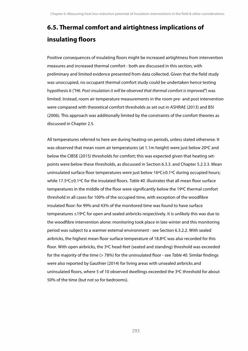
Chapter 6: Measuring heat loss reduction potential of insulation interventions in the field & other considerations
293
6.5. Thermal comfort and airtightness implications of
insulating floors
Positive consequences of insulating floors might be increased airtightness from intervention
measures and increased thermal comfort - both are discussed in this section, with
preliminary and limited evidence presented from data collected. Given that the field study
was unoccupied, no occupant thermal comfort study could be undertaken hence testing
hypothesis 6 ("H6. Post-insulation it will be observed that thermal comfort is improved") was
limited. Instead, room air temperature measurements in the room pre- and post intervention
were compared with theoretical comfort thresholds as set out in ASHRAE (2013) and BSI
(2006). This approach was additionally limited by the constraints of the comfort theories as
discussed in Chapter 2.5.
All temperatures referred to here are during heating-on periods, unless stated otherwise. It
was observed that mean room air temperatures (at 1.1m height) were just below 20ºC and
below the CIBSE (2015) thresholds for comfort; this was expected given that heating set-
points were below these thresholds, as discussed in Section 6.3.3. and Chapter 5.2.3.3. Mean
uninsulated surface floor temperatures were just below 16ºC±0.1ºC during occupied hours;
while 17.5ºC±0.1ºC for the insulated floors. Table 40. illustrates that all mean floor surface
temperatures in the middle of the floor were significantly below the 19ºC thermal comfort
threshold in all cases for 100% of the occupied time, with exception of the woodfibre
insulated floor: for 99% and 43% of the monitored time was found to have surface
temperatures ≤19ºC for open and sealed airbricks respectively. It is unlikely this was due to
the woodfibre intervention alone: monitoring took place in late winter and this monitoring
period was subject to a warmer external environment - see Section 6.3.2.2. With sealed
airbricks, the highest mean floor surface temperature of 18.8ºC was also recorded for this
floor. With open airbricks, the 3ºC head-feet (seated and standing) threshold was exceeded
for the majority of the time (> 78%) for the uninsulated floor - see Table 40. Similar findings
were also reported by Gauthier (2014) for living areas with unsealed airbricks and
uninsulated floors, where 5 of 10 observed dwellings exceeded the 3ºC threshold for about
50% of the time (but not so for bedrooms).
PhD Thesis Pelsmakers, S. 2016
294
Thermal comfort variables or thresholds
All open airbricks, apart from bead insulated Sealed airbricks
Heated/occupied hours only. Measured in middle of living room.
uninsulated
floor
bead insulated
floor
woodfibre insulated floor
uninsulated floor
woodfibre insulated floor
Mean floor surface temperature (middle floor, location 10)
15.7±0.1ºC 17.5±0.1ºC 17.5±0.1ºC 16.8±0.1ºC 18.8±0.1ºC
% of time floor surface temperatures < 19ºC
100% 100% 99% 100% 43%
Mean temperature 1.1m high
19.6±0.1ºC 19.7±0.1ºC 19.7±0.1ºC 19.7±0.1ºC 20.2±0.1ºC
Mean temperature difference feet and head (seated) in ªC (0.1-1.1m)†††††
3.7±0.14ºC 3.2±0.14ºC 3.2±0.14ºC 3.7±0.14ºC 2.1±0.14ºC
Average temp difference feet and head (standing) in ªC (0.1-1.7m)‡‡‡‡‡
4.6±0.14ºC 4.1±0.14ºC 4±0.14ºC 4.7±0.14ºC 2.8±0.14ºC
% of time !3ºC seated 78% 65% 59% 77% 8%
% of time !3ºC standing 92% 89% 82% 100% 26%
External temperatures (during occupied hours)
5.9 5.7 7.6 7.3 12.1
Table 40. presents the mean surface temperatures in the middle of the floor, the !T between feet
and head when seated (0.1m-1.1m) and standing (0.1m-1.7m) and % of time that these
thresholds were "3ºC threshold.
††††† Error margin is estimated from the quadratic sum of the two individual instrument errors of each measurand. ‡‡‡‡‡ idem
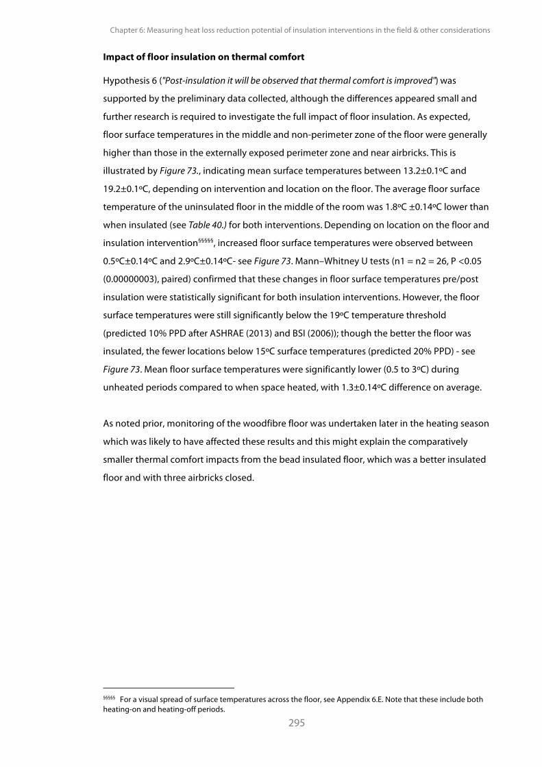
Chapter 6: Measuring heat loss reduction potential of insulation interventions in the field & other considerations
295
Impact of floor insulation on thermal comfort
Hypothesis 6 ("Post-insulation it will be observed that thermal comfort is improved") was
supported by the preliminary data collected, although the differences appeared small and
further research is required to investigate the full impact of floor insulation. As expected,
floor surface temperatures in the middle and non-perimeter zone of the floor were generally
higher than those in the externally exposed perimeter zone and near airbricks. This is
illustrated by Figure 73., indicating mean surface temperatures between 13.2±0.1ºC and
19.2±0.1ºC, depending on intervention and location on the floor. The average floor surface
temperature of the uninsulated floor in the middle of the room was 1.8ºC ±0.14ºC lower than
when insulated (see Table 40.) for both interventions. Depending on location on the floor and
insulation intervention§§§§§, increased floor surface temperatures were observed between
0.5ºC±0.14ºC and 2.9ºC±0.14ºC- see Figure 73. Mann–Whitney U tests (n1 = n2 = 26, P <0.05
(0.00000003), paired) confirmed that these changes in floor surface temperatures pre/post
insulation were statistically significant for both insulation interventions. However, the floor
surface temperatures were still significantly below the 19ºC temperature threshold
(predicted 10% PPD after ASHRAE (2013) and BSI (2006)); though the better the floor was
insulated, the fewer locations below 15ºC surface temperatures (predicted 20% PPD) - see
Figure 73. Mean floor surface temperatures were significantly lower (0.5 to 3ºC) during
unheated periods compared to when space heated, with 1.3±0.14ºC difference on average.
As noted prior, monitoring of the woodfibre floor was undertaken later in the heating season
which was likely to have affected these results and this might explain the comparatively
smaller thermal comfort impacts from the bead insulated floor, which was a better insulated
floor and with three airbricks closed.
§§§§§ For a visual spread of surface temperatures across the floor, see Appendix 6.E. Note that these include both heating-on and heating-off periods.
PhD Thesis Pelsmakers, S. 2016
296
Figure 73. Mean floor surface temperatures during heating-on periods when uninsulated (black
data points), or wood fibre insulated (WF, grey data points), (both with open airbricks) or when
bead filled (red data points, sealed airbricks). The light pink shaded zone indicates the expected
10% PPD thermal discomfort zone with floor surface temperatures <19ºC and the darker pink
zone indicates 20% PPD with floor surface temperatures <15ºC. Margins of instrument error of
±0.1 ºC are not visible on this graph. PPD after ASHRAE (2013) and BSI (2006). As expected, the
better insulated the floor was, generally the higher the observed mean floor surface temperatures;
the highest mean surface temperatures were observed for the bead-insulated floor (red data
points) and the lowest for the uninsulated floor (black data points).
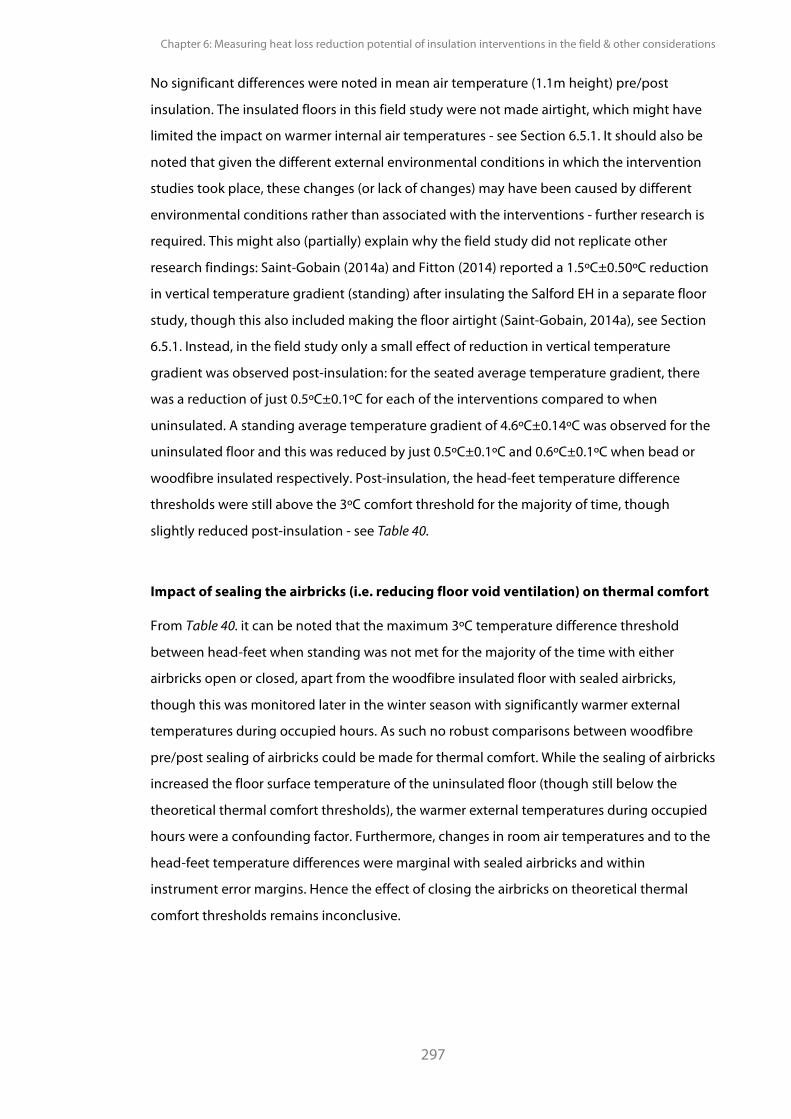
Chapter 6: Measuring heat loss reduction potential of insulation interventions in the field & other considerations
297
No significant differences were noted in mean air temperature (1.1m height) pre/post
insulation. The insulated floors in this field study were not made airtight, which might have
limited the impact on warmer internal air temperatures - see Section 6.5.1. It should also be
noted that given the different external environmental conditions in which the intervention
studies took place, these changes (or lack of changes) may have been caused by different
environmental conditions rather than associated with the interventions - further research is
required. This might also (partially) explain why the field study did not replicate other
research findings: Saint-Gobain (2014a) and Fitton (2014) reported a 1.5ºC±0.50ºC reduction
in vertical temperature gradient (standing) after insulating the Salford EH in a separate floor
study, though this also included making the floor airtight (Saint-Gobain, 2014a), see Section
6.5.1. Instead, in the field study only a small effect of reduction in vertical temperature
gradient was observed post-insulation: for the seated average temperature gradient, there
was a reduction of just 0.5ºC±0.1ºC for each of the interventions compared to when
uninsulated. A standing average temperature gradient of 4.6ºC±0.14ºC was observed for the
uninsulated floor and this was reduced by just 0.5ºC±0.1ºC and 0.6ºC±0.1ºC when bead or
woodfibre insulated respectively. Post-insulation, the head-feet temperature difference
thresholds were still above the 3ºC comfort threshold for the majority of time, though
slightly reduced post-insulation - see Table 40.
Impact of sealing the airbricks (i.e. reducing floor void ventilation) on thermal comfort
From Table 40. it can be noted that the maximum 3ºC temperature difference threshold
between head-feet when standing was not met for the majority of the time with either
airbricks open or closed, apart from the woodfibre insulated floor with sealed airbricks,
though this was monitored later in the winter season with significantly warmer external
temperatures during occupied hours. As such no robust comparisons between woodfibre
pre/post sealing of airbricks could be made for thermal comfort. While the sealing of airbricks
increased the floor surface temperature of the uninsulated floor (though still below the
theoretical thermal comfort thresholds), the warmer external temperatures during occupied
hours were a confounding factor. Furthermore, changes in room air temperatures and to the
head-feet temperature differences were marginal with sealed airbricks and within
instrument error margins. Hence the effect of closing the airbricks on theoretical thermal
comfort thresholds remains inconclusive.
PhD Thesis Pelsmakers, S. 2016
298
6.5.1. Airtightness after floor insulation As discussed in Chapter 3.2.6., in-situ measured U-values exclude the heat loss from air
leakage through floors (i.e. ingress of uncontrolled external and void air coming inside
through gaps and cracks in the floor). McGrath (1996), Hartless (1994) and Basset (1988)
suggest that airflow moves up through the floor to internal spaces rather than cross-
ventilated from one floor void end to another.******Associated thermal comfort impacts might
lead to compensating energy-use behaviour by occupants; for example, increasing air
temperatures to offset draughts or discomfort from cold floor surface temperatures (Olesen,
1979, Rock, 2013). In addition, as discussed in Chapter 2.7., air infiltration through the floor
void could also bring contaminants into indoor spaces, hence increasing airtightness of the
floor may be important in terms of energy use, local thermal comfort sensation and health
(Sherman).
Stephen's (1998) large scale study of 411 dwellings found that about half had suspended
timber ground floors with air change rates of 16.5 ach-1 at 50Pa, as expected higher than the
remaining solid ground floors with ~11.5 ach-1 at 50Pa. As anticipated, air leakage was found
to be worse with standard square-edged floorboards compared to tongue and grooved
boards, where most leakage occurs around service penetrations and wall/floor junctions
(Stephen, 1998). For seven houses, the relative air leakage from suspended timber ground
floors with bare floorboards was observed to be 3.5% to 25.4% of the total dwelling air
leakage (Stephen, 1998) while Lilly (1988) found this to be on average 65% (based on one
test-house with seven airbricks); different variables of the study houses (such as floor areas)
make comparisons challenging.
For the field study, a limited air leakage study was conducted: dwelling air leakage was
investigated by (a). measuring dwelling airtightness with the uninsulated floor; (b.)
measuring dwelling airtightness post-insulation interventions and with sealed airbricks and
(c.) estimating a relative improvement in airtightness after sealing the floor for the same field
study dwelling with the Standard Assessment Procedure (SAP). No internal airflows or
internal airflow velocity were measured in the case study house, limiting understanding of
the impact of floor airtightness on thermal comfort. No separate floor air leakage was
measured for reasons as discussed in Chapter 3.2.4.
****** In this study, the living room and kitchen floor voids were isolated in any case - see Chapter 5.2.
Chapter 6: Measuring heat loss reduction potential of insulation interventions in the field & other considerations
299
6.5.1.1. SAP and airtightness assumptions
SAP and RdSAP (Reduced SAP) are used for the modelling of new or existing buildings and
for building regulation compliance but could benefit from input refinement to more
accurately predict actual fabric performance and energy use (May, 2012, Gentry, 2010, ZCH,
2014). (Rd)SAP make three simplified input assumptions about air leakage through the floor
(BRE, 2014), assuming that floor infiltration depends on dwelling age bands with pre-1982
dwellings having 'unsealed' floors and more recent floor constructions are assumed to be
'sealed':
• 0.2 ach-1 for unsealed floors (pre-1982);
• 0.1 ach-1 for sealed floors (post-1982);
• and 0 ach-1 for solid ground floors.
It is unknown what the above assumptions are based on; floor air leakage is one of several
variables assumed in the dwelling's infiltration heat loss (alongside infiltration through
windows, entrance doors, chimneys and fans) and depends on dwelling exposure to winds
and typical monthly average wind-speeds. Modelling the field study with an unsealed floor,
SAP estimated a whole house ventilative heat loss (W/K) of about 20% more than if this were
a solid ground floor. Just a 10% improvement was estimated from sealing the unsealed floor,
though it is unclear what assumptions the 'sealing' of the floor are based on. In any case, this
suggests only a limited benefit when making the floor airtight for this field-study, according
to RdSAP.
PhD Thesis Pelsmakers, S. 2016
300
6.5.1.2. Blower door tests: findings and discussion
Blower door tests were undertaken to investigate the impact of floor insulation and airbrick
sealing on the overall dwelling airtightness, in accordance with ATTMA (2010) test standards
and envelope area calculations.
It was hypothesised that installation of floor insulation would improve dwelling airtightness
(Hypothesis 5a), as was reported by Saint-Gobain for the Salford Energy House, where
reductions of 42% for floor insulation installation are reported (Saint-Gobain, 2014a, Saint-
Gobain, 2014b); Banfill (2011) also reported similar results. In addition, by sealing airbricks,
the air leakage from the airbricks might be estimated; however no tests were undertaken to
estimate the proportional air leakage from the floor to the whole dwelling ventilation rate.
This is because - as discussed in Chapter 3.2.4. - tracer gas techniques were not practical for
mixing in floor void spaces (Edwards, 1990) and no pressurisation fans were available to
(de)pressurise the floor void through the airbricks as undertaken by for example DeWitt
(1994). Temporary sealing of the floor surface was not successful due to the effect of the
blower door test on the temporary seals.
The average of the pressurisation and depressurisation tests are presented in Table 41., based
on 7 pressurisation points for each (i.e. approximately 65Pa, 57Pa, 49Pa, 41Pa, 33Pa, 25Pa and
20Pa). According to ISO (2006) the typical uncertainty of air permeability tests in calm
conditions (i.e. windspeed <0.45 m/s) is ±5 to ±10%, and can be as much as ±20% in windy
conditions. BSI (2001) states higher uncertainties of less than ±15% in calm conditions and as
much as ±40% in windy conditions, though typically between ±5 and ±10%. In this study, a
±10% measurement error was applied as generally the tests were conducted in calm
conditions - see Table 41. Measurements were repeated on different days for the same
intervention where possible; these were all within 0 to ±5% of one another and well within
the above stated margins of error. For comparison purposes, results presented here are
based on tests conducted with most similar external conditions as the other interventions,
especially taking wind-speed into account. It is unknown when the UCL blower door test kit
was last calibrated, which might have impacted on results - though its quantity is unknown.
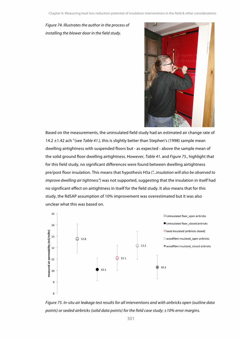
Chapter 6: Measuring heat loss reduction potential of insulation interventions in the field & other considerations
301
Figure 74. Illustrates the author in the process of
installing the blower door in the field study.
Based on the measurements, the uninsulated field study had an estimated air change rate of
14.2 ±1.42 ach-1(see Table 41.), this is slightly better than Stephen's (1998) sample mean
dwelling airtightness with suspended floors but - as expected - above the sample mean of
the solid ground floor dwelling airtightness. However, Table 41. and Figure 75., highlight that
for this field study, no significant differences were found between dwelling airtightness
pre/post floor insulation. This means that hypothesis H5a ("...insulation will also be observed to
improve dwelling air tightness") was not supported, suggesting that the insulation in itself had
no significant effect on airtightness in itself for the field study. It also means that for this
study, the RdSAP assumption of 10% improvement was overestimated but it was also
unclear what this was based on.
Figure 75. In-situ air leakage test results for all interventions and with airbricks open (outline data
points) or sealed airbricks (solid data points) for the field case study; ±10% error margins.
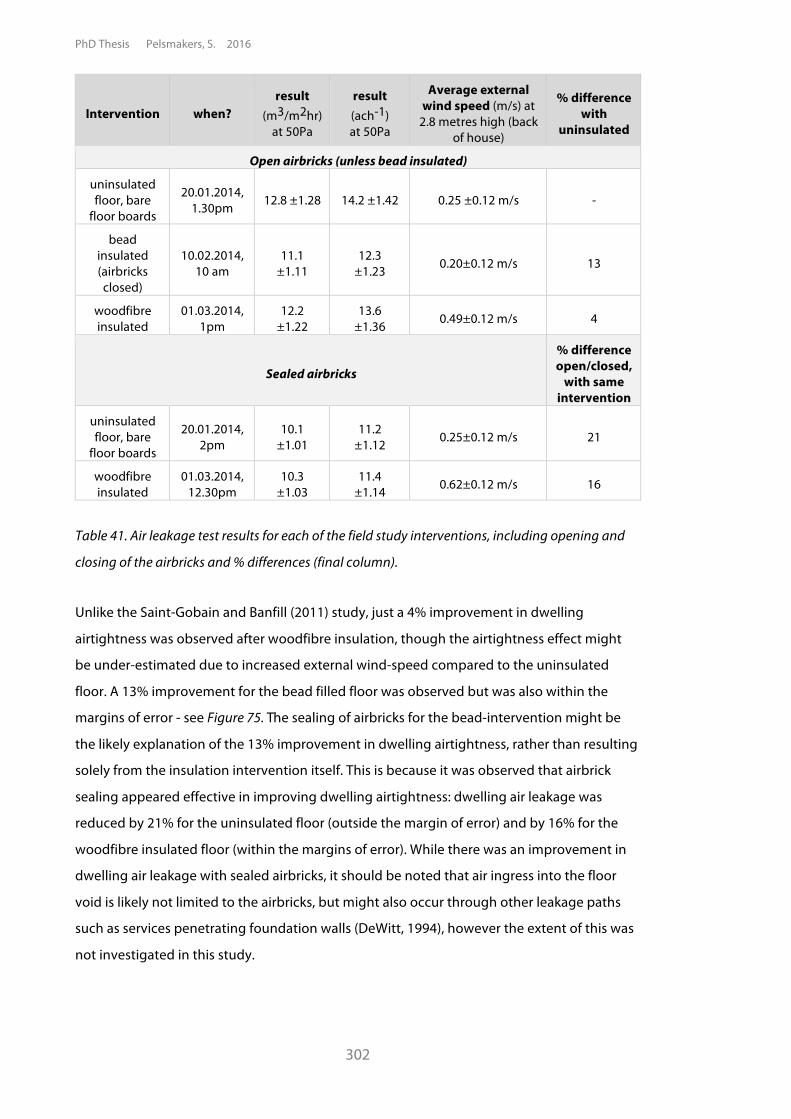
PhD Thesis Pelsmakers, S. 2016
302
Intervention when? result
(m3/m2hr) at 50Pa
result (ach-1) at 50Pa
Average external wind speed (m/s) at
2.8 metres high (back of house)
% difference with
uninsulated
Open airbricks (unless bead insulated)
uninsulated floor, bare
floor boards
20.01.2014, 1.30pm 12.8 ±1.28 14.2 ±1.42 0.25 ±0.12 m/s -
bead insulated (airbricks closed)
10.02.2014, 10 am
11.1 ±1.11
12.3 ±1.23 0.20±0.12 m/s 13
woodfibre insulated
01.03.2014, 1pm
12.2 ±1.22
13.6 ±1.36 0.49±0.12 m/s 4
Sealed airbricks
% difference open/closed,
with same intervention
uninsulated floor, bare
floor boards
20.01.2014, 2pm
10.1 ±1.01
11.2 ±1.12 0.25±0.12 m/s 21
woodfibre insulated
01.03.2014, 12.30pm
10.3 ±1.03
11.4 ±1.14 0.62±0.12 m/s 16
Table 41. Air leakage test results for each of the field study interventions, including opening and
closing of the airbricks and % differences (final column).
Unlike the Saint-Gobain and Banfill (2011) study, just a 4% improvement in dwelling
airtightness was observed after woodfibre insulation, though the airtightness effect might
be under-estimated due to increased external wind-speed compared to the uninsulated
floor. A 13% improvement for the bead filled floor was observed but was also within the
margins of error - see Figure 75. The sealing of airbricks for the bead-intervention might be
the likely explanation of the 13% improvement in dwelling airtightness, rather than resulting
solely from the insulation intervention itself. This is because it was observed that airbrick
sealing appeared effective in improving dwelling airtightness: dwelling air leakage was
reduced by 21% for the uninsulated floor (outside the margin of error) and by 16% for the
woodfibre insulated floor (within the margins of error). While there was an improvement in
dwelling air leakage with sealed airbricks, it should be noted that air ingress into the floor
void is likely not limited to the airbricks, but might also occur through other leakage paths
such as services penetrating foundation walls (DeWitt, 1994), however the extent of this was
not investigated in this study.
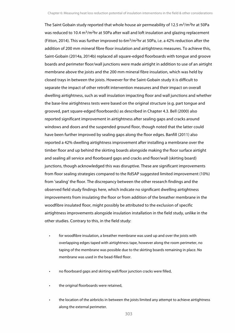
Chapter 6: Measuring heat loss reduction potential of insulation interventions in the field & other considerations
303
The Saint Gobain study reported that whole house air permeability of 12.5 m3/m2hr at 50Pa
was reduced to 10.4 m3/m2hr at 50Pa after wall and loft insulation and glazing replacement
(Fitton, 2014). This was further improved to 6m3/m2hr at 50Pa, i.e. a 42% reduction after the
addition of 200 mm mineral fibre floor insulation and airtightness measures. To achieve this,
Saint-Gobain (2014a, 2014b) replaced all square-edged floorboards with tongue and groove
boards and perimeter floor/wall junctions were made airtight in addition to use of an airtight
membrane above the joists and the 200 mm mineral fibre insulation, which was held by
closed trays in between the joists. However for the Saint-Gobain study it is difficult to
separate the impact of other retrofit intervention measures and their impact on overall
dwelling airtightness, such as wall insulation impacting floor and wall junctions and whether
the base-line airtightness tests were based on the original structure (e.g. part tongue and
grooved, part square-edged floorboards) as described in Chapter 4.3. Bell (2000) also
reported significant improvement in airtightness after sealing gaps and cracks around
windows and doors and the suspended ground floor, though noted that the latter could
have been further improved by sealing gaps along the floor edges. Banfill (2011) also
reported a 42% dwelling airtightness improvement after installing a membrane over the
timber floor and up behind the skirting boards alongside making the floor surface airtight
and sealing all service and floorboard gaps and cracks and floor/wall (skirting board)
junctions, though acknowledged this was disruptive. These are significant improvements
from floor sealing strategies compared to the RdSAP suggested limited improvement (10%)
from 'sealing' the floor. The discrepancy between the other research findings and the
observed field study findings here, which indicate no significant dwelling airtightness
improvements from insulating the floor or from addition of the breather membrane in the
woodfibre insulated floor, might possibly be attributed to the exclusion of specific
airtightness improvements alongside insulation installation in the field study, unlike in the
other studies. Contrary to this, in the field study:
• for woodfibre insulation, a breather membrane was used up and over the joists with
overlapping edges taped with airtightness tape, however along the room perimeter, no
taping of the membrane was possible due to the skirting boards remaining in place. No
membrane was used in the bead-filled floor.
• no floorboard gaps and skirting wall/floor junction cracks were filled,
• the original floorboards were retained,
• the location of the airbricks in between the joists limited any attempt to achieve airtightness
along the external perimeter.
PhD Thesis Pelsmakers, S. 2016
304
It is unknown whether different insulation materials and other interventions might have lead
to improved airtightness or not; though as Stevens (2013) noted for solid wall insulation,
improved airtightness will be highly variable without specifically improving fabric
airtightness alongside the insulation measure.
This indicates that without a deliberate airtightness strategy there might be no significant
airtightness benefits from insulating suspended timber ground floors, as also generally
reported elsewhere for other construction elements in other retrofit projects, e.g. Banfill
(2011); the filling of gaps and cracks is also recommended by several guidance documents to
reduce draughts and in order to improve airtightness (for example EST (2007), Rickaby (2014)
and BRE (2000)).
Chapter 6: Measuring heat loss reduction potential of insulation interventions in the field & other considerations
305
6.6. Implications for policy and retrofit decision-making Using current modelled values, the relatively small floor thermal transmittance might explain
why so far the main focus of heat loss reduction has been that of the building's
superstructure (i.e. roofs and walls) and not from floors. As such, in some dwelling retrofits
the suspended ground floor remained uninsulated, off-setting its predicted heat-transfer
with increased insulation elsewhere (TSB, 2012). Clearly, by doing so, ground floor heat-
transfer increases proportionally as the rest of the building's fabric is upgraded; it was
illustrated that the proportional floor heat-transfer generally became the largest heat-
transfer contributor of the opaque fabric elements (disregarding infiltration losses). However,
when taking into account in-situ measured floor U-values as found in the field study,
proportional floor heat-transfer was significantly higher and hence the impact of insulating
the floor might be underestimated.
Furthermore, RdSAP assumes 150mm insulation in between joists, however for the field
study just 100mm between joists was practically achievable (unless bead-filled). The
modelled performance of 100mm woodfibre insulation between joists met the Part L1B
recommended U-value requirements for upgrading floors when using current models,
but fell short of these design recommendations when in-situ measured. This was
partially explained by installation quality, however such problems are also likely to
occur in other buildings.
If the above observations are more broadly confirmed in pre-1919 housing stock, it
would have significant implications for policy and retrofit decision-making. For example
given the disruption involved in insulating ground floors, they might be left uninsulated
if U-values are underestimated by models and if proportional U-value reductions of
interventions are also underestimated. The estimated pay-back of upgrade measures on
which decisions are based might also exceed the ≤15 year stipulation for regulations to
apply, meaning that there would be reduced incentives to insulate floors, when in fact
the actual space-heating energy reductions might be much greater than assumed with
faster payback. Calculated payback times will differ depending on the extent of exposed
perimeter and whether the installation is DIY or carried out by professionals; payback figures
were quoted as little as 2 years (WHICH?, 2015) and 3 to 8 years by Thorpe (2015) while 4 to
46 years if the building is gas-centrally heated and depending on insulation method (based
on £25/m2 and £70/m2 (EH, 2013)).
PhD Thesis Pelsmakers, S. 2016
306
Payback assumptions are however unclear; and it appears that the 2 years is based on DIY
installation (WHICH?, 2015); which can be as little as £100 to as much as £750 for a
professional installation; while Shorrock (2005) states £50 to £1000. Dowson (2012)
calculated a payback of about 30 years at a cost of £1000 for suspended timber ground floor
insulation. Clearly if the payback is based on wrongful assumptions about the floor's initial
U-value, the actual payback potential would differ and might reduce the above payback
figures significantly, making floor-insulation more cost-effective and with faster payback.
Furthermore, if stock-models assume Part L1B standards for the upgrade of floors (or
assume -like RdSAP- 150mm between joists), this might underestimate the actual heat-
transfer when the insulated floors do not meet either standards, leading to uncertainty
in energy and carbon emission models and associated policy-making. The 15% assumed
'in-use' factor (DECC, 2012) might be underestimated depending on floor characteristics
and insulation installation technique and quality. Adjusting modelled values with the
15% 'in-use' factor might align modelled and in-situ measured more closely, however
Part L1B recommended design U-values may no longer be met. Despite this, U-values
higher than those recommended in Part L1B might help prevent void conditions
becoming ideal for mould growth - as argued by Airaksinen (2003), while providing some
thermal comfort benefits from insulating floors. Hence undertaking floor upgrades to
reduce heat-transfer and compensatory energy use and increase occupant thermal comfort
might need to be carefully balanced with the effect this might have on floor void conditions
to protect occupant health, though at present these considerations are poorly characterised
and further research is required.
The field study findings also indicated that there might be significant benefit in lower
disruption heat loss reduction interventions, such as winter airbrick sealing. However,
further research is required with regards to the longer term impact of airbrick sealing on
the timber floor structure, which was not undertaken in this study. Thermal comfort
benefits from sealing the airbricks were inconclusive and more research is required,
especially related to occupant perception and impact on room airflow, neither of which were
part of the field study. Depending on sleeper wall locations and construction, installing
insulation along the perimeter only might also be effective, though further research is
required into its efficacy. Given the large proportion of heat-transfer from the ground in
especially ground floor apartments, it might be beneficial for retrofit campaigns and policy
to prioritise insulation measures for these dwelling typologies.
Chapter 6: Measuring heat loss reduction potential of insulation interventions in the field & other considerations
307
The significant floor U-value reductions achieved in this field study suggest that
scaling-up insulation interventions to the entire housing stock could have a significant
impact on energy reduction. Improving the in-situ characterisation of floor U-values and their
likely variation will facilitate a more accurate prediction of the current performance and
hence supports a more accurate prediction of the impact of interventions in support of
carbon reduction policies in the UK housing stock.
6.7. Discussion and summary
Two floor insulation interventions were undertaken in an unoccupied field study house:
100mm woodfibre insulation between joists and bead-filling the void (sealed airbricks). High
resolution in-situ heat-flow measurements were undertaken in the same 27 locations on the
floor as in the uninsulated floor study. Airbricks were also sealed for the woodfibre
intervention to investigate the effect of airbrick ventilation on observed heat-flow. This
chapter mainly addressed research question 3 (How does the in-situ thermal performance of
a case study floor change after intervention measures? "), and supplemented knowledge of
floor interventions and also floor airtightness and theoretical thermal comfort comparisons
by exploring secondary research question 3.1. ("What are the thermal comfort implications of
insulated and uninsulated floors?). For research ethics and generalisability of case-study
findings, see Section 3.4.3. and 3.4.4.
As in the previous chapters, several hypotheses were tested and most were supported by the
field study analysis and findings; in particular the first part of hypothesis H5:"There will be a
significant decrease observed in thermal transmittance after insulation installation" was
supported with significant reductions in U-values for the woodfibre insulated floor (65%) and
92% for the bead insulated floor. These reductions exceeded the margins of measurement
uncertainty and differences in pre/post intervention Up-values were considered statistically
significant. However, dwelling airtightness was not significantly improved post-insulation
and H5a was not supported; this might be explained by the lack of specific airtightness
measures as part of the insulation intervention.
PhD Thesis Pelsmakers, S. 2016
308
Additionally, perimeter Up-values were (statistically) significantly larger compared to the
non-perimeter zone (H2), though significantly reduced for the bead-insulated floor (H2a),
which also had a reduced spread of point U-values (H4). The reduced spread for insulated
floors (H4) was only observed for the bead-insulated floor and was not observed in the
woodfibre insulated floor, possibly due to insulation installation inhomogeneities. The effect
of sealing of airbricks on heat-flow reduction could not be ascertained for the woodfibre
insulated floor due to data quality issues, hence hypothesis H3 and H3a could not be tested.
In addition, for the field study it was found that the discrepancy between modelled and
in-situ estimated U-values reduced the better insulated the floor was. While the modelled
versus in-situ measured U-value gap was reduced for insulated floors, current models
appeared to underestimate the proportional efficacy of insulation interventions; they
significantly underestimated the initial U-value of the uninsulated floor - see Chapter 5. The
superseded CIBSE-1986 model outputs also appeared to more closely align with in-situ
measured values, however further research is required in a larger sample whether this is
accidental or due to being a better floor U-value model-fit. Adjusting the woodfibre insulated
floor model to take account of installation quality issues after in-situ observations, slightly
reduced the divergence between modelled and in-situ U-values. This highlighted also the
value of in-situ measurements for model accuracy. Despite this, the woodfibre insulated floor
U-value - as in-situ estimated - fell short of the design values recommended by Part L1B
building regulations. Using a different material with lower thermal conductivity should lead
to a better in-situ thermal performance; however lower conductivity insulation might be
limited to those (vapour-impermeable) materials not recommended by English Heritage (EH,
2010) - see Appendix 2.B. Furthermore, better performing insulations often tend to be rigid
boards which are more difficult to cut and install between uneven joist spacings. A solution
might be to insulate the perimeter with lower conductivity materials to reduce the
limitations of these materials and to maximise the heat-flow reduction impact in the areas of
greatest heat-transfer. Depending on sleeper wall location and connecting openings to the
rest of the void, perimeter insulation only might also be effective; further research would be
required into the efficacy and practicality of doing so.
Chapter 6: Measuring heat loss reduction potential of insulation interventions in the field & other considerations
309
The field study also reiterated the value of high-resolution monitoring and the limited value
of low-resolution measurements to derive the whole floor U-value; uncertainty associated
with this slightly decreased when floor insulation significantly reduced the spread of Up-
values across the floor, i.e. for the bead insulated floor in this study with sealed airbricks.
Nevertheless the reduced spread of Up-values might not occur post-insulation because
airbricks are normally kept open; thus a substantial spread of Up-values might remain. Hence
low resolution in-situ pre/post studies are also likely at risk of over-or underestimating the
insulated floor U-value and the insulation efficacy, depending on the observed locations.
Other issues highlighted from this study were that good installation quality might maximise
heat-flow reduction, such as a tight fit between insulation material and joists and floorboards
and special attention along the perimeter walls and near airbricks is likely required.
Upgrading of floors might lead to increased occupant thermal comfort, however generally
the floor surface temperatures did not meet thermal comfort thresholds pre-or post
insulation, though some limited evidence supported H6 that thermal comfort was improved
post-insulation. This was mostly evidenced with (statistically significant) warmer floor surface
temperatures (though generally still below theoretical thermal comfort thresholds). There
was also a shorter duration of head-toe temperature differences >3ºC when seated or
standing; though these latter improvements were small in this field study. As noted above
and contrary to other research, no increased airtightness was observed post-insulation, likely
due to the lack of specific airtightness measures undertaken alongside the interventions and
partly because of difficulty in insulation installation along the perimeter and near the
airbricks. This indicated that without specific airtightness measures while installing floor
insulation, there might be a missed opportunity for improved airtightness. However, as
noted by Stephen (1998) and Henschel (1992), making the floor more airtight is likely to
change floor void ventilation and this might effect mould growth risk, though this is poorly
characterised and has been noted for further research. Upgrading floors also changes floor
void conditions, which in some countries lead to moisture build-up and mould growth in
floor voids (see Chapter 2). These organisms can then affect building structure and occupant
health if mould spores transfer into living spaces above. Due to short-term measurements,
this study could not evaluate floor voids pre/post insulation interventions; short-term
monitoring periods are not a good indicator of floor void conditions: the variables are
influenced by the seasons and hence longer term monitoring is required to take account of
the fluctuating seasonal conditions that occur in voids - see discussion in Chapter 2 and
Chapter 5.3.7.3.
PhD Thesis Pelsmakers, S. 2016
310
The field study also lead to practical insights, useful for future in-situ measuring and
intervention studies. Those listed below are in addition to those already reported above or in
Chapter 4.5 and 5.5.:
• The high resolution in-situ heat-flux measurements approach was able to quantify
the efficacy of pre/post interventions outside the margins of measurement
uncertainty. Further research is required to investigate if this remains the case for
more subtle interventions, such as addition of radiant barriers, carpet etc.
• Generally for the field study it took between 9 and 15 days to obtain valid U-value
results with unsealed airbricks, however in-situ heat-flux measurements later in
March were found to be problematic due to changing environmental conditions.
• Long-term floor void monitoring is required to ensure seasonal changes are
captured.
Several areas for further research were highlighted, including pre/post insulation studies in a
larger and diverse sample; long-term monitoring of void conditions and floor system heat-
flow at high-resolution. Other further research areas include occupant responses to draughts
and cold feet, research into compensatory energy use due to local thermal discomfort, floor
airtightness (including void pressurisation/tracer gases); characterisation of UK floor voids,
impact of floor insulation on the whole house (changes to void airflow etc.). Measuring a
large sample of a variety of different floors are required to test the above observations in
the pre-1919 housing stock and to confirm any implications for policy and retrofit
decision-making.
Chapter 7: Conclusions, reflections and further research
311
Chapter 7: Conclusions, reflections and
further research
7.1. Introduction
Understanding the actual versus the predicted performance of a construction element is
important to ensure that appropriate retrofit decision-making and intervention choices
support carbon reduction policies and meet carbon reduction targets. There are millions of
UK properties with suspended timber ground floors, yet at present the actual thermal
performance of such floors and the impact and the implications of insulating them are
poorly characterised. The primary purpose of this PhD research was to investigate the
thermal performance of suspended timber ground floors and how to estimate in-situ floor
U-values. The research aimed to gain and add to the understanding of the actual
performance of uninsulated floors and the heat loss reduction potential of interventions and
what the benefits and drawbacks of insulating such floors might be. The following research
questions were raised:
1. How should in-situ suspended timber ground floor U-values be estimated?
2. What is the in-situ measured thermal transmittance of floors and how does it
compare to model predictions?
3. How does the in-situ thermal performance of a case study floor change after
intervention measures?
3.1 What are the thermal comfort implications of insulated and uninsulated
floors?
In response to these questions, six hypotheses were developed as listed in Table 42. These
hypotheses were tested by undertaking in-situ heat-flux measurements in the Salford Energy
House (STUDY 2) and in a field case-study house (STUDY 4A). The impact of sealing of
airbricks on estimated thermal transmittances was investigated in both studies, while STUDY
4A was also subject to two insulation interventions: full-fill EPS-bead insulation in the floor
void and woodfibre insulation between the joists (STUDY 4B). This concluding chapter draws
together the different research findings, policy implications and opportunities for further
research, alongside overarching reflections on these results. For ease of reference and where
relevant, the hypotheses numbers (see Table 42.) have been added in brackets.

PhD Thesis Pelsmakers, S. 2016
312
H1. There will be a large observed spread of Up-values across the
uninsulated floor
See Chapter 4
and 5
H2. There will be increased perimeter Up-values observed compared
to locations further away from the external wall (i.e. the non-
perimeter zone).
H2a. This will be observed both for insulated and uninsulated floors,
albeit reduced for the latter.
See Chapter 4
and 5
See Chapter 6
H3. There will be increased thermal transmittance observed with
unsealed airbricks compared to sealed airbricks.
H3a. and this effect will be proportionally smaller in insulated than in
un-insulated floors.
See Chapter 4
and 5
See Chapter 6
H4. There will be a reduced spread of Up-values observed for the
insulated floor compared to the uninsulated floor. See Chapter 6
H5. There will be a significant decrease observed in thermal
transmittance after insulation installation.
H5a. insulation will also be observed to improve dwelling air
tightness
See Chapter 6
H6. Post-insulation it will be observed that thermal comfort is
improved. See Chapter 6
Table 42. Research hypotheses
Chapter 7: Conclusions, reflections and further research
313
7.2. Summary findings The main research findings, based on primary data collected in two main studies and two
exploratory studies are summarised below. For summary of undertaken studies, see Table 43.
below.
• Overall there was a large spread of Up-values across the uninsulated floor (H1), with
increased thermal transmittance along the perimeter compared to the non-
perimeter floor zone (H3). This was observed in both STUDY 2 and 4A.
• Sealing of airbricks reduced the whole floor thermal transmittance of the uninsulated
floors(H4) by 17% and 31%, as observed in STUDY 2 and STUDY 4A1 respectively.
• The large variation of Up-values across the floor and the perimeter effect reduced
once the floor was insulated (H2a, H3a), however these effects appeared dependent
on installation method and quality (STUDY 4B).
• STUDY 4B also verified the significant U-value reductions achieved after insulation
interventions (H5), achieving average whole-floor U-value reductions of 65% and
92% for the woodfibre insulated and EPS-bead insulated floor respectively.
• However, improved dwelling airtightness after insulating floors (H5a) was not
observed in STUDY 4B, which suggested that separate attention to airtightness
measures are likely to be required to improve airtightness in this study.
• While some key thermal comfort indicators appeared slightly improved for insulated
floors (H6) (especially warmer floor surface temperatures), the floor studied did not
meet several thermal comfort thresholds, even post-insulation.
• A divergence between modelled and in-situ measured U-values was observed, for
both STUDY 2 and STUDY 4A, where current models seemed to underestimate in-situ
estimated U-values. However further research is required to investigate if this
disparity exists across the wide housing stock and what the causes of this disparity
are.
• In STUDY 4B it was observed that this modelled and in-situ measured disparity
reduced the better insulated the floor was.
A particularly important conclusion that can be drawn from the in-situ data is that, because
of the perimeter effect and the large variation of Up-values across the floor, a limited number
of point measurements are highly unlikely to be representative of the whole floor's U-value
and hence would not provide data suitable to be compared with theoretical models, which
are based on whole floor U-values.
1 For Study 4 there was considerable uncertainty due to the short-term monitoring period. See Chapter 5.3.7.
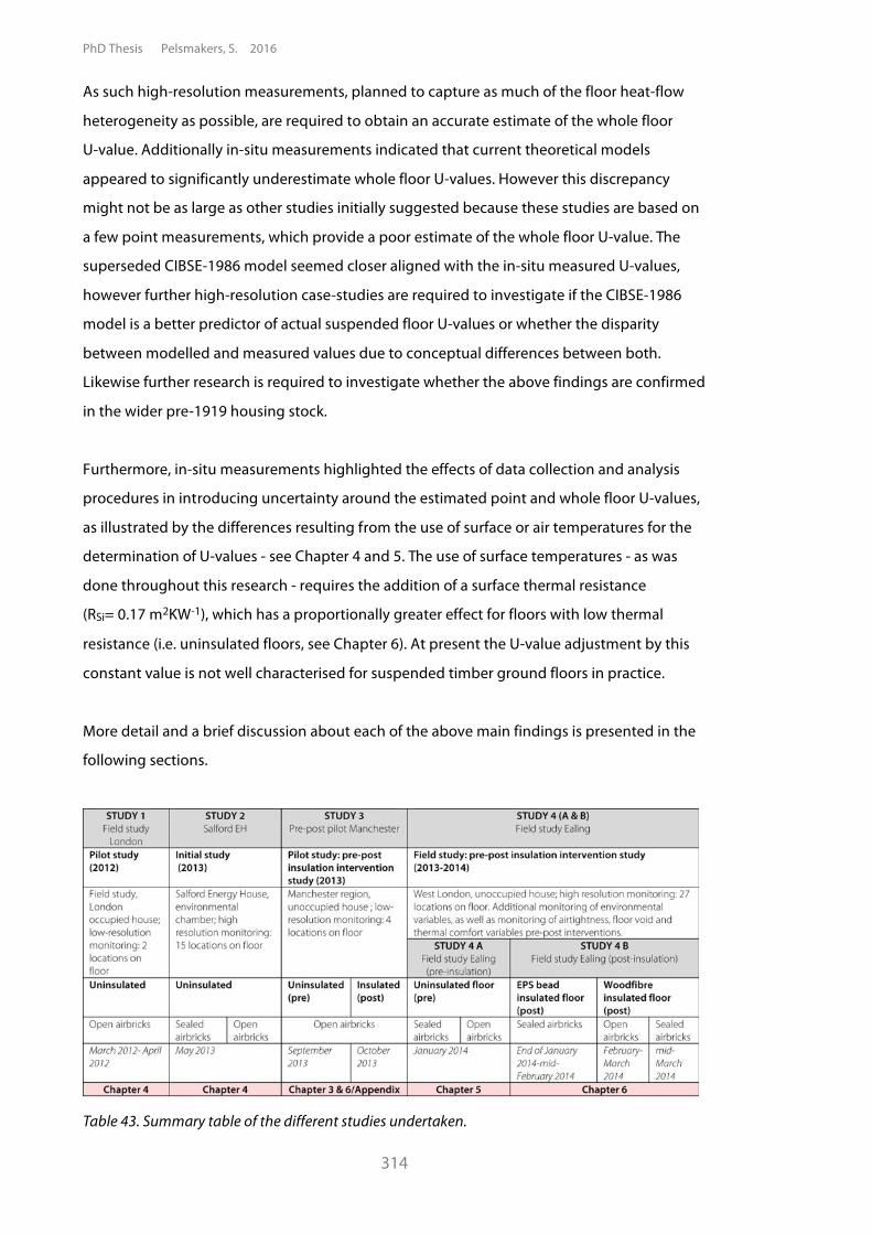
PhD Thesis Pelsmakers, S. 2016
314
As such high-resolution measurements, planned to capture as much of the floor heat-flow
heterogeneity as possible, are required to obtain an accurate estimate of the whole floor
U-value. Additionally in-situ measurements indicated that current theoretical models
appeared to significantly underestimate whole floor U-values. However this discrepancy
might not be as large as other studies initially suggested because these studies are based on
a few point measurements, which provide a poor estimate of the whole floor U-value. The
superseded CIBSE-1986 model seemed closer aligned with the in-situ measured U-values,
however further high-resolution case-studies are required to investigate if the CIBSE-1986
model is a better predictor of actual suspended floor U-values or whether the disparity
between modelled and measured values due to conceptual differences between both.
Likewise further research is required to investigate whether the above findings are confirmed
in the wider pre-1919 housing stock.
Furthermore, in-situ measurements highlighted the effects of data collection and analysis
procedures in introducing uncertainty around the estimated point and whole floor U-values,
as illustrated by the differences resulting from the use of surface or air temperatures for the
determination of U-values - see Chapter 4 and 5. The use of surface temperatures - as was
done throughout this research - requires the addition of a surface thermal resistance
(RSi= 0.17 m2KW-1), which has a proportionally greater effect for floors with low thermal
resistance (i.e. uninsulated floors, see Chapter 6). At present the U-value adjustment by this
constant value is not well characterised for suspended timber ground floors in practice.
More detail and a brief discussion about each of the above main findings is presented in the
following sections.
Table 43. Summary table of the different studies undertaken.
Chapter 7: Conclusions, reflections and further research
315
7.2.1. Floor U-values This section summarises the findings related to the first part of the second research question
"What is the in-situ measured thermal transmittance of floors and how does it compare to model
predictions?".
The analysis of the data presented in Chapters 4 and 5 demonstrated that - in line with
physical theory - suspended timber ground floors had increased thermal transmittance along
the perimeter (H2). There was also a large variation of Up-values (H1), related to the varying
airflow through airbricks and distance from the exposed perimeter walls. It was also
observed that increased sub-floor ventilation through open airbricks increased the thermal
transmittance compared to sealed airbricks (H3). These effects were clearly observed in the
Salford EH (STUDY 2) and the field case-study (STUDY 4A), though for STUDY 4 there was
considerable uncertainty due to the short-term monitoring period - see Chapter 5.2.3 and
5.3.7.
The specific results observed in these two cases are not directly representative of the entire
pre-1919 housing stock, however the trends arising from physical principles are likely to be
transferable. The analysis of these two studies also highlighted that some dwelling-specific
characteristics can interact with the theoretical expectations. For instance, in both cases the
floors had structural properties affecting the airbrick airflow in the void: sleeper wall
presence in STUDY 4 and joist direction and large joist depths in STUDY 2 might have
enhanced the perimeter effect by acting as an obstruction to airflow to the rest of the void
and buffering other floor areas, leading to lower observed Up-values elsewhere. This
highlights that the research needs to be considered on a case-by-case basis if detailed
knowledge is required.
Furthermore, in the field study low void airflow was measured away from the airbricks,
though the results from one single dwelling can only highlight that this observation needs to
be verified in a larger sample to identify whether this is a general phenomenon or specific to
this dwelling and/or due to how the research was undertaken and how the data was
collected, as discussed in Chapter 5. Two further important parameters that need to be
analysed in a larger sample are the number and position of airbricks (below or between
joists) as a function of floor area and exposed perimeter to understand the impact of these
variables on floor thermal transmittance better.
PhD Thesis Pelsmakers, S. 2016
316
In summary, the results presented in Chapters 4, 5 and 6 have shown that the variation of
Up-values across the floor and the perimeter effect (and 'airbrick effect') are a general floor
thermal performance trend and at the same time are an intrinsic property of each floor and
dependent on each floor's characteristics.
7.2.2. In-situ heat-flux measuring techniques This section addresses the first research question "How should in-situ suspended timber ground
floor U-values be estimated?". The research highlighted that recording representative and
repeatable in-situ measurements as well as transparency about analysis and uncertainty
estimation are an essential component of insightful research and performance evaluation to
enable comparison between studies and with models. Chapters 3, 4, 5 and 6 highlighted the
complexity of estimating in-situ U-values for suspended timber ground floors and comparing
these results with models and other studies. Particularly significant are the impact of
different data collection and analysis techniques, especially sensor positions, monitoring
research design and analysis techniques on estimated U-values. The inhomogeneity of room
temperatures makes the use of air temperatures for the determination of floor U-values
challenging: depending where air temperatures were measured, different U-values were
estimated. While use of surface temperatures is more practical and might be more replicable,
this also had associated uncertainties due to the addition of a constant surface thermal
resistance; though in the field these results were observed within the margins of error.
Further research is required in this area.
It was observed that low-resolution in-situ pre-post studies are at risk of over- or
underestimating the insulation efficacy, depending on where measurements were made.
Hence a high-resolution in-situ measuring approach, i.e. where many point-locations on the
floor are monitored, is generally applicable, and reduces the biases that perimeter effect and
construction heterogeneities are likely to cause to low-resolution measuring approaches.
Comparing U-values obtained from paired sensors with the whole floor estimated
U-value highlighted the limitations of low-resolution monitoring. Based on STUDY 2 and
STUDY 4, only a small proportion of the paired sensor locations would overlap with the
whole floor U-value error margins obtained from high-resolution monitoring. For this small
proportion, generally combinations of two central floor locations or a combination of one
perimeter and one rear point location were closest to whole floor U-values, though sensors in
central floor locations might not be practical to monitor in occupied dwellings. The better
insulated a floor, the lower the spread of Up-values as was the case for the bead-insulated
floor (with sealed airbricks).
Chapter 7: Conclusions, reflections and further research
317
In these conditions a low-resolution measurement might have a slightly better chance of
reflecting the whole floor U-value; however it is often not until measuring at high
resolution that the above can be confirmed. A large uncertainty still remains when
obtaining whole floor U-value estimates from just a few point measurements.
Additionally, further high-resolution monitoring in a larger sample is required to investigate
if these observations are more broadly confirmed. A high-resolution measuring approach is
especially valuable when comparing whole floor in-situ U-values to models, because models
treat the floor as a whole, and thus the in-situ measurements must be strongly
representative of the whole floor. High resolution monitoring is also required to understand
the effect of a different number of airbricks, sleeper walls etc.
Finally, in-situ measurements have a level of uncertainty associated with the estimation of
U-values, such as instrument error (intrinsic), measuring condition errors (extrinsic errors)
and the natural variability of U over the monitoring period as an inherent characteristic of an
element's actual thermal transmittance in dynamic situations. The applied uncertainty
estimation in this thesis drew on the ISO-9869 standard for intrinsic and extrinsic error
estimates. However the natural variability of U was estimated by the standard deviation (sd)
of daily or hourly U-values in the field or in the thermal chamber respectively. U-values and
their final uncertainties must be clearly communicated to instil confidence in findings and
comparisons between studies and interventions so as to avoid drawing inaccurate
conclusions.
The refined in-situ heat-flux measuring techniques developed in this research (including
error- and data analysis techniques and presentation of results) and the value of high-
resolution data collection have wider applicability and transferability and are likely to be
advantageous to in-situ heat-flux monitoring campaigns of other construction elements.
7.2.3. Predicted versus measured U-values This section addresses the second research question "What is the in-situ measured thermal
transmittance of floors and how does it compare to model predictions?"
U-value models are based on simplified inputs and assumptions and the floor is
modelled as a whole. Both models and in-situ heat-flux measurements are two
complementary approaches to the understanding and determination of whole floor
U-values. Models take advantage of physical theory, which require in-situ measurements to
be validated and refined.
PhD Thesis Pelsmakers, S. 2016
318
In-situ heat-flux measurements take advantage of the theoretical framework of models to
identify and refine what and where to measure in a real world setting. Differences between
models and in-situ results provide an opportunity to understand more deeply both
approaches and improve both. However, at present in-situ data is generally based on few
floors measured at low resolution, which hinders both the advancement of both in-situ
measuring techniques for floors and validating modelling approaches. The data presented in
this thesis is thus an opportunity to start to evaluate how and why high-resolution in-situ
data and models differ.
While whole floor in-situ U-values estimated from high-resolution monitoring allowed
direct comparison to models, other model assumptions made the direct comparison of
results less straightforward (e.g. assumed negligible ground thermal mass, assumed material
conductivities, wind-speeds etc.). Additionally, there might be some conceptual differences
between modelled and in-situ measured floor U-values: for instance inhomogenous room
temperatures, short-term thermal mass effects and dynamic external conditions occur in
reality while floor U-value models assume annual steady-state heat-flow as a proxy for
seasonal heat-transfer. Floor U-value models also exclude linear floor/wall thermal bridge
junctions; but in-situ measurements might have been affected by heat-flow through such
junctions. It remains unclear however what the individual or combined impact is of these
variables on the modelled outputs and how this affects comparison with in-situ
measurements - further research is required.
For both high-resolution STUDY 2 and STUDY 4A, U-values from current models
appeared to underestimate the in-situ measured whole floor U-values (e.g. 1.04±0.12
Wm2K-1 for STUDY 4A versus 0.57 Wm2K-1 when modelled with ISO-13370). In STUDY 4B,
the divergence between modelled and in-situ measured floor U-values reduced the
better insulated the floor became: 0.36±0.11 Wm2K-1 in-situ measured versus 0.23
Wm2K-1 modelled and 0.09±0.03 Wm2K-1 in-situ measured versus 0.08 Wm2K-1 when
modelled, for woodfibre and bead insulated respectively. Different input assumptions
and different models could significantly diverge U-value predictions, such as assumed
ground conductivities and assumed airbrick openings and wind-speeds. For the floors
studied, the withdrawn CIBSE-1986 floor U-value model appeared to better match the
in-situ measured whole floor U-value compared to the other (more recent) models,
though this match was also very dependent on model assumptions and further research
is required to investigate if this model is a better predictor of actual floor U-values.
Chapter 7: Conclusions, reflections and further research
319
The importance of model assumptions and the value of actual in-situ survey information
could be seen when adjusting the woodfibre floor U-value model following in-situ
observations of reduced perimeter insulation near airbricks and presence of airgaps.
Adjusting modelled U-values for this slightly reduced the divergence between modelled and
in-situ U-values, highlighting also the value of in-situ measurements for increased model
accuracy. However, further research is also required whether the disparity between modelled
and measured values is real or due to conceptual differences between both.
Based on STUDY 4B, current models slightly underestimated the efficacy of insulation
interventions, mainly because they significantly underestimated the initial uninsulated floor
U-value. If these findings are more broadly confirmed for a larger sample, it could have
potentially large impacts on homeowner choices and policy direction for the UK housing
stock.
7.2.4. Insulating floors: impact on floor heat loss and thermal
comfort The third thesis research question "How does the in-situ thermal performance of a case-study
floor change after intervention measures?" and its related question (3.1.) "What are the thermal
comfort implications of insulated and uninsulated floors?" are important given that there are
millions of floors yet to be insulated but it is unknown what the actual benefits of doing so
are.
Chapter 6 demonstrated that insulating floors can lead to significant U-value reductions
(overall 65% reduction with 100mm woodfibre, and 92% when full-filling the void with EPS
beads and sealing airbricks). Both the modelled U-values of the floor interventions met the
recommended regulatory recommendations for floor upgrades. However, despite the
significant thermal transmittance reductions, the in-situ estimated woodfibre insulated
whole floor U-value fell short of the recommended regulatory design value. This was because
the in-situ estimated floor U-value was initially higher than assumed, while models also
excluded installation quality issues and areas of reduced insulation. However the discrepancy
between modelled versus in-situ measured values reduced the better insulated the floor. The
bead filled void intervention met the recommended regulatory U-values for upgrading floor
structures, however there may be unintended consequences associated with this
intervention, which were not investigated here due to the short-term monitoring intervals.
PhD Thesis Pelsmakers, S. 2016
320
After insulation the perimeter effect was reduced, though a reduced spread of Up-values was
only observed for the bead insulated floor, due to the sealing of the airbricks and
introduction of a large thermal resistance in the void. However, the woodfibre insulated floor
still had a large spread of Up-values, likely due to the open airbricks and insulation
installation heterogeneities. This result highlighted that installation quality is likely to be
important to maximise thermal transmittance reduction: a tight fit between insulation
material and joists and floorboards is essential to avoid thermal bypasses; special attention
along the perimeter walls and near airbricks is required - though this may be easier to
achieve in dwellings with airbricks below instead of in between joists. No increased dwelling
airtightness was observed post-insulation for the woodfibre floor studied due to the lack of
specific airtightness measures undertaken alongside the interventions and due to insulation
installation quality near the perimeter and airbricks. Sealing of airbricks however improved
dwelling airtightness, and was measured outside the margins of error for the uninsulated
floor but within the margins of error for the insulated floors. For STUDY 4B, the findings
indicate that without taking specific airtightness measures while installing floor insulation,
there might be a missed opportunity for improved airtightness.
Energy and carbon reductions are not the only reasons to consider upgrading floors: a
benefit of insulating the ground floor is to increase occupant thermal comfort. Given that the
studies were undertaken in unoccupied spaces, no occupant thermal comfort surveys were
undertaken but instead comparisons of monitored variables were made against thermal
comfort thresholds. The results presented in Chapter 6.5. indicated that thermal comfort
might be positively affected by insulating the floor (especially warmer floor surface
temperatures), though generally the improvements were small and even after insulation, the
thermal comfort thresholds were not met.
Due to the short-term nature of the insulation interventions, the impact of insulation on floor
void conditions could not be studied and this has been highlighted for further research.
Chapter 7: Conclusions, reflections and further research
321
7.3. Research limitations and further research The case-study approach used in this thesis could not provide population-wide inferences,
though it allowed testing specific hypotheses, which can be the basis for further work and
wider generalisation. A number of limitations (some, such as case availability, were
unavoidable) became apparent both in the research approach and in the data available,
though understanding these limitations presents novel and further research opportunities.
Throughout this research it became apparent that both longer-term studies and larger
samples are necessary to investigate whether the trends and observations from this research
replicate across other floors and to be able to infer strong conclusions for the wider UK
housing stock. Five main and interconnecting areas for further research were identified and
are discussed overleaf.
A. High-resolution floor heat-flow should be monitored in a much larger sample,
including different dwelling types and floor and void typologies and located in different UK
geographical locations to understand if the research findings transfer to the wider UK
housing stock. Secondly, longer measuring periods to improve the understanding of
seasonal influences, and measurement of model input variables might help to refine model
input assumptions and reduce disparities between modelled and in-situ measured U-values
(and help clarify the impact of some of the conceptual differences). In particular it might be
useful to measure party-wall and foundation wall heat-fluxes, ground temperatures,
moisture content and ground heat-fluxes at different depths. Such additional variables
might also aid model refinement and investigation of other models, including the
development of archetype (floor) stock models and studies of linear thermal bridging.
Further investigation of void obstructions (e.g. sleeper walls) and impact on sub-floor heat-
flow and airflow (requiring multi-directional void measurements) would add to this study.
Further research might include additional air temperature measurements and room airflow
to investigate the thermal resistance of the surface boundary layer across the floor. Isolating
the effect of void service pipes and the 'heat recovery' of downward heat-flow by stack effect
would add to the understanding of the complexity of floor heat loss.
B. In-situ measuring techniques could be further refined and developed for
occupied houses and for purposeful low resolution measuring to understand the ‘minimum’
high resolution monitoring needed. Further research into which internal temperatures to use
alongside a detailed study of the impact of airflow on surface resistances in different
locations on the floor will help refine the data- and error analysis (and model assumptions).
Dynamic data analysis might also be beneficial but is undeveloped at present for floors.
PhD Thesis Pelsmakers, S. 2016
322
Adapting blower-door tests to measure the airtightness of the floor separately and use of
void tracer gases would enable a more detailed study of upward floor void airflow in order to
understand the floor air leakage paths. Developing larger heat-flux plate transducers - as
described by Cox-Smith (2008a) and Isaacs (1985b) - instead of the current heat-flux sensors
used might also be of benefit.
C. Thermal comfort implications of cold surfaces, vertical stratification and pre/post
insulation interventions need to be further investigated in a larger sample and in occupied
dwellings where it is possible to enable occupant thermal comfort surveys. Additionally,
further research into compensating energy use from local thermal discomfort (including
cold surfaces and upward draughts) is needed to fully understand the implications of
occupant discomfort on energy use behaviour. The author received a World University
Network (WUN) grant with contributions from the Sheffield School of Architecture and the
architecture department at Sydney University to research the "Effect of uninsulated floors on
occupant thermal comfort" at Professor de Dear's Internal Environmental (IEQ) Lab in Sydney
(August-September 2016).
D. Future floor insulation studies would benefit from a wider variety of insulation
materials and methods and longer-term in-situ heat-flux measuring both pre-and post-
intervention, leading to a financial pay-back analysis of different measures. This should
include the investigation into the efficacy of underlay and carpet and perimeter insulation
only, and the viability of sealing of airbricks over winter alongside RH monitoring as less
disruptive and more cost-effective heat loss reduction solutions. More research is also
required to fully understand the impact of insulation installation and airtightness practices
on the efficacy of floor heat loss interventions, which can inform industry practice. Finally,
research is required to investigate changing floor void conditions and the impact of
insulating the floor on neighbouring (uninsulated) floors and vice versa.
E. mould growth risk research was significantly constrained in this study due to the
short-term nature of the study. Mould growth is a precursor to fungal decay and structural
damage, and an important consideration is that mould spores could transfer from the void to
the living space, and can pose a health hazard. Undertaking floor upgrades to reduce energy
use and increase occupant thermal comfort need to be carefully balanced with the effect this
might have on floor void conditions, however the possible risks of insulation in terms of
mould or fungal growth are poorly characterised in the UK. Hence it will be important to
focus on long term pre/post intervention monitoring to investigate the effects of airbrick
sealing and how void conditions change after insulation for a variety of case-studies.
Chapter 7: Conclusions, reflections and further research
323
A long-term monitoring programme of a large sample of (for example ECO-insulated floors)
would support this investigation, alongside development and validation of mould growth
models specifically for pre-1919 UK suspended ground floors. Finally, long term
characterisation of void ventilation, stack airflow and pressure differentials between
void/external/internal spaces with air sampling might support increased understanding of
mould spore transfer to indoor spaces, and support their potential health effects. The impact
of different ventilation mechanisms and improved airtightness as part of building retrofit on
void air flow also requires further study. This research is intended to be expanded in
collaboration with Professor Airaksinen at VTT in Finland.
7.4. Policy implications
Despite slow uptake of floor insulation, thousands of floors were insulated as part of the
ECO-policy, yet the impact on heat loss reduction and on thermal comfort and floor void
conditions remains poorly characterised. STUDY 4B demonstrated that significant U-value
reductions could be achieved by insulating floors. As there are millions of uninsulated floors,
scaling-up those reductions could lead to potentially significant energy and associated
carbon emissions reductions across the existing housing stock. However, a better
understanding of the impact of heat loss reduction measures on floor void conditions is
critical to avoid jeopardising occupant health - as highlighted in further research.
STUDY 4 highlighted that proportional floor heat-flow might be significantly greater
than assumed at present and that estimated proportional U-value reductions might
exceed those assumed by models. If these above observations are more broadly
confirmed in the pre-1919 housing stock, it might create a barrier to robust retrofit
decision-making for consumers, industry and policy-makers. Firstly, if the floor U-value is
underestimated and if efficacy of interventions is also underestimated, floors might be
left uninsulated, possibly compounded by the disruption involved in insulating ground
floors. Secondly, the estimated pay-back of upgrade measures on which decisions are
based, might also exceed the !15 year payback stipulation for regulations to apply,
reducing incentives to insulate floors. Yet in reality the actual space-heating energy
reductions might be much greater than assumed with faster payback. Thirdly, a low floor
U-value prediction discourages the insulation of floors, focusing attention on other fabric
interventions such as walls and roofs first. This strategy might be particularly flawed for
ground floor apartments as proportional floor heat-transfer is likely to be more significant
than other fabric elements. Finally, erroneous assumptions about the final floor
performance post-insulation can lead to erroneous stock and forecasting models based
on those assumptions.
PhD Thesis Pelsmakers, S. 2016
324
The first step to reducing these possible uncertainties is a high-resolution in-situ measuring
campaign of a larger sample and variety of floors, as described in the previous section.
Further possible policy implications, which require further study of floors:
• There are uncertainties associated with floor U-value models, including ISO-13370 on which
(Rd)SAP is based and which is used in the UK for regulatory approval, policy and funding
decision-making. Research is required into the model assumptions and suitability of its
conceptual approach for suspended timber ground floors to ensure policy and retrofit
decision-making is underpinned by suitable models.
• Default RdSAP assumptions lead to a certain percentage improvement in dwelling
airtightness from insulating floors. However, this study supported other research suggesting
that without specific additional floor airtightness measures, airtightness improvements might
be limited. Likewise, default RdSAP assumptions are 150mm insulation in between joists,
which might often not be achieved because of joist depth and airbrick locations. Policy-
making must reflect the practical limitations of achieving this level of insulation and
airtightness and this should be reflected in stock models and energy-reduction assumptions
and allowed for in payback assumptions and models. For instance, the woodfibre insulated
in-situ floor U-value in this study fell short of meeting the recommended regulatory and
modelled floor U-value post-intervention due to technical detailing and installation
quality issues likely to exist in other floor insulation installations elsewhere. At present
guidance for floor insulation is limited and little attention is given to practicalities and
details of insulating floors. Industry and policy guidance could highlight the importance
of separate airtightness measures and insulation installation quality to maximise floor
heat loss reduction.
• It is unknown whether the current regulatory design U-value recommendations for floor
upgrades have a negative impact on floor void conditions and associated occupant health.
Thus regulatory recommendations and tools such as RdSAP should be based on much larger
in-situ evidence and recognise practical and technical limitations, as well as inter-connections
between floor U-values and floor void humidity and risk of mould growth and associated risks
to occupant health issues.
• Due to the decision-making implications, researchers themselves need to be aware of the
uncertainties associated with modelling and in-situ estimated U-values and communicate
them clearly to policy-makers and industry. Government policy especially should be made
with these uncertainties in mind.
Clearly, improving the in-situ characterisation of floor heat loss and their likely variation will
facilitate a more accurate prediction of the current performance and hence supports a more
accurate prediction of the impact and risks of interventions in support of carbon reduction
policies in the UK housing stock.
Chapter 7: Conclusions, reflections and further research
325
7.5. Conclusion In summary, this research contributed to an increased understanding of suspended timber
ground floor thermal performance and methodological approaches of in-situ measuring of
floors. The practical difficulty of having access to floors and instruments for research
purposes meant that only a few cases were available for in-situ measurement. Nevertheless
the in-situ results verified physical theory and that there was a large spread of Up-values
across the uninsulated floor with increased Up-values closer to the exposed perimeter. The
large variation of Up-values across the floor and the perimeter effect remained but reduced
for the insulated floor. Furthermore, based on the few case studies, disparities between in-
situ measured and modelled floor U-values were identified and suggested that current floor
U-values may underestimate the actual floor system's thermal transmittance. This modelled
and in-situ measured disparity reduced the better insulated the floor was.
Significant thermal transmittance reductions were achieved from insulating the floor
(between 65% and 92%, depending on method), however improved dwelling airtightness
after insulating floors was not observed. Improved airtightness of up to 21% was observed
for sealing of airbricks, which also reduced the floor U-value (17 to 31% depending on case
study)2. Some key thermal comfort indicators appeared slightly improved for insulated floors,
but the floor studied did not meet several thermal comfort thresholds, even post-insulation.
With regards to floor void conditions, longitudinal studies are required for analysis and this
was outside the scope if this PhD research.
The data collected for this thesis highlighted that the thermal behaviour of floors is complex
and affected by a number of environmental and structural factors. Interventions aiming to
change the thermal behaviour of floors are themselves affected by those environmental and
structural factors which need to be considered to maximise the benefit of floor insulation.
This thesis research also identified a number of issues (measuring approaches, actual
U-values, heat loss reductions from interventions, model versus in-situ measurement
disparities) with significant practical and policy implications. It also highlighted the
importance of appropriate data uncertainty assessment and the need to report research
findings and procedures transparently.
2 For Study 4 there was considerable uncertainty due to the short-term monitoring period. See Chapter 5.3.7.
PhD Thesis Pelsmakers, S. 2016
326
Furthermore the methodological considerations about in-situ floor measurements are likely
to have wider applicability to other cases and research of floor U-value estimations in the
future: a direct implication of the large spread of Up-values is that a limited number of
U-value point measurements are highly unlikely to be representative of the whole floor's
U-value. Instead, high-resolution measurements are required, which is a departure from
current monitoring campaigns. Furthermore, the refined in-situ heat-flux measuring
techniques, including high-resolution data collection developed in this research, have wider
applicability and are transferable to in-situ heat-flux monitoring campaigns of other
construction elements.
Finally, if the modelled underestimation of actual floor U-values is more broadly
confirmed in the pre-1919 housing stock, it would have significant implications for
policy and retrofit decision-making.

References
327
References
PhD Thesis Pelsmakers, S. 2016
328
ADJALI, M. H., DAVIES, M. & REES, S. W. 2004. A comparative study of design guide calculations and measured heat loss through the ground. Building and Environment, 39, 1301-1311. ADJALI, M. H., DAVIES,M., REES,S.W., LITTLER,J. 2000. Temperatures in and under a slab-on-ground floor:
two- and three-dimensional numerical simulations and comparison with experimental data. Building and Environment, Elsevier, 35(2000), 665-662.
AIRAKSINEN, M. 2003. MOISTURE AND FUNGAL SPORE TRANSPORT IN OUTDOOR AIR-VENTILATED CRAWL SPACES IN A COLD CLIMATE - REPORT A7. PhD, Helsinki University of Technology.
AIRAKSINEN, M. 18.11.2013 2013. RE: Meeting with Prof. Miimu Airaksinen regarding VTT mould growth model & data collection for crawl spaces (18.11.2013). Type to PELSMAKERS, S.
AIRAKSINEN, M., JARNSTROM, H., KOVANEN, K., VIITANEN, H., SAARELA, K. Ventilation and building related symptoms. Proceedings of Clima 2007 WellBeing Indoors, 2007.
AIRAKSINEN, M., KURNITSKI, J., PASANEN, P., SEPPANEN, O. n.d. FUNGAL SPORE TRANSPORT THROUGH A BUILDING STRUCTURE.
AIRAKSINEN, M., PASANEN, P., KURNITSKI, J. & SEPPANEN, O. 2004. Microbial contamination of indoor air due to leakages from crawl space: a field study. Indoor Air, 14, 55-64.
ANDERSON, B. 1991a. U-values of uninsulated ground floors: Relationship with floor dimensions. Building Services Engineering Research and Technology, 12(3).
ANDERSON, B. 2006. Conventions for U-value calculations. BRE. ANDERSON, B., CHAPMAN, P.F., CUTLAND, N.G, DICKSON, C.M., HENDERSON, G., HENDERSON, J.H., ILES, P.J.,
KSOMINA, L., SHORROCK, L.D. 2001. BREDEM-12 Model Description. Watford: BRE. ANDERSON, B. R. 1984. SITE-TESTING THERMAL PERFORMANCE: a CIB survey. Taylor & Francis. ANDERSON, B. R. 1991b. Calculation of the Steady-State Heat Transfer Through a Slab-on-Ground Floor.
Building and Environment, 26, 405-415. ANDERSON, M. J. 2003. Design and analysis of monitoring andexperiments for environmental scientists.
Ravenna: University of Auckland. ARENS, E., HUMPHREYS, M. A., DE DEAR, R. & ZHANG, H. 2010. Are ‘class A’ temperature requirements
realistic or desirable? Building and Environment, 45, 4-10. ASHRAE. ASHRAE Recommended practices for controlling moisture in crawl spaces -. In: ASHRAE, ed. Ashrae
Transactions 1994, Symposium on recommended practices for controlling moisture in crawl spaces - a collection of papers, 1994 New Orleans, Louisiana. ASHRAE.
ASHRAE 2013a. ANSI/ASHRAE Standard 55-2013 - Thermal Environmental Conditions for Human Occupancy. Atlanta: ASHRAE.
ASHRAE 2013b. BSR/ASHRAE Standard 55P, Thermal Environmental Conditions for Human Occupancy (draft). Atlanta: ASHRAE.
ASTM 2007a. C1046-95(2007) Standard Practice for In-Situ Measurement of Heat Flux and Temperature on Building Envelope Components. USA: ASTM international.
ASTM 2007b. C1155 – 95(2007)Standard Practice for Determining Thermal Resistance of Building Envelope Components from the In-Situ Data. USA: ASTM International.
ASTM 2007(2012). ASTM C1130: Standard Practice for Calibrating Thin Heat Flux Transducers. USA: ASTM International.
ASTM 2013a. C1046-95(2013) Standard Practice for In-Situ Measurement of Heat Flux and Temperature on Building Envelope Components. USA: ASTM international.
ASTM 2013b. C1155 – 95(2013)Standard Practice for Determining Thermal Resistance of Building Envelope Components from the In-Situ Data. USA: ASTM International.
ATTMA 2010. TECHNICAL STANDARD L1. - MEASURING AIR PERMEABILITY OF BUILDING ENVELOPES (DWELLINGS). Northampton: The Air Tightness Testing & Measurement Association c/o the British Institute of Non-Destructive Testing.
AUDENAERT, A., BRIFFAERTS, K. & ENGELS, L. 2011. Practical versus theoretical domestic energy consumption for space heating. Energy Policy, 39, 5219-5227.
BAELI, M. 2013. Residential retrofit: 20 case studies, London, Riba Publishing. BAKER, P. 2011a. In situ U-value and ‘co-heating’ test measurements in a traditional house at New Bolsover,
Derbyshire. Glasgow Caledonian University. BAKER, P. 2011b. Technical Paper 10: U-values and traditional buildings. In situ measurements and their
comparisons to calculated values. In: HISTORIC SCOTLAND, C. G. (ed.). Glasgow Glasgow Caledonian University.
BALES, E., BOMBERG, M., COURVILLE, G.E. 1985. Building applicatons of heat flux transducers - ASTM Special Technical Publication 885, USA, ASTM.
References
329
BANFILL, P., SIMPSON, S., HAINES, V., MALLABAND, B. Energy-led retrofitting of solid wall dwellings - technical and user perspectives on airtightness. In: RUDDOCK, L. E. A. E., ed. COBRA 2011 - Proceedings of the RICS Construction and Property Conference, 12-13th September 2011, 2011 University of Salford, Manchester, UK. COBRA 2011 - the Royal Institution of Chartered Surveyors In- ternational Research Conference, 430-440.
BARKER BAUSELL, R. 1994. Conducting meaningful experiments - 40 steps to becoming a scientist, USA, Sage Publications.
BARRETT M, L. R., ORESZCZYN T,STEADMAN P 2006. How to support growth with less energy. BASSET, M. R. 1988. Natural Airflows between Roof, Subfloor, and Living Spaces. In: AIVC (ed.) AIVC 9th
Conference. Belgium. BAYLESS., D. n.d. Statistical Rejection of “Bad” Data – Chauvenet’s Criterion [Online]. Ohio University
Available: http://www.ohio.edu/people/bayless/seniorlab/chauvenet.pdf [Accessed 01.03 2015].
BBA 2014. BBA Agrement Certificate Warmfill Ltd - 02/3938 (Warmfill Silver). Warford British Board of Agrement.
BEAUMONT, A. 2007. W07 - Housing regeneration and maintenance - Hard to Treat Homes in England. International Conference - Sustainable Urban Areas. Rotterdam.
BELL, M., LOWE, R. 2000. Energy efficient modernisation of housing: a UK case study. Energy and Buildings, 32(2000), 267-280.
BELL, M., WINGFIELD, J., MILES-SHENTON, D. & SEAVERS, J. 2010. Low carbon housing: lessons from Elm Tree Mews. Joseph Rowntree Foundation, York.
BERNIER, P., AINGER, C. & FENNER, R. A. 2010. Assessing the sustainability merits of retrofitting existing homes. Proceedings of the ICE - Engineering Sustainability, 163, 197-207.
BILLINGTON, N. S. 1948. THE WARMTH OF FLOORS—A PHYSICAL STUDY. The Journal of Hygiene 46(4), 445-450.
BIRCHALL, S., PEARSON, C., BROWN, R. 2011. Solid Wall Insulation Field Trials - Report Baseline Performance of the Property Sample. London.
BOARDMAN, B., DARBY, S., KILLIP, G., HINNELLS, M., JARDINE, C.N., PALMER, J., SINDEN, G. 2005. 40% house. Oxford: Environmental Change Institute, University of Oxford.
BOS, K. V. D. 16.02.2012 2012. RE: HPF01 - measuring soil fluxes. Type to PELSMAKERS, S. BRAGER, G., ZHANG, H. & ARENS, E. 2015. Evolving opportunities for providing thermal comfort. Building
Research & Information, 43, 274-287. BRE 1991. BRE Digest 364 - Design of timber floors to prevent decay. In: BRE (ed.). BRE 1998. Good repair guide 17 - repairing and replacing ground floors. BRE 2000. Good Practice Guide 294, Refurbishment guidance for solid-walled houses - ground floors. BRE 2011. The government's Standard Assessment Procedure for Energy rating of dwellings, SAP 2009,
incorporating RdSAP 2009. Watford: BRE. BRE 2012. RdSAP 2009: Appendix T: Improvement measures. BRE 2014a. BRE Report: In-situ measurements of wall U-values in English housing. Watford: BRE. BRE 2014b. SAP 2012 - The Government's Standard Assessment Procedure for Energy Rating of Dwellings,
2012 edition. Watford: BRE. BRE 2014c. Solid wall heat losses and the potential for energy saving - literature Review. Watford: BRE BROOK, D. 1994. Home Moisture problems (reprinted 2008). Oregon State University. BSI 1998. Thermal performance of buildings: Qualitative detection of thermal irregularities in building
envelopes: Infrared method - BS EN 13187-1999. London: BSI. BSI 2001. BS EN - 13829:2001 - Thermal performance of buildings - Determination of air permeability of
buildings - Fan pressurization method. BSI 2002. Ergonomics of the thermal environment — Instruments for measuring physical quantities. BS EN
ISO 7726:2001. BSI 2006. Ergonomics of the thermal environment — Analytical determination and interpretation of
thermal comfort using calculation of the PMV and PPD indices and local thermal comfort criteria. BS EN 7730:2005.
BSI 2007. Building components and building elements - Thermal resistance and thermal transmittance - Calculation Method ISO 6946: 2007). London: ISO.
BSI 2008. Thermal bridges in building construction — Linear thermal transmittance — Simplified methods and default values (ISO 14683:2007). London: BSI.
BSI 2009a. Thermal bridges in building construction - Heat flow and surface temperatures - Detailed calculations (ISO 10211: 2007). London: BSI Group.
BSI 2009b. Thermal performance of buildings - Heat transfer via the ground - Calculation methods ( ISO 13370:2007). Brussels: BSI.

PhD Thesis Pelsmakers, S. 2016
330
BSI 2014. ISO 9869-1:2014- Thermal insulation — Building elements — Insitu measurement of thermal resistance and thermal transmittance; Part 1: Heat flow meter method. BSI.
BUILDDESK 2012. Build Desk U 3.4.: Build Desk. BURKE, S. n.d. Advantages and Risks Associated with Crawl Space Foundations. Lund University. BYRNE, A., BYRNE, G., DAVIES, A. & ROBINSON, A. J. 2013. Transient and quasi-steady thermal behaviour of a
building envelope due to retrofitted cavity wall and ceiling insulation. Energy Buildings. Elsevier. CCC 2011. Household Energy Bills- impacts of meeting carbon budgets. London: Committee on Climate
Change. CEN 1996. NEN-EN 12494-1996 - Building components and elements: in situ measurement of the surface
to surface thermal resistance. CEN. CESARATTO, P. G. & DE CARLI, M. 2012. A measuring campaign of thermal conductance in situ and possible
impacts on net energy demand in buildings. Energy and Buildings. Elsevier. CESARATTO, P. G., DE CARLI, M. & MARINETTI, S. 2011. Effect of different parameters on the in situ thermal
conductance evaluation. Energy and Buildings. Elsevier. CHAPMAN, J. L., R. AND EVERETT, R 1985a. The Pennyland Project - ETSU- S- 1046(S). Milton Keynes Open
University. CHAPMAN, J. L., R. AND EVERETT, R 1985b. The Pennyland Project - ETSU- S- 1046(S) - Executive Summary.
ETSU. Milton Keynes: Energy Research Group, Open University CHILDS, P. R. N., GREENWOOD, J.R., LONG. C.A. 1999. Heat flux measurement techniques. Proceedings
Institution of Mechnaical Engineers, 213 Part C 655-677. CHRENKO, F. A. 1957. THE EFFECTS OF THE TEMPERATURES OF THE FLOOR SURFACE AND OF THE AIR ON
THERMAL SENSATIONS AND THE SKIN TEMPERATURE OF THE FEET. British Journal of Industrial Medicine, 14, 13-21.
CIBSE 1986. CIBSE Guide - Section A3 - Thermal properties of building structures. In: CIBSE (ed.) CIBSE Guide. UK: CIBSE.
CIBSE 1996. CIBSE GUIDE A- Section 3 - Thermal properties of building structures - Draft Version 11. UK: CIBSE.
CIBSE 2006. CIBSE GUIDE A- Environmental Design, Norfolk, CIBSE. CIBSE 2015. CIBSE GUIDE A- Environmental Design, Suffolk, UK, CIBSE. CLINCH, J. P., HEALY, J.D. 2001. Cost-benefit analysis of domestic energy efficiency. Energy Policy, 29, 113-
124. COLLINGS, J. 2008. Victorian and Edwardian Houses: A Guide to Care and Maintenance, UK, Crowood. COLLINGS, S. 30.10.2014 2015. RE: Suspended floor insulation. Type to PELSMAKERS, S. COOK, M. G. 2009. Energy Efficiency in Old Houses, Wiltshire, Crowood Press. COULTER, J. n.d. Liabilities of Vented Crawl Spaces, Their Impacts on Indoor Air Quality in Southeastern U.S.
Homes and One Intervention Strategy. COX-SMITH, I. 2008a. In-situ measurement of thermal resistance of suspended floors - Study Report SR-202
(2008). Branz. COX-SMITH, I. 2008b. Underfloor reflective foil. Branz. CROSBIE, T. & BAKER, K. 2010. Energy-efficiency interventions in housing: learning from the inhabitants.
Building Research & Information, 38, 70-79. CURRIE, J., WILLIAMSON, J.B., STINSON, J. 2013. Technical paper 19: Monitoring thermal upgrades to ten
traditional properties. In: SCOTLAND, H. (ed.). Scotland: Historic Scotland/Edinburgh Napier University.
CZAKO, A. 08.09.2015 2015. RE: Insulation material summary - Ufloor. Type to PELSMAKERS, S. CZICHOS, H., SITO, T., SMOTH LE. 2011. Springer Handbook of Metrology and Testing, Springer. D'AMELIO, V. 13-20.08.2012 2012a. RE: RE_ quick query Type to PELSMAKERS, S. D'AMELIO, V. 07.06.2012 2012b. RE: RE- URGENT Type to PELSMAKERS, S. DAVIES, M. G. 1993. Heat Loss from a Solid Ground Floor. Building and Environment, 28, 347-359. DCLG 2006. Review of Sustainability of Existing Buidings. The Energy Efficiency of Dwellings – Initial
Analysis. London: Department for Communities and Local Government. DCLG 2009. English House condition survey 2007-Annual Report. London: Comunities & local government. DCLG 2010. English Housing survey- Housing Stock Report 2008. London: Comunities & local government. DCLG 2012. English Housing Survey HOUSEHOLDS 2010-11. London: National Statistics/DCLG. DE DEAR, R. 2011. Revisiting an old hypothesis of human thermal perception: alliesthesia. Building Research
& Information, 39, 108-117. DECC 2009. Low Carbon Transition Plan. In: DECC (ed.). London: HMRC. DECC 2011a. The Carbon Plan: Delivering our low carbon future. London. DECC 2011b. Green Deal and energy company obligation - Consultation Document. London. DECC 2011c. Planning our electric future: a white paper for secure, affordable and low-carbon electricity.
References
331
DECC 2011d. Research Summary - Understanding potential consumer response to the Green Deal. In: CHANGE, D. O. E. A. C. (ed.). London: Department of Energy and Climate Change.
DECC 2012a. The Energy Efficiency Strategy: The Energy-Efficiency Opportunity in the UK. London. DECC 2012b. How the Green Deal will reflect the in-situ performance of energy efficiency measures. In: DECC
(ed.). London. DECC. 2012c. RE: Personal meeting with DECC at UCL Energy Institute, Jan 6th 2012, London. DECC 2012d. Statistical release: Experimental Statistics; Estimates of home insulation levels in Great Britain:
January 2012. In: CHANGE, D. O. E. C. (ed.). London: Department of Energy & Climate Change. DECC 2014. Green Deal and ECO measures Update 2014. DECC. DECC 2015a. Changes to green home improvement policies announced today. DECC. DECC 2015b. Data tables: Green Deal and ECO statistics. In: DECC (ed.). London: DECC. DECC 2015c. Data tables: Green Deal, ECO and insulation levels, up to September 2015. In: DECC (ed.).
London: DECC. DECC 2015d. Digest of United Kingdom Energy Statistics 2105 (DUKES). London: DECC. DECC 2015e. Domestic Green Deal, Energy Company Obligation and Insulation Levels in Great Britain,
Detailed report. In: DECC (ed.). London: DECC. DECC. 2015f. Green Deal: energy saving for your home; 6. The Green Deal Home Improvement fund [Online].
Available: https://http://www.gov.uk/green-deal-energy-saving-measures/get-money-back-from-the-green-deal-home-improvement-fund [Accessed 27.03 2015].
DELSANTE, A. E. 1989. Steady-State Heat Losses from the Core and Perimeter Regions of a Slab-on-Ground Floor. Building and Environment, 24, 253-257.
DELSANTE, A. E. 1990. A Comparison Between Measured and Calculated Heat Losses Through a Slab-on-Ground Floor. Building and Environment, 25, 25-31.
DESOGUS, G., MURA, S. & RICCIU, R. 2011. Comparing different approaches to in situ measurement of building components thermal resistance. Energy and Buildings, 43, 2613-2620.
DEWITT, C. A., BUNN, J.M. 1994. Airflow through crawl space foundation vents. Ashrae Transactions 1994, Symposium on recommended practices for controlling moisture in crawl spaces. ASHRAE.
DFPNI 2012. Building Regulations ( Northern Ireland) 2012 Guidance - Technical Booklet F1 - Conservation of fuel and power in dwellings. Department of Finance and Personnel.
DORAN, S. 2001. DETR Framework Project Report : Field investigations of the thermal performance of construction elements as built. Glasgow: BRE East Kilbride.
DORAN, S. C. B. 2008. Thermal Transmittance of walls of dwellings before and after application of cavity wall insulation.
DOUGLAS, J. 1997. The development of ground floor constructions: part II". Structural Survey, 15, 151-156. DOUGLAS, J. 1998a. The development of ground floor constructions: part 6 (subfloors). Structural Survey,
16, 193-199. DOUGLAS, J. 1998b. The development of ground floor constructions: part III (damp proofing materials).
Structural Survey, 16, 18-22. DOUGLAS, J. 1998c. The development of ground floor constructions: part IV (damp proofing methods).
Structural Survey, 16, 76-80. DOUGLAS, J. & SINGH, J. 1995. Investigating dry rot in buildings. Building Research & Information, 23, 345-
352. DOWSON, M., POOLE, A., HARRISON, D. & SUSMAN, G. 2012. Domestic UK retrofit challenge: Barriers,
incentives and current performance leading into the Green Deal. Energy Policy, 50, 294-305. DYTHAM, C. 2011. Choosing and using statistics - a biologist's guide, UK, Wiley-Blackwell. EBERHARDT, L. L., THOMAS, J. M. 1991. Designing Environmental Field Studies. Ecological Monographs, Vol.
61, No. 1 (Mar., 1991), pp. 53-73, Vol. 61, pp. 53-73. EC 2011. A Roadmap for moving to a competitive low carbon economy in 2050. Brussels: European
Commission. EDWARDS, R., HARTLESS, R., GAZE, A. 1990. Measurement of Sub-floor ventilation rates - comparison with
BREVENT predictions. In: AIVC (ed.) 11th AIVC Conference. Italy. EH 2010. English Heritage, Energy Efficiency in Historic Buildings. Insulation of Suspended timber floors. EH 2013. Improving Historic Soho's Environmental Performance - Practical Retrofitting Guidance. London:
English Heritage. EMERY, A. F., HEERWAGEN, D. R., KIPPENHAN, C. J. & STEELE, D. E. 2007. Measured and Predicted Thermal
Performance of a Residential Basement. HVAC&R Research, 13, 39-57. EST 2004. CE83 - Energy efficient refurbishment of existing housing. EST 2005a. CE97- Energy Efficiency Best Practice in Housing. Advanced insulation in housing refurbishment. EST 2005b. Energy Efficiency Best Practice in Housing Advanced insulation in housing refurbishment. London: EST.
PhD Thesis Pelsmakers, S. 2016
332
EST 2006a. CE184 - practical refurbishment of solid-walled houses. London: EST. EST 2006b. GPG171 - Domestic energy efficiency primer. EST 2006c. Post-construction testing -a professional’s guide to testing housing for energy efficiency ;
General information report 64. London: EST. EST 2007. CE83 - Energy efficient refurbishment of existing housing. London: EST. EVERETT, R. H., A. AND DOGGART, J. 1985. Linford Low Energy Houses- ETSU - S - 1025. Milton Keynes:
Energy Research Group, Open University. FARNELL. 2014. Servisol heatsink compound - Technical data [Online]. Available:
http://www.farnell.com/datasheets/319602.pdf [Accessed 11.11 2014]. FICCO, G., IANNETTA, F., IANNIELLO, E., D’AMBROSIO ALFANO, F. R. & DELL’ISOLA, M. 2015. U-value in situ
measurement for energy diagnosis of existing buildings. Energy and Buildings, 104, 108-121. FIEDLER, K., SCHUTZ, E. & GEH, S. 2001. Detection of microbial volatile organic compounds (MVOCs)
produced by moulds on various materials. International Journal of Hygiene and Environmental Health, 204, 111-21.
FITTON, R., FARMER, D., WEAVER, M. 2014. Presentation at 'Retrofit in Practice: Waht next?' workshop at the Newcastle University AHRA 'Industries of Architecture 2014 conference. Presentation title: Salford Energy House – in-depth study of a fabric whole house retrofit
. Newcastle. FLYNN, K. A., QUARLES, S.L., DOST, W.A. 1994. Comparison of ambient conditions and wood mositure
contents in crawl spaces in a California condominium complex. Ashrae Transactions 1994, Symposium on recommended practices for controlling moisture in crawl spaces.
FLYVBJERG, B. 2006. Five Misunderstandings About Case-Study Research. Qualitative Inquiry. FOX, M., COLEY, D., GOODHEW, S., DE WILDE, P. 2012. COMPARING TRANSIENT SIMULATION WITH
THERMOGRAPHY TIME SERIES. In: ENGLAND, I. (ed.) First Building Simulation and Optimization Conference. Loughborough, UK: IPBSPA.
FRANKLAND, A. W., HAY, M.J. 1951. Dry rot as a cause of allergic complaints. Acta Allergologica, IV, 186-200. FRAUNHOFER 2015. WUFI Bio FRIEDMAN, K. S. 2014. Examining English planning as a barrier to the thermal improvement of conservation
propertie; Chapter 6: Perspectives of Those who submit applications. Cambridge University. GAUTHIER, S., SHIPWORTH, D. 2014. VARIABILITY OF THERMAL STRATIFICATION IN NATURALLY VENTILATED
RESIDENTIAL BUILDINGS. BSO 2014. London, UCL. GENTRY, M. S. D. S. M. S. A. 2010. English Heritage Scoping Study Final Report v1. In: EH (ed.). Unpublished. GLA. 2004 Maps and diagrams - Map 3D.5 - Types of Habitat Soil [Online]. London: Greater London Authority( GLA). Available:
http://www.london.gov.uk/thelondonplan/images/maps-diagrams/jpg/map-3d-5.jpg [Accessed April 23rd 2012].
GLASS, G. V., WILLSON, V.L., GOTTMAN, J.M. 2008. Design and analysis of time-series experiments, USA, Information Age Publishing.
GORI, V., BIDDULPH, P., ELWELL, C, SCOTT, S., RYE, C., LOWE, R., ORESZCYN, T. 2014. Seasonal factors influencing the estimation of the U-value of a wall. In: UCL (ed.) BSO. London: BSO.
GOVERNMENT, W. 2014. Building Regulations 2010 Approved Document L1B, ‘Conservation of fuel and Power in Existing dwellings’; for use in Wales.
GRIFFITHS, N. 2007. The Eco-House manual - How to carry out environmentally friendly improvements to your home., Somerset, Yeovil.
GRINZATO, E., VAVILOV, V.KAUPPINEN, T. 1998. Quantitative infrared thermography in buildings. Energy and Buildings, 29, 1-9.
GUERRA SANTIN, O. 2011. Behavioural Patterns and User Profiles related to energy consumption for heating. Energy and Buildings, 43, 2662-2672.
GUERRA-SANTIN, O., ITARD, L. 2010. Occupants' behaviour: determinants and effects on residential heating consumption. Building Research & Information, 38, 318-338.
GUPTA, R., CHANDIWALA, SMITA 2010. Understanding occupants: feedback techniques for large-scale low-carbon domestic refurbishments. Building Research & Information, 38, 530-548.
H. ALTAMIRANO-MEDINA, M. D., I. RIDLEY, D. MUMOVIC AND T. ORESZCZYN 2009. Guidelines to Avoid Mould Growth in Buildings. ADVANCES IN BUILDING ENERGY RESEARCH 3, 221-236.
HAGENTOFT, C. E. 2001. Introduction to Building Physics, Sweden, Studentlitteratur. HAGENTOFT, C. E. & BLOMBERG, T. 2000. Heat losses to the ground from buildings. HAMILTON, I., DAVIES, M., RIDLEY, I., ORESZCZYN, T., BARRETT, M., LOWE, R., HONG, S., WILKINSON, P.,
CHALABI, Z. 2011. The impact of housing energy efficiency improvements on reduced exposure to cold -- the 'temperature take back factor'. Building Services Engineering Research and Technology, 32, 85-98.
References
333
HARRIS, D. J. 1994. Heat losses from suspended timber floors with insulation. 15th AIVC Conference. UK. HARRIS, D. J. 1995. Moisture beneath suspended timber floors. Structural Survey, 13, 11-15. HARRIS, D. J. March 6th, 2013 2013. RE: Email regarding Harris' 1997 paper to obtain additional information
with regards to data collection and analysis. Type to PELSMAKERS, S. HARRIS, D. J., DUDEK, S. J. M. 1997. Heat losses from suspended timber floors. Laboratory experiments
measuring heat losses through flooring utilizing a variety of insulation and ventilation rates to determine appropriate strategies for retrofitting insulation. Building Research & Information, 25, 226-233.
HARRIS, D. J., DUDEK, S.J-M 1993. The variation of heat loss through suspended floors with ventilation rate. 14th AIVC Conference. Denmark.
HARTLESS, R. 1996. Subfloor and house ventilation rates: comparing measured and predicted values. 17th AIVC conference. Sweden.
HARTLESS, R. 04.04.2012 2012. RE: Meeting with Richard Hartless at the BRE about BREVENT and heatloss from suspended timber ground floors. Type to PELSMAKERS, S.
HARTLESS, R., WHITE,M. 1994. Measuring subfloor ventilation rates. 15th AIVC Conference. UK. HARTLESS, R. P., LLEWELLYN, J.W. 1999. Measuring and modelling moisture and tempertaure beneath a
suspended timber floor. AIVC conference 1999. HAWKES, D., SOUZA, C. 1981. Passive Solar heating in existing housing - a survey of the hosuing stock of
Cambridge. Cambridge Martin Centre for The Energy Technology Support Unit (ETSU). HE, J., YOUNG, A.N., ORESZCZYN, T. 2005. AIR CONDITIONING ENERGY USE IN HOUSES IN SOUTHERN
ENGLAND. Dynamic Analysis, Simulation and Testing applied to the Energy and Environmental Performance of Buildings. Athens.
HENSCHEL, B. D. 1992. Indoor Radon Reduction in Crawl-spaceHouses: a Review of Alternative Approaches. Indoor Air, 2, 272-287.
HILL, W. W. 2005. Crawlspace Ventilation - Position paper prepared for the Indiana Building Code Committee at the request of Bill Fox. In: COLLEGE OF ARCHITECTURE AND PLANNING, B. S. U. (ed.).
HIRST, E. 1986. ACTUAL ENERGY SAVINGS AFTER RETROFIT - ELECTRICALLY HEATED HOMES IN THE PACIFIC-NORTHWEST. Energy, 11, 299-308.
HONG, S., RIDLEY, I., ORESZCYN, T., WARM FRONT STUDY GROUP 2006. The Impact of energy efficient refurbishmnent on the airtightness in English dwellings. Energy and Buildings 38(10): 1171-1181.
HUEBNER, G. M., MCMICHAEL, M., SHIPWORTH, D., SHIPWORTH, M., DURAND-DAUBIN, M. & SUMMERFIELD, A. 2013. Heating patterns in English homes: Comparing results from a national survey against common model assumptions. Building and Environment, 70, 298-305.
HUEBNER, G. M., MCMICHAEL, M., SHIPWORTH, D., SHIPWORTH, M., DURAND-DAUBIN, M. & SUMMERFIELD, A. J. 2014. The shape of warmth: temperature profiles in living rooms. Building Research & Information, 1-12.
HUKKA, A., VIITANEN, H.A. 1999. A mathematical model of mould growth on wooden material. Wood Science and Technology, 475-485.
HUKSEFLUX HFP01 HEAT FLUX PLATE / HEAT FLUX SENSOR. In: HUKSEFLUX (ed.). Hukseflux. HUKSEFLUX 2006. HFP01 & HFP03 manual version 0612. Delft: Hukseflux Thermal Sensors. HUKSEFLUX. 2012. Thermal conductivity measurement [Online]. Available:
http://www.hukseflux.com/thermalScience/thermalConductivity.html [Accessed 06.06 2012]. IEA. 2011-2015. Annex 58 Reliable Building Energy Performance Characterisation Based on Full Scale
Dynamic Measurements [Online]. Available: http://www.ecbcs.org/annexes/annex58.htm. IEA 2012. Annex 58: ST 3. I Common Exercise on Data Analysis. Opaque Wall. First results. IPCC 2013. Climate Change 2013: The Physical Science Basis - WORKING GROUP I CONTRIBUTION TO THE FIFTH ASSESSMENT REPORT OF THE INTERGOVERNMENTAL PANEL ON CLIMATE CHANGE. In: IPCC (ed.). UK and NY. ISAACS, N. 1985a. Engineering application of heat flux sensors in buildings - Technical Note. In: BALES, E.,
BOMBERG, M., COURVILLE, G.E. B (ed.) uilding applicatons of heat flux transducers - ASTM Special Technical Publication 885. USA: ASTM.
ISAACS, N. P., TRETHOWEN, H.A. 1985b. R46- A Survey of House Insulation. In: BRANZ (ed.). New Zealand: BRANZ.
ISAKSSON, T., THELANDERSSON, S., EKSTRAND-TOBIN, A. & JOHANSSON, P. 2010. Critical conditions for onset of mould growth under varying climate conditions. Building and Environment, 45, 1712-1721.
ISO 1994. ISO 9869:1994- Thermal Insulation - Building elements - in-situ measurement of thermal resistance and thermal transmittance. ISO.
ISO 2006. ISO-9972-2006(E): Thermal performance of buildings — Determination of air permeability of buildings — Fan pressurization method. Switserland: ISO.
PhD Thesis Pelsmakers, S. 2016
334
JANSSEN, H., CARMELIET, J. & HENS, H. 2004. The influence of soil moisture transfer on building heat loss via the ground. Building and Environment, 39, 825-836.
JCGM 2008. Evaluation of measurement data — Guide to the expression of uncertainty in measurement - JCGM 100:2008 (GUM 1995 with minor corrections).
JCGM 2009. Evaluation of measurement data — An introduction to the "Guide to the expression of uncertainty in measurement" and related documents - JCGM 104:2009.
JOHANSSON, P. 2012. Critical Moisture Conditions for Mould Growth on Building Materials. Licentiate thesis, Lund University
JOHANSSON, P., EKSTRAND-TOBIN, A., SVENSSON, T. & BOK, G. 2012. Laboratory study to determine the critical moisture level for mould growth on building materials. International Biodeterioration & Biodegradation, 73, 23-32.
KARAGIOZIS, A. N. 2005. Hygrothermal Performance Study (Experimental & Modeling) PHASE 2A - Field Study Comparison of the Energy and Moisture Performance Characteristics of Ventilated Versus Sealed Crawl Spaces in the South: Instrument #: DE-FC26-00NT40995. In: LABORATORY, O. R. N. (ed.). Tenessee - USA.
KAVGIC, M., MAVROGIANNI, A., MUMOVIC, D., SUMMERFIELD, A., STEVANOVIC, Z. & DJUROVIC-PETROVIC, M. 2010. A review of bottom-up building stock models for energy consumption in the residential sector. Building and Environment, 45, 1683-1697.
KHALED, N., ROUISSI, K. & KRARTI, M. 2012. Impact of Layered Soil on Foundation Heat Transfer for Slab-On Grade Floors. Journal of Solar Energy Engineering, 134, 021007.
KILLIP, G. 2008. Building A Greener Britain - Transforming the UK’s Existing Housing Stock. Environmental Change Institute, University of Oxford
A report for the Federation of Master Builders. KILLIP, G. 2011. Implications of an 80% CO2 emissions reduction target for small and medium- sized
enterprises (SMEs) in the UK housing refurbishment industry. PhD thesis, University of Oxford. KIPP&ZONEN n.d. CMP3 Pyrnamoter - instruction/information sheet. Netherlands: Kipp & Zonen. KORPI, A., JARNBERG, J. & PASANEN, A. L. 2009. Microbial volatile organic compounds. Crit Rev Toxicol, 39,
139-93. KROGER, T., VEPSALAINEN,K., REIMAN, M., KESKIKURU, T., HALONEN, R., KOKOTTI,H. 2007. The
determiniation of conditions for microbial growth in crawl spaces. In: AIVC (ed.) 2nd PALENC Conference and 28th AIVC Conference on Building Low Energy Cooling and Advanced Ventilation Technologies in the 21st Century, September 2007, Crete island, Greece.
KURNITSKI, J. 2001. Ground moisture evaporation in crawl spaces. Building and Environment, 36, 359-373. KURNITSKI, J., MATILAINEN, M. 2000. Moisture conditions of outdoor air-ventilated crawl spaces in
apartment buildings in a cold climate. Energy and buildings 33, 15-29. LEAMAN, A., BORDASS, B. 2004. Streamlining Survey Techniques. Closing the Loop, Post Occupancy
Evaluation: the next steps. Windsor. LEAMAN, A., STEVENSON, F. & BORDASS, B. 2010. Building evaluation: practice and principles. Building
Research & Information, 38, 564-577. LEB. 2011a. LB Greenwich - How low can we go? [Online]. Low energy Building database. Available:
http://www.lowenergybuildings.org.uk/viewproject.php?id=17 - images [Accessed 11.08 2015].
LEB. 2011b. Passiv Haus Retrofit: refurb and regenerate [Online]. Low energy Building database. Available: http://www.lowenergybuildings.org.uk/viewproject.php?id=77 - strategies [Accessed 11.08 2015].
LEE, P., LAM, P. T. I., YIK, F. W. H. & CHAN, E. H. W. 2013. Probabilistic risk assessment of the energy saving shortfall in energy performance contracting projects-A case study. Energy and Buildings, 66, 353-363.
LEEDSMET. 2009. AIRTIGHTNESS OF UK HOUSING [Online]. LeedsMet. Available: http://www.leedsmet.ac.uk/teaching/vsite/low_carbon_housing/airtightness/housing/index.htm [Accessed April 10th 2012].
LI, F. G. N., SMITH, A. Z. P., BIDDULPH, P., HAMILTON, I. G., LOWE, R., MAVROGIANNI, A., OIKONOMOU, E., RASLAN, R., STAMP, S., STONE, A., SUMMERFIELD, A. J., VEITCH, D., GORI, V. & ORESZCZYN, T. 2014. Solid-wall U-values: heat flux measurements compared with standard assumptions. Building Research & Information, 1-15.
LILLY, J. P., PIGGINS, J.M., STANWAY,R.J. 1988. A study of the ventilation characteristics of a suspended floor. 9th AIVC Conference. Gent.
LIN, L., SHERMAN, P. 2007. Paper SA11: Cleaning Data the Chauvenet Way. SESUG Proceedings. LIPINSKI, T. 2015. Q-Bot—A Robotic Solution for Insulation of Homes. IEE RobotIcs & Automation Magazine,
20-21.
References
335
LOWE, R. 2007a. Technical options and strategies for decarbonizing UK housing. Building Research & Information, 35, 412-425.
LOWE, R. J., WINGFIELD, J., BELL, M., BELL, J.M. 2007b. Evidence for heat losses via party wall cavities in masonry construction. Building Services Engineering Research and Technology, 28, 161-181.
LSTIBUREK, J. 2004. Conditioned Crawl Space Construction, Performance and Codes. buildingscience.com. LSTIBUREK, J. 2008. New Light in Crawlspaces. Insight, buildingscience.com. LUGG, A., PROBERT,D. 1997. Indoor radon gas: A potential health hazard resulting from implementing
energy-efficiency measures. Applied Energy, 56, 93-196. MACKENZIE, F., POUT, C. , SHORROCK, L., MATTHEWS, A., HENDERSON,J. 2010. Energy Efficiency in new and
existing buildings. Comparative costs and CO2 savings. Watford: BRE. MALLABURN, P. S. & EYRE, N. 2013. Lessons from energy efficiency policy and programmesin the UK from
1973 to 2013. Energy Efficiency, 7, 23-41. MATILAINEN, M., KURNITSKI,J. 2003. Moisture conditions in highly insulated outdoor ventilated crawl
spaces in cold climates. Energy and Buildings, 35(2003). MAY, N. 15.12.2013 2013. RE: RE- natural floor insulation material. Type to PELSMAKERS, S. MAY, N., RYE C 2012. Responsible Retrofit of Traditional Buildings. A report on existing research and
guidance with recommendations by STBA. MCGRATH, P. T., LAI, E. & ROCHE, M. 1999. Air infiltration through cracks in suspended timber floors. Building
Services Engineering Research and Technology, 20, 45-50. MCGRATH, P. T., MCMANUS, J. 1996. Air infiltration from basements and sub-floors to the living space.
Building Services Engineering Research and Technology, 17(2), 85-87. MCINTYRE, D. A. 1985. In situ measurement of U-values. Building Services Engineering Research and
Technology, 6:1. MCMULLAN, R. 2002. Environmental Science in Building, Hampshire, Palgrave Macmillan. METOFFICE. 2012a. April 2012 [Online]. Available:
http://www.metoffice.gov.uk/climate/uk/2012/april.html [Accessed July 12th 2012]. METOFFICE. 2012b. March 2012 [Online]. Available:
http://www.metoffice.gov.uk/climate/uk/2012/march.html [Accessed July 12th 2012]. METOFFICE. 2015. Southern England: climate [Online]. Available:
http://www.metoffice.gov.uk/climate/uk/regional-climates/so [Accessed 09.09. 2015]. MICHAELS, K. B., NEVINS, R.G., FEYERHERM, A.M. 1964. The effect of floor surface temperature on comfort -
Part II, College age females ASHRAE TRANSACTIONS, 1860, 37-43. MILES-SHENTON, D., WINGFIELD, J, SUTTON, R., BELL, M. 2011. Final Report to Joseph Rowntree Housing
Trust Project Title: Temple Avenue Project Part 1/2 Evaluation of design & construction and measurement of fabric performance. Leeds: Leeds Metropolitan
University. MING XU, T. Y., HISASHI KOTANI 2001. Vertical Profiles of Temperature and Contaminant Concentration in
Rooms Ventilated by Displacement with Heat Loss through Room Envelopes. Indoor air, 2001:11, 111-119.
MIRSADEGHI, M., CÓSTOLA, D., BLOCKEN, B. & HENSEN, J. L. M. 2013. Review of external convective heat transfer coefficient models in building energy simulation programs: Implementation and uncertainty. Applied Thermal Engineering. Elsevier Ltd.
MORTON, D. 2013. RE: Meeting with surveyor David Morton (25.01.2013). MOSES, C. S. 1954. CONDENSATION AND DECAY PREVENTION UNDER BASEMENTLESS HOUSES. In:
LABORATORY, F. P. (ed.). Madison, Wisconsin: Forest Service U. S. Department of Agriculture. MUMOVIC, D., SANTAMOURIS, M. 2009. A handbook of Sustainable Building Design & Engineering. An Integrated Approach to energy, health and operational performance, London, Earthscan. MUNRO, A. F., CHRENKO, F.A. 1948. THE EFFECTS OF AIR TEMPERATURE AND VELOCITY AND OF VARIOUS
FLOORING MATERIALS ON THE THERMAL SENSATIONS AND SKIN TEMPERATURE OF THE FEET. The Journal of Hygiene, 46(4), 451-463.
MUTHESIUS, S. 1984. The English Terraced House, Yale, Yale University Press. NBS 2010a. BUILDING REGS PART F1 Means of Ventilation. In: HMRC (ed.). NBS 2010b. Part L1 - AppendixA: Tables of U-Values NBS 2013. PART C building Regulations Site Preparation and resistance to contaminants and moisture -
including 2013 changes. London: NBS. NBS 2015. Building Regulations Approved Document Part L1B, ‘Conservation of fuel and Power in Existing
dwellings’; 2010 edition - incorporating2010, 2011 and 2013 amendments; for use in England. Newcastle: NBS.
NEF. 2011. Save money by adding insulation to your home [Online]. National Energy Foundation Available: http://www.nef.org.uk/energysaving/insulation.htm [Accessed Feb 2013 2013].
PhD Thesis Pelsmakers, S. 2016
336
NEVINS, R. G., FEYERHERM, A.M. 1967. Effect of floor surface temperature on comfort - Part IV:cold floors. ASHRAE TRANSACTIONS, 2049.
NHBC 2012. Low and zero carbon homes: understanding the performance challenge (NF41). Watford. NIELSEN, K. F., HOLM, G., UTTRUP, L. P. & NIELSEN, P. A. 2004. Mould growth on building materials under low
water activities. Influence of humidity and temperature on fungal growth and secondary metabolism. International Biodeterioration & Biodegradation, 54, 325-336.
OFGEM 2013. Community Energy Saving Programme - Update OFGEM. 2015. Energy Company Obligation (ECO) [Online]. Available:
https://http://www.ofgem.gov.uk/environmental-programmes/energy-company-obligation-eco [Accessed 21.09.2015.
OLDENGARM 1988. FIELD EXPERIENCES OF AIRBORNE MOISTURE TRANSFER IN RESIDENTIAL BUILDINGS. In: AIVC (ed.) 9th AIVC Conference. Belgium.
OLESEN, B. W. 1977. Thermal comfort requirements for floors occupied by people with bare feet. ASHRAE Journal, No. 2451, 41-57.
OLESEN, B. W. 2000. Guidelines for Comfort. Ashrae Journal, 42, 41-46. OLESEN, B. W., BRAGER, G.S. 2004. A Better Way to Predict Comfort: The New ASHRAE Standard 55-2004.
ASHRAE Journal. OLESEN, B. W., MORTENSEN, E., THORSHAUGE, J., BERG-MUNCH, B. 1980. Thermal comfort in a room heated
by different methods. ASHRAE Journal, No. 2556, 34-48. OLESEN, B. W., SCHOLER, M., FANGER, P.O. 1979. Discomfort caused by vertical air temperature differences
Denmark: Laboratory of Heating and air Conditioining, Technical University of Denmark. OLIVER, A. 1997. Dampness in Buildings, Wiley-Blackwell. ONS 2011. Regional Trends Online Tables, 07: Housing. In: STATISTICS, O. F. N. (ed.). Online: ONS. ORESZCZYN, T., PRETLOVE, S.E.C. 1999. Condensation Targeter II: Modelling surface relative humidity to
predict mould growth in dwellings Building Services Engineering Research and Technology, 20 143-153.
PAAVILAINEN, J., JARNSTROM, H., SAARELA, K., SARLIN, T., VIITANEN, H, AIRAKSINEN, M. n.d. Simulation of moisture and microbial problems in building.
PALMER, J., COOPER, I. 2011. Great Britain's Housing Energy fact file - 2011. DECC. PARK, J. H., SCHLEIFF, P. L., ATTFIELD, M. D., COX-GANSER, J. M. & KREISS, K. 2004. Building-related
respiratory symptoms can be predicted with semi-quantitative indices of exposure to dampness and mold. Indoor Air, 14, 425-33.
PARK, S., NORREFELDT, V., STRATBUECKER, S., JANG, Y.-S. & GRUEN, G. 2013. Methodological approach for calibration of building energy performance simulation models applied to a common "measurement and verification" process. Bauphysik, 35, 235-241.
PARKINSON, T. & DE DEAR, R. 2014. Thermal pleasure in built environments: physiology of alliesthesia. Building Research & Information, 43, 288-301.
PARSONS, K. C. 2003. Human Thermal Environments: The Effects of Hot, Moderate and Cold Environments on Human Health, Comfort and Performance. , London, Taylor and Francis.
PASANEN, A.-L., KALLIOKOSKI, P, PASANEN, P., JANTUNEN, M.J, NEVALAINEN, A. 1991. LABORATORY STUDIES ON THE RELATION- SHIP BETWEEN FUNGAL GROWTH AND ATMOSPHERIC TEMPERATURE AND HUMIDITY. Environment International, 17, 225-228.
PASANEN, P. O., KOLARI, S., PASANEN, A-L., KURNITSKI, J. 2001. Fungal Growth on Wood Surfaces at Different Moisture Conditions in Crawl Spaces. IAQ, 1-5.
PATHAN, A., YOUNG, A., ORESZCZYN. UK Domestic Air Conditioning: A study of occupant use and energy efficiency. Air Conditioning and the Low Carbon Cooling Challenge,, 2008 Windsor. Network for Comfort and Energy Use in Buildings, http://nceub.org.uk.
PAVATEX 2013. Declaration of Performance Woodfibre board In accordance with Annex V of Regulation No. 305/2011. Swiss: Pavatex.
PELSMAKERS, S. 2012. How to measure and estimate heat-loss from un-insulated suspended timber ground floors in pre-1919 dwellings? MRes, UCL.
PELSMAKERS, S. 2013. Pre-1919 un-insulated suspended timber ground floors: Estimating in-situ heat-loss and heat-loss reduction potential of interventions; Case for upgrade: Upgrade Report UCL Energy Institute. London: UCL.
PERSILY, A. K., EMMERICH, S.J. 2009. Effects of Air Infiltration and Ventilation. In: ASTM (ed.). PHI 2007. PHPP - Passive House Planning Package. 2007 ed. Darmstadt: PHI. POWER, A. 2008. Does demolition or refurbishment of old and inefficient homes help to increase our
environmental, social and economic viability? Energy Policy, 36, 4487-4501. Q-BOT. 2015. q-bot [Online]. Available: http://www.q-bot.co/ [Accessed 11.08 2015].
References
337
RBKC n.d. Cost Effective Retrofit Solutions for Solid Wall Properties - A study for the Royal Borough of Kensington & Chelsea. Energy Solutions, London. London.
REES, S. W., ZHOU, Z., THOMAS, H.R. 2001. The influence of soil moisture content variations on heat losses from earth-contact structures: an initial assessment. Building and Environment, 36, 167-165.
RETROVIVE. 2015. Your floor doesn't have to be cold! [Online]. Available: http://retrovivefloor.com/ [Accessed 11.08 2015].
RHEE-DUVERNE, S., BAKER, P. 2013. Research into the thermal performance of traditional brick walls. In: EH (ed.).
RICKABY, R. 2014a. An introduction to low carbon refurbishment, London, Construction Products Association.
RICKABY, R. 07.11.2014 2014b. RE: RE_ CPA - suspended timber ground floor U-value. Type to PELSMAKERS, S.
RIDOUT, B. 2001. Timber Decay in Buildings: The Conservation Approach to Treatment. APT Bulletin, 32, 58-60.
RIFFAT, S. B., EID, M. 1988. Measurement of Air Flow Between the Floors of Houses Using a Portable SF6 System. Energy and Buildings, 12, 67-75.
ROBERTS, S. 2008. Altering existing buildings in the UK. Energy Policy, 36, 4482-4486. ROBSON, C. 2011. Real World Research, Uk, Wiley. ROCK, I. A. 2013. Home Insulation manual - How to cut energy bills and make your home warm and
comfortable, UK Haynes Publishing. ROCK, I. A., MACMILLAN, I.R. 2005. The Victorian House manual. Care and repair for all popular house types,
Somerset, Haynes Publishing. ROSE, W. B. A review of the regulatory and technical literarure related to crawl space moisture control.
Ashrae Transactions 1994, Symposium on recommended practices for controlling moisture in crawl spaces, 1994a. 1289-1301.
ROSE, W. B., TEN WOLDE, A. 1994b. Moisture Control in Crawl Spaces. Wood Design Focus, 5, 11-14. ROSENOW, J. & GALVIN, R. 2013. Evaluating the evaluations: Evidence from energy efficiency programmes
in Germany and the UK. Energy and Buildings, 62, 450-458. ROSS, S. M. 2003. Peirce's criterion for the elimination of suspect experimental data. Journal of Engineering
Technology, Fall 2003. RRR. 2015. Estimated average windspeeds London [Online]. RRR (Renew, Reuse, Recycle). Available:
thesis_chapter 1_2_3_4_5_6_7_all.docx [Accessed 20.06 2015]. RYE, C. 2010. THE SPAB RESEARCH REPORT 1.U-VALUE REPORT. In: SPAB (ed.). RYE, C., HUBBARD, D. 2011. The Performance of Traditional Buildings: the SPAB Building Performance
Survey 2011 Interim Findings. In: ARCHIMETRICS (ed.). RYE, C., SCOTT, C. 2012. THE SPAB RESEARCH REPORT 1.U-VALUE REPORT, revised 2012 In: SPAB (ed.). RYE, C., SCOTT, C., HUBBARD, D. 2013. THE SPAB RESEARCH REPORT 2. The SPAB Building Performance
Survey. In: SPAB (ed.). SAINT-GOBAIN 2014a. Energy House - the very fabric of whole house retrofit. In: SAINT-GOBAIN (ed.). SAINT-GOBAIN 2014b. Video: Salford Energy House - Floor & Internal Wall Insulation. SALFORD, T. U. O. 2013. Unique experiment finds good and bad energy use difference of £600 a year
[Online]. Salford University. Available: http://www.salford.ac.uk/energy/about/energy-news/unique-experiment-finds-good-and-bad-energy-use-difference-of-600-a-year [Accessed 22.06. 2015].
SALISBURY, A. 2013. SPAB/STBA Technical Panel Energy Efficiency Research Update Conference, 18.06.2013; Presentation 11 - The Green Deal and Traditional Buildings DECC research and findings by Amy Salisbury, Science and innovation Team DECC. In: DECC (ed.). London
SALTELLI, A., CHAN, K., SCOTT, E.M. 2008. Sensitivity Analysis, UK, Wiley. SAMUELSON, I. 1994. Moisture control in crawl spaces. In: ASHRAE (ed.) Ashrae Transactions 1994,
Symposium on recommended practices for controlling moisture in crawl spaces. ASHRAE. SAUNDERS, M., LEWIS, P., THORNHILL, A 2009. Research methods for business students, England, Pearson
Education. SBSA 2010. Scottish building Standards - Section 6. U-values of ground floors and basements. SBSA 2015. Domestic Handbook 2015 - Section 6 Energy. SDC 2006. Stock Take: Delivering Improvements in Existing Housing. Sustainable Development
Commission. . London. SEDLBAUER, K. n.d. Prediction of mould fungus formation on the surface of and inside building
components. PhD, Fraunhofer Institute for Building Physics. SEQUEIRA, S., FAY, R., SARGISON, J. & SORIANO, F. 2010. A preliminary analysis of subfloor ventilation data:
bridging the gap between theory and experiment. Architectural Science Review, 53, 315-322.
PhD Thesis Pelsmakers, S. 2016
338
SHERMAN, M. 1987. Estimation of infiltration from leakage and climate indicators. Energy and Buildings, 10, 81-86.
SHERMAN, M., CHAN, R. n.d. LAWRENCE BERKELEY NATIONAL LABORATORY REPORT NO. LBNL-53356 - Building Airtightness: Research and Practice. In: LBNL (ed.) LAWRENCE BERKELEY NATIONAL LABORATORY REPORT NO. LBNL-53356. LAWRENCE BERKELEY NATIONAL LABORATORY.
SHIPP, P. H. 1985. Heat flux sensor applications for below-grade energy studies. In: BALES, E., BOMBERG, M., COURVILLE, G.E. B (ed.) uilding applicatons of heat flux transducers - ASTM Special Technical Publication 885. USA: ASTM.
SHIPWORTH, M. 2011. Thermostat settings in English houses: No evidence of change between 1984 and 2007. Building and Environment, 46, 635-642.
SHIPWORTH, M., FIRTH, S. K., GENTRY, M. I., WRIGHT, A. J., SHIPWORTH, D. T. & LOMAS, K. J. 2010. Central heating thermostat settings and timing: building demographics. Building Research & Information, 38, 50-69.
SHORROCK, L. D., HENSERSON, J., UTLEY, J.I. 2005. Reducing Carbon Emissions from the UK Housing Stock - BR 480. In: BRE (ed.). Watford: BRE.
SHRUBSOLE, C., MACMILLAN, A., DAVIES, M. & MAY, N. 2014. 100 Unintended consequences of policies to improve the energy efficiency of the UK housing stock. Indoor and Built Environment, 23, 340-352.
SILVERMAN, D. 2010. Doing Qualitative Research. 3rd Edn, London, Sage. SINGH, J. 1998. Dry Rot and Other Wood-Destroying Fungi: Their Occurrence, Biology, Pathology and
Control. Indoor + Built Environment, 8, 3-20. SIVIOUR, J. B. 1994. Experimental U-values of some house walls. Building Services Engineering Research and
Technology, 15:35. SIVIOUR, J. B., MCINTYRE, D.A. 1982. U-value meters in theory and practice. Building Services Engineering
Research and Technology, 3:61. SNOW, J. 2012a. Refurbishment Case Study 7 - Scotstarvit Tower Cottage, Cupar Thermal upgrades & installation of radiant heating. Edinburgh: Historic Scotland. SNOW, J. 11th June 2012 2012b. RE: Timber suspended ground floors - in situ heatloss Type to PELSMAKERS,
S. SONG, G. S. 2008. Effect of floor surface temperature on blood flow and skin temperature in the foot. Indoor
Air, 18, 511-20. SPIEGEL, M. R., STEPHENS, L.J. 1999. Theory and Problems of Statistics - Third Edition, USA, McGraw-Hill. SPOONER, D. C. 1982. Heat loss measurements through an insulated domestic ground floor. Building
Services Engineering Research and Technology. SAGE Publications. SQUIRES, G. L. 2001. Practical Physics, Cambridge, UK, Cambridge University Press. STAFFORD, A., GORSE, C., SHAO, L., CLCF, EST 2011. The retrofit challenge: delivering low carbon buildings.
CLCF - Centre for Low Carbon Futures. STAKE, R. E. 1995. The art of Case study research, USA, Sage publications. STAMP, S. 2015. Assessing Uncertainty in Co-heating Tests: A Whole Building Steady State Heat Loss
Measurement - draft PhD thesis. PhD, UCL. STEPHEN, R. K. 1998. Airtightness in UK dwellings: BRE's test results and their significance. Watford: BRE for
DETR. STEVENS, G., BRADFORD, J. 2013. Do U-value insulation? England’s field trial of solid wall insulation. ECEEE
2013 Summer Study. STEVENSON, F., LEAMAN, A. (EDITORS) 2010. Special issue: Housing Occupancy Feedback: linking
behaviours and performance. Building Research & Information, 38. STILES, L., CUSTER, M. Reduction of moisture in wood joists in crawl spaces - a study of seventeen houses in
Southern New Jersey. In: ASHRAE, ed. Ashrae Transactions 1994, Symposium on recommended practices for controlling moisture in crawl spaces - a collection of papers, 1994. ASHRAE, 1314-1324.
STINSON, J. August 16th 2012. RE: U-Value and Hygrothermal Monitoring for Historic Scotland Type to PELSMAKERS, S.
STOTT, P. A., GILLETT,N.P., HEGERL, G.C. ET AL 2010. Detection and attribution of climate change: a regional perspective. WILEY INTERDISCIPLINARY REVIEWS-CLIMATE CHANGE 1, MAR-APR 2010 192-211.
SUMMERFIELD, A., ORESZCYN, T., PATHAN, A., HONG, S. 2009. Occupant Behaviour and energy use. In: MUMOVIC, D., SANTAMOURIS, M. (ed.) A handbook of Sustainable Building Design &
Engineering. An Integrated Approach to energy, health and operational performance. London: Earthscan. SUNIKKA-BLANK, M. & GALVIN, R. 2012. Introducing the prebound effect: the gap between performance and
actual energy consumption. Building Research & Information, 40, 260-273. SZOKOLAY, S. V. 2008. Introduction to architectural Science. The basis of sustainable Design, Oxford, The
Architectural Press.
References
339
TAIT, J. 2010. Upgrading subfloor insulation. Branz. TAYLOR, J. R. 1997. An Introduction to Error Analysis. The study of uncertainties in physical measurements,
USA, University Science Books. THOMAS, H. R., REES, S. W. 2009. Measured and simulated heat transfer to foundation soils. Géotechnique,
59, 365-375. THOMAS, H. R., REES, S.W. 1999. The thermal performance of ground foor slabs. A full scale in-situ
experiment. Building and Environment, Elsevier, 34(1999), 139-164. THORPE, D. 2010. Sustainable Home Refurbishment, London, Earthscan. THORPE, D. 15.03.2013 2013. RE: U-value source floors. Type to PELSMAKERS, S. THORPE, D. 2015. How Do I Insulate a Floor? [Online]. Available:
http://www.superhomes.org.uk/resources/insulate-a-floor/ [Accessed 11.08 2015]. TRETHOWEN, H. 1986. Measurement Errors with Surface-mounted Heat Flux Sensors. Building and
Environment, 21, 41-56. TRETHOWEN, H. A., DELSANTE, A.E. Four-year on-site measurement of heat flow in slab-on-ground floors
with wet soils. Thermal Envelopes VII/Thermal Analysis of Building Systems - Principles. TSB. 2011. Shaftesbury Park Terrace [Online]. Available:
http://www.retrofitforthefuture.org/projectPDF.php?id=42 [Accessed 01.06 2012]. TSB. 2012. Low Energy Building Database [Online]. Available: http://www.retrofitforthefuture.org/
[Accessed 05.06. 2012]. TSONGAS, G. A. Crawl space moisture conditions in new and existing northwest homes. Ashrae
Transactions 1994, Symposium on recommended practices for controlling moisture in crawl spaces, 1994. ASHRAE, 1326-1332.
VECTOR_INSTRUMENTS. n.d. A100R Contact Closure (Switching) Anemometer [Online]. Available: http://www.windspeed.co.uk/ws/index.php?option=displaypage&Itemid=67&op=page&SubMenu= - downloads [Accessed 20.08 2015].
VERDIER, T., COUTAND, M., BERTRON, A. & ROQUES, C. 2014. A review of indoor microbial growth across building materials and sampling and analysis methods. Building and Environment, 80, 136-149.
VEREECKEN, E. & ROELS, S. 2012. Review of mould prediction models and their influence on mould risk evaluation. Building and Environment, 51, 296-310.
VEREECKEN, E., VANOIRBEEK, K. & ROELS, S. 2015. Towards a more thoughtful use of mould prediction models: A critical view on experimental mould growth research. Journal of Building Physics.
VIITANEN, H., OJANEN, T. 2007. Improved Model to Predict Mold Growth in Building Materials. ASHRAE. VIITANEN, H., VINHA, J., SALMINEN, K., OJANEN, T., PEUHKURI, R., PAAJANEN, L. & LAHDESMAKI, K. 2010.
Moisture and Bio-deterioration Risk of Building Materials and Structures. Journal of Building Physics, 33, 201-224.
WARD, T., SANDERS, C. 2007. BR497: Conventions for Calculating Linear Thermal Transmittance and Temperature Factors.pdf>. In: BRE (ed.). Watford, UK: BRE.
WCC 2012. Retrofitting Historic Buildings. In: COUNCIL, W. C. (ed.). Westminster City Council. WEISS, J., DUNKELBERG, E. & VOGELPOHL, T. 2012. Improving policy instruments to better tap into
homeowner refurbishment potential: Lessons learned from a case study in Germany. Energy Policy, 44, 406-415.
WELSH, P. A. 1995. Reducing Indoor Radon Levels in a UK Test House Using Different Ventilation Strategies. In: BRE (ed.).
WERTHER, N. W. S. 2010. ANALYSIS OF CLIMATE CONDITIONS IN CRAWL SPACES WITH HIGH INSULATED WOODEN FLOOR PLATES FOR PREVENTION OF STRUCTURAL DAMAGES. WCTE World Conference on Timber Engineering - 2010.
WETHERILL M., S., W., ABBOTT, C. The influence of UK energy policy on low carbon retrofit in UK housing. School of the Built Environment, University of Salford.
WHICH? 2015. Floor Insulation [Online]. Available: http://www.which.co.uk/energy/creating-an-energy-saving-home/guides/floor-insulation/ [Accessed 11.08 2015].
WHO 2009. DAMP AND MOULD - Health risks, prevention and remedial actions. Denmark: WHO Regional Office for Europe.
WILLIAMSON, T., DELSANTE, A. Investigation of a Model for the Ventilation of Suspended Floors. Proceedings of 40th Annual ANZAScA Conference, 2006a Adelaide. The University of Adelaide,, pp 159-166.
WILLIAMSON, T., DELSANTE, A. An Investigation of the Ventilation Requirements to Prevent Deterioration of Timber and Mould Growth beneath Suspended Floors. In: ADELAIDE, T. U. O., ed. Proceedings of 40th Annual ANZAScA Conference, , 2006b Adelaide. pp 143-150.

PhD Thesis Pelsmakers, S. 2016
340
WILLIAMSON, T., OLWENY,M. 2000. Heat Flow Through Timber Floors & Results of the Monitoring Programme - Design of environmentally responsible housing for Australia with emphasis on the use of timber. In Design of Environmentally Responsible Housing for Australia: With Emphasis on the Use of Timber, Bennetts, H. & Williamson, T.J. (Eds.). Adelaide.
WINGFIELD, J., BELL, M., MILES-SHENTON, D. 2010a. Report to Eurisol -Investigations of the Party Wall Thermal Bypass in Timber Frame Dwellings. Leeds Leeds Beckett University.
WINGFIELD, J., JOHNSTON, D., MILES-SHENTON, D. & BELL, M., 2010b. Whole House Heat Loss Test Method (Coheating). Leeds: CEBE.
WINGFIELD, J., MILES-SHENTON, D., NELL, M. 2009. Evaluation of the Party Wall Thermal Bypass in Masonry Dwellings. Leeds: Leeds Beckett University.
WINTERTON, R. H. S. 1997. Heat Transfer, USA, Oxford University Press. YATES, T. 2006. Sustainable refurbishment of Victorian Housing. Guidance, assessment method and case
studies. Watford: BRE Trust. ZCH. 2011. What is Zero Carbon? [Online]. Available: http://www.zerocarbonhub.org/definition.aspx. ZCH 2013. Closing the gap beween design and as-built performance. In: HUB, Z. C. (ed.). ZCH 2014. Closing the gap between design and as-built performance-end of term report July 2014. ZERO CARBON HUB, N. 2010. A review of the modelling tool and assumptions - Overview of findings and
recommendations. ZHANG, H., ARENS, E., HUIZENGA, C., TAEYOUNG, H. 2009a. Thermal sensation and comfort models for non-
uniform and transient environments: Part I: local sensation of individual body parts. Building and Environment.
ZHANG, H., HUIZENGA, C., ARENS, E., YU, T. MODELING THERMAL COMFORT IN STRATIFIED ENVIRONMENTS. Proceedings of Indoor Air 2005, 2005 Beijing. 133-137.
ZHANG, H. A., E., HUIZENGA, C., TAEYOUNG, H. 2009b. Thermal sensation and comfort models for non-uniform and transient environments: Part II: local comfort of individual body parts. Building and Environment.
ZHANG, H. A., E., HUIZENGA, C., TAEYOUNG, H. 2009c. Thermal sensation and comfort models for non-uniform and transient environments: Part III: whole-body sensation and comfort. Building and Environment.

Appendices
341
Appendices
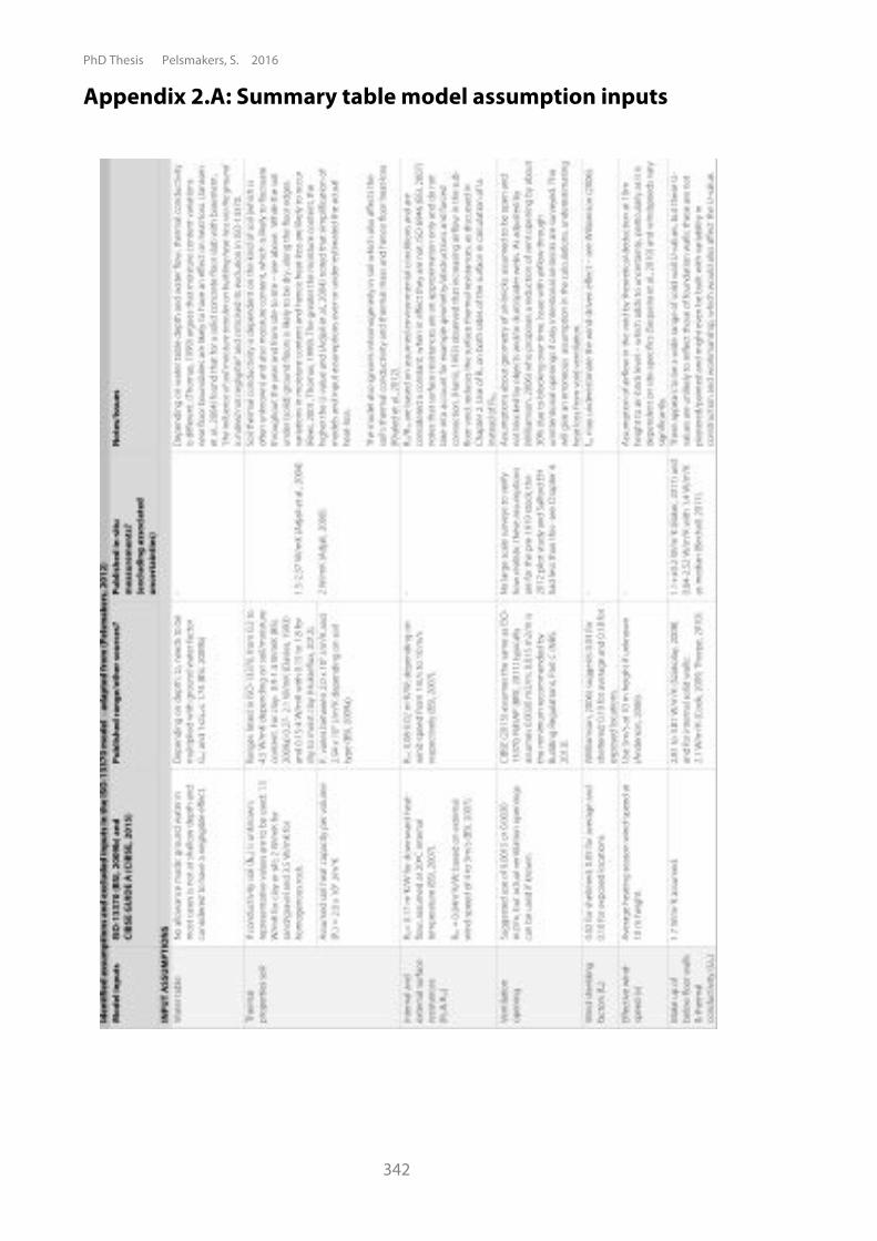
PhD Thesis Pelsmakers, S. 2016
342
Appendix 2.A: Summary table model assumption inputs
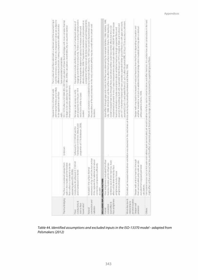
Appendices
343
Table 44. Identified assumptions and excluded inputs in the ISO-13370 model - adapted from Pelsmakers (2012)
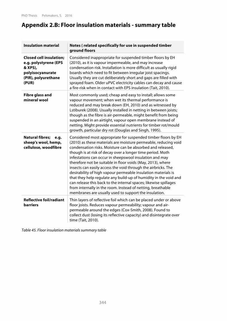
PhD Thesis Pelsmakers, S. 2016
344
Appendix 2.B: Floor insulation materials - summary table
Insulation material Notes ( related specifically for use in suspended timber ground floors
Closed cell insulation; e.g. polystyrene (EPS & XPS), polyisocyanurate (PIR), polyurethane (PUR)
Considered inappropriate for suspended timber floors by EH (2010), as it is vapour impermeable, and may increase condensation risk. Installation is more difficult as usually rigid boards which need to fit between irregular joist spacings. Usually they are cut deliberately short and gaps are filled with sprayed foam. Older uPVC electricity cables can decay and cause a fire-risk when in contact with EPS insulation (Tait, 2010).
Fibre glass and mineral wool
Most commonly used; cheap and easy to install; allows some vapour movement; when wet its thermal performance is reduced and may break down (EH, 2010) and as witnessed by Lstiburek (2008). Usually installed in netting in between joists; though as the fibre is air-permeable, might benefit from being suspended in an airtight, vapour open membrane instead of netting. Might provide essential nutrients for timber rot/mould growth, particular dry rot (Douglas and Singh, 1995).
Natural fibres; e.g. sheep's wool, hemp, cellulose, woodfibre
Considered most appropriate for suspended timber floors by EH (2010) as these materials are moisture permeable, reducing void condensation risks. Moisture can be absorbed and released, though is at risk of decay over a longer time period. Moth infestations can occur in sheepswool insulation and may therefore not be suitable in floor voids (May, 2013), where insects can easily access the void through the airbricks. The desirability of high vapour permeable insulation materials is that they help regulate any build-up of humidity in the void and can release this back to the internal spaces; likewise spillages from internally in the room. Instead of netting, breathable membranes are usually used to support the insulation.
Reflective foil/radiant barriers
Thin layers of reflective foil which can be placed under or above floor joists. Reduces vapour permeability; vapour and air-permeable around the edges (Cox-Smith, 2008). Found to collect dust (losing its reflective capacity) and disintegrate over time (Tait, 2010).
Table 45. Floor insulation materials summary table
Appendices
345
Appendix 2.C: Summary of the main fungi found in
buildings
Timber decay does not generally occur below 22-24% WMC, often lowered to 20% as a safety
measure (Ridout, 2001) (or equivalent to around 90% RH (EH, 2010)). However timber decay
might not occur below 28-30% WMC, which is associated with relative humidities of at least
95% (EH, 2010).
The lower the WMC, the less susceptible to decay (Oliver, 1997) and is ideally below 15%
WMC (Ridout, 2001) (or <75% RH (EH, 2010)). This is also the threshold to minimise wood-
boring insects infestations, which is greater in decayed timbers (Oliver, 1997, EH, 2010),
though wood boring beetles can survive in 12% WMC (Ridout, 2001)(or RH of about 62% (EH,
2010)).
Characteristics and optimal growing conditions for the main building timber-decaying
fungal organisms (dry rot and wet rot) as well as non-timber decaying moulds are
summarised in Table 46. All airborne spores can be a health hazard but in all cases remedy
and prevention of moisture build-up and water penetration eventually kills the fungus
(Ridout, 2001, Oliver, 1997) and reduces occupant exposure. From summary Table 3. it can
be noted that wet rot requires higher moisture thresholds, while for moulds, thresholds for
growth are lower. At very high RH (> 97% RH or wet materials) bacteria also cause smell and
health problems similar to mould fungi (Viitanen et al., 2010).

PhD Thesis Pelsmakers, S. 2016
346
Dry rot (Serpula lacrymans, wood-rotting fungi
• One of the most common fungi in buildings in the UK (Douglas and Singh, 1995).
• High moisture conditions can occur with inadequate floor void ventilation (Oliver, 1997)
• Optimal and rapid growth at 21-23ºC with WMC of 30-40% (Douglas and Singh, 1995, Oliver, 1997), requiring >90% RH at minimum >20ºC (Ridout, 2001). It can grow at lower thresholds, though decay will be slow (Ridout, 2001). Others found ideal RH of 99% (or 26-30% WMC)(Ridout, 2001).
• Its food source is timber or other cellulose based materials (Douglas and Singh, 1995) and it needs a source of calcium, which is present in damp cement/lime mortar and in plaster (Ridout, 2001, Douglas and Singh, 1995), and other organic material, such as rock or glass wool insulation (Douglas and Singh, 1995), commonly used in buildings (EH, 2010), including floors.
• It requires stable, unchanging environments to thrive in and is therefore often limited to the damp zone; while remedying the source of moisture makes the fungus dormant and eventually kills it, it could take up to a year or longer at lower temperatures before the fungus is killed (Ridout, 2001).
• Fungal spores can remain viable for several years (Ridout, 2001). • If conditions allow, dry rot can colonise other areas and grow through
brick, but needs high RH for active growth (Ridout, 2001). • Chemical treatments do not remain effective in continuing damp
conditions so remedying the dampness is a priority (Ridout, 2001).
Wet rot, includes 'cellar rot' (Coniophora puteana, wood-rotting fungi)
• Occurs when timber is continuously damp, for example where it is supported by wet brick work or soil (Ridout, 2001) and is common in poorly ventilated floor voids (Oliver, 1997).
• Optimal growing conditions are 20-25ºC with WMC above 30% (Ridout, 2001, Douglas and Singh, 1995) (i.e. ~100% RH); with optimal WMC of 50-60% (Oliver, 1997).
• Does not require calcium for growth.
Moulds (non-wood-rotting fungi)
• Mould fungi do not tend to decay timbers but have superficial growth on surfaces and may stain surfaces (Ridout, 2001)
• Typically grows on timber in conditions of >70% RH (Oliver, 1997). • Mould can grow on EPS and mineral wool insulation during long-term
exposure to RH >97% (Viitanen, 2007). Table 46. Summary of the main fungi found in buildings.
Appendices
347
Appendix 2.D: Floor void moisture management solutions
Some possible solutions to floor void moisture management are summarised below from literature:
• Moisture problems in insulated Californian floor voids were remedied with the introduction
of ground covers (Flynn, 1994) while (Werther, 2010) also observed 10% to 15% reductions
in summer void RH in a Leipzig test cell after introducing a ground cover.
• Ground insulation was found to reduce moisture build-up in insulated floor voids due to the
wall and ground thermal mass preventing the cooling of summer air in the void, reducing
high void RH (Matilainen, 2003, Airaksinen, 2003, Kurnitski, 2000) in Finland; (Samuelson,
1994) in Sweden and (Werther, 2010) in Germany. An increase in winter RH is likely: the floor
void loses the beneficial thermal mass effect in autumn and winter, creating a yearly void
condition similar to the external environment (Samuelson, 1994), though summer
temperatures are lifted by a few degrees and this might often be enough to bring void RH to
a safe level (Kurnitski, 2000).
• Insulation of foundation walls might not be effective in balancing summer moisture build-up
in insulated suspended ground floors in Finland (Matilainen, 2003, Airaksinen, 2003). Heat
transfer in summer might help increase summer void temperatures (Matilainen, 2003) rather
than act as a heat sink, but this is likely to depend on the type of wall and its thermal mass
capacity.
• To avoid surface condensation and mould growth, (NBS, 2013) requires all areas of a new or
upgraded floor to have a U-value of 0.70 Wm2K-1 or better (i.e. less), with 0.25 Wm2K-1 as
target U-value. However, suspended ground floor U-values may need to be balanced against
void moisture build-up: air temperatures in the floor can be raised by reducing floor
insulation as this increases the downward heat-flow, raising void RH, as observed by
(Samuelson, 1994) and (Airaksinen, 2003). However, in winter, this is likely to be associated
with increased energy use and thermal discomfort (Airaksinen, 2003). (Airaksinen, 2003)
observed that floors with a typical U-value of 0.2 Wm2K-1 had average 2ºC colder void air
temperatures and void RH almost 10% higher than floors with 0.4 Wm2K-1 U-value.
• Floor voids can also be heated mechanically to keep RH within acceptable limits and can be
controlled to kick in when 70% RH is exceeded (Samuelson, 1994) or 75% RH as suggested by
(Airaksinen, 2003). While this may prevent floor void mould growth and in turn transferral
into internal spaces, this is at the expense of increased energy use and incurs capital and
running cost. This is probably best combined with sealed void ventilation to prevent humid
air entering and heat-loss.
• Increased ventilation in the summer only works to dry the floor void if it removes more
moisture than it adds due to the increased evaporation rate of ground moisture and
additional high RH of the external summer air being brought into the void (Kurnitski, 2001)
(Kurnitski, 2000, Airaksinen, 2003).
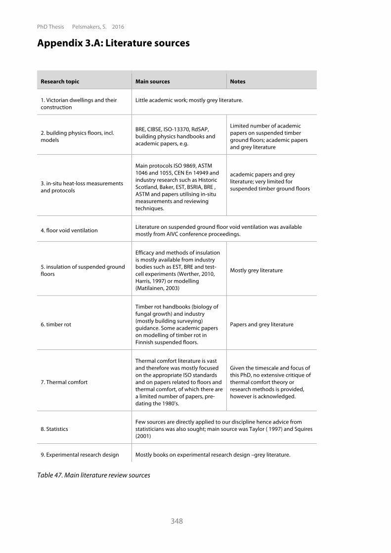
PhD Thesis Pelsmakers, S. 2016
348
Appendix 3.A: Literature sources
Research topic Main sources Notes
1. Victorian dwellings and their construction
Little academic work; mostly grey literature.
2. building physics floors, incl. models
BRE, CIBSE, ISO-13370, RdSAP, building physics handbooks and academic papers, e.g.
Limited number of academic papers on suspended timber ground floors; academic papers and grey literature
3. in-situ heat-loss measurements and protocols
Main protocols ISO 9869, ASTM 1046 and 1055, CEN En 14949 and industry research such as Historic Scotland, Baker, EST, BSRIA, BRE , ASTM and papers utilising in-situ measurements and reviewing techniques.
academic papers and grey literature; very limited for suspended timber ground floors
4. floor void ventilation Literature on suspended ground floor void ventilation was available mostly from AIVC conference proceedings.
5. insulation of suspended ground floors
Efficacy and methods of insulation is mostly available from industry bodies such as EST, BRE and test-cell experiments (Werther, 2010, Harris, 1997) or modelling (Matilainen, 2003)
Mostly grey literature
6. timber rot
Timber rot handbooks (biology of fungal growth) and industry (mostly building surveying) guidance. Some academic papers on modelling of timber rot in Finnish suspended floors.
Papers and grey literature
7. Thermal comfort
Thermal comfort literature is vast and therefore was mostly focused on the appropriate ISO standards and on papers related to floors and thermal comfort, of which there are a limited number of papers, pre-dating the 1980's.
Given the timescale and focus of this PhD, no extensive critique of thermal comfort theory or research methods is provided, however is acknowledged.
8. Statistics Few sources are directly applied to our discipline hence advice from statisticians was also sought; main source was Taylor ( 1997) and Squires (2001)
9. Experimental research design Mostly books on experimental research design –grey literature.
Table 47. Main literature review sources
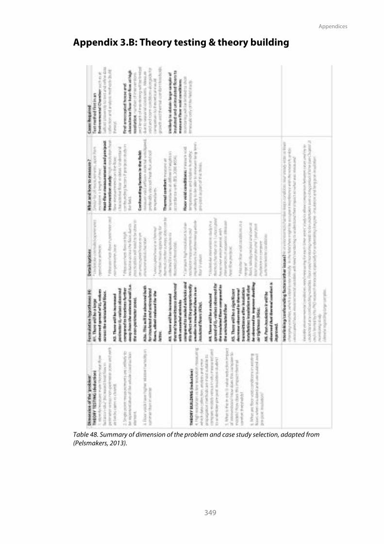
Appendices
349
Appendix 3.B: Theory testing & theory building
Table 48. Summary of dimension of the problem and case study selection, adapted from (Pelsmakers, 2013).
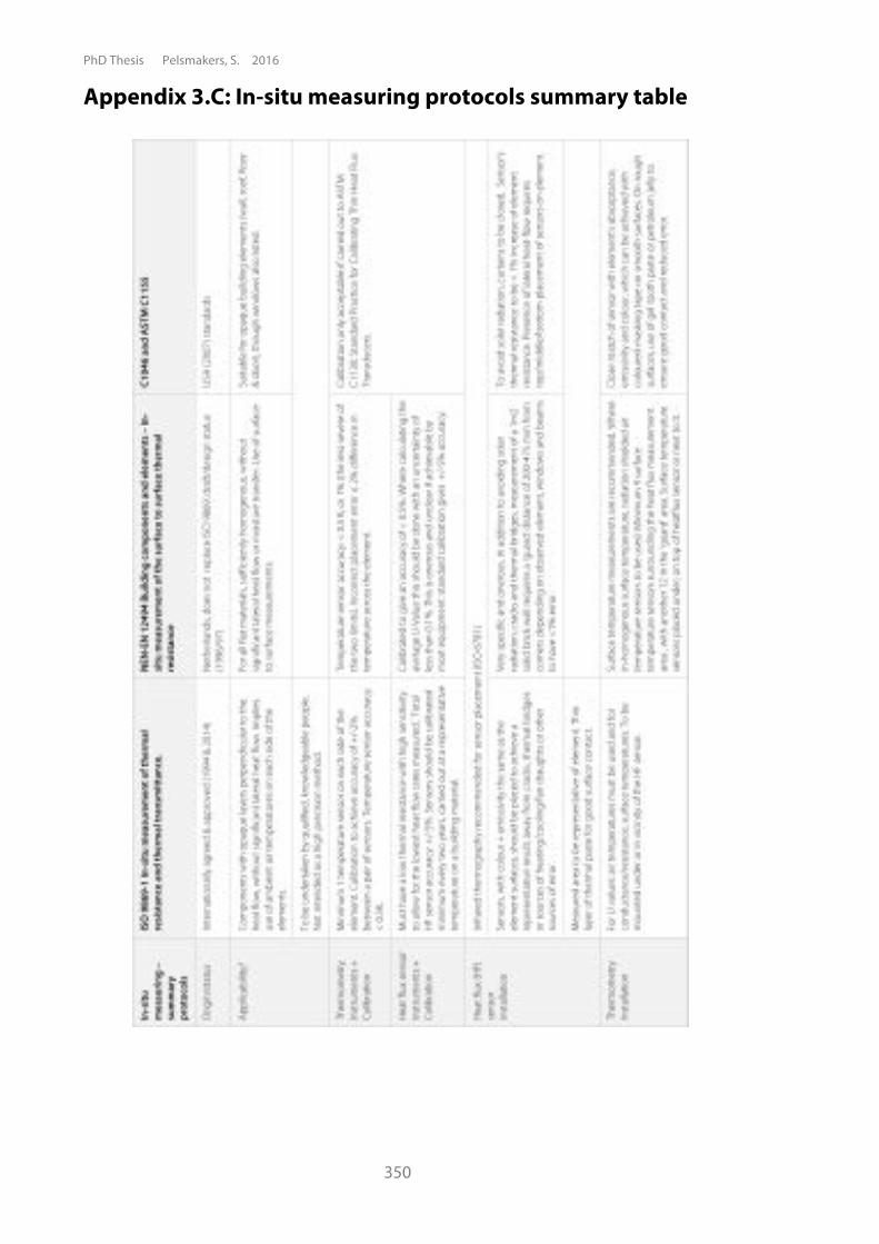
PhD Thesis Pelsmakers, S. 2016
350
Appendix 3.C: In-situ measuring protocols summary table
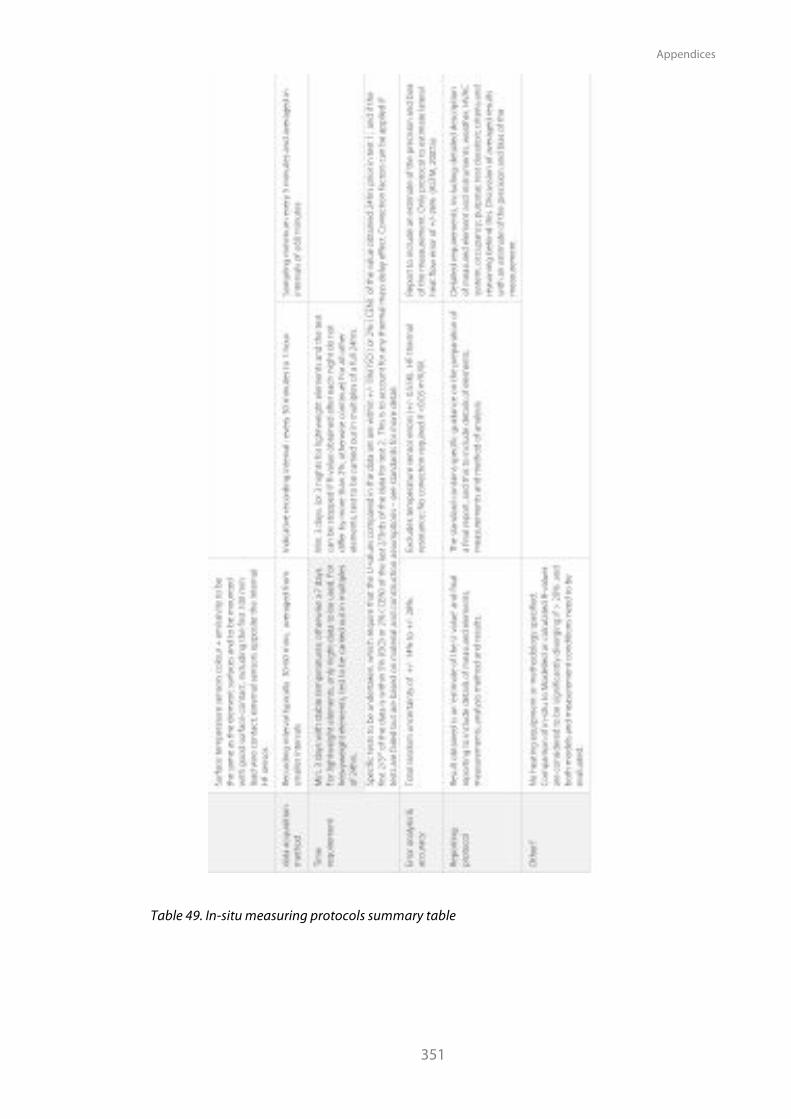
Appendices
351
Table 49. In-situ measuring protocols summary table
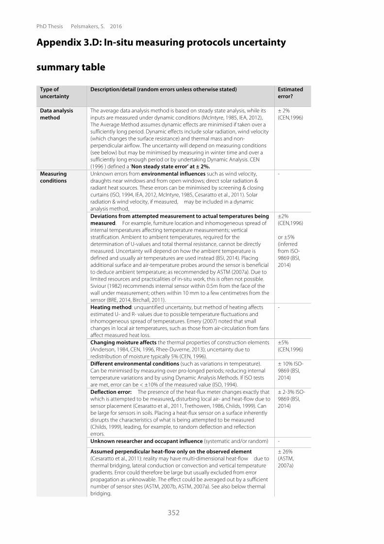
PhD Thesis Pelsmakers, S. 2016
352
Appendix 3.D: In-situ measuring protocols uncertainty
summary table
Type of uncertainty
Description/detail (random errors unless otherwise stated) Estimated error?
Data analysis method
The average data analysis method is based on steady state analysis, while its inputs are measured under dynamic conditions (McIntyre, 1985, IEA, 2012), The Average Method assumes dynamic effects are minimised if taken over a sufficiently long period. Dynamic effects include solar radiation, wind velocity (which changes the surface resistance) and thermal mass and non-perpendicular airflow. The uncertainty will depend on measuring conditions (see below) but may be minimised by measuring in winter time and over a sufficiently long enough period or by undertaking Dynamic Analysis. CEN (1996 ) defined a ‘Non steady state error’ at ± 2%.
± 2% (CEN,1996)
Measuring conditions
Unknown errors from environmental influences such as wind velocity, draughts near windows and from open windows; direct solar radiation & radiant heat sources. These errors can be minimised by screening & closing curtains (ISO, 1994, IEA, 2012, McIntyre, 1985, Cesaratto et al., 2011). Solar radiation & wind velocity, if measured, may be included in a dynamic analysis method,
-
Deviations from attempted measurement to actual temperatures being measured. For example, furniture location and inhomogeneous spread of internal temperatures affecting temperature measurements; vertical stratification. Ambient to ambient temperatures, required for the determination of U-values and total thermal resistance, cannot be directly measured. Uncertainty will depend on how the ambient temperature is defined and usually air temperatures are used instead (BSI, 2014). Placing additional surface and air-temperature probes around the sensor is beneficial to deduce ambient temperature; as recommended by ASTM (2007a). Due to limited resources and practicalities of in-situ work, this is often not possible. Siviour (1982) recommends internal sensor within 0.5m from the face of the wall under measurement; others within 10 mm to a few centimetres from the sensor (BRE, 2014, Birchall, 2011).
±2% (CEN,1996) or ±5% (inferred from ISO-9869 (BSI, 2014)
Heating method: unquantified uncertainty, but method of heating affects estimated U- and R- values due to possible temperature fluctuations and inhomogeneous spread of temperatures. Emery (2007) noted that small changes in local air temperatures, such as those from air-circulation from fans affect measured heat loss.
-
Changing moisture affects the thermal properties of construction elements (Anderson, 1984, CEN, 1996, Rhee-Duverne, 2013); uncertainty due to redistribution of moisture typically 5% (CEN, 1996).
±5% (CEN,1996)
Different environmental conditions (such as variations in temperature). Can be minimised by measuring over pro-longed periods; reducing internal temperature variations and by using Dynamic Analysis Methods. If ISO tests are met, error can be < ±10% of the measured value (ISO, 1994).
± 10% ISO-9869 (BSI, 2014)
Deflection error: The presence of the heat-flux meter changes exactly that which is attempted to be measured, disturbing local air- and heat-flow due to sensor placement (Cesaratto et al., 2011, Trethowen, 1986, Childs, 1999). Can be large for sensors in soils. Placing a heat-flux sensor on a surface inherently disrupts the characteristics of what is being attempted to be measured (Childs, 1999), leading, for example, to random deflection and reflection errors.
± 2-3% ISO-9869 (BSI, 2014)
Unknown researcher and occupant influence (systematic and/or random) -
Assumed perpendicular heat-flow only on the observed element (Cesaratto et al., 2011): reality may have multi-dimensional heat-flow due to thermal bridging, lateral conduction or convection and vertical temperature gradients. Error could therefore be large but usually excluded from error propagation as unknowable. The effect could be averaged out by a sufficient number of sensor sites (ASTM, 2007b, ASTM, 2007a). See also below thermal bridging.
± 26% (ASTM, 2007a)
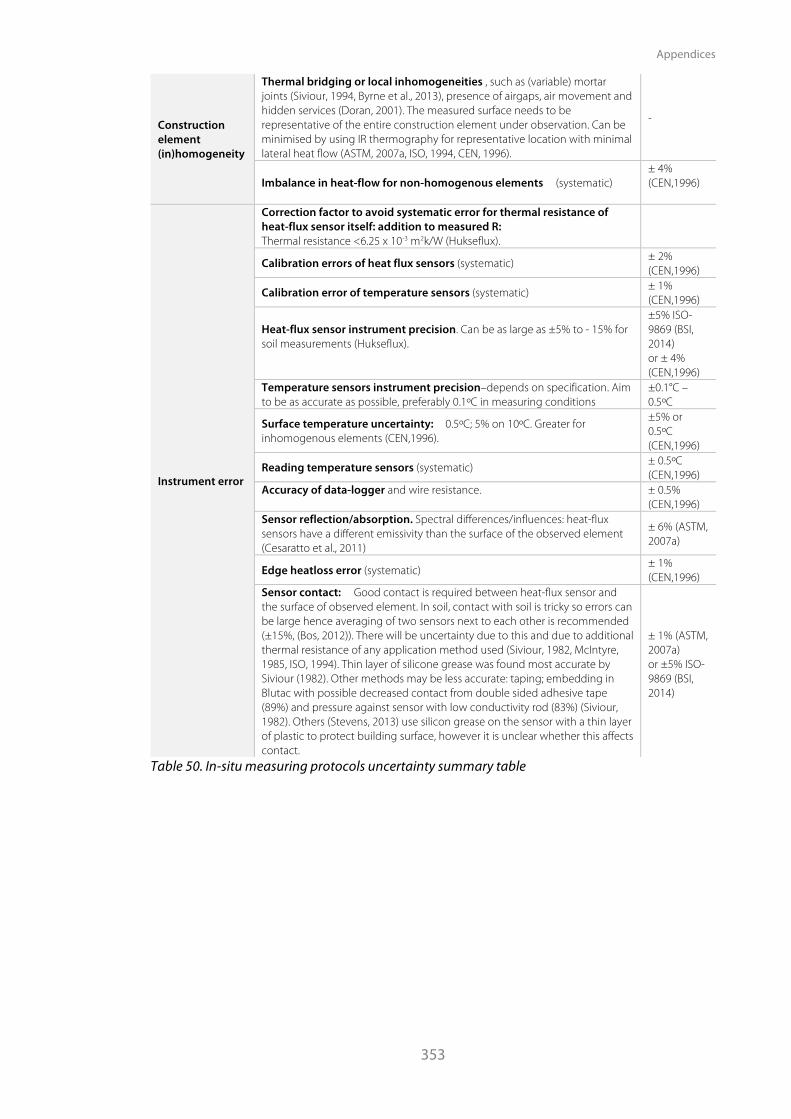
Appendices
353
Construction element (in)homogeneity
Thermal bridging or local inhomogeneities , such as (variable) mortar joints (Siviour, 1994, Byrne et al., 2013), presence of airgaps, air movement and hidden services (Doran, 2001). The measured surface needs to be representative of the entire construction element under observation. Can be minimised by using IR thermography for representative location with minimal lateral heat flow (ASTM, 2007a, ISO, 1994, CEN, 1996).
-
Imbalance in heat-flow for non-homogenous elements (systematic) ± 4% (CEN,1996)
Instrument error
Correction factor to avoid systematic error for thermal resistance of heat-flux sensor itself: addition to measured R: Thermal resistance <6.25 x 10⁻³ m2k/W (Hukseflux).
Calibration errors of heat flux sensors (systematic) ± 2% (CEN,1996)
Calibration error of temperature sensors (systematic) ± 1% (CEN,1996)
Heat-flux sensor instrument precision. Can be as large as ±5% to - 15% for soil measurements (Hukseflux).
±5% ISO-9869 (BSI, 2014) or ± 4% (CEN,1996)
Temperature sensors instrument precision–depends on specification. Aim to be as accurate as possible, preferably 0.1ºC in measuring conditions
±0.1°C – 0.5ºC
Surface temperature uncertainty: 0.5ºC; 5% on 10ºC. Greater for inhomogenous elements (CEN,1996).
±5% or 0.5ºC (CEN,1996)
Reading temperature sensors (systematic) ± 0.5ºC (CEN,1996)
Accuracy of data-logger and wire resistance. ± 0.5% (CEN,1996)
Sensor reflection/absorption. Spectral differences/influences: heat-flux sensors have a different emissivity than the surface of the observed element (Cesaratto et al., 2011)
± 6% (ASTM, 2007a)
Edge heatloss error (systematic) ± 1% (CEN,1996)
Sensor contact: Good contact is required between heat-flux sensor and the surface of observed element. In soil, contact with soil is tricky so errors can be large hence averaging of two sensors next to each other is recommended (±15%, (Bos, 2012)). There will be uncertainty due to this and due to additional thermal resistance of any application method used (Siviour, 1982, McIntyre, 1985, ISO, 1994). Thin layer of silicone grease was found most accurate by Siviour (1982). Other methods may be less accurate: taping; embedding in Blutac with possible decreased contact from double sided adhesive tape (89%) and pressure against sensor with low conductivity rod (83%) (Siviour, 1982). Others (Stevens, 2013) use silicon grease on the sensor with a thin layer of plastic to protect building surface, however it is unclear whether this affects contact.
± 1% (ASTM, 2007a) or ±5% ISO-9869 (BSI, 2014)
Table 50. In-situ measuring protocols uncertainty summary table
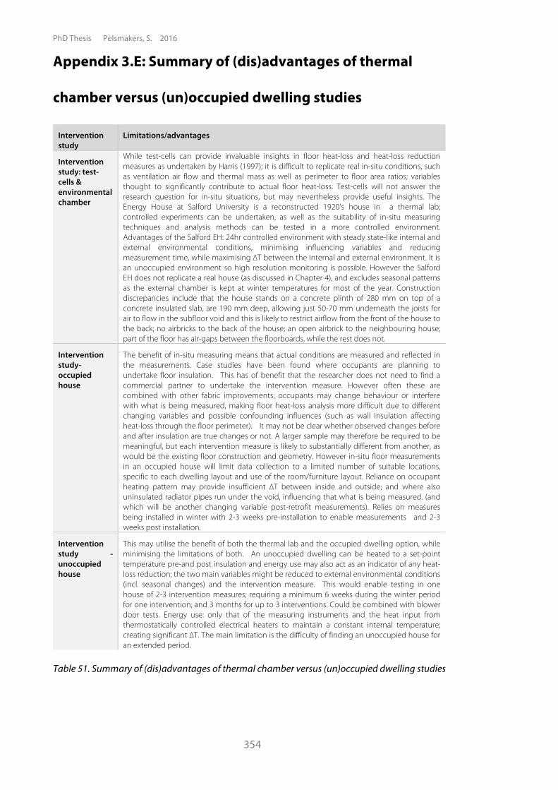
PhD Thesis Pelsmakers, S. 2016
354
Appendix 3.E: Summary of (dis)advantages of thermal
chamber versus (un)occupied dwelling studies
Intervention study
Limitations/advantages
Intervention study: test-cells & environmental chamber
While test-cells can provide invaluable insights in floor heat-loss and heat-loss reduction measures as undertaken by Harris (1997); it is difficult to replicate real in-situ conditions, such as ventilation air flow and thermal mass as well as perimeter to floor area ratios; variables thought to significantly contribute to actual floor heat-loss. Test-cells will not answer the research question for in-situ situations, but may nevertheless provide useful insights. The Energy House at Salford University is a reconstructed 1920’s house in a thermal lab; controlled experiments can be undertaken, as well as the suitability of in-situ measuring techniques and analysis methods can be tested in a more controlled environment. Advantages of the Salford EH: 24hr controlled environment with steady state-like internal and external environmental conditions, minimising influencing variables and reducing measurement time, while maximising !T between the internal and external environment. It is an unoccupied environment so high resolution monitoring is possible. However the Salford EH does not replicate a real house (as discussed in Chapter 4), and excludes seasonal patterns as the external chamber is kept at winter temperatures for most of the year. Construction discrepancies include that the house stands on a concrete plinth of 280 mm on top of a concrete insulated slab, are 190 mm deep, allowing just 50-70 mm underneath the joists for air to flow in the subfloor void and this is likely to restrict airflow from the front of the house to the back; no airbricks to the back of the house; an open airbrick to the neighbouring house; part of the floor has air-gaps between the floorboards, while the rest does not.
Intervention study- occupied house
The benefit of in-situ measuring means that actual conditions are measured and reflected in the measurements. Case studies have been found where occupants are planning to undertake floor insulation. This has of benefit that the researcher does not need to find a commercial partner to undertake the intervention measure. However often these are combined with other fabric improvements; occupants may change behaviour or interfere with what is being measured, making floor heat-loss analysis more difficult due to different changing variables and possible confounding influences (such as wall insulation affecting heat-loss through the floor perimeter). It may not be clear whether observed changes before and after insulation are true changes or not. A larger sample may therefore be required to be meaningful, but each intervention measure is likely to substantially different from another, as would be the existing floor construction and geometry. However in-situ floor measurements in an occupied house will limit data collection to a limited number of suitable locations, specific to each dwelling layout and use of the room/furniture layout. Reliance on occupant heating pattern may provide insufficient !T between inside and outside; and where also uninsulated radiator pipes run under the void, influencing that what is being measured. (and which will be another changing variable post-retrofit measurements). Relies on measures being installed in winter with 2-3 weeks pre-installation to enable measurements and 2-3 weeks post installation.
Intervention study - unoccupied house
This may utilise the benefit of both the thermal lab and the occupied dwelling option, while minimising the limitations of both. An unoccupied dwelling can be heated to a set-point temperature pre-and post insulation and energy use may also act as an indicator of any heat-loss reduction; the two main variables might be reduced to external environmental conditions (incl. seasonal changes) and the intervention measure. This would enable testing in one house of 2-3 intervention measures; requiring a minimum 6 weeks during the winter period for one intervention; and 3 months for up to 3 interventions. Could be combined with blower door tests. Energy use: only that of the measuring instruments and the heat input from thermostatically controlled electrical heaters to maintain a constant internal temperature; creating significant !T. The main limitation is the difficulty of finding an unoccupied house for an extended period.
Table 51. Summary of (dis)advantages of thermal chamber versus (un)occupied dwelling studies

Appendices
355
Appendix 3.F: Information sheets and informed consent
STUDY 1
Initial Project letter, followed by additional info letter and consent form below.
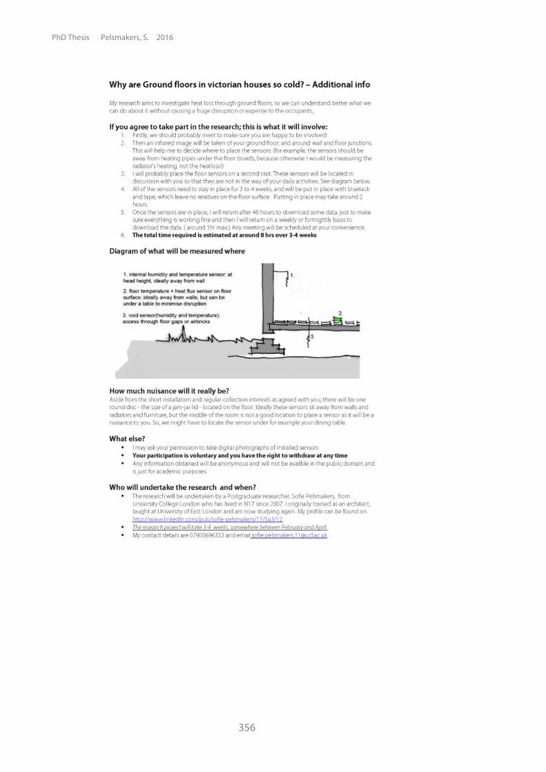
PhD Thesis Pelsmakers, S. 2016
356
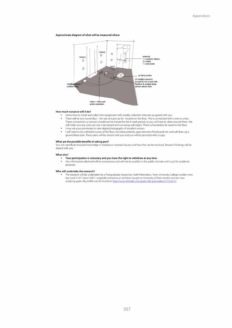
Appendices
357

PhD Thesis Pelsmakers, S. 2016
358
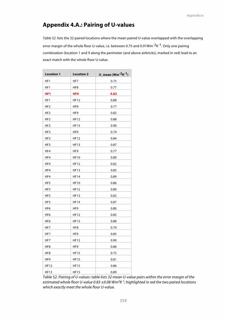
Appendices
359
Appendix 4.A.: Pairing of U-values
Table 52. lists the 32 paired locations where the mean paired U-value overlapped with the overlapping
error margin of the whole floor U-value, i.e. between 0.75 and 0.91Wm-2K-1. Only one pairing
combination (location 1 and 9 along the perimeter (and above airbricks), marked in red) lead to an
exact match with the whole floor U-value.
Location 1 Location 2 U_mean (Wm-2K-1)
HF1 HF7 0.75
HF1 HF8 0.77
HF1 HF9 0.83
HF1 HF12 0.88
HF2 HF8 0.77
HF2 HF9 0.82
HF2 HF12 0.88
HF2 HF13 0.90
HF3 HF9 0.79
HF3 HF12 0.84
HF3 HF13 0.87
HF4 HF9 0.77
HF4 HF10 0.89
HF4 HF12 0.82
HF4 HF13 0.85
HF4 HF14 0.89
HF5 HF10 0.86
HF5 HF12 0.80
HF5 HF13 0.82
HF5 HF14 0.87
HF6 HF9 0.80
HF6 HF12 0.85
HF6 HF13 0.88
HF7 HF8 0.79
HF7 HF9 0.85
HF7 HF12 0.90
HF8 HF9 0.86
HF8 HF15 0.75
HF9 HF15 0.81
HF12 HF15 0.86
HF13 HF15 0.89 Table 52. Pairing of U-values: table lists 32 mean U-value pairs within the error margin of the estimated whole floor U-value 0.83 ±0.08 Wm2K-1; highlighted in red the two paired locations which exactly meet the whole floor U-value.
PhD Thesis Pelsmakers, S. 2016
360
Appendix 5.A: Research management and ethical
considerations - STUDY 4A/B Several research management and ethical considerations were taken into account for this field study and are summarised below:
• Informed Consent and risk assessment were agreed with the home-owner. Interventions
were agreed with the home-owner in advance via email; Building Regulations notification or
approval did not apply as the improved part was <50% of the ground floor (NBS, 2015).
• A reciprocal NDA was signed with Downs Energy: the purpose of this was to enable Downs
Energy to test a floor void filling technique typically used for cavity-filling; while also
acknowledging the researcher's expertise input.
• UCL insurance for equipment and third party insurance were obtained for the duration of
the study.
• Access to the house: as agreed, the owner was kept up to date of progress on a regular basis
via emails and was notified by text message each time the researcher entered and left the
unoccupied property; this was typically 2 to 3 days per week, sometimes daily during an
intervention study. The department's 'buddy scheme' for lone working was also
implemented: i.e. two people were identified and given prior details of site-visits, with
approximate arrival and departure times and sending of text messages upon entering and
leaving. If the researcher did not text at the expected departure time, the 'buddy' would
attempt to contact the researcher and if failure to do so, would alert emergency services (this
was however never necessary).
• Disruption to neighbours was minimised: neighbours were notified of any building works
and suitable times agreed (such as avoiding certain weekdays or times) to minimise noise and
other disruption. After the main field study, neighbours were also notified by text message
upon returning for data collection as the house was still unoccupied.
• Sealing of the airbricks is considered to be risky to the health of the floor and might
contribute to structural damage or void mould growth (Oliver, 1997, Burke, n.d., Douglas,
1998b, Douglas, 1998a, BRE, 1991, Singh, 1998). Hence, with approval from the home-owner,
airbricks were sealed for short periods only (< 1 week) for the monitoring of heat-flow for
each intervention in this condition; airbricks were sealed for a longer period during the EPS
bead intervention. In all cases, the floor void conditions (temperature and RH) were
continuously monitored in 3 locations which would allow the study to be disrupted if critical
moisture levels for mould growth would be exceeded. Void data was transferred wirelessly
from below the void to an easily accessible data logger above the floor void to allow void
condition checks at every data collection period - at least twice a week - without having to lift
the floorboards.

Appendices
361
information sheet
Information Sheet Research Study You are being invited to take part in a research project. Before you decide whether or not to take part, it is important for you to understand why the research is being done and what it will involve. You will be given a copy of this information sheet. Title of Project: Measuring heat-loss through pre-1919 suspended timber ground floors, before + after interventions Researcher's name: Sofie Pelsmakers Work address: xxxxx Contact details: Tel: xxxxx email: xxxxx What is the purpose of my study? My research investigates the heatloss of pre-1919 floors and what the reduction potential is of certain interventions and the possible unintended consequences of insulating such floors, for example increased humidity in the floor void. I will be undertaking measurements and interventions as described below. Interventions will be agreed with you at prior to undertaking them. What will it involve?
1. A detailed survey will be undertaken of the external and internal territory to undertake a heatloss model. Particular interest is where ground meets walls (up to 1 meter height), and down into the crawl space area, depending on access. The survey can be made available to you upon request. 2. In some cases, floorboards will be removed to gain access to the void and – at later stages – to undertake the intervention. Such work will not be undertaken without prior discussion and agreement with you. 3. Photographs will be taken of the floor void and of internal or external wall surfaces, but will never show any personal or private effects or any objects or identifiable property. Access to images can be obtained at any time and you have the right to ask any to be deleted. 4. 15-20 heatflux sensors will be placed on the floor, in the void soil, on the foundation wall and foundation party wall (depending on access) as well as on the external wall to measure heatloss. This is alongside surface temperature measurements; internal, external and void air tempertaure measurements and Relative Humidity as well as external and void windspeeds. 5. The above research will take place in your unoccupied house from December to mid-March or as agreed. The researcher confirms that UCL's Public Liability Insurance covers any accidental damage. The researcher will email and/or send a text message (as agreed with you) in advance of entering the property, upon entering and when leaving the property. At all times the property will be left secured as per owner instructions. 6. The house will be electrically heated at a typical occupant heating pattern and with frost protection over this 12-14 week period. The electrical heaters will be PAT tested by UCL. Meter readings will be taken periodically and the energy use over the entire research period will be paid for by the researcher. This can be ~ £300 per month and a discussion is required with homeowner how to arrange bill payment. 7. Initial work will involve lifting the carpet to place void sensors, followed by heat-loss measurements on the carpet, on bare floorboards (carpet will be removed), and with (to be confirmed and as agreed prior) a radiant barrier and full floor insulation between the joists. In between each intervention, airbricks will be closed for a 1 week period to investigate the effect on observed heat-loss, void windspoeds and void RH . Blower door tests are also likely to be undertaken. 8. Due to high-resolution of data collection over a ~ 12-14 month period, it will take several months afterwards to analyse the data, however the results of the study can be shared with you once the data has been analysed and they are available. The sharing of results will be done in confidence, until results are published.
How much nuisance will it be? The whole process will take 2-3 months, with regular ( ~ twice weekly visits) by the researcher. Your separate approval and agreement will be required prior to any invasive works being undertaken such

PhD Thesis Pelsmakers, S. 2016
362
as lifting or cutting of floorboards and installing insulation, which will require some additoonal time to review and agree the proposals. What are the possible benefits in taking part? By agreeing to allow this study to take place in your unoccupied house, you will contribute towards knowledge of heatloss and floor conditions in existing houses and solutions for insulating them. Research findings can be shared with you upon your request. If the researcher finds any suggestion of evidence of an unhealthy floor or any other issues during the period, this will be shared with you, although this is not a professional survey and there is no guarantee that any problems will be found or will be identified correctly and no liability lies with the researcher in this aspect. You will end up with a freely improved/insulated floor at the end of the study. What else?
• Your participation is voluntary and you have the right to withdraw at any time • Any information obtained will be anonymous and is just for research purposes. • If you decide to take part you will be given this information sheet to keep and be asked to sign a consent form. • Please discuss the information above with others if you wish or ask the researcher if there is anything that is not clear or if you would like more information. • It is up to you to decide whether to take part or not; choosing not to take part will not disadvantage you in any way. If you do decide to take part you are still free to withdraw at any time and without giving a reason.
Appendices
363
Informed consent form example
Informed consent form for participants in research studies Please complete this form after you have read the Information Sheet and/or listened to an explanation about the research. Title of Project: Measuring heat-loss through pre-1919 suspended timber ground floors, before + after interventions Researcher's name: Sofie Pelsmakers Work address: xxxx Contact details: Tel: xxxx Thank you for your interest in taking part in this research. Before you agree to take part, the person organising the research must explain the project to you. If you have any questions arising from the Information Sheet or explanation already given to you, please ask the researcher before you decide whether to join in. You will be given a copy of this Consent Form to keep and refer to at any time. Participant's Statement
1. I comfirm that I have read the notes written above and the Information Sheet, and understand what the study involves. I have had the opportunity to consider the information, ask questions and have had these answered satisfactorily. If I have further queries about the study, I know I can get in touch with the researchers through the above contact details. 2. I understand that my participation in the study is entirely voluntary and that if I decide at any time that I no longer wish to take part in this project, I can notify the researcher and withdraw immediately, without giving reason. In the event that I withdraw from the study, any collected data will be kept by the researcher, and associated analysis will still be made. I will allow the researcher to come and collect any dataloggers/instruments in my property, which remain property of the researcher at all times. 3. I hereby agree to participate in the research study, which involves the researcher undertaking the monitoring and interventions for ~ 12-14 weeks, as described in the information sheet. 4. No personal data will be collected and any collected non-personal data will be anonymised and treated as confidential. 5. I understand that the information collected will be used and retained for the length of the study and beyond this (see point 6) and I can have access to the findings as described in the information sheet. 6. I agree that the data collected may be used by others for future research beyond the length of the study or the researcher's study time. I am assured that confidentiality will be upheld. 7. I understand that the data collected belongs to the project and that this information can be used by the researcher in presentations and publications and I can obtain a copy upon request. Confidentiality and anonymity will be maintained and it will not be possible to identify me from any publications. 8. I understand that digital photo's may be taken of wall and floor surfaces and the floor void but will never show any personal or private effects or any objects or identifiable property. I understand that I can obtain access to any images at any time and that I have the right to ask any to be deleted. 9. I understand and agree that if the researcher has evidence suggesting an unhealthy structure, the researcher will inform me. However, I understand that this is not a professional survey and there is no guarantee that problems will be found or will be identified correctly nor that liability rests with the researcher. The researcher is covered by UCL's Public Liability Insurance to undertake this field-work.

PhD Thesis Pelsmakers, S. 2016
364
10. I agree that the research project named above has been explained to me to my satisfaction and I agree to take part in this study.
Name of participant: Signed: Date: Name of Researcher: Signed: Date:

Appendices
365
Health & safety risk assessment

PhD Thesis Pelsmakers, S. 2016
366

Appendices
367

PhD Thesis Pelsmakers, S. 2016
368
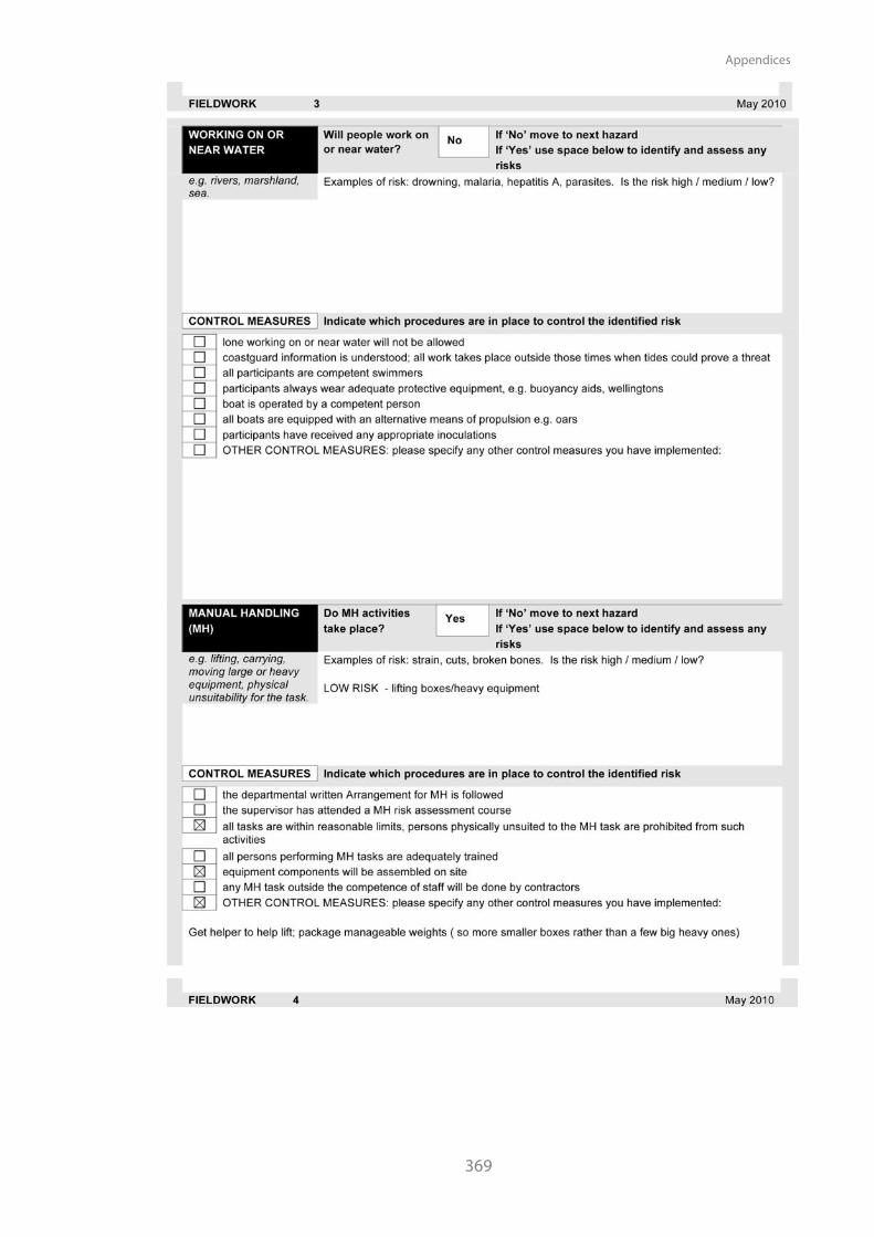
Appendices
369

PhD Thesis Pelsmakers, S. 2016
370
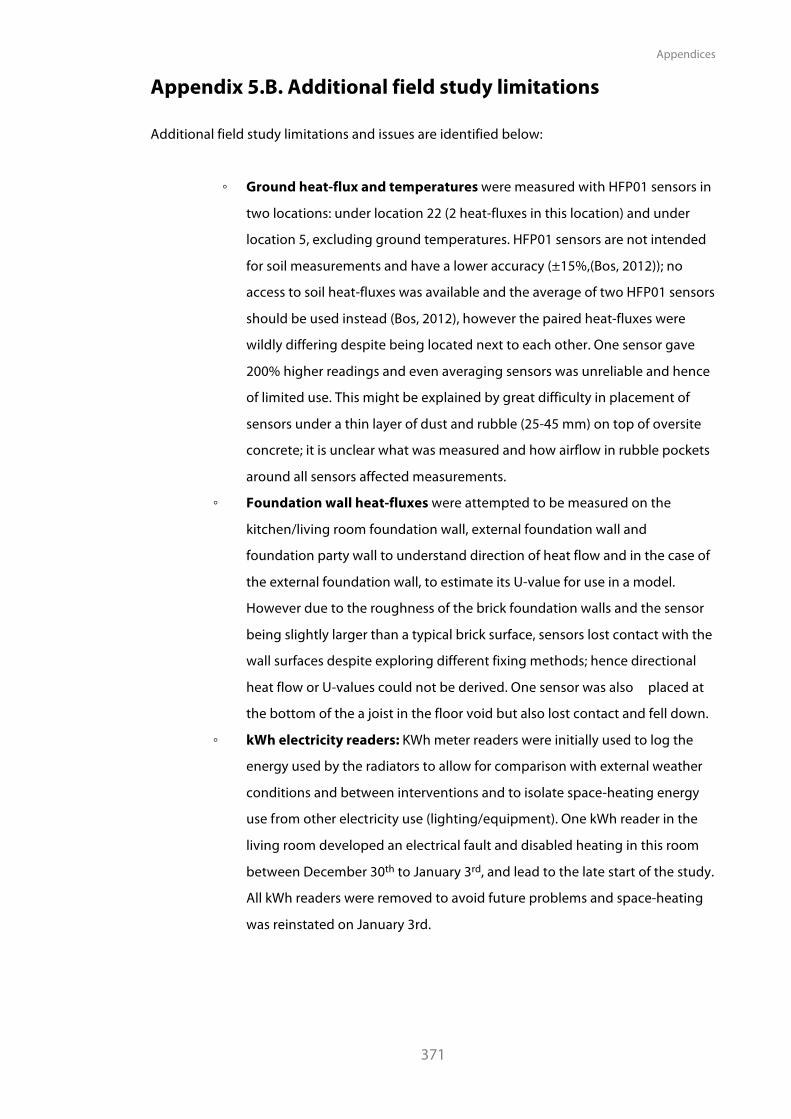
Appendices
371
Appendix 5.B. Additional field study limitations
Additional field study limitations and issues are identified below:
◦ Ground heat-flux and temperatures were measured with HFP01 sensors in
two locations: under location 22 (2 heat-fluxes in this location) and under
location 5, excluding ground temperatures. HFP01 sensors are not intended
for soil measurements and have a lower accuracy (±15%,(Bos, 2012)); no
access to soil heat-fluxes was available and the average of two HFP01 sensors
should be used instead (Bos, 2012), however the paired heat-fluxes were
wildly differing despite being located next to each other. One sensor gave
200% higher readings and even averaging sensors was unreliable and hence
of limited use. This might be explained by great difficulty in placement of
sensors under a thin layer of dust and rubble (25-45 mm) on top of oversite
concrete; it is unclear what was measured and how airflow in rubble pockets
around all sensors affected measurements.
◦ Foundation wall heat-fluxes were attempted to be measured on the
kitchen/living room foundation wall, external foundation wall and
foundation party wall to understand direction of heat flow and in the case of
the external foundation wall, to estimate its U-value for use in a model.
However due to the roughness of the brick foundation walls and the sensor
being slightly larger than a typical brick surface, sensors lost contact with the
wall surfaces despite exploring different fixing methods; hence directional
heat flow or U-values could not be derived. One sensor was also placed at
the bottom of the a joist in the floor void but also lost contact and fell down.
◦ kWh electricity readers: KWh meter readers were initially used to log the
energy used by the radiators to allow for comparison with external weather
conditions and between interventions and to isolate space-heating energy
use from other electricity use (lighting/equipment). One kWh reader in the
living room developed an electrical fault and disabled heating in this room
between December 30th to January 3rd, and lead to the late start of the study.
All kWh readers were removed to avoid future problems and space-heating
was reinstated on January 3rd.
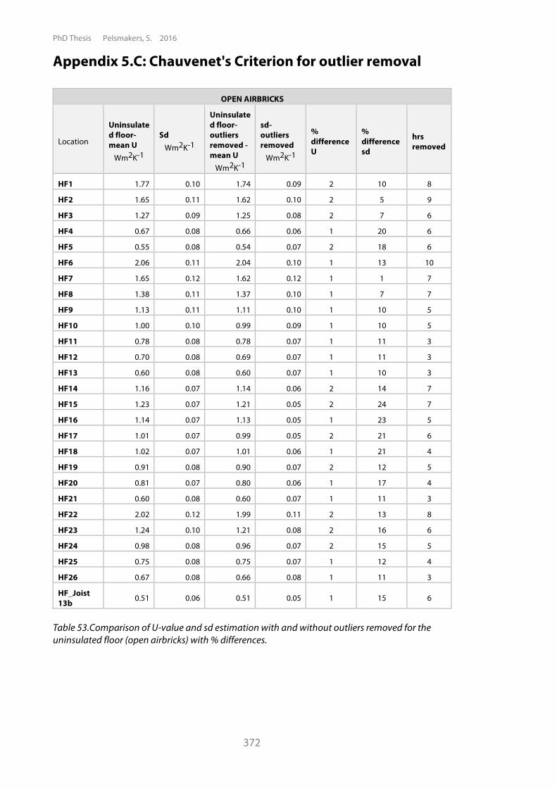
PhD Thesis Pelsmakers, S. 2016
372
Appendix 5.C: Chauvenet's Criterion for outlier removal
OPEN AIRBRICKS
Location
Uninsulated floor- mean U
Wm2K-1
Sd Wm2K-1
Uninsulated floor- outliers removed - mean U
Wm2K-1
sd- outliers removed
Wm2K-1
% difference U
% difference sd
hrs removed
HF1 1.77 0.10 1.74 0.09 2 10 8
HF2 1.65 0.11 1.62 0.10 2 5 9
HF3 1.27 0.09 1.25 0.08 2 7 6
HF4 0.67 0.08 0.66 0.06 1 20 6
HF5 0.55 0.08 0.54 0.07 2 18 6
HF6 2.06 0.11 2.04 0.10 1 13 10
HF7 1.65 0.12 1.62 0.12 1 1 7
HF8 1.38 0.11 1.37 0.10 1 7 7
HF9 1.13 0.11 1.11 0.10 1 10 5
HF10 1.00 0.10 0.99 0.09 1 10 5
HF11 0.78 0.08 0.78 0.07 1 11 3
HF12 0.70 0.08 0.69 0.07 1 11 3
HF13 0.60 0.08 0.60 0.07 1 10 3
HF14 1.16 0.07 1.14 0.06 2 14 7
HF15 1.23 0.07 1.21 0.05 2 24 7
HF16 1.14 0.07 1.13 0.05 1 23 5
HF17 1.01 0.07 0.99 0.05 2 21 6
HF18 1.02 0.07 1.01 0.06 1 21 4
HF19 0.91 0.08 0.90 0.07 2 12 5
HF20 0.81 0.07 0.80 0.06 1 17 4
HF21 0.60 0.08 0.60 0.07 1 11 3
HF22 2.02 0.12 1.99 0.11 2 13 8
HF23 1.24 0.10 1.21 0.08 2 16 6
HF24 0.98 0.08 0.96 0.07 2 15 5
HF25 0.75 0.08 0.75 0.07 1 12 4
HF26 0.67 0.08 0.66 0.08 1 11 3
HF_Joist 13b 0.51 0.06 0.51 0.05 1 15 6
Table 53.Comparison of U-value and sd estimation with and without outliers removed for the uninsulated floor (open airbricks) with % differences.
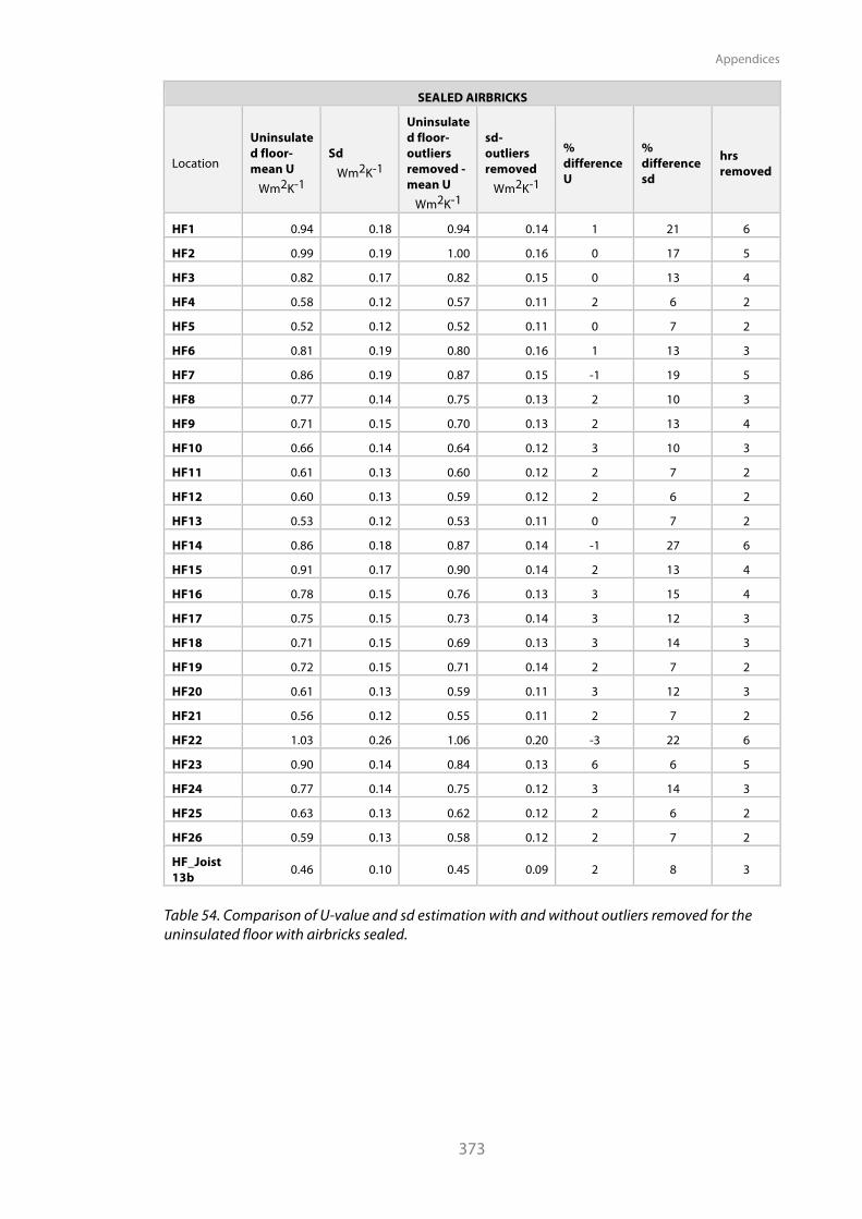
Appendices
373
SEALED AIRBRICKS
Location
Uninsulated floor- mean U
Wm2K-1
Sd Wm2K-1
Uninsulated floor- outliers removed - mean U
Wm2K-1
sd- outliers removed
Wm2K-1
% difference U
% difference sd
hrs removed
HF1 0.94 0.18 0.94 0.14 1 21 6
HF2 0.99 0.19 1.00 0.16 0 17 5
HF3 0.82 0.17 0.82 0.15 0 13 4
HF4 0.58 0.12 0.57 0.11 2 6 2
HF5 0.52 0.12 0.52 0.11 0 7 2
HF6 0.81 0.19 0.80 0.16 1 13 3
HF7 0.86 0.19 0.87 0.15 -1 19 5
HF8 0.77 0.14 0.75 0.13 2 10 3
HF9 0.71 0.15 0.70 0.13 2 13 4
HF10 0.66 0.14 0.64 0.12 3 10 3
HF11 0.61 0.13 0.60 0.12 2 7 2
HF12 0.60 0.13 0.59 0.12 2 6 2
HF13 0.53 0.12 0.53 0.11 0 7 2
HF14 0.86 0.18 0.87 0.14 -1 27 6
HF15 0.91 0.17 0.90 0.14 2 13 4
HF16 0.78 0.15 0.76 0.13 3 15 4
HF17 0.75 0.15 0.73 0.14 3 12 3
HF18 0.71 0.15 0.69 0.13 3 14 3
HF19 0.72 0.15 0.71 0.14 2 7 2
HF20 0.61 0.13 0.59 0.11 3 12 3
HF21 0.56 0.12 0.55 0.11 2 7 2
HF22 1.03 0.26 1.06 0.20 -3 22 6
HF23 0.90 0.14 0.84 0.13 6 6 5
HF24 0.77 0.14 0.75 0.12 3 14 3
HF25 0.63 0.13 0.62 0.12 2 6 2
HF26 0.59 0.13 0.58 0.12 2 7 2
HF_Joist 13b 0.46 0.10 0.45 0.09 2 8 3
Table 54. Comparison of U-value and sd estimation with and without outliers removed for the uninsulated floor with airbricks sealed.
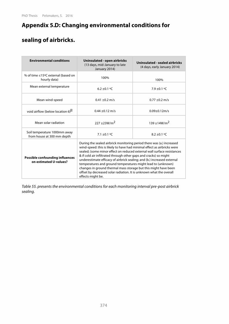
PhD Thesis Pelsmakers, S. 2016
374
Appendix 5.D: Changing environmental conditions for
sealing of airbricks.
Environmental conditions Uninsulated - open airbricks (13 days, mid-January to late
January 2014)
Uninsulated - sealed airbricks (4 days, early January 2014)
% of time !15ºC external (based on hourly data) 100%
100%
Mean external temperature 6.2 ±0.1 ºC 7.9 ±0.1 ºC
Mean wind-speed 0.41 ±0.2 m/s 0.77 ±0.2 m/s
void airflow (below location 6)� 0.44 ±0.12 m/s 0.09±0.12m/s
Mean solar radiation 227 ±23W/m2 139 ±14W/m2
Soil temperature 1000mm away from house at 300 mm depth 7.1 ±0.1 ºC 8.2 ±0.1 ºC
Possible confounding influences on estimated U-values?
During the sealed airbrick monitoring period there was (a.) increased wind-speed: this is likely to have had minimal effect as airbricks were sealed; (some minor effect on reduced external wall surface resistances & if cold air infiltrated through other gaps and cracks) so might underestimate efficacy of airbrick sealing; and (b.) increased external temperatures and ground temperatures might lead to (unknown) changes in ground thermal mass storage but this might have been offset by decreased solar radiation. It is unknown what the overall effects might be.
Table 55. presents the environmental conditions for each monitoring interval pre-post airbrick sealing.
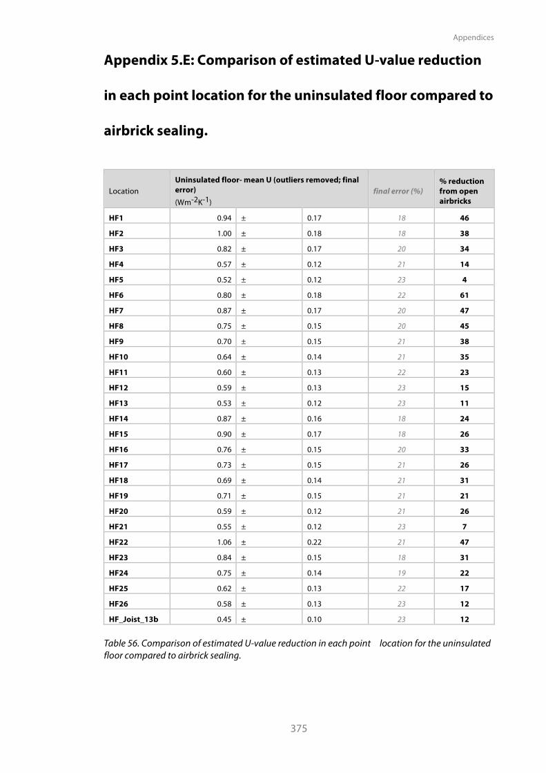
Appendices
375
Appendix 5.E: Comparison of estimated U-value reduction
in each point location for the uninsulated floor compared to
airbrick sealing.
Location Uninsulated floor- mean U (outliers removed; final error) (Wm-2K-1)
final error (%) % reduction from open airbricks
HF1 0.94 ± 0.17 18 46
HF2 1.00 ± 0.18 18 38
HF3 0.82 ± 0.17 20 34
HF4 0.57 ± 0.12 21 14
HF5 0.52 ± 0.12 23 4
HF6 0.80 ± 0.18 22 61
HF7 0.87 ± 0.17 20 47
HF8 0.75 ± 0.15 20 45
HF9 0.70 ± 0.15 21 38
HF10 0.64 ± 0.14 21 35
HF11 0.60 ± 0.13 22 23
HF12 0.59 ± 0.13 23 15
HF13 0.53 ± 0.12 23 11
HF14 0.87 ± 0.16 18 24
HF15 0.90 ± 0.17 18 26
HF16 0.76 ± 0.15 20 33
HF17 0.73 ± 0.15 21 26
HF18 0.69 ± 0.14 21 31
HF19 0.71 ± 0.15 21 21
HF20 0.59 ± 0.12 21 26
HF21 0.55 ± 0.12 23 7
HF22 1.06 ± 0.22 21 47
HF23 0.84 ± 0.15 18 31
HF24 0.75 ± 0.14 19 22
HF25 0.62 ± 0.13 22 17
HF26 0.58 ± 0.13 23 12
HF_Joist_13b 0.45 ± 0.10 23 12 Table 56. Comparison of estimated U-value reduction in each point location for the uninsulated floor compared to airbrick sealing.
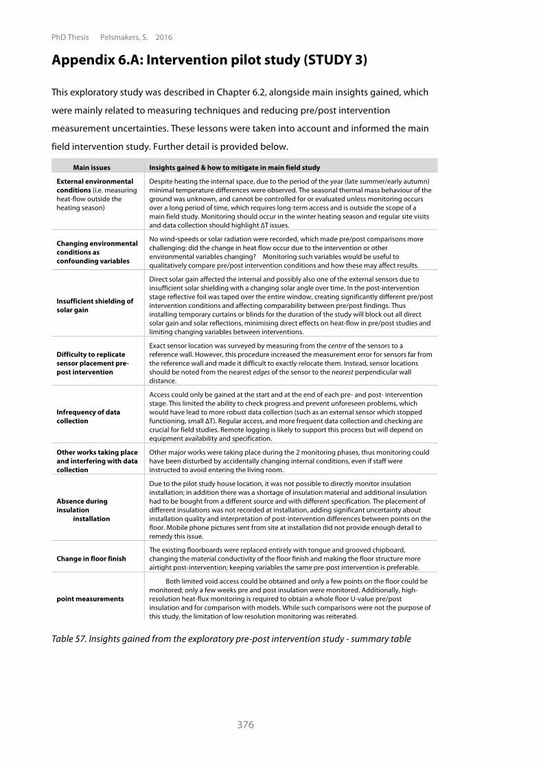
PhD Thesis Pelsmakers, S. 2016
376
Appendix 6.A: Intervention pilot study (STUDY 3)
This exploratory study was described in Chapter 6.2, alongside main insights gained, which
were mainly related to measuring techniques and reducing pre/post intervention
measurement uncertainties. These lessons were taken into account and informed the main
field intervention study. Further detail is provided below.
Main issues Insights gained & how to mitigate in main field study
External environmental conditions (i.e. measuring heat-flow outside the heating season)
Despite heating the internal space, due to the period of the year (late summer/early autumn) minimal temperature differences were observed. The seasonal thermal mass behaviour of the ground was unknown, and cannot be controlled for or evaluated unless monitoring occurs over a long period of time, which requires long-term access and is outside the scope of a main field study. Monitoring should occur in the winter heating season and regular site visits and data collection should highlight "T issues.
Changing environmental conditions as confounding variables
No wind-speeds or solar radiation were recorded, which made pre/post comparisons more challenging: did the change in heat flow occur due to the intervention or other environmental variables changing? Monitoring such variables would be useful to qualitatively compare pre/post intervention conditions and how these may affect results.
Insufficient shielding of solar gain
Direct solar gain affected the internal and possibly also one of the external sensors due to insufficient solar shielding with a changing solar angle over time. In the post-intervention stage reflective foil was taped over the entire window, creating significantly different pre/post intervention conditions and affecting comparability between pre/post findings. Thus installing temporary curtains or blinds for the duration of the study will block out all direct solar gain and solar reflections, minimising direct effects on heat-flow in pre/post studies and limiting changing variables between interventions.
Difficulty to replicate sensor placement pre-post intervention
Exact sensor location was surveyed by measuring from the centre of the sensors to a reference wall. However, this procedure increased the measurement error for sensors far from the reference wall and made it difficult to exactly relocate them. Instead, sensor locations should be noted from the nearest edges of the sensor to the nearest perpendicular wall distance.
Infrequency of data collection
Access could only be gained at the start and at the end of each pre- and post- intervention stage. This limited the ability to check progress and prevent unforeseen problems, which would have lead to more robust data collection (such as an external sensor which stopped functioning, small "T). Regular access, and more frequent data collection and checking are crucial for field studies. Remote logging is likely to support this process but will depend on equipment availability and specification.
Other works taking place and interfering with data collection
Other major works were taking place during the 2 monitoring phases, thus monitoring could have been disturbed by accidentally changing internal conditions, even if staff were instructed to avoid entering the living room.
Absence during insulation
installation
Due to the pilot study house location, it was not possible to directly monitor insulation installation; in addition there was a shortage of insulation material and additional insulation had to be bought from a different source and with different specification. The placement of different insulations was not recorded at installation, adding significant uncertainty about installation quality and interpretation of post-intervention differences between points on the floor. Mobile phone pictures sent from site at installation did not provide enough detail to remedy this issue.
Change in floor finish The existing floorboards were replaced entirely with tongue and grooved chipboard, changing the material conductivity of the floor finish and making the floor structure more airtight post-intervention; keeping variables the same pre-post intervention is preferable.
point measurements
Both limited void access could be obtained and only a few points on the floor could be monitored; only a few weeks pre and post insulation were monitored. Additionally, high-resolution heat-flux monitoring is required to obtain a whole floor U-value pre/post insulation and for comparison with models. While such comparisons were not the purpose of this study, the limitation of low resolution monitoring was reiterated.
Table 57. Insights gained from the exploratory pre-post intervention study - summary table
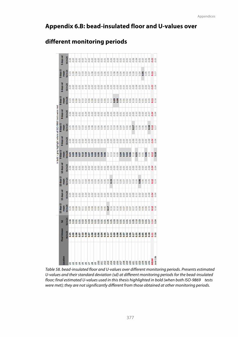
Appendices
377
Appendix 6.B: bead-insulated floor and U-values over
different monitoring periods
Table 58. bead-insulated floor and U-values over different monitoring periods. Presents estimated U-values and their standard deviation (sd) at different monitoring periods for the bead-insulated floor; final estimated U-values used in this thesis highlighted in bold (when both ISO-9869 tests were met); they are not significantly different from those obtained at other monitoring periods.
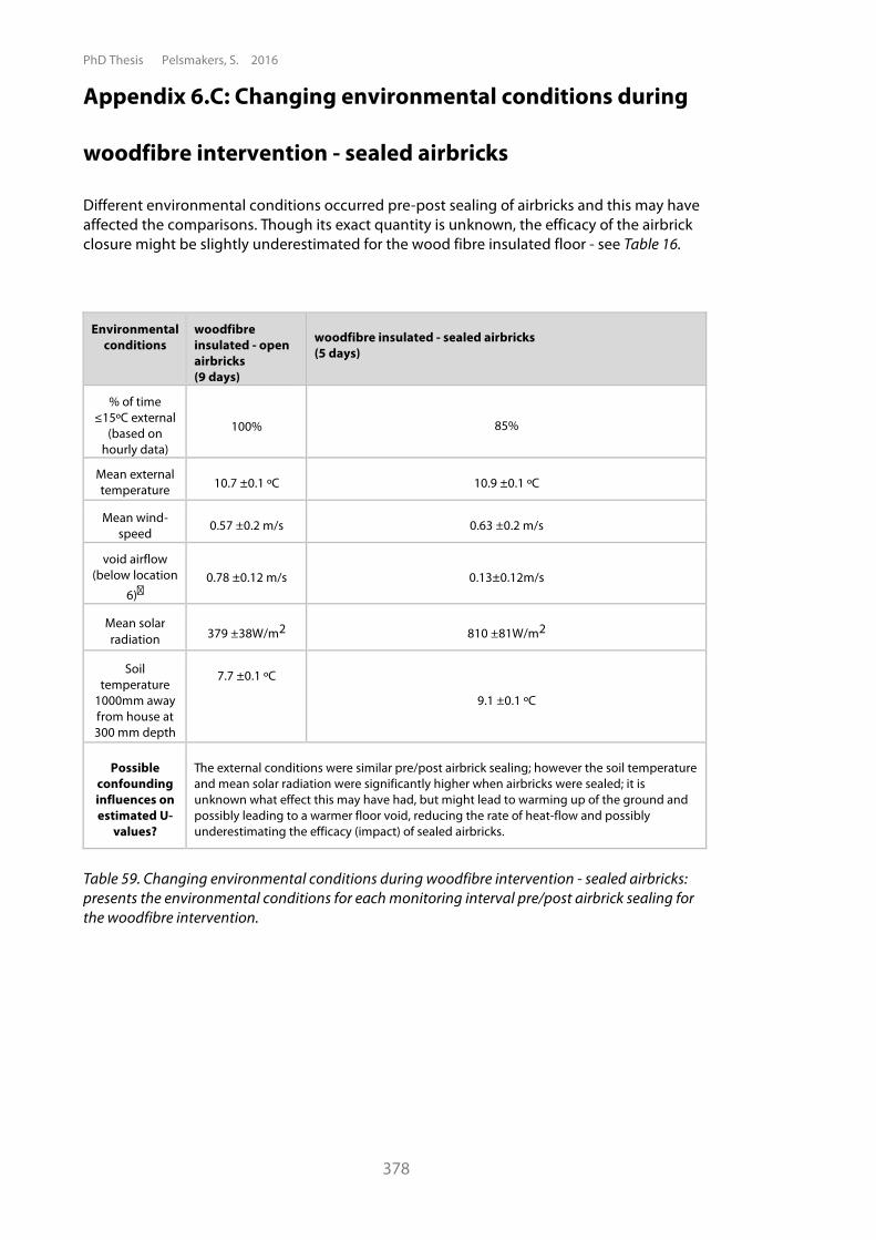
PhD Thesis Pelsmakers, S. 2016
378
Appendix 6.C: Changing environmental conditions during
woodfibre intervention - sealed airbricks
Different environmental conditions occurred pre-post sealing of airbricks and this may have affected the comparisons. Though its exact quantity is unknown, the efficacy of the airbrick closure might be slightly underestimated for the wood fibre insulated floor - see Table 16.
Environmental conditions
woodfibre insulated - open airbricks (9 days)
woodfibre insulated - sealed airbricks (5 days)
% of time !15ºC external
(based on hourly data)
100% 85%
Mean external temperature 10.7 ±0.1 ºC 10.9 ±0.1 ºC
Mean wind-speed 0.57 ±0.2 m/s 0.63 ±0.2 m/s
void airflow (below location
6)� 0.78 ±0.12 m/s 0.13±0.12m/s
Mean solar radiation 379 ±38W/m2 810 ±81W/m2
Soil temperature
1000mm away from house at 300 mm depth
7.7 ±0.1 ºC
9.1 ±0.1 ºC
Possible confounding influences on estimated U-
values?
The external conditions were similar pre/post airbrick sealing; however the soil temperature and mean solar radiation were significantly higher when airbricks were sealed; it is unknown what effect this may have had, but might lead to warming up of the ground and possibly leading to a warmer floor void, reducing the rate of heat-flow and possibly underestimating the efficacy (impact) of sealed airbricks.
Table 59. Changing environmental conditions during woodfibre intervention - sealed airbricks: presents the environmental conditions for each monitoring interval pre/post airbrick sealing for the woodfibre intervention.
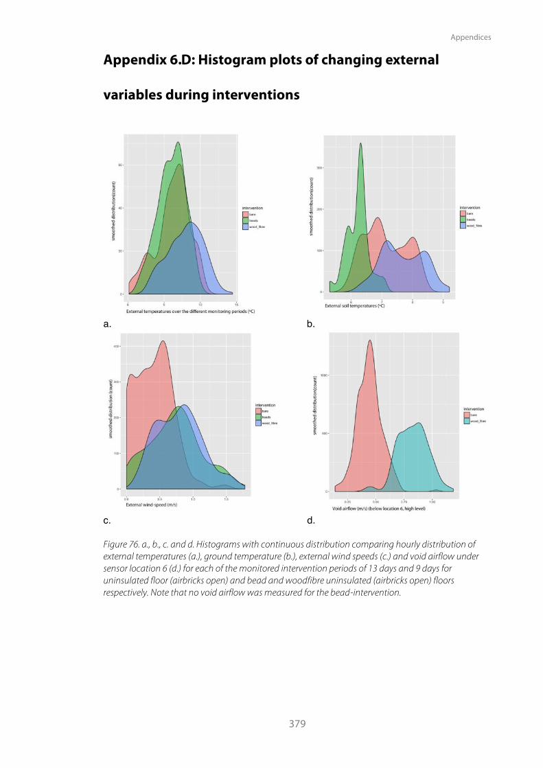
Appendices
379
Appendix 6.D: Histogram plots of changing external
variables during interventions
a. b.
c. d. Figure 76. a., b., c. and d. Histograms with continuous distribution comparing hourly distribution of external temperatures (a.), ground temperature (b.), external wind speeds (c.) and void airflow under sensor location 6 (d.) for each of the monitored intervention periods of 13 days and 9 days for uninsulated floor (airbricks open) and bead and woodfibre uninsulated (airbricks open) floors respectively. Note that no void airflow was measured for the bead-intervention.
PhD Thesis Pelsmakers, S. 2016
380
Appendix 6.E: Field study surface temperatures
As expected and as observed in the Salford EH, once insulated, the floor surface
temperatures (including heated and unheated periods) increased by on average 1.8ºC for
both interventions, though this might be overestimated for the woodfibre intervention given
the warmer external temperatures during that monitoring period. On average surface
temperatures were also 1.2ºC to 1.3ºC warmer with sealed airbricks for the uninsulated and
woodfibre insulated floor respectively. Warmer floor surfaces are beneficial for occupant
thermal comfort; however even when insulated, floor surface temperatures were below
19ºC; implications of this on thermal comfort are discussed in Chapter 6.5. Note that the
figures below are based on mean surface temperatures of the full monitoring period, while
the thermal comfort discussion is based on surface temperatures during occupied (heated)
periods (when typically higher surface temperatures were observed).
As Figure 77., Figure 78 and Figure 79. Illustrate that the floor surfaces are significantly colder
in the perimeter region (as low as 13ºC in the uninsulated floor) compared to the non-
perimeter region (up to 16ºC in the uninsulated floor). The impact of interventions increases
floor surface temperatures above average in the perimeter zone (by 2.0±0.14ºC to 2.1±0.14ºC
compared to 1.6±0.14ºC to 1.7±0.14ºC for the non-perimeter zone for woodfibre and bead
intervention respectively). The effect of the perimeter and airbrick airflow is much more
significant in the uninsulated floor compared to the insulated floors; though Figure 4. also
illustrates the effect of installation issues in location 3 and 21 - as described in Chapter
6.4.3.1.
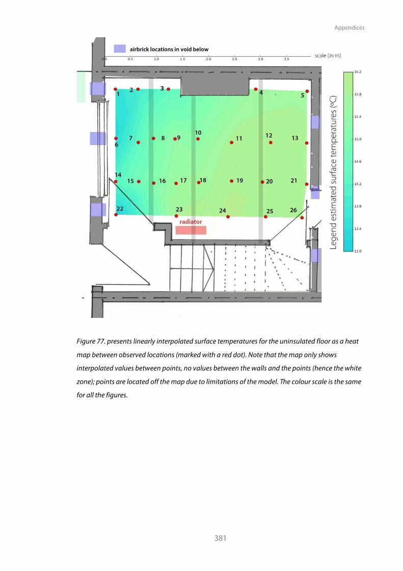
Appendices
381
Figure 77. presents linearly interpolated surface temperatures for the uninsulated floor as a heat
map between observed locations (marked with a red dot). Note that the map only shows
interpolated values between points, no values between the walls and the points (hence the white
zone); points are located off the map due to limitations of the model. The colour scale is the same
for all the figures.

PhD Thesis Pelsmakers, S. 2016
382
Figure 78. as previous figure but for bead insulated floor
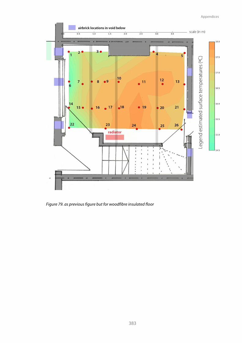
Appendices
383
Figure 79. as previous figure but for woodfibre insulated floor