post-seismic ionospheric response to the 11 april 2012 east indian ocean doublet earthquake

Sunil et al. Earth, Planets and Space (2015) 67:37 DOI 10.1186/s40623-015-0200-8

FULL PAPER Open Access

Post-seismic ionospheric response to the 11 April2012 East Indian Ocean doublet earthquakeAnakuzhikkal Sudarsanan Sunil, Mala S Bagiya*, Chappidi Divakar Reddy, Manish Kumar and Durbha Sai Ramesh

Abstract

The 11 April 2012 East Indian Ocean earthquake is unique because of its largest ever recorded aftershock. The mainearthquake occurred with a magnitude of 8.6 Mw and was followed by a strong aftershock (8.2 Mw). Our analysisof the main shock indicates that the rupture was a mixture of strike-slip and thrust faults, and significant verticalsurface displacements were observed during the event. The prime interest here is to study the post-seismicionospheric disturbances, along with their characteristics. As both earthquakes had large magnitudes, they providedan opportunity to minimize the ambiguity in identifying the corresponding seismic-induced ionosphericdisturbances. Approximately 10 min after both seismic events, the nearby ionosphere started to manifest electrondensity perturbations that were investigated using GPS-TEC measurements. The epicenters of both events werelocated south of the magnetic equator, and it is believed that the varying magnetic field inclination might beresponsible for the observed north-south asymmetry in the post-seismic total electron content (TEC) disturbances.These disturbances are observed to propagate up to approximately 1,500 km towards the north side of theepicenter and up to only a few hundred kilometers on the south side. The frequency analysis of the post-seismicTEC disturbances after both earthquakes exhibits the dominant presence of acoustic frequencies varying betweenapproximately 4.0 to 6.0 mHz. The estimated propagation velocities of the post-seismic TEC disturbances during themain shock (0.89 km/s) and aftershock (0.77 km/s) confirm the presence of an acoustic frequency as the generativemode for the observed TEC fluctuations.

Keywords: Strike-slip faults; Post-seismic ionospheric disturbances; Acoustic waves during seismic events;Earthquake and GPS-TEC

BackgroundThe origin of perturbations in ionospheric electrondensity can be traced to various sources. They can ori-ginate due to forces either from above (e.g., solar, geo-magnetic) or below (e.g., lower atmospheric, seismic)the ionosphere. In particular, seismic activity is one ofthe potential sources that can affect the ionosphericelectron density at smaller scales prior to, during, orafter an earthquake occurrence (e.g., Liu et al. 2010;Rolland et al. 2011a, Rolland et al. 2011b; Astafyevaet al. 2013). These electron density variations are, re-spectively, known as pre-, co-, and post-seismic iono-spheric disturbances. It is well known that during theoccurrence of an earthquake, the surface experienceshorizontal as well as vertical displacements, depending

* Correspondence: [email protected] Institute of Geomagnetism, Plot 5, Sector 18, Near Kalamboli Highway,New Panvel (W), Navi Mumbai 410218, India

© 2015 Sunil et al.; licensee Springer. This is anAttribution License (http://creativecommons.orin any medium, provided the original work is p

upon the type of rupture fault. Normal and reversethrust faults lead to significant vertical surface dis-placements during the earthquake, while strike-slipfaults alone generally produce only horizontal displace-ments. Shallow thrust earthquakes, giving strong verti-cal ground displacements, produce infrasonic pressurewaves in the vicinity of the neutral atmosphere. Theseneutral atmospheric disturbances, known as acousticgravity waves, propagate upwards to ionospheric alti-tudes and create disturbances in the electron densitythere (e.g., Calais and Minster 1998). These distur-bances are well known as seismo-traveling ionosphericdisturbances (STID) (e.g., Liu et al. 2011) or co-seismicionospheric disturbances (CID) (e.g., Heki and Ping2005). In addition to ground vertical motion, horizon-tally propagating Rayleigh surface waves (Oliver 1962)also introduce acoustic waves into the nearby neutralatmosphere, which later arrive at the ionospheric

Open Access article distributed under the terms of the Creative Commonsg/licenses/by/4.0), which permits unrestricted use, distribution, and reproductionroperly credited.

mailto:[email protected]

http://creativecommons.org/licenses/by/4.0

Sunil et al. Earth, Planets and Space (2015) 67:37 of 12

altitudes and generate electron density variations there.The Rayleigh wave propagates horizontally with typicalvelocities of approximately 3 to 5 km/s on the surfaceof the Earth. While propagating away from the epicen-ter, it generates acoustic wave perturbations that reachionospheric altitudes and create electron density varia-tions. Although the first effects to be seen in the iono-sphere would be due to vertical surface displacementsduring the shock, the far-field ionospheric perturba-tions due to the Rayleigh wave would appear earlier be-cause of its higher velocity. It is conjectured thattsunami waves in the ocean generate gravity waves thatpropagate obliquely upwards and interact with theionospheric electron density.Acoustic gravity waves are mainly generated immedi-

ately after the main shock (e.g., Astafyeva et al. 2009;Matsumura et al. 2011; Saito et al. 2011; Rolland et al.2011a) and reach ionospheric altitudes after 10 to15 min of the main shock. It is believed that upwardpropagation of wave perturbations happens in the vicin-ity of the earthquake epicenter or within the so-calledearthquake preparation zone. Using a case study, Otsukaet al. (2006) suggested that there can be multiple sourcesfor acoustic wave generation along the rupture thatpropagate away from the epicenter at the rupture vel-ocity. Heki and Ping (2005) have empirically shown thatonly acoustic waves emanating within the zenith anglesof 0° to 20° can reach ionospheric heights and affect theelectron density. The remaining waves get reflected,mainly because of atmospheric temperature variations,and return to the ground. Acoustic waves at ionosphericheights would introduce electron density perturbationsthat propagate further along geomagnetic field lines.Heki and Ping (2005) have empirically shown thatpropagation along the field lines is highly dependent onthe magnetic inclination of that region. According tothem, if the angle between the acoustic-wave-inducedpost-seismic ionospheric perturbations and the localgeomagnetic field is either 0 or 180, then propagationwill be hampered. In other cases, perturbations canpropagate farther depending on the angle with respectto the geomagnetic field lines.Induced ionospheric electron density perturbations

related to seismic activity are often observed with vari-ous radio techniques, such as HF Doppler sounding,ionosonde, and global positioning system (GPS) (e.g.,Tanaka et al. 1984; Yao et al. 2012; Rolland et al. 2011a;Rolland et al. 2011b). In recent times, the GPS networkhas been widely used to study co- and post-seismicionospheric disturbances (e.g., Liu et al. 2010; Rollandet al. 2011a; Rolland et al. 2011b; Astafyeva et al. 2013and references therein). Individual investigations (e.g.,Liu et al. 2010; Rolland et al. 2011a; Rolland et al.2011b; Tsugawa et al. 2011; Kakinami et al. 2012) have

been able to characterize the different types of seismic-induced ionospheric disturbances, such as those pro-duced by acoustic waves caused by propagatingRayleigh surface waves, by acoustic waves and atmos-pheric gravity waves from the ionospheric epicenter,and by co-seismic surface motions, the post-seismic4-min monoperiodic atmospheric resonances, tsunamis,and co-seismic depletion in GPS-derived total electroncontent (TEC) followed by enhancements over thetsunami origin region.In the present case, we investigate various characteris-

tics of post-seismic ionospheric disturbances (propaga-tion extent, generative wave frequency, propagationvelocity, and direction) associated with the Indian Oceandoublet earthquake that occurred on 11 April 2012.From the point of view of seismicity, this particularearthquake is unique in many ways (Pollitz et al. 2012;Yue et al. 2012). This was the largest strike-slip earth-quake ever recorded. The main earthquake (8.6 Mw)was followed by a powerful aftershock of 8.2 Mw, thehighest ever recorded aftershock. Although many resultshave been reported (e.g., Perevalova et al. 2014 and ref-erences therein) pertaining to the post-seismic iono-spheric variations, this particular case study is new fromthe point of view of the complex earthquake fault mech-anisms. This aspect, in terms of the vertical surface dis-placements, is discussed in detail. This is significantbecause, as strike-slip earthquakes are less frequent innature, post-seismic ionospheric disturbances that per-tain to strike-slip earthquakes have rarely been reported(e.g., Astafyeva et al. 2014). Another major reason forselecting this event is to minimize the ambiguities inidentifying the relatively feeble (small-scale) earthquake-induced post-ionospheric disturbances. It is often difficultto unambiguously associate the observed ionosphericdisturbances during a seismic event exclusively to theevent, since competing candidate phenomena can alsooperate in the same time window. This ambiguity is ad-dressed in this study, and it is also demonstrated thatthe observed ionospheric disturbances are indeed in-duced by the earthquakes. The selected time window ofevents illustrates two major earthquakes that occurredwith a time gap of approximately 2 h and 5 min. Bothquakes occurred before sunset on a geomagneticallyquiet day (Ap = 4). These may preclude many other po-tential sources of ionospheric disturbance. The follow-ing sections describe the observations and discussionspertaining to the ionospheric response to this twin seis-mic event.

MethodsFigure 1a shows the earthquake epicenters during bothearthquakes. The first earthquake with Mw = 8.6(08:38:37 UTC) in the Indian Ocean, about 100 km west

(b)

(c)

(a)

Figure 1 (See legend on next page.)


(See figure on previous page.)Figure 1 Locations of the earthquake epicenters, beach ball diagrams showing the four-fault mechanisms, and vertical surfacedisplacement. (a) Locations of epicenters during the main shock (red star) and aftershock (yellow star). Locations of GPS receiver stations used inthe present study are also shown in the plot. Red triangles show the IGS GPS receiver stations, while green triangles represent the SuGAr GPSreceiver stations. (b) Four-fault mechanisms during the main shock that lasted approximately 160 s. The parameters used to plot the faultmechanisms are from Yue et al. (2012) and are shown here in the table below the plot. It is clear that the main shock occurred with a mixtureof strike-slip and thrust faulting. (c) Vertical surface displacement associated with the main shock. It can be seen that because of the small thrustcomponent, a significant vertical displacement of approximately 2.27 m was observed near the epicenter during the main shock.


of the Sumatra subduction zone, was the largest intra-plate strike-slip earthquake in history. The epicenter ofthis event was located at 2.31°N, 93.06°E (shown by thered star in the figure). After approximately 2 hours(10:43:00 UTC), it triggered another great strike-slipearthquake of Mw = 8.2 in its vicinity, with an epicenterat 0.77°N, 92.45°E (shown by the yellow star in thefigure). Figure 1b represents the beach ball diagramshowing the four-fault mechanisms during the mainshock. It can be seen that the main earthquake sourcehas strike-slip and thrust mechanisms.From the tectonics point of view, this twin earthquake

event had a very complex four-fault rupture during themain shock, and the large aftershock occurred with a bi-lateral rupture fault (Pollitz et al. 2012; Yue et al. 2012).The possible four-fault mechanisms simulated with thestrike, dip, and rake values taken from Yue et al. (2012)are represented in Figure 1b for the main shock. It canbe seen that it was not a pure strike-slip earthquake.The main rupture lasted for approximately 160 s (Yueet al. 2012), exhibiting a mixture of strike-slip and thrustfaulting (e.g., Meng et al. 2012). It is known that duringa pure strike-slip earthquake, the surface may not ex-perience any significant vertical displacements. Thus, thevertical mechanical oscillations in the earth-bounded at-mosphere, and later its manifestations to ionosphericheights, may not be significant during any pure strike-slip event. In order to justify the mixed-fault mechanismduring the main shock (Figure 1b), vertical surface dis-placements were simulated with the help of Okada(1985) and the parameters given by Yue et al. (2012).Figure 1c shows the vertical displacement simulated overthe time period of approximately 110 s for four differ-ent focal parameters. It is noted that the surface sur-rounding the epicenter had oscillated up and downsignificantly during the main shock, with a maximumvertical displacement of approximately 2.27 m. Asmentioned earlier, the vertical surface displacementsproduce infrasonic pressure waves in the nearby atmos-phere, which propagate upward with increasing ampli-tude as the atmospheric density decreases with height.There is convincing evidence that the neutral atmos-pheric perturbations manifest as ionospheric electrondensity perturbations at different heights, from 100 kmto as high as 300 km (e.g., Rolland et al. 2011a).

To identify the post-seismic ionospheric disturbancesassociated with this twin seismic event, if any, GPS-TECdata from the Sumatran GPS Array (SuGAr) and Inter-national GNSS Service (IGS) networks were extracted(source: http://sopac.ucsd.edu). GPS stations used inthe present investigations are shown as triangles inFigure 1a. Green triangles represent the SuGAr stations,while red triangles represent the IGS stations. The data-sampling rate for SuGAr receivers is 15 s, and that ofthe IGS receivers is 30 s.TEC represents the total number of free electrons

along the line of sight from satellite to receiver. It ismainly weighted by the ionospheric F-region (the regionwhere maximum ionization occurs); thus, it provides anopportunity to detect any acoustic, gravity, or both typesof wave perturbations in the upper atmosphere. TEC,both from SuGAr and IGS receivers, are calculated hereusing differential carrier phase measurements and codemeasurements available in the receiver-independent ex-change (RINEX) file format. The dual frequency carrierphase measurements provide the smooth slant TEC withan integer ambiguity. Slant TEC calculated from thecode measurements are absolute but noisy. We calcu-lated the absolute slant TEC using code measurements,and smoothed it with the carrier phase measurements.The estimated slant TEC is converted to vertical TEC(VTEC) using a mapping function (Mannucci et al.1993) as follows:

VTEC ¼ M � STEC ð1Þ

M ¼ 1−cos Eð Þ1þ h

RE

!2" #12

ð2Þ

where E is the satellite elevation angle, h is the iono-spheric shell height (300 km is used here), and RE is theEarth’s mean radius. The VTEC is corrected for themonthly satellite differential code biases (source: ftp://ftp.unibe.ch/aiub/CODE/). For further study, the abso-lute VTEC is subtracted from its previous value every30 s. This is a simple two-point differentiation (Liu et al.2006), and the resultant VTEC is called the differentialTEC. To minimize the multipath effect, an elevationmask of 20° is applied.

http://sopac.ucsd.edu

ftp://ftp.unibe.ch/aiub/CODE/

ftp://ftp.unibe.ch/aiub/CODE/


Results and discussionPropagation characteristics of post-seismic ionosphericdisturbancesWhile examining the differential TEC variations duringand after the earthquakes, it was noticed that approxi-mately 10 to 12 min after the occurrence of both earth-quakes, sudden irregular TEC fluctuations were observedby more than one satellite at various GPS sites on 11 April2012. Henceforth, the satellites will be identified by theirpseudo random number (PRN). After the first earthquake,PRN 32 and PRN 16 showed TEC fluctuations, while PRN32 and PRN 20 detected similar types of TEC variationsafter the second earthquake.To confirm that the observed TEC fluctuations on

April 11 were due to the twin seismic activity, the differ-ential TEC variations at one of the SuGAr stations,umlh, as observed by PRN 32, were examined. The dif-ferential TEC variations observed at umlh for five con-secutive days starting from April 9 through April 13,2012 are presented in Figure 2. It can be seen that sud-den TEC variations are clearly identifiable approximately10 min after the origin time of both the earthquakes onApril 11. No such variations were observed on theremaining 4 days.Figure 3a depicts the locations of various SuGAr and IGS

stations (triangles) along with the ionospheric piercing

April

April

April

April

April

Figure 2 Differential TEC variations on 9 to 13 April 2012 from one Searthquakes. It can be seen that after both events, the TEC started to show

point (IPP) positions of PRN 32 (blue circles) and PRN 16(red circles) calculated at an ionospheric height of 300 kmapproximately 10 min after the first earthquake on April11. The respective IPPs are labeled according to the re-ceiving station codes. As mentioned earlier, the post-seismic TEC variations after the second earthquake wereobserved by PRN 32 (blue circles) and PRN 20 (red cir-cles). The observational IPP positions for these PRNs areshown in Figure 3b. Both earthquakes locations are labeledand represented by star symbols in the figures.Figure 4a,b shows the differential TEC variations from

08:00 to 10:00 UTC as observed by PRN 32 and PRN 16at various stations depicted in Figure 3a. By assumingthat the Earths’ surface remains flat a few degreesaround the equator, the horizontal slant distance be-tween the epicenter and each IPP is calculated andshown in Figure 4a,b. Although the distance from thehighest initial uplifted height is more suitable while cal-culating the distances from the epicenter (e.g., Kakinamiet al. 2012, 2013), these values may not change signifi-cantly in our case, since the epicenter (2.31°N, 93.06°E)and the place of highest initial height (2.35°N, 93.55°E)are nearby. Clear signatures of post-seismic TEC distur-bances were clearly observed by both PRNs approxi-mately 10 min after the first earthquake occurrence. It isalso notable that the largest magnitude of the seismically

13, 2012

12, 2012

11, 2012

10, 2012

9, 2012

uGAr station, umlh. Two red bars show the times of bothirregular fluctuations. These fluctuations were absent on other days.

(a)

(b)Figure 3 Plots showing locations of various SuGAr and IGS stations and positions for PRN 32 and PRN 20. (a) Plot showing IPP positionsfor PRN 32 (blue circles) and PRN 16 (red circles) approximately 10 min after the main shock. (b) IPP positions for PRN 32 (blue circles) and PRN20 (red circles) approximately 10 min after the aftershock. Green curved lines represent magnetic declination, while red curved lines representmagnetic inclination.


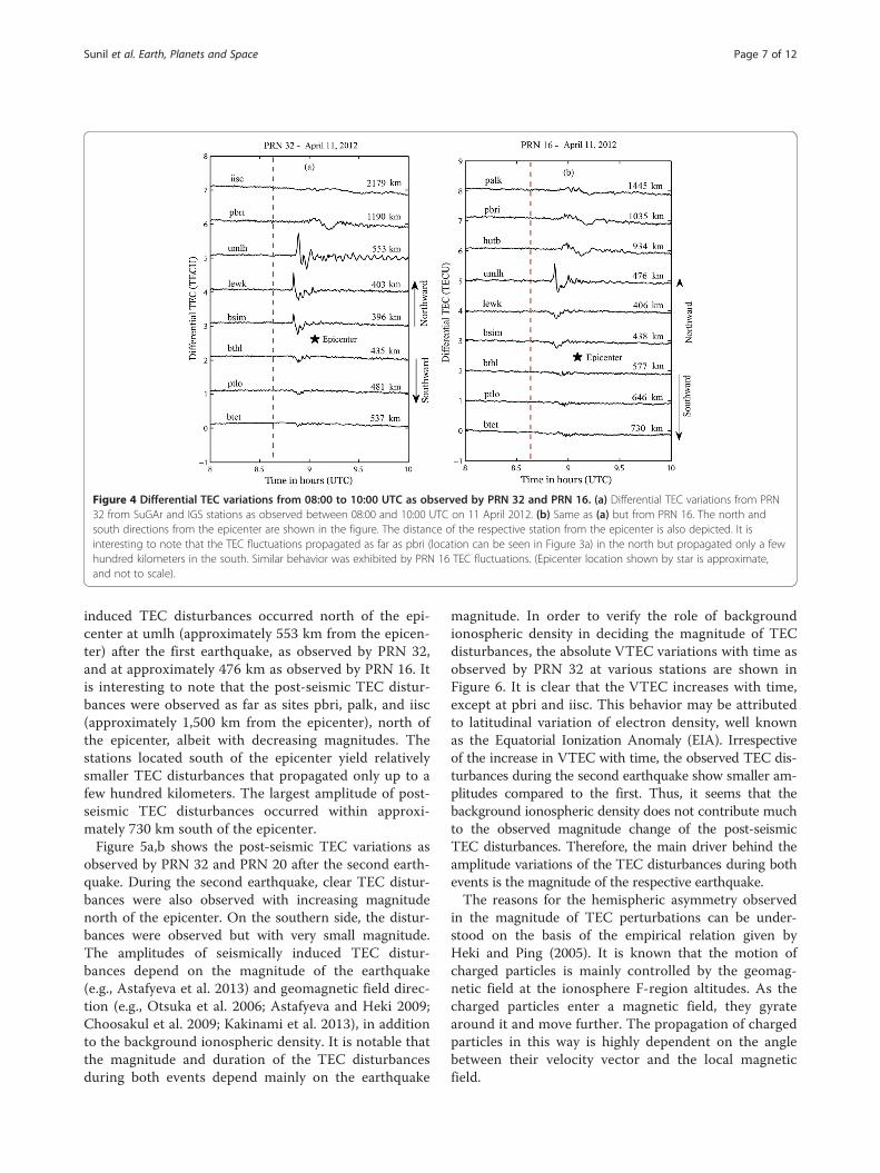
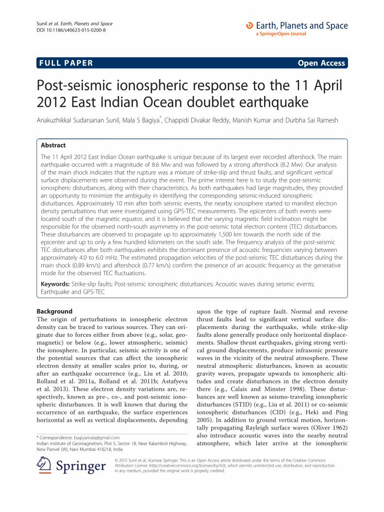
Figure 4 Differential TEC variations from 08:00 to 10:00 UTC as observed by PRN 32 and PRN 16. (a) Differential TEC variations from PRN32 from SuGAr and IGS stations as observed between 08:00 and 10:00 UTC on 11 April 2012. (b) Same as (a) but from PRN 16. The north andsouth directions from the epicenter are shown in the figure. The distance of the respective station from the epicenter is also depicted. It isinteresting to note that the TEC fluctuations propagated as far as pbri (location can be seen in Figure 3a) in the north but propagated only a fewhundred kilometers in the south. Similar behavior was exhibited by PRN 16 TEC fluctuations. (Epicenter location shown by star is approximate,and not to scale).


induced TEC disturbances occurred north of the epi-center at umlh (approximately 553 km from the epicen-ter) after the first earthquake, as observed by PRN 32,and at approximately 476 km as observed by PRN 16. Itis interesting to note that the post-seismic TEC distur-bances were observed as far as sites pbri, palk, and iisc(approximately 1,500 km from the epicenter), north ofthe epicenter, albeit with decreasing magnitudes. Thestations located south of the epicenter yield relativelysmaller TEC disturbances that propagated only up to afew hundred kilometers. The largest amplitude of post-seismic TEC disturbances occurred within approxi-mately 730 km south of the epicenter.Figure 5a,b shows the post-seismic TEC variations as

observed by PRN 32 and PRN 20 after the second earth-quake. During the second earthquake, clear TEC distur-bances were also observed with increasing magnitudenorth of the epicenter. On the southern side, the distur-bances were observed but with very small magnitude.The amplitudes of seismically induced TEC distur-bances depend on the magnitude of the earthquake(e.g., Astafyeva et al. 2013) and geomagnetic field direc-tion (e.g., Otsuka et al. 2006; Astafyeva and Heki 2009;Choosakul et al. 2009; Kakinami et al. 2013), in additionto the background ionospheric density. It is notable thatthe magnitude and duration of the TEC disturbancesduring both events depend mainly on the earthquake

magnitude. In order to verify the role of backgroundionospheric density in deciding the magnitude of TECdisturbances, the absolute VTEC variations with time asobserved by PRN 32 at various stations are shown inFigure 6. It is clear that the VTEC increases with time,except at pbri and iisc. This behavior may be attributedto latitudinal variation of electron density, well knownas the Equatorial Ionization Anomaly (EIA). Irrespectiveof the increase in VTEC with time, the observed TEC dis-turbances during the second earthquake show smaller am-plitudes compared to the first. Thus, it seems that thebackground ionospheric density does not contribute muchto the observed magnitude change of the post-seismicTEC disturbances. Therefore, the main driver behind theamplitude variations of the TEC disturbances during bothevents is the magnitude of the respective earthquake.The reasons for the hemispheric asymmetry observed

in the magnitude of TEC perturbations can be under-stood on the basis of the empirical relation given byHeki and Ping (2005). It is known that the motion ofcharged particles is mainly controlled by the geomag-netic field at the ionosphere F-region altitudes. As thecharged particles enter a magnetic field, they gyratearound it and move further. The propagation of chargedparticles in this way is highly dependent on the anglebetween their velocity vector and the local magneticfield.

Figure 6 Absolute VTEC variations as observed by PRN 32 atvarious SuGAr and IGS stations on 11 April 2012.

Figure 5 Same as Figure 4, but for PRN 32 (a) and PRN 20 (b) at 10:00 to 12:00 UTC. It can be seen that the TEC fluctuations were feebleafter the aftershock compared to what was observed after the main shock. (Epicenter location shown by star is approximate, and not to scale).


During a seismic event, once excited by an acousticwave or acoustic gravity waves, further propagation ofpost-seismic ionospheric electron density disturbancesdepends on their orientation with respect to the ambientmagnetic field direction. If the propagating wave frontsare parallel to the ambient geomagnetic field, then theLorentz force under whose influence the perturbationscan travel further would be zero. In such a scenario, thedensity disturbances may not propagate ahead and ceasewithin a short duration.The geomagnetic dip angle at the epicenter of the first

earthquake is −13.59°, and the declination is −1.5°. Thegeomagnetic inclination and declination of the secondearthquake epicenter is −17.26° and −1.74°, respectively.The magnetic field components (dip and declination) forthis region are calculated using the InternationalGeomagnetic Reference Field (IGRF) 11 and shown inFigure 3a,b with dotted lines. IGRF 11 is a standardmathematical description of the Earth’s main magneticfield. The latest version (IGRF 11) released by the Inter-national Association of Geomagnetism and Aeronomy(IAGA) is used here to derive the field inclination anddeclination. It can be seen that the epicenter of the firstearthquake is in the magnetic southern hemisphere. Thesouthward-propagating TEC perturbations would be-come parallel to the more inclined geomagnetic field inthe southern hemisphere within a short time duration.Thus, the TEC perturbations propagating in the south-ern hemisphere occur within a very short distance fromthe epicenter. It seems that the TEC perturbations had


almost merged with the background after this. In contrast,the northward-propagating TEC perturbations could travelcomparatively longer distances because the inclination grad-ually decreases towards the magnetic equator side of the epi-center. The magnetic equator-ward propagation of TECperturbations after both earthquakes reached as far as sitepbri to the north.

Evidence of the role of acoustic resonant frequenciesin producing post-seismic ionospheric disturbancesUsing the free oscillation modes of the Earth with the at-mosphere, Lognonné et al. (1998) predicted two infra-sonic frequencies that fall in the range of 3.7 to 3.8 mHzand 4.35 to 4.48 mHz, at which strong coupling betweenthe Earth and its atmosphere occurs. These frequenciesare termed fundamental acoustic resonance frequencies.Rolland et al. (2011a) confirmed the existence of thesefrequencies during their study of the great Tohokuearthquake and showed that these frequencies remainedtrapped for approximately 2 h after the main shock. Inaddition, they also recorded the signatures of the gravityacoustic mode (ranging between 0.5 and 2.9 mHz) forapproximately 1 h at ionospheric heights in terms ofTEC perturbations. However, Saito et al. (2011) reported,using TEC observations, an acoustic resonance lastingfor 4 h in the vicinity of the epicenter during the Tohokuearthquake.In order to identify the frequency range that might have

caused the observed post-seismic ionospheric distur-bances, the absolute slant TEC observations from PRN 32are detrended by subtracting the seven-point (105 s) mov-ing average from slant TEC every 15 s. This procedure

(a)

Max power = 139.9 TECU2

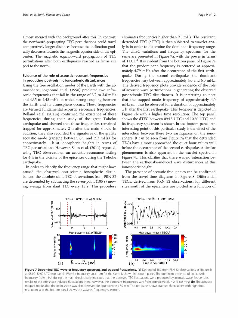
Figure 7 Detrended TEC, wavelet frequency spectrum, and trapped flat 08:00–12:00 UTC (top panel). Wavelet frequency spectrum for the samefrequency (4.49 mHz) during the main shock clearly indicates that the obsesimilar to the aftershock-induced fluctuations. Here, however, the dominantrapped mode after the main shock was also observed for approximately 5resolution, and the bottom panel shows the wavelet frequency spectrum.

eliminates frequencies higher than 9.5 mHz. The resultant,detrended TEC (dTEC) is then subjected to wavelet ana-lysis in order to determine the dominant frequency range.The dTEC variations and frequency spectrum for thesame are presented in Figure 7a, with the power in termsof TECU2. It is evident from the bottom panel of Figure 7athat the predominant frequency is centered at approxi-mately 4.79 mHz after the occurrence of the first earth-quake. During the second earthquake, the dominantfrequencies vary between approximately 4.0 and 6.0 mHz.The derived frequency plots provide evidence of the roleof acoustic wave perturbations in generating the observedpost-seismic TEC disturbances. It is interesting to notethat the trapped mode frequency of approximately 4.0mHz can also be observed for a duration of approximately1 h after the first earthquake. This behavior is depicted inFigure 7b with a higher time resolution. The top panelshows the dTEC between 09:15 UTC and 10:30 UTC, andits frequency spectrum is shown in the bottom panel. Aninteresting point of this particular study is the effect of theinteraction between these two earthquakes on the iono-sphere. It can be seen from Figure 7a that the detrendedTECs have almost approached the quiet hour values wellbefore the occurrence of the second earthquake. A similarphenomenon is also apparent in the wavelet spectra inFigure 7b. This clarifies that there was no interaction be-tween the earthquake-induced wave disturbances at thisionospheric height.The presence of acoustic frequencies can be confirmed

from the travel time diagrams in Figure 8. DifferentialTECs, derived from PRN 32 observations, for differentsites south of the epicenters are plotted as a function of

(b)

Max power = 52.1 TECU2

uctuations. (a) Detrended TEC from PRN 32 observations at site umlhis shown in bottom panel. The dominant presence of an acousticrved TEC fluctuations were produced by acoustic wave frequencies,t frequencies vary from approximately 4.0 to 6.0 mHz. (b) The acoustic0 min. The top panel shows trapped fluctuations with high-time

Figure 8 Travel time diagrams for ionospheric TEC perturbations as a function of time and epicentral distance. Propagation velocitiesafter the main shock and the aftershock are shown for PRN 32 in (a) and (b), respectively.


time (in UTC) and epicentral distance (line of sight dis-tance between IPP at 300-km altitude and epicenter).The velocity is estimated as the slope of the line shownin the figure. The line shows the arrival of the post-seismic disturbances at respective sites. It can be seenthat the velocity values are 0.89 and 0.77 km/s for thefirst and second earthquakes, respectively. The derivedvelocities indicate that acoustic waves are indeed themain driver of the observed post-seismic TEC distur-bances during both events. North of the epicenter,there were fewer observing stations during the secondearthquake. Thus, in order to reduce the ambiguity,only the southern stations are considered for the vel-ocity calculation.The obtained acoustic velocities during both earth-

quakes rule out the possibility of a Rayleigh wave as oneof the generative mechanisms for the observed post-seismic TEC disturbances using the present dataset.Thus, it can be stated that multiple acoustic wavesources propagating along the rupture after the twinseismic event might have induced acoustic waves in thenearby atmosphere, which results in excited ionosphericelectron density perturbations on arrival at ionosphericaltitudes.The GPS satellite IPP velocity is approximately 1 km/s

at the height of approximately 300 km. This height isthe IPP height where the TEC calculation is performed.This means that, at a height of approximately 300 km,the satellite IPP velocity value is very close to the esti-mated post-seismic TEC disturbance velocities. In viewof this, there would not be any significant relativisticDoppler shift in the power spectrum of Figure 7a due tosatellite motion. However, the change in generative

frequency from approximately 4.79 mHz during the firstevent to approximately 5 mHz during the second eventmay be due to the change in the ionospheric F-regionwind velocity. The F-region wind velocity varies withlocal time, so in the absence of direct wind measure-ments and accurate model values, this frequency shiftcan only be stated in terms of F-region changing windvelocity.

ConclusionsUsing GPS TEC measurements, we analyzed the iono-spheric signatures of the 2012 Indian Ocean doubletearthquake. Two major earthquakes with magnitudesMw = 8.6 and Mw = 8.2 occurred on 11 April 2012, andthe ionosphere responded by producing TEC distur-bances over the Indian Ocean and at stations located asfar as India approximately 10 min after the main shocks.The epicenters of both earthquakes are located south ofthe geomagnetic equator. The fault mechanism and as-sociated vertical surface displacements derived usingthe available parameters (Yue et al. 2012) during themain shock show that the rupture had strike-slip as wellas thrust faulting components. The post-seismic TECdisturbances propagated over a longer distance fromthe epicenter (approximately 1,500 km) in the northerndirection and shorter distances (approximately 700 km)on the southern side. The velocity estimation, using thedistance between the IPPs at different times and thecorresponding time values, shows that the post-seismicTEC disturbances traveled at the acoustic wave velocity.The wavelet analysis of TEC fluctuations, detrendedover a period of 105 s, clearly demonstrate the presenceof oscillations lasting for 1 h with a frequency of


approximately 4 mHz, and this frequency is close to theatmospheric resonance frequencies (3.7 and 4.4 mHz).The normal modes need to be recalculated to consider thedepth of the ocean and other variables near the epicenterof these earthquakes. They would then provide more real-istic acoustic resonant frequencies in this case study.The estimated propagation velocities of the post-seismic TEC disturbances during the main shock(0.89 km/s) and aftershock (0.77 km/s) confirm thepresence of acoustic frequencies as the generativemode for the observed TEC fluctuations. The presentdoublet earthquake event provided an opportunity tominimize the ambiguities in identifying even small-scale seismic-induced ionospheric disturbances. Thevarious characteristics of post-seismic ionospheric dis-turbances, such as generative frequency, propagationvelocity, and propagation direction, are addressed, andtheir respective physical mechanisms are discussed.

AbbreviationsCID: Co-seismic ionospheric disturbances; dTEC: Detrended TEC; GPS: Globalpositioning system; IAGA: International Association of Geomagnetism andAeronomy; IGRF: International Geomagnetic Reference Field;IGS: International GNSS Service; IPPs: Ionospheric piercing points;PRN: Pseudo random number; RINEX: Receiver-independent exchange;STID: Seismo-traveling ionospheric disturbance; SuGAr: Sumatran GPS Array;TEC: Total electron content.

Competing interestsThe authors declare that they have no competing interests.

Authors’ contributionsAS carried out the analysis and drafted the initial text. MB evaluated theinitial text for scientific content and co-drafted the manuscript. CDR and DSRgave very important suggestions at various stages of this work. DSRco-drafted the manuscript. MK contributed to the fault mechanism analysis.All authors read and approved the final manuscript.

AcknowledgementsThe authors gratefully acknowledge the Scripps Orbit and Permanent ArrayCenter (SOPAC) for providing GPS data from the IGS and SuGAr networks. ASis grateful to the Department of Science and Technology (DST), India, forproviding the research fellowship. This work is part of the newinterdisciplinary initiative of the Indian Institute of Geomagnetism (IIG), NaviMumbai, India. This work is supported by the Department of Science andTechnology (DST), India.

Received: 13 August 2014 Accepted: 28 January 2015

ReferencesAstafyeva E, Heki K (2009) Dependence of waveform of near-field coseismic

ionospheric disturbances on focal mechanisms. Earth PlanetsSpace 61:939–943

Astafyeva E, Heki K, Kiryushkin V, Afraimovich EL, Shalimov S (2009) Two-modelong-distance propagation of coseismic ionosphere disturbances. J GeophysRes 114:A10307, doi:10.1029/2008JA013853

Astafyeva E, Shalimov S, Olshanskaya E, Lognonné P (2013) Ionospheric responseto earthquakes of different magnitudes: larger quakes perturb theionosphere stronger and longer. Geophys Res Lett 40:1675–1681,doi:10.1002/grl.50398

Astafyeva E, Rolland LM, Sladen A (2014) Strike-slip earthquakes can also bedetected in the ionosphere. Earth Planet Sci Lett 405:180–193

Calais E, Minster JB (1998) GPS, earthquakes, the ionosphere, and the SpaceShuttle. Phys Earth Planet Inter 105:167–181, doi:10.1016/S0031-9201(97)00089-7

Choosakul N, Saito A, Iyemori T, Hashizume M (2009) Excitation of 4-min periodicionospheric variations following the great Sumatra-Andaman earthquake in2004. J Geophys Res 114:A10313, doi:10.1029/2008JA013915

Heki K, Ping J (2005) Directivity and apparent velocity of the coseismicionospheric disturbances observed with a dense GPS array. Earth Planet SciLett 236:845–855, doi:10.1016/j.epsl.2005.06.010

Kakinami Y, Kamogawa M, Tanioka Y, Watanabe S, Gusman AR, Liu JY, WatanabeY, Mogi T (2012) Tsunamigenic ionospheric hole. Geophys Res Lett39:L00G27, doi:10.1029/2011GL050159

Kakinami Y, Kamogawa M, Kakinami Y, Watanabe S, Odaka M, Mogi T, Liu J-Y, SunY-Y, Yamada T (2013) Ionospheric ripples excited by superimposedwavefronts associated with Rayleigh waves in the thermosphere. J GeophysRes Space Physics 118:905–911, doi:10.1002/jgra.50099

Liu J-Y, TsaiYB MKF, Chen YI, Tsai HF, Lin CH, Kamogawa M, Lee CP (2006)Ionospheric GPS total electron content (TEC) disturbances triggered by the26 December 2004 Indian Ocean tsunami. J Geophys Res 111:A05303,doi:10.1029/2005JA011200

Liu J-Y, Tsai HF, Lin CH, Kamogawa M, Chen YI, Lin CH, Huang BS, Yu SB, Yeh YH(2010) Coseismic ionospheric disturbances triggered by the Chi-Chiearthquake. J Geophys Res 115:A08303, doi:10.1029/2009JA014943

Liu J-Y, Chen CH, Lin CH, Tsai HF, Chen CH, Kamogawa M (2011) Ionosphericdisturbances triggered by the 11 March 2011 M9.0 Tohoku Earthquake. JGeophys Res 116:A06319, doi:10.1029/2011JA016761

Lognonné P, Clévédé E, Kanamori H (1998) Computation of seismograms andatmospheric oscillations by normal-mode summation for a spherical Earthmodel with realistic atmosphere. Geophys J Int 135:388–406

Mannucci AJ, Wilson BD, Edwards CD (1993) A new method for monitoring theEarth’s ionospheric total electron content using the GPS Global Network. TheInstitute of Navigation, Alexandria, VA, pp 1323–1332, Proceedings of IONGPS-93, the 6th International Technical Meeting of the Satellite Division ofThe Institute of Navigation, Salt Lake City, UT, 22–24 September

Matsumura M, Saito A, Iyemori T, Shinagawa H, Tsugawa T, Otsuka Y, Nishioka M,Chen CH (2011) Numerical simulations of atmospheric waves excited by the2011 off the Pacific coast of Tohoku Earthquake. Earth Planets Space63(7):885–889

Meng L, Ampuero J-P, Stock J, Duputel Z, Luo Y, Tsai VC (2012) Earthquake in amaze: compressional rupture branching during the 2012 Mw 8.6 SumatraEarthquake. Science 337:724–726, doi:10.1126/science.1224030

Okada Y (1985) Surface deformation due to shear and tensile faults in ahalf-space. Bull Seismol Soc Am 75:1135–1154

Oliver JA (1962) A summary of observed seismic surface wave dispersion. BullSeismol Soc Am 52:81–86

Otsuka Y, Kotake N, Tsugawa T, Shiokawa K, Ogawa T, Effendy SS, Kawamura M,Maruyama T, Hemmakorn N, Komolmis T (2006) GPS detection of totalelectron content variations over Indonesia and Thailand following the 26December 2004 earthquake. Earth Planets Space 58:159–165

Perevalova NP, Sankov VA, AstafyevaE ZAS (2014) Threshold magnitude forionospheric TEC response to earthquakes. JAtmos Solar-TerrPhys 108:77–90

Pollitz F, Sevilgen V, Stein RS, Bürgmann R (2012) The 11 April 2012 east IndianOcean earthquake triggered large aftershocks worldwide.Nature 490:250–253, doi:10.1038/nature11504

Rolland L, Lognonné P, Astafyeva E, Kherani A, Kobayashi N, Mann M, MunekaneH (2011a) The resonant response of the ionosphere imaged after the 2011Tohoku-Oki earthquake. Earth Planet Space 63:853–857, doi:10.5047/eps.2011.06.020

Rolland LM, Lognonné P, Munekane H (2011b) Detection and modeling ofRayleigh wave induced patterns in the ionosphere. J Geophys Res116:A05320, doi:10.1029/2010JA016060

Saito A, Tsugawa T, Otsuka Y, Nishioka M, Iyemori T, Matsumura M, Saito S,Chen CH, Goi Y, Choosakul N (2011) Acoustic resonance and plasmadepletion detected by GPS total electron content observation after the2011 off the Pacific coast of Tohoku Earthquake. Earth Planets Space63(7):863–867

Tanaka T, Ichinose T, Shibata T, Okuzawa T, Sato Y, Ogawa T, Nagasawa C(1984) HF-Doppler observations of acoustic waves excited by theUrakawa-Oki earthquake on 21 March 1982. JAtmos Solar-TerrPhys46:233–245

Tsugawa T, Saito A, Otsuka Y, Nishioka M, Maruyama T, Kato H, Nagatsuma T,Murata KT (2011) Ionospheric disturbances detected by GPS total electroncontent observation after the 2011 off the Pacific coast of TohokuEarthquake. Earth Planets Space 63:875–879, doi:10.5047/eps.2011.06.035


Yao YB, Chen P, Wu H, Zhang S, Peng W (2012) Analysis of ionosphericanomalies before the 2011 Mw 9.0 Japan earthquake. Chinese Sci Bull57(5):500–510, doi:10.1007/s11434-011-4851-y

Yue H, Lay T, Koper KD (2012) En échelon and orthogonal fault ruptures of the11 April 2012 great intraplate earthquakes. Nature 490:245–249, doi:10.1038/nature11492

Submit your manuscript to a journal and benefi t from:

7 Convenient online submission

7 Rigorous peer review

7 Immediate publication on acceptance

7 Open access: articles freely available online

7 High visibility within the fi eld

7 Retaining the copyright to your article

Submit your next manuscript at 7 springeropen.com

post-seismic ionospheric response to the 11 april 2012 east indian ocean doublet earthquake

Documents