April 16, 2015

Higgs Dark Matter from a Warped Extra-Dimension

– the truncated-inert-doublet model

Aqeel Ahmed,a,b,† Bohdan Grzadkowski,a John F. Gunionb and Yun Jiangb

aFaculty of Physics, University of Warsaw,

Pasteura 5, 02-093 Warsaw, PolandbDepartment of Physics, University of California,

Davis, CA 95616, U.S.A.

E-mail: aqeel.ahmed@fuw.edu.pl, bohdan.grzadkowski@fuw.edu.pl,

jfgunion@ucdavis.edu, yunjiang@ucdavis.edu

Abstract: We construct a 5D Z2-symmetric model with three D3-branes: two IR ones

with negative tension located at ends of an extra-dimensional interval and one UV-brane

with positive tension placed in the middle of the interval. Within this setup we investigate

the low-energy effective theory for the bulk SM bosonic sector. The Z2-even zero-modes

correspond to known standard degrees of freedom, whereas the Z2-odd zero modes might

serve as dark sector. We discuss two scenarios for spontaneous breaking of the gauge

symmetry, one based on expansion of the bulk Higgs field around extra-dimensional vev

with non-trivial profile and the second in which the symmetry breaking is triggered by

a vev of Kaluza-Klein modes of the bulk Higgs field. It is shown that they lead to the

same low-energy effective theory. The effective low-energy scalar sector contains a scalar

which mimics the Standard Model (SM) Higgs boson and a second stable scalar particle

(dark-Higgs) that is a dark matter candidate; the latter is a component of the zero-mode of

Z2-odd Higgs doublet. The model that results from the Z2-symmetric background geometry

resembles the Inert Two Higgs Doublet Model. The effective theory turns out to have an

extra residual SU(2)×U(1) global symmetry that is reminiscent of an underlying 5D gauge

transformation for odd degrees of freedom. At tree level the SM Higgs and the dark-Higgs

have the same mass; however, when leading radiative corrections are taken into account the

dark-Higgs turns out to be heavier than the SM Higgs. Implications for dark matter are

discussed; it is found that the dark-Higgs can provide only a small fraction of the observed

dark matter abundance.

Keywords: Warped Extra Dimensions, Dark matter, Bulk Higgs

†On leave of absence from National Centre for Physics, Quaid-i-Azam University Campus, Islamabad

45320, Pakistan

arX

iv:1

504.

0370

6v1

[he

p-ph

] 1

4 A

pr 2

015

Contents

1 Introduction 1

2 A Z2 symmetric warped extra-dimension and KK-parity 5

2.1 The IR-UV-IR model 5

2.2 KK-Parity 6

3 SSB in the IR-UV-IR model: the Abelian Higgs mechanism 7

3.1 SSB by vacuum expectation values of KK modes 9

3.2 SSB by a vacuum expectation value of the 5D Higgs field 13

4 SM EWSB by bulk Higgs doublet – the truncated-inert-doublet model 18

4.1 Quantum corrections to scalar masses 23

4.2 Dark matter relic abundance 26

5 Summary 28

A SSB in the IR-UV-IR model: the real scalar case 30

A.1 SSB by vacuum expectation values of KK modes 30

A.2 SSB by a vacuum expectation value of the 5D scalar field 35

1 Introduction

0 πrc

+y

−yUV

0 ≤ y ≤ L

IR

Figure 1: Cartoon of RS1 geometry.

The seminal work of Randall and Sun-

drum (RS) [1] provides an elegant solu-

tion to the hierarchy problem. Their pro-

posal involves an extra-dimension with

a non-trivial warp factor due to the

assumed anti-de Sitter (AdS) geome-

try along the extra-dimension. In their

model an AdS geometry on an S1/Z2 orbifold is considered which is equivalent to a line-

element 0 ≤ y ≤ L, where y is the coordinate of the fifth-dimension and L = πrc, with rcbeing the radius of the circle in the fifth-dimension. Moreover, their model involves two

D3-branes localized on the fixed points of the orbifold, a “UV-brane” at y = 0 and an

“IR-brane” at y = L (our nomenclature will become clear below), see Fig. 1. The solution

for the RS geometry is [1, 2],

ds2 = e2A(y)ηµνdxµdxν + dy2, with A(y) = −k|y|, (1.1)

where k is the inverse of the AdS radius. In the original RS1 model [1] it was assumed that

the Standard Model (SM) is localized on the IR-brane, whereas gravity is localized on the

– 1 –

UV-brane and propagates through the bulk to the IR-brane. They famously showed that

if the 5D fundamental theory involves only one mass scale M∗ – the Planck mass in 5D –

then, due to the presence of non-trivial warping along the extra-dimension, the effective

mass scale on the IR-brane is rescaled to mKK ∼ ke−kL ∼ O( TeV) and hence ameliorates

the hierarchy problem for mild values of kL ∼ O(35).

Soon after the RS proposal, many important improvements to the model were consid-

ered. First, a stabilization mechanism for the RS1 setup was proposed by Goldberger and

Wise [3]; it employs a real scalar field in the bulk of AdS geometry with localized potentials

on both of the branes, see also [4]. A second interesting observation, which could poten-

tially solve the fermion mass hierarchy problem within the SM, was made by many groups

[5–9]. The core idea of these works was to allow all the SM fields to propogate in the RS1

bulk, except the Higgs field which was kept localized on the IR-brane. In this way, the

zero-modes of these bulk fields correspond to the SM fields and the overlap of y-dependent

profiles of fermionic fields with the Higgs field could generate the required fermion mass

hierarchy. To suppress the EW precision observables, the symmetry of the gauge group was

enhanced by introducing custodial symmetry in Ref. [10]. The common lore, in the RS1

model and its extensions, was to keep the Higgs field localized on the IR-brane in order to

solve the hierarchy problem. The first attempt to consider the Higgs field in the bulk of

RS1 was made by Luty and Okui [11]. They employed AdS/CFT duality 1 to argue that a

bulk Higgs scenario can address the hierarchy problem by making the Higgs mass operator

marginal in the dual CFT.

A study of electroweak symmetry breaking (EWSB) within the Bulk Higgs scenario was

first performed in the RS1 setup by Davoudiasl et al. [14]; they showed that the zero-mode

of the bulk Higgs is tachyonic and hence could lead to a vacuum expectation value (vev)

at the TeV scale. Recently there have been many studies where a bulk Higgs scenario is

considered from different perspectives — see for example: a study with custodial symmetry

in the Higgs sector[15]; models with a soft wall setup [16]; bulk Higgs mediated FCNC’s [17];

suppression of EW precision observables by modifying the warped metric near the IR-brane

[18–20]; and, a bulk Higgs as the modulus stabilization field (Higgs–radion unification)

[21]. Different phenomenological aspects after the Higgs discovery were explored in [22–

28]. These phenomenological studies show that the RS1 model with bulk SM fields and its

descendants with modified geometry (RS-like warped geometries in general) are consistent

with the current experimental bounds and EW precision data.

A separate category of generalization of the RS models was based on the assumption

that the singular branes are replaced with thick branes which are smooth field configura-

tions of the bulk scalar field, see e.g. [4] and [29, 30].

As we discussed above, RS-like warped geometries, being consistent with the experi-

mental data, offer an attractive solution to many of the fundamental puzzles of the SM,

mostly through geometric means. In the same spirit, one can ask if RS-like warped extra-

dimensions can shed some light on another outstanding puzzle of SM, the lack of a candidate

for dark matter (DM) which constitutes 83% of the observed matter in the universe [31]. It

1For the phenomenological applications of AdS/CFT with RS1 geometry, see for example [12, 13].

– 2 –

appears that unlike (flat) universal extra-dimensions (UED), where the KK-modes of the

bulk fields can be even and odd under KK-parity (implying that the lowest KK-odd parti-

cle (LKP) could be a natural dark matter candidate [32, 33]), RS1-like models (involving

two branes and warped bulk) are unable to offer an analogue of KK-parity. The reason

lies in the fact that the RS1 geometry is just a single slice of AdS space and, since warped,

cannot be symmetric around any point along the extra-dimension and hence does not allow

a KK-parity. As a result it cannot accommodate a realistic dark matter candidate. To cure

this problem in the warped geometries, usually extra discrete symmetries are introduced

such that the SM fields are even while the DM is odd under such discrete symmetries in

order to make it stable [34–37]. Another way to mend this problem in warped geometries

is to introduce an additional hidden sector with some local gauge symmetries such that

only DM is charged under the hidden sector gauge symmetries and it couples to the SM

very weakly [38, 39], (see also [40]).

An alternative to introducing additional symmetries, is to extend the RS1-like warped

geometry in such a way that the whole geometric setup becomes symmetric around a fixed

point in the bulk. Two Z2 symmetric warped configurations are possible. In the first,

two identical AdS patches are symmetrically glued together at a UV fixed point, while

in the second two identical AdS pathes are symmetrically glued together at an IR fixed

point. The geometric configuration when the two AdS copies are glued together at the UV

fixed point will be referred as “IR-UV-IR geometry”, whereas the geometry corresponding

to the setup when two AdS copies are glued at the IR fixed point is called “UV-IR-UV

geometry”. We will only consider the IR-UV-IR geometric setup — it is straight forward

to extend our analysis to the UV-IR-UV geometries. (A common pathology associated

with this latter type of geometry is the appearance of ghosts.) We consider an interval

y ∈ [−L,L] in the extra-dimension, where on each end of the interval y = ±L there is a

D3 brane with negative tension (in Sec. 2.1 it will be clear why we need negative tension

branes) and at the center of the interval, y = 0, we place a positive tension brane where we

assume that gravity is localized. We call the boundary branes “IR-branes” and the brane

at y = 0 we term the “UV-brane”. The IR-UV-IR geometry and a pictorial description of

such a geometric setup is shown in Fig. 2. Since the brane tensions of the two IR-branes

are the same, this geometry is Z2 symmetric. We are aware of only two earlier attempts to

construct a similar setup. The first [41] treated the lowest odd KK gauge mode as the DM

candidate. The second employed a kink-like UV thick brane [42] and the corresponding

dark-matter was the first odd KK-radion [43].

In this work, we place all the SM fields, including the Higgs doublet, in the bulk of

the IR-UV-IR geometry. The geometric Z2 parity (y → −y symmetry) leads to “warped

KK-parity”, i.e. there are towers of even and odd KK-modes corresponding to each bulk

field. We focus on EWSB induced by the bulk Higgs doublet and low energy aspects of

the 4D effective theory for the even and odd zero-modes assuming the KK-mass scale is

high enough ∼ O(few) TeV. In the effective theory the even and odd Higgs doublets

mimic a two-Higgs-doublet model (2HDM) scenario – the truncated inert-doublet model –

with the odd doublet similar to the inert doublet but without corresponding pseudoscalar

and charged scalars. All the parameters of this truncated 2HDM are determined by the

– 3 –

UV

-bran

e

IR-b

ran

e

IR-b

ran

e

e−2k|y|e−2k|y|

y = 0

y = Ly = −L

ΛBΛB xµ

y

Figure 2: The geometric configuration for IR-UV-IR setup, the parameters are defined in Sec. 2.1.

fundamental 5D parameters of the theory and the choice of boundary conditions for the

fields at ±L. (Note that the boundary or “jump” conditions at y = 0 follow from the bulk

equations of motion in the case of even modes, whereas odd modes are required to be zero

by symmetry.) There are many possible alternative choices for the b.c. at ±L. We allow

the y-derivative of a field to have an arbitrary value at ±L as opposed to requiring that the

field value itself be zero, i.e. we employ Neumann or mixed b.c. rather than Dirichlet b.c. at

±L. Only the former yields a non-trivial theory allowing spontaneous symmetry breaking

(SSB), whereas the latter leads to an explicit symmetry breaking scenario in which there

are no Goldstone modes and the gauge bosons do not acquire mass. With these choices, the

symmetric setup yields an odd Higgs zero-mode that is a natural candidate for dark matter.

We compute the one-loop quadratic (in cutoff) corrections to the two scalar zero modes

within the effective theory and discuss their mass splitting. The dark matter candidate is

a WIMP — we calculate its relic abundance in the cold dark matter paradigm.

The paper is composed as follows. In Sec. 2, we setup the IR-UV-IR geometric

configuration and provide background solutions. We also discuss the manifestation of KK-

parity due the Z2 geometric setup. An Abelian Higgs mechanism, with a complex scalar

field and a gauge field, is studied in our background geometry in Sec. 3. In the Abelian

case we lay down the foundation for SSB due to bulk Higgs, which is later useful for the

case of EWSB in the SM. Two apparently different approaches are considered to study

SSB in the Abelian case: (i) SSB by vacuum expectation values of the KK modes; and,

(ii) SSB via a vacuum expectation value of the 5D Higgs field. Low energy (zero-mode)

4D effective theories are obtained within the two approaches and we find that the effective

theories are identical up to corrections of order O(m2

0/m2KK

), where m0 and mKK are the

zero-mode mass and KK-mass scale, respectively. Section 4 contains the main part of our

work. There, we focus on EWSB for the SM gauge sector due to the bulk Higgs doublet

in our Z2 symmetric geometry and obtain a low-energy 4D effective theory containing

all the SM fields plus a real scalar – a dark matter candidate – which is odd under the

discrete Z2 symmetry. In the subsequent two subsections of Sec. 4, we consider the

quantum corrections to the scalar masses below the KK-scale ∼ O(few) TeV and explore

the possible implications of the dark-matter candidate by calculating its relic abundance.

We summarize and give our conclusions in Sec. 5. For a warmup, Appendix A discusses

SSB of a discrete symmetry with a real scalar in the bulk of our geometric setup.

– 4 –

2 A Z2 symmetric warped extra-dimension and KK-parity

In this section we provide the background solution for the Z2 symmetric background (IR-

UV-IR) geometry and show how KK-parity is manifested within this geometric setup.

2.1 The IR-UV-IR model

We consider the IR-UV-IR warped geometry compactified on an interval, −L ≤ y ≤ L,

where a D3-brane with positive tension is located at the UV fixed point, y = 0, and two

negative tension D3-branes are located at the IR fixed points, y = ±L. The 5D gravity

action SG for such a geometry can be written as 2,

SG =

∫d5x√−g

R

2− ΛB − λUV δ(y)− λIRδ(y + L)− λIRδ(y − L)

+ SGH , (2.1)

where R is the Ricci scalar, ΛB is the bulk cosmological constant and λUV (λIR) are the

brane tensions at the UV(IR) fixed points. Since our geometry is compact with boundaries,

the action contains the Gibbons-Hawking boundary term, 3

SGH = −∫∂M

d4x√−gK, (2.2)

where K is the intrinsic curvature of the surface of the boundary manifold ∂M, given by

K = −gµν∇µnν = gµνΓMµνnM , (2.3)

with nM being the unit normal vector to the surface of the boundary manifold ∂M and gµνis the induced boundary metric. For the 5D manifold with 4D Poincare invariance (n5 = 1

and nµ = 0), the intrinsic curvature reduces to

K = −1

2gµν∂5gµν . (2.4)

The solution of the Einstein equations resulting from the above action is the RS metric

(1.1), where the AdS curvature k is related to ΛB by

ΛB = 6k2. (2.5)

Since the above setup is compactified on an interval y ∈ [−L,L], rather than on a

circle as in RS1, one needs to be careful and show that the solution (1.1) is compatible

with the boundaries and that the effective 4D cosmological constant is zero, see also [44].

We will see below that we need a fine tuning between the 5D cosmological constant ΛBand the brane tensions λUV,IR in order to get zero 4D cosmological constant. One can

calculate the effective 4D cosmological constant Λ4 from the action (2.1) by integrating

out the extra-dimension,

Λ4 = −∫ L

−Ldy√−g

R

2− ΛB − λUV δ(y)− λIR

[δ(y + L) + δ(y − L)

]+√−gK

∣∣∣L−L,

(2.6)

2We use the metric signature (−,+,+,+,+) and the unit system such that the 5D Planck mass M∗ = 1.3The Gibbons–Hawking boundary term is needed in order to cancel the variation of the Ricci tensor at

the boundaries so that the RS metric (1.1) is indeed a solution of the Einstein equations of motion.

– 5 –

where R = −20A′2 − 8A′′ and ΛB = −6A′2 corresponding to the solution (1.1). Using

A(y) = −k|y| we find,

Λ4 = 2e−4kL (λIR + 3k) + (λUV − 6k) , (2.7)

which can only be zero if

λUV = 6k and λIR = −3k. (2.8)

This result explicitly shows that one needs a positive tension brane at y = 0 and two

negative tension branes at y = ±L in order to obtain zero 4D cosmological constant. This

is the usual fine tuning which appears in brane world scenarios [1, 3, 4]. Hence we have

a 5D geometry with AdS solution (1.1) with negative bulk cosmological constant and a

positive tension brane in the middle and two equal negative tension branes at the end of

the interval, see Fig. 2.

2.2 KK-Parity

The IR-UV-IR geometry is Z2-symmetric and we will consider this symmetry to be exact

for our 5D theory. If the 5D theory has this Z2-parity (symmetry) then the Schrodinger-like

potential for all the fields is symmetric, resulting in even (symmetric) and odd (antisym-

metric) eigenmodes under this parity. Thus, a general field Φ(x, y) can be KK decomposed,

Φ(x, y) =∑n

φn(x)fn(y),

and, due to the Z2 geometry, the wave functions fn(y) are either even or odd. As a result,

we can write

Φ(x, y) = Φ(+)(x, y) + Φ(−)(x, y), (2.9)

where

Φ(+)(x, y) =∑n

φ(+)n (x)f (+)

n (y)y→−y−−−−→ Φ(+)(x, y),

Φ(−)(x, y) =∑n

φ(−)n (x)f (−)

n (y)y→−y−−−−→ −Φ(−)(x, y).

Due to the symmetry, a single odd KK-mode cannot couple to two even KK-modes, which

will ensure that the lowest odd KK-mode will be stable. This is the geometric manifestation

of KK-parity in a warped extra-dimension.

Furthermore, as the geometry is Z2 symmetric in y ∈ [−L,L], the continuity conditions

for odd and even modes at y = 0 strongly impact the physics scenario. Our choice will

be that the odd (even) modes satisfy Dirichlet (Neumann or mixed) boundary conditions

(b.c.) at y = 0, respectively. As for the odd modes, continuity implies that they must

be zero at y = 0, but we could also have demanded the Neumann conditions that their y

derivative be zero at y = 0. We choose not to impose this additional b.c. in this work. As

regards the even modes, one cannot choose Dirichlet b.c. at y = 0 because of the presence

of the UV-brane and associated “jump” conditions following from the equations of motion.

– 6 –

3 SSB in the IR-UV-IR model: the Abelian Higgs mechanism

In this section we will discuss the mechanism of spontaneous symmetry breaking (SSB)

for an Abelian case with the Higgs field (a complex scalar) in the IR-UV-IR geometry of

Sec. 2.1. The metric is given by Eq. (1.1), we will neglect the back reaction of the bulk

fields on the geometry. We will borrow most of our results from Appendix A, and focus

here on gauge-symmetric aspects of the model. We start by specifying the 5D Abelian

action,

SAb = −∫d5x√−g

1

4FMNF

MN + |DMH|2 + µ2BH

∗H

+ VIR(H)δ(y + L) + VUV (H)δ(y) + VIR(H)δ(y − L)

, (3.1)

where DM ≡ ∂M − ig5AM with the 5D U(1) coupling constant g54 and FMN ≡ ∂MAN −

∂NAM . We require that the bulk potential and the UV-brane potential have only quadratic

terms whereas the IR-brane potential is allowed to have a quartic term:

VUV (H) =m2UV

kH∗H, VIR(H) = −m

2IR

kH∗H +

λIRk2

(H∗H)2 . (3.2)

In this way EWSB is mainly triggered by the IR-brane. Above, H is a complex scalar field

and the parametrization is such that mUV and mIR have mass dimensions while λIR is

dimensionless. The gauge transformations can be written as

H(x, y)→ H ′(x, y) = eiΛ(x,y)H(x, y), (3.3)

AM (x, y)→ A′M (x, y) = AM (x, y) +1

g5∂MΛ(x, y), (3.4)

where Λ(x, y) is the gauge parameter.

As one can see from the toy model discussed in Appendix A, the fields in the IR-UV-IR

setup have even and odd bulk wave functions implied by the geometric KK-parity. Hence,

in our Abelian model, it is convenient to decompose the generic Higgs and the gauge field

into fields of definite parity as follows

H(x, y) = H(+)(x, y) +H(−)(x, y), AM (x, y) = A(+)M (x, y) +A

(−)M (x, y), (3.5)

where ± denotes the even and odd states. The gauge transformations for the even and odd

parity modes are,

A(±)µ (x, y)→ A

′(±)µ (x, y) =A(±)

µ (x, y) +1

g5∂µΛ(±)(x, y), (3.6)

A(±)5 (x, y)→ A

′(±)5 (x, y) =A

(±)5 (x, y) +

1

g5∂5Λ(∓)(x, y). (3.7)(

H(+)

H(−)

)→(H′(+)

H′(−)

)=eiΛ

(+)1eiΛ(−)τ1

(H(+)

H(−)

), (3.8)

4The 5D coupling constant g5 has mass dimension −1/2.

– 7 –

where 1 is a 2× 2 unit matrix, whereas τ1 =

(0 1

1 0

)is the Pauli matrix.

With this decomposition the above action can be written as

SAb = −∫d5x√−g

1

4F (+)µν F

µν(+) +

1

2F

(+)µ5 Fµ5

(+) +DMH(+)∗DMH(+) + µ2

BH(+)∗H(+)

+1

4F (−)µν F

µν(−) +

1

2F

(−)µ5 Fµ5

(−) +DMH(−)∗DMH(−) + µ2

BH(−)∗H(−)

+ VIR(H(±))δ(y + L) + VUV (H(+))δ(y) + VIR(H(±))δ(y − L)

, (3.9)

where,

F (±)µν ≡ ∂µA(±)

ν − ∂µA(±)ν , F

(±)µ5 ≡ ∂µA

(±)5 − ∂5A

(∓)µ . (3.10)

The brane localized potentials for the Higgs field, VUV (H) and VIR(H), can be written in

terms of even and odd parity modes as

VUV (H(+)) =m2UV

k|H(+)|2, (3.11)

VIR(H(±)) =− m2IR

k|H(+)|2 − m2

IR

k|H(−)|2 +

λIRk2|H(+)|4 +

λIRk2|H(−)|4

+4λIRk2|H(+)|2|H(−)|2 +

λIRk2

((H(+)∗H(−))2 + h.c.

). (3.12)

In the above, we have not written H(−) terms in VUV since H(−)(0) = 0. Moreover, we have

not written terms in the above action, including the potentials, which are explicitly odd as

they will not contribute after integration over the y-coordinate. One can easily check that

the above brane potentials are invariant under the gauge transformations defined above.

Also note that F(±)µν and F

(±)µ5 are gauge invariant under the gauge transformations (3.6)

and (3.7). In the even/odd basis, the covariant derivatives Dµ and D5 following from

DM ≡ ∂M − ig5AM , take the form

Dµ

(H(+)

H(−)

)≡[∂µ − ig5

(A

(+)µ A

(−)µ

A(−)µ A

(+)µ

)](H(+)

H(−)

), (3.13)

D5

(H(+)

H(−)

)≡[∂5 − ig5

(A

(−)5 A

(+)5

A(+)5 A

(−)5

)](H(+)

H(−)

). (3.14)

Under the gauge transformations the covariant derivative transforms as

DM

(H(+)

H(−)

)→ D′M

(H ′(+)

H ′(−)

)= eiΛ

(+)1eiΛ(−)τ1DM

(H(+)

H(−)

), (3.15)

i.e. it transforms the same way as complex scalar field transforms (3.8). It is important to

note that the above action is manifestly gauge invariant under the gauge group U(1)′×U(1).

The next two subsections are devoted to two possible strategies for implementing

spontaneous gauge symmetry breaking for this Abelian U(1) symmetric case. We are going

to describe and compare: (i) SSB by vacuum expectation values of the KK modes and (ii)

– 8 –

SSB by a y-dependent vacuum expectation value of the 5D Higgs field. Readers can either

follow and continue, or, as we would advise, one may consider warming up within a toy

model of a real scalar field and spontaneous symmetry breaking as discussed in Appendix

A and then return to the following subsections. In Appendix A we also consider the above

two possible approaches to SSB.

3.1 SSB by vacuum expectation values of KK modes

In this case we will choose the 5D axial gauge, A(±)5 = 0. This gauge is realized by choosing

the gauge parameter such that,

Λ(±)(x, y) = −g5

∫dyA

(∓)5 (x, y) + Λ(±)(x), (3.16)

where Λ(±)(x) is the integration constant (residual gauge freedom) and only depends on

xµ. Note that the Λ(−)(x), being an odd function of y, must vanish. Consequently, we are

left with only one 4D gauge function, Λ(+)(x).

In this gauge, the Abelian action reduces to,

SAb = −∫d5x√−g

1

4F (+)µν F

µν(+) +

1

2∂5A

(+)µ ∂5Aµ(+) +DMH

(+)∗DMH(+) + µ2B|H(+)|2

+1

4F (−)µν F

µν(−) +

1

2∂5A

(−)µ ∂5Aµ(−) +DMH

(−)∗DMH(−) + µ2B|H(−)|2

+ VIR(H(±))δ(y + L) + VUV (H(+))δ(y) + VIR(H(±))δ(y − L)

, (3.17)

where the brane potentials are given by Eqs. (3.11) and (3.12). It is convenient to

parametrize the complex scalar field H(±)(x, y) in the following form,(H(+)

H(−)

)≡ eig5(π(+)1+π(−)τ1)

(Φ(+)

Φ(−)

), (3.18)

where Φ(±)(x, y) and π(±)(x, y) are real scalar fields. We KK-decompose the scalar fields

Φ(±)(x, y), π(±)(x, y) and the gauge fields A(±)µ (x, y) as

Φ(±)(x, y) =∑n

Φ(±)n (x)f (±)

n (y), (3.19)

π(±)(x, y) =∑n

π(±)n (x)a(±)

n (y), (3.20)

A(±)µ (x, y) =

∑n

A(±)nµ (x)a(±)

n (y), (3.21)

where the wave-functions f(±)n (y) satisfy Eq. (A.8) from Appendix A.1. (We borrow the

results for the wave-functions f(±)n (y) from Appendix A.1.) We choose that gauge wave-

functions a(±)n (y) to satisfy

−∂5

(e2A(y)∂5a

(±)n (y)

)=m2

A(±)na(±)n (y), (3.22)

– 9 –

as consistent with the equations of motion following from Eq. (3.17). The a(±)n satisfy the

following orthonormality conditions,∫ +L

−Ldya(±)

m (y)a(±)n (y) = δmn. (3.23)

It is worth commenting here that the gauge field A(±)µ (x, y) and the scalar field π(±)(x, y)

share the same y-dependent KK-eigen bases a(±)n (y), as is necessitated (see below) by the

Higgs mechanism. The KK-modes satisfy (4)A(±)nµ (x) = m2

A(±)n

A(±)nµ (x). The boundary

(jump) conditions for a(±)n (y) at y = 0 and y = ±L are,

∂5a(+)n (y)

∣∣∣0+

= 0, a(−)n (y)

∣∣∣0+

= 0, ∂5a(±)n (y)

∣∣∣±L∓

= 0. (3.24)

We choose the Neumann b.c. for a(+)n (y) at y = 0,±L in order to insure that we get

non-zero even zero-mode gauge profiles. With regard to the odd modes, we have chosen

the Neumann b.c. of ∂5a(−)n (±L) = 0 — the other choice of a

(−)n (±L) = 0 would lead to a

trivial theory with a(−)n (y) = 0 everywhere.

With the above KK-decomposition we can write the effective 4D action for the Abelian

case, with the Higgs brane localized potentials, as

SAb =−∫d4x

1

4Fn(+)µν Fµνn(+) +

1

2m2

A(+)nAn(+)µ Aµn(+) +

1

4Fn(−)µν Fµνn(−) +

1

2m2

A(−)nAn(−)µ Aµn(−)

+ ∂µΦ(+)n ∂µΦ(+)

n +m2(+)n Φ(+)2

n + ∂µΦ(−)n ∂µΦ(−)

n +m2(−)n Φ(−)2

n

+(g

(+)2klmnΦ(+)

m Φ(+)n + g

(+)2klmnΦ(−)

m Φ(−)n

)(A

(+)kµ − ∂µπ

(+)k

)(A

(+)µl − ∂µπ(+)

l

)+(g

(−)2klmnΦ(+)

m Φ(+)n + g

(−)2klmnΦ(−)

m Φ(−)n

)(A

(−)kµ − ∂µπ

(−)k

)(A

(−)µl − ∂µπ(−)

l

)+ 4g2

klmnΦ(+)m Φ(−)

n

(A

(+)kµ − ∂µπ

(+)k

)(A

(−)µl − ∂µπ(−)

l

)+ 6λklmnΦ

(+)k Φ

(+)l Φ(−)

m Φ(−)n

+ λ(+)klmnΦ

(+)k Φ

(+)l Φ(+)

m Φ(+)n + λ

(−)klmnΦ

(−)k Φ

(−)l Φ(−)

m Φ(−)n

, (3.25)

where the indices in this action are raised and lowered by Minkowski metric and the coupling

constants are given as

λ(±)klmn = e4A(L)λIR

k2f

(±)k f

(±)l f (±)

m f (±)n

∣∣∣L, λklmn = e4A(L)λIR

k2f

(+)k f

(+)l f (−)

m f (−)n

∣∣∣L, (3.26)

g(±)2klmn = g2

5

∫ L

−Ldye2A(y)a

(±)k a

(±)l f (+)

m f (+)n , (3.27)

g(±)2klmn = g2

5

∫ L

−Ldye2A(y)a

(±)k a

(±)l f (−)

m f (−)n , (3.28)

g2klmn = g2

5

∫ L

−Ldye2A(y)a

(+)k a

(−)l f (+)

m f (−)n , (3.29)

where the superscripts ± on the coupling constants are just for notational purposes and

do not refer to the parity.

– 10 –

The above action is valid for all KK-modes. Assuming that the KK-scale is high

enough, i.e. mKK ∼ O(few) TeV, we can employ the effective theory where only the lowest

modes (zero-modes with masses much below mKK) are considered. Equation (3.22) along

with the b.c. (3.24) imply that the odd zero-mode wave-function of the gauge boson is

zero, i.e. a(−)0 = 0. As a result, in the effective theory the odd zero-mode gauge boson

A(−)0µ and odd parity Goldstone mode π

(−)0 are not present. In contrast, the even zero-mode

wave-function for the gauge boson has a constant profile in the bulk, i.e. a(+)0 = 1/

√2L,

implying that the couplings of the even zero-mode gauge boson g+00mn and g+

00mn are equal

(see Eq. (3.27)), which, in turn, implies g(+)00mn = g

(+)00mn ≡ g4δmn, with g4 ≡ g5/

√2L. The

forms of the scalar zero-mode wave functions f(±)0 (y) are given by Eq. (A.25). We can now

write down the low-energy effective action for the zero-modes:

SeffAb = −∫d4x

1

4F 0(+)µν Fµν0(+) + ∂µΦ

(+)0 ∂µΦ

(+)0 − µ2Φ

(+)20 + ∂µΦ

(−)0 ∂µΦ

(−)0 − µ2Φ

(−)20

+(g

(+)20000 Φ

(+)20 + g

(+)20000 Φ

(−)20

)(A

(+)0µ − ∂µπ

(+)0

)2

+ λ(+)0000Φ

(+)40 + λ

(−)0000Φ

(−)40 + 6λ0000Φ

(+)20 Φ

(−)20

, (3.30)

where the couplings can be read from Eqs. (3.26) and (3.27) and the mass parameter µ is

defined as µ2 ≡ (1 + β)m2KKδIR, with the parameters defined as

δIR ≡m2IR

k2− 2(2 + β), mKK ≡ ke−kL and β ≡

√4 + µ2

B/k2. (3.31)

By using the results from Appendix A, we get the following couplings in terms of the

parameters of the fundamental theory:

λ(±)0000 = λ0000 ' λ ≡ λIR(1 + β)2, (3.32)

g(+)0000 = g

(+)0000 = g4 ≡

g5√2L. (3.33)

Our effective theory could also be parameterized by redefining A(+)0µ (x) ≡ Aµ(x), π

(+)0 (x) ≡

π(x) and

H1(x) ≡ eig4π(x)Φ(+)0 (x), H2(x) ≡ eig4π(x)Φ

(−)0 (x), (3.34)

in which case the above effective action can be written in a nice gauge covariant form as

SeffAb = −∫d4x

1

4FµνF

µν +DµH∗1DµH1 +DµH∗2DµH2 + V (H1, H2)

, (3.35)

where the covariant derivative is defined as

Dµ ≡ ∂µ − ig4Aµ, (3.36)

and the scalar potential can be written as

V (H1, H2) =− µ2|H1|2 − µ2|H2|2 + λ|H1|4 + λ|H2|4 + 6λ|H1|2|H2|2.

– 11 –

It is important to note that, after choosing the gauge A5(x, y) = 0, we are left with

a residual gauge freedom with a single purely 4D gauge parameter Λ(+)(x) such that the

above Lagrangian is invariant under the U(1) gauge transformation,

Aµ(x)→ A′µ(x) = Aµ(x) +1

g4∂µΛ(+)(x), (3.37)

H1(x)→ H ′1(x) = eig4Λ(+)H1(x), H2(x)→ H ′2(x) = eig4Λ(+)

H2(x). (3.38)

Thus, besides Z′2 × Z2 symmetry, the above potential is invariant under U(1)′ × U(1).

One U(1) has been gauged while the other is a remnant of the global unbroken symmetry

associated with the odd gauge transformation (Λ(−)) defined in Eqs. (3.7)-(3.8).

As illustrated in the toy model Appendix A.1, we choose the vacuum such that the

even parity Higgs H1 acquires a vev, whereas the odd parity Higgs H2 does not. That

choice of vacuum implies values of v1 and v2 given by,

v21 =

µ2

λ, v2 = 0. (3.39)

Now let us consider the fluctuations of the above fields around our choice of the vacuum,

H1(x) =1√2

(v1 + h

)eig4π(x), H2(x) =

1√2χeig4π(x). (3.40)

We rewrite our effective action (3.35) only up to the quadratic order in fluctuations as

S(2)Ab =−

∫d4x

1

4FµνF

µν +g2

4v21

2

(Aµ − ∂µπ

)2+

1

2∂µh∂

µh+1

2m2hh

2 +1

2∂µχ∂

µχ+1

2m2χχ

2

.

(3.41)

The mixing between Aµ and π in the above action can be removed by an appropriate 4D

gauge choice. Here we will choose the 4D unitary gauge such that π = 0 and the gauge

field acquires mass. The remaining scalars are h and χ with masses

m2h = m2

χ = 2µ2. (3.42)

Hence, the full effective Abelian action can be written in the 4D unitary gauge as

SeffAb = −∫d4x

1

4FµνF

µν +1

2m2AAµA

µ +1

2∂µh∂

µh+1

2m2hh

2 +1

2∂µχ∂

µχ+1

2m2χχ

2

+ µ√λh(h2 + 3χ2

)+

1

4λh4 +

1

4λχ4 +

3

2λh2χ2

+µ√λhAµA

µ +1

2g2

4

(h2 + χ2

)AµA

µ

, (3.43)

where

m2A ≡ g2

4v21 = g2

4

µ2

λ. (3.44)

To summarize, the zero-mode effective theory for the Abelian case has two real scalars with

equal mass and a massive gauge boson. Also, the above action is invariant under the Z2

symmetry h→ h and χ→ −χ.

– 12 –

3.2 SSB by a vacuum expectation value of the 5D Higgs field

In this subsection, we write the complex scalar fields H(±) as(H(+)(x, y)

H(−)(x, y)

)=

1√2eig5(π(+)(x,y)1+π(−)(x,y)τ1)

(v(y) + h(+)(x, y)

h(−)(x, y)

). (3.45)

As mentioned above, the vev v(y) is only associated with the even Higgs field H(+). The

fluctuations h(+)(x, y) and π(+)(x, y) are even, whereas the fluctuations h(−)(x, y) and

π(−)(x, y) are odd under the Z2 geometric parity.

We can write the action Eq. (3.9) up to quadratic order in fields as

S(2)Ab =−

∫d5x

1

4F (+)µν F

(+)µν +1

2e2A(y)

((∂µA

(+)5 )2 + (∂5A

(+)µ )2 + g2

5v2A(+)

µ A(+)µ)

+(e2A(y)g2

5v2π(+) − ∂5(e2A(y)A

(−)5 )

)∂µA

(+)µ +1

2e2A(y)

((∂µh

(+))2 + g25v

2(∂µπ(+))2

)+

1

2e4A(y)

((∂5v + ∂5h

(+))2 + g25v

2(A

(−)5 − ∂5π

(+))2

+ µ2B(v + h(+))2

)+

1

4F (−)µν F

(−)µν +1

2e2A(y)

((∂µA

(−)5 )2 + (∂5A

(−)µ )2 + g2

5v2A(−)

µ A(−)µ)

+(e2A(y)g2

5v2π(−) − ∂5(e2A(y)A

(+)5 )

)∂µA

(−)µ +1

2e2A(y)

((∂µh

(−))2 + g25v

2(∂µπ(−))2

)+

1

2e4A(y)

((∂5h

(−))2 + g25v

2(A

(+)5 − ∂5π

(−))2

+ µ2Bh

(−)2)

. (3.46)

where the indices are raised and lowered by the Minkowski metric. The bulk equation of

motion for the background Higgs vev corresponding to the above action is(− 1

2∂5

(e4A(y)∂5

)+

1

2µ2Be

4A(y))v(y) = 0, (3.47)

and the bulk equations of motion for all the fluctuations are(− 1

2e2A(y)(4) − 1

2∂5

(e4A(y)∂5

)+

1

2µ2Be

4A(y))h(±)(x, y) = 0, (3.48)

(4)A(±)µ + ∂5

(M2A∂5A

(±)µ

)−M2

AA(±)µ − ∂µ

(∂νA(±)

ν + ∂5(e2A(y)A(∓)5 )−M2

Aπ(±))

= 0,

(3.49)

(4)A(±)5 − ∂5

(∂νA(∓)

ν

)−M2

A

(A

(±)5 − ∂5π

(∓))

= 0, (3.50)

(4)π(±) − ∂νA(±)ν −M−2

A ∂5

(M2Ae

2A(y)(A(∓)5 − ∂5π

(±)))

= 0, (3.51)

where M2A ≡ g2

5v2(y)e2A(y). The jump conditions at the UV-brane following from the

equations of motion above are:(∂5 −

∂VUV (v)

∂v

)v(y)

∣∣∣0+

= 0,

(∂5 −

∂2VUV (v)

∂v2

)h(+)(x, y)

∣∣∣0+

= 0, (3.52)

whereas the odd fields must vanish at y = 0. In addition, we choose the boundary conditions

at ±L following the logic of our earlier discussion (see Eq. (3.24) and Appendix A.2):(±∂5 +

∂VIR(v)

∂v

)v(y)

∣∣∣±L∓

= 0,

(±∂5 +

∂2VIR(v)

∂v2

)h(±)(x, y)

∣∣∣±L∓

= 0, (3.53)

– 13 –

∂µA(±)5 (x, y)− ∂5A

(∓)µ (x, y)

∣∣∣±L∓

= 0, A(∓)5 (x, y)− ∂5π

(±)(x, y)∣∣∣±L∓

= 0, (3.54)

where L± ≡ L± ε for ε→ 0.

In the above action there are mixing terms of ∂µA(±)µ with the scalars π(±) and A

(±)5 ,

which can be canceled by adding the following gauge fixing Lagrangian to the above action,

SGF = −∫d5x

1

2ξ

[∂µA

µ(+) − ξ(M2Aπ

(+) − ∂5

(e2A(y)A

(−)5

))]2

+1

2ξ

[∂µA

µ(−) − ξ(M2Aπ

(−) − ∂5

(e2A(y)A

(+)5

))]2. (3.55)

One can identify the Goldstone modes from the above two Eqs. (3.46) and (3.55):

Π(+)(x, y) ≡ M2Aπ

(+) − ∂5

(e2A(y)A

(−)5

), (3.56)

Π(−)(x, y) ≡ M2Aπ

(−) − ∂5

(e2A(y)A

(+)5

), (3.57)

along with the two pseudoscalars A(±)5 (x, y) given as

A(+)5 (x, y) ≡ A

(+)5 − ∂5π

(−), (3.58)

A(−)5 (x, y) ≡ A

(−)5 − ∂5π

(+). (3.59)

The resulting four pseudoscalars above along with the two h(±) scalar fields agrees with the

naive counting before SSB of three even-parity scalars (h(+)(x, y), π(+)(x, y) and A(+)5 (x, y))

and three odd-parity scalars (h(−)(x, y), π(−)(x, y) and A(−)5 (x, y)). It is seen from the

Eq. (3.46) quadratic action that both the even and odd gauge bosons A(±)µ (x, y) acquire

mass from the Higgs mechanism, whereby the two Goldstone bosons are eaten up by these

gauge bosons.

In order to obtain an effective 4D Lagrangian we need to integrate the above quadratic

Lagrangian over the y-coordinate. The first step to achieve this is to decompose all the

fields in KK-modes. We will use the following decomposition,

A(±)µ (x, y) =

∑n

A(±)nµ (x)a(±)

n (y), (3.60)

Π(±)(x, y) =∑n

Π(±)n (x)a(±)

n (y)m(±)An, A(±)

5 (x, y) =∑n

A(±)n (x)η(±)

n (y), (3.61)

h(+)(x, y) =∑n

hn(x)f (+)n (y), h(−)(x, y) =

∑n

χn(x)f (−)n (y) (3.62)

where a(±)n (y), η

(±)n (y) and f

(±)n (y) are the 5D profiles for the vector fields (the same for the

Goldstone fields), the pseudoscalars and the Higgs bosons, respectively. The Higgs profiles

f(±)n (y) are exactly the same as in Appendix A.2 since they follow the same e.o.m and b.c.;

thus, we use the same forms here. The e.o.m. for the wave-functions a(±)n (y) and η

(±)n (y)

are

−∂5(e2A(y)∂5a(±)n (y)) +M2

Aa(±)n (y) = m

(±)2An

a(±)n (y), (3.63)

– 14 –

−∂5

(M−2A ∂5(M2

Ae2A(y)η(±)

n (y)))

+M2Aη

(±)n (y) = m

(±)2An

η(±)n (y), (3.64)

where m(±)An

and m(±)An

are the KK-masses for A(±)nµ (x) and φ

(±)n (x). The normalization

conditions for the an(y) and ηn(y) wave-functions are∫ +L

−Ldya(±)

m (y)a(±)n (y) = δmn,

∫ +L

−LdyM2Ae

2A(y)

m(±)Am

m(±)An

η(±)m (y)η(±)

n (y) = δmn. (3.65)

Following the general strategy mentioned in Sec. 2.2, we choose the y = 0 b.c. for the even

wave functions as Neumann b.c., whereas all the odd-mode wave functions satisfy Dirichlet

b.c. at y = 0:

∂5a(+)n (y)

∣∣∣0

= 0, a(−)n (y)

∣∣∣0

= 0, ∂5η(+)n (y)

∣∣∣0

= 0 η(−)n (y)

∣∣∣0

= 0. (3.66)

The b.c. for wave-functions a(±)n and η

(±)n at y = ±L follow from Eq. (3.54),

∂5a(±)n (y)

∣∣∣±L

= 0, η(±)n (y)

∣∣∣±L

= 0. (3.67)

One can also easily find the KK-decomposition of the fluctuation fields A(±)5 (x, y) and

π(±)(x, y) in terms of Goldstone bosons Π(±) and the physical scalars A(±)5 from Eqs. (3.56)-

(3.59):

A(±)5 (x, y) =

∑n

(Π

(∓)n (x)

m(∓)An

∂5a(∓)n (y)− M2

A

(m(±)An

)2A(±)n (x)η(±)

n (y)

), (3.68)

π(±)(x, y) =∑n

(Π

(±)n (x)

m(±)An

a(±)n (y)− M−2

A

(m(∓)An

)2∂5

(M2Ae

2A(y)η(∓)n (y)

)A(∓)n (x)

), (3.69)

By using the above KK-decomposition, one gets the 4D effective action

S(2)Ab = −

∫d5x

1

2A(+)nµ

(−ηµν(4) +

(1− 1

ξ

)∂µ∂ν + m

(+)2An

ηµν)A(+)nν

+1

2A(−)nµ

(−ηµν(4) +

(1− 1

ξ

)∂µ∂ν + m

(−)2An

ηµν)A(−)nν

+1

2(∂µΠ(+)

n )2 +1

2ξm

(+)2An

(Π(+)n )2 +

1

2(∂µΠ(−)

n )2 +1

2ξm

(−)2An

(Π(−)n )2

+1

2(∂µA(+)

n )2 +1

2m

(+)2An

(A(+)n )2 +

1

2(∂µA(−)

n )2 +1

2m

(−)2An

(A(−)n )2

+1

2(∂µhn)2 +

1

2m2hn(hn)2 +

1

2(∂µχn)2 +

1

2m2χn

(χn)2

. (3.70)

The above quadratic action is valid for all KK-modes. Below, we consider the low-energy

effective theory obtained by assuming that the KK-mass scale is high enough that we

can integrate out all the heavier KK modes and keep only the zero-modes of the theory.

From here on, we choose the unitary gauge such that ξ → ∞ which implies Π(±)n (x) → 0.

Moreover, with our choice of boundary conditions for a(−)0 (y) and η

(±)0 (y) in Eqs. (3.66) and

– 15 –

-4 -2 0 2 4y

fv(y)

f(+)0 (y)

f(−)0 (y)

-0.4 -0.2 0.0 0.2 0.4y

fv(y)

f(+)0 (y)

f(−)0 (y)

Figure 3: The left graph shows the profile of the vev fv(y) and the zero-mode profiles f(±)0 (y) as

functions of y with all the fundamental parameters of order one and kL = 5. (We use a mild value

of kL to show the small differences near the IR-brane which will be hard to see if we use kL ' 35,

this latter value being that required (see main text) to solve the hierarchy problem.) The right plot

is the same as the left but focused near the origin.

(3.67) one can see that the corresponding wave-functions for zero-modes are vanishing, i.e.

there will be no zero-modes A(−)0µ (x) and A(±)

0 (x) in our effective theory. The y-dependent

vev and the zero-mode profiles for even and odd Higgs are given by (see Appendix A.2),

v(y) ≡ v4fv(y), with v4 ≡ µ/√λ, fv(y) ≡

√k(1 + β)ekLe(2+β)k(|y|−L), (3.71)

f(±)0 (|y|) ≈

√k(1 + β)ekLe(2+β)k(|y|−L), f

(−)0 (y) = ε(y)f

(−)0 (|y|), (3.72)

where µ2 ≡ (1 +β)m2KKδIR and λ ≡ λIR(1 +β)2. It is important to comment here that at

the leading order the vev profile and zero-mode profiles are the same. However, there are

finite corrections which are suppressed by O(m2h/m

2KK

)as given below and also depicted

in Fig. 3,

f(±)0 (|y|)fv(|y|)

= 1 +m2h

m2KK

(1− e2k(|y|−L)

4(1 + β)+O

( m2h

m2KK

)). (3.73)

We can now write down the effective theory for the zero-modes in the unitary gauge:

Seff = −∫d4x

1

4FµνF

µν +1

2m2AAµA

µ +1

2∂µh∂

µh+1

2m2hh

2 +1

2∂µχ∂

µχ+1

2m2χχ

2

+1

4λh4 +

1

4λχ4 +

3

2λh2χ2 + λv4h

(h2 + 3χ2

)+ λv4hAµA

µ +1

2g2

4

(h2 + χ2

)AµA

µ

, (3.74)

where we have denoted A(+)0µ (x) ≡ Aµ(x) and we have suppressed the zero-mode subscript

‘0’ for all modes. Adopting the results of Appendix A.2, one can easily find the masses of

the zero-mode scalars at leading order:

m2h = m2

χ ' 2µ2, (3.75)

where µ was defined above. For the mass of the gauge boson mA one finds at the leading

order

m2A '

1

2L

∫ L

−LdyM2

A = g24v

24, where g4 ≡ g5/

√2L. (3.76)

– 16 –

In order to facilitate comparison between the two approaches, we collect information

concerning all the low-energy degrees of freedom for both pictures in Table 1. Comparing

the effective theories obtained within EWSB induced by the Higgs KK-mode vev and by

a 5D-Higgs vev in (3.43) and (3.74) one finds that both approaches give exactly the same

zero-mode effective theory up to O(m2h/m

2KK ∼ 10−3) corrections. We have checked that

the scalar masses are exactly same to all orders in the expansion parameter m2h/m

2KK .

In contrast, the gauge boson masses and the couplings can have subleading differences

of order O(m2h/m

2KK). Note that we have neglected all the effects due to the non-zero

KK-modes, such effects being suppressed by their masses, i.e. O(m2h/m

2n). Hence we

conclude that the two approaches to EWSB discussed above give the same low-energy

(zero-mode) effective theory aside from small deviations of order O(m2h/m

2KK). To make

this comparison more transparent we summarize the parameters of both effective theories in

terms of the fundamental parameters of the 5D theory in Table 2. The observed agreement

is a non-trivial verification of the results obtained here.

EWSB by KK mode vev EWSB by 5D Higgs vev

5D fields KK-modes n = 0 n 6= 0 KK-modes n = 0 n 6= 0

ReH(+) φ(+)n (x) 3 3 hn(x) 3 3

ReH(−) φ(−)n (x) 3 3 χn(x) 3 3

ImH(+) π(+)n (x) 7(4D g.c.) 3 Π

(+)n (x) 7(4D g.c.) 7(4D g.c.)

ImH(−) π(−)n (x) 7(b.c.) 3 Π

(−)n (x) 7(4D g.c.) 7(4D g.c.)

A(+)5 A

(+)5n (x) 7(5D g.c.) 7(5D g.c.) A(+)

n (x) 7(b.c.) 3

A(−)5 A

(−)5n (x) 7(5D g.c.) 7(5D g.c.) A(−)

n (x) 7(b.c.) 3

A(+)µ A

(+)nµ (x) 3 3 A

(+)nµ (x) 3 3

A(−)µ A

(−)nµ (x) 7(b.c.) 3 A

(−)nµ (x) 7(b.c.) 3

Table 1: Comparison of dynamical d.o.f. between KK-mode-vev and 5D-Higgs-vev EWSB. The

b.c. (boundary condition) and g.c. (gauge choice) show why a given mode is not present in the

corresponding effective theory. Note that Π(±)n is a mixture of π

(±)n and A

(±)5n , see (3.56)-(3.57).

EWSB by KK mode vev EWSB by 5D Higgs vev Comment

f0(y) '√k(1 + β)ekLe(2+β)k(|y|−L) f0(y) '

√k(1 + β)ekLe(2+β)k(|y|−L) same

v21 = µ2

λ

(1−O

(m2

h

m2KK

))v2

4 = µ2

λ and fv(y) = f0(y) O(

m2h

m2KK

)m2h = m2

χ = 2µ2(

1−O(

m2h

m2KK

))m2h = m2

χ = 2µ2(

1−O(

m2h

m2KK

))same

a0(y) = 1√2L

a0(y) = 1√2L

(1 +O

(m2

h

m2KK

))O(

m2h

m2KK

)g4 = g5√

2Lg4 = g5√

2L

(1−O

(m2

h

m2KK

))O(

m2h

m2KK

)m2A =

g252L

µ2

λ

(1−O

(m2

h

m2KK

))m2A =

g252L

µ2

λ

(1−O

(m2

h

m2KK

))O(

m2h

m2KK

)Table 2: Comparison of the effective parameters in terms of the fundamental parameters of the

5D theory, where µ2 ≡ (1 + β)m2KKδIR and λ = (1 + β)2λIR. Here we have explicitly shown

corrections of order the expansion parameter m2h/m

2KK ∼ 10−3 and have neglected any differences

of order O(e−2βkL

); the latter are extremely small for β > 0 and kL ∼ 35.

– 17 –

4 SM EWSB by bulk Higgs doublet – the truncated-inert-doublet model

In this section we consider all the SM fields in the bulk and study the phenomenological

implications of our symmetric geometry.

The 5D action for the electroweak sector of the SM can be written as

S = −∫d5x√−g

1

4F aMNF

aMN +1

4BMNB

MN + |DMH|2 + µ2B|H|2

+ VIR(H)δ(y + L) + VUV (H)δ(y) + VIR(H)δ(y − L)

, (4.1)

where F aMN and BMN are the 5D field strength tensors for SU(2) and U(1)Y , respectively

with a being the number generators of SU(2). Above, H is the SU(2) doublet and its

brane potentials are

VUV (H) =m2UV

k|H|2, VIR(H) = −m

2IR

k|H|2 +

λIRk2|H|4. (4.2)

In our approach, we do not put the Higgs quartic terms in the bulk or on the UV-brane

since we want EWSB to take place near the IR-brane. The covariant derivative DM is

defined as follows:

DM = ∂M − ig5

2τaAaM − i

g′52BM , (4.3)

where τa are Pauli matrices and g5(g′5) is the coupling constant for the AaM (BM ) fields.

It is instructive to make the usual redefinition of the gauge fields,

W±M ≡1√2

(A1M ∓ iA2

M

), (4.4)

ZM ≡1√

g25 + g′25

(g5A

3M − g′5BM

), (4.5)

AM ≡1√

g25 + g′25

(g′5A

3M + g5BM

). (4.6)

Analogous to the 4D procedure, we define the 5D Weinberg angle θ as follows:

cos θ ≡ g5√g2

5 + g′25, sin θ ≡ g′5√

g25 + g′25

. (4.7)

The 5D gauge fields corresponding to the gauge group SU(2)× U(1)Y are then

AM (x, y) ≡(

sin θAM + cos2 θ−sin2 θ2 cos θ ZM

1√2W+M

1√2W−M − 1

2 cos θZM

). (4.8)

The gauge transformations for the Higgs doublet H(x, y) and gauge matrix AM under the

gauge group SU(2)× U(1)Y can be written as

H(x, y)→ H ′(x, y) = U(x, y)H(x, y), (4.9)

AM (x, y)→ A′M (x, y) = U(x, y)AM (x, y)U−1(x, y)− i

g5(∂MU(x, y))U−1(x, y), (4.10)

– 18 –

where U(x, y) is the unitary matrix corresponding to the fundamental representation of

SU(2)× U(1)Y gauge transformations.

We will choose the 5D axial gauge analogous to the Abelian case by taking A5(x, y) = 0.

Note that we can always find U(x, y) such that the axial gauge is manifest, i.e. A5(x, y) = 0.

We employ an axial gauge choice for the non-Abelian case of the form

U(x, y) = U(x)Pe−ig5∫ y0 dy

′A5(x,y′), (4.11)

where U(x) is the residual 4D gauge transformation and P denotes path-ordering of the

exponential. Another key point for the later discussion is that this 4D residual gauge

transformation U(x) is independent of y and thus automatically even under the geometric

parity.

As we have demonstrated in Sec. 3, due to the symmetric geometry the background

fields in the IR-UV-IR setup separate into even and odd bulk wave functions. Hence, it is

straightforward to generalize the results obtained in Sec. 3 for the Abelian model to the

electroweak sector of the SM. Let us start by decomposing the Higgs doublet and gauge

fields into components of definite parity as follows:

H(x, y) = H(+)(x, y) +H(−)(x, y), VM (x, y) = V(+)M (x, y) + V

(−)M (x, y), (4.12)

where VM ≡ (AM ,W±M , ZM ). We can write the action (4.1) up to quadratic level in the

A5(x, y) = 0 gauge as

S(2) =−∫d5x√−g

1

2W+

(+)µνW−µν(+) + ∂5W

+(+)µ∂

5W−µ(+) +1

4Z(+)µν Zµν(+) +

1

2∂5Z

(+)µ ∂5Zµ(+)

+1

2W+

(−)µνW−µν(−) + ∂5W

+(−)µ∂

5W−µ(−) +1

4Z(−)µν Zµν(−) +

1

2∂5Z

(−)µ ∂5Zµ(−)

+1

4F (+)µν Fµν(+) +

1

2∂5A

(+)µ ∂5A

µ(+) +

1

4F (−)µν Fµν(−) +

1

2∂5A

(−)µ ∂5Aµ(−)

+ DMH(+)†DMH(+) + µ2B|H(+)|2 + DMH(−)†DMH(−) + µ2

B|H(−)|2

+m2UV

k|H(+)|2δ(y)− m2

IR

k

(|H(+)|2 + |H(−)|2

)[δ(y + L) + δ(y − L)

], (4.13)

where we have adopted the following definitions:

V(±)µν ≡ ∂µV (±)

ν − ∂ν V (±)µ , F (±)

µν ≡ ∂µA(±)ν − ∂νA(±)

µ , (4.14)

Dµ

(H(+)

H(−)

)≡[∂µ − ig5

(A(+)µ A(−)

µ

A(−)µ A(+)

µ

)](H(+)

H(−)

), (4.15)

D5

(H(+)

H(−)

)≡[∂5 − ig5

(A(−)

5 A(+)5

A(+)5 A(−)

5

)](H(+)

H(−)

), (4.16)

where Vµ ≡ (W±µ , Zµ) and A(±)M was defined in (4.8).

It is convenient to write the Higgs doublets in the following form:(H(+)

H(−)

)= eig5(Π(+)1+Π(−)τ1)

(H(+)

H(−)

), (4.17)

– 19 –

where H and Π are defined as (the parity indices are suppressed)

H(x, y) ≡ 1√2

(0

h(x, y)

), (4.18)

Π(x, y) ≡(

cos2 θ−sin2 θ2 cos θ πZ

1√2π+W

1√2π−W − 1

2 cos θπZ

). (4.19)

We KK-decompose the Higgs doublets H(±)(x, y) and the gauge fields V(±)µ (x, y) as

H(±)(x, y) =∑n

H(±)n (x)f (±)

n (y), (4.20)

π(±)

V(x, y) =

∑n

π(±)

V n(x)a

(±)

V n(y), (4.21)

V (±)µ (x, y) =

∑n

V (±)nµ (x)a

(±)Vn

(y), (4.22)

where the wave-functions f(±)n (y) and a

(±)Vn

(y) satisfy

−∂5(e4A(y)∂5f(±)n (y)) + µ2

Be4A(y)f (±)

n (y) = m2(±)n e2A(y)f (±)

n (y), (4.23)

−∂5(e2A(y)∂5a(±)Vn

(y)) = m2

V(±)n

a(±)Vn

(y), (4.24)

and, for our background geometry, A(y) = −k|y|. The y-dependent wave functions f(±)n (y)

and a(±)Vn

(y) satisfy the following orthonormality conditions:∫ +L

−Ldye2A(y)f (±)

m (y)f (±)n (y) = δmn,

∫ +L

−Ldya

(±)Vm

(y)a(±)Vn

(y) = δmn. (4.25)

The even modes are subject to jump conditions at y = 0 while the odd modes are con-

strained by continuity at y = 0, resulting in the following boundary conditions:(∂5 −

m2UV

k

)f (+)n (y)

∣∣∣0+

= 0, f (−)n (y)

∣∣∣0+

= 0, (4.26)

∂5a(+)Vn

(y)∣∣∣0+

= 0, a(−)Vn

(y)∣∣∣0+

= 0. (4.27)

The b.c. at y = ±L are:(±∂5 −

m2IR

k

)f (±)n (y)

∣∣∣±L∓

= 0, ∂5a(±)Vn

(y)∣∣∣±L∓

= 0. (4.28)

As pointed out in the Abelian case, the choices of b.c. for a(+)n (y) at y = 0,±L are motivated

by the requirement that the even zero-mode profiles for gauge boson be non-zero.

It is worth mentioning here that the choice of writing the Higgs doublets H(±) in the

form of Eq. (4.17) and using the KK decomposition for the pseudoscalars π(±)

Vas given

in Eq. (4.21) are both motivated by model-building considerations discussed below. The

other possibility is to choose different KK bases and b.c. for the pseudoscalars π(±)

Vsuch

– 20 –

that after SSB these pseudoscalars become Nambu-Goldstone bosons (NGB). The even

zero-mode gauge bosons would then acquire masses by eating up the even-parity NGB,

whereas the odd-parity NGB would remain in the spectrum (the odd zero-mode gauge

boson fields being zero, see below). An effective potential for the odd-parity NGB would

be generated through their interactions with gauge bosons, hence making them pseudo-

NGB. We don’t follow this approach here but it is an interesting possibility in which the

neutral odd pseudo-NGB would be a composite dark Higgs in the dual CFT description.5

We assume that the KK-scale is high enough, i.e. mKK ∼ O(few) TeV, that we can

consider an effective theory where only the lowest modes (zero-modes with masses much

below mKK) are kept. It is important to note that the odd zero-mode wave functions

obey a(−)V0

(y) = 0, as can be easily seen from Eq. (4.24) along with the b.c. (4.27) and

(4.28). As a consequence of a(−)V0

(y) = 0, the odd zero-mode gauge fields V(−)

0µ (x) and the

odd Goldstone modes π(−)

V0(x) will not be present in the effective 4D theory. Moreover, the

even zero-mode gauge profile is constant, i.e. a(+)V0

(y) = 1/√

2L. Using the results from

Sec. 3, we can determine the values of the couplings and mass parameters in the effective

4D theory in terms of the parameters of the fundamental 5D theory. The result is that we

can write down the effective 4D action for the zero-modes as

S(2)eff =−

∫d4x

1

4F0(+)µν Fµν0(+) +

1

4Z0(+)µν Zµν0(+) +

1

2W+0(+)µν W−µν0(+) + ∂µH(+)†

0 ∂µH(+)0

+ ∂µH(−)†0 ∂µH(−)

0 +m2(+)0 |H(+)

0 |2 +m2(−)0 |H(−)

0 |2 − ig4∂µH(+)†0 MµH(+)

0

+ ig4H(+)†0 M†µ∂µH(+)

0 + g24H(+)†

0 M†µMµH(+)0 + g2

4H(−)†0 M†µMµH(−)

0

, (4.29)

where Mµ is defined as

Mµ ≡ U†A(+)0µ U +

i

g4U†∂µU, (4.30)

with U ≡ eig4Π(+)0 and g4 ≡ g5/

√2L. In the above action H(±)

0 are real doublets defined in

Eq. (4.18), implying that H(±)†0 = H(±)ᵀ

0 , whereas A(+)0µ and Π

(+)0 are defined as (below we

suppress the parity indices and zero-mode index):

Aµ(x) ≡(

sin θAµ + cos2 θ−sin2 θ2 cos θ Zµ

1√2W+µ

1√2W−µ − 1

2 cos θZµ

), (4.31)

Π(x) ≡(

cos2 θ−sin2 θ2 cos θ πZ

1√2π+W

1√2π−W − 1

2 cos θπZ

). (4.32)

It is important to comment here that the above action is manifestly gauge invariant under

the following SU(2)× U(1)Y gauge transformation,

A(+)µ → U A(+)

µ U † − i

g4(∂µU)U †, U→ Ueig4Π(+)

, (4.33)

5At the final stages of the present work, Ref. [45] appeared where the authors considered composite dark

sectors. A similar construction can be naturally realized as a CFT dual to the model considered here.

– 21 –

whereas theH(±)0 are gauge invariant under the 4D residual gauge transformation U . Equa-

tion (4.29) is a non-Abelian analog of the Abelian zero-mode action given by (3.30).

We introduce a convenient notion for our effective theory by redefining V(+)

0µ (x) ≡Vµ(x), π

(+)

V 0(x) ≡ πV (x), Π

(+)0 (x) ≡ Π(x) and

H1(x) ≡ eig4Π(x)H(+)0 (x), H2(x) ≡ eig4Π(x)H(−)

0 (x). (4.34)

Now the above effective action, including the scalar interaction terms, can be written in a

nice gauge covariant form as6

Seff = −∫d4x

1

4FµνFµν +

1

4ZµνZµν +

1

2W+µνW−µν

+(DµH1

)†DµH1 +(DµH2

)†DµH2 + V (H1, H2)

, (4.35)

where the scalar potential can be written as

V (H1, H2) =− µ2|H1|2 − µ2|H2|2 + λ|H1|4 + λ|H2|4 + 6λ|H1|2|H2|2. (4.36)

The covariant derivative D is defined as

Dµ = ∂µ − ig4A(+)µ , (4.37)

where Aµ is defined in Eq. (4.31). In the above scalar potential the mass parameter µ is

defined as (see Sec. A.1 and Appendix A.1),

µ2 ≡ −m2(±)0 = (1 + β)m2

KKδIR,

where δIR, mKK and β are defined in Eq. (3.31).

Concerning the symmetries of the above potential, one can notice that V (H1, H2) is

invariant under [SU(2) × U(1)Y ]′ × [SU(2) × U(1)Y ], where one of the blocks has been

gauged while the other one survived as a global symmetry. The zero-modes of the four

odd vector bosons (W(−)±0µ , Z

(−)0µ and A

(−)0µ ) and the three would-be-Goldstone bosons Π

(−)0

have been removed by appropriate b.c., implying that the corresponding gauge symmetry

has been broken explicitly. What remains is the truncated inert doublet model, that con-

tains H1,2, and the corresponding residual SU(2)× U(1)Y global symmetry of the action.

Symmetry under the above mentioned U(1)′ × U(1) implies in particular that V (H1, H2)

is also invariant under various Z2’s, for example H1 → −H1, H2 → −H2 and H1 → ±H2.

As explained in the Abelian case, we choose the vacuum such that the even parity

Higgs field H1 acquires a vev, whereas the odd parity Higgs field H2 does not, i.e.

v21 ≡ v2 =

µ2

λ, v2 = 0. (4.38)

Let us now consider fluctuations around the vacuum of our choice

H1(x) =1√2eig4Π

(0

v + h

), H2(x) =

1√2eig4Π

(0

χ

), (4.39)

6Note that the action of Eq. (4.35) is a non-Abelian version of the Abelian zero-mode action (3.35).

– 22 –

where Π (defined in Eq. (4.32)) contains the pseudoscalar Goldstone bosons πW±,Z . We

choose the unitary gauge in which πW±,Z are gauged away, that is they are eaten up by

the massive gauge bosons W±µ and Zµ. Hence in the unitary gauge our effective action up

to the quadratic order in fluctuations is

S(2)eff = −

∫d4x

1

2W+µνW−µν +

1

4ZµνZµν +

1

4FµνFµν +m2

WW+µ W

−µ +1

2m2ZZµZ

µ

+1

2∂µh∂

µh+1

2m2hh

2 +1

2∂µχ∂

µχ+1

2m2χχ

2

, (4.40)

where the masses are,

m2h = m2

χ = 2µ2, m2W =

1

4g2

4

µ2

λ, m2

Z =1

4

(g2

4 + g′24

)µ2

λ=

m2W

cos2 θW. (4.41)

It is worth noticing here that the Higgs massmh and the dark scalar massmχ are degenerate

at the tree level. However, as we demonstrate below, this degeneracy is lifted by the

quantum corrections predicted by the effective theory below the KK-mass scale. The

interaction terms for effective theory can be written as

Sint = −∫d4x

λvh3 +

λ

4h4 +

λ

4χ4 + 3λvhχ2 +

3

2λh2χ2 +

g24

2vW+

µ W−µh

+g2

4

4W+µ W

−µ(h2 + χ2) +1

4(g2

4 + g′24 )vhZµZµ +

1

8(g2

4 + g′24 )ZµZµ(h2 + χ2)

, (4.42)

where we have omitted terms involving gauge interactions alone as they are irrelevant to

our discussion below.

4.1 Quantum corrections to scalar masses

In this subsection we will study the quantum corrections to the tree-level scalar masses of

the Higgs boson h and the dark matter candidate χ.

Before proceeding further, we want to point out here that in this work we have not

studied fermions in our geometric setup since our focus is on the bosonic sector of the SM

and EWSB. For the sake of self-consistency, we mention here three possibilities for fermion

localization and their implications in our geometric setup:

1. In this first scenario, one takes the heavy (top) quarks to be localized towards the

IR-brane, while the light quarks and leptons are localized towards the UV-brane.

Through this geometric localization one can address the fermion mass hierarchy prob-

lem. In this scenario the even and odd zero-modes corresponding to the heavy quarks

will be almost degenerate in our symmetric geometry, whereas the odd zero-modes

corresponding to the light quarks could be much heavier than their corresponding

even zero-modes [41, 42].

2. In the second scenario, all the fermions have flat zero-mode profiles. This can be

achieved by the choice of appropriate bulk mass parameters for the fermions. As a

consequence of flat profiles the odd fermion zero-modes have to disappear and the

even zero-modes will correspond to the SM fermions (in this case the fermion mass

hierarchy problem is reintroduced).

– 23 –

h h

t

t h h

W,Z

h h

h, χ

χ χ

W,Z

χ χ

h, χ

Figure 4: One-loop diagrams in the unitary gauge contributing to the Higgs boson mass and the

DM scalar mass.

3. In the third scenario all the fermions are localized towards UV-brane. In this case the

masses of all odd zero-modes of the fermions could be heavier than their corresponding

even zero-modes.

In this study we implicitly limit ourselves to the last two cases in order that the dark Higgs

be the lightest odd particle and all the other odd zero-modes are either not present in

our low-energy effective theory or they are much heavier that the dark Higgs, which will

therefore be the only relevant dark matter candidate. For either of the choices 2. or 3.

above, the top Yukawa coupling yt in the low-energy effective theory will be the same as in

the SM and the top-quark loop correction to the SM Higgs boson mass will be exactly as in

the SM up to the KK cutoff. In case 2., the n 6= 0 fermion KK-modes are all much heavier

than the KK cutoff, mKK , and will not significantly influence the radiative corrections to

the SM Higgs mass. We leave the study of the complete fermionic sector associated with

our geometric setup for future studies.

The quantum corrections to the Higgs boson (h) mass and the dark-Higgs (χ) mass

within our effective theory below the KK-scale are quite essential for breaking the mass

degeneracy of Eq. (4.41). For instance, at the 1-loop level of the perturbative expansion,

the main contributions (quadratically divergent) to the masses of the SM Higgs and the

dark-Higgs come from the exchanges of the top quark (t), massive gauge bosons (W, Z),

Higgs boson (h) and the dark-Higgs (χ) in the loop, see Fig. 4.7 It is instructive to write

the general 1-loop effective scalar potential Veff (H1, H2) for our effective theory, described

in the previous section, as 8

Veff (H1, H2) = V0(H1, H2) + V1(H1, H2), (4.43)

where V0(H1, H2) is the tree level scalar potential given by Eq. (4.36) and V1(H1, H2) is

the 1-loop effective potential, given by (see for example Refs. [46–48])

V1(H1, H2) =Λ2

32π2

[3(g2

4 +1

2(g2

4 + g′24 ) + 8λ)

(|H1|2 + |H2|2)− 12y2t |H1|2

]+ · · · , (4.44)

7Another scalar which could be potentially present in our effective theory is the radion, which is respon-

sible for the stabilization of the set-up. The stabilization mechanism is beyond the scope of the present

work, as here we assume a rigid geometrical background with no fluctuations of the 5D metric. However, we

want to comment here that if the radion were present in our effective theory, because of it bosonic nature

it would likely reduce the fine-tuning much in the manner that the χ does.8Note that in this section we are considering the Higgs doublets H1,2 in the unitary gauge, such that

H1(x) = 1√2

(0

v1 + h

)and H2(x) = 1√

2

(0

v2 + χ

), where at tree level our choice was v1 = v and v2 = 0.

– 24 –

where yt is the top Yukawa coupling, related to top mass through m2t = y2

t v2/2. We use

the momentum cut-off regularization. Also it is important to comment here that H2 is

odd under the geometric Z2 parity, implying that it does not couple to the even zero-mode

fermions. Moreover, we consider only the quadratically divergent part of the effective

scalar potential and the ellipses in the above equation represent the terms which are not

quadratically divergent.

The minimization of the effective potential Veff (H1, H2), i.e.

∂Veff∂Hi

∣∣∣Hi=〈Hi〉

= 0, where 〈Hi〉 =1√2

(0

vi

)i = 1, 2 (4.45)

gives the following set of conditions for the global minimum,

λv21 = µ2 − δµ2 − 3λv2

2, or v1 = 0, (4.46)

and

λv22 = µ2 − δµ2 +

3

8

Λ2

π2y2t − 3λv2

1, or v2 = 0, (4.47)

where δµ2 is given by

δµ2 =3Λ2

32π2

[g2

4 +1

2(g2

4 + g′24 ) + 8λ− 4y2t

]. (4.48)

Of the four possible global minima of Eqs. (4.46) and (4.47), we will choose the vacuum

such that H1 acquires the vev, whereas H2 does not:

v1 = v, v2 = 0,

where v ' 246 GeV is the vacuum expectation value of the SM Higgs doublet. With this

choice of vacuum, the 1-loop corrected masses for the fluctuations around the vacuum are

m2h =

∂2Veff (H1, H2)

∂H21

∣∣∣H1=v,H2=0

=(− µ2 + δµ2

)+ 3λv2 = 2λv2, (4.49)

m2χ =

∂2Veff (H1, H2)

∂H22

∣∣∣H1=v,H2=0

=(− µ2 + δµ2

)+ 3λv2 +

3

8

Λ2

π2y2t ,

= 2λv2 +3

4

Λ2

π2v2m2t . (4.50)

To get mh = 125 GeV, equivalent to v ' 246 GeV, we need to fine-tune the parameters of

the theory. To quantify the level of fine-tuning, we employ the Barbieri–Giudice fine-tuning

measure ∆mh[47–49]:

∆mh≡∣∣∣∣δµ2

µ2

∣∣∣∣ =

∣∣∣∣δm2h

m2h

∣∣∣∣ . (4.51)

We plot the fine-tuning measure ∆mhas a function of the effective cutoff scale Λ in Fig.

5. If one allows fine-tuning of about 10%, i.e. ∆mh= 10, then the effective cutoff scale is

Λ ' 2 TeV. The most stringent bounds on the KK-scale mKK in RS1 geometry with a

bulk Higgs come from EWPT by fitting the S, T and U parameters [25]. The lower bound

– 25 –

0 1 2 3 4 50

10

20

30

40

50

60

70

Λ[TeV]

∆m

h

0 1 2 3 4 5

200

400

600

800

1000

Λ[TeV]

mχ[GeV

]

Figure 5: The left plot gives the value of the fine-tuning measure ∆mhfor a Higgs mass of 125 GeV

as a function of the cutoff Λ. The right plot shows the dependence of mχ on Λ for mh = 125 GeV.

In our model Λ = mKK . The vertical gray line indicates the current lower bound on the KK mass

scale coming from EWPT as computed in our model for β = 0, mKK & 2.5 TeV.

on the KK mass scale in our model (AdS geometry, i.e. A(y) = −k|y|) is mKK & 2.5 TeV

for β = 0 and mKK & 4.3 TeV for β = 10 at 95% C.L. [25]. This implies a tension between

fine-tuning (naturalness) and the lower bound on the KK mass scale mKK . The region

within the gray lines in Fig. 5 shows the current bounds on the KK mass scale for our

geometry and the associated fine-tuning. It is important to comment here that a slight

modification to the AdS geometry (for example, models with soft wall or thick branes) leads

to a considerable relaxation of the above mentioned lower bound on KK mass scale [18–20].

For instance, a mild modification to the AdS metric in the vicinity of the IR-brane can

relax the KK mass scale to mKK & 1 TeV [18–20, 28]. Needless to say, the generalization

of our model to modified AdS geometries with soft walls or thick branes is possible.

The 1-loop quantum corrected dark matter squared mass m2χ is:

m2χ = m2

h +3

4

Λ2

π2v2m2t . (4.52)

Hence, mχ is raised linearly with the cut-off scale Λ. This is illustrated in Fig. 5. An

interesting aspect of our model is that dark matter is predicted to be heavier than the

SM Higgs boson. A natural value of the cutoff coincides with the mass of the first KK

excitations, which are experimentally limited [50] to lie above a few TeV (depending on

model details and KK mode sought). Requiring that the fine-tuning measure ∆mhbe less

than 100 implies that mKK should be below about 6 TeV. Meanwhile, the strongest version

of the EWPT bound requires mKK >∼ 2.5 TeV, corresponding to mχ ∼ 500 GeV, for which

∆mhis a very modest ∼ 18. In short, our model is most consistent for 500 GeV <∼ mχ <∼

1200 GeV.

4.2 Dark matter relic abundance

In this subsection we calculate the dark matter relic abundance. The diagrams contributing

to dark matter annihilation are shown in Fig. 6. The squared amplitudes |M|2 correspond-

– 26 –

χ

χ

W,Z

W,Z

χ

χ

hW,Z

W,Z

χ

χ

hf

f

χ

χ

h

h

χ

χ

hh

h

χ

χ

χ

h

h

χ

χ

χ

h

h

Figure 6: Dark matter annihilation diagrams.

ing to the contribution of each final state to dark matter annihilation are:

∣∣∣M(χχ→ V V )∣∣∣2 =

4m4V

SV v4

(1 +

3m2h

s−m2h

)22 +

(1− s

2m2V

)2 , (4.53)

∣∣M(χχ→ ff)∣∣2 = 18Nc

m2fm

4h

v4

s− 4m2f

(s−m2h)2

, (4.54)

|M(χχ→ hh)|2 =9m4

h

2v4

[1 + 3m2

h

(1

s−m2h

+1

t−m2χ

+1

u−m2χ

)]2

, (4.55)

where V = W,Z and SW = 1 and SZ = 2 are the symmetry factors accounting for the

identical particles in the final state; Nc refers to the number of “color” degrees of freedom

for the given fermion and s, t, u are the Mandelstam variables. Here, we ignore the loop-

induced γγ and Zγ final states, which are strongly suppressed. Note that the first term

in the parenthesis in eq. (4.53) and the first term in the square bracket in eq. (4.55) arise

from the χχV V and the χχhh contact interactions, respectively. The former channel is

present in our model since χ is a component of the (truncated) odd SU(2) doublet.

In the left panel of Fig. 7 we plot the annihilation cross-section for the contributing

channels as a function of mχ. (Note that the parameter Λ would only enter if we performed

this calculation at the one-loop level.) As seen from the plot, the total cross section is dom-

inated by WW and ZZ final states. The main contributions for these final states are those

generated by the contact interactions χχV V . In fact, in our model, the V V final states

are additionally enhanced by a constructive interference of the contact χχV V interaction

with the s-channel Higgs-exchange diagram. In addition, for low mχ, there is a compa-

rable contribution from χχ annihilation into hh. (The dip at mχ ∼ 210 GeV is caused

by cancellation between the contact interaction and s, t, u-channel diagrams.) Fermionic

final states are always irrelevant; even χχ → tt production is very small in comparison to

χχ → V V . Then, adopting the standard s-wave cold dark matter approximation [51], we

find the present χ abundance Ωχh2 shown in the right panel of Fig. 7. We observe that

Ωχh2 < 10−4 once the EWPT bound of mχ >∼ 500 GeV is imposed. Clearly, some other

dark matter component is needed within this model to satisfy the Planck measurement,

Ωχh2 ∼ 0.1 [31].

– 27 –

200 400 600 800 100010-12

10-10

10-8

10-6

σ0[G

eV−2]

mχ[GeV]

σtotal

σWW

σZZ

σhh

σtt

σbb

σττ

200 400 600 800 1000

1

2

3

4

5

mχ[GeV]

Ωχh2×10

4

Figure 7: The above graphs show the annihilation cross-section σ0 for different final states (left)

and the χ abundance Ωχh2 × 104 (right) as a function of dark matter mass mχ.

5 Summary

In this paper, we constructed a model with Z2 geometric symmetry such that two identical

AdS patches are glued together at y = 0, where y is the coordinate of the fifth dimension.

We considered three D3-branes, one at y = 0 referred to as the UV-brane where gravity

is assumed to be localized and two branes at y = ±L referred to as IR-branes. The

motivation of this work is twofold: (i) to analyze the situation where EWSB is due to the

bulk Higgs in this Z2 symmetric geometry; and (ii) to discuss the lowest odd KK-mode

as a dark matter candidate. Concerning EWSB, we discussed in detail many important

aspects of SSB due to a bulk Higgs. We first considered the Abelian gauge group and

then generalized to the SM gauge group. In the Abelian case, we followed two apparently

different approaches to SSB due to a bulk Higgs field acquring a vacuum expectation

value. In one approach, symmetry breaking is triggered by a vev of the KK zero-mode of

the bulk Higgs field. The second approach is based on the expansion of the bulk Higgs

field around an extra-dimensional vev with non-trivial y profile. The comparison between

the two Abelian scenarios is summarized in Tables 1 and 2. The (zero-mode) effective

theories obtained from the two approaches are identical and the most intriguing feature of

the Abelian Higgs mechanism is that the even and odd Higgs zero-modes have degenerate

mass at tree-level — a feature that is also present in the SM case.

To achieve SSB, the choice of boundary conditions for the fields at ±L is critical. In

both the above two approaches to the Abelian case, we allowed the y-derivative of a field

to have an arbitrary value at ±L as opposed to requiring that the field value itself be zero,

i.e. we employed Neumann or mixed b.c. rather than Dirichlet b.c. at ±L. The latter

choice would have led to an explicit symmetry breaking scenario in which there are no

Goldstone modes and the gauge bosons do not acquire mass. (Note that the boundary or

“jump” conditions at y = 0 follow from the bulk equations of motion in the case of even

modes, whereas odd modes are required to be zero by symmetry.)

Following this introductory material, we considered EWSB assuming that the SM

gauge group is present in the bulk of our Z2 symmetric 5D warped model. The zero-

mode effective theory appropriate at scales below the KK scale, mKK , was obtained. For

appropriate Higgs field potentials in the bulk and localized at the UV and IR-branes, SM-

– 28 –

like EWSB is obtained when only the IR-branes have a quartic potential term. In contrast,

quadratic mass-squared terms are allowed both on the branes and in the bulk. Of course,

to achieve spontaneous EWSB, we employed the same boundary conditions as delineated

above for the Abelian model. The resulting model has the following features.

• Due to warped KK-parity all fields develop even and odd towers of KK-modes in the

4D effective theory.

• Assuming that the KK-scale is high enough (mKK ∼ O(few) TeV), we derive the low

energy effective theory which includes only zero-modes of the theory.

• In the effective theory, the symmetry of the model is [SU(2) × U(1)Y ]′ × [SU(2) ×U(1)Y ], where the unprimed symmetry group is gauged while the other stays as a

global symmetry. The zero-mode odd gauge fields and the corresponding Goldstone

modes from the odd Higgs doublet are eliminated due to the b.c..

• In the low energy effective theory, we are left with all the SM fields plus a dark-Higgs

– the odd zero-mode Higgs. This dark-Higgs and the SM Higgs (the even zero-mode)

are degenerate at tree level.

• In order to get the SM Higgs mass of 125 GeV, we need to fine-tune the 5D funda-

mental parameters of theory to about 1%−5%, where the upper bound is determined

by the lower bound on the KK scale coming from EWPT requirements.

• We computed the one-loop quantum corrections to the tree-level masses of the SM

Higgs and the dark Higgs assuming that the cutoff scale of our effective theory is the

KK-scale, mKK . One finds that the dark-Higgs mass is necessarily larger than the

SM Higgs mass, the difference being quadratically dependent on mKK .

• Requiring that the fine-tuning measure ∆mhbe less than 100 implies that mKK

should be below about 6 TeV. Meanwhile, the strongest version of the EWPT bound

requires mKK >∼ 2.5 TeV, corresponding to mχ ∼ 500 GeV, for which ∆mhis a very

modest ∼ 18. In short, our model is most consistent for 500 GeV <∼ mχ <∼ 1200 GeV.

• We calculate the relic abundance of the dark-Higgs in the cold dark matter approxi-

mation. Formχ in the above preferred range, Ωχh2 < 10−4 as compared to the current

experimental value of ∼ 0.1. To obtain a more consistent dark matter density, one

needs to either assume another DM particle or perform a more rigorous analysis of

our model by considering the even and odd higher KK-modes in the effective theory.

Acknowledgements

JG and YJ are supported in part by US DOE grant DE-SC-000999. AA and BG acknowl-

edge partial support by the National Science Centre (Poland) research project, decision

no DEC-2014/13/B/ST2/03969. The work of AA was partially supported by the Foun-

dation for Polish Science International PhD Projects Programme co-financed by the EU

European Regional Development Fund. AA and BG are grateful to the Mainz Institute for

Theoretical Physics (MITP) and the University of California Davis for their hospitality and

– 29 –

partial support during the completion of this work. JG and YJ acknowledge hospitality

and partial support by Warsaw University during the course of the project. AA would like

to thank Adam Falkowski, Matthias Neubert and Mariano Quiros for useful discussions.

A SSB in the IR-UV-IR model: the real scalar case

In this Appendix, we consider a real scalar in the geometric setup layout in Sec. 2.1 in

order to understand some of the general properties of fields in this geometry. The action

for this toy model with a real scalar field Φ(x, y) is:

Stoy = −∫d5x√−g

1

2gMN∇MΦ∇NΦ +

1

2µ2BΦ2

+ VIR(Φ)δ(y + L) + VUV (Φ)δ(y) + VIR(Φ)δ(y − L)

, (A.1)

where µB is bulk mass parameter and,

VUV (Φ) =m2UV

2kΦ2, VIR(Φ) = −m

2IR

2kΦ2 +

λIR4k2

Φ4, (A.2)

are the scalar field potentials localized on the UV and IR-branes, respectively. The back-

ground metric for the IR-UV-IR geometric setup is given by Eq. (1.1). It is important to

note that the above action has a discrete Z2 symmetry, i.e. Φ(x, y)→ −Φ(x, y). In the fol-

lowing two sub-Appendices we consider two different strategies for spontaneous symmetry

breaking (SSB) of the discrete symmetry: (i) SSB by vacuum expectation values of KK

modes, and (ii) SSB by a vacuum expectation value of the 5D scalar field. Later we will

compare the effective theories obtained within the two approaches.

A.1 SSB by vacuum expectation values of KK modes

In this approach, we KK-decompose the scalar field Φ(x, y) of the above action (A.1) as

Φ(x, y) =∑n

Φn(x)fn(y). (A.3)

The wave-functions fn(y) satisfy the following e.o.m and orthonormality condition in the

bulk,

−∂5

(e4A(y)∂5fn(y)

)+ µ2

Be4A(y)fn(y) + e4A(y)m

2UV

kfn(y)δ(y) = m2

ne2A(y)fn(y), (A.4)∫ +L

−Ldye2A(y)fm(y)fn(y) = δmn. (A.5)

In the presence of Dirac delta function δ(y) (UV-brane) at y = 0 there is a discontinuity

(jump) in the first derivatives of fn(y). The corresponding jump condition at y = 0 and

the boundary conditions at y = ±L are:(∂5 −

m2UV

2k

)fn(y)

∣∣∣0+

= 0,

(±∂5 −

m2IR

2k

)fn(y)

∣∣∣±L∓

= 0, (A.6)

– 30 –

where 0+ ≡ 0 + ε and L± ≡ L ± ε with ε → 0. Equation (A.4) together with the jump-

boundary conditions (A.6) defines the basis for the KK decomposition. It is easy to see that

the choice of (A.4) implied by the orthogonality relations (A.5) eliminates non-diagonal

bulk mass terms (i.e. quadratic in fn(y)) in the effective 4D action. The first condition in

(A.6) is dictated by integrating (A.4) around y = 0 (jump across the UV-brane), while the

second one is imposed in order to eliminate non-diagonal terms ∝ ∂5fn(y)fm(y)|±L∓ at the

ends of the interval.9 This strategy will be often employed hereafter and in the main text

to get rid of the non-diagonal quadratic KK terms.

Since our the background geometry is Z2 symmetric under extra-dimension y therefore

the solutions of the Eq. (A.4) will have even and odd solutions w.r.t. y. We denote the

even and odd wave-functions as f(+)n (y) and f

(−)n (y), respectively. It is instructive to write

the KK-decomposition (A.51) as

Φ(x, y) = Φ(+)(x, y) + Φ(−)(x, y),

=∑n

Φ(+)n (x)f (+)

n (|y|) + ε(y)∑n

Φ(−)n (x)f (−)

n (|y|), (A.7)

where ε(y) is ±1 for y ≷ 0. We rewrite Eq. (A.4) as

− ∂5

(e4A(y)∂5f

(±)n (y)

)+ µ2

Be4A(y)f (±)

n (y) + e4A(y)m2UV

kf (±)n (y)δ(y) = m2

ne2A(y)f (±)

n (y).

(A.8)

The jump and boundary conditions for the even and odd profiles follow from Eq. (A.6),(∂5 −

m2UV

2k

)f (+)n (y)

∣∣∣0+

= 0, f (−)n (y)

∣∣∣0+

= 0. (A.9)(±∂5 −

m2IR

k

)f (±)n (y)

∣∣∣±L∓

= 0. (A.10)

For our geometric setup, we find the following general solutions of Eq. (A.8):

f (+)n (y) =

e2k|y|

N(+)n

[Jβ

(m(+)n ek|y|/k

)+ b(+)

n Yβ

(m(+)n ek|y|/k

)], (A.11)

f (−)n (y) = ε(y)

e2k|y|

N(−)n

[Jβ

(m(−)n ek|y|/k

)+ b(−)

n Yβ

(m(−)n ek|y|/k

)], (A.12)

where Jβ and Yβ are the Bessel functions with weight β ≡√

4 + µ2B/k

2, which parameter-

izes the bulk mass. Above N(±)n and b

(±)n are the two integration constants for each parity

mode. Where N(±)n are fixed by the orthogonality condition (A.5). The coefficients b

(+)n

and b(−)n are implied by the jump conditions at y = 0 for even and odd wave functions:

b(+)n = −

k2δUV Jβ

(m

(+)nk

)+ km

(+)n Jβ+1

(m

(+)nk

)k2δUV Yβ

(m

(+)nk

)+ km

(+)n Yβ+1

(m

(+)nk

) , b(−)n = −

Jβ

(m

(−)nk

)Yβ

(m

(−)nk

) , (A.13)

9The other choice fn(y)|±L = 0 eliminates all the IR-brane interactions, which is not interesting case.

– 31 –

where δUV is the UV-brane dimensionless parameter defined as

δUV ≡m2UV

k2− 2(2 + β). (A.14)

Now the boundary condition at y = ±L implies the following equation whose roots deter-

mine the mass spectrum of the KK-modes,

m(±)n

mKK

(Jβ+1

(ekLm

(±)n

k

)+ b(±)

n Yβ+1

(ekLm

(±)n

k

))

= −1

2δIR

(Jβ

(ekLm

(±)n

k

)+ b(±)

n Yβ

(ekLm

(±)n

k

)), (A.15)

where mKK and the IR-brane dimensionless parameter δIR are defined in Eq. (3.31). We

solve the above equation for the KK mass eigenvalues in the approximation kL 1 and

m(±)n k, such that one can set b

(±)n ≈ 0. With this simplification we get the following

zero-mode mass m(±)0 eigenvalue equation:

m(±)0

mKK

Jβ+1

(m

(±)0

mKK

)Jβ

(m

(±)0

mKK

) ' −1

2δIR. (A.16)

Expanding around m(±)0 ∼ 0, we find the following mass for the zero-mode,

m2(±)0 ' −(1 + β)m2

KKδIR

[1− δIR

2 + β+

2δ2IR

(2 + β)2(3 + β)+O(δ3

IR)

], (A.17)

Note that the above zero-mode mass must be negative in order to trigger the spontaneous

symmetry breaking. Therefore we assume at this point that δIR > 0. The above solution

implies that for the values of δIR ∼ O(1) the zero-mode mass is of the order of KK mass

scale mKK . In order to have a light zero-mode mass (order of the electroweak scale),

we need to fine-tune δIR such that |m(±)0 | mKK which implies that δIR ∼ 10−3 for

mKK ∼ O(few) TeV (required by the recent data from EWPT, see Sec. 4.1). For the

non-zero KK mode masses (excited KK states for n 6= 0) we assume that m(±)n ≥ mKK so

that we can treat δIR ≈ 0.10 Hence the non-zero KK-mode masses m(±)n read:

m(±)n '

(n+

β

2− 3

4

)πmKK , (A.18)

which implies that the masses of even and odd excited KK-modes is degenerate in the

approximations considered here.

Now we can write the 4D effective action for the toy model (A.1) by using the above

KK-decomposition and integrating over the extra-dimension y, as:

Stoy = −∫d4x

1

2∂µΦ(+)

n ∂µΦ(+)n +

1

2∂µΦ(−)

n ∂µΦ(−)n +

1

2m2(+)n Φ2(+)

n +1

2m2(−)n Φ2(−)

n

10For the zero-mode mass this approximation does not hold, as m(±)0 /mKK is of same order as δIR ∼ 10−3.

– 32 –

+λ

(+)klmn

4Φ

(+)k Φ

(+)l Φ(+)

m Φ(+)n +

λ(−)klmn

4Φ

(−)k Φ

(−)l Φ(−)

m Φ(−)n +

3

2λklmnΦ

(+)k Φ

(+)l Φ(−)

m Φ(−)n

,

(A.19)

where λ(±)klmn and λklmn are the quartic couplings given by,

λ(±)klmn = e4A(L)λIR

k2f

(±)k f

(±)l f (±)

m f (±)n

∣∣∣L, λklmn = e4A(L)λIR

k2f

(+)k f

(+)l f (−)

m f (−)n

∣∣∣L. (A.20)

The above action (A.19) is symmetric under Z′2 × Z2 under which Φ(+)n → −Φ

(+)n and

Φ(−)n → −Φ

(−)n , respectively. Note that it has been taken into account that the integration

of the IR-brane delta functions will provides a factor of 1/2 instead of 1, as our geometry

is an interval, assuming that there is nothing outside the [−L,+L] interval. The above

effective action is valid for all the KK-modes. In order to get the low-energy effective

action we limit ourself to zero-modes only. The low energy (zero-mode) effective action for

our toy model is:

Sefftoy = −∫d4x

1

2∂µΦ

(+)0 ∂µΦ

(+)0 +

1

2∂µΦ

(−)0 ∂µΦ

(−)0 − 1

2µ2Φ

2(+)0 − 1

2µ2Φ

2(−)0

+λ

(+)0000

4Φ

4(+)0 +

λ(−)0000

4Φ

4(−)0 +

3

2λ0000Φ

2(+)0 Φ

2(−)0

, (A.21)

where λ(±)0000 and λ0000 are given by Eq. (A.20), whereas µ is the zero-mode mass parameter

defined as

−m(±)20 ' µ2 ≡ (1 + β)m2

KKδIR, (A.22)

In order to get more insight of the above results we determined the wave-function for

the zero-modes f(±)0 (y).11 In the above mentioned approximation, kL 1 and m

(±)0 k

such that b(±)0 ≈ 0, the wave-functions for zero-modes f

(±)0 (y) have the following simple

form,

f(±)0 (|y|) ' e2k|y|

N(±)0

Jβ

(m

(±)0

kek|y|

), (A.23)

where f(−)0 (y) = ε(y)f

(−)0 (|y|). The normalization N

(±)0 can be fixed by Eq. (A.5):

N2(±)0 = 2

∫ L

0dy

e2kyJβ

(m

(±)0

keky

)2 ' e2kL

k(1 + β)Jβ

(m

(±)0

kekL

)2

. (A.24)

We get the zero-mode wave-functions f(±)0 (y), after expanding the Bessel functions around

the zero arguments (m(±)0 ≈ 0), as

f(±)0 (|y|) '

√k(1 + β)ekLe(2+β)k(|y|−L). (A.25)

11One can also get the solutions for the zero-mode wave functions f(±)0 (y) by solving the Eq. (A.4) for

m(±)0 = 0, instead of following our approach.

– 33 –

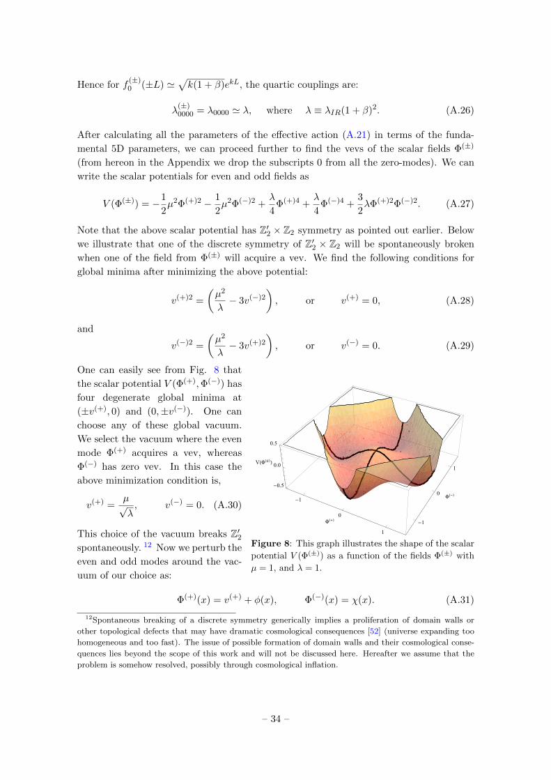
Hence for f(±)0 (±L) '

√k(1 + β)ekL, the quartic couplings are:

λ(±)0000 = λ0000 ' λ, where λ ≡ λIR(1 + β)2. (A.26)

After calculating all the parameters of the effective action (A.21) in terms of the funda-

mental 5D parameters, we can proceed further to find the vevs of the scalar fields Φ(±)

(from hereon in the Appendix we drop the subscripts 0 from all the zero-modes). We can

write the scalar potentials for even and odd fields as

V (Φ(±)) = −1

2µ2Φ(+)2 − 1

2µ2Φ(−)2 +

λ

4Φ(+)4 +

λ

4Φ(−)4 +

3

2λΦ(+)2Φ(−)2. (A.27)

Note that the above scalar potential has Z′2 × Z2 symmetry as pointed out earlier. Below

we illustrate that one of the discrete symmetry of Z′2 × Z2 will be spontaneously broken

when one of the field from Φ(±) will acquire a vev. We find the following conditions for

global minima after minimizing the above potential:

v(+)2 =

(µ2

λ− 3v(−)2

), or v(+) = 0, (A.28)

and

v(−)2 =

(µ2

λ− 3v(+)2

), or v(−) = 0. (A.29)

-1

0

1

FH+L -1

0

1

FH-L-0.5

0.0

0.5

VHFH≤LL

Figure 8: This graph illustrates the shape of the scalar

potential V (Φ(±)) as a function of the fields Φ(±) with

µ = 1, and λ = 1.

One can easily see from Fig. 8 that

the scalar potential V (Φ(+),Φ(−)) has

four degenerate global minima at

(±v(+), 0) and (0,±v(−)). One can

choose any of these global vacuum.

We select the vacuum where the even

mode Φ(+) acquires a vev, whereas

Φ(−) has zero vev. In this case the

above minimization condition is,

v(+) =µ√λ, v(−) = 0. (A.30)

This choice of the vacuum breaks Z′2spontaneously. 12 Now we perturb the

even and odd modes around the vac-

uum of our choice as:

Φ(+)(x) = v(+) + φ(x), Φ(−)(x) = χ(x). (A.31)

12Spontaneous breaking of a discrete symmetry generically implies a proliferation of domain walls or

other topological defects that may have dramatic cosmological consequences [52] (universe expanding too

homogeneous and too fast). The issue of possible formation of domain walls and their cosmological conse-

quences lies beyond the scope of this work and will not be discussed here. Hereafter we assume that the

problem is somehow resolved, possibly through cosmological inflation.

– 34 –

The effective toy action in terms of the even and odd fluctuations can be written as

Sefftoy = −∫d4x

1

2∂µφ∂

µφ+1

2∂µχ∂

µχ+1

2m2φ2 +

1

2m2χ2 +

λ

4φ4 +

λ

4χ4

+√λµφ

(φ2 + 3χ2

)+

3

2λφ2χ2

, (A.32)

where m2 ≡ 2µ2. It is important to note that both even and odd fluctuations have the same

mass m and the same quartic coupling λ. Moreover, the above action has an unbroken

discrete Z2 symmetry, under which the fields transform as φ→ +φ and χ→ −χ.

A.2 SSB by a vacuum expectation value of the 5D scalar field

In this approach we perturb the 5D scalar field Φ(x, y) around a y-dependent vev v(y) as

Φ(x, y) = v(y) + φ(x, y), (A.33)

where v(y) is the background solution for the toy action (A.1) and φ(x, y) is a perturbation

around the background vev v(y). The e.o.m. for v(y) and φ(x, y) read as:(− ∂5

(e4A(y)∂5

)+ µ2

Be4A(y)

)v(y)

= −e4A(y)

(∂VIR(v)

∂vδ(y + L) +

∂VUV (v)

∂vδ(y) +

∂VIR(v)

∂vδ(y − L)

), (A.34)(

− e2A(y)(4) − ∂5

(e4A(y)∂5

)+ µ2

Be4A(y)

)φ(x, y)

= −e4A(y)

(∂2VIR(v)

∂v2φδ(y + L) +

∂2VUV (v)

∂v2φδ(y) +

∂2VIR(v)

∂v2φδ(y − L)

). (A.35)

Note that the above e.o.m. for the perturbation φ(x, y) (A.35) is obtained by Taylor series

expansion of the potentials around the background v(y) and it is only up to quadratic order

in field φ(x, y) such that the KK-mass matrix for the field φ(x, y) is diagonal. The presence

of delta functions on the r.h.s. of the above equations suggests that there should be jumps

across the branes. The following jump and boundary conditions for v(y) and φ(x, y) are

implied by the general strategy adopted in the main text,(∂5 −

m2UV

2k

)v(y)

∣∣∣0+

= 0,

(±∂5 −

m2IR

2k+λIR2k2

v2(y)

)v(y)

∣∣∣±L∓

= 0, (A.36)(∂5 −

m2UV

2k

)φ(x, y)

∣∣∣0+

= 0,

(±∂5 −

m2IR

2k+

3λIR2k2

v2(y)

)φ(x, y)

∣∣∣±L∓

= 0. (A.37)

Our geometric setup is Z2 symmetric, therefore the solutions corresponding to the bulk

e.o.m. for v(y) Eq. (A.34) are even and odd under y → −y. Hence, we can look for the

solutions possessing a definite parity; the even v(+)(y) and the odd v(−)(y). As discussed

in the main text, the jump conditions for the even and odd solutions are different at y = 0:(∂5 −

m2UV

2k

)v(+)(y)

∣∣∣0+

= 0, v(−)(y)∣∣∣0

= 0, (A.38)

– 35 –

The b.c. at y = ±L for the even and odd solutions are the same:(±∂5 −

m2IR

2k+λIR2k2

v2(±)(y)

)v(±)(y)

∣∣∣±L∓

= 0. (A.39)

We find the following solutions for the even and odd background vevs:

v(+)(y) = A(+)e(2+β)k|y| +B(+)e(2−β)k|y|, − L ≤ y ≤ L, (A.40)

v(−)(y) = A(−)ε(y)(e(2+β)k|y| − e(2−β)k|y|

), − L ≤ y ≤ L, (A.41)

where A(+), B(+) and A(−) are the integration constants. (Note the second integration

constant (B(−)) for the odd solution v(−)(y) is fixed by the continuity condition at y =

0) These integration constants can be fixed by the b.c. (A.38) and (A.39). Above β

parameterizes the bulk mass as β ≡√

4 + µ2B/k

2. For the even background solution, we

apply the jump condition (A.38) at y = 0 to get one of the integration constant as

B(+) = −m2UV − 2(2 + β)k2

m2UV − 2(2− β)k2

A(+) = − δUVδUV + 4β

A(+), (A.42)

where δUV is defined in Eq. (A.14). Since β > 0 therefore the second term in the above

solution for v(+)(y) has negligible effect on the shape of the profile near the IR-brane. The

constant A(+) is fixed by the boundary condition at y = ±L:

A(+) = ±√

k3

λIR

(δIR −

δUV (δIR + 4β)

δUV + 4βe−2βkL

)e−(2+β)kL

(1− e−2βkLδUV

δUV + 4β

)−3/2

, (A.43)

where δIR is defined in Eq. (3.31). For kL 1 and β > 0, the second terms in both

parentheses above are negligible in the region of interest (near the IR-brane). Hence the

background even solution for the scalar field can be written as:

v(+)(y) ' ±√k3δIRλIR

e(2+β)k(|y|−L), (A.44)

From the above solution we conclude that for λIR > 0 (as required by the positivity of the

tree-level potential) one needs δIR > 0, i.e. m2IR/k

2 > 2(2 + β).

Similarly one can determine the integration constant A(−) by applying the boundary

condition at y = ±L, for kL 1, we find:

A(−) = ±√

k3

λIRδIRe

−(2+β)kL. (A.45)

Hence the solution for odd profile v(−)(y) reads:

v(−)(y) = ±√k3δIRλIR

ε(y)(e(2+β)k(|y|−L) − e−2βkLe(2−β)k(|y|−L)

). (A.46)

– 36 –

Again the second term in the above solution is negligible for β > 0 and kL 1, therefore

the final form of the odd solution is,

v(−)(y) ' ±√k3δIRλIR

ε(y)e(2+β)k(|y|−L). (A.47)

We have shown above that the background solutions of 5D scalar field are even or

odd parity under extra-dimensional Z2 parity. Since our geometric setup is symmetric,

therefore we also choose the even background solution v(+)(y) for the scalar field. With

this choice of the background solution, the fluctuations will have a definite parity. It is

instructive to rewrite the even background solution (A.44) as

v(+)(y) ' v4fv(y), (A.48)

where the constant vev v4 and the y-dependent vev profile fv(y) are:

v4 =

√m2KKδIR

λIR(1 + β), fv(y) =

√k(1 + β)ekLe(2+β)k(|y|−L). (A.49)

The y-dependent vev profile satisfies the orthonormality condition∫ L

−Ldye2A(y)f2

v (y) = 1. (A.50)

As we will show below, comparing the effective theories obtained by the two different

mechanisms of SSB discussed in this appendix, the constant factor of y-dependent vev, i.e.

v4 has the same value as the vev v1 obtained in the previous section. This is an important

result and we will comment on this at the end this section. It is worth mentioning here that

the quartic term in the IR-brane potential is crucial for a non-trivial vev profile v(±)(y).

If the quartic term would have been absent in the VIR, i.e. λIR = 0, then the b.c. (A.38)

and (A.39) would have implied v(±)(y) = 0. Even though the quartic term is not in the

bulk (only localized at the IR-brane), nevertheless, the b.c. imply the non-zero profile in

the bulk.

Next we deal with the fluctuation field φ(x, y) by KK-decomposing it as

φ(x, y) =∑n

φn(x)fn(y), (A.51)

such that the e.o.m. for the wave-function fn(y) follows from Eq. (A.35),

− ∂5(e4A(y)∂5fn(y)) + µ2Be

4A(y)fn(y) + e4A(y)m2UV

kfn(y)δ(y) = m2

ne2A(y)fn(y), (A.52)

where A(y) = −k|y| and the KK-modes satisfy (4)φn(x) = m2nφn(x). Our symmetric Z2

geometry implies that the solutions of the Eq. (A.52) are even and odd under y → −y. As

the wave functions are even f(+)n (y) and odd f

(−)n (y) therefore it is instructive to rewrite

the KK-decomposition for the fluctuation field φ(x, y) (A.51) as:

φ(x, y) =∑n

φ(+)n (x)f (+)

n (|y|) + ε(y)∑n

φ(−)n (x)f (−)

n (|y|), (A.53)

– 37 –

where ε(y) is ±1 for y ≷ 0. The even and odd solutions are subject to different jump

conditions at y = 0. The jump and boundary conditions for f(±)n (y) follow from Eq.

(A.37) as: (∂5 −

m2UV

2k

)f (+)n (y)

∣∣∣0+

= 0, f (−)n (y)

∣∣∣0

= 0, (A.54)(±∂5 −

m2IR

2k+

3λIR2k2

v2(y)

)f (±)n (y)

∣∣∣±L∓

= 0. (A.55)

Now we write the 4D effective action for the toy model (A.1) by using the above

KK-decomposition and integrating over the extra-dimension y, as

Sefftoy = −∫d4x

1

2∂µφ

(+)n ∂µφ(+)

n +1

2∂µφ

(−)n ∂µφ(−)

n +1

2m2(+)n φ2(+)

n +1

2m2(−)n φ2(−)

n

+ λ(+)lmnφ

(+)l φ(+)

m φ(+)n + 3λ

(−)lmnφ

(+)l φ(−)

m φ(−)n +

λ(+)klmn

4φ

(+)k φ

(+)l φ(+)

m φ(+)n

+λ

(−)klmn

4φ

(−)k φ

(−)l φ(+)

m φ(+)n +

3

2λklmnφ

(+)k φ

(+)l φ(−)

m φ(−)n

, (A.56)

where,

λ(±)lmn =

λIRk2

v4e4A(y)fv(y)f

(+)l (y)f (±)

m (y)f (±)n (y)

∣∣∣L, (A.57)

λ(±)klmn =

λIRk2

e4A(y)f(±)k (y)f

(±)l (y)f (±)

m (y)f (±)n (y)

∣∣∣L, (A.58)

λklmn =λIRk2

e4A(y)f(+)k (y)f

(+)l (y)f (−)

m (y)f (−)n (y)

∣∣∣L. (A.59)

For the warped (AdS) geometry the general solutions for Eq. (A.52) corresponding to

the even and odd f(±)n (y) are the same as in Eqs. (A.11) and (A.12). From the b.c. at

y = ±L we get the following equation whose roots will determine the mass spectrum of

the KK-modes,

m(±)n

mKK

(Jβ+1

(ekLm

(±)n

k

)+ b(±)

n Yβ+1

(ekLm

(±)n

k

))

= δIR

(Jβ

(ekLm

(±)n

k

)+ b(±)

n Yβ

(ekLm

(±)n

k

)), (A.60)

where mKK and δIR are defined in Eq. (3.31). In the approximation kL 1 and m(±)0 k,

we find b(±)n ≈ 0. Hence the above mass eigenvalue equation takes the following form for

the zero-mode masses m(±)0 ,

m(±)0

mKK

Jβ+1

(m

(±)0

mKK

)Jβ

(m

(±)0

mKK

) ' δIR. (A.61)

– 38 –

We expand the above expression around m(±)0 ∼ 0 to get the following masses for the

zero-modes,

m2(±)0 ' 2(1 + β)m2

KKδIR

[1− δIR

2 + β+

2δ2IR

(2 + β)2(3 + β)+O(δ3

IR)

]. (A.62)

As explained in the above sub-Appendix, in order to have the light zero-mode mass ∼O(100) GeV, we need to fine-tune δIR ∼ 10−3. The above result also implies that the odd

zero-mode is degenerate in the mass with the even scalar mass. For the non-zero modes

(excited KK-modes) we assume that m(±)n /mKK δIR, hence the m

(±)n for the non-zero

KK-modes (n 6= 0) are:

m(±)n '

(n+

β

2− 3

4

)πmKK , (A.63)

which implies that the masses of the even and odd excited KK-modes are degenerate in

the approximations considered above.

Assuming the KK-scale mKK is large enough, we can write down the low-energy ef-

fective action for the lowest even and odd modes φ(±)0 from the toy action (A.56) as:

Sefftoy = −∫d4x

1

2∂µφ

(+)0 ∂µφ

(+)0 +

1

2∂µφ

(−)0 ∂µφ

(−)0 +

1

2m

(+)20 φ

(+)20 +

1

2m

(−)20 φ

(−)20

+ λ(+)000φ

(+)30 + 3λ

(−)000φ

(+)0 φ

(−)20 +

λ(+)0000

4φ

(+)40 +

λ(−)0000

4φ

(−)40 +

3λ0000

2φ

(+)20 φ

(−)20

,

(A.64)

where the vev profile and zero-modes at the location of IR-brane, i.e, fv(L) ≈ f(±)0 (L) ≈√

k(1 + β)ekL (note that zero-mode profile f(±)0 (y) = f

(±)0 (y) where f

(±)0 (y) is given in Eq.

(A.25)). The couplings take the following values from Eqs. (A.57) and (A.59):

λ(±)000 '

√λµ, λ

(±)0000 = λ0000 ' λ, (A.65)

where we defined

v4 =

√m2KKδIR

λIR(1 + β)=

µ√λ, (A.66)

with µ2 ≡ (1 + β)m2KKδIR and λ ≡ λIR(1 + β)2. Simplifying our notation (φ

(+)0 = φ,

φ(−)0 = χ and m0 = m), we can write the above effective action (A.64) in the following

form:

Seff = −∫d4x

1

2∂µφ∂

µφ+1

2∂µχ∂

µχ+1

2m2φ2 +

1

2m2χ2 +

λ

4φ4 +

λ

4χ4

+√λµφ

(φ2 + 3χ2

)+

3

2λφ2χ2

, (A.67)

where m0 is the mass of the zero-modes given by Eq. (A.62); the leading term is, m20 = 2µ2.

Let us conclude this Appendix with the comparison of the effective theories obtained

in the previous sub-Appendix (A.32) and here (A.67). It is straight forward to see that

– 39 –

the low energy (zero-mode) d.o.f. in the both actions are same. Moreover, the effective

theories are identical, for example, all the masses and coupling constants are same in

terms of 5D fundamental parameters of the theory. This is a non-trivial matching and

the core of this matching lies in the fact, as discussed above, that the y-dependent vev

v(y) can be written as constat v4 times the normalized y-dependent profile fv(y) such that

v4 = v1 = µ√λ

and f0(y) ' fv(y), where v1 and f0(y) are the vev and the zero-mode profile,

respectively, obtained in the previous sub-appendix. Once this matching is achieved then

we can conceive ourselves that all the masses and coupling constants in both low-energy

effective theories are exactly identical. In other words, consistently with our expectations,

the KK-expansion and the expansion around y-dependent vev do commute (at least for

the zero modes).

References

[1] L. Randall and R. Sundrum, A Large mass hierarchy from a small extra dimension,

Phys.Rev.Lett. 83 (1999) 3370–3373, [hep-ph/9905221].

[2] L. Randall and R. Sundrum, An Alternative to compactification, Phys.Rev.Lett. 83 (1999)

4690–4693, [hep-th/9906064].

[3] W. D. Goldberger and M. B. Wise, Modulus stabilization with bulk fields, Phys.Rev.Lett. 83

(1999) 4922–4925, [hep-ph/9907447].

[4] O. DeWolfe, D. Freedman, S. Gubser, and A. Karch, Modeling the fifth-dimension with

scalars and gravity, Phys.Rev. D62 (2000) 046008, [hep-th/9909134].

[5] H. Davoudiasl, J. Hewett, and T. Rizzo, Bulk gauge fields in the Randall-Sundrum model,

Phys.Lett. B473 (2000) 43–49, [hep-ph/9911262].

[6] Y. Grossman and M. Neubert, Neutrino masses and mixings in nonfactorizable geometry,

Phys.Lett. B474 (2000) 361–371, [hep-ph/9912408].

[7] S. Chang, J. Hisano, H. Nakano, N. Okada, and M. Yamaguchi, Bulk standard model in the

Randall-Sundrum background, Phys.Rev. D62 (2000) 084025, [hep-ph/9912498].

[8] T. Gherghetta and A. Pomarol, Bulk fields and supersymmetry in a slice of AdS, Nucl.Phys.

B586 (2000) 141–162, [hep-ph/0003129].

[9] S. J. Huber and Q. Shafi, Fermion masses, mixings and proton decay in a Randall-Sundrum

model, Phys.Lett. B498 (2001) 256–262, [hep-ph/0010195].

[10] K. Agashe, A. Delgado, M. J. May, and R. Sundrum, RS1, custodial isospin and precision

tests, JHEP 0308 (2003) 050, [hep-ph/0308036].

[11] M. A. Luty and T. Okui, Conformal technicolor, JHEP 0609 (2006) 070, [hep-ph/0409274].

[12] N. Arkani-Hamed, M. Porrati, and L. Randall, Holography and phenomenology, JHEP 0108

(2001) 017, [hep-th/0012148].

[13] R. Rattazzi and A. Zaffaroni, Comments on the holographic picture of the Randall-Sundrum

model, JHEP 0104 (2001) 021, [hep-th/0012248].

[14] H. Davoudiasl, B. Lillie, and T. G. Rizzo, Off-the-wall Higgs in the universal

Randall-Sundrum model, JHEP 0608 (2006) 042, [hep-ph/0508279].

– 40 –

[15] G. Cacciapaglia, C. Csaki, G. Marandella, and J. Terning, The Gaugephobic Higgs, JHEP

0702 (2007) 036, [hep-ph/0611358].

[16] A. Falkowski and M. Perez-Victoria, Electroweak Breaking on a Soft Wall, JHEP 0812

(2008) 107, [arXiv:0806.1737].

[17] A. Azatov, M. Toharia, and L. Zhu, Higgs Mediated FCNC’s in Warped Extra Dimensions,

Phys.Rev. D80 (2009) 035016, [arXiv:0906.1990].

[18] J. A. Cabrer, G. von Gersdorff, and M. Quiros, Warped Electroweak Breaking Without

Custodial Symmetry, Phys.Lett. B697 (2011) 208–214, [arXiv:1011.2205].

[19] J. A. Cabrer, G. von Gersdorff, and M. Quiros, Suppressing Electroweak Precision

Observables in 5D Warped Models, JHEP 1105 (2011) 083, [arXiv:1103.1388].

[20] J. A. Cabrer, G. von Gersdorff, and M. Quiros, Improving Naturalness in Warped Models

with a Heavy Bulk Higgs Boson, Phys.Rev. D84 (2011) 035024, [arXiv:1104.3149].

[21] M. Geller, S. Bar-Shalom, and A. Soni, Higgs-radion unification: radius stabilization by an

SU(2) bulk doublet and the 126 GeV scalar, Phys.Rev. D89 (2014) 095015,

[arXiv:1312.3331].

[22] P. R. Archer, The Fermion Mass Hierarchy in Models with Warped Extra Dimensions and a

Bulk Higgs, JHEP 1209 (2012) 095, [arXiv:1204.4730].

[23] M. Frank, N. Pourtolami, and M. Toharia, Higgs Bosons in Warped Space, from the Bulk to

the Brane, Phys.Rev. D87 (2013), no. 9 096003, [arXiv:1301.7692].

[24] R. Malm, M. Neubert, K. Novotny, and C. Schmell, 5D perspective on Higgs production at

the boundary of a warped extra dimension, JHEP 1401 (2014) 173, [arXiv:1303.5702].

[25] P. R. Archer, M. Carena, A. Carmona, and M. Neubert, Higgs Production and Decay in

Models of a Warped Extra Dimension with a Bulk Higgs, JHEP 1501 (2015) 060,

[arXiv:1408.5406].

[26] B. M. Dillon and S. J. Huber, Non-Custodial Warped Extra Dimensions at the LHC?,

arXiv:1410.7345.

[27] K. Agashe, A. Azatov, Y. Cui, L. Randall, and M. Son, Warped Dipole Completed, with a

Tower of Higgs Bosons, arXiv:1412.6468.

[28] A. M. Iyer, K. Sridhar, and S. K. Vempati, Bulk RS models, Electroweak Precision tests and

the 125 GeV Higgs, arXiv:1502.06206.

[29] A. Ahmed and B. Grzadkowski, Brane modeling in warped extra-dimension, JHEP 1301

(2013) 177, [arXiv:1210.6708].

[30] A. Ahmed, L. Dulny, and B. Grzadkowski, Generalized Randall-Sundrum model with a single

thick brane, Eur.Phys.J. C74 (2014) 2862, [arXiv:1312.3577].

[31] Planck Collaboration, P. Ade et al., Planck 2015 results. XIII. Cosmological parameters,

arXiv:1502.01589.

[32] G. Servant and T. M. Tait, Is the lightest Kaluza-Klein particle a viable dark matter

candidate?, Nucl.Phys. B650 (2003) 391–419, [hep-ph/0206071].

[33] H.-C. Cheng, J. L. Feng, and K. T. Matchev, Kaluza-Klein dark matter, Phys.Rev.Lett. 89

(2002) 211301, [hep-ph/0207125].

– 41 –

[34] K. Agashe and G. Servant, Warped unification, proton stability and dark matter,

Phys.Rev.Lett. 93 (2004) 231805, [hep-ph/0403143].

[35] G. Panico, E. Ponton, J. Santiago, and M. Serone, Dark Matter and Electroweak Symmetry

Breaking in Models with Warped Extra Dimensions, Phys.Rev. D77 (2008) 115012,

[arXiv:0801.1645].

[36] E. Ponton and L. Randall, TeV Scale Singlet Dark Matter, JHEP 0904 (2009) 080,

[arXiv:0811.1029].

[37] L. Vecchi, Majorana dark matter in warped extra dimensions, Phys.Rev. D90 (2014), no. 2

025017, [arXiv:1310.7862].

[38] T. Gherghetta and B. von Harling, A Warped Model of Dark Matter, JHEP 1004 (2010)

039, [arXiv:1002.2967].

[39] B. von Harling and K. L. McDonald, Secluded Dark Matter Coupled to a Hidden CFT, JHEP

1208 (2012) 048, [arXiv:1203.6646].

[40] A. R. Frey, R. J. Danos, and J. M. Cline, Warped Kaluza-Klein Dark Matter, JHEP 0911

(2009) 102, [arXiv:0908.1387].

[41] K. Agashe, A. Falkowski, I. Low, and G. Servant, KK Parity in Warped Extra Dimension,

JHEP 0804 (2008) 027, [arXiv:0712.2455].

[42] A. D. Medina and E. Ponton, Warped Universal Extra Dimensions, JHEP 1106 (2011) 009,

[arXiv:1012.5298].

[43] A. D. Medina and E. Ponton, Warped Radion Dark Matter, JHEP 1109 (2011) 016,

[arXiv:1104.4124].

[44] Z. Lalak and R. Matyszkiewicz, Boundary terms in brane worlds, JHEP 0111 (2001) 027,

[hep-th/0110141].

[45] A. Carmona and M. Chala, Composite Dark Sectors, arXiv:1504.00332.

[46] B. Grzadkowski and J. Wudka, Pragmatic approach to the little hierarchy problem: the case

for Dark Matter and neutrino physics, Phys.Rev.Lett. 103 (2009) 091802,

[arXiv:0902.0628].

[47] C. F. Kolda and H. Murayama, The Higgs mass and new physics scales in the minimal

standard model, JHEP 0007 (2000) 035, [hep-ph/0003170].

[48] J. Casas, J. Espinosa, and I. Hidalgo, Implications for new physics from fine-tuning

arguments. 1. Application to SUSY and seesaw cases, JHEP 0411 (2004) 057,

[hep-ph/0410298].

[49] R. Barbieri and G. Giudice, Upper Bounds on Supersymmetric Particle Masses, Nucl.Phys.

B306 (1988) 63.

[50] Particle Data Group Collaboration, K. Olive et al., Review of Particle Physics,

Chin.Phys. C38 (2014) 090001.

[51] E. W. Kolb and M. S. Turner, The Early Universe, Front.Phys. 69 (1990) 1–547.

[52] Y. Zeldovich, I. Y. Kobzarev, and L. Okun, Cosmological Consequences of the Spontaneous

Breakdown of Discrete Symmetry, Zh.Eksp.Teor.Fiz. 67 (1974) 3–11.

– 42 –