Political heterogeneity, electoral

surprise and the growth in

unemployment:

The Norwegian partisan cycle.

Leif Helland ∗

Department of Public Governance

Norwegian School of Management

January 5, 2009

∗Address: Nydalsveien 37, 0447 Oslo. E-mail: leif.helland@bi.no. Useful comments to

an earlier version where kindly provided by Fredrik Carlsen, Kai Leitemo, Espen Moen,

Christian Riis and Rune Sørensen.

1

Introduction

In rational partisan theory (RPT) the economy is described by a Lucas sup-

ply side function, rational expectations, and nominal rigidities in wage and

price contracting (Alesina 1987, 1988). Partisan differences are assumed to

exist. In particular, growth in output and employment above the natural rate

is valued more by leftist than rightist parties.1 After an election, therefore,

leftist (rightist) majority-winners inflate the economy at a higher (lower) rate

than rightist (leftist) majority-winners, and a post electoral boom (bust) is

generated. The effect is temporary and fades away as existing wage and price

contracts are replaced. The more surprising the election result is, and the

more the parties differ in their valuation of employment, the stronger is the

electoral impact.

RPT assume that partisan preferences are stable across electoral periods.

Empirically, this is a questionable assumption.2 Party platforms are rewrit-

ten prior to each campaign, and are subject to interpretations after elections.3

As a result partisan preferences tend to vary across as well as within elec-

toral periods. The model in section 2 expose partisan preferences to random

exogenous shocks, inducing variance over time. Variation in partisan pref-

erences is controlled for in the empirical specifications of section 3. It turns

out that such variation is a powerful predictor of partisan cycles.

A number of tests of RPT exist. One approach is to capture post-electoral

business cycles by interventions that are turned on in t periods following

1Leftist parties may also care less than rightist parties about the costs of inflation, but

such a difference is not necessary to drive the results.2As emphasized by for instance Franzese and Jusko 2006.3Programs may be viewed as incomplete contracts between the party congress (the

principal) and the elected representatives that make the decisions (the agent).

2

an election (Alesina and Rosenthal 1995, Alesina, Londregan and Rosenthal

1993, Alesina, Roubini and Cohen 1997: chapters 4 and 6). Another ap-

proach consists in comparing average growth and unemployment rates the

first year(s) after elections with average growth and unemployment rates

during the preceding two years (Paldam 1991, Paldam 1997). More sophis-

ticated tests of RPT depart from surprise variables based on expectations

about future policymakers. A common approach is to extract expectations

about majority winners from vote-shares obtained by alternative majorities

in polls using an options pricing model (Alesina et al. 1997: chapter 5, Cohen

1993, Carlsen and Pedersen 1999).4 An objection to this approach is that

policy is decided by a majority of seats, not a majority of votes. Depend-

ing on the specifics of electoral rules, seat- shares may deviate substantially

from vote-shares.5 For this reason we examine, in section 3, the robustness of

RPT to changing the expectations argument from votes to seats. It turns out

that electoral surprises based on votes, rather than on seats, have the most

pronounced effects on unemployment growth in our data. This is somewhat

puzzling.

Traditionally, at least since Paldam’s seminal article in 1979, the decision

4An alternative is to use data from election-markets, as for instance in Fowler 2006.

Election market data are not available for Norway over the period in question. Another

sophisticated approach is to fit a set of regressions across elections, explaining the incum-

bents vote share as a function of both opinion polls and macroeconomic variables. The

predictions can then be used to compute election win probabilities for the incumbent.

Chappell and Keech 1988 provides the pioneering work of this approach, while Carlsen

and Pedersen 1999 represents a more recent application. The approach presumes some

kind of retrospective voting based on economic performance of incumbents, which is not

a part of RPT. Consequently, we do not use this approach.5For instance: after 1945 eight different governments held a majority of the seats in

the Norwegian parliament, none of which had a majority of the popular vote in national

elections.

3

maker of interest in RPT is assumed to be the government. For this to give

good meaning arbitrary restrictions have to be placed on data generated by

parliamentary democracies.6 In this paper we take a different view, and as-

sume that the parliamentary majority is the decision-maker of interest. This

does away with the need for arbitrary restrictions on the data.

At the same time, governments are routinely replaced outside the electoral

cycle in parliamentary systems. Such replacements constitute genuine sur-

prises. For non-electoral replacements to produce political cycles, govern-

ments must possess some amount of independent policy-making power. We

investigate the policy-making powers of governments, by checking for the

macroeconomic effects of non-electoral replacements. Such replacements do

not have business cycle effects in our data, indicating that macroeconomic

policy is placed firmly within the domain of parliamentary majorities in Nor-

way.

Monthly unemployment data from the early eighties onwards are used to

check for the presence of a rational partisan business cycle. Existing tests

employ yearly or quarterly data. Using monthly data allow us to keep better

track of political events, and provides us with statistical power in series of

relatively short duration. Series of short duration decreases the probability

of drawing data from different politico-economic regimes. This makes short

duration data desirable. In addition, Norwegian data are of course particu-

larly suited to a test of the RPT, since Norway is the only western parliament

6Paldam 1979:326 provides an example: ”In order to conduct a statistical study some

very clear-cut criteria have to be found to decide whether a government is stable. Two

rules have been used. They must both be fulfilled. Rule 1: The government should have a

parliamentary majority. Rule 2: The government remains in power throughout the normal

election period.”

4

with a fixed election term (as assumed in RPT).

The article is organized as follows. The next section contains the model,

while section three describes the data. Section four confronts model and

data. Section five offers some conclusions.

Model

The economy is described by a simple supply function:7

ut = u∗ + wt − πt (1)

In (1) ut is the realized change in unemployment in period t, u∗ is the (time

invariant) natural rate of unemployment, π is inflation, and wt is nominal

wage growth. The ruling majority is assumed to control the inflation rate.

It is further assumed that t is an election period, and that elections are held

every second period. Nominal wage contracts are signed at the beginning of

t before the election result is known, and terminate at the end of t.

Inflation is rationally expected and wage setters aim at keeping real wages

stable, so that wt = π∈t = E(πt|It−1), where I is the information set. I in-

clude every decision relevant fact known at time t-1 (including the structure

of the model that follows). Thus, (1) can be rewritten:

ut = u∗ + π∈t − πt (2)

There are two, ideologically immobile, electoral alternatives - or blocks - for

which the votes may be cast, these are denoted k=(Socialist, Conservative).8

7For micro-foundations and interpretations c.f. Blanchard and Fischer 1989, chapter 8.8The electoral alternatives might be candidates, parties, parliamentary governments

or legislative majorities (in seats or in votes). In the empirical analysis of the paper we

5

The alternatives have loss functions defined over unemployment growth and

inflation:

`kt =

∞∑t=0

δt

[−θk

t ut − 1

2

(πt − πk

)2]

(3)

In (3) δ < 1 is the common discount factor, θkt > 0 is the marginal cost of

increased unemployment and πk is target inflation, with πSoc ≥ πCon ≥ 0.

As a slight modification of standard RPT, let θkt be a stochastic variable

in the range (θt, θt). We take θkt to be determined by independent and iden-

tical draws from a unimodal and symmetric distribution with mean θ̃kt . This

ensures that historical inflation rates do not convey information about future

inflation rates.

Let G(θkt ) be the cumulative distribution function of θk

t , with correspond-

ing density g(θkt ). Assume that θSoc

t > θCon

t . With this assumption, optimal

inflation rates (to be determined) will obey the condition πCon∗t < πSoc∗

t ∀t(while allowing for variation in πk∗

t due to random shocks). The larger is

g(θ̃t), of course, the smaller are the shocks.

For any pair (θ′Soct , θ

′Cont ) that satisfies (θ

′Soct − θSoc

t ) = (θ′Cont − θCon

t ), it

is assumed that g(θ′Soct ) = g(θ

′Cont ). Or in words, the distribution around the

mean of the optimal inflation rate is identical for the electoral alternatives.

For this reason risk attitudes do not influence wage setting.

The draw of θkt is revealed for every player when a winner sets policy. Policy

focus on legislative majorities. The formalization that follows reduces the maximization

problem to a one-dimensional choice. One may ask why the parties do not converge on

the median position on this dimension. Several answers may be given. A good overview

of partial convergence results is given by Alesina and Rosenthal 1995, chapter 2.

6

is set after elections in election periods, and after wage contracts have been

signed in non-election periods.

The model is solved using a backwards induction argument.9 Inserting (2)

in (3) and maximizing with respect to πt we obtain the optimal rates of

inflation:

πk∗t = θk

t + πk = πt (4)

In what follows we set πSoc = πCon = 0 without loss of generality. Voters

are assumed to have loss functions of the type presented in 3, and to vary

in their optimal inflation rates. Votes are cast for the electoral alternative

promising the smallest loss. There is uncertainty about the distribution of

optimal inflation rates in the voter population, and the electoral outcome

is therefore uncertain. Let P signify the probability that the socialist block

gains a majority in the upcoming election.10 The expected (post-election)

inflation rate for period t is then:

π∈t = P θ̃Soct + (1− P )θ̃Con

t (5)

In period t+1 the majority in charge is common knowledge, and contracts

are based on either π∈t+1 = θ̃Soct or π∈t+1 = θ̃Con

t depending on which block

won the election in t.

Finally, inserting [5] and [4] in [2] provides the unemployment-growth equa-

tions for the two electoral alternatives:

9Intra-party conflicts due to last term effects for some members are assumed away. For

an overlapping generation model where such effects are taken account of, see Alesina and

Spear 1988.10Roemer 1992 derives this probability from primitives (c.f. also Alesina and Cukierman

1990 for some special results).

7

uSoct = u∗ + (1− P )(θ̃Con

t − θSoct ) ≤ 0 (6)

uCont = u∗ − P (θCon

t − θ̃Soct ) ≥ 0 (7)

Thus, a change in the rate of unemployment can either be caused by an elec-

toral surprise (in an election period), or a random shock due to intra-party

bargaining over the marginal costs of unemployment (in any period). The

central implication is that unemployment increases (decreases) following a

conservative (socialist) victory. This effect is stronger: a) the more unlikely

(likely) a socialist victory is, and b) the more pronounced the political con-

flict between the two blocs is.

With added costs in terms of notational complexity the model may be ex-

tended to a multi period setting (Carlsen and Pedersen 1999). This formalizes

the nature of the post-electoral cycle, where the effect of a surprise gradually

fades away as contracts are rewritten. Since this aspect is quite intuitive, we

content ourselves by dealing with it in the empirical specifications.

Data

Our electoral data covers 342 months, starting with 1976:12 and ending with

2005:05. The electoral alternatives are defined in terms of socialist and non-

socialist majorities. As socialist parties we include the Labor party and every

party to the left of it on the left-right scale of politics, as tapped by voter

self-placements in National election surveys.11

Two kinds of expectations are computed: the probability of having a so-

11Obtainable at Norwegian Social Science Data Services (http://www.nsd.uib.no/).

8

cialist majority in votes after the upcoming election, and the probability

of having a socialist majority in seats after the upcoming election. Both

computations depart from monthly polls.12 To calculate the probability of

a socialist majority in seats, polls are first transformed into seats using the

program CELIUS. The program takes into account various (minor) changes

in electoral rules that have been implemented during the period.13

For any given month the vote-shares (seat-shares) of the socialist parties

are added. The probability of a socialist majority vote-share (seat-share) in

the election τ−t months ahead is then computed applying the option pricing

method.14 Norwegian national elections are fixed, and occur in September

with four-year intervals (so τ − t ranges between 0 and 48 months).

The probability of a socialist majority in the upcoming election, Pt, is con-

tingent on the number of months reminding before the election, the current

vote-share (seat-share) of the socialist block (xSoct = Socialist seatshare,

Socialist voteshare), the mean monthly change in the polls µt, and the

standard deviation of month-to-month changes in the polls σt. The mean

and standard deviation of changes are calculated using a cumulative moving

average technique, utilizing data from the first available poll (1976:12) up to

and including the present month (t).

Vote-shares (seat-shares) are converted into probabilities for a socialist ma-

jority by the following formula, where Φ signifies the standardized, cumu-

lative, normal distribution (and movements in the polls are assumed to be

12Recorded by MMI on a monthly basis since 1976:12.13Program developed by Bernt Aardal at the Institute for Social Research, Oslo

(http://home.online.no/ b-aardal/).14Pioneered by Black and Shooles 1973, and introduced to political economy by Cohen

1993.

9

i.i.d):

Pt = Φ

(xSoc

t + µtτ − 0.5

σt

√τ

)(8)

Figure 1a displays the probability of a socialist majority in votes, and the

socialist vote share on a month-to-month basis. Figure 1b displays the cor-

responding probability of a socialist majority in seats, and the socialist seat

share on a month-to-month basis.

[Figures 1a and 1b about here]

From the estimated probabilities of a socialist majority in the upcoming

election our surprise variable is constructed in the following way:

Electoral Surprise = DSoct − 1

N

N−1∑i=0

Pt−i (9)

In (9) N is the length of a nominal wage contract and DSoct is a dummy that

takes the value one after a socialist victory, and zero after a non-socialist vic-

tory. Since we lack firm knowledge about the precise term structure of wage

contracts, we assume that they are signed uniformly across time. The surprise

variable captures the expected post-electoral change in employment, with a

positive sign for socialist majorities and a negative sign for non-socialist ma-

jorities. The magnitude of the surprise determines the magnitude of the

effect on employment, and as contracts are rewritten the effects of the elec-

toral surprise on employment fades away.

We follow the convention of denoting a surprise variable calculated on the

probability of a socialist vote share (V ote Surprise)t, while a surprise vari-

able calculated on the probability of a socialist seat share is denoted (Seat Surprise)t.

The surprise variables are based on nominal wage contracts of 24 months du-

ration, and 12 months lag for policy to work. Both choices are based on best

fit in our data.

10

According to (6) and (7) the effect on employment also depends (multi-

plicatively) on the magnitude of partisan disagreements.15 We capture the

magnitude of such disagreements by a measure based on fractional statements

by the Labor party and the Conservative party - the two major parties in

each block - on budgetary matters in parliament. Only statements recorded

in the Finance committee is used.16 The Finance committee is the coordi-

nating committee in the parliaments economic policy making, and economic

policy making is primarily made in the budget.17

Denote fractional statements that both parties participate in by Sij, while

statements that only one of the two parties participates in is denoted Si and

Sj respectively. Define the statement score of party i as Si

Si+Sij≡ fi, and

the corresponding statement score of party j asSj

Sj+Sij≡ fj. The statement

scores are simply the fraction of statements that one party did not have in

common with the other party. The disagreement score of the two parties is

defined as:

0 ≤ 1

2(fi,t + fj,t) ≡ (Disagreement)t ≤ 1 (10)

The score in (10) is calculated on an annual basis, but follows parliamentary

sessions from June to June rather than the calendar year.

One may of course suspect that the disagreement score varies with the parlia-

15Since the theoretical model suggests a multiplicative term, we include this product

alone rather than specifying the full interaction model. This is in line with for instance

the specifications used by Alesina et al. 1997:198 to model the multiplicative effects of par-

tisanship and election in business cycle models. Further discussion on the appropriateness

of including the product alone is given by Kam & Franzese 2007:99-102.16Obtainable at Norwegian Social Science Data Services (http://www.nsd.uib.no/).17Norwegian parliamentary committees are organized along party lines, and deviations

from the party line are very rare occurrences.

11

mentary base of governments, through the opposition’s incentives to produce

statements. To check for this suspicion we regress the disagreement score on

dummies for coalition governments and majority governments, as well as a

time trend:

Disagreement = − .411[−4.91]

+ .016Coalition[1.08]

− .035Majority[−1.36]

+ .001t[10.88]

(11)

The estimate is based on robust regression for years greater than 1978 (the

first year OECD data on change in G7 unemployment is made available, and

where our analysis starts). As can be seen, only the constant and the time

trend are significantly different from zero at conventional levels (T-values are

reported in brackets). The F-statistics for the model is highly significant.

With this as a background, we use the product of the disagreement score

in (10) and the surprise variable in (9) to capture the implications of RPT,

as they are stated in (6) and (7).

There are four replacements of governments outside of elections in our data.18

They all go in a leftist direction as measured by party-voter’s self-placements

in National Election Surveys. In June 1983 the Conservative Party’s (CoP)

minority government was supplemented with the Center Party (CeP) and

the Christian Peoples Party (CPP). In May 1986 a non-socialist minority

coalition composed of CoP, CeP and CPP was replaced by a minority gov-

ernment consisting of the Labor Party (LP). In October 1990 a non-socialist

minority coalition composed of the CoP, CeP and the CPP was replaced by

a minority government consisting of the LP. Finally, in April 2000 a non-

socialist minority coalition composed of the CeP, CPP and the Liberal Party

was replaced by a minority government consisting of LP.

18Remember that there are only five elections in the data set, so the data is not partic-

ularly biased in favor of governmental change in elections.

12

Replacements of this kind are genuine surprises that cannot be predicted

with any confidence ex ante. To the extent that governments possess dis-

cressionary powers to inflate (deflate) the economy and increase (decrease)

employment, one would expect them to exploit genuine surprises created

by replacements outside of elections. Denote the measure of replacement-

surprises (Gov − change)t. Since all replacements in our data go to the left

we may define this measure as:

(Gov − Change)t =T+N−1∑

t=T

1

N(12)

In (12) t=T is the month of government replacement. The measure starts

out with unity in t=T, and is reduced by increments of 1/N each month

until month t=T+N where all contracts have been rewritten and the mea-

sure reaches a steady state of zero. The measure captures the idea that a

surprise government can fully exploit existing contracts until they are rewrit-

ten, provided that it has the discressionary powers to set policy independent

of the current parliamentary majority. Since we are looking at a socialist

surprise, the effect on changes in employment is taken to be positive. To en-

sure comparability with the electoral surprise variables calculated from (9),

Government change is also based on contract lengths of 24 months and a lag

of 12 months for policy to work.

Our last political variables are a set of intervention terms that are turned

on in the twelve, nine and six months preceding an election respectively.

The intervention terms are labeled Dt(Election− 12), Dt(Election− 9) and

Dt(Election − 6) (with obvious reference). They represent controls for an

opportunistic cycle, in which any ruling majority will try to create a pre elec-

toral boom, in order to get reelected (Nordhaus 1975, Linbeck 1976, Clark

et al. 1998, Clark and Hallerberg 2000).

13

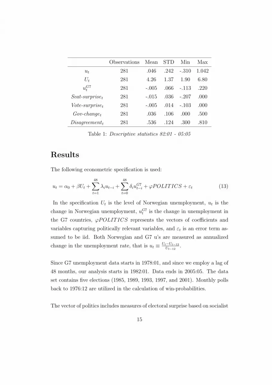
Table 1 presents descriptive statistics for relevant variables. A few things

are worth noting. Firstly, the surprise variables (calculated on the basis of

votes as well as seats) have maximum at zero. Thus, there where no surpris-

ing socialist majorities during the period in question. The reason is simply

that no socialist majority in either seats or votes materialized in the pe-

riod analyzed. Secondly, the variable capturing extra-electoral government

changes has a maximum of 0.5 and a minimum of zero. The reason is that

such changes are assumed to be genuinely surprising, that all such changes

in the period goes in the left direction (+1), and that a contract length is 24

months, but policy only starts working 12 months after an election. Lastly,

the Norwegian unemployment growth has wider extreme bounds and lager

standard deviation than the unemployment growth in the G7 countries. This

is so firstly because we calculate percentage growth, and because the unem-

ployment level in the G7 countries far exceeds the Norwegian unemployment

level. Secondly, the standard deviation of the G7 growth is the standard

deviation of an average, which tends to bring it down.

Figure 2 displays timelines for our three central independents: the surprise

variables calculated on the basis of (9) for seat-shares and vote-shares re-

spectively, and the disagreement score calculated on the basis of (10). The

vertical lines represent election dates.

[Figure 2 about here]

14

Observations Mean STD Min Max

ut 281 .046 .242 -.310 1.042

Ut 281 4.26 1.37 1.90 6.80

uGt

7 281 -.005 .066 -.113 .220

Seat-surpriset 281 -.015 .036 -.207 .000

Vote-surpriset 281 -.005 .014 -.103 .000

Gov-changet 281 .036 .106 .000 .500

Disagreement t 281 .536 .124 .300 .810

Table 1: Descriptive statistics 82:01 - 05:05

Results

The following econometric specification is used:

ut = α0 + βUt +48∑

t=1

λiut−i +48∑

t=0

δiuG7t−i + ϕPOLITICS + εt (13)

In the specification Ut is the level of Norwegian unemployment, ut is the

change in Norwegian unemployment, uG7t is the change in unemployment in

the G7 countries, ϕPOLITICS represents the vectors of coefficients and

variables capturing politically relevant variables, and εt is an error term as-

sumed to be iid. Both Norwegian and G7 u’s are measured as annualized

change in the unemployment rate, that is ut ≡ Ut−Ut−12

Ut−12.

Since G7 unemployment data starts in 1978:01, and since we employ a lag of

48 months, our analysis starts in 1982:01. Data ends in 2005:05. The data

set contains five elections (1985, 1989, 1993, 1997, and 2001). Monthly polls

back to 1976:12 are utilized in the calculation of win-probabilities.

The vector of politics includes measures of electoral surprise based on socialist

15

vote-shares and seat-shares respectively, genuine surprises following govern-

ment replacements outside elections, disagreement scores based on fractional

statements, and intervention terms capturing pre-electoral months.

The usual time series techniques where employed. Dicky-Fuller tests for

stationarity where carried out, and autocorrelation was accounted for by lag-

ging the dependent. The optimal number of lags was determined by the

Breusch-Goodfrey Lagrange multiplier test. Finally, we estimated the re-

gressions by maximum likeliehood, using robust standard errors, in order to

weed out heteroscedasticity. Results are presented in table 2.

Note first that the coefficients of both surprise variables have signs in ac-

cordance with RPT, and are significant at conventional levels (models I and

III): The more the election result deviates from expectations, the more un-

employment growth changes. This is in opposition to Carlsen and Pedersen

1999, who fails to find significant effects of RPT using quarterly Norwegian

output data from the late seventies to the early nineties. In our data a

non-socialist surprise significantly accelerates unemployment growth, while

a socialist surprise significantly decelerates it. The coefficient of surprises

calculated on the basis of vote-shares, are almost two and a half times as

strong as the coefficient of surprises calculated on the basis of seat-shares.

This is somewhat odd, given that policy is decided by a majority of seats,

not a majority of votes.

A possible explanation lies in a particular assumption underlying the cal-

culation of seat-shares from polls in CELIUS, namely that the party vote

registered in any monthly poll follows the geographical distribution from the

last election. Direct empirical evaluation of the assumption is not feasible

16

Model: I II III IV V VI VII

Seat-surpriset -.140

(.002)

Seat-surpriset× -.274

Disagreement t (.049)

Vote-surpriset -.331

(.024)

Vote-surpriset× -.660 -.581 -.581 -.703

Disagreement t (.051) (.093) (.093) (.047)

Dt(Election-12) .004

(.430)

Dt(Election-9) .004

(.411)

Dt(Election-6) .003

(.651)

Gov-changet .017 .022 .014 .020 .016 .025 .016

(.530) (.414) (.601) (.471) (.557) (.348) (.554)

Ut -.002 -.002 -.003 -.003 -.002 -.002 -.003

(.157) (.249) (.111) (.184) (.232) (.232) (.148)

Constant .009 .008 .012 .010 .010 .009 .010

(.252) (.359) (.162) (.241) (.230) (.261) (.211)

N 281 281 281 281 281 281 281

Log-L 586 573 586 573 573 573 573

Table 2: Maximum likelihood estimates (p-values). Dependent: Annual-

ized change in Norwegian unemployment rates. 48 months lagged annualized

change in Norwegian and G7 unemployment rates included but non reported.

17

since monthly polls are drawn from a national sample that is unrepresenta-

tive when broken down on election districts. Nevertheless, assuming a stable

geographical distribution over 48 months at a time seems excessively restric-

tive. This is all the more so since the geographical distribution of the party

vote tends to change quite a bit over elections.

A more fundamental challenge is that seat-shares may respond quite violently

to minor changes in vote-shares. For example, transferring one percentage

point of the popular vote from the Labor party to the Conservative party

in the election of 2005, would induce a loss of five seats on the Labor party.

These seats, however, would be distributed on the non-socialist parties with

one seat each for the Christian Democratic Party and the Progress party,

and three seats for the Conservative Party. The example illustrates that ag-

gregating seat-shares from nineteen electoral districts that use a complicated

PR system, may produce surprising results.19 Consequently, requiring agents

to be able to transform vote-shares from polls into consistent beliefs about

the probability of a socialist majority in seats, may well be asking too much.

Basing beliefs directly on vote-shares may constitute a workable proxy for

the agents.

Second, we notice from table 2 that the products of the surprise variables and

the political disagreement variable have signs in accordance with the expec-

tations from RPT, and are significantly different from zero at conventional

levels (models II and IV). Thus, as before, unemployment accelerates after

19The current system allocates seats by use of the St. Lgues method with 1.4 as first

divisor in 19 electoral districts with magnitudes between 4 and 17 mandates. The first 150

mandates are allocated in the electoral districts, while the last 19 mandates are allocated

on a national basis, based on largest remainders. The system has been subjected to various

minor changes over the period in question. Such changes are taken account of in CELIUS.

18

a non-socialist surprise, and decelerates after a socialist surprise. However,

a higher level of disagreement now induces a greater change in the unem-

ployment growth for a given electoral surprise. As can be seen, the absolute

values of the coefficients on the surprise variables are approximately doubled,

when multiplied by the level of disagreement (compare models I and II, and

models III and IV respectively). Since the average level of disagreement is

approximately 1/2 (c.f. table 1), however, the coefficient estimates of the

products are in broad agreement with the coefficient estimates of the sur-

prise variables (models I and III).

Third, we observe that the pre-electoral dummies are not significantly dif-

ferent from zero at conventional levels in any of the specifications of table 2

(models V, VI and VII). Thus, once we check for the determinants of rational

partisan cycles, there is no indication of adaptive cycles of the opportunistic

kind.20

Finally, an interesting finding is that genuinely surprising changes in the

partisan composition of government does not significantly alter the growth

of unemployment for any of the models in table 2. We interpret this in the

following way: The crucial policies affecting unemployment are effectively set

by parliamentary majorities, indicating that parliament has overcome agency

problems in this policy area. We note that Alesina, Roubini and Cohen

(1997:148-63) fail to find statistically valid evidence of a Norwegian ratio-

nal partisan cycle in quarterly unemployment data over the period 1972:1 -

1993:4. The authors employ a crude test with interventions that are turned

20Opportunistic cycles with adaptive expectations where originally conceived by Nord-

haus 1975 and Lindbeck 1976. Recent refinements and tests are found in Clark and Haller-

berg 2000 for debt and monetary aggregates, and in Clark et al. 1998 for unemployment

and growth.

19

on in a specified number of quarters after a change in government, whether

such a change takes place in elections or not. Our findings indicate that their

result may have been produced by a badly specified political variable that

confuses electoral surprise related to relevant majoritarian decision makers

with non-consequential changes in government.

What, then, are the substantive effects of electoral surprises on unemploy-

ment growth? Figure 3 shows two differences. First, the difference between

the values predicted by model III and the values predicted by equation [13]

with no politic-variables included (votesurprise). Second, the difference be-

tween the values predicted by model IV and the values predicted by equation

[13] with no politic-variables included (votesurprise-disagreement). These

differences convey the substantial effects of policy surprises on unemploy-

ment.

[Figure 3 about here]

The strongest effects are found after the elections of 1985 and 1994. About a

year after these elections (when policy starts to work), unemployment grows

with approximately 2 percent, and thereafter gradually returns to trend (as

contracts are replaced). As is evident from figure 2, both of these elections

saw sizeable socialist surprises (a vote share surprise of about 8-10 percent),

while the level of disagreement was fairly low.

The elections of 1989 and 1997 both saw moderate, and comparable, so-

cialist surprises (again calculated in vote-shares). While the 1997 election

was followed by an unemployment growth above one percent a year after

election, no policy effect is evident after the 1989 election. Figure 2 indicates

why. While the level of disagreement in the 1989 election was slightly below

average, disagreements in the 1997 election reached the highest level in the

20

period.

The elections of 1981 and 2001 where equally unsurprising (calculated in

vote-shares). The absence of a deviation between expectations and realiza-

tions in these elections hindered a partisan cycle in unemployment growth

(not withstanding the fact that partisan differences where quite pronounced

in the 2001 election).

Conclusions

Tests of RPT in parliamentary systems have commonly assumed that the

authority to set policy in the macro-economic sphere rests with the govern-

ment. The present article questions this assumption on empirical grounds.

Having accounted for the electoral surprises relating to parliamentary majori-

ties, extra-electoral changes in the composition of governments adds nothing

to the explanation of a Norwegian rational partisan cycle in unemployment

growth. A conjecture that should be put to the test is that the same holds

true for other parliamentary systems.

Given that macro-economic policy is the domain of majorities in parlia-

mentary systems, agent’s expectations ought to be based on likely major-

ity winners in seats, not in votes. This is so simply because policy is set

by a majority in seats. However, our data does not support the conjecture

that voters form beliefs about likely majorities in seats. This finding may

certainly result from measurement errors in our seat-surprise variable. More

fundamentally, however, we contend that difficulties in forming consistent be-

liefs about likely majority-seat winners are severe in multi-constituency PR

systems. Our conjecture is that rational agents may instead use vote-shares

from the polls as a proxy in forming such beliefs. More research should be

21

directed towards gaining a firmer understanding of belief formation in multi-

constituency PR systems.

A cornerstone in RPT is the implication that the more electoral alterna-

tives deviate in terms of policy preferences for a given electoral surprise, the

more should output and unemployment react to a change of policy makers.

Surprisingly, this implication has not been tested previously. Using disagree-

ment scores from Norwegian political history, we obtain support for this

important implication in our data. Thus, the magnitude of rational political

cycles is contingent on the disagreements between electoral alternatives. At

least this holds for fluctuations in Norwegian unemployment growth since the

early 80s. If this finding is general, as theory claims it is, electoral surprises

of comparable magnitudes could lead to widely different fluctuations in real

variables like unemployment growth. Future research in RPT should explore

such contingencies.

22

REFERENCES

Alesina, A. (1987): Macroeconomic Policy in a Two-Party System as a Re-

peated Game. Quarterly Journal of Economics 102: 651-78.

Alesina, A. (1988): Credibility and Policy Convergence in a Two-Party

System with Rational Voters. American Economic Review 78:796-806.

Alesina, A., N. Roubini and G. Cohen (1997): Political Cycles and the

Macroeconomy. Cambridge Mass.: The MIT-Press.

Alesina, A. and H. Rosenthal (1995): Partisan Politics, Divided Govern-

ment and the Economy. Cambridge: Cambridge University Press.

Alesina, A., J. Londregan and H. Rosenthal (1993): A Model of the

Political Economy of the United States. American Political Science Review

87:12-33.

Alesina, A. and A. Cukierman (1990): The Politics of Ambiguity. Quar-

terly Journal of Economic 105:829-50.

Alesina, A. and S. Spear (1988): An Overlapping Generations Model of

Electoral Competition. Journal of Public Economics 37:359-79.

Black, F. and M. Scholes (1973): The Pricing of Options and Corporate

Liabilities. Journal of Political Economy 81: 637-54.

Blanchard, O. and S. Fischer (1989): Lectures on Macroeconomics. Cam-

bridge Mass.: The MIT-Press.

Carlsen, F. and E. Pedersen (1999): Rational Partisan Theory: Evidence

for seven OECD economies. Economics and Politics 11:13-32.

Chappell, H. and W. Keech (1988): The unemployment consequences of

partisan monetary policies. Southern Economic Journal 55:107-22.

Clark, W., U. Reichert, S. Lomas and K. Parker (1998): International

and Domestic Constraints on Political Business Cycles in OECD Economies.

International Organization 52(1): 87-120.

Clark, W. and M. Hallerberg (2000): Mobile Capital, Domestic Institu-

tions, and Electorally Induced Monetary and Fiscal Policy. The American

23

Political Science Review 94(2): 323-46.

Cohen, G. (1993): Pre- and post-electoral macroeconomic fluctuations.

Harvard University. PhD dissertation.

Fowler, J. (2006): Elections and Markets: The effect of Partisanship,

Policy Risk, and Electoral Margins on the Economy. The Journal of Politics

68:89-103.

Franzese, R. and K. Jusko (2006): Political-Economic Cycles. In: B.

Weingast and D. Wittman (eds.): The Oxford Handbook of Political Econ-

omy. Oxford: Oxford University Press.

Kam, C. and R. Franzese (2007): Modeling and interpreting interactive

hypotheses in regression analysis. Ann Arbor: The University of Michigan

Press.

Lindbeck, A. (1976): Stabilization Policies in Open Economies with En-

dogenous Politicians. American Economic Review, Papers and Proceedings :

1-19.

Nordhaus, W. (1975): The Political Business Cycle. Review of Economic

Studies 42:169-90.

Paldam, M. (1997): Political Business Cycles. In: D. Mueller (ed.): Per-

spectives on Public Choice. Cambridge: Cambridge University Press.

Paldam, M. (1991): Politics matters after all: testing of Alesina’s theory

of RE partisan cycles on data from 17 countries. In: N. Thygesen and K.

Velupillai (eds.): Business cycles: theories, evidence and analysis. London:

MacMillian.

Paldam, M. (1979): Is there an electoral cycle? A Comparative Study of

National Accounts. Scandinavian Journal of Economics 81:323-42.

Roemer, J. (1992): The emergence of party ideology when voters are un-

certain about how the economy works. Working paper 396. Institute of Gov-

ernmental Affairs / University of California at Davis.

24

020

4060

8010

0

1975m1 1980m1 1985m1 1990m1 1995m1 2000m1 2005m1period

soc_voteshare prsoc_votes

Figure 1a: Socialist share of votes and probability of a socialist majority in votes.

020

4060

8010

0

1975m1 1980m1 1985m1 1990m1 1995m1 2000m1 2005m1period

soc_seatshare prsoc_seats

Figure 1b: Socialist share of seats and probability of a socialist majority in seats.

.3.4

.5.6

.7.8

disa

gree

men

t

-.2-.1

5-.1

-.05

0

1980m1 1985m1 1990m1 1995m1 2000m1 2005m1period...

seatshare_surprise voteshare_surprisedisagreement

Figure 2: Surprise variables and partisan disagreement.

-1

01

2

1980m1 1985m1 1990m1 1995m1 2000m1 2005m1period

votesurprise votesurprise_disagreement

Figure 3: Effects of vote surprise and disagreement. Percent change in annualized unemployment.