phylogenetics methods lecture
TRANSCRIPT
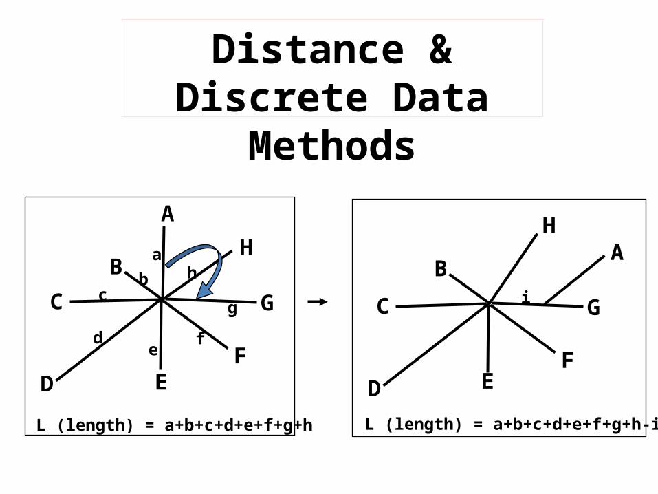
Distance & Discrete Data
MethodsA
B
D EF
G
H
C
ab
c
d e fg
hA
C
EF
G
HB
D
i
L (length) = a+b+c+d+e+f+g+h L (length) = a+b+c+d+e+f+g+h-i
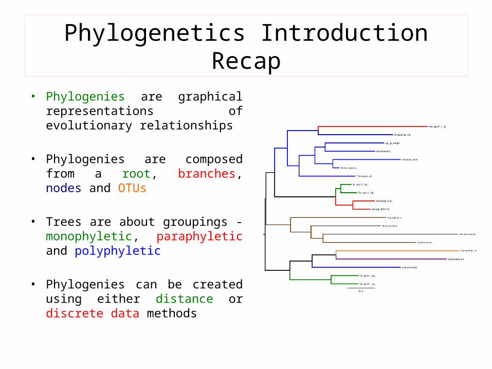
Phylogenetics Introduction Recap
• Phylogenies are graphical representations of evolutionary relationships
• Phylogenies are composed from a root, branches, nodes and OTUs
• Trees are about groupings - monophyletic, paraphyletic and polyphyletic
• Phylogenies can be created using either distance or discrete data methods
v methods: parsimony, maximum likelihood, bayesian inference
Distance methods
Discrete data (tree searching) methods
Two Main Categories of Phylogenetic Methods
v methods: (UPGMA), neighbour-joiningv UPGMA - relatively crude methods, no longer used for phylogenetic analysisv Neighbour-joining (NJ) - fast and accurate with ‘clean’ datasets
v Parsimony - more sophisticated than NJv Maximum likelihood and bayesian inference - the gold standard phylogenetic methods. Discussed in third year evolution lectures
It is preferable to use more than one phylogenetic method for your data
v Tree based single metric: % difference (distance) between sequences
v Also referred to as “clustering” or “algorithmic” methods
vTake data (matrix of % D), plug into equation, -> tree, one solution onlyv Fast, easy, reasonably accurate, good enough for many things
Distance methods
v Problematic with missing data, particularly non-overlapping sequences
v Rarely used by phylogeneticists, but popular with non-specialists
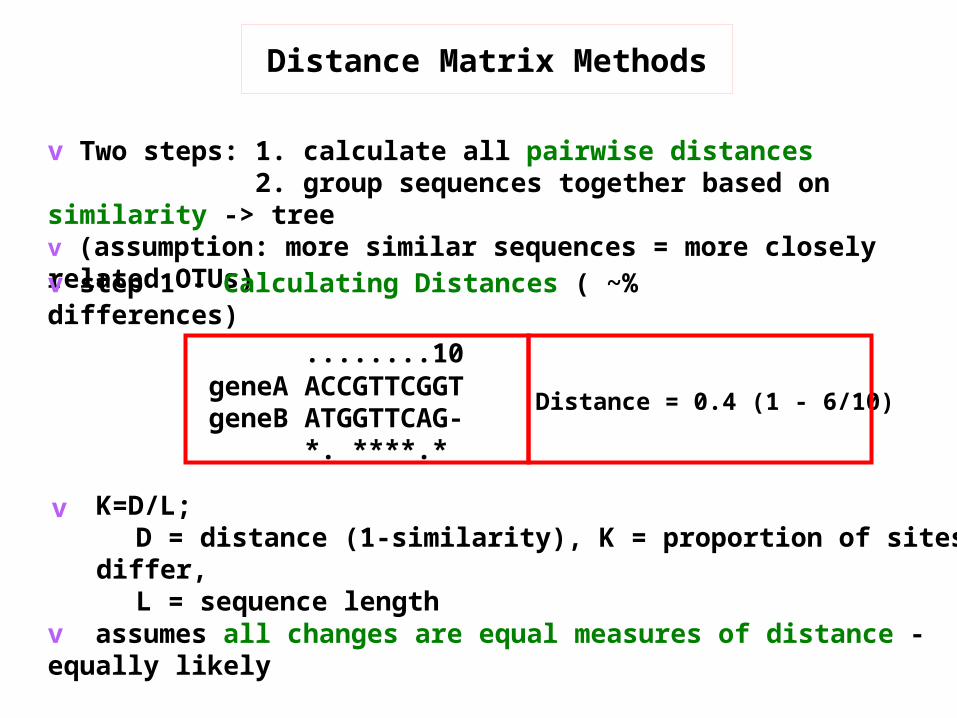
v Two steps: 1. calculate all pairwise distances 2. group sequences together based on
similarity -> treev (assumption: more similar sequences = more closely related OTUs)
v assumes all changes are equal measures of distance - equally likely
v step 1 - Calculating Distances ( ~% differences)
K=D/L; D = distance (1-similarity), K = proportion of sites that
differ, L = sequence length
v
........10geneA ACCGTTCGGTgeneB ATGGTTCAG- *. ****.*
Distance = 0.4 (1 - 6/10)
Distance Matrix Methods
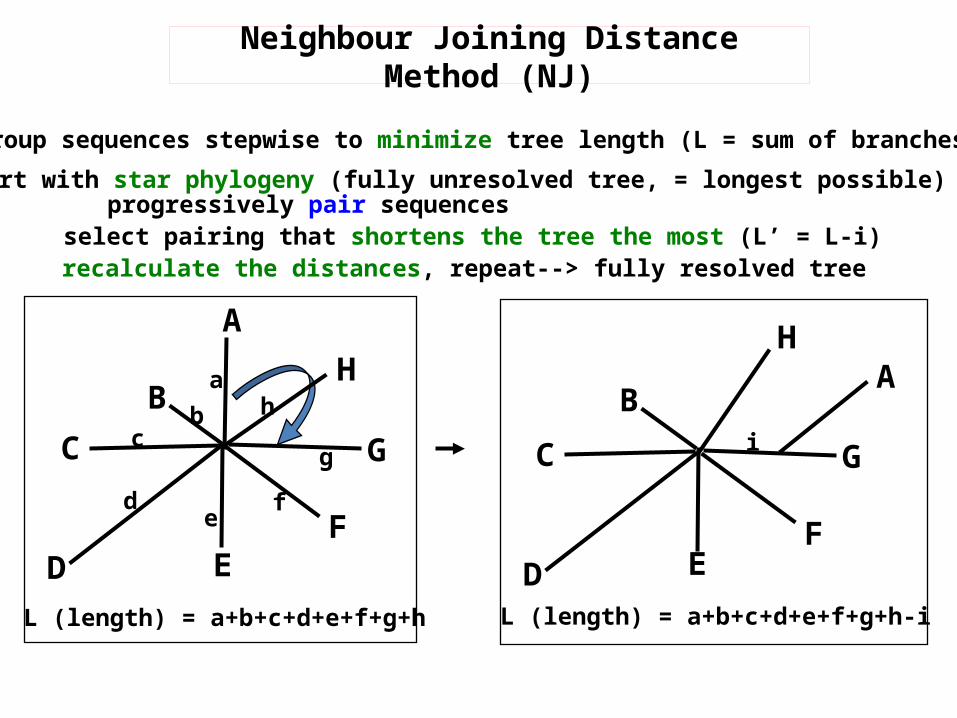
v Group sequences stepwise to minimize tree length (L = sum of branches)v start with star phylogeny (fully unresolved tree, = longest possible)
progressively pair sequencesselect pairing that shortens the tree the most (L’ = L-i)recalculate the distances, repeat--> fully resolved tree
L (length) = a+b+c+d+e+f+g+h L (length) = a+b+c+d+e+f+g+h-i
A
B
D EF
G
H
C
ab
c
d e fg
hA
C
EF
G
HB
D
i
Neighbour Joining Distance Method (NJ)
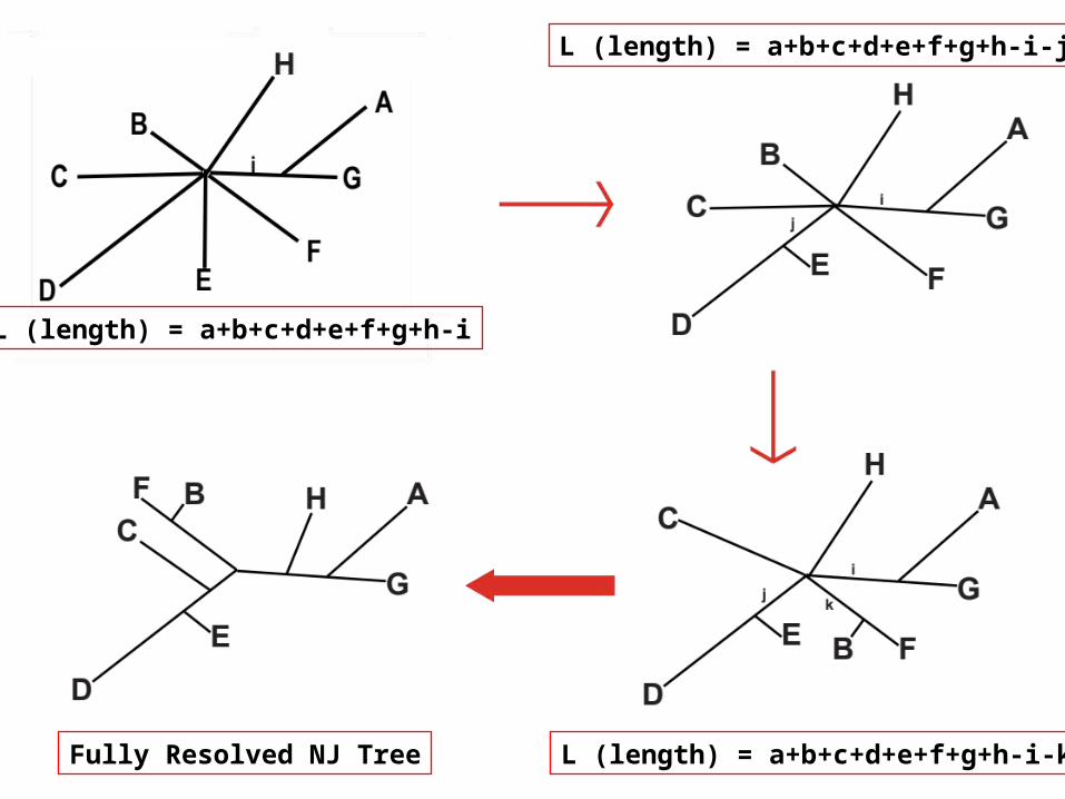
L (length) = a+b+c+d+e+f+g+h-i
L (length) = a+b+c+d+e+f+g+h-i-j
L (length) = a+b+c+d+e+f+g+h-i-kFully Resolved NJ Tree
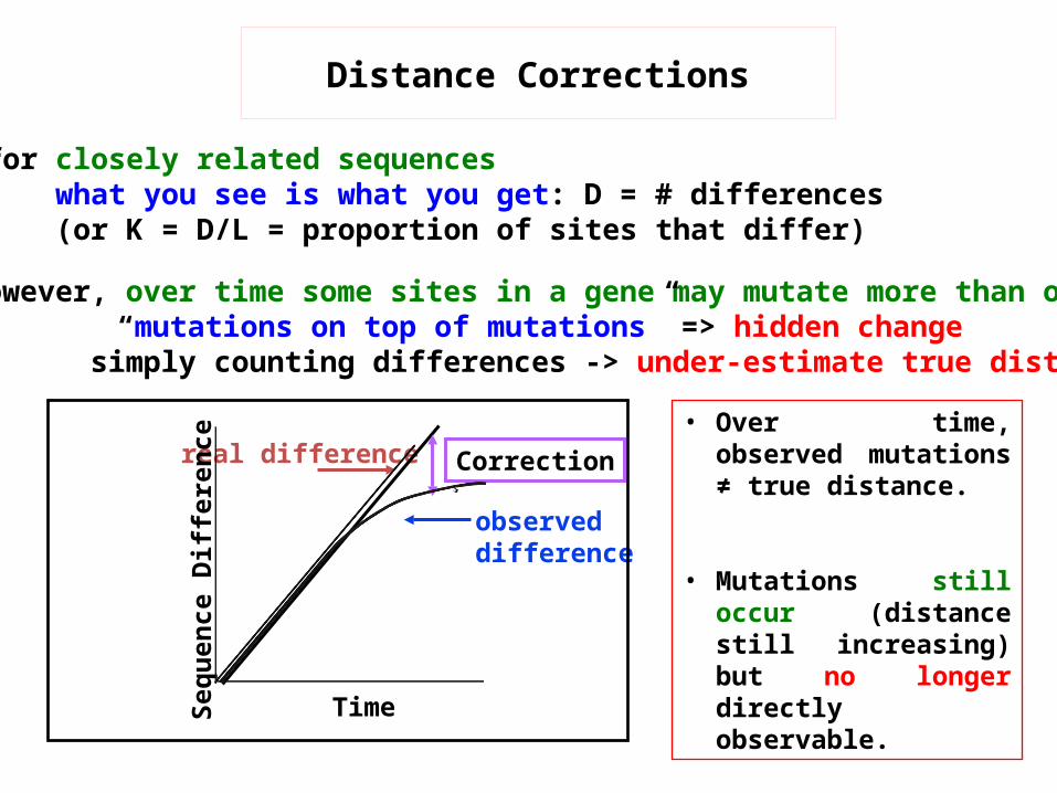
v for closely related sequenceswhat you see is what you get: D = # differences(or K = D/L = proportion of sites that differ)
v however, over time some sites in a gene may mutate more than once“mutations on top of mutations” => hidden change
simply counting differences -> under-estimate true distance
observed difference
real difference
Sequ
ence D
iffe
renc
e
Time
Correction
Distance Corrections
• Over time, observed mutations ≠ true distance.
• Mutations still occur (distance still increasing) but no longer directly observable.
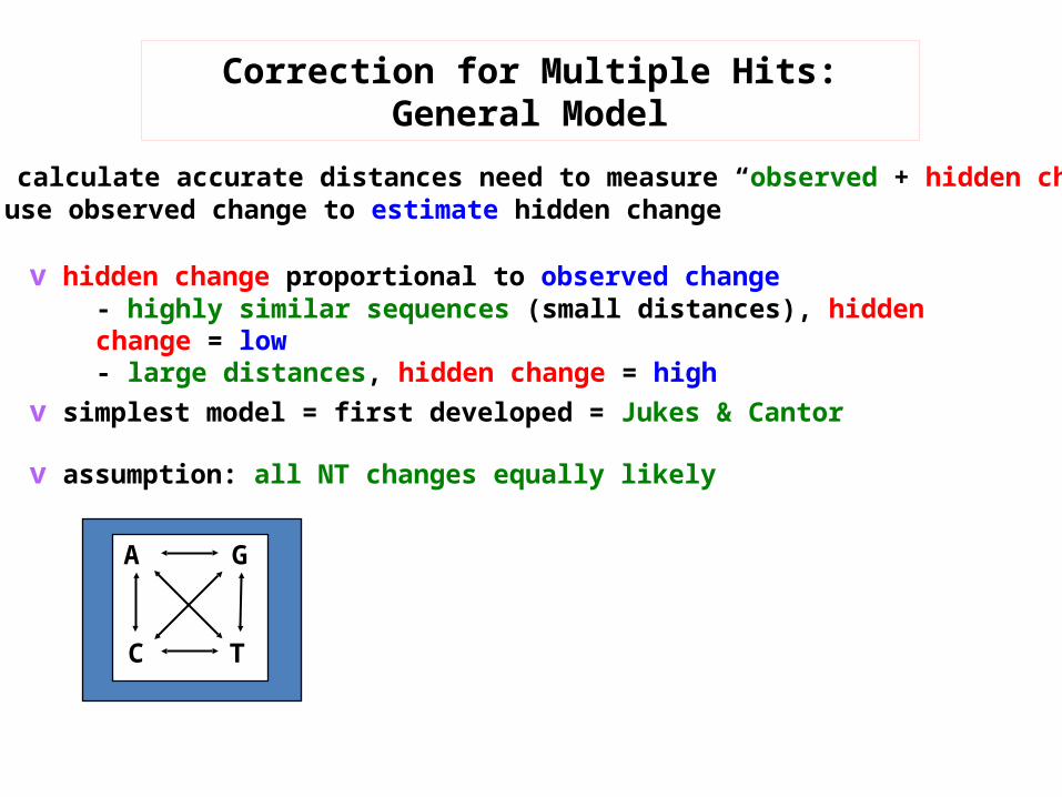
v To calculate accurate distances need to measure “observed + hidden change” use observed change to estimate hidden change
A
C
G
T
v simplest model = first developed = Jukes & Cantor
Correction for Multiple Hits:General Model
v hidden change proportional to observed change- highly similar sequences (small distances), hidden change = low- large distances, hidden change = high
v assumption: all NT changes equally likely
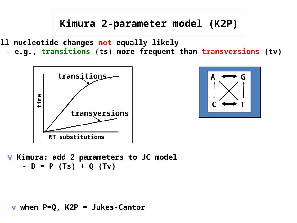
v all nucleotide changes not equally likely- e.g., transitions (ts) more frequent than transversions (tv)
v when P=Q, K2P = Jukes-Cantor
transitions
transversions
NT substitutions
time
Kimura 2-parameter model (K2P)
v Kimura: add 2 parameters to JC model- D = P (Ts) + Q (Tv)
A
C
G
T
vonly meaningful if comparing related things, things with shared ancestryvi.e., homologous sites in homologous sequences
vfirst step in phylogenetic analysis: evaluate the alignment
Phylogeny = reconstructing the past based on present statev
vevery column in alignment = an hypothesis of homologyif homology is violated -> misinformationgarbage in -> garbage out
Molecular Phylogeny Step 1A Tree is Only As Good as the Alignment Its Based On
vremove all regions where you can’t be certain of homology
vsecond step in phylogenetic analysis: evaluate the treevGenerate support values for each node in your treevBootstrap analyses are employed for most phylogenetic treesv Trees without support values are of limited use -
neither your nor your readers can know if nodes are reliable or artefacts
advantages- can use with any phylogenetic method- well understood
v simplest test = bootstrap also oldest, easiest, most widely used, best understood
Phylogenetic analysis may -> best solution with available data, but how reliable is the tree?
Evaluating Trees: Bootstrap Analysis
- it works: tested in lab with populations of viruses:- simulate evolution, sequence -> tree, bootstrap (Hillis & Bull, 1993, Syst Biol 42: 182-192)
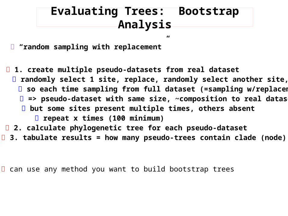
“random sampling with replacement”
3. tabulate results = how many pseudo-trees contain clade (node) x 2. calculate phylogenetic tree for each pseudo-dataset
repeat x times (100 minimum) but some sites present multiple times, others absent => pseudo-dataset with same size, ~composition to real dataset so each time sampling from full dataset (=sampling w/replacement)
randomly select 1 site, replace, randomly select another site, etc. 1. create multiple pseudo-datasets from real dataset
Evaluating Trees: Bootstrap Analysis
can use any method you want to build bootstrap trees
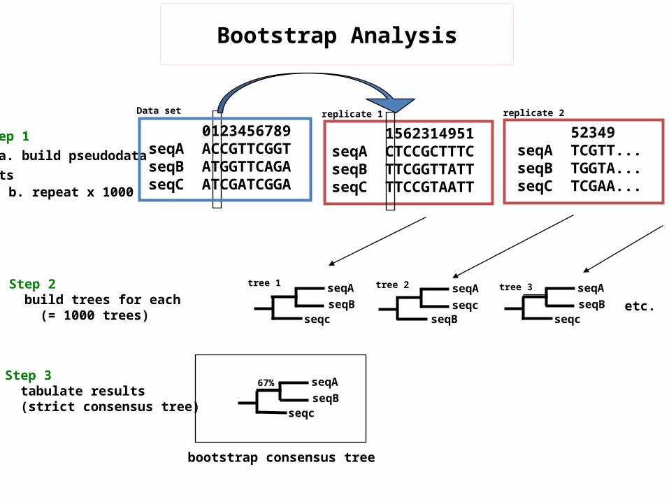
Step 1 a. build pseudodata sets
0123456789seqA ACCGTTCGGTseqB ATGGTTCAGAseqC ATCGATCGGA
Data set
Step 2 build trees for each (= 1000 trees)
seqAseqB
seqc
tree 1 seqA
seqBseqc
tree 2 seqAseqB
seqc
tree 3
etc.
67%Step 3 tabulate results (strict consensus tree)
seqAseqB
seqc
bootstrap consensus tree
52349seqA TCGTT...seqB TGGTA...seqC TCGAA...
replicate 2
b. repeat x 1000
1562314951seqA CTCCGCTTTCseqB TTCGGTTATTseqC TTCCGTAATT
replicate 1
Bootstrap Analysis
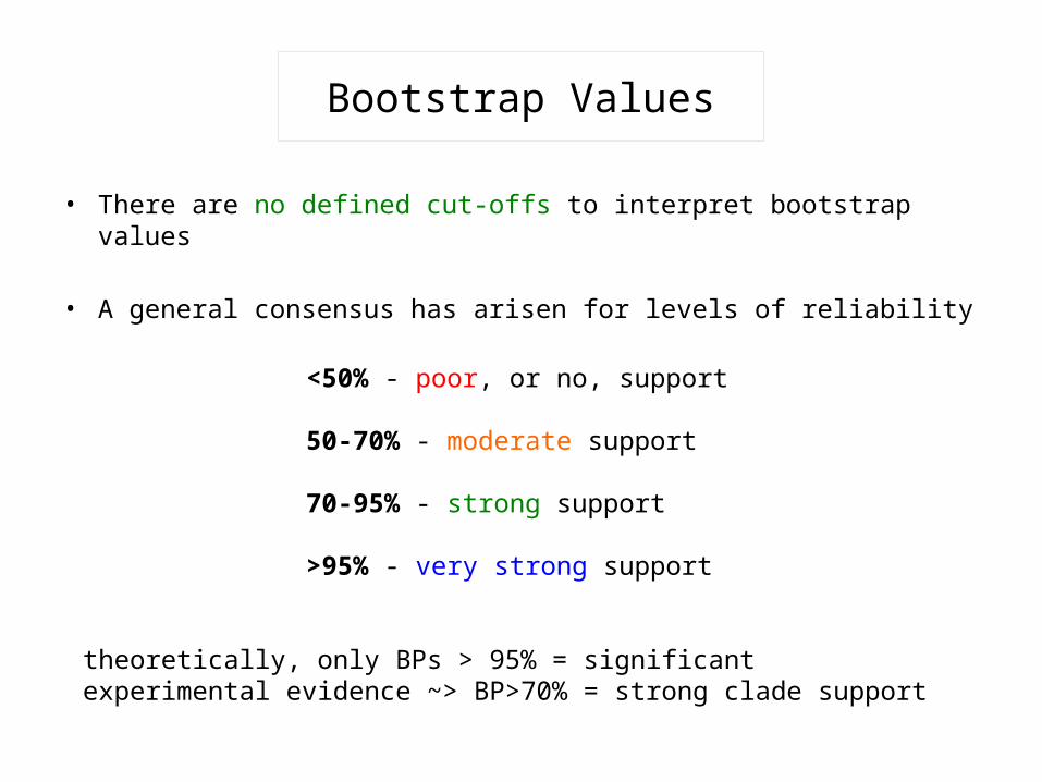
Bootstrap Values
• There are no defined cut-offs to interpret bootstrap values
• A general consensus has arisen for levels of reliability
<50% - poor, or no, support
50-70% - moderate support
70-95% - strong support
>95% - very strong support
theoretically, only BPs > 95% = significantexperimental evidence ~> BP>70% = strong clade support
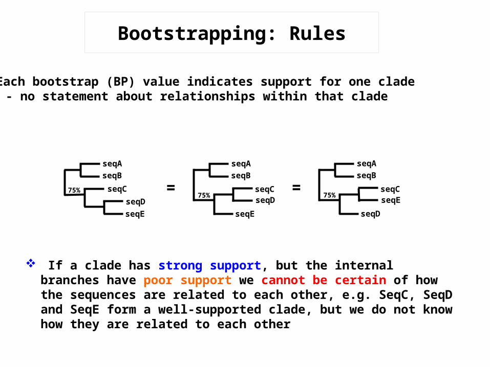
Bootstrapping: Rules
Each bootstrap (BP) value indicates support for one clade- no statement about relationships within that clade
=seqAseqB
75% seqCseqDseqE
If a clade has strong support, but the internal branches have poor support we cannot be certain of how the sequences are related to each other, e.g. SeqC, SeqD and SeqE form a well-supported clade, but we do not know how they are related to each other
seqAseqB
75%seqCseqD
seqE
=seqAseqB
75%seqCseqE
seqD
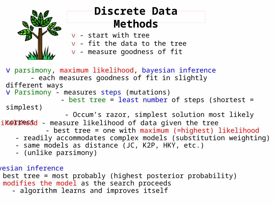
v - start with treev - fit the data to the tree v - measure goodness of fit
v parsimony, maximum likelihood, bayesian inference - each measures goodness of fit in slightly different ways
Discrete Data Methods
v Parsimony - measures steps (mutations) - best tree = least number of steps (shortest = simplest)
- Occum’s razor, simplest solution most likely correctv Likelihood - measure likelihood of data given the tree
- best tree = one with maximum (=highest) likelihood- readily accommodates complex models (substitution weighting)- same models as distance (JC, K2P, HKY, etc.)- (unlike parsimony)
v bayesian inference- best tree = most probably (highest posterior probability)- modifies the model as the search proceeds
- algorithm learns and improves itself
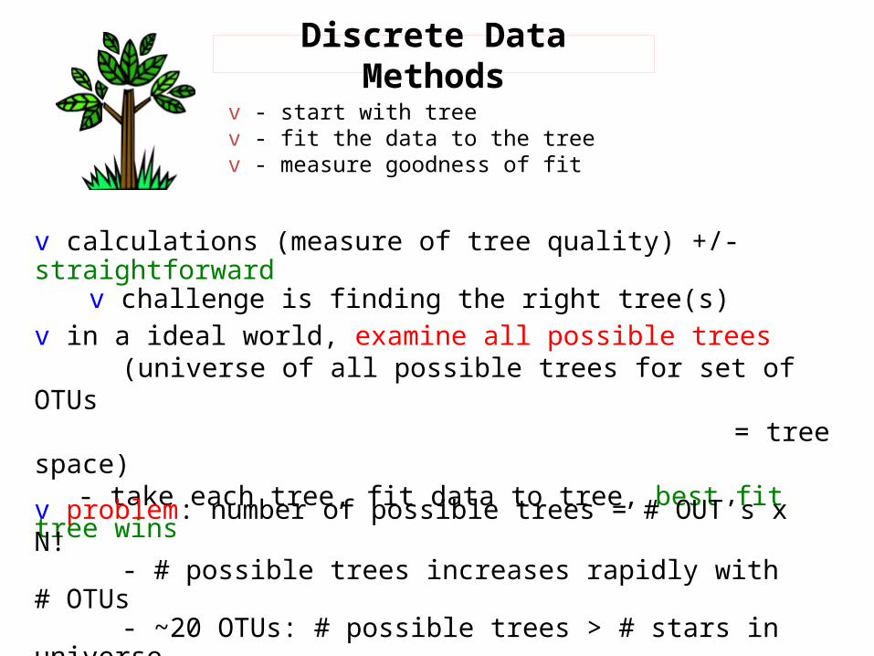
v - start with treev - fit the data to the tree v - measure goodness of fit
v calculations (measure of tree quality) +/- straightforward
v challenge is finding the right tree(s)v in a ideal world, examine all possible trees
(universe of all possible trees for set of OTUs
= tree space)
- take each tree, fit data to tree, best fit tree winsv problem: number of possible trees = # OUT’s x N!
- # possible trees increases rapidly with # OTUs
- ~20 OTUs: # possible trees > # stars in universe
- exhaustive search impossible > 14 OTUs
Discrete Data Methods
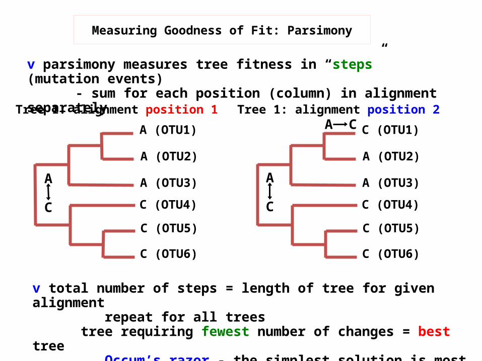
v total number of steps = length of tree for given alignment repeat for all trees
tree requiring fewest number of changes = best tree
Occum’s razor - the simplest solution is most likely correct
Measuring Goodness of Fit: Parsimony
C (OTU1)
A (OTU2)
A (OTU3)C (OTU4)C (OTU5)
C (OTU6)
A
C
A CA (OTU1)
A (OTU2)
A (OTU3)C (OTU4)C (OTU5)
C (OTU6)
A
C
Tree 1: alignment position 1 Tree 1: alignment position 2
v parsimony measures tree fitness in “steps” (mutation events) - sum for each position (column) in alignment separately
1 2 3 4 5seq-a G T C A A
seq-b G C C A A
seq-c A C G A A
seq-d A C G T A
a
b
c
d
a
d
b
c
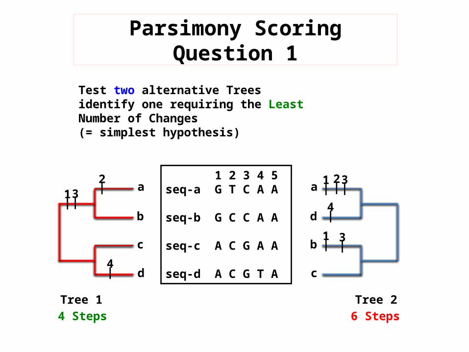
Parsimony Scoring Question 1
Test two alternative Trees identify one requiring the Least Number of Changes(= simplest hypothesis)
1|1|
1|
2| 2|3|3|
4|
4|3|
Tree 1 Tree 24 Steps 6 Steps
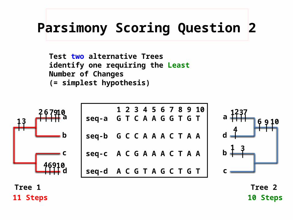
Parsimony Scoring Question 2
1 2 3 4 5 6 7 8 9 10seq-a G T C A A G G T G T
seq-b G C C A A A C T A A
seq-c A C G A A A C T A A
seq-d A C G T A G C T G T
a
b
c
d
a
d
b
c
Test two alternative Trees identify one requiring the Least Number of Changes(= simplest hypothesis)
1|1|
1|
2| 2|3|3|
4|
4|3|
Tree 1 Tree 211 Steps 10 Steps
10|
6|
6|
6|7|7|9|
9|
9|10|
10|
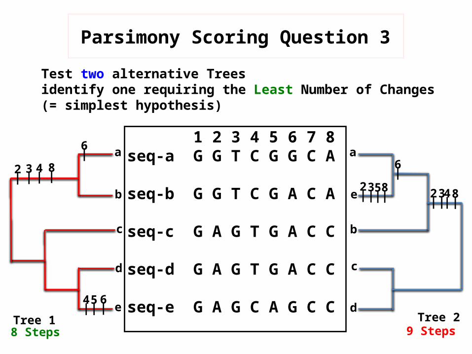
Parsimony Scoring Question 3
1 2 3 4 5 6 7 8 seq-a G G T C G G C A seq-b G G T C G A C A
seq-c G A G T G A C C
seq-d G A G T G A C C
seq-e G A G C A G C C
Test two alternative Trees identify one requiring the Least Number of Changes(= simplest hypothesis)
a a
b
bc
c
d
d
e
eTree 1 Tree 2
2|2|
2|
3|3| 3|
4|
4|
4|
5|
5|
6|
6|6|8|
8| 8|
8 Steps 9 Steps
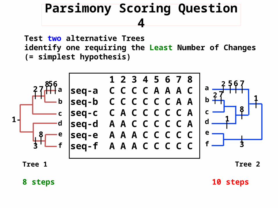
1 2 3 4 5 6 7 8 seq-a C C C C A A A C seq-b C C C C C C A Aseq-c C A C C C C C Aseq-d A A C C C C C Aseq-e A A A C C C C Cseq-f A A A C C C C C
Test two alternative Trees identify one requiring the Least Number of Changes(= simplest hypothesis)
8 steps 10 steps
abcdef
abcdef
1-
2|
|3
5|6|7|
8|
8|1|
1|8|
Parsimony Scoring Question 4
2|
2|
|3
5|6| 7|7|
Tree 1 Tree 2
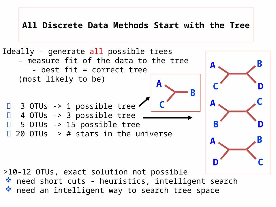
All Discrete Data Methods Start with the Tree
Ideally - generate all possible trees - measure fit of the data to the tree - best fit = correct tree
(most likely to be)
3 OTUs -> 1 possible tree 4 OTUs -> 3 possible tree 5 OTUs -> 15 possible tree 20 OTUs > # stars in the universe
>10-12 OTUs, exact solution not possible need short cuts - heuristics, intelligent search need an intelligent way to search tree space
A B
C DA C
B DA B
D C
AB
C
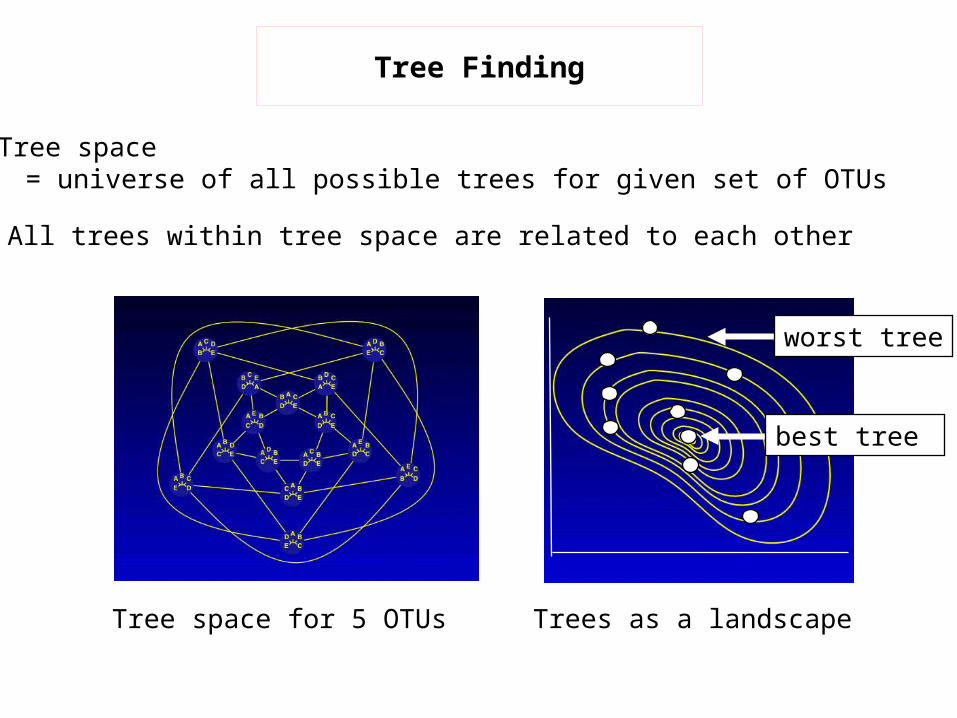
Trees as a landscape
Tree Finding
Tree space= universe of all possible trees for given set of OTUs
All trees within tree space are related to each other
Tree space for 5 OTUs
worst tree
best tree
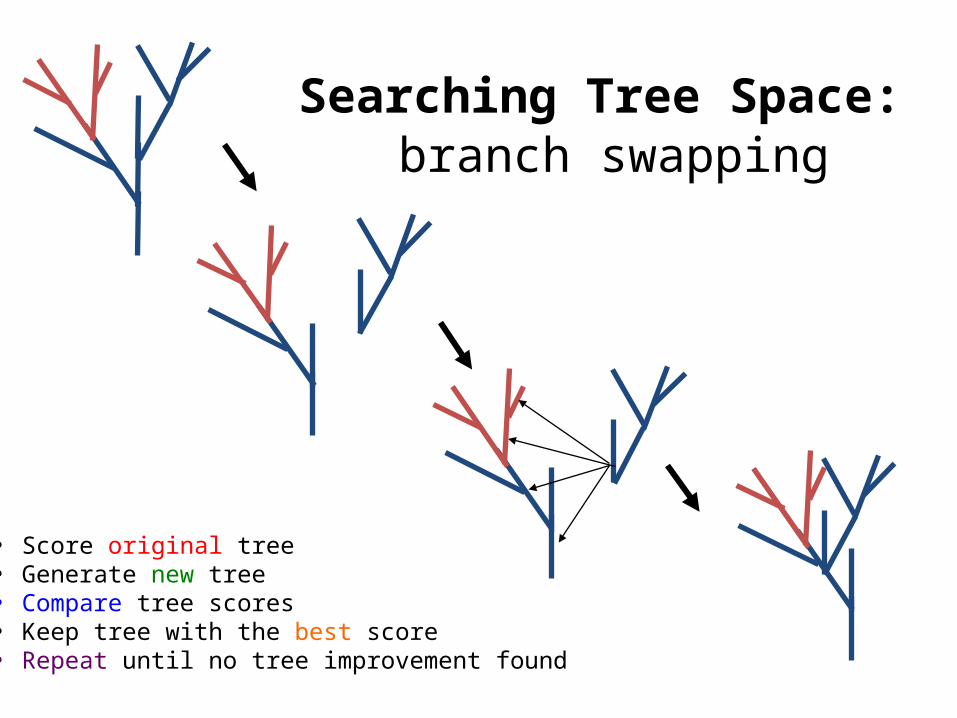
branch swappingSearching Tree Space:
• Score original tree• Generate new tree• Compare tree scores• Keep tree with the best score• Repeat until no tree improvement found
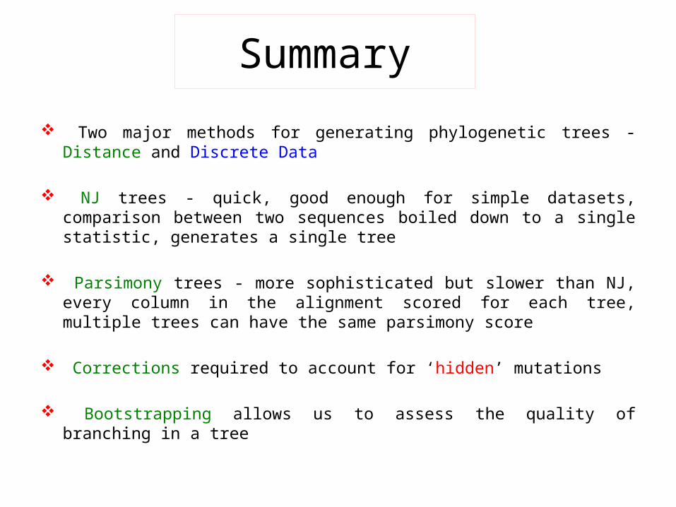
Summary Two major methods for generating phylogenetic trees -
Distance and Discrete Data
NJ trees - quick, good enough for simple datasets, comparison between two sequences boiled down to a single statistic, generates a single tree
Parsimony trees - more sophisticated but slower than NJ, every column in the alignment scored for each tree, multiple trees can have the same parsimony score
Corrections required to account for ‘hidden’ mutations
Bootstrapping allows us to assess the quality of branching in a tree