el512: lecture 1
TRANSCRIPT
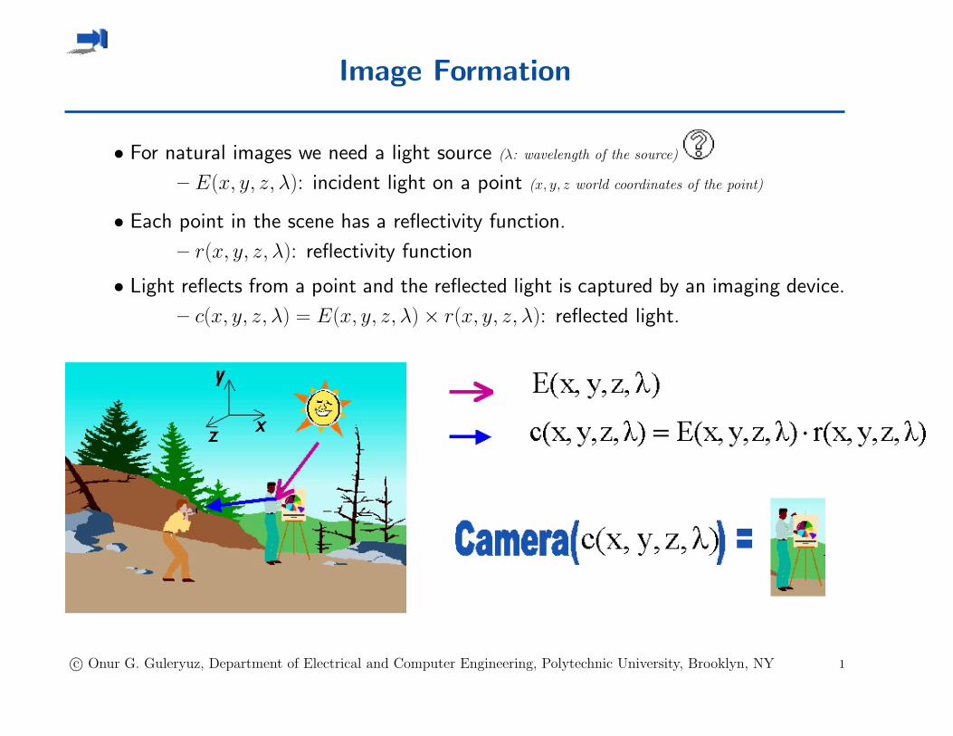
Image Formation
• For natural images we need a light source (λ: wavelength of the source) .
– E(x, y, z, λ): incident light on a point (x, y, z world coordinates of the point)
• Each point in the scene has a reflectivity function.
– r(x, y, z, λ): reflectivity function
• Light reflects from a point and the reflected light is captured by an imaging device.
– c(x, y, z, λ) = E(x, y, z, λ)× r(x, y, z, λ): reflected light.
c© Onur G. Guleryuz, Department of Electrical and Computer Engineering, Polytechnic University, Brooklyn, NY 1
Inside the Camera - Projection
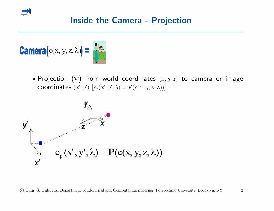
• Projection (P) from world coordinates (x, y, z) to camera or imagecoordinates (x′, y′) [cp(x
′, y′, λ) = P(c(x, y, z, λ))].
c© Onur G. Guleryuz, Department of Electrical and Computer Engineering, Polytechnic University, Brooklyn, NY 2
Projections
• There are two types of projections (P) of interest to us:
1. Perspective Projection
– Objects closer to the capture device appear bigger. Mostimage formation situations can be considered to be underthis category, including images taken by camera and thehuman eye.
2. Ortographic Projection
– This is “unnatural”. Objects appear the same size re-gardless of their distance to the “capture device”.
• Both types of projections can be represented via mathematical for-mulas. Ortographic projection is easier and is sometimes used as amathematical convenience. For more details see [1].
c© Onur G. Guleryuz, Department of Electrical and Computer Engineering, Polytechnic University, Brooklyn, NY 3
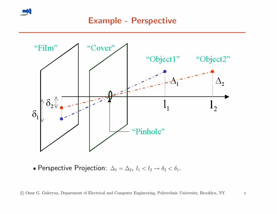
Example - Perspective
• Perspective Projection: ∆1 = ∆2, l1 < l2 → δ2 < δ1.
c© Onur G. Guleryuz, Department of Electrical and Computer Engineering, Polytechnic University, Brooklyn, NY 4
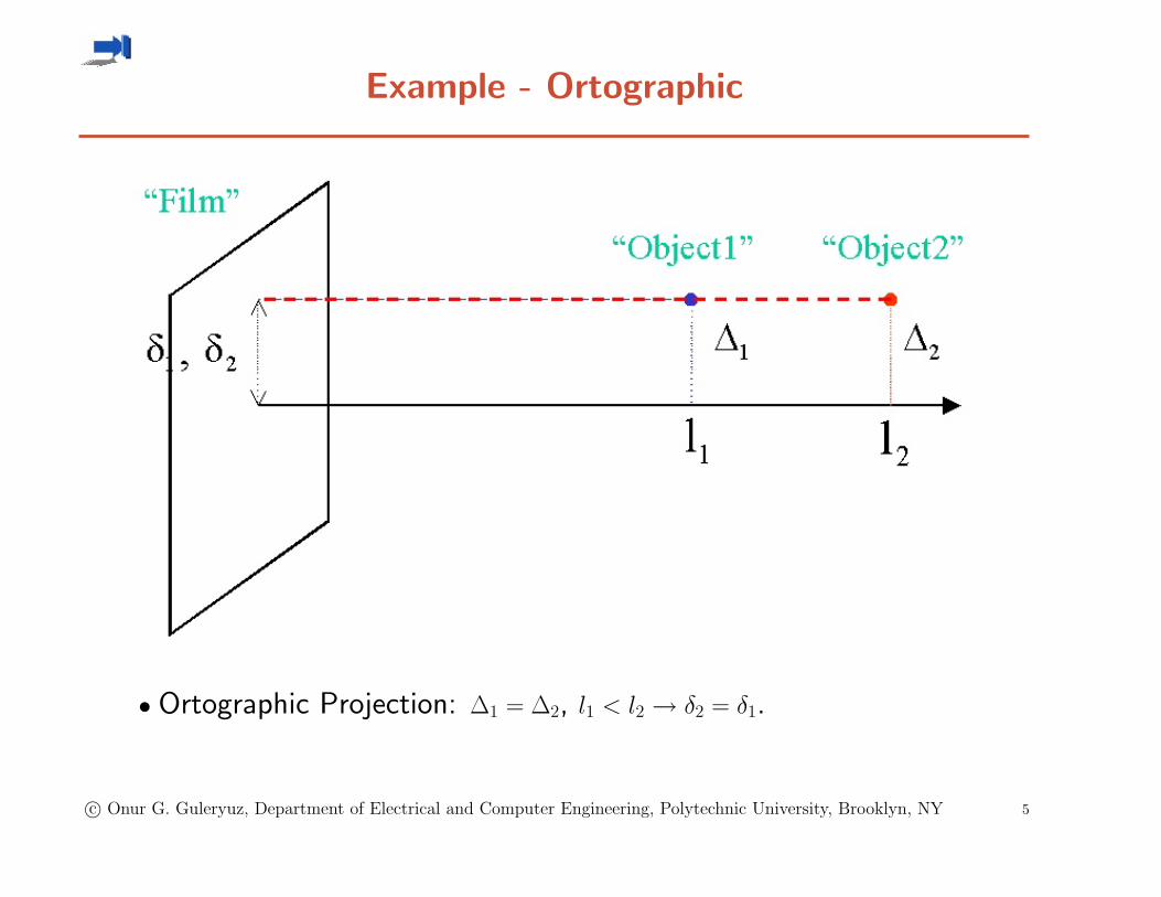
Example - Ortographic
• Ortographic Projection: ∆1 = ∆2, l1 < l2 → δ2 = δ1.
c© Onur G. Guleryuz, Department of Electrical and Computer Engineering, Polytechnic University, Brooklyn, NY 5
Inside the Camera - Sensitivity
• Once we have cp(x′, y′, λ) the characteristics of the capture device take
over.
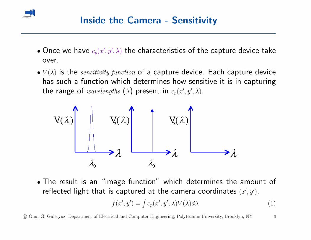
• V (λ) is the sensitivity function of a capture device. Each capture devicehas such a function which determines how sensitive it is in capturingthe range of wavelengths (λ) present in cp(x
′, y′, λ).
• The result is an “image function” which determines the amount ofreflected light that is captured at the camera coordinates (x′, y′).
f (x′, y′) =∫
cp(x′, y′, λ)V (λ)dλ (1)
c© Onur G. Guleryuz, Department of Electrical and Computer Engineering, Polytechnic University, Brooklyn, NY 6
Example
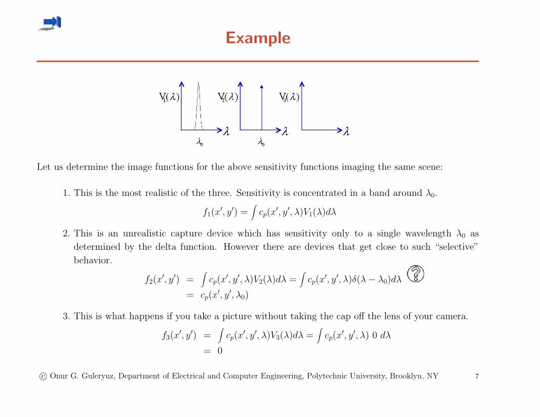
Let us determine the image functions for the above sensitivity functions imaging the same scene:
1. This is the most realistic of the three. Sensitivity is concentrated in a band around λ0.
f1(x′, y′) =
∫cp(x
′, y′, λ)V1(λ)dλ
2. This is an unrealistic capture device which has sensitivity only to a single wavelength λ0 as
determined by the delta function. However there are devices that get close to such “selective”
behavior.
f2(x′, y′) =
∫cp(x
′, y′, λ)V2(λ)dλ =∫
cp(x′, y′, λ)δ(λ− λ0)dλ
= cp(x′, y′, λ0)
3. This is what happens if you take a picture without taking the cap off the lens of your camera.
f3(x′, y′) =
∫cp(x
′, y′, λ)V3(λ)dλ =∫
cp(x′, y′, λ) 0 dλ
= 0
c© Onur G. Guleryuz, Department of Electrical and Computer Engineering, Polytechnic University, Brooklyn, NY 7
Sensitivity and Color
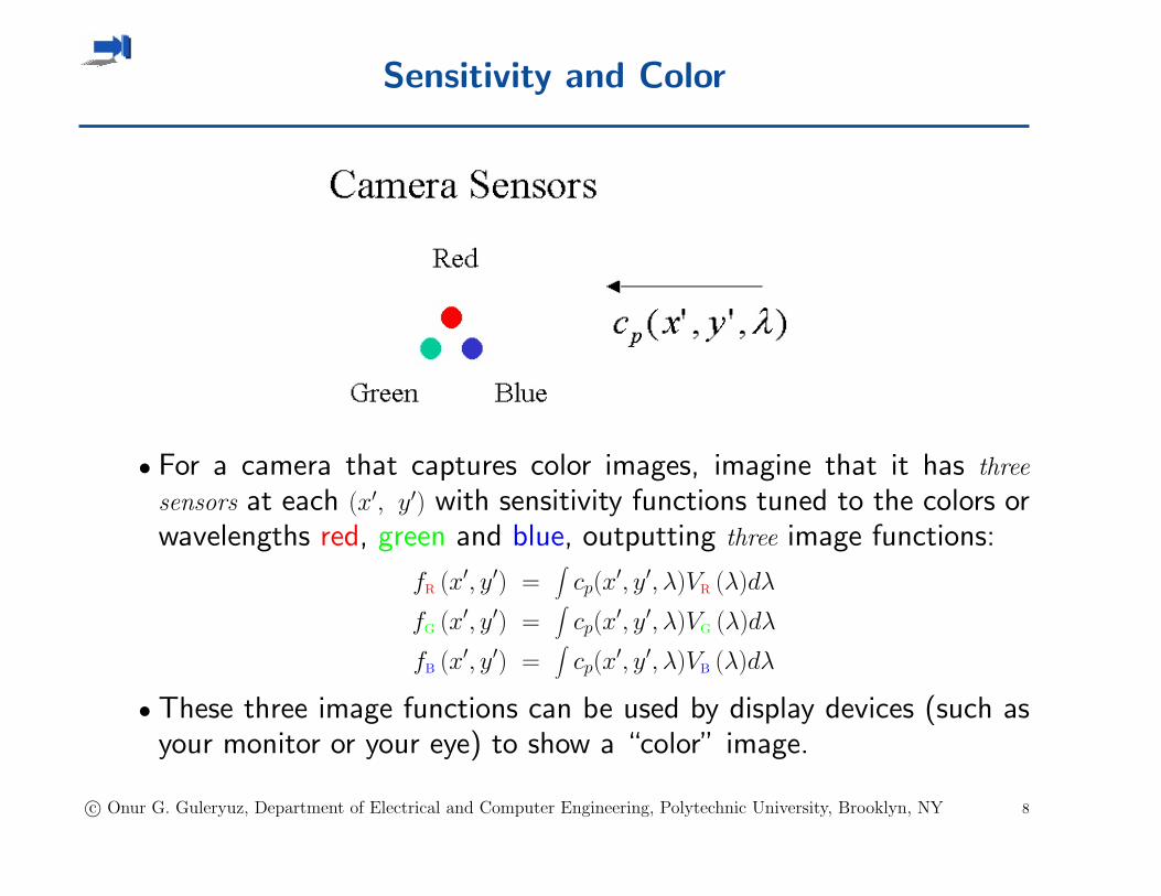
• For a camera that captures color images, imagine that it has three
sensors at each (x′, y′) with sensitivity functions tuned to the colors orwavelengths red, green and blue, outputting three image functions:
fR (x′, y′) =∫
cp(x′, y′, λ)VR (λ)dλ
fG (x′, y′) =∫
cp(x′, y′, λ)VG (λ)dλ
fB (x′, y′) =∫
cp(x′, y′, λ)VB (λ)dλ
• These three image functions can be used by display devices (such asyour monitor or your eye) to show a “color” image.
c© Onur G. Guleryuz, Department of Electrical and Computer Engineering, Polytechnic University, Brooklyn, NY 8
Summary
• The image function fC (x′, y′) (C = R, G, B) is formed as:
fC (x′, y′) =∫
cp(x′, y′, λ)VC (λ)dλ (2)
• It is the result of:
1. Incident light E(x, y, z, λ) at the point (x, y, z) in the scene,
2. The reflectivity function r(x, y, z, λ) of this point,
3. The formation of the reflected light c(x, y, z, λ) = E(x, y, z, λ) ×r(x, y, z, λ),
4. The projection of the reflected light c(x, y, z, λ) from the three
dimensional world coordinates to two dimensional camera coor-dinates which forms cp(x
′, y′, λ),
5. The sensitivity function(s) of the camera V (λ).
c© Onur G. Guleryuz, Department of Electrical and Computer Engineering, Polytechnic University, Brooklyn, NY 9
Digital Image Formation
• The image function fC (x′, y′) is still a function of x′ ∈ [x′min, x′max] and y′ ∈
[y′min, y′max] which vary in a continuum given by the respective intervals.
• The values taken by the image function are real numbers which againvary in a continuum or interval fC (x′, y′) ∈ [fmin, fmax].
• Digital computers cannot process parameters/functions that vary in acontinuum.
• We have to discretize:
1. x′, y′ ⇒ x′i, y′j (i = 0, . . . , N − 1, j = 0, . . . , M − 1): Sampling
2. fC (x′i, y′j) ⇒ f̂C (x′i, y
′j): Quantization.
c© Onur G. Guleryuz, Department of Electrical and Computer Engineering, Polytechnic University, Brooklyn, NY 10
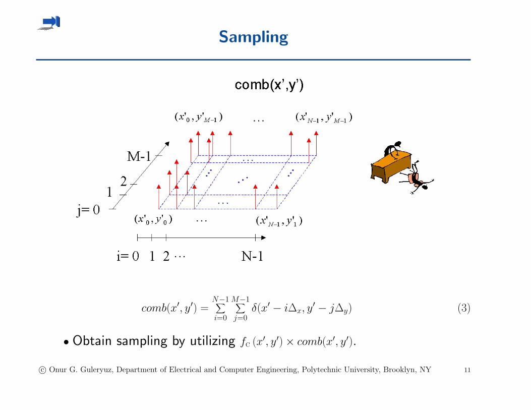
Sampling
comb(x′, y′) =N−1∑
i=0
M−1∑
j=0δ(x′ − i∆x, y
′ − j∆y) (3)
• Obtain sampling by utilizing fC (x′, y′)× comb(x′, y′).
c© Onur G. Guleryuz, Department of Electrical and Computer Engineering, Polytechnic University, Brooklyn, NY 11
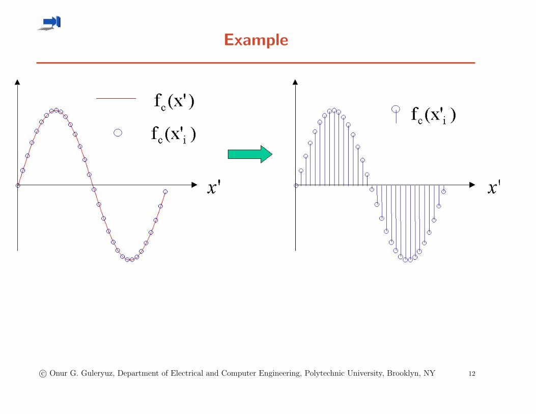
Example
c© Onur G. Guleryuz, Department of Electrical and Computer Engineering, Polytechnic University, Brooklyn, NY 12
Idealized Sampling
• We will later see that by utilizing fC (x′, y′) × comb(x′, y′), it is possibleto discretize (x′, y′) and obtain a new “image function” that is definedon the discrete grid (x′i, y
′j) (i = 0, . . . , N − 1, j = 0, . . . , M − 1).
• For now assume that we somehow obtain the sampled image functionfC (x′i, y
′j).
• To denote this discretization refer to fC (x′i, y′j) as fC (i, j) from now on.
c© Onur G. Guleryuz, Department of Electrical and Computer Engineering, Polytechnic University, Brooklyn, NY 13
Quantization
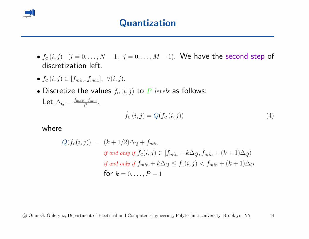
• fC (i, j) (i = 0, . . . , N − 1, j = 0, . . . , M − 1). We have the second step ofdiscretization left.
• fC (i, j) ∈ [fmin, fmax], ∀(i, j).
• Discretize the values fC (i, j) to P levels as follows:
Let ∆Q = fmax−fminP .
f̂C (i, j) = Q(fC (i, j)) (4)
where
Q(fC(i, j)) = (k + 1/2)∆Q + fmin
if and only if fC(i, j) ∈ [fmin + k∆Q, fmin + (k + 1)∆Q)
if and only if fmin + k∆Q ≤ fC(i, j) < fmin + (k + 1)∆Q
for k = 0, . . . , P − 1
c© Onur G. Guleryuz, Department of Electrical and Computer Engineering, Polytechnic University, Brooklyn, NY 14
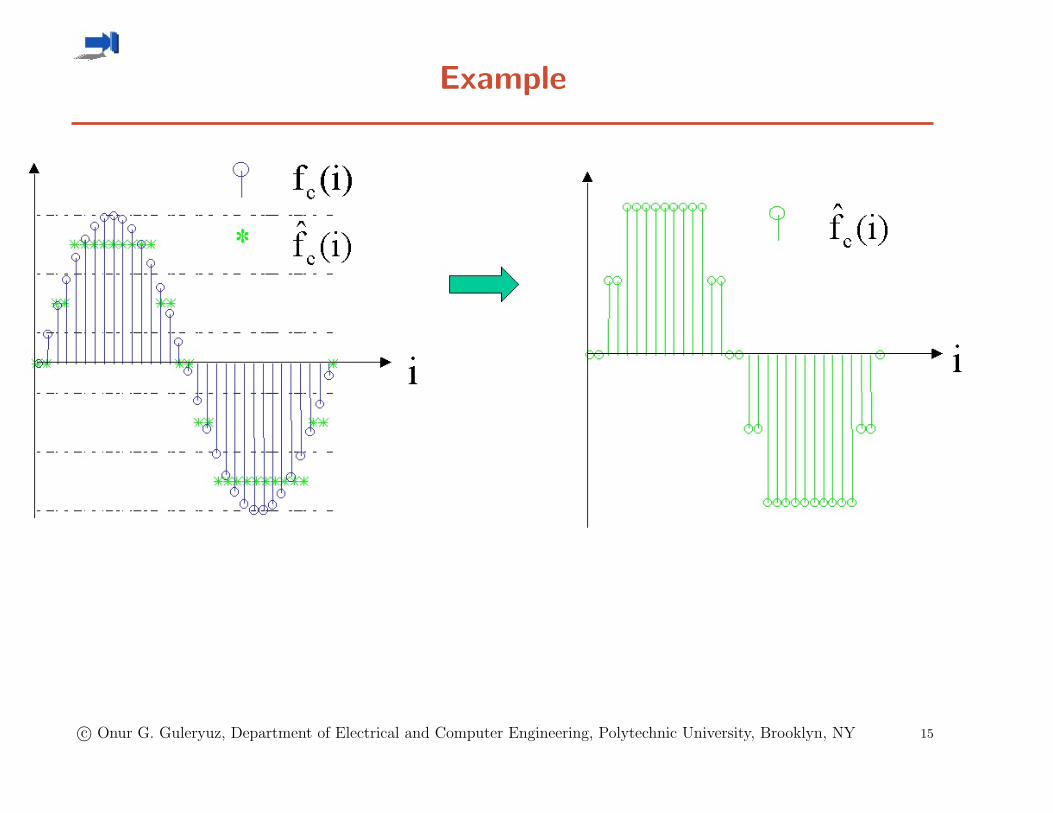
Example
c© Onur G. Guleryuz, Department of Electrical and Computer Engineering, Polytechnic University, Brooklyn, NY 15
Quantization to P levels
• Typically P = 28 = 256 and we have log2(P ) = log2(28) = 8 bit quantization.
• We have thus achieved the second step of discretization.
• From now on omit references to fmin, fmax and unless otherwise statedassume that the original digital images are quantized to 8 bits or 256
levels.
• To denote this refer to f̂C (i, j) as taking integer values k where 0 ≤ k ≤255, i.e., let us say that
f̂C(i, j) ∈ {0, . . . , 255} (5)
c© Onur G. Guleryuz, Department of Electrical and Computer Engineering, Polytechnic University, Brooklyn, NY 16
Summary
• “Let there be light” → incident light → reflectivity → reflected light→ projection → sensitivity → fC (x′, y′).
• Sampling: fC (x′, y′) → fC (i, j).
• Quantization: fC(i, j) → f̂C(i, j) ∈ {0, . . . , 255}.
c© Onur G. Guleryuz, Department of Electrical and Computer Engineering, Polytechnic University, Brooklyn, NY 17
(R,G,B) Parameterization of Full Color Images
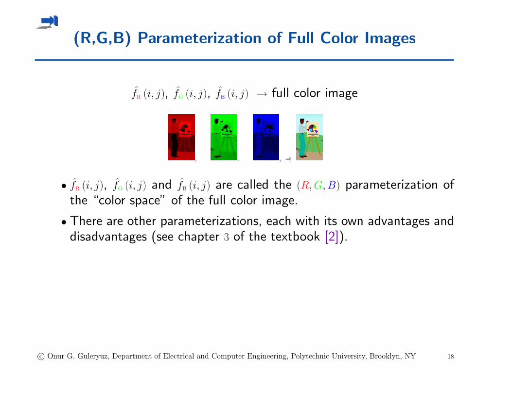
f̂R (i, j), f̂G (i, j), f̂B (i, j) → full color image
, , , ⇒
• f̂R (i, j), f̂G (i, j) and f̂B (i, j) are called the (R, G, B) parameterization ofthe “color space” of the full color image.
• There are other parameterizations, each with its own advantages anddisadvantages (see chapter 3 of the textbook [2]).
c© Onur G. Guleryuz, Department of Electrical and Computer Engineering, Polytechnic University, Brooklyn, NY 18
Grayscale Images
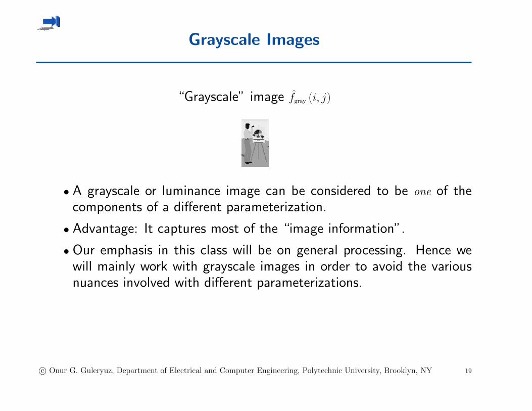
“Grayscale” image f̂gray (i, j)
• A grayscale or luminance image can be considered to be one of thecomponents of a different parameterization.
• Advantage: It captures most of the “image information”.
• Our emphasis in this class will be on general processing. Hence wewill mainly work with grayscale images in order to avoid the variousnuances involved with different parameterizations.
c© Onur G. Guleryuz, Department of Electrical and Computer Engineering, Polytechnic University, Brooklyn, NY 19
Images as Matrices
• Recalling the image formation operations we have discussed, note thatthe image f̂gray (i, j) is an N ×M matrix with integer entries in the range0, . . . , 255.
• From now on suppress ˆ( )gray
and denote an image as a matrix “A” (orB, . . ., etc.) with elements A(i, j) ∈ {0, . . . , 255} for i = 0, . . . , N − 1 , j =
0, . . . , M − 1.
• So we will be processing matrices!
• Warning: Some processing we will do will take an image A withA(i, j) ∈ {0, . . . , 255} into a new matrix B which may not have integerentries!
In these cases we must suitably scale and round the elements of B inorder to display it as an image.
c© Onur G. Guleryuz, Department of Electrical and Computer Engineering, Polytechnic University, Brooklyn, NY 20
Matrices and Matlab
• The software package Matlab is a very easy to use tool that specializesin matrices.
• We will be utilizing Matlab for all processing, examples, homeworks,etc.
• If you do not have access to Matlab, a copy licensed for use in EL 512will be provided to you. See the end of this lecture for instructionsand details.
c© Onur G. Guleryuz, Department of Electrical and Computer Engineering, Polytechnic University, Brooklyn, NY 21
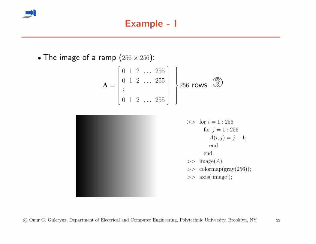
Example - I
• The image of a ramp (256× 256):
A =
0 1 2 . . . 255
0 1 2 . . . 255...0 1 2 . . . 255
256 rows
>> for i = 1 : 256
for j = 1 : 256
A(i, j) = j − 1;
end
end
>> image(A);
>> colormap(gray(256));
>> axis(’image’);
c© Onur G. Guleryuz, Department of Electrical and Computer Engineering, Polytechnic University, Brooklyn, NY 22
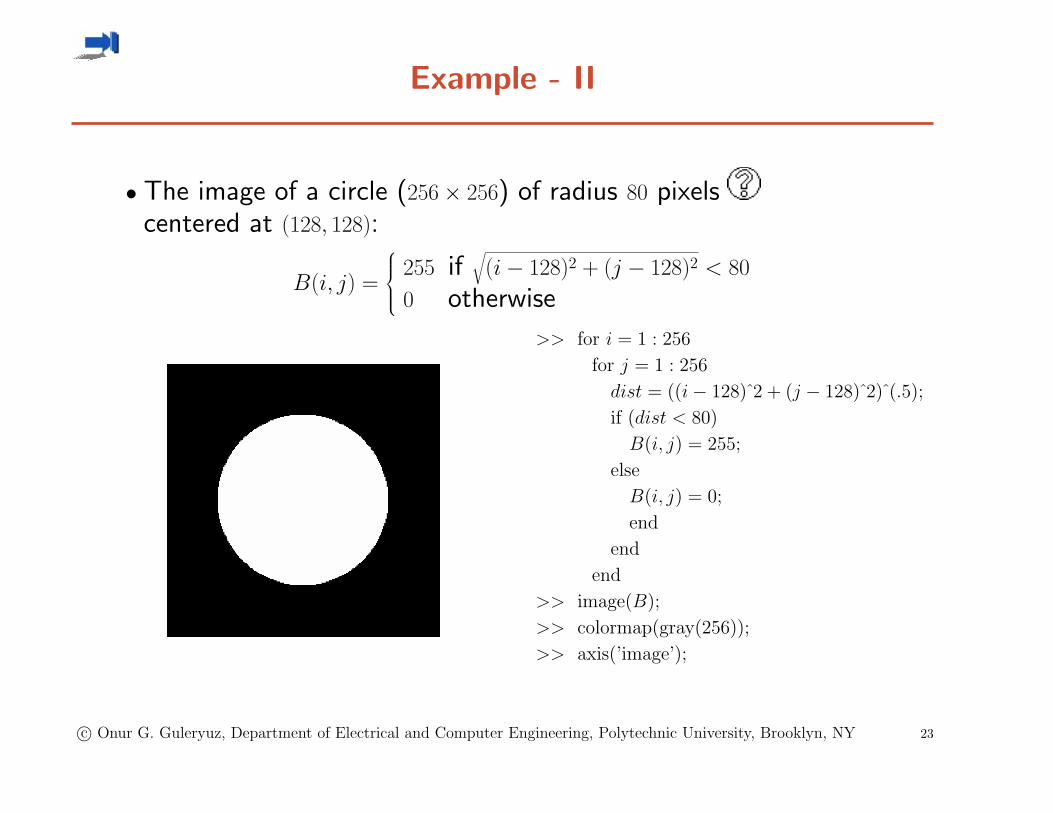
Example - II
• The image of a circle (256× 256) of radius 80 pixelscentered at (128, 128):
B(i, j) =
255 if√(i− 128)2 + (j − 128)2 < 80
0 otherwise
>> for i = 1 : 256
for j = 1 : 256
dist = ((i− 128)̂ 2 + (j − 128)̂ 2)̂ (.5);
if (dist < 80)
B(i, j) = 255;
else
B(i, j) = 0;
end
end
end
>> image(B);
>> colormap(gray(256));
>> axis(’image’);
c© Onur G. Guleryuz, Department of Electrical and Computer Engineering, Polytechnic University, Brooklyn, NY 23
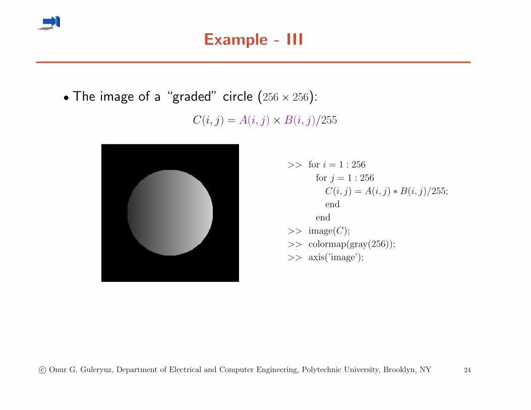
Example - III
• The image of a “graded” circle (256× 256):
C(i, j) = A(i, j)×B(i, j)/255
>> for i = 1 : 256
for j = 1 : 256
C(i, j) = A(i, j) ∗B(i, j)/255;
end
end
>> image(C);
>> colormap(gray(256));
>> axis(’image’);
c© Onur G. Guleryuz, Department of Electrical and Computer Engineering, Polytechnic University, Brooklyn, NY 24
Homework I
1. If necessary, get a copy of matlab including a handout that givesan introduction to matlab. You may do so at the Multimedia Lab.(LC 008) in the Brooklyn campus. The preferred time is Wednesdayafternoon.
2. Get a picture of yourself taken. Make sure it is 8 bit grayscale and learn
how to read your picture into matlab as a matrix. Again, you may doso at the Multimedia Lab. (LC 008) in the Brooklyn campus.
3. Display your image and obtain a printout. Try “>> help print” forinstructions within matlab.
If you are at a different campus and have problems with the above instruc-tions please send me email. Please note that this is a one time event, i.e.,do your best.
c© Onur G. Guleryuz, Department of Electrical and Computer Engineering, Polytechnic University, Brooklyn, NY 25

References
[1] B. K. P. Horn, Robot Vision. Cambridge, MA: MIT Press, 1986.
[2] A. K. Jain, Fundamentals of Digital Image Processing. Englewood Cliffs, NJ:Prentice Hall, 1989.
c© Onur G. Guleryuz, Department of Electrical and Computer Engineering, Polytechnic University, Brooklyn, NY 26