arX

iv:0

808.

3230

v1 [

mat

h.O

C]

24 A

ug 2

008

1

Phase Transitions on Fixed Connected Graphs

and Random Graphs in the Presence of NoiseJialing Liu, Vikas Yadav, Hullas Sehgal, Joshua M. Olson, Haifeng Liu, and Nicola Elia

Abstract

In this paper, we study the phase transition behavior emerging from the interactions among multiple

agents in the presence of noise. We propose a simple discrete-time model in which a group of non-mobile

agents form either a fixed connected graph or a random graph process, and each agent, taking bipolar

value either+1 or −1, updates its value according to its previous value and the noisy measurements of

the values of the agents connected to it. We present proofs for the occurrence of the following phase

transition behavior: At a noise level higher than some threshold, the system generates symmetric behavior

(vapor or melt of magnetization) or disagreement; whereas at a noise level lower than the threshold, the

system exhibits spontaneous symmetry breaking (solid or magnetization) or consensus. The threshold

is found analytically. The phase transition occurs for any dimension. Finally, we demonstrate the phase

transition behavior and all analytic results using simulations. This result may be found useful in the

study of the collective behavior of complex systems under communication constraints.

Index Terms

Phase transitions, consensus, limited communication, networked dynamical systems, random graphs

I. INTRODUCTION

A phase transition in a system refers to the sudden change of asystem property as some parameter of

the system crosses a certain threshold value. Phase transitions have been observed in a wide variety of

studies, such as in physics, chemistry, biology, complex systems, computer science, and random graphs,

to list a few. It leads to long term attention in the literature, from physicists such as Ising [1] in the

1920’s to mathematicians such as Erdos and Renyi [2] in the1960’s, from complex systems theorists

such as Langton [3] in the 1990’s to control scientists such as Olfati-Saber [4] in the 2000’s.

Ising and other physicists have thoroughly studied the simple but “realistic enough” Ising model, for

the understanding of phase transitions in magnetism, lattice gases, etc. In an Ising model, each node

J. Liu was partially supported by NSF under Grant ECS-0093950. A preliminary version of this paper has appeared in

Proceedings of the 44th IEEE Conference on Decision and Control and European Control Conference (CDC-ECC’05). Thiswork was performed when the authors were with the Departmentof Electrical and Computer Engineering, Iowa State University,

Ames, IA 50011, USA.J. Liu is with Motorola Inc., 600 N. US-45, Libertyville, IL 60048 USA (e-mail: jialingliu@motorola.com).

V. Yadav is with Garmin International, Olathe, KS 66062 USA (e-mail: vikas.yadav@garmin.com).

H. Sehgal is with Electrical Engineering Department, University of Minnesota (Twin Cities), Minneapolis, MN 55455 USA(e-mail: sehga008 @umn.edu).

J. M. Olson is with Raytheon Missile Systems, Tucson, AZ 85743 USA (email: joshuam olson@raytheon.com).H. Liu is with California Independent System Operator, Folsom, CA 95630 USA (e-mail: hliu@caiso.com).

N. Elia is with the Department of Electrical and Computer Engineering, Iowa State University, Ames, IA 50011 USA (e-mail:

nelia@iastate.edu).

can take one of two values, and the neighboring nodes have an energetic preference to take the same

value, under some constraints such as a temperature one. It is observed that, for an Ising model with

dimension at least 2, a temperature higher than a critical point leads to symmetric behavior (e.g., “melt”

of magnetization, or vapor), whereas a temperature lower than that point leads to asymmetric behavior

(e.g., magnetization, or liquid). The Ising model is a discrete-time discrete-state model, and is closely

related to the Hopfield networks and cellular automata.

Erdos and Renyi [2] showed that, graphs of sizes slightly less than a certain threshold are very

unlikely to have some properties, whereas graphs with a few more edges are almost certain to have

these properties. This is called a phase transition of random graphs, see for example [5].

Viscek et al [6] showed that a two-dimensional nonlinear model exhibitsa phase transition in the

sense of spontaneous symmetry breaking as the noise level crosses a threshold. This model consists

of a two-dimensional square-shaped box filled with particles represented as point objects in continuous

motion. The following assumptions are also adopted: 1) the particles are randomly distributed over the

box initially; 2) all particles have the same absolute valueof velocity; and 3) the initial headings of

the particles are randomly distributed. Each particle updates its heading using the average of its own

heading and the headings of all other particles within a radius r, which is called thenearest neighbor

rule. Included for each particle in this model is a random noise (which may be viewed as measurement

noise or actuation noise) with a uniform probability distribution on the interval[−η, η]. The result of

[6] is to demonstrate using simulations that a phase transition occurs when the noise level crosses a

threshold which depends on the particle density. Below the threshold, all particles tend to align their

headings along some direction, and above the threshold, theparticles move towards different directions.

Czirok et al [7] presented a one-dimensional model which also exhibits aphase transition for a group

of mobile particles. These two models are discrete-time continuous-state models.

Schweitzeret al [8] studied the spatial-temporal evolution of the populations of two species, where the

update scheme depends nonlinearly on the local frequency ofspecies. Depending on the probability of

transition from one species to the other, the system evolvesto either extinction of one species (agreement)

or non-stationary co-existence or random co-existence (disagreement).

We note that phase transition problems are sometimes associated with flocking / swarming / formation

/ consensus / agreement problems. Though the interest and focus of these problems are often indepen-

dent of the phase transition study, these problems typically exhibit phase transitions when parameters,

conditions, or structures change. These problems and the phase transition problems may also share

some common techniques in order to establish stability / instability over similar underlying models,

such as common Lyapunov function techniques, graph theoretic techniques, and stochastic dynamical

systems techniques. More specifically, the phase transitions occurring in flocking may be classified

into two categories: angular phase transitions that leads to alignment (see e.g. [6]), and spatial self-

organization in which multiple agents tend to form special patterns or structures in space, such as lattice

type structures. Examples of the latter category include [9]–[11]. In [9], Mogilner and Edelstein-Keshet

investigated swarming in which the dynamical objects interacts depending on angular orientations and

spatial positions, and a phase transition is observed. In [10], Levine et al presented a simple model

to study spatial self-organization in flocking showing thatall the agents tend to localize in a special

pattern in one- and in two-dimensions with all-to-all communication. We refer to [4], [11]–[14] for

some recent studies of phase transitions and the consensus /agreement problems over networks. Olfati-

Saber [4] studied the consensus problem using a random rewiring algorithm (see also [15]) to connect

nodes, and showed that the Laplacian spectrum of this network may undergo a dramatic shift, which is

referred to as a spectral phase transition and leads to extremely fast convergence to the consensus value.

In [16], Hatano and Mesbahi established agreement of multiple agents over a network that forms an

Erdos random graph process, in which each agent updates itsstate linearly according to the perfect state

information of its nearest neighbors. Hatano and Mesbahi also studied another facet of the distributed

agreement problem in the stochastic setting in [14], namelythe agreement over noisy network that forms

a Poisson random graph.

Jadbabaieet al [17] provided a rigorous proof for the alignment of moving particles under the nearest

neighbor rule without measurement noise or actuation noise. Different from the switched nonlinear model

used in [6], the model in [17] is a switched linear model. Furthermore, this model also assumes that

over every finite period of time the particles arejointly connectedfor the length of the entire interval.

Due to the noiseless assumption made in [17], the phase transitions observed in [6] will not occur.

Under these assumptions, Jadbabaieet al proved that the nearest neighbor rule leads to alignment of

all particles. One may be interested in finding Lyapunov functions (preferably quadratic) to show the

convergence or alignment (see [12], [13] for convergence proofs based on common Lyapunov functions

for models different from [17]). However, [6] showed that a common quadratic Lyapunov function does

not exist for this switched linear model. On the other hand, anon-quadratic Lyapunov function can be

constructed to prove the convergence, as suggested by Megretski [18] and later independently found by

Moreau [19]. See also [20], [21] for extension of [17].

In this paper, we propose a discrete-time discrete-state model in which a group of agents form either

a fixed connected graph or a random graph process, and each agent (node) updates its value according to

its previous value and the noisy measurements of the neighboring agent values. We prove that, when the

noise level crosses some threshold from above, the system exhibits spontaneous symmetry breaking. We

may view that the high noise level corresponds to high temperature (or strong thermal agitation), where

the molecules exhibit disorder and symmetry; and the low noise level corresponds to low temperature,

where the molecules exhibit order and asymmetry.

We emphasize that the proposed model is rather simple and hence admits a complete mathematical

analysis of the phase transition behavior. First, the phasetransition in a fixed connected graph presented

in this paper is simpler than the phase transition in the Ising model. As one indicator of the simplicity,

note that the Ising model of dimension higher than two involves intractable computation complexity

when attempting to solve for the value for each node under thetemperature constraint, namely, such

a problem is NP-complete [22]. Also the Ising model needs dimension two or higher to generate the

phase transition, whereas our phase transition occurs for any dimension. To the best of our knowledge,

the proposed model is one of the simplest that exhibits a phase transition in a fixed graph, and is

mathematically provable to generate a sharp phase transition. Note that many other phase transitions

elude rigorous mathematical analysis due to their complexity [3], [4], [6], [7], [22]. Second, the phase

transition on a random graph is also simpler than the phase transition on a random graph observed in

[2]. Compared with the models in [6] and [7], our models have discrete-states and do not allow the

mobility of agents, which greatly simplifies the systems dynamics and allows rigorous proofs of the

phase transition behavior. The simplicity of our phase transitions may help us to identify the essence of

general phase transition phenomena.

Our study also sheds light on the research on the consensus problems, cooperation of multiple-agent

systems, and collective behavior of complex systems, all under communication constraints. Hence, this

study fits into the general framework of investigating the interactions between control/dynamical systems

and information; see e.g. [23]–[29] and references therein. More specifically, we may interpret our phase

transition in the consensus problem framework, where the disagreement due to unreliable communication

is replaced by agreement when the communication quality improves to a certain level. In other words, our

work characterizes the significance of information in reaching agreement. However, unlike the average-

consensus problem (cf. [13]) with the properties that, 1) there exists an invariant quantity during the

evolution, and 2) the limiting behavior reaches the averageof the initial states of the system, our models

reach agreement without these properties when the noise level is low. This is because the presence of

noise prevents the conservation of the sum of the node valuesduring the evolution. The study of entropy

flows (or information flow) [23], [30] may help identify an invariant quantity of the system. We remark

that a more thorough study of the consensus problem raised inthis paper is beyond the scope of this

paper and will be pursued elsewhere.

Organization: In Section 2 we introduce the models. In Section 3 we state ourmain results and

provide the proofs. In Section 4 we present numerical examples. Finally we conclude the paper and

discuss future research directions.

II. M ODELS ON THE GRAPHS

This section introduces some of the terms that are frequently used in this paper as well as the two

models to be investigated. We focus only on undirected graphs.

A. Graphs and random graph processes

A graph G := (V,E) consists of a setV := 1, 2, ..., N of elements called vertices or nodes, and a

setE of node pairs called edges, withE ⊆ Ec := (i, j)|i, j ∈ V . Such a graph issimpleif it has no

self loops, i.e.(i, j) 6∈ E if i = j. We consider simple graphs only. A graphG is connectedif it has a

path between each pair of distinct nodesi and j, where by apath between nodesi and j we mean a

sequence of distinct edges ofG of the form (i, k1), (k1, k2), . . . , (km, j) ∈ E. Radiusr from nodei to

nodej means that the minimum path length, i.e., the minimum numberof edges connectingi to j, is

equal tor.

A fixedgraphG has a node setV and an edge setE that consists of fixed edges, that is, the elements

of E are deterministic and do not change dynamically with time.

A randomgraphG consists of a node setV and an edge setE := E(ω), whereω ∈ Ω, (Ω,F , P )

forms a probability space. HereΩ is the set of all possible graphs of total number ofn, where

n := 2N(N−1)

2 ; (1)

F is the power set ofΩ; andP is a probability measure that assigns a probability to everyω ∈ Ω. In

this paper, we focus on the well-known Erdos random graphs [5], namely, it holds that

P (ω) =1

n. (2)

In other words, we can view eachE(ω) as a result ofN(N − 1)/2 independent tosses of fair coins,

where a head corresponds to switching on the associated edgeand a tail corresponds to switching off

the associated edge. Notice that the introduction of randomness to a graph implies that, all results for

random graphs hold asymptotically and in a probability sense, such as “hold with probability one”.

A random graph processis a stochastic process that describes a random graph evolving with time.

In other words, it is a sequenceG(k)∞k=0 of random graphs (defined on a common probability space

(Ω,F , P )) wherek is interpreted as the time index (cf. [5]). For a random graphprocess, the edge set

changes withk, and we denote the edge set at timek asE(k). In this paper, we assume that the edge

formation at timek is independent of that at timel, if k 6= l.

The neighborhoodNi(k) of the ith node at timek is a set consisting of all nodes within radius 1,

including theith node itself. The value that a node assumes is itsnode value. Thevalenceor degreeof

the ith node is(|Ni(k)| − 1), where|Ni(k)| denotes the number of elements inNi(k). The adjacency

matrix of G(k) is an N × N matrix whose(i, j)th entry is 1 if the node pair(i, j) ∈ E(k) and 0

otherwise. Note that the graphs can model lattice systems with any dimension.

B. System on a graph

A system on a graphconsists of a graph, fixed or forming a random process, an initial condition that

assigns each node (agent) a node value, and an update rule of the node values. In this paper, we assume

that each node can take value either+1 or −1, and theupdate rulefor the ith node at the(k + 1)st

instant is given by

xi(k + 1) = sign[vi(k) + ξi(k)] , (3)

whereξi(k) is thenoiserandom variable, uniformly distributed in interval[−η, η] and independent across

time and space and independent of the initial conditionx(0), and

vi(k) :=

∑

j∈Ni(k) xj(k)

|Ni(k)|; (4)

that is,vi(k) is the average of the node values in the neighborhoodNi(k). Hereη is called thenoise

level. This update rule resembles the one in [7], with their antisymmetric function being replaced by a

sign function. It may also be viewed as a specific update rule for a Hopfield neuron whose connections

with others are noisy.

Thestate of the systemat time instantk, denotedx(k), is the collection of all node values(x1(k), · · · , xN (k)).

The state sumat time instantk, denotedS(k), is defined as

S(k) :=N∑

i=1

xi(k). (5)

With a slight abuse of notation, we represent the state with all +1s and all -1s (i.e. the consensus states)

as +N and−N , respectively. We call a statetransient if this state reappears with probability strictly

less than one. We call a staterecurrent if this state reappears with probability one. We call a stateX

absorbingif the one-step transition probability fromX to X is one.

C. Model with a fixed graph

The first model considered is a system on a fixed graph. In this model, the node connections or

the edges remain unchanged throughout. Hence, every node has a fixed neighborhood at all times, and

the degree of each node as well as the adjacency matrix are constant. The node value gets updated

according to the update rule (3). We will assume that the fixedgraph is connected. An example of such

a fixed graph model is a communication network with fixed nodesand fixed but noisy channels. Another

example is a Hopfield network with fixed neurons and fixed but noisy channels connecting them.

D. Model with a random graph process

The second model considered is a system on a graph forming a random process. In this model, the

node connections, namely the edges of the random graph, change dynamically throughout, and the edge

formations at timek are random according to distributionP (k). Hence every node may have different

neighborhoods at different times, and the adjacency matrixand degrees change with time. The node

value gets updated also according to the update rule (3). An example of this model could be an ad-hoc

sensor network in which the communication links between thesensors appear and disappear dynamically.

Another example is an erasure network in which the communication channels are noisy and erasing with

some probability, see for example [31].

In both models, the system state can take2J values, where

J := 2N−1 (6)

and the state sum takes values in the setN := −N,−N +2, · · · , N − 2, N, whereN ≥ 2 is the total

number of nodes. Note that|N | = N + 1 ≥ 3. Both models also form Markov chains, since the next

state does not depend on previous state if the current state is given.

We useξ(k) to represent(ξ1(k), · · · , ξN (k)), ξk to represent(ξ(0), · · · , ξ(k)), Gk to represent

(G(0), · · · , G(k)), andx(k) to represent(x1(k), · · · , xN (k)).

III. M AIN RESULTS AND PROOFS

Our main result states that,for a system on a fixed connected graph or on a graph forming a random

process, there is a provable sharp phase transition when thenoise level crosses some threshold. Here

the phase transition is in the sense that the symmetry exhibited at high noise level is broken suddenly

when the noise level crosses the threshold from above, or equivalently the disagreement (or disorder)

of the nodes at high noise level becomes agreement (or order)below the threshold. In what follows,

we first discuss the case in which the graph has a fixed structure, and then the case in which the graph

forms a random process.

A. Model with a fixed graph

Proposition 1. For any given fixed connected graph, letD be the maximum number of nodes in one

neighborhood.

i) If the noise level is such thatη ∈ (1− 2/D, 1], then the system will converge toagreement, namely

all nodes will converge to either all+1s or all −1s.

ii) If the noise level is such thatη > 1, thenES(k) tends to zero ask goes to infinity, i.e., the system

will converge todisagreementin which approximately half of the nodes are+1s and the other half are

−1s.

Remark 1. Notice that(1− 2/D) is guaranteed to be nonnegative for any connected graph withmore

than one node, sinceD ≥ 2. Note also that ifη < (1− 2/D), the system does not necessarily converge

to states±N . To see this, simply consider a one-dimensional cellular automaton withN nodes forming

a circle. The neighborhood of a node is defined as one node to the left, one node to the right, and itself.

ThereforeD = 3, and if η < 1/3, the update rule becomes a majority voting rule. Then the initial

conditionx(0) of the system with alternate+1s and−1s will lead to constant oscillations betweenx(0)

and a left cyclic shift ofx(0), i.e., it will not reach agreement ifη < 1/3. However, this does not mean

that in general our condition1 ≥ η > (1 − 2/D) is a necessary condition for agreement; a sufficient

and necessary condition is under current investigation. Attractors like thisx(0) may be viewed as local

attractors (whereas±N may be viewed as global attractors) which can be eliminated by considering a

randomizedgraph, see the next subsection.

The proof of Proposition 1 needs the following lemmas.

Lemma 1. For any given fixed connected graph, ifη ∈ (1−2/D, 1], then the states±N are absorbing,

and all other states are transient.

Lemma 2. For any given fixed connected graph, ifη > 1, then the states form an ergodic Markov chain

with a unique steady-state distribution for any initial condition x(0).

Proof of Lemma 1: At states±N , the noise is not strong enough to flip any node value. Thus,±N

are absorbing. On the other hand, all other states are neither absorbing nor recurrent. To see this, let

M 6= ±N be any state, which leads to thatM contains a mixture of+1s and−1s. Due to the connectivity

of the graph, we can always find a nodei with node valuexi(k) = −1 whose neighborhoodNi(k)

(including xi(k) itself) contains both+1s and−1s. Then for suchxi(k), it holds that

|vi(k)| ≤D − 2

D, (7)

with equality if only one node inNi(k) has a different sign than all other nodes and ifNi(k) contains

D nodes. Hence a noise larger than(D − 2)/D flips xi(k). Precisely,

Pr[xi(k + 1) = +1|xi(k) = −1]

= Pr [vi(k) + ξi(k) > 0|xi(k) = −1]

≥ Pr

[

ξi(k) >D − 2

D

∣

∣

∣

∣

xi(k) = −1

]

=1

2

(

1 −D − 2

Dη

)

> 0.

(8)

Note that the conditioning is removed due to the independence assumptions on noise. Thus, for state

M , the probability that onlyxi flips and no other node changes its value is non-zero. This follows

that, with a positive probability the state sum forM will be increased by2. Likewise, with a positive

probabilityM can be decreased by 2. SinceM 6= ±N is an arbitrary state, by induction, the probability

of transition (in possibly multiple steps) fromM to ±N is nonzero. SoM is transient.

Proof of Lemma 2: It is sufficient to prove that the state forms an irreducible and aperiodic Markov

chain.

To see the irreducibility, note that ifη > 1, M 6= ±N can jump to any other states with a positive

probability, similar to Lemma 1. Additionally,±N can also jump to any other states with a positive

probability. For state+N , it holds that

Pr[xi(k + 1) = −1|xl(k) = +1, l = 1, · · · , N ]

= Pr [vi(k) + ξi(k) < 0| xl(k) = +1, l = 1, · · · , N ]

= Pr[ξi(k) < −1|xl(k) = +1, l = 1, · · · , N ]

=1

2η(η − 1) > 0,

(9)

so any node can flip its value with a positive probability. Similar result holds for state−N . Then this

Markov chain is irreducible.

To see the aperiodicity, let us use−xi to denote the flippedxi. The state transition cycle from

(x1(k), x2(k), ∗) to (−x1(k),−x2(k), ∗) to (−x1(k), x2(k), ∗) and back to(x1(k), x2(k), ∗) has period

3, where∗ is any fixed configuration for(x3(k), · · · , xN (k)). However, the state transition cycle from

(x1(k),∆) to (−x1(k),∆) and back to(x1(k),∆) has period 2, where∆ is any fixed configuration for

(x2(k), · · · , xN (k)). Note that such cycles occur with positive probabilities. Then the Markov chain is

aperiodic.

Proof of Proposition 1: If η ∈ (1−2/D, 1], by Lemma 1, the associated Markov chain will converge

to either+N or −N with probability 1, namely agreement. Ifη > 1, from Lemma 2 we know that

the associated Markov chain is ergodic, and notice that the Markov chain has a symmetric structure

for statesx and−x. Thenπ(x) = π(−x) (rigorous proof is included in Appendix), whereπ(x) is the

stationary probability of statex. Hence the expectation of state sum is

ES∼πS =∑

x

(

π(x)N∑

i=1

xi

)

= 0. (10)

Therefore,ES(k) converges to zero, and the numbers of+1s and−1s will asymptotically become equal.

B. Model with a random graph process

For an Erdos random graph, we assume that the edge connections are randomly and independently

changing from time to time. The randomization of the connections symmetrizes the system behavior

and leads to agreement even for an arbitrarily small but positive noise level.

Proposition 2. Consider an Erdos random graph process.

i) If the noise level is such that0 < η ≤ 1, then the system will converge toagreement, namely the

state will converge to+N or −N .

ii) If the noise level is such thatη > 1, then ES(k) exponentially converges to zero with decay

exponentln η as k goes to infinity, i.e., the system will exponentially converge todisagreementin which

about half of the node values are+1s and the other half are−1s.

The proof of this proposition needs the following lemmas. Weremark that it is straightforward to

generalize the lemmas to a binomial random graph, in which the probability of forming an edge is

changed from0.5 to an arbitraryp ∈ (0, 1).

Lemma 3. For any Erdos random graph process, ifη ∈ (0, 1], then±N are absorbing, and all other

states are transient.

Lemma 4. For any Erdos random graph process, ifη > 1, then it holds thatES(k) exponentially tends

to zero ask goes to infinity. The decay exponent isln η.

Proof of Lemma 3: If 0 < η ≤ 1, it is easy to see that±N are absorbing. For any stateM 6= ±N ,

it holds thatM must be a mixture of both+1s and−1s. Hence we can findi and j in V such that

xi(k) = −1 and xj(k) = +1. Since each of then graphs (recall (1)) has a positive probability, the

probability thatxi is connected toxj only is positive. Then in this case,vi(k) is 0 and hence an arbitrarily

small but positive noise may flipxi with a positive probability. In addition, each node other thanxi has

a positive probability to keep its previous value, thus witha positive probability, the state sum forM

can be increased by2. Therefore anyM 6= ±N are transient.

Proof of Lemma 4: For any Erdos random graph, ifη > 1, then no state is absorbing, since with a

positive probability the noise can flip any node value in any configuration. Therefore, with a nonzero

probability the state of the system can jump to any other states.

Now let us analyze the evolution ofES(k). Fix the time to bek. Assumex(k) is given. Then for

eachi, xi(k + 1) is given by (3). The randomness inxi(k + 1) is due to the noiseξi(k) and the graph

G(k). It holds that

E[xi(k + 1)|x(k)]

= E sign[vi(k) + ξi(k)|x(k)]

= Pr[vi(k) + ξi(k) > 0|x(k)] × (+1)

+Pr[vi(k) + ξi(k) < 0|x(k)] × (−1)

= Pr[ξi(k) > −vi(k)|x(k)] − Pr[ξi(k) < −vi(k)|x(k)]

=∑

vi(k)

Pr[ξi(k) > −vi(k)|vi(k)]Pr[vi(k)|x(k)]

−∑

vi(k)

Pr[ξi(k) < −vi(k)|vi(k)]Pr[vi(k)|x(k)]

=∑

vi(k)

[

η + vi(k)

2η−

η − vi(k)

2η

]

Pr[vi(k)|x(k)]

=∑

vi(k)

vi(k)

ηPr[vi(k)|x(k)]

=1

ηE[vi(k)|x(k)].

(11)

Then we computeE(vi(k)|x(k)). Since conditioned onx(k), the randomness invi(k) comes from

G(k) only, this expectation boils down to the expectation of the average of node values in a neighborhood,

averaged over all possiblen graph structures. Let us count in then graph structures the number of

different neighborhood types containing nodei. Among those neighborhoods containing nodei, there

are

m := 2(N−1)(N−2)/2 ×

(

N − 1

m

)

(12)

types of neighborhoods for which|Ni(k)| = (m + 1) wherem = 0, 1, · · · , N − 1. To see this, simply

notice that the graph formed by nodes other thani can have any edge formation and hence the number

of types of2(N−1)(N−2)/2, and that nodei needs to selectm out of the other(N − 1) nodes in order

to have|Ni(k)| = (m + 1).

Therefore,E[vi(k)|x(k)]

=∑

G(k)

[vi(k)|x(k), G(k)]Pr[G(k)]

=1

n

∑

G(k)

[∑

j∈Ni(k) xj(k)

|Ni(k)|

∣

∣

∣

∣

∣

x(k), G(k)

]

=1

n

∑

G(k)

[

xi(k)

|Ni(k)|

∣

∣

∣

∣

x(k), G(k)

]

+

1

n

∑

G(k)

[∑

j∈Ni(k),j 6=i xj(k)

|Ni(k)|

∣

∣

∣

∣

∣

x(k), G(k)

]

.

(13)

Now first note that∑

G(k)

[

xi(k)

|Ni(k)|

∣

∣

∣

∣

x(k), G(k)

]

=N−1∑

m=0

[

xi(k)

m + 1m

∣

∣

∣

∣

x(k)

]

. (14)

Then note that in the summation

∑

G(k)

[∑

j∈Ni(k),j 6=i xj(k)

|Ni(k)|

∣

∣

∣

∣

∣

x(k), G(k)

]

, (15)

each nodej 6= i will be countedm× mN−1 times for those neighborhood types such thatj ∈ Ni(k) and

|Ni(k)| = (m + 1), so it holds that

∑

G(k)

[∑

j∈Ni(k),j 6=i xj(k)

|Ni(k)|

∣

∣

∣

∣

∣

x(k), G(k)

]

=∑

j 6=i

N−1∑

m=0

[

xj(k)

m + 1m

m

N − 1

∣

∣

∣

∣

x(k)

]

.

(16)

Thus, we haveE[vi(k)|x(k)] = c1xi(k) +

∑

j 6=i

c2xj(k), (17)

where

c1 :=2(N−1)(N−2)/2

n

N−1∑

m=0

(

N − 1

m

)

×1

m + 1,

c2 =2(N−1)(N−2)/2

n(N − 1)

N−1∑

m=1

(

N − 1

m

)

×m

m + 1.

(18)

This yields that, in view of (11),

E[xi(k + 1)|x(k)] =1

η

c1xi(k) + c2

∑

j 6=i

xj(k)

, (19)

and henceE[S(k + 1)|x(k)]

=N∑

i=1

E[xi(k + 1)|x(k)]

=1

η[c1S(k) + c2(N − 1)S(k)|x(k)]

=1

η

1

2N−1

N−1∑

m=0

(

N − 1

m

)

(S(k)|x(k))

=1

η

N∑

i=1

xi(k).

(20)

Therefore, the expected state sum at the next time is

E(S(k + 1)) = E[E(S(k + 1)|x(k))]

=1

ηES(k).

(21)

Sinceη > 1, the above recursion converges to zero exponentially, and the decay exponent is

−1

kln

ES(k)

ES(0)= − ln

1

η= ln η. (22)

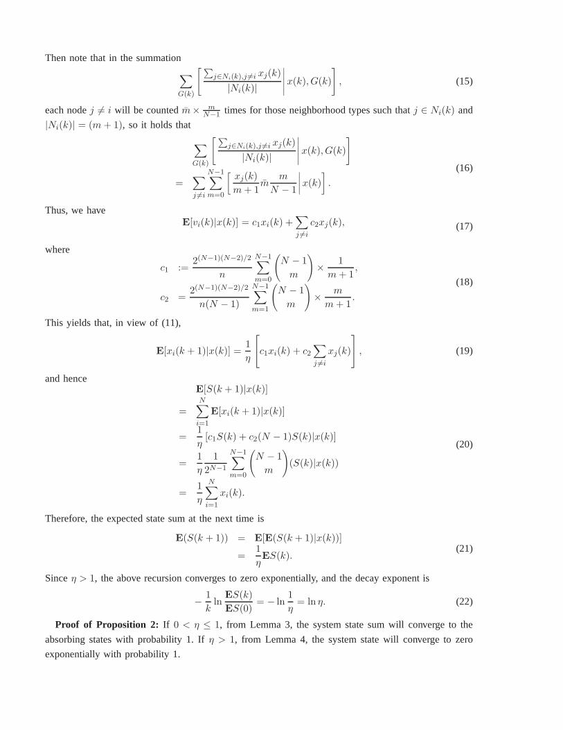
Proof of Proposition 2: If 0 < η ≤ 1, from Lemma 3, the system state sum will converge to the

absorbing states with probability 1. Ifη > 1, from Lemma 4, the system state will converge to zero

exponentially with probability 1.

IV. N UMERICAL RESULTS

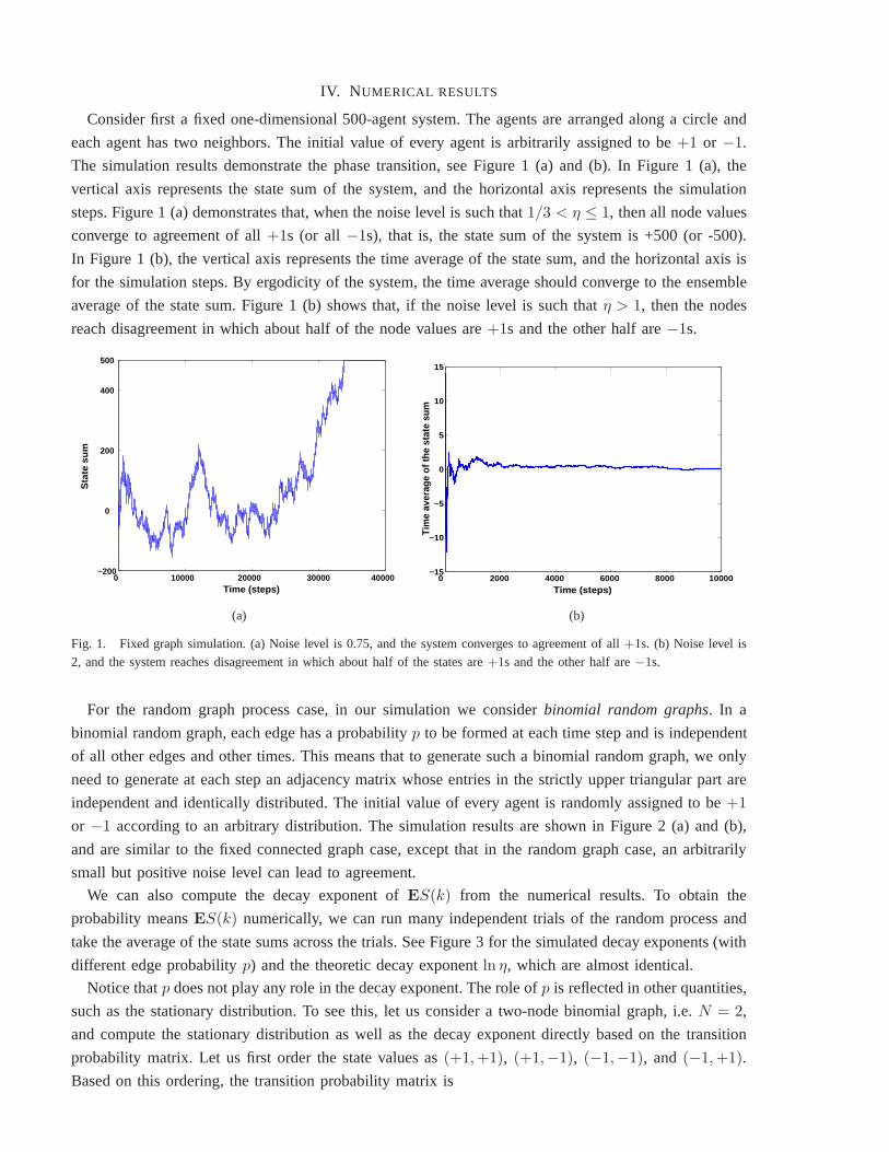
Consider first a fixed one-dimensional 500-agent system. Theagents are arranged along a circle and

each agent has two neighbors. The initial value of every agent is arbitrarily assigned to be+1 or −1.

The simulation results demonstrate the phase transition, see Figure 1 (a) and (b). In Figure 1 (a), the

vertical axis represents the state sum of the system, and thehorizontal axis represents the simulation

steps. Figure 1 (a) demonstrates that, when the noise level is such that1/3 < η ≤ 1, then all node values

converge to agreement of all+1s (or all −1s), that is, the state sum of the system is +500 (or -500).

In Figure 1 (b), the vertical axis represents the time average of the state sum, and the horizontal axis is

for the simulation steps. By ergodicity of the system, the time average should converge to the ensemble

average of the state sum. Figure 1 (b) shows that, if the noiselevel is such thatη > 1, then the nodes

reach disagreement in which about half of the node values are+1s and the other half are−1s.

0 10000 20000 30000 40000 −200

0

200

400

500

Time (steps)

Sta

te s

um

(a)

0 2000 4000 6000 8000 10000−15

−10

−5

0

5

10

15

Tim

e av

erag

e of

the

stat

e su

m

Time (steps)

(b)

Fig. 1. Fixed graph simulation. (a) Noise level is 0.75, and the system converges to agreement of all+1s. (b) Noise level is

2, and the system reaches disagreement in which about half ofthe states are+1s and the other half are−1s.

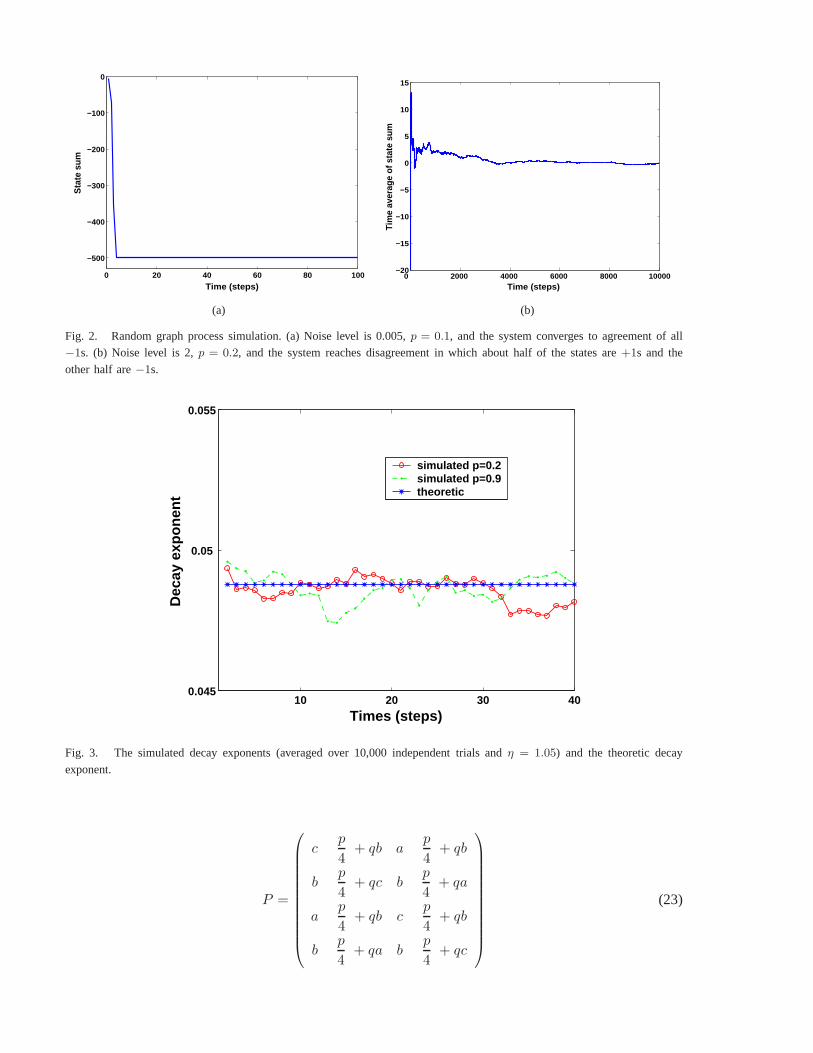
For the random graph process case, in our simulation we consider binomial random graphs. In a

binomial random graph, each edge has a probabilityp to be formed at each time step and is independent

of all other edges and other times. This means that to generate such a binomial random graph, we only

need to generate at each step an adjacency matrix whose entries in the strictly upper triangular part are

independent and identically distributed. The initial value of every agent is randomly assigned to be+1

or −1 according to an arbitrary distribution. The simulation results are shown in Figure 2 (a) and (b),

and are similar to the fixed connected graph case, except thatin the random graph case, an arbitrarily

small but positive noise level can lead to agreement.

We can also compute the decay exponent ofES(k) from the numerical results. To obtain the

probability meansES(k) numerically, we can run many independent trials of the random process and

take the average of the state sums across the trials. See Figure 3 for the simulated decay exponents (with

different edge probabilityp) and the theoretic decay exponentln η, which are almost identical.

Notice thatp does not play any role in the decay exponent. The role ofp is reflected in other quantities,

such as the stationary distribution. To see this, let us consider a two-node binomial graph, i.e.N = 2,

and compute the stationary distribution as well as the decayexponent directly based on the transition

probability matrix. Let us first order the state values as(+1,+1), (+1,−1), (−1,−1), and (−1,+1).

Based on this ordering, the transition probability matrix is

0 20 40 60 80 100

−500

−400

−300

−200

−100

0S

tate

sum

Time (steps)

(a)

0 2000 4000 6000 8000 10000−20

−15

−10

−5

0

5

10

15

Tim

e av

erag

e of

sta

te s

um

Time (steps)

(b)

Fig. 2. Random graph process simulation. (a) Noise level is 0.005, p = 0.1, and the system converges to agreement of all−1s. (b) Noise level is 2,p = 0.2, and the system reaches disagreement in which about half of the states are+1s and the

other half are−1s.

10 20 30 400.045

0.05

0.055

Times (steps)

Dec

ay e

xpon

ent

simulated p=0.2simulated p=0.9theoretic

Fig. 3. The simulated decay exponents (averaged over 10,000independent trials andη = 1.05) and the theoretic decay

exponent.

P =

cp

4+ qb a

p

4+ qb

bp

4+ qc b

p

4+ qa

ap

4+ qb c

p

4+ qb

bp

4+ qa b

p

4+ qc

(23)

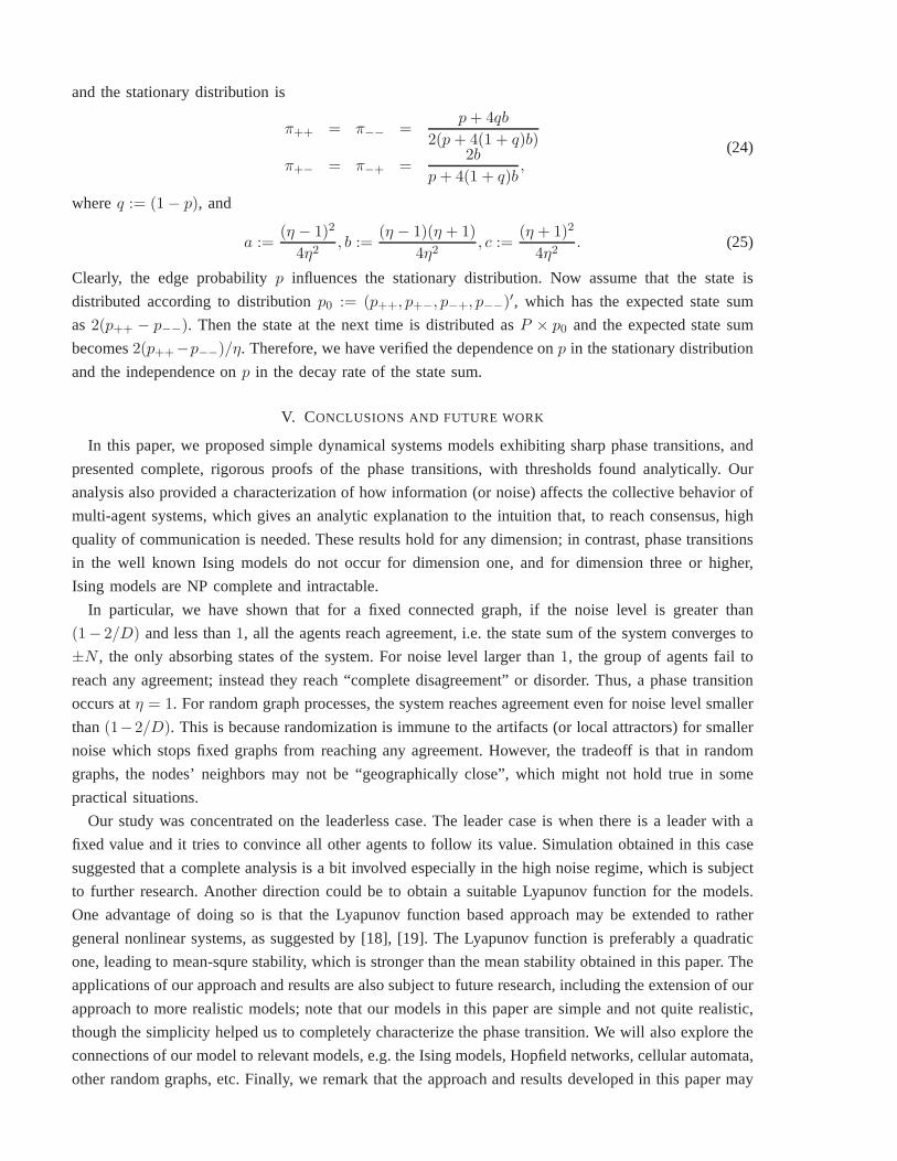
and the stationary distribution is

π++ = π−− =p + 4qb

2(p + 4(1 + q)b)

π+− = π−+ =2b

p + 4(1 + q)b,

(24)

whereq := (1 − p), and

a :=(η − 1)2

4η2, b :=

(η − 1)(η + 1)

4η2, c :=

(η + 1)2

4η2. (25)

Clearly, the edge probabilityp influences the stationary distribution. Now assume that thestate is

distributed according to distributionp0 := (p++, p+−, p−+, p−−)′, which has the expected state sum

as2(p++ − p−−). Then the state at the next time is distributed asP × p0 and the expected state sum

becomes2(p++−p−−)/η. Therefore, we have verified the dependence onp in the stationary distribution

and the independence onp in the decay rate of the state sum.

V. CONCLUSIONS AND FUTURE WORK

In this paper, we proposed simple dynamical systems models exhibiting sharp phase transitions, and

presented complete, rigorous proofs of the phase transitions, with thresholds found analytically. Our

analysis also provided a characterization of how information (or noise) affects the collective behavior of

multi-agent systems, which gives an analytic explanation to the intuition that, to reach consensus, high

quality of communication is needed. These results hold for any dimension; in contrast, phase transitions

in the well known Ising models do not occur for dimension one,and for dimension three or higher,

Ising models are NP complete and intractable.

In particular, we have shown that for a fixed connected graph,if the noise level is greater than

(1− 2/D) and less than1, all the agents reach agreement, i.e. the state sum of the system converges to

±N , the only absorbing states of the system. For noise level larger than1, the group of agents fail to

reach any agreement; instead they reach “complete disagreement” or disorder. Thus, a phase transition

occurs atη = 1. For random graph processes, the system reaches agreement even for noise level smaller

than(1−2/D). This is because randomization is immune to the artifacts (or local attractors) for smaller

noise which stops fixed graphs from reaching any agreement. However, the tradeoff is that in random

graphs, the nodes’ neighbors may not be “geographically close”, which might not hold true in some

practical situations.

Our study was concentrated on the leaderless case. The leader case is when there is a leader with a

fixed value and it tries to convince all other agents to followits value. Simulation obtained in this case

suggested that a complete analysis is a bit involved especially in the high noise regime, which is subject

to further research. Another direction could be to obtain a suitable Lyapunov function for the models.

One advantage of doing so is that the Lyapunov function basedapproach may be extended to rather

general nonlinear systems, as suggested by [18], [19]. The Lyapunov function is preferably a quadratic

one, leading to mean-squre stability, which is stronger than the mean stability obtained in this paper. The

applications of our approach and results are also subject tofuture research, including the extension of our

approach to more realistic models; note that our models in this paper are simple and not quite realistic,

though the simplicity helped us to completely characterizethe phase transition. We will also explore the

connections of our model to relevant models, e.g. the Ising models, Hopfield networks, cellular automata,

other random graphs, etc. Finally, we remark that the approach and results developed in this paper may

be found useful to study more general dynamical systems under communication constraints, such as

cooperation with limited communication, complex systems in the presence of noise, etc. The study of

such problems would help establish insights on how information (or limited information) interacts with

system dynamics to generate various types of interesting system behavior.

APPENDIX

We prove thatπ(x) = π(−x) for any x in four steps.

Step 1: Establish a one-to-one mapping between the2J possible values (see (6)) that the state of

the system can take and integers±1,±2, · · · ,±J , such that if statex is mapped to+j, then state−x

is mapped to−j. Now aggregate the states as follows. Letj := (j,−j) for any j = 1, · · · , J . Then

we induce from the Markov processx(k)∞k=0 another Markov processx(k)∞k=0, where the latter

is defined on the induced state space consisting of alljs. Note that it is straightforward to verify that

xk∞k=0 forms a Markov process on the induced state space, and this Markov process is ergodic.

Step 2: Denote the transition probability matrix for process x(k)∞k=0 as p, and the corresponding

stationary distribution vector asπ := (π(1), π(2), ..., π(J))′. Then it holds thatπ = pπ. By ergodicity,

π is non-zero and unique (i.e., the matrix(I − p) must be rank deficient).

Step 3: For the Markov processx(k)∞k=0, denote the stationary distribution vector asπ := (π′1, π

′2)

′,

whereπ1 = (π(+1), π(+2), ..., π(+J))′ andπ2 = (π(−1), π(−2), ..., π(−J))′ . It can be verified that, by

the symmetry that the state transitioni → j has the same probability as the state transition(−i) → (−j),

the transition probability matrix has the following particular form:

p :=

(

A B

B A

)

. (26)

Step 4: By ergodicity ofx(k)∞k=0, it holds that

π = pπ (27)

or equivalently,π1 = Aπ1 + Bπ2

π2 = Bπ1 + Aπ2.(28)

However, it can be easily seen thatp = A + B. Notice that

π1 = π2 = π (29)

solves (28), i.e.,π0 := (π′, π′)′ solves (27) and is non-zero. By ergodicity, the non-zero solution is

unique, and henceπ0 must be the solution to (27), which follows thatπ(j) = π(−j) for any j or

π(x) = π(−x) for any x.

REFERENCES

[1] B. Cipra. An introduction to the Ising model.American Mathematical Monthly, 94:937–959, 1987.

[2] P. Erdos and A. Renyi. On the evolution of random graphs. Publ. Math. Inst. Hungar. Acad. Sci., 5:17–61, 1960.

[3] C. G. Langton. Computation at the edge of chaos: Phase transitions and emergent computation.Physica D, 42:12–37,1990.

[4] R. Olfati-Saber. Ultrafast consensus in small-world networks. Proc. of American Control Conference, pages 2371–2378,June 2005.

[5] S. Janson, T. Luczak, and A. Rucinski.Random Graphs. Wiley, New York, 2000.

[6] T. Vicsek, A. Czirok, E. Ben Jacob, I. Cohen, and O. Schochet. Novel type of phase transitions in a system of self-driven

particles.Physical Review Letters, 75:1226-1229, 1995.[7] A. Czirok, A. L. Barabasi, and T. Vicsek. Collective motion of self-propelled particles: Kinetic phase transitionin one

dimension.Physical Review Letters, 82:209-212, 1999.[8] F. Schweitzer, L. Behera, and H. Muhlenbein. Frequency dependent invasion in a spatial environment.Physical Review

E, accepted, 2005.

[9] A. Mogilner and L. Edelstein-Keshet. Spatio-angular order in populations of self-aligning objects: formation of orientedpatches.Physica D, 89:346–367, 1996.

[10] H. Levine, W. J. Rappel, and I. Cohen. Self-organization in systems of self-propelled particles.Physical Review E, 63,2001.

[11] R. Olfati-Saber. Flocking for multi-agent dynamic system: Algorithm and theory. IEEE Trans. on Automat. Contr.,

51(3):401–420, March 2006.[12] R. Olfati-Saber and R. M. Murray. Consensus Protocols for Networks of Dynamic Agents.Proc. of American Control

Conference, pages 951–956, June 2003.[13] R. Olfati-Saber and R. M. Murray. Consensus Problems inNetworks of Agents with Switching Topology and Time-Delays.

IEEE Trans. Automat. Contr., 49(9):1520–1533, Sept. 2004.

[14] Y. Hatano, A. K. Das, and M. Mesbahi. Agreement in presence of noise: Pseudogradients on random geometric networks.Proceedings of the 44th IEE Conference on Decision and Control, pages 6382–6387, Dec. 2005.

[15] D. Watts and S. H. Strogatz. Collective dynamics of ‘small-world’ networks. Nature, 393:325–328, 1998.[16] Y. Hatano and M. Mesbahi. Agreement over random networks. IEEE Trans. Automat. Contr., 50(11):1867–1872, Nov.

2005.

[17] A. Jadbabaie, J. Lin, and A. S. Morse. Coordination of groups of mobile autonomous agents using nearest neighbor rules.IEEE Trans. Automat. Contr., 48(6):988–1001, 2003.

[18] A. Megretski. Personal communication, 2002.

[19] L. Moreau. Stability of multiagent systems with time-dependent communication links.IEEE Trans. on Automat. Contr.,50(2):169–182, Feb. 2005.

[20] H. G. Tanner, A. Jadbabaie, and G. J. Pappas. Stable flocking of mobile agents, part I: fixed topology.Proc. of 42nd

IEEE Conference on Decision and Control, pages 2010–2015, Dec. 2003.

[21] H. G. Tanner, A. Jadbabaie, and G. J. Pappas. Stable flocking of mobile agents, part II: dynamical topology.Proc. of

42nd IEEE Conference on Decision and Control, pages 2016–2021, Dec. 2003.[22] B. Cipra. Mathematics: Statistical physicists phase out a dream.Science, 288(5471):1561 – 1562, 2000.

[23] D. R. Wolf. Information and Correlation in Statistical Mechanical Systems. PhD thesis, University of Texas, Austin,Austin, Texas, 1996.

[24] S. K. Mitter. Control with limited information.IEEE Information Theory Society Newsletter, 50:1–23, Dec. 2000.

[25] S. Tatikonda.Control Under Communication Constraints. PhD thesis, MIT, Cambridge, MA, Aug. 2000.[26] A. Sahai.Anytime Information Theory. PhD thesis, MIT, Cambridge, MA, 2001.

[27] N. Elia. When Bode meets Shannon: Control-oriented feedback communication schemes.IEEE Trans. Automat. Contr.,49(9):1477–1488, Sept. 2004.

[28] J. A. Fax and R. M. Murray. Information flow and cooperative control of vehicle formations.IEEE Trans. Automat.

Contr., 49(9):1465 – 1476, Sept. 2004.[29] J. Liu. Fundamental Limits in Gaussian Channels with Feedback: Confluence of Communication, Estimation, and Control.

PhD thesis, Iowa State University, Ames, IA, Apr. 2006.[30] S. K. Mitter and N. Newton. Information and entropy flow in the Kalman-Bucy filter.J. of Stat. Phys., 118:145–176,

Jan. 2005.

[31] D. Julian. Erasure networks.Proc. IEEE International Symposium on Information Theory, page 757, July 2002.