phase field theory modeling of methane fluxes from exposed natural gas hydrate reservoirs
TRANSCRIPT

Phase field theory modeling of methane fluxes from exposed natural gas hydratereservoirsPilvi-Helinä Kivelä, Khuram Baig, Muhammad Qasim, and Bjo/rn Kvamme
Citation: AIP Conference Proceedings 1504, 351 (2012); doi: 10.1063/1.4771728 View online: http://dx.doi.org/10.1063/1.4771728 View Table of Contents: http://scitation.aip.org/content/aip/proceeding/aipcp/1504?ver=pdfcov Published by the AIP Publishing Articles you may be interested in Seismic investigation of natural methane hydrate deposits J. Acoust. Soc. Am. 122, 2982 (2007); 10.1121/1.2942633 A potential model for methane in water describing correctly the solubility of the gas and the properties of themethane hydrate J. Chem. Phys. 125, 074510 (2006); 10.1063/1.2335450 Phase transformation of methane hydrate under high pressure J. Chem. Phys. 122, 024714 (2005); 10.1063/1.1830411 Theory of phase transitions in solid methanes. IX. The infrared absorption of methane in rare gas matrices J. Chem. Phys. 58, 1001 (1973); 10.1063/1.1679282 Hydration of Negative Ions in the Gas Phase J. Chem. Phys. 49, 817 (1968); 10.1063/1.1670145
This article is copyrighted as indicated in the article. Reuse of AIP content is subject to the terms at: http://scitation.aip.org/termsconditions. Downloaded to IP:
129.177.37.86 On: Fri, 26 Sep 2014 06:58:22

Phase Field Theory Modeling of Methane Fluxes from Exposed Natural Gas Hydrate Reservoirs
Pilvi-Helinä Kivelä, Khuram Baig, Muhammad Qasim and Bjørn Kvamme1
University of Bergen, Department of Physics and Technology, Allégaten 55, N-5007 Bergen, Norway
Abstract. Fluxes of methane from offshore natural gas hydrate into the oceans vary in intensity from massive bubble columns of natural gas all the way down to fluxes which are not visible within human eye resolution. The driving force for these fluxes is that methane hydrate is not stable towards nether minerals nor towards under saturated water. As such fluxes of methane from deep below hydrates zones may diffuse through fluid channels separating the hydrates from minerals surfaces and reach the seafloor. Additional hydrate fluxes from hydrates dissociating towards under saturated water will have different characteristics depending on the level of dynamics in the actual reservoirs. If the kinetic rate of hydrate dissociation is smaller than the mass transport rate of distributing released gas into the surrounding water through diffusion then hydrodynamics of bubble formation is not an issue and Phase Field Theory (PFT) simulations without hydrodynamics is expected to be adequate [1, 2]. In this work we present simulated results corresponding to thermodynamic conditions from a hydrate field offshore Norway and discuss these results with in situ observations. Observed fluxes are lower than what can be expected from hydrate dissociating and molecularly diffusing into the surrounding water. The PFT model was modified to account for the hydrodynamics. The modified model gave higher fluxes, but still lower than the observed in situ fluxes.
Keywords: Phase Field Theory; Methane Fluxes, Hydrate PACS: 30
INTRODUCTION
Gas hydrates, also called clathrates, are crystalline solids which look like ice, and which occur when water molecules form a cage-like structure around a non-polar or slightly polar molecule (eg. CO2, H2S). These enclathrated molecules are called guest molecules and obviously have to fit into the cavities in terms of volume. In the oil and gas industry the most common guest molecules are methane, ethane, propane, butane, carbon dioxide and hydrogen-sulfide. This work will focus only on methane as guest molecule. The methane guest molecules in gas hydrates are mainly microbially generated; however, thermogenic methane is observed in gas hydrate of the Gulf of Mexico, the Caspian Sea, and a few other places where there are known petroleum systems [3]. The most remarkable property of methane hydrates are that it compresses the guest molecule into a very dense and compact arrangement, such as 1m3 of solid methane hydrate with 100 percent void occupancy by methane will release roughly 164 m3 of methane [4] at standard conditions of temperature and pressure.
Natural gas hydrates are widely distributed in sediments along continental margins, and harbor enormous amounts of energy. Massive hydrates that outcrop the sea floor have been reported in the Gulf of Mexico [5]. Hydrate accumulations have also been found in the upper sediment layers of Hydrate ridge, off the coast of Oregon and a fishing trawler off Vancouver Island recently recovered a bulk of hydrate of approximately 1000kg [6]. Håkon Mosby Mud Volcano of Bear Island in the Barents Sea with hydrates are openly exposed at the sea bottom [7]. These are only few examples of the worldwide evidences of unstable hydrate occurrences that leaks methane to the oceans and eventually may be a source of methane increase in the atmosphere.
The primary focus in this work is on the dissociation of methane hydrates due to thermodynamic instabilities. Hydrates in reservoirs are subject to potential contact with minerals, aqueous solution and gas, depending on the state of the system and the fluid fluxes through the hydrate section. From a thermodynamic point of view the first question that arises is whether the system can reach equilibrium or not according to Gibbs phase rule (see Gibbs phase rule [8, 9]). Equilibrium requires the equality of temperature, pressure, and chemical potential in all phases. In the case of dissociation, gas hydrate generally becomes unstable by changing the P/T conditions in a way that the
International Conference of Computational Methods in Sciences and Engineering 2009AIP Conf. Proc. 1504, 351-363 (2012); doi: 10.1063/1.4771728
© 2012 American Institute of Physics 978-0-7354-1122-7/$30.00
351 This article is copyrighted as indicated in the article. Reuse of AIP content is subject to the terms at: http://scitation.aip.org/termsconditions. Downloaded to IP:
129.177.37.86 On: Fri, 26 Sep 2014 06:58:22
hydrate phase is not stable anymore, i.e., that the chemical potential of the gas component is lower in the free gas phase than in the hydrate phase [6] and/or water is more stable as a liquid or ice phase. In a reservoir the local temperature is given by the geothermal gradient and the pressure is given by the static column above. Equilibrium in this system can only be achieved if the number of degrees of freedom is 2 (Gibbs phase rule). This implies that a hydrate surrounded by mineral (and corresponding adsorbed phase on the surface), aqueous phase and only methane will be over determined and cannot reach a unique equilibrium situation. These systems will progress dynamically towards local and global minimum free energy at all times.
Leakage of methane from reservoirs that are exposed towards the ocean floor will have an impact on the local ecological environments. Biological organisms will consume some of the released methane. Other portions of the methane will react with sulphur and other inorganic compounds. Released carbon dioxide from the biologically catalyzed sulphur reactions will to a large degree dissolve in the aqueous phase and may result in precipitation of solid carbonates. Some portion of the released methane will also be distributed in the ocean as methane and might end up in the atmosphere. Sassen et al.,(1997) [10] have analyzed such hydrates reservoir from outside the Gulf of Mexico, where released gas from exposed hydrate reservoirs form free gas bubbles. The kinetic rates of dissociation of hydrate exposed to seawater are essential in the understanding of the carbon balance related to released methane and subsequent amounts of released methane that reaches the atmosphere. Methane is in comparison 24 times greater in the creation of the green house effect than carbon dioxide [11].
The greenhouse gases like methane and chlorofluorocarbons have been the main cause of rapid global warming, which has been discussed in several publications during the past [12-17]. Therefore, an important global challenge is to be able to make reasonable predictions of the dissociation fluxes of exposed hydrate reservoirs, and the associated methane that escapes to the atmosphere after biological consumption and conversion through inorganic and organic reactions.
PHASE FIELD THEORY
Phase field model follows the formulation of Wheeler et al. [18], which historically has been mostly applied to descriptions of the isothermal phase transition between ideal binary-alloy liquid and solid phases. In this work the model is applied to essentially only two phases in the sense that the fluid thermodynamics is treated appropriately in the absence of hydrodynamics. Due to the absence of hydrodynamics there is no need to distinguish between gas phase and liquid phase other than making sure that the transport properties are handled appropriately. The diffusivity of water is lower than gas diffusivity so provided that the gas density is high enough to provide access to guest molecules the water movement and reorganization is expected to be the kinetic rate limiting within the implicit mass transport contributions. The phase field is an order parameter describing the phase of the system as a function of spatial and time coordinates. The field is allowed to vary continuously on the range from solid to liquid.
An isothermal solution of two different components A and B were considered which may exist in two different phases, solid and liquid, contained in a fixed region . For the hydrate system the component A is water and component B is methane molecule. The solid state is represented by the hydrate and an aqueous solution is the liquid phase. The solidi cation of hydrate is described in terms of the scalar phase field and the local solute concentration of component B denoted by . The field is a structural order parameter assuming the values
in the solid and in the liquid [19]. Intermediate values correspond to the interface between the two phases. The starting point of the model is a free energy functional,
, (1)
which is an integration over the system volume of the free energy density and a gradient term correction to ensure a higher free energy at the interface between phases. The free energy density is given by
. (2)
The phase field switches on and off the solid and liquid contributions and through the function
and note that and . This function was derived from density functional theory studies of binary alloys and has been adopted also for our system of hydrate phase transitions. The binary alloys are normally treated as ideal solutions. The thermodynamics for the hydrate system is treated more rigorously
352 This article is copyrighted as indicated in the article. Reuse of AIP content is subject to the terms at: http://scitation.aip.org/termsconditions. Downloaded to IP:
129.177.37.86 On: Fri, 26 Sep 2014 06:58:22

and the free energy densities are presented in thermodynamics section. The function ensures a double well form of the with a free energy scale , with . In the phase field model the concentration of component B in mole fraction is represented by . That is , the fraction of component B to the total. With the assumption that the molar volume is constant, the mole fraction concentration and the volume concentration are related by , where is the average molar volume [19]. Without hydrodynamics the impact of density difference is not accounted for and molar density is approximated constant. And as such the mole fractions of a certain element in the grid will be equal to the volume fractions. In order to derive a kinetic model it is assume that the system evolves in time so that its total free energy decreases monotonically. Given that the phase field is not a conserved quantity, the simplest form for the evolution that ensures a minimization of the free energy is
, (3)
, (4)
where and are the mobilities associated with coarse-grained equation of motion, which in turn are related
to their microscopic counter parts. To reproduce bulk fluid diffusion , where is the diffusion coefficient with m2/s the diffusion coefficient in the liquid [6] and m2/s for the solid [20].
Hydrate Thermodynamics
The thermodynamics of the hydrate is based on the model by Kvamme et al. [21] and van der Waals and Platteeuw [22]. The expression for chemical potential of water in hydrate is
. (5)
The expression for the chemical potential for water in hydrate with one type of guest molecule is
, (6)
Here is the chemical potential for water in an empty hydrate structure. The sum is over small and large
cavities, where is the number of type cavities per water molecule. is the filling fraction of cavity given as , where is the molar fraction with respect to cavity . The chemical potential for the guest molecule is
, (7)
where is the free energy of inclusion of guest molecule in cavity . Assuming that the chemical potential
in the different cavity types are equal, an expression for the ratio between the filling fractions was obtained. Requiring that the specific mole fractions add up to the total mole fraction and solving a second order equation, an expression for the chemical potentials as a function of the total mole fraction was obtained.
Fluid Thermodynamics
The chemical potential of methane has the general form in the aqueous phase derived from excess thermodynamics
353 This article is copyrighted as indicated in the article. Reuse of AIP content is subject to the terms at: http://scitation.aip.org/termsconditions. Downloaded to IP:
129.177.37.86 On: Fri, 26 Sep 2014 06:58:22
is th
componentinfinitely sequilibriumlow, using value for zexperiment
Where
Duhem equ
Where
hydrate form
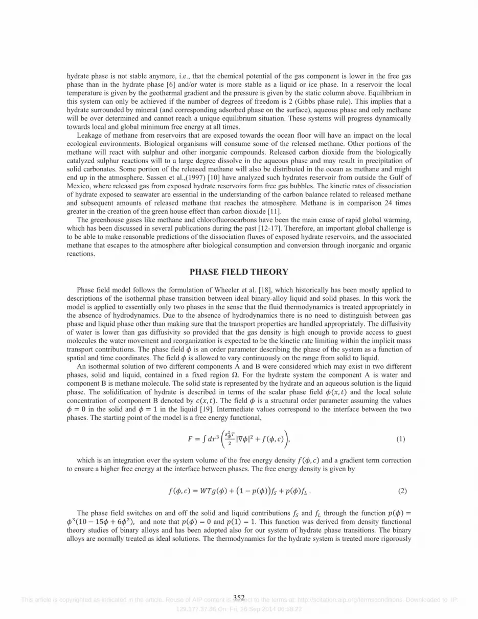
The phathe hydrategeometry sliquid wateEach grid imethod wh
Figure 1. Simgrid points a
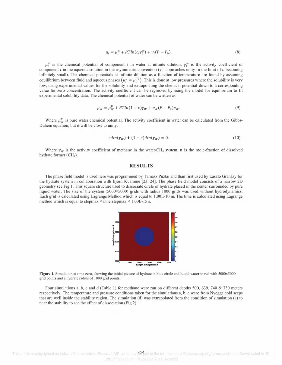
Four sim
respectivelythat are wenear the sta
he chemical t in the aquemall). The ch
m between fluiexperimental
zero concentratal solubility d
is pure wuation, but it w
is the actmer (CH4).
ase field modee system in coee Fig.1. This
er. The size os calculated u
hich is equal to
mulation at timand a hydrate ra
mulations a, by. The temper
ell inside the sability to see th
potential of eous solution ihemical potenid and aqueouvalues for th
ation. The acdata. The chem
ater chemicalwill be close to
tivity coefficie
el is used hereollaboration ws square structof the system using Lagrango stepmax × in
me zero, showingadius of 1000 gr
b, c and d (Tarature and prestability regionhe effect of di
component in the asymmentials at infinius phases he solubility antivity coeffici
mical potential
potential. Tho unity.
ent of methan
e was programwith Bjørn Kvture used to di(5000×5000) e Method whinnerstepmax ×
g the initial picrid points.
able 1) for messure condition. The simulaissociation (Fi
in water at metric conventi
ite dilution as. This
and extrapolatiient can be re
al of water can
he activity coe
ne in the wat
RESULTS
mmed by Tamvamme [23, 2issociate circlgrids with ra
ich is equal to× 1.00E-15 s.
cture of hydrate
ethane were rons taken for tation (d) was ig.2).
.
infinite dilution ( appros a function ois done at lowing the chemiegressed by u
n be written as
efficient in wa
.
er/CH4 system
S
masz Puztai and24]. The phasee of hydrate padius 1000 gro 1.00E-10 m.
in blue circle a
un on differenthe simulationextrapolated f
tion, is thaches unity in
of temperaturew pressures whical potential using the mod:
.
ater can be ca
m. is the m
d than first use field model placed in the crids was used
The time is c
and liquid water
nt depths 500ns a, b, c werefrom the cond
he activity con the limit of e are found b
where the solubdown to a codel for equilib
alculated from
mole-fraction o
sed by László consists of a
center surround without hydrcalculated usin
r in red with 50
0, 639, 740 &e from Nyeggdition of simu
(8)
oefficient of becoming
by assuming bility is very orresponding brium to fit
(9)
m the Gibbs-
(10)
of dissolved
Gránásy for a narrow 2D nded by pure rodynamics. ng Lagrange
000x5000
730 meters a cold seeps
ulation (a) to
354 This article is copyrighted as indicated in the article. Reuse of AIP content is subject to the terms at: http://scitation.aip.org/termsconditions. Downloaded to IP:
129.177.37.86 On: Fri, 26 Sep 2014 06:58:22
The temHaflidason of the Storsouth and th
Table 1. Sim
Simulations N
Temperature
Pressure (bar
All the simratio betweas 1 : 2.5. Table 2. The
Grid points fo
Corresponding
No. of time st
Total time in s
Mole fraction
Mole fraction
The CH
Figure
mperature and[25] at Nyegg
regga Slide, ohe Vøring Ba
mulation conditiName
e (K)
r)
mulations wereeen solid and l
e properties useor all four simul
g area in m2
eps
seconds
of CH4 in hydr
of water in liqu
H4 concentratio
e 2. Extrapolatio
d pressure coga cold seeps n the border sin to the nort
ions. a
273.25
50
e run to 16.13liquid was adj
ed to setup the slations
rate
uid phase
on initially wa
on of temperatu
onditions for located on thbetween two th [26].
B
273.2
63.9
3E+06 total tijusted as to ac
simulations.
as adjusted to
ure 273.25 K an
simulation bhe edge of the
large oil/gas
21
0
ime steps thischieve the stab
0.14 in the hy
nd pressure 50 b
b and c is thNorwegian cprone sedime
c
273.17
740
s corresponds bility. In this
ydrate (Table 2
bar to near the s
he same as continental sloentary basins—
d
281.53
72.56
to the time ocase the solid
50
2.
16
16
0.
1.
2).
stability.
considered byope and the no— the Møre B
of 16.13ns (Tad to liquid rati
000×5000
.50E-13
6.384E+06
6.384E-09
.14
.0
y Chen and orthern flank Basin to the
able 2). The io was taken
355 This article is copyrighted as indicated in the article. Reuse of AIP content is subject to the terms at: http://scitation.aip.org/termsconditions. Downloaded to IP:
129.177.37.86 On: Fri, 26 Sep 2014 06:58:22
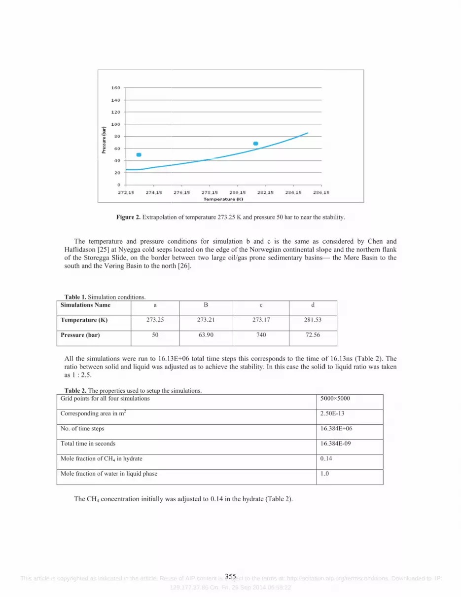
Concentration profiles
The concentrations have been calculated inside and outside the hydrate at different time intervals for all the simulations shown in Fig.3 & Fig.4.
Figure 3. Methane concentration inside the hydrate at different points. A, B, C, D & E are points which 10.0E-9Å, 30.0Å, 60. 0Å, 80.0Å & 1000.0Å away from the original interface respectively. Where a, b, c & d are depths 500, 639, 740 & 730 meters respectively.
Initially (t=0) Fig.3 & Fig.4, the mole fraction equals the initial values which show that CH4 has not yet diffused. To get the clear vision of diffusion inside the hydrate, the concentrations have been taken on five points A, B, C, D & E corresponding to values 10Å, 30Å, 60Å, 80Å and 1000Å respectively, showing distance from the original interface. If the concentration of methane drops below the hydrate stability limit for the given temperature and pressure, a chemical potential driving force towards dissociation will arise as shown in Fig.3 lines A, B, C and D. The sudden drop in concentrations in all four cases is due the hydrate completely dissociated. The maximum mole fraction decreased from 0.14 to 0.004469, 0.004565, 0.004814 and 0.003219 in all four cases respectively, this difference in fractions due to the effect of concentration gradient as moving away from the original interface.
0 0.5 1 1.5
x 10-8
0
0.05
0.1
0.15simulation a
ABCDE
0 0.5 1 1.5
x 10-8
0
0.05
0.1
0.15simulation b
0 0.5 1 1.5
x 10-8
0
0.05
0.1
simulation c
Con
cent
ratio
n(M
ole
Frac
tion)
Time (Sec)
0 0.5 1 1.5
x 10-8
0
0.05
0.1
simulation d
356 This article is copyrighted as indicated in the article. Reuse of AIP content is subject to the terms at: http://scitation.aip.org/termsconditions. Downloaded to IP:
129.177.37.86 On: Fri, 26 Sep 2014 06:58:22
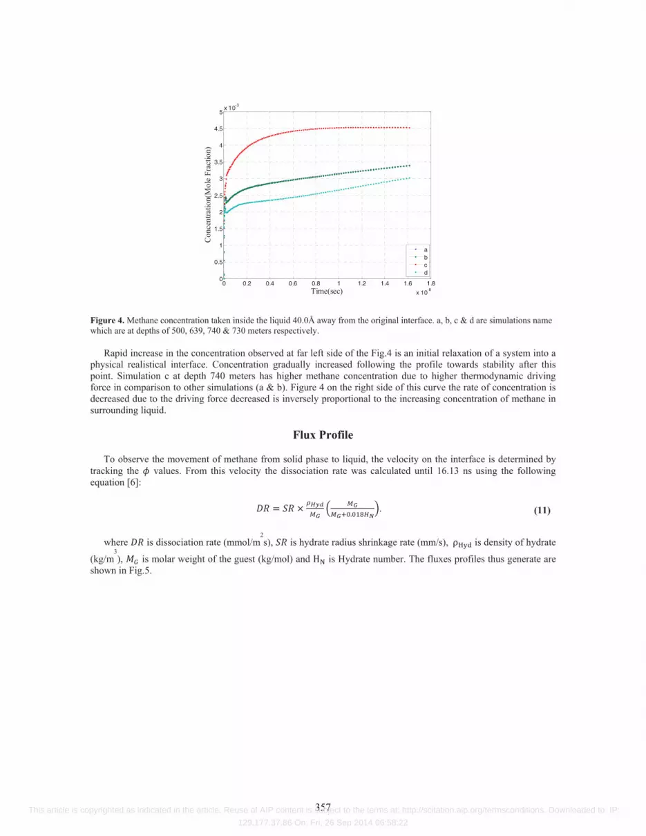
Figure 4. Methane concentration taken inside the liquid 40.0Å away from the original interface. a, b, c & d are simulations name which are at depths of 500, 639, 740 & 730 meters respectively.
Rapid increase in the concentration observed at far left side of the Fig.4 is an initial relaxation of a system into a
physical realistical interface. Concentration gradually increased following the profile towards stability after this point. Simulation c at depth 740 meters has higher methane concentration due to higher thermodynamic driving force in comparison to other simulations (a & b). Figure 4 on the right side of this curve the rate of concentration is decreased due to the driving force decreased is inversely proportional to the increasing concentration of methane in surrounding liquid.
Flux Profile
To observe the movement of methane from solid phase to liquid, the velocity on the interface is determined by tracking the values. From this velocity the dissociation rate was calculated until 16.13 ns using the following equation [6]:
. (11) where is dissociation rate (mmol/m
2s), is hydrate radius shrinkage rate (mm/s), is density of hydrate
(kg/m3), is molar weight of the guest (kg/mol) and is Hydrate number. The fluxes profiles thus generate are
shown in Fig.5.
0 0.2 0.4 0.6 0.8 1 1.2 1.4 1.6 1.8
x 10-8
0
0.5
1
1.5
2
2.5
3
3.5
4
4.5
5x 10
-3
Time(sec)
Conc
entra
tion(
Mol
e Fr
actio
n)
abcd
357 This article is copyrighted as indicated in the article. Reuse of AIP content is subject to the terms at: http://scitation.aip.org/termsconditions. Downloaded to IP:
129.177.37.86 On: Fri, 26 Sep 2014 06:58:22
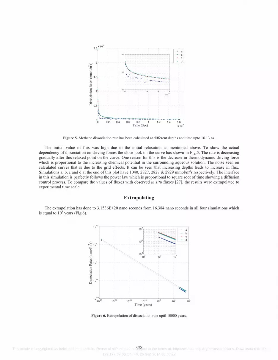
Figure 5. Methane dissociation rate has been calculated at different depths and time upto 16.13 ns.
The initial value of flux was high due to the initial relaxation as mentioned above. To show the actual dependency of dissociation on driving forces the close look on the curve has shown in Fig.5. The rate is decreasing gradually after this relaxed point on the curve. One reason for this is the decrease in thermodynamic driving force which is proportional to the increasing chemical potential in the surrounding aqueous solution. The noise seen on calculated curves that is due to the grid effects. It can be seen that increasing depths leads to increase in flux. Simulations a, b, c and d at the end of this plot have 1040, 2827, 2827 & 2929 mmol/m2s respectively. The interface in this simulation is perfectly follows the power law which is proportional to square root of time showing a diffusion control process. To compare the values of fluxes with observed in situ fluxes [27], the results were extrapolated to experimental time scale.
Extrapolating
The extrapolation has done to 3.1536E+20 nano seconds from 16.384 nano seconds in all four simulations which is equal to 104 years (Fig.6).
Figure 6. Extrapolation of dissociation rate uptil 10000 years.
0 0.2 0.4 0.6 0.8 1 1.2 1.4 1.6
x 10-8
0
0.5
1
1.5
2
2.5x 10
5
Time (Sec)
Dis
soci
atio
n Ra
tes (
mm
ol/m
2 s)
abcd
0 2 4 6 8
x 10-9
103
104
105
10-25
10-20
10-15
10-10
10-5
100
105
10-10
10-5
100
105
1010
Time (years)
Dis
soci
atio
n Ra
tes
(mm
ol/m
2 s)
abcd
102
103
104
10-9
10-8
10-7
358 This article is copyrighted as indicated in the article. Reuse of AIP content is subject to the terms at: http://scitation.aip.org/termsconditions. Downloaded to IP:
129.177.37.86 On: Fri, 26 Sep 2014 06:58:22

Due to the length of the time scale the values were plotted in the figure with 100 years of time intervals. After
10000 years the dissociation rates were 6.539E-09, 1.441E-08, 1.557E-008 & 1.45E-08 mmol/m2s converted to 0.2062, 0.4544, 0.4910 and 0.4573 mmol/m2yr units for simulations a, b, c and d respectively.
Chen and Haflidason [27] have calculated the fluxes in Nyegga region using cores from inside of pockmarks. Sulfate gradients measured in the southeast of Nyegga at depth 639 to 740 meters indicate that methane fluxes are 15 to 49 mmol/m2yr. The simulation b and c runs on the same conditions and shows deviation from the experimental results. From the limited background data on the Nyegga samples and the Nyegga system as such it remains very uncertain at this point what the observed values actually reflect. It could be the lack of pressurized core sampling [28] or might be due to absence of hydrodynamics. Even if hydrodynamics and the corresponding bubble formation were included the reported fluxes seem very high and are likely to be dominated by hydrate forming and dissociating dynamically in addition to allowing free gas to pass and migrate upwards due to large size of channels (20-200 m wide) known as pipes (see the fracture channels on the seismic images in [29]) which is not able to be blocked down to very low permeability. As a further work the hydrodynamics effect is also included in the phase field model.
Phase field model with hydrodynamics
To encounter the effect of fluid flow, density change and gravity, an extended phase field model is formed. This is achieved by coupling the time evolution with the Euler’s Equations. An incompressible and viscous fluid is considered. The mass density is assumed to be dependent on composition and phase. The phase and concentration fields enter the hydrodynamic equations as described by [30-32].
,
. (12)
Here is the mass density, the velocity and is the gravitational acceleration. While
, (13) is the generalization of stress tensor [30-32]. represents non-dissipative part and represents the dissipative
part of the stress tensor. is unit tensor, represents the diadic product and represents the pressure. The hydrodynamic equations couples back into time evolution partial differential equation via the convection
term,
, (14)
. (15)
Physical properties
The free energies were calculated using the same pressure and temperature conditions as considered by the Chen and Haflidason at Nyegga site [27]. As it was observed that the reported fluxes were too high then the calculated fluxes, when the phase field model without hydrodynamics was used. It is believed that by addition of hydrodynamics, the calculated fluxes will be truer in comparison with the previous phase field model, but will still remain lower than the reported fluxes. As observed in situ fluxes are likely to be dominated by channeling of free gas (see the fracture channels on the seismic image in [29]) from below hydrate stability zone rather than hydrate dissociation. This is likely being the one reason for large deviation between model calculations and reported fluxes. Salinity of surrounding water will also increase dissociation rates.
359 This article is copyrighted as indicated in the article. Reuse of AIP content is subject to the terms at: http://scitation.aip.org/termsconditions. Downloaded to IP:
129.177.37.86 On: Fri, 26 Sep 2014 06:58:22

Numerical results
The simulation for phase field model without hydrodynamics is modified for the phase field model with hydrodynamics. The two hydrodynamics equations (12) were added in the code and time evolution were changed accordingly. The model has been implemented on a (1000×1000) grid system to see the dissociation of methane hydrate on a planar surface. A circular hydrate was assumed with radius of 200 Å and center at the (500,500) and with pure water in surrounding of the hydrate. It can be seen that the hydrate to system ratio is the same as was considered for previous simulations. This setup can be seen in Fig.7. Pressure and temperature were assumed to remain constant in the system at 63.9 bar and 273.21 K respectively inside the hydrate stability region. These are the same pressure and temperature conditions considered by Chen and Haflidason [27], which were taken from Nyegga cold seeps and are well inside the stability region. The grid resolution was 1 Å, and the time step was 1e-15 s. The standard value of 9.8 m/s2 for gravity was taken, the water and hydrate densities were 1000 kg/m3 and 914.0081 kg/m3. In parallel a simulation with phase field without hydrodynamics was also run using the same setup and same pressure and temperature values. This was done to see the difference in flux due the effect of hydrodynamics. Both the simulations were run on multiple processors.
Figure 7. Initial grid system showing hydrate circle (blue) in center and pure water (red) in surrounding.
Comparison of Fluxes
The fluxes were calculated using the same strategy mentioned before for both modified and unmodified phase field models. Both the flux profiles are plotted in Fig.8.
Figure 8. Flux comparison of modified phase field model with unmodified model.
0 200 400 600 800 1000
0
100
200
300
400
500
600
700
800
900
1000 0
0.1
0.2
0.3
0.4
0.5
0.6
0.7
0.8
0.9
1
0 0.2 0.4 0.6 0.8 1 1.2
x 10-8
0
0.5
1
1.5
2
2.5x 10
6
Time (sec)
Dis
soci
atio
n ra
te (m
mol
/m2 s)
With HydrodynamicsWithout hydrodynamics
4.89 4.9 4.91 4.92 4.93
x 10-9
655
660
665
670
675
680
685
360 This article is copyrighted as indicated in the article. Reuse of AIP content is subject to the terms at: http://scitation.aip.org/termsconditions. Downloaded to IP:
129.177.37.86 On: Fri, 26 Sep 2014 06:58:22

Figure 8 shows a clear difference between fluxes calculated through both the phase field models. A zoom of a
small portion of the whole plot is also shown to see the difference. To see this difference even more clear a difference plot both fluxes is presented in Fig.9, clearly suggests that the dissociation is faster due to the effect of hydrodynamics.
Figure 9. Difference of fluxes (flux by modified model – flux by unmodified model).
In Fig.8, the interface under both simulations follows perfectly a power law , indicating a diffusion controlled process. A square root function can be fitted to interpolate interface fluxes at experimental time scale. Initially, the fluxes show deviation from this due to the lower driving forces, but the long time behavior follow the same power law. The dissociation rates are extrapolated at the experimental time scale namely up to 10,000 years as shown in Fig.10.
Figure 10. Extrapolation on experimental time scale (a) unmodified simulation (b) modified simulation. The dissociation rates after 10,000 years were 7.99299202780297mmol/m2year and
7.9930301065474mmol/m2year for unmodified and modified simulation respectively. Cleary, with the hydrodynamics effect the flux went a bit high, but still lower than the observed in situ fluxes by Chen and Haflidason [25].
CONCLUSION
Phase field simulation without hydrodynamic effect has been applied to model the dissociation of CH4 from exposed natural gas hydrate in Nyegga. The only experimental data available for direct comparison is by Chen and Haflidason. The phase field theory first used was without hydrodynamics effect and the calculated fluxes were lower
0 0.2 0.4 0.6 0.8 1 1.2
x 10-8
-10
0
10
20
30
40
50
60
70
80
Diff
eren
ce o
f dis
soci
atio
n ra
tes (
mm
ol/m
2 s)
Time (sec)
1/2t
102
103
10410
-7
10-6
10-5 (a)
Time (year)
Dis
soci
atio
n ra
te (m
mol
/m2 ye
ar)
102
103
10410
-7
10-6
10-5 (b)
Time (year)
Dis
soci
atio
n ra
te (m
mol
/m2 ye
ar)
361 This article is copyrighted as indicated in the article. Reuse of AIP content is subject to the terms at: http://scitation.aip.org/termsconditions. Downloaded to IP:
129.177.37.86 On: Fri, 26 Sep 2014 06:58:22
than experimentally calculated fluxes. This behavior was expected because experimental fluxes are likely to be dominated by channeling of free gas from below hydrate stability zone rather than hydrate dissociation as already explained. Salinity of surrounding will also increase dissociation rates. But increase in surrounding fluid methane concentration will reduce calculated fluxes due to reducing thermodynamics driving force.
The phase field theory used also has few deficiencies, like lack of hydrodynamic effects, salinity effects etc in the model. Therefore, to get truer phase field simulation a hydrodynamics model was introduced and implemented in the simulation. It was observed that the new fluxes were larger than the fluxes calculated through previous phase field model. The interface in all simulations between the liquid and solid perfectly follows the power law which is proportional to square root of time showing diffusion control process.
REFERENCES
1. Kvamme, B. and T. Kuznetsova, Investigation into stability and interfacial properties of CO2 hydrate-aqueous fluid system. Mathematical and Computer Modeling, 2009.
2. Svandal, A. and B. Kvamme, Modeling the dissociation of carbon dioxide and methane hydrate using the Phase Field Theory. Journal of Mathematical Chemistry, 2009. 46(3): p. 763.
3. Kvenvolden, K.A., A review of the geochemistry of methane in natural gas hydrate. Organic Geochemistry, 1995. 23(11-12): p. 997-1008.
4. Davidson, D.W., et al., Natural gas hydrates in northern Canada. In:3rd international conference on Permafrost. p. 938-43. 1978.
5. MacDonald, I.R., et al., Gas hydrate that breaches the sea floor on the continental slope of the Gulf of Mexico. 1994. p. 699-702.
6. Rehder, G., et al., Dissolution rates of pure methane hydrate and carbon-dioxide hydrate in undersaturated seawater at 1000-m depth. Geochimica et Cosmochimica Acta, 2004. 68(2): p. 285-292.
7. Egorov, A.V., et al., Gas hydrates that outcrop on the sea floor: stability models. Geo-Marine Letters, 1999. 19(1): p. 68-75.
8. Greiner, W., L. Neise, and H. Stocker, Thermodynamics and statistical mechanics. 1995: Springer-Verlag New York Inc.
9. Sloan, E.D. and C.A. Koh, Clathrate hydrates of natural gases. 3rd ed. Chemical industries. 2008, Boca Raton, FL: CRC Press. xxv, 721 p., [8] p. of plates.
10. Sassen, R. and I.R. MacDonald. Thermogenic Gas Hydrates, Gulf of Mexico Continental Slope. in Proc. 213th ACS National Meeting. 1997.
11. Wuebbles, D.J. and K. Hayhoe, Atmospheric methane and global change. Earth-Science Reviews, 2002. 57(3-4): p. 177-210.
12. Bains, S., et al., Termination of global warmth at the Palaeocene/Eocene boundary through productivity feedback. Nature, 2000. 407(6801): p. 171-174.
13. Beerling, D.J., M.R. Lomas, and D.R. Gröcke, On the nature of methane gas-hydrate dissociation during the Toarcian and Aptian oceanic anoxic events. . American Journal of Science, 2002. 302: p. 28–499.
14. Dickens, G.R., CLIMATE: A Methane Trigger for Rapid Warming? 2003. p. 1017-. 15. Glasby, G.P., Potential impact on climate of the exploitation of methane hydrate deposits offshore. Marine and
Petroleum Geology, 2003. 20(2): p. 163-175. 16. Hesselbo, S.P., et al., Massive dissociation of gas hydrate during a Jurassic anoxic event. Nature, 2002. 406 p. 392–
395. 17. Kennett, J.P., et al., Carbon Isotopic Evidence for Methane Hydrate Instability During Quaternary Interstadials. 2000.
p. 128-133. 18. Wheeler, A.A., W.J. Boettinger, and G.B. McFadden, Phase-field model for isothermal phase transitions in binary
alloys. Physical Review A, 1992. 45(10): p. 7424-7439. 19. Svandal, A., Modeling hydrate phase transitions using mean-field approches. 2006, University of Bergen: Bergen. p. 1-
37. 20. Radhakrishnan, R., et al., A consistent and verifiable macroscopic model for the dissolution of liquid CO2 in water
under hydrate forming conditions. Energy Conversion and Management, 2003. 44 (5): p. pp. 771 - 780. 21. Kvamme, B. and H. Tanaka, Thermodynamic stability of hydrate s for ethane, ethylene and carbon dioxide. . J. Chem.
Phys., 1995. 99: p. 7114-7119. 22. van der Waals, J.H. and J.C. Platteeuw, Clathrate Solutions. Advances in Chemical Physics, 1959. 2(1): p. 1-57. 23. Kvamme, B., et al., Kinetics of solid hydrate formation by carbon dioxide: Phase field theory of hydrate nucleation and
magnetic resonance imaging. Physical chemistry chemical physics, 2003. 6(9). 24. Nakashiki, N., Lake-type storage concepts for CO2 disposal option. Waste Management, 1998. 17(5-6): p. 361-367. 25. Chen, Y., H. Haflidason, and J. Knies, Methane fluxes from pockmark areas in Nyegga, Norwegian Sea., in
International Geological Conference. 2008. p. 6.-14. August 2008.
362 This article is copyrighted as indicated in the article. Reuse of AIP content is subject to the terms at: http://scitation.aip.org/termsconditions. Downloaded to IP:
129.177.37.86 On: Fri, 26 Sep 2014 06:58:22

26. Bunz, S., J. Mienert, and C. Berndt, Geological controls on the Storegga gas-hydrate system of the mid-Norwegian continental margin. Earth and planetary Science Letters, 2003. 209(3-4): p. 291-307.
27. Chen, Y., H. Haflidason, and J. knies, Methane fluxes from pockmark areas in Nyegga, Norwegian Sea, in International Geological Conference. 2008.
28. Long, D., et al., Sediment - Hosted Gas Hydrates: New Insights on Natural and Synthetic Systems (eds). Vol. 319. 2009, London The Geological Society, Special Publication. 81 - 91.
29. Berndt, C., S. Bunz, and J. Mienert, Polygonal fault systems on the mid-Norwegian margin: a long-term source for fluid flow. Geological Society, London, Special Publications, 2003. 216(1): p. 283-290.
30. Conti, M., Density change effects on crystal growth fromthe melt. Physical Review, 2001. E 64(051601). 31. Conti, M. and M. Fermani, Interface dynamics and solute traping in alloy solidification with density change. Physical
Review, 2003. E 67(026117). 32. Conti, M., Advection flow effects in the growth of a free dendrite. Physical Review, 2004. E 69(022601).
363 This article is copyrighted as indicated in the article. Reuse of AIP content is subject to the terms at: http://scitation.aip.org/termsconditions. Downloaded to IP:
129.177.37.86 On: Fri, 26 Sep 2014 06:58:22