This content has been downloaded from IOPscience. Please scroll down to see the full text.

Download details:

IP Address: 210.51.23.91

This content was downloaded on 19/10/2013 at 08:17

Please note that terms and conditions apply.

Performance of the electronic readout of the ATLAS liquid argon calorimeters

View the table of contents for this issue, or go to the journal homepage for more

2010 JINST 5 P09003

(http://iopscience.iop.org/1748-0221/5/09/P09003)

Home Search Collections Journals About Contact us My IOPscience

2010 JINST 5 P09003

PUBLISHED BY IOP PUBLISHING FOR SISSA

RECEIVED: May 5, 2010ACCEPTED: June 30, 2010

PUBLISHED: September 7, 2010

Performance of the electronic readout of the ATLASliquid argon calorimeters

H. Abreu,t M. Aharrouche,n M. Aleksa, f L. Aperio-Bella,b J.P. Archambault,e

S. Arfaoui, f ,o O. Arnaez,b E. Auge,t M. Aurousseau,b S. Bahinipati,a J. Ban,x,g

D. Banfi,p,q A. Barajas,r T. Barillari,r A. Bazan,b F. Bellachia,b O. Beloborodova,s

D. Benchekroun,v K. Benslama,u N. Berger,b F. Berghaus,ac P. Bernat,t R. Bernier,t

N. Besson,w S. Binet,t J.B. Blanchard,t A. Blondel, j V. Bobrovnikov,s O. Bohner,t

M. Boonekamp,w S. Bordoni,m M. Bouchel,t C. Bourdarios,t A. Bozzone,t

H.M. Braun,ad D. Breton,t H. Brettel,r G. Brooijmans,g R. Caputo,y T. Carli, f

L. Carminati,p,q S. Caughron,g P. Cavalleri,m D. Cavalli,p E. Chareyre,m R.L. Chase,t

S.V. Chekulaev,ab H. Chen,d A. Cheplakov,l R. Chiche,t M. Citterio,p C. Cojocaru,e

J. Colas,b C. Collard,t J. Collot,k M. Consonni,b M. Cooke,g K. Copic,g,1 G.C. Costa,p

L. Courneyea,ac D. Cuisy,t W.D. Cwienk,r D. Damazio,d D. Dannheim, f ,r

S. De Cecco,m X. De la Broise,w C. De La Taille,t J.B. De Vivie,t B. Debennerot,t E.Delagnes,w M. Delmastro, f F. Derue,m S. Dhaliwal,aa L. Di Ciaccio,b O. Doan,b

F. Dudziak,t L. Duflot,t N. Dumont-Dayot,b D. Dzahini,k S. Elles,b E. Ertel,n

M. Escalier,t A.I. Etienvre,w I. Falleau,t M. Fanti,p,q T. Farooque,aa P. Favre,t

Lo. Fayard,t J. Fent,r J. Ferencei,x A. Fischer,r D. Fournier,t L. Fournier,b M. Fras,r

R. Froeschl, f T. Gadfort,d M.L. Gallin Martel,k A. Gibson,aa D. Gillberg,e

D.M. Gingrich,a T. Goepfert,i J. Goodson,y M. Gouighri,v C. Goy,b V. Grassi,p

J. Gray,y T. Guillemin,b B. Guo,aa J. Habring,r C. Handel,n L. Heelan,e H. Heintz,r

L. Helary,b S. Henrot-Versille,t L. Hervas, f J. Hobbs,y J. Hoffman,h J.Y. Hostachy,k

A. Hoummada,v J. Hrivnac,t T. Hrynova,b F. Hubaut,o J. Huber,r

L. Iconomidou-Fayard,t P. Iengo,b P. Imbert,t R. Ishmukhametov,h A. Jantsch,r

N. Javadov,l S. Jezequel,b M. Jimenez Belenguer, f X.Y Ju,u M. Kado,t

A. Kalinowski,u D. Kar,u A. Karev,r I. Katsanos,g M. Kazarinov,l N. Kerschen, f

J. Kierstead,d M.S. Kim,a A. Kiryunin,r E. Kladiva,x N. Knecht,aa M. Kobel,i

I. Koletsou,b S. Konig,n P. Krieger,aa V. Kukhtin,l M. Kuna,o L. Kurchaninov,r,ab

J. Labbe,b,k D. Lacour,m E. Ladygin,l R. Lafaye,b B. Laforge,m D. Lamarra, j

1Corresponding author.

c© 2010 CERN for the benefit of the ATLAS collaboration, published under license by IOP Publishing Ltd andSISSA. Content may be used under the terms of the Creative Commons Attribution-Non-Commercial-ShareAlike3.0 license. Any further distribution of this work must maintain attribution to the author(s) and the publishedarticle’s title, journal citation and DOI.

doi:10.1088/1748-0221/5/09/P09003

2010 JINST 5 P09003

W. Lampl,c F. Lanni,d S. Laplace,b H. Laskus,r A. Le Coguie,w O. Le Dortz,m

C. Le Maner,aa M. Lechowski,t S.C. Lee,z M. Lefebvre,ac K. Leonhardt,i L. Lethiec,t

J. Leveque,o Z. Liang,z Ch. Liu,e T. Liu,h Y. Liu,o P. Loch,c J. Lu,a H. Ma,d W. Mader,i

S. Majewski,d N. Makovec,t D. Makowiecki,d L. Mandelli,p P.S. Mangeard,o

B. Mansoulie,w J.F. Marchand,b G. Marchiori,m D. Martin,m G. Martin-Chassard,t

B. Martin dit Latour, j A. Marzin,w A. Maslennikov,s N. Massol,b P. Matricon,t

D. Maximov,s M. Mazzanti,p T. McCarthy,y R. McPherson,ac S. Menke,r J.P. Meyer,w

Y. Ming,u E. Monnier,o P. Mooshofer,r A. Neganov,l F. Niedercorn,t I. Nikolic-Audit,m

I.M. Nugent,ab G. Oakham,e H. Oberlack,r J. Ocariz,m J. Odier,o C.J. Oram,ab I. Orlov,s

R. Orr,aa J.A. Parsons,g S. Peleganchuk,s A. Penson,g L. Perini,p,q P. Perrodo,b

G. Perrot,b A. Perus,t E. Petit,o I. Pisarev,l M. Plamondon,ac P. Poffenberger,ac

L. Poggioli,t G. Pospelov,r P. Pralavorio,o J. Prast,b X. Prudent,i H. Przysiezniak,b

P. Puzo,t M. Quentin,t V. Radeka,d S. Rajagopalan,d E. Rauter,r O. Reimann,r

S. Rescia,d B. Resende,o J.P. Richer,t,k M. Ridel,m R. Rios,h L. Roos,m

G. Rosenbaum,aa H. Rosenzweig,t O. Rossetto,k W. Roudil,t D. Rousseau,t X. Ruan,t

A. Rudert,r N. Rusakovich,l P. Rusquart,t J. Rutherfoord,c G. Sauvage,b A. Savine,c

J. Schaarschmidt,i P. Schacht,r A. Schaffer,t M. Schram,e P. Schwemling,m

N. Seguin Moreau,t F. Seifert,i L. Serin,t R. Seuster,r,ac A. Shalyugin,l M. Shupe,c

S. Simion,t P. Sinervo,aa W. Sippach,g K. Skovpen,s R. Sliwa,t A. Soukharev,s

F. Spano,g P. Stavina,x A. Straessner,i P. Strizenec,x R. Stroynowski,h A. Talyshev,s

S. Tapprogge,n F. Tarrade,d G.F. Tartarelli,p R. Teuscher,aa Yu. Tikhonov,s V. Tocut,t

D. Tompkins,c P. Thompson,aa S. Tisserant,o T. Todorov,b F. Tomasz,x

S. Trincaz-Duvoid,m N. Trinh Thi,m S. Trochet,t B. Trocme,k K. Tschann-Grimm,y

D. Tsionou,b R. Ueno,e G. Unal, f D. Urbaniec,g Y. Usov,l K. Voss,ac J.J. Veillet,t

M. Vincter,e S. Vogt,r Z. Weng,z K. Whalen,e F. Wicek,t H. Wilkens, f

I. Wingerter-Seez,b E. Wulf,g Z. Yang,e J. Ye,h L. Yuan,m A. Yurkewicz,y P. Zarzhitsky,h

D. Zerwas,t H. Zhang,o L. Zhang,g N. Zhou,g J. Zimmer,r R. Zitounb and L. Zivkovicg

aUniversity of Alberta, Department of Physics, Centre for Particle Physics,Edmonton, AB T6G 2G7, Canada

bLAPP, Universite de Savoie, CNTS/IN2P3, Annecy-le-Vieux, FrancecUniversity of Arizona, Department of Physics, Tucson, AZ 85721, United States of AmericadBrookhaven National Laboratory, Physics Department,Bldg. 510A, Upton, NY 11973, United States of America

eCarleton University, Department of Physics, 1125 Colonel By Drive, Ottawa ON K1S 5B6, Canadaf CERN, CH 1211 Geneva 23, SwitzerlandgColumbia University, Nevis Laboratory, 136 So. Broadway, Irvington, NY 10533, United States of AmericahSouthern Methodist University, Physics Department,106 Fondren Science Building, Dallas, TX 75275-0175, United States of America

iTechnical University Dresden, Institut fuer Kern- und Teilchenphysik,Zellescher Weg 19, D-01069 Dresden, Germany

jUniversite de Geneve, section de Physique, 24 rue Ernest Ansermet, CH-1211 Geneva 4, Switzerland

2010 JINST 5 P09003

kLaboratoire de Physique Subatomique et de Cosmologie, CNRS/IN2P3, Universite Joseph Fourier, INPG,53 avenue des Martyrs, FR 38026 Grenoble Cedex, France

lJoint Institute for Nuclear Research, JINR Dubna, RU 141 980Moscow Region, RussiamLaboratoire de Physique Nucleaire et de Hautes Energies, Universite Pierre et Marie Curie (Paris 6),

Universite Denis Diderot (Paris 7), CNRS/IN2P3,Tour 33, 4 place Jussieu, FR 75252 Paris Cedex 05, France

nUniversitaet Mainz, Institut fuer Physik, Staudinger Weg 7, DE 55099 Mainz, GermanyoCPPM, Aix-Marseille Universite, CNRS/IN2P3, Marseille, FrancepINFN Sezione di Milano, via Celoria 16, IT - 20133 Milano, ItalyqUniversita di Milano, Dipartimento di Fisica, via Celoria 16, IT-20133 Milano, ItalyrMax-Planck-Institut fur Physik, (Werner-Heisenberg-Institut),Fohringer Ring 6, 80805 Munchen, Germany

sBudker Institute of Nuclear Physics (BINP), RU Novosibirsk 630 090, RussiatLAL, Universite Paris-Sud, IN2P3/CNRS, Orsay, FranceuUniversity of Regina, Physics Department, CanadavUniversite Hassan II, Faculte des Sciences Ain Chock, B.P. 5366, MA - CasablancawCEA, DSM/IRFU, Centre d’Etudes de Saclay, FR 91191 Gif-sur-Yvette, FrancexComenius University, Faculty of Mathematics, Physics & Informatics,Mlynska dolina F2, SK 84258 Bratislava, Institute of Experimental Physics of the Slovak Academy ofSciences, Dept. of Subnuclear Physics, Watsonova 47, SK 04353 Kosice, Slovak Republic

yStony Brook University, Department of Physics and Astronomy,Nicolls Road, Stony Brook, NY 11794-3800, United States of America

zInsitute of Physics, Academia Sinica, TW-Taipei 11529, TaiwanaaUniversity of Toronto, Department of Physics, 60 Saint George Street, Toronto M5S 1A7, Ontario, CanadaabTRIUMF, 4004 Wesbrook Mall, Vancouver, B.C. V6T 2A3, CanadaacUniversity of Victoria, Department of Physics and Astronomy,

P.O. Box 3055, Victoria B.C., V8W 3P6, CanadaadBergische Universitat, Fachbereich C, Physik,

Postfach 100127, Gauss-Strasse 20, D- 42097 Wuppertal, Germany

E-mail: kcopic@nevis.columbia.edu

ABSTRACT: The ATLAS detector has been designed for operation at the Large Hadron Colliderat CERN. ATLAS includes electromagnetic and hadronic liquid argon calorimeters, with almost200,000 channels of data that must be sampled at the LHC bunch crossing frequency of 40 MHz.The calorimeter electronics calibration and readout are performed by custom electronics developedspecifically for these purposes. This paper describes the system performance of the ATLAS liquidargon calibration and readout electronics, including noise, energy and time resolution, and longterm stability, with data taken mainly from full-system calibration runs performed after installationof the system in the ATLAS detector hall at CERN.

KEYWORDS: Digital signal processing (DSP); Electronic detector readout concepts (gas, liquid);Calorimeters; Front-end electronics for detector readout

– 1 –

2010 JINST 5 P09003

Contents

1 Introduction 1

2 Overview of the ATLAS LAr readout electronics 2

3 Pulse reconstruction and calibration 5

4 Pedestal and noise performance 94.1 Electronic noise 104.2 System isolation and noise performance 114.3 Coherent noise 124.4 Pedestal and noise stability 12

5 Energy measurement 145.1 Energy resolution of the electromagnetic calorimeter 155.2 Linearity 165.3 Stability of the energy measurement 165.4 Crosstalk 17

6 Time measurement 176.1 Time resolution 186.2 Time uniformity 20

7 Performance of the Back End electronics 207.1 Digital signal processing 207.2 Processing time 23

8 Summary 23

1 Introduction

ATLAS [1] is a large general-purpose particle detector designed for operation at the Large HadronCollider (LHC) [2] at CERN. The LHC will create proton-proton collisions with a center-of-massenergy up to 14 TeV. The ATLAS detector is made up of several concentric systems designedto measure the properties of particles created in these collisions. Closest to the collision point,semiconductor and transition radiation trackers measure the interactions of charged particles as theypass through ATLAS. The trackers are contained inside of a 2 T solenoid, which provides chargeidentification for the particles. Outside of the solenoid, liquid argon (LAr) and tile calorimetersmeasure the energy of particle showers. Farthest from the collision point, a muon spectrometerwith an air-core toroid system detects muons which pass through the rest of the detector.

– 1 –

2010 JINST 5 P09003

The LAr calorimeters are sampling calorimeters with LAr used as the active medium. Thereare several subdetectors inside three separate cryostats. The electromagnetic barrel (EMB) calorime-ter, inside its own cryostat, provides coverage in the central region of the detector. Two endcap (EC)cryostats each contain an electromagnetic endcap (EMEC) calorimeter, a hadronic endcap (HEC)calorimeter, and a forward calorimeter (FCal). Each detector is segmented such that particles trav-eling from the collision point encounter towers in the η−φ plane.1 For the electromagnetic (EM)calorimeters, these towers are projective. In addition to this transverse segmentation, the calorime-ters are also divided into layers in depth. In the region |η | < 1.8, particles first encounter aninstrumented argon layer called the presampler (PS). The PS measurement is used to estimate en-ergy lost upstream in this region, where at least two radiation lengths of material are present. Thereare two to three EM layers in the EMB or EMEC, depending on the η position. Behind the EMEC,the HEC has four layers in depth. The FCal has three layers, reaching the highest η of 4.9. Thedetector capacitance over the various subsystems ranges from 20 pF to 3 nF, with the EMB rangingfrom ∼200 pF to 2 nF, for example. More details about the design, construction, and performanceof the calorimeters themselves can be found in reference [1] and the references contained therein.The state of the system at the start of the LHC running is described in reference [3].

The LAr calorimeters are read out via a system of custom electronics. Wherever possible, thesame front end and back end electronics are used for the different subdetectors. Previous papers [4–7] have described in detail the overall system architecture as well as the design and implementationof individual components of the LAr readout. The purpose of this paper is to describe the fullsystem performance of these custom electronics. Often, a result for only one subdetector is shown,but as the electronics are identical unless otherwise stated, the result will hold for all the LArsystems. The measured performance of the precision readout of the individual calorimeter channelsis presented, including some results from dedicated tests but focusing on analyses of calibrationdata taken during the commissioning of the entire system, as it is now installed in the ATLAScavern at CERN.

This paper is organized as follows: section 2 provides a brief overview of the LAr readoutelectronics, followed in section 3 by a description of the methods used to reconstruct the calorime-ter pulses. System performance results are then presented, with section 4 discussing the pedestaland noise performance, section 5 the energy reconstruction including linearity and resolution, sec-tion 6 the timing performance, and section 7 the performance of the Back End electronics. A briefsummary then follows in section 8.

2 Overview of the ATLAS LAr readout electronics

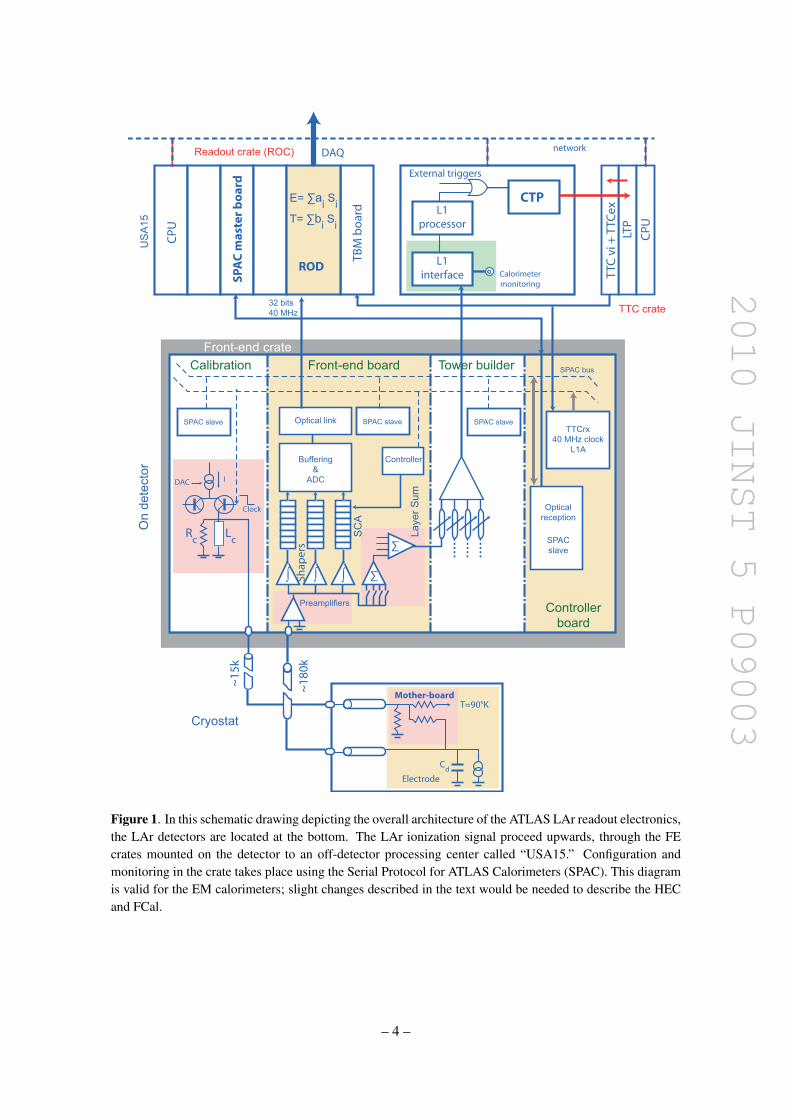
The electronic readout of the ATLAS LAr calorimeters, depicted schematically in figure 1, is di-vided into a Front End (FE) system [4] of circuit boards mounted in custom crates directly on thedetector cryostats, and a Back End (BE) system [5] of VME-based boards located off the detector,outside the detector hall. The FE system includes Front End Boards (FEBs) [6], which perform thereadout and digitization of the calorimeter signals, calibration boards [7] which inject precision cal-ibration signals, layer sum boards which produce analog sums for the Level 1 (L1) trigger system,

1In the ATLAS coordinate system, φ is the azimuthal angle around the axis of the beam; θ is the polar angle fromthe beam axis. The pseudorapidity, η , is defined as η =− ln tan(θ/2).

– 2 –

2010 JINST 5 P09003

and control boards which receive and distribute the 40 MHz LHC clock as well as other configu-ration and control signals. The BE electronics are made up primarily of Read Out Driver (ROD)boards which receive the digitized signals from the FEBs over 1.6 Gbps optical links. The RODsperform digital filtering, formatting, and monitoring of the calorimeter signals before transmittingthe processed data to the ATLAS data acquisition system (DAQ).

The LAr readout was designed to meet demanding specifications. The ATLAS LAr calorime-ters are finely segmented, with a total of 182,468 channels to be read out. With each FEB handlingup to 128 channels, a total of 1524 FEBs are required, distributed among 58 FE crates mounted onthe various cryostats. All of the on-detector FE electronics have been built to withstand the highlevels of radiation [8, 9] which result from the collisions of the intense LHC beams. The FEBssample the LAr calorimeter signals at the LHC bunch crossing frequency of 40 MHz and store thesamples during the latency of the ATLAS L1 trigger system. For an initial maximum L1 triggerrate of 75 kHz (increasing later to 100 kHz), the FEB reads out five samples per channel, with littledead time. For special calibration runs where one wants to measure the entire waveform, the FEBcan also read out up to 32 samples per channel, but at a lower trigger rate. Measuring the energydeposited in each calorimeter channel with excellent resolution over a wide dynamic range of 16to 17 bits (from tens of MeV to a few TeV per cell) is the primary goal. At the same time, coherentnoise is minimized to less than 5% of the incoherent noise, to minimize the effect on physics anal-ysis. The electronics also provide inputs to the L1 trigger at 40 MHz. Performance results fromcommissioning the L1 trigger system itself are presented elsewhere [10].

The FEB architecture is illustrated schematically in figure 2. The raw signals from the calorime-ter are mapped onto the FEB inputs as they emerge from cryostat feedthroughs. On the FEB, thesignals are first subject to several stages of analog processing. Preamplifier hybrids terminate thelong signal cables from the detector, and amplify the raw signals; three versions of preamplifierswith different impedance and maximum input currents are used to match the detector capacitancesand dynamic ranges of the calorimeter sections. In the case of the HEC [11], cryogenic preampli-fiers mounted on the detector inside the cryostat provide some amplification of the signals beforethey reach the FEBs, and the preamplifiers on the FEB are replaced by preshapers that provide apole-zero cancellation to adapt to the widely varying HEC detector capacitance in order to equalizethe pulse shapes before the analog summing that is done for the L1 trigger system. The preshapersinvert, amplify and shape the signal so that the signals from the HEC will have the same polarityand approximately the same shape as the signals from the other LAr calorimeters.

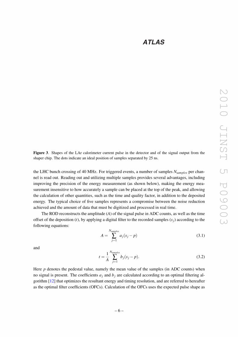
The preamplifier or preshaper outputs are split and further amplified by shaper chips on theFEB to produce three overlapping linear gain scales. The gain ratios are ∼10 in order to cover theentire dynamic range, with gain values of 1 for low gain, 9.9 for medium gain, and 93 for highgain. Each signal is subject to a fast bipolar CR-(RC)2 shaping function with τ = RC = 13 ns.The triangular input current pulse from the detector and the output from the shaper are depicted forthe case of a typical EMB cell in figure 3. The ionization current for the EMB is approximately 3µA/GeV, with the actual value depending on η , as shown in reference [1]. The single differentiationof the shaper serves to remove the long tail from the detector response, while the two integrationslimit the bandwidth in order to reduce the noise.

The shaped signals are sampled at the LHC bunch crossing frequency of 40 MHz by switched-capacitor array (SCA) analog pipeline chips. The SCAs store the signals in analog form during the

– 3 –

2010 JINST 5 P09003

TTC

vi +

TTC

exLT

P

CPU

CPU

SPA

C m

aste

r b

oard

ROD

TBM

boa

rd

E= !ai Si T= !bi Si

CTP

External triggers

L1processor

L1interface Calorimeter

monitoring

Rc Lc

DAC

Clock

I

!

!

Optical link

Controller

Opticalreception

SPACslave

Preamplifiers

Buffering&

ADC

SPAC slaveSPAC slave SPAC slave

Calibration Tower builder

Controllerboard

Front-end boardFront-end crate

TTCrx40 MHz clock

L1A

SPAC bus

TTC crate

Readout crate (ROC)

32 bits40 MHz

USA

15O

n de

tect

or

Cryostat

SCA

Laye

r Sum

~15

k

~18

0k

Mother-board

Electrode

T=90°K

networkDAQ

Shap

ers

! ! !

Cd

Figure 1. In this schematic drawing depicting the overall architecture of the ATLAS LAr readout electronics,the LAr detectors are located at the bottom. The LAr ionization signal proceed upwards, through the FEcrates mounted on the detector to an off-detector processing center called “USA15.” Configuration andmonitoring in the crate takes place using the Serial Protocol for ATLAS Calorimeters (SPAC). This diagramis valid for the EM calorimeters; slight changes described in the text would be needed to describe the HECand FCal.

– 4 –

2010 JINST 5 P09003

!

101

100

!

ShaperPreamp

LSB

T ADC

SMUX

OTx

MUX

144 cells

4

SCA

128

Analogue

trigger sum

channels

Detectorinputs

OpAmp

to ROD

12GLINK

GSEL

Figure 2. In this schematic block diagram of the FEB architecture, the data flow is shown for four of the128 channels per board. The data comes from the detectors on the top left. The analog sums exit on thebottom left through the Layer Sum Boards (LSBs) while the digital results are transmitted to the next levelof processing through optical transmitters (OTxs) on the right. If these were HEC channels, the preampswould be replaced by preshapers, as described in the text.

L1 trigger latency. For events accepted by the L1 trigger, typically five samples per channel are readout from the SCA and digitized using a 12-bit Analog to Digital Converter (ADC). To optimize theprecision of the energy measurement, the Gain Selector chips (GSEL) choose for each channel, ineach event, which of the three gains to use, based on the value of the peak sample in the mediumgain compared to two reference thresholds. The FEBs can also be configured to read out one ormore fixed gains, a feature that is used for certain calibration runs. The digitized data are formatted,multiplexed, serialized, and then transmitted optically from each FEB to the corresponding RODof the BE electronics.

The RODs, described in more detail in section 7, perform digital processing of the samplesfor each channel to produce optimized measures of the energy. For channels passing an energythreshold, the time of the deposition and a “quality factor” are also calculated. For those channelspassing a second (higher) threshold, the values of the raw samples are also written out, in additionto the results of the processing, to allow additional checks to be performed offline for large energydeposits. The quality factor, defined more precisely in section 7, quantifies whether pulses matchexpectations or whether they may be mismeasured, for example from waveform distortions pro-duced by energy depositions in neighboring bunch crossings, a phenomenon known as “pile-up”.

During development of the electronics, a partial FE system test was performed at BrookhavenNational Laboratory (BNL) in 2004 using final prototypes of the various FE boards. Several con-figurations were tested, the largest of which corresponded to the setup required to read out one“half-crate” of the EMB (including 14 FEBs, one calibration board, and the associated trigger andcontrol boards). This configuration included 1792 readout channels, corresponding to ∼1.6% ofthe channels in the entire EMB, or ∼0.9% of the total LAr calorimeter system. The purpose of theBNL test was to verify that the overall FE system met the required performance specifications, be-fore launching production of the various boards. A similar partial system test of the BE electronicswas performed at CERN in 2004.

3 Pulse reconstruction and calibration

As depicted in figure 3, a triangular current pulse is produced when charged particles ionize theliquid argon in the high-voltage potential present in the gap between two absorber plates. Once thesignal reaches the FEB, a bipolar shaping function is applied and the shaped signal is sampled at

– 5 –

2010 JINST 5 P09003

ATLAS

Figure 3. Shapes of the LAr calorimeter current pulse in the detector and of the signal output from theshaper chip. The dots indicate an ideal position of samples separated by 25 ns.

the LHC bunch crossing of 40 MHz. For triggered events, a number of samples Nsamples per chan-nel is read out. Reading out and utilizing multiple samples provides several advantages, includingimproving the precision of the energy measurement (as shown below), making the energy mea-surement insensitive to how accurately a sample can be placed at the top of the peak, and allowingthe calculation of other quantities, such as the time and quality factor, in addition to the depositedenergy. The typical choice of five samples represents a compromise between the noise reductionachieved and the amount of data that must be digitized and processed in real time.

The ROD reconstructs the amplitude (A) of the signal pulse in ADC counts, as well as the timeoffset of the deposition (t), by applying a digital filter to the recorded samples (s j) according to thefollowing equations:

A =Nsamples

∑j=1

a j(s j− p) (3.1)

and

t =1A

Nsamples

∑j=1

b j(s j− p). (3.2)

Here p denotes the pedestal value, namely the mean value of the samples (in ADC counts) whenno signal is present. The coefficients a j and b j are calculated according to an optimal filtering al-gorithm [12] that optimizes the resultant energy and timing resolution, and are referred to hereafteras the optimal filter coefficients (OFCs). Calculation of the OFCs uses the expected pulse shape as

– 6 –

2010 JINST 5 P09003

well as the noise auto-correlation matrix for the samples. As this is the total noise, the OFCs willdepend on the luminosity, to take into account the noise from the electronics and pile-up together.

It is necessary to convert the reconstructed pulse amplitude A to the deposited energy (E) inMeV. The conversion is performed as follows for the majority of the LAr systems:

E = FµA→MeV×FDAC→µA×1

MphysMcali

×Nramps

∑j=(0,1)

G jA j (3.3)

The factor FµA→MeV relates the ionization current in the calorimeter to the energy deposited,and depends on factors such as the sampling fraction of the calorimeter in question. The valuesfor each channel have been determined from test beam data using production calorimeter modules,and validated with a detailed detector simulation. Studies with particles from LHC collisions, andin particular, high-statistics samples of Z→ e+e− decays, will be used to determine values whichoptimize the in situ performance for the ATLAS EM calorimeters. The factor FDAC→µA convertsthe Digital-to-Analog Converter (DAC) setting of the calibration board to the injected current, andis determined from known parameters of the calibration boards and injection resistors. The factorMphysMcali

quantifies the ratio of response to a calibration pulse and an ionization pulse correspondingto the same input current. The factor G j is the electronic gain of the channel, which is determinedfrom electronic calibration runs as described later in this section. The sum over j starts fromj = 0 in medium and low gain only, while in high gain, j = 1 is the first term used. The rampfit polynomial order Nramps is usually 1 such that a linear fit performed, but it can be increased ifrelevant non-linearity is found in any channel/gain.

As explained below, a series of three types of electronic calibration runs, dubbed Pedestal,Ramp, and Delay runs, provides many of the inputs needed for the cell energy, time and qualityfactor computations. These runs are taken regularly, usually separately for high, medium, and lowgains in order to calibrate all channels and all gains. Typically, a set of Pedestal and Ramp runs istaken daily. A more complete set, including Delay runs, is taken every week. Data are processedautomatically and checked daily.

During a Pedestal run, the FEBs are triggered and read out without any input signal present.The pedestal value p for each cell is computed as the average sample value over ∼3000 eventsrecorded with typically 32 samples. The noise is computed as the root-mean-square (RMS) of thepedestal value, while the auto-correlation matrix of the noise, Vi j, is computed as

Vi j =⟨si× s j

⟩,

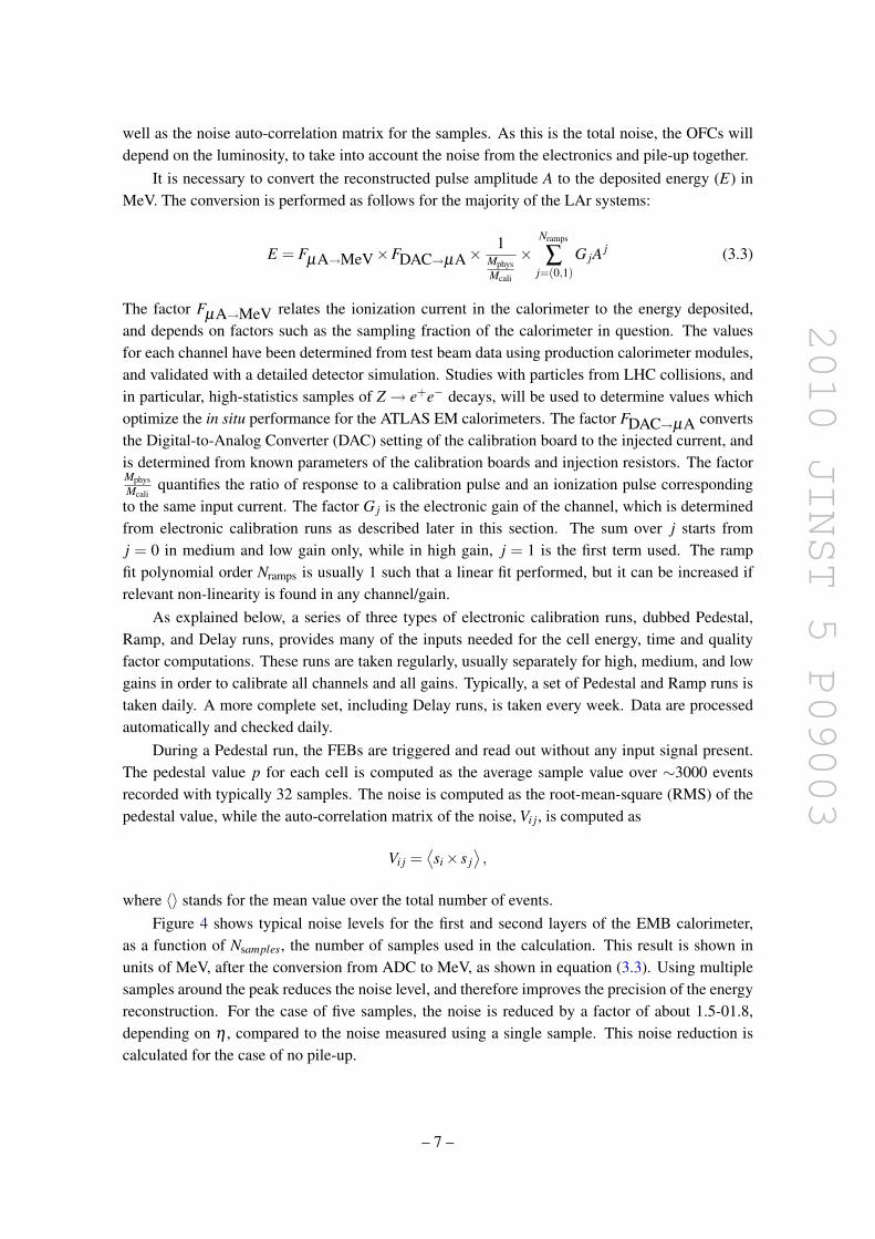
where 〈〉 stands for the mean value over the total number of events.Figure 4 shows typical noise levels for the first and second layers of the EMB calorimeter,

as a function of Nsamples, the number of samples used in the calculation. This result is shown inunits of MeV, after the conversion from ADC to MeV, as shown in equation (3.3). Using multiplesamples around the peak reduces the noise level, and therefore improves the precision of the energyreconstruction. For the case of five samples, the noise is reduced by a factor of about 1.5-01.8,depending on η , compared to the noise measured using a single sample. This noise reduction iscalculated for the case of no pile-up.

– 7 –

2010 JINST 5 P09003

0 5 10 15 20 25 30

Noi

se (M

eV)

10

15

20

25

30

35

40

45ATLAS

Number of Samples

Figure 4. Typical noise levels for the EMB first (triangles) and second (circles) layers as a function of thenumber of samples used to calculate the deposited energy.

Additional calibration runs use the calibration board to inject precise pulses with programmableamplitudes and delays. The pulse amplitudes are set by programming a precision DAC on the cal-ibration board, and the timing of the pulse can also be programmed. The calibration pulses areinjected through precision resistors mounted directly on the detectors inside the cryostat for theEMB and EMEC calorimeters. These calibration signals are exponential before shaping, approxi-mating the triangular ionization pulse.

During a Ramp run, the timing of the pulses is held fixed and a set of typically 100 eventsis taken with pulses of a fixed amplitude, or DAC value. Different sets of events with differentDAC values are taken to map the response over the entire dynamic range. The gain (G) of thereadout is determined as the slope of the linear fit of the reconstructed pulse amplitude versus DACsetting. Averaging over the 100 events for each DAC setting improves the precision in the gaindetermination by suppressing the noise.

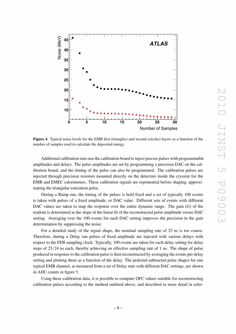
For a detailed study of the signal shape, the nominal sampling rate of 25 ns is too coarse.Therefore, during a Delay run pulses of fixed amplitude are injected with various delays withrespect to the FEB sampling clock. Typically, 100 events are taken for each delay setting for delaysteps of 25/24 ns each, thereby achieving an effective sampling rate of 1 ns. The shape of pulseproduced in response to the calibration pulse is then reconstructed by averaging the events per delaysetting and plotting them as a function of the delay. The pedestal-subtracted pulse shapes for onetypical EMB channel, as measured from a set of Delay runs with different DAC settings, are shownin ADC counts in figure 5.

Using these calibration data, it is possible to compute OFC values suitable for reconstructingcalibration pulses according to the method outlined above, and described in more detail in refer-

– 8 –

2010 JINST 5 P09003

Time (ns)

0 100 200 300 400 500 600 700 800

Ampl

itude

-500

0

500

1000

1500

2000

2500

3000

ATLAS

Figure 5. Pulse shapes (measured in ADC counts after subtraction of the pedestal) for a typical channel inthe EMB calorimeter as reconstructed using a set of Delay runs, each with a different DAC setting. For moredetails, see the text.

ences [12, 13]. OFC values suitable for reconstructing ionization signals from particles depositingenergy in the calorimeters are calculated in a similar way. However, to obtain a precise descrip-tion of the ionization pulse shape one must account for the differences in injection point and inshape between the exponential calibration pulses and the triangular ionization pulses, as well asother effects including crosstalk in the calorimeters and electronics, and reflections at the variousconnectors and interfaces between the detectors and the readout. A precision at the level of ∼1%on the ionization pulse is obtained using methods described in detail in references [14, 15], with acorresponding precision on the signal amplitude of∼0.2%. During LHC operations, high statisticssamples will allow further cross checks of the understanding of the detailed pulse shapes.

The required calibration constants for each channel, including pedestals and OFC values, areuploaded to the RODs at the start of data-taking, where they are used to process the data read outfrom the FEBs in real time in order to calculate the deposited energy in MeV, peaking time in unitsof 10 ps, and the quality factor.

4 Pedestal and noise performance

The pedestal values of all channels are measured frequently as part of the regular calibrationsdescribed in the previous section. During LHC running, the pedestal values and noise can bemonitored by random triggers in, for example, empty bunch crossings where no collisions areexpected. The pedestals are an important input to the pulse amplitude reconstruction; frequentPedestal runs allow for long term monitoring of the noise and pedestal stability.

In order to allow the negative lobe of the pulse to be measured, the FEB is designed such thateach channel has a pedestal value of ∼1000 ADC counts. This is important in order to be able to

– 9 –

2010 JINST 5 P09003

||0 0.5 1 1.5 2 2.5 3 3.5 4 4.5 5

Elec

troni

c no

ise

(MeV

)

10

210

310PSEM1EM2EM3

FCal1FCal2FCal3HEC1HEC2HEC3HEC4

ATLAS

η

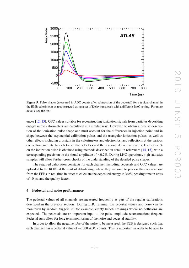
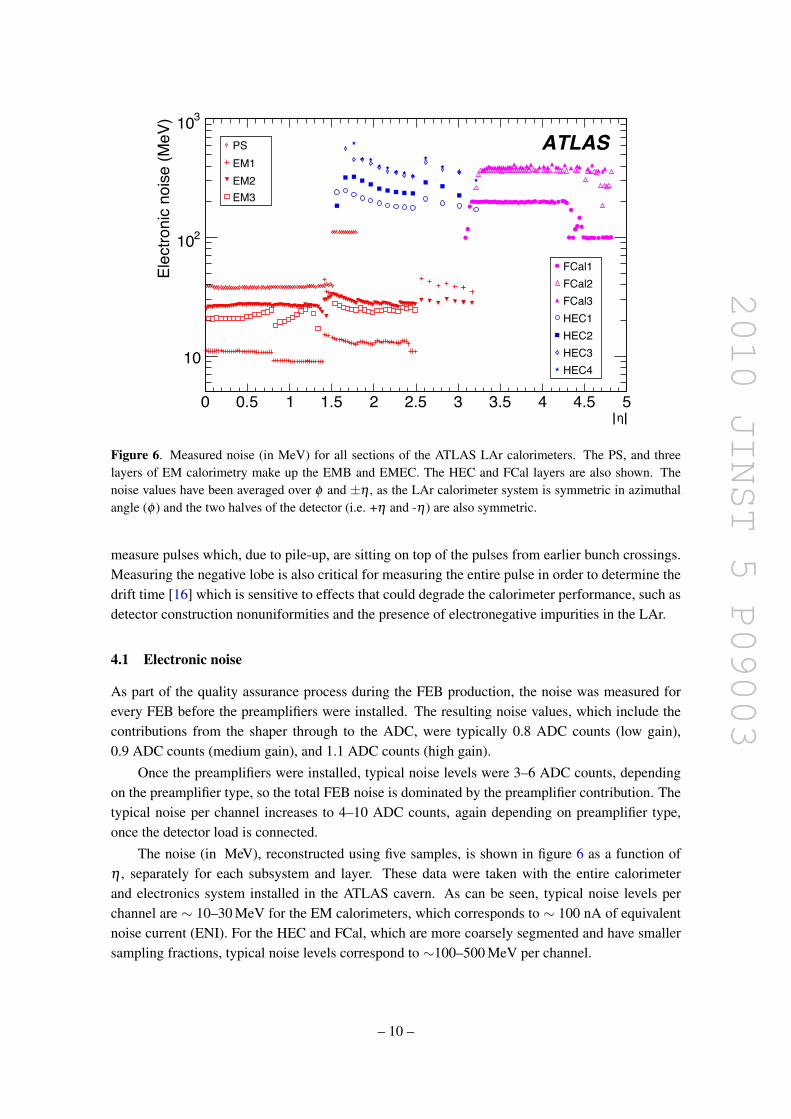
Figure 6. Measured noise (in MeV) for all sections of the ATLAS LAr calorimeters. The PS, and threelayers of EM calorimetry make up the EMB and EMEC. The HEC and FCal layers are also shown. Thenoise values have been averaged over φ and ±η , as the LAr calorimeter system is symmetric in azimuthalangle (φ ) and the two halves of the detector (i.e. +η and -η) are also symmetric.

measure pulses which, due to pile-up, are sitting on top of the pulses from earlier bunch crossings.Measuring the negative lobe is also critical for measuring the entire pulse in order to determine thedrift time [16] which is sensitive to effects that could degrade the calorimeter performance, such asdetector construction nonuniformities and the presence of electronegative impurities in the LAr.

4.1 Electronic noise

As part of the quality assurance process during the FEB production, the noise was measured forevery FEB before the preamplifiers were installed. The resulting noise values, which include thecontributions from the shaper through to the ADC, were typically 0.8 ADC counts (low gain),0.9 ADC counts (medium gain), and 1.1 ADC counts (high gain).

Once the preamplifiers were installed, typical noise levels were 3–6 ADC counts, dependingon the preamplifier type, so the total FEB noise is dominated by the preamplifier contribution. Thetypical noise per channel increases to 4–10 ADC counts, again depending on preamplifier type,once the detector load is connected.

The noise (in MeV), reconstructed using five samples, is shown in figure 6 as a function ofη , separately for each subsystem and layer. These data were taken with the entire calorimeterand electronics system installed in the ATLAS cavern. As can be seen, typical noise levels perchannel are ∼ 10–30 MeV for the EM calorimeters, which corresponds to ∼ 100 nA of equivalentnoise current (ENI). For the HEC and FCal, which are more coarsely segmented and have smallersampling fractions, typical noise levels correspond to ∼100–500 MeV per channel.

– 10 –

2010 JINST 5 P09003

4.2 System isolation and noise performance

To ensure good performance of the completed ATLAS detector, ATLAS adopted and enforcedstringent specifications for electromagnetic compatibility (EMC) and electromagnetic interference(EMI) among its various subdetectors. The specifications included careful grounding schemes toensure the isolation of individual systems.

Both the FEB [6] and the FE crate system [4] were designed with careful attention to EMC andEMI issues. During the BNL test, dedicated investigations were performed to evaluate the EMC andEMI behavior of the LAr readout electronics. As described in more detail in reference [17], giventhat the most troublesome potential source of interference is likely to be near field RF magneticfields produced by currents in nearby cables, these tests included measuring the coherent noise inthe presence of magnetic fields generated by a small loop (about 15 cm in diameter) driven by a50 W broadband power amplifier and mounted near the FE crate, monitored using a calibrated loopantenna. The power amplifier was driven with the RF output of a network analyzer to sweep overthe range from 1 MHz to 40 MHz, with a narrow (100 Hz) filter bandwidth, to evaluate the impactas a function of frequency. The largest impact on the coherent noise was observed for a frequencyof 28.5 MHz, due to EMI coupling into the inputs of the preamplifiers mounted on the FEBs. Themaximum sensitivity could be characterized approximately as an expected coherent noise of 10% ofthe total noise per channel for an external field of 1 mA/m at a frequency of 28.5 MHz. Such a fieldcould be generated, for example, from a differential current of 30 mA flowing in a pair of parallelwires mounted a distance of 10 cm from the FE crate. However, in most systems (including thoseimplemented in ATLAS), the wires would be twisted and also shielded, so a significantly higherdifferential current would be required to generate such a radiated field.

An ATLAS-specific test was performed at BNL by mounting a board emulating the digitaloutput data driver for the Transition Radiation Tracker (TRT) detector near the LAr FE crate. FourTRT cables, each with 20 twisted pairs, were looped on the side of the LAr FE crate, mimickingthe location of the TRT cables in ATLAS, where they pass close to the EMB FE crates as theyexit the detector. The effect on the FEB performance of the EMI emitted from the TRT cables wasextremely small, with an increase of the coherent noise of ∼ 0.3% per channel for 20 MHz datatransmission, and only ∼ 0.08% per channel at 40 MHz. The effect of the operation of the FEBsand other LAr FE electronics on the TRT bit error rate was also studied, but was so small as to notto generate any errors during a run of 60 hours at 40 Mb/s, corresponding to a limit of the bit errorrate of less than 10−14.

Dedicated tests were performed in the ATLAS cavern to investigate the EMC and stabilityof the DC power distribution system used for the LAr readout, which includes AC/DC convertersthat are located outside the detector hall in USA15. Long cables from USA15 are used to driveDC/DC converters located close to each FE crate on the detector. The tests, described in detail inreference [18], included studies that demonstrated the guaranteed stability of the power distributionsystem, and measurements of common-mode and differential-mode noise along the power cable,as well as of EMI emissions of the power cable.

The grounding and isolation scheme implemented for the LAr calorimeters as installed inthe ATLAS cavern is discussed in detail in reference [4]. As explained there, the shields of thehigh voltage (HV) cables are connected on the side of the USA15 ground but were originally

– 11 –

2010 JINST 5 P09003

disconnected at the cryostat end. However, during commissioning tests in the ATLAS cavern, largehigh frequency noise signals were observed in the LAr readout, especially for the PS channels. Thesource of the noise was established as an AC potential difference between the USA15 ground andthe cryostat ground, which was entering the cryostats by coupling to the HV cables. The installationof a 1 µF capacitor between the shield of the HV cables (USA15 ground) and the HV filter ground(cryostat ground) cured this noise problem.

4.3 Coherent noise

Given the fine granularity of the LAr calorimeter, typically 50–100 calorimeter cells are summed tomeasure the energy of an electron or photon, and even more channels must be summed for a typicaljet or for more global quantities such as missing transverse energy (MET). Therefore, minimizingthe coherent noise is particularly critical, and the specifications of the LAr readout require that thecoherent noise be kept below 5% of the incoherent noise.

In the BNL test, the coherent noise within one FEB was measured by comparing the RMSnoise of the digital sum of n channels with the square root of n times the average RMS noise perchannel. The quadratic difference is a measure of the coherent noise. The measurements showedthat the coherent noise per channel was less than 2% of the incoherent noise. For larger sums, suchas over the 14 FEBs in the BNL crate test, the coherent noise dropped even further, to less than 1%of the incoherent noise.

The coherent noise is particularly sensitive to the grounding and isolation conditions. Forexample, at one stage during detector commissioning in the ATLAS cavern, a large coherent noisecontribution was observed for one octant of the PS in the EMB. Investigations revealed that a HVcable feeding this octant had a broken shield, caused by a broken connection to the 1 µF capacitor.The noise problem was cured once the faulty HV cable was replaced with a spare.

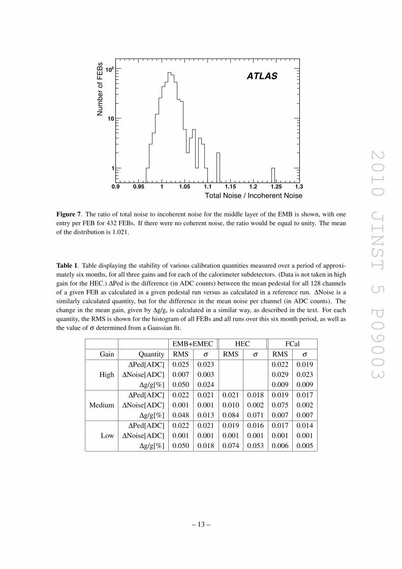
The coherent noise analysis was repeated to determine the in situ performance as measuredfor the calorimeters installed in the ATLAS cavern. Figure 7 shows that the level of coherent noiseper channel within the second layer of the EMB is typically 2–3%. The second layer is especiallyimportant, as it contains the largest part of EM showers. The coherent noise is also low in the firstand third layers, about 6% and 2% respectively. These levels are per FEB, while data from morethan one FEB will be used when constructing clusters of energy, further reducing the coherentnoise. The combination of the intrinsic FEB performance plus the effectiveness of the EMC/EMImeasures described in the previous section has led to excellent in situ coherent noise performance.

4.4 Pedestal and noise stability

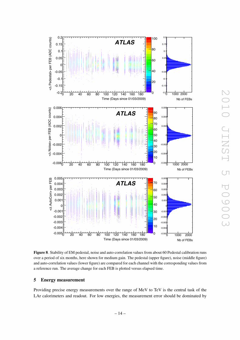
The stability of the pedestal, noise and auto-correlation values has been monitored over extendedperiods of time, using data taken with the complete detector. Sample results as measured over aperiod of about six months in early 2009 are shown for the EMB and EMEC together in figure 8.The HEC and FCal have similar stability results.

The stability is further quantified in table 1. For example, typical variations in pedestal valuesfor single channels are at the level of 0.02 ADC counts. This corresponds to an energy of about1 MeV for the medium gain of the EMB and EMEC, about 2 MeV for the HEC and 10 MeV for theFCAL. Noise variations are typically less than 0.01 ADC counts for high gain in the EM calorime-ters, ∼ 0.02 ADC counts in the FCal, and an order of magnitude less for medium and low gains.

– 12 –

2010 JINST 5 P09003

Total Noise / Incoherent Noise0.9 0.95 1 1.05 1.1 1.15 1.2 1.25 1.3

Num

ber o

f FEB

s

1

10

210ATLAS

Figure 7. The ratio of total noise to incoherent noise for the middle layer of the EMB is shown, with oneentry per FEB for 432 FEBs. If there were no coherent noise, the ratio would be equal to unity. The meanof the distribution is 1.021.

Table 1. Table displaying the stability of various calibration quantities measured over a period of approxi-mately six months, for all three gains and for each of the calorimeter subdetectors. (Data is not taken in highgain for the HEC.) ∆Ped is the difference (in ADC counts) between the mean pedestal for all 128 channelsof a given FEB as calculated in a given pedestal run versus as calculated in a reference run. ∆Noise is asimilarly calculated quantity, but for the difference in the mean noise per channel (in ADC counts). Thechange in the mean gain, given by ∆g/g, is calculated in a similar way, as described in the text. For eachquantity, the RMS is shown for the histogram of all FEBs and all runs over this six month period, as well asthe value of σ determined from a Gaussian fit.

EMB+EMEC HEC FCalGain Quantity RMS σ RMS σ RMS σ

∆Ped[ADC] 0.025 0.023 0.022 0.019High ∆Noise[ADC] 0.007 0.003 0.029 0.023

∆g/g[%] 0.050 0.024 0.009 0.009∆Ped[ADC] 0.022 0.021 0.021 0.018 0.019 0.017

Medium ∆Noise[ADC] 0.001 0.001 0.010 0.002 0.075 0.002∆g/g[%] 0.048 0.013 0.084 0.071 0.007 0.007

∆Ped[ADC] 0.022 0.021 0.019 0.016 0.017 0.014Low ∆Noise[ADC] 0.001 0.001 0.001 0.001 0.001 0.001

∆g/g[%] 0.050 0.018 0.074 0.053 0.006 0.005

– 13 –

2010 JINST 5 P09003

Time (Days since 01/03/2009)0 20 40 60 80 100 120 140 160 180

Ped

esta

l> p

er F

EB (A

DC

cou

nts)

<

-0.2

-0.15

-0.1

-0.05

0

0.05

0.1

0.15

0.2

0

20

40

60

80

100

Nb of FEBs0 1000 2000-0.2

-0.15

-0.1

-0.05

0

0.05

0.1

0.15

0.2

ATLAS

Time (Days since 01/03/2009)0 20 40 60 80 100 120 140 160 180

Noi

se>

per F

EB (A

DC

cou

nts)

Δ<

-0.006

-0.004

-0.002

0

0.002

0.004

0.006

0102030405060708090

Nb of FEBs0 1000 2000-0.006

-0.004

-0.002

0

0.002

0.004

0.006

ATLAS

Time (Days since 01/03/2009)0 20 40 60 80 100 120 140 160 180

Aut

oCor

r> p

er F

EBΔ<

-0.005-0.004-0.003-0.002-0.001

00.0010.0020.0030.0040.005

0

10

20

30

40

50

60

70

Nb of FEBs0 1000 2000-0.005

-0.004

-0.003

-0.002

-0.001

0

0.001

0.002

0.003

0.004

0.005

ATLAS

Figure 8. Stability of EM pedestal, noise and auto-correlation values from about 60 Pedestal calibration runsover a period of six months, here shown for medium gain. The pedestal (upper figure), noise (middle figure)and auto-correlation values (lower figure) are compared for each channel with the corresponding values froma reference run. The average change for each FEB is plotted versus elapsed time.

5 Energy measurement

Providing precise energy measurements over the range of MeV to TeV is the central task of theLAr calorimeters and readout. For low energies, the measurement error should be dominated by

– 14 –

2010 JINST 5 P09003

the noise. The calibration of the calorimeter readout should be understood at a level of precisionof 0.25% to control the overall constant term in the energy resolution function, as defined later inequation (5.1).

Since analog summing is used to make the L1 trigger towers, meeting the specified triggerperformance requires that channels within a given analog sum have an energy response which isuniform within 5%. The preamplifier gains are, in fact, uniform to within 1–2% [6], exceeding thisspecification.

5.1 Energy resolution of the electromagnetic calorimeter

Ramp runs can be used to determine the contribution of the electronics to the resolution for recon-structing the energy deposited in a channel. Figure 9 shows the relative energy resolution, σ(E)/E,versus energy for a representative channel in the second layer of the EMB calorimeter. The plotsuperimposes results for all three gain scales. The value used for σ of a given point is the RMS,calculated over 100 pulses, of a single sample measured at the peak of the pulse.

The data are compared to an estimate of the energy resolution in one cell with the form of thecurve given by:

σ(E)E

=a√E⊕b⊕ c

E(5.1)

where the energy is measured in GeV and ⊕ indicates addition in quadrature. For the purposeof this comparison, a = 10%, which is the typical stochastic term for an electromagnetic shower,b = 0.25% for the local constant term, and c = 45 MeV is the noise measured from a single samplefor the considered cell in high gain. The second, “constant,” term dominates at high energy, so itespecially important to minimize. Here, b = 0.25% is the specification for the local constant term,applicable to a single channel with the aim of limiting the global constant term across the entirecalorimeter to less than 0.7%. In test beam studies before the final system was installed, a samplingterm of 10% and local constant term of 0.17% were measured for the EMB [19].

The high gain signal, which is used to reconstruct relatively low energies, is applicable up toabout 25 GeV, after which it saturates. The values of σ for the high gain are dominated by the noise,which is about 45 MeV for a single sample for this particular channel. Therefore, the resolutionimproves roughly like 1/E, reaching a level of 0.2% for energies near 25 GeV.

The resolution for medium gain is just under 0.4% at the energy of 25 GeV, where it takes overfrom high gain. The medium gain resolution improves roughly like 1/E until saturation is reachednear 250 GeV, where the resolution is below 0.07%.

For higher energies, the low gain readout would be used. The low gain has a resolution below0.4% at the crossover point of 250 GeV, and then improves roughly like 1/E to provide a resolutionbetter than 0.07% for the highest energies, in the 1–2 TeV range.

Since the RMS of a single sample is used for the σ values in the figure, the results shown donot take into account the improvement by a factor 1.5–1.8 that is achieved in suppressing the noiseby using OFCs from five samples, as described previously (see figure 4). As the points shown forthis channel are in units of energy, rather than ADC counts, factors to convert from DAC to µAand µA to MeV have been applied. Figure 9 demonstrates that the energy resolution of the LArelectronic readout does not significantly contribute to the overall energy resolution.

– 15 –

2010 JINST 5 P09003

Energy (GeV)

1 102

103

10

(E)

/ E

(%

)σ

-110

1

10

High Gain

Medium Gain

Low Gain

Calorimeter Resolution

ATLAS

Figure 9. Energy resolution versus energy of a representative EMB second layer channel, as measuredduring Ramp runs. The points represent the data, while the solid curve shows a parametrization of the totalcalorimeter energy resolution, given by equation (5.1). For more details, see the text.

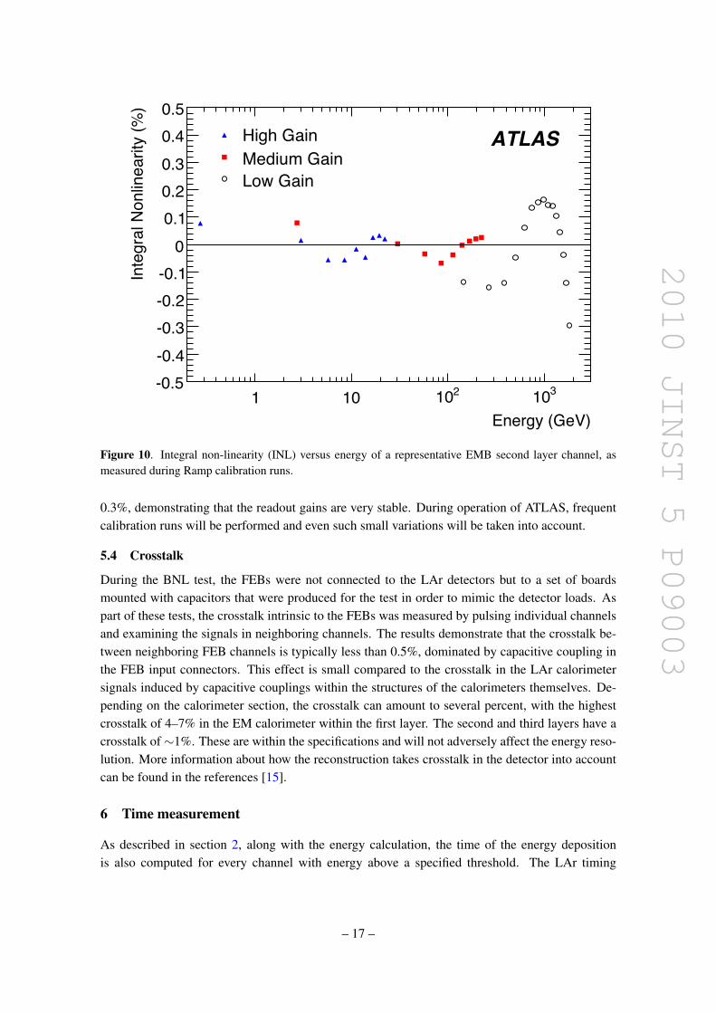
5.2 Linearity

Ramp calibration runs are used to determine the linearity for reconstructing the energy deposited ina channel. Figure 10 shows the integral non-linearity (INL) versus energy for the same channel ofthe second layer of the EMB as in figure 9. The plot superimposes results for all three gain scales.The INL is defined at each point i and for each gain as

INLi = (Emeasured,i−Efit,i)/Emax. (5.2)

Here, Efit,i is the result for point i of a straight-line fit to all the data points of the gain in question,while Emax is the value of the maximum energy point used for that gain.

The results indicate that the readout electronics are linear to typically 0.2% or better, includingthe combined effects of both the FEB that measures and reads out the calorimeter signals and thecalibration board that generates and injects calibration pulses.

5.3 Stability of the energy measurement

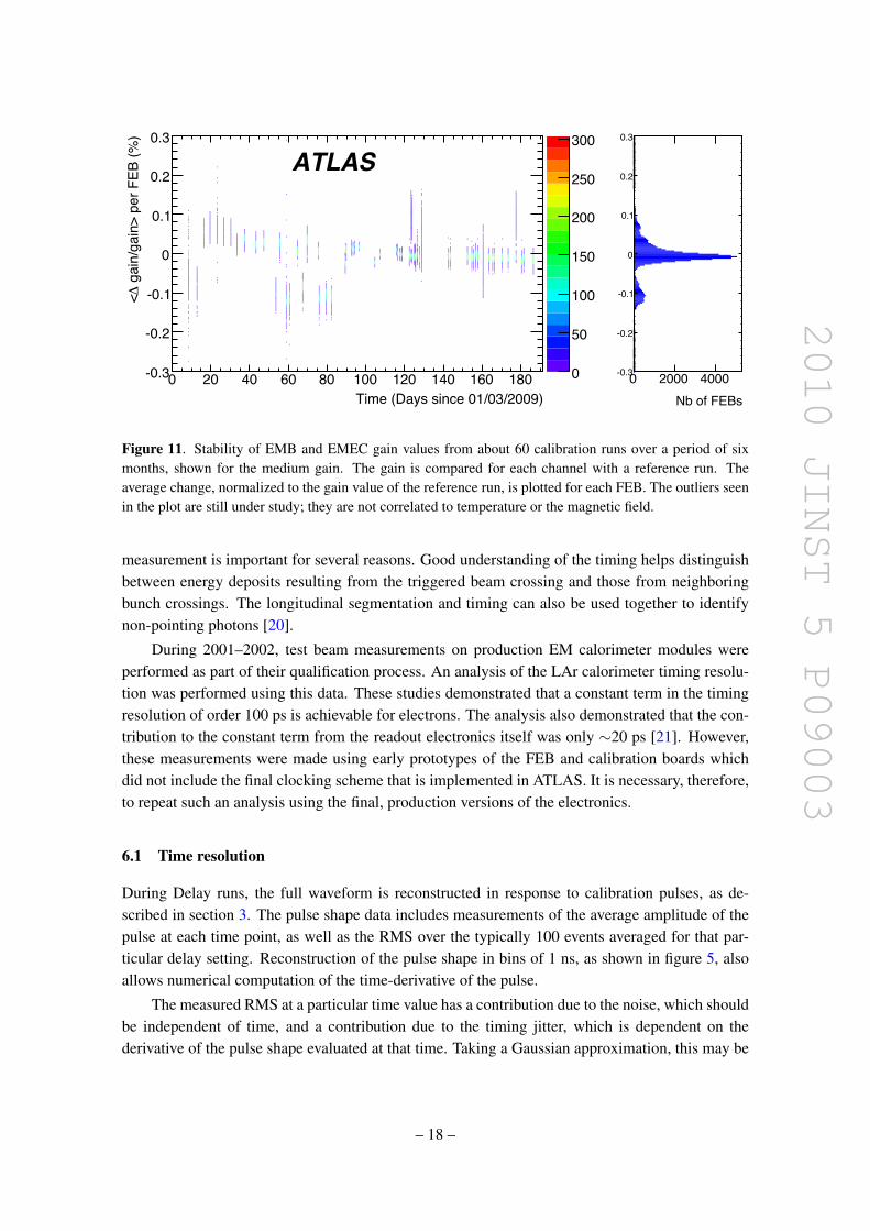
The stability of the gain of the LAr readout can be studied by comparing the results of calibrationruns taken over an extended period of time. Figure 11 shows the fractional change in gain forthe medium gain readout of the EMB and EMEC. It has been obtained from an analysis of Rampruns taken over a period of six months in early 2009. The stability of the measured gains for thevarious calorimeters was summarized in table 1. The variations with time are typically within

– 16 –

2010 JINST 5 P09003

Energy (GeV)

1 102

103

10

Inte

gra

l N

onlinearity

(%

)

-0.5

-0.4

-0.3

-0.2

-0.1

0

0.1

0.2

0.3

0.4

0.5

High Gain

Medium Gain

Low Gain

ATLAS

Figure 10. Integral non-linearity (INL) versus energy of a representative EMB second layer channel, asmeasured during Ramp calibration runs.

0.3%, demonstrating that the readout gains are very stable. During operation of ATLAS, frequentcalibration runs will be performed and even such small variations will be taken into account.

5.4 Crosstalk

During the BNL test, the FEBs were not connected to the LAr detectors but to a set of boardsmounted with capacitors that were produced for the test in order to mimic the detector loads. Aspart of these tests, the crosstalk intrinsic to the FEBs was measured by pulsing individual channelsand examining the signals in neighboring channels. The results demonstrate that the crosstalk be-tween neighboring FEB channels is typically less than 0.5%, dominated by capacitive coupling inthe FEB input connectors. This effect is small compared to the crosstalk in the LAr calorimetersignals induced by capacitive couplings within the structures of the calorimeters themselves. De-pending on the calorimeter section, the crosstalk can amount to several percent, with the highestcrosstalk of 4–7% in the EM calorimeter within the first layer. The second and third layers have acrosstalk of∼1%. These are within the specifications and will not adversely affect the energy reso-lution. More information about how the reconstruction takes crosstalk in the detector into accountcan be found in the references [15].

6 Time measurement

As described in section 2, along with the energy calculation, the time of the energy depositionis also computed for every channel with energy above a specified threshold. The LAr timing

– 17 –

2010 JINST 5 P09003

Time (Days since 01/03/2009)0 20 40 60 80 100 120 140 160 180

gai

n/ga

in>

per F

EB (%

)Δ<

-0.3

-0.2

-0.1

0

0.1

0.2

0.3

0

50

100

150

200

250

300

Nb of FEBs0 2000 4000-0.3

-0.2

-0.1

0

0.1

0.2

0.3

ATLAS

Figure 11. Stability of EMB and EMEC gain values from about 60 calibration runs over a period of sixmonths, shown for the medium gain. The gain is compared for each channel with a reference run. Theaverage change, normalized to the gain value of the reference run, is plotted for each FEB. The outliers seenin the plot are still under study; they are not correlated to temperature or the magnetic field.

measurement is important for several reasons. Good understanding of the timing helps distinguishbetween energy deposits resulting from the triggered beam crossing and those from neighboringbunch crossings. The longitudinal segmentation and timing can also be used together to identifynon-pointing photons [20].

During 2001–2002, test beam measurements on production EM calorimeter modules wereperformed as part of their qualification process. An analysis of the LAr calorimeter timing resolu-tion was performed using this data. These studies demonstrated that a constant term in the timingresolution of order 100 ps is achievable for electrons. The analysis also demonstrated that the con-tribution to the constant term from the readout electronics itself was only ∼20 ps [21]. However,these measurements were made using early prototypes of the FEB and calibration boards whichdid not include the final clocking scheme that is implemented in ATLAS. It is necessary, therefore,to repeat such an analysis using the final, production versions of the electronics.

6.1 Time resolution

During Delay runs, the full waveform is reconstructed in response to calibration pulses, as de-scribed in section 3. The pulse shape data includes measurements of the average amplitude of thepulse at each time point, as well as the RMS over the typically 100 events averaged for that par-ticular delay setting. Reconstruction of the pulse shape in bins of 1 ns, as shown in figure 5, alsoallows numerical computation of the time-derivative of the pulse.

The measured RMS at a particular time value has a contribution due to the noise, which shouldbe independent of time, and a contribution due to the timing jitter, which is dependent on thederivative of the pulse shape evaluated at that time. Taking a Gaussian approximation, this may be

– 18 –

2010 JINST 5 P09003

-25 -20 -15 -10 -5 0 5 10 15 20 250

50

100

150

200

250

Calibration Board

Jitte

r (ps

)ATLAS

Figure 12. Jitter for the EMEC for calibration runs. As explained in more detail in the text, the jitter for datataken from LHC collisions will be less than for calibration runs.

expressed quantitatively as:

σ2total = σ

2n +

(d fdt

)2

×σ2t

where σn is the single-sample noise level, σt is the timing jitter, and d fdt is the time-derivative of

the pulse shape f (t) evaluated at that time. Therefore, studying the total signal spread, σtotal as afunction of the time-derivative, which varies at different points on the pulse, allows a determinationof the timing jitter.

Figure 12 shows the jitter determined from calibration signals for all the calibration boards inthe EMEC. The typical jitter is around 70 ps.

On the calibration board, the 40 MHz clock is received and recovered by the custom TTCrxASIC [22], and this clock is used to trigger the calibration pulse. Previous studies have demon-strated that the jitter from the TTCrx chip itself is sufficient to explain the values seen in figure 12.

As described previously, the calibration system is used to make the measurements required asinput for the determination of the OFC values used for reconstructing ionization pulses. Jitter inthe calibration pulses has negligible impact on the pulse reconstruction in Ramp and Delay runs,because 100 events are typically averaged. While there are variations seen from one calibrationboard to another, the typical jitter values are low enough that they will not significantly impact thedetermination of the OFC values.

The readout via the FEB alone has lower jitter. While it also uses the TTCrx for clock recovery,the FEB design incorporates a dedicated component, the QPLL [23], to reduce the jitter on theTTCrx clock. This was necessary to guarantee stable operation of the 1.6 Gbps optical link used oneach FEB to transfer the data to the RODs, whose driving clock must be generated by multiplying

– 19 –

2010 JINST 5 P09003

up from the 40 MHz input clock. An additional benefit of the QPLL is that the jitter reduction alsotranslates to better timing resolution for the readout of LAr ionization signals (where the calibrationboard is not involved). During production qualification, the jitter of each FEB was measured [6]and was required to be less than 20 ps. Typical values are 10 ps or less.

6.2 Time uniformity

The FEB is designed such that one overall time offset per FEB can be programmed. This allowsthe sampling phase to be adjusted in order to, for example, place a sample near the expected peakof the shaped calorimeter signals.

The relative timing of the ionization signals in various calorimeter channels can be predictedfrom the timing information measured in calibration runs by applying corrections for effects suchas the time-of-flight of the particles from the collision point and various cable lengths. As detailedin reference [3], such an analysis has been performed and compared with the timing results asobtained from cosmic ray data and first beam events. The agreement between the prediction andthe measurements is within±2 ns in the EM and HEC calorimeters, and within±5 ns for the FCal.With first collisions, the timing of illuminated cells has been verified at the level of ±1 ns.

7 Performance of the Back End electronics

The LAr Back End (BE) system [5] is responsible for communicating with the FE crates, receiving,monitoring and digitally processing the calorimeter data from the FEBs, as well as communicatingwith the ATLAS trigger system.

The main component of the BE system is the ROD, which receives signals from the FEBs overapproximately 70 m optical fibers. A ROD is connected to up to 8 FEBs, processing a maximum of1024 channels. A ROD holds four Processing Units (PUs), each with two Digital Signal Processor(DSP) blocks, such that one DSP block is responsible for processing the data from one FEB. TheROD checks, processes, and formats the data coming from the FEBs. As the raw data will gen-erally not be recorded offline, monitoring histograms are also important to help verify the output.RODs send their output signals through optical fibers to the next level of the ATLAS trigger andDAQ system.

The computations performed by the DSP must meet stringent requirements for processingtime, memory, and bandwidth. During LHC collision data-taking, the RODs must process the datawith a L1 trigger rate up to 75 kHz, implying an average of 13 µs per event for data processing.During calibration runs, the trigger rate is much lower, only a few 100 Hz.

7.1 Digital signal processing

The main function of the LAr ROD DSP block is to process the calorimeter data which has beendigitized and read out by the corresponding FEB. The optimal filtering algorithm is applied by theDSP to calculate the deposited energy from the calorimeter samples. For any cell that passes a pro-grammable energy threshold, the time of the deposition and the quality factor are also calculated.For cells passing a second threshold, all the samples of the signal are read out, in addition to theprocessed quantities.

– 20 –

2010 JINST 5 P09003

Each ROD DSP block includes an Input FPGA (InFPGA), a DSP, and an Output FIFO. TheInFPGA receives and parallelizes the incoming FEB data, and verifies its integrity (by performingparity and other data consistency checks) to detect possible data corruption due to single eventupsets or other effects. Using 32 kbits of its embedded memory, configured as a dual-port memory,the InFPGA stores the FEB data before its transmission to the DSP. This memory is separated intotwo banks, to one of which incoming data is written, while the other is read out by the DSP. Thememory is configured as Random Access Memory (RAM) to allow the incoming data to be writtento non-consecutive addresses. This reorganization of the incoming FEB data allows optimization ofits use by the DSP processing algorithm, so that the memory is seen by the DSP as a FIFO. Once acomplete FEB event is stored in the memory, or if the number of words written in the bank reachesthe data block size set by the DSP, the InFPGA sends an interrupt to the DSP which launches adirect memory access to read the event.

The 720 MHz TMS320C6414GLZ is a high performance fixed-point DSP, executing up to5.7× 109 instructions per second. The core processor has 64 general purpose 32-bit registersand eight independent functional units: two multipliers for a 32-bit result and six arithmetic logicunits. The DSP peripherals include two glueless external memory interfaces (EMIF), configuredas a synchronous memory interface. The first EMIF, the 64-bit wide “EMIFA” is used to inputFEB data, whereas the second 16-bit wide “EMIFB” is used to output the results of the DSPprocessing algorithms. The DSP uses a two-level cache-based architecture. The Level 1 cacheconsists of a 128 kbit program memory and a 128 kbit data memory. The Level 2 cache consists ofan 8 Mbit memory which is shared between program and data. This memory is used to store theDSP software, the input and output data buffers, histograms, and calibration constants. A dedicatedmemory map, as well as pipelined memory accesses, are used to optimize the performance whenaccessing data. To decrease the software complexity and simplify its legibility and maintenance,the DSP code is written in C and optimized by the compiler.

In the following discussion, the computation will be described for the typical case of fivesamples being read out. To process each event in the allowed time, the input data, calculationalgorithm, and output of the DSP computations are optimized. To streamline the calculation of thedeposited energy, equation (3.3) can be re-written as:

E = FADC→ MeV×A =5

∑j=1

α js j−Pa (7.1)

where the factor FADC→ MeV combines the various multiplicative factors in equation (3.3), and weintroduce the definitions that α j = FADC→ MeV× a j and Pa is defined in table 2. The G0 term inequation (3.3) for the medium and low gain in the EM and low gain in the HEC is absorbed intothe new definition of the pedestals (Pa). In a similar manner, equation (3.2) can be rewritten as:

E× t =5

∑j=1

β js j−Pb (7.2)

with β j = FADC→ MeV×b j and Pb = FADC→ MeV× p∑5j=1 b j. Since the divide operation required to

calculate the time from equation (7.2) does not map efficiently onto the fixed-point DSP, the inverseof the energy is instead retrieved from a Look-Up table (LUT) and used to obtain the time:

t = (E× t)×LUT(E−G′0) . (7.3)

– 21 –

2010 JINST 5 P09003

Table 2. Packed calibration constants and scales that are loaded in the DSP for use in the calculations of thedeposited energy, time and quality factor. Most of them are defined in the text. The scales na and nb are notcalibration constants, they are scales (2nX ) by which the constants are multiplied have 16-bit integers. Theyare themselves coded on 16 bits. The ”G′0” constant is the gain factor (G0) with conversion factors applied.The predicted pulse shape, g j, with the maximum normalized to 1, is used in the definition of hJ .

Constant Formula Number/channel/gain Formatα j a j×FADC→ MeV 5 16-bit integerna – 1 16-bit integerβ j b j×FADC→ MeV 5 16-bit integernb – 1 16-bit integerP p 1 16-bit integer

Pa ∑ j α j(p− G′0∑ j α j

) 1 32-bit integer

Pb p∑ j β j 1 32-bit integerh j g j/FADC→ MeV 5 16-bit integer

Total number per channel 22×3 = 66Size per channel 1152 bits

The LUT is implemented as a table of 16-bit words and requires a total memory allocation of4 kBytes. G′0 is zero for high gain in the EM, and medium and high gain in the HEC; for the othergains it is G0, converted into energy units.

The quality factor Q compares the results from the measured samples and the expectation forthe pulse as defined here:

Q =5

∑j=1

(s j− p− (E−G′0)×h j

)2 . (7.4)

The constants h j are calculated as samples at the appropriate time positions on the expected pulseshape, normalized to unit pulse height, and G′0 if defined as explained above.

To optimize the processing time, the calibration constants are stored in the DSP in the sameorder as the samples coming from the FEB. Optimization for memory usage is also important.The conditions database containing the LAr calibration constants is one of the greatest memoryconsumers in ATLAS. The calibration constants used to compute the energy, time and qualityfactor in the DSP are prepared and packed in integer formats. A summary of all of the constantsthat are loaded into the DSP, and the formats used, is given in table 2.

While the ROD input bandwidth is determined by the FEB output and the preprocessing donebefore the DSP on the ROD, the output bandwidth is a result of the DSP computations and out-put data formatting. To comply with both bandwidth and data reduction requirements, the DSPalgorithms must minimize the amount of data without losing significant information. The valueof the calculated energy is packed into 16 bits (13 bits of mantissa, 2 bits of range and 1 bit ofsign). The time is packed as a signed 16-bit integer, and the quality factor is packed as an unsigned16-bit integer. For the energy and time calculations, the numerical precision is given by the valueof the least significant bit (LSB). This corresponds to 10 ps for the time. The LSB for the energy,

– 22 –

2010 JINST 5 P09003

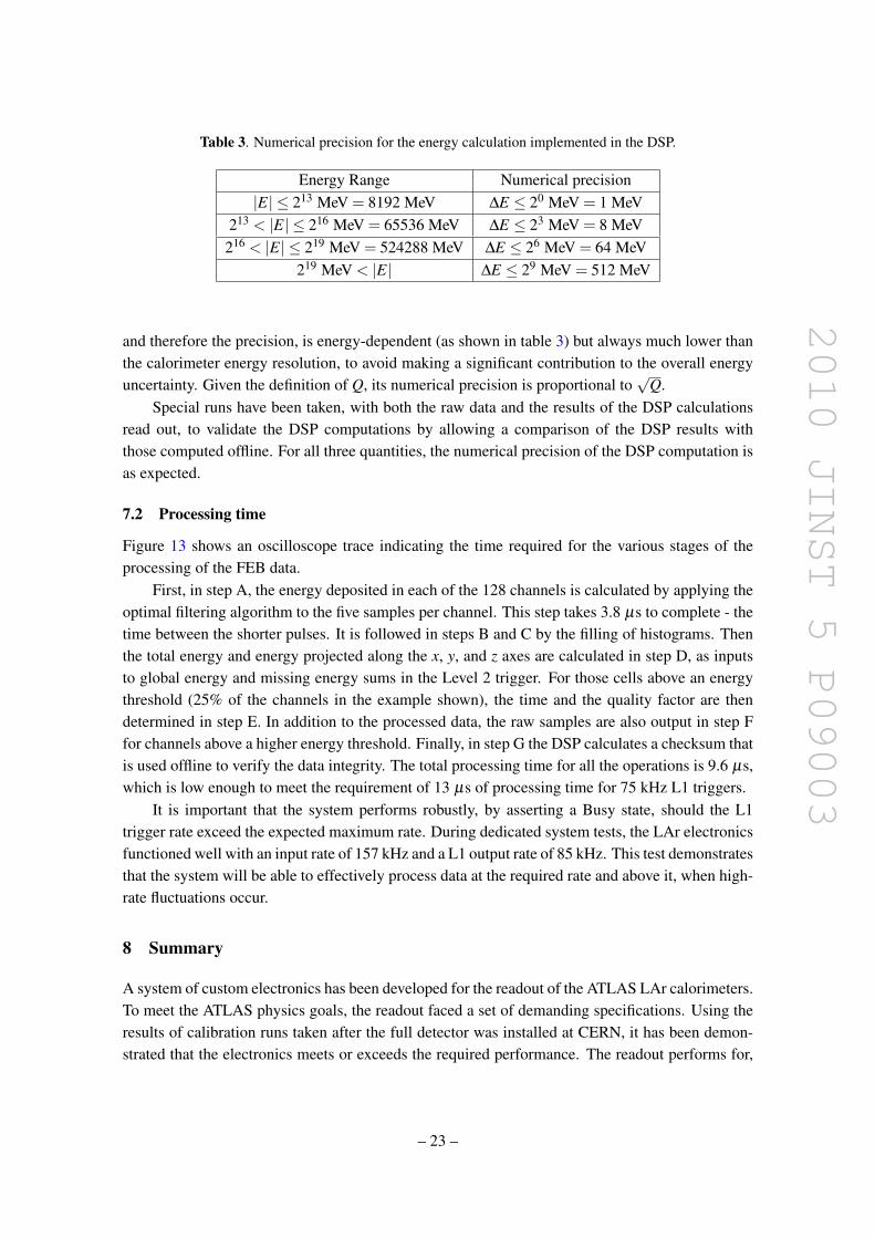
Table 3. Numerical precision for the energy calculation implemented in the DSP.

Energy Range Numerical precision|E| ≤ 213 MeV = 8192 MeV ∆E ≤ 20 MeV = 1 MeV

213 < |E| ≤ 216 MeV = 65536 MeV ∆E ≤ 23 MeV = 8 MeV216 < |E| ≤ 219 MeV = 524288 MeV ∆E ≤ 26 MeV = 64 MeV

219 MeV < |E| ∆E ≤ 29 MeV = 512 MeV

and therefore the precision, is energy-dependent (as shown in table 3) but always much lower thanthe calorimeter energy resolution, to avoid making a significant contribution to the overall energyuncertainty. Given the definition of Q, its numerical precision is proportional to

√Q.

Special runs have been taken, with both the raw data and the results of the DSP calculationsread out, to validate the DSP computations by allowing a comparison of the DSP results withthose computed offline. For all three quantities, the numerical precision of the DSP computation isas expected.

7.2 Processing time

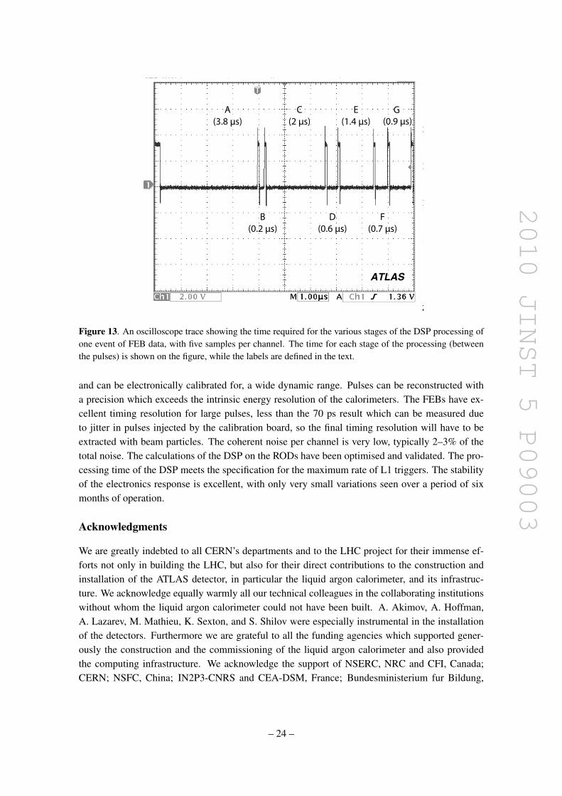
Figure 13 shows an oscilloscope trace indicating the time required for the various stages of theprocessing of the FEB data.

First, in step A, the energy deposited in each of the 128 channels is calculated by applying theoptimal filtering algorithm to the five samples per channel. This step takes 3.8 µs to complete - thetime between the shorter pulses. It is followed in steps B and C by the filling of histograms. Thenthe total energy and energy projected along the x, y, and z axes are calculated in step D, as inputsto global energy and missing energy sums in the Level 2 trigger. For those cells above an energythreshold (25% of the channels in the example shown), the time and the quality factor are thendetermined in step E. In addition to the processed data, the raw samples are also output in step Ffor channels above a higher energy threshold. Finally, in step G the DSP calculates a checksum thatis used offline to verify the data integrity. The total processing time for all the operations is 9.6 µs,which is low enough to meet the requirement of 13 µs of processing time for 75 kHz L1 triggers.

It is important that the system performs robustly, by asserting a Busy state, should the L1trigger rate exceed the expected maximum rate. During dedicated system tests, the LAr electronicsfunctioned well with an input rate of 157 kHz and a L1 output rate of 85 kHz. This test demonstratesthat the system will be able to effectively process data at the required rate and above it, when high-rate fluctuations occur.

8 Summary

A system of custom electronics has been developed for the readout of the ATLAS LAr calorimeters.To meet the ATLAS physics goals, the readout faced a set of demanding specifications. Using theresults of calibration runs taken after the full detector was installed at CERN, it has been demon-strated that the electronics meets or exceeds the required performance. The readout performs for,

– 23 –

2010 JINST 5 P09003

A(3.8 μs)

C(2 μs)

B(0.2 μs)

D(0.6 μs)

E(1.4 μs)

F(0.7 μs)

G(0.9 μs)

ATLAS

Figure 13. An oscilloscope trace showing the time required for the various stages of the DSP processing ofone event of FEB data, with five samples per channel. The time for each stage of the processing (betweenthe pulses) is shown on the figure, while the labels are defined in the text.

and can be electronically calibrated for, a wide dynamic range. Pulses can be reconstructed witha precision which exceeds the intrinsic energy resolution of the calorimeters. The FEBs have ex-cellent timing resolution for large pulses, less than the 70 ps result which can be measured dueto jitter in pulses injected by the calibration board, so the final timing resolution will have to beextracted with beam particles. The coherent noise per channel is very low, typically 2–3% of thetotal noise. The calculations of the DSP on the RODs have been optimised and validated. The pro-cessing time of the DSP meets the specification for the maximum rate of L1 triggers. The stabilityof the electronics response is excellent, with only very small variations seen over a period of sixmonths of operation.

Acknowledgments

We are greatly indebted to all CERN’s departments and to the LHC project for their immense ef-forts not only in building the LHC, but also for their direct contributions to the construction andinstallation of the ATLAS detector, in particular the liquid argon calorimeter, and its infrastruc-ture. We acknowledge equally warmly all our technical colleagues in the collaborating institutionswithout whom the liquid argon calorimeter could not have been built. A. Akimov, A. Hoffman,A. Lazarev, M. Mathieu, K. Sexton, and S. Shilov were especially instrumental in the installationof the detectors. Furthermore we are grateful to all the funding agencies which supported gener-ously the construction and the commissioning of the liquid argon calorimeter and also providedthe computing infrastructure. We acknowledge the support of NSERC, NRC and CFI, Canada;CERN; NSFC, China; IN2P3-CNRS and CEA-DSM, France; Bundesministerium fur Bildung,

– 24 –

2010 JINST 5 P09003

Wissenschaft, Forschung Technologie under contracts including number 05HA8EX16 (Wupper-tal), Germany; INFN, Italy; CNRST, Morocco; Ministry of Education and Science and Innova-tions, and Russian Federal Agency of Atomic Energy; JINR; Slovak Grant Agency of the Ministryof Education of the Slovak Republic and the Slovak Academy of Sciences, Project No. 2/0061/08;Ministerio de Educacion y Ciencia, Spain; The Swedish Research Council, The Knut and AliceWallenberg Foundation, Sweden; Swiss National Science Foundation, and Canton of Bern andGeneva, Switzerland; National Science Council, Taiwan; Department of Energy and National Sci-ence Foundation, United States of America.

References

[1] ATLAS collaboration, G. Aad et al., The ATLAS Experiment at the CERN Large Hadron Collider,2008 JINST 3 S08003.

[2] L. Evans and P. Bryant (eds.), LHC Machine, 2008 JINST 3 S08001.

[3] ATLAS collaboration, G. Aad et al., Readiness of the ATLAS Liquid Argon Calorimeter for LHCCollisions, arXiv:0912.2642, accepted for publication by Eur. Phys. J C.

[4] N.J. Buchanan et al., ATLAS liquid argon calorimeter front end electronics, 2008 JINST 3 P09003.

[5] LIQUID ARGON BACK END ELECTRONICS collaboration, A. Bazan et al., ATLAS liquid argoncalorimeter back end electronics, 2007 JINST 2 P06002.

[6] N.J. Buchanan et al., Design and implementation of the Front End Board for the readout of theATLAS liquid argon calorimeters, 2008 JINST 3 P03004.

[7] J. Colas et al., Electronics calibration board for the ATLAS liquid argon calorimeters, Nucl. Instrum.Meth. A 593 (2008) 269.

[8] N.J. Buchanan et al., Radiation qualification of the front-end electronics for the readout of the ATLASliquid argon calorimeters, 2008 JINST 3 P10005.

[9] J. Ban et al., Radiation hardness tests of GaAs amplifiers operated in liquid argon in the ATLAScalorimeter, Nucl. Instrum. Meth. A 594 (2008) 389.

[10] C. Boulahouache et al., The ATLAS LAr calorimeter Level 1 trigger signal pre-processing system:Installation, commissioning and calibration results, accepted for publication in IEEE Trans. Nucl.Sci.

[11] J. Ban et al., Cold electronics for the liquid argon hadronic end-cap calorimeter of ATLAS, Nucl.Instrum. Meth. A 556 (2006) 158;E. Ladygin et al., Preshaper for the hadronic endcap calorimeter, available athttps://edms.cern.ch/document/875444/1.

[12] W.E. Cleland and E.G. Stern, Signal processing considerations for liquid ionization calorimeters in ahigh rate environment, Nucl. Instrum. Meth. A 338 (1994) 467.

[13] M. Aleksa et al., ATLAS combined testbeam: computation and validation of the electronic calibrationconstants for the electromagnetic calorimeter, ATL-LARG-PUB-2006-003,available athttp://cdsweb.cern.ch/record/942528.

[14] D. Banfi, M. Delmastro and M. Fanti, Cell response equalisation of the ATLAS electromagneticcalorimeter without the direct knowledge of the ionisation signals, 2006 JINST 1 P08001.

– 25 –

2010 JINST 5 P09003

[15] C. Collard et al., Prediction of signal amplitude and shape for the ATLAS electromagneticcalorimeter, ATL-LARG-PUB-2007-010, available athttp://cdsweb.cern.ch/record/1058294.

[16] ATLAS collaboration, G. Aad et al., Drift Time Measurement in the ATLAS Liquid ArgonElectromagnetic Calorimeter using Cosmic Muons, arXiv:1002.4189.

[17] B. Chase et al., Characterization of the coherent noise, electromagnetic compatibility andelectromagnetic interference of the ATLAS EM calorimeter front end board, in Proceedings of the 5thWorkshop on Electronics for the LHC Experiments (LEB 99), Snowmass, U.S.A., September 1999,pg. 222-226.

[18] G. Blanchot et al., Electromagnetic compatibility of a DC power distribution system for the ATLASliquid argon calorimeter, in Proceedings of the 11th Workshop on Electronics for LHC and FutureExperiments (LECC 2005), Heidelberg, Germany, September 2005.

[19] ATLAS ELECTROMAGNETIC BARREL CALORIMETER collaboration, M. Aharrouche et al., Energylinearity and resolution of the ATLAS electromagnetic barrel calorimeter in an electron test- beam,Nucl. Instrum. Meth. A 568 (2006) 601.

[20] ATLAS collaboration, ATLAS detector and physics performance technical design report,CERN-LHCC-99-014/015 (1999), available athttp://atlasinfo.cern.ch/Atlas/GROUPS/PHYSICS/TDR/access.html.

[21] M. Aharrouche et al., Time resolution of the ATLAS barrel liquid argon electromagnetic calorimeter,Nucl. Instrum. Meth. A 597 (2008) 178.

[22] J. Christiansen, A. Marchioro, P. Moreira and A. Sancho, Receiver ASIC for timing, trigger andcontrol distribution in LHC experiments, IEEE Trans. Nucl. Sci. 43 (1996) 1773.

[23] Data sheet for the quartz crystal phase-locked loop (QPLL), available athttp://proj-qpll.web.cern.ch/proj-qpll/.

– 26 –