performance evaluation of trajectory queries on multiprocessor and cluster

Jan Zizka et al. (Eds) : CCSEIT, AIAP, DMDB, MoWiN, CoSIT, CRIS, SIGL, ICBB, CNSA-2016 pp. 145–163, 2016. © CS & IT-CSCP 2016 DOI : 10.5121/csit.2016.60612

PERFORMANCE EVALUATION OF

TRAJECTORY QUERIES ON MULTIPROCESSOR AND CLUSTER

Christine Niyizamwiyitira and Lars Lundberg

Department of Computer Science and Engineering, Blekinge Institute of Technology SE-37179 Karlskrona, Sweden

[email protected], [email protected]

ABSTRACT

In this study, we evaluate the performance of trajectory queries that are handled by Cassandra,

MongoDB, and PostgreSQL. The evaluation is conducted on a multiprocessor and a cluster.

Telecommunication companies collect a lot of data from their mobile users. These data must be

analysed in order to support business decisions, such as infrastructure planning. The optimal

choice of hardware platform and database can be different from a query to another. We use data

collected from Telenor Sverige, a telecommunication company that operates in Sweden. These

data are collected every five minutes for an entire week in a medium sized city. The execution

time results show that Cassandra performs much better than MongoDB and PostgreSQL for

queries that do not have spatial features. Statio’s Cassandra Lucene index incorporates a

geospatial index into Cassandra, thus making Cassandra to perform similarly as MongoDB to

handle spatial queries. In four use cases, namely, distance query, k-nearest neigbhor query,

range query, and region query, Cassandra performs much better than MongoDB and

PostgreSQL for two cases, namely range query and region query. The scalability is also good for

these two use cases.

KEYWORDS

Databases evaluation, Trajectory queries, Multiprocessor and cluster, NoSQL database,

Cassandra, MongoDB, PostgreSQL.

1. INTRODUCTION

Large scale organisations continuously generate data at very high speeds. These data are often complex and heterogeneous, and data analysis is a high priority. The challenges include what technology in terms of software and hardware to use in order to handle data efficiently. The analysis is needed in different fields such as transportation optimization, different business analytics for telecommunication companies that seek to know common patterns from their mobile users.

146 Computer Science & Information Technology (CS & IT)

The analysis comprises querying some points of interests in big data sets. Querying big data can be time consuming and expensive without the right software and hardware. In this paper, various databases were proposed to analyse such data. However, there is no single database that fits all queries. The same holds for hardware infrastructure there is no single hardware platform that fits all databases. We consider a case of trajectory data of a telecommunication company where analysing large data volumes trajectory data of mobile users becomes very important. We evaluate the performance of trajectory queries in order to contribute to business decision support systems. Trajectory data represents information that describes the localization of the user in time and space. In the context of this paper, a telecommunication company wants to optimize the use of cell antennas and localize different points of interests in order to expand its business. In order to successfully process trajectory data, it requires a proper choice of databases and hardware that efficiently respond to different queries. We use trajectory data that are collected from Telenor Sverige (a telecommunication company that operates in Sweden). Mobile users' position is tracked every five minutes for the entire week (Monday to Sunday) from a medium size city. We are interested to know how mobile users move around the city during the hour, day, and the week. This will give insights about typical behavior in certain area at certain time. We expect periodic movement in some areas, e.g., at the location of stores, restaurants’ location during lunch time. Without loss of generality, we define queries that return points of interests such as nearest cell location from a certain position of a mobile user. The contribution of this study is to solve business complex problem that is,

• Define queries that optimize the point of interests, e.g., nearest point of interest, the most visited place at a certain time, and more.

• Choice of database technology to use for different types of query. • Choice of hardware infrastructure to use for each of the databases.

This data is modelled as spatio-temporal data where at a given time � a mobile user is located at a position (�, �). The location of a mobile user is a triples (�, �, �) such that user’s position is represented as a spatial-temporal point �� with �� = (��, �� , ��). By optimizing points of interests, different types of queries are proposed. They differ in terms of what are their input and output: • Distance query which finds points of interests that are located in equal or less than a distance,

e.g., one kilometer from a certain position of a mobile user.

• K-Nearest neighbor query that finds K nearest points of interests from a certain position of a mobile user.

• Range query that finds points of interests within a space range from a certain position of a

mobile user.

Computer Science & Information Technology (CS & IT) 147

• Region query that finds the region that a mobile user frequently passes through at certain time throughout the week.

The performance of different queries is evaluated on three open sources databases; Cassandra, MongoDB, and PostgreSQL. We choose to use open source databases for the sake of allowing the study reproducibility. The hardware configuration is done on a single node, and on multiple nodes (distributed) in a cluster. The execution time of each of the queries at each database on different hardware infrastructure is measured. Since the company knows the locations that are the most, or the least visited during a certain time, in order to avoid overloading and underloading at such locations, antenna planning will be updated accordingly. For business expansion, a busy location during lunch time is for e.g., convenient for putting up a restaurant. Moreover, the performance measurement shows which database is better for which specific query on which hardware infrastructure, thus contributing to business support systems. The rest of the paper is organized as follows; Section 2 defines the concepts, Section 3 summarizes the related work, Section 4 describes the configuration and gives the databases overview, Section 5 presents results and discussions, finally Section 6 draws conclusions.

2. TRAJECTORY DATA

2.1 Definition of Trajectory

Trajectory is a function from a temporal domain to a range of spatial values, i.e., it has a beginning time and an ending time during which a space has been travelled (see Equation 1)[1].

�� → �� (1)

A complete trajectory is characterized by a list of triples � = (�, �, �), thus a trajectory is defined as a sequence of positions Ʈ��.

Ʈ�� = ��, ��, … , �� (2)

where �� = (��, �� , ��) represents a spatio-temporal point, Figure 1 shows such trajectory.

Figure 1. Mobile user’s trajectory as a sequence of triples


In this study, the trajectory data has space extent that is represented by latitude and longitude. With � represents latitude and � represents longitude, and the time that is represented by �; i.e., a mobile user is located at position (�, �) at time � 2.2. Definition of Trajectory Queries

Trajectories queries are historical spatio-temporal data which are the foundation of many applications such as traffic analysis, mobile user’s behavior, and many others [2], [3]. Trajectories queries make analytics possible, e.g., mobile users’ positions at a certain time. In the context of location optimization, common trajectory queries that we consider in this study are following; Distance query, Nearest neighbor query, Range query, and Region query. Figure 2 describes query types, where �� represents different cell-city names, each �� is represented by (��, ��) where �� is latitude and �� is longitude. Distance query returns cell-cities that are located at a distance from ��, e.g., within distance L from the position of ��. The query returns ��, � , �!, �". At a given fixed time or time interval, we are retrieving two cell-cities that are the most close to city ��, that is K-NN query with # = 2. Given a space range[&, '], range query returns the cell-cities that belong to that space range. Region query returns the cell-city that a given user frequently visits. e.g., user Bob passes mostly through cell-city �) (see Figure 2).

Figure 2. Visualization for Query Types

2.2.1. Distance Query

Definition: Distance query returns all point of interest (e.g., gas stations) whose distance (according to a distance metric) from a given position that is less than a threshold [2], [3]. Figure 3 shows inputs to distance query.


Figure 1. Distance Query

Example: find cells that are located in less than 1km from a certain mobile user’s position. In terms of latitude and longitude coordinates, a query that covers the circle of 10 km radius from a user position at (��, ��) = (1.3963, −0.6981) is expressed for different databases as follows;

• In Cassandra

2'3'�4 cell_city 5678 9:;<=<�� >?'6' ��@(<AB:_<AD��, ′�B<=��@: ��: ";::=��A", 9G��: [��: "H�:_D<��A��", B<�=D:place, =��<�GD�: 1.3963, =:AH<�GD�:

− 0.6981, 9��_D<��A��: "10#9"� ] ��′)

• In MongoDB

D;. 8:;<=<��. B<AD ( � =:��<:A ∶ � $A��@∶ [−0.6981, 1.3963], $9��K<��A��: 10 � �, ��==_�L4M: 1�)

• In PostgreSQL

2'3'�4 ��==_�<�� 5678 8:;<=<�� >?'6' arccos (sinU��V ∗ sin(�) + cosU��)V ∗ cos (�) ∗ cos (� − (��))) ∗ 6 <= 10 ; (3)

With 6 is the radius of earth, 6 = 6371 km

In order to index latitude and longitude columns so that the database understand the query, the circle of radius 10 km is bounded by a minimum and a maximum coordinates, let’s say �[�� =(�[�� , �[��) and �[\] = (�[\] , �[\]), then query (3) becomes as follows;

2'3'�4 ��==_�<�� 5678 9:;<=<�� >?'6' (� => �[�� _`K � ≤ �[\]) _`K (� >= �[�� _`K � <= �[\]) _`K

�@��:�(�<A(��) ∗ �<A(�) + �:�(��) ∗ �:�(�) ∗ �:�(� − (��))) <= @ ;

With @ is the angular radius of the query circle, @ = D<��A��/��@�ℎ @�D<G� �[�� = � − @ �[\] = � + @ �[�� = � − ∆� �[\] = � + ∆� ∆� = arccos( ( cos(@) − sin(�e) ∗ sin(�) ) / ( cos(�e) ∗ cos(�) ) )

With �e = arcsin(sin(�)/cos(@). More on positions’ angles calculation is found in [4].


2.2.2. k Nearest Neighbor Query

Definition: k-Nearest Neighbor (KNN) Query returns k points of interest which are the closest to a given position (�, �) [5], [6]; and k results are ordered by proximity. KNN can be bounded with a distance, in that case, KNN behaves like a distance query, if k is not indicated. Figure 4 shows inputs to kNN query, where kNN is bounded within a distance.

Figure 4. kNN query

Example: find five nearest cells from a mobile user’s position. A typical query that select 5 nearest cells within 10 km is as follows;

• In Cassandra

2'3'�4 cell_city 5678 8:;<=<�� >?'6' ��@(<AB:_<AD��, ′� B<=��@ ∶ ��: ";::=��A", 9G��: [��: "H�:_D<��A��",

B<�=D: "�=��", =��<�GD�: 1.3963, =:AH<�GD�: − 0.6981, 9��_D<��A��: "10#9"� ] ��′) 3L8L4 5 • In MongoDB

D;. 8:;<=<��. B<AD( � =:��<:A ∶ � $A��@ ∶ [ −0.6981, 1.3963], $9��K<��A��: 0.10 � �, �cell_city: 1�). =<9<�(5)

• In PostgreSQL

2'3'�4 ��==_�<�� 5678 9:;<=<�� >?'6' (� => �[�� _`K � ≤ �[\]) _`K (� >= �[�� _`K � <

= �[\]) _`K�@��:� g�<AU��V ∗ �<A(�) + �:�U��V ∗ �:�(�)∗ �:� h� − U��Vij ≤ @ 76K'6 &M � _2�, � _2� 3L8L4 5

2.2.3. Range Query

Definition: Range query returns all point of interest (e.g., gas stations) that are located within a certain space shape (polygon) [2]. Figure 5 shows inputs to range query to find cells that belong to a polygon.


Figure 2. Range query

Example: find cells within a space range that is indicated by a polygon from a mobile user position [longitude, Latitude] coordinates. A typical query that select cells that are located within a geographical bounding box (polygon shape), e. g, a triangle from a mobile user position coordinates: [ 12.300398, 57.569256] within ([ 11.300398, 56.569256 ], [12.300398, 58.569256 ]) is as follows;

• In Cassandra

2'3'�4 cell_city 5678 8:;<=<�� >?'6' ��@(<AB:_<AD��, ′� B<=��@ ∶ ��: ";::=��A", 9G��: [��: "H�:_;;:�", B<�=D: "�=��",

9<A_=��<�GD�: 11.300398, 9��_=��<�GD�: 12.300398 9<A_=:AH<�GD�: 56.569256, 9��_=:AH<�GD�: 58.569256 � ] ��′) • In mongoDB

D;. 8:;<=<��. B<AD (� =:��<:A ∶ � $H�:><�ℎ<A: � $�:=�H:A: [ [ 12.300398, 57.569256], [ 11.300398, 56.569256 ],

[12.300398, 58.569256 ] ] ��, ��==_�<��) • PostgreSQL

The following is a typical query range query between two points �[�� = (�[��, �[��) and �[\] = (�[\], �[\]) with � is latitude and y is longitude. Example: �[�� = (1.2393, −1.8184) and �[\] = (1.5532, 0.4221).

2'3'�4 ��==_�<�� 5678 9:;<=<�� >?'6' (� => 1.2393 _`K � ≤ 1.5532) _`K (� >= −1.8184 _`K � <= 0.4221)

2.2.4. Region Query

Generally, trajectories of mobile users are independent each other, however, they contain common behavior traits such as passing through a region at a certain regular period, e.g., passing through the shopping center during lunch time. Definition: identify the region which is more likely to be passed by a given user at a certain time based on the many other relevant regions to that user [2]. In the context of this study, the knowledge about region reveals which cell city that many users mostly pass by, this cell city might have some point of interests such as stores, high way junction. Figure 6 shows inputs to region query to find cell city that is the most visited at certain time.


Figure 3. Region query

Example: find the cell city that is frequently passed by the same mobile users during a certain time every day for the entire week. A typical query that returns the cell city that is the most visited during interval [12: 10: 00,13: 10: 00] is as follows;

• In Cassandra

2'3'�4 KL24L`�4 cell_city 5678 8:;<=<�� pℎ�@� 4<9� = ′12: 10: 00′ �AD 4<9� <= ′13: 10: 00′ r67st ;� cell_city O6K'6 &M "�:GA�" K'2�

• In MongoDB

D;. 8:;<=<��. B<AD( �4<9�: �$H�: ′12: 10: 00′, $=�: ′13: 10: 00′��,

�cell_city: 1� ). D<��<A��(). �:GA�()

• In PostgreSQL

2'3'�4 cell_city, �:GA�(∗) B@:9 9:;<=<�� >?'6' � ≥ 12: 10: 00 �AD �

≤ 13: 10: 00 r67st ;� cell_city O6K'6 &M "�:GA�" K'2�

3. RELATED WORK

In [7], authors propose an approach and implementation of spatio-temporal database systems. This approach treats time-changing geometries, whether they change in discrete or continuous steps. The same can be used to tackle spatio-temporal data in the other databases. We rather evaluate trajectory queries on existing general purpose databases notably Cassandra, PostgreSQL, and MongoDB. In [8], author describes requirements for database that support location based-service for spatio-temporal data. A list of ten representative queries for stationary and moving reference objects are proposed. Some of those queries that are related to this study are given in section two. In [9], Dieter studied trajectory moving point object, he explained three scenarios, namely constrained movement, unconstraint movement and movement in networks. Different techniques to index and to query these scenarios define their respective processing performance. Author modelled the trajectory as triples (x,y,t), we use the same model in this study. In [10], authors introduced querying moving objects (trajectory) in SECONDO, the latter is a DBMS prototyping environment particularly geared for extension by algebra modules for nonstandard applications. The querying is done using SQL-like language. In our study, we are querying moving object using SQL and Not Only SQL (NoSQL) querying languages on top of different databases. Continuously, authors provide a benchmark on range queries and nearest


neighbor queries on SECONDO DBMS for moving data object in Berlin. The moving object data was generated using computer simulation based on the map of Berlin [11]. This benchmark could be extended to other queries such as region queries, distance queries, and so on. In our study, we apply these queries on real world trajectory data, i.e., mobile users’ trajectory from Telenor Sverige. In [5], authors introduced a new type of query Reverse Nearest Neighbor (RNN) which is the opposite to Nearest Neighbor (NN). RNN can be useful in applications where moving objects agree to provide some kind of service to each other, whenever a service is need it is requested from the nearest neighbor. An object knows objects that it will serve in the future using RNN. RNN and NN are relatively represented by distance query in our study. In [12], authors studied aggregate query language over GIS and no-spatial data stored in a data warehouse. In [13], authors studied k-nearest search algorithm for historical moving object trajectories, this k-nearest neighbor is one of the queries that is considered in our study. In [14], authors presents techniques for indexing and querying moving object trajectories. This data is represented as three dimension (3D) space, where two dimensions correspond to space and one dimension corresponds to time. We also represent our data in 3D as (x,y,t), with x,y represents space whereas t represents time. Query processing on multiprocessor has been studied in [15], authors implemented an emulator of parallel DBMS that uses cluster with multiprocessor. This study is different from ours in a sense that we evaluate query processing on real physical hardware with existing general purpose databases. Query processing on FPGA and GPU on spatial-temporal data was studied in [16]. Authors present a FPGA and GPU implementation that process complex queries in parallel, the study did not investigate the performance on various existing databases, the distributed environment was not also considered, whereas, in our study we investigate query processing on various databases on top of different computational platforms including cluster. In [17], authors conducted a survey on mining massive-scale spatio-temporal trajectory data based on parallel computing platforms such as GPU, MapReduce and FPGA, again existing general purpose databases were not evaluated. Authors presented a hardware implementation for converting geohash codes to and from longitude/latitude pairs for Spatio-temporal data [18], the study shows that longitude and latitude coordinates are the key points for modelling spatio-temporal data. In our paper, we also use these coordinates for location based querying.

4. DATABASE OVERVIEW AND CONFIGURATION

The development of technology involves big data that is structured and unstructured. The presence of unstructured data stimulates the invention of new databases, since Relational Database Management Systems (RDBMS) that uses Structured Query Language (SQL) to deal with structured data only becomes unable to handle unstructured data. A new data model, Not Only SQL (NoSQL) was introduced to deal also with unstructured data [19]. Main features of NoSQL follow CAP theorem (Consistency, Availability, and Partition tolerance). The core idea of CAP is that a distributed system cannot meet the three distinct needs simultaneously. According to data models, NoSQL can be relational, key value based, column based, and document based. In this study we choose three open source databases that have diverse features of SQL (PostgreSQL) and NoSQL (Cassandra and MongoDB).


Key value data model means that a value corresponds to a key, column based uses tables as the data model, the data is stored by column, each column is the index of the database, queries are applied to column, whereby each column is treated one by one. Document based database stores in JSON or XML format, each document (similar to a row in RDBMS) is indexed and it has a key. 4.1. Cassandra Apache Cassandra is an open-source NoSQL column based database. It is a top level Apache project born at Facebook and built on Amazon’s Dynamo and Google’s BigTable. It is a distributed database for managing large amounts of structured data across many commodity servers, while providing highly available service and no single point of failure. In CAP, Cassandra has availability and partition tolerance (AP) with eventual consistency. Cassandra offers continuous availability, linear scale performance, operational simplicity and easy data distribution across multiple data centers and cloud availability zones. Cassandra has a masterless ring architecture [23]. Keyspace is similar to database in RDBMS, inside keyspace there are tables which are similar to tables in RDBMS, column and rows are similar to those of RDBMS’ tables. The querying language is Cassandra Query Language (CQL) is almost similar to SQL in RDBMS [24]. 4.2. MongoDB MongoDB is an open-source NoSQL document database, MongoDB is written in C++. MongoDB has database, inside a database there are collections, these are like table in RDBMS, Inside a collection there are documents, these are like a tuple/row in RDBMS, and inside a document there are fields which are like column in RDBMS [21], [22]. MongoDB is consistent and partition tolerant. 4.3. PostgreSQL PostgreSQL is an open source Object RDBMS that has two features according to CAP theorem, those are availability, i.e., each user can always read and write. PostgreSQL consists of consistency, i.e., all users have the same view of data. PostgreSQL organises data in column and rows [20, p. 3]. 4.4. Single Node Installation

Two types of server are used, 1. Hardware type 1: Dell powerEdge R320 Operating system: Ubuntu 14.04.3 LTS x86_64 RAM memory: 23 GB RAM Harddisk size: 279.4GB 0 disk Processor (Intel(R) Xeon(R) CPU E5-2420 v2) has 12 cores, each core is hyperthreaded into 2 cores, this give 24 virtual cores. These servers are exclusive, i.e., they are only running our databases.

2. Hardware type2: Fujitsu RX600S5 Operating system: Ubuntu 13.04 LTS X86_64 The RAM memory: 1024 GB.


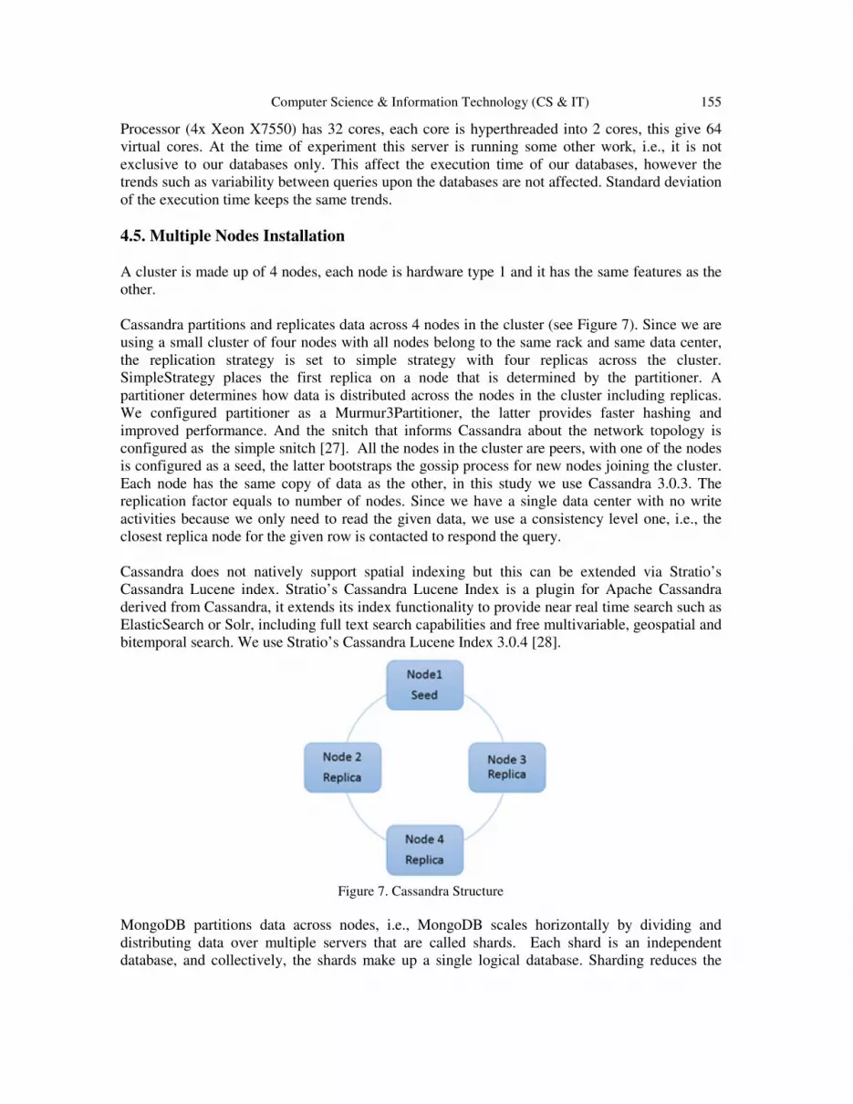
Processor (4x Xeon X7550) has 32 cores, each core is hyperthreaded into 2 cores, this give 64 virtual cores. At the time of experiment this server is running some other work, i.e., it is not exclusive to our databases only. This affect the execution time of our databases, however the trends such as variability between queries upon the databases are not affected. Standard deviation of the execution time keeps the same trends. 4.5. Multiple Nodes Installation A cluster is made up of 4 nodes, each node is hardware type 1 and it has the same features as the other. Cassandra partitions and replicates data across 4 nodes in the cluster (see Figure 7). Since we are using a small cluster of four nodes with all nodes belong to the same rack and same data center, the replication strategy is set to simple strategy with four replicas across the cluster. SimpleStrategy places the first replica on a node that is determined by the partitioner. A partitioner determines how data is distributed across the nodes in the cluster including replicas. We configured partitioner as a Murmur3Partitioner, the latter provides faster hashing and improved performance. And the snitch that informs Cassandra about the network topology is configured as the simple snitch [27]. All the nodes in the cluster are peers, with one of the nodes is configured as a seed, the latter bootstraps the gossip process for new nodes joining the cluster. Each node has the same copy of data as the other, in this study we use Cassandra 3.0.3. The replication factor equals to number of nodes. Since we have a single data center with no write activities because we only need to read the given data, we use a consistency level one, i.e., the closest replica node for the given row is contacted to respond the query. Cassandra does not natively support spatial indexing but this can be extended via Stratio’s Cassandra Lucene index. Stratio’s Cassandra Lucene Index is a plugin for Apache Cassandra derived from Cassandra, it extends its index functionality to provide near real time search such as ElasticSearch or Solr, including full text search capabilities and free multivariable, geospatial and bitemporal search. We use Stratio’s Cassandra Lucene Index 3.0.4 [28].

Figure 7. Cassandra Structure

MongoDB partitions data across nodes, i.e., MongoDB scales horizontally by dividing and distributing data over multiple servers that are called shards. Each shard is an independent database, and collectively, the shards make up a single logical database. Sharding reduces the


number of operations each shard handles. Each shard processes fewer operations as the cluster grows. As a result, a cluster can increase capacity and throughput horizontally (by adding nodes in the cluster). Sharding reduces the amount of data that each server needs to store. Each shard stores less data as the cluster grows [26]. Sharded cluster (contains shards, config servers and mongos instances). We use three shards, each on a node. In Figure 8, we see config servers that holds the metadata about the cluster such as the shard location of the data, they must be three servers. There is also Mongos server that serves as the routing service that process queries throughout the cluster. Mongos is installed on its own node, whereas config servers and shards are installed on the same nodes (1, 2, 3) as it shown in the Figure 8. Since we have three shards, each shard contains a third of the total data. Mongo will be eventually available if we replicate each shard on different nodes. In this study we install MongoDB 3.0.9. MongoDB has built in spatial query functions.

Figure 4. MongoDB Structure

Figure 5. PostgreSQL Structure

PostgreSQL is installed on the cluster in master/ slave replication mode (see Figure 9). Nodes serve each other in pool using pgpool2 [25]. Pgpool 2 provides, load balancing and data redundancy. In order to keep available the data, each slave holds a copy of data and it is read-only, there are three slaves, thus three replicas. Whereas in order to keep the consistency of the, only the master can read and write. Master and pgpool 2 are installed on the same node. In this


study we install PostgreSQL version 9.3.11. PostgreSQL does not have explicit spatial query functions, thus, we have to use mathematical functions in order to query the database using geographical coordinates. 4.6. Data Description The mobility or location update is generated when a handset is generating traffic either downloading or uploading. Mobility is captured in five minutes intervals and include all cells during those five minutes. Mobility is indicated by number of cells within timeframe and the distance between those cells. The data we use in this paper is collected every five minutes for the entire week in a small medium size city. We have a collection of two millions five hundred ninety three thousands three hundred sixty records (2,593,360) for different users. Every record has eighteen attributes (18 x 2,593,360). Those attributes are; UserId, SiteId, weekday, Time, ProfileId, SegmentId, SourceGSM, SourceUMTS, SourceLTE, Easting, Northing, Latitude decimal, Longitude decimal, Cell municipality, Cell county, Cell city, Cell postcode, Cell address. This data is populated in Cassandra and PostgreSQL without any transformation. Whereas, in MongoDB, coordinates attributes (latitude and longitude) were combined into an array location attribute in order to be able to use built in spatial function in MongoDB.

5. RESULTS AND DISCUSSION

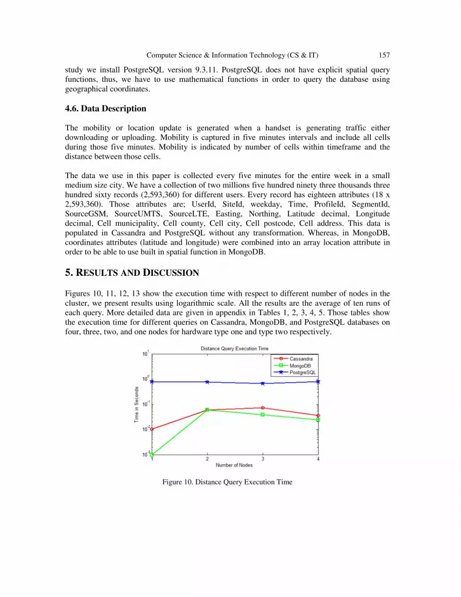
Figures 10, 11, 12, 13 show the execution time with respect to different number of nodes in the cluster, we present results using logarithmic scale. All the results are the average of ten runs of each query. More detailed data are given in appendix in Tables 1, 2, 3, 4, 5. Those tables show the execution time for different queries on Cassandra, MongoDB, and PostgreSQL databases on four, three, two, and one nodes for hardware type one and type two respectively.

Figure 10. Distance Query Execution Time


Figure 6. K nearest Neighbor Query Execution Time

Figure 7. Range Query Execution Time

Figure 13. Region Query Execution Time


It is observed that Cassandra has the shortest execution time for range and region queries, particularly for region query. Region query has one input which is time, it does not involve spatial features or geographical shapes, e.g., sphere, near, within. It is clear that Cassandra outperforms much better than MongoDB and PostgreSQL for general purpose queries. E.g., Region query involves time only as input. For queries that contain geographical or specific spatial features, MongoDB seems to perform almost as Cassandra when the latter is indexed by Stratio Lucene Index (see Figure 10, 11, 12). In figure 13, MongoDB has longer execution than Cassandra and PostgreSQL for region query, this is caused by aggregation query process which seems to be slower in MongoDB. In all queries, when we run a query for the first time, we observed that for Cassandra, it takes longer than the next runs. We have to mention that Lucene makes a huge use of caching, therefore the first query will be especially slow due to the cost of initializing caches [26]. Thus, we disregard the first run of each query when measuring the performance. Whereas for MongoDB and PostgreSQL the same query on the same hardware, runs almost with relatively same execution time. Spatial queries have the longest execution time in PostgreSQL, the reason is that we have to use mathematical functions to represent geographical locations. This involves different steps of calculation, thus, making it longer (see Figure 10, 11, 12). The scalability according to increase of number of nodes is significant for Cassandra and MongoDB for range query. The reason is that the range query involves a partition of the data according to range specification, hence the cache is relatively not overloaded. Whereas the scalability is not very noticed for the other queries which covers the whole data, thus consuming much cache which results in slowing the execution time. In terms of processing, PostgreSQL does not exploit the increase of number of nodes, since nodes are used for replication purposes in order to keep the database available. MongoDB distributes data across shards, in order to provide high availability, we need to replicate each shard on its own server, e.g., in our case we have three shards, in order to have a second copy of the whole data, we need three more servers, in total we need 6 servers for 2 copies. However, for Cassandra, since we have a full copy of data at each node, i.e., for 4 nodes cluster we have 4 copies of data. This feature makes Cassandra to be attractive than MongoDB in cases where a number of servers is a constraints. Furthermore if Mongos fails, the whole database fails, the same holds for PostgreSQL, if the master goes down, the whole database cannot operate anymore. Whereas, for Cassandra, if any node goes down, others keep working.

6. CONCLUSIONS In this study, we evaluated the performance of trajectory queries on Cassandra, MongoDB, and PostgreSQL on Multiprocessor and cluster environment. The evaluation is conducted on data collected from a Telecommunication Company. We observed that Cassandra performs much better than MongoDB and PostgreSQL to handle queries that do not contain special geographical features such as sphere shape, near coordinates (example of region query that involves time as input). MongoDB has natively a built in function for spatial queries, this speeds up the query response time. In order to speed up Cassandra while handling spatial queries, we incorporate Stratio’s Cassandra Lucene Index which holds spatial indexes. This gives same performance as using MongoDB and even better for some queries. MongoDB seems to handle aggregate query slower than Cassandra and PostgreSQL (e.g., region query involves two steps of aggregation).


Since we are using open source databases, the choice of which database to use depends merely on the needs and preferences, for instance MongoDB is well documented comparing to Cassandra. MongoDB uses XML language that is understood by internet, thus if one would like to work with different data traffic over internet MongoDB is a good choice. From developer perspective, it is easier to implement and integrate plugins to Cassandra than MongoDB. Cassandra seems to be updated every couple of weeks, this tick-tock releases are not immediately compatible with some plugin as it is the case in this paper, we have to use Cassandra 3.0.3 in order to be able to use Stratio’s Cassandra Lucene Index 3.0.4, while at the moment, the current release is 3.4. One would choose to use PostgreSQL if relational database features is important to handle the data. In terms of servers, if there is a constraint of number of servers, Cassandra is more preferable since it economically uses a less number of servers comparing to what MongoDB will require to provide same features. APPENDIX In tables 1, 2, 3, 4, 5, E.time is the average execution time of ten runs, Stdev is the standard deviation.

Table 1. Query processing time (in seconds) on 4 nodes installation (Dell powerEdge R320)

Query types Cassandra MongoDB PostgreSQL

E. time Stdev E. time Stdev E. time Stdev

Distance Q 0.036 0.077 0.024 0.011 0.79 0.0005

K-n Neighbors Q 0.029 0.005 0.024 0.0107 0.881 0.015

Range Q 0.008 0.008 0.021 1.83E-18 0.621 0.001

Region Q 0.045 0.011 1.562 0.030 1.221 0.001

Table 2. Query processing time (in seconds) on 3 nodes installation (Dell powerEdge R320)



Distance Q 0.073 0.013 0.039 0.010 0.666 0.0005

K-n Neighbors Q 0.018 0.006 0.039 7.31E-18 0.886 0.015

Range Q 0.0130 0.024 0.04 0.011 0.666 0.001

Region Q 0.0515 0.021 1.593 0.030

1.222 0.001


Table 1. Query processing time (in seconds) on 2 nodes installation (Dell powerEdge R320).



Distance Q 0.060 0.008

0.059 0.011

0.766 0.0008

K-n Neighbors Q 0.031 0.025 0.059 0.017 0.822 0.0007

Range Q 0.0147 0.002

0.045 7.31E-18

0.611 0.0006

Region Q 0.0518 0.024 1.633 0.030 1.225 0.001

Table 4. Query processing time (in seconds) on a single node installation (Dell powerEdge R320).



Distance Q 0.017 0.076 0.001 2.2857E-19 0.789 0.0008

K-n Neighbors Q 0.012 0.007 0.001 2.29E-19 0.882 0.0007

Range Q 0.028 0.023

0.048 0.000422 0.621 0.0006

Region Q 0.054 0.019

2.526 0.066 1.225 0.0016

Table 5. Query processing time (in seconds) on a single node installation (Fujitsu RX600S5).



Distance Q 1.121 0.001 1.579 0.298

2.243 0.181

K-n Neighbors Q 1.012 0.012

1.432 0.089 2.363 0.001

Range Q 1.432 0.001

1.654 0.068

2.154 0.001

Region Q 2.132 0.002 4.260 0.257 3.268 0.0009

ACKNOWLEDGEMENTS This work is part of the research project "Scalable resource-efficient systems for big data analytics" funded by the Knowledge Foundation (grant: 20140032) in Sweden. We also thank HPI-FSOC, and Telenor Sverige. REFERENCES [1] S. Spaccapietra, C. Parent, M. L. Damiani, J. A. de Macedo, F. Porto, and C. Vangenot, “A

conceptual view on trajectories,” Data Knowl. Eng., vol. 65, no. 1, pp. 126–146, 2008. [2] Y. Zheng and X. Zhou, Computing with spatial trajectories. Springer Science & Business Media,

2011.


[3] N. Pelekis and Y. Theodoridis, Mobility data management and exploration. Springer, 2014. [4] Jan, philip Matuschek, “Finding Points Within a Distance of a Latitude/Longitude Using Bounding

Coordinates.” [Online]. Available: http://janmatuschek.de/LatitudeLongitudeBoundingCoordinates#SQLQueries. [Accessed: 07-Mar-2016].

[5] R. Benetis, C. S. Jensen, G. Karčiauskas, and S. Šaltenis, “Nearest neighbor and reverse nearest

neighbor queries for moving objects,” in Database Engineering and Applications Symposium, 2002. Proceedings. International, 2002, pp. 44–53.

[6] E. Frentzos, K. Gratsias, N. Pelekis, and Y. Theodoridis, “Nearest neighbor search on moving object

trajectories,” in Advances in Spatial and Temporal Databases, Springer, 2005, pp. 328–345. [7] M. Erwig, R. H. Gu, M. Schneider, M. Vazirgiannis, and others, “Spatio-temporal data types: An

approach to modeling and querying moving objects in databases,” GeoInformatica, vol. 3, no. 3, pp. 269–296, 1999.

[8] Y. Theodoridis, “Ten benchmark database queries for location-based services,” Comput. J., vol. 46,

no. 6, pp. 713–725, 2003. [9] D. Pfoser, “Indexing the trajectories of moving objects,” IEEE Data Eng Bull, vol. 25, no. 2, pp. 3–9,

2002. [10] V. T. De Almeida, R. H. Güting, and T. Behr, “Querying moving objects in secondo,” in null, 2006,

p. 47. [11] C. Düntgen, T. Behr, and R. H. Güting, “BerlinMOD: a benchmark for moving object databases,”

VLDB J., vol. 18, no. 6, pp. 1335–1368, 2009. [12] L. I. Gómez, B. Kuijpers, and A. A. Vaisman, “Aggregation languages for moving object and places

of interest,” in Proceedings of the 2008 ACM symposium on Applied computing, 2008, pp. 857–862. [13] Y.-J. Gao, C. Li, G.-C. Chen, L. Chen, X.-T. Jiang, and C. Chen, “Efficient k-nearest-neighbor search

algorithms for historical moving object trajectories,” J. Comput. Sci. Technol., vol. 22, no. 2, pp. 232–244, 2007.

[14] D. Pfoser, C. S. Jensen, Y. Theodoridis, and others, “Novel approaches to the indexing of moving

object trajectories,” in Proceedings of VLDB, 2000, pp. 395–406. [15] K. Y. Besedin and P. S. Kostenetskiy, “Simulating of query processing on multiprocessor database

systems with modern coprocessors,” in Information and Communication Technology, Electronics and Microelectronics (MIPRO), 2014 37th International Convention on, 2014, pp. 1614–1616.

[16] R. Moussalli, I. Absalyamov, M. R. Vieira, W. Najjar, and V. J. Tsotras, “High performance FPGA

and GPU complex pattern matching over spatio-temporal streams,” GeoInformatica, vol. 19, no. 2, pp. 405–434, Aug. 2014.

[17] P. Huang and B. Yuan, “Mining Massive-Scale Spatiotemporal Trajectories in Parallel: A Survey,” in

Trends and Applications in Knowledge Discovery and Data Mining, Springer, 2015, pp. 41–52.

Computer Science & Information Technology (CS & IT)

[18] R. Moussalli, M. Srivatsa, and S. Asaad, “Fast and Flexible Conversion of Geohash Codes to and from Latitude/Longitude Coordinates,” in Field(FCCM), 2015 IEEE 23rd Annual International Symposium on, 2015, pp. 179

[19] J. Han, E. Haihong, G. Le, and J. Du, “Survey on NoSQL database,” in Pervasive computing and

applications (ICPCA), 2011 6th international conference on, 2011, pp. 363 [20] “What is Apache Cassandra?,” Planet Cassandra, 18

http://www.planetcassandra.org/what [21] “CQL.” [Online]. Available:

http://docs.datastax.com/en//cassandra/2.0/cassandra/cql [22] tutorialspoint.com, “MongoDB Overview,” www.tutorialspoint.com. [Online]. Available:

http://www.tutorialspoint.com/mongodb/mongodb_overview.htm. [Accessed: 23 [23] “MongoDB for GIANT Ideas,” MongoDB. [Onlin

Available: https://www.mongodb.com/. [Accessed: 23 [24] J. Worsley and J. D. Drake, Practical PostgreSQL. O’Reilly Media, Inc., 2002. [25] “Data distribution and replication.” [Online]. Available:

https://docs.datastax.com/en/cassandra/2.html. [Accessed: 25-Feb-2016].

[26] “Stratio/cassandra-lucene-index,” GitHub. [Online]. Available: https://github.com/Stratio/cassandra

lucene-index. [Accessed: 23-Mar [27] “Sharding Introduction — MongoDB Manual 3.2,”

https://github.com/mongodb/docs/blob/master/source/core/shardingAvailable: https://docs.mongodb.org/manual/core/sharding

[28] “Distributed PostgreSQL, http://www.postgresql.org/docs/9.1/static/high AUTHORS

Christine Niyizamwiyitira is currently a PhD student in Computer science at Blekinge Institute of Technology (BTH) in Sweden in Computer Science and Engineering Department. She completed her masters in 2010 in computer engineering from Korea university of Technology (KUT) in South Korea. She works at University of Rwanda as assistant lecturer. Her research interests includes Real time systems, cloud computing, high performance computing, Database performance, and Voice based application. Her current Research focuses on Scheduling of real time systems on Virtual Machines (uniprocessor & multiprocessor) and Big data processing. Lars Lundberg is a professor in Computer Systems Engineering at the Department of Computer Science and Engineering at Blekinge Institute of Technology in Sweden. He has a M.Sc. in Computer Science from Linköping University (1986) and a Ph.D. in Computer Engineering from Lund University (1993). His research interests include parallel and cluster computing, realLundberg's current work focuses on performance and availability aspects.

Computer Science & Information Technology (CS & IT)

R. Moussalli, M. Srivatsa, and S. Asaad, “Fast and Flexible Conversion of Geohash Codes to and from Latitude/Longitude Coordinates,” in Field-Programmable Custom Computing Machines

M), 2015 IEEE 23rd Annual International Symposium on, 2015, pp. 179–186.

J. Han, E. Haihong, G. Le, and J. Du, “Survey on NoSQL database,” in Pervasive computing and applications (ICPCA), 2011 6th international conference on, 2011, pp. 363–366.

“What is Apache Cassandra?,” Planet Cassandra, 18-Jun-2015. [Online]. Available: http://www.planetcassandra.org/what-is-apache-cassandra/. [Accessed: 23-Feb-2016].

http://docs.datastax.com/en//cassandra/2.0/cassandra/cql.html. [Accessed: 23-Feb-2016].

tutorialspoint.com, “MongoDB Overview,” www.tutorialspoint.com. [Online]. Available: http://www.tutorialspoint.com/mongodb/mongodb_overview.htm. [Accessed: 23-Feb-2016].

“MongoDB for GIANT Ideas,” MongoDB. [Online]. Available: https://www.mongodb.com/. [Accessed: 23-Feb-2016].

J. Worsley and J. D. Drake, Practical PostgreSQL. O’Reilly Media, Inc., 2002.

“Data distribution and replication.” [Online]. Available: https://docs.datastax.com/en/cassandra/2.0/cassandra/architecture/architectureDataDistributeAbout_c.

2016].

index,” GitHub. [Online]. Available: https://github.com/Stratio/cassandraMar-2016].

MongoDB Manual 3.2,” https://github.com/mongodb/docs/blob/master/source/core/sharding-introduction.txt. [Online]. Available: https://docs.mongodb.org/manual/core/sharding-introduction/. [Accessed: 24

http://www.postgresql.org/docs/9.1/static/high-availability.html.”

is currently a PhD student in Computer science at Blekinge Institute of Technology (BTH) in Sweden in Computer Science and Engineering

e completed her masters in 2010 in computer engineering from Korea university of Technology (KUT) in South Korea. She works at University of Rwanda as assistant lecturer. Her research interests includes Real time systems, cloud

computing, Database performance, and Voice based application. Her current Research focuses on Scheduling of real time systems on Virtual Machines (uniprocessor & multiprocessor) and Big data processing.

is a professor in Computer Systems Engineering at the Department of Computer Science and Engineering at Blekinge Institute of Technology in Sweden. He has a M.Sc. in Computer Science from Linköping University (1986) and a Ph.D. in

m Lund University (1993). His research interests include parallel and cluster computing, real-time systems and software engineering. Professor Lundberg's current work focuses on performance and availability aspects.

163

R. Moussalli, M. Srivatsa, and S. Asaad, “Fast and Flexible Conversion of Geohash Codes to and Programmable Custom Computing Machines

J. Han, E. Haihong, G. Le, and J. Du, “Survey on NoSQL database,” in Pervasive computing and

2015. [Online]. Available:

2016].

tutorialspoint.com, “MongoDB Overview,” www.tutorialspoint.com. [Online]. Available: 2016].

0/cassandra/architecture/architectureDataDistributeAbout_c.

index,” GitHub. [Online]. Available: https://github.com/Stratio/cassandra-

introduction.txt. [Online]. introduction/. [Accessed: 24-Feb-2016].

availability.html.”

performance evaluation of trajectory queries on multiprocessor and cluster

Documents