performance evaluation of open queueing networks with arbitrary configurations and finite buffers

© J.C. Baltzer AG, Science Publishers

Performance evaluation of open queueing networkswith arbitrary configuration and finite buffers

H.S. Leea, A. Bouhchouchb, Y. Dalleryc and Y. FreinbaDepartment of Industrial Engineering, Kyung Hee University,

Kiheung, Yongin-goon, 449-701 Kyunggi-do, Korea

bLaboratoire d’Automatique de Grenoble, UMR 5528 CNRS,Institut National Polytechnique de Grenoble,

BP 46, F-38402 Saint Martin d’Hères, France

cLaboratoire MASI, URA 818 CNRS, Université Pierre et Marie Curie,4, Place Jussieu, F-75252 Paris Cedex 05, France

We consider an open queueing network consisting of servers linked in an arbitraryconfiguration with exponential service times and separated by intermediate finite buffers.The model allows any number of saturated servers (never starved) and exit servers (neverblocked). The considered blocking mechanism is blocking-after-service. In the case ofsimultaneous blocking, blocked customers enter the destination node on a first-blocked-first-enter basis. If feedback loops exist in the network, deadlocks may arise. We assumethat a deadlock is detected and resolved instantaneously by transferring all the blockedcustomers simultaneously. In this paper, we present an approximation method to analyzethis kind of networks. The method decomposes the original network into subsystems. Eachsubsystem is composed of one or many upstream servers and one downstream server,separated by a finite buffer. The upstream and downstream servers are characterized byexponential service time distributions. Based on the symmetrical approach [2], we developan algorithm to determine the unknown parameters corresponding to each subsystem. Theclass of models considered in this paper includes the class of open loss models for feed-forward networks considered by Lee and Pollock [11]. For this class of models, we canshow that the system of equations in our algorithm is equivalent to the one used in thealgorithm proposed by Lee and Pollock. As a result, our algorithm provides the same resultsas the algorithm of Lee and Pollock for this class of models. However, it is observed thatour algorithm takes less CPU execution time than the one proposed by Lee and Pollock. Forthe cases of networks with feedback loops, extensive numerical experiments show that thenew algorithm, in general, converges very fast and yields accurate results compared withthose obtained by simulation as long as deadlocks do not occur too frequently. Moreover,for the merge configuration, we provide the proof of the convergence of the algorithm aswell as the existence and uniqueness of the solution by exploiting the properties associatedwith a symmetric approach.

Keywords: queueing networks with finite buffers, blocking, performance analysis, decom-position techniques

Annals of Operations Research 79(1998)181–206 181

1. Introduction

Queueing networks with finite buffers are useful for modeling and analyzingdiscrete event systems, including manufacturing systems, computer systems and com-munication systems. In the case of manufacturing systems, flow line systems can bemodeled as tandem configuration of queueing networks with finite buffers while jobshop systems can be modeled as arbitrary configuration of queueing networks withfinite buffers.

In queueing networks with finite buffers, blocking may occur because of thefiniteness of buffers. Different types of blocking mechanisms have been consideredin the literature [13]: blocking-after-service (also referred to as type-1 blocking, trans-fer blocking, and manufacturing blocking), blocking-before-service (also referred toas type-2 blocking, service blocking, and communication blocking), and repetitive-service blocking (also referred to as type-3 blocking, and rejection blocking). Inblocking-after-service, a server is blocked if the destination buffer of the customer isfull after completion of the service of a customer. In blocking-before-service, theservice of a customer is not allowed to start until there is room available in its desti-nation buffer. In repetitive-service blocking, a customer attempts to join its destinationbuffer upon service completion. If this buffer is full, the customer receives anotherservice and this is repeated until space becomes available in the destination buffer. Acomparison of these types of blocking can be found in Onvural and Perros [12] andPerros [13]; see also [3].

In general, queueing networks with finite buffers are difficult to analyze due toblocking. Therefore, only under limited conditions, can exact solutions be obtained.For this reason, most analyses are based on approximation, numerical or simulationmethods. Many approximation methods have been proposed for analyzing open queue-ing networks with finite buffers. See Perros [13] and Dallery and Gershwin [3] fora complete list of references. Most of the approximation analyses are based ondecomposition. The basic idea is to decompose the queueing network into individualsubsystems and analyze each subsystem in isolation.

According to the recent work by Dallery and Frein [2] for the tandem configura-tion under blocking-after-service, all decomposition methods involve three steps: (1)the characterization of the subsystem, (2) the derivation of a set of equations to deter-mine the unknown parameters of each subsystem, (3) the derivation of an algorithmfor solving this set of equations. They observed that although three sets of equationscan be derived to determine the unknown parameters in step 2, only two sets ofequations are actually used. Therefore, decomposition methods can be classified intothree main approaches according to which equation sets are used in step 2. They foundthat these three approaches yield the same results if subsystems are characterized andsolved in the same way. One of these approaches, which offers a symmetrical view ofdecomposition, is of special interest because the algorithm based on this symmetricalapproach is, in general, faster than those based on the other approaches. Moreover, in

H.S. Lee et al.y Open queueing networks182

the case of exponential characterization of subsystems, they proved the convergenceof the algorithm as well as the existence and uniqueness of the solution associatedwith the symmetrical approach.

In this study, we extend the symmetrical approach to the arbitrary configurationof open queueing networks with exponential service times and under blocking-after-service. Some approximate algorithms have been developed for the analysis of arbi-trary configurations of open queueing networks with finite buffers. Labetoulle andPujolle [9] and Kerbache and Smith [5] developed decomposition algorithmsunder repetitive-service blocking with fixed destination. Kouvatsos and Xenios [7]developed an approximation algorithm under repetitive-service blocking with randomdestination using a maximum entropy method. In this study, service times as well asinterarrival times are assumed to have a generalized exponential distribution. Theyextended the maximum entropy algorithm to the queueing networks with multipleserver nodes and under repetitive-service blocking [8]. The maximum entropy algo-rithm was further generalized by Kouvatsos and Denazis [6] to the open queueingnetworks under repetitive-service blocking with random destination and multiple jobclasses.

For the analysis of open queueing networks with arbitrary configuration andunder blocking-after-service, some approximate algorithms have been developedby Takahashi et al. [15], Altiok and Perros [1], Perros and Snyder [14], Jun andPerros [4] and Lee and Pollock [11]. In these algorithms, except for the algorithm byJun and Perros, feedback loops are not allowed, i.e., only networks with feed-forwardtopologies are considered. In these previous algorithms, open loss models wereanalyzed in which external arrivals occur to one [1, 14,15] or more than one node[4, 11] in accordance with Poisson processes. External arrival which occurs when thebuffer is full is assumed to be lost. Another common feature of these algorithms is theway the network is decomposed. In these algorithms, each subsystem consists of afinite buffer and a server fed by an external arrival process. In the algorithm ofTakahashi et al., the arrival process to each subsystem is characterized by a Poissonprocess and the service time at each subsystem is characterized by an exponentialdistribution. In this algorithm, a set of simultaneous nonlinear equations are developedto determine the unknown parameters. In the algorithm of Altiok and Perros, the arrivalprocess to each subsystem is characterized by a Poisson process, while the servicetime at each subsystem is characterized by a phase-type distribution. Perros and Snyderdeveloped an improved algorithm over that by Altiok and Perros. They characterizedservice times at each subsystem by a two-phase Coxian (C2) distribution. Jun andPerros extended this algorithm to the network with feedback loops. In this algorithm,it is assumed that a deadlock is resolved instantaneously by exchanging all the blockedcustomers simultaneously. In this algorithm, the arrival process to each subsystemis characterized by a Poisson process and the service time at each subsystem ischaracterized by a C2 distribution, as in the algorithm of Perros and Snyder. However,in order for this C2 distribution to reflect all the possible blocking delays and deadlocks

183H.S. Lee et al.y Open queueing networks

in the original system, a very complicated phase-type distribution should be con-structed beforehand. This phase-type distribution is then simplified to the C2 distri-bution using a three-moment approximation. Although this algorithm is reported to bevery accurate, it appears that due to the complicated feature, the use of this algorithmis restricted to networks which consist of nodes with at most two directly linkedupstream servers. In the algorithm of Lee and Pollock, service time at each subsystemis characterized by an exponential distribution. However, in this algorithm, the arrivalprocess to each subsystem is not characterized by a single Poisson process. Instead, itis characterized by several independent Poisson processes, each of which is consideredto be generated by the upstream server directly linked to the node represented by thesubsystem. In addition to using a more accurate representation of the arrival process,each subsystem is analyzed exactly by using an efficient state aggregation technique.Due to this fact, Lee and Pollock’s algorithm is reported to provide very accurateresults despite the simplification of exponential characterizations.

Owing to this merit, we use, in our algorithm, the procedure developed in Lee andPollock to analyze each subsystem. In fact, our algorithm characterizes and analyzesthe subsystem in the same way as Lee and Pollock’s algorithm. Consequently, for theclass of models considered by Lee and Pollock, our algorithm yields the same resultsas their algorithm. However, our algorithm is more general than the algorithm of Leeand Pollock in that our algorithm can analyze a more general class of networks thanthe one considered by Lee and Pollock, namely networks with loops. In addition, sinceour algorithm is based on the symmetrical approach, it has some advantages over theprevious algorithms as observed in the case of tandem configuration. That is, ouralgorithm is faster than the previous algorithms and, in case of merge configuration,the convergence of the algorithm as well as the existence and uniqueness of the solu-tion can be proved.

This paper is organized as follows. In section 2, after describing the model, wepresent the new approximation method. Three steps which are involved in the decom-position method are described in detail. In section 3, to show the performance ofthe algorithm, computational results are reported for the various problem sets withdifferent topologies. In section 4, we establish some theoretical properties for themerge configuration such as convergence, existence and uniqueness. Finally, someconclusions are given in section 5.

2. Decomposition method

2.1. Description of the model

The network we consider consists of servers linked in an arbitrary configurationwith exponential service times separated by intermediate finite buffers. The modelallows any number of saturated servers (never starved) and exit servers (neverblocked). We assume that there are M non-saturated servers and each non-saturated

184 H.S. Lee et al.y Open queueing networks

server has an intermediate finite buffer preceding it. The non-saturated servers will bedenoted by Si , for i = 1,…,M, and the buffer preceding server Si is denoted by Bi , fori = 1,…,M. In comparison with the classical open model, we call this type of networkthe saturated model since there is no external arrival process.

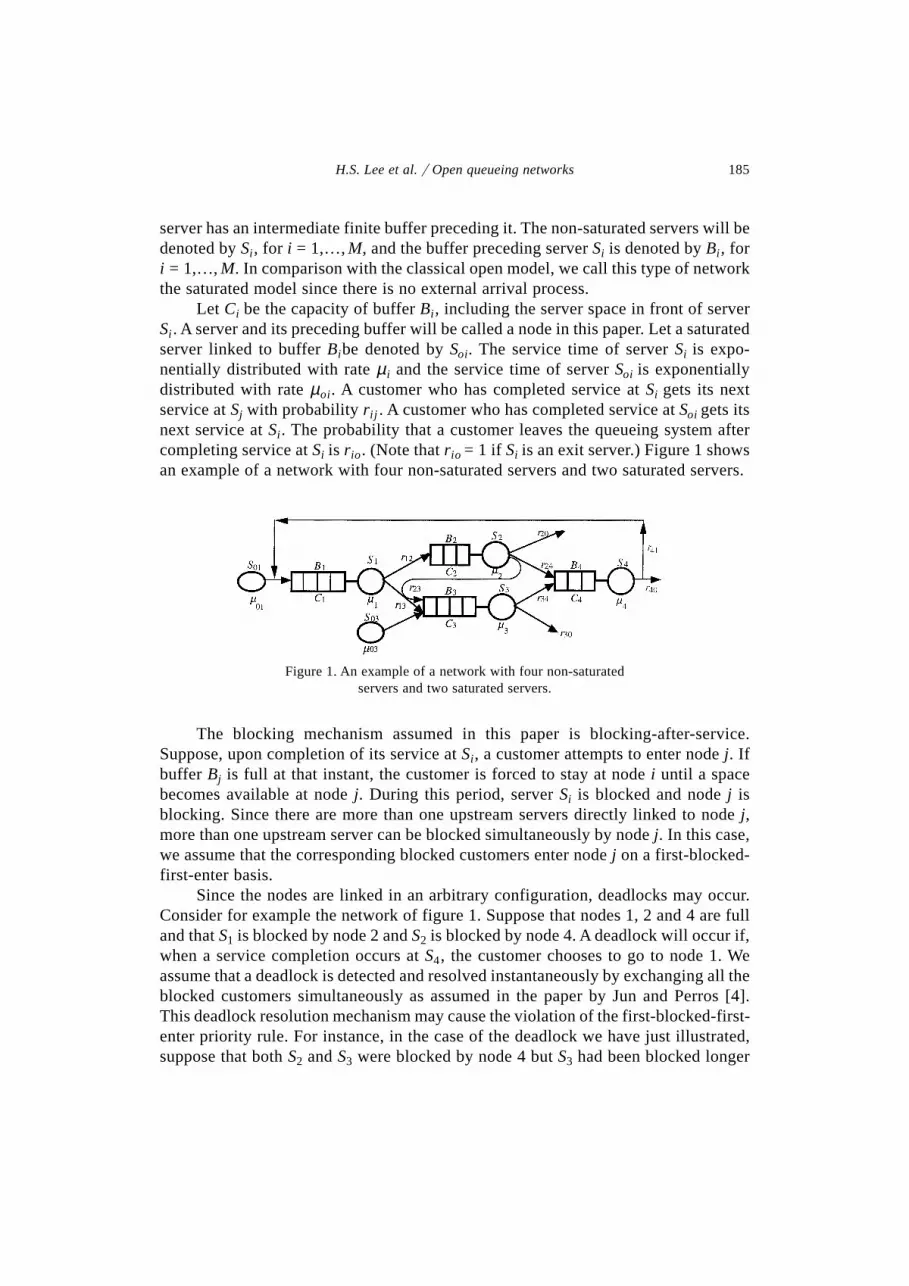
Let Ci be the capacity of buffer Bi , including the server space in front of serverSi . A server and its preceding buffer will be called a node in this paper. Let a saturatedserver linked to buffer Bibe denoted by Soi. The service time of server Si is expo-nentially distributed with rate µi and the service time of server Soi is exponentiallydistributed with rate µoi. A customer who has completed service at Si gets its nextservice at Sj with probability rij . A customer who has completed service at Soi gets itsnext service at Si . The probability that a customer leaves the queueing system aftercompleting service at Si is rio. (Note that rio = 1 if Si is an exit server.) Figure 1 showsan example of a network with four non-saturated servers and two saturated servers.

Figure 1. An example of a network with four non-saturatedservers and two saturated servers.

The blocking mechanism assumed in this paper is blocking-after-service.Suppose, upon completion of its service at Si , a customer attempts to enter node j. Ifbuffer Bj is full at that instant, the customer is forced to stay at node i until a spacebecomes available at node j. During this period, server Si is blocked and node j isblocking. Since there are more than one upstream servers directly linked to node j,more than one upstream server can be blocked simultaneously by node j. In this case,we assume that the corresponding blocked customers enter node j on a first-blocked-first-enter basis.

Since the nodes are linked in an arbitrary configuration, deadlocks may occur.Consider for example the network of figure 1. Suppose that nodes 1, 2 and 4 are fulland that S1 is blocked by node 2 and S2 is blocked by node 4. A deadlock will occur if,when a service completion occurs at S4, the customer chooses to go to node 1. Weassume that a deadlock is detected and resolved instantaneously by exchanging all theblocked customers simultaneously as assumed in the paper by Jun and Perros [4].This deadlock resolution mechanism may cause the violation of the first-blocked-first-enter priority rule. For instance, in the case of the deadlock we have just illustrated,suppose that both S2 and S3 were blocked by node 4 but S3 had been blocked longer


than S2. In this case, when a deadlock occurs, a customer at S2 instead of the one at S3

enters node 4 according to the deadlock resolution mechanism.We have assumed that the blocking mechanism at any server is blocking-after-

service. Alternatively, we also allow saturated servers to operate under a repetitive-service blocking mechanism. By doing that, the class of models considered in thispaper includes the class of open loss models considered by previous authors [1,4,11,14,15], in which each node can be fed by an external Poisson arrival process. Theopen loss model equivalent to the saturated model in figure 1 assuming that the block-ing mechanism at S01 and S03 is repetitive-service blocking is shown in figure 2.

Let Ui denote the index set of upstream servers directly linked to buffer Bi andDi denote the index set of downstream buffers directly linked to server Si . Let Ni denote|Ui|, i.e., the number of elements in set Ui . Also, let f (i, j), for i = 1,…,Nj, be theindex of the i th upstream server directly linked to buffer Bj . If there is a saturatedserver preceding Bj , this server is always considered to be the first upstream server ofnode j. For instance, for the network in figure 1, we have:

U1 = 01, 4, U3 = 03, 1, 2, D2 = 3, 4, N1 = 2, N3 = 3,

f (1,3) = 03, f (2,3) = 1, f (3,3) = 2.

2.2. Decomposition of the original system

To analyze the network, we will use the decomposition method which decom-poses the original network into M subsystems, T( j ), j = 1,…,M. Subsystem T( j ) iscomposed of a set of upstream servers Sui ( j ), i = 1,…,Nj and a downstream serverSd( j ), separated by a finite buffer B( j ). The upstream servers Sui ( j ) are never starvedand the downstream server Sd( j ) is never blocked. Subsystem T( j ) approximates theflow of customers in buffer Bj of the original system. In T( j ), the intermediate bufferB( j ) has the same capacity Cj as that of buffer Bj . Server Sui ( j ) represents node f (i, j)and its upstream nodes in the original model, and server Sd( j ) represents server Sj andits downstream nodes in the original model. Figure 3 shows how the original model offigure 1 is decomposed into subsystems.

Figure 2. The equivalent open loss model.


2.3. Characterization and analysis of subsystems

In this paper, we characterize the upstream and downstream servers at each sub-system by exponential distributions. Let the service rates of Sui( j ) and Sd( j ) be µui( j )and µd( j ), respectively. If the values of µui( j ), i = 1,…,Nj , and µd( j ) are given, we cananalyze subsystem T( j ) exactly by the procedure developed in Lee and Pollock [11].To analyze subsystem T( j ) (see figure 4), we define the state of T( j ) to be the number

Figure 3. Decomposition of the model into subsystems.

Figure 4. Subsystem T( j ).


of customers in B( j ) plus the ones being blocked by Sd( j ) if Sd( j ) is blocking. Thus,Cj + n represents the state that n upstream servers are being blocked by Sd( j ).

Let

P(n: j ) = steady state probability that T( j ) is in state n, n = 0,…,Cj + Nj ,

bui(n: j ) = probability that n servers are blocked by Sd( j ) including Sui( j ), n = 1,…,Nj ,

bui( j ) = probability that Sui ( j ) is blocked by Sd( j ),

Ps( j ) = probability that Sd( j ) is starved at the service completion instant,

Pbi(n: j ) = probability that at the service completion instant, the server Sui ( j ) sees nother servers being blocked by Sd( j ), n = 0,…,Nj – 1.

Then, from the results in Lee and Pollock [11], the steady-state probability P(n: j )can be obtained by solving the birth and death process shown in figure 5 or figure 6.Figure 5 represents the state-transition-rate diagram when the service mechanism atSu1( j ) is blocking-after-service, while figure 6 represents the state-transition-ratediagram when the service mechanism at Su1( j ) is repetitive-service blocking.

Figure 5. State-transition-rate diagram when the service mechanismat Su1( j ) is blocking-after-service.

Figure 6. State-transition-rate diagram when the service mechanismat Su1( j) is repetitive blocking.

Once the steady-state probabilities are obtained, the blocking probabilities canbe computed by again using the results in Lee and Pollock as follows:

b n jj

P C n j n Nuiui n

i

nj j( : )

( )( : ), , , , ( )= + = …−µ Ω

Ω1 1 2 1


where Ωn

iuik

ni i kn

j− =−

< <≡ ∏∑ −1 11

1 1µ ( ),L ik ∈1, 2,…, i – 1, i + 1,…,Nj in the case of

blocking-after-service at Su1( j ) and ik ∈2, 3,…, i – 1 , i + 1,…,Nj in the case ofrepetitive-service blocking at Su1( j ).

The steady-state probability that server Sui( j ) is blocked by server Sd( j ) can nowbe computed as

b j b n jui uin

N j

( ) ( : ). ( )==

∑1

2

Finally, the starvation probabilities and the blocking probabilities at the servicecompletion epochs are given by (for details, refer to Lee et al. [10])

(3)

(4)

2.4. Decomposition equations

In section 2.3, we analyzed the subsystem assuming that the parameter valuesare known. These parameter values, however, are not known but should be determined.Notice that the unknown parameters are the set of service rates µui( j ), i = 1, 2,…,Nj ,j = 1, 2,…,M and µd( j ), j = 1, 2,…,M. As a result, we have a total of M + ∑M

j =1Nj

unknowns. To determine these unknowns, we need a set of M + ∑Mj =1Nj independent

equations. First consider the saturated server S0j and exit server Sk in the originalmodel. Since S0j has no upstream nodes in the original model, server Su1( j ) in sub-system T( j ) represents S0j in the original model. Similarly, since Sk has no downstreamnodes in the original model, server Sd(k) in subsystem T(k) represents Sk in the originalmodel. Consequently, we have µu1( j ) = µ0j , µd(k) = µk for these servers. Therefore,we have as many boundary conditions as the number of saturated servers and exitservers in the original model.

We now derive three different sets of equations that can be used to determine theremaining set of unknowns. In deriving the sets of equations to determine the unknownparameters, we do not consider the effect of a deadlock because consideration of itwill make the model too complicated to solve the networks in a general case. There-fore, sets of equations are derived under the conditions as if there is no deadlock. Oneset of equations is related to the service processes of the downstream servers Sd( j ).Since the server Sd( j ) represents the part of the original model downstream of bufferB( j ), the service time of Sd( j ) corresponds to the time between the beginning of aservice at Sj and the transfer of the customer into one of the downstream buffers. Thistime is composed of a service time of server Sj and, possibly, a blocking time. Blockingoccurs if the destination buffer is full at the service completion instant at Sj . Note that


P jP j

P j

P n jP C n j b n j

b jn N

s

bij ui

uij

( )( : )

( ; ),

( : )( : ) ( : )

( ), , , , , .

=−

=+ −

−= … −

11 0

10 1 2 1

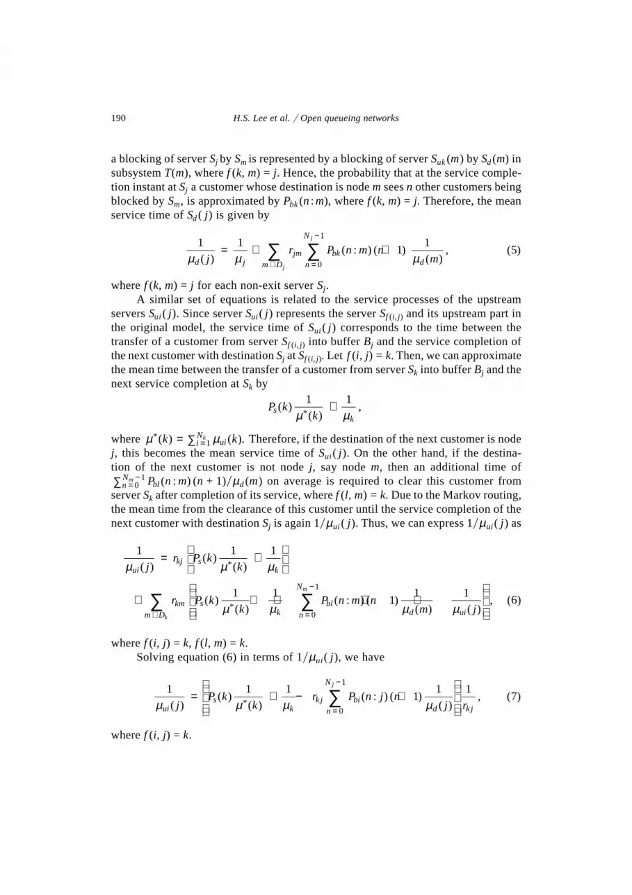
a blocking of server Sj by Sm is represented by a blocking of server Suk(m) by Sd(m) insubsystem T(m), where f (k, m) = j. Hence, the probability that at the service comple-tion instant at Sj a customer whose destination is node m sees n other customers beingblocked by Sm, is approximated by Pbk(n:m), where f (k, m) = j. Therefore, the meanservice time of Sd( j ) is given by

1 11

15

0

1

µ µ µd jjm bk

dn

N

m Dj

r P n m nm

j

j( )

( : ) ( )( )

, ( )= + +=

−

∈∑∑

where f (k, m) = j for each non-exit server Sj .A similar set of equations is related to the service processes of the upstream

servers Sui( j ). Since serverSui ( j ) represents the server Sf (i, j) and its upstream part inthe original model, the service time of Sui ( j ) corresponds to the time between thetransfer of a customer from server Sf (i, j) into buffer Bj and the service completion ofthe next customer with destination Sj at Sf (i, j). Let f (i, j) = k. Then, we can approximatethe mean time between the transfer of a customer from server Sk into buffer Bj and thenext service completion at Sk by

P kk

sk

( )( )

,*

1 1

µ µ+

where µ µ*( ) ( ).k kuiiNk= ∑ = 1 Therefore, if the destination of the next customer is node

j, this becomes the mean service time of Sui ( j ). On the other hand, if the destina-tion of the next customer is not node j, say node m, then an additional time of

P n mblnNm ( : )=

−∑ 01 (n + 1)yµd(m) on average is required to clear this customer from

server Sk after completion of its service, where f (l, m) = k. Due to the Markov routing,the mean time from the clearance of this customer until the service completion of thenext customer with destination Sj is again 1yµui ( j ). Thus, we can express 1yµui ( j ) as

1 1 1

1 11

1 1

0

1

µ µ µ

µ µ µ µ

uikj s

k

km sk n

N

bld uim D

jr P k

k

r P kk

P n m nm j

m

k

( )( )

( )

( )( )

( : ) ( )( ) ( )

,

*

*

= +

+ + + + +

=

−

∈∑∑ (6)

where f (i, j) = k, f (l, m) = k.Solving equation (6) in terms of 1yµui( j ), we have

1 1 11

1 17

0

1

µ µ µ µuis

kk j bi

dn

N

k jjP k

kr P n j n

j r

j

( )( )

( )( : ) ( )

( ), ( )

*= + − +

=

−

∑

where f (i, j) = k.


Finally, a third set of equations is related to the conservation of flow. Let Xd(i )be the throughput of Sd(i ) (or T(i )) and Xui( j ) be the throughput of Sui ( j ). Then, thefollowing relationships should hold between the throughput of two subsystems tosatisfy the conservation of flow:

X j X k rui d k j( ) ( ) , ( )= 8

where f (i, j) = k, for i = 1, 2,…,Nj , j = 1, 2,…,M.We have obtained three sets of equations. However, it can be easily checked that

the number of equations in any two sets of equations is the same as the number ofunknown parameters. Therefore, to determine the unknown parameters, we only needtwo sets of equations. Let SE1 be a system of equations consisting of equations (5)and (8). Let SE2 be a system of equations consisting of equations (7) and (8). Similarly,let SE3 be a system of equations consisting of equations (5) and (7). Since we canchoose any system of equations among SE1, SE2, and SE3 to determine the unknownparameters, three different types of algorithms can be devised. As Dallery and Freinproved for the tandem configuration [2], we can prove that the following lemma holdsfor the arbitrary configuration.

Lemma 1. Any solution of SE3 satisfies the conservation of flow equation (8).

Proof. Note that throughputs Xd(k) and Xui ( j ) can be expressed, respectively, as:

, (9)

(10)

From equation (10) together with equations (7) and (9), we have

X j P kk j

r P n j nj r

P n j nj

r P k

ui sd

k jn

N

bid k j

n

N

bid

k j s

j

j

( ) ( )( ) ( )

( : ) ( )( )

( : ) ( )( )

( )

*= + − +

+ +

=

=

−

=

− −

∑

∑

1 11

1 1

11 1

0

1

0

1 1

µ µ µ

µ µµ µ*( ) ( )( ) ,

k kX k r

dd k j+

=

−1

1

where f (i, j ) = k. u

Lemma 1 implies that any solution of SE3 will satisfy (8). The proof of lemma 1can be reversed to show that (5) and (8) imply (7), and similarly (7) and (8) imply (5).As a result, we have the following corollary.

X kk

P kk

X jj

P n j nj

dd

s

uiui n

N

bid

j

( )( )

( )( )

( )( )

( : ) ( )( )

.

*= +

= + +

−

=

− −

∑

1 1

11

1

1

0

1 1

µ µ

µ µ


Corollary 1 . The three systems of equations SE1, SE2, SE3 are equivalent.

Corollary 1 indicates that different algorithms based on different systems ofequations yield the same results if subsystems are characterized and solved in thesame way. The previous algorithms such as those of Altiok and Perros [1], Perros andSnyder [14], Jun and Perros [4], and Lee and Pollock [11] are all developed based onSE1. The algorithm we develop in this paper is based on SE3. As will be shown later,the algorithm based on SE3 has several advantages over the algorithms based on SE1or SE2, in addition to offering a symmetrical view of decomposition.

2.5. The computational algorithm

This section describes an algorithm to solve the system of equations, SE3. Ouralgorithm is an iterative algorithm with a single loop. Since the network is linked inan arbitrary configuration, each subsystem can be analyzed in any order within a loop.For convenience, we analyze subsystems T( j ) in the order j = 1,…,M. Within eachloop, to analyze subsystem T( j ), we first calculate the service rate of the downstreamserver, µd( j ), using equation (5). To do this, we need the values of Pbk(n:m) for allm ∈Dj , where f (k, m) = j. We use the values of Pbk(n:m) which have been obtainedmost recently. That is, if subsystem T(m) has already been analyzed in this loop, weuse the values updated in this loop. On the other hand, if subsystem T(m) has not beenanalyzed in this loop, we use the values updated in the previous loop. Once µd( j ) isupdated, using the values of µui ( j ) which have been updated most recently, we analyzesubsystem T( j ) using the procedure presented in section 2.3. Then we calculate Ps( j )and Pbi(n: j ) using equations (3) and (4), respectively. After these probabilities areobtained, we calculate new values of µui(k) for all k ∈Dj , where f (i, k) = j, usingequation (7). In each iteration step of the algorithm, some computational effort can besaved because some parameter values do not have to be calculated for the followingcases: (i) Ps( j ) if Sj is an exit server, (ii) µu1( j ) if the first upstream server linked to Bj

is a saturated server, (iii) µd( j ) if Sj is an exit server, (iv) Pbi(n: j ) if a saturated serveris the only upstream server linked to Bj . The algorithm continues until the upstreamand downstream service rates become close enough between two successive itera-tions. The initial values of the parameters µd( j ), µui( j ) and Pbi(n: j ) are obtained byassuming that neither blocking nor starvation exist. This algorithm, which we willcall algorithm 1 in this paper, is summarized as follows:

Algorithm 1

Initialization:

Set µd( j ) = µj, j = 1,…,Mµui( j ) = µk ∗ r kj , where f (i, j) = k, for i = 1,…,Nj , j = 1,...,MPbi(n: j ) = 0, for i = 1,…,Nj , j = 1,...,M


Iteration step:

For j =1, 2,…,M do:1. Calculate µd( j ) using (5).2. Calculate Ps( j ) using (3).3. Calculate Pbi(n: j ) using (4), n = 0, 1,…,Nj – 1, i = 1, 2,…,Nj .4. Calculate µui(k) using (7), for all k ∈Dj, where f (i,k) = j.

Convergence step:

If convergence condition is satisfied, stop.Otherwise, go to the iteration step.

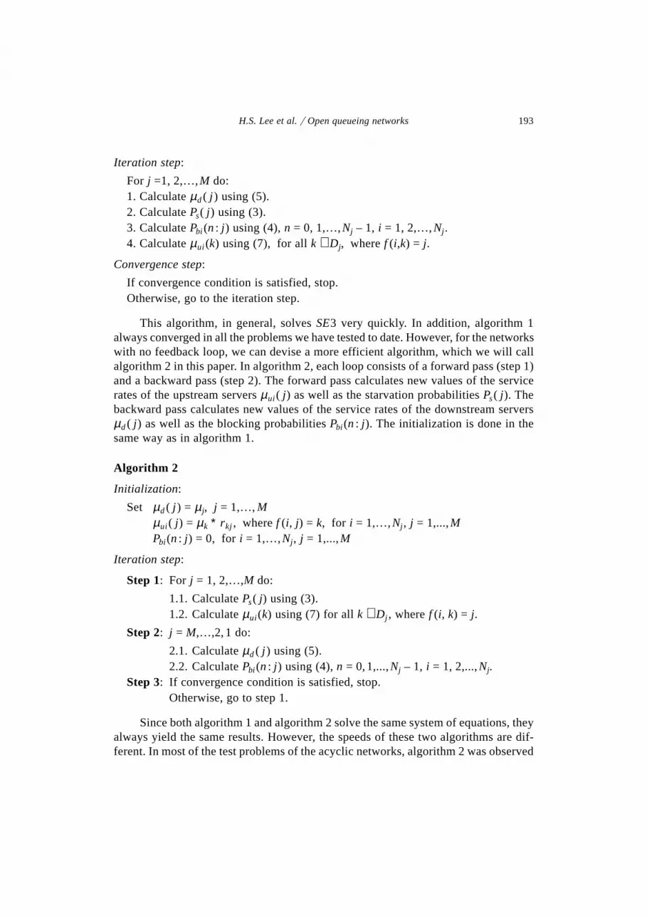
This algorithm, in general, solves SE3 very quickly. In addition, algorithm 1always converged in all the problems we have tested to date. However, for the networkswith no feedback loop, we can devise a more efficient algorithm, which we will callalgorithm 2 in this paper. In algorithm 2, each loop consists of a forward pass (step 1)and a backward pass (step 2). The forward pass calculates new values of the servicerates of the upstream servers µui ( j ) as well as the starvation probabilities Ps( j ). Thebackward pass calculates new values of the service rates of the downstream serversµd( j ) as well as the blocking probabilities Pbi(n : j ). The initialization is done in thesame way as in algorithm 1.

Algorithm 2

Initialization:

Set µd( j ) = µj, j = 1,…,Mµui( j ) = µk ∗ r kj , where f (i, j) = k, for i = 1,…,Nj , j = 1,...,MPbi(n: j ) = 0, for i = 1,…,Nj , j = 1,...,M

Iteration step:

Step 1: For j = 1, 2,…,M do:

1.1. Calculate Ps( j) using (3).1.2. Calculate µui(k) using (7) for all k ∈Dj , where f (i, k) = j.

Step 2: j = M,…,2, 1 do:

2.1. Calculate µd( j ) using (5).2.2. Calculate Pbi(n: j ) using (4), n = 0,1,...,Nj – 1, i = 1, 2,...,Nj.

Step 3: If convergence condition is satisfied, stop.Otherwise, go to step 1.

Since both algorithm 1 and algorithm 2 solve the same system of equations, theyalways yield the same results. However, the speeds of these two algorithms are dif-ferent. In most of the test problems of the acyclic networks, algorithm 2 was observed


to converge faster than algorithm 1. For the test problems of the networks with veryfew feedback loops, the speeds of these two algorithms were observed to be almostcomparable. However, for the networks with many feedback loops, it was observedthat algorithm 1 usually converged faster than algorithm 2. Through numerical experi-ments, it was also found that algorithm 2 did not converge in some large-size networkproblems with many feedback loops, although it converged in all the acyclic networkproblems tested to date. For this reason, we recommend that algorithm 1 be used forthe networks with feedback loops, while algorithm 2 be used for the networks withoutfeedback loops. We have not been able to prove the convergence of the algorithm inthe general case. In the case of a merge configuration, however, as will be shown insection 4, we did prove the convergence of algorithm 2 as well as the existence anduniqueness of the solution by exploiting the properties pertaining to the system ofequations, SE3.

3. Computational results

In order to test the accuracy and the speed of the approximation method, bothalgorithm 1 and algorithm 2 were implemented on an IBM PC 586 and tested on avariety of problems. The results of the approximation method were compared withthose of simulation. Each simulation was run until at least 300,000 customers departedfrom the system. If the network has no feedback loop and the blocking mechanism atthe saturated servers is repetitive-service blocking, our algorithm yields the sameresults as the algorithm of Lee and Pollock [11] because decomposition into sub-systems, characterization of the subsystem and analysis of the subsystem are done inthe same way in these algorithms. In order to compare the speed of algorithm 2 to thatof Lee and Pollock’s algorithm, we have tested both algorithms on the set of problemspresented in Lee and Pollock. From the results of the experiments, we have observedthat the number of iterations needed for convergence by algorithm 2 is always lessthan or equal to that needed for convergence by Lee and Pollock’s algorithm. As aresult, algorithm 2 takes less CPU time than the previous algorithm using the sameconvergence criterion. The CPU execution time as well as the number of iterationswas observed to be reduced by about 15% on average in algorithm 2 compared withthat in Lee and Pollock’s algorithm. The maximum number of iterations needed forconvergence was eight in algorithm 2, while it was ten in Lee and Pollock’s algorithmon the set of problems presented in Lee and Pollock [11].

We have also tested our algorithm for the networks with feedback loops. Theresults are summarized in tables 1 to 4 for the various performance measures. In eachtable, the probability that there are n customers at node i is denoted by Pi (n) and themean queue length at node i is denoted by Li . Table 1 gives results for the three-nodenetwork in figure 7 and table 2 gives results for the four-node network in figure 8.Table 3 gives results for the eight-node network in figure 9. The blocking mechanismat the saturated servers is assumed to be repetitive-service blocking for the networks


Figure 7. The three-node network.

Table 1

Comparisons with simulation for the three-node networks with feedback loops.

Case Measures Simulation Approx. Rel. error (%)

C = (2, 2, 2), µ = (1, 1, 1) P1(0) 0.206 0.210 1.94P1(2) 0.458 0.483 5.46L1 1.252 1.273 1.68P2(0) 0.265 0.287 8.30P2(2) 0.450 0.452 0.44L2 1.185 1.166 – 1.60P3(0) 0.376 0.389 3.46P3(2) 0.334 0.335 0.30L3 0.959 0.946 – 1.36

C = (1, 1, 1), µ = (1.5, 1.5, 1.5) P1(0) 0.510 0.478 – 6.27P1(1) 0.490 0.522 6.53L1 0.490 0.522 6.53P2(0) 0.526 0.532 1.14P2(1) 0.474 0.468 – 1.27L2 0.474 0.468 – 1.27P3(0) 0.610 0.620 1.64P3(1) 0.390 0.380 – 2.56L3 0.390 0.380 – 2.56

C = (3, 3, 3), µ = (1.5, 1.5, 1.5) P1(0) 0.312 0.311 – 0.32P1(3) 0.191 0.202 5.76L1 1.300 1.317 1.31P2(0) 0.332 0.338 1.81P2(3) 0.222 0.232 4.50L2 1.301 1.307 0.46P3(0) 0.391 0.396 1.28P3(3) 0.175 0.179 2.29L3 1.128 1.130 0.18

C = (2, 2, 2), µ = (2, 2, 2) P1(0) 0.489 0.481 – 1.64P1(2) 0.195 0.210 7.69L1 0.706 0.729 3.26P2(0) 0.498 0.501 0.60P2(2) 0.213 0.228 7.04L2 0.715 0.727 1.68P3(0) 0.547 0.550 0.55P3(2) 0.180 0.186 3.33L3 0.634 0.636 0.32


Table 2

Comparisons with simulation for the four-node networks with feedback loops.

Case Measures Simulation Approx. Rel. error (%)

C = (1, 1, 1, 1), µ = (1.0, 0.5, 0.5, 1.0) P1(0) 0.364 0.338 – 7.14P1(1) 0.636 0.662 4.09L1 0.636 0.662 4.09P2(0) 0.490 0.477 – 2.65P2(1) 0.510 0.523 2.55L2 0.510 0.523 2.55P3(0) 0.389 0.394 1.29P3(1) 0.611 0.606 – 0.82L3 0.611 0.606 – 0.82P4(0) 0.589 0.589 0.00P4(1) 0.411 0.411 0.00L4 0.411 0.411 0.00

C = (2, 2, 2, 2), µ = (1.5, 0.8, 0.8, 1.5) P1(0) 0.367 0.351 – 4.36P1(2) 0.311 0.323 3.86L1 0.945 0.972 2.86P2(0) 0.516 0.509 – 1.36P2(2) 0.186 0.203 9.14L2 0.670 0.693 3.43P3(0) 0.363 0.366 0.83P3(2) 0.342 0.352 2.92L3 0.980 0.986 0.61P4(0) 0.523 0.523 0.00P4(2) 0.210 0.216 2.86L4 0.688 0.693 0.73

C = (2, 2, 2, 2), µ = (2.0, 1.0, 1.0, 2.0) P1(0) 0.482 0.471 – 2.28P1(2) 0.213 0.217 1.88L1 0.731 0.746 2.05P2(0) 0.595 0.589 – 1.01P2(2) 0.134 0.145 8.21L2 0.538 0.557 3.53P3(0) 0.445 0.445 0.00P3(2) 0.263 0.273 3.80L3 0.818 0.828 1.22P4(0) 0.599 0.600 0.17P4(2) 0.149 0.154 3.36L4 0.550 0.554 0.73

Figure 8. The four-node network.


in figures 7 and 8, while it is assumed to be blocking-after-service for the network infigure 9. Since all these problems have feedback loops, deadlocks occur in theseproblems. The frequency of deadlocks, however, is not very high, although significant.

Figure 9. The eight-node network.

Table 3

Comparisons with simulation for the eight-node networks with feedback loops.

C = (2, 2, 2, 2, 2, 2, 2, 2) C = (2, 2, 2, 2, 2, 2, 2, 2)µ = (1.5, 1.0, 1.0, 1.0, 1.0, 1.0, 1.0, 1.5) µ = (2.0, 1.5, 1.5, 1.5, 1.5, 1.5, 1.5, 2.0)

Measures Simulation Approx. Rel. error (%) Measures Simulation Approx. Rel. error (%)

P1(0) 0.220 0.221 0.45 P1(0) 0.417 0.421 0.96P1(2) 0.547 0.539 – 1.46 P1(2) 0.311 0.302 – 2.89L1 1.317 1.318 0.08 L1 0.895 0.881 – 1.56P2(0) 0.434 0.426 – 1.84 P2(0) 0.614 0.616 0.33P2(2) 0.306 0.309 0.98 P2(2) 0.145 0.142 – 2.07L2 0.872 0.882 1.15 L2 0.531 0.527 – 0.75P3(0) 0.415 0.406 – 2.17 P3(0) 0.599 0.600 0.17P3(2) 0.315 0.318 0.95 P3(2) 0.153 0.149 – 2.61L3 0.900 0.912 1.33 L3 0.554 0.550 – 0.72P4(0) 0.377 0.373 – 1.06 P4(0) 0.549 0.552 0.55P4(2) 0.348 0.352 1.15 P4(2) 0.187 0.185 – 1.07L4 0.971 0.979 0.82 L4 0.639 0.634 – 0.78P5(0) 0.434 0.426 – 1.84 P5(0) 0.613 0.616 0.49P5(2) 0.305 0.309 1.31 P5(2) 0.145 0.142 – 2.07L5 0.871 0.882 1.26 L5 0.532 0.527 – 0.94P6(0) 0.416 0.406 – 2.40 P6(0) 0.598 0.600 – 0.33P6(2) 0.315 0.318 0.95 P6(2) 0.154 0.149 – 3.25L6 0.898 0.912 1.56 L6 0.556 0.550 – 1.08P7(0) 0.376 0.373 – 0.80 P7(0) 0.547 0.552 0.91P7(2) 0.363 0.352 – 3.03 P7(2) 0.189 0.185 – 2.12L7 0.972 0.979 0.72 L7 0.643 0.634 – 1.40P8(0) 0.280 0.274 – 2.14 P8(0) 0.368 0.364 – 1.09P8(2) 0.492 0.492 0.00 P8(2) 0.380 0.380 0.00L8 1.212 1.217 0.41 L8 1.012 1.015 0.30


The number of deadlocks which have been observed during simulation until 300,000customers departed from the system ranges between 530 and 8,300.

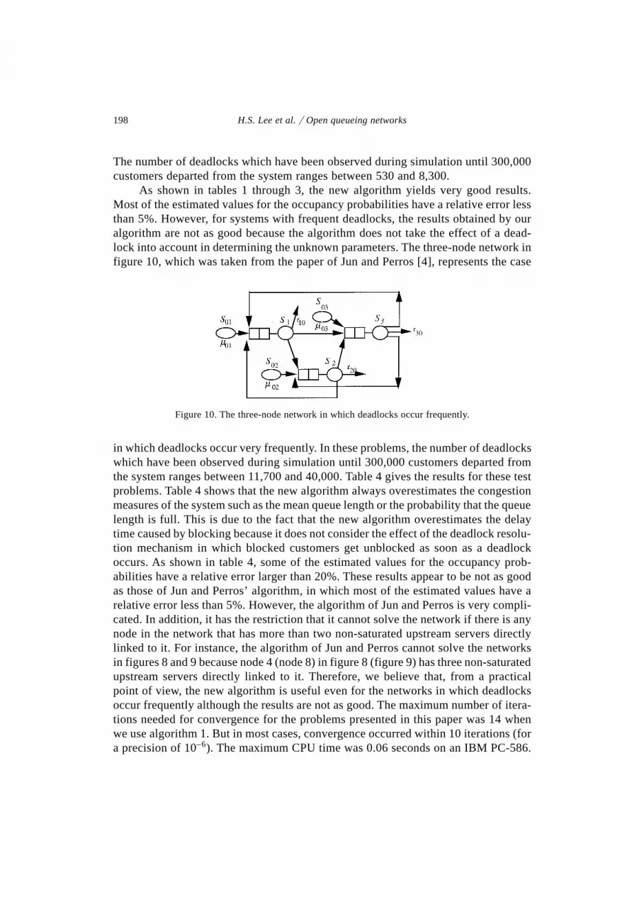
As shown in tables 1 through 3, the new algorithm yields very good results.Most of the estimated values for the occupancy probabilities have a relative error lessthan 5%. However, for systems with frequent deadlocks, the results obtained by ouralgorithm are not as good because the algorithm does not take the effect of a dead-lock into account in determining the unknown parameters. The three-node network infigure 10, which was taken from the paper of Jun and Perros [4], represents the case

Figure 10. The three-node network in which deadlocks occur frequently.

in which deadlocks occur very frequently. In these problems, the number of deadlockswhich have been observed during simulation until 300,000 customers departed fromthe system ranges between 11,700 and 40,000. Table 4 gives the results for these testproblems. Table 4 shows that the new algorithm always overestimates the congestionmeasures of the system such as the mean queue length or the probability that the queuelength is full. This is due to the fact that the new algorithm overestimates the delaytime caused by blocking because it does not consider the effect of the deadlock resolu-tion mechanism in which blocked customers get unblocked as soon as a deadlockoccurs. As shown in table 4, some of the estimated values for the occupancy prob-abilities have a relative error larger than 20%. These results appear to be not as goodas those of Jun and Perros’ algorithm, in which most of the estimated values have arelative error less than 5%. However, the algorithm of Jun and Perros is very compli-cated. In addition, it has the restriction that it cannot solve the network if there is anynode in the network that has more than two non-saturated upstream servers directlylinked to it. For instance, the algorithm of Jun and Perros cannot solve the networksin figures 8 and 9 because node 4 (node 8) in figure 8 (figure 9) has three non-saturatedupstream servers directly linked to it. Therefore, we believe that, from a practicalpoint of view, the new algorithm is useful even for the networks in which deadlocksoccur frequently although the results are not as good. The maximum number of itera-tions needed for convergence for the problems presented in this paper was 14 whenwe use algorithm 1. But in most cases, convergence occurred within 10 iterations (fora precision of 10–6). The maximum CPU time was 0.06 seconds on an IBM PC-586.


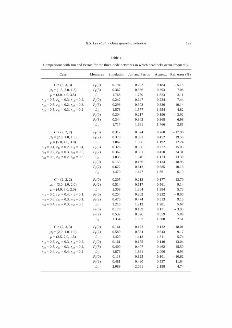
Table 4

Comparisons with Jun and Perros for the three-node networks in which deadlocks occur frequently.

Case Measures Simulation Jun and Perros Approx. Rel. error (%)

C = (3, 3, 3) P1(0) 0.194 0.202 0.184 – 5.15

µ0 = (1.5, 2.0, 1.8) P1(3) 0.367 0.366 0.393 7.08

µ = (3.0, 4.0, 3.5) L1 1.768 1.750 1.823 3.11

r 10 = 0.5, r12 = 0.3, r13 = 0.2, P2(0) 0.242 0.247 0.224 – 7.44

r 20 = 0.5, r21 = 0.2, r23 = 0.3, P2(3) 0.296 0.303 0.326 10.14

r 30 = 0.5, r31 = 0.3, r32 = 0.2 L2 1.578 1.577 1.654 4.82

P3(0) 0.204 0.217 0.196 – 3.92

P3(3) 0.344 0.343 0.368 6.98

L3 1.717 1.691 1.766 2.85

C = (2, 2, 2) P1(0) 0.317 0.324 0.260 – 17.98

µ0 = (2.0, 1.0, 1.5) P1(2) 0.378 0.391 0.452 19.58

µ = (5.0, 4.0, 3.0) L1 1.062 1.066 1.192 12.24

r 10 = 0.4, r12 = 0.2, r13 = 0.4, P2(0) 0.326 0.336 0.277 15.03

r 20 = 0.2, r21 = 0.3, r23 = 0.5, P2(2) 0.362 0.381 0.450 24.31

r 30 = 0.5, r31 = 0.2, r32 = 0.3 L2 1.035 1.046 1.173 13.30

P3(0) 0.153 0.166 0.124 – 18.95

P3(2) 0.622 0.612 0.685 10.13

L3 1.470 1.447 1.561 6.19

C = (2, 2, 2) P1(0) 0.205 0.213 0.177 – 13.70

µ0 = (3.0, 1.0, 2.0) P1(2) 0.514 0.517 0.561 9.14

µ = (4.0, 3.0, 2.0) L1 1.309 1.304 1.384 5.73

r 10 = 0.5, r12 = 0.4, r13 = 0.1, P2(0) 0.254 0.262 0.232 – 8.66

r 20 = 0.6, r21 = 0.3, r23 = 0.1, P2(2) 0.470 0.474 0.513 9.15

r 30 = 0.4, r31 = 0.3, r32 = 0.3 L2 1.216 1.212 1.281 5.67

P3(0) 0.178 0.189 0.171 – 3.93

P3(2) 0.532 0.526 0.559 5.08

L3 1.354 1.337 1.388 2.51

C = (2, 3, 3) P1(0) 0.161 0.172 0.132 – 18.01

µ0 = (2.0, 1.0, 1.0) P1(2) 0.589 0.584 0.643 9.17

µ = (2.5, 2.0, 1.5) L1 1.429 1.412 1.511 5.74

r 10 = 0.5, r12 = 0.3, r13 = 0.2, P2(0) 0.161 0.175 0.140 – 13.04

r 20 = 0.5, r21 = 0.3, r23 = 0.2, P2(3) 0.400 0.407 0.462 15.50

r 30 = 0.4, r31 = 0.4, r32 = 0.2 L2 1.876 1.861 2.006 6.93

P3(0) 0.113 0.125 0.101 – 10.62

P3(3) 0.481 0.480 0.537 11.64

L3 2.089 2.061 2.188 4.74


4. Properties of algorithm 2 for the merge configuration

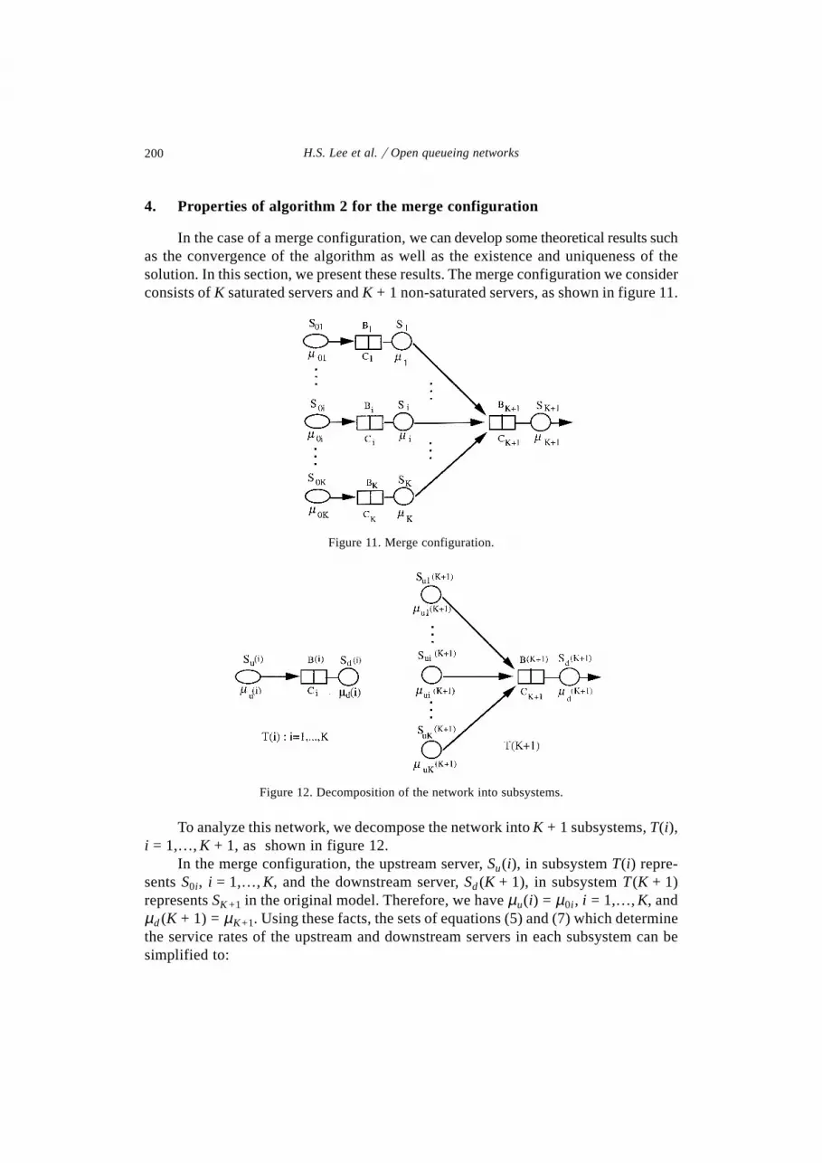
In the case of a merge configuration, we can develop some theoretical results suchas the convergence of the algorithm as well as the existence and uniqueness of thesolution. In this section, we present these results. The merge configuration we considerconsists of K saturated servers and K + 1 non-saturated servers, as shown in figure 11.

To analyze this network, we decompose the network into K + 1 subsystems, T(i),i = 1,…,K + 1, as shown in figure 12.

In the merge configuration, the upstream server, Su(i), in subsystem T(i) repre-sents S0i , i = 1,…,K, and the downstream server, Sd(K + 1), in subsystem T(K + 1)represents SK +1 in the original model. Therefore, we have µu(i) = µ0i , i = 1,…,K, andµd(K + 1) = µK+1. Using these facts, the sets of equations (5) and (7) which determinethe service rates of the upstream and downstream servers in each subsystem can besimplified to:

Figure 11. Merge configuration.

Figure 12. Decomposition of the network into subsystems.


As a result, we have the following simple version of algorithm 2, which we will callalgorithm 2(M).

Algorithm 2(M)

Initialization:

Set µu(i) = µ0i , i = 1,…,K, µd(i) = µi , i = 1,…,K + 1.

Iteration step:

Step 1: For i = 1, 2,…,K do:

1.1. Calculate PS(i) using (3).1.2. Calculate µui (K + 1) using (12).

Step 2:2.1. Calculate Pbi(n : K + 1) using (4), n = 0, 1,…,K – 1, i = 1, 2,…,K.2.2. Calculate µd(i) using (11), i = 1, 2,…,K.

Step 3: If convergence condition is satisfied, stop.Otherwise, go to step 1.

To prove the theoretical results pertaining to this algorithm, we need to developsome properties associated with each subsystem. We give three of these propertiesbelow. Since the proofs of these properties are very long and somewhat involved, wedo not provide them in this paper for the sake of conciseness. The proof of property 1is given in Dallery and Frein [2] and the proofs of properties 2 and 3 can be found inLee et al. [10].

Property 1. Let µ µu di i1 1( ), ( ) and µ µu di i2 2( ), ( ) be two sets of parameters to subsystemT(i), 1 ≤ i ≤ K. Supposeµ µu ui i1 2( ) ( ).= Then the following relationship holds:

1 11 1

11

1

1

1 11

0

1

1

0

µ µ µ

µ µ µ

d ibi

n

K

K

ui iS

i

iP n K n i K

KP i i K

( )( : ) ( ) , , , ,

( )( ) , , , .

= + + + = …

−= + = …

=

−

+∑ (11)

(12)

Property 2.

P n K n K j K i Kbj uin

K

( : ) ( ) ( ), , , , , , .− + + = … = …=

−

∑ 1 1 1 1 10

1

is increasing in µ

Property 3. Consider the following two sets of parameters pertaining to subsystemT(K + 1):

If then andµ µd d s s d di i P i P i X i X i2 1 2 1 2 1( ) ( ) ( ) ( ) ( ) ( ).≤ ≤ ≤


Supposeµ µd dK K1 21 1( ) ( ).+ = + Define sets A, B and C such that

where S= 1, 2,…,K. Then the following relationships hold:

We are now ready to provide the proofs for the existence and uniqueness of thesolution as well as the convergence of the algorithm. The general procedure of theproofs is the same as the one in Dallery and Frein [2] for the tandem configuration.The following property, stated as theorem 1, answers the question of uniqueness ofthe solution provided that the existence is guaranteed.

Theorem 1. The system of equations SE3 has at most one solution.

Proof. We assume that SE3 has two different solutions and show that this leads to acontradiction. All the quantities that pertain to the first solution (respectively, thesecond solution) will be denoted by a superscript 1 (respectively, 2). Letµd

j i( ) andµui

j K( )+ 1 , for i = 1,…,K, j = 1, 2, be the two solutions. Define sets A, B and C suchthat

where S= 1, 2,…,K. Then from property 1, it follows for each subsystem T(i) fori ∈A, that

Applying this result to (12), we obtain

Since SE3 satisfies conservation of flow, the fact thatX i X id d2 1( ) ( )< implies that

(13)

( ( ), , ( )), ( ),

( ( ), , ( )), ( ).

µ µ µ

µ µ µ

u uK d

u uK d

K K K

K K K

11 1 1

12 2 2

1 1 1

1 1 1

+ … + +

+ … + +

A i S K K

B i S K K

C i S K K

ui ui

ui ui

ui ui

= + < +

= + > +

= + = +

∈

∈

∈

( ) ( ),

( ) ( ),

( ) ( ),

y

y

y

µ µ

µ µ

µ µ

1 2

1 2

1 2

1 1

1 1

1 1

X K X K X K X Kui ui ui uii Bi Bi Ai A

1 2 1 21 1 1 1( ) ( ) ( ) ( ).+ < + + > +∈∈∈∈∑∑∑∑ and

A i S i i

B i S i i

C i S i i

d d

d d

d d

= >

= <

= =

∈∈∈

( ) ( ),

( ) ( ),

( ) ( ),

y

y

y

µ µ

µ µ

µ µ

1 2

1 2

1 2

P i P i X i X i i As s d d2 1 2 1( ) ( ) ( ) ( ) .< < ∈and for

µ µui uiK K i A1 21 1( ) ( ) .+ < + ∈for

X K X K i Aui ui2 11 1( ) ( ) .+ < + ∈for


Similarly, for each subsystem, T(i) for i ∈B, we have

(14)

Inequalities (13) and (14) imply that

These inequalities, however, are a contradiction to property 3. u

We now provide the proof of the convergence of algorithm 2(M).

Theorem 2. Algorithm 2(M) always converges to a solution of system SE3.

Proof. It is easy to check that algorithm 2 (therefore, algorithm 2(M)) is nothing butthe method of Gauss–Seidel applied to the system of fixed point type equations. Theaim of the algorithm is to solve system SE3 and therefore to obtain values for theunknown parameters µui(K + 1) and µd(i), for i = 1,…,K. It consists of an initializationstep followed by an iteration step. During each iteration, new values of Ps(i), µui(K + 1)Pbi(n: K + 1) and µd(i) are obtained. Let n denote the index of the iteration. Let Pn

s (i),µui

nbinK P n k( ), ( : )+ +1 1 and µd

n i( ) denote the parameters obtained during the nthiteration. Letµd i0( ), i = 1,…,K denote the initial value of the service rate of Sd(i) givenby µ µd ii0( ) ,= i = 1,…,K.During the nth iteration, steps 1 and 2 are successively executed. In step 1, subsystemsT(i), i = 1,…,K, are successively analyzed. The parameters of subsystem T(i) arethen µui

n K( )+ 1 and µdn i−1( ). Similarly, in step 2, subsystems T(i), for i = K,…,1, are

successively analyzed. The parameters of subsystem T(i) are thenµuin K( )+ 1 and

µdn i( ). Note that we haveµ µu

nii( ) = , i = 1,…,K, and µ µd

nKK( )+ = +1 1 for any n.

Part 1. In the first part of the proof, we show that for any two successive iterations nand n + 1, we have

(15)and

(16)

Part a. Consider step 1 of the algorithm. Let us show that

(17)

P i P i X i X i K K

X K X K

s s d d ui ui

ui ui

1 2 1 2 2 1

1 2

1 1

1 1

( ) ( ), ( ) ( ), ( ) ( ),

( ) ( ).

< < + < +

+ < +

µ µ

X K X K X K X Kui ui ui uii Bi Bi Ai A

1 2 1 21 1 1 1( ) ( ) ( ) ( ).+ > + + < +∈∈∈∈∑∑∑∑ and

µ µuin

uinK K i K+ + ≥ + = …1 1 1 1( ) ( ), , ,for

µ µdn

dni i i K+ ≤ = …1 1( ) ( ) , , .for

If for then

for

µ µ

µ µdn

dn

uin

uin

i i i K

K K i K

( ) ( ) , , ,

( ) ( ) , , .

≤ = …

+ ≥ + = …

−

+

1

1

1

1 1 1


Consider subsystem T(i). From property 1, we obtainP i P isn

sn+ ≤1( ) ( ) for i = 1,...,K.

Now from (12), we getµ µuin

uinK K+ + ≥ +1 1 1( ) ( ). Then by induction on i, we obtain

(17).

Part b. Consider step 2 of the algorithm. Let us show that

(18)

From property 2, we obtain

P j K j P j K jbkn

Kbkn

Kj

K

j

K+

+ +=

−

=

−

+ + ≥ + +∑∑ 1

1 10

1

0

1

1 11

1 11

( : ) ( ) ( : ) ( ) .µ µ

Now from (11), we getµ µdn

dni i+ ≤1( ) ( ) for i = 1,…,K. Then by induction on i, we

obtain (18).

Part c. From (17) and (18), we get the implication

(19)

From (11), it follows that

Then (15) and (16) follow from (19) and (20).

Part 2. Equation (15) states that each series ( ), , , µuin K n+ = …1 1 2 for i = 1,…,K

is non-decreasing. Moreover, from (12), it follows thatµ µuin

iK( ) .+ ≤1 Therefore,as each series is non-decreasing and upper bounded, it converges. Similarly, equa-tion (16) states that each series ( ), , , µd

n i n = …1 2 for i = 1,…,K is non-increasing.Moreover, from (11) it follows that

µµ µ

µ µdn i K

K ii

K( ) .≥

++

+

1

1

This bound is obtained by considering the case whereP K Kbin( : ) .− + =1 1 1 There-

fore, as each series is non-increasing and lower bounded, it converges. Now, since thealgorithm is the application of the method of Gauss– Seidel to solve the system ofequations SE3, the asymptotic values ofµ µd

nuini K( ), ( ),+ 1 i = 1, 2,…,K, are indeed

a solution of SE3. u

We know from theorem 2 that SE3 has at least one solution. Furthermore, fromtheorem 1, we know that SE3 cannot have two or more solutions. Therefore, we havethe following property, stated as corollary 2.

If for then

for

µ µ

µ µuin

uin

dn

dn

K K i K

i i i K

+

+

+ ≥ + = …

≤ = …

1

1

1 1 1

1

( ) ( ) , , ,

( ) ( ) , , .

If then

and

µ µ

µ µ µ µdn

dn

uin

uin

dn

dn

i i i K

K K i i i K

( ) ( ), , , ,

( ) ( ) ( ) ( ), , , .

≤ = …

+ ≥ + ≤ = …

−

+ +

1

1 1

1

1 1 1

µ µd di i i K1 0 1 20( ) ( ) , , . ( )≤ = …for


Corollary 2 . The solution of the system of equations SE3 exists and is unique.

From corollary 1, the three systems of equations are equivalent. Thus, the solutionof the system of equations SE1 (and SE2) also exists and is unique.

5. ConclusionsWe have presented a new approximate algorithm for analyzing an arbitrary con-

figuration of open queueing networks with finite buffers. The approximate techniquedecomposes the network into a set of subsystems. Each subsystem is composed ofone or many upstream servers and one downstream server separated by a finite buffer.The new algorithm is based on the symmetrical approach and offers a symmetricalrepresentation of the decomposition method. The new algorithm is quite simplebecause service times at each subsystem are characterized by exponential distributions.The new algorithm is also very general in that it can analyze all the classes of modelsconsidered by the previous studies under blocking-after-service mechanism. For theclass of models considered by Lee and Pollock [11], the new algorithm yields thesame results as that of Lee and Pollock. The numerical results, however, have shownthat the new algorithm takes less CPU execution time than the one proposed by Leeand Pollock. As reported in Lee and Pollock [11], the new algorithm yields veryaccurate results for the cases of networks without feedback loops. For the cases ofnetworks with feedback loops, the numerical results have shown that the new algorithmusually converges fast and yields good results unless deadlocks occur too frequently.In particular, for the merge configuration, we could prove the convergence of thealgorithm as well as the existence and uniqueness of the solution, which to the best ofour knowledge has never been done previously. This new algorithm holds promise asa useful tool in the analysis of arbitrary configuration of open queueing networkswith finite buffers.

Acknowledgement

The research of the first author was supported through KOSEF Grant 951-1010-012-2.

References

[1] T. Altiok and H.G. Perros, Approximate analysis of arbitrary configurations of open queueingnetworks with blocking, Annals of Oper. Res. 9(1987)481–509.

[2] Y. Dallery and Y. Frein, On decomposition methods for tandem queueing networks with blocking,Oper. Res. 41(1993)386–399.

[3] Y. Dallery and S.B. Gershwin, Manufacturing flow line aystems: A review of models and analyticalresults, Queueing Sys. 12(1992)3– 94.

[4] K.P. Jun and H.G. Perros, Approximate analysis of arbitrary configuration of queueing networkswith blocking, in: Proc. 1st International Workshop on Queueing Networks with Blocking, North-Holland, Amsterdam, 1989, pp. 259–280.


[5] L. Kerbache and J. MacGregor Smith, The generalized expansion method for open finite queueingnetworks, Eur. J. Oper. Res. 32(1987)448– 461.

[6] D.D. Kouvatsos and S.G. Denazis, Entropy maximized queueing networks with blocking andmultiple job classes, Perform. Eval. 17(1993)189 –205.

[7] D.D. Kouvatsos and N.P. Xenios, Maximum entropy analysis of general queueing networks withblocking, in: Proc. 1st International Workshop on Queueing Networks with Blocking, North-Holland, Amsterdam, 1989, pp 281– 309.

[8] D.D. Kouvatsos and N.P. Xenios, MEM for arbitrary queueing networks with multiple generalservers and repetitive-service-blocking, Perform. Eval. 10(1989)169– 195.

[9] J. Labetoulle and G. Pujolle, Isolation method in a network of queues, IEEE Trans. Soft. Eng.6(1980)373–381.

[10] H.S. Lee, A. Bouhchouch, Y. Dallery and Y. Frein, Performance evaluation of open queueing net-works with arbitrary configuration and finite buffers, Technical Report, Dept. of Industrial Eng.,Kyung Hee Univ., Korea, 1996.

[11] H.S. Lee and S.M. Pollock, Approximate analysis of open acyclic exponential queueing networkswith blocking, Oper. Res. 38(1990)1123–1134.

[12] R.O. Onvural and H.G. Perros, On equivalencies of blocking mechanisms in queueing networkswith blocking, Oper. Res. Lett. 5(1986)293–297.

[13] H.G. Perros, Queueing Networks with Blocking, Oxford University Press, New York, 1994.[14] H.G. Perros and P.M. Snyder, A computationally efficient approximation algorithm for analyzing

open queueing networks with blocking, Perform. Eval. 9(1989)217– 224.[15] Y. Takahashi, H. Miyahara and J. Hasegawa, An approximation method for open restricted queueing

networks, Oper. Res. 28(1980)594– 602.


performance evaluation of open queueing networks with arbitrary configurations and finite buffers

Documents