performance analysis of time-reversal music

IEEE TRANSACTIONS ON SIGNAL PROCESSING, VOL. *, NO. *, MONTH YYYY 1

Performance Analysis of Time-Reversal MUSICD. Ciuonzo, Member, IEEE, G. Romano, and R. Solimene

Abstract—In this paper we study the performance of multiplesignal classification (MUSIC) in computational time-reversal(TR) applications. The analysis builds upon classical results onfirst-order perturbation of singular value decomposition. Theclosed form of mean-squared error (MSE) matrix of TR-MUSICis derived for the single-frequency case in both multistatic co-located and non co-located scenarios. The proposed analysisis compared with Cramér-Rao lower-bound (CRLB) and itis exploited for comparison of TR-MUSIC when linear and(non linear) multiple-scattering is present. Finally, a numericalanalysis is provided to confirm the theoretical findings.

Index Terms—Time-Reversal, radar imaging, TR-MUSIC,CRLB, MSE matrix.

I. INTRODUCTION

T IME-REVERSAL (TR) techniques collect all those meth-ods which exploit the invariance of wave equation (in

lossless and stationary media) after time reversing to providefocusing on a scattering object or radiating source. This isachieved by re-transmitting a time-reversed version of thescattered/radiated field collected over an array of sensor andcan be achieved physically [2] or synthetically. In the lattercase (computational TR) the time-reversing procedure consistsin numerically back-propagating the field data by using aknown Green’s function representative of the host mediumwithin which propagation takes place [3].

Accordingly, synthetic-TR provides a powerful tool toachieve target detection and localization and represents therationale upon which a lot of imaging procedures are foundedin different applicative contexts. Radar imaging [4], subsur-face prospecting [5], through-the-wall imaging [6] and breastcancer detection [7], [8], [9], [10] are only few examples ofTR-imaging successful application.

The key mathematical entity in TR-imaging is the so-calledmultistatic data matrix (MDM), whose entries consist of thescattered field due to each available Tx-Rx pair. In particular,the decomposition of TR operator (DORT) method exploitsthe spectrum of such a matrix so that imaging is obtained

Copyright (c) 2015 IEEE. Personal use of this material is permitted.However, permission to use this material for any other purposes must beobtained from the IEEE by sending a request to [email protected] received 23th December 2014; accepted March 13, 2015. Theassociate editor coordinating the review of this manuscript and approving itfor publication was Prof. Ana Perez-Neira.Part of this paper was presented at 8th IEEE Sensor Array and MultichannelSignal Processing Workshop (SAM’14), Spain, Jun. 2014 (see [1]).This work was supported by the Italian Ministry of University and Researchthrough the Futuro in Ricerca (FIRB) initiative under the project MICENEA(RBFR12A7CD).D. Ciuonzo is with the Dept. of Electrical Engineering and InformationTechnologies (DIETI), University of Naples “Federico II”, Naples, Italy.Email: [email protected]. Romano and R. Solimene are with the Dept. of Industrial and InformationEngineering (DIII), Second University of Naples, Aversa (CE), Italy. Email:{gianmarco.romano, raffaele.solimene}@unina2.it

…

…

Tx

Rx

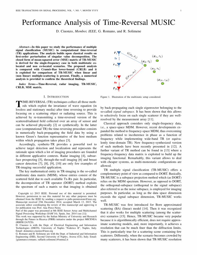
Figure 1. Illustration of the multistatic setup considered.

by back-propagating each single eigenvector belonging to theso-called signal subspace. It has been shown that this allowsto selectively focus on each single scatterer if they are well-resolved by the measurement array [11].

Classical approach considers only single-frequency data,i.e., a space-space MDM. However, recent developments ex-panded the method to frequency-space MDM, thus overcomingproblems related to incoherence in phase as a function offrequency while implementing wide-band TR (or equiva-lently time-domain TR). New frequency-synthesized versionof such methods have been recently presented in [12]. Afurther variant of TR method can be found in [13] where afrequency-frequency data matrix is exploited to build up theimaging functional. Remarkably, this variant allows to dealwith cheaper systems, as multi-monostatic configurations areallowed.

TR multiple signal classification (TR-MUSIC) offers acomplementary point of view as compared to DORT. Basically,TR-MUSIC is a subspace projection method which (as DORT)relies on the MDM spectrum. However, as opposed to DORT,the orthogonal-subspace (orthogonal to the signal subspace)also referred to as the noise subspace, is employed for imagingpurposes. In particular, as long as the data space dimensionexceeds the signal subspace dimension, TR-MUSIC workswell.

TR-MUSIC was first introduced for Born approximatedscattering (BA) (linear) model [14]. Then it was recognizedthat it also works for multiple scattering (among the scatter-ers) scenarios [15]. Hence, TR-MUSIC became very popularbecause it is algorithmically efficient, does not require approx-imate scattering models, and, more importantly, it achieves aresolution that can be much finer than the diffraction limits.This is particularly true for a scattering scene containing fewscatterers. Differently, when the scenario becomes crowded bymany scatterers, it has been shown that TR-MUSIC resolution

2 IEEE TRANSACTIONS ON SIGNAL PROCESSING, VOL. *, NO. *, MONTH YYYY

ability deteriorates as the number of scatterers in a givenspatial region exceeds the corresponding degrees of freedomassociated to the same region [16]. TR-MUSIC theory hasbeen expanded to consider extended scatterers as well in [17].

Research activities on TR-methods tackled different scat-tering scenario conditions. The case of lossy and dispersivescenarios has been addressed in [18], whereas time-varyinghost medium has been considered in [19]. More in general thecase of random host medium has been considered as well, andit has been shown how TR-methods are statistically stable dueto the self-averaging property of wide-band TR procedure [20].The case of complex scattering objects has been addressed in[21] (see also references therein).

In this paper we are concerned with the study of theperformance achievable by TR-MUSIC in locating point-likescatterers with additive noise matrix corrupting data.

A vast literature on the performance analysis of MUSICfor direction-of-arrival (DOA) estimation exists [22]. Thedevelopment of MUSIC algorithm traces back to [23]. Perfor-mance analysis in terms of resolution property was pioneeredby [24] for a simple scenario, while a detailed analysis ofMUSIC mean-squared error (MSE) can be found in the works[25], [26], [27], [28]. Theoretical performance analysis waslater extended in order to account for array modeling errorsboth in terms of MSE (through a first-order perturbationapproach) [29] and resolution [30]. The MSE/bias analysisin the presence of modeling errors was then considered via asecond-order subspace perturbation approach in [31], while theresolution capability of MUSIC was studied under the sameframework in [32]. Finally, a MSE/bias analysis, conditionedon the resolution event, was recently introduced in [33].

It is worth noticing that such results cannot be directlyapplied to TR-MUSIC because in TR framework scatter-ers/sources are generally assumed to be deterministic and moreimportantly a single snapshot is used, whereas DOA results forMUSIC refer to multiple snapshots and are often developedunder asymptotic (i.e., a very large number of snapshots)conditions. Unluckily, to the best of our knowledge, no suchcorresponding theoretical results are present in the literaturefor TR-MUSIC.

Yet, performance evaluation results have been reported formaximum-likelihood estimator (MLE) and other sub-optimalestimators for computational TR were presented in [34], bothfor BA and Foldy-Lax (FL) (non linear) models. The additionaltask of estimating scattering potential via a non-iterative(approximate) formula is addressed in [15] for location-onlyestimators. A theoretical study on performance, based on theCramér-Rao lower bound (CRLB), was presented in [35],both for BA and FL models. Sensitivity analysis of severalcomputational TR techniques to non-matching assumptions isstudied in [36].

The main contributions of the present manuscript are sum-marized as follows. We provide a theoretical performanceanalysis of TR-MUSIC in terms of the MSE matrix of theposition estimates. The presented result is achieved via: (i)a first-order approximation of position error vector and (ii)a first-order perturbation of singular value decomposition(SVD) [37]. The result is thus valid asymptotically (i.e. in

the high signal-to-noise regime). Both co-located and nonco-located multistatic (narrowband) setups with either BA orFL scattering are considered in this paper. The presentedresults complement those found in DOA literature [22] andcan be used to highlight the performance dependence of TR-MUSIC on the scatterers and measurement configurations.Some preliminary numerical examples for simple scatteringscenes are presented in order to validate the derived results.To this end, the TR-MUSIC single-frequency space-spaceformulation is considered in the framework of scalar scatteringscenarios for both two-dimensional and three-dimensionalgeometries. In particular, it is shown that the CRLB, thoughbeing representative of MLE asymptotic performance, does notaccurately predict TR-MUSIC performance, as opposed to theproposed expression. The latter is further used to compare theasymptotic MSE attainable under both BA and FL models.

The remainder of the manuscript is organized as follows:Sec. II describes the system model and gives preliminaries onSVD perturbation analysis. Sec. III presents the theoreticalperformance analysis of TR-MUSIC algorithm whereas itsvalidation is shown in Sec. IV via numerical simulations.Finally, conclusions are drawn in Sec. V. The paper containsalso different appendices where proofs and derivations ofintermediate results exploited in the manuscript are reportedfor reader’s convenience.

Notation - Lower-case (resp. Upper-case) bold letters denotecolumn vectors (resp. matrices), with an (resp. an,m) being thenth (resp. the (n,m)th) element of a (resp. A); ∇x{b(x)} ∈CN and Hx{b(x)} ∈ CN×N denote the gradient and Hessianoperators of {b(x) : x ∈ RN → C}, while Jx{c(x)} ∈CN×P is the Jacobian of {c(x) : x ∈ RN → CP };E{·}, (·)t, (·)†, Tr [·], (·)− < (·), ∠(·), δ(·), ‖·‖F and ‖·‖denote expectation, transpose, Hermitian, matrix trace, pseudo-inverse, real part, phase, Kronecker delta, Frobenius norm and`2 norm operators, respectively; the curled inequality symbol� (and its strict form �) is used to denote generalized matrixinequality: for any symmetric matrix A ∈ RN×N , A � 0(resp. A � 0) means that A is a positive semidefinite (resp.positive definite) matrix;ON×M (resp. IN ) denotes the N×Mnull (resp. identity) matrix; 0N (resp. 1N ) denotes the null(resp. ones) vector of length N ; diag(a) denotes the diagonalmatrix obtained from the vector a; x1:M denotes the vectorobtained by concatenation as x1:M ,

[xt1 · · · xtM

]t;

vec(M) stacks the first to the last columns of the matrixM one under another to form a long vector; Σx denotesthe covariance matrix of the complex-valued random vectorx; NC(µ,Σ) denotes a proper complex Gaussian pdf withmean vector µ and covariance matrix Σ; U(a, b) denotes acontinuous-valued uniform pdf with support [a, b]; finally thesymbol ∼ means “distributed as”.

II. SYSTEM MODEL

The system model is described as follows. We considerlocalization of point-like scatterers with a multistatic setup,as shown in Fig. 1. We assume that M point scatterers1 are

1The number of scatterers M is assumed to be known, as usually done inarray-processing literature [22].

CIUONZO et al.: PERFORMANCE ANALYSIS OF TIME-REVERSAL MUSIC 3

located at unknown positions {xk}Mk=1 in Rp with unknownscattering potentials {τk}Mk=1 in C. The transmit array con-sists of NT isotropic point elements located at the pointsri ∈ Rp, i ∈ ST , {1, . . . , NT }, while the receive arrayis formed by NR point receivers located at positions r` ∈ Rp,` ∈ SR , {1, . . . , NR}. The illuminators first send signals tothe probed scenario (in a known homogeneous backgroundwith wavenumber κ) and the transducer array records thereceived signals. The (single-frequency) measurement modelis then [34]:

Kn = K(x1:M , τ ) +W (1)= GR(x1:M )M(x1:M , τ )GT (x1:M )t +W (2)

where K(x1:M , τ ) ∈ CNR×NT and Kn ∈ CNR×NTdenote the multistatic data matrix (MDM) in frequency-domain and the measurement matrix, respectively. Further-more, W ∈ CNR×NT is a noise matrix whose elements2

vec(W ) ∼ NC(0NTNR , σ2w INTNR). Additionally, we have

denoted: (i) the vector of scattering coefficients as τ ,[τ1 · · · τM

]t ∈ CM ; (ii) the transmit and the receivearray matrices, as GT (x1:M ) ∈ CNT×M and GR(x1:M ) ∈CNR×M , respectively. The latter are defined explicitly as:

GT (x1:M ) ,[gT (x1) gT (x2) · · · gT (xM )

]; (3)

GR(x1:M ) ,[gR(x1) gR(x2) · · · gR(xM )

]. (4)

In Eq. (3), gT (x) ∈ CNT denotes the transmit Green’sfunction vector as a function of the arbitrary location x ∈ Rp,that is:

gT (x) ,[G(r1,x) G(r2,x) · · · G(rNT ,x)

]t. (5)

On the other hand, in Eq. (3), gR(x) ∈ CNR denotes thereceive Green’s function vector as a function of x, namely:

gR(x) ,[G(r1,x) G(r2,x) · · · G(rNR ,x)

]t. (6)

It is worth noticing that the functional dependence of Eqs. (5)and (6) is only due to G(x′,x), which denotes the relevant(scalar) background Green function [14]. Finally, in Eq. (2) thematrix M(x1:M , τ ) ∈ CM×M for BA model [14] is definedas

M(x1:M , τ ) , T (τ ) = diag(τ ), (7)

while in the case of FL model we have [35]

M(x1:M , τ ) ,[T−1(τ )− S(x1:M )

]−1, (8)

where the (m,n)th element of S(x1:M ) is defined as follows:

sm,n(x1:M ) ,

{G(xm,xn) m 6= n

0 m = n. (9)

Our performance analysis of TR-MUSIC is general and willconsider both models in Eqs. (7) and (8).

2It is worth noticing that the MSE expressions obtained hereinafter willonly depend on the second-order moments of the noise. Hence identical resultsapply in the case of different noise pdfs [37].

A. TR-MUSIC

Co-located scenario: In the co-located setup we haveNT = NR = N , GT (x1:M ) = GR(x1:M ) = G(x1:M ) andgT (x) = gR(x) = g(x). In this case, TR-MUSIC requiresthe evaluation of the following spatial spectrum [14]

P(x, Un) ,∥∥∥U †n g(x)

∥∥∥2

= g(x)† Pn g(x), (10)

where Un ∈ CN×(N−M) is the matrix of left singular vectorsof Kn associated to the noise subspace and Pn , (UnU

†n)

(i.e. the “noisy” projector into the left noise subspace). It canbe shown that Eq. (10) equals zero when x equals the truescatterers locations {xk}Mk=1 in the noise-free case (i.e. whenUn = Un, the latter being the eigenvector matrix associatedto the left noise subspace of K(x1:M , τ )) and thus the Mlargest local maxima of P(x, Un)−1 are generally chosen asthe estimated positions {xk}Mk=1 [14].

Non co-located scenario: In the non co-located setup, sev-eral TR-MUSIC variants have been proposed in the literature[15]. A first approach consists in using the so-called Rx modeTR-MUSIC. In this case the evaluated spatial spectrum (underthe assumption M < NR) is:

PR(x, Un) ,∥∥∥U †n gR(x)

∥∥∥2

= gR(x)† PR,n gR(x) (11)

where Un ∈ CNR×(NR−M) is the matrix of left singu-lar vectors of Kn associated to the noise subspace andPR,n , (UnU

†n) (i.e. the “noisy” projector into the left noise

subspace). A second (dual) approach, denoted as Tx mode TR-MUSIC, constructs the following spatial spectrum (under theassumption M < NT ):

PT (x, Vn) ,∥∥∥V †n g∗T (x)

∥∥∥2

= gT (x)t PT,n g∗T (x) (12)

where Vn ∈ CNT×(NT−M) is the matrix of right singu-lar vectors of Kn associated to the noise subspace andPT,n , (VnV

†n ) (i.e. the “noisy” projector into the right

noise subspace). Finally, a combined version of the mentionedversions, denoted as Tx+Rx TR-MUSIC, can be built as (underthe assumption M < min{NT , NR}) [15]:

PTR(x; Un, Vn) , PT (x, Vn) + PR(x, Un). (13)

Similarly as for the co-located setup, the M largest local max-ima of PR(x, Un)−1, PT (x, Vn)−1 and PTR(x; Un, Vn)−1

are chosen as the estimated positions {xk}Mk=1.

B. Preliminaries on SVD Perturbation

In this sub-section we give preliminaries on first-order SVDperturbation, following [37], [38]. First, we consider a rank de-ficient matrix A ∈ CR×T with rank equal to δ < min{R, T}.It can be easily shown that its SVD A = U ΣV † can berewritten as:

A =(Us Un

)( Σs Oδ×δOδ×δ Oδ×δ

)(V †sV †n

), (14)

where δ , (R − δ) and δ , (T − δ), respectively. Addi-tionally, Us ∈ CR×δ and Vs ∈ CT×δ (resp. Un ∈ CR×δand Vn ∈ CT×δ) have been used to denote the unitary


bases of the left and right signal subspaces (resp. orthogonalsubspaces) in Eq. (14). Secondly, we take the perturbed matrixA = (A + N), where N represents a perturbing matrix.Similarly as in Eq. (14), the SVD of A = UΣV † is rewrittenas

A =(Us Un

)( Σs Oδ×δOδ×δ Σn

)(V †sV †n

)(15)

which underlines the effect ofN on the spectral representationof A. Indeed we notice that, as opposed to Eq. (14), A maybe full-rank in general. Furthermore, Eq. (15) underlines themodification of the left and right principal directions due toN . This can be stressed as:

Us = Us + ∆Us, Un = Un + ∆Un, (16)Vs = Vs + ∆Vs, Vn = Vn + ∆Vn, (17)

where ∆(·) terms in Eqs. (16) and (17) are in general compli-cated functions of N . However, when N has a “small magni-tude” (its meaning will be clarified hereinafter) in comparisonto A, a first-order perturbation (i.e. ∆(·) are approximatedas linear functions of N ), originally proposed in [39] andsuccessively applied in [27], [37], will be accurate. Clearly, asmall perturbation is typically observed in the high signal-to-noise ratio (SNR) regime. Based on these reasons, thefollowing lemma will be used to build our analysis.

Lemma 1. The perturbed orthogonal left subspace Un (resp.right subspace Vn) is spanned by Un + UsB (resp. Vn +VsB) and the perturbed signal left subspace Us (resp. rightsubspace Vs) is spanned by Us + UnC (resp. Vs + VnC),where C and B (resp. C and B) are matrices whose normsare of the order of the norm of N , which can be any sub-multiplicative one such as the `2 or the Frobenius norms.

The explicit expressions for ∆Un and ∆Vn, valid up tothe first order, are:

∆Un = UsB = −Us Σ−1s V †s N

†Un; (18)∆Vn = Vs B = −Vs Σ−1

s U †s N Vn. (19)

Correspondingly, C = −B† and C = −B† hold, thus giving:

∆Us = UnC = PR,nN Vs Σ−1s ; (20)

∆Vs = Vn C = PT,nN†Us Σ−1

s . (21)

In Eqs. (20) and (21) we have defined PR,n , UnU†n and

PT,n , VnV†n , respectively. Furthermore, we notice that in

obtaining Eqs. (18-21), “in-space” perturbation terms (e.g.the contribution to ∆Us depending on Us), which havebeen shown to be linear with N (and thus not negligible atfirst-order), are not considered. The reason is that these donot affect performance analysis of subspace-based estimationmethods (since the corresponding subspace projector is notaltered), which (TR-)MUSIC belongs to [40].

III. PERFORMANCE ANALYSIS

A. Co-located scenario

Here we generalize the classical steps used for MUSICperformance analysis in DOA estimation [27], [37] to our

model. It is known that, for true scatterers location, we have:

P(xk,Un) = 0, k ∈ {1, . . . ,M} (22)

However, due to the perturbing matrixW , TR-MUSIC obtainsan imperfect estimate xk = (xk+∆xk). We first use a (first-order) Taylor-series expansion of ∇x{P(x, Un)}) around xkto approximate ∆xk as:

∆xk ≈ − (Hx{P(x, Un)}−1∇x{P(x, Un)})∣∣∣x=xk

(23)

For notational simplicity we denote n(x, Un) ,−∇x{P(x, Un)} and D(x, Un) , Hx{P(x, Un)}.Secondly, we show that n(x,Un) can be expressed as

n(x,Un) = −∇x{g(x)†Pn g(x)} (24)

= −Jx{g(x)}†Pn g(x)− Jx{g(x)}tP ∗n g(x)∗ (25)

= −2<{Jx{g(x)}†Pn g(x)

}(26)

which holds independently on Un. The terms n(xk, Un) andD(xk, Un) can be expressed as:

n(xk, Un) = n(xk,Un) + ∆n , n+ ∆n (27)D(xk, Un) = D(xk,Un) + ∆D ,D + ∆D (28)

In the above equations the perturbations ∆n and ∆D areboth linear functions of ∆Un when a first-order approximationis considered. Using the orthogonality property U †n g(xk) =0(N−M), we have n(xk,Un) = n = 0p. Hence, ∆xk can befurther approximated as follows:

∆xk = (D(xk,Un) + ∆D)−1

∆n (29)

= (D + ∆D)−1

∆n =(I +D−1∆D

)−1D−1∆n (30)

=

+∞∑k=0

(−D−1∆D

)k (D−1∆n

)≈D−1∆n (31)

where in Eq. (30) we have used the Neumann series [41] andin Eq. (31) we retained only the first-order term. A sufficientcondition for invertibility3 of matrix D is shown to be (N −M) ≥ p in Appendix B, along with a detailed discussion onits structural properties. The vector ∆n can be evaluated fromthe closed form of n(xk, Un) given in Eq. (26):

n(xk, Un) = −2<{J†k(UnU†n)g(xk)} = (32)

−2<{J†k UnU

†n g(xk) + J†k∆Un(∆Un)†g(xk)+

J†kUn(∆Un)†g(xk) + J†k∆UnU†n g(xk)

}(33)

where we have used the short-hand notation Jk ,Jx{g(x)}|x=xk

. It is apparent from Eq. (33) that both first

3We remark that lack of invertibility of D corresponds to analogousdegenerate scenarios when applying the classic MSE analysis for MUSICin DOA estimation. Thus the assumptions in the present study do notimpose additional limitations with respect to those for MSE analysis ofMUSIC-based DOA estimation [27]. Indeed, in the aforementioned case,analogous rationale leads to the following expression for the first orderapproximation of angle-of-arrival estimation error ∆θk , (θk − θk), that is∆θk ≈ −

∂P(θ,Un)∂θ /∂

2P(θ,Un)

∂θ2

∣∣∣θ=θk

≈ ∆ND

, where the scalar D ∈ R

equals D , ∂2P(θ,Un)

∂θ2

∣∣∣θ=θk

= 2<{ ∂g(θ)†

∂θ

∣∣∣∣θ=θk

Pn∂g(θ)∂θ

∣∣∣θ=θk

}.

Therefore, similarly as in our analysis, a first-order approximation cannot beapplied when the second derivative of the pseudo-spectrum is null at θ = θk .


and last terms are zero since U †n g(xk) = 0(N−M), while thesecond term is quadratic in ∆Un and thus can be discardedin a first-order analysis. Thus, Eq. (33) is approximated by:

n(xk, Un) ≈ −2<{J†kUn(∆Un)†g(xk)} (34)

From direct comparison of Eqs. (27) and (34), we obtain:

∆n = −2<{J†kUn(∆Un)†g(xk)}. (35)

We now focus on the explicit form of D = D(xk,Un), whichis found as:

D = D(xk,Un) = Hx{P(x,Un)}|x=xk(36)

= Hx{g(x)†Pn g(x)}∣∣x=xk

= 2<{J†k Pn Jk} (37)

where the last equality is proved in Appendix A. Hence, inview of Eqs. (31), (35) and (37), we obtain:

∆xk ≈ −<{J†k Pn Jk}−1 <{J†kUn(∆Un)†g(xk)} (38)

Now we substitute Eq. (18) in Eq. (38), thus leading to:

∆xk ≈ <{J†k Pn Jk}−1<{J†k PnW K−(x1:M , τ ) g(xk)}

(39)

where we have exploited K−(x1:M , τ ) = (Vs Σ−1s U

†s ) .

Aiming at notational simplicity, we further define αk ,K−(x1:M , τ ) g(xk), Bk , P †n Jk and Γk , <{J†k Pn Jk},which allow us to rewrite Eq. (39) as:

∆xk ≈ Γ−1k <

{B†kW αk

}(40)

Since the first-order perturbation ∆xk is linear in the noisematrix W , it follows immediately4 E{∆xk} ≈ 0p. Then thecovariance matrix of ∆xk equals the MSE matrix of xk (i.e.the estimated position of kth target is unbiased at high-SNR).

We can now turn our attention to the explicit (approximate)evaluation of Σ∆xk = E{∆xk∆xtk}. It is shown in Ap-pendix C that its closed form expression is given by:

Σ∆xk ≈ 1

2σ2w ‖αk‖

2Γ−1k <{B

†kBk}

(Γ−1k

)t(41)

Further simplifications, exploiting analogous steps as in [37],are obtained as follows. First we notice that <{B†kBk} = Γk(since Pn = Pn

† = Pn2) and Γk = Γ†k. Secondly, we use

the definition αk = K−(x1:M , τ )g(xk). Finally, combiningthese results, leads to a refined expression for Eq. (41):

Σ∆xk ≈σ2w

2

∥∥K−(x1:M , τ ) g(xk)∥∥2 <{J†k Pn Jk}

−1

(42)

B. Non co-located scenario (separate modes)In the case of either Rx or Tx mode TR-MUSIC, we can

readily exploit results in Sec. III-A. In fact, it can be shownthat Eq. (23) specializes to

∆xR,k ≈ − (Hx{PR(x, Un)}−1∇x{PR(x, Un)})∣∣∣x=xk

∆xT,k ≈ − (Hx{PT (x, Vn)}−1∇x{PT (x, Vn)})∣∣∣x=xk

(43)

4Indeed Bk = P †n Jk is actually a deterministic matrix (and thus can be

put outside the expectation), since Pn denotes the orthogonal projector of thenoise-free (i.e. independent on W ) MDM, that is K(x1:M , τ ).

for Rx and Tx mode spatial spectrums, respectively. Sim-ilarly, for the sake of brevity we denote nR(x, Un) ,−∇x{PR(x, Un)}, nT (x, Vn) , −∇x{PT (x, Vn)},DR(x, Un) , Hx{PR(x, Un)} and DT (x, Vn) ,Hx{PT (x, Vn)}. Therefore, Eq. (26) generalizes to

nR(xk, Un) = −2<{J†R,k(UnU†n) gR(xk)}, (44)

nT (xk, Vn) = −2<{J tT,k(VnV†n ) gT (xk)∗}, (45)

where we have defined JR,k , Jx{gR(x)}|x=xkand JT,k ,

Jx{gT (x)}|x=xk. The first-order approximations for ∆xR,k

and ∆xT,k are given similarly as5:

∆xR,k ≈ D−1R ∆nR (46)

∆xT,k ≈ D−1T ∆nT (47)

where DR , 2<{J†R,k PR,n JR,k} and DT ,2<{J tT,k PT,n J∗T,k}, respectively. Also, the closed formexpressions for ∆nR and ∆nT are given by:

∆nR = −2<{J†R,kUn(∆Un)†gR(xk)}; (48)

∆nT = −2<{J tT,kVn(∆Vn)†gT (xk)∗}. (49)

Finally, after giving the following definitions for ease ofnotation

αR,k ,K−(x1:M , τ ) gR(xk), BR,k , P †R,nJR,k,

αT,k ,(K−(x1:M , τ )

)†gT (xk)∗, BT,k , P †T,nJ

∗T,k,

ΓR,k , <{J†R,k PR,n JR,k}, ΓT,k , <{J tT,k PT,n J∗T,k},(50)

and putting all together, we get:

∆xR,k ≈ Γ−1T,k <

{B†T,kW

†αT,k

}; (51)

∆xT,k ≈ Γ−1R,k <

{B†R,kW αR,k

}. (52)

Similarly to the co-located case, both ∆xR,k and ∆xT,k arelinear functions of W , thus E{∆xR,k} = E{∆xT,k} ≈ 0p;hence also in this setup the covariance matrix of ∆xR,k (resp.∆xT,k) equals the MSE matrix of xR,k (resp. xT,k), that is,the estimated position of kth target is unbiased at high-SNR.

By means of similar steps as in Appendix C, we analogouslyobtain the closed form expressions for the MSE matrix of Rxand Tx modes TR-MUSIC (cf. Eqs. (11) and (12)):

Σ∆xR,k ≈1

2σ2w ‖αR,k‖

2Γ−1R,k <{B

†R,kBR,k}

(Γ−1R,k

)t(53)

Σ∆xT,k ≈1

2σ2w ‖αT,k‖

2Γ−1T,k <{B

†T,kBT,k}

(Γ−1T,k

)t(54)

Similar considerations as in the co-located case lead to thecorresponding refined expressions:

Σ∆xR,k ≈σ2w

2

∥∥K−(x1:M , τ ) gR(xk)∥∥2 <{J†R,k PR,n JR,k}

−1

(55)

Σ∆xT,k ≈σ2w

2

∥∥∥(K−(x1:M , τ ))†g∗T (xk)

∥∥∥2

<{J tT,k PT,n J∗T,k}−1

(56)

5Analogous considerations as the co-located scenario apply to invertibilityof matrices DR and DT , respectively.


C. Non co-located scenario (Tx/Rx spectrum)Analogously to the previous sections, we need to

evaluate DTR(x, Un, Vn) , Hx{PTR(x, Un, Vn)} andnTR(x, Un, Vn) , −∇x{PTR(x, Un, Vn)}. First, it can beeasily shown that:

nTR(x, Un, Vn) = nR(x, Un) + nT (x, Vn); (57)DTR(x, Un, Vn) = DR(x, Un) +DT (x, Vn). (58)

Thus Eq. (57) is exploited to observe that at first-order:

nTR(x, Un, Vn) ≈∆nR + ∆nT , (59)

where ∆nR and ∆nT are given as in Eqs. (48) and (49).Also, by exploiting Eq. (58), we obtain:

DTR ,DTR(xk,Un,Vn) = DR +DT . (60)

From similar considerations, perturbing noise matrix W leadsto xTR,k = (xk + ∆xTR,k), where ∆xTR,k is approximatedat the first order as

∆xTR,k ≈ (DR +DT )−1 (∆nR + ∆nT ) , (61)

and it can be expressed explicitly as:

∆xTR,k ≈ Γ−1TR,k <{B

†T,kW

†αT,k + B†R,kW αR,k};(62)

where we have denoted ΓTR,k , (ΓT,k + ΓR,k). First it isapparent that E{∆xTR,k} ≈ 0p; this is somewhat expectedsince any linear combination of two unbiased estimators is stillunbiased [42]. Consequently, the MSE matrix of xTR,k canbe evaluated as the covariance matrix of ∆xTR,k.

Finally, as reported in Appendix D, we obtain the closedform expression for the MSE matrix for the Tx/Rx TR-MUSIC, shown in Eq. (63) at the top of the next page. Itis worth remarking that the covariance matrix is not simplygiven the sum of the corresponding contributions of Tx andRx modes, since they are correlated (actually the “perturbing”matrix W is the same for both of them).

D. {Jk, JT,k,JR,k} in homogeneous 2-D/3-D backgroundSince the obtained MSE matrix expression requires the

closed form for Jk = Jx{g(x)}|x=xkin a co-located scenario

(resp. JR,k and JT,k in a non co-located setup), hereinafterwe derive its explicit form for the case of 2-D/3-D propagationin a homogeneous background. Such a result will be used inSec. IV; in 2-D scenario G(x′,x) = H

(1)0 (κ ‖x′ − x‖) (we

discard the irrelevant constant term j4 ), where H

(1)n (·) and

κ = 2πλ denote the nth order Hankel function of the first kind

and the wavenumber (λ is the wavelength), respectively. On

the other hand, in 3-D scenario G(x′,x) =

exp(jκ‖x′−x‖)‖x′−x‖

holds (we drop the irrelevant constant term 14π ).

We simply notice that the ith row of each of the consid-ered matrices equals ∇x{G(qi,x)}t, thus (here qi denotes ageneric fixed point in 2-D/3-D space, in our case the positionof a Tx/Rx array element)

∇x{G(qi,x)} = ∇x

{H

(1)0 (κ ‖qi − x‖)

}(64)

= κH(1)1 (κ ‖qi − x‖)

(qi − x)

‖qi − x‖(65)

for 2-D case, where in Eq. (65) we have exploited therecursions in Hankel functions derivatives [43]. Differently,for 3-D case we obtain:

∇x{G(qi,x)} = ∇x

{exp(jκ ‖qi − x‖)‖qi − x‖

}(66)

= exp(jκ ‖qi − x‖) (1− jκ ‖qi − x‖)(qi − x)

‖qi − x‖3(67)

E. BA vs FL models - MSE gain

Here we will focus on the co-located setup in order tokeep simplicity of our theoretical analysis. We will comparetheoretical (high-SNR) performance of TR-MUSIC with BAand FL models. It was shown in [35] that FL scatteringimproves performance with respect to BA model, througha CRLB-based comparison. However, as we will show inSec. IV, the CRLB is only representative of MLE performance,the latter being unfeasible (in terms of complexity) from apractical point of view. Therefore it is of interest to assess therelative performance (via high-SNR MSE expression obtainedin Eq. (42)) attained by TR-MUSIC under both BA and FLmodels.

Hence, we start from Eq. (42) and more specifically we: (i)consider the trace of the covariance (MSE) matrix of xk, (ii)evaluate the closed form expressions under both the modelsand (iii) analyze their ratio. In order to accomplish this task,we first define6:

γmsek ,

Tr [Σ∆xk,f ]

Tr [Σ∆xk,b]=

∥∥∥K−f (x1:M , τ ) g(xk)

∥∥∥2

∥∥∥K−b (x1:M , τ ) g(xk)

∥∥∥2 (68)

where the subscripts “f” and “b” refer to the correspondingquantities under FL and BA models, respectively. Last equalityin Eq. (68) is obtained observing that Pn is the same underboth the considered models. Then, after some manipulations,we can express γmse

k as:

γmsek =

g(xk)† [Us,f Σ−1s,f V

†s,f Vs,f Σ−1

s,fU†s,f ] g(xk)

g(xk)† [Us,b Σ−1s,bV

†s,b Vs,b Σ−1

s,bU†s,b] g(xk)

(69)

=g(xk)† [Us,f Σ−2

s,f U†s,f ] g(xk)

g(xk)† [Us,b Σ−2s,bU

†s,b] g(xk)

(70)

=

∑Mm=1 λ

−1f,m

∥∥∥u†s,f,m g(xk)∥∥∥2

∑Mm=1 λ

−1b,m

∥∥∥u†s,b,m g(xk)∥∥∥2 (71)

where Kb(x1:M , τ ) = (Us,bΣs,bV†s,b) and Kf(x1:M , τ ) =

(Us,fΣs,fV†s,f) are the SVDs of MDM with BA and FL

models, respectively. Also, in Eq. (70) we exploited theunitarity property (V †s,bVs,b) = (V †s,fVs,f) = IM . Finally, inEq. (71) we denoted λb,m and us,b,m (resp. λf,m and us,f,m)as the mth eigenvalue of the TR operator (Kb)†Kb (resp.(Kf)

†Kf ) [14] and the mth column of Us,b (resp. Us,f ), re-spectively. We will show in Sec. IV that the theoretical resultsagree with [44] and are, only at first glance in contraposition

6Hereinafter, for the sake of simplicity, we will consider Eq. (42) holdingwith equality since we are in a high-SNR regime.


Σ∆xTR,k ≈σ2w

2Γ−1TR,k (‖αR,k‖2 ΓR,k + ‖αT,k‖2 ΓT,k + <{B†T,k αR,k α

tT,k B

∗R,k + B†R,k αT,k α

tR,k B

∗T,k}) (Γ−1

TR,k)t (63)

with those given in [35], in terms of CRLB of localizationparameters.

IV. NUMERICAL RESULTS

In this section we confirm our theoretical findings throughsimulations. First, we define SNR , ‖K(x1:M )‖2F

NT NR σ2w

and we con-sider a setup where λ = 1 (thus κ = 2π) and λ

2 -spacedTx/Rx arrays are employed. Secondly, to quantify the levelof multiple scattering (analogously as in [15]) we define the

index η ,‖Kf (x1:M ,τ )−Kb(x1:M ,τ )‖

F

‖Kb(x1:M ,τ )‖Fwhere Kb(x1:M , τ )

and Kf(x1:M , τ ) denote the MDM generated according toEqs. (7) and (8), respectively. For the sake of simplicity, ourexamples consider M = 2 targets in the area of interest. Whennot otherwise specified, we assume that the targets are locatedat x1 =

[−1 −6

]tand x2 =

[+1 −6

]tand have

scattering coefficients τ =[

3 4]t

.Co-located setup - simulated vs. theoretical MSE: we first

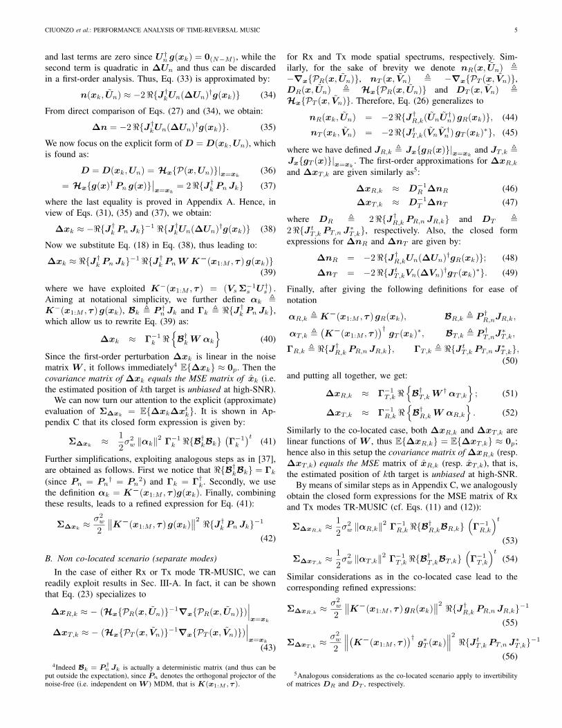
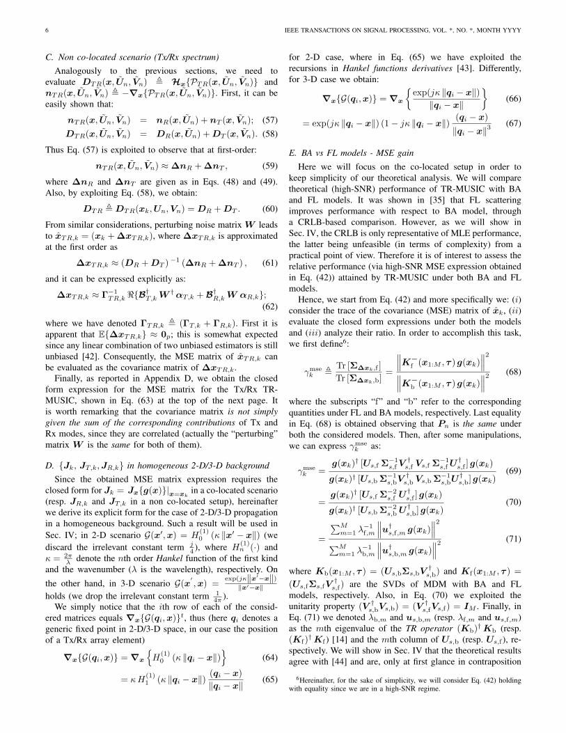
consider a multistatic experiment with a co-located Tx/Rxarray of N = 11 elements, as shown in Fig. 2; in thiscase we have η = (0.8232). Fig. 3 plots the MSE (i.e.Tr[E{‖xk − xk‖2}]) of each target vs. SNR (in dB) wheneither TR-MUSIC (cf. Eq. (10)) or MLE [34] is adopted7

(dashed lines). Correspondingly, theoretical MSE of TR-MUSIC (obtained via Eq. (42)) and CRLB8 are both reportedin solid lines. Results for both BA and FL models are given.First, it is apparent that Monte Carlo (MC) based TR-MUSICperformance approach theoretical ones as the SNR grows, thusconfirming our theoretical analysis. Secondly, MLE rapidlyapproaches the CRLB, as predicted from the theory [42].However, it is worth noticing how theoretical MSE predictedfor TR-MUSIC differs significantly from CRLB, thus moti-vating the need of the presented results for a (meaningful)TR-MUSIC theoretical performance evaluation. Interestingly,TR-MUSIC performance does not achieve the CRLB evenin the case of a DWBA model, which can be seen as thedeterministic analogous of a diagonal covariance matrix forMUSIC applied to DOA estimation [22]; this underlines thesignificant difference of the present setup with respect to MU-SIC performance assessment in DOA estimation. Furthermore,for this particular experiment, TR-MUSIC (high-SNR) MSEof each target under BA model is significantly lower than thatunder FL scattering, thus disagreeing with the CRLB. Such aresult may seem counter-intuitive at first glance; however thisis explained since TR-MUSIC is a sub-optimal estimator (thusit does not asymptotically achieve the CRLB as the MLE) andadditionally it does not exploit FL model peculiarities (cf. Eqs.(8-10)).

7Simulated performances are based on 5 · 103 Monte Carlo runs.8The closed form of CRLB for BA and FL models is omitted here for the

sake of brevity and can be found in [35].

−8 −6 −4 −2 0 2 4 6 8−8

−6

−4

−2

0

X [in λ]

Y [i

n λ]

TargetsTx−Rx array

Figure 2. Geometry for the considered imaging problem in 2-D space; co-located setup.

0 2 4 6 8 10 12 14 16 18 20

10−3

10−2

10−1

100

SNR [dB]

MS

E [

λ2 ]

Target 1 − BA modelTarget 2 − BA modelTarget 1 − FL modelTarget 2 − FL model

TR−MUSIC (Sim. + Th.)

MLE + CRLB

Figure 3. Co-located 2-D case: MSE vs. SNR; theoretical (CRLB and TR-MUSIC (obtained via Eq. (42)), in solid lines) vs. simulated (MC-based MLEand TR-MUSIC, in dashed lines) performance.

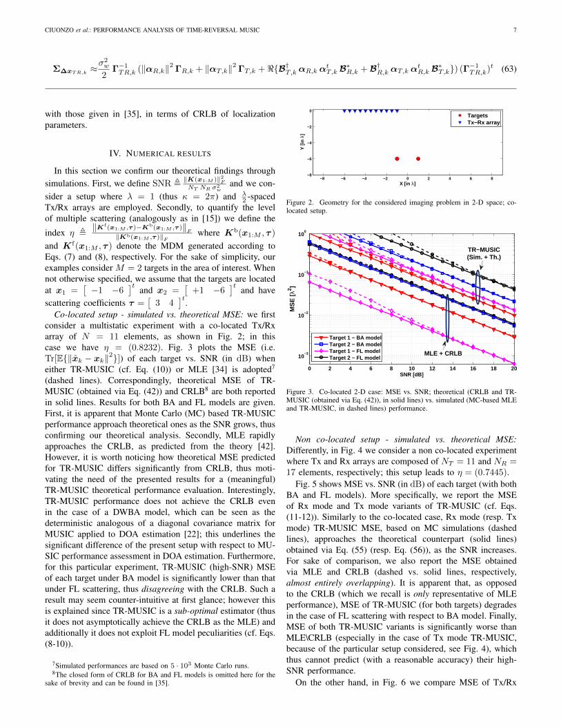
Non co-located setup - simulated vs. theoretical MSE:Differently, in Fig. 4 we consider a non co-located experimentwhere Tx and Rx arrays are composed of NT = 11 and NR =17 elements, respectively; this setup leads to η = (0.7445).

Fig. 5 shows MSE vs. SNR (in dB) of each target (with bothBA and FL models). More specifically, we report the MSEof Rx mode and Tx mode variants of TR-MUSIC (cf. Eqs.(11-12)). Similarly to the co-located case, Rx mode (resp. Txmode) TR-MUSIC MSE, based on MC simulations (dashedlines), approaches the theoretical counterpart (solid lines)obtained via Eq. (55) (resp. Eq. (56)), as the SNR increases.For sake of comparison, we also report the MSE obtainedvia MLE and CRLB (dashed vs. solid lines, respectively,almost entirely overlapping). It is apparent that, as opposedto the CRLB (which we recall is only representative of MLEperformance), MSE of TR-MUSIC (for both targets) degradesin the case of FL scattering with respect to BA model. Finally,MSE of both TR-MUSIC variants is significantly worse thanMLE\CRLB (especially in the case of Tx mode TR-MUSIC,because of the particular setup considered, see Fig. 4), whichthus cannot predict (with a reasonable accuracy) their high-SNR performance.

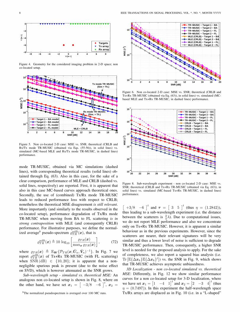
On the other hand, in Fig. 6 we compare MSE of Tx/Rx


−8 −6 −4 −2 0 2 4 6 8−8

−6

−4

−2

0

X [in λ]

Y [i

n λ]

TargetsTx arrayRx array

Figure 4. Geometry for the considered imaging problem in 2-D space; nonco-located setup.

0 2 4 6 8 10 12 14 16 18 20

10−4

10−3

10−2

10−1

100

SNR [dB]

MS

E [

λ2 ]

Target 1 − BA modelTarget 2 − BA modelTarget 1 − FL modelTarget 2 − FL model

Tx mode TR−MUSIC(Sim + Th.)

Rx mode TR−MUSIC(Sim. + Th.)

MLE + CRLB

Figure 5. Non co-located 2-D case: MSE vs. SNR; theoretical (CRLB andRx/Tx mode TR-MUSIC (obtained via Eqs. (55-56)), in solid lines) vs.simulated (MC-based MLE and Rx/Tx mode TR-MUSIC, in dashed lines)performance.

mode TR-MUSIC, obtained via MC simulations (dashedlines), with corresponding theoretical results (solid lines) ob-tained through Eq. (63). Also in this case, for the sake of aclear comparison, performance of MLE and CRLB (dashed vs.solid lines, respectively) are reported. First, it is apparent thatalso in this case MC-based curves approach theoretical ones.Secondly, the use of (combined) Tx/Rx mode TR-MUSICleads to reduced performance loss with respect to CRLB;nonetheless the theoretical MSE disagreement is still relevant.More importantly (and similarly to the results observed in theco-located setup), performance degradation of Tx/Rx modeTR-MUSIC when moving from BA to FL scattering is instrong contraposition with MLE (and consequently CRLB)performance. For illustrative purposes, we define the normal-ized average9 pseudo-spectrum %ndB

TR (x), that is

%ndBTR (x) , 10 log10

[%TR(x)

maxx %TR(x)

], (72)

where %TR(x) , EW {PTR(x; Un, Vn)−1}. In Fig. 7 wereport %ndB

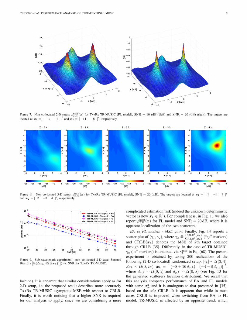
TR (x) of Tx+Rx TR-MUSIC (with FL scattering)when SNR (dB) ∈ {10, 20}; it is apparent that a non-negligible spurious peak is present (due to the noise effecton SVD), which is however attenuated as the SNR grows.

Sub-wavelength setup - simulated vs. theoretical MSE: Ananalogous non co-located setup is shown in Fig. 8, where onthe other hand, we have set x1 =

[−3/8 −6

]t, x2 =

9The normalized pseudospectrum is averaged over 100 MC runs.

0 2 4 6 8 10 12 14 16 18 2010

−4

10−3

10−2

SNR [dB]

MS

E [

λ2 ]

TR−MUSIC − Target 1 − BATR−MUSIC − Target 2 − BA TR−MUSIC − Target 1 − FLTR−MUSIC − Target 2 − FLMLE (CRLB) − Target 1 − BAMLE (CRLB) − Target 2 − BAMLE (CRLB) − Target 1 − FLMLE (CRLB) − Target 2 − FL

Figure 6. Non co-located 2-D case: MSE vs. SNR; theoretical (CRLB andTx+Rx TR-MUSIC (obtained via Eq. (63)), in solid lines) vs. simulated (MC-based MLE and Tx+Rx TR-MUSIC, in dashed lines) performance.

20 22 24 26 28 30 32 34 36 38 4010

−6

10−5

10−4

10−3

10−2

10−1

SNR [dB]

MS

E [

λ2 ]

TR−MUSIC − Target 1 − BA TR−MUSIC − Target 2 − BA TR−MUSIC − Target 1 − FL TR−MUSIC − Target 2 − FL CRLB − Target 1 − BA CRLB − Target 2 − BA CRLB − Target 1 − FL CRLB − Target 2 − FL

Figure 8. Sub-wavelength experiment - non co-located 2-D case: MSE vs.SNR; theoretical (CRLB and Tx+Rx TR-MUSIC (obtained via Eq. (63)), insolid lines) vs. simulated (MC-based Tx+Rx TR-MUSIC, in dashed lines)performance.

[+3/8 −6

]tand τ =

[3 5

]t(thus η = (1.2842)),

thus leading to a sub-wavelength experiment (i.e. the distancebetween the scatterers is 3

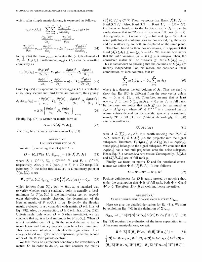
4λ). Due to computational issues,we do not report MLE performance and also we concentrateonly on Tx+Rx TR-MUSIC. However, it is apparent a similarbehaviour as in the previous experiments. However, since thescatterers are nearer, their relevant signatures will be verysimilar and thus a lower level of noise is sufficient to degradeTR-MUSIC performance. Then, consequently, a higher SNRlevel is needed for the proposed analysis to apply. For the sakeof completeness, we also report a squared bias analysis (i.e.Tr [E{∆xk}E{∆xk}t]) vs. the SNR in Fig. 9, which showsthat TR-MUSIC achieves asymptotic unbiasedness.

3D Localization - non co-located simulated vs. theoreticalMSE: Differently, in Fig. 12 we show similar performancecurves for a non co-located setup for 3-D localization, wherewe have set x1 =

[1 −4 1

]tand x2 =

[2 −3 4

]t(thus

η = (0.7497)). In this experiment the half-wavelength spaceTx/Rx arrays are displaced as in Fig. 10 (i.e. in a “L-shaped”


−2

−1

0

1

2

−8

−7

−6

−5

−4−20

−15

−10

−5

0

X [in λ]

Y [in λ]

[dB

]

−2−1

01

2

−8

−7

−6

−5

−4−30

−25

−20

−15

−10

−5

0

X [in λ]

Y [in λ]

[dB

]

Figure 7. Non co-located 2-D setup: %ndBTR (x) for Tx+Rx TR-MUSIC (FL model), SNR = 10 (dB) (left) and SNR = 20 (dB) (right). The targets are

located at x1 =[−1 −6

]t and x2 =[

+1 −6]t, respectively.

X [in λ]

Y [i

n λ]

Z = 0 λ

−4 −2 0 2 4−8

−7

−6

−5

−4

−3

−2

−1

0

[dB]−25 −20 −15 −10 −5 0

X [in λ]

Y [i

n λ]

Z = 1 λ

−4 −2 0 2 4−8

−7

−6

−5

−4

−3

−2

−1

0

[dB]−25 −20 −15 −10 −5 0

X [in λ]

Y [i

n λ]

Z = 2 λ

−4 −2 0 2 4−8

−7

−6

−5

−4

−3

−2

−1

0

[dB]−25 −20 −15 −10 −5 0

X [in λ]

Y [i

n λ]

Z = 3 λ

−4 −2 0 2 4−8

−7

−6

−5

−4

−3

−2

−1

0

[dB]−25 −20 −15 −10 −5 0

X [in λ]

Y [i

n λ]

Z = 4 λ

−4 −2 0 2 4−8

−7

−6

−5

−4

−3

−2

−1

0

[dB]−25 −20 −15 −10 −5 0

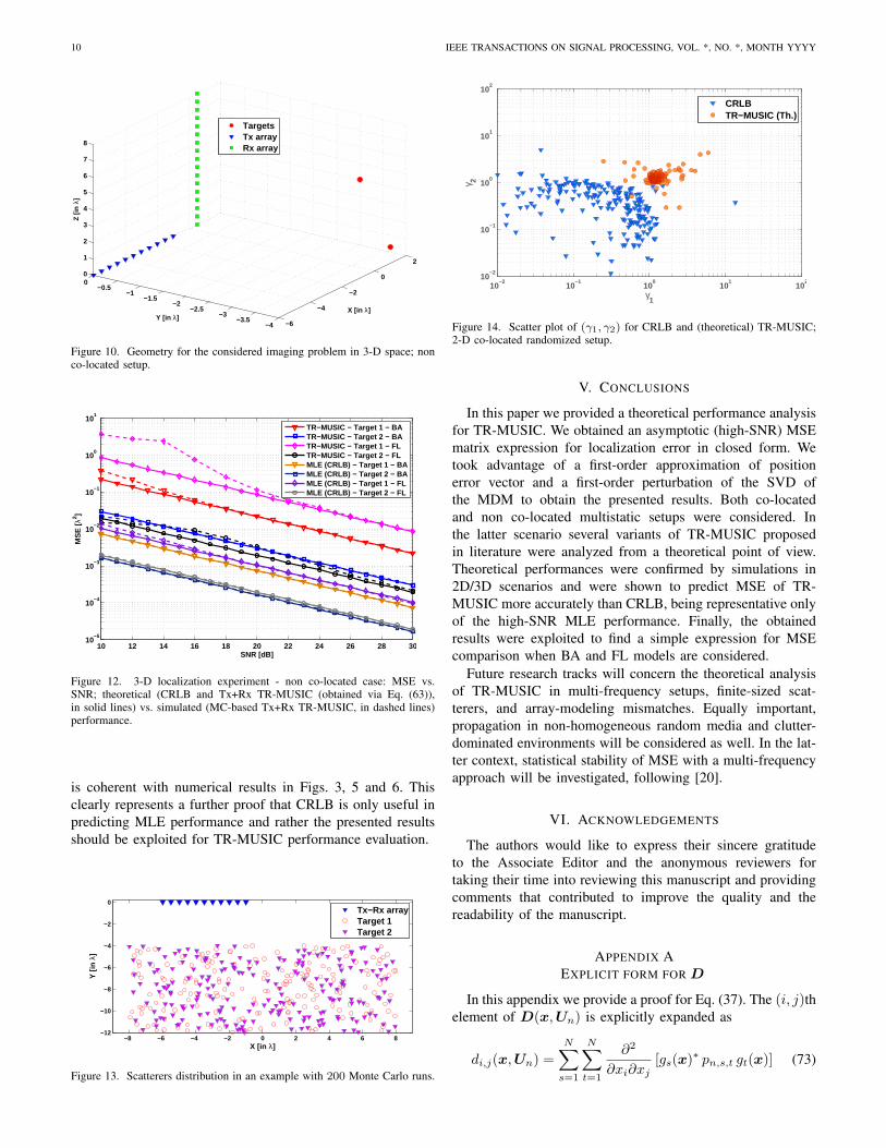
Figure 11. Non co-located 3-D setup: %ndBTR (x) for Tx+Rx TR-MUSIC (FL model), SNR = 20 (dB). The targets are located at x1 = [ 1 −4 1 ]t

and x2 = [ 2 −3 4 ]t, respectively.

20 22 24 26 28 30 32 34 36 38 4010

−8

10−6

10−4

10−2

SNR [dB]

Squ

ared

Bia

s [

λ2 ]

TR−MUSIC − Target 1 − BA TR−MUSIC − Target 2 − BA TR−MUSIC − Target 1 − FL TR−MUSIC − Target 2 − FL

Figure 9. Sub-wavelength experiment - non co-located 2-D case: SquaredBias (Tr

[E{∆xk}E{∆xk}t

]) vs. SNR for Tx+Rx TR-MUSIC.

fashion). It is apparent that similar considerations apply as for2-D setup, i.e. the proposed result describes more accuratelyTx+Rx TR-MUSIC asymptotic MSE with respect to CRLB.Finally, it is worth noticing that a higher SNR is requiredfor our analysis to apply, since we are considering a more

complicated estimation task (indeed the unknown deterministicvector is now xk ∈ R3). For completeness, in Fig. 11 we alsoreport %ndB

TR (x) for FL model and SNR = 20 dB, where it isapparent localization of the two scatterers.

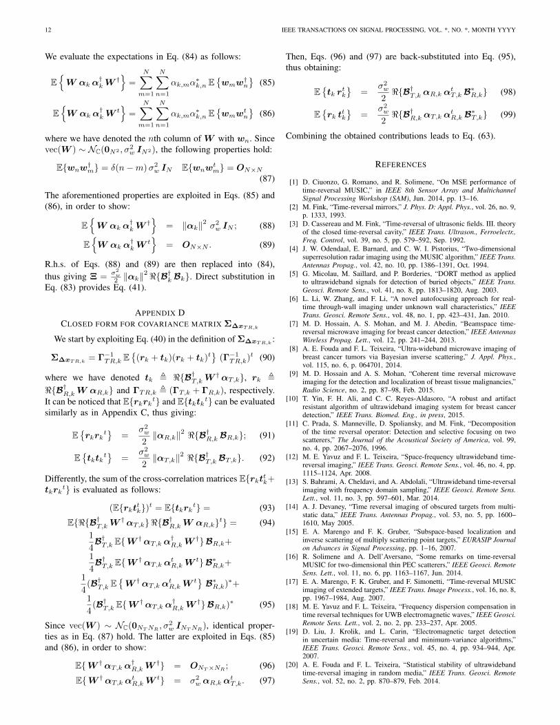
BA vs FL models - MSE gain: Finally, Fig. 14 reports ascatter plot of (γ1, γ2), where γk , CRLBf (xk)

CRLBb(xk)(“5” markers)

and CRLB(xk) denotes the MSE of kth target obtainedthrough CRLB [35]. Differently, in the case of TR-MUSIC,γk (“◦” markers) is obtained via γmse

k in Eq. (68). The presentexperiment is obtained by taking 200 realizations of thefollowing (2-D co-located) randomized setup: |τk| ∼ U(3, 4),∠τk ∼ U(0, 2π), xk = [ (−8 + 16 dx,k) (−4− 8 dy,k)]

t,

where dx,k ∼ U(0, λ) and dy,k ∼ U(0, λ) (see Fig. 13 forthe generated scatterers location distribution). We recall thatthis analysis compares performance of BA and FL modelswith same σ2

w and it is analogous to that presented in [35],based on the sole CRLB. It is apparent that while in mostcases CRLB is improved when switching from BA to FLmodel, TR-MUSIC is affected by an opposite trend, which


−6

−4

−2

0

2

−4−3.5

−3−2.5

−2−1.5

−1−0.5

00

1

2

3

4

5

6

7

8

X [in λ]Y [in λ]

Z [i

n λ]

TargetsTx arrayRx array

Figure 10. Geometry for the considered imaging problem in 3-D space; nonco-located setup.

10 12 14 16 18 20 22 24 26 28 3010

−5

10−4

10−3

10−2

10−1

100

101

SNR [dB]

MS

E [

λ2 ]

TR−MUSIC − Target 1 − BA TR−MUSIC − Target 2 − BA TR−MUSIC − Target 1 − FL TR−MUSIC − Target 2 − FL MLE (CRLB) − Target 1 − BA MLE (CRLB) − Target 2 − BA MLE (CRLB) − Target 1 − FL MLE (CRLB) − Target 2 − FL

Figure 12. 3-D localization experiment - non co-located case: MSE vs.SNR; theoretical (CRLB and Tx+Rx TR-MUSIC (obtained via Eq. (63)),in solid lines) vs. simulated (MC-based Tx+Rx TR-MUSIC, in dashed lines)performance.

is coherent with numerical results in Figs. 3, 5 and 6. Thisclearly represents a further proof that CRLB is only useful inpredicting MLE performance and rather the presented resultsshould be exploited for TR-MUSIC performance evaluation.

−8 −6 −4 −2 0 2 4 6 8−12

−10

−8

−6

−4

−2

0

X [in λ]

Y [i

n λ]

Tx−Rx arrayTarget 1Target 2

Figure 13. Scatterers distribution in an example with 200 Monte Carlo runs.

10−2

10−1

100

101

102

10−2

10−1

100

101

102

γ1

γ 2

CRLBTR−MUSIC (Th.)

Figure 14. Scatter plot of (γ1, γ2) for CRLB and (theoretical) TR-MUSIC;2-D co-located randomized setup.

V. CONCLUSIONS

In this paper we provided a theoretical performance analysisfor TR-MUSIC. We obtained an asymptotic (high-SNR) MSEmatrix expression for localization error in closed form. Wetook advantage of a first-order approximation of positionerror vector and a first-order perturbation of the SVD ofthe MDM to obtain the presented results. Both co-locatedand non co-located multistatic setups were considered. Inthe latter scenario several variants of TR-MUSIC proposedin literature were analyzed from a theoretical point of view.Theoretical performances were confirmed by simulations in2D/3D scenarios and were shown to predict MSE of TR-MUSIC more accurately than CRLB, being representative onlyof the high-SNR MLE performance. Finally, the obtainedresults were exploited to find a simple expression for MSEcomparison when BA and FL models are considered.

Future research tracks will concern the theoretical analysisof TR-MUSIC in multi-frequency setups, finite-sized scat-terers, and array-modeling mismatches. Equally important,propagation in non-homogeneous random media and clutter-dominated environments will be considered as well. In the lat-ter context, statistical stability of MSE with a multi-frequencyapproach will be investigated, following [20].

VI. ACKNOWLEDGEMENTS

The authors would like to express their sincere gratitudeto the Associate Editor and the anonymous reviewers fortaking their time into reviewing this manuscript and providingcomments that contributed to improve the quality and thereadability of the manuscript.

APPENDIX AEXPLICIT FORM FOR D

In this appendix we provide a proof for Eq. (37). The (i, j)thelement of D(x,Un) is explicitly expanded as

di,j(x,Un) =

N∑s=1

N∑t=1

∂2

∂xi∂xj[gs(x)∗ pn,s,t gt(x)] (73)


which, after simple manipulations, is expressed as follows:

di,j(x,Un) =

N∑s=1

N∑t=1

[∂2gs(x)∗

∂xi∂xjpn,s,t gt(x)+

∂gs(x)∗

∂xjpn,s,t

∂gt(x)

∂xi+

∂gs(x)∗

∂xipn,s,t

∂gt(x)

∂xj+ gs(x)∗ pn,s,t

∂2gt(x)

∂xi∂xj

](74)

In Eq. (74) the term pn,s,t indicates the (s, t)th element ofPn , (UnU

†n). Furthermore, di,j(x,Un) can be rewritten

compactly as

di,j(x,Un) =∂2g(x)†

∂xi∂xjPn g(x) +

∂g(x)†

∂xjPn

∂g(x)

∂xi+

∂g(x)†

∂xiPn

∂g(x)

∂xj+ g(x)†Pn

∂2g(x)

∂xi∂xj(75)

From Eq. (75) it is apparent that when di,j(x,Un) is evaluatedat xk, only second and third terms are non-zero, thus giving:

di,j(xk,Un) =

(∂g(x)†

∂xjPn

∂g(x)

∂xi+∂g(x)†

∂xiPn

∂g(x)

∂xj

)∣∣∣∣x=xk

= 2 <{∂g(x)†

∂xiPn

∂g(x)

∂xj

}∣∣∣∣x=xk

(76)

Finally, Eq. (76) is written in matrix form as

D = 2<{J†k Pn Jk}, (77)

where Jk has the same meaning as in Eq. (33).

APPENDIX BON INVERTIBILITY OF D

We start by recalling that D ∈ Rp×p is:

D = Hx{P(x,Un)}|x=xk= 2<{J†k Pn Jk} (78)

where Jk ∈ CN×p, Un ∈ CN×(N−M) and Pn ∈ CN×N ,respectively. Also, p = 2 (resp. p = 3) in a 2D (resp. 3D)geometry. In the noise-free case, xk is a stationary point ofP(x,Un), since

∇x{P(x,Un)}|x=xk= 2<

{J†k Pn g(xk)

}= 0p, (79)

which follows from U †n g(xk) = 0N−M . A standard wayto verify whether such a stationary point is actually a local-minimum for P(x,Un) is the multivariate test on second-order derivative, namely checking the determinant of theHessian matrix of P(x,Un) in xk. Evidently, the Hessianmatrix evaluated in xk coincides with matrix D (cf. l.h.s. ofEq. (78)). Also, by construction, D � 0 (cf. r.h.s. of Eq. (78)).Unfortunately, only when D � 0 (thus invertible), we canconclude that xk is a local minimum for P(x,Un). When Dis not invertible (viz. D � 0) the second derivative test isinconclusive and thus xk may not even be a local minimum.This degenerate situation invalidates the significance of ananalysis based on Taylor series expansion up to the secondorder of TR-MUSIC pseudospectrum.

We thus focus on (sufficient) conditions for invertibility ofmatrix D. In order to do so, we first consider the matrix

(J†k Pn Jk) ∈ Cp×p. Then, we notice that Rank(J†kPnJk) =Rank(U †nJk). Also, Rank(U †n) = Rank(Un) = (N −M).On the other hand, as to the Jacobian matrix Jk, it can beeasily shown that in 2D case it is always full rank (p = 2).Analogously, in 3D scenario Jk is full rank (p = 3), unlesssome pathological configurations are considered, e.g. the arrayand the scatterer xk are both are displaced on the same plane.

Therefore, based on these considerations, it is apparent thatRank(J†kPnJk) ≤ min{p,N −M}. We assume hereinafterthat the mild condition (N −M) ≥ p is satisfied. Then, theconsidered matrix will be full-rank iff Rank{U †nJk} = p.This is tantamount to showing that the columns of U †nJk arelinearly independent. For this reason, we consider a linearcombination of such columns, that is:

p∑h=1

αhU†n jk,h = U †n

p∑h=1

αh jk,h (80)

where jk,h denotes the hth column of Jk. Thus we need toshow that Eq. (80) is different from the zero vector unlessαh = 0, h ∈ {1, . . . p}. Therefore, assume that at leastone αh 6= 0, then

∑ph=1 αh jk,h 6= 0N as Jk is full rank.

Furthermore, we notice that each jhk can be rearranged asjk,h = Ahg(xk), where Ah ∈ CN×N is a diagonal matrixwhose entries depend on the specific geometry considered,namely 2D or 3D (cf. Eqs. (65-67)). Accordingly, Eq. (80)can be rewritten as:

U †nAg(xk) (81)

with A ,∑ph=1 αhA

h. It is worth noticing that PsA 6=APs, where Ps , UsU

†s (i.e. the projector into the signal

subspace). Therefore, PsAg(xk) 6= APsg(xk) = Ag(xk),since g(xk) belongs to the signal subspace. We conclude thatAg(xk) has a non-null projection onto the noise subspace.Hence Eq. (81) cannot be a zero vector. Consequently, (U †nJk)and (J†kPnJk) are of full rank p.

Finally, we focus on matrix D and for notational conve-nience we define Ψ , (J†kPnJk). It thus follows:

D = Ψ + Ψ∗ = Ψ + Ψt (82)

Positive definiteness for D is easily proved by noticing that,under the assumption that Ψ is of full rank, both Ψ � 0 andΨt � 0. Therefore, D � 0 as well and hence invertible.

APPENDIX CCLOSED FORM FOR COVARIANCE MATRIX Σ∆xk

Here we give the detailed derivation for Eq. (41). We startby exploiting Eq. (40) in the definition of Σ∆xk :

Σ∆xk =Γ−1k E{<{B†kW αk}<{B†kW αk}t}(Γ−1

k )t (83)

Eq. (83) requires the evaluation of the inner expectation term.After some manipulations, we get:

Ξ , E{<{B†kW αk}<{B†kW αk}t } = (84)1

4[B†k E{W αk α

†kW

†}Bk + B†k E{W αk α†kW

t}B∗k+

(B†k E{W αk α†kW

t}B∗k + B†k E{W αk α†kW

†}Bk)∗]


We evaluate the expectations in Eq. (84) as follows:

E{W αk α

†kW

†}

=

N∑m=1

N∑n=1

αk,mα∗k,n E

{wmw

†n

}(85)

E{W αk α

†kW

t}

=

N∑m=1

N∑n=1

αk,mα∗k,n E

{wmw

tn

}(86)

where we have denoted the nth column of W with wn. Sincevec(W ) ∼ NC(0N2 , σ2

w IN2), the following properties hold:

E{wnw†m} = δ(n−m)σ2w IN E{wnwt

m} = ON×N(87)

The aforementioned properties are exploited in Eqs. (85) and(86), in order to show:

E{W αk α

†kW

†}

= ‖αk‖2 σ2w IN ; (88)

E{W αk α

†kW

t}

= ON×N . (89)

R.h.s. of Eqs. (88) and (89) are then replaced into (84),thus giving Ξ =

σ2w

2 ‖αk‖2<{B†k Bk}. Direct substitution in

Eq. (83) provides Eq. (41).

APPENDIX DCLOSED FORM FOR COVARIANCE MATRIX Σ∆xTR,k

We start by exploiting Eq. (40) in the definition of Σ∆xTR,k :

Σ∆xTR,k = Γ−1TR,k E

{(rk + tk)(rk + tk)t

}(Γ−1

TR,k)t (90)

where we have denoted tk , <{B†T,kW †αT,k}, rk ,

<{B†R,kW αR,k} and ΓTR,k , (ΓT,k + ΓR,k), respectively.It can be noticed that E{rkrkt} and E{tktkt} can be evaluatedsimilarly as in Appendix C, thus giving:

E{rkrk

t}

=σ2w

2‖αR,k‖2 <{B†R,k BR,k}; (91)

E{tktk

t}

=σ2w

2‖αT,k‖2 <{B†T,k BT,k}. (92)

Differently, the sum of the cross-correlation matrices E{rkttk+tkrk

t} is evaluated as follows:

(E{rkttk})t = E{tkrkt} = (93)

E{<{B†T,kW†αT,k}<{B†R,kW αR,k}t} = (94)

1

4B†T,k E{W

†αT,k α†R,kW

†}BR,k+

1

4B†T,k E{W

†αT,k αtR,kW

t}B∗R,k+

1

4(B†T,k E

{W †αT,k α

tR,kW

t}B∗R,k)∗+

1

4(B†T,k E{W

†αT,k α†R,kW

†}BR,k)∗ (95)

Since vec(W ) ∼ NC(0NTNR , σ2w INTNR), identical proper-

ties as in Eq. (87) hold. The latter are exploited in Eqs. (85)and (86), in order to show:

E{W †αT,k α†R,kW

†} = ONT×NR ; (96)

E{W †αT,k αtR,kW

t} = σ2w αR,k α

tT,k. (97)

Then, Eqs. (96) and (97) are back-substituted into Eq. (95),thus obtaining:

E{tk r

tk

}=

σ2w

2<{B†T,k αR,k α

tT,k B

∗R,k} (98)

E{rk t

tk

}=

σ2w

2<{B†R,k αT,k α

tR,k B

∗T,k} (99)

Combining the obtained contributions leads to Eq. (63).

REFERENCES

[1] D. Ciuonzo, G. Romano, and R. Solimene, “On MSE performance oftime-reversal MUSIC,” in IEEE 8th Sensor Array and MultichannelSignal Processing Workshop (SAM), Jun. 2014, pp. 13–16.

[2] M. Fink, “Time-reversal mirrors,” J. Phys. D: Appl. Phys., vol. 26, no. 9,p. 1333, 1993.

[3] D. Cassereau and M. Fink, “Time-reversal of ultrasonic fields. III. theoryof the closed time-reversal cavity,” IEEE Trans. Ultrason., Ferroelectr.,Freq. Control, vol. 39, no. 5, pp. 579–592, Sep. 1992.

[4] J. W. Odendaal, E. Barnard, and C. W. I. Pistorius, “Two-dimensionalsuperresolution radar imaging using the MUSIC algorithm,” IEEE Trans.Antennas Propag., vol. 42, no. 10, pp. 1386–1391, Oct. 1994.

[5] G. Micolau, M. Saillard, and P. Borderies, “DORT method as appliedto ultrawideband signals for detection of buried objects,” IEEE Trans.Geosci. Remote Sens., vol. 41, no. 8, pp. 1813–1820, Aug. 2003.

[6] L. Li, W. Zhang, and F. Li, “A novel autofocusing approach for real-time through-wall imaging under unknown wall characteristics,” IEEETrans. Geosci. Remote Sens., vol. 48, no. 1, pp. 423–431, Jan. 2010.

[7] M. D. Hossain, A. S. Mohan, and M. J. Abedin, “Beamspace time-reversal microwave imaging for breast cancer detection,” IEEE AntennasWireless Propag. Lett., vol. 12, pp. 241–244, 2013.

[8] A. E. Fouda and F. L. Teixeira, “Ultra-wideband microwave imaging ofbreast cancer tumors via Bayesian inverse scattering,” J. Appl. Phys.,vol. 115, no. 6, p. 064701, 2014.

[9] M. D. Hossain and A. S. Mohan, “Coherent time reversal microwaveimaging for the detection and localization of breast tissue malignancies,”Radio Science, no. 2, pp. 87–98, Feb. 2015.

[10] T. Yin, F. H. Ali, and C. C. Reyes-Aldasoro, “A robust and artifactresistant algorithm of ultrawideband imaging system for breast cancerdetection,” IEEE Trans. Biomed. Eng., in press, 2015.

[11] C. Prada, S. Manneville, D. Spoliansky, and M. Fink, “Decompositionof the time reversal operator: Detection and selective focusing on twoscatterers,” The Journal of the Acoustical Society of America, vol. 99,no. 4, pp. 2067–2076, 1996.

[12] M. E. Yavuz and F. L. Teixeira, “Space-frequency ultrawideband time-reversal imaging,” IEEE Trans. Geosci. Remote Sens., vol. 46, no. 4, pp.1115–1124, Apr. 2008.

[13] S. Bahrami, A. Cheldavi, and A. Abdolali, “Ultrawideband time-reversalimaging with frequency domain sampling,” IEEE Geosci. Remote Sens.Lett., vol. 11, no. 3, pp. 597–601, Mar. 2014.

[14] A. J. Devaney, “Time reversal imaging of obscured targets from multi-static data,” IEEE Trans. Antennas Propag., vol. 53, no. 5, pp. 1600–1610, May 2005.

[15] E. A. Marengo and F. K. Gruber, “Subspace-based localization andinverse scattering of multiply scattering point targets,” EURASIP Journalon Advances in Signal Processing, pp. 1–16, 2007.

[16] R. Solimene and A. Dell’Aversano, “Some remarks on time-reversalMUSIC for two-dimensional thin PEC scatterers,” IEEE Geosci. RemoteSens. Lett., vol. 11, no. 6, pp. 1163–1167, Jun. 2014.

[17] E. A. Marengo, F. K. Gruber, and F. Simonetti, “Time-reversal MUSICimaging of extended targets,” IEEE Trans. Image Process., vol. 16, no. 8,pp. 1967–1984, Aug. 2007.

[18] M. E. Yavuz and F. L. Teixeira, “Frequency dispersion compensation intime reversal techniques for UWB electromagnetic waves,” IEEE Geosci.Remote Sens. Lett., vol. 2, no. 2, pp. 233–237, Apr. 2005.

[19] D. Liu, J. Krolik, and L. Carin, “Electromagnetic target detectionin uncertain media: Time-reversal and minimum-variance algorithms,”IEEE Trans. Geosci. Remote Sens., vol. 45, no. 4, pp. 934–944, Apr.2007.

[20] A. E. Fouda and F. L. Teixeira, “Statistical stability of ultrawidebandtime-reversal imaging in random media,” IEEE Trans. Geosci. RemoteSens., vol. 52, no. 2, pp. 870–879, Feb. 2014.


[21] X.-F. Liu, B.-Z.Wang, and J. L.-W. Li, “Transmitting-mode time reversalimaging using MUSIC algorithm for surveillance in wireless sensornetwork,” IEEE Trans. Antennas Propag., vol. 60, no. 1, pp. 220–230,Jan. 2012.

[22] H. Krim and M. Viberg, “Two decades of array signal processingresearch: the parametric approach,” IEEE Signal Process. Mag., vol. 13,no. 4, pp. 67–94, 1996.

[23] R. Schmidt, “Multiple emitter location and signal parameter estimation,”IEEE Trans. Antennas Propag., vol. 34, no. 3, pp. 276–280, 1986.

[24] M. Kaveh and A. Barabell, “The statistical performance of the MUSICand the minimum-norm algorithms in resolving plane waves in noise,”IEEE Trans. Acoust., Speech, Signal Process., vol. 34, no. 2, pp. 331–341, 1986.

[25] P. Stoica and A. Nehorai, “MUSIC, maximum likelihood, and Cramér-Rao bound,” IEEE Trans. Acoust., Speech, Signal Process., vol. 37, no. 5,pp. 720–741, May 1989.

[26] ——, “MUSIC, maximum likelihood, and Cramér-Rao bound: furtherresults and comparisons,” IEEE Trans. Acoust., Speech, Signal Process.,vol. 38, no. 12, pp. 2140–2150, Dec. 1990.

[27] F. Li and R. J. Vaccaro, “Analysis of min-norm and MUSIC witharbitrary array geometry,” IEEE Trans. Aerosp. Electron. Syst., vol. 26,no. 6, pp. 976–985, 1990.

[28] B. Porat and B. Friedlander, “Analysis of the asymptotic relative effi-ciency of the MUSIC algorithm,” IEEE Trans. Acoust., Speech, SignalProcess., vol. 36, no. 4, pp. 532–544, Apr. 1988.

[29] A. L. Swindlehurst and T. Kailath, “A performance analysis of subspace-based methods in the presence of model errors, Part I: the MUSICalgorithm,” IEEE Trans. Signal Process., vol. 40, no. 7, pp. 1758–1774,Jul. 1992.

[30] B. Friedlander, “A sensitivity analysis of the MUSIC algorithm,” IEEETrans. Acoust., Speech, Signal Process., vol. 38, no. 10, pp. 1740–1751,Oct. 1990.

[31] A. Ferréol, P. Larzabal, and M. Viberg, “On the asymptotic performanceanalysis of subspace DOA estimation in the presence of modeling errors:case of MUSIC,” IEEE Trans. Signal Process., vol. 54, no. 3, pp. 907–920, Mar. 2006.

[32] ——, “On the resolution probability of MUSIC in presence of modelingerrors,” IEEE Trans. Signal Process., vol. 56, no. 5, pp. 1945–1953, May2008.

[33] ——, “Statistical analysis of the MUSIC algorithm in the presence ofmodeling errors, taking into account the resolution probability,” IEEETrans. Signal Process., vol. 58, no. 8, pp. 4156–4166, Aug. 2010.

[34] G. Shi and A. Nehorai, “Maximum likelihood estimation of pointscatterers for computational time-reversal imaging,” Communications inInformation & Systems, vol. 5, no. 2, pp. 227–256, 2005.

[35] ——, “Cramér-Rao bound analysis on multiple scattering in multistaticpoint-scatterer estimation,” IEEE Trans. Signal Process., vol. 55, no. 6,pp. 2840–2850, Jun. 2007.

[36] M. E. Yavuz and F. L. Teixeira, “On the sensitivity of time-reversalimaging techniques to model perturbations,” IEEE Trans. AntennasPropag., vol. 56, no. 3, pp. 834–843, Mar. 2008.

[37] F. Li, H. Liu, and R. J. Vaccaro, “Performance analysis for DOAestimation algorithms: unification, simplification, and observations,”IEEE Trans. Aerosp. Electron. Syst., vol. 29, no. 4, pp. 1170–1184,1993.

[38] Z. Xu, “Perturbation analysis for subspace decomposition with appli-cations in subspace-based algorithms,” IEEE Trans. Signal Process.,vol. 50, no. 11, pp. 2820–2830, Nov. 2002.

[39] G. W. Stewart, “Error and perturbation bounds for subspaces associatedwith certain eigenvalue problems,” SIAM review, vol. 15, no. 4, pp. 727–764, 1973.

[40] J. Liu, X. Liu, and X. Ma, “First-order perturbation analysis of singularvectors in singular value decomposition,” IEEE Trans. Signal Process.,vol. 56, no. 7, pp. 3044–3049, Jul. 2008.

[41] D. S. Bernstein, Matrix mathematics: theory, facts, and formulas.Princeton University Press, 2009.

[42] S. M. Kay, Fundamentals of Statistical Signal Processing, Volume 1:Estimation Theory. Prentice Hall PTR, 1993.

[43] G. B. Arfken, H. J. Weber, and F. E. Harris, Mathematical methods forphysicists: A comprehensive guide. Academic press, 2011.

[44] F. K. Gruber, E. A. Marengo, and A. J. Devaney, “Time-reversal imag-ing with multiple signal classification considering multiple scatteringbetween the targets,” The Journal of the Acoustical Society of America,vol. 115, pp. 3042–3047, Jun. 2004.

Domenico Ciuonzo (S’11-M’14) was born inAversa, Italy, on June 29th, 1985. He receivedthe B.Sc. (summa cum laude), the M.Sc. (summacum laude) degrees in computer engineering andthe Ph.D. in electronic engineering, respectively in2007, 2009 and 2013, from the Second Universityof Naples (SUN), Aversa, Italy. In 2011 he wasinvolved in the Visiting Researcher Programme ofCentre for Maritime Research and Experimentation,La Spezia, Italy, within the "Maritime SituationAwareness" project. In 2012 he was a visiting

scholar at the Electrical and Computer Engineering Department of Universityof Connecticut (UConn), Storrs, US. In 2013-2014 he was a PostDoc atDept. of Industrial and Information Engineering of SUN, under the project“MICENEA”, funded by MIUR within the program Futuro in Ricerca (FIRB)2013. Since 2014 he is a PostDoc researcher at DIETI, University of Naples,“Federico II”, Italy. His research interests are mainly in the areas of DataFusion, Statistical Signal Processing, Target Tracking and Wireless SensorNetworks. The quality of his reviewing activity was recognized by theEditorial Board of IEEE COMMUNICATIONS LETTERS, which nominatedhim “Exemplary Reviewer” for the year 2013. Dr. Ciuonzo currently servesas Associate Editor for the IEEE AEROSPACE AND ELECTRONIC SYSTEMSMAGAZINE.

Gianmarco Romano is currently Assistant Profes-sor at the Department of Industrial and InformationEngineering, Second University of Naples, Aversa(CE), Italy. He received the “Laurea” degree in Elec-tronic Engineering from the University of Naples“Federico II” and the Ph.D. degree from the SecondUniversity of Naples, in 2000 and 2004, respectively.From 2000 to 2002 he has been Researcher at theNational Laboratory for Multimedia Communica-tions (C.N.I.T.) in Naples, Italy. In 2003 he wasVisiting Scholar at the Department of Electrical and

Electronic Engineering, University of Connecticut, Storrs, USA. Since 2005 hehas been with the Department of Information Engineering, Second Universityof Naples and in 2006 has been appointed Assistant Professor. His researchinterests fall within the areas of communications and signal processing.

Raffaele Solimene received the laurea degree(summa cum laude) in 1999 and the Ph.D. degreein 2003 in electronic engineering, both from theSeconda Università di Napoli (SUN), Aversa, Italy.In 2002, he became an assistant professor at theFaculty of Engineering of the University Mediter-ranea of Reggio Calabria, Italy. Since 2006, he hasbeen with the Dipartimento di Ingegneria Industrialee dell’Informazione at SUN where he is currently anassociate professor. He serves as associate editor forInternational Journal of Antennas and Propagation

for Mathematical Problems in Engineering. His research activities focus oninverse problems with a applications like nondestructive subsurface investiga-tions, through-the-wall imaging and breast cancer detection.

performance analysis of time-reversal music

Documents