people born in the middle east but residing in the netherlands: invariant population size estimates...

The Annals of Applied Statistics2012, Vol. 6, No. 3, 831–852DOI: 10.1214/12-AOAS536© Institute of Mathematical Statistics, 2012

PEOPLE BORN IN THE MIDDLE EAST BUT RESIDING IN THENETHERLANDS: INVARIANT POPULATION SIZE ESTIMATES

AND THE ROLE OF ACTIVE AND PASSIVE COVARIATES

BY PETER G. M. VAN DER HEIJDEN, JOE WHITTAKER, MAARTEN CRUYFF,BART BAKKER AND RIK VAN DER VLIET

Utrecht University, Lancaster University, Utrecht University, StatisticsNetherlands and Statistics Netherlands

Including covariates in loglinear models of population registers improvespopulation size estimates for two reasons. First, it is possible to take hetero-geneity of inclusion probabilities over the levels of a covariate into account;and second, it allows subdivision of the estimated population by the levels ofthe covariates, giving insight into characteristics of individuals that are notincluded in any of the registers. The issue of whether or not marginalizing thefull table of registers by covariates over one or more covariates leaves the esti-mated population size estimate invariant is intimately related to collapsibilityof contingency tables [Biometrika 70 (1983) 567–578]. We show that, withinformation from two registers, population size invariance is equivalent to thesimultaneous collapsibility of each margin consisting of one register and thecovariates. We give a short path characterization of the loglinear model whichdescribes when marginalizing over a covariate leads to different populationsize estimates. Covariates that are collapsible are called passive, to distin-guish them from covariates that are not collapsible and are termed active.We make the case that it can be useful to include passive covariates withinthe estimation model, because they allow a finer description of the popula-tion in terms of these covariates. As an example we discuss the estimationof the population size of people born in the Middle East but residing in theNetherlands.

1. Introduction. A well-known technique for estimating the size of a humanpopulation is to find two or more registers of this population, to link the indi-viduals in the registers and to estimate the number of individuals that occur inneither of the registers [Fienberg (1972); Bishop, Fienberg and Holland (1975);Cormack (1989); International Working Group for Disease Monitoring and Fore-casting, IWGDMF (1995)]. For example, with two registers A and B , linkage givesa count of individuals in A but not in B , a count of individuals in B but not in A,and a count of individuals both in A and B . The counts form a contingency tabledenoted by A × B , with the variable labeled A being short for “inclusion in reg-ister A” taking the levels “yes” and “no,” and likewise for register B . In this table

Received August 2011; revised January 2012.Key words and phrases. Population size estimation, capture–recapture, collapsibility, multiple

record-systems estimation, missing data, structural zeros.

831

http://www.imstat.org/aoas/

http://dx.doi.org/10.1214/12-AOAS536

http://www.imstat.org

832 P. G. M. VAN DER HEIJDEN ET AL.

the cell “no, no” has a zero count by definition, and the statistical problem is tobetter estimate this value in the population. An improved population size estimateis obtained by adding this estimated count of missed individuals to the counts ofindividuals found in at least one of the registers.

With two registers the usual assumptions under which a population size esti-mate is obtained are as follows: inclusion in register A is independent of inclusionin register B; and in at least one of the two registers the inclusion probabilities arehomogeneous [see Chao et al. (2001) and Zwane, van der Pal and van der Heij-den (2004)]. Interestingly, it is often, but incorrectly, supposed that both inclusionprobabilities have to be homogeneous. Other assumptions are that the population isclosed and that it is possible to link the individuals in registers A and B perfectly.

However, it is generally agreed that these assumptions are unlikely to hold inhuman populations. Three approaches may be adopted to make the impact of pos-sible violations less severe. One approach is to include covariates into the model, inparticular, covariates whose levels have heterogeneous inclusion probabilities forboth registers [see Bishop, Fienberg and Holland (1975); Baker (1990); comparePollock (2002)]. Then loglinear models can be fitted to the higher-way contin-gency table of registers A and B and the covariates. The restrictive independenceassumption is replaced by a less restrictive assumption of independence of A andB conditional on the covariates; and subpopulation size estimates are derived (onefor every level of the covariates) that add up to a population size estimate. Anotherapproach is to include a third register, and to analyze the three-way contingencytable with loglinear models that may include one or more two-factor interactions,thus getting rid of the independence assumption. Here the (less stringent) assump-tion made is that the three-factor interaction is absent. However, including a thirdregister is not always possible, as it is not available, or because there is no infor-mation that makes it possible to link the individuals in the third register to boththe first and to the second register. A third approach makes use of a latent vari-able to take heterogeneity of inclusion probabilities into account [see Fienberg,Johnson and Junker (1999); Bartolucci and Forcina (2001)]. Of course, these threeapproaches are not exclusive and may be used concurrently in one model.

When the approach is adopted to use covariates, the question is which covariatesshould be chosen. In the traditional approach, only covariates that are available ineach of the registers can be chosen. Recently, Zwane and van der Heijden (2007)showed that it is also possible to use covariates that are not available in each ofthe registers. For example, when a covariate is available in register A but not in B ,the values of the covariate missed by B are estimated under a missing-at-randomassumption [Little and Rubin (1987)]; and the subpopulation size estimates arethen derived as a by-product. Whether or not the covariates are available in each ofthe registers, the number of possible loglinear models that can be fit grows rapidly.

In this paper we study the (in)variance of population size estimates derived fromloglinear models that include covariates. Including covariates in loglinear modelsof population registers improves population size estimates for two reasons. First, it

ACTIVE AND PASSIVE COVARIATES 833

is possible to take heterogeneity of inclusion probabilities over the levels of a co-variate into account; and second, it allows subdivision of the estimated populationby the levels of the covariates, giving insight into characteristics of individuals thatare not included in any of the registers. The issue of whether or not marginalizingthe full table of registers by covariates over one or more covariates leaves the es-timated population size estimate invariant is intimately related to collapsibility ofcontingency tables. With information from two registers it is shown that populationsize invariance is equivalent to the simultaneous collapsibility of each margin con-sisting of one register and the covariates. Covariates that are collapsible are calledpassive, to distinguish them from covariates that are not collapsible and are termedactive. We make the case that it may be useful to include passive covariates withinthe estimation model, because they allow a description of the population in termsof these covariates. As an example we discuss the estimation of the population sizeof people born in the Middle East but residing in the Netherlands.

By focusing on population size estimates, collapsibility in loglinear models isstudied in this paper from a different perspective than found in Bishop, Fienbergand Holland (1975) who are interested in parametric collapsibility. Our work ap-plies model collapsibility of Asmussen and Edwards (1983), later discussed byWhittaker [(1990), pages 394–401] and Kim and Kim (2006), concerning the com-mutativity of model fitting and marginalization. We use model collapsibility in thecontext of population size invariance and show invariance requires model collapsi-bility of each margin consisting of one register and the covariates. A novel featureis to apply collapsibility in the context of a table containing structural zeros. Wegive a short path characterization of the loglinear model which describes whenmarginalizing over a covariate leads to different population size estimates.

The second result can be fruitfully applied in population size estimation. In aspecific loglinear model, we denote covariates as passive when they are collapsi-ble and active when they are not collapsible. In principle, the approach of Zwaneand van der Heijden (2007) permits the inclusion of many passive covariates in amodel; we make a case for including such passive covariates because they allowthe description of both the observed part as well as the unobserved of the popula-tion in terms of these covariates.

The paper is built up as follows. In Section 2 we discuss the data to be analyzed.These refer to the population of people with Afghan, Iranian and Iraqi nationalityresiding in the Netherlands. In Section 3 we discuss theoretical properties of theloglinear models in the context of population size estimation. This is discussed indetail for the case of two registers. We illustrate the two properties of loglinearmodels using a number of examples, and then prove the properties using resultsfrom graphical models. We distinguish the standard situation that every covariateis available in each of the registers from the situation that there are one or more co-variates that are available in only one of the registers [Zwane and van der Heijden(2007)]. For completeness we also discuss the situation when three registers areavailable and illustrate that the same properties apply. In Section 4 we develop the


notion of active and passive covariates, and in Section 5 we present an example.We end with a discussion. In Appendix A we extend the work of Asmussen andEdwards (1983) to population size invariance.

2. The population of people with Middle Eastern nationality staying in theNetherlands. The preparations for the 2011 round of the Census are in progressat the time of writing. More countries now make use of administrative data (ratherthan polling) for that purpose. There are countries who are repeating this method,such as Denmark, Finland and the Netherlands, and more than ten European coun-tries that are using administrative data for the first time [Valente (2010)]. The ad-ministrative registers are combined by data-linking and micro-integration to cleanand improve consistency. The outcome of these processes is called a statisticalregister or a register for short.

The most important administrative register to be used in the Netherland Cen-sus is an automated system of decentralized (municipal) population registers (inDutch, Gemeentelijke BasisAdminstratie, referred to by the abbreviation GBA).This register is used for the definition of the population. The GBA contains allinformation on people that are legally allowed to reside in the Netherlands and areregistered as such. The register is accurate for that part of the population such aspeople with the Dutch nationality and foreigners that carry documents that allowthem to be in the Netherlands for work, study, asylum, and their close relatives.However, these data do not cover the total population, in particular, those residingin the Netherlands but who are not allowed to stay under current Dutch law. Theselatter groups are sometimes referred to as undocumented foreigners or illegal im-migrants.

Under Census regulations a quality report is obligatory, and one of the aspectsthat needs to be addressed is the undercoverage of the Census data. This asks foran estimate of the size of the population that is not included in the GBA. In thispaper we approach the problem by linking the GBA to another register and thenapply population size estimation methods to arrive at an estimate of the total pop-ulation. Therefore, we implicitly estimate that part of the population not coveredby the GBA. The second register that we employ is the central Police RecognitionSystem or HerkenningsDienst Systeem (HKS) that is a collection of decentralizedregistration systems kept by 25 separate Dutch police regions. In HKS suspectsof offences are registered. Each report of an offence has a suspect identificationwhere, if possible, information about the suspect is copied from the GBA. If a sus-pect does not appear in the GBA, finger prints are taken so that he or she can befound in the HKS if apprehension at a later stage occurs.

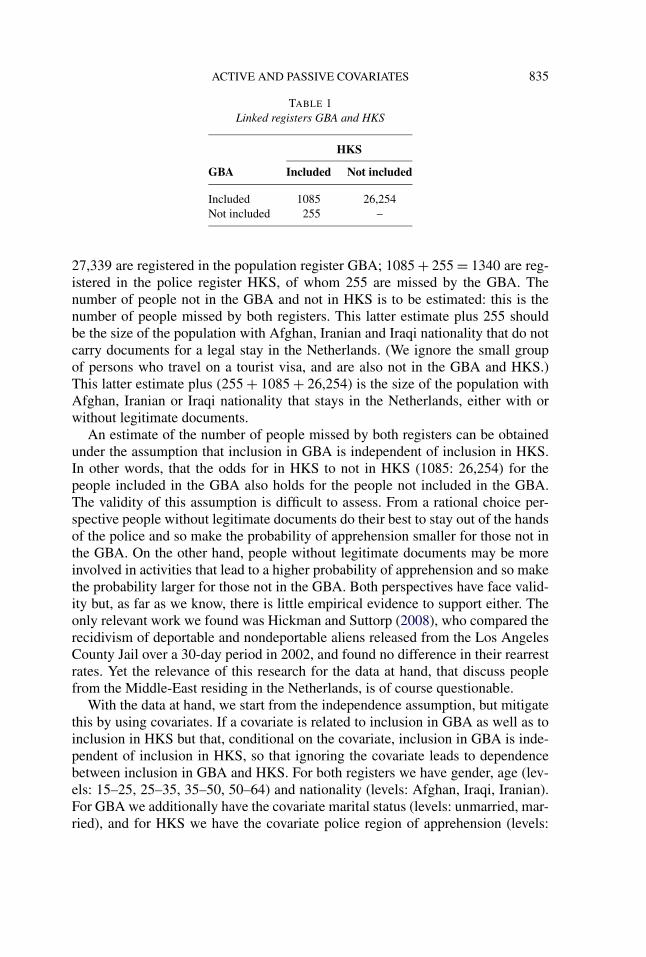
We test the methodology described in the next sections using previously col-lected data of the 15–64 year old age group of people with Afghan, Iranian or Iraqinationality. For the GBA we extract the registered information of 2007. For HKSwe extract information on apprehensions made during 2007. Table 1 illustrates theproblem. For people with Afghan, Iranian or Iraqi nationality 1085 + 26,254 =


TABLE 1Linked registers GBA and HKS

HKS

GBA Included Not included

Included 1085 26,254Not included 255 –

27,339 are registered in the population register GBA; 1085 + 255 = 1340 are reg-istered in the police register HKS, of whom 255 are missed by the GBA. Thenumber of people not in the GBA and not in HKS is to be estimated: this is thenumber of people missed by both registers. This latter estimate plus 255 shouldbe the size of the population with Afghan, Iranian and Iraqi nationality that do notcarry documents for a legal stay in the Netherlands. (We ignore the small groupof persons who travel on a tourist visa, and are also not in the GBA and HKS.)This latter estimate plus (255 + 1085 + 26,254) is the size of the population withAfghan, Iranian or Iraqi nationality that stays in the Netherlands, either with orwithout legitimate documents.

An estimate of the number of people missed by both registers can be obtainedunder the assumption that inclusion in GBA is independent of inclusion in HKS.In other words, that the odds for in HKS to not in HKS (1085: 26,254) for thepeople included in the GBA also holds for the people not included in the GBA.The validity of this assumption is difficult to assess. From a rational choice per-spective people without legitimate documents do their best to stay out of the handsof the police and so make the probability of apprehension smaller for those not inthe GBA. On the other hand, people without legitimate documents may be moreinvolved in activities that lead to a higher probability of apprehension and so makethe probability larger for those not in the GBA. Both perspectives have face valid-ity but, as far as we know, there is little empirical evidence to support either. Theonly relevant work we found was Hickman and Suttorp (2008), who compared therecidivism of deportable and nondeportable aliens released from the Los AngelesCounty Jail over a 30-day period in 2002, and found no difference in their rearrestrates. Yet the relevance of this research for the data at hand, that discuss peoplefrom the Middle-East residing in the Netherlands, is of course questionable.

With the data at hand, we start from the independence assumption, but mitigatethis by using covariates. If a covariate is related to inclusion in GBA as well as toinclusion in HKS but that, conditional on the covariate, inclusion in GBA is inde-pendent of inclusion in HKS, so that ignoring the covariate leads to dependencebetween inclusion in GBA and HKS. For both registers we have gender, age (lev-els: 15–25, 25–35, 35–50, 50–64) and nationality (levels: Afghan, Iraqi, Iranian).For GBA we additionally have the covariate marital status (levels: unmarried, mar-ried), and for HKS we have the covariate police region of apprehension (levels:


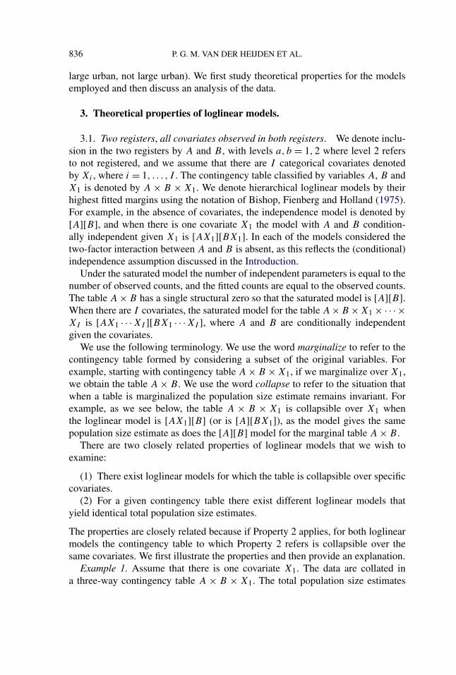
large urban, not large urban). We first study theoretical properties for the modelsemployed and then discuss an analysis of the data.

3. Theoretical properties of loglinear models.

3.1. Two registers, all covariates observed in both registers. We denote inclu-sion in the two registers by A and B , with levels a, b = 1,2 where level 2 refersto not registered, and we assume that there are I categorical covariates denotedby Xi , where i = 1, . . . , I . The contingency table classified by variables A, B andX1 is denoted by A × B × X1. We denote hierarchical loglinear models by theirhighest fitted margins using the notation of Bishop, Fienberg and Holland (1975).For example, in the absence of covariates, the independence model is denoted by[A][B], and when there is one covariate X1 the model with A and B condition-ally independent given X1 is [AX1][BX1]. In each of the models considered thetwo-factor interaction between A and B is absent, as this reflects the (conditional)independence assumption discussed in the Introduction.

Under the saturated model the number of independent parameters is equal to thenumber of observed counts, and the fitted counts are equal to the observed counts.The table A × B has a single structural zero so that the saturated model is [A][B].When there are I covariates, the saturated model for the table A×B ×X1 × · · ·×XI is [AX1 · · ·XI ][BX1 · · ·XI ], where A and B are conditionally independentgiven the covariates.

We use the following terminology. We use the word marginalize to refer to thecontingency table formed by considering a subset of the original variables. Forexample, starting with contingency table A × B × X1, if we marginalize over X1,we obtain the table A × B . We use the word collapse to refer to the situation thatwhen a table is marginalized the population size estimate remains invariant. Forexample, as we see below, the table A × B × X1 is collapsible over X1 whenthe loglinear model is [AX1][B] (or is [A][BX1]), as the model gives the samepopulation size estimate as does the [A][B] model for the marginal table A × B .

There are two closely related properties of loglinear models that we wish toexamine:

(1) There exist loglinear models for which the table is collapsible over specificcovariates.

(2) For a given contingency table there exist different loglinear models thatyield identical total population size estimates.

The properties are closely related because if Property 2 applies, for both loglinearmodels the contingency table to which Property 2 refers is collapsible over thesame covariates. We first illustrate the properties and then provide an explanation.

Example 1. Assume that there is one covariate X1. The data are collated ina three-way contingency table A × B × X1. The total population size estimates


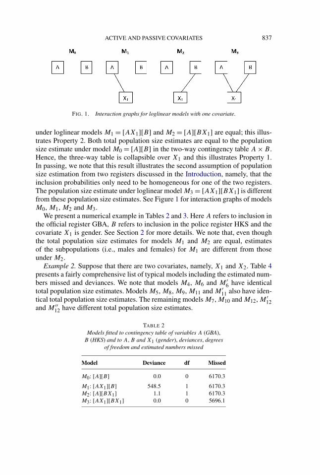
FIG. 1. Interaction graphs for loglinear models with one covariate.

under loglinear models M1 = [AX1][B] and M2 = [A][BX1] are equal; this illus-trates Property 2. Both total population size estimates are equal to the populationsize estimate under model M0 = [A][B] in the two-way contingency table A × B .Hence, the three-way table is collapsible over X1 and this illustrates Property 1.In passing, we note that this result illustrates the second assumption of populationsize estimation from two registers discussed in the Introduction, namely, that theinclusion probabilities only need to be homogeneous for one of the two registers.The population size estimate under loglinear model M3 = [AX1][BX1] is differentfrom these population size estimates. See Figure 1 for interaction graphs of modelsM0, M1, M2 and M3.

We present a numerical example in Tables 2 and 3. Here A refers to inclusion inthe official register GBA, B refers to inclusion in the police register HKS and thecovariate X1 is gender. See Section 2 for more details. We note that, even thoughthe total population size estimates for models M1 and M2 are equal, estimatesof the subpopulations (i.e., males and females) for M1 are different from thoseunder M2.

Example 2. Suppose that there are two covariates, namely, X1 and X2. Table 4presents a fairly comprehensive list of typical models including the estimated num-bers missed and deviances. We note that models M4, M6 and M ′

6 have identicaltotal population size estimates. Models M5, M8, M9, M11 and M ′

11 also have iden-tical total population size estimates. The remaining models M7, M10 and M12, M ′

12and M ′′

12 have different total population size estimates.

TABLE 2Models fitted to contingency table of variables A (GBA),

B (HKS) and to A,B and X1 (gender), deviances, degreesof freedom and estimated numbers missed

Model Deviance df Missed

M0: [A][B] 0.0 0 6170.3

M1: [AX1][B] 548.5 1 6170.3M2: [A][BX1] 1.1 1 6170.3M3: [AX1][BX1] 0.0 0 5696.1


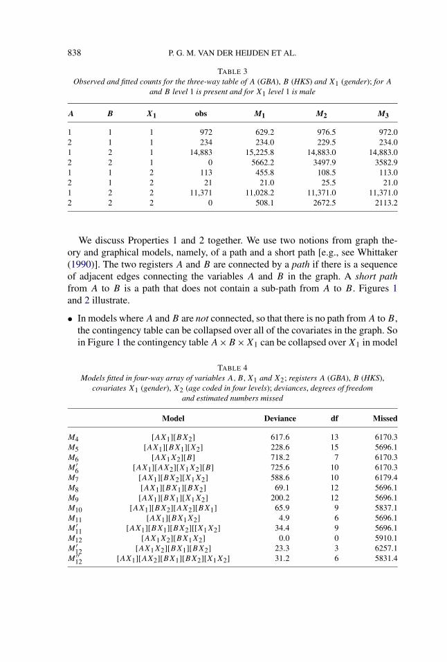
TABLE 3Observed and fitted counts for the three-way table of A (GBA), B (HKS) and X1 (gender); for A

and B level 1 is present and for X1 level 1 is male

A B X1 obs M1 M2 M3

1 1 1 972 629.2 976.5 972.02 1 1 234 234.0 229.5 234.01 2 1 14,883 15,225.8 14,883.0 14,883.02 2 1 0 5662.2 3497.9 3582.91 1 2 113 455.8 108.5 113.02 1 2 21 21.0 25.5 21.01 2 2 11,371 11,028.2 11,371.0 11,371.02 2 2 0 508.1 2672.5 2113.2

We discuss Properties 1 and 2 together. We use two notions from graph the-ory and graphical models, namely, of a path and a short path [e.g., see Whittaker(1990)]. The two registers A and B are connected by a path if there is a sequenceof adjacent edges connecting the variables A and B in the graph. A short pathfrom A to B is a path that does not contain a sub-path from A to B . Figures 1and 2 illustrate.

• In models where A and B are not connected, so that there is no path from A to B ,the contingency table can be collapsed over all of the covariates in the graph. Soin Figure 1 the contingency table A×B ×X1 can be collapsed over X1 in model

TABLE 4Models fitted in four-way array of variables A,B,X1 and X2; registers A (GBA), B (HKS),

covariates X1 (gender), X2 (age coded in four levels); deviances, degrees of freedomand estimated numbers missed

Model Deviance df Missed

M4 [AX1][BX2] 617.6 13 6170.3M5 [AX1][BX1][X2] 228.6 15 5696.1M6 [AX1X2][B] 718.2 7 6170.3M ′

6 [AX1][AX2][X1X2][B] 725.6 10 6170.3M7 [AX1][BX2][X1X2] 588.6 10 6179.4M8 [AX1][BX1][BX2] 69.1 12 5696.1M9 [AX1][BX1][X1X2] 200.2 12 5696.1M10 [AX1][BX2][AX2][BX1] 65.9 9 5837.1M11 [AX1][BX1X2] 4.9 6 5696.1M ′

11 [AX1][BX1][BX2][[X1X2] 34.4 9 5696.1M12 [AX1X2][BX1X2] 0.0 0 5910.1M ′

12 [AX1X2][BX1][BX2] 23.3 3 6257.1M ′′

12 [AX1][AX2][BX1][BX2][X1X2] 31.2 6 5831.4


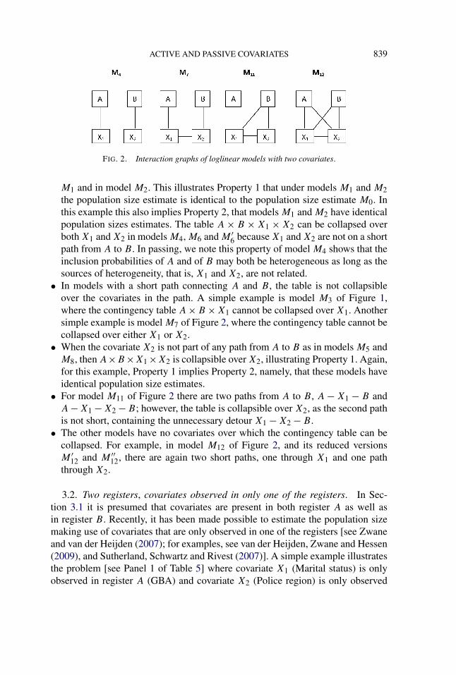
FIG. 2. Interaction graphs of loglinear models with two covariates.

M1 and in model M2. This illustrates Property 1 that under models M1 and M2the population size estimate is identical to the population size estimate M0. Inthis example this also implies Property 2, that models M1 and M2 have identicalpopulation sizes estimates. The table A × B × X1 × X2 can be collapsed overboth X1 and X2 in models M4, M6 and M ′

6 because X1 and X2 are not on a shortpath from A to B . In passing, we note this property of model M4 shows that theinclusion probabilities of A and of B may both be heterogeneous as long as thesources of heterogeneity, that is, X1 and X2, are not related.

• In models with a short path connecting A and B , the table is not collapsibleover the covariates in the path. A simple example is model M3 of Figure 1,where the contingency table A × B × X1 cannot be collapsed over X1. Anothersimple example is model M7 of Figure 2, where the contingency table cannot becollapsed over either X1 or X2.

• When the covariate X2 is not part of any path from A to B as in models M5 andM8, then A×B ×X1 ×X2 is collapsible over X2, illustrating Property 1. Again,for this example, Property 1 implies Property 2, namely, that these models haveidentical population size estimates.

• For model M11 of Figure 2 there are two paths from A to B , A − X1 − B andA − X1 − X2 − B; however, the table is collapsible over X2, as the second pathis not short, containing the unnecessary detour X1 − X2 − B .

• The other models have no covariates over which the contingency table can becollapsed. For example, in model M12 of Figure 2, and its reduced versionsM ′

12 and M ′′12, there are again two short paths, one through X1 and one path

through X2.

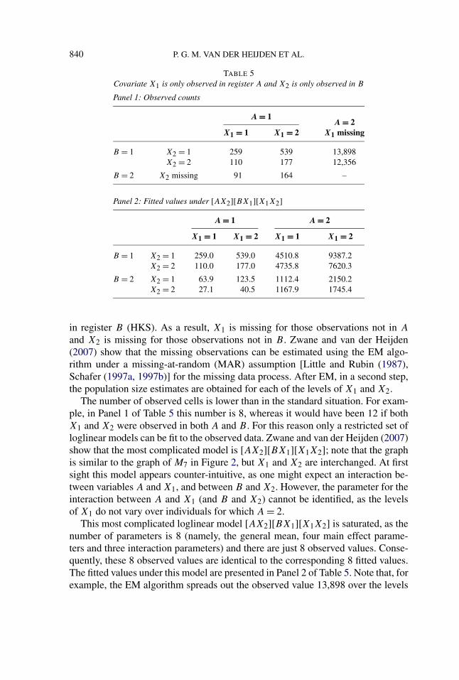
3.2. Two registers, covariates observed in only one of the registers. In Sec-tion 3.1 it is presumed that covariates are present in both register A as well asin register B . Recently, it has been made possible to estimate the population sizemaking use of covariates that are only observed in one of the registers [see Zwaneand van der Heijden (2007); for examples, see van der Heijden, Zwane and Hessen(2009), and Sutherland, Schwartz and Rivest (2007)]. A simple example illustratesthe problem [see Panel 1 of Table 5] where covariate X1 (Marital status) is onlyobserved in register A (GBA) and covariate X2 (Police region) is only observed


TABLE 5Covariate X1 is only observed in register A and X2 is only observed in B

Panel 1: Observed counts

A = 1A = 2

X1 = 1 X1 = 2 X1 missing

B = 1 X2 = 1 259 539 13,898X2 = 2 110 177 12,356

B = 2 X2 missing 91 164 –

Panel 2: Fitted values under [AX2][BX1][X1X2]A = 1 A = 2

X1 = 1 X1 = 2 X1 = 1 X1 = 2

B = 1 X2 = 1 259.0 539.0 4510.8 9387.2X2 = 2 110.0 177.0 4735.8 7620.3

B = 2 X2 = 1 63.9 123.5 1112.4 2150.2X2 = 2 27.1 40.5 1167.9 1745.4

in register B (HKS). As a result, X1 is missing for those observations not in A

and X2 is missing for those observations not in B . Zwane and van der Heijden(2007) show that the missing observations can be estimated using the EM algo-rithm under a missing-at-random (MAR) assumption [Little and Rubin (1987),Schafer (1997a, 1997b)] for the missing data process. After EM, in a second step,the population size estimates are obtained for each of the levels of X1 and X2.

The number of observed cells is lower than in the standard situation. For exam-ple, in Panel 1 of Table 5 this number is 8, whereas it would have been 12 if bothX1 and X2 were observed in both A and B . For this reason only a restricted set ofloglinear models can be fit to the observed data. Zwane and van der Heijden (2007)show that the most complicated model is [AX2][BX1][X1X2]; note that the graphis similar to the graph of M7 in Figure 2, but X1 and X2 are interchanged. At firstsight this model appears counter-intuitive, as one might expect an interaction be-tween variables A and X1, and between B and X2. However, the parameter for theinteraction between A and X1 (and B and X2) cannot be identified, as the levelsof X1 do not vary over individuals for which A = 2.

This most complicated loglinear model [AX2][BX1][X1X2] is saturated, as thenumber of parameters is 8 (namely, the general mean, four main effect parame-ters and three interaction parameters) and there are just 8 observed values. Conse-quently, these 8 observed values are identical to the corresponding 8 fitted values.The fitted values under this model are presented in Panel 2 of Table 5. Note that, forexample, the EM algorithm spreads out the observed value 13,898 over the levels


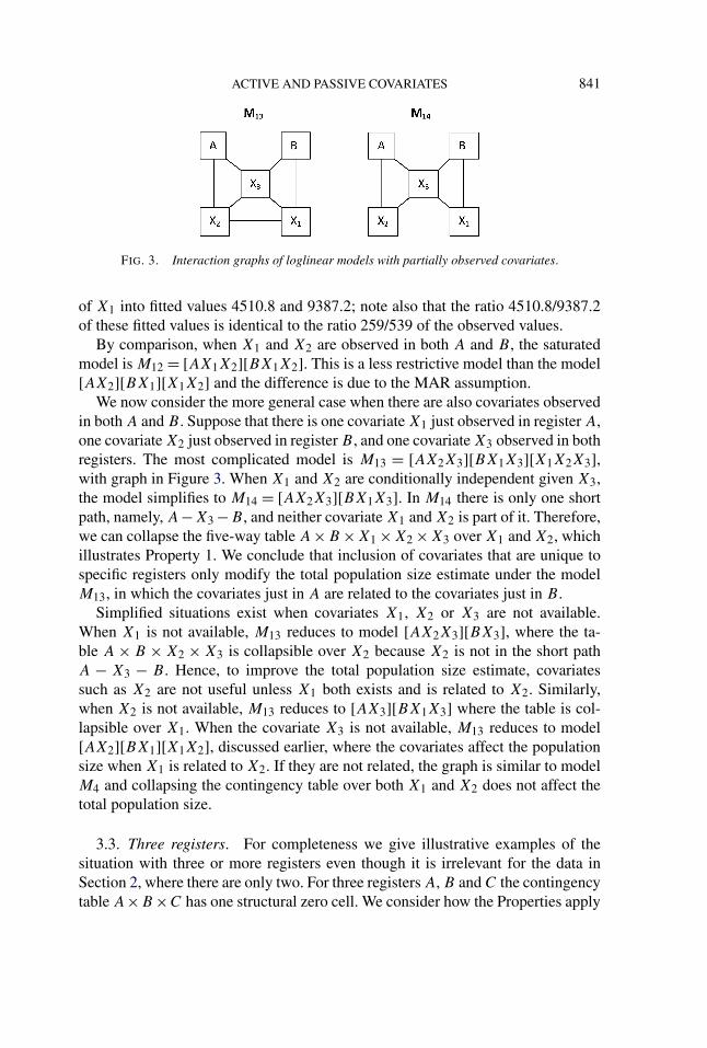
FIG. 3. Interaction graphs of loglinear models with partially observed covariates.

of X1 into fitted values 4510.8 and 9387.2; note also that the ratio 4510.8/9387.2of these fitted values is identical to the ratio 259/539 of the observed values.

By comparison, when X1 and X2 are observed in both A and B , the saturatedmodel is M12 = [AX1X2][BX1X2]. This is a less restrictive model than the model[AX2][BX1][X1X2] and the difference is due to the MAR assumption.

We now consider the more general case when there are also covariates observedin both A and B . Suppose that there is one covariate X1 just observed in register A,one covariate X2 just observed in register B , and one covariate X3 observed in bothregisters. The most complicated model is M13 = [AX2X3][BX1X3][X1X2X3],with graph in Figure 3. When X1 and X2 are conditionally independent given X3,the model simplifies to M14 = [AX2X3][BX1X3]. In M14 there is only one shortpath, namely, A−X3 −B , and neither covariate X1 and X2 is part of it. Therefore,we can collapse the five-way table A×B ×X1 ×X2 ×X3 over X1 and X2, whichillustrates Property 1. We conclude that inclusion of covariates that are unique tospecific registers only modify the total population size estimate under the modelM13, in which the covariates just in A are related to the covariates just in B .

Simplified situations exist when covariates X1, X2 or X3 are not available.When X1 is not available, M13 reduces to model [AX2X3][BX3], where the ta-ble A × B × X2 × X3 is collapsible over X2 because X2 is not in the short pathA − X3 − B . Hence, to improve the total population size estimate, covariatessuch as X2 are not useful unless X1 both exists and is related to X2. Similarly,when X2 is not available, M13 reduces to [AX3][BX1X3] where the table is col-lapsible over X1. When the covariate X3 is not available, M13 reduces to model[AX2][BX1][X1X2], discussed earlier, where the covariates affect the populationsize when X1 is related to X2. If they are not related, the graph is similar to modelM4 and collapsing the contingency table over both X1 and X2 does not affect thetotal population size.

3.3. Three registers. For completeness we give illustrative examples of thesituation with three or more registers even though it is irrelevant for the data inSection 2, where there are only two. For three registers A, B and C the contingencytable A×B ×C has one structural zero cell. We consider how the Properties apply


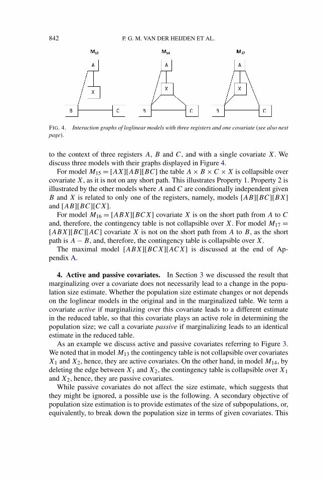
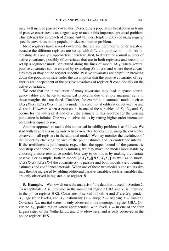
FIG. 4. Interaction graphs of loglinear models with three registers and one covariate (see also nextpage).

to the context of three registers A, B and C, and with a single covariate X. Wediscuss three models with their graphs displayed in Figure 4.

For model M15 = [AX][AB][BC] the table A × B × C × X is collapsible overcovariate X, as it is not on any short path. This illustrates Property 1. Property 2 isillustrated by the other models where A and C are conditionally independent givenB and X is related to only one of the registers, namely, models [AB][BC][BX]and [AB][BC][CX].

For model M16 = [ABX][BCX] covariate X is on the short path from A to C

and, therefore, the contingency table is not collapsible over X. For model M17 =[ABX][BC][AC] covariate X is not on the short path from A to B , as the shortpath is A − B , and, therefore, the contingency table is collapsible over X.

The maximal model [ABX][BCX][ACX] is discussed at the end of Ap-pendix A.

4. Active and passive covariates. In Section 3 we discussed the result thatmarginalizing over a covariate does not necessarily lead to a change in the popu-lation size estimate. Whether the population size estimate changes or not dependson the loglinear models in the original and in the marginalized table. We term acovariate active if marginalizing over this covariate leads to a different estimatein the reduced table, so that this covariate plays an active role in determining thepopulation size; we call a covariate passive if marginalizing leads to an identicalestimate in the reduced table.

As an example we discuss active and passive covariates referring to Figure 3.We noted that in model M13 the contingency table is not collapsible over covariatesX1 and X2, hence, they are active covariates. On the other hand, in model M14, bydeleting the edge between X1 and X2, the contingency table is collapsible over X1and X2, hence, they are passive covariates.

While passive covariates do not affect the size estimate, which suggests thatthey might be ignored, a possible use is the following. A secondary objective ofpopulation size estimation is to provide estimates of the size of subpopulations, or,equivalently, to break down the population size in terms of given covariates. This


may well include passive covariates. Describing a population breakdown in termsof passive covariates is an elegant way to tackle this important practical problem.This extends the approach of Zwane and van der Heijden (2007) of using registerspecific covariates in the population size estimation problem.

Most registers have several covariates that are not common to other registers,because the different registers are set up with different purposes in mind. An in-teresting data analytic approach is, therefore, first, to determine a small number ofactive covariates, possibly of covariates that are in both registers; and second, toset up a loglinear model structured along the lines of model M14, where severalpassive covariates can be entered by extending X1 or X2, and where these covari-ates may or may not be register specific. Passive covariates are helpful in breakingdown the population size under the assumption that the passive covariates of reg-ister A are independent of the passive covariates of register B conditionally on theactive covariates.

We note that the introduction of many covariates may lead to sparse contin-gency tables and hence to numerical problems due to empty marginal cells inthose margins that are fitted. Consider, for example, a saturated model such as[AX1X2X3][BX1X2X3]. In this model the conditional odds ratios between A andB are 1. However, when a zero count in one of the subtables of X1,X2 and X3occurs for the levels of A and of B , the estimate in this subtable for the missingpopulation is infinite. One way to solve this is by setting higher order interactionparameters equal to zero.

Another approach to tackle this numerical instability problem is as follows. Westart with an analysis using only active covariates, for example, using the covariatesobserved in all registers in the saturated model. We may monitor the usefulness ofthe model by checking the size of the point estimate and its confidence interval.If the usefulness is problematic (e.g., when the upper bound of the parametricbootstrap confidence interval is infinite), we may make the model more stable bychoosing a more restrictive model. One way to do this is by making a covariatepassive. For example, both in model [AX1X2][BX1X2X3] as well as in model[AX1X2X3][BX1X2] the covariate X3 is passive and both models yield identicalestimates and confidence intervals. When one of these two model is chosen, its sizemay then be increased by adding additional passive variables, such as variables thatare only observed in register A or register B .

5. Example. We now discuss the analysis of the data introduced in Section 2.To recapitulate, A is inclusion in the municipal register GBA and B is inclusionin the police register HKS. Covariates observed in both A and B are X1, gender,X2, age (four levels), and X3, nationality (1 = Iraqi; 2 = Afghan; 3 = Iranian).Covariate X4, marital status, is only observed in the municipal register GBA. Co-variate X5, police region where apprehended, with levels 1 = in one of the fourlargest cities of the Netherlands, and 2 = elsewhere, and is only observed in thepolice register HKS.


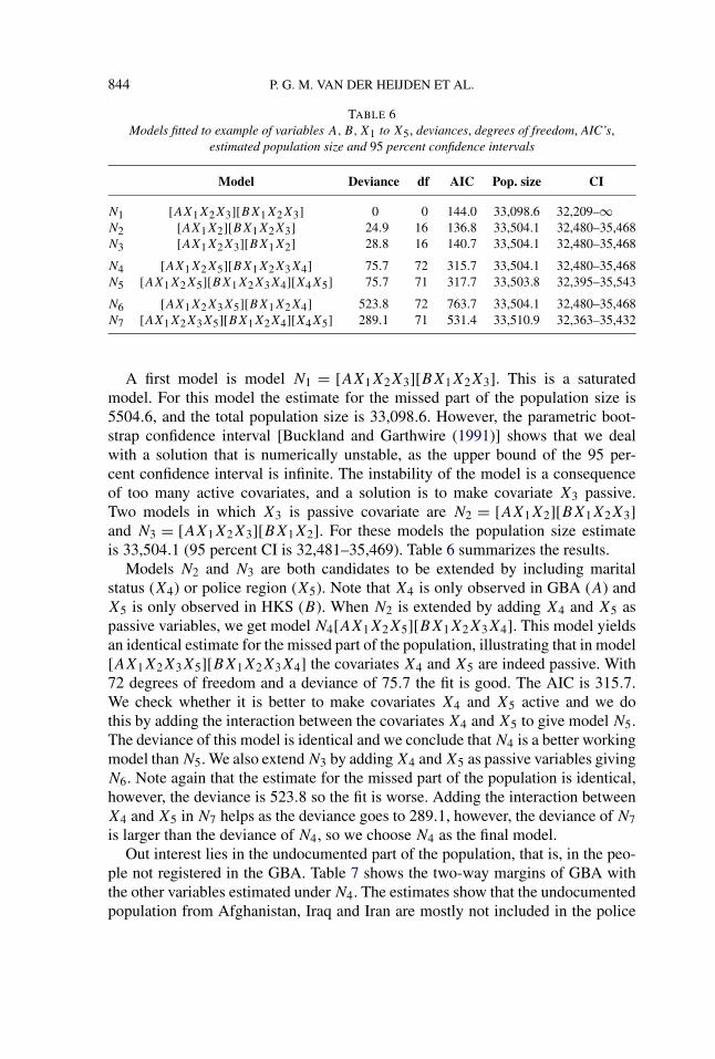
TABLE 6Models fitted to example of variables A,B,X1 to X5, deviances, degrees of freedom, AIC’s,

estimated population size and 95 percent confidence intervals

Model Deviance df AIC Pop. size CI

N1 [AX1X2X3][BX1X2X3] 0 0 144.0 33,098.6 32,209–∞N2 [AX1X2][BX1X2X3] 24.9 16 136.8 33,504.1 32,480–35,468N3 [AX1X2X3][BX1X2] 28.8 16 140.7 33,504.1 32,480–35,468

N4 [AX1X2X5][BX1X2X3X4] 75.7 72 315.7 33,504.1 32,480–35,468N5 [AX1X2X5][BX1X2X3X4][X4X5] 75.7 71 317.7 33,503.8 32,395–35,543

N6 [AX1X2X3X5][BX1X2X4] 523.8 72 763.7 33,504.1 32,480–35,468N7 [AX1X2X3X5][BX1X2X4][X4X5] 289.1 71 531.4 33,510.9 32,363–35,432

A first model is model N1 = [AX1X2X3][BX1X2X3]. This is a saturatedmodel. For this model the estimate for the missed part of the population size is5504.6, and the total population size is 33,098.6. However, the parametric boot-strap confidence interval [Buckland and Garthwire (1991)] shows that we dealwith a solution that is numerically unstable, as the upper bound of the 95 per-cent confidence interval is infinite. The instability of the model is a consequenceof too many active covariates, and a solution is to make covariate X3 passive.Two models in which X3 is passive covariate are N2 = [AX1X2][BX1X2X3]and N3 = [AX1X2X3][BX1X2]. For these models the population size estimateis 33,504.1 (95 percent CI is 32,481–35,469). Table 6 summarizes the results.

Models N2 and N3 are both candidates to be extended by including maritalstatus (X4) or police region (X5). Note that X4 is only observed in GBA (A) andX5 is only observed in HKS (B). When N2 is extended by adding X4 and X5 aspassive variables, we get model N4[AX1X2X5][BX1X2X3X4]. This model yieldsan identical estimate for the missed part of the population, illustrating that in model[AX1X2X3X5][BX1X2X3X4] the covariates X4 and X5 are indeed passive. With72 degrees of freedom and a deviance of 75.7 the fit is good. The AIC is 315.7.We check whether it is better to make covariates X4 and X5 active and we dothis by adding the interaction between the covariates X4 and X5 to give model N5.The deviance of this model is identical and we conclude that N4 is a better workingmodel than N5. We also extend N3 by adding X4 and X5 as passive variables givingN6. Note again that the estimate for the missed part of the population is identical,however, the deviance is 523.8 so the fit is worse. Adding the interaction betweenX4 and X5 in N7 helps as the deviance goes to 289.1, however, the deviance of N7is larger than the deviance of N4, so we choose N4 as the final model.

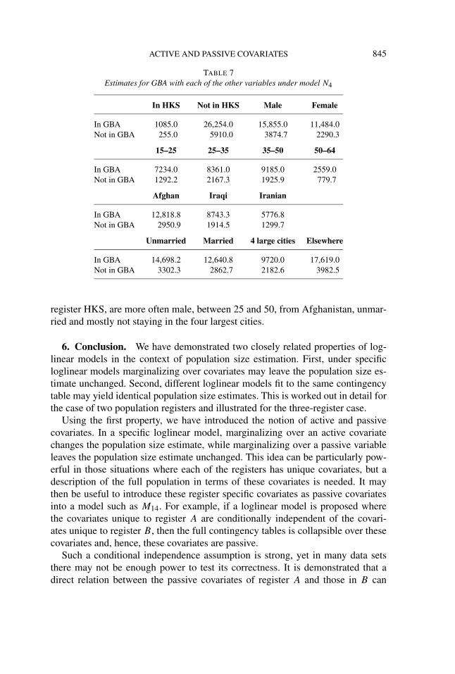
Out interest lies in the undocumented part of the population, that is, in the peo-ple not registered in the GBA. Table 7 shows the two-way margins of GBA withthe other variables estimated under N4. The estimates show that the undocumentedpopulation from Afghanistan, Iraq and Iran are mostly not included in the police


TABLE 7Estimates for GBA with each of the other variables under model N4

In HKS Not in HKS Male Female

In GBA 1085.0 26,254.0 15,855.0 11,484.0Not in GBA 255.0 5910.0 3874.7 2290.3

15–25 25–35 35–50 50–64

In GBA 7234.0 8361.0 9185.0 2559.0Not in GBA 1292.2 2167.3 1925.9 779.7

Afghan Iraqi Iranian

In GBA 12,818.8 8743.3 5776.8Not in GBA 2950.9 1914.5 1299.7

Unmarried Married 4 large cities Elsewhere

In GBA 14,698.2 12,640.8 9720.0 17,619.0Not in GBA 3302.3 2862.7 2182.6 3982.5

register HKS, are more often male, between 25 and 50, from Afghanistan, unmar-ried and mostly not staying in the four largest cities.

6. Conclusion. We have demonstrated two closely related properties of log-linear models in the context of population size estimation. First, under specificloglinear models marginalizing over covariates may leave the population size es-timate unchanged. Second, different loglinear models fit to the same contingencytable may yield identical population size estimates. This is worked out in detail forthe case of two population registers and illustrated for the three-register case.

Using the first property, we have introduced the notion of active and passivecovariates. In a specific loglinear model, marginalizing over an active covariatechanges the population size estimate, while marginalizing over a passive variableleaves the population size estimate unchanged. This idea can be particularly pow-erful in those situations where each of the registers has unique covariates, but adescription of the full population in terms of these covariates is needed. It maythen be useful to introduce these register specific covariates as passive covariatesinto a model such as M14. For example, if a loglinear model is proposed wherethe covariates unique to register A are conditionally independent of the covari-ates unique to register B , then the full contingency tables is collapsible over thesecovariates and, hence, these covariates are passive.

Such a conditional independence assumption is strong, yet in many data setsthere may not be enough power to test its correctness. It is demonstrated that adirect relation between the passive covariates of register A and those in B can


only be assessed among those individuals that are in both register A and B . Ifthere is overlap between register A and B , with relatively many individuals in bothA and B , the relationship between the passive covariates of A and B can easilybe assessed; conversely, if the overlap is small, there is little power to establishwhether or not this relation should be included in the model.

This new methodology should be of use for estimating the missing populationdue to undercoverage in the 2011 Census of the Netherlands where the size of thetotal population can be estimated by application of loglinear models. It could alsobe applied to countries that use register information to estimate the undercoverageof their Population Register as well as to countries which use traditional methods.The use of passive covariates gives insight into which characteristics individualshave that are not covered by the Census and thereby illuminate the bias due to theundercoverage.

In the Introduction we mentioned latent variable models that take heterogeneityof inclusion probabilities into account. For this purpose both Fienberg, Johnsonand Junker (1999) as well as in Bartolucci and Forcina (2001) proposed general-izations of the so-called Rasch model. It is beyond the scope of this paper to studycollapsibility properties for their models in the presence of covariates. However, itis interesting to note that one important specific form of the Rasch model, the so-called extended Rasch model, is mathematically equivalent to the loglinear modelthat includes three two-factor interactions that are identical and a three-factor inter-action [see Hessen (2011); this loglinear model is also used in IWGDMF (1995),where it is referred to as a heterogeneity model]. Collapsibility properties of thisloglinear model can be studied using the perspective presented in this paper.

APPENDIX A: IDENTIFICATION OF EQUIVALENT MODELS

We establish which models listed in Figures 1–4 have the same estimates, andwhich do not, by showing that models for population size estimation are modelcollapsible onto two margins; and by demonstrating how the short path criterionidentifies noninvariance of population size estimates. Our method is to apply theAsmussen and Edwards (1983) criterion to the population size estimation modelwhich contains structural zeros.

A.1. Model collapsibility. First we recall the model collapsibility conditionof Asmussen and Edwards (1983). Consider a table classified by two sets of factorsY and Z, so that the saturated model is [YZ], and maximum likelihood estimationunder product multinomial sampling. The authors give conditions on the hierar-chical loglinear model M ⊂ [YZ] under which

p̂NY (y) = ∑

z

p̂MYZ(y, z),(A.1)

where the right-hand side (RHS) is the margin of the MLE under the model M forthe full table, while the LHS is the MLE under the restricted model N for the mar-gin obtained by deleting terms in Z from each generator of M . Their Theorem 2.3


states that M is (model) collapsible onto the margin Y , that is, (A.1) holds, if andonly if the boundary of every connected component of Z is contained in a gen-erator of M . A corollary to this result is that estimates computed under N havethe same sampling distribution as those under M , and hence the same confidenceintervals.

Implicit in their derivation is that the space on which the table is defined isa Cartesian product of the factors. We argue that the population size estima-tion model cannot be defined on a Cartesian product of registers, for in ourcontext if p were defined on A × B × X with A, B = {1,2}, then we requirep(2,2, x) = 0 to reflect a structural zero. If so, the maximal loglinear model wouldbe M = [ABX] with a three factor interaction, as logp contains the interactionterm λABX(2,2, x) = −∞. Furthermore, application of model collapsibility sug-gests M = [ABX] is model collapsible onto [AB], which may be shown by coun-terexample to be false.

A.2. Models for population size estimation. For population size estimationthe appropriate sample space S for two registers is

S = {(a, b); (a, b) = (1,1), (1,2), (2,1)},as (2,2) cannot be observed, and the sample space for the whole survey is S × X ,where X is the Cartesian product of the discrete spaces for the covariates. Anyloglinear model M with probability mass function pM

SX is defined and fitted onthis space. The loglinear expansion of logpM

SX(a, b, x) under the maximal modelM = [AX][BX] is

λ + λA(a) + λB(b) + λX(x) + λAX(a, x) + λBX(b, x)(A.2)

for (a, b, x) ∈ S × X . The λ parameters satisfy corner point constraints to ensureidentifiability, but are otherwise arbitrary. This is an instance of a hierarchical log-linear model; an equivalent parameterization is to write the highest order maineffect as λSX(s, x), but this obscures the submodels of interest. The register A

taking values in A defines the marginal probability pMAX of pM

SX , similarly pMBX .

Asmussen and Edwards (1983) define the interaction graph to be the graph witha node for each factor classifying the table and an edge between two nodes if thereis a generator in the model containing both. Consequently, the graphs in Figures 1–4 are the interaction graphs of particular population size models. The interactiongraph of M = [AX][BX] is that of M3 in Figure 1 with X replacing X1.

These graphs cannot be interpreted as conditional independence graphs in whichthe missing edge between A and B leads to the statement A ⊥⊥ B|X, as this is falseon the restricted space S × X ; for instance, if X is empty, and M = [A][B], thenP(A = 1,B = 1) �= pA(1)pB(1). However, conditional independence interpreta-tions between a register and covariates, and between two covariates are possible.

With the population size estimation model at (A.2) defined on the right space,S × X , we can now employ model collapsibility to show this model is collapsibleonto two margins.


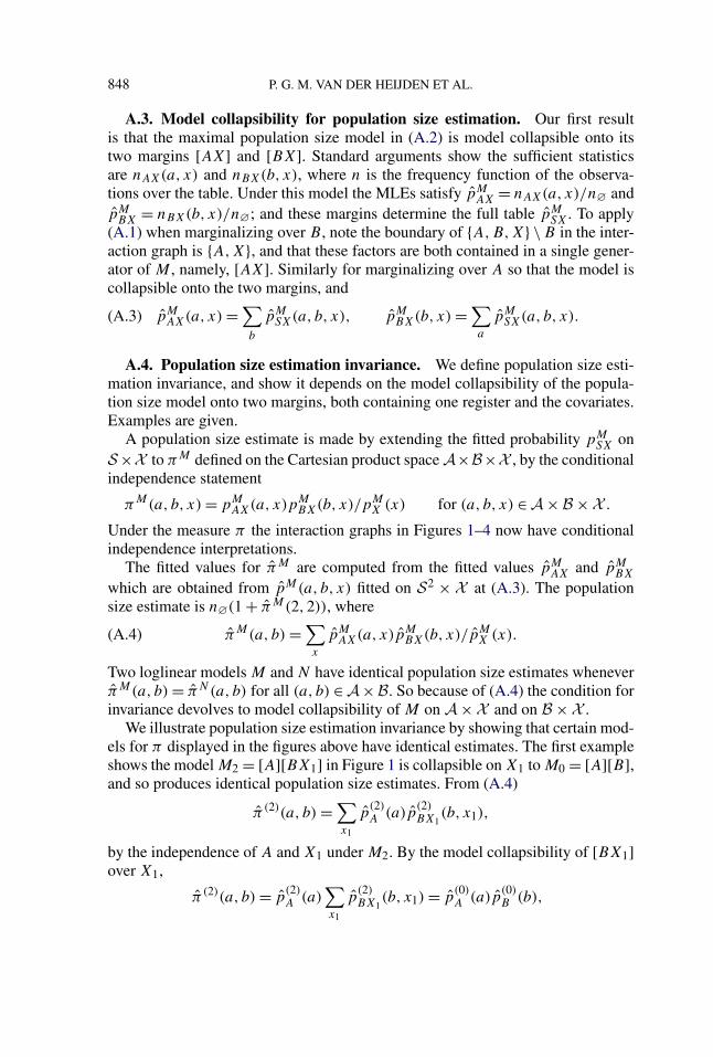
A.3. Model collapsibility for population size estimation. Our first resultis that the maximal population size model in (A.2) is model collapsible onto itstwo margins [AX] and [BX]. Standard arguments show the sufficient statisticsare nAX(a, x) and nBX(b, x), where n is the frequency function of the observa-tions over the table. Under this model the MLEs satisfy p̂M

AX = nAX(a, x)/n∅ andp̂M

BX = nBX(b, x)/n∅; and these margins determine the full table p̂MSX . To apply

(A.1) when marginalizing over B , note the boundary of {A,B,X} \ B in the inter-action graph is {A,X}, and that these factors are both contained in a single gener-ator of M , namely, [AX]. Similarly for marginalizing over A so that the model iscollapsible onto the two margins, and

p̂MAX(a, x) = ∑

b

p̂MSX(a, b, x), p̂M

BX(b, x) = ∑

a

p̂MSX(a, b, x).(A.3)

A.4. Population size estimation invariance. We define population size esti-mation invariance, and show it depends on the model collapsibility of the popula-tion size model onto two margins, both containing one register and the covariates.Examples are given.

A population size estimate is made by extending the fitted probability pMSX on

S × X to πM defined on the Cartesian product space A × B × X , by the conditionalindependence statement

πM(a, b, x) = pMAX(a, x)pM

BX(b, x)/pMX (x) for (a, b, x) ∈ A × B × X .

Under the measure π the interaction graphs in Figures 1–4 now have conditionalindependence interpretations.

The fitted values for π̂M are computed from the fitted values p̂MAX and p̂M

BX

which are obtained from p̂M(a, b, x) fitted on S 2 × X at (A.3). The populationsize estimate is n∅(1 + π̂M(2,2)), where

π̂M(a, b) = ∑

x

p̂MAX(a, x)p̂M

BX(b, x)/p̂MX (x).(A.4)

Two loglinear models M and N have identical population size estimates wheneverπ̂M(a, b) = π̂N(a, b) for all (a, b) ∈ A × B. So because of (A.4) the condition forinvariance devolves to model collapsibility of M on A × X and on B × X .

We illustrate population size estimation invariance by showing that certain mod-els for π displayed in the figures above have identical estimates. The first exampleshows the model M2 = [A][BX1] in Figure 1 is collapsible on X1 to M0 = [A][B],and so produces identical population size estimates. From (A.4)

π̂ (2)(a, b) = ∑

x1

p̂(2)A (a)p̂

(2)BX1

(b, x1),

by the independence of A and X1 under M2. By the model collapsibility of [BX1]over X1,

π̂ (2)(a, b) = p̂(2)A (a)

∑

x1

p̂(2)BX1

(b, x1) = p̂(0)A (a)p̂

(0)B (b),


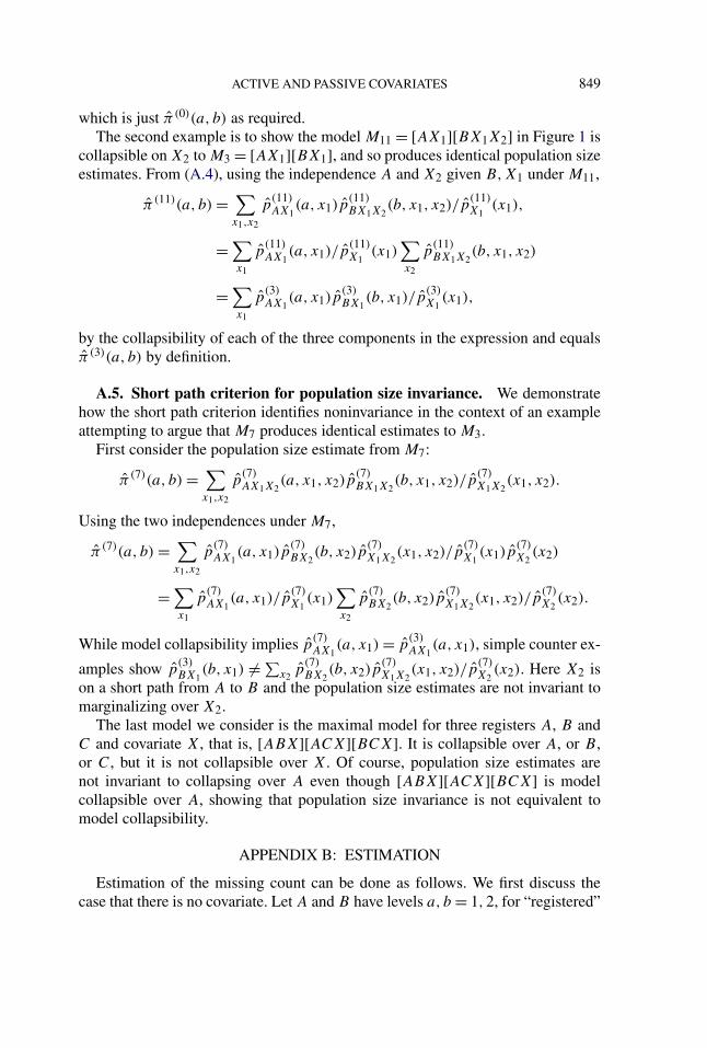
which is just π̂ (0)(a, b) as required.The second example is to show the model M11 = [AX1][BX1X2] in Figure 1 is

collapsible on X2 to M3 = [AX1][BX1], and so produces identical population sizeestimates. From (A.4), using the independence A and X2 given B,X1 under M11,

π̂ (11)(a, b) = ∑

x1,x2

p̂(11)AX1

(a, x1)p̂(11)BX1X2

(b, x1, x2)/p̂(11)X1

(x1),

= ∑

x1

p̂(11)AX1

(a, x1)/p̂(11)X1

(x1)∑

x2

p̂(11)BX1X2

(b, x1, x2)

= ∑

x1

p̂(3)AX1

(a, x1)p̂(3)BX1

(b, x1)/p̂(3)X1

(x1),

by the collapsibility of each of the three components in the expression and equalsπ̂ (3)(a, b) by definition.

A.5. Short path criterion for population size invariance. We demonstratehow the short path criterion identifies noninvariance in the context of an exampleattempting to argue that M7 produces identical estimates to M3.

First consider the population size estimate from M7:

π̂ (7)(a, b) = ∑

x1,x2

p̂(7)AX1X2

(a, x1, x2)p̂(7)BX1X2

(b, x1, x2)/p̂(7)X1X2

(x1, x2).

Using the two independences under M7,

π̂ (7)(a, b) = ∑

x1,x2

p̂(7)AX1

(a, x1)p̂(7)BX2

(b, x2)p̂(7)X1X2

(x1, x2)/p̂(7)X1

(x1)p̂(7)X2

(x2)

= ∑

x1

p̂(7)AX1

(a, x1)/p̂(7)X1

(x1)∑

x2

p̂(7)BX2

(b, x2)p̂(7)X1X2

(x1, x2)/p̂(7)X2

(x2).

While model collapsibility implies p̂(7)AX1

(a, x1) = p̂(3)AX1

(a, x1), simple counter ex-

amples show p̂(3)BX1

(b, x1) �= ∑x2

p̂(7)BX2

(b, x2)p̂(7)X1X2

(x1, x2)/p̂(7)X2

(x2). Here X2 ison a short path from A to B and the population size estimates are not invariant tomarginalizing over X2.

The last model we consider is the maximal model for three registers A, B andC and covariate X, that is, [ABX][ACX][BCX]. It is collapsible over A, or B ,or C, but it is not collapsible over X. Of course, population size estimates arenot invariant to collapsing over A even though [ABX][ACX][BCX] is modelcollapsible over A, showing that population size invariance is not equivalent tomodel collapsibility.

APPENDIX B: ESTIMATION

Estimation of the missing count can be done as follows. We first discuss thecase that there is no covariate. Let A and B have levels a, b = 1,2, for “registered”


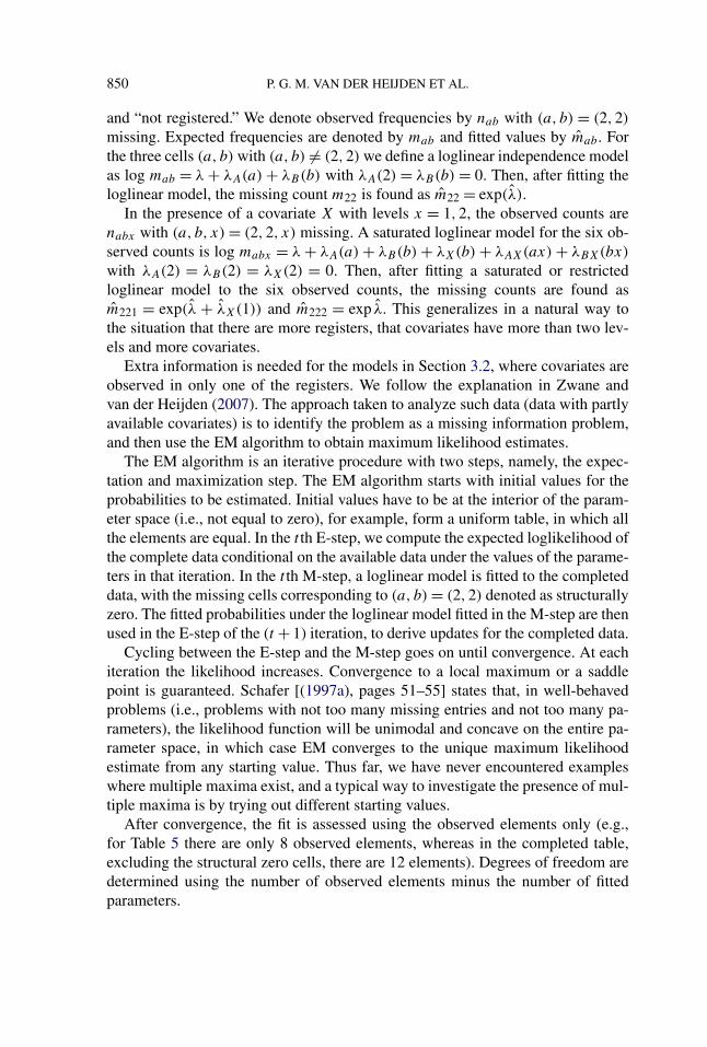
and “not registered.” We denote observed frequencies by nab with (a, b) = (2,2)

missing. Expected frequencies are denoted by mab and fitted values by m̂ab. Forthe three cells (a, b) with (a, b) �= (2,2) we define a loglinear independence modelas log mab = λ + λA(a) + λB(b) with λA(2) = λB(b) = 0. Then, after fitting theloglinear model, the missing count m22 is found as m̂22 = exp(λ̂).

In the presence of a covariate X with levels x = 1,2, the observed counts arenabx with (a, b, x) = (2,2, x) missing. A saturated loglinear model for the six ob-served counts is log mabx = λ + λA(a) + λB(b) + λX(b) + λAX(ax) + λBX(bx)

with λA(2) = λB(2) = λX(2) = 0. Then, after fitting a saturated or restrictedloglinear model to the six observed counts, the missing counts are found asm̂221 = exp(λ̂ + λ̂X(1)) and m̂222 = exp λ̂. This generalizes in a natural way tothe situation that there are more registers, that covariates have more than two lev-els and more covariates.

Extra information is needed for the models in Section 3.2, where covariates areobserved in only one of the registers. We follow the explanation in Zwane andvan der Heijden (2007). The approach taken to analyze such data (data with partlyavailable covariates) is to identify the problem as a missing information problem,and then use the EM algorithm to obtain maximum likelihood estimates.

The EM algorithm is an iterative procedure with two steps, namely, the expec-tation and maximization step. The EM algorithm starts with initial values for theprobabilities to be estimated. Initial values have to be at the interior of the param-eter space (i.e., not equal to zero), for example, form a uniform table, in which allthe elements are equal. In the t th E-step, we compute the expected loglikelihood ofthe complete data conditional on the available data under the values of the parame-ters in that iteration. In the t th M-step, a loglinear model is fitted to the completeddata, with the missing cells corresponding to (a, b) = (2,2) denoted as structurallyzero. The fitted probabilities under the loglinear model fitted in the M-step are thenused in the E-step of the (t + 1) iteration, to derive updates for the completed data.

Cycling between the E-step and the M-step goes on until convergence. At eachiteration the likelihood increases. Convergence to a local maximum or a saddlepoint is guaranteed. Schafer [(1997a), pages 51–55] states that, in well-behavedproblems (i.e., problems with not too many missing entries and not too many pa-rameters), the likelihood function will be unimodal and concave on the entire pa-rameter space, in which case EM converges to the unique maximum likelihoodestimate from any starting value. Thus far, we have never encountered exampleswhere multiple maxima exist, and a typical way to investigate the presence of mul-tiple maxima is by trying out different starting values.

After convergence, the fit is assessed using the observed elements only (e.g.,for Table 5 there are only 8 observed elements, whereas in the completed table,excluding the structural zero cells, there are 12 elements). Degrees of freedom aredetermined using the number of observed elements minus the number of fittedparameters.


The values for the missing cells corresponding to (a, b) = (2,2) are assessedusing the method that we described above.

We use parametric bootstrap confidence intervals because they provide a sim-ple way to find the confidence intervals when the contingency table is not fullyobserved. To compute the bootstrapped confidence intervals for a specific loglin-ear model, we need to first compute the population size under this model and theprobabilities on the completed data under this model, that is, by including the cellsthat cannot be observed by design. A first multinomial sample is drawn given theseparameters, and the sample is then reformatted to be identical to the observed data.The specific loglinear model used is then fitted to the resulting data, resulting inthe first bootstrap sample estimate of the population size. If K bootstrap samplesare needed, then this is repeated K times. By ordering the K bootstrap populationsize estimates, a confidence interval can be constructed.

SUPPLEMENTARY MATERIAL

Estimation in R (DOI: 10.1214/12-AOAS536SUPP; .pdf). We make use of theCAT-procedure in R (Meng and Rubin (1991); Schafer [(1997a), Chapters 7 and 8],(1997b)). The CAT-procedure is a routine for the analysis of categorical variabledata sets with missing values. We describe our application of this procedure indetail in the supplemental article [van der Heijden et al. (2012)].

REFERENCES

ASMUSSEN, S. and EDWARDS, D. (1983). Collapsibility and response variables in contingencytables. Biometrika 70 567–578. MR0725370

BAKER, S. (1990). A simple EM algorithm for capture–recapture data with categorical covariates(with discussion). Biometrics 46 1193–1197.

BARTOLUCCI, F. and FORCINA, A. (2001). Analysis of capture–recapture data with a Rasch-typemodel allowing for conditional dependence and multidimensionality. Biometrics 57 714–719.MR1859808

BISHOP, Y. M. M., FIENBERG, S. E. and HOLLAND, P. W. (1975). Discrete Multivariate Analysis:Theory and Practice. The MIT Press, Cambridge, MA. MR0381130

BUCKLAND, S. and GARTHWIRE, P. (1991). Quantifying precision of mark-recapture estimatesusing the bootstrap and related methods. Biometrics 47 255–268.

CHAO, A., TSAY, P. K., LIN, S. H., SHAU, W. Y. and CHAO, D. Y. (2001). The applications ofcapture–recapture models to epidemiological data. Stat. Med. 20 3123–3157.

CORMACK, R. (1989). Log-linear models for capture–recapture. Biometrics 45 395–413.FIENBERG, S. E. (1972). The multiple recapture census for closed populations and incomplete 2k

contingency tables. Biometrika 59 591–603. MR0383619FIENBERG, S., JOHNSON, M. and JUNKER, B. (1999). Classical multilevel and Bayesian ap-

proaches to population size estimation using multiple lists. J. Roy. Statist. Soc. Ser. A 162 383–406.

HESSEN, D. J. (2011). Loglinear representations of multivariate Bernoulli Rasch models. British J.Math. Statist. Psych. 64 337–354. MR2816783

HICKMAN, L. J. and SUTTORP, M. J. (2008). Are deportable aliens a unique threat to public safety?Comparing the recidivism of deportable and nondeportable aliens. Crime and Public Policy 759–82.

http://dx.doi.org/10.1214/12-AOAS536SUPP

http://www.ams.org/mathscinet-getitem?mr=0725370






IWGDMF: INTERNATIONAL WORKING GROUP FOR DISEASE MONITORING AND FORECAST-ING (1995). Capture–recapture and multiple record systems estimation. Part i. History and theo-retical development. American Journal of Epidemiology 142 1059–1068.

KIM, S.-H. and KIM, S.-H. (2006). A note on collapsibility in DAG models of contingency tables.Scand. J. Stat. 33 575–590. MR2298066

LITTLE, R. J. A. and RUBIN, D. B. (1987). Statistical Analysis with Missing Data. Wiley, NewYork. MR0890519

MENG, X. L. and RUBIN, D. B. (1991). IPF for contingency tables with missing data via the ECMalgorithm. In Proceedings of the Statistical Computing Section of the American Statistical Asso-ciation 244–247. Amer. Statist. Assoc., Washington, DC.

POLLOCK, K. H. (2002). The use of auxiliary variables in capture–recapture modelling: Anoverview. J. Appl. Stat. 29 85–106. MR1881048

SCHAFER, J. L. (1997a). Analysis of Incomplete Multivariate Data. Monographs on Statistics andApplied Probability 72. Chapman & Hall, London. MR1692799

SCHAFER, J. (1997b). Imputation of missing covariates under a general linear mixed model. Dept.Statistics, Penn State Univ.

SUTHERLAND, J. M., SCHWARZ, C. J. and RIVEST, L.-P. (2007). Multilist population estimationwith incomplete and partial stratification. Biometrics 63 910–916. MR2395810

VALENTE, P. (2010). Main results of the UNECE/UNSD survey on the 2010/2011 round of censusesin the UNECE region. Eurostat, Luxembourg.

VAN DER HEIJDEN, P. G. M., ZWANE, E. and HESSEN, D. (2009). Structurally missing data prob-lems in multiple list capture–recapture data. AStA Adv. Stat. Anal. 93 5–21. MR2476297

VAN DER HEIJDEN, P. G. M., WHITTAKER, J., CRUYFF, M., BAKKER, B. and VAN DER VLIET, R.(2012). Supplement to “People born in the Middle East but residing in the Netherlands: Invari-ant population size estimates and the role of active and passive covariates.” DOI:10.1214/12-AOAS536SUPP.

WHITTAKER, J. (1990). Graphical Models in Applied Multivariate Statistics. Wiley, Chichester.MR1112133

ZWANE, E. N. and VAN DER HEIJDEN, P. G. M. (2007). Analysing capture–recapture data whensome variables of heterogeneous catchability are not collected or asked in all registrations. Stat.Med. 26 1069–1089. MR2339234

ZWANE, E., VAN DER PAL, K. and VAN DER HEIJDEN, P. G. M. (2004). The multiple-recordsystems estimator when registrations refer to different but overlapping populations. Stat. Med. 232267–2281.

P. G. M. VAN DER HEIJDEN

M. CRUYFF

DEPARTMENT OF METHODOLOGY

AND STATISTICS

UTRECHT UNIVERSITY

POSTBUS 80.140, 3508TC UTRECHT

THE NETHERLANDS

E-MAIL: [email protected]@uu.nl

J. WHITTAKER

DEPARTMENT OF MATHEMATICS

AND STATISTICS

LANCASTER UNIVERSITY

BAILRIGG

LANCASTER

UNITED KINGDOM

E-MAIL: [email protected]

B. BAKKER

R. VAN DER VLIET

STATISTICS NETHERLANDS

POSTBUS 24500, 2490HA DEN HAAG

THE NETHERLANDS

E-MAIL: [email protected]@cbs.nl










mailto:[email protected]






people born in the middle east but residing in the netherlands: invariant population size estimates...

Documents