Patient-calibrated agent-based modelling of

ductal carcinoma in situ (DCIS) I: Model

formulation and analysis

Paul Macklin 1,2,3, Mary E. Edgerton 4, Alastair Thompson 4,5,

Vittorio Cristini 3,6

Abstract

Ductal carcinoma in situ (DCIS)–an important precursor to invasive breast cancer–is typically diagnosed as microcalcifications in mammograms. However, the effectiveuse of mammograms and other patient data to plan treatment has been restrictedby our limited understanding of DCIS growth and calcification.

We develop a mechanistic, agent-based model of DCIS that is broadly applicable be-yond breast cancer. The motion of each cell is determined by a balance of adhesive,repulsive, and motile forces. Interaction forces are governed by potential functionsthat can model heterophilic and homophilic adhesion, interaction between cells ofunequal size and phenotype, and interaction with a basement membrane. Each cellhas a phenotypic state that is governed by exponentially-distributed random vari-ables. This is a natural generalisation of prevalent models, and provides a rigorousway to vary transition probabilities with variable time step sizes and the microenvi-ronment. Each agent has a detailed “submodel” of the cell volume changes duringproliferation and necrosis (including the first model for the fast time scale processesof swelling and lysis), and we are the first to account for cell calcification. We simu-late the microenvironment through coupled reaction-diffusion equations. The resultis a modelling framework that is well-suited to investigating the biophysical mecha-nisms of DCIS growth and calcification. An analysis of the model’s volume-averagedbehaviour yields new insight on the relationship between intraductal oxygen levels,proliferation, and heterogeneous cell signalling; we test these ideas against patientimmunohistochemistry data.

This paper is the first in a two-part series on DCIS modelling. In Part II, we useour analysis to develop a patient-specific model calibration protocol, simulate DCISin a virtual patient, generate macroscopic predictions on DCIS microstructure andclinical progression, and test these against large, independent sets of clinical data.

Key words: agent-based modelling, tumour simulation, nonhomogeneous Poissonprocesses, necrosis, biomechanics, calcification, ductal carcinoma in situ (DCIS)1991 MSC: 65C20, 92B05, 92C05

Preprint submitted to Journal of Theoretical Biology 5 January 2011

1 Introduction

Ductal carcinoma in situ (DCIS), a type of breast cancer where growth isconfined within the breast ductal/lobular units, is the most prevalent precur-sor to invasive ductal breast cancer (IC). Breast cancer is the second-leadingcause of death in women in the United States. The American Cancer Soci-ety predicted that 50,000 new cases of DCIS alone (excluding other formsof pre-invasive change such as lobular carcinoma in situ) and 180,000 newcases of IC would be diagnosed in 2007 (Jemal et al., 2007; American Can-cer Society, 2007). Co-existing DCIS is expected in 80% of IC, or 144,000cases (Lampejo et al., 1994). While DCIS itself is not life-threatening, it is avery important precursor to IC because (1) it can be treated and (2) if leftuntreated, it has a high probability of progression to IC, which is a deadly dis-ease (Page et al., 1982; Kerlikowske et al., 2003; Sanders et al., 2005). Whilethe detection and treatment of DCIS have greatly improved over the last fewdecades, problems persist. DCIS can be difficult to detect by mammography,the principle modality in breast screening, or to distinguish from other aber-rant lesions (Venkatesan et al., 2009). This can lead to “false positives” ofDCIS and overtreatment, including unnecessary surgery. On the other hand,even in cases where DCIS excision is truly warranted, multiple proceduresmay be required to fully eliminate all DCIS, due to the differences betweenthe pre-operative estimated and actual resected histopathology findings (e.g.,of the tumour size and shape) (Cheng et al., 1997; Silverstein, 1997; Cabiogluet al., 2007; Dillon et al., 2007). Hence, a solid scientific understanding ofDCIS progression is required to improve clinical decision making.

There are many open questions on DCIS biology which contribute to the cur-rent uncertainty in clinical practice. How does DCIS progress from a few pro-liferating cells to detectable lesions potentially including microcalcifications?How do heterogeneities in cell mechanics and other phenotypic characteris-tics give rise to specific DCIS morphologies? Is the gap that is often observedbetween the tumour’s viable rim and the necrotic core simply an artifact of his-tologic preparation, or is it indicative of further biomechanical processes? Can

Email address: macklin@maths.dundee.ac.uk (Paul Macklin).URL: http://www.maths.dundee.ac.uk/macklin (Paul Macklin).

1 Corresponding author2 Division of Mathematics, University of Dundee, Dundee, Scotland, UK3 Formerly of: School of Biomedical Informatics, University of Texas Health ScienceCenter, Houston, TX, USA4 M.D. Anderson Cancer Center, Houston, TX, USA5 Department of Surgery and Molecular Oncology, University of Dundee, Dundee,Scotland, UK6 Departments of Pathology and Chemical Engineering, University of New Mexico,Albuquerque, NM, USA

2

observations from immunohistochemistry (IHC) and histopathology images beused to estimate important physiological constants? Conversely, can mathe-matical modelling provide new insight on interpretting these data? What is therelationship between the microcalcifications observed in mammography andtumour morphology? How can we calibrate patient-specific models to limitedand often noisy histopathologic data, often from only a single time point?

These clinically-pertinent scientific questions motivate our model develop-ment. Mathematical modelling has already seen use in understanding andpredicting the growth of DCIS or its approach towards a steady state. Frankset al. (2003a,b, 2005) and Owen et al. (2004) have used continuum modelsto investigate tumour growth in breast ducts, including the impact of vol-ume loss in the necrotic core, ductal expansion, and the influence of basementmembrane (BM) adhesion (Franks et al., 2003a,b, 2005; Owen et al., 2004);this work can be traced to a long history of work by Ward and King (e.g.,Ward and King (1997)) that includes model parameterisation by matching toexperiments. Rejniak and co-workers applied an immersed boundary methodto individual polarised cells; their model was able to reproduce several com-plex DCIS sub-types (Rejniak, 2007; Rejniak and Dillon, 2007; Rejniak andAnderson, 2008a,b). More recently, Norton et al. (2010) conducted a similarinvestigation of the relationship between polarised cell adhesion, intraductalpressure, and DCIS morphology in 2D using a lattice-free agent model andwere able to produce nontrivial tumour microstructures (e.g., cribriform pat-terns). Gatenby et al. (2007), Silva et al. (2010), and Smallbone et al. (2007)have investigated the role of hypoxia, glycolysis, and acidosis in DCIS evolu-tion in 2D and 3D using cellular automata (CA) methods by including detailedmetabolic sub-models. Bankhead III et al. (2007) conducted early 3-D simula-tions of tumour cell heirarchy using CA techniques. Sontag and Axelrod (2005)combined population-scale models with machine learning techniques and sta-tistical analyses to postulate new hypotheses on DCIS mutation pathwaysfrom benign precursors, while Enderling et al. (2006, 2007) studied DNA mu-tation within DCIS and recurrence (particularly following radiation therapy)using continuum and CA methods. Mannes et al. (2002) used CA methods toinvestigate Pagetoid spread.

All this work has provided a degree of insight into DCIS, but has not fullyanswered the questions we posed. Typical CA methods cannot accuratelymodel cell mechanics, particularly proliferation by tumour cells when fully sur-rounded by other cells. Such proliferation, which is regularly observed in DCISimmunohistochemistry, can only be approximated in CA methods by intro-ducing complex, often phenomenological rules to push multiple cells throughthe simulated domain. Population-based ordinary differential equation (ODE)models do not account for spatial heterogeneity and hence cannot investigatethe impact of heterogeneous mechanics, substrate transport, and their inter-action. To date, none have modelled the process of microcalcification, and

3

existing “sub-models” of necrosis have been simple volume loss terms, andhave not considered the individual effects of cell swelling and lysis. Indeed,many prevalent models do not include necrosis. The work by Norton et al.(2010) shows promise, but it has yet to predict tumour biophysics as emer-gent phenomena because it imposed many of its mechanical, proliferation,viable rim size, and apoptosis properties a priori as algorithmic rules. The de-tailed morphological model of Rejniak and colleagues has produced impressiveresults, but faces computational limits when applied to large numbers of cells.Continuum models can overcome these limits, but calibration to molecular-and cell-scale data is not straightforward, particularly for phenomenological“lumped” parameters (Macklin et al., 2010b). We are currently approachingthis issue as a multiscale information flow, by upscaling calibrated cell-scalemodels to the continuum scale (Edgerton et al., 2011). See also the discussionin Cristini and Lowengrub (2010) and recent multiscale modelling reviews(Deisboeck et al., 2010; Lowengrub et al., 2010). To our knowledge, there hasbeen no prior patient-specific calibration to the proliferative and apoptoticindices generally measured in breast biopsies at any scale of modelling.

We presently develop a lattice-free, agent-based cell model that can be ap-plied to many problems, exemplified by DCIS. The cells (agents) are modelledas objects subject to a balance of adhesive, repulsive, and motile forces thatdetermine their motion. Cell-cell and cell-basement membrane interaction me-chanics are modelled using potential functions that can account for finite in-teraction distances, both heterophilic and homophilic adhesion, uncertainty incell morphology and position, and interaction between cells of variable sizesand types. We introduce a level set formulation of the basement membranemorphology that is well-suited to future deformation modelling, and providesa generalised framework for the exchange of forces between discrete cell objectsand extended macroscopic objects with nontrivial geometries.

Each cell is endowed with a phenotypic state, and phenotypic transitions aregoverned by exponentially-distributed random variables that depend upon thecell’s internal state and the local microenvironment. This modelling choice isconsistent with experimental biology dating back as far as the 1970s (e.g,Smith and Martin (1973)), is a natural extension of prevalent phenotypictransition models in widespread use today, provides a rigorous method tovary the model’s probabilities with the microenvironment and with variabletime step sizes (e.g, those arising from numerical stability criteria), and lendsitself to mathematical analysis.

Our choice of functional relationship between the quiescent-to-proliferativephenotypic transition rate and oxygen availability yields predictions that wetest quantitatively against actual breast patient data. We include detailed“sub-models” of cell volume change during proliferation and necrosis (includ-ing the effects of swelling and lysis), which are able to predict subtle mi-

4

crostructures in the viable rim-necrotic core boundary for the first time, aswell as the important impact of mechanical relaxation by lysing cells in thenecrotic core. Our model is the first to investigate the development of cellularcalcifications towards a clinically-detectable state. We couple the agents to themicroenvironment in a composite modelling framework by solving continuumreaction-diffusion equations for substrates that are altered by the cells. Tomake the model predictive, we constrain all major model parameters by sur-veying a broad swath of the experimental and theoretical biology literaturethrough a “mathematical lens.” Lastly, we provide the first patient-specificmodel calibration protocol that can estimate the remaining population dy-namic and mechanical parameters based upon immunohistochemistry for pro-liferation (Ki-67, given as proliferative index), apoptosis (cleaved Caspase-3, given as apoptotic index), and various morphological measurements fromhematoxylin and eosin (H&E) histopathology images at a single time point,allowing us to avoid the inherently inaccurate problem of estimating timederivatives from noisy patient data derived from a single sampling.

The organisation of this paper is as follows: In Section 1.1, we discuss thespecific biology of normal breast epithelium and DCIS. After discussing rele-vant prior agent-based modelling (with a focus on DCIS) in Section 1.2, weintroduce a composite agent-based cell model in Section 2 that builds uponand extends this reviewed work. In Section 3, we analyse the volume-averagedbehaviour of the model in non-hypoxic regions. We close Part I by apply-ing our volume-averaged analysis to individual breast ducts to formulate andtest quantitative hypotheses on the relationships between oxygen, prolifera-tion, and cell signalling heterogeneity in actual immunohistochemistry data(Section 4). We detail our interaction potential functions in Appendix A.

In Part II (Macklin et al., 2011), we apply our model to DCIS, introduceand test a patient-specific model calibration protocol based upon immunohis-tochemistry and histopathology, describe our numerical algorithms, simulateand analyse long-time DCIS growth in an individual, anonymised patient, andgenerate predictions on the rate of DCIS growth, the microstructure of the vi-able rim and necrotic core, and the relationship between the size of a tumouron a mammogram at the time of diagnosis (measured as a microcalcification)and its true morphological size, as measured by a pathologist post-operatively.These results are all tested against patient pathology and clinical data.

1.1 Ductal carcinoma in situ (DCIS) of the breast

Patient-specific DCIS simulation both motivates our model development andserves as a test bed for the resulting framework. We now discuss the specificbiology of normal breast tissue and how that biology is subverted in DCIS.

5

For further pertinent biological background (including support for some mod-elling assumptions), see Macklin (2010) and the references therein. The biologydiscussed below is generally applicable to most epithelial malignancies.

1.1.1 Biology of breast duct epithelium

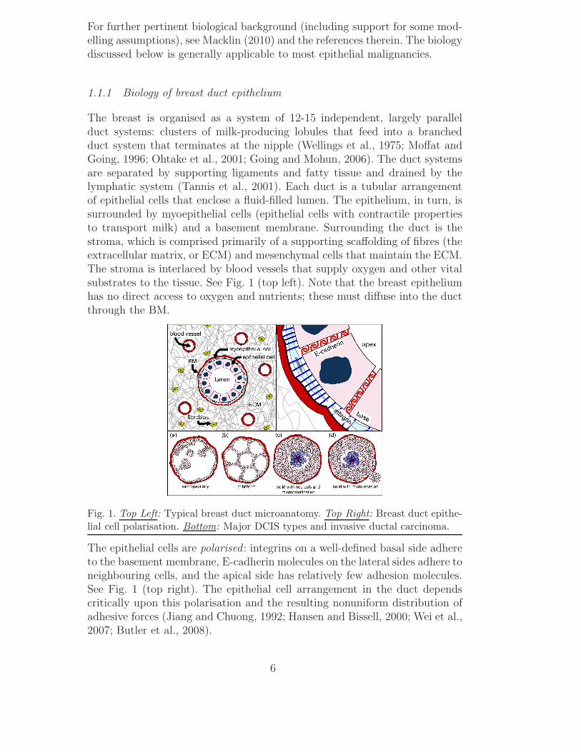
The breast is organised as a system of 12-15 independent, largely parallelduct systems: clusters of milk-producing lobules that feed into a branchedduct system that terminates at the nipple (Wellings et al., 1975; Moffat andGoing, 1996; Ohtake et al., 2001; Going and Mohun, 2006). The duct systemsare separated by supporting ligaments and fatty tissue and drained by thelymphatic system (Tannis et al., 2001). Each duct is a tubular arrangementof epithelial cells that enclose a fluid-filled lumen. The epithelium, in turn, issurrounded by myoepithelial cells (epithelial cells with contractile propertiesto transport milk) and a basement membrane. Surrounding the duct is thestroma, which is comprised primarily of a supporting scaffolding of fibres (theextracellular matrix, or ECM) and mesenchymal cells that maintain the ECM.The stroma is interlaced by blood vessels that supply oxygen and other vitalsubstrates to the tissue. See Fig. 1 (top left). Note that the breast epitheliumhas no direct access to oxygen and nutrients; these must diffuse into the ductthrough the BM.

Fig. 1. Top Left: Typical breast duct microanatomy. Top Right: Breast duct epithe-lial cell polarisation. Bottom: Major DCIS types and invasive ductal carcinoma.

The epithelial cells are polarised : integrins on a well-defined basal side adhereto the basement membrane, E-cadherin molecules on the lateral sides adhere toneighbouring cells, and the apical side has relatively few adhesion molecules.See Fig. 1 (top right). The epithelial cell arrangement in the duct dependscritically upon this polarisation and the resulting nonuniform distribution ofadhesive forces (Jiang and Chuong, 1992; Hansen and Bissell, 2000; Wei et al.,2007; Butler et al., 2008).

6

While the epithelial cell population oscillates with the menstrual cycle (Khanet al., 1998, 1999), on average proliferation and apoptosis balance to maintainhomeostasis. Microenvironmental changes can trigger signalling responses thatlead to proliferation or apoptosis, which ordinarily helps to safeguard thenormal tissue architecture. For example, a decrease of E-cadherin signalling(following apoptosis in a neighbouring cell) can increase β-catenin signalling,which eventually increases proliferation to replace the missing cell (Conacci-Sorrell et al., 2002; Hansen and Bissell, 2000; Wei et al., 2007). Adhesionto the BM triggers integrin signalling and downstream production of survivalproteins that inhibit apoptosis (Ilic et al., 1998; Giancotti and Ruoslahti, 1999;Stupack and Cheresh, 2002). Loss of attachment to the BM therefore allowsone type of apoptosis (anoikis) to occur, thus preventing overgrowth of cellsinto the lumen (Danes et al., 2008). Hormones such as estrogen, progesterone,prolactin, and epidermal growth factor can affect epithelial cell proliferationand apoptosis prior to lactation (Anderson, 2004), during breast involution(Baxter et al., 2007), and in cancer (Simpson et al., 2005).

1.1.2 Biology of DCIS

Overexpressed oncogenes and underexpressed tumour suppressor genes candisrupt the balance of epithelial cell proliferation and apoptosis, leading tooverproliferation. This can occur typically either by the accumulation of DNAmutations (genetic damage) or DNA amplification (Simpson et al., 2005), orepigenetic anomalies (Ai et al., 2006). The transformation from regular breastepithelium to carcinoma is thought to occur in stages. For simplicity, we setaside the relatively benign precursor transformations (e.g., atypical ductalhyperplasia) which have a low risk for subsequent invasive breast cancer (Page,1992) and focus on DCIS.

In the most well-differentiated classes of DCIS, the epithelial cells maintaintheir polarity and anisotropic adhesion receptor distributions, resulting in par-tial recapitulation of the non-pathological duct structure within the lumen.These demonstrate either finger-like growths into the lumen (micropapillary:see Fig. 1 (bottom:a)), or arrangements of duct-like structures (cribriform:see Fig. 1 (bottom:b)) (Silverstein, 2000). The cells in solid type DCIS lackpolarity and do not develop these microstructures. Instead, the cells prolifer-ate until filling the entire lumen (Fig. 1 (bottom:c)) (Danes et al., 2008). Theproliferating cells uptake oxygen and nutrients as they diffuse into the duct,causing substrate gradients to form. If the central oxygen level is sufficientlydepleted, a necrotic core of debris forms (comedo-type solid DCIS: see Fig. 1(bottom:c)) (Silverstein, 2000). These necrotic cells are typically not phagocy-tosed; instead, they swell and burst (Barros et al., 2001), and their solid (i.e.,non-water) components are slowly calcified (Stomper and Margolin, 1994). Itis these calcifications that are generally detected by mammograms when di-

7

agnosing DCIS (Ciatto et al., 1994). The BM blocks DCIS from invading thestroma, thereby impeding spread through the stroma, invasion into lymphovas-cular channels and hence metastasis. Further mutations can transform DCISinto invasive ductal carcinoma, whose cells move along the duct, secrete matrixmetalloproteinases (MMPs) to degrade the BM and subsequently invade thestroma (Fig. 1 (bottom:d)). See Silver and Tavassoli (1998) and Adamovichand Simmons (2003).

While it is tempting to regard DCIS as a linear progression from regular ep-ithelium to cribriform or micropapillary (“partially transformed”) to solid type(“fully transformed”), the morphological and molecular pathway is currentlyan open question (Erbas et al., 2006; Rennstam and Hedenfalk, 2006). Theexcellent modelling and analysis by Sontag and Axelrod (2005) strongly re-futes a linear progression model. The dominant type of DCIS in any particularcase may depend upon the underlying molecular changes. For example, crib-riform DCIS could arise from hyperproliferative cells where genes regulatingpolarisation are functionally intact.

1.2 A sampling of prior agent-based cell modelling

It is beyond the scope of this paper to review all discrete biomathematicsmodelling; instead, we briefly review relevant prior agent-based models. For abroader and deeper review of discrete modelling, please see Lowengrub et al.(2010) and Macklin et al. (2010b) and the references therein.

While cellular automata methods are efficient for linking molecular- and cell-ular-scale biology in large numbers of virtual cells, they cannot accuratelymodel cell and tissue mechanics due to the limitations they place upon cellarrangement (must be grid-aligned), size (all cells have equal size), velocity(cells move one cell diameter per time step), and interactions (can only inter-act with up to 8 neighbours in 2D). In particular, proliferation is disallowed incells that are surrounded by cells in the adjacent computational mesh points;in actual tissue, interior cells can proliferate by deforming and pushing neigh-bouring cells into non-lattice configurations. In this paper, we use agent-basedmodelling (ABM), which eliminates the computational lattice and instead as-signs each cell a position that evolves under the influence of forces actingupon it. Note that ABMs are sometimes referred to as individual-based mod-els or particle methods. Alternative approaches include the lattice-gas method(Dormann and Deutsch, 2002), off-lattice cellular automata methods such asVoronoi-Delaunay models (Schaller and Meyer-Hermann, 2005), the immersedboundary cell model (Rejniak, 2007; Rejniak and Dillon, 2007; Rejniak andAnderson, 2008a,b), and the cellular potts technique (a.k.a. Graner-Glazier-Hogeweg model) (Graner and Glazier, 1992; Glazier and Garner, 1993).

8

An excellent agent-based model was developed by Drasdo, Hohme and co-workers (Drasdo et al., 1995; Drasdo and Hohme, 2003, 2005; Drasdo, 2005).Cells are modelled as roughly spherical, slightly compressible, and capable ofmigration, growth and division. Cell adhesion and repulsion (from limitationson cell deformation and compressibility) are modelled by introducing an inter-action energy; cells respond to proliferation and apoptosis in their neighboursby moving to reduce the total interaction energy using a stochastic algorithm.Ramis-Conde et al. (2008a,b) used a similar agent model, but instead used in-teraction potential functions to simulate cell-cell mechanics: cells move downthe gradient of the potential, analogous to minimizing the interaction en-ergy. Their work included a basic accounting for the cell-cell surface contactarea, and related the strength of cell-cell adhesion to the concentration of E-cadherin/β-catenin complexes in the contact regions. Others have modelledcells as deformable viscoelastic ellipsoids (e.g., Dallon and Othmer (2004)).

Drasdo et al. (1995) initially developed their agent model to study epithelialcell-fibroblast-fibrocyte aggregations in connective tissue. More recently, theyapplied it to avascular tumour growth (Drasdo and Hohme, 2003), with bio-physical and kinetic parameters drawn from experimental literature (Drasdoand Hohme, 2005). More recently, Byrne and Drasdo (2009) upscaled a dis-crete model to calibrate a continuum tumour growth model, in part by us-ing a cell velocity-based approximation of the proliferative pressure to cal-ibrate the continuum-scale mechanics. Drasdo and co-workers were able tomechanistically model biomechanical growth limitations and the epithelial-to-mesenchymal transition in tumour cells, and they made testable hypotheses onthe links between tumour hypoglycemia and the size of the necrotic core. Galleet al. (2005, 2009) extended the approach to include cell-BM adhesion, andits impact on cell differentiation and tumour monolayer progression. Ramis-Conde et al. (2008a,b) used their model to investigate the links between asophisticated subcellular model of E-cadherin/β-catenin signalling, intercellu-lar signalling, and tissue morphology.

The very recent agent model of Norton et al. (2010) represented cell-cell ad-hesion and repulsion using a linear damped spring model, incorporated bothapoptosis and necrosis, duct wall adhesion (through adhesion to myoepithelialcells), asymmetric progenitor cell division, and a simplified model of intraduc-tal fluid pressure. The model recapitulated solid-type, comedo-type, micropap-illary, and cribriform DCIS, illustrating the great potential in an agent-basedmodelling approach. However, the model lacked substrate transport, necro-sis was modelled by imposing the viable rim thickness a priori rather thanthrough a combination of cell energetics and transport limitations, and pro-liferating cells were randomly distributed across the viable rim with uniformdistribution; this contradicts immunohistochemical observations of the distri-bution of proliferating DCIS cells within the duct (e.g., as in Fig. 7). Theauthors did not treat necrotic core mechanics, which has a great impact on

9

the overall tumour morphology and rate of tumour advance in the duct. (SeePart II (Macklin et al., 2011).) The observed microstructures were only partlymechanistic because the model enforced polarised cell-cell adhesion and “mi-crolumens” algorithmically; in a mechanistic model, the tumour microstruc-ture should not be imposed, but rather emerge naturally from the model’sbiophysics and population dynamics.

2 Agent-Based Cell Model

We now fully elaborate a discrete, cell-scale modelling framework that we firstintroduced in Macklin et al. (2009a, 2010b), which combines and extends someof the major features described in the models reviewed in Section 1.2. Our ob-jective is a model that is sufficiently mechanistic that cellular and multicellularbehaviour manifest themselves as emergent phenomena of the model, ratherthan through computational rules that are imposed a priori. We employ amodular design (in software and mathematics) that allows “sub-models” (e.g.,molecular signalling, cell morphology) to be expanded, simplified, or outrightreplaced as necessary. Where possible, we choose simple sub-models and testthe model framework’s success in recapitulating correct DCIS behaviour.

Cells are modelled as physical objects that exchange forces; essential molecularbiology is incorporated through carefully-chosen constitutive relations. We at-tempt to model the mechanics, time duration, and biology of each phenotypicstate as accurately as our data will allow; this should facilitate calibration tomolecular- and cellular data. The agents interact with the micronenvironmentthrough coupled partial differential equations governing substrate transport.We use the same model for both cancerous and non-cancerous cells. Function-ally, the cells differ primarily in the values of their proliferation, apoptosis,and other parameters; this is analogous to the downstream effects of alteredoncogenes and tumour suppressor genes (Hanahan and Weinberg, 2000).

In this discussion, cells are not polarised. We do not currently focus on stemcell dynamics; this can readily be added by identifying agents as stem cells,progenitor cells, or differentiated cells, and assigning each class different phe-notypic characteristics. Thus, we focus on the growth and dynamics of DCIS,rather than its initiation. We do not explicitly model cell morphology, butrather total, nuclear, and solid volume. Where cell morphology is necessary,we approximate it as spherical, similarly to Ramis-Conde et al. (2008a,b).This approximation is further discussed in Section 2.1. Basement membranesare modelled using level set functions (Section 2.2), which can be adapted tomodel BM deformation (as discussed in Macklin et al. (2010b)).

10

2.1 Physical characteristics and mechanics

We endow each cell with a position x, velocity v, total volume V , solid volumeVS, and nuclear volume VN . We assume that x and v are at the cell’s centreof mass and volume. While we do not explicitly track the cell morphology, wetrack the equivalent cell and nuclear radii (respectively R and RN) via

V =4

3πR3, VN =

4

3πR3

N. (1)

See Fig. 2:left. For simplicity, we assume that VN is fixed throughout the cellcycle, and the solid volume maintains a constant percentage VS/V of the totalcell volume until entering the necrotic state. (See Section 2.5.4.)

Each cell has a maximum adhesion interaction distance RA ≥ R, which weuse to express several effects. Because cells are deformable, they can stretchbeyond R to maintain or create adhesive bonds. As we do not explicitly trackthe cell morphology, there is inherent uncertainty as to maximum extent ofthe cell boundary relative to its centre of mass; RA needs to be sufficientlylarge to account for this. This effect is increased by random actin polymeri-sation/depolymerisation dynamics, which serve to randomly perturb the cellboundary (Gov and Gopinathan, 2006). See Fig. 2:right.

The cells are allowed to partly overlap to account for cell deformation. (Fig. 2:right.) We model the relative rigidity of the nucleus (relative to the cytoplasm)by introducing increased mechanical resistance to compression at a distancesless than RN from the cell centre; see Section 2.3.5 and Appendix A. Notethat as RN ↑ R (most of the cell resists compression) or RA ↓ R (cells cannotdeform to maintain adhesive contact), the cells behave like a granular material.

2.2 Basement membrane morphology

Let us denote the intraductal space (including both the epithelium and thelumen) by Ω and the basement membrane by ∂Ω. We represent ∂Ω implicitlywith an auxilliary signed distance function d (a level set function) satisfying

d(x) > 0 x ∈ Ω

d(x) = 0 x ∈ ∂Ω

d(x) < 0 x /∈ Ω = Ω ∪ ∂Ω.

(2)

Additionally, |∇d| ≡ 1. See Fig. 3.

This formulation can describe arbitrary BM geometries such as branch points

11

Fig. 2. Cell morphology and mechanics: Left: We track the cell volume V andnuclear volume VN (with equivalent spherical radii R and RN), and solid volume VS.RA is the maximum adhesive interaction distance. Right: We account for uncertaintyin the cell morphology by allowing the equivalent radii to overlap (left two cells),and by allowing adhesive contact beyond their equivalent radii (right two cells).

Fig. 3. BM morphology: Left: The BM separates the epithelium and lumen fromthe stroma. Right: The signed distance function d represents the BM implicitly asits zero isocontour. d > 0 on the epithelial side, and d < 0 on the stromal side.

in breast duct tree structures. The normal vector n to the BM surface (orientedinto the epithelium) is given by n = ∇d, and ∇ · n gives the mean geometriccurvature of the BM. This implicit representation is well-suited to describing amoving BM as it is deformed by mechanical stresses (e.g., due to proliferatingtumour cells, as in Ribba et al. (2006)). See Macklin and Lowengrub (2005,2006, 2007, 2008); Frieboes et al. (2007) and Macklin et al. (2009b), where weused this method to describe moving tumour boundaries.

2.3 Forces acting upon the cells

Each cell is subject to competing forces that determine its motion. Cells ad-here to other cells (cell-cell adhesion: Fcca), the extracellular matrix (cell-ECMadhesion: Fcma), and the basement membrane (cell-BM adhesion: Fcba), cal-cified debris adheres to other calcified debris (debris-debris adhesion: Fdda),

12

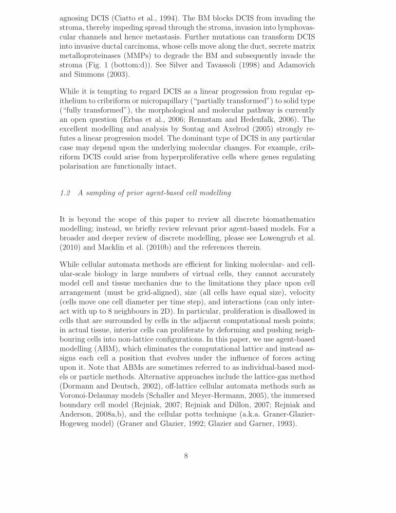
cells and calcified debris resist compression by other cells and debris (cell-cellrepulsion: Fccr), and the basement membrane resists its penetration and de-formation by cells and debris (cell-BM repulsion: Fcbr). Motile cells experiencea net locomotive force Floc along the direction of intended travel. In addition,moving cells and debris experience a drag force Fdrag by the luminal and in-terstitial fluids, which we model by Fdrag = −νvi. See Fig. 4. We currentlyneglect the impact of interstitial fluid pressure; this is equivalent to assumingthe free flow of water, similarly to current continuum-scale mixture models(e.g., as in Wise et al. (2008); Bearer et al. (2009)). We express the balanceof forces acting on cell i by Newton’s second law:

mivi =N(t)∑

j=1j 6=i

(Fij

cca + Fijccr + Fij

dda

)+ Fi

cma + Ficba + Fi

cbr + Filoc + Fi

drag. (3)

Here, N(t) is the number of cells in the simulation at time t. In this work, wefocus on the impact of adhesive and repulsive forces, and set Floc = 0

Fig. 4. Agent model forces: On Cell 5, find labelled the cell-cell adhesive (F5jcca)

and repulsive (F5jccr) forces, and the cell-BM adhesive (F5

cba) and repulsive (F5cbr)

forces. We label the net cell locomative force Filoc for Cell 6 (undergoing motility

along the BM) and Cell 7 (undergoing motility within the ECM). We show thecell-ECM adhesive force (F7

cma) and fluid drag (F7drag) for Cell 7.

2.3.1 Cell-cell adhesion (Fcca):

Adhesion molecules on a cell’s surface bond with adhesive ligands (targetmolecules) on nearby cells. Hence, the strength of the adhesive force betweenthe cells is (to first order) proportional to the product of the receptor andligand expressions. The adhesion strength increases as the cells are drawnmore closely together, bringing more surface area (and receptor-ligand pairs)into direct contact. We model the force imparted by cell j on cell i by

Fijcca = −αccafi,j∇ϕ

(xj − xi;R

icca +Rj

cca, ncca

), (4)

13

where fi,j describes the specific molecular biology of the adhesion, Ricca is cell

i’s maximum adhesion interaction distance, and αcca is constant. The adhesivepotential function ϕ and the parameter ncca are detailed in Appendix A.

Homophilic adhesion: In homophilic adhesion (e.g., Panorchan et al. (2006)),adhesion receptors E bond with identical ligands E . Hence,

fi,j = EiEj, (5)

where Ei is cell i’s (nondimensionalised) E receptor expression.

Heterophilic adhesion: In heterophilic cell-cell adhesion (e.g, Springer(1990); Terol et al. (2003); Lucio et al. (1998)), adhesion receptors IA bondwith dissimilar ligands IB, and vice versa. Hence,

fi,j = IA,iIB,j + IB,iIA,j, (6)

where IA,i and IB,i are cell i’s (nondimensionalised) IA and IB expressions.

2.3.2 Cell-ECM adhesion (Fcma):

Integrins IE on the cell surface form heterophilic bonds with suitable lig-ands LE in the ECM. We assume that LE is distributed proportionally to the(nondimensional) ECM density E. If IE is distributed uniformly across thecell surface and E varies slowly relative to the spatial size of a single cell, thencells at rest encounter a uniform pull from Fcma in all directions, resulting inzero net cell-ECM force. For cells in motion, Fcma resists that motion similarlyto drag due to the energy required to overcome I − L bonds:

Fcma = −αcmaIE,iEvi. (7)

Here, αcma is a constant. If E or LE varies with a higher spatial frequency, orif IE is not uniformly distributed, then the finite half-life of IE − LE bondswill lead to net haptotactic-type migration up gradients of E (Macklin et al.,2010b). We model this effect as part of the net locomotive force Floc.

2.3.3 Cell-BM adhesion (Fcba):

Integrin molecules on the cell surface form heterophilic bonds with specificligands LB (generally laminin and fibronectin (Butler et al., 2008)) on thebasement membrane (with density 0 < B < 1). We assume that LB is dis-tributed proportionally to the (nondimensional) BM density B. Hence, the

14

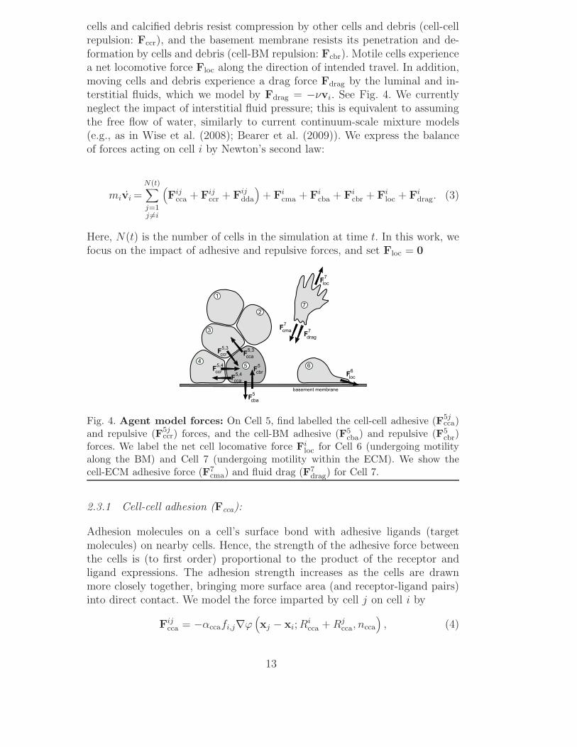
strength of the cell-BM adhesive force is proportional to its integrin surfacereceptor expression and B. Furthermore, the strength of the adhesion increasesas the cell approaches the BM, bringing more cell adhesion receptors in contactwith their ligands on the BM. We model this adhesive force on cell i by

Ficba = −αcbaIB,iB∇ϕ

(d(xi)n (xi) ;R

icba, ncba

), (8)

where αcba is a constant, d is the distance to the basement membrane, n isnormal to the basement membrane (oriented towards the epithelial side ofthe membrane; see Section 2.2), ncba is as described in Appendix A, and IB,i

and Ricba are cell i’s (nondimensionalised) integrin receptor expression and

maximum cell-BM adhesion interaction distance, respectively.

2.3.4 (Calcified) debris-(calcified) debris adhesion (Fdda):

We model adhesion between calcified debris particles similarly to homophiliccell-cell adhesion: calcite crystals in the interacting calcified debris particlesremain strongly bonded as part of the microcalcification. We model this co-hesive force between the calcified debris particles i and j by

Fijdda = −αddaCiCj∇ϕ

(xj − xi;R

idda +Rj

dda, ndda

), (9)

where αdda is a constant, Ci and Ridda are cell i’s (nondimensionalised) degree

of calcification and maximum debris-debris adhesion interaction distance, andndda is the exponent described in Appendix A.

2.3.5 Cell-cell repulsion (including calcified debris) (Fccr):

Cells resist compression by other cells due to the structure of their cytoskele-tons, the incompressibility of their cytoplasm, and the surface tension of theirmembranes. We introduce a cell-cell repulsive force that is zero when cells arejust touching, and increases rapidly as the cells are pressed together, particu-larly when their nuclei are in close proximity. We approximate cell deformationby allowing partial cell overlap. See Section 2.1. We model Fccr by

Fijccr = −αccr∇ψ

(xj − xi;R

iN +Rj

N, Ri +Rj ,M, nccr

), (10)

where αccr is a constant, RiN and Ri are cell i’s nuclear radius and radius,

respectively, and M and nccr are described in Appendix A.

15

2.3.6 Cell-BM repulsion (including debris) (Fcbr):

We model the basement membrane as rigid and thus resistant to deformationand penetration by the cells and debris. We model this force by

Ficbr = −αcbrB∇ψ

(d(xi)n (xi) ;R

iN, Ri,M, ncbr

), (11)

where αcbr is a constant, d is the distance to the BM, RiN and Ri are described

earlier, and M and ncbr are described in Appendix A. We discuss plannedwork to model viscoplastic membrane expansion in Macklin et al. (2010b).

2.4 “Inertialess” assumption; Relationship to continuum-scale Darcy’s law

Similarly to Drasdo et al. (1995); Galle et al. (2005) and Ramis-Conde et al.(2008b) and as discussed in Lowengrub et al. (2010), we make the “inertialess”assumption that the forces equilibrate quickly, and so |mivi| ≈ 0. Hence, weapproximate

∑F = 0 and solve for the cell velocity from Eq. 3:

vi =1

ν + αcmaIE,iE

N(t)∑

j=1j 6=i

(Fij

cca + Fijdda + Fij

ccr

)+ Fi

cba + Ficbr + Fi

loc

.(12)

This has a convenient interpretation: each term 1ν+αcmaIE,iE

F is the “terminal”

(equilibrium) velocity of the cell when fluid drag, cell-ECM adhesion, and F

are the only forces acting upon it. Here, “” represents any individual forceabove, e.g., cba, cca, etc., and N(t) is the number of simulated cells at time t.

It is interesting to compare Eq. 12 with Darcy’s law, the basis of manycontinuum-scale tumour models such as Cristini et al. (2003); Macklin andLowengrub (2005, 2006, 2007, 2008) and Macklin et al. (2009b). In these mod-els, tumour growth is considered as incompressible flow in a porous medium(the ECM). A mechanical pressure P is used to model tissue mechanics asa balance of proliferation-induced stresses, adhesion, and tissue relaxation. Ifu(x, t) is the mean tissue velocity at x, then the Darcy’s law formulation ofthe tissue mechanics is given by

u = −µ∇P. (13)

See the extensive review, discussion, and references in Lowengrub et al. (2010).

The mobility coefficient µ models the ability of cells to mechanically respondto pressure gradients by overcoming cell-cell and cell-ECM adhesive bonds,or by deforming the ECM (Macklin and Lowengrub, 2007). In Frieboes et al.

16

(2007) and Macklin et al. (2009b), we introduced a functional relationshipbetween the mobility µ and the ECM density E of the form

µ =1

α + βE + 1εS, (14)

where S is a “structure variable” that models the presence (S = 1) or absence(S = 0) of rigid barriers, ε ≈ 0, and α and β are constants. When S = 0,Eq. 14 is identical to the coefficient in Eq. 12. While Eq. 14 was initially cho-sen as the simplest possible with biologically-reasonable qualitative behaviour(mobility decreases as the ECM density increases, rendering the tissue less“permeable” to cells), we now see it is fully consistent with the cell-scale bio-physics presented above.

2.5 Cell States

We endow each agent with a phenotypic state S(t) in the state spaceQ,P,A,H,N , C,M (introduced below). Quiescent cells (Q) are in a “rest-ing state” (G0, in terms of the cell cycle); this is the “default” state in theframework. We model the transitions between cell states as stochastic eventsgoverned by exponentially-distributed random variables that are linked to thecell’s genetic and proteomic state, as well as the microenvironment. Theseexponentially-distributed variables can be regarded as arising from nonhomo-geneous Poisson processes; the interested reader can find a brief discussion inthe supplementary material.

For a transition to state S2 from the current state S1, and for any interval(t, t+∆t], we use the general form

Pr (S(t +∆t) = S2|S(t) = S1) = 1− exp

(−∫ t+∆t

tα12(S, •, )(s) ds

), (15)

where α12 (S, •, ) (t) is the intensity function, • represents the cell’s internal(genetic and proteomic) state, and represents the state of the surroundingmicroenvironment sampled at the cell’s position x(t). Note that for small ∆t,

Pr (S(t +∆t) = S2|S(t) = S1) = α12 (S, •, ) (t)∆t +O(∆t2

); (16)

when α12 is constant, we recover (to second order) the commonly-used con-stant transition probabilites for fixed step sizes ∆t; these may be regarded asapproximations to our more general model here.

If S1 → S2 transitions depend upon two separate processes with characteristictransition intensities α′

12 and α∗12, we may choose α12 = α′

12 + α∗12 when these

17

Fig. 5. Phenotypic transition network in the agent-based model.

processes are independent. In this case, for small ∆t,

Pr (S(t +∆t) = S2|S(t) = S1) ≈(α′12 (S, •, ) (t) + α∗

12 (S, •, ) (t))∆t (17)

which is approximately the probability of a S1 → S2 transition due to eitherthe α′

12 process or the α∗12 process.

If the processes are not independent, we choose the form α12 = α′12α

∗12, yielding

Pr (S(t +∆t) = S2|S(t) = S1) ≈(α′12 (S, •, ) (t) · α

∗12 (S, •, ) (t)

)∆t, (18)

which is approximately the probabilty of both α′12 and α

∗12 processes “allowing”

an S1 → S2 transition; α′12 and α

∗12 are rate-limiting processes for one another.

In our cell phenotypic state space, quiescent cells can become proliferative(P), apoptotic (A), or motile (M). (In the work below, we shall neglect themotile state.) Cells in any state can become hypoxic (H); hypoxic cells canrecover to their previous state or become necrotic (N ), and necrotic cells aredegraded and gradually replaced by (clinically-detectable) calcified debris (C).See Fig. 5. The subcellular scale is built into this framework by making therandom exponential variables depend upon the microenvironment and thecell’s internal properties.

Note that cell cycle models have also been developed to regulate the P → Qtransition (e.g., Abbott et al. (2006) and Zhang et al. (2007)), and signallingnetworks have been developed to regulate the Q → P,A,M transitions.These can be directly integrated into the agent framework presented here bymodifying the stochastic parameters or by outright replacing the exponentialrandom variables with deterministic processes (Macklin et al., 2010b). Some

18

excellent examples of agent-based modelling with subcellular signalling com-ponents include Chen et al. (2009b,a); Kharait et al. (2007); Wang et al. (2007)and Zhang et al. (2007, 2009).

2.5.1 Proliferation (P):

As suggested by experimental and theoretical work as early as Smith andMartin (1973), quiescent cells enter the proliferative state (i.e., progress fromG0 to S) with a probability that depends upon the microenvironment. Wemodel the probability of a quiescent cell entering the proliferative state in thetime interval (t, t+∆t] via an exponential random variable:

Pr (S(t +∆t) = P|S(t) = Q) = 1− exp

(−∫ t+∆t

tαP(S, •, )(s) ds

)

≈ 1− exp(−αP(S, •, )(t)∆t) , (19)

where the approximation best holds when αP varies slowly relative to ∆t.

Assuming a correlation between the microenvironmental oxygen level σ (non-dimensionalised by the far-field oxygen level in non-diseased, normoxic tissue)and proliferation (See Section 4, as well as the excellent discussion and refer-ences in Silva and Gatenby (2010)), we expect αP to increase with σ. Hence:

αP = αP(S, σ, •, )(t) =

αP(•, )

σ−σH

1−σH

if S(t) = Q

0 else,(20)

where σH is a threshold oxygen value at which cells become hypoxic, andαP(•, ) is the cell’s Q → P transition rate when σ = 1 (i.e., in normoxic, non-pathologic tissue), which depends upon the cell’s genetic profile and proteinsignalling state (•) and the local microenvironment (). Note that in tumours,low oxygenation is the norm (Gatenby et al., 2007; Smallbone et al., 2007),and so σ is far below 1. In Part II, we generally find that σH ∼ 0.2 and σ < 0.4.

For simplicity, we model αP as constant for and specific to each cell type. InMacklin et al. (2010b), we discuss how to incorporate • (i.e., a cell’s internalprotein expression) and (as sampled by a cell’s surface receptors) into αP

through a subcellular molecular signalling model. We note that models havebeen developed that reduce the proliferation rate in response to mechanicalstresses (e.g., see the excellent description by Shraiman (2005)); in the con-text of the model, the cell samples these stresses from continuum-scale fieldvariables or tensors (i.e., “”) to reduce αP.

Once a cell has entered the proliferative state P, it remains in that state untildividing into two identical daughter cells of half volume, which themselves

19

remain in P until “maturing” into full-sized cells at the end of G1. Thereafter,the daughter cells are placed in the “default” quiescent state Q to simulatethe transition from G1 to G0. We now describe these events in greater detail.

Define τ to the ellapsed time since the cell entered the cell cycle from Q.Similarly to Ramis-Conde et al. (2008b), we divide the cell cycle (with durationτP) into the S-M phases and the G1 phase (with duration τG1). While τP andτG1 may generally depend upon the microenvironment and the cell’s internalstate, we currently model them as fixed for any given cell type.

Fig. 6. P submodel: A cell enters P from the quiescent state Q, modelling theG0 to S transition. It then remains in P until dividing into two identical daughtercells of half volume. The daughter cells also remain in P until completing G1 and“maturing” into full-sized cells; thereafter, they enter the “default” state Q.

At time τ = τP − τG1 (at the end of M), we divide the cell into two identicaldaughter cells with half the mass and volume of the parent cell. We assumethat both daughter cells evenly inherit the parent cell’s surface receptor expres-sions, internal protein expressions, and genetic characteristics (as embodiedby the phenotypic state transition parameters). We position the daughter cellsrandomly, subject to two constraints:

(1) The daughter cells preserve the parent cell’s centre of volume; and(2) The daughter cells (when considered as spheres) are fully contained within

the same volume as the former parent cell.

We accomplish this by placing the daughter cell centres symmetrically aboutthe parent cell’s centre, such that they fit within the parent cell’s equivalentsphere. See Fig. 6. Thus, the cells partially overlap after mitosis; cell-cell re-pulsive forces (see Section 2.3.5) subsequently push them apart. This overlappartly accounts for the non-spherical cell geometry following mitosis.

20

We simulate a proliferating cell’s changing volume V by

V (τ) =

V0 0 ≤ τ ≤ τP − τG1

12V0(1 + τG1+(τ−τP)

τG1

)τP − τG1 ≤ τ ≤ τP,

(21)

where V0 is the cell’s “mature” volume.

2.5.2 Apoptosis (A):

Apoptotic cells undergo “programmed” cell death in response to signallingevents. As with proliferation, we model entry into A using an exponentially-distributed random variable with parameter αA(t) = αA(S, •, )(t). We as-sume no correlation between apoptosis and oxygen (Edgerton et al., 2011):

Pr (S(t +∆t) = A|S(t) = Q) = 1− exp

(−∫ t+∆t

tαA(s) ds

)

≈ 1− exp(−αA(t)∆t) , (22)

where

αA(t) = αA(S, •, )(t) =

αA(•, ) if S(t) = Q

0 else,(23)

and where does not include oxygen σ, but may include other microenvi-ronmental stimuli such as proximity of the BM (anoikis), chemotherapy, orcontinuum-scale mechanical stresses that increase αA as in Shraiman (2005).Cells remain in the apoptotic state for a fixed amount of time τA; afterwardthey are removed from the simulation to model phagocytosis of apoptoticbodies. Their previously-occupied volume is made available to the surround-ing cells to model the release of the cells’ water content after lysis.

2.5.3 Hypoxia (H):

Cells enter the hypoxic state at any time that σ < σH. Hypoxic cells have anexposure time-dependent probability of becoming necrotic:

Pr (S(t +∆t) = N|S(t) = H) = 1− exp

(−∫ t+∆t

tβH(σ)(s) ds

)ds

≈ 1− exp(−βH (σ) (t)∆t) . (24)

We currently model βH(σ)(t) as constant, although it could readily be madedependent upon σ to more explicitly model energy depletion, such as in Small-bone et al. (2007) and Silva and Gatenby (2010). If σ > σH (normoxia is

21

restored) at time t + ∆t and the cell has not become necrotic, it returns toits former state and resumes its activity. For example, if the cell transitionedfrom P to H after spending τ time in the cell cycle, and normoxic conditionsare restored, then it returns to P with τ time having ellapsed in its cell cycleprogression. Notice that by Eq. 24, the probability that a cell succumbs tohypoxia increases with ∆t whenever S = H, independently of previous states.Hence, this probability scales (nonlinearly) with its cumulative exposure timeto hypoxia. This construct could model cell response to other stressors (e.g.,chemotherapy), similarly to “area under the curve” models (e.g., El-Karehand Secomb (2003, 2005)).

2.5.4 Necrosis (N ):

In our model, a hypoxic cell has a probability of irreversibly entering thenecrotic state, simulating depletion of its ATP store. We can also simplify themodel and neglect the hypoxic state by letting βH → ∞.

We assume that a cell remains in N for a fixed amount of time τN, duringwhich time its surface receptors and subcellular structures degrade, it losesits liquid volume, and calcium is deposited (primarily) in its solid fraction.We define τNL to be the length of time for the cell to swell, lyse, and lose itswater content, τNS the time for all surface receptors to degrade and becomefunctionally inactive, and τC, the time for calcification to occur. We assumethat τNL ≤ τNS < τC = τN. In Macklin et al. (2009a) we found that a simplifiedmodel (where τN = τNS = τNL = τC) could not reproduce certain morphologicalaspects of the viable rim-necrotic core interface in breast cancer.

If τ is the elapsed time spent in the necrotic state, we model the degradationof the surface receptor species S (scaled by the non-necrotic expression level)by exponential decay with rate constant log 100/τNS; the constant is chosen sothat S(τNS) = 0.01 S(0), i.e., virtually all of the surface receptor is degradedby time τ = τNS. After time τNS, we set S = 0.

To model the necrotic cell’s volume change, let fNS be the maximum percent-age increase in the cell’s volume (just prior to lysis), and let V0 be the cell’svolume at the onset of necrosis. Then

V (τ) =

V0(1 + fNS

ττNL

)if 0 ≤ τ < τNL

VS if τNL < τ,(25)

where VS is the cell’s solid volume. If the cell’s nuclear radius RN exceeds itsequivalent radius R after lysis, then we set RN = R. To model uncertainty inthe cell morphology during lysis, we randomly perturb its location x such that

its new radius R(τNL) is contained within its swelled radius R(0) (1 + fNS)1

3 .

22

Lastly, we assume a constant rate of cell calcification, with the necrotic cellreaching a clinically-detectable level of calcification at time τC. If C is thenondimensional degree of calcification, then C(t) = τ/τC.

2.5.5 Calcified debris (C):

Necrotic cells are gradually calcified until reaching a clinically-detectable levelof calcification; such cells make an irreversible N → C transition. Lackingfunctional adhesion receptors, these cells only adhere to other calcified debris;this is a simplified model of the crystalline bonds in the calcification.

2.6 Dynamic coupling with the microenvironment with upscaling

We integrate the agent model with the microenvironment as part of a discrete-continuum composite model, demonstrating here with a coupling to oxy-gen transport; further examples including ECM-MMP dynamics are given inMacklin et al. (2010b). We do this by introducing field variables for key mi-croenvironmental components (e.g., oxygen, signalling molecules, extracellularmatrix, etc.) that are updated according to continuum equations. The distri-butions of these variables affect the cell agents’ evolution as already described;simultaneously, the agents impact the evolution of the continuum variables.In the language of Deisboeck et al. (2010), this is a composite hybrid model.

2.6.1 Oxygen transport

All cell agents uptake oxygen as a part of metabolism. At the macroscopicscale, this is modelled by

∂σ

∂t= ∇ · (D∇σ)− λσ, (26)

where σ is oxygen, D is its diffusion constant, and λ is the (spatiotemporallyvariable) uptake/decay rate. Suppose that viable (non-necrotic, non-calcified)tumour cells uptake oxygen at a rate λt, host cells at a rate λh, and elsewhereoxygen “decays” (by reacting with the molecular landscape) at a low back-ground rate λb. Suppose that in a small neighbourhood B of x, tumour cells,host cells, and stroma (non-cells) respectively occupy fractions ft, fh, and fbof B, where ft + fh + fb = 1. Then λ(x) is given by

λ(x) ≈ ftλt + fhλh + fbλb, (27)

i.e., by averaging the uptake rates with weighting according to the tissuecomposition near x. This is consistent with the uptake rate model by Hoehme

23

and Drasdo (2010), which they based upon the experimental literature.

We could further decompose ft and fh according to cell phenotype, if the up-take rates were expected to vary. In numerical implementations, we generallycompute λ at a scale that resolves the cells (e.g., mesh size ∼ 1 µm) and thenupscale it to the computational mesh. See Part II (Macklin et al., 2011). Inthis formulation, the cell uptake rate varies with the tumour microstructure,which, in turn, evolves according to nutrient and oxygen availability.

Boundary conditions vary by the biology of the modelled problem. In our work,we set σ = σB (for a fixed boundary value σB on the basement membraneand inside the stroma (wherever d ≤ 0) to model the release of oxygen bya pre-existent vasculature in the stroma. Wherever the simulation boundaryintersects lumen, we use Neumann boundary conditions.

3 Analysis of the volume-averaged model behaviour

Let us fix a volume Ω contained within a non-hypoxic, non-necrotic tissue (i.e.,all cells i in Ω satisfy Si /∈ H,N , C). We analyse the population dynamics inthe simplified Q-A-P cell state network; this analysis is the basis of the modelcalibration in Part II (Macklin et al., 2011). Let P (t), A(t), and Q(t) denotethe number of proliferating, apoptosing, and quiescent cells in Ω at time t,respectively. Let N(t) = P + A + Q. If 〈αP〉(t) = 1

|Ω|

∫Ω αP dV is the mean

value of αP at time t throughout Ω, then the net number of cells enteringstate P in the time interval [t, t +∆t) is approximately

P (t+∆t) =P (t) + Pr (S(t +∆t) = P|S(t) = Q)Q(t)−1

τPP (t)∆t

≈P (t) +(1− e−〈αP〉∆t

)Q(t)−

1

τPP (t)∆t, (28)

whose limit as ∆t ↓ 0 (after some rearrangement) is

P = 〈αP〉Q−1

τPP. (29)

Similarly,

A=αAQ−1

τAA (30)

Q=21

τPP − (〈αP〉+ αA)Q. (31)

24

Summing these, we obtain

N =1

τPP −

1

τAA. (32)

Next, define PI = P/N and AI = A/N to be the proliferative and apoptoticindices, respectively. We can express the equations above in terms of AI and PIby dividing by N and using Eq. 32 to properly treat d

dt(P/N) and d

dt(A/N).

After simplifying, we obtain a nonlinear system of ODEs for PI and AI:

PI = 〈αP〉 (1−AI− PI)−1

τP

(PI + PI2

)+

1

τAAI · PI (33)

AI=αA (1− AI− PI)−1

τA

(AI− AI2

)−

1

τPAI · PI. (34)

These equations are far simpler to compare to immunohistochemical measure-ments, which are generally given in terms of AI and PI.

Lastly, let us nondimensionalise the equations by letting t = t t, where t isdimensionless. Then if f ′ = d

dtf , we have

1

tPI′ = 〈αP〉 (1−AI− PI)−

1

τP

(PI + PI2

)+

1

τAAI · PI (35)

1

tAI′ =αA (1− AI− PI)−

1

τA

(AI− AI2

)−

1

τPAI · PI. (36)

The cell cycle length τP is on the order of 1 day (e.g., as in Owen et al.(2004)), and in Part II (Macklin et al., 2011), we determine that τA is of similarmagnitude. Thus, if we choose t ∼ O (10 day) or greater, then we can assumethat 1

tPI′ = 0 = 1

tAI′ and conclude that the local cell state dynamics reach

steady state after after 10-100 days. This is significant, because it allows usto calibrate the population dynamic parameters (αA, αP, τA, and τP) withoutthe inherent difficulty of estimating time derivatives from often noisy in vitroand immunohistochemistry data. This result is consistent with our earliermathematical analysis in Macklin and Lowengrub (2007), which hypothesised“local equilibriation” of the tumour microstructure, even during growth.

4 Volume-averaged model behaviour, and testable hypotheses

We conclude Part I by applying a volume-averaged analysis to the viable rimin DCIS to generate biological hypotheses that we test against immunohis-tochemistry data. For fixed AI, PI, τA, and τP, we can use Eqs. 33-34 to

25

determine 〈αP〉 and αA, and ultimately, αP ; see Part II for full details (Mack-lin et al., 2011). In Macklin et al. (2009a), we instead treated αA and αP andconstant and solved the nonlinear ODE system for PI and AI to steady stateas a function of 0 ≤ σ ≤ 1. This analysis led us to predict Michaelis-Mentenpopulation kinetics as an emergent model phenomenon: for sufficient oxygenavailability, proliferation saturates, indicating that oxygenation is no longerthe primary growth-limiting factor.

Fig. 7. Ki-67 immunohistochemistry for ducts F3 (left) and F19 (right) foranonymised case 100019. Ki-67 positive nuclei stain dark red; Ki-67 negative nucleiare counterstained light blue. A colour verison of this image is available online.

We now test this hypothesis based upon a careful analysis of Ki-67 immuno-histochemistry in two exemplar ducts (F3 and F19) for a DCIS patient (anon-ymised case 100019) (Edgerton et al., 2011). See Fig. 7. For each of theseducts, we calculate the distance of all nuclei and Ki-67 positive nuclei to theduct wall, the mean distance from the duct centroid to the duct wall (i.e.,the radius Rduct), and the mean duct viable rim thickness T . Next, we createa histogram of Ki-67-positive nucleus distances to the duct wall (Fig. 8, firstrow), all nucleus distances to the duct wall using the same histogram “bins”(Fig. 8, second row), and divide these to obtain the proliferative index (PI)versus distance from the duct wall (Fig. 8, third row).

Next, we estimate the 3-D steady-state oxygen profile through the ducts (as-sumed radially symmetric with no variation in the longitudinal direction):

0 = L2(σ′′ +

1

rσ′)− σ, 0 < r < Rduct (37)

with boundary conditions

σ(Rduct − T ) = σH, σ′(0) = 0, (38)

26

0 20 40 60 80 100 1200

10

20

30

40

50

60

70Histogram of Ki−67 vs. Distance From Duct Wall

Distance from Duct Wall (µm)

Num

ber

of K

i−67

Pos

itive

Nuc

lei

0 10 20 30 40 50 60 70 80 900

10

20

30

40

50

60

70Histogram of Ki−67 vs. Distance From Duct Wall

Distance from Duct Wall (µm)

Num

ber

of K

i−67

Pos

itive

Nuc

lei

0 20 40 60 80 100 1200

20

40

60

80

100

120

140

160Histogram of Nucleus Distance From Duct Wall

Distance from Duct Wall (µm)

Num

ber

Nuc

lei

0 10 20 30 40 50 60 70 80 900

50

100

150

200

250Histogram of Nucleus Distance From Duct Wall

Distance from Duct Wall (µm)N

umbe

r N

ucle

i

0 20 40 60 80 100 1200.05

0.1

0.15

0.2

0.25

0.3

0.35

0.4

0.45Proliferative Index (PI) vs. Distance from Duct Wall

Distance from Duct Wall (µm)

Pro

lifer

ativ

e In

dex

(PI)

10 20 30 40 50 60 70 800

0.05

0.1

0.15

0.2

0.25

0.3

0.35Proliferative Index (PI) vs. Distance from Duct Wall

Distance from Duct Wall (µm)

Pro

lifer

ativ

e In

dex

(PI)

Fig. 8. Histograms of Ki-67 positive nuclei vs. distance from duct wall (top row), allnuclei vs. distance from duct wall (middle row), and proliferative index vs. distancefrom the duct wall (bottom row). Left column: Duct F3. Right column: Duct F19.

The solution is

σ(r) =σH

I0(Rduct−T

L

)I0(r

L

), (39)

where In is the nth-order modifed Bessel function of the first kind, σ is nondi-mensionalised by the normoxic oxygen level in non-pathological tissue,L = 100 µm, and σH = 0.2. (See Part II.) The mean value of the oxygensolution in the viable rim (Rduct − T < r < Rduct) is given explicitly by

〈σ〉 =(

2LσH2RductT − T 2

)RductI1

(Rduct

L

)− (Rduct − T ) I1

(Rduct−T

L

)

I0(Rduct−T

L

)

. (40)

27

For the duct in F3,

Rduct ≈ 188.4634 µm, T ≈ 119.0256 µm, and 〈σ〉 ≈ 0.282145,

and for the duct in F19,

Rduct ≈ 217.5548 µm, T ≈ 97.9602 µm, and 〈σ〉 ≈ 0.280459.

0.2 0.22 0.24 0.26 0.28 0.3 0.32 0.34 0.360

0.05

0.1

0.15

0.2

0.25

0.3

0.35

0.4

0.45Proliferative Index (PI) vs. Oxygen

Oxygen (nondimensional)

Pro

lifer

ativ

e In

dex

(PI)

Fig. 9. Comparison of the predicted PI curve (solid curve) with data from duct F3(dashed curve) and duct F19 (dotted curve) for case 100019.

By correlating the oxygen solutions with the PI profiles, we estimate the rela-tionship between the measured PI and σ in the ducts. We plot these curves forF3 (dashed curve) and F19 (dotted curve) against the predicted curve (solidcurve) from Macklin et al. (2009a) in Fig. 9. The theoretical predictions andmeasurements agree qualitatively but not quantitatively. We conclude thatwhile proliferation correlates with oxygen levels throughout the tumour, oxy-genation alone cannot fully determine PI. Hence, there must be additionalheterogeneities in other microenvironmental factors (e.g., EGF), gene expres-sion, or protein signalling across the tumour.

The next natural question is whether we can account for these heterogeneitieswith our current functional form by applying the same analysis to the indi-vidual ducts. We use AI = 0.008838 in each duct, and PI, Rduct, and T asmeasured separately for each duct above. For the duct in F3,

PI = 0.281030, αA ≈ 0.00162405 h−1,

〈αP〉 ≈ 0.0277579 h−1, and αP (S, •) ≈ 0.270331 h−1;

and for the duct in F19,

28

0.2 0.22 0.24 0.26 0.28 0.3 0.32 0.34 0.360

0.05

0.1

0.15

0.2

0.25

0.3

0.35

0.4

0.45Proliferative Index (PI) vs. Oxygen

Oxygen (nondimensional)P

rolif

erat

ive

Inde

x (P

I)

Fig. 10. Comparison of the hypothesised (solid) and measured (dashed and dotted)PI vs. σ curves for duct F3 (dashed) duct F19 (dotted).

PI = 0.148045, αA ≈ 0.00129067 h−1,

〈αP〉 ≈ 0.0110190 h−1, and αP(S, •) ≈ 0.109562 h−1.

Using this, we generate PI-vs-σ curves for the individual ducts based upon Eq.33 and compare them to the measured data in Fig. 10. There is generally muchimproved quantitative agreement between the predicted (solid) and measured(dashed and dotted) curves. The difference in the predicted curves for the twoducts is due to the substantial difference in αP : αP is much greater for F3,which has the overall higher PI curve.

We next examine the data in the ducts (Fig. 7) within the context of ourmodelling framework and the predicted PI-vs-σ curves to generate additionalbiological hypotheses. Notice that the cell density is lower in F3 (Fig. 7 left:larger nuclei with greater spacing between cells) than in F19 (Fig. 7 right:smaller nuclei with less spacing between cells). These lead us to hypothesisethat αP decreases with increasing cell density. E-cadherin/β-catenin signallingmay be the physiological explanation of the phenomenon: when E-cadherinis bound to E-cadherin on a neighboring cell, β-catenin binds to the phos-phorylated receptors, blocking its downstream pro-proliferative activity. (SeeSection 1.1.) For higher cell densities, more cell surfaces are in contact witheach other, providing greater opportunities for E-cadherin binding; we conse-quently hypothesise that cell density correlates with cell cycle blockade by theE-cadherin/β-catenin pathway, resulting in the apparent relationship betweencell density and αP . Further evidence can be seen in duct F19 (Fig. 7, right):the majority of the proliferation activity is in a single layer of cells along theduct wall. Because these cells are adhered to the basement membrane, theypresent less surface for E-cadherin binding activity (relative to the interiorcells), resulting in reduced E-cadherin blockade of proliferation.

These hypotheses can be tested by correlating αP with cell density in a larger

29

number of ducts, performing IHC for β-catenin activity, and correlating β-catenin-mediated transcription (indicated by presence of β-catenin in the nu-clei) with cell density and distance from the duct wall. One could use thesedata to hypothesise, calibrate, and test new functional forms for αP, such as:

αP(S, σ, •, ) = αP (•, )

(1− E〈E〉

ρ

ρmax

)(σ − σH1− σH

), (41)

where ρ is the local cell density, PI ≈ 0 when ρ = ρmax, E is the cell’s (nondi-mensional) E-cadherin expression, and 〈E〉 is the tumour’s mean E-cadherinexpression. In such a formulation, αP (•, ) determines the cell’s Q → P tran-sition rate in normoxic conditions with minimal E-cadherin signalling.

5 Discussion and Looking Forward

In this work, we developed and analysed an agent-based model of ductal car-cinoma in situ (DCIS) of the breast. Our work refines and makes more explicitthe biological underpinnings of current agent-based cell models, particularlyregarding finite cell-cell interaction distances, the need for partial cell over-lap to account for uncertainty in cell positions and morphology, and a morerigorous way to vary phenotypic transition probabilities with the time stepsize, the cell’s internal state, and the microenvironment. We provide the mostdetailed model to date of cell necrosis, and are the first to model cell cal-cification. Our analysis of the model steady-state, volume-veraged dynamicslead to quantitative predictions on the relationship between cell proliferation,oxygen availability, and cell signalling heterogeneity; these predictions weretested against actual patient data, yielding further insight on DCIS biology.

In Part II (Macklin et al., 2011), we use this analysis to develop a patient-specific calibration protocol, which is broadly applicable to well-formulatedagent-based models. We test this protocol using data from an actual DCISpatient to simulate DCIS in 1.5 mm length of breast duct for 45 days. Thesimulation results will lead to quantitative predictions on the rate of DCISgrowth (approximately 1 cm/year), which we shall validate against indepen-dent clinical data. The model will predict a (linear) relationship between thesize of a calcification (as measured pre-operatively in a mammogram) and theactual tumour size (as measured post-operatively by a pathologist)–this, too,is successfully validated against a large set of clinical data. Lastly, the modelwill yield new insight on the biological and biomechanical underpinnings of thegrowing body of statistical knowledge that has been accumulated on DCIS,raising the possibilty of improved clinical planning and treatment of DCIS.

30

Acknowledgements

We thank: the Cullen Trust for Health Care (VC, MEE, PM) for generoussupport; the National Institutes of Health (NIH) for the Physical SciencesOncology Center grants 1U54CA143907 (VC, PM) for Multi-scale ComplexSystems Transdisciplinary Analysis of Response to Therapy–MC-START, and1U54CA143837 (VC, PM) for the Center for Transport Oncophysics; the NIHfor the Integrative Cancer Biology Program grant 1U54CA149196 (VC, PM)for the Center for Systematic Modeling of Cancer Development; and finallythe National Science Foundation for grant DMS-0818104 (VC). We are grate-ful for funding under the European Research Council Advanced InvestigatorGrant (ERC AdG) 227619, “M5CGS–From Mutations to Metastases: Multi-scale Mathematical Modelling of Cancer Growth and Spread” (PM).

We thank the Division of Mathematics at the University of Dundee andthe School of Biomedical Informatics at the University of Texas Health Sci-ence Center-Houston (UTHSC-H) for generous computational support andresources. We appreciate assistance from Yao-Li Chuang (University of NewMexico) for accessing data from Edgerton et al. (2011). PM thanks JohnLowengrub (University of California-Irvine), Hermann Frieboes (University ofLouisville), Dirk Drasdo (INRIA Rocquencourt/Paris), James Glazier and Ma-ceij Swat (University of Indiana), and Mark Chaplain (University of Dundee)for useful discussions.

References

R. G. Abbott, S. Forrest, and K. J. Pienta. Simulating the hallmarks of cancer.Artif. Life, 12(4):617–34, 2006. doi: 10.1162/artl.2006.12.4.617.

T. L. Adamovich and R. M. Simmons. Ductal carcinoma in situ withmicroinvasion. Am. J. Surg., 186(2):112–6, 2003. doi: 10.1016/S0002-9610(03)00166-1.

L. Ai, W.-J. Kim, T.-Y. Kim, C. R. Fields, N. A. Massoll, K. D. Robertson,and K. D. Brown. Epigenetic silencing of the tumor suppressor cystatin moccurs during breast cancer progression. Canc. Res., 66(16):7899–909, 2006.doi: 10.1158/0008-5472.CAN-06-0576.

American Cancer Society. American cancer society breast cancer facts andfigures 2007-2008. Atlanta: American Cancer Society, Inc., 2007.

E. Anderson. Cellular homeostasis and the breast. Maturitas, 48(S1):13–7,2004. doi: 10.1016/j.maturitas.2004.02.010.

A. Bankhead III, N. S. Magnuson, and R. B. Heckendorn. Cellular automa-ton simulation examining progenitor heirarchy structure effects on mam-mary ductal carcinoma in situ. J. Theor. Biol., 246(3):491–8, 2007. doi:10.1016/j.jtbi.2007.01.011.

31

L. F. Barros, T. Hermosilla, and J. Castro. Necrotic volume increase andthe early physiology of necrosis. Comp. Biochem. Physiol. A. Mol. Integr.Physiol., 130(3):401–9, 2001. doi: 10.1016/S1095-6433(01)00438-X.

F. O. Baxter, K. Neoh, and M. C. Tevendale. The beginning of the end: Deathsignaling in early involution. J. Mamm. Gland Biol. Neoplas., 12(1):3–13,2007. doi: 10.1007/s10911-007-9033-9.

E. L. Bearer, J. S. Lowengrub, Y.-L. Chuang, H. B. Frieboes, F. Jin, S. M.Wise, M. Ferrari, D. B. Agus, and V. Cristini. Multiparameter computa-tional modeling of tumor invasion. Cancer Res., 69(10):4493–501, 2009. doi:10.1158/0008-5472.CAN-08-3834.

L. M. Butler, S. Khan, G. E. Rainger, and G. B. Nash. Effects of endothelialbasement membrane on neutrophil adhesion and migration. Cell. Immun.,251(1):56–61, 2008. doi: 10.1016/j.cellimm.2008.04.004.

H. M. Byrne and D. Drasdo. Individual-based and continuum models of grow-ing cell populations: A comparison. J. Math. Biol., 58(4–5):657–87, 2009.doi: 10.1007/s00285-008-0212-0.

N. Cabioglu, K. K. Hunt, A. A. Sahin, H. M. Kuerer, G. V. Babiera, S. E.Singletary, G. J. Whitman, M. I. Ross, F. C. Ames, B. W. Feig, T. A. Buch-holz, and F. Meric-Bernstam. Role for intraoperative margin assessment inpatients undergoing breast-conserving surgery. Ann. Surg. Oncol., 14(4):1458–71, 2007. doi: 10.1245/s10434-006-9236-0.

L. L. Chen, L. Zhang, J. Yoon, and T. S. Deisboeck. Cancer cell motil-ity: optimizing spatial search strategies. Biosys., 95(3):234–42, 2009a. doi:10.1016/j.biosystems.2008.11.001.

W. W. Chen, B. Schoeberl, P. J. Jasper, M. Niepel, U. B. Nielsen, D. A.Lauffenburger, and P. K. Sorger. Input-output behavior of ErbB signalingpathways as revealed by a mass action model trained against dynamic data.Mol. Syst. Biol., 5(1):239ff, 2009b. doi: 10.1038/msb.2008.74.

L. Cheng, N. K. Al-Kaisi, N. H. Gordon, A. Y. Liu, F. Gebrail, and R. R.Shenk. Relationship between the size and margin status of ductal carcinomain situ of the breast and residual disease. J. Natl. Cancer Inst., 89(18):1356–60, 1997.

S. Ciatto, S. Bianchi, and V. Vezzosi. Mammographic appearance of calci-fications as a predictor of intraductal carcinoma histologic subtype. Eur.Radiology, 4(1):23–6, 1994. doi: 10.1007/BF00177382.

M. Conacci-Sorrell, J. Zhurinsky, and A. Ben-Zeev. The cadherin-cateninadhesion system in signaling and cancer. J. Clin. Invest., 109(8):987–91,2002. doi: 10.1172/JCI15429.

V. Cristini and J. Lowengrub. Multiscale modeling of cancer. CambridgeUniversity Press, Cambridge, UK, 2010. ISBN 978-0521884426.

V. Cristini, J. S. Lowengrub, and Q. Nie. Nonlinear simulation of tumorgrowth. J. Math. Biol., 46(3):191–224, 2003. doi: 10.1007/s00285-002-0174-6.

J. C. Dallon and H. G. Othmer. How cellular movement determines the collec-tive force generated by the dictyostelium discoideum slug. J. Theor. Biol.,

32

231(2):203–22, 2004. doi: 10.1016/j.jtbi.2004.06.015.C. G. Danes, S. L. Wyszomierski, J. Lu, C. L. Neal, W. Yang, and D. Yu. 14-3-3ζ down-regulates p53 in mammary epithelial cells and confers luminalfilling. Canc. Res., 68(6):1760–7, 2008. doi: 10.1158/0008-5472.CAN-07-3177.

T. S. Deisboeck, Z. Wang, P. Macklin, and V. Cristini. Multiscale cancermodeling. Annu. Rev. Biomed. Eng., 2010. (in review).

M. F. Dillon, E. W. McDermott, A. O’Doherty, C. M. Quinn, A. D. Hill, andN. O’Higgins. Factors affecting successful breast conservation for ductal car-cinoma in situ. Ann. Surg. Oncol., 14(5):1618–28, 2007. doi: 10.1245/s10434-006-9246-y.

S. Dormann and A. Deutsch. Modeling of self-organized avascular tumorgrowth with a hybrid cellular automaton. In Silico Biology, 2(3):393–406,2002.

D. Drasdo. Coarse graining in simulated cell populations. Adv. Complex Sys.,8(2 & 3):319–63, 2005. doi: 10.1142/S0219525905000440.

D. Drasdo and S. Hohme. Individual-based approaches to birth and death inavascular tumors. Math. Comput. Modelling, 37(11):1163–75, 2003.

D. Drasdo and S. Hohme. A single-scale-based model of tumor growth invitro: monolayers and spheroids. Phys. Biol., 2(3):133–47, 2005. doi:10.1088/1478-3975/2/3/001.

D. Drasdo, R. Kree, and J. S. McCaskill. Monte-carlo approach to tissuecell populations. Phys. Rev. E, 52(6):6635–57, 1995. doi: 10.1103/Phys-RevE.52.6635.

M. E. Edgerton, P. Macklin, Y.-L. Chuang, G. Tomaiuolo, W. Yang, J. Kim,A. K. K. L. Kumar, S. Sanga, A. D. M. Broom, A. Segura, S. Kaliki, K.-A.Do, and V. Cristini. An application of a multiscale mathematical modelingframework of ductal carcinoma in situ. PLoS Med., 2011. (submitted).

A. W. El-Kareh and T. W. Secomb. A mathematical model for cisplatincellular pharmacodynamics. Neoplasia, 5(2):161–9, 2003.

A. W. El-Kareh and T. W. Secomb. Two-mechanism peak concentrationmodel for cellular pharmacodynamics of doxorubicin. Neoplasia, 7(7):705–13, 2005.

H. Enderling, A. R. A. Anderson, M. A. J. Chaplain, A. J. Munro, and J. S.Vaidya. Mathematical modelling of radiotherapy strategies for early breastcancer. J. Theor. Biol., 241(1):158–71, 2006. doi: 10.1016/j.jtbi.2005.11.015.

H. Enderling, M. A. J. Chaplain, A. R. A. Anderson, and J. S. Vaidya. Amathematical model of breast cancer development, local treatment and re-currence. J. Theor. Biol., 246:245–259, 2007.

B. Erbas, E. Provenzano, J. Armes, and D. Gertig. The natural history ofductal carcinoma in situ of the breast: a review. Breast Canc. Res. Treat.,97(2):135–44, 2006. doi: 10.1007/s10549-005-9101-z.

S. J. Franks, H. M. Byrne, J. R. King, J. C. E. Underwood, and C. E. Lewis.Modelling the early growth of ductal carcinoma in situ of the breast. J.Math. Biol., 47(5):424–452, 2003a. doi: 10.1007/s00285-003-0214-x.

33

S. J. Franks, H. M. Byrne, H. Mudhar, J. C. E. Underwood, and C. E. Lewis.Modelling the growth of comedo ductal carcinoma in situ. Math. Med. Biol.,20(3):277–308, 2003b. doi: 10.1093/imammb/20.3.277.

S. J. Franks, H. M. Byrne, J. C. E. Underwood, and C. E. Lewis. Bi-ological inferences from a mathematical model of comedo ductal carci-noma in situ of the breast. J. Theor. Biol., 232(4):523–43, 2005. doi:10.1016/j.jtbi.2004.08.032.

H. B. Frieboes, J. S. Lowengrub, S. Wise, X. Zheng, P. Macklin, E. L. Bearer,and V. Cristini. Computer simulations of glioma growth and morphology.NeuroImage, 37(S1):S59–S70, 2007. doi: 10.1016/j.neuroimage.2007.03.008.

J. Galle, M. Loeffler, and D. Drasdo. Modeling the effect of deregulated prolif-eration and apoptosis on the growth dynamics of epithelial cell populationsin vitro. Biophys. J., 88(1):62–75, 2005. doi: 10.1529/biophysj.104.041459.

J. Galle, M. Hoffmann, and G. Aust. From single cells to tissue architecture-abottom-up approach to modelling the spatio-temporal organisation of com-plex multi-cellular systems. J. Math. Biol., 58(1–2):261–83, 2009. doi:10.1007/s00285-008-0172-4.

R. A. Gatenby, K. Smallbone, P. K. Maini, F. Rose, J. Averill, R. B. Nagle,L. Worrall, and R. J. Gillies. Cellular adaptations to hypoxia and acidosisduring somatic evolution of breast cancer. Br. J. Cancer, 97(5):646–53,2007. doi: 10.1038/sj.bjc.6603922.

F. G. Giancotti and E. Ruoslahti. Integrin signaling. Science, 285(5430):1028–32, 1999. doi: 10.1126/science.285.5430.1028.

J. A. Glazier and F. Garner. Simulation of the differential adhesion drivenrearrangement of biological cells. Phys. Rev. E, 47(3):2128–54, 1993. doi:10.1103/PhysRevE.47.2128.

J. J. Going and T. J. Mohun. Human breast duct anatomy, the ’sick lobe’hypothesis and intraductal approaches to breast cancer. Breast. Canc. Res.and Treat., 97(3):0167–6806, 2006. doi: 10.1007/s10549-005-9122-7.

N. S. Gov and A. Gopinathan. Dynamics of membranes driven by actinpolymerization. Biophys. J., 90(2):454–69, 2006. doi: 10.1529/bio-physj.105.062224.

F. Graner and J. A. Glazier. Simulation of biological cell sorting using a two-dimensional extended potts model. Phys. Rev. Lett., 69(13):2013–6, 1992.doi: 10.1103/PhysRevLett.69.2013.

D. Hanahan and R. A. Weinberg. The hallmarks of cancer. Cell, 100(1):57–70,2000. doi: 10.1016/S0092-8674(00)81683-9.

R. K. Hansen and M. J. Bissell. Tissue architecture and breast cancer: the roleof extracellular matrix and steroid hormones. Endocrine-Related Cancer, 7(2):95–113, 2000. doi: 10.1677/erc.0.0070095.

S. Hoehme and D. Drasdo. Biomechanical versus nutrient control: what deter-mines the growth dynamics of mammalian cell populations. 17(3):166–87,2010. doi: 10.1080/08898480.2010.491032.

D. Ilic, E. A. Almeida, D. D. Schlaepfer, P. Dazin, S. Aizawa, and C. H.Damsky. Extracellular matrix survival signals transduced by focal adhesion

34

kinase suppress p53-mediated apoptosis. J. Cell Biol., 143(2):547–60, 1998.doi: 10.1083/jcb.143.2.547.

A. Jemal, R. Siegel, E. Ward, T. Murray, J. Xu, and M. J. Thun. Cancerstatistics, 2007. CA Cancer J. Clin., 57(1):43–66, 2007. doi: 10.3322/canj-clin.57.1.43.

T. X. Jiang and C. M. Chuong. Mechanism of skin morphogenesis I: Analyseswith antibodies to adhesion molecules tenascin, NCAM, and integrin. Dev.Biol., 150(1):82–98, 1992. doi: 10.1016/0012-1606(92)90009-6.

K. Kerlikowske, A. Molinaro, I. Cha, B. M. Ljung, V. L. Ernster, K. Stew-art, K. Chew, D. H. Moore 2nd, and F. Waldman. Characteristics as-sociated with recurrence among women with ductal carcinoma in situtreated by lumpectomy. J. Natl. Cancer Inst., 95(22):1692–702, 2003. doi:10.1093/jnci/djg097.

S. Khan, M. Rogers, K. Khurana, M. Meguid, and P. Numann. Estrogenreceptor expression in benign breast epithelium and breast cancer risk. J.Natl. Canc. Inst., 90(1):37–42, 1998.

S. Khan, A. Sachdeva, S. Naim, M. Meguid, W. Marx, H. Simon, et al. Thenormal breast epithelium of women with breast cancer displays an aberrantresponse to estradiol. Canc. Epidemiol. Biomarkers Prev., 8:867–72, 1999.

S. Kharait, S. Hautaniemi, S. Wu, A. Iwabu, D. A. Lauffenburger, andA. Wells. Decision tree modeling predicts effects of inhibiting contractilitysignaling on cell motility. BMC Syst. Biol., 1:9ff, 2007. doi: 10.1186/1752-0509-1-9.

O. T. Lampejo, D. M. Barnes, P. Smith, and R. R. Millis. Evaluation ofinfiltrating ductal carcinomas with a DCIS component: correlation of thehistologic type of the in situ component with grade of the infiltrating com-ponent. Semin. Diagn. Pathol., 11(3):215–22, 1994.

J. S. Lowengrub, H. B. Frieboes, F. Jin, Y.-L. Chuang, X. Li, P. Macklin,S. M. Wise, and V. Cristini. Nonlinear modeling of cancer: Bridging thegap between cells and tumors. Nonlinearity, 23(1):R1–R91, 2010. doi:10.1088/0951-7715/23/1/R01.

P. J. Lucio, M. T. Faria, A. M. Pinto, M. R. da Silva, M. E. Correia Jr., R. J.da Costa, and A. B. Parreira. Expression of adhesion molecules in chronicB-cell lymphoproliferative disorders. Haematologica, 83(2):104–11, 1998.

P. Macklin. Biological background. Cristini and Lowengrub (2010), chapter 2,pages 8–24. ISBN 978-0521884426.

P. Macklin and J. S. Lowengrub. Evolving interfaces via gradients of geometry-dependent interior poisson problems: application to tumor growth. J. Com-put. Phys., 203(1):191–220, 2005. doi: 10.1016/j.jcp.2004.08.010.

P. Macklin and J. S. Lowengrub. An improved geometry-aware curvature dis-cretization for level set methods: application to tumor growth. J. Comput.Phys., 215(2):392–401, 2006. doi: 10.1016/j.jcp.2005.11.016.

P. Macklin and J. S. Lowengrub. Nonlinear simulation of the effect of mi-croenvironment on tumor growth. J. Theor. Biol., 245(4):677–704, 2007.doi: 10.1016/j.jtbi.2006.12.004.

35

P. Macklin and J. S. Lowengrub. A new ghost cell/level set method for movingboundary problems: Application to tumor growth. J. Sci. Comp., 35(2–3):266–99, 2008. doi: 10.1007/s10915-008-9190-z.

P. Macklin, J. Kim, G. Tomaiuolo, M. E. Edgerton, and V. Cristini. Agent-based modeling of ductal carcinoma in situ: Application to patient-specificbreast cancer modeling. In Pham (2009), chapter 4, pages 77–112. ISBN978-1-4419-0810-0.

P. Macklin, S. McDougall, A. R. A. Anderson, M. A. J. Chaplain, V. Cristini,and J. Lowengrub. Multiscale modeling and nonlinear simulation of vasculartumour growth. J. Math. Biol., 58(4–5):765–98, 2009b. doi: 10.1007/s00285-008-0216-9.

P. Macklin, M. E. Edgerton, and V. Cristini. Agent-based cell modeling:application to breast cancer. Cristini and Lowengrub (2010), chapter 10,pages 216–244. ISBN 978-0521884426.

P. Macklin, M. E. Edgerton, J. Lowengrub, and V. Cristini. Discrete cellmodeling. Cristini and Lowengrub (2010), chapter 6, pages 92–126. ISBN978-0521884426.

P. Macklin, M. E. Edgerton, and V. Cristini. Patient-calibrated agent-basedmodelling of ductal carcinoma in situ (DCIS) II: From microscopic measure-ments to macroscopic predictions of clinical progression. J. Theor. Biol.,2011. (in review).

K. D. Mannes, M. E. Edgerton, J. F. Simpson, R. A. Jenson, and D. L. Page.Pagetoid spread in ductal carcinoma in situ: Characterization and computersimulation. In United States and Canadian Academy of Pathology (USCAP)Annual Meeting 2002, Chicago, 2002.

D. F. Moffat and J. J. Going. Three dimensional anatomy of complete ductsystems in human breast: pathological and developmental implications. J.Clin. Pathol., 49(1):48–52, 1996. doi: 10.1136/jcp.49.1.48.

K.-A. Norton, M. Wininger, G. Bhanot, S. Ganesan, N. Barnard, and T. Shin-brot. A 2D mechanistic model of breast ductal carcinoma in situ (DCIS)morphology and progression. J. Theor. Biol., 263(4):393–406, 2010. doi:10.1016/j.jtbi.2009.11.024.

T. Ohtake, I. Kimijima, T. Fukushima, M. Yasuda, K. Sekikawa,S. Takenoshita, and R. Abe. Computer-assisted complete three-dimensionalreconstruction of the mammary ductal/lobular systems. Cancer, 91(12):2263–72, 2001. doi: 10.1002/1097-0142(20010615)91:12<2263::AID-CNCR1257>3.0.CO;2-5.

M. R. Owen, H. M. Byrne, and C. E. Lewis. Mathematical modelling of theuse of macrophages as vehicles for drug-delivery to hypoxic tumour sites. J.Theor. Biol., 226(4):377–391, 2004. doi: 10.1016/j.jtbi.2003.09.004.

D. L. Page. The clinical significance of mammary epithelial hyperplasia.Breast, 1(1):3–7, 1992. doi: 10.1016/0960-9776(92)90003-K.

D. L. Page, W. D. Dupont, L. W. Rogers, and M. Landenberger. In-traductal carcinoma of the breast: follow-up after biopsy only. Can-cer, 49(4):751–8, 1982. doi: 10.1002/1097-0142(19820215)49:4<751::AID-

36

CNCR2820490426>3.0.CO;2-Y.P. Panorchan, M. S. Thompson, K. J. Davis, Y. Tseng, K. Konstantopou-los, and D. Wirtz. Single-molecule analysis of cadherin-mediated cell-celladhesion. J. Cell Sci., 119(1):66–74, 2006. doi: 10.1242/jcs.02719.

T. Pham, editor. Computational Biology: Issues and Applications in Oncology.Springer, New York, NY USA, 2009. ISBN 978-1-4419-0810-0.

I. Ramis-Conde, M. A. J. Chaplain, and A. R. A. Anderson. Mathematicalmodelling of cancer cell invasion of tissue. Math. Comp. Model., 47(5–6):533–545, 2008a. doi: 10.1016/j.mcm.2007.02.034.

I. Ramis-Conde, D. Drasdo, A. R. A. Anderson, and M. A. J. Chaplain. Mod-eling the influence of the e-cadherin-beta-catenin pathway in cancer cellinvasion: A multiscale approach. Biophys. J., 95(1):155–165, 2008b. doi:10.1529/biophysj.107.114678.

K. A. Rejniak. An immersed boundary framework for modeling the growth ofindividual cells: An application to the early tumour development. J.Theor.Biol., 247(1):186–204, 2007. doi: 10.1016/j.jtbi.2007.02.019.

K. A. Rejniak and A. R. A. Anderson. A computational study of the develop-ment of epithelial acini: I. sufficient conditions for the formation of a hollowstructure. Bull. Math. Biol., 70(3):677–712, 2008a. doi: 10.1007/s11538-007-9274-1.

K. A. Rejniak and A. R. A. Anderson. A computational study of the devel-opment of epithelial acini: II. necessary conditions for structure and lumenstability. Bull. Math. Biol., 70(5):1450–79, 2008b. doi: 10.1007/s11538-008-9308-3.

K. A. Rejniak and R. H. Dillon. A single cell-based model of the ductaltumor microarchitecture. Comp. Math. Meth. Med., 8(1):51–69, 2007. doi:10.1080/17486700701303143.

K. Rennstam and I. Hedenfalk. High-throughput genomic technology in re-search and clinical management of breast cancer. molecular signatures ofprogression from benign epithelium to metastatic breast cancer. BreastCanc. Res., 8(4):213ff, 2006. doi: 10.1186/bcr1528.

B. Ribba, O. Saut, T. Colin, D. Bresch, E. Grenier, and J. P. Boissel. Amultiscale mathematical model of avascular tumor growth to investigatethe therapeutic benefit of anti-invasive agents. J. Theor. Biol., 243(4):532–41, 2006. doi: 10.1016/j.jtbi.2006.07.013.

M. E. Sanders, P. A. Schuyler, W. D. Dupont, and D. L. Page. The naturalhistory of low-grade ductal carcinoma in situ of the breast in women treatedby biopsy only revealed over 30 years of long-term follow-up. Cancer, 103(12):2481–4, 2005. doi: 10.1002/cncr.21069.

G. Schaller and M. Meyer-Hermann. Multicellular tumor spheroid in an off-lattice Voronoi-Delaunay cell model. Phys. Rev. E, 71(5):051910, 2005. doi:10.1103/PhysRevE.71.051910.

B. I. Shraiman. Mechanical feedback as a possible regulator of tis-sue growth. Proc. Natl. Acad. Sci. USA, 102(9):3318–23, 2005. doi:10.1073/pnas.0404782102.

37

A. S. Silva and R. A. Gatenby. A theoretical quantitative model for evolu-tion of cancer chemotherapy resistance. Biol. Direct, 5(1):25ff, 2010. doi:10.1186/1745-6150-5-25.

A. S. Silva, R. A. Gatenby, R. J. Gillies, and J. A. Yunes. A quantitativetheoretical model for the development of malignancy in ductal carcinomain situ. J. Theor. Biol., 262(4):601–13, 2010. doi: 10.1016/j.jtbi.2009.10.031.

S. A. Silver and F. A. Tavassoli. Ductal carcinoma in situ with microinvasion.Breast J., 4(5):344–8, 1998. doi: 10.1046/j.1524-4741.1998.450344.x.

M. J. Silverstein. Predicting residual disease and local recurrence in patientswith ductal carcinoma in situ. J. Natl. Cancer Inst., 89(18):1330–1, 1997.

M. J. Silverstein. Ductal carcinoma in situ of the breast. Annu. Rev. Med.,51(1):17–32, 2000. doi: 10.1146/annurev.med.51.1.17.

P. T. Simpson, J. S. Reis-Filho, T. Gale, and S. R. Lakhani. Molecu-lar evolution of breast cancer. J. Pathol., 205(2):248–54, 2005. doi:10.1002/path.1691.

K. Smallbone, R. A. Gatenby, R. J. Gillies, P. K. Maini, and D. J. Gavaghan.Metabolic changes during carcinogenesis: Potential impact on invasiveness.J. Theor. Biol., 244(2):703–713, 2007. doi: 10.1016/j.jtbi.2006.09.010.

J. A. Smith and L. Martin. Do cells cycle? Proc. Natl. Acad. Sci. USA, 70:1263–67, 1973. URL http://www.pnas.org/content/70/4/1263.

L. Sontag and D. E. Axelrod. Evaluation of pathways for progression ofheterogeneous breast tumors. J. Theor. Biol., 232(2):179–89, 2005. doi:10.1016/j.jtbi.2004.08.002.

T. A. Springer. Adhesion receptors of the immune system. Nature, 346(6283):425–34, 1990. doi: 10.1038/346425a0.

P. C. Stomper and F. R. Margolin. Ductal carcinoma in situ: the mammog-rapher’s perspective. Am. J. Roentgenology, 162:585–91, 1994.

D. G. Stupack and D. A. Cheresh. Get a ligand, get a life: Integrins,signaling and cell survival. J. Cell. Sci., 115(19):3729–38, 2002. doi:10.1242/jcs.00071.

P. J. Tannis, O. E. Nieweg, R. A. Valdes Olmos, and B. B. R. Kroon. Anatomyand physiology of lymphatic drainage of the breast from the perspectiveof sentinel node biopsy. J. Am. Coll. Surg., 192(3):399–409, 2001. doi:10.1016/S1072-7515(00)00776-6.

M. J. Terol, M. Tormo, J. A. Martinez-Climent, I. Marugan, I. Benet, A. Fer-randez, A. Teruel, R. Ferrer, and J. Garcia-Conde. Soluble intercellularadhesion molecule-1 (s-ICAM-1/s-CD54) in diffuse large B-cell lymphoma:association with clinical characteristics and outcome. Ann. Oncol., 14(3):467–74, 2003. doi: 10.1093/annonc/mdg057.

A. Venkatesan, P. Chu, K. Kerlikowske, E. A. Sickles, and R. Smith-Bindman.Positive predictive value of specific mammographic findings accordingto reader and patient variables. Radiology, 250(3):648–57, 2009. doi:10.1148/radiol.2503080541.

Z. Wang, L. Zhang, J. Sagotsky, and T. S. Deisboeck. Simulating non-smallcell lung cancer with a multiscale agent-based model. Theor. Biol. Med.

38

Model., 4:50ff, 2007. doi: 10.1186/1742-4682-4-50.J. P. Ward and J. R. King. Mathematical modelling of avascular tumourgrowth. IMA J. Math. Appl. Medicine Biol., 14(1):36–69, 1997. doi:10.1093/imammb/14.1.39.

C. Wei, M. Larsen, M. P. Hoffman, and K. M. Yamada. Self-organization andbranching morphogenesis of primary salivary epithelial cells. Tissue Eng.,13(4):721–35, 2007. doi: 10.1089/ten.2006.0123.

S. R. Wellings, H. M. Jensen, and R. G. Marcum. An atlas of subgross pathol-ogy of the human breast with special reference to possible precancerouslesions. J. Natl. Cancer Inst., 55(2):231–73, 1975.

S. M. Wise, J. S. Lowengrub, H. B. Frieboes, and V. Cristini.Three-dimensional multispecies nonlinear tumor growth–I. model andnumerical method. J. Theor. Biol., 253(3):524–43, 2008. doi:10.1016/j.jtbi.2008.03.027.

L. Zhang, C. A. Athale, and T. S. Deisboeck. Development of a three-dimensional multiscale agent-based tumor model: simulating gene-proteininteraction profiles, cell phenotypes and multicellular patterns in brain can-cer. J. Theor. Biol., 244(7):96–107, 2007. doi: 10.1016/j.jtbi.2006.06.034.

L. Zhang, Z. Wang, J. A. Sagotsky, and T. S. Deisboeck. Multiscaleagent-based cancer modeling. J. Math. Biol., 58(4–5):545–59, 2009. doi:10.1007/s00285-008-0211-1.

A A simple family of potential functions

As in Drasdo et al. (1995); Drasdo and Hohme (2003, 2005); Drasdo (2005);Ramis-Conde et al. (2008a,b), and Byrne and Drasdo (2009), we use potentialfunctions to model biomechanical interactions between cells and the microen-vironment. We now define two potential functions ϕ (for adhesion) and ψ (formechanical resistance/repulsion) used in the agent model. These potentialsare updated from those presented in Macklin et al. (2009a, 2010a,b). A gooddiscussion of the use of potential functions to mediate cell-cell interactionsfor individual-based models can be found in Byrne and Drasdo (2009). Recentwork by Ramis-Conde et al. (2008a,b) ties potential functions to more detailedmodels of intracellular mechanics and E-cadherin dynamics.

For the adhesion potential ϕ, let RA be the cell’s maximum adhesive interac-tion distance. For any n ∈ N, define ϕ first by its gradient:

∇ϕ(r;RA, n) =

(1− |r|

RA

)n+1r

|r|, 0 ≤ |r| ≤ RA

0 else,(A.1)

39

and so

ϕ(r;RA, n) =

− RA

n+2

(1− |r|

RA

)n+20 ≤ |r| ≤ RA

0 else.(A.2)

Note that ϕ and its derivatives have compact support, to model the finiteinteraction distance between cells; this is computationally beneficial as well(Macklin et al., 2009a, 2010b). The baseline case n = 0 is a linear ramping tothe maximum force when |r| = 0. For n > 0, ϕ tapers off smoothly.

We apply ϕ to the adhesive force imparted on cell i by cell j via

Fijcca = −αcca∇ϕ

(xj − xi;R

iA +Rj

A, nicca

). (A.3)

Note that this takes into account the deformability of both cells by usingRi

A+RjA. When we apply ϕ to cell-BM adhesion (as applied to cell i), we have

Ficba = −αcba∇ϕ

(d (xi)n (xi) ;R

iA, n

icba

), (A.4)

where d (xi) is the distance of cell i to the basement membrane, and the n (xi)is normal to the membrane (facing the epithelial side of the BM). Noticethat setting the maximum interaction distance to Ri

A is consistent with ourmodelling simplification that the basement membrane is non-deformable.

Similarly, we define the repulsion potential ψ through its gradient. If m is afixed nonnegative integer, RN is the nuclear radius, R is the cell’s radius, andM ≥ 1 is the cell’s maximum repulsive force, define

∇ψ(r;RN, R,M,m) =

−(c |r|RN

+M)

r

|r|0 ≤ |r| ≤ RN

−(1− |r|

R

)m+1r

|r|RN ≤ |r| ≤ R

0 else,

(A.5)

where

c =

((1−

RN

R

)m+1

−M

). (A.6)

We can obtain ψ by directly integrating ∇ψ with respect to |x| as we did forϕ (although it is not necessary for our model).

As with ϕ, ψ and its derivatives have compact support; this models the factthat cells only repel one another when they are in physical contact. We makeψ linear in the nuclear region (with M ≥ 1) to model a stiffer material andallow the nuclear and cytoskeletal mechanics to be specified independently.

When we apply ψ to the repulsive force imparted by cell j on cell i, we have

Fijccr = −αccr∇ψ

(xj − xi;R

iN +Rj

N, Ri +Rj ,Mi, n

iccr

). (A.7)

40

−0.1

0.0

1.5αccaφ + αccrψ

0 RNs R RAr

−0.1

0.0

0.5−

∂

∂ r(αccaφ + αccrψ)

0 RNs R RAr

Fig. A.1. Potential functions and derivatives for m = n = 1, and M = 1,αccr = 1, and αcca = 0.5184. Left : αccrψ + αccaϕ. Right : −

∂∂r

(αccrψ + αccaϕ).

When we apply ψ to cell-BM repulsion (as applied to cell i), we have

Ficbr = −αcbr∇ψ

(d (xi)n (xi) ;R

iN, R

i,M i, nicbr

). (A.8)

In Fig. A.1, we plot αccrψ + αccaϕ and − ∂∂r

(αccrψ + αccaϕ) for αccr = 1,αcca = 0.5184, R = 10, RA = 12, RN = 5, s = 7, M = 1, and n = m = 1.

41