Partition Function and Base Pairing Probabilities forRNA-RNA Interaction PredictionFenix W.D. Huang 1, Jing Qin 1, Christian M. Reidys 1,2∗, andPeter F. Stadler3−7

1Center for Combinatorics, LPMC-TJKLC, Nankai University Tianjin 300071, P.R. China2College of Life Science, Nankai University Tianjin 300071, P.R. China3Bioinformatics Group, Department of Computer Science, and Interdisciplinary Center forBioinformatics, University of Leipzig, Hartelstrasse 16-18, D-04107 Leipzig, Germany.

4Max Planck Institute for Mathematics in the Sciences, Inselstrasse 22, D-04103 Leipzig, Germany5RNomics Group, Fraunhofer Institut for Cell Therapy and Immunology, Perlickstraße 1,D-04103Leipzig, Germany

6Inst. f. Theoretical Chemistry, University of Vienna, Wahringerstrasse 17, A-1090 Vienna, Austria7The Santa Fe Institute, 1399 Hyde Park Rd., Santa Fe, New Mexico, USA

ABSTRACTThe RNA-RNA interaction problems (RIP) deals with the

energetically optimal structure of two RNA molecules that bind toeach other. The standard model introduced by Alkan et al. (J.Comput. Biol. 13: 267-282, 2006) allows secondary structures inboth partners as well as additional base pairs between the twoRNAs subject to certain restrictions that allow a polynomial timedynamic programming solution. We derive the partition function forRIP based on a notion of “tight structures” as an alternative to theapproach of Chitsaz et al. (Bioinformatics, 25, i365-i373, 2009).This dynamic programming approach is extended here by a full-fledged computation of the base pairing probabilities. The O(N6)

time and O(N4) space algorithm is implemented in C (availablefrom http://www.combinatorics.cn/cbpc/rip.html) and isefficient enough to investigate for instance the interactions of smallbacterial RNAs and their target mRNAs.

1 INTRODUCTIONRNA-RNA interactions constitute one of the fundamental mechanismsof cellular regulation. In an important subclass, small RNAsspecifically bind a larger (m)RNA target. Examples include theregulation of translation in both prokaryotes (Narberhaus and Vogel,2007) and eukaryotes (McManus and Sharp, 2002; Banerjee andSlack, 2002), the targeting of chemical modifications (Bachellerieet al., 2002), and insertion editing (Benne, 1992), transcriptionalcontrol (Kugel and Goodrich, 2007). The common theme in manyRNA classes, including miRNAs, siRNAs, snRNAs, gRNAs, andsnoRNAs is the formation of RNA-RNA interaction structures thatare more complex than simple sense-antisense interactions. Theability to predict the details of RNA-RNA interactions both in terms

∗to whom correspondence should be addressed. Phone: *86-22-2350-6800;Fax: *86-22-2350-9272;duck@santafe.edu

of the thermodynamics of binding in its structural consequencesis a necessary prerequisite to understanding RNA based regulationmechanisms. The exact location of binding and the subsequentimpact of the interaction on the structure of the target moleculecan have profound biological consequences. In the case of sRNA-mRNA interactions, these details decide whether the sRNA is apositive or negative regulator of transcription depending on whetherbinding exposes or covers the Shine-Dalgarno sequence (Sharmaet al., 2007; Majdalaniet al., 2002). Similar effects have beenobserved using artificially designed opener and closer RNAs thatregulate the binding of theHuRprotein to human mRNAs (Meisneret al., 2004; Hackermulleret al., 2005).

In its most general form, the RNA-RNA interaction problem(RIP) is NP-complete (Alkanet al., 2006; Mneimneh, 2007). Theargument for this statement is based on an extension of the workof Akutsu (2000) for RNA folding with pseudoknots. Polynomial-time algorithms can be derived, however, by restricting the spaceof allowed configurations in ways that are similar to pseudoknotfolding algorithms (Rivas and Eddy, 1999). The second majorproblem concerns the energy parameters since the standard looptypes (hairpins, internal and multiloops) are insufficient; for theadditional types, such as kissing hairpins, experimental data arevirtually absent. Tertiary interactions, furthermore, are likely to havea significant impact.

Several restricted versions of RNA-RNA interaction have beenconsidered in the literature. The simplest approach concatenatesthe two interacting sequences, essentially employing a slightlymodified secondary structure folding algorithm. The algorithmsRNAcofold (Hofacker et al., 1994; Bernhartet al., 2006),pairfold (Andronescuet al., 2005), andNUPACK (Ren et al.,2005) belong to this class. One major shortcoming of this approachis that it cannot predict important motifs such as kissing-hairpinloops. The paradigm of concatenation has also been generalizedto the pseudoknot folding algorithm of Rivas and Eddy (1999).

1© The Author (2009). Published by Oxford University Press. All rights reserved. For Permissions, please email: journals.permissions@oxfordjournals.org

Associate Editor: Prof. Ivo Hofacker

Bioinformatics Advance Access published August 11, 2009 by guest on A

ugust 20, 2015http://bioinform

atics.oxfordjournals.org/D

ownloaded from

F.W.D. Huang, J. Qin, C.M. Reidys, P.F. Stadler

The resulting model, however, still does not generate all relevantinteraction structures (Chitsazet al., 2009; Qin and Reidys, 2008).An alternative approach is to neglect all internal base pairingsin either strand and to compute the minimum free energy (mfe)secondary structure for their hybridization under this constraint.For instance,RNAduplex andRNAhybrid (Rehmsmeieret al.,2004) follow this paradigm.RNAup (Muckstein et al., 2006,2008) andintaRNA (Buschet al., 2008) restrict interactions toa single interval that remains unpaired in the secondary structurefor each partner. These models have proved particularly useful forbacterial sRNA-mRNA interactions. Due to the highly conservedinteraction motif, snoRNA-target interaction structures can be dealtwith efficiently using specialized tools (Taferet al., 2009).

Pervouchine (2004) and Alkanet al. (2006) independentlyderived and implemented mfe folding algorithms for predicting thejoint secondary structure of two interacting RNA molecules withpolynomial time complexity. In their model, a “joint structure”means that the intramolecular structures of each molecule arepseudoknot-free, the intermolecular binding pairs are noncrossingand there exist no so-called “zigzags”, see Fig. 1(A) and 2(A) forexamples of the “joint structures”. The optimal “joint structure”can be computed inO(N6) time andO(N4) space by means ofdynamic programming.

Recently, Chitsazet al. (2009) presentedpiRNA, a tool that usesdynamic programming algorithm to compute the partition functionof “joint structures”, also inO(N6) time. The algorithmic coresof the forward recursions ofpiRNA and rip were developedindependently. Albeit differing in design details, they are equivalent.In addition, we identified here a basic data structure that forms thebasis for computing additional important quantities such as the basepairing probability matrix, and probabilities of hybrid formations(see (Huanget al., 2009) for the latter). Further differences betweenthe two approaches will be discussed in Section 5.

The key innovation for passing from the mfe folding of Alkanet al. (2006) to the partition function is a unique grammar bywhich each interaction structure can be generated. Then, thecomputation of the partition function follows McCaskill’s approachfor RNA secondary structures (McCaskill, 1990). The key idea isto identify a certain subclass of interaction structures that serveas building blocks in a recursive decomposition generalizing theloop decomposition of secondary structures. These are the “tightstructures”, a generalization of the subsecondary structures enclosedby a unique closing pair.

In the following two sections we first derive a grammar that allowsthe unambiguous parsing of zigzag-free interaction structures, thusforming the basis for the computation of the partition function inO(N6) time andO(N4) memory, corresponding the mfe algorithmof Alkan et al. (2006). Then we proceed by deriving the recursionsfor the base pairing probabilities, which are based on a conceptualreversing of the production rules. Indeed, one has to compute thepairing probabilities by explicitly “tracing back” all contributingjoint structures. The output ofrip consists of the partition function,the base pairing probability matrix and the joint structure predictedby the maximal weighted (in terms of the base pair probabilities)matching (mwm) algorithm (Cary and Stormo, 1995; Gabow, 1973)and the most likely hybrid loops.

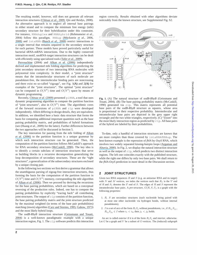
The sodB-RhyB interaction structure (Geissmann and Touati,2004) is a well-known paradigmatic example with a uniqueinteraction region, Fig. 1. Therip software predicts this interaction

region correctly. Results obtained with other algorithms deviatenoticeably from the known structure, see Supplemental Fig. S2.

( )A

AUACGCACAAUAAGGCUAUUGUACGUAUGCAAAUUAAUAAUAAAGGAGAGUAGCAAUGUCAUUCGAAUUACCUGCACUACCAUAUGC

UUUUCGGUCGUGGGCCGACCGAUUCAUUAUGACCUUCGUUACACUCGUUACAGCACGAAAGUCCAAGAGGCGCUCCCAGAAGGACUAGCG

5'-

3 -'

-5'

-3 '

( )C

( )B

A U A C G C A C A A U A A G G C U A U U G U A C G U A U G C A A A U U A A U A A U A A A G G A G A G U A G C A A U G U C A U U C G A A U U A C C U G C A C U A C C A U A U G C G C G A U C A G G A A G A C C C U C G C G G A G A A C C U G A A A G C A C G A C A U U G C U C A C A U U G C U U C C A G U A U U A C U U A G C C A G C C G G G U G C U G G C U U U U

AU

AC

GC

AC

AA

UA

AG

GC

UA

UU

GU

AC

GU

AU

GC

AA

AU

UA

AU

AA

UA

AA

GG

AG

AG

UA

GC

AA

UG

UC

AU

UC

GA

AU

UA

CC

UG

CA

CU

AC

CA

UA

UG

CG

CG

AU

CA

GG

AA

GA

CC

CU

CG

CG

GA

GA

AC

CU

GA

AA

GC

AC

GA

CA

UU

GC

UC

AC

AU

UG

CU

UC

CA

GU

AU

UA

CU

UA

GC

CA

GC

CG

GG

UG

CU

GG

CU

UU

U

CUUA

CUGUAACGA

UGA

GCAC

GACAUUGCU

CAC

5'

5'3'

3'

95.60%

98.85%

98.90%

98.68%

98.59%

98.88%

99.04%

98.80%

96.70%

sodB

RhyB

RhyBsodB

Fig. 1. (A) The natural structure ofsodB-RhyB (Geissmann andTouati, 2004). (B) The base pairing probability matrix (McCaskill,1990) generated viarip. This matrix represents all potentialbase pairs of thesodB-RhyB structure as squares, whose areais proportional to their respective probability. Intermolecular andintramolecular base pairs are depicted in the grey upper rightrectangle and the two white triangles, respectively. (C) “Zoom” intothe most likely interaction region as predicted byrip. All base pairsof the hybrid are labeled by their probabilities.

To-date, only a handful of interaction structures are known thatare more complex than those covered byintaRNA/RNAup. Thebest-known example is the repression offhlA by OxySRNA, whichinvolves two widely separated kissing-hairpin loops (Argaman andAltuvia, 2000). In Fig. 2, we display the natural interaction structureas well as the output ofrip, which predicts two distinct interactionregions. The left one coincides exactly with the published structure,while the right one differs by only two base pairs. We shall return tothe fhlA-OxySprediction in more detail in the Discussion section.

2 JOINT STRUCTURESGiven two RNA sequencesR andS (e.g. an antisense RNA and its target)with N andM vertices, we index the vertices such thatR1 is the5′ endof R andS1 denotes the3′ end ofS. The edges ofR andS represent theintramolecular base pairs. Apre-structure, G(R, S, I), is a graph with thefollowing properties:

1. R, S are secondary structures (each nucleotide being paired withat most one other nucleotide via hydrogen bonds, without internalpseudoknots);

2. I is a set of arcs of the formRiSj without pseudoknots, i.e., ifRi1Sj1 ,Ri2Sj2 ∈ I wherei1 < i2, thenj1 < j2 holds.

An arc is calledexterior if it is of the form RiSj andinterior, otherwise.Let G be a graph andV be a subset ofG-vertices. The(induced) subgraph

2

by guest on August 20, 2015

http://bioinformatics.oxfordjournals.org/

Dow

nloaded from

RIP: Partition Function and Base Pairing Probabilities

A G U U A G U C A A U G A C C U U U U G C A C C G C U U U G C G G U G C U U U C C U G G A A G A A C A A A A U G U C A U A U A C A C C G A U G A G U G A U C U C G G A C A A C A A G G G U U G U U C G A C A U C A C U C G G A C A C U A G A A A C G G A G C G G C A C C U C U U U U A A C C C U U G A A G U C A C U G C C C G U U U C G A G A G U U U C U C A A C U C G A A U A A C U A A A G C C A A C G U G A A C U U U U G C G G A U C U C C A G G A U C C G C U U U U U U U

AG

UU

AG

UC

AA

UG

AC

CU

UU

UG

CA

CC

GC

UU

UG

CG

GU

GC

UU

UC

CU

GG

AA

GA

AC

AA

AA

UG

UC

AU

AU

AC

AC

CG

AU

GA

GU

GA

UC

UC

GG

AC

AA

CA

AG

GG

UU

GU

UC

GA

CA

UC

AC

UC

GG

AC

AC

UA

GA

AA

CG

GA

GC

GG

CA

CC

UC

UU

UU

AA

CC

CU

UG

AA

GU

CA

CU

GC

CC

GU

UU

CG

AG

AG

UU

UC

UC

AA

CU

CG

AA

UA

AC

UA

AA

GC

CA

AC

GU

GA

AC

UU

UU

GC

GG

AU

CU

CC

AG

GA

UC

CG

CU

UU

UU

UU

AGUUAGUCAAUGACCUUUUGCACCGCUUUGCGGUGCUUUCCUGGAAGAACAAAAUGUCAUAUACACCGAUGAGUGAUCUCGGACAACAAGGGUUGUUCGACAUCACUCGGACACUA

UUUUUUUCGCCUAGGACCUCUAGGCGUUUUCAAGUGCAACCGAAAUCAAUAAGCUCAACUCUUUGAGAGCUUUGCCCGUCACUGAAGUUCCCAAUUUUCUCCACGGCGAGGCAAAG

5’-

3’-

-3’

-5’

fhlA

OxyS

(A)

(B)

UCCUGGA

AGGACCU

UUC5’

CCU

3’

CU5’

AG3’

C

AAGGGUUG

GUUCCCAAC

CAA

5’

AA

G3’

UU5’

UU

3’

fhlA

fhlA

OxyS

OxyS

(C)

72.46%

3.42%11.67%83.90%99.54%99.96%99.96%99.73%96.91%87.69%

92.02%95.70%96.04%

96.11%96.17%

63.20%

Fig. 2. (A) The natural structure off hlA-OxyS(Chitsazet al., 2009).(B) The base pairing probability matrix see the caption of Fig. 1 fornotation. (C) “Zoom” into the two distinct, most likely interactionregions, as predicted byrip.

of G induced byV has vertex setV and contains allG-edges having bothincident vertices inV . In particular, we useS[i, j] to denote the subgraphof the pre-structureG(R, S, I) induced bySi, Si+1, . . . , Sj, whereS[i, i] = Si andS[i, i − 1] = ∅. In absence of interactions a pre-structureis a pair of induced secondary structures onR andS, which we will refer toas a pair ofsegments. A segmentS[i1, j1] is called maximal if there is nosegment,S[i, j] strictly containingS[i1, j1].

An interior arcRi1Rj1 is an R-ancestorof the exterior arcRiSj if i1 <i < j1. Analogously,Si2Sj2 is anS-ancestor ofRiSj if i2 < j < j2. Thesets ofR-ancestors andS-ancestors ofRiSj are denoted byAR(RiSj)andAS(RiSj), respectively. We will also refer toRiSj as a descendantof Ri1Rj1 andSi2Sj2 in this situation. TheR- andS-ancestors ofRiSj

with minimum arc-length are referred to asR- andS-parents, see Fig. 3,(A). Finally, we callRi1Rj1 andSi2Sj2 dependent if they have a commondescendant and independent, otherwise.

1 2 3 4 5 6 7 81 2 3 4 5 6(A) (B)

Fig. 3. (A) Ancestors and parents: for the exterior arcR3S4, we have thefollowing ancestor setsAR(R3S4) = R1R6, R2R4 andAS(R3S4) =S2S6, S3S5. In particular, R2R4 and S3S5 are theR-parent andS-parent respectively.(B) Subsumed and equivalent arcs:R1R8 subsumesS1S4 andS5S8. Furthermore,R2R5 is equivalent toS1S4.

Suppose there is an exterior arcRaSb with ancestorsRiRj andSi′Sj′ .ThenRiRj is subsumedin Si′Sj′ , if for any RkSk′ ∈ I′, i < k < jimpliesi′ < k′ < j′, see Fig. 3,(B). If Ri1Rj1 is subsumed inSi2Sj2 andvice versa, we call these arcsequivalent. A zigzag, is a subgraph containing

two dependent interior arcsRi1Rj1 andSi2Sj2 neither one subsuming theother, see Fig. 4,(A).

1 24

1 23

1 2 3 4 5(A) (B) 12

8

13 16

12 15

1718

1617

23

20

Fig. 4. (A): A zigzag, generated byR2S1, R3S3 and R5S4. (B): Wepartition the joint structureJ1,24;1,23 in segments and tight structures.

A joint structure, J(R, S, I), is a zigzag-free pre-structure, see Fig. 4,(B). Joint structures are exactly the configurations that are considered inthe maximum matching approach of Pervouchine (2004), in the energyminimization algorithm of Alkanet al. (2006), and in the partition functionapproach of Chitsazet al. (2009). The subgraph of a joint structureJ(R, S, I) induced by a pair of subsequencesRi, Ri+1, . . . , Rj andSh, Sh+1, . . . , Sℓ is denoted byJi,j;h,ℓ. In particular, J(R, S, I) =J1,N;1,M . We say RaRb(SaSb, RaSb) ∈ Ji,j;h,ℓ if and only ifRaRb(SaSb, RaSb) is an edge of the graphJi,j;h,ℓ. Furthermore,Ji,j;h,ℓ ⊂ Ja,b;c,d if and only if Ji,j;h,ℓ is a subgraph ofJa,b;c,d inducedby Ri, . . . , Rj andSh, . . . , Sℓ.

We next define atight structure (ts). Given a joint structure,Ja,b;c,d, itstight Ja′,b′;c′,d′ is either a single exterior arcRa′Sc′ (in the casea′ =b′ and c′ = d′), or the minimal block centered around the leftmost andrightmost exterior arcsαl, αr , (possibly being equal) and an interior arcsubsuming both, i.e.,Ja′,b′;c′,d′ is tight in Ja,b;c,d if it has either an arcRa′Rb′ or Sc′Sd′ if a′ 6= b′ or c′ 6= d′.

More formally, letJa′,b′;c′,d′ be contained inJa,b;c,d with rightmostand leftmost exterior arcRiSj andRi0Sj0 and letM be the set ofRiSj -ancestors inJa,b;c,d with maximal length. ThenJa′,b′;c′,d′ is tight inJa,b;c,d if

1. for M = ∅: Ja′,b′;c′,d′ = RiSj;

2. for M = Ri1Rj1: Ja′,b′;c′,d′ = Ji1,j1;c′,j , wherec′ is the origin(left) of theS-ancestor ofRi0Sj0 with maximal length (ori0 if thereis none). The caseM = Sr1Ss1 is analogous;

3. for M = Ri1Rj1 , Sr1Ss1, supposeRi1Rj1 subsumesSr1Ss1 .Then Ja′,b′;c′,d′ = Ji1,j1;x1,s1

, where x1 is the origin ofthe S-ancestor ofRi0Sj0 with maximal length (ori0 if there isnone). In particular,Ja′,b′;c′,d′ = Ji1,j1;r1,s1

when Ri1Rj1 isequivalent withSr1Ss1 . The case, whereSr1Ss1 subsumesRi1Rj1

is analogous.

In the following, a ts is denoted byJTi,j;h,ℓ. If Ja′,b′;c′,d′ is tight inJa,b;c,d,

then we callJa,b;c,d its envelope. By construction, the notion of ts isdepending on its envelope. There are only four basic types of ts, see Fig. 5:

: RiSh = Ji,j;h,ℓ andi = j, h = ℓ;

: RiRj ∈ Ji,j;h,ℓ andShSℓ 6∈ J

i,j;h,ℓ;

: RiRj , ShSℓ ∈ Ji,j;h,ℓ;

: ShSℓ ∈ Ji,j;h,ℓ andRiRj 6∈ J

i,j;h,ℓ.

In the Supplemental Material we prove:

PROPOSITION2.1. LetJa,b;c,d be a joint structure. Then

1. any exterior arcRiSj in Ja,b;c,d is contained in a uniqueJa,b;c,d-ts;

3

by guest on August 20, 2015

http://bioinformatics.oxfordjournals.org/

Dow

nloaded from

F.W.D. Huang, J. Qin, C.M. Reidys, P.F. Stadler

Fig. 5. From left to right: tights of type, , and.

2. Ja,b;c,d decomposes into a unique collection ofJa,b;c,d-ts andmaximal segments.

Given a ts,Ji0,j0;r,s (or J

i,j;r0,s0), we introducedouble tight structures

as maximal substructure whose distinct leftmost and rightmost blocks aretights. By construction, therefore, each dts contains at least two tights.

More formally, given a tsJi0,j0;r,s, adouble-tight structure, J

DT |i,j;r,s , in

Ji0,j0;r,s, wherei0 < i < j < j0, is defined as follows: there exists labels

a, b, c, d wherei ≤ a < b ≤ j andr ≤ c < d ≤ s. Furthermore, two tsJT

i,a;r,c andJTb,j;d,s in Ji0+1,j0−1;r,s such that

JDT |i,j;r,s = JT

i,a;r,c∪Ja+1,b−1;c+1,d−1∪JTb,j;d,s . (2.1)

Here, the disjoint union∪ refers to both the vertex and arc sets of the joint

structures, see Fig. 6. The case of a dts,JDT |i,j;r,s , within a ts,J

i,j;r0,s0,

is defined accordingly. By abuse of terminology, we simply useJDTi,j;r,s in

order to denote eitherJDT |i,j;r,s or J

DT |i,j;r,s .

6

151

11

202 21

1

Fig. 6. A dts JDT |6,15;1,11 in J2,20;1,11 . Note that the joint structure

J1,21;1,11 itself is -tight. Here, J2,15;1,11 is neither a ts nor a rts inJ2,20;1,11.

With the help of dts, as illustrated in Fig. 7,Procedure (b), we decomposea ts as follows:Let J

i,j;r,s be a ts of type and letRh1Sℓ1 andRh2

Sℓ2 be the leftmostand rightmost exterior arcs inJi,j;r,s andi + 1 ≤ i1 ≤ j1 ≤ j − 1. ThenJi+1,j−1;r,s decomposes into

8

>

>

>

>

<

>

>

>

>

:

R[i + 1, i1 − 1]∪J,i1,j1;r,s∪R[j1 + 1, j − 1],

if JTRh1

Sℓ1= JT

Rh2Sℓ2

;

R[i + 1, i1 − 1]∪JDTi1,j1;r,s∪R[j1 + 1, j − 1],

otherwise,

(2.2)

where J,i1,j1;r,s denotes aJi+1,j−1;r,s-ts of type or and JT

RhSℓ

denotes the unique ts inJi+1,j−1;r,s contain the exterior arcRhSℓ.

Analogously, in case of a tsJi,j;r,s with leftmost and rightmost exterior

arcsRh1Sℓ1 andRh2

Sℓ2 , andr + 1 ≤ r1 ≤ s1 ≤ s − 1, Ji,j;r+1,s−1

can be decomposed in the form8

>

>

>

>

<

>

>

>

>

:

S[r + 1, r1 − 1]∪J,i,j;r1,s1

∪S[s1 + 1, s − 1],

if JTRh1

Sℓ1= JT

Rh2Sℓ2

;

S[r + 1, r1 − 1]∪JDTi,j;r1,s1

∪S[s1 + 1, s − 1],

otherwise,

(2.3)

whereJ,i1,j1;r,s denotes aJi,j;r+1,s−1-tight of type or .

For a tsJi,j;r,s with i + 1 ≤ i1 ≤ j1 ≤ j − 1 we analogously derive

Ji+1,j−1;r,s =

R[i + 1, i1 − 1]∪J,i1,j1;r,s∪R[j1 + 1, j − 1],

(2.4)

whereJ,i1,j1;r,s denotes aJi+1,j−1;r,s-tight of type or .

Prop.(2.1) and equ. (2.1-2.4) establish, for each joint structure, a uniquedecomposition into interior and exterior arcs.

3 THE PARTITION FUNCTION

3.1 Refined DecompositionThe unique decomposition of ts would formally suffice to construct apartition function algorithm. Indeed, each decomposition step, such asequ. (2.1-2.4), corresponds to a multiplicative recursion relation for thepartition function associated with the joint structures. However, this wouldresult in an unwieldy expensive implementation. The reason are the multiplebreak pointsa, b, c, d, . . . , each of which corresponding to a nestedfor-loop.

We therefore introduce a refined decomposition that reduces the numberof break points. For this purpose we call a joint structureright-tight if itsrightmost block is a ts. We adopt the point of view of Algebraic DynamicProgramming (Giegerich and Meyer, 2002) and regard each decompositionrule as a production in a suitable grammar. Fig. 7 summarizes two majorsteps in the decomposition: (I) the “arc-removal” reducing ts and dts. Thescheme is complemented by the usual loop decomposition of secondarystructures, and (II) the “block-decomposition” splitting joint structures intoblocks.

The details of the decomposition procedures are collected in the SM,where we show that for eachJ1,N;1,M there exists a unique decomposition-tree (parse-tree), denoted byTJ1,N ;1,M

. This tree has rootJ1,N;1,M andall other vertices correspond to specific substructures ofJ1,N;1,M obtainedby the successive application of the decomposition steps of Fig. 7 and theloop decomposition of the secondary structures, see Fig. 8.

3.2 Extended Loop ModelThe standard energy model for RNA folding (Mathewset al., 1999),presented in the SM, is consistent with the basic decomposition of secondarystructures. In addition, joint structures give rise to two further types of loops.Following Chitsazet al.(2009), we call themhybrid andkissing-loop, Fig. 9.

• A hybrid is a maximal sequence of intermolecular interior loops formedby ℓ ≥ 2 exterior arcsRi1Sj1 , . . . , Riℓ

SjℓwhereRih

Sjhis nested

within Rih+1Sjh+1

and where the internal segmentsR[ih+1, ih+1−1] andS[jh +1, jh+1−1] consist of single-stranded nucleotides. I.e. ,a hybrid is the maximal unbranched stem-loop formed by external arcs.

• A kissing-loopis either a pair,(RiRj , R[i + 1, j − 1]), where the setof RiRj -children,, Ri1Sj1 , . . . where i < i1 < j is nonempty,or a pair (SiSj , S[i + 1, j − 1]), where the set ofSiSj-childrenRi1Sj1 , . . . wherei < j1 < j is nonempty.

Kissing loops have been singled out for logical reasons and because someinvestigations into their thermodynamic properties have been reported in theliterature (Gagoet al., 2005). For details of the parametrization employed inrip we refer to the SM.

Let us now have a closer look at the energy evaluation ofJi,j;h,ℓ.Each decomposition step in Fig. 7 results in substructures whose energieswe assume to contribute additively and generalized loops that need to beevaluated directly. There are the following two scenarios:I. Arc removal. Most of the decomposition operations in Procedure (b)displayed in Fig. 7 can be viewed as the “removal” of an arc (corresponding

4

by guest on August 20, 2015

http://bioinformatics.oxfordjournals.org/

Dow

nloaded from

RIP: Partition Function and Base Pairing Probabilities

or

or

or

or or

or

oror

Procedure (b)

Procedure (a)

= or or

A B C D E F G H J K

R

S

R

S

R R R R

S

R R R R R R

S S SS S

R S

Fig. 7. Illustration of Procedure (a) the reduction of arbitrary joint structuresand rts, and Procedure (b) the decomposition of tight structures. The panelbelow indicates the 10 different types of structural components:A, B:maximal secondary structure segmentsR[i, j], S[r, s]; C: arbitrary jointstructureJi,j;r,s; D: right-tight structuresJRT

i,j;r,s; E: double-tight structure

JDTi,j;r,s; F: tight structure of type, or ; G: type tight J

i,j;r,s, thesolid curved line (top and bottom) denotes an arc and a single horizontalline (top and bottom) denotes the backbone;H: type tight J

i,j;r,s,a solid curved line (top) denotes an arc, a single horizontal line (top)denotes the backbone and a double-horizontal line (bottom) denotes that thetwo terminals are not paired with each other;J: type tight J

i,j;r,s, asolid curved line (bottom) denotes an arc, a single horizontal line (bottom)denotes the backbone and a double-horizontal line (top) indicates that thetwo terminals are not paired with each other;K : an exterior arc.

Fig. 8. The decomposition treeTJ1,15;1,8for the joint structureJ1,15;1,8.

5’

5’3’

3’

5’ 3’

3’ 5’5’ 3’

3’ 5’

5’

3’

5’

3’

(A) (B)

Fig. 9. The two new loop-types: hybrid(A) and kissing-loop(B).

to the closing pair of a loop in secondary structure folding) followed bydecomposition. Both, loop-type as well as the subsequent decompositionsteps depend on the newly exposed structural elements. Following theapproach of Zuker and Stiegler (1981) for secondary structures, we treat theloop-decomposition problem by introducing additional matrices. Withoutloss of generality, we can assume that we open an interior base pairRiRj .

The set of base pairs onR[i, j] consists of all interior pairsRpRq withi ≤ p < q ≤ j and all exterior pairsRpSh with i ≤ p ≤ j. An interior arcis exposedonR[i + 1, j − 1] if and only if it is not enclosed by any interiorarc inR[i, j]. An exterior arc isexposedonR[i + 1, j − 1] if and only if itis not a descendant of any interior arc inR[i+1, j−1]. GivenRij , the arcsexposed onR[i+1, j−1] corresponds to the base pairsimmediately interiorof RiRj . Let us writeER[i,j] = Ei

R[i,j]∪Ee

R[i,j]for this set of “exposed

base pairs” and its subsets of interior and exterior arcs. As in secondarystructure folding, the loop type is determined byER[i,j] := ER as follows:ER = ∅, hairpin loop;ER = Ei

R and|ER| = 1, interior loop (includingbulge and stacks);ER = Ei

R, |ER| ≥ 2, multi-branch loop;ER = EeR,

kissing-hairpin loop;|EiR|, |Ee

R| ≥ 1, general kissing-loop.This picture needs to be refined even further since the arc removal is

coupled with further decomposition of the intervalR[i + 1, j − 1]. Thisprompts us to distinguish ts and dts with different classes of exposed basepairs on one or both strands. It will be convenient, furthermore to includeinformation on the type of loop in which it was found.

A ts Ji,j;h,ℓ is of type E, if S[h, ℓ] is not enclosed in any base pair

(J,Ei,j;h,ℓ). SupposeJ

i,j;h,ℓ is located immediately interior to the closingpairSpSq (p < h < ℓ < q). If the loop closed bySpSq is a multiloop, then

Ji,j;h,ℓ is of typeM (J,M

i,j;h,ℓ). If SpSq is contained in a kissing-loop, wedistinguish the typesF andK, depending on whether or notEe

S[h,ℓ]= ∅.

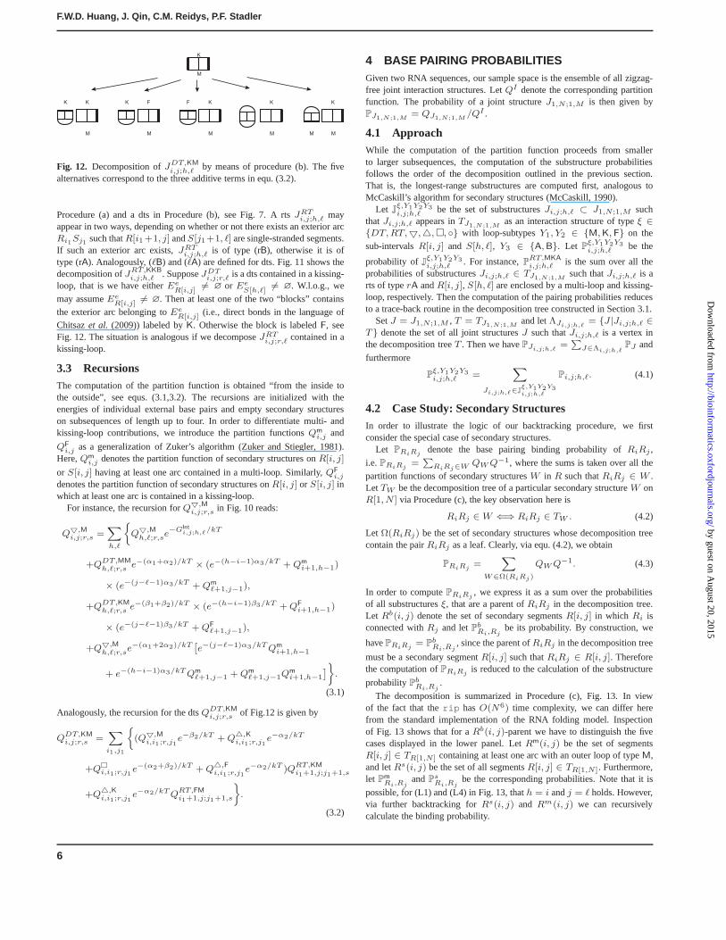
Fig. 10 displays this decomposition forJ,Mi,j;r,s.

M

M

K

I

i j

K

M

M

M M

MM

i jji j ji i

MR RR R R RII

Fig. 10. Further refinement: the four decompositions ofJ,Mi,j;r,s via

Procedure (b). A box labeled by “I” denotes a single-stranded segment. ThelettersI, M andK denote the loop-type and the type of the exposed arc(s) ofthe dts. See Fig. 7 for more details on the notation. The four cases correspondto the four contributions in equ. (3.1).

For a dtsJDTp,q,r,s (denoted by “E” in Fig. 7) we need to determine the type

of the exposed pairs of bothR[p, q] andS[r, s]. Hence each such structurewill be indexed by two types. In total, we arrive at 18 distinct cases sincesome combinations cannot occur. For instance, a dts cannot be external inbothR andS, that is, typeEE does not exist, whereE means external.

K

B

K

A

K

K

K

B

K

B

K

F

F

F

K

F

K

I

I

R

S

KN

N

Fig. 11. Decomposition ofJRT,KKB

i,j;h,ℓ by means of procedure (b). Here apair of boxes labeled by “N” denote a pair of secondary segments having theproperty that at least one of them is not single-stranded.

II. Block decomposition. The second type of decomposition is the splittingof joint structures into “blocks”, such as the decompositions of a rts in

5

by guest on August 20, 2015

http://bioinformatics.oxfordjournals.org/

Dow

nloaded from

F.W.D. Huang, J. Qin, C.M. Reidys, P.F. Stadler

M

M M M

K

K F KK K

MM

K

M

KF

Fig. 12. Decomposition ofJDT,KM

i,j;h,ℓ by means of procedure (b). The fivealternatives correspond to the three additive terms in equ. (3.2).

Procedure (a) and a dts in Procedure (b), see Fig. 7. A rtsJRTi,j;h,ℓ may

appear in two ways, depending on whether or not there exists an exterior arcRi1Sj1 such thatR[i1+1, j] andS[j1+1, ℓ] are single-stranded segments.If such an exterior arc exists,JRT

i,j;h,ℓ is of type (rB), otherwise it is oftype (rA). Analogously, (ℓB) and (ℓA) are defined for dts. Fig. 11 shows thedecomposition ofJRT,KKB

i,j;h,ℓ . SupposeJDTi,j;r,ℓ is a dts contained in a kissing-

loop, that is we have eitherEeR[i,j]

6= ∅ or EeS[h,ℓ]

6= ∅. W.l.o.g., we

may assumeEeR[i,j]

6= ∅. Then at least one of the two “blocks” containsthe exterior arc belonging toEe

R[i,j](i.e., direct bonds in the language of

Chitsazet al. (2009)) labeled byK. Otherwise the block is labeledF, seeFig. 12. The situation is analogous if we decomposeJRT

i,j;r,ℓ contained in akissing-loop.

3.3 RecursionsThe computation of the partition function is obtained “from the inside tothe outside”, see equs. (3.1,3.2). The recursions are initialized with theenergies of individual external base pairs and empty secondary structureson subsequences of length up to four. In order to differentiate multi- andkissing-loop contributions, we introduce the partition functionsQm

i,j and

QFi,j as a generalization of Zuker’s algorithm (Zuker and Stiegler, 1981).

Here,Qmi,j denotes the partition function of secondary structures onR[i, j]

or S[i, j] having at least one arc contained in a multi-loop. Similarly,QFi,j

denotes the partition function of secondary structures onR[i, j] or S[i, j] inwhich at least one arc is contained in a kissing-loop.

For instance, the recursion forQ,Mi,j;r,s in Fig. 10 reads:

Q,Mi,j;r,s =

X

h,ℓ

Q,Mh,ℓ;r,se−GInt

i,j;h,ℓ/kT

+QDT,MM

h,ℓ;r,s e−(α1+α2)/kT × (e−(h−i−1)α3/kT + Qmi+1,h−1)

× (e−(j−ℓ−1)α3/kT + Qmℓ+1,j−1),

+QDT,KM

h,ℓ;r,s e−(β1+β2)/kT × (e−(h−i−1)β3/kT + QFi+1,h−1)

× (e−(j−ℓ−1)β3/kT + QFℓ+1,j−1),

+Q,Mh,ℓ;r,se−(α1+2α2)/kT

ˆ

e−(j−ℓ−1)α3/kT Qmi+1,h−1

+ e−(h−i−1)α3/kT Qmℓ+1,j−1 + Qm

ℓ+1,j−1Qmi+1,h−1

˜

ff

.

(3.1)

Analogously, the recursion for the dtsQDT,KMi,j;r,s of Fig.12 is given by

QDT,KMi,j;r,s =

X

i1,j1

(Q,Mi,i1;r,j1

e−β2/kT + Q,Ki,i1;r,j1

e−α2/kT

+Qi,i1;r,j1

e−(α2+β2)/kT + Q,Fi,i1;r,j1

e−α2/kT )QRT,KMi1+1,j;j1+1,s

+Q,Ki,i1;r,j1

e−α2/kT QRT,FMi1+1,j;j1+1,s

ff

.

(3.2)

4 BASE PAIRING PROBABILITIESGiven two RNA sequences, our sample space is the ensemble of all zigzag-free joint interaction structures. LetQI denote the corresponding partitionfunction. The probability of a joint structureJ1,N;1,M is then given byPJ1,N ;1,M

= QJ1,N ;1,M/QI .

4.1 ApproachWhile the computation of the partition function proceeds from smallerto larger subsequences, the computation of the substructure probabilitiesfollows the order of the decomposition outlined in the previous section.That is, the longest-range substructures are computed first, analogous toMcCaskill’s algorithm for secondary structures (McCaskill, 1990).

Let Jξ,Y1Y2Y3

i,j;h,ℓ be the set of substructuresJi,j;h,ℓ ⊂ J1,N;1,M suchthat Ji,j;h,ℓ appears inTJ1,N ;1,M

as an interaction structure of typeξ ∈DT, RT,,, , with loop-subtypesY1, Y2 ∈ M, K, F on thesub-intervalsR[i, j] and S[h, ℓ], Y3 ∈ A, B. Let P

ξ,Y1Y2Y3

i,j;h,ℓ be the

probability of Jξ,Y1Y2Y3

i,j;h,ℓ . For instance,PRT,MKA

i,j;h,ℓ is the sum over all theprobabilities of substructuresJi,j;h,ℓ ∈ TJ1,N ;1,M

such thatJi,j;h,ℓ is arts of typerA andR[i, j], S[h, ℓ] are enclosed by a multi-loop and kissing-loop, respectively. Then the computation of the pairing probabilities reducesto a trace-back routine in the decomposition tree constructed in Section 3.1.

SetJ = J1,N;1,M , T = TJ1,N ;1,Mand letΛJi,j;h,ℓ

= J |Ji,j;h,ℓ ∈T denote the set of all joint structuresJ such thatJi,j;h,ℓ is a vertex inthe decomposition treeT . Then we havePJi,j;h,ℓ

=P

J∈Λi,j;h,ℓPJ and

furthermore

Pξ,Y1Y2Y3

i,j;h,ℓ =X

Ji,j;h,ℓ∈Jξ,Y1Y2Y3i,j;h,ℓ

Pi,j;h,ℓ. (4.1)

4.2 Case Study: Secondary StructuresIn order to illustrate the logic of our backtracking procedure, we firstconsider the special case of secondary structures.

Let PRiRjdenote the base pairing binding probability ofRiRj ,

i.e. PRiRj=

P

RiRj∈W QW Q−1, where the sums is taken over all the

partition functions of secondary structuresW in R such thatRiRj ∈ W .Let TW be the decomposition tree of a particular secondary structureW onR[1, N ] via Procedure (c), the key observation here is

RiRj ∈ W ⇐⇒ RiRj ∈ TW . (4.2)

Let Ω(RiRj) be the set of secondary structures whose decomposition treecontain the pairRiRj as a leaf. Clearly, via equ. (4.2), we obtain

PRiRj=

X

W∈Ω(RiRj)

QW Q−1. (4.3)

In order to computePRiRj, we express it as a sum over the probabilities

of all substructuresξ, that are a parent ofRiRj in the decomposition tree.Let Rb(i, j) denote the set of secondary segmentsR[i, j] in which Ri isconnected withRj and letPb

Ri,Rjbe its probability. By construction, we

havePRiRj= Pb

Ri,Rj, since the parent ofRiRj in the decomposition tree

must be a secondary segmentR[i, j] such thatRiRj ∈ R[i, j]. Thereforethe computation ofPRiRj

is reduced to the calculation of the substructure

probabilityPbRi,Rj

.

The decomposition is summarized in Procedure (c), Fig. 13. In viewof the fact that therip hasO(N6) time complexity, we can differ herefrom the standard implementation of the RNA folding model. Inspectionof Fig. 13 shows that for aRb(i, j)-parent we have to distinguish the fivecases displayed in the lower panel. LetRm(i, j) be the set of segmentsR[i, j] ∈ TR[1,N] containing at least one arc with an outer loop of typeM,and letRs(i, j) be the set of all segmentsR[i, j] ∈ TR[1,N]. Furthermore,let Pm

Ri,RjandPs

Ri,Rjbe the corresponding probabilities. Note that it is

possible, for (L1) and (L4) in Fig. 13, thath = i andj = ℓ holds. However,via further backtracking forRs(i, j) and Rm(i, j) we can recursivelycalculate the binding probability.

6

by guest on August 20, 2015

http://bioinformatics.oxfordjournals.org/

Dow

nloaded from

RIP: Partition Function and Base Pairing Probabilities

Following the logic of Fig. 13, we obtain

PbRi,Rj

=X

h,ℓ

PsRh,Rℓ

Qsh,i−1Qb

i,j

Qsh,ℓ

+ PbRh,Rℓ

Qbi,je−GInt

h,ℓ;i,j/kT

Qbh,ℓ

+PbRh,Rℓ

Qmh+1,i−1Qb

i,je−(α1+2α2+(ℓ−j−1)α3)/kT

Qbh,ℓ

+PmRh,Rℓ

Qbi,je−(α2+(i−h+ℓ−j)α3)/kT

Qmh,ℓ

+PmRh,Rℓ

Qmh,i−1Qb

i,je−(α2+(ℓ−j)α3)/kT

Qmh,ℓ

ff

.

(4.4)

where the lines correspond to the five loop types (L1-L5) in Fig. 13.Analogously, the recursions for the base pairing probabilitiesPm

Ri,Rjand

PsRi,Rj

are given by

PmRi,Rj

=X

h,ℓ

PbRi−1,Rℓ

e−(α1+2α2+(ℓ−1−h)α3)/kT

×Qb

j+1,hQmi,j

Qbi−1,ℓ

+ PmRi,Rℓ

Qmi,jQb

j+1,he−(α2+(ℓ−h)α3)/kT

Qmi,ℓ

ff

PsRi,Rj

=X

h,ℓ

PsRi,Rℓ

Qsi,jQb

j+1,h

Qsi,ℓ

.

(4.5)

4.3 Base pairing probabilities for joint structuresSet Σ1 = J | RiRj ∈ J. We apply the same strategy to the jointstructures appearing in Fig. 7. LetQI denote the partition function whichsums over all the possible joint structuresJ1,N;1,M . Then PRi,Rj

=P

J∈Σ1QJ/QI . In order to computePRiRj

we classifyΣ1 accordingto the parent ofRiRj in T :

Σ1 = J | R[i, j] ∈ T, R[i, j] ∈ Rb(i, j)

∪[

h,ℓ

J | Ji,j;h,ℓ ∈ T, Ji,j;h,ℓ ∈ Ji,j;h,ℓ

∪[

h,ℓ

J | Ji,j;h,ℓ ∈ T, Ji,j;h,ℓ ∈ Ji,j;h,ℓ,

(4.6)

which translates to

PRiRj= P

bRi,Rj

+X

h,ℓ

P,E,M,F,Ki,j;h,ℓ +

X

h,ℓ

Pi,j;h,ℓ, (4.7)

where P,E,M,F,Ki,j;h,ℓ = P,E + P,M + P,F + P,K for identical

positionsi, j, h, ℓ. Analogously, we obtain for pairs inS:

Σ2 = J | S[h, ℓ] ∈ T, S[h, ℓ] ∈ Sb[h, ℓ]

∪[

i,j

J | Ji,j;h,ℓ ∈ T, Ji,j;h,ℓ ∈ Ji,j;h,ℓ,

(4.8)

and thereforePSiSj= Pb

Si,Sj+

P

h,ℓ Ph,ℓ;i,j , with P = P,E +

P,M + P,K + P,F.Note that the expressions forPRiRj

andPSiSjare not symmetric. This

is due to the fact that our decomposition routine give preference to arc-removals inR over those inS. This asymmetry is necessary to ensure thatthe decomposition in Fig. 7 is unambiguous.

Finally, we calculate the binding probability of an exterior arcRiSj .SinceRiSj is a ts of type, PRiSj

is directly given by the probabilityof this special substructure in equ. (4.1).

b u m s

i ji j i ji j

b

bs u

i j

i jh

lh

l

s

h l

b

lh lh

b b uu mu

i j i jh l h llhm

uuu b um

lh

Forward RecursionL1

L2

L3

L4

L5

b b

b

b

b

b

s

u

u

u

m

m

m

mu

i j

i j

i j

h l

h l

h l

h l h l

h l

h l

lh

bs u

i jh l

b

i j lh

uu

Backtracking

Fig. 13. Top. Extended version of Procedure (c) showing the productionsfor general structures, structures and enclosed by pairs, and multi-loops. Thefour types of segments are shown below: InRb(i, j), Ri, Rj is paired,Ru(i, j) denotes stretches of unpaired bases,Rm(i, j) denotes parts ofmultiloops with containing least one arc, andRs(i, j) denotes arbitrarysegments.Below. Backtracking for secondary structures: for a parent ofRb(i, j) we have five cases according to Procedure (c): external (L1),interior loop (L2), closing pair of a multi-loop (L3), (L4) and (L5) denotethe scenarios arising from decomposing aRm(h, ℓ)-segment. See equ. (4.4)for the corresponding recursions.

In order to compute the binding probabilities of both interior and exteriorarcs, the key is to employ an “inverse” grammar induced by tracing back inthe decomposition tree as displayed in Supplement Materials [SM, Fig. 5].

5 RESULTS AND DISCUSSIONIn this contribution we have introduced a framework in whichboth the partition function and the base pairing probabilities ofzigzag-free RNA-RNA interactions can be derived in a naturalway. Our approach is implemented in the software packageripusing the full standard energy model for RNA secondary structurestogether with a multi-loop-like additive parametrization for kissing-loops. In comparison withpiRNA (Chitsazet al., 2009),rip isbased on a different but equivalent decomposition grammar. Thevery encouraging data on the accuracy of the predicted interactionenergies reported by Chitsazet al. (2009) therefore carry over torip as well.

The notion of tights, which have a central role in our presentation,is also implicit in the work of Chitsazet al. (2009). The focus onthe underlying combinatorial aspects, however, leads us to highlightin particular the decomposition tree, which provides a naturalframework in which to proceed beyond the algorithmic core of thepartition function itself. Indeed, the decomposition tree facilitatesthe derivation of the base pairing probabilities. Related questions,

7

by guest on August 20, 2015

http://bioinformatics.oxfordjournals.org/

Dow

nloaded from

F.W.D. Huang, J. Qin, C.M. Reidys, P.F. Stadler

I II III IV58,47: 50.3% 21,69: 56.5% 34,55: 45.7% 83,45: 17.3%59,46: 54.8% 20,70: 59.5% 35,54: 51.0% 82,46: 18.9%60,45: 52.9% 19,71: 29.8% 36,53: 49.9% 81,47: 18.5%61,44: 28.8%

Table 1. The base pairing probabilities of the four alternative hybridsI, II, III and IV for fhlA-OxyS, predicted byrip, see Fig. 2. Eachentry represents the positions infhlA(R)-OxyS(S) and the base pairprobability. For instance,58, 47 : 50.3% is equivalent toPR58S47 =0.503.

such as that for the probability of complete hybrids (Huanget al.,2009) can be answered along the same lines. While the currentimplementation ofpiRNA Chitsazet al. (2009) concentrates onmelting temperature in order to validate the partition function,rip focusses on a detailed analysis of the interaction structuresthemselves. To this end, we also compute the unweighted maximumexpected accuracy structure, which is given as the maximummatching with weights given by the base pairing probabilities. On amore technical level,piRNA andrip differ in the decompositionof tights:piRNA utilizes a4D gap-matrix by means of the Dirks-Pierce algorithm Dirks and Pierce (2003), whilerip employs twodistinct2D-matrices inspired by Zuker’s recursion. For details, werefer to the SM.

Back-tracing of the base pairing patterns that underlie the freeenergy of RNA-RNA binding is of great importance in detailedstudies of ncRNA-mRNA interactions. The details of the bindingsites have a crucial impact on the interpretation of the computationalresults and on the comparison of the computational prediction andexperimental data. It was shown by Mucksteinet al. (2008), forinstance, that positive and negative regulation of bacterial mRNAscan be distinguished depending on whether the interaction structurecontains the Shine-Dalgarno sequence in stable stem or exposed inan predominantly unpaired region.

Only a small number of interaction structures have beendescribed so far that are more complex than those computableby RNAup/intaRNA. It is not clear, however, whether complexinteractions are truly rare in nature, or whether multi-point contactssuch as that of thefhlA-OxySinteraction structure (Argaman andAltuvia, 2000) are rarely observed experimentally because they aretypically excluded from candidate lists due to the lack of readilydetectable pairing regions. A survey withrip may be suitable toprovide us with a much more unbiased picture. Fig. 2 shows, that,modulo two base pairs,rip identifies the two distinct hybrids infhlA-OxyS, correctly. Table 1 furthermore establishes, that the latterare indeed uniquely identified.

Fig. 14 compares the output ofrip with several other,established, folding algorithms.

Following Chitsazet al. (2009), we stipulate an independentinitialization energy, σ0, for each hybrid, and scaled energiesfor its base pairs. Many other RNA-cofolding algorithms, likeRNAcofold (Bernhartet al., 2006) and Dimitrov and Zuker (2004)assume a single initialization energy,ε. This energy model cana posteriori be derived fromrip, once the partition function ofthe joint structuresQI and the partition functionsQR and QS

have been computed. LetΩ1 be the set of all joint structureshaving at least one external arc and denote byΩ0 the set of all

AGUUAGUCAAUGACCUUUUGCACCGCUUUGCGGUGCUUUCCUGGAAGAACAAAAUGUCAUAUACACCGAUGAGUGAUCUCGGACAACAAGGGUUGUUCGACAUCACUCGGACACUA

UUUUUUUCGCCUAGGACCUCUAGGCGUUUUCAAGUGCAACCGAAAUCAAUAAGCUCAACUCUUUGAGAGCUUUGCCCGUCACUGAAGUUCCCAAUUUUCUCCACGGCGAGGCAAAG

5’-

3’-

-3’

-5’

RNAplex

AGUUAGUCAAUGACCUUUUGCACCGCUUUGCGGUGCUUUCCUGGAAGAACAAAAUGUCAUAUACACCGAUGAGUGAUCUCGGACAACAAGGGUUGUUCGACAUCACUCGGACACUA

UUUUUUUCGCCUAGGACCUCUAGGCGUUUUCAAGUGCAACCGAAAUCAAUAAGCUCAACUCUUUGAGAGCUUUGCCCGUCACUGAAGUUCCCAAUUUUCUCCACGGCGAGGCAAAG

5’-

3’-

-3’

-5’

RNAup

AGUUAGUCAAUGACCUUUUGCACCGCUUUGCGGUGCUUUCCUGGAAGAACAAAAUGUCAUAUACACCGAUGAGUGAUCUCGGACAACAAGGGUUGUUCGACAUCACUCGGACACUA

UUUUUUUCGCCUAGGACCUCUAGGCGUUUUCAAGUGCAACCGAAAUCAAUAAGCUCAACUCUUUGAGAGCUUUGCCCGUCACUGAAGUUCCCAAUUUUCUCCACGGCGAGGCAAAG

5’-

3’-

-3’

-5’

IntaRNA

AGUUAGUCAAUGACCUUUUGCACCGCUUUGCGGUGCUUUCCUGGAAGAACAAAAUGUCAUAUACACCGAUGAGUGAUCUCGGACAACAAGGGUUGUUCGACAUCACUCGGACACUA

UUUUUUUCGCCUAGGACCUCUAGGCGUUUUCAAGUGCAACCGAAAUCAAUAAGCUCAACUCUUUGAGAGCUUUGCCCGUCACUGAAGUUCCCAAUUUUCUCCACGGCGAGGCAAAG

5’-

3’-

-3’

-5’

RNAHybrid

AGUUAGUCAAUGACCUUUUGCACCGCUUUGCGGUGCUUUCCUGGAAGAACAAAAUGUCAUAUACACCGAUGAGUGAUCUCGGACAACAAGGGUUGUUCGACAUCACUCGGACACUA

UUUUUUUCGCCUAGGACCUCUAGGCGUUUUCAAGUGCAACCGAAAUCAAUAAGCUCAACUCUUUGAGAGCUUUGCCCGUCACUGAAGUUCCCAAUUUUCUCCACGGCGAGGCAAAG

5’-

3’-

-3’

-5’

NaturalfhlA

OxyS

OxyS

fhlA

OxyS

fhlA

OxyS

fhlA

OxyS

fhlA

Fig. 14. The natural structure of thefhlA-OxySinteraction and theresults predicted by several algorithms includingRNAplex.

structures that have none. ThenQrip = Q(Ω1) + Q(Ω0), whereQ(Ω0) = QRQS . Taking the initiation term into account, wecomputeQ = Q(Ω1) exp(−ε/kT ) + QRQS , from which weobtain the corrected value forQ(Ω1). As shown by Bernhartet al.(2006), the base pairing probabilities can be rescaled via

Pǫij =

ˆ

Prip

ij Qrip− Pij(Ω0)QRQS

˜

e−ε/kT + Pij(Ω0)QRQS

[Qrip− QRQS]e−ε/kT + QRQS.

(5.1)We have focussed here on the algorithmic context for computing

detailed models of RNA-RNA interactions in the most generalframework that is computationally feasible at the moment. Thecurrent implementation ofrip may, due to the computational costsincurred by several dozens of interdependent 4-dimensional arrays,be viewed “just” as a reference. However, in all computed examples,rip quite accurately reproduced the interaction regions. We arehere in a similar position as with the Sankoff algorithm (whichaddresses the closely related dynamic programming problem ofsimultaneous alignment and structure prediction). While the fullimplementations are slow and of limited use in particular in large-scale studies, they are instrumental in optimizing the procedureand in devising efficient nearly exact pruning heuristics that candramatically reduce the fraction of array entries that need to becomputed (Havgaardet al., 2007).

The constructions presented here give rise to several variations.Point in case being the computation of hybrid probabilities, i.e., theprobabilitiesP

Hy

i,j;h,ℓ that R[i, j] and S[h, ℓ] form an “interactionstem” or a even an entire uninterrupted interaction region Huanget al. (2009). Another line of research concerns improved energymodels for more complex types of loops Isambert and Siggia (2000).

The algorithmic approach taken here was motivated by acombinatorial analysis of zigzag-free interaction structures. Froma mathematical point of view, our approach is centered around thenotions of tight structures and their decomposition trees (the latterbeing described in the appendix). A detailed mathematical analysis,in particular the derivation of the generating function and furtherenumeration results, will be discussed elsewhere.

In order to store the partition function and the base pairingprobabilities of joint structures inrip, we employ4-dimensionalarrays. For the recursion for the partition function,QI , we use16 matrices,24 matrices forQRT , 18 matrices forQDT and 45

8

by guest on August 20, 2015

http://bioinformatics.oxfordjournals.org/

Dow

nloaded from

RIP: Partition Function and Base Pairing Probabilities

matrices forQT , in the context of taking into account the loopenergy. The complete set of partition function recursions and alldetails on the particular implementation ofrip can be found athttp://www.combinatorics.cn/cbpc/rip.html. Thespace complexity ofrip is O(N4). Summations in our recursionequations run over at most two independent indices. Therefore, thetime complexity inrip is O(N6). In order to obtain the pairingprobabilities we trace back in the decomposition tree. Thus, we havethe same space complexity and time complexity as for calculatingthe partition function.

ACKNOWLEDGEMENTSWe thank Bill Chen and Sven Findeiß for comments on the manuscript.This work was supported by the 973 Project of the Ministry of Scienceand Technology, the PCSIRT Project of the Ministry of Education, and theNational Science Foundation of China to CMR and his lab, grant No. STA850/7-1 of the Deutsche Forschungsgemeinschaft under the auspices of SPP-1258 “Small Regulatory RNAs in Prokaryotes”, as well as the EuropeanCommunity FP-6 project SYNLET (Contract Number 043312) to PFS andhis lab.

REFERENCESAkutsu, T. (2000) Dynamic programming algorithms for RNA secondary structure

prediction with pseudoknots.Disc. Appl. Math., 104, 45–62.Alkan, C., Karakoc, E., Nadeau, J., Sahinalp, S. and Zhang, K. (2006) RNA-RNA

interaction prediction and antisense RNA target search.J. Comput. Biol., 13, 267–282.

Andronescu, M., Zhang, Z. and Condon, A. (2005) Secondary structure prediction ofinteracting RNA molecules.J. Mol. Biol., 345, 1101–1112.

Argaman, L. and Altuvia, S. (2000)fhlA repression byOxySRNA: kissing complexformation at two sites results in a stable antisense-target RNA complex.J. Mol.Biol., 300, 1101–1112.

Bachellerie, J., Cavaille, J. and Huttenhofer, A. (2002) The expanding snoRNA world.Biochimie, 84, 775–790.

Banerjee, D. and Slack, F. (2002) Control of developmental timing by small temporalRNAs: a paradigm for RNA-mediated regulation of gene expression.Bioessays,24, 119–129.

Benne, R. (1992) RNA editing in trypanosomes. The use of guide RNAs.Mol.Biol.Rep., 16, 217–227.

Bernhart, S., Tafer, H., Muckstein, U., Flamm, C., Stadler, P. and Hofacker, I. (2006)Partition function and base pairing probabilities of RNA heterodimers.AlgorithmsMol. Biol., 1, 3–3.

Busch, A., Richter, A. and Backofen, R. (2008) IntaRNA: efficient prediction ofbacterial sRNA targets incorporating target site accessibility and seed regions.Bioinformatics, 24, 2849–2856.

Cary, R. and Stormo, G. (1995) Graph-theoretic approach to RNA modeling usingcomparative data.Proc. Int. Conf. Intell. Syst. Mol. Biol., 3, 75–80.

Chitsaz, H., Salari, R., Sahinalp, S. and Backofen, R. (2009) A partition functionalgorithm for interacting nucleic acid strands.Bioinformatics, 25, i365–i373.

Dimitrov, R. A. and Zuker, M. (2004) Prediction of hybridization and melting fordouble-stranded nucleic acids.Biophys. J., 87, 215–226.

Dirks, R. and Pierce, N. (2003) A partition function algorithm for nucleoic acidsecondary structure inluding pseudoknots.J. Comput. Chem., 24, 1664–1677.

Gabow, H. (1973)Implementation of algorithms for maximum matching on nonbipartitegraphs. Ph.D. thesis, Stanford University, Stanford (California). 248p.

Gago, S., De la Pena, M. and Flores, R. (2005) A kissing-loop interaction in ahammerhead viroid RNA critical for its in vitro folding and in vivo viability.RNA,11, 1073–1083.

Geissmann, T. and Touati, D. (2004) Hfq, a new chaperoning role: binding to messengerRNA determines access for small RNA regulator.EMBO J., 23, 396–405.

Giegerich, R. and Meyer, C. (2002)Lecture Notes In Computer Science, volume 2422,chapter Algebraic Dynamic Programming, pp. 349–364. Springer-Verlag.

Hackermuller, J., Meisner, N., Auer, M., Jaritz, M. and Stadler, P. (2005) Theeffect of RNA secondary structures on RNA-ligand binding and the modifier RNAmechanism: a quantitative model.Gene, 345, 3–12.

Havgaard, J., Torarinsson, E. and Gorodkin, J. (2007) Fast pairwise structural RNAalignments by pruning of the dynamical programming matrix.PLoS Comput. Biol.,3, 1896–1908.

Hofacker, I., Fontana, W., Stadler, P., Bonhoeffer, L., Tacker, M. and Schuster, P. (1994)Fast folding and comparison of RNA secondary structures.Monatsh. Chem., 125,167–188.

Huang, F., Qin, J., Reidys, C. and Stadler, P. (2009) Target prediction for RNA-RNAinteraction. Submitted.

Isambert, H. and Siggia, E. (2000) Modeling RNA folding paths with pseudoknots:application to hepatitis delta virus ribozyme.Proc. Natl. Acad. Sci. USA, 97, 6515–6520.

Kugel, J. and Goodrich, J. (2007) An RNA transcriptional regulator templates its ownregulatory RNA.Nat. Struct. Mol. Biol., 3, 89–90.

Majdalani, N., Hernandez, D. and Gottesman, S. (2002) Regulation and mode of actionof the second small RNA activator of RpoS translation, RprA.Mol. Microbiol., 46,813–826.

Mathews, D., Sabina, J., Zuker, M. and Turner, D. (1999) Expanded sequencedependence of thermodynamic parameters improves prediction of RNA secondarystructure.J. Mol. Biol., 288, 911–940.

McCaskill, J. (1990) The equilibrium partition function and base pair bindingprobabilities for RNA secondary structure.Biopolymers, 29, 1105–1119.

McManus, M. and Sharp, P. (2002) Gene silencing in mammals by small interferingRNAs. Nature Reviews, 3, 737–747.

Meisner, N., Hackermuller, J., Uhl, V., Aszodi, A., Jaritz, M. and Auer, M.(2004) mRNA openers and closers: modulating AU-rich element-controlled mRNAstability by a molecular switch in mRNA secondary structure.Chembiochem., 5,1432–1447.

Mneimneh, S. (2007) On the approximation of optimal structures for RNA-RNA interaction. IEEE/ACM Trans. Comp. Biol. Bioinf. In press,doi.ieeecomputersociety.org/10.1109/TCBB.2007.70258.

Muckstein, U., Tafer, H., Bernhard, S., Hernandez-Rosales, M., Vogel, J., Stadler, P.and Hofacker, I. (2008) Translational control by RNA-RNA interaction: Improvedcomputation of RNA-RNA binding thermodynamics. In Elloumi, M., Kung, J.,Linial, M., Murphy, R. F., Schneider, K. and Toma, C. T. (eds.),BioInformaticsResearch and Development — BIRD 2008, volume 13 ofComm. Comp. Inf. Sci., pp.114–127. Springer, Berlin.

Muckstein, U., Tafer, H., Hackermuller, J., Bernhard, S., Stadler, P. and Hofacker, I.(2006) Thermodynamics of RNA-RNA binding.Bioinformatics, 22, 1177–1182.Earlier version in:German Conference on Bioinformatics 2005, Torda andrew andKurtz, Stefan and Rarey, Matthias (eds.), Lecture Notes in InformaticsP-71, pp3-13, Gesellschaft f. Informatik, Bonn 2005.

Narberhaus, F. and Vogel, J. (2007) Sensory and regulatory RNAs in prokaryotes: Anew german research focus.RNA Biol., 4, 160–164.

Pervouchine, D. (2004)IRIS: Intermolecular RNA interaction search.Proc. GenomeInformatics, 15, 92–101.

Qin, J. and Reidys, C. (2008) A framework for RNA tertiary interaction. Submitted.Rehmsmeier, M., Steffen, P., Hochsmann, M. and Giegerich, R. (2004) Fast and

effective prediction of microRNA/target duplexes.Gene, 10, 1507–1517.Ren, J., Rastegari, B., Condon, A. and Hoos, H. (2005) Hotknots: heuristic prediction

of microRNA secondary structures including pseudoknots.RNA, 11, 1494–1504.Rivas, E. and Eddy, S. (1999) A dynamic programming algorithms for RNA structure

prediction including pseudoknots.J. Mol. Biol., 285, 2053–2068.Sharma, C., Darfeuille, F., Plantinga, T. and Vogel, J. (2007) A small RNA regulates

multiple ABC transporter mRNAs by targeting C/A-rich elements inside andupstream of ribosome-binding sites.Genes & Dev., 21, 2804–2817.

Tafer, H., Kehr, S., Hertel, J. and Stadler, P. (2009)RNAsnoop: Efficient targetprediction for box H/ACA snoRNAs. Submitted.

Zuker, M. and Stiegler, P. (1981) Optimal computer folding of large RNA sequencesusing thermodynamics and auxiliary information.Nucleic Acids Res., 9, 133–148.

9

by guest on August 20, 2015

http://bioinformatics.oxfordjournals.org/

Dow

nloaded from