particles and contiuum - modeling pulse propagation and scattering in a dispersive medium:...
TRANSCRIPT
1 of 10 8/31/2006 1:29 PM
Modeling Pulse Propagation and Scattering in a Dispersive Medium: Performance of MPI/OpenMP Hybrid Code
Abstract
Accurate modeling of pulse propagation and scattering is of great importance to the Navy. In a non-dispersive medium a fourth order in time and space 2-D Finite Difference Time Domain (FDTD) scheme representation of the linear wave equation can be used. However when the medium is dispersive one is required to take into account the frequency dependent attenuation and phase velocity. Using a theory first proposed by Blackstock, the linear wave equation has been modified by adding an additional term (the derivative of the convolution between the causal time domain propagation factor and the acoustic pressure) that takes into account the dispersive nature of the medium. This additional term transforms the calculation from one suitable to a workstation into one very much suited to a large-scale computational platform, both in terms of computation and memory. With appropriate distribution of data, good scaling can be achieved up to thousands of processors. Due to the simple structure of the code, it is easily parallelized using three different techniques: pure MPI, pure OpenMP and a hybrid MPI/OpenMP. We use this real life application to evaluate the performance of the latest multi-cpu/multicore platforms available from the DoD HPCMP. 1. Introduction
The presence of bubble plumes underneath the sea surface as the result of breaking waves changes the medium from weakly dispersive to highly dispersive. Accurate modeling of pulse propagation and scattering in such a medium therefore
requires the inclusion of attenuation and its causal companion, dispersion. The plumes are also a source of additional scattering, usually only amenable to approximate solutions upon invoking strong approx-imations and neglecting attenuation and dispersion. The ability to incorporate attenuation and dispersion directly in the time domain has until recently received little attention.
For acoustic propagation in a linear
medium, Sabot [1] introduced the concept of a convolutional propagation operator that plays the role of a causal propagation factor in the time domain. Waters et al. [2] showed that Szabo's operator could be used for a broader class of media, provided the attenuation possesses a Fourier transform in a distribution sense. Norton and Novarini [3] clarified the use of the operator and demonstrated its validity by solving the inhomogeneous wave equation including the causal convolutional propagation operator via a finite-difference time-domain (FDTD) scheme. The inclusion of the operator in modeling propagation in a homogeneous medium correctly carries the information on attenuation and dispersion into the time domain. As a measure of the effectiveness of using the local operators to model a spatially
Robert Rosenberg Guy Norton Jorge C. Novarini Naval Research Laboratory Naval Research Laboratory Planning Systems, Inc. [email protected] [email protected] [email protected] Wendell Anderson Marco Lanzagorta Naval Research Laboratory ITT, Advanced Engineering and Sciences [email protected] [email protected]
Permission to make digital or hard copies of all or part of this work for personal or classroom use is granted without fee provided that copies are not made or distributed for profit or commercial advantage and that copies bear this notice and the full citation on the first page. To copy otherwise, to republish, to post on servers or to redistribute to lists, requires prior specific permission and/or a fee. SC2006 November 2006, Tampa, Florida, USA U.S. Government Work Not Protected By U.S. Copyright
2 of 10 8/31/2006 1:29 PM
varying medium, [4] the convolutional propagation operator was then used to model 2D pulse propagation in the presence of an interface between two dispersive media via FDTD. The inclusion of the local convolutional propagation operator correctly carries information on attenuation and dispersion into the time domain for both the backscattered and transmitted fields.
In this work a fourth order (in time and
space) 2-D Time Domain Finite Difference scheme, which includes attenuation and dispersion via the convolution operator, is used to model backscattering of broadband signals from a composite sub-surface bubble cloud composed of two different plumes beneath a random rough sea-surface. This is a complex problem for which exact analytical solutions are not available.
2. Numerical Modeling
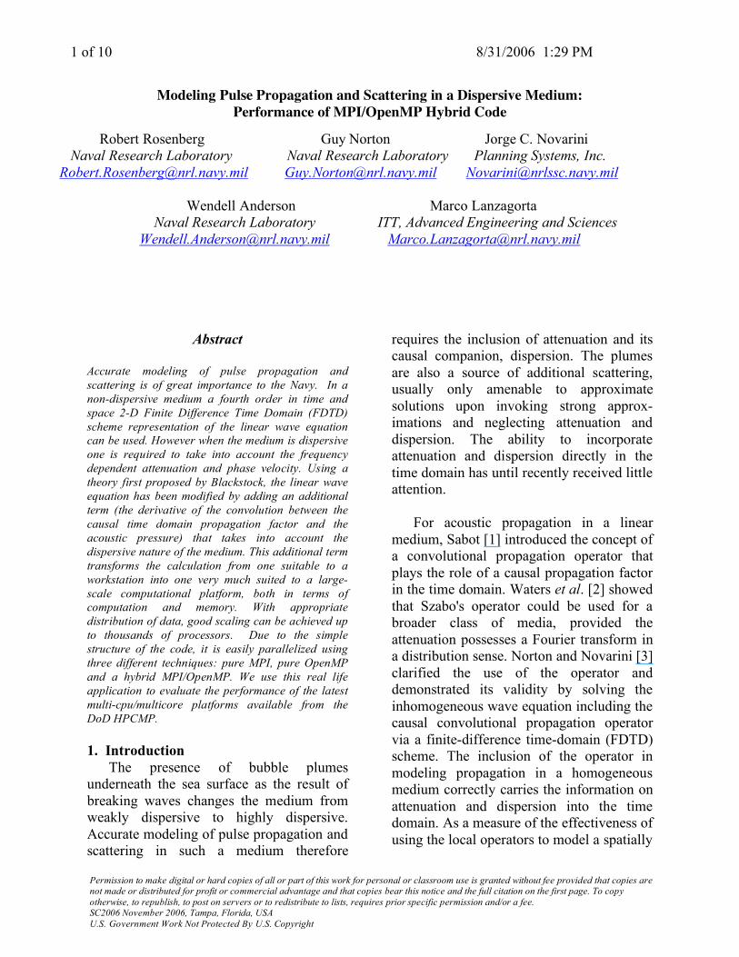
Figure 1 sketches the basic geometry of the simulated experiment. The upper medium is assumed to be air. A pressure released rough surface separates the air from the water. The composite bubble cloud consists of two classifications of bubble plumes. The so-called gamma plume (void fraction between 10-7 and 10-6) is the larger cloud spanning 13.75m at the top and 1m at the bottom. The smaller beta plume (between 10-4 and 10-3) is 3.4m at the top and 0.2 m at the bottom. Attenuation and dispersion are strong for the beta plume and weaker for the gamma plume. The broadband source signal is a doublet with location at a range of 5m and depth 15m. The time step is 3.051758x10⁻⁶ seconds.
The computational domain is a 2000 by
2000 2D grid. The composite bubble cloud occupies 176,726 grid points.
0 5 10 15 20
20
15
10
5
0
Range (m)
Composite Bubble Cloud
Air
Water
Source/Receiver
Figure 1: Geometry for the numerical experiments.
The computation is governed by a
modified wave equation appropriate for an isotropic lossy linear medium:
!2p r, t( ) "
1
c0
2
#2 p r ,t( )
#t2
"1
c0
L$ t( ) % p r, t( ) = & r " rs( )s t( )
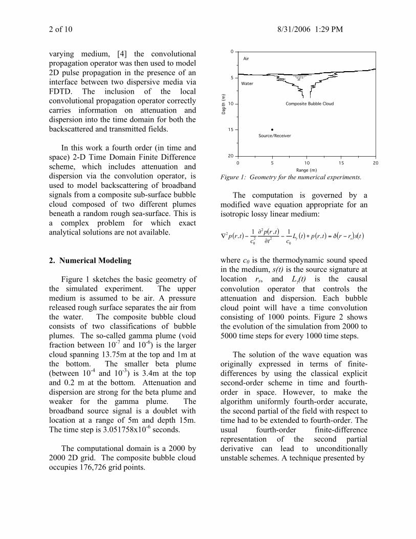
where c0 is the thermodynamic sound speed in the medium, s(t) is the source signature at location rs, and Lγ(t) is the causal convolution operator that controls the attenuation and dispersion. Each bubble cloud point will have a time convolution consisting of 1000 points. Figure 2 shows the evolution of the simulation from 2000 to 5000 time steps for every 1000 time steps.
The solution of the wave equation was originally expressed in terms of finite-differences by using the classical explicit second-order scheme in time and fourth-order in space. However, to make the algorithm uniformly fourth-order accurate, the second partial of the field with respect to time had to be extended to fourth-order. The usual fourth-order finite-difference representation of the second partial derivative can lead to unconditionally unstable schemes. A technique presented by
3 of 10 8/31/2006 1:29 PM
Figure 2: Time Evolution of Pulse Propagation. Time steps 2000, 3000, 4000 and 5000 are shown.
Cohen [5] that is based on the "modified equation approach" was used to obtain fourth-order accuracy in time. This technique while improving the accuracy in time preserves the simplicity of the second-order accurate time-step scheme. Absorbing Boundary Conditions (ABC) were imposed at the edges of the numerical grid using the Complementary Operators Method (COM) [6], a differential equation-based ABC. An alternative method is to terminate the grid with the use of an absorbing material, as is done in the Perfectly Matched Layer (PML) method originally proposed by Berenger [7].
The algorithm breaks down into five parts. The first is an initialization (INIT) section followed by a time loop around the other four sections, which include the Finite Difference Time Domain update (FDTD), the convolutional sum (CONV), source integration (SRC) and finally the application of boundary conditions (BOUND).
The INIT section reads in the parameters
for the simulation, including the data for the phase constants for the 176,726 grid points that constitute the bubble plumes. Arrays for sound velocity, density and wave number are also set for the complete grid.
The FDTD section advances the
standard part of the wave equation by one time step. It is a doubly nested do-loop with the inner loop over the x “range” positions and the outer loop over the z “depth” positions.
The CONV section applies a
convolution sum to the bubble plume grid points to account for the attenuation and dispersion interactions with the source pulse. The convolution is taken over 1000 time steps and a separate array is used to store the wave function values for every bubble plume grid point for the last 1000 time steps.
4 of 10 8/31/2006 1:29 PM
The convolution sum must be calculated for each grid point in the bubble plumes
The SRC and BOUND sections
affect a limited number of grid points and thus only account for a fraction of a percent of the elapsed CPU time. The SRC section propagates the source pulse and the BOUND section applies the absorbing boundary conditions. 3. DoD HPCMP Platforms Here we describe two of the Naval Reserach Laboratory’s (NRL) latest compu-tational platforms. Both platforms can be considered superclusters since they consist of commodity processors with a custom interconnect.[9] They represent very balanced systems compared to typical clusters that employ only commodity interconnects.
The SGI ALTIX consists of 32 “C-Bricks” containing four nodes each with two Intel Itanium II processors for a total of 256 processors. Each processor has 9MB of L3 cache and 8 GB of memory. The processors are connected by SGI’s fast 6.4GB/s cache coherent NUMAlink 4 interconnect fabric with a dual fat tree topology. This fast interconnect allows the Altix, unlike typical Linux clusters, to have a Distributed Shared Memory (DSM) architecture permitting both shared memory and distributed memory applications to be executed across the entire machine. The operating system is a single image OS based on a 64 bit Suse Linux.
The Cray XD1 is the newest NRL
system. It consists of two cabinets with 12 chassis each, each chassis with six blades, each blade with two AMD 275 dual-core Opteron processors for a total of 576 cores. Each core has 1MB of L2 cache and each
node has 2GB of memory. The nodes are connected with a Rapid Array Interconnect (RAI) in a Fat Tree topology at 12.8 GB/s per node.
The XD1 has dual core Opteron
processors. Putting more cores on a chip increases the contention for shared memory. To alleviate this problem, the Opterons processors are connected with a high speed HyperTransport interconnect. Table 1 compares the characteristics of the two NRL platforms.
Clock FP Memory
Bandwidth MPI Latency
MPI Bandwidth
Altix 1.6GHz 4 10.2GB/s per CPU
1.0µs 3.2GB/s
XD1 2.2GHz 2 12.8GB/s per node
1.7µs 2.0GB/s
Table 1: NRL Platform Characteristics. FP indicates the number of floating point operations per cycle and MPI Bandwidth indicates only the one-way rate. Latency is quoted for short messages only.
These latest platforms consist of high bandwidth, low latency interconnects and efficient implementations of MPI, so it is of interest to see how hybrid codes perform on these newer systems. 4. Hybrid Codes
Current high performance computers incorporate multi-CPU or multi-core architectures, which provide a natural programming paradigm for hybrid codes.[10] This new design emphasis has gained popularity due to the cooling problem when increasing the processor clock frequency beyond 4.0GHz[9]. Since the computational performance of a single processor cannot be improved by increasing the clock frequency, architectures have instead been adding more processors to each
5 of 10 8/31/2006 1:29 PM
node, more cores to each chip, or adding computational accelerators such as GPUs or FPGAs.
Much work has been done on
examining the performance of hybrid codes that employ both MPI and OpenMP parallel-ization.[10-17] Applications include bench-mark applications, Computational Fluid Dynamics, Weather modeling and Quantum Monte Carlo. In most cases MPI is considered optimal for coarse grain (or task) parallelism and OpenMP is optimal for fine grain (or data) parallelism.[12] The two types of parallelism often result in quite different performance, with only the former scaling to hundreds of processors. Motivation for constructing a hybrid code is to reduce the point-to-point communication overhead of MPI at the expense of introducing OpenMP overhead due to thread creation and increased contention for shared memory.
The results in the literature have
dealt mostly with benchmark codes like the NAS Parallel Benchmarks[13],[16] or real applications that do not scale well. [10],[12],[13],[15] Poor scaling, i.e., good scaling up to only a small number of processors (less than 64, say) is usually observed in the OpenMP version of the code, where only loop level parallelism is utilized. In order to improve scaling of the OpenMP version, a Single Program Multiple Data (SPMD) programming style must be used - an extreme programming effort, similar to that of converting the original serial code to MPI[16]. Because of the relatively simple structure of the code under consideration, we were able to easily generate the SPMD OpenMP version. Thus, we achieve good scaling in both the MPI and OpenMP.
5. Pure MPI Implementation The FDTD calculation uses a 2D
uniform grid to simulate the ocean, surface and air, with x being the range and z being the depth. Future simulations will employ a 3D model currently still in development. We partition the grid in the z direction only using the 1D MPI_cart_create call without periodicity. Since the FDTD calculation requires two adjacent wave function values in both the x and z direction, we need to include two additional rows, as halo cells, both at the top and bottom, for each processors domain. Communication of the halo cells is performed every time step using MPI_sendrecv calls along with an MPI derived data type for the two halo rows. These messages were of a constant size (independent of the number of processors) of 16KBs. The original implementation used just non-blocking sends and receives, but the MPI_sendrecv call reduced the MPI over-head by an order of magnitude on the XD1.
The CONV calculation is a little
more challenging. Less than 5% of the ocean grid points are involved in the CONV calculation; let us call these bubble points. In order to avoid load imbalance, the bubble points have to be distributed among the processors in a proper fashion. We considered two different ways of doing this distribution.
Minimizing the amount of code
changes motivated our first attempt.[18] Originally, the rows of the computation domain were distributed equally among the processors. However, if we change the row distributions such that each processor has the same amount of work, then we can achieve better load balance. This method achieved very good load balance when we optimized the row distribution. However, we had to optimize the row distribution for
6 of 10 8/31/2006 1:29 PM
every platform since a unit amount work in CONV and FDTD will vary from platform to platform.
The second method simply distributes the bubble points equally among all the processors. Although simple in concept, the recoding effort involved two more MPI communication sections.
For each time step, ocean wave
function values are both sent and received from processor to processor in order to update the bubble point values. After the CONV is finished, the reverse process, sending and receiving bubble point wave function values, is performed in order to update the ocean wave function values where the bubble points reside. We explicitly gather both ocean and bubble points into arrays and then use MPI derived data types to send these arrays. Non-blocking sends and receives along with persistent communication calls are used to transfer the data.
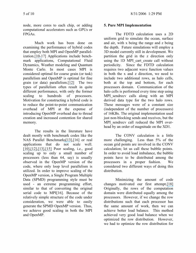
We expect the message sizes to vary
from one processor to another, so we looked at the message size distribution generated from the message sizes that each processor sends and receives. Figure 3 shows the message size distribution for 64 and 384 processors. The message size decreases as
the number of processors increase with the distribution being roughly uniform between the minimum and maximum sizes for that processor count.
An attempt was made to overlap
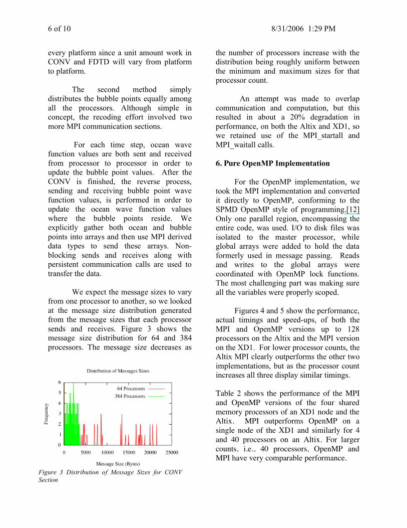
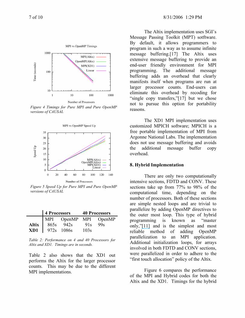
communication and computation, but this resulted in about a 20% degradation in performance, on both the Altix and XD1, so we retained use of the MPI_startall and MPI_waitall calls. 6. Pure OpenMP Implementation For the OpenMP implementation, we took the MPI implementation and converted it directly to OpenMP, conforming to the SPMD OpenMP style of programming.[12] Only one parallel region, encompassing the entire code, was used. I/O to disk files was isolated to the master processor, while global arrays were added to hold the data formerly used in message passing. Reads and writes to the global arrays were coordinated with OpenMP lock functions. The most challenging part was making sure all the variables were properly scoped. Figures 4 and 5 show the performance, actual timings and speed-ups, of both the MPI and OpenMP versions up to 128 processors on the Altix and the MPI version on the XD1. For lower processor counts, the Altix MPI clearly outperforms the other two implementations, but as the processor count increases all three display similar timings. Table 2 shows the performance of the MPI and OpenMP versions of the four shared memory processors of an XD1 node and the Altix. MPI outperforms OpenMP on a single node of the XD1 and similarly for 4 and 40 processors on an Altix. For larger counts, i.e., 40 processors, OpenMP and MPI have very comparable performance.
Figure 3 Distribution of Message Sizes for CONV Section
7 of 10 8/31/2006 1:29 PM
4 Processors 40 Processors MPI OpenMP MPI OpenMP Altix 865s 942s 91s 99s XD1 972s 1086s 103s Table 2: Performance on 4 and 40 Processors for Altix and XD1. Timings are in seconds. Table 2 also shows that the XD1 out performs the Altix for the larger processor counts. This may be due to the different MPI implementations.
The Altix implementation uses SGI’s Message Passing Toolkit (MPT) sotftware. By default, it allows programmers to program in such a way as to assume infinite message buffering.[17] The Altix uses extensive message buffering to provide an end-user friendly environment for MPI programming. The additional message buffering adds an overhead that clearly manifests itself when programs are run at larger processor counts. End-users can eliminate this overhead by recoding for “single copy transfers,”[17] but we chose not to pursue this option for portability reasons.
The XD1 MPI implementation uses
customized MPICH software; MPICH is a free portable implementation of MPI from Argonne National Labs. The implementation does not use message buffering and avoids the additional message buffer copy overhead. 8. Hybrid Implementation
There are only two computationally intensive sections, FDTD and CONV. These sections take up from 77% to 98% of the computational time, depending on the number of processors. Both of these sections are simple nested loops and are trivial to parallelize by adding OpenMP directives to the outer most loop. This type of hybrid programming is known as “master only,”[11] and is the simplest and most reliable method of adding OpenMP parallelization to an MPI application. Additional initialization loops, for arrays involved in both FDTD and CONV sections, were parallelized in order to adhere to the “first touch allocation” policy of the Altix.
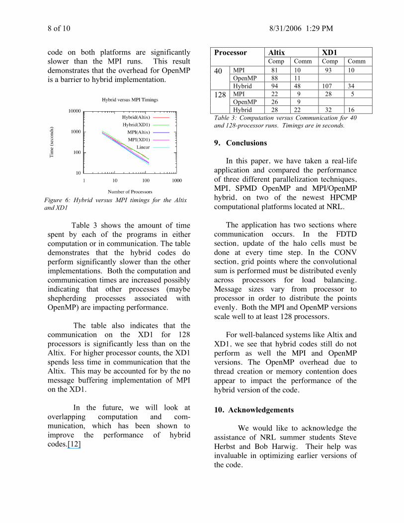
Figure 6 compares the performance
of the MPI and Hybrid codes for both the Altix and the XD1. Timings for the hybrid
Figure 5 Speed Up for Pure MPI and Pure OpenMP versions of CAUSAL
Figure 4 Timings for Pure MPI and Pure OpenMP versions of CAUSAL
8 of 10 8/31/2006 1:29 PM
code on both platforms are significantly slower than the MPI runs. This result demonstrates that the overhead for OpenMP is a barrier to hybrid implementation.
Table 3 shows the amount of time
spent by each of the programs in either computation or in communication. The table demonstrates that the hybrid codes do perform significantly slower than the other implementations. Both the computation and communication times are increased possibly indicating that other processes (maybe shepherding processes associated with OpenMP) are impacting performance.
The table also indicates that the
communication on the XD1 for 128 processors is significantly less than on the Altix. For higher processor counts, the XD1 spends less time in communication that the Altix. This may be accounted for by the no message buffering implementation of MPI on the XD1.
In the future, we will look at
overlapping computation and com-munication, which has been shown to improve the performance of hybrid codes.[12]
Altix XD1 Processor Count Comp Comm Comp Comm
MPI 81 10 93 10 OpenMP 88 11
40
Hybrid 94 48 107 34 MPI 22 9 28 5 OpenMP 26 9
128
Hybrid 28 22 32 16 Table 3: Computation versus Communication for 40 and 128-processor runs. Timings are in seconds. 9. Conclusions
In this paper, we have taken a real-life application and compared the performance of three different parallelization techniques, MPI, SPMD OpenMP and MPI/OpenMP hybrid, on two of the newest HPCMP computational platforms located at NRL.
The application has two sections where
communication occurs. In the FDTD section, update of the halo cells must be done at every time step. In the CONV section, grid points where the convolutional sum is performed must be distributed evenly across processors for load balancing. Message sizes vary from processor to processor in order to distribute the points evenly. Both the MPI and OpenMP versions scale well to at least 128 processors.
For well-balanced systems like Altix and
XD1, we see that hybrid codes still do not perform as well the MPI and OpenMP versions. The OpenMP overhead due to thread creation or memory contention does appear to impact the performance of the hybrid version of the code. 10. Acknowledgements
We would like to acknowledge the
assistance of NRL summer students Steve Herbst and Bob Harwig. Their help was invaluable in optimizing earlier versions of the code.
Figure 6: Hybrid versus MPI timings for the Altix and XD1
9 of 10 8/31/2006 1:29 PM
11. References
[1] T. L. Szabo, "Time domain wave equations for lossy media obeying a frequency power law," J. Acoust. Soc. Am, 96,pp. 491-500, 1994.
[2] K. R. Waters, M. S. Hughes, G. H. Brandenburger, and J. G. Miller, "On a time-domain representation of the Kramers-Kronig dispersion relations," J. Acoust. Soc. Am. 108, pp. 2114-2119, 2000.
[3] G. V. Norton and J. C. Novarini, "Including dispersion and attenuation directly in the time domain for wave propagation in isotropic media," J. Acoust. Soc. Am. 113, pp. 3024-3031, 2003.
[4] G. V. Norton and J. C. Novarini, "Including dispersion and attenuation in time domain modelling of pulse propagation in spatially-varying media," accepted for publication in J. Comp. Acoust.
[5] G. Cohen, Higher-Order Numerical Methods for Transient Wave Equations, Springer, pp. 35-63, 2001.
[6] J. B. Schneider and O. M. Ramahi, "The complementary operators method applied to acoustic finite-difference time-domain simulations," J. Acoust. Soc. Am., 104, pp. 686-693, 1998.
[7] J. P. Berenger, "A perfectly matched layer for the absorption of electromagnetic waves," J. Comput. Phys., 114, pp. 185-200, 1994.
[8] G. V. Norton, W. Anderson, J. C. Novarini, R. Rosenberg and M. Lanzagorta, “Modelling Pulse Propagation and Scattering in a Dispersive Medium using the Cray MTA-2,” Cray Users Group Conference Proceedings, Albuquerque, NM, 2005.
[9] J. Dongarra, “Self-Adapting Numerical Software (SANS) – Effort and Fault Tolerance in Linear Algebra Algorithms,” Sixth International Conference on Parallel Processing and Applied Mathematics, Poznan, Poland, September 11-14, 2005.
[10] G. Mahinthakumar, F. Saied, "A Hybrid MPI-OpenMP Implementation of an Implicit Finite Element Code on Parallel Architectures," International Journal of High Performance Computing Applications, Vol. 16, No. 4, 371-393 (2002)
[11] Rolf Rabenseifner and Gerhard Wellein, Comparison of Parallel Programming Models on Clusters of SMP Nodes. In Modelling, Simulation and Optimization of Complex Processes (Proceedings of the International Conference on High Performance Scientific Computing, March 10-14, 2003, Hanoi, Vietnam) Bock, H.G.; Kostina, E.; Phu, H.X.; Rannacher, R. (Eds.), pp 409-426, Springer, 2004.
[12] Y. He and C. Ding, Hybrid OpenMP and MPI Programming and Tuning. 2004 NERSC User Group (NUG) Meeting, Berkeley, CA, June 2004.
[13] G. Jost, H. Jin, D. an Mey and F.F. Hatay, Comparing OpenMP, MPI, and Hybrid Programming Paradigms on an SMP Cluster, NAS Technical Report NAS-03-019, November 2003.
[14] D.K. Kaushik, D.E. Keyes, W.D. Gropp and B.F. Smith, Understanding the Performance of Hybrid (distributed / shared memory) Programming Model, Spring 2001 Seminar, Department of Compute Science, Old Dominion University, USA, Feb 8, 2001.
[15] L. Smith and M. Bull, Development of mixed mode MPI/OpenMP
10 of 10 8/31/2006 1:29 PM
applications, Scientific Programming 9, (2001) 83-98.
[16] S. Fulcomer, Hybrid Programming, Brown CCV Parallel Programming Workshop, Spring 2005.
[17] J. Boney, J.Wilson, S. Levine, Message Passing Toolkit: MPI Programmer’s Manual, SGI Ed.: S. Wilkening, Document Number:007-3687-010, 1996,1998-2003.
[18] G.V. Norton, J.C. Novarini, W. Anderson, R. Rosenberg and M. Lanzagorta, Modeling Pulse Propa-gation and Scattering in a Dispersive Medium, Proceedings of the HPCMP Users Group Conference 2005, Nash-ville, TN June 27-30, 2005, pp. 52-57.