parallelization of dira and ctmod using openmp and opencl
TRANSCRIPT
Institutionen för systemteknik
Department of Electrical Engineering
Examensarbete
Parallelization of DIRA and CTmod
using OpenMP and OpenCL
Master thesis performed in Information Coding
by
Alexander Örtenberg
LiTH-ISY-EX--15/4834--SE Linköping 2015
TEKNISKA HÖGSKOLAN
LINKÖPINGS UNIVERSITET
Department of Electrical Engineering
Linköping University
S-581 83 Linköping, Sweden
Linköpings tekniska högskola
Institutionen för systemteknik
581 83 Linköping


Parallelization of DIRA and CTmod
using OpenMP and OpenCL
Master thesis in Information Coding
at Linköping Institute of Technology
by
Alexander Örtenberg
LiTH-ISY-EX--15/4834--SE
Supervisor: Alexandr Malusek
IMH, Linköping Universitet
Jens Ogniewski
ISY, Linköpings Universitet
Examiner: Ingemar Ragnemalm
ISY, Linköpings Universitet
Linköping 2015-06-11


Presentation Date
2015-06-01
Publishing Date (Electronic version)
2015-06-11
Department and Division
Department of Electrical Engineering
URL, Electronic Version http://www.ep.liu.se
Publication Title
Parallelization of DIRA and CTmod using OpenMP and OpenCL
Author(s)
Alexander Örtenberg
Abstract
Parallelization is the answer to the ever-growing demands of computing power by taking advantage of multi-core
processor technology and modern many-core graphics compute units. Multi-core CPUs and many-core GPUs
have the potential to substantially reduce the execution time of a program but it is often a challenging task to
ensure that all available hardware is utilized. OpenMP and OpenCL are two parallel programming frameworks
that have been developed to allow programmers to focus on high-level parallelism rather than dealing with low-
level thread creation and management. This thesis applies these frameworks to the area of computed tomography
by parallelizing the image reconstruction algorithm DIRA and the photon transport simulation toolkit CTmod.
DIRA is a model-based iterative reconstruction algorithm in dual-energy computed tomography, which has the
potential to improve the accuracy of dose planning in radiation therapy. CTmod is a toolkit for simulating
primary and scatter projections in computed tomography to optimize scanner design and image reconstruction
algorithms. The results presented in this thesis show that parallelization combined with computational
optimization substantially decreased execution times of these codes. For DIRA the execution time was reduced
from two minutes to just eight seconds when using four iterations and a 16-core CPU so a speedup of 15 was
achieved. CTmod produced similar results with a speedup of 14 when using a 16-core CPU. The results also
showed that for these particular problems GPU computing was not the best solution.
Number of pages: 56
Keywords
Parallelization, OpenMP, OpenCL, Computed Tomography, Iterative Reconstruction
Language
X English
Other (specify below)
Number of Pages
56
Type of Publication
Licentiate thesis
X Degree thesis
Thesis C-level
Thesis D-level
Report
Other (specify below)
ISBN (Licentiate thesis)
ISRN: LiTH-ISY-EX--15/4834--SE
Title of series (Licentiate thesis)
Series number/ISSN (Licentiate thesis)


1
ABSTRACT
Parallelization is the answer to the ever-growing demands of computing power by
taking advantage of multi-core processor technology and modern many-core graphics
compute units. Multi-core CPUs and many-core GPUs have the potential to
substantially reduce the execution time of a program but it is often a challenging task to
ensure that all available hardware is utilized. OpenMP and OpenCL are two parallel
programming frameworks that have been developed to allow programmers to focus on
high-level parallelism rather than dealing with low-level thread creation and
management. This thesis applies these frameworks to the area of computed tomography
by parallelizing the image reconstruction algorithm DIRA and the photon transport
simulation toolkit CTmod. DIRA is a model-based iterative reconstruction algorithm in
dual-energy computed tomography, which has the potential to improve the accuracy of
dose planning in radiation therapy. CTmod is a toolkit for simulating primary and
scatter projections in computed tomography to optimize scanner design and image
reconstruction algorithms. The results presented in this thesis show that parallelization
combined with computational optimization substantially decreased execution times of
these codes. For DIRA the execution time was reduced from two minutes to just eight
seconds when using four iterations and a 16-core CPU so a speedup of 15 was achieved.
CTmod produced similar results with a speedup of 14 when using a 16-core CPU. The
results also showed that for these particular problems GPU computing was not the best
solution.

2
ACKNOWLEDGEMENT
I would like to start by thanking my examiner Ingemar Ragnemalm and my supervisor
Jens Ogniewski for their time and advice during this project. A great thanks to Alexandr
Malusek for making this project possible and supplying me with everything I needed to
complete it; hardware, software, advice, comments and guidance. Thanks to the people
at Radiofysik for a fun and welcoming place to work on my thesis.
I would also like to thank NSC, the National Supercomputer Centre at Linköping
University, for providing scalable hardware on which I could test the performance of
DIRA and CTmod. Thanks to Peter Kjellström for helping me with the Intel Xeon Phi
architecture and trying to compile the ROOT toolkit, and Peter Münger for setting up
the project at NSC. Finally I would like to thank Maria Magnusson for having the
patience to explain DIRA and its components as well as suggesting alternative methods
to use.
To my parents, for their never-ending support: Thank you.

3
TABLE OF CONTENTS
1. INTRODUCTION 5
1.1. Purpose and goal 6
1.2. Related work 6
2. BACKGROUND 9
2.1. Processor Concepts and Parallelization 9
2.1.1. Multi-core 9
2.1.2. Cache 9
2.1.3. Pipeline and branching 10
2.1.4. Parallelization 10
2.1.5. Synchronization 11
2.1.6. Speedup 12
2.1.7. OpenMP 13
2.1.8. OpenCL 15
2.1.9. GPU Architecture 17
2.1.10. Xeon Phi 19
2.2. Principles of Computed Tomography 20
2.2.1. Photon Interactions 20
2.2.2. Computed Tomography 21
2.3. DIRA 23
2.3.1. Filtered backprojection 24
2.3.2. Material Decomposition 24
2.3.3. Forward projection 25
2.3.4. Polychromatic projections 27
2.4. CTmod 27
3. METHODS 29
3.1. Hardware 29
3.2. DIRA 29
3.2.1. Filtered backprojection 31
3.2.2. Material decomposition 32
3.2.3. Forward projection 32
3.2.4. Polychromatic projections 33
4
3.3. CTmod 34
4. RESULTS 35
4.1. DIRA 35
4.1.1. Filtered backprojection 38
4.1.2. Material Decomposition 38
4.1.3. Forward projection 39
4.1.4. Polychromatic projections 40
4.1.5. Platform performance 41
4.2. CTmod 41
5. DISCUSSION 43
5.1. DIRA 43
5.1.1. Code management 43
5.1.2. Filtered backprojection 44
5.1.3. Material decomposition 44
5.1.4. Forward projection 45
5.2. CTmod 46
BIBLIOGRAPHY 49
APPENDIX A 53
1. Polychromatic Projections – MATLAB 53
2. Polychromatic Projections – C 54
3. Polychromatic Projections – C with OpenMP 55
4. Polychromatic Projections – OpenCL 56

5
1. INTRODUCTION
Parallelization is the next step in keeping up with the ever-growing need for additional
computational power. The single processor system is no longer able to provide the
performance required due to limitations in clock speed, caused by power and heat
problems, the restricted instruction-level parallelism available and memory access
bottlenecks. The limitations of the single processor system lead to the introduction of
multi- and many-core systems, but they require software developers to explicitly write
programs with parallelization in mind to fully utilize all cores. To aid the developers a
set of parallel paradigms have evolved that provide simple and easy to use methods for
unlocking the powers of parallelization by abstracting the tedious tasks of low-level
thread and core management. In this thesis two of these paradigms, Open
MultiProcessing (OpenMP) and Open Computing Language (OpenCL), are used to
parallelize codes in the area of computed tomography. In this area there are still many
codes that have not yet been parallelized to take advantage of the additional computing
power provided by multi-core processors and many-core graphics processing units,
leading to unnecessarily long execution times, making the user pointlessly wait for
results. Some of these codes include, but are not limited to, the iterative reconstruction
algorithm DIRA and the CTmod toolkit.
Using dual-energy CT (DECT) instead of single-energy CT has the potential to improve
quantitative tissue classification by providing additional information of the scanned
object and improve dose planning accuracy in radiation treatment. There are still
problems with beam hardening and scatter artifacts in the reconstructed images altering
the CT values, causing the tissue classification to incorrectly decompose the image. This
can for example result in bone tissue being classified as soft tissue, such as protein or
fat. A new method, DECT Iterative Reconstruction Algorithm (DIRA), has been
developed in Linköping and has the potential to remove the beam hardening artifacts
while keeping the CT numbers intact.
Photons that have not interacted inside a phantom carry useful information to the
detector array, but the scattering of photons causes scatter artifacts, visible as cupping or
streaks when reconstructing images. The scattering of photons is especially strong in
cone beam CT as the amount of scatter is dependent on the beam width, where a wider
beam increases the scatter. Other factors playing a role in the scattering are the tube
voltage, the size of the phantom, the usage of collimators and bowtie filters as well as
the detector array setup. The ability to study how these factors affect the projections is
helpful in the optimization of image reconstruction algorithms and CT scanner design.
The simulation toolkit CTmod, written in C++ and based on the analysis framework
ROOT [1] by CERN, was developed to calculate scatter projections using the Monte
Carlo method. Many of the toolkit’s features are not readily available in general purpose
Monte Carlo codes like Geant4, MCNP and FLUKA.

6
1.1. PURPOSE AND GOAL
The purpose of this thesis is to improve the execution times of DIRA and CTmod by
taking advantage of the multiple cores provided by modern CPUs and many cores by
modern GPUs using the frameworks OpenMP and OpenCL. The single-threaded
execution time of DIRA is in the range of several minutes per slice, depending on the
hardware used and the number of iterations the algorithm performs. Some diagnostic
protocols use volumetric scans consisting of tens or hundreds of slices [2]. These would
require hours of computation to complete.
The execution time of CTmod is dependent on the configuration chosen, where the
number of photon histories to simulate, the complexity of the geometry and the detector
array setup are all factors. A single-threaded simulation can take hours to complete.
Parallelization would open up new possibilities regarding the complexity of simulation,
application of the code in clinical practice and execution on new hardware architectures,
such as Intel Xeon Phi [3].
There are alternative frameworks available for writing parallel programs such as
Message Passing Interface, MPI [4], for CPUs and Compute Unified Device
Architecture, CUDA [5], for GPUs. For parallelization on the CPU the choice was made
to use OpenMP instead of MPI as the utilization of a distributed memory system was
not required. For GPU parallelization there are two alternatives, OpenCL and CUDA.
CUDA is developed and maintained by NVIDIA and as such can only be used on their
GPUs. OpenCL does not have the same restriction and can run on a wider range of both
CPU and GPU architectures so in order to make the parallelization as general as
possible the choice was made to use OpenCL.
1.2. RELATED WORK
DIRA’s approach to image reconstruction has been unique till 2014 and so there is little
possibility to compare it with competing projects. More is known about parallelization
of other image reconstruction algorithms like the filtered backprojection or noise-
suppressing iterative image algorithms, for example described in [6]. Any comparison
is, however, complicated by the fact that vendors often do not disclose implementation
details of their algorithms.
There are several codes that can simulate CT scanners. Some of them are specialized,
like GATE, MCGPU and CTsim, others are just adaptations of general-purpose MC
codes like MCNPX, EGSnrc and FLUKA. As those codes typically simulate very many
independent particle histories, their parallelization can be done by splitting the
simulation to several smaller jobs, where each job simulates a subset of the histories.
Results from these jobs are then summarized by a master process. Implementation
details of such solutions are listed below for several selected codes. The open source
software GATE (Geant4 Application for Tomographic Emission) [7] supports
simulations of Computed Tomography, Radiotherapy, PET (Positron Emitted
Tomography) and SPECT (Single Photon Emission Computed Tomography)
experiments. GATE uses a parallel computing platform to run simulations in a cluster to
7
shorten the setup time and provide fast data output handling. It also supports CUDA for
PET and CT applications. GATE is an extension of Geant4 [8], a toolkit for the
simulation of the passage of particles through matter. Geant4 includes facilities for
handling geometry, tracking, detector response, run management, visualization and user
interface. The parallel implementation ParGATE, using MPI, achieved a speedup of 170
with 100 workers. The superlinear speedup occurred due to inefficiencies in the
sequential program caused by the overhead of writing large files [9].
MCNPX (Monte Carlo N-Particle eXtended) [10] is a general-purpose Monte Carlo
radiation transport code. It can simulate 34 particle types (including nucleons and light
ions) at almost all energies. It uses the MPI library [4] to allow for parallel processing.
According to [11] a speedup of 11 was possible to achieve with 31 cores.
The code MCGPU is a massively multi-threaded GPU-accelerated x-ray transport
simulation code that can generate radiographic projection images and CT scans of the
human anatomy [12]. It uses the CUDA [5] library to execute the simulations in parallel
on NVIDIA GPUs. It also uses the MPI library to allow for execution on multiple
GPUs. The code is in the public domain and developed by the U. S. Food and Drug
Administration (FDA). Evaluation showed that MCGPU on a NVIDIA C2070 GPU
achieved a speedup of 6 compared to a quad-core Xeon processor [13].

8

9
2. BACKGROUND
This section serves as an introduction to (i) processor architecture, (ii) parallelization,
and (iii) physics and algorithms of computed tomography. It also briefly describes the
OpenMP and OpenCL frameworks for parallelization of programs, and how the
performance improvement of parallelization is measured. The GPU architecture is
shortly described and the new Xeon Phi architecture is introduced.
2.1. PROCESSOR CONCEPTS AND PARALLELIZATION
2.1.1. MULTI-CORE
A core refers to a processing unit capable of reading and executing program
instructions, such as addition, subtraction, multiplication and conditional statements
(also known as if-then-else statements). A multi-core processor is a single computing
component with two or more independent processing units (cores). The term multi-core
refers to multi-core CPUs, other hardware architectures such as the GPU or the Intel
Many Integrated Core (MIC), brand name Xeon Phi, are not included. In the beginning
of 2015 a modern desktop CPU typically had 4 cores, while a server CPU from Intel
could have up to 18 cores [14] or 16 cores for AMD [15].
2.1.2. CACHE
The cache is a component acting as a small but fast memory on the CPU, storing data or
instructions. A modern CPU has multiple independent caches, separating the
instructions and the data. The advantage to using a cache is speed; it is able to more
quickly provide the CPU with the instructions to execute as well as fulfill requests for
data, compared to retrieval from main memory. A cache hit refers to the situation when
requested data is available in the cache and a cache miss is the opposite of a hit; the data
is not available in the cache. A cache miss causes a delay as the data is fetched from the
main memory. The execution time of a program is affected by the number of cache hits
as retrieving data from the main memory is much slower. Modern CPUs typically have
three caches named L1, L2 and L3 where each core has individual L1 and L2 but L3 is
shared. L1 is the smallest and fastest cache and is checked first. If there is no hit the L2
is checked and finally the L3 cache is checked. Latencies of the Intel Core i7 Xeon 5500
Series CPU caches for a theoretical CPU clock speed of 2 GHz are in table 1 [16]:
Table 1: CPU cache and main memory latencies in seconds for the Intel® Xeon® Processor 5500 Series with a
CPU clock speed of 2 GHz.
Data source Latency
L1 Cache hit ~4 cycles (2 ns)
L2 Cache hit ~10 cycles (5 ns)
L3 Cache hit ~60 cycles (30 ns)
Local DRAM ~60 ns
According to table 1, a hit in the L1 cache is 30 times faster than a retrieval of data from
the main memory.
10
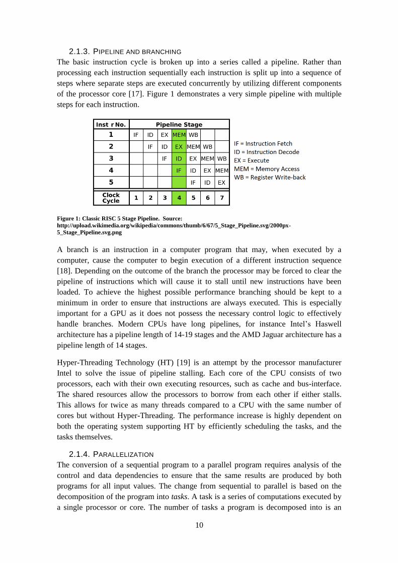
2.1.3. PIPELINE AND BRANCHING
The basic instruction cycle is broken up into a series called a pipeline. Rather than
processing each instruction sequentially each instruction is split up into a sequence of
steps where separate steps are executed concurrently by utilizing different components
of the processor core [17]. Figure 1 demonstrates a very simple pipeline with multiple
steps for each instruction.
Figure 1: Classic RISC 5 Stage Pipeline. Source:
http://upload.wikimedia.org/wikipedia/commons/thumb/6/67/5_Stage_Pipeline.svg/2000px-
5_Stage_Pipeline.svg.png
A branch is an instruction in a computer program that may, when executed by a
computer, cause the computer to begin execution of a different instruction sequence
[18]. Depending on the outcome of the branch the processor may be forced to clear the
pipeline of instructions which will cause it to stall until new instructions have been
loaded. To achieve the highest possible performance branching should be kept to a
minimum in order to ensure that instructions are always executed. This is especially
important for a GPU as it does not possess the necessary control logic to effectively
handle branches. Modern CPUs have long pipelines, for instance Intel’s Haswell
architecture has a pipeline length of 14-19 stages and the AMD Jaguar architecture has a
pipeline length of 14 stages.
Hyper-Threading Technology (HT) [19] is an attempt by the processor manufacturer
Intel to solve the issue of pipeline stalling. Each core of the CPU consists of two
processors, each with their own executing resources, such as cache and bus-interface.
The shared resources allow the processors to borrow from each other if either stalls.
This allows for twice as many threads compared to a CPU with the same number of
cores but without Hyper-Threading. The performance increase is highly dependent on
both the operating system supporting HT by efficiently scheduling the tasks, and the
tasks themselves.
2.1.4. PARALLELIZATION
The conversion of a sequential program to a parallel program requires analysis of the
control and data dependencies to ensure that the same results are produced by both
programs for all input values. The change from sequential to parallel is based on the
decomposition of the program into tasks. A task is a series of computations executed by
a single processor or core. The number of tasks a program is decomposed into is an
11
upper limit on the level of parallelism possible and the number of cores that can be
utilized. The goal of the decomposition is to create enough tasks so that (i) all available
cores are kept busy and (ii) the computational part large is enough that the execution
time is long compared to the time required to schedule and map the tasks to different
processors. For example, assume we want to apply a function f() for every element in a
matrix A of size M×N. If the operations the function performs are independent for every
element in the matrix, then a maximum of M×N tasks can be created. But the
computational complexity of f() might be low and it is more efficient to only create M
tasks to reduce the time for scheduling and mapping of the tasks to the processors.
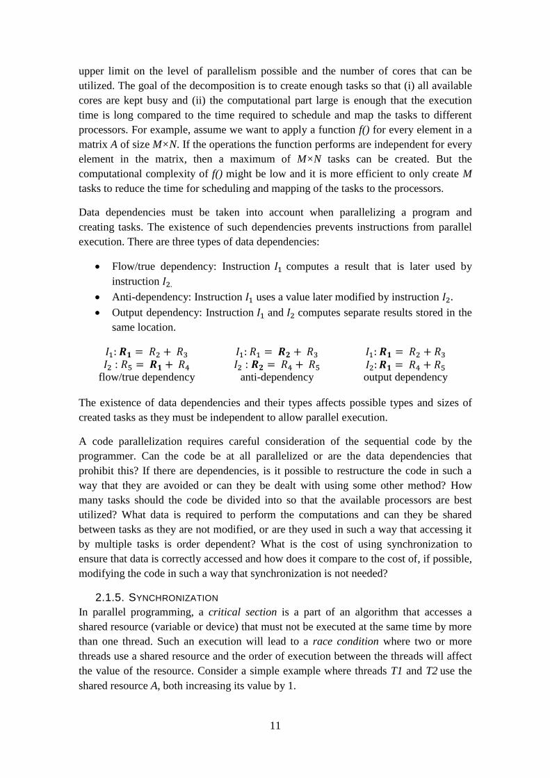
Data dependencies must be taken into account when parallelizing a program and
creating tasks. The existence of such dependencies prevents instructions from parallel
execution. There are three types of data dependencies:
Flow/true dependency: Instruction 𝐼1 computes a result that is later used by
instruction 𝐼2.
Anti-dependency: Instruction 𝐼1 uses a value later modified by instruction 𝐼2.
Output dependency: Instruction 𝐼1 and 𝐼2 computes separate results stored in the
same location.
𝐼1: 𝑹𝟏 = 𝑅2 + 𝑅3
𝐼2 : 𝑅5 = 𝑹𝟏 + 𝑅4
flow/true dependency
𝐼1: 𝑅1 = 𝑹𝟐 + 𝑅3
𝐼2 : 𝑹𝟐 = 𝑅4 + 𝑅5
anti-dependency
𝐼1: 𝑹𝟏 = 𝑅2 + 𝑅3
𝐼2: 𝑹𝟏 = 𝑅4 + 𝑅5 output dependency
The existence of data dependencies and their types affects possible types and sizes of
created tasks as they must be independent to allow parallel execution.
A code parallelization requires careful consideration of the sequential code by the
programmer. Can the code be at all parallelized or are the data dependencies that
prohibit this? If there are dependencies, is it possible to restructure the code in such a
way that they are avoided or can they be dealt with using some other method? How
many tasks should the code be divided into so that the available processors are best
utilized? What data is required to perform the computations and can they be shared
between tasks as they are not modified, or are they used in such a way that accessing it
by multiple tasks is order dependent? What is the cost of using synchronization to
ensure that data is correctly accessed and how does it compare to the cost of, if possible,
modifying the code in such a way that synchronization is not needed?
2.1.5. SYNCHRONIZATION
In parallel programming, a critical section is a part of an algorithm that accesses a
shared resource (variable or device) that must not be executed at the same time by more
than one thread. Such an execution will lead to a race condition where two or more
threads use a shared resource and the order of execution between the threads will affect
the value of the resource. Consider a simple example where threads T1 and T2 use the
shared resource A, both increasing its value by 1.

12
Value of A T1 T2 Value of A T1 T2
A = 0 Read A A = 0 Read A
A = 0 A = A + 1 A = 0 Read A
A = 1 Write A A = 0 A = A + 1
A = 1 Read A A = 0 A = A + 1
A = 1 A = A + 1 A = 1 Write A
A = 2 Write A A = 1 Write A
In the two examples the value of 𝐴 differs due to the different execution orders for
threads T1 and T2. To ensure that the shared resource is not accessed by multiple
threads at the same time, mutual exclusion must be guaranteed. The most common way
to do this is by using a lock, a shared object that provide two operations: acquire_lock()
and release_lock(). The lock can have two values, free and locked where the initial
value of the lock is free. To enter a critical section the thread must first acquire the lock
by testing its value. If it is free then the lock can be taken by the thread, which updates
the value of the lock to locked. If the lock is already taken by another thread it must wait
until the value of the lock is set to free by that thread. When the lock is acquired by the
thread it can enter the critical section and release the lock after finishing execution of
the critical section [20].
2.1.6. SPEEDUP
The benefits of parallelism are measured by comparing the execution time of a
sequential implementation of program to its parallel counterpart. The comparison is
often based on the relative change in execution time, expressed as speedup. The
speedup 𝑆𝑝(𝑛) of a parallel program with parallel execution time 𝑇𝑝(𝑛) is defined as
𝑆𝑝(𝑛) =
𝑇∗(𝑛)
𝑇𝑝(𝑛) ,
(2.1)
where 𝑝 is the number of processors used to solve a problem of size 𝑛 and 𝑇∗(𝑛) is the
execution time of the best sequential implementation. Due to difficulties in determining
and implementing the best sequential algorithm, the speedup is often computed by using
the sequential version of the parallel implementation.
It is possible for an algorithm to achieve super-linear speedup, where 𝑆𝑝(𝑛) > 𝑝. This
is often caused by cache effects: A single processor might not fit the entire data set into
its local cache and thus cache misses will appear during the computation. The data set
can be split into fractions when using multiple processors and each fraction might fit
into the local cache of each processor, thereby avoiding cache misses. Super-linear
speedup is very rare and it is unlikely that even the ideal speedup (𝑆𝑝(𝑛) = 𝑝) is
achieved. The parallel implementation introduces additional overhead for managing the
parallelism. Synchronization, uneven load balancing and data exchange between
processors are all factors that can add overhead. It could also be that the parallel
program contains parts that have to be executed in sequence due to data dependencies,

13
causing the other processors to wait. If the speedup is linear then it scales with the
number of additional cores used at the same rate: (𝑆𝑝(𝑛) = 𝑘 ∗ 𝑝) where 0 < 𝑘 ≤ 1.
The number of processors is an upper bound for the possible speedup. Data
dependencies leading to sequential execution also limit the degree of parallelism.
Amdahl’s Law describes the speedup when a constant fraction of a parallel program
must be executed sequentially. Denoting the fraction of the sequential execution time 𝑓,
where 0 ≤ 𝑓 ≤ 1, the execution can be divided into two parts, the sequential execution
time 𝑓 ∗ 𝑇∗(𝑛) and the parallel execution time (1−𝑓)
𝑝∗ 𝑇∗(𝑛) where 𝑝 is the number of
processors. The attainable speedup is
𝑆𝑝(𝑛) =
𝑇∗(𝑛)
𝑓 × 𝑇∗(𝑛) +(1 − 𝑓)𝑝 × 𝑇∗(𝑛)
= 1
𝑓 +1 − 𝑓𝑝
≤1
𝑓.
(2.2)
As an example, assume that 10% of a program must be executed sequentially. This
gives 𝑓 = 0.1 and 𝑆𝑝(𝑛) ≤ 1
0.1= 10 . No matter the number of processors used, the
speedup cannot be higher than 10 [21].
2.1.7. OPENMP
OpenMP is a specification for a set of compiler directives, library routines, and
environment variables that can be used to specify high-level parallelism in FORTRAN
and C/C++ programs [22]. It is supported by a wide range of compilers, such as GCC
(the GNU Compiler Collection) and ICC (Intel C++ Compiler), and is supported by
most processor architectures and operating systems. It uses a set of preprocessor
directives and keywords to generate multi-threaded code at compile time for a shared
memory system. A short example using some of the OpenMP directives available:
#pragma omp parallel private(thread_id)
{ thread_id = omp_get_thread_num(); printf("thread id: %i \n", thread_id);
#pragma omp for for(i=0;i<X;++i) { a[i] = b[i] + c[i]; } }
#pragma omp indicates that OpenMP should be used for the section. parallel specifies
that the region should be parallelized and for is used to indicate a for-loop. The loop is
split automatically so that each individual thread computes different iterations. The
directive private(thread_id) indicates that the variable thread_id should not be shared
among threads, but a local, private copy needs to be created and allocated for each
thread. The function call to omp_get_thread_num() retrieves the thread’s internal
identification number. Every thread makes its own call to the function printf, each with
a different value for the argument %i, their unique value of thread_id.
14
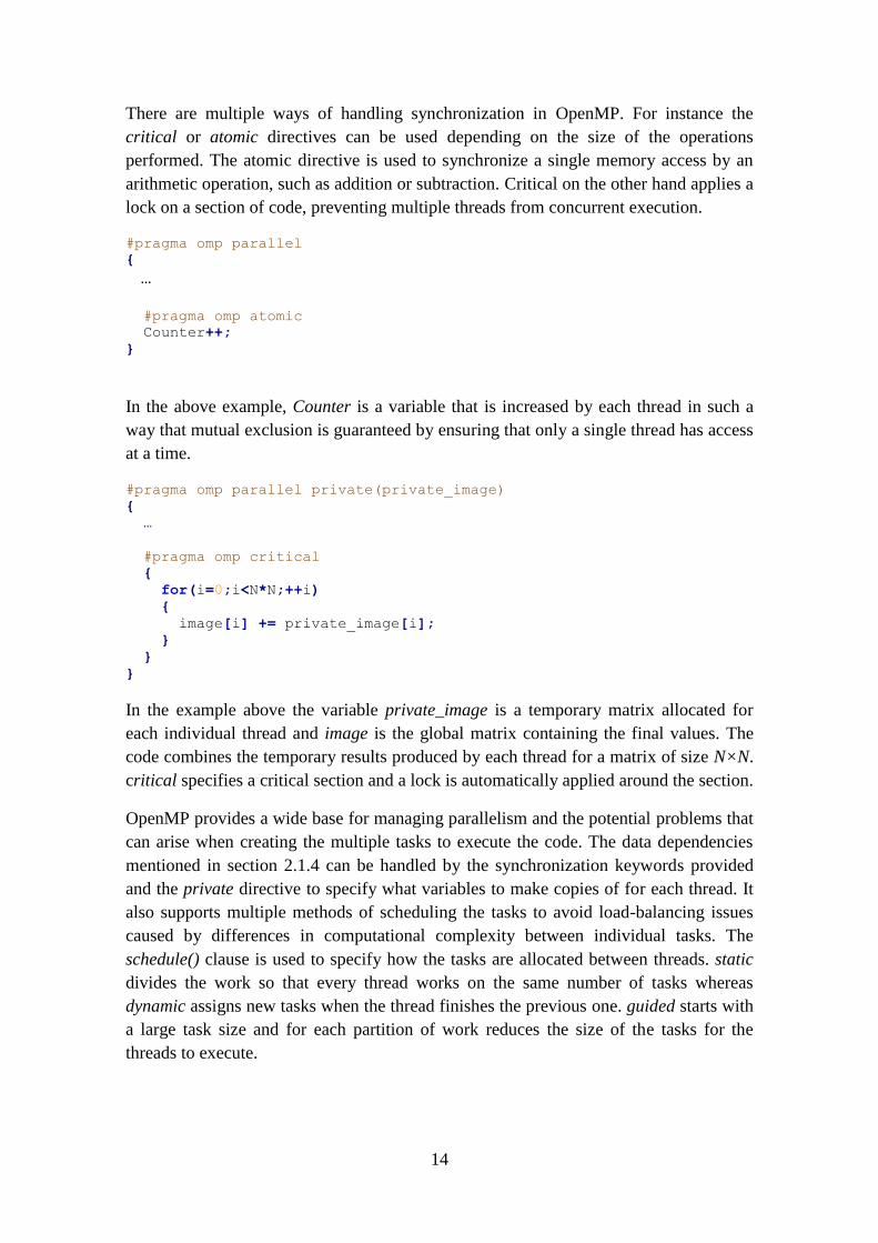
There are multiple ways of handling synchronization in OpenMP. For instance the
critical or atomic directives can be used depending on the size of the operations
performed. The atomic directive is used to synchronize a single memory access by an
arithmetic operation, such as addition or subtraction. Critical on the other hand applies a
lock on a section of code, preventing multiple threads from concurrent execution.
#pragma omp parallel
{
… #pragma omp atomic
Counter++; }
In the above example, Counter is a variable that is increased by each thread in such a
way that mutual exclusion is guaranteed by ensuring that only a single thread has access
at a time.
#pragma omp parallel private(private_image)
{
…
#pragma omp critical
{ for(i=0;i<N*N;++i) { image[i] += private_image[i]; } } }
In the example above the variable private_image is a temporary matrix allocated for
each individual thread and image is the global matrix containing the final values. The
code combines the temporary results produced by each thread for a matrix of size N×N.
critical specifies a critical section and a lock is automatically applied around the section.
OpenMP provides a wide base for managing parallelism and the potential problems that
can arise when creating the multiple tasks to execute the code. The data dependencies
mentioned in section 2.1.4 can be handled by the synchronization keywords provided
and the private directive to specify what variables to make copies of for each thread. It
also supports multiple methods of scheduling the tasks to avoid load-balancing issues
caused by differences in computational complexity between individual tasks. The
schedule() clause is used to specify how the tasks are allocated between threads. static
divides the work so that every thread works on the same number of tasks whereas
dynamic assigns new tasks when the thread finishes the previous one. guided starts with
a large task size and for each partition of work reduces the size of the tasks for the
threads to execute.

15
2.1.8. OPENCL
OpenCL™ is an open, royalty-free standard for cross-platform, parallel programming of
modern processors found in personal computers, servers and handheld/embedded
devices [23]. OpenCL is a framework for parallel programming that allows for
execution on a multitude of different hardware architectures such as AMD, Intel, and
IBM CPUs and AMD, NVIDIA and Qualcomm GPUs. OpenCL executes on devices
consisting of one or more compute unit(s) which in turn is divided into processing
elements, performing the computations. The device executes a kernel by defining
multiple points in an index space and for every point executes an instance of the kernel.
The instance is referred to as a work-item and is identified by its point in the index
space, known as a global id. Work-items are grouped into a work-group. An example of
a simple OpenCL kernel:
__kernel void sum(global int *a, global int *b, global int *c) { int work_item_id = get_global_id(0); a[work_item_id] = b[work_item_id] + c[work_item_id]; }
To calculate the sum of matrices 𝑏 and 𝑐 the work is divided such that a work-item
calculates a single element. The global id is specified outside of the kernel by the host
and each work-item is assigned a unique id.
Figure 2: OpenCL memory architecture. Source:
http://developer.amd.com/wordpress/media/2012/11/Fig1.png
OpenCL uses four different types of memory [24] as seen in figure 2:
1. Global memory: Any work-item can read and write from all elements. (The
slowest to access.)

16
2. Constant memory: A part of the global memory dedicated to data that is only
read.
3. Local memory: A part of memory available only to a specific work-group. (Fast
access.)
4. Private memory: A part of memory available only to a specific work-item. (The
fastest access.)
Global memory should be avoided at all costs due to the high access latency. Storing
data in local or private memory has a much lower latency but the memory’s full
utilization may be difficult because of its small size. According to [25] Appendix D the
total amount of local memory available per compute unit is 256 kB on the AMD
RADEON HD 7000 series. Storing a matrix with the dimensions 512×512 where each
data element is 8 bytes large requires a total of
512 × 512 × 8 𝐵 = 2 097 152 𝐵 = 2 𝑀𝐵
of memory. The matrix cannot be stored in its entirety in the local memory so the global
or constant memory has to be used. To utilize the speed of the local memory a small
part of the matrix can be read at a time and copied to the local memory; these operations
add additional overhead when the many threads read their required data.
An OpenCL code has a different structure compared to an OpenMP code. For OpenCL
the kernel describes what each work-item shall do, whereas for OpenMP the pragmas
and keyword are used to specify how to break down the code into tasks that can be
scheduled on multiple processors. As OpenCL supports both CPU and GPU
architectures, which greatly differ in code execution, additional setup is required in
order to run the code. First, a platform with a device must be specified on which the
code is to be executed. In order to use the device a context must be created to manage (i)
a queue of commands to the device, (ii) memory to and from the kernel, and (iii) the
program and kernel objects for code execution.
The OpenCL kernel uses the C99 standard with some restrictions. There is no support
for classes and templates and dynamic memory allocation is not allowed; it limits the
code that can be written. The focus is on solving a single problem of a known size, not
on flexibility and ability to handle multiple configurations.
17
2.1.9. GPU ARCHITECTURE
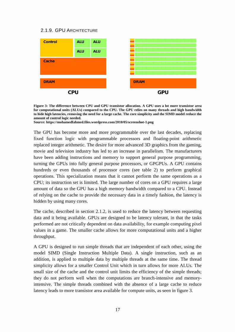
Figure 3: The difference between CPU and GPU transistor allocation. A GPU uses a lot more transistor area
for computational units (ALUs) compared to the CPU. The GPU relies on many threads and high bandwidth
to hide high latencies, removing the need for a large cache. The core simplicity and the SIMD model reduce the
amount of control logic needed.
Source: https://mohamedfahmed.files.wordpress.com/2010/05/screenshot-1.png
The GPU has become more and more programmable over the last decades, replacing
fixed function logic with programmable processors and floating-point arithmetic
replaced integer arithmetic. The desire for more advanced 3D graphics from the gaming,
movie and television industry has led to an increase in parallelism. The manufacturers
have been adding instructions and memory to support general purpose programming,
turning the GPUs into fully general purpose processors, or GPGPUs. A GPU contains
hundreds or even thousands of processor cores (see table 2) to perform graphical
operations. This specialization means that it cannot perform the same operations as a
CPU; its instruction set is limited. The large number of cores on a GPU requires a large
amount of data so the GPU has a high memory bandwidth compared to a CPU. Instead
of relying on the cache to provide the necessary data in a timely fashion, the latency is
hidden by using many cores.
The cache, described in section 2.1.2, is used to reduce the latency between requesting
data and it being available. GPUs are designed to be latency tolerant, in that the tasks
performed are not critically dependent on data availability, for example computing pixel
values in a game. The smaller cache allows for more computational units and a higher
throughput.
A GPU is designed to run simple threads that are independent of each other, using the
model SIMD (Single Instruction Multiple Data). A single instruction, such as an
addition, is applied to multiple data by multiple threads at the same time. The thread
simplicity allows for a smaller Control Unit which in turn allows for more ALUs. The
small size of the cache and the control unit limits the efficiency of the simple threads;
they do not perform well when the computations are branch-intensive and memory-
intensive. The simple threads combined with the absence of a large cache to reduce
latency leads to more transistor area available for compute units, as seen in figure 3.
18
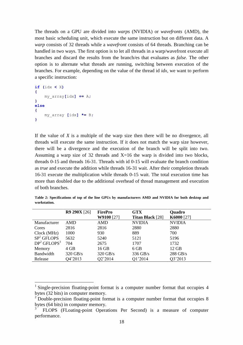
The threads on a GPU are divided into warps (NVIDIA) or wavefronts (AMD), the
most basic scheduling unit, which execute the same instruction but on different data. A
warp consists of 32 threads while a wavefront consists of 64 threads. Branching can be
handled in two ways. The first option is to let all threads in a warp/wavefront execute all
branches and discard the results from the branch/es that evaluates as false. The other
option is to alternate what threads are running, switching between execution of the
branches. For example, depending on the value of the thread id idx, we want to perform
a specific instruction:
if (idx < X) { my_array[idx] += A; } else { my_array [idx] *= B; }
If the value of X is a multiple of the warp size then there will be no divergence, all
threads will execute the same instruction. If it does not match the warp size however,
there will be a divergence and the execution of the branch will be split into two.
Assuming a warp size of 32 threads and X=16 the warp is divided into two blocks,
threads 0-15 and threads 16-31. Threads with id 0-15 will evaluate the branch condition
as true and execute the addition while threads 16-31 wait. After their completion threads
16-31 execute the multiplication while threads 0-15 wait. The total execution time has
more than doubled due to the additional overhead of thread management and execution
of both branches.
Table 2: Specifications of top of the line GPUs by manufacturers AMD and NVIDIA for both desktop and
workstation.
R9 290X [26] FirePro
W9100 [27] GTX
Titan Black [28] Quadro
K6000 [27]
Manufacturer AMD AMD NVIDIA NVIDIA
Cores 2816 2816 2880 2880
Clock (MHz) 1000 930 889 700
SP1 GFLOPS 5632 5240 5121 5196
DP2 GFLOPS
3 704 2675 1707 1732
Memory 4 GB 16 GB 6 GB 12 GB
Bandwidth 320 GB/s 320 GB/s 336 GB/s 288 GB/s
Release Q4’2013 Q2’2014 Q1’2014 Q3’2013
1 Single-precision floating-point format is a computer number format that occupies 4
bytes (32 bits) in computer memory. 2 Double-precision floating-point format is a computer number format that occupies 8
bytes (64 bits) in computer memory. 3
FLOPS (FLoating-point Operations Per Second) is a measure of computer
performance.
19
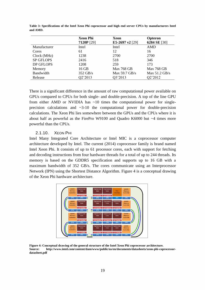
Table 3: Specifications of the Intel Xeon Phi coprocessor and high end server CPUs by manufacturers Intel
and AMD.
Xeon Phi
7120P [29] Xeon
E5-2697 v2 [29] Opteron
6284 SE [30]
Manufacturer Intel Intel AMD
Cores 61 12 16
Clock (MHz) 1238 2700 2700
SP GFLOPS 2416 518 346
DP GFLOPS 1208 259 173
Memory 16 GB Max 768 GB Max 768 GB
Bandwidth 352 GB/s Max 59.7 GB/s Max 51.2 GB/s
Release Q2’2013 Q3’2013 Q2’2012
There is a significant difference in the amount of raw computational power available on
GPUs compared to CPUs for both single- and double-precision. A top of the line GPU
from either AMD or NVIDIA has ~10 times the computational power for single-
precision calculations and ~3-10 the computational power for double-precision
calculations. The Xeon Phi lies somewhere between the GPUs and the CPUs where it is
about half as powerful as the FirePro W9100 and Quadro K6000 but ~4 times more
powerful than the CPUs.
2.1.10. XEON PHI
Intel Many Integrated Core Architecture or Intel MIC is a coprocessor computer
architecture developed by Intel. The current (2014) coprocessor family is brand named
Intel Xeon Phi. It consists of up to 61 processor cores, each with support for fetching
and decoding instructions from four hardware threads for a total of up to 244 threads. Its
memory is based on the GDDR5 specification and supports up to 16 GB with a
maximum bandwidth of 352 GB/s. The cores communicate using an Interprocessor
Network (IPN) using the Shortest Distance Algorithm. Figure 4 is a conceptual drawing
of the Xeon Phi hardware architecture.
Figure 4: Conceptual drawing of the general structure of the Intel Xeon Phi coprocessor architecture.
Source: http://www.intel.com/content/dam/www/public/us/en/documents/datasheets/xeon-phi-coprocessor-
datasheet.pdf

20
The Intel MPI library can be used on the Xeon Phi in three different modes: offload,
coprocessor only and symmetric. In offload mode, the MPI communications occur only
between host processor/s and the coprocessor/s are used exclusively through the offload
capabilities of the compiler. With coprocessor only mode the MPI processes reside
solely inside the coprocessor. The required libraries and the application to run are
uploaded to the coprocessor and can be launched from either the host or from the
coprocessor. In symmetric mode both the host CPU/s and the coprocessor/s are involved
in the execution of MPI processes and the related MPI communications.
The Xeon Phi architecture also supports OpenMP, OpenCL, Intel Threading Building
Blocks and POSIX threads for parallelization. Programs using these tools can run
offload and native mode on the Xeon Phi. Offload mode starts execution on a CPU and
transfers the heavy computations to the Xeon Phi at run time. For OpenMP this can be
specified with #pragma omp target data device(1) map() available on several compilers,
and the Intel specific #pragma offload. Native mode compiles the code directly for the
Xeon Phi architecture using the -mmic option and builds the required libraries. The files
are then transferred from the host to the Xeon Phi and run manually by the user.
2.2. PRINCIPLES OF COMPUTED TOMOGRAPHY
2.2.1. PHOTON INTERACTIONS
Photons with energies between 1 and 150 keV interact with the irradiated material via
photoelectric effect, coherent scattering and incoherent (Compton) scattering.
Interactions occurring only outside this range, such as pair-production, are not
considered in this thesis.
A photoelectric effect is an interaction between a photon and a tightly bound orbital
electron of an atom [31]. The photon is absorbed and all of its energy is given to the
orbital electron, which is then ejected from the atom with kinetic energy equivalent to
the photon energy minus the binding energy of the ejected electron. As the photon
energy, 𝐸, increases, the cross section of the photoelectric effect decreases rapidly; for
instance as 𝐸−3 in the energy region of 100 keV and below. As the atomic number, 𝑍,
of a material increases, the cross section of the photoelectric effect increases rapidly; for
instance the photoelectric mass attenuation coefficient depends on 𝑍3 in the energy
region around 100 keV.
A coherent (Rayleigh) scattering is a photon interaction process in which photons are
elastically scattered by bound atomic electrons. The atom is neither excited nor ionized
[31]. The interaction causes the direction of the photon to change.
An incoherent (Compton) scattering is an inelastic scattering of a photon with an atom.
It typically occurs for a loosely bound orbital electron. The energy given to the electron
depends on the initial photon energy and the scattering angle. The cross section is
dependent on the photon energy, see figure 5. Corresponding linear attenuation
coefficient is proportional to the electron density.
21
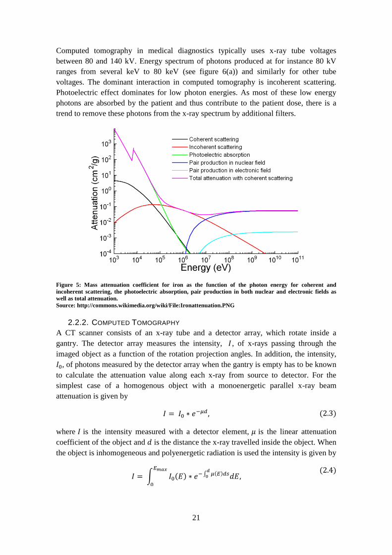
Computed tomography in medical diagnostics typically uses x-ray tube voltages
between 80 and 140 kV. Energy spectrum of photons produced at for instance 80 kV
ranges from several keV to 80 keV (see figure 6(a)) and similarly for other tube
voltages. The dominant interaction in computed tomography is incoherent scattering.
Photoelectric effect dominates for low photon energies. As most of these low energy
photons are absorbed by the patient and thus contribute to the patient dose, there is a
trend to remove these photons from the x-ray spectrum by additional filters.
Figure 5: Mass attenuation coefficient for iron as the function of the photon energy for coherent and
incoherent scattering, the photoelectric absorption, pair production in both nuclear and electronic fields as
well as total attenuation.
Source: http://commons.wikimedia.org/wiki/File:Ironattenuation.PNG
2.2.2. COMPUTED TOMOGRAPHY
A CT scanner consists of an x-ray tube and a detector array, which rotate inside a
gantry. The detector array measures the intensity, 𝐼 , of x-rays passing through the
imaged object as a function of the rotation projection angles. In addition, the intensity,
𝐼0, of photons measured by the detector array when the gantry is empty has to be known
to calculate the attenuation value along each x-ray from source to detector. For the
simplest case of a homogenous object with a monoenergetic parallel x-ray beam
attenuation is given by
𝐼 = 𝐼0 ∗ 𝑒−𝜇𝑑, (2.3)
where 𝐼 is the intensity measured with a detector element, 𝜇 is the linear attenuation
coefficient of the object and 𝑑 is the distance the x-ray travelled inside the object. When
the object is inhomogeneous and polyenergetic radiation is used the intensity is given by
𝐼 = ∫ 𝐼0(𝐸) ∗ 𝑒
−∫ 𝜇(𝐸)𝑑𝑠𝑑0 𝑑𝐸
𝐸𝑚𝑎𝑥
0
, (2.4)

22
where 𝐼0(𝐸) is the distribution initial intensity with respect to energy, 𝐸𝑚𝑎𝑥 is the
maximum photon energy in the x-ray tube energy spectrum, ∫ 𝜇(𝐸)𝑑𝑠𝑑
0 is the energy
dependent line integral (the radiological path) through the imaged object placed inside a
circle with diameter 𝑑.
In the case of classical image reconstruction algorithms assuming monoenergetic beams
(e.g. the filtered backprojection), the usage of polyenergetic radiation leads to image
artifacts for the following reason. The energy spectra of photons entering and exiting the
object differ, see figure 6; the x-ray beam hardens as it moves through the object. The
corresponding beam hardening artifact manifests itself in the reconstructed images as a
darkening in the center of a homogenous object (cupping), or a darkening between two
highly absorbent objects in the image. Figure 7 shows the darkening effect between two
highly attenuating objects.
Figure 6: Comparison of energy spectra in front of (a) and behind (b) the imaged object. Source: “An iterative
algorithm for quantitative tissue decomposition using DECT”, Oscar Grandell, 2012.
Figure 7: Images reconstructed using filtered backprojection. (a) The polyenergetic beam led to a strong beam
hardening artifact. (b) The beam hardening artifact is not present for a monoenergetic beam. Source: “An
iterative algorithm for quantitative tissue decomposition using DECT”, Oscar Grandell, 2012.
The X-ray tube’s voltage (kV) affects the average energy of the photons in the X-ray
beam. Changing the tube voltage results in an alteration of the average photon energy
and a corresponding modification of the attenuation of the X-ray beam in the materials
scanned. For example, scanning an object with 80 kV results in a different attenuation
23
than with 140 kV. In addition, this attenuation also depends on the type of material or
tissue scanned (the atomic number of the material). Dual-Energy Computed
Tomography (DECT) exploits this effect by using two X-ray sources simultaneously at
different voltages to acquire two data sets showing different attenuation levels. In the
resulting images, the material-specific difference in attenuation makes a classification of
the elemental composition of the scanned tissue feasible [32].
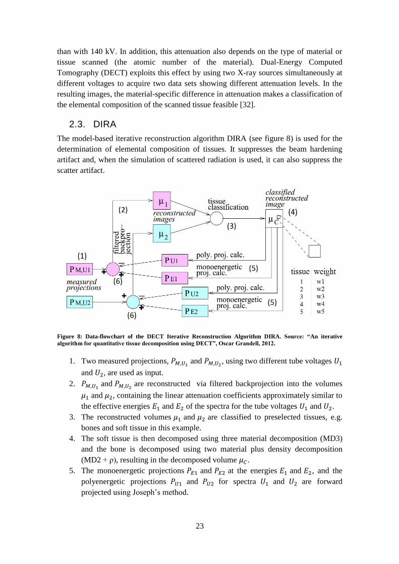
2.3. DIRA
The model-based iterative reconstruction algorithm DIRA (see figure 8) is used for the
determination of elemental composition of tissues. It suppresses the beam hardening
artifact and, when the simulation of scattered radiation is used, it can also suppress the
scatter artifact.
Figure 8: Data-flowchart of the DECT Iterative Reconstruction Algorithm DIRA. Source: “An iterative
algorithm for quantitative tissue decomposition using DECT”, Oscar Grandell, 2012.
1. Two measured projections, 𝑃𝑀,𝑈1 and 𝑃𝑀,𝑈2, using two different tube voltages 𝑈1
and 𝑈2, are used as input.
2. 𝑃𝑀,𝑈1 and 𝑃𝑀,𝑈2 are reconstructed via filtered backprojection into the volumes
𝜇1 and 𝜇2, containing the linear attenuation coefficients approximately similar to
the effective energies 𝐸1 and 𝐸2 of the spectra for the tube voltages 𝑈1 and 𝑈2.
3. The reconstructed volumes 𝜇1 and 𝜇2 are classified to preselected tissues, e.g.
bones and soft tissue in this example.
4. The soft tissue is then decomposed using three material decomposition (MD3)
and the bone is decomposed using two material plus density decomposition
(MD2 + ρ), resulting in the decomposed volume 𝜇𝐶.
5. The monoenergetic projections 𝑃𝐸1 and 𝑃𝐸2 at the energies 𝐸1 and 𝐸2, and the
polyenergetic projections 𝑃𝑈1 and 𝑃𝑈2 for spectra 𝑈1 and 𝑈2 are forward
projected using Joseph’s method.

24
6. The differences between the monoenergetic projections 𝑃𝐸1 and 𝑃𝐸2 and the
polyenergetic projections 𝑃𝑈1 and 𝑃𝑈2 are calculated and added to the measured
projections to create the corrected projections 𝑃𝑀′,𝑈1 and 𝑃𝑀′,𝑈2.
7. 𝑃𝑀′,𝑈1 and 𝑃𝑀′,𝑈2 are then used in the next iteration as the new measured
projections. After a number of iterations the beam hardening artifacts are
removed and accurate mass fractions of the base materials as well as the density
for the bone tissue obtained.
2.3.1. FILTERED BACKPROJECTION
The Radon transform 𝑔(𝑠, 𝜃) of a function 𝑓(𝑥, 𝑦) is the line integral of the values of
𝑓(𝑥, 𝑦) along the line inclined at angle 𝜃 from the x-axis at a distance 𝑠 from the origin
𝑔(𝑠, 𝜃) = ∫ 𝑓(𝑠 𝑐𝑜𝑠(𝜃) − 𝑢𝑠𝑖𝑛(𝜃), 𝑠 sin(𝜃) + 𝑢 cos(𝜃))
∞
−∞
𝑑𝑢.
(2.5)
The value of 𝑔(𝑠, 𝜃) is the sum of values 𝑓(𝑥, 𝑦) along the line 𝐿. Backprojection is
defined as
𝑏(𝑥, 𝑦) = ∫ 𝑔(𝑠, 𝜃)𝑑𝜃.
𝜋
0
(2.6)
Replacing the integral in equation (2.6) with a sum gives
�̃�(𝑥, 𝑦) = ∑𝑔(𝑠𝑘, 𝜃𝑘)∆𝜃,
𝑝
𝑘=1
(2.7)
where 𝑝 is the number of projections, 𝜃𝑘 is the kth angular position of the detector, 𝑠𝑘 is
the location along the detector and ∆𝜃 is the angular step between 2 projections. Using
only backprojection will produce a blurry the image. The blurriness is removed by
applying a ramp filter on the projection data, before performing the backprojection. This
gives
𝑓(𝑥, 𝑦) = ∫ �̂�(𝑠, 𝜃)𝑑𝜃
𝜋
0
𝑜𝑟 𝑓(𝑥, 𝑦) = ∑ �̂�(𝑠𝑘, 𝜃𝑘)∆𝜃
𝑝
𝑘=1
, (2.8)
where �̂�(𝑠, 𝜃) and �̂�(𝑠𝑘 , 𝜃𝑘) are filtered with a ramp filter [33].
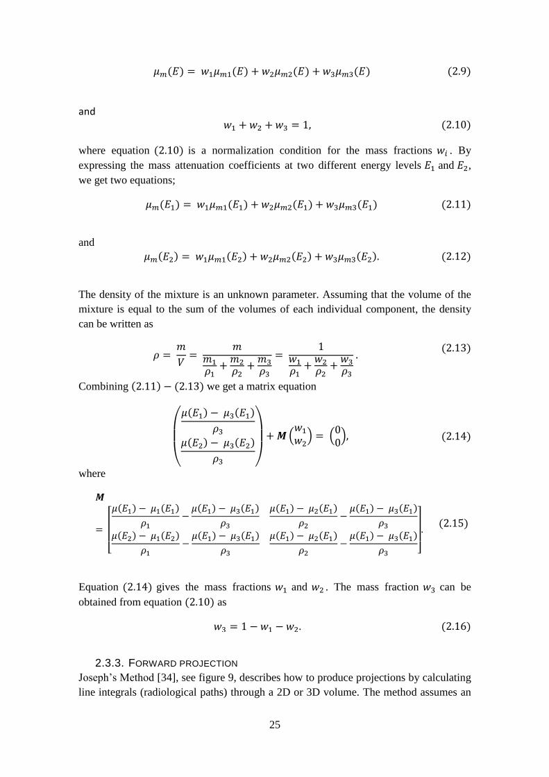
2.3.2. MATERIAL DECOMPOSITION
Assume that a mixture consists of three separate components, with mass attenuation
coefficients 𝜇𝑚,1, 𝜇𝑚,2 and 𝜇𝑚,3, defined as 𝜇𝑚,𝑖 =𝜇𝑖
𝜌𝑖, where 𝜇𝑖 is the linear attenuation
coefficient and 𝜌𝑖 is the density. The mass attenuation coefficient of the mixture 𝜇𝑚(𝐸)
at photon energy 𝐸 can be calculated from the mixture law as
25
𝜇𝑚(𝐸) = 𝑤1𝜇𝑚1(𝐸) + 𝑤2𝜇𝑚2(𝐸) + 𝑤3𝜇𝑚3(𝐸) (2.9)
and 𝑤1 + 𝑤2 +𝑤3 = 1, (2.10)
where equation (2.10) is a normalization condition for the mass fractions 𝑤𝑖 . By
expressing the mass attenuation coefficients at two different energy levels 𝐸1 and 𝐸2,
we get two equations;
𝜇𝑚(𝐸1) = 𝑤1𝜇𝑚1(𝐸1) + 𝑤2𝜇𝑚2(𝐸1) + 𝑤3𝜇𝑚3(𝐸1) (2.11)
and 𝜇𝑚(𝐸2) = 𝑤1𝜇𝑚1(𝐸2) + 𝑤2𝜇𝑚2(𝐸2) + 𝑤3𝜇𝑚3(𝐸2). (2.12)
The density of the mixture is an unknown parameter. Assuming that the volume of the
mixture is equal to the sum of the volumes of each individual component, the density
can be written as
𝜌 =
𝑚
𝑉=
𝑚𝑚1
𝜌1+𝑚2
𝜌2+𝑚3
𝜌3
= 1
𝑤1𝜌1+𝑤2𝜌2+𝑤3𝜌3
. (2.13)
Combining (2.11) − (2.13) we get a matrix equation
(
𝜇(𝐸1) − 𝜇3(𝐸1)
𝜌3𝜇(𝐸2) − 𝜇3(𝐸2)
𝜌3 )
+𝑴(
𝑤1𝑤2) = (
00),
(2.14)
where
𝑴
=
[ 𝜇(𝐸1) − 𝜇1(𝐸1)
𝜌1−𝜇(𝐸1) − 𝜇3(𝐸1)
𝜌3
𝜇(𝐸1) − 𝜇2(𝐸1)
𝜌2−𝜇(𝐸1) − 𝜇3(𝐸1)
𝜌3𝜇(𝐸2) − 𝜇1(𝐸2)
𝜌1−𝜇(𝐸1) − 𝜇3(𝐸1)
𝜌3
𝜇(𝐸1) − 𝜇2(𝐸1)
𝜌2−𝜇(𝐸1) − 𝜇3(𝐸1)
𝜌3 ]
.
(2.15)
Equation (2.14) gives the mass fractions 𝑤1 and 𝑤2 . The mass fraction 𝑤3 can be
obtained from equation (2.10) as
𝑤3 = 1 − 𝑤1 − 𝑤2. (2.16)
2.3.3. FORWARD PROJECTION
Joseph’s Method [34], see figure 9, describes how to produce projections by calculating
line integrals (radiological paths) through a 2D or 3D volume. The method assumes an

26
image consists of 𝑁 × 𝑁 pixels and that the image function 𝑓(𝑥, 𝑦) is constant over the
domain of each pixel. Consider a straight line K specified as
𝑦(𝑥) = −𝑥 cot(𝜃) + 𝑦𝑜 (2.17)
or
𝑥(𝑦) = − y tan(𝜃) + 𝑥𝑜 , (2.18)
where 𝜃 is the angle to the y-axis, 𝑦𝑜 is the cross-point with the 𝑦-axis and 𝑥𝑜 is the
cross-point with the 𝑥-axis. The line integral 𝑆(𝐾) is dependent on whether the ray’s
direction is aligned with the direction of the 𝑦- or 𝑥-axis. It can be written as
𝑆(𝐾) =
{
1
|𝑠𝑖𝑛𝜃|∫𝑓(𝑥, 𝑦(𝑥))𝑑𝑥
1
|𝑐𝑜𝑠𝜃|∫𝑓(𝑥(𝑦), 𝑦)𝑑𝑦
𝑓𝑜𝑟 |𝑠𝑖𝑛𝜃| ≥ 1
√2
𝑓𝑜𝑟 |𝑐𝑜𝑠𝜃| ≥ 1
√2
(2.19)
By using the Riemann sum to approximate, equation (2.19) can be written as (for the x-
directional integral)
𝑆(𝐾) = 1
|𝑠𝑖𝑛𝜃|[∑ 𝑃𝑛,𝑛′ + 𝜆𝑛(𝑃𝑛,𝑛′+1 − 𝑃𝑛,𝑛′) + 𝑇1 + 𝑇𝑁
𝑁−1
𝑛=2
].
(2.20)
The terms 𝑇1 and 𝑇𝑁 represent the first and the last pixel on the line and are treated
separately. 𝜆𝑛 is defined as 𝜆𝑛 = 𝑦(𝑥𝑛) − 𝑛´, where 𝑛´ = the integer part of 𝑦(𝑥𝑛).
𝑃𝑛,𝑛′ and 𝑃𝑛,𝑛′+1 are pixel values. If no pixels are treated separately, 𝑇1 = 0 and
𝑇𝑁 = 0, and rewriting the interpolation, the final equation becomes
𝑆(𝐾) = 1
|𝑠𝑖𝑛𝜃|[∑((1 − 𝜆𝑛)𝑃𝑛,𝑛′ + 𝜆𝑛𝑃𝑛,𝑛′+1)
𝑁
𝑛=1
].
(2.21)
Figure 9: Joseph's method of line-integration along one axis using bi-linear interpolation. Source: "Cone-beam
Reconstruction using Filtered Backprojection”, Henrik Thurbell, 2001.

27
There are two ways of calculating the projections, either using inverse mapping or
forward mapping. The image transforms can be described as
𝑥 = 𝑀−1(𝑥)
(2.22)
and
𝑥′ = 𝑀(𝑥),
(2.23)
where 𝑥 is the input image, 𝑥′ the output image and 𝑀 the mapping function with 𝑀−1
its inverse [35]. Inverse mapping is a destination-driven method where a pixel in the
output image is calculated from the input image. Forward mapping is a source-driven
method where a pixel in the input image is mapped onto the output image.
2.3.4. POLYCHROMATIC PROJECTIONS
The monoenergetic projection 𝑃𝑚𝐸 at effective energy 𝐸1 for base material 𝑚 with
mass attenuation coefficient 𝜎𝑚𝐸 can be calculated using Joseph’s method:
𝑃𝑚𝐸1 = 𝜎𝑚𝐸𝜌𝑚𝑙𝑚. (2.24)
The polychromatic projection is also calculated by using Joseph’s method by using
𝑃𝑈1 = 𝑙𝑛(
𝑆𝑖𝑛𝑆0) = −𝑙𝑛 (
𝑆0𝑆𝑖𝑛),
(2.25)
where 𝑆𝑖𝑛 is the incident-photon intensity and 𝑆0 is the existing-photon intensity given
by
𝑆𝑖𝑛 = ∑ 𝐸𝑁(𝐸)
𝐸𝑚𝑎𝑥
0
(2.26)
and
𝑆0 = ∑ 𝐸𝑁(𝐸)𝑒−(∑ 𝜇𝑚𝐸(𝐸)𝜌𝑚𝑀𝑚=1 𝑙𝑚),
𝐸𝑚𝑎𝑥
0
(2.27)
where 𝐸 is the photon energy, 𝑁(𝐸) the number of photons, 𝜇𝑚𝐸(𝐸) the mass
attenuation coefficient, 𝜌𝑚 the material density and 𝑙𝑚 the length of the intersection
with material 𝑚.
2.4. CTMOD
CTmod is a toolkit written in C++ that simulates primary and scatter projections in
computed tomography. It can be used in the optimization of CT scanner design and
image reconstruction algorithms by evaluating the effects of factors like the tube
voltage, phantom size, beam collimators and detector array construction. The toolkit is
based on CERN’s data analysis framework ROOT [36]. It simulates the transport of
28
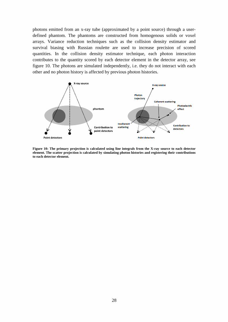
photons emitted from an x-ray tube (approximated by a point source) through a user-
defined phantom. The phantoms are constructed from homogenous solids or voxel
arrays. Variance reduction techniques such as the collision density estimator and
survival biasing with Russian roulette are used to increase precision of scored
quantities. In the collision density estimator technique, each photon interaction
contributes to the quantity scored by each detector element in the detector array, see
figure 10. The photons are simulated independently, i.e. they do not interact with each
other and no photon history is affected by previous photon histories.
Figure 10: The primary projection is calculated using line integrals from the X-ray source to each detector
element. The scatter projection is calculated by simulating photon histories and registering their contributions
to each detector element.

29
3. METHODS
This chapter describes the changes made to the DIRA and the CTmod codes. For DIRA
these changes include rewriting MATLAB-code to C-code, altering computations and
the parallelization of the algorithm. The CTmod code was modified to allow parallel
photon transport simulation.
3.1. HARDWARE
Several systems were used to test the performance improvements of DIRA and CTmod,
and to evaluate how well the parallelization scales when using multiple cores. Table 4
contains information on the CPUs used in the performance evaluations. The Intel
Celeron T1600 and Intel Xeon E5-2660 were used to evaluate the performance of
DIRA. For CTmod the Intel Xeon E5-2660 was used to evaluate the performance
scaling and the Xeon W3520 was used to compare the difference between Hyper-
Threading enabled and disabled. To evaluate OpenCL performance the AMD R7 260X
desktop GPU, table 5, was used.
Table 4: Specifications of the CPUs used to evaluate the performance of DIRA and CTmod.
Celeron® T1600 [37] Xeon® E5-2660 [38] Xeon® W3520 [39]
Manufacturer Intel Intel Intel
Cores 2 8 4
Clock speed (MHz) 1.66 GHz 2.2 GHz 2.66 GHz
HT No Yes Yes
L1 Cache 32 KB instruction
32 KB data
32 KB instruction
32 KB data
32 KB instruction
32 KB data
L2 Cache 1 MB 256 KB 256 KB
L3 Cache - 20 MB 8 MB
Access to Intel Xeon E5-2660 was provided by NSC [40], The National Supercomputer
Centre in Sweden, using their Triolith system. Every compute node consists of two
CPUs with Hyper-Threading disabled, for a total of 16 cores per node.
Table 5: Specifications of the GPU used to evaluate the OpenCL implementations of DIRA functions.
R7 Series 260X [41] Manufacturer AMD
Cores 896
Clock speed (MHz) 1.1 GHz
Single-precision GFLOPS 1971
Double-precision GFLOPS 123
Memory 2 GB
Bandwidth 104 GB/s
3.2. DIRA
The first step of an iteration is to calculate the monoenergetic and polychromatic
projections, performed in two steps. The individual materials are forward projected with
the sinogramJc function to create sinograms of each material. These are then used as the
base to calculate the projections. The polychromatic projections are calculated with the

30
computePolyProj function. To create the reconstructed volume the filtered
backprojection is applied with the built-in MATLAB iradon function or the new
inverseRadon function. The volume is decomposed into materials using the functions
MD2 and MD3. The functions computePolyProj, MD2 and MD3 were originally written
in MATLAB and have been converted to C or C++ code to allow for parallelization
using OpenMP and OpenCL.
The different versions of each updated function are provided in separate files. The user
can select what version to use for each function; it is not limited to the same
implementation for all functions. For example, computePolyProj consists of four files
containing four different versions:
1. computePolyProj.m – The old implementation written in MATLAB code.
2. computePolyProjc.c – The new implementation in C code.
3. openmp_computePolyProjc.c – The new implementation in C with OpenMP.
4. opencl_computePolyProjc.cpp – The new implementation in C++ with
OpenCL.
The version to use is dependent on the user’s available software and hardware. All
versions except the original MATLAB code require a supported and compatible
compiler. The OpenCL version also requires a supported CPU or GPU to execute the
code.
Figure 11: Left: A color map of material numbers in the transversal slice of the pelvic region of the ICRP 110
voxel phantom. Ellipses were used to construct a mathematical model of the slice. Right: Masks defining soft
tissue, bone and prostate regions in DIRA. Darker region inside the prostate was used for calculation of the
average mass fraction.
Two examples were used when testing DIRA, slice113 and slice113B. Both are based
on the ICRP 110 male voxel phantom, see figure 11, where slice113B centers the
phantom in a smaller field of view and uses quarter offset. More information on the
phantom is available on the project’s webpage [42] and in the proceedings of the 2014
SPIE conference [43]. Figures 12 and 13 show the resulting material decomposition of
the original image and material decomposition after 4 iterations of DIRA.

31
Figure 12: Mass fractions (in %) of adipose tissue, water and muscle for the slice113 example after 𝟎𝒕𝒉
iteration of DIRA. Strong artifacts caused by beam hardening are clearly visible.
Figure 13: The same as in figure 12 but after the 𝟒𝒕𝒉 iteration of DIRA. The suppression of beam hardening
artifacts is clearly visible.
3.2.1. FILTERED BACKPROJECTION
MATLAB already provides an implementation of the filtered backprojection with the
iradon function call. Figure 14 is an example of the output produced by this function.
This implementation is written in C and parallelized. A new implementation based on
the works of Jeff Orchard [44] for the backprojection and the filtering from MATLAB’s
iradon function was made. The general implementation of backprojection is to place
each value of a projection along a line through the output image. This implementation
suffers from low performance caused by slow memory accesses and cache misses due to
the order of accessing elements in the output image. The new implementation improves
on this by changing the order in which the projection values are placed onto the output
image. For each projection the projection values are placed onto each row in the output
image in the correct position.
32
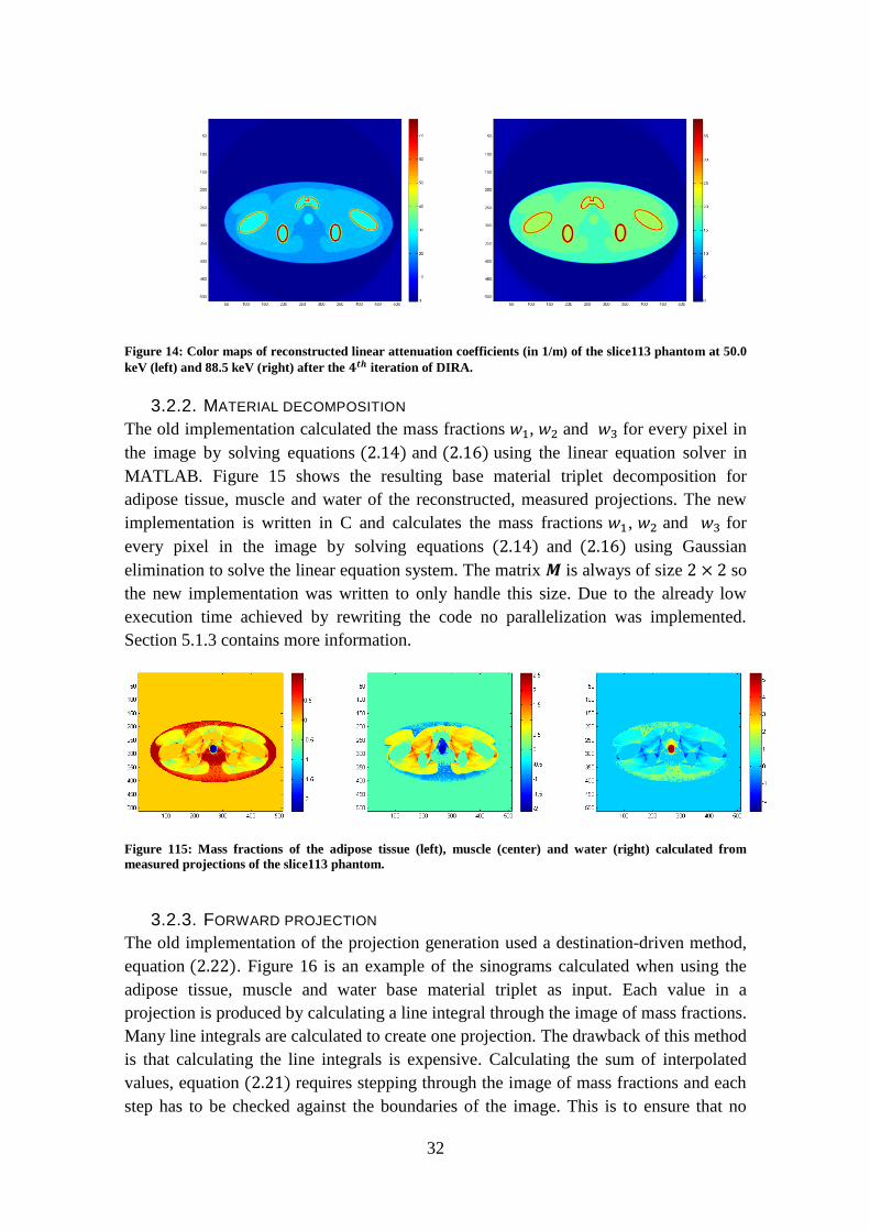
Figure 14: Color maps of reconstructed linear attenuation coefficients (in 1/m) of the slice113 phantom at 50.0
keV (left) and 88.5 keV (right) after the 𝟒𝒕𝒉 iteration of DIRA.
3.2.2. MATERIAL DECOMPOSITION
The old implementation calculated the mass fractions 𝑤1, 𝑤2 and 𝑤3 for every pixel in
the image by solving equations (2.14) and (2.16) using the linear equation solver in
MATLAB. Figure 15 shows the resulting base material triplet decomposition for
adipose tissue, muscle and water of the reconstructed, measured projections. The new
implementation is written in C and calculates the mass fractions 𝑤1, 𝑤2 and 𝑤3 for
every pixel in the image by solving equations (2.14) and (2.16) using Gaussian
elimination to solve the linear equation system. The matrix 𝑴 is always of size 2 × 2 so
the new implementation was written to only handle this size. Due to the already low
execution time achieved by rewriting the code no parallelization was implemented.
Section 5.1.3 contains more information.
Figure 115: Mass fractions of the adipose tissue (left), muscle (center) and water (right) calculated from
measured projections of the slice113 phantom.
3.2.3. FORWARD PROJECTION
The old implementation of the projection generation used a destination-driven method,
equation (2.22). Figure 16 is an example of the sinograms calculated when using the
adipose tissue, muscle and water base material triplet as input. Each value in a
projection is produced by calculating a line integral through the image of mass fractions.
Many line integrals are calculated to create one projection. The drawback of this method
is that calculating the line integrals is expensive. Calculating the sum of interpolated
values, equation (2.21) requires stepping through the image of mass fractions and each
step has to be checked against the boundaries of the image. This is to ensure that no

33
wrong values are accessed. Checking the boundaries of the image is expensive as it
introduces a branching operation for each check.
The new implementation of the projection generation uses a source-driven method,
equation (2.23). Each individual pixel’s contribution to each projection is calculated.
Pixels outside of a circle with its center in the middle of the image of mass fractions and
a radius of ⌈𝑖𝑚𝑎𝑔𝑒 𝑤𝑖𝑑𝑡ℎ
2⌉ , can produce coordinate values outside of the sinogram,
depending on the angle 𝜃𝑘 and are excluded. A pixel in the input image must have a
non-zero value to contribute to the projections. All pixels with a value of zero are also
excluded. The number of pixels to process depends on the input image. As an example,
excluding half of the pixels in the mass fraction image reduces the computational load
by half and the execution time is halved.
Figure 16: Sinograms containing calculated forward projections for individual base materials of the slice113
phantom. The base material triplet consisted of adipose tissue (left), muscle (center) and water (right).
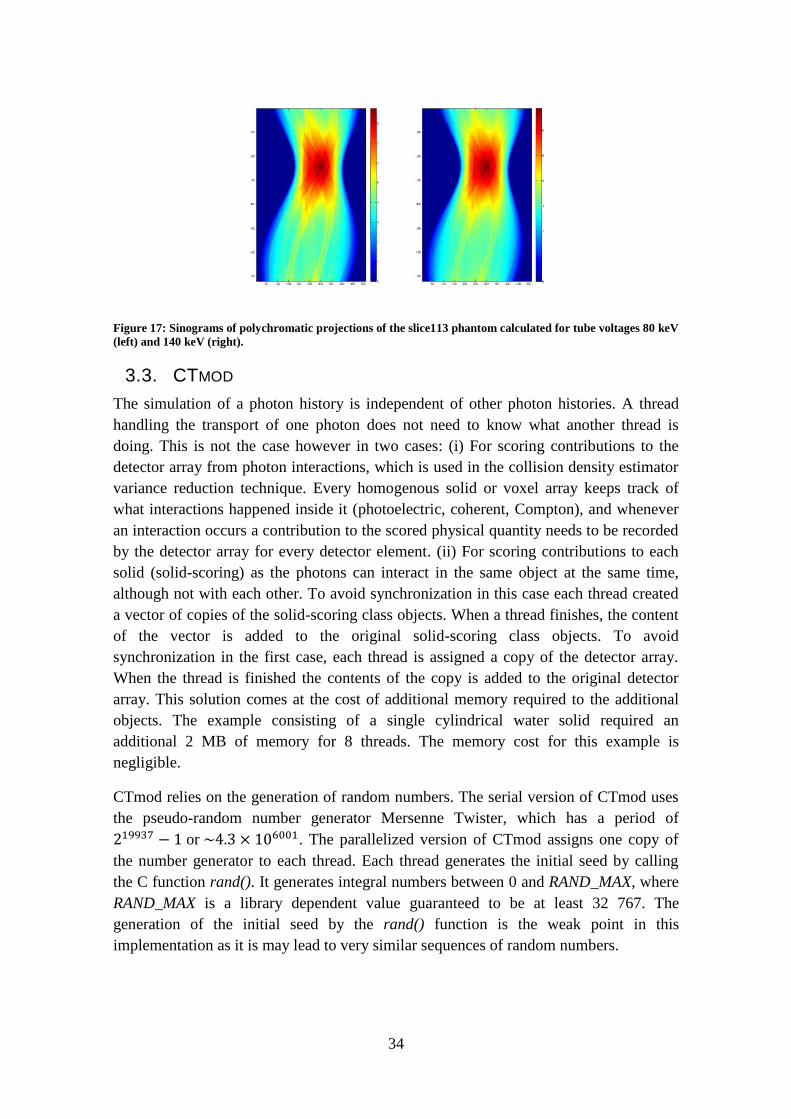
3.2.4. POLYCHROMATIC PROJECTIONS
A polychromatic projection sinogram contains radiological paths (line integrals)
through the imaged object as functions of projection angle and detector element index,
see figure 17. Such a sinogram can be calculated by summing contributions from
individual base material sinograms (section 3.2.3) weighted with energy spectra of
photons, see equation (2.27). For every pixel in the polychromatic sinogram the sum 𝑆0
in equation (2.27) can be calculated independently of other pixels. The old
implementation of calculating the polychromatic projections was changed from “for
every energy calculate the sum for the entire image” to “for every pixel in the image
calculate the sum for all energies”. The largest number of individual tasks possible
equals the total number of pixels. For instance 367 920 tasks can be created for an
image size of 511×720. For a GPU with thousands of computational units this gives
each compute unit hundreds of pixels to process. The change in computational order
also affects the memory allocation. Instead of allocating the entire matrix to store
temporary results, each task allocates one floating-point number. The GPU
implementation uses the much faster private memory to store temporary data, instead of
storing the entire image in high latency global memory. The CPU implementation with
OpenMP creates one task for each row of the polychromatic projection sinogram.
34
Figure 17: Sinograms of polychromatic projections of the slice113 phantom calculated for tube voltages 80 keV
(left) and 140 keV (right).
3.3. CTMOD
The simulation of a photon history is independent of other photon histories. A thread
handling the transport of one photon does not need to know what another thread is
doing. This is not the case however in two cases: (i) For scoring contributions to the
detector array from photon interactions, which is used in the collision density estimator
variance reduction technique. Every homogenous solid or voxel array keeps track of
what interactions happened inside it (photoelectric, coherent, Compton), and whenever
an interaction occurs a contribution to the scored physical quantity needs to be recorded
by the detector array for every detector element. (ii) For scoring contributions to each
solid (solid-scoring) as the photons can interact in the same object at the same time,
although not with each other. To avoid synchronization in this case each thread created
a vector of copies of the solid-scoring class objects. When a thread finishes, the content
of the vector is added to the original solid-scoring class objects. To avoid
synchronization in the first case, each thread is assigned a copy of the detector array.
When the thread is finished the contents of the copy is added to the original detector
array. This solution comes at the cost of additional memory required to the additional
objects. The example consisting of a single cylindrical water solid required an
additional 2 MB of memory for 8 threads. The memory cost for this example is
negligible.
CTmod relies on the generation of random numbers. The serial version of CTmod uses
the pseudo-random number generator Mersenne Twister, which has a period of
219937 − 1 or ~4.3 × 106001. The parallelized version of CTmod assigns one copy of
the number generator to each thread. Each thread generates the initial seed by calling
the C function rand(). It generates integral numbers between 0 and RAND_MAX, where
RAND_MAX is a library dependent value guaranteed to be at least 32 767. The
generation of the initial seed by the rand() function is the weak point in this
implementation as it is may lead to very similar sequences of random numbers.
35
4. RESULTS
This section contains the results of the optimization and parallelization of DIRA and the
parallelization of CTmod. All results were taken from systems where the CPU could be
fully utilized; no other tasks were scheduled to run at the same time. DIRA consists of
three parts: (i) Loading the necessary data, (ii) performing the computations and (iii)
saving the results. The performance impact of the loading and saving parts is
mentioned. The performance of each considered function for the computational part is
presented as well as the overall performance of DIRA. For CTmod only the
performance of the computational part is presented, not the performance of the loading
and saving part as it varies with the complexity of the geometry.
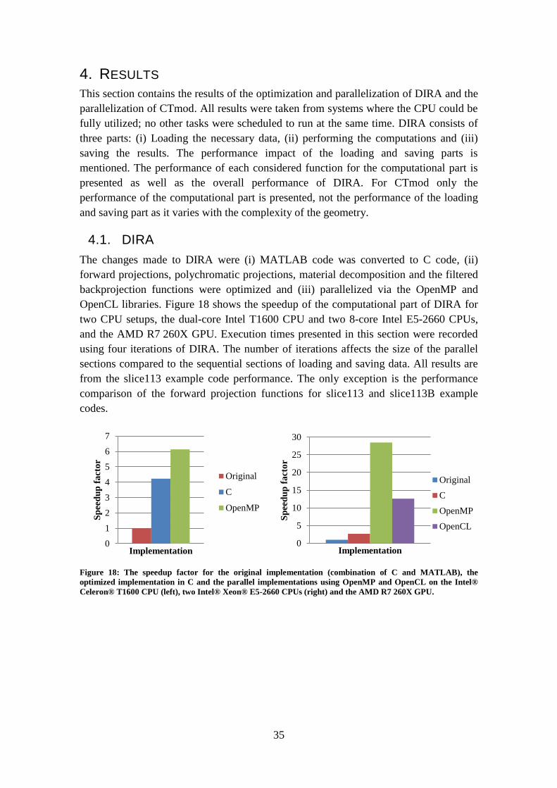
4.1. DIRA
The changes made to DIRA were (i) MATLAB code was converted to C code, (ii)
forward projections, polychromatic projections, material decomposition and the filtered
backprojection functions were optimized and (iii) parallelized via the OpenMP and
OpenCL libraries. Figure 18 shows the speedup of the computational part of DIRA for
two CPU setups, the dual-core Intel T1600 CPU and two 8-core Intel E5-2660 CPUs,
and the AMD R7 260X GPU. Execution times presented in this section were recorded
using four iterations of DIRA. The number of iterations affects the size of the parallel
sections compared to the sequential sections of loading and saving data. All results are
from the slice113 example code performance. The only exception is the performance
comparison of the forward projection functions for slice113 and slice113B example
codes.
Figure 18: The speedup factor for the original implementation (combination of C and MATLAB), the
optimized implementation in C and the parallel implementations using OpenMP and OpenCL on the Intel®
Celeron® T1600 CPU (left), two Intel® Xeon® E5-2660 CPUs (right) and the AMD R7 260X GPU.
0
1
2
3
4
5
6
7
Sp
eed
up
fa
cto
r
Implementation
Original
C
OpenMP
0
5
10
15
20
25
30
Sp
eed
up
fa
cto
r
Implementation
Original
C
OpenMP
OpenCL

36
Table 6: Execution times for the forward projection, polychromatic projection, filtered backprojection,
material decomposition, loading, saving and the total time for the original, the C and the OpenMP
implementations on the Intel T1600 CPU.
Function Original (s) C (s) OpenMP (s)
Forward projection
117.54 12.65 7.14
Polychromatic projection 57.83 18.22 11.59
Filtered backprojection 17.64 13.08 10.38
Material decomposition 5.68 0.24 0.20
Loading 2.35 2.34 2.32
Saving 1.31 1.30 1.29
Total time 202.35 47.81 32.93
Table 7: Execution times for the forward projection, polychromatic projection, filtered backprojection,
material decomposition, loading, saving and the total time for the original, the C and the OpenMP
implementations on two Intel E5-2660 CPUs as well as the OpenCL implementations on the AMD R260X
GPU.
Function Original (s) C (s) OpenMP (s) OpenCL (s)
Forward projection
106.45 10.59 0.97 3.25
Polychromatic projection 8.90 11.25 1.18 1.03
Filtered backprojection 1.63 22.11 1.96 4.29
Material decomposition 2.56 0.06 0.08 0.07
Loading 1.78 1.79 1.79 1.44
Saving 1.95 1.91 1.93 0.33
Total time 123.28 47.71 7.92 11.25
Figure 19: Speedup factor as a function of the number of cores when using parallelized implementation on two
Intel® Xeon® E5-2660 CPUs.
Figure 19 shows how the overall performance of DIRA and the performance of each
parallelized function scales with additional cores. The scaling is neither linear nor ideal.
The drop-off in performance is due to (i) the overhead introduced with the
parallelization and (ii) the limitations in cache and memory bandwidth when reading
and writing data. The time it takes to create and terminate threads in the parallel
implementation increases as the number of threads increases. For every thread memory
0
2
4
6
8
10
12
1 2 3 4 5 6 7 8 9 10 11 12 13 14 15 16
Sp
eed
up
fa
cto
r
Number of cores
DIRA
forward projection
backprojection
polychromatic
projection
37
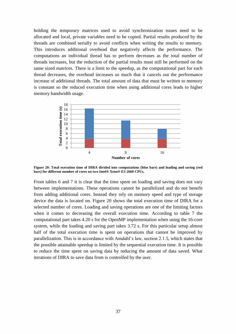
holding the temporary matrices used to avoid synchronization issues need to be
allocated and local, private variables need to be copied. Partial results produced by the
threads are combined serially to avoid conflicts when writing the results to memory.
This introduces additional overhead that negatively affects the performance. The
computations an individual thread has to perform decreases as the total number of
threads increases, but the reduction of the partial results must still be performed on the
same sized matrices. There is a limit to the speedup, as the computational part for each
thread decreases, the overhead increases so much that it cancels out the performance
increase of additional threads. The total amount of data that must be written to memory
is constant so the reduced execution time when using additional cores leads to higher
memory bandwidth usage.
Figure 20: Total execution time of DIRA divided into computations (blue bars) and loading and saving (red
bars) for different number of cores on two Intel® Xeon® E5-2660 CPUs.
From tables 6 and 7 it is clear that the time spent on loading and saving does not vary
between implementations. These operations cannot be parallelized and do not benefit
from adding additional cores. Instead they rely on memory speed and type of storage
device the data is located on. Figure 20 shows the total execution time of DIRA for a
selected number of cores. Loading and saving operations are one of the limiting factors
when it comes to decreasing the overall execution time. According to table 7 the
computational part takes 4.20 s for the OpenMP implementation when using the 16-core
system, while the loading and saving part takes 3.72 s. For this particular setup almost
half of the total execution time is spent on operations that cannot be improved by
parallelization. This is in accordance with Amdahl’s law, section 2.1.5, which states that
the possible attainable speedup is limited by the sequential execution time. It is possible
to reduce the time spent on saving data by reducing the amount of data saved. What
iterations of DIRA to save data from is controlled by the user.
0
2
4
6
8
10
12
14
16
18
4 8 16
To
tal
exec
uti
on
tim
e (s
)
Number of cores

38
4.1.1. FILTERED BACKPROJECTION
Figure 21: Speedup comparisons of the provided iradon function and new inverseRadon function on the Intel
T1600 CPU (left) and two Intel E5-2660 CPUs (right).
Figure 21 shows that the OpenMP implementation of the filtered backprojection gave a
small increase in speedup on the dual-core Intel T1600 CPU and a slightly decreased
speedup on the two Intel E5-2660 CPUs when compared to the old implementation
using MATLAB’s iradon function. The large difference between the old
implementation and the new implementation in C presented in figure 21 for the Intel
E5-2660 indicates that the iradon function runs in parallel. The exact cause the
performance difference is unknown as the source code for the iradon function is not
available. Figure 19 shows that the speedup for the filtered backprojection matches the
overall speedup of the algorithm with a factor of 11.3 when using 16 cores. The non-
ideal speedup is due to the parallelization overhead, which is too large compared to the
low execution time of each function call. According to table 7 the total execution time
of the filtered backprojections is 1.96 s for the Intel E5-2660 CPUs. This is for 10
function calls, with an average execution time of 0.196 s per function call. The size of
computations for each thread decreases as more threads are added, but the reduction
operation of combining the partial results from the threads increases in size, limiting the
potential speedup.
4.1.2. MATERIAL DECOMPOSITION
Figure 22: Comparison of the old implementation in MATLAB and the new in C for the material
decomposition on the Intel T1600 CPU.
0.0
0.2
0.4
0.6
0.8
1.0
1.2
1.4
1.6
1.8S
pee
du
p f
act
or
Implementation
Original
C
OpenMP
0.0
0.2
0.4
0.6
0.8
1.0
1.2
Sp
eed
up
fa
cto
r
Implementation
Original
C
OpenMP
OpenCL
0
10
20
30
40
50
Sp
eed
up
fa
cto
r
Implementation
Original
C
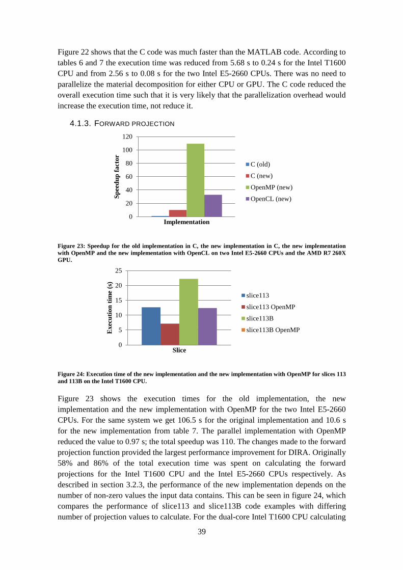
39
Figure 22 shows that the C code was much faster than the MATLAB code. According to
tables 6 and 7 the execution time was reduced from 5.68 s to 0.24 s for the Intel T1600
CPU and from 2.56 s to 0.08 s for the two Intel E5-2660 CPUs. There was no need to
parallelize the material decomposition for either CPU or GPU. The C code reduced the
overall execution time such that it is very likely that the parallelization overhead would
increase the execution time, not reduce it.
4.1.3. FORWARD PROJECTION
Figure 23: Speedup for the old implementation in C, the new implementation in C, the new implementation
with OpenMP and the new implementation with OpenCL on two Intel E5-2660 CPUs and the AMD R7 260X
GPU.
Figure 24: Execution time of the new implementation and the new implementation with OpenMP for slices 113
and 113B on the Intel T1600 CPU.
Figure 23 shows the execution times for the old implementation, the new
implementation and the new implementation with OpenMP for the two Intel E5-2660
CPUs. For the same system we get 106.5 s for the original implementation and 10.6 s
for the new implementation from table 7. The parallel implementation with OpenMP
reduced the value to 0.97 s; the total speedup was 110. The changes made to the forward
projection function provided the largest performance improvement for DIRA. Originally
58% and 86% of the total execution time was spent on calculating the forward
projections for the Intel T1600 CPU and the Intel E5-2660 CPUs respectively. As
described in section 3.2.3, the performance of the new implementation depends on the
number of non-zero values the input data contains. This can be seen in figure 24, which
compares the performance of slice113 and slice113B code examples with differing
number of projection values to calculate. For the dual-core Intel T1600 CPU calculating
0
20
40
60
80
100
120
Sp
eed
up
fa
cto
r
Implementation
C (old)
C (new)
OpenMP (new)
OpenCL (new)
0
5
10
15
20
25
Exec
uti
on
tim
e (s
)
Slice
slice113
slice113 OpenMP
slice113B
slice113B OpenMP

40
the forward projections for the slice113 example is almost twice as fast compared to the
slice113B example. This matches the differences in the number calculated projection
values. For the slice113 example a total of 202 171 projection values are calculated and
for the slice113B example the number is 394 462; the ratio of the number of projections
values is 394 462
202 171= 1.95.
4.1.4. POLYCHROMATIC PROJECTIONS
Figure 25: Speedup for the old MATLAB implementation, the new C implementation and the OpenMP
implementation on the Intel T1600 (left). Speedup for the old MATLAB implementation, the new C
implementation and the OpenMP implementation on two Intel E5-2660 CPUs and the OpenCL
implementation on the AMD R7 260X GPU (right).
There is a noticeable performance difference between the MATLAB implementation
and the C implementation for the two systems used. The Intel T1600 shows a significant
performance increase, while the Intel E5-2660 shows a slight performance decrease. It
is difficult to pinpoint the exact reason for this difference, but it could be caused by the
large matrix needed for the old MATLAB implementation: a matrix of size 511 ×
720 × 134 × 8 𝐵 ≈ 376 𝑀𝐵 is allocated to hold temporary results. How the two
systems handles allocating and managing this amount of data could be the reason why
there is a large performance difference between them.
Figure 25 shows that the OpenCL implementation running on the AMD R7 260X GPU
outperforms the OpenMP implementation running on the 16-core system. The changed
order of computations produced a large number of independent calculations and allowed
for full usage of the GPU architecture. The OpenCL implementation initializes the
kernel to perform the computations and perform the actual computations. The total
execution time is 1.03 s for four function calls, with an average of 0.25 s or 250 ms for
one function call. Of this about 100 ms is spent on building the kernel and the remaining
150 ms on executing the kernel. The time it takes to build the kernel is static; it does not
change between function calls. A faster GPU would only be able to improve the 150 ms
of executing the kernel, not the 250 ms total time for the function call. Changing the
structure of DIRA so that the kernel is only built once would require a converting all
MATLAB code to C code and was not performed. The additional complexity of this
would make future updates more difficult. Usability was chosen over performance.
0
1
2
3
4
5
6
Sp
eed
up
fac
tor
Implementation
MATLAB
C
OpenMP
0
2
4
6
8
10
Sp
eed
up
fac
tor
Implementation
MATLAB
C
OpenMP
OpenCL

41
4.1.5. PLATFORM PERFORMANCE
A comparison between two different operating systems running on the same hardware
was made. Windows 7 with Microsoft Visual Studio 2014 was tested against Ubuntu
14.04 with GCC, both utilizing the Intel 3570K quad-core CPU and using MATLAB
R2014b.
Table 8: Execution times for the original, C and OpenMP implementations on Windows 7 with Visual Studio.
Function Original (s) C (s) OpenMP (s)
Forward projection
28.28 4.02 1.33
Polychromatic projection 8.24 5.24 1.92
Filtered backprojection 2.22 4.60 1.73
Material decomposition 2.33 0.07 0.05
Loading 0.70 0.89 0.73
Saving 0.63 0.85 0.84
Total time 42.39 15.66 6.59
Table 9: Execution times for the original, C and OpenMP implementations on Ubuntu 14.04 with GCC.
Function Original (s) C (s) OpenMP (s)
Forward projection
99.94 8.48 3.39
Polychromatic projection 8.53 7.08 3.17
Filtered backprojection 3.24 5.13 7.08
Material decomposition 2.59 0.04 0.05
Loading 1.02 0.74 0.98
Saving 0.24 0.24 0.24
Total time 115.57 21.71 14.91
Execution on Ubuntu showed some unexpected results for the forward projections
where the original implementations was 3 times slower, the C implementation was 2
times slower and the OpenMP implementation 3 times slower. This can be seen in
tables 8 and 9. The results for the filtered backprojection were odd: the parallel
OpenMP implementation was slower than the single-threaded C implementation. The
exact cause of this behavior is unclear, but it is likely due to differences in how the two
systems compile and execute C code. It is possible to specify the level of optimization
to use when compiling the code by using compiler-specific optimization flags. For GCC
these are -Ox where 0 ≤ 𝑥 ≤ 3 and for Visual Studio /Ox is used, where 𝑥 =
1, 2, 𝑏, 𝑑, 𝑔, 𝑖, 𝑠, 𝑡, 𝑥 𝑜𝑟 𝑦. Tests showed that there was no performance increase when the
flags were used, for both platforms. These results are from execution on two specific
systems and do not reflect the performance of other systems.
4.2. CTMOD
The performance of CTmod was evaluated on two Intel Xeon E5-2660 CPU with 8
cores each, for a total of 16 cores. Two example codes were used to measure the
performance: cylinder01 which uses a single solid cylinder as the geometry, and
spr_voxel_array which uses a voxel array to represent the human body. Both example
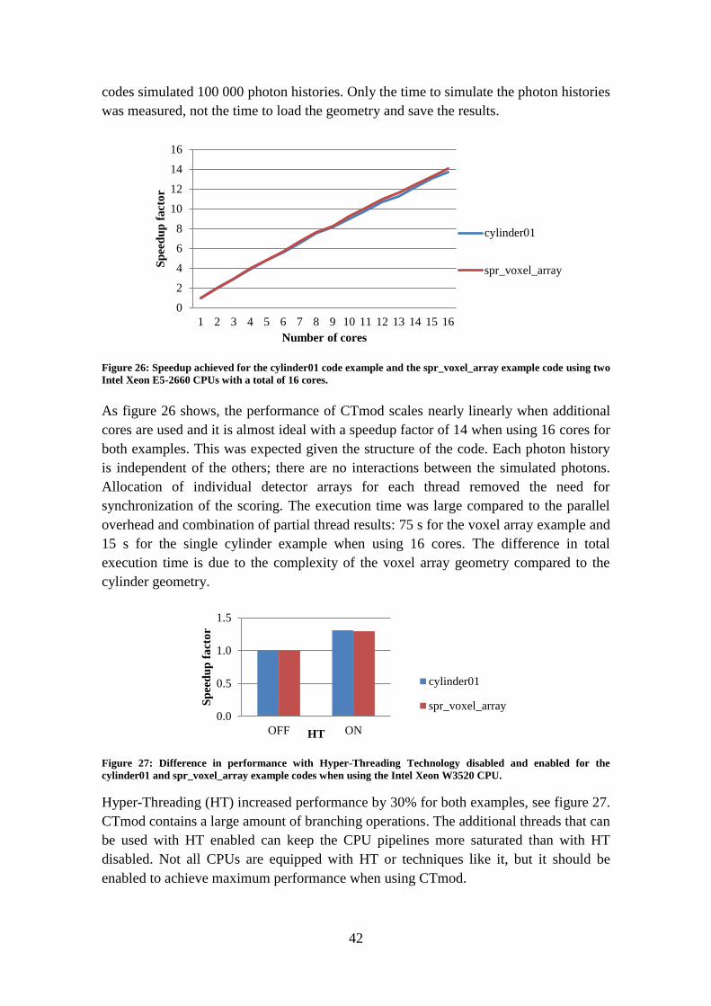
42
codes simulated 100 000 photon histories. Only the time to simulate the photon histories
was measured, not the time to load the geometry and save the results.
Figure 26: Speedup achieved for the cylinder01 code example and the spr_voxel_array example code using two
Intel Xeon E5-2660 CPUs with a total of 16 cores.
As figure 26 shows, the performance of CTmod scales nearly linearly when additional
cores are used and it is almost ideal with a speedup factor of 14 when using 16 cores for
both examples. This was expected given the structure of the code. Each photon history
is independent of the others; there are no interactions between the simulated photons.
Allocation of individual detector arrays for each thread removed the need for
synchronization of the scoring. The execution time was large compared to the parallel
overhead and combination of partial thread results: 75 s for the voxel array example and
15 s for the single cylinder example when using 16 cores. The difference in total
execution time is due to the complexity of the voxel array geometry compared to the
cylinder geometry.
Figure 27: Difference in performance with Hyper-Threading Technology disabled and enabled for the
cylinder01 and spr_voxel_array example codes when using the Intel Xeon W3520 CPU.
Hyper-Threading (HT) increased performance by 30% for both examples, see figure 27.
CTmod contains a large amount of branching operations. The additional threads that can
be used with HT enabled can keep the CPU pipelines more saturated than with HT
disabled. Not all CPUs are equipped with HT or techniques like it, but it should be
enabled to achieve maximum performance when using CTmod.
0
2
4
6
8
10
12
14
16
1 2 3 4 5 6 7 8 9 10 11 12 13 14 15 16
Sp
eed
up
fa
cto
r
Number of cores
cylinder01
spr_voxel_array
0.0
0.5
1.0
1.5
OFF ON
Sp
eed
up
fa
cto
r
HT
cylinder01
spr_voxel_array
43
5. DISCUSSION
This section discusses the changes made to the DIRA and CTmod codes and the
resulting performance improvements. It also contains a discussion on why the OpenCL
implementations of the filtered backprojection and forward projection functions in
DIRA did not provide the expected performance and why a GPU implementation of the
CTmod code was not made.
5.1. DIRA
The change to C code from MATLAB code and updating how the forward projections
of individual base materials are calculated gave a speedup of 4.2 for the dual-core Intel
T1600 CPU and 2.6 for the two 8-core Intel E5-2660 CPUs. With parallelization using
OpenMP speedups of 6.1 and 15.6 where achieved respectively. The code speedup did
not scale linearly with additional cores as 16 cores only gave an increase of a factor 10.
This was due to the many short function calls in DIRA creating a large parallelization
overhead compared to the computation time and the fixed time to load and save data
that cannot be reduced.
The forward projection and filtered backprojection functions were parallelized for GPU
but the implementations did not give a performance increase. Both functions are very
memory-intensive and produce more output data than what is given as input. This meant
either synchronizing memory accesses (which introduce large overheads) or limit the
task parallelization. Using OpenCL instead of OpenMP also introduces additional
overhead due to building the kernel that executes the code.
Section 4.1.5 contains a comparison between two platforms, Windows and Ubuntu, both
using the same hardware and MATLAB version. These results depend on many factors
affecting code execution time such as operating system, compiler and compiler version
as well as MATLAB version. One test is not enough to draw generally valid
conclusions. The user should, if possible, examine the performance of different
platforms to achieve the best results.
5.1.1. CODE MANAGEMENT
Table 10 lists implementation files of functions analyzed and optimized in this thesis.
Selecting the correct file to use is dependent on what software and hardware is available
to the user. This makes maintaining and updating the code complex as there are many
combinations of files that the user can select from. The user also has to be
knowledgeable on how to compile the files not written in MATLAB code. For the C
implementation the files are converted into binary MEX-files with the MATLAB
command mex filename. For the OpenMP implementations the user also has to indicate
that the code is to use the OpenMP framework by specifying compiler flags. For
Windows this is done with mex filename COMPFLAGS="/openmp $COMPFLAGS"
and for UNIX systems mex filename CFLAGS="\$CFLAGS -fopenmp"
LDFLAGS="\$LDFLAGS -fopenmp". The OpenCL version also requires that the user
have the correct drivers installed for the GPU as well as the APP SDK by AMD or the
CUDA toolkit by NVIDIA. A compilation script is provided for both Windows and
44
UNIX to automatically compile the files. Any future updates to the parallel sections of
DIRA will require knowledge on how to write parallel code as well as how to compile
it. This introduces another level of complexity that was not in the single-threaded
version of DIRA.
Table 10: Available implementations of the filtered backprojection, material decomposition, forward
projection and polychromatic projection functions in DIRA.
MATLAB C OpenMP OpenCL
Filtered backprojection - Old + New New New
Material decomposition Old New - -
Forward projection - Old + New New New
Polychromatic projection Old New New New
5.1.2. FILTERED BACKPROJECTION
Each projection in the sinogram is backprojected over the output image. With 𝑘
projection angles and an output image size of 𝑁 × 𝑁 a total of 𝑘 × 𝑁 × 𝑁 values are
placed onto it, meaning more data is produced than what is given as input to the
function. Where to place the values in the output image is dependent on the angle and
multiple projections place values on the same position in the output image, which
requires synchronization. The simplest way to avoid the need for synchronization is by
allocating matrices to store temporary results and combining the results after execution.
Doing so will limit the number of tasks that can be created as the number of matrices
that can be allocated is limited by the available memory. An alternative to allocating
temporary matrices is to instead assign each task to an output row, which reads the
projection values from the sinogram and places them onto that row. This avoids the
synchronization issue but the number of tasks that can be created limited by the number
of rows in the output image. Either method of implementation is limited in the number
of tasks that can be created and will not allow for full GPU utilization. The GPU
implementation is also limited by the overhead of building the kernel. Filtered
backprojection is performed a total of five times, once for the initial reconstruction and
once for each iteration of DIRA. The code structure of DIRA means that the kernel is
built each time filtered backprojection is performed. Building the kernel each iterations
gives a large overhead compared to building the kernel only once.
5.1.3. MATERIAL DECOMPOSITION
The large improvement in the execution time is due to the differences in the MATLAB
and C languages and how they manage and execute code. MATLAB is an interpreted
language; the MATLAB interpreter converts each line of code for direct execution by
the processor. C is a compiled language; a compiler compiles the code to machine code
which is stored in a binary file for later execution. The compilation introduces a delay
before code execution but additional optimization can be performed to improve
performance.
As described in section 3.2.4, mass fractions are calculated by solving equation (2.14).
For every pixel value in the image, the matrix 𝑴 is assigned new values. The old

45
MATLAB implementation allocated and returned the memory needed for matrix 𝑴 for
every pixel processed, introducing a significant amount of overhead. The new
implementation in C allocates and de-allocates the memory only once for the whole
matrix 𝑴.
5.1.4. FORWARD PROJECTION
From tables 7 and 8 we get that the total execution time for all calls to the sinogramJc
function takes 0.97 s for the 16-core Intel E5-2660 CPUs and 1.33 s for the quad-core
Intel 3570K CPU using the parallel OpenMP implementation. Four iterations of DIRA
and five forward projections in each iteration equal a total of 20 function calls. This
gives an average execution time of 0.97 𝑠
20= 0.0485 𝑠 ~0.05 𝑠 and
1.33 𝑠
20=
0.0665 𝑠 ~0.07 𝑠 respectively.
In order to assess how well the forward projection function can be parallelized we need
to look at the operations it performs. The old implementation used the destination-
driven method of calculating a line integral through the image of mass fractions to
produce one projection in the sinogram. Using 𝑑 detector elements gives 𝑑 projection
values for one projection and with 𝑘 angles 𝜃1 . . 𝜃𝑘 a total of 𝑝 × 𝑘 projection values
are computed for one sinogram. If one line integral is one task a total of 𝑝 × 𝑘 tasks can
be created. The problem with this method is, as previously mentioned in section 3.2.3,
the branching operations required to ensure that each step of the line integral is within
the bounds of the image. The memory accesses are also a problem as the entire input
image must be available to every task as it is not possible to determine beforehand what
pixel values in the image the line integral cuts through. For an OpenCL implementation
the input image is too large to fit into private or local memory and must be kept in
global memory. The OpenCL implementation of the destination-driven method
computed one sinogram in ~0.7 𝑠 when using the AMD R7 260X GPU, compared to
the ~0.05 𝑠 for the OpenMP implementation using two Intel E5-2660 CPUs.
The alternative is to use the new, source-driven method. Each pixel value in the input
image produces two projection values in the sinogram for every projection angle 𝜃1 . . 𝜃𝑘
for a total of 2𝑘 values per pixel. With an input image size of 𝑁 ×𝑁 this creates at most
2𝑘 × 𝑁 × 𝑁 values if all pixels in the input image contribute to the projections. The
problem with this method is that multiple pixels will produce values for the same index
in the sinogram and synchronization is required. Synchronization is only supported in
OpenCL between work-items in a work-group, not between work-groups so this is not
an option. Matrices could be allocated to hold temporary results, but this would limit the
number of tasks as the GPU memory is limited and the summation of the temporary
results causes significant overhead. The synchronization issues were avoided by
switching the order of computations such that each calculated projection is one task and
each task iterates over all pixels in the input image. As each angle produces a projection
the number of tasks was limited to the number of angles. This meant that a GPU with
more cores than angles to calculate projections for was not fully utilized. The source-
driven method computed the forward projections in 3.25 s when using the AMD

46
R7 260X GPU, compared to the 0.97 s for the two Intel E5-2660 CPUs and the 1.33 s
when using the Intel 3570K CPU.
The article [6] describes an implementation of an iterative reconstruction algorithm
using NVIDIA’s toolkit CUDA for parallelization using GPU. The authors used the
ordered subset convex algorithm, which updates the image estimate in multiple steps
using a subset of all projections. For the forward projection they used a destination-
driven method by multi-sampling x-rays through the voxels and averaging the results.
Each thread on the GPU was assigned a single detector pixel. No performance numbers
are mentioned in the article and no comparison is made to a CPU implementation
making it difficult to determine if the GPU implementation is better. Testing showed
that for DIRA the source-driven method implemented for CPU is faster than both a
source-driven and destination-driven GPU implementation.
5.2. CTMOD
An OpenCL version of CTmod was planned but due to time constraints and unsuitable
code structure it was not implemented. The transport of the photons is dependent on the
geometry they are transported through, how the geometry is represented and what setup
is used for the detector array. This allows for many different configurations but it is also
the cause of the code’s complexity; CTmod consists of over 100 classes. OpenCL uses
a kernel that is separate from the main code so all necessary data, structures and
functions need be accessed from the kernel. OpenCL does not support classes making
the task of converting CTmod to support OpenCL very time consuming. A complete
rewrite of the code was required and the time to do so was not available.
A parallel random number generator was implemented in CTmod by creating thread-
local copies of the Mersenne Twister generator, where the initial seeds were generated
randomly by the C-function 𝑟𝑎𝑛𝑑(). The drawback to this implementation is that it can
produce sequences that are nearly identical for many iterations before diverging, if the
initial seeds are almost the same. An updated version of the Mersenne Twister addresses
this issue by improving the initialization, but the problem of initial seeds still persists in
the CTmod implementation. One solution to this problem is to implement a parallel
version of the Mersenne Twister, described for example in [45]. In the article CUDA is
used to parallelize the random number generator for NVIDIA GPUs, but the method
described can be used for both CPU and GPU. The generation of random numbers is
divided into blocks where each block skips ahead to a given point in the sequence and
from there generate the random numbers.
The time consuming section of CTmod is the scoring of contributions from individual
photon interactions by the detector array, not the transport of the photons. The code
could be modified to perform the photon transport and detector array scoring in two
separate steps. The photon transport generates random numbers and evaluates branches
based on these numbers, which the CPU does better than a GPU. The less branch-
intensive detector array scoring is then run on the GPU as each detector array element is
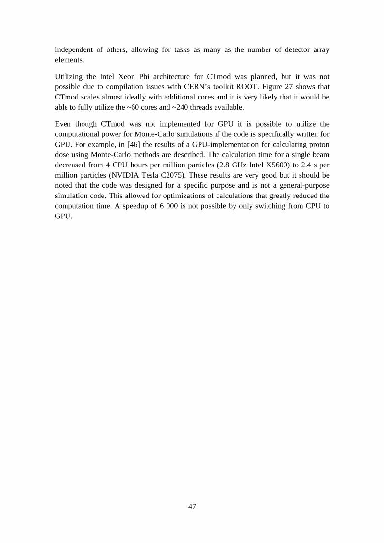
47
independent of others, allowing for tasks as many as the number of detector array
elements.
Utilizing the Intel Xeon Phi architecture for CTmod was planned, but it was not
possible due to compilation issues with CERN’s toolkit ROOT. Figure 27 shows that
CTmod scales almost ideally with additional cores and it is very likely that it would be
able to fully utilize the ~60 cores and ~240 threads available.
Even though CTmod was not implemented for GPU it is possible to utilize the
computational power for Monte-Carlo simulations if the code is specifically written for
GPU. For example, in [46] the results of a GPU-implementation for calculating proton
dose using Monte-Carlo methods are described. The calculation time for a single beam
decreased from 4 CPU hours per million particles (2.8 GHz Intel X5600) to 2.4 s per
million particles (NVIDIA Tesla C2075). These results are very good but it should be
noted that the code was designed for a specific purpose and is not a general-purpose
simulation code. This allowed for optimizations of calculations that greatly reduced the
computation time. A speedup of 6 000 is not possible by only switching from CPU to
GPU.

48

49
BIBLIOGRAPHY
[1] T. R. Team, "ROOT Data Analysis Framework," CERN, [Online]. Available:
https://root.cern.ch/drupal/. [Accessed 27 03 2015].
[2] S. Ulzheimer and T. Flohr, "Multislice CT: Current Technology and Future
Developments," in Multislice CT, 3rd Edition ed., Springer, p. 5.
[3] Intel®, "Intel® Xeon Phi™ Product Family," [Online]. Available:
http://www.intel.com/content/www/us/en/processors/xeon/xeon-phi-
detail.html. [Accessed 03 02 2015].
[4] T. O. M. Project, "Open MPI: Open Source High Performance Computing,"
[Online]. Available: http://www.open-mpi.org/. [Accessed 26 01 2015].
[5] NVIDIA, "Parallel Programming and Computing Platform CUDA," NVIDIA,
[Online]. Available: http://www.nvidia.com/object/cuda_home_new.html.
[Accessed 26 01 2015].
[6] M. Beister, D. Kolditz and W. A. Kalender, "Iterative reconstruction methods in
X-ray CT," Eurpoean Journal of Medical Physics, vol. 28, pp. 94-108, 2012.
[7] "GATE," OpenGATE collaboration, [Online]. Available:
http://www.opengatecollaboration.org/home. [Accessed 26 01 2015].
[8] "Geant4: A toolkit for the simulation of the passage of particles through matter,"
[Online]. Available: http://geant4.cern.ch/. [Accessed 26 1 2015].
[9] F. R. Rannou, N. Vega-Acevedo and Z. El Bitar, "A parallel computational model
for GATE simulations," Computer methods and programs in biomedicine,
vol. 112, pp. 673-683, 2013.
[10] "MCNPX home Page," RSICC, [Online]. Available: https://mcnpx.lanl.gov/.
[Accessed 26 01 2015].
[11] D. M. Usang, M. H. Rabir, M. A. S. Salleh and M. P. Abu, "Performance of MPI
parallel processing implemented by MCNP5/MCNPX for criticality
benchmark problems," in Seminar R&D Nuclear Malaysia, 2012.
[12] "mcgpu Monte Carlo simulation of x-ray transport in a GPU with CUDA," U. S.
Food and Drug Administration (FDA), [Online]. Available:
https://code.google.com/p/mcgpu/. [Accessed 26 01 2015].
[13] D. Tisseur, A. Andrieux, M. Costin and A. Vabre, "Monte Carlo simulation of the
scattered beam in radiography non-destructive testing context," in Joint
International Conference on Supercomputing in Nuclear Applications and
Monte Carlo 2013, Paris, France, 2013.
[14] Intel®, "Intel® Xeon® Processor E5 v3 Family," 2014. [Online]. Available:
http://ark.intel.com/products/family/78583/Intel-Xeon-Processor-E5-v3-
Family#@Server. [Accessed 17 11 2014].
[15] AMD, "AMD Opteron™ 6300 Series Processors," [Online]. Available:
http://www.amd.com/en-us/products/server/opteron/6000/6300. [Accessed 19
11 2014].
[16] Intel®, "Intel® Xeon® Processor 5500 Series," 2014. [Online]. Available:
https://software.intel.com/sites/products/collateral/hpc/vtune/performance_an
alysis_guide.pdf. [Accessed 17 11 2014].
[17] A. Y. Zomaya, M. Abd-El-Barr and H. El-Rewini, "Pipelining Design
Techniques," in Fundamentals of Computer Organization and Architecture,

50
Wiley-Interscience, 2014, pp. 185-190.
[18] G. Lipovski, "Control Instructions," in Introduction to Microcontrollers (Second
Edition), Academic Press, 2014, pp. 47-54.
[19] R. Gerber and A. Binstock, Programming with Hyper-Threading Technology:
How to Write Multithreaded Software for Intel IA-32 Processors, Intel Press,
2004.
[20] M. Raynal, "The Mutual Exclusion Problem," in Concurrent Programming:
Algorithms, Principles, and Foundations, Springer, 2013, pp. 3-13.
[21] T. Rauber and G. Rünger, in Parallel Programming for Multicore and Cluster
Systems, Springer, 2007, pp. 181-182.
[22] OpenMP ARB Corporation, 11 2014. [Online]. Available:
http://openmp.org/openmp-faq.html#WhatIs.
[23] Khronos Group, 11 2014. [Online]. Available: https://www.khronos.org/opencl/.
[24] Khronos Group, 11 2014. [Online]. Available:
https://www.khronos.org/registry/cl/specs/opencl-1.0.pdf.
[25] AMD, "AMD Accelerated Parallel Processing OpenCL Programming Guide,"
[Online]. Available:
developer.amd.com/wordpress/media/2013/07/AMD_Accelerated_Parallel_P
rocessing_OpenCL_Programming_Guide-rev-2.7.pdf. [Accessed 17 11
2014].
[26] C. Angelini and I. Wallossek, "Radeon R9 290X Review," Tom's Hardware,
[Online]. Available: http://www.tomshardware.com/reviews/radeon-r9-290x-
hawaii-review,3650.html. [Accessed 16 02 2015].
[27] I. Wallossek, "AMD FirePro W9100 Review," Tom's Hardware, [Online].
Available: http://www.tomshardware.com/reviews/firepro-w9100-
performance,3810.html. [Accessed 16 02 2015].
[28] I. Wallossek, "Gigabyte GeForce GTX Titan Black," Tom's Hardware, [Online].
Available: http://www.tomshardware.com/reviews/gigabyte-geforce-gtx-titan-
black-ghz-edition,3821.html. [Accessed 16 02 2015].
[29] Intel, "Intel® Xeon Phi™ Product Family," Intel, [Online]. Available:
http://www.intel.com/content/www/us/en/benchmarks/server/xeon-phi/xeon-
phi-theoretical-maximums.html. [Accessed 16 02 2015].
[30] AMD, "HPC Processor Comparison v2 2012," [Online]. Available:
http://sites.amd.com/us/Documents/49747D_HPC_Processor_Comparison_v3
_July2012.pdf. [Accessed 16 02 2015].
[31] E. B. Podgorsak, Radiation Physics for Medical Physicists, Springer, p. 214.
[32] SIEMENS, Dual Energy CT SOMATOM Definition.
[33] P. P. Bruyant, "Analytic and Iterative Reconstruction Algorithms in SPECT," The
Journal of Nuclear Medicine, vol. 43, no. 10, pp. 1343-1358, October 1.
2002.
[34] J. PM, "An Improved Algorithm for Reprojecting Rays through Pixel Images,"
IEEE Trans Med Imaging, Vols. MI-1, no. 3, pp. 192-6, 1982.
[35] B. Jähne, Digital Image Processing, Volume 1, Springer, 2005, p. 276.
[36] T. R. Team, "ROOT Data Analysis Framework," [Online]. Available:
https://root.cern.ch/drupal/. [Accessed 06 02 2015].
[37] Intel®, "Intel® Celeron® Processor T1600," Intel®, [Online]. Available:
51
http://ark.intel.com/products/38979/Intel-Celeron-Processor-T1600-1M-
Cache-1_66-GHz-667-MHz-FSB. [Accessed 17 11 2014].
[38] Intel®, "Intel® Xeon® Processor E5-2660," Intel®, [Online]. Available:
http://ark.intel.com/products/64584/Intel-Xeon-Processor-E5-2660-20M-
Cache-2_20-GHz-8_00-GTs-Intel-QPI. [Accessed 17 11 2014].
[39] "Intel® Xeon® Processor W3520," Intel®, [Online]. Available:
http://ark.intel.com/products/39718/Intel-Xeon-Processor-W3520-8M-Cache-
2_66-GHz-4_80-GTs-Intel-QPI. [Accessed 15 01 2015].
[40] NSC, "National Supercomputer Centre at Linköping University," NSC, [Online].
Available: https://www.nsc.liu.se/. [Accessed 17 11 2014].
[41] AMD, "AMD Radeon™ R7 Series Graphics," AMD, [Online]. Available:
http://www.amd.com/en-us/products/graphics/desktop/r7#. [Accessed 17 11
2014].
[42] A. Malusek, "cmiv-dira," [Online]. Available: https://code.google.com/p/cmiv-
dira/. [Accessed 13 02 2015].
[43] A. Malusek, M. Magnusson, M. Sandborg, R. Westin and G. Alm Carlsson,
"Prostate tissue decomposition via DECT using the model based iterative
image reconstruction algorithm DIRA," in Medical Imaging 2014: Physics of
Medical Imaging, San Diego, California, USA , 2014.
[44] J. Orchard, "MATLAB Central File Exchange," MATLAB, [Online]. Available:
http://www.mathworks.com/matlabcentral/fileexchange/12852-iradon-speedy.
[Accessed 19 11 2014].
[45] T. Bradley, J. du Toit, M. Giles, R. Tong and P. Woodhams, "Parallelisation
Techniques for Random Number Generators".
[46] D. Giantsoudi, J. Schuemann, X. Jia, S. Dowdell, S. Jiang and H. Paganetti,
"Validation of a GPU-based Monte-Carlo code (gPMC) for proton radiation
therapy: clinical cases study," Physics in Medicine and Biology, vol. 60, pp.
2257-2269, 2015.
[47] M. Magnusson, A. Malusek, A. Muhammad and G. Alm Carlsson, "Iterative
Reconstruction for Quantitative Tissue Decomposition in Dual-Energy CT,"
Pro c. Scandinavian Conference on Image Analysis, SCIA, 2011, 23-27 May.
[48] O. Grandell, "An iterative reconstruction algorithm for quantitative tissue decomp
osition using DECT," 2012.
[49] M. Magnusson, A. Malusek, A. Muhammad and G. Alm Carlsson,
"Determination of quantitative tissue composition by iterative reconstruction
on 3d," in Pro c. of the 11th International Meeting on Fully
ThreeDimensional Image Reconstruction in Radiology and Nuclear Medicine,
2011.
[50] B. De Man, J. Nuyts, P. Dupont, G. Marchal and P. Suetens, "An Iterative
Maximum-Likelihood Polychromatic Algorithm for CT," IEEE
TRANSACTIONS ON MEDICAL IMAGING, vol. 20, no. 10, pp. 999-1008,
2001.
[51] M. Vajteršic, P. Zinterhof and R. Trobec, "Overview – Parallel Computing:
Numerics, Applications, and Trends," in Parallel Computing, Springer, 2014,
p. 1.
[52] G. M. Amdahl, "Validity of the single processor approach to achieving large scale
computing capabilities," in AFIPS spring joint computer conference, 1967.
52
[53] G. T. Herman, "Backprojection," in Fundamentals of Computerized Tomography,
Springer, p. 125.
[54] W. A. Kalender, "Principle of Computed Tomography," in Computed
Tomography, Publicis, 2005, pp. 22-25.
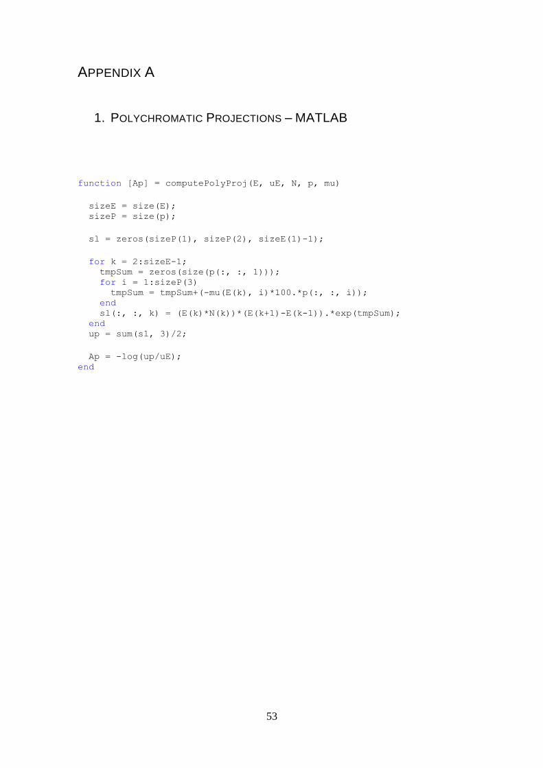
53
APPENDIX A
1. POLYCHROMATIC PROJECTIONS – MATLAB
function [Ap] = computePolyProj(E, uE, N, p, mu)
sizeE = size(E); sizeP = size(p);
sl = zeros(sizeP(1), sizeP(2), sizeE(1)-1);
for k = 2:sizeE-1; tmpSum = zeros(size(p(:, :, 1))); for i = 1:sizeP(3) tmpSum = tmpSum+(-mu(E(k), i)*100.*p(:, :, i)); end sl(:, :, k) = (E(k)*N(k))*(E(k+1)-E(k-1)).*exp(tmpSum); end up = sum(sl, 3)/2;
Ap = -log(up/uE); end
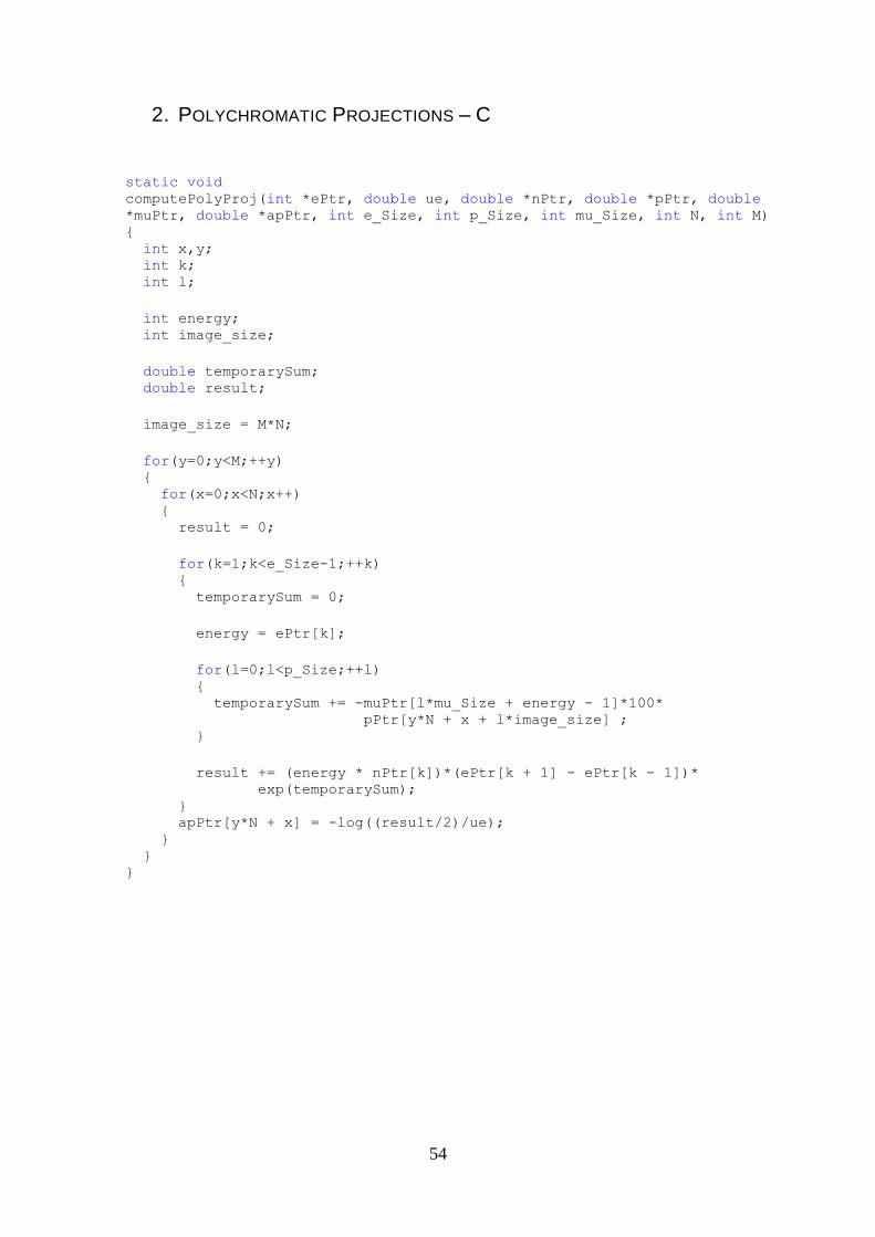
54
2. POLYCHROMATIC PROJECTIONS – C
static void computePolyProj(int *ePtr, double ue, double *nPtr, double *pPtr, double
*muPtr, double *apPtr, int e_Size, int p_Size, int mu_Size, int N, int M) { int x,y; int k; int l; int energy; int image_size; double temporarySum; double result; image_size = M*N; for(y=0;y<M;++y) { for(x=0;x<N;x++) { result = 0; for(k=1;k<e_Size-1;++k) { temporarySum = 0; energy = ePtr[k]; for(l=0;l<p_Size;++l) { temporarySum += -muPtr[l*mu_Size + energy - 1]*100* pPtr[y*N + x + l*image_size] ; } result += (energy * nPtr[k])*(ePtr[k + 1] - ePtr[k - 1])* exp(temporarySum); } apPtr[y*N + x] = -log((result/2)/ue); } } }
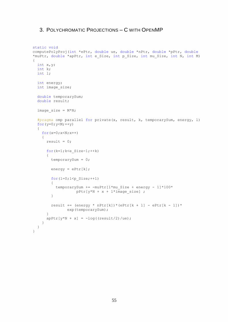
55
3. POLYCHROMATIC PROJECTIONS – C WITH OPENMP
static void computePolyProj(int *ePtr, double ue, double *nPtr, double *pPtr, double
*muPtr, double *apPtr, int e_Size, int p_Size, int mu_Size, int N, int M) { int x,y; int k; int l; int energy; int image_size; double temporarySum; double result; image_size = M*N; #pragma omp parallel for private(x, result, k, temporarySum, energy, l) for(y=0;y<M;++y) { for(x=0;x<N;x++) { result = 0; for(k=1;k<e_Size-1;++k) { temporarySum = 0; energy = ePtr[k]; for(l=0;l<p_Size;++l) { temporarySum += -muPtr[l*mu_Size + energy - 1]*100* pPtr[y*N + x + l*image_size] ; } result += (energy * nPtr[k])*(ePtr[k + 1] - ePtr[k - 1])* exp(temporarySum); } apPtr[y*N + x] = -log((result/2)/ue); } } }
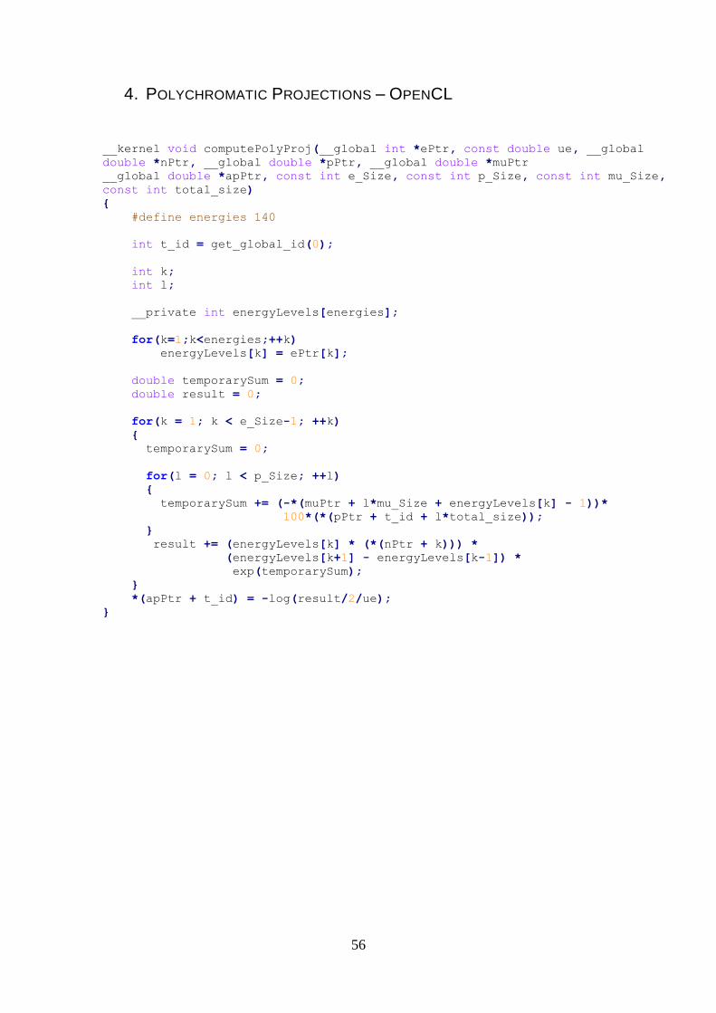
56
4. POLYCHROMATIC PROJECTIONS – OPENCL
__kernel void computePolyProj(__global int *ePtr, const double ue, __global
double *nPtr, __global double *pPtr, __global double *muPtr
__global double *apPtr, const int e_Size, const int p_Size, const int mu_Size,
const int total_size)
{
#define energies 140
int t_id = get_global_id(0);
int k;
int l;
__private int energyLevels[energies];
for(k=1;k<energies;++k)
energyLevels[k] = ePtr[k];
double temporarySum = 0;
double result = 0;
for(k = 1; k < e_Size-1; ++k)
{
temporarySum = 0;
for(l = 0; l < p_Size; ++l)
{
temporarySum += (-*(muPtr + l*mu_Size + energyLevels[k] - 1))*
100*(*(pPtr + t_id + l*total_size));
}
result += (energyLevels[k] * (*(nPtr + k))) *
(energyLevels[k+1] - energyLevels[k-1]) *
exp(temporarySum);
}
*(apPtr + t_id) = -log(result/2/ue);
}