part one: i. single−equation regression models

Gujarati: Basic

Econometrics, Fourth

Edition

I. Single−Equation

Regression Models

5. Two−Variable

Regression: Interval

Estimation and Hypothesis

Testing

© The McGraw−Hill

Companies, 2004

119

Beware of testing too many hypotheses; the more you torture the data, the morelikely they are to confess, but confession obtained under duress may not be admis-sible in the court of scientific opinion.1

As pointed out in Chapter 4, estimation and hypothesis testing constitutethe two major branches of classical statistics. The theory of estimation con-sists of two parts: point estimation and interval estimation. We have dis-cussed point estimation thoroughly in the previous two chapters where weintroduced the OLS and ML methods of point estimation. In this chapter wefirst consider interval estimation and then take up the topic of hypothesistesting, a topic intimately related to interval estimation.

5.1 STATISTICAL PREREQUISITES

Before we demonstrate the actual mechanics of establishing confidence in-tervals and testing statistical hypotheses, it is assumed that the reader is fa-miliar with the fundamental concepts of probability and statistics. Althoughnot a substitute for a basic course in statistics, Appendix A provides theessentials of statistics with which the reader should be totally familiar.Key concepts such as probability, probability distributions, Type I andType II errors, level of significance, power of a statistical test, andconfidence interval are crucial for understanding the material covered inthis and the following chapters.

1Stephen M. Stigler, “Testing Hypothesis or Fitting Models? Another Look at Mass Extinc-tions,” in Matthew H. Nitecki and Antoni Hoffman, eds., Neutral Models in Biology, OxfordUniversity Press, Oxford, 1987, p. 148.

5TWO-VARIABLEREGRESSION: INTERVALESTIMATION ANDHYPOTHESIS TESTING

Gujarati: Basic


Edition


Regression Models

5. Two−Variable



Testing


Companies, 2004

120 PART ONE: SINGLE-EQUATION REGRESSION MODELS

2Also known as the probability of committing a Type I error. A Type I error consists inrejecting a true hypothesis, whereas a Type II error consists in accepting a false hypothesis.(This topic is discussed more fully in App. A.) The symbol α is also known as the size of the(statistical) test.

5.2 INTERVAL ESTIMATION: SOME BASIC IDEAS

To fix the ideas, consider the hypothetical consumption-income exampleof Chapter 3. Equation (3.6.2) shows that the estimated marginal propensityto consume (MPC) β2 is 0.5091, which is a single (point) estimate of theunknown population MPC β2. How reliable is this estimate? As noted inChapter 3, because of sampling fluctuations, a single estimate is likely todiffer from the true value, although in repeated sampling its mean value isexpected to be equal to the true value. [Note: E(β2) = β2.] Now in statisticsthe reliability of a point estimator is measured by its standard error. There-fore, instead of relying on the point estimate alone, we may construct aninterval around the point estimator, say within two or three standard errorson either side of the point estimator, such that this interval has, say, 95 per-cent probability of including the true parameter value. This is roughly theidea behind interval estimation.To be more specific, assume that we want to find out how “close” is, say,

β2 to β2. For this purpose we try to find out two positive numbers δ and α,the latter lying between 0 and 1, such that the probability that the randominterval (β2 − δ, β2 + δ) contains the true β2 is 1− α. Symbolically,

Pr (β2 − δ ≤ β2 ≤ β2 + δ) = 1− α (5.2.1)

Such an interval, if it exists, is known as a confidence interval; 1− α isknown as the confidence coefficient; and α (0 < α < 1) is known as thelevel of significance.2 The endpoints of the confidence interval are knownas the confidence limits (also known as critical values), β2 − δ being thelower confidence limit and β2 + δ the upper confidence limit. In passing,note that in practice α and 1− α are often expressed in percentage forms as100α and 100(1 − α) percent.Equation (5.2.1) shows that an interval estimator, in contrast to a

point estimator, is an interval constructed in such a manner that it has aspecified probability 1 − α of including within its limits the true value of theparameter. For example, if α = 0.05, or 5 percent, (5.2.1) would read: Theprobability that the (random) interval shown there includes the true β2 is0.95, or 95 percent. The interval estimator thus gives a range of valueswithin which the true β2 may lie.It is very important to know the following aspects of interval estimation:

1. Equation (5.2.1) does not say that the probability of β2 lying betweenthe given limits is 1 − α. Since β2, although an unknown, is assumed to besome fixed number, either it lies in the interval or it does not. What (5.2.1)

Gujarati: Basic


Edition


Regression Models

5. Two−Variable



Testing


Companies, 2004

CHAPTER FIVE: TWO VARIABLE REGRESSION: INTERVAL ESTIMATION AND HYPOTHESIS TESTING 121

states is that, for the method described in this chapter, the probability ofconstructing an interval that contains β2 is 1 − α.

2. The interval (5.2.1) is a random interval; that is, it will vary from onesample to the next because it is based on β2, which is random. (Why?)

3. Since the confidence interval is random, the probability statementsattached to it should be understood in the long-run sense, that is, repeatedsampling. More specifically, (5.2.1) means: If in repeated sampling confi-dence intervals like it are constructed a great many times on the 1 − α prob-ability basis, then, in the long run, on the average, such intervals will enclosein 1 − α of the cases the true value of the parameter.

4. As noted in 2, the interval (5.2.1) is random so long as β2 is not known.But once we have a specific sample and once we obtain a specific numericalvalue of β2, the interval (5.2.1) is no longer random; it is fixed. In this case,we cannot make the probabilistic statement (5.2.1); that is, we cannot saythat the probability is 1 − α that a given fixed interval includes the true β2. Inthis situation β2 is either in the fixed interval or outside it. Therefore, theprobability is either 1 or 0. Thus, for our hypothetical consumption-incomeexample, if the 95% confidence interval were obtained as (0.4268 ≤ β2 ≤0.5914), as we do shortly in (5.3.9), we cannot say the probability is 95%that this interval includes the true β2. That probability is either 1 or 0.

How are the confidence intervals constructed? From the preceding dis-cussion one may expect that if the sampling or probability distributionsof the estimators are known, one can make confidence interval statementssuch as (5.2.1). In Chapter 4 we saw that under the assumption of normal-ity of the disturbances ui the OLS estimators β1 and β2 are themselvesnormally distributed and that the OLS estimator σ 2 is related to the χ2 (chi-square) distribution. It would then seem that the task of constructing confi-dence intervals is a simple one. And it is!

5.3 CONFIDENCE INTERVALS FOR REGRESSION

COEFFICIENTS β1AND β2

Confidence Interval for β2

It was shown in Chapter 4, Section 4.3, that, with the normality assump-tion for ui, the OLS estimators β1 and β2 are themselves normally distrib-uted with means and variances given therein. Therefore, for example, thevariable

Z = β2 − β2

se (β2)

=(β2 − β2)

√

∑

x2i

σ

(5.3.1)

Gujarati: Basic


Edition


Regression Models

5. Two−Variable



Testing


Companies, 2004


3Some authors prefer to write (5.3.5) with the df explicitly indicated. Thus, they would write

Pr [β2 − t(n−2),α/2 se (β2) ≤ β2 ≤ β2 + t(n−2)α/2 se (β2)] = 1− α

But for simplicity we will stick to our notation; the context clarifies the appropriate df involved.

as noted in (4.3.6), is a standardized normal variable. It therefore seems thatwe can use the normal distribution tomake probabilistic statements about β2provided the true population variance σ 2 is known. If σ 2 is known, an impor-tant property of a normally distributed variable with mean µ and variance σ 2

is that the area under the normal curve between µ± σ is about 68 percent,that between the limits µ± 2σ is about 95 percent, and that between µ± 3σis about 99.7 percent.But σ 2 is rarely known, and in practice it is determined by the unbiased

estimator σ 2. If we replace σ by σ , (5.3.1) may be written as

t = β2 − β2

se (β2)= estimator− parameter

estimated standard error of estimator

=(β2 − β2)

√

∑

x2i

σ

(5.3.2)

where the se (β2) now refers to the estimated standard error. It can be shown(see Appendix 5A, Section 5A.2) that the t variable thus defined follows the tdistribution with n − 2 df. [Note the difference between (5.3.1) and (5.3.2).]Therefore, instead of using the normal distribution, we can use the t distri-bution to establish a confidence interval for β2 as follows:

Pr (−tα/2 ≤ t ≤ tα/2) = 1− α (5.3.3)

where the t value in the middle of this double inequality is the t value givenby (5.3.2) and where tα/2 is the value of the t variable obtained from the tdistribution for α/2 level of significance and n − 2 df; it is often called thecritical t value at α/2 level of significance. Substitution of (5.3.2) into (5.3.3)yields

Pr

[

−tα/2 ≤ β2 − β2

se (β2)≤ tα/2

]

= 1− α (5.3.4)

Rearranging (5.3.4), we obtain

(5.3.5)3Pr [β2 − tα/2 se (β2) ≤ β2 ≤ β2 + tα/2 se (β2)] = 1− α

Gujarati: Basic


Edition


Regression Models

5. Two−Variable



Testing


Companies, 2004


Equation (5.3.5) provides a 100(1 − α) percent confidence interval for β2,which can be written more compactly as

100(1 − α)% confidence interval for β2:

(5.3.6)

Arguing analogously, and using (4.3.1) and (4.3.2), we can then write:

(5.3.7)

or, more compactly,

100(1 − α)% confidence interval for β1:

(5.3.8)

Notice an important feature of the confidence intervals given in (5.3.6)and (5.3.8): In both cases the width of the confidence interval is proportionalto the standard error of the estimator. That is, the larger the standard error,the larger is the width of the confidence interval. Put differently, the largerthe standard error of the estimator, the greater is the uncertainty of esti-mating the true value of the unknown parameter. Thus, the standard errorof an estimator is often described as a measure of the precision of the esti-mator, i.e., how precisely the estimator measures the true population value.Returning to our illustrative consumption–income example, in Chapter 3

(Section 3.6) we found that β2 = 0.5091, se (β2) = 0.0357, and df = 8. If weassume α = 5%, that is, 95% confidence coefficient, then the t table showsthat for 8 df the critical tα/2 = t0.025 = 2.306. Substituting these values in(5.3.5), the reader should verify that the 95% confidence interval for β2 is asfollows:

0.4268 ≤ β2 ≤ 0.5914 (5.3.9)

Or, using (5.3.6), it is

0.5091± 2.306(0.0357)

that is,

0.5091± 0.0823 (5.3.10)

The interpretation of this confidence interval is: Given the confi-dence coefficient of 95%, in the long run, in 95 out of 100 cases intervals like

β1 ± tα/2 se (β1)

Pr [β1 − tα/2 se (β1) ≤ β1 ≤ β1 + tα/2 se (β1)] = 1− α

β2 ± tα/2 se (β2)

Gujarati: Basic


Edition


Regression Models

5. Two−Variable



Testing


Companies, 2004


4For an accessible discussion, see John Neter, William Wasserman, and Michael H. Kutner,Applied Linear Regression Models, Richard D. Irwin, Homewood, Ill., 1983, Chap. 5.

(0.4268, 0.5914) will contain the true β2. But, as warned earlier, we cannotsay that the probability is 95 percent that the specific interval (0.4268 to0.5914) contains the true β2 because this interval is now fixed and no longerrandom; therefore, β2 either lies in it or does not: The probability that thespecified fixed interval includes the true β2 is therefore 1 or 0.

Confidence Interval for β1

Following (5.3.7), the reader can easily verify that the 95% confidence inter-val for β1 of our consumption–income example is

9.6643 ≤ β1 ≤ 39.2448 (5.3.11)

Or, using (5.3.8), we find it is

24.4545± 2.306(6.4138)

that is,

24.4545± 14.7902 (5.3.12)

Again you should be careful in interpreting this confidence interval. Inthe long run, in 95 out of 100 cases intervals like (5.3.11) will contain thetrue β1; the probability that this particular fixed interval includes the true β1is either 1 or 0.

Confidence Interval for β1 and β2 Simultaneously

There are occasions when one needs to construct a joint confidence intervalfor β1 and β2 such that with a confidence coefficient (1 − α), say, 95%, that in-terval includes β1 and β2 simultaneously. Since this topic is involved, the in-terested reader may want to consult appropriate references.4We will touchon this topic briefly in Chapters 8 and 10.

5.4 CONFIDENCE INTERVAL FOR σ2

As pointed out in Chapter 4, Section 4.3, under the normality assumption,the variable

χ2 = (n− 2)σ 2

σ 2(5.4.1)

Gujarati: Basic


Edition


Regression Models

5. Two−Variable



Testing


Companies, 2004


f(χ2)

χ2

Density

95%2.5% 2.5%

17.5346 2.1797

χ20.025

χ20.975

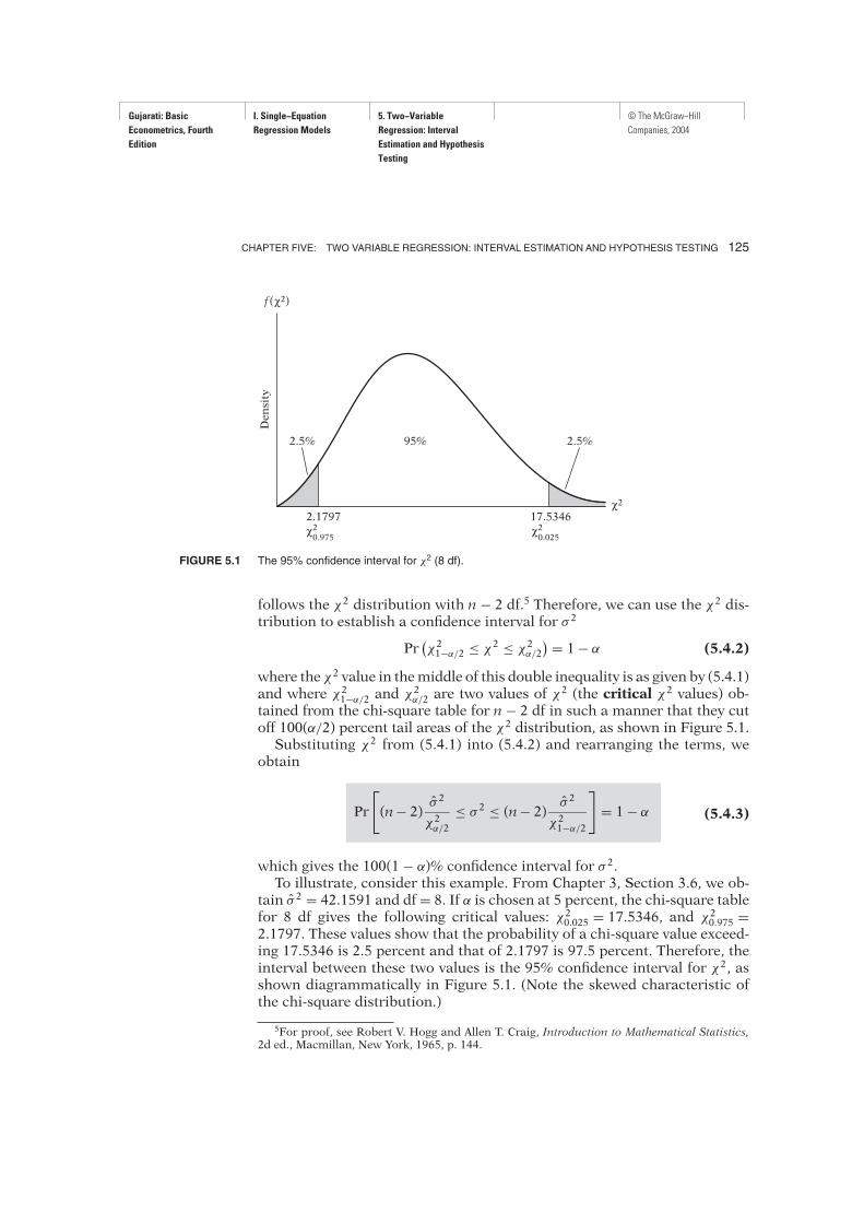
FIGURE 5.1 The 95% confidence interval for χ2 (8 df).

follows the χ2 distribution with n − 2 df.5 Therefore, we can use the χ2 dis-tribution to establish a confidence interval for σ 2

Pr(

χ21−α/2 ≤ χ2 ≤ χ2α/2)

= 1− α (5.4.2)

where the χ2 value in themiddle of this double inequality is as given by (5.4.1)and where χ21−α/2 and χ2

α/2 are two values of χ2 (the critical χ2 values) ob-

tained from the chi-square table for n − 2 df in such a manner that they cutoff 100(α/2) percent tail areas of the χ2 distribution, as shown in Figure 5.1.Substituting χ2 from (5.4.1) into (5.4.2) and rearranging the terms, we

obtain

(5.4.3)

which gives the 100(1 − α)% confidence interval for σ 2.To illustrate, consider this example. From Chapter 3, Section 3.6, we ob-

tain σ 2 = 42.1591 and df = 8. If α is chosen at 5 percent, the chi-square tablefor 8 df gives the following critical values: χ20.025 = 17.5346, and χ20.975 =2.1797. These values show that the probability of a chi-square value exceed-ing 17.5346 is 2.5 percent and that of 2.1797 is 97.5 percent. Therefore, theinterval between these two values is the 95% confidence interval for χ2, asshown diagrammatically in Figure 5.1. (Note the skewed characteristic ofthe chi-square distribution.)

Pr

[

(n− 2)σ 2

χ2α/2

≤ σ 2 ≤ (n− 2)σ 2

χ21−α/2

]

= 1− α

5For proof, see Robert V. Hogg and Allen T. Craig, Introduction to Mathematical Statistics,2d ed., Macmillan, New York, 1965, p. 144.

Gujarati: Basic


Edition


Regression Models

5. Two−Variable



Testing


Companies, 2004


6A statistical hypothesis is called a simple hypothesis if it specifies the precise value(s)of the parameter(s) of a probability density function; otherwise, it is called a composite hy-pothesis. For example, in the normal pdf (1/σ

√2π) exp {− 1

2 [(X − µ)/σ ]2}, if we assert thatH1:µ = 15 and σ = 2, it is a simple hypothesis; but if H1:µ = 15 and σ > 15, it is a compositehypothesis, because the standard deviation does not have a specific value.

Substituting the data of our example into (5.4.3), the reader should verifythat the 95% confidence interval for σ 2 is as follows:

19.2347 ≤ σ 2 ≤ 154.7336 (5.4.4)

The interpretation of this interval is: If we establish 95% confidencelimits on σ 2 and if we maintain a priori that these limits will include true σ 2,we shall be right in the long run 95 percent of the time.

5.5 HYPOTHESIS TESTING: GENERAL COMMENTS

Having discussed the problem of point and interval estimation, we shall nowconsider the topic of hypothesis testing. In this section we discuss brieflysome general aspects of this topic; Appendix A gives some additional details.The problem of statistical hypothesis testing may be stated simply as fol-

lows: Is a given observation or finding compatible with some stated hypothe-sis or not? The word “compatible,” as used here, means “sufficiently” closeto the hypothesized value so that we do not reject the stated hypothesis.Thus, if some theory or prior experience leads us to believe that the trueslope coefficient β2 of the consumption–income example is unity, is the ob-served β2 = 0.5091 obtained from the sample of Table 3.2 consistent withthe stated hypothesis? If it is, we do not reject the hypothesis; otherwise, wemay reject it.In the language of statistics, the stated hypothesis is known as the null

hypothesis and is denoted by the symbol H0. The null hypothesis is usu-ally tested against an alternative hypothesis (also known as maintainedhypothesis) denoted by H1, which may state, for example, that true β2 isdifferent from unity. The alternative hypothesis may be simple or compos-ite.6 For example, H1:β2 = 1.5 is a simple hypothesis, but H1:β2 )= 1.5 is acomposite hypothesis.The theory of hypothesis testing is concerned with developing rules or

procedures for deciding whether to reject or not reject the null hypothesis.There are two mutually complementary approaches for devising such rules,namely, confidence interval and test of significance. Both these ap-proaches predicate that the variable (statistic or estimator) under consider-ation has some probability distribution and that hypothesis testing involvesmaking statements or assertions about the value(s) of the parameter(s) ofsuch distribution. For example, we know that with the normality assump-tion β2 is normally distributed with mean equal to β2 and variance given by(4.3.5). If we hypothesize that β2 = 1, we are making an assertion about one

Gujarati: Basic


Edition


Regression Models

5. Two−Variable



Testing


Companies, 2004


Decision Rule: Construct a 100(1 − α)% confidence interval for β2. If the β2 under H0 falls

within this confidence interval, do not reject H0, but if it falls outside this interval, reject H0.

of the parameters of the normal distribution, namely, the mean. Most of thestatistical hypotheses encountered in this text will be of this type—makingassertions about one or more values of the parameters of some assumedprobability distribution such as the normal, F, t, or χ2. How this is accom-plished is discussed in the following two sections.

5.6 HYPOTHESIS TESTING:

THE CONFIDENCE-INTERVAL APPROACH

Two-Sided or Two-Tail Test

To illustrate the confidence-interval approach, once again we revert to theconsumption–income example. As we know, the estimatedmarginal propen-sity to consume (MPC), β2, is 0.5091. Suppose we postulate that

H0:β2 = 0.3

H1:β2 )= 0.3

that is, the true MPC is 0.3 under the null hypothesis but it is less than orgreater than 0.3 under the alternative hypothesis. The null hypothesis is asimple hypothesis, whereas the alternative hypothesis is composite; actuallyit is what is known as a two-sided hypothesis. Very often such a two-sidedalternative hypothesis reflects the fact that we do not have a strong a pri-ori or theoretical expectation about the direction in which the alternativehypothesis should move from the null hypothesis.Is the observed β2 compatible with H0? To answer this question, let us refer

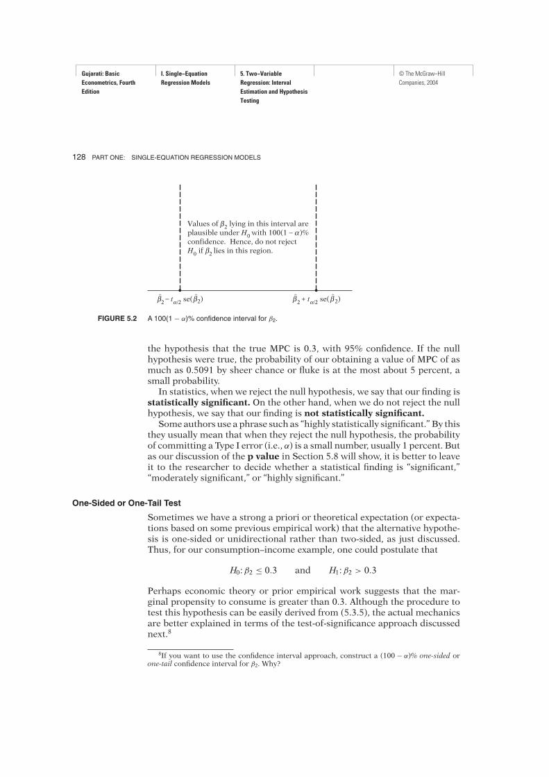
to the confidence interval (5.3.9). We know that in the long run intervals like(0.4268, 0.5914) will contain the true β2 with 95 percent probability. Conse-quently, in the long run (i.e., repeated sampling) such intervals provide arange or limits within which the true β2 may lie with a confidence coefficientof, say, 95%. Thus, the confidence interval provides a set of plausible nullhypotheses. Therefore, if β2 underH0 falls within the 100(1 − α)% confidenceinterval, we do not reject the null hypothesis; if it lies outside the interval, wemay reject it.7 This range is illustrated schematically in Figure 5.2.

7Always bear in mind that there is a 100α percent chance that the confidence interval doesnot contain β2 under H0 even though the hypothesis is correct. In short, there is a 100α percentchance of committing a Type I error. Thus, if α = 0.05, there is a 5 percent chance that wecould reject the null hypothesis even though it is true.

Following this rule, for our hypothetical example, H0:β2 = 0.3 clearly liesoutside the 95% confidence interval given in (5.3.9). Therefore, we can reject

Gujarati: Basic


Edition


Regression Models

5. Two−Variable



Testing


Companies, 2004


β2– tα/2 se(β2)βα β

2+ tα/2 se(β2)ββ α

αValues of β

2 lying in this interval are

plausible under H0with 100 (1 – )%

confidence. Hence, do not reject

H0 if β

2lies in this region.β

β

β

FIGURE 5.2 A 100(1 − α)% confidence interval for β2.

8If you want to use the confidence interval approach, construct a (100 − α)% one-sided orone-tail confidence interval for β2. Why?

the hypothesis that the true MPC is 0.3, with 95% confidence. If the nullhypothesis were true, the probability of our obtaining a value of MPC of asmuch as 0.5091 by sheer chance or fluke is at the most about 5 percent, asmall probability.In statistics, when we reject the null hypothesis, we say that our finding is

statistically significant. On the other hand, when we do not reject the nullhypothesis, we say that our finding is not statistically significant.Some authors use a phrase such as “highly statistically significant.” By this

they usually mean that when they reject the null hypothesis, the probabilityof committing a Type I error (i.e., α) is a small number, usually 1 percent. Butas our discussion of the p value in Section 5.8 will show, it is better to leaveit to the researcher to decide whether a statistical finding is “significant,”“moderately significant,” or “highly significant.”

One-Sided or One-Tail Test

Sometimes we have a strong a priori or theoretical expectation (or expecta-tions based on some previous empirical work) that the alternative hypothe-sis is one-sided or unidirectional rather than two-sided, as just discussed.Thus, for our consumption–income example, one could postulate that

H0:β2 ≤ 0.3 and H1:β2 > 0.3

Perhaps economic theory or prior empirical work suggests that the mar-ginal propensity to consume is greater than 0.3. Although the procedure totest this hypothesis can be easily derived from (5.3.5), the actual mechanicsare better explained in terms of the test-of-significance approach discussednext.8

Gujarati: Basic


Edition


Regression Models

5. Two−Variable



Testing


Companies, 2004


9Details may be found in E. L. Lehman, Testing Statistical Hypotheses, John Wiley & Sons,New York, 1959.

5.7 HYPOTHESIS TESTING:

THE TEST-OF-SIGNIFICANCE APPROACH

Testing the Significance of Regression Coefficients: The t Test

An alternative but complementary approach to the confidence-intervalmethod of testing statistical hypotheses is the test-of-significance ap-proach developed along independent lines by R. A. Fisher and jointly byNeyman and Pearson.9 Broadly speaking, a test of significance is a pro-cedure by which sample results are used to verify the truth or falsity ofa null hypothesis. The key idea behind tests of significance is that of a teststatistic (estimator) and the sampling distribution of such a statistic underthe null hypothesis. The decision to accept or reject H0 is made on the basisof the value of the test statistic obtained from the data at hand.As an illustration, recall that under the normality assumption the variable

t = β2 − β2

se (β2)

=(β2 − β2)

√

∑

x2i

σ

(5.3.2)

follows the t distribution with n − 2 df. If the value of true β2 is specifiedunder the null hypothesis, the t value of (5.3.2) can readily be computedfrom the available sample, and therefore it can serve as a test statistic. Andsince this test statistic follows the t distribution, confidence-interval state-ments such as the following can be made:

Pr

[

−tα/2 ≤ β2 − β*2

se (β2)≤ tα/2

]

= 1− α (5.7.1)

where β*2 is the value of β2 under H0 and where −tα/2 and tα/2 are the valuesof t (the critical t values) obtained from the t table for (α/2) level of signifi-cance and n − 2 df [cf. (5.3.4)]. The t table is given in Appendix D.Rearranging (5.7.1), we obtain

(5.7.2)

which gives the interval in which β2 will fall with 1 − α probability, givenβ2 = β*2 . In the language of hypothesis testing, the 100(1 − α)% confidenceinterval established in (5.7.2) is known as the region of acceptance (of

Pr [β*2 − tα/2 se (β2) ≤ β2 ≤ β*2 + tα/2 se (β2)] = 1− α

Gujarati: Basic


Edition


Regression Models

5. Two−Variable



Testing


Companies, 2004


the null hypothesis) and the region(s) outside the confidence interval is (are)called the region(s) of rejection (of H0) or the critical region(s). As notedpreviously, the confidence limits, the endpoints of the confidence interval,are also called critical values.The intimate connection between the confidence-interval and test-of-

significance approaches to hypothesis testing can now be seen by compar-ing (5.3.5) with (5.7.2). In the confidence-interval procedure we try to estab-lish a range or an interval that has a certain probability of including the truebut unknown β2, whereas in the test-of-significance approach we hypothe-size some value for β2 and try to see whether the computed β2 lies withinreasonable (confidence) limits around the hypothesized value.Once again let us revert to our consumption–income example. We know

that β2 = 0.5091, se (β2) = 0.0357, and df = 8. If we assume α = 5 percent,tα/2 = 2.306. If we let H0:β2 = β*2 = 0.3 and H1:β2 )= 0.3, (5.7.2) becomes

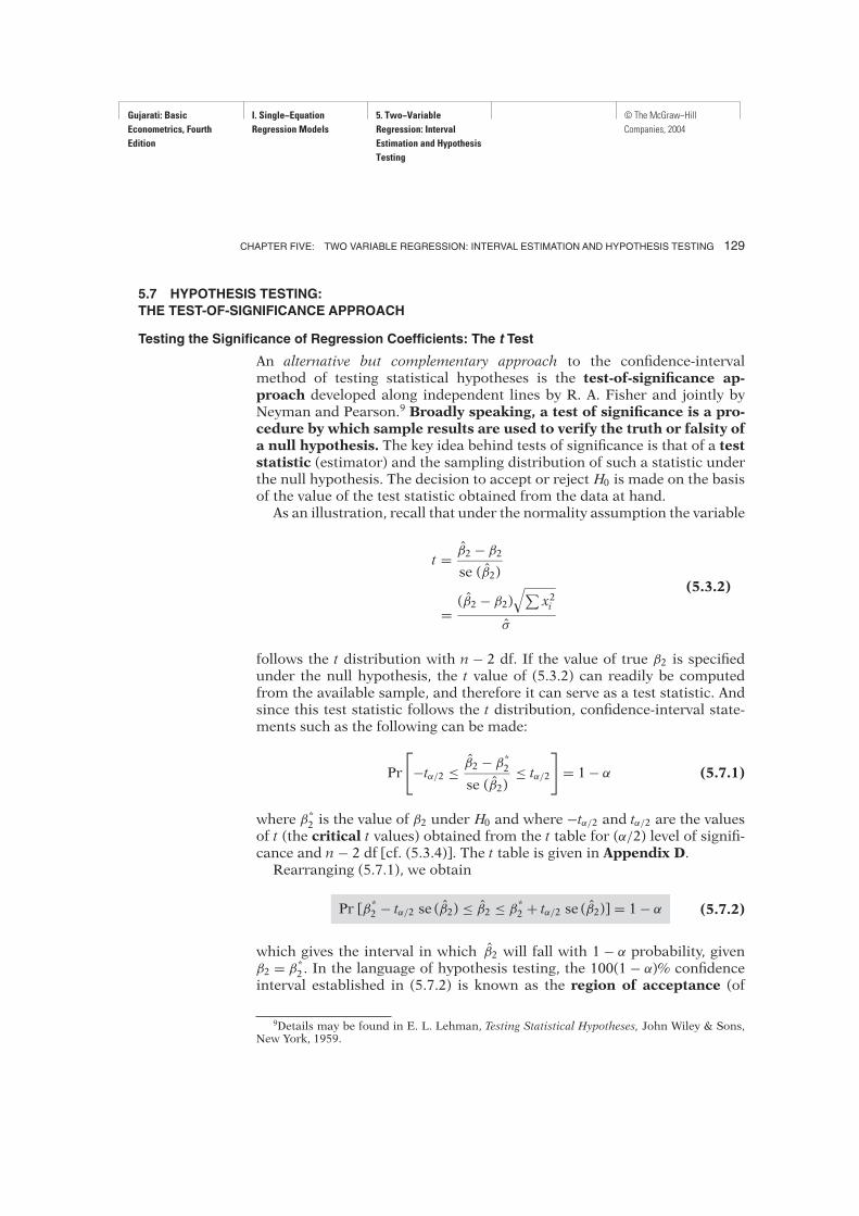
Pr (0.2177 ≤ β2 ≤ 0.3823) = 0.95 (5.7.3)10

as shown diagrammatically in Figure 5.3. Since the observed β2 lies in thecritical region, we reject the null hypothesis that true β2 = 0.3.In practice, there is no need to estimate (5.7.2) explicitly. One can com-

pute the t value in the middle of the double inequality given by (5.7.1) andsee whether it lies between the critical t values or outside them. For ourexample,

t = 0.5091− 0.3

0.0357= 5.86 (5.7.4)

Density

f ( 2)β

Critical

region

2.5%

b2 = 0.5091

lies in this

critical region

2.5%

b2β

0.2177 0.3 0.3823

ˆ2β

FIGURE 5.3 The 95% confidence interval for β2 under the hypothesis that β2 = 0.3.

10In Sec. 5.2, point 4, it was stated that we cannot say that the probability is 95 percent thatthe fixed interval (0.4268, 0.5914) includes the true β2. But we can make the probabilistic state-ment given in (5.7.3) because β2, being an estimator, is a random variable.

Gujarati: Basic


Edition


Regression Models

5. Two−Variable



Testing


Companies, 2004


Density

f(t)

t

Critical

region

2.5%

t = 5.86

lies in this

critical region

2.5%

–2.306 0 +2.306

95%

Region of

acceptance

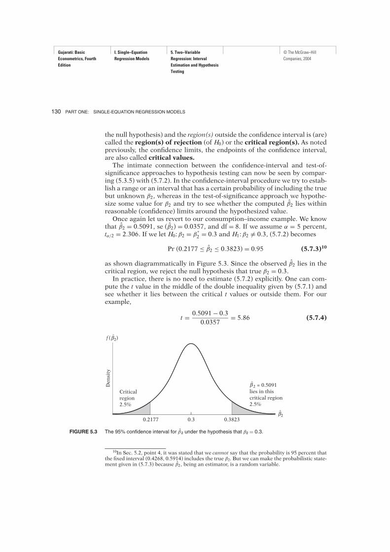
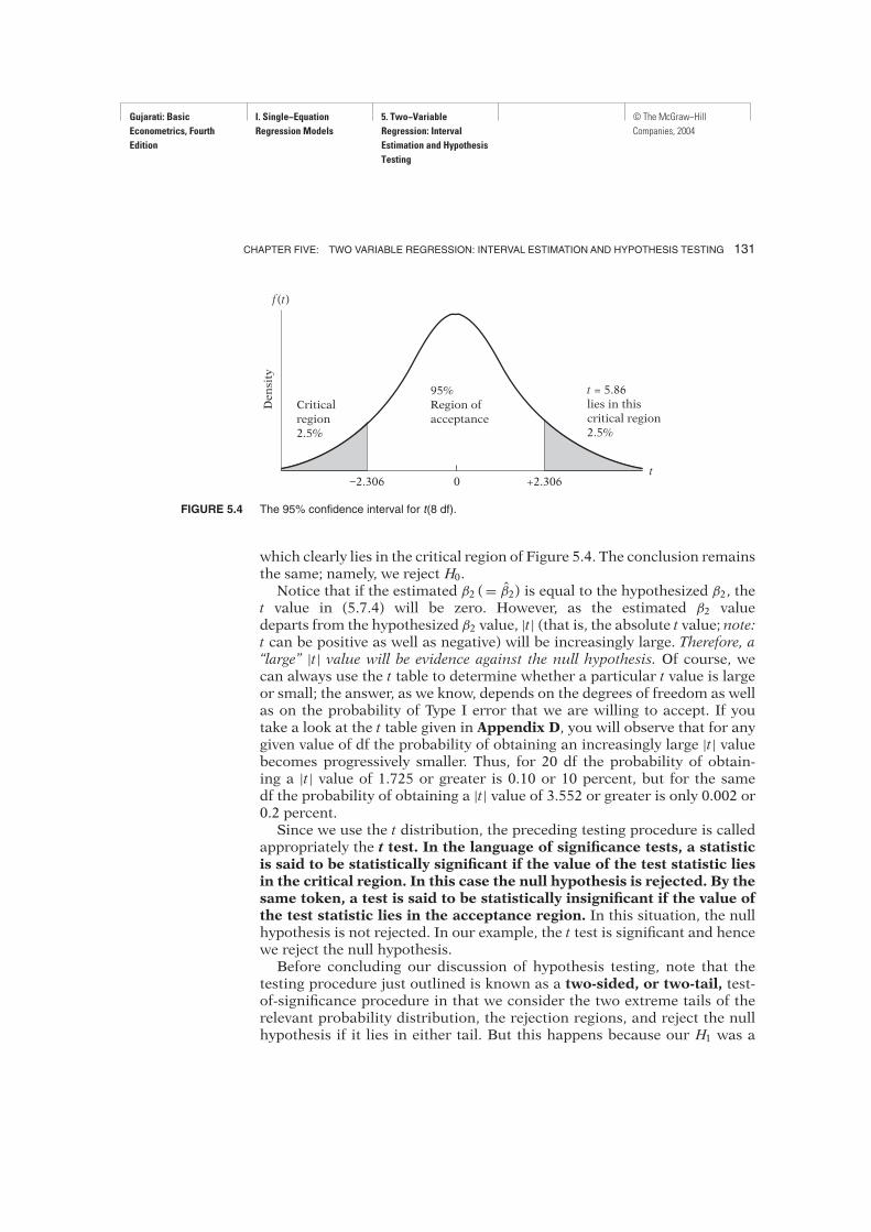
FIGURE 5.4 The 95% confidence interval for t(8 df).

which clearly lies in the critical region of Figure 5.4. The conclusion remainsthe same; namely, we reject H0.Notice that if the estimated β2 (= β2) is equal to the hypothesized β2, the

t value in (5.7.4) will be zero. However, as the estimated β2 valuedeparts from the hypothesized β2 value, |t| (that is, the absolute t value; note:t can be positive as well as negative) will be increasingly large. Therefore, a“large” |t| value will be evidence against the null hypothesis. Of course, wecan always use the t table to determine whether a particular t value is largeor small; the answer, as we know, depends on the degrees of freedom as wellas on the probability of Type I error that we are willing to accept. If youtake a look at the t table given in Appendix D, you will observe that for anygiven value of df the probability of obtaining an increasingly large |t| valuebecomes progressively smaller. Thus, for 20 df the probability of obtain-ing a |t| value of 1.725 or greater is 0.10 or 10 percent, but for the samedf the probability of obtaining a |t| value of 3.552 or greater is only 0.002 or0.2 percent.Since we use the t distribution, the preceding testing procedure is called

appropriately the t test. In the language of significance tests, a statisticis said to be statistically significant if the value of the test statistic liesin the critical region. In this case the null hypothesis is rejected. By thesame token, a test is said to be statistically insignificant if the value ofthe test statistic lies in the acceptance region. In this situation, the nullhypothesis is not rejected. In our example, the t test is significant and hencewe reject the null hypothesis.Before concluding our discussion of hypothesis testing, note that the

testing procedure just outlined is known as a two-sided, or two-tail, test-of-significance procedure in that we consider the two extreme tails of therelevant probability distribution, the rejection regions, and reject the nullhypothesis if it lies in either tail. But this happens because our H1 was a

Gujarati: Basic


Edition


Regression Models

5. Two−Variable



Testing


Companies, 2004


1.860

t0.05 (8 df)

95%

Region of

acceptance

[b2 + 1.860 se( b )]b2βb2β

Density

f(t)

t

t = 5.86

lies in this

critical region

5%

0

95%

Region of

acceptance

Density

f(b2)β

b2β

b2 = 0.5091

lies in this

critical region

2.5%

b2β

0.3 0.3664

*

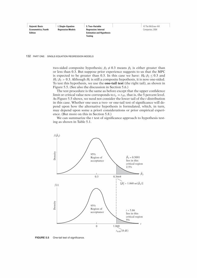
FIGURE 5.5 One-tail test of significance.

two-sided composite hypothesis; β2 )= 0.3 means β2 is either greater thanor less than 0.3. But suppose prior experience suggests to us that the MPCis expected to be greater than 0.3. In this case we have: H0:β2 ≤ 0.3 andH1:β2 > 0.3. Although H1 is still a composite hypothesis, it is now one-sided.To test this hypothesis, we use the one-tail test (the right tail), as shown inFigure 5.5. (See also the discussion in Section 5.6.)The test procedure is the same as before except that the upper confidence

limit or critical value now corresponds to tα = t.05, that is, the 5 percent level.As Figure 5.5 shows, we need not consider the lower tail of the t distributionin this case. Whether one uses a two- or one-tail test of significance will de-pend upon how the alternative hypothesis is formulated, which, in turn,may depend upon some a priori considerations or prior empirical experi-ence. (But more on this in Section 5.8.)We can summarize the t test of significance approach to hypothesis test-

ing as shown in Table 5.1.

Gujarati: Basic


Edition


Regression Models

5. Two−Variable



Testing


Companies, 2004


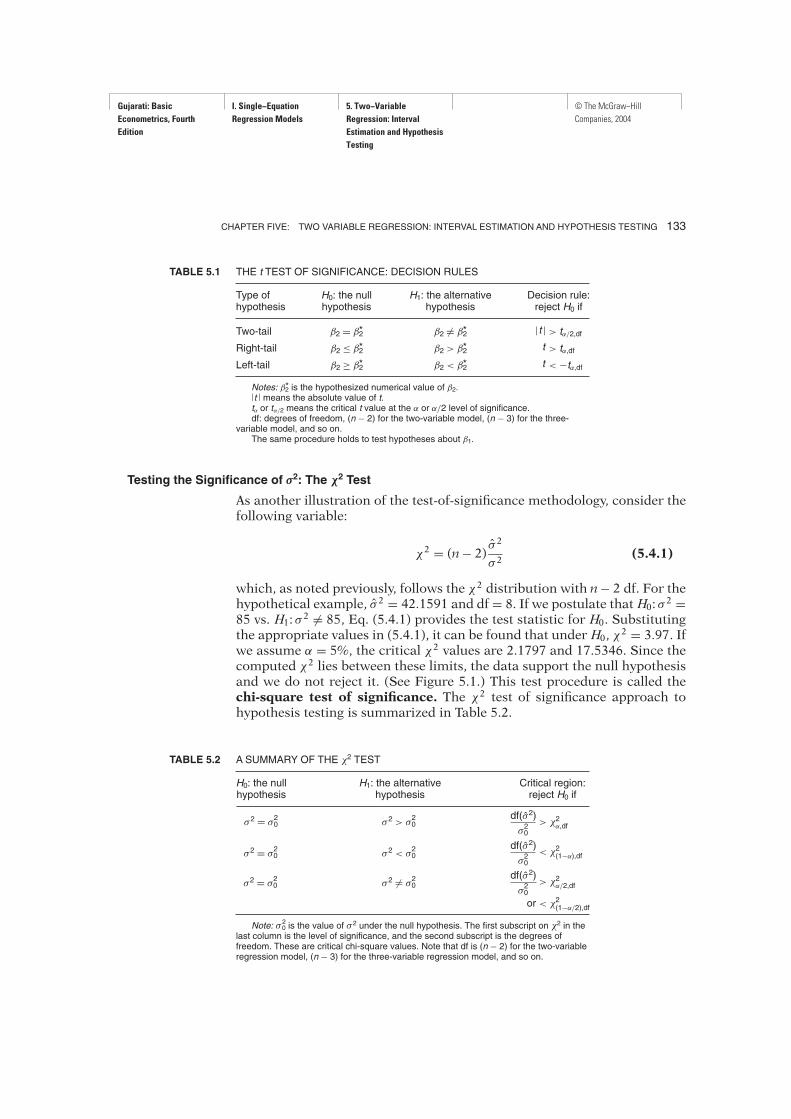
TABLE 5.1 THE t TEST OF SIGNIFICANCE: DECISION RULES

Type of H0: the null H1: the alternative Decision rule:hypothesis hypothesis hypothesis reject H0 if

Two-tail β2 = β2* β2 )= β2* |t | > tα/2,dfRight-tail β2 ≤ β2* β2 > β2* t > tα,df

Left-tail β2 ≥ β2* β2 < β2* t < −tα,df

Notes: β*2 is the hypothesized numerical value of β2.|t | means the absolute value of t.tα or tα/2 means the critical t value at the α or α/2 level of significance.df: degrees of freedom, (n − 2) for the two-variable model, (n − 3) for the three-

variable model, and so on.The same procedure holds to test hypotheses about β1.

TABLE 5.2 A SUMMARY OF THE χ2 TEST

H0: the null H1: the alternative Critical region:hypothesis hypothesis reject H0 if

σ2 = σ20 σ2 > σ

20

σ2 = σ20 σ2 < σ

20

σ2 = σ20 σ2 )= σ

20

or < χ2(1−α/2),df

Note: σ20 is the value of σ

2 under the null hypothesis. The first subscript on χ2 in thelast column is the level of significance, and the second subscript is the degrees offreedom. These are critical chi-square values. Note that df is (n − 2) for the two-variableregression model, (n − 3) for the three-variable regression model, and so on.

df(σ2)> χ2

α/2,dfσ20

df(σ2)< χ2(1−α),df

σ20

df(σ2)> χ2

α,dfσ20

Testing the Significance of σ2: The χ2 Test

As another illustration of the test-of-significance methodology, consider thefollowing variable:

χ2 = (n− 2)σ 2

σ 2(5.4.1)

which, as noted previously, follows the χ2 distribution with n− 2 df. For thehypothetical example, σ 2 = 42.1591 and df = 8. If we postulate that H0: σ

2 =85 vs. H1: σ

2 )= 85, Eq. (5.4.1) provides the test statistic for H0. Substitutingthe appropriate values in (5.4.1), it can be found that under H0, χ

2 = 3.97. Ifwe assume α = 5%, the critical χ2 values are 2.1797 and 17.5346. Since thecomputed χ2 lies between these limits, the data support the null hypothesisand we do not reject it. (See Figure 5.1.) This test procedure is called thechi-square test of significance. The χ2 test of significance approach tohypothesis testing is summarized in Table 5.2.

Gujarati: Basic


Edition


Regression Models

5. Two−Variable



Testing


Companies, 2004


5.8 HYPOTHESIS TESTING: SOME PRACTICAL ASPECTS

The Meaning of “Accepting” or “Rejecting” a Hypothesis

If on the basis of a test of significance, say, the t test, we decide to “accept”the null hypothesis, all we are saying is that on the basis of the sample evi-dence we have no reason to reject it; we are not saying that the null hypoth-esis is true beyond any doubt. Why? To answer this, let us revert to ourconsumption–income example and assume that H0:β2 (MPC) = 0.50. Nowthe estimated value of the MPC is β2 = 0.5091 with a se (β2) = 0.0357. Thenon the basis of the t test we find that t = (0.5091 − 0.50)/0.0357 = 0.25,which is insignificant, say, at α = 5%. Therefore, we say “accept” H0. Butnow let us assume H0:β2 = 0.48. Applying the t test, we obtain t = (0.5091 −0.48)/0.0357 = 0.82, which too is statistically insignificant. So now we say“accept” this H0. Which of these two null hypotheses is the “truth”? We donot know. Therefore, in “accepting” a null hypothesis we should always beaware that another null hypothesis may be equally compatible with thedata. It is therefore preferable to say that we may accept the null hypothesisrather than we (do) accept it. Better still,

. . . just as a court pronounces a verdict as “not guilty” rather than “innocent,” sothe conclusion of a statistical test is “do not reject” rather than “accept.”11

The “Zero” Null Hypothesis and the “2-t” Rule of Thumb

A null hypothesis that is commonly tested in empirical work is H0:β2 = 0,that is, the slope coefficient is zero. This “zero” null hypothesis is a kind ofstraw man, the objective being to find out whether Y is related at all to X, theexplanatory variable. If there is no relationship between Y and X to beginwith, then testing a hypothesis such as β2 = 0.3 or any other value is mean-ingless.This null hypothesis can be easily tested by the confidence interval or the

t-test approach discussed in the preceding sections. But very often such for-mal testing can be shortcut by adopting the “2-t” rule of significance, whichmay be stated as

11Jan Kmenta, Elements of Econometrics,Macmillan, New York, 1971, p. 114.

The rationale for this rule is not too difficult to grasp. From (5.7.1) weknow that we will reject H0:β2 = 0 if

t = β2/se (β2) > tα/2 when β2 > 0

“2-t” Rule of Thumb. If the number of degrees of freedom is 20 or more and if α, the level

of significance, is set at 0.05, then the null hypothesis β2 = 0 can be rejected if the t value

[ = β2/se (β2)] computed from (5.3.2) exceeds 2 in absolute value.

Gujarati: Basic


Edition


Regression Models

5. Two−Variable



Testing


Companies, 2004


12For an interesting discussion about formulating hypotheses, see J. Bradford De Longand Kevin Lang, “Are All Economic Hypotheses False?” Journal of Political Economy, vol. 100,no. 6, 1992, pp. 1257–1272.

or

t = β2/se (β2) < −tα/2 when β2 < 0

or when

|t| =∣

∣

∣

∣

∣

β2

se (β2)

∣

∣

∣

∣

∣

> tα/2 (5.8.1)

for the appropriate degrees of freedom.Now if we examine the t table given in Appendix D, we see that for df of

about 20 or more a computed t value in excess of 2 (in absolute terms), say,2.1, is statistically significant at the 5 percent level, implying rejection of thenull hypothesis. Therefore, if we find that for 20 or more df the computedt value is, say, 2.5 or 3, we do not even have to refer to the t table to assessthe significance of the estimated slope coefficient. Of course, one can alwaysrefer to the t table to obtain the precise level of significance, and one shouldalways do so when the df are fewer than, say, 20.In passing, note that if we are testing the one-sided hypothesis β2 = 0

versus β2 > 0 or β2 < 0, then we should reject the null hypothesis if

|t| =∣

∣

∣

∣

∣

β2

se (β2)

∣

∣

∣

∣

∣

> tα (5.8.2)

If we fix α at 0.05, then from the t table we observe that for 20 or more df at value in excess of 1.73 is statistically significant at the 5 percent level of sig-nificance (one-tail). Hence, whenever a t value exceeds, say, 1.8 (in absoluteterms) and the df are 20 or more, one need not consult the t table for thestatistical significance of the observed coefficient. Of course, if we choose αat 0.01 or any other level, we will have to decide on the appropriate t valueas the benchmark value. But by now the reader should be able to do that.

Forming the Null and Alternative Hypotheses12

Given the null and the alternative hypotheses, testing them for statisticalsignificance should no longer be a mystery. But how does one formulatethese hypotheses? There are no hard-and-fast rules. Very often the phenom-enon under study will suggest the nature of the null and alternative hy-potheses. For example, consider the capital market line (CML) of portfoliotheory, which postulates that Ei = β1 + β2σi , where E = expected return onportfolio and σ = the standard deviation of return, a measure of risk. Sincereturn and risk are expected to be positively related—the higher the risk, the

Gujarati: Basic


Edition


Regression Models

5. Two−Variable



Testing


Companies, 2004


higher the return—the natural alternative hypothesis to the null hypothesisthat β2 = 0would be β2 > 0. That is, one would not choose to consider valuesof β2 less than zero.But consider the case of the demand for money. As we shall show later,

one of the important determinants of the demand for money is income.Prior studies of the money demand functions have shown that the incomeelasticity of demand for money (the percent change in the demand formoney for a 1 percent change in income) has typically ranged between 0.7and 1.3. Therefore, in a new study of demand for money, if one postulatesthat the income-elasticity coefficient β2 is 1, the alternative hypothesis couldbe that β2 )= 1, a two-sided alternative hypothesis.Thus, theoretical expectations or prior empirical work or both can be

relied upon to formulate hypotheses. But no matter how the hypotheses areformed, it is extremely important that the researcher establish these hypothesesbefore carrying out the empirical investigation. Otherwise, he or she will beguilty of circular reasoning or self-fulfilling prophesies. That is, if one were toformulate hypotheses after examining the empirical results, there may be thetemptation to form hypotheses that justify one’s results. Such a practiceshould be avoided at all costs, at least for the sake of scientific objectivity.Keep in mind the Stigler quotation given at the beginning of this chapter!

Choosing α, the Level of Significance

It should be clear from the discussion so far that whether we reject or do notreject the null hypothesis depends critically on α, the level of significanceor the probability of committing a Type I error—the probability of rejectingthe true hypothesis. In Appendix A we discuss fully the nature of a Type Ierror, its relationship to a Type II error (the probability of accepting the falsehypothesis) and why classical statistics generally concentrates on a Type Ierror. But even then, why is α commonly fixed at the 1, 5, or at the most10 percent levels? As a matter of fact, there is nothing sacrosanct aboutthese values; any other values will do just as well.In an introductory book like this it is not possible to discuss in depth why

one chooses the 1, 5, or 10 percent levels of significance, for that will take usinto the field of statistical decision making, a discipline unto itself. A briefsummary, however, can be offered. As we discuss in Appendix A, for a givensample size, if we try to reduce a Type I error, a Type II error increases, and viceversa. That is, given the sample size, if we try to reduce the probability of re-jecting the true hypothesis, we at the same time increase the probability of ac-cepting the false hypothesis. So there is a tradeoff involved between these twotypes of errors, given the sample size. Now the only way we can decide aboutthe tradeoff is to find out the relative costs of the two types of errors. Then,

If the error of rejecting the null hypothesis which is in fact true (Error Type I) iscostly relative to the error of not rejecting the null hypothesis which is in fact

Gujarati: Basic


Edition


Regression Models

5. Two−Variable



Testing


Companies, 2004


13Jan Kmenta, Elements of Econometrics, Macmillan, New York, 1971, pp. 126–127.14One can obtain the p value using electronic statistical tables to several decimal places.

Unfortunately, the conventional statistical tables, for lack of space, cannot be that refined. Moststatistical packages now routinely print out the p values.

false (Error Type II), it will be rational to set the probability of the first kindof error low. If, on the other hand, the cost of making Error Type I is low rela-tive to the cost of making Error Type II, it will pay to make the probability of thefirst kind of error high (thus making the probability of the second type of errorlow).13

Of course, the rub is that we rarely know the costs of making the two typesof errors. Thus, applied econometricians generally follow the practice of set-ting the value of α at a 1 or a 5 or at most a 10 percent level and choose a teststatistic that would make the probability of committing a Type II error assmall as possible. Since one minus the probability of committing a Type IIerror is known as the power of the test, this procedure amounts to maxi-mizing the power of the test. (See Appendix A for a discussion of the powerof a test.)But all this problem with choosing the appropriate value of α can be

avoided if we use what is known as the p value of the test statistic, which isdiscussed next.

The Exact Level of Significance: The p Value

As just noted, the Achilles heel of the classical approach to hypothesis test-ing is its arbitrariness in selecting α. Once a test statistic (e.g., the t statistic)is obtained in a given example, why not simply go to the appropriate statis-tical table and find out the actual probability of obtaining a value of the teststatistic as much as or greater than that obtained in the example? This prob-ability is called the p value (i.e., probability value), also known as theobserved or exact level of significance or the exact probability of com-mitting a Type I error.More technically, the p value is defined as the low-est significance level at which a null hypothesis can be rejected.To illustrate, let us return to our consumption–income example. Given

the null hypothesis that the true MPC is 0.3, we obtained a t value of 5.86 in(5.7.4). What is the p value of obtaining a t value of as much as or greaterthan 5.86? Looking up the t table given in Appendix D, we observe that for8 df the probability of obtaining such a t value must be much smaller than0.001 (one-tail) or 0.002 (two-tail). By using the computer, it can be shownthat the probability of obtaining a t value of 5.86 or greater (for 8 df) isabout 0.000189.14 This is the p value of the observed t statistic. This ob-served, or exact, level of significance of the t statistic is much smaller thanthe conventionally, and arbitrarily, fixed level of significance, such as 1, 5, or10 percent. As a matter of fact, if we were to use the p value just computed,

Gujarati: Basic


Edition


Regression Models

5. Two−Variable



Testing


Companies, 2004


and reject the null hypothesis that the true MPC is 0.3, the probability ofour committing a Type I error is only about 0.02 percent, that is, only about2 in 10,000!As we noted earlier, if the data do not support the null hypothesis, |t| ob-

tained under the null hypothesis will be “large” and therefore the p value ofobtaining such a |t| value will be “small.” In other words, for a given samplesize, as |t| increases, the p value decreases, and one can therefore reject thenull hypothesis with increasing confidence.What is the relationship of the p value to the level of significance α? If we

make the habit of fixing α equal to the p value of a test statistic (e.g., the t sta-tistic), then there is no conflict between the two values. To put it differently,it is better to give up fixing α arbitrarily at some level and simplychoose the p value of the test statistic. It is preferable to leave it to thereader to decide whether to reject the null hypothesis at the given p value. Ifin an application the p value of a test statistic happens to be, say, 0.145, or14.5 percent, and if the reader wants to reject the null hypothesis at this(exact) level of significance, so be it. Nothing is wrong with taking a chanceof being wrong 14.5 percent of the time if you reject the true null hypothe-sis. Similarly, as in our consumption–income example, there is nothingwrong if the researcher wants to choose a p value of about 0.02 percent andnot take a chance of being wrong more than 2 out of 10,000 times. After all,some investigators may be risk-lovers and some risk-averters!In the rest of this text, we will generally quote the p value of a given test

statistic. Some readers may want to fix α at some level and reject the nullhypothesis if the p value is less than α. That is their choice.

Statistical Significance versus Practical Significance

Let us revert to our consumption–income example and now hypothesizethat the true MPC is 0.61 (H0:β2 = 0.61). On the basis of our sample resultof β2 = 0.5091, we obtained the interval (0.4268, 0.5914) with 95 percentconfidence. Since this interval does not include 0.61, we can, with 95 per-cent confidence, say that our estimate is statistically significant, that is,significantly different from 0.61.But what is the practical or substantive significance of our finding? That

is, what difference does it make if we take the MPC to be 0.61 rather than0.5091? Is the 0.1009 difference between the two MPCs that important prac-tically?The answer to this question depends on what we really do with these es-

timates. For example, from macroeconomics we know that the income mul-tiplier is 1/(1 −MPC). Thus, if MPC is 0.5091, the multiplier is 2.04, but it is2.56 if MPC is equal to 0.61. That is, if the government were to increase itsexpenditure by $1 to lift the economy out of a recession, income will even-tually increase by $2.04 if the MPC is 0.5091 but by $2.56 if the MPC is 0.61.And that difference could very well be crucial to resuscitating the economy.

Gujarati: Basic


Edition


Regression Models

5. Two−Variable



Testing


Companies, 2004


15Arthur S. Goldberger, A Course in Econometrics, Harvard University Press, Cambridge,Massachusetts, 1991, p. 240. Note bj is the OLS estimator of βj and σbj is its standard error. Fora corroborating view, see D. N. McCloskey, “The Loss Function Has Been Mislaid: The Rhetoricof Significance Tests,” American Economic Review, vol. 75, 1985, pp. 201–205. See also D. N.McCloskey and S. T. Ziliak, “The Standard Error of Regression,” Journal of Economic Litera-ture, vol. 37, 1996, pp. 97–114.

16See their article cited in footnote 12, p. 1271.17For a somewhat different perspective, see Carter Hill, William Griffiths, and George Judge,

Undergraduate Econometrics,Wiley & Sons, New York, 2001, p. 108.

The point of all this discussion is that one should not confuse statisticalsignificance with practical, or economic, significance. As Goldberger notes:

When a null, say, βj = 1, is specified, the likely intent is that βj is close to 1, soclose that for all practical purposes it may be treated as if it were 1. But whether1.1 is “practically the same as” 1.0 is a matter of economics, not of statistics. Onecannot resolve the matter by relying on a hypothesis test, because the test statis-tic [t = ] (bj − 1)/σbj measures the estimated coefficient in standard error units,which are not meaningful units in which to measure the economic parameterβj − 1. It may be a good idea to reserve the term “significance” for the statisticalconcept, adopting “substantial” for the economic concept.15

The point made by Goldberger is important. As sample size becomes verylarge, issues of statistical significance become much less important but is-sues of economic significance become critical. Indeed, since with very largesamples almost any null hypothesis will be rejected, there may be studies inwhich the magnitude of the point estimates may be the only issue.

The Choice between Confidence-Interval and

Test-of-Significance Approaches to Hypothesis Testing

In most applied economic analyses, the null hypothesis is set up as a strawman and the objective of the empirical work is to knock it down, that is, re-ject the null hypothesis. Thus, in our consumption–income example, thenull hypothesis that the MPC β2 = 0 is patently absurd, but we often use itto dramatize the empirical results. Apparently editors of reputed journalsdo not find it exciting to publish an empirical piece that does not reject thenull hypothesis. Somehow the finding that the MPC is statistically differentfrom zero is more newsworthy than the finding that it is equal to, say, 0.7!Thus, J. Bradford De Long and Kevin Lang argue that it is better for

economists

. . . to concentrate on the magnitudes of coefficients and to report confidencelevels and not significance tests. If all or almost all null hypotheses are false, thereis little point in concentrating on whether or not an estimate is indistinguishablefrom its predicted value under the null. Instead, we wish to cast light on whatmodels are good approximations, which requires that we know ranges of para-meter values that are excluded by empirical estimates.16

In short, these authors prefer the confidence-interval approach to the test-of-significance approach. The reader may want to keep this advice in mind.17

Gujarati: Basic


Edition


Regression Models

5. Two−Variable



Testing


Companies, 2004


5.9 REGRESSION ANALYSIS AND ANALYSIS OF VARIANCE

In this section we study regression analysis from the point of view of theanalysis of variance and introduce the reader to an illuminating and com-plementary way of looking at the statistical inference problem.In Chapter 3, Section 3.5, we developed the following identity:

∑

y2i =∑

y2i +∑

u2i = β22

∑

x2i +∑

u2i (3.5.2)

that is, TSS = ESS + RSS, which decomposed the total sum of squares(TSS) into two components: explained sum of squares (ESS) and residualsum of squares (RSS). A study of these components of TSS is known as theanalysis of variance (ANOVA) from the regression viewpoint.Associated with any sum of squares is its df, the number of independent

observations on which it is based. TSS has n− 1df because we lose 1 df incomputing the sample mean Y. RSS has n− 2df. (Why?) (Note: This is trueonly for the two-variable regression model with the intercept β1 present.)ESS has 1 df (again true of the two-variable case only), which follows fromthe fact that ESS = β22

∑

x2i is a function of β2 only, since ∑

x2i is known.Let us arrange the various sums of squares and their associated df in

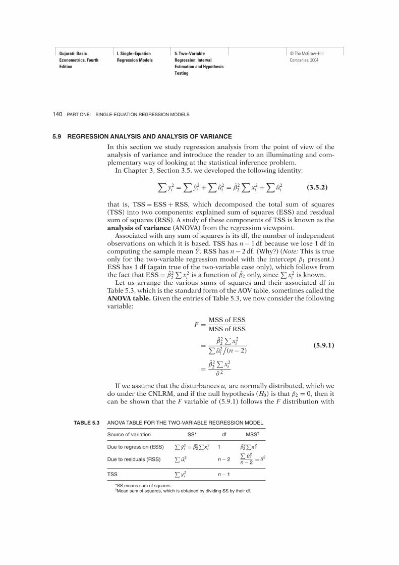
Table 5.3, which is the standard form of the AOV table, sometimes called theANOVA table. Given the entries of Table 5.3, we now consider the followingvariable:

F = MSS of ESS

MSS of RSS

= β22∑

x2i∑

u2i/

(n− 2)(5.9.1)

= β22∑

x2iσ 2

If we assume that the disturbances ui are normally distributed, which wedo under the CNLRM, and if the null hypothesis (H0) is that β2 = 0, then itcan be shown that the F variable of (5.9.1) follows the F distribution with

TABLE 5.3 ANOVA TABLE FOR THE TWO-VARIABLE REGRESSION MODEL

Source of variation SS* df MSS†

Due to regression (ESS)∑

y 2i = β22∑

x 2i 1 β22∑

x 2i

Due to residuals (RSS)∑

u 2i n − 2

TSS∑

y 2i n − 1

*SS means sum of squares.†Mean sum of squares, which is obtained by dividing SS by their df.

∑

u2i = σ2

n − 2

Gujarati: Basic


Edition


Regression Models

5. Two−Variable



Testing


Companies, 2004


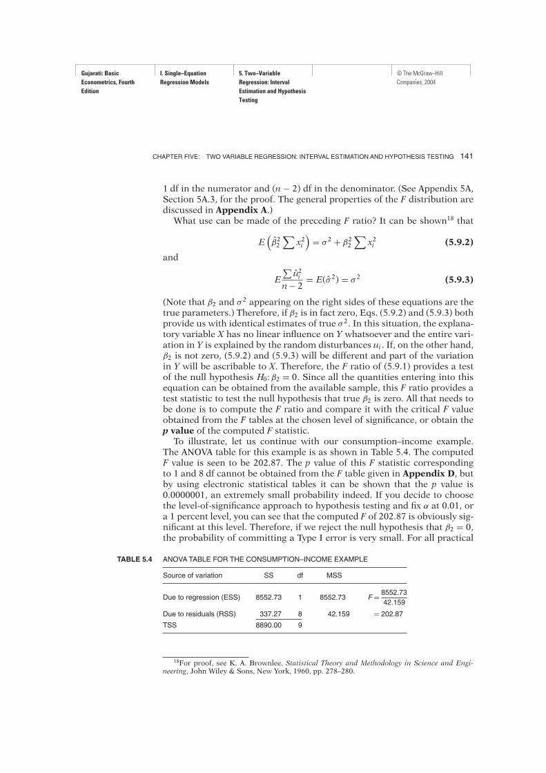
TABLE 5.4 ANOVA TABLE FOR THE CONSUMPTION–INCOME EXAMPLE

Source of variation SS df MSS

Due to regression (ESS) 8552.73 1 8552.73 F = 8552.73

42.159

Due to residuals (RSS) 337.27 8 42.159 = 202.87

TSS 8890.00 9

1 df in the numerator and (n − 2) df in the denominator. (See Appendix 5A,Section 5A.3, for the proof. The general properties of the F distribution arediscussed in Appendix A.)What use can be made of the preceding F ratio? It can be shown18 that

E(

β22

∑

x2i

)

= σ 2 + β22

∑

x2i (5.9.2)

and

E

∑

u2in− 2

= E(σ 2) = σ 2 (5.9.3)

(Note that β2 and σ2 appearing on the right sides of these equations are the

true parameters.) Therefore, if β2 is in fact zero, Eqs. (5.9.2) and (5.9.3) bothprovide us with identical estimates of true σ 2. In this situation, the explana-tory variable X has no linear influence on Y whatsoever and the entire vari-ation in Y is explained by the random disturbances ui . If, on the other hand,β2 is not zero, (5.9.2) and (5.9.3) will be different and part of the variationin Y will be ascribable to X. Therefore, the F ratio of (5.9.1) provides a testof the null hypothesis H0:β2 = 0. Since all the quantities entering into thisequation can be obtained from the available sample, this F ratio provides atest statistic to test the null hypothesis that true β2 is zero. All that needs tobe done is to compute the F ratio and compare it with the critical F valueobtained from the F tables at the chosen level of significance, or obtain thep value of the computed F statistic.To illustrate, let us continue with our consumption–income example.

The ANOVA table for this example is as shown in Table 5.4. The computedF value is seen to be 202.87. The p value of this F statistic correspondingto 1 and 8 df cannot be obtained from the F table given in Appendix D, butby using electronic statistical tables it can be shown that the p value is0.0000001, an extremely small probability indeed. If you decide to choosethe level-of-significance approach to hypothesis testing and fix α at 0.01, ora 1 percent level, you can see that the computed F of 202.87 is obviously sig-nificant at this level. Therefore, if we reject the null hypothesis that β2 = 0,the probability of committing a Type I error is very small. For all practical

18For proof, see K. A. Brownlee, Statistical Theory and Methodology in Science and Engi-neering, John Wiley & Sons, New York, 1960, pp. 278–280.

Gujarati: Basic


Edition


Regression Models

5. Two−Variable



Testing


Companies, 2004


purposes, our sample could not have come from a population with zero β2value and we can conclude with great confidence that X, income, does affectY, consumption expenditure.Refer to Theorem 5.7 of Appendix 5A.1, which states that the square of the

t value with k df is an F value with 1 df in the numerator and k df in the de-nominator. For our consumption–income example, if we assume H0:β2 = 0,then from (5.3.2) it can be easily verified that the estimated t value is 14.26.This t value has 8 df. Under the same null hypothesis, the F value was 202.87with 1 and 8 df. Hence (14.24)2 = F value, except for the rounding errors.Thus, the t and the F tests provide us with two alternative but comple-

mentary ways of testing the null hypothesis that β2 = 0. If this is the case,why not just rely on the t test and not worry about the F test and the ac-companying analysis of variance? For the two-variable model there really isno need to resort to the F test. But when we consider the topic of multipleregression we will see that the F test has several interesting applications thatmake it a very useful and powerful method of testing statistical hypotheses.

5.10 APPLICATION OF REGRESSION ANALYSIS:

THE PROBLEM OF PREDICTION

On the basis of the sample data of Table 3.2 we obtained the following sam-ple regression:

Yi = 24.4545+ 0.5091Xi (3.6.2)

where Yt is the estimator of true E(Yi) corresponding to given X. What usecan be made of this historical regression? One use is to “predict” or “fore-cast” the future consumption expenditure Y corresponding to some givenlevel of income X. Now there are two kinds of predictions: (1) prediction ofthe conditional mean value of Y corresponding to a chosen X, say, X0, thatis the point on the population regression line itself (see Figure 2.2), and(2) prediction of an individual Y value corresponding to X0. We shall callthese two predictions the mean prediction and individual prediction.

Mean Prediction19

To fix the ideas, assume that X0 = 100 andwewant to predictE(Y | X0 = 100).Now it can be shown that the historical regression (3.6.2) provides the pointestimate of this mean prediction as follows:

Y0 = β1 + β2X0

= 24.4545+ 0.5091(100) (5.10.1)

= 75.3645

19For the proofs of the various statements made, see App. 5A, Sec. 5A.4.

Gujarati: Basic


Edition


Regression Models

5. Two−Variable



Testing


Companies, 2004


where Y0 = estimator of E(Y | X0). It can be proved that this point predictoris a best linear unbiased estimator (BLUE).Since Y0 is an estimator, it is likely to be different from its true value. The

difference between the two values will give some idea about the predictionor forecast error. To assess this error, we need to find out the samplingdistribution of Y0. It is shown in Appendix 5A, Section 5A.4, that Y0 inEq. (5.10.1) is normally distributed with mean (β1 + β2X0) and the varianceis given by the following formula:

(5.10.2)

By replacing the unknown σ 2 by its unbiased estimator σ 2, we see that thevariable

t = Y0 − (β1 + β2X0)

se (Y0)(5.10.3)

follows the t distribution with n− 2 df. The t distribution can therefore beused to derive confidence intervals for the true E(Y0 | X0) and test hypothe-ses about it in the usual manner, namely,

(5.10.4)

where se (Y0) is obtained from (5.10.2).For our data (see Table 3.3),

var (Y0) = 42.159

[

1

10+ (100− 170)2

33,000

]

= 10.4759

and

se (Y0) = 3.2366

Therefore, the 95% confidence interval for true E(Y | X0) = β1 + β2X0 is givenby

75.3645− 2.306(3.2366) ≤ E(Y0 | X = 100) ≤ 75.3645+ 2.306(3.2366)

that is,

67.9010 ≤ E(Y | X = 100) ≤ 82.8381 (5.10.5)

Pr [β1 + β2X0 − tα/2 se (Y0) ≤ β1 + β2X0 ≤ β1 + β2X0 + tα/2 se (Y0)] = 1− α

var (Y0) = σ 2[

1

n+ (X0 − X)2

∑

x2i

]

Gujarati: Basic


Edition


Regression Models

5. Two−Variable



Testing


Companies, 2004


170

150

130

110

90

70

50

00 60 80 100 120 140 200180160 220 240 260

Confidence interval

for mean Y

Confidence interval

for individual Y

Yi = 24.4545 + 0.5091Xi

Y

X

92

83

58

68

X

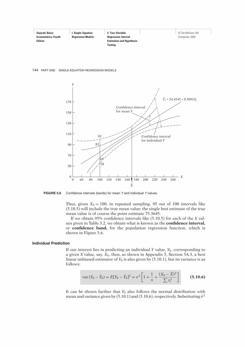
FIGURE 5.6 Confidence intervals (bands) for mean Y and individual Y values.

Thus, given X0 = 100, in repeated sampling, 95 out of 100 intervals like(5.10.5) will include the true mean value; the single best estimate of the truemean value is of course the point estimate 75.3645.If we obtain 95% confidence intervals like (5.10.5) for each of the X val-

ues given in Table 3.2, we obtain what is known as the confidence interval,or confidence band, for the population regression function, which isshown in Figure 5.6.

Individual Prediction

If our interest lies in predicting an individual Y value, Y0, corresponding toa given X value, say, X0, then, as shown in Appendix 5, Section 5A.3, a bestlinear unbiased estimator of Y0 is also given by (5.10.1), but its variance is asfollows:

(5.10.6)

It can be shown further that Y0 also follows the normal distribution withmean and variance given by (5.10.1) and (5.10.6), respectively. Substituting σ 2

var (Y0 − Y0) = E[Y0 − Y0]2 = σ 2[

1+ 1

n+ (X0 − X)2

∑

x2i

]

Gujarati: Basic


Edition


Regression Models

5. Two−Variable



Testing


Companies, 2004


for the unknown σ 2, it follows that

t = Y0 − Y0se (Y0 − Y0)

also follows the t distribution. Therefore, the t distribution can be used todraw inferences about the trueY0. Continuingwith our consumption–incomeexample, we see that the point prediction of Y0 is 75.3645, the same as thatof Y0, and its variance is 52.6349 (the reader should verify this calculation).Therefore, the 95% confidence interval for Y0 corresponding to X0 = 100 isseen to be

(58.6345 ≤ Y0 | X0 = 100 ≤ 92.0945) (5.10.7)

Comparing this interval with (5.10.5), we see that the confidence intervalfor individual Y0 is wider than that for the mean value of Y0. (Why?) Com-puting confidence intervals like (5.10.7) conditional upon the X values givenin Table 3.2, we obtain the 95% confidence band for the individual Y valuescorresponding to these X values. This confidence band along with the confi-dence band for Y0 associated with the same X’s is shown in Figure 5.6.Notice an important feature of the confidence bands shown in Figure 5.6.

The width of these bands is smallest when X0 = X. (Why?) However, thewidth widens sharply as X0 moves away from X. (Why?) This change wouldsuggest that the predictive ability of the historical sample regression linefalls markedly as X0 departs progressively from X. Therefore, one shouldexercise great caution in “extrapolating” the historical regression lineto predict E(Y | X0) or Y0 associated with a given X0 that is far removedfrom the sample mean X.

5.11 REPORTING THE RESULTS OF REGRESSION ANALYSIS

There are various ways of reporting the results of regression analysis, butin this text we shall use the following format, employing the consumption–income example of Chapter 3 as an illustration:

Yi = 24.4545 + 0.5091Xi

se = (6.4138) (0.0357) r2 = 0.9621(5.11.1)

t = (3.8128) (14.2605) df = 8

p = (0.002571) (0.000000289) F1,8 = 202.87

In Eq. (5.11.1) the figures in the first set of parentheses are the estimatedstandard errors of the regression coefficients, the figures in the second setare estimated t values computed from (5.3.2) under the null hypothesis that

Gujarati: Basic


Edition


Regression Models

5. Two−Variable



Testing


Companies, 2004


the true population value of each regression coefficient individually is zero(e.g., 3.8128 = 24.4545 ÷ 6.4138), and the figures in the third set are theestimated p values. Thus, for 8 df the probability of obtaining a t value of3.8128 or greater is 0.0026 and the probability of obtaining a t value of14.2605 or larger is about 0.0000003.By presenting the p values of the estimated t coefficients, we can see at

once the exact level of significance of each estimated t value. Thus, underthe null hypothesis that the true population intercept value is zero, theexact probability (i.e., the p value) of obtaining a t value of 3.8128 or greateris only about 0.0026. Therefore, if we reject this null hypothesis, the proba-bility of our committing a Type I error is about 26 in 10,000, a very smallprobability indeed. For all practical purposes we can say that the true pop-ulation intercept is different from zero. Likewise, the p value of the esti-mated slope coefficient is zero for all practical purposes. If the true MPCwere in fact zero, our chances of obtaining an MPC of 0.5091 would bepractically zero. Hence we can reject the null hypothesis that the true MPCis zero.Earlier we showed the intimate connection between the F and t statistics,

namely, F1,k = t2k . Under the null hypothesis that the true β2 = 0, (5.11.1)shows that the F value is 202.87 (for 1 numerator and 8 denominator df)and the t value is about 14.24 (8 df); as expected, the former value is thesquare of the latter value, except for the roundoff errors. The ANOVA tablefor this problem has already been discussed.

5.12 EVALUATING THE RESULTS OF REGRESSION ANALYSIS

In Figure I.4 of the Introduction we sketched the anatomy of econometricmodeling. Now that we have presented the results of regression analysis ofour consumption–income example in (5.11.1), we would like to question theadequacy of the fitted model. How “good” is the fitted model? We need somecriteria with which to answer this question.First, are the signs of the estimated coefficients in accordance with theo-

retical or prior expectations? A priori, β2, the marginal propensity to con-sume (MPC) in the consumption function, should be positive. In the presentexample it is. Second, if theory says that the relationship should be not onlypositive but also statistically significant, is this the case in the present appli-cation? As we discussed in Section 5.11, the MPC is not only positive butalso statistically significantly different from zero; the p value of the esti-mated t value is extremely small. The same comments apply about the inter-cept coefficient. Third, how well does the regression model explain variationin the consumption expenditure? One can use r2 to answer this question. Inthe present example r2 is about 0.96, which is a very high value consideringthat r2 can be at most 1.Thus, the model we have chosen for explaining consumption expenditure

behavior seems quite good. But before we sign off, we would like to find out

Gujarati: Basic


Edition


Regression Models

5. Two−Variable



Testing


Companies, 2004


whether our model satisfies the assumptions of CNLRM. We will not look atthe various assumptions now because the model is patently so simple. Butthere is one assumption that we would like to check, namely, the normalityof the disturbance term, ui . Recall that the t and F tests used before requirethat the error term follow the normal distribution. Otherwise, the testingprocedure will not be valid in small, or finite, samples.

Normality Tests

Although several tests of normality are discussed in the literature, we willconsider just three: (1) histogram of residuals; (2) normal probability plot(NPP), a graphical device; and (3) the Jarque–Bera test.

Histogram of Residuals. A histogram of residuals is a simple graphicdevice that is used to learn something about the shape of the PDF of a ran-dom variable. On the horizontal axis, we divide the values of the variableof interest (e.g., OLS residuals) into suitable intervals, and in each classinterval we erect rectangles equal in height to the number of observations(i.e., frequency) in that class interval. If you mentally superimpose the bell-shaped normal distribution curve on the histogram, you will get some ideaas to whether normal (PDF) approximation may be appropriate. A concreteexample is given in Section 5.13 (see Figure 5.8). It is always a good practiceto plot the histogram of the residuals as a rough and ready method of test-ing for the normality assumption.

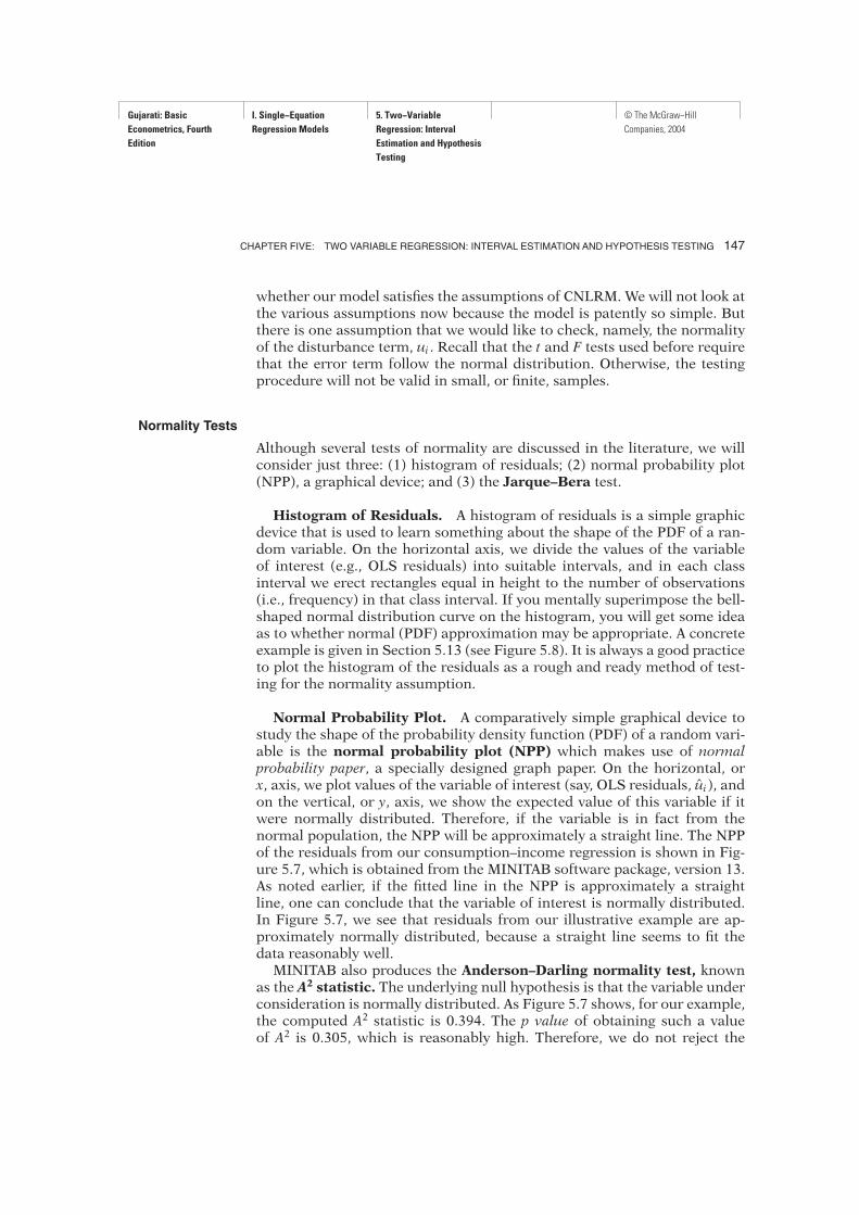
Normal Probability Plot. A comparatively simple graphical device tostudy the shape of the probability density function (PDF) of a random vari-able is the normal probability plot (NPP) which makes use of normalprobability paper, a specially designed graph paper. On the horizontal, orx, axis, we plot values of the variable of interest (say, OLS residuals, ui), andon the vertical, or y, axis, we show the expected value of this variable if itwere normally distributed. Therefore, if the variable is in fact from thenormal population, the NPP will be approximately a straight line. The NPPof the residuals from our consumption–income regression is shown in Fig-ure 5.7, which is obtained from the MINITAB software package, version 13.As noted earlier, if the fitted line in the NPP is approximately a straightline, one can conclude that the variable of interest is normally distributed.In Figure 5.7, we see that residuals from our illustrative example are ap-proximately normally distributed, because a straight line seems to fit thedata reasonably well.MINITAB also produces the Anderson–Darling normality test, known

as the A2 statistic. The underlying null hypothesis is that the variable underconsideration is normally distributed. As Figure 5.7 shows, for our example,the computed A2 statistic is 0.394. The p value of obtaining such a valueof A2 is 0.305, which is reasonably high. Therefore, we do not reject the

Gujarati: Basic


Edition


Regression Models

5. Two−Variable



Testing


Companies, 2004


–10

.001

–5 0

RESI1

A2 � 0.394P-value � 0.305

Average � 0.0000000StDev � 6.12166N � 10

5

.01

.05

.20

.50

Probability

.80

.95

.99

.999

FIGURE 5.7 Residuals from consumption–income regression.

20See C. M. Jarque and A. K. Bera, “A Test for Normality of Observations and RegressionResiduals,” International Statistical Review, vol. 55, 1987, pp. 163–172.

hypothesis that the residuals from our consumption–income example arenormally distributed. Incidentally, Figure 5.7 shows the parameters of the(normal) distribution, the mean is approximately 0 and the standard devia-tion is about 6.12.

Jarque–Bera (JB) Test of Normality.20 The JB test of normality is anasymptotic, or large-sample, test. It is also based on the OLS residuals. Thistest first computes the skewness and kurtosis (discussed in Appendix A)measures of the OLS residuals and uses the following test statistic:

JB = n[

S2

6+ (K − 3)2

24

]

(5.12.1)

where n = sample size, S = skewness coefficient, and K = kurtosis coeffi-cient. For a normally distributed variable, S = 0 and K = 3. Therefore, theJB test of normality is a test of the joint hypothesis that S and K are 0 and 3,respectively. In that case the value of the JB statistic is expected to be 0.Under the null hypothesis that the residuals are normally distributed,

Jarque and Bera showed that asymptotically (i.e., in large samples) the JBstatistic given in (5.12.1) follows the chi-square distribution with 2 df. If thecomputed p value of the JB statistic in an application is sufficiently low,which will happen if the value of the statistic is very different from 0, onecan reject the hypothesis that the residuals are normally distributed. But if

Gujarati: Basic


Edition


Regression Models

5. Two−Variable



Testing


Companies, 2004


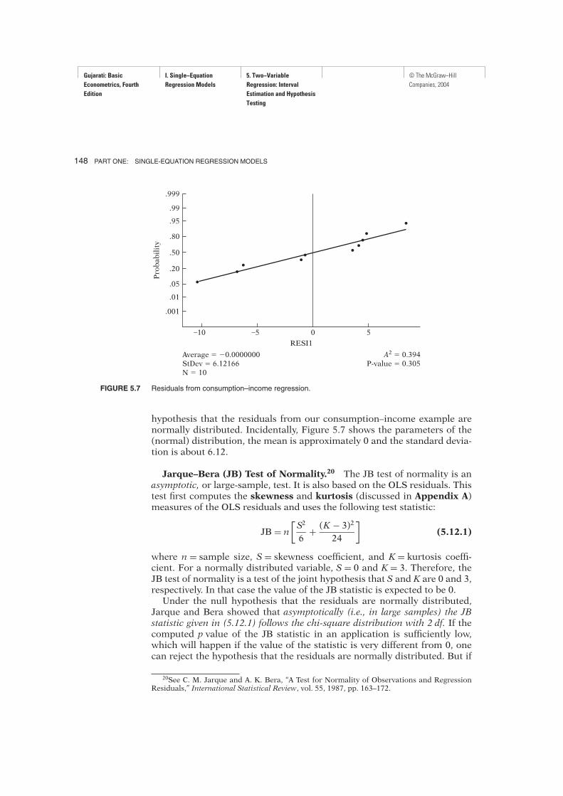
the p value is reasonably high, which will happen if the value of the statisticis close to zero, we do not reject the normality assumption.The sample size in our consumption–income example is rather small.

Hence, strictly speaking one should not use the JB statistic. If we mechani-cally apply the JB formula to our example, the JB statistic turns out to be0.7769. The p value of obtaining such a value from the chi-square distribu-tion with 2 df is about 0.68, which is quite high. In other words, we may notreject the normality assumption for our example. Of course, bear in mindthe warning about the sample size.

Other Tests of Model Adequacy

Remember that the CNLRM makes many more assumptions than the nor-mality of the error term. As we examine econometric theory further, we willconsider several tests of model adequacy (see Chapter 13). Until then, keepin mind that our regression modeling is based on several simplifying as-sumptions that may not hold in each and every case.

A CONCLUDING EXAMPLE

Let us return to Example 3.2 about food expenditure in

India. Using the data given in (3.7.2) and adopting the

format of (5.11.1), we obtain the following expenditure

equation:

FoodExpi = 94.2087 + 0.4368 TotalExpi

se = (50.8563) (0.0783)

t = (1.8524) (5.5770)(5.12.2)

p = (0.0695) (0.0000)*

r 2 = 0.3698; df = 53

F1,53 = 31.1034 (p value = 0.0000)*

where * denotes extremely small.

First, let us interpret this regression. As expected,

there is a positive relationship between expenditure on

food and total expenditure. If total expenditure went up by

a rupee, on average, expenditure on food increased by

about 44 paise. If total expenditure were zero, the average

expenditure on food would be about 94 rupees. Of course,

this mechanical interpretation of the intercept may not

make much economic sense. The r 2 value of about 0.37

means that 37 percent of the variation in food expenditure

is explained by total expenditure, a proxy for income.

Suppose we want to test the null hypothesis that

there is no relationship between food expenditure and

total expenditure, that is, the true slope coefficient β2 = 0.

The estimated value of β2 is 0.4368. If the null hypothesis

were true, what is the probability of obtaining a value of

0.4368? Under the null hypothesis, we observe from

(5.12.2) that the t value is 5.5770 and the p value of ob-

taining such a t value is practically zero. In other words,

we can reject the null hypothesis resoundingly. But sup-

pose the null hypothesis were that β2 = 0.5. Now what?

Using the t test we obtain:

t = 0.4368− 0.5

0.0783= −0.8071

The probability of obtaining a |t | of 0.8071 is greater than20 percent. Hence we do not reject the hypothesis that

the true β2 is 0.5.

Notice that, under the null hypothesis, the true slope

coefficient is zero, the F value is 31.1034, as shown in

(5.12.2). Under the same null hypothesis, we obtained a

t value of 5.5770. If we square this value, we obtain

31.1029, which is about the same as the F value, again

showing the close relationship between the t and the F

statistic. (Note: The numerator df for the F statistic must

be 1, which is the case here.)

Using the estimated residuals from the regression,

what can we say about the probability distribution of

the error term? The information is given in Figure 5.8.

As the figure shows, the residuals from the food expen-

diture regression seem to be symmetrically distributed.

Application of the Jarque–Bera test shows that the JB

statistic is about 0.2576, and the probability of obtaining

such a statistic under the normality assumption is about

(Continued)

Gujarati: Basic


Edition


Regression Models

5. Two−Variable



Testing


Companies, 2004


5.13 SUMMARY AND CONCLUSIONS

1. Estimation and hypothesis testing constitute the twomain branches ofclassical statistics. Having discussed the problem of estimation in Chapters 3and 4, we have taken up the problem of hypothesis testing in this chapter.

2. Hypothesis testing answers this question: Is a given finding compati-ble with a stated hypothesis or not?

3. There are two mutually complementary approaches to answering thepreceding question: confidence interval and test of significance.

4. Underlying the confidence-interval approach is the concept of inter-val estimation. An interval estimator is an interval or range constructed insuch a manner that it has a specified probability of including within its lim-its the true value of the unknown parameter. The interval thus constructed isknown as a confidence interval,which is often stated in percent form, suchas 90 or 95%. The confidence interval provides a set of plausible hypothesesabout the value of the unknown parameter. If the null-hypothesized valuelies in the confidence interval, the hypothesis is not rejected, whereas if it liesoutside this interval, the null hypothesis can be rejected.

5. In the significance test procedure, one develops a test statistic andexamines its sampling distribution under the null hypothesis. The test sta-tistic usually follows a well-defined probability distribution such as the nor-mal, t, F, or chi-square. Once a test statistic (e.g., the t statistic) is computed

88 percent. Therefore, we do not reject the hypothesis

that the error terms are normally distributed. But keep in

mind that the sample size of 55 observations may not be

large enough.

We leave it to the reader to establish confidence in-

tervals for the two regression coefficients as well as to

obtain the normal probability plot and do mean and indi-

vidual predictions.

14

12

10

8

Number of Observations

Residuals

6

4

2

0–150 –100 –50 0 50 100 150

Series: Residuals

Sample 1 55

Observations 55

Mean –1.19 10–14

Median 7.747849

Maximum 171.5859

Minimum –153.7664

Std. dev. 66.23382

Skewness 0.119816

Kurtosis 3.234473

Jarque–Bera 0.257585

Probability 0.879156

FIGURE 5.8 Residuals from the food expenditure regression.

A CONCLUDING EXAMPLE (Continued)

Gujarati: Basic


Edition


Regression Models

5. Two−Variable



Testing


Companies, 2004


from the data at hand, its p value can be easily obtained. The p value givesthe exact probability of obtaining the estimated test statistic under the nullhypothesis. If this p value is small, one can reject the null hypothesis, but ifit is large one may not reject it. What constitutes a small or large p value isup to the investigator. In choosing the p value the investigator has to bear inmind the probabilities of committing Type I and Type II errors.

6. In practice, one should be careful in fixing α, the probability of com-mitting a Type I error, at arbitrary values such as 1, 5, or 10 percent. It isbetter to quote the p value of the test statistic. Also, the statistical signifi-cance of an estimate should not be confused with its practical significance.

7. Of course, hypothesis testing presumes that the model chosen for em-pirical analysis is adequate in the sense that it does not violate one or moreassumptions underlying the classical normal linear regression model.Therefore, tests of model adequacy should precede tests of hypothesis. Thischapter introduced one such test, the normality test, to find out whetherthe error term follows the normal distribution. Since in small, or finite, sam-ples, the t, F, and chi-square tests require the normality assumption, it isimportant that this assumption be checked formally.

8. If the model is deemed practically adequate, it may be used for fore-casting purposes. But in forecasting the future values of the regressand,one should not go too far out of the sample range of the regressor values.Otherwise, forecasting errors can increase dramatically.

EXERCISES

Questions

5.1. State with reason whether the following statements are true, false, or un-certain. Be precise.a. The t test of significance discussed in this chapter requires that thesampling distributions of estimators β1 and β2 follow the normaldistribution.

b. Even though the disturbance term in the CLRM is not normally dis-tributed, the OLS estimators are still unbiased.

c. If there is no intercept in the regression model, the estimated ui (= ui )will not sum to zero.

d. The p value and the size of a test statistic mean the same thing.e. In a regression model that contains the intercept, the sum of the resid-uals is always zero.

f. If a null hypothesis is not rejected, it is true.g. The higher the value of σ 2 , the larger is the variance of β2 given in (3.3.1).h. The conditional and unconditional means of a random variable are the

same things.i. In the two-variable PRF, if the slope coefficient β2 is zero, the intercept

β1 is estimated by the sample mean Y .j. The conditional variance, var (Yi | Xi ) = σ 2, and the unconditional vari-ance of Y, var (Y) = σ 2Y , will be the same if X had no influence on Y.

Gujarati: Basic


Edition


Regression Models

5. Two−Variable



Testing


Companies, 2004


5.2. Set up the ANOVA table in the manner of Table 5.4 for the regressionmodel given in (3.7.2) and test the hypothesis that there is no relationshipbetween food expenditure and total expenditure in India.

5.3. From the data given in Table 2.6 on earnings and education, we obtainedthe following regression [see Eq. (3.7.3)]:

Meanwagei = 0.7437 + 0.6416 Educationi

se = (0.8355) ( )

t = ( ) (9.6536) r2 = 0.8944 n = 13

a. Fill in the missing numbers.b. How do you interpret the coefficient 0.6416?c. Would you reject the hypothesis that education has no effect whatso-ever on wages? Which test do you use? And why? What is the p valueof your test statistic?

d. Set up the ANOVA table for this example and test the hypothesis thatthe slope coefficient is zero. Which test do you use and why?

e. Suppose in the regression given above the r2 value was not given toyou. Could you have obtained it from the other information given inthe regression?

5.4. Let ρ2 represent the true population coefficient of correlation. Supposeyou want to test the hypothesis that ρ2 = 0. Verbally explain how youwould test this hypothesis. Hint: Use Eq. (3.5.11). See also exercise 5.7.

5.5. What is known as the characteristic line of modern investment analysisis simply the regression line obtained from the following model:

rit = αi + βirmt + ut

where rit = the rate of return on the ith security in time trmt = the rate of return on the market portfolio in time tut = stochastic disturbance term

In this model βi is known as the beta coefficient of the ith security, ameasure of market (or systematic) risk of a security.*

On the basis of 240 monthly rates of return for the period 1956–1976,Fogler and Ganapathy obtained the following characteristic line for IBMstock in relation to the market portfolio index developed at the Universityof Chicago†:

rit = 0.7264+ 1.0598rmt r 2 = 0.4710

se = (0.3001) (0.0728) df = 238

F1,238 = 211 .896

a. A security whose beta coefficient is greater than one is said to be avolatile or aggressive security. Was IBM a volatile security in the timeperiod under study?

*See Haim Levy and Marshall Sarnat, Portfolio and Investment Selection: Theory and Prac-tice, Prentice-Hall International, Englewood Cliffs, N.J., 1984, Chap. 12.

†H. Russell Fogler and Sundaram Ganapathy, Financial Econometrics, Prentice Hall, Engle-wood Cliffs, N.J., 1982, p. 13.

Gujarati: Basic


Edition


Regression Models

5. Two−Variable



Testing


Companies, 2004


b. Is the intercept coefficient significantly different from zero? If it is,what is its practical meaning?

5.6. Equation (5.3.5) can also be written as

Pr [β2 − tα/2se (β2) < β2 < β2 + tα/2se (β2)] = 1 − α

That is, the weak inequality (≤) can be replaced by the strong inequality(<). Why?

5.7. R. A. Fisher has derived the sampling distribution of the correlation coef-ficient defined in (3.5.13). If it is assumed that the variables X and Y arejointly normally distributed, that is, if they come from a bivariate normaldistribution (see Appendix 4A, exercise 4.1), then under the assumptionthat the population correlation coefficient ρ is zero, it can be shown thatt = r

√n− 2/

√1 − r 2 follows Student’s t distribution with n− 2 df.* Show

that this t value is identical with the t value given in (5.3.2) under the nullhypothesis that β2 = 0. Hence establish that under the same null hypoth-esis F = t2 . (See Section 5.9.)

Problems

5.8. Consider the following regression output†:

Yi = 0.2033 + 0.6560Xt

se = (0.0976) (0.1961)

r2 = 0.397 RSS = 0.0544 ESS = 0.0358

where Y = labor force participation rate (LFPR) of women in 1972 andX = LFPR of women in 1968. The regression results were obtained from asample of 19 cities in the United States.a. How do you interpret this regression?b. Test the hypothesis: H0 : β2 = 1 against H1 : β2 > 1. Which test do youuse? And why? What are the underlying assumptions of the test(s) youuse?

c. Suppose that the LFPR in 1968 was 0.58 (or 58 percent). On the basisof the regression results given above, what is the mean LFPR in 1972?Establish a 95% confidence interval for the mean prediction.

d. How would you test the hypothesis that the error term in the popula-tion regression is normally distribute? Show the necessary calculations.

5.9. Table 5.5 gives data on average public teacher pay (annual salary in dollars)and spending on public schools per pupil (dollars) in 1985 for 50 states andthe District of Columbia.

*If ρ is in fact zero, Fisher has shown that r follows the same t distribution provided eitherX or Y is normally distributed. But if ρ is not equal to zero, both variables must be normally dis-tributed. See R. L. Anderson and T. A. Bancroft, Statistical Theory in Research, McGraw-Hill,New York, 1952, pp. 87–88.

†Adapted from Samprit Chatterjee, Ali S. Hadi, and Bertram Price, Regression Analysis byExample, 3d ed., Wiley Interscience, New York, 2000, pp. 46–47.

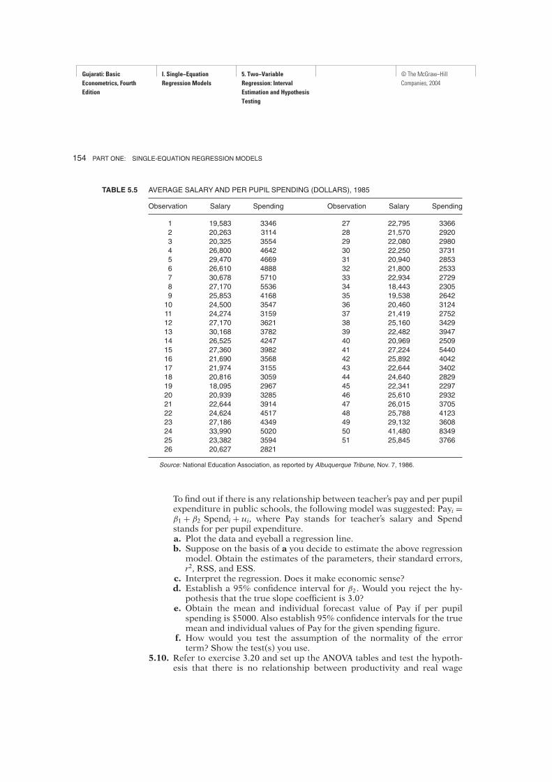
Gujarati: Basic


Edition


Regression Models

5. Two−Variable



Testing


Companies, 2004


To find out if there is any relationship between teacher’s pay and per pupilexpenditure in public schools, the following model was suggested: Payi =β1 + β2 Spendi + ui, where Pay stands for teacher’s salary and Spendstands for per pupil expenditure.a. Plot the data and eyeball a regression line.b. Suppose on the basis of a you decide to estimate the above regressionmodel. Obtain the estimates of the parameters, their standard errors,r2, RSS, and ESS.

c. Interpret the regression. Does it make economic sense?d. Establish a 95% confidence interval for β2 . Would you reject the hy-

pothesis that the true slope coefficient is 3.0?e. Obtain the mean and individual forecast value of Pay if per pupilspending is $5000. Also establish 95% confidence intervals for the truemean and individual values of Pay for the given spending figure.

f. How would you test the assumption of the normality of the errorterm? Show the test(s) you use.

5.10. Refer to exercise 3.20 and set up the ANOVA tables and test the hypoth-esis that there is no relationship between productivity and real wage

TABLE 5.5 AVERAGE SALARY AND PER PUPIL SPENDING (DOLLARS), 1985

Observation Salary Spending Observation Salary Spending

1 19,583 3346 27 22,795 3366

2 20,263 3114 28 21,570 2920

3 20,325 3554 29 22,080 2980

4 26,800 4642 30 22,250 3731

5 29,470 4669 31 20,940 2853

6 26,610 4888 32 21,800 2533

7 30,678 5710 33 22,934 2729

8 27,170 5536 34 18,443 2305

9 25,853 4168 35 19,538 2642

10 24,500 3547 36 20,460 3124

11 24,274 3159 37 21,419 2752

12 27,170 3621 38 25,160 3429

13 30,168 3782 39 22,482 3947

14 26,525 4247 40 20,969 2509

15 27,360 3982 41 27,224 5440

16 21,690 3568 42 25,892 4042

17 21,974 3155 43 22,644 3402

18 20,816 3059 44 24,640 2829

19 18,095 2967 45 22,341 2297

20 20,939 3285 46 25,610 2932

21 22,644 3914 47 26,015 3705

22 24,624 4517 48 25,788 4123

23 27,186 4349 49 29,132 3608

24 33,990 5020 50 41,480 8349

25 23,382 3594 51 25,845 3766

26 20,627 2821

Source: National Education Association, as reported by Albuquerque Tribune, Nov. 7, 1986.

Gujarati: Basic


Edition


Regression Models

5. Two−Variable



Testing


Companies, 2004


compensation. Do this for both the business and nonfarm businesssectors.

5.11. Refer to exercise 1.7.a. Plot the data with impressions on the vertical axis and advertisingexpenditure on the horizontal axis. What kind of relationship do youobserve?

b. Would it be appropriate to fit a bivariate linear regression model to thedata? Why or why not? If not, what type of regression model will youfit the data to? Do we have the necessary tools to fit such a model?

c. Suppose you do not plot the data and simply fit the bivariate regres-sion model to the data. Obtain the usual regression output. Save theresults for a later look at this problem.

5.12. Refer to exercise 1.1.a. Plot the U.S. Consumer Price Index (CPI) against the Canadian CPI.What does the plot show?

b. Suppose you want to predict the U.S. CPI on the basis of the CanadianCPI. Develop a suitable model.

c. Test the hypothesis that there is no relationship between the twoCPIs. Use α = 5% . If you reject the null hypothesis, does that mean theCanadian CPI “causes” the U.S. CPI? Why or why not?

5.13. Refer to exercise 3.22.a. Estimate the two regressions given there, obtaining standard errorsand the other usual output.

b. Test the hypothesis that the disturbances in the two regression modelsare normally distributed.

c. In the gold price regression, test the hypothesis that β2 = 1, that is,there is a one-to-one relationship between gold prices and CPI (i.e., goldis a perfect hedge). What is the p value of the estimated test statistic?

d. Repeat step c for the NYSE Index regression. Is investment in thestock market a perfect hedge against inflation? What is the null hy-pothesis you are testing? What is its p value?

e. Between gold and stock, which investment would you choose? What isthe basis of your decision?

5.14. Table 5.6 gives data on GNP and four definitions of the money stock forthe United States for 1970–1983. Regressing GNP on the various defini-tions of money, we obtain the results shown in Table 5.7. The monetarists or quantity theorists maintain that nominal income

(i.e., nominal GNP) is largely determined by changes in the quantity or thestock of money, although there is no consensus as to the “right” definitionofmoney. Given the results in the preceding table, consider these questions:a. Which definition ofmoney seems to be closely related to nominal GNP?b. Since the r2 terms are uniformly high, does this fact mean that ourchoice for definition of money does not matter?

c. If the Fed wants to control the money supply, which one of thesemoney measures is a better target for that purpose? Can you tell fromthe regression results?

5.15. Suppose the equation of an indifference curve between two goods is

XiYi = β1 + β2Xi

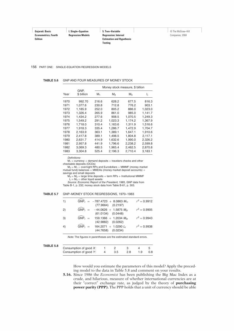
Gujarati: Basic


Edition


Regression Models

5. Two−Variable



Testing


Companies, 2004


TABLE 5.6 GNPAND FOUR MEASURES OF MONEY STOCK

GNP,Money stock measure, $ billion

Year $ billion M1 M2 M3 L

1970 992.70 216.6 628.2 677.5 816.3

1971 1,077.6 230.8 712.8 776.2 903.1

1972 1,185.9 252.0 805.2 886.0 1,023.0

1973 1,326.4 265.9 861.0 985.0 1,141.7

1974 1,434.2 277.6 908.5 1,070.5 1,249.3

1975 1,549.2 291.2 1,023.3 1,174.2 1,367.9

1976 1,718.0 310.4 1,163.6 1,311.9 1,516.6

1977 1,918.3 335.4 1,286.7 1,472.9 1,704.7

1978 2,163.9 363.1 1,389.1 1,647.1 1,910.6

1979 2,417.8 389.1 1,498.5 1,804.8 2,117.1

1980 2,631.7 414.9 1,632.6 1,990.0 2,326.2

1981 2,957.8 441.9 1,796.6 2,238.2 2,599.8

1982 3,069.3 480.5 1,965.4 2,462.5 2,870.8

1983 3,304.8 525.4 2,196.3 2,710.4 3,183.1

Definitions:M1 = currency + demand deposits + travelers checks and other

checkable deposits (OCDs)M2 = M1 + overnight RPs and Eurodollars + MMMF (money market

mutual fund) balances + MMDAs (money market deposit accounts) +savings and small deposits

M3 = M2 + large time deposits + term RPs + Institutional MMMFL = M3 + other liquid assetsSource: Economic Report of the President, 1985, GNP data from

Table B-1, p. 232; money stock data from Table B-61, p. 303.

TABLE 5.7 GNP–MONEY STOCK REGRESSIONS, 1970–1983

1) GNPt = −787.4723 + 8.0863 M1t r 2 = 0.9912

(77.9664) (0.2197)

2) GNPt = −44.0626 + 1.5875 M2t r 2 = 0.9905

(61.0134) (0.0448)

3) GNPt = 159.1366 + 1.2034 M3t r 2 = 0.9943

(42.9882) (0.0262)

4) GNPt = 164.2071 + 1.0290 Lt r 2 = 0.9938

(44.7658) (0.0234)

Note: The figures in parentheses are the estimated standard errors.

Consumption of good X : 1 2 3 4 5

Consumption of good Y : 4 3.5 2.8 1.9 0.8

TABLE 5.8

How would you estimate the parameters of this model? Apply the preced-ing model to the data in Table 5.8 and comment on your results.

5.16. Since 1986 the Economist has been publishing the Big Mac Index as acrude, and hilarious, measure of whether international currencies are attheir “correct” exchange rate, as judged by the theory of purchasingpower parity (PPP). The PPP holds that a unit of currency should be able

Gujarati: Basic


Edition


Regression Models

5. Two−Variable



Testing


Companies, 2004


to buy the same bundle of goods in all countries. The proponents of PPPargue that, in the long run, currencies tend to move toward their PPP. TheEconomist uses McDonald’s Big Mac as a representative bundle and givesthe information in Table 5.9.Consider the following regression model:

Yi = β1 + β2Xi + ui

where Y = actual exchange rate and X = implied PPP of the dollar.

TABLE 5.9 THE HAMBURGER STANDARD

Under (−)/Actual $ over (+)Big Mac prices

Implied exchange valuationIn local In PPP* of rate against thecurrency dollars the dollar April 17, 2001 dollar, %

United States† $2.54 2.54 – – –

Argentina Peso2.50 2.50 0.98 1.00 −2

Australia A$3.00 1.52 1.18 1.98 −40

Brazil Real3.60 1.64 1.42 2.19 −35

Britain £1.99 2.85 1.28‡ 1.43‡ 12

Canada C$3.33 2.14 1.31 1.56 −16

Chile Peso1260 2.10 496 601 −17

China Yuan9.90 1.20 3.90 8.28 −53

Czech Rep Koruna56.00 1.43 22.0 39.0 −44

Denmark DKr24.75 2.93 9.74 8.46 15

Euro area 2.57 2.27 0.99§ 0.88§ −11

France FFr18.5 2.49 7.28 7.44 −2

Germany DM5.10 2.30 2.01 2.22 −9

Italy Lire4300 1.96 1693 2195 −23

Spain Pta395 2.09 156 189 −18

Hong Kong HK$10.70 1.37 4.21 7.80 −46

Hungary Forint399 1.32 157 303 −48

Indonesia Rupiah14700 1.35 5787 10855 −47

Japan ¥294 2.38 116 124 −6

Malaysia M$4.52 1.19 1.78 3.80 −53

Mexico Peso21.9 2.36 8.62 9.29 −7

New Zealand NZ$3.60 1.46 1.42 2.47 −43

Philippines Peso59.00 1.17 23.2 50.3 −54

Poland Zloty5.90 1.46 2.32 4.03 −42

Russia Rouble35.00 1.21 13.8 28.9 −52

Singapore S$3.30 1.82 1.30 1.81 −28

South Africa Rand9.70 1.19 3.82 8.13 −53

South Korea Won3000 2.27 1181 1325 −11

Sweden SKr24.0 2.33 9.45 10.28 −8

Switzerland SFr6.30 3.65 2.48 1.73 44

Taiwan NT$70.0 2.13 27.6 32.9 −16

Thailand Baht55.0 1.21 21.7 45.5 −52

*Purchasing power parity: local price divided by price in the United States.†Average of New York, Chicago, San Francisco, and Atlanta.‡Dollars per pound.§Dollars per euro.Source: McDonald’s; The Economist, April 21, 2001.

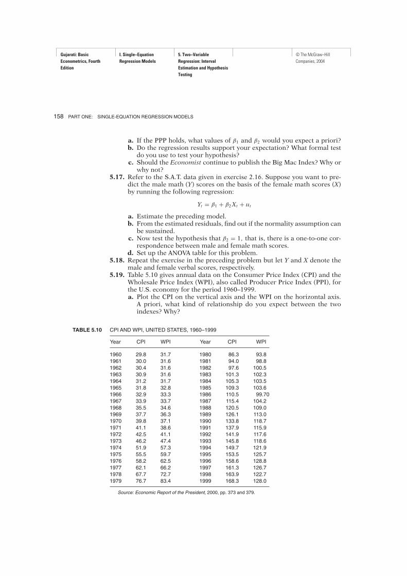
Gujarati: Basic


Edition


Regression Models

5. Two−Variable



Testing


Companies, 2004


a. If the PPP holds, what values of β1 and β2 would you expect a priori?b. Do the regression results support your expectation? What formal testdo you use to test your hypothesis?

c. Should the Economist continue to publish the Big Mac Index? Why orwhy not?

5.17. Refer to the S.A.T. data given in exercise 2.16. Suppose you want to pre-dict the male math (Y) scores on the basis of the female math scores (X)by running the following regression:

Yt = β1 + β2Xt + ut

a. Estimate the preceding model.b. From the estimated residuals, find out if the normality assumption canbe sustained.

c. Now test the hypothesis that β2 = 1, that is, there is a one-to-one cor-respondence between male and female math scores.

d. Set up the ANOVA table for this problem.5.18. Repeat the exercise in the preceding problem but let Y and X denote the

male and female verbal scores, respectively.5.19. Table 5.10 gives annual data on the Consumer Price Index (CPI) and the

Wholesale Price Index (WPI), also called Producer Price Index (PPI), forthe U.S. economy for the period 1960–1999.a. Plot the CPI on the vertical axis and the WPI on the horizontal axis.A priori, what kind of relationship do you expect between the twoindexes? Why?

Year CPI WPI Year CPI WPI

1960 29.8 31.7 1980 86.3 93.8

1961 30.0 31.6 1981 94.0 98.8

1962 30.4 31.6 1982 97.6 100.5

1963 30.9 31.6 1983 101.3 102.3

1964 31.2 31.7 1984 105.3 103.5

1965 31.8 32.8 1985 109.3 103.6

1966 32.9 33.3 1986 110.5 99.70

1967 33.9 33.7 1987 115.4 104.2

1968 35.5 34.6 1988 120.5 109.0

1969 37.7 36.3 1989 126.1 113.0

1970 39.8 37.1 1990 133.8 118.7

1971 41.1 38.6 1991 137.9 115.9

1972 42.5 41.1 1992 141.9 117.6

1973 46.2 47.4 1993 145.8 118.6

1974 51.9 57.3 1994 149.7 121.9

1975 55.5 59.7 1995 153.5 125.7

1976 58.2 62.5 1996 158.6 128.8

1977 62.1 66.2 1997 161.3 126.7

1978 67.7 72.7 1998 163.9 122.7

1979 76.7 83.4 1999 168.3 128.0

Source: Economic Report of the President, 2000, pp. 373 and 379.

TABLE 5.10 CPI AND WPI, UNITED STATES, 1960–1999

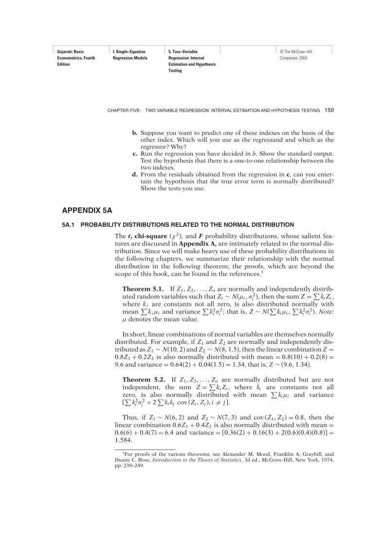
Gujarati: Basic


Edition


Regression Models

5. Two−Variable



Testing


Companies, 2004


b. Suppose you want to predict one of these indexes on the basis of theother index. Which will you use as the regressand and which as theregressor? Why?

c. Run the regression you have decided in b. Show the standard output.Test the hypothesis that there is a one-to-one relationship between thetwo indexes.

d. From the residuals obtained from the regression in c, can you enter-tain the hypothesis that the true error term is normally distributed?Show the tests you use.

APPENDIX 5A

5A.1 PROBABILITY DISTRIBUTIONS RELATED TO THE NORMAL DISTRIBUTION

The t, chi-square (χ2), and F probability distributions, whose salient fea-tures are discussed in Appendix A, are intimately related to the normal dis-tribution. Since we will make heavy use of these probability distributions inthe following chapters, we summarize their relationship with the normaldistribution in the following theorem; the proofs, which are beyond thescope of this book, can be found in the references.1

Theorem 5.1. If Z1, Z2, . . . , Zn are normally and independently distrib-uted random variables such that Zi ∼ N(µi , σ

2i ), then the sum Z =

∑

kiZi ,where ki are constants not all zero, is also distributed normally withmean

∑

kiµi and variance ∑

k2i σ2i ; that is, Z ∼ N(

∑

kiµi ,∑

k2i σ2i ). Note:

µ denotes the mean value.

In short, linear combinations of normal variables are themselves normallydistributed. For example, if Z1 and Z2 are normally and independently dis-tributed as Z1 ∼ N(10, 2) and Z2 ∼ N(8, 1.5), then the linear combination Z =0.8Z1 + 0.2Z2 is also normally distributed with mean = 0.8(10) + 0.2(8) =9.6 and variance = 0.64(2) + 0.04(1.5) = 1.34, that is, Z ∼ (9.6, 1.34).

Theorem 5.2. If Z1, Z2, . . . , Zn are normally distributed but are notindependent, the sum Z =

∑

kiZi , where ki are constants not allzero, is also normally distributed with mean

∑

kiµi and variance[∑

k2i σ2i + 2

∑

kikj cov (Zi , Zj ), i )= j].

Thus, if Z1 ∼ N(6, 2) and Z2 ∼ N(7, 3) and cov (Z1, Z2) = 0.8, then thelinear combination 0.6Z1 + 0.4Z2 is also normally distributed with mean =0.6(6) + 0.4(7) = 6.4 and variance = [0.36(2) + 0.16(3) + 2(0.6)(0.4)(0.8)] =1.584.

1For proofs of the various theorems, see Alexander M. Mood, Franklin A. Graybill, andDuane C. Bose, Introduction to the Theory of Statistics, 3d ed., McGraw-Hill, New York, 1974,pp. 239–249.

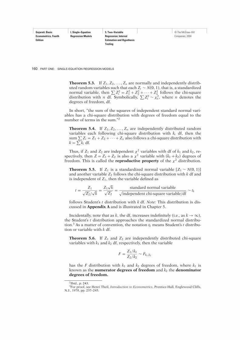
Gujarati: Basic


Edition


Regression Models

5. Two−Variable



Testing


Companies, 2004


Theorem 5.3. If Z1, Z2, . . . , Zn are normally and independently distrib-uted random variables such that each Zi ∼ N(0, 1), that is, a standardizednormal variable, then

∑

Z2i = Z21 + Z22 + · · · + Z2n follows the chi-squaredistribution with n df. Symbolically,

∑

Z2i ∼ χ2n , where n denotes thedegrees of freedom, df.

In short, “the sum of the squares of independent standard normal vari-ables has a chi-square distribution with degrees of freedom equal to thenumber of terms in the sum.”2

Theorem 5.4. If Z1, Z2, . . . , Zn are independently distributed randomvariables each following chi-square distribution with ki df, then thesum

∑

Zi = Z1 + Z2 + · · · + Zn also follows a chi-square distribution withk =∑

ki df.

Thus, if Z1 and Z2 are independent χ2 variables with df of k1 and k2, re-

spectively, then Z = Z1 + Z2 is also a χ2 variable with (k1 + k2) degrees of

freedom. This is called the reproductive property of the χ2 distribution.

Theorem 5.5. If Z1 is a standardized normal variable [Z1 ∼ N(0, 1)]and another variable Z2 follows the chi-square distribution with k df andis independent of Z1, then the variable defined as

t = Z1√Z2/

√k

= Z1√k√

Z2= standard normal variable√

independent chi-square variable/df∼ tk

follows Student’s t distribution with k df. Note: This distribution is dis-cussed in Appendix A and is illustrated in Chapter 5.

Incidentally, note that as k, the df, increases indefinitely (i.e., as k→ ∞),the Student’s t distribution approaches the standardized normal distribu-tion.3 As a matter of convention, the notation tk means Student’s t distribu-tion or variable with k df.

Theorem 5.6. If Z1 and Z2 are independently distributed chi-squarevariables with k1 and k2 df, respectively, then the variable

F = Z1/k1

Z2/k2∼ Fk1,k2

has the F distribution with k1 and k2 degrees of freedom, where k1 isknown as the numerator degrees of freedom and k2 the denominatordegrees of freedom.

2Ibid., p. 243.3For proof, see Henri Theil, Introduction to Econometrics, Prentice-Hall, Englewood Cliffs,

N.J., 1978, pp. 237–245.

Gujarati: Basic


Edition


Regression Models

5. Two−Variable



Testing


Companies, 2004


Again as a matter of convention, the notation Fk1,k2 means an F variablewith k1 and k2 degrees of freedom, the df in the numerator being quoted first.In other words, Theorem 5.6 states that the F variable is simply the ratio

of two independently distributed chi-square variables divided by their re-spective degrees of freedom.

Theorem 5.7. The square of (Student’s) t variable with k df has an F dis-tribution with k1 = 1 df in the numerator and k2 = k df in the denomina-tor.4 That is,

F1,k = t2kNote that for this equality to hold, the numerator df of the F variable

must be 1. Thus, F1,4 = t24 or F1,23 = t223 and so on.As noted, we will see the practical utility of the preceding theorems as

we progress.

Theorem 5.8. For large denominator df, the numerator df times the Fvalue is approximately equal to the chi-square value with the numeratordf. Thus,

mFm,n = χ2m as n→ ∞

Theorem 5.9. For sufficiently large df, the chi-square distribution canbe approximated by the standard normal distribution as follows:

Z =√

2χ2 −√2k− 1 ∼ N(0, 1)

where k denotes df.

5A.2 DERIVATION OF EQUATION (5.3.2)

Let

Z1 = β2 − β2

se (β2)=(β2 − β2)

√

x2i

σ(1)

and

Z2 = (n− 2)σ 2

σ 2(2)

Provided σ is known, Z1 follows the standardized normal distribution; thatis, Z1 ∼ N(0, 1). (Why?) Z2, follows the χ2 distribution with (n− 2) df.5

4For proof, see Eqs. (5.3.2) and (5.9.1).5For proof, see Robert V. Hogg and Allen T. Craig, Introduction to Mathematical Statistics,

2d ed., Macmillan, New York, 1965, p. 144.

Gujarati: Basic


Edition


Regression Models

5. Two−Variable



Testing


Companies, 2004


Furthermore, it can be shown that Z2 is distributed independently of Z1.6

Therefore, by virtue of Theorem 5.5, the variable

t = Z1√n− 2√Z2

(3)

follows the t distribution with n− 2 df. Substitution of (1) and (2) into (3)gives Eq. (5.3.2).

5A.3 DERIVATION OF EQUATION (5.9.1)

Equation (1) shows that Z1 ∼ N(0, 1). Therefore, by Theorem 5.3, the pre-ceding quantity

Z21 = (β2 − β2)2∑

x2iσ 2

follows the χ2 distribution with 1 df. As noted in Section 5A.1,

Z2 = (n− 2)σ 2

σ 2=∑

u2iσ 2

also follows the χ2 distribution with n− 2 df. Moreover, as noted in Sec-tion 4.3, Z2 is distributed independently of Z1. Then from Theorem 5.6, itfollows that

F =Z21/

1

Z2/(n− 2)= (β2 − β2)

2(∑

x2i )∑

u2i/

(n− 2)

follows the F distribution with 1 and n− 2 df, respectively. Under the nullhypothesis H0:β2 = 0, the preceding F ratio reduces to Eq. (5.9.1).

5.A.4 DERIVATIONS OF EQUATIONS (5.10.2) AND (5.10.6)

Variance of Mean Prediction

Given Xi = X0, the true mean prediction E(Y0 | X0) is given by

E(Y0 | X0) = β1 + β2X0 (1)

We estimate (1) from

Y0 = β1 + β2X0 (2)

Taking the expectation of (2), given X0, we get

E(Y0) = E(β1)+ E(β2)X0

= β1 + β2X0

6For proof, see J. Johnston, Econometric Methods, McGraw-Hill, 3d ed., New York, 1984,pp. 181–182. (Knowledge of matrix algebra is required to follow the proof.)

Gujarati: Basic


Edition


Regression Models

5. Two−Variable



Testing


Companies, 2004


because β1 and β2 are unbiased estimators. Therefore,

E(Y0) = E(Y0 | X0) = β1 + β2X0 (3)

That is, Y0 is an unbiased predictor of E(Y0 | X0).Now using the property that var (a+ b) = var (a)+ var (b)+ 2 cov (a, b),

we obtain

var (Y0) = var (β1)+ var (β2)X20 + 2 cov (β1β2)X0 (4)

Using the formulas for variances and covariance of β1 and β2 given in(3.3.1), (3.3.3), and (3.3.9) and manipulating terms, we obtain

var (Y0) = σ 2[

1

n+ (X0 − X)2

∑

x2i

]

= (5.10.2)

Variance of Individual Prediction

We want to predict an individual Y corresponding to X = X0; that is, wewant to obtain

Y0 = β1 + β2X0 + u0 (5)

We predict this as

Y0 = β1 + β2X0 (6)

The prediction error, Y0 − Y0, is

Y0 − Y0 = β1 + β2X0 + u0 − (β1 + β2X0)

= (β1 − β1)+ (β2 − β2)X0 + u0(7)

Therefore,

E(Y0 − Y0) = E(β1 − β1)+ E(β2 − β2)X0 − E(u0)

= 0

because β1, β2 are unbiased, X0 is a fixed number, and E(u0) is zero by as-sumption.Squaring (7) on both sides and taking expectations, we get var (Y0 − Y0) =

var (β1)+ X20 var (β2)+ 2X0 cov (β1, β2)+ var (uo). Using the variance and co-variance formulas for β1 and β2 given earlier, and noting that var (u0) = σ 2,we obtain

var (Y0 − Y0) = σ 2[

1+ 1

n+ (X0 − X)2

∑

x2i

]

= (5.10.6)

part one: i. single−equation regression models

Documents