1

Parsimonious path openings and closingsVincent Morard , Petr Dokladal and Etienne Decenciere

Abstract—Path openings and closings are morphological toolsused to preserve long, thin and tortuous structures in gray levelimages. They explore all paths from a defined class, and filterthem with a length criterion. However, most paths are redundant,making the process generally slow.

Parsimonious path openings and closings are introduced in thispaper to solve this problem. These operators only consider asubset of the paths considered by classical path openings, thusachieving a substantial speed-up, while obtaining similar results.Moreover, a recently introduced one dimensional (1-D) openingalgorithm is applied along each selected path. Its complexity islinear with respect to the number of pixels, independent of thesize of the opening. Furthermore, it is fast for any input dataaccuracy (integer or floating point) and works in stream.

Parsimonious path openings are also extended to incompletepaths, i.e. paths containing gaps. Noise-corrupted paths can thusbe processed with the same approach and complexity.

These parsimonious operators achieve a several orders ofmagnitude speed-up. Examples are shown for incomplete pathopenings, where computing times are brought from minutes totens of milliseconds, while obtaining similar results.

Index Terms—Path operators, curvilinear structures, mathe-matical morphology, complete and incomplete paths.

I. INTRODUCTION

Thin structures extraction is a non-trivial task in imageprocessing. It requires adapted tools, used in a great rangeof applications, from the biomedical field to the industrialdomain. Blood vessels extraction from eye fundus images [1],[2], microglia tree-like form in confocal microscope images[3], guide-wire segmentation in X-ray fluoroscopy [4], roaddetection from remote sensing images [5] or automated cracksdetection from metallic pieces for non-destructive testing [6],[7] are some examples.

In the literature, the typical approach to enhance thinstructures is to compute the supremum of openings with linearstructuring elements (SE) in many orientations [8], [9]. Thesame strategy can be used with a bank of directional Gaborfilters or difference of Gaussians filters [10]. However, tortuousstructures are difficult to detect with this kind of approach.Using adaptive mathematical morphology methods improvesthe detection. Tankyevych et al. [11] introduced hessian basedfilters to detect curvilinear lines. In [7], the SE are able to adapt

Copyright (c) 2013 IEEE. Personal use of this material is permitted.However, permission to use this material for any other purposes must beobtained from the IEEE by sending a request to pubs-permissions@ieee.org.

Vincent Morard was at the time of writing this paper with Centre forMathematical Morphology, MINES ParisTech, Fontainebleau, France, Email:vincent.morard@mines-paristech.fr

Petr Dokladal is with Centre for Mathematical Morphology, MINES Paris-Tech, 35, rue Saint Honore, 77300 Fontainebleau, France, tel: +33 (0)1 64 6947 98, Email: petr.dokladal@mines-paristech.fr

Etienne Decenciere is with Centre for Mathematical Morphology, MINESParisTech, 35, rue Saint Honore, 77300 Fontainebleau, France, tel: +33 (0)164 69 48 09, Email: etienne.decenciere@mines-paristech.fr

their shapes to enhance very thin cracks of any tortuosity. Areaopenings, introduced by Vincent [12], are considered as thefirst attribute openings, later generalized by Breen and Jonesto obtain attribute thinnings [13]. Indeed, using non-increasingcriteria to build attribute thinnings yields interesting filters todetect thin structures. For instance, the inertia of the connectedcomponents, weighted by their area, gives an interesting shapedescriptor for elongated structures [14], [15]. More recently,thinnings based on geodesic attributes have been shown toefficiently characterize structures according to their length,tortuosity or elongation [6], [16]. Finally, the so-called pathopenings (PO) [17]–[19] use underlying directed acyclic graphto measure the path length.

All these methods have the same drawback: their lackof robustness with respect to noise. Indeed, thin elongatedstructures we are looking for can be easily corrupted by noise,resulting in disconnected paths. Heijmans et al. [19] haveproposed incomplete path openings, able to deal with gaps inpaths. Later, Talbot and Appleton [20] proposed an efficientalgorithm to compute both complete and incomplete pathopenings. It has logarithmic complexity w.r.t. the length of thepaths and linear w.r.t. the width of the gaps, resulting in longcomputation timings, unsuitable for time-critical applications.A recent work by Cokelaer et al. [21] presents a more effi-cient, robust to noise version of path operators, unfortunately,computing time is still not compatible with high-throughputcomputing.

A good robustness to noise also offers the semi-local orglobal approach proposed in Rouchdy and Cohen [3] orBismuth et al. [4]. Both exploit the spatial density of locallyshortest paths designed to converge to thin, curvilinear imagestructures to enhance. Based on this ideas, several techniquescan be used to enhance or detect structures: voting [3] andvoting, pruning or cost minimization in the polygonal pathimage [4].

The approach developed in this paper is motivated by theneed to detect thin, long, tortuous and possibly noisy structuresin a computationally demanding framework. The methodsfrom the state of the art that fulfill the best these requirementsare indeed path openings with complete or incomplete paths[20]. Here, we propose the Parsimonious path opening (PPO) anew fast operator for detecting the same set of structures, usingcomplete or incomplete paths. PPO only explore a relevantsubset of all paths in the image, to reduce the computationtime by several orders of magnitude. Hence, the results ofPPO are not exactly the same as classical path openings butthey are fast, accurate and robust to noise.

This paper is organized as follows. We first recall thetheory of classical path openings (Sec. II). Then, we describethe extraction of the relevant subset of paths in the image(Sec. III), the filtering strategies available (Sec. IV), the

2

practical considerations (Sec. V) and the operator accuracy(Sec. VI). Finally, we present some results through an appli-cation: the detection of cracks from road pavement images.We also study the algorithmic complexity and we propose atiming comparison with classical path openings (Sec. VII).

II. BASIC NOTIONS ON PATH OPENINGS

Path openings [18], [19] were introduced to offer a higherflexibility compared to the supremum of linear openings. Webriefly recall here their definition and characteristics.

A. Connectivity graph and maximal paths

A two-dimensional binary image X can be described as asubset of a rectangular sub-domain D of Z2. We equip D witha directed acyclic graph G : D →P(D), where P(D) is thepower set of D. For any two points x and y of D, we say thatx is linked to y on G if, and only if, y ∈ G(x). G− is theinverse of G, defined by G− : D → P(D) and for all x inD, y ∈ G−(x) (i.e. x is linked to y on G−) if, and only if,x ∈ G(y) (i.e. y is linked to x on G). GX is the subgraph ofG obtained when the graph is restricted to X .

Fig. 1 illustrates some classical graphs used in practice forG.

Let us introduce now the definition of a path on GX :

Definition 1A sequence π = (x1, x2, . . . , xn), n ∈ N, of points is a pathofGX if, and only if, ∀i ∈ N, 1 ≤ i ≤ n−1, xi+1 ∈ GX(xi)(xi is linked to xi+1 on GX ). The path length is equal to n.Points x1 and xn are its starting and end points. The set of allpaths of GX is denoted ΠGX

.

On each point x of D we define λGX(x) (or λ(x), when

there is no ambiguity) as the maximal length of all the pathsof ΠGX

going through x. If x does not belong to X , thenλ(x) is equal to zero. Given that the considered graphs arefinite, and without loops, the values of λ are finite.

B. Binary path opening

Map λ can be efficiently computed using a scan of GX ,followed by a scan of G−X : let λ+ (reps. λ−) be the mapwhich gives, for each point x of D, the maximal length ofthe paths of ΠGX

(resp. ΠG−X

) ending at x. λ+ and λ− areefficiently computed thanks to the following equations:

λ+(x) = maxy∈GX(x)

λ+(y) + 1, (1)

λ−(x) = maxy∈G−

X(x)λ−(y) + 1. (2)

An example of λ+ and λ− is shown in Fig. 2 (b and c). Finally,λ is simply computed as follows, for all x ∈ D:

λ(x) = λ+(x) + λ−(x)− 1. (3)

For a given pixel x, λ(x) gives the length of the longest pathsgoing through it. If we remove from X all the points where λis smaller than a given constant L, we obtain an operator whichis idempotent, increasing and anti-extensive (see Heijmans et

al. [19] for the details), therefore, it is an opening, called apath opening (PO) of size L, and written ΓPO

L (X):

ΓPOL (X) = {x ∈ X|λGX

(x) ≥ L}. (4)

Such an opening, when based on any of the graphs illus-trated in Fig. 1, is by design not rotation invariant, an oftenwelcome property. In order to improve on this aspect, onecan use the fact that the supremum of openings is still anopening [22]: four openings are in practice computed, basedon the four graphs depicted in Fig. 1, and their supremum iscomputed.

In the following ΓPOL will denote the path opening of size

L based on this supremum.

C. Gray level path openings

Let f : D → V be a gray level image, where V is a finitesubset of R, such as {0, 1, . . . , 255}. Finally, ∞V and −∞V

respectively denote the maximal and minimal values of V .Let Xh = {x | f(x) ≥ h} be the upper level set obtained

by thresholding f at level h. Given that the binary openingΓPOL is increasing, it commutes with thresholding. Thence, the

extension to gray level images is direct:

∀x ∈ D, γPOL (f)(x) = ∨{h ∈ V | x ∈ ΓPO

L (Xh(f))}. (5)

Using equation 5 to compute gray level path openings iseasy, but it is never used in practice because it would bemuch too slow. In [23], an efficient update of λ+ and λ−

is proposed, which achieves a large speed up factor. Thisupdate is improved in Luengo Hendriks [24] to be able toeasily work with n-D images. The same paper [24] alsoproposes a constraint on the connectivity to prevent pathsfrom zigzagging and overestimating the length of diagonallyoriented segments. Later, Cokelaer et al [21] use a differentway of making the path opening less sensitive to noise withn-D images. These three papers bring notable improvementson path opening timings, but the algorithms are still too slowfor many applications. Parsimonious path operators, presentedin the following sections, address this issue.

In what follows, we present and illustrate this work withthe extraction of bright structures in an image, with no lossof generality. Path closings (resp. parsimonious path closings)are computed using path openings (resp. parsimonious pathopenings) on the inverted image.

III. PARSIMONIOUS SET OF PATHS

The principal idea behind the notion of parsimonious pathsis to work with a restricted set of paths instead of exploringall of them. In fact, the set of paths will be so sparse, thatmost points in the image will not be crossed by any of them.

In the original definition of path openings, the number ofpaths grows exponentially with the size of the image. However,only few out of these paths bring relevant information. In thefollowing, we deal with the problem of building a relevantsubset of paths.

For the extraction of bright structures, the relevant pathshave to follow the brightest structures of the image. Since this

3

(a) (b) (c) (d)

Fig. 1. Example of commonly used graphs: (a) paths having an orientation from south to north (S-N). (b) SW-NE paths, (c) W-E paths and (d) NW-SEpaths

0

0000000

0 0 0 0

0004000

0

1 5

0 3 3 0 0 0

0010200

0 1 1 0 0 0 0

0 0 0 0 0 0 0

0

0000000

0 0 0 0

0002000

0

1 1

0 3 3 0 0 0

0040400

0 5 5 0 0 0 0

0 0 0 0 0 0 0

0

0000000

0 0 0 0

0005000

0

1 5

0 5 5 0 0 0

0040500

0 5 5 0 0 0 0

0 0 0 0 0 0 0

(a) (b) (c) (d)

Fig. 2. Path openings computation: (a) input binary image, (b) upstream distance map λ+, (c) downstream distance map λ−, and (d) maximal path lengthmap λ.

will usually leave other pixels devoided of a path, we willspeak about parsimonious path openings.

Three strategies are proposed in this section to select arelevant subset of paths. The last one is a generalization ofthe first two. Hereafter, D, the definition domain or supportof f , will be a rectangular subset of Z2, and G will be adirected acyclic graph.

A. Locally maximal paths

The strategy called locally maximal paths (LMP) performsa local search for bright structures. Definition 1 relative to apath is extended as follows:

Definition 2

πLMP = (x1, . . . xn) is a locally maximal path if, and onlyif, the starting point of the path belongs to a boundary of Dand if, ∀xi ∈ πLMP, 0 ≤ i ≤ n, we have:

xi+1 ∈ argmaxxj∈G(xi)

{f(xj)}. (6)

Equation 6 is used to iteratively construct a path from astarting point. The path ends when there is no successor toxn. We note that several successors of a pixel xi may have thesame gray-scale value. In that case, the principal orientation ispreserved by selecting the central pixel defined by the graph.

Pixels from the boundary of D are used as starting pointsfor each selected graph. Thus, we define ΠLMP

f :

Definition 3

The set ΠLMPf = {πLMP

1 , . . . , πLMPp }, is the set of locally

maximal paths of f .

Fig. 4(b) proposes an illustration of this set. Pixels that belongto at least one path of the set appear as white ; other pixels areblack. The original image shows a molecule of DNA observedwith an electron microscope [18] (Fig. 4(a)). We note that thenumber of paths in the image is very low in comparison withthe number of paths considered by path openings. We alsoobserve that most pixels are black (no path crossing them).This method is not only sparse with respect to paths, but alsowith respect to pixels.

With this strategy, the search for the next pixel of a path isonly local and the required time is very low. However, suchpaths are not very robust to noise. For instance, impulsivenoise can disturb and deviate a path from a thin structure. Toimprove noise robustness, we make a global search for thepaths with a second strategy, namely globally maximal paths(GMP).

B. Globally maximal paths

To build a path, we use graph theory to search for thehighest path between two pixels of the image. To explain thenotion of highest path, let us see the image as a topographicalsurface where high (resp. low) gray-scale values correspondto high (resp. low) altitudes. A globally maximal path (GMP)is a path between two points such that the average gray-scale value is the highest one among all available paths.The Dijkstra algorithm allows such search. However, giventhat the graph is directed and acyclic, specific algorithmscan be used to provide fast algorithms. They are part ofdynamic programming approaches and known as longest pathalgorithms [25]–[28]. The definition of a globally maximalpath is given as follows:

4

Definition 4

πGMP = (x1, . . . xn) is a globally maximal path if, andonly if, the starting and end points of the path belong to aboundary of D and if we have:

πGMP ∈ argmaxπ∈ΠG

(1

card(π)

∑xi∈π

f(xi)

). (7)

For a given point from the boundary of D, several globallymaximal paths can be found. In practice, we select the path thatpreserves the principal orientation of the graph. Computing aGMP from all boundary pixels of the support D and for everyconsidered graph, we obtain ΠGMP

f :

Definition 5

ΠGMPf = {πGMP

1 , . . . , πGMPp }, is the set of globally maximal

paths of f .

This set is depicted on Fig. 4(g). We observe that thepaths tend to go straight towards a bright structure, and thenthey follow it as far as they can. It is a global approach,robust to noise. With this strategy, the size of zones with noinformation (no path going through them) is larger than withlocally maximal paths. We call these zones blind regions, sincestructures localized in these regions are not analyzed. Withglobally maximal paths, large and bright structures attract allpaths; short and a bright structures found in their vicinity mightnot be seen.

GMP need more computation time than LMP and the sizeof blind regions is larger. Nevertheless, the robustness w.r.tnoise is much higher than with LMP. Below we introduce anew general formalism that allows for intermediate strategies.We call this generalization the β-maximal paths (βMP).

C. β-maximal paths

The idea of βMP is to localize the globally maximal pathsby subdividing the image support. With a given graph, saysouth to north (Fig. 1(a)), the image is divided into severalhorizontal stripes β pixels height, as illustrated in Fig. 3.

1

2

3

4

n

Fig. 3. Construction of β maximal paths with the concatenation of globallymaximal paths.

From a starting point x1 localized on the bottom boundaryof the support D, we compute πGMP = (x1, . . . , xβ) on the

(a) Input image (500×160 pixels)

(b) ΠLMP: locally maximal paths (β = 1)

(c) Π5MP: β maximal paths (β = 5)

(d) Π10MP: β maximal paths (β = 10)

(e) Π30MP: β maximal paths (β = 30)

(f) Π50MP: β maximal paths (β = 50)

(g) ΠGMP: global maximal paths (β =∞)

Fig. 4. Illustration of the sets of parsimonious paths on a given image (a).Pixels in white belong to at least one path of the set; other pixels appear inblack. The graphs used are defined in Fig. 1.

5

first stripe. Then, xβ is the new starting point and we iteratethis process until there is no successor to xn with the graphG.

Definition 6

πβMP = (x1, . . . , xn) is a β maximal path if, and only if,the starting point of the path belongs to a boundary of D andif πβMP is the concatenation of globally maximal paths πGMP

on stripes of size β.

Computing βMP from all boundary pixels of the support Dand for every graph G, we get ΠβMP

f :

Definition 7

ΠβMPf = {πβMP

1 , . . . , πβMPp }, is the set of all the β maximal

paths of f .

By definition, β maximal paths generalize previous methods:LMP are obtained with β=1 and GMP with β=∞. This methodunifies the path extraction strategy and is used to compute theset of paths of Fig. 4. Thus, we control the trade-off betweennoise robustness and blind regions size. The choice of β isapplication dependent. On a noisy image, a high value for βis preferable. On the contrary, if the signal to noise ratio ishigh, a small value will reduce the size of blind regions.

Now that we have proposed a general strategy to extractparsimonious paths, below we explain how to:• filter an image along each path;• combine the results along each path to obtain a 2-D

operator.

IV. PATHS OPERATORS

We will see in this section how, from an operator workingon single paths, we can build an operator working on the wholeimage.

A. General strategy

Recall that D is the support of function f , also writtenspt(f), and Π = {πi} denotes a collection of paths of D.The restriction of f to the path π, denoted by f/π , can beconsidered as a one-dimensional signal. Furthermore, recallthat the set of values V is a finite subset of R.

Let ξf/π be the application of a 1-D operator ξ to frestricted to π. Using ξ we obtain a result for each path πi ofΠ. Notice that for any x belonging to the intersection of twodifferent paths πi and πj , one generally obtains ξf/πi

(x) 6=ξf/πj

(x). Hence, we need a method to produce a single value.Let spt(Π) denote the support of Π, i.e. the set of all

points of D which belong to at least one path of Π. Theillustrations of different sets of parsimonious paths given inFig. 4 correspond in fact to this domain. We can extend ξf/πto spt(Π) by taking:

ξf(x) = ⊗π3xπ∈Π

ξ(f/π)(x), (8)

where ⊗ is a binary operator such as∨

or∧

(i.e. supremumor infimum). In practice, the choice of the binary operator will

depend upon the desired properties of the resulting operator.Several examples are described in the following sections.

We now have a result on all points belonging to at least onepath. However, Eq. 8 does not define ξf(x), for x outside thesupport of Π.

The β-maximal strategy constrains the paths to go throughthe brightest structures of the image (the support of the pathsspt(Π)). These are usually the structures of interest. Eventhough one may focus only on these objects, e.g. for measuringpurposes, having a result for each pixel of the image support(spt(f)) can be useful, e.g. for filtering or preprocessingpurposes.

The first and simpler strategy consists of using a constantvalue outside spt(Π), e.g. the minimum or maximum of V , oreven the original f . Another strategy is using a morphologicalreconstruction under/above f in order to propagate the resultsto the entire D. We will come back to this strategy insection V-D.

B. Parsimonious path openings

The first step to obtaining parsimonious path openings(PPO) is the choice of a convenient ξ. We naturally take the1-D opening of size L, γL and use

∨in Eq. 8 to compute a

value for each x ∈ spt(Π):

γΠL (f)(x) =

∨π3xπ∈Π

γL(f/π)(x), x ∈ spt(Π)

−∞V otherwise(9)

we pad D outside spt(Π) by −∞V to ensure the anti-extensiveness of the operator.

Based on the fact that γΠL is built from openings using

supremums, and that outside spt(Π) the result is set to theminimal value of V , it can be demonstrated that this operatoris an opening.

Note that if Π covers all the nodes of the graph, thenspt(Π)=D and no padding is necessary.

Concerning path closings, as in the classical path openingdefinition by Heijmans et al. [19], they can be obtained byduality: ϕ(f)=−γ(−f). However it should be noted that Πf

and Π−f are not the same. Whereas Πf selects the brightstructures Π−f selects the dark ones.

C. Interlude: why parsimonious path openings are openings?

The set of paths Π is a function of the image f , written Πf .So, what can we say about γΠf

L ? It can be shown that althoughanti-extensivity remains a valid property, increasingness andidempotence are lost. Therefore this more general operator isnot an opening.

From a practical point of view, to avoid an unexpectedbehavior of serially composed operators, once Πf is defined, itshould remain constant. For example, for building granulome-tries [29] (see Section VI later) it is necessary to use the sameΠ in all stages. Similarly, when computing alternate sequentialfilters, it is logical to compute once Πf and Π−f and usethem, respectively, in computing all subsequent openings andclosings.

6

(a) Input image (500×160 pixels) (b) PPO γΠL L=50

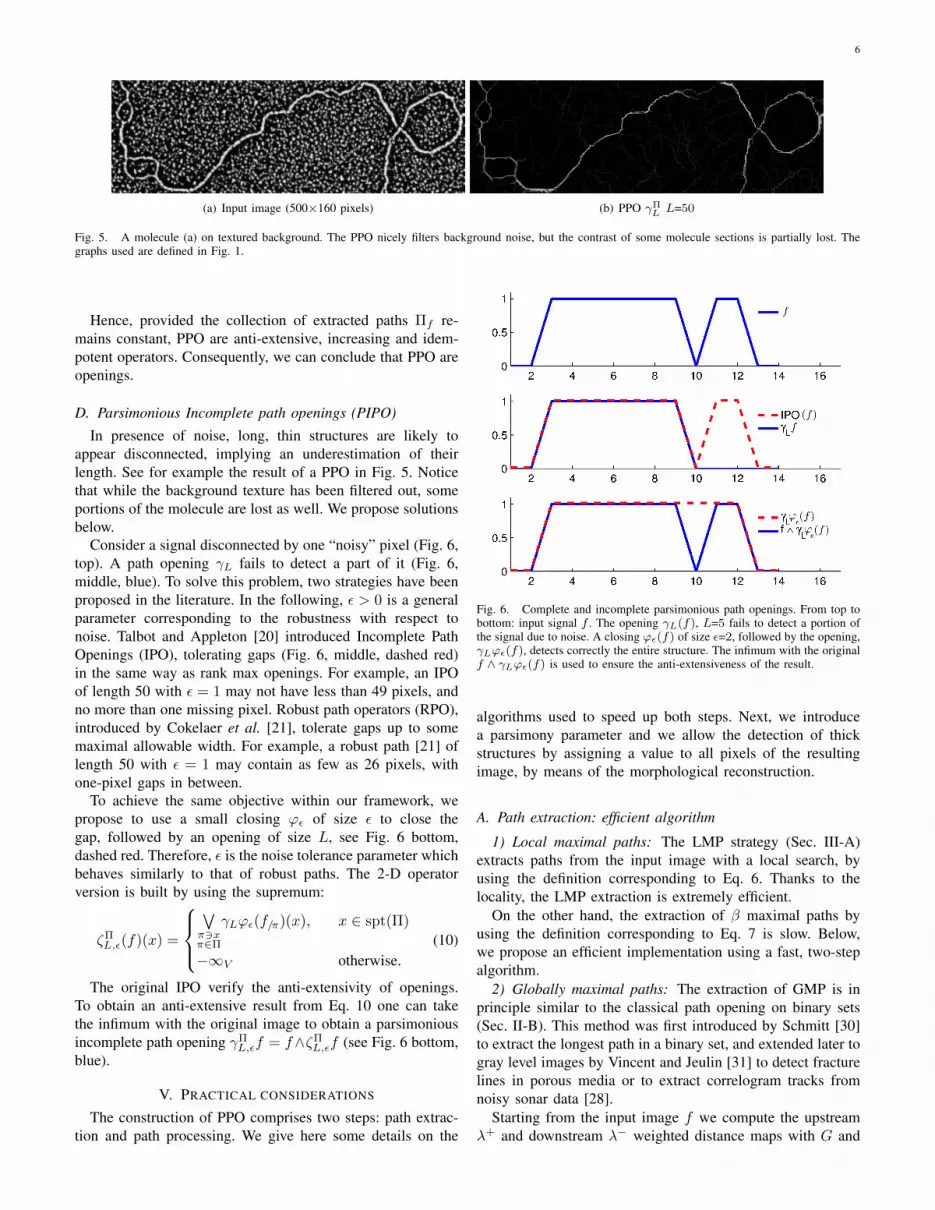
Fig. 5. A molecule (a) on textured background. The PPO nicely filters background noise, but the contrast of some molecule sections is partially lost. Thegraphs used are defined in Fig. 1.

Hence, provided the collection of extracted paths Πf re-mains constant, PPO are anti-extensive, increasing and idem-potent operators. Consequently, we can conclude that PPO areopenings.

D. Parsimonious Incomplete path openings (PIPO)

In presence of noise, long, thin structures are likely toappear disconnected, implying an underestimation of theirlength. See for example the result of a PPO in Fig. 5. Noticethat while the background texture has been filtered out, someportions of the molecule are lost as well. We propose solutionsbelow.

Consider a signal disconnected by one “noisy” pixel (Fig. 6,top). A path opening γL fails to detect a part of it (Fig. 6,middle, blue). To solve this problem, two strategies have beenproposed in the literature. In the following, ε > 0 is a generalparameter corresponding to the robustness with respect tonoise. Talbot and Appleton [20] introduced Incomplete PathOpenings (IPO), tolerating gaps (Fig. 6, middle, dashed red)in the same way as rank max openings. For example, an IPOof length 50 with ε = 1 may not have less than 49 pixels, andno more than one missing pixel. Robust path operators (RPO),introduced by Cokelaer et al. [21], tolerate gaps up to somemaximal allowable width. For example, a robust path [21] oflength 50 with ε = 1 may contain as few as 26 pixels, withone-pixel gaps in between.

To achieve the same objective within our framework, wepropose to use a small closing ϕε of size ε to close thegap, followed by an opening of size L, see Fig. 6 bottom,dashed red. Therefore, ε is the noise tolerance parameter whichbehaves similarly to that of robust paths. The 2-D operatorversion is built by using the supremum:

ζΠL,ε(f)(x) =

∨π3xπ∈Π

γLϕε(f/π)(x), x ∈ spt(Π)

−∞V otherwise.(10)

The original IPO verify the anti-extensivity of openings.To obtain an anti-extensive result from Eq. 10 one can takethe infimum with the original image to obtain a parsimoniousincomplete path opening γΠ

L,εf = f∧ζΠL,εf (see Fig. 6 bottom,

blue).

V. PRACTICAL CONSIDERATIONS

The construction of PPO comprises two steps: path extrac-tion and path processing. We give here some details on the

Fig. 6. Complete and incomplete parsimonious path openings. From top tobottom: input signal f . The opening γL(f), L=5 fails to detect a portion ofthe signal due to noise. A closing ϕε(f) of size ε=2, followed by the opening,γLϕε(f), detects correctly the entire structure. The infimum with the originalf ∧ γLϕε(f) is used to ensure the anti-extensiveness of the result.

algorithms used to speed up both steps. Next, we introducea parsimony parameter and we allow the detection of thickstructures by assigning a value to all pixels of the resultingimage, by means of the morphological reconstruction.

A. Path extraction: efficient algorithm

1) Local maximal paths: The LMP strategy (Sec. III-A)extracts paths from the input image with a local search, byusing the definition corresponding to Eq. 6. Thanks to thelocality, the LMP extraction is extremely efficient.

On the other hand, the extraction of β maximal paths byusing the definition corresponding to Eq. 7 is slow. Below,we propose an efficient implementation using a fast, two-stepalgorithm.

2) Globally maximal paths: The extraction of GMP is inprinciple similar to the classical path opening on binary sets(Sec. II-B). This method was first introduced by Schmitt [30]to extract the longest path in a binary set, and extended later togray level images by Vincent and Jeulin [31] to detect fracturelines in porous media or to extract correlogram tracks fromnoisy sonar data [28].

Starting from the input image f we compute the upstreamλ+ and downstream λ− weighted distance maps with G and

7

(a) PO of size L=50 (b) IPO of size L=50 (ε=2)

(c) PPO of size L=50 (β=5) (d) PIPO of size L=50 (ε=2, β=5)

(e) RPO of size L=50 (f) RPO of size L=50 (ε=2)

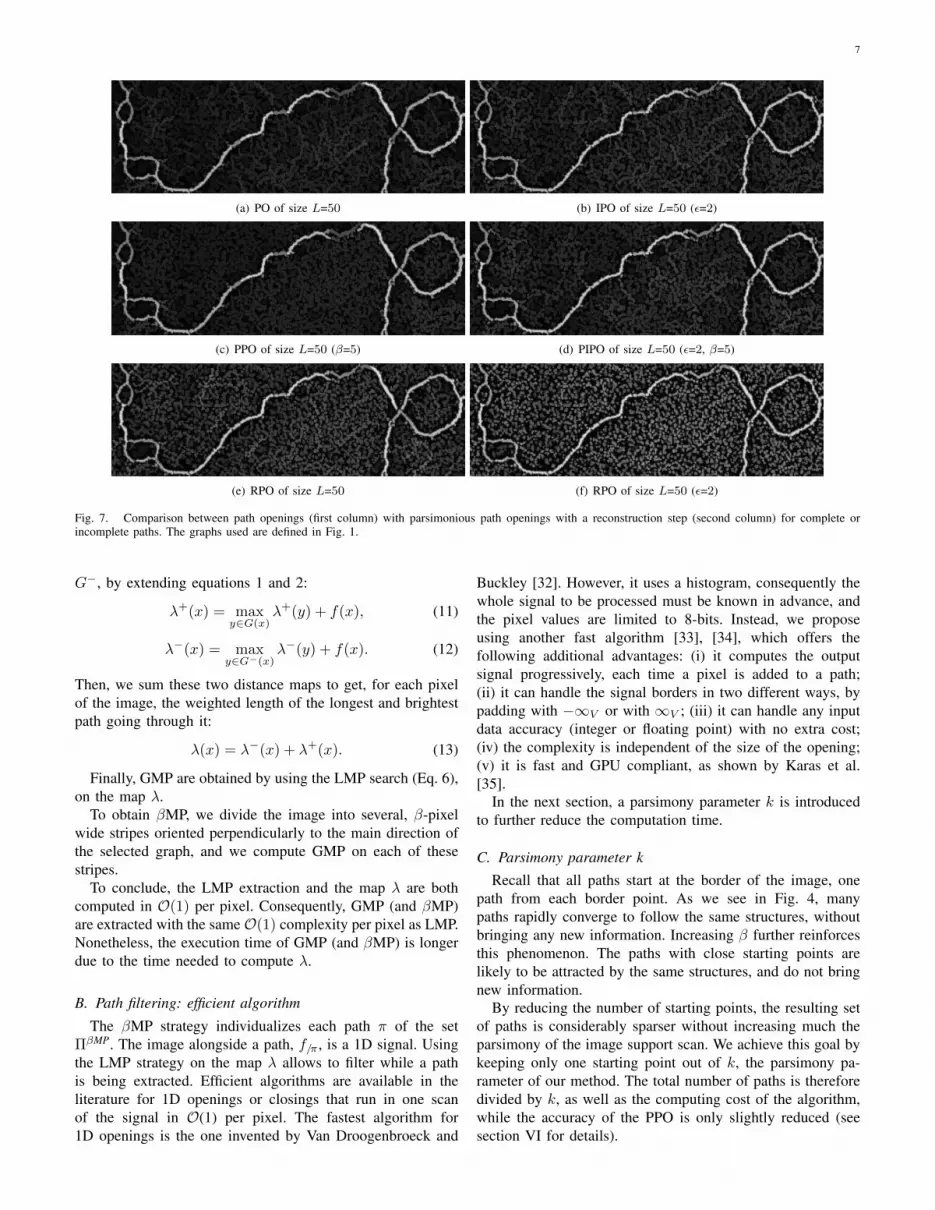
Fig. 7. Comparison between path openings (first column) with parsimonious path openings with a reconstruction step (second column) for complete orincomplete paths. The graphs used are defined in Fig. 1.

G−, by extending equations 1 and 2:

λ+(x) = maxy∈G(x)

λ+(y) + f(x), (11)

λ−(x) = maxy∈G−(x)

λ−(y) + f(x). (12)

Then, we sum these two distance maps to get, for each pixelof the image, the weighted length of the longest and brightestpath going through it:

λ(x) = λ−(x) + λ+(x). (13)

Finally, GMP are obtained by using the LMP search (Eq. 6),on the map λ.

To obtain βMP, we divide the image into several, β-pixelwide stripes oriented perpendicularly to the main direction ofthe selected graph, and we compute GMP on each of thesestripes.

To conclude, the LMP extraction and the map λ are bothcomputed in O(1) per pixel. Consequently, GMP (and βMP)are extracted with the same O(1) complexity per pixel as LMP.Nonetheless, the execution time of GMP (and βMP) is longerdue to the time needed to compute λ.

B. Path filtering: efficient algorithm

The βMP strategy individualizes each path π of the setΠβMP. The image alongside a path, f/π , is a 1D signal. Usingthe LMP strategy on the map λ allows to filter while a pathis being extracted. Efficient algorithms are available in theliterature for 1D openings or closings that run in one scanof the signal in O(1) per pixel. The fastest algorithm for1D openings is the one invented by Van Droogenbroeck and

Buckley [32]. However, it uses a histogram, consequently thewhole signal to be processed must be known in advance, andthe pixel values are limited to 8-bits. Instead, we proposeusing another fast algorithm [33], [34], which offers thefollowing additional advantages: (i) it computes the outputsignal progressively, each time a pixel is added to a path;(ii) it can handle the signal borders in two different ways, bypadding with −∞V or with ∞V ; (iii) it can handle any inputdata accuracy (integer or floating point) with no extra cost;(iv) the complexity is independent of the size of the opening;(v) it is fast and GPU compliant, as shown by Karas et al.[35].

In the next section, a parsimony parameter k is introducedto further reduce the computation time.

C. Parsimony parameter k

Recall that all paths start at the border of the image, onepath from each border point. As we see in Fig. 4, manypaths rapidly converge to follow the same structures, withoutbringing any new information. Increasing β further reinforcesthis phenomenon. The paths with close starting points arelikely to be attracted by the same structures, and do not bringnew information.

By reducing the number of starting points, the resulting setof paths is considerably sparser without increasing much theparsimony of the image support scan. We achieve this goal bykeeping only one starting point out of k, the parsimony pa-rameter of our method. The total number of paths is thereforedivided by k, as well as the computing cost of the algorithm,while the accuracy of the PPO is only slightly reduced (seesection VI for details).

8

D. Morphological reconstruction

PPO is a sparse operator and yields a thin representation ofobjects. Should one need a thick detection, PPO results can bereconstructed under the original image. Efficient implementa-tions of the morphological reconstruction are available in theliterature [36], [37]. Their complexity is linear with respect tothe image size.

Fig. 7 illustrates the DNA molecule extraction from thenoisy background using parsimonious path openings followedby a reconstruction to ease the comparison with classical pathopenings and with robust path openings. Figs. 7(a), 7(c) and7(e) compare PO, PPO and RPO with complete paths whereasFigs. 7(b), 7(d) and 7(f) illustrate the results for incompletepaths with a tolerance ε of 2 pixels. Very similar results areobtained using PPO with a significant reduction of the timings(see Sec. VII-B).

Using incomplete paths improves the detection since thinstructures are reconnected. However, it also reconnects noisypixels, preserving some structures in the image background.Thus, tuning the parameter ε is a trade-off between the sizeof the gaps to fill and the level of noise.

In the following section, the accuracy of PPO with respectto length measurements is studied.

VI. ACCURACY OF PPO

In order to evaluate the accuracy of PPO, we will applythem to binary images containing segments of known length,and compare the measured length distribution using PPO withthe theoretical one.

Size distributions are usually computed by a residual ap-proach with a collection of increasing-size filters commonlyknown as granulometry, introduced by Matheron [29], [38].Let us us consider a binary image f , and a set of paths Πf

computed on f . The family of PPO {γΠL}L≥1 is a granulom-

etry. Note that we have dropped the f index on Π, as the setof paths is computed once and for all, and then kept constant,for reasons explained in section IV-C. The corresponding sizedistribution is, for non-negative integers L:

SDL = Meas(γΠL − γΠ

L−1). (14)

In the present case, the measure Meas is the number ofconnected components of the binary image. Eq. (14) measuresthe length distribution.

PPO suffer from two types of error. The first one is theanisotropy of the length measurement, also present in theoriginal PO. It comes from the discretization of the path onthe Z2 grid. The second error is due to the parsimonious scanof the support. The following text analyzes the phenomena atthe origin of these errors and their impact on the accuracy.

Let x be a measurement, and m the correct value. Therelative measure error is:

err =x−mm

. (15)

A positive err means overestimation, whereas a negative errmeans underestimation.

(a) thick line segment

(b) thin line segment

Fig. 8. Relative error of measuring the length of a straight isolated linesegment with respect to its orientation. Segment length L = 80. (a) width2px, (b) thin segment. Note: For thin segments the errors of PO and CPOcoincide.

In our case x and m are distributions (expressed as prob-ability density functions or counts in case of histograms).A number of measures exist to compare probability densityfunctions or histograms (see [39] for a review of most commondistances or divergences). However, none of these suits ourcase for the following reasons: i) The metric behind themajority of the distances considers the probability densityfunction as a vector in an orthogonal space. Nonetheless, thehistogram bins in our case are not orthogonal. ii) A distance isalways positive, which does not reflect the difference betweenunder- and over-estimation of a measure. iii) No distanceor metric is correlated to the usually used relative measureerror as in eq. 15. This means that for singleton distributions(containing only one point) we would not obtain the samevalue as with eq. 15.

Consequently, we define an equivalent of Eq. 15 for twohistograms X and M , with respective mean values equalto X and M . We define the relative error of the measureddistribution X to the ground truth distribution M as:

err =X −MM

. (16)

This error evaluation has the following properties: Thedifference X −M is insensitive to the standard deviation ofeither distribution, that can be evaluated separately. It does notrequire the histograms to be normalized nor aligned. X andM can have different count sum and either X and M or bothcan be scalars. If both are scalars then eq. 16 is equivalent toeq. 15.

The first experiment evaluates the isotropy, see Fig. 8. Itreports the relative error of measuring the length of an isolated,straight segment w.r.t. its orientation. It compares PPO to pathopenings (PO) by Talbot and Appleton [20] and constrainedpath openings (CPO) by Hendriks [24]. The segment is 80

9

(a) orientation: 45◦

(b) orientation: 55◦

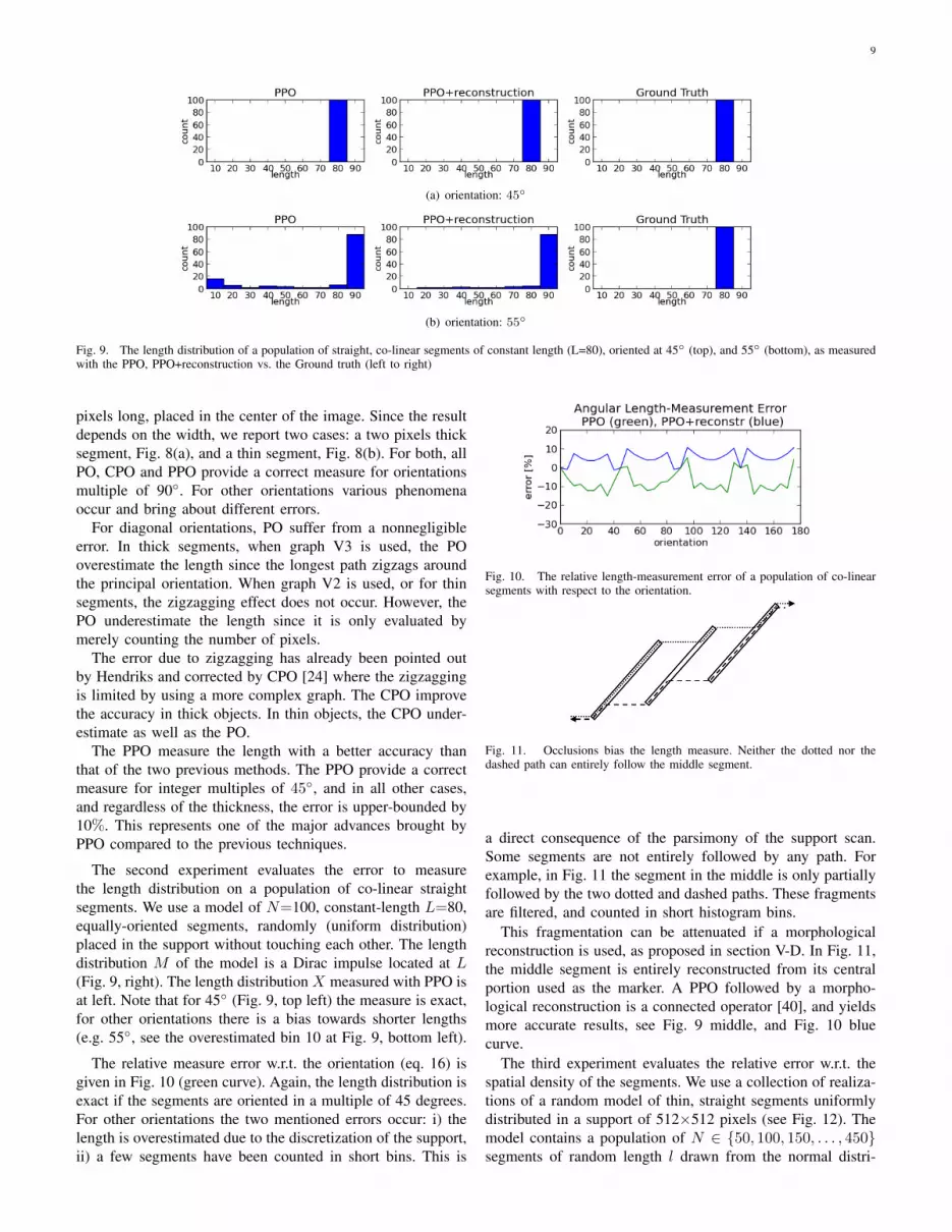
Fig. 9. The length distribution of a population of straight, co-linear segments of constant length (L=80), oriented at 45◦ (top), and 55◦ (bottom), as measuredwith the PPO, PPO+reconstruction vs. the Ground truth (left to right)

pixels long, placed in the center of the image. Since the resultdepends on the width, we report two cases: a two pixels thicksegment, Fig. 8(a), and a thin segment, Fig. 8(b). For both, allPO, CPO and PPO provide a correct measure for orientationsmultiple of 90◦. For other orientations various phenomenaoccur and bring about different errors.

For diagonal orientations, PO suffer from a nonnegligibleerror. In thick segments, when graph V3 is used, the POoverestimate the length since the longest path zigzags aroundthe principal orientation. When graph V2 is used, or for thinsegments, the zigzagging effect does not occur. However, thePO underestimate the length since it is only evaluated bymerely counting the number of pixels.

The error due to zigzagging has already been pointed outby Hendriks and corrected by CPO [24] where the zigzaggingis limited by using a more complex graph. The CPO improvethe accuracy in thick objects. In thin objects, the CPO under-estimate as well as the PO.

The PPO measure the length with a better accuracy thanthat of the two previous methods. The PPO provide a correctmeasure for integer multiples of 45◦, and in all other cases,and regardless of the thickness, the error is upper-bounded by10%. This represents one of the major advances brought byPPO compared to the previous techniques.

The second experiment evaluates the error to measurethe length distribution on a population of co-linear straightsegments. We use a model of N=100, constant-length L=80,equally-oriented segments, randomly (uniform distribution)placed in the support without touching each other. The lengthdistribution M of the model is a Dirac impulse located at L(Fig. 9, right). The length distribution X measured with PPO isat left. Note that for 45◦ (Fig. 9, top left) the measure is exact,for other orientations there is a bias towards shorter lengths(e.g. 55◦, see the overestimated bin 10 at Fig. 9, bottom left).

The relative measure error w.r.t. the orientation (eq. 16) isgiven in Fig. 10 (green curve). Again, the length distribution isexact if the segments are oriented in a multiple of 45 degrees.For other orientations the two mentioned errors occur: i) thelength is overestimated due to the discretization of the support,ii) a few segments have been counted in short bins. This is

Fig. 10. The relative length-measurement error of a population of co-linearsegments with respect to the orientation.

Fig. 11. Occlusions bias the length measure. Neither the dotted nor thedashed path can entirely follow the middle segment.

a direct consequence of the parsimony of the support scan.Some segments are not entirely followed by any path. Forexample, in Fig. 11 the segment in the middle is only partiallyfollowed by the two dotted and dashed paths. These fragmentsare filtered, and counted in short histogram bins.

This fragmentation can be attenuated if a morphologicalreconstruction is used, as proposed in section V-D. In Fig. 11,the middle segment is entirely reconstructed from its centralportion used as the marker. A PPO followed by a morpho-logical reconstruction is a connected operator [40], and yieldsmore accurate results, see Fig. 9 middle, and Fig. 10 bluecurve.

The third experiment evaluates the relative error w.r.t. thespatial density of the segments. We use a collection of realiza-tions of a random model of thin, straight segments uniformlydistributed in a support of 512×512 pixels (see Fig. 12). Themodel contains a population of N ∈ {50, 100, 150, . . . , 450}segments of random length l drawn from the normal distri-

10

bution N (µ, σ) with L = N (40, 20), bounded in the (5, 90)interval. The segments have a random (uniformly distributed)orientation and are placed in the support without touching eachother.

We observe that the fragmentation in sparsely populatedmedia (N=50) does not occur, as illustrated in Fig. 13,top, and increases with the density of the population (seethe overestimated bin 10 in Fig. 13, bottom). Indeed, thefragmentation cannot be completely avoided even by using thereconstruction since it may happen that no marker remains toreconstruct the segment.

To complete the error evaluation w.r.t. the density of themedia see the two following Figs. 14 and 15 that confirm thatwith increasing number of segments N the error increasestowards stronger underestimation. Both figures are providedfor various values of the parameters k and β. One canobserve that the error also increases with increasing parsimony(increasing k) and decreasing locality (increasing β).

Note that the two length measurement errors, i.e. theoverestimation and the one due to occlusions (as in Figs. 10and 11) are additive. Hence, there are situations where theycompensate as e.g. Fig. 14, 50 segments, k=10. However,this compensation is illusory since both errors still occur, andtheir compensation depends of hazardous, random geometricalconfigurations in the measured structures.

It is interesting to observe however that even for densepopulations, as shown in Fig. 12 (right), i.e. a situation deemedunfavorable to a parsimonious approach, PPO parameters canbe chosen in such a way that the absolute error is smallerthan 10%. The choice of these parameters remains howeveran open, application dependant, question. For example, thechoice of ε is directly linked to the noise level of the image;the higher the noise, the higher ε should be, at the expense ofpotential unwanted connections between structures that wouldhave been otherwise erased. As it will be seen in the followingsection, it should be noted that the user has in practice largefreedom in the choice of his parameters, as the running timeof PPO and PIPO is not impaired by large parameter values.

VII. COMPLEXITY AND TIMINGS

A. ComplexityIn the original version of PO, the number of paths passing

through one pixel is exponential w.r.t. the length L. Conse-quently, if implemented in a naive way, PO have exponentialcomplexity. An implementation with logarithmic complexityw.r.t. L has been proposed in [23]. More recently, the com-plexity of incomplete paths has been decreased to logarithmicw.r.t. L and linear w.r.t. the tolerance ε [20].

Here we analyze the complexity of PPO, split into two parts:path extraction and path filtering.

We have shown above that the collection of paths βMP canbe extracted in O(1) per pixel (Sec. V-A), and that an imagef can be filtered alongside a path π also in O(1) per sample(Sec. V-B). To complete the analysis of complexity we needto count the number of paths, and evaluate their length.

For a given image f , with D=spt(f) a W×H rectangle(width×height), we have 2W vertical and 2H horizontal paths.

Fig. 14. Relative error w.r.t. to the number of segments and the parsimonyparameter: k=1, 5, 10 (blue, green, red).

Fig. 15. Relative error w.r.t. the number of segments and the parameter β=1, 20, 50 (blue, green, red).

Vertical paths are H pixels long, and horizontal paths areW pixels long. After dropping multiplicative constants, thisyields a linear complexity of O(HW ) when only horizontaland vertical paths are used.

When diagonal paths are used, the complexity slightlyincreases. We count a total of 4(H + W ) diagonal paths(for four principal diagonal orientations). The diagonal pathshave unequal length, bounded though by H+W . This yields aslightly higher complexity of O((H +W )2), yet still a linearfactor of the support size card(D)=HW .

Therefore, the complexity of PPO and PIPO is proportionalto the number of pixels in the images, and independent of thelength L and the tolerance ε of incomplete paths, which is animprovement with respect to the state of the art.

B. Timings

PPO have a low complexity and have been designed toaddress the timing issues of classical path operators. Wecompare here the timings of PO, RPO and CPO with theapproach used in this paper (PPO). Fig. 16 shows a benchmarkfor complete and incomplete paths. The gain is huge and weverify that PPO run in constant time with respect to L. Forcomplete paths, the computation time is reduced by a factor 75between PO and PPO, with k=1. The gap between incompletepath openings and parsimonious incomplete path openings iseven larger. We reduce average time by a factor 3100 withk=10.

In another experiment, we benchmark PPO against param-eters β, ε and k, with the same image of size 768×576. Wecheck in Fig. 17 that the timings are independent of β (exceptfor β=1, which does not use the weighted distance map λ).Regarding the gap tolerance ε, an overhead is introduced forε > 1 by the closing step. With the parsimony parameter

11

(a) N = 50 (b) N = 450

Fig. 12. Two realizations of the random gaussian length distribution model with N segments.

(a) N = 50 segments

(b) N = 450 segments

Fig. 13. Length distributions measured with PPO+reconstruction vs. PO by Talbot and Appleton [20] vs. ground-truth for N segments.

k, timings decrease with 1k as expected from the theoretical

complexity.The last benchmark, Fig. 18, exhibits the execution time

against the image size. The timings confirm the linear com-plexity of the algorithm.

VIII. CONCLUSIONS

This paper presents a new family of parsimonious operatorsfor image processing, based on paths. In comparison withclassical path openings, only a relevant subset of paths is usedto retrieve similar information.

The extraction of paths is decoupled from the path filtering,which brings two major advantages: i) a new, general scanstrategy allows tuning the search continuously from local toglobal, which gives the possibility to find a trade-off betweenaccuracy and robustness to noise; ii) it allows defining differentoperators alongside the same collection of paths, to operateon the same objects. For instance, the combination of a pathopening with a closing allows reconnecting discontinued brightstructures, thus achieving results similar to those obtained withincomplete path openings, tolerant to missing pixels in paths.

An efficient filtering algorithm [33] is used to computeopenings or closings alongside a path. It runs in O(1) perpixel regardless the size. It decreases the complexity of bothpath opening and incomplete path opening to a constant.

Consequently, the timings are several orders of magnitudelower in comparison with classical (incomplete) path openings,with comparable results. Hence, PPO are usable in high-throughput, industrial applications. Additionally, this filteringalgorithm allows : i) using arbitrary data accuracy (integeror floating point), and ii) handling the border effect in twodifferent ways (extending the support with −∞V or with∞V ).

We provide a thorough study of the accuracy to showthat processing a conveniently chosen subset of paths canprovide a result sufficient for certain applications. Such aparsimonious approach has allowed us to bridge the gapbetween an interesting methodological tool (path openings)and a practical, computation intensive, real-world application.

This work opens different research perspectives.Parsimonious path operators can be extended to 3D images.

In fact, a first series of tests shows that starting from the 3Dimage borders, and using a 3D graph, gives interesting results.However, parameter β has to be chosen with care, since thesize of blind regions tends to be larger on 3D images. On theother hand, the fragmentation due to occlusions (cf. Fig. 11)is smaller in 3D.

The proposed strategy only uses paths seeded at the imageborder. Other starting points could be considered, for examplewith a random placement, as in the geodesic voting approach[3]. This could help alleviate the blind region problem that mayoccur sometimes in images with a lot of branching features.

12

10

100

1000

10000

100000

1 10 100

Co

mp

uta

tio

n t

ime

(m

s)

IPO ε = 6

IPO ε = 4

IPO ε =2

RPO ε = 5

CPO

PO

RPO

PPO k = 1, ε = 6

PPO k = 1

PPO k = 5, ε = 6

PPO k = 5

PPO k = 10, ε = 6

PPO k = 10

1 10 100Size of the opening L (in pixel)

Fig. 16. Benchmark between path openings and parsimonious path openings(β=1) for complete and incomplete paths. The timings are plotted in ms w. r.t. L (log-log scale). The input image size is 768×576 pixels. The benchmarkswere made with one thread of a laptop computer (Intel Core i7-2860QM CPU@ 2.50GHz) by taking the average value from 100 realizations.

0

50

100

150

200

250

300

350

1 11 21 31 41

Co

mp

uta

tio

n t

ime

(in

ms)

Parameter ε

Parameter β

Parameter k

1 11 21 31 41

Size of the parameters

Fig. 17. Influence of the parameters (ε, β and k) on the computation timeof parsimonious path openings (Intel Core i7-2860QM CPU @ 2.50GHz).

Fig. 18. Execution time of parsimonious path openings (β=1, ε=1, k=1) vsimage size.

Other morphological parsimonious image representations canbe also considered, based for example on image extrema, orimage ridges and valleys.

Finally, instead of closing-opening, one can also use therank-max opening to filter the paths in Eq. 10. This will makethe PPO behave more like IPO rather than the RPO.

ACKNOWLEDGMENTS

This work was made possible thanks to the support of the“Pole ASTech” and the “Pole Nucleaire de Bourgogne”, andhas been financed by the French “Departement de Seine etMarne”

The authors are grateful to Hugues Talbot (A2SI ESIEE,IGM) and Francois Cokelaer (IFP) for providing the codes oftheir respective path-based algorithms.

The authors also wish to thank the anonymous reviewersfor their comments.

REFERENCES

[1] C. Sinthanayothin, J. Boyce, H. Cook, and T. Williamson, “Automatedlocalisation of the optic disc, fovea, and retinal blood vessels from digitalcolour fundus images,” British Journal of Ophthalmology, vol. 83, no. 8,pp. 902–910, 1999.

[2] T. Walter and J.-C. Klein, “Segmentation of color fundus images of thehuman retina: Detection of the optic disc and the vascular tree usingmorphological techniques,” in Medical Data Analysis, ser. LectureNotes in Computer Science, J. Crespo, V. Maojo, and F. Martin, Eds.Springer Berlin Heidelberg, 2001, vol. 2199, pp. 282–287. [Online].Available: http://dx.doi.org/10.1007/3-540-45497-7 43

[3] Y. Rouchdy and L. Cohen, “Image segmentation by geodesic voting.application to the extraction of tree structures from confocal microscopeimages,” in Pattern Recognition, 2008. ICPR 2008. 19th InternationalConference on. IEEE, 2008, pp. 1–5.

[4] V. Bismuth, R. Vaillant, H. Talbot, and L. Najman, “Curvilinear structureenhancement with the polygonal path image-application to guide-wiresegmentation in x-ray fluoroscopy,” in Medical Image Computing andComputer-Assisted Intervention–MICCAI 2012. Springer, 2012, pp.9–16.

[5] S. Valero, J. Chanussot, J. Benediktsson, H. Talbot, and B. Waske,“Advanced directional mathematical morphology for the detection of theroad network in very high resolution remote sensing images,” PatternRecognition Letters, vol. 31, no. 10, pp. 1120–1127, 2010.

[6] V. Morard, E. Decenciere, and P. Dokladal, “Geodesic attributes thin-nings and thickenings,” in Mathematical Morphology and Its Appli-cations to Image and Signal Processing, Lecture Notes in ComputerScience, vol. 6671. Springer, 2011, pp. 200–211.

[7] V. Morard, E. Decenciere, and P. Dokladal, “Region growing structuringelements and new operators based on their shape,” in 13th IASTEDInternational Conference on Signal and Image Processing (SIP), Proc.of, vol. 759, 2011, pp. 1–8.

[8] J. D. Kurdy B., “Directional mathematical morphology operations,” inIn 5th European Congress For Stereology, Acta Stereologica, vol. 8/2,1989.

[9] P. Soille and H. Talbot, “Directional morphological filtering,” PatternAnalysis and Machine Intelligence, IEEE Transactions on, vol. 23,no. 11, pp. 1313–1329, 2001.

[10] T. Koller, G. Gerig, G. Szekely, and D. Dettwiler, “Multiscale detectionof curvilinear structures in 2-D and 3-D image data,” in Computer Vision.Proceedings of the Fifth International Conference on. IEEE, 1995, pp.864–869.

[11] O. Tankyevych, H. Talbot, and P. Dokladal, “Curvilinear morpho-hessianfilter,” in 5th IEEE International Symposium on Biomedical Imaging(ISBI), 2008, pp. 1011–1014.

[12] L. Vincent, “Morphological area openings and closings for grey-scaleimages,” in Proceedings of NATO Shape in Picture Workshop. Drieber-gen, The Netherlands, Springer-Verlag, 1994, pp. 197–208.

[13] E. Breen and R. Jones, “Attribute openings, thinnings, and granulome-tries,” Computer Vision and Image Understanding, vol. 64, pp. 377–389,Nov. 1996.

13

[14] M. Wilkinson and M. Westenberg, “Shape preserving filament enhance-ment filtering,” in Medical Image Computing and Computer-AssistedIntervention–MICCAI 2001, vol. 2208, 2001, pp. 770–777.

[15] E. Urbach and M. Wilkinson, “Shape-only granulometries and grey-scaleshape filters,” in Proc. Int. Symp. Math. Morphology (ISMM), vol. 2002,2002, pp. 305–314.

[16] V. Morard, E. Decenciere, and P. Dokladal, “Efficient geodesic attributethinnings based on the barycentric diameter,” Journal of MathematicalImaging and Vision, vol. 46, no. 1, pp. 128–142, 2013.

[17] M. Buckley and H. Talbot, “Flexible linear openings and closings,”Computational Imaging and Vision, vol. 18, pp. 109–118, 2000.

[18] H. Heijmans, M. Buckley, and H. Talbot, “Path openings and closings,”Probability, Networks and Algorithms, no. E 0403, pp. 1–21, 2004.

[19] ——, “Path openings and closings,” Journal of Mathematical Imagingand Vision, vol. 22, no. 2, pp. 107–119, 2005.

[20] H. Talbot and B. Appleton, “Efficient complete and incomplete pathopenings and closings,” Image and Vision Computing, vol. 25, no. 4,pp. 416–425, 2007.

[21] F. Cokelaer, H. Talbot, and J. Chanussot, “Efficient Robust d-Dimensional Path Operators,” Selected Topics in Signal Processing,IEEE journal of, vol. 6, no. 7, November 2012.

[22] J. Serra, Image analysis and mathematical morphology. AcademicPress, London, 1982, vol. 1.

[23] B. Appleton and H. Talbot, “Efficient path openings and closings,” inMathematical Morphology: 40 Years On, Computational Imaging andVision, vol. 30. Springer Netherlands, 2005, pp. 33–42.

[24] C. Luengo Hendriks, “Constrained and dimensionality-independent pathopenings,” Image Processing, IEEE Transactions on, vol. 19, no. 6, pp.1587–1595, 2010.

[25] R. Bellman, “Dynamic programming,” Science, vol. 153, no. 3731, pp.34–37, 1966.

[26] G. Gallo and S. Pallottino, “Shortest path algorithms,” Annals ofOperations Research, vol. 13, no. 1, pp. 1–79, 1988.

[27] M. Buckley and J. Yang, “Regularised shortest-path extraction,” PatternRecognition Letters, vol. 18, no. 7, pp. 621–629, 1997.

[28] L. Vincent, “Minimal path algorithms for the robust detection of linearfeatures in gray images,” Computational Imaging and Vision, vol. 12,pp. 331–338, 1998.

[29] G. Matheron, Random sets and integral geometry. New York: Wiley,1974.

[30] M. Schmitt, “Des algorithmes morphologiques a l’intelligence artifi-cielle,” Ph.D. dissertation, Ecole Nationale Superieure des Mines deParis, 1989.

[31] L. Vincent and D. Jeulin, “Minimal paths and crack propagation simu-lations,” Acta Stereologica, vol. 8, no. 2, pp. 487–494, 1989.

[32] M. Van Droogenbroeck and M. Buckley, “Morphological erosions andopenings: fast algorithms based on anchors,” Journal of MathematicalImaging and Vision, vol. 22, no. 2, pp. 121–142, 2005.

[33] V. Morard, P. Dokladal, and E. Decenciere, “Linear openings in arbitraryorientation in O(1) per pixel,” in Acoustics, Speech and Signal Process-ing, IEEE International Conference on. IEEE, 2011, pp. 1457–1460.

[34] V. Morard, P. Dokladal, and E. Decenciere, “One-dimensional openings,granulometries and component trees in O(1) per pixel,” Selected Topicsin Signal Processing, IEEE journal of, pp. 1–10, 2011.

[35] P. Karas, V. Morard, J. Bartovsky, T. Grandpierre, E. Dokladalova,P. Matula, and P. Dokladal, “GPU Implementation of Linear Morpho-logical Openings with Arbitrary Angle,” Journal of Real-Time ImageProcessing, pp. 1–15, 2012, DOI : 10.1007/s11554-012-0248-7.

[36] L. Vincent, “Morphological grayscale reconstruction in image analysis:Applications and efficient algorithms,” Image Processing, IEEE Trans-actions on, vol. 2, no. 2, pp. 176–201, 1993.

[37] K. Robinson and P. Whelan, “Efficient morphological reconstruction: adownhill filter,” Pattern Recognition Letters, vol. 25, no. 15, pp. 1759–1767, 2004.

[38] G. Matheron, Elements pour une Theorie des Milieux Poreux. Masson,1967.

[39] S.-H. Cha, “Comprehensive Survey on Distance/Similarity Measuresbetween Probability Density Functions,” Mathematical Models andMethods in Applied Sciences, Intl. journal of, vol. 1, no. 4, pp. 300–307,2007.

[40] P. Salembier and J. Serra, “Flat zones filtering, connected operatorsand filters by reconstruction,” IEEE Transactions on Image Processing,vol. 3, no. 8, pp. 1153–1160, 1995.

Vincent Morard Vincent Morard has graduatedfrom the French engineering school CPE Lyonin 2009 and received his PhD in 2012 fromMINES ParisTech at the Center for MathematicalMorphology. Since October 2012, he works forSAFRAN (French multinational aircraft&rocket en-gine, aerospace component and security company)as a research engineer specialized in non-destructivetesting using 3D image processing. His researchinterests include mathematical morphology, patternrecognition, non-destructive testing and statistical

learning.

Petr Dokladal Petr Dokladal is a senior researcherwith the Centre for Mathematical Morphology, ajoint research centre of Armines and MINES Paris-Tech, Paris, France. He graduated from the Tech-nical University in Brno, Czech Republic, in 1994,as a telecommunication engineer and received hisPh.D. degree in 2000 from the University of Marnela Vallee, France, in general computer sciences,specialized in image processing. His received hishabilitation from the Paris Est University in 2013.His research interests include image segmentation,

pattern recognition and non-destructive testing.

Etienne Decenciere Etienne Decenciere receivedthe engineering degree in 1994, the Ph.D. degreein mathematical morphology in 1997, both fromMINES ParisTech, and the Habilitation in 2008 fromthe Jean Monnet University. He holds a researchfellow position at the Centre for Mathematical Mor-phology of MINES ParisTech. His main researchinterests are in mathematical morphology, imagesegmentation, non-destructive testing, and biomed-ical applications.