parallel memetic algorithms for independent job scheduling in computational grids
TRANSCRIPT

Carlos Cotta and Jano van Hemert (Eds.)
Recent Advances in Evolutionary Computation for Combinatorial Optimization

Studies in Computational Intelligence,Volume 153
Editor-in-ChiefProf. Janusz KacprzykSystems Research InstitutePolish Academy of Sciencesul. Newelska 601-447 WarsawPolandE-mail: [email protected]
Further volumes of this series can be found on our homepage:springer.com
Vol. 131. Roger Lee and Haeng-Kon Kim (Eds.)Computer and Information Science, 2008ISBN 978-3-540-79186-7
Vol. 132. Danil Prokhorov (Ed.)Computational Intelligence in Automotive Applications, 2008ISBN 978-3-540-79256-7
Vol. 133. Manuel Grana and Richard J. Duro (Eds.)Computational Intelligence for Remote Sensing, 2008ISBN 978-3-540-79352-6
Vol. 134. Ngoc Thanh Nguyen and Radoslaw Katarzyniak (Eds.)New Challenges in Applied Intelligence Technologies, 2008ISBN 978-3-540-79354-0
Vol. 135. Hsinchun Chen and Christopher C.Yang (Eds.)Intelligence and Security Informatics, 2008ISBN 978-3-540-69207-2
Vol. 136. Carlos Cotta, Marc Sevauxand Kenneth Sorensen (Eds.)Adaptive and Multilevel Metaheuristics, 2008ISBN 978-3-540-79437-0
Vol. 137. Lakhmi C. Jain, Mika Sato-Ilic, Maria Virvou,George A. Tsihrintzis,Valentina Emilia Balasand Canicious Abeynayake (Eds.)Computational Intelligence Paradigms, 2008ISBN 978-3-540-79473-8
Vol. 138. Bruno Apolloni,Witold Pedrycz, Simone Bassisand Dario MalchiodiThe Puzzle of Granular Computing, 2008ISBN 978-3-540-79863-7
Vol. 139. Jan DrugowitschDesign and Analysis of Learning Classifier Systems, 2008ISBN 978-3-540-79865-1
Vol. 140. Nadia Magnenat-Thalmann, Lakhmi C. Jainand N. Ichalkaranje (Eds.)New Advances in Virtual Humans, 2008ISBN 978-3-540-79867-5
Vol. 141. Christa Sommerer, Lakhmi C. Jainand Laurent Mignonneau (Eds.)The Art and Science of Interface and Interaction Design (Vol. 1),2008ISBN 978-3-540-79869-9
Vol. 142. George A. Tsihrintzis, Maria Virvou, Robert J. Howlettand Lakhmi C. Jain (Eds.)New Directions in Intelligent Interactive Multimedia,2008ISBN 978-3-540-68126-7
Vol. 143. Uday K. Chakraborty (Ed.)Advances in Differential Evolution, 2008ISBN 978-3-540-68827-3
Vol. 144.Andreas Fink and Franz Rothlauf (Eds.)Advances in Computational Intelligence in Transport, Logistics,and Supply Chain Management, 2008ISBN 978-3-540-69024-5
Vol. 145. Mikhail Ju. Moshkov, Marcin Piliszczukand Beata ZieloskoPartial Covers, Reducts and Decision Rules in Rough Sets, 2008ISBN 978-3-540-69027-6
Vol. 146. Fatos Xhafa and Ajith Abraham (Eds.)Metaheuristics for Scheduling in Distributed ComputingEnvironments, 2008ISBN 978-3-540-69260-7
Vol. 147. Oliver KramerSelf-Adaptive Heuristics for Evolutionary Computation, 2008ISBN 978-3-540-69280-5
Vol. 148. Philipp LimbourgDependability Modelling under Uncertainty, 2008ISBN 978-3-540-69286-7
Vol. 149. Roger Lee (Ed.)Software Engineering, Artificial Intelligence, Networking andParallel/Distributed Computing, 2008ISBN 978-3-540-70559-8
Vol. 150. Roger Lee (Ed.)Software Engineering Research, Management andApplications, 2008ISBN 978-3-540-70774-5
Vol. 151. Tomasz G. Smolinski, Mariofanna G. Milanovaand Aboul-Ella Hassanien (Eds.)Computational Intelligence in Biomedicine and Bioinformatics,2008ISBN 978-3-540-70776-9
Vol. 152. Jaroslaw StepaniukRough – Granular Computing in Knowledge Discovery and DataMining, 2008ISBN 978-3-540-70800-1
Vol. 153. Carlos Cotta and Jano van Hemert (Eds.)Recent Advances in Evolutionary Computation forCombinatorial Optimization, 2008ISBN 978-3-540-70806-3

Carlos CottaJano van Hemert(Eds.)
Recent Advances in EvolutionaryComputation for CombinatorialOptimization
123

Carlos CottaETSI Informatica (3.2.49)Campus de TeatinosUniversidad de Malaga29071, MalagaSpainEmail: [email protected]
Jano van HemertNational e-Science CentreUniversity of Edinburgh15 South College StreetEdinburgh EH8 9AAUnited KingdomEmail: [email protected]
ISBN 978-3-540-70806-3 e-ISBN 978-3-540-70807-0
DOI 10.1007/978-3-540-70807-0
Studies in Computational Intelligence ISSN 1860949X
Library of Congress Control Number: 2008931010
c© 2008 Springer-Verlag Berlin Heidelberg
This work is subject to copyright. All rights are reserved, whether the whole or part of thematerial is concerned, specifically the rights of translation, reprinting, reuse of illustrations,recitation, broadcasting, reproduction on microfilm or in any other way, and storage in databanks.Duplication of this publication or parts thereof is permitted only under the provisions ofthe German Copyright Law of September 9, 1965, in its current version, and permission for usemust always be obtained from Springer.Violations are liable to prosecution under the GermanCopyright Law.
The use of general descriptive names, registered names, trademarks, etc. in this publicationdoes not imply, even in the absence of a specific statement, that such names are exempt fromthe relevant protective laws and regulations and therefore free for general use.
Typeset & Cover Design: Scientific Publishing Services Pvt. Ltd., Chennai, India.
Printed in acid-free paper
9 8 7 6 5 4 3 2 1springer.com

“Invention consists in avoiding the constructing of uselesscontraptions and in constructing the useful combinations which are
in infinite minority.”
Henri Poincare (1854–1912)

Preface
Combinatorial optimisation is a ubiquitous discipline. Its applications range fromtelecommunications to logistics, from manufacturing to personnel scheduling,from bioinformatics to management, and a long et cetera. Combinatorial opti-misation problems (COPs) are characterised by the need of finding an optimalor quasi-optimal assignment of values to a number of discrete variables, withrespect to a certain objective function or to a collection of objective functions.The economical, technological and societal impact of this class of problems is outof question, and has driven the on-going quest for effective solving strategies.
Initial approaches for tackling COPs were based on exact methods, but theintrinsic complexity of most problems in the area make such methods unafford-able for realistic problem instances. Approximate methods have been definedas well as, but in general these are far from practical too, and do not providea systematic line of attack to deal with COPs. Parameterised complexity algo-rithms allow efficiently solving certain COPs for which the intrinsic hardness isisolated within an internal structural parameter, whose value can be kept small.For the remaining problems (most COPs actually), practical solving requiresthe use of metaheuristic approaches such as, evolutionary algorithms, swarmintelligence and local search techniques. Dating back to the last decades of thetwentieth century, these methods trade completeness for pragmatic effectiveness,thereby providing probably optimal or quasi-optimal solutions to a plethora ofhard COPs.
The application of metaheuristics to COPs is an active field in which new the-oretical developments, new algorithmic models, and new application areas arecontinuously emerging. In this sense, this volume presents recent advances in thearea of metaheuristic combinatorial optimisation. The most popular metaheuris-tic family is evolutionary computation (EC), and as such an important part ofthe volume deals with EC approaches. However, contributions in this volume arenot restricted to EC, and comprise metaheuristics as a whole. Indeed, amongthe essential lessons learned in the last years, the removal of dogmatic artificialbarriers between metaheuristic families has been a key factor for the success ofthese techniques, and this is also reflected in this book. Most articles in this

VIII Preface
collection are extended versions of selected papers from the 7th Conference onEvolutionary Computation and Metaheuristics in Combinatorial Optimization(EvoCOP’2007 – Valencia, Spain). First organised in 2001 and held annuallysince then, EvoCOP has grown to be a reference event in metaheuristic com-binatorial optimisation, with a very strong selection process and high qualitycontributions each year. This quality is reflected in all contributions comprisedhere.
The volume is organised in five blocks. The first one is devoted to theoreticaldevelopments and methodological issues. In the first paper, Craven addresses aproblem in the area of combinatorial group theory, and analyzes the behaviorof evolutionary algorithms on it. Ridge and Kudenko deal with an importantissue in metaheuristic combinatorial optimization, namely determining whethera problem characteristic affects heuristic performance. They use a design-of-experiments approach for this purpose. Aguirre and Tanaka analyze the behaviorof evolutionary algorithms within the well-known framework of NK-landscapes,paying special attention to scalability. Finally, Balaprakash, Birattari and Stuztlepropose a principled approach to the design of stochastic local search algorithm,based on a structured engineering-like methodology.
The second block is centered on hybrid metaheuristics. Pirkwieser, Raidl andPuchinger propose a combination of evolutionary algorithms and Lagrangean de-composition, and show its effectiveness on a constrained variant of the spanningtree problem. Nepomuceno, Pinheiro, and Coelho tackle a constrained cuttingproblem using a master-slave combination of metaheuristics and exact methodsbased on mathematical programming. Alba and Luque address a problem fromsequence analysis using a genetic algorithm that incorporates a specific localsearch method as evolutionary operator. Finally, Neri, Kotilainen and Vapa usememetic algorithms to train neural networks that are used in turn to locateresources in P2P networks.
The third block focuses specifically on constrained problems. Musliu presentsan iterated local search algorithm for finding small-width tree decompositionsof constraint graphs. This algorithm is successfully tested on vertex coloringinstances. Luna, Alba, Nebro and Pedraza consider a frequency assignment prob-lem in GSM networks. They approach this problem via mutation-based evo-lutionary algorithms and simulated annealing. Finally, Juhos and van Hemertpresent some reduction heuristics for the graph coloring problem, and show thatthese can be used to improve the performance of other solvers for this problem.
The fourth block comprises contributions on the travelling salesman prob-lem (TSP) and routing problems. Firstly, Fischer and Merz describe a strategyfor simplifying TSP instances based on fixing some edges, and show that sub-stantial time gains are possible with little or none performance degradation.Subsequently, Manniezzo and Roffilli address a routing problem in the area ofwaste collection, and compare different metaheuristics on large-scale real-worldinstances. Labadi, Prins and Reghioui consider a related routing problem too,and propose a memetic algorithm with population management that is shownto be very competitive. Finally, Julstrom consider a facility location problem,

Preface IX
and use an evolutionary algorithm with a permutational decoder for its resolu-tion. The algorithm features different heuristics for reordering elements in thesolutions.
Lastly, the fifth block is devoted to scheduling problems. Firstly, Ballestınconsider a resource reting problem with time lags, and compare the performanceof several metaheuristics. It is shown that some evolutionary metaheuristicscan outperform truncated branch-and-bound of this problem. Fernandes andLourenco tackle job-shop scheduling problems using an algorithm that com-bines GRASP and branch and bound. The hybrid algorithm compares favorablywith other heuristics for this problem. Finally, Xhafa and Duran consider ajob scheduling problem in computational grids, and propose the use of parallelmemetic algorithms. The results indicate the usefulness of this approach.
We would like to thank all the people who made this volume possible, startingby the authors who contributed the technical content of the book. We also thankProf. Janusz Kacprzyk for his support to the development of this project. Last,but not least, we thank Dr. Thomas Ditzinger and the editorial staff of Springerfor their kind attention and help.
Malaga (Spain), Edinburgh (Scotland, UK) Carlos CottaMarch 2008 Jano van Hemert

Contents
Part I: Theory and Methodology
1 An Evolutionary Algorithm for the Solution ofTwo-Variable Word Equations in Partially CommutativeGroupsMatthew J. Craven . . . . . . . . . . . . . . . . . . . . . . . . . . . . . . . . . . . . . . . . . . . . . . . . 3
2 Determining Whether a Problem Characteristic AffectsHeuristic PerformanceEnda Ridge, Daniel Kudenko . . . . . . . . . . . . . . . . . . . . . . . . . . . . . . . . . . . . . . . 21
3 Performance and Scalability of Genetic Algorithms onNK-LandscapesHernan Aguirre, Kiyoshi Tanaka . . . . . . . . . . . . . . . . . . . . . . . . . . . . . . . . . . . . 37
4 Engineering Stochastic Local Search Algorithms: A CaseStudy in Estimation-Based Local Search for the ProbabilisticTravelling Salesman ProblemPrasanna Balaprakash, Mauro Birattari, Thomas Stutzle . . . . . . . . . . . . . . . 53
Part II: Hybrid Approaches
5 A Lagrangian Decomposition/Evolutionary AlgorithmHybrid for the Knapsack Constrained Maximum SpanningTree ProblemSandro Pirkwieser, Gunther R. Raidl, Jakob Puchinger . . . . . . . . . . . . . . . . 69
6 A Hybrid Optimization Framework for Cutting andPacking ProblemsNapoleao Nepomuceno, Placido Pinheiro, Andre L.V. Coelho . . . . . . . . . . . 87

XII Contents
7 A Hybrid Genetic Algorithm for the DNA FragmentAssembly ProblemEnrique Alba, Gabriel Luque . . . . . . . . . . . . . . . . . . . . . . . . . . . . . . . . . . . . . . . 101
8 A Memetic-Neural Approach to Discover Resources inP2P NetworksFerrante Neri, Niko Kotilainen, Mikko Vapa . . . . . . . . . . . . . . . . . . . . . . . . . . 113
Part III: Constrained Problems
9 An Iterative Heuristic Algorithm for Tree DecompositionNysret Musliu . . . . . . . . . . . . . . . . . . . . . . . . . . . . . . . . . . . . . . . . . . . . . . . . . . . . 133
10 Search Intensification in Metaheuristics for Solving theAutomatic Frequency Problem in GSMFrancisco Luna, Enrique Alba, Antonio J. Nebro, Salvador Pedraza . . . . . . 151
11 Contraction-Based Heuristics to Improve the Efficiencyof Algorithms Solving the Graph Colouring ProblemIstvan Juhos, Jano van Hemert . . . . . . . . . . . . . . . . . . . . . . . . . . . . . . . . . . . . . 167
Part IV: Scheduling
12 Different Codifications and Metaheuristic Algorithms forthe Resource Renting Problem with Minimum and MaximumTime LagsFrancisco Ballestın . . . . . . . . . . . . . . . . . . . . . . . . . . . . . . . . . . . . . . . . . . . . . . . . 187
13 A Simple Optimised Search Heuristic for the Job ShopScheduling ProblemSusana Fernandes, Helena R. Lourenco . . . . . . . . . . . . . . . . . . . . . . . . . . . . . . 203
14 Parallel Memetic Algorithms for Independent JobScheduling in Computational GridsFatos Xhafa, Bernat Duran . . . . . . . . . . . . . . . . . . . . . . . . . . . . . . . . . . . . . . . . 219
Part V: Routing and Travelling Salesman Problems
15 Reducing the Size of Travelling Salesman ProblemInstances by Fixing EdgesThomas Fischer, Peter Merz . . . . . . . . . . . . . . . . . . . . . . . . . . . . . . . . . . . . . . . 243
16 Algorithms for Large Directed Capacitated Arc RoutingProblem InstancesVittorio Maniezzo, Matteo Roffilli . . . . . . . . . . . . . . . . . . . . . . . . . . . . . . . . . . . 259

Contents XIII
17 An Evolutionary Algorithm with Distance Measure forthe Split Delivery Capacitated Arc Routing ProblemNacima Labadi, Christian Prins, Mohamed Reghioui . . . . . . . . . . . . . . . . . . . 275
18 A Permutation Coding with Heuristics for theUncapacitated Facility Location ProblemBryant A. Julstrom . . . . . . . . . . . . . . . . . . . . . . . . . . . . . . . . . . . . . . . . . . . . . . . 295
References . . . . . . . . . . . . . . . . . . . . . . . . . . . . . . . . . . . . . . . . . . . . . . . . . . . . . . 309
Index . . . . . . . . . . . . . . . . . . . . . . . . . . . . . . . . . . . . . . . . . . . . . . . . . . . . . . . . . . . 333
Author Index . . . . . . . . . . . . . . . . . . . . . . . . . . . . . . . . . . . . . . . . . . . . . . . . . . . 337

List of Contributors
Hernan AguirreShinshu University4-17-1 WakasatoNagano, [email protected]
Enrique AlbaUniversidad de MalagaCampus Teatinos29071 [email protected]
Prasanna BalaprakashUniversite Libre de BruxellesAv. F. Roosevelt 50B-1050 [email protected]
Francisco BallestınPublic University of NavarraCampus de Arrosada31006 [email protected]
Mauro BirattariUniversite Libre de BruxellesAv. F. Roosevelt 50B-1050 [email protected]
Andre L.V. CoelhoUniversidade de FortalezaAv. Washington Soares 1321Sala J-30, Fortaleza, [email protected]
Matthew J. CravenUniversity of ExeterNorth Park RoadExeter EX4 4QFUnited [email protected]
Bernat DuranPolytechnic University of CataloniaC/Jordi Girona 1-308034 [email protected]
Susana FernandesUniversidade do Algarve8000-117 [email protected]
Thomas FischerUniversity of KaiserslauternP.O. Box 3049D-67653 [email protected]

XVI List of Contributors
Jano van HemertUniversity of Edinburgh15 South College StreetEH8 9AA EdinburghUnited [email protected]
Istvan JuhosUniversity of SzegedP.O. Box 6526701 [email protected]
Bryant A. JulstromSt. Cloud State UniversitySt. Cloud, MN 56301United States of [email protected]
Niko KotilainenUniversity of JyvaskylaP.O. Box 35 (Agora), [email protected]
Daniel KudenkoUniversity of YorkYork YO10 5DDUnited [email protected]
Nacima LabadiUniversity of Technology of TroyesBP 206010010 Troyes [email protected]
Helena R. LourencoUnivertitat Pompeu FabraRamon Trias Fargas 25-2708005 [email protected]
Francisco LunaUniversidad de MalagaCampus Teatinos29071 [email protected]
Gabriel LugueUniversidad de MalagaCampus Teatinos29071 [email protected]
Vittorio ManiezzoUniversity of BolognaMura Anteo Zamboni, 740127 [email protected]
Peter MerzUniversity of KaiserslauternP.O. Box 3049D-67653 [email protected]
Nysret MusliuVienna University of TechnologyFavoritenstrasse 9–11/1861A-1040 [email protected]
Antonio J. NebroUniversidad de MalagaCampus Teatinos29071 [email protected]
Napoleao NepomucenoUniversidade de FortalezaAv. Washington Soares 1321Sala J-30, Fortaleza, [email protected]

List of Contributors XVII
Ferrante NeriUniversity of JyvaskylaP.O. Box 35 (Agora), [email protected]
Salvador PedrazaOptimi Corp.Parque Tecnologico de Andalucia29590 Campanillas [email protected]
Placido PinheiroUniversidade de FortalezaAv. Washington Soares 1321Sala J-30, Fortaleza, [email protected]
Sandro PirkwieserVienna University of TechnologyFavoritenstrae 9–11A-1040 [email protected]
Christian PrinsUniversity of Technology of TroyesBP 206010010 Troyes [email protected]
Jakob PuchingerUniversity of MelbourneVic [email protected]
Gunther RaidlVienna University of TechnologyFavoritenstrae 9–11A-1040 [email protected]
Mohamed ReghiouiUniversity of Technology of TroyesBP 206010010 Troyes CedexFrancemohamed.reghioui [email protected]
Enda RidgeUniversity of YorkYork YO10 5DDUnited [email protected]
Matteo RoffilliUniversity of BolognaMura Anteo Zamboni, 740127 [email protected]
Thomas StutzleUniversite Libre de BruxellesAv. F. Roosevelt 50B-1050 [email protected]
Kiyoshi TanakaShinshu University4-17-1 WakasatoNagano, [email protected]
Mikko VapaUniversity of JyvaskylaP.O. Box 35 (Agora), [email protected]
Fatos XhafaPolytechnic University of CataloniaC/Jordi Girona 1-308034 [email protected]

1
An Evolutionary Algorithm for the Solution ofTwo-Variable Word Equations in PartiallyCommutative Groups
Matthew J. Craven
Mathematical Sciences, University of Exeter, North Park Road, Exeter EX4 4QF, [email protected]
Summary. We describe an implementation of an evolutionary algorithm on partiallycommutative groups and apply it to solve certain two-variable word equations on a sub-class of these groups, transforming a problem in combinatorial group theory into oneof combinatorial optimisation. We give results which indicate efficient and successfulbehaviour of the evolutionary algorithm, hinting at the presence of a new degeneratedeterministic solution and a framework for further results in similar group-theoreticproblems. This paper is an expanded and updated version of [4], presented at EvoCOP2007.
Keywords: Evolutionary Algorithm, Infinite Group, Partially Commutative, Semi-deterministic.
1.1 Introduction
1.1.1 History and Background
Genetic algorithms were introduced by Holland [7] and have enjoyed a recentrenaissance in many applications including engineering, scheduling and attackingproblems such as the travelling salesman and graph colouring problems. However,the use of these algorithms in group theory [1, 10, 11] has been in operation fora comparatively short time.
This paper discusses an adaptation of genetic algorithms to solve certain two-variable word equations from combinatorial group theory. We shall augmentthe genetic algorithm with a semi-deterministic predictive method of choosingspecific kinds of reproductive algorithms to execute, so making an evolutionaryalgorithm (hereafter referred to as an EA).
We work over a subclass of partially commutative groups (which are alsoknown as graph groups [13]), omitting a survey of the theory of the groups hereand focusing on certain applications.
There exists an explicit solution for many problems in this setting. The biau-tomaticity of the partially commutative groups was established in [13], so as acorollary the conjugacy problem is solvable. Wrathall [16] gave a fast algorithmfor the word problem based upon restricting the problem to a monoid generated
C. Cotta and J. van Hemert (Eds.): Recent Advances in Evol. Comp., SCI 153, pp. 3–19, 2008.springerlink.com c© Springer-Verlag Berlin Heidelberg 2008

4 M.J. Craven
by the group generators and their formal inverses. In [15], an algorithm is givenfor the conjugacy problem; it is linear time by a stack-based computation model.
Our work is an original experimental investigation of EAs in this setting todetermine why they seem to be effective in certain areas of combinatorial grouptheory and to determine bounds for what happens for given problems. This isdone by translating problems involving two-variable word equations to combi-natorial optimisation problems. To our knowledge, our work and the distinctalgebraic approach of [2] provide the only attacks on the above problem in par-tially commutative groups.
Firstly we outline the pertinent theory of partially commutative groups whichwe use directly.
1.1.2 Partially Commutative Groups
Let X = x1, x2, . . . , xn be a finite set and define the operation of multiplicationof xi, xj ∈ X to be the juxtaposition xixj . As in [15], we specify a partiallycommutative group G(X) by X and the collection of all elements from X thatcommute; that is, the set of all pairs (xi, xj) such that xi, xj ∈ X and xixj =xjxi. For example, take X = x1, x2, x3, x4 and suppose that x1x4 = x4x1 andx2x3 = x3x2. Then we denote this group G(X) = 〈X : [x1, x4], [x2, x3]〉.
The elements of X are called generators for G(X). Note that for general G(X)some generators commute and some do not, and there are no other non-trivialrelations between the generators. We concentrate on a particular subclass of theabove groups. For a set X with n elements as above, define the group
Vn = 〈X : [xi, xj ] if |i − j| ≥ 2〉 .
For example, in the group V4 the pairs of elements that commute with each otherare (x1, x3), (x1, x4) and (x2, x4). We may also write this as V (X) assuming anarbitrary set X . The elements of Vn are represented by group words written asproducts of generators. We use xμ
i to denote μ successive multiplications of thegenerator xi; for example, x4
2 = x2x2x2x2. Denote the empty word ε ∈ Vn. Thelength, l(u), of a word u ∈ Vn is the minimal number of single generators fromwhich u can be written. For example u = x2
1x2x−11 x4 ∈ V4 is a word of length
five.For a subset, Y , of the set X we say the group V (Y ) is a parabolic subgroup
of V (X). It is easily observed that any partially commutative group G may berealised as a subgroup of Vn given a sufficiently large rank n.
Vershik [14] solved the word problem (that is, deciding whether two givenwords are equal) in Vn by means of reducing words to their normal form. TheKnuth-Bendix normal form of a word u ∈ Vn of length l(u) may be thought ofas the “shortest form” of u and is given by the unique expression
u = xμ1i1
xμ2i2
. . . xμk
ik

1 An Evolutionary Algorithm for the Solution 5
such that all μi = 0, l(u) =∑
|μi| and
i) if ij = 1 then ij+1 > 1;ii) if ij = m < n then ij+1 = m − 1 or ij+1 > m;iii) if ij = n then ij+1 = n − 1.
The name of the above form follows from the Knuth-Bendix algorithm withordering x1 < x−1
1 < x2 < x−12 < . . . < xn < x−1
n . We omit further discussion ofthis here; the interested reader is referred to [8] for a description of the algorithm.
The algorithm to produce the above normal form is essentially a restrictionof the stack-based (or heap-based) algorithm of [16], and we thus conjecturethat the normal form of a word u ∈ Vn may be computed efficiently in timeO (l(u) log l(u)) for the “average case”. By computational experiment, this seemsto be the case, with a “worst case” complexity of O
(l(u)2
)in exceptional cir-
cumstances. From now on we write u to mean the normal form of the word u,and use the expression u
.= v (equivalence) to mean that u = v. For a wordu ∈ Vn, we say that
RF (u) = xαi : l(ux−α
i ) = l(u) − 1, α = ±1
is the roof of u and
FL(u) = xαi : l(x−α
i u) = l(u) − 1, α = ±1
is the floor of u. The roof (respectively the floor) of u correspond to the gen-erators which may be cancelled after their inverses are juxtaposed to the right(respectively the left) end of u to create the word u′, which is then reduced toits normal form u′. For instance, if u = x−1
1 x2x6x−15 x4x1 then RF (u) = x1, x4
and FL(u) = x−11 , x6. To verify x4 is in the roof of u we juxtapose x−1
4 to theright of u and reduce to normal form, as follows:
ux−14 = x−1
1 x2x6x−15 x4x1x
−14
→ x−11 x2x1x6x
−15 = ux−1
4
Thus l(u) = 6 and l(ux−14 ) = 5, confirming the above.
1.2 Statement of Problem
Given the group Vn and two words a, b in the group, we wish to determinewhether a and b lie in the same double coset with respect to given subgroups.In other words, consider the following problem:
The Double Coset Search Problem (DCSP)
Given two parabolic subgroups V (Y ) and V (Z) of the group Vn and twowords a, b ∈ Vn such that b ∈ V (Y ) a V (Z), find words x ∈ V (Y ) andy ∈ V (Z) such that b
.= xay.

6 M.J. Craven
As an application of our work, note that our defined groups, Vn, are inherentlyrelated to the braid groups, a rich source of primitives for algebraic cryptography.In particular, the DCSP over the group Vn is an analogue of an established braidgroup primitive. The problem is also not a decision problem; we already knowthat b
.= xay for some x and y. The reader is invited to consult [9] for furtherdetails of the braid group primitive.
We attack this two-variable group word problem by transforming it into one ofcombinatorial optimisation. In the following exposition, an instance of the DCSPis specified by a pair (a, b) of given words, each in Vn, and the notation M((a, b))denotes the set of all feasible solutions to the given instance. We will use a GAto iteratively produce “approximations” to solutions to the DCSP, and denotean “approximation” for a solution (x, y) ∈ M((a, b)) by (χ, ζ) ∈ V (Y ) × V (Z).
Combinatorial Optimisation DCSP
Input: Two words a, b ∈ Vn.Constraints: M((a, b)) = (χ, ζ) ∈ V (Y ) × V (Z) : χaζ
.= b.Costs: The function C((χ, ζ)) = l(χaζb−1) ≥ 0.Goal: Minimise C.Output: The pair (χ, ζ) for which C is minimal.
As above, the cost of the pair (χ, ζ) is a non-negative integer imposed by theabove function C. The length function defined on Vn takes non-negative values;hence an optimal solution for the instance is a pair (χ, ζ) such that C((χ, ζ)) = 0.Therefore our goal is to minimise the cost function C.
Regarding the complexity of the above problem, it is clear that the numberof possible words in the group Vn is infinite. Moreover, [14] gives a formulafor the reduced number of “non-equivalent” group words which form the searchspace, and suggests this number is still very large. For example, there are around3.005× 1017 non-equivalent words of length at most twenty in V10; this number,and by implication the size of the search space, grows rapidly as the bound onword length is increased. Hence without considering search space structure, apurely brute force attack would be unproductive for “longer” words. To the bestof our knowledge, there were no other proposed attacks before our experimentalwork.
In the next section we expand these notions and detail the method we use tosolve this optimisation problem.
1.3 Genetic Algorithms on the Group Vn
1.3.1 An Introduction to the Approach
For brevity we do not discuss the elementary concepts of genetic algorithms here,but refer the reader to [7,12] for a discussion of their many interesting propertiesand remark that we use standard terms such as cost-proportionate selection andreproductive method in the usual way.

1 An Evolutionary Algorithm for the Solution 7
We give a brief introduction to our approach. We begin with an initial popula-tion of “randomly generated” pairs of words, each pair of which is treated as anapproximation to a solution (x, y) ∈ M((a, b)) of an instance (a, b) of the DCSP.We explicitly note that the GA does not know either of the words x or y. Eachpair of words in the population is ranked according to some cost function whichmeasures how “closely” the given pair of words approximates (x, y). After thatwe systematically imitate natural selection and breeding methods to produce anew population, consisting of modified pairs of words from our initial population.Each pair of words in this new population is then ranked as before. We continueto iterate populations in this way to gather steadily closer approximations to asolution (x, y) until we arrive at a solution (or otherwise) to our equation.
1.3.2 The Representation and Computation of Words
We work over the group Vn and two given parabolic subgroups V (Y ) and V (Z),and wish the genetic algorithm to find an exact solution to a posed instance(a, b). This is where we differ a little from the established genetic algorithmparadigm. We naturally represent a group word u = xμ1
i1xμ2
i2. . . xμk
ikof arbitrary
length by a string of integers, where we consecutively map each generator of theword u according to the map
xεi
i →
+i if εi = +1−i if εi = −1 .
Thus a generator power xμi
i is represented by a string of |μi| repetitions of theinteger sign(μi) i. For example, if u = x−1
1 x4x2x−23 x7 ∈ V7 then u is represented
by the string -1 4 2 -3 -3 7. In this context the length of u is equal to thenumber of integers in its natural string representation.
We define a chromosome to be the genetic algorithm representation of a pair,(χ, ζ), of words, and note, again, that each word is naturally of variable length.A population is a multiset consisting of a fixed number, p, of chromosomes. Thegenetic algorithm has two populations in memory, the current population andthe next generation. As is traditional, the current population contains the chro-mosomes under consideration at the current iteration of the algorithm, and thenext generation has chromosomes deposited into it by the algorithm, which formthe current population on the next iteration. A subpopulation is a submultisetof a given population.
We use the natural representation for ease of algebraic operation, acknowl-edging that faster or more sophisticated data structures exist (for example thestack-based data structure of [15]). However we believe the simplicity of our rep-resentation yields relatively uncomplicated reproductive algorithms. In contrast,we believe a stack-based data structure yields reproductive methods of consid-erable complexity. We give our reproductive methods in the next subsection.
Besides normal form reduction of a word u we use pseudo-reduction of u. Let xij1
, x−1ij1
, . . . , xijm, x−1
ijm be the generators which would be removed from u if
we were to reduce u to normal form. Pseudo-reduction of u is defined as simply

8 M.J. Craven
removing the above generators from u, with no reordering of the resulting word(as there would be for normal form). For example, if u = x6x8x
−11 x2x
−18 x−1
2 x6x4x5then its pseudo-normal form is u = x6x
−11 x6x4x5 and the normal form of u
is u = x−11 x4x
26x5. Clearly, we have l(u) = l(u). This form is also efficiently
computable, with complexity at most that of the algorithm used to computethe normal form u. By saying we find the pseudo-normal form of a chromosome(χ, ζ), we refer to the calculation of the pseudo-normal form of each of thecomponents χ and ζ. Note that a word is not assumed to be in any given formunless we state otherwise.
1.3.3 Reproduction
The following reproduction methods are adaptations of standard genetic algo-rithm reproduction methods. The methods act on a subpopulation to give a childchromosome, which we insert into the next population (more details are givenin Section 1.5).
1. Sexual (crossover): by some selection function, input two parent chromo-somes c1 and c2 from the current population. Choose one random segmentfrom c1, one from c2 and output the concatenation of the segments.
2. Asexual: input a parent chromosome c, given by a selection function, from thecurrent population. Output one child chromosome by one of the following:a) Insertion of a random generator into a random position of c.b) Deletion of a generator at a random position of c.c) Substitution of a generator located at a random position in c with a
random generator.3. Continuance: return several chromosomes c1, c2, . . . , cm chosen by some se-
lection algorithm, such that the first one returned is the “fittest” chromosome(see the next subsection). This method is known as partially elitist.
4. Non-Local Admission: return a random chromosome by some algorithm.Each component of the chromosome is generated by choosing generatorsg1, . . . , gk ∈ X uniformly at random and taking the component to be theword g1 . . . gk.
It is clear that before the cost (and so the normal form) of a chromosome c iscalculated, insertion increases the length of c and deletion decreases the lengthof c. This gives a ready analogy of “growing” solutions of DCSP instances fromthe chromosomes, and, by calculating the roof and floor of c, we may deducethat over several generations the lengths of respective chromosomes change atvarying rates.
With the exception of continuance, the methods are repeated for each childchromosome required.
1.3.4 The Cost Function
In a sense, a cost function induces a partial metric over the search space togive a measure of the “distance” of a chromosome from a solution. Denote the

1 An Evolutionary Algorithm for the Solution 9
solution of an instance of the DCSP by (x, y) and a chromosome by (χ, ζ). LetE(χ, ζ) = χaζb−1; for simplicity we denote this expression by E. The normalform of the above expression is denoted E. When (χ, ζ) is a solution to aninstance, we have E = ε (the empty word) with defined length l(E) = 0.
The cost function we use is as follows: given a chromosome (χ, ζ) its cost isgiven by the formula C((χ, ζ)) = l(E). This value is computed for every chromo-some in the current population at each iteration of the algorithm. This meanswe seek to minimise the value of C((χ, ζ)) as we iterate the genetic algorithm.
1.3.5 Selection Algorithms
We realise continuance by roulette wheel selection. This is cost proportionate. Aswe will see in Algorithm 1.2, we implicitly require the population to be orderedbest cost first. To this end, write the population as a list (χ1, ζ1), . . . , (χp, ζp)where C((χ1, ζ1)) ≤ C((χ2, ζ2)) ≤ . . . ≤ C((χp, ζp)). The selection algorithm isgiven by Algorithm 1.1.
Algorithm 1.1. Roulette Wheel SelectionInput: The population size p; the population chromosomes (χi, ζi); their costs
C((χi, ζi)); and ns, the number of chromosomes to selectOutput: ns chromosomes from the population
1. Let W ←∑p
i=1 C((χi, ζi));2. Compute the sequence ps such that ps((χi, ζi)) ← C((χi,ζi))
W;
3. Reverse the sequence ps;4. For j = 1, . . . , p, compute qj ←
∑ji=1 ps((χi, ζi));
5. For t = 1, . . . , ns, doa) If t = 1 output (χ1, ζ1), the chromosome with least cost. End.b) Else
i. Choose a random r ∈ [0, 1];ii. Output (χk, ζk) such that qk−1 < r < qk. End.
Observe that this algorithm respects the requirement that chromosomes withleast cost are selected more often. For crossover we use tournament selection,where we input three randomly chosen chromosomes in the current populationand select the two with least cost. If all three have identical cost, then select thefirst two chosen. Selection of chromosomes for asexual reproduction is at randomfrom the current population.
1.4 Traceback
In a variety of ways, cost functions are a large part of a GA. The reproductionmethods often specify that a random generator is chosen, and depending upon cer-tain conditions, some generators may be more “advantageous” than others. Under

10 M.J. Craven
a given cost function, a generator that is advantageous is one which when insertedor substituted into a given chromosome produces a decrease in cost of that chro-mosome (rather than an increase). Consider the following simple example.
Let w = f1f2f−13 f7f
−15 be a “chromosome”, with a simple cost function
C(w) = w and suppose we wish to insert a generator between positions threeand four in w. Note that w has length l(w) = 5. If we insert f2 into w atthat point then we produce w′ = f1f2f
−13 f2 f7f
−15 and l(w′) = 6 (an increase
in chromosome length). On the other hand, inserting f−11 at the same point
produces w′ = f1f2f−13 f−1
1 f7f−15 and l(w′) = 4 (a decrease in chromosome
length). In fact, the insertion of any generator g from the set f3, f5, f−17 in
the above position of w causes a reduction in the length of “chromosome”. Thatis, an advantageous generator g is the inverse of any generator from the setRF (f1f2f
−13 ) ∪ FL(f7f
−15 ); this is just union of the roof of subword f1f2f
−13 to
the left of the insertion point and the floor of the subword f7f−15 to the right.
The number of advantageous generators for the above word w is three, which iscertainly less than 2n (the total number of available generators for insertion).Hence reducing the number of possible choices of generator may serve to guidea GA based on the above cost function and increase the likelihood of reducingcost.
Unfortunately, the situation for our cost function is not so simple becausewhat we must consider are four words a, b, χ, ζ and also all the positions inthose four words. To compute the cost of (χ, ζ) for every possible generator(all 2n of them) and position in the components χ and ζ is clearly inefficienton a practical scale. We give a possible semi-deterministic (and more efficient)approach to reducing the number of choices of generator for insertion, and termthe approach traceback.
In brief, we take the instance given by (a, b) and use the component wordsa and b to determine properties of a feasible solution (x, y) ∈ M((a, b)) to theinstance. This approach exploits the “geometry” of the search space by trackingthe process of reduction of the expression E = χaζb−1 to its normal form in Vn
and proceeds as follows.
1.4.1 General Description of Traceback Procedure
Recall Y and Z respectively denote the set of generators of the parabolic sub-groups G(Y ) and G(Z). Suppose we have a chromosome (χ, ζ) at some stage ofthe GA computation. Form the expression E = χaζb−1 associated to the giveninstance of the DCSP and label each generator from χ and ζ with its positionin the product χζ. Then reduce E to its normal form E; during reduction thelabels travel with their associated generators. As a result some generators fromχ or ζ may be cancelled and some may not, and at the end of the reductionprocedure the set of labels of the non-cancelled generators of χ and ζ give theoriginal positions.
The generators in Vn which commute mean that the chromosome may be splitinto blocks βi. Each block is formed from at least one consecutive generatorof χ and ζ which move together under reduction of the expression E. Let B be

1 An Evolutionary Algorithm for the Solution 11
the set of all blocks from the above process. Now a block βm ∈ B and a positionq (which we call the recommended position) at either the left or right end ofthat block are randomly chosen. Depending upon the position chosen, take thesubword δ between either the current and next block βm+1 or the current andprior block βm−1 (if available). If there is just a single block, then take thesubword δ to be between (the single block) β1 and the end or beginning of E.
Now identify the word χ or ζ from which the position q originated and itsassociated generating set S = Y or S = Z. The position q is at either the leftor right end of the chosen block. So depending on the end of the block chosen,randomly select the inverse of a generator from RF (δ) ∩ S or FL(δ) ∩ S. Callthis the recommended generator g. Note if both χ and ζ are entirely cancelled(and so B is empty), we return a random recommended generator and position.
With these, the insertion algorithm inserts the inverse of the generator onthe appropriate side of the recommended position in χ or ζ. In the cases ofsubstitution and deletion, we substitute the recommended generator or deletethe generator at the recommended position. We now give an example for theDCSP over the group V10 with the two parabolic subgroups of V (Y ) = V7 andV (Z) = V10.
1.4.2 Example of Traceback on a Given Instance
Take the short DCSP instance
(a, b) = (x22x3x4x5x
−14 x7x
−16 x9x10, x2
2x4x5x−14 x3x7x
−16 x10x9)
and let the current chromosome be (χ, ζ) = (x3x−12 x−1
3 x5x7, x5x2x3x−17 x10).
Represent the labels of the positions of the generators in χ and ζ by the followingnumbers immediately above each generator:
0 1 2 3 4x3 x−1
2 x−13 x5 x7︸ ︷︷ ︸
χ
5 6 7 8 9x5 x2 x3 x−1
7 x10︸ ︷︷ ︸ζ
Forming the expression E and reducing it to its Knuth-Bendix normal formgives
E =
0 1 2 3 4x3 x−1
2 x−13 x2 x2 x3 x−1
2 x5 x4 x5 x−14 x7 x7
5 8 9x−1
6 x5 x4 x−17 x6 x−1
5 x−14 x−1
7 x9 x10 x10 x−19 x−1
10
which contains eight remaining generators from (χ, ζ). Take the cost to beC((χ, ζ)) = l(E) = 26, the number of generators in E above. There are threeblocks for χ:
β1 =0 1 2x3 x−1
2 x3, β2 =
3x5
, β3 =4x7

12 M.J. Craven
and three for ζ:
β4 = 5x5
, β5 =8
x−17
, β6 = 9x10
Suppose we choose the position labeled ‘8’, which is in the component ζ andgives the block β5. This is a block of length one; by the stated rule, we may takethe word to the left or the right of the block as our choice for δ.
Suppose we choose the word to the right, so δ = x6x−15 x−1
4 x−17 x9x10 and in
this case, S = x1, . . . , x10. So we choose a random generator from FL(δ)∩S =x6, x9. Choosing g = x6 and inserting its inverse on the right of the generatorlabeled by ‘8’ in the component ζ gives
ζ′ = x5x2x3x−17 x−1
6 x10,
and we take the other component of the chromosome to be χ′ = χ. The costbecomes C((χ′, ζ′)) = l(χ′aζ′b−1) = 25. Note that we could have taken anyblock and the permitted directions to create the subword δ. In this case, thereare eleven choices of δ, clearly considerably fewer than the total number ofsubwords of E. Traceback provides a significant increase in performance overmerely random selection (this is easily calculated in the above example to be bya factor of 38). We shall use traceback in conjunction with our genetic algorithmto form the evolutionary algorithm.
In the next section we give the pseudocode of the EA and detail the methodswe use to test its performance.
1.5 Setup of the Evolutionary Algorithm
1.5.1 Specification of Output Alphabet
Let n = 2m for some integer m > 2. Define the subsets of generatorsY = x1, . . . , xm−1, Z = xm+2, . . . , xn and two corresponding parabolic sub-groups G(Y ) = 〈Y 〉 , G(Z) = 〈Z〉. Clearly G(Y ) and G(Z) commute as groups:if we take any m > 2 and any words xy ∈ G(Y ), xz ∈ G(Z) then xyxz = xzxy .We direct the interested reader to [9] for information on the importance of thepreceding statement. Given an instance (a, b) of the DCSP with parabolic sub-groups as above, we will seek a representative for each of the two words x ∈ G(Y )and y ∈ G(Z) that are a solution to the DCSP. Let us label this problem (P ).
1.5.2 The Algorithm and Its Parameters
Given a chromosome (χ, ζ) we choose crossover to act on either χ or ζ at ran-dom, and fix the other component of the chromosome. Insertion is performedaccording to the position in χ or ζ given by traceback and substitution is with arandom generator, both such that if the generator chosen cancels with an imme-diately neighbouring generator from the word then another random generator ischosen. We choose to use pseudo-normal form for all chromosomes to remove allredundant generators while preserving the internal ordering of (χ, ζ).

1 An Evolutionary Algorithm for the Solution 13
By experiment, EA behaviour and performance is mostly controlled by theparameter set chosen. A parameter set is specified by the population size p andnumbers of children begat by each reproduction algorithm. The collection ofnumbers of children is given by a multiset of non-negative integers P = pi,where
∑pi = p and each pi is given, in order, by the number of crossovers,
selections, substitutions, deletions, insertions and random chromosomes. Theparameter set is held constant throughout a GA run; clearly self-adaptation ofthe parameter set may be a fruitful area of future research in this area. The EAis summarised in Algorithm 1.2.
The positive integer σ is an example of a termination criterion, where theEA terminates if more than σ populations have been generated. We also refer tothis as suicide. In all cases here, σ is chosen by experimentation; EA runs thatcontinued beyond σ populations were found to be unlikely to produce a successfulconclusion. Note that step 4(e) of the above algorithm covers all reproductivealgorithms as detailed in Section 1.3.3; for instance, we require consideration oftwo chromosomes from the entire population for crossover and consideration ofjust one chromosome for an asexual operation.
By deterministic search we found a population size of p = 200 and parameterset P = 5, 33, 4, 128, 30, 0 for which the EA performs well when n = 10. This
Algorithm 1.2. EA for DCSPInput: The parameter set, words a, b and their lengths l(a), l(b), termination control
σ, initial length LI
Output: A solution (χ, ζ) or timeout; i, the number of populations computed
1. Generate the initial population P0, consisting of p random (unreduced)chromosomes (χ, ζ) of initial length LI ;
2. i ← 0;3. Reduce every chromosome in the population to its pseudo-normal form.4. While i < σ do
a) For j = 1, . . . , p doi. Reduce each pair (χj , ζj) ∈ Pi to its pseudo-normal form (χj , ζj);ii. Form the expression E = χj a ζj b−1;iii. Perform the traceback algorithm to give C((χj , ζj)), recommended
generator g and recommended position q;b) Sort current population Pi into least-cost-first order and label the
chromosomes (χ1, ζ1), . . . , (χp, ζp);c) If the cost of (χ1, ζ1) is zero then return solution (χ1, ζ1) and the generation
count i. END.
d) Pi+1 ← ∅;e) For j = 1, . . . , p do
i. Using the data obtained in step 4(a)(iii), perform the appropriatereproductive algorithm on either the population Pi or the chromosome(s)within and denote the resulting chromosome (χ′
j , ζ′j);
ii. Pi+1 ← Pi+1 ∪ (χ′j , ζ
′j);
f) i ← i + 1.5. Return failure. END.

14 M.J. Craven
means that the three most beneficial reproduction algorithms were insertion,substitution and selection.
We observed that the EA exhibits the well-known common characteristic ofsensitivity to changes in parameter set; we consider this in future work. Onceagain by experimentation, we found an optimal length of one for each word inour initial population, P0. We now devote the remainder of the paper to ourresults of testing the EA and analysis of the data collected.
1.5.3 Method of Testing
We wished to test the performance of the EA on “randomly generated” instancesof problem (P ). Define the length of an instance of the problem (P ) to be theset of lengths l(a), l(x), l(y) of words a, x, y ∈ Vn used to create that instance.Each of the words a, x and y are generated by the following simple random walkon Vn. To generate a word u of given length k = l(u), first randomly generate anunreduced word u1 of unreduced length l(u1) = k. Then if l(u1) < k, randomlygenerate a word u2 of unreduced length k − l(u1), take u = u1u2 and repeatthis procedure until we produce a word u = u1u2 . . . ur with l(u) equal to therequired length k.
We identified two key input data for the EA: the length of an instance of (P )and the group rank, n. Two types of tests were performed, varying these data:
1. Test of the EA with long instances while keeping the rank small;2. Test of the EA with instances of moderate length while increasing the rank.
The algorithms and tests were developed and conducted in GNU C++ on aPentium IV 2.53GHz computer with 1GB of RAM running Debian Linux 3.0.
1.5.4 Results
Define the generation count to be the number of populations (and so iterations)required to solve a given instance; see the counter i in Algorithm 1.2. We presentthe results of the tests and follow this in Section 1.5.5 with discussion of theresults.
Increasing Length
We tested the EA on eight randomly generated instances (I1)–(I8) with therank of the group Vn fixed at n = 10. The instances (I1)–(I8) were generatedbeginning with l(a) = 128 and l(x) = l(y) = 16 for instance (I1) and progressingto the following instance by doubling the length l(a) or both of the lengths l(x)and l(y). The EA was run ten times on each instance and the mean runtimet in seconds and mean generation count g across all runs of that instance wastaken. For each collection of runs of an instance we took the standard deviationσg of the generation counts and the mean time in seconds taken to compute eachpopulation. A summary of results is given by Table 1.1.

1 An Evolutionary Algorithm for the Solution 15
Table 1.1. Results of increasing instance lengths for fixed rank n = 10
Instance l(a) l(x) l(y) g t σg sec/gen
I1 128 16 16 183 59 68.3 0.323I2 128 32 32 313 105 198.5 0.339I3 256 64 64 780 380 325.5 0.515I4 512 64 64 623 376 205.8 0.607I5 512 128 128 731 562 84.4 0.769I6 1024 128 128 1342 801 307.1 0.598I7 1024 256 256 5947 5921 1525.3 1.004I8 2048 512 512 14805 58444 3576.4 3.849
Increasing Rank. These tests were designed to keep the lengths of computedwords relatively small while allowing the rank n to increase. We no longer imposethe condition of l(x) = l(y). Take s to be the arithmetic mean of the lengths ofx and y. Instances were constructed by taking n = 10, 20 or 40 and generatinga random word a of maximal length 750, random words x and y of maximallength 150 and then reducing the new b = xay to its normal form b.
We then ran the EA once on each of 505 randomly generated instances forn = 10, with 145 instances for n = 20 and 52 instances for n = 40. We tookthe time t in seconds to produce a solution and the respective generation countg. The data collected is summarised on Table 1.2 by grouping the lengths, s, ofinstances into intervals of length fifteen. For example, the range 75–90 means allinstances where s ∈ [75, 90). Across each interval we computed the means g andt along with the standard deviation σg. We now give a discussion of the resultsand some conjectures.
1.5.5 Discussion
Firstly, the mean times (in seconds) given by Tables 1.1 and 1.2 depend uponthe time complexity of the underlying algebraic operations. We conjecture for
Table 1.2. Results of increasing rank from n = 10 (upper rows) to n = 20 (centrerows) and n = 40 (lower rows)
s 15–30 30–45 45–60 60–75 75–90 90–105 105–120 120–135 135–150
g 227 467 619 965 1120 1740 1673 2057 2412t 44 94 123 207 244 384 399 525 652g 646 2391 2593 4349 4351 8585 8178 8103 10351t 251 897 876 1943 1737 3339 3265 4104 4337g 1341 1496 2252 1721 6832 14333 14363 - -t 949 1053 836 1142 5727 10037 11031 - -

16 M.J. Craven
n = 10 that these have time complexity no greater than O(k log k) where k isthe mean length of all words across the entire run of the EA that we wish toreduce.
Table 1.1 shows we have a good method for solving large scale problem in-stances when the rank is n = 10. By Table 1.2 we observe that the EA operatesvery well in most cases across problem instances where the mean length of x andy is less than 150 and rank at most forty. Fixing s in a given range, the meangeneration count increases at an approximately linearithmic rate as n increases.This seems to hold for all n up to forty, so we conjecture that for a mean instanceof problem (P ) with given rank n and instance length s the generation count foran average run of the EA lies between O(sn) and O(sn log n). This conjecturemeans the EA generation count depends linearly on s.
To verify this conjecture we present Figure 1.1, a scatter diagram of the dataused to produce the statistics on the n = 10 rows of Table 1.2. Each point onthe diagram records an instance length s and its corresponding generation countg, and for comparison has the three lines g = sn, g = sn2 and g = sn log nsuperimposed.
Fig. 1.1. Scatter diagram depicting the instance lengths and corresponding generationcounts of all experiments for n = 10
From the figure we notice that the conjecture seems to be a reasonable one,with the vast majority of points lying beneath the line g = sn log n and in allcases beneath the line g = sn2 (which would correspond to quadratic depen-dency). The corresponding scatter diagrams for n = 20 and n = 40 show iden-tical behaviour; for brevity, we do not give the corresponding scatter diagramshere.

1 An Evolutionary Algorithm for the Solution 17
As n increases across the full range of instances of problem (P ), increasingnumbers of suicides tend to occur as the EA encounters increasing numbers oflocal minima. These may be partially explained by observing traceback. For nlarge, we are likely to have many more blocks than for n small (as the likelihoodof two arbitrary generators commuting is larger). While traceback is much moreefficient than a purely random method, this means that there are a greaternumber of chances to read the subword δ between blocks. Indeed, there may beso many possible subwords δ that it may take many EA iterations to reduce cost.This is one situation in which the EA is said to encounter a likely local minimum,and is manifest as the cost value of the top chromosome in the current populationnot changing over a (given) number of generations. We give an example of thissituation.
Consider the following typical GA output, where c denotes the cost of thechromosome and l denotes the length of the components shown. Suppose thebest chromosomes from populations 44 and 64 (before and after a likely localminimum) are:
Gen 44 (c = 302) : x = 9 6 5 6 7 4 5 -6 7 5 -3 -3 (l = 12)
y = -20 14 12 14 -20 -20 (l = 6)
Gen 64 (c = 300) : x = 9 8 1 7 6 5 6 7 4 5 -6 7 9 5 -3 -3(l = 16)
y = 14 12 12 -20 14 15 -14 -14 -16 17 15 14 -20 15 -19 -20-20 -19 -20 18 -17 -16 (l = 22)
In this case, the population stagnates for twenty generations. Notice thatcost reduction (from a cost value of 302 to 300) is not made by a small changein chromosome length, but by a large one. Hence the likely local minimum hasbeen overcome: the component χ grows by four generators and ζ by sixteen. Thisovercoming of a likely local minimum may be accomplished by several differentmethods, of which we suggest two below.
It happened that the cost reduction in the above example was made whena chromosome of greater cost in the ordered population was selected and thenmutated, as the new chromosome at population 64 is far longer. We call thispromotion, where a chromosome is “promoted” by an asexual reproduction al-gorithm from a lower position in the ordered population and becomes of lowercost than the current “best” chromosome. In this situation it seems tracebackacts as a topological sorting method on the generators of the expression E,giving complex systems of cancellations in E which result in a cost deductiongreater than one. This suggests that finetuning the parameter set to focus moreon reproduction lower in the population and reproduction which causes largerchanges in word length may improve performance.
The growth of components may also be due to crossover, where two randomsubwords from components of two chromosomes are juxtaposed. This means

18 M.J. Craven
that there is potential for much larger growth in chromosome length than thatobtained by simple mutation. Indeed, [3] conjectures that
“It seems plausible to conjecture that sexual mating has the purpose toovercome situations where asexual evolution is stagnant.”
Bremermann [3, p. 102]
In our experience this tends to be more effective than promotion. Consequently,this implies the EA performs well in comparison to asexual hillclimbing methods.Indeed, this is the case in practice: by making appropriate parameter choices wemay simulate such a hillclimb, which experimentally we find encounters manymore local minima. These local minima seem to require substantial changes inthe forms of chromosome components χ and ζ (as above); this clearly cannot bedone by mere asexual reproduction.
1.6 Conclusions
We have shown that we have a successful EA for solution of the DCSP overpartially commutative groups. The evidence for this is given by Tables 1.1 and1.2, which indicate that the EA successfully solves the DCSP for a large numberof different ranks, n, and instance lengths ranging from the very short to “long”(where the hidden words x and y are of length 512).
We have at least for reasonable values of n an indication of a good underlyingdeterministic algorithm based on traceback (which is itself semi-deterministic).In fact, such deterministic algorithms were developed in [2] as the result ofthe analysis of experimental data arising from our work. This hints that thesearch space has a “good” structure, in some sense, and may be exploited byappropriately sensitive EAs and other artificial intelligence technologies in ourframework.
Indeed, the refinement of our EA into other classes of metaheuristic algorithmsthrough the inclusion of certain sub-algorithms provides tantalising possibilitiesfor future work. For example, a specialised local search may be included to createa memetic algorithm. This would be especially useful in the identification oflocal minima within appropriately defined neighbourhoods, and may encourageincreased efficiency of algorithmic solution of the problem as well as shed lightupon the underlying search space structure.
A second algorithm, which is degenerate and, at worst, semi-deterministic,may be produced from our EA by restricting the EA to a small populationof chromosomes and performing (degenerate versions of) only those reproduc-tive algorithms necessary to achieve diversity of the population and overcomelocal minima. We found the necessary reproductive algorithms to be those ofinsertion, selection and crossover. Notice that only five crossover operations areperformed in the parameter set given in Section 1.5.2; interestingly, we foundthat only a small number of crossover operations were beneficial for our EA. Alarger number of crossover operations encouraged very high population diversity

1 An Evolutionary Algorithm for the Solution 19
and large generation counts, whereas performing no crossover operations at alltransformed the EA into a hillclimb which falls victim to multiple local minima(as detailed above).
Our framework may be easily extended to other two-variable equations overthe partially commutative groups, and with some work, to other group struc-tures, creating a platform for algebraic computation. If we consider partially com-mutative structures by themselves, there have been several fruitful programmesproducing theoretical methods for the decidability and the solvability of generalequations [5,6]. The tantalising goal is to create an evolutionary platform for so-lution of general equations over various classes of group structure, thus creatingan experimental study of solution methods and in turn motivating improvementson the classification of the types of equations that may be solved over specifictypes of group.

2
Determining Whether a ProblemCharacteristic Affects Heuristic PerformanceA Rigorous Design of Experiments Approach
Enda Ridge and Daniel Kudenko
The Department of Computer Science, The University of York, [email protected], [email protected]
Summary. This chapter presents a rigorous Design of Experiments (DOE) approachfor determining whether a problem characteristic affects the performance of a heuristic.Specifically, it reports a study on the effect of the cost matrix standard deviation ofsymmetric Travelling Salesman Problem (TSP) instances on the performance of AntColony Optimisation (ACO) heuristics. Results demonstrate that for a given instancesize, an increase in the standard deviation of the cost matrix of instances results in anincrease in the difficulty of the instances. This implies that for ACO, it is insufficient toreport results on problems classified only by problem size, as has been commonly donein most ACO research to date. Some description of the cost matrix distribution is alsorequired when attempting to explain and predict the performance of these heuristicson the TSP. The study should serve as a template for similar investigations with otherproblems and other heuristics.
Keywords: Design of Experiments, Nest Hierarchical Design, Problem Difficulty, AntColony Optimisation.
2.1 Introduction and Motivation
Ant Colony Optimisation (ACO) algorithms [17] are a relatively new class ofstochastic metaheuristic for typical Operations Research (OR) problems of dis-crete combinatorial optimisation. To date, research has yielded important in-sights into ACO behaviour and its relation to other heuristics. However, therehas been no rigorous study of the relationship between ACO algorithms and thedifficulty of problem instances. Specifically, in researching ACO algorithms forthe Travelling Salesperson Problem (TSP), it has generally been assumed thatproblem instance size is the main indicator of problem difficulty. Cheeseman etal [18] have shown that there is a relationship between the standard deviation ofthe edge lengths of a TSP instance and the difficulty of the problem for an ex-act algorithm. This leads us to wonder whether the standard deviation of edgeslengths may also have a significant effect on problem difficulty for the ACOheuristics. Intuitively, it would seem so. An integral component of the constructsolutions phase of ACO algorithms depends on the relative lengths of edges in
C. Cotta and J. van Hemert (Eds.): Recent Advances in Evol. Comp., SCI 153, pp. 21–35, 2008.springerlink.com c© Springer-Verlag Berlin Heidelberg 2008

22 E. Ridge and D. Kudenko
the TSP. These edge lengths are often stored in a TSP cost matrix. The proba-bility with which an artificial ant chooses the next node in its solution depends,among other things, on the relative length of edges connecting to the nodes beingconsidered. This study hypothesises that a high variance in the distribution ofedge lengths results in a problem with a different difficulty to a problem with alow variance in the distribution of edge lengths.
This research question is important for several reasons. Current research onACO algorithms for the TSP does not report the problem characteristic of stan-dard deviation of edge lengths. Assuming that such a problem characteristicaffects performance, this means that for instances of the same or similar sizes,differences in performance are confounded with possible differences in standarddeviation of edge lengths. Consequently, too much variation in performance isattributed to problem size and none to problem edge length standard deviation.Furthermore, in attempts to model ACO performance, all important problemcharacteristics must be incorporated into the model so that the relationship be-tween problems, tuning parameters and performance can be understood. Withthis understanding, performance on a new instance can be satisfactorily pre-dicted given the salient characteristics of the instance.
This study focuses on Ant Colony System (ACS) [19] and Max-Min Ant Sys-tem (MMAS) [20] since the field frequently cites these as its best performingalgorithms. This study uses the TSP. The difficulty of solving the TSP to opti-mality, despite its conceptually simple description, has made it a very popularproblem for the development and testing of combinatorial optimisation tech-niques. The TSP “has served as a testbed for almost every new algorithmicidea, and was one of the first optimization problems conjectured to be ‘hard’ ina specific technical sense” [21, p. 37]. This is particularly so for algorithms in theAnt Colony Optimisation (ACO) field where ‘a good performance on the TSPis often taken as a proof of their usefulness’ [17, p. 65].
The study emphasises the use of established Design of Experiment (DOE) [22]techniques and statistical tools to explore data and test hypotheses. It thus ad-dresses many concerns raised in the literature over the field’s lack of experimentalrigour [23, 24, 25]. The designs and analyses from this paper can be applied toother stochastic heuristics for the TSP and other problem types that heuristicssolve. In fact, there is an increasing awareness of the need for the experimentdesigns and statistical analysis techniques that this chapter illustrates [26].
The next Section gives a brief background on the study’s ACO algorithms,ACS and MMAS. Section 2.3 describes the research methodology. Sections 2.4and Section 2.5 describe the results from the experiments. Related work is cov-ered in Section 2.6. The chapter ends with its conclusions and directions forfuture work.
2.2 Background
Given a number of cities and the costs of travelling from any city to any othercity, the Travelling Salesperson Problem (TSP) is the problem of finding the

2 Whether a Problem Characteristic Affects Heuristic Performance 23
cheapest round-trip route that visits each city exactly once. This has applicationin problems of traffic routing and manufacture among others [27]. The TSP isbest represented by a graph of nodes (representing cities) and edges (representingthe costs of visiting cites).
Ant Colony Optimisation algorithms are discrete combinatorial optimisationheuristics inspired by the foraging activities of natural ants. Broadly, the ACOalgorithms work by placing a set of artificial ants on the TSP nodes. The antsbuild TSP solutions by moving between nodes along the graph edges. Thesemovements are probabilistic and are influenced both by a heuristic function andthe levels of a real-valued marker called a pheromone. Their movement decisionsalso favour nodes that are part of a candidate list, a list of the least costlycities from a given city. The iterated activities of artificial ants lead to somecombinations of edges becoming more reinforced with pheromone than others.Eventually the ants converge on a solution.
It is common practice to hybridise ACO algorithms with local search [28]procedures. This study focuses on ACS and MMAS as constructive heuristicsand so omits any such procedure. This does not detract from the proposedexperiment design, methodology and analysis. The interested reader is referredto a recent text [17] for further information on ACO algorithms.
2.3 Method
This section describes the general experiment design issues relevant to this chap-ter. Others have discussed these in detail [29] for heuristics in general. Furtherinformation on Design of Experiments in general [22] and its adaptation forheuristic tuning [30] is available in the literature.
2.3.1 Response Variables
Response variables are those variables we measure because they represent the ef-fects which interest us. A good reflection of problem difficulty is the solution qual-ity that a heuristic produces and so in this study, solution quality is the response ofinterest. Birattari [31] briefly discusses measures of solution quality. He dismissesthe use of relative error since it is not invariant under some transformations ofthe problem, as first noted by Zemel [32]. An example is given of how an affinetransformation1 of the distance between cities in the TSP, leaves a problem thatis essentially the same but has a different relative error of solutions. Birattari in-stead uses a variant of Zemel’s differential approximation measure [33] defined as:
cde(c, i) =c − ci
crndi − ci
(2.1)
1 An affine transformation is any transformation that preserves collinearity (i.e., allpoints lying on a line initially still lie on a line after transformation) and ratios ofdistances (e.g., the midpoint of a line segment remains the midpoint after transfor-mation). Geometric contraction, expansion, dilation, reflection, rotation, and shearare all affine transformations.

24 E. Ridge and D. Kudenko
where cde(c, i) is the differential error of a solution instance i with cost c, ci isthe optimal solution cost and crnd
i is the expected cost of a random solutionto instance i. An additional feature of this Adjusted Differential Approximation(ADA) is that its value when applied to a randomly generated solution will be1. The measure therefore indicates how good a method is relative to the mosttrivial random method. In this way it can be considered as incorporating a lowerbracketing standard [34].
Nonetheless, percentage relative error from optimum is still the more popularsolution quality measure and so this study records and analyses both measures.The measures will be highly correlated but it is worthwhile to analyse themseparately and to see what effect the choice of response has on the study’sconclusions.
Concorde [35] was used to calculate the optima of the instances. Expected val-ues of random solutions were calculated as the average of 200 solutions generatedby randomly permuting the order of cities to create tours.
2.3.2 Instances
Problem instances were created using a modification of the portmgen generatorfrom the DIMACS TSP challenge [36]. The original portmgen created a cost ma-trix by choosing edge lengths uniformly randomly within a certain range. Weadjusted the generator so that edge costs could be drawn from any distribu-tion. In particular, we followed Cheeseman et al ’s [18] approach and drew edgelengths from a Log-Normal distribution. Although Cheeseman et al did not statetheir motivation for using such a distribution, a plot of the normalised relativefrequencies of the normalised edge costs of instances from a popular online bench-mark library, TSPLIB [37], shows that the majority have a Log-Normal shape(Figure 2.1).
bier127
0.00
0.20
0.40
0.60
0.80
1.00
0.00 0.20 0.41 0.61 0.82Normalised Edge Length
Nor
mal
ised
Rel
ativ
e Fr
eque
ncy
Fig. 2.1. Normalised relative frequency of normalised edge lengths of TSPLIB instancebier127. The normalised distribution of edge lengths demonstrates a characteristicLog-Normal shape.

2 Whether a Problem Characteristic Affects Heuristic Performance 25
0
0.5
1
0 0.2 0.4 0.6 0.8Normalised Edge Lengths
Nor
mal
ised
Rel
ativ
e Fr
eque
ncy
Mean 100, StDev 70Mean 100, StDev 30Mean 100, StDev 10
Fig. 2.2. Normalised relative frequencies of normalised edge lengths for 3 instancesof the same size and same mean cost. Instances are distinguished by their standarddeviation.
An appropriate choice of inputs to our modified portmgen results in edgeswith a Log-Normal distribution and a desired mean and standard deviation.Figure 2.2 shows normalised relative frequencies of the normalised edge costs ofthree generated instances.
Standard deviation of TSP edge lengths was varied across 5 levels: 10, 30, 50,70 and 100. Three problem sizes; 300, 500 and 700 were used in the experiments.The same set of instances was used for the ACS and MMAS heuristics and thesame instance was used for replicates of a design point.
2.3.3 Factors, Levels and Ranges
There are two types of factors or variables thought to influence the responses.Design factors are those that we vary in anticipation that they have an effect onthe responses. Held-constant factors may have an effect on the response but arenot of interest and so are fixed at the same value during all experiments.
Design Factors
There were two design factors. The first was the standard deviation of edgelengths in an instance. This was a fixed factor, since its levels were set by theexperimenter. Five levels: 10, 30, 50, 70 and 100 were used. The second fac-tor was the individual instances with a given level of standard deviation ofedge lengths. This was a random factor since instance uniqueness was causedby the problem generator and so was not under the experimenter’s directcontrol. Ten instances were created within each level of edge length standarddeviation.

26 E. Ridge and D. Kudenko
Held-constant Factors
Computations for pheromone update were limited to the candidate list length(Section 2.2). Both problem size and edge length mean were fixed for a given ex-periment. The held constant tuning parameter settings for the ACS and MMASheuristics are listed in Table 2.1.
Table 2.1. Parameter settings for the ACS and MMAS algorithms. Values are takenfrom the original publications [17,20]. See these for a description of the tuning param-eters and the MMAS and ACS heuristics.
Parameter Symbol ACS MMAS
Ants m 10 25
Pheromone emphasis α 1 1
Heuristic emphasis β 2 2
Candidate List length 15 20
Exploration threshold q0 0.9 N/A
Pheromone decay ρglobal 0.1 0.8
Pheromone decay ρlocal 0.1 N/A
Solution construction Sequential Sequential
These tuning parameter values were used because they are listed in the field’smain book [17] and are often adopted in the literature. It is important to stressthat this research’s use of parameter values from the literature by no meansimplies support for such a ‘folk’ approach to parameter selection in general. Se-lecting parameter values as done here strengthens the study’s conclusions in twoways. It shows that results were not contrived by searching for a unique set oftuning parameter values that would demonstrate the hypothesised effect. Fur-thermore, it makes the research conclusions applicable to all other research thathas used these tuning parameter settings without the justification of a methodi-cal tuning procedure. Recall from the motivation (Section 2.1) that demonstrat-ing an effect of edge length standard deviation on performance with even oneset of tuning parameter values is sufficient to merit the factor’s consideration inparameter tuning studies. The results from this research have been confirmedby such studies [38, 39].
2.3.4 Experiment Design, Power and Replicates
This study uses a two-stage nested (or hierarchical) design. Consider this anal-ogy. A company receives stock from several suppliers. They test the quality ofthis stock by taking 10 samples from each supplier’s batch. They wish to de-termine whether there is a significant overall difference in supplier quality and

2 Whether a Problem Characteristic Affects Heuristic Performance 27
whether there is a significant quality difference in samples within a supplier’sbatch. Supplier and sample are factors. A full factorial design2 of the supplier andsample factors is inappropriate because samples are unique to their supplier. Thenested design accounts for this uniqueness by grouping samples within a givenlevel of supplier. Supplier is termed the parent factor and batches are the nestedfactor.
A similar situation arises in this research. An algorithm encounters TSP in-stances with different levels of standard deviation of cost matrix. We want todetermine whether there is a significant overall difference in algorithm solutionquality for different levels of standard deviation. We also want to determinewhether there is a significant difference in algorithm quality between instancesthat have the same standard deviation. Figure 2.3 illustrates the two-stage nesteddesign schematically.
1
1 2 3
2
4 5 6
Parent Factor
Nested Factor
Observations
y111
y112
y11r
y121
y122
y12r
y131
y132
y13r
y241
y242
y24r
y251
y252
y25r
y261
y262
y26r
Fig. 2.3. Schematic for the Two-Stage Nested Design with r replicates. (adaptedfrom [22]). Note the nested factor numbering to emphasise the uniqueness of the nestedfactor levels within a given level of the parent factor.
The standard deviation of the generated instance is the parent factor andthe individual instance number is the nested factor. Therefore, an individualtreatment consists of running the algorithm on a particular instance generatedwith a particular standard deviation. This design applies to an instance of agiven size and therefore cannot capture possible interactions between instancesize and instance standard deviation. Capturing such interactions would requirea more complicated crossed nested design. This research uses the simpler designto demonstrate that standard deviation is important for a given size. Interac-tions are captured in the more complicated designs used in tuning ACS [38] andMMAS [39].
The heuristics are probabilistic and so repeated runs with identical inputs(instances, parameter settings etc.) will produce different results. All treatmentsare thus replicated in a work up procedure [64]. This involved adding replicates
2 A full factorial design is one in which all levels of all factors are completely crossedwith one another.

28 E. Ridge and D. Kudenko
to the designs until sufficient power of 80% was reached given the study’s signif-icance level of 1% and the variability of the data collected. Power was calculatedwith Lenth’s power calculator [65]. For all experiments, 10 replicates were suffi-cient to meet these requirements.
2.3.5 Performing the Experiment
Randomised run order
Available computational resources necessitated running experiments across avariety of similar machines. Runs were executed in a randomised order acrossthese machines to counteract any uncontrollable nuisance factors3. While suchrandomising is strictly not necessary when measuring a machine-independentresponse, it is good practice nonetheless.
Stopping Criterion
The choice of stopping criterion for an experiment run is difficult when heuristicscan continue to run and improve indefinitely. CPU time is not encouraged bysome as a reproducible metric [29] and so some time independent metric such asa combinatorial count of an algorithm operation is often used.
A problem with this approach is that our choice of combinatorial count canbias our results. Should we stop after 1000 iterations or 1001? We mitigatethis concern by taking evenly spaced measurements over 5000 iterations of thealgorithms and separately analysing the data at all measurements. Note that amore formal detection of possible differences introduced by different stoppingcriteria would have required a different experiment design.
2.4 Analysis
The two-stage nested designs were analysed with the General Linear Model.Standard deviation was treated as a fixed factor since we explicitly chose itslevels and instance was treated as a random factor. The technical reasons forthis decision in the context of experiments with heuristics have recently beenwell explained in the heuristics literature [26].
2.4.1 Transformations
Tomake thedata amenable to statistical analysis, a transformationof the responseswas required for each analysis.The transformationswere either a log10 transforma-tion, inverse square root transformation or a square root transformation.3 A nuisance factor is one that we know affects the responses but we have no control
over it. Two typical examples in experiments with heuristics are network traffic andbackground CPU processes.

2 Whether a Problem Characteristic Affects Heuristic Performance 29
2.4.2 Outliers
An outlier is a data value that is either unusually large or unusually small relativeto the rest of the data. Outliers are important because their presence can distortdata and render statistical analyses inaccurate. There are several approachesto dealing with outliers. In this research, outliers were deleted and the modelbuilding repeated until the models passed the usual ANOVA diagnostics for theANOVA assumptions of model fit, normality, constant variance, time-dependenteffects and leverage. Figure 2.4 lists the number of outliers deleted during theanalysis of each experiment.
Algorithm Problemsize ADA Relative
ErrorACS 300 3 3
500 0 2700 5 4
MMAS 300 3 7500 1 2700 4 2
Fig. 2.4. Number of outliers deleted during the analysis of each experiment. Eachexperiment had a total of 500 data points.
Further details on the analyses and diagnostics are available in many text-books [22].
2.5 Results
Figures 2.5 to 8 illustrate the results for both algorithms on problems of size 300and size 700. Problems of size 500 showed the same trend and so are omitted.In all cases, the effect of Standard Deviation on solution quality was deemedstatistically significant at the p < 0.01 level. The effect of instance was alsodeemed statistically significant. However, an examination of the plots that followshows that only Standard Deviation has a practically significant effect. In each ofthese box-plots, the horizontal axis shows the standard deviation of the instances’cost matrices at five levels. This is repeated along the horizontal axis at themeasurement points used. The vertical axis shows the solution quality responsein its original scale. There is a separate plot for each algorithm and each problemsize. Outliers have been included in the plots.
An increase in problem standard deviation gives an increase in the relativeerror of solutions produced. Instances with a higher standard deviation are moredifficult to solve. Conclusions from the data were the same at all measurementpoints.

30 E. Ridge and D. Kudenko
A:problemStDevRelErr 5000RelErr 4000RelErr 3000RelErr 2000RelErr 1000
1007050301010070503010100705030101007050301010070503010
14
12
10
8
6
4
2
0
Relative Error, ACS, size 300, mean 100
Fig. 2.5. Results of ACS applied to problems of size 300
A:problemStDevRel Err 5000Rel Err 4000Rel Err 3000Rel Err 2000Rel Err 1000
1007050301010070503010100705030101007050301010070503010
18
16
14
12
10
8
6
4
2
0
Relative Error, ACS, size 700, mean 100
Fig. 2.6. Results of ACS applied to problems of size 700
The opposite trend was observed in the Adjusted Differential Approximationresponse. Figure 9 illustrates one such trend. The ADA value decreases as edgelength standard deviation increases. This can be understood by examining aplot of the components of ADA (Equation (2.1)), the absolute solution value,optimal solution value and expected random solution value (Section 2.3.1). While

2 Whether a Problem Characteristic Affects Heuristic Performance 31
A:problemStDevRel Err 5000Rel Err 4000Rel Err 3000Rel Err 2000Rel Err 1000
1007050301010070503010100705030101007050301010070503010
20
15
10
5
Relative Error, MMAS, size 300, mean 100
Fig. 2.7. Results of MMAS applied to problems of size 300
A:problemStDevRel Err 5000Rel Err 4000Rel Err 3000Rel Err 2000Rel Err 1000
1007050301010070503010100705030101007050301010070503010
25
20
15
10
5
Relative Error MMAS, size 700, mean 100
Fig. 2.8. Results of MMAS applied to problems of size 700
increasing standard deviation has no effect on the expected random solution, ithas a strong effect on both the optimal and absolute solution values. As standarddeviation increases, the ACO heuristics’ performance deteriorates, coming closerto the performance of a random solution.

32 E. Ridge and D. Kudenko
A:problemStDevADA 5000ADA 4000ADA 3000ADA 2000ADA 1000
1007050301010070503010100705030101007050301010070503010
5
4
3
2
1
0
ADA, ACS, size 300, mean 100
Fig. 2.9. Results of ACS applied to problems of size 300
0
5,000
10,000
15,000
20,000
25,000
30,000
35,000
30 40 50 60 70 80 90 100
standard deviation of edge lengths
abso
lute
sol
utio
n va
lue
ExpectedRandomOptimum
Absolute
Fig. 2.10. Plots of the values affecting ADA calculation. The values of absolute solutionand optimum solution decrease with increasing standard deviation of edge lengths. Theexpected random solution value remains unchanged.
2.6 Related Work
There has been some related work on problem difficulty for exact and heuristicalgorithms. Cheeseman et al [18] investigated the effect of cost matrix standarddeviation on the difficulty of Travelling Salesperson Problems for an exact algo-rithm. Three problem sizes of 16, 32 and 48 were investigated. For each problem

2 Whether a Problem Characteristic Affects Heuristic Performance 33
size, many instances were generated such that each instance had the same meancost but a varying standard deviation of cost. This varying standard deviationfollowed a Log-Normal distribution. The computational effort for an exact al-gorithm to solve each of these instances was measured and plotted against thestandard deviation of cost matrix. This study differs from that of Cheesemanet al [18] in that it uses larger problem sizes and a heuristic algorithm ratherthan exact algorithm. Furthermore, its conclusions are reinforced with a rigorousDOE approach and statistical analyses.
Fischer et al [66] investigated the influence of Euclidean TSP structure onthe performance of two algorithms, one exact and one heuristic. The formerwas branch-and-cut [35] and the latter was the iterated Lin-Kernighan algo-rithm [67]. In particular, the TSP structural characteristic investigated was thedistribution of cities in Euclidean space. The authors varied this distributionby taking a structured problem instance and applying an increasing perturba-tion to the city distribution until the instance resembled a randomly distributedproblem. There were two perturbation operators. A reduction operator removedbetween 1% to 75% of the cities in the original instance. A shake operator offsetcities from their original location. Using 16 original instances, 100 perturbed in-stances were created for each of 8 levels of the perturbation factor. Performanceon perturbed instances was compared to 100 instances created by uniformly ran-domly distributing cities in a square. Predictably, increased perturbation lead toincreased solution times that were closer to the times for a completely randominstance of the same size. It was therefore concluded that random EuclideanTSP instances are relatively hard to solve compared to structured instances.The reduction operator confounded changed problem structure with a reductionin problem size, a known factor in problem difficulty. This paper fixes problemsize and cost matrix mean and controls cost matrix standard deviation, thusavoiding any such confounding.
Most recently, Van Hemert [68] evolved problem instances of a fixed sizethat were difficult to solve for two heuristics: Chained Lin-Kernighan and LinKernighan with Cluster Compensation. TSP instances of size 100 were createdby uniform randomly selecting 100 coordinates from a 400x400 grid. This seemsto be a similar generation approach to the portgen generator from the DIMACSTSP challenge. An initial population of such instances was evolved for each ofthe algorithms where higher fitness was assigned to instances that required agreater effort to solve. This effort was a combinatorial count of the algorithms’most time-consuming procedure.
Van Hemert then analysed the evolved instances using several interestingmetrics. His aim was to determine whether the evolutionary procedure madethe instances more difficult to solve and whether that difficulty was specificto the algorithm. To verify whether difficult properties were shared betweenalgorithms, each algorithm was run on the other algorithm’s evolved problemset. A set evolved for one algorithm was less difficult for the other algorithm.However, the alternative evolved set still required more effort than the randomset indicating that some difficult instance properties were shared by both evolved

34 E. Ridge and D. Kudenko
problem sets. Our approach began with a specific hypothesis about a singleproblem characteristic and its effect on problem hardness. Van Hemert’s, bycontrast, evolved hard instances and then attempted to infer, post-hoc, whichcharacteristics might be responsible for that hardness. If the researcher’s aimis to stress test a heuristic, then we believe Van Hemert’s approach is moreappropriate. The approach presented here is appropriate when isolating a specificproblem characteristic that may affect problem hardness.
To our knowledge, this chapter presents the first rigorous experiments on thehardness of problem instances for ACO heuristics. Recent results in screeningfactors affecting ACO performance [69] and on modelling the parameter, probleminstance and performance relationship [38, 39] confirm the results of this study.
2.7 Conclusions
Our conclusions from the aforementioned results are as follows. For the Stutzleimplementations of ACS and MMAS, applied to symmetric TSP instances gen-erated with log-normally distributed edge lengths such that all instances havea fixed cost matrix mean of 100 and a cost matrix standard deviation varyingfrom 10 to 100:
1. a change in cost matrix standard deviation leads to a statistically and prac-tically significant change in the difficulty of the problem instances for thesealgorithms.
2. there is no practically significant difference in difficulty between instancesthat have the same size, cost matrix mean and cost matrix standard devia-tion.
3. there is no practically significant difference between the difficulty measuredafter 1000 algorithm iterations and 5000 algorithm iterations.
4. conclusions were the same for the relative error and Adjusted DifferentialApproximation responses.
2.7.1 Implications
These results are important for the ACO community for the following reasons:
• They demonstrate in a rigorous, designed experiment fashion, that qualityof solution of an ACO TSP algorithm is affected by the standard deviationof the cost matrix.
• They demonstrate that cost matrix standard deviation must be consid-ered as a factor when building predictive models of ACO TSP algorithmperformance.
• They clearly show that performance analysis papers using ACO TSP al-gorithms must report instance cost matrix standard deviation as well asinstance size since two instances with the same size can differ significantly indifficulty.

2 Whether a Problem Characteristic Affects Heuristic Performance 35
• They motivate an improvement in benchmarks libraries so that they providea wider crossing of both instance size and instance cost matrix standarddeviation.
2.7.2 Assumptions and Restrictions
For completeness and for clarity, we state that this research does not examinethe following issues.
• It did not examine clustered problem instances or grid problem instances.These are other common forms of TSP in which nodes appear in clusters andin a very structured grid pattern respectively. The conclusions should not beapplied to other TSP types without a repetition of this case study.
• Algorithm performance was not being examined since no claim was madeabout the suitability of the parameter values for the instances encountered.Rather, the aim was to demonstrate an effect for standard deviation and soargue that it should be included as a factor in experiments that do examinealgorithm performance.
• We cannot make a direct comparison between algorithms since algorithmswere not tuned methodically. That is, we are not entitled to say that ACSdid better than MMAS on, say, instance X with a standard deviation of Y.
• We cannot make a direct comparison of the response values for different sizedinstances. Clearly, 3000 iterations explores a bigger fraction of the searchspace for 300-city problems than for 500 city problems. Such a comparisoncould be made if it was clear how to scale iterations with problem size. Suchscaling is an open question.
2.8 Future Work
There are several avenues of future work leading from this study.The same analysis is worthwhile for other popular ACO algorithms. The code
provided by Stutzle also has implementations of Best-Worst Ant System, AntSystem, Rank-Based Ant System and Elitist Ant System. The use of a well-established Design of Experiments approach with two-stage nested designs andanalysis with the General Linear Model could also be applied to other heuristicsfor the TSP. It is important that we introduce such rigour into the field so thatwe can move from the competitive testing of highly engineered designs to thescientific evaluation of hypotheses about algorithms.
Recall that we have used fixed algorithm parameter settings from the liter-ature. Screening experiments and Response Surface models have since estab-lished which of these parameters interact with cost matrix standard deviationto affect performance [38,39]. Further Design of Experiments studies are neededto confirm these results and to investigate similar research questions for otherheuristics.

3
Performance and Scalability of GeneticAlgorithms on NK-Landscapes
Hernan Aguirre and Kiyoshi Tanaka
Shinshu University, Faculty of Engineering, 4-17-1 Wakasato, Nagano, 380-8553 [email protected], [email protected]
Summary. This work studies the working principles, performance, and scalabilityof genetic algorithms on NK-landscapes varying the degree of epistasis interactions.Previous works that have focused mostly on recombination have shown that simplegenetic algorithms, and some improved ones, perform worse than random bit climbersand not better than random search on landscapes of increased epistasis. In our work,in addition to recombination, we also study the effects on performance of selection,mutation, and drift. We show that an appropriate selection pressure and postponingdrift make genetic algorithms quite robust on NK-landscapes, outperforming randombit climber on a broad range of classes of problems. We also show that the interaction ofparallel varying-mutation with crossover improves further the reliability of the geneticalgorithm.
Keywords: Genetic Algorithms, NK-Landscapes, Epistasis, Nonlinear Fitness Func-tions, Selection, Drift, Mutation, Recombination.
3.1 Introduction
Nonlinear correlations among variables and its impact on the structure of fit-ness landscapes and performance of optimizers is an important area of researchin evolutionary combinatorial optimization. In the context of genetic algorithms(GAs), nonlinearities in fitness functions due to changes in the values of interact-ing bits are referred as epistasis. Epistasis has been recognized as an importantfactor that makes a problem difficult for combinatorial optimization algorithmsand its influence on the performance of GAs is being increasingly investigated.Particularly, Kauffman’s NK-landscapes model of epistatic interactions [40] hasbeen used in several studies to test the performance of GAs on stochasticallygenerated fitness functions on bit strings, parameterized with N bits and Kepistatic interactions among bits (see Section 3.3 for closely related works).
This work studies the working principles, performance, and scalability of GAson NK-landscapes varying the degree of epistasis interactions. Previous relatedworks have shown that the performance of simple GAs and some improved onesare worse than random bit climbers for most values of epistatic interactionsK and not better than random search for medium and high epistasis. These
C. Cotta and J. van Hemert (Eds.): Recent Advances in Evol. Comp., SCI 153, pp. 37–52, 2008.springerlink.com c© Springer-Verlag Berlin Heidelberg 2008

38 H. Aguirre and K. Tanaka
previous works have mostly focused on recombination. In our work, in addi-tion to recombination, we also study the effects on performance of selection,mutation, and drift. Adaptive evolution is a search process driven by selec-tion, drift, mutation, and recombination over fitness landscapes [40]. All theseprocesses, interactions, and effects are important within a GA and need to beproperly understood in order to achieve good performance in highly difficultproblems.
In our study, we take a model of a parallel varying-mutation GA (GA-SRM)to emphasize each of the four processes mentioned above. Experiments are con-ducted for NK-landscapes with N = 96 varying K from 0 to 48. Results bya random bit climber RBC+ are also included for reference. We show that anappropriate selection pressure and postponing drift make GAs quite robust onNK-landscapes. Compared to strictly local search algorithms, we see that evensimple GAs with these two features perform better than RBC+ for a broadrange of classes of problems (K ≥ 4). We also show that the interaction of par-allel varying-mutation with crossover improves further the reliability of the GAfor 12 < K < 32. Contrary to intuition, we find that for small K a mutation-only evolutionary algorithm is very effective and crossover may be omitted; butthe relative importance of crossover interacting with varying-mutation increaseswith K performing better than mutation alone for K > 12.
This work gives good insights on how to improve GAs by understanding betterthe behavior that arises from the interaction of all major processes involved inthe algorithm. It is also a valuable guide to practitioners on how to configureproperly the GA to achieve better results as the nonlinearity and complexity ofthe problem increases.
3.2 Epistasis and NK-Landscapes
Epistasis is a term used in biology to describe a range of non-additive phenomenadue to the nonlinear inter-dependence of gene values, in which the expressionof one gene masks the genotypic effect of another. In the context of GA thisterminology is used to describe nonlinearities in fitness functions due to changesin the values of interacting bits. An implication of epistatic interactions amongbits is that the fitness function develops conflicting constraints [41]. That is, amutation in one bit may improve its own contribution to fitness, but it maydecrease the contributions of other bits with which it interacts. Hence, epistaticinteractions increase the difficulty in trying to optimize all bits simultaneously.Kauffman [40] designed a family of problems, the NK-landscapes, to explore howepistasis is linked to the ruggedness of search spaces. Here epistasis correspondsto the degree of interaction between genes (bits), and ruggedness is related tolocal optima, their number, and their density. In essence, NK-landscapes arestochastically generated fitness functions on bit strings, parameterized with Nbits and K epistatic interactions between bits. More formally, an NK-landscapeis a function f : BN → where B = 0, 1, N is the bit string length, andK is the number of bits in the string that epistatically interact with each bit.

3 Performance and Scalability of Genetic Algorithms 39
0.67100
1 00x
0.34001
0.83000
f3z1 x3 z2
0 1 1 0 00 00 1 1 0 00 0
( ) ( )323
31 zxz
0.68010
0.10011
0.24101
0.60110
0.64111
0.67100
1 00x
0.34001
0.83000
f3z1 x3 z2
0 1 1 0 00 00 1 1 0 00 0
( ) ( )323
31 zxz
0.68010
0.10011
0.24101
0.60110
0.64111
Fig. 3.1. Example of fitness function f3(x3, z(3)1 , z
(3)2 ) associated to bit x3 in which x3
epistatically interacts with its left and right neighbouring bits, z(3)1 = x2 and z
(3)2 = x4
(N = 8, K = 2)
Kauffman’s original NK-landscape [40] can be expressed as an average of Nfunctions as follows
f(x) =1N
N∑i=1
fi(xi, z(i)1 , z
(i)2 , · · · , z
(i)K ) (3.1)
where fi : BK+1 → gives the fitness contribution of bit xi , and z(i)1 , z
(i)2 , · · · ,
z(i)K are the K bits interacting with bit xi in the string x. That is, there is one
fitness function associated to each bit in the string. NK-landscapes are stochas-tically generated and usually the fitness contribution fi of bit xi is a number be-tween [0.0, 1.0] drawn from a uniform distribution. Figure 3.1 shows an exampleof the fitness function f3(x3, z
(3)1 , z
(3)2 ) associated to bit x3 for N = 8, K = 2, in
which x3 epistatically interacts with its left and right neighbouring bits, z(3)1 = x2
and z(3)2 = x4, respectively.
For a giving N , we can tune the ruggedness of the fitness function by varyingK. In the limits, K = 0 corresponds to a model in which there are no epistaticinteractions and the fitness contribution from each bit value is simply additive,which yields a single peaked smooth fitness landscape. On the opposite extreme,K = N−1 corresponds to a model in which each bit value is epistatically affectedby all other bits, yielding a maximally rugged fully random fitness landscape.Varying K from 0 to N − 1 gives a family of increasingly rugged multi- peakedlandscapes.
Besides defining N and K, it is also possible to arrange the epistatic patternbetween bit xi and K other interacting bits. That is, the distribution of theK bits among the N . Kauffman investigated NK-landscapes with two kinds ofepistatic patterns: (i) nearest neighbour, in which a bit interacts with its K/2left and K/2 right adjacent bits, and (ii) random, in which a bit interacts withK other randomly chosen bits in the chromosome. By varying N , K, and the

40 H. Aguirre and K. Tanaka
distribution of K among the N , we can study the effects of the size of thesearch space, intensity of epistatic interactions, and epistatic pattern on theperformance of genetic algorithms.
The reader is referred to Altenberg [41], Heckendorn et al. [42], and Smithand Smith [43,44] for extensions of NK-landscapes to a more general frameworkof tunable random landscapes.
3.3 Related Works
NK-landscapes have been the center of several theoretical and empirical studiesboth for the statistical properties of the generated landscapes and for their GA-hardness [45, 46, 47, 48, 49]. Most previous works that focus on the performanceof GAs on NK-landscapes have limited their study to small landscapes, typically10 ≤ N ≤ 48, and observed the behavior of GAs only for few generations.
Recently, studies are being conducted on larger landscapes, expending moreevaluations, and the performance of GAs are being benchmarked against localsearch and hill climbers [50,42,51]. Merz and Freisleben [50] studied the perfor-mance of evolutionary algorithms on high-dimensional landscapes with N up to1024 bits, but with low epistasis (K = 2, 4, 11) relative to N . Works by Heck-endorn et al. [42] and Mathias et al. [51] are closely related to our work thatfocuses on the effectiveness and scalability of GAs on NK-landscapes varyingthe epistasis among bits from low to high values. Heckendorn et al. [42] analyzedthe epistatic features of embedded landscapes showing that for NK-landscapesall the schema information is random if K is sufficiently large, predicting thata standard GA would have no advantage over a strictly local search algorithm.To verify this, Heckendorn et al. [42] empirically compared the performance of arandom bit climber (RBC+), a simple GA, and the enhanced CHC (Eshelman’sadaptive GA that combines a conservative selection strategy with a highly dis-ruptive crossover operator) [52] known to be robust in a wide variety of problems.Experiments were conducted for N = 100 varying K from 0 to 65. A strikingresult of this study was the overall better performance of the random bit climberRBC+. Motivated by [42], Mathias et al. [51] provided an exhaustive experimen-tal examination of the performance of similar algorithms, including also Davis’RBC [53]. A main conclusion of this study is that over the range 19 ≤ N ≤ 100there is a niche for the enhanced CHC in the region of N > 30 for K = 1 andN > 60 for 1 ≤ K < 12. Yet, this niche is very narrow compared to the broadregion where RBC and RBC+ show superiority.
Thought works by Heckendorn et al. [42] and Mathias et al. [51] have mostlyfocused on recombination or recombination enhanced GAs (like CHC), the con-clusions achieved by these works have been extended to the overall perfor-mance of GAs. These, unfortunately, have given the wrong impression thatGAs are doomed to perform badly on epistatic and k-satisfiability problems(kSAT) [42].

3 Performance and Scalability of Genetic Algorithms 41
3.4 The Algorithms
3.4.1 GA-SRM
GA-SRM [54, 55] is a generational, non-elitist, genetic algorithm that achievesgood exploration-exploitation balances by applying varying-mutation parallel torecombination and including a truncated selection mechanism enhanced with afitness duplicates prevention method.
Namely, GA-SRM applies a varying-mutation operator parallel (concurrent)to the conventional crossover & background mutation operator. The varying-mutation operator is called Self-Reproduction with Mutation (SRM). SRM cre-ates λSRM offspring by mutation alone with a high mutation rate that variesadaptively during the generations, as explained below. The crossover & back-ground mutation operator (CM) creates λCM offspring by conventional crossoverand successive mutation with a fixed, small, mutation rate p
(CM)m per bit. SRM
parallel (concurrent) to CM avoids interferences between high mutations andcrossover, increasing the levels of cooperation to introduce beneficial mutationsand favorable recombinations.
Offspring created by SRM and CM coexist and compete to reproduce byway of (μ, λ) proportional selection [57]. This selection method is extinctive innature. That is, the number of parents μ is smaller than the total number ofcreated offspring λ = λSRM +λCM . Selection pressure can be easily adjusted bychanging the values of μ [57].
GA-SRM enhances selection by preventing fitness duplicates. If several in-dividuals have exactly the same fitness then one of them is chosen at randomand kept. The other equal fitness individuals are eliminated from the population.The fitness duplicates elimination is carried out before extinctive selection is per-formed. Preventing duplicates removes an unwanted source of selective bias [58],postpones drift, and allows a fair competition between offspring created by CMand SRM.
Mutation rate within SRM is dynamically adjusted every time a normalizedmutants survival ratio γ falls under a threshold τ . The normalized mutant sur-vival ratio is specified by
γ =μSRM
λSRM· λ
μ(3.2)
where μSRM is the number of individuals created by SRM present in the parentpopulation P (t) after extinctive selection. The block diagram of GA-SRM isdepicted in Figure 3.2.
Higher mutations imply that more than one bit will be mutated in each indi-vidual and several strategies are possible for choosing the bits that will undergomutation [54,56]. One mutation strategy is called Adaptive Dynamic-Probability(ADP). ADP subjects to mutation every bit of the chromosome with probabil-ity p
(SRM)m per bit, reducing it by a coefficient β each time γ falls under the
threshold τ . Mutation rate p(SRM)m varies from an initial high rate α to 1/N per
bit, where N is the bit string length. Other mutation strategy is called Adaptive

42 H. Aguirre and K. Tanaka
P(t) μ
Proportional Selection
λCM : λSRM
λCM
λCM
C
M λSRM
SRM
λ = λCM + λSRM
Extinctive Selection
pm(CM)
CM
(μ < λ)
pm(SRM)
μSRMP(t) μ
Proportional Selection
λCM : λSRM
λCM
λCM
C
M λSRM
SRM
λ = λCM + λSRM
Extinctive Selection
pm(CM)
CM
(μ < λ)
pm(SRM)
μSRM
Fig. 3.2. Block diagram of GA-SRM
Dynamic-Segment. ADS directs mutation only to the bits within a segment ofthe chromosome using constant high mutation probability p
(SRM)m = α per bit,
reducing the mutation segment size by a coefficient β every time γ falls underτ . The mutation segment varies from N to 1/α. Both ADP and ADS flip inaverage the same number of bits. Unless indicated otherwise, mutation strategyused for SRM in this work is ADP.
3.4.2 RBC+
RBC+ [42] is a variant of a random bit climber (RBC) defined by Davis [53]. Bothare local search algorithms that use a single bit neighbourhood. We implementRBC+ following indications given in [42, 51, 53].
RBC+ begins with a random string of length N . A random permutation ofthe string positions is created and bits are complemented (i.e. flipped) one at thetime following the order indicated by the random permutation. Each time a bit iscomplemented the string is re-evaluated. All changes that result in equally goodor better solutions are kept and accounted as an accepted change. After testingall N positions indicated by the random permutation, if accepted changes weredetected a new permutation of string positions is generated and testing continues.If no accepted changes were detected a local optimum has been found, in whichcase RBC+ opts for a “soft-restart”. That is, a random bit is complemented, thechange is accepted regardless of the resulting fitness, a new permutation of stringpositions is generated, and testing continues. These soft-restarts are allowed until5 × N changes are accepted (including the bit changes that constituted the softrestarts). When RBC+ has exhausted the possibility of a soft-restart it optsfor a “hard-restart” generating a new random bit string. This process continuesuntil a given total number of evaluations have been expended. The differencebetween RBC and RBC+ is the inclusion of soft-restarts in the latter.

3 Performance and Scalability of Genetic Algorithms 43
3.5 Configurations for Performance Observation
In order to observe and compare the effect on performance of selection, paral-lel varying-mutation, and recombination, we use the following algorithms: (i) Asimple canonical GA with proportional selection and crossover & backgroundmutation (CM), denoted as cGA; (ii) a simple GA with (μ, λ) proportional se-lection and CM, denoted as GA(μ, λ); (iii) a GA that uses (μ, λ) proportionalselection, CM, and parallel varying-mutation SRM, denoted as GA-SRM(μ, λ);and (iv) a version of GA-SRM(μ, λ) with no crossover (pc = 0.0), denoted asM-SRM(μ, λ). To observe the effect of drift the algorithms are used with the fit-ness duplicates elimination feature either on or off. The superscript ed attachedto the name of a GA indicates that the elimination of duplicates feature is on,i.e. cGAed, GAed(μ, λ), GA-SRMed(μ, λ), and M-SRMed(μ, λ).
The offspring population is set to 200 and all GAs use linear scaling, two-pointcrossover as the recombination operator and the standard bit-flipping methodas the mutation operator after crossover. Linear scaling is implemented as in-dicated in [59] (p.79), where the coefficients a and b that implement the lineartransformation f ′ = af + b are chosen to enforce equality of the raw (f) andscaled (f ′) average fitness values and cause the maximum scaled fitness to betwice the average fitness. The number of evaluations is set to 2 × 10⁶ for bothGAs and RBC+. The genetic operators parameters used for the GAs are sum-marized in Table 3.1. In the case of GA-SRM, from our experiments we observedthat values of β in the range 1.1 < β ≤ 2 produce similar good results. Settingβ > 2 caused a too fast reduction of mutation rate and the algorithm attainedinferior results. Fixing β = 2 we sampled the threshold τ for all combinations ofN and K. Results presented here use the best sampled τ .
We conduct our study on NK-landscapes with N = 96 bits, varying the num-ber of epistatic interactions from K = 0 to K = 48 in increments of 4. For eachcombination of N and K, 50 different problems are randomly generated. Weuse landscapes with random epistatic patterns among bits and consider circu-lar genotypes to avoid boundary effects. The figures plot the mean value of thebest solution observed over the 50 problems starting each time with the sameinitial population. The vertical bars overlaying the mean curves represent 95%confidence intervals. Note that we maximize all problems.
Table 3.1. Genetic algorithms’s parameters
Parameter cGA GA(μ, λ) GA-SRM(μ, λ) ADP M-SRM(μ, λ) ADPSelection Proportional (μ, λ) Prop. (μ, λ) Prop. (μ, λ) Prop.
pc 0.6 0.6 0.6 0.0p(CM)m 1/N 1/N 1/N 1/N
p(SRM)m – – [α = 0.5, 1/N ] [α = 0.5, 1/N ]
β = 2, = N β = 2, = NλCM : λSRM – – 1 : 1 1 : 1

44 H. Aguirre and K. Tanaka
3.6 Performance Observation, Insights on GA Behavior,and Discussion
3.6.1 Selection
First, we recall some properties of NK-landscapes and observe the effect of se-lection on the performance of a simple GA. Figure 3.3 plots results by cGA(200)and GA with (μ, λ)=(100,200), (60,200), (30,200). Results by the random bitclimber RBC+ are also included for comparison.
As indicated in Section 3.2, K = 0 corresponds to an additive genetic model(no epistatic interactions) that yields a single peaked smooth fitness landscapewith its optimum located around 0.66 due to the central limit theorem. Allalgorithms are expected to find the global optimum in this kind of landscape,which can be seen in Figure 3.3 for K = 0.
On the opposite extreme, K = N −1 corresponds to a maximally rugged fullyrandom fitness landscape in which each bit is epistatically affected by all otherbits. Results for K = N − 1 are not included in this work, but all algorithms areexpected to perform equally badly, not better than random search, due to therandom nature of the landscape.
As K increases the landscapes change from smooth through a family of in-creasingly rugged landscapes to fully uncorrelated landscapes. In [40], samplingthe landscapes by one-mutant adaptive walks, it was observed that low levels ofepistatic interactions increase the number of peaks and seem to bend the land-scape yielding optima higher than the K = 0 landscape. Further increasing Kwould make fitness landscapes more multi-peaked, but it would cause a com-plexity catastrophe [40], i.e. the attainable optima fall toward the mean fitnessof the landscape. Recent works, using exhaustive search for N ≤ 25, confirm
950 16 32 488 24 40
Fitness
K
cGA(200) GA(100,200) GA(60,200) GA(30,200) RBC+
0.6
0.62
0.64
0.66
0.68
0.7
0.72
0.74
0.76
0.78
0.8
0.6
0.62
0.64
0.66
0.68
0.7
0.72
0.74
0.76
0.78
0.8
Fig. 3.3. Higher selection pressure

3 Performance and Scalability of Genetic Algorithms 45
that there is a positive correlation between K and the number of peaks [43]and that the global optima of the landscape increase for small K [51]. Note fromFigure 3.3 that the highest optima is for small K. Contrary to [40], however, [43]and [51] show that the global optima remains high as K increases from small tolarge values. Thus, another important observation from Figure 3.3 is that thedecreasing best values found by the algorithms when K increases (K > 4) indi-cates that the search performance is in fact worsening, and not that the valuesof the attainable optima in the NK-landscapes fall toward the mean fitness ofthe landscape as erroneously predicted in [40].
For 0 < K < N − 1, different from K = 0 and K = N − 1, differencesin performance by the GAs can be seen. From Figure 3.3 some important ob-servations regarding the performance of the algorithms are as follows. (i) cGAdoes relatively well for very low epistasis (K ≤ 8) but its performance fallssharply for medium and high epistasis (K ≥ 12). Similar behavior by anothersimple GA has been observed in [42] and [51]. (ii) GA(μ, λ) that includes anstronger selection pressure performs worse than cGA for low epistasis but itoutperforms cGA(200) for medium and high epistasis (K ≥ 12). The behaviorsof GA(100,200), GA(60,200), and GA(30,200) are similar. Results by cGA andGA(μ, λ) indicate the importance of an appropriate selection pressure to pull thepopulation to fittest regions of the search space (note that the genetic operatorsare the same in both algorithms). The selection pressure induced by propor-tional selection seems to be appropriate only for very small K. As K increases astronger selection pressure works better. (iii) The overall performance of RBC+is better than both cGA and GA(μ, λ).
3.6.2 Duplicates Elimination
Second, we observe the effect of genetic drift by setting on the fitness duplicateselimination feature. Genetic drift emerges from the stochastic operators ofselection, recombination, and mutation. Genetic drift refers to the change on bit(allele) frequencies due to chance alone, particularly in small populations wherean extreme consequence of it is the homogenization of the population. As shownbelow, in NK-landscapes, fitness duplicates elimination is an effective way of elim-inating clones without calculating hamming distances among the individuals.
Figure 3.4 plots results by cGAed(200) and GAed(μ, λ) with (μ, λ)= (100,200), (60,200), (30,200). Results by cGA(200) and RBC+ are also included forcomparison. From this figure we can see that eliminating duplicates affects differ-ently the performance of the GAs. (i) It deteriorates even more the performanceof cGA. (ii) On the other hand, the combination of higher selection pressure withduplicates elimination produces a striking increase on performance. Note that allGAed(μ, λ) algorithms achieved higher optima than RBC+ for 4 ≤ K ≤ 40. Theoptima achieved by GAed(100,200) is lower than RBC+ for K = 48. However,note that GAed(60,200) and GAed(30,200) achieved higher optima than RBC+.This suggest that for K = 48 even the pressure imposed by (μ, λ)=(100,200) isnot strong enough.

46 H. Aguirre and K. Tanaka
950 16 32 488 24 40
Fitness
K
cGA(200) cGAed(200) RBC+
GAed(100,200) GAed(60,200) GAed(30,200)
0.6
0.62
0.64
0.66
0.68
0.7
0.72
0.74
0.76
0.78
0.8
0.6
0.62
0.64
0.66
0.68
0.7
0.72
0.74
0.76
0.78
0.8
Fig. 3.4. Duplicates elimination
950 16 32 488 24 40
Fitness
K
2x10⁵ 2x10⁶ Eval. GAed(100,200) RBC+
0.6
0.62
0.64
0.66
0.68
0.7
0.72
0.74
0.76
0.78
0.8
0.6
0.62
0.64
0.66
0.68
0.7
0.72
0.74
0.76
0.78
0.8
Fig. 3.5. Mean fitness after 2 × 10⁵ and 2 × 10⁶ evaluations
In our study we run the algorithms for 2×10⁶ evaluations whereas only 2×10⁵
evaluations have been used in previous studies [42, 51]. Figure 3.5 illustratesthe optima achieved by GAed(100,200) and RBC+ after 2 × 10⁵ and 2 × 10⁶
evaluations. From this figure we can see that allocating more evaluations allowsboth algorithms to find higher optima, being the rate of improvement by the GAgreater than the random bit climber RBC+. Note that for most values of K,even after 2 × 10⁶ evaluations, RBC+ still does not reach the optima achievedby GAed(100,200) after 2 × 10⁵ evaluations.
As shown in Section 3.6.1, as K increases a higher selection pressure improvesthe performance of the simple GA. However, it would also increase the likelihood

3 Performance and Scalability of Genetic Algorithms 47
Offspring Ranking
Fitness
GA(100,200) λ λ−d Generation
10 100 2000
(d=62)
0 50 100 150 2000.4
0.45
0.5
0.55
0.6
0.65
0.7
0.75
Fig. 3.6. Offspring ranking by GA(μ, λ)(K = 12)
Offspring Ranking
Fitness
GAed(100,200) λ λ−d Generation
10 100 2000
(d=13)
0 50 100 150 2000.4
0.45
0.5
0.55
0.6
0.65
0.7
0.75
Fig. 3.7. Offspring ranking by GAed
(μ, λ) (K = 12)
of duplicates. Preventing duplicates distributes more fairly selective pressure inthe population, removes an unwanted source of selective bias in the algorithm [58]and postpones genetic drift [60], [61]. GAed(μ, λ) takes advantage of the higherselection pressure avoiding the unwanted selective bias. The drop in performanceby cGAed compared to cGA suggests that the latter uses the duplicates as a wayto increase its selection pressure. In the following we elaborate further on theeffects of no eliminating duplicates.
Figure 3.6 illustrates with thick lines the ranking of the λ offspring by theGA(100,200), which does not eliminate duplicates, for generations 10, 100 and2000 during one run of the algorithm (K = 12). The offspring with highest fitnessis giving rank 1. The horizontal segments in those lines indicate the presence ofduplicates. This figure also illustrates with thin lines what the rank of the λ − dnot duplicates offspring would be, where d is the number of duplicates. From thisfigure we can see that if duplicates are not eliminated they accumulate rapidly. Inthis example, the number of duplicates at generation 10 is 7, which increases to62 at generation 100 and to 80 at generation 2000. Figure 3.7 presents a similarplot for GAed(100,200), which does eliminate duplicates. In this case the thick(thin) lines indicate the ranking of the offspring after (before) duplicates elimi-nation. From this figure we can see that, compared to GA(100,200), eliminatingduplicates at each generation prevent them from increasing their number. Notethat at generation 100 there are only 13 duplicates and that at generation 2000their number remains similar (this effect can be observed with more detail inFigure 3.9 for various values of K). The plots in Figure 3.6 can be interpreted asthe cumulative effect of drift on the population composition, whereas the plotsin Figure 3.7 as the instantaneous effect of it. An important conclusion fromboth figures is that by eliminating duplicates we can increase substantially thelikelihood that the algorithm will explore a larger number of different candidatesolutions, which increases the possibility of finding higher optima.

48 H. Aguirre and K. Tanaka
Offspring Ranking
Fitness
GA(100,200) λ Generation
10 100 2000
0 50 100 150 2000.1
1
10
100
Fig. 3.8. Accumulated fitness of theunique genotype offspring, (K = 12)
K=4K=12K=24K=48
Generations ( x 100)
Duplicates
K=48
GAed(100,200)
GAed(60,200)
0 25 50 75 1000
5
10
15
20
25
Fig. 3.9. Number of eliminated dupli-cates
Another important aspect of duplicates is related to selection. In the case ofalgorithms that do not eliminate duplicates, such GA(100,200), selection of par-ents will be based on the ranking of the all λ offspring as shown by the thickerlines in Figure 3.6, which contains ensembles of clones (i.e. individuals with thesame genotype besides having the same fitness). From a genotype uniquenesspoint of view, each ensemble of clones represents one individual. However, theselection mechanism will assign a selection probability to each clone, the samefor all clones within an ensemble, as if they were different individuals. As a con-sequence, the chances of selecting a given genotype are multiplied by the numberof clones of that genotype present in the offspring population. To illustrate thisbetter, Figure 3.8 plots the fitness of unique genotypes when duplicates are noteliminated. Here, an ensemble of clones is treated as one individual and its fitnessis the accumulated fitness of the clones in the ensemble. In the figure, ensemblesof clones can be clearly recognized by the peaks in the curves. This figure clearlyindicates that low fitness genotypes (due to the duplicates effect) can end upwith higher selective advantage than high fitness unique genotypes. It shouldbe noted that this unwanted selective bias, which is not based in actual fitness,cannot be avoided by fitness scaling mechanisms, ranking procedures, or evenextinctive (truncated) deterministic selection schemes (such (μ, λ) Selection).
In the case of eliminating duplicates, selection of parents will be based on theranking of the λ − d unique genotype offspring as shown by the thicker lines inFigure 3.7. In this case, selection will depend exclusively on the fitness of theindividuals.
Figure 3.9 illustrates the number of fitness duplicates over the generationseliminated by GAed(100,200) for landscapes with values of K = 4, 12, 24, 48and the number of duplicates eliminated by GAed(60,200) for K = 48. Most ofthese fitness duplicates were actual clones. For K = 4, as an example, 148,993fitness duplicates were created during the 10,000 generations (average in the 50

3 Performance and Scalability of Genetic Algorithms 49
runs). Out of these, 99.88% corresponded to actual clones. Similar percentageswere observed for other values of K.
3.6.3 Parallel Varying-Mutation
Third, we observe the effect of parallel varying-mutation. Figure 3.10 plots re-sults by GA-SRMed(100,200). Results by cGA(200), GAed(100,200) and RBC+are also included for comparison. From this figure the following observations arerelevant. (i) The inclusion of parallel varying-mutation can improve further con-vergence reliability. Note that GA-SRMed(100,200) with ADP achieves higheroptima than GAed(100,200) for 4 ≤ K < 32. For K = 32 and K = 40, how-ever, GA-SRMed(100,200) is not better than GAed(100,200), which indicates thatvarying-mutation is not working properly at this values of K. (ii) The optimaachieved by GAed(100,200) is lower than RBC+ for K = 48, which seems to becaused by a lack of appropriate selection pressure as mentioned in Section 3.6.2.However, for the same selection pressure, GA-SRMed(100,200) achieved higheroptima than RBC+. This nicely shows that the effectiveness of a given selectionpressure is not only correlated to the complexity of the landscape, but also tothe effectiveness of the operators searching in that landscape. In the case of GA-SRMed(100,200), the inclusion of varying-mutation increases the effectiveness ofthe operators, hiding selection deficiencies. It would be better to correct selectionpressure and try to use mutation to improve further the search.
3.6.4 No Crossover
Next, we observe the effect of (not) using recombination. Figure 3.11 plots resultsby M-SRMed(100,200), which is a GA-SRMed(100,200) with crossover turned off.Results by GA-SRMed(100,200), GAed(100,200), and RBC+ are also includedfor comparison. From this figure the following observations are important. (i)For K ≤ 12 the mutation-only algorithm M-SRMed(100,200) performs similaror better than GA-SRMed(100,200) that includes crossover. For some instancesof other combinatorial optimization problems it has also been shown that amutation-only evolutionary algorithm can produce similar or better results withhigher efficiency than a GA that includes crossover, see for example [62]. ForK ≥ 16, GA-SRM that includes both crossover and parallel varying-mutationachieves higher optima; note that the difference between GA-SRM and M-SRMincreases with K. (ii) Similar to GA-SRM, the mutation-only algorithm M-SRMachieves higher optima than RBC+ for K ≥ 4, which illustrates the potential ofevolutionary algorithms, population based, with or without recombination, overstrictly local search algorithms in a broad range of classes of problems. This isin accordance with theoretical studies of first hitting time of population-basedevolutionary algorithms. He and Yao [63] have shown that in some cases theaverage computation time and the first hitting probability of an evolutionaryalgorithm can be improved by introducing a population.
The behavior of M-SRM compared with GA-SRM is at first glance counterin-tuitive and deserves further explanation. Results in [42] imply that the usefulness

50 H. Aguirre and K. Tanaka
950 16 32 488 24 40
Fitness
K
cGA(200) GAed(100,200) GA-SRMed(100,200) RBC+
0.6
0.62
0.64
0.66
0.68
0.7
0.72
0.74
0.76
0.78
0.8
0.6
0.62
0.64
0.66
0.68
0.7
0.72
0.74
0.76
0.78
0.8
Fig. 3.10. Parallel varying-mutation
950 16 32 488 24 40
Fitness
K
M-SRMed(100,200) GAed(100,200) GA-SRMed(100,200) RBC+
0.6
0.62
0.64
0.66
0.68
0.7
0.72
0.74
0.76
0.78
0.8
0.6
0.62
0.64
0.66
0.68
0.7
0.72
0.74
0.76
0.78
0.8
Fig. 3.11. No recombination, M-SRMed(100,200)
of recombination would decrease with K. However, Figure 3.11 seems to implyexactly the opposite. A sensible explanation for these apparently opposing resultscomes from the structure of the underlying fitness landscape. Kauffman [40] hasshown that clustering of high peaks can arise as a feature of landscapes structurewithout obvious modularity, as is the case of NK-landscapes with K epistaticinputs to each site chosen at random among sites. In this case, recombinationwould be a useful search strategy because the location of high peaks carry in-formation about the location of the other high peaks [40].

3 Performance and Scalability of Genetic Algorithms 51
In the case of small K the problems are the easier and a mutation-only EAproves to be very effective, although the landscape is more structured than forhigh K. As K increases the structure of the landscape fades away, decreasing alsothe effectiveness of recombination. However, what figure Figure 3.11 is showingis that the decay of mutation alone seems to be faster than the decay of recom-bination interacting with varying-mutation as the complexity of the landscapeincreases with K and its structure fades. In other words, the relative importanceof recombination interacting with varying-mutation increases with K respect tomutation alone. In this work we used two-point crossover as the recombinationoperator. It would be interesting to investigate the effects of other recombinationoperators, such as one-point and uniform crossover.
3.7 Epitasis Pattern and Mutation Strategy
Finally, the effect of the mutation strategy used in parallel varying-mutation is in-vestigated on landscapes with different patterns of epistasis when the fitness du-plicates feature is on. Figure 3.12 and Figure 3.13 plots results for NK-landscapeswith random and nearest neighbour pattern of epistasis by GA-SRMed(100,200)with either ADS or ADP. Results by the other algorithms are also included forcomparison. From the figures, we can see that mutation strategy seems not tohave effect in landscapes with random pattern of epistasis when the fitness du-plicates feature is on. Note that performance by GA-SRMed(100,200) with ADSor ADP is very similar for any value of K. However, for nearest neighbour itis observed that for 4 ≤ K < 32 the strategy that mutates within a continuemutation segment, i.e. ADS, performs better than the strategy that mutates anybit of the chromosome, i.e. ADP.
Looking at Figure 3.12 and Figure 3.13 it can be seen that the behav-ior of RBC+ is similar in both kinds of landscapes with the exception ofK = 4. However, note that the behavior of cGA is more robust in landscapes
950 16 32 488 24 40
Fitness
K
cGA(200) GAed(100,200) ADSed(100,200) ADPed(100,200) RBC+
0.6
0.62
0.64
0.66
0.68
0.7
0.72
0.74
0.76
0.78
0.8
0.6
0.62
0.64
0.66
0.68
0.7
0.72
0.74
0.76
0.78
0.8
Fig. 3.12. Random epistasis
950 16 32 488 24 40
Fitness
K
cGA(200) GAed(100,200) ADSed(100,200) ADPed(100,200) RBC+
0.6
0.62
0.64
0.66
0.68
0.7
0.72
0.74
0.76
0.78
0.8
0.6
0.62
0.64
0.66
0.68
0.7
0.72
0.74
0.76
0.78
0.8
Fig. 3.13. Nearest neighbour epistasis

52 H. Aguirre and K. Tanaka
with nearest neighbour than random pattern of epistasis. Similarly, it can be seenthat higher fitness is achieved by GA-SRM on nearest neighbour than on randomlandscapes. These results are in accordance with Altenberg [47], who suggeststhat GA-friendlier representations could be evolved in order to facilitate goodperformance. Precisely, the better performance by ADS shows that a mutationstrategy appropriate to the representation could further improve performance.
3.8 Conclusions
We have examined the effects of selection, drift, mutation, and recombinationon NK-landscapes with N = 96 bits, varying K from 0 to 48 on landscapes withrandom patterns of epistasis. We showed that GAs can be robust algorithmson NK-landscapes postponing drift by eliminating fitness duplicates and using aselection pressure stronger than a canonical GA. Even simple GAs with these twofeatures performed better than the single bit climber RBC+ for a broad rangeof classes of problems (K ≥ 4). We also showed that the interaction of parallelvarying-mutation with crossover (GA-SRM) improves further the reliability ofthe GA. Contrary to intuition we found that a mutation-only EA can perform aswell as GA-SRM that includes crossover for small values of K, where crossoveris supposed to be advantageous. However, we found that the decay of mutationalone seems to be faster than the decay of crossover interacting with varying-mutation as the complexity of the landscape increases with K and its structurefades. In other words, the relative importance of recombination interacting withvarying-mutation increased with K respect to mutation alone. Finally, we showedthat performance can be improved on landscapes with nearest neighbour patternsof epistasis by using a segment mutation strategy.
NK-landscapes are useful for testing the GA’s overall performance on a broadrange of sub-classes of epistatic problems and also for testing each one of themajor processes involved in a GA. This work gives good insights on how to im-prove GAs by understanding better the behavior that arises from the interactionof all major processes involved in the algorithm. It is also a valuable guide topractitioners on how to configure properly the GA to achieve better results asthe non-linearity and complexity of the problem increases.
In this work we have focused on single objective fitness landscapes. At present,there is work in progress on the performance of evolutionary algorithms on multi-objective epistatic landscapes. We will report these results in the near future.As future works, we would like to extend our study including a comparison withalgorithms that incorporate linkage learning. Also, we should look deeper intothe relationship among selection pressure, the range for varying-mutation, andK to incorporate heuristics that can increase the adaptability of GAs accordingto the complexity of the problem.

4
Engineering Stochastic Local SearchAlgorithms: A Case Study in Estimation-BasedLocal Search for the Probabilistic TravellingSalesman Problem
Prasanna Balaprakash, Mauro Birattari, and Thomas Stutzle
IRIDIA, CoDE, Universite Libre de Bruxelles, Brussels, Belgiumpbalapra,mbiro,[email protected]
Summary. In this article, we describe the steps that have been followed in the de-velopment of a high performing stochastic local search algorithm for the probabilis-tic travelling salesman problem, a paradigmatic combinatorial stochastic optimizationproblem. In fact, we have followed a bottom-up algorithm engineering process thatstarts from basic algorithms (here, iterative improvement) and adds complexity step-by-step. An extensive experimental campaign has given insight into the advantagesand disadvantages of the prototype algorithms obtained at the various steps and di-rected the further algorithm development. The final stochastic local search algorithmwas shown to substantially outperform the previous best algorithms known for thisproblem. Besides the systematic engineering process for the development of stochasticlocal search algorithms followed here, the main reason for the high performance of ourfinal algorithm is the innovative adoption of techniques for the estimation of the costof neighboring solutions using delta evaluation.
Keywords: Stochastic Local Search, Algorithm Engineering, Stochastic OptimizationProblems, Probabilistic Travelling Salesman Problem, Estimation-Based Local Search.
4.1 Introduction
Stochastic local search (SLS) algorithms are powerful tools for tackling computa-tionally hard decision and optimization problems that arise in many applicationareas. The field of SLS is rather vast and there exists a large variety of algorith-mic techniques and strategies. They range from simple constructive and iterativeimprovement algorithms to general purpose SLS methods such as iterated localsearch, tabu search, and ant colony optimization.
A frequently used approach for the development of SLS algorithms appears tobe that the algorithm designer takes his favorite general-purpose SLS method.Then, this method is adapted in a sometimes more, often less organized wayto the problem under consideration, guided by the researcher’s intuitions andprevious experiences.
There is an increasing awareness that the development of SLS algorithmsshould be done in a more structured way, ideally in an engineering style
C. Cotta and J. van Hemert (Eds.): Recent Advances in Evol. Comp., SCI 153, pp. 53–66, 2008.springerlink.com c© Springer-Verlag Berlin Heidelberg 2008

54 P. Balaprakash, M. Birattari, and T. Stutzle
following a well-defined process and applying a set of well established proce-dures. One possibility is to follow a bottom-up engineering process that startsfrom basic algorithms and adds complexity step-by-step. Such a process couldbe organized as follows. First, start by analyzing the problem under concernand gaining insights into its structure and possibly previous work on it. Second,develop basic constructive and iterative improvement algorithms and analyzethem experimentally. Third, integrate these basic heuristics into simple SLSmethods to improve upon their performance. Fourth, if deemed necessary, addmore advanced concepts to extend the SLS algorithm by, for example, considerpopulations. Clearly, such an approach is to be considered an iterative one whereinsights gained through experiments at one level may lead to further refinementsat the same or at previous levels.
In this chapter, we illustrate the steps that we have followed in the devel-opment of new state-of-the-art algorithms for the probabilistic travelling
salesman problem (PTSP). In fact, we were following a bottom-up approach,which in this case was mainly focused on the implementation and refinement ofa very effective iterative improvement algorithm. As it will be shown later, thisprocess was supported by a comprehensive experimental analysis, the usage ofthe automatic tuning of some algorithm parameters, an efficient implementationof supporting data structures, and an integration of the iterative improvementalgorithm into an iterated local search.
The high-level steps of the adopted bottom-up approach materialize in thefollowing main elements. The main underlying ideas contributing to the suc-cess of this research were (i) the inclusion of speed-up techniques known fromthe deterministic TSP to the PTSP local search algorithms, and (ii) the use ofempirical estimation in the evaluation of local search moves. These ideas havebeen implemented into a new estimation-based iterative improvement algorithmfor the PTSP. Experimental results with the final iterated local search algo-rithm show that we actually have obtained a new state-of-the-art algorithm thatoutperforms the previous best algorithm for this problem.
4.2 The Probabilistic Travelling Salesman Problem
The PTSP [70] is a paradigmatic example of routing problems under uncer-tainty. It is similar to the TSP with the only difference that each node has aprobability of requiring being visited. The a priori optimization approach [71]for the PTSP consists in finding an a priori solution that visits all the nodes andthat minimizes the expected cost of a posteriori solutions. The a priori solutionmust be found prior to knowing which nodes are to be visited. The associateda posteriori solution is computed after knowing which nodes need to be vis-ited. It is obtained by skipping the nodes that do not require being visited andvisiting the others in the order in which they appear in the a priori solution.An illustration is given in Figure 4.1. Formally, a PTSP instance is defined ona complete graph G = (V, A, C, P ), where V = 1, 2, . . . , n is a set of nodes,A = 〈i, j〉 : i, j ∈ V, i = j is the set of edges that completely connects the

4 Engineering Stochastic Local Search Algorithms 55
Fig. 4.1. An a priori solution for a PTSP instance with 8 nodes. The nodes in thea priori solution are visited in the order 1, 2, 3, 4, 5, 6, 7, 8, and 1. Assume that arealization of ω prescribes that nodes 1, 3, 4, 7, and 8 are to be visited. The a posteriorisolution visits then nodes in the order in which they appear in the a priori solutionand skips nodes 2, 5, and 6 since they do not require being visited.
nodes, C = cij : 〈i, j〉 ∈ A is a set of costs associated with edges, and P =pi : i ∈ V is a set of probabilities that for each node i specifies its probabilitypi of requiring being visited. Hence, for the PTSP the stochastic element of theproblem is defined by a random variable ω that is distributed according to ann-variate Bernoulli distribution and a realization of ω is a binary vector of sizen where a ’1’ in position i indicates that node i requires being visited and a ’0’indicates that it does not. We assume that the costs are symmetric. The goalin the PTSP is to find an a priori solution that minimizes the expected cost ofthe a posteriori solution, where the expectation is computed with respect to thegiven n-variate Bernoulli distribution.
4.3 Iterative Improvement Algorithms for the PTSP
Iterative improvement algorithms start from some initial solution and repeatedlytry to move from a current solution x to a lower cost neighboring one. An iterativeimprovement search terminates in a local optimum, that is, a solution that doesnot have any improving neighbor. In the PTSP literature, mainly 2-exchangeand node-insertion neighbourhood structures were considered (see Figure 4.2for examples).
Crucial to the performance of many iterative improvement algorithms is thepossibility of performing delta evaluation, that is, of computing the cost of aneighbor by only considering the cost contribution of the solution componentsin which the two solutions differ. For example, in the case of a 2-exchange movethat deletes edges 〈a, b〉 and 〈c, d〉 and adds edges 〈a, c〉 and 〈b, d〉, the costdifference is given by ca,c + cb,d − ca,b − cc,d.
2-p-opt and 1-shift, the current state-of-the-art iterative improvement al-gorithms for the PTSP, use analytical computations, that is, closed-form expres-sions based on heavy mathematical derivations, for correctly taking into account

56 P. Balaprakash, M. Birattari, and T. Stutzle
(a) (b)
Fig. 4.2. Plot 2(a) shows a 2-exchange move that is obtained by deleting two edges〈1, 2〉 and 〈5, 6〉 of the solution and by replacing them with 〈1, 5〉 and 〈2, 6〉. Plot 2(b)shows a node-insertion move obtained by deleting node 1 from its current position inthe solution and inserting it between nodes 5 and 6.
the random variable ω in such a delta evaluation [72, 73, 74]. Unfortunately, toallow the re-use of already computed expressions and, thus, to make the deltaevaluation more efficient, 2-p-opt and 1-shift require to scan the neighbour-hood in a fixed lexicographic order.
4.4 Engineering an Iterative Improvement Algorithm forthe PTSP
We now present the main steps that we followed for engineering an iterativeimprovement algorithm for the PTSP. It is based on two main hypotheses.
Hypothesis 1: Exploiting known TSP speed-up techniques can increase com-putation speed.
Hypothesis 2: We can use estimations of the costs for the delta evaluation tomake the local search faster.
4.4.1 Introducing TSP Speed-Up Techniques
Iterative improvement algorithms for the TSP strongly exploit neighbourhoodreduction techniques such as fixed radius search, candidate lists, and don’t lookbits [75,76]. These techniques allow the local search to focus on the most relevantpart for obtaining improvements by pruning a large part of the neighbourhood.While reducing very strongly the number of neighbors, the exploitation of thesetechniques does not allow to scan the neighbourhood in the lexicographic order,which is required to use the speed-ups of the delta evaluation as it is used in2-p-opt and 1-shift.
We implemented an iterative improvement algorithm using the three abovementioned TSP speed-up techniques. For doing so, we have to compute the costdifference between two neighboring solutions from scratch. This is done by using

4 Engineering Stochastic Local Search Algorithms 57
the closed-form expressions proposed for the 2-exchange and the node-insertionneighbourhood structures [74]. In fact, we implemented an iterative improve-ment algorithm based on the 2.5-exchange neighbourhood [77]. The 2.5-exchangeneighbourhood is well-known in TSP solving and it combines the node-insertionneighbourhood and the 2-exchange neighbourhood structure into a hybrid one.We call the resulting algorithm 2.5-opt-ACs, where AC and s stand for analyticalcomputation and speedup, respectively.
2.5-opt-ACs was experimentally compared to 2-p-opt and 1-shift. Ouranalysis is based on PTSP instances that we obtained from TSP instances gen-erated with the DIMACS instance generator [78]. They are homogeneous PTSPinstances, where all nodes of an instance have a same probability p of appearingin a realization. We carried out experiments on clustered instances of 300 nodes,where the nodes are arranged in a number of clusters, in a 106 × 106 square. Weconsidered the following probability levels: [0.1, 0.9] with a step size of 0.1. Allalgorithms were implemented in C and the source codes were compiled with gcc,version 3.3. Experiments were carried out on AMD OpteronTM244 1.75 GHzprocessors with 1 MB L2-Cache and 2 GB RAM, running under the Rocks Clus-ter GNU/Linux. Each iterative improvement algorithm is run until it reaches alocal optimum. (In the following we present only some of the most importantresults; more details are given in [79].)
The results given in Figure 4.3, which illustrate the development of the averagecost obtained, show that 2.5-opt-ACs dominates 2-p-opt and 1-shift. Irre-spective of the probability value, 2.5-opt-ACs reaches local optima about fourtimes faster than 2-p-opt. Compared to 1-shift, the same holds when p ≥ 0.5;for small p, however, the speed difference between 2.5-opt-ACs and 1-shift issmall. Concerning the average cost of local optima found, 2.5-opt-ACs is be-tween 2% and 5% better than 2-p-opt. The same trend is true when comparedto 1-shift, except for p ≤ 0.3, where the difference between 2.5-opt-ACs and1-shift is small. All the observed cost differences are statistically significant,as shown by the t-test; an exception is for p ≤ 0.2, where the difference between2.5-opt-ACs and 1-shift is not significant.
4.4.2 Estimation-Based Local Search
Empirical estimation is a technique for estimating the expectation throughMonte Carlo simulation. Empirical estimation can also be applied to estimatethe cost for the delta evaluation. This has the advantage that one can use anyneighbourhood structure without requiring complex mathematical derivations.In particular, the 2.5-exchange neighbourhood can easily be used. Clearly, anestimation-based delta evaluation procedure also does not impose constraints onthe order of exploring the neighbourhood. Thus, it is easy to integrate the TSPneighbourhood reduction techniques. Given these advantages, our hypothesis isthat the estimation-based delta evaluation procedure can lead to a very fast andhighly effective iterative improvement algorithms.
In empirical estimation, an unbiased estimator of F (x) for a solution x canbe computed using M independent realizations of the random variable ω and

58 P. Balaprakash, M. Birattari, and T. Stutzle
1.00
1.10
1.20
1.30
p = 0.1
1e−04 1e−03 1e−02 1e−01 1e+00 1e+01
Normalized computational time
Nor
mal
ized
cos
t of t
he s
olut
ions
Clustered instances; Size = 300;
1.00
1.10
1.20
1.30
p = 0.2
1e−04 1e−03 1e−02 1e−01 1e+00 1e+01
1.00
1.10
1.20
1.30
p = 0.5
1e−04 1e−03 1e−02 1e−01 1e+00 1e+01
1.00
1.10
1.20
1.30
p = 0.9
1e−04 1e−03 1e−02 1e−01 1e+00 1e+01
2.5−opt−ACs 1−shift 2−p−opt
Fig. 4.3. Experimental results on clustered homogeneous PTSP instances of size 300.The plots represent the development of the average cost of the solutions obtained by2-p-opt and 1-shift normalized by the one obtained by 2.5-opt-ACs. Each algorithmis stopped when it reaches a local optimum.
the resulting costs of these a posteriori solutions [80, 79]. The cost differencebetween a solution x and a neighboring solution x′ can then be estimated byFM (x′) − FM (x), which is given by:
FM (x′) − FM (x) =1M
M∑r=1
(f(x′, ωr) − f(x, ωr)
). (4.1)
We use the same M realizations for all steps of the iterative improvement algo-rithms. Alternatively, one may sample for each comparison M new realizations;however, this was proven to be not effective in our experiments (for detailssee [79]).
For estimating the cost differences between two neighboring a priori solutionsby a realization ω, one needs to identify the edges that are not common in thetwo a posteriori solutions. This is done as follows. For every edge 〈i, j〉 that isdeleted from x, one needs to find the corresponding edge 〈i∗, j∗〉 that is deletedin the a posteriori solution of x. This so-called a posteriori edge is obtained

4 Engineering Stochastic Local Search Algorithms 59
1.00
1.10
1.20
1.30
p = 0.1
1e−04 1e−03 1e−02 1e−01 1e+00 1e+01
Normalized computational time
Nor
mal
ized
cos
t of t
he s
olut
ions
Clustered instances; Size = 300;
1.00
1.10
1.20
1.30
p = 0.2
1e−04 1e−03 1e−02 1e−01 1e+00 1e+01
1.00
1.10
1.20
1.30
p = 0.5
1e−04 1e−03 1e−02 1e−01 1e+00 1e+01
1.00
1.10
1.20
1.30
p = 0.9
1e−04 1e−03 1e−02 1e−01 1e+00 1e+01
2.5−opt−EEs−100 2.5−opt−ACs
Fig. 4.4. Experimental results on clustered homogeneous PTSP instances of size 300.The plots represent the average solution cost obtained by 2.5-opt-EEs-100 normalizedby the one obtained by 2.5-opt-ACs. Each algorithm is stopped upon reaching a localoptimum.
as follows. If node i requires being visited, we have i∗ = i; otherwise, i∗ is thefirst predecessor of i in x such that ω[i∗] = 1, that is, the first predecessor thatrequires being visited. If node j requires being visited, then j∗ = j; otherwise,j∗ is the first successor of j such that ω[j∗] = 1. In a 2-exchange move thatdeletes the edges 〈a, b〉 and 〈c, d〉 from x and replaces them by 〈a, c〉 and 〈b, d〉,hence, first the corresponding a posteriori edges 〈a∗, b∗〉 and 〈c∗, d∗〉 for a givenrealization ω are to be identified. The cost difference between the two a posteriorisolutions is then given by ca∗,c∗ + cb∗,d∗ − ca∗,b∗ − cc∗,d∗ . and Eq. 4.1 then simplysums the cost differences for each of the M realizations. This procedure can bedirectly extended to node-insertion moves. Furthermore, the algorithm adoptsthe neighbourhood reduction techniques fixed-radius search, candidate lists, anddon’t look bits [81, 77, 75]. We call the resulting first-improvement algorithm2.5-opt-EEs. (See [79] for more details).
As a default, we use 100 realizations in 2.5-opt-EEs, which is indicated bydenoting this version as 2.5-opt-EEs-100. Next, we compare 2.5-opt-EEs--100 with 2.5-opt-ACs; these two algorithms differ only in the delta evaluation

60 P. Balaprakash, M. Birattari, and T. Stutzle
1.00
1.10
1.20
1.30
p = 0.1
1e−04 1e−03 1e−02 1e−01 1e+00 1e+01
Normalized computational time
Nor
mal
ized
cos
t of t
he s
olut
ions
Clustered instances; Size = 1000;
1.00
1.10
1.20
1.30
p = 0.2
1e−04 1e−03 1e−02 1e−01 1e+00 1e+01
1.00
1.10
1.20
1.30
p = 0.5
1e−04 1e−03 1e−02 1e−01 1e+00 1e+01
1.00
1.10
1.20
1.30
p = 0.9
1e−04 1e−03 1e−02 1e−01 1e+00 1e+01
2.5−opt−EEs−10 2.5−opt−EEs−100 2.5−opt−EEs−1000 2.5−opt−EEs−ACs 1−shift 2−p−opt
Fig. 4.5. Experimental results on clustered homogeneous PTSP instances of size1000. The plots give the solution cost obtained by 2.5-opt-EEs-10, 2.5-opt-EEs--100, 2.5-opt-EEs-1000, 1-shift, and 2-p-opt normalized by the one obtained by2.5-opt-ACs. Each algorithm stops upon reaching a local optimum.
procedure: empirical estimation versus analytical computation. Figure 4.4 givesthe experimental results. Both algorithms reach similar average costs with theonly exception of p = 0.1, where 2.5-opt-EEs-100 returns local optima withan average cost that is approximately 2% higher than that of 2.5-opt-ACs.However, 2.5-opt-EEs-100 is much faster than 2.5-opt-ACs; it reaches localoptima, irrespective of the probability value, approximately 1.5 orders of mag-nitude faster.
The poorer solution cost of 2.5-opt-EEs-100 for p = 0.1 can be attributedto the number of realizations used to estimate the cost difference between twosolutions. Since the variance of the cost difference estimator is very high at lowprobability levels, the adoption of 100 realizations is not sufficient to obtaina good estimate of the cost difference. We therefore added experiments to ex-amine the impact of the number of realizations considered on the performanceof 2.5-opt-EEs. For this purpose, we consider samples of size 10, 100, and1000 and we denote the algorithms 2.5-opt-EEs-10, 2.5-opt-EEs-100, and2.5-opt-EEs-1000. We considered PTSP instances with 1000 nodes, which aregenerated in the same way as described before, to study the performance of the

4 Engineering Stochastic Local Search Algorithms 61
algorithms when applied to large instances. (For a PTSP instance size of 1000,2.5-opt-ACs, 2-p-opt, and 1-shift suffer from numerical problems and theyneed to resort to an arbitrary precision arithmetic for p > 0.5 [79], which makesthem even slower.) The results are given in Figure 4.5.
As conjectured, the use of a large number of realizations, in our case M =1000, is effective with respect to the cost of the local optima for low probabil-ity values. Even though larger sample sizes incur more computation time, thetotal search time is very short compared to the analytical computation algo-rithms. On the other hand, the use of few realizations, in our case M = 10, doesnot lead to a further very significant reduction of computation time: concerningthe average computation time, 2.5-opt-EEs-10 is faster than 2.5-opt-EEs--100 approximately by a factor of two, while 2.5-opt-EEs-1000 is slower than2.5-opt-EEs-100 by a factor of four. Nonetheless, an important observation isthat 2.5-opt-EEs-1000 is approximately 1.5 orders of magnitude faster than2.5-opt-ACs. Concerning the average solution cost, 2.5-opt-EEs-1000 is simi-lar to 2.5-opt-EEs-100 and 2.5-opt-ACs with the exception of p = 0.1, wherethe average cost of the local optima obtained by 2.5-opt-EEs-1000 is approxi-mately 3% lower than that of 2.5-opt-EEs-100 and comparable with the one of2.5-opt-ACs. 2.5-opt-EEs-10 reaches clearly much worse costs than the otherestimation-based algorithms; only for high probability values it appears to becompetitive.
With respect to the instance size, the trends concerning the relative perfor-mance of 2.5-opt-EEs-100 and 2.5-opt-ACs are similar as for instances of size300.However, the differences between the computation times of the two algorithmsare larger and 2.5-opt-EEs-100 reaches, irrespective of the value of p, local op-tima approximately 2.3 orders of magnitude faster than 2.5-opt-ACs. Similarly,for the comparison between 2.5-opt-ACsand 1-shift and 2-p-opt, respectively,the results for instance size 1000 are analogous to those for instance size 300.
4.4.3 Improving the Estimation-Based Local Search
The results of the previous section clearly show that the performance of2.5-opt-EEs depends on the number of realizations and the probabilities as-sociated with the nodes. In particular, for low probability values, 2.5-opt-EEsis less effective with few realizations. This insight led to our third hypothesis:
Hypothesis 3: 2.5-opt-EEs can be improved by choosing an appropriatesample size and a special treatment of the low probability cases.
Two main ideas were developed to improve 2.5-opt-EEs. The first is to use anadaptive sampling procedure that selects the appropriate number of realizationswith respect to the variance of the cost estimator. In fact, as shown in [82], thevariance of the cost of the a posteriori solutions depends strongly on the proba-bilities associated with the nodes: the smaller the probability values, the higherthe variance. The increased variance could be handled by increasing the samplesize since averaging over a large number of realizations reduces the variance of

62 P. Balaprakash, M. Birattari, and T. Stutzle
the estimator. However, for high probability values using a large number of re-alizations is a waste of time. For addressing this issue, we adopted an adaptivesampling procedure that makes use of Student’s t-test in the following way: Giventwo neighboring a priori solutions, the cost difference between their correspond-ing a posteriori solutions is sequentially computed on a number of realizations.Once the t-test rejects the null hypothesis of zero cost difference, the compu-tation is stopped; if the null hypothesis cannot be rejected, the computationis stopped after a maximum of M realizations, where M is a parameter. Thesign of the estimator determines the solution of lower cost. The estimation-basediterative improvement algorithm that adds adaptive sampling to 2.5-opt-EEswill be called 2.5-opt-EEas.
The second main idea is to adopt the importance sampling technique for re-ducing the variance of the estimator when dealing with highly stochastic probleminstances: given two neighboring a priori solutions, this technique considers, in-stead of realizations from the given distribution ω, realizations from anotherdistribution ω∗—the so-called biased distribution. ω∗ forces the nodes involvedin the cost difference computation to occur more frequently. The resulting costdifference between two a posteriori solutions for each realization is correctedfor the adoption of the biased distribution and the correction is given by thelikelihood ratio of the original distribution with respect to the biased distribu-tion. We denote 2.5-opt-EEais the algorithm that adds to 2.5-opt-EEas theabove described importance sampling procedure. Note that the adoption of theimportance sampling technique in 2.5-opt-EEas requires additional parame-ters for defining the biased distribution. These parameters have been tuned byIterative F-Race [83]. We refer the reader to [82] for a more detailed descrip-tion of 2.5-opt-EEais and its tuning.
Next, we compared the performance of 2.5-opt-EEas and 2.5-opt-EEaisto 2.5-opt-EEs, which does not use an adaptive sample size and importancesampling. In the case of 2.5-opt-EEs, we again consider samples of size 10, 100,and 1000. The clustered instances of 1000 nodes are used for the experimentswith the probability levels [0.050, 0.200] with a step size of 0.025 and [0.3, 0.9]with a step size of 0.1. Results of the comparison are given in Figure 4.6, where2.5-opt-EEs-1000 is taken as a reference. (We only highlight the most impor-tant results; more details are given in [82].)
The computational results show that, especially for low probabilities,2.5-opt-EEais is more effective than the other algorithms. For what concernsthe comparison of 2.5-opt-EEais and 2.5-opt-EEas, the results show thatthe adoption of importance sampling allows the former to achieve high qualitysolutions for very low probabilities, that is, for p < 0.2—the average cost ofthe local optima obtained by 2.5-opt-EEais is between 1% and 3% less thanthat of 2.5-opt-EEas. The observed differences are significant according to thepaired t-test. For p ≥ 0.3, the average solution cost and the computation timeof 2.5-opt-EEais are comparable to the ones of 2.5-opt-EEas.
Concerning the comparison to 2.5-opt-EEs, the following results are mostnoteworthy. 2.5-opt-EEais reaches an average solution similar to that of

4 Engineering Stochastic Local Search Algorithms 63
1.00
1.10
1.20
1.30
p = 0.050
1e−04 1e−03 1e−02 1e−01 1e+00 1e+01
1.00
1.10
1.20
1.30
p = 0.075
1e−04 1e−03 1e−02 1e−01 1e+00 1e+01
1.00
1.10
1.20
1.30
p = 0.150
1e−04 1e−03 1e−02 1e−01 1e+00 1e+01
1.00
1.10
1.20
1.30
p = 0.500
1e−04 1e−03 1e−02 1e−01 1e+00 1e+01
Normalized computational time
Nor
mal
ized
cos
t of t
he s
olut
ions
Clustered instances; Size = 1000;
Fig. 4.6. Experimental results on clustered homogeneous PTSP instances of size 1000.The plots represent the cost of the solutions obtained by 2.5-opt-EEas, 2.5-opt--EEais, 2.5-opt-EEs-10, and 2.5-opt-EEs-100 normalized by the one obtained by2.5-opt-EEs-1000. Each algorithm is stopped when it reaches a local optimum.
2.5-opt-EEs-1000, but it does so approximately four times faster. Compared to2.5-opt-EEs-100, 2.5-opt-EEais reaches for low probability values, p ≤ 0.2,an average cost that is between 1% and 3% lower (the differences are statisticallysignificant according to the paired t-test), while for p ≥ 0.3 the two algorithmsare comparable. Taking into account both the computation time and the costof the solutions obtained, we can see that 2.5-opt-EEais emerges as a clearwinner among the considered estimation-based algorithms.
Finally, we compared 2.5-opt-EEais with 2.5-opt-ACs. In order to avoidover-tuning [84], we generated 100 new instances for each probability level. Theresults are shown in Figure 4.7. The computational results show that 2.5-opt--EEais is very competitive. Regarding the time required to reach local optima,irrespective of the probability levels, 2.5-opt-EEais is approximately 2 orders ofmagnitude faster than 2.5-opt-ACs. The average cost of local optima obtainedby 2.5-opt-EEais is comparable to the one of 2.5-opt-ACs.

64 P. Balaprakash, M. Birattari, and T. Stutzle
1.00
1.10
1.20
1.30
p = 0.050
1e−04 1e−03 1e−02 1e−01 1e+00 1e+01
1.00
1.10
1.20
1.30
p = 0.075
1e−04 1e−03 1e−02 1e−01 1e+00 1e+01
1.00
1.10
1.20
1.30
p = 0.150
1e−04 1e−03 1e−02 1e−01 1e+00 1e+01
1.00
1.10
1.20
1.30
p = 0.500
1e−04 1e−03 1e−02 1e−01 1e+00 1e+01
Normalized computational time
Nor
mal
ized
cos
t of t
he s
olut
ions
Clustered instances; Size = 1000;
Fig. 4.7. Experimental results on clustered homogeneous PTSP instances of size 1000.The plots represent the solution cost obtained by 2.5-opt-EEais normalized by theone obtained by 2.5-opt-ACs. Each algorithm stops upon reaching a local optimum.
4.5 Estimation Based Iterated Local Search
As a final step, we tried to derive a new state-of-the-art SLS algorithm for thePTSP. Clearly, the significant performance gains obtained by 2.5-opt-EEaisover the previous state-of-the-art iterative improvement algorithms should makethis feasible. Given the very high performance of iterated local search (ILS) [85]algorithms for the TSP, we decided to adopt this general-purpose SLS methodalso for the PTSP. That is, we implement our fourth hypothesis:
Hypothesis 4: 2.5-opt-EEais is a good candidate procedure to derive a newstate-of-the-art SLS algorithm for the PTSP.
Our ILS algorithm is a straightforward adaptation of ILS algorithms for theTSP. It starts from a nearest neighbor tour and uses 2.5-opt-EEais as thesubsidiary local search algorithm. The acceptance criterion compares two localoptima by using the t-test with up to a maximum of n realizations. If no statis-tically significant difference is detected, the solution with lower cost estimate isaccepted. The perturbation consists of a number of simple moves. In particular,

4 Engineering Stochastic Local Search Algorithms 65
0.9
1.0
1.1
1.2
1.3
p = 0.1
1e−01 1e+00 1e+01 1e+02 1e+03 1e+04
0.9
1.0
1.1
1.2
1.3
p = 0.2
1e−01 1e+00 1e+01 1e+02 1e+03 1e+04
0.9
1.0
1.1
1.2
1.3
p = 0.3
1e−01 1e+00 1e+01 1e+02 1e+03 1e+04
0.9
1.0
1.1
1.2
1.3
p = 0.5
1e−01 1e+00 1e+01 1e+02 1e+03 1e+04
Average computation time
Nor
mal
ized
cos
t of t
he s
olut
ions
Clustered instances; Size = 1000;
Fig. 4.8. Experimental results on clustered homogeneous PTSP instances of size 1000.Each algorithm is allowed to run for 10 000 seconds. The plots give the solution costobtained by ILS-2.5-opt-EEais normalized by the one obtained by ACS/1-shift.
we perform two random double-bridge moves and perturbe the position of ps%of the nodes, where ps is a parameter. This change of the position is done bypicking uniformly at random ps% of nodes, removing them from the tour andthen re-inserting them again according to the farthest insertion heuristic. Thiscomposite perturbation is motivated by the change of the usefulness of edgeexchange moves and insertion moves, as indicated by the crossover in the rel-ative performance of 2-p-opt and 1-shift. We denote the final algorithm byILS-2.5-opt-EEais.
We first tuned the parameter ps of ILS-2.5-opt-EEais using IterativeF-Race, resulting in a value of ps = 6. Next, we compared its performance toACS/1-shift [86], an ant colony optimization algorithm [87] that uses 1-shiftas the underlying local search and was shown to be a state-of-the-art stochasticlocal search algorithm for the PTSP. For this task, we adopted the parametersettings of ACS/1-shift that were fine-tuned in [86]. We compared the twoalgorithms on clustered instances with 1000 nodes using 10 000 seconds as astopping criterion.

66 P. Balaprakash, M. Birattari, and T. Stutzle
The experimental results in Figure 4.8 show that ILS-2.5-opt-EEais out-performs ACS/1-shift both in terms of final solution quality and computationtime to reach a specific bound on the solution quality. In fact, the final averagesolution cost of ILS-2.5-opt-EEais is between 1% and 5% lower that that ofACS/1-shift; all observed differences are statistically significant according to apaired t-test with α = 0.05.
4.6 Conclusions
In this chapter, we presented a case study in engineering an effective SLS al-gorithm for the PTSP. Our approach has used a bottom-up process. It had theparticularity that it focused very strongly on the development and refinementof the underlying iterative improvement algorithm. We do not claim that thisstrong focus on this element of the process is always necessary. In fact, this pro-cess required, in this particular case, a significant number of new ideas. However,we strongly believe that this bottom-up approach is a potentially very successfulway of deriving very high performing algorithms.
SLS engineering is relatively a new area of research in SLS algorithms and itis receiving considerable attention in recent years. Therefore, it has a numberof avenues open for further contributions. One of the main focus of researchin SLS engineering is to develop a framework of principled procedures for SLSdesign, implementation, analysis, and in-depth experimental studies. Moreover,SLS engineering needs a tight integration with tools that support the algorithmdevelopment process such as software frameworks, statistical tools, experimentaldesign, automated tuning, search space analysis, and efficient data structures.Given researchers’ and practitioners’ quest for high performing algorithms, westrongly believe that SLS engineering is going to play a major role in designingSLS algorithms.
Acknowledgements
The authors thank Leonora Bianchi for providing the source code of 2-p-optand 1-shift. This research has been supported by COMP2SYS, a Marie CurieTraining Site funded by the Commission of the European Community, and bythe ANTS project, an Action de Recherche Concertee funded by the FrenchCommunity of Belgium. The authors acknowledge support from the fund forscientific research F.R.S.-FNRS of the French Community of Belgium.

5
A Lagrangian Decomposition/EvolutionaryAlgorithm Hybrid for the KnapsackConstrained Maximum Spanning Tree Problem
Sandro Pirkwieser1, Gunther R. Raidl1, and Jakob Puchinger2
1 Institute of Computer Graphics and AlgorithmsVienna University of Technology, Vienna, Austriapirkwieser,[email protected]
2 NICTA Victoria LaboratoryThe University of Melbourne, [email protected]
Summary. We present a Lagrangian decomposition approach for the Knapsack Con-strained Maximum Spanning Tree problem yielding upper bounds as well as heuristicsolutions. This method is further combined with an evolutionary algorithm to a sequen-tial hybrid approach. Thorough experimental investigations, including a comparison toa previously suggested simpler Lagrangian relaxation based method, document theadvantages of our approach. Most of the upper bounds derived by Lagrangian decom-position are optimal, and when additionally applying local search (LS) and combiningit with the evolutionary algorithm, large and supposedly hard instances can be ei-ther solved to provable optimality or with a very small remaining gap in reasonabletime.
Keywords: Knapsack Constrained Maximum Spanning Tree, Lagrangian Decompo-sition, Evolutionary Algorithm, Hybrid Approach, Volume Algorithm, Local Search.
5.1 Introduction
The Knapsack Constrained Maximum Spanning Tree (KCMST) problem arisesin practice in situations where the aim is to design a profitable communicationnetwork under a strict limit on total costs, e.g. for cable laying or similar resourceconstraints.
We are given an undirected connected graph G = (V, E) with node set V andedge set E ⊆ V × V representing all possible connections. Each edge e ∈ E hasassociated a weight we ∈ Z+ (corresponding to costs) and a profit pe ∈ Z+. Inaddition, a weight limit (capacity) c > 0 is specified. A feasible KCMST is aspanning tree GT = (V, T ), T ⊆ E on G, i.e. a cycle-free subgraph connectingall nodes, whose weight
∑e∈T we does not exceed c. The objective is to find a
KCMST with maximum total profit∑
e∈T pe.
C. Cotta and J. van Hemert (Eds.): Recent Advances in Evol. Comp., SCI 153, pp. 69–85, 2008.springerlink.com c© Springer-Verlag Berlin Heidelberg 2008

70 S. Pirkwieser, G.R. Raidl, and J. Puchinger
pe we
c = 400
∑e∈T pe = 584∑e∈T we = 396
Fig. 5.1. Exemplary KCMST instance and its solution
More formally, we can introduce binary variables xe, ∀e ∈ E, indicating whichedges are part of the solution, i.e. xe = 1 ↔ e ∈ T and xe = 0 otherwise, andwrite the KCMST problem as:
max p(x) =∑e∈E
pexe (5.1)
s. t. x represents a spanning tree on G (5.2)∑e∈E
wexe ≤ c (5.3)
xe ∈ 0, 1 ∀e ∈ E (5.4)
Obviously, the problem represents a combination of the classical minimum span-ning tree (MST) problem (with changed sign in the objective function) and theclassical 0–1 knapsack problem due to constraint (5.3). Yamada et al. [88] gavea proof for the KCMST problem’s NP-hardness. An exemplary instance and itssolution are shown in Fig. 5.1.
After summarizing previous work for this problem in the next section, wepresent a Lagrangian decomposition approach in Section 5.3. It is able to yieldtight upper bounds as well as lower bounds corresponding to feasible heuristicsolutions. The latter are gained via a Lagrangian heuristic including local search.Section 5.4 describes an evolutionary algorithm for the KCMST problem utilizingthe edge-set representation. Section 5.5 explains how this evolutionary algorithmcan be effectively combined with the Lagrangian decomposition approach ina sequential manner. Computational results are presented in Section 5.6. Theresults document the excellent performance of the whole hybrid system, whichis able to solve many test instances with planar graphs of up to 12000 nodes andcomplete graphs up to 300 nodes to provable optimality or with a very smallgap in reasonable time.
This article extends our previous conference contribution [89] in various ways:more algorithmic details are presented, in particular concerning the volume al-gorithm for solving the Lagrangian dual; a new comparison of the Lagrangiandecomposition with a previously proposed simpler Lagrangian relaxation is

5 A Lagrangian Decomposition/EA Hybrid for the KCMST Problem 71
performed; and substantially more computational results for a larger varietyof differently structured test instances are included.
5.2 Previous Work
In the literature, the KCMST problem is known under several different namesand as minimization and maximization variants. As the minimization problemcan trivially be transformed into a maximization variant, we ignore this differ-ence in the following. Aggarwal et al. [90] were the first describing this problemand called it MST problem subject to a side constraint. They proved its NP-hardness and proposed a branch-and-bound approach for solving it. Jornstenand Migdalas [91] (MST network subject to a budget constraint) describe a La-grangian relaxation (LR) in which the knapsack constraint (5.3) is relaxed, yield-ing a simple minimum spanning tree problem which can be solved efficiently.They further document the superiority of Lagrangian decomposition, and subse-quently solving each subproblem to optimality, for generating valid bounds. Anapproximation algorithm also based on LR and a method to reduce the prob-lem size is suggested in [92] (constrained MST problem). The later articles fromXue [93] (weight-constrained MST ) and Juttner [94] (constrained minimum costspanning tree problem) deal with two similar primal-dual algorithms. Recently,Yamada et al. [88] (KCMST problem) also described a LR approach, whichyields feasible heuristic solutions, too. These are further improved by a 2-optlocal search. In order to determine provable optimal solutions for instances ofrestricted size, the LR is embedded in a branch-and-bound framework. Whilethe approach is able to optimally solve instances with up to 1000 nodes and2800 edges when edge weights and profits are uncorrelated, performance de-grades substantially in the correlated case. Our Lagrangian decomposition ap-proach was introduced in the first author’s master thesis [95]. Finally, the recentmaster thesis of Henn [96] gives an overview on previous work, introduces away to reduce the problem size and presents another exact branch-and-boundscheme.
Generally, LR is a commonly used technique from the area of mathematicalprogramming to determine upper bounds for maximization problems. Thoughthe solutions obtained are in general infeasible for the original problem, theycan lend themselves to create feasible solutions and thus to derive lower bounds,too. For a general introduction to LR, see [120,121,122].
Since LR plays a fundamental role in the mentioned previous work, we brieflypresent its straight-forward application to the KCMST problem. We denote itas KCMST-LR(λ):
max p(x) =∑e∈E
xe(pe − λwe) + λc (5.5)
s. t. x represents a spanning tree (5.6)xe ∈ 0, 1 ∀e ∈ E (5.7)

72 S. Pirkwieser, G.R. Raidl, and J. Puchinger
In order to find a best suited Lagrangian multiplier λ ≥ 0 for the relaxed weightconstraint, one has to solve the Lagrangian dual problem:
minλ≥0 v(KCMST-LR(λ)), (5.8)
where the objective value of the optimal solution of KCMST-LR(λ) is denotedby v(KCMST-LR(λ)).
5.3 Lagrangian Decomposition for the KCMST Problem
Lagrangian decomposition (LD) is a special variant of LR that can be meaningfulwhen there is evidence of two or possibly more intertwined subproblems, and eachof them can be efficiently solved on its own by specialized algorithms.
As the KCMST problem is a natural combination of the maximum spanningtree problem and the 0–1 knapsack problem, we apply LD with the aim of such apartitioning. For this purpose, we duplicate variables xe, ∀e ∈ E, by introducingnew, corresponding variables ye and including linking constraints, leading to thefollowing equivalent reformulation:
max p(x) =∑e∈E
pexe (5.9)
s. t. x represents a spanning tree (5.10)∑e∈E
weye ≤ c (5.11)
xe = ye ∀e ∈ E (5.12)xe, ye ∈ 0, 1 ∀e ∈ E (5.13)
The next step is to relax the linking constraints (5.12) in a Lagrangian fash-ion using Lagrangian multipliers λe ∈ R, ∀e ∈ E. By doing so we obtain theLagrangian decomposition of the original problem, denoted by KCMST-LD(λ):
max p(x) =∑e∈E
pexe −∑e∈E
λe(xe − ye) (5.14)
s. t. x represents a spanning tree (5.15)∑e∈E
weye ≤ c (5.16)
xe, ye ∈ 0, 1 ∀e ∈ E (5.17)
Stating KCMST-LD(λ) in a more compact way and emphasizing the now inde-pendent subproblems yields
(MST) max (p − λ)T x | x = a spanning tree, x ∈ 0, 1E + (5.18)(KP) max λT y | wT y ≤ c, y ∈ 0, 1E. (5.19)
For a particular λ, the maximum spanning tree (MST) subproblem (5.18)can be efficiently solved by standard algorithms. In our implementation we ap-ply Kruskal’s algorithm [123] based on a union-find data structure when the

5 A Lagrangian Decomposition/EA Hybrid for the KCMST Problem 73
underlying graph is sparse and Prim’s algorithm [124] utilizing a pairing heapwith dynamic insertion [125] for dense graphs. The 0–1 knapsack subproblem(5.19) is known to be weakly NP-hard, and practically highly efficient dynamicprogramming approaches exist [126]; we apply the COMBO algorithm [127].
It follows from LR theory that for any choice of Lagrangian multipliers λ,the optimal solution value to KCMST-LD(λ), denoted by v(KCMST-LD(λ)), isalways at least as large as the optimal solution value of the original KCMSTproblem, i.e., KCMST-LD(λ) provides a valid upper bound. To obtain the tight-est (smallest) upper bound, we have to solve the Lagrangian dual problem:
minλ∈RE v(KCMST-LD(λ)). (5.20)
5.3.1 Solving the Lagrangian Dual Problem
The dual problem (5.20) is piecewise linear and convex, and standard algorithmslike an iterative subgradient approach can be applied for (approximately) solv-ing it. More specifically, we use the volume algorithm [128] which has beenreported to outperform standard subgradient methods in many cases includingset covering, set partitioning, max cut, and Steiner tree problems [129,130]. Ourpreliminary tests on the KCMST problem also indicated its superiority over astandard subgradient algorithm [95]. The volume algorithm’s name is inspiredby the fact that primal solutions are considered and that their values comefrom approximating the volumes below the active faces of the dual problem. SeeAlgorithm 5.1 for a pseudocode description.
The derived upper and lower bounds are stored in variables zUB and zLB,respectively. The primal vectors of the two subproblems, which represent anapproximation to a primal solution, are denoted by xP and yP, the Lagrangianmultiplier vector is λ.
At the beginning in line 1 an initial solution is created by solving the MSTproblem using edge values ve = pe/we, if this fails ve = 1/we. In this way, eitherwe derive a feasible solution or the problem instance is infeasible. In line 1 theLagrangian multipliers are initialized to λe = 0.5pe. We remark that this aswell as some other specific settings in the volume algorithm may influence thefinal solution quality significantly. Our choices are based on preliminary testspartly documented in [95] and the primary intention to find a relatively simpleand generally robust configuration. The primal vectors are initialized in line 1.The target value T is always estimated by T := 0.95zLB with the exceptionT := 0.95T if zUB < 1.05T . Parameter f is initialized with 0.1 and multiplied by0.67 after 20 consecutive red iterations (i.e. no better upper bound was found)when f > 10−8 and is multiplied by 1.1 after a green iteration (i.e. a better upperbound was found and vt · (xt − yt) ≥ 0) when f < 1. These two parametersinfluence the step size, which determines the amount of change of the Lagrangianmultipliers. Factor α controls the update of the primal vectors. It is initializedwith 0.01 and periodically checked after every 100 iterations: if the upper bounddecreased less than 1% and α > 10−5 then α := 0.85α. These initializationsare done in line 1 and the update in line 1. The volume algorithm terminates

74 S. Pirkwieser, G.R. Raidl, and J. Puchinger
Algorithm 5.1. Volume Algorithm applied to KCMSTResult: best lower bound zLB, best upper bound zUB and best solution found
solbest
(sol, p(sol)) ← getInitialSolution();1
solbest ← sol;2
zLB ← p(sol);3
choose initial values for λ;4
(z0MST,x0) ← solve MST(p − λ); // see (5.18)5
(z0KP,y0) ← solve KP(λ); // see (5.19)6
zUB = z0MST + z0
KP;7
(xP,yP) = (x0,y0); // initialize primal values8
initialize T , f and α accordingly;9
t = 0; // iteration counter10
steps = 0;11
while zLB = zUB and steps = stepsmax do12
t = t + 1;13
vt = xP − yP; // determine actual subgradients14
s = f(zUB − T )/||vt||2; // determine step size15
λt = λ + svt; // determine actual multipliers16
(ztMST,xt) ← solve MST(p − λt);17
(ztKP,yt) ← solve KP(λt);18
zt = ztMST + zt
KP; // actual upper bound19
LagrangianHeuristic(xt); // see Section 5.3.320
// update zLB and solbest
(xP, yP) = α(xt, yt) + (1 − α)(xP,yP); // update primal values21
if zt < zUB then // better (lower) upper bound found22
if zt < zUB then23
steps = 0;24
else25
steps = steps + 1;26
zUB = zt; // update best upper bound27
λ = λt; // update multipliers28
else // no improvement, red iteration29
steps = steps + 1;30
update T , f and α accordingly;31
when either the lower and upper bounds become identical and, thus, an optimalsolution has been reached, or when the upper bound did not improve over thelast 300 iterations, i.e. stepsmax is set to 300 in line 1. All these update rules aresimilar to those used in [130].
In each iteration the current subgradients vt, the step size s, and the new mul-tipliers λt are determined. Using these multipliers both subproblems are solvedand the upper bound zt is calculated. Furthermore, a Lagrangian heuristic, de-scribed in Section 5.3.3, is applied to the solution of the MST subproblem, ifnecessary updating the lower bound and the best solution so far. Afterwardsthe primal values are updated using α; they are a convex combination of the

5 A Lagrangian Decomposition/EA Hybrid for the KCMST Problem 75
preceding dual solutions x0,y0 to xt and yt. Only in case a better (i.e. lower)upper bound is found, the multipliers are set to the new values, and steps isreset to 0 iff zt < zUB.
5.3.2 Strength of the Lagrangian Decomposition
According to integer linear programming theory, LR always yields a bound thatis at least as good as the one obtained by the corresponding linear programming(LP) relaxation, providing the Lagrangian dual problem is solved to optimality.The LR’s bound can be substantially better when the relaxed problem does notfulfill the integrality property , i.e., the solution to the LP relaxation of therelaxed problem – KCMST-LD(λ) in our case – is in general not integer.
To see whether or not this condition is fulfilled here, we have to consider bothindependent subproblems. For the MST problem, compact models having theintegrality property exist, see e.g. [131]. For the knapsack problem, however, theintegrality property is not fulfilled. Thus, we may expect to obtain bounds thatare better than those from the linear programming relaxation of KCMST.
In comparison, in the LR approach from [88, 94] the knapsack constraint isrelaxed and only the MST problem remains. This approach therefore fulfills theintegrality property and, thus, is in general weaker than our LD.
We further remark that the proposed LD can in principle be strengthened byadding the cardinality constraint
∑e∈E ye = |V | − 1 to the knapsack subprob-
lem. The resulting cardinality constrained or exact k-item knapsack problemis still only weakly NP-hard, and pseudo-polynomial algorithms based on dy-namic programming are known for it [126]. Our investigations indicate, however,that the computational demand required for solving this refined formulation isin practice substantially higher and does not pay off the typically only smallimprovement of the obtained bound [95].
5.3.3 Deriving Lower Bounds
In some iterations of the volume algorithm, the obtained spanning tree is feasiblewith respect to the knapsack constraint and can be directly used as a lowerbound. Hence, we have already a trivial Lagrangian heuristic . In order to furtherimprove such solutions this heuristic is strengthened by consecutively applyinga local search based on the following edge exchange move.
1. Select an edge (u, v) ∈ E \ T to be considered for inclusion.2. Determine the path P ⊆ T connecting nodes u and v in the current tree.
Including e in T would yield the cycle P ∪ (u, v).3. Identify a least profitable edge e ∈ P that may be replaced by (u, v) without
violating the knapsack constraint:
e = minargpe | e ∈ E ∧ w(T ) − we + w(u,v) ≤ c
, (5.21)
where w(T ) =∑
e∈T we. In case of ties, an edge with largest weight is chosen.

76 S. Pirkwieser, G.R. Raidl, and J. Puchinger
4. If replacing e by (u, v) improves the solution, i.e. pe < p(u,v) ∨ (pe = p(u,v) ∧we > w(u,v)), perform this exchange.
For selecting edge (u, v) in step 1 we consider two possibilities:
Random selection: Randomly select an edge from E \ T .Greedy selection: At the beginning of the local search, all edges are sorted ac-
cording to decreasing p′e = pe−λe, the reduced profits used to solve the MSTsubproblem. Then, in every iteration of local search, the next less profitableedge not active in the current solution is selected. This results in a greedysearch where every edge is considered at most once.
Since Lagrangian multipliers are supposed to be of better quality in later phasesof the optimization process, local search is only applied when the ratio of theincumbent lower and upper bounds is larger than a certain threshold τ . Localsearch stops after ρ consecutive non-improving iterations have been performed.
5.4 A Suitable Evolutionary Algorithm
Evolutionary algorithms (EAs) have often proven to be well suited for findinggood approximate solutions to hard network design problems. In particular forconstrained spanning tree problems, a large variety of EAs applying very differentrepresentations and variation operators have been described, see e.g. [132] for anoverview.
Here, we apply an EA based on a direct edge-set representation for heuris-tically solving the KCMST problem, since this encoding and its correspondingvariation operators are known to provide strong locality and heritability. Fur-thermore, variation operators can efficiently be performed in time that depends(almost) only linearly on the number of nodes. In fact, our EA closely followsthe description of the EA for the degree constrained minimum spanning treeproblem in [132]. Only the initialization and variation operators are adapted toconform with the knapsack constraint.
The general framework is steady-state, i.e. in each iteration one feasible off-spring solution is created by means of recombination, mutation, and eventuallylocal improvement, and it replaces the worst solution in the population. Dupli-cates are not allowed in the population; they are always immediately discarded.The EA’s operators work as follows.
Initialization. To obtain a diversified initial population, a random spanning treeconstruction based on Kruskal’s algorithm is used. Edges are selected witha bias towards those with high profits. The specifically applied techniquecorresponds to that in [132]. In case a generated solution is infeasible withrespect to the knapsack constraint, it is stochastically repaired by iterativelyselecting a not yet included edge at random, adding it to the tree, andremoving an edge with highest weight from the induced cycle.
Recombination. An offspring is derived from two selected parental solutions insuch a way that the new solution candidate always exclusively consists of

5 A Lagrangian Decomposition/EA Hybrid for the KCMST Problem 77
inherited edges: In a first step all edges contained in both parents are imme-diately adopted. The remaining parental edges are merged into a single can-didate list. From this list, we iteratively select edges by binary tournamentswith replacement favoring high-profit edges. Selected edges are included inthe solution if they do not introduce a cycle; otherwise, they are discarded.The process is repeated until a complete spanning tree is obtained. Finally,its validity with respect to the knapsack constraint is checked. An infeasi-ble solution is repaired in the same way as during initialization, but onlyconsidering parental edges for inclusion.
Mutation. We perform mutation by inserting a randomly selected new edge andremoving another edge from the introduced cycle. The choice of the edgeto be included is biased towards high-profit edges by utilizing a normally-distributed rank-based selection as described in [132]. The edge to be re-moved from the induced cycle is chosen at random among those edges whoseremoval would retain a feasible solution.
Local Search. With a certain probability, a newly derived candidate solution isfurther improved by the local search procedure described in Section 5.3.3.
5.5 Hybrid Lagrangian Evolutionary Algorithm
Preliminary tests clearly indicated that the EA cannot compete with the perfor-mance of LD in terms of running time and solution quality. However, followingsimilar ideas as described in [130] for the price-collecting Steiner tree problem,we can successfully apply the EA for finding better final solutions after perform-ing LD. Hereby, the EA is adapted to exploit a variety of (intermediate) resultsfrom LD. In detail, the following steps are performed after LD has terminatedand before the EA is executed:1. If the profit of the best feasible solution obtained by LD corresponds to the
determined upper bound, we already have an optimal solution. No furtheractions are required.
2. For the selection of edges during initialization, recombination, and mutationof the EA, original edge profits pe are replaced by reduced profits p′e = pe−λe.In this way, Lagrangian dual variables are exploited, and the heuristic searchemphasizes the inclusion of edges that turned out to be beneficial in LD.
3. The edge set to be considered by the EA is reduced from E to a subset E′
containing only those edges that appeared in any of the feasible solutionsencountered by LD. For this purpose, LD is extended to mark these edges.
4. The best feasible solution obtained by LD is included in the EA’s initialpopulation.
5. Finally, the upper bound obtained by LD is passed to the EA and exploitedby it as an additional stopping criterion: When a solution with a correspond-ing total profit is found, it is optimal and the EA terminates.
An outline of the collaboration is given in Fig. 5.2.

78 S. Pirkwieser, G.R. Raidl, and J. Puchinger
KCMST−LD
best solution
updated edge−profits and reduced edge list
KCMST−EAupper bound
Hybrid Lagrangian EA
Fig. 5.2. Information exchange in the hybrid approach
5.6 Computational Results
The described algorithms have been tested on a large variety of different probleminstances, and comparisons regarding the strength of the Lagrangian dual havebeen performed in particular with the previous LR based primal-dual methodof [94]. This section includes several representative results; further details canbe found in [95]. All experiments were performed on a 2.2GHz AMD Athlon 64PC with 2GB RAM.
We show and compare results for the Lagrangian relaxation (LR) basedon [94], our Lagrangian decomposition with the simple primal heuristic (LD)and optionally local search (LD+LS), and the combination of LD and the EA(LD+LS+EA).
5.6.1 Test Instances
Unfortunately, no test instances from previously published algorithms for theKCMST problem are publicly available or could be obtained from the authors.As in [88], we consider instances based on complete graphs K|V |,γ and planargraphs P|V |,|E|,γ . Parameter γ represents the type of correlation between profitsand weights:uncorrelated (“u”): pe and we, e ∈ E, are independently chosen from the integer
interval [1, 100];weakly correlated (“w”): we is chosen as before, and pe := 0.8we + ve, where
ve is randomly selected from [1, 20];strongly correlated (“s”): we is chosen as before, and pe := 0.9we + 10.
For details on the methods used to construct the planar graphs, we refer to[88, 95]. Since we could not obtain the original instances, we created them inthe same way by our own. In addition we constructed larger maximal planargraphs P|V |,γ , i.e. graphs that cannot be augmented by any further edge withoutviolating planarity (for |V | > 2 : |E| = 3|V | − 6). In case of complete graphs,the knapsack capacity is c = 20|V | − 20, in case of (maximal) planar graphsc = 35|V |.

5 A Lagrangian Decomposition/EA Hybrid for the KCMST Problem 79
In particular for larger strongly correlated instances, we recognized that theyare often easier to solve due to the relatively small number of possible profitand weight values and the resulting high probability for edges having assignedexactly the same profit/weight values. For example in case of our largest P8000,s
instances, there are 23994 edges but only 100 different profit/weight combi-nations. In the expected case this leads to ≈ 240 edges sharing each possibleprofit/weight value pair. Therefore, we also created maximal planar graphs froma profit (weight) interval of [1, 1000] and correspondingly scaled the correlationsand the knapsack capacity. We denote these refined instances as P∗
|V |,γ .We further created particularly challenging test instances according to the
description in [96]. They are based on random and complete graphs and thefollowing special profit/weight correlations.outliers (“o”): pe and we lie with probability 0.9 in [1001, 2000] and with prob-
ability 0.1 in [1, 1000].weakly correlated (“w2”): pe are uniformly distributed in [1, 1000] and
we = min1000, X + 0.5pe with X chosen randomly in [1, 1000].strongly correlated (“s2”): pe are uniformly distributed in [1, 1000] and
we = pe + 20 + β with β uniformly in [−20, 20].
To determine capacity c, the weight of the profit-maximal tree W1 (in case ofseveral such trees, the one having the least weight is chosen) and the weightof the weight-minimal tree W2 are computed. Then c is derived in one of thefollowing ways: c = (W1 + W2)/4 (low limit “l”), c = (W1 + W2)/2 (mediumlimit “m”), or c = 3(W1 + W2)/4 (high limit “h”). The variant used is given asadditional subscript δ in the instance class name.
For each considered type, size, correlation, and capacity combination, 10 in-dependent instances had been created.
5.6.2 Parameter Settings
In addition to the settings already described in Section 5.3.1 we are using thefollowing setup for computing the results presented here.
For the optional local search, greedy edge selection is used for random andcomplete graphs with an application threshold set to τ = 0.99 and random edgeselection with τ = 0.995 for the maximal planar graphs. In all cases ρ = 100is used as maximum number of iterations without improvement. Heuristicallyderived solutions are not used for updating the target value T , thus the localsearch does not directly influence the volume algorithm.
For the EA, the population size is 100, binary tournament selection is used,and recombination and mutation are always applied. For the biasing towardsedges with higher profits, parameters α and β (see [132]) are both set to 1.5. Localsearch is applied with a probability of 20% for each new candidate solution in thesame manner as described before, except with ρ = 50. The maximum numberof iterations is 10000 for (maximal) planar graphs and 30000 for random andcomplete graphs. In case of maximal planar graphs the edge set reduction wasapplied.

80 S. Pirkwieser, G.R. Raidl, and J. Puchinger
5.6.3 Comparing LR and LD
To see the performance differences between Lagrangian decomposition and thesimpler Lagrangian relaxation,we compared our algorithmto a re-implementationof the method described in [94]. We made this choice since preliminary tests re-vealed that this method combines the good upper bounds of the bisection methodin [88] and the good lower bounds of the primal-dual algorithm in [93] and, thus,outperforms both. Results on planar, complete, and random graphs are shown inTable 5.1; average values over 10 different instances are printed. Column t[s] statesthe CPU-time in seconds, iter are the number of iterations. The table further listsrelative errors of the achieved lower bounds %-gapL =
p∗−p
p∗ · 100% and those of
the upper bound %-gapU = p−p∗
p∗ ·100%, with p and p being the derived lower andupper bounds, respectively, and the optimal solution value p∗ was determined byan exact approach1.
Most importantly, we can see that LD achieves in almost all cases substantiallysmaller gaps than LR and is never worse. In fact, LD’s %-gapU is never larger
Table 5.1. Comparison between Lagrangian relaxation and decomposition
InstanceJuttner [94] Our approach
LR LDt[s] iter %-gapL %-gapU t[s] iter %-gapL %-gapU
P50,127,u <0.01 6 0.4046 0.1349 0.05 805 0.0140 0.0478P50,127,w <0.01 6 1.0079 0.0485 0.09 704 0.0097 0.0291P50,127,s <0.01 4 4.3953 0 0.11 741 0.0487 0P100,260,u <0.01 7 0.2035 0.0249 0.10 726 0 0.0055P100,260,w <0.01 7 1.8282 0.0144 0.12 730 0.0072 0.0072P100,260,s <0.01 5 4.5438 0 0.16 746 0.0121 0K20,u <0.01 6 0.5369 0.2684 0.04 708 0.0061 0.0732K20,w <0.01 5 2.6822 0.1293 0.06 628 0.0485 0.0162K20,s <0.01 4 13.5186 0 0.08 723 0.0378 0K40,u <0.01 6 0.1935 0.0164 0.11 680 0.0055 0.0055K40,w <0.01 7 1.5371 0 0.23 721 0 0K40,s <0.01 4 5.6600 0 0.26 964 0.0459 0K100,u 0.02 7 0.0454 0.0010 0.80 970 0 0.0010K100,w 0.02 7 2.9257 0 1.32 978 0.0058 0K100,s 0.01 4 5.7794 0 2.10 1529 0.0866 0R100,1238,o,l <0.01 8 0.2208 0.0429 5.79 2443 0.0039 0.0096R100,1238,o,m <0.01 8 0.0563 0.0068 0.87 1069 0.0012 0.0016R100,1238,o,h <0.01 6 5.8593 0.0007 0.34 784 0 0.0002R100,1238,w2,l <0.01 9 0.5505 0.0413 2.72 1591 0.0036 0.0126R100,1238,w2,m <0.01 9 0.1772 0.0143 1.11 1024 0.0050 0.0051R100,1238,w2,h <0.01 8 0.0315 0.0065 0.48 865 0.0010 0.0005R100,1238,s2,l <0.01 8 1.9856 0.0035 3.66 1063 0.0106 0.0020R100,1238,s2,m <0.01 7 2.1569 0.0008 3.57 973 0.0045 0.0004R100,1238,s2,h <0.01 8 0.3101 0.0005 3.22 979 0.0027 0.0003avg. values <0.01 6 2.3587 0.0314 1.14 964 0.0150 0.0090
1 We also implemented a yet unpublished exact branch-and-cut algorithm, which is ableto solve these instances to proven optimality.

5 A Lagrangian Decomposition/EA Hybrid for the KCMST Problem 81
than 0.073% and %-gapL is always below 0.087%, whereas the maxima of LR are≈0.27% and even ≈13.5%, respectively. Thus, in the course of solving LD muchmore high-quality feasible solutions are derived. As already observed in [88],strongly correlated instances are typically harder than uncorrelated ones, andHenn [96] also considered those with low capacity limit to be more challenging.
Sometimes LD is able to solve the instances to optimality but cannot provetheir optimality since the upper bounds were not tight enough. In general, wecan conclude that LD already delivers excellent bounds in short time.
5.6.4 LD Combined with LS and EA
In order to investigate the performance of the proposed LD+LS and theLD+LS+EA hybrid, we turn to the larger maximal planar graphs, for whichTable 5.2 presents results. Average values over 10 instances and 10 runs perinstance (for the stochastic algorithms) are reported. If appropriate we state inthe last row the average of these values over all instances.
We state again t[s] and iter , but also the average lower bounds LB , i.e. theobjective values of the best feasible solutions. Upper bounds (UB) are expressedin terms of the relative gap to these lower bounds: gap = (UB − LB)/LB ;corresponding standard deviations are listed in columns σgap . Columns %-Optshow percentage of instances for which the gap is zero and, thus, optimality hasbeen proven.
For LD+LS+EA, the table also lists the overall time t[s], LB , correspondinggap information, the percentage of overall optimal solutions %-Opt, and addi-tionally the average number of EA iterations iterEA, the relative amount of edgesdiscarded after performing LD red = (|E|− |E′|)/|E| · 100%, and the percentageof optimal solutions %-OptEA, among %-Opt, found by the EA.
The solutions obtained by LD are already quite good and gaps are in generalsmall. Applying the local search (LD+LS) always improves the average lowerbound and in some cases helps to find more provably optimal solutions, whichin turn reduces the number of iterations of the volume algorithm. The hybridapproach (LD+LS+EA) further boosts the average solution quality in almost allcases and substantially increases the numbers of solutions for which optimalitycould be proven. As expected, the finer-grained P∗
|V |,γ instances with larger profitand weight ranges are for all algorithms significantly harder to solve than thecoarse-grained P|V |,γ instances. The possible edge-set reduction decreases withincreasing correlation and range. We remark that these large graphs are muchharder to solve than the ones used in [88], thus the results are very satisfying;for LD+LS+EA, the gap is always less than 0.00023%.
Tests on random and complete graphs are shown in Table 5.3. The generalresults are quite similar than before, i.e. the local search as well as the EAare both consistently improving the quality. Preliminary tests suggested not toreduce the edge-sets on these type of instances; otherwise too many improvingedges are missing. In comparison to the results presented by Henn [96], ourapproach was also highly successful on the challenging instances with outliercorrelation (instances R|V |,|E|,o,δ and K|V |,o,δ). In particular, LD+LS+EA was

82 S. Pirkwieser, G.R. Raidl, and J. Puchinger
Tab
le5.
2.R
esul
tsof
Lag
rang
ian
deco
mpo
sition
and
hybr
idal
gorith
ms
onm
axim
alpl
anar
grap
hs
Inst
ance
LD
LD
+LS
LD
+LS+
EA
t[s]
iter
LB
gap
σga
p%
-Opt
t[s]
iter
LB
gap
σga
p%
-Opt
t[s]
red
iter
EA
LB
gap
σga
p%
-Opt
%-O
ptEA
[·10−
5]
[·10−
5]
[·10−
5]
[·10−
5]
[·10−
5]
[·10−
5]
P20
00,u
1.48
791
1477
99.5
00.
0683
0.20
4990
2.28
782
1477
99.5
50.
0342
0.14
8995
2.90
41.2
115
014
7799
.60
00
100
5P
2000
,w1.
5285
385
570.
500.
3519
0.75
1380
2.38
844
8557
0.63
0.19
940.
5261
864.
2642
.61
457
8557
0.78
0.02
350.
1643
9812
P20
00,s
2.12
1030
8252
1.70
1.93
892.
3118
402.
6686
882
523.
300
010
02.
6621
.99
082
523.
300
010
00
P40
00,u
3.35
859
2948
72.0
00.
0340
0.10
1990
5.59
841
2948
72.0
30.
0238
0.08
6693
8.64
40.1
731
629
4872
.10
00
100
7P
4000
,w4.
1910
5317
0956
.70
0.81
950.
9155
406.
1597
817
0957
.79
0.18
130.
306
7214
.66
43.8
284
217
0958
.06
0.02
340.
1147
9624
P40
00,s
4.71
1066
1650
49.8
01.
0300
0.85
9030
5.99
915
1650
51.4
40.
0364
0.14
3994
9.95
19.9
241
016
5051
.48
0.01
210.
0848
984
P60
00,u
5.66
912
4419
77.8
00.
0680
0.10
3870
9.33
886
4419
77.9
60.
0317
0.07
8686
15.4
140
.25
339
4419
78.1
00
010
014
P60
00,w
6.55
1022
2563
17.4
00.
3904
0.46
2150
9.25
964
2563
18.0
90.
1210
0.24
5276
24.4
745
.14
909
2563
18.3
60.
0156
0.07
6496
20P
6000
,s8.
1411
5724
7587
.90
1.73
681.
3032
2010
.44
996
2475
92.0
40.
0646
0.14
8184
33.7
319
.94
1401
2475
92.0
90.
0444
0.12
6489
5P
8000
,u8.
3296
058
9446
.50
0.10
170.
1357
6013
.81
918
5894
46.8
90.
0356
0.07
781
28.4
439
.98
595
5894
47.0
90.
0017
0.01
6899
18P
8000
,w9.
7811
0734
1902
.50
0.55
550.
5139
3014
.18
1037
3419
03.8
50.
1609
0.21
2458
48.4
044
.82
1384
3419
04.3
70.
0088
0.04
9997
39P
8000
,s10
.88
1125
3301
17.1
01.
5147
1.30
6520
14.2
099
033
0121
.86
0.07
270.
1294
7657
.00
17.9
917
2733
0121
.96
0.04
240.
1051
8610
P∗ 20
00,u
3.90
1189
1475
226.
300.
2432
0.30
7620
5.74
1189
1475
226.
590.
2236
0.27
5120
34.8
540
.22
8000
1475
226.
930.
2007
0.24
6620
0P
∗ 2000
,w3.
8711
5185
4766
.40
0.46
850.
5092
105.
3211
5185
4767
.24
0.36
980.
3156
1038
.34
39.6
789
0685
4768
.45
0.22
810.
1500
122
P∗ 20
00,s
4.80
1263
8294
62.2
00.
7475
0.58
7710
6.17
1122
8294
68.1
30.
0326
0.05
3573
16.6
14.
9825
9782
9468
.15
0.03
010.
0522
752
P∗ 40
00,u
7.39
1230
2942
682.
800.
1565
0.12
6230
11.1
712
3029
4268
3.21
0.14
250.
1175
3074
.33
40.5
370
0029
4268
4.72
0.09
110.
0812
300
P∗ 40
00,w
6.92
1179
1708
837.
700.
6200
0.46
7820
9.89
1179
1708
840.
680.
4457
0.33
0620
80.8
539
.36
7852
1708
845.
200.
1813
0.14
5423
3P
∗ 4000
,s8.
1512
8816
5902
3.60
0.50
630.
3548
011
.92
1183
1659
031.
560.
0265
0.02
9956
54.2
44.
5343
2016
5903
1.59
0.02
470.
0296
593
P∗ 60
00,u
9.45
1178
4409
459.
000.
0727
0.08
2730
15.2
211
7844
0945
9.28
0.06
640.
0789
3012
2.01
39.8
870
0044
0946
0.15
0.04
650.
0445
300
P∗ 60
00,w
10.4
112
5625
6136
0.20
0.45
290.
3598
015
.40
1256
2561
365.
540.
2444
0.12
990
166.
2538
.06
9683
2561
369.
060.
1069
0.07
999
9P
∗ 6000
,s12
.15
1335
2488
583.
600.
4983
0.70
2110
18.1
011
8624
8859
5.69
0.01
250.
0194
7067
.86
4.06
2967
2488
595.
700.
0121
0.01
9371
1P
∗ 8000
,u13
.83
1290
5884
437.
600.
0952
0.05
560
22.5
112
9058
8443
8.27
0.08
380.
0433
023
2.95
40.1
296
6758
8443
9.85
0.05
690.
0354
55
P∗ 80
00,w
12.5
811
8934
1746
8.90
0.11
120.
1093
4018
.76
1183
3417
469.
290.
0998
0.10
3842
136.
0840
.59
5414
3417
471.
210.
0436
0.05
6549
7P
∗ 8000
,s15
.43
1298
3318
159.
400.
4460
0.39
3420
25.9
012
1933
1817
3.87
0.00
990.
0142
6710
5.05
3.90
3246
3318
173.
890.
0093
0.01
3969
2av
g.va
lues
7.31
1115
–0.
5428
0.54
2733
.710
.93
1057
–0.
1132
0.15
0559
.157
.49
––
–0.
0501
0.07
0567
.18.
0

5 A Lagrangian Decomposition/EA Hybrid for the KCMST Problem 83
Tab
le5.
3.R
esul
tsof
Lag
rang
ian
deco
mpo
sition
and
hybr
idal
gorith
ms
onra
ndom
and
com
plet
egr
aphs
with
rang
e10
00
Inst
ance
LD
LD
+LS
LD
+LS+
EA
t[s]
iter
LB
gap
σga
p%
-Opt
t[s]
iter
LB
gap
σga
p%
-Opt
t[s]
(red
)∗iter
EA
LB
gap
σga
p%
-Opt
%-O
ptEA
[·10−
5]
[·10−
5]
[·10−
5]
[·10−
5]
[·10−
5]
[·10−
5]
R30
0,11
213,
o,l
9.53
1737
5428
39.4
01.
7477
1.83
2610
11.7
217
3754
2840
.60
1.52
711.
5937
1029
.99
92.9
327
000
5428
43.6
30.
9706
0.69
2810
0R
300,
1121
3,o,m
7.10
1536
5807
16.5
00.
2583
0.24
6430
8.89
1506
5807
16.6
00.
2411
0.25
7640
21.4
391
.63
1800
058
0716
.64
0.23
420.
2477
400
R30
0,11
213,
o,h
3.57
1260
5914
09.0
00.
1690
0.25
0750
5.11
1259
5914
09.3
00.
1183
0.13
2050
13.7
391
.02
1228
559
1409
.54
0.07
780.
1132
6414
R30
0,11
213,
s2
,l24
.58
1563
7746
6.60
8.52
095.
6046
2024
.45
1409
7747
3.00
0.25
810.
5161
8024
.69
80.6
433
677
473.
200
010
020
R30
0,11
213,
s2
,m15
.37
1351
1552
44.8
05.
4064
5.11
650
14.7
710
5115
5253
.20
00
100
14.7
381
.54
015
5253
.20
00
100
0R
300,
1121
3,s2
,h16
.52
1332
2328
77.7
06.
5305
5.26
6810
16.7
412
3823
2892
.50
0.17
180.
2847
7018
.34
85.2
822
2223
2892
.89
0.00
430.
0428
9929
R30
0,22
425,
o,l
26.3
933
2456
8771
.90
6.83
836.
1475
1032
.10
3324
5687
88.8
03.
8714
4.33
2710
52.0
895
.24
2670
056
8796
.00
2.60
423.
3654
111
R30
0,22
425,
o,m
14.7
019
4358
8410
.30
0.22
100.
2020
3018
.83
1943
5884
10.5
00.
1870
0.16
0530
33.0
595
.46
1807
858
8410
.80
0.13
600.
1272
4010
R30
0,22
425,
o,h
7.28
1358
5943
73.5
00.
0168
0.05
0590
10.1
013
5859
4373
.50
0.01
680.
0505
9012
.40
94.5
430
0059
4373
.50
0.01
680.
0505
900
R30
0,22
425,
s2
,l44
.08
2059
7744
5.70
12.2
628
9.01
700
42.5
817
9377
455.
200
010
042
.58
86.2
60
7745
5.20
00
100
0R
300,
2242
5,s2
,m29
.69
1687
1549
40.3
07.
8185
8.90
0710
28.8
113
9215
4952
.40
00
100
28.8
193
.71
015
4952
.40
00
100
0R
300,
2242
5,s2
,h34
.63
1964
2324
24.8
016
.274
112
.565
910
36.5
518
8523
2461
.90
0.30
130.
3874
5044
.59
89.3
910
682
2324
62.3
70.
0990
0.18
1177
27K
300,
o,l
247.
2919
163
5826
46.0
04.
0334
7.17
4910
316.
3319
163
5826
60.3
01.
5789
1.44
3510
333.
9897
.50
2700
058
2663
.46
1.03
660.
8511
100
K30
0,o,m
40.4
429
0959
2797
.70
0.18
560.
1401
3045
.96
2864
5927
97.9
00.
1518
0.14
0140
55.1
997
.70
1021
259
2798
.50
0.05
060.
0773
7030
K30
0,o,h
30.1
323
7359
6076
.40
0.05
030.
1074
8035
.49
2371
5960
76.5
00.
0336
0.06
7180
36.1
396
.94
1239
5960
76.7
00
010
020
K30
0,s2,l
63.2
024
9577
225.
7028
.626
920
.844
20
60.8
021
9577
247.
800
010
060
.80
93.0
70
7724
7.80
00
100
0K
300,
s2,m
62.2
527
0415
4445
.00
12.4
958
8.33
940
59.1
124
0415
4464
.30
00
100
59.1
194
.48
015
4464
.30
00
100
0K
300,
s2,h
76.6
033
9623
1665
.00
15.9
285
18.7
408
1078
.10
3142
2317
01.9
00
010
078
.10
92.7
70
2317
01.9
00
010
00
avg.
valu
es41
.85
3008
–7.
0769
6.14
1522
.047
.02
2890
–0.
4698
0.52
0364
.053
.318
3–
––
0.29
050.
3193
72.8
8.3
∗ No
edge
-set
redu
ctio
nap
plie
d,on
lyst
ates
poss
ible
amou
nt.

84 S. Pirkwieser, G.R. Raidl, and J. Puchinger
able to solve larger instances (300 instead of 200 nodes) to proven optimalityor with a very small gap than could be tackled by Henn’s branch-and-bound.We further solved nearly all strongly correlated graph instances to optimality(80 out of 90 with local search, and on average 86 out of 90 with the hybridalgorithm), which also documents that the derived upper bounds are in factalmost always optimal. In case of these graphs particularly the local search washighly effective. The remaining gap of LD+LS+EA is never worse than 0.0026%.In particular for R300,22425,s2,l and R300,22425,s2,h instances, our algorithm neededsubstantially less CPU time than [96]2.
5.7 Conclusions
We presented a Lagrangian decomposition approach for the NP-hard KCMSTproblem to derive upper bounds as well as heuristic solutions. Experimental re-sults on large and diverse graphs revealed that the upper bounds are extremelytight, in fact most of the time even optimal. Heuristic solutions can be signifi-cantly improved by applying a local search, and many instances can be solvedto provable optimality already in this way.
For the remaining instances a sequential combination of LD with an evolution-ary algorithm has been described. The EA makes use of the edge-set encodingand corresponding problem-specific operators and exploits results from LD inseveral ways. In particular, the graph can be shrunk by only considering edgesalso appearing in heuristic solutions of LD, Lagrangian dual variables are ex-ploited by using final reduced costs for biasing the selection of edges in the EA’soperators, and the best solution obtained from LD is provided to the EA as seedin the initial population.
Computational results document the effectiveness of the hybrid approach.The EA always improves the quality and sometimes is able to close the gapand provide proven optimal solutions in many of the remaining difficult cases.Hereby, the increase in running time one has to pay is mostly only moderate.
The logical next step we want to pursue is to embed the LD or even thehybrid LD/EA into an exact branch-and-bound algorithm, similar to the onein [88] which makes use of the simple Lagrangian relaxation. Another possibilitywould be to employ the EA in an intertwined way with an exact method. Thiswould permit us to compare the results with other exact methods in a moredirect way.
In general, we believe that such combinations of Lagrangian relaxation andmetaheuristics like evolutionary algorithms are highly promising for many com-binatorial optimization tasks. Future work therefore includes the considerationof further problems, but also the closer investigation of other forms of collabora-tion between Lagrangian relaxation based methods and metaheuristics, includingintertwined and parallel models.2 They used a roughly comparable test environment, a 2x 86 64 AMD Opteron
workstation.

5 A Lagrangian Decomposition/EA Hybrid for the KCMST Problem 85
Acknowledgements
The Institute of Computer Graphics and Algorithms is supported by the Euro-pean RTN ADONET under grant 504438, by the Austrian Exchange Service,Acciones Integradas Austria/Spain, under grant 13/2006 and by the AustrianScience Fund (FWF) under contract number P20342-N13.
NICTA is funded by the Australian Government’s Backing Australia’s Abilityinitiative, in part through the Australian Research Council.

6
A Hybrid Optimization Framework for Cuttingand Packing ProblemsCase Study on Constrained 2D Non-guillotine Cutting
Napoleao Nepomuceno, Placido Pinheiro, and Andre L.V. Coelho
Universidade de Fortaleza, Mestrado em Informatica AplicadaAv. Washington Soares 1321, Sala J-30, Fortaleza, CE, Brazil, [email protected], [email protected], [email protected]
Summary. This work presents a hybrid optimization framework for tackling cut-ting and packing problems, which is based upon a particular combination schemebetween heuristic and exact methods. A metaheuristic engine works as a generatorof reduced instances for the original optimization problem, which are formulated asmathematical programming models. These instances, in turn, are solved by an exactoptimization technique (solver), and the performance measures accomplished by therespective models are interpreted as score (fitness) values by the metaheuristic, thusguiding its search process. As a means to assess the potentialities behind the novelapproach, we provide an instantiation of the framework for dealing specifically withthe constrained two-dimensional non-guillotine cutting problem. Computational exper-iments performed over standard benchmark problems are reported and discussed here,evidencing the effectiveness of the novel approach.
Keywords: Hybrid Methods, Combinatorial Optimization, Cutting and Packing.
6.1 Introduction
The inherent difficulty and the enormous practical relevance of solving hardreal-world problems in the field of combinatorial optimization have led to alarge research effort in the development of heuristic methods aimed at findinggood approximate solutions. And, arguably, one of the most important outcomesof such effort has been realized through the characterization of metaheuristics[108], that is, heuristic archetypes whose conceptual components show flexibilityenough for being tailored and/or extended to cope better with the intricaciesarising in different classes of applications.
Well-known examples of metaheuristic models include [100]: the several evo-lutionary computation dialects (e.g., genetic algorithms, evolutionary program-ming and evolution strategies) and their extensions (e.g., cultural algorithms,memetic algorithms, scatter search, and differential evolution); the recently-proposed swarm intelligence models (like particle swarm and ant colonyoptimization), as well as other bio-inspired approaches (like neural and im-mune network models); and trajectory-based methods (e.g., simulated annealing,
C. Cotta and J. van Hemert (Eds.): Recent Advances in Evol. Comp., SCI 153, pp. 87–99, 2008.springerlink.com c© Springer-Verlag Berlin Heidelberg 2008

88 N. Nepomuceno, P. Pinheiro, and A.L.V. Coelho
GRASP, and tabu and variable neighborhood searches). Usually, such meta-heuristic algorithms have succeeded in providing a proper balance between theefficiency and effectiveness criteria while tackling many non-trivial optimizationproblems, even though it is common-sense knowledge that they can not bear anysort of guarantee of the optimality of the solutions they find.
However, it is also quite consensual that there is still much room for theconceptualization of more sophisticated solution methods in this research area.In this regard, in recent years, it has become ever more evident that a skilledcombination of concepts stemming from different metaheuristics can be a verypromising strategy one should recur to when having to confront complicatedoptimization tasks. The hybridization of metaheuristics with other operationsresearch techniques has been shown great appeal as well, as they typicallyrepresent complementary perspectives over the problem solving process as awhole. In general, combinations of components coming from different meta-heuristics and/or from more conventional exact methods into a unique opti-mization framework have been referred to by the label of “hybrid metaheuristics”[99, 115].
In this work, we present an optimization framework for tackling cutting andpacking problems, which is based upon a methodology that complies directlywith the aforementioned hybridization precept. This methodology involves a par-ticular combination scheme between heuristic and exact methods, which is sum-marized as follows. A metaheuristic engine – currently implemented in the formof a genetic algorithm (GA) – works as a generator of reduced instances for theoriginal optimization problem, formulated as mathematical programming (viz.,integer linear programming (ILP)) models. These instances, in turn, are solved byan exact optimization technique (solver), and the performance measures accom-plished by the respective models are interpreted as score (fitness) values by themetaheuristic, thus guiding its search process. As a means to assess the poten-tialities behind the novel approach, we provide an instantiation of the frameworkfor dealing specifically with the constrained two-dimensional non-guillotine cut-ting problem. Computational experiments performed over standard benchmarkproblems are reported and discussed here, evidencing the effectiveness of thenovel approach.
The remainder of the paper is organized as follows. In Section 6.2, we con-vey more information regarding some relatively novel hybrid metaheuristicapproaches in optimization, and also discuss the constrained two-dimensionalnon-guillotine cutting problem. In Section 6.3, the hybrid framework is intro-duced in a step-by-step basis. In Section 6.4, the framework is instantiated fortreating the specific problem we have described before. Then, in Section 6.5, wepresent and discuss some simulation results we have achieved by experiment-ing with the benchmark problem instances. This is done in order to assess theeffectiveness of the novel approach by contrasting its performance with thatachieved by alternative approaches. In Section 6.6, some final remarks with in-dication for future work conclude the paper.

6 A Hybrid Optimization Framework for Cutting and Packing Problems 89
6.2 Related Work
In this section, we first provide a brief outline of the recent advances in thefield of hybrid metaheuristics. Then, we concentrate on the description of theconstrained two-dimensional non-guillotine cutting problem.
6.2.1 Outline of Some Hybrid Metaheuristic Approaches
Over the last years, interest in hybrid metaheuristics has risen considerablyamong researchers in combinatorial optimization. Combinations of methods suchas simulated annealing, tabu search and evolutionary algorithms have yieldedvery powerful search methods [117]. This can be evidenced by the diversity ofworks about this topic found in the literature.
In [111], for instance, a hybrid approach that combines simulated anneal-ing with local search heuristics is introduced to solve the travelling salesmanproblem. In [110], the author presented a hybrid method that applies simulatedannealing to improve the population obtained by a genetic algorithm. In [102],a local search algorithm, which utilizes problem-specific knowledge, is incorpo-rated into the genetic operators of a GA instance to solve the multi-constraintknapsack problem. In [112], various kinds of local search are embedded in anevolutionary algorithm for locally improving candidate solutions obtained fromvariation operators.
It is only rather recently that hybrid algorithms which take ideas from bothexact and heuristic local search techniques have been proposed. These techniquesare traditionally seen as pertaining to two distinct branches of research towardthe effective solution of combinatorial optimization problems, each one havingparticular advantages and disadvantages. Therefore, it appears to be a straight-forward idea to try to combine these two distinct techniques into more powerfulalgorithms [105].
There have been very different attempts to combine strategies and methodsfrom these two scientific streams. Some of these hybrids mainly aim at providingoptimal solutions in shorter time, while others primarily focus on getting betterheuristic solutions [114]. For instance, in order to reduce the search space, in[118], the authors combine tabu search with an exact method for solving the0-1 multidimensional knapsack problem. By other means, in [103], a two-phasehybrid method is proposed where high quality tours for the travelling salesmanproblem are generated, and the sub-problem induced by the set of previous toursis solved exactly on the restricted graph. Recently, some promising conceptssuch as local branching [107] make use of a general-purpose commercial solveras a black-box tool to explore effectively suitable solution subspaces defined andcontrolled at a strategic level by a simple external branching framework.
In [117], the author has recently presented a taxonomy of hybrid metaheuris-tic components, which distinguishes the hybridization into two levels. In thelow-level scheme, the result is a functional composition of a single optimizationmethod. In this hybrid class, a given function of a metaheuristic is replaced by

90 N. Nepomuceno, P. Pinheiro, and A.L.V. Coelho
another metaheuristic. Conversely, in the high-level scheme, the different meta-heuristics are self-contained, and there is no direct relationship to the internalworkings of the others. By other means, in [114], an alternative classification ofexisting approaches combining exact and metaheuristic algorithms for combina-torial optimization is presented, whereby the following two main categories aredistinguished: (i) collaborative combinations; and (ii) integrative combinations.By collaboration, it means that the constituent algorithms exchange informationto each other, but none is part of the other. The algorithms may be executedsequentially, intertwined, or in parallel. By integration, it means that one tech-nique is a subordinate component of the other. Thus, there is the distinctionbetween a master algorithm – which can be either an exact or a metaheuristicalgorithm – and a slave algorithm. An alternative classification of hybridizationmethods can be found in [115].
6.2.2 The Constrained Two-Dimensional Non-guillotine CuttingProblem
The constrained two-dimensional non-guillotine cutting problem consists of cut-ting rectangular pieces from a single large rectangular object, as shown inFig. 6.1. Each piece is of fixed orientation and must be cut with its edges par-allel to the edges of the object. The number of pieces of each type that are cutmust lie within prescribed limits and, in addition, the cuts may not go fromone end to another. Each piece has an associated value and the objective is tomaximise the total value of the pieces cut. This problem has been shown to beNP-Complete [104], meaning that it is impossible to find their optimal solutionby resorting to an enumerative, brute-force approach alone, except in trivialcases.
In [104], two combinatory methods that generate constrained cutting patternsby successive horizontal and vertical builds of ordered rectangles are investigated
Fig. 6.1. A two-dimensional non-guillotine cutting pattern

6 A Hybrid Optimization Framework for Cutting and Packing Problems 91
to tackle this problem. Each of the algorithms uses a parameter to bound themaximum waste they may create. Error bounds measure how close the patternwastes are to the waste of the optimal solution. These algorithms are fast andcan yield efficient solutions when applied to small problems.
In [97], a tree search approach is presented based upon the lagrangean relax-ation of a 0-1 integer linear programming formulation of the problem to derivean upper bound on the optimal solution. The formulation makes use of vari-ables that relate to whether or not a piece of a particular type is cut with itsbottom-left hand corner at a certain position. Subgradient optimization is usedto optimize the bound derived from the lagrangean relaxation. Problem reduc-tion tests derived from both the original problem and the lagrangean relaxationare given. This procedure is oriented to the solving of moderately-sized problems.
By other means, in [109], a new exact tree-search procedure is introduced.The algorithm limits the size of the tree search by using a bound derived froma lagrangean relaxation of the problem. Subgradient optimization is used to op-timize this bound. Reduction tests derived from both the original problem andthe lagrangean relaxation version produce substantial computational gains. Thecomputational performance of the algorithm indicates that it is an effective pro-cedure capable of optimally solving practical two-dimensional cutting problemsof medium size.
In [106], the authors combined the use of a data structure for characterizingfeasible packings with new classes of lower bounds, as well as other heuristics, inorder to develop a two-level tree search algorithm for solving high-dimensionalpacking problems to optimality. In that approach, projections of cut pieces aremade onto both the horizontal and vertical edges of the stock rectangle. Eachsuch projection is translated into a graph, where the nodes in the graph are thecut pieces and an edge joins two nodes if the projections of the correspondingcut pieces overlap. The authors showed that a cutting pattern is feasible if andonly if the projection graphs have certain properties, and also that problemsof considerable size can be solved to optimality in reasonable time with thisapproach.
In a recent paper [98], Beasley introduced a new non-linear formulation of theconstrained two-dimensional non-guillotine cutting problem. Based upon thisformulation, a population heuristic is conceived, which explicitly works with apopulation of solutions and combine them together in some way to generate newsolutions. Computational results for that heuristic approach applied to typicaltest problems taken from the literature are conveyed by the authors, and areused as reference here for the purpose of comparison.
6.3 Hybrid Framework
The proposed framework prescribes the integration of two distinct conceptualcomponents, according to the setting illustrated in Fig. 6.2. The first componentis named as the Generator of Reduced Instances (GRI), which is in charge ofproducing reduced instances of the original problem. In theory, any metaheuristic

92 N. Nepomuceno, P. Pinheiro, and A.L.V. Coelho
technique can be recruited for such a purpose, provided that the reductionscarried out always respect the constraints imposed by the problem at hand.This is necessary to ensure that an optimal solution found for any novel probleminstance would also be a feasible solution to the original problem. Conversely, therole of the second element, referred to as the Solver of Reduced Instances (SRI),is to interpret and solve any of the generated problem instances coming out of theGRI. The optimal objective function values achieved with the solving of thesesub-problems will serve as feedback to the GRI, in a manner as to guide its searchprocess, although other performance measures (such as the computational costsinvolved or number of unfulfilled constraints, in case of constrained optimization)could be somehow employed as well. Any exact optimization technique (solver)could be, in thesis, a valid candidate to act as SRI.
Fig. 6.2. The hybrid framework under investigation
According to the aforementioned classification proposed in [114], the method-ology falls into the category of integrative combinations. The quality of the so-lutions to the instances generated by the metaheuristic is determined when thesub-problems are solved by the exact method, and the best solution obtainedthroughout the whole metaheuristic process is deemed to be the final solution tothe original problem. However, there are cases where it is not possible to solve,or even generate, the reduced problem instance, due to its complexity and/or toother computational limitations of the solver environment. Thus, roughly speak-ing, the hybrid framework operates with the pragmatic perspective of providingeffective solutions to complicated optimization tasks by searching for derivedsub-problems that can still be directly handled by the exact methods one has cur-rently at his/her disposal. Fig. 6.3 represents, hypothetically, the search space ofthe GRI metaheuristic, as well as demonstrates the distribution of sub-problemsaccording to its dimension (size), solution quality, and the applicability of theSRI. The solution space of the framework is restricted to the sub-problems wherethe SRI is applicable.

6 A Hybrid Optimization Framework for Cutting and Packing Problems 93
Fig. 6.3. Hypothetical search space of the GRI metaheuristic
Basically, the hybrid methodology, as informally described so far, roughlycomprehends a sequence of three distinctive steps, discussed in the following.
Mathematical Formulation of the Problem
In this stage, the aspects to be incorporated in the formal model and the sup-positions that can be made relative to the problem itself need to be specified.The desired objectives, the decision variables, and the considered constraints, allneed to be made explicit in the mathematical formulation adopted.
Identification of the Reducible Structures
In principle, it would be possible to setup the entire model and solve the originalproblem using an exact method. However, the number of variables and con-straints tends to grow extraordinarily in practical cases. In this step, the taskis to identify the main entities that contribute somehow to the increase in theproblem dimension. Thus, the idea is to generate and solve only sub-problemsin an efficient way.
Specification of the Metaheuristic Sub-problem Generator
Finally, the choice of the metaheuristic technique to act as GRI should be done.This issue, like the previous one, deserves greater attention by the frameworkuser, since it is the GRI component that is in charge to discover the reducedversion of the original problem that could still provide the more adequate solutionto it.
In the following, we present an instantiation of the proposed hybrid frameworkto cope specifically with the constrained two-dimensional non-guillotine cuttingproblem. A previous successful application of this approach for another cuttingand packing problem can be found in [113].

94 N. Nepomuceno, P. Pinheiro, and A.L.V. Coelho
6.4 Case Study
Here, the three steps of the methodology are revisited, each one providing de-tailed information pertaining exclusively to the constrained two-dimensionalnon-guillotine cutting problem.
Mathematical Formulation
To formulate the constrained two-dimensional non-guillotine cutting problem,we resort to the ILP model proposed in [97]. Consider a set of items groupedinto m types. For each item type i, characterized by its length, width (li, wi),and value vi, there is an associated number of items bi. Consider also a largeobject that has (L, W ) as its length and width dimensions respectively. Theitems should be cut orthogonally from the object. Each 0-1 variable xipq alludesto the decision of whether to cut or not an item of type i at the coordinate (p, q).
xipq =
1, if an item of type i is allocated at position (p, q)0, otherwise .
(6.1)
It can be assumed that p and q belong, respectively, to the following dis-cretization sets:
P = p | p =m∑
i=1
αili, p ≤ L − minli, i = 1, . . . , m, αi ≥ 0, αi ∈ Z , (6.2)
Q = q | q =m∑
i=1
βiwi, q ≤ W − minwi, i = 1, . . . , m, βi ≥ 0, βi ∈ Z . (6.3)
To avoid interposition of items, the incidence matrix is defined as aipqrs:
aipqrs =
1, if p ≤ r ≤ p + li − 1 and q ≤ s ≤ q + wi − 10, otherwise .
(6.4)
which should be computed a priori for each type i (i = 1, . . . , m), for eachcoordinate (p, q) and for each coordinate (r, s). Other important set definitionscome as follows:
Pi = p | p ∈ P, p ≤ L − li , (6.5)
Qi = q | q ∈ Q, q ≤ W − wi . (6.6)
Finally, the constrained two-dimensional non-guillotine cutting problem canbe formulated as:
maxm∑
i=1
∑p∈Pi
∑q∈Qi
vixipq

6 A Hybrid Optimization Framework for Cutting and Packing Problems 95
s.t.m∑
i=1
∑p∈Pi
∑q∈Qi
aipqrsxipq ≤ 1, ∀r ∈ P, s ∈ Q
∑p∈Pi
∑q∈Qi
xipq ≤ bi, i = 1, . . . , m
with xipq ∈ 0, 1, i = 1, . . . , m, ∀p ∈ P, q ∈ Q
Identification of the Reducible Structures
The number of cutting patterns of the model under investigation can be definedby the amount of types m and by the cardinality of the discretization sets,namely |P | and |Q|. Several reduced instances of the original problem can thenbe eventually generated by excluding some of the types and/or some positionsdemarcated by the discretization sets.
Specification of the Metaheuristic Sub-problem Generator
A modified genetic algorithm has been implemented to account for the GRI task.Each of its individuals is represented by a binary chromosome, which encodes aparticular set of discretization points to the aforementioned ILP model. In thisencoding, each gene (bit) represents one possible element of discretization alonga particular dimension, as shown in Fig. 6.4. Assigning a null value to a bit meansthat its associated element of discretization will not be used for the constructionof the reduced problem; by flipping the value to one, the element will take partin the reduced problem instance. As mentioned earlier, each sub-problem shouldbe solved by an exact method playing the role of the SRI. The optimal solutionvalue attained for this problem instance is assigned as the fitness value of itscorresponding GA individual.
Fig. 6.4. The chromosome representation

96 N. Nepomuceno, P. Pinheiro, and A.L.V. Coelho
For the initial population, n chromosomes are generated in the following man-ner: One of the items is randomly chosen and, then, only the elements propor-tional to the respective dimensions of this item will be considered for beingselected to take part in the problem instance. Standard selection/variation op-erators are applied iteratively over the individuals across generations. More pre-cisely, individuals are selected for mating and for replacement with the help ofthe roulette wheel selection mechanism. Furthermore, the single-point crossoveris adopted with rate τc, whereas the simple mutation operator is applied withdifferent rates for each chromosome segment. These mutation rates vary ac-cording to the length of the respective discretization set: τmP = 1/|P | andτmQ = 1/|Q|. A maximum number of iterations τg, a prefixed interval of con-vergence c, as well as a maximum limit on the execution time of the wholeframework t, are used in concert as stopping criteria.
6.5 Computational Experiments
To evaluate the potentialities behind the proposed hybrid framework (HF), a se-ries of experiments have been carried out by our group, and some of the resultsachieved so far are discussed here. We have performed experiments over 21 typ-ical test problems taken from the literature for which the optimal solutions arealready known. These problems are: Beasley01 -Beasley12, taken from [97]; Had-Chr03 and HadChr11, taken from [109]; Wang01, taken from [119]; ChrWhi03,taken from [101]; and FekSch01 -FekSch05, taken from [106].
For conducting these experiments, the GRI metaheuristic was developed inDelphi language, whereas an implementation of the overall hybrid frameworkhas been executed and tested on an Intel Pentium 4 3.2 GHz platform with 1GBof RAM memory available. For implementing the SRI component, we have madeuse of a LINGO 8.0 DLL [116] as well. The control parameters of the GA enginewere set as follows, after performing some experimental calibration: n = 100individuals, τc = 0.5, τg = 50 iterations, c = 10 iterations, and t = 7, 200 seconds.Moreover, as the optimal solutions for these test problems are known in advance,we have also decided to abort the framework execution whenever the optimalsolution is discovered. In Table 6.1, for each problem instance, we present thebest final solution achieved with the population heuristic (PH) proposed in [98],the standalone application of the LINGO solver, and the HF approach, alongwith the actual optimal solution.
The hybrid framework has presented very satisfactory results. Taking as ref-erence the scores achieved by Beasley [98], the hybrid framework presents bettersolutions (even though with high costs in terms of computation time for the largerproblems), with the average percentage deviation from optimality of 0.37%, pre-vailing over the score of 1.24% achieved by Beasley. For the smaller test probleminstances, the hybrid framework achieved the optimal solution very quickly (seeFig. 6.5 for an example). Moreover, it is clear that the hybrid framework is itself

6 A Hybrid Optimization Framework for Cutting and Packing Problems 97
Table 6.1. Computational Results
Problem PH Best PH Time Lingo Lingo Time HF Best HF Time OptimalInstance Solution in seconds Solution in seconds Solution in seconds SolutionBeasley01 164 0.02 164 0.80 164 0.06 164Beasley02 230 0.16 230 20.69 230 0.08 230Beasley03 247 0.53 247 9.27 247 0.45 247Beasley04 268 0.01 268 0.48 268 0.08 268Beasley05 358 0.11 358 5.03 358 0.22 358Beasley06 289 0.43 289 59.09 289 0.31 289Beasley07 430 0.01 430 80.50 430 0.17 430Beasley08 834 3.25 834 143.80 834 1.89 834Beasley09 924 2.18 n/f – 924 78.06 924Beasley10 1452 0.03 1452 1151.83 1452 1.42 1452Beasley11 1688 0.60 n/f – 1688 17.84 1688Beasley12 1801 3.48 n/f – 1865 18.78 1865HadChr03 1178 0.03 1178 204.11 1178 0.06 1178HadChr11 1270 0.04 n/f – 1270 0.81 1270Wang01 2721 6.86 n/f – 2726 3507.61 2726ChrWhi03 1720 8.63 n/f – 1860 415.22 1860FekSch01 27486 19.71 n/f – 27360 5773.08 27718FekSch02 21976 13.19 n/f – 21888 7200.00 22502FekSch03 23743 11.46 n/f – 23743 5997.21 24019FekSch04 31269 32.08 n/f – 32018 7200.00 32893FekSch05 26332 83.44 n/f – 27923 830.53 27923
Fig. 6.5. Dynamics of the GA evolutionary process: A step-by-step improvement untilreaching the optimum, for instance Wang01
adding value, providing optimal solutions in shorter time than the standaloneapplication of the LINGO solver and presenting feasible solutions for all testproblems.

98 N. Nepomuceno, P. Pinheiro, and A.L.V. Coelho
Fig. 6.6. Dynamics of the GA evolutionary process: Difficulties to reach the optimaldue to premature convergence, for instance FekSch02
However, there were problems where the whole approach could not succeedas well, like instances FekSch01 -FekSch04 – see Fig. 6.6. Perhaps these probleminstances are associated with huge search spaces (due to the particular dimen-sions of some of the items included), and the GRI component, as currentlyimplemented, could not keep up with the task of exploring well some promisingregions of these solution spaces.
6.6 Final Remarks
In this work, we investigate the application of a novel hybrid framework for cop-ing with the constrained two-dimensional non-guillotine cutting problem. Theframework is based upon a particular type of hybridization between approxi-mate and exact optimization algorithms. A series of experiments conducted overbenchmark instances were also reported and discussed here in a manner as toassess the potentialities of the framework. Overall, the optimization performanceachieved with the new methodology have been satisfactory, taking as referencethe results achieved by other approaches and taking into account the inherentdifficulties associated with the C&P class of problems – indeed, some probleminstances could not be directly solved through the application of the exact opti-mization package alone.
As future work, we plan to investigate the impact of other forms of feedbackcoming from the SRI component – like the positions effectively used at the solu-tion of the sub-problem –, in a manner as to allow a more tailored redefinition ofthe sub-problems supplied by the GRI and a better exploration of the solutionspace. In order to evaluate the generalization level behind this approach, we planto develop and test other instantiations of the framework for coping with other

6 A Hybrid Optimization Framework for Cutting and Packing Problems 99
types of hard combinatorial optimization problems. Likewise, it is in our plansto investigate other types of metaheuristics (like trajectory-based or even hybridones to play the role of the GRI component in the framework. Parallel versionsof the hybrid framework are also underway.
Acknowledgements
The first and third authors gratefully acknowledge the financial support receivedfrom CAPES, through a Ph.D. scholarship, and from CNPq/FUNCAP, througha DCR grant (project number 23661-04).

7
A Hybrid Genetic Algorithm for the DNAFragment Assembly Problem
Enrique Alba and Gabriel Luque
E.T.S.I. InformaticaCampus Teatinos, 29071 Malaga (Spain)eat,[email protected]
Summary. In this paper we propose and study the behavior of a new hybrid heuristicalgorithm for the DNA fragment assembly problem. The DNA fragment assembly isa problem solved in the early phases of the genome project and thus very important,since the other steps depend on its accuracy. This is an NP-hard combinatorial op-timization problem which is growing in importance and complexity as more researchcenters become involved on sequencing new genomes. Our contribution is a hybridmethod that combines a promising heuristic, PALS, with a well-know metaheuristic,a genetic algorithm, obtaining as result a very efficient assembler that allows to findoptimal solutions for large instances of this problem.
Keywords: DNA Fragment Assembly, Hybridization, Genetic Algorithm, ProblemAware Local Search.
7.1 Introduction
With the advance of computational science, bioinformatics has become moreand more attractive to researchers in the field of computational biology. Ge-nomic data analysis using computational approaches is very popular as well.The primary goal of a genomic project is to determine the complete sequenceof the genome and its genetic contents. Thus, a genome project is accomplishedin two steps; the first one is the genome sequencing and the second one is thegenome annotation (i.e., the process of identifying the boundaries between genesand other features in raw DNA sequence).
In this chapter, we focus on the genome sequencing, which is also known as theDNA fragment assembly problem. The DNA fragment assembly occurs in thevery beginning of the process and therefore other steps depend on its accuracy.At present, DNA sequences that are longer than 600 base-pairs (bps) cannot rou-tinely be sequenced accurately. For example, human DNA is about 3.2 billionnucleotides in length and cannot be read at once. Hence, long strands of DNAneed to be broken into small fragments for sequencing in a process called shotgunsequencing. In this approach, several copies of a portion of DNA are proucedand each copy is broken into many random segments short enough to be se-quenced automatically. But this process does not keep neither the ordering of the
C. Cotta and J. van Hemert (Eds.): Recent Advances in Evol. Comp., SCI 153, pp. 101–112, 2008.springerlink.com c© Springer-Verlag Berlin Heidelberg 2008

102 E. Alba and G. Luque
fragments nor the portion from which a particular fragment came. This leads tothe DNA fragment assembly problem [133] in which these short sequences haveto be reassembled to their (supposed) original form. The automation allows shot-gun sequencing to proceed far faster than traditional methods. But comparingall the tiny pieces and matching up the overlaps requires massive computationor carefully designed programs.
The assembly problem is therefore a combinatorial optimization problem that,even in the absence of noise, is NP-hard [134]: given k fragments, there are2kk! possible combinations. Over the past decade a number of fragment assem-bly packages have been developed and used to sequence different organisms.The most popular packages are PHRAP, TIGR assembler [135], STROLL [136],CAP3 [137], Celera assembler [138], and EULER [139]. These packages deal withthe previously described challenges to different extents, but none of them solvesall of them. Each package automates fragment assembly using a variety of algo-rithms. The most popular techniques are greedy-based procedures while otherapproaches have tackled the problem with metaheuristics [140]. Recently, Albaand Luque [141] proposed a new promising heuristic for this problem, PALS,in which the search is guided by an estimation of the number of contigs. Thisestimation is one key point in reducing the computational demands of the tech-nique. We here extend [141] and design a new hybrid method based on thatheuristic. This method consists of a genetic algorithm (GA), which uses PALSas a mutation operator. We compare the results of our new approach with the“pure” methods, GA and PALS.
The remainder of this chapter is organized as follows. In the next section, wepresent background information about the DNA fragment assembly problem. InSection 7.3, the details of the used algorithms are presented. We analyze theresults of our experiments in Section 7.5. Last, we end this chapter by givingour final thoughts and conclusions in Section 7.6.
7.2 The DNA Fragment Assembly Problem
In order to determine the function of specific genes, scientists have learned toread the sequence of nucleotides comprising a DNA sequence in a process calledDNA sequencing. To do that, multiple exact copies of the original DNA sequenceare made. Each copy is then cut into short fragments at random positions. Theseare the first three steps depicted in Fig. 7.1 and they take place in the laboratory.After the fragment set is obtained, a traditional assemble approach is followedin this order: overlap, layout, and then consensus. To ensure that enough frag-ments overlap, the reading of fragments continues until a coverage is satisfied.These steps are the last three ones in Fig. 7.1. In what follows, we give a briefdescription of each of the three phases, namely overlap, layout, and consensus.
Overlap Phase - Find the overlapping fragments. This phase consists in find-ing the best or longest match between the suffix of one sequence and theprefix of another. In this step, we compare all possible pairs of fragments to

7 A Hybrid Genetic Algorithm for the DNA Fragment Assembly Problem 103
1. Duplicate and2. Sonicate
3. Sequence
4. Call Bases
CCGTAGCCGGGATCCCGTCC
CCCGAACAGGCTCCCGCCGTAGCCG
AAGCTTTTTCCCGAACAGGCTCCCG
CCGTAGCCGGGATCCCGTCC
CCCGAACAGGCTCCCGCCGTAGCCG
AAGCTTTTCTCCCGAACAGGCTCCCG
5. Layout
AAGCTTTTCTCCCGAACAGGCTCCCGCCGTAGCCGGGATCCCGTCC
6. Call Consensus
Fig. 7.1. Graphical representation of DNA sequencing and assembly
determine their similarity. Usually, a dynamic programming algorithm appliedto semiglobal alignment is used in this step. The intuition behind finding thepairwise overlap is that fragments with a high overlap are very likely next toeach other in the target sequence.
Layout Phase - Find the order of fragments based on the computed similarityscore. This is the most difficult step because it is hard to tell the true overlapdue to the following challenges:

104 E. Alba and G. Luque
1. Unknown orientation: After the original sequence is cut into many fragments,the orientation is lost. One does not know which strand should be selected.If one fragment does not have any overlap with another, it is still possiblethat its reverse complement might have such an overlap.
2. Base call errors: There are three types of base call errors: substitution, in-sertion, and deletion. They occur due to experimental errors in the elec-trophoresis procedure (the method used in the laboratories to read the DNAsequences). Errors affect the detection of fragment overlaps. Hence, the con-sensus determination requires multiple alignments in highly coverage regions.
3. Incomplete coverage: It happens when the algorithm is not able to assemblea given set of fragments into a single contig. A contig is a sequence in whichthe overlap between adjacent fragments is greater or equal to a predefinedthreshold (cutoff parameter).
4. Repeated regions: “Repeats” are sequences that appear two or more times inthe target DNA. Repeated regions have caused problems in many genome-sequencing projects, and none of the current assembly programs can handlethem perfectly.
5. Chimeras and contamination: Chimeras arise when two fragments that arenot adjacent or overlapping on the target molecule join together into onefragment. Contamination occurs due to the incomplete purification of thefragment from the vector DNA.
After the order is determined, the progressive alignment algorithm is appliedto combine all the pairwise alignments obtained in the overlap phase.
Consensus Phase - Derive the DNA sequence from the layout. The most com-mon technique used in this phase is to apply the majority rule in building theconsensus.
To measure the quality of a consensus, we can look at the distribution of thecoverage. Coverage at a base position is defined as the number of fragments atthat position. It is a measure of the redundancy of the fragment data, and itdenotes the number of fragments, on average, in which a given nucleotide in thetarget DNA is expected to appear. It is computed as the number of bases readfrom fragments over the length of the target DNA [133].
Coverage =∑n
i=1 length of the fragment i
target sequence length(7.1)
where n is the number of fragments. The higher the coverage, the fewer numberof the gaps, and the better the result.
7.3 Algorithms
In this section we detail the three proposed algorithms that we have designedto solve the DNA fragment assembly problem. Firstly, we explain the two can-nonical methods, a GA and PALS (Problem Aware Local Search), and then weaddress the hybrid one (GA+PALS).

7 A Hybrid Genetic Algorithm for the DNA Fragment Assembly Problem 105
7.4 Genetic Algorithm
A genetic algorithm [143] is an iterative technique that applies stochastic oper-ators on a pool of individuals (the population). Every individual in the popu-lation is the encoded version of a tentative solution. Initially, this population israndomly generated. An evaluation function associates a fitness value to everyindividual indicating its suitability to the problem.
The genetic algorithm that we have developed for the solution of the DNAfragment assembly follows the basic structured shown in Algorithm 7.1. In nextparagraphs we give some details about the most important issues of our GAimplementation.
Algorithm 7.1. Basic GAGenerate (P(0))t := 0while not Termination Criterion(P(t)) do
Evaluate(P(t))P’(t) := Selection(P(t))P’(t) := Recombination(P’(t))P’(t) := Mutation(P’(t))P(t+1) := Replacement(P(t), P’(t))t := t+1
end whilereturn Best Solution Found
For the indivuals, we use a permutation representation with integer numberencoding. A permutation of integers represents a sequence of fragment numbers,where successive fragments are later assumed to overlap. The solution in thisrepresentation requires a list of fragments assigned with a unique integer ID.For example, 8 fragments will need eight identifiers: 0, 1, 2, 3, 4, 5, 6, 7. Thepermutation representation requires special operators to make sure that we al-ways get legal (feasible) solutions. In order to maintain a legal solution, the twoconditions that must be satisfied are (1) all fragments must be presented in theordering, and (2) no duplicate fragments are allowed in the ordering. For exam-ple, one possible ordering for 4 fragments is 3 0 2 1. It means that fragment 3 isat the first position and fragment 0 is at the second position, and so on.
In the DNA fragment assembly problem, the fitness function measures themultiple sequences alignment quality and finds the best scoring alignment. Par-sons, Forrest, and Burks mentioned two different fitness functions [144]. In thiswork, we use the first one. This function sums the overlap score for adjacentfragments in a given solution. When this fitness function is used, the objective isto maximize such a score. It means that the best individual will have the highestscore.
F (l) =n−2∑i=0
wf [i],f [i+1], (7.2)

106 E. Alba and G. Luque
where wi,j is the overlap between fragments i and j. This function have severaldrawbacks, but despite them and its apperent simplicity it is very difficult tofind a better one (see next subsection).
For our experimental runs, we use the order-based crossover (OX) as recom-bination operator. The order-based crossover operator first copies the fragmentID between two random positions in Parent1 into the offspring’s correspondingpositions. We then copy the rest of the fragments from Parent2 into the offspringin the relative order presented in Parent2. If the fragment ID is already presentin the offspring, then we skip that fragment. The method preserves the feasibilityof every string in the population.
Finally, the swap mutation operator is applied to maintain diversity in thepopulation. This operator randomly selects two positions from a permutationand then swaps the two fragment positions. Since this operator does not intro-duce any duplicate number in the permutation, the solution it produces is alwaysfeasible.
7.4.1 Problem Aware Local Search (PALS)
Classical assemblers use fitness functions that favor solutions in which strongoverlap occurs between adjacent fragments in the layouts, using equations likeEq. 7.2. However, the actual objective is to obtain an order of the fragments thatminimizes the number of contigs, with the goal of reaching one single contig, i.e.,a complete DNA sequence composed of all the overlapping fragments. Therefore,the number of contigs is always used as the high-level criterion to judge the wholequality of the results, since it is difficult to capture the dynamics of the probleminto other mathematical functions. Contig values are computed by applying a fi-nal step of refinement with a greedy heuristic regularly used in this domain [145].We have even found that in some (extreme) cases it is possible that a solutionwith a better fitness (using Eq. 7.2) than other one generates a larger number ofcontigs (worse solution). All this suggests that the fitness (overlapping) shouldbe complemented with the actual number of contigs.
And here we arrive to the true obstacle: the calculation of the number ofcontigs is a quite time-consuming operations, and this definitely precludes anyalgorithm to use it. A solution to this problem is the utilization of a method whichshould not need to know the exact number of contigs, thus being computationallylight. Our key contribution is to indirectly estimate the number of contigs bymeasuring the number of contigs that are created or destroyed when tentativesolutions are manipulated in the algorithm. We propose a variation of Lin’s 2-opt [146] for the DNA field, which does not only use the overlap among thefragments, but that it also takes into account (in an intelligent manner) thenumber of contigs that have been created or destroyed. The pseudo-code of ourproposed method is shown in Algorithm 7.2.
Our algorithm works on a single solution (an integer permutation) which isgenerated using the GenerateInitialSolution method, and it is iterativelymodified by the application of movements in a structured manner. A movement

7 A Hybrid Genetic Algorithm for the DNA Fragment Assembly Problem 107
Algorithm 7.2. PALSs ← GenerateInitialSolution() Create the initial solutionrepeat
L ← ∅for i = 0 to N do
for j = 0 to N doΔc, Δf ← CalculaeDelta(s,i,j) See Algorithm 7.3if Δc >= 0 then
L ← L∪ < i, j, Δf , Δc > Add candidate movements to Lend if
end forend forif L <> ∅ then
< i, j, Δf , Δc >← Select(L) Select a movement among the candidatesApplyMovement(s,i,j) Modify the solution
end ifuntil no changesreturn: s
is a perturbation (ApplyMovement method) that, given a solution s, and twopositions i and j, reverses the subpermutation between the positions i and j.
The key step in PALS is the calculation of the variation in the overlap (Δf )and in the number of contigs (Δc) among the current solution and the resultingsolution after applying a movement (see Algorithm 7.3). This calculation is com-putationally light since we do not calculate neither the fitness function nor thenumber of contigs, but instead we estimate the variation of these values. To dothis, we only need to analyze the affected fragments by the tentative movement(i, j, i − 1, and j + 1), reducing the overlap score of affected fragments of thecurrent solution and adding the one of the modified solution to Δf (equations oflines 4-5 of Algorithm 7.3) and testing if some current contig is broken (first twoif statements of Algorithm 7.3) or two contigs are merged (last two if statementsof Algorithm 7.3) by the movement operator.
In each iteration, PALS makes these calculations for all possible movements,storing the candidate movements in a list L. Our method only considers thosecandidate movements that do not increase the number of contigs (Δc ≤ 0). Onceit has completed the previous calculations, the method selects a movement of thelist L and applies it. The algorithm stops when no more candidate movementsare generated.
To complete the definition of our method we must decide how the initial solu-tion is generated (GenerationInitialSolution method) and how a movementis selected among all possible candidates (Select method). In [141] we testedseveral alternatives for these operations, and we concluded that the best settingis to start from a random solution and to select the best movement found ineach iteration.

108 E. Alba and G. Luque
Algorithm 7.3. CalculateDelta(s,i,j) functionΔc ← 0Δf ← 0Calculate the variation in the overlapΔf = ws[i−1]s[j] + ws[i]s[j+1) Add the overlap of the modified solutionΔf = Δf − ws[i−1],s[i] − ws[j]s[j+1] Remove the overlap of the current solutionTest if a contig is broken, and if so, it increases the number of contigsif ws[i−1]s[i] > cutoff then
Δc = Δc + 1end ifif ws[j]s[j+1] > cutoff then
Δc = Δc + 1end ifTest if two contig are merged, and if so, it decreases the number of contigsif ws[i−1]s[j] > cutoff then
Δc = Δc − 1end ifif ws[i]s[j+1] > cutoff then
Δc = Δc − 1end ifreturn: Δf , Δc
7.4.2 Hybrid Approach
Finally, we define here the hybrid algorithm proposed in this article. In its broad-est sense, hybridization refers to the inclusion of problem-dependent knowledgein a general search algorithm [147] in one of two ways: strong hybrids, whereproblem-knowledge is included as problem-dependent representation and/or op-erators, and weak hybrids, where several algorithms are combined in some man-ner to yield the new hybrid algorithm. Therefore, we define a weak hybrid calledGA+PALS, where a GA uses PALS as an additional evolutionary operator. The
Algorithm 7.4. Hybrid GA+PALSGenerate (P(0))t := 0while not Termination Criterion(P(t)) do
Evaluate(P(t))P’(t) := Selection(P(t))P’(t) := Recombination(P’(t))P’(t) := Mutation(P’(t))P’(t) := PALS(P’(t))P(t+1) := Replacement(P(t), P’(t))t := t+1
end whilereturn Best Solution Found

7 A Hybrid Genetic Algorithm for the DNA Fragment Assembly Problem 109
pseudo-code of this approach is shown in Algorithm 7.4. In the main loop of thismethod after the traditional recombination and mutation operators are applied,several solutions are randomly selected (according to a very low probability)from the current offspring and they are improved using the local search algo-rithm. The rationale for this sort of hybridization is that, while the GA locates“good” regions of the search space (exploration), PALS allows for exploitation inthe best regions found by its partner (neighbourhood intensification). Evidently,the motivation in this case is to see if, by taking the best of these two heuris-tics (i.e., the genetic algorithm and PALS), we could produce another heuristicwhich would perform better than any of the two approaches from which it wascreated (new emergent behaviour).
7.5 Experimental Results
In this section we analyze the behavior of our proposed GA+PALS method.First, the target problem instances used and the parameter setting are pre-sented in Section 7.5.1. In the next subsection, we study the results of the differ-ent algorithms presented previously in Section 7.3, and finally, we compare ourapproaches with other assemblers.
The experiments have been executed on a Intel Pentium IV 2.8GHz with 1GBrunning SuSE Linux 8.1. Because of the stochastic nature of the algorithms, weperformed 30 independent runs of each test to gather meaningful experimen-tal data and apply statistical confidence metrics to validate our results andconclusions.
7.5.1 Target Problem Instances and Parameter Settings
To test and analyze the performance of our algorithm we generated several prob-lem instances with GenFrag [148]. GenFrag takes a known DNA sequence anduses it as a parent strand from which random fragments are generated accord-ing to the criteria supplied by the user (mean fragment length and coverage ofparent sequence).
We have chosen a large sequence from the NCBI web site1: the Neurosporacrassa (common bread mold) BAC, with accession number BX842596, which is77,292 bases long. The instances generated are free from errors of types 4 and 5(see Section 7.2) and the remainder errors are considered and eliminated duringthe calculation of the overlap among the fragments.
We must remark that the instance is quite complex. It is often the case thatresearches use only one or two instances of low-medium sizes (15-30k bases long).We dare to include two large instances (up to 77k bases long) because the efficiencyof our technique, that will be shown to be competitive to modern assemblers.
We experimented with coverage 4 and 7. These instances are very hard sincethey are generated from very long sequences using a small/medium value of
1 http://www.ncbi.nlm.nih.gov/

110 E. Alba and G. Luque
Table 7.1. Information of datasets. Accession numbers are used as instance names.
Parameters BX842596Coverage 4 7
Mean fragment length 708 703Number of fragments 442 773
Name BX842596(4) BX842596(7)
Table 7.2. Parameters for GA and GA+PALS
Paramter ValueIndependent runs 30Cutoff 30Max Evaluations 512000Popsize 1024Pc 0.8Pm 0.2Selection RankingPPALS 2/Popsize
coverage and a very restrictive cutoff (threshold to join adjacent fragments inthe same contig). The combination of these parameters produces a very complexinstance. For example, longer target sequences have been solved in the literature[137], however they have a higher coverage which makes them not so difficult. Thereason is that the coverage measures the redundancy of the data, and the highercoverage, the easier the problem. The cutoff, which we have set to thirty (a veryhigh value), provides one filter for spurious overlaps introduced by experimentalerror. Instances with these features have been solved in the past only when targetsequences vary from 20k to 50k base pairs [144,145,149] while we solve instancesup to 70k base pairs.
Table 7.1 presents information about the specific fragments sets we use to testour algorithm.
From these previous analyses, we conclude that the best settings for our prob-lem instances of the fragment assembly problem are the following: the GA usesa population size of 1024 individuals, OX as crossover operator (with probabil-ity 0.8), and with an edge swap mutation operator (with probability 0.2). Weuse the same configuration for the hybrid one, including the PALS as additionalevolutionary operator with a very low probability (2/population size). A sum-mary of the conditions for our experimentation is found in Table 7.2. Valuesin the tables are average results over 30 independent runs. Since we deal withstochastic algorithms, we have carried out an statistical analysis of the resultswhich consists of the following steps. A Kolmogorov-Smirnov test is performedin order to check whether the variables are normal or not. All the Kolmogorov-Smirnov normality tests in this work were not successful, and therefore we usea non-parametric test: Kruskal-Wallis (with 95% of confidence).

7 A Hybrid Genetic Algorithm for the DNA Fragment Assembly Problem 111
7.5.2 Performance Analysis
We thoroughly compare in this section the results obtained by the hybridGA+PALS, a GA and the PALS heuristic itself. Additionally, these algorithmsare compared versus some of the most popular assemblers in the literature interms of the final number of assembled contigs in the last part of this section.
We show in tables 7.3 and 7.4 the results obtained by the studied algorithmsfor instance BX842596 with coverage 4 and 7, respectively. Specifically, we com-pare the algorithms in terms of the best and average solutions found, the bestand average number of contigs in the solution, and the average elapsed wall clocktime. The best results are bolded. All the obtained results are statistically sig-nificant (it is indicated by + symbol in Test row).
In these two tables we can see that the proposed hybrid method is the best ofthe three compared algorithms for the two studied instances in terms of best andaverage solution found, and the number of contigs in the solution. This meansthat GA+PALS is very good at finding accurate solutions, which is the maingoal of biologists. Conversely, it is much slower than PALS, as it was expected.The GA is the worst algorithm with statistically significant results in all thecases (Test row).
An interesting finding is that, even though the GA is the worst algorithm, itbecomes the more accurate after hybridizing it with PALS as a local search step.Also, although the run time is clearly penalized (population driven search), it isstill highly competitive with the existing assemblers (see Table 7.5) in the liter-ature (which require several hours). Indeed, the hybrid method is not only themost accurate of the compared algorithms, but also very robust in its accuracy(lowest average contigs, see Table 7.3). Additionally, since GAs are very eas-ily parallelizable [150], the utilization of parallel platforms or even grid systemsmight allow a considerable reduction of the execution time.
Table 7.3. Comparison of the studied algorithms. Instance BX842596(4).
Best Average Best Average TimeSolution Solution Contigs Contigs (seconds)
PALS 227130 226744.33 4 9.90 3.87GA 92772 88996.60 6 14.29 32.62GA+PALS 228810 227331.24 2 4.71 298.06Test • + • + +
Table 7.4. Comparison of the studied algorithms. Instance BX842596(7).
Best Average Best Average TimeSolution Solution Contigs Contigs (seconds)
PALS 443512 440779.30 2 7.80 24.84GA 308297 304330.60 4 14.29 185.77GA+PALS 445426 443234.81 2 3.69 1531.31Test • + • + +

112 E. Alba and G. Luque
Table 7.5. Best final number of contigs for the studied assemblers and for otherspecialized systems
PALS GA GA+PALSPMA CAP3 Pharp[145] [137] [142]
BX842596(4) 4 6 2 7 6 6BX842596(7) 2 4 2 2 2 2
The three studied algorithms are compared versus some of the most importantassemblers existing in the literature in Table 7.5. These algorithms are a pat-tern matching algorithm (PMA) [145] and two commercially available packages:CAP3 [137] and Phrap [142]. From this table we can conclude that the proposedGA+PALS is a really competitive tool in the best trade-off for biologists andcomputer scientists, clearly outperforming all the compared algorithms, and thusrepresenting a new state of the art.
7.6 Conclusions
The DNA fragment assembly is a very complex problem in computational bi-ology. Since the problem is NP-hard, the optimal solution is at impossible tofind for real cases, only for very small problem instances. Hence, computationaltechniques of affordable complexity such as heuristics are needed for it.
We proposed in this chapter a new hybrid algorithm for solving the DNAfragment assembly problem. The algorithm was obtained after hybridizing a GAwith the PALS heuristic, a recently proposed algorithm that represents the stateof the art for this problem. The resulting algorithm clearly improves the results ofPALS, as well as those of an equivalent GA without local search. The drawbackis that the resulting GA+PALS considerably increases the computational timewith respect to PALS.
In the future we plan to study new designs that will allow to reduce the com-putational time of the hybrid method. Concretely, we plan to focus on paralleland distributed models. Also, another open research line is the development ofnew recombination operators that could allow to calculate an estimation of thecontigs created or destroyed by the operator as 2-opt permits.
Acknowledgments
The authors are partially supported by the Ministry of Science and Technologyand FEDER under contract TIN2005-08818-C04-01 (the OPLINK project).

8
A Memetic-Neural Approach to DiscoverResources in P2P Networks
Ferrante Neri, Niko Kotilainen, and Mikko Vapa
Department of Mathematical Information Technology, Agora, University ofJyvaskyla, P.O. Box 35 (Agora), FI-40014 University of Jyvaskyla, [email protected], [email protected], [email protected]
Summary. This chapter proposes a neural network based approach for solving the re-source discovery problem in Peer to Peer (P2P) networks and an Adaptive Global LocalMemetic Algorithm (AGLMA) for performing in training of the neural network. Theneural network, which is a multi-layer perceptron neural network, allows the P2P nodesto efficiently locate resources desired by the user. The necessity of testing the networkin various working conditions, aiming to obtain a robust neural network, introducesnoise in the objective function. The AGLMA is a memetic algorithm which employstwo local search algorithms adaptively activated by an evolutionary framework. Theselocal searchers, having different features according to the exploration logic and thepivot rule, have the role of exploring decision space from different and complemen-tary perspectives. Furthermore, the AGLMA makes an adaptive noise compensationby means of explicit averaging on the fitness values and a dynamic population sizingwhich aims to follow the necessity of the optimization process. The numerical resultsdemonstrate that the proposed computational intelligence approach leads to an efficientresource discovery strategy and that the AGLMA outperforms an algorithm classicallyemployed for executing the neural network training.
Keywords:Memetic Algorithms, NeuralNetworks,P2P Networks, Telecommunication,Noisy Optimization Problems.
8.1 Introduction
During recent years the use of peer-to-peer networks (P2P) has significantlyincreased. P2P networks are widely used to share files or communicate witheach other using Voice over Peer-to-Peer (VoP2P) systems, for example Skype.Due to the large number of users and large files being shared communicationload induced to the underlying routers is enormous and thus demand of highperformance in peer-to-peer networks is constantly growing.
In order to obtain a proper functioning of a peer-to-peer network a crucialpoint is to efficiently execute the peer-to-peer resource discovery, meaning thesearch of information (files, users, devices etc.) within a network of computersconnected by Internet. An improper resource discovery mechanism would leadto overwhelming query traffic within the P2P network and consequently to awaste of bandwidth of each single user connected to the network.
C. Cotta and J. van Hemert (Eds.): Recent Advances in Evol. Comp., SCI 153, pp. 113–129, 2008.springerlink.com c© Springer-Verlag Berlin Heidelberg 2008

114 F. Neri, N. Kotilainen, and M. Vapa
Although several proposals are present in commercial packages (e.g., Gnutella[151] and KaZaA), this problem is still intensively studied in literature. Resourcediscovery strategies can be divided into two classes: breadth-first search anddepth-first search. Breadth-First Search (BFS) strategies forward a query to mul-tiple neighbors at the same time whereas Depth-First Search (DFS) strategiesforward only to one neighbor. In both strategies, the choice of those neighborsreceiving the query is carried out by heuristic methods. These heuristics mightbe stochastic e.g. random selection [152], or based on deterministic rules [153].
BFS strategies have been used in Gnutella [151], where the query is forwardedto all neighbors and the forwarding is controlled by a time-to-live parameter. Thisparameter is defined as the amount of hops required to forward the query. Twonodes are said to be n hops apart if the shortest path between them has lengthn [153]. The main disadvantage of the Gnutella’s mechanism is that it generatesa massive traffic of query messages when the time-to-live parameter is high thusleading to a consumption of an unacceptable amount of bandwidth.
In order to reduce query traffic, Lv et al. [152] proposed the Expanding Ring.This strategy establishes that the time-to-live parameter is gradually increaseduntil enough resources have been found. Although use of the Expanding Ringis beneficial in terms of query reduction, it introduces some delay to resourcediscovery and thus implies a longer waiting time for the user. Kalogeraki etal. [154] proposed a Modified Random Breadth-First Search (MRBFS) as an en-hancement of the Gnutella’s algorithm. In MRBFS, only a subset of neighborsare selected randomly for forwarding. They also proposed an intelligent searchmechanism which stores the performance of the queries previously done for eachneighbor. This memory storage is then used to direct the subsequent queries. Fol-lowing the ideas of Kalogeraki et al., Menasce [155] proposed that only a subsetof neighbors are randomly selected for forwarding. Yang and Garcia-Molina [153]proposed the Directed BFS (DBFS), which selects the first neighbor based onone of several heuristics and further uses BFS for forwarding the query. Theyalso proposed the use of local indices for replicating resources to a certain radiusof hops from a node. In Gnutella2 [156] a trial query is sent to the neighborsand, on the basis of obtained results, an estimate of how widely the actual queryshould be forwarded is calculated.
In the DFS strategies, selection of the neighbor chosen for the query forward-ing is performed by means of heuristics. The main problem related to use ofthis strategy is the proper choice of this heuristic. A popular heuristic employedwith this aim is the random walker which selects the neighbor randomly. Therandom walker terminates when a predefined number of hops have been trav-elled or when enough resources have been found. Lv et al. [152] studied theuse of multiple random walkers which periodically check the query originatorin order to verify if the query should still be forwarded further. Tsoumakosand Roussopoulos [157] proposed an Adaptive Probabilistic Search (APS). TheAPS makes use of feedback from previous queries in order to tune probabilitiesfor further forwarding of random walkers. Crespo and Garcia-Molina [158] pro-posed the routing indices, which provide shortcuts for random walkers in locating

8 A Memetic-Neural Approach to Discover Resources in P2P Networks 115
resources. Sarshar et al. [159] proposed the Percolation Search Algorithm (PSA)for power-law networks. The idea is to replicate a copy of resources to a sufficientnumber of nodes and thus ensure that resource discovery algorithm locates atleast one replica of the resource.
The main limitation of the previous studies, for both BFS and DFS strategies,is that all the approaches are restricted to only one search strategy. On thecontrary, for the same P2P network, in some conditions it is preferable to employboth BFS and DFS strategies. In order to obtain a flexible search strategy,which intelligently takes into account the working conditions of the P2P network,Vapa et al. [160] proposed a neural network based approach (NeuroSearch). Thisstrategy combines multiple heuristics as inputs of a neural network in order toclassify among all its neighbors those which will receive the query, thus it doesnot fix a priori the search strategy (breadth-first or depth-first) to be employed.Depending on the working conditions of the P2P network, NeuroSearch canalternate between both search strategies during a single query.
Since NeuroSearch is based on a neural network, it obviously follows that aninitial training is needed. The resulting optimization problem is very challengingbecause neural networks have a large number of weights varying from minus toplus infinity. In addition, in order to obtain a robust search strategy it is requiredthat training is performed in various working conditions of a P2P network. Itis therefore required that many queries are executed, thus making the trainingproblem computationally expensive and the optimization environment noisy.
8.2 NeuroSearch - Neural Network Based QueryForwarding
As highlighted above, NeuroSearch [160] is a neural network-based approach forsolving the resource discovery problem. NeuroSearch combines different localinformation units together as an input to multi-layer perceptron (MLP) neu-ral network [161]. Multi-layer perceptron is a non-linear function approximator,which is organized into different layers: an input layer, one or more hidden layersand an output layer. Adjacent layers are connected together with weights, theseweights are the parameters of the function approximator to be determined bythe learning process. Hidden and output layers contain neurons, which take aweighted sum of outputs from the previous layer and use a non-linear trans-fer function to produce output to the next layer. NeuroSearch uses two hiddenlayers, both having 10 neurons and two different transfer functions in hiddenand output layers. The structure of this neural network has been selected onthe basis of previous studies carried out by means of the P2PRealm simulationframework [162].
We characterize the query forwarding situation with a model consisting of1)the previous forwarding node, 2)the currently forwarding node and 3)the re-ceiver of the currently forwarding node. Upon receiving a query, the currentlyforwarding node selects the first of its neighbors and determines the inputs,

116 F. Neri, N. Kotilainen, and M. Vapa
related to that neighbor, of the neural network. Then, the neural network outputis calculated. This output establishes whether or not the query will be forwardedto the neighbor. Next, all other neighbors including the previous forwardingnode, are processed in a similar manner by means of the same neural network.If some of the neighbors were forwarded, then new query forwarding situationswill occur until all forwarding nodes have decided not to forward query further.
Fig. 8.1 shows the functioning of a P2P network with neural network basedforwarding.
Fig. 8.1. Query Forwarding
The circles shown in the figure represent the peers of the P2P network. Thearcs between the peers represent the Transmission Control Protocol (TCP) com-munication links between the peers. The rectangles represent a neural networkevaluation for different neighbors. More specifically, node A denoted with a ques-tion mark begins a query. It attempts to forward the query to node B. The neuralnetwork in rectangle 1. outputs zero and therefore the query is not forwarded.Instead the second evaluation for node C, shown in rectangle 2, outputs one andthe query is forwarded to node C. Then node C attempts to forward the queryto neighbor nodes and the nodes B and D receives the query. In the last stepsnodes B and D do not forward the query further and the query ends. The queryenters nodes C and D denoted with an exclamation mark thereby locating tworesource instances.
8.2.1 The Set of the Neural Network Inputs
The MLP uses constant, binary and discrete valued inputs as an information formaking forwarding decisions. Each input Ij is a neuron and all 22 inputs I formthe input layer.
The following input is constant:
(1) Bias takes value 1. Bias is needed in MLP neural networks to approximatefunctions with non-zero output in case of zero input.

8 A Memetic-Neural Approach to Discover Resources in P2P Networks 117
The following inputs are binary:
(2) Sent scores 1 if the query has already been forwarded to the receiver. Oth-erwise it scores 0.(3) CurrentVisited scores 1 if the query has already been received by the cur-rently forwarding node, else it scores 0.(4) From is a binary variable indicating whether a query was received from thisreceiver. From scores 1 if the current query was received from this receiver. Oth-erwise it scores 0.(5) RandomNeighbor scores 1 for a randomly selected receiver and 0 for otherreceivers in the current node.(6) EnoughReplies scores 1, if through the query path used by the current queryan equal number or more resources have been found as were given in RepliesTo-Get input parameter (see below). Otherwise EnoughReplies scores 0.The following inputs are discrete:(7) Hops is the number of edges the query has travelled in a P2P network (seedefinition of Hops in section 8.1).(8) ToNeighbors is the number of neighbors connected to the receiver.(9) CurrentNeighbors is the number of neighbors connected to the currently for-warding node.(10) FromNeighbors is the number of neighbors connected to the previous for-warding node.(11) InitiatorNeighbors is the number of neighbors connected to the queryinitiator.(12) NeighborsOrder is a number associated to each neighbor connected to theforwarding peer. The NeighborsOrder is assigned by ascent sorting and enumer-ating (0, 1, 2...) the neighbors according to their degree. By degree of a peer nodewe mean the number of neighbors connected to it.(13) FromNeighborsOrder, indicates the NeighborsOrder of the previous forward-ing node.(14) RepliesNow is the number of replies the query locates in its query path.(15) PacketsNow is the number of packets the query produces in its query path.(16) RepliesToGet is the number of resources that need to be located.(17) Forwarded is the number of times the currently forwarding node has for-warded the query.(18) NotForwarded is the number of times the current node did not forward thequery.(19) DecisionsLeft is the number of forwarding “decisions” the current node willstill make for the current query message i.e. how many neighbors have not yetbeen evaluated for forwarding the query message.(20) SentCounter is the number of times the current query has already beenforwarded to the receiver.(21) CurrentVisitedCounter is the number of times the query has already beenreceived by the currently forwarding node.(22) BranchingResourcesMissing estimates how many resources on averageshould still be located from the current query path. First the estimate is set

118 F. Neri, N. Kotilainen, and M. Vapa
to the value of RepliesToGet. The estimate is updated each time the currentnode has made all the forwarding decisions. If the current node contained thequeried resource, the value is decreased by one. The estimate is then updateddepending on whether the current value is positive or negative. In case of a pos-itive value, the current value is divided with the number of neighbors receivingthe query. In case of a negative value, the current value is multiplied by thenumber of neighbors, which will receive the query.
8.2.2 Input Scaling
To ensure that all inputs are in the range of [0, 1] the discrete inputs need to bescaled. The discrete inputs can be classified into three categories according totheir original range of variability.
(a) Inputs in the range of [0, ∞] are Hops, NeighborsOrder, FromNeighborsOr-der, RepliesNow, PacketsNow, RepliesToGet, Forwarded, NotForwarded, Deci-sionsLeft, SentCounter andCurrentVisitedCounter and they are scaled with thefunction s(Ij) = 1
Ij+1(b)Inputs in the range of [1, ∞] are ToNeighbors, CurrentNeighbors, FromNeigh-bors and InitiatorNeighbors and they are scaled with s(Ij) = 1
Ij
(c)BranchingResourcesMissing is in the range of [−∞, ∞] and it is scaled withthe sigmoid function s(I22) = 1
1+e−I22
The scaled inputs I are then given to the neural network.
8.2.3 Calculation of the Neural Network Output
The neurons on the hidden layers contain the transfer function t(a) = 21+e−2a −1
where a is the sum of the outcoming weighted outputs from the previous (inputor first hidden) layer and Bias.
The output layer neuron contains a transfer function
u(a) =
0 if a < 01 if a ≥ 0 (8.1)
where a is the sum of the outcoming weighted outputs from the second hiddenlayer. The output function is thus defined as follows:
O = f (I) = u
⎛⎝w3,1 +
L∑l=2
w3,lt
⎛⎝w2,1,l +
K∑k=2
w2,k,lt
⎛⎝ J∑
j=1
w1,j,ksj (Ij)
⎞⎠
⎞⎠
⎞⎠
(8.2)
where J is the number of inputs, K is the number of neurons on the second layer,L is the number of neurons on the third layer, w1,j,k is the weight from the jth
input to kth neuron on the first hidden layer, w2,k,l is the weight from the kth
neuron on the first hidden layer to lth neuron on the second hidden layer andw3,l is the weight from the lth neuron on the second hidden layer to the output

8 A Memetic-Neural Approach to Discover Resources in P2P Networks 119
neuron, w2,1,l is the bias weight associated to the second hidden layer and w3,1is the bias weight associated to the output layer.
Output O can take a boolean value indicating whether the query is forwardedto the neighbor node currently being taken into consideration. The neural net-work output is calculated separately for each neighbor node and after the calcu-lations, the query is sent to neighbor nodes which had an output value 1.
8.3 The Optimization Problem
The neural network described above is supposed to handle the communicationand data transfer between a couple of peers. As in all cases of the neural networks,its proper functioning is subject to correctly executed training. The training of aneural network consists of determination of the set of weight coefficients W . Asshown in formula (8.2), the weights can be divided into three categories on thebasis of the layer to which they belong to. There are 22 input neurons and 10neurons on both the hidden layers. Since one input is constant (Bias) the totalamount of weights is 22 ∗ 9 + 10 ∗ 9 + 10 = 298. The weights can take values inthe range [−∞, ∞] .
8.3.1 Fitness Formulation
In order to estimate the quality of a candidate solution, the performance of theP2P network is analyzed with the aid of a simulator whose working principles aredescribed in [162]. More specifically, the set of weights is given to the simulatorand a certain number n of queries are performed. The total fitness over the nqueries is given by:
F =n∑
j=1
Fj(W ) (8.3)
where Fj is the fitness contribution from each query. It is important to remarkthat multiple queries are needed in order to ensure that the neural network isrobust in different query conditions. In addition, for each query the amount ofAvailable Resources (AR) instances is known. Thus, AR is a constant value givena priori.
For each query, the simulator returns two outputs:(a) the number of query packets P used in the query(b) the number of found resource instances R during the query
For details regarding the simulation see [162]. These outputs are combined inthe following way in order to determine each Fj :
Fj =
⎧⎪⎪⎨⎪⎪⎩
0 if P > 3001 − 1
P+1 if P ≤ 300 AND R = 050 ∗ R − P if P ≤ 300 AND 0 < R < AR
250 ∗ AR
2 − P if P ≤ 300 AND AR2 < R
(8.4)

120 F. Neri, N. Kotilainen, and M. Vapa
In formula (8.4), the constant values 300 and 50 have been set according tothe criterion explained in [160].
The first condition in (8.4) ensures that the neural network should eventuallystop forwarding the queries. The second condition controls that if no resourcesare found then the neural network increases the number of query packets sent tothe network. The third condition states that if the number of found resources isnot enough then the neural network develops only by locating more resources.The fourth condition ensures that when half of the available resource instancesare found from the network the fitness grows if the neural network uses fewerquery packets. The fourth condition also upperbounds Fj to 50 ∗ AR
2 − AR2 =
49∗ AR2 , because it is imposed that when half of the resource instances are found
P is at minimum AR2 .
Thus, the problem of discovering resources in the P2P network consists of themaximization of F in a 298-dimension continuous space:
max (F (W )) in [−∞, ∞]298 (8.5)
Due to the necessity of ensuring robustness of the neural network in differentqueries, the fitness value varies with the chosen query. The querying peer and thequeried resource need to be changed to ensure that the neural network is not justspecialized for searching resources from one part of the network or one particularresource alone. Since n (in our case n = 10) queries are required and they arechosen at random, fitness F is noisy. This noise does not have any peculiarityand therefore it can hardly be approximated by a known distribution function.Let us indicate with PN the distribution of this noise and thus re-formulate theproblem in equation (8.5)
max (F (W ) + Z) in [−∞, ∞]298 ;Z ∼ PN (8.6)
8.3.2 Features of the Decision Space and the Fitness Landscape
As highlighted above, the optimization problem is highly multivariate and is de-fined in a continuous domain. It obviously follows that the problem is quite chal-lenging due to a high dimensionality. In addition, presence of the noise enhancesthe difficulty of the problem because it introduces some “false” optima into thelandscape which disturb the functioning of any optimization algorithm [163,164].
Due to the structure of each Fj (see equation (8.4)), the fitness landscapecontains discontinuities. In particular, it is relevant to observe that due to thefirst condition in (8.4) the fitness landscape contains some plateaus with a nullvalue as well as some other areas which take non-null values and contain avariability. In order to give a rough description of the fitness landscape, thefollowing test has been designed. 2 million candidate solutions have been pseudo-randomly sampled by means of a uniform distribution within the decision space.Fig. 8.2 and 8.3 show the histogram and distribution curve, respectively, relatedto this test. It should be noted that the y-axis has a logarithmic scale. Fig. 8.2shows that about half the points take a null fitness value and Fig. 8.3 shows that

8 A Memetic-Neural Approach to Discover Resources in P2P Networks 121
1
10
100
1000
10000
100000
1e+06
0 500 1000 1500 2000 2500 3000 3500
occurrences
fitness value
Fig. 8.2. Histogram of Fitness Values
1
10
100
1000
10000
100000
1e+06
0 500 1000 1500 2000 2500 3000 3500
occurrences
fitness value
Fig. 8.3. Distribution of Fitness Values
the distribution curve contains a very high, sharp peak in zero and other lowersharp peaks before 500. This obviously means the fitness landscape contains someplateau areas for low fitness values (up to 500) and a variational area for highfitness values. In other words the fitness landscape is locally flat and containsseveral areas having a small variation in fitness values [165, 166]. This featureof the fitness landscape makes the optimization problem very challenging sincemany optimization algorithms can easily stagnate or prematurely converge in asuboptimal plateau.
8.4 The Adaptive Global-Local Memetic Algorithm
In order to solve the problem in (8.5), an Adaptive Global-Local MemeticAlgorithm (AGLMA) has been implemented.
8.4.1 Initialization
An initial sampling made up of Sipop individual has been executed pseudo-
randomly with a uniform distribution function over the interval [−0.2, 0.2]. Thischoice can be briefly justified in the following way. The weights of the initial setof neural networks must be small and comparable among each other in order toavoid one or a few weights dominating with respect to the others as suggestedin [167,168].
8.4.2 Parent Selection and Variation Operators
All individuals of the population Spop undergo recombination and each parentgenerates an offspring. The variation occurs as follows. For each candidate solu-tion i is associated a self-adaptive vector hi which represents a scale factor forthe exploration. More specifically, at the first generation the self-adaptive vectorshi are pseudo-randomly generated with uniform distribution within [−0.2, 0.2].
At the subsequent generations each self-adaptive vector is updated accordingto [167,168]:
hk+1i (j) = hk
i (j) e(τNj(0,1)) for j = 1, 2...n (8.7)
where k is the index of generation, j is the index of variable (n = 298), Nj (0, 1)is a Gaussian random variable and τ = 1√
2√
n= 0.1659. Each corresponding

122 F. Neri, N. Kotilainen, and M. Vapa
candidate solution Wi is then perturbed according to the following formula[167,168]:
W k+1i (j) = W k
i + hk+1i (j)Nj (0, 1) for j = 1, 2...n (8.8)
It is interesting to observe that each component hki (j) of the self-adaptive vec-
tor at the kth generation can be seen as the standard deviation of a Gaussianperturbation.
8.4.3 Fitness Function
In order to take into account the noise, function F is calculated ns times (wherens stands for number of samples) and an Explicit Averaging technique is applied[164, 169]. More specifically each set of weights of a neural network (candidatesolution) is evaluated by means of the following formula:
F = F imean − σi
√ns
(8.9)
where F imean and σi are respectively the mean value and standard deviation
related to the ns samples performed to the ith candidate solution.The penalty term σi√
nstakes into account the distribution of the data and
the number of performed samples [170]. Since the noise strictly depends on thesolution under consideration, it follows that for some solutions the value of σi isrelatively small (stable solutions) and so the penalization is small. On the otherhand, other solutions could be unstable and score 0 during some samples anda high performance value during other samples. In these cases σi is quite largeand the penalization must be significant.
8.4.4 Local Searchers
Two local search algorithms with different features in terms of search logic andpivot rule have been employed. These local searchers have the role of support-ing the evolutionary framework, offering new search directions and exploiting theavailable genotypes [171, 172]. The Simulated Annealing (SA) metaheuristic[173], [174] has been chosen since it offers an exploratory perspective in the de-cision space which can choose a search direction leading to a basin of attractiondifferent from where starting point W0 is. The exploration is performed by usingthe same mutation scheme as was described in equations (8.7) and (8.8) for aninitial self-adaptive vector h0 pseudo-randomly sampled in [−0.2, 0.2]. The mainreason for employing the SA in the AGLMA is that the evolutionary frameworkshould be assisted in finding better solutions which improve the available genotypewhile at the same time exploring areas of the decision space not yet explored. Itaccepts with a certain probability solutions with worse performance in order toobtain a global enhancement in a more promising basin of attraction. In addition,the exploratory logic aims to overcome discontinuities of the fitness landscape andto “jump” into a plateau having better performance. For these reasons the SA hasbeen employed as a “global” local searcher.

8 A Memetic-Neural Approach to Discover Resources in P2P Networks 123
The application of the SA local searcher can be successful in most cases, inthe early generations, and in the late generations as well. Moreover, due to itsstructure the SA can efficiently offer solutions in unexplored basins of attractionsand, therefore, prevent an undesired premature convergence. The most delicateissue related to the SA is choice of parameters. The SA has two parameters whichare the budget and the initial temperature Temp0. The budget has been fixed at600 fitness evaluations (in order to have a constant computational cost for theSA). The setting of the initial temperature Temp0 is performed as explained insection 8.4.5. The temperature Temp is reduced according to a hyperbolic lawfollowing the suggestions in [175].
The Hooke-Jeeves Algorithm (HJA) [176, 177] is a deterministic localsearcher which has a steepest descent pivot rule. Briefly the implemented HJAconsists of the following. An initial radius d0 (in our implementation d0 = 0.5)an initial candidate solution W0 and a direction exploratory matrix are required.In this implementation a standard identity matrix I has been chosen due to thehypercubic features of the decision space. Let us indicate with I(m, :) the mth
row of the direction matrix with m = 1, 2..n (n = 298).The HJA consists of an exploratory move and a pattern move. Indicating
with Wcb the current best candidate solution and with d the generic radius ofthe search, the HJA during the exploratory move samples the points Wcb(m)+dI(m, :) with m = 1, 2..n and the points Wcb(m) − dI(m, :) with m = 1, 2..n onlyalong those directions which turned out unsuccessful during the “+” move. Then,if a new current best is found Wcb is updated and the pattern move is executed.If a new current best is not found, d is halved and the exploration is repeated.
The HJA pattern move is an aggressive attempt of the algorithm which aimsto exploit promising search directions. Rather than centering the following ex-ploration at the most promising explored candidate solution (Wcb), the HJAtries to move further [178]. The algorithm centers the subsequent exploratorymove at Wcb ±dI(m, :) (“+” or “-” on the basis of the best direction). If this sec-ond exploratory move does not outperform F (Wcb) (the exploratory move fails),then an exploratory move with Wcb as the center is performed. The HJA stopseither when d < 0.01 or when the budget condition of 1000 fitness evaluation isreached.
The HJA is supposed to efficiently exploit promising solutions enhancing theirgenotype in a meta-Lamarckian logic and thus assist the evolutionary frameworkin quickly climbing the basin of attractions. In this sense the HJA can be con-sidered as a kind of “local” local searcher integrated in the AGLMA.
8.4.5 Adaptation
An adaptation has been implemented taking into account the features of thiskind of fitness landscape in order to design a robust algorithm [179,171]. At theend of each generation the following parameter is calculated:
ψ = 1 −∣∣∣∣∣ Favg − Fbest
Fworst − Fbest
∣∣∣∣∣ (8.10)

124 F. Neri, N. Kotilainen, and M. Vapa
where Fworst, Fbest, and Favg are the worst, best, and average of the fitnessfunction values in the population, respectively.
As highlighted in [166], ψ is a fitness-based measurement of the fitness di-versity which is well-suited for flat fitness landscapes. The employment of thisparameter, taking into account the presence of plateaus in the fitness landscape.ψ, measures the population diversity in terms of fitness and is relative to therange of the fitness values [Fbest, Fworst] in the population. Thus, even when allfitness values are very similar, leading to Fbest and Fworst being close to eachother, ψ still gives a well scaled measure, since it uses the relative distance ofFavg from Fbest. The population has high diversity when ψ ≈ 1 and low diversitywhen ψ ≈ 0. A low diversity means that the population is converging (possi-bly in a suboptimal plateau). This parameter has been used in order to controlcoordination among the local searchers and a dynamic population size.
8.4.6 Coordination of the Local Searchers
ψ has been employed in order to execute an adaptive coordination of the localsearchers so as to let them assist the evolutionary framework in the optimizationprocess.
The SA is activated by the condition ψ ∈ [0.1, 0.5]. This adaptive rule is basedon the observation that for values of ψ > 0.5, the fitness diversity is high andthen the evolutionary framework needs to have a high exploitation of the avail-able genotypes (see [180], [166] and [181]). In other words, under this conditionthe evolutionary framework does not require the assistance of a local searcher. Onthe other hand, if ψ < 0.5 the fitness diversity is decreasing and the applicationof the SA can introduce a new genotype in the population which can prevent apremature convergence. Basically, the SA has the potential to detect new promis-ing solutions outside a suboptimal plateau into which the population could havefallen. In this sense, the SA has been employed as a local searcher with “global” ex-ploratory features. The condition regarding the lower bound of usability of the SA(ψ > 0.1) is due to the consideration that if ψ < 0.1 convergence is approachingand the fitness value has already been drastically reduced.
Thus, the SA has the role of exploiting already existing good genotypes butnevertheless to explore other areas of the decision space. Due to its structure,the SA could lead new search directions but its application can lead to a so-lution which is worse than that which it started with. For this reason, in ourimplementation it is applied to the second best individual. The initial temper-ature Temp0 has to be chosen for this local searcher. It is adaptively set to beTemp0 =
∣∣∣Favg − Fbest
∣∣∣. This means that the algorithm does not accept worsesolutions when the convergence has practically occurred.
The HJA is activated when ψ < 0.2 and is applied to the solution with bestperformance. The basic idea behind this adaptive rule is that the HJA has therole of quickly improving the best solution while staying in the same basin ofattraction. In this light, the action of the HJA can be seen as purely “local”.The condition ψ < 0.2 means that the HJA is employed when there are somechances that optimal convergence is approaching. An early application of this

8 A Memetic-Neural Approach to Discover Resources in P2P Networks 125
local searcher can be inefficient since a high exploitation of solutions having poorfitness values would not lead to significant improvements of the population.
It should be noted that in the range ψ ∈ [0.1, 0.2] both the local searchers areapplied to the best two individuals of the population. This range is very criti-cal for the algorithm because the population is tending towards a convergencebut still has not reached such a condition. In this case, there is a high risk ofpremature convergence due to the presence of plateaus and suboptimal basinsof attraction or false minima introduced by noise. Thus, the two local searchersare supposed to “compete and cooperate” within the same generation, mergingthe “global” search power of the SA and the “local” search power of the HJAunder supervision of the evolutionary framework.
An additional rule has been implemented. When the SA has succeeded inenhancing the starting solution, the algorithm attempts to further enhance it bythe application of the HJA. This choice can be justified by the consideration thatwhen the SA succeeds, it returns a solution having better performance with agenotype (usually) quite different from the starting one and, therefore, belongingto a region of the decision space which has not yet been exploited.
8.4.7 Dynamic Population Size in Survivor Selection
The adaptation controls the population size whose dynamic variation has twocombined roles. The first is to massively explore the decision space and thusprevent a possible premature convergence (see [182], [180]), the second is toImplicitly Average in order to compensate for noise by means of the evaluations ofsimilar individuals [169]. The population is resized at each generation accordingto the formula:
Spop = Sfpop + Sv
pop · (1 − ψ) , (8.11)
where Sfpop and Sv
pop are the fixed minimum and maximum sizes of the variablepopulation Spop, respectively.
The coefficient ψ is then used to dynamically set the population size [183,184]in order to prevent a premature convergence and stagnation. According to thefirst role, when the population is highly diverse a small number of solutionsneed to be exploited. When ψ ≈ 0 the population is converging and a largerpopulation size is required to increase the exploration. The main idea is thatif a population is in a suboptimal plateau an increase of the population sizeenhances the chances of detecting new promising areas of the decision space andthus prevent premature convergence. On the other hand, if the population isspread out in the decision space it is highly desirable that the most promisingsolution leads the search and that the algorithm exploits this promising searchdirection.
According to the second role, it is well-known that large population sizesare helpful in defeating the noise (Implicitly Averaging) [185,186]. Furthermore,recent studies [187,170] have noted that the noise jeopardizes proper functioningof the selection mechanisms, especially in cases of low fitness diversity since thenoise introduces a disturbance in pair-wise comparison. Therefore, the AGLMA

126 F. Neri, N. Kotilainen, and M. Vapa
Pseudo-Random Initial Sampling of the weights W and self-adaptive parameters h;Fitness evaluation of the initial population by F = F i
mean − σi√
ns;
Calculate ψ = 1 −∣∣∣∣ Favg−Fbest
Fworst−Fbest
∣∣∣∣;while budget conditions and ψ > 0.01
for all the individuals ifor all the variables j
hi (j) = hi (j) e(τNj(0,1));Wi (j) = Wi + hi (j) Nj (0, 1);
end-forend-forFitness evaluation of the population by F = F i
mean − σi√
ns;
Sort the population made up of parents and offsprings according to their fitness values;if ψ ∈ [0.1, 0.5]
Execute the SA on the individual with the 2nd best performance;if ψ < 0.2
Execute the HJA on the individual with the best performance;end-ifif the SA succeeds
Execute the HJA on the individual enhanced by the SA;end-if
end-ifCalculate Spop = Sf
pop + Svpop · (1 − ψ);
Select the Spop best individuals to the subsequent generation;
Calculate ψ = 1 −∣∣∣∣ Favg −Fbest
Fworst−Fbest
∣∣∣∣;end-while
Fig. 8.4. AGLMA pseudo-code
aims to employ a large population size in critical conditions (low diversity) anda small population size when a massive averaging is unnecessary.
After the calculation of Spop in equation (8.11), the AGLMA selects for thesubsequent generation, among parents and offspring, the Spop candidate solutionshaving the best performance.
The algorithm stops when either a budget condition on the number of fitnessevaluations is satisfied or ψ takes a value smaller than 0.01.
Fig. 8.4 shows the pseudo-code of the AGLMA.
8.5 Numerical Results
For the AGLMA 30 simulation experiments have been executed. Each exper-iment has been stopped after 1500000 fitness evaluations. At the end of eachgeneration, the best fitness value has been saved. These values have been av-eraged over the 30 experiments available. The average over the 30 experimentsdefines the Average Best Fitness (ABF). Analogously, 30 experiments have beencarried out with the Checkers Algorithm (CA) described in [167,168] accordingto the implementation in [160], and the ACA which is the CA with the fitness asshown in (8.9) and the adaptive population size as shown in (8.11). In additiona standard real valued Genetic Algorithm (GA) has been run for the problemunder study. The GA employs an arithmetic blend crossover and a Gaussian mu-tation. For the same P2P network, the BFS according to the implementation in

8 A Memetic-Neural Approach to Discover Resources in P2P Networks 127
Gnutella and the random walker DFS proposed in [152] have been applied. Table8.1 shows the parameter settings for the three algorithms and the optimizationresults. The final fitness F b obtained by the most successful experiment (overthe 30 sample runs), the related number of query packets P used in the queryand the number of found resource instances R during the query are given. Inaddition the average best fitness at the end of the experiments < F >, the finalfitness of the least successful experiment Fw and the related standard deviationare shown. Since the BFS follows a deterministic logic, thus only one fitness valueis shown. On the contrary, the DFS under study employs a stochastic structureand thus the same statistic analysis as that of GA, CA, ACA and AGLMA over30 experiments has been carried out.
Numerical results in Table 8.1 show that the methods employing the neu-ral network approach are more promising than the classical methods for P2Pnetworks. Moreover, AGLMA and ACA outperform the CA and the AGLMAslightly outperformed the ACA in terms of final solution found. The GA per-formed significantly worse than the other optimization algorithms.
Fig. 8.5 shows a graphical representation of the solution in the most successfulexperiment (over the 30 carried out) returned by the proposed AGLMA. Anindex of the weights are shown on the x-axis and the corresponding weightvalues are shown on the y-axis (see the crosses in figure).
As shown in Fig. 8.5, according to AGLMA, we propose a neural network havinga set of 298 weights, which take small values. More specifically, the proposed neuralnetwork contains 296 weight values between -1 and 1. On the contrary, two weightsbelonging to the first hidden layer take the values of around -1.5 and 1.5.
Table 8.1. Parameter setting and numerical results
PARAMETER AGLMA CA ACA GA BFS DFS
EVOLUTIONARY FRAMEWORK
Sipop 30 30 30 30 – –
Spop ∈ [20, 40] 30 ∈ [20, 40] 30 – –
sample size ns 10 – 10 – – –
SIMULATED ANNEALING
initial temperature Temp0 adaptive – – – – –
temperature decrease hyperbolic – – – – –
maximum budget per run 600 – – – – –
HOOKE-JEEVES ALGORITHM
exploratory radius ∈ [0.5, 0.01] – – – – –
maximum budget per run 1000 – – – – –
NUMERICAL RESULTS
P 350 372 355 497 819 514
R 81 81 81 85 81 81
F b 3700 3678 3695 3366 3231 3536
< F > 3654 3582 3647 2705 – 3363
F w 3506 3502 3504 0 – 3056
std 36.98 37.71 36.47 1068 – 107.9

128 F. Neri, N. Kotilainen, and M. Vapa
-2
-1.5
-1
-0.5
0
0.5
1
1.5
2
0 50 100 150 200 250 300
weight value
weight index
Fig. 8.5. Distribution of Neural Network Weights
0 5 10 15x 10
5
2000
2500
3000
3500
fitness evaluation
aver
age
bes
t fi
tnes
s
CA
AGLMA
ACA
GA
Fig. 8.6. Comparison of the algorithmicperformance
1 1.1 1.2 1.3 1.4 1.5x 10
6
3560
3580
3600
3620
3640
3660
3680
fitness evaluation
aver
age
bes
t fi
tnes
s
CA
AGLMA
ACA
Fig. 8.7. Comparison of the algorithmicperformance (zoom)
Fig. 8.6 shows the comparison of the performance over the 1.5 × 10⁶ fitnessevaluations and Fig. 8.7 shows a zoom detail of the algorithmic performance.
Fig. 8.6 shows that the AGLMA has a slower convergence than the CA andthe ACA but it reaches a final solution having better performance. It is also clearthat the ACA has intermediate performance between the CA and AGLMA. TheACA trend, in early generations, has a rise quicker than the AGLMA but slowerthan the CA. On the other hand, in late generations, the ACA outperformsthe CA but not the AGLMA. As shown in Fig. 8.6, the GA performed muchworse than the CA structured algorithms (CA, ACA, AGLMA) also in terms ofconvergence speed.
It can be remarked that the ACA can be seen as an AGLMA which doesnot employ local searchers but only executes Implicit (dynamic population size)and Explicit Averaging (ns re-samples and modified fitness). In other words,the ACA does not contain the memetic components but does contain the noisefiltering components. Fig. 8.7 shows that the ACA and the AGLMA are muchmore robust to noise than the CA. In fact, as shown in Fig. 8.7, the trend ofthe CA performance contains a high amplitude (about 20) and frequency ripplearound a mean value, while the ACA and AGLMA performance are roughlymonotonic. The oscillatory trend of the CA performance is due to an incorrectestimation of candidate solutions. The quick initial rise of the CA performance

8 A Memetic-Neural Approach to Discover Resources in P2P Networks 129
is, according to our interpretation, also due to an overestimation of an unstablesolution. On the contrary, the ACA and the AGLMA efficiently filter the noiseand select only reliable solutions for the subsequent generations.
Regarding effectiveness of the local searchers, the comparison between theACA and the AGLMA shows that the AGLMA slightly outperforms the ACAtending to converge to a solution having a better performance. Moreover it isshown that after 1.5 × 10⁶ fitness evaluations, the trend of the AGLMA stillcontinues to grow whilst the other trends seem to have reached a final value.
8.6 Conclusion
This chapter proposes an Adaptive Global Local Memetic Algorithm (AGLMA)for performing the training of a neural network, which is employed as compu-tational intelligence logic in P2P resource discovery. The AGLMA employs av-eraging strategies for adaptively executing noise filtering and local searchers inorder to handle the multivariate fitness landscape. These local searchers executethe global and local search of the decision space from different perspectives. Thenumerical results show that the application of the AGLMA leads to a satisfac-tory neural network training and thus to an efficient P2P network functioning.The comparison with two popular metaheuristics present in literature shows thatthe proposed approach seems to be promising in terms of final solution foundand reliability in noise environment. Matching with another algorithm with in-termediate features highlights the effectiveness of each algorithmic componentintegrated in the proposed algorithm.
The proposed neural network along with the learning strategy carried by theAGLMA allows the efficient location of resourceswith little query traffic. Thus, theuser of the P2P network obtains plentiful amounts of information about resourceswithout consuming a large portion of his own bandwidth for query traffic.
Acknowledgements
We wish to thank Teemu Keltanen and Andrea Caponio for their kind supportin analyzing the data.

9
An Iterative Heuristic Algorithm for TreeDecomposition
Nysret Musliu
Institute for Information Systems, Vienna University of Technology, Vienna, [email protected]
Summary. Many instances of NP-hard problems can be solved efficiently if thetreewidth of their corresponding graph is small. Finding the optimal tree decompo-sitions is an NP-hard problem and different algorithms have been proposed in theliterature for generation of tree decompositions of small width. In this chapter wepresent a new iterated local search algorithm to find good upper bounds for treewidthof an undirected graph. The iterated local search algorithm consists from the con-struction phase, and includes the mechanism for perturbation of solutions, and themechanism for accepting of solutions for the next iteration. In the construction phasethe solutions are generated by the heuristics which search for good elimination orderingof nodes of graph based on moving of only vertices that produce the largest clique inthe elimination process. We proposed and evaluated different perturbation mechanismsand acceptance criteria. The proposed algorithm is tested on DIMACS instances forvertex colouring, and is compared with the existing approaches in the literature. Thedescribed algorithm has a good time performance and for several instances improvesthe best existing upper bounds for the treewidth.
Keywords: Graph Decomposition, Tree Decomposition, Constraint Satisfaction Prob-lem, Heuristics, Iterated Local Search.
9.1 Introduction
The concept of tree decomposition is very important due to the fact that manyinstances of constraint satisfaction problems and in general NP-hard problemscan be solved in polynomial time if their treewidth is bounded by a constant.The process of solving problems with bounded treewidth includes two phases. Inthe first phase the tree decomposition with small upper bound for treewidth isgenerated. The second phase includes solving a problem (based on the generatedtree decomposition) with a particular algorithm such as for example dynamicprogramming. The efficiency of solving of problem based on its tree decomposi-tion depends from the width of the tree decomposition. Thus it is of high interestto generate tree decompositions with small width.
Tree decomposition has been used for several applications, like combinato-rial optimization problems, expert systems, computational biology etc. The useof tree decomposition for inference problems in probabilistic networks is shown
C. Cotta and J. van Hemert (Eds.): Recent Advances in Evol. Comp., SCI 153, pp. 133–150, 2008.springerlink.com c© Springer-Verlag Berlin Heidelberg 2008

134 N. Musliu
in [188]. Koster et al [189] propose the application of tree decompositions forfrequency assignment problem. Tree decomposition has also been applied forproblem of vertex cover on planar graphs [190]. Further, the solving of partialconstraint satisfaction problems (e.g. MAX-SAT) with tree decomposition basedmethod has been investigated in [191]. In computational biology tree decompo-sitions has been used for protein structure prediction [192] etc.
In this paper we investigate the generation of tree decompositions of undi-rected graphs. The concept of tree decompositions has been first introduced byRobertson and Seymour [193]:
Definition 1. (see [193], [194]) Let G = (V, E) be a graph. A tree decompositionof G is a pair (T, χ), where T = (I, F ) is a tree with node set I and edge set F ,and χ = χi : i ∈ I is a family of subsets of V , one for each node of T , suchthat
1.⋃
i∈I χi = V ,2. for every edge (v, w) ∈ E, there is an i ∈ I with v ∈ χi and w ∈ χi, and3. for all i, j, k ∈ I, if j is on the path from i to k in T , then χi ∩ χk ⊆ χj.
The width of a tree decomposition is maxi∈I |χi| − 1. The treewidth of a graphG, denoted by tw(G), is the minimum width over all possible tree decompositionsof G.
Figure 9.1 shows a graph G (19 vertices) and a possible tree decompositionof G. The width of shown tree decomposition is 5.
For the given graph G the treewidth can be found from its triangulation.Further we will give basic definitions, explain how the triangulation of graphcan be constructed, and give lemmas which give relation between the treewidthand the triangulated graph.
Two vertices u and v of graph G(V, E) are neighbours, if they are connectedwith an edge e ∈ E. The neighbourhood of vertex v is defined as: N(v) := w|w ∈V, (v, w) ∈ E. A set of vertices is clique if they are fully connected. An edge
1,11,17,19
5,6,7,8,9
3,4,5,6,7,8 12,16,17,18,19
11,12,17,18,191,2,3,4,5,6
12,15,16,18,19
12,13,14,15,18,197,9,10
Fig. 9.1. A graph G (left) and a tree decomposition of G (right)

9 An Iterative Heuristic Algorithm for Tree Decomposition 135
connecting two non-adjacent vertices in the cycle is called chord. The graph is tri-angulated if there exist a chord in every cycle of length larger than 3.
A vertex of a graph is simplicial if its neighbours form a clique. An ordering ofnodes σ(1, 2, . . . , n) of V is called a perfect elimination ordering for G if for anyi ∈ 1, 2, . . . , n, σ(i) is a simplicial vertex in G[σ(i), . . . , σ(n)] [195]. In [196]it is proved that the graph G is triangulated if and only if it has a perfectelimination ordering. Given an elimination ordering of nodes the triangulationH of graph G can be constructed as following. Initially H = G, then in theprocess of elimination of vertices, the next vertex in order to be eliminated ismade simplicial vertex by adding of new edges to connect all its neighbours incurrent G and H . The vertex is then eliminated from G. This process is repeatedfor all vertices in the ordering.
The process of elimination of nodes from the given graph G is illustratedin Figure 9.2. Suppose that we have given the following elimination ordering:10, 9, 8, . . .. The vertex 10 is first eliminated from G. When this vertex is elim-inated no new edges are added in the graph G and H (graph H is not shownin the figure), as all neighbours of node 10 are connected. Further from the re-mained graph G the vertex 9 is eliminated. To connect all neighbours of vertex9, two new edges are added in G and H (edges (5, 8) and (6, 7)). The processof elimination continues until the triangulation H is obtained. A more detaileddescription of the algorithm for constructing a graph’s triangulation for a givenelimination ordering is found in [194].
For generation of tree decomposition during the vertex elimination process, firstthe nodes of tree decomposition are created. This is illustrated in Figure 9.2. Whenvertex 10 is eliminated a new tree decomposition node is created. This node con-tains the vertex 10 and all other vertices which are connected with this vertexin current graph G. Further the next tree node with vertices 5, 6, 7, 8, 9 is cre-ated when the vertex 9 is eliminated. To the end of elimination process all tree
Fig. 9.2. Illustration of the elimination of nodes 10, 9, and 8, and generation of treedecomposition nodes during the construction of triangulated graph

136 N. Musliu
decomposition nodes will be created. The created tree nodes should be connected,such that the connectedness condition for the vertices is fulfilled. This is the thirdcondition in the tree decomposition definition. To fulfil this condition the tree de-composition nodes are connected as following. The tree decomposition node withvertices 10, 9, 8 that is created when vertex 10 is eliminated, is connected withthe tree decomposition node which will be created when the next vertex in theordering which appear in 10, 9, 8 is eliminated. In this case the node 10, 9, 8should be connected with the node created when vertex 9 is eliminated, becausethis is the next vertex in the ordering that is contained in 10, 9, 8. This rule is fur-ther applied for connection of other tree decomposition nodes, and from the grapha part of tree decomposition in Figure 9.1 will be constructed.
The treewidth of a triangulated graph can be calculated based on its cliques.For the given triangulated graph the treewidth is equal to its largest clique minus1 [197]. Moreover, the largest clique of trinagulated graph can be calculated inpolynomial time. The complexity of calculation of the largest clique for thetriangulated graphs is O(|V | + |E|) [197]. For every graph G = (V, E), thereexists a triangulation of G, G = (V, E
⋃Et), with tw(G) = tw(G) . Thus,
finding the treewidth of a graph G is equivalent to finding a triangulation G ofG with minimum clique size (for more information see [194]).
9.1.1 Algorithms for Tree Decompositions
For the given graph and integer k, deciding whether the graph has a treedecomposition with a treewidth at most k is an NP-hard problem [198]. Tosolve this problem different complete and heuristic algorithms have been pro-posed in the literature. Examples of complete algorithms for tree decompositionsare [199], [200], and [201]. Gogate and Dechter [200] reported good results fortree decompositions by using the branch and bound algorithm. They showedthat their algorithm is superior compared to the algorithm proposed in [199].The branch and bound algorithm proposed in [200] applies different pruning tech-niques, and provides anytime solutions, which are good upper bounds for treedecompositions. The algorithm proposed in [201] includes several other pruningand reduction rules and is used successfully for small graphs.
Heuristic techniques for generation of tree decompositions with small widthare mainly based on searching for a good perfect elimination ordering of graphnodes. Several heuristics that run in polynomial time have been proposed forfinding a good elimination ordering of nodes. These heuristics select the orderingof nodes based on different criteria, such as the degree of the nodes, the numberof edges to be added to make the node simplicial etc.
Maximum Cardinality Search (MCS) proposed by Tarjan and Yannakakis[202], initially selects a random vertex of the graph to be the first vertex in theelimination ordering. The next vertex will be picked such that it has the highestconnectivity with the vertices previously selected in the elimination ordering.The ties are broken randomly. MCS repeats this process iteratively until allvertices are selected.

9 An Iterative Heuristic Algorithm for Tree Decomposition 137
The min-fill heuristic first picks the vertex which adds the smallest numberof edges when eliminated (the ties are broken randomly). The selected vertex ismade simplicial and it is eliminated from the graph. The next vertex in the order-ing will be any vertex that adds the minimum number of edges when eliminatedfrom the graph. This process is repeated iteratively until the whole eliminationordering is constructed.
Minimum degree heuristic picks first the vertex with the minimum degree.Further, the vertex that has the minimum number of unselected neighbours willbe chosen as the next node in the elimination ordering. This process is repeatediteratively.
MCS, min-fill, and min-degree heuristics run in polynomial time and usuallyproduce tree decomposition in a reasonable amount of time. According to [200]the min-fill heuristic performs better than MCS and min-degree heuristic. Al-though these heuristics give sometimes good upper bounds for tree decompo-sitions, with more advanced techniques, usually better upper bounds can befound for most problems. Min-degree heuristic has been improved by Clautiauxet al [195] by adding a new criterion based on the lower bound of the treewidthfor the graph obtained when the node is eliminated. For other types of heuristicsbased on the elimination ordering of nodes see [194].
Metaheuristic approaches have also been used for tree decomposition. Simu-lated annealing was used by Kjaerulff [203] for similar problem to tree decom-position. Application of genetic algorithm for tree decompositions is presentedin [204]. The algorithm proposed by [204] with some changes in fitness functionhas been tested on different problems for tree decompositions in [205]. A tabusearch approach for generation of the tree decompositions has been proposedby Clautiaux et al [195]. The authors reported good results for DIMACS ver-tex colouring instances [206]. Their approach improved the previous results inliterature for 53% of instances. Some of the results in [195] have been furtherimproved by Gogate and Dechter [200]. The reader is referred to [207] for otherapproximation algorithms, and the information for lower bound algorithms.
In this chapter we propose new heuristic algorithms with the aim of improvingexisting upper bounds for tree decomposition and reducing the running time ofalgorithms for different problems. Two simple heuristics for searching of goodelimination orderings of vertices are proposed. These local search heuristics arebased on changing of positions of nodes in ordering, which cause the largestclique when eliminated. The proposed heuristics are exploited by a new iteratedlocal search algorithm in the construction phase. The iterative local search algo-rithm applies iteratively the construction heuristic and additionally includes theperturbation mechanism and the solution acceptance criteria. These algorithmshave been applied in 62 DIMACS instances for vertex colouring. For several prob-lems we report new upper bounds for the treewidth, and for most of problems thetree decomposition is generated in a reasonable amount of time. Our results havebeen compared with the results reported in [194], [200], [195], and [205] which toour best knowledge report the best results known yet in literature consideringthe width of tree decompositions for these instances. For up to date information

138 N. Musliu
for the best upper and lower bounds for treewidth for different instances thereader is referred to TreewidthLIB:http://www.cs.uu.nl/ hansb/treewidthlib/.
9.2 An Iterative Local Search Algorithm
As described in the previous section, the generation of tree decomposition withsmall width can be done by finding an appropriate elimination ordering whichproduces a triangulated graph with smallest maximum clique size. In this sectionwe present an algorithm which searches among the possible ordering of nodesto find small treewidth for the given graph. The algorithm contains a localsearch heuristic for constructing a good ordering, and the iterative process, dur-ing which the algorithm calls the local search techniques with the initial solutionthat is produced in previous iteration. The algorithm includes also a mechanismfor acceptance of a candidate solution for the next iteration. Although the con-structing phase is very important, choosing the appropriate perturbation in eachiteration as well as the mechanism for acceptance of solution are also very im-portant to obtain good results using an iterative local search algorithm. Theproposed algorithm is presented in Algorithm 1.
The algorithm starts with an initial solution which takes an order of nodes asthey appear in the input. Better initial solutions can also be constructed by usingother heuristics which run in polynomial time, such as Maximum CardinalitySearch, min-fill heuristic, etc. However, as the proposed method usually finds fast
Algorithm 9.1. Iterative heuristic algorithm - IHAGenerate initial solution S1
BestSolution = S1
while Termination Criteria is not fulfilled doS2 = ConstructionPhase(S1)
if Solution S2 fulfils the acceptance criteria thenS1 = S2
elseS1 = BestSolution
end if
Apply perturbation in solution S1
Update BestSolution if solution S2 has better (or equal) width than thecurrent best solution
end while
RETURN BestSolution

9 An Iterative Heuristic Algorithm for Tree Decomposition 139
a solution produced by these heuristics, our algorithm starts with an orderingof nodes given in the input.
After construction of the initial solution the iterative phase starts. In thisphase iteratively the construction method is called, then the solution producedin the construction phase is tested if it fulfils the acceptance criteria, and theperturbation mechanism is applied. The construction phase includes the localsearch procedure which is used to improve the input solution. We propose twodifferent local search techniques that can be used in the construction phase.These techniques are described in Section 9.2.1. The solution returned from theconstruction phase will be accepted for the next iteration if it fulfils the specificcriteria determined by the solution acceptance mechanism. We experimentedwith different possibilities for the acceptance of the solution returned from theconstruction phase. These variants are described in Section 9.2.3. If the solutiondoes not fulfil the acceptance criteria this solution will be discarded and thebest current found solution is selected. In the selected solution the perturbationmechanism is applied. Different possibilities are used for perturbation. Types ofperturbation used for experimentation are described in Section 9.2.2. The per-turbed solution is given as an input solution in the next call of the constructionphase. This process continues until the termination criterion is fulfilled. For thetermination criteria we used a time limit.
9.2.1 Local Search Techniques
We propose two local search methods for generation of a good solution whichwill be used as an initial solution with some perturbation in the next call of thesame local search algorithm. Both techniques are based on the idea of movingonly those vertices in the ordering, which cause the largest clique during theelimination process. The motivation for using this method is the reduction ofthe number of solutions that should be evaluated. The first proposed technique(LS1) is presented in Algorithm 2.
The proposed algorithm applies a simple heuristic. In the current solution avertex is chosen randomly among the vertices that produce the largest clique inthe elimination process. Then the selected vertex is moved from its position. Weexperimented with two types of moves. In the first variant the vertex is insertedin a random position in the elimination ordering, while in the second variant thevertex is swapped with another vertex located in a randomly selected position,i.e. the two chosen vertices change their position in the elimination ordering. Theswap move was shown to give better results. The heuristic will stop if the solutionis not improved after a certain number of iterations. We experimented withdifferent MAXNotImprovments. LS1 alone is a simple heuristic and usuallycan not produce good results for tree decomposition. However, by using thisheuristic as a construction heuristic in the iterated local search algorithm (seeAlgorithm 1) good results for tree decomposition are obtained.
The second proposed heuristic (LS2) is presented in Algorithm 3. This tech-nique is similar to algorithm LS1. However, this technique differs from LS1 con-sidering the exploration of the neighbourhood. In LS2 in some of iterations the

140 N. Musliu
Algorithm 9.2. Local Search Algorithm 1 - LS1 (InputSolution)BestLSSolution = InputSolutionNrNotImprovments = 0
while NrNotImprovments < MAXNotImprovments doIn current solution (InputSolution) select a vertex in the elimination orderingwhich causes the largest clique when eliminated - ties are broken randomly ifthere are several vertices which cause the clique equal with the largest clique
Swap this vertex with another vertex located in a randomly chosen position
if the current solution is better than BestLSSolution thenBestLSSolution = InputSolutionNrNotImprovments = 0
elseNrNotImprovments + +
end if
end while
RETURN BestLSSolution
neighbourhood of solution consist from only one solution which is generated withswapping of vertex in the elimination ordering which causes the largest clique,with another vertex located in the randomly chosen position. The use of thisneighbourhood in particular iteration will depend from the parameter p, whichdetermines the probability of applying this neighbourhood in each iteration. Weexperimented with different values for parameter p. With probability 1−p, othertype of neighbourhood will be explored. The neighbourhood of current solutionin this case consists from all solutions which can be obtained by swapping ofa vertex in the elimination ordering which causes the largest clique, with thevertices in the elimination ordering, which are its neighbours. The best solutionfrom the generated neighbourhood is selected for the next iteration in the LS2.Note that in this technique the number of solutions that have to be evaluated ismuch larger than in LS1. In particular in the first phase of search the node whichcauses the largest clique usually has many neighbours and thus the number ofsolution to be evaluated when the second type of neighbourhood is used is equalto the size of the largest clique produced during the elimination process.
9.2.2 Perturbation
During the perturbation phase the solution obtained by local search procedureis perturbed and the newly obtained solution is used as an initial solution forthe new call of the local search technique. The main idea is to avoid the randomrestart. Instead of random restart the solution is perturbed with a bigger move(s)

9 An Iterative Heuristic Algorithm for Tree Decomposition 141
Algorithm 9.3. Local Search Algorithm 2 - LS2 (InputSolution)BestLSSolution = InputSolutionNrNotImprovments = 0
while NrNotImprovments < MAXNotImprovments doWith probability p:
Select a vertex in the elimination ordering which causes the largest clique (tiesare broken randomly)
Swap this vertex with another vertex located in the randomly chosen position
With probability 1 − p:Select a vertex in the elimination ordering which causes the largest clique (tiesare broken randomly)
Generate neighbourhood of the solution by swapping the selected vertex withits neighbours, i.e. all solutions are generated by swapping the selected vertexwith its neighbours
Select the best solution from the generated neighbourhood
if the current solution is better than BestLSSolution thenBestLSSolution = CurrentSolutionNrNotImprovments = 0
elseNrNotImprovments + +
end if
end while
RETURN BestLSSolution
as those applied in the local search technique. This enables some diversificationthat helps to escape from the local optimum, but avoids beginning from scratch(as in case of random restart), which is very time consuming. We propose threeperturbation mechanisms:
• RandPert: N vertices are chosen randomly and they are moved into newrandom positions in the ordering.
• MaxCliquePer: All nodes that produce the maximal clique in the eliminationordering are inserted in a new randomly chosen positions in the ordering.
• DestroyPartPert: All nodes between two positions (selected randomly) in theordering are inserted in the new randomly chosen positions in the ordering.
The perturbation RandPert just perturbs the solution with a larger randommove and would be kind or random restart if N is very large. Keeping N smaller

142 N. Musliu
avoids restarting from completely new solution, and the perturbed solution dif-fers not much from the previous solution. MaxCliquePer concentrates on movingof only vertices which produce maximal clique in the elimination ordering. Thebasic idea for this perturbation is to apply a technique similar to min-conflictheuristic, by moving only the vertices that cause large treewidth. DestroyPart-Pert is similar to RandPert, except that the selected nodes to be moved arelocated near each other in the elimination ordering.
Determining the number of nodes N that will be moved is complex and maybe dependent on the problem. To avoid this problem we propose an adaptive per-turbation mechanism that takes into consideration the feedback from the searchprocess. The number of nodes N varies from 2 to some number y (determinedexperimentally), and the algorithm begins with small perturbation with N = 2.If during the iterative process (for a determined number of iterations) the localsearch technique produces solutions with same tree width for more than 20% ofcases, the size of perturbation is increased by 1, otherwise the size of N will bedecreased by 1. This enables an automatic change of perturbation size based onthe repetition of solutions with the same width.
We applied each perturbation mechanism separately, and additionally con-sidered combination of two perturbations. The mixed perturbation applies (inAlgorithm 1) two perturbations: RandPert, and MaxCliquePer. The algorithmstarts with RandPert, and switches alternatively between two perturbations ifthe solution is not improved for a determined number of iterations. Note thatwe experimented with different sizes of perturbation sizes for each type of per-turbation. The experimental evaluation of different perturbations is presentedin Section 9.3.
9.2.3 Acceptance of Solution in Iterated Algorithm
Different techniques can be applied for acceptance of the solution obtained bythe local search technique. If the solution is accepted it will be perturbed and willserve as an initial solution for the next call of one of the local search techniques.We experimented with the following variants for acceptance of solution for thenext iteration (see Algorithm 1):
• Solution returned from the construction phase is accepted only if it has abetter width than the best current existing solution.
• Solution returned from the construction phase is always accepted.• Solution is accepted if its treewidth is smaller than the treewidth of the best
yet found solution plus x, where x is an integer.
The first variant for acceptance of solution is very restrictive. In this variantthe solution from the construction phase will be accepted only if it improves thebest existing solution. Otherwise, the best existing solution is perturbed and it isused as input solution for next call of the construction phase. In second variantof acceptance of solution, the iterated local search applies the perturbation in asolution returned from the construction phase, independently from the quality ofproduced solution. The third variant is between the first and the second variant,

9 An Iterative Heuristic Algorithm for Tree Decomposition 143
and in this case the solution which does not improve the best existing solutioncan be accepted for the next iteration, if its width is smaller than the best foundwidth plus some bound.
9.3 Evaluation of Algorithms
The algorithms described in Section 9.2 are experimentally tested in DIMACSvertex colouring instances. Using our algorithm we experimented with two pro-posed local search techniques for construction phase, different perturbation, dif-ferent acceptance criteria, swap move, and different termination criteria for thelocal search procedures. For algorithm LS2 we experimented with different prob-abilities for p. Considering the acceptance of solution in iterated local search weexperimented with three variants described in Section 9.2.3. For the third variantwe experimented with x = 2 and x = 3. We did experiments with three types ofperturbations: RandPert, MaxCliquePer, and DestroyPartPer. Additionally, weexperimented with combination of RandPert and MaxCliquePer. For each typeof perturbation mechanism we experimented with different perturbation sizes.
In Table 9.1 results for different perturbations mechanisms for 20 DIMACSproblems are presented. These problems are selected among the hardest prob-lems in each class of DIMACS problems. The results for all problems and thecomparison with the results in the literature are presented in the next section.The perturbation mechanisms shown in Table 9.1 are the following:
• (P1) RandPert with size of perturbation 3• (P2) RandPert with the size of perturbation 8• (P3) MaxCliquePer• (P4) DestroyPartPer with perturbation size 5• (P5) DestroyPartPer with perturbation size 10• (P6) Mixed perturbation (RandPert+MaxCliquePer) with the size of pertur-
bation 3• (P7) Mixed perturbation with perturbation size 8• (P8) Mixed perturbation with the adaptive perturbation (with size 2-11)
In the mixed perturbation are used both RandPert and MaxCliquePer pertur-bations. Initially RandPert is applied. Further the algorithm switches alterna-tively between two perturbations RandPert and MaxCliquePer, when IHA runsfor 100 iterations without improvement of best existing solution.
The results in Table 9.1 presents the average width of tree decompositionsover 5 runs for each example. Maximal run time of each run is 500 seconds, andthe algorithm stops after 200 seconds of non improvement of the best solution.Based on the results give in the Table 9.1 we can conclude that consideringthe tree width the best results are obtained with the perturbation P6 and P8.Similar results are obtained with perturbations P1. Perturbation which includesonly moving of nodes with largest cliques gives the worse results and in generalfor other perturbations, if the size of perturbation is large the results are worse.

144 N. Musliu
Table 9.1. Comparision of different perturbation mechanisms
Instance P1 P2 P3 P4 P5 P6 P7 P8games120.col 33 33.4 32.8 33 33.2 32.2 32.4 32.4queen14 14 145 146 146.6 143.6 144.6 142.6 145.6 143.2queen15 15 168.4 168.4 168 168.4 169.2 167.2 167 165.4queen16 16 189.2 193.4 194.2 191.4 193.2 191.4 191 190.8inithx.i.3.col 35 35 35 35 35 35 35 35miles500.col 24.2 25.2 23.2 24.6 25.4 24.2 23.8 24.2myciel7.col 67.2 66 67.2 67.2 66.6 69 66 66school1.col 189 195.2 226.4 189.8 196.2 193.4 199.4 187.4school1 nsh 186.2 174 181.6 165.6 169.2 173 165.8 170.6zeroin.i.3.col 32.8 32.8 32.6 32.8 33 32.6 33 32.6le450 5a.col 263.6 280.6 301.4 271.4 290.2 272 278.8 279.4le450 15b.col 278.4 284.6 287.4 279.6 290.6 278.4 282 279.6le450 25a.col 240 245.4 253 244.4 251.8 234.8 240.8 240.2le450 25b.col 237.4 244.6 248.2 241.6 253.2 235.4 243.2 235.8le450 25c.col 331.2 339.8 353.6 336.8 339.8 340 336.4 334le450 25d.col 337.4 346 351.6 341 343.6 337 339 337.2DSJC125.1.col 61.6 62.2 61.2 61.2 63.2 63 62 61.8DSJC125.5.col 108.2 108.4 108 108.4 108.4 108.2 108.2 108DSJC250.1.col 171.2 172.6 176 172 176.2 171.6 171.6 171.6DSJC250.5.col 230.6 231.2 231 230.2 231 230.6 231 230.2
The current best results presented in this paper are obtained with the iterativeheuristic algorithm (IHA) and these parameters: LS1 algorithm (see Algorithm2) is used in the construction phase and this algorithm stops if the solution doesnot improve for 10 iterations (MAXNotImprovments = 10). In the perturba-tion phase are used both RandPert and MaxCliquePer perturbations. InitiallyRandPert with N = 2 − 11 is applied. Further the algorithm switches alterna-tively between two perturbations RandPert and MaxCliquePer, when IHA runsfor 100 iterations without improvement of a solution. For accepting of solutionin IHA the third variant is used. The solution produced in construction phaseis accepted if its width is smaller than the width of the best current solutionplus 3.
9.3.1 Comparison with Results in Literature
In this section we report on computational results obtained with the currentimplementation of methods described in this paper. The results for 62 DIMACSvertex colouring instances are given. These instances have been used for testingof several methods for tree decompositions proposed in the literature (see [194],[195], and [200]). Our algorithms have been implemented in C++ and the currentexperiments were performed with a Intel Pentium 4 CPU 3GHz, 1GB RAM.

9 An Iterative Heuristic Algorithm for Tree Decomposition 145
Table 9.2. Algorithms comparison regarding treewidth for DIMACS graph colouringinstances
Instance |V |/|E| KBH TabuS BB GA-b GA-avg IHA-b IHA-avg IHA-sdanna 138 / 986 12 12 12 12 12 12 12 0david 87 / 812 13 13 13 13 13 13 13 0huck 74 / 602 10 10 10 10 10 10 10 0
homer 561 / 3258 31 31 31 31 31 31 31.2 0.42jean 80 / 508 9 9 9 9 9 9 9 0
games120 120 / 638 37 33 - 32 32 32 32.2 0.42queen5 5 25 / 160 18 18 18 18 18 18 18 0queen6 6 36 / 290 26 25 25 26 26 25 25 0queen7 7 49 / 476 35 35 35 35 35.2 35 35 0queen8 8 64 / 728 46 46 46 45 46 45 45.3 0.48queen9 9 81 / 1056 59 58 59 58 58.5 58 58.1 0.31
queen10 10 100 / 1470 73 72 72 72 72.4 72 72.3 0.67queen11 11 121 / 1980 89 88 89 87 88.2 87 87.7 0.94queen12 12 144 / 2596 106 104 110 104 105.7 103 104.4 1.17queen13 13 169 / 3328 125 122 125 121 123.1 121 122.2 1.22queen14 14 196 / 4186 145 141 143 141 144 140 142.6 1.64queen15 15 225 / 5180 167 163 167 162 164.8 162 166.3 2.62queen16 16 256 / 6320 191 186 205 186 188.5 186 188.2 1.47fpsol2.i.1 269 / 11654 66 66 66 66 66 66 66 0fpsol2.i.2 363 / 8691 31 31 31 32 32.6 31 31.1 0.31fpsol2.i.3 363 / 8688 31 31 31 31 32.3 31 31.2 0.42inithx.i.1 519 / 18707 56 56 56 56 56 56 56 0inithx.i.2 558 / 13979 35 35 31 35 35 35 35 0inithx.i.3 559 / 13969 35 35 31 35 35 35 35 0miles1000 128 / 3216 49 49 49 50 50 49 49.2 0.42miles1500 128 / 5198 77 77 77 77 77 77 77 0miles250 125 / 387 9 9 9 10 10 9 9.3 0.48miles500 128 / 1170 22 22 22 24 24.1 22 23.5 1.08miles750 128 / 2113 37 36 37 37 37 36 36.9 0.56mulsol.i.1 138 / 3925 50 50 50 50 50 50 50 0mulsol.i.2 173 / 3885 32 32 32 32 32 32 32 0mulsol.i.3 174 / 3916 32 32 32 32 32 32 32 0mulsol.i.4 175 / 3946 32 32 32 32 32 32 32 0mulsol.i.5 176 / 3973 31 31 31 31 31 31 31 0myciel3 11 / 20 5 5 5 5 5 5 5 0myciel4 23 / 71 11 10 10 10 10 10 10 0myciel5 47 / 236 20 19 19 19 19 19 19 0myciel6 95 / 755 35 35 35 35 35 35 35.4 0.84myciel7 191 / 2360 74 66 54 66 66 66 67.2 1.68school1 385 / 19095 244 188 - 185 192.5 178 190.5 17.1
school1 nsh 352 / 14612 192 162 - 157 163.1 152 156.4 3.59zeroin.i.1 126 / 4100 50 50 - 50 50 50 50 0zeroin.i.2 157 / 3541 33 32 - 32 32.7 32 32.7 0.48zeroin.i.3 157 / 3540 33 32 - 32 32.9 32 32.6 0.51

146 N. Musliu
Table 9.3. Algorithms comparison regarding treewidth for DIMACS graph colouringinstances
Instance |V |/|E| KBH TabuS BB GA-b GA-avg IHA-b IHA-avg IHA-sdle450 5a 450 / 5714 310 256 307 243 248.3 244 250 3.39le450 5b 450 / 5734 313 254 309 248 249.9 246 249.3 2.4le450 5c 450 / 9803 340 272 315 265 267.1 266 273 5.77le450 5d 450 / 9757 326 278 303 265 265.6 265 267.2 2.39le450 15a 450 / 8168 296 272 - 265 268.7 262 267.9 3.31le450 15b 450 / 8169 296 270 289 265 269 258 266.7 4.76le450 15c 450 / 16680 376 359 372 351 352.8 350 355.4 3.71le450 15d 450 / 16750 375 360 371 353 356.9 355 357.5 1.71le450 25a 450 / 8260 255 234 255 225 228.2 216 222.6 4.35le450 25b 450 / 8263 251 233 251 227 234.5 219 227.2 4.39le450 25c 450 / 17343 355 327 349 320 327.1 322 327.4 2.63le450 25d 450 / 17425 356 336 349 327 330.1 328 332.3 3.19dsjc125.1 125 / 736 67 65 64 61 61.9 60 61.1 0.87dsjc125.5 125 / 3891 110 109 109 109 109.2 108 108 0dsjc125.9 125 / 6961 119 119 119 119 119 119 119 0dsjc250.1 250 / 3218 179 173 176 169 169.7 167 168.6 0.84dsjc250.5 250 / 15668 233 232 231 230 231.4 229 230.1 0.73dsjc250.9 250 / 27897 243 243 243 243 243.1 243 243 0
We compare our results with the results reported in [194], [195], and [200].Additionally we include the recent results obtained by Genetic Algorithm [205].The results reported in [194] are obtained in Pentium 3, 800 Mhz processor. Re-sults reported in [195] are obtained with Pentium 3, 1GHz processor, and resultsreported in [200] are obtained with Pentium-4, 2.4 Ghz, 2GB RAM machine.Genetic algorithm [205] has been evaluated in a Intel(R) Xeon(TM) 3.20 GHz,4 GB RAM. To our best knowledge these papers present the best existing upperbounds for treewidth for these 62 instances.
In Tables 9.2 and 9.3 the results for the treewidth for DIMACS graph colour-ing instances are presented. First and second columns of the tables present theinstances and the number of nodes and edges for each instance. In column KBHare shown the best results obtained by algorithms in [194]. The TabuS columnpresents the results reported in [195], while the column BB shows the results ob-tained with the branch and bound algorithm proposed in [200]. Columns GA-band GA-avg represents results obtained with Genetic Algorithm [205]. ColumnGA-b presents the best width obtained in 10 runs, and the column GA-avg givesthe average of treewidth over 10 runs. The last three columns present resultsobtained by our algorithm proposed in this paper with the settings which weregiven in the previous section. In our algorithm are executed 10 runs for eachinstance. In column IHA-b is given the best width obtained in 10 runs for eachinstance, the column IHA-avg gives the average of treewidth over 10 runs, andthe column IHA-sd presents the standard deviation of treewidth over 10 runs.
In Tables 9.4 and 9.5 for each instance is given the time (in seconds) needed toproduce the treewidth presented in Tables 9.2 and 9.3 for all algorithms. The time

9 An Iterative Heuristic Algorithm for Tree Decomposition 147
Table 9.4. Algorithms comparison regarding time needed for generation of tree de-compositions
Instance KBH TabuS BB GA IHA-b(avg) IHA-b(sd) IHA-t(avg)anna 1.24 2776.93 1.64 213 0.1 0 11david 0.56 796.81 77.6538 154 0.1 0 11huck 0.24 488.76 0.041 120 0.1 0 11
homer 556.82 157716.56 10800 1118 127 89 327.8jean 0.29 513.76 0.05 120 0 0 11
games120 5.2 2372.71 - 462 145.8 76.45 346.8queen5 5 0.04 100.36 5.409 33 0.1 0 11queen6 6 0.16 225.55 81.32 51 0.1 0.3 11.1queen7 7 0.51 322.4 543.3 92 0.1 0 11queen8 8 1.49 617.57 10800 167 28.8 51.9 229.8queen9 9 3.91 1527.13 10800 230 5.2 8.06 206.2
queen10 10 9.97 3532.78 10800 339 28.3 44.84 229.3queen11 11 23.36 5395.74 10800 497 29.6 35.6 230.6queen12 12 49.93 10345.14 10800 633 106.7 122.31 304.2queen13 13 107.62 16769.58 10800 906 3266.12 2739.4 10001queen14 14 215.36 29479.91 10800 1181 5282.2 3496.39 10001queen15 15 416.25 47856.25 10800 1544 3029.51 2740.95 10001queen16 16 773.09 73373.12 10800 2093 7764.57 1819.88 10001
results given in [200] present the time in which the best solutions are found. Theresults given in [195] present the time of the overall run of the algorithm in oneinstance (number of iterations is 20000 and the algorithm stops after 10000 non-improving solutions). The running time of GA [205] is presented in column GA.For our algorithm are given the average time in which the best solution is found(IHA-b(avg)), the standard deviation (IHA-b(sd)) for the times in which thebest solutions are found, and the time of the overall run of algorithm (IHA-total(avg)) in each instance (avg indicates that the average over ten runs is taken).IHA algorithm stops for easy instances after 10 seconds of non improvement ofsolution, for middle instances after 200 seconds, and for harder instances after10000 seconds of non improvement of solution. The maximal running time ofalgorithm for each instance is set to be 10000 seconds.
Based on the results given in Tables 9.2 and 9.3 we conclude that consideringthe best result over 10 runs, our algorithm gives better results for 35 instancescompared to [194] for the upper bound of treewidth, whereas algorithms in [194]does not outperform our algorithm in any instance. Comparing KBH to IHAaverage over 10 runs, KBH gives better results for 7 instances, and IHA-avg for35 instances. Compared to the algorithm proposed in [195] our approach givesbetter upper bounds for 25 instances, whereas algorithm in [195] gives no bet-ter upper bounds than our algorithm. Comparing TabuS to our average, TabuSgive better results for 21 instances, whereas IHA-avg gives better results for 18instances. Further, compared to branch and bound algorithm proposed in[200] our algorithm gives better upper bounds for treewidth for 24 instances,whereas the branch and bound algorithm gives better results compared to our

148 N. Musliu
Table 9.5. Algorithms comparison regarding time needed for generation of tree de-compositions
Instance KBH TabuS BB GA IHA-b(avg) IHA-b(sd) IHA-t(avg)fpsol2.i.1 319.34 63050.58 0.587076 1982 4.8 1.54 15.8fpsol2.i.2 8068.88 78770.05 0.510367 1445 8.4 3.74 19.4fpsol2.i.3 8131.78 79132.7 0.492061 1462 8.7 3.86 19.7inithx.i.1 37455.1 101007.52 26.3043 3378 10.2 2.04 21.2inithx.i.2 37437.2 121353.69 0.05661 2317 11.7 5.6 22.7inithx.i.3 36566.8 119080.85 0.02734 2261 10.6 2.63 21.6miles1000 14.39 5696.73 10800 559 54.2 56.64 255.2miles1500 29.12 6290.44 6.759 457 0.7 0.48 11.7miles250 10.62 1898.29 1.788 242 2.9 3.69 13.9miles500 4.37 4659.31 1704.62 442 81 70.36 282miles750 8.13 3585.68 10800 536 112.2 86.85 313.2mulsol.i.1 240.24 3226.77 1.407 671 0.1 0 11mulsol.i.2 508.71 12310.37 3.583 584 0.8 0.42 11.8mulsol.i.3 527.89 9201.45 3.541 579 0.5 0.52 11.5mulsol.i.4 535.72 8040.28 3.622 578 0.9 0.32 11.9mulsol.i.5 549.55 13014.81 3.651 584 1.1 0.56 12.1myciel3 0 72.5 0.059279 14 0.1 0 11myciel4 0.02 84.31 0.205 34 0.1 0 11myciel5 2 211.73 112.12 80 0.1 0 11myciel6 29.83 1992.42 10800 232 0.4 0.96 11.4myciel7 634.32 19924.58 10800 757 18.2 17.23 219.2school1 41141.1 137966.73 - 4684 5157.13 2497.5 10001
school1 nsh 2059.52 180300.1 - 4239 5468.9 2642.63 10001zeroin.i.1 17.78 2595.92 - 641 0.1 0.3 11.1zeroin.i.2 448.74 4825.51 - 594 43 72.84 244zeroin.i.3 437.06 8898.8 - 585 22 38.82 223le450 5a 7836.99 130096.77 10800 6433 7110.3 1789.35 10001le450 5b 7909.11 187405.33 10800 6732 5989.9 2449.72 10001le450 5c 103637.17 182102.37 10800 5917 4934.8 3367.84 10001le450 5d 96227.4 182275.69 10800 5402 4033.8 2347.88 10001le450 15a 6887.15 117042.59 - 6876 6191 2504.55 10001le450 15b 6886.84 197527.14 10800 6423 6385.7 2646.55 10001le450 15c 122069 143451.73 10800 4997 4368.9 3102.73 10001le450 15d 127602 117990.3 10800 4864 3441.8 2767.31 10001le450 25a 4478.3 143963.41 10800 6025 7377.9 1615.93 10001le450 25b 4869.97 184165.21 10800 6045 6905.8 2241.92 10001le450 25c 10998.68 151719.58 10800 6189 5345.9 2886.93 10001le450 25d 11376.02 189175.4 10800 6712 4118.9 3464.8 10001dsjc125.1 171.54 1532.93 10800 501 334.95 392.15 10001dsjc125.5 38.07 2509.97 10800 261 66.0 72.73 267.0dsjc125.9 55.6 1623.44 260.879 110 0.1 0 11.0dsjc250.1 5507.86 28606.12 10800 1878 4162.4 2386.89 10001dsjc250.5 1111.66 14743.35 10800 648 753.5 925.69 10001dsjc250.9 1414.58 30167.7 10800 238 0.5 0.69 11.3

9 An Iterative Heuristic Algorithm for Tree Decomposition 149
algorithm for 3 instances. Comparing this algorithm to our average, this algo-rithm gives better results for 11 examples, whereas IHA-avg is better for 24instances. Considering comparison of GA and IHA, for the best width over 10runs, our algorithm gives better results for 20 problems, whereas GA gives betterresults for 5 problems. For the average width in 10 runs, IHA-avg is better thanGA-avg in 29 examples, whereas GA-avg is better than IHA-avg in 12 examples.Overall our algorithm is very good compared to other algorithms considering thewidth, and it gives new upper bounds for 14 instances (cells of table in bold).
Considering the time, a direct comparison of algorithms cannot be done, asthe algorithms are executed in computers with different processors and memory.However, as we can see based on the results in Tables 9.4 and 9.5 our algorithmgives good time performance and for some instances it decreases significantly thetime needed for generation of tree decompositions. Based on our experiments theefficiency of our algorithm is due to applying of LS1 algorithm in the constructionphase of IHA. In LS1 only one solution is evaluated during each iteration. Whenusing LS2 the number of solutions to be evaluated during most of iterations ismuch larger.
9.4 Conclusions
In this chapter, we presented a new heuristic algorithm for finding upper boundsfor treewidth. The proposed algorithm has a structure of iterated local searchalgorithm and it includes different perturbation mechanisms and different vari-ants for acceptance of solution for the next iteration. For the construction phasetwo simple local search based heuristics are proposed. Although the proposedconstructive heuristics are simple, the whole iterated local search algorithm thatuses these heuristics in a construction phase gives good results for tree decom-position. In particular using of construction method which includes only movingof nodes that produce the largest clique in the elimination ordering has beenshown to be more efficient.
The proposed algorithm has been applied in 62 DIMACS vertex colour-ing instances, and our results have been compared with the best existing up-per bounds for treewidth of these instances. The results show that our al-gorithm achieves good results for the upper bound of treewidth for differ-ent size of instances. In particular the algorithm improves the best existingtreewidth upper bounds for many instances, and it has a good time perfor-mance.
For the future work we are considering the hybridization of our algorithmwith the genetic algorithm for generation of tree decomposition. Furthermore,the algorithms described in this chapter can be used for generation ofgeneralized hypertree decomposition (GHD). Generalized hypertree decompo-sition is a concept than includes additional condition and it is applied directly

150 N. Musliu
into the hypergraph. Good tree decomposition usually produce good generalizedhypertree decomposition and the methods used for tree decomposition can beextended to generate GHD.
Acknowledgements
This paper was supported by the Austrian Science Fund (FWF) project: Nr.P17222-N04, Complementary Approaches to Constraint Satisfaction.

10
Search Intensification in Metaheuristics forSolving the Automatic Frequency Problem inGSM
Francisco Luna1, Enrique Alba1, Antonio J. Nebro1, and Salvador Pedraza2
1 Department of Computer Science, University of Malaga (Spain)flv,eat,[email protected]
2 Optimi Corp., Edif. Inst. Universitarios, Malaga (Spain)[email protected]
Summary. Frequency assignment is a well-known problem in Operations Researchfor which different mathematical models exist depending on the application specificconditions. However, most of these models are far from considering actual technolo-gies currently deployed in GSM networks (e.g. frequency hopping). These technologiesallow the network capacity to be actually increased to some extent by avoiding theinterferences provoked by channel reuse due to the limited available radio spectrum,thus improving the Quality of Service (QoS) for subscribers and an income for theoperators as well. Therefore, the automatic generation of frequency plans in real GSMnetworks is of great importance for present GSM operators. This is known as the Au-tomatic Frequency Planning (AFP) problem. In this work, we focus on solving thisproblem for a realistic-sized, real-world GSM network with several metaheuristics fea-turing enhanced intensification strategies, namely (1, λ) Evolutionary Algorithms andSimulated Annealing. This research line has been investigated because these algorithmshave proven to perform the best for this problem in the literature. By using the samebasic specialized operators and the same computational effort, SA has shown to out-perform EAs by computing frequency plans which provoke lower interferences.
Keywords: Real-World Frequency Planning, Evolutionary Algorithms, SimulatedAnnealing.
10.1 Introduction
The success of the Global System for Mobile communication (GSM) [208], amulti-service cellular radio system, lies in efficiently using the scarcely availableradio spectrum. The available frequency band is slotted into channels (or frequen-cies) which have to be allocated to the elementary transceivers (TRXs) installedin the base stations of the network. This problem is known as the AutomaticFrequency Planning (AFP) problem, the Frequency Assignment Problem (FAP),or the Channel Assignment Problem (CAP). Several different problem types are This work has been partially funded by the Spanish Ministry of Education and
Science and FEDER under contract TIN2005-08818-C04-01 (the OPLINK project).
C. Cotta and J. van Hemert (Eds.): Recent Advances in Evol. Comp., SCI 153, pp. 151–166, 2008.springerlink.com c© Springer-Verlag Berlin Heidelberg 2008

152 F. Luna et al.
subsumed under these general terms and many mathematical models have beenproposed since the late sixties [209,210]. This work is focussed on concepts andmodels which are relevant for current GSM frequency planning [211] and noton simplified models of the abstract problem. In GSM, a network operator hasusually a small number of frequencies (typically few dozens) available to satisfythe demand of several thousands TRXs. A reuse of these frequencies is thereforeunavoidable. However, frequency reuse is limited by interferences which couldlead the quality of service (QoS) for subscribers to be reduced to unsatisfactorylevels. Consequently, the automatic generation of frequency plans in real GSMnetworks is a very important task for present GSM operators not only in the ini-tial deployment of the system, but also in subsequent expansions/modificationsof the network, solving unpredicted interference reports, and/or handling antic-ipated scenarios (e.g. an expected increase in the traffic demand in some areas).Additionally, several interference reduction techniques (e.g. frequency hopping,discontinuous transmission, or dynamic power control) [211] have been proposedto enhance the capacity of a given network while using the same frequency spec-trum. These techniques are currently in use in present GSM networks and theymust be carefully considered in AFP problems.
In this work we have addressed not only a real-world GSM network instancewith real data and realistic size (more than 2600 TRXs to be assigned just 18frequencies), but we have also used a commercial tool which implements accu-rate models for all the system components (signal propagation, TRX, locations,etc.) and actually deployed GSM interference reduction technologies. This toolallows us to evaluate the quality of the tentative frequency plans manipulated bythe metaheuristic algorithms applied. Both the data as well as the software forevaluating the frequency plans are provided by Optimi Corp.TM . It should benoted here that standard benchmarks like the Philadelphia instances, CELAR,and COST 259 [210] do not consider such technologies and therefore most of theproposed optimization algorithms are rarely faced with a real GSM frequencyplanning problem as we are actually doing in this work.
The AFP problem is a generalization of the graph coloring problem, and thusit is NP-hard [212]. As a consequence, using exact algorithms to solve real-sizedinstances of AFP problems is not practical, and therefore other approaches arerequired. Many different methods have been proposed in the literature [209] and,among them, metaheuristic algorithms have proved to be particularly effective.Metaheuristics [213,214] are stochastic algorithms that sacrifice the guarantee offinding optimal solutions for the sake of (hopefully) getting accurate (also opti-mal) ones in a reasonable time. This fact is even more important in commercialtools, in which the GSM operator cannot wait for very long times to obtain afrequency plan.
This paper further investigates on the research lines presented in [215]. In thisprevious work, the real-world AFP problem has been addressed with Evolution-ary Algorithms (EAs) [216]. Specifically, a fast and accurate (1, λ) EA has beenused. The main reason to make this decision had to do not only with the fact thatthese EAs do not need to recombine individuals, but alsowith its population-based

10 Search Intensification in Metaheuristics for Solving the AFP in GSM 153
evolutionary behavior and the low cost per iteration. After evaluating several con-figurations of the (1, λ) EA, Luna et al. have concluded in [215] that the settingswith the enhanced intensification capabilities reported the best frequency plansfor the GSM network instance faced. Bearing this in mind, we have continued herethe study about intensification strategies in two ways with the aim of engineer-ing an improved algorithm that allows this complex problem to be solved with ahigher accuracy. On the one hand, we have stressed even more the intensificationfeatures of the (1, λ) EA. By using the same search operators, we have paid at-tention to the λ value. It is clear that if the (1, λ) EAs stop when computing thesame number of function evaluations, smaller values for λ make these algorithmsiterate for longer, what therefore means a larger exploitation of the search expe-rience, that is, enhanced intensification capabilities. While values of λ = 10 andλ = 20 have been tried in [215], we have analyzed here two new values λ = 1 andλ = 5. On the other hand, we have evaluated a second metaheuristic with deeplymarked search intensification features: Simulated Annealing (SA) [217]. SA hasbeen widely used in the literature for solving classical frequency assignment prob-lems [209] and it has been included in this study not only because it fits perfectly inthe kind of metaheuristics with the enhanced intensification search features, butalso because it allows us to reuse the highly specialized search operators developedin [215], namely, solution initialization and perturbation. Let us now summarizethe contributions of this work:
• We have studied two new configurations of the (1, λ) EA that enhance itsintensification capabilities with the aim of improving the results obtainedpreviously for the AFP instance solved.
• By using the same operators as the (1, λ) EA, a SA algorithm has beenconsidered. This is the first time that this kind of technique is applied to ourreal-world approach of the AFP problem. The results indicate that SA clearlyoutperforms all the (1, λ) EAs in the resulting frequency plans computed,what shows the suitability of this algorithm for solving this problem: a newbest solution for the given instance has been found.
The paper is structured as follows. In the next section, we provide the readerwith details on the frequency planning in GSM networks. Section 10.3 describesthe two algorithms applied along with the search operators used. The results ofthe experiments are presented and analyzed in Section 10.4. Finally, conclusionsand future lines of research are discussed in the last section.
10.2 Frequency Planning in GSM Networks
This section is devoted to presenting details on the frequency planning taskfor a GSM network. We first provide the reader with a brief description of theGSM architecture. Next, we give the relevant concepts to the frequency planningproblem that will be used along this paper.

154 F. Luna et al.
BSC
BSC
MSC
VLR
HLR
AUC
EIR
MSC VLR
BTS
BTS
BTS
BTS
BTS - Base Station
BSC - Base Station Contoller
MSC - Mobile Switching Center
VLR - Visitor Location Register
HLR - Home Location Register
AUC - Authentification Center
EIR - Equipment Identity Register
Air
Interface
A-Bis
Interface
A
Interface
D
C
E
F
PSTN
B
B,C,D,E,F - MAP Interfaces
Fig. 10.1. Outline of the GSM network architecture
10.2.1 The GSM System
An outline of the GSM network architecture is shown in Fig. 10.1. As it canbe seen, GSM networks are built out of many different components. The mostrelevant ones to frequency planning are the Base Transceiver Station (BTS) andthe transceivers (TRXs). Essentially, a BTS is a set of TRXs. In GSM, one TRXis shared by up to eight users in TDMA (Time Division Multiple Access) mode.The main role of a TRX is to provide conversion between the digital traffic dataon the network side and radio communication between the mobile terminal andthe GSM network. The site at which a BTS is installed is usually organized insectors: one to three sectors are typical. Each sector defines a cell.
The solid lines connecting components in Fig. 10.1 carry both traffic informa-tion (voice or data) as well as the “in-band” signaling information. The dashedlines are signaling lines. The information exchanged over these lines is necessaryfor supporting user mobility, network features, operation and maintenance, au-thentication, encryption, and many other functions necessary for the network’sproper operation. Figure 10.1 shows the different network components and in-terfaces within a GSM network.
10.2.2 The Automatic Frequency Planning Problem
The frequency planning is the last step in the layout of a GSM network. Priorto tackling this problem, the network designer has to address some other issues:where to install the BTSs or how to set configuration parameters of the anten-nae (tilt, azimuth, etc.), among others [218]. Once the sites for the BTSs areselected and the sector layout is decided, the number of TRXs to be installedper sector has to be fixed. This number depends on the traffic demand that thecorresponding sector has to support. The result of this process is a quantity of

10 Search Intensification in Metaheuristics for Solving the AFP in GSM 155
B1'''
B2'''B3'''
E1'''
E2'''E3'''
B1''
B2''B3''
G1''
G2''G3''
A1''
A2''A3''
G1'
G2'G3'
D1'
D2'D3'
F1'
F2'F3'
B1
B2B3
G1
G2G3
E1
E2E3
C1
C2C3
D1
D2D3
A1
A2A3
F1
F2F3
Serving Sector
First Order Neighbors
Second Order Neighbors(coming from C2!)
Fig. 10.2. An example of GSM network
TRXs per cell. A channel has to be allocated to every TRX and this is the maingoal of the AFP [211]. Essentially, three kinds of allocation exist: Fixed ChannelAllocation (FCA), Dynamic Channel Allocation (DCA), and Hybrid ChannelAllocation. In FCA, the channels are permanently allocated to each TRX, whilein DCA the channels are allocated dynamically upon request. Hybrid ChannelAllocation (HCA) schemes combine FCA and DCA. Neither DCA nor HCA aresupported in GSM, so we only consider FCA.
We now explain the most important parameters to be taken into accountin GSM frequency planning. Let us consider the example network shown inFig. 10.2, in which each site has three installed sectors (e.g. site A operatesA1, A2, and A3). The first issue is the implicit topology which results fromthe previous steps in the network design. In this topology, each sector has anassociated list of neighbors containing the possible handover candidates for themobile residing in a specific cell. These neighbors are further distinguished intofirst order (those which can potentially provoke strong interference to the servingsector) and second order neighbors. In Fig. 10.2, A2 is the serving sector andthe first order neighbors defined are A1, A3, C2, D1, D2, E2, F3, G1, G2, andB1′′′, whereas, if we consider C2, second order neighbors of A2 are F1, F2, C1,C3, D2′, D3′, A3′′, B1′′, B3′′, G1′′, G3′′, and E1′′′.
As stated before, each sector in a site defines a cell; the number of TRXsinstalled in each cell depends on the traffic demand. A valid channel from theavailable spectrum has to be allocated to each TRX. Due to technical and regu-latory restrictions, some channels in the spectrum may not be available in everycell. They are called locally blocked and they can be specified for each cell.

156 F. Luna et al.
Each cell operates one Broadcast Control CHannel (BCCH), which broadcastscell organization information. The TRX allocating the BCCH can also carryuser data. When this channel does not meet the traffic demand, some additionalTRXs have to be installed to which new dedicated channels are assigned fortraffic data. These are called Traffic CHannels (TCHs).
In GSM, significant interference may occur if the same or adjacent channelsare used in neighboring cells. Correspondingly, they are named co-channel andadj-channel interference. Many different constraints are defined to avoid stronginterference in the GSM network. These constraints are based on how closethe channels assigned to a pair of TRXs may be. These are called separationconstraints, and they seek to ensure the proper transmission and reception ateach TRX and/or that the call handover between cells is supported. Severalsources of constraint separation exists: co-site separation, when two or moreTRXs are installed in the same site, or co-cell separation, when two TRXs servethe same cell (i.e., they are installed in the same sector).
This is intentionally an informal description of the AFP problem in GSMnetworks. It is out the scope of this work to propose a precise model of theproblem, since we use a proprietary software which is aware of all these concepts,as well as the consideration of all the existing interference reduction techniquesdeveloped for efficiently using the scarce frequency spectrum available in GSM.
10.3 Algorithms for Solving the AFP Problem
Both EAs and SA have been widely used for solving many existing flavors of thefrequency assignment problem [209,210,211]. The main drawback of using EAshas to do with the fact that crossover operators such as single point crossoverdo not perform well on this problem [219]. Indeed, it does not make sense torandomly exchange different, possibly non-related assignments of two given fre-quency plans. With respect to EAs, our approach here is to use an (1, λ) EA,since the recombination operator is not required. The SA algorithm does notneed to recombine solutions either and therefore it is a very suitable approachfor facing this problem. In fact, recent publications have successfully appliedSA to solve not only classical [209] but also an advanced models of the prob-lem (e.g., the work of Bjorklund et al. [220], which tackles frequency hoppingoptimization).
Next, after giving some insights on the fitness function of the optimizationproblem and the solution encoding used, the two optimization algorithms aredescribed along with the methods used for generating the initial solutions andperturbing them.
10.3.1 Fitness Function
As it was stated before, we have used a proprietary application provided byOptimi Corp.TM, that allows us to estimate the performance of the tentativefrequency plans generated by the evolutionary optimizer. Factors like Frame

10 Search Intensification in Metaheuristics for Solving the AFP in GSM 157
Erasure Rate, Block Error Rate, RxQual, and BER are evaluated. This com-mercial tool combines all aspects of network configuration (BCCHs, TCHs, etc.)including interference reduction techniques (frequency hopping, discontinuoustransmission, etc.) in a unique cost function, C, which measures the impact ofproposed frequency plans on capacity, coverage, QoS objectives, and networkexpenditures. This function can be roughly defined as:
C =∑
v
(CostIM (v) · E (v) + CostNeighbor (v)) , (10.1)
that is, for each sector v which is a potential victim of interference, the associatedcost is composed of two terms, a signaling cost computed with the interferencematrix (CostIM (v)) that is scaled by the traffic allocated to v, E (v), and a costcoming from the current frequency assignment in the neighbors of v. Of course,the lower the total cost the better the frequency plan, i.e., this is a minimizationproblem.
10.3.2 Solution Encoding
The solution encoding determines both the search space and the subsequentset of search operators that can be applied during the exploration of this searchspace. Let T be the number of TRXs needed to meet the traffic demand of a givenGSM network. Each TRX has to be assigned a channel. Let Fi ⊂ N be the setof available channels for the transceiver i, i = 1, 2, 3, . . . , T . A solution p (a fre-quency plan) is encoded as a T -length integer array p = [f1, f2, f3, . . . , fT ] , p ∈F1 × F2 × · · · × FT , where fi ∈ Fi is the channel assigned to TRX i. The fitnessfunction (see the previous section) is aware of adding problem specific informa-tion to each transceiver, i.e., whether it allocates either a BCCH channel or aTCH channel, whether it is a frequency hopping TRX, etc.
As an example, Fig. 10.3 displays the representation of a frequency plan p forthe GSM network shown in Fig. 10.2. We have assumed that the traffic demandin the example network is fulfilled by one single TRX per sector (TRX A1, TRXA2, etc.).
146
F = 134, 135, ..., 151A1
137 150 134A1 A2 G2’’’
T = 84
G3’’’
Solution p
F = 134, 135, ..., 151A2
F = 134, 135, ..., 151G3’’’
Fig. 10.3. Solution encoding example

158 F. Luna et al.
10.3.3 (1, λ) EA
This optimization technique firstly generates an initial solution. Next, the algo-rithm perturbs and evaluates this solution at each iteration, from which λ newones are obtained. Then, the best solution taken from the newly generated λ in-dividuals is moved to the next iteration. An outline of the algorithm is shown inFig. 10.4. Other works using a similar algorithmic approach for the AFP problemcan be found in [219,221].
1: s = new Solution();2: PAux = new Population(λ);3: init(s);4: evaluate(s);5: for iteration = 0 to NUMBER OF ITERATIONS do6: for i = 1 to λ do7: perturbation = perturb(s);8: evaluate(perturbation);9: PAux = addTo(PAux,perturbation);10: end for11: s = bestIndividual(PAux);12: end for
Fig. 10.4. Pseudocode of the (1, λ) EA
As stated before, the seeding procedure for generating the initial solutionand the perturbation operator are the core components defining the explorationcapabilities of the (1, λ) EA. The definition of these two procedures is detailedin Sections 10.3.5 and 10.3.6.
10.3.4 Simulated Annealing
The SA algorithm is a stochastic relaxation technique, which has its origins instatistical mechanics. SA can be seen as one way of trying to allow the basicdynamics of hill-climbing to be able to escape local optima of poor solutionquality [217]. As the (1, λ) EA, SA firstly generates an initial solution (line 3 inFig. 10.5) and then it guides the original local search method in the followingway. A new solution s1 is generated by perturbing the current one, s0 (line 8).Once evaluated, SA has to decide whether it keeps the current solution or it useswith the newly generated one. This decision is made in the accept() functionthat appears in line 10 of Fig. 10.5. This way, s1 is always accepted as the newcurrent solution if s1 is better than s0, i.e., v1 < v0. To allow the search toescape a local optimum, moves that increase the objective function value areaccepted with a probability exp(−(v1−v0)/T ) if s1 is worse (v1 > v0), where Tis a parameter called the “temperature”. The value of T varies from a relativelylarge value to a small value close to zero. These values are controlled by a cooling

10 Search Intensification in Metaheuristics for Solving the AFP in GSM 159
1: t = 0;2: initialize(T);3: s0 = new Solution();4: v0 = evaluate(s0);5: repeat6: repeat7: t = t + 1;8: s1 = perturb(s0,T);9: v1 = evaluate(s0,T);10: if accept(v0,v1,T)11: s0 = s1;12: v0 = v1;13: end if14: until (t mod Markov Chain length) == 015: T = update(T)16: until ’loop stop criterion’ satisfied
Fig. 10.5. Pseudocode of SA
schedule, which specifies the initial, and temperature values at each stage of thealgorithm. We have used here a proportional cooling scheduling in which thetemperature, Ti, at step i is computed as:
Ti = T0
(T0
TN
) iN
(10.2)
where T0 and TN are the initial and final temperatures of the algorithm andN is the number of steps of the algorithm. An additional parameter of SAis the Markov Chain Length, that defines the number of consecutive steps atwhich the algorithm uses the same temperature in the acceptance criterion.The algorithm stops when a given temperature is reached or a preprogrammednumber of iterations are computed.
As it can be seen, the operation and performance of this optimization tech-nique strongly depends on the initial seeding and the perturbation used, sincehaving a badly designed operators could guide the search towards low-qualityregions of the search space.
10.3.5 Solution Initialization
Individuals are initialized site by site using a constructive method. For each sitein the GSM network, a optimal frequency assignment is heuristically computedindependently, without taking into account possible interferences from any othersite. A simple greedy heuristic [209] is the method used (see Fig. 10.6 for itspseudocode). Given a site s, all its TRXs installed are randomly ranked (line 3).Then, random frequencies are assigned to the TRXs so that neither co-channelnor adjacent-channel interferences are provoked (lines 5 and 6). We want to note

160 F. Luna et al.
1: trxs = frequencies = ∅;2: trxs = TRXsFromSite(s);3: random shuffle(trxs);4: for t in trxs do5: f = chooseInterferenceFreeFrequency(t,frequencies);6: assign(t,f);7: frequencies = insert(frequencies,t);8: end while
Fig. 10.6. Pseudocode of a greedy heuristic
that the available radio spectrum is large enough to generate optimal frequencyassignments within a site most times, i.e., we are applying the greedy heuristicindependently only to the TRXs within a site. This way we avoid the mostimportant source of strong interference through the network: those involvingTRXs installed in the same site or sector.
Finally, the individual undergoes a heuristic which is based on the Dsaturwith Costs heuristic [211]. Here, all the TRXs of the network are ranked so thehardest ones to deal with are assigned first. The measure used for “hardest todeal with” consists of accurate information given by the simulator about theimportance of the TRXs (interference provoked, capacity overload, etc.), ratherthan using the generalization of saturation and space degrees of Dsatur withCosts. Next, each TRX is assigned the frequency presently incurring the leastadditional interference. The main goal of this phase is to reach “good” solutionsin very short times. This is usually a requirement within commercial applications,the context of this work. Using this greedy phase is also the main reason to usethe (1, λ) strategy. Indeed, the greedy step leads the search towards a localminimum and it makes the non-elitist (1, λ) strategy suitable for the searchbecause it avoids getting stuck in this region of the search space.
10.3.6 Perturbation Operator
In both the (1, λ) EA and SA, the perturbation operator largely determines thesearch capabilities of the algorithm. The mechanism used is based on modifyingthe channels allocated to a number of transceivers. The operator first has toselect the set of TRXs to be modified and, next, it chooses the new channelswhich will be allocated. The two proposed methods are as follows:
1. TRX Selection: At each operation, one single site is perturbed. The way ofselecting the site is to choose first a TRX t and then the site considered is theone at which t is installed. The strategy used is Binary Tournament, whichuses the same information from the simulator as the last greedy operationin the initialization method (see Section 10.3.5). Given two randomly chosenTRXs, this strategy returns the “hardest to deal with”, i.e., the one whichis preferred to be updated first. With this configuration, the perturbation

10 Search Intensification in Metaheuristics for Solving the AFP in GSM 161
1: trxs = TRXsFromSite(s);2: applySimpleGreedyHeuristic(s);3: trxs = rank(trxs);4: for t in trxs do5: f = chooseMinimumInterferenceFrequency(t,neighbors(s));6: assign(t,f);7: end for
Fig. 10.7. Pseudocode of frequency selection strategy
mainly promotes intensification. In [215], a random strategy was also pro-posed and evaluated, but it reported lower quality results and it has beenno longer considered here.
2. Frequency Selection: Let s be the site chosen in the previous step. Firstly,s is assigned a interference-free frequency planning with the same strategyused in the initialization method. We have therefore avoided the strongestintra-site interferences. The next step aims at refining this frequency plan byreducing the interferences with the neighboring sites. The strategy proceedsiterating through all the TRXs installed in s. Again, these TRXs are rankedin decreasing order with the accurate information coming from the simulator.Finally, for each TRX t, if a frequency f , different from the currently assignedone, allows both to keep the intra-site interference-free assignment and toreduce the interference from the neighbors, then t is assigned f ; otherwise, itdoes nothing. All the available frequencies for t are examined. A pseudocodeof the method is included in Fig. 10.7. Note that this procedure guaranteesthat no interference will occur among the TRXs installed in a site.
10.4 Experiments
In this section we turn to present the experiments conducted to evaluate the newconfigurations of the (1, λ) EA and the SA algorithm. We firstly give some detailsof the GSM network instance used. The experiments with different configurationsof the evolutionary optimizer are presented and analyzed afterwards.
10.4.1 GSM Instance Used
The GSM network used here has 711 sectors with 2,612 TRXs installed. Thatis, the length of the individuals in the EA is 2,612. Each TRX has 18 availablechannels and therefore the search space to be explored has a size of 182,612.Figure 10.8 displays the network topology. Each triangle represents a sectorizedantenna in which operate several TRXs. As it can be seen, the instance presentsclustered plus non-clustered zones where no classical hexagonal cell shapes exist(typically used in simplified models of the problem). Additional topological in-formation indicates that, on average, each TRX has 25.08 first order neighbors

162 F. Luna et al.
Fig. 10.8. Topology of the GSM instance used
and 96.60 second order neighbors, thus showing the high complexity of this AFPinstance, in which the available spectrum is much smaller than the average num-ber of neighbors. Indeed, only 18 channels can be allocated to TRXs with 25.08potential first order neighbors. We also want to remark that this real networkoperates with advanced interference reduction technologies and it employs accu-rate interference information which has been actually measured at a cell-to-celllevel (neither predictions nor distance-driven estimations are used).
10.4.2 Results
We have conducted experiments with two new configurations of the (1, λ) EA,λ = 5 and λ = 1, and SA. The perturbation operator shared by both EAs andSA has the strongest intensification strategy which uses Binary Tournament asTRX selection scheme (the configurations with λ2 = 0 in [215]). After somepreliminary experimentation, the SA algorithm has been configured with thefollowing values: T0 = 10, TN = 0.1, Markov Chain Length = 30 steps, andN = 100, 000 steps. All the algorithms stop when 100,000 function evaluationshave been computed.
We have made 30 independent runs of each experiment and the results ob-tained are shown in Table 10.1. Since we are dealing with stochastic algorithmsand we want to provide the results with confidence, a precise statistical analy-sis has been performed throughout this work [222, 223]. After comparing thenormality and homoscedasticity of the distributions, we have used the non-parametric Kruskal-Wallis test to compare their medians because some of themfollow a gaussian distribution and some others do not. We always consider inthis work a confidence level of 95% (i.e., significance level of 5% or p-value un-der 0.05) in the statistical tests, which means that the differences are unlikelyto have occurred by chance with a probability of 95%. In this case, the test hasbeen successful and the last row has been therefore marked with a “+” symbol.

10 Search Intensification in Metaheuristics for Solving the AFP in GSM 163
Table 10.1. AFP costs of the (1, λ) EAs and SA.
AlgorithmAFP Costsx IQR
(1,1) EA 10,462 2,760(1,5) EA 4,947 78(1,10) EA 4,680 148(1,20) EA 4,787 151SA 4,327 95
Statistical test +
Table 10.2. Post-hoc testing
(1,5)EA +(1,10)EA + +(1,20)EA + + −SA + + + +
(1,1) EA (1,5) EA (1,10) EA (1,20) EA
Looking for homogeneity in the presentation of the results, Table 10.1 respec-tively includes the median, x, and interquartile range, IQR, as measures oflocation (or central tendency) and statistical dispersion, because, on the onehand, some samples follow a gaussian distribution while others do not, and, onthe other hand, mean and median are theoretically the same for gaussian distri-butions. Indeed, whereas the median is a feasible measure of central tendency inboth gaussian and non-gaussian distributions, using the mean only makes sensefor gaussian ones. The same holds for the standard deviation and the interquar-tile range. The best result has a gray colored background.
To further analyze the results statistically, we have then included a post-hoctesting phase in Table 10.2 which allows for a multiple comparison of samples.We have used the multcompare function provided by Matlab c©. This functionautomatically chooses the most appropriate type of critical value to be usedin the multiple comparison, which ranges from the more conservative HSD orTukey-Kramer method to less conservative Scheffe’s S procedure [224]. The sameconfidence level has been kept for this testing phase (α = 0.05). The “+”symbolsin the table point out that most pairwise comparisons among the algorithms aresignificant.
Let us start analyzing the results of the two new (1, λ) EAs using λ = 1 andλ = 5. Since the algorithms compute the same number of function evaluations(100,000 evals), (1,1) EA and (1,5) EA iterate 100,000 and 20,000 times, respec-tively. As stated before, the goal of these new experiments is to check whetherintensifying the search leads this algorithm to computer more accurate frequencyplans for our GSM network. The reported results are clear: the (1,10) EA is themost accurate algorithm out of the four EAs for the solved instance. Statistical

164 F. Luna et al.
confidence exists with respect to the (1,1) EA and the (1,5) EA (see the “+”symbols in Table 10.2).
On the one hand, the AFP costs get worse (increase) as the value of λdecreases, that is, the new balance between intensification and diversificationreached by the two new configurations makes the algorithm to get stuck infrequency plans provoking stronger interference in the GSM network. We canexplain the lower performance of these two new configs because, even thoughthey are allowed to iterate for longer thus deeply exploiting the search expe-rience, the number of solutions manipulated at each step of the algorithm issmaller and therefore the chance of generating and choosing a good solution forthe next iteration is reduced. (Note that the current solution is always replace byone of the λ offsprings, even if they all have a higher AFP cost, i.e., a non elitistscheme.) This fact makes, since the beginning of the exploration, the search tobe guided towards regions of the search space with low quality solutions. Thisis specially problematic in the (1,1) EA, in which the current solution is alwaysreplaced by the newly generated one at each step. To better illustrate this fact,Fig. 10.9 displays a graphical tracking of the AFP cost (fitness) of the currentsolution for the (1,1) EA, (1,5) EA, and (1,10) EA during the computation (the(1,20) EA behaves similarly to the λ = 10 config and its inclusion in this figureshows nothing relevant). Note the logarithmic scale in the y axis. It can be seenthat the search of the (1,1) EA is almost random and its best solution is indeedthe initial one which results from the greedy phase. This behavior is drasticallyreduced in the (1,5) EA. In general, the perturbation operator is able to gen-erate an acceptable solution in five trials, which allows the search to progressproperly. Finally, Fig. 10.9 clearly shows that the AFP cost in the (1,10) EAevolves smoothly, enabling the algorithm to always exploring high quality areasof the search space.
On the other hand, the AFP costs are also worse (higher) when λ = 20.This configuration iterates for half the number of steps of (1,10) EA (5,000 in-stead of 10,000) so as to compute the same number of function evaluation. Asalready explained in [215], iterating for longer, and thus enhancing the intensifi-cation capabilities, allows the algorithm to reach higher quality frequency plans(provoking lower interference). Therefore, we can conclude that the (1,10) EAachieves the best balance between intensification/diversification in the studiedEAs for solving the given AFP problem instance.
As to the EAs, we also want to show that, however, the λ = 5 and λ = 20settings have computed very competitive solutions compared to the (1,10) EA(4,947 and 4,787 against 4,680 on average) while keeping a very small IQRvalue at the same time. These IQR values in these three EAs indicate thatthey all are very robust, reaching very high quality frequency plans in all theindependent runs. It should be noted that robustness is a highly desirable featurefor commercial tools because it guarantee, to some extent, that the solver willalways provide the user with a final solution (frequency plan) which is accurateenough.

10 Search Intensification in Metaheuristics for Solving the AFP in GSM 165
1000
10000
100000
1000000
0
2500
0
5000
0
7500
0
1000
00
Function Evaluations
AF
Pc
os
t
(1,1) EA (1,5) EA (1,10) EA
Fig. 10.9. Fitness of the current individual at each iteration of the three (1, λ) EA
4000
5000
6000
7000
8000
9000
10000
0
2500
0
5000
0
7500
0
1000
00
Function Evaluations
AF
Pc
os
t
(1,10) EA SA
Fig. 10.10. AFP cost of the current individual at each iteration of the (1, 10) EA andSA
The results of the SA algorithm are included in the fifth row of Table 10.1.With the configuration described at the beginning of this section, SA runs for100,000 iterations (one evaluation per iteration). The AFP cost obtained by SAare clearly better (smaller) than those computed in any of the studied (1, λ) EAs.This cost value (4,327) is the best solution found so far for this instance ofthe AFP problem. The cost reduction reached is 9.61%, 7.54%, 12.53%, and58.64%, with respect to EAs with the λ = 20, λ = 10, λ = 5, and λ = 1configurations, respectively. Additionally, the last row of Table 10.1 and thefourth row of Table 10.2 indicate that all the previous claims are supportedwith statistical confidence (at 95% level). Since both the solution initialization

166 F. Luna et al.
method and the perturbation operator are shared by the two kind of algorithms,we consider that the search engine of SA (acceptance criterion of worse solutions,cooling schedule, etc.) is the responsible for the reduction of the AFP costs.Figure 10.10 graphically shows the different behavior of the best EA (λ = 10)and the SA algorithm during one single run. (No logarithmic scale has beenused here.) As expected, the (1,10) EA reaches better solutions than SA in thebeginning because, at this phase, the probability of accepting a bad solution ishigher in SA. However, while SA continues improving the solution until the endbecause fewer worse solutions are accepted, the EA finds difficulties at this stagedue to its non-elitist scheme (the best solutions can be lost).
10.5 Conclusions and Future Work
This paper analyzes the utilization of (1, λ) EAs and SA to solve the AFPproblem in a real-world GSM network composed of 2,612 transceivers. Insteadof using a mathematical formulation of this optimization problem, we have useda commercial application which allows the target frequency plannings to beaccurately evaluated in a real scenario where current technologies are in use (e.g.frequency hopping, discontinuous transmission, dynamic power control, etc.).
We have used advanced operators for initializing the individuals and for gen-erating the offspring. Then, different configurations for the evolutionary algo-rithms have been proposed and evaluated with λ = 5 and λ = 1, in order tocheck whether intensifying the search be means of reducing the value of λ (whichconsequently means iterating for longer and thus deeply exploiting the searchexperience). They have been compared to the configurations proposed in [215],with λ = 10 and λ = 20. The new experiments have shown that the configura-tion with λ = 10 reached the best (lowest) AFP costs among the EAs, i.e., it hascomputed the frequency plans with the lower interference in the network. Thispoints out that, for the instance solved and with the initialization and perturba-tion operators used, decreasing the value of λ and iterating for longer make the(1, λ) EA to reach worse (smaller) AFP costs. The config with λ = 1 performsspecially badly because, at each step of the algorithm, the current solution isalways replaced by the newly generated one. On the other hand, the (1,10) EAalso improves upon the config with λ = 20, so therefore it can be stated that the(1,10) EA has reached the best balance between intensification/diversificationamong the EAs for the solved AFP problem instance. The results of SA clearlyoutperform those obtained by any of the EAs used. Since they share the same op-erators (initialization and perturbation), we can conclude that the search engineof this technique is very well suited for solving this problem.
As future work, we plan to develop new search operators and new metaheuris-tic algorithms to solve this problem. Their evaluation with the current instanceand other real-world GSM networks is also an ongoing research line.

11
Contraction-Based Heuristics to Improve theEfficiency of Algorithms Solving the GraphColouring Problem
Istvan Juhos1 and Jano van Hemert2
1 Department of Computer Algorithms and Artificial Intelligence,University of Szeged, [email protected]
2 National e-Science Institute, School of Informatics, University of Edinburgh,United [email protected]
Summary. Graph vertex colouring can be defined in such a way where colour assign-ments are substituted by vertex contractions. We present various hypergraph represen-tations for the graph colouring problem all based on the approach where vertices aremerged into groups. In this paper, we explain this approach and identify three reasonsthat make it useful. First, generally, this approach provides a potential decrease incomputational complexity. Second, it provides a uniform and compact way in whichalgorithms, be it of a complete or a heuristic nature, can be defined and progress to-ward a colouring. Last, it opens the way to novel applications that extract informationuseful to guide algorithms during their search. These approaches can be useful in thedesign of an algorithm.
Keywords: Graph Contraction, Graph Colouring, Graph Representation, Heuristics,Graph Homomorphisms, Evolutionary Computation.
11.1 Introduction
The graph colouring problem (GCP) is an important problem from the classof non-deterministic polynomial problems. It has many applications in the realworld such as scheduling, register allocation in compilers, frequency assignmentand pattern matching. To allow these applications to handle larger problems, itis important fast algorithms are developed. Especially as high-performance com-puting is becoming more readily available, it is worthwhile to develop algorithmsthat can make use of parallelism.
A graph G = (V, E) consists of a set of vertices V and a set of edges E ⊆ V ×Vdefines a relation over the set of vertices. We let n = |V |, m = |E|, d(v) is thedegree of a vertex v ∈ V and A is the adjacency matrix of G. A colouring c of agraph is a map of colours to vertices (c : V → C) where C is the set of coloursused. There can be several such mappings, which can be denoted if necessary(e.g. c1, c2, . . . ). A colouring c is a k-colouring iff |C| = k. It is a proper or validcolouring if for every (v, w) ∈ E : c(v) = c(w). In general, when we refer to a
C. Cotta and J. van Hemert (Eds.): Recent Advances in Evol. Comp., SCI 153, pp. 167–184, 2008.springerlink.com c© Springer-Verlag Berlin Heidelberg 2008

168 I. Juhos and J. van Hemert
colouring we mean a valid colouring, unless the context indicates otherwise. Thechromatic number χ(G) of a graph G is the smallest k for which there exists a k-colouring of G. A colouring algorithm makes colouring steps, i.e., it progressivelychooses an uncoloured vertex and then assigns it a colour. Let t ∈ 1, . . . , n bethe number of steps made.
The graph colouring approaches discussed here will construct a colouring fora graph by progressively contracting the graph. This condensed graph is thencoloured. The colouring of intermediate graphs in examples serves only to helpthe reader follow the process. In reality, contractions themselves define the wholecolouring process.
The operations that allow these contractions are naturally parallel. More-over, they allow us to extract heuristic information to better guide the search.Two types of graph contractions exist in the literature. The first is the vertex-contraction; when unconnected or connected vertices are identified as one vertex,some original edges can either be kept or removed. The name ’contraction’ canbe seen as a merge or a form of coalescing ( [225,226,227,228,229,230,231,232,233, 234, 235]) as well. The latter is commonly used in the domain of registerallocation problems, which can be modeled as a graph colouring problem. Inthe colouring model of the register allocation, vertices are coalesced where thisis safe, in order to eliminate move operations between distinct variables (regis-ters). The second is the edge-contraction. This approach is similar to the ideadescribed in case of vertices whenever two edges are merged together, verticescan be merged.
The purpose of the merging can either be simplification or the combinationof several simple graphs into one larger graph. Both edge and vertex contractiontechniques are valuable in proof by induction on the number of vertices of edgesin a graph, where we can assume that a property holds for all contractions of agraph and use this to show it for the larger graph.
Usually, colouring algorithms use vertex merging for graph simplification andgraph combination. Simplification is done by merging two or more unconnectedvertices to get fewer vertices before or during colouring. In [225], [226] and [227]preprocessing of graphs is performed before colouring, where two vertices in agraph are merged to one if they are of the same colour in all colourings. Thisis analogous to studies of the development of a backbone or spine in the satis-fiability problem [236,237]. Here, the application of merging refers to removingone of two unconnected vertices. In fact, we could remove also edges that belongto the removed vertex. The only reason to perform these merges is to removeunnecessary or unimportant vertices from the graph in order to make it sim-pler. Those vertices that fulfil some specific condition, will be removed from thedata structure, which describes the graph. This process will result in the loss ofinformation.
The second approach is to consider two graphs, which have some colouringproperties. For example the property could be that they are not k-colourable.Then, the two graphs are joined by merging vertices from both graphs to create a

11 Contraction-Based Heuristics to Improve the Efficiency of Algorithms 169
more complex graph, where the aim is that the original properties are inherited.In both cases the identified vertices get the same colour.
Register allocation can be modelled as a graph colouring problem, but it ismodelled in other ways too. Coalescing is a terminology frequently used insteadof merging, where two register are coalesced. If the problem is represented bygraph colouring, coalescing is the same as merging unconnected vertices. Registercoalescing techniques can be identified as vertex merging in a graph colouringproblem [228,229,230,231,232].
Using the idea of graph contraction we will describe an efficient graph colour-ing model, where contractions are performed on unconnected vertices. We willdefine two well known and two novel heuristics based on this model. The modelitself serves as a framework to describe graph colouring algorithms in a concisemanner. Moreover, we show how the model allows an increase in the performanceof certain algorithms by exploiting the data structures of the model through sev-eral heuristics.
11.2 Representing Solutions to Graph Colouring asHomomorphisms
We define merge operations to perform contraction of the original graph andsubsequent contractions. A merge operation takes two unconnected vertices froma graph G = (V, E) and produces a new graph G′ = (V ′, E′) where these verticesbecome one hyper-vertex. If edges exist between another vertex and both theoriginal vertices, then these become one hyper-edge. If v1, v2 ∈ V are mergedto v1, v2 ∈ V ′ and both (v1, u), (v2, u) ∈ E then (v1, v2, u) ∈ E′ is called ahyper-edge. Examples of merge operations are shown in Figure 11.1. The mergeoperation is applied similarly to hyper-vertices.
By repeating merge operations we will end up with a complete graph. If duringeach merge operation we ensure only hyper-vertices and vertices are mergedthat have no edges between them, we then can assign all the vertices from theoriginal graph that are merged into the same hyper-vertex one unique colour.The number of hyper-vertices in the final contracted graph corresponds to thenumber of colours in a valid colouring of the original graph. As Figure 11.1shows, the order in which one attempts to merge vertices will determine thefinal colouring. Different colourings may use different number of colours. Wewill investigate a number of different strategies for making choices about whichvertices to merge.
Graph colouring solvers make use of constraint checks during colouring. Theadjacency checks to verify if assigned colourings are valid play a key role in theoverall performance (see [238, 233, 234, 235]). The number of checks depends onthe representation of the solution, the algorithm using the representation andthe intrinsic difficulty of the problem. Graph colouring problem are known toexhibit an increase in difficulty in the so-called phase transition area [227]. Inour experiments we will test several algorithms on problems in this area.

170 I. Juhos and J. van Hemert
merge(r1,r4)
merge(r2,r5)
merge(r2,r6)
merge(r3,r5)
(a) (b)
(c)
(d)
(e)
v1
v2
v4
v5
v6
v3v5 v3
v2,v6
v1,v4
v3,v5
v2,v6
v1,v4
v5
v3
v2v6
v1,v4
v1,v4
v2,v5 v6
v3
Fig. 11.1. Examples of the result of two different merge orders P1 = v1, v4, v2, v5, v3, v6
and P2 = v1, v4, v2, v6, v3, v5. The double-lined edges are hyper-edges and double-linednodes are hyper-nodes. The P1 order yields a 4-colouring (c), however with the P2
order we get a 3-colouring (e).
Merge operations and the contracted graphs can reduce the number of con-straint checks considerably [239]. There are two main possibilities to check if acolour can be assigned to a vertex. Either one examines the already colouredvertices for adjacency or one checks the neighbours of the vertex to validatethe same colouring is not assigned to any of these. Using merge operations, wewill have colour groups instead of sets of coloured vertices, thereby reducing theamount of checks required. In [235] a speed-up of about log n is derived bothempirically and theoretically.
11.3 Vertex Colouring by Graph Homomorphisms
In this section we describe a valid vertex colouring of a graph G via severalhomomorphisms. Let φ be a homomorphism, we define φ in the following ways,
1. φ : V → C defines an assignment from vertices to colours. It provides a validcolouring if φ(u) = φ(v) ⇒ (u, v) /∈ E. Let the number of assigned coloursbe k, it defines the quality of the assignment when minimising the numberof colours used (See Figure 11.2). We can represent the coloured graph bya composite structure 〈G, C〉. A homomorphism can be defined by atomicsteps, where at each step one vertex is coloured. These steps will be definedin Section 11.3.1.
2. The second homomorphism groups vertices of the same colour together toform hyper-vertices, i.e., colour sets. The edges defined between normaland hyper-vertices (colour sets) provide an implicit representation of thecolouring by the special graph formed this way. An example is shown in

11 Contraction-Based Heuristics to Improve the Efficiency of Algorithms 171
(1)
V
G0
C
<G,C>
(2) (3)
Gn-k
=Kk Gn-k
Fig. 11.2. Three homomorphisms from graphs to colourings
Figure 11.2. In this homomorphism, vertices grouped together form hyper-vertices as colour sets. The original vertices are associated with the colourset(s) where its adjacent vertices reside. When a normal vertex has more thanone adjacent vertex in a colour set, then all the edges are folded into onehyper-edge. The cardinality of all the edges that were merged are assignedas a weight to the hyper-edge. This way we can keep track of the vertices inrelation to the colours, and the cardinality allows us to measure the strengthof such a relationship. We present a basic and a weighted representationof the contracted graph above, where vertices and edges are merged intoone hyper-vertex or hyper-edge. The matrices that result from these mergeoperations are non-square, which is why the representation is called a table.Due to the basic and weighed edges, there are two types of representations,a Binary (BMT) and an Integer (IMT) type. The assigned An−k matrixdimension is k × n. Columns represents normal vertices and rows refer tohyper-vertices, i.e., colour-sets. Zeros in a row define the members of thehyper-vertex. Non-zeros define edges between hyper-vertices and vertices.
3. The third homomorphism comes from the second by contracting normalnodes in color sets to one node. Let us define φ : G → K. It assigns acomplete graph K to G. The number of vertices of K defines the quality ofthe colouring. The colouring is valid iff φV (u) = φV (v) ⇒ (u, v) /∈ E. If weconsider the original colour assignment then we merge all the vertices thathave the same colour assigned. In other words, we can create the homomor-phism by atomic sequential steps such as, colouring or merging one vertexat a time. Hence n − k steps are needed to get Kk. An example is shown inFigure 11.2. In the previous homomorphism, the merge operations per-formed on G result in a complete graph on k vertices: Kk. Vertices as-signed with the same colour are collapsed into a hyper-vertex, and all edgesthat connect to these vertices are collapsed into a hyper-edge. We provide a

172 I. Juhos and J. van Hemert
representation of the resulting graph by two different matrices. The first ma-trix does not rely on the number of collapsed edges it is the basic adjacencymatrix that represents the graph Kk, while the second does and it is theweighed adjacency matrix of the same graph. Here, the homomorphism isperformed on the relevant matrices φ : A0 → An−k. As the matrices thatarise during the steps are square matrices, this model is called the MergeSquare (MS) model. If we do not keep track of the cardinality of the edgeswe call this the Binary Merge Square model. Otherwise, we call this theInteger Merge Square model.
11.3.1 Merge Operations as Atomic Transformation Steps of theHomomorphisms
The different matrix representations require different kinds of merge operations.By combining two of these representations with two operations we will providefour colouring models. The representations are the Binary Merge Square or In-teger Merge Square and the Binary Merge Table or Integer Merge Table, whichare denoted by A,, T, respectively. Merge Squares refers to the adjacencymatrix of the merged graph. The Integer types assign weights to the (hyper-)edges according to the number of edges merged into hyper-edges. The Binarytypes collapse these edges simply into one common edge. The tables keep trackof the vertices that were merged into a hyper-vertex and their cardinality. Thegraph depicted in Figure 11.3 and its adjacency matrix will be used in examplesto explain the different models.
The zeroth element of the steps is the adjacency matrix of G in all cases:
A0 = 0 = T 0 =
0 := A
We only deal with valid colourings, hence only non-adjacent vertices can bemerged together. In case of Merge Squares representations columns and rowsrefer to the same (hyper-)vertex/colour-set. Thus, the condition of the mergedepends on the relation between hyper-vertices; the coincidence of the appro-priate row and column of the Merge Square must be zero. We can easily seethat this condition is the same for Merge Tables (MT). Hence, we have to check
v1
v2
v4
v5
v6
v3
v1 v2 v3 v4 v5 v6
r1 0 1 1 0 0 1r2 1 0 1 0 0 0r3 1 1 0 1 0 1r4 0 0 1 0 1 0r5 0 0 0 1 0 1r6 1 0 1 0 1 0
Fig. 11.3. A graph G and its adjacency matrix: v-s refer to vertices and r-s refer torows, i.e., colours

11 Contraction-Based Heuristics to Improve the Efficiency of Algorithms 173
the adjacency between a normal vertex (which refers to an MT column) anda hyper-vertex/colour-set (which refers to an MT row). We can summarise themerge conditions by at
ij = tij = ttij = t
ij = 0. Consequently atji = t
ji = 0 andthanks to the inherited graph property at
ii = atjj = t
ii = tjj = 0.
We define the following matrices:
P : eie′j M : eje′j W = P − M ,
where P (Plus) will be used for addition (or bitwise or operation) of the j-throw of a matrix to its i-th row. M (Minus) will support the subtraction of thej-th row from itself, thereby setting its components to zero. This could be donealso by a bitwise exclusive or (xor). W combines these operations together.Let a and b define the i-th and j-th row vector of a merge matrix in step t.We need only n − k contraction steps to get a solution instead of n needed bythe traditional colouring methods. As much hardware nowadays provide CPUswith vector operations, this opens the possibility to perform the atomic mergeoperations in one CPU operation, thereby increasing the efficiency.
We now define the four models formulated both as row/column operations andmatrix manipulations. First the integer-based models and then the binary-basedmodel, which do not track the number of edges folded into a hyper-edge.
Integer Merge Table (IMT) model
Row based formulation of the i-th and j-th row of after merging j-th vertexinto i-th: let i is the i-th row and i is the column vector.
t+1i = a + b ,
t+1j
= 0 (11.1)
Matrix based formulation:
t+1 = t + W
t = (I + W )t (11.2)
In the example below, rows r1 and r4 are merged, after which the row corre-sponding to colour c4 is removed.
v1 v2 v3 v4 v5 v6
r1 0 1 1 0 0 1r2 1 0 1 0 0 0r3 1 1 0 1 0 1r4 0 0 1 0 1 0r5 0 0 0 1 0 1r6 1 0 1 0 1 0
v1 v2 v3 v4 v5 v6
r1, r4 0 1 2 0 1 1r2 1 0 1 0 0 0r3 1 1 0 1 0 1r4 0 0 0 0 0 0r5 0 0 0 1 0 1r6 1 0 1 0 1 0
v1 v2 v3 v4 v5 v6
r1, r4 0 1 2 0 1 1r2 1 0 1 0 0 0r3 1 1 0 1 0 1r5 0 0 0 1 0 1r6 1 0 1 0 1 0
Integer Merge Square (IMS) model
Row/column based formulation: let i be the i-th row and i be the columnvector and define j and j in the same way for the j-th row and column.

174 I. Juhos and J. van Hemert
t+1i = a + b ,
t+1j = 0′ (11.3)
t+1i = a′ + b′ ,
t+1j = 0 (11.4)
Matrix based formulation:
t+1 = t + W
t +tW ′ (11.5)
Since, tij = 0 and t
ji = 0, hence WtW ′=0. Due to this fact we can rewrite
(11.5) as
t+1 = (I + W )t(I + W )′ (11.6)
In the example below, a merge square has caused both columns and rows tobe merged. The result is an adjacency matrix of the merged graph with weightson the edges, which describe the number of edges that were merged.
v1 v2 v3 v4 v5 v6
r1 0 1 1 0 0 1r2 1 0 1 0 0 0r3 1 1 0 1 0 1r4 0 0 1 0 1 0r5 0 0 0 1 0 1r6 1 0 1 0 1 0
v1, v4 v2 v3 v4 v5 v6
r1, r4 0 1 2 0 1 1r2 1 0 1 0 0 0r3 2 1 0 0 0 1r4 0 0 0 0 0 0r5 1 0 0 0 0 1r6 1 0 1 0 1 0
v1, v4 v2 v3 v5 v6
r1, r4 0 1 2 1 1r2 1 0 1 0 0r3 2 1 0 0 1r5 1 0 0 0 1r6 1 0 1 1 0
Binary Merge Table Model (BMT) model
Row based formulations:
tt+1i = a ∨ b , tt+1
j = 0 (11.7)
tt+1i =
t+1i − a • b , tt+1
j = 0 (11.8)
a • b = diag(a′b) =∑
i
(a′b)ei
Matrix based formulations:
T t+1 = T t ∨ PT t − MT t (11.9)
T t+1 = t+1 −
∑j
(a′b)Eji (11.10)
In the example below, row r4 is merged with row r1 to form r1, r4, afterwhich r4 is deleted.
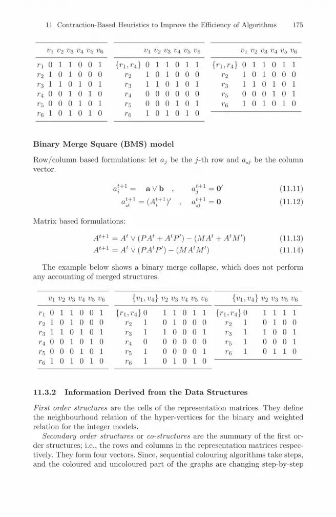
11 Contraction-Based Heuristics to Improve the Efficiency of Algorithms 175
v1 v2 v3 v4 v5 v6
r1 0 1 1 0 0 1r2 1 0 1 0 0 0r3 1 1 0 1 0 1r4 0 0 1 0 1 0r5 0 0 0 1 0 1r6 1 0 1 0 1 0
v1 v2 v3 v4 v5 v6
r1, r4 0 1 1 0 1 1r2 1 0 1 0 0 0r3 1 1 0 1 0 1r4 0 0 0 0 0 0r5 0 0 0 1 0 1r6 1 0 1 0 1 0
v1 v2 v3 v4 v5 v6
r1, r4 0 1 1 0 1 1r2 1 0 1 0 0 0r3 1 1 0 1 0 1r5 0 0 0 1 0 1r6 1 0 1 0 1 0
Binary Merge Square (BMS) model
Row/column based formulations: let aj be the j-th row and a j be the columnvector.
at+1i = a ∨ b , at+1
j = 0′ (11.11)
at+1i = (At+1
i )′ , at+1j = 0 (11.12)
Matrix based formulations:
At+1 = At ∨ (PAt + AtP ′) − (MAt + AtM ′) (11.13)At+1 = At ∨ (PAtP ′) − (MAtM ′) (11.14)
The example below shows a binary merge collapse, which does not performany accounting of merged structures.
v1 v2 v3 v4 v5 v6
r1 0 1 1 0 0 1r2 1 0 1 0 0 0r3 1 1 0 1 0 1r4 0 0 1 0 1 0r5 0 0 0 1 0 1r6 1 0 1 0 1 0
v1, v4 v2 v3 v4 v5 v6
r1, r4 0 1 1 0 1 1r2 1 0 1 0 0 0r3 1 1 0 0 0 1r4 0 0 0 0 0 0r5 1 0 0 0 0 1r6 1 0 1 0 1 0
v1, v4 v2 v3 v5 v6
r1, r4 0 1 1 1 1r2 1 0 1 0 0r3 1 1 0 0 1r5 1 0 0 0 1r6 1 0 1 1 0
11.3.2 Information Derived from the Data Structures
First order structures are the cells of the representation matrices. They definethe neighbourhood relation of the hyper-vertices for the binary and weightedrelation for the integer models.
Secondary order structures or co-structures are the summary of the first or-der structures; i.e., the rows and columns in the representation matrices respec-tively. They form four vectors. Since, sequential colouring algorithms take steps,and the coloured and uncoloured part of the graphs are changing step-by-step

176 I. Juhos and J. van Hemert
7
v1
v2
v4
v5
v6
v3
(a)
(b)
r1 0 1 1 0 0 1r2 1 0 1 0 0 0r3 1 1 0 1 0 1r4 0 0 1 0 1 0r5 0 0 0 1 0 1r6 1 0 1 0 1 0
v1 v2 v3 v4 v5 v6 0 1 2 1 1 25 0 1 2 0 1 1 4
0 1 1 1 1 2
v1 v2 v3 v4 v5 v6
r1,r4
2 0 0 0 1 0 1 2r5
v5 v3
v2v6
v1,v4
(c)
(b) 1 1 2 1 25 0 1 2 1 1 4
1 1 1 1 2
r1,r4
2 0 0 0 0 1 2r5
v5 v3
v2v6
v1,v4
v1,v4 v2 v3 v5 v6
6 6
7 (b)
(c)
(d)
Fig. 11.4. The original graph, its induced sub-IMT and then its induced sub-IMSwhen colouring is in progress. (a) gives the sum of the degree of the nodes, (b) givesthe number adjacent vertices already assigned a colour, (c) gives the degree of thehyper-vertex, and (d) gives the number of coloured hyper-edges.
it is worth to define these structures separately to the coloured/merged anduncoloured/non-merged sub-graphs. To identify these partial sums we use col
and unc superscripts. We can obtain the sum of the rows and columns of binarymerge matrices from their integer pairs by counting their non-zero elements.Hence, in Figure 11.4 only the left side of the sub-matrices sum the columnsand the right side sum the non-zero elements to get the relevant summary inthe binary matrix. This is the same for the columns, where the top vector is thesum of the rows and the bottom is the number of non-zeros. The second orderstructures are denoted by τ , using t,b,l,r indices as subscript to refer to the top,bottom, left and right vector.
Third order structures are formed by summarising the secondary order struc-tures. These can be divided into two parts similar to the second order structuresaccording to the coloured and uncoloured sub-graphs. These structures are de-noted by ζ. In this study, they will be used in the fitness function of the evolu-tionary algorithm. The top-left sums the top vector (or the left vector) and thebottom-right sums the bottom vector (or the right vector). These are shown inbold font in Figure 11.4.
11.4 Heuristics Based on Merge Model Structures
before we define the heuristics, we first introduce two abstract sequential algo-rithms. These are appropriate for defining existing or novel GCP solvers in aconcise manner.

11 Contraction-Based Heuristics to Improve the Efficiency of Algorithms 177
Definition 1 (Sequential contraction algorithm 1 (SCA1))
1. Choose a non-merged/uncoloured vertex v2. Choose a non-neighbour hyper-vertex/colour-set r to v3. Merge v to r4. If there exists a non-merged vertex then continue with Step 1
Definition 2 (Sequential contraction algorithm 2 (SCA2))
1. Choose a hyper-vertex/colour-set r2. Choose a non-neighbor non-merged/uncoloured vertex v to r3. Merge v to r4. If there exists a non-merged vertex then continue with Step 1
The proceedings of the DIMACS Challenge II [240] states a core problem ofthe algorithm design for graph colouring: it is crucial to find an initially goodsolution, because each algorithm needs exhaustive searching to find an opti-mal solution, hence the problem becomes NP-hard to solve. There are severalpolynomial algorithms (see [241, 242, 243, 244]), which provide a guarantee forthe approximation of the colouring for a given number of colours. For example,Erdos heuristics [242] guarantees at most O(n/logχ(n)) number of colours inthe worst case. Several algorithms have improved upon this bound, but many ofthem use the main technique introduced by Erdos. We will define this heuristicsin our model. Another reference method is the well known heuristic of Brelaz;the DSatur algorithm, which works very well on graphs that have a small chro-matic number. Two additional novel heuristics are introduced: the DotProd
and Cos heuristics.
DSatur
DSatur is a SCA1 type algorithm. Where the choice of colouring the next un-coloured vertex v is determined by colour saturation degree. As colour saturationis calculated by observing the colours of neighbouring vertices, it requires O(n2)constraint checks. However, if we merge the already coloured vertices, e.g., usingMTs, we have the possibility to obtain this information by observing at mostthe number of hyper-vertices for v. Hence, O(nkt) constraint checks are required,where kt is the number of colours used in step t. The bottom co-structure of therelevant sub-IMT provide the saturation degree exactly which gives O(n) com-putational effort to find the largest one. Hence, IMT is an appropriate structurefor the definition. Here, the choice for hyper-vertex/colour-set is done in a greedymanner.
Definition 3 (Non-merged/Uncoloured vertex choice of the DSaturimt)
1. Find those non-merged/uncoloured vertices which have the highest saturateddegree: S = arg maxu τcol
b (u) : u ∈ V unc
2. Choose those vertices from S that have the highest non-merged/uncoloured-degree: N = arg maxv τunc
b (v)3. Choose the first vertex from the set N

178 I. Juhos and J. van Hemert
DotProd
This heuristic is based on a novel technique, which is shown to be useful in [239].Two vertices of a contracted graph are compared by consulting the correspondingBMS rows. The dot product of these rows gives a valuable measurement for thecommon edges in the graph. These values are the same in binary MT and MSbut can differ between the binary and integer variations. Application of theDotProd heuristics to the BMS representation provides the Recursive LargestFirst (RLF) algorithm. Unfortunately the name RLF is somewhat misleading,since the largest first itself does not define exactly where largest first is relatingto. The meaning of it differs throughout the literature. Here, we introduce aDotProd heuristic that is combined with the BMS representation and theSCA2 type algorithm, which results in the RLF of Dutton and Birgham [245].We explore only thess combinations, but other combinations are possible, makingthe DotProd a more general technique.
Definition 4 (Non-merged/Uncoloured vertex choice of theDotProdbms)
1. Find those non-merged/uncoloured vertices which have the largest num-ber of common neighbours with the first hyper-vertex (colour set): S =arg maxu 〈u, r〉 : u ∈ V unc
2. Choose the first vertex from the set S
Cos
The Cos heuristics is the second novel heuristics introduced here. It is derivedfrom DotProd by normalisation of the dot product. As opposed to DotProd,Cos takes in consideration the number of non-common neighbours as well. Inthe following definition we provide an algorithm of type SCA2 that uses the Cos
heuristics to choose the next vector:
Definition 5 (Non-merged/Uncoloured vertex choice of the Cosbms)
1. Find the non-merged (i.e., uncoloured) vertices that have the largest numberof common neighbours with the first hyper-vertex (colour set), and that havethe least number of constraints: S = argmaxu
〈u,r〉‖u‖‖r‖ ≡ argmaxu
〈u,r〉‖u‖ ≡
arg maxu〈u,r〉τr(u) : u ∈ V unc
2. Choose the first vertex from the set S
Pal Erdos O(n/ log n) number of colours guaranteed heuristic
The approach [242, page 245] is as follows. Take the first colour and assign itto the vertex v that has the minimum degree. Vertex v and its neighbours areremoved from the graph. Continue the algorithm in the remaining sub-graph inthe same fashion until the sub-graph becomes empty, then take the next colourand use the algorithm for the non-coloured vertices and so on until each vertexis assigned a colour.

11 Contraction-Based Heuristics to Improve the Efficiency of Algorithms 179
All of representations are suitable as a basis for this heuristic. It uses SCA2,where the choice for the next target r-th (hyper-)vertex/colour-set for mergingand colouring is greedy.
Definition 6 (Non-merged/Uncoloured vertex choice of the Erdosbmt)
1. Choose an uncoloured vertex with minimum degree. S = arg minu τuncb (u)
2. Choose the first vertex from the set S
The Erdos and DSatur heuristics make use of the secondary order struc-tures, whereas the other two, DotProd and Cos, make use of the first orderinformation. The Erdos heuristic uses similar assumptions as DSatur but inthe opposite direction, which becomes clear in the results from the experiments.
11.5 An Evolutionary Algorithm Based on Merge Models
We apply an evolutionary algorithm (EA) to guide the heuristics. It uses theBMT representation for colouring and the SCA1 contraction scheme. The geno-type is a permutation of the vertices, i.e., the rows of the BMT. The phenotypeis a final BMT, where no rows can be merged further. Vertex selection is definedby an initial random ordering of all vertices. The order is then evolved by theEA toward an optimum directed by both the fitness function and the geneticoperators of the EA. The strategy for merging of selected vertices is guided byone of the DotProd and Cos heuristics.
An intuitive way of measuring the quality of an individual (permutation) p inthe population is by counting the number of rows remaining in the final BMT.This equals to the number of colours k(p) used in the colouring of the graph,which needs to be minimised. When we know the optimal colouring1 is χ thenwe may normalise the fitness function to g(p) = k(p) − χ. This function givesa rather low diversity of fitnesses of the individuals in a population because itcannot distinguish between two individuals that use an equal number of colours.This problem is called the fitness granularity problem. We modify the fitnessfunction introduced in [234] to allow the use of first and second order structuresintroduced in Section 11.3.2.
The fitness relies on the heuristic that one generally wants to avoid highly con-straint vertices and rows in order to have a higher chance of successful mergesat a later stage, commonly called a succeed-first strategy. It works as follows.After the last merge the final BMT defines the groups of vertices with the samecolour. There are k(p)−χ over-coloured vertices, i.e., merged rows. Generally, weuse the indices of the over-coloured vertices to calculate the number of verticesthat need to be minimized (see g(p) above). But these vertices are not neces-sarily responsible for the over-coloured graph. Therefore, we choose to countthe hyper-vertices that violates the least constraints in the final hyper-graph.To cope better with the fitness granularity problem we should modify the g(p)according to the constraints of the over-coloured vertices discussed previously.1 In our experiments χ is defined in advance.

180 I. Juhos and J. van Hemert
The fitness function used in the EA is then defined as follows. Let ζunc(p) denotethe number of constraints, i.e., non-zero elements, in the rows of the final BMTthat belong to the over-coloured vertices, i.e., the sum of the smallest k(p) − χvalues of the right co-structure of the uncoloured vertices. This is the uncolouredportion of the (right-bottom) third order structure. The fitness function becomesf(p) = g(p)ζunc(p). Here, the cardinality of the problem is known, and used asa termination criterium (f(p) = 0) to determine the efficiency of the algorithm.For the case where we do not know the cardinality of the problem, this approachcan be used by leaving out the normalisation step.
Procedure EAdot and EAcos
1. population = generate initial permutations randomly2. repeat
evaluate each permutation p:merge pj − th unmerged vertex v into hyper-vertex r by DotProd or Cos
calculate f(p) = (k(p) − χ)ζunc(p)populationxover = xover(population, probxover)populationmut = mutate(populationxover , probmut))population = select2-tour(population ∪ populationxover ∪ populationmut)
3. until termination condition
Fig. 11.5. The EA meta-heuristic uses directly the BMT structure and either theDotProd or Cos merge strategy
Figure 11.5 shows the outline of the evolutionary algorithm. It uses a gener-ational model with 2-tournament selection and replacement, where it employselitism of size one. This setting is used in all experiments. The initial populationis created with 100 random individuals. Two variation operators are used toprovide offspring. First, the 2-point order-based crossover (ox2) [246, in SectionC3.3.3.1] is applied. Second, a simple swap mutation operator, which selects atrandom two different items in the permutation and then swaps. The probabilityof using ox2 is set to 0.4 and the probability for using the simple swap mutationis set to 0.6. These parameter settings are taken from previous experiments [234].
The Erdos heuristic guarantees its performance. We omit this heuristics fromthe EA, as we would not be able to guarantee this property once embeddedin the EA. A baseline version of the EA called EAnoheur serves a basis of thecomparison. and the DSatur with backtracking is used as well, as it is commonlyused as a reference method. Moreover, as this algorithm performs an exhaustivesearch it is useful to find the optimal solutions to some of the problem instances;some of the instances are too difficult for it to solve and we have to terminate itprematurely.
11.6 Experiments and Results
The test suites are generated using the well known graph k-colouring generatorof Culberson [247]. It consists of k-colourable graphs with 200 vertices, where

11 Contraction-Based Heuristics to Improve the Efficiency of Algorithms 181
3
3.5
4
4.5
5
5.5
6
6.5
0 0.02 0.04 0.06 0.08 0.1 0.12 0.14 0.16 0.18 0.2
Ave
rage
num
ber
of c
olor
s us
ed
Average density of edges in the graphs
cosbmsdotprodbms
Erd s bmsdsaturimt
5
6
7
8
9
10
11
12
0.05 0.1 0.15 0.2 0.25 0.3 0.35 0.4
Ave
rage
num
ber
of c
olor
s us
ed
Average density of edges in the graphs
cosbmsdotprodbms
Erd s bmsdsaturimt
8
10
12
14
16
18
20
22
24
26
0.1 0.2 0.3 0.4 0.5 0.6 0.7 0.8 0.9
Ave
rage
num
ber
of c
olor
s us
ed
Average density of edges in the graphs
cosbmsdotprodbms
Erd s bmsdsaturimt
15
20
25
30
35
40
45
0.3 0.4 0.5 0.6 0.7 0.8 0.9 1
Ave
rage
num
ber
of c
olor
s us
ed
Average density of edges in the graphs
cosbmsdotprodbms
Erd s bmsdsaturimt
Fig. 11.6. Average number of colours used in sequential colouring heuristics. χ is 3,5, 10, and 20, respectively in the sequence of figures.

182 I. Juhos and J. van Hemert
3
3.5
4
4.5
5
5.5
0.02 0.03 0.04 0.05 0.06 0.07
Ave
rage
num
ber
of c
olor
s us
ed
Average density of edges in the graphs
EAcos,bmtEAdotprod,bmt
EAnoheurBacktrackdsatur,imt
3
4
5
6
7
8
9
10
0.04 0.06 0.08 0.1 0.12 0.14 0.16 0.18
Ave
rage
num
ber
of c
olor
s us
ed
Average density of edges in the graphs
EAcos,bmtEAdotprod,bmt
EAnoheurBacktrackdsatur,imt
8
10
12
14
16
18
20
22
24
0.3 0.35 0.4 0.45 0.5 0.55 0.6
Ave
rage
num
ber
of c
olor
s us
ed
Average density of edges in the graphs
EAcos,bmtEAdotprod,bmt
EAnoheurBacktrackdsatur,imt
20
25
30
35
40
0.5 0.55 0.6 0.65 0.7 0.75 0.8
Ave
rage
num
ber
of c
olor
s us
ed
Average density of edges in the graphs
EAcos,bmtEAdotprod,bmt
EAnoheurBacktrackdsatur,imt
Fig. 11.7. Averaged number of colours used in the EA experiments. χ is 3, 5, 10, and20, respectively in the sequence of the figures.

11 Contraction-Based Heuristics to Improve the Efficiency of Algorithms 183
k is set to 3, 5, 10 and 20. For k = 20, ten vertices will form a colour set,therefore we do not use any larger chromatic number. The edge density of thegraphs is varied in a region called the phase transition. This is where hard tosolve problem instances are generally found, which is observed in the results as atypical easy-hard-easy pattern. The graphs are all generated to be equi-partite,which means that a solution should use each colour approximately as much asany other. The suite consists of groups where each group is a k-colouring with20 unique instances.
In the first experiment, we compare the heuristics from Section 11.4 whenembedded in DSatur. Figure 11.6 shows the results for each of the heuristics.Cos heuristics performed clearly better than the others except for the 3-colouringwhere DSatur performs equally well. The DotProd is ranked second. WhileDSatur performs well on sparse graphs having small chromatic number, Erdos
heuristics performs well on graphs that require more colours, especially on densegraphs, i.e., that have a high average density of edges. Interesting is the locationof the phase transitions. Figure 11.6 shows that it depends not only on the edgedensity of the graphs but also on the applied algorithm, especially the graphdensity where DSatur exhibits its worst performance moves away from theothers with increasing k. DSatur and Erdos heuristics apply only second orderinformation as opposed to the other two algorithms where first order informationis used. The Erdos heuristic uses the secondary order structures in the oppositedirection to DSatur and our results show how that affects the performance asthe effectiveness flips for different ends of the chromatic number of graphs.
While sequential algorithms make one run to get their result, EA experimentsare performed several times due to the random nature of the algorithm. Thereforea reduced number of instances is selected from the previous experiments. Oneset consists of five instances, except for 3 and 5 colourable instances where theset contains ten instances because the diversity of the results of the solvers islow for small chromatic numbers. On each instance we perform ten independentruns and calculate averages over the total number of runs. 3-colouring needsmore instances to get more confident results.
Figure 11.7 shows the results for the EA with two different heuristics. Alsoshown are results for the reference EA without heuristics and the DSatur ex-haustive algorithm. Similar to the previous experiments, the Cos heuristics per-forms well, especially for larger k, and the DotProd is a close second. DSatur
is the strongest algorithm on 3-colourable graphs, always finding the optimumnumber of colours.
11.7 Conclusions
In this paper, we introduced four kinds of Merge Models for representing graphcolouring problems. It forms a good basis for developing efficient graph colouringalgorithms because of its three beneficial properties: a significant reduction inconstraint checks, access to heuristics that help guide the search, and a compact

184 I. Juhos and J. van Hemert
description of algorithms. We showed how existing algorithms can be describedin terms of the Merge Model concisely.
By incorporating the models in an exhaustive algorithm, Dsatur, and in ameta-heuristic, an evolutionary algorithm based on a permutation, we showedhow the effectiveness of these algorithms can be improved.
Acknowledgements
This work is supported by the High Performance Computing Group of theUniversity of Szeged. The second author is supported through the e-ScienceData Information & Knowledge Transformation project funded by the ScottishFunding Council.

12
Different Codifications and MetaheuristicAlgorithms for the Resource Renting Problemwith Minimum and Maximum Time Lags
Francisco Ballestın
Department of Statistics and OR, Public University of Navarra, Pamplona, [email protected]
Summary. Most work in project scheduling problems has been done with so-calledregular objective functions, where a solution S never dominates another solution S’ ifno activity is scheduled earlier in S than in S’. This has provided with techniques andmetaheuristic frameworks to create heuristic algorithms for these kinds of problems,something which does not exist in the nonregular case. One of these problems is theResource Renting Problem, which models the renting of resources. In this paper wecompare the quality of three algorithms for this problem, one adapted from the regularcase, another specially designed for the problem and a third that might be adapted forother problems. We will also show that two of these algorithms are capable of outper-forming a branch-and-bound procedure that exists for the problem.
Keywords: Project Scheduling, Temporal Constraints, Nonregular Objective Func-tion, Metaheuristic Algorithms.
12.1 Introduction
Project scheduling consists in finding a time interval for the processing of activi-ties whose start times are restricted by the start times of other activities. In manypractical and academic uses of project scheduling each activity consumes someresources that are expensive and/or constrained. There are many different objec-tive functions in this field, but they can be clearly distinguished between regularand nonregular. A regular measure of performance is a non-decreasing functionof the activity completion times (in the case of a minimisation problem). Themost important (regular) objective function is the makespan or project length,but there are others like the minimisation of the mean flowtime or the meanweighted tardiness. These performance measures - especially the makespan -have received much attention, which has led to many heuristic algorithms. Someof them can be easily adapted to other project scheduling problems with regularobjective functions, “regular problems”, sometimes even if we add additionalrestrictions. We refer to the surveys [359], [354] and [361].
In the last years scheduling problems with nonregular measures of perfor-mance have gained increasing attention (cf. [374]). Some popular nonregularmeasures of performance in the literature are the maximisation of the net present
C. Cotta and J. van Hemert (Eds.): Recent Advances in Evol. Comp., SCI 153, pp. 187–202, 2008.springerlink.com c© Springer-Verlag Berlin Heidelberg 2008

188 F. Ballestın
value of the project ( [375]), the minimisation of the weighted earliness-tardinesspenalty costs of the activities in a project ( [350]), the Resource Levelling Prob-lem (RLP, [352]) and the Resource Investment Problem (RIP), which modelsthe purchase of resources ( [369] and [370]). In the RIP, the usage of resources isassociated to a cost of making this resource available, independently of the time.Hence, making resource units available means buying them. For many real-lifeprojects, however, the use of resources is associated with time-dependent costs,e.g. for heavy machinery or manpower in civil engineering. That is why theresource renting problem has been proposed (see [371]) where, besides time-independent fixed renting costs, time-dependent variable renting costs are givenfor the resources. Hence, the RRP models the renting of resources. For resourceacquisition via buying and renting see also [347]. In project scheduling problemswith nonregular objective functions, “nonregular problems”, there is apparentlyno common heuristic framework that can be adapted to new problems, and aspecific algorithm should be theoretically developed each time. An exception tothis are the methods developed in [368], some of which will be used in this paper.However, algorithms can be adapted from the regular case just by introducingseveral changes like the schedule generation scheme. Although this can be easilydone, the problem is the quality offered by this approach. Besides, some proce-dures can be developed that can be used for several problems without makingtoo many adjustments. The goals of this paper are threefold: first of all, wewant to study the quality difference between an adaptation of an algorithm fora regular problem and a specially designed algorithm for the RRP. Secondly, thecodification and crossover of that latter algorithm, already schematised in [349],deserve further attention and examples. Finally, we will also propose a heuristicwhich does not need much problem knowledge and that can be adapted to othernonregular problems. The next section contains the formal definition of the op-timisation problem. In section 3 the three metaheuristic algorithms for the RRPare described. Finally, computational experience with the proposed proceduresis presented in Section 4.
12.2 Preliminaries
12.2.1 Model of the Problem
In this section we follow [371] and [368]. We want to carry out a project whichconsists of n+2 activities numbered 0, 1, . . . , n+1, with dummy activities 0 andn + 1 representing the beginning and termination of the project, respectively.We denote V the set of all activities of the project, which coincides with thenode set of a corresponding activity-on-node project network. Let pj ∈ Z+ bethe duration (or processing time) and Sj ∈ Z+ be the start time of activity jwhere S0 = 0. Then Sn+1 represents the project duration (or makespan) whichis restricted by the constraint Sn+1 ≤ d , being d ∈ Z+ a prescribed maximumproject duration (deadline). In the project network, a minimum time lag dmin
ij ∈Z+ between the start of two different activities i and j, i.e., Si − Sj ≥ dmin
ij ,

12 Different Codifications and Metaheuristic Algorithms for the RRP 189
is modelled as an arc 〈i, j〉 in the project network with weight δij = dminij . A
maximum time lag dmaxij ∈ Z+ between the start of activities i and j means
Sj − Si ≤ dmaxij , and is modelled as an arc 〈j, i〉 with weight δij = −dmax
ij .The arc set of the project network is denoted by E. We assume that a set Rof renewable resources is required for carrying out the project activities. Eachactivity j requires rjk ∈ Z+ (j ∈ V, k ∈ R) units of resource k during eachperiod of its duration, where the dummy activities do not need any resources.The usage of resources incurs fixed and variable costs. Fixed renting costs cf
arise when bringing a unit of resource to service and often represents a deliveryor transportation cost for resource unit rented. Variable renting costs cv refer toone unit of resource and one unit of time for which the resource unit is rented.Accordingly, the provision of one unit of resource k for a time interval of t timeunits length leads to fixed costs of cf
k and to variable costs of tcvk. We assume
that cfk ∈ Z+\0 and cv
k ∈ Z+\0 for all resources k ∈ R. Given a scheduleS, let A(S, t) := i ∈ V |Si ≤ t < Si + pi be the set of activities in progressat time t and let rk(S, t) :=
∑i∈A(S,t) rik be the amount of resource k required
at time t. Without loss of generality we assume the condition of integrality forpoints in time where the capacities of the resources k ∈ R can be increased ordecreased. Given a schedule S, we have to decide on how many units of resourcek ∈ R are to be rented at each point in time t ∈ [0, d]. That is, we should choosea renting policy ϕ(S, .) := (ϕk(S, .))k∈R, where ϕk(S, t) (or ϕkt for short) isthe amount of resource k rented at time t ∈ [0, d]. We can restrict ourselves tostep functions ϕk(S, .) with finitely many jump discontinuities and continuous
from the right. Given renting policy ϕk(S, .), cvk
∫ d
0 ϕk(S, t)dt represents the totalvariable renting cost for resource k and planning horizon d. Let Jk be the finiteset of jump discontinuities of function ϕk(S, .) on interval [0, d] and min be thesmallest of those jump points. For t ∈ Jk\τmin, let t := maxτ ∈ Jk|τ < t bethe largest jump point of function ϕk(S, .) less than t and for t ∈ Jk, let
Δ+ϕkt :=
[ϕk(S, t) − ϕk(S, τt)]+, if t > τmin
ϕk(S, τmin), otherwise (12.1)
be the increase in the amount or resource k rented at time t. Then the totalfixed renting cost for resource k equals cf
k
∑t∈Jk
Δ+ϕkt.A feasible renting policy ϕ(S, .) must fulfil ϕk(S, t) ≥ rk(S, t) for all k ∈ R
and t ∈ [0, d]. Given schedule S, we will look for the optimal renting pol-icy ϕ(S, .), the feasible renting policy that minimises the total renting cost∑
k∈R
[cvk
∫ d
0 ϕk(S, t)dt + cfk
∑t∈Jk
Δ+ϕkt
].
The objective function f of the resource renting problem represents the totalrenting cost belonging to an optimal renting policy for schedule S and reads asfollows
f(S) :=∑k∈R
minϕ(S,·)≥rk(S,·)
[cvk
∫ d
0ϕk(S, t)dt + cf
k
∑t∈Jk
Δ+ϕkt
](12.2)

190 F. Ballestın
Fig. 12.1. Example problem Fig. 12.2. S, a feasible solution for theproblem
Fig. 12.3. A feasible renting policy forS
Fig. 12.4. Another feasible rentingpolicy for S
Let ϕ∗k(S, .) be an optimal renting policy for schedule S and k ∈ R. The
resource renting problem subject to temporal constraints RRP/max consistsof finding a schedule S which satisfies and minimises objective function f . Thisproblem is denoted PS∞|temp, d|ΣΣcv
kϕkt+cfkΔ+ϕkt (cf. [368]) and is NP-hard
as an extension of the RIP /max (cf. [371]). It is not straightforward to calculatethe optimal renting for a schedule, but polinomial procedures are available in[371] and [368]. We are going to comment some of the definitions taking as anexample the project depicted in Figure 12.1. We will fix a deadline d of 14. Afeasible solution for this project is shown in Figure 12.2, where both minimumand maximum time lags are observed and the deadline is not exceeded. As anexample, note that the start time of activity 7 is 12, not more than 2 unitsbigger (exactly two units bigger) than the start time of activity 5. This is inconcordance with the maximum time lag between activities 5 and 7 of 2 units.Let us compare several renting policies for this solution. As always, a feasiblerenting policy is ϕ1(t) = r(S, t)∀t and other two feasible renting policies can beseen in Figure 12.3 (ϕ2) and Figure 12.4 (ϕ3). Table 12.2 shows the objectivefunction of the three policies when different fixed and variable renting cost aregiven. The different scenarios considered are shown in Table 12.1. As an example,the fixed renting cost of 2 is calculated as follows. At time t = 0 we demand 2

12 Different Codifications and Metaheuristic Algorithms for the RRP 191
Table 12.1. Scenarios considered
Scenario Sc1 Sc2 Sc3
cf 1 3 7cv 1 1 1cv/cf 1 1/3 1/7
Table 12.2. Objective function for S for the different considered scenarios
Costs due to proc. cost Rent cost Total cost (obj. func.)
Sc1 Sc2 Sc3 any Sc Sc1 Sc2 Sc3
ϕ1 5·1 = 5 5·3 = 15 5·7 = 35 20·1 = 20 25 35 55ϕ2 3·1 = 3 3·3 = 9 3·7 = 21 24·1 = 24 27 33 45ϕ3 2·1 = 2 2·3 = 6 2·7 = 14 28·1 = 28 30 34 42
units of the single resource. At time t = 6 we release one unit of the resource,which we need (and demand) at time t = 10. This means that we demand 3 unitsof resource at different times, which means 3·cf units of fixed renting cost in thedifferent scenarios. Regarding the variable renting cost of this renting policy, ininterval [0, 6[ two units of the resource are available. Note that in interval [2, 4[we only need one unit of the resource, but we would have to demand anotherunit of resource at time t = 4. However, this would be a different renting policy.In interval [6, 10[ one unit of the resource is available and in [10, 14] two units ofthe resource are available. All in all, we have (6−0)·2+(10−6)·1+(14−10)·2 =24 units available, which means 24·cr units of variable renting cost and a totalof 3·cf + 24·cr units of cost. When cv/cf is 1 or more (Sc1), it is more efficientto have few resources available at each time, because it is inexpensive to procurenew resources when needed. In this case, solutions where the renting policy isvery similar to the resource profile (in our case ϕ1) are the best. When cv/cf
approximates 0 (Sc3), it is very expensive to obtain new resources. Therefore itis better to have many of them available at each time, even if we do not use themall at each interval. The best solutions are then similar to ϕ(t) = max(r(S, t))∀t,i.e. in our case ϕ3 is the best. Note that the limit, RRP with cv/cf = 0 is thesame as RIP. In not so extreme scenarios the optimal policy does not look likeϕ1 or ϕ3. In Sc2, the best renting policy is ϕ2.
12.2.2 Candidates for Optimal Solution
As shown in [368], it is enough to search in the space of quasistable schedules inorder to find an optimal solution for the RRP. This means that, when we schedulean activity i in a partial schedule, we only have to look at integral points t in set[ESi, LSi]
⋂ESi, LSi, Sj +pj, j ∈ C, Sj −pi, j ∈ C. ESi(LSi) denotes the
earliest (latest) start time where act i can be scheduled and C the set of activities

192 F. Ballestın
already scheduled. Throughout the paper we will only take into account thesepoints in time t when we schedule an activity, but we will not mention it again.
12.3 Metaheuristic Algorithms for the RRP
In this section we describe the metaheuristic algorithms we have applied to theRRP. The first ones, adapGA and specGA, share the same algorithmic structurebut use a totally different codification and crossover. On the one hand, the codifi-cation and crossover of adapGA, an algorithm adapted from a Genetic Algorithm(GA) for the regular case, are the ones used in that algorithm and have proved theirusefulness in those optimisation problems. On the other hand, these elements arecompletely new in specGA, the GA specially designed for the RRP. Both GA’scan be regarded as memetic algorithms ( [365] and [366]), since they include animprovement method after the recombination. Finally, a third metaheuristic al-gorithm IG is schematised. This algorithm does not need a deep knowledge of theproblem and could be adapted to other nonregular optimisation problems.
12.3.1 Algorithm Adapted from a Regular Problem (adapGA)
One of the goals of this paper is to calculate the quality difference betweenperforming the minimal adaptations from a specially designed algorithm andan algorithm for a regular problem. In order to achieve this we will use exactlythe same framework for both algorithms and the only differences between themwill be the codification and crossover operator. As a framework we have used aGA plus an Improvement Procedure (IP), that has been adapted (with more orfewer changes) to several problems with success. The original algorithm withoutIP appears in [357]. Some of the problems where it has been adapted are themulti-mode RCPSP ( [358]), the RCPSP with preemption ( [353]), the RCPSPwith due dates ( [351]) or the stochastic RCPSP ( [348]). For an introduction intoGAs, a heuristic meta strategy to solve hard optimisation problems that followthe basic principles of biological evolution, we refer to [143]. The codification usedby adapGA will be a simplification of the activity list, a widely used codificationin regular problems. The simplification is a permutation, which can be used dueto the fact that there are no resource restrictions in our problem, and an activitylist is a perturbation of the activities that fulfils the positive time lags betweenactivities. The crossover used by adapGA will be the two-point crossover forpermutations (cf. [357]). It will be followed by a perturbation similar to the oneused in that algorithm. The outline of the algorithm for adapGA and specGA -without including the perturbation for adapGA - is as follows. After calculatingthe initial population POP with the multi pass algorithm MP plus IP appliedto each solution, the procedure adds to POP in each iteration a new populationof the same size with children generated by the crossover and improved by IP.The best individuals of this joint population constitute the population for thenext iteration. The different adaptations of the GA for the RRP are explainedin the next subsections.

12 Different Codifications and Metaheuristic Algorithms for the RRP 193
Schedule Generation Scheme (SGS) and codification
In the book of [368], some priority rules were described for different types ofobjective functions. These priority rules consists basically in choosing an orderfor the activities - a permutation of the activities - and scheduling the activitiesin this order locally optimal. I.e., at the best time t with regards to the objectivefunction in the feasible time window. We use the same untie rule as in [367]:we choose the smallest minimizer t when we schedule activity i if i < |V |/2 ,else we choose the greatest minimizer t. This method of creating one or severalsolutions can be transformed into a codification and a SGS for many nonregularobjective functions: a perturbation of the activities and the SGS that schedulesthe activities in that order locally optimal.
Improvement Procedure
Regarding the IP, it is more difficult to devise general procedures useful formany nonregular objective functions. One possibility for the not sum-separableobjective functions is the following. After using SGS mentioned in section 3.1.1the activities are not longer locally optimal scheduled. A simple but effectiveIP (cf. [352]) consists in iteratively choosing a not already chosen activity, un-scheduling it and then scheduling it locally optimal.
Procedure to calculate the initial population
With the priority rules described in 3.1.1 and the IP described in the foregoingsection it is straightforward to create an initial population for an algorithm; oneonly needs to use some sort of sampling procedure or multi pass algorithm MP(cf. [360]). In our case, we use the regret-based random sampling method (cf.Drexl, 1991) with priority rules MST-GRR, with MST = minimum slack time(LSh − ESh) and GRR = greatest resource requirements first. The second ruleis used as an untie rule.
12.3.2 Specially Designed Algorithm (specGA)
As we have already mentioned, specGA also follows the structure presented inthe foregoing section. However, it uses a different codification and crossover,described in the next section. This algorithm was schematised in [349].
Codification of a solution
We use n+2 sets to codify a solution S, one for the whole schedule and anotherfor each activity. The set for the schedule is framework(S), with framework(S)= i ∈ V/Si = d0i or Si = −dn+1,i , where d0i denotes the length of thelongest path between activities 0 and i and di,n+1 is the length of the longestpath between activities n + 1 and i if we introduce the arc < n + 1, 0 > in thenetwork with weight δn+1,0 = −d. Besides, for each activity i we calculate the

194 F. Ballestın
set of activities that finish exactly when i begins. We call this set before(i, S) =j ∈ V/Sj + dj = Si. It is straightforward to calculate these sets while buildinga schedule. In the schedule S of Figure 12.2, framework(S) = 1, 2, 7, becaused01 = d02 = 0 = S1 = S2 and −dn+1,7 = 12 = S7. Besides, before(7, S) = 5, 6or before(4, S) = ∅. This definition of codification is fully workable in combina-tion with the crossover described in the next section. However, it is an incompletecodification in the sense that there might exist activities which do not belong toframework(S) or to any before(j,S) and for which before(i,S) = ∅. We are notgoing to dwell on this theme because the way to schedule activities - locally op-timal - tends to schedule activities after or before other activities and so we willnot often find such situations. At any rate, if we wanted to work with a completecodification we could use the concept of weighted spanning tree. See [368] forthe definition and algorithms based on this concept.
Crossover
The crossover used in specGA tries to transfer good qualities from the parentsto the children. The objective function somehow penalises the positive jumpsin the resource utilisation; a good schedule will therefore have few points whereresources are newly rented. So, the flow of resources is important, much morewhich activities are scheduled right after which others than where exactly anactivity is scheduled. Our crossover relies on trying to schedule one after the otheractivities that are scheduled one after the other in the mother M and/or thefather F . The pseudo-code from the operator is given in Scheme 1. Specifically,in order to obtain the daughter D from M and F , we first schedule the activitiesin framework(M) in the same interval as in M . Afterwards we select at eachiteration an unscheduled activity and schedule it, until we end with a completesolution. The son can be obtained by changing the roles of the mother and thefather. To further describe an iteration in the construction of the daughter, weneed sets C, C , Eleg1 and Eleg2. C and C contain the scheduled and unscheduledactivities, respectively. Eleg1 and Eleg2 are subsets of C that are recalculatedat each iteration. Suppose that an unscheduled activity i is scheduled right after(right before) a scheduled activity j in M and in F (a condition imposed on bothparents). If i can be scheduled at a certain iteration right after (right before) jin D, then i belongs to Eleg1 at that iteration. If we select i to be scheduledat that iteration, we will mimic the behaviour of i in M and F and schedule itright after (right before) j. Note that this does not imply that the start time ofi is the same in the different solutions. Eleg2 works in a similar way to Eleg1,the only difference is that we relax the condition and demand it just on oneof the parents. At each iteration we randomly select an activity from Eleg1 orfrom Eleg2 if Eleg1 is empty and schedule it. We scrutinised the sets in thisorder because we prefer that the daughter inherits structures present in the twosolutions at the same time. If both sets Eleg1 and Eleg2 are empty, we choosean activity i randomly and we schedule it at the best point in time with respectto the objective function.

12 Different Codifications and Metaheuristic Algorithms for the RRP 195
Scheme 1. Pseudo-code to obtain the daughter D by recombining the mother Mand the father F .
1. i ∈ framework(M) do SDi = SM
i , C = V \framework(M), C = ∅.2. While C = ∅
2.1 Calculate Eleg1. If Eleg1 = ∅, select randomly an activity i ∈ Eleg1.2.2 Else calculate Eleg2. If Eleg2 = ∅, select randomly an activity i ∈ Eleg2.2.3 Else select randomly an activity i ∈ C.2.4 If ∃j/i ∈ before(j, M) ∪ before(j, F ) with SD
j − di ∈ [ESi, LSi], thent∗ := SD
j −di. Else if ∃j/j ∈ before(i, M)∪before(i, F ) with SDj +dj ∈
[ESi, LSi], then, t∗ := SDj + dj . Else choose the best t∗ available.
2.5 Schedule i at t∗, C = C\i, C = C ∪ i. Update ESi and LSi∀i ∈ C.3. Return solution D.
Eleg1 = i ∈ C : ∃j ∈ C/i ∈ before(j, M) ∩ before(j, F ) with SDj − di ∈
[ESi, LSi] or ∃j ∈ C/j ∈ before(i, M)∩before(i, F ) with SDj +dj ∈ [ESi, LSi].
Eleg2 = i ∈ C : ∃j ∈ C/i ∈ before(j, M) ∪ before(j, F ) with SDj − di ∈
[ESi, LSi] or ∃j ∈ C/j ∈ before(i, M)∪before(i, F ) with SDj +dj ∈ [ESi, LSi].
Let us see an example of the crossover operator, using the mother M thatappears as S in Figure 12.3 (with ϕ2 as the renting policy) and the feasiblefather F appearing in Figure 12.5 (together with its optimal renting policy). Ifwe consider cv = 1 and cf = 3, the objective functions of M and F are 33 and3·(1 + 1 + 1 + 3) + 1·(1·4 + 2·4 + 3·2 + 3·2) = 42, respectively. In the first step of
Fig. 12.5. A feasible solution for theproblem F
Fig. 12.6. First and second step in theconstruction of D
Fig. 12.7. Third step in the construc-tion of D
Fig. 12.8. Solution D = final outcomeof the crossover operator Solution

196 F. Ballestın
the crossover, we schedule the activities in framework(S) = 1, 2, 7 in the sametime intervals as in M . The crossover relies on looking, at each moment, whichactivities are scheduled in M and/or in F right before or right after the activitiesalready scheduled. For example, activity 5 is scheduled right before activity 7in M but not in F and activity 6 is scheduled right after activity 2 in F , butnot in M . This means that both activities belong to Eleg2 (activity 5 because5 ∈ before(7, M) ⊆ before(7, M) ∪ before(7, F ) and activity 6 because 2 ∈before(6, F ) ⊆ before(6, M) ∪ before(6, F )). However, activity 3 is scheduledright after activity 2 both in M and in F , which means activity 2 ∈ before(3,M) ∩ before(3, F ) and thus activity 2 ∈ Eleg1. In fact, this is the only activityin Eleg1, so it is chosen to be scheduled in step 2 of the algorithm. Note thatthis activity does not begin at the same time in M and F . However, the “chain”2-3 does occur in M and in F , and this is what we want the daughter to inherit.So, we schedule activity 3 after 2, obtaining the partial schedule depicted inFigure 12.6. To schedule the next activity we need to recalculate Eleg1 andEleg2, which are Eleg1= ∅ and Eleg2 = 4, 5, 6. We must select one activityrandomly from Eleg2, let us say we select 4. Activity 4 is in Eleg2 because 4 ∈before(3, F ). This means we have to schedule it before 3, obtaining the partialschedule of Figure 12.7. Note that now activity 6 becomes a candidate to be anelement of Eleg1, because activity 4 ∈ before(6, M) ∩ before(6, F ). However,the maximum time lag between activities 6 and 7 of 6 units makes that LS6 =6, because activity 7 begins at time 12. If we scheduled activity 6 right after 4 inthe partial schedule of Figure 12.7 it would begin at time 4, which would not bein concordance with this time lag. Saying it in another way, activity 6 does notbelong to Eleg1 because SD
4 + d4 /∈ [ES6, LS6], which is a part of the definitionof activities in Eleg1 and Eleg2. So, we have again to resort to Eleg2 = 5, 6.Both activities are scheduled before activity 7 in M , and this is plausible in thepartial solution, so they are scheduled before 7, obtaining the final solution Ddepicted in Figure 12.8 (together with its optimal renting policy). The objectivefunction of D is 3·(2+2)+1·(2·6+2·4) = 12+20 = 32, optimal for this problem.
12.3.3 Improved Algorithm (finalGA)
The algorithm presented in the previous section can be further improved bymeans of a diversification. The algorithm adapGA will be compared withspecGA, but we will compare finalGA, the algorithm developed in this section,with a Branch and Bound (B&B) that exits in the literature. When certain con-ditions hold, finalGA build a new population by applying the function Differentto each solution of the old population, followed by IP. The function Differentcalculates a new solution from each individual of the old population, randomlyselecting and unscheduling n/2 activities. Afterwards it schedules them ran-domly one by one. Finally, IP is applied to the new solution. The conditionsfor the application of the diversification are that all the individuals share thesame objective function or that itmax iterations without improvement of theworst individual have passed. The outline of the algorithm finalGA reads asfollows:

12 Different Codifications and Metaheuristic Algorithms for the RRP 197
Scheme 2. FinalGA
1. POP = MP + IP (nPop); nit = 0.2. For i = 1,. . ., niter
2.1 If (Best = Worst or nit = itmax)2.1.1 For every S ∈ POP :
2.1.1.1 S′ = Different(S).2.1.1.2 S′ = IP (S′).
2.1.2 POP ′ = POP ′ ∩ S′.2.1.3 POP = POP ′
2.2 Else apply an iteration of specGA. If the worst solution is improved: nit= 0; else nit = nit + 1.
3. Return the best solution found in the algorithm.
We have fixed itmax = 5 in some preliminary tests. The algorithm finalGAuses two multi-pass procedures in the construction of the population. Apart fromusing MP (see section 3.1), it also uses MP2, where the schedule of an activityis biased.
12.3.4 An Iterated Greedy Approach for the RRP (IG)
In this section we are going to present a heuristic algorithm that obtains rea-sonable good quality solutions without using any special designed codificationor crossover. The algorithm is a population-based Iterated Greedy IG ( [363]). Abasic IG begins with an initial solution and, iteratively, calculates a new solutionfrom the solution model and decides whether to replace the solution model withthe new solution. Each new solution is calculated by eliminating some elementsof the solution model and reintegrating them, where it is assumed that a solutionS can be represented as a sequence of solution components. Iterated greedy algo-rithms have been applied with success, for example, to the set covering problem( [364]), in the field of scheduling ( [372]) and project scheduling ( [352]). Inthis paper we are going to adapt the IG appearing in this last paper. Here is theoutline of the IG for the RRP.
Scheme 3. IG
1. Generate an initial population P of size sp.2. Repeat until stopping condition is met
2.1 Select a schedule S from P .2.2 Draw a uniformly distributed random number u ∈ [0, 1[.2.3 If u < 0.5 then apply operator MA to S and obtain S′.2.4 Else apply operator MB to S and obtain S′.2.5 Put S′ := IP (S′).2.6 Select worst schedule S′′ in population P .2.7 If f(S′) < f(S′′) then replace S′′ by S′ in P .
3. Return the best solution found in the algorithm.
Since the applied IG is population-based, it can be also classified as an evo-lutionary algorithm without recombination.

198 F. Ballestın
Basic method of building a schedule
We use the same method to build schedules as in adapGA: to select an orderfor the activities and to schedule them in this order at the time t in its timewindows that minimises the additional cost in the objective function. The essen-tial difference with adapGA is that we now work with a preliminary fixed partialschedule and only schedule a subset of the activities. Obviously, the scheduledactivities restrain the time window of the not yet scheduled activities. Finally,we must mention that there is no need to calculate the complete optimal rent-ing policy each time. We have developed a procedure to update the optimalrenting policy of a partial schedule when an activity is scheduled in an interval[t, t’].
Initial population
The initial population is similar to the one in the GAs, because the rule to choosethe activity to be scheduled next is MST-GRR. However, a different method isused in order to introduce randomness in the construction of schedules. Wealso introduce some random bias in the activity selection, but employing themethod introduced by [373] under the name of a β-biased random sampling. Ineach iteration, we follow deterministically the rule MST-GRD with probabilityβ Otherwise, we select among the rest of unscheduled activities with the regret-based random sampling method. On average, 100(1 − β) is the percentage ofiterations in which we deviate from the MST-GRD rule of Algorithm 2. Thecomputational experiments discussed in Section 4 have been performed with aβ value of 0.9, chosen after initial tests on a training set.
Operator MA
This operator is exactly the same as in the IG for the RLP. We choose tworandom integers t′, t′′ with 0 = t′ < t′′ = Sn+1. The activities to be unscheduledare the ones not beginning in [t′, t′′[. These activities are ordered accordingto their MST and subsequently scheduled. With a certain probability a theactivity i to be scheduled is not scheduled at the best time t with respect to theincrease in the objective function but at a random time t among the possiblestart times. After some preliminary experiments we have chosen a = 0.2 for ourimplementation.
Operator MB
The idea behind this operator is to unschedule “critical” activities, those activ-ities that most contribute to the objective function. In the RLP, reschedulingan activity i in a peak of the schedule is more beneficial than rescheduling it ifis scheduled in a valley. In the RRP we want to penalise those activities thatare scheduled in a peak just after a valley, because in that case we have a big

12 Different Codifications and Metaheuristic Algorithms for the RRP 199
amount of cost due to the fixed costs. Concretely, the penalisation of an activityi in schedule S is
⎧⎪⎪⎨⎪⎪⎩
∑k∈R
rk (S, 0), if Si = 0
∑k∈R
max (0, rk (S, Si) − rk (S, Si − 1)), if Si > 0(12.3)
The set U of activities to be unscheduled is constructed stepwise. Startingwith U = ∅ , in each iteration we select one real activity i from the set ofremaining activities j according to a roulette-wheel strategy and add i to U .The slot sizes of activities j are chosen to be equal to the penalisations. Afterpreliminary results we state that the inclusion of the second operator in the IGdoes not improve the average results of the algorithm. Therefore, the IG willonly work with the first operator. We have included its definition since it was ofuse in the RLP and it can be useful for other problems.
12.4 Computational Results
In this section we will provide computational results for the different algorithmswe have described in the foregoing paragraphs. First the metaheuristic algo-rithms will be compared to assert their ranking. Then we will compare theresults of finalGA with those of a B&B algorithm of the literature.
12.4.1 Test Bed
The tests are based upon a test bed including 3 different sets, UBO10c, UBO20cand UBO50c, having each instance of UBOnc n activities. The instances havebeen generated using the problem generator ProGen/max by [362]. Several pa-rameters such as the problem size n control the random construction of prob-lem instances by ProGen/max. In addition, we fix a level for the deadline dof the project and for the cost quotient CQ, the ratio of variable renting costsand fixed renting costs, i.e. cv
k = CQcfk(k ∈ R). The test set includes 1800
problem instances for each combination of 10, 20 and 50 real activities. Thesettings for the cost quotient and the project deadline have been chosen tobe CQ ∈ 0, 0.1, 0.2, 0.5, 1, and d ∈ d0,n+1, 1.1d0,n+1, 1.25d0,n+1, 1.5d0,n+1, .Note that the settings for the project deadline ensure that each generatedRRP/max-instance possesses a feasible solution. Since there are already sev-eral instances for each combination of parameters each algorithm will only berun once. The sets UBO10c and UBO20c were used in [371] and we will compareour best algorithm with the B&B described in this paper in these sets. As far aswe know, there are no other results for the RRP published in the literature. Wewill use UBO50c in order to compare the different heuristic algorithms we havedeveloped. The comparison will be done by contrasting the average deviations

200 F. Ballestın
with respect to a lower bound calculated by the B&B. All results refer to aPentium personal computer with 1.4GHz clock pulse and 512MB RAM.
12.4.2 Comparison between the Metaheuristic Algorithms
In this section we compare the results of the different metaheuristic algorithms.We have imposed several time limits to compare the algorithms, concretely 1,5, 10 and 25 seconds, allowing only a change in the population size in the algo-rithms. The graph in Figure 12.9 shows the average deviation with respect tothe lower bound of the different algorithms and the different time limits. Usinga Wilcoxon signed-rank test ( [376]) we obtain that all differences between ev-ery pair of algorithms are significative for all time limits. This is true even inthe case of specGA and finalGA and a time limit of 25 seconds. We can drawseveral conclusions based on the results. First of all, as somehow expected, theworst results come from adapGA. This fact eliminates the naive possibility ofjust adapting the algorithms from regular problems. We must also add that thepoverty of the results would have been much greater had it not been for tech-niques such as the improvement procedure or the sampling procedure for theinitial population. Secondly, the best results are obtained by the specially de-signed algorithm. However, the IG obtains a quality not far away from specGAand even from finalGA. The difference with these algorithms does not increaseas the time limit increases, thus proving that a not so specialised algorithm canoffer high quality solutions for short and long time limits for a problem with anonregular objective function. Finally, the diversification introduced in specGAallows the algorithm to obtain better results, but the difference decreases as thetime limit increases.
22.00%
23.00%
24.00%
25.00%
26.00%
27.00%
28.00%
29.00%
30.00%
31.00%
32.00%
1sec 5sec 10sec 25sec
adapGA
IG
specGA
finalGA
Fig. 12.9. Comparison among the different algorithms with different time limits

12 Different Codifications and Metaheuristic Algorithms for the RRP 201
12.4.3 Comparison with B&BN
In this section we compare the results of finalGA with B&BN , the B&B from[371] and state the quality of the IG in small instances. We use UBO10c andUBO20c, presenting the results for the different combinations of the two mostimportant parameters, CQ and d . Table 12.3 contains the average deviationof finalGA with respect to the optimal solution found by the exact algorithm.B&BN needed an average of 5.07 seconds to find them. With a time limit of10 minutes, the B&B was not able to find all the optimal solutions in UBO20c.Table 12.4 shows the improvement average the metaheuristic obtains over the(truncated) B&B. We have imposed a time limit of 0.5 seconds and 1 second onthe metaheuristic algorithms in UBO10c and UBO20c respectively. The averageCPU time of the B&BN in UBO20 is 528.46 seconds. Note that all algorithmshave been run with the same computer.
As we can see in the Tables, finalGA obtains near-optimal results in UBO10,being the global average over the 1800 instances 0.05%. Besides, it clearly out-performs the (truncated) B&BN in UBO20. The reason is that B&BN is notable to find all optimal solutions (only 14.78% of them) and in many of the restof the cases the solution calculated by finalGA is of a higher quality. On average,the solutions of the metaheuristic are 10% better than those of the B&B. If weanalyse the effect of the parameters, the highest effect come from CQ. For lowerCQ’s the improvement is higher than 10%, whereas it is 2-5% for the largerCQ’s . The effect of d/d0,n+1 is not so obvious, being the improvement slightlyhigher in cases 1.1 and 1.25, except when CQ = 0. Regarding the IG, its averagedeviation with respect to the optimal solutions in UBO10c is 0.25%, whereasthe solutions obtained in UBO20c are only 0.71% worse than those obtained byfinalGA.
Table 12.3. Averages of finalGA with respect to the optimal solutions in UBO10c
d/d0,n+1 0 0.1 0.2 0.5 1 TOTAL
1 0.00% 0.01% 0.00% 0.00% 0.00% 0.00%1.1 0.01% 0.07% 0.04% 0.02% 0.01% 0.03%1.25 0.03% 0.11% 0.16% 0.06% 0.03% 0.08%1.5 0.14% 0.12% 0.11% 0.06% 0.01% 0.09%Average 0.05% 0.08% 0.08% 0.04% 0.01% 0.05%
Table 12.4. Improvement average of finalGA with respect to B&BN in UBO20c
d/d0,n+1 0 0.1 0.2 0.5 1 TOTAL
1 23.75% 13.98% 10.04% 5.23% 2.88% 11.18%1.1 14.12% 17.42% 11.93% 6.52% 3.73% 10.70%1.25 27.58% 15.43% 11.14% 6.32% 3.73% 12.84%1.5 30.17% 12.30% 9.10% 5.17% 2.96% 11.94%Average 23.90% 14.73% 10.56% 5.81% 3.32% 11.67%

202 F. Ballestın
12.5 Summary and Concluding Remarks
The RRP, a project scheduling problem with a resource-based objective func-tion, enables us to model the renting of resources and is therefore interesting inpractice. Its objective function is of the nonregular type and is therefore difficultto create a heuristic algorithm from scratch. In this paper we have used theRRP to compare three metaheuristic algorithms. The first one (adapGA) is onethat uses a codification and crossover typically used in problems with regularobjective function. We have observed that the direct use of these elements leadsto bad results even using an improvement procedure and the “correct” Sched-ule Generation Scheme. The second algorithm (specGA) is a specially designedmetaheuristic algorithm and the third algorithm (IG) is nearer the first than thesecond in terms of adaptation to the problem. The IG obtains quality solutionswithout having to devise a special codification or crossover. The best news is thatthe principles applied in this algorithm - fixing some activities and reschedulingthe rest of them locally optimal - can be applied to several project schedulingproblems with a nonregular objective function. Computational results show thatboth the specialised algorithm with a diversification (finalGA) as well as the IGobtain near-optimal solutions in UBO10c and already outperform the truncatedB&B when the projects have 20 activities.
Acknowledgements
We thank Hartwig Nubel for providing us with the executable branch and boundfile. This research was partially supported by the Ministerio de Educacion yCiencia under contract DPI2007-63100.

13
A Simple Optimised Search Heuristic for theJob Shop Scheduling Problem
Susana Fernandes1 and Helena R. Lourenco2
1 Universidade do Algarve, Faro, [email protected]
2 Univertitat Pompeu Fabra, Barcelona, [email protected]
Summary. This paper presents a simple Optimised Search Heuristic for the Job ShopScheduling problem that combines a GRASP heuristic with a branch-and-bound algo-rithm. The proposed method is compared with similar approaches and leads to betterresults in terms of solution quality and computing times.
Keywords: Job-Shop Scheduling, Hybrid Metaheuristic, Optimised Search Heuristics,GRASP, Exact Methods.
13.1 Introduction
The job shop scheduling problem has been known to the operations researchcommunity since the early 50’s [392]. It is considered a particularly hard com-binatorial optimisation problem of the NP-hard class [391] and it has numerouspractical applications; which makes it an excellent test problem for the quality ofnew scheduling algorithms. These are main reasons for the vast bibliography onboth exact and heuristic methods applied to this particular scheduling problem.The paper of Jain and Meeran, [392], includes an exhaustive survey not onlyof the evolution of the definition of the problem, but also of all the techniquesapplied to it.
Recently a new class of procedures that combine local search based (meta)heuristics and exact algorithms have been developed, we denominate them Op-timised Search Heuristics (OSH) [389].
This paper presents a simple OSH procedure for the job shop scheduling prob-lem that combines a GRASP heuristic with a branch-and-bound algorithm. Inthe next section, we introduce the job shop scheduling problem. In section 13.3,we present a short review of existent OSH methods applied to this problem andin section 13.4 we describe in detail the OSH method developed. In section 13.5,we present the computational results along with comparisons to other similarprocedures applied to the job shop scheduling problem. Section 13.6 concludesthis paper and discusses some ideas for future research.
C. Cotta and J. van Hemert (Eds.): Recent Advances in Evol. Comp., SCI 153, pp. 203–218, 2008.springerlink.com c© Springer-Verlag Berlin Heidelberg 2008

204 S. Fernandes and H.R. Lourenco
13.2 The Job Shop Scheduling Problem
The Job Shop Scheduling Problem (JSSP) considers a set of jobs to be processedon a set of machines. Each job is defined by an ordered set of operations andeach operation is assigned to a machine with a predefined constant processingtime (preemption is not allowed). The order of the operations within the jobsand its correspondent machines are fixed a priori and independent from job tojob. To solve the problem we need to find a sequence of operations on eachmachine respecting some constraints and optimising some objective function.It is assumed that two consecutive operations of the same job are assigned todifferent machines, each machine can only process one operation at a time andthat different machines can not process the same job simultaneously. We willadopt the maximum of the completion time of all jobs - the makespan - as theobjective function.
Formally let O = 0, 1, . . . , o + 1 be the set of operations with 0 and o + 1dummy operations representing the start and end of all jobs, respectively. Let Mbe the set of machines, A the set of arcs between consecutive operations of eachjob and Ek the set of all possible pairs of operations processed by machine k,with k ∈ M . We define pi > 0 as the constant processing time of operation i andti is the decision variable representing the start time of operation i. The followingmathematical formulation for the job shop scheduling problem is widely used byresearchers:
(P )
min to+1s.t. tj − ti ≥ pi (i, j) ∈ A
ti ≥ 0 i ∈ Otj − ti ≥ pi ∨ ti − tj ≥ pj (i, j) ∈ Ek, k ∈ M
(1)(2)(3)
The constraints (1) state the precedence of operations within jobs and alsothat no two operations of the same job can be processed simultaneously (becausepi > 0). Expressions (3) are named “capacity constraints” and assure there areno overlaps of operations at the machines. A feasible solution for the problem isa schedule of operations respecting all these constraints.
The job shop scheduling problem is usually represented by a disjunctive graph[399] G = (O, A, E). Where O is the node set, corresponding to the set ofoperations. A is the set of arcs between consecutive operations of the same job,and E is the set of edges between operations processed by the same machine.Each node i has weight pi, with p0 = po+1 = 0. There is a subset of nodes Ok
and a subset of edges Ek for each machine that together form the disjunctiveclique Ck = (Ok, Ek) of graph G. For every node j of O\0, o + 1 there areunique nodes i and l such that arcs (i, j) and (j, l) are elements of A. Node i iscalled the job predecessor of node j - jp(j) and l is the job successor of j - js(j).
Finding a solution to the job shop scheduling problem means replacing ev-ery edge of the respective graph with a directed arc, constructing an acyclicdirected graph DS = (O, A ∪ S) where S = ∪kSk corresponds to an acyclicunion of sequences of operations for each machine k (this implies that a solu-tion can be built sequencing one machine at a time). For any given solution, the

A Simple OSH for the Job Shop Scheduling Problem 205
operation processed immediately before operation i in the same machine is calledthe machine predecessor of i - mp(i); analogously ms(i) is the operation thatimmediately succeeds i at the same machine.
The optimal solution is the one represented by the graph DS having thecritical path from 0 to o + 1 with the smallest length.
13.3 Review of Optimised Search Heuristics
In the literature we can find a few works combining metaheuristics with exactalgorithms applied to the job shop scheduling problem, designated as OptimisedSearch Heuristics (OSH) by Fernandes and Lourenco [389]. Different combina-tions of different procedures are present in the literature, and there are severalapplications of the OSH methods to different problems (see the web page ofFernandes and Lourenco)1.
Chen, Talukdar and Sadeh [384] and Denzinger and Offermann [387] design par-allel algorithms that use asynchronous agents information to build solutions; someof these agents are genetic algorithms, others are branch-and-bound algorithms.
Tamura, Hirahara, Hatono and Umano [405] design a genetic algorithm wherethe fitness of each individual, whose chromosomes represent each variable ofthe integer programming formulation, is the bound obtained solving lagrangianrelaxations.
The works of Adams et al. [377], Applegate and Cook [379], Caseau and Labur-the [383] and Balas and Vazacopoulos [380] all use an exact algorithm to solve asub problem within a local search heuristic for the job shop scheduling. Caseau andLaburthe [383] build a local search where the neighbourhood structure is definedby a subproblem that is exactly solved using constraint programming. Applegateand Cook [379] develop the shuffle heuristic. At each step of the local search theprocessing orders of the jobs on a small number of machines is fixed, and a branch-and-bound algorithm completes the schedule. The shifting bottleneck heuristic,due to Adams, Balas and Zawack [377], is an Iterated local Search with a con-struction heuristic that uses a branch-and-bound to solve the subproblems of onemachine with release and due dates. Balas and Vazacopoulos [380] work with theshifting bottleneck heuristic and design a guided local search, over a tree searchstructure, that reconstructs partially destroyed solutions.
Lourenco [394] and Lourenco and Zwijnenburg [395] use branch-and-boundalgorithms to strategically guide an iterated local search and a tabu search al-gorithm. The diversification of the search is achieved by applying a branch-and-bound method to solve a one-machine scheduling problem subproblem obtainedfrom the incumbent solution.
In the work of Schaal, Fadil, Silti and Tolla [400] an interior point methodgenerates initial solutions of the linear relaxation. A genetic algorithm findsinteger solutions. A cut is generated based on the integer solutions found andthe interior point method is applied again to diversify the search. This procedureis defined for the generalized job shop problem.1 http://www.econ.upf.edu/˜ramalhin/OSHwebpage/index.html

206 S. Fernandes and H.R. Lourenco
The interesting work of Danna, Rothberg and Le Pape [385] “applies the spiritof metaheuristics” in an exact algorithm. Within each node of a branch-and-cuttree, the solution of the linear relaxation is used to define the neighbourhoodof the current best feasible solution. The local search consists in solving therestricted MIP problem defined by the neighbourhood.
13.4 Optimised Search Heuristic - GRASP-B&B
We developed a simple Optimised Search Heuristic that combines a GRASPalgorithm with a branch-and-bound method. Here the branch-and-bound is usedwithin the GRASP to solve subproblems of one machine scheduling.
GRASP means “Greedy Randomised Adaptive Search Procedure”, [388]. Itis an iterative process where each iteration consists of two steps: a randomisedbuilding step of a greedy nature and a local search step. At the building phase,a feasible solution is constructed joining one element at a time. Each element isevaluated by a greedy function and incorporated (or not) in a restricted candi-date list (RCL) according to its evaluation. The element to join the solution ischosen randomly from the RCL.
Each time a new element is added to the partial solution, if it has alreadymore than one element, the algorithm proceeds with the local search step. Thecurrent solution is updated by the local optimum and this process of two stepsis repeated until the solution is complete. Next, we describe the OSH methodGRASP-B&B developed to solve the job shop scheduling problem. The mainspirit of this heuristic is combining a GRASP method with a branch-and-boundto efficiently solve the JSSP.
13.4.1 The Building Step
In this section, we describe in detail the building step of the GRASP-B&B heuris-tic. We define the sequence of operations at each machine as the elements to jointhe solution, and the makespan (max (ti + pi + qi) , i ∈ Ok, k ∈ M) as the greedyfunction to evaluate them. In order to build the restricted candidate list (RCL),we find the optimal solution and optimal makespan, f (xk), for the one machineproblems corresponding to all machines not yet scheduled. We identify the best(f) and worst (f) optimal makespans over all machines considered. A machine k
is included in the RCL if f (xk) ≥ f − α(f − f
), where f (xk) is the makespan
of machine k and α is a uniform random number in (0, 1). This semi-greedy ran-domised procedure is biased towards the machine with the higher makespan, thebottleneck machine, in the sense that machines with low values of makespan haveless probability of being included in the restricted candidate list.
The building step requires a procedure to solve the one-machine schedulingproblem. To solve this problem we use the branch-and-bound algorithm of Car-lier [382]. The objective function of the algorithm is to minimize the completiontime of all jobs. This one machine scheduling problem considers that to each job

A Simple OSH for the Job Shop Scheduling Problem 207
Algorithm 13.1. Semigreedy(K)α := Random (0, 1)f := max f (xk) , k ∈ Kf := min f (xk) , k ∈ KRCL := foreach k ∈ K
iff (xk) ≥ f − α(f − f
)RCL := RCL ∪ k
return RandomChoice (RCL)
j there are associated the following values that are obtained from the current so-lution: the processing time pj , a release date rj and an amount of time qj that thejob stays in the system after being processed. Considering the job shop problemand its disjunctive graph representation, the release date of each operation i - ri isobtained as the longest path from the beginning to i, and its tail qi as the longestpath from i to the end, without the processing time of i.
The one-machine branch-and-bound procedure implemented works as follows:At each node of the branch-and-bound tree the upper bound is computed usingthe algorithm of Schrage [401]. This algorithm gives priority to higher valuesof the tails qi when scheduling released jobs. We break ties by preferring largerprocessing times. The computation of the lower bound is based on the criticalpath with more jobs of the solution found by the algorithm of Schrage [401]and on a critical job, defined by some properties proved by Carlier [382]. Thevalue of the solution with preemption is used to strengthen this lower bound.We introduce a slight modification, forcing the lower bound of a node never tobe smaller than the one of its father in the tree. The algorithm of Carlier [382]uses some proven properties of the one machine scheduling problem to definethe branching strategy, and also to reduce the number of inspected nodes of thebranch-and-bound tree. When applying the algorithm to problems with 50 ormore jobs, we observed that a lot of time was spent inspecting nodes of the tree,after having already found the optimal solution. So, to reduce the computationaltimes, we introduced a condition restricting the number of nodes of the tree: thealgorithm is stopped if there have been inspected more then n3 nodes after thelast reduction of the difference between the upper and lower bound of the tree (nis the number of jobs). We designated this procedure as Carlier B&B(k), where kis the machine considered to be optimized, and output the optimal one-machineschedule and the respective optimal value.
The way the one-machine branch-and-bound procedure is used within thebuilding step is described next. At the first iteration we consider the graphD = (O, A) (without the edges connecting operations that share the same ma-chine) to compute release dates and tails. Incorporating a new machine in thesolution means adding to the graph the arcs representing the sequence of oper-ations in that machine. In terms of the mathematical formulation, this meanschoosing one of the inequalities of the disjunctive constraints (3) correspondent

208 S. Fernandes and H.R. Lourenco
to the machine. We then update the makespan of the partial solution and therelease dates and tails of unscheduled operations, using the same procedure asthe one used in the algorithm of Taillard [404]. We designate this procedure thatcomputes the makespan of a partial solution x for the JSSP as TAILLARD(x).
13.4.2 The Local Search Step
In order to build a simple local search procedure we need to design a neighbour-hood structure (defined by moves between solutions), the way to inspect theneighbourhood of a given solution, and a procedure to evaluate the quality ofeach neighbour solution. It is said that a solution B is a neighbour of a solutionA if we can achieve B by performing a neighbourhood defining move in A.
We use a neighbourhood structure very similar to the NB neighbourhood ofDell’Amico and Trubian [386] and the one of Balas and Vazacopoulos [380]. Todescribe the moves that define this neighbourhood we use the notion of blocksof critical operations. A block of critical operations is a maximal ordered set ofconsecutive operations of a critical path (in the disjunctive graph that representsthe solution), sharing the same machine. Let L (i, j) denote the length of thecritical path from node i to node j. Borrowing the nomination of Balas andVazacopoulos [380] we speak of forward and backward moves over forward andbackward critical pairs of operations.Two operations u and v form a forward critical pair (u, v) if:
1. they both belong to the same block;2. v is the last operation of the block;3. operation js(v) also belongs to the same critical path;4. the length of the critical path from v to o + 1 is not less than the length of
the critical path from js(u) to o + 1 (L(v, o + 1) ≥ L(js(u), o + 1)).
Two operations u and v form a backward critical pair (u, v) if:
1. they both belong to the same block;2. u is the first operation of the block;3. operation jp(u) also belongs to the same critical path;4. the length of the critical path from 0 to u, including the processing time of
u, is not less than the length of the critical path from 0 to jp(v), includingthe processing time of jp(v) (L(0, u) + pu ≥ L(0, jp(v)) + pjp(v)).
Conditions 4 are included to guarantee that all moves lead to feasible solu-tions [380]. A forward move is executed by moving operation u to be processedimmediately after operation v. A backward move is executed by moving opera-tion v to be processed immediately before operation u.
The neighbourhood considered in the GRASP-B&B is slightly different from theone considered in Dell’Amico and Trubian [386] and Balas and Vazacopoulos [380]and it considers partial solutions obtained at each iteration of the GRASP-B&Bheuristic. Therefore the local search is applied to a partial solution where a sub-set of all machines is scheduled. This neighbourhood is designated by N(x, M\K),

A Simple OSH for the Job Shop Scheduling Problem 209
where x is a partial solution, M is the set of all machines and K is the set of ma-chines not yet scheduled in the building phase.When inspecting the neighbourhoodN(x, M\K), we stop whenever we find a neighbour with a best evaluation valuethan the makespan of x. To evaluate the quality of a neighbour of a partial solutionx, obtained by a move over a critical pair (u, v), we need only to compute the lengthof all the longest paths through the operations that were between u and v in thecritical path of solution x. This evaluation is computed using the same procedureas the one used in the algorithm of Taillard [404], TAILLARD(x). The local searchphase consists in the two procedures described in Algorithm 13.2.
Algorithm 13.2. LocalSearch(x, f(x), M\K)LocalSearch(x, f(x), M\K)
s := neighbour(x, f(x), M\K)while s = x
x := ss := neighbour(x, f(x), M\K)
return s
Neighbour(x, f(x), M\K)
foreach s ∈ N(x, M\K)f(x) := evaluation(move(x → s))iff(s) < f(x)
return sreturn x
Algorithm 13.3. GRASP-B&B(runs)M = 1, . . . , mfor r = 1 to runs
x := K := M
while K = foreach k ∈ K
xk := CARLIER B&B(k)k∗ := SEMIGREEDY (K)x := x ∪ xk∗
f(x) := TAILLARD(x)K := K\ k∗if |K| < |M | − 1
x := LOCALSEARCH(x, f(x), M\K)if x∗ not initialised or f(x) < f∗
x∗ := xf∗ := f(x)
return x∗

210 S. Fernandes and H.R. Lourenco
13.4.3 GRASP-B&B
In this section, we present the complete GRASP-B&B implemented, that consid-ers the two phases previously described. Let runs be the total number of runs,M the set of machines of the instance and f(x) the makespan of a solution x.The full GRASP-B&B method can be generally described by Algorithm 13.3.
This metaheuristic has only one parameter to be defined: the number of runsto perform (line (2)). The step of line (8) is the only one using randomness.When applied to an instance with m machines, in each run of the metaheuristic,the branch-and-bound algorithm is called m × (m + 1)/2 times (line (7)); thelocal search is executed m − 1 times (line (13)); the procedure semigreedy (line(8)) and the algorithm of Taillard (line (10)) are executed m times.
13.5 Computational Results
We have tested the algorithm GRASP-B&B on the benchmark instances abz5-9 [377], ft6, ft10, ft20 [390], la01-40 [393], orb01-10 [379], swv01-20 [402], ta01-70 [403] and yn1-4 [406]. The algorithm has been run 100 times for each instanceon a Pentium 4 CPU 2.80 GHz and coded in C.
We show the results of running the algorithm for each instance using theboxplots of REUB , the percentage of relative error to the best known upperbound (UB) calculated as follows:
REUB(x) = 100 × f(x) − UB
UB(13.1)
The boxplots in figures 13.1, 13.2, 13.3, 13.4, 13.5 and 13.5 show that the qual-ity achieved is more dependent on the ratio n/m than on the absolute numbers
abz5 abz6 abz7 abz8 abz9
0
5
10
15
20
25
GRASP_B&B: % from best UB
Instances
100*
(Res
ults
−U
B)/
UB
ft06 ft10 ft20
0
5
10
15
20
GRASP_B&B: % from best UB
Instances
100*
(Res
ults
−U
B)/
UB
Fig. 13.1. GRASP-B&B: Boxplots of the REUB - abz and ft instances

A Simple OSH for the Job Shop Scheduling Problem 211
la01 la03 la05 la07 la09
0
5
10
15
20
25
GRASP_B&B: % from best UB
Instances
100*
(Res
ults
−U
B)/
UB
la11 la13 la15 la17 la19
0
5
10
15
20
GRASP_B&B: % from best UB
Instances
100*
(Res
ults
−U
B)/
UB
la21 la23 la25 la27 la29
5
10
15
20
25
GRASP_B&B: % from best UB
Instances
100*
(Res
ults
−U
B)/
UB
la31 la33 la35 la37 la39
0
5
10
15
20
GRASP_B&B: % from best UB
Instances
100*
(Res
ults
−U
B)/
UB
Fig. 13.2. GRASP-B&B: Boxplots of REUB - la instances
orb01 orb03 orb05 orb07 orb09
5
10
15
20
25
30
GRASP_B&B: % from best UB
Instances
100*
(Res
ults
−U
B)/
UB
yn1 yn2 yn3 yn4
10
15
20
25
GRASP_B&B: % from best UB
Instances
100*
(Res
ults
−U
B)/
UB
Fig. 13.3. GRASP-B&B: Boxplots of REUB - orb and yn instances

212 S. Fernandes and H.R. Lourenco
swv01 swv03 swv05 swv07 swv09
10
15
20
25
30
35
40
GRASP_B&B: % from best UB
Instances
100*
(Res
ults
−U
B)/
UB
swv11 swv13 swv15 swv17 swv19
0
10
20
30
40
GRASP_B&B: % from best UB
Instances
100*
(Res
ults
−U
B)/
UB
Fig. 13.4. GRASP-B&B: Boxplots of REUB - swv instances
ta01 ta03 ta05 ta07 ta09
5
10
15
20
25
30
GRASP_B&B: % from best UB
Instances
100*
(Res
ults
−U
B)/
UB
ta11 ta13 ta15 ta17 ta19
10
15
20
25
30
GRASP_B&B: % from best UB
Instances
100*
(Res
ults
−U
B)/
UB
ta21 ta23 ta25 ta27 ta29
5
10
15
20
25
30
GRASP_B&B: % from best UB
Instances
100*
(Res
ults
−U
B)/
UB
ta31 ta33 ta35 ta37 ta39
5
10
15
20
25
30
35
GRASP_B&B: % from best UB
Instances
100*
(Res
ults
−U
B)/
UB
Fig. 13.5. GRASP-B&B: Boxplots of REUB - ta instances

A Simple OSH for the Job Shop Scheduling Problem 213
ta41 ta43 ta45 ta47 ta49
15
20
25
30
35
GRASP_B&B: % from best UB
Instances
100*
(Res
ults
−U
B)/
UB
ta51 ta53 ta55 ta57 ta59
5
10
15
20
25
30
GRASP_B&B: % from best UB
Instances
100*
(Res
ults
−U
B)/
UB
ta61 ta63 ta65 ta67 ta69
10
15
20
25
30
GRASP_B&B: % from best UB
Instances
100*
(Res
ults
−U
B)/
UB
Fig. 13.5. (continued)
of jobs and machines. There is no big dispersion of the solution values achievedby the algorithm in the 100 runs executed, except maybe for instance la3. Thenumber of times the algorithm achieves the best values reported is high enough,so these values are not considered outliers of the distribution of the results,except for instances ft06 and la38. On the other end, the worse values occurvery seldom and are outliers for the majority of the instances. We gathered thevalues of the best known upper bounds from [392,396,397,398].
13.5.1 Comparison to Other Procedures
GRASP-B&B OSH heuristic is a very simple GRASP algorithm with a construc-tion phase very similar to the one of the shifting bottleneck. Therefore, we showcomparative results to two other very similar methods: a simple GRASP heuristic

214 S. Fernandes and H.R. Lourenco
Table 13.1. GRASP-B&B vs GRASP: abz instances
instance GRASP-B&B ttime (s) GRASP time (s)
abz5 1258 0.7650 1238 6030abz6 952 0.7660 947 62310abz7 725 10.9070 667 349740abz8 734 10.5160 729 365820abz9 754 10.4690 758 343710
Table 13.2. GRASP-B&B vs GRASP: ft instances
instance GRASP-B&B ttime (s) GRASP time (s)
ft06 55 0.1400 55 70ft10 970 1.0000 938 261290ft20 1283 0.4690 1169 387430
Table 13.3. GRASP-B&B vs GRASP: orb instances
instance GRASP-B&B ttime (s) GRASP time (s)
orb01 1145 0.9850 1070 116290orb02 918 0.9530 889 152380orb03 1098 1.0150 1021 124310orb04 1066 1.1250 1031 124310orb05 911 0.8750 891 112280orb06 1050 1.0460 1013 124310orb07 414 1.0630 397 128320orb08 945 1.0310 909 124310orb09 978 0.9060 945 124310orb10 991 0.8430 953 116290
of Binato, Hery, Loewenstern and Resende [381] and the Shifting Bottleneckheuristic by Adams, Balas and Zawack [377].
Comparison to GRASP of Binato, Hery, Loewenstern and Resende
The GRASP heuristic by Binato, Hery, Loewenstern and Resende [381] has adifferent building step in the construction phase, which consists in schedulingone operation at each step. In their computational results, they present the timein seconds per thousand iterations (an iteration is one building phase followedby a local search) and the thousands of iterations. For a comparison purposewe multiply these values to get the total computation time. For GRASP-B&B

A Simple OSH for the Job Shop Scheduling Problem 215
Table 13.4. GRASP-B&B vs GRASP: la instances
instance GRASP-B&B ttime (s) GRASP time (s)
la01 666 0.1720 666 140la02 667 0.1560 655 140la03 605 0.2190 604 65130la04 607 0.1710 590 130la05 593 0.1100 593 130la06 926 0.1710 926 240la07 890 0.2030 890 250la08 863 0.2970 863 240la09 951 0.2810 951 290la10 958 0.1410 958 250la11 1222 0.2660 1222 410la12 1039 0.2650 1039 390la13 1150 0.3750 1150 430la14 1292 0.2180 1292 390la15 1207 0.9060 1207 410la16 1012 0.7350 946 155310la17 787 0.7660 784 60300la18 854 0.7500 848 58290la19 861 0.9690 842 31310la20 920 0.8130 907 160320la21 1092 2.0460 1091 325650la22 955 1.7970 960 315630la23 1049 1.8900 1032 65650la24 971 1.8440 978 64640la25 1027 1.7960 1028 64640la26 1265 3.3750 1271 109080la27 1308 3.5620 1320 110090la28 1301 3.0000 1293 110090la29 1248 3.2960 1293 112110la30 1382 3.3280 1368 106050la31 1784 7.0160 1784 231290la32 1850 6.2350 1850 241390la33 1719 7.9060 1719 241390la34 1721 8.2810 1753 240380la35 1888 5.6880 1888 222200la36 1325 4.2650 1334 115360la37 1479 4.7970 1457 115360la38 1274 5.1090 1267 118720la39 1309 4.4530 1290 115360la40 1291 5.3910 1259 123200

216 S. Fernandes and H.R. Lourenco
Table 13.5. GRASP-B&B vs Shifting Bottleneck: abz instances
instance GRASP-B&B ttime (s) Shifting Bottleneck time (s)
abz5 1258 0.7650 1306 5.7abz6 952 0.7660 962 12.67abz7 725 10.9070 730 118.87abz8 734 10.5160 774 125.02abz9 754 10.4690 751 94.32
Table 13.6. GRASP-B&B vs Shifting Bottleneck: ft instances
instance GRASP-B&B ttime (s) Shifting Bottleneck time (s)
ft06 55 0.1400 55 1.5ft10 970 1.0000 1015 10.1ft20 1283 0.4690 1290 3.5
we present the total time of all runs (ttime), in seconds. As the tables 13.1,13.2, 13.3 and 13.4 show, our algorithm is much faster. Whenever our GRASPachieves a solution not worse than theirs, we present the respective value in bold.This happens for 26 of the 58 instances whose results where compared.
Comparison to the Shifting Bottleneck Heuristic
The main difference of the Shifting Bottleneck procedure, [377], and GRASP-B&B is the random selection of the machine to be scheduled. In the ShiftingBottleneck the machine to be scheduled is always the bottleneck machine. Thecomparison between the shifting bottleneck procedure and the GRASP-B&B isalso presented next, in tables 13.5, 13.6 and 13.7. Comparing the computationtimes of both procedures, the GRASP-B&B is slightly faster than the shiftingbottleneck for smaller instances. Given the distinct computers used in the ex-periments we would say that this is not meaningful, but the difference does getaccentuated as the dimensions grow.
Whenever GRASP-B&B achieves a solution better than the shifting bottle-neck procedure, we present its value in bold. This happens in 29 of the 48 in-stances whose results where compared, and in 16 of the remaining 19 instancesthe best value found was the same.
13.6 Conclusions
In this work we present a very simple Optimised Search Heuristic, the GRASP-B&B to solve the Job-Shop Scheduling problem. This method is intended to bea starting point for a more elaborated metaheuristic, since it obtains reasonablesolutions in very short running times. The main idea behind the GRASP-B&B

A Simple OSH for the Job Shop Scheduling Problem 217
Table 13.7. GRASP-B&B vs Shifting Bottleneck: la instances
instance GRASP-B&B ttime (s) Shifting Bottleneck time (s)
la01 666 0.1720 666 1.26la02 667 0.1560 720 1.69la03 605 0.2190 623 2.46la04 607 0.1710 597 2.79la05 593 0.1100 593 0.52la06 926 0.1710 926 1.28la07 890 0.2030 890 1.51la08 863 0.2970 868 2.41la09 951 0.2810 951 0.85la10 958 0.1410 959 0.81la11 1222 0.2660 1222 2.03la12 1039 0.2650 1039 0.87la13 1150 0.3750 1150 1.23la14 1292 0.2180 1292 0.94la15 1207 0.9060 1207 3.09la16 1012 0.7350 1021 6.48la17 787 0.7660 796 4.58la18 854 0.7500 891 10.2la19 861 0.9690 875 7.4la20 920 0.8130 924 10.2la21 1092 2.0460 1172 21.9la22 955 1.7970 1040 19.2la23 1049 1.8900 1061 24.6la24 971 1.8440 1000 25.5la25 1027 1.7960 1048 27.9la26 1265 3.3750 1304 48.5la27 1308 3.5620 1325 45.5la28 1301 3.0000 1256 28.5la29 1248 3.2960 1294 48la30 1382 3.3280 1403 37.8la31 1784 7.0160 1784 38.3la32 1850 6.2350 1850 29.1la33 1719 7.9060 1719 25.6la34 1721 8.2810 1721 27.6la35 1888 5.6880 1888 21.3la36 1325 4.2650 1351 46.9la37 1479 4.7970 1485 6104la38 1274 5.1090 1280 57.5la39 1309 4.4530 1321 71.8la40 1291 5.3910 1326 76.7

218 S. Fernandes and H.R. Lourenco
heuristic is to insert in each iteration of the building phase of the GRASP methodthe complete solution of one-machine scheduling problems solved by a branch-an-bound method, instead of insert one sequence of two individual operations asit is usual in other GRASP methods for this problem.
We have compared it with other similar methods also used as an initial-ization phase within more complex algorithms; namely a GRASP of Binato,Hery, Loewenstern and Resende [381], which is the base for a GRASP withpath-relinking procedure of Aiex, Binato and Resende [378], and the ShiftingBottleneck procedure of Adams, Balas and Zawack [377], incorporated in the suc-cessful guided local search of Balas and Vazacopoulos [380]. The comparison tothe GRASP of Binato, Hery, Loewenstern and Resende shows that the GRASP-B&B is much faster than theirs. The quality of their best solution is slightlybetter than ours in 60% of the instances tested. When comparing GRASP-B&Bwith the Shifting Bottleneck, the first one is still faster, and it achieves bettersolutions, except for 3 of the comparable instances. Therefore we can conclude,that the GRASP-B&B is a good method to use as the initialization phase ofmore elaborated and complex methods to solve the job-shop scheduling prob-lem. As future research, we are working on this elaborated method also usingOSH ideas, i.e. combing heuristic and exact methods procedures.
Acknowledgements
The work of Susana Fernandes is suported by the the programm POCI2010of the Portuguese Fundacao para a Ciencia e Tecnologia. The work of HelenaR. Lourenco is supported by Ministerio de Educacion y Ciencia, Spain, MEC-SEJ2006-12291.

14
Parallel Memetic Algorithms for IndependentJob Scheduling in Computational Grids
Fatos Xhafa and Bernat Duran
Polytechnic University of Catalonia, Department of Languages and InformaticsSystems, C/Jordi Girona 1-3, 08034 Barcelona, Spainfatos,[email protected]
Summary. In this chapter we present parallel implementations of Memetic Algo-rithms (MAs) for the problem of scheduling independent jobs in computational grids.The problem of scheduling in computational grids is known for its high demandingcomputational time. In this work we exploit the intrinsic parallel nature of MAs aswell as the fact that computational grids offer large amount of resources, a part ofwhich could be used to compute the efficient allocation of jobs to grid resources.
The parallel models exploited in this work for MAs include both fine-grained andcoarse-grained parallelization and their hybridization. The resulting schedulers havebeen tested through different grid scenarios generated by a grid simulator to matchdifferent possible configurations of computational grids in terms of size (number ofjobs and resources) and computational characteristics of resources. All in all, the resultof this work showed that Parallel MAs are very good alternatives in order to matchdifferent performance requirement on fast scheduling of jobs to grid resources.
Keywords: Memetic Algorithms, Independent Job Scheduling, Computational Grids,Parallelisation, Two Level Granulation.
14.1 Introduction
In this chapter we present several parallel implementation of Memetic Algorithms(MAs), both unstructured and structured, for the problem of independent jobscheduling to grid resources. The scheduling problem is at the heart of anyComputational Grid (CG) [415, 416]. Due to this, the job scheduling problemis increasingly receiving the attention of researchers from the grid computingcommunity with the objective of designing schedulers for high performance grid-enabled applications. The independent job scheduling on computational grids iscomputationally hard. Therefore the use of heuristics is the de facto approachin order to cope in practice with its difficulty. Thus, the evolutionary computingresearch community has already started to examine this problem [407,411,420,423,413]. Yet, the parallelization of meta-heuristics, in particular of MAs [422],for the resolution of the problem has not been explored.
This work builds upon previous work on MAs for independent job schedul-ing [424]. One of the most advantageous characteristics of the family of Evo-lutionary Algorithms (EAs) is the intrinsic parallel nature of their structure.
C. Cotta and J. van Hemert (Eds.): Recent Advances in Evol. Comp., SCI 153, pp. 219–239, 2008.springerlink.com c© Springer-Verlag Berlin Heidelberg 2008

220 F. Xhafa and B. Duran
Holland [418] in his early works introduced the first ideas for defining a paral-lel structure for EAs. The main observation here is that the algorithms basedon populations of individuals could have a very complex structure, yet easilydecomposable in smaller structures. This decomposition could be very usefulto distribute the work of the algorithm to different processors. The objectiveof parallelizing EAs is essentially to distributed the burden of work during thesearch to different processors in such a way that the overall search time withinthe same (sequential) exploration is reduced. Therefore, the parallelization ofEAs, in general, and MAs, in particular, could be beneficial for the resolution ofthe independent job scheduling in computational grids. Moreover, parallelizingEAs could imply not only the reduction of resolution time or better quality ofsolutions; it is also a source for new ideas in re-structuring the EA algorithm,differently from its original sequential structure, which could eventually lead tobetter performance of the algorithm.
In this chapter three different models of parallelizing unstructured MAs andCellular MAs (here after refereed to as MAs and cMAs, resp.) are studied: (a)the model of independent searches, referred to as Independent Runs (IR) modelfor MAs; (b) the Master-Slave (MS) for MAs; and, (c) parallel hybridizationamong the coarse-grained and fine-grained models (also referred to as Two LevelGranulation) for cMAs. The IR model consists of simultaneous execution of in-dependent searches. In the MS model, the search algorithm is executed by amaster processor, which delegates independent sub-tasks of high computationalcost to the rest of processors (slaves). In the context of MAs, different slaveprocessors could apply different local search procedures [421, 419] on the indi-viduals of the population. Finally, hybrid parallel implementation is done forcMAs by combining the coarse-grained model, at a first hierarchical level, andthe fine-grained model, at a second hierarchical level.
The proposed parallel MAs are implemented in C++ and MPI using a skele-ton for MAs [409], extended for the purposes of this work. The implementationsare extensively tested, on the one hand, to identify a set of appropriate values forthe search parameters and, on the other, to compare the results for the makespanparameter obtained by different parallel implementations and the correspondingsequential versions. To this end we have used different grid scenarios generatedusing a grid simulator [425] to match different possible configurations of compu-tational grids in terms of size (number of jobs and resources) and computationalcharacteristics of resources.
The remainder of the chapter is organized as follows. We give in Section 14.2the description of independent job scheduling problem. An overview on the tax-onomy of parallel models for meta-heuristics and their application to MAs andcMAs is given in Section 14.3. The implementation of the parallel MAs is givenin Section 14.4. The experimental study and some relevant computational resultsare presented in Section 14.5. We conclude in Section 14.6 with most importantaspects of this work and indicate directions for future work.

14 Parallel Memetic Algorithms for Independent Job Scheduling 221
14.2 Job Scheduling on Computational Grids
For the purposes of this work, we consider the following scheduling scenario:the tasks being submitted to the grid are independent and are not preemptive,that is, they cannot change the resource they has been assigned to once theirexecution is started, unless the resource is dropped from the grid.
The problem of job scheduling is formulated by using Expected Time to Com-pute (ETC) matrix model (see e.g. Braun et al. [410]). In this model, we have anestimation or prediction of the computational load of each task, the computingcapacity of each resource, and an estimation of the prior load of the resources. Inthe Expected Time to Compute matrix ETC[t][m] indicates the expected time tocompute task t in resource m. The entries ETC[t][m] could be computed, for in-stance, by dividing the workload of task t by the computing capacity of resourcem. An instance of the problem is defined as follows: (a) A number of independent(user/application) tasks that must be scheduled. Any task has to be processedentirely in unique resource; (b) A number of heterogeneous machines candidatesto participate in the planning; (c) The workload (in millions of instructions) ofeach task; (d) The computing capacity of each machine (in mips); (e) The timereadym when the machine will have finished the previously assigned tasks; and,(f) The expected time to compute ETC matrix of size nb tasks×nb machines.
In this work the objective is to minimize the makespan parameter (the prob-lem is multi-objective in its general formulation), that is, Makespan is a the timewhen finishes the latest task: makespan : minSi∈Schedmaxj∈Jobs Fj, where Fj
denotes the time when task j finalizes, Sched is the set of all possible schedulesand Jobs the set of all jobs to be scheduled. For the purposes of computation, itis better to express makespan in terms of the completion time of machines. Letcompletion[m] indicates the time in which machine m will finalize the processingof the previous assigned tasks as well as of those already planned tasks for themachine. Its value is calculated as follows:
completion[m] = ready times[m] +∑
j∈Tasks | schedule[j]=mETC[j][m].
Then, makespan = maxcompletion[i] | i ∈ Machines.
14.3 Overview of the Taxonomy of the Parallel Modelsfor Memetic Algorithms
In this work we are based on the classification of the parallel models accordingto the taxonomy introduced by Crainic and Toulose [414] (see Fig. 14.1).
Low level parallelism: The model of low level parallelism is based on thesimultaneous execution of the operations of the execution flow of the sequentialmethod that can be executed in different processors. In this type of parallelismbelongs the Master-Slave (MS) model, in which the search method is organized

222 F. Xhafa and B. Duran
Parallel Models
Low level parallelism Data decomposition Multiple searches
Problem Decomposition Search space decomposition Independent Cooperative
Fig. 14.1. Classification of Parallel Models
in a main process (master) that carries out the search and several processes(slaves), which execute the different sub-tasks of the search that the masterdelegates to them. This model is interesting for EAs given that in such algorithmsseveral independent operations can be easily identified and performed in parallel.
Data decomposition: This type of parallelism considers the data decompo-sition for the resolution of the problem. Two classes of parallelism can be dis-tinguished here according to whether the problem is decomposed into smallerproblems or whether the space of solutions is divided into smaller regions (eachprocessor solves exactly the same problem but treating a smaller data subset):(a) Problem decomposition: the problem is divided into subproblems that are as-signed to different processes, the solutions of the subproblems are later combinedinto the solution of the original problem; and, (b) Search space decomposition:the decomposition is carried out in the space of solutions by assigning disjointedregions to slave processors.
14.3.1 Multiple Searches
The parallel schemes in this category are those that perform several simultane-ous searches of the same space of solutions. The searches can be more or lessindependent among them, but in any case they work as independent entitiesin their own and thus different searches need not to have the same configura-tion. The strategy of multiple searches differs thus according to the degree ofdependence established among them.
Independent searches: The independent searches consist of searches amongwhich there is no communication at all. Notice that in this model we run asequential version of the MAs /cMAs so this model doesn’t introduce modifica-tions to the sequential version of the algorithm. Yet, this model is particularlyinteresting when different searches use different configurations that is, differentstarting populations and values for the search parameters. In this setting largerregions of search space could be explored by different searches. We refer to thismodel as Independent Runs - Different Strategies (IR-DS). The advantage ofthis model is not in the reduction in the execution time, but in the possibilityof each independent search to explore a region of the solution space within thesame time and therefore the possibility to find a better solution is increased. Thedifferent configurations are automatically generated alleviating thus the burden

14 Parallel Memetic Algorithms for Independent Job Scheduling 223
to the user to manually introduce the values of the parameters. Moreover, theautomatic configuration of different independent searches allows a much moreversatile resolution of the problem, which is very suitable in the planning in realtime of jobs in a computational grid due to its dynamics.
Cooperative searches: The cooperative search model consist of searches with acertain degree of cooperation and interdependence. The different strategies thatfall into this category are distinguished through several parameters: a) the topol-ogy that establishes the relation among the processes; b) the communicationmech-anism; c) the information exchanged by the processes; d) the time period used toexchange information; and e) the synchronism among the processes (synchronizedor asynchronous communication).
Regarding the Parallel Evolutionary Algorithms (PEAs), two cooperativesearch strategies are usually distinguished: the coarse-grained and the fine-grained strategy.
The coarse-grained strategy divides the global population of the EA in sub-populations assigned to different processors and each processor applies the EAon the corresponding sub-population. This sub-population, however, doesn’tevolve independently but rather according to migration policy of individualsin such a way that the exchanged individuals influence the evolution of thesub-populations. Thus, new parameters that guide the search appear: a policyof selection of the individuals to be exchanged (emigration policy), the num-ber of individuals to be exchanged (migration rate), the time interval when theexchange takes place (migration interval) and the policy that integrates theexchanged individuals into the corresponding sub-populations (immigration pol-icy). Besides, depending on how the migratory flows are established among thesub-populations, in the coarse-grained strategy two models are distinguished: (a)Island model : an exchange of individuals among any couple of sub-populations(islands) can be done; and (b) Steeping-stone model : a relation among the sub-populations is established so that only exchanges of individuals among neighbor-ing sub-populations can be done (it is necessary to establish a certain topologyamong the sub-populations).
In the fine-grained strategy the population of individuals is equally divided intosmall sub-populations, with trend of a cardinality 1, that is, just an individualis assigned to each processor. The subsets of individuals are related througha topology in neighboring groups influencing, thus, on the convergence of thepopulation. The cMA designed in this work follows this model in a sequentialsetting, where the individuals of the population are structured in a 2D toroidalgrid and the individuals are only combined with the neighboring individuals(according to the type of chosen neighborhood).
14.3.2 Hybrid Models
There are several strategies based on the hierarchical combination of the paral-lel models presented above, where different types of parallelism are established

224 F. Xhafa and B. Duran
at different hierarchical levels. In [412] are surveyed some of the hybridizationpossibilities studied in the literature.
Coarse-grained + fine-grained: The coarse-grained model is combined ata first level, by dividing the population into sub-populations and establishinga migration mechanism among them, with the fine-grained model at a secondlevel, in which each sub-population is structured in a topology (see Fig. 14.2,left). This strategy was originally proposed in [417].
Coarse-grained + Master-Slave: Different processors (coarse-grained modelat a first level) divide the population into sub-populations and each master pro-cessor delegates tasks to slave processors following the model Master-Slave at asecond level (see Fig. 14.2, right). This models simply reduces the computationalcost of the coarse-grained model.
Fig. 14.2. Hierarchic PEA: coarse-grained model at 1st level and fine-grained modelat 2nd level (left); Hierarchic PEA: coarse-grained at 1st level and MS at 2nd level(right)
Coarse-grained + coarse-grained: This model applies the coarse-grained attwo hierarchical levels. The population is divided into sub-populations, and eachsub-population on its own is divided into sub-populations; two different mecha-nisms of migration for the two hierarchical levels are applied (see Fig. 14.3, left).
Coarse-grained + fine-grained for cMA algorithm: In this model the gridstructure of the population is distributed to different processors in such a waythat two hierarchical levels are established: the first formed by the processorsrelated among them in a grid topology (coarse-grained steeping-stone model) andthe other one by the grid of individuals in each processor (see Fig. 14.3, right).The joint performance of all processors has to produce the evolution of only onepopulation structured in a grid (fine-grained). Notice that the division of thepopulation in sub-populations (coarse-grained model) at the first level establishesblocks of semi-isolated individuals and thus the behavior of a structured andparallelized population differs from the behavior of the same population in asequential model.
14.4 Design and Implementation of the Parallel EAs(PEAs)
We show now the design and implementation of the parallel models for MAsusing an algorithmic skeleton.

14 Parallel Memetic Algorithms for Independent Job Scheduling 225
Fig. 14.3. Hierarchic PEA: coarse-grained model at 1st and 2nd level (left); ParallelcMA coarse-grained + fine-grained (right)
14.4.1 Extension of the MALLBA Skeletons
The implementation of the parallel models uses as a basis the MALLBA skele-tons [408] adopted and extended here for the case of MAs and cMAs. Theskeleton encapsulates the different models of parallelism in different classesthrough inheritance from the Solver base class (Solver Seq, Solver IR andSolver MS, shown in Fig. 14.4). The design of the skeleton achieves the separa-tion between the provided part, which implements the generic parallel models,from the required part, which implements the problem dependent features of theskeleton.
Problem Solution
Local_Search_Engine
Population
Solver Setup
Solver_Seq Solver_IR Solver_MS
1
1 1 k
1 11
1 1
1
*
Classes Required
Classes Provided
Solver IR DS Solver TGL
Fig. 14.4. The parallel skeleton for MAs and cMAs
As can be seen from Fig. 14.4, apart from IR and MS implementations, twonew parallel models have been implemented, namely, a) the model IR DS forthe Parallel MAs (PMA) and Parallel Cellular MA (PCMA) and b) Two LevelGranulation model for PCMA. Also, the Solver MS class has been extended tosupport PMA algorithm.
Communication cost in the parallel models: A key aspect in the imple-mentation of the different parallel models is to achieve a reduced communicationtime among the processors. Depending on the running environment the commu-nication cost could suppose a bottleneck that reduces drastically the expectedspeed up. In order to minimize the communication time we have minimized theamount of information exchanged among the processors. More precisely, the data

226 F. Xhafa and B. Duran
exchanged most frequently in PEAs is the solution to be manipulated by the pro-cessors. This is not critical in the IR and IR-DS models but could be critical incase of MS and TLG models since solutions are frequently exchanged. Instead ofsending the whole solution, we implemented sending/receiving routines, whichsend only changes in the new solution, given that the processors know the pre-vious solution. This approach reduces drastically the communication time sincethe changes are those produced by the local perturbation, which are small orvery small changes.
Generation and use of different search strategies: A search strategy isdefined as a starting population and a set of values for the search parameters. Inorder to establish the different configurations of the searches, which are automat-ically generated and assigned to processors. The user is required to only providethe range of values for each parameter (liminf, limsup) and a probability dis-tribution (Constant, Normal, Uniform, Exponential or Triangular) for choosingthe value of the parameter. Regarding the MS model, we have also introducedthe novelty that each slave processor can use its own strategy for the search, thatis, the individuals of the same population are locally perturbed using differentlocal search methods. It is important to notice that this feature of the parallelimplementation implies that the behavior of the MS model is different from thesequential algorithm.
14.4.2 Communication and Migration in TLG Model for the cMAs
As we already mentioned, in this model we have two hierarchical levels, thecoarse-grained and fine-grained levels. Regarding the first we have to decide theexchange protocol for the individuals and regarding the second we have to specifythe migration policy.
Communication in the coarse-grained level: Two types of communicationscan be established. a) Synchronous communication: the processors exchange theindividuals in pre-established stages of the algorithm, precisely at the end ofeach iteration, in such a way that the neighboring processor will not have themodifications carried out until the exchange take place; and b) Asynchronouscommunication: any sub-population can dispose of the updated individuals ofthe neighboring sub-populations, that is, the modification of an individual isimmediately available for the rest of sub-populations. The communication modelused in this work is a) since it combines a synchronous model of semi-isolatedsub-populations with the asynchronous model in each sub-population.
Fine-grained level: This second hierarchical level corresponds to the sub-population level, which preserves the grid topology but now a set of migrationoperators must be defined in order to “export” and “import” individuals inneighboring sub-populations. Due to this, now the 2D torodidal grid topology isnot applicable; instead, a virtual topology is used (see Fig. 14.5).

14 Parallel Memetic Algorithms for Independent Job Scheduling 227
Fig. 14.5. Virtual topology of neighboring sub-populations
14.4.3 Design and Implementation of the Coarse-Grained SteepingStone Level
Given the specifications of a global population, that is, the parameters of popu-lation height, population width, number of recombinations and number of muta-tions, the global population is divided into several sub-populations, assigned tothe different available processors in such a way that cMA can be applied to thesub-populations and by achieving the global evolution of a unique populationwith the specified parameters. Two roles are distinguished for the processors:a main processor in charge of mapping the sub-populations to the processorsand to carefully distribute the number of recombinations and mutations to beperformed by the processors, and the secondary processors that work on sub-populations in a coordinated way among them and with the main processor. Thealgorithm run by the main processor is shown in Fig. 14.6.
Mapping of the population to p processorsFor each independent run do
While stopping condition is not met doFor i=0 to p do
send signal of continuation to processor icalculate #recombinations and #mutations for processor isend #recombinations and #mutations to processor i
EndForEndWhileReceive the result from the execution of each processorCalculate the best solution and running time statistics
EndFor
Fig. 14.6. Main processors’ algorithm in the coarse-grained steeping stone level
Regarding the secondary processors, these have to execute the cMA algorithmon their sub-population. In this case, the algorithm is essentially the sequentialversion of the algorithm except that new elements are added to perform thedistribution of the population (see Fig. 14.7).

228 F. Xhafa and B. Duran
Receive the sub-population size and the set ofneighboring processors V./*Construct sub-population P*/For each independent run do
Initialize the grid P(t=0) with n individuals/*Permutations containing the order used forthe recombination and mutation of the individuals*/Initialize rec order and mut orderFor each individual i of P, apply local search on iEvaluate the individuals of PExchange the shared individuals with V/*Reception of the stopping signal */While not (stopping signal) do
Receive #recombinations and #mutationsFor j = 1 to #recombinations do
SelectToRecombine S ⊆ NP [rec order.current()]i’ := Recombination of SLocal search on i’; Evaluation of i’Substitute P[rec order.current()] by i’rec order.next()
EndForFor j = 1 to #mutations do
i = P[mut order.current()]i’ := Mutation of i; Local search on i’; Evaluation of i’Substitute P[mut order.current()] by i’mut order.next()
EndForUpdate rec order and mut orderExchange the updates of the solutions shared with VReceive stopping signal
EndWhileSend results to the main processor
EndFor
Fig. 14.7. Secondary processors’s algorithm in the coarse-grained steeping stone level
Next, we detail the set of operators used in the coarse-grained level, suchas mapping of the population or the exchange of individuals (the rest of cMAoperators are omitted here).
Mapping of the population: The mapping of the population consists in di-viding it into p grids, where p is the number of secondary processors. There-fore, we have to fix the value ph (number of cells per column), pw (numberof cells per row) and hp (the cell width). The following conditions must holdp = ph × pw, hp × wp × p = h × w, where h and w are the height and thewidth of the global population, resp. It is attempted to preserve the proportionsof the population (relation between the height and the width) in each of thesmall grids, in such a way that the subdivision of the population has to be the“squarest” possible, where the difference between ph and pw is minimum. Theideal case is that where p has an exact square root (ph = pw =
√p), yielding to
perfect proportions: hp = h/√
p and wp = w/√
p, hw = hp
wp.
The extreme case corresponds to p a prime number; in this case the populationwould remain in p portions in a same dimension (in our approach divided intop rows).

14 Parallel Memetic Algorithms for Independent Job Scheduling 229
Next, the topology of the secondary processors is established as a 2D toroidalgrid, in which each processor is assigned the corresponding neighbors. More pre-cisely, a vector of 8 positions contains the identifiers of the 8 neighboring proces-sors. The processors will exchange the individuals according to the neighborhoodpattern established at fine-grained level.
Computing the number of recombination and mutations: Given the to-tal number of recombination and mutations, it is necessary to distribute themuniformly for each sub-population in order to avoid possible imbalances (moreevolved sub-populations). The distribution is thus done at random and is gen-erated at each iteration in order to avoid the same scheme along the algorithm.
Exchange of the individuals: Two types of exchanges are distinguished: in thefirst, the exchange takes place just after having initialized the sub-populationsand, in the second, the exchange takes place at the end of each iteration. The waythe solutions are sent and received as well as the number and the set of exchangedsolutions depend on the target and origin processor respectively, therefore, itdepends on the neighborhood pattern established among the processors. Theseaspects are encapsulated in the fine-grained level, since it is at this level wherethe distribution of the individuals in space is known.
The exchange protocol applied here consists in sending and reception of solu-tions in an ordered way to avoid a deadlock situation. For each cardinal point,the processors initially export the corresponding solutions to the neighbor that itfinds in that direction, next expect the reception of the solutions from the reversedirection in such a way that the exchange is guaranteed without blocking.
14.4.4 Design and Implementation of the Fine-Grained Level
Recall that the fine-grained level deals with the structure of the population.Each sub-population has to maintain a sequence of replicated individuals corre-sponding to the individuals the sub-population requires from the neighbors. Thedistribution of these replicas in the grid and the rules of how to inter-operatewith the rest of individuals are established by the cMA algorithm. Besides, thesub-population has to provide other sub-population mechanisms to extract andto import individuals according to the position (north, south,...).
Extension of the population structure: In order to manage the replicas ofthe neighboring individuals in the population, and that these interact with theproper individuals of the population in a transparent way, the grid has beenbroadened in such a way that in the central part there is the real sub-populationand in the peripheral parts are placed the replicas according to their origin. Thesereplicas are useful only in the recombination of the neighboring individuals.
Note that the new region of replicas depends directly on the pattern of theneighborhood, avoiding to import replicas that will never be needed. We show inFig. 14.8 the graphical representation of the extension of the grid with replicasfor five most important topologies (panmixia, L5, L9, C9 and C13).

230 F. Xhafa and B. Duran
Panmixia L5 C9 C13 L9
Fig. 14.8. Representation of a population of 3×3 individuals and the replicated regionaccording to the neighborhood pattern
Importing replicas: Another issue is the design of the operators for importa-tion of replicas and immigration operators. The former is used for initializingthe population and thus complete solutions are imported, while the later servesfor updating the replicas. In the first case the whole solution is copied for eachreplica and, in the second case, are applied just the changes to the solution.
The position from which the replicas will be imported depends on the cardinalpoint where the individuals come from (see Fig. 14.9, left). The individuals areimported following a fixed arbitrary order (left-right and up-down). It shouldbe noted however that this order should be the same in exporting the centralindividuals, so as to not alter the virtual neighborhoods among the individualsof the neighboring sub-populations.
North
export (south)
import (south)
Fig. 14.9. Importing of individuals coming from the north neighbor in a C13 neigh-borhood pattern (left); Correspondence of the exporting and importing individualsbetween north-south neighbors (right)
Exporting replicas: The operators of exporting and emigration of individualscorrespond to the opposite versions of the import operator. In the exportationoperator whole copies corresponding to the central individuals are exported,while in emigration only the resulting modifications are exported as new changesof the same individuals only in case they have been modified. The export protocolcoincides with that of import operator (left-right and up-down), as shown inFig. 14.9 (right).

14 Parallel Memetic Algorithms for Independent Job Scheduling 231
14.5 Experimental Study
In this section we present the experimental study to evaluate the performanceand improvement of the implemented parallel models for MAs and cMAs. Noticethat we are especially interested to evaluate the trade-off between the quality ofsolutions and the computation time given the dynamic nature of grid systems.Two criteria, directly related to the performance of the parallel implementations,have been considered: (a) the speed-up (or the reduction in computation timeobtained by the parallelism) and (b) the performance of those parallel versions,which behave differently from their sequential version.
For the first criterion, the speed-up is computed in the usual way, that is,S(p) = Ts/Tp, where Ts and Tp are the sequential and parallel execution time,resp. Regarding the second criterion, as we already mentioned, some models ofparallelism considered in this work introduce changes, which make the parallelalgorithms to behave differently from their sequential versions; in a certain sense,we could speak of two different algorithms, in this case. More precisely, from theparallel models considered in this work, the MS for MAs –which differs fromthe sequential model in the fact that different mechanisms of local search canbe applied on the individuals of the same population–, and the TLG for cMA,in which the division of the population into partially isolated small grids altersthe behavior that would show the same population without the coarse-graineddistribution.
We note that in all computational results shown in next subsections, thenumber of processors refers to the total number os processors participating inthe execution. Thus, in the case of IR-DS model, having p processors means thatp− 1 independent searches are executed and for the MS model there is a masterprocessor and p − 1 slave processors. Finally, in the TLG model, p indicates thenumber of subdivisions of the population.
It should also be mentioned that no speedup is provided by the independentsearches model, which consists of just running the sequential version in differentprocessors.
14.5.1 Speed up Analysis
A group of four instances of semi-consistent ETC matrices has been generatedusing a grid simulator [425] and used for this experimental study; their sizes areshown in Table 14.1. For each instances, computational results are reported forMS implementation for the Parallel MA (PMA) and TLG implementation forthe Parallel cMA (PcMA). The results are averaged over 20 executions usingmachines of our department PC cluster of usual configuration1.
Performance of MS implementations
The values of the parameters used in PMA algorithm are shown in Table 14.2.The number of generations has been fixed to 100 and the size of the population1 All computers have the same configuration running Linux as operating system (Red-
hat distribution).

232 F. Xhafa and B. Duran
Table 14.1. Instance sizes used in the speedup analysis
Small Medium Large Very LargeNb. of Tasks 512 1024 2048 4096Nb. of Resources 32 64 128 256
Table 14.2. Parameter values used in PMA algorithm
nb generations 100nb solutions to recombine 3
nb recombinations 0.2× population sizenb mutations 0.8× population size
start choice MCT and LJFR-SJFRselect choice Random Selection
recombine choice One point recombinationrecombine selection Binary Tournamentrec selection extra 0.9
mutate choice Rebalance-Bothmutate extra parameter 0.6
mutate selection Best Selectionlocal search choice LMCTS
nb local search iterations 10nb ls not improving iterations 4
add only if better false
Table 14.3. Size of the population established according to the instance size
Small Medium Large Very LargePopulation size 50 60 70 75
has been settled to follow a gradual slow down according to the increase of theinstance size (see Table 14.3).
In the table, MCT and LJFR-SJFR denote two deterministic methods usedto generate initial solutions; they stand for Minimum Completion Time andLongest-Job to Fastest Resource -Shortest Job to Fastest Resource, resp. LMCTS(Local MCT Swap) is the local search methods used.
We present in Table 14.4 the execution and communication time among theprocessors for large and very large size instances. Notice that we have omittedthe makespan value since, in order to measure the communication time the samelocal search mechanism is used in the slave processors.
Table 14.4. Execution and communication time for large size instances (left) and verylarge size instances (right) for MS implementation
Nprocs t(s) tcomm(s)1 268.98 03 220.46 7.064 161.58 6.895 122.15 6.547 91.29 6.438 73.09 6.32
Nprocs t(s) tcomm(s)1 602.64 03 499.06 14.14 353.51 13.745 268.21 13.197 191.97 13.258 176.94 13.13

14 Parallel Memetic Algorithms for Independent Job Scheduling 233
Table 14.5. Parameter values used in the evaluation of the PCMA algorithm
nb generations 200nb solutions to recombine 3
nb recombinations 1×population height×population widthnb mutations 0.5×population height×population widthstart choice MCT and LJFR-SJFR
neighborhood pattern C9recombination order FLS
mutation order NRSrecombine choice One point recombination
recombine selection N Tournamentrec selection extra 3
mutate choice Rebalance-Bothmutate extra parameter 0.6
local search choice LMCTSnb local search iterations 5
nb ls not improving iterations +∞lsearch extra parameter 0
add only if better true
Table 14.6. Population size according to instance size
Small Medium Large Very LargePopulation size (height×width) 6×6 6×6 7×7 7×7
As can be observed, for all of instances the reduction in the execution time isvery considerable with the increase of the number of processors. The reduction intime follows an evolution similar to Ts/ log(p− 1) function, for p > 2 processors.
Performance of Two Level Granulation implementation
The configuration of parameters used in TLG is shown in Table 14.5. The onlyparameter that varies is the population size whose value is fixed according to theinstance size (see Table 14.6). It should be noticed that the population size valueis fixed independently of the number of processors, therefore the population sizehas to be large enough to ensure admissible sub-divisions in TLG. The numberof generations has been fixed to 200.
The makespan values2, the execution and communication time in TLG im-plementation according to the instance size and number of processors used aregiven in Tables 14.7. Notice that the number of processors coincides with thenumber of sub-divisions of the population.
A qualitative improvement is observed in the value of makespan as the numberof processors increases. This implies that for a same configuration and workload,the division of the cellular population in smaller grids benefits the search. Be-sides, a clear improvement is observed in the execution time with the increasein the number of processors.
However, TLG implementation doesn’t behave as regularly as the MS, whichcould be explained by the fact that according to the number of processors a dif-ferent structure of the sub-population is established at the coarse-grained level.2 In arbitrary time units.

234 F. Xhafa and B. Duran
Table 14.7. Makespan values, execution and communication time for small size in-stances (left) and medium size instances (right) in TLG implementation
Nprocs Makespan t(s) tcomm(s)1 1834405.18 81.45 03 1803143.55 53.9 1.014 1806527.72 32.48 1.566 1796988.74 33 1.518 1767354.44 24.74 1.79 1791683.11 32.61 1.68
Nprocs Makespan t(s) tcomm(s)1 1179876.25 186.26 03 1155363.36 102.08 1.074 1152594.67 71.02 1.596 1148556.35 61.26 1.548 1134427.8 39.88 1.769 1146915.11 47.81 1.74
Table 14.8. Makespan values, execution and communication time for large size in-stances (left) and very large size instances (right) in TLG implementation
Nprocs Makespan t(s) tcomm(s)1 768778.44 588.93 03 753870.58 239.17 1.464 748673.41 190.07 1.926 745782.64 147.1 2.228 743934.16 104.65 2.169 745861.82 92.5 2.06
Nprocs Makespan t(s) tcomm(s)1 490088.47 1242.77 03 481851.38 515.65 2.434 481153.9 393.14 2.666 478877.1 279.29 3.938 477989.05 191.69 3.799 476626.85 175.41 3.17
As a matter of fact, the makespan improvement as well as the communicationtime depend more on the concrete value of the number of processors (e.g. when itis a primer number) rather than the amount of processors used. The most evidentcase is that when the number of processors p is a prime number in which casethe grid is divided into p rows. This phenomenon minimizes the communicationtime significantly due to the vertical cuts in the grid (lateral communication),but on the other hand it implies a deformation of the proportions given by theuser to construct the sub-populations, without respecting the relation betweenthe height and the width of the global population.
Again, the execution time follows the function Ts/ log(p − 1) although not asadjusted as in the case of MS implementation.
14.5.2 Qualitative Improvement of the Makespan Results
The experimental study presented in previous section aimed at identifying therelation of execution and communication time with the increasing number ofprocessors, respectively. This is important to further analyze the qualitative im-provement in the makespan of the schedule, which is the main objective of theconsidered parallel implementations. On the other hand, we also noticed that,independently of the execution time, there could be a qualitative improvementdue to the introduction of new elements in the parallel versions of the algorithms,which yields to “new” algorithms. In the case of MS this behavior is due to thefact that each processor can apply different local search procedures to the indi-viduals of the population. In the TLG model the new behavior comes from thefact that by dividing a population into sub-populations, these become partiallyisolated since they don’t share the individuals in asynchronous way, as in thesequential cMA algorithm. Finally, the IR-DS model behaves essentially as the

14 Parallel Memetic Algorithms for Independent Job Scheduling 235
sequential algorithm, although qualitative improvements are possible by usingthe best configuration in each independent search.
We used different size instances (small, medium, large and very large) toobserve the improvement obtained by each parallel model according to the par-ticular algorithm that it has been applied to, namely, Parallel MA and ParallelcMA. Again, the results are averaged over 20 executions carried out in same PCcluster (see above). The maximum execution time has been fixed to 90 seconds,which is considered as a reasonable time interval for scheduling independent jobsin real grid environments.
Comparison of IR-DS, MS and sequential implementations of PMA
We present next the configuration used in PMA as well as the makespan valuesobtained with IR-DS, MS and sequential implementations, respectively, of thePMA. Based on the computational results we can compare the improvementsby the IR-DS and MS implementations of PMA with respect to the sequentialimplementation according to instance size and number of processors.
Notice that, in order to generate the different strategies for the IR model,lower and upper bounds for the parameters should be fixed. These values aregiven in Fig. 14.10; the range of the population size according to instance size isshown in Table 14.9.
In Fig. 14.10, MCT (Minimum Completion Time) and LJFR-SJFR (Longest-Job to Fastest Resource -Shortest Job to Fastest Resource) are the deterministicmethods used to generate initial solutions. LMCTS (Local MCT Swap) andLMCTM (Local MCT Move) are the local search methods used, resp.
Parameter Inferior limit Superior limit Distribution nb_generations (max 90 s) nb_solutions_to_recombine 2 4 uniform nb_recombinations 0,1× population_size 0,4× population_size uniform nb_mutations 0,7× population_size 0,9× population_size uniform start_choice MCT and LJFR-SJFR select_choice Random select_extra_parameter ∅ recombine_choice One point recombination recombine_selection Binary Tournament rec_selection_extra 0,7 1 uniform mutate_choice Rebalance-Both mutate_extra_parameter 0,5 1 normal mutate_selection Best Selection mut_selection_extra ∅ local_search_choice LMCTS and LMCTM nb_local_search_iterations 5 20 uniform nb_ls_not_improving_iterations 0,5×nb_local_search_iterations 1×nb_local_search_iterations uniform lsearch_extra_parameter ∅ Boolean parameter Likelihood add_only_if_better 0,1
Fig. 14.10. Configuration of the IR-DS implementation for PMA

236 F. Xhafa and B. Duran
Table 14.9. Population size in IR-DS implementation for PMA
Small Medium Large Very LargePopulation size 50 60 70 75
(sequential mode)Population size [35,65] uniform [45,75] u. [55,85] u. [60,90] u.
(IR-DS) [inf, sup], distr. [45,75] u.
Table 14.10. Makespan values obtained by the PMA versions IR-DS and MS for smallsize instances (left) and medium size instances (right)
Nprocs PMA(IR) PMA(MS)(Seq) 1632339.51
3 1636429.04 1634867.644 1622557.25 1620267.95
5-6 1609863.35 1609296.357-8 1610404.06 1601005.429 1611584 1594404.15
Nprocs PMA(IR) PMA(MS)(Seq) 1008864.68
3 1021601.5 989279.284 992045.54 975075.05
5-6 986709.91 973972.777-8 976843.64 960896.639 979943.91 952360.84
Table 14.11. Makespan values obtained by the PMA versions IR-DS and MS for largesize instances (left) and very large size instances (right)
Nprocs PMA(IR) PMA(MS)(Seq) 654102.25
3 663821.81 658875.394 645805.22 647980.86
5-6 648881.96 644351.727-8 641974.1 639227.829 640485.7 633337.48
Nprocs PMA(IR) PMA(MS)(Seq) 441155.97
3 444951.86 449175.514 440938.81 441038.385 439542.5 440562.977 438428.26 436174.149 437178.6 432571.49
The computational results for makespan parameter are given in Tables 14.10and 14.11 (the best value of both implementations is shown in bold). As canbe observed from the tables, the makespan value is improved, compared to thesequential implementation, as the number of processors increases. We exemplifythe makespan reductions by both implementations in Fig. 14.11, where we cansee that MS implementation outperforms the IR-DS implementation.
940000,00
950000,00
960000,00
970000,00
980000,00
990000,00
1000000,00
1010000,00
1020000,00
1030000,00
0 2 4 6 8 10Nprocs
Mak
espa
n
MS
IR-DS
Fig. 14.11. Makespan reduction of IR-DS and MS implementations of the PMA for amedium size instance

14 Parallel Memetic Algorithms for Independent Job Scheduling 237
Parameter Inferior limit Superior limit Distrib. nb _generations (max 90 s) nb_solutions_to_recombine 2 4 uniform
uniform
uniformnb_recombinations 0,8× population_height×population_width
1× popu lation_height×population_width
nb_mutations 0,4× population_height×population_width
0,6× population_height×population_width
start_choice MCT and L JFR-SJFR
neighborhood_patte rn L 5, L 9, C9
recombination_order FLS mutation_order NRS recombine_choice One point recombination recombine_selection N Tournament rec_selection_extra 3
mutate_choice R ebalance-B oth mutate_extra_parameter 0,5 1 normal local_search_choice LMCTS and LMCTM nb_local_search_iterations 3 15 nb_ls_not_improving_iterations 0,3×nb_local_search_iterations 1×nb_local_search_iterations lsearch_extra_parameter ∅Boolean parameter Likelihood add_ only_if_better 0,8
uniform
uniform
uniformuniform
Fig. 14.12. Configuration of the IR-DS implementation for PCMA
Table 14.12. Population size in IR-DS implementation for PCMA
Small Medium Large Very LargeSizes sequential mode (height×width) 5×5 6×6 6×6 7×7
Height (IR-DS) [inf, sup], distr. [4,6] uniform [5,7] u. [5,7] u. [6,8] u.Width (IR-DS) [inf, sup], distr. [4,6] uniform [5,7] u. [5,7] u. [6,8] u.
Comparison of IR-DS, TLG and sequential implementations of PCMA
The configuration used in PCMA as well as the makespan values obtained withIR-DS, TLG and sequential implementations, respectively, of the CPMA arepresented next. Based on the computational results we can compare the im-provements by the IR-DS and MS implementations of CPMA with respect tothe sequential implementation according to instance size and number of proces-sors participated in the search.
Again, in order to generate the different strategies for the IR model, lower andupper bounds for the parameters are fixed. These values are given in Fig. 14.12and the range of the population size according to instance size is shown inTable 14.12.
As can be seen from the configuration of the IR-DS model, the proportionsof the structured population are not fixed, therefore the independent searchesnot only could vary in the number of individuals but also in the structure of thepopulation. The patterns of the neighborhood used are those that guarantee amore acceptable behavior, discarding the panmixia and C13 since both favor atoo intense search policy. The most influential operators in the search have beenfixed in order to avoid the negative effect of the bad configurations of searches.

238 F. Xhafa and B. Duran
Table 14.13. Sizes of the population used in TLG
Nprocs Small Medium Large Very Large3 6×4 6×6 6×6 7×74 5×5 6×6 6×6 7×76 6×4 6×6 6×6 7×78 8×4 8×4 8×4 7×79 6×6 6×6 6×6 7×7
Table 14.14. Makespan values obtained by the PMA versions IR-DS and TLG forsmall size instances (left) and medium size instances (right)
Nprocs PCMA(IR-DS) PCMA(TLG)(Seq) 1595730.87
3 1618178.02 1591373.74 1614640.4 1581589.48
5-6 1579210.6 1572990.767-8 1580631.56 1568097.949 1574928.9 1578471.46
Nprocs PCMA(IR-DS) PCMA(TLG)(Seq) 1087018.94
3 1071528.14 1044949.774 1032718.9 1012936.09
5-6 1027370.45 1000646.617-8 1017213.54 983838.589 1018227.21 989905.15
The local search procedures used, are again LMCTS and LMCTM, as in thecase of PMA algorithm.
An additional aspect to take into account in the context of the sub-populationsis that of the their size. The decision has been to maintain the number of individ-uals and the pattern of the population as in the sequential model. For the TLGmodel better results are obtained with smaller populations; indeed, smaller sizepopulations are computationally less expensive and the cellular structure seemto protect them from a premature convergence. We show in Table 14.13, the val-ues of the height and the width according to the instance size and the numberof processors used.
The computational results for the makespan parameter obtained from IR-DSand TLG implementations of PCMA are shown in Table 14.14 and Table 14.15(the best value of both implementations is shown in bold). The IR-DS shows thesame behavior: initially with the increasing number of processors, the makespanis reduced and later it’s stagnated. In in a certain sense this behavior showsthe usefulness but also the limitations of the independent searches with differ-ent strategies. Regarding TLG implementation, the results show a considerableimprovement outperforming the IR-DS model. However, as in the case of MSimplementation, the communication cost of the model shows to be considerablewith the increase of the number of processors, which goes in detriment of the
Table 14.15. Makespan values obtained by the PMA versions IR-DS and TLG forlarge size instances (left) and very large size instances (right)
Nprocs PCMA(IR) PCMA(TLG)(Seq) 767549.31
3 750571.49 741375.894 746843.73 727341.88
5-6 734531 717319.027-8 736794.5 701782.129 733531.82 695951.31
Nprocs PCMA(IR) PCMA(TLG)(Seq) 500354.57
3 499817.34 399661.474 496147.31 356350.92
5-6 493774.6 356528.667-8 492910.19 478943.69 492125.28 475351.07

14 Parallel Memetic Algorithms for Independent Job Scheduling 239
proper search time. On the other hand, it’s not worth increasing the popula-tion size since it doesn’t improve the quality of the results with less processorswithout increasing the total execution time.
14.6 Conclusions
In this chapter we have presented the implementation and the computationalevaluation of three parallel models of Memetic Algorithms (MAs) for the In-dependent Job Scheduling problem in Computational Grids. The IndependentSearch with Different Strategies (IR-DS), the Master-Slave (MS) and a hybridiza-tion between the coarse-grained and fine-grained models (Two Level Granulation–TLG) are considered. The interest of these models is twofold. First, these mod-els can contribute to finding better solutions, either by searching larger areas ofthe solution space or by speeding up the running time of the algorithms. Second,for the Cellular MAs (cMA), some parallel models, such as MS and TLG behavedifferently from their sequential versions. These structural differences could perse yield better performance of cMAs.
The extensive experimental results using different size instances (from small tovery large) generated with a grid simulator showed that all these models provideimportant qualitative improvements for makespan parameter as compared to thesequential versions. From a practical perspective, the parallel implementationsof MAs and cMAs are very good alternatives for scheduling in computationalgrids since they are able to obtain a very accentuated reduction in the makespanvalue of the schedule.
In our future work we plan to use the resulting Parallel MAs and parallel cMA-based schedulers as part of grid applications and evaluate their performance ina real grid environment.

19
Reducing the Size of Travelling SalesmanProblem Instances by Fixing Edges
Thomas Fischer and Peter Merz
Distributed Algorithms Group, Department of Computer Science,University of Kaiserslautern, Germanyfischer,[email protected]
Summary. The Travelling Salesman Problem (TSP) is a well-known NP-hard com-binatorial optimization problem, for which a large variety of evolutionary algorithmsare known. However, with instance size the effort to find good solutions increases con-siderably. Here, we discuss a set of eight edge fixing heuristics to transform large TSPproblems into smaller problems, which can be solved easily with existing algorithms.The edge fixing heuristics exploit properties of the TSP such as nearest neighbour re-lations or relative edge length. We argue, that after expanding a reduced tour back tothe original instance, the result is nearly as good as applying the used solver to theoriginal problem instance, but requires significantly less time to be achieved.
Keywords: Travelling Salesman Problem, Search Space Reduction, Minimum Span-ning Tree, Nearest Neighbour.
19.1 Introduction
The Travelling Salesman Problem (TSP) is a widely studied combinatorial op-timization problem, which is known to be NP-hard [248].
Let G = (V, E, d) be an edge-weighted, directed graph, where V is the setof n = |V | vertices, E ⊆ V × V the set of (directed) edges and d : E → R
+
a distance function assigning a distance d(e) to each edge e ∈ E. A path isa list (u1, . . . , uk) of vertices ui ∈ V (i = 1, . . . k) holding (ui, ui+1) ∈ E fori = 1, . . . , k − 1. A Hamiltonian cycle in G is a path p = (u1, . . . , uk, u1) in G,where k = n and
⋃ki=1 ui = V (each vertex is visited exactly once except for
u1). The TSP’s objective is to find a Hamiltonian cycle t for G that minimizesthe cost function C(t) =
∑k−1i=1 d((ui, ui+1)) + d((uk, u1)) (sum of weights of the
edges in t). Depending on the distance function d, a TSP instance may be eithersymmetric (for all u1, u2 ∈ V holds d((u1, u2)) = d(u2, u1))) or asymmetric(otherwise). Most applications and benchmark problems are Euclidean, i. e., thevertices V correspond to points in a Euclidean space (mostly 2-dimensional)and the distance function represents a Euclidean distance metric. The followingdiscussion focuses on symmetric, Euclidean problem instances.
C. Cotta and J. van Hemert (Eds.): Recent Advances in Evol. Comp., SCI 153, pp. 243–258, 2008.springerlink.com c© Springer-Verlag Berlin Heidelberg 2008

244 T. Fischer and P. Merz
Different types of algorithms for the TSP are known, such as exact algo-rithms [249,250,251] or local search algorithms. Local search algorithms requirethe construction of an initial solution before starting to improve this solution.Common construction heuristics for the TSP are the nearest neighbour heuris-tics, greedy heuristics, and insertion heuristics. Well-known local search algo-rithms for the TSP are k-exchange operators, which remove k edges from a tourand insert k new edges (k ∈ 2, 3 for practical cases). A tour is k-opt, if thereis no k-exchange which improves the tour’s quality. To improve the speed of thistype of local search, the search of exchanges can be restricted to a limited set ofcandidate edges or the concept of don’t look bits can be used, which allows toskip exchange moves when no improvement is expected. An extension to k-optalgorithms is the LK algorithm [252], which keeps k variable. Here, a given tour istransferred into a 1-tree on which a sequence of 1-exchange moves is performed.The algorithm allows to backtrack and thus undo intermediate exchange moves.Finally when fulfilling the gain criterion, the 1-tree can be transferred back intoa valid TSP tour by a final 1-exchange move. The Lin-Kernighan algorithm isknown for its complexity and open design choices.
Among the best performing TSP algorithms are those utilizing Lin-Kernighanlocal search within an evolutionary framework such as Iterated Lin-Kernighan[253] or Memetic Algorithms [254,255]. Even exact algorithms like Branch&Cutrely on these heuristics. The heuristic used in Concorde [256] to find near-optimum solutions to large TSP instances is essentially a memetic algorithmusing the Lin-Kernighan (LK) heuristic as local search and tour-merging [257]for recombination [258].
Other algorithms have been proposed for the TSP such as Simulated An-nealing, Tabu Search, Ant Colony Optimization [259], or Evolutionary Algo-rithms [260,261].
As the TSP is NP-hard, computation time is expected to grow exponentiallywith the instance size. E. g. for a TSP instance with 24 978 cities, an exactalgorithm required 85 CPU years to prove a known tour’s optimality [262]. Usinga comparable environment, sophisticated heuristic algorithms such as Helsgaun’sLK (LK-H) [263] are expected to find solutions with 1 % excess within a few hoursat most.
The problem of time consumption can be approached by distributing thecomputation among a set of computers using distributed evolutionary algorithms(DEA) [264,265]. Another problem when solving extremely large TSP instancessuch as the World TSP [266] is the memory consumption, as data structuressuch as neighbour or candidate lists have to be maintained. We address thisproblem in this paper by proposing different edge fixing heuristics, which mayreduce the problem to a size suitable for standard TSP solvers. In the generalfixing scheme, some heuristic selects edges of an existing tour for fixing; paths offixed edges are merged into a single fixed edge reducing the instance size. Fixededges are ‘tabu’ for the TSP solver, which is applied to the reduced instance ina second step. Finally, the optimized tour is expanded back to a valid solutionfor the original problem by releasing fixed edges and paths.

19 Reducing the Size of TSP Instances by Fixing Edges 245
In the remainder of this section related work is presented. In Sec. 19.2 problemreduction techniques based on fixing edges are discussed. A set of TSP instancesis analyzed in Sec. 19.3 regarding the discussed fixing heuristics. In Sec. 19.4 theresults when applying the fixing heuristics to an evolutionary local search arediscussed. Finally, our findings are summarized in Sec. 19.5.
19.1.1 Related Work
Only limited research regarding the reduction of TSP instances in combinationwith evolutionary local search has been done. The primary related work to ourconcept is the multilevel approach by Walshaw [267], which has been applied toseveral graph problems including the TSP [268]. Basically, multilevel algorithmswork as follows: In the first phase a given graph is recursively coarsened bymatching and merging node pairs generating smaller graphs at each level. Thecoarsening stops with a minimum size graph, for which an optimal solution caneasily be found. In the second phase, the recursion backtracks, uncoarseningeach intermediate graph and finally resulting in a valid solution of the originalproblem. In each uncoarsening step, the current solution is refined by someoptimization algorithm. It has been reported that this strategy results in bettersolutions compared to applying the optimization algorithm to the original graphonly. When uncoarsening again, the optimization algorithm can improve thecurrent level’s solution based on an already good solution found in the previouslevel. As the coarsening step defines the solution space of a recursion level, itsstrategy is crucical for the quality of the multilevel algorithm.
In [268] the multilevel approach has been applied to the TSP using a CLK al-gorithm [269] for optimization. Here, a multilevel variant (called MLCN/10LK)of CLK gains better results than the unmodified CLK, being nearly 4 timesfaster. The coarsening heuristic applied to the TSP’s graph matches node pairsby adding a fixed edge connecting both nodes In each step, nodes are selectedand matched with their nearest neighbour, if feasible. Nodes involved in an(unsuccessful) matching may not be used in another matching at the same re-cursion level to prevent the generation of sub-tours. Recursion stops when onlytwo nodes and one connecting edge are left. The difference to our approach willbe evident after the categorization in the following section.
19.2 Problem Reduction by Fixing Edges
To reduce a TSP instance’s size different approaches can be taken. Approachescan be either node-based or edge-based. Both can be divided further whetherthey operate on a TSP instance or use an existing solution, respectively.
A node-based approach may work as follows: Subsets of nodes can be mergedinto meta-nodes (cluster) thus generating a smaller TSP instance. Within ameta-node a cost-effective path connecting all nodes has to be found. The path’send nodes will be connected to the edges connecting the meta-node to its neigh-bour nodes building a tour through all meta-nodes. Problems for this approach

246 T. Fischer and P. Merz
(a) (b) (c) (d) (e)
Fig. 19.1. Examples of node-based and edge-based problem reductions. Starting fromthe original problem instance (a), the node-based approach assigns node sets to clusters(marked by dashed boxes) and defines a spanning path within each cluster (b). Subse-quently, in (c) only representatives of the clusters have to be considered (black nodes,here arbitrarily located at each cluster’s center), whereas the original nodes (white) canbe ignored. For the edge-based approach, edges to be fixed have to be selected (dottedlines in (d)). Subsequently, paths can be merged to single edges and inner path nodes(white) may be ignored (e).
are (i) how to group nodes into meta-nodes (ii) how to define distances betweenmeta-nodes (iii) which two nodes of a cluster will have outbound edges. In anedge-based approach, a sequence of edges can be merged into a meta-edge, calleda fixed path. Subsequently, the inner edges and nodes are no longer visible andthis meta-edge has to occur in every valid tour for this instance. Compared to thenode-based approach, problems (ii) and (iii) do not apply, as the original nodedistances are still valid and a fixed path has exactly two nodes with outboundedges. So, the central problem is how to select edges merged into a meta-edge.Examples for both node-based and edge-based problem reductions are shown inFig. 19.1.
Edges selected for merging into meta-edges may be chosen based on instanceinformation only or on a candidate tour’s structure. The former approach mayselect from an instance with n nodes any of the n(n−1)/2 edges for a mergingstep, the latter approach reuses only edges from a given tour (n edges). Thetour-based approach’s advantage is a smaller search space and the reuse of anexisting tour’s inherent knowledge. Additionally, this approach can easily beintegrated into memetic algorithms. A disadvantage is that the restriction totour edges will limit the fixing effect especially in early stages of a local searchwhen the tour quality is not sufficient.
Walshaw’s multilevel TSP approach focuses on an edge-based approach con-sidering the TSP instance only. In this paper, we will discuss edge-based ap-proaches, too, but focus on the following tour-based edge fixing heuristics:
Minimum Spanning Tree (MST): Tour edges get fixed when they occur ina minimum spanning tree (MST) for the tour’s instance. This can be moti-vated by the affinity between the TSP and the MST problem [270], as thelatter can be used to establish a lower bound for the TSP. However, globalinstance knowledge in form of an MST (complexity of O(m + n log n) form edges using Fibonacci heaps) has to be available in advance.

19 Reducing the Size of TSP Instances by Fixing Edges 247
Alternate Minimum Spanning Tree (altMST): Here, a second minimumspanning tree is built where edges from the previous MST are tabu. Thisedge selection uses edges from both spanning trees as it is guaranteed thateach node in the combined spanning tree graph has at least two adjacentedges like a TSP tour.
Nearest Neighbour (NN): As already exploited by the nearest neighbourtour construction heuristic, edges between a node and it’s nearest neigh-bour are likely to occur in optimal tours thus being promising fixing can-didates, too. Determining nearest neighbour lists may be computationallyexpensive (complexity of O(n2 log n)), but can be sped up e. g. by usingkd-trees [271,272].
Second Nearest Neighbour (NN2): This edge selection heuristic considersboth edges to the nearest and the second nearest neighbours. Motivationfor this selection is that a lower bound for TSP tours uses the distances ofeach node to its two nearest neighbours.
Lighter than Median (<M): Edges whose length is less than the medianover all edges’ lengths in a tour are selected, as it is beneficial to keep shortedges by fixing them and leaving longer edges for further optimization.The most expensive operation of this approach is the necessary sorting ofall tour edges (complexity of O(n log n)). There may be tours that havevery few different edge lengths resulting in a small number of edges thatare strictly shorter than the median.
Lighter than or equal to Median (≤M): Similar to the previous strategy(<M), but edges whose length is equal to the median are also fixed.
Close Pairs (CP): Here, a tour edge’s length is compared to the lengths ofthe two neighbouring edges. The edge will be fixed if and only if it isshorter than both neighbouring edges and the edge’s nodes therefore forma close pair. This approach considers only local knowledge (edge and itstwo neighbour edges) allowing it to be applied even on large instances. Itis expected to work well in graphs with both sparse and dense regions.
Relaxed Close Pairs (CPR): Like the Close Pairs selection approach, an edge’slength is compared to the edge’s neighbour edges. Here, however, the edgeunder consideration will be fixed if it is shorter than any of both neighbour-ing edges.
The selection heuristics described above can be grouped into four pairs, whereone heuristic of each pair represents a ‘pure’ approach (MST, NN, <M, CP),whereas the other heuristic represents a ‘relaxed’ approach (Alternate MST,Second NN, ≤M, Relaxed CP), which will select more edges in addition to theselected edges from the pure approach. This allows the user to select betweentwo strength levels for each concept of edge selection.
For the Lighter than Median variant (<M) and the Close Pairs variant (CP),at most half of all edges may be selected. This statement, however, does not holdfor their respective counterparts ≤M and Relaxed CP.
In the example in Fig. 19.2, solid lines represent tour edges and dotted linesrepresent edges of the minimal spanning tree (MST). Out of 7 tour edges, 5 edges
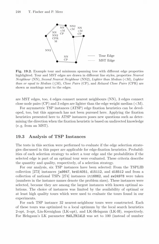
248 T. Fischer and P. Merz
NNNN2CPR
M
NN<MCP
NN2<M
NN2
NN<MCP
NNCP
Tour EdgeMST Edge
Fig. 19.2. Example tour and minimum spanning tree with different edge propertieshighlighted. Tour and MST edges are drawn in different line styles, properties NearestNeighbour (NN), Second Nearest Neighbour (NN2), Lighter than Median (<M), Lighterthan or equal to Median (≤M), Close Pairs (CP), and Relaxed Close Pairs (CPR) areshown as markings next to the edges.
are MST edges, too, 4 edges connect nearest neighbours (NN), 3 edges connectclose node pairs (CP) and 3 edges are lighter than the edge weight median (<M).
For asymmetric TSP instances (ATSP) edge fixation heuristics can be devel-oped, too, but this approach has not been pursued here. Applying the fixationheuristics presented here to ATSP instances poses new questions such as deter-mining the direction when the fixation heuristic is based on undirected knowledge(e. g. from an MST).
19.3 Analysis of TSP Instances
The tests in this section were performed to evaluate if the edge selection strate-gies discussed in this paper are applicable for edge-fixation heuristics. Probabil-ities of each selection strategy to select a tour edge and the probabilities if theselected edge is part of an optimal tour were evaluated. These criteria describethe quantity and quality, respectively, of a selection strategy.
For our analysis, six TSP instances have been selected: From the TSPLIBcollection [273] instances ja9847, brd14051, d15112, and d18512 and from acollection of national TSPs [274] instances it16862, and sw24978 were taken(numbers in the instance names denote the problem sizes). These instances wereselected, because they are among the largest instances with known optimal so-lutions. The choice of instances was limited by the availability of optimal orat least high quality tours which were used to evaluate the tours found in ourexperiments.
For each TSP instance 32 nearest-neighbour tours were constructed. Eachof these tours was optimized to a local optimum by the local search heuristics2-opt, 3-opt, Lin-Kernighan (LK-opt), and LK-Helsgaun (LK-H), respectively.For Helsgaun’s LK parameter MAX TRIALS was set to 100 (instead of number

19 Reducing the Size of TSP Instances by Fixing Edges 249
Table 19.1. Probabilities (in percent) for edges in a tour to match certain criteria.The data is grouped by TSP instance and tour type. The eight right most columnscontain the original and the conditional probabilities for the edge fixation heuristicsMST, altMST, NN, and NN2.
Tou
rTyp
e
P(O
PT)
P(M
ST)
P(O
PT|M
ST)
P(a
ltM
ST)
P(O
PT|a
ltM
ST)
P(N
N)
P(O
PT|N
N)
P(N
N2)
P(O
PT|N
N2)
ja9847
NN 64.90 75.70 75.93 88.26 71.72 61.91 77.51 83.33 72.342-opt 70.06 76.68 78.98 90.28 75.21 62.55 80.23 84.14 76.213-opt 74.81 78.39 81.49 92.20 78.38 64.34 82.30 85.42 79.67LK-opt 79.73 78.41 84.79 93.29 81.96 63.93 85.40 85.46 83.64LK-H 93.28 76.98 94.74 92.88 93.86 61.85 94.70 84.41 94.43optimal 100.00 75.92 100.00 92.47 100.00 60.30 100.00 83.72 100.00
brd14051
NN 59.34 70.44 73.38 85.64 67.60 58.38 74.75 83.46 66.582-opt 65.34 73.71 75.95 89.82 70.81 60.34 77.40 84.70 71.583-opt 70.79 76.41 78.72 92.51 74.42 62.75 79.81 86.39 75.78LK-opt 77.22 77.49 82.69 94.42 79.20 62.88 83.56 86.92 81.16LK-H 92.56 76.75 93.98 94.53 93.02 61.07 94.08 86.53 93.76optimal 100.00 75.50 100.00 93.94 100.00 59.28 100.00 85.65 100.00
d15112
NN 61.38 71.35 74.31 86.95 69.01 59.09 76.08 83.48 68.832-opt 66.05 73.63 76.12 90.19 71.28 60.47 77.78 84.56 72.393-opt 71.03 76.06 78.60 92.52 74.55 63.04 79.86 86.33 76.06LK-opt 76.88 77.13 82.17 94.27 78.85 63.17 83.31 86.83 80.96LK-H 92.46 76.25 93.78 94.37 92.87 61.33 94.07 86.40 93.81optimal 100.00 74.85 100.00 93.85 100.00 59.69 100.00 85.63 100.00
it16862
NN 61.44 72.35 74.39 86.89 68.87 60.12 76.05 82.87 69.152-opt 66.86 74.78 76.73 89.88 72.06 61.96 78.14 84.23 73.193-opt 71.89 76.95 79.29 92.06 75.49 64.23 80.38 85.80 76.96LK-opt 77.27 77.63 82.57 93.60 79.36 64.22 83.58 86.13 81.37LK-H 91.23 76.63 92.83 93.50 91.77 62.63 92.98 85.51 92.66optimal 100.00 74.98 100.00 92.79 100.00 60.58 100.00 84.43 100.00
d18512
NN 60.91 71.81 74.01 87.10 68.41 59.31 75.72 83.92 68.222-opt 65.83 74.24 76.02 90.43 70.95 60.67 77.62 84.76 72.143-opt 70.79 76.76 78.48 92.79 74.28 62.96 79.78 86.46 75.86LK-opt 77.17 77.68 82.53 94.59 79.10 62.91 83.58 86.83 81.22LK-H 92.68 76.83 94.06 94.67 93.16 61.10 94.19 86.41 93.99optimal 100.00 75.48 100.00 94.16 100.00 59.32 100.00 85.60 100.00
sw24978
NN 65.46 76.23 75.26 88.55 72.12 65.59 75.79 85.27 71.942-opt 68.22 75.62 76.95 90.23 73.18 64.25 77.71 85.26 73.863-opt 72.29 77.01 79.11 92.06 75.83 65.54 79.65 86.31 76.88LK-opt 76.72 77.04 82.03 93.33 78.92 64.53 82.67 86.14 80.72LK-H 90.32 76.16 92.11 93.28 90.94 62.93 92.14 85.52 91.86optimal 100.00 74.58 100.00 92.57 100.00 60.89 100.00 84.49 100.00

250 T. Fischer and P. Merz
Table 19.2. Probabilities (in percent) for edges in a tour to match certain criteria.The data is grouped by TSP instance and tour type. The eight right most columnscontain the original and the conditional probabilities for the edge fixation heuristics<M, ≤M, CP, and CPR.
Tou
rTyp
e
P(O
PT)
P(<
M)
P(O
PT|<
M)
P(≤
M)
P(O
PT|≤
M)
P(C
P)
P(O
PT|C
P)
P(C
PR)
P(O
PT|C
PR)
ja9847
NN 64.90 46.02 74.20 56.95 74.13 34.49 75.72 71.99 71.282-opt 70.06 45.42 78.05 56.80 77.63 32.46 78.90 71.04 75.553-opt 74.81 45.94 80.89 57.68 80.46 31.28 81.76 69.93 79.41LK-opt 79.73 45.68 84.43 57.35 84.02 29.90 84.94 68.44 82.95LK-H 93.28 44.45 93.81 56.02 93.84 27.00 94.81 64.68 94.17optimal 100.00 43.75 100.00 55.22 100.00 25.93 100.00 63.11 100.00
brd14051
NN 59.34 54.85 71.31 57.09 70.98 40.01 71.94 75.21 67.112-opt 65.34 53.38 74.98 55.60 74.68 38.40 75.70 74.60 72.163-opt 70.79 52.35 78.10 54.68 77.90 37.22 78.79 73.69 76.41LK-opt 77.22 52.15 82.51 54.60 82.27 35.18 83.10 71.91 81.02LK-H 92.56 48.57 93.73 51.21 93.72 31.73 93.93 68.21 93.38optimal 100.00 47.83 100.00 50.45 100.00 30.34 100.00 66.46 100.00
d15112
NN 61.38 54.65 72.14 55.42 72.02 39.61 73.51 75.62 68.532-opt 66.05 54.13 74.67 54.87 74.55 38.55 76.14 75.33 72.413-opt 71.03 53.60 77.72 54.44 77.64 37.68 79.05 74.70 76.33LK-opt 76.88 52.43 81.73 53.27 81.69 35.92 82.72 73.24 80.58LK-H 92.46 50.63 93.27 51.59 93.28 32.56 93.84 69.62 93.26optimal 100.00 49.79 100.00 50.75 100.00 31.25 100.00 67.79 100.00
it16862
NN 61.44 52.58 73.39 64.02 70.60 32.78 73.52 70.53 68.862-opt 66.86 53.85 76.32 64.34 74.45 30.64 76.44 69.26 73.233-opt 71.89 54.57 79.23 54.86 79.14 29.09 79.29 67.75 77.23LK-opt 77.27 53.45 82.71 53.90 82.62 27.38 82.88 65.56 81.12LK-H 91.23 51.22 92.48 51.80 92.46 24.15 92.92 61.49 92.24optimal 100.00 49.92 100.00 50.49 100.00 22.88 100.00 59.23 100.00
d18512
NN 60.91 55.37 72.60 58.62 72.38 39.19 73.23 74.74 68.502-opt 65.83 53.91 75.31 55.75 75.12 38.07 76.09 74.34 72.523-opt 70.79 53.20 78.22 55.07 78.04 37.13 78.90 73.50 76.45LK-opt 77.17 53.01 82.36 54.94 82.22 35.26 82.94 71.68 81.05LK-H 92.68 49.99 93.77 51.76 93.75 31.67 94.08 67.81 93.52optimal 100.00 49.06 100.00 50.83 100.00 30.34 100.00 66.10 100.00
sw24978
NN 65.46 42.58 74.52 58.33 74.34 24.92 74.93 66.03 71.122-opt 68.22 41.17 76.71 58.38 75.34 25.05 76.98 66.19 73.793-opt 72.29 41.80 78.86 59.56 77.58 24.31 79.16 65.15 77.07LK-opt 76.72 41.19 81.89 59.48 80.55 23.34 82.04 63.14 80.30LK-H 90.32 40.30 91.26 58.55 90.77 20.56 92.43 59.19 91.47optimal 100.00 39.15 100.00 57.46 100.00 19.36 100.00 57.07 100.00

19 Reducing the Size of TSP Instances by Fixing Edges 251
of cities). Totally, 960 tours were constructed to test the fixing heuristic whenapplied to tours of different quality levels.
Each heuristic’s selection scheme was applied to the set of 960 tours. Averagevalues over each set of 32 tours with the same setup were taken andsummarized in Tables 19.1 and 19.2. Here, the first column sets the instanceunder consideration. The ‘Type’ column determines in which local optimum thetours are located. Column ‘P(OPT)’ shows for a local optimal tour the percent-age of edges that also occur in the known global optimal tour. Columns ‘P(MST)’,‘P(altMST)’, ‘P(NN)’, ‘P(NN2)’, ‘P(<M)’, ‘P(≤M)’, ‘P(CP)’, and ‘P(CPR)’ con-tain the probability that an edge from a local optimal tour matches the given prop-erty. Columns ‘P(OPT|MST)’, ‘P(OPT|altMST)’, ‘P(OPT|NN)’, ‘P(OPT|NN2)’,‘P(OPT|<M)’, ‘P(OPT|≤M)’, ‘P(OPT|CP)’, and ‘P(OPT|CPR)’ contain condi-tional probabilities, that an edge in a local optimal tour is part of the global optimaltour, given that it matches the properties MST, altMST, NN, NN2, <M, ≤M, CP,or CPR, respectively.
19.3.1 Results of the Analysis
Column ‘P(OPT)’ shows the percentage of edges from a local optimal tour oc-curring in the global optimal tour. The better a tour construction and improve-ment heuristic works, the more edges the resulting tour has in common with theoptimal tour. Whereas tours constructed by a nearest neighbour constructionheuristic share about 60–65 % of all edges with optimal tours (depending onthe instance), tours found by subsequently applied local search algorithms arebetter, ranging from 65–70 % for 2-opt to more than 90 % for LK-H-opt tours.
As each edge selection strategy has different criteria how to select edges, theydiffer in the number of optimal edges. The most edges get chosen by the altMSTstrategy (column ‘P(altMST)’ in Table 19.1) selecting about 85–95 % of all touredges. Other strategies select less edges: From NN2 with 80–90 % and MST with70–80 % via CPR with 60–75 % and NN with 60–65 % down to ≤M, <M, andCP with 50–65 %, 40–55 %, and 20–40 % of all edges, respectively. The numberof selected edges is highest in most cases for strategies MST, altMST, NN, andNN2 when applied to 3-opt or LK-opt tours regardless of the TSP instance,whereas it is highest for strategies ≤M, <M, CP, and CPR when applied tonearest neighbour and 2-opt tours.
However, the quantity (number of edges selected for fixing) is not the onlycriterion to rate a selection strategy. Selected edges were checked whether theyoccur in the corresponding known optimal tour, too. When applying a fixingheuristic to a sub-optimal tour, a good heuristic should more likely select edgesthat occur in the optimal tour, too, rather than edges that do not occur in theoptimal tour. Therefore we were interested in the probability that a sub-optimaltour’s edge selected by an edge selection strategy would actually be containedin an optimal tour (‘true positive’) rather than being a ‘false positive’.
The quality of an edge selection strategy can be estimated by comparingits conditional probability (e. g. column ‘P(OPT|MST)’ for the MST heuristic)with the probability of an edge to part of an optimal tour (column ‘P(OPT)’). A

252 T. Fischer and P. Merz
selection strategy that randomly selects edges would have a conditional probabil-ity equal to ‘P(OPT)’, whereas a purposive strategy is expected to have higherprobability values. This property holds for each of our strategies. Furthermore,it can be observed that strategies with higher conditional probabilities selectless edges for fixation compared to selection strategies with lower conditionalprobabilities. E. g. for 2-opt tours of the instance d15112, the probability of anedge to be part of an optimal tour is 66.1 %. For the edge selection strategy NN,60.5 % of all edges would be selected, of which 77.8 % occur also in the optimaltour. By contrast, the edge selection strategy MST selects 90.2 % of the edges,but only 71.3 % of those are part of an optimal tour.
Generally, the value of ‘P(OPT)’ increases with tour quality. E. g. for instancesw24978, nearest neighbour tours share about 65 % of all edges with the optimaltour. This proportion increases with better tours up to LK-H optimized tourswhich share 90 % of all edges with the optimal tour.
19.4 Experimental Setup and Results
For the experimental evaluation, the fixing heuristics have been integrated intoa simple TSP solver written in Java. The solver works as follows: Each tourwas reduced using one of the fixing heuristics and subsequently improved byan iterated local search (ILS) algorithm. In each iteration of the algorithm thecurrent tour was perturbed and locally optimized by an LK implementation,enriched to handle fixed edges. For the perturbation a variable-strength double-bridge move (DBM) was used increasing the number of DBMs each two non-improving iterations. At the end of each iteration the new tour was comparedto the previous tour and discarded if no improvement was found, otherwisekept for subsequent iterations. The iterations would stop after 2 non-improvingiterations. Finally, the improved tour was expanded back to a solution for theoriginal TSP instance. This reducing and expansion procedure was repeated10 times on each solution. For comparison, all tours were optimized by theiterated local search algorithm without any reduction, too. This solver was notdesigned to compete with state-of-the-art solvers, but merely to evaluate ourfixation heuristics. Each parameter setup was tested by applying it to the toursdescribed in Sec. 19.3; average values were used for the following discussion.Computation times are utilized CPU time on a 3.0GHz Pentium 4 system with512MB memory running Linux.
Tables 19.3 and 19.4 hold the results for the different setups applied to theILS and are structured as follows: Rows are grouped by instance (ja9847 tosw24978) and by starting tour for the ILS (‘NN’ to ‘LK-H’). The instancesare ordered by number of cities, the starting tours are ordered by descendingtour length. Columns are grouped into blocks, where the first block summarizesan ILS setup without any fixation and the subsequent blocks summarize ILSsetups with each fixation heuristics (‘MST’ to ‘Second Nearest Neighbour’ and‘Light Median <’ to ‘Relaxed Close Pairs’). Each column block consists of fourcolumns: Improvement found when applying the ILS, required CPU time until

19 Reducing the Size of TSP Instances by Fixing Edges 253
Tab
le19
.3.
Res
ults
for
diffe
rent
setu
psof
inst
ance
,st
art
tour
,an
dfix
ing
heur
istics
.T
heda
tais
grou
ped
byT
SPin
stan
cean
dto
urty
pe.T
here
sult
colu
mns
are
grou
ped
into
five
bloc
ksfo
rth
efix
ing
heur
istics
‘No
Fix
ing’
,‘M
ST’,
‘Alter
nate
MST
’,‘N
eare
stN
eigh
bour
’,an
d‘S
econ
dN
eare
stN
eigh
bour
’co
nsisting
offo
urco
lum
nsea
ch:A
chie
ved
impr
ovem
ent
from
star
ting
tour
,ut
ilize
dC
PU
tim
e,fr
action
offr
eeed
ges
afte
rfix
ing
and
size
ofth
ere
duce
din
stan
ce(b
ased
onnu
mbe
rof
node
s).
No
Fix
ing
MST
Alt
ernate
MST
Nea
rest
Nei
ghbour
Sec
ond
Nea
rest
Nei
ghbour
Instance
StartTourType
Impr.[%]
CPUTime[s]
FreeEdges[%]
Red.Size[%]
Impr.[%]
CPUTime[s]
FreeEdges[%]
Red.Size[%]
Impr.[%]
CPUTime[s]
FreeEdges[%]
Red.Size[%]
Impr.[%]
CPUTime[s]
FreeEdges[%]
Red.Size[%]
Impr.[%]
CPUTime[s]
FreeEdges[%]
Red.Size[%]
ja9847
NN
22.7
164.2
––
20.8
19.3
55.9
40.9
17.2
8.1
55.4
22.6
22.0
40.6
54.4
69.8
19.9
13.2
53.9
32.2
2-o
pt
13.6
171.3
––
11.9
18.7
55.3
41.9
9.2
7.0
53.5
21.1
13.1
41.2
54.4
70.3
11.0
13.1
53.1
31.6
3-o
pt
6.1
162.6
––
4.7
16.4
54.7
43.0
3.1
4.9
52.4
19.4
5.6
38.0
54.3
70.9
4.0
10.4
52.3
31.3
LK
-opt
1.0
139.1
––
1.1
13.2
54.7
45.3
0.9
3.0
52.1
16.8
0.9
32.4
55.1
73.0
1.0
7.6
52.2
30.9
LK
-H0.0
77.0
––
0.0
7.7
54.1
44.5
0.0
1.6
51.7
15.0
0.0
19.5
54.8
72.4
0.0
4.2
51.7
28.6
brd14051
NN
23.2
128.5
––
20.9
21.4
56.6
46.5
16.0
7.9
55.4
24.2
22.4
45.3
55.3
72.5
19.2
13.8
54.5
34.4
2-o
pt
12.5
135.6
––
9.9
21.5
55.6
46.6
6.2
6.0
53.0
22.2
11.6
46.9
54.9
72.5
8.5
12.3
53.2
33.7
3-o
pt
6.0
139.8
––
3.9
19.1
55.1
47.3
2.0
4.0
51.9
19.6
5.1
46.2
54.8
72.6
2.9
9.9
52.4
33.3
LK
-opt
0.4
122.1
––
0.1
12.7
55.0
48.9
0.0
1.5
51.5
14.5
0.2
33.6
55.8
75.1
0.0
5.4
52.0
30.7
LK
-H0.0
56.7
––
0.0
7.7
54.3
45.4
0.0
1.0
50.9
11.8
0.0
20.4
55.1
73.8
0.0
2.9
51.5
25.6
d15112
NN
21.7
163.7
––
19.0
22.9
57.0
46.4
14.3
7.8
55.6
23.9
20.7
49.1
55.5
71.4
17.2
12.8
54.5
33.4
2-o
pt
11.7
171.1
––
9.0
23.4
56.0
47.2
5.4
5.8
53.1
22.0
10.6
51.7
55.2
71.8
7.5
12.1
53.2
33.2
3-o
pt
5.8
179.0
––
3.5
21.2
55.3
48.1
1.8
3.7
52.2
19.7
4.8
51.6
55.0
72.0
2.6
9.5
52.5
32.6
LK
-opt
0.5
160.9
––
0.0
13.6
55.2
49.5
0.0
1.4
51.7
15.0
0.1
37.6
56.0
74.6
0.0
5.1
52.1
30.2
LK
-H0.0
66.9
––
0.0
8.4
54.3
46.3
0.0
1.0
51.3
12.1
0.0
22.6
55.2
73.3
0.0
2.8
51.5
25.3
it16862
NN
22.3
241.1
––
19.7
35.0
56.2
45.1
15.3
13.1
54.9
24.2
21.4
70.2
55.1
70.0
18.1
21.7
53.7
33.7
2-o
pt
12.4
249.3
––
9.8
33.7
55.4
45.7
6.4
10.6
53.0
22.5
11.5
73.0
54.9
70.3
8.5
20.1
52.8
33.3
3-o
pt
5.9
250.4
––
3.8
30.7
54.9
46.4
2.0
7.1
52.1
20.5
5.1
71.8
54.7
70.4
2.9
16.0
52.2
32.9
LK
-opt
0.7
223.7
––
0.2
21.8
55.0
48.5
0.1
3.4
51.6
16.7
0.4
57.8
55.4
72.9
0.1
9.8
51.9
31.6
LK
-H0.0
96.6
––
0.0
11.7
54.4
46.0
0.0
1.8
51.3
14.2
0.0
30.9
55.0
71.8
0.0
5.0
51.5
27.7
d18512
NN
21.6
191.8
––
19.0
31.1
56.6
46.0
14.2
9.9
55.6
23.5
20.7
67.6
55.2
72.4
17.4
18.5
54.5
33.7
2-o
pt
11.4
202.0
––
8.8
30.8
55.7
46.8
5.1
7.4
53.0
21.9
10.5
72.0
55.0
72.7
7.4
17.5
53.2
33.6
3-o
pt
5.8
212.0
––
3.6
27.8
55.2
47.7
1.8
4.8
52.0
19.3
4.9
74.5
54.8
73.0
2.7
13.6
52.4
33.2
LK
-opt
0.4
187.9
––
0.0
18.8
55.0
49.0
0.0
1.8
51.5
14.4
0.1
51.5
55.8
75.4
0.0
7.5
52.0
30.7
LK
-H0.0
85.4
––
0.0
11.3
54.1
45.3
0.0
1.2
51.1
11.4
0.0
31.3
55.1
73.8
0.0
4.0
51.5
25.5
sw24978
NN
19.9
540.6
––
16.8
58.5
56.7
42.8
13.3
20.1
55.8
22.8
18.7
132.7
54.9
65.8
15.5
33.8
54.5
31.5
2-o
pt
11.6
588.5
––
9.0
65.5
55.9
45.0
6.1
16.6
53.4
21.9
10.5
147.8
54.9
67.5
7.9
35.5
53.2
32.4
3-o
pt
5.8
590.7
––
3.8
60.2
55.3
46.6
2.1
11.7
52.2
20.5
4.9
143.5
54.9
68.4
3.0
28.2
52.4
32.4
LK
-opt
0.5
474.0
––
0.1
39.3
55.3
49.2
0.0
5.0
51.8
17.4
0.3
103.7
55.9
71.7
0.1
16.2
52.1
31.7
LK
-H0.0
196.3
––
0.0
22.2
54.6
47.0
0.0
2.9
51.4
14.7
0.0
54.5
55.3
70.8
0.0
8.3
51.5
28.0

254 T. Fischer and P. Merz
Tab
le19
.4.
Res
ults
for
diffe
rent
setu
psof
inst
ance
,st
art
tour
,an
dfix
ing
heur
istics
.T
heda
tais
grou
ped
byT
SPin
stan
cean
dto
urty
pe.T
here
sult
colu
mns
are
grou
ped
into
five
bloc
ksfo
rth
efix
ing
heur
istics
‘No
Fix
ing’
,‘L
ight
Med
ian
<’,
‘Lig
htM
edia
n≤
’,‘C
lose
Pai
rs’,
and
‘Rel
axed
Clo
sePai
rs’co
nsisting
offo
urco
lum
nsea
ch:A
chie
ved
impr
ovem
ent
from
star
ting
tour
,ut
ilize
dC
PU
tim
e,fr
action
offr
eeed
ges
afte
rfix
ing
and
size
ofth
ere
duce
din
stan
ce(b
ased
onnu
mbe
rof
node
s).
No
Fix
ing
Lig
ht
Med
ian
<Lig
ht
Med
ian
≤C
lose
Pair
sR
elaxed
Clo
sePair
s
Instance
StartTourType
Impr.[%]
CPUTime[s]
FreeEdges[%]
Red.Size[%]
Impr.[%]
CPUTime[s]
FreeEdges[%]
Red.Size[%]
Impr.[%]
CPUTime[s]
FreeEdges[%]
Red.Size[%]
Impr.[%]
CPUTime[s]
FreeEdges[%]
Red.Size[%]
Impr.[%]
CPUTime[s]
FreeEdges[%]
Red.Size[%]
ja9847
NN
22.7
164.2
––
22.2
59.7
76.5
73.3
21.8
42.9
71.6
63.2
22.3
110.5
73.2
100.0
20.8
42.6
51.6
68.0
2-o
pt
13.6
171.3
––
13.2
59.3
76.4
73.4
13.1
44.1
71.5
62.9
13.5
111.6
73.3
100.0
11.9
42.6
51.7
68.4
3-o
pt
6.1
162.6
––
5.9
55.9
76.4
73.4
5.7
40.6
71.4
62.7
6.2
107.8
73.4
100.0
5.0
36.8
51.9
69.1
LK
-opt
1.0
139.1
––
1.2
48.7
76.5
73.7
1.5
33.1
71.6
63.0
1.1
94.3
73.6
100.0
0.7
25.5
52.3
69.7
LK
-H0.0
77.0
––
0.0
27.4
76.5
73.5
0.0
19.4
71.5
62.7
0.0
53.0
74.1
100.0
0.0
17.9
52.6
70.0
brd14051
NN
23.2
128.5
––
21.7
50.1
73.7
68.7
21.6
47.6
72.7
66.6
23.1
105.3
68.9
100.0
20.9
48.8
50.4
64.4
2-o
pt
12.5
135.6
––
11.2
49.9
73.8
68.4
11.0
47.4
72.8
66.0
12.4
105.5
68.9
100.0
10.2
46.6
50.4
64.9
3-o
pt
6.0
139.8
––
5.1
49.2
74.2
68.6
5.0
43.8
72.9
65.8
5.9
109.4
68.9
100.0
4.2
38.9
50.5
65.6
LK
-opt
0.4
122.1
––
0.3
36.8
74.3
67.9
0.2
33.7
73.3
65.6
0.4
82.6
69.2
100.0
0.1
21.3
50.6
66.4
LK
-H0.0
56.7
––
0.0
23.0
75.7
69.1
0.0
21.5
74.5
66.7
0.0
43.8
69.6
100.0
0.0
14.8
50.6
66.2
d15112
NN
21.7
163.7
––
20.1
52.3
75.4
66.7
20.0
50.5
75.2
65.8
21.5
118.3
68.3
100.0
19.0
50.4
50.1
62.0
2-o
pt
11.7
171.1
––
10.3
53.4
75.4
66.8
10.2
51.6
75.1
65.8
11.5
128.6
68.3
100.0
9.0
47.9
50.1
62.6
3-o
pt
5.8
179.0
––
4.7
51.5
75.5
66.8
4.7
49.0
75.2
65.9
5.5
121.4
68.3
100.0
3.7
38.2
50.2
63.4
LK
-opt
0.5
160.9
––
0.2
37.6
75.8
66.4
0.2
35.7
75.5
65.5
0.3
97.3
68.5
100.0
0.0
21.0
50.2
64.1
LK
-H0.0
66.9
––
0.0
22.2
76.3
65.9
0.0
21.5
76.0
64.9
0.0
49.3
68.9
100.0
0.0
15.4
50.2
63.8
it16862
NN
22.3
241.1
––
21.3
89.4
71.5
70.7
19.5
55.0
67.7
55.6
22.3
190.9
75.9
100.0
20.4
93.5
52.6
72.1
2-o
pt
12.4
249.3
––
11.7
89.1
71.5
70.5
11.6
86.4
71.0
68.8
12.4
203.8
76.1
100.0
10.6
90.4
52.8
72.7
3-o
pt
5.9
250.4
––
5.4
85.8
71.6
70.7
5.3
85.6
71.4
69.7
5.9
198.2
76.2
100.0
4.6
80.8
53.1
73.6
LK
-opt
0.7
223.7
––
0.6
69.0
71.5
70.2
0.5
67.6
71.5
69.6
0.7
176.9
76.4
100.0
0.2
50.1
53.7
74.8
LK
-H0.0
96.6
––
0.0
35.2
71.6
70.1
0.0
34.6
71.5
69.4
0.0
77.4
77.2
100.0
0.0
31.2
54.1
75.2
d18512
NN
21.6
191.8
––
20.2
77.8
73.0
70.1
20.0
71.7
71.7
67.4
21.5
162.1
68.9
100.0
19.3
75.4
50.5
64.9
2-o
pt
11.4
202.0
––
10.2
78.5
73.0
70.1
10.1
73.7
72.3
68.3
11.3
168.8
68.9
100.0
9.1
73.9
50.5
65.4
3-o
pt
5.8
212.0
––
4.9
74.7
73.1
69.9
4.8
72.4
72.4
68.1
5.6
166.7
68.9
100.0
4.0
59.9
50.5
66.2
LK
-opt
0.4
187.9
––
0.2
56.5
73.3
69.8
0.2
53.5
72.5
67.9
0.3
133.0
69.2
100.0
0.0
32.7
50.7
67.0
LK
-H0.0
85.4
––
0.0
32.4
73.5
69.3
0.0
30.7
72.8
67.5
0.0
67.3
69.7
100.0
0.0
23.2
50.8
66.7
sw24978
NN
19.9
540.6
––
19.2
219.7
77.4
77.3
18.5
128.9
71.4
61.7
19.9
462.8
79.8
100.0
18.2
213.0
54.1
74.5
2-o
pt
11.6
588.5
––
11.1
244.4
77.2
78.2
10.3
135.4
71.1
61.4
11.7
472.2
79.7
100.0
9.9
213.3
54.2
74.6
3-o
pt
5.8
590.7
––
5.4
234.0
77.0
78.5
4.8
126.3
71.0
61.2
5.9
481.3
79.8
100.0
4.6
176.3
54.5
75.5
LK
-opt
0.5
474.0
––
0.4
186.6
77.1
79.6
0.3
92.0
71.1
61.3
0.6
389.5
80.0
100.0
0.1
108.3
55.2
76.6
LK
-H0.0
196.3
––
0.0
87.4
76.9
79.2
0.0
48.1
71.1
60.0
0.0
163.5
80.6
100.0
0.0
64.7
55.7
77.1

19 Reducing the Size of TSP Instances by Fixing Edges 255
termination, size of the reduced instance (normalized to number of cities), andfraction of edges that are fixed (tabu for any ILS operation).
For every instance and each fixing heuristics (including no fixing) holds thatthe better the starting tour is, the smaller are the improvements found by theILS. Applying our TSP solver to nearest neighbour tours (Tables 19.3 and 19.4,rows with start tour type ‘NN’) results improvements of about 15–20 % formost setups (columns ‘Impr. [%]’). For better starting tours, less improvementis achieved, down to improvements of 0 % for starting tours coming from LK-H.
Each fixing ILS setup can be compared with the corresponding ILS setupwithout fixing regarding improvement on the given start tour and the requiredCPU time. The following observations can be drawn from Tables 19.3 and 19.4:
• For non-fixing setups, the CPU time is always higher compared to fixingsetups, as the effective problem size is larger for the non-fixing setup. How-ever, time consumption does not directly map to better tour quality.
• The Close Pairs (CP) fixing heuristic yields in improvements as good asfor non-fixing ILS, but requires significantly less time to reach these qualitylevels. E. g. for instance brd14051 starting with 3-opt tours, both the non-fixing ILS and the CP fixing ILS improve the start tour by about 6 %, but theCP variant requires only 109.4 s, whereas the non-fixing ILS requires 139.8 s.
• For the other fixing heuristics hold that they consume both less CPU time andresult in less improvements compared to the Close Pairs heuristic. Althoughthis makes comparing the different fixing strategies hard, improvements arestill competitive while requiring significantly less CPU time compared to thenon-fixing ILS.
• Among all fixation-based ILS setups, the Alternate MST heuristic results inboth the smallest improvements and lowest running times compared to theother fixation heuristics. E. g. for instance sw24978 starting with 2-opt tours,the Alternate MST heuristic results in an improvement of 6.1 % consuming16.6 s, whereas the next closest heuristic (Second Nearest Neighbour) findsimprovements of 7.9 % consuming 41.0 s.
Comparing CPU time consumption versus possible improvement, the fixationheuristics can be put into three groups as visualized Fig. 19.3, which comparesthe improvements for each fixing heuristics applied to 3-opt tours. Both timeand improvement are normalized for each of the six TSP instances by the valuesfrom the runs without fixing.
1. The ‘expensive’, but good Close Pairs heuristic reaching improvements asgood as the non-fixing ILS requiring only 3/4 of the time.
2. The ‘medium’ heuristics Relaxed Close Pairs, NN, ≤M and <M with nor-malized improvement above 75 % and normalized time of less than 50 %.
3. The ‘cheap’, but not so good heuristics (Alternate MST, Second NN, andMST) each having a normalized time of less than 25 % (quarter of the CPUtime) and a normalized improvement of about 35 %, 50 %, and 65%, respec-tively. The outlier of each of the three heuristics are due to instance ja9847.

256 T. Fischer and P. Merz
0.25
0.5
0.75
1
0.000 0.250 0.500 0.750 1.000
Nor
mal
ized
Impr
ovem
ent
Normalized Time
MSTMST2
NNNN2LM <
LM <=CP
CPRNo fixation
Fig. 19.3. For each of the six instances using 3-opt starting tours, improvements andCPU time of the ILS with fixation (MST, Alternate MST, NN, Second NN, <M, ≤M,CP, and Relaxed CP) are normalized with the results from ILS runs without fixation
Relaxed Close Pairs performs worst in the group of ‘medium’ heuristics bridgingthe gap to the ‘cheap’ heuristics.
For all fixing heuristics the size of the original instance has been compared tothe corresponding reduced instances’ size (in percent, columns ‘Red. Size [%]’ inTables 19.3 and 19.4) and the number of free edges within the reduced instance(in percent, columns ‘Free Edges [%]’).
• In most cases, the number of free edges and the reduced instances’ size isabout the same for each combination of instance and fixing heuristic, regard-less of the starting tour type.
• For Close Pairs (CP) fixations holds that the reduced instance’s size equalsalways the original instance’s size, as fixed edges can not have neighbouringedges that are fixed, too, as this would contradict the selection criterion.Thus, no nodes are redundant.
• For all combinations of instance and start tour, the Alternate MST fixingheuristic is the most progressive one resulting in the smallest instances. Here,fixed instances have on average less than the quarter the number of citiescompared to the original instances. Within these reduced instances, morethan half of the edges are free for the local search. E. g. for instance d15112and 3-opt tours, only 19.7 % of the original nodes are left, whereas comparableheuristics leave e. g. 32.6 % (Second NN) or 48.1 % (MST).
• The Nearest Neighbour heuristic reduces most instance types for about thesame level (to 70–75 % of the original size); instance sw24978 has a rela-tive size of 65.8 % to 70.8 %. Similar observations can be made for the Sec-ond Nearest Neighbour heuristic which reduces that instance size to about

19 Reducing the Size of TSP Instances by Fixing Edges 257
30–35 % except for setups starting from LK-H tours, which get reduced toless than 30 % of their original size.
• The Nearest Neighbour, Second Nearest Neighbour, MST and Alternate MSTheuristics have very stable percentages of free edges. For the Nearest Neigh-bour and the MST heuristics, the values range only between 54.3 % to 56.0 %and 54.1 % to 57.0 %, respectively. For the Second Nearest Neighbour heuris-tic and Alternate MST, these values are only marginally smaller rangingbetween 51.5 % to 54, 5 % and 50.9 % to 55.8%, respectively.
• The Lighter than Median heuristic leaves about 70–75 % of all edges freefor modification. The similar, but more greedy Lighter or equal to Medianheuristic leaves, depending on instance, about the same percentage of edgesavailable (instances d15112, it16862, and d18512) or a smaller fraction (in-stances ja9847, brd14051, sw24978).
• The Close Pairs fixing heuristic leaves between 68–81 % of all edges free(depending on instance), which results in the largest absolute number of freeedges among all fixing heuristics considering that reduced instances have thesame size as the original instance.
• The Relaxed Close Pairs fixing heuristic has the smallest proportion of freeedges among all fixing heuristics (about 50–55 %). The reduced instances’ sizediffers among instances from 62.0–64.1 % (instance d15112) to 74.5–77.1 %(instance sw24978).
As discussed, the proposed edge selection heuristics offer a range of choicesfor reducing the search space and thus affecting the expected solution quality.Selection heuristics which are very progressively (Alternate MST, Second NN,and MST) may considerably reduce the computation time to find a local opti-mum but this greediness will notably reduce the gain of the local search. Otherheuristics that are more selective (e. g. Close Pairs) fix less edges and thus allowthe local search to exploit a larger search space which still requires less timecompared to a local search in the original instance. Accepting a minor decreasebut achieving a considerable saving in time is interesting when using the problemreduction algorithm as part of a metaheuristic such as a memetic algorithm oran ant colony optimization algorithm.
19.5 Conclusion
In order to extend current memetic algorithms for the TSP to find close to opti-mum solutions for large TSP instances, we studied several edge-based problemreduction techniques that can easily be incorporated into an evolutionary localsearch framework. We have shown that fixing edges in TSP tours can consid-erably reduce the computation time of a TSP solver compared to applying thesame solver to the unmodified problem instance. Still, the solutions found whenusing fixing heuristics are nearly as good as the solutions found without fixing.Therefore, edge fixing is a feasible approach to tackle tours that are otherwisetoo large for solvers regarding memory or time consumption.

258 T. Fischer and P. Merz
When selecting one of the proposed fixing heuristics, a trade-off between ex-pected solution quality, computation time, or required preprocessing steps hasto be made. E. g. the Alternate MST heuristic is expected to consume the leasttime, but requires building two MSTs in advance and has the worst results amongall fixing heuristics. Better results can be expected e. g. from the MST heuristic,which requires building only one MST. The Close Pairs strategy can be used ifno global knowledge is available, but here too few edges get fixed to decreasean instance’s size considerably. As a compromise regarding time and quality,either the Nearest Neighbour (NN), the Lighter or equal to Median (≤M), orthe Lighter than Median (<M) heuristics can be applied.

16
Algorithms for Large Directed Capacitated ArcRouting Problem InstancesUrban Solid Waste Collection Operational Support
Vittorio Maniezzo and Matteo Roffilli
Department of Computer Science, University of Bologna, Italyvittorio.maniezzo,[email protected]
Summary. Solid waste collection in urban areas is a central topic for local environ-mental agencies. The operational problem, the definition of collection routes given thevehicle fleet, can greatly benefit of computerized support already for medium sizedtown. While the operational constraints can vary, the core problem can be identifiedas a capacitated arc routing problem on large directed graphs (DCARP). This paperreports about the effectiveness of different metaheuristics on large DCARP instancesderived from real-world applications.
Keywords: Combinatorial Optimization, Capacitated Arc Routing, Problem Reduc-tion, Metaheuristics, Data Perturbation, Garbage Collection.
16.1 Introduction
The widely acknowledged increase in solid waste production, together with theincreased concern about environmental issues, have led local governments andagencies to devote resources to solid waste collection policy planning. The prob-lem, difficult per se, is further complicated by differential collection and recyclingpolicies: this leads to scenarios where manual planning of waste collection caneasily yield severely inefficient solutions. It is known in fact that an efficient plan-ning can have a significant impact on the overall costs of solid waste collectionlogistics [275].
Waste collection, as most logistic activities, can be studied at different levels:strategical, tactical, operational. In this work we concentrate on operationalplanning, where a vehicle fleet and the service demand are given and the objectiveis to design the vehicle trips in order to minimize operational costs subject toservice constraints.
Specifically, this work derives from an experience of decision support for thewaste collection sectors of municipalities of towns with about 100000 inhabitants,with the objective of designing vehicle collection routes subject to a number ofoperational constraints. The reported results are for an abstraction level whichdoes not consider several very specific issues, such as union agreements, third-party or personal contracts, etc. The problem to solve is modeled as a Capaci-tated Arc Routing Problem (CARP) on a directed graph and solved accordingly.
C. Cotta and J. van Hemert (Eds.): Recent Advances in Evol. Comp., SCI 153, pp. 259–274, 2008.springerlink.com c© Springer-Verlag Berlin Heidelberg 2008

260 V. Maniezzo and M. Roffilli
The instances to be solved are bigger than the state of the art ones. Originalheuristic approaches had to be designed in order to meet the solution quality andthe allowed computation time specifications. The reported results have a rele-vance beyond the specific application, as several activities of real-world relevancecan be modeled as CARP: foremost among them are mail collection or delivery,snow removal, street sweeping. The CARP is in fact a powerful problem model,which was originally proposed by Golden and Wong [276], and which, given itsactual interest, have then been studied by many researches. Dror [277] collecteda significant number of applications of CARP variants and of correspondingsolution methodologies. For a survey the reader is also referred to [278].
In the literature, several heuristic approaches have been proposed for theCARP, while the only exact techniques so far were published by Hirabayashiet al. [279], who proposed a Branch and Bound algorithm and by Baldacciand Maniezzo [280], who transformed CARP instances into Capacitated VehicleRouting Problem (CVRP) equivalents and proceeded solving these last. More-over, Belenguer and Benavent [281] and recently Wøhlk [282] proposed effectivelower bounds.
However, being CARP NP-hard, exact techniques can seldom cope with thedimension of real-world instances. These call for heuristic and metaheuristicapproaches: among the most recent proposals we remind the tabu search of Be-lenguer et al. [283], the tabu search of Hertz et al. [284], the Variable Neighbor-hood Descent VND-CARP of the same authors [285] and the genetic algorithmof Lacomme et al. [286]. For a recent review, see [287].
As for more real-world oriented researches, we remind the work of Amberg etal. [288], who studied the M-CARP, that is a multidepot CARP with heteroge-neous vehicle fleet, by means of a tabu search, of Xin [289], who implementeda decision support system for waste collection in rural areas based on a simpleAugment-Merge heuristic, of Snizek et al. [290] dealing with urban solid wastecollection and of Bodin and Levy [291].
The general strategy adopted in this work is that of translating CARP intonode routing problem instances and then studying solution methodologies forthe resulting data. Different approaches were compared, both directly applied toCARP data and to node routing translations. Among those, the most effectiveone is based on data perturbation [292] coupled with Variable NeighborhoodSearch (VNS) and acting on a node routing problem reformulation.
The paper is structured as follows.Section 16.2 introduces the problem of urban solid state waste collection and
its reduction to directed CARP. Section 16.3 presents the methodology we used,first transforming DCARP into Asymmetric CVRP (ACVRP) instances, thenapplying three variants of VNS to the resulting instances. Section 16.4 reportsabout the computational results we obtained, both on standard CARP test setsand on DCARP instances derived from real-world applications. Finally, Section16.5 contains the conclusions of this work.

16 Algorithms for Large Directed CARP Instances 261
ONE-WAY
A
B
C
D
1 2
3
4
5 6
7
8
Fig. 16.1. Conversion of a road network into a graph. Bin C can be emptied only bya vehicle which travels the directed arc (3, 4). Bin D can be emptied only by a vehiclewhich travels the directed arc (6, 7). A vehicle travelling along the one-way arc (1, 2)can empty both bin A and B.
16.2 Urban Solid State Waste Collection
The problem is defined over the road network of the town to support. Thenetwork is used as a basis for geocoding all problem elements, which are:
• one or more depots, where vehicles are stationed;• landfills and disposal plants, where waste has to be brought;• waste bins, which are usually specialized for differential collections. In our
examples, we had the following waste types: i) undifferentiated; ii) plastics;iii) glass; iv) paper; v)biologic or organic.
A number of vehicles are available, where each vehicle can load only bins ofgiven types and has a capacity specified as a maximum number of bins. Theactual problem faced asks for designing the routes of the available vehicles, inorder to collect all specified bins, satisfying capacity and bin compatibility con-straints, forbidding partial bin collection, with the objective of minimizing thetotal travel distance. Moreover, bins can be collected only within given timewidows.
Bins are set in an urban context, which can be modeled by means of a directedgraph. One way streets and forbidden turns have to be considered. Each bin ismoreover set on one specific side of the street. A vehicle driving along a streetcan usually collect all bins of a compatible type on the right side of that street.In case of one-way streets, the vehicle can instead collect both bins on the rightand on the left side of the street, if adequately equipped.
Figure 16.1 hints at some issues of urban bin collection when modeled on agraph.

262 V. Maniezzo and M. Roffilli
This work reports about an optimization procedure for an abstract version ofthe general problem, in that we consider only one depot and one disposal facilityper waste type. Moreover, time windows are not considered and the number ofvehicles is an input parameter and not a decision variable, thus the objectivefunction is only given by the total distance traveled. However, the extension toactual settings is a lesser effort when compared to the ability of solving the coreproblem for actual dimension. This problem can be formulated as an extension ofa well known problem from the literature: the Capacitated Arc Routing Problem.
16.2.1 Capacitated Arc Routing Problem
CARP was originally proposed by Golden and Wong [276] and is usually studiedin a version which would correspond to an instance of the waste collection prob-lem with a single depot, a single disposal unit coincident with the depot, onlyone bin type, a non-heterogeneous fleet and no temporal constraints. Moreover,the graph is undirected and bins are positioned on an arc, not on one side of anarc. Different mathematical formulations have been proposed for this version ofthe CARP ( [276], [281], [278]), all of them for the undirected case. The problemwe have to solve is however characterized by the fact that the road network ofinterest must be modeled as a directed graph, thus the problem to solve is aDirected CARP (DCARP). We can take advantage of this in the mathematicalformulation of the problem.
16.2.2 Transformation into an ACVRP
The huge dimension of the graphs we had to deal with, rules out the possibil-ity to apply either exact methods or sophisticated heuristics. Our approach forsolving the DCARP instances is based on their transformation into AsymmetricCapacitated Vehicle Routing Problem instances. CARP and CVRP are in factclosely related, the main difference being that in the CARP clients are set onarcs while in the CVRP clients are set on the nodes.
The CVRP has been more thoroughly studied in the literature and, eventhough instances of our size are still out of the current state of the art, efficientheuristics are available for instances bigger than the CARP ones.
The possibility to transform a CARP instance into a CVRP one is well-known,having been first proposed in the literature by Pearn et al. [293]. This transforma-tion, when applied to a CARP defined on a graph with m mandatory edges, re-sults in a CVRP with 3m + 1 nodes. More recently, Baldacci and Maniezzo [280]presented an alternative transformation which results in a CVRP with 2m + 1nodes.
This transformation is of general validity, however, we can take advantage ofthe need to work on digraphs and use a modified approach which transforms aDCARP instance in an ACVRP one, by simply associating with each DCARPmandatory arc an ACVRP node which inherits the arc demand, by maintainingthe depot node, and by redefining distances according to the formulation ofsection 16.2.1.

16 Algorithms for Large Directed CARP Instances 263
Specifically, we compute the all pairs shortest paths matrix among every out-going vertex j, including depot node 0, and every incoming vertex h, includingdepot node 0, for each pair of nodes (ij), (hl) ∈ R, being R the set of mandatoryarcs. We then add the cost cij , (ij) ∈ R, to the cost dist(ij) of each path exitingfrom j. This results in a graph with m + 1 nodes and O(m2) arcs, which definesan instance of ACVRP having the solution set which can be mapped 1 to 1 intoequivalent DCARP solutions.
In the case of our application, the transformation function parses a DCARPinstance and rewrites it as an equivalent ACVRP instance having:
- the same vehicle set with the same capacity constraints;- the objective function defined over the cost matrix as computed above;- multiple routes per vehicle, where the first one starts from the depot and
ends at the disposal, all other ones start and end at the disposal except forthe last one, which starts at the disposal and ends at the depot;
- vehicle objections associated to each client: clients associated to nodes cor-responding to two-ways roads can be serviced by any vehicle, while clientsassociated to nodes corresponding to one-way roads can be serviced only byvehicles which can load bins both from their left and from their right side.
Figure 16.2 shows the transformation on a simple graph.
5
0
12
4
7
6
9
8
11
10
3
0
3,7
10,11
4,8
1,2
Fig. 16.2. CARP→CVRP. a) DCARP graph. b) ACVRP graph (all edges are pairsof arcs).
Since the ACVRP graph has a number of nodes corresponding to the numberof clients of the DCARP instance, in the waste collection case we get a smallergraph than the original road network. The computational complexity is notdetermined by the road network graph, but by the number of clients.
16.3 New Metaheuristics
Unfortunately, the size of the ACVRP instances of interest for us are very big(hundreds or thousands of nodes) thus all but very simple heuristics are ruled

264 V. Maniezzo and M. Roffilli
out. We implemented three such heuristics; all of them make use of a local searchprocedure based on the following neighborhoods:
1. move of a client within one same route;2. move of a client from a route to another;3. swap of two clients within one same route;4. swap of two clients of different routes;5. 3-opt within one same route;6. single point route crossover [286].
The basic approach we used for solving the ACVRP instances was a modifiedIterated Variable Neighborhood Search. Variable Neighborhood Search (VNS) isan approach proposed by Mladenovic and Hansen [294], whose basic frameworkis the following:
Algorithm 16.1. Variable Neighborhood Search(Initialization)Define the set of neighborhood structures Nk, k = 1, ...., kmax to be used duringsearch.Generate an initial solution x.repeat
k = 1repeat
(Shaking)Randomly generate a solution x′ in the k-th neighborhood of x, x′ ∈ Nk(x)k=1(Local search)Find the local optimum x′ using neighborhood k.if x′ is better than x then
x = x′
k = 1else
k = k + 1end if
until k > kmax
until (termination condition)
Notice that the Shaking at line 7 implements a search diversification whichpermits to escape form cyclic dynamics. The way shaking is implemented deeplyaffects the algorithm performance. We implemented three different shakingstrategies: i) random multistart, ii) a genetic algorithm and iii) data pertur-bation.
Before describing the three variants, we present the initial solution construc-tion procedure, which is common to the three of them. To construct initialsolutions we used a two phase algorithm [295] because it is fast and consistentlyproduces solutions of reasonable quality.

16 Algorithms for Large Directed CARP Instances 265
16.3.1 Two Phase Construction Algorithm
The two phase algorithm [295], constructs a solution in two different ways, oneper phase, starting from the same pivots. We remind that a pivot is the firstclient assigned to a vehicle, its proper choice is essential for the construction ofa good route as it determines the area where the vehicle will operate. Usually,pivots are chosen as the customers hardest to service, therefore nodes whichhave high requests, which are far from the depot, which are far from previouslyconsidered routes, etc. The two phases share only the pivot set and are other-wise independent from one another. The solution proposed is the best amongthe two obtained. The first phase is a standard parallel construction based onextramileage criteria. The pseudocode is as follows.
Algorithm 16.2. Phase 1for each vehicle k = 1, . . . , K, choose a pivot and initialize one routeq = n − K /*number of unserviced clients*/while (q > 0) do
Compute the extra mileage for inserting each client in each position of each routeInsert the best client in the best position of the best routeq = q − 1
end while
The second phase, which tries to use implicit dual information obtained fromthe solution of the first, is more involved and is as follows.
Algorithm 16.3. Phase 2Use the same K pivots as in phase 1Initialize a route for each pivot: let p(h) be the pivot of route h, h = 1, . . . , KCompute the extramileage e(i, h) for inserting client i in route h, for eachunserviced client i and for each route h:e(i, h) = c0i + cip(h) − cp(h)0
let hmin be the route for which e(i, h) is minimizedlet hsec be the route for which e(i, h) is the second minimumFor each client i, compute the regret g(i) which estimates the cost for inserting i inhis second-best tour:g(i) = e(i, hsec) − e(i, hmin)Order the clients by decreasing regrets g(i), i = 1, . . . , nrepeat
take the client with highest regret still unserviced and insert it in the bestpossible route (hmin, hsec, . . .)
until all clients are serviced

266 V. Maniezzo and M. Roffilli
16.3.2 Multistart Algorithm
This is a straightforward repeated local search algorithm, where at each iterationsearch is started from a different seed solution, constructed independently fromthose constructed before. The pseudocode is as follows.
Algorithm 16.4. Multistart algorithmS = ∅, f(S) = ∞repeat
Construct solution S1 with the Phase 1 of the Two Phase algorithmApply VNS to S1 obtaining S′
1
if (f(S′1) < f(S)) then
S = S′1
end ifConstruct solution S2 with the Phase 2 of the Two Phase algorithmApply VNS to S2, obtaining S′
2
if (f(S′2) < f(S)) then
S = S′2
end ifuntil termination conditionreturn S
The key to the Multistart (MS) algorithm is its ability to start from differentseed solutions. The seed solutions are constructed by the multistart algorithm,which in turns depends on the pivots choice. We used a probabilistic node diffi-culty quantification function in order to get different seed solutions. The functionis given by the following formula:
(difficulty degree) q(i) = αdi + β
(c0i +
∑k∈U
cik
)(16.1)
where di is the weight of node i, cij is the distance between nodes i and j andU is the set of already chosen pivots. α and β are two user-defined parameters.
Given the difficulty degrees, the actual pivot choice is demanded to a monte-carlo extraction.The termination condition is the disjunction of:
- Elapsed CPU time is grater than a given limit;- Number of iterations is greater than a given limit;- The best solution cost is equal to a (known) optimal value.
The user parameters for this algorithm are the following:
1. limit to maximum CPU time;2. limit to maximum number of iterations;3. maximum number of vehicles;4. vehicle capacity;5. parameters in the pivot choice function.

16 Algorithms for Large Directed CARP Instances 267
16.3.3 Genetic Algorithm
The multistart algorithm has no dependencies among the different seed solu-tions. As an alternative, we designed a Genetic Algorithm (GA) [296] to let theevolution learn the best pivot set. The implemented GA has a very standardstructure, based on selection (roulette wheel), crossover and mutation. The indi-viduals encode which, among the different clients, are chosen to be pivot in theresulting solution. The individual is encoded as a binary string, with as manybits as clients and a bit set to 1 if the corresponding client is a pivot. The pop-ulation is randomly initialized with individuals with a number of 1s, that is anumber of routes, estimated as follows:
(number of pivot) numpivot =⌈
K∑n
i=1 di∑Kj=1 Cj
⌉(16.2)
where Cj is the capacity of vehicle j. Mutation and crossover operators arestandard (random mutation, two points crossover), with the only caution thatthe number of 1s of each individual is restored to numpivot in case it is changed.Having defined the pivots, the remaining of the algorithm is as described for themultistart, with two phase to construct solutions and VNS to optimize them.
Algorithm 16.5. Genetic AlgorithmEstimate the number of pivots: numpivotGenerate a population P of dimPop individualsEach individual has numpivot randomly chosen bits set to 1repeat
for all individual i ∈ P doConstruct a solution s with the Two Phase algorithm using the pivots in iApply VNS to s obtaining s′
end forfor all individual i ∈P do
compute the fitness as a function of the cost of s′
end forGenerate a new population P ′ from P by selection, crossover and mutationP = P ′
until termination condition
Termination condition and parameters are the same as in MS, with three more:
1. population dimension;2. crossover probability;3. mutation probability.
To transform costs (to be minimized) into fitness (to be maximized) we usedDynamic Fitness Scaling [297].

268 V. Maniezzo and M. Roffilli
16.3.4 Data Perturbation
Data Perturbation (DP) is a technique originally proposed by Codenotti et al.[292] which can be framed within an Iterated Local Search approach [298] withthe objective of modifying in a controlled way the successive starting solutions.Whereas the more usual approach in VNS is to modify a solution in order to getthe new starting one, DP suggests to modify input data. Several works adoptedthis approach, see for example [299], [300], [301].
If P ′ is the result of the perturbation of instance P , it is possible to definean injective function f : P → P ′ which associates each element of P with anelement of P ′. Given f(S), where S is a local optimum of P obtained by somelocal search, a perturbated solution S′ can be obtained as S′ = f(S). It is nowpossible to apply to S′, which is not necessarily a local optimum for P ′, thelocal search on the perturbed data, thus obtaining S′′. Finally, going back to theoriginal instance P it is possible to construct the solution T as T = f−1(S′′).Again, T usually is not a local optimum for P , thus applying the local searchwe get a new local optimum T ′ for the original instance. This procedure can beapplied iteratively. Perturbation was originally presented for the TSP [292], anda suggested data perturbation functions was ε − move, where each datum i isperturbed of a value εi: in the case of a geocoded Euclidean TSP this could beimplemented by displacing each town in a random direction and recomputingthe distance matrix.
This idea can obviously be applied to other problems, the general structureof a data perturbation algorithm is the following:
Algorithm 16.6. Data perturbationFind an initial locally optimal solution S for instance Prepeat
perturb P obtaining a new instance P ′
find the solution S′ corresponding to S in P ′
find a new solution S′′ for P ′ applying a local search starting from S′
transform S′′ into the corresponding solution T for Papply a local search to T obtaining T ′
if z(T ′) < z(S) thenS = T ′
end ifuntil termination conditionreturn S
This general structure was made easier in our case by the fact that steps 4and 6 were not necessary, since any solution is feasible both in the original andin the perturbed settings. Our procedure is as follows.
First we constructed an initial solution for the input instance P by means ofphase one of the two phases algorithm. Then we applied to it the VNS obtaining asolution S, which is a local optimum for P . The perturbation of P into P ′ is then

16 Algorithms for Large Directed CARP Instances 269
obtained by perturbing each entry cij of the client distance matrix, specificallyby computing:
c′ij = cij ± k100cij , k random in [0, δ]
where δ is a parameter (maximum percentage variation of original value).Then we apply to S only a local search based on the swap of nodes between
different routes and we obtain a solution S′ for P ′. Actually, S′ is also a solutionfor P , albeit usually not a local optimum. We can thus apply to S′ the completeVNS obtaining solution S′′, which is a local optimum for P .
Algorithm 16.7. Data perturbation for CVRP-CARPConstruct an initial solution for the input instance P (parallel extramileage) andapply to it VNS algorithm obtaining S, local optimum for Prepeat
Perturb the distance matrix of P obtaining P ′
Apply to S the 1-1 swap local search on P ′ obtaining S′, local optimum for P ′
/* S′ is also a solution for P */Apply to S′ VNS algorithm on P obtaining S′′, local optimum for Pif z(S′′) < z(S) then
S = S′′
end ifuntil termination conditionreturn S
Notice that there is no need to transform solution S′, computed on P ′, into afeasible solution for P , as the perturbation used does not impact on the problemconstraints. All feasible solutions for P are such also for P ′ and vice-versa. Boththe algorithm parameters and the termination conditions are the same as forMS.
16.4 Computational Results
We have implemented the three variants of VNS (MS, GA and DP). All algo-rithms were tested on the same test instances and on the same computer, aPentium 4, 2.8GHz with 512Mbyte of RAM, running under Windows XP.To test the algorithms we used four sets of instances:
DeArmon instances [302]. Presented in 1981, these are relatively easy, small-sized undirected CARP instances widely used in the literature.
Benavent instances [303]. Proposed in 1997, again small-sized undirected CARPwith 24 to 50 nodes and from 34 to 97 arcs, all mandatory.
Set M, real world. These are four instances adapted from real-world problems.The first two ones have 246 nodes and 611 arcs, 14 or 179 of which manda-tory; the second two ones have 1222 nodes and 1842 arcs, 5 and 200 of whichare mandatory.

270 V. Maniezzo and M. Roffilli
Set L, real world. These are five different instances, modeling the centers of thetwo towns of about 100000 and 150000 inhabitants, respectively. The two Cinstances, after some preprocessing of the CARP graph, have 1222 nodes,1842 arcs, 300 of which are mandatory (two different client samples of 300bins), the R ones have 12388 nodes, 19045 arcs, 1400 of which are mandatory(three different samples).
The DeArmon and the Benavent instances are undirected CARP instances,the M and L are directed CARP instances. We first present results on the firsttwo sets, then on the two real-world ones. All tables in this Section show thefollowing columns:
Instance: instance identifier.|V |: number of nodes of the instance graph.|E|: number of arcs of the instance graph.|A|: number of selected clients.|K|: number of vehicles.MS: best solution found by algorithm MS.GA: best solution found by algorithm GA.DP : best solution found by algorithm DP.V ND: best solution found by algorithm VND-CARP.Talg: CPU time, in seconds, used by algorithm alg to find its best solution.
16.4.1 Algorithm Setting
Algorithm MS was run using the following parameters setting: Max number ofiterations: 10000, Max CPU time: 180 seconds The most influential parameteris Nv, number of available vehicles. We ran the algorithm 3 times for each Nvvalue, for a number of different values, and report the best result obtained.
Algorithm GA was run using the following parameters settings: Max numberof iterations: 10000, Max CPU time: 180 seconds, α = 2, β = 1, μ = 50, N = 40,pc = 0.6, τ = 3, pm = 3
n
Table 16.1. Analysis of the impact of δ (DeArmon and Benavent instances). Valuesare the solution costs.
Instance DP,δ = 5 DP,δ = 10 DP,δ = 20 DP,δ = 401 316 316 316 31610 352 350 350 35211 323 319 319 32523 156 156 156 1561.B 187 184 183 1872.C 457 457 457 4593.B 87 87 87 875.A 431 425 423 4358.C 563 561 559 563

16 Algorithms for Large Directed CARP Instances 271
Algorithm DP was run using the following parameters settings: Max numberof iterations: 10000, Max CPU time: 180 seconds, α = 2, β = 1, μ = 50, δ = 20.
Table 16.1 shows some results obtained on some DeArmon and Benaventinstances for setting parameter δ, thus the sensitivity to this value.
16.4.2 Algorithm Comparison
Tables 16.2 and 16.3 report the best results obtained by the different algorithmson the DeArmon and Benavent instances.
Table 16.2. Comparison on the DeArmon instances
Instance VND MS TMS GA TGA DP TDP
1 316 316 0.01 316 0.01 316 0.012 339 339 0.01 339 0.03 339 0.013 275 275 0.01 275 0.01 275 0.014 287 287 0.01 287 0.01 287 0.015 377 377 0.03 377 0.01 377 0.026 298 298 0.01 298 0.01 298 0.017 325 325 0.01 325 0.01 325 0.0110 350 350 0.55 350 2.60 350 1.9211 315 315 11.78 315 14.98 315 2.3512 275 275 0.01 275 0.06 275 0.0114 458 458 0.06 458 0.01 458 0.0115 544 544 0.01 544 0.01 544 0.0116 100 100 0.01 100 0.01 100 0.0117 58 58 0.01 58 0.01 58 0.0118 127 127 0.06 127 0.11 127 0.0119 91 91 0.01 91 0.01 91 0.0120 164 164 0.01 164 0.01 164 0.0121 55 55 0.21 55 0.48 55 0.0722 121 121 0.24 121 0.53 121 0.0223 156 156 0.66 156 2.79 156 0.0424 200 200 0.14 200 14.98 200 1.3025 235 235 1.06 235 1.01 235 0.88
Given the transformation UCARP → DCARP, which was based on the VND-CARP solution, the reference value is that found by VND-CARP itself. Whencompared to it, the three VNS variants show comparable performance on simpleDeArmon instances, both with respect to the quality of the solution and to thetime to get it.
The Benavent instances are more challenging and permit to discriminate moreamong the algorithms. On the bigger instances, MS encountered some difficulties;GA performed better than MS and DP was the best of the three, being able toget in 19 cases out of 26 the same result of VND-CARP in comparable CPU time.Given these results, we used only DP for further testing on harder instances.

272 V. Maniezzo and M. Roffilli
Table 16.3. Comparison on the Benavent instances
Instance VND MS TMS GA TGA DP TDP
1.A 173 173 0.12 173 0.02 173 0.091.B 178 183 14.98 183 14.98 179 4.841.C 248 248 0.01 248 0.10 248 0.022.A 227 227 0.02 227 0.01 227 0.452.B 259 259 8.40 259 10.49 259 1.022.C 457 457 2.47 457 1.52 457 0.063.A 81 81 0.59 81 0.17 81 0.033.B 87 87 0.03 87 0.68 87 0.023.C 140 140 0.08 140 0.96 140 0.064.A 400 408 14.98 406 14.98 400 3.174.B 414 426 14.99 422 14.99 418 14.984.C 428 444 14.98 440 14.99 436 14.984.D 544 560 14.99 558 14.98 556 14.985.A 423 427 14.98 423 6.14 423 5.185.B 449 457 15.00 451 14.99 451 14.985.C 474 483 14.98 482 14.99 480 14.985.D 599 611 14.98 608 14.98 599 4.666.A 223 223 1.76 223 4.67 223 0.126.B 233 233 1.34 233 5.84 233 0.136.C 325 331 14.98 331 14.98 325 0.577.A 279 279 2.22 279 0.28 279 3.307.B 283 283 0.05 283 0.44 283 0.507.C 335 345 14.98 343 14.98 335 0.058.A 386 386 2.52 386 9.00 386 2.578.B 403 403 1.99 403 3.32 403 7.778.C 538 563 14.98 559 14.98 544 14.989.A 323 323 0.78 323 0.76 323 0.259.B 331 331 3.09 331 2.61 331 2.139.C 339 339 4.63 339 3.13 339 2.219.D 413 413 21.22 413 19.64 413 7.8410.A 428 428 0.88 428 0.96 428 0.2510.B 436 436 2.45 436 2.72 436 2.8310.C 451 451 6.79 453 7.48 451 8.3910.D 556 556 11.13 552 12.07 556 7.28
16.4.3 Real World Cases
The section presents results on bigger instances derived from real-world prob-lems, much bigger than those analyzed so far, and for which the set R of clientsis a subset of the set of arcs.The first set of tests was aimed at ascertaining theapplicability of the VND-CARP to bigger instances. We used testset M for this.Being it composed of DCARP instances, the opposite transformation of that de-scribed in Section 16.2.2 was in order. This is fortunately very straightforward,requiring only the redefinition of arcs as edges since the instances were already

16 Algorithms for Large Directed CARP Instances 273
Table 16.4. VND-CARP applied to testset M
Instance |V | |E| |A| TV ND
C mini 246 611 14 18.53C mini 246 611 179 118.72C 1222 1842 5 116.39C 1222 1842 200 >3600
defined with the depot coinciding with the disposal. We ran VND-CARP on thefour instances of testset M obtaining the results shown in Table 16.4.
As appears from Table 16.4, VND-CARP cannot scale up to real-world in-stances. Only the smaller instances could be solved in reasonable time, eventhough the number of clients was kept small in all instances. This is mainly be-cause the solution is represented as a list of all nodes traversed by each vehicle,whose number grows with the number of arcs of the graph, and not as a list ofthe clients as in the case of DP. For this reason, on the bigger instances of set Lwe applied only the DP algorithm.
16.4.4 Results of DP Algorithm
Table 16.5 shows the results obtained by DP algorithm applied to the large-scaleinstances of testset L. For each instance, we report the number of vehicles K, thenumber of selected clients A, the cost of the solution of the 2 phase initialization2p and the time in seconds to produce it T2p, the best found solution DP , thetime in seconds to produce it TDP and the total CPU time allowed Ttot. In alltests the termination condition was set on the maximum number of iterationsNumIter, which was set to 20000 for the C instances and to 10000 for the Rones.
Table 16.5. DP applied to real world instances
Instance |V | |E| |A| |K| 2p T2p DP TDP Ttot
C1 1222 1842 300 3 43475 0.23 38245 8924 24073C2 1222 1842 300 3 65996 0.50 56273 16939 17464R1 12388 19045 1400 13 826358 7.20 574389 16664 22521R2 12388 19045 1400 13 768036 5.19 528974 17856 18620R3 12388 19045 1400 13 779252 5.27 533121 16939 17464
Notice how the instance dimensions, coupled with the computational resourcesavailable, induced a high CPU time for processing the requested number ofiterations. The two C instances could be improved of 12.03% and of 14.73%,respectively, while the R instances got an improvement of 30.49%, 31.13% andof 31.59%, respectively.
The high CPU time needed to produce the best solution found in all casestestifies that search is actively going on and that probably an even higher numberof iterations would produce still better results.

274 V. Maniezzo and M. Roffilli
16.5 Conclusions
The paper reported about an approach for the management of urban wastecollection. A transformation of the problem into a node routing equivalent isshown and different metaheuristics are tested on it, both from the literature andoriginal. Computational results testify the effectiveness of a perturbation-basedVNS approach. This technique proved also to be able to scale to real-worldinstances, having dimensions much greater than those so far attacked in theliterature. Considering that waste collection in bigger towns is usually plannedby first partitioning the town into zones, and then solving the routing for eachzone, we believe that the proposed approach can be considered an option foractual routing also for larger municipalities.

17
An Evolutionary Algorithm with DistanceMeasure for the Split Delivery CapacitatedArc Routing Problem
Nacima Labadi, Christian Prins, and Mohamed Reghioui
Institute Charles Delaunay, University of Technology of Troyes, BP 2060, 10010Troyes Cedex, Francenacima.labadi,christian.prins,mohamed.reghioui [email protected]
Summary. This chapter deals with the Split Delivery Capacitated Arc Routing Prob-lem or SDCARP. Contrary to the classical Capacitated Arc Routing Problem or CARP,an edge may be serviced by more than one vehicle. An integer linear program, an inser-tion heuristic and a memetic algorithm with population management are proposed forthis problem seldom studied. The algorithm calls an effective local search procedure,which contains new moves able to split demands. Compared to one of the best meta-heuristics for the CARP, we show that splitting demands can bring important savingsand reduce significantly the number of required vehicles.
Keywords: Capacitated Arc Routing Problem, Split Delivery, Memetic Algorithm,Population Management, Distance Measure.
17.1 Introduction
The Capacitated Arc Routing Problem (CARP) has various applications likemail delivery, waste collection or street maintenance. It is usually defined on anundirected weighted graph, with identical vehicles at a depot node. Some edgeswith known demands must be serviced by vehicles. The goal is to determine aset of trips to process all these required edges, knowing that each edge must beserviced by one vehicle. This constraint is relaxed in the Split Delivery CARP(SDCARP): each edge may be served by different trips. This problem can bemet in urban refuse collection: indeed, a vehicle may become full in the middleof an edge (street) and using a CARP model is not realistic.
Most of works dealing with split demands concern the split delivery vehiclerouting problem (SDVRP), introduced by Dror and Trudeau. [304, 305]. Later,these authors showed that allowing split deliveries results in significant savingsin total cost and number of vehicles used, especially when the average demandper customer exceeds 10% of vehicle capacity (Dror et al. [306]).
Archetti et al. [307] have shown recently that the SDVRP is NP-hard, evenfor unit demands and a vehicle capacity greater than 2, provided edge costs aresymmetric and satisfy the triangle inequality: this proof can be transposed tothe SDCARP. Two versions of the SDVRP are studied in literature. In the first
C. Cotta and J. van Hemert (Eds.): Recent Advances in Evol. Comp., SCI 153, pp. 275–294, 2008.springerlink.com c© Springer-Verlag Berlin Heidelberg 2008

276 N. Labadi, C. Prins, and M. Reghioui
version, the maximum number of vehicles which may be used is imposed. In thesecond one, this number is left as a decision variable.
Concerning the first version, Belenguer et al. [308] proposed a cutting planealgorithm, studied lower bounds and succeeded in solving small instances tooptimality. Very recently, Mingzhou et al. [309] have presented a two-stage al-gorithm with valid inequalities, while Mota et al. [310] have designed the firstmetaheuristic, a scatter search. Concerning the second version, the first heuris-tic was presented by Dror and Trudeau. [304]. The results obtained by theseauthors were improved by Archetti et al. [311], using a tabu search algorithm.Frizzell and Giffin [312,313] studied an SDVRP variant with time windows and agrid network. They developed constructive heuristics that use certain structuralfeatures of the problem.
The SDCARP literature is more scarce: to the best of our knowledge, only twostudies are publicly available. Mullaseril et al. [314] proposed an adaptation ofthe SDVRP heuristic of Dror and Trudeau for the SDCARP with time windows.This method was used to solve a livestock feed distribution problem. In hisPh.D., Gueguen [315] transforms the SDCARP with time windows into a noderouting formulation solvable by a column generation approach. Contrary to theVRP, there are still relatively few metaheuristics in the CARP literature, andeven less for its variants. For instance, two metaheuristics are available for theCARP with time windows or CARPTW (Labadi et al. [316] and Wøhlk [317]),but none for the SDCARP.
This chapter bridges the gap by presenting a memetic algorithm (MA) for theSDCARP. It is organized as follows. Section 17.2 introduces an integer linearmodel for the SDCARP. Three initial heuristics and the main components ofthe memetic algorithm are presented respectively in Section 17.3 and 17.4. InSection 17.5, numerical experiments are conducted to evaluate the effectivenessof the approach. Some conclusions are given in Section 17.6.
17.2 Problem Statement and Linear Formulation
The SDCARP can be defined on an undirected graph G = (V, E), where V is aset of n nodes, including one depot at node 1, and E a set of m edges. Each edge[i, j] ∈ E has a cost (length) cij . R ⊆ E is a subset of τ required edges. Eachrequired edge [i, j] has a positive demand dij . F is a fleet of K vehicles with alimited capacity W , located at the depot.
The SDCARP is the problem of finding a minimum-length traversal of re-quired edges, such that each required edge is serviced by at least one vehicle. Inour version, all data are integer, U-turns on an edge [i, j] are forbidden after apartial service, and no demand exceeds vehicle capacity. U-turns are not handledbecause they require the knowledge of the distribution of demand along the edge,to compute the fraction of demand satisfied. As for large demands, consider forinstance one edge with dij = 2.7 × W : it can be satisfied using three vehicles,including two full ones. By pre-computing such full trips and removing satisfied

17 An Evolutionary Algorithm with Distance Measure for the SDCARP 277
demands from the data, one can assume without loss of generality that dij ≤ Wfor each required edge [i, j].
The SDCARP can be formulated as the following integer linear program. Letxijk be the number of times vehicle k traverses edge [i, j] from i to j, lijk abinary variable equal to 1 if and only if vehicle k serves [i, j] from i to j, andrijk the amount of demand of [i, j] serviced by vehicle k. The uk
S and ykS are
additional binary variables used in subtour elimination constraints.
Minimize :∑
k∈F
∑(i,j)∈A cij · xijk (1)
s.t.∑j∈Γ (i)(xijk − xjik) = 0 ∀i ∈ V, ∀k ∈ F (2)
xijk ≥ lijk ∀(i, j) ∈ AR, ∀k ∈ F (3)∑k∈F (lijk + ljik) ≥ 1 ∀[i, j] ∈ R (4)∑[i,j]∈R rijk ≤ W ∀k ∈ F (5)∑k∈F rijk = dij ∀[i, j] ∈ R (6)
dij · (lijk + ljik) ≥ rijk ∀[i, j] ∈ R, ∀k ∈ F (7)
∑i∈S
∑j∈S xijk − n2yk
S ≤ |S| − 1∑i∈S
∑j∈S xijk + uk
S ≥ 1uk
S + ykS ≤ 1
⎫⎬⎭ ∀S = ∅, S ⊆ V \ 1, ∀k ∈ F (8)
xijk ∈ IN ∀(i, j) ∈ A, ∀k ∈ F (9)lijk ∈ 0, 1 ∀(i, j) ∈ AR, ∀k ∈ F (10)rijk ∈ IN ∀[i, j] ∈ R, ∀k ∈ F (11)uk
s , yks ∈ 0, 1 ∀S = ∅, S ⊆ V \ 1, ∀k ∈ F (12)
Variables x and l depend on edge directions, contrary to variables r. To betterhandle these directions, the formulation uses the set of arcs A obtained by re-placing each edge [i, j] by two arcs (i, j) and (j, i), and the set of arcs AR ⊆ Acorresponding to the required edges. In reality, a vehicle may service one givenedge several times. But since the shortest paths between required edges satisfythe triangle inequality, such solutions are dominated by the ones in which eachrequired edge is serviced at most once by one given trip. This explains the useof binary variables lijk.
The objective function (1), to be minimized, is the total length of the trips.Constraints (2) ensure trip continuity (Γ (i) is the set of successors of node i).Constraints (3) state that each edge serviced by this vehicle is also traversed bythe same vehicle. Constraints (4) guarantee that each required edge is servicedby at least one vehicle, in any direction. Vehicles capacity is respected thanks toconstraints (5). The demand of each edge must be completely satisfied, whichis enforced by constraints (6). Constraints (7) ensure that a partial service ofedge [i, j] by vehicle k implies that the edge is serviced by k. Constraints (8)are subtour elimination constraints introduced by Golden and Wong [318] inan integer linear program for the CARP. The remaining constraints define thevariables.

278 N. Labadi, C. Prins, and M. Reghioui
We have tried to solve the LP model with the commercial solver CPLEX 9.However, the software was not able to solve problems with more than 10 requirededges. This justifies the need of an effective heuristic method, able to solve largerinstances to near-optimality in reasonable time.
17.3 Heuristics
Let μ =∑
[i,j]∈R
∑k∈F (lijk + ljik) be the total number of edge services in an
SDCARP solution. The minimum value being the number of required edges τ ,we can define the splitting level as the ratio μ/τ . This ratio is sensitive to d/W ,where d denotes the average demand per required edge. When demands aresmall compared to vehicle capacity, the CARP and SDCARP optimal solutionsare quite close in terms of total cost and number of vehicles. But the gap infavour of the SDCARP solution increases quickly with d/W . An extreme case iswhen d/W > 0.5: in that case, any CARP solution needs one trip per requirededge and splitting demands can lead to important savings.
This section presents three heuristics used for the initial population of ourmemetic algorithm. The two first are classical CARP heuristics, Augment-Mergeand Path-Scanning: they are not affected by the ratio d/W . The third one is anew insertion heuristic able to split demands and called Split-Insertion Heuristicor SIH. SIH is expected to return better solutions than Augment-Merge andPath-Scanning, especially for large ratios d/W .
17.3.1 Augment-Merge and Path-Scanning
Augment-Merge (AM) is a greedy heuristic for the CARP proposed by Goldenand Wong [318]. The heuristic is composed of two phases. In the first phase,called Augment, each edge is serviced by a unique trip. The number of trips isthen reduced by absorbing the trips with small demands: if a trip T traversesthe unique required edge e of another trip T ′, e may be serviced by T and T ′
may be suppressed.The second phase called Merge is similar to the famous savings heuristic
introduced by Clarke and Wright [319] for the Vehicle Routing Problem (VRP):pairs of trips are merged if vehicle capacity allows it and if this decreases thetotal cost. In each iteration, all feasible mergers are evaluated and the one whichresults in the largest saving is executed. The algorithm stops when no additionalimprovement is possible.
The second heuristic is the Path-Scanning heuristic (PS), which was firstpresented for the classical CARP by Golden et al. [320]. PS builds one trip at atime using the nearest neighbour principle. Each iteration computes the set ofedges not yet serviced and closest to the last edge of the incumbent trip. For atrip T built up to an edge e, one iteration determines the edge f closest to e andadds it at the end of T . Ties are broken using five priority rules. One solution iscomputed for each rule and the best one is returned at the end.

17 An Evolutionary Algorithm with Distance Measure for the SDCARP 279
17.3.2 Split-Insertion Heuristic for the SDCARP
SIH is inspired by the best-insertion heuristic (BIH) for the VRP. BIH startswith one empty trip. In each iteration, it computes the minimum insertion costfor each unrouted customer and performs the best insertion. When the residualtrip capacity becomes too small to accept additional customers, a new emptytrip is created.
SIH transposes this principle to the SDCARP (required edges are inserted),while adding the possibility of splitting a demand de to insert it into a subsetof trips S offering enough capacity, i.e.,
∑k∈S(W −
∑[i,j]∈R rijk) ≥ de. We call
such an operation a split-insertion. SIH performs ordinary insertions to fill thefirst trip, like BIH. After the creation of the second trip, each iteration evaluatesthe cost variations of all feasible insertions and split-insertions and executes thebest one.
The idea of split-insertions was introduced by Dror and Trudeau [304] for alocal search for the SDVRP. However, to limit running time, these authors enu-merate only the possible insertions into a limited number of trips k, explainingwhy they call such moves k-split interchanges. In fact, we show in the sequel thatit is possible to determine efficiently the optimal split-insertion, without fixingk a priori.
Let e be the required edge to be inserted into existing trips, S the set of tripsin which e can be inserted (the vehicle is not full), aj the residual capacity of tripj, zj the cost of a best insertion of e into j, yj the amount of demand inserted intoj and xj a binary variable equal to 1 if trip j is used for insertion. The optimalsplit-insertion for e corresponds to the following integer linear program.
min∑j∈S
zjxj (17.13)
∑j∈S
yj = de (17.14)
0 ≤ yj ≤ ajxj ∀j ∈ S (17.15)yj ∈ IN, xj ∈ 0, 1 ∀j ∈ S (17.16)
In fact, this integer linear formulation can be replaced by the 0-1 knapsack below.Indeed, constraints (17.14) and (17.15) imply constraints (17.18), the optimalsolution x∗ of the knapsack problem tells us which trips must be used, and thedemand de may be assigned as we wish to these trips, for instance using the verysimple Algorithm 17.1.
min∑j∈S
zjxj (17.17)
∑j∈S
ajxj ≥ de (17.18)
xj ∈ 0, 1 ∀j ∈ S (17.19)
Using dynamic programming (DP), the knapsack problem can be solved pseudo-polynomially in O(|S|·(
∑j∈S aj −de)) . In practice, this technique is fast enough

280 N. Labadi, C. Prins, and M. Reghioui
Algorithm 17.1. Insertion of demand de using the knapsack solution1: repeat2: j ← arg min zp|p ∈ S ∧ x∗
p = 1 ∧ ap = 03: w ← minde, aj4: Insert one copy of edge e in trip j, with an amount w5: de ← de − w; aj := aj − w6: until de = 0
because the number of trips |S| is much smaller than the number of requirededges τ . We actually implemented this DP method and the MA running timeincreased by 30% on average, which is tolerable.
a) an SDCARP instance
2
2 2 2
2
4
444
4
4
a
b
c
b) partial solution 1
a
b
c
10
c) partial solution 2
a
b
c
10 10
d) final solution
a
b
c
14 14
Fig. 17.1. An instance solved by SIH in three iterations
However, we tried also the greedy heuristic of Algorithm 17.2, with insertionsin increasing order of the zj/aj . Preliminary tests have shown that this heuristicis much faster than the DP method: it can be implemented in O(|S|(τ +log |S|)).Moreover, it is optimal in 66% of cases for the small knapsacks generated by ourSDCARP instances. On average, the substitution of the DP method by theheuristic does not degrade the best solution cost returned by the MA. This iswhy the greedy heuristic is implemented in the final version of our MA.
Figure 17.1 shows a small example solved optimally in three iterations by SIH.The numbers are edge lengths and there are three required edges a, b and c. All

17 An Evolutionary Algorithm with Distance Measure for the SDCARP 281
Algorithm 17.2. Insertion of demand de using the greedy heuristic1: Sort the |S| trips in increasing order of zj/aj in a list λ2: i ← 03: repeat4: i ← i + 15: w ← minde, aλi6: Perform a best insertion of edge e in trip λi, with an amount w7: de ← de − w8: until de = 0
demands are equal to 2 and W = 3. At iteration 1, any edge can be insertedin the initial trip, with a cost variation +10. Assume a is selected. Since noother insertion is possible, a new empty trip is created. Edges b and c have thesame insertion cost of +10, assume c is inserted in the second trip. An ordinaryinsertion is impossible for b without creating a new trip, but a split-insertioninto the two existing trips is possible, with a cost variation +8.
17.4 Memetic Algorithm with Population Management
A memetic algorithm (MA) is a genetic algorithm, in which intensification isperformed by applying an improvement procedure (local search) to new solu-tions. The concept was introduced by Moscato (see [321] for a tutorial) and hasproven its effectiveness on many combinatorial optimization problems.
The memetic algorithm with population management (MA|PM) is a morepowerful version recently proposed by Sorensen and Sevaux [322]. In additionto the traditional MA components, MA|PM uses a distance measure in solu-tion space to control population diversity. More precisely, let D(A, B) be thedistance between two solutions A and B in solution space and, by extension,D(A, Pop) = minS∈Pop(D(A, S)) the minimum distance between a solution Aand a population Pop. MA|PM accepts a new solution A only if its distance toPop is not smaller than a given threshold value Δ, i.e., if D(A, Pop) ≥ Δ. Thethreshold may be constant or dynamically adjusted during the search.
17.4.1 Chromosomes and Evaluation
A chromosome X is defined by two lists. In the first list T , each of the τ requirededges appears once or more, depending on the splitting level. An edge e mayoccur as one of its two possible directions, denoted by e and e′ in the sequel (inpractice e′ = τ + e). Implicit shortest paths are assumed between the depot andthe first edge, between two consecutive edges, and between the last edge and thedepot. A second list Q specifies the amount of demand satisfied for each edgeoccurrence in the first list. No trip delimiter is used: the chromosome can beviewed as a giant tour performed by a vehicle with infinite capacity, allowed tovisit each required edge several times.

282 N. Labadi, C. Prins, and M. Reghioui
List T : 2 1 5 4 3 2’ 1 2List Q: 3 4 2 2 4 6 5 2
Fig. 17.2. An SDCARP chromosome
Figure 17.2 gives a simple example with τ = 5 required edges: the only split edgesare 1 and 2, with respective demands 9 and 11. Both are serviced twice, edge1 always in the same direction and edge 2 in two directions. In the sequel, thelists belonging to several chromosomes are distinguished using the chromosomename as prefix, e.g., X.T .
To convert a chromosome X into a feasible SDCARP solution, we extend anoptimal splitting procedure called Split and proposed by Lacomme et al. for theCARP [323]. Split for the CARP builds an auxiliary graph H = (V, A, Z) whichdescribes all ways of splitting the giant tour X.T into capacity-feasible trips. Vcontains τ + 1 nodes indexed from 0 onwards. A contains one arc (i − 1, j) foreach feasible trip (subsequence of edges) (Ti, Ti+1, . . . , Tj). The weight zi−1,j ofarc (i − 1, j) is the cost of the associated trip.
The optimal splitting, subject to the sequence imposed by T , is obtained bycomputing a shortest path from node 0 to node τ in H . The trips in the resultingsolution S = Split(X) correspond to the arcs of the shortest path. The cost F (S)of this solution is the cost of the shortest path and also the fitness adopted forchromosome X . Since H contains O(τ2) arcs in the worst case, the shortestpath can be computed with the same complexity, using the version of Bellman’salgorithm for directed acyclic graphs.
For the SDCARP, due to split demands, T may contain more than τ edgeservices and a trip (Ti, Ti+1, . . . , Tj) may visit several times some edges. Sincethe triangle inequality holds, the trip cost does not increase if all visits exceptone are suppressed for each split edge. The problem of setting the best possiblecost on the arc which models the trip in H is equivalent to removing superfluousvisits to minimize the cost of the resulting trip. This problem is sometimes easy.For instance, if T contains a trip (1, 5, 1, 3, 1), the only split edge is 1 and thereare only three ways of removing redundant visits: keep either the first, secondor third occurrence. However, the running time increases quickly for SDCARPsolutions with high splitting levels.
We decided to use a simpler but faster method: for each split edge in a trip, wekeep the first visit and delete the others. This method is not always optimal butSplit can still be implemented in O(τ2). In fact, preliminary tests have shownthat this sub-optimal policy is not a real drawback: in most cases, the localsearch is able to relocate the edge at a better position in the trip, if any.
17.4.2 Distance Measure
The distance measure proposed for the SDCARP extends a metric proposed byMartı et al. [324] for permutation problems like the TSP. Given two permutations

17 An Evolutionary Algorithm with Distance Measure for the SDCARP 283
A BA.T : 3’ 2 1 3 1’ 2’ B.T : 1’ 2’ 3 1 2A.Q: 1 1 1 1 1 1 B.Q: 1 1 2 1 1
Matrix MA Matrix MB |MA − MB |1 2 3 1’ 2’ 3’ 1 2 3 1’ 2’ 3’ 1 2 3 1’ 2’ 3’
1 0 0 1 0 0 1 1 0 1 0 0 0 0 1 0 1 1 0 0 12 2 0 0 0 0 0 2 1 0 0 0 0 0 2 1 0 0 0 0 03 0 0 0 1 0 0 3 1 0 0 0 0 0 3 1 0 0 1 0 01’ 0 0 0 0 2 0 1’ 0 0 0 0 1 1 1’ 0 0 0 0 1 12’ 0 0 1 0 0 0 2’ 0 0 1 1 0 0 2’ 0 0 0 1 0 03’ 0 1 0 1 0 0 3’ 0 1 0 0 0 0 3’ 0 0 0 1 0 0
Fig. 17.3. Example of distance computation
of n elements A and B, Martı’s distance is the number of consecutive pairs(Ai, Ai+1), i < n, which are “broken” (no longer consecutive) in B.
For the SDCARP, A and B may have different lengths and each edge u mayoccur several times in each chromosome, using traversal directions u and u′.Martı’s distance is no longer a metric if we try to transpose it for the SDCARP,as shown by the following example. Let A = (1, 2, 3, 1′, 2) and B = (2, 3, 1, 2′).If e and e′ are considered as two distinct entities, we find D(A, B) = 3 andD(B, A) = 2: the symmetry property does not hold. If directions are ignored,i.e., if e and e′ are interpreted as two equivalent symbols for the same edge, weget D(A, B) = D(B, A) = 0, although A and B are visibly quite different.
To compute a suitable distance, we define for a chromosome X a matrix MX ,2τ × 2τ , in which MX
uv is the number of times the pair (u, v) or (v′, u′) occursin X . This matrix is easily built by browsing the chromosome. The distance isthen defined as D(A, B) =
∑2τu=1
∑2τv=1 |MA
uv − MBuv|/2. Figure 17.3 gives an
example of distance between two chromosomes A and B, for an instance withτ = 3 required edges. We find D(A, B) = 5.
This measure is a semi-metric with integer values. Indeed, for any three chro-mosomes A, B and C, we have A = B ⇒ D(A, B) = 0, D(A, B) = D(B, A)and D(A, B) + D(B, C) ≥ D(A, C). In fact, D is also reversal-independent, i.e.,D(A, A) = 0 and D(A, B) = D(A, B), where A denotes the mirror of A (invertedstring). This property is interesting because A and A give two equivalent SD-CARP solutions after evaluatation by Split : the trips are performed backwardsby the vehicles in the second solution, but the total cost does not change. Infact, if we consider that A and A are two equivalent chromosomes, D is a truemetric because we have D(A, B) = 0 ⇔ (A = B) ∨ (A = B).
17.4.3 Initial Population
The population Pop consists of a fixed number nc of chromosomes, alwayskept sorted in increasing order of cost. To build the initial population, we first

284 N. Labadi, C. Prins, and M. Reghioui
generate three good solutions using the Augment-Merge, Path-Scanning and theSDCARP insertion heuristic SIH described in Section 17.3. The population isthen completed with random solutions which include a few split demands.
Each random solution is generated as follows. First, a giant tour T containingthe τ required edges is generated, with a random order and a random traversaldirection for each edge. Starting from the first edge, T is then partitioned intosuccessive trips with a greedy heuristic. Each trip is completed when the vehiclegets full or if adding one more edge would violate vehicle capacity. In the secondcase, the incumbent edge is split to fill the vehicle completely and its residualdemand is used to start a new trip. Hence, only the first and last edges of eachtrip may be split in the resulting solution.
Contrary to new solutions resulting from crossovers, we do not require thatD(A, B) ≥ Δ for any two initial solutions A and B, but all initial solutions mustbe distinct, i.e., D(A, B) = 0. In practice, starting from an empty population, thethree heuristic solutions and then the random solutions are generated one by oneand converted into chromosomes by concatenating the sequences of edges of theirtrips. The resulting chromosome A is added to the population if D(A, Pop) = 0,otherwise it is discarded. Therefore, in general, more than nc−3 random solutionsmust be generated to fill Pop.
17.4.4 Selection, Crossover and Replacement
At each MA iteration, two parents A and B are randomly selected using thebinary tournament method: two solutions are randomly selected from the pop-ulation and the best one is taken for A. The same process is repeated toget B.
The recombination operator is a cyclic, one-point crossover for chromosomeswith different lengths. Only one child-solution C is generated. The positionk after which A and B are cut is randomly drawn in the integer interval[1, min|A|, |B| − 1]. Child C is initialized with the first k edges of A and theassociated amounts. The child solution is completed by browsing circularly thesecond parent B, from position k+1 onwards. There are two cases when inspect-ing the current edge B.Ti = e in B. If the demand de is already satisfied in C,we skip the edge. Otherwise, it is appended to C and its amount C.Qi = B.Qi
is eventually truncated to guarantee that the total amount serviced in C doesnot exceed its demand de.
Figure 17.4 depicts one example of crossover for 5 customers and k = 3. Thevertical bars indicate the cutting points. Subsequence (2, 1, 5) is copied into Cand then B is scanned circularly from position 4 onward. Edge 3 is not presentin C and can be appended with its demand: C.T4 ← 3 and C.Q4 ← 4. Edge 1 iscopied but its amount is truncated to 5, because 4 units of demand are alreadyserviced in C. Edge 5 is ignored because d5 is already satisfied. Edge 2 is copied,with an amount reduced to 8. Edge 4 is entirely copied. Finally, the last edgebrowsed (2) is ignored.
The resulting child is finally evaluated with Split. A chromosome R is ran-domly selected to be replaced by child C. R is chosen in the worst half of Pop.

17 An Evolutionary Algorithm with Distance Measure for the SDCARP 285
Parent A Parent BA.T : 2 1 5 | 4 3 2’ 1 2 B.T : 2 4 2 | 3 1 5A.Q: 3 4 2 | 2 4 6 5 2 B.Q: 9 2 2 | 4 9 2
Child CC.T : 2 1 5 | 3 1 2 4C.Q: 3 4 2 | 4 5 8 2
Fig. 17.4. Example of crossover for the SDCARP
If D(C, Pop \ R) ≥ Δ, R is replaced by C in Pop. However, to avoid missinga new best solution, C is also accepted if its cost is smaller than the cost of thecurrent best solution, Pop(1). In all other cases, C is discarded.
In the MA|PM framework initially introduced by Sorensen and Sevaux [322],when the diversity test fails for a new solution C, this solution is mutated untilthe test is successful. In general, this technique degrades the cost of C and is time-consuming, because the repeated application of a random mutation operator hasoften a limited impact on D(C, Pop). The MA|PM provides better solutions onaverage if C is rejected, provided the population is rather small (nc ≤ 30 forinstance), to avoid excessive rejection rates.
17.4.5 Local Search
Local search is used in memetic algorithms to intensify the search, since clas-sical genetic algorithms are in general not aggressive enough on combinatorialoptimization problems, compared to tabu search for instance. In our MA, recallthat the child C generated by a crossover is converted by Split into an SDCARPsolution S. The local search is applied with a given probability pLS to S and thetrips of the resulting solution are concatenated to rebuild C. In fact, this localsearch is a loop in which two local search procedures are called.
The first internal local search evaluates some moves already developed for theCARP and two new moves able to split edges. Classical moves for the CARPinclude the transfer of a string of one or two required edges (Or-opt moves), theexchange of two strings with up to two edges each (2-interchanges), and 2-optmoves. All these moves are similar to the well-known moves designed for theTravelling Salesman Problem (TSP), but with three main differences:
• They can be applied to one or two trips.• The two traversal directions are evaluated when reinserting one edge.• If one edge e is partially treated by a trip and if another partial service of e is
moved to this trip, the amount transferred is aggregated with the first visit.This guarantees the dominance property already mentioned for the linearmodel: all services in a trip must concern distinct required edges.
The first new move, depicted in the upper part of figure 17.5, exchanges tworequired edges e and f pertaining to two distinct trips and split the one with

286 N. Labadi, C. Prins, and M. Reghioui
e
f
f
e
f
e
q(f)>q(e)
q(e)>q(f)
q(f)+q(g)>q(e)
f
e
g
f
e
g
e
f
g
q(e)>q(f)+q(g)
Fig. 17.5. New moves for the SDCARP
the largest amount. Let Te, pe, se, and qe respectively denote the trip containingone given service of e, the predecessor and successor of e in this trip and theamount received. If qe > qf , f is removed with its amount from Tf and insertedbefore or after e in Te (the best position is selected).
In parallel, a copy of e with an amount qe − qf is created in Tf , to replacethe visit to f which has been moved. If qe < qf , the move is similar, except thatthe roles of e and f are swapped. The case qe = qf is ignored: it corresponds toa standard exchange tested in the CARP moves. Note that the new move doesnot affect trip loads: in particular, it works on two full vehicles.
In the second new move, e is swapped with a pair (f, g) of consecutive requirededges (lower part of Figure 17.5). If qe > qf + qg, the pair (f, g) is completely

17 An Evolutionary Algorithm with Distance Measure for the SDCARP 287
removed from Tf and inserted before or after e in Te (whichever is the best),while a copy of e with a quantity qe − qf − qg is inserted at the old location. Ifqe < qf + qg and qe ≥ qf , e and f are exchanged without splitting but a copyof g is moved to Te, with an amount qf + qg − qe. The case qe = qf + qg is aclassical interchange of e with (f, g), evaluated by the CARP moves.
The moves in the second internal local search consists of removing one requirededge from all the routes in which it is serviced and performing a best split-insertion, exactly like in the SIH initial heuristic of Section 17.3.
Algorithm 17.3. Local search1: repeat2: F ← F (S)3: S ← CARPandNewMoves (S)4: S ← SplitInsertions (S)5: until (F (S) = F )
Algorithm 17.3 gives the structure of the whole local search. Each iteration of thefirst internal local search, CARPandNewMoves, searches for the first improvingCARP move and executes it if found. Otherwise, the new moves are evaluatedand the first improving one, if any, is executed. This process is repeated untilsolution S cannot be improved. The second internal local search, SplitInsertions,is then called. Each of its iterations checks all feasible split-insertions and per-forms the best improving move, contrary to CARPandNewMoves. The main loopstops when no further cost decrease is possible.
17.4.6 General Structure of the Algorithm
The structure of the resulting MA|PM is summarized by algorithm 17.4. It startsby building the initial population Pop of nc distinct chromosomes. These chro-mosomes are evaluated and the population is then sorted in increasing orderof costs to facilitate its management. The for loop performs a fixed number ofphases np, each consisting in a short MA (repeat loop) followed by a partialreplacement procedure.
Each iteration of the short MA selects two parent-chromosomes P1 and P2using the binary tournament technique. The crossover is applied to get one newchromosome C, which is converted by Split into an SDCARP solution S. Witha given probability pLS , solution S is improved by the local search LS and thetrips of the resulting solution are concatenated by the Concat procedure, toreturn to a chromosome format.
The diversity check of the MA|PM is then applied to decide whether C isgoing to replace a chromosome R randomly selected in the worst half of Pop.The selection rule for R guarantees the elistism property, i.e., the best solution ispreserved. C replaces R if its distance to Pop\T is at least Δ. However, to avoidloosing a new best solution, C is also accepted if it improves upon Pop(1). Due

288 N. Labadi, C. Prins, and M. Reghioui
Algorithm 17.4. General structure of the MA|PM1: Generate an initial population Pop of nc distinct chromosomes2: Evaluate each chromosome using Split3: Sort Pop in ascending order of costs4: for p ← 1 to np do5: Initialize Δ6: α, β ← 07: repeat8: α ← α + 19: Select two parents P1 and P2 in Pop by binary tournament
10: C ← Crossover (P1, P2)11: S ← Split(C)12: if random < pLS then13: S ← LS(S)14: C ← Concat(S)15: end if16: Choose a chromosome R to be replaced in Pop(nc/2) . . . P op(nc)17: if (D(C, Pop \ R) ≥ Δ) or (F (C) < F (Pop[1])) then18: β ← 019: Replace R with C20: Shift C to keep Pop sorted21: else22: β ← β + 123: end if24: Update Δ25: until (α = αmax) or (β = βmax)26: Pop ← PartialReplacement(Pop)27: end for
to this exception and to the initial population structure, the distance betweenany two solutions in Pop may be smaller than Δ.
The short MA stops after a given number of iterations αmax or after a givennumber of iterations βmax without improving the best solution. The currentphase ends by a partial renewal of the population (PartialReplacement proce-dure): the nk best solutions are kept (nk is a given parameter), while the otherare replaced by new random chromosomes.
It is important to note that no mutation operator is used in this MA, contraryto the general MA model proposed by Moscato [321]. The role of mutation(increase diversity) is here played by the population management based on adistance measure. Moreover, the local search is not systematically applied tonew solutions, for two reasons: a) more than 90% of the MA running time isspent in LS and a systematic local search would be too time-consuming, b)since the crossover used is able to change the splitting level, the generation ofnew solutions not improved by LS brings another source of diversification.
Concerning the diversity threshold Δ, four strategies were evaluated. The sim-plest one is the constant policy. For instance, Δ = 0 corresponds to an ordinary

17 An Evolutionary Algorithm with Distance Measure for the SDCARP 289
MA since clones (identical solutions) are allowed, while Δ = 1 guarantees apopulation without clones. Larger constant values improve diversity at the ex-pense of higher rejection rates of children. The increasing policy is more elab-orate: starting from an initial value Δmin ≥ 1 for which clones are alreadyprohibited, the threshold is increased linearly during iterations, until reachinga final value Δmax for which clones are still forbidden. The decreasing policy issimilar, Δ being linearly decreased. Finally, we have tested an increasing policywith resets : it corresponds to the basic increasing policy, but Δ is reset to Δmin
each time the current best solution is improved.
17.5 Computational Results
17.5.1 Instances, Implementation and Parameters
The computational evaluation is based on two sets of 42 instances each, gen-erated by modifying the demands in standard CARP instances which can bedownloaded at http://www.uv.es/∼belengue/carp.html. The other data ofthe CARP instances are not changed: network, edge costs, position of depot andvehicle capacity. Each set contains 6 original CARP instances plus 6 groups of6 new instances. Like Dror and Trudeau [304] for SDVRP instances, each groupis obtained by taking the original instances and redefining each edge demandby randomly drawing one integer in a given interval defined by two fractions ofvehicle capacity. The intervals for the 6 groups are [0.01,0.1], [0.1,0.3], [0.1,0.5],[0.1,0.9], [0.3,0.7] and [0.7,0.9].
The first set called sdgdb is derived from rather small classical CARP in-stances, used for instance in [323]: gdb8, gdb11, gdb14, gdb17, gdb20 and gdb23.The number of nodes n ranges from 7 to 27 and the number of edges m from21 to 55, all required (τ = m). The second set or sdval files contains largerproblems, generated from the six classical CARP instances val1A, val1B, val1C,val7C, val8C, val9D, in which n and m vary respectively from 24 to 50 and from39 to 92. Like in the sdgdb files, all edges are required. The selection of originalinstances aims at having different problem sizes, while discarding some instanceswith many unit demands, which cannot be split.
All algorithmic components are implemented in Delphi and executed on a 3GHz PC with Windows XP Pro. After several preliminary tests, the MA|PMparameters were tuned as follows to get the best results on average: small pop-ulation of nc = 30 chromosomes, number of phases np = 10, maximum numberof iterations αmax = 3000, maximum number of iterations without improvementβmax = 2000, local search rate pLS = 0.3, number of solutions kept in partialreplacements nk = 1 (i.e., only the best solution is kept).
Concerning the diversity control, the decreasing and increasing policies clearlydominate the constant policy and the increasing policy with resets explained inSection 17.4, but the decreasing policy slightly outperforms the increasing one.The threshold Δ is initialized to 25% of the average inter-solution distance in thepopulation at the beginning of each phase (initial population or after a partial

290 N. Labadi, C. Prins, and M. Reghioui
replacement), i.e. Δmax = 1/4 · (∑
X,Y ∈Pop,X =Y D(X, Y ))/(nc · (nc− 1)/2), anddecremented every (Δmax − 1)/αmax iterations to end with Δmin = 1.
It is important to note that the population at the beginning of each phasedisplays a strong diversity: most solutions are randomly generated and localsearch is not applied to them.
17.5.2 Results
Since no good lower bound is available for our instances, the MA|PM is comparedto one of the best metaheuristics for the CARP, the memetic algorithm fromLacomme et al. [323]. Tables 1 and 2 share a common format to compare thetwo algorithms instance by instance, on both sets of benchmarks.
The first four columns indicate respectively the instance name, the intervalof demands, the number of nodes n and the number of edges m, always equalto the number of required edges τ . Column 5 gives the results obtained by theCARP MA and listed in [323]. Solution costs found by our method are givenin the SDCARP MA|PM column. The next two columns present respectivelythe savings obtained when splitting is allowed, in terms of total distance andnumber of vehicles used. The T ime column gives the running time in secondsfor the MA|PM. The last row displays the average value of each column.
The solution values reported are all obtained for one run and one single settingof parameters, the one detailed in previous subsection. The asterisks for theCARP instances (first group of each set) and the CARP MA indicate optimalsolutions. The optimality for all gdb files except gdb08 and for val1A and val1Bwas already proven in [323], because the CARP MA reached a tight lower bounddesigned by Belenguer and Benavent [325]. The optimality for gdb08, val1C andval7C has been proven more recently by Longo et al. [326], using a transformationinto a VRP problem solved by branch-and-cut.
The results for CARP instances indicate that the MA|PM in which splittingdemands is allowed does not improve the solution values achieved by the CARPMA. This can be explained by the rather small demands in these instances. Anexception is val1C, which is improved by splitting because the average demandper customer is larger. It is reassuring to see that MA|PM is always as good asthe CARP MA, except on one instance (val8C).
Concerning the new sgdb instances, tables 1 and 2 show that MA|PM startsimproving the total cost and the number of vehicles used when the averagedemand per customer reaches 30% of vehicle capacity (group C). An exception issdgdb23-A: in spite of small demands, the distance is not improved but MA|PMsaves two vehicles. The savings increase with the splitting level and reach 15.36%for the distance (sdgdb08-F) and 11 vehicles (sdgdb23-F).
Lacomme et al. report an average running time of 5.29 seconds for the CARPMA, on a 1 GHz Pentium III PC. This small duration is possible using an addi-tional stopping criterion based on excellent lower bounds: on all gdb instancesexcept one, these bounds are quickly achieved by the CARP MA. The averageduration of MA|PM for the SDCARP is much larger (86.55 seconds) for threemain reasons: a) no lower bound is available to stop the algorithm before its

17 An Evolutionary Algorithm with Distance Measure for the SDCARP 291
Table 17.1. Results for SDGDB files
Instance Demand Nodes Edges CARP SDCARP Distance Vehicles Timename interval n m MA MA|PM saved % saved (s)gdb08 0.04-0.33 27 46 *348 348 0.00 0 78.37gdb11 0.02-0.18 22 45 *395 395 0.00 0 78.34gdb14 0.05-0.38 7 21 *100 100 0.00 0 40.14gdb17 0.05-0.19 8 28 *91 91 0.00 0 43.39gdb20 0.04-0.33 11 22 *121 121 0.00 0 55.58gdb23 0.04-0.33 11 55 *233 233 0.00 0 93.88sdgdb08-A 0.01-0.1 27 46 250 250 0.00 0 73.49sdgdb11-A 0.01-0.1 22 45 387 387 0.00 0 74.86sdgdb14-A 0.01-0.1 7 21 96 96 0.00 0 37.81sdgdb17-A 0.01-0.1 8 28 91 91 0.00 0 40.75sdgdb20-A 0.01-0.1 11 22 121 121 0.00 0 38.83sdgdb23-A 0.01-0.1 11 55 223 223 0.00 2 94.76sdgdb08-B 0.1-0.3 27 46 334 334 0.00 0 79.00sdgdb11-B 0.1-0.3 22 45 467 467 0.00 0 137.09sdgdb14-B 0.1-0.3 7 21 100 100 0.00 0 42.23sdgdb17-B 0.1-0.3 8 28 91 91 0.00 0 46.74sdgdb20-B 0.1-0.3 11 22 123 123 0.00 0 40.11sdgdb23-B 0.1-0.3 11 55 235 235 0.00 0 93.94sdgdb08-C 0.1-0.5 27 46 412 404 1.94 1 208.59sdgdb11-C 0.1-0.5 22 45 550 544 1.09 0 139.84sdgdb14-C 0.1-0.5 7 21 104 104 0.00 0 40.66sdgdb17-C 0.1-0.5 8 28 95 95 0.00 0 49.39sdgdb20-C 0.1-0.5 11 22 128 128 0.00 0 42.36sdgdb23-C 0.1-0.5 11 55 245 245 0.00 0 143.08sdgdb08-D 0.1-0.9 27 46 742 673 9.30 1 89.45sdgdb11-D 0.1-0.9 22 45 834 773 7.31 2 117.06sdgdb14-D 0.1-0.9 7 21 120 118 1.66 0 51.39sdgdb17-D 0.1-0.9 8 28 111 107 3.60 2 64.08sdgdb20-D 0.1-0.9 11 22 163 153 6.13 2 44.06sdgdb23-D 0.1-0.9 11 55 283 277 2.12 1 103.77sdgdb08-E 0.3-0.7 27 46 727 665 8.53 2 222.55sdgdb11-E 0.3-0.7 22 45 799 750 6.13 2 146.27sdgdb14-E 0.3-0.7 7 21 144 138 4.16 0 41.05sdgdb17-E 0.3-0.7 8 28 109 107 1.83 1 62.06sdgdb20-E 0.3-0.7 11 22 176 159 9.66 3 42.95sdgdb23-E 0.3-0.7 11 55 311 297 4.50 3 102.72sdgdb08-F 0.7-0.9 27 46 1165 986 15.36 9 179.50sdgdb11-F 0.7-0.9 22 45 1301 1133 12.91 8 211.14sdgdb14-F 0.7-0.9 7 21 210 178 15.24 4 79.75sdgdb17-F 0.7-0.9 8 28 133 125 6.02 4 50.01sdgdb20-F 0.7-0.9 11 22 217 201 7.37 3 44.11sdgdb23-F 0.7-0.9 11 55 403 361 10.42 11 170.05Average 316.24 298.26 3.32 1.45 86.55

292 N. Labadi, C. Prins, and M. Reghioui
Table 17.2. Results for SDVAL files
Instance Demand Nodes Edges CARP SDCARP Distance Vehicles Timename interval n m MA MA|PM saved % saved (s)val1A 0.01-0.09 24 39 *173 173 0.00 0 41.19val1B 0.02-0.16 24 39 *173 173 0.00 0 58.58val1C 0.04-0.42 24 39 *245 239 2.45 0 93.63val7C 0.05-0.25 40 66 *334 334 0.00 0 97.31val8C 0.06-0.28 30 63 527 535 -1.52 0 97.58val9D 0.03-0.23 50 92 391 391 0.00 0 161.14sdval1A-A 0.01-0.1 24 39 173 173 0.00 0 41.98sdval1B-A 0.01-0.1 24 39 173 173 0.00 0 42.19sdval1C-A 0.01-0.1 24 39 173 173 0.00 0 41.67sdval7C-A 0.01-0.1 40 66 283 283 0.00 0 92.20sdval8C-A 0.01-0.1 30 63 386 386 0.00 0 87.58sdval9D-A 0.01-0.1 50 92 332 332 0.00 0 189.00sdval1A-B 0.1-0.3 24 39 237 235 0.84 0 58.23sdval1B-B 0.1-0.3 24 39 245 245 0.00 0 42.98sdval1C-B 0.1-0.3 24 39 236 235 0.42 0 45.14sdval7C-B 0.1-0.3 40 66 406 402 0.99 0 117.48sdval8C-B 0.1-0.3 30 63 631 637 -0.95 0 81.50sdval9D-B 0.1-0.3 50 92 561 557 0.71 1 310.64sdval1A-C 0.1-0.5 24 39 306 298 2.61 0 59.94sdval1B-C 0.1-0.5 24 39 326 314 3.68 0 69.74sdval1C-C 0.1-0.5 24 39 314 306 2.55 1 45.47sdval7C-C 0.1-0.5 40 66 542 533 1.66 0 123.78sdval8C-C 0.1-0.5 30 63 912 909 0.33 1 215.09sdval9D-C 0.1-0.5 50 92 752 739 1.73 1 514.81sdval1A-D 0.1-0.9 24 39 499 444 11.02 2 77.64sdval1B-D 0.1-0.9 24 39 496 450 9.27 2 75.36sdval1C-D 0.1-0.9 24 39 456 432 5.26 1 45.62sdval7C-D 0.1-0.9 40 66 899 817 9.12 6 129.51sdval8C-D 0.1-0.9 30 63 1395 1325 5.02 3 258.75sdval9D-D 0.1-0.9 50 92 1159 1087 6.21 3 655.98sdval1A-E 0.3-0.7 24 39 504 450 10.71 2 62.67sdval1B-E 0.3-0.7 24 39 481 446 7.28 1 73.64sdval1C-E 0.3-0.7 24 39 485 447 7.84 2 46.73sdval7C-E 0.3-0.7 40 66 978 839 14.21 8 282.51sdval8C-E 0.3-0.7 30 63 1372 1319 3.86 2 233.84sdval9D-E 0.3-0.7 50 92 1236 1103 10.76 3 685.33sdval1A-F 0.7-0.9 24 39 798 687 13.91 7 85.55sdval1B-F 0.7-0.9 24 39 798 689 13.66 7 58.41sdval1C-F 0.7-0.9 24 39 798 706 11.53 7 51.08sdval7C-F 0.7-0.9 40 66 1387 1218 12.18 11 447.39sdval8C-F 0.7-0.9 30 63 2413 2064 14.46 12 139.78sdval9D-F 0.7-0.9 50 92 1979 1680 15.11 17 693.24Average 642.10 594.71 4.69% 2.38 162.66

17 An Evolutionary Algorithm with Distance Measure for the SDCARP 293
planned number of iterations, b) the local search is more involved with its split-ting moves and c) some iterations are not productive because the new solutionis rejected by the distance test. If the MA running time is scaled for our 3 GHzPC (1.76 s approximately), the SDCARP algorithm is 49 slower than the CARPMA.
Similar conclusions can be deduced from table 2 for the sdval instances. Thistime, compared to the CARP MA, some instances are improved as from anaverage demand per customer equal to 0.2 (group B). The distance saved reaches15.11% and the decrease in the number of vehicles 17 for sdval9D-F. For thisproblem, note that the CARP solution requires 92 vehicles, since the demandsin [0.7W, 09.W ] imply one trip per required edge.
Compared to gdb files, the average running time increases, due to instancesize: 2.7 minutes instead of 1.4. However, the time ratio MA|PM/MA is muchsmaller: in [323], the CARP MA requires 38.35 seconds on average on a 1 GHzPC, corresponding approximately to 12.78 seconds on our machine: the ratio isclose to 13, versus 49 for sdgdb instances. The savings are more substantial onsdval problems: this can be explained by larger vehicle capacities.
17.6 Conclusion
This article investigates an NP-hard vehicle routing problem problem never stud-ied before, to the best of our knowledge: the Split Delivery CARP or SDCARP.The proposed solution method is a memetic algorithm with population manage-ment (MA|PM). This metaheuristic is based on a non-trivial distance measure tocontrol population diversity, and on new moves able to split edges and to grouppartial services. Compared to the case witout splitting (standard CARP), sig-nificant savings can be obtained, especially when the average customer demandrepresents an important fraction of vehicle capacity.
The advantage of allowing splitting was not obvious. The papers devotedto the SDVRP consider instances without service times at customers. In theSDCARP, the length of a split edge is counted each time the edge is traversedfor a partial service and split deliveries seem less appealing. In spite of thisimportant difference with the SDVRP, splitting can be an interesting option.
The current implementation could be perfected, the weak point being therather large running times which can be explained by the lack of tight lowerbounds to stop the algorithm earlier. The design of such bound is in progress,using a cutting plane algorithm based on a compact integer linear programmingformulation of the SDCARP.
Possible extensions of the SDCARP include time windows and U-turns inthe middle of an edge. Time windows are often present in real applications likemunicipal waste collection: for instance, operations must be stopped during rushhours or in case of works in some streets. The U-turns are allowed on the nodesbut not on the edges in the SDCARP version studied in this paper. Nevertheless,U-turns on edges are possible in some applications, like treating railroads withherbicides. In such applications, the volume of pesticide sprayed is proportional

294 N. Labadi, C. Prins, and M. Reghioui
to the length treated: the distribution of demand along each edge is then uniformand a formulation with U-turns would be possible.
Acknowledgements
This research is part of a larger project on complex vehicle routing problems,funded by the Champagne – Ardenne Regional Council (France) and the Euro-pean Social Fund. The authors wish to thank J.-M. Belenguer and E. Benaventfor fruitful discussions on the SDCARP.

18
A Permutation Coding with Heuristics for theUncapacitated Facility Location Problem
Bryant A. Julstrom
Department of Computer Science, St. Cloud State University,St. Cloud, MN 56301 [email protected]
Summary. Given a collection of warehouse locations, each with a fixed cost, and cus-tomers to be served from those warehouses, each with a cost associated with both thecustomer and the one warehouse from which the customer is served, the uncapacitatedfacility location problem seeks to identify a subset of the warehouse locations thatminimizes the total cost. A genetic algorithm for this NP-hard problem encodes candi-date subsets of the warehouse locations as permutations of all the available locations; agreedy decoder identifies the subset that such a chromosome represents. Three heuristicextensions reorder chromosomes so that they list included locations before excluded;mutate chromosomes by always swapping an included location with an arbitrary one;and re-scan the included locations to exclude any whose exclusion reduces the totalcost. Four versions of the GA implement none, one, two, or all of these extensions. Intests on 235 publicly available problem instances whose optimum solutions are known,all the versions outperform a straightforward binary-coded GA, and the heuristic ex-tensions enable the version that uses them all to find optimum solutions very quicklyon almost every trial on the test instances. The heuristic techniques should be effectivein permutation-coded evolutionary algorithms for other problems that seek subsets ofinitially unknown sizes.
Keywords: Permutation Coding, Greedy Decoder, Heuristics, Facility Location,Warehouse Location, Plant Location.
18.1 Introduction
Diversified Products Company (DiPCo) is opening a new service area. The com-pany has contracted with a number of customers in the area and it has identifiedlocations at which it might open warehouses from which to serve those customers.Its managers must now choose the particular locations at which DiPCo will es-tablish its facilities.
The company incurs fixed costs for each warehouse it establishes, and thesecosts differ; some locations are more expensive than others. Each customer willbe served from one warehouse, and the costs of providing that service varyacross both the warehouse locations and the customers. The managers seek toopen warehouses at a set of locations that minimizes their total cost, which is thesum of the selected locations’ fixed costs and the costs of serving customers from
C. Cotta and J. van Hemert (Eds.): Recent Advances in Evol. Comp., SCI 153, pp. 295–307, 2008.springerlink.com c© Springer-Verlag Berlin Heidelberg 2008

296 B.A. Julstrom
those locations. DiPCo’s managers are facing an instance of the uncapacitatedfacility location problem.
The standard evolutionary coding of candidate solutions to this problem isbinary strings of length equal to the number of warehouse locations; 1 indicatesthat a warehouse will be established at the corresponding location; 0 that onewill not. Here, however, a genetic algorithm encodes candidate sets of warehouselocations as permutations of all the available locations. A greedy decoder identi-fies the subset of the available locations that each such chromosome represents.
The permutation coding supports three heuristic extensions. The first reorderseach chromosome so that it lists the locations included in the subset that thechromosome represents before it lists the excluded locations. The second mod-ifies the traditional swapping mutation operator to guarantee that at least oneincluded location will always be swapped. The third re-scans the included lo-cations that a chromosome lists and excludes any whose exclusion reduces thetotal cost of maintaining the warehouses and serving the customers.
A standard genetic algorithm represents candidate sets of locations withbinary strings, and to these chromosomes it applies two-point crossover andposition-by-position mutation. Four versions of the permutation-coded GA im-plement none, one, two, or all of the heuristic extensions. All five algorithms arecompared on 235 publicly available instances of the uncapacitated facility loca-tion problem whose optimum solutions are known. All the GAs are at least fairlyeffective on the test instances, though all the versions of the permutation-codedGA return better results on average than does the binary-coded algorithm. Inthe permutation-coded GA, the reordering step alone makes little difference, butit supports the other two extensions, which together enable the algorithm to findoptimum solutions very quickly on almost every trial.
The following sections of this chapter describe the uncapacitated facility lo-cation problem formally and in more detail; present the permutation coding,operators appropriate to it, and the three heuristic extensions; summarize thegenetic algorithm’s structure and its several versions; and report on trials of thebinary-coded GA and the versions of the permutation-coded GA on the testproblem instances.
18.2 The Problem
Let I be a set of n locations at which warehouses may be established. Associatedwith each location i ∈ I is the fixed cost wi of operating a warehouse at thatlocation. Let J be a set of m customers. Associated with each customer j ∈ Jand each warehouse location i ∈ I is the cost ci,j of serving customer j fromlocation i. Each customer will be served from exactly one warehouse, and everywarehouse, wherever established, has the capacity to serve all the customersthat may be assigned to it. We seek a set of warehouse locations that minimizesthe total cost of serving the customers. Note that the number of warehousesto be established is not specified and that once their locations are chosen, eachcustomer j will be served by the warehouse i for which ci,j is smallest.

18 A Permutation Coding with Heuristics for the UFLP 297
Fig. 18.1. An instance of the uncapacitated facility location problem with n = 30warehouse locations and m = 100 customers and its solution. Small dots are customers,solid disks are chosen warehouse locations, open circles are other warehouse locations,and the Euclidean distance between each customer and each location represents thecost of serving that customer from that location.
More formally, given the sets I and J and the costs wi and ci,j , we seek asubset S ⊆ I that minimizes the sum
C(S) =∑i∈S
wi +m∑
j=1
mini∈S
ci,j. (18.1)
This is the uncapacitated facility location problem (UFLP), also called theunconstrained or uncapacitated warehouse location problem and the simple plantlocation problem.
Figure 18.1 shows an instance of the UFLP in which n = 30, m = 100,the warehouses’ fixed costs increase from left to right, and ci,j is the Euclideandistance between warehouse location i and customer j. In the figure, small dotsrepresent customers, and solid larger disks represent chosen warehouse locations.Open disks represent locations at which warehouses are not established; thoughthey are close to many customers, their fixed costs exclude them.
The UFLP is similar to but distinct from the p-median (or k-median) problem.In the latter, there is only one set of locations, and the number p of them thatwill be chosen as “near” the others is a fixed parameter of the problem. Inthe capacitated location problem, each customer has nonzero demand and eachwarehouse has a capacity; the sum of a warehouse’s customers’ demands cannotexceed the warehouse’s capacity. Though some simple instances of the UFLP can

298 B.A. Julstrom
be solved in polynomial time [327], in general the problem is, like the p-medianand capacitated facility location problems, NP-hard [328] [329].
The uncapacitated facility location problem has many applications in opera-tions research and other areas and so has been extensively studied. Researchershave applied to it a variety of exact and heuristic techniques. Dearing [330], Gao,Robinson, and Powell [331], and Krarup and Pruzan [329] have all surveyed al-gorithms for the problem.
Among the heuristics applied to the UFLP have been evolutionary algorithmsby Kratica, Filipovic, and Tosic [332], Horng, Lin, Liu, and Kao [333], Kratica,Tosic, Filipovic, and Ljubic [334], and Jaramillo, Bhadury, and Batta [335]. Re-searchers have also described EAs for the capacitated problem (e.g. Rao, Hana-gandi, and Buescher [336]). Each of these algorithms represented candidate setsof warehouse locations with binary strings of length n, as described above.
Recently, Yigit, Aydin, and Turkbey [337] encoded candidate subsets of ware-house locations directly as sets; that is, as lists of included locations. Threeoperators on these chromosomes add a location, remove a location, or both,respectively. These operators identify neighboring candidate solutions in shortruns of simulated annealing that replace the usual genetic operators in evolu-tionary algorithms for the UFLP; there is no crossover operator. Yigit, Aydin,and Turkbey report good results on a variety of test instances, including someused here.
18.3 A Permutation Coding
Candidate subsets of warehouse locations in the UFLP can also be representedto good effect by permutations of all the available locations, with a decodingalgorithm that identifies the subsets such chromosomes represent. This sectiondescribes such a coding, a greedy decoder and operators appropriate to it, andthree heuristic extensions of these algorithms.
18.3.1 The Coding and Its Evaluation
A candidate solution to an instance of the uncapacitated facility location problemis a subset of the instance’s n warehouse locations. Let a chromosome be apermutation of all the locations, only some of which, in general, are members ofthe subset that the permutation represents.
A greedy algorithm decodes and evaluates chromosomes. The subset of thewarehouse locations that a chromosome represents always includes the first lo-cation the chromosome lists, and initially a warehouse at this location servesevery customer; that is, the cost is sum of the fixed cost of the first location andthe sum of the costs of serving all the customers from there. The decoder thenscans the remaining locations, in their order in the chromosome. If a warehouseat a location reduces the total cost of serving the customers, then that locationis included in the subset; otherwise, it is not. When all the locations have beenconsidered in chromosome order, the chromosome’s fitness is the total cost (18.1)incurred by the chosen warehouse locations.

18 A Permutation Coding with Heuristics for the UFLP 299
Every chromosome—every permutation of the warehouse locations—represents a candidate solution to the target UFLP instance; there are no in-valid chromosomes. Also, the coding is redundant: A chromosome determines theorder in which the decoder examines the warehouse locations; rearranging thechromosome does not always change the subset of locations to which it decodes,so several different chromosomes may represent the same subset.
The following sketch summarizes the decoder. In it, chr[·] is a chromosome;that is, a permutation of the potential warehouse locations. S is the developingsubset of warehouse locations, and C is the cost of serving the customers fromthe locations in S.
S ← chr[0] ;C ← wchr[0] +
∑mj=1 cchr[0],j;
for p from 2 to n − 1S′ ← S ∪ chr[p] ;C′ ←
∑i∈S wi +
∑mj=1 mini∈Sci,j;
if C′ < CS ← S′;C ← C′;
fitness ← C;
Note that the computation of C′ can be done efficiently by keeping trackof the currently-included warehouse location that us closest to each customer.Consideration of each location p then requires, for each customer, only two arraylook-ups and a comparison.
18.3.2 Operators
A wide variety of crossover operators have been described for chromosomes thatare permutations [338, pp.52–56] [339, pp.216–233] [340]. However, researchersdeveloped these operators for problems that sought optimum orderings of prob-lem elements, such as job-shop scheduling and the familiar Travelling SalesmanProblem. The UFLP seeks an optimum subset of warehouse locations.
Here, a chromosome determines the order in which the decoder considers loca-tions, and locations listed early in a chromosome are more likely to be includedin the subset the chromosome represents than are locations listed later. An ap-propriate crossover for these permutations is alternation: build an offspring byalternating the locations listed in two parents, then eliminate duplicates; eachlocation’s first appearance survives. For example, if n = 6, the alternation of (42 1 0 3 5) and (2 5 3 0 1 4) is (4 2 2 5 1 3 0 0 3 1 5 4); removing duplicatesyields (4 2 5 1 3 0). This operator tends to keep locations that appear early inparent chromosomes near the front of offspring, so that locations likely to be in-cluded in parents’ subsets are likely to be included in the subsets their offspringrepresent.
A mutation operator regularly used with permutations simply swaps the ware-house locations at two random positions in the parent chromosome: (4 2 1 0 3 5)

300 B.A. Julstrom
might become (4 2 3 0 1 5). It is possible that an offspring of mutation will rep-resent the same solution as its parent, particularly when both swapped locationsfall near the end of the chromosome and are therefore unlikely to be included inthe chromosome’s subset.
18.3.3 Heuristic Extensions
The permutation coding of candidate subsets, the greedy decoder, and the op-erators just described admit several heuristic extensions that—we will see—markedly improve the coding’s effectiveness.
First, locations listed early in a chromosome are likely to be included in thesubset the decoder identifies, and those listed later are not, but in general achromosome will interleave included and excluded locations. An extension ofthe decoder reorders the locations in each chromosome so that those in thechromosome’s subset precede the excluded locations, though within each group,order is preserved.
For example, if the chromosome (4 5 0 2 1 3) decodes to the subset 4, 5, 2,this step reorders the chromosome to become (4 5 2 0 1 3); the included ware-house locations precede the excluded ones, without changing the included subset.The chromosome itself is augmented with the number of included locations, thusthe length of the chromosome’s prefix that they occupy.
Second, with chromosomes rearranged by the extended decoder, mutationcan easily be modified to always swap an included warehouse location with anarbitrary one. This mutation will make an included location less likely to beincluded and an excluded location more likely, or reverse the order in whichtwo included locations are examined. In either case, it increases the likelihoodthat the subset an offspring chromosome represents will differ from its parent’ssubset.
The decoder includes a location in a subset when the location lowers the totalcost of serving the customers. Locations listed and included later may renderearlier inclusions unnecessary; removing some earlier locations might furtherreduce the total cost. One more step, then, can follow evaluation and reordering.This step re-examines the included locations, which now form a prefix of thechromosome. When the removal of a warehouse from one of these locationsreduces the total cost, that location is swapped with the last location in theprefix and the subset size is reduced by one; that is, that location is no longerpart of the solution. This step can be thought of as a directed local search aroundthe original chromosome’s solution.
The following sketch summarizes the local search step. Again, chr[·] is achromosome, S is the subset of included warehouse locations, and C is the costof serving the customers from the locations in S. In addition, is the number oflocations in S; that is, the length of the prefix of chr[·] that they occupy.
for p from 0 to − 1S′ ← S− chr[p];C′ ←
∑i∈S′ wi +
∑mj=1 mini∈S′ci,j;

18 A Permutation Coding with Heuristics for the UFLP 301
if C′ < CS ← S′;C ← C′;swap( chr[p], chr[ − 1] ); ← − 1;
For example, suppose that n = 10 and the chromosome (7 3 8 6 1 2 0 9 54) represents the subset 7, 3, 8, 6, 1, 2, so that = 6. Rescanning the first sixlocations that the chromosome lists reveals that excluding location 8 reduces thetotal cost. The resulting chromosome is then (7 3 2 6 1 8 0 9 5 4), representingthe subset 7, 3, 2, 6, 1 and with = 5.
In the early nineteenth century, Lamarck suggested that characteristics organ-isms acquired during their lifetimes might be passed on to their offspring [341,pp.76–80]. Though biologically impossible—no natural mechanism purposefullymodifies an organism’s genotype—Lamarckian modification can aid seach in evo-lutionary algorithms. Here, both the reordering and re-scanning heuristic stepsmodify the GA’s chromosomes outside of its Darwinian mechanisms and so canbe considered Lamarckian.
Memetic algorithms [342] are hybrid heuristics that combine evolutionary,population-based search and local, individual search. Here, reordering is notmemetic, since it does not investigate or change the represented solution, but re-scanning is. Re-scanning looks at neighboring solutions, seeking improvementsand recording in the chromosome those it finds.
The three heuristic extensions were effective in a permutation-coded geneticalgorithm for the minimum-label spanning tree problem [343]; here too theysignificantly improve a GA’s performance, as we will see.
18.4 A Genetic Algorithm
The permutation coding of candidate subsets of warehouse locations, the varia-tion operators, and the three heuristic steps described in the previoussection were implemented in a straightforward generational genetic algorithm.The GA initializes its population with random permutations of the targetUFLP instance’s warehouse locations. It selects chromosomes to be parents ink-tournaments without replacement, and it generates each offspring by applyingeither mutation or crossover to one or two parents, respectively. The algorithmis 1-elitist; it copies the best chromosome of the current generation unchangedinto the next. It runs through a fixed number of generations.
Four versions of the GA differ in the number of heuristic steps fromSection 18.3.3 that they apply. The first, called GA0, applies none of these steps.The second, GA1, reorders chromosomes so that the locations included in thesubset it represents precede the excluded ones. The third, GA2, extends GA1with heuristic mutation; recall that this operator takes advantage of the reorder-ing of chromosomes to always exchange an included location with an arbitraryone. The fourth version, GA3, augments GA2 by re-scanning each reorderedchromosome’s included locations to exclude those whose exclusion reduces the

302 B.A. Julstrom
Table 18.1. The heuristic steps implemented by the three versions of the geneticalgorithm
HeuristicVersion Reordering mutation Re-scanning
GA0 No No NoGA1 Yes No NoGA2 Yes Yes NoGA3 Yes Yes Yes
total cost. Table 18.1 summarizes these variations. All four versions apply thealternation crossover operator.
GA0, GA1, GA2, and GA3 were implemented in C++, and in the compar-isons that the next section describes, the GA’s parameter values were constantacross the four versions. On a UFLP instance with n warehouse locations, itspopulation contained 2n chromosomes. The size of its selection tournamentswas two, and each tournament’s winner was selected with probability 0.90, itsloser with probability 0.10, so selection pressure was moderate. The probabilitythat crossover generated each offspring chromosome was 0.70, that of mutation0.30, and the GA ran through 10n generations or until it encountered a knownoptimum solution.
For comparison, a binary-coded genetic algorithm was also implemented. Itrepresented candidate sets of warehouse locations as binary strings whose bitsindicated the inclusion or exclusion of the locations, and it applied two-pointcrossover and position-by-position mutation to these chromosomes. Its structureand parameters were otherwise identical to those of the permutation-coded GA,and in its mutation operator, the probability that any one bit would be invertedwas 1/n. We can call this algorithm BGA.
18.5 Comparisons
The binary-coded GA and the four versions of the permutation-coded GA, withtheir various levels of heuristic enhancement, were compared on 235 instances ofthe uncapacitated facility location problem. Fifteen of the instances are found inBeasley’s OR-Library1 [344], as described in [345]. Twelve of these instances aresmall, with 16, 25, or 50 warehouse locations and 50 customers. They are namedcap71 through cap74, cap101 through cap104, and cap131 through cap134,respectively. The last three are larger, with 100 locations and 1000 customers;these are named capa, capb, and capc.
The remaining 220 UFLP instances were described by Bilde and Krarup2
[346]. 100 of these instances have 30 warehouse locations and 80 customers; theyare named Di.j, with i, j ∈ 1, 2, . . . , 10. The other 120 instances have 50
1 http://people.brunel.ac.uk/ mastjjb/jeb/info.html2 http://www.mpi-inf.mpg.de/departments/d1/projects/benchmarks/UflLib/

18 A Permutation Coding with Heuristics for the UFLP 303
locations and 100 customers; they are named B1.j, C1.j, and Ei.j, with i, j∈ 1, 2, . . . , 10. All these instances are non-metric and were randomly generated.The costs of optimum solutions for both the OR-Library and the Bilde-Krarupinstances are known, so we can easily evaluate the performances of the severalgenetic algorithms and the contributions of the heuristic techniques.
BGA, GA0, GA1, GA2, and GA3 were each run 40 independent times on eachUFLP instance, on a Pentium 4 processor with 1Gb of memory, running at 2.56GHz under Red Hat Linux 9.0. Table 18.2 summarizes the results of these trials.
It is impractical—and not particularly instructive—to present the results foreach of the 235 instances individually. For each group of instances, then, the tablelists its numbers of warehouse locations and customers and the total number oftrials on the group’s instances. For each GA on each group of instances, thetable lists the number of trials that found optimum solutions (“Hits”), the meanpercentage by which the GA’s best solutions exceeded the known optimum costs,and the mean standard deviation of those percentages. Note that three of theOR-Library groups contain four instances and one contains three, while eachgroup of Bilde-Krarup instances contains ten individual problems.
All the genetic algorithms return good results on the test UFLP instances.The worst performance is that of the binary-coded GA on the E2 instancesof Bilde and Krarup, where the costs of the solutions its returns exceed theoptimum costs by an average of 1.425%. All the versions of the permutation-coded GA consistently outperform the binary-coded algorithm. Even GA0, withno heuristic enhancements, finds optimum solutions more often than does BGA.Moreover, GA0’s mean errors are less than those of BGA on every set of instancesexcept two (Bilde and Krarup’s D7 and E7 instances).
The consistent superiority of even GA0 to BGA can, I think, be attributedto the decoding algorithm that identifies the set of locations that a chromosomerepresents. The decoder is greedy, including a location only if it reduces the totalcost computed at each step, while the the binary coding represents all subsets—including those of high cost—uniformly. With the permutation coding and itsdecoder, a GA avoids representing and examining many poor solutions.
Though the binary-coded GA sometimes fails to find optimum solutions tothe smaller (m = 50) problem instances from the OR-Library, these instancesoffer no challenge to any version of the permutation-coded GA. All four versionsfind optimum solutions on every trial when n = 16 and 25, and when n = 50,GA0 and GA1 miss on only six trials out of 160 and GA1 and GA2 hit everytime.
More generally, all four versions of the permutation-coded GA perform wellon all the instances, though it is no surprise that GA0, with no heuristic steps,is the weakest of them. The worst performance is delivered by GA0 on the E1and E2 instances of Bilde and Krarup. On the former, it finds optimum solutionson 164 out of 400 trials, with mean error—excess cost above the optima—of0.736%. On the latter, the number of hits is 168, with mean error of 0.775%.On all the other instances, the proportion of hits is larger and the mean error is

304 B.A. Julstrom
Tab
le18
.2.
Sum
mar
yof
the
tria
lsof
the
bina
ry-c
oded
GA
and
the
four
vers
ions
ofth
epe
rmut
atio
n-co
ded
GA
onth
eO
R-L
ibra
ryU
FLP
inst
ance
san
dth
eB
ilde-
Kra
rup
inst
ance
s.Fo
rea
chse
tof
inst
ance
s,th
eta
ble
lists
its
num
bers
ofw
areh
ouse
loca
tion
s(n
)an
dcu
stom
ers
(m)
and
the
tota
lnu
mbe
rof
tria
lson
the
inst
ance
s.Fo
rea
chG
Aon
each
set
ofin
stan
ces,
the
tabl
elis
tsth
eto
talnu
mbe
rof
runs
that
foun
dop
tim
a(H
its)
,the
aver
age
perc
enta
geby
whi
chth
etr
ials’s
olut
ions
exce
eded
the
optim
a(+
%),
and
the
aver
age
stan
dard
devi
atio
nsof
thos
epe
rcen
tage
s(s
(%))
.
BG
AG
A0
GA
1G
A2
GA
3In
st.
nm
Tri
als
Hit
s+
%s(
%)
Hit
s+
%s(
%)
Hit
s+
%s(
%)
Hit
s+
%s(
%)
Hit
s+
%s(
%)
cap7*
1650
160
154
0.00
70.
016
160
0.00
00.
000
160
0.00
00.
000
160
0.00
00.
000
160
0.00
00.
000
cap10*
2550
160
790.
033
0.03
416
00.
000
0.00
016
00.
000
0.00
016
00.
000
0.00
016
00.
000
0.00
0cap13*
5050
160
910.
041
0.06
115
80.
001
0.00
715
60.
002
0.00
616
00.
000
0.00
016
00.
000
0.00
0cap[abc]
100
1000
120
530.
385
0.50
761
0.26
10.
291
620.
311
0.25
710
60.
011
0.00
910
00.
011
0.00
8B1
5010
040
034
60.
069
0.20
837
40.
020
0.03
536
80.
022
0.02
340
00.
000
0.00
040
00.
000
0.00
0C1
5010
040
021
70.
660
0.97
225
30.
371
0.66
926
50.
303
0.49
931
00.
106
0.10
937
80.
019
0.03
6D1
3080
400
152
0.82
80.
882
219
0.40
60.
622
232
0.32
00.
529
273
0.14
40.
241
352
0.02
60.
037
D2
3080
400
134
0.95
00.
916
204
0.50
30.
603
220
0.45
10.
571
330
0.16
90.
268
379
0.03
10.
088
D3
3080
400
199
0.67
20.
937
266
0.31
30.
556
264
0.29
60.
481
376
0.04
00.
096
400
0.00
00.
000
D4
3080
400
250
0.53
70.
964
313
0.20
10.
396
306
0.21
60.
404
391
0.01
10.
024
400
0.00
00.
000
D5
3080
400
293
0.34
80.
626
357
0.12
50.
288
352
0.11
50.
276
400
0.00
00.
000
400
0.00
00.
000
D6
3080
400
214
0.63
20.
700
344
0.16
40.
259
338
0.20
50.
271
389
0.03
30.
066
400
0.00
00.
000
D7
3080
400
328
0.36
20.
820
376
0.08
30.
180
376
0.08
30.
180
400
0.00
00.
000
400
0.00
00.
000
D8
3080
400
252
0.77
90.
989
330
0.31
70.
521
333
0.30
70.
515
400
0.00
00.
000
400
0.00
00.
000
D9
3080
400
334
0.29
90.
764
381
0.04
80.
213
383
0.05
40.
230
400
0.00
00.
000
400
0.00
00.
000
D10
3080
400
242
0.82
51.
181
321
0.30
70.
471
321
0.30
60.
474
400
0.00
00.
000
400
0.00
00.
000
E1
5010
040
013
01.
213
1.22
416
40.
736
0.78
619
50.
637
0.76
729
40.
200
0.27
637
40.
026
0.06
9E2
5010
040
091
1.42
51.
238
168
0.77
50.
829
163
0.77
50.
864
329
0.04
90.
402
377
0.03
10.
074
E3
5010
040
013
51.
141
1.20
420
70.
586
0.74
720
30.
607
0.76
435
40.
119
0.23
339
70.
008
0.03
7E4
5010
040
018
30.
755
0.97
225
00.
322
0.49
324
90.
320
0.48
137
90.
026
0.10
439
60.
003
0.01
5E5
5010
040
019
40.
977
1.16
625
70.
479
0.74
225
60.
496
0.75
638
00.
006
0.02
040
00.
000
0.00
0E6
5010
040
017
90.
982
1.14
626
00.
495
0.73
026
40.
489
0.75
438
30.
018
0.03
040
00.
000
0.00
0E7
5010
040
021
80.
632
0.86
728
30.
267
0.42
028
10.
283
0.43
538
30.
010
0.02
939
10.
004
0.01
1E8
5010
040
021
20.
890
1.12
131
50.
282
0.41
531
80.
263
0.40
238
50.
045
0.05
938
70.
039
0.05
7E9
5010
040
024
40.
627
0.79
332
80.
249
0.46
532
90.
234
0.48
440
00.
000
0.00
040
00.
000
0.00
0E10
5010
040
024
70.
592
0.79
531
00.
247
0.46
632
10.
203
0.45
340
00.
000
0.00
040
00.
000
0.00
0

18 A Permutation Coding with Heuristics for the UFLP 305
smaller; on no other group of instances is GA0’s mean error greater than 0.586%or is its proportion of hits less that 51%.
Reordering chromosomes so that they list included warehouse locations beforeexcluded ones distinguishes GA1 from GA0, but this step alone has little visibleeffect on the algorithm’s performance. Of the 26 sets of instances, GA1 findsoptimum solutions more often than does GA0 on 11, less often on 11, and thesame number of times on the remaining four. (These last include the two smallestsets from the OR-Library, on which every version always hits.) The mean errorpercentages are similarly inconsistent. Though the reordering step does not itselfmake the GA more effective, reordering enables the other heuristic steps, whichdo consistently improve the GA’s performance.
GA2 implements the heuristic mutation, which swaps an included warehouselocation with an arbitrary one. With this operator, GA2 identifies optimumsolutions more often than GA0 or GA1 on every set of instances except thoseon which the simpler algorithms’ performances were already perfect. Often thenumber of hits increases by half or more; for example, from 204 out of 400 forGA0 to 330 for GA2 on the D2 instances and from 168 out of 400 for GA0 to 329for GA2 on the E2 instances. On no set of instances is GA2’s mean error greaterthan 0.2% (E1), and it hits on every trial on eleven instance sets of the 26.
The degree to which the heuristic mutation operator improves the GA’s perfor-mance might seem surprising. However, the sets of included warehouse locationsare usually small with respect to all the available locations, so naive mutationoften reorders excluded locations, reproducing the parental solution and addinglittle to the search. By almost always changing the subset of included loca-tions that a chromosome represents, heuristic mutation implements a wider andmore aggressive investigation of the search space. Indeed, the heuristic mutationcarries out approximately the same local search that makes the hybrid of sim-ulated annealing and an evolutionary algorithm described by Yigit, Aydin, andTurkbey [337] so effective.
GA3 augments GA2 by re-scanning chromosomes’ included locations, andthis step yields marked improvement over GA2. On the cap[abc] instances,the largest used here, GA3 identifies optimum solutions slightly less often thandoes GA2 (106 hits out of 120 vs. 100), and its mean error is the same, but onall the other sets of instances, GA3 identifies optimum solutions more often (ifGA2’s performance was not already perfect), and its mean error is smaller. Inparticular, GA3 hits on every trial on 16 instance sets out of 26, and its meanerror is never more that 0.039% (the E8 instances of Bilde and Krarup).
In addition to hitting on every trial on the smaller OR-Library instances, allthe versions of the GA found optimum solutions on every trial on twelve otherindividual instances. These allow us to examine the performance improvementsoccasioned by the three heuristic techniques in another way: by comparing themean numbers of generations and the mean clock times that the GA versionsexpended to find those optima. Table 18.3 lists these values for the four GAversions applied to these twelve instances.

306 B.A. Julstrom
Table 18.3. For the individual UFLP instances on which every version of the GAalways found optimum solutions, the mean numbers of generations Gens and the meanclock times t in seconds required by the four versions to find those optima, and thestandard deviations s(t) of the times
Instance GA0 GA1 GA2 GA3n m Gens t s(t) Gens t s(t) Gens t s(t) Gens t s(t)
cap13450 50 48.6 0.233 0.360 30.6 0.151 0.167 10.6 0.058 0.036 0.8 0.013 0.005B1.8 50 100 84.9 0.854 0.779 69.6 0.694 0.786 15.1 0.163 0.103 0.6 0.027 0.010D4.5 30 80 26.7 0.077 0.108 16.8 0.050 0.060 5.6 0.019 0.015 0.8 0.008 0.005D5.2 30 80 30.9 0.091 0.102 32.6 0.096 0.115 10.0 0.033 0.027 0.7 0.007 0.006D6.5 30 80 46.8 0.136 0.209 33.4 0.097 0.149 9.6 0.032 0.032 2.2 0.013 0.014D7.3 30 80 18.2 0.057 0.095 14.9 0.048 0.076 4.4 0.017 0.020 0.3 0.006 0.006D8.2 30 80 18.2 0.058 0.100 11.0 0.037 0.053 4.5 0.018 0.015 0.2 0.005 0.005D9.6 30 80 21.6 0.069 0.092 15.3 0.050 0.074 4.9 0.019 0.013 0.2 0.005 0.005D10.7 30 80 9.0 0.031 0.042 9.2 0.032 0.040 3.2 0.014 0.010 2.6 0.015 0.011E5.7 50 100 25.3 0.270 0.327 33.4 0.350 0.803 7.3 0.088 0.048 1.0 0.027 0.013E7.8 50 100 16.2 0.188 0.359 18.0 0.206 0.314 4.8 0.066 0.035 1.8 0.040 0.012E9.3 50 100 23.9 0.295 0.443 26.6 0.326 0.484 5.6 0.078 0.058 0.6 0.023 0.011E10.3 50 100 19.9 0.251 0.369 25.1 0.312 0.622 5.1 0.073 0.069 0.2 0.018 0.009
Though the simple reordering of chromosomes that GA1 implements does notalways reduce the number of generations or the time required to find an optimumset of warehouse locations, the trend is otherwise monotonic and decisive. Theaddition of heuristic mutation (GA2) and then re-scanning (GA3) significantlyreduces the computational effort and the clock time that the GA requires to find(in these cases) optimum solutions. The results on instance E5.7 are typical.GA0 finds optimum solutions in an average of 25.3 generations and an averageof 0.271 seconds. GA1 takes slightly longer, both in generations and in time, butGA2 is faster than GA0 and GA1, and GA3 is faster than GA2. On average, GA3requires only one generation and less than three one-hundredths of a second tofind an optimal solution to UFLP instance E5.7. The differences between GA1and GA2 and between GA2 and GA3 lie on the edge of significance, but GA3 isdecisively and significantly faster than the original permutation-coded GA withno heuristic enhancements.
Average generation counts less than one indicate that some trials of GA3found optimum solutions in the initial population. This indicates the power ofthe re-scanning heuristic.
Our conclusions are clear. Even in its naive form (GA0), the permutation-coded GA is fairly effective on the test UFLP instances and superior to a straight-forward binary-coded GA. The three heuristic enhancements—reorderingchromosomes so that they list included locations before excluded, heuristic mu-tation, and re-scanning included locations—consistently and decisively improvethe GA’s performance. The version that implements them all—GA3—often findsoptimum solutions very quickly. In all its trials on all the test UFLP instances,

18 A Permutation Coding with Heuristics for the UFLP 307
it found optimum sets of warehouse locations on 9211 trials out of 9400 (98%),and its mean error was less than 0.008%.
Further, though this project has primarily investigated the benefits that theseveral heuristics confer on a permutation-coded GA that searches a space ofsubsets of varying sizes, the GA’s final version is competitive with other re-cent EAs for the problem. For example, on the cap[abc] instances from theOR-Library, GA3 is as effective as and faster than the evolutionary simulatedannealing algorithm of Yigit, Aydin, and Turkbey [337].
18.6 Conclusion
A genetic algorithm for the uncapacitated facility location problem encodes can-didate subsets of warehouse locations as permutations of all the locations. Agreedy decoder identifies the subset of locations that a chromosome represents;it scans the locations in chromosome order and includes those whose inclusionreduces the total cost of serving the customers.
A base version of the GA implements crossover by alternating the elements oftwo parent chromosomes followed by removing duplicate elements and mutationby swapping two random elements of a parent chromosome. Heuristic enhance-ments yield other versions. These enhancements include reordering chromosomesso that the locations included in the subsets they represent are listed before theexcluded locations, mutating chromosomes by swapping an included locationwith an arbitrary one, and re-scanning the prefix of a chromosome that listsits included locations to remove any whose removal reduces the total cost. Abinary-coded GA, with two-point crossover and position-by-position mutation,was also implemented as a standard of comparison.
All the versions of the permutation-coded GA outperformed the binary-codedalgorithm. Within the permutation-coded GA, the reordering heuristic alonehas only a limited effect, but it enables the other two heuristics, which improvethe algorithm’s performance significantly. In tests on 235 UFLP instances, theversion that implements all three heuristic techniques almost always finds anoptimum solution and almost always very quickly.
More generally, the heuristic techniques presented here could be applied inan evolutionary algorithm for any problem that seeks an optimum subset, ofinitially unknown size, of problem elements and that encodes candidate solu-tions as permutations of those elements. The improved performance that thesetechniques provide in the present GA suggests that they would be effective onother problems as well.

References
1. Booth, R.F., Bormotov, D.Y., Borovik, A.V.: Genetic Algorithms and Equationsin Free Groups and Semigroups. Contemp. Math. 349, 63–80 (2004)
2. Borovik, A.V., Esyp, E.S., Kazatchkov, I.V., Remeslennikov, V.N.: DivisibilityTheory and Complexity of Algorithms for Free Partially Commutative Groups.Contemp. Math. 378 (2005); (Groups, Languages, Algorithms)
3. Bremermann, H.J.: Optimization Through Evolution and Recombination. In:Yovits, M.C., et al. (eds.) Self-Organizing Systems, Washington, Spartan Books,pp. 93–106 (1962)
4. Craven, M.J.: Genetic Algorithms for Word Problems in Partially CommutativeGroups. In: Cotta, C., van Hemert, J.I. (eds.) EvoCOP 2007. LNCS, vol. 4446,pp. 48–59. Springer, Heidelberg (2007)
5. Diekert, V., Matiyasevich, Y., Muscholl, A.: Solving Word Equations ModuloPartial Commutations. Theor. Comp. Sci. 224, 215–235 (1999)
6. Diekert, V., Muscholl, A.: Solvability of Equations in Free Partially CommutativeGroups is Decidable. Int. J. Algebra and Computation 16, 1047–1070 (2006)
7. Holland, J.: Adaptation in Natural and Artificial Systems. MIT Press, Cambridge(1998) (5th printing)
8. Knuth, D., Bendix, P.: Simple Word Problems in Universal Algebra. In: Leech,J. (ed.) Computational Problems in Abstract Algebras, pp. 263–297. PergamonPress, Oxford (1970)
9. Ko, K.-H.: Braid Group and Cryptography. In: 19th SECANTS, Oxford (2002)10. Miasnikov, A.D.: Genetic Algorithms and the Andrews-Curtis Conjecture. Int. J.
Algebra Comput. 9(6), 671–686 (1999)11. Miasnikov, A.D., Myasnikov, A.G.: Whitehead Method and Genetic Algorithms.
Contemp. Math. 349, 89–114 (2004)12. Michalewicz, Z.: Genetic Algorithms + Data Structures = Evolution Programs.
Springer, Berlin (1996) (3rd rev. and extended ed.)13. VanWyk, L.: Graph Groups are Biautomatic. J. Pure Appl. Algebra 94(3), 341–
352 (1994)14. Vershik, A., Nechaev, S., Bikbov, R.: Statistical Properties of Braid Groups in
Locally Free Approximation. Comm. Math. Phys. 212, 59–128 (2000)15. Wrathall, C.: Free partially commutative groups, Combinatorics, Computing and
Complexity. Math. Appl. (Chinese Ser. 1) 195–216 (1989)16. Wrathall, C.: The Word Problem for Free Partially Commutative Groups. J. Sym-
bolic Comp. 6, 99–104 (1988)

310 References
17. Dorigo, M., Stutzle, T.: Ant Colony Optimization. MIT Press, Massachusetts(2004)
18. Cheeseman, P., Kanefsky, B., Taylor, W.M.: Where the Really Hard ProblemsAre. In: Proceedings of the Twelfth International Conference on Artificial Intelli-gence, vol. 1, pp. 331–337. Morgan Kaufmann Publishers, Inc., USA (1991)
19. Dorigo, M., Gambardella, L.M.: Ant Colony System: A Cooperative LearningApproach to the Traveling Salesman Problem. IEEE Transactions on EvolutionaryComputation 1(1), 53–66 (1997)
20. Stutzle, T., Hoos, H.H.: Max-Min Ant System. Future Generation Computer Sys-tems 16(8), 889–914 (2000)
21. Johnson, D.S., Papadimitriou, C.H.: Computational Complexity. In: Lawler, E.L.,Lenstra, J.K., Kan, A.H.G.R., Shmoys, D.B. (eds.) The Traveling Salesman Prob-lem. Wiley Series in Discrete Mathematics and Optimization, pp. 37–85. JohnWiley and Sons, Chichester (1995)
22. Montgomery, D.C.: Design and Analysis of Experiments, 6th edn. John Wileyand Sons Inc., Chichester (2005)
23. Eiben, A., Jelasity, M.: A critical note on experimental research methodology inEC. In: Proceedings of the 2002 IEEE Congress on Evolutionary Computation,pp. 582–587. IEEE, Los Alamitos (2002)
24. Ridge, E., Curry, E.: A Roadmap of Nature-Inspired Systems Research and De-velopment. Multi-Agent and Grid Systems 3(1) (2007)
25. Hooker, J.N.: Testing heuristics: We have it all wrong. Journal of Heuristics 1,33–42 (1996)
26. Bang-Jensen, J., Chiarandini, M., Goegebeur, Y., Jørgensen, B.: Mixed Models forthe Analysis of Local Search Components. In: Stutzle, T., Birattari, M., H. Hoos,H. (eds.) SLS 2007. LNCS, vol. 4638, pp. 91–105. Springer, Heidelberg (2007)
27. Lawler, E.L., Lenstra, J.K., Kan, A.H.G.R., Shmoys, D.B. (eds.): The TravelingSalesman Problem – A Guided Tour of Combinatorial Optimization. Wiley Seriesin Discrete Mathematics and Optimization. John Wiley and Sons, New York(1995)
28. Hoos, H., Stutzle, T.: Stochastic Local Search, Foundations and Applications.Morgan Kaufmann, San Francisco (2004)
29. Johnson, D.S.: A Theoretician’s Guide to the Experimental Analysis of Algo-rithms. In: Proceedings of the Fifth and Sixth DIMACS Implementation Chal-lenges, pp. 215–250. American Mathematical Society (2002)
30. Ridge, E.: Design of Experiments for the Tuning of Optimisation Algorithms.PhD thesis, Department of Computer Science, The University of York (2007)
31. Birattari, M.: The Problem of Tuning Metaheuristics. PhD, Faculte des SciencesAppliquees, Universite Libre de Bruxelles (2006)
32. Zemel, E.: Measuring the quality of approximate solutions to zero-one program-ming problems. Mathematics of Operations Research 6, 319–332 (1981)
33. Zlochin, M., Dorigo, M.: Model based search for combinatorial optimization: acomparative study. In: Guervos, J.J.M., Adamidis, P.A., Beyer, H.-G., Fernandez-Villacanas, J.-L., Schwefel, H.-P. (eds.) PPSN 2002. LNCS, vol. 2439, pp. 651–661.Springer, Heidelberg (2002)
34. Cohen, P.R.: Empirical Methods for Artificial Intelligence. MIT Press, Cambridge(1995)
35. Applegate, D., Bixby, R., Chvatal, V., Cook, W.: Implementing the Dantzig-Fulkerson-Johnson algorithm for large traveling salesman problems. MathematicalProgramming Series B 97(1-2), 91–153 (2003)

References 311
36. Goldwasser, M., Johnson, D.S., McGeoch, C.C. (eds.): Proceedings of the Fifthand Sixth DIMACS Implementation Challenges. American Mathematical Society(2002)
37. Reinelt, G.: TSPLIB – A traveling salesman problem library. ORSA Journal ofComputing 3, 376–384 (1991)
38. Ridge, E., Kudenko, D.: Analyzing Heuristic Performance with Response SurfaceModels: Prediction, Optimization and Robustness. In: Proceedings of the Geneticand Evolutionary Computation Conference, vol. 1, pp. 150–157. ACM, New York(2007)
39. Ridge, E., Kudenko, D.: Tuning the Performance of the MMAS Heuristic. In:Stutzle, T., Birattari, M., Hoos, H. (eds.) SLS 2007. LNCS, vol. 4638, pp. 46–60.Springer, Heidelberg (2007)
40. Kauffman, S.A.: The Origins of Order: Self-Organization and Selection in Evolu-tion, pp. 33–67. Oxford Univ. Press, Oxford (1993)
41. Altenberg, L.: Fitness Landscapes: NK Landscapes. In: Handbook of EvolutionaryComputation, pp. B2.7: 5–10. Institute of Physics Publishing & Oxford Univ.Press, Oxford (1997)
42. Heckendorn, R., Rana, S., Whitley, D.: Test Function Generators as EmbeddedLandscapes. In: Foundations of Genetic Algorithms, vol. 5, pp. 183–198. MorganKaufmann, San Francisco (1999)
43. Smith, R.E., Smith, J.E.: An Examination of Tunable, Random Search Land-scapes. In: Foundations of Genetic Algorithms, vol. 5, pp. 165–182. Morgan Kauf-mann, San Francisco (1999)
44. Smith, R.E., Smith, J.E.: New Methods for Tunable, Random Landscapes. In:Foundations of Genetic Algorithms, vol. 6, pp. 47–67. Morgan Kaufmann, SanFrancisco (2001)
45. Davidor, Y.: Epistasis Variance: A Viewpoint of GA-Hardness. In: Foundationsof Genetic Algorithms, pp. 23–35. Morgan Kaufmann, San Francisco (1991)
46. Manderick, B., de Weger, M., Spiessens, P.: The Genetic Algorithm and the Struc-ture of the Fitness Landscape. In: Proc. 4th Int’l Conf. on Genetic Algorithms,pp. 143–150. Morgan Kaufmann, San Francisco (1991)
47. Altenberg, L.: Evolving Better Representations through Selective GenomeGrowth. In: Proc. 1st IEEE Conf. on Evolutionary Computation, pp. 182–187.IEEE Press, Los Alamitos (1994)
48. De Jong, K.A., Potter, M.A., Spears, W.M.: Using Problem Generators to Explorethe Effects of Epistasis. In: Proc. 7th Int’l Conf. Genetic Algorithms, pp. 338–345.Morgan Kaufmann, San Francisco (1997)
49. Smith, J.E.: Self Adaptation in Evolutionary Algorithms. PhD Thesis, Universityof the West of England, Bristol (1998)
50. Merz, P., Freisleben, B.: On the Effectiveness of Evolutionary Search in High-Dimensional NK-Landscapes. In: Proc. of the 1998 IEEE Int’l Conf. on Evolu-tionary Computation, pp. 741–745. IEEE Press, Los Alamitos (1998)
51. Mathias, K.E., Eshelman, L.J., Schaffer, D.: Niches in NK-Landscapes. In: Foun-dations of Genetic Algorithms, vol. 6, pp. 27–46. Morgan Kaufmann, San Fran-cisco (2001)
52. Eshelman, L.J.: The CHC Adaptive Search Algorithm: How to Have a Save SearchWhen Engaging in Nontraditional Genetic Recombination. In: Foundations ofGenetic Algorithms, pp. 265–283. Morgan Kaufmann, San Francisco (1991)
53. Davis, L.: Bit-Climbing, Representational Bias, and Test Suite Design. In: Proc.4th Int’l Conf. on Genetic Algorithms, pp. 18–23. Morgan Kaufmann, San Fran-cisco (1991)

312 References
54. Aguirre, H., Tanaka, K., Sugimura, T.: Cooperative Model for Genetic Operatorsto Improve GAs. In: Proc. IEEE Int’l Conf. on Information, Intelligence, andSystems, pp. 98–106. IEEE Press, Los Alamitos (1999)
55. Aguirre, H., Tanaka, K., Sugimura, T., Oshita, S.: Cooperative-CompetitiveModel for Genetic Operators: Contributions of Extinctive Selection and Paral-lel Genetic Operators. In: Proc. Late Breaking Papers Genetic and EvolutionaryComputation Conference, pp. 6–14. Morgan Kaufmann, San Francisco (2000)
56. Shinkai, M., Aguirre, H., Tanaka, K.: Mutation Strategy Improves GA’s Perfor-mance on Epistatic Problems. In: Proc. 2002 IEEE World Congress on Compu-tational Intelligence, pp. 795–800. IEEE Press, Los Alamitos (2002)
57. Back, T.: Evolutionary Algorithms in Theory and Practice. Oxford Univ. Press,Oxford (1996)
58. Whitley, D.: The GENITOR Algorithm and Selection Pressure: Why Rank-BasedAllocation of Reproductive Trials is Best. In: Proc. 3rd Intl. Conf. on GeneticAlgorithms, pp. 116–121. Morgan Kaufmann, San Francisco (1989)
59. Goldberg, D.E.: Genetic Algorithms in Search, Optimization and Machine Learn-ing. Addison-Wesley, Reading (1989)
60. Eshelman, L., Schaffer, D.: Preventing Premature Convergence in Genetic Algo-rithms by Preventing Incest. In: Proc. 4th Intl. Conf. on Genetic Algorithms, pp.115–122. Morgan Kaufmann, San Francisco (1991)
61. Schaffer, D., Mani, M., Eshelman, L., Mathias, K.: The Effect of Incest Preventionon Genetic Drift. In: Foundations of Genetic Algorithms, vol. 5, pp. 235–243.Morgan Kaufmann, San Francisco (1999)
62. Liang, K.H., Yao, X., Newton, C., Hoffman, D.: Solving Cutting Stock Problemsby Evolutionary Programming. In: Porto, V.W., Waagen, D. (eds.) EP 1998.LNCS, vol. 1447, pp. 291–300. Springer, Heidelberg (1998)
63. He, J., Yao, X.: From an Individual to a Population: An Analysis of the FirstHitting Time of Population-Based Evolutionary Algorithms. IEEE Transactionson Evolutionary Computation 6(5), 495–511 (2002)
64. Czarn, A., MacNish, C., Vijayan, K., Turlach, B., Gupta, R.: Statistical Ex-ploratory Analysis of Genetic Algorithms. IEEE Transactions on EvolutionaryComputation 8(4), 405–421 (2004)
65. Lenth, R.V.: Java Applets for Power and Sample Size (2006)66. Fischer, T., Stutzle, T., Hoos, H., Merz, P.: An Analysis Of The Hardness Of
TSP Instances For Two High Performance Algorithms. In: Proceedings of theSixth Metaheuristics International Conference, pp. 361–367 (2005)
67. Helsgaun, K.: An effective implementation of the Lin-Kernighan traveling sales-man heuristic. European Journal of Operational Research 126(1), 106–130 (2000)
68. van Hemert, J.I.: Property Analysis of Symmetric Travelling Salesman ProblemInstances Acquired Through Evolution. In: Raidl, G.R., Gottlieb, J. (eds.) Evo-COP 2005. LNCS, vol. 3448, pp. 122–131. Springer, Heidelberg (2005)
69. Ridge, E., Kudenko, D.: Screening the Parameters Affecting Heuristic Perfor-mance. In: Proceedings of the Genetic and Evolutionary Computation Conference,vol. 1, ACM, New York (2007)
70. Jaillet, P.: Probabilistic Traveling Salesman Problems. PhD thesis, MassachusettsInstitute of Technology, Cambridge, MA (1985)
71. Bertsimas, D., Jaillet, P., Odoni, A.: A priori optimization. Operations Re-search 38(6), 1019–1033 (1990)
72. Bertsimas, D.: Probabilistic Combinatorial Optimization Problems. PhD thesis,Massachusetts Institute of Technology, Cambridge, MA (1988)

References 313
73. Bianchi, L., Knowles, J., Bowler, N.: Local search for the probabilistic travelingsalesman problem: Correction to the 2-p-opt and 1-shift algorithms. EuropeanJournal of Operational Research 162(1), 206–219 (2005)
74. Bianchi, L.: Ant Colony Optimization and Local Search for the Probabilistic Trav-eling Salesman Problem: A Case Study in Stochastic Combinatorial Optimization.PhD thesis, Universite Libre de Bruxelles, Brussels, Belgium (2006)
75. Johnson, D.S., McGeoch, L.A.: The travelling salesman problem: A case study inlocal optimization. In: Aarts, E.H.L., Lenstra, J.K. (eds.) Local Search in Com-binatorial Optimization, pp. 215–310. John Wiley & Sons, Chichester (1997)
76. Hoos, H., Stutzle, T.: Stochastic Local Search: Foundations and Applications.Morgan Kaufmann, San Francisco (2005)
77. Bentley, J.L.: Fast algorithms for geometric traveling salesman problems. ORSAJournal on Computing 4(4), 387–411 (1992)
78. Johnson, D.S., McGeoch, L.A., Rego, C., Glover, F.: 8th DIMACS implementationchallenge (2001)
79. Birattari, M., Balaprakash, P., Stutzle, T., Dorigo, M.: Estimation-basedlocal search for stochastic combinatorial optimization. Technical ReportTR/IRIDIA/2007–003, IRIDIA, Universite Libre de Bruxelles, Brussels, Belgium(2007)
80. Gutjahr, W.: S-ACO: An ant based approach to combinatorial optimization underuncertainity. In: Dorigo, M., Birattari, M., Blum, C., Gambardella, L.M., Mon-dada, F., Stutzle, T. (eds.) ANTS 2004. LNCS, vol. 3172, pp. 238–249. Springer,Heidelberg (2004)
81. Martin, O., Otto, S.W., Felten, E.W.: Large-step Markov chains for the travelingsalesman problem. Complex Systems 5(3), 299–326 (1991)
82. Balaprakash, P., Birattari, M., Stutzle, T., Dorigo, M.: Adaptive sample size andimportance sampling in estimation-based local search for stochastic combinato-rial optimization: A complete analysis. Technical Report TR/IRIDIA/2007–014,IRIDIA, Universite Libre de Bruxelles, Brussels, Belgium (2007)
83. Balaprakash, P., Birattari, M., Stutzle, T.: Improvement strategies for the F-Race algorithm: Sampling design and iterative refinement. In: Bartz-Beielstein,T., Blesa Aguilera, M.J., Blum, C., Naujoks, B., Roli, A., Rudolph, G., Sampels,M. (eds.) HCI/ICCV 2007. LNCS, vol. 4771, pp. 113–127. Springer, Heidelberg(2007)
84. Birattari, M.: The Problem of Tuning Metaheuristics as Seen from a MachineLearning Perspective. PhD thesis, Universite Libre de Bruxelles, Brussels, Bel-gium (2004)
85. Lourenco, H.R., Martin, O., Stutzle, T.: Iterated local search. In: Glover, F.,Kochenberger, G. (eds.) Handbook of Metaheuristics, pp. 321–353. Kluwar Aca-demic Publishers, Norwell (2002)
86. Bianchi, L., Gambardella, L.: Ant colony optimization and local search basedon exact and estimated objective values for the probabilistic traveling salesmanproblem. Technical Report IDSIA-06-07, IDSIA, Lugano, Switzerland (2007)
87. Dorigo, M., Stutzle, T.: Ant Colony Optimization. MIT Press, Cambridge (2004)88. Yamada, T., Watanabe, K., Katakoa, S.: Algorithms to solve the knapsack con-
strained maximum spanning tree problem. Int. Journal of Computer Mathemat-ics 82(1), 23–34 (2005)
89. Pirkwieser, S., Raidl, G.R., Puchinger, J.: Combining Lagrangian decompositionwith an evolutionary algorithm for the knapsack constrained maximum spanningtree problem. In: Cotta, C., van Hemert, J. (eds.) EvoCOP 2007. LNCS, vol. 4446,pp. 176–187. Springer, Heidelberg (2007)

314 References
90. Aggarwal, V., Aneja, Y., Nair, K.: Minimal spanning tree subject to a side con-straint. Comput. & Operations Res. 9(4), 287–296 (1982)
91. Jornsten, K., Migdalas, S.: Designing a minimal spanning tree network subject toa budget constraint. Optimization 19(4), 475–484 (1988)
92. Ravi, R., Goemans, M.X.: The constrained minimum spanning tree problem. In:Karlsson, R., Lingas, A. (eds.) SWAT 1996. LNCS, vol. 1097, pp. 66–75. Springer,Heidelberg (extended abstract, 1996)
93. Xue, G.: Primal-dual algorithms for computing weight-constrained shortest pathsand weight-constrained minimum spanning trees. In: IEEE International Perfor-mance, Computing & Communications Conference, pp. 271–277 (2000)
94. Juttner, A.: On resource constrained optimization problems. In: 4th Japanese-Hungarian Symposium on Discrete Mathematics and Its Applications (2005)
95. Pirkwieser, S.: A Lagrangian Decomposition Approach Combined with Meta-heuristics for the Knapsack Constrained Maximum Spanning Tree Problem. Mas-ter’s thesis, Vienna University of Technology, Institute of Computer Graphics andAlgorithms (October 2006)
96. Henn, S.T.: Weight-constrained minimal spanning tree problem. Master’s thesis,University of Kaiserslautern, Department of Mathematics (May 2007)
97. Beasley, J.E.: An Exact Two-dimensional Non-guillotine Cutting Tree Search Pro-cedure. Operations Research 33(1), 49–64 (1985)
98. Beasley, J.E.: A Population Heuristic for Constrained Two-dimensional Non-guillotine Cutting. European Journal of Operational Research 156(3), 601–627(2004)
99. Blesa, M.J., Blum, C., Roli, A., Sampels, M.: Hybrid Metaheuristics. In: Blesa,M.J., Blum, C., Roli, A., Sampels, M. (eds.) HM 2005. LNCS, vol. 3636. Springer,Heidelberg (2005)
100. Blum, C., Roli, A.: Metaheuristics in Combinatorial Optimization: Overview andConceptual Comparison. ACM Computing Surveys 35(3), 268–308 (2003)
101. Christofides, N., Whitlock, C.: An Algorithm for Two-dimensional Cutting Prob-lems. Operations Research 25, 31–44 (1977)
102. Chu, P.C.: A Genetic Algorithm Approach for Combinatorial Optimization Prob-lems. PhD Thesis, University of London (1997)
103. Cook, W., Seymour, P.: Tour Merging via Branch-Decomposition. INFORMSJournal on Computing 15(3), 233–248 (2003)
104. Dowsland, K.A., Dowsland, W.B.: Packing Problems. European Journal of Oper-ational Research 56(1), 2–14 (1992)
105. Dumitrescu, I., Stutzle, T.: Combinations of Local Search and Exact Algorithms.In: Raidl, G.R., Cagnoni, S., Cardalda, J.J.R., Corne, D.W., Gottlieb, J., Guillot,A., Hart, E., Johnson, C.G., Marchiori, E., Meyer, J.-A., Middendorf, M. (eds.)EvoIASP 2003, EvoWorkshops 2003, EvoSTIM 2003, EvoROB/EvoRobot 2003,EvoCOP 2003, EvoBIO 2003, and EvoMUSART 2003. LNCS, vol. 2611, pp. 211–224. Springer, Heidelberg (2003)
106. Fekete, S.P., Schepers, J.: A New Exact Algorithm for General Orthogonal D-dimensional Knapsack Problems. In: Burkard, R.E., Woeginger, G.J. (eds.) ESA1997. LNCS, vol. 1284, pp. 144–156. Springer, Heidelberg (1997)
107. Fischetti, M., Lodi, A.: Local branching. Mathematical Programming 98, 23–47(2003)
108. Glover, F., Kochenberger, G.A.: Handbook of Metaheuristics. Kluwer, Dordrecht(2003)

References 315
109. Hadjiconstantinou, E., Christofides, N.: An Exact Algorithm for General, Orthog-onal, Two-dimensional Knapsack Problems. European Journal of Operational Re-search 83, 39–56 (1995)
110. Mahfoud, S.W., Goldberg, D.E.: Parallel Recombinative Simulated Annealing: AGenetic Algorithm. Parallel Computing 21(1), 1–28 (1995)
111. Martin, O., Otto, S.W., Felten, E.W.: Large-step Markov Chains for the TSP:Incorporating Local Search Heuristics. Operations Research Letters 11(4), 219–224 (1992)
112. Moscato, P.: Memetic algorithms: A short introduction. In: New Ideas in Opti-mization, pp. 219–234. McGraw Hill, New York (1999)
113. Nepomuceno, N.V., Pinheiro, P.R., Coelho, A.L.V.: Tackling the Container Load-ing Problem: A Hybrid Approach Based on Integer Linear Programming andGenetic Algorithms. In: Cotta, C., van Hemert, J. (eds.) EvoCOP 2007. LNCS,vol. 4446, pp. 154–165. Springer, Heidelberg (2007)
114. Puchinger, J., Raidl, G.: Combining Metaheuristics and Exact Algorithms inCombinatorial Optimization: A Survey and Classification. In: Mira, J., Alvarez,J.R. (eds.) IWINAC 2005. LNCS, vol. 3562, pp. 41–53. Springer, Heidelberg (2005)
115. Raidl, G.R.: A Unified View on Hybrid Metaheuristics. In: Almeida, F., BlesaAguilera, M.J., Blum, C., Moreno Vega, J.M., Perez Perez, M., Roli, A., Sampels,M. (eds.) HM 2006. LNCS, vol. 4030, pp. 1–12. Springer, Heidelberg (2006)
116. Schrage, L.: Optimization Modeling with LINGO. LINDO Systems, Inc. (2000)117. Talbi, E.G.: A Taxonomy of Hybrid Metaheuristics. Journal of Heuristics 8(5),
541–564 (2002)118. Vasquez, M., Hao, J.K.: A Hybrid Approach for the 0-1 Multidimensional Knap-
sack Problem. In: Proceedings of the 17th International Joint Conference on Ar-tificial Intelligence, pp. 328–333 (2001)
119. Wang, P.Y.: Two Algorithms for Constrained Two-dimensional Cutting StockProblems. Operations Research 31(3), 573–586 (1983)
120. Fisher, M.L.: The Lagrangian Relaxation Method for Solving Integer Program-ming Problems. Management Science 27(1), 1–18 (1981)
121. Fisher, M.L.: An application oriented guide to Lagrangean Relaxation. Inter-faces 15, 10–21 (1985)
122. Beasley, J.E.: Lagrangian relaxation. In: Reeves, C.R. (ed.) Modern HeuristicTechniques for Combinatorial Problems, pp. 243–303. John Wiley & Sons, Inc,New York (1993)
123. Kruskal, J.B.: On the shortest spanning subtree of a graph and the travellingsalesman problem. In: Proc. of the AMS, vol. 7, pp. 48–50 (1956)
124. Prim, R.C.: Shortest connection networks and some generalizations. Bell SystemsTechnology Journal 36, 1389–1401 (1957)
125. Fredman, M.L., Sedgewick, R., Sleator, D.D., Tarjan, R.E.: The pairing heap: anew form of self-adjusting heap. Algorithmica 1(1), 111–129 (1986)
126. Kellerer, H., Pferschy, U., Pisinger, D.: Knapsack Problems. Springer, Heidelberg(2004)
127. Martello, S., Pisinger, D., Toth, P.: Dynamic programming and strong bounds forthe 0–1 knapsack problem. Management Science 45, 414–424 (1999)
128. Barahona, F., Anbil, R.: The volume algorithm: producing primal solutions witha subgradient method. Mathematical Programming 87(3), 385–399 (2000)
129. Bahiense, L., Barahona, F., Porto, O.: Solving steiner tree problems in graphswith lagrangian relaxation. Journal of Combinatorial Optimization 7(3), 259–282(2003)

316 References
130. Haouari, M., Siala, J.C.: A hybrid Lagrangian genetic algorithm for the prizecollecting Steiner tree problem. Comput. & Operations Res. 33(5), 1274–1288(2006)
131. Magnanti, T.L., Wolsey, L.A.: Optimal trees. In: Ball, M.O., et al. (eds.) Hand-books in Operations Research and Management Science, vol. 7, pp. 503–615. El-sevier Science, Amsterdam (1995)
132. Julstrom, B.A., Raidl, G.R.: Edge sets: an effective evolutionary coding of span-ning trees. IEEE Transactions on Evolutionary Computation 7(3), 225–239 (2003)
133. Setubal, J., Meidanis, J.: 4 – Fragment Assembly of DNA. In: Introduction toComputational Molecular Biology, University of Campinas, Brazil, pp. 105–139(1997)
134. Pop, M.: Shotgun sequence assembly. Advances in Computers 60, 194–248 (2004)135. Sutton, G.G., White, O., Adams, M.D., Kerlavage, A.R.: TIGR Assembler: A
new tool for assembling large shotgun sequencing projects. Genome Science &Technology, 9–19 (1995)
136. Chen, T., Skiena, S.S.: Trie-based data structures for sequence assembly. In: TheEighth Symposium on Combinatorial Pattern Matching, pp. 206–223 (1998)
137. Huang, X., Madan, A.: CAP3: A DNA sequence assembly program. Genome Re-search 9, 868–877 (1999)
138. Myers, E.W.: Towards simplifying and accurately formulating fragment assembly.Journal of Computational Biology 2(2), 275–290 (2000)
139. Pevzner, P.A.: Computational molecular biology: An algorithmic approach. MITPress, London (2000)
140. Luque, G., Alba, E.: Metaheuristics for the DNA Fragment Assembly Problem.International Journal of Computational Intelligence Research 1(2), 98–108 (2006)
141. Alba, E., Luque, G.: A new local search algorithm for the dna fragment assemblyproblem. In: Cotta, C., van Hemert, J. (eds.) EvoCOP 2007. LNCS, vol. 4446.Springer, Heidelberg (2007)
142. Green, P.: Phrap (1994),http://www.mbt.washington.edu/phrap.docs/phrap.html
143. Goldberg, D.E.: Genetic Algorithms in Search, Optimization and Machine Learn-ing. Addison-Wesley, Reading (1989)
144. Parsons, R., Forrest, S., Burks, C.: Genetic algorithms, operators, and DNA frag-ment assembly. Machine Learning 21, 11–33 (1995)
145. Li, L., Khuri, S.: A comparison of DNA fragment assembly algorithms. In: In-ternational Conference on Mathematics and Engineering Techniques in Medicineand Biological Sciences, pp. 329–335 (2004)
146. Lin, S., Kernighan, B.: An effective heuristic algorithm for TSP. Operations Re-search 21, 498–516 (1973)
147. Cotta, C.: A study of hybridisation techniques and their application to the designof evolutionary algorithms. AI Communications 11(3-4), 223–224 (1998)
148. Engle, M.L., Burks, C.: Artificially generated data sets for testing DNA fragmentassembly algorithms. Genomics 16 (1993)
149. Jing, Y., Khuri, S.: Exact and heuristic algorithms for the DNA fragment as-sembly problem. In: Proceedings of the IEEE Computer Society BioinformaticsConference, Stanford Univeristy, pp. 581–582. IEEE Press, Los Alamitos (2003)
150. Alba, E. (ed.): Parallel Metaheuristics: A New Class of Algorithms. In: Paralleland Distributed Computing, Wiley, Chichester (2005)
151. Oram, A. (ed.): Peer-to-Peer: Harnessing the Power of Disruptive Technologies.O’Reilly & Associates, Sebastopol (2001)

References 317
152. Lv, Q., Cao, P., Cohen, E., Li, K., Shenker, S.: Search and replication in unstruc-tured peer-to-peer networks. In: Proceedings of the 16th International Conferenceon Supercomputing, pp. 84–95. ACM Press, New York (2002)
153. Yang, B., Garcia-Molina, H.: Improving search in peer-to-peer networks. In: Pro-ceedings of the 22nd International Conference on Distributed Computing Systems(ICDCS 2002), pp. 5–14 (2002)
154. Kalogeraki, V., Gunopulos, D., Zeinalipour-Yazti, D.: A local search mechanismfor peer-to-peer networks. In: Proceedings of the 11th International Conferenceon Information and Knowledge Management, pp. 300–307. ACM Press, New York(2002)
155. Menasce, D.A.: Scalable P2P search. IEEE Internet Computing 7(2), 83–87 (2003)156. Fisk, A.: Gnutella dynamic query protocol v0.1. Gnutella Developer’s Forum (May
2003)157. Tsoumakos, D., Roussopoulos, N.: Adaptive probabilistic search for peer-to-peer
networks. In: Proceedings of the Third IEEE International Conference on P2PComputing (P2P 2003), pp. 102–109. IEEE Press, Los Alamitos (2003)
158. Crespo, A., Garcia-Molina, H.: Routing indices for peer-to-peer systems. In: Pro-ceedings of the 22nd IEEE International Conference on Distributed ComputingSystems (ICDCS 2002), pp. 23–33. IEEE Press, Los Alamitos (2002)
159. Sarshar, N., Boykin, P.O., Roychowdhury, V.P.: Percolation search in power lawnetworks: Making unstructured peer-to-peer networks scalable. In: Proceedingsof the Fourth International Conference on P2P Computing (P2P 2004), pp. 2–9.IEEE Press, Los Alamitos (2004)
160. Vapa, M., Kotilainen, N., Auvinen, A., Kainulainen, H., Vuori, J.: Resource dis-covery in P2P networks using evolutionary neural networks. In: InternationalConference on Advances in Intelligent Systems – Theory and Applications, paperidentification number 067-04 (2004)
161. Engelbrecht, A.: Computational Intelligence – An Introduction. J. Wiley andSons, Chichester (2002)
162. Kotilainen, N., Vapa, M., Keltanen, T., Auvinen, A., Vuori, J.: P2PRealm –peer-to-peer network simulator. In: International Workshop on Computer-AidedModeling, Analysis and Design of Communication Links and Networks, pp. 93–99.IEEE Communications Society, Los Alamitos (2006)
163. Deb, K.: Multi-objective Optimization using Evolutionary Algorithms, pp. 147–149. John Wiley and Sons LTD., Chichester (2001)
164. Branke, J.: Evolutionary Optimization in Dynamic Environments, pp. 125–172.Kluwer A. P., Netherlands (2001)
165. Derrida, B., Peliti, L.: Evolution in a flat fitness landscape. Bulletin of Mathe-matical Biology 53, 355–382 (1991)
166. Neri, F., Toivanen, J., Cascella, G.L., Ong, Y.S.: An adaptive multimeme algo-rithm for designing HIV multidrug therapies. IEEE/ACM Transactions on Com-putational Biology and Bioinformatics, Special Issue on Computational Intelli-gence Approaches in Computational Biology and Bioinformatics 4(2), 264–278(2007)
167. Chellapilla, K., Fogel, D.: Evolving neural networks to play checkers withoutrelying on expert knowledge. IEEE Transactions on Neural Networks 10(6), 1382–1391 (1999)
168. Chellapilla, K., Fogel, D.: Evolving an expert checkers playing program withoutusing human expertise. IEEE Transactions on Evolutionary Computation 5(4),422–428 (2001)

318 References
169. Jin, Y., Branke, J.: Evolutionary optimization in uncertain environments – asurvey. IEEE Transactions on Evolutionary Computation 9(3), 303–317 (2005)
170. Neri, F., Cascella, G.L., Salvatore, N., Kononova, A.V., Acciani, G.: Prudent-daring vs tolerant survivor selection schemes in control design of electric drives.In: Rothlauf, F., Branke, J., Cagnoni, S., Costa, E., Cotta, C., Drechsler, R.,Lutton, E., Machado, P., Moore, J.H., Romero, J., Smith, G.D., Squillero, G.,Takagi, H. (eds.) EvoWorkshops 2006. LNCS, vol. 3907, pp. 805–809. Springer,Heidelberg (2006)
171. Krasnogor, N.: Toward robust memetic algorithms. In: Hart, W.E., Krasnogor,N., Smith, J.E. (eds.) Recent Advances in Memetic Algorithms, pp. 185–207.Springer, Berlin (2004)
172. Ong, Y.S., Keane, A.J.: Meta-lamarckian learning in memetic algorithms. IEEETransactions on Evolutionary Computation 8, 99–110 (2004)
173. Kirkpatrick, S., Gelatt, C.D.J., Vecchi, M.P.: Optimization by simulated anneal-ing. Science (220), 671–680 (1983)
174. Cerny, V.: A thermodynamical approach to the traveling salesman problem. Jour-nal of Optimization, Theory and Applications 45(1), 41–51 (1985)
175. Szu, H., Hartley, R.: Fast simulated annealing. Physics Letters A 122, 157–162(1987)
176. Hooke, R., Jeeves, T.A.: Direct search solution of numerical and statistical prob-lems. Journal of the ACM 8, 212–229 (1961)
177. Kaupe, F.: Algorithm 178: direct search. Communications of the ACM 6(6), 313–314 (1963)
178. Kelley, C.T.: Iterative Methods of Optimization, pp. 212–229. SIAM, Philadelphia(1999)
179. Krasnogor, N., Blackburne, B., Burke, E., Hirst, J.: Multimeme algorithms forproteine structure prediction. In: Guervos, J.J.M., Adamidis, P.A., Beyer, H.-G.,Fernandez-Villacanas, J.-L., Schwefel, H.-P. (eds.) PPSN 2002. LNCS, vol. 2439,pp. 769–778. Springer, Heidelberg (2002)
180. Caponio, A., Cascella, G.L., Neri, F., Salvatore, N., Sumner, M.: A fast adaptivememetic algorithm for on-line and off-line control design of pmsm drives. IEEETransactions on System Man and Cybernetics-part B, special issue on MemeticAlgorithms 37(1), 28–41 (2007)
181. Neri, F., Makinen, R.A.E.: Hierarchical evolutionary algorithms and noise com-pensation via adaptation. In: Yang, S., Ong, Y.S., Jin, Y. (eds.) EvolutionaryComputation in Dynamic and Uncertain Environments. Studies in ComputationalIntelligence, pp. 345–369. Springer, Heidelberg (2007)
182. Eiben, A.E., Smith, J.E.: Introduction to Evolutionary Computation. Springer,Berlin (2003)
183. Back, T.: The interaction rate of mutation rate, selection, and self-adaptationwithin a genetic algorithm. In: Proceedings of Parallel Problem Solving fromNature (PPSN-II), pp. 85–94. Elsevier Science, Amsterdam (1992)
184. Eiben, A.E., Hinterding, R., Michaelwicz, Z.: Parameter control. In: Baeck, T.,Fogel, D.B., Michaelwicz, Z. (eds.) Evolutionary Computation 2, Advanced Algo-rithms and Operators, pp. 170–187. Institute of Physics Publishing (2000)
185. Fitzpatrick, J.M., Grefenstette, J.J.: Genetic algorithms in noisy enviroments.Machine Learning 3, 101–120 (1988)
186. Miller, B.L., Goldberg, D.E.: Genetic algorithms, selection schemes, and the vary-ing effects of noise. Evolutionary Computation 4(2), 113–131 (1996)

References 319
187. Schmidt, C., Branke, J., Chick, S.E.: Integrating techniques from statistical rank-ing into evolutionary algorithms. In: Rothlauf, F., Branke, J., Cagnoni, S., Costa,E., Cotta, C., Drechsler, R., Lutton, E., Machado, P., Moore, J.H., Romero,J., Smith, G.D., Squillero, G., Takagi, H. (eds.) EvoWorkshops 2006. LNCS,vol. 3907, pp. 752–763. Springer, Heidelberg (2006)
188. Lauritzen, S., Spiegelhalter, D.: Local computations with probabilities on graph-ical structures and their application to expert systems. Journal of the Royal Sta-tistical Society, Series B 50, 157–224 (1988)
189. Koster, A.M., van Hoesel, S.P., Kolen, A.W.: Optimal solutions for frequencyassignment problems via tree decomposition. In: Widmayer, P., Neyer, G., Ei-denbenz, S. (eds.) WG 1999. LNCS, vol. 1665, pp. 338–350. Springer, Heidelberg(1999)
190. Alber, J., Dorn, F., Niedermeier, R.: Experimental evaluation of a tree decom-position based algorithm for vertex cover on planar graphs. Discrete AppliedMathematics 145, 210–219 (2004)
191. Koster, A., van Hoesel, S., Kolen, A.: Solving partial constraint satisfaction prob-lems with tree-decomposition. Networks 40(3), 170–180 (2002)
192. Xu, J., Jiao, F., Berger, B.: A tree-decomposition approach to protein structureprediction. In: Proceedings of the IEEE Computational Systems BioinformaticsConference, pp. 247–256 (2005)
193. Robertson, N., Seymour, P.D.: Graph minors II: Algorithmic aspects of tree-width. Journal Algorithms 7, 309–322 (1986)
194. Koster, A., Bodlaender, H., van Hoesel, S.: Treewidth: Computational exper-iments. In: Electronic Notes in Discrete Mathematics, vol. 8, Elsevier SciencePublishers, Amsterdam (2001)
195. Clautiaux, F., Moukrim, A., Negre, S., Carlier, J.: Heuristic and meta-heurisisticmethods for computing graph treewidth. RAIRO Oper. Res. 38, 13–26 (2004)
196. Fulkerson, D.R., Gross, O.: Incidence matrices and interval graphs. Pacific Journalof Mathematics 15, 835–855 (1965)
197. Gavril, F.: Algorithms for minimum coloring, maximum clique, minimum coloringcliques and maximum independent set of a chordal graph. SIAM J. Comput. 1,180–187 (1972)
198. Arnborg, S., Corneil, D.G., Proskurowski, A.: Complexity of finding embeddingsin a k-tree. SIAM J. Alg. Disc. Meth. 8, 277–284 (1987)
199. Shoikhet, K., Geiger, D.: A practical algorithm for finding optimal triangulations.In: Proc. of National Conference on Artificial Intelligence (AAAI 1997), pp. 185–190 (1997)
200. Gogate, V., Dechter, R.: A complete anytime algorithm for treewidth. In: Pro-ceedings of the 20th Annual Conference on Uncertainty in Artificial Intelligence,UAI 2004, pp. 201–208 (2004)
201. Bachoore, E., Bodlaender, H.: A branch and bound algorithm for exact, upper,and lower bounds on treewidth. In: Cheng, S.-W., Poon, C.K. (eds.) AAIM 2006.LNCS, vol. 4041, pp. 255–266. Springer, Heidelberg (2006)
202. Tarjan, R., Yannakakis, M.: Simple linear-time algorithm to test chordality ofgraphs, test acyclicity of hypergraphs, and selectively reduce acyclic hypergraphs.SIAM J. Comput. 13, 566–579 (1984)
203. Kjaerulff, U.: Optimal decomposition of probabilistic networks by simulated an-nealing. Statistics and Computing 2(1), 2–17 (1992)
204. Larranaga, P., Kujipers, C., Poza, M., Murga, R.: Decomposing bayesian net-works: triangulation of the moral graph with genetic algorithms. Statistics andComputing 7(1), 19–34 (1997)

320 References
205. Musliu, N., Schafhauser, W.: Genetic algorithms for generalized hypertree decom-positions. European Journal of Industrial Engineering 1(3), 317–340 (2007)
206. Johnson, D.S., Trick, M.A.: The second dimacs implementation challenge: NP-hard problems: Maximum clique, graph coloring, and satisfiability. Series in Dis-crete Mathematics and Theoretical Computer Science. American MathematicalSociety (1993)
207. Bodlaender, H.L.: Discovering treewidth. In: Vojtas, P., Bielikova, M., Charron-Bost, B., Sykora, O. (eds.) SOFSEM 2005. LNCS, vol. 3381, pp. 1–16. Springer,Heidelberg (2005)
208. Mouly, M., Paulet, M.B.: The GSM System for Mobile Communications. Moulyet Paulet, Palaiseau (1992)
209. Aardal, K.I., van Hoesel, S.P.M., Koster, A.M.C.A., Mannino, C., Sassano, A.:Models and solution techniques for frequency assignment problems. Annals ofOperations Research 153(1), 79–129 (2007)
210. FAP Web: http://fap.zib.de/211. Eisenblatter, A.: Frequency Assignment in GSM Networks: Models, Heuristics,
and Lower Bounds. PhD thesis, Technische Universitat Berlin (2001)212. Hale, W.K.: Frequency assignment: Theory and applications. Proceedings of the
IEEE 68(12), 1497–1514 (1980)213. Blum, C., Roli, A.: Metaheuristics in Combinatorial Optimization: Overview and
Conceptual Comparison. ACM Computing Surveys 35(3), 268–308 (2003)214. Glover, F.W., Kochenberger, G.A.: Handbook of Metaheuristics. Kluwer, Dor-
drecht (2003)215. Luna, F., Alba, E., Nebro, A.J., Pedraza, S.: Evolutionary algorithms for real-
world instances of the automatic frequency planning problem in GSM networks.In: Cotta, C., van Hemert, J. (eds.) EvoCOP 2007. LNCS, vol. 4446, pp. 108–120.Springer, Heidelberg (2007)
216. Back, T.: Evolutionary Algorithms: Theory and Practice. Oxford University Press,New York (1996)
217. Kirkpatrick, S., Gelatt, C.D., Vecchi, M.P.: Optimization by simulated annealing.Science 220, 671–680 (1983)
218. Mishra, A.R.: Radio Network Planning and Optimisation. In: Fundamentals ofCellular Network Planning and Optimisation: 2G/2.5G/3G. Evolution to 4G, pp.21–54. Wiley, Chichester (2004)
219. Dorne, R., Hao, J.K.: An evolutionary approach for frequency assignment in cellu-lar radio networks. In: Proc. of the IEEE Int. Conf. on Evolutionary Computation,pp. 539–544 (1995)
220. Bjorklund, P., Varbrand, P., Yuan, D.: Optimal frequency planning in mobilenetworks with frequency hopping. Computers and Operations Research 32, 169–186
221. Vidyarthi, G., Ngom, A., Stojmenovic, I.: A hybrid channel assignment approachusing an efficient evolutionary strategy in wireless mobile networks. IEEE Trans-actions on Vehicular Technology 54(5), 1887–1895 (2005)
222. Demsar, J.: Statistical comparison of classifiers over multiple data sets. Journalof Machine Learning Research 7, 1–30 (2006)
223. Sheskin, D.J.: Handbook of Parametric and Nonparametric Statistical Procedures.CRC Press, Boca Raton (2003)
224. Hochberg, Y., Tamhane, A.C.: Multiple Comparison Procedures. Wiley, Chich-ester (1987)

References 321
225. Cheeseman, P., Kanefsky, B., Taylor, W.M.: Where the really hard problemsare. In: Proceedings of the Twelfth International Joint Conference on ArtificialIntelligence (IJCAI 1991), Sidney, Australia, pp. 331–337 (1991)
226. Vegdahl, S.R.: Using node merging to enhance graph coloring. In: PLDI 1999:Proceedings of the ACM SIGPLAN 1999 conference on Programming languagedesign and implementation, NY, USA, pp. 150–154. ACM Press, New York (1999)
227. Culberson, J., Gent, I.: Frozen development in graph coloring. Theor. Comput.Sci. 265(1-2), 227–264 (2001)
228. Vassilakis, C.: An optimisation scheme for coalesce/valid time selection operatorsequences. SIGMOD Record 29(1), 38–43 (2000)
229. Briggs, P., Cooper, K., Torczon, L.: Improvements to graph coloring register al-location. ACM Trans. Program. Lang. Syst. 16(3), 428–455 (1994)
230. George, L., Appel, A.: Iterated register coalescing. ACM Trans. Program. Lang.Syst. 18(3), 300–324 (1996)
231. Lueh, G.Y., Gross, T., Adl-Tabatabai, A.R.: Global register allocation based ongraph fusion. In: Languages and Compilers for Parallel Computing, pp. 246–265(1996)
232. Park, J., Moon, S.M.: Optimistic register coalescing. ACM Trans. Program. Lang.Syst. 26(4), 735–765 (2004)
233. Juhos, I., Toth, A., van Hemert, J.: Binary merge model representation of thegraph colouring problem. In: Gottlieb, J., Raidl, G.R. (eds.) EvoCOP 2004. LNCS,vol. 3004, pp. 124–134. Springer, Heidelberg (2004)
234. Juhos, I., Toth, A., van Hemert, J.: Heuristic colour assignment strategies formerge models in graph colouring. In: Raidl, G.R., Gottlieb, J. (eds.) EvoCOP2005. LNCS, vol. 3448, pp. 132–143. Springer, Heidelberg (2005)
235. Juhos, I., van Hemert, J.: Improving graph colouring algorithms and heuristics bya novel representation. In: Gottlieb, J., Raidl, G.R. (eds.) EvoCOP 2006. LNCS,vol. 3906, pp. 123–134. Springer, Heidelberg (2006)
236. Monasson, R., Zecchina, R., Kirkpatrick, S., Selman, B., Troyansky, L.: Determin-ing computational complexity from characteristic phase transitions. Nature 400,133–137 (1999)
237. Bollobas, B., Borgs, C., Chayes, J., Kim, J., Wilson, D.: The scaling window ofthe 2-SAT transition. Random Structures and Algorithms 18(3), 201–256 (2001)
238. Craenen, B., Eiben, A., van Hemert, J.: Comparing evolutionary algorithms onbinary constraint satisfaction problems. IEEE Transactions on Evolutionary Com-putation 7(5), 424–444 (2003)
239. Juhos, I., van Hemert, J.: Increasing the efficiency of graph colouring algorithmswith a representation based on vector operations. Journal of Software 1(2), 24–33(2006)
240. Johnson, D.J., Trick, M.A. (eds.): Cliques, Coloring, and Satisfiability: SecondDIMACS Implementation Challenge, Workshop, October 11–13, 1993. AmericanMathematical Society, Boston (1996)
241. Wigderson, A.: Improving the performance for approximate graph coloring. Jour-nal of the ACM 30(4), 729–735 (1983)
242. Graham, R.L., Grotschel, M., Lovasz, L. (eds.): Handbook of combinatorics, vol. 1.MIT Press, Cambridge (1995)
243. Halldorsson, M.M.: A still better performance guarantee for approximate graphcoloring. Inf. Process. Lett. 45(1), 19–23 (1993)
244. Blum, A.: New approximation algorithms for graph coloring. J. ACM 41(3), 470–516 (1994)

322 References
245. Dutton, R.D., Brigham, R.C.: A new graph coloring algorithm. Computer Jour-nal 24, 85–86 (1981)
246. Back, T., Fogel, D., Michalewicz, Z. (eds.): Handbook of Evolutionary Compu-tation. Institute of Physics Publishing Ltd, Bristol and Oxford University Press,Oxford (1997)
247. Culberson, J.: Iterated greedy graph coloring and the difficulty landscape. Tech-nical Report TR 92-07, University of Alberta, Dept. of Computing Science (1992)
248. Garey, M.R., Johnson, D.S.: Computers and Intractability: A Guide to the Theoryof NP-Completeness. W. H. Freeman, San Francisco (1979)
249. Padberg, M., Rinaldi, G.: A Branch-and-Cut Algorithm for the Resolution ofLarge-Scale Symmetric Traveling Salesman Problems. SIAM Review 33(1), 60–100 (1991)
250. Applegate, D., Bixby, R., Chvatal, V., Cook, W.J.: On the Solution of TravelingSalesman Problems. Documenta Mathematica Extra Volume ICM III, 645–656(1998)
251. Applegate, D., Bixby, R., Chvatal, V., Cook, W.J.: Implementing the Dantzig-Fulkerson-Johnson Algorithm for large Traveling Salesman Problems. Mathemat-ical Programming 97, 91–153 (2003)
252. Lin, S., Kernighan, B.W.: An Effective Heuristic Algorithm for the Traveling-Salesman Problem. Operations Research 21(2), 498–516 (1973)
253. Johnson, D.S.: Local optimization and the traveling salesman problem. In: Pa-terson, M. (ed.) ICALP 1990. LNCS, vol. 443, pp. 446–461. Springer, Heidelberg(1990)
254. Moscato, P., Norman, M.G.: A Memetic Approach for the Traveling SalesmanProblem Implementation of a Computational Ecology for Combinatorial Opti-mization on Message-Passing Systems. In: Valero, M., Onate, E., Jane, M., Lar-riba, J.L., Suarez, B. (eds.) Parallel Computing and Transputer Applications, pp.177–186. IOS Press, Amsterdam (1992)
255. Merz, P., Freisleben, B.: Memetic Algorithms for the Traveling Salesman Problem.Complex Systems 13(4), 297–345 (2001)
256. Applegate, D., Bixby, R., Chvatal, V., Cook, W.J.: Concorde TSP Solver (2005),http://www.tsp.gatech.edu/concorde/
257. Cook, W.J., Seymour, P.: Tour Merging via Branch-Decomposition. INFORMSJournal on Computing 15(3), 233–248 (2003)
258. Applegate, D., Bixby, R., Chvatal, V., Cook, W.J.: Finding Cuts in the TSP(a Preliminary Report). Technical Report 95-05, Rutgers University, Piscataway,NJ, USA (1995)
259. Dorigo, M., Stutzle, T.: Ant Colony Optimization. MIT Press, Cambridge (2004)260. Muhlenbein, H., Gorges-Schleuter, M., Kramer, O.: Evolution Algorithms in Com-
binatorial Optimization. Parallel Computing 7(1), 65–85 (1988)261. Nagata, Y.: New eax crossover for large tsp instances. In: Runarsson, T.P., Beyer,
H.-G., Burke, E.K., Merelo-Guervos, J.J., Whitley, L.D., Yao, X. (eds.) PPSN2006. LNCS, vol. 4193, pp. 372–381. Springer, Heidelberg (2006)
262. Cook, W.J.: Log of SW24978 Computation (2004),http://www.tsp.gatech.edu/world/swlog.html
263. Helsgaun, K.: An Effective Implementation of the Lin-Kernighan Traveling Sales-man Heuristic. European Journal of Operational Research 126(1), 106–130 (2000)
264. Arenas, M.G., Collet, P., Eiben, A.E., et al.: A Framework for DistributedEvolutionary Algorithms. In: Guervos, J.J.M., Adamidis, P.A., Beyer, H.-G.,Fernandez-Villacanas, J.-L., Schwefel, H.-P. (eds.) PPSN 2002. LNCS, vol. 2439,pp. 665–675. Springer, Heidelberg (2002)

References 323
265. Fischer, T., Merz, P.: Embedding a Chained Lin-Kernighan Algorithm into a Dis-tributed Algorithm. In: MIC 2005: 6th Metaheuristics International Conference,Vienna, Austria (2005)
266. Cook, W.J.: World Traveling Salesman Problem,http://www.tsp.gatech.edu/world/ (2005)
267. Walshaw, C.: Multilevel Refinement for Combinatorial Optimisation Problems.Annals of Operations Research 131, 325–372 (2004)
268. Walshaw, C.: A Multilevel Approach to the Travelling Salesman Problem. Oper-ations Research 50(5), 862–877 (2002)
269. Applegate, D., Cook, W.J., Rohe, A.: Chained Lin-Kernighan for Large TravelingSalesman Problems. INFORMS Journal on Computing 15(1), 82–92 (2003)
270. Kruskal, J.B.: On the Shortest Spanning Subtree of a Graph and the TravelingSalesman Problem. Proceedings of the American Mathematical Society 7, 48–50(1956)
271. Friedman, J.H., Baskett, F., Shustek, L.H.: An Algorithm for Finding NearestNeighbors. IEEE Transactions on Computers (TOC) C-24, 1000–1006 (1975)
272. Sproull, R.F.: Refinements to Nearest-Neighbor Searching in k-Dimensional Trees.Algorithmica 6(4), 579–589 (1991)
273. Reinelt, G.: TSPLIB – a traveling salesman problem library. ORSA Journal onComputing 3(4), 376–384 (1991),http://www.iwr.uni-heidelberg.de/groups/comopt/software/TSPLIB95/
274. Cook, W.J.: National Traveling Salesman Problems (2005),http://www.tsp.gatech.edu/world/countries.html
275. Barbarosoglu, G., Ozgur, D.: Tabu search algorithm for the vehicle routing prob-lem. Computers and Operations Research 26, 225–270 (1999)
276. Golden, B., Wong, R.: Capacitated arc routing problems. Networks 11, 305–315(1981)
277. Dror, M.: ARC ROUTING: Theory, Solutions and Applications. Kluwer AcademicPublishers, Dordrecht (2000)
278. Assad, A., Golden, B.: Arc routing methods and applications. In: Ball, M.O., et al.(eds.) Network Routing of Handbooks in Operations Research and ManagementScience, vol. 8, pp. 375–483. Elsevier, Amsterdam (1995)
279. Hirabayashi, R., Saruwatari, Y., Nishida, N.: Tour construction algorithmfor the capacitated arc routing problems. Asia Pacific Journal of OperationsReasearch 9(2), 155–175 (1992)
280. Baldacci, R., Maniezzo, V.: Exact methods based on node-routing formulationsfor undirected arc-routing problems. Networks 47(1), 52–60 (2006)
281. Belenguer, J.M., Benavent, E.: The capacitated arc routing problem: Valid in-equalities and facets. Computational Optimization & Applications 10(2), 165–187(1998)
282. hlk, S.W.: New lower bound for the capacitated arc routing problem. Comput.Oper. Res. 33(12), 3458–3472 (2006)
283. Belenguer, J.M., Benavent, E., Cognata, F.: A metaheuristic for the capacitatedarc routing problem. 11, 305–315 (Unpublished manuscript, 1997)
284. Hertz, A., Laporte, G., Mittaz, M.: A tabu search heuristic for the capacitatedarc routing problem. Operations Research 48, 129–135 (2000)
285. Hertz, A., Laporte, G., Mittaz, M.: A variable neighborhood descent algorithmfor the undirected capacitated arc routing problem. Transportation Science 35,425–434 (2001)

324 References
286. Lacomme, P., Prins, C., Ramdane-Cherif, W.: A genetic algorithm for the capaci-tated routing problem and its extensions. In: Boers, E.J.W.et al. (eds.): EvoWork-shop 2001, pp. 473–483 (2001)
287. Hertz, A., Mittaz, M.: Heuristic algorithms. In: Dror, M. (ed.) Arc Routing:Theory, Solutions, and Applications, pp. 327–386. Kluwer Academic Publishers,Dordrecht (2000)
288. Amberg, A., Domschke, W., Voß, S.: Multiple center capacitated arc routingproblems: A tabu search algorithm using capacitated trees. European Journal ofOperational Research 124, 360–376 (2000)
289. Xin, X.: Hanblen swroute: A gis based spatial decision support system for design-ing solid waste collection routes in rural countries. Technical report, The Univer-sity of Tennessee, Knoxville, U.S.A (2000)
290. Snizek, J., Bodin, L., Levy, L., Ball, M.: Capacitated arc routing problem withvehicle-site dependencies: the philadelphia experience. In: Toth, P., Vigo, D. (eds.)The Vehicle Routing Problem, pp. 287–308. SIAM, Philadelphia (2002)
291. Bodin, L., Levy, L.: Scheduling of local delivery carrier routes for the united statespostal service. In: Dror, M. (ed.) Arc Routing: theory, solutions and applications,pp. 419–442. Kluwer Acad. Publ., Dordrecht (2000)
292. Codenotti, B., Manzini, G., Margara, L., Resta, G.: Perturbation: An efficienttechnique for the solution of very large instance of the euclidean tsp. INFORMSJournal on Computing 8, 125–133 (1996)
293. Pearn, W.L., Assad, A., Golden, B.: Transforming arc routing into node routingproblems. Computers and Operations Research 14, 285–288 (1987)
294. Mladenovic, N., Hansen, P.: Variable neighborhood search. Computers Oper.Res. 24, 1097–1100 (1997)
295. Christofides, N., Mingozzi, A., Toth, P.: The vehicle routing problem. In:Christofides, N., Mingozzi, A., Toth, P., Sandi, C. (eds.) Combinatorial Opti-mization, pp. 315–338. Wiley, Chichester (1979)
296. Goldberg, D.: Genetic Algorithms in Search, Optimization and Machine Learning.Addison-Wesley Longman Publishing Co., Inc., Amsterdam (1989)
297. Maniezzo, V.: Genetic evolution of the topology and weight distribution of neuralnetworks. IEEE Transactions on Neural Networks 5(1), 39–53 (1994)
298. Martin, O., Otto, S., Felten, E.: Large-step markov chains for the tsp incorporatinglocal search heuristics. Operations Research Letters 11(4), 219–224 (1992)
299. Canuto, S., Resende, M., Ribeiro, C.: Local search with perturbations for theprize-collecting steiner tree problem in graphs. Networks 38, 50–58 (2001)
300. Renaud, J., Boctor, F., Laporte, G.: Perturbation heuristics for the pickup anddelivery traveling salesman problem. Computers and Operations Research 29,1129–1141 (2002)
301. Ribeiro, C., Uchoa, E., Werneck, R.: A hybrid grasp with perturbations for thesteiner problem in graphs. INFORMS Journal on Computing 14, 228–246 (2002)
302. DeArmon, J.: A comparison of heuristics for the capacitated chinese postmanproblem. MSc Thesis, University of Maryland (1981)
303. Belenguer, J., Benavent, E.: A cutting plane algorithm for the capacitated arcrouting problem. Comput. Oper. Res. 30(5), 705–728 (2003)
304. Dror, M., Trudeau, P.: Savings by split delivery routing. Transportation Sci-ence 23, 141–145 (1989)
305. Dror, M., Trudeau, P.: Split delivery routing. Naval Research Logistics 37, 383–402 (1990)
306. Dror, M., Laporte, G., Trudeau, P.: Vehicle routing with split deliveries. DiscreteApplied Mathematics 50, 239–254 (1994)

References 325
307. Archetti, C., Mansini, R., Speranza, M.: Complexity and reducibility of the skipdelivery problem. Transportation Science 39(2), 182–187 (2005)
308. Belenguer, J., Martinez, M., Mota, E.: A lower bound for the split delivery vehiclerouting problem. Operations Research 48(5), 801–810 (2000)
309. Mingzhou, J., Kai, L., Royce, O.: A two-stage algorithm with valid inequalitiesfor the split delivery vehicle routing problem. International Journal of ProductionEconomics 105, 228–242 (2007)
310. Mota, E., Campos, V., Corberan, A.: A new metaheuristic for the vehicle routingproblem with split demands. In: Cotta, C., van Hemert, J. (eds.) EvoCOP 2007.LNCS, vol. 4446, pp. 121–129. Springer, Heidelberg (2007)
311. Archetti, C., Hertz, A., Speranza, M.: A tabu search algorithm for the split de-livery vehicle routing problem. Transportation Science 40(1), 64–73 (2006)
312. Frizzell, P., Giffin, J.: The bounded split delivery vehicle routing problem withgrid networks distances. Asia Pacific Journal of Operations Research 9, 101–116(1992)
313. Frizzell, P., Giffin, J.: The split delivery vehicle scheduling problem with timewindows and grid network distances. Computers and Operations Research 22(6),655–667 (1995)
314. Mullaseril, P., Dror, M., Leung, J.: Split-delivery routing heuristics in livestockfeed distribution. Journal of the Operational Research Society 48, 107–116 (1997)
315. Gueguen, C.: Exact solution methods for vehicle routing problems. PhD thesis,Central School of Paris, France (1999); (in French)
316. Labadi, N., Prins, C., Reghioui, M.: GRASP with path relinking for the capaci-tated arc routing problem with time windows. In: Giacobini, M. (ed.) EvoWork-shops 2007. LNCS, vol. 4448, pp. 722–731. Springer, Heidelberg (2007)
317. Wøhlk, S.: Contributions to arc routing. PhD thesis, Faculty of Social Sciences,University of Southern Denmark (2005)
318. Golden, B., Wong, R.: Capacitated arc routing problems. Networks 11, 305–315(1981)
319. Clarke, G., Wright, J.: Scheduling of vehicles from a central depot to a numberof delivery points. Operations Research 12, 568–581 (1964)
320. Golden, B., DeArmon, J., Baker, E.: Computational experiments with algorithmsfor a class of routing problems. Computers and Operations Research 10(1), 47–59(1983)
321. Moscato, P.: Memetic algorithms: a short introduction. In: Corne, D., Dorigo, M.,Glover, F. (eds.) New ideas in optimization, pp. 219–234. McGraw-Hill, New York(1999)
322. Sorensen, K., Sevaux, M.: MA|PM: memetic algorithms with population manage-ment. Computers and Operations Research 33, 1214–1225 (2006)
323. Lacomme, P., Prins, C., Ramdane-Cherif, W.: Competitive memetic algorithmsfor arc routing problems. Annals of Operations Research 131, 159–185 (2004)
324. Martı, R., Laguna, M., Campos, V.: Scatter search vs genetic algorithms: anexperimental evaluation with permutation problems. In: Rego, C., Alidaee, B.(eds.) Metaheuristic optimization via memory and evolution, tabu search andscatter search, pp. 263–283. Springer, Heidelberg (2005)
325. Belenguer, J., Benavent, E.: A cutting plane algorithm for the capacitated arcrouting problem. Computers and Operations Research 30, 705–728 (2003)
326. Longo, H., de Aragao, M.P., Uchoa, E.: Solving capacitated arc routing problemsusing a transformation to the CVRP. Computers and Operations Research 33,1823–1837 (2006)

326 References
327. Grishukhin, V.P.: On polynomial solvability conditions for the simplest plant lo-cation problem. In: Kelmans, A.K., Ivanov, S. (eds.) Selected Topics in DiscreteMathematics. American Mathematical Society, Providence (1994)
328. Cornuejols, G., Nemhauser, G.L., Wolsey, L.A.: The uncapacitated facility lo-cation problem. In: Francis, R.L., Mirchandani, P.B. (eds.) Discrete LocationTheory, pp. 119–171. Wiley-Interscience, New York (1990)
329. Krarup, J., Pruzan, P.M.: The simple plant location problem: Survey and synthe-sis. European Journal of Operational Research 12, 36–57 (1983)
330. Dearing, P.M.: Location problems. Operations Research Letters 4, 95–98 (1985)331. Gao, L.L., Robinson, E.P.: Uncapacitated facility location: General solution pro-
cedure and computational experience. European Journal of Operational Re-search 76, 410–427 (1994)
332. Kratica, J., Filipovic, V., Tosic, D.: Solving the uncapacitated warehouse locationproblem by SGA with add-heuristic. In: Proceedings of the XV ECPD Interna-tional Conference on Material Handling and Warehousing. 2.28–2.32 (1998)
333. Horng, J.T., Lin, L.Y., Liu, B.J., Kao, C.Y.: Resolution of simple plant loca-tion problems using an adapted genetic algorithm. In: Proceedings of the 1999Congress on Evolutionary Computation, Piscataway, NJ, vol. 2, pp. 1186–1193.IEEE Press, Los Alamitos (1999)
334. Kratica, J., Tosic, D., Filipovic, V., Ljubic, I.: Solving the simple plant locationproblem by genetic algorithm. RAIRO Operations Research 35, 127–142 (2001)
335. Jaramillo, J.H., Bhadury, J., Batta, R.: On the use of genetic algorithms to solvelocation problems. Computers and Operations Research 29, 761–779 (2002)
336. Rao, R., Hanagandi, V., Buescher, K.: Solution of the optimal plant location andsizing problem using simulated annealing and genetic algorithms. In: Proceedings:International Federation of Operations Research Societies (October 1995)
337. Yigit, V., Aydin, M.E., Turkbey, O.: Solving large-scale uncapacitated facilitylocation problems with evolutionary simulated annealing. International Journalof Production Research 44(22), 4773–4791 (2006)
338. Eiben, A.E., Smith, J.E.: Introduction to Evolutionary Computing. Springer,Berlin (2003)
339. Michalewicz, Z.: Genetic Algorithms + Data Structures = Evolution Programs,3rd edn. Springer, Berlin (1996)
340. Whitley, D.: Permutations. In: Back, T., Fogel, D.B., Michalewicz, T. (eds.) Evo-lutionary Computation 1, pp. 274–284. Institute of Physics Publishing, Bristol(2000)
341. Gould, S.J.: The Panda’s Thumb. W. W. Norton and Co., New York (1980)342. Moscato, P.: On evolution, search, optimization, genetic algorithms and martial
arts: Towards memetic algorithms. Technical Report Caltech Concurrent Com-putation Program Report 826, California Institute of Technology (1989)
343. Nummela, J., Julstrom, B.A.: An effective genetic algorithm for the minimum-label spanning tree problem. In: M.K. et al. (eds.): Proceedings of the Geneticand Evolutionary Computation Conference: GECCO 2006, New York, vol. 1, pp.553–557. The ACM Press, New York (2006)
344. Beasley, J.E.: Obtaining test problems via Internet. Journal of Global Optimiza-tion 8, 429–433 (1996)
345. Beasley, J.E.: Langrangean heuristics for location problems. European Journal ofOperational Research 65, 383–399 (1993)
346. Bilde, O., Krarup, J.: Sharp lower bounds and efficient algorithms for the simpleplant location problem. Annals of Discrete Mathematics 1, 79–97 (1977)

References 327
347. Ahuja, H.N.: Construction performance control by networks. John Wiley, NewYork (1976)
348. Ballestın, F.: When it is worthwhile to work with the stochastic RCPSP? Journalof Scheduling 10(3), 153–166 (2007)
349. Ballestın, F.: A Genetic Algorithm for the Resource Renting Problem with Min-imum and Maximum Time Lags. In: Cotta, C., van Hemert, J. (eds.) EvoCOP2007. LNCS, vol. 4446, pp. 25–35. Springer, Heidelberg (2007)
350. Ballestın, F., Trautmann, N.: An iterated-local-search heuristic for the resource-constrained weighted earliness-tardiness project.International Journal of Produc-tion Research (to appear, 2007)
351. Ballestın, F., Valls, V., Quintanilla, S.: Due Dates and RCPSP. In: Jozefowska, J.,Weglarz, J. (eds.) Perspectives in Modern Project Scheduling, ch. 4, pp. 79–104.Springer, Berlin (2006)
352. Ballestın, F., Schwindt, C., Zimmermann, J.: Resource leveling in make-to-orderproduction: modeling and heuristic solution method. International Journal of Op-erations Research 4, 50–62 (2007)
353. Ballestın, F., Valls, V., Quintanilla, M.: Preemption in resource-constrainedproject scheduling. European Journal of Operational Research (to appear, 2007)
354. Brucker, P., Drexl, A., Mohring, R., Neumann, K., Pesch, E.: Resource-Constrained Project Scheduling: Notation, Classification, Models, and Methods.European Journal of Operational Research 112, 3–41 (1999)
355. Drexl, A.: Scheduling of project networks by job assignment. Management Sci-ence 37, 1590–1602 (1991)
356. Goldberg, D.E.: Genetic algorithms in search, optimization, and machine learning.Addison-Wesley, Reading (1989)
357. Hartmann, S.: A competitive genetic algorithm for resource-constrained projectscheduling. Naval Research Logistics 45, 733–750 (1998)
358. Hartmann, S.: Project scheduling with multiple modes: a genetic algorithm. An-nals of Operations Research 102, 111–135 (2001)
359. Herroelen, W., De Reyck, B., Demeulemeester, E.: Resource-Constrained ProjectScheduling: A Survey of Recent Developments. Computers and Operations Re-search 25(4), 279–302 (1998)
360. Kolisch, R., Hartmann, S.: Heuristic algorithms for the resource-constrainedproject scheduling problem: Classification and computational analysis. In:Weglarz, J. (ed.) Project Scheduling – Recent Models, Algorithms and Appli-cations, pp. 147–178. Kluwer Academic Publishers, Boston (1999)
361. Kolisch, R., Padman, R.: An Integrated Survey of Deterministic Project Schedul-ing. Omega 29, 249–272 (2001)
362. Kolisch, R., Schwindt, C., Sprecher, A.: Benchmark instances for project schedul-ing problems. In: Weglarz, J. (ed.) Project scheduling – recent models, algorithmsand applications, pp. 197–212. Kluwer, Boston (1999)
363. Lourenco, H.R., Martin, O., Stutzle, T.: Iterated Local Search. In: Glover, F.,Kochenberger, G. (eds.) Handbook of Metaheuristics, pp. 321–353. Kluwer Aca-demic Publishers, Norwell (2002)
364. Marchiori, E., Steenbeek, A.: An evolutionary algorithm for large set coveringproblems with applications to airline crew scheduling. In: Oates, M.J., Lanzi,P.L., Li, Y., Cagnoni, S., Corne, D.W., Fogarty, T.C., Poli, R., Smith, G.D. (eds.)EvoIASP 2000, EvoWorkshops 2000, EvoFlight 2000, EvoSCONDI 2000, EvoS-TIM 2000, EvoTEL 2000, and EvoROB/EvoRobot 2000. LNCS, vol. 1803, pp.367–381. Springer, Heidelberg (2000)

328 References
365. Moscato, P.: On Evolution, Search, Optimization, Genetic Algorithms and MartialArts: Toward Memetic Algorithms. Caltech Concurrent Computation Program,C3P Report 826 (1989)
366. Moscato, P.: Memetic Algorithms. In: Pardalos, P.M., Resende, M.G.C. (eds.)Handbook of Applied Optimization, pp. 157–167. Oxford University Press, Oxford(2002)
367. Neumann, K., Zimmermann, J.: Resource levelling for projects with schedule-dependent time windows. European Journal of Operational Research 117, 591–605(1999)
368. Neumann, K., Schwindt, C., Zimmermann, J.: Project Scheduling with Time Win-dows and Scarce Resources. Springer, Berlin (2003)
369. Nubel, H.: A branch-and-bound procedure for the resource investment problemsubject to temporal constraints. Technical Report WIOR-516. University of Karl-sruhe (1998)
370. Nubel, H.: Minimierung der Ressourcenkosten fur Projekte mit planungsabhangi-gen Zeitfenstern. Gabler, Wiesbaden (1999)
371. Nubel, H.: The resource renting problem subject to temporal constraints. ORSpektrum 23, 359–381 (2001)
372. Ruiz, R., Stutzle, T.: A simple and effective iterated greedy algorithm for thepermutation flowshop scheduling problem. European Journal of Operational Re-search (2006)
373. Valls, V., Quintanilla, S., Ballestın, F.: Resource-constrained project schedul-ing: a critical activity reordering heuristic. European Journal of Operational Re-search 149(2), 282–301 (2003)
374. Vanhoucke, M., Demeulemeester, E., Herroelen, W.: An exact procedure for theresource-constrained weighted earliness-tardiness project scheduling problem. An-nals of Operations Research 102, 179–196 (2001)
375. Vanhoucke, M., Demeulemeester, E., Herroelen, W.: On maximizing the netpresent value of a project under renewable resource constraints. ManagementScience 47(8), 1113–1121 (2001)
376. Wilcoxon, F.: Individual Comparisons by Ranking Methods. Biometrics 1, 80–83(1945)
377. Adams, J., Balas, E., Zawack, D.: The Shifting Bottleneck Procedure for Job ShopScheduling. Management Science 34, 391–401 (1988)
378. Aiex, R.M., Binato, S., Resende, M.G.C.: Parallel GRASP with Path-Relinkingfor Job Shop Scheduling. Parallel Computing 29, 393–430 (2002)
379. Applegate, D., Cook, W.: A Computational Study of the Job-Shop SchedulingProblem. ORSA Journal on Computing 3, 149–156 (1991)
380. Balas, E., Vazacopoulos, A.: Guided Local Search with Shifting Bottleneck forJob Shop Scheduling. Management Science 44, 262–275 (1998)
381. Binato, S., Hery, W.J., Loewenstern, D.M., Resende, M.G.C.: A GRASP for JobShop Scheduling. In: Ribeiro, C.C., Hansen, P. (eds.) Essays and surveys on meta-heuristics, pp. 59–79. Kluwer Academic Publishers, Dordrecht (2001)
382. Carlier, J.: The one-machine sequencing problem. European Journal of Opera-tional Research 11, 42–47 (1982)
383. Caseau, Y., Laburthe, F.: Disjunctive scheduling with task intervals. TechnicalReport LIENS 95-25, Ecole Normale Superieure Paris (1995)
384. Chen, S., Talukdar, S., Sadeh, N.: Job-shop-scheduling by a team of asynchronousagentes. In: Proceedings of the IJCAI 1993 Workshop on Knowledge-Based Pro-duction, Scheduling and Control, Chambery France (1993)

References 329
385. Danna, E., Rothberg, E., Pape, C.L.: Exploring relaxation induced neighborhoodsto improve MIP solutions. Mathematical Programming Ser. A 102, 71–90 (2005)
386. Dell’Amico, M., Trubian, M.: Applying Tabu-Search to the Job-Shop SchedulingProblem. Annals of Operations Research 41, 231–252 (1993)
387. Denzinger, J., Offermann, T.: On Cooperation between Evolutionary Algorithmsand other Search Paradigms. In: Proceedings of the CEC 1999 – Congress onEvolutionary Computational 1999, Washington, pp. 2317–2324. IEEE Press, LosAlamitos (1999)
388. Feo, T., Resende, M.G.C.: Greedy Randomized Adaptive Search Procedures. Jour-nal of Global Optimization 6, 109–133 (1995)
389. Fernandes, S., Lourenco. H.R. Optimized Search Heuristics. Universitat PompeuFabra, Barcelona, Spain (2007),http://www.econ.upf.edu/~ramalhin/OSHwebpage/
390. Fisher, H., Thompson, G.L.: Probabilistic learning combinations of local job-shopscheduling rules. In: Muth, J.F., Thompson, G.L. (eds.) Industrial Scheduling,pp. 225–251. Prentice Hall, Englewood Cliffs (1963)
391. Garey, M.R., Johnson, D.S.: Computers and Intractability: A Guide to the Theoryof NP-Completeness. Freeman, San Francisco (1979)
392. Jain, A.S., Meeran, S.: Deterministic job shop scheduling: Past, present and fu-ture. European Journal of Operational Research 133, 390–434 (1999)
393. Lawrence, S.: Resource Constrained Project Scheduling: an Experimental Investi-gation of Heuristic Scheduling techniques. Graduate School of Industrial Admin-istration, Carnegie-Mellon University (1984)
394. Lourenco, H.R.: Job-shop scheduling: Computational study of local search andlarge-step optimization methods. European Journal of Operational Research 83,347–367 (1995)
395. Lourenco, H.R., Zwijnenburg, M.: Combining large-step optimization with tabu-search: Application to the job-shop scheduling problem. In: Osman, I.H., Kelly,J.P. (eds.) Meta-heuristics: Theory & Applications, pp. 219–236. Kluwer Aca-demic Publishers, Dordrecht (1996)
396. Nowicki, E., Smutnicki, C.: Some new tools to solve the job shop problem. Tech-nical Report, 60/2002, Institute of Engineering Cybernetics, Wroclaw Universityof Technology (2002)
397. Nowicki, E., Smutnicki, C.: An Advanced Tabu Search Algorithm for the JobShop Problem. Journal of Scheduling 8, 145–159 (2005)
398. Nowicki, E., Smutnicki, C.: A Fast Taboo Search Algorithm for the Job ShopProblem. Management Science 42, 797–813 (1996)
399. Roy, B., Sussman, B.: Les probems d’ordonnancement avec constraintes disjonc-tives. Note DS 9 bis, SEMA, Paris (1964)
400. Schaal, A., Fadil, A., Silti, H.M., Tolla, P.: Meta heuristics diversification of gen-eralized job shop scheduling based upon mathematical programming techniques.In: Proceedings of the CP-AI-OR 1999, Ferrara, Italy (1999)
401. Schrage, L.: Solving resource-constrained network problems by implicit enumera-tion: Non pre-emptive case. Operations Research 18, 263–278 (1970)
402. Storer, R.H., Wu, S.D., Vaccari, R.: New search spaces for sequencing prob-lems with application to job shop scheduling. Management Science 38, 1495–1509(1992)
403. Taillard, E.D.: Benchmarks for Basic Scheduling Problems. European Journal ofOperational Research 64, 278–285 (1993)
404. Taillard, E.D.: Parallel Taboo Search Techniques for the Job Shop SchedulingProblem. ORSA Journal on Computing 6, 108–117 (1994)

330 References
405. Tamura, H., Hirahara, A., Hatono, I., Umano, M.: An approximate solutionmethod for combinatorial optimisation. Transactions of the Society of Instrumentand Control Engineers 130, 329–336 (1994)
406. Yamada, T., Nakano, R.: A genetic algorithm applicable to large-scale job-shopproblems. In: Manner, R., Manderick, B. (eds.) Parallel Problem Solving fromNature, vol. 2, pp. 281–290. Elsevier Science, Amsterdam (1992)
407. Abraham, A., Buyya, R., Nath, B.: Nature’s heuristics for scheduling jobs oncomputational grids. In: Proceedings of the 8th IEEE International Conferenceon Advanced Computing and Communications, pp. 45–52. Tata McGraw-Hill,New York (2000)
408. Alba, E., Almeida, F., Blesa, M., Cotta, C., Diaz, M., Dorta, I., Gabarro, J.,Leon, C., Luque, G., Petit, J., Rodriguez, C., Rojas, A., Xhafa, F.: Efficient par-allel LAN/WAN algorithms for optimization. the mallba project. Parallel Com-puting 32(5-6), 415–440 (2006)
409. Blesa, M.J., Moscato, P., Xhafa, F.: A memetic algorithm for the minimumweighted k-cardinality tree subgraph problem. In: de Sousa, J.P. (ed.) Metaheuris-tic International Conference, vol. 1, pp. 85–91 (2001)
410. Braun, T.D., Siegel, H.J., Beck, N., Boloni, L.L., Maheswaran, M., Reuther, A.I.,Robertson, J.P., Theys, M.D., Yao, B.: A comparison of eleven static heuristics formapping a class of independent tasks onto heterogeneous distributed computingsystems. J. of Parallel and Distributed Comp. 61(6), 810–837 (2001)
411. Buyya, R., Abramson, D., Giddy, J.: Nimrod/G: An architecture for a resourcemanagement and scheduling system in a global computational grid. In: The 4thInt. Conf. on High Performance Comp., pp. 283–289. IEEE Press, Los Alamitos(2000)
412. Cant-Paz, E.: A Survey of Parallel Genetic Algorithms. Calculateurs Paralleles,Reseaux et Systems Repartis 10(2), 141–171 (1998)
413. Carretero, J., Xhafa, F.: Using genetic algorithms for scheduling jobs in large scalegrid applications. Journal of Technological and Economic Development 12(1), 11–17 (2006)
414. Crainic, T., Toulouse, M.: Parallel Metaheuristics. In: Crainic, T.G., Laporte, G.(eds.) Fleet Management and Logistics, pp. 205–251. Kluwer, Dordrecht (1998)
415. Foster, I., Kesselman, C.: The Grid – Blueprint for a New Computing Infrastruc-ture. Morgan Kaufmann Publishers, San Francisco (1998)
416. Foster, I., Kesselman, C., Tuecke, S.: The anatomy of the grid: Enabling scalablevirtual organization. International Journal of Supercomputer Applications 15(3),200–222 (2001)
417. Gruau, F.: Neural networks synthesis using cellular encoding and the geneticalgorithm, Ph.D. Thesis, Universit Claude Bernard-Lyon I, France (1994)
418. Holland, J.: Adaptation in Natural and Artificial Systems. University of MichiganPress, Ann Arbor (1975)
419. Hoos, H.H., Stutzle, T.: Stochastic Local Search: Foundations and Applications.Elsevier/Morgan Kaufmann, San Francisco (2005)
420. Di Martino, V., Mililotti, M.: Sub optimal scheduling in a grid using geneticalgorithms. Parallel Computing 30, 553–565 (2004)
421. Michalewicz, Z., Fogel, D.B.: How to solve it: modern heuristics. Springer, Hei-delberg (2000)
422. Moscato, P.: On evolution, search, optimization, genetic algorithms and martialarts: Towards memetic algorithms. Techrep N. 826, CalTech, USA (1989)

References 331
423. Zomaya, A.Y., Teh, Y.H.: Observations on using genetic algorithms for dynamicload-balancing. IEEE Trans. on Parallel and Distributed Sys. 12(9), 899–911(2001)
424. Xhafa, F.: A Hybrid Evolutionary Heuristic for Job Scheduling on Computa-tional Grids. In: Grosan, Abraham, and Ishibuchi (eds.), Hybrid EvolutionaryAlgorithms, Studies in Computational Intelligence, ch. 13. Springer (2007)
425. Xhafa, F., Carretero, J., Barolli, L., Durresi, A.: Requirements for a an event-based simulation package for grid systems. Journal of Interconnection Net-wors 8(2), 63–178 (2007)

Index
(1, λ) EA 152, 158p-median problem 2981-shift 552-p-opt 552.5-opt-ACs 572.5-opt-EEais 622.5-opt-EEas 622.5-opt-EEs 59ILS-2.5-opt-EEais 65
adaptiveglobal-local memetic algorithm 121population size 125sampling 61
algorithmic skeleton 220analytical computation 55automatic frequency planning 151, 154
bottom-up process 54branch and bound 196, 201, 207breadth-first search 114
candidate list 56capacitated arc routing problem 262,
275CARP with time windows 276split delivering CARP 275
capacitated facility location problem298
chained LK, see Lin-Kernighan, CLKchannel assignment problem 151close pairs 247codification 192Concorde 244
constrained two-dimensionalnon-guillotine cutting problem 90
constraint checks 169cooperative searches model 223
coarse-grained strategy 223fine-grained strategy 223steeping-stone model 223
crossover 192, 194alternation 299order-based 106
datadecomposition 222perturbation 268
delta evaluation 55depth-first search 114design of experiments 23
design factors 25held-constant factors 25two-stage nested design 26
DIMACS 143, 177diversification 196, 200DNA fragment assembly problem 102don’t look bits 56double coset search problem 5drift 41DSatur
algorithm 177with costs 160
dual problem 73
edgea posteriori 58fixation 246

334 Index
empirical estimation 57cost difference 58
epistasis 38Euclidean distance metric 243evolutionary algorithm 77, 219
F-race 65fitness diversity 123fixed radius search 56frequency assignment problem 151
genetic algorithm 6, 41, 95, 192, 267Gnutella 114graph 167
chromatic number 168coalescing 168colouring 167contraction 168merge operations 169
graph colouring 146Culberson generator 180homomorphism 170hyper-edge 169hyper-vertex 169problem 167valid colouring 167
GRASP 206grid
computational grid 219grid simulator 220
GSM network 154
Hamiltonian cycle 243Helsgaun’s LK, see Lin-Kernighan, LK-Hheuristic
aument-merge 278Cos heuristic 178DotProd heuristics 178optimised search heuristics 205Pal Erdos heuristic 178path scanning 278split inversion 278
Hooke-Jeeves algorithm 123hybrid
cooperative model 223GA+PALS 108GRASP+B&B 206hybrid approach 78hybrid framework 91integrative combination 92
Lagrangean EA 77metaheuristic 89parallel model
coarse-grained 224fine-grained 224
strong 108weak 108
ILS, see iterated local searchintegrality property 75iterated greedy 197, 200iterated local search 64, 141, 252
estimation-based 64
Kazaa 114knapsack
constraint 71knapsack constrained maximum
spanning tree problem 69knapsack problem 70
Lagrangiandecomposition 72dual problem 73heuristic 75relaxation 71
Lin-Kernighan 244CLK 245LK-H 244, 248LK-opt 248
LK, see Lin-Kernighanlocal search 81, 122, 138, 139, 208, 220,
244, 2852-opt 2483-opt 248estimation-based 57iterated local search 64, 141, 252multistart 266random bit climber 42stochastic local search 53–66VNS 264
memetic algorithm 121, 192, 219, 244,281, 301
cellular memetic algorithm 220global-local memetic algorithm 121with population management 281
modelbinary merge square model 175binary merge table model 174

Index 335
integer merge square model 173integer merge table model 173
Monte Carlo simulation 57MST, see spanning tree, minimum
spanning treemulti-layer perceptron 115multilevel approach 246mutation
heuristic 300
nearest neighbour 247neighbourhood
1-exchange move 2442-exchange 552.5-exchange 57double-bridge move 252NB neighbourhood 208node-insertion 55pattern 229
C13 229C9 229L5 229L9 229panmixia 229
neural network 118multi-layer perceptron 115
NK-landscapes 39noise filtering 122non-linear fitness function 38
objective functionsnon-regular 193regular 187
PALS 106parallel
hybrid modelstwo level granulation 220
independent runs model 220master slave model 220models 225
communication time 225Speedup 231
taxonomy of models 221partially commutative groups 4peer-to-peer
networks 113voice over peer-to-peer 113
permutation 298coding 296
re-scanning 300reordering 300
project scheduling 187, 197, 202
query traffic 115
RCPSP 192renting
fixed renting costs 189, 199renting policy 189, 198resource renting problem 187, 188,
190variable renting costs 189, 199
resourcediscovery 113renewable resources 189resource investment problem 188,
190resource levelling problem 188, 198resource renting problem 187, 188,
190
samplingadaptive sampling 61importance sampling 62
Schedule Generation Scheme (SGS)193
schedulingdeadline 188, 199independent job scheduling 219, 221
completion time 221expected time to compute model
221makespan 221
job shop scheduling problem 204makespan 187, 188, 221maximum time lag 189project scheduling 187, 197, 202quasistable schedules 191
sequential contraction algorithm 177simple plant location problem 297simulated annealing 122, 153, 158solution
a posteriori 54a priori 54
spanning tree 69knapsack constrained maximum
spanning tree problem 69minimum spanning tree 246
split delivery routing problem 275

336 Index
stochastic local search 53engineering 53–66
structurefirst order structures 175second order structures 175third order structures 176
traceback 9travelling salesman problem 54, 243
definition 243Euclidean travelling salesman problem
268neighbourhood reduction techniques
56probabilistic travelling salesman
problem 54speed-up techniques 56
TSPLIB 248tree
1-tree 244kd-tree 247decomposition 134treewidth 134
TSP, see travelling salesman problem
uncapacitated facility location problem297
unconstrained warehouse locationproblem 297
urban bin collection 261
variable neighbourhood search 264vertex colouring 143volume algorithm 73

Author Index
Aguirre, Hernan 37Alba, Enrique 101, 151
Balaprakash, Prasanna 53Ballestın, Francisco 187Birattari, Mauro 53
Coelho, Andre L.V. 87Craven, Matthew J. 3
Duran, Bernat 219
Fernandes, Susana 203Fischer, Thomas 243
Juhos, Istvan 167Julstrom, Bryant A. 295
Kotilainen, Niko 113Kudenko, Daniel 21
Labadi, Nacima 275Lourenco, Helena R. 203Luna, Francisco 151Luque, Gabriel 101
Maniezzo, Vittorio 259Merz, Peter 243Musliu, Nysret 133
Nebro, Antonio J. 151Nepomuceno, Napoleao 87Neri, Ferrante 113
Pedraza, Salvador 151Pinheiro, Placido 87Pirkwieser, Sandro 69Prins, Christian 275Puchinger, Jakob 69
Raidl, Gunther R. 69Reghioui, Mohamed 275Ridge, Enda 21Roffilli, Matteo 259
Stutzle, Thomas 53
Tanaka, Kiyoshi 37
van Hemert, Jano 167Vapa, Mikko 113
Xhafa, Fatos 219