Dynamic Scheduling of Lightpaths in Lambda Grids

Umar Farooq, Shikharesh Majumdar, Eric W. Parsons Department of Systems and Computer Engineering, Carleton University, Ottawa, Canada

Email: {ufarooq, majumdar, eparsons} @ sce.carleton.ca

Abstract - Dynamic optical networks hold the potential of satisfying very large bandwidth requirements of many of the Grid applications. However, encapsulation of optical network elements into manageable Grid resources and dynamic provisioning of lightpaths is necessary to meet the complex demand patterns of the Grid applications and to optimize usage of optical network components. In this paper, we first present a scalable algorithm for an NP-Hard problem of scheduling on-demand and advance reservation requests for lightpaths. We then investigate in detail the effect of proportion of advance reservations, laxity and distribution of the size of data transfer requests on performance through extensive experimentation. The paper also investigates that how much improvement in performance can be gained by segmenting large data transfer requests into multiple requests of smaller sizes and up to what percentage of overheads is segmentation justified in scheduling of lightpaths. We demonstrate how laxity can be exchanged for segmentation to achieve high utilization of lightpaths.

I. INTRODUCTION

With the evolution of the Grid, bandwidth requirement of many applications has increased drastically and is expected to increase even more rapidly in the near future. Projects such as Compact Muon Solenoid [1] that currently generate couple of Terabytes per year are expected to generate 1 Exabytes per year by 2018 [2]. Other data intensive applications include high-energy physics projects such as [3] and [4], and applications such as the digital sky survey and meteorological forecasting. Many emerging Grid applications such as interactive HDTV, remote medicine and video games for Grids will also have very large bandwidth requirements. The substantial decrease in the price of optical bandwidth since the industry adoption of Wave Division Multiplexing (WDM) makes emerging generation of advanced optical networks with dynamic lightpath provisioning ideal candidates to satisfy the bandwidth requirements of the aforementioned applications. This gives rise to the concept of Lambda Grids – Grids that employ WDM networks and optical switches to interconnect computing clusters with dynamically provisioned multi-gigabit rate bandwidth lightpaths. For Lambda Grids, abstraction and encapsulation of optical network resources into manageable, schedulable and dynamically provisioned Grid entities is necessary not only to meet the constraints and complex demand patterns of the Grid applications but also to optimize overall resource consumption of the optical network elements. Moreover, in order to meet the QoS constraints of Grid applications and to support co-allocation and co-scheduling of optical network resources with other Grid resources, optical network elements would need to be reserved in advance for their guaranteed availability. Advance reservation of lightpaths is essential for applications such as remote medicine. The concept of

application-controlled lightpaths for their availability during a fixed time period is being used in projects such as UCLP [5].

Although WDM and tunable technologies combined with optical switching can provide dynamic allocation of bandwidth at the fiber or wavelength/sub-wavelength granularity, optical networks have been developed with traditional applications in mind and hence encapsulation of optical resources into a set of Grid services for their dynamic allocation and reservation by Grid applications imposes a number of challenges. Travostino et al. presents Grid network service architecture for interfacing the Grid to the dynamic optical network as a service [6]. They encapsulate the optical network into an OGSI-compliant network service to match the complex requirements of the data-intensive Grid applications. They consider data transfer scenarios where a Grid application requests data transfers between a given source and destination within a certain future time window. Network Resource Service reserves the optical network resource for a specific time in future for each of the incoming requests. By considering requests for a single lightpath, they show that requests will need to be rescheduled to accommodate incoming under constrained requests. Scheduling data transfer requests with a given size, start time and a deadline is an NP-Hard problem [7] but authors in [6] have not presented any algorithm for such scheduling that can find a feasible schedule, if one exists.

In this paper, we consider the scenario presented in [6] for advance reservations of lightpaths in a Grid based optical network and develop a scalable algorithm for scheduling advance reservation requests with a given size, start time, and deadline. At the arrival of a new request, the algorithm reschedules earlier requests if necessary and finds a feasible schedule if one exits. The algorithm is not limited to the reservations of lightpaths but can also be applied to the reservation of other Grid resources where applications reserve resources for a given size of the task, start time and laxity. Laxity of a task on a certain resource is the difference between its deadline and the time at which it would finish executing on that resource if it starts executing at its start time. In addition to advance reservation requests, the algorithm can also schedule best effort jobs that do not reserve the resources in advance and do not have a deadline to meet. Such jobs are commonly known as On-Demand (OD) requests in the Grid community.

Some of our preliminary research on scheduling with advance reservations in Grids has been published in [8]. In this paper, we focus on scheduling of lightpaths in the context of Lambda Grids. The contributions of the paper are listed. The paper presents a scalable algorithm for scheduling

on-demand and advance reservation requests with given

5400-7803-9277-9/05/$20.00/©2005 IEEE

sizes, start times and laxities. It presents the results of the experiments that we have conducted to study the effect of workload parameters such as proportion of advance reservations, laxity and mean and variance of the size of data transfer requests on the performance of the underlying optical network.

As the proportion of advance reservations increases, utilization of the optical network goes down because of the generation of time slots in the schedule where no requests can be accommodated. Segmenting data transfer requests into multiple requests of smaller sizes can potentially improve performance by filling in small empty time slots. However, this process involves switching and other overheads that can be quite substantial in an optical network. This paper investigates that how much improvement in performance can be gained by segmenting data into smaller chunks and up to what percentage of overheads is segmentation justified in scheduling of on-demand and advance reservation requests for lightpaths.

The paper also attempts to answer questions such as “Can laxity be exchanged for segmentation to achieve high performance?” and “Does the effect of segmentation diminish as laxity increases?”

Finally, the paper briefly discusses resource level policies to prevent starvation of on-demand requests.

The rest of the paper is organized as follows. Section II briefly reviews the related work. In Section III, we discuss the NP hard problem and present our algorithm for finding a solution. We provide details on our experimental setup in Section IV. Section V studies in detail the effect of workload parameters, laxity and data segmentation on the performance. We conclude the paper in Section VI.

II. BACKGROUND AND RELATED WORK

Advance reservations (ARs) were introduced as a part of Globus Architecture for Reservation and Allocation (GARA) [9] to guarantee resource availability at the execution time of the application. Advance reservations of multiple resources for a specific time in future ensure that all resources would be simultaneously available at the execution time of the application. As by reserving resources in advance one can provide an upper bound on the response time, ARs can also be used for ensuring end-to-end quality of service. For jobs with sequential tasks, the response time of the first resource in sequence can become the start time of the reservation for the second resource and so on; thus guaranteeing the end-to-end response time. Advance reservations have been studied in numerous contexts such as architecture for ensuring end-to-end quality of service for network applications [10], architecture for data-intensive collaboration [11], scheduling of data placement activities [12], job scheduler for clusters and supercomputers [13] and Grid based architecture for dynamic optical networks [6]. Smith [14] and Sulistio [15] have investigated the performance of advance reservations based scheduling. Their work, however, assumes that there is no laxity in the reservation window.

Naikastam et al. [16] have developed a tool for specifying on-demand and advance reservation requests for dynamic optical networks. They also study the performance of different algorithms for choosing appropriate light paths requested by ARs [16]. Their work also assumes that there is no laxity in the reservation window and hence rejects all incoming requests that overlap with any of the previously committed reservation. However, as in [6], this paper considers laxity in the reservation window. The idea of laxity is not new to the scientific community where task requests are commonly specified with a ready time, an execution time and a deadline, and the deadline is usually greater than the sum of the ready and execution times.

Scheduling advance reservation requests with a given start time, service time and a given laxity is an NP-Hard problem [7]. Algorithms presented in the real-time domain [7, 17] for solving similar problems have different goals – instead of maximizing utilization of the resource they try to minimize the response time of the critical task. In addition, these algorithms assume that all tasks to be scheduled are known in advance, which is not true for the Grid domain where tasks arrive one by one. Moreover, these algorithms do not scale for large number of tasks that are common in the Grid domain. It has been reported in [17] that for a problem size of 100 tasks, the algorithm presented in [7] was unable to terminate after generating several tens of thousand of nodes (temporary schedules) while the algorithm in [17] generated a few thousand nodes. The number of nodes grows exponentially as the problem size increases [17]. Furthermore, the algorithm presented in [7] does not support preemptable tasks while the algorithm presented in [17] requires explicit preempt relations between tasks for supporting preemption. We have modified the algorithm presented in the real-time domain for making it suitable for the Grid domain. The algorithm is presented in this paper. Our modified algorithm can successfully schedule hundreds of thousands of tasks, and is capable of studying scenarios involving both non-preemptable and preemptable tasks.

III. SCHEDULING ADVANCE RESERVATION REQUESTS WITH GIVEN LAXITIES

A. Problem Definition

In order to understand the problem of scheduling advance reservations with given laxities, let us consider the following definitions and assumptions.

Ready or Start Time (ti): Ready time is the time at which the task associated with an on-demand request is available to be picked up for execution. Start time of an advance reservation request is the time by which the application must make the task associated with the request available to the resource. A task can never start executing before its ready or start time.

Service Time (eib): Service time of a task i on a resource b is the time the task i takes to complete on the resource b. For example, in case of data transfer requests service time is the actual time the network takes to transfer the data from source

541

to the destination. For compute tasks, service time is the time taken the by task to finish executing on a resource. As in [14, 15, 16], we assume that properties of the task such as the number of compute cycles in case of a compute task or bytes to be transferred in case of a network task are either known in advance or some statistics are available for their calculation. We also assume that when a task is executing on a resource, the resource does not execute any other task and hence service time of the task can be calculated by using appropriate statistics for the resource and the task.

Deadline (di): Deadline of a task is the absolute deadline before which the task must be finished. Once committed a resource ensures that a deadline associated with each AR is met. In case of on-demand requests, the deadline to finish the task is assumed to be infinity. We discuss in Section V-C, how a resource can implement policies to prevent starvation of the ODs.

Percentage Laxity: Laxity of a task i on a resource b is given by:

Laxity = di – ti – eib (1)

We define percentage laxity L’ of a task i on a resource b as:

L’ = Laxity of task i on resource b / eib (2) Non-Preemptable (Non-Segmentable) and Preemptable (Segmentable) Tasks: Non-preemptable tasks are those that can not be resumed later. Hence, if for some reason their execution is interrupted they need to be restarted from the beginning. Preemptable tasks, on the other hand can be resumed later from the point of interruption. We consider the effect of overheads associated with task preemption and its resumption on performance. For network tasks, segmentability means the ability to break up data transfer request into multiple requests and to be able to schedule different chunks of the data at different times. Such segmentation might result in switching and other overheads.

Scheduled-Time: Scheduled-time of a certain task is the time at which it is scheduled to start its execution under the current schedule of the resource. Different segments of a preemptable task may be scheduled to be executed at different times.

A Grid resource would receive requests from different applications for execution of different tasks. The problem for a given resource b to solve is:

Problem 1: Given a set of tasks {i, j, …, k} and sets of ready or start times {ti, tj, …, tk}, service times {eib, ejb, …, ekb} and deadlines {di, dj, …, dk}, schedule tasks {i, j, …, k} such that each task i starts executing after its ready or start time ti and finishes before its deadline di.

B. Algorithm for Scheduling Advance Reservation Requests with Laxities

Since in a Grid environment considered in the research new requests arrive continuously, the resource at the arrival

of every new request tries to find a feasible schedule for the set of tasks already in schedule and the new request. If a feasible schedule is found, the request is committed and the new task is added to the set of scheduled tasks. Otherwise, the request is rejected. As each task finishes executing on the resource, it is removed from the set of scheduled tasks.

It has been shown previously [7] that Problem 1 is an NP-Hard problem. Algorithms presented in the real-time domain [7, 17] for solving this problem do not scale for large number of tasks as mentioned in Section II and their completion times grow exponentially with the number of tasks. These algorithms first find an initial schedule for the tasks using one of the well know strategies such as the earliest-deadline-first strategy and then improve on the initial solution to reduce the lateness of the task that realizes the value of maximum lateness. They use branch and bound technique to find the optimal solution.

In order to scale the algorithm for much larger number of tasks in the Grid domain, we present an algorithm in this paper that we call the SSS (Scaling through Subset Scheduling) Algorithm. Whenever a new request arrives, the SSS algorithm first finds all those tasks in the resource schedule that can affect the feasibility of the new schedule with the new request and then tries to work out a feasible schedule for only that subset of tasks S. This prevents the completion time of the algorithm from growing exponentially with the number of tasks. By definition, S contains at least all those tasks that if not included in S, the resulting new schedule is infeasible while a feasible schedule exists. Thus, given the new request and the current resource schedule, the SSS algorithm always accommodates the new request in the resource schedule if it is feasible to do so. The discussion on finding that subset S is explained later in this section.

Once the exact subset of tasks S is known, an initial solution can be worked out for that subset and the new request using any of the well-known strategies such as the earliest-deadline-first and the least-laxity-first. We have modified the earliest-deadline-first strategy, for scenarios involving both non-preemptable and preemptable tasks for finding the initial solution. The modified strategy uses work-conservation principle and can be given as a sequence of following steps:

Step 1: Declare and initialize variable t and pT equal to zero. Step 2: Find among S, all tasks with ti <= t. If no such task

exists, set t equal to the earliest ti among all tasks in S. Step 3: Among all tasks in S with ti <= t, select a task with the

earliest di. Break ties by selecting a task with the highest eib. If the task selected is preemptable, go to Step 5.

Step 4: Schedule the selected task at time t and set t = ti + eib. Remove the task from S and go to Step 7.

Step 5: If eib is the execution time of the selected task and di its deadline, then among all tasks in S with tk <= t + eib find all tasks with deadline less than di. If no such task exists, go to Step 4. Otherwise, among that set of tasks find a task with the earliest tk and set pT equal to its ready or start time.

542

Step 6: Place the task selected in Step 3 from t to pT. Preempt that task at time pT. Update the execution time of that task in S as eib = eib – (pT – t). Set t = pT.

Step 7: If S is not empty, set pT equal to zero and go to Step 2. Otherwise, the initial solution is complete.

The sequence of steps presented above shows that for non-preemptable tasks we do not remove the task until it finishes its execution on the resource even if during its execution a new task with a lower deadline becomes available for execution. This is because the task is non-preemptable. For preemptable tasks, we strictly use the earliest-deadline-first strategy.

The initial solution, as obtained above, consists of periods of continuous utilization of the resource called blocks with idle periods separating the blocks. If the initial solution is feasible, we accept the new request and update the overall schedule of the resource. If it is infeasible, we check by calculating lower bounds on the lateness of tasks using equations given in [7], whether the lateness of the task that misses its deadline by more time than any other task, known as critical task, can be improved. If the lateness of the critical task cannot be improved, the solution is called optimal and we reject the new request. If the solution is infeasible but not optimal, we find a subset of tasks that if scheduled after the critical task can improve its lateness. Such a subset is known as generating set. It can be shown that if the initial solution is calculated using earliest-deadline-first strategy or any of its derivates, generating set consists of the set of non-preemptable tasks that belongs to the same block as the critical task and have deadlines greater than that of the critical task [7]. For each task in the generating set, we can find a new solution by scheduling that task after the critical task. This can be done by setting the start or ready time of that task equal to the start time of the critical task and then obtaining a new solution using the modified earliest-deadline-first strategy. The resulting solutions where each solution corresponds to each task in the generating set, if infeasible, can further be improved by finding their critical tasks and corresponding generating sets. This process is continued and we get a tree of solutions with the initial solution at its root. Each solution in a tree is known as a node. This process of node generation is continued until either a feasible solution is found or the algorithm determines that no feasible solution exists. In the algorithms presented in the real-time domain, all tasks are known in advance. However, in a Grid domain tasks arrive one by one. Hence, if the initial solution is infeasible but there exists more than one feasible solutions corresponding to more than one tasks in the generating set, there is no way to know in advance, selection of which task in generating set to produce the child node can get the maximum benefit later on. This is because some of the tasks might have already executed when a certain new request arrives. Selecting a task with the least execution time can maximize current utilization of the resource while selecting one with the highest deadline can decrease the probability of infeasibility of a potential future schedule. In order to balance

the two factors – current utilization and flexibility in scheduling – the algorithm first calculates the effective laxity of generating set tasks as seen at the start time of the critical task. If i is the critical task and j one of the tasks in the generating set, effective laxity of j at ti can be given as dj – ejb – ti. The algorithm then selects the task with the highest effective laxity to produce the child node. Note here that the algorithm selects a task with the highest flexibility and hence minimizes the chance of an infeasible schedule. At the same time, if two tasks have equal deadlines, a task with a lower execution time would be selected to produce a child node. This would increase the current utilization of the resource.

As the number of tasks in the initial solution increases, the number of nodes in the search tree grows exponentially, making the process inscalable for large number of tasks. As mentioned earlier, we solve this problem by finding a suitable subset of tasks in the current resource schedule before obtaining the initial solution. In order to find that subset S, we first create a timeline of all tasks in queue and all advance reservations already committed, using their scheduled-times as determined during the previous run of the algorithm. Then we find out a suitable start point and end point on that timeline such that all tasks that belong to S lie between these two points. Initially, we set S = {New Task} and start point SP and end point EP as follows:

SP = max {current system time, min {ti for all tasks i in S}} EP = max {di for all tasks i in S} Then we add tasks in S during each iteration according to

the following rules: 1. If any job i not in S has ti >= SP and its scheduled-time < EP, then add i to S. 2. If any job i not in S has a scheduled-time < EP and it finishes its execution after SP, then add i to S.

We update SP and EP after each iteration. The iterations continue until no new task is added to S. When S is obtained using the given methodology, all tasks that can affect the feasibility of the new schedule are included in S and we call S is complete. We further optimized the algorithm to reduce its completion time and we present the optimized algorithm next.

Let TIU be total time units encountered during the algorithm at which the resource was idle and let TIUS be total idle time units in the current idle segment of resource schedule. Let SP and EP be the current start point and end point respectively and let ti, eib and di be the start time, execution time and deadline of the new task request.

Step 1: Initialize TIU and TIUS = 0 and SP and EP = ti. Set S = {New Task}.

Step 2: Check if any of the following conditions is true, A. If EP < di and the new task is a preemptable task and

TIU equals eib. B. EP is equal to the highest deadline among all tasks in

S. C. TIU = x*eib. D. TIUS = y*eib.

543

Where x and y are the tuning parameters for the algorithm. If any of the above conditions is true, break out of the algorithm.

Step 3: If no task is scheduled at EP, increment TIU, TIUS and EP by 1 and go to Step 2. Otherwise, go to step 4.

Step 4: Set TIUS = 0. Call the task scheduled at EP, task j. Increment EP by 1 recursively as long as in the resource schedule task j is scheduled at EP. If task j is already in S, go to Step 2. Otherwise, add it to S, and check if tj < SP. If it is not, go to Step 2. Otherwise, check if j has a finite deadline. If it does not have a finite deadline, set SP equal to scheduled-time of j and go to Step 2.

Step 5: If tj < current system time, add all tasks scheduled between current system time and SP to S and set SP = current system time and go to Step 2. Otherwise, add all tasks that are scheduled between tj and SP to S.

Step 6: Find all tasks scheduled between tj and SP that have a start time less than tj and have a finite deadline. If no such task exists set SP = tj and go to Step 2.

Step 7: Set SP = tj and select among the tasks found in Step 6, the one with the earliest start time and call it task j. Go to Step 5.

If S is obtained using the above algorithm, all tasks that are scheduled before start point but after the current system time are those that finish their execution before the start time of any of the tasks in S. Hence, they will not affect the scheduled-time of any of the tasks in S and hence of the new request. Note that, in Step 4 and Step 6, if the task that has a start time less than start point is an OD request we do not set SP equal to its start time. The reason is that an OD can be delayed indefinitely and hence can never make an AR miss its deadline. In the above algorithm, the terminating condition A is derived from the fact that a preemptable task can execute whenever the resource is idle. Hence, the resulting schedule will always be feasible. Thus by definition, S is complete. If condition B is true and the resulting schedule is an infeasible schedule, then the new task cannot be accommodated in the current schedule even if we include all the tasks that are scheduled after the end point. The reason is that the tasks that are scheduled after the end point can not improve the lateness of the critical task. Hence, for Condition B as well, S is complete. Parameters x and y (x > y) in condition C and D respectively are the tuning parameters for the algorithm and depends on the nature and size of tasks in the schedule No task that is scheduled after the end point can delay the execution of any of the tasks in S. However, the tasks in S may affect the scheduled-time of the tasks scheduled after the end point. If such a condition occurs then during the schedule update process, there exist conflicts in the resulting schedule. In order to avoid such conflicts, it is advisable to over estimate the end point when terminating through conditions C and D. This can be done by suitably selecting x and y. However, if a conflict still occurs, we re-obtain S and the new schedule. This process is repeated until no conflict occurs.

The SSS main algorithm can be written as a sequence of following steps:

Step 1: Whenever a new request arrives, obtain S using the methodology described earlier.

Step 2: Determine the initial solution using modified earliest-deadline-first strategy and check it for feasibility and optimality. If the initial solution is feasible, go to Step 5. If the initial solution is infeasible and optimal, go to Step 6. Otherwise, initialize a new vector of nodes v. Determine the generating set for the initial solution and add initial solution to v.

Step 3: If v is empty, go to Step 6. Otherwise, produce a child node of the last node in v. This is done by setting the start or ready time of the task with the highest effective laxity in the generating set equal to ti. Remove that task from generating set of last node in v. If the resulting generating set size of that node is zero, remove that node from v.

Step 4: Obtain a solution for the new child node using modified earliest-deadline-first strategy and check it for feasibility and optimality. If the solution is feasible, go to Step 5. If the solution is infeasible but not optimal, determine its generating set and add the solution to vector v. Go to Step 3.

Step 5: Check if the new task is accepted would there be any schedule conflicts during the schedule update process. If there are schedule conflicts, re-obtain S using the algorithm given earlier, setting initial value of end point equal to the current end point and go to step 2. Otherwise, accept the task and break out of the algorithm.

Step 6: Reject the new task.

Note that the SSS algorithm limit the growth of nodes with the number of tasks by, a) running the algorithm for a subset of tasks, b) by logically selecting and producing only one node at a time. This reduces the number of open nodes in memory by a large factor. As opposed to at least thousands of nodes, in algorithms presented in [7, 17], for just 100 tasks, the SSS algorithm never had more than 120 nodes in memory for even 100,000 tasks. We discuss the performance of the SSS algorithm in Section V-D.

In order to study the scenarios in which overheads are associated with task preemption and its resumption, we make some modifications in the SSS algorithm. The details of the algorithm for studying scenarios with overheads are available in [19].

IV. EXPERIMENTAL SETUP

In order to study the performance of advance reservation based scheduling of lightpaths in a Grid based dynamic optical network, we wrote a simulator. The simulation model models a lightpath as a resource which is subjected to arrivals of data transfer requests. Each transfer request or task is a schedulable entity and is associated with a start time and a deadline by which it must be completed. Using an open model we assume that a stream of requests arrives at a resource (lightpath) and a scheduler is deployed for scheduling of the tasks on the resource. The scheduler maintains a timeline of the scheduled-times of different transfer requests and sends update messages to sources of

544

data transfer requests for the current scheduled-time(s) of their data transfer request(s). At the scheduled-time of a particular transfer, the source of that transfer initiates the data transfer. For transfer requests that can be segmented, the source is informed of the scheduled-times of different segments of the requests. We assume that the system has capabilities to break up a data transfer requests into segments at the source and re-assemble it at the receiver. Note that data in optical form is not buffered at any point.

A. Performance Metric

The following performance metrics have been used for evaluation.

Probability of Blocking (Pb): Pb is the probability that a data transfer request would be rejected because it cannot be accommodated in the current schedule without violating the deadlines of any of the requests. It can be calculated as:

Pb = Total Number of Requests Rejected / Total Number of Requests (3)

Utilization (U): U of a lightpath is the fraction of the total time the lightpath is transferring data. This does not include the time spent in switching and other overheads associated with data segmentation.

Mean Response Time of On-Demand Requests (ROD): ROD is the mean time between the submission of an on-demand request and its completion.

Mean Response Time of Advance Reservation Requests (RAR): RAR is the mean time between the start time of an advance reservation request and the time of completion of the task associated with that request.

B. Workload Parameters

Following are the workload parameters of interest.

Service Times of Tasks: For some of our experiments, we have used a uniform distribution for the size of the data transfer requests. A uniform distribution for modeling size of tasks has been used in other researches on advance reservation based scheduling (see [15], for example). This research models service time of the tasks uniformly distributed between 10 minutes and 90 minutes with a mean of 50 minutes. For data transfer requests on a Grid based dynamic optical network such a distribution of service times corresponds to data transfer requests between 10GByte and 100GByte on the OMNInet optical network [6, 18].

Uniform distribution has a relatively small co-efficient of variation. To study the effect of high variability in the sizes of the data transfer requests we have also used a bi-phase hyper-exponential distribution with a co-efficient of variation of 2. We choose the mean of hyper-exponentially distributed execution time E to be equal to 50 minutes which is equal to the mean E of the uniform distribution.

Mean Arrival Rate (λ): The preliminary experiments showed that a low arrival rate, which results in poor utilization of the

lightpath, does not generate interesting results while a very high arrival rate saturates the system by generating more requests than the lightpath can handle. Thus, a mean arrival rate λ of 0.014 requests per minute is used. The arrival process followed a Poisson distribution. If all requests are accepted then this arrival rate results in a utilization of 0.7 (= 0.014 * 50). This value of maximum utilization is consistent with earlier research on AR based scheduling [14].

Time between the Arrival of an Advance Reservation Request and its Start Time (TS): Unlike on-demand requests that submit their tasks to the resource at the time of request, advance reservation requests reserve the resource for some time in future. In our experiments, ARs can request to reserve the lightpath for any time between the current system time and the next 12 hours. This time between the arrival of an advance reservation request and its start time is modeled as a uniform distribution. Such a distribution is also used in other studies such as [14]. The results show that if we change TS, it has a negligible effect on the overall system performance.

Proportion of Advance Reservations (PAR): PAR is the proportion of advance reservation requests in the total number of requests. We study system performance for different values of PAR by varying it between 0, where all requests are on-demand, and 1, where all requests are advance reservations, in the steps of 0.1. Total number of requests always remains the same.

Mean Percentage Laxity (L): A uniform distribution for the laxity of tasks is used with the lowest value of the distribution fixed at 0. Mean percentage laxity L is varied between 0% and 500%.

Data Segmentation: For the experiments, we consider two scenarios with respect to data segmentation. In the first scenario, all data transfer requests are non-segmentable and each time the lightpath is allocated for the complete duration of the request. In the second scenario, data is segmented if necessary to improve the utilization of the lightpath. In this scenario, the scheduler schedules different chunks of the request at different times. We consider switching and other overheads for the scenario with data segmentation.

Priority of Advance Reservations over On-Demand Requests: We have done the experiments for two types of scenarios with respect to the priority of advance reservations over on-demand requests. In the first type, ARs have high priority and they can delay any number of ODs arbitrarily. Such scenarios can result in large wait times for the on-demand requests. In the second type, ARs can delay ODs only to a certain degree. In this paper, we present results only for the first type of scenario. The results for the second type are available in [19].

C. Accuracy of the Results

Tests were run long enough, and repeated multiple times, to obtain reasonably small confidence intervals for the performance metric. For uniformly distributed E, we obtained confidence intervals of ±1% for Pb, ±0.2% for U and ±1.5%

545

for ROD and RAR at a confidence level of 99%. For hyper-exponentially distributed E, confidence intervals of ±3% for Pb, ±0.6% for U and ±5% for ROD and RAR were obtained at a confidence level of 95%. For all graphs to be presented in Section V, the mean of the performance metric is plotted.

Table 1 summarizes the cases studied in this paper. The values of the fixed parameters in these experiments are λ = 0.014 requests/minute, E = 50 minutes and TS = 6 hours. Levels of PAR = 0 to 1 in the steps of 0.1 and levels of L = {0, 20, 60,100,150,200,500}%

TABLE 1 CASES STUDIED IN THE EXPERIMENTS.

Case No. Data Segmentation Distribution of Task

Service Times Symbol

1 No Uniform NU

2 Yes, with and without overheads Uniform SU

3 No Hyper-Exponential NH

4 Yes, with and without overheads Hyper-Exponential SH

V. SYSTEM PERFORMANCE

A. Effect of Proportion of Advance Reservations and Laxity

This section presents the effect of the proportion of advance reservations and laxity on the performance of scheduling advance reservation and on-demand request for lightpaths in a Grid based dynamic optical network. Due to space limitation, we only briefly discuss the NU case in Table 1 in this section. Results and details for other cases are available in [19]. Some of the results for the NU case have been published in [8] but in order to explain the results in the next sections they are also included in this paper.

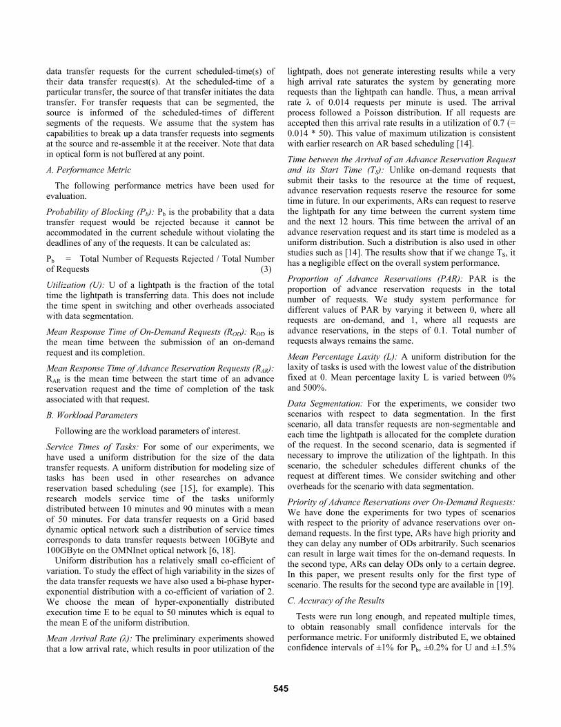
Probability of Blocking: Fig. 1 shows that with an increase in PAR, Pb increases. This is because that unlike ODs that do not have any deadlines ARs have finite deadlines. As the proportion of ARs in the workload increases, it becomes increasingly difficult to schedule them while meeting their deadlines. Thus, more and more ARs are rejected. The results show that this increase is not linear and there exists a knee on the curve for a given value of laxity after which Pb increases more rapidly. Given the mean laxity of the tasks, a resource can limit the ratio of requests it accepts as ARs equal to the value of PAR corresponding to the knee of the curve to keep Pb at reasonable levels. The figure also shows that with an increase in L, Pb decreases substantially. As expected, laxity can improve the performance of scheduling AR requests for lightpaths significantly by providing more flexibility in task scheduling. The effect becomes more pronounced with the increase in percentage of ARs. Thus for 80% requests arriving as ARs, L = 200% can decrease Pb by 82.93% compared to the case in which ARs have no laxity.

Utilization: Pb and U are related to each other as follows:

U = λ*(1 – Pb)*(R – W) (4)

Where R is the mean response time of the tasks accepted and W their mean wait time. Note that R – W is not always equal to E since tasks with higher service times have a high probability of being rejected.

Thus, as Pb increases with the increase in PAR, U decreases. The results available in [8] shows that by having some laxity in the tasks we can substantially counter the decrease in U with the increase in PAR. Just like the curves for Pb, the curves for U are also characterized by a knee that can act as a suitable operating point [8].

Since U and Pb are related, for the rest of the paper, we present curves only for U.

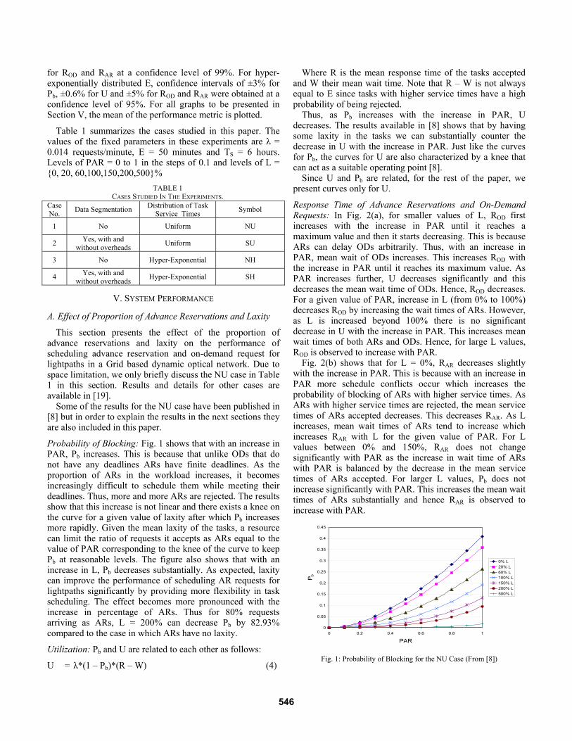
Response Time of Advance Reservations and On-Demand Requests: In Fig. 2(a), for smaller values of L, ROD first increases with the increase in PAR until it reaches a maximum value and then it starts decreasing. This is because ARs can delay ODs arbitrarily. Thus, with an increase in PAR, mean wait of ODs increases. This increases ROD with the increase in PAR until it reaches its maximum value. As PAR increases further, U decreases significantly and this decreases the mean wait time of ODs. Hence, ROD decreases. For a given value of PAR, increase in L (from 0% to 100%) decreases ROD by increasing the wait times of ARs. However, as L is increased beyond 100% there is no significant decrease in U with the increase in PAR. This increases mean wait times of both ARs and ODs. Hence, for large L values, ROD is observed to increase with PAR. Fig. 2(b) shows that for L = 0%, RAR decreases slightly with the increase in PAR. This is because with an increase in PAR more schedule conflicts occur which increases the probability of blocking of ARs with higher service times. As ARs with higher service times are rejected, the mean service times of ARs accepted decreases. This decreases RAR. As L increases, mean wait times of ARs tend to increase which increases RAR with L for the given value of PAR. For L values between 0% and 150%, RAR does not change significantly with PAR as the increase in wait time of ARs with PAR is balanced by the decrease in the mean service times of ARs accepted. For larger L values, Pb does not increase significantly with PAR. This increases the mean wait times of ARs substantially and hence RAR is observed to increase with PAR.

0

0.05

0.1

0.15

0.2

0.25

0.3

0.35

0.4

0.45

0 0.2 0.4 0.6 0.8 1

PAR

P b

0% L20% L60% L100% L150% L200% L500% L

Fig. 1: Probability of Blocking for the NU Case (From [8])

546

(a)

100

120

140

160

180

200

220

240

260

0 0.2 0.4 0.6 0.8 1

PAR

RO

D (m

inut

es) 0% L

20% L60% L100% L150% L200% L500% L

(b)

0

10

20

30

40

50

60

70

80

90

100

110

120

0 0.2 0.4 0.6 0.8 1

PAR

RAR

(min

utes

) 0% L20% L60% L100% L150% L200% L500% L

Fig. 2: Response Time for the NU Case (From [8])

(a) Effect of PAR on ROD (b) Effect of PAR on RAR

B. Effect of Data Segmentation

This section presents the effect of data segmentation on the performance. We, thus, compare the results for the NU and NH cases in Table 1 where data is not segmented with the SU and SH cases where data is segmented. For the SU and SH cases, we not only consider the scenario in which no overheads are associated with data segmentation but also introduce overheads O as a percentage of mean service times E of the tasks. O represents time spent in overheads such as path tear down and network reconfiguration. When a client accesses the optical network through a control plane mechanism such as Optical Dynamic Intelligent Network Service (ODIN) [20], the total time spent in overheads is just less than 1 minute [6] including the ODIN server processing delay, path tear down and network reconfiguration. However, if the client accesses the optical network through a customer portal the total time spent in overheads can be order of few minutes as in addition to the delays incurred in the control plane mechanisms there are delays at the portal server that handles billing and account aspects. We vary O between 0% of E (0 minutes) representing the ideal case to 30% of E (15 minutes) representing the worst case scenario.

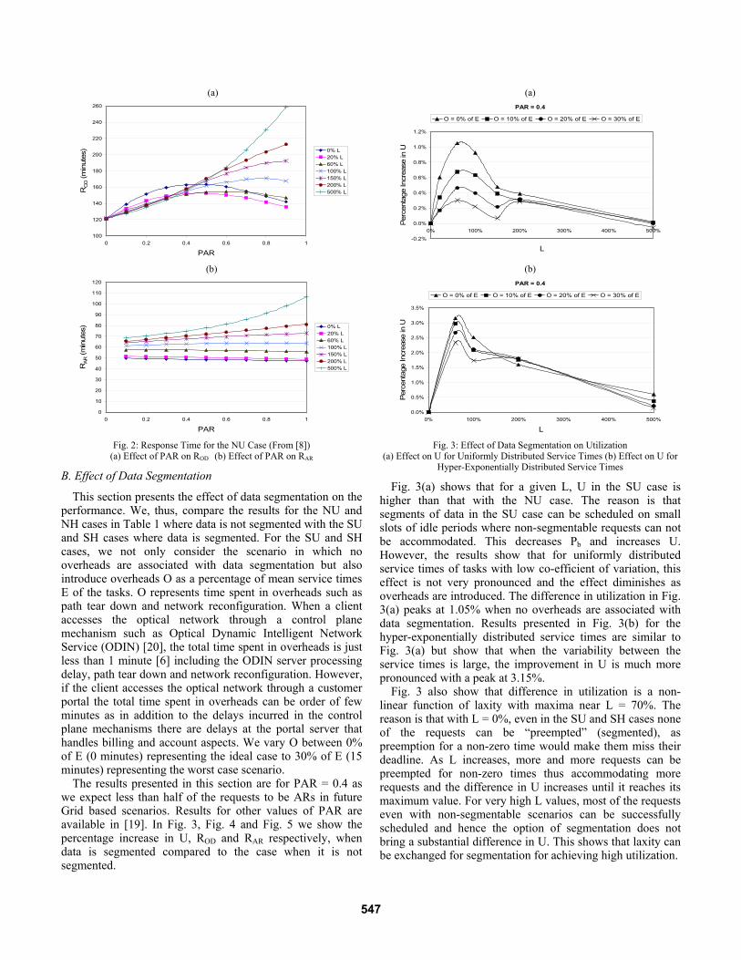
The results presented in this section are for PAR = 0.4 as we expect less than half of the requests to be ARs in future Grid based scenarios. Results for other values of PAR are available in [19]. In Fig. 3, Fig. 4 and Fig. 5 we show the percentage increase in U, ROD and RAR respectively, when data is segmented compared to the case when it is not segmented.

(a) PAR = 0.4

-0.2%

0.0%

0.2%

0.4%

0.6%

0.8%

1.0%

1.2%

0% 100% 200% 300% 400% 500%

L

Perc

enta

ge In

crea

se in

U

O = 0% of E O = 10% of E O = 20% of E O = 30% of E

(b)

PAR = 0.4

0.0%

0.5%

1.0%

1.5%

2.0%

2.5%

3.0%

3.5%

0% 100% 200% 300% 400% 500%

L

Perc

enta

ge In

crea

se in

U

O = 0% of E O = 10% of E O = 20% of E O = 30% of E

Fig. 3: Effect of Data Segmentation on Utilization

(a) Effect on U for Uniformly Distributed Service Times (b) Effect on U for Hyper-Exponentially Distributed Service Times

Fig. 3(a) shows that for a given L, U in the SU case is higher than that with the NU case. The reason is that segments of data in the SU case can be scheduled on small slots of idle periods where non-segmentable requests can not be accommodated. This decreases Pb and increases U. However, the results show that for uniformly distributed service times of tasks with low co-efficient of variation, this effect is not very pronounced and the effect diminishes as overheads are introduced. The difference in utilization in Fig. 3(a) peaks at 1.05% when no overheads are associated with data segmentation. Results presented in Fig. 3(b) for the hyper-exponentially distributed service times are similar to Fig. 3(a) but show that when the variability between the service times is large, the improvement in U is much more pronounced with a peak at 3.15%.

Fig. 3 also show that difference in utilization is a non-linear function of laxity with maxima near L = 70%. The reason is that with L = 0%, even in the SU and SH cases none of the requests can be “preempted” (segmented), as preemption for a non-zero time would make them miss their deadline. As L increases, more and more requests can be preempted for non-zero times thus accommodating more requests and the difference in U increases until it reaches its maximum value. For very high L values, most of the requests even with non-segmentable scenarios can be successfully scheduled and hence the option of segmentation does not bring a substantial difference in U. This shows that laxity can be exchanged for segmentation for achieving high utilization.

547

(a) PAR = 0.4

-30%

-20%

-10%

0%

10%

20%

30%

40%

0% 100% 200% 300% 400% 500%

L

Perc

enta

ge In

crea

se in

RO

D

O = 0% of E O = 10% of E O = 20% of E O = 30% of E

(b)

PAR = 0.4

-70%

-60%

-50%

-40%

-30%

-20%

-10%

0%0% 100% 200% 300% 400% 500%

L

Perc

enta

ge In

crea

se in

RO

D

O = 0% of E O = 10% of E O = 20% of E O = 30% of E

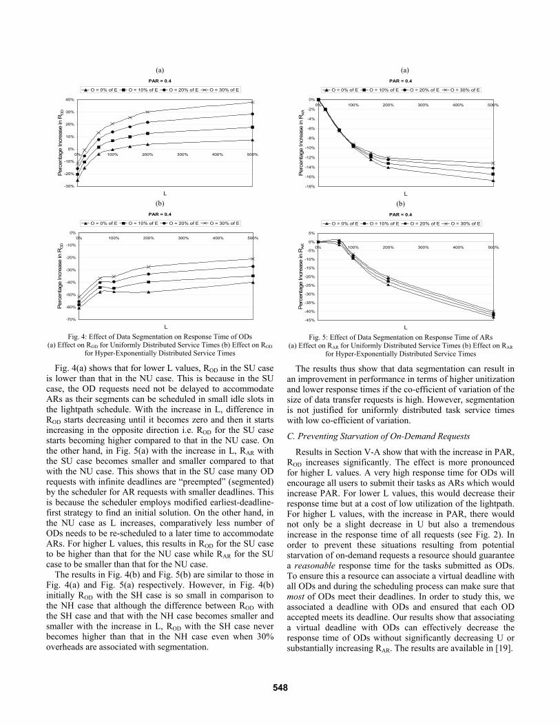
Fig. 4: Effect of Data Segmentation on Response Time of ODs

(a) Effect on ROD for Uniformly Distributed Service Times (b) Effect on ROD for Hyper-Exponentially Distributed Service Times

Fig. 4(a) shows that for lower L values, ROD in the SU case is lower than that in the NU case. This is because in the SU case, the OD requests need not be delayed to accommodate ARs as their segments can be scheduled in small idle slots in the lightpath schedule. With the increase in L, difference in ROD starts decreasing until it becomes zero and then it starts increasing in the opposite direction i.e. ROD for the SU case starts becoming higher compared to that in the NU case. On the other hand, in Fig. 5(a) with the increase in L, RAR with the SU case becomes smaller and smaller compared to that with the NU case. This shows that in the SU case many OD requests with infinite deadlines are “preempted” (segmented) by the scheduler for AR requests with smaller deadlines. This is because the scheduler employs modified earliest-deadline-first strategy to find an initial solution. On the other hand, in the NU case as L increases, comparatively less number of ODs needs to be re-scheduled to a later time to accommodate ARs. For higher L values, this results in ROD for the SU case to be higher than that for the NU case while RAR for the SU case to be smaller than that for the NU case.

The results in Fig. 4(b) and Fig. 5(b) are similar to those in Fig. 4(a) and Fig. 5(a) respectively. However, in Fig. 4(b) initially ROD with the SH case is so small in comparison to the NH case that although the difference between ROD with the SH case and that with the NH case becomes smaller and smaller with the increase in L, ROD with the SH case never becomes higher than that in the NH case even when 30% overheads are associated with segmentation.

(a) PAR = 0.4

-18%

-16%

-14%

-12%

-10%

-8%

-6%

-4%

-2%

0%0% 100% 200% 300% 400% 500%

L

Perc

enta

ge In

crea

se in

RA

R

O = 0% of E O = 10% of E O = 20% of E O = 30% of E

(b)

PAR = 0.4

-45%

-40%

-35%

-30%

-25%

-20%

-15%

-10%

-5%

0%

5%

0% 100% 200% 300% 400% 500%

L

Perc

enta

ge In

crea

se in

RA

R

O = 0% of E O = 10% of E O = 20% of E O = 30% of E

Fig. 5: Effect of Data Segmentation on Response Time of ARs

(a) Effect on RAR for Uniformly Distributed Service Times (b) Effect on RAR for Hyper-Exponentially Distributed Service Times

The results thus show that data segmentation can result in an improvement in performance in terms of higher unitization and lower response times if the co-efficient of variation of the size of data transfer requests is high. However, segmentation is not justified for uniformly distributed task service times with low co-efficient of variation.

C. Preventing Starvation of On-Demand Requests

Results in Section V-A show that with the increase in PAR, ROD increases significantly. The effect is more pronounced for higher L values. A very high response time for ODs will encourage all users to submit their tasks as ARs which would increase PAR. For lower L values, this would decrease their response time but at a cost of low utilization of the lightpath. For higher L values, with the increase in PAR, there would not only be a slight decrease in U but also a tremendous increase in the response time of all requests (see Fig. 2). In order to prevent these situations resulting from potential starvation of on-demand requests a resource should guarantee a reasonable response time for the tasks submitted as ODs. To ensure this a resource can associate a virtual deadline with all ODs and during the scheduling process can make sure that most of ODs meet their deadlines. In order to study this, we associated a deadline with ODs and ensured that each OD accepted meets its deadline. Our results show that associating a virtual deadline with ODs can effectively decrease the response time of ODs without significantly decreasing U or substantially increasing RAR. The results are available in [19].

548

D. Performance of the SSS Algorithm

The SSS algorithm for scheduling advance reservation requests with laxities successfully scheduled hundreds of thousands of tasks. The results show that the mean number of nodes produced to schedule given number of tasks depends on PAR and L in addition to the distribution of service times of the tasks. Maximum numbers of nodes open at one time, for 100,000 tasks never exceeded 120. Detailed analysis of the performance of the algorithm is available in [19].

VI. CONCLUSIONS

Dynamic optical networks hold the potential of satisfying very large bandwidth requirements of many of the Grid applications. However, encapsulation of optical network elements into manageable Grid resources and dynamic provisioning of lightpaths is necessary to meet the demands of the Grid applications and to optimize usage of optical network components. In this paper, we presented an algorithm to dynamically schedule on-demand and advance reservation requests for lightpaths. The results show that the algorithm is scalable and suits well the needs of the Grid domain.

The performance results obtained using the algorithm show that laxity in the reservation window can significantly improve the performance of the network by reducing the probability of blocking and increasing lightpath utilization. The effect is more pronounced for the cases where proportion of advance reservations is high. When Pb is plotted against PAR, there exists a knee on the curve for a given value of laxity after which Pb increases more rapidly. Given the mean laxity of the tasks, the network can limit the ratio of requests it accepts as ARs equal to the value of PAR at the knee of the curve to keep Pb at reasonable levels.

We also investigated the effect of data segmentation on system performance. The results show that choice of segmentation depends largely on the distribution of the task service times. When the variance between the service times is small, there is no significant advantage in segmenting data. For the values of the parameters in the experiments, maximum increase in utilization for uniformly distributed task service times is 1.05% and it diminishes as overheads of segmentation are considered. For hyper-exponentially distributed task service times with a co-efficient of variation of 2, the effect of data segmentation is much more pronounced. In our experiments, for hyper-exponentially distributed service times, data segmentation resulted in an increase in utilization of up to 3.15% and substantial decrease of up to 60.7% in ROD and up to 43.38% in RAR.

The results also show that the improvement in performance with segmentation is sensitive to L. With the workload parameters in the experiments, maximum improvement in utilization is achieved near L = 70%. At higher L values, difference in utilization diminishes. This suggests that laxity can be exchanged for data segmentation to achieve high utilization of lightpaths.

REFERENCES

[1] The compact Muon Solenoid Project. http://cmsinfo.cern.ch/ [2] PPDG Deliverables to CMS. http://www.ppdg.net/archives/ppdg/2001/

doc00017.doc [3] K. Marzullo, M. Ogg, A. Ricciardi, A. Amoroso, F. Calkins, E.

Rothfus, “Nile: Wide-area computing for high energy physics,” in the Proc. of the 7th ACM SIGOPS European Workshop, Connemara, Ireland, Sept. 1996.

[4] W. Allcock, J. Bester, J. Bresnahan, A. Chervenak, I. Foster, C. Kesselman, S. Meder, V. Nefedova, D. Quesnel, S. Tuecke, “Secure, Efficient Data Transport and Replica Management for High-Performance Data-Intensive Computing,” in the Proc. of the IEEE Mass Storage Conference, San Diego, CA, pp. 13-28, April 2001.

[5] User Controlled Lightpaths. http://www.canarie.ca/canet4/uclp/ [6] T. Lavian, S. Merrill, H. Cohen, D. Hoang, J. Mambretti, S. Figueira,

D. Cutrell, S. Naiksatam, F. Travostino, “A Grid Network Service Architecture for Dynamic Optical Networks,” submitted to the Journal of Grid Computing, special issue on High Performance Networking.

[7] G. McMahon, M. Florian, “On Scheduling with Ready Times and Due Dates To Minimize Maximum Lateness”, Operations Research, vol. 23, no. 3, pp. 475-482, May-June, 1975.

[8] U. Farooq, S. Majumdar, E. W. Parsons, “Impact of Laxity on Scheduling with Advance Reservations in Grids”, in the Proc. of the 13th IEEE International Symposium on Modeling, Analysis, and Simulation of Computer and Telecommunication Systems, Atlanta, Georgia, USA, September, 2005.

[9] I. Foster, C. Kesselman, C. Lee, R. Lindell, K. Nahrstedt, A. Roy, “A Distributed Resource Management Architecture that Supports Advance Reservations and Co-Allocation,” in the Proc. of the 7th International Workshop on Quality of Service, London, UK, May 1999.

[10] I. Foster, A. Roy, V. Sander, “A Quality of Service Architecture that Combines Resource Reservation and Application Adaptation,” in the Proc. of the 8th International Workshop on Quality of Service, Pittsburgh, PA, USA, pp. 181-188, June 2000.

[11] I. Foster, J. Vockler, M. Wilde, Y. Zhao, “The Virtual Data Grid: A New Model and Architecture for Data-Intensive Collaboration,” in the Proc.s of the First CIDR - Biennial Conference on Innovative Data Systems Research, Asilomar, CA, USA, Jan. 2003.

[12] T. Kosar and M. Livny, “Stork: Making Data Placement a First Class Citizen in the Grid,” in Proc. of 24th IEEE International Conference on Distributed Computing Systems, Tokyo, Japan, March 2004.

[13] The Maui Scheduling System. http://www.mhpcc.edu/ maui. [14] W. Smith, I. Foster, V. Taylor, “On Scheduling with Advanced

Reservations,” in the Proc. of the IEEE/ACM 14th International Parallel and Distributed Processing Symposium, Cancun, Mexico, May 2000.

[15] A. Sulistio, R. Buyya, “A Grid Simulation Infrastructure Supporting Advance Reservation,” in the Proc. of the 16th International Conference on Parallel and Distributed Computing and Systems, Cambridge, Boston, USA, Nov. 2004.

[16] S. Figueira, N. Kaushik, S. Naiksatam, S. A. Chiappari, N. Bhatnagar, “Advance Reservation of Light-paths in Optical-Network Based Grids,” in the Proc. of 1st International Workshop on Networks for Grid, San Jose, CA, USA, Oct. 2004.

[17] J. Xu, D. Parnas, “Scheduling Processes With Release Times, Deadlines, Precedence And Exclusion Relations,” IEEE Transactions on Software Engineering, vol. 16, no. 3, pp. 360-369, 1990.

[18] S. Figueira, S. Naiksatam, H. Cohen, D. Cutrell, D. Gutierrez, D. B. Hoang, T. Lavian, J. Mambretti, S. Merrill, F. Travostino, “DWDM-RAM: Enabling Grid Services with Dynamic Optical Networks,” in the Proc. of the 4th IEEE International Symposium on Cluster Computing and the Grid, Chicago, IL, USA, April 2004.

[19] U. Farooq, S. Majumdar, E. W. Parsons, “Efficiently Scheduling Advance Reservations in Grids,” Technical Report SCE-05-14, Department of Systems and Computer Engineering, Carleton University, Ottawa, Canada, August 2005.

[20] J. Mambretti, J. Weinberger, J. Chen, E. Bacon, F. Yeh, D. Lillethun, B. Grossman, Y. Gu, M. Mazzuco, “The Photonic TeraStream: Enabling Next Generation Applications Through Intelligent Optical Networking at iGrid 2002,” Journal of Future Comp. Systems, pp.897-908, Aug. 2003.

549