Oxford Physics Department

Notes on General Relativity

Steven Balbus

Version: January 25, 2017

1

These notes are intended for classroom use. There is little here that is original, but a few results are.If you would like to quote from these notes and are unable to find an original literature reference,please contact me by email first.

Thank you in advance for your cooperation.

Steven Balbus

2

Recommended TextsHobson, M. P., Efstathiou, G., and Lasenby, A. N. 2006, General Relativity: An Introductionfor Physicists, (Cambridge: Cambridge University Press) Referenced as HEL06.

A very clear, very well-blended book, admirably covering the mathematics, physics, andastrophysics of GR. Excellent presentation of black holes and gravitational radiation. Theexplanation of the geodesic equation and the affine connection is very clear and enlightening.Not so much on cosmology, though a nice introduction to the physics of inflation. Overall, myfavourite text on this topic. (The metric has a different sign convention in HEL06 comparedwith Weinberg 1972 & MTW [see below], as well as these notes. Be careful.)

Weinberg, S. 1972, Gravitation and Cosmology. Principles and Applications of the GeneralTheory of Relativity, (New York: John Wiley) Referenced as W72.

What is now the classic reference by the great man, but lacking any discussion whatsoeverof black holes, and almost nothing on the geometrical interpretation of the equations. Theauthor is explicit in his aversion to anything geometrical: gravity is a field theory with amere geometrical “analogy” according to Weinberg. But there is no way to make sense of theequations, in any profound sense, without immersing onself in geometry. More suprisingly,given the author’s skill set, I find that many calculations are often performed awkwardly,with far more effort and baggage than is required. The detailed sections on classical physicalcosmology are its main strength. Weinberg also has a more recent graduate text on cosmologyper se, (Cosmology 2007, Oxford: Oxford University Press). This is very complete but at anadvanced level.

Misner, C. W., Thorne, K. S., and Wheeler, J. A. 1973, Gravitation, (New York: Freeman)Referenced as MTW.

At 1280 pages, don’t drop this on your toe, not even the paperback version. MTW, as it isknown, is often criticised for its sheer bulk, its seemingly endless meanderings, its cuteness,and its laboured strivings at building mathematical and physical intuition at every possiblestep. But look. I must say, in the end, there really is a lot of very good material in here,much that is difficult to find anywhere else. It is a monumental achievement. It is also theopposite of Weinberg: geometry is front and centre from start to finish, and there is lots andlots of black hole and gravitational radiation physics, 40+ years on more timely than ever.I very much recommend its insightful discussion on gravitational radiation, now part of thecourse syllabus. There is a “Track 1” and “Track 2” for aid in navigation; Track 1 containsthe essentials.

Hartle, J. B. 2003, Gravity: An Introduction to Einstein’s General Theory of Relativity, (SanFrancisco: Addison-Wesley)

This is GR Lite, at a very different level from the previous three texts. But for what it ismeant to be, it succeeds very well. Coming into the subject cold, this is not a bad place tostart to get the lay of the land, to understand the issues in their broadest context, and to betreated to a very accessible presentation. This is a difficult subject. There will be times inyour study of GR when it will be difficult to see the forest for the trees, when you will feeloverwhelmed with the calculations, drowning in a sea of indices and Riemannian formalism.Everything will be all right: just spend some time with this text.

3

Ryden, Barbara 2017, Introduction to Cosmology, (Cambridge: Cambridge University Press)

Very recent and therefore up-to-date second edition of an award-winning text. The style isclear and lucid, the level is right, and the choice of topics is excellent. Less GR and moreastrophysical in content but with a blend appropriate to the subject matter. Ryden is alwaysvery careful in her writing, making this a real pleasure to read. Warmly recommended.

A few other texts of interest:

Binney J, and Temaine, S. 2008, Galactic Dynamics, (Princeton: Princeton University Press)Masterful text on galaxies with an excellent cosmology treatment in the appendix. Veryreadable, given the high level of mathematics.

Longair, M., 2006, The Cosmic Century, (Cambridge: Cambridge University Press) Excel-lent blend of observations, theory and history of cosmology, as part of a more general study.Good general reference for anyone interested in astrophysics.

Landau, L., and Lifschitz, E. M. 1962, Classical Theory of Fields, (Oxford: Pergamon)Classic advanced text; original and interesting treatment of gavitational radiation. Dedicatedstudents only!

Peebles, P. J. E. 1993, Principles of Physical Cosmology, (Princeton: Princeton UniversityPress) Authoritative advanced treatment by the leading cosmologist of the 20th century, butin my view a difficult and sometimes frustrating read.

Shapiro, S., and Teukolsky S. 1983, Black Holes, White Dwarfs, and Neutron Stars, (Wiley:New York) Very clear text with a nice summary of applications of GR to compact objectsand good physical discussions. Level is appropriate to this course.

4

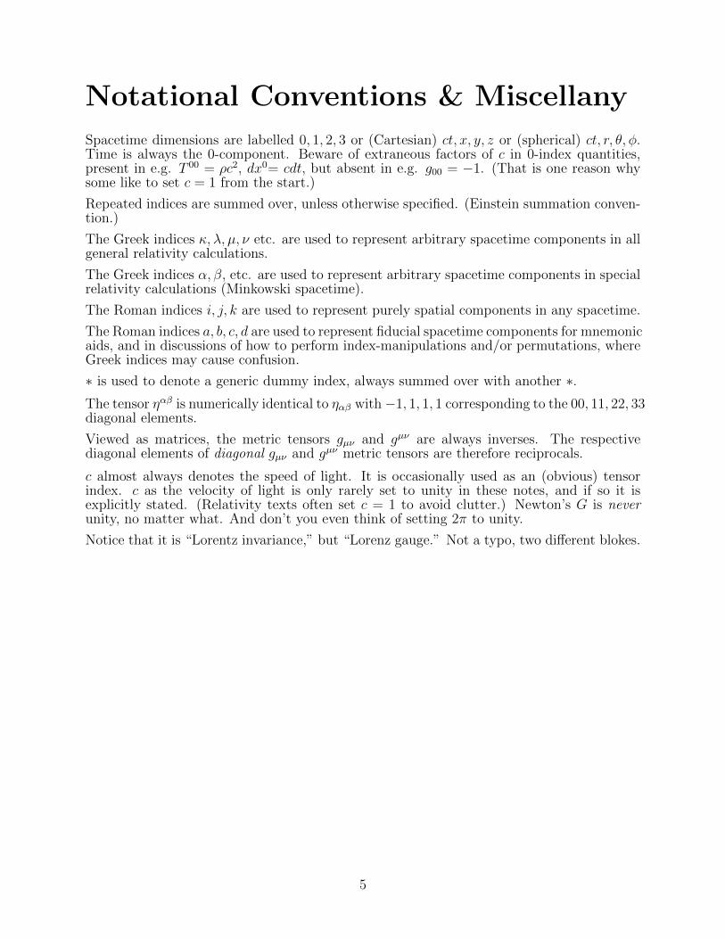
Notational Conventions & Miscellany

Spacetime dimensions are labelled 0, 1, 2, 3 or (Cartesian) ct, x, y, z or (spherical) ct, r, θ, φ.Time is always the 0-component. Beware of extraneous factors of c in 0-index quantities,present in e.g. T 00 = ρc2, dx0= cdt, but absent in e.g. g00 = −1. (That is one reason whysome like to set c = 1 from the start.)

Repeated indices are summed over, unless otherwise specified. (Einstein summation conven-tion.)

The Greek indices κ, λ, µ, ν etc. are used to represent arbitrary spacetime components in allgeneral relativity calculations.

The Greek indices α, β, etc. are used to represent arbitrary spacetime components in specialrelativity calculations (Minkowski spacetime).

The Roman indices i, j, k are used to represent purely spatial components in any spacetime.

The Roman indices a, b, c, d are used to represent fiducial spacetime components for mnemonicaids, and in discussions of how to perform index-manipulations and/or permutations, whereGreek indices may cause confusion.

∗ is used to denote a generic dummy index, always summed over with another ∗.The tensor ηαβ is numerically identical to ηαβ with−1, 1, 1, 1 corresponding to the 00, 11, 22, 33diagonal elements.

Viewed as matrices, the metric tensors gµν and gµν are always inverses. The respectivediagonal elements of diagonal gµν and gµν metric tensors are therefore reciprocals.

c almost always denotes the speed of light. It is occasionally used as an (obvious) tensorindex. c as the velocity of light is only rarely set to unity in these notes, and if so it isexplicitly stated. (Relativity texts often set c = 1 to avoid clutter.) Newton’s G is neverunity, no matter what. And don’t you even think of setting 2π to unity.

Notice that it is “Lorentz invariance,” but “Lorenz gauge.” Not a typo, two different blokes.

5

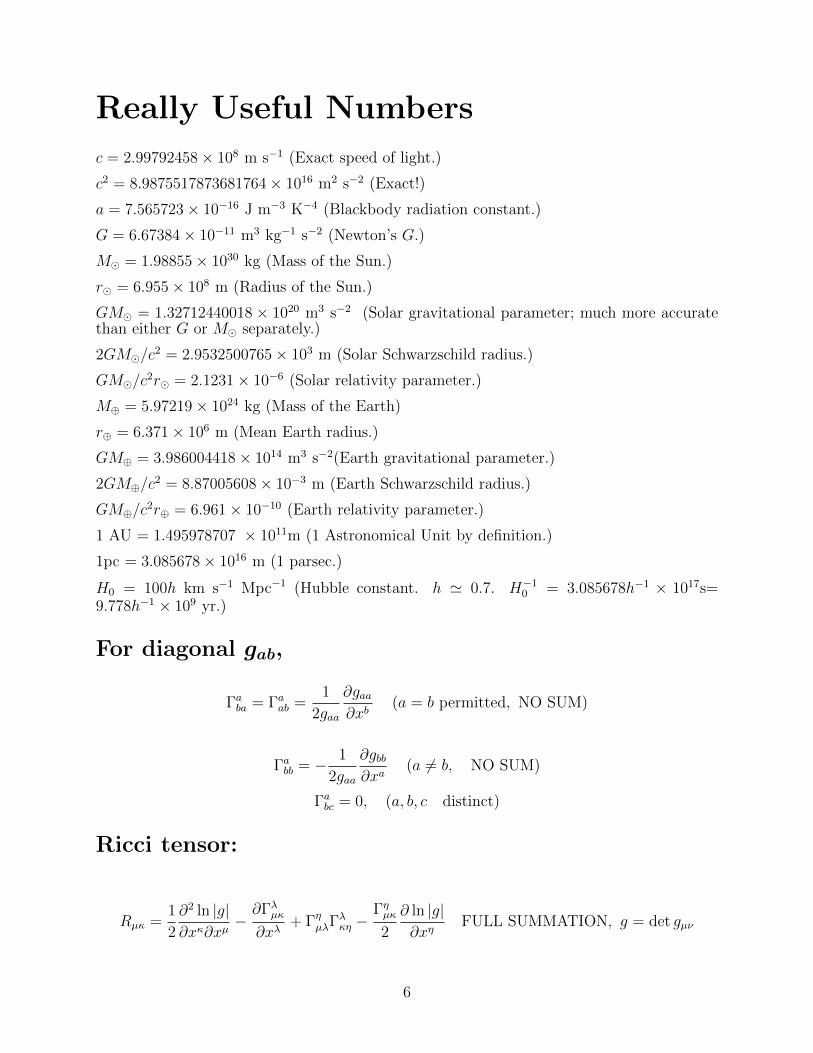
Really Useful Numbers

c = 2.99792458× 108 m s−1 (Exact speed of light.)

c2 = 8.9875517873681764× 1016 m2 s−2 (Exact!)

a = 7.565723× 10−16 J m−3 K−4 (Blackbody radiation constant.)

G = 6.67384× 10−11 m3 kg−1 s−2 (Newton’s G.)

M = 1.98855× 1030 kg (Mass of the Sun.)

r = 6.955× 108 m (Radius of the Sun.)

GM = 1.32712440018 × 1020 m3 s−2 (Solar gravitational parameter; much more accuratethan either G or M separately.)

2GM/c2 = 2.9532500765× 103 m (Solar Schwarzschild radius.)

GM/c2r = 2.1231× 10−6 (Solar relativity parameter.)

M⊕ = 5.97219× 1024 kg (Mass of the Earth)

r⊕ = 6.371× 106 m (Mean Earth radius.)

GM⊕ = 3.986004418× 1014 m3 s−2(Earth gravitational parameter.)

2GM⊕/c2 = 8.87005608× 10−3 m (Earth Schwarzschild radius.)

GM⊕/c2r⊕ = 6.961× 10−10 (Earth relativity parameter.)

1 AU = 1.495978707 × 1011m (1 Astronomical Unit by definition.)

1pc = 3.085678× 1016 m (1 parsec.)

H0 = 100h km s−1 Mpc−1 (Hubble constant. h ' 0.7. H−10 = 3.085678h−1 × 1017s=9.778h−1 × 109 yr.)

For diagonal gab,

Γaba = Γaab =1

2gaa

∂gaa∂xb

(a = b permitted, NO SUM)

Γabb = − 1

2gaa

∂gbb∂xa

(a 6= b, NO SUM)

Γabc = 0, (a, b, c distinct)

Ricci tensor:

Rµκ =1

2

∂2 ln |g|∂xκ∂xµ

−∂Γλµκ∂xλ

+ ΓηµλΓλκη −

Γηµκ2

∂ ln |g|∂xη

FULL SUMMATION, g = det gµν

6

Contents

1 An overview 10

1.1 The legacy of Maxwell . . . . . . . . . . . . . . . . . . . . . . . . . . . . . . 10

1.2 The legacy of Newton . . . . . . . . . . . . . . . . . . . . . . . . . . . . . . . 11

1.3 The need for a geometrical framework . . . . . . . . . . . . . . . . . . . . . . 11

2 The toolbox of geometrical theory: special relativity 14

2.1 The 4-vector formalism . . . . . . . . . . . . . . . . . . . . . . . . . . . . . . 14

2.2 More on 4-vectors . . . . . . . . . . . . . . . . . . . . . . . . . . . . . . . . . 17

2.2.1 Transformation of gradients . . . . . . . . . . . . . . . . . . . . . . . 17

2.2.2 Transformation matrix . . . . . . . . . . . . . . . . . . . . . . . . . . 18

2.2.3 Tensors . . . . . . . . . . . . . . . . . . . . . . . . . . . . . . . . . . 19

2.2.4 Conservation of Tαβ . . . . . . . . . . . . . . . . . . . . . . . . . . . 21

3 The effects of gravity 23

3.1 The Principle of Equivalence . . . . . . . . . . . . . . . . . . . . . . . . . . . 23

3.2 The geodesic equation . . . . . . . . . . . . . . . . . . . . . . . . . . . . . . 25

3.3 The metric tensor . . . . . . . . . . . . . . . . . . . . . . . . . . . . . . . . . 27

3.4 The relationship between the metric tensor and affine connection . . . . . . . 27

3.5 Variational calculation of the geodesic equation . . . . . . . . . . . . . . . . 28

3.6 The Newtonian limit . . . . . . . . . . . . . . . . . . . . . . . . . . . . . . . 30

4 Tensor Analysis 34

4.1 Transformation laws . . . . . . . . . . . . . . . . . . . . . . . . . . . . . . . 34

4.2 The covariant derivative . . . . . . . . . . . . . . . . . . . . . . . . . . . . . 36

4.3 The affine connection and basis vectors . . . . . . . . . . . . . . . . . . . . . 39

4.4 Volume element . . . . . . . . . . . . . . . . . . . . . . . . . . . . . . . . . . 41

4.5 Covariant div, grad, curl, and all that . . . . . . . . . . . . . . . . . . . . . . 41

4.6 Hydrostatic equilibrium . . . . . . . . . . . . . . . . . . . . . . . . . . . . . 43

4.7 Covariant differentiation and parallel transport . . . . . . . . . . . . . . . . . 44

5 The curvature tensor 46

5.1 Commutation rule for covariant derivatives . . . . . . . . . . . . . . . . . . . 46

5.2 Parallel transport . . . . . . . . . . . . . . . . . . . . . . . . . . . . . . . . . 47

5.3 Algebraic identities of Rσνλρ . . . . . . . . . . . . . . . . . . . . . . . . . . . 49

5.3.1 Remembering the curvature tensor formula. . . . . . . . . . . . . . . 49

5.4 Rλµνκ: fully covariant form . . . . . . . . . . . . . . . . . . . . . . . . . . . . 49

7

5.5 The Ricci Tensor . . . . . . . . . . . . . . . . . . . . . . . . . . . . . . . . . 51

5.6 The Bianchi Identities . . . . . . . . . . . . . . . . . . . . . . . . . . . . . . 51

6 The Einstein Field Equations 54

6.1 Formulation . . . . . . . . . . . . . . . . . . . . . . . . . . . . . . . . . . . . 54

6.2 Coordinate ambiguities . . . . . . . . . . . . . . . . . . . . . . . . . . . . . . 57

6.3 The Schwarzschild Solution . . . . . . . . . . . . . . . . . . . . . . . . . . . 57

6.4 The Schwarzschild Radius . . . . . . . . . . . . . . . . . . . . . . . . . . . . 62

6.5 Schwarzschild spacetime. . . . . . . . . . . . . . . . . . . . . . . . . . . . . . 64

6.5.1 Radial photon geodesic . . . . . . . . . . . . . . . . . . . . . . . . . . 64

6.5.2 Orbital equations . . . . . . . . . . . . . . . . . . . . . . . . . . . . . 65

6.6 The deflection of light by an intervening body. . . . . . . . . . . . . . . . . . 66

6.7 The advance of the perihelion of Mercury . . . . . . . . . . . . . . . . . . . . 69

6.7.1 Newtonian orbits . . . . . . . . . . . . . . . . . . . . . . . . . . . . . 69

6.7.2 The perihelion advance of Mercury . . . . . . . . . . . . . . . . . . . 72

6.8 Shapiro delay: the fourth protocol . . . . . . . . . . . . . . . . . . . . . . . . 73

7 Gravitational Radiation 76

7.1 The linearised gravitational wave equation . . . . . . . . . . . . . . . . . . . 78

7.1.1 Come to think of it... . . . . . . . . . . . . . . . . . . . . . . . . . . . 83

7.2 Plane waves . . . . . . . . . . . . . . . . . . . . . . . . . . . . . . . . . . . . 84

7.2.1 The transverse-traceless (TT) gauge . . . . . . . . . . . . . . . . . . . 84

7.3 The quadrupole formula . . . . . . . . . . . . . . . . . . . . . . . . . . . . . 85

7.4 Radiated Energy . . . . . . . . . . . . . . . . . . . . . . . . . . . . . . . . . 87

7.4.1 A useful toy problem . . . . . . . . . . . . . . . . . . . . . . . . . . . 87

7.5 A conserved energy flux for linearised gravity . . . . . . . . . . . . . . . . . . 88

7.6 The energy loss formula for gravitational waves . . . . . . . . . . . . . . . . 90

7.7 Gravitational radiation from binary stars . . . . . . . . . . . . . . . . . . . . 93

7.8 Detection of gravitational radiation . . . . . . . . . . . . . . . . . . . . . . . 95

7.8.1 Preliminary comments . . . . . . . . . . . . . . . . . . . . . . . . . . 95

7.8.2 Indirect methods: orbital energy loss in binary pulsars . . . . . . . . 97

7.8.3 Direct methods: LIGO . . . . . . . . . . . . . . . . . . . . . . . . . . 100

7.8.4 Direct methods: Pulsar timing array . . . . . . . . . . . . . . . . . . 103

8 Cosmology 105

8.1 Introduction . . . . . . . . . . . . . . . . . . . . . . . . . . . . . . . . . . . . 105

8.1.1 Newtonian cosmology . . . . . . . . . . . . . . . . . . . . . . . . . . . 105

8

8.1.2 The dynamical equation of motion . . . . . . . . . . . . . . . . . . . 107

8.1.3 Cosmological redshift . . . . . . . . . . . . . . . . . . . . . . . . . . . 108

8.2 Cosmology models for the impatient . . . . . . . . . . . . . . . . . . . . . . . 108

8.2.1 The large-scale spacetime metric . . . . . . . . . . . . . . . . . . . . 108

8.2.2 The Einstein-de Sitter universe: a useful toy model . . . . . . . . . . 110

8.3 The Friedman-Robertson-Walker Metric . . . . . . . . . . . . . . . . . . . . 112

8.3.1 Maximally symmetric 3-spaces . . . . . . . . . . . . . . . . . . . . . . 113

8.4 Large scale dynamics . . . . . . . . . . . . . . . . . . . . . . . . . . . . . . . 115

8.4.1 The effect of a cosmological constant . . . . . . . . . . . . . . . . . . 115

8.4.2 Formal analysis . . . . . . . . . . . . . . . . . . . . . . . . . . . . . . 116

8.5 The classic, matter-dominated universes . . . . . . . . . . . . . . . . . . . . 120

8.6 Our Universe . . . . . . . . . . . . . . . . . . . . . . . . . . . . . . . . . . . 121

8.6.1 Prologue . . . . . . . . . . . . . . . . . . . . . . . . . . . . . . . . . . 121

8.6.2 A Universe of ordinary matter and vacuum energy . . . . . . . . . . . 122

8.6.3 The parameter q0 . . . . . . . . . . . . . . . . . . . . . . . . . . . . . 123

8.7 Radiation-dominated universe . . . . . . . . . . . . . . . . . . . . . . . . . . 124

8.8 Observational foundations of cosmology . . . . . . . . . . . . . . . . . . . . . 127

8.8.1 Detection of cosmlogical redshifts . . . . . . . . . . . . . . . . . . . . 127

8.8.2 The cosmic distance ladder . . . . . . . . . . . . . . . . . . . . . . . . 127

8.8.3 The redshift–magnitude relation . . . . . . . . . . . . . . . . . . . . . 129

8.9 The growth of density perturbations in an expanding universe . . . . . . . . 132

8.10 The Cosmic Microwave Background Radiation . . . . . . . . . . . . . . . . . 134

8.10.1 Prologue . . . . . . . . . . . . . . . . . . . . . . . . . . . . . . . . . . 134

8.10.2 An observable cosmic radiation signature: the Gamow argument . . . 136

8.10.3 The cosmic microwave background (CMB): subsequent developments 139

8.11 Thermal history of the Universe . . . . . . . . . . . . . . . . . . . . . . . . . 140

8.11.1 Prologue . . . . . . . . . . . . . . . . . . . . . . . . . . . . . . . . . . 140

8.11.2 Helium nucleosynthesis . . . . . . . . . . . . . . . . . . . . . . . . . . 142

8.11.3 Neutrino and photon temperatures . . . . . . . . . . . . . . . . . . . 144

8.11.4 Ionisation of Hydrogen . . . . . . . . . . . . . . . . . . . . . . . . . . 145

8.11.5 Inflationary Models . . . . . . . . . . . . . . . . . . . . . . . . . . . 147

8.11.6 A Final Word . . . . . . . . . . . . . . . . . . . . . . . . . . . . . . . 155

9

Most of the fundamental ideas of

science are essentially simple, and

may, as a rule, be expressed in a

language comprehensible to everyone.

— Albert Einstein

1 An overview

1.1 The legacy of Maxwell

We are told by the historians that the greatest Roman generals would have their mostimportant victories celebrated with a triumph. The streets would line with adoring crowds,cheering wildly in support of their hero as he passed by in a grand procession. But theRomans astutely realised the need for a counterpoise, so a slave would ride with the general,whispering in his ear, “All glory is fleeting.”

All glory is fleeting. And never more so than in theoretical physics. No sooner is a triumphhailed, but unforseen puzzles emerge that couldn’t possibly have been anticipated before thebreakthrough. The mid-nineteenth century reduction of all electromagnetic phenomena tofour equations, the “Maxwell Equations,” is very much a case in point.

Maxwell’s equations united electricity, magnetism, and optics, showing them to be differ-ent manifestations of the same field. The theory accounted for the existence of electromag-netic waves, explained how they propagate, and that the propagation velocity is 1/

√ε0µ0 (ε0

is the permitivity, and µ0 the permeability, of free space). This combination is numericallyprecisely equal to the speed of light. Light is electromagnetic radiation! The existence ofelectromagnetic raditation was then verified by brilliant experiments carried out by HeinrichHertz in 1887, in which the radiation was directly generated and detected.

But Maxwell’s theory, for all its success, had disquieting features when one probed. Forone, there seemed to be no provision in the theory for allowing the velocity of light to changewith the observer’s velocity. The speed of light is aways 1/

√ε0µ0. A related point was

that simple Galilean invariance was not obeyed, i.e. absolute velocities seemed to affect thephysics, something that had not been seen before. Lorentz and Larmor in the late nineteenthcentury discovered that Maxwell’s equations did have a simple mathematical velocity trans-formation that left them invariant, but it was not Galilean, and most bizarrely, it involvedchanging the time. The non-Galilean character of the transformation equation relative tothe “aetherial medium” hosting the waves was put down, a bit vaguely, to electromagneticinteractions between charged particles that truly changed the length of the object. In otherwords, the non-Galilean transformation were somehow electrodynamical in origin. As to thetime change...well, one would just have to put up with it as an aetherial formality.

All was resolved in 1905 when Einstein showed how, by adopting as a postulates (i)that the speed of light was constant in all frames (as had already been indicated by a bodyof irrefutable experiments, including the famous Michelson-Morley investigation); (ii) theabandonment of the increasingly problematic aether medium that supposedly hosted thesewaves; and (iii) reinstating the truly essential Galilean notion that relative uniform velocitycannot be detected by any physical experiment, that the “Lorentz transformations” (asthey had become known) must follow. All equations of physics, not just electromagneticphenomena, had to be invariant in form under these Lorentz transformations, even withits peculiar relative time variable. The non-Galilean transformations were purely kinematic

10

in this view, having nothing in particular to do with electrodynamics: they were muchmore general. These ideas and the consequences that ensued collectively became known asrelativity theory, in reference to the invariance of form with respect to relative velocities.The relativity theory stemming from Maxwell’s equations is rightly regarded as one of thecrown jewels of 20th century physics. In other words, a triumph.

1.2 The legacy of Newton

Another triumph, another problem. If indeed, all of physics had to be compatible withrelativity, what of Newtonian gravity? It works incredibly well, yet it is manifestly notcompatible with relativity, because Poisson’s equation

∇2Φ = 4πGρ (1)

implies instantaneous transmission of changes in the gravitational field from source to poten-tial. (Here Φ is the Newtonian potential function, G the Newtonian gravitational constant,and ρ the mass density.) Wiggle the density locally, and throughout all of space there mustinstantaneously be a wiggle in Φ, as given by equaton (1).

In Maxwell’s theory, the electrostatic potential satisfies its own Poisson equation, but theappropriate time-dependent potential obeys a wave equation:

∇2Φ− 1

c2∂2Φ

∂t2= − ρ

ε0, (2)

and solutions of this equation propagate signals at the speed of light c. In retrospect, this israther simple. Mightn’t it be the same for gravity?

No. The problem is that the source of the signals for the electric potential field, i.e. thecharge density, behaves differently from the source for the gravity potential field, i.e. the massdensity. The electrical charge of an individual bit of matter does not change when the matteris viewed in motion, but the mass does: the mass increases with velocity. This seeminglysimple detail complicates everything. Moreover, in a relativisitic theory, energy, like matter,is a source of a gravitational field, including the distributed energy of the gravitational fielditself! A relativisitic theory of gravity would have to be nonlinear. In such a time-dependenttheory of gravity, it is not even clear a priori what the appropriate mathematical objectsshould be on either the right side or the left side of the wave equation. Come to think of it,should we be using a wave equation at all?

1.3 The need for a geometrical framework

In 1908, the mathematician Hermann Minkowski came along and argued that one shouldview the Lorentz transformations not merely as a set of rules for how coordinates (including atime coordinate) change from one constant-velocity reference frame to another, but that thesecoordinates should be regarded as living in their own sort of pseudo-Euclidian geometry—aspacetime, if you will: Minkowski spacetime.

To understand the motivation for this, start simply. We know that in ordinary Euclidianspace we are free to choose any coordinates we like, and it can make no difference to thedescription of the space itself, for example, in measuring how far apart objects are. If (x, y)is a set of Cartesian coordinates for the plane, and (x′, y′) another coordinate set related tothe first by a rotation, then

dx2 + dy2 = dx′2 + dy′2 (3)

11

i.e., the distance between two closely spaced points is the same number, regardless of thecoordinates used. dx2 + dy2 is said to be an “invariant.”

Now, an abstraction. There is nothing special from a mathematical viewpoint aboutthe use of dx2 + dy2 as our so-called metric. Imagine a space in which the metric invariantwas dy2 − dx2. From a purely mathematical point of view, we needn’t worry about theplus/minus sign. An invariant is an invariant. However, with dy2 − dx2 as our invariant, weare describing a Minkowski space, with dy = cdt and dx an ordinary space interval, just asbefore. The fact that c2dt2−dx2 is an invariant quantity is precisely what we need in order toguarantee that the speed of light is always constant—an invariant! In this case, c2dt2 − dx2is always zero for light propagation along x, whatever coordinates (read “observers”) areinvolved, and more generally,

c2dt2 − dx2 − dy2 − dz2 = 0 (4)

will guarantee the same in any direction. We have thus taken a kinematical requirement—that the speed of light be a universal constant—and given it a geometrical interpretation interms of an invariant quantity (a “quadratic form” as it is sometimes called) in Minkowskispace. Rather, Minkowski’s spacetime.

Pause. As the French would say, “Bof.” And so what? Call it whatever you like. Whoneeds obfuscating mathematical pretence? Eschew obfuscation! The Lorentz transformstands on its own! That was very much Einstein’s initial take on Minkowski’s pesky littlemeddling with his theory.

However, it is the geometrical viewpoint that is the more fundamental. In Minkowski’s1908 paper, we find the first mention of 4-vectors, of relativistic tensors, of the Maxwellequations in manifestly covariant form, and the realisation that the magnetic and vectorpotentials combine to form a 4-vector. This is more than “uberflussige Gelehrsamkeit”(superfluous erudition), Einstein’s dismissive term for the whole business. In 1912, Einsteinchanged his opinion. His great revelation, his big idea, was that gravity arises becausethe effect of the presence of matter in the universe is to distort Minkowski’s spacetime.Minkowski spacetime is physical, and embedded spacetime distortions manifest themselvesas what we view as the force of gravity. These same distortions must therefore become, inthe limit of weak gravity, familiar Newtonian theory. Gravity itself is a purely geometricalphenomenon.

Now that is one big idea. It is an idea that will take the rest of this course—and beyond—to explain. How did Einstein make this leap? Why did he change his mind? Where did thisnotion of geometry come from?

From a simple observation. In a freely falling elevator, or more safely in an aircraftexecuting a ballistic parabolic arch, one feels “weightless.” That is, the effect of gravity canbe made to locally disappear in the appropriate reference frame—the right coordinates. Thisis because gravity has exactly the same effect on all types mass, regardless of composition,which is precisely what we would expect if objects were responding to background geometricaldistortions instead of an applied force. In the effective absence of gravity, we locally returnto the environment of undistorted (“flat,” in mathematical parlance) Minkowski spacetime,much as a flat Euclidian tangent plane is an excellent local approximation to the surfaceof a curved sphere. This is why it is easy to be fooled into thinking that the earth isflat, if your view is local. “Tangent plane coordinates” on small scale road maps locallyeliminate spherical geometry complications, but if we are flying to Hong Kong, the earth’scurvature is important. Einstein’s notion that the effect of gravity is to cause a geometricaldistortion of an otherwise flat Minkowski spacetime, and therefore that it is always possibleto find coordinates in which these local distortions may be eliminated to leading order, isthe foundational insight of general relativity. It is known as the Equivalence Principle. Wewill have more to say on this topic.

12

Spacetime. Spacetime. Bringing in time, you see, is everything. Who would have thoughtof it? Non-Euclidean geometry as developed by the great mathematician Bernhard Riemannbegins with just the notion we’ve been discussing, that any space looks locally flat. Rieman-nian geometry is the natural language of gravitational theory, and Riemann himself had thenotion that gravity might arise from a non-Euclidian curvature in three-dimensional space.He got nowhere, because time was not part of his geometry. It was the (underrated) geniusof Minkowski to incorporate time into a purely geometrical theory that allowed Einstein totake the crucial next step, freeing himself to think of gravity in geometrical terms, withouthaving to ponder over whether it made any sense to have time as part of a geometricalframework. In fact, the Newtonian limit is reached not from the leading order curvatureterms in the spatial part of the geometry, but from the leading order “curvature” (if that isthe word) of the time dimension.

Riemann created the mathematics of non-Euclidian geometry. Minkoswki realised thatnatural language of the Lorentz transformations was neither electrodynamical, nor evenreally kinematic, it was geometrical. But you need to include time as a component of thegeometrical interpretation! Einstein took the great leap of realising that gravity arises fromthe distortions of Minkowski’s flat spacetime created by the existence of matter.

Well done. You now understand the conceptual framework of general relativity, and thatis itself a giant leap. From here on, it is just a matter of the technical details. But then, youand I also can paint like Leonardo da Vinci. It is just a matter of the technical details.

13

From henceforth, space by itself and

time by itself, have vanished into the

merest shadows, and only a blend of

the two exists in its own right.

— Hermann Minkowski

2 The toolbox of geometrical theory: special relativity

In what sense is general relativity “general?” In the sense that since we are dealing withan abstract spacetime geometry, the essential mathematical description must be the samein any coordinate system at all, not just those related by constant velocity reference frameshifts, nor even just those coordinate transformations that make tangible physical senseas belonging to some observer or another. Any mathematically proper coordinates at all,however unusual. Full stop.

We need the coordinates for our description of the structure of spacetime, but somehowthe essential physics (and other mathematical properties) must not depend on which coordi-nates we use, and it is no easy business to formulate a theory which satisfies this restriction.We owe a great deal to Bernhard Riemann for coming up with a complete mathematicaltheory for these non-Euclidian geometries. The sort of geometry in which it is always pos-sible to find coordinates in which the space looks locally smooth is known as a Riemannianmanifold. Mathematicians would say that an n-dimensional manifold is homeomorphic to n-dimensional Euclidian space. Actually, since our invariant interval c2dt2−dx2 is not a simplesum of squares, but contains a minus sign, the manifold is said to be pseudo-Riemannian.Pseudo or no, the descriptive mathematical machinery is the same.

The objects that geometrical theories work with are scalars, vectors, and higher ordertensors. You have certainly seen scalars and vectors before in your other physics courses,and you may have encountered tensors as well. We will need to be very careful how we definethese objects, and very careful to distinguish them from objects that look like vectors andtensors (because they have the appropriate number of components) but actually are not.

To set the stage, we begin with the simplest geometrical objects of Minkowski spacetimethat are not just simple scalars: the 4-vectors.

2.1 The 4-vector formalism

In their most elementary form, the familiar Lorentz transformations from “fixed” laboratorycoordinates (t, x, y, z) to moving frame coordinates (t′, x′, y′, z′) take the form

ct′ = γ(ct− vx/c) = γ(ct− βx) (5)

x′ = γ(x− vt) = γ(x− βct) (6)

y′ = y (7)

z′ = z (8)

where v is the relative velocity (taken along the x axis), c the speed of light, β = v/c and

γ ≡ 1√1− v2/c2

≡ 1√1− β2

(9)

14

is the Lorentz factor. The primed frame can be thought of as the frame moving with anobject we are studying, that is to say the object’s rest frame. To go backwards to find (x, t)as a function (x′, t′), just interchange the primed and unprimed coordinates in the aboveequations, and then flip the sign of v. Do you understand why this works?

Exercise. Show that in a coordinate free representation, the Lorentz transformations are

ct′ = γ(ct− β · x) (10)

x′ = x+(γ − 1)

β2(β · x)β − γctβ (11)

where cβ = v is the vector velocity and boldface x’s are spatial vectors. (Hint: This is not nearlyas scary as it looks! Note that β/β is just a unit vector in the direction of the velocity and sortout the components of the equation.)

Exercise. The Lorentz transformation can be made to look more rotation-like by using hyperbolictrigonometry. The idea is to place equations (5)–(8) on the same footing as the transformation ofCartesian position vector components under a simple rotation, say about the z axis:

x′ = x cos θ + y sin θ (12)

y′ = −x sin θ + y cos θ (13)

z′ = z (14)

Show that if we defineβ ≡ tanh ζ, (15)

thenγ = cosh ζ, γβ = sinh ζ, (16)

andct′ = ct cosh ζ − x sinh ζ, (17)

x′ = −ct sinh ζ + x cosh ζ. (18)

What happens if we apply this transformation twice, once with “angle” ζ from (x, t) to (x′, t′), thenwith angle ξ from (x′, t′) to (x′′, t′′)? How is (x, t) related to (x′′, t′′)?

Following on, rotations can be made to look more Lorentz-like by introducing

α ≡ tan θ, Γ ≡ 1√1 + α2

(19)

Then show that (12) and (13) become

x′ = Γ(x+ αy) (20)

y′ = Γ(y − αx) (21)

Thus, while a having a different appearance, the Lorentz and rotational transformations havemathematical structures that are similar.

Of course lots of quantities besides position are vectors, and it is possible (indeed de-sirable) just to define a quantity as a vector if its individual components satisfy equations(12)–(14). Likewise, we find that many quantities in physics obey the transformation laws of

15

equations (5–8), and it is therefore natural to give them a name and to probe their proper-ties more deeply. We call these quantities 4-vectors. They consist of an ordinary vector V ,together with an extra component —a “time-like” component we will designate as V 0. (Weuse superscripts for a reason that will become clear later.) The“space-like” components arethen V 1, V 2, V 3. The generic form for a 4-vector is written V α, with α taking on the values0 through 3. Symbolically,

V α = (V 0,V ) (22)

We have seen that (ct,x) is one 4-vector. Another, you may recall, is the 4-momentum,

pα = (E/c,p) (23)

where p is the ordinary momentum vector and E is the total energy. Of course, we speak ofrelativisitic momentum and energy:

p = γmv, E = γmc2 (24)

where m is a particle’s rest mass. Just as

(ct)2 − x2 (25)

is an invariant quantity under Lorentz transformations, so too is

E2 − (pc)2 = m2c4 (26)

A rather plain 4-vector is pα without the coefficient of m. This is the 4-velocity Uα,

Uα = γ(c,v) (27)

Note that in the rest frame of a particle, U0 = c (a constant) and the ordinary 3-velocitycomponents U = 0. To get to any other frame, just use (“boost with”) the Lorentz trans-formation. (Be careful with the sign of v). We don’t have to worry that we boost along oneaxis only, whereas the velocity has three components. If you wish, just rotate the axes, afterwe’ve boosted. This sorts out all the 3-vector components the way you’d like, and leaves thetime (“0”) component untouched.

Humble in appearance, the 4-velocity is a most important 4-vector. Via the simple trickof boosting, the 4-velocity may be used as the starting point for constructing many otherimportant physical 4-vectors. Consider, for example, a charge density ρ0 which is at rest.We may create a 4-vector which, in the rest frame, has only one component: ρ0c is the lonelytime component and the ordinary spatial vector components are all zero. It is just like Uα,only with a different normalisation constant. Now boost! The resulting 4-vector is denoted

Jα = γ(cρ0,vρ0) (28)

The time component gives the charge density in any frame, and the 3- vector components arethe corresponding standard current density J ! This 4-current is the fundamental 4-vectorof Maxwell’s theory. As the source of the fields, this 4-vector source current is the basis forMaxwell’s electrodynamics being a fully relativistic theory. J0 is the source of the electricfield potential function Φ, and J is the source of the magnetic field vector potential A.Moreover, as we will shortly see,

Aα = (Φ,A/c) (29)

is itself a 4-vector! From here, we can generate the electromagnetic fields themselves fromthe potentials by constructing a tensor...well, we are getting a bit ahead of ourselves.

16

2.2 More on 4-vectors

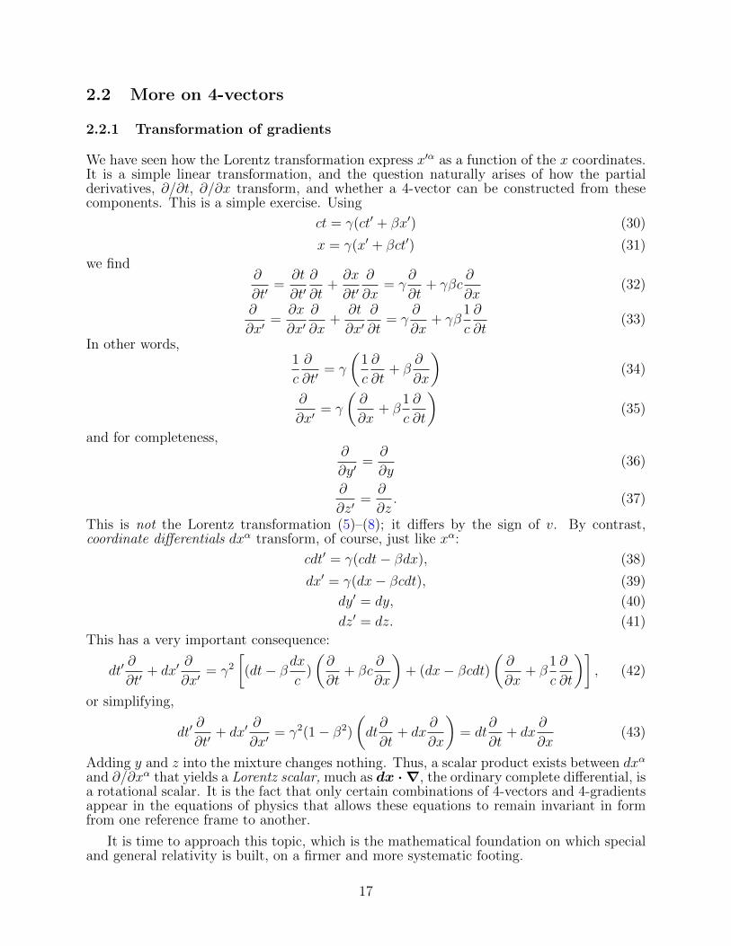
2.2.1 Transformation of gradients

We have seen how the Lorentz transformation express x′α as a function of the x coordinates.It is a simple linear transformation, and the question naturally arises of how the partialderivatives, ∂/∂t, ∂/∂x transform, and whether a 4-vector can be constructed from thesecomponents. This is a simple exercise. Using

ct = γ(ct′ + βx′) (30)

x = γ(x′ + βct′) (31)

we find∂

∂t′=∂t

∂t′∂

∂t+∂x

∂t′∂

∂x= γ

∂

∂t+ γβc

∂

∂x(32)

∂

∂x′=∂x

∂x′∂

∂x+

∂t

∂x′∂

∂t= γ

∂

∂x+ γβ

1

c

∂

∂t(33)

In other words,1

c

∂

∂t′= γ

(1

c

∂

∂t+ β

∂

∂x

)(34)

∂

∂x′= γ

(∂

∂x+ β

1

c

∂

∂t

)(35)

and for completeness,∂

∂y′=∂

∂y(36)

∂

∂z′=∂

∂z. (37)

This is not the Lorentz transformation (5)–(8); it differs by the sign of v. By contrast,coordinate differentials dxα transform, of course, just like xα:

cdt′ = γ(cdt− βdx), (38)

dx′ = γ(dx− βcdt), (39)

dy′ = dy, (40)

dz′ = dz. (41)

This has a very important consequence:

dt′∂

∂t′+ dx′

∂

∂x′= γ2

[(dt− βdx

c)

(∂

∂t+ βc

∂

∂x

)+ (dx− βcdt)

(∂

∂x+ β

1

c

∂

∂t

)], (42)

or simplifying,

dt′∂

∂t′+ dx′

∂

∂x′= γ2(1− β2)

(dt∂

∂t+ dx

∂

∂x

)= dt

∂

∂t+ dx

∂

∂x(43)

Adding y and z into the mixture changes nothing. Thus, a scalar product exists between dxα

and ∂/∂xα that yields a Lorentz scalar, much as dx · ∇, the ordinary complete differential, isa rotational scalar. It is the fact that only certain combinations of 4-vectors and 4-gradientsappear in the equations of physics that allows these equations to remain invariant in formfrom one reference frame to another.

It is time to approach this topic, which is the mathematical foundation on which specialand general relativity is built, on a firmer and more systematic footing.

17

2.2.2 Transformation matrix

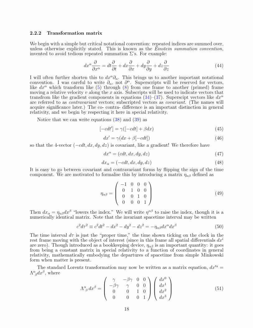
We begin with a simple but critical notational convention: repeated indices are summed over,unless otherwise explicitly stated. This is known as the Einstein summation convention,invented to avoid tedious repeated summation Σ’s. For example:

dxα∂

∂xα= dt

∂

∂t+ dx

∂

∂x+ dy

∂

∂y+ dz

∂

∂z(44)

I will often further shorten this to dxα∂α. This brings us to another important notationalconvention. I was careful to write ∂α, not ∂α. Superscripts will be reserved for vectors,like dxα which transform like (5) through (8) from one frame to another (primed) framemoving a relative velocity v along the x axis. Subscripts will be used to indicate vectors thattransfrom like the gradient components in equations (34)–(37). Superscipt vectors like dxα

are referred to as contravariant vectors; subscripted vectors as covariant. (The names willacquire significance later.) The co- contra- difference is an important distinction in generalrelativity, and we begin by respecting it here in special relativity.

Notice that we can write equations (38) and (39) as

[−cdt′] = γ([−cdt] + βdx) (45)

dx′ = γ(dx+ β[−cdt]) (46)

so that the 4-vector (−cdt, dx, dy, dz) is covariant, like a gradient! We therefore have

dxα = (cdt, dx, dy, dz) (47)

dxα = (−cdt, dx, dy, dz) (48)

It is easy to go between covariant and contravariant forms by flipping the sign of the timecomponent. We are motivated to formalise this by introducing a matrix ηαβ defined as

ηαβ =

−1 0 0 00 1 0 00 0 1 00 0 0 1

(49)

Then dxα = ηαβdxβ “lowers the index.” We will write ηαβ to raise the index, though it is a

numerically identical matrix. Note that the invariant spacetime interval may be written

c2dτ 2 ≡ c2dt2 − dx2 − dy2 − dz2 = −ηαβdxαdxβ (50)

The time interval dτ is just the “proper time,” the time shown ticking on the clock in therest frame moving with the object of interest (since in this frame all spatial differentials dxi

are zero). Though introduced as a bookkeeping device, ηαβ is an important quantity: it goesfrom being a constant matrix in special relativity to a function of coordinates in generalrelativity, mathematically embodying the departures of spacetime from simple Minkowskiform when matter is present.

The standard Lorentz transformation may now be written as a matrix equation, dx′α =Λα

βdxβ, where

Λαβ dx

β =

γ −βγ 0 0−βγ γ 0 0

0 0 1 00 0 0 1

dx0

dx1

dx2

dx3

(51)

18

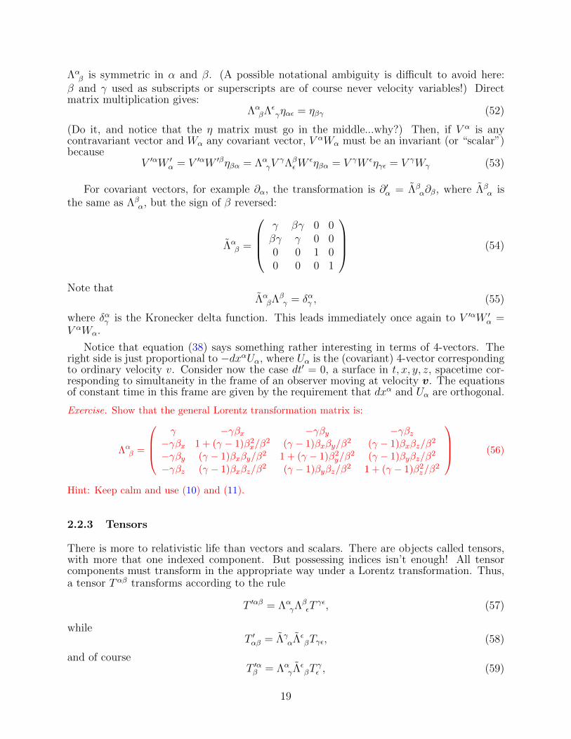
Λαβ is symmetric in α and β. (A possible notational ambiguity is difficult to avoid here:

β and γ used as subscripts or superscripts are of course never velocity variables!) Directmatrix multiplication gives:

ΛαβΛε

γηαε = ηβγ (52)

(Do it, and notice that the η matrix must go in the middle...why?) Then, if V α is anycontravariant vector and Wα any covariant vector, V αWα must be an invariant (or “scalar”)because

V ′αW ′α = V ′αW ′βηβα = Λα

γVγΛβ

εWεηβα = V γW εηγε = V γWγ (53)

For covariant vectors, for example ∂α, the transformation is ∂′α = Λβα∂β, where Λβ

α isthe same as Λβ

α, but the sign of β reversed:

Λαβ =

γ βγ 0 0βγ γ 0 00 0 1 00 0 0 1

(54)

Note thatΛα

βΛβγ = δαγ , (55)

where δαγ is the Kronecker delta function. This leads immediately once again to V ′αW ′α =

V αWα.

Notice that equation (38) says something rather interesting in terms of 4-vectors. Theright side is just proportional to −dxαUα, where Uα is the (covariant) 4-vector correspondingto ordinary velocity v. Consider now the case dt′ = 0, a surface in t, x, y, z, spacetime cor-responding to simultaneity in the frame of an observer moving at velocity v. The equationsof constant time in this frame are given by the requirement that dxα and Uα are orthogonal.

Exercise. Show that the general Lorentz transformation matrix is:

Λαβ =

γ −γβx −γβy −γβz−γβx 1 + (γ − 1)β2x/β

2 (γ − 1)βxβy/β2 (γ − 1)βxβz/β

2

−γβy (γ − 1)βxβy/β2 1 + (γ − 1)β2y/β

2 (γ − 1)βyβz/β2

−γβz (γ − 1)βxβz/β2 (γ − 1)βyβz/β

2 1 + (γ − 1)β2z/β2

(56)

Hint: Keep calm and use (10) and (11).

2.2.3 Tensors

There is more to relativistic life than vectors and scalars. There are objects called tensors,with more that one indexed component. But possessing indices isn’t enough! All tensorcomponents must transform in the appropriate way under a Lorentz transformation. Thus,a tensor Tαβ transforms according to the rule

T ′αβ = ΛαγΛ

βεT

γε, (57)

whileT ′αβ = Λγ

αΛεβTγε, (58)

and of courseT ′αβ = Λα

γΛεβT

γε , (59)

19

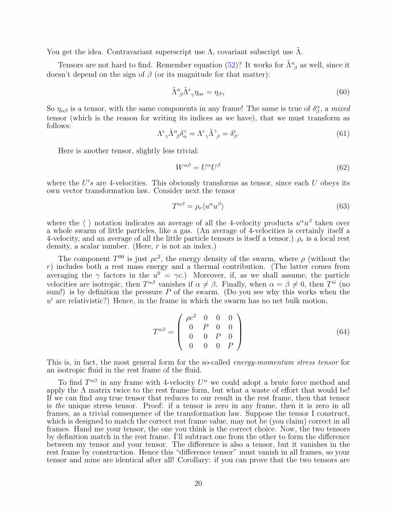
You get the idea. Contravariant superscript use Λ, covariant subscript use Λ.

Tensors are not hard to find. Remember equation (52)? It works for Λαβ as well, since it

doesn’t depend on the sign of β (or its magnitude for that matter):

ΛαβΛε

γηαε = ηβγ (60)

So ηαβ is a tensor, with the same components in any frame! The same is true of δαβ , a mixedtensor (which is the reason for writing its indices as we have), that we must transform asfollows:

ΛεγΛ

αβδ

γα = Λε

γΛγβ = δεβ. (61)

Here is another tensor, slightly less trivial:

Wαβ = UαUβ (62)

where the U ′s are 4-velocities. This obviously transforms as tensor, since each U obeys itsown vector transformation law. Consider next the tensor

Tαβ = ρr〈uαuβ〉 (63)

where the 〈 〉 notation indicates an average of all the 4-velocity products uαuβ taken overa whole swarm of little particles, like a gas. (An average of 4-velocities is certainly itself a4-velocity, and an average of all the little particle tensors is itself a tensor.) ρr is a local restdensity, a scalar number. (Here, r is not an index.)

The component T 00 is just ρc2, the energy density of the swarm, where ρ (without ther) includes both a rest mass energy and a thermal contribution. (The latter comes fromaveraging the γ factors in the u0 = γc.) Moreover, if, as we shall assume, the particlevelocities are isotropic, then Tαβ vanishes if α 6= β. Finally, when α = β 6= 0, then T ii (nosum!) is by definition the pressure P of the swarm. (Do you see why this works when theui are relativistic?) Hence, in the frame in which the swarm has no net bulk motion,

Tαβ =

ρc2 0 0 00 P 0 00 0 P 00 0 0 P

(64)

This is, in fact, the most general form for the so-called energy-momentum stress tensor foran isotropic fluid in the rest frame of the fluid.

To find Tαβ in any frame with 4-velocity Uα we could adopt a brute force method andapply the Λ matrix twice to the rest frame form, but what a waste of effort that would be!If we can find any true tensor that reduces to our result in the rest frame, then that tensoris the unique stress tensor. Proof: if a tensor is zero in any frame, then it is zero in allframes, as a trivial consequence of the transformation law. Suppose the tensor I construct,which is designed to match the correct rest frame value, may not be (you claim) correct in allframes. Hand me your tensor, the one you think is the correct choice. Now, the two tensorsby definition match in the rest frame. I’ll subtract one from the other to form the differencebetween my tensor and your tensor. The difference is also a tensor, but it vanishes in therest frame by construction. Hence this “difference tensor” must vanish in all frames, so yourtensor and mine are identical after all! Corollary: if you can prove that the two tensors are

20

the same in any one particular frame, then they are the same in all frames. This is a veryuseful ploy.

The only two tensors we have at our disposal to construct Tαβ are ηαβ and UαUβ, andthere is only one linear superposition that matches the rest frame value and does the trick:

Tαβ = Pηαβ + (ρ+ P/c2)UαUβ (65)

This is the general form of energy-momentum stress tensor appropriate to an ideal fluid.

2.2.4 Conservation of Tαβ

One of the most salient properties of Tαβ is that it is conserved, in the sense of

∂Tαβ

∂xα= 0 (66)

Since gradients of tensors transform as tensors, this must be true in all frames. What,exactly, are we conserving?

First, the time-like 0-component of this equation is

∂

∂t

[γ2(ρ+

Pv2

c4

)]+∇·

[γ2(ρ+

P

c2

)v

]= 0 (67)

which is the relativistic version of mass conservation,

∂ρ

∂t+∇·(ρv) = 0. (68)

Elevated in special relativity, it becomes a statement of energy conservation. So one of thethings we are conserving is energy. (And not just rest mass energy by the way, thermalenergy as well!) This is good.

The spatial part of the conservation equation reads

∂

∂t

[γ2(ρ+

P

c2

)vi

]+

(∂

∂xj

)[γ2(ρ+

P

c2

)vivj

]+∂P

∂xi= 0 (69)

You may recognise this as Euler’s equation of motion, a statement of momentum conserva-tion, upgraded to special relativity. Conserving momentum is also good.

What if there are other external forces? The idea is that these are included by expressingthem in terms of the divergence of their own stress tensor. Then it is the total Tαβ including,say, electromagnetic fields, that comes into play. What about the force of gravity? That, itwill turn out, is on an all-together different footing.

You start now to gain a sense of the difficulty in constructing a theory of gravity com-patible with relativity. The density ρ is part of the stress tensor, and it is the entire stresstensor in a relativistic theory that would have to be the source of the gravitational field,just as the entire 4-current Jα is the source of electromangetic fields. No fair just pickingthe component you want. Relativistic theories work with scalars, vectors and tensors topreserve their invariance properties from one frame to another. This insight is already anachievement: we can, for example, expect pressure to play a role in generating gravitational

21

fields. Would you have guessed that? Our relativistic gravity equation maybe ought to looksomething like :

∇2Gµν − 1

c2∂2Gµν

∂t2= T µν (70)

where Gµν is some sort of, I don’t know, conserved tensor guy for the...spacetime geome-try and stuff? In Maxwell’s theory we had a 4-vector (Aα) operated on by the so-called“d’Alembertian operator” ∇2 − (1/c)2∂2/∂t2 on the left side of the equation and a source(Jα) on the right. So now we just need to find a Gµν tensor to go with T µν . Right?

Actually, this really is a pretty good guess. It is more-or-less correct for weak fields, andmost of the time gravity is a weak field. But...well...patience. One step at a time.

22

Then there occurred to me the

‘glucklichste Gedanke meines Lebens,’

the happiest thought of my life, in the

following form. The gravitational field

has only a relative existence in a way

similar to the electric field generated

by magnetoelectric induction. Because

for an observer falling freely from the

roof of a house there exists—at least

in his immediate surroundings—no

gravitational field.

— Albert Einstein

1

3 The effects of gravity

The central idea of general relativity is that presence of mass (more precisely the presenceof any stress-energy tensor component) causes departures from flat Minkowski spacetimeto appear, and that other matter (or radiation) responds to these distortions in some way.There are then really two questions: (i) How does the affected matter/radiation move inthe presence of a distorted spacetime?; and (ii) How does the stress-energy tensor distortthe spacetime in the first place? The first question is purely computational, and fairlystraightforward to answer. It lays the groundwork for answering the much more difficultsecond question, so let us begin here.

3.1 The Principle of Equivalence

We have discussed the notion that by going into a frame of reference that is in free-fall, theeffects of gravity disappear. In this era in which space travel is common, we are all familiarwith astronauts in free-fall orbits, and the sense of weightlessness that is produced. Thismanifestation of the Equivalence Principle is so palpable that hearing total mishmasheslike “In orbit there is no gravity” from an over-eager science correspondent is a commonexperience. (Our own BBC correspondent in Oxford Astrophysics, Prof. Christopher Lintott,would certainly never say such a thing.)

The idea behind the equivalence principle is that the m in F = ma and the m in theforce of gravity Fg = mg are the same m and thus the acceleration caused by gravity, g, isinvariant for any mass. We could imagine, for example, that F = mIa and Fg = mgg, wheremg is some kind of “massy” property that might vary from one type of body to anotherwith the same mI . In this case, the acceleration a is mgg/mI , i.e., it varies with the ratio ofinertial to gravitational mass from one body to another. How well can we actually measurethis ratio, or what is more to the point, how well do we know that it is truly a universalconstant for all types of matter?

The answer is very, very well indeed. We don’t of course do anything as crude as directlymeasure the rate at which objects fall to the ground any more, a la Galileo and the towerof Pisa. As with all classic precision gravity experiments (including those of Galileo!) we

1With apologies to any readers who may actually have fallen off the roof of a house—safe space statement.

23

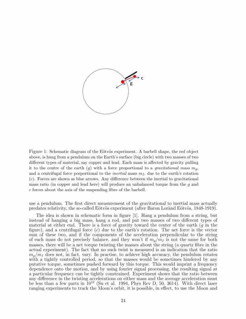
c g

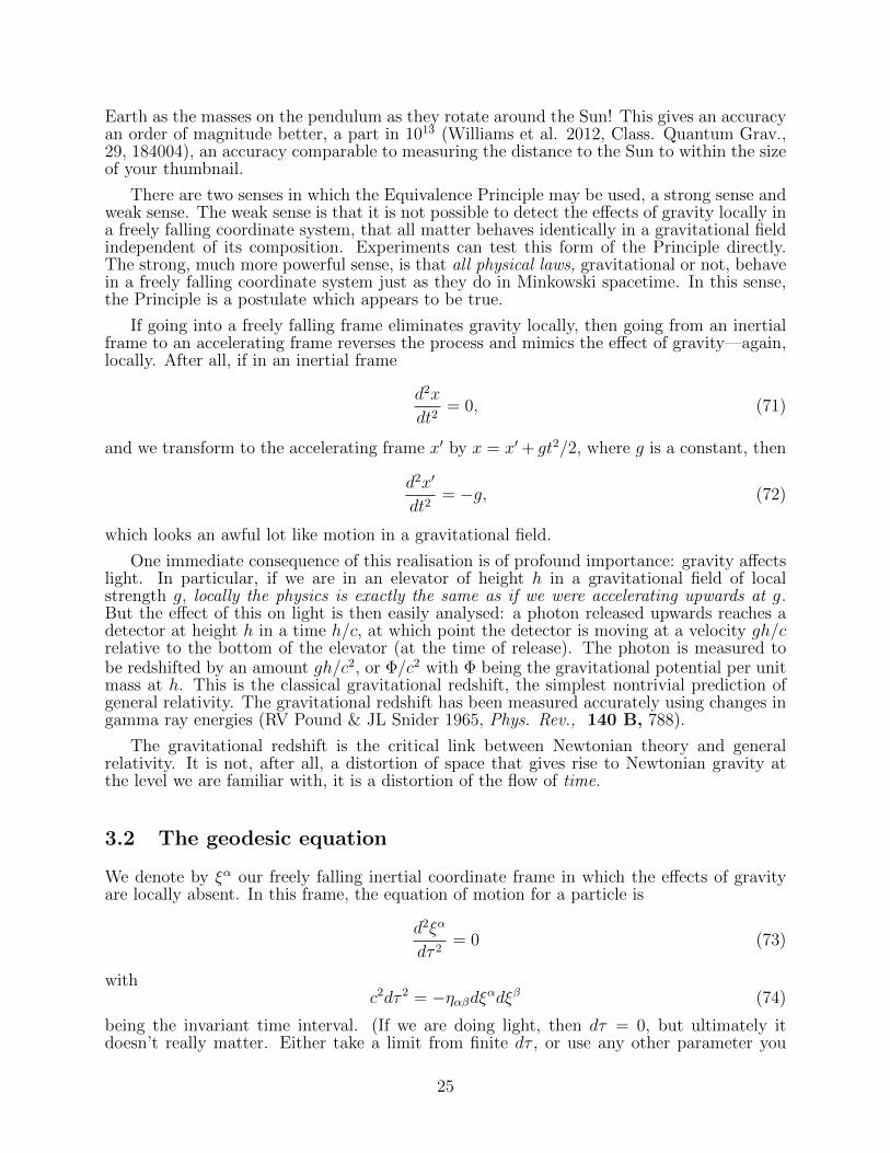
Figure 1: Schematic diagram of the Eotvos experiment. A barbell shape, the red objectabove, is hung from a pendulum on the Earth’s surface (big circle) with two masses of twodifferent types of material, say copper and lead. Each mass is affected by gravity pullingit to the centre of the earth (g) with a force proportional to a gravitational mass mg,and a centrifugal force porportional to the inertial mass mI , due to the earth’s rotation(c). Forces are shown as blue arrows. Any difference between the inertial to gravitationalmass ratio (in copper and lead here) will produce an unbalanced torque from the g andc forces about the axis of the suspending fibre of the barbell.

use a pendulum. The first direct measurement of the gravitational to inertial mass actuallypredates relativity, the so-called Eotvos experiment (after Baron Lorand Eotvos, 1848-1919).

The idea is shown in schematic form in figure [1]. Hang a pendulum from a string, butinstead of hanging a big mass, hang a rod, and put two masses of two different types ofmaterial at either end. There is a force of gravity toward the center of the earth (g in thefigure), and a centrifugal force (c) due to the earth’s rotation. The net force is the vectorsum of these two, and if the components of the acceleration perpendicular to the stringof each mass do not precisely balance, and they won’t if mg/mI is not the same for bothmasses, there will be a net torque twisting the masses about the string (a quartz fibre in theactual experiment). The fact that no such twist is measured is an indication that the ratiomg/mI does not, in fact, vary. In practise, to achieve high accuracy, the pendulum rotateswith a tightly controlled period, so that the masses would be sometimes hindered by anyputative torque, sometimes pushed forward by this torque. This would imprint a frequencydependence onto the motion, and by using fourier signal processing, the resulting signal ata particular frequency can be tightly constrained. Experiment shows that the ratio betweenany difference in the twisting accelerations on either mass and the average acceleration mustbe less than a few parts in 1012 (Su et al. 1994, Phys Rev D, 50, 3614). With direct laserranging experiments to track the Moon’s orbit, it is possible, in effect, to use the Moon and

24

Earth as the masses on the pendulum as they rotate around the Sun! This gives an accuracyan order of magnitude better, a part in 1013 (Williams et al. 2012, Class. Quantum Grav.,29, 184004), an accuracy comparable to measuring the distance to the Sun to within the sizeof your thumbnail.

There are two senses in which the Equivalence Principle may be used, a strong sense andweak sense. The weak sense is that it is not possible to detect the effects of gravity locally ina freely falling coordinate system, that all matter behaves identically in a gravitational fieldindependent of its composition. Experiments can test this form of the Principle directly.The strong, much more powerful sense, is that all physical laws, gravitational or not, behavein a freely falling coordinate system just as they do in Minkowski spacetime. In this sense,the Principle is a postulate which appears to be true.

If going into a freely falling frame eliminates gravity locally, then going from an inertialframe to an accelerating frame reverses the process and mimics the effect of gravity—again,locally. After all, if in an inertial frame

d2x

dt2= 0, (71)

and we transform to the accelerating frame x′ by x = x′+ gt2/2, where g is a constant, then

d2x′

dt2= −g, (72)

which looks an awful lot like motion in a gravitational field.

One immediate consequence of this realisation is of profound importance: gravity affectslight. In particular, if we are in an elevator of height h in a gravitational field of localstrength g, locally the physics is exactly the same as if we were accelerating upwards at g.But the effect of this on light is then easily analysed: a photon released upwards reaches adetector at height h in a time h/c, at which point the detector is moving at a velocity gh/crelative to the bottom of the elevator (at the time of release). The photon is measured tobe redshifted by an amount gh/c2, or Φ/c2 with Φ being the gravitational potential per unitmass at h. This is the classical gravitational redshift, the simplest nontrivial prediction ofgeneral relativity. The gravitational redshift has been measured accurately using changes ingamma ray energies (RV Pound & JL Snider 1965, Phys. Rev., 140 B, 788).

The gravitational redshift is the critical link between Newtonian theory and generalrelativity. It is not, after all, a distortion of space that gives rise to Newtonian gravity atthe level we are familiar with, it is a distortion of the flow of time.

3.2 The geodesic equation

We denote by ξα our freely falling inertial coordinate frame in which the effects of gravityare locally absent. In this frame, the equation of motion for a particle is

d2ξα

dτ 2= 0 (73)

withc2dτ 2 = −ηαβdξαdξβ (74)

being the invariant time interval. (If we are doing light, then dτ = 0, but ultimately itdoesn’t really matter. Either take a limit from finite dτ , or use any other parameter you

25

fancy, like your wristwatch. In the end, we won’t use τ or your watch. As for dξα, it is justthe freely-falling guy’s ruler and his wristwatch.) Next, write this equation in any other setof coordinates you like, and call them xµ. Our inertial coordinates ξα will be some functionor other of the xµ so

0 =d2ξα

dτ 2=d

dτ

(∂ξα

∂xµdxµ

dτ

)(75)

where we have used the chain rule to express dξα/dτ in terms of dxµ/dτ . Carrying out thedifferentiation,

0 =∂ξα

∂xµd2xµ

dτ 2+

∂2ξα

∂xµ∂xνdxµ

dτ

dxν

dτ(76)

where now the chain rule has been used on ∂ξα/∂xµ. This may not look very promising.But if we multiply this equation by ∂xλ/∂ξα, and remember to sum over α now, then thechain rule in the form

∂xλ

∂ξα∂ξα

∂xµ= δλµ (77)

rescues us. (We are using the chain rule repeatedly and will certainly continue to do so,again and again. Make sure you understand this, and that you understand what variablesare being held constant when the partial derivatives are taken. Deciding what is constant isjust as important as doing the differentiation!) Our equation becomes

d2xλ

dτ 2+ Γλµν

dxµ

dτ

dxν

dτ= 0, (78)

where

Γλµν =∂xλ

∂ξα∂2ξα

∂xµ∂xν(79)

is known as the affine connection, and is a quantity of central importance in the study ofRiemannian geometry and relativity theory in particular. You should be able to prove, usingthe chain rule of partial derivatives, an identity for the second derivatives of ξα that we willuse shortly:

∂2ξα

∂xµ∂xν=∂ξα

∂xλΓλµν (80)

(How does this work out when used in equation [76]?)

No need to worry, despite the funny notation. (Early relativity texts liked to usegothic font Gλ

µν for the affine connection, which must have imbued it with a nice steam-punk terror.) There is nothing especially mysterious about the affine connection. You useit all the time, probably without realising it. For example, in cylindrical (r, θ) coordinates,

when you use the combinations r−rθ2 or rθ+2rθ for your radial and tangential accelerations,you are using the affine connection and the geodesic equation. In the first case, Γrθθ = −r;in the second, Γθrθ = 1/r. (What happened to the 2?)

Exercise. Prove the last statements using ξx = r cos θ, ξy = r sin θ.

Exercise. On the surface of a unit-radius sphere, choose any point as your North Pole, work incolatitude θ and azimuth φ coordinates, and show that locally near the North Pole ξx = θ cosφ,ξy = θ sinφ. It is in this sense that the ξα coordinates are tied to a local region of the space nearthe North Pole point. In our freely-falling coordinate system, the local coordinates are tied to apoint in spacetime.

26

3.3 The metric tensor

In our locally inertial coordinates, the invariant spacetime interval is

c2dτ 2 = −ηαβdξαdξβ, (81)

so that in any other coordinates, dξα = (∂ξα/dxµ)dxµ and

c2dτ 2 = −ηαβ∂ξα

∂xµ∂ξβ

∂xνdxµdxν ≡ −gµνdxµdxν (82)

where

gµν = ηαβ∂ξα

∂xµ∂ξβ

∂xν(83)

is known as the metric tensor. The metric tensor embodies the information of how coordinatedifferentials combine to form the invariant interval of our spacetime, and once we know gµν ,we know everything, including (as we shall see) the affine connections Γλµν . The object ofgeneral relativity theory is to compute gµν for a given distribution of mass (more precisely,a given stress energy tensor), and a key goal of this course is to find the field equations thatenable us to do so.

3.4 The relationship between the metric tensor and affine connec-tion

Because of their reliance of the local freely falling inertial coordinates ξα, the gµν and Γλµνquantities are awkward to use in their present formulation. Fortunately, there is a directrelationship between Γλµν and the first derivatives of gµν that will allow us to become free oflocal bondage, permitting us to dispense with the ξα altogether. Though their existence iscrucial to formulate the mathematical structure, the practical need of the ξ’s to carry outcalculations is minimal.

Differentiate equation (83):

∂gµν∂xλ

= ηαβ∂2ξα

∂xλ∂xµ∂ξβ

∂xν+ ηαβ

∂ξα

∂xµ∂2ξβ

∂xλ∂xν(84)

Now use (80) for the second derivatives of ξ:

∂gµν∂xλ

= ηαβ∂ξα

∂xρ∂ξβ

∂xνΓρλµ + ηαβ

∂ξα

∂xµ∂ξβ

∂xρΓρλν (85)

All remaining ξ derivatives may be absorbed as part of the metric tensor, leading to

∂gµν∂xλ

= gρνΓρλµ + gµρΓ

ρλν (86)

It remains only to unweave the Γ’s from the cloth of indices. This is done by first adding∂gλν/∂x

µ to the above, then subtracting it with indices µ and ν reversed.

∂gµν∂xλ

+∂gλν∂xµ

− ∂gλµ∂xν

= gρνΓρλµ +gρµΓρλν + gρνΓ

ρµλ +gρλΓ

ρµν −gρµΓρνλ −gρλΓ

ρνµ (87)

27

Remembering that Γ is symmetric in its bottom indices, only the gρν terms survive, leaving

∂gµν∂xλ

+∂gλν∂xµ

− ∂gλµ∂xν

= 2gρνΓρµλ (88)

Our last step is to mulitply by the inverse matrix gνσ, defined by

gνσgρν = δσρ , (89)

leaving us with the pretty result

Γσµλ =gνσ

2

(∂gµν∂xλ

+∂gλν∂xµ

− ∂gλµ∂xν

). (90)

Notice that there is no mention of the ξ’s. The affine connection is completely specified bygµν and the derivatives of gµν in whatever coordinates you like. In practise, the inverse matrixis not difficult to find, as we will usually work with metric tensors whose off diagonal termsvanish. (Gain confidence once again by practising the geodesic equation with cylindricalcoordinates grr = 1, gθθ = r2 and using [90.]) Note as well that with some very simple indexrelabeling, equation (88) leads directly to the mathematical identity

gρνΓρµλ

dxµ

dτ

dxλ

dτ=

(∂gµν∂xλ

− 1

2

∂gλµ∂xν

)dxµ

dτ

dxλ

dτ. (91)

We’ll use this in a moment.

Exercise. Prove that gνσ is given explicitly by

gνσ = ηαβ∂xν

∂ξα∂xσ

∂ξβ

Exercise. Prove the identities of page 6 of the notes for a diagonal metric gab,

Γaba = Γaab =1

2gaa

∂gaa∂xb

(a = b permitted, NO SUM)

Γabb = − 1

2gaa

∂gbb∂xa

(a 6= b, NO SUM)

Γabc = 0, (a, b, c distinct)

3.5 Variational calculation of the geodesic equation

The physical significance of the relationship between the metric tensor and affine connectionmay be understood by a variational calculation. Off all possible paths in our spacetimefrom some point A to another B, which leaves the proper time an extremum (in this case, amaximum)? The motivation for this formulation is obvious: “The shortest distance betweentwo points is a straight line,” and the equations for this line-geodesic are d2ξi/ds

2 = 0 inCartesian coordinates. This is an elementary property of Euclidian space. We may ask whatis the shortest distance between two points in a more general curved space as well, andthis question naturally lends itself to a variational approach. What is less obvious is thatthis mathematical machinery, which was fashioned for generalising the spacelike straight line

28

equation d2ξi/ds2 = 0 to more general non-Euclidian geometries, also works for generalisinga dynamical equation of the form d2ξi/dτ 2 = 0, where now we are using invariant timelikeintervals, to geodesics embedded in distorted Minkowski geometries.

We describe our path by some external parameter p, which could be anything really,perhaps the time on your very own wristwatch in your rest frame. (I don’t want to startwith τ , because dτ = 0 for light.) Then the proper time from A to B is

TAB =

∫ B

A

dτ

dpdp =

1

c

∫ B

A

(−gµν

dxµ

dp

dxν

dp

)1/2

dp (92)

Next, vary xλ to xλ + δxλ (we are regarding xλ as a function of p remember), with δxλ

vanishing at the end points A and B. We find

δTAB =1

2c

∫ B

A

(−gµν

dxµ

dp

dxν

dp

)−1/2(−∂gµν∂xλ

δxλdxµ

dp

dxν

dp− 2gµν

dδxµ

dp

dxν

dp

)dp (93)

(Do you understand the final term in the integral?)

Since the leading inverse square root in the integrand is just dp/dτ , δTAB simplifies to

δTAB =1

2c

∫ B

A

(−∂gµν∂xλ

δxλdxµ

dτ

dxν

dτ− 2gµν

dδxµ

dτ

dxν

dτ

)dτ, (94)

and p has vanished from sight. We now integrate the second term by parts, noting that thecontribution from the endpoints has been specified to vanish. Remembering that

dgλνdτ

=dxσ

dτ

∂gλν∂xσ

, (95)

we find

δTAB =1

c

∫ B

A

(−1

2

∂gµν∂xλ

dxµ

dτ

dxν

dτ+∂gλν∂xσ

dxσ

dτ

dxν

dτ+ gλν

d2xν

dτ 2

)δxλ dτ (96)

or

δTAB =1

c

∫ B

A

[(−1

2

∂gµν∂xλ

+∂gλν∂xµ

)dxµ

dτ

dxν

dτ+ gλν

d2xν

dτ 2

]δxλ dτ (97)

Finally, using equation (91), we obtain

δTAB =1

c

∫ B

A

[(dxµ

dτ

dxσ

dτΓνµσ +

d2xν

dτ 2

)gλν

]δxλ dτ (98)

Thus, if the geodesic equation (78) is satisfied, δTAB = 0 is satisfied, and the proper time isan extremum. The name “geodesic” is used in geometry to describe the path of minimumdistance between two points in a manifold, and it is therefore gratifying to see that there isa correspondence between a local “straight line” with zero curvature, and the local elimina-tion of a gravitational field with the resulting zero acceleration, along the lines if the firstparagraph of this section. In the first case, the proper choice of local coordinates results inthe second derivative with respect to an invariant spatial interval vanishing; in the secondcase, the proper choice of coordinates means that the second derivative with respect to aninvariant time interval vanishes, but the essential mathematics is the same.

29

There is often a very practical side to working with the variational method: it can bemuch easier to obtain the equations of motion for a given gµν this way than to construct themdirectly. For example, the method quickly produces all the non-vanishing affine connectioncomponents, just read them off as the coefficients of (dxµ/dτ)(dxν/dτ). You don’t have tofind them by trial and error. These quantities are then available for any variety of purposes(and they are needed for many).

Here is another trick. You should have little difficulty showing that if we apply theEuler-Lagrange variational method directly to the following functional L,

L = gµν xµxν ,

where the dot is d/dτ , the resulting Euler-Lagrange equation

d

dτ

(∂L∂xρ

)− ∂L∂xρ

= 0

is just the standard geodesic equation of motion! This is often the easiest way to proceed.

Indeed, in classical mechanics, we all know that the equations of motion may be derivedfrom a Lagrangian variational principle of least action, an integral involving the differencebetween kinetic and potential energies. This doesn’t seem geometrical at all. What is theconnection with what we’ve just done? How do we make contact with Newtonian mechanicsfrom the geodesic equation?

3.6 The Newtonian limit

We consider the case of a slowly moving mass (“slow” of course means relative to c, thespeed of light) in a weak gravitational field (GM/rc2 1). Since cdt |dx|, the geodesicequation greatly simplfies:

d2xµ

dτ 2+ Γµ00

(cdt

dτ

)2

= 0. (99)

Now

Γµ00 =1

2gµν(∂g0ν∂(cdt)

+∂g0ν∂(cdt)

− ∂g00∂xν

)(100)

In the Newtonian limit, the largest of the g derivatives is the spatial gradient, hence

Γµ00 ' −1

2gµν

∂g00∂xν

(101)

Since the gravitational field is weak, gαβ differs very little from the Minkoswki value:

gαβ = ηαβ + hαβ, hαβ 1, (102)

and the µ = 0 geodesic equation is

d2t

dτ 2+

1

2

∂h00∂t

(dt

dτ

)2

= 0 (103)

Clearly, the second term is zero for a static field, and will prove to be tiny when the gravita-tional field changes with time under nonrelativistic conditions—we are, after all, calculating

30

the difference between proper time and observer time! Dropping this term we find that tand τ are linearly related, so that the spatial components of the geodesic equation become

d2x

dt2− c2

2∇h00 = 0 (104)

Isaac Newton would say:d2x

dt2+∇Φ = 0, (105)

with Φ being the classical gravitational potential. The two views are consistent if

h00 ' −2Φ

c2, g00 ' −

(1 +

2Φ

c2

)(106)

In other words, the gravitational potential force emerges as a sort of centripital term, similarin structure to the centripital force in the standard radial equation of motion. This is aremarkable result. It is by no means obvious that a purely geometrical geodesic equationcan serve the role of a Newtonian gravitational potential gradient force equation, but itcan. Moreover, it teaches us that the Newtonian limit of general relativity is all in the timecomponent, h00. It is now possible to measure directly the differences in the rate at whichclocks run at heights separated by 100 m or so on the Earth’s surface.

The quantity h00 is a dimensionless number of order v2/c2, where v is a velocity typicalof the system, an orbital speed or just the square root of a potential. Note that h00 isdetermined by the dynamical equations only up to an additive constant. Here we havechosen the constant to make the geometry Minkowskian at large distances from any matter.At the surface of a spherical object of mass M and radius R,

h00 ' 2× 10−6(M

M

)(RR

)(107)

where M is the mass of the sun (about 2× 1030 kg) and R is the radius of the sun (about7 × 108 m). As an exercise, you may wish to look up masses of planets and other typesof stars and evaluate h00. What is its value at the surface of a white dwarf (mass of thesun, radius of the earth)? What about a neutron star (mass of the sun, radius of Oxford)?How many decimal points are needed to see the time difference in two digital clocks at a onemeter separation in height on the earth?

We are now able to relate the geodesic equation to the principle of least action in classicalmechanics. In the Newtonian limit, our variational integral becomes∫ [

c2(1 + 2Φ/c2)dt2 − d|x|2]1/2

(108)

(Remember our compact notation: dt2 ≡ (dt)2, d|x|2 = (d|x|)2.) Expanding the square root,∫c

(1 +

Φ

c2− v2

2c2+ ...

)dt (109)

where v2 ≡ (d|x|/dt)2. Thus, minimising the Lagrangian (kinetic energy minus potentialenergy) is the same as maximising the proper time interval! What an unexpected andbeautiful connection.

31

What we have calculated in this section is nothing more than our old friend the gravi-tational redshift, with which we began our formal study of general relativity. The invariantspacetime interval dτ , the proper time, is given by

c2dτ 2 = −gµνdxµdxν (110)

For an observer at rest at location x, the time interval registered on a clock will be

dτ(x) = [−g00(x)]1/2dt (111)

where dt is the time interval registered at infinity, where −g00 → 1. (Compare: the “properlength” on the unit sphere for an interval at constant θ is sin θdφ, where dφ is the lengthregistered by an equatorial observer.) If the interval between two wave crest crossings isfound to be dτ(y) at location y, it will be dτ(x) when the light reaches x and it will be dtat infinity. In general,

dτ(y)

dτ(x)=

[g00(y)

g00(x)

]1/2, (112)

and in particulardτ(R)

dt=ν(∞)

ν= [−g00(R)]1/2 (113)

where ν = 1/dτ(R) is, for example, an atomic transition frequency measured at rest at thesurface R of a body, and ν(∞) the corresponding frequency measured a long distance away.Interestingly, the value of g00 that we have derived in the Newtonian limit is, in fact, theexact relativisitic value of g00 around a point mass M ! (A black hole.) The precise redshiftformula is

ν∞ =

(1− 2GM

Rc2

)1/2

ν (114)

The redshift as measured by wavelength becomes infinite from light emerging from radiusR = 2GM/c2, the so-called Schwarzschild radius (about 3 km for a point with the mass ofthe sun!).

Historically, general relativity theory was supported in its infancy by the reported detec-tion of a gravitational redshift in a spectral line observed from the surface of the white dwarfstar Sirius B in 1925 by W.S. Adams. It “killed two birds with one stone,” as the leadingastronomer A.S. Eddington remarked. For it not only proved the existence of white dwarfstars (at the time controversial since the mechanism of pressure support was unknown), themeasurement also confirmed an early and important prediction of general relativity theory:the redshift of light due to gravity.

Alas, the modern consensus is that the actual measurements were flawed! Adams knewwhat he was looking for and found it. Though he was premature, the activity this apparentlypositive observation imparted to the study of white dwarfs and relativity theory turned outto be very fruitful indeed. But we were lucky. Incorrect but well regarded single-investigatorobservations have in the past caused much confusion and needless wrangling, as well as yearsof wasted effort.

The first definitive test for gravitational redshift came much later, and it was terrestrial:the 1959 Pound and Rebka experiment performed at Harvard University’s Jefferson Towermeasured the frequency shift of a 14.4 keV gamma ray falling (if that is the word for a gammaray) 22.6 m. Pound & Rebka were able to measure the shift in energy—just a few parts in1014—by what was at the time the new and novel technique of Mossbauer spectroscopy.

32

Exercise. A novel application of the gravitational redshift is provided by Bohr’s refutation ofan argument put forth by Einstein purportedly showing that an experiment could in principle bedesigned to bypass the quantum uncertainty relation ∆E∆t ≥ h. The idea is to hang a boxcontaining a photon by a spring suspended in a gravitational field g. At some precise time ashutter is opened and the photon leaves. You weigh the box before and after the photon. There isin principle no interference between the arbitrarily accurate change in box weight and the arbitrarilyaccurate time at which the shutter is opened. Or is there?

1.) Show that box apparatus satisfies an equation of the form

Mx = −Mg − kx

where M is the mass of the apparatus, x is the displacement, and k is the spring constant. Beforerelease, the box is in equilibrium at x = −gM/k.

2.) Show that the momentum of the box apparatus after a short time interval ∆t from when thephoton escapes is

δp = −gδmω

sin(ω∆t) '= −gδm∆t

where δm is the (uncertain!) photon mass and ω2 = k/M . With δp ∼ gδm∆t, the uncertaintyprinciple then dictates an uncertain location of the box position δx given by gδmδx∆t ∼ h. Butthis is location uncertainty, not time uncertainty.

3.) Now the gravitational redshift comes in! Show that if there is an uncertainty in position δx,there is an uncertainty in the time of release: δt ∼ (gδx/c2)∆t.

4.) Finally use this in part (2) to establish δE δt ∼ h with δE = δmc2.

Why does general relativity come into nonrelativistic quantum mechanics in such a fundamentalway? Because the gravitational redshift is relativity theory’s point-of-contact with classical New-tonian mechanics, and Newtonian mechanics when blended with the uncertainty principle is thestart of nonrelativistic quantum mechanics.

A final thought

We Newtonian beings, with our natural mode of thinking in terms of forces and responses,would naturally say “How interesting, the force of gravity distorts the flow time.” This isthe way I have been describing the gravitational redshift throught this chapter. But Einsteinhas given us a more profound insight. It is not that gravity distorts the flow of time. AnEinsteinian being, brought up from the cradle to be comfortable with a spacetime point-of-view, would, upon hearing this comment, cock their head and say: “What are you talkingabout? Newtonian gravity is the distortion of the flow of time. It is a simple geometricdistortion that is brought about by the presence of matter.” This is a better way to thinkof it. The nearby effect of weak gravity is indeed a distortion in the flow of time; the distanteffect of weak gravity is gravitational radiation, and this, we shall see, is a distortion of space.

33

4 Tensor Analysis

Further, the dignity of the science

seems to require that every possible

means be explored itself for the solution

of a problem so elegant and so cele-

brated.

— Carl Friedrich Gauss

A mathematical equation is valid in the presence of general gravitational fields when

i.) It is a valid equation in the absence of gravity and respects Lorentz invariance.

ii.) It preserves its form, not just under Lorentz transformations, but under any coordinatetransformation, x→ x′.

What does “preserves its form” mean? It means that the equation must be written in termsof quantities that transform as scalars, vectors, and higher ranked tensors under generalcoordinate transformations. From (ii), we see that if we can find one coordinate system inwhich our equation holds, it will hold in any set of coordinates. But by (i), the equationdoes hold in locally freely falling coordinates, in which the effect of gravity is locally absent.The effect of gravity is strictly embodied in the two key quantities that emerge from thecalculus of coordinate transformations: the metric tensor gµν and its first derivatives in Γλµν .This approach is known as the Principle of General Covariance, and it is a very powerfultool indeed.

4.1 Transformation laws

The simplest vector one can write down is the ordinary coordinate differential dxµ. If x′µ =x′µ(x), there is no doubt how the dx′µ are related to the dxµ. It is called the chain rule, andit is by now very familiar:

dx′µ =∂x′µ

∂xνdxν (115)

Be careful to distinguish between the coordinates xµ, which can be pretty much anything,and their differentials dxµ, which are true vectors. Indeed, any set of quantities V µ thattransforms in this way is known as a contravariant vector:

V ′µ =∂x′µ

∂xνV ν (116)

The contravariant 4-vector is simply Uµ = dxµ/dτ , a generalisation of the special relativisticdξα/dτ . A covariant vector, by contrast, transforms as

U ′µ =∂xν

∂x′µUν (117)

“CO LOW, PRIME BELOW.” (Sorry. Maybe you can do better.) These definitions ofcontravariant and covariant vectors are consistent with those we first introduced in our

34

discussions of the Lorentz matrices Λαβ and Λβ

α in Chapter 2, but now generalised fromspecific linear transformations to arbitrary transformations.

The simplest covariant vector is the gradient ∂/∂xµ of a scalar Φ. Once again, the chainrule tells us how to transform from one set of coordinates to another—we’ve no choice:

∂Φ

∂x′µ=∂xν

∂x′µ∂Φ

∂xν(118)

The generalisation to tensor transformation laws is immediate. A contravariant tensor T µν

transforms as

T ′µν =∂x′µ

∂xρ∂x′ν

∂xσT ρσ (119)

a covariant tensor Tµν as

T ′µν =∂xρ

∂x′µ∂xσ

∂x′νTρσ (120)

and a mixed tensor T µν as

T ′µν =∂x′µ

∂xρ∂xσ

∂x′νT ρσ (121)

The generalisation to mixed tensors of arbitrary rank should be self-evident.

By this definition the metric tensor gµν really is a covariant tensor, just as its notationwould lead you to believe, because

g′µν ≡ ηαβ∂ξα

∂x′µ∂ξβ

∂x′ν= ηαβ

∂ξα

∂xλ∂ξβ

∂xρ∂xλ

∂x′µ∂xρ

∂x′ν≡ gλρ

∂xλ

∂x′µ∂xρ

∂x′ν(122)

and the same for the contravariant gµν . But the gradient of a vector is not, in general, atensor or a vector:

∂V ′λ

∂x′µ=

∂

∂x′µ

(∂x′λ

∂xνV ν

)=∂x′λ

∂xν∂xρ

∂x′µ∂V ν

∂xρ+

∂2x′λ

∂xρ∂xν∂xρ

∂x′µV ν (123)

The first term is just what we would have wanted if we were searching for a tensor trans-formation law. But oh those pesky second order derivatives—the final term spoils it all.This of course vanishes when the coordinate transformation is linear (as when we found thatvector derivatives are perfectly good tensors under the Lorentz transformations), but not ingeneral. We will show in the next section that while the gradient of a vector is in generalnot a tensor, there is an elegant solution around this problem.

Tensors can be created and manipulated in many ways. For example, direct products oftensors are tensors:

W µνρσ = T µνSρσ. (124)

Linear combinations of tensors multiplied by scalars of the same rank are obviously tensorsof the same rank. A tensor can lower its index by multiplying by gµν or raise it with gµν :

T ′ρµ ≡ g′µνT′νρ =

∂xσ

∂x′µ∂xλ

∂x′ν∂x′ν

∂xκ∂x′ρ

∂xτgσλT

κτ =∂xσ

∂x′µ∂x′ρ

∂xτgσκT

κτ (125)

which indeed transforms as a tensor of mixed second rank, T ρµ . To clarify: multiplying T µν

by any covariant tensor Sρµ generates a mixed tensor Mνρ , but we adopt the very useful

35

convention of keeping the name T νρ when multiplying by Sρµ = gρµ, and thinking of theindex as “being lowered.” (And of course index-raising for multiplication by gρµ.)

Mixed tensors can “contract” to scalars. Start with T µν . Then consider the transforma-tion of T µµ:

T ′µµ =∂x′µ

∂xν∂xρ

∂x′µT νρ = δρνT

νρ = T νν (126)

i.e., T µµ is a scalar T . Exactly the same type of calculation shows that T µνµ is a vector T ν ,and so on. Remember to contract “up–down:” T µµ = T , not T µµ = T .

The generalisation of the familiar scalar dot product between vectors Aµ and Bµ isAµBµ = gµνA

µBν . We are often interested in just the spatial part of 4-vectors, the 3-vectorAi. Then, in a non-Euclidian 3-space, the local angle between two vectors may be writtenas the ratio

cos ∆θ =AiBi

(AjAj BkBk)1/2=

gijAiBj

(gklAkAl gmnBmBn)1/2(127)

the analogue of A ·B/(|A||B|). If we are given two parameterised curves, perhaps twoorbits xi(p) and yi(p), and wish to know the angle between them at some particular point,this angle becomes

cos ∆θ =xiyi

(xjxj ykyk)1/2=

gijxiyj

(gklxkxl gmnymyn)1/2

where the dot notation denotes d/dp. Do you see why this is so?

4.2 The covariant derivative

Recall the geodesic equationd2xλ

dτ 2+ Γλµν

dxµ

dτ

dxν

dτ= 0. (128)

The left hand side has one free index component, and the right hand side surely is a vector:the trivial zero vector. Since this equation is valid in any coordinates, the left side needsto transform as a vector. What is interesting is that neither of the two terms by itself is avector, yet somehow their sum transforms as a vector.

Rewrite the geodesic equation as follows. Denote dxλ/dτ , a true vector, as Uλ. Then

Uµ

[∂Uλ

∂xµ+ ΓλµνU

ν

]= 0 (129)

Ah ha! Since the left side must be a vector, the stuff in square brackets must be a tensor: itis contracted with a vector Uµ to produce a vector—namely zero. The square brackets mustcontain a mixed tensor of rank two. Now, Γλµν vanishes in locally free falling coordinates,in which we know that simple partial derivatives of vectors are indeed tensors. So thisprescription tells us how to upgrade the notion of a partial derivative to the status of atensor: to make a tensor out of a plain old partial derivative, form the quantity

∂Uλ

∂xµ+ ΓλµνU

ν ≡ Uλ;µ (130)

36

the so called covariant derivative. Following convention, we use a semicolon to denote co-variant differentiation. (Some authors get tired of writing out ordinary partial derivativesand so use a comma for this (e.g V ν

, µ), but it is more clear to use full partial derivativenotation, and we shall abide by this in these notes, if not always in lecture.) The covariantderivative is a true tensor, taking on a plain partial derivative form only in local freely fallingcoordinates. We therefore have our partial derivative generalisation to tensor form!

You know, this is really too important a result not to check in detail. Perhaps youthink there is something special about the geodesic equation, or something special aboutour Uλ. In addition to this concern, we need to understand how to construct the covariantderivative of covariant vectors, and of more general tensors. (Talk about confusing. Noticethe use of the word “covariant” twice in that last statement in two very different senses.Apologies for this awkward, but completely standard, mathematical nomenclature.) If youare already convinced that the covariant derivative really is a tensor, just skip down to rightafter equation (137). You won’t learn anything more than you already know in the next longparagraph, and there is a lot of calculation.

The first thing we need to do is to establish the transformation law for Γλµν . This is justrepeated application of the chain rule:

Γ′λµν ≡∂x′λ

∂ξα∂2ξα

∂x′µ∂x′ν=∂x′λ

∂xρ∂xρ

∂ξα∂

∂x′µ

(∂xσ

∂x′ν∂ξα

∂xσ

)(131)

Carrying through the derivative,

Γ′λµν =∂x′λ

∂xρ∂xρ

∂ξα

(∂xσ

∂x′ν∂xτ

∂x′µ∂2ξα

∂xτ∂xσ+

∂2xσ

∂x′µ∂x′ν∂ξα

∂xσ

)(132)

Cleaning up, and recognising an affine connection when we see one, helps to rid us of thesemeddlesome ξ’s:

Γ′λµν =∂x′λ

∂xρ∂xτ

∂x′µ∂xσ

∂x′νΓρτσ +

∂x′λ

∂xρ∂2xρ

∂x′µ∂x′ν(133)

This may also be written

Γ′λµν =∂x′λ

∂xρ∂xτ

∂x′µ∂xσ

∂x′νΓρτσ −

∂xρ

∂x′ν∂xσ

∂x′µ∂2x′λ

∂xσ∂xρ(134)

Do you see why? (Hint: Either integrate ∂/∂x′µ by parts or differentiate the identity

∂x′λ

∂xρ∂xρ

∂x′ν= δλν .)

Hence

Γ′λµνV′ν =

(∂x′λ

∂xρ∂xτ

∂x′µ∂xσ

∂x′νΓρτσ −

∂xρ

∂x′ν∂xσ

∂x′µ∂2x′λ

∂xρ∂xσ

)∂x′ν

∂xηV η, (135)

and spotting some tricky sums over ∂x′ν that turn into Kronecker delta functions,

Γ′λµνV′ν =

∂x′λ

∂xρ∂xτ

∂x′µΓρτσV

σ − ∂xσ

∂x′µ∂2x′λ

∂xρ∂xσV ρ (136)

Finally, adding this to (123), the unwanted terms cancel just as they should. We thus obtain

∂V ′λ

∂x′µ+ Γ′λµνV

′ν =∂x′λ

∂xν∂xρ

∂x′µ

(∂V ν

∂xρ+ ΓνρσV

σ

), (137)

37

as desired. This combination really does transform as a tensor ought to.

It is now a one-step process to deduce how covariant derivatives work for covariant vectors.Consider

VλVλ;µ = Vλ

∂V λ

∂xµ+ ΓλµνV

νVλ (138)

which is a perfectly good covariant vector. Integrating by parts the first term on the right,and then switching dummy indices λ and ν in the final term, this expression is identical to

∂(V λVλ)

∂xµ− V λ

[∂Vλ∂xµ− ΓνµλVν

]. (139)

Since the first term is the covariant gradient of a scalar (zero actually, because V λVλ = −c2in local inertial coordinates and it’s a scalar, so its always c2), and the entire expression mustbe a good covariant vector, the term in square brackets must be a purely covariant tensorof rank two. We have very quickly found our generalisation for the covariant derivative of acovariant vector:

Vλ;µ =∂Vλ∂xµ− ΓνµλVν (140)

That this really is a vector can also be directly verified via a calculation exactly similar toour previous one for the covariant derivative of a contravariant vector.

Covariant derivatives of tensors are now simple to deduce. The tensor T λκ must formallytransform like a contravariant vector if we “freeze” one of its indices at some particularcomponent and allow the other to take on all component values. Since the formula must besymmetric in the two indices,

T λκ;µ =∂T λκ

∂xµ+ ΓλµνT

νκ + ΓκνµTλν (141)

and then it should also follow

Tλκ;µ =∂Tλκ∂xµ

− ΓνλµTνκ − ΓνκµTλν (142)

and of course

T λκ;µ =∂T λκ∂xµ

+ ΓλνµTνκ − ΓνµκT

λν (143)

The generalisation to tensors of arbitrary rank should now be self-evident. To generate theaffine connection terms, freeze all indices in your tensor, then unfreeze them one-by-one,treating each unfrozen index as either a covariant or contravariant vector, depending uponwhether it is down or up. Practise this until it is second-nature.

We now can give a precise rule for how to take an equation that is valid in specialrelativity, and upgrade it to the general relativistic theory of gravity. Work exclusively with4-vectors and 4-tensors. Replace ηαβ with gµν. Take ordinary derivatives and turn them intocovariant derivatives. Voila: your equation is set for the presence of gravitational fields.

It will not have escaped your attention, I am sure, that applying (142) to gµν produces

gµν;λ =∂gµν∂xλ

− gρνΓρµλ − gµρΓρνλ = 0 (144)

where equation (86) has been used for the last equality. The covariant derivatives of gµνvanish. This is exactly what we would have predicted, since the ordinary derivatives of ηαβ

38

vanish in special relativity, and thus the covariant derivative of gµν should vanish in thepresence of gravitational fields. It’s just the general relativistic upgrade of ∂ηαβ/∂x

γ = 0.

Here are two important technical points that are easily shown. (You should do so explic-itly.)

i.) The covariant derivative obeys the Leibniz rule for products. For example:

(T µνUλκ);ρ = T µν;ρ Uλκ + T µνUλκ;ρ,

(V µVµ);ν = V µ(Vµ);ν + Vµ(V µ);ν = V µ∂Vµ

∂xν+ Vµ

∂Vµ∂xν

(Γ′s cancel!)

ii.) The operation of contracting two tensor indices commutes with covariant differentiation.It does not matter which you do first. Check it out in the second example above.

4.3 The affine connection and basis vectors

The reader may be wondering how this all relates to our notions of, say, spherical or polargeometry and their associated sets of unit vectors and coordinates. The answer is: verysimply. Our discussion will be straightforward and intuitive, rather than rigorous.

A vector V may be expanded in a set of basis vectors,

V = V aea (145)

where we sum over the repeated a, but a here on a bold-faced vector refers to a particularvector in the basis set. The V a are the usual vector contravariant components: old friends,just numbers. Note that the sum is not a scalar formed from a contraction! We’ve usedroman letters here to help avoid that pitfall.

The covariant components are associated with what mathematicians are pleased to calla dual basis:

V = Vbeb (146)

Same V mind you, just different ways of representing its components. If the e’s seem alittle abstract, don’t worry, just take them at a formal level for the moment. You’ve seensomething very like them before in elementary treatments of vectors.

The basis and the dual basis are related by a dot product rule,

ea·eb = δba. (147)

This dot product rule relates the vectors of orthonormal bases. The basis vectors transformjust as good old vectors should:

e′a =∂xb

∂x′aeb, e′a =

∂x′a

∂xbeb. (148)

Note that the dot product rule gives

V ·V = V aVbea·eb = V aVbδba = V aVa, (149)

as we would expect. On the other hand, expanding the differential line element ds,

ds2 = eadxa·ebdxb = ea·ebdxadxb (150)

39

so that we recover the metric tensor

gab = ea·eb (151)

Exactly the same style calculation gives

gab = ea·eb (152)

These last two equations tell us first that gab is the coefficient of ea in an expansion of thevector eb in the usual basis:

eb = gabea, (153)

and tell us second that gab is the coefficient of ea in an expansion of the vector eb in the dualbasis:

eb = gabea (154)

We’ve recovered the rules for raising and lowering indices, in this case for the entire basisvector.

Basis vectors change with coordinate position, as pretty much all vectors do in general.We define an thrice-indexed object object Γbac by

∂ea∂xc

= Γbaceb (155)

so thatΓbac = eb·∂cea ≡ ∂c(ea·eb)− ea·∂ceb = −ea·∂ceb. (156)

(Remember the shorthand notation ∂/∂xc = ∂c.) The last equality gives the expansion

∂eb

∂xc= −Γbace

a (157)

Consider ∂cgab = ∂c(ea·eb). Using (155),

∂cgab = (∂cea)·eb + ea·(∂ceb) = Γdaced·eb + ea·Γdbced, (158)

or finally∂cgab = Γdacgdb + Γdbcgad, (159)

exactly what we found in (86)! This leads, in turn, precisely to (90), the equation for theaffine connection in terms of the g partial derivatives. We now have a more intuitive under-standing of what the Γ’s really represent: they are expansion coefficients for the derivativesof basis vectors, which is how we are used to thinking of the extra acceleration terms innon Cartesian coordinates when we first encounter them in our first mechanics courses. InCartesian coordinates, the Γbac just go away.

Finally, consider

∂a(Vbeb) = (∂aV

b)eb + V b∂aeb = (∂aVb)eb + V bΓcabec (160)

Taking the dot product with ed:

ed·∂a(V beb) = ∂aVd + V bΓdab ≡ V d

;a, (161)

40

just the familiar covariant derivative of a contravariant vector. This one you should be ableto do yourself:

ed·∂a(Vbeb) = ∂aVd − VbΓbad ≡ Vd;a, (162)

the covariant derivative of a covariant vector. This gives us some understanding as to whythe true tensors formed from the partial derivatives of a vector V are not simply ∂aV

d and∂aVd, but rather ed·∂a(V beb) and ed·∂a(Vbeb) respectively. Our terse and purely coordinatenotation avoids the use of the e bases, but at a cost of missing a deeper and ultimatelysimplifying mathematical structure. We can see an old maxim of mathematicians in action:good mathematics starts with good definitions.

4.4 Volume element

The transformation of the metric tensor gµν may be thought of as a matrix equation:

g′µν =∂xκ

∂x′µgκλ

∂xλ

∂x′ν(163)

Remembering that the determinant of the product of matrices is the product of the deter-minants, we find

g′ =

∣∣∣∣ ∂x∂x′∣∣∣∣2 g (164)

where g is the determinant of gµν (just the product of the diagonal terms for the diagonalmetrics we will be using), and the notation |∂x′/∂x| indicates the Jacobian of the transfor-mation x → x′. The significance of this result is that there is another quantity that alsotransforms with a Jacobian factor: the volume element d4x.

d4x′ =

∣∣∣∣∂x′∂x

∣∣∣∣ d4x. (165)

This means √−g′ d4x′ =

√−g∣∣∣∣ ∂x∂x′

∣∣∣∣ ∣∣∣∣∂x′∂x

∣∣∣∣ d4x =√−g d4x. (166)

In other words,√−g d4x is the invariant volume element of curved spacetime. The minus

sign is used merely as an absolute value to keep the quantities positive. In flat Minkowskispace time, d4x is invariant by itself.

Euclidian example: in going from Cartesian (g = 1) to cylindrical polar (g = R2) tospherical coordinates (g = r4 sin2 θ), we have dx dy dz = RdRdz dφ = r2 sin θ dr dθ dφ. Youknew that. For a diagonal gµν , our formula gives a volume element of√

|g11g22g33g00|dx1 dx2 dx3 dx0,just the product of the proper differential intervals. That also makes sense.

4.5 Covariant div, grad, curl, and all that

The ordinary partial derivative of a scalar transforms generally as covariant vector, so in thiscase there is no distinction between a covariant and standard partial derivative. Anothereasy result is

Vµ;ν − Vν;µ =∂Vµ∂xν− ∂Vν∂xµ

. (167)

41

(The affine connection terms are symmetric in the two lower indices, so they cancel.) Moreinteresting is

V µ;µ =

∂V µ

∂xµ+ ΓµµλV

λ (168)

where by definition

Γµµλ =gµρ

2

(∂gρµ∂xλ

+∂gρλ∂xµ

− ∂gµλ∂xρ

)(169)

Now, gµρ is symmetric in its indices, whereas the last two g derivatives combined are anti-symmetric in the same indices, so that combination disappears entirely. We are left with

Γµµλ =gµρ

2

∂gρµ∂xλ

(170)

In this course, we will be dealing entirely with diagonal metric tensors, in which µ = ρ fornonvanishing entries, and gµρ is the reciprocal of gµρ. In this simple case,

Γµµλ =1

2

∂ ln |g|∂xλ

(171)

where g is as usual the determinant of gµν , here just the product of the diagonal elements.Though our result seems specific to diagonal gµν , W72 pp. 106-7, shows that this result istrue for any gµν .

2

The covariant divergence (168) becomes

V µ;µ =

1√|g|∂(√|g|V µ)

∂xµ(172)

a neat and tidy result. Note that ∫ √|g|d4xV µ

;µ = 0 (173)

if V µ vanishes sufficiently rapidly) at infinity. (Why?)

We cannot leave the covariant derivative without discussing T µν;µ , the covariant divergenceof T µν . Conserved stress tensors are, after all, general relativity’s “coin of the realm.” Writethis one out:

T µν;µ =∂T µν

∂xµ+ ΓµµλT

λν + ΓνµλTµλ, (174)

and using (171), we may condense this to

T µν;µ =1√|g|∂(√|g|T µν)∂xµ

+ ΓνµλTµλ. (175)

For an antisymmetric tensor, call it Aµν , the last term drops out because Γ is symmetric inits lower indices:

Aµν;µ =1√|g|∂(√|g|Aµν)∂xµ

(176)

2Sketchy proof for the mathematically inclined: For matrix M , trace Tr, differential δ, to first orderin δ we have δ ln detM = ln det(M + δM) − ln detM = ln detM−1(M + δM) = ln det(1 + M−1δM) =ln(1 + TrM−1δM) = TrM−1δM . Can you supply the missing details?

42

4.6 Hydrostatic equilibrium

You have been patient and waded through a sea of indices, and it is time to be rewarded.We will do our first real physics problem in general relativity: hydrostatic equilibrium.

In Newtonian mechanics, you will recall that hydrostatic equilibrium represents a balancebetween a pressure gradient and the force of gravity. In general relativity this is completelyencapsulated in the condition

T µν;µ = 0

applied to the energy-momentum stress tensor (65), upgraded to covariant status:

T µν = Pgµν + (ρ+ P/c2)UµUν (177)

Our conservation equation is

0 = T µν;µ = gµν∂P

∂xµ+[(ρ+ P/c2)UµUν

];µ

(178)

where we have made use of the Leibniz rule for the covariant derivative of a product, andthe fact that the gµν covariant derivative vanishes. Using (175):

0 = gµν∂P

∂xµ+

1

|g|1/2∂

∂xµ[|g|1/2(ρ+ P/c2)UµUν

]+ Γνµλ(ρ+ P/c2)UµUλ (179)

In static equilibrium, all the U components vanish except U0. To determine this, we use

gµνUµUν = −c2 (180)

the upgraded version of special relativity’s ηαβUαUβ = −c2. Thus,

(U0)2 = − c2

g00, (181)

and with

Γν00 = −gµν

2

∂g00∂xµ

, (182)

our equation reduces to

0 = gµν[∂P

∂xµ+(ρc2 + P

) ∂ ln |g00|1/2

∂xµ

](183)

Since gµν has a perfectly good inverse, the term in square brackets must be zero:

∂P

∂xµ+(ρc2 + P

) ∂ ln |g00|1/2

∂xµ= 0 (184)

This is the general relativistic equation of hydrostatic equilibrium. Compare this with theNewtonian counterpart:

∇P + ρ∇Φ = 0 (185)

The difference for a static problem is the replacement of ρ by ρ+ P/c2 for the inertial massdensity, and the use of ln |g00|1/2 for the potential (to which it reduces in the Newtonianlimit).

43

If P = P (ρ), P ′ ≡ dP/dρ, equation (184) may be formally integrated:∫P ′(ρ) dρ

P (ρ) + ρc2+ ln |g00|1/2 = constant. (186)

Exercise. Solve the GR equation of hydrostatic equilibrium exactly for the case |g00| = (1 −2GM/rc2)1/2 (e.g., near the surface of a neutron star) and P = Kργ for γ ≥ 1.

4.7 Covariant differentiation and parallel transport

In this section, we view covariant differentiation in a different light. We make no newtechnical developments, rather we understand the content of the geodesic equation in adifferent way. Start with a by now old friend,

d2xλ

dτ 2+ Γλµν

dxµ

dτ

dxν

dτ= 0. (187)

Writing dxλ/dτ as the vector it is, V λ, to help our thinking a bit,

dV λ

dτ+ Γλµν

dxµ

dτV ν = 0, (188)

a covariant formulation of the statement that the vector V λ is conserved along a geodesicpath. But the covariance property of this statement has nothing to do with the specificidentity of V λ with dxλ/dτ . The full left-side would of this equation is a covariant vector forany V λ as long as V λ itself is a bona fide contravariant vector. The right side simply tells usthat the covariant left side is zero (because in this case momentum is conserved.) Therefore,just as we “upgrade” from special to general relativity the partial derivative,

∂V α

∂xβ→ ∂V λ

∂xµ+ ΓλµνV

ν ≡ V λ;µ (189)

we upgrade the derivative along a path x(τ) in the same way by multiplying by dxµ/dτ andsumming over the index µ:

dV α

dτ→ dV λ

dτ+ Γλµν

dxµ

dτV ν ≡ DV λ

Dτ(190)

DV λ/Dτ is a true vector; the transformation

DV ′λ

Dτ=∂x′λ

∂xµDV µ

Dτ(191)

may be verified directly. (The inhomogeneous contributions from the Γ transformation andthe derivatives of the derivatives of the coordinate transformation coefficients cancel in amanner exactly analogous to our original covariant partial derviative calculation.)

Exactly the same reasoning is used to define the covariant derivative for a covariantvector,

dVλdτ− Γνµλ

dxµ

dτVν ≡

DVλDτ

. (192)

44

and for tensors, e.g.:dT σλdτ

+ Γσµνdxν

dτT µλ − Γνλµ

dxµ

dτT σν ≡

DT σλDτ

. (193)

When a vector or tensor quantity is carried along a path that does not change in alocally inertially reference frame (d/dτ = 0), this statment becomes in arbitrary coordinatesD/Dτ = 0, the same physical result expressed in a covariant language. (Once again thisworks because of identical agreement in the inertial coordinates, and then zero is zero in anycoordinate frame.) The condition D/Dτ = 0 is known as parallel transport. A steady vector,for example, may always point along the y axis as we move it around in the xy plane, but itsr and θ components will have to change in order to keep this true! How those componentschange is the content of the parallel transport equation.

Now, if we do a round trip and come back to our exact starting point, does a vector haveto have the same value it began with? You might think that the answer must be yes, but itturns out to be more complicated than that. Indeed, it is a most interesting question...

The stage is now set to introduce the key tensor embodying the gravitational distortionof spacetime.

45

5 The curvature tensor

The properties which distinguish space

from other conceivable triply-extended

magnitudes are only to be deduced

from experience...At every point the

three-directional measure of curvature

can have an arbitrary value if only the

effective curvature of every measurable

region of space does not differ notice-

ably from zero.

— G. F. B. Riemann

5.1 Commutation rule for covariant derivatives

The covariant derivative shares many properties with the ordinary partial derivative: it is alinear operator, it obeys the Leibniz rule, and it allows true tensor status to be bestowed uponpartial derivatives under any coordinate transformation. A natural question arises. Ordinarypartial derivatives commute: the order in which they are taken does not matter, providedsuitable smoothness conditions are present. Is the same true of covariant derivatives? DoesV µ;σ;τ equal V µ

;τ ;σ?

Just do it.

V µ;σ =

∂V µ

∂xσ+ ΓµνσV

ν ≡ T µσ (194)

Then

T µσ;τ =∂T µσ∂xτ

+ ΓµντTνσ − ΓνστT

µν , (195)

or

T µσ;τ =∂2V µ

∂xτ∂xσ+

∂

∂xτ(ΓµλσV

λ)

+ Γµντ

(∂V ν

∂xσ+ ΓνλσV

λ

)− Γνστ

(∂V µ

∂xν+ ΓµλνV

λ

)(196)

The first term and the last group (proportional to Γνστ ) are manifestly symmetric in σ andτ , and so will vanish when the same calculation is done with the indices reversed and thensubtracted off. A bit of inspection shows that the same is true for all the remaining termsproportional to the partial derivatives of V µ. The residual terms from taking the covariantderivative commutator are

T µσ;τ − T µτ ;σ =

[∂Γµλσ∂xτ

− ∂Γµλτ∂xσ

+ ΓµντΓνλσ − ΓµνσΓνλτ

]V λ, (197)

which we may write asT µσ;τ − T µτ ;σ = Rµ

λστVλ (198)

Now the right side of this equation must be a tensor, and V λ is an arbitrary vector, whichmeans that Rµ

λστ needs to transform its coordinates as a tensor. That it does so may also

46

be verified explicitly in a nasty calculation (if you want to see it spelt out in detail, see W72pp.132-3). We conclude that

Rµλστ =

∂Γµλσ∂xτ

− ∂Γµλτ∂xσ

+ ΓµντΓνλσ − ΓµνσΓνλτ (199)

is indeed a true tensor, and it is called the curvature tensor. In fact, it may be shown (W72p. 134) that this is the only tensor that is linear in the second derivatives of gµν and containsonly its first and second derivatives.

Why do we refer to this mixed tensor as the “curvature tensor?” Well, we begin toanswer this by noting that it vanishes in ordinary flat Minkowski spacetime—we simplychoose Cartesian coordinates to do our calculation. Then, because Rµ

λστ is a tensor, if it iszero in one set of coordinates, it is zero in all. Commuting covariant derivatives makes sensein this case, since they amount to ordinary derivatives. So distortions from Minkowski spaceare essential.

Exercise. What is the (much simpler) form of Rµλστ in local inertial coordinates? It is often

convenient to work in such coordinates to prove a result, and then generalise it to arbitrarycoordinates using the the fact that Rµ

λστ is a tensor.

5.2 Parallel transport

Our intuition sharpens with the yet more striking example of parallel transport. Consider avector Vλ whose covariant derivative along a curve x(τ) vanishes. Then,

dVλdτ

= Γµλνdxν

dτVµ (200)

Consider next a tiny round trip journey over a closed path in which Vλ is changing by theabove prescription. If we remain in the neighbourhood of some point Xρ, with xρ passingthrough Xρ at some instant τ0, x

ρ(τ0) = Xρ, we Taylor expand as follows:

Γµλν(x) = Γµλν(X) + (xρ −Xρ)∂Γµλν∂Xρ

+ ... (201)

Vµ(x) = Vµ(X) + (xρ −Xρ)dVµdXρ

+ ... = Vµ(X) + (xρ −Xρ)Γσµρ(X)Vσ(X) + ... (202)

(we have used the parallel transport equation for the derivative term in Vµ), whence

Γµλν(x)Vµ(x) = ΓµλνVµ + (xρ −Xρ)Vσ

(∂Γσλν∂Xρ

+ ΓσµρΓµλν

)+ ... (203)

where all quantities on the right (except x!) are evaluated at X. Integrating

dVλ = Γµλν(x)Vµ(x) dxν (204)

around a tiny closed path∮

, and using (204) and (203), we find that there is a change inthe starting value ∆Vλ arising from the term linear in xρ given by

∆Vλ =

(∂Γσλν∂Xρ

+ ΓσµρΓµλν

)Vσ

∮xρ dxν (205)

47

The integral∮xρdxν certainly doesn’t vanish. (Try integrating it around a unit square

in the xy plane.) But it is antisymmetric in ρ and ν. (Integrate by parts and note thatthe integrated term vanishes, being an exact differential.) That means the part of the ΓΓterm that survives the ρν summation is the part that is antisymmetric in (ρ, ν). Since anyobject depending on two indices, say A(ρ, ν), can be written as a symmetric part plus anantisymmetric part,

1

2[A(ρ, ν) + A(ν, ρ)] +

1

2[A(ρ, ν)− A(ν, ρ)],

we find

∆Vλ =1

2Rσ

λνρVσ

∮xρ dxν (206)

where

Rσλνρ =

(∂Γσλν∂Xρ

−∂Γσλρ∂Xν

+ ΓσµρΓµλν − ΓσµνΓ

µλρ

)(207)

is precisely the curvature tensor. Parallel transport of a vector around a closed curve doesnot change the vector, unless the enclosed area has a nonvanishing curvature tensor. In fact,“the enclosed area” can be given a more intuitive if we think of integrating around a verytiny square in the ρν hyperplane. Then the closed loop integral is just the directed areadxρdxν :

∆Vλ =1

2Rσ

λνρVσdxρ dxν . (208)

The conversion of a tiny closed loop integral to an enclosed surface area element reminds usa bit of Stokes theorem, and it will not be surprising to see that there is an analogy here tothe identity “divergence of curl equals zero”. We will see this shortly.

Exercise. A laboratory demonstration. Take a pencil and move it round the surfaceof a flat desktop without rotating the pencil. Moving the pencil around a closed path,always parallel to itself, will not change its orientation. Now do the same on the surface of aspherical globe. Take a small pencil, pointed poleward, and move it from the equator alongthe 0 meridian through Greenwich till you hit the north pole. Now, once again parallel toitself, move the pencil down the 90E meridian till you come to the equator. Finally, onceagain parallel to itself, slide the pencil along the equator to return to the starting point atthe prime meridian.

Has the pencil orientation changed from its initial one? Explain.

Curvature3, or more precisely the departure of spacetime from Minkowski structure,reveals itself through the existence of the curvature tensor Rσ

λνρ. If spacetime is Minkowski-flat, every component of the curvature tensor vanishes. An important consequence is thatparallel transport around a closed loop can result in a vector or tensor not returning toits orginal value, if the closed loop encompasses matter (or its energy equivalent). Anexperiment was proposed in the 1960’s to measure the precession of a gyroscope orbiting theearth due to the effects of the spacetime curvature tensor. This eventually evolved into asatellite known as Gravity Probe B, a $750,000,000 mission, launched in 2004. Alas, it wasplagued by technical problems for many years, and its results were controversial because ofunexpectedly high noise levels (solar activity). A final publication of science results in 2011claims to have verified the predictions of general relativity to high accuracy, including aneven smaller effect known as “frame dragging” from the earth’s rotation, but my sense is

3“Curvature” is one of these somewhat misleading mathematical labels that has stuck, like “imaginary”numbers. The name implies an external dimension into which the space is curved or embedded, an unnec-essary complication. The space is simply distorted.

48

that there is lingering uneasiness in the physics community regarding the handling of thenoise. Do an internet search on Gravity Probe B and judge for yourself!

When GPB was first proposed in the early 1960’s, tests of general relativity were veryfew and far between. Any potentially observable result was novel and worth exploring. Sincethat time, experimental GR has evolved tremendously. We live in a world of gravitationallensing, exquisitely sensitive Shapiro time delays, and beautiful confirmations of gravitationalradiation, first via the binary pulsar system PSR1913+16, and now the recent direct signaldetection of GW150914 via advanced LIGO. All of these will be discussed in later chapters.At this point it borders on the ludicrous to entertain serious doubt that the crudest leadingorder general relativity parallel transport prediction is correct. (In fact, it looks like we haveseen this effect directly in close binary pulsar systems.) Elaborately engineered artificialgyroscopes, precessing by teeny-tiny amounts in earth orbit don’t seem very exciting anymore to 21st century physicists.

5.3 Algebraic identities of Rσνλρ

5.3.1 Remembering the curvature tensor formula.

It is helpful to have a mnemonic for generating the curvature tensor. The hard part iskeeping track of the indices. Remember that the tensor itself is just a sum of derivatives ofΓ, and quadratic products of Γ. That part is easy to remember, since the curvature tensorhas “dimensions” of 1/x2, where x represents a coordinate. To remember the coordinatejuggling of Ra

bcd start with:∂Γabc∂xd

+ Γ∗bcΓad∗

where the first abcd ordering is simple to remember since it follows the same placement inRa

bcd, and ∗ is a dummy variable. For the second ΓΓ term, remember to just write outthe lower bcd indices straight across, making the last unfilled space a dummy index ∗. Thecounterpart dummy index that is summed over must then be the upper slot on the other Γ,since there is no self-contracted Γ in the full curvature tensor. There is then only one placeleft for upper a. To finish off, just subtract the same thing with c and d reversed. Think ofit as swapping your CD’s. We arrive at:

Rabcd =

∂Γabc∂xd

− ∂Γabd∂xc

+ Γ∗bcΓad∗ − Γ∗bdΓ

ac∗ (209)

5.4 Rλµνκ: fully covariant form

The fully covariant form of the stress tensor can be written so that it involves only second-order derivatives of gµν and products of Γs, with no Γ partial derivatives. The second-orderg-derivatives, which are linear terms, will be our point of contact with Newtonian theoryfrom the full field equations. But hang on, we have a bit of heavy weather ahead.

We defineRλµνκ = gλσR

σµνκ (210)

or

Rλµνκ = gλσ

[∂Γσµν∂xκ

−∂Γσµκ∂xν

+ ΓηµνΓσκη − ΓηµκΓ

σνη

](211)

Remembering the definition of the affine connection (90), the right side of (211) is

49

gλσ2

∂

∂xκ

[gσρ(∂gρµ∂xν

+∂gρν∂xµ

− ∂gµν∂xρ

)]− gλσ

2

∂

∂xν

[gσρ(∂gρµ∂xκ

+∂gρκ∂xµ

− ∂gµκ∂xρ

)]+ gλσ

(ΓµνλΓ

σκη − ΓηµκΓ

σνη

)(212)

The xκ and xν partial derivatives will operate on the gσρ term and the g-derivative terms. Letus begin with the second group, the ∂g/∂x derivatives, as it is simpler. With gλσg

σρ = δλρ ,the terms that are linear in the second order g derivatives are

1

2

(∂2gλν∂xκ∂xµ

− ∂2gµν∂xκ∂xλ

− ∂2gλκ∂xν∂xµ

+∂2gµκ∂xν∂xλ

)(213)

If you can sense the beginnings of the classical wave equation lurking in these linear secondorder derivatives, the leading terms when gµν departs only a little from ηµν , then you arevery much on the right track.

We are not done of course. We have the terms proportional to the κ and ν derivativesof gσρ, which certainly do not vanish in general. But the covariant derivative of the metrictensor gλσ does vanish, so invoke this sleight-of-hand integration by parts:

gλσ∂gσρ

∂xκ= −gσρ∂gλσ

∂xκ= −gσρ (Γηκλgησ + Γηκσgηλ) (214)

where in the final equality, equation (142) has been used. By bringing gσρ out from thepartial derivative, it recombines to form affine connections once again. All the remainingterms of Rλµνκ from (212) are now of the form gΓΓ:

− (Γηκλgησ +Γηκσgηλ) Γσµν + (Γηνλgησ +Γηνσgηλ) Γσµκ + gλσ(ΓηµνΓ

σκη −ΓηµκΓ

σνη

), (215)

It is not obvious at first, but with a little colour coding and index agility to help, you shouldbe able to see four of these six gΓΓ terms cancel out— the second group with the fifth, thefourth group with the sixth—leaving only the first and third terms:

gησ(ΓηνλΓ

σµκ − ΓηκλΓ

σµν

)(216)

Adding together the terms in (213) and (216), we arrive at

Rλµνκ =1

2

(∂2gλν∂xκ∂xµ

− ∂2gµν∂xκ∂xλ

− ∂2gλκ∂xν∂xµ

+∂2gµκ∂xν∂xλ

)+ gησ

(ΓηνλΓ

σµκ − ΓηκλΓ

σµν

)(217)

Exercise. What is Rλµνκ in local inertial coordinates?

Note the following important symmetry properties for the indices of Rλµνκ. Because theymay be expressed as vanishing tensor equations, they may be established in any coordinateframe, so we choose a local frame in which the Γ vanish. They are then easily verified fromthe terms linear in the g derivatives in (217):

Rλµνκ = Rνκλµ (symmetry) (218)

Rλµνκ = −Rµλνκ = −Rλµκν = Rµλκν (antisymmetry) (219)

Rλµνκ +Rλκµν +Rλνκµ = 0 (cyclic) (220)

50

5.5 The Ricci Tensor

The Ricci tensor is the curvature tensor contracted on its (raised) first and third indices,Ra

bad. In terms of the covariant curvature tensor:

Rµκ = gλνRλµνκ = gλνRνκλµ (by symmetry) = gνλRνκλµ = Rκµ (221)

so that the Ricci tensor is symmetric.

The Ricci tensor is an extremely important tensor in general relativity. Indeed, we shallvery soon see that Rµν = 0 is Einstein’s Laplace equation. There is enough information hereto calculate the deflection of light by a gravitating body or the advance of a planet’s orbitalperihelion! What is tricky is to guess the general relativistic version of the Poisson equation,and no, it is not Rµν proportional to the stress energy tensor Tµν . (It wouldn’t be very trickythen, would it?) Notice that while Rλ

µνκ = 0 implies that the Ricci tensor vanishes, theconverse does not follow: Rµν = 0 does not necessarily mean that the full curvature tensor(covariant or otherwise) vanishes.

Exercise. Fun with the Ricci tensor. Prove first that

Rµκ =∂Γλµλ∂xκ

−∂Γλµκ∂xλ

+ ΓηµλΓλκη − ΓηµκΓ

λλη.

Next show thatRµκ = −gλνRµλνκ = −gλνRλµκν = gλνRµλκν ,

and that gλµRλµνκ = gνκRλµνκ = 0. Why does this mean that Rµκ is the only second rankcovariant tensor that can be formed from contracting Rλµνκ?

We are not quite through contracting. We may form the curvature scalar

R ≡ Rµµ (222)

another very important quantity in general relativity.

Exercise. The curvature scalar is unique. Prove that

R = gνλgµκRλµνκ = −gνλgµκRµλνκ

and thatgλµgνκRλµνκ = 0.

Justify the title of this exercise.

5.6 The Bianchi Identities

The covariant curvature tensor obeys a very important differential identity, analogous todiv(curl)=0. These are the Bianchi identities. We prove the Bianchi identities in ourfavourite freely falling inertial coordinates with Γ = 0, and since we will be showing that atensor is zero in these coordinates, it is zero in all coordinates. In Γ = 0 coordinates,

Rλµνκ;η =1

2

∂

∂xη

(∂2gλν∂xκ∂xµ

− ∂2gµν∂xκ∂xλ

− ∂2gλκ∂xµ∂xν

+∂2gµκ∂xν∂xλ

)(223)

51

The Bianchi identities follow from cycling κ goes to ν, ν goes to η, η goes to κ. Leave λ andµ alone. Repeat. Add the original Rλµνκ;η and the two cycled expressions together. You willfind that this gives

Rλµνκ;η +Rλµην;κ +Rλµκη;ν = 0 (224)

An easy way to check the bookkeeping on this is just to pay attention to the g’s: onceyou’ve picked a particular value of ∂2gab in the numerator, the other ∂xc indices downstairsare unambiguous, since as coordinate derivatives their order is immaterial. The first termin (224) is then just shown: (gλν ,−gµν ,−gλκ, gµκ). Cycle to get the second group for thesecond Bianchi term, (gλη,−gµη,−gλν , gµν). The final term then is (gλκ,−gµκ,−gλη, gµη).Look: every g has its opposite when you add these all up, so the sum is clearly zero.

We would like to get equation (224) into the form of a single vanishing covariant tensordivergence, for reasons that will soon become very clear. Toward this goal, contract λ withν, remembering the symmetries in (219). (E.g.: in the second term on the left side of [224],swap ν and η before contracting, changing the sign.) We find,

Rµκ;η −Rµη;κ +Rνµκη;ν = 0 (225)

Next, contract µ with κ:R;η −Rµ

η;µ −Rνη;ν = 0 (226)

(Did you understand the manipulations to get that final term on the left? First set things up with:

Rνµκη;ν = gνσRσµκη;ν = −gνσRµσκη;ν

Now it is easy to raise µ and contract with κ:

−gνσRµσµη;ν = −gνσRση;ν = −Rνη;ν)

Cleaning things up, our contracted identity (226) becomes:

(δµηR− 2Rµη );µ = 0. (227)

Raising η (we are allowed, of course, to bring gνη inside the covariant derivative to do this—why?), and dividing by −2 puts this identity into its classic “zero-divergence” form:(

Rµν − gµνR2

);µ

= 0 (228)

The generic tensor combination Aµν − gµνA/2 will appear repeatedly in our study of gravi-tational radiation.

Einstein did not know equation (228) when he was struggling mightily with his theory,but to be fair neither did most mathematicians! The identities were actually first discov-ered by the German mathematician A. Voss in 1880, then independently in 1889 by Ricci.These results were then quickly forgotten, even, it seems, by Ricci himself. Bianchi thenrediscovered them on his own in 1902, but they were still not widely known in the mathe-matics community in 1915. This was a pity, because the Bianchi identities have been calledthe “royal road to the Gravitational Field Equations ” by Einstein’s biographer A. Pais. Itseems to have been the mathematician H. Weyl who in 1917 first recognised the importanceof the Bianchi identitites for relativity, but the particular derivation we have followed wasnot formulated until 1922, by Harward.

The reason for the identities’ importance is precisely analogous to Maxwell’s understand-ing of the restrictions that the curl operator imposes on the field it generates, and to why the

52

displacement current needs to be added to the equation ∇×B = µ0J . Taking the diver-gence of this equation gives zero identically on the left—the divergence of the curl is zero—sothe right hand source term must also have a vanishing divergence. In other words, it mustbecome a statement of some sort of physical conservation law. Maxwell needed and invoked aphysical “displacement current,” (1/c2)∂E/∂t, and added it to the right side of the equation.The ensuing physical conservation law corresponded to the conservation of electric charge,now built into the fundamental formulation of Maxwell’s Equations. Here, we shall use theBianchi identities as an analogue (and it really is a precise mathematical analogue) of “thedivergence of the curl is zero,” a geometrical constraint that ensures that the GravitationalField Equations have conservation of the stress energy tensor automatically built into theirfundamental formulation, just as Maxwell’s Field Equations have charge conservation builtinto their underlying structure. What is good for Maxwell is good for Einstein.

53

6 The Einstein Field Equations

In the spring of 1913, Planck and

Nernst had come to Zurich for the

purpose of sounding out Einstein about

his possible interest in moving to

Berlin...Planck [asked him] what he

was working on, and Einstein described

general relativity as it was then. Planck

said ‘As an older friend, I must advise

you against it for in the first place

you will not succeed; and even if you

succeed, no one will believe you.’

— A. Pais, writing in ‘Subtle is the

Lord’

6.1 Formulation

We will now apply the principle of general covariance to the gravitational field itself. Whatis the relativistic analogue of ∇2Φ = 4πGρ? We have now built up a sufficiently strongmathematical arsenal from Riemannian geometry to be able to give a satisfactory answer tothis question.

We know that we must work with vectors and tensors to maintain general covariance, andthat the Newtonian-Poisson source, ρ, is a mere component of a more general stress-energytensor Tµν (in covariant tensor form) in relativity. We expect therefore that the gravitionalfield equations will take the form

Gµν = CTµν (229)

where Gµν is a tensor comprised of gµν and its second derivatives, or products of the firstderivatives of gµν . We guess this since i) we know that in the Newtonian limit the largestcomponent of gµν is the g00 ' −1 − 2Φ/c2 component; ii) we need to recover the Poissonequation; and iii) we assume that we are seeking a theory of gravity that does not change itscharacter with scale: it has no characteristic length associated with it where the field changesfundamentally in character. The last condition may strike you as a bit too restrictive. Whoordered that? Well, umm...OK, we now know this is actually wrong. It is wrong when appliedto the Universe at large! But it is the simplest assumption that we can make that will satisfyall the basic requirements of a good theory. We’ll come back to the general relativity updatesonce we have operating system GR1.0 installed.

Next, we know that the stress energy tensor is conserved in the sense of T µν;ν = 0. Wealso know from our work with the Bianchi identities of the previous section that this willautomatically be satisfied if we take Gµν to be proportional to the particular linear combi-nation

Gµν ∝ Rµν −gµνR

2

(Notice that there is no difficulty shifting indices up or down as considerations demand: ourindex shifters gµν and gµν all have vanishing covariant derivatives and can moved inside and

54

outside of semi-colons.) We have determined the field equations of gravity up to an overallnormalisation:

Rµν −gµνR

2= CTµν (230)

The final step is to recover the Newtonian limit. In this limit, Tµν is dominated by T00, andgµν can be replaced by ηαβ when shifting indices. The leading order derivative of gµν thatenters into the field equations comes from

g00 ' −1− 2Φ

c2

where Φ is the usual Newtonian potential. In what follows, we use i, j, k to indicate spatialindices, and 0 will always be reserved for time.

The exact 00 component of the field equation reads,

R00 −1

2g00R = CT00 (231)

To determine R, notice that while Tij is small (compared with T00), Rij is not small! It isbecause Tij is small and Rij is not that the latter must nearly cancel with the R term in theij component of our equation:

Rij −1

2gijR = CTij (small), (232)

so that in the Newtonian limit, with gij ' ηij,

Rij '1

2ηijR→ Ri

j '1

2δijR. (233)

Taking the trace of (233),

3

2R ' Rk

k ≡ R−R00 ' R +R00 → R ' 2R00. (234)

Therefore, returning to (231) with g00 ' η00,

CT00 = R00 −1

2η00R = R00 +

1

2(2R00) = 2R00. (235)

Calculating R00 explicitly,

R00 = Rλ0λ0 = ηλρRρ0λ0 = −R0000 +R1010 +R2020 +R3030. (236)

Now, we need only the linear part of Rλµνκ in the weak field limit:

Rλµνκ =1

2

(∂2gλν∂xκ∂xµ

− ∂2gµν∂xκ∂xλ

− ∂2gλκ∂xν∂xµ

+∂2gµκ∂xν∂xλ

), (237)

and in the static limit only the final term on the right side of this equation survives:

R0000 ' 0, Ri0j0 =1

2

∂2g00∂xi∂xj

. (238)

55

Finally,

CT00 = Cρc2 = 2R00 = 2× 1

2∇2g00 = − 2

c2∇2Φ (239)

This happily agrees with the Poisson equation if C = −8πG/c4. Hello Isaac Newton. AsEinstein himself put it: “No fairer destiny could be allotted to any physical theory, than thatit should of itself point out the way to the introduction of a more comprehensive theory, inwhich it lives on as a limiting case.” We therefore arrive at the Einstein Field Equations:

Gµν ≡ Rµν −1

2gµνR = −8πG

c4Tµν (240)

The Field Equations first appeared in Einstein’s notes on 25 November 1915, just over ahundred years ago, after an inadvertent competition with the mathematician David Hilbert,triggered by an Einstein colloquium at Gottingen. (Talk about being scooped! Hilbertactually derived the Field Equations first, by a variational method, but rightly insisted ongiving Einstein full credit for the physical theory. Incidentally, in common with Einstein,Hilbert didn’t know the Bianchi identities.)

It is useful to have these equations in a slightly different form. Contracting µ and ν, weobtain

R =8πG

c4T (241)

Thus, it is possible to rewrite the original equation with only the Ricci tensor on the leftside:

Rµν = −8πG

c4

(Tµν −

1

2gµνT

)≡ −8πG

c4Sµν (242)

where we have introduced the source term,

Sµν = Tµν −1

2gµνT, (243)

the “Bianchi form” of the stress tensor. In vacuum, the Field Equations reduce to theirLaplace form,

Rµν = 0 (244)

One final point. If we allow the possibility that gravity could change its form on differentscales, it is always possible to add a term of the form ±Λgµν to Gµν , where Λ is a constant(positive by convention), without violating the conservation of Tµν condition. This is becausethe covariant derivatives of gµν vanish identically, so that Tµν is still conserved. Einstein,pursuing the consequences of his theory for cosmology, realised that his Field Equations didnot produce a static universe. This is bad, he thought, everyone knows the Universe is static.So he sought a source of static stabilisation, adding an offsetting, positive Λ term to the rightside of the Field Equations:

Rµν −1

2gµνR = −8πG

c4Tµν + Λgµν (245)

and dubbed Λ the cosmological constant. Had he not done so, he could have made a spec-tacular prediction: the Universe is dynamic, a player in its own game, and must be eitherexpanding or contracting.4 With the historical discovery of an expanding univese, Einsteinretracted the Λ term, calling it “the biggest mistake of my life.”

4Even within the context of straight Euclidian geometry and Newtonian dynamics, uniform expansion ofan infinite space avoids the self-consistency problems associated with a static model. I’ve never understoodwhy this simple point is not emphasised more.

56

Surprise. We now know that this term is, in fact, present on the largest cosmologicalscales, and on these scales it is not a small effect. It mimics (and may well be) an energydensity of the vacuum itself. It is measured to be 70% of the effective energy density in theUniverse. It is to be emphasised that Λ must be taken into account only on the largest scales,over which the locally much higher baryon and dark matter inhomogeneities are loweredby effective smoothing; Λ is otherwise quite negligible. The so-called biggest mistake ofEinstein’s life was therefore quadratic in amplitude: one factor of error for introducing Λ forthe wrong reason, the second factor for retracting Λ for the wrong reason!

Except for cosmological problems, we will always assume Λ = 0.

6.2 Coordinate ambiguities

There is no unique solution to the Field Equation because of the fact that they have beenconstructed to admit a new solution by a transformation of coordinates. To make this pointas clear as possible, imagine that we have worked hard, solved for the metric gµν , and in turnsout to be plain old Minkowski space.5 Denote the coordinates as t for the time dimensionand α, β, γ for the spatial dimensions. Even if we restrict ourselves to diagonal gµν , we mighthave found that the diagonal entries are (−1, 1, 1, 1) or (−1, 1, α2, 1) or (−1, 1, α2, α2 sin2 β)depending upon whether we happen to be using Cartesian (x, y, z), cylindrical (R, φ, z),or spherical (r, θ, φ) spatial coordinate systems. Thus, we always have the freedom to workwith coordinates that simplify our equations or that make physical properties of our solutionsmore transparent.

This is particularly useful for gravitational radiation. You may remember when youstudied electromagnetic radiation that the equations for the potentials (both A and Φ)simplified considerably when a particular gauge was used—the Lorenz gauge. A differentgauge could have been used and the potential would have looked different, but the fieldswould have been the same. The same is true for gravitational radiation, in which coordinatetransformations play this role, but in a very peculiar way: we change the components of gµνas though a coordinate transformation were taking place, but we actually keep our workingcoordinates the same! What seems like an elementary blunder is actually perfectly correct,and will be explained more fully in Chapter 7.

For the problem of determining gµν around a point mass—the Schwarzschild black hole—we will choose to work with coordinates that look as much as possible like standard sphericalcoordinates.

6.3 The Schwarzschild Solution

We wish to determine the form of the metric tensor gµν for the spacetime surrounding a pointmass M by solving the equation Rµν = 0, subject to the appropriate boundary conditions.

Because the spacetime is static and spherically symmetric, we expect the invariant lineelement to take the form

− c2dτ 2 = −B c2dt2 + Adr2 + C dΩ2 (246)

where dΩ is the (undistorted) solid angle,

dΩ2 = dθ2 + sin2 θ dφ2

5Don’t smirk. If we’re using awkward coordinates, it can be very hard to tell. You’ll see.

57

and A, B, and C are all functions of the radial variable. We may choose our coordinates sothat C is defined to be r2 (if it is not already, do a coordinate transformation r′2 = C(r)and then drop the ′). A and B will then be some unknown functions of r to be determined.Our metric is now in “standard form:”

− c2dτ 2 = −B(r) c2dt2 + A(r) dr2 + r2 (dθ2 + sin2 θ dφ2) (247)

We may now read the components of gµν :

gtt = −B(r) grr = A(r) gθθ = r2 gφφ = r2 sin2 θ (248)

and its inverse gµν ,

gtt = −B−1(r) grr = A−1(r) gθθ = r−2 gφφ = r−2(sin θ)−2 (249)

The determinant of gµν is −g, where

g = r4AB sin2 θ (250)

We have seen that the affine connection for a diagonal metric tensor will be of the form

Γaab = Γaba =1

2gaa

∂gaa∂xb

no sum on a, with a = b permitted; or

Γabb = − 1

2gaa

∂gbb∂xa

no sum on a or b, with a and b distinct. The nonvanishing components follow straightfor-wardly:

Γttr = Γtrt =B′

2B

Γrtt =B′

2AΓrrr =

A′

2AΓrθθ = − r

AΓrφφ = −r sin2 θ

A

Γθrθ = Γθθr =1

rΓθφφ = − sin θ cos θ

Γφφr = Γφrφ =1

rΓφφθ = Γφθφ = cot θ (251)

where A′ = dA/dr, B′ = dB/dr. We will also make use of this table to compute the orbitsin a Schwarzschild geometry.

Next, we need the Ricci Tensor:

Rµκ ≡ Rλµλκ =

∂Γλµλ∂xκ

−∂Γλµκ∂xλ

+ ΓηµλΓλκη − ΓηµκΓ

λλη (252)

Remembering equation (171), this may be written

Rµκ =1

2

∂2 ln g

∂xκ∂xµ−∂Γλµκ∂xλ

+ ΓηµλΓλκη −

Γηµκ2

∂ ln g

∂xη(253)

58

Right. First Rtt. Remember, static fields.

Rtt = −∂Γrtt∂r

+ ΓηtλΓλtη − ΓηttΓ

λλη

= − ∂∂r

(B′

2A

)+ ΓttλΓ

λtt + ΓrtλΓ

λtr − ΓrttΓ

λλr

= − ∂∂r

(B′

2A

)+ ΓttrΓ

rtt + ΓrttΓ

ttr −

Γrtt2

∂ ln g

∂r

= −(B′′

2A

)+B′A′

2A2+

B′2

4AB+

B′2

4AB− B′

4A

(A′

A+

B′

B+

4

r

)This gives

Rtt = −B′′

2A+B′

4A

(B′

B+A′

A

)− B′

rA(254)

Next, Rrr:

Rrr =1

2

∂2 ln g

∂r2− ∂Γrrr

∂r+ ΓηrλΓ

λrη −

Γrrr2

∂ ln g

∂r

=1

2

∂

∂r

(A′

A+B′

B+

4

r

)−

∂

∂r

(A′

2A

)+ ΓηrλΓ

λrη −

A′

4A

(A′

A+B′

B+

4

r

)=B′′

2B− 1

2

(B′

B

)2

− 2

r2+(Γtrt)2

+ (Γrrr)2 +

(Γθrθ)2

+(

Γφrφ

)2− 1

4

(A′

A

)2

− A′B′

4AB− A′

rA

=B′′

2B− 1

2

(B′

B

)2

−2

r2+B′2

4B2+

A′2

4A2+

1

r2+

1

r2−

1

4

(A′

A

)2

− A′B′

4AB− A′

rA

So that finally

Rrr =B′′

2B− 1

4

B′

B

(A′

A+B′

B

)− A′

rA(255)

Tired? Well, here is a spoiler: all we will need for the problem at hand is Rtt and Rrr, soyou can now skip to the end of the section. For the true fanatics, we are just getting warmedup! On to Rθθ:

Rθθ =∂Γλθλ∂θ− ∂Γλθθ∂xλ

+ ΓηθλΓλθη − ΓηθθΓ

λλη

=1

2

∂2 ln g

∂θ2− ∂Γrθθ

∂r+ ΓηθλΓ

λθη − ΓrθθΓ

λλr

=d(cot θ)

dθ+d

dr

( rA

)+ ΓηθλΓ

λθη +

r

2A

∂ ln g

∂r

= − 1

sin2 θ+

1

A− rA′

A2+ ΓrθλΓ

λθr + ΓθθλΓ

λθθ + ΓφθλΓ

λθφ +

r

2A

(A′

A+B′

B+

4

r

)= − 1

sin2 θ+

3

A− rA′

2A2+ ΓrθθΓ

θθr + ΓθθrΓ

rθθ +

(Γφθφ

)2+

rB′

2AB

59

= − 1

sin2 θ+

3

A− rA′

2A2− 2

A+ cot2 θ +

rB′

2AB

The trigonometric terms add to −1. We finally obtain

Rθθ = −1 +1

A+

r

2A

(−A

′

A+B′

B

)(256)

Rφφ is the last nonvanishing Ricci component. No whining now! The first term in (252)vanishes, since nothing in the metric depends on φ. Then,

Rφφ = −∂Γλφφ∂xλ

+ ΓηφλΓλφη −

Γηφφ2

∂ ln |g|∂xη

= −∂Γrφφ∂r−∂Γθφφ∂θ

+ ΓrφλΓλφr + ΓθφλΓ

λφθ + ΓφφλΓ

λφφ −

1

2Γrφφ

∂ ln |g|∂r

− 1

2Γθφφ

∂ ln |g|∂θ

=∂

∂r

(r sin2 θ

A

)+∂

∂θ(sin θ cos θ) + ΓrφφΓφφr + ΓθφφΓφφθ + ΓφφrΓ

rφφ + ΓφφθΓ

θφφ

+1

2sin θ cos θ

∂ ln sin2 θ

∂θ+

1

2

(r sin2 θ

A

)(A′

A+B′

B+

4

r

)

=sin2 θ

A−rA

′ sin2 θ

A2+

cos2 θ−sin2 θ−

sin2 θ

A−

cos2 θ−sin2 θ

A−

cos2 θ+cos2 θ+

r sin2 θ

2A

(A′

A+B′

B+

4

r

)= sin2 θ

[r

2A

(−A

′

A+B′

B

)+

1

A− 1

]= sin2 θRθθ

The fact that Rφφ = sin2 θRθθ and that Rµν = 0 if µ and ν are not equal are consequencesof the spherical symmetry and time reversal symmetry of the problem repsectively. If thefirst relation did not hold, or if Rij did not vanish when i and j were different spatialcoordinates, then an ordinary rotation of the axes would change the relative form of thetensor components, despite the spherical symmetry. This is impossible. If Rti ≡ Rit werenon-vanishing (i is again a spatial index), the coordinate transformation t′ = −t wouldchange the components of the Ricci tensor. But a static Rµν must be invariant to this formof time reversal coordinate change. (Why?) Note that this argument is not true for Rtt.(Why not?)

Learn to think like a mathematical physicist in this kind of a calculation, taking intoaccount the symmetries that are present, and you will save a lot of work.

Exercise. Self-gravitating masses in general relativity. We are solving in this sectionthe vacuum equations Rµν = 0, but it is of great interest for stellar structure and cosmologyto have a set of equations for a self-gravitating spherical mass. Toward that end, we recallequation (242):

Rµν = −8πG

c4Sµν ≡ −

8πG

c4

(Tµν −

gµν2T λλ

)Let us evaluate Sµν for the case of an isotropic stress energy tensor of an ideal gas in its restframe. With

gtt = −B, grr = A, gθθ = r2, gφφ = r2 sin2 θ,

the stress-energy tensorTµν = Pgµν + (ρ+ P/c2)UµUν ,

60

where Uµ is the 4-velocity, show that, in addition to the trivial condition

Ur = Uθ = Uφ = 0,

we must have Ut = −c√B (remember equation [180]) and that

Stt =B

2(3P + ρc2), Srr =

A

2(ρc2 − P ), Sθθ =

r2

2(ρc2 − P )

We will develop the solutions of Rµν = −8πGSµν/c4 shortly.

Enough. We have more than we need to solve the problem at hand. To solve the equationsRµν = 0 is now a rather easy task. Two components will suffice (we have only A and B tosolve for after all), all others then vanish identically. In particular, work with Rrr and Rtt,both of which must separately vanish, so

Rrr

A+Rtt

B= − 1

rA

(A′

A+B′

B

)= 0 (257)

whence we findAB = constant = 1 (258)

where the constant must be unity since A and B go over to their Minkowski values at largedistances. The condition that Rtt = 0 is now from (254) simply

B′′ +2B′

r= 0, (259)

which means that B is a linear superposition of a constant plus another constant times 1/r.But B must approach unity at large r, so the first constant is one, and we know from long agothat the next order term at large distances must be 2Φ/c2 in order to recover the Newtonianlimit. Hence,

B = 1− 2GM

rc2, A =

(1− 2GM

rc2

)−1(260)

The Schwarzschild Metric for the spacetime around a point mass is exactly

−c2dτ 2 = −(

1− 2GM

rc2

)c2dt2 +

(1− 2GM

rc2

)−1dr2 + r2dθ2 + r2 sin2 θ dφ2 (261)

This remarkable, simple and critically important exact solution of the Einstein Field Equa-tion was obtained in 1916 by Karl Schwarzschild from the trenches of World War I. Tragically,Schwarzschild did not survive the war,6 dying from a skin infection five months after findinghis marvelous solution. He managed to communicate his result fully in a letter to Einstein.His last letter to Einstein was dated December 22, 1915, some 28 days after the formulationof the Field Equations.

Exercise. The Tolman-Oppenheimer-Volkoff Equation. Let us strike again while theiron is hot. Referring back to the previous exercise, we repeat part of our Schwarzschild

6The senseless WWI deaths of Karl Schwarzschild for the Germans and of Henry Moseley (of Oxford) forthe British were incalculable losses for science. Schwarzschild’s son Martin, a 4-year-old at the time of hisfather’s death, also became a great astrophysicist, developing much of the modern theory of stellar evolution.

61

calculation, but with the source terms Sµν retained. Form a familiar combination onceagain:

Rrr

A+Rtt

B= − 1

rA

(A′

A+B′

B

)= −8πG

c4

(SttB

+SrrA

)= −8πG

c4(P + ρc2)

Show now that adding 2Rθθ/r2 eliminates the B dependence:

Rrr

A+Rtt

B+

2Rθθ

r2= − 2A′

rA2− 2

r2+

2

Ar2= −16πGρ

c2.

Solve this equation for A and show that the solution with finite A(0) is

A(r) =

(1− 2GM(r)

r

)−1, M(r) =

∫ r

0

4πρ(r′) r′2 dr′

Finally, use the equation Rθθ = −8GπSθθ/c4 together with hydrostatic equilibrium (184)

(for the term B′/B in Rθθ) to obtain the celebrated Tolman-Oppenheimer-Volkoff equationfor the interior structure of general relativistic stars:

dP

dr= −GM(r) ρ

r2

(1 +

P

ρc2

)(1 +

4πr3P

M(r) c2

)(1− 2GM(r)

rc2

)−1This is a rather long, but completely straightforward, exercise.

Students of stellar structure will recognise the classical equation hydrostatic equilibriumequation for a Newtonian star, with three correction terms. The final factor on the right ispurely geometrical, the radial curvature term A from the metric. The corrective replacementof ρ by ρ + P/c2 arises even in the special relativistic equations of motion for the inertialdensity; for inertial purposes P/c2 is an effective density. Finally the modification of thegravitatingM(r) term (toM(r)+4πr3P/c2) also includes a contribution from the pressure,as though an additional effective mass density 3P (r)/c2 were spread throughout the interiorspherical volume within r, even though P (r) is just the local pressure. Note that in massivestars, this pressure could be radiative.

6.4 The Schwarzschild Radius

It will not have escaped the reader’s attention that at

r =2GM

c2≡ RS (262)

the metric becomes singular in appearance. RS is known as the Schwarzschild radius. Nu-merically, normalising M to one solar mass M,

RS = 2.95 (M/M) km, (263)

which is well inside any normal star! The Schwarzschild radius is part of the external vacuumspacetime only for black holes. Indeed, it is what makes black holes black. At least it wasthought to be the feature that made black holes truly black, until Hawking came along in

62

1974 and showed us that quantum field theory changes the behaviour of black holes. But asusual, we are getting ahead of ourselves. Let us stick to classical theory.

I have been careful to write “singular in appearance” because in fact, the spacetimeis perfectly well behaved at r = RS. It is only the coordinates that become strained atthis point, and these coordinates have been introduced, you will recall, so that they wouldbe familiar to us, we few, we happy band of observers at infinity, as ordinary sphericalcoordinates. The curvature scalar R, for example, remains zero without so much as a rippleas we pass through r = RS. We can see this coordinate effect staring at us if we start withthe ordinary metric on the unit sphere,

ds2 = dθ2 + sin2 θ dφ2,

and change coordinates to x = sin θ:

ds2 =dx2

1− x2+ x2dφ2.

This looks horrible at x = 1, but in reality nothing is happening. Since x is just the distancefrom the z-axis to spherical surface (i.e. cylindrical radius), the “singularity” simply reflectsthe fact that at the equator x has reached its maximum value 1. So, dx must be zero atthis point. x is just a bad coordinate at the equator; φ is a bad coordinate at the pole. Badcoordinates happen to good spacetimes. Get over it.

The physical interpretation of the first two terms of the metric (261) is that the propertime interval at a fixed spatial location is given by

dt

(1− 2GM

rc2

)1/2

(proper time interval at fixed location). (264)

The proper radial distance interval at a fixed angular location and time is

dr

(1− 2GM

rc2

)−1/2(proper radial distance interval at fixed time & angle). (265)

Exercise. Getting rid of the Schwarzschild coordinate singularity. A challengeproblem for the adventurous student only. Make sure you want to do this be-fore you start. Consider the rather unusual coordinate transformation found by MartinKruskal. Start with our standard spherical coordinates t, r, θ, φ and introduce new r′ and t′

coordinates:

r′2 − c2t′2 = c2T 2

(rc2

2GM− 1

)exp

(rc2

2GM

)2r′ct′

r′2 + c2t′2= tanh

(c3t

2GM

)where T is an arbitrary constant. Show that the Schwarzschild metric transforms to

−c2dτ 2 =

(32G3M3

c8rT 2

)exp

(−rc2

2GM

)(c2dt′2 − dr′2)− r2dΩ2

where T is arbitrary constant with dimensions of time, and r is the implicit solution of ourfirst equation for r′2 − c2t′2. The right side of this equation has a minimum of −c2T 2 atr = 0, hence we must have

r′2 > c2(t′2 − T 2)

always. When t′ < T there is no problem. But when t′ > T there are two distinct regions:r′ = ±c

√t′2 − T 2! Then the metric has a real singularity at either of these values of r′ (which

is just r = 0), but still no singularity at r′ = ±ct′, the value r = RS.

63

6.5 Schwarzschild spacetime.

6.5.1 Radial photon geodesic

This doesn’t mean that there is nothing of interest happening at r = RS.

For starters, the gravitational redshift recorded by an observer at infinity relative tosomeone at rest at location r in the Schwarzschild spacetime is given (we now know) preciselyby

dt =dτ

(1− 2GM/rc2)1/2(Exact.) (266)

so that at r → RS, signals arrive at a distant observer’s post infinitely redshifted. Whatdoes this mean?

Comfortably sitting in the Clarendon Labs, monitoring the radio signals my hardworkinggraduate student is sending me whilst en route on a perfectly reasonable thesis mission to takemeasurements of the r = RS tidal forces in a nearby black hole, I grow increasingly impatient.Not only are the incessant complaints becoming progressively more torpid and drawn out,the transmission frequency keeps shifting to longer and longer wavelengths, slipping out ofmy receiver’s bandpass. Most irritating. Eventually, all contact is lost. (Typical.) I neverreceive any signal of any kind from within RS. RS is said to be the location of the eventhorizon. The singularity at r = 0 is present, but completely hidden from the outside worldat R = RS within an event horizon. It is what Roger Penrose has aptly named “cosmiccensorship.”

The time coordinate change for light to travel from rA to rB following its geodesic pathis given by setting

−(1− 2GM/rc2)c2dt2 + dr2/(1− 2GM/rc2) = 0

and then computing

tAB =

∫ B

A

dt =1

c

∫ rB

rA

dr

(1− 2GM/rc2)=rB − rA

c+RS

cln

(rB −RS

rA −RS

)(267)

which will be recognised as the Newtonian time interval plus a logarithmic correction pro-poritional to the Schwarzschild radius RS. Note that our expression becomes infinite whena path endpoint includes RS. When RS may be considered small over the entire integrationpath, to leading order

tAB 'rB − rA

c+RS

cln

(rArB

)=rB − rA

c

(1 +

RS ln(rA/rB)

rB − rA

)(268)

A GPS satellite orbits at an altitude of 20,200 km, and the radius of the earth is 6370 km.RS for the earth is only 9mm! (Make a fist. Squeeze the entire earth inside it. You’re noteven close to making a black hole.) Then, the general relativisitic correction factor is

RS

rB − rA' 9× 10−3

(20, 200− 6370)× 103= 6.5× 10−10

This level of accuracy, about a part in 109, is needed for determining positions on the surfaceof the earth to a precision of a few meters (as when your GPS intones “Turn right onto theLon-don Road.”). How does the gravitational effect compare with the second order kinematictime dilation due to the satellite’s motion? You should find them comparable.

64

6.5.2 Orbital equations

Start with the geodesic equation, written in terms of an arbitrary time parameter p:

d2xλ

dp2+ Γλµν

dxµ

dp

dxν

dp= 0 (269)

It doesn’t matter what p is, just use your watch. Using the table of equation (251), it is veryeasy to write down the equations for the orbits in a Schwarzschild geometry:

d2(ct)

dp2+B′

B

dr

dp

d(ct)

dp= 0, (270)

d2r

dp2+B′

2A

(cdt

dp

)2

+A′

2A

(dr

dp

)2

− r

A

(dθ

dp

)2

− r sin2 θ

A

(dφ

dp

)2

= 0, (271)

d2θ

dp2+

2

r

dr

dp

dθ

dp− sin θ cos θ

(dφ

dp

)2

= 0, (272)

d2φ

dp2+

2

r

dr

dp

dφ

dp+ 2 cot θ

dθ

dp

dφ

dp= 0. (273)

Obviously, it is silly to keep θ as a variable. The orbit may be set to the θ = π/2 plane.Then, our equations become:

d2(ct)

dp2+B′

B

dr

dp

d(ct)

dp= 0, (274)

d2r

dp2+B′

2A

(cdt

dp

)2

+A′

2A

(dr

dp

)2

− r

A

(dφ

dp

)2

= 0, (275)

d2φ

dp2+

2

r

dr

dp

dφ

dp= 0. (276)

Remember that A and B are functions of r! Then, the first and last of these equations areparticularly simple:

d

dp

(Bcdt

dp

)= 0 (277)

d

dp

(r2dφ

dp

)= 0 (278)

It is convenient to choose our parameter p to be close to the time:

dt

dp= B−1, (279)

and of course general relativity conserves angular momentum for a spherical geometry:

r2dφ

dp= J (constant) (280)

65

Finally, just as we may form an energy integration constant from the radial motion equationin Newtonian theory, so too in Schwarzschild geometry. Multiplying (275) by 2Adr/dp, andusing our results for dt/dp and dφ/dp, we find:

d

dp

[A

(dr

dp

)2

+J2

r2− c2

B

]= 0 (281)

or

A

(dr

dp

)2

+J2

r2− c2

B= −E (constant.) (282)

For θ = π/2 orbits,

− c2(dτ

dp

)2

= −B c2(dt

dp

)2

+A

(dr

dp

)2

+r2(dφ

dp

)2

= −c2

B+A

(dr

dp

)2

+J2

r2= −E, (283)

using our results for dt/dp, dr/dp and dφ/dp. Hence for matter, E > 0, while E = 0 forphotons. To leading Newtonian order E ' c2, i.e. the rest mass energy per unit mass!Substituting for B in (282), we find that extremal values of orbital r locations correspond to(

1− 2GM

rc2

)(J2

r2+ E

)− c2 = 0 (284)

for matter, and thus to (1− 2GM

rc2

)J2

r2− c2 = 0 (285)

for photons.

The radial equation of motion may be written for dr/dτ , dr/dt, or dr/dφ respectively(we use AB = 1): (

dr

dτ

)2

+c2

A

(1 +

J2

Er2

)=c4

E(286)(

dr

dt

)2

+B2

A

(E +

J2

r2

)=Bc2

A(287)(

dr

dφ

)2

+r2

A

(1 +

Er2

J2

)=c2r4

J2(288)

From here, it is simply a matter of evaluating a (perhaps complicated) integral over r toobtain a solution.

6.6 The deflection of light by an intervening body.

The first prediction made by General Relativity Theory that could be tested was thatstarlight passing by the limb of the sun would be slightly but measurably deflected by thegravitational field. This type of measurement can only be done, of course, when the sun iscompletely eclipsed by the moon. Fortunately, the timing of the appearance of the theorywith an eclipse was ideal. One of the longest total solar eclipses of the century occured on29 May 1919. The path of totality extended from a strip in South America to central Africa.

66

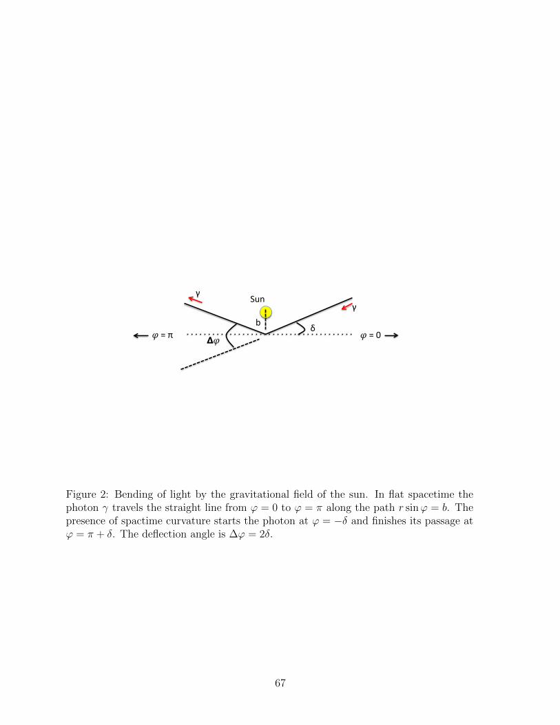
b

𝝙𝜑

γ γ

Sun

δ 𝜑 = 0 𝜑 = π

Figure 2: Bending of light by the gravitational field of the sun. In flat spacetime thephoton γ travels the straight line from ϕ = 0 to ϕ = π along the path r sinϕ = b. Thepresence of spactime curvature starts the photon at ϕ = −δ and finishes its passage atϕ = π + δ. The deflection angle is ∆ϕ = 2δ.

67

An expedition headed by A.S. Eddington observed the eclipse from the island of Principe,off the west coast of Africa. Measurements of thirteen stars confirmed not only that gravityaffected the propagation of light, but that it did so by an amount in much better accordwith general relativity theory than with a Newtonian “corpuscular theory,” with the testmass velocity set equal to c. (The latter gives a deflection angle half as large as GR, inessence because the 2GM/rc2 terms in both the dt and dx metric coefficients contributeequally to the photon deflection, whereas in the Newtonian limit only the dt modification isretained—as we know.) This success earned Einstein press coverage that today is normallyreserved for rock stars. Everybody knew who Albert Einstein was!

Today, not only mere deflection, but “gravitational lensing” and image formation acrossthe electromagnetic spectrum are standard astronomical techniques to probe matter in allits forms: from small planets to huge, diffuse cosmological agglomerations of dark matter.

Let us return to the classic test. As in Newtonian dynamics, it turns out to be easier towork with u ≡ 1/r, in which case (

du

dφ

)2

=1

r4

(dr

dφ

)2

. (289)

Equation (288) with B = 1/A and E = 0 for a photon may be written

1

r4

(dr

dφ

)2

+B

r2=c2

J= constant (290)

In terms of u: (du

dφ

)2

+ u2(

1− 2GMu

c2

)=c2

J(291)

Differentiating with respect to φ (du/dφ ≡ u′) leads quickly to

u′′ + u =3GM

c2u2 ≡ 3εu2. (292)

We treat ε ≡ GM/c2 as a small parameter. We expand u as u = u0+u1, with u1 = O(εu0)u0 (read “u1 is of order ε times u0 and much smaller than u0”). Then, terms of order unitymust obey the equation

u′′0 + u0 = 0, (293)

and the terms of order ε must obey the equation

u′′1 + u1 = 3εu20. (294)

To leading order (u = u0), nothing happens: the photon moves in a straight line. If thepoint of closest approach is the impact parameter b, then the equation for a straight line isr sinφ = b, or

u0 =sinφ

b(295)

which is the unique solution to equation (293) with boundary conditions r = ∞ at φ = 0and φ = π.

At order ε, there is a deflection from a straight line due to the presence of u1:

u′′1 + u1 = 3εu20 =3ε

b2sin2 φ =

3ε

2b2(1− cos 2φ) (296)

68

Clearly, we need to search for solutions of the form u1 = U + V cos 2φ, where U and V areconstants. Substituting this into (296), we easily find find U = 3ε/2b2 and V = ε/2b2. Oursolution is then

1

r= u0 + u1 =

sinφ

b+

3ε

2b2+ε cos 2φ

2b2(297)

With ε = 0, the solution describes a straight line, r sinφ = b. The first order effects ofincluding ε incorporate the tiny deflections from this straight line. The ε = 0 solution sendsr off to infinity at φ = 0 and φ = π. We may compute the leading order small changes tothese two “infinity angles” by using φ = 0 and φ = π in the correction ε cos 2φ term. Thenwe find that r goes off to infinity not at φ = 0 and π, but at the slightly corrected valuesφ = −δ and φ = π + δ where

δ =2ε

b(298)

In other words, there is now a total deflection angle ∆φ from a straight line of 2δ, or

∆φ =4GM

bc2= 1.75 arcseconds for the Sun. (299)

Happily, arcsecond deflections were just at the limit of reliable photographic methods ofmeasurement in 1919. Those arcsecond deflections unleashed a truly revolutionary paradigmshift. For once, the word is not an exaggeration.

6.7 The advance of the perihelion of Mercury

For Einstein personally, the revolution had started earlier, even before he had his FieldEquations. The vacuum form of the Field Equations is, as we know, sufficient to describethe spacetime outside the gravitational source bodies themselves. Working with the equationRµν = 0, Einstein found, and on 18 November 1915 presented, the explanation of a 60-year-old astronomical puzzle: what was the cause of Mercury’s excess perihelion advance of 43′′

per century? The directly measured perihelion advance is actually much larger than this,but after the interactions from all the planets are taken into account, the excess 43′′ percentury is an unexplained residual of 7.5% of the total. According to Einstein’s biographerA. Pais, the discovery that this precise perihelion advance emerged from general relativitywas

“...by far the strongest emotional experience in Einstein’s scientific life, perhaps in all his life.Nature had spoken to him. He had to be right.”

6.7.1 Newtonian orbits

Interestingly, the perihelion first-order GR calculation is not much more difficult than straightNewtonian. GR introduces a 1/r2 term in the effective gravitational potential, but there isalready a 1/r2 term from the centrifugal term! Other corrections do not add substantivelyto the difficulty. We thus begin with a detailed review of the Newtonian problem, and wewill play off this solution for the GR perihelion advance.

Conservation of energy isv2r2

+J2

2r2− GM

r= E (300)

where J is the (constant) specific angular momentum r2dφ/dt and E is the constant energyper unit mass. (In this Newtonian case, when the two bodies have comparable masses, M is

69

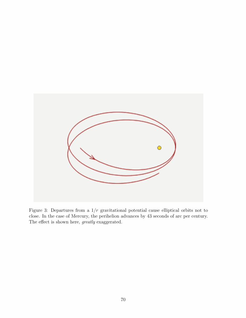
Figure 3: Departures from a 1/r gravitational potential cause elliptical orbits not toclose. In the case of Mercury, the perihelion advances by 43 seconds of arc per century.The effect is shown here, greatly exaggerated.

70

actually the sum of the individual masses, and r the relative separation of the two bodies.)This is just the low energy limit of (286), whose exact form we may write as

1

2

(dr

dτ

)2

+c2

E

(J2

2r2

)− GM

r

(1 +

GMJ2

r2E

)=

(c2 − E

2E

)c2. (301)

We now identify E with c2 to leading order, and to next order (c2 − E)/2 with E (i.e. themechanical energy above and beyond the rest mass energy). The Newtonian equation maybe written

vr =dr

dφ

dφ

dt=J

r2dr

dφ= ±

(2E +

2GM

r− J2

r2

)1/2

(302)

and thence separated: ∫J dr

r2(

2E +2GM

r− J2

r2

)1/2= ±φ (303)

With u = 1/r, ∫du(

2EJ2

+2GMu

J2− u2

)1/2= ∓φ (304)

or ∫du[

2EJ2

+G2M2

J4−(u− GM

J2

)2]1/2 = ∓φ (305)

Don’t be put off by all the fluff. The integral is standard trigonometric:

cos−1

u− GM

J2(2EJ2

+G2M2

J4

)1/2

= ±φ (306)

In terms of r = 1/u this equation unfolds and simplifies to

r =J2/GM

1 + ε cosφ, ε2 ≡ 1 +

2EJ2

G2M2(307)

With E < 0 we find that ε < 1, and that (307) is just the equation for a classical ellipticalorbit of eccentricity ε. We identify the semi-latus rectum,

L = J2/GM (308)

the perihelion (radius of closest approach) r− and the aphelion (radius of farthest extent)r+,

r− =L

1 + ε, r+ =

L

1− ε,

1

L=

1

2

(1

r++

1

r−

)(309)

71

and the semi-major axis

a =1

2(r+ + r−), whence L = a(1− ε2) (310)

Notice that the zeros of the denominator in the integral (305) occur at u− = 1/r− andu+ = 1/r+, corresponding in our arccosine function to φ equals 0 and π respectively.

Exercise.) The Shows must go on. Show that the semi-minor axis of an ellipse is b = a√

1− ε2.Show that the area of an ellipse is πab. Show that the total energy of a two-body bound system is−Gm1m2/2a, independent of ε. Show that the period of a two-body bound system is 2π

√a3/GM ,

independent of ε. (There is a very simple way to do the latter!)

6.7.2 The perihelion advance of Mercury

Equation (288) may be written in terms of u = 1/r as(du

dφ

)2

+

(1− 2GMu

c2

)(u2 +

E

J2

)=c2

J2. (311)

Now differentiate with respect to φ and simplify. The resulting equation is:

u′′ + u =GME

c2J2+

3GMu2

c2' GM

J2+

3GMu2

c2(312)

since E is very close to c2 for Mercury and the difference here is immaterial. The Newtonianlimit corresponds to dropping the final term on the right side of the equation; the resultingsolution is

u ≡ uN =GM

J2(1 + ε cosφ) or r =

J2/GM

1 + ε cosφ(313)

where ε is an arbitrary constant. This is just the classic equation for a conic section, withhyperbolic (ε > 1), parabolic (ε = 1) and ellipsoidal (ε < 1) solutions. For ellipses, ε is theeccentricity.

The general relativistic term 3GMu2/c2 is of course very small, so we are entirely justifiedin using the Newtonian solution for u2 in this higher order term. Writing u = uN + δu withuN given by (313), the differential equation becomes

d2δu

dφ2+ δu =

3(GM)3

c2J4(1 + 2ε cosφ+ ε2 cos2 φ). (314)

In Problem Set 2, you will be asked to solve this equation. The resulting solution foru = uN + δu may be written

u ' GM

J2(1 + ε cos[φ(1− α)]) (315)

where α = 3(GM/Jc)2. Thus, the perihelion occurs not with a φ-period of 2π, but with aslightly longer period of

2π

1− α' 2π + 2πα, (316)

72

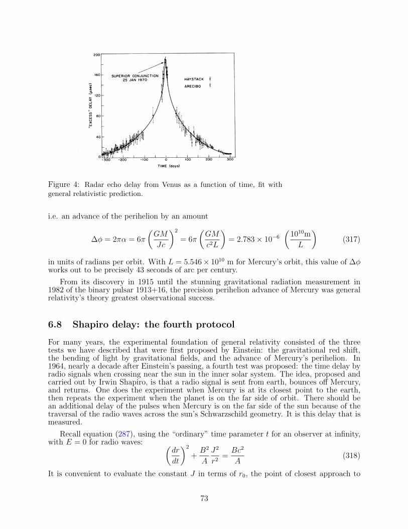
Figure 4: Radar echo delay from Venus as a function of time, fit withgeneral relativistic prediction.

i.e. an advance of the perihelion by an amount

∆φ = 2πα = 6π

(GM

Jc

)2

= 6π

(GM

c2L

)= 2.783× 10−6

(1010m

L

)(317)

in units of radians per orbit. With L = 5.546× 1010 m for Mercury’s orbit, this value of ∆φworks out to be precisely 43 seconds of arc per century.

From its discovery in 1915 until the stunning gravitational radiation measurement in1982 of the binary pulsar 1913+16, the precision perihelion advance of Mercury was generalrelativity’s theory greatest observational success.

6.8 Shapiro delay: the fourth protocol

For many years, the experimental foundation of general relativity consisted of the threetests we have described that were first proposed by Einstein: the gravitational red shift,the bending of light by gravitational fields, and the advance of Mercury’s perihelion. In1964, nearly a decade after Einstein’s passing, a fourth test was proposed: the time delay byradio signals when crossing near the sun in the inner solar system. The idea, proposed andcarried out by Irwin Shapiro, is that a radio signal is sent from earth, bounces off Mercury,and returns. One does the experiment when Mercury is at its closest point to the earth,then repeats the experiment when the planet is on the far side of orbit. There should bean additional delay of the pulses when Mercury is on the far side of the sun because of thetraversal of the radio waves across the sun’s Schwarzschild geometry. It is this delay that ismeasured.

Recall equation (287), using the “ordinary” time parameter t for an observer at infinity,with E = 0 for radio waves: (

dr

dt

)2

+B2

A

J2

r2=Bc2

A(318)

It is convenient to evaluate the constant J in terms of r0, the point of closest approach to

73

the sun. With dr/dt = 0, we easily find

J2 =r20c

2

B0

(319)

where B0 ≡ B(r0). The differential equation then separates and we find that the time t(r, r0)to traverse from r0 to r (or vice-versa) is

t(r, r0) =1

c

∫ r

r0

Adr(1− B

B0

r20r2

)1/2, (320)

where we have made use of AB = 1. Expanding to first order in GM/c2r with B =1− 2GM/c2r:

1− B

B0

r20r2' 1−

[1 +

2GM

c2

(1

r0− 1

r

)]r20r2. (321)

This may now be rewritten as:

1− B

B0

r20r2'(

1− r20r2

)(1− 2GMr0

c2r(r + r0)

)(322)

Using this in our time integral for t(r0, r) and expanding,

t(r0, r) =1

c

∫ r

r0

dr

(1− r20

r2

)−1/2(1 +

2GM

rc2+

GMr0c2r(r + r0)

)(323)

The required integrals are

1

c

∫ r

r0

r dr

(r2 − r20)1/2=

1

c(r2 − r20)1/2 (324)

2GM

c3

∫ r

r0

dr

(r2 − r20)1/2=

2GM

c3cosh−1

(r

r0

)=

2GM

c3ln

(r

r0+

√r2

r20− 1

)(325)

GMr0c3

∫ r

r0

dr

(r + r0)(r2 − r20)1/2=GM

c3

√r − r0r + r0

(326)

Thus,

t(r, r0) =1

c(r2 − r20)1/2 +

2GM

c3ln

(r

r0+

√r2

r20− 1

)+GM

c3

√r − r0r + r0

(327)

We are interested in 2t(r1, r0) ± 2t(r2, r0) for the path from the earth at r1, reflected fromthe planet (at r2), and back. The ± sign depends upon whether the signal passes throughr0 while enroute to the planet, i.e. on whether the planet is on the far side or the near sideof the sun.

It may seem straightforward to plug in values appropriate to the earth’s radial locationand the planet’s (either Mercury or Venus, in fact), compute the “expected Newtonian time”for transit (a sum of the first terms) and then measure the actual time for comparison with

74

our formula. In practise, to know what the delay is, we have to know what the Newtoniantransit time is to fantastic accuracy! In fact, the way this is done is to treat the problemnot as a measurement of a single delay time, but as an entire function of time given byour solution (327) with r = r(t). Figure (3) shows such a fit near the passage of superiorconjunction (i.e. the far side orbital near the sun in sky projection), in excellent agreementwith theory. Exactly how the parameterisation is carried out would take us too far afield;there is some discussion in W72 pp. 202–207, and an abundance of topical information onthe internet under “Shapiro delay.”

Modern applications of the Shaprio delay use pulsars as signal probes, whose time passageproperties are altered by the presence of gravitational waves, a topic for the next chapter.

75

They are not objective, and (like abso-

lute velocity) are not detectable by any

conceivable experiment. They are merely

sinuosities in the co-ordinate system, and

the only speed of propagation relevant to

them is “the speed of thought.”

— A. S. Eddington writing in 1922 of

Einstein’s suspicions.

On September 14, 2015, at 09:50:45 UTC

the two detectors of the Laser Interfer-

ometer Gravitational Wave Observatory

simultaneously observed a transient grav-

itational wave signal. The signal sweeps

upwards from 35 to 250 Hz with a peak

gravitational wave strain of 1 × 10−21. It

matches the waveform predicted by general

relativity for the inspiral and merger of a

pair of black holes and the ringdown of the

resulting single black hole.

— B. P. Abbott et al., 2016, Physical

Review Letters, 116, 061102

7 Gravitational Radiation

Gravity is spoken in the three languages. First, there is traditional Newtonian potentialtheory, the language used by most practising astrophysicists. Then, there is the language ofEinstein’s General Relativity Theory, the language of Riemannian geometry that we havebeen studying. Finally, there is the language of quantum field theory: gravity is a theoryof the exchange of spin 2 particles, gravitons, much as electromagnetism is a theory arisingfrom the exchange of spin 1 photons. Just as the starting point of quantum electrodynamicsis the radiation theory of Maxwell, the starting point of quantum gravity must be a classicalradiation theory of gravity. Unlike quantum electrodynamics, the most accurate physicaltheory ever created, there is no quantum theory of gravity at present, and there is not evena consensus approach. Quantum gravity is therefore very much an active area of ongoingresearch. For the theorist, this is reason enough to study the theory of gravitational radi-ation in general relativity. But there are good reasons for the practical astrophysicist toget involved. In Februrary 2016, the first detection of gravitational waves was announced.The event signal had been received and recorded on September 14, 2015, and is denotedG[ravitational]W[ave]150914. The detection was so clean, and matched the wave form pre-dictions of general relativity in such detail, there can be no doubt that the detection wasgenuine. A new way to probe the most impenetrable parts of the Universe is at hand.

76

The theory of general relativity in the limit when gµν is very close to ηµν is a classicaltheory of gravitational radiation, and not just Newtonian theory, in the same way thatMaxwellian Electrodynamics is a classical radiation theory. The field equations for thedifference gµν − ηµν become, in the weak field limit, a set of rather ordinary looking waveequations with source terms, much like Maxwell’s Equations. The principal difference is thatelectrodynamics is sourced by a vector quantity (the vector potential A with the potentialΦ combine to form a 4-vector), whereas gravitational fields in general relativity are sourcedby a tensor quantity (the stress tensor Tµν). This becomes a major difference when werelax the condition that the gravity field be weak: the gravitational radiation itself makes acontribution to its own source, something electromagnetic radiation cannot do. But this isnot completely unprecedented. We have seen this sort of thing before, in a classical context:sound waves can themselves generate acoustical disturbances, and one of the things thathappens is a shock wave, or sonic boom. While a few somewhat pathological mathematicalsolutions for exact gravitational radiation waves are known, in general people either work inthe weak field limit or resort to numerical solutions of the field equations. Even with powerfulcomputers, however, precise numerical solutions of the field equations for astrophysicallyinteresting problems—like merging black holes—have long been a major technical problem.In the last decade, a breakthrough has occurred, and it is now possible to compute highlyaccurate wave forms for these kinds of problems, with critically important predictions forthe new generation of gravitational wave detectors.

As we have noted, astrophysicists have perhaps the most important reason of all tounderstand gravitational radiation: we are on the verge of what will surely be a golden ageof gravitational wave astronomy. That gravitational radiation truly exists was establishedin 1974, when a close binary system (7.75 hour period) with a neutron star and a pulsar(PSR 1913+16) was discovered by Hulse and Taylor. So much orbital information could beextracted from this remarkable system that it was possible to predict, then measure, the rateof orbital decay (more precisely, the speed-up of the period of the decaying orbit) caused bythe energy carried off by gravitational radiation. The resulting inspiral period shortening,though incredibly tiny in any practical sense, was large enough to be cleanly and clearlymeasurable. General relativity turned out to be exactly correct (Taylor & Weisberg, ApJ,1982, 253, 908), and the 1993 Nobel Prize in Physics was duly awarded to Hulse and Taylorfor this historical achievement.

The September 2015 gravitational wave detection pushed back the envelope dramatically.It established that i) the reception and analysis of gravitational waves is technically feasibleand will soon become a widely-used probe of the universe; ii) black holes exist beyond anydoubt whatsoever, this truly is the proverbial “smoking-gun”; iii) the full dynamical contentof strong field general relativity on time and length scales characteristic of stellar systemsis completely correct. This achievement is an historical milestone in physics. Some havespeculated that its impact on astronomy will rival Galileo’s introduction of the telescope.Perhaps Hertz’s 1887 detection of electromagnetic radiation in the lab is another apt com-parison. (Commerical exploitation of gravity waves is probably some ways off. Maybe it willbe licenced someday as a revenue source.)

There is more to come. In the near future, extremely delicate pulsar timing experiments,in which arrival times of pulses are measured to fantastic precision, will come on line. Inessence, this is a measure of the Shapiro delay, not caused by the Sun or a star, but by thepassage of a gravitational wave.

The subject of gravitational radiation is complicated and computationally intensive. Eventhe basics will involve some effort on your part. I hope you will agree that the effort is wellrewarded.

77

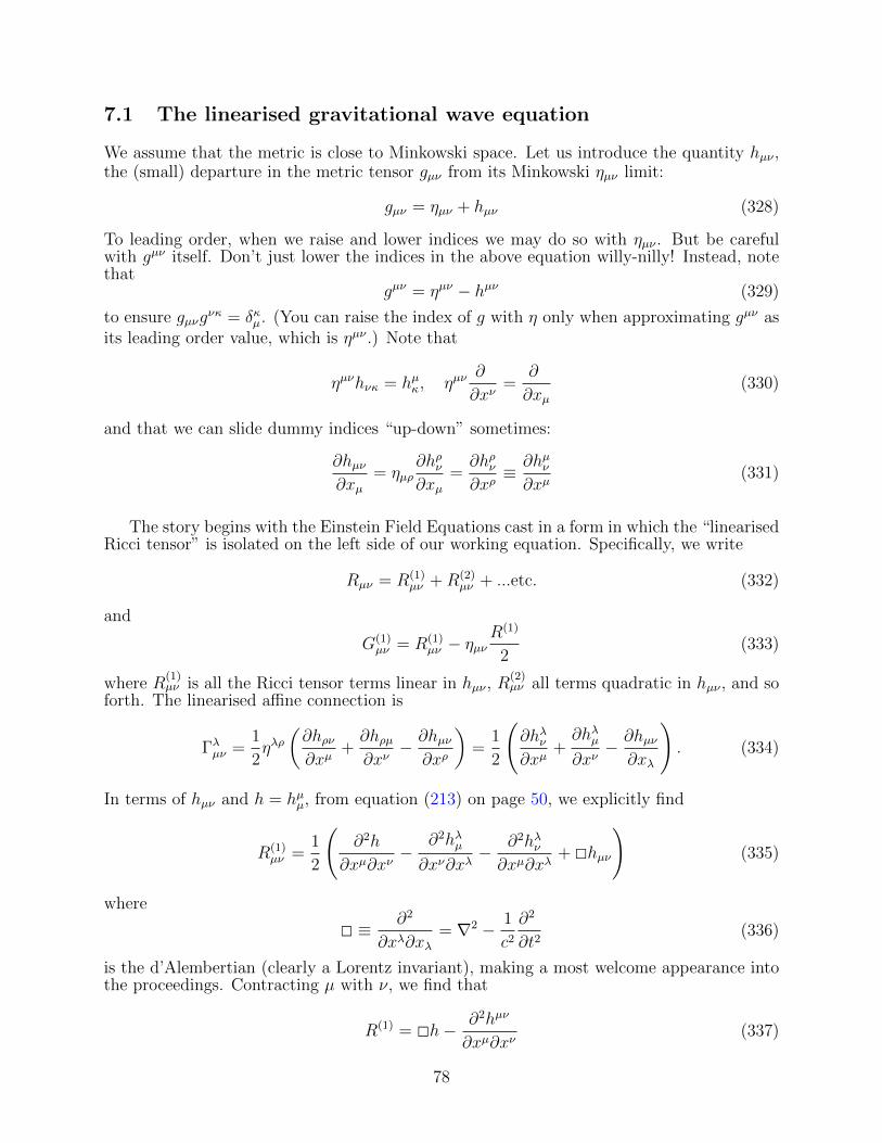
7.1 The linearised gravitational wave equation

We assume that the metric is close to Minkowski space. Let us introduce the quantity hµν ,the (small) departure in the metric tensor gµν from its Minkowski ηµν limit:

gµν = ηµν + hµν (328)

To leading order, when we raise and lower indices we may do so with ηµν . But be carefulwith gµν itself. Don’t just lower the indices in the above equation willy-nilly! Instead, notethat

gµν = ηµν − hµν (329)

to ensure gµνgνκ = δκµ. (You can raise the index of g with η only when approximating gµν as

its leading order value, which is ηµν .) Note that

ηµνhνκ = hµκ, ηµν∂

∂xν=

∂

∂xµ(330)

and that we can slide dummy indices “up-down” sometimes:

∂hµν∂xµ

= ηµρ∂hρν∂xµ

=∂hρν∂xρ≡ ∂hµν∂xµ

(331)

The story begins with the Einstein Field Equations cast in a form in which the “linearisedRicci tensor” is isolated on the left side of our working equation. Specifically, we write

Rµν = R(1)µν +R(2)

µν + ...etc. (332)

and

G(1)µν = R(1)

µν − ηµνR(1)

2(333)

where R(1)µν is all the Ricci tensor terms linear in hµν , R

(2)µν all terms quadratic in hµν , and so

forth. The linearised affine connection is

Γλµν =1

2ηλρ(∂hρν∂xµ

+∂hρµ∂xν

− ∂hµν∂xρ

)=

1

2

(∂hλν∂xµ

+∂hλµ∂xν− ∂hµν

∂xλ

). (334)

In terms of hµν and h = hµµ, from equation (213) on page 50, we explicitly find

R(1)µν =

1

2

(∂2h

∂xµ∂xν−

∂2hλµ∂xν∂xλ

− ∂2hλν∂xµ∂xλ

+ 2hµν

)(335)

where

2 ≡ ∂2

∂xλ∂xλ= ∇2 − 1

c2∂2

∂t2(336)

is the d’Alembertian (clearly a Lorentz invariant), making a most welcome appearance intothe proceedings. Contracting µ with ν, we find that

R(1) = 2h− ∂2hµν

∂xµ∂xν(337)

78

where we have made use of∂hλµ∂xµ

=∂hλµ

∂xµ.

Assembling G(1)µν , we find

G(1)µν =

1

2

[∂2h

∂xµ∂xν−

∂2hλµ∂xλ∂xν

− ∂2hλν∂xλ∂xµ

+ 2hµν − ηµν(

2h− ∂2hλρ

∂xλ∂xρ

)]. (338)

The full, nonlinear Field Equations may then formally be written

G(1)µν = −

(8πGTµνc4

+Gµν −G(1)µν

)≡ −8πG(Tµν + τµν)

c4, (339)

where

τµν =c4

8πG(Gµν −G(1)

µν ) ' c4

8πG

(R(2)µν − ηµν

R(2)

2

)(340)

Though composed of geometrical terms, the quantity τµν is written on the right side of theequation with the stress energy tensor Tµν , and is interpreted as the stress energy contributionof the gravitational radiation itself. We shall have more to say on this in section 7.4. In lineartheory, τµν is neglected in comparison with the ordinary matter Tµν .

This is a bit disappointing to behold. Even the linearised Field Equations look to bea mess! But then, you may have forgotten that the raw Maxwell wave equations for thepotentials are no present, either. You will permit me to remind you. Here are the equationsfor the scalar potential Φ and vector potential A:

∇2Φ +1

c

∂

∂t(∇·A) = −4πρ (341)

∇2A− 1

c2∂2A

∂t2−∇

(∇·A+

1

c

∂Φ

∂t

)= −4π

cJ (342)

(Note: I have used esu units, which are much more natural for relativity. Here ρ is theelectric charge density.)

Exercise. In covariant notation, with Aα = (Φ,A) and Jα = (ρ,J/c) representing respec-tively the potential and source term 4-vectors, the original general equations look a bit morepresentable. The only contravariant 4-vectors that we can form which are second order inthe derivatives of Aα are 2Aα and ∂α∂βA

β. Show that if ∂αJα = 0 identically, then our

equation relating Aα to Jα must be of the form

2Aα − ∂α∂βAβ = CJα

where C is a constant to be determined, and that gauge invariance of this equation againstAα → Aα + ∂αΛ follows without any further modification. So how do we determine C?

We know the story here well. Work in the Lorenz gauge, which we are always free to do:

∇·A+1

c

∂Φ

∂t= 0 (343)

79

In covariant 4-vector language, this is just ∂αAα = 0. Then, the dynamical equations

simplify:

∇2Φ− 1

c2∂Φ

∂t2= 2Φ = −4πρ (344)

∇2A− 1

c2∂2A

∂t2= 2A = −4π

cJ (345)

This is nicer. Physically transparent Lorentz-invariant wave equations emerge. Might some-thing similar happen for the Einstein Field Equations?

That the answer might be YES is supported by noticing that G(1)µν can be written entirely

in terms of the “Bianchi-like” quantity

hµν = hµν −ηµνh

2, or hµν = hµν −

δµνh

2. (346)

Using this in (338), the linearised Field Equation becomes

2G(1)µν = 2hµν −

∂2hλµ∂xν∂xλ

− ∂2hλν∂xµ∂xλ

+ ηµν∂2hλρ

∂xλ∂xρ= −16πGTµν

c4. (347)

(It is easiest to verify this by starting with (347), substituting with (346), and showing thatthis leads to (338).)

Interesting. Except for 2hµν , every term in this equation involves the divergence of hµνor hµν . Hmmm. Shades of Maxwell’s ∂Aα/∂xα. In the Maxwell case, the freedom of gaugeinvariance allowed us to pick the gauge in which ∂Aα/∂xα = 0. Does our equation have agauge invariance that will allow us to do the same for gravitational radiation so that we canset these h-divergence derivatives to zero?

It does. Go back to equation (338) and on the right side, change hµν to h′µν , where

h′µν = hµν −∂ξν∂xµ− ∂ξµ∂xν

, (348)

and the ξµ represent any vector function. You will find that the form of the equationis completely unchanged, i.e. the ξµ terms cancel out identically! This is a true gaugeinvariance.

In this case, what is happening is that an infinitesimal coordinate transformation itselfis acting as a gauge transformation. If

x′µ = xµ + ξµ(x), or xµ = x′µ − ξµ(x′) to lead order. (349)

then

g′µν = η′µν + h′µν =∂xρ

∂x′µ∂xσ

∂x′νgρσ =

(δρµ −

∂ξρ

∂xµ

)(δσν −

∂ξσ

∂xν

)(ηρσ + hρσ) (350)

With η′ identical to η, we must have

h′µν = hµν −∂ξν∂xµ− ∂ξµ∂xν

(351)

80

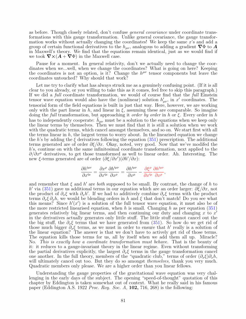
as before. Though closely related, don’t confuse general covariance under coordinate trans-formations with this gauge transformation. Unlike general covariance, the gauge transfor-mation works without actually changing the coordinates! We keep the same x’s and add agroup of certain functional derivatives to the hµν , analogous to adding a gradient ∇Φ to Ain Maxwell’s theory. We find that the equations remain identical, just as we would find ifwe took ∇×(A+∇Φ) in the Maxwell case.

Pause for a moment. In general relativity, don’t we actually need to change the coor-dinates when we...well, when we change the coordinates? What is going on here? Keepingthe coordinates is not an option, is it? Change the hµν tensor components but leave thecoordinates untouched? Why should that work?

Let me try to clarify what has always struck me as a genuinely confusing point. (If it is allclear to you already, or you willing to take this as it comes, feel free to skip this paragraph.)If we did a full coordinate transformation, we would of course find that the full Einsteintensor wave equation would also have the (nonlinear) solution h′µν , in x′ coordinates. Thetensorial form of the field equations is built in just that way. Here, however, we are workingonly with the part linear in h, and linear in ξ, assuming these are comparable. So imaginedoing the full transformation, but approaching it order by order in h or ξ. Every order in hhas to independently cooperate: hµν must be a solution to the equations when we keep onlythe linear terms by themselves. Then we must find that it is still a solution when we workwith the quadratic terms, which cancel amongst themselves, and so on. We start first with allthe terms linear in h, the largest terms to worry about. In the linearised equation we changethe h’s by adding the ξ derivatives following the equation (351) prescription. The additionalterms generated are of order ∂ξ/∂x. Okay, noted, very good. Now that we’ve modifed theh’s, continue on with the same infinitesimal coordinate transformation, next applied to the∂/∂xµ derivatives, to get those transformed as well to linear order. Ah. Interesting. Thenew ξ-terms generated are of order (∂ξ/∂x′)(∂h′/∂x):

∂h′µν

∂x′µ=∂xρ

∂x′µ∂h′µν

∂xρ=∂h′µν

∂xµ− ∂ξρ

∂x′µ∂h′µν

∂xρ,

and remember that ξ and h′ are both supposed to be small. By contrast, the change of h toh′ via (351) gave us additional terms in our equation which are an order larger: ∂ξ/∂x, notthe product of ∂xξ with ∂xh

′. If we had to additively combine ∂xξ terms with the productterms ∂xξ ∂xh, we would be blending orders in h and ξ that don’t match! Do you see whatthis means? Since h′(x′) is a solution of the full tensor wave equation, it must also be ofthe more restricted linearised equation, when h is small. Changing h as per equation (351)generates relatively big linear terms, and then continuing our duty and changing x to x′

in the derivatives actually generates only little stuff. The little stuff cannot cancel out thethe big stuff, the ∂xξ terms that we have generated from (351). So how do we get rid ofthose much bigger ∂xξ terms, as we must in order to ensure that h′ really is a solution ofthe linear equation? The answer is that we don’t have to actively get rid of those terms.The equation kills those terms for us, all by itself when we add them all up. Miracle?No. This is exactly how a coordinate transformation must behave. That is the beauty ofit: it reduces to a gauge-invariant theory in the linear regime. Even without transformingthe partial derivatives explicitly, the largest ∂xξ terms in the gauge transformation cancelone another. In the full theory, members of the “quadratic club,” terms of order (∂xξ)∂xh,will ultimately cancel out too. But they do so amongst themselves, thank you very much.Quadratic members only please. We are a higher order than you linear fellows.

Understanding the gauge properties of the gravitational wave equation was very chal-lenging in the early days of the subject. The opening “speed-of-thought” quotation of thischapter by Eddington is taken somewhat out of context. What he really said in his famouspaper (Eddington A.S. 1922 Proc. Roy. Soc. A, 102, 716, 268) is the following:

81

“Weyl has classified plane gravitational waves into three types, viz.: (1) longitudinal-longitudinal;(2) longitudinal-transverse; (3) transverse-transverse. The present investigation leads to the con-clusion that transverse-transverse waves are propagated with the speed of light in all systems ofco-ordindates. Waves of the first and second types have no fixed velocity—a result which rousessuspicion as to their objective existence. Einstein had also become suspicious of these waves (inso far as they occur in his special co-ordinate system) for another reason, because he found theyconvey no energy. They are not objective and (like absolute velocity) are not detectable by anyconceivable experiment. They are merely sinuosities in the co-ordinate system, and the only speedof propagation relevant to them is the ‘speed of thought.’ ”

The quotation is often taken to be dismissive of the entire notion of gravitational radi-ation, which it clearly is not. Rather, it is directed toward those solutions which we wouldnow say are gauge-dependent (either of the first two types of waves, which involve at leastone longitudinal component) and those which are gauge-independent (the third, completelytransverse, type). Physical solutions must ultimately be gauge independent. Matters wouldhave been clear to someone who bothered to examine the components of the Riemann cur-vature tensor. The first two types of waves would have produced an identically zero Rλ

µνκ.They produce no curvature; they are indeed “merely sinuosities in the co-ordinate system,”and they are are unphysical.

Back to our problem. Just as the Lorenz gauge ∂αAα = 0 was useful in the case of

Maxwell’s equations, so now is the so-called harmonic gauge:

∂hµν∂xµ

=∂hµν∂xµ− 1

2

∂h

∂xν= 0 (352)

In this gauge, the Field Equations (347) take the “wave-equation” form

2hµν = −16πGTµνc4

(353)

How we can be sure that, even with our gauge freedom, we can find the right ξµ to get intoa harmonic gauge and ensure the emergence of (353)? Well, if we have been unfortunateenough to be working in a gauge in which equation (352) is not satisfied, then form h′µν a laequation (351) and demand that ∂h′µν /∂x

µ = (1/2)∂h′/∂xν . We find that this implies

2ξν =∂hµν∂xµ

, (354)

a wave equation for ξν identical in form to (353). For this equation, a solution certainlyexists. Indeed, our experience with electrodynamics has taught us that the solution to thefundamental radiation equation (353) takes the form

hµν(r, t) =4G

c4

∫Tµν(r

′, t−R/c)R

d3r′, R ≡ |r − r′| (355)

and hence a similar solution exisits for (354). The hµν , like their electrodynamic counterparts,are determined at time t and location r by a source intergration over r′ taken at the retardedtimes t′ ≡ t − R/c. In other words, disturbances in the gravitational field travel at a finitespeed, the speed of light c.

Exercise. Show that for a source with motions near the speed of light, like merging blackholes, hµν (or hµν for that matter) is of order RS/r, where RS is the Schwarzschild radius

82

based on the total mass of the system in question and r is the distance to the source. Youwant to know how big hµν is going to be in your detector when black holes merge? Countthe number of expected Schwarzschild radii to the source and take the reciprocal. With M tot

equal to the total mass measured in solar masses, show that hµν ∼ 3M tot

/rkm, measuring rin km. We are pushing our weak field approximation here, but to this order it works fine.We’ll give a sharper estimate shortly.

7.1.1 Come to think of it...

You may not have actually seen the solution (355) before, or maybe, you know, you justneed a little reminding. It is important. Let’s derive it.

Consider the equation

− 1

c2∂2Ψ

∂t2+∇2Ψ = −4πf(r, t) (356)

We specialise to the Green’s function solution

− 1

c2∂2G

∂t2+∇2G = −4πδ(r)δ(t) (357)

Of course, our particular choice of origin is immaterial, as is our zero of time, so that weshall replace r by R ≡ r − r′ and t by τ ≡ t − t′ at the end of the calculation, with theprimed values being fiducial reference points. The form of the solution we find here will stillbe valid with the shifts of space and time origins.

Fourier transform (357) by integrating over∫eiωtdt and denote the fourier transform of

G by G:k2G+∇2G = −4πδ(r) (358)

where k2 = ω2/c2. Clearly G is a function only of r, hence the solution to the homogeneousequation away from the origin,

d2(rG)

dr2+ k2(rG) = 0,

is easily found to be G = e±ikr/r. The delta function behaviour is actually already includedhere, as can be seen by taking the limit k → 0, in which we recover the correct potential ofa point charge, with the proper normalisation already in place. The back transform gives

G =1

2πr

∫ ∞−∞

e±ikr−iωt dω (359)

which we recognise as a Dirac delta function (remember ω/k = c):

G =δ(t± r/c)

r→ δ(t− r/c)

r→ δ(τ −R/c)

R(360)

where we have selected the retarded time solution t− r/c as a nod to causality, and movedthence to (τ , R) variables for an arbitary time and space origin. We see that a flash at t = t′

located at r = r′ produces an effect at a time R/c later, at a distance R from the flash. Thegeneral solution constructed from our Green’s function is

Ψ =

∫f(r′, t′)

Rδ(t− t′ −R/c)dt′dr′ =

∫f(r′, t′)

Rdr′ (361)

where in the final integral we have set t′ = t−R/c, the retarded time.

83

7.2 Plane waves

To understand more fully the solution (355), consider the problem in which Tµν has anoscillatory time dependence, e−iωt

′. Since we are dealing with a linear theory, this isn’t

particularly restrictive, since any well-behaved time dependence can be represented by aFourier sum. The source, say a binary star system, occupies a finite volume. We seek thesolution for hµν at distances huge compared with the scale of the source itself, i.e. r r′.Then,

R ' r − er · r′ (362)

where er is a unit vector in the r direction, and

hµν(r, t) ' exp[i(kr − ωt)] 4G

rc4

∫Tµν(r

′) exp(−ik · r′) d3r (363)

with k = (ω/c)er the wavenumber in the radial direction. Since r is huge, this has theasymptotic form of a plane wave. Hence, hµν and thus hµν itself have the form of simpleplane waves, travelling in the radial direction, at large distances from the source generatingthem. These waves turn out to have some remarkable polarisation properties, which we nowdiscuss.

7.2.1 The transverse-traceless (TT) gauge

Consider a traveling plane wave for hµν , orienting our z axis along k, so that

k0 = ω/c, k1 = 0, k2 = 0, k3 = ω/c and k0 = −ω/c, ki = ki (364)

where as usual we raise and lower indices with ηµνor its numerical identical dual ηµν .

Then hµν takes the formhµν = eµνa exp(ikρx

ρ) (365)

where a is an amplitude and eµν = eνµ a polarisation tensor, again with the η’s raising andlowering subscripts. Thus

eij = eij = eij (366)

e0i = −ei0 = e0i = −e0i (367)

e00 = e00 = −e00 (368)

The harmonic constraint∂hµν∂xµ

=1

2

∂hµµ∂xν

(369)

implieskµe

µν = kνe

µµ/2 (370)

For ν = 0 this meansk0e

00 + k3e

30 = k0(e

ii + e00)/2, (371)

or− (e00 + e30) = (eii − e00)/2. (372)

When ν = j (a spatial index),

k0e0j + k3e

3j = kj(eii − e00)/2 (373)

84

The j = 1 and j = 2 cases reduce to

e01 + e31 = e02 + e32 = 0, (374)

while j = 3 yieldse03 + e33 = (eii − e00)/2 = −(e00 + e03) (375)

Equations (374) and the first=last equality of (375) yield

e01 = −e31, e02 = −e32, e03 = −(e00 + e33)/2 (376)

Using the above expression for e03 in the first=second equality of (375) then gives

e22 = −e11 (377)

Of the 10 independent components of the symmetric eµν the harmonic condition (369) thusenables us to express e0i and e22 in terms of e3i, e00, and e11. These latter 5 components plusa sixth, e12, remain unconstrained for the moment.

But wait! We have not yet used the gauge freedom of equation (351) within the harmonicconstraint. We can still continue to eliminate components of eµν . In particular, let us choose

ξµ(x) = iεµ exp(ikρxρ) (378)

where the εµ are four constants to be chosen. This satisfies 2ξµ=0, and therefore does notchange the harmonic coordinate condition, ∂µh

µν = 0. Then following the prescription of

(351), we generate a new, but physically equivalent polarisation tensor,

e′µν = eµν + kµεν + kνεµ (379)

and by choosing the εµ appropriately, we can eliminate all of the e′µν except for e′11, e′22 = −e′11,

and e′12. In particular, using (379),

e′11 = e11, e′12 = e12 (380)

unchanged. But with k = ω/c,

e′13 = e13 + kε1, e′23 = e23 + kε2, e′33 = e33 + 2kε3, e′00 = e00 − 2kε0, (381)

so that these four components may be set to zero by a simple choice of the εµ. When workingwith plane waves we may always choose this gauge, which is transverse (since the only eijcomponents that are present are transverse to the z direction of propagation) and traceless(since e11 = −e22). Oddly enough, this gauge is named the transverse-traceless (TT) gauge.Notice that in the TT gauge, hµν vanishes if any of its indices are 0, whether raised orlowered.

7.3 The quadrupole formula

In the limit of large r (“compact source approximation”), equation (355) is:

hµν(r, t) =4G

rc4

∫T µν(r′, t′)d3r′, (382)

85

where t′ = t − r/c is the retarded time. Moreover, for the TT gauge, we are interested inthe spatial ij components of this equation, since all time indices vanish. (Also, because hµνis traceless, we need not distinguish between h and h.) The integral over Tij may be cast ina very convenient form as follows.

0 =

∫∂(x′jT ik)

∂x′kd3r′ =

∫ (∂T ik

∂x′k

)x′j d3r′ +

∫T ij d3r′, (383)

where the first equality follows because the first integral reduces to a surface integration ofT ik at infinity, where it is presumed to vanish. Thus∫

T ij d3r′ = −∫ (

∂T ik

∂x′k

)x′j d3r′ =

∫ (∂T i0

∂x′0

)x′j d3r′ =

1

c

d

dt′

∫T i0x′j d3r′ (384)

where the second equality uses the conservation of T µν . Remember that t′ is the retardedtime. As Tij is symmetric in its indices,

d

dt′

∫T i0x′j d3r′ =

d

dt′

∫T j0x′i d3r′ (385)

Continuing in this same spirit,

0 =

∫∂(T 0kx′ix′j)

∂x′kd3r′ =

∫ (∂T 0k

∂x′k

)x′ix′j d3r′ +

∫(T 0ix′j + T 0jx′i) d3r′ (386)

Using exactly the same reasoning as before,∫(T 0ix′j + T 0jx′i) d3r′ =

1

c

d

dt′

∫T 00x′ix′j d3r′ (387)

Therefore, ∫T ij d3r′ =

1

2c2d2

dt′2

∫T 00x′ix′j d3r′ (388)

Inserting this in (382), we obtain the quadrupole formula for gravitational radiation:

hij =2G

c6r

d2I ij

dt′2(389)

where I ij is the quadrupole-moment tensor of the energy density:

I ij =

∫T 00x′ix′j d3r′ (390)

To estimate this numerically, we write

d2I ij

dt′2∼Ma2c2ω2 (391)

where M is the characteristic mass of the rotating system, a an internal separation, and ωa characteristic frequency, an orbital frequency for a binary say. Then

hij ∼ 2GMa2ω2

c4r' 7× 10−22(M/M)(a211ω

27/r100) (392)

86

where M/M is the mass in solar masses, a11 the separation in units of 1011 cm (about aseparation of one solar radius), ω7 the frequency associated with a 7 hour orbital period(similar to PSR193+16) and r100 the distance in units of 100 parsecs, some 3× 1020 cm. Atypical rather large h one might expect at earth from a local astronomical source is then oforder 10−21.

What about the LIGO source, GW150914? How does our formula work in this case? Thedistance in this case is cosmological, not local, with r = 1.2 × 1022 km, or in astronomicalparlance, about 400 megaparsecs (Mpc). In this case, we write (392) as

hij ∼ 2GMa2ω2

c4r=

(2.9532

rkm

)(M

M

)(aωc

)2' 1× 10−22

M/MrGpc

(aωc

)2, (393)

since 2GM/c2 is just the Sun’s Schwarzschild radius. (One Gpc=103Mpc = 3.0856 ×

1022km.) The point is that (aω/c)2 is a number not very different from 1 for a relativisticsource, perhaps 0.1 or so. Plugging in numbers with M/M = 60 and (aω/c)2 = 0.1, we findhij = 1.5× 10−21, just about as observed at peak amplitude.

Exercise. Prove that hij given by (389) is an exact solution of 2hij = 0, for any r, even if r is notlarge.

7.4 Radiated Energy

7.4.1 A useful toy problem

We have yet to make the link between hµν and the actual energy flux that is carried off bythese time varying metric coefficients. Relating metric coefficients to energy is not trivial.To see how to do this, start with a simpler toy problem. Imagine that the wave equation forgeneral relativity looked like this:

− 1

c2∂2Φ

∂t2+∇2Φ = 4πGρ (394)

This is what a relativisitic theory would look like if the source ρ were just a simple scalarquantity, instead of a component of a stress tensor. Then, if we multiply by (1/4πG)∂Φ/∂t,integrate (∂Φ/∂t)∇2Φ by parts and regroup, this leads to

− 1

8πG

∂

∂t

[(∂Φ

∂t

)2

+ |∇Φ|2]

+∇·(

1

4πG

∂Φ

∂t∇Φ

)= ρ

∂Φ

∂t. (395)

But

ρ∂Φ

∂t=∂(ρΦ)

∂t− Φ

∂ρ

∂t=∂(ρΦ)

∂t+ Φ∇·(ρv) =

∂(ρΦ)

∂t+∇·(ρvΦ)− ρv·∇Φ (396)

where v is the velocity and the mass conservation equation

∂ρ

∂t+∇·(ρv) = 0

87

has been used in the second “= ” sign from the left. Combining (395) and (396), and thenrearranging the terms a bit leads to

∂

∂t

[ρΦ +

1

8πG

((∂Φ

∂t

)2

+ |∇Φ|2)]

+∇·(ρvΦ− 1

4πG

∂Φ

∂t∇Φ

)= ρv·∇Φ (397)

The right side is just minus the rate at which work is being done on the sources per unitvolume. (The force per unit volume, you recall, is −ρ∇Φ.) For the usual case of interestwhen the source ρ vanishes outside a certain radius, the left side may then be readily inter-preted as a far-field wave energy density of [(∂tΦ)2 + |∇Φ|2]/8πG and a wave energy flux of−(∂tΦ)∇Φ/4πG. (Is the sign of the flux sensible for outgoing waves?) The question we raisehere is whether an analogous method might work on the more involved linear wave equationof tensorial general relativity. The answer is YES, but we have to set things up properly.We can’t be casual. And, needless to say, it is a bit more messy index-wise!

7.5 A conserved energy flux for linearised gravity

Start with equation (347):

2hµν −∂2hλµ∂xν∂xλ

− ∂2hλν∂xµ∂xλ

+ ηµν∂2hλρ

∂xλ∂xρ= −16πGTµν

c4. (398)

Contract on µν: the first term on the left becomes 2h, the second and third each become−∂2hλρ/∂xλ∂xρ, while the final contraction turns ηµν into a factor of 4. (Why?) This leadsus to

2h+ 2∂2hλρ

∂xλ∂xρ= −κT (399)

where we have written κ = 16πG/c4. We then recast our original equation as

2hµν −∂2hλµ∂xν∂xλ

− ∂2hλν∂xµ∂xλ

+ ηµν2h = −κSµν (400)

where we have introduced the source function

Sµν = Tµν −ηµνT

2(401)

Now multiply (400) by ∂hµν/∂xσ, summing over µ and ν as usual but keeping σ free. Thefirst term on the left becomes

∂hµν

∂xσ2hµν =

∂hµν

∂xσ∂2hµν∂xρ∂xρ

=∂

∂xρ

(∂hµν∂xρ

∂hµν

∂xσ

)− ∂hµν

∂xρ∂2hµν

∂xρ∂xσ

=∂

∂xρ

(∂hµν∂xρ

∂hµν

∂xσ

)− ∂hµν

∂xρ∂

∂xσ∂h

µν

∂xρ=

∂

∂xρ

(∂hµν∂xρ

∂hµν

∂xσ

)− ∂

∂xσ

(1

2

∂hµν∂xρ

∂hµν

∂xρ

)(402)

Do you see why the final equality is valid for the ∂/∂xσ exact derivative? It doesn’t matterwhich group of µν on the h’s is the up group and which is the down group.

88

Now that you’ve seen the tricks of the trade, you should be able to juggle the indiceswith me and recast all the terms as exact derivatives: we are aiming to get a pure divergenceon the left side. The second term is

−∂2hλµ∂xν∂xλ

∂hµν

∂xσ= − ∂2hλµ

∂xν∂xλ∂hµν∂xσ

= − ∂

∂xν

(∂hλµ

∂xλ∂hµν∂xσ

)+∂hλµ

∂xλ∂2hµν∂xσ∂xν

or, replacing ν with ρ in the first group on the right,

−∂2hλµ∂xν∂xλ

∂hµν

∂xσ= − ∂

∂xρ

(∂hλµ

∂xλ∂hµρ∂xσ

)+

1

2

∂

∂xσ

(∂hλµ

∂xλ∂hµν∂xν

)(403)

The third term is

− ∂2hλν∂xµ∂xλ

∂hµν

∂xσ

But this is exactly the same as the term we’ve just done: just interchange the dummy indicesµ and ν and remember that hµν is symmetric in µν. So there is no need to do any morehere. The fourth and final term of the left side of equation is

− 1

2

∂h

∂xσ∂2h

∂xρ∂xρ= −1

2

∂

∂xρ

(∂h

∂xρ∂h

∂xσ

)+

1

4

∂

∂xσ

(∂h

∂xρ∂h

∂xρ

). (404)

Thus, after dividing our fundamental equation by 2κ, the left side of equation (400) takes anice compact form

∂Uρσ∂xρ

= −Sµν∂hµν

∂xσ= −Tµν

∂hµν

∂xσ, (405)

whereUρσ = Tρσ + ηρσS. (406)

S is the scalar density:

S = −(

1

4κ

∂hµν∂xρ

∂hµν

∂xρ

)+

1

2κ

(∂hλµ

∂xλ∂hµν∂xν

)+

1

8κ

(∂h

∂xρ∂h

∂xρ

), (407)

and Tρσ is a flux tensor:

Tρσ =1

2κ

(∂hµν∂xρ

∂hµν

∂xσ

)− 1

κ

(∂hλµ

∂xλ∂hµρ∂xσ

)− 1

4κ

(∂h

∂xρ∂h

∂xσ

). (408)

By working with plane waves in standard harmonic coordinates, ∂hλµ/∂xλ = 0, and Uρσbecomes symmetric in ρσ. Remembering kρk

ρ = 0 for the TT gauge, we find the simpleresult

Uρσ =c4

32πG

(∂hµν∂xρ

∂hµν

∂xσ

)(TT gauge). (409)

Why did we choose to divide by 2κ for our overall constant? Why not just κ, or for thatmatter, 4κ? It is the right side of our energy equation that tells this story. This is

− 1

2Sµν

∂hµν

∂xσ= −1

2

(Tµν −

ηµν2T)(∂hµν

∂xσ− ηµν

2

∂h

∂xσ

)= −1

2Tµν

∂hµν

∂xσ. (410)

89

Choose σ = 0, the time component. We work in the Newtonian limit h00 ' −2Φ/c2, whereΦ is a Newtonian gravitational potential. In the µν summation on the right side of theequation, we are then dominated by the 00 components of both hµν and Tµν . Now, weare about to do a number of integration by parts. But we will always ignore the exactderivative! Why? Because the exact derivative of a perioidic function (and everything hereis periodic) must oscillate away to zero on average. But in general the products of theperiodic functions don’t oscillate to zero; for example the average of cos2(ωt)2 = 1/2. Thuswe keep these product terms, but only if they are not an exact derivative. Using the rightarrow → to mean “integrate by parts and ignore the pure derivatives” (as inconsequentialfor wave losses), we perform the following manipulations on the right side of equation (410):

− 1

2T00

∂h00

∂x0→ 1

2

∂T00∂x0

h00 = −1

2

∂T 0i

∂xih00 → 1

2T 0i∂h

00

∂xi' −ρv

c·∇Φ, (411)

where the first equality follows from ∂νT0ν = 0. We have arrived on the right at an expression

for the rate at which the effective Newtonian potential does net work on the matter. Whyis that 1/c there? Don’t worry, it cancels out with the same factor on the left (flux) side ofthe original equation. What about the sign of this? This expression is negative if the force−ρ∇Φ is oppositely directed to the velocity, so that the source is losing energy by generatingoutgoing waves. Our harmonic gauge expression (409) for T0i is also negative for an outwardflowing wave that is a function of the argument (r− ct), r being spherical radius and t time.By contrast, T 0i would be positive, as befits an outward moving wave energy.

The fact that division by 2κ produces a source corresponding to the rate at which work isdone on the Newtonian sources (when σ = 0) means that our overall normalisation is indeedcorrect. The σ = 0 energy flux of (409) is the true energy flux of gravitational radiation inthe weak field limit:

F i = Fi = cT i0 = −cTi0 = − c4

32πG

(∂hµν∂xi

∂hµν

∂t

)(TT gauge). (412)

7.6 The energy loss formula for gravitational waves

Our next step is to evaluate the transverse and traceless components of hij, denoted hTTij , interms of the transverse and traceless components of Iij. Begin with the traceless component,denoted Jij:

Jij = Iij −δij3I (413)

where I is the trace of Iij. Next, we address the transverse property. The projection of avector v onto a plane perpendicular to a unit direction vector n is accomplished simply byremoving the component of v along n. Denoting the resulting projected vector as w,

w = v − (n · v)n (414)

orwj = (δij − ninj)vi ≡ Pijvi (415)

where we have introduced the projection tensor

Pij = δij − ninj,

with the easily shown properties

niPij = njPij = 0, PijPjk = Pik, Pii = 2. (416)

90

Projecting tensor components presents no difficulties,

wij = PikPjlvkl → niwij = njwij = 0, (417)

nor does the extraction of a projected tensor that is both traceless and transverse:

wTTij =

(PikPjl −

1

2PijPkl

)vkl → wTTii = (PikPil − Pkl)vkl = (Pkl − Pkl)vkl = 0. (418)

Let us define

JTTij =

(PikPjl −

1

2PijPkl

)Jkl. (419)

Notice now that (Jij − JTTij )JTTij is the contraction of the nontranverse part of Jij with itsfully transverse part. It ought to vanish, if there is any justice. Happily, it does:

(Jij − JTTij )JTTij = JijJTTij − Jkl(PikPjl −

1

2PijPkl)(PimPjn −

1

2PijPmn)Jmn (420)

Following the rules carefully in (416) and remembering Pij = Pji, this is

JijJTTij − Jkl(PmkPnl −

1

2PklPmn −

1

2PmnPkl +

1

2PmnPkl)Jmn = JijJ

TTij − JklJTTkl = 0 (421)

This will come in very handy in a moment.

Next, we write down the traceless-transverse part of the quadrupole formula:

hTTij =2G

c6r

d2JTTijdt′2

. (422)

Recalling that t′ = t− r/c and the JTT ’s are functions of t′ (not t!),

∂hTTij∂t

=2G

c6r

d3JTTijdt′3

,∂hTTij∂r

= −2G

c7r

d3JTTijdt′3

(423)

where, in the second expression we retain only the dominant term in 1/r. The radial flux ofgravitational waves is then given by (412):

Fr =G

8πr2c9d3JTTijdt′3

d3JTTijdt′3

(424)

The 1/c9 dependence ultimately translates into a 1/c5 dependence for Newtonian sources,since each of the J ’s carries a c2 factor.

The final step is to write out JTTij in terms of the Jij via the projection operator. It ishere that the fact that Jij is traceless is a computational help.(

PikPjl −1

2PijPkl

)= (δik − nink)(δjl − njnl)−

1

2(δij − ninj)(δkl − nknl) (425)

Thus, with Jkl traceless, we find

JTTij =

(PikPjl −

1

2PijPkl

)Jkl = Jij +

1

2(δij + ninj)nknlJkl − ninkJjk − njnkJik (426)

91

If we now write ...JTTij

...JTTij = [

...J ij + (

...JTTij −

...J ij)]

...JTTij , (427)

then we’ve seen in (420) and (421) that

(...JTTij −

...J ij)

...JTTij = 0,

and we are left with

...J ij

...JTTij ≡

...J ij(

...J ij +

1

2(δij + ninj)nknl

...J kl − nink

...J jk − njnk

...J ik) =

...J ij

...J ij − 2njnk

...J ij

...J ik +

1

2ninjnknl

...J ij

...J kl (428)

We conclude:

...JTTij

...JTTij =

...J ij

...JTTij =

...J ij

...J ij − 2

...J ij

...J iknjnk +

1

2

...J ij

...J klninjnknl (429)

The gravitational wave luminosity is an integration of this distribution over all solid angles,

LGW =

∫r2Fr dΩ (430)

To evaluate this, you will need ∫ninj dΩ =

4π

3δij. (431)

This is pretty simple: if the two vector components of n are not the same, the integralvanishes by symmetry (e.g. the average of xy over a sphere is zero). That means it isproportional to a delta function. To get the constant C of proportionality, take the trace ofboth sides:

∫dΩ = 4π = 3C. More scary looking is the other identity you’ll need:∫

ninjnknl dΩ =4π

15(δijδkl + δikδjl + δilδkj), (432)

but keep calm and think. The only way the integral cannot vanish is if two of the indicesagree with one another and the remaining two indices also agree with one another. (Maybethe second pair is just the same pair as the first, maybe not.) This pairwise index agreementrequirement is precisely what the symmetric combination of delta functions ensures, summedover the three different ways the agreement can occur. To get the 4π/15 factor, set i = j andsum, and the same thing with l = k. The integral on the left is then trivially

∫nininlnl dΩ =∫

dΩ = 4π. The combination of delta functions is 9 + 3 + 3 = 15. Hence the normalisationfactor 4π/15. Putting this all together via (424), (429), (431) and (432), and carrying out theangular integral, the total gravitational luminosity is given by a beautifully simple formula,first derived by Albert Einstein7 in 1918:

LGW =G

8πc9×[4π − 2× 4π

3+

1

2× 4π

15× (0 + 1 + 1)

]...J ij

...J ij

which amounts to:

LGW =G

5c9...J ij

...J ij =

G

5c9

(...I ij

...I ij −

1

3

...I ii

...I jj

)(433)

7Actually, Einstein found a coefficient of 1/10, not 1/5. Eddington put matters right a few years later.Tricky business, this gravitational radiation.

92

7.7 Gravitational radiation from binary stars

In W72, the detection of gravitational radiation looms as a very distant possibility, andrightly so. The section covering this topic devotes its attention to the possibility that rapidlyrotating neutron stars might, just might, be a good source. Alas, for this to occur theneutron star would have to possess a sizeable and rapidly varying quadrupole moment, andthis neutron stars do not seem to possess. Neutron stars are nearly exact spheres, even whenrotating rapidly as pulsars. They are in essence perfectly axisymmetric; were they to haveany quadrupole moment, it would hardly change with time.

The possibility that Keplerian orbits might be interesting from the point-of-view of mea-suring gravitational radiation is never mentioned in W72. Certainly ordinary orbits involvingordinary stars are not a promising source. But compact objects (white dwarfs, neutron starsor black holes) in very close binaries, with orbital periods measured in hours, were discoveredwithin two years of the book’s publication, and these turn out to be extremely interesting.They are the central focus of modern day gravitational wave research. As we have notedearlier, the first confirmation of the existence of gravitational radiation came from the bi-nary pulsar system 1913+16, in which the change in the orbital period from the loss ofwave energy was inferred via the changing interval of the arrival times of the pulsar signal.The radiation level of the gravitational waves itself was well below the threshold of directdetection at the time (and still today at the frequencies of interest). Over long enough timescales, a tight binary of compact objects, black holes in the most spectacular manifestation,may lose enough energy through gravitational radiation that the resulting inspiral goes allthe way to completion and the system either coalesces or explodes. Predictions suggest thatthere are enough merging binaries in the universe to produce a rather high detection rate:several per year at a minimum. LIGO has already published its first detection, and given howquickly it was found when the threshold detector upgrade was made, there are grounds foroptimism for more to come8. The final frenzied seconds of black holes coalescence will emitdetectable gravitational wave signatures rich in physical content at frequencies that LIGOis tuned for. Such waveforms can now also be determined numerically to high precision (F.Pretorius 2005, Phys. Rev. Lett. 95, 121101). In the near future, they will very likely bedetected on a regular basis.

Let us apply equation (433) to the case of two point masses in a classical Keplerian orbit.There is of course no contradiction between assuming a classical orbit and calculating itsgravitational energy loss. We are working here in the regime in which the losses themselvesexert only a tiny change on the orbit over one period, and the objects themselves, while closeby ordinary astronomical standards, are separated by a distance well beyond their respectiveSchwarzschild radii. (Pretorius [2005] does not make this restriction, of course!)

The orbital elements are defined on page 71. The separation r of the two bodies is givenas a function of azimuth φ as

r =L

1 + ε cosφ(434)

where L is the semilatus rectum and ε is the orbital eccentricity. With M being the totalmass of the individual objects, M = m1 + m2, l the constant specific angular momentum(we forego J for angular momentum to avoid confusion with Jij), and a is the semi-majoraxis, we have

r2dφ

dt= l, L =

l2

GM= a(1− ε2) (435)

8Update: yes indeed! There is now a second confirmed black hole merger, GW151226, and a third likelymerger, though at a formal statistical level short of full GW status: LVT151012. LVT stands for “LIGOVIRGO Transient.”

93

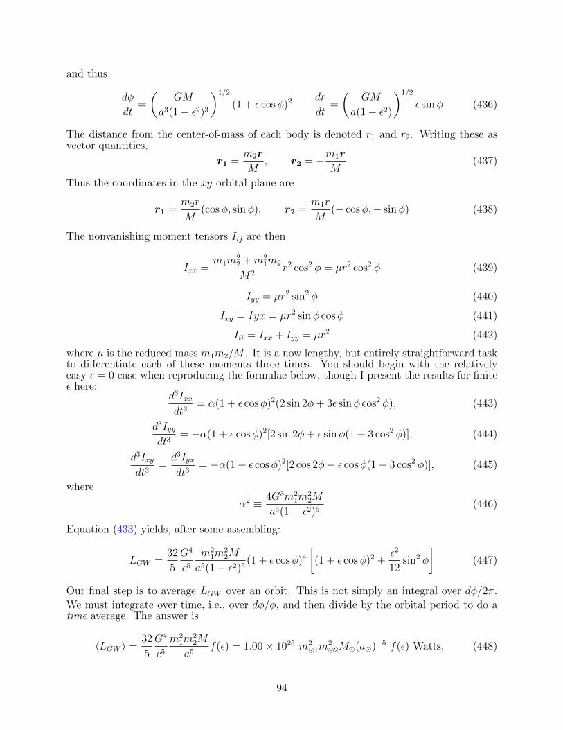
and thus

dφ

dt=

(GM

a3(1− ε2)3

)1/2

(1 + ε cosφ)2dr

dt=

(GM

a(1− ε2)

)1/2

ε sinφ (436)

The distance from the center-of-mass of each body is denoted r1 and r2. Writing these asvector quantities,

r1 =m2r

M, r2 = −m1r

M(437)

Thus the coordinates in the xy orbital plane are

r1 =m2r

M(cosφ, sinφ), r2 =

m1r

M(− cosφ,− sinφ) (438)

The nonvanishing moment tensors Iij are then

Ixx =m1m

22 +m2

1m2

M2r2 cos2 φ = µr2 cos2 φ (439)

Iyy = µr2 sin2 φ (440)

Ixy = Iyx = µr2 sinφ cosφ (441)

Iii = Ixx + Iyy = µr2 (442)

where µ is the reduced mass m1m2/M . It is a now lengthy, but entirely straightforward taskto differentiate each of these moments three times. You should begin with the relativelyeasy ε = 0 case when reproducing the formulae below, though I present the results for finiteε here:

d3Ixxdt3

= α(1 + ε cosφ)2(2 sin 2φ+ 3ε sinφ cos2 φ), (443)

d3Iyydt3

= −α(1 + ε cosφ)2[2 sin 2φ+ ε sinφ(1 + 3 cos2 φ)], (444)

d3Ixydt3

=d3Iyxdt3

= −α(1 + ε cosφ)2[2 cos 2φ− ε cosφ(1− 3 cos2 φ)], (445)

where

α2 ≡ 4G3m21m

22M

a5(1− ε2)5(446)

Equation (433) yields, after some assembling:

LGW =32

5

G4

c5m2

1m22M

a5(1− ε2)5(1 + ε cosφ)4

[(1 + ε cosφ)2 +

ε2

12sin2 φ

](447)

Our final step is to average LGW over an orbit. This is not simply an integral over dφ/2π.

We must integrate over time, i.e., over dφ/φ, and then divide by the orbital period to do atime average. The answer is

〈LGW 〉 =32

5

G4

c5m2

1m22M

a5f(ε) = 1.00× 1025 m2

1m22M(a)−5 f(ε) Watts, (448)

94

where

f(ε) =1 + (73/24)ε2 + (37/96)ε4

(1− ε2)7/2(449)

and indicates solar units of mass (1.99×1030 kg) and length (one solar radius is 6.955×108

m). (Peters and Mathews 1963).

Exercise. Show that following the procedure described above, the time-averaged luminosity〈LGW 〉time is given by the expression

〈LGW 〉time =32

5

G4

c5m2

1m22M

a5(1− ε2)7/2

⟨(1 + ε cosφ)2

[(1 + ε cosφ)2 +

ε2

12sin2 φ

]⟩angle

,

where the average on the right is over 2π angles in φ. Use the fact that the angular averageof cos2 φ is 1/2 and the average of cos4 φ is 3/8 to derive equation (448).

Equations (448) and (449) give the famous gravitational wave energy loss formula for aclassical Keplerian orbit. Notice the dramatic effect of finite eccentricity via the f(ε) function.The first binary pulsar to be discovered, PSR1913+16, has an eccentricity of about 0.62, andthus an enhancement of its gravitational wave energy loss that is boosted by more than anorder of magnitude relative to a circular orbit.

This whole problem must have seemed like an utter flight of fancy in 1963: the conceptof a neutron star was barely credible and not taken seriously; the notion of pulsar timingwas simply beyond conceptualisation. A lesson, perhaps, that no good calculation of aninteresting physical problem ever goes to waste!

Exercise. When we studied Schwarzschild orbits, there was an exercise to show that thetotal Newtonian orbital energy of a bound two body system is −Gm1m2/2a and that thesystem period is proportional to a3/2, independent of the eccentricity. Use these results toshow that the orbital period change due to the loss of gravitational radiation is given by

P = −192π

5

(m1m2

M2

)(GMac2

)5/2

f(ε)

with M = m1 +m2 as before. This P is a measurable quantity! Stay tuned.

Exercise. Now that you’re an expert in the the two-body gravitational radiation problem,let’s move on to three! Show that three equal masses revolving around their common centre-of-mass emit no quadrupole gravitational radiation.

7.8 Detection of gravitational radiation

7.8.1 Preliminary comments

The history of gravitational radiation has been somewhat checkered. Albert Einstein himselfstumbled several times, both conceptually and computationally. Arguments of fundamentalprinciple persisted through the early 1960’s; technical arguments still go on.

At the core of the early controversy was the question of whether gravitational radiationexisted at all! The now classic Peters and Mathews paper of 1963 begins with a disclaimerthat they are assuming that the “standard interpretation” of the theory is correct. The

95

confusion concerned whether the behaviour of hµν potentials were just some sort of math-ematical coordinate effect, devoid of any actual physical consequences. For example, if wecalculate the affine connection Γµνλ and apply the geodesic equation,

d2xµ

dτ 2+ Γµνλ

dxν

dτ

dxλ

dτ= 0 (450)

and ask what happens to a particle initially at rest with dxν/dτ = (−c,0). The subsequentevolution of the spatial velocity components is then

d2xi

dτ 2+ Γi00c

2 = 0 (451)

But equation (334) clearly shows that Γi00 = 0 since any h with a zero index vanishes forour TT plane waves. The particle evidently remains at rest. Is there really no effect ofgravitational radiation on ordinary matter?!

Coordinates, coordinates, coordinates. The point, once again, is that coordinates bythemselves mean nothing, any more than does the statement “My house is located at thevector (2, 1.3).” By now we should have learned this lesson. We picked our gauge to makelife simple, and we have simply found a coordinate system that is frozen to the individualparticles. There is nothing more to it than that. The proper spatial separation betweentwo particles with coordinate separation dxi is ds2 = (ηij − hij)dxi dxj, and that separationsurely is not constant because h11, h22, and h12 = h21 are wiggling even while the dxi arefixed. Indeed, to first order in hij, we may write

ds2 = ηij(dxi − hikdxk/2)(dxj − hjmdxm/2).

This makes the physical interpretation easy: the passing wave increments the initially undis-turbed spatial interval dxi by an amount −hikdxk/2. It was Richard Feynman who in 1955seems to have given the simplest and most convincing argument for the existence of grav-itational waves. If the separation is between two beads on a rigid stick and the beads arefree to slide, they will oscillate with the tidal force of the wave. If there is now a tiny bit ofstickiness, the beads will heat the stick. Where did that energy come from? It could onlybe the wave. The “sticky bead argument” became iconic in the relativity community.

The two independent states of linear polarisation of a gravitational wave are sometimesreferred to as + and ×, “plus” and “cross.” The behave similarly, but rotated by 45. The+ wave as it passes initially causes a prolate distortion along the vertical part of the plussign, squeezes from prolate to oblate distorting along the vertical axis, then squeezes inwardfrom oblate to prolate once again. The × wave shows the same oscillation pattern along arotation pattern rotated by 45. (An excellent animation is shown in the Wikipedia article“Gravitational Waves.”) These are true physical distortions caused by the tidal force of thegravitational wave.

In the midst of what had been intensively theoretical investigations and debate surround-ing the nature of gravitational radiation, in 1968 a physicist named Joseph Weber calmlyannounced that he had detected gravitational radiation experimentally in his basement lab,coming in prodigious amounts from the centre of the Milk Way Galaxy, thank you verymuch. His technique was to use what are now called “Weber bars”, giant cylinders of alu-minum fitted with special piezoelectric devices that can convert tiny mechanical oscillationsinto electrical signals. The gravitational waves distorted these great big bars by a tiny, tinyamount, and the signals were picked up. Or at least that was the idea. The dimensionlessrelative strain δl/l of a bar of length l due to passing wave would be of order hij, or 10−21

by our optimistic estimate. To make a long, rather sad story very short, Weber was in

96

error in several different ways, and ultimately his experiment was completely discredited.Yet his legacy was not wholly negative: the possibility of actually detecting gravitationalwaves hadn’t been taken very seriously up to this point. Post Weber, the idea graduallytook hold in the physics establishment. People asked themselves how we might actually goabout detecting these signals. It became part of the mainstream, with leading figures inrelativity getting directly involved. The detection of gravitational radiation is not a task fora clever lone researcher working in the basement of university building, any more than was,say, finding the Higgs boson. Substantial resources of the National Science Foundation inthe US and a research team numbering in the thousands were needed for the constructionand testing of viable gravitational wave receptors. Almost fifty years after Weber, the LIGOfacility has at last cleanly detected the exquisitely gentle tensorial strains of gravitationalwaves at the level of h ∼ 10−21. The LIGO mirrors did not crack from side-to-side, but theydid flutter a bit in the gravitational breeze. This truly borders on magic: if the effectivelength of LIGO’s interferomter arm is taken is taken to be l = 10 km, then δl is 10−15 cm,one percent of the radius of a proton!

The next exercise is strongly recommended.

Exercise. Weaker than weak interactions. Imagine a gravitational detector of twoidentical masses m separated by a distance l symmetrically about the origin along the x-axis. Along comes a plane wave gravitational wave front, propagating along the z-axis, withhxx = −hyy = Axx cos(kz − ωt) and no other components. The masses vibrate in response.Show that, to linear order in Axx,

...I xx =

1

2mc4ω3l2Axx sinωt,

that there are no other...I ij, and that the masses radiate an average gravitational wave

luminosity of

〈LGW 〉 =G

60c5m2ω6l4A2

xx

Next, show that the average energy flux for our incoming plane wave radiation is, fromequation (412),

F =c3ω2A2

xx

64πG.

The cross section for gravitational interaction (dimensions of area) is defined to be the ratioof the average luminosity to the average incoming flux. Why is this a good definition for thecross section? Show that this ratio is

σ =16πG2m2ω4l4

15c8=

4

15πR2

S

(ωl

c

)4

where RS = 2Gm/c2 is the Schwarzschild radius of each mass. Evaluate this numerically form = 10kg, l = 10m, ω = 20 rad s−1 (motivated by GW150914). Compare this with a typicalweak interaction cross section of 10−48m2. Just how weak is gravitational scattering?

7.8.2 Indirect methods: orbital energy loss in binary pulsars

In 1974, a remarkable binary system was discovered by Hulse and Taylor (1975, ApJ Letters,195, L51). One of the stars was a pulsar with a pulse period of 59 milliseconds, i.e., a neutronstar that rotates about 17 times a second. The orbital period was 7.75 hours, a very tight

97

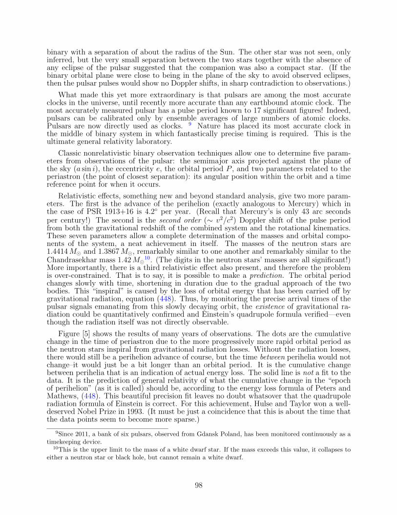
binary with a separation of about the radius of the Sun. The other star was not seen, onlyinferred, but the very small separation between the two stars together with the absence ofany eclipse of the pulsar suggested that the companion was also a compact star. (If thebinary orbital plane were close to being in the plane of the sky to avoid observed eclipses,then the pulsar pulses would show no Doppler shifts, in sharp contradiction to observations.)

What made this yet more extraordinary is that pulsars are among the most accurateclocks in the universe, until recently more accurate than any earthbound atomic clock. Themost accurately measured pulsar has a pulse period known to 17 significant figures! Indeed,pulsars can be calibrated only by ensemble averages of large numbers of atomic clocks.Pulsars are now directly used as clocks. 9 Nature has placed its most accurate clock inthe middle of binary system in which fantastically precise timing is required. This is theultimate general relativity laboratory.

Classic nonrelativistic binary observation techniques allow one to determine five param-eters from observations of the pulsar: the semimajor axis projected against the plane ofthe sky (a sin i), the eccentricity e, the orbital period P , and two parameters related to theperiastron (the point of closest separation): its angular position within the orbit and a timereference point for when it occurs.

Relativistic effects, something new and beyond standard analysis, give two more param-eters. The first is the advance of the perihelion (exactly analogous to Mercury) which inthe case of PSR 1913+16 is 4.2 per year. (Recall that Mercury’s is only 43 arc secondsper century!) The second is the second order (∼ v2/c2) Doppler shift of the pulse periodfrom both the gravitational redshift of the combined system and the rotational kinematics.These seven parameters allow a complete determination of the masses and orbital compo-nents of the system, a neat achievement in itself. The masses of the neutron stars are1.4414M and 1.3867M, remarkably similar to one another and remarkably similar to theChandrasekhar mass 1.42M

10. (The digits in the neutron stars’ masses are all significant!)More importantly, there is a third relativistic effect also present, and therefore the problemis over-constrained. That is to say, it is possible to make a prediction. The orbital periodchanges slowly with time, shortening in duration due to the gradual approach of the twobodies. This “inspiral” is caused by the loss of orbital energy that has been carried off bygravitational radiation, equation (448). Thus, by monitoring the precise arrival times of thepulsar signals emanating from this slowly decaying orbit, the existence of gravitational ra-diation could be quantitatively confirmed and Einstein’s quadrupole formula verified—eventhough the radiation itself was not directly observable.

Figure [5] shows the results of many years of observations. The dots are the cumulativechange in the time of periastron due to the more progressively more rapid orbital period asthe neutron stars inspiral from gravitational radiation losses. Without the radiation losses,there would still be a perihelion advance of course, but the time between perihelia would notchange–it would just be a bit longer than an orbital period. It is the cumulative changebetween perihelia that is an indication of actual energy loss. The solid line is not a fit to thedata. It is the prediction of general relativity of what the cumulative change in the “epochof perihelion” (as it is called) should be, according to the energy loss formula of Peters andMathews, (448). This beautiful precision fit leaves no doubt whatsover that the quadrupoleradiation formula of Einstein is correct. For this achievement, Hulse and Taylor won a well-deserved Nobel Prize in 1993. (It must be just a coincidence that this is about the time thatthe data points seem to become more sparse.)

9Since 2011, a bank of six pulsars, observed from Gdansk Poland, has been monitored continuously as atimekeeping device.

10This is the upper limit to the mass of a white dwarf star. If the mass exceeds this value, it collapses toeither a neutron star or black hole, but cannot remain a white dwarf.

98

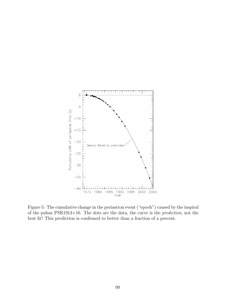
Figure 5: The cumulative change in the periastron event (“epoch”) caused by the inspiralof the pulsar PSR1913+16. The dots are the data, the curve is the prediction, not thebest fit! This prediction is confirmed to better than a fraction of a percent.

99

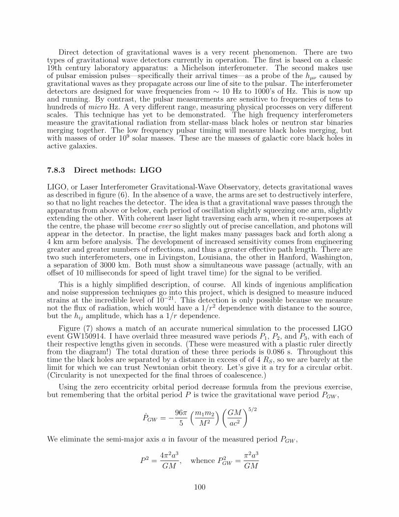
Direct detection of gravitational waves is a very recent phenomenon. There are twotypes of gravitational wave detectors currently in operation. The first is based on a classic19th century laboratory apparatus: a Michelson interferometer. The second makes useof pulsar emission pulses—specifically their arrival times—as a probe of the hµν caused bygravitational waves as they propagate across our line of site to the pulsar. The interferometerdetectors are designed for wave frequencies from ∼ 10 Hz to 1000’s of Hz. This is now upand running. By contrast, the pulsar measurements are sensitive to frequencies of tens tohundreds of micro Hz. A very different range, measuring physical processes on very differentscales. This technique has yet to be demonstrated. The high frequency interferometersmeasure the gravitational radiation from stellar-mass black holes or neutron star binariesmerging together. The low frequency pulsar timing will measure black holes merging, butwith masses of order 109 solar masses. These are the masses of galactic core black holes inactive galaxies.

7.8.3 Direct methods: LIGO

LIGO, or Laser Interferometer Gravitational-Wave Observatory, detects gravitational wavesas described in figure (6). In the absence of a wave, the arms are set to destructively interfere,so that no light reaches the detector. The idea is that a gravitational wave passes through theapparatus from above or below, each period of oscillation slightly squeezing one arm, slightlyextending the other. With coherent laser light traversing each arm, when it re-superposes atthe centre, the phase will become ever so slightly out of precise cancellation, and photons willappear in the detector. In practise, the light makes many passages back and forth along a4 km arm before analysis. The development of increased sensitivity comes from engineeringgreater and greater numbers of reflections, and thus a greater effective path length. There aretwo such interferometers, one in Livingston, Louisiana, the other in Hanford, Washington,a separation of 3000 km. Both must show a simultaneous wave passage (actually, with anoffset of 10 milliseconds for speed of light travel time) for the signal to be verified.

This is a highly simplified description, of course. All kinds of ingenious amplificationand noise suppression techniques go into this project, which is designed to measure inducedstrains at the incredible level of 10−21. This detection is only possible because we measurenot the flux of radiation, which would have a 1/r2 dependence with distance to the source,but the hij amplitude, which has a 1/r dependence.

Figure (7) shows a match of an accurate numerical simulation to the processed LIGOevent GW150914. I have overlaid three measured wave periods P1, P2, and P3, with each oftheir respective lengths given in seconds. (These were measured with a plastic ruler directlyfrom the diagram!) The total duration of these three periods is 0.086 s. Throughout thistime the black holes are separated by a distance in excess of of 4 RS, so we are barely at thelimit for which we can trust Newtonian orbit theory. Let’s give it a try for a circular orbit.(Circularity is not unexpected for the final throes of coalescence.)

Using the zero eccentricity orbital period decrease formula from the previous exercise,but remembering that the orbital period P is twice the gravitational wave period PGW ,

PGW = −96π

5

(m1m2

M2

)(GMac2

)5/2

We eliminate the semi-major axis a in favour of the measured period PGW ,

P 2 =4π2a3

GM, whence P 2

GW =π2a3

GM

100

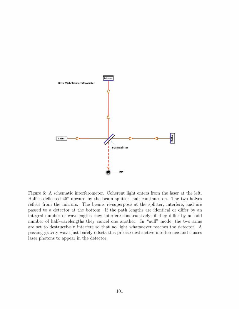
Figure 6: A schematic interferometer. Coherent light enters from the laser at the left.Half is deflected 45 upward by the beam splitter, half continues on. The two halvesreflect from the mirrors. The beams re-superpose at the splitter, interfere, and arepassed to a detector at the bottom. If the path lengths are identical or differ by anintegral number of wavelengths they interfere constructively; if they differ by an oddnumber of half-wavelengths they cancel one another. In “null” mode, the two armsare set to destructively interfere so that no light whatsoever reaches the detector. Apassing gravity wave just barely offsets this precise destructive interference and causeslaser photons to appear in the detector.

101

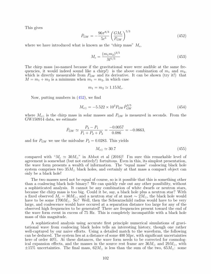
This gives

PGW = −96π8/3

5c5

(GMc

PGW

)5/3

(452)

where we have introduced what is known as the “chirp mass” Mc,

Mc =(m1m2)

3/5

M1/5(453)

The chirp mass (so-named because if the gravitational wave were audible at the same fre-quencies, it would indeed sound like a chirp!) is the above combination of m1 and m2,which is directly measurable from PGW and its derivative. It can be shown (try it!) thatM = m1 +m2 is a minimum when m1 = m2, in which case

m1 = m2 ' 1.15Mc.

Now, putting numbers in (452), we find

Mc = −5.522× 103PGW P3/5GW (454)

where Mc is the chirp mass in solar masses and PGW is measured in seconds. From theGW150914 data, we estimate

PGW 'P3 − P1

P1 + P2 + P3

=−0.0057

0.086= −0.0663,

and for PGW we use the midvalue P2 = 0.0283. This yields

Mc ' 30.7 (455)

compared with “Mc ' 30M” in Abbot et al (2016)! I’m sure this remarkable level ofagreement is somewhat (but not entirely!) fortuitous. Even in this, its simplest presentation,the wave form presents a wealth of information. The “equal mass” coalescing black holesystem comprises two 35M black holes, and certainly at that mass a compact object canonly be a black hole!

The two masses need not be equal of course, so is it possible that this is something otherthan a coalescing black hole binary? We can quickly rule out any other possibility, withouta sophisticated analysis. It cannot be any combination of white dwarfs or neutron stars,because the chirp mass is too big. Could it be, say, a black hole plus a neutron star? Witha fixed observed Mc = 30M, and a neutron star of at most ∼ 2M, the black hole wouldhave to be some 1700M. So? Well, then the Schwarzschild radius would have to be verylarge, and coalescence would have occured at a separation distance too large for any of theobserved high frequencies to be generated! There are frequencies present toward the end ofthe wave form event in excess of 75 Hz. This is completely incompatible with a black holemass of this magnitude.

A sophisticated analysis using accurate first principle numerical simulations of gravi-tational wave from coalescing black holes tells an interesting history, though one ratherwell-captured by our naive efforts. Using a detailed match to the waveform, the followingcan be deduced. The system lies at a distance of some 400 Mpc, with significant uncertaintieshere of order 40%. At these distances, the wave form needs to be corrected for cosmolog-ical expansion effects, and the masses in the source rest frame are 36M and 29M, with±15% uncertainties. The final mass, 62M is less than the sum of the two, 65M: some

102

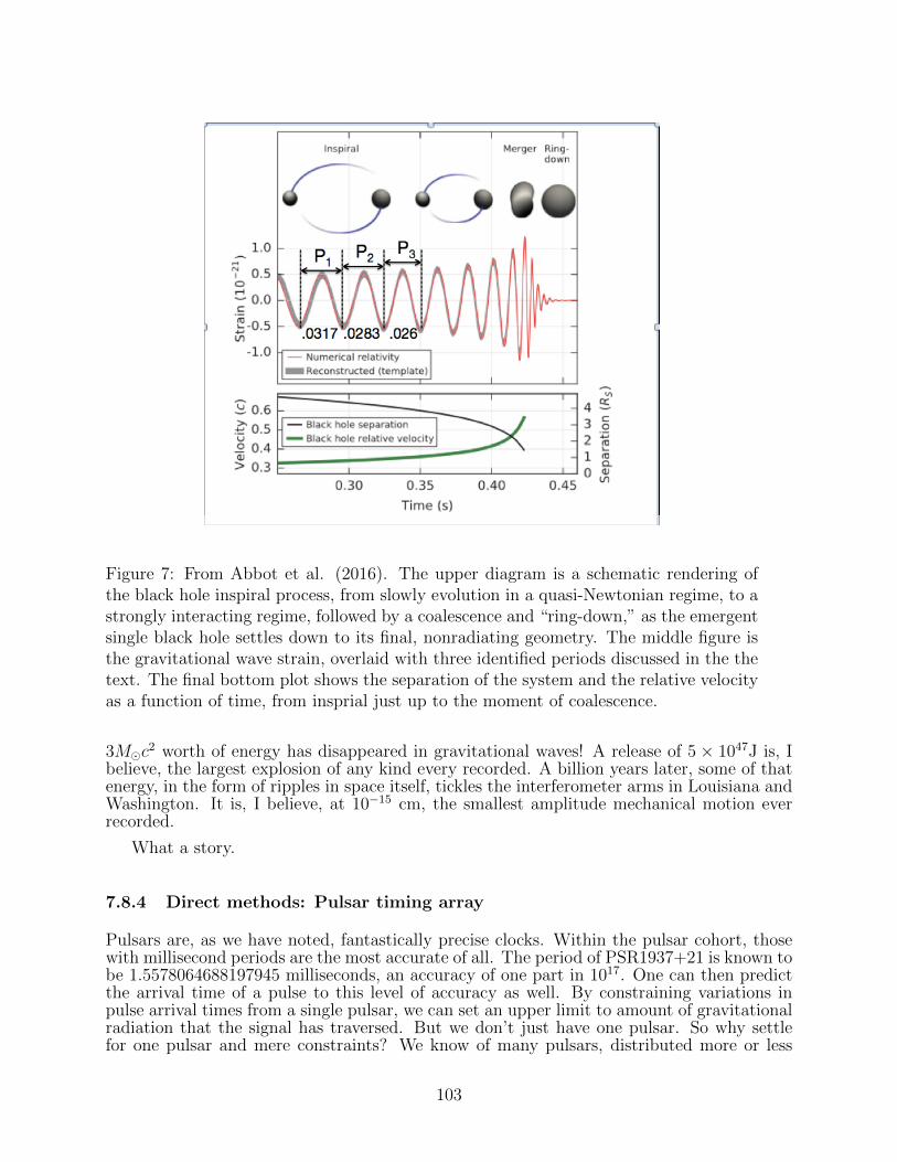
Figure 7: From Abbot et al. (2016). The upper diagram is a schematic rendering ofthe black hole inspiral process, from slowly evolution in a quasi-Newtonian regime, to astrongly interacting regime, followed by a coalescence and “ring-down,” as the emergentsingle black hole settles down to its final, nonradiating geometry. The middle figure isthe gravitational wave strain, overlaid with three identified periods discussed in the thetext. The final bottom plot shows the separation of the system and the relative velocityas a function of time, from insprial just up to the moment of coalescence.

3Mc2 worth of energy has disappeared in gravitational waves! A release of 5 × 1047J is, I

believe, the largest explosion of any kind every recorded. A billion years later, some of thatenergy, in the form of ripples in space itself, tickles the interferometer arms in Louisiana andWashington. It is, I believe, at 10−15 cm, the smallest amplitude mechanical motion everrecorded.

What a story.

7.8.4 Direct methods: Pulsar timing array

Pulsars are, as we have noted, fantastically precise clocks. Within the pulsar cohort, thosewith millisecond periods are the most accurate of all. The period of PSR1937+21 is known tobe 1.5578064688197945 milliseconds, an accuracy of one part in 1017. One can then predictthe arrival time of a pulse to this level of accuracy as well. By constraining variations inpulse arrival times from a single pulsar, we can set an upper limit to amount of gravitationalradiation that the signal has traversed. But we don’t just have one pulsar. So why settlefor one pulsar and mere constraints? We know of many pulsars, distributed more or less

103

Figure 8: A schematic view of a gravitational wave passing throughan array of pulsar probes.

uniformly through the galaxy. If the arrival times from this “pulsar timing array” (PTA) werecorrelated with one another in a mathematically calculable manner, this would be a directindication of the the deformation of space caused by the passage of a gravitational wave. Thistechnique is sensitive to very long wavelength gravitational radiation, light-years in extent.This is very difficult to do because all other sources introducing a spurious correlation mustbe scrupulously eliminated. LIGO too has noise issues, but unlike pulsar blips propagatingthrough the interstellar medium, LIGO’s signal is very clean and all hardware is accessible.Thus, PTA has its share of skeptics. At the time of this writing, there are only upper limitsfrom the PTA measurements.

104

Despite its name, the big bang theory is

not really a theory of a bang at all. It is

really only a theory of the aftermath of a

bang.

— Alan Guth

8 Cosmology

8.1 Introduction

8.1.1 Newtonian cosmology

The subject of the origin of the Universe is irresistible to the scientist and layperson alike.What went bang? Where did the Universe come from? What happened along the way?Where are we headed? The theory of general relativity, with its rigorous mathematicalformulation of the large-scale geometry of spacetime, provides both the conceptual andtechnical apparatus to understand the structure and evolution of the Universe. We arefortunate to live in an era in which many precise answers to these great questions are athand. Moreover, while we need general relativity to put ourselves on a truly firm footing, wecan get quite far using very simple ideas and hardly any relativity at all! Not only can, weabsolutely should begin this way. Let us start with some very Newtonian dynamics and seewhat there is to see. Then, knowing a bit of what to expect and where we are headed, we willbe in a much better position to revisit “the problem of the Universe” on a fully relativisiticbasis.

A plausible but naive model of the Universe might be one in which space is ordinarystatic Euclidian space, and the galaxies fill up this space uniformly (on average) everywhere.Putting aside the question of the origin of such a structure (let’s say it has existed for alltime) and the problem that the cumulative light received at any location would be infinite(“Olber’s paradox”–that’s tougher to get around: let’s say maybe we turned on the galaxiesat some finite time in the past11), the static Euclidian model is not even mathematicallyself-consistent.

Consider the analysis from Figure [9]. There are two observers, one at the centre of thesphere labelled of radius r1, the other at the centre of sphere r2. Each calculates the expectedacceleration at the location of the big black dot, which is a point on the surface of each ofthe spheres. Our model universe is spherically symmetric about r1, but it is also sphericallysymmetric about r2. Hence the following conundrum:

The observer at the centre of the r1 sphere ignores the effect of the spherically symmetricmass exterior to the black point and concludes that the acceleration at the dot’s location is

a1 =GM(within r1)

r21=

4πGρr13

(456)

directed toward the centre of the r1 sphere. (Here ρ is meant to be the average uniform massdensity of the Universe.) But the observer at the origin of the r2 sphere claims, by identicalreasoning, that the acceleration must be a2 = 4πGρr2/3 directed toward the centre of r2!Both cannot be correct.

11See W72, pp. 611-13.

105

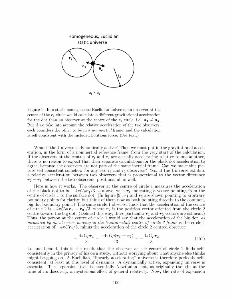
Homogeneous, Euclidian sta2c universe

r1

r2

a1 ≠ a2

a1 a2

Figure 9: In a static homogeneous Euclidian universe, an observer at thecenter of the r1 circle would calculate a different gravitational accelerationfor the dot than an observer at the centre of the r2 circle, i.e. a1 6= a2.But if we take into account the relative acceleration of the two observers,each considers the other to be in a noninertial frame, and the calculationis self-consistent with the included fictitious force. (See text.)

What if the Universe is dynamically active? Then we must put in the gravitational accel-eration, in the form of a noninertial reference frame, from the very start of the calculation.If the observers at the centres of r1 and r2 are actually accelerating relative to one another,there is no reason to expect that their separate calculations for the black dot acceleration toagree, because the observers are not part of the same inertial frame! Can we make this pic-ture self-consistent somehow for any two r1 and r2 observers? Yes. If the Universe exhibitsa relative acceleration between two observers that is proportional to the vector differencer2 − r1 between the two observers’ positions, all is well.

Here is how it works. The observer at the centre of circle 1 measures the accelerationof the black dot to be −4πGρr1/3 as above, with r1 indicating a vector pointing from thecentre of circle 1 to the surface dot. (In figure [9], r1 and r2 are shown pointing to arbitraryboundary points for clarity; but think of them now as both pointing directly to the common,big dot boundary point.) The same circle 1 observer finds that the acceleration of the centreof circle 2 is −4πGρ(r1 − r2)/3, where r2 is the position vector oriented from the circle 2centre toward the big dot. (Defined this way, these particular r1 and r2 vectors are colinear.)Thus, the person at the centre of circle 1 would say that the acceleration of the big dot, asmeasured by an observer moving in the (noninerital) centre of circle 2 frame is the circle 1acceleration of −4πGr1/3, minus the acceleration of the circle 2 centred observer:

− 4πGρr13

− −4πGρ(r1 − r2)

3= −4πGρr2

3(457)

Lo and behold, this is the result that the observer at the centre of circle 2 finds self-consistently in the privacy of his own study, without worrying about what anyone else thinksmight be going on. A Euclidian, “linearly accelerating” universe is therefore perfectly self-consistent, at least at this level of dynamics. A dynamically active, expanding universe isessential. The expansion itself is essentially Newtonian, not, as originally thought at thetime of its discovery, a mysterious effect of general relativity. Now, the rate of expansion

106

naively ought to be slowing, since this is what gravity does: an object thrown from thesurface of the earth slows down as its distance from the surface increases. As we shall soonsee however, our Universe is a bit more devious than that. There is still some mystery herebeyond the realm of the purely Newtonian.

8.1.2 The dynamical equation of motion

A simple way to describe the internal acceleration of the Universe is to begin with thespatially homogeneous but time-dependent relative expansion between two locations. Theseparation between two arbitrary points separated by a distance r(t) may be written

r(t) = R(t)l (458)

where l is a comoving coordinate that labels a fixed radial distance from us in the space—fixed in the sense of being fixed to the expanding space, like latitude and longitude wouldbe on the surface of an inflating globe. If we take l to have dimensions of length, then R(t)is a dimensionless function of time alone. It is a scale factor that embodies the dynamicalbehaviour of the Universe. The velocity v = dr/dt ≡ r of a “fixed” point expanding withspace is then

v(t) = Rl = (R/R)r. (459)

We should emphasise the vector character of this relationship:

v(t) = (R/R)r (460)

where r is a vector pointing outward from our arbitrarily chosen origin. Then, the accelera-tion is

a(t) =dv

dt= (R/R)r (461)

(Why didn’t we differentiate r(t)/R(t)?) But we already know the relative accelerationbetween two points, because we know Newtonian physics. We’ve just worked it out a momentago! You can easily see that the above discussions (especially equation [456]) imply that wemust have :

− 4πGρ

3=R

R(462)

Notice how l disappears: this is an equation for the scale factor R, and that does not dependon where you are. Next, multiply this by RR and integrate, assuming that mass is conservedin the usual way, i.e. ρR3 is constant. (Why is this “the usual way?”) We then obtain

R2 − 8πGρR2

3= 2E (463)

where E is an energy-like integration constant. This, in a simple, apparently naive Euclidian-Newtonian approach, would be our fundamental dynamical cosmological equation for theevolution of the Universe. Amazingly, providing that we are prepared to allow the massdensity ρ is to be upgraded to an energy density divided by c2 that includes all contributions(in particular radiation and vacuum energy), this innocent little equation turns out to be farmore general: it is exactly correct in full relativity theory! More on this anon.

107

8.1.3 Cosmological redshift

The expansion of the Universe leads to a very important kinematic effect known as thecosmological redshift. Since the Universe is expanding, a travelling photon is constantlyovertaking sources that are moving away from it. If a photon has a wavelength λ at somelocation r, when the photon passes an observer a distance dr = cdt away, moving at a relativevelocity R dr/R, the observer measures a Doppler change in wavelength dλ determined byequation (460):

dλ

λ=v

c=

R

cRdr =

R

Rdt, (464)

or in other words1

λ

dλ

dt≡ λ

λ=R

R. (465)

Solving for λ, we find that it is linearly proportional to R. It is as though the wavelengthstretches with the rest of the Universe! This is a very general kinematic result, a property ofany model that is symmetrically expanding. (Sneak preview: this of course means that thefrequency goes down as 1/R. But the frequency of a photon is, in essence, its energy. Theentire Universe must be radiatively cooling. Energy is not conserved in the expansion; theentropy in a voulme R3, which is proportional to the third power of the temperature timesR3, is.)

We are free, and it is customary, to choose our coordinates in such a way that the currentvalue of R is 1, with R becoming smaller and smaller as we go back in time. If a photonis emitted with a wavelength λe at some time t in the past, the wavelength we would nowmeasure (λ0) is formally expressed as

λ0 = λe(1 + z) (466)

where z is defined by this equation and known as the redshift parameter. Therefore,

λ0λe

= 1 + z =1

R(t)(467)

The advantage to using z, as opposed to the more geometrical quantity R, is that z is directlyobserved by astronomers. But the two are mathematically equivalent via this completelygeneral equation, R = 1/(1 + z). If you measure a redshift of 2, it has come from a timewhen the Universe had one-third of its current size.

We have been, you will notice, pretty informal, just organising our common sense. It iscustomary for cosmology courses to begin with a heavy dose of historical material relatedto the discovery of the expansion of the Universe. We will get to this in short order, but Ihave taken a somewhat different tack here, in part because much of the historical materialis rather well-known these days, but mainly because it is not often appreciated how fardirect Newtonian reasoning can take one in establishing a viable cosmological model of theUniverse. Let us examine one very simple model, and then see how formal general theorygets us to the same place in the end.

8.2 Cosmology models for the impatient

8.2.1 The large-scale spacetime metric

Euclid, Newton and pure thought can take us very far, even farther than we have venturedup to now. Because the Newtonian approach on which we are about to embark is going to

108

work remarkably well, here is a brief reminder as to why we actually do need relativity inour study of the large scale structure of the Universe. Let us understand what it is at stake.

First, we require a Riemannian metric structure to ensure that the speed of light is a uni-versal constant c, especially when traversing a dynamically evolving spacetime background.It is rather easy to see what the form this metric must take in the simplest model of anexpanding Euclidian Universe. Symmetry demands that time must flow the same for all ob-servers comoving with the universal expansion, and we can always choose time to be a linearfunction of the time coordinate. Space is uniformly expanding at the same rate everywhere.So if space itself is Euclidian, the spacetime metric practically leaps out of the page,

− c2dτ 2 = −c2dt2 +R2(dx2 + dy2 + dz2) (468)

where we have used the usual (x, y, z) Cartesian coordinates, and R satisfies equation (463).Here x, y, z are all comoving with the expansion, in essence the l coordinate of the previoussection. In particular, for a photon heading directly toward us along our line of sight froma distant source,

Rdl

dt= −c (469)

where dl is interpreted as the change in radial comoving coordinate induced by the photon’spassage. This equation describes an ant crawling along the surface of an expanding spherefrom, say, the pole to the equator, moving at a constant velocity c. In this case, think of dlas the change in latitude.

Equation (468) really does appear to be the true form of the spacetime metric for ourUniverse. Space is in fact very nearly, or perhaps even precisely, Euclidian. As a math-ematical point, this need not be the case even if we demand perfect symmetry, any morethan a perfectly symmetric two-dimensional surface must be a plane. We could preserve ourglobal maximal spatial symmetry and have a curved space, just like the surface of sphere.This, in common with a flat plane, is symmetric about every point, but is obviously dis-torted relative to a plane. The case of a two-dimensional spherical surface is readily graspedbecause we can easily embed it in three dimensions and form a mental image. It is finitein area and said to be positively curved. There is also a perfectly viable flaring, negativelycurved two-dimensional surface. A saddle begins to capture its essence, but not quite, be-cause the curvature is not uniform in a saddle. The case of a uniformly negatively curvedsurface cannot be embedded in three dimensions, so it is hard to picture in your mind’s eye!There are perfectly good positively and negatively three-dimensional spaces as well, whichare logically possible alternative symmetric structures for the space of our Universe. Theyjust happen not to fit the data. It is fortunate for us that the real Universe seems also to bemathematically the simplest. We will study these other symmetric spaces later; for now weconfine our attention to expanding, good old, “flat” Euclidian space.

Second, we need relativity in the form of the Birkhoff theorem to justify properly theargument neglecting exterior contributions from outside the arbitraily chosen spheres weused in section 8.1. The Newtonian description strictly can’t be applied to an infinite sys-tem, whereas nothing prevents us from using Birkhoff’s theorem applied to an unboundedsymmetric spacetime.

Third, we need a relativistically valid argument to arrive at equation (463). Nothing inthe Newtonian derivation hints at this level of generality. We shall return to this carefullyin section 8.3.

Fourth, we need relativity theory to relate the constant E to the geometry of our space.For now, we restrict ourselves to the case E = 0, which will turn out to be the only solutionconsistent with the adoption of a flat Euclidian spatial geometry, the sort of universe we doseem to live in.

109

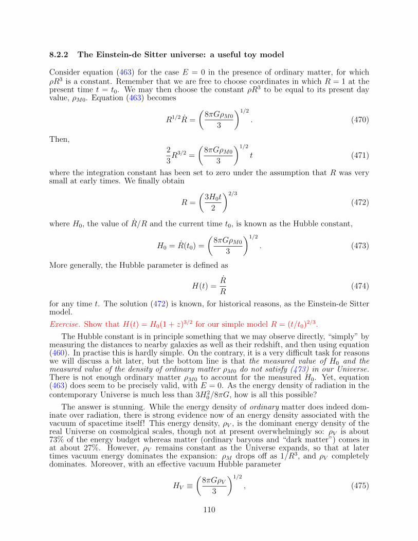
8.2.2 The Einstein-de Sitter universe: a useful toy model

Consider equation (463) for the case E = 0 in the presence of ordinary matter, for whichρR3 is a constant. Remember that we are free to choose coordinates in which R = 1 at thepresent time t = t0. We may then choose the constant ρR3 to be equal to its present dayvalue, ρM0. Equation (463) becomes

R1/2R =

(8πGρM0

3

)1/2

. (470)

Then,

2

3R3/2 =

(8πGρM0

3

)1/2

t (471)

where the integration constant has been set to zero under the assumption that R was verysmall at early times. We finally obtain

R =

(3H0t

2

)2/3

(472)

where H0, the value of R/R and the current time t0, is known as the Hubble constant,

H0 = R(t0) =

(8πGρM0

3

)1/2

. (473)

More generally, the Hubble parameter is defined as

H(t) =R

R(474)

for any time t. The solution (472) is known, for historical reasons, as the Einstein-de Sittermodel.

Exercise. Show that H(t) = H0(1 + z)3/2 for our simple model R = (t/t0)2/3.

The Hubble constant is in principle something that we may observe directly, “simply” bymeasuring the distances to nearby galaxies as well as their redshift, and then using equation(460). In practise this is hardly simple. On the contrary, it is a very difficult task for reasonswe will discuss a bit later, but the bottom line is that the measured value of H0 and themeasured value of the density of ordinary matter ρM0 do not satisfy (473) in our Universe.There is not enough ordinary matter ρM0 to account for the measured H0. Yet, equation(463) does seem to be precisely valid, with E = 0. As the energy density of radiation in thecontemporary Universe is much less than 3H2

0/8πG, how is all this possible?

The answer is stunning. While the energy density of ordinary matter does indeed dom-inate over radiation, there is strong evidence now of an energy density associated with thevacuum of spacetime itself! This energy density, ρV , is the dominant energy density of thereal Universe on cosmolgical scales, though not at present overwhelmingly so: ρV is about73% of the energy budget whereas matter (ordinary baryons and “dark matter”) comes inat about 27%. However, ρV remains constant as the Universe expands, so that at latertimes vacuum energy dominates the expansion: ρM drops off as 1/R3, and ρV completelydominates. Moreover, with an effective vacuum Hubble parameter

HV ≡(

8πGρV3

)1/2

, (475)

110

equation (463) at later times takes the form

R = HVR (476)

orR ∝ exp(HV t) (477)

the Universe will expand exponentially! In other words, rather than gravity slowly deceler-ating the expansion by the mutual Newtonian attractive force, the vacuum energy densitywill actively drive an ever more vigorous repulsive force. The Universe was expanding moreslowly in the past than in the present. It is this particular discovery which led to our cur-rent understanding of the remarkable expansion dynamics. The Nobel Prize in Physics wasawarded to Perlmutter, Schmidt and Riess in 2011 for the use of distant supernovae as a toolfor unravelling the dynamics of the Universe from early to later times. We are currently inthe epoch where exponential expansion is taking over.

Equations (467), (469) and (473) may be combined to answer the following question.If we measure a photon of redshift z, from what value of l did it originate? This is animportant question because it provides the link between observations and geometry. WithR(t) = (t/t0)

2/3 = (3H0t/2)2/3, equation (469) may be be integrated over the path of thephoton from its emission at l at time t:∫ l

0

dl′ = −c∫ t

t0

dt′

R= ct

2/30

∫ t0

t

dt′

t′2/3= 3ct0

(1−√R)

=2c

H0

(1− 1√

1 + z

)≡ l(z) (478)

This is a very interesting equation for many reasons. First, note that as z →∞, l→ 2c/H0,a constant. The most distant photons—and therefore the most distant regions that maycausally influence us—come from l = 2c/H0. This quantity is known as the horizon, denotedlH . Beyond the horizon, we can see—and be influenced by—nothing. This particular value oflH = 2c/H0 is associated with the Einstein–de Sitter model, but the existence of a horizon is ageneral feature of many cosmologies and will generally be a multiple of c/H0. Do not confusethis cosmological horizon, sometimes called a “particle horizon” with the event horizon ofa black hole. The particle horizon is notionally outward, the length over which a a causaleffect may be exerted. The event horizon is notionally inward, the radius within which nocausal contact with the outside world is possible.

Physical distances are given not by l, but by Rl. Since R = 1 currently, 2c/H0 is thecurrent physical scale of the horizon as well. There is nothing special about now, however.We could be doing this analysis at any time t, and the scale of the horizon at time t in theE-de S model would then be 2c/H(t) = 2c/[H0(1 + z)3/2]. So here is another interestingquestion. The farthest back in time that we can see is to a redshift of about z = 1500. Athigher redsifts the Universe was completely opaque. Just as we can only see to the opaquesurface of the Sun, but not its interior, we can only see back in time to when the Universebecame opaque to photons. Question: what would be the subtended angular size of thehorizon ΘH at z = 1500, as we it measure today? This is an important question becausewe would not expect the Universe to be very smooth or regular or correlated in any way onangular scales bigger than this. (The E-dS model doesn’t actually hold during the radiationdominated phase, but it will serve to make our point.) The angular size of the horizon isgiven by the following expression:

ΘH =2c

H0(1 + z)3/2R(z)l(z)=

2c

H0(1 + z)1/2l(z)=

1√1 + z − 1

(479)

The first equality sets the horizon angle equal to the actual physical size of the horizon atredshift z, divided by d = R(z)l(z), the distance to redshift z at the earlier time corresponding

111

to redshift z (not now!). This d is the relevant distance to the photon sources at the momentof the radiation emission. The Universe was a smaller place then, and we cannot, we mustnot, use the current proper distance, which would be l(z) times R0 = 1. If you plug inz = 1500 into (479) and convert ΘH to degrees, you’ll find ΘH = 1.5, about 3 timesthe diameter of the full moon. But the Universe looks very regular on much, much largerangular scales, indeed over the entire sky! Even if our model is only crude, it highlights animportant problem. We will see later in this course how modern cosmology addresses thispuzzle. Simply put, how does the Universe know about itself in a global sense, given that ittakes signals, even signals travelling at the speed of light, so long to cross it? What we havehere, ladies and gentleman, is a failure to communicate.

By the way, the fact that the Universe was “on top of us” at early times has anothersurprising consequence. Assuming that the average physical size of a galaxy isn’t changingvery much with time, if we calculate the average angular size of a galaxy, we find that at lowredshift, all is normal: the more distant galaxies appear to be smaller. But then, at higherand higher redshifts, the galaxies appear to be growing larger on the sky! Why? Because atlarge z, the Universe was, well, on top of us. The “distance-to-redshift-z” formula is

l(z)R(z) =2c

H0(1 + z)3/2

(√1 + z − 1

)(480)

At low z, this is increasing linearly with z, which is intuitive: bigger redshift, more distant.But at large z this declines as 1/z, since the Universe was a smaller place.

Exercise. At what redshift would the average galaxy appear to be smallest in this model?(Answer: z = 5/4.)

8.3 The Friedman-Robertson-Walker Metric

Let us start very simply. The ordinary metric for a planar two-dimensional space (“2-space”)without curvature may be written in cylindrical coordinates as

ds2 = d$2 +$2dφ2 (481)

where the radial $ and angular φ polar coordinates are related to ordinary Cartesian x andy coordinates by the familiar formulae:

x = $ cosφ, y = $ sinφ (482)

As we have noted, this flat 2-space is not the most general globally symmetric 2-spacepossible. The space could, for example, be distorted like the 2-surface of a sphere, yetretain the symmetry of every point being equivalent. The metric for a spherical surface iswell-known:

ds2 = a2dθ2 + a2 sin2 θdφ2 (483)

where a is the radius of the sphere. Now, we know how to go between cylindrical polar andspherical coordinates: set $ = a sin θ. This may be viewed as a purely formal transformationof coordinates, but in our mind’s eye we picture θ in physical terms as the colatitude measureddown from the z axis. But don’t expect to recover (481) from (483) via this simple coordinatechange sin θ = $/a. Instead, we find that the spherical surface metric becomes:

ds2 =d$2

1−$2/a2+$2dφ2 (484)

112

which is a different space from the planar surface (481) altogether. It is of course the samespherical surface space we started with by any other name, agreeing with (481) only in thelimit a → ∞. Changing coordinates does not change the geometry, i.e., it does not changethe curvature scalars. A plane may be regarded as the surface of a sphere only in the limita→∞.

Let’s stretch ourselves a bit and consider, at a formal level, the closely related metric

ds2 =d$2

1 +$2/a2+$2dφ2, (485)

which upon substituing sinhχ = $/a reverts to

ds2 = a2dχ2 + a2 sinh2 χdφ2 (486)

the fundamental symmetry properties of the metric are unaffected by the ±$2 sign flip. Theflip in sign simply changes the sign of the constant curvature surface from positive (convex,think sphere) to negative (flaring, think saddle). The characteristic form of the metric tensorcomponent grr = 1/(1 ± $2/a2) will reappear when we go from curved 2-space, to curved3-space.

8.3.1 Maximally symmetric 3-spaces

It is perhaps best to begin with the conclusion, which ought not to suprise you. The most gen-eral form of the three dimensional metric tensor that is maximally symmetric—homogeneousand isotropic about every point—takes the form

− c2dτ 2 = −c2dt2 +R2(t)

(dr2

1− r2/a2+ r2dθ2 + r2 sin2 θ

)(487)

where we allow ourselves the liberty of taking a2 to be positive or negative.

The derivation for a 3-space hypersurface for a sphere in four dimensions is not difficult.The surface of 4-sphere (Cartesian coordinates w, x, y, z) is given by

w2 + x2 + y2 + z2 = a2 = constant. (488)

Thus, on this surface, a small change in w2 is restricted to satisfy:

d(w2) = −d(x2 + y2 + z2) ≡ −d(r2)→ dw = −rdr/w (489)

with r2 ≡ x2 + y2 + z2. Hence,

(dw)2 =r2(dr)2

w2=r2(dr)2

a2 − r2(490)

The line element in 4-space is

ds2 = dx2 + dy2 + dz2 + dw2 = dr2 + r2dθ2 + r2 sin2 θ dφ2 + dw2 (491)

and with (dw)2 given by (490), there follows immediately the line element of the 3-surfaceof a 4-sphere, analogous to our expression for the ordinary spherical surface metric (483):

ds2 =dr2

1− r2/a2+ r2dθ2 + r2 sin2 θdφ2, (492)

113

just as we see in equation (487). An alternative form for (492) is sometimes useful withoutthe singular denominator. Set r = a sinχ. Then

ds2 = a2dχ2 + a2 sin2 χdθ2 + a2 sin2 χ sin2 θdφ2 (493)

Exercise. Would you care to hazard a guess as to what the line element of the 4-surface ofa 5-sphere looks like either in the form of (492) or (493)?

The corresponding negatively curved 3-surface has line elements

ds2 =dr2

1 + r2/a2+ r2dθ2 + r2 sin2 θdφ2, (494)

and, with r = sinhχ,

ds2 = a2dχ2 + a2 sinh2 χdθ2 + a2 sinh2 χ sin2 θdφ2 (495)

Not convinced that these are the unique metrics for the most general, maximally sym-metric forms of these curved spaces? You say you want proof? I’ll give you proof! W72,Chapter 13. Have fun. (Lite version: HEL06, Chapter 14.) We won’t pursue the uniquenessquestion further in these notes, as it is too much of a mathematical diversion (and certainlynot on the syllabus). We will keep physics front and centre.

It is customary in some textbooks to use r′ = r/a as the radial variable, and absorb thefactor of a into the definition of what you mean by the scale factor R(t). If you do that,then you give up on the convenience of setting the current value of R equal to 1. Droppingnow the ′ on r′, the general FRW metric is written,

− c2dτ 2 = −c2dt2 +R2(t)

(dr2

1− kr2+ r2dθ2 + r2 sin2 θ

)(496)

where the constant k is +1 for a positively curved space, −1 for a negatively curved space,and 0 for a flat space. This will be our underlying fundamental geometrical model for theUniverse:

g00 = −1, grr = R2(t)/(1− kr2), gθθ = R2(t)r2, gφφ = R2(t)r2 sin2 θ. (497)

Be careful! In (496), R has dimensions of length, and r is dimensionless. In (487), R isdimensionless and r has dimensions of length.

In section 8.2.2, we used the notation l(z) to denote the integral of cdt/R from somedistant time t to present time t0 in an Einstein-de Sitter model. We will continue to use thisnotation for FRW metrics with spatial curvature. Physical distances are then Rl(z), whereR is taken at some time t that depends upon the application of interest. The r− l differencewill appear only when we look at l as a function of the r coordinate in a curved spacetime,

dl = d(sin−1 r) (k = 1), dl = d(sinh−1 r) (k = −1).

But dl = dr for k = 0, which fortunately seems to be our beloved Universe. In dealing withour Universe, therefore, we will use r or r(z) for our comoving coordinate.

As an example of how to use our formalism, consider the question of how large a volumeof space is being sampled out to a redshift of zm, some maximum value. Photons arriving atthe current epoch t0 with redshift z come from a comoving coordinate

r = c

∫ t0

t

dt′

R(t′)= c

∫ 1

R

dR′

R′R′= c

∫ zm

0

dz

(1 + z)R(z)≡ r(z)

114

where R is given by equation (463) quite generally, expressed in terms of R = 1/(1+z). Thevolume of photons within redshift zm is formally given by

V = 4π

∫ r

0

R3 r′2dr′√1− kr′2

, (498)

a function of r related to redshift by using r = r(zm). But what do we use for R insidethis integral? That depends on the question. If we are interested in the current net volumeof these sources, then R = R0, a constant, and life is simple. If we are interested in thenet volume of all the sources occupied at the time of their emission, then we would use Ras a function of r or z from equation (478) (whichever is simplest) to do the integral. Forexample, the current volume V in an E-dS (k = 0, R0 = 1) universe for sources out to amaximum redshift zm is simply

V =4π

3

(2c

H0

)3(1− 1√

1 + zm

)3

(499)

8.4 Large scale dynamics

8.4.1 The effect of a cosmological constant

Begin first with the Field Equations including the cosmological constant, equation (245):

Rµν −gµν2R = −8πG

c4Tµν + Λgµν (500)

Recal the stress energy tensor for a perfect fluid:

Tµν = Pgµν + (ρ+ P/c2)UµUν . (501)

We may arrange the right side source term of (500) as follows:

− 8πG

c4Tµν + Λgµν = −8πG

c4

[P gµν +

(ρ+

P

c2

)UµUν

], (502)

where

P = P − c4Λ

8πG, ρ = ρ+

c2Λ

8πG(503)

In other words, the effect of a cosmological constant is to leave the left side of the FieldEquations untouched and to leave the right side of the Field Equations in the form of astress tensor for a perfect fluid, but with the density acquiring a constant additive termc2Λ/8πG and the pressure acquiring a constant term of the opposite sign, −c4Λ/8πG!

This is simple, almost trivial, mathematics, but profound physics. The effect of a cosmo-logical constant is as if the vacuum itself had an energy density EV = ρV c

2 = c4Λ/8πG anda pressure PV = −c4Λ/8πG. Does it make sense that the vacuum has a negative pressure,equal to its energy density but opposite in sign? Yes! By the first law of thermodynamics,if the vacuum volume expands by dV , the first law states that the change in energy perunit volume of expansion, which is just dE/dV ≡ ρV c

2, must be −PV , which indeed it is.

115

More revealingly, if we recall the form of the stress energy tensor of the vacuum, but withoutassuming PV = −ρV c2, then

Tµν (V ) = PV gµν + (ρV + PV /c2)UµUν , (504)

and the last group of terms would change the form of the vacuum stress energy going fromone constant velocity observer to another. In other words, you could tell if you were movingrelative to the vacuum! That is strictly not allowed. The vacuum stress must always beproportional to gµν , and to gµν alone. The only way this can occur is if PV = −ρV c2.

An early general relativity advocate, Sir Arthur Eddington was particularly partial to acosmological constant, and was fond of commenting that to set Λ = 0 would be to “knock thebottom out of space.” At the time this was probably viewed as Eddington in his customarycurmudgeon mode; today the insight seems downright prescient. Nowadays, physicists liketo think less in terms of a cosmological constant and place more conceptual emphasis onthe notion of a vacuum energy density. What is the reason for its existence? Why does ithave the value that it does? If ρV is not strictly constant, general relativity would be wrong.Are the actual observational data supportive of a truly constant value for ρV ? The valueof ρV probably emerged from the same type of “renormalisation process” (for those of youfamiliar with this concept) that has produced finite values for the masses for the fundamentalparticles. How do we calculate this? These are some of the most difficult questions in all ofphysics.

For present purposes, we put these fascinating issues to the side, and continue our devel-opment of large scale models of the Universe without the formal appearance of a cosmologicalconstant, but with the understanding that we may add the appropriate contributions to thedensity ρ and pressure P to account precisely for the effects of Λ.

8.4.2 Formal analysis

We shall use the Field Equations in terms of the source function Sµν = Tµν − gµνT/2,

Rµν = −8πG

c4Sµν . (505)

In our comoving coordinates, the only component of the 4-velocity Uµ that does not vanish isU0 = −c (from the relation g00(U0)2 = −c2 and U0 = g00U

0). The nonvanishing componentsof Tµν are then

T00 = ρc2, Tij = Pgij. (506)

Which meansT 00 = −ρc2, T ij = δijP, T = T µµ = −ρc2 + 3P (507)

We shall need

S00 = T00 −g002T =

1

2(ρc2 + 3P ), Sij =

1

2gij(ρc

2 − P ) (508)

To calculate R00, begin with our expression for the Ricci tensor, (253):

Rµκ =1

2

∂2 ln |g|∂xκ∂xµ

−∂Γλµκ∂xλ

+ ΓηµλΓλκη −

Γηµκ2

∂ ln |g|∂xη

where g is the determinant of the metric tensor gµν given by (497). Defining

f(r) = 1/(1− kr2),

116

we have|g| = R6(t) r4 f(r) sin2 θ (509)

For diagonal metrics, Γaab = ∂b(ln gaa)/2 and Γbaa = −(∂bgaa)/2gbb (no sum on a). ThereforeΓλ00 = 0, and our expression for R00 simplifies to

R00 =1

2

∂2 ln |g|∂x0∂x0

+ Γη0λΓλ0η =

1

2

∂2 ln |g|∂x0∂x0

+ Γr0rΓr0r + Γθ0θΓ

θ0θ + Γφ0φΓφ0φ (510)

With1

2

∂2 ln |g|∂x0∂x0

=3R

Rc2− 3R2

R2c2, Γr0r = Γθ0θ = Γφ0φ =

R

Rc, (511)

the 00 component of (500) becomes

R = −4πGR

3

(ρ+

3P

c2

)(512)

which differs from our Newtonian equation (462) only by an additional, apparently verysmall, term of 3P/c2 as an effective source of gravitation. However, during the time whenthe Universe was dominated by radiation, this term was important, and even now it turnsout to be not only important, but negative as well! During the so-called inflationary phase,3P/c2 was hugely important. We will have much more to say about all of this later.

The rr component of the Field Equations is a bit more involved. Ready? With f ′ ≡df/dr, we prepare a working table in advance of all the results we will need:

Rrr =1

2

∂2 ln |g|∂r2

− ∂Γλrr∂xλ

+ ΓηrλΓλrη −

1

2Γηrr

∂ ln |g|∂xη

(513)

Γrrr =1

2grr

∂grr∂r

=f ′

2f, Γ0

rr = − 1

2cg00

∂grr∂t

=fRR

c, Γr0r =

1

2cgrr

∂grr∂t

=R

Rc(514)

Γφφr =1

2gφφ

∂gφφ∂r

= Γθθr =1

2gθθ

∂gθθ∂r

=1

r(515)

∂ ln |g|∂r

=f ′

f+

4

r,

1

2

∂2 ln |g|∂r2

=1

2

f ′′

f− 1

2

(f ′)2

f 2− 2

r2,

∂Γ0rr

∂x0=

1

c2

(fR2 + fRR

)(516)

∂ ln |g|∂t

=6R

R,

∂Γrrr∂r

=f ′′

2f− (f ′)2

2f 2(517)

Putting it all together:

Rrr =1

2

∂2 ln |g|∂r2

− ∂Γrrr∂r− ∂Γ0

rr

∂x0+ (Γrrr)

2 +(

Γθθr

)2+(

Γφφr

)2+ 2Γ0

rrΓrr0 −

Γrrr2

∂ ln |g|∂r

− Γ0rr

2c

∂ ln |g|∂t

=f ′′

2f−(f ′)2

2f2−2

r2−

[f ′′

2f−(f ′)2

2f2

]− 1

c2

(fR2 + fRR

)+

(f ′)2

4f2+2

r2+

2fR2

c2− f ′

4f

(f ′

f+

4

r

)− 3fR2

c2

Thus, with f ′/f = 2krf ,

Rrr = −2fR2

c2− fRR

c2− 2kf = −8πG

c4Srr = −4πG

c4grr(ρc

2 − P ) = −4πR2Gf

c4(ρc2 − P )

117

or2R2 +RR + 2kc2 = 4πGR2(ρ− P/c2) (518)

Notice that r has disappeared, as it must! (Why must it?) Eliminating R from (518) viaequation (512) and simplifying the result leads to

R2 − 8πGρR2

3= −kc2 (519)

This is exactly the Newtonian equation (463) with the constant 2E “identified with” −kc2.But be careful. The Newtonian version (463) was formulated with R dimensionless. Inequation (519), R has been rescaled to have dimensions of length. To compare like-with-like we should repeat the calculation with the radial line element of the metric (487). Don’tpanic: this just amounts to replacing k with 1/a2. We then have more properly, 2E = −c2/a2,carrying dimensions of R2 or 1/t2. But the major point is that equation (463) is valid infull general relativity! And, as we have just seen, the dynamical Newtonian energy constantmay be identified with the geometrical curvature of the space.

One final item in our analysis. We have not yet made use of the equation for the conser-vation of energy-momentum, based on (175) and the Bianchi Identities:

T µν;µ =1√|g|∂(√|g|T µν)∂xµ

+ ΓνµλTµλ = 0. (520)

This constraint is of course built into the Field Equations themselves, and so adds no newinformation to our problem. But we may ask whether use of this equation from the startmight have saved us some labour in getting to (519): it was a long derivation after all. Theanswer is an interesting “yes” and “no.”

The ν = 0 component of (520) reads

T µ0;µ =1√|g|∂(√|g|T 00)

∂x0+ Γ0

µλTµλ = 0. (521)

Only affine connections of the form Γ0ii (spatial index i, no sum) are present, and with

Γ0ii = − 1

2g00

∂gii∂x0

=1

2

∂gii∂x0

, T 00 = ρc2, T ii = Pgii =P

gii, (NO i SUMS)

equation (521) becomes:

1

R3

∂(R3ρc2)

∂t+ 3P

R

R= 0→ ρ+ 3

(ρ+

P

c2

)R

R= 0. (522)

Notice how this embodies at once the law of conservation of mass (in the large c limit), andthe first law of thermodynamics, dE = −PdV .

Exercise. Justify the last statement, and show that a pure vacuum energy density universesatisfies (522).

If we now use (522) to substitute for P in (512), after a little rearranging we easily arriveat the result

d

dt

(R2)

=8πG

3

d

dt

(ρR2

)(523)

118

which in turn immediately integrates to (519)! This is surely a much more efficient routeto (519), except...except that we cannot relate the integration constant that emerges from(523) to the spatial curvature constant k. True, we have a faster route to our final equation,but with only dynamical information. Equation (519) is after all just a statement of energyconservation, as seen clearly from our Newtonian derivation. Without explicitly consideringthe Ricci Rrr component, we lose the geometrical connection between Newtonian E (just anintegration constant) and −kc2. We therefore have consistency between the energy conser-vation and Ricci approaches, but not true equivalence. A subtle and interesting distinction.

We may, however, work with the dynamical cosmological equation in its Newtonian formwith absolutely no loss of generality

R2 − 8πGρR2

3= 2E, (524)

where E is an energy integration constant, which can now be set by the convenient conventionthat R = 1 at the current time t0. We write 2E in terms of observable quantities, H0, theHubble constant R0 and ρ0c

2, the current average value of the energy density of the Universe:

H20

(1− 8πGρ0

3H20

)≡ H2

0 (1− Ω0) = 2E, (525)

where Ω0 parameter is

Ω0 =8πGρ03H2

0

(526)

The Universe is positively curved (closed) or negatively curved (open) according to whetherthe measured value of Ω0 is larger or smaller than unity. Defining the critical mass densityρc by

ρc =3H2

0

8πG(527)

the critical energy density in the Universe is ρcc2. We have not yet assumed anything about

the sources of ρ; they could involve a vacuum energy. The currently best measured value ofH0 (in standard astronomical units) is 67.6 km s−1 Mpc−1,12 or H0 ' 2.2 × 10−18 s1 . Thisnumber implies a critical density of 8.6×10−27 kg (about 5 hydrogen atoms) per cubic meter.The best so-called “concordance models” all point to an Ω0 = 1, E = 0, universe, but only if70% of ρ0c

2 comes from the vacuum! About 25% comes from dark matter, which is matterthat is not luminous but whose presence is inferred from its gravitational effects, and just5% comes from ordinary baryonic matter in the form of gas and stars. We will denote thecurrent vacuum contribution to Ω as ΩV 0 and the matter contribution as ΩM0. We have inaddition a contribution from radiation, Ωγ0, and while it is quite negligible now, in the earlyuniverse (z ≥ 1500) it was completely dominant, even over the vacuum component. Indeed,all the Ω’s are time-dependent quantities. The Universe went through a radiation-dominatedphase, followed by a mass-dominated phase, and at about a redshift of 2, it started to switchto a vacuum-dominated phase, a transition we are currently still experiencing.

We live in interesting times.

12One “megaparsec,” or Mpc is one million parsecs. One parsec (“pc”) is the distance from the solar systemat which the Earth–Sun semi-major axis would subtend an angle of one arcsecond: 1 pc = 3.8056×1013 km,1 Mpc = 3.8056× 1018 km. Stars are typically separated by 1 pc in galaxies, galaxies from one another byabout 1Mpc.

119

8.5 The classic, matter-dominated universes

Let us return to the good old days, when the idea that the Universe was driven by “theenergy density of the vacuum” was the stuff of Star Trek conventions, not something thatserious-minded physicists spent their time with. The expansion dynamics of the Universewas thought to be dominated by matter, pure and simple, after a relatively brief phase whenradiation dominated. Matter obeys the constraint that ρ(t)R3(t) remains constant with time.The dynamical equation of the Universe may then be written

R2 = H20

(1− ΩM0 +

ΩM0

R

)(528)

or ∫ R

0

dR′√1− ΩM0 + (ΩM0/R′)

=

∫ R

0

R′1/2dR′√(1− ΩM0)R′ + ΩM0

= H0t (529)

The nature of the integral depends upon whether ΩM0 is less than, equal to, or greater than,1. The case ΩM0 = 1 is trivial and leads immediately to

R =

(3H0t

2

)2/3

(530)

our Einstein-de Sitter solution (472). According to (524) with E = 0, the average density isthen given explicitly by

ρ =R2

R2

3

8πG=

1

6πGt2(531)

Consider next the case ΩM0 > 1, that of a Closed Universe. Then (529) may be written:∫ R

0

R′1/2dR′√1− (1− Ω−1M0)R

′= Ω

1/2M0H0t (532)

Set(1− Ω−1M0)R

′ = sin2 θ′ (533)

Then (532) becomes

2

(1− Ω−1M0)3/2

∫ θ

0

sin2 θ′ dθ′ =1

(1− Ω−1M0)3/2

∫ θ

0

(1− cos 2θ′) dθ′ = Ω1/2M0H0t (534)

or2θ − sin 2θ

2(1− Ω−1M0)3/2

= Ω1/2M0H0t (535)

With η = 2θ, our final solution is in the form of a parameterisation:

R =1− cos η

2(1− Ω−1M0), H0t =

η − sin η

2√

ΩM0(1− Ω−1M0)3

(536)

Some readers may recognise these equations for R and H0t as describing a cycloid, which isthe path taken by a fixed point on the circumference of a wheel as the wheel rolls forward.

120

Precisely analogous expressions emerge for the case ΩM0 < 1, which are easily verified from(529):

R =cosh η − 1

2(Ω−1M0 − 1), H0t =

sinh η − η

2√

ΩM0(Ω−1M0 − 1)3

(537)

This is the solution for negative curvature, an Open Universe.

Exercise. Show that the equations analogous to (530), (536) and (537) for the FRW metric(496) are respectively

R = ω1/3t2/3 (Einstein− deSitter)

R =ω

c2

(1− cos η

2

), ct =

ω

c2

(η − sin η

2

)(closed)

R =ω

c2

(cosh η − 1

2

), ct =

ω

c2

(sinh η − η

2

)(open)

where ω = 8πGρM0R30/3. Show that cdt = Rdη for the last two cases.

Exercise. Show that as η → 0, both (536) and (537) reduce to R = Ω1/30 [3H0t/2]2/3 (the

same of course as [530] for Ω0 = 1), and at late times (537) becomes the “coasting” solution,

R =√

1− Ω0H0t. This means that a plot of all possible solutions of R(t) versus Ω1/20 H0t

would converge to exactly same solution at early times, regardless of Ω0. Figure (10) showsthis behaviour quite clearly.

What if Ω0 = 0? Show then that R = H0t for all times. Wait. Could a universe reallybe expanding if there is nothing in it? Expanding with respect to exactly what, please? SeeProblem Set.

8.6 Our Universe

8.6.1 Prologue

Throughout most the 20th century, the goal of cosmology was to figure out which of thethree standard model scenarios actually holds: do we live in an open, closed, or criticaluniverse? Solutions with a cosmological constant were relegated to the realm of disreputablespeculation, perhaps the last small chapter of a textbook, under the rubric of “AlternativeCosmologies.” If you decided to sneak a look at this, you would be careful to lock youroffice door. All of that changed in 1998-9, when the results of two cosmological surveys ofsupernovae (Perlmutter et al. 1998 ApJ, 517, 565; Riess et al. 1999 Astron J., 116, 1009)produced compelling evidence that the rate of expansion of the Universe is increasing withtime, and that the spatial geometry of the Universe was flat (k = 0), even with what hadseemed to be an under density of matter.

Though something of a shock at the time, for years there had been evidence that some-thing was amiss with standard models. Without something to increase the rate of theUniverse’s expansion, the measured rather large value of H0 consistently gave an embarras-ingly short lifetime for the Universe, less than the inferred ages of the oldest stars! (Thecurrent stellar record holder is HE 1523-0901 at a spry 13.2 billion years.) People were awarethat a cosmological constant could fix this, but to get an observationally reasonable balancebetween the energy density of ordinary matter and a vacuum energy density seemed like adesperate appeal to “it-just-so-happens” fine-tuning. But the new millenium brought with

121

it unambiguous evidence that this is the way things are: our Universe is about 30% non-relativistic matter, 70% vacuum energy, and boasts a Euclidian spatial geometry. So rightnow it just so happens that there is a bit more than twice as much energy in the vacuum asthere is in ordinary matter. Nobody has the foggiest idea why.

8.6.2 A Universe of ordinary matter and vacuum energy

It is perhaps some consolation that we can give a simple mathematical function for the scalefactor R(t) of our Universe. With E = 0 for a Euclidian space, (524) is

R =

(8πGρ

3

)1/2

R (538)

The energy density ρc2 is a combination of nonrelativistic matter ρM , for which ρR3 is aconstant, and a vacuum energy density ρV which remains constant. With ρM0 the currentvalue of ρM and R0 = 1, ρM = ρM0/R

3 and therefore

ρR2 = ρVR2 +

ρM0

R(539)

Substituting (539) into (538) leads to

R1/2 dR√ρM0 + ρVR3

=

√8πG

3dt. (540)

Integration then yields∫R1/2 dR√ρM0 + ρVR3

=2

3

∫d(R)3/2√ρM0 + ρVR3

=2

3

1√ρV

sinh−1(√

ρVρM0

R3/2

)=

√8πG

3t (541)

Equation (541) then tells us:

R3/2 =

√ρM0

ρVsinh

(3

2

√8πGρV

3t

). (542)

In terms of the Ω parameters, we have

ΩM =8πGρM0

3H20

, ΩV =8πGρV

3H20

, (543)

henceforth dropping the 0 subscript on the Ω’s with the understanding that these parametersrefer to current time. The dynamical equation of motion (538) at the present epoch tells usdirectly that

ΩM + ΩV = 1. (544)

In terms of the observationally accessible quantity ΩM , the scale factorR becomes

R =1

(Ω−1M − 1)1/3sinh2/3

(3

2

√1− ΩM H0t

), (545)

122

or, with ΩM = 0.27,R = 0.7178 sinh2/3(1.282H0t). (546)

This gives a current age of the Universe t0 of

H0t0 =2 sinh−1(

√Ω−1M − 1)

3√

1− ΩM

=sinh−1[(0.7178)−3/2]

1.282= 0.992, (547)

i.e., t0 is almost precisely 1/H0 ' 13.7 billion years. (This calculation ignores the brief periodof the Universe’s history when it was radiation dominated.)

Exercise. Show that the redshift z is related to the time t since the big bang by

z = 1.393 sinh−2/3(

1.271t

t0

)− 1

If a civilisation develops 5 billion years after the big bang and we detect their signals(!), atwhat redshift would they be coming from?

8.6.3 The parameter q0

As we look back in time the Hubble parameter R/R may be expanded in a Taylor series intime:

H(t) =R

R= H0 + (t− t0)

(R

R−H2

0

)+ ... (548)

since R2/R2 at the present is H20 . This may be written

H(t) = H0 +H20 (t0 − t)(1 + q0) (549)

where

q0 ≡ −RR

R2→ − R0

H20

for R0 = 1 (550)

is known as the deceleration parameter. In units where R0 = 1, q0 = −R0/H20 . Then, since

(1 + z)R(t) = 1, to leading order in z, z = H0(t0 − t) and

H(z) = H0[1 + z(1 + q0)] (551)

Note that if q0 < 0, the Universe is accelerating. To illustrate the usefulness of q0, considerthe often needed integral

∫cdt/R(t). With R0 = 1, t− t0 = δt,

1

R(t0 + δt)= 1− δtR0 + (δt)2(R2

0 −R0

2) + ... = 1 + z (552)

hence δt = −z/H0 to leading order and to next order (with (δt)2 = z2/H20 in the correction

quaratic term),

− δt = t0 − t =1

H0

[z −

(1 +

q02

)z2]

+ ... (553)

123

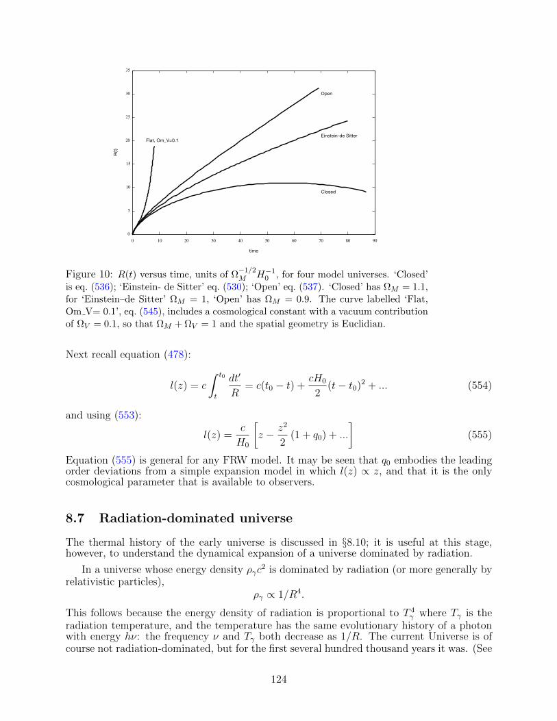
Figure 10: R(t) versus time, units of Ω−1/2M H−10 , for four model universes. ‘Closed’

is eq. (536); ‘Einstein- de Sitter’ eq. (530); ‘Open’ eq. (537). ‘Closed’ has ΩM = 1.1,for ‘Einstein–de Sitter’ ΩM = 1, ‘Open’ has ΩM = 0.9. The curve labelled ‘Flat,Om V= 0.1’, eq. (545), includes a cosmological constant with a vacuum contributionof ΩV = 0.1, so that ΩM + ΩV = 1 and the spatial geometry is Euclidian.

Next recall equation (478):

l(z) = c

∫ t0

t

dt′

R= c(t0 − t) +

cH0

2(t− t0)2 + ... (554)

and using (553):

l(z) =c

H0

[z − z2

2(1 + q0) + ...

](555)

Equation (555) is general for any FRW model. It may be seen that q0 embodies the leadingorder deviations from a simple expansion model in which l(z) ∝ z, and that it is the onlycosmological parameter that is available to observers.

8.7 Radiation-dominated universe

The thermal history of the early universe is discussed in §8.10; it is useful at this stage,however, to understand the dynamical expansion of a universe dominated by radiation.

In a universe whose energy density ργc2 is dominated by radiation (or more generally by

relativistic particles),ργ ∝ 1/R4.

This follows because the energy density of radiation is proportional to T 4γ where Tγ is the

radiation temperature, and the temperature has the same evolutionary history of a photonwith energy hν: the frequency ν and Tγ both decrease as 1/R. The current Universe is ofcourse not radiation-dominated, but for the first several hundred thousand years it was. (See

124

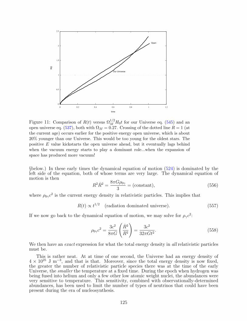
Figure 11: Comparison of R(t) versus Ω1/2M H0t for our Universe eq. (545) and an

open universe eq. (537), both with ΩM = 0.27. Crossing of the dotted line R = 1 (atthe current age) occurs earlier for the positive energy open universe, which is about20% younger than our Universe. This would be too young for the oldest stars. Thepositive E value kickstarts the open universe ahead, but it eventually lags behindwhen the vacuum energy starts to play a dominant role...when the expansion ofspace has produced more vacuum!

§below.) In these early times the dynamical equation of motion (524) is dominated by theleft side of the equation, both of whose terms are very large. The dynamical equation ofmotion is then

R2R2 =8πGρ0γ

3= (constant), (556)

where ρ0γc2 is the current energy density in relativistic particles. This implies that

R(t) ∝ t1/2 (radiation dominated universe). (557)

If we now go back to the dynamical equation of motion, we may solve for ργc2:

ρ0γc2 =

3c2

8πG

(R2

R2

)=

3c2

32πGt2. (558)

We then have an exact expression for what the total energy density in all relativistic particlesmust be.

This is rather neat. At at time of one second, the Universe had an energy density of4 × 1025 J m−3, and that is that. Moreover, since the total energy density is now fixed,the greater the number of relativistic particle species there was at the time of the earlyUniverse, the smaller the temperature at a fixed time. During the epoch when hydrogen wasbeing fused into helium and only a few other low atomic weight nuclei, the abundances werevery sensitive to temperature. This sensitivity, combined with observationally-determinedabundances, has been used to limit the number of types of neutrinos that could have beenpresent during the era of nucleosynthesis.

125

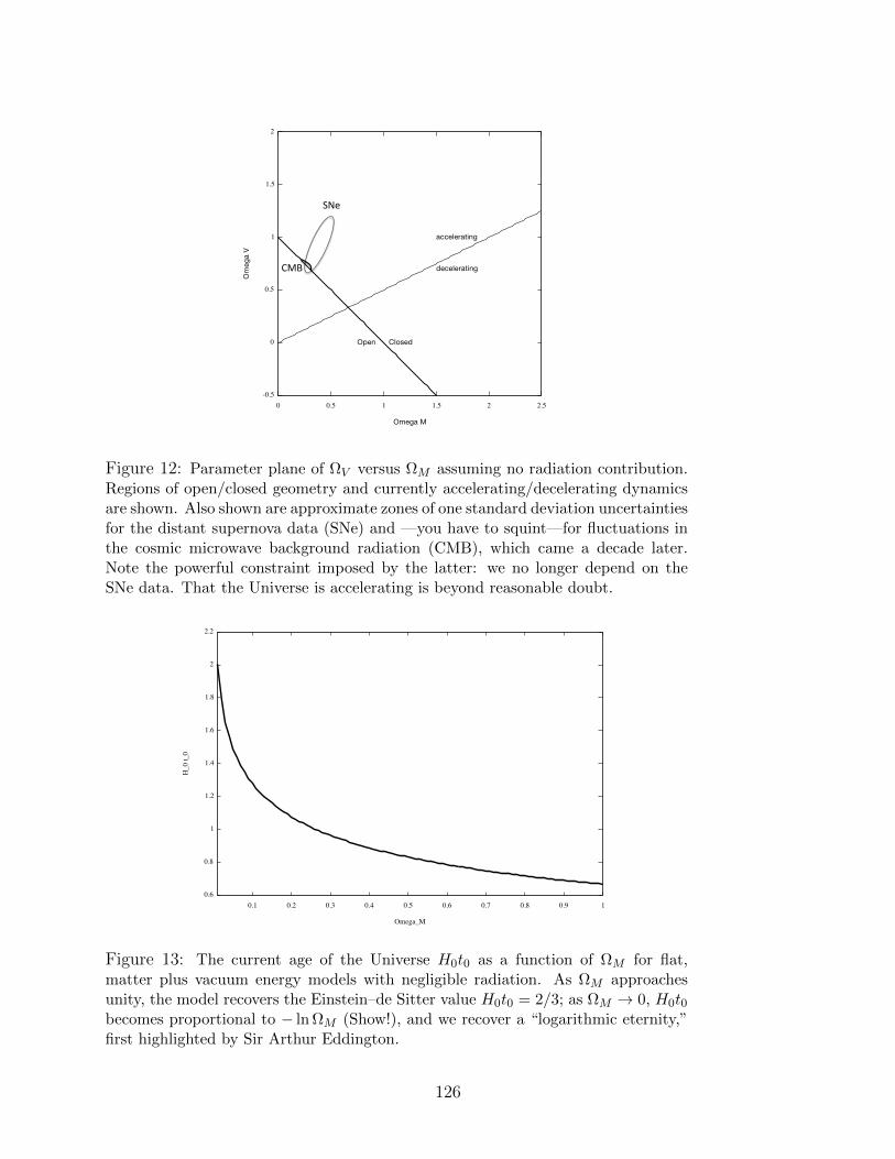
SNe

CMB

Figure 12: Parameter plane of ΩV versus ΩM assuming no radiation contribution.Regions of open/closed geometry and currently accelerating/decelerating dynamicsare shown. Also shown are approximate zones of one standard deviation uncertaintiesfor the distant supernova data (SNe) and —you have to squint—for fluctuations inthe cosmic microwave background radiation (CMB), which came a decade later.Note the powerful constraint imposed by the latter: we no longer depend on theSNe data. That the Universe is accelerating is beyond reasonable doubt.

Figure 13: The current age of the Universe H0t0 as a function of ΩM for flat,matter plus vacuum energy models with negligible radiation. As ΩM approachesunity, the model recovers the Einstein–de Sitter value H0t0 = 2/3; as ΩM → 0, H0t0becomes proportional to − ln ΩM (Show!), and we recover a “logarithmic eternity,”first highlighted by Sir Arthur Eddington.

126

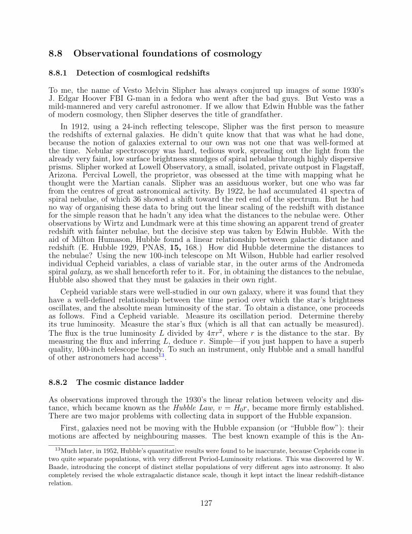
8.8 Observational foundations of cosmology

8.8.1 Detection of cosmlogical redshifts

To me, the name of Vesto Melvin Slipher has always conjured up images of some 1930’sJ. Edgar Hoover FBI G-man in a fedora who went after the bad guys. But Vesto was amild-mannered and very careful astronomer. If we allow that Edwin Hubble was the fatherof modern cosmology, then Slipher deserves the title of grandfather.

In 1912, using a 24-inch reflecting telescope, Slipher was the first person to measurethe redshifts of external galaxies. He didn’t quite know that that was what he had done,because the notion of galaxies external to our own was not one that was well-formed atthe time. Nebular spectroscopy was hard, tedious work, spreading out the light from thealready very faint, low surface brightness smudges of spiral nebulae through highly dispersiveprisms. Slipher worked at Lowell Observatory, a small, isolated, private outpost in Flagstaff,Arizona. Percival Lowell, the proprietor, was obsessed at the time with mapping what hethought were the Martian canals. Slipher was an assiduous worker, but one who was farfrom the centres of great astronomical activity. By 1922, he had accumulated 41 spectra ofspiral nebulae, of which 36 showed a shift toward the red end of the spectrum. But he hadno way of organising these data to bring out the linear scaling of the redshift with distancefor the simple reason that he hadn’t any idea what the distances to the nebulae were. Otherobservations by Wirtz and Lundmark were at this time showing an apparent trend of greaterredshift with fainter nebulae, but the decisive step was taken by Edwin Hubble. With theaid of Milton Humason, Hubble found a linear relationship between galactic distance andredshift (E. Hubble 1929, PNAS, 15, 168.) How did Hubble determine the distances tothe nebulae? Using the new 100-inch telescope on Mt Wilson, Hubble had earlier resolvedindividual Cepheid variables, a class of variable star, in the outer arms of the Andromedaspiral galaxy, as we shall henceforth refer to it. For, in obtaining the distances to the nebulae,Hubble also showed that they must be galaxies in their own right.

Cepheid variable stars were well-studied in our own galaxy, where it was found that theyhave a well-defined relationship between the time period over which the star’s brightnessoscillates, and the absolute mean luminosity of the star. To obtain a distance, one proceedsas follows. Find a Cepheid variable. Measure its oscillation period. Determine therebyits true luminosity. Measure the star’s flux (which is all that can actually be measured).The flux is the true luminosity L divided by 4πr2, where r is the distance to the star. Bymeasuring the flux and inferring L, deduce r. Simple—if you just happen to have a superbquality, 100-inch telescope handy. To such an instrument, only Hubble and a small handfulof other astronomers had access13.

8.8.2 The cosmic distance ladder

As observations improved through the 1930’s the linear relation between velocity and dis-tance, which became known as the Hubble Law, v = H0r, became more firmly established.There are two major problems with collecting data in support of the Hubble expansion.

First, galaxies need not be moving with the Hubble expansion (or “Hubble flow”): theirmotions are affected by neighbouring masses. The best known example of this is the An-

13Much later, in 1952, Hubble’s quantitative results were found to be inaccurate, because Cepheids come intwo quite separate populations, with very different Period-Luminosity relations. This was discovered by W.Baade, introducing the concept of distinct stellar populations of very different ages into astronomy. It alsocompletely revised the whole extragalactic distance scale, though it kept intact the linear redshift-distancerelation.

127

dromeda galaxy, whose is redshift is in fact a blueshift! It is approaching us (the Milky WayGalaxy) at about 300 km per second. This problem is greatest for nearby galaxies whose“peculiar velocity” (deviation from Hubble flow) is a large fraction of its recession velocity.Second, it is very difficult to establish distances to cosmological objects. We can estab-lish distances to relatively nearby objects realtively easily, but these galaxies are preciselythe ones affected by large peculiar velocities. Those galaxies unaffected by large peculiarvelocities are the ones whose distances are difficult to establish!

But observational astronomers are resourceful, and they have come up with a number ofingenious techniques which have served them well. The idea is to create a cosmic “distanceladder” (perhaps better described as a linked chain) in which you start with direct mea-surements on certain objects, and use those measurments to calibrate other objects moredistant. Then repeat. Here is how it works.

Start with our solar system. These days, we can bounce radar singals off planets andmeasure the time of flight (even testing general relativity in the process, as we have seen) toget extremely accurate distances. Next, we make use of our knowledge of the astronomicalunit (AU) thus obtained to use the classic technique of trigonometric parallax. This makesuse of the fact that the earth’s motion around the sun creates a baseline of about 2 AUfrom which we have a different perspective on nearby stars. We see nearby stars shift inangular position on the sky relative to their much more distant counterparts. The angularshift is inversely proportional to the distance from the solar system. We define the unit ofdistance known as a parsec (pc) as the distance that 1 AU would subtend 1 second of arc.We can turn this perspective around and say that the parallax angle, perversely denoted asπ in the astronomical literature and deduced from the shift in a star’s apparent position,corresponds to a distance to the star of 1/π parsecs when π is in arcseconds. (One parsec is' 3.085678× 1016 m. Because 1 AU is a defined exact quantity, so is 1 pc.)

The next rung in the ladder is known as spectroscopic parallax. There is no actualparallax, just an analogue. The idea is that you use the method of trigonometric parallax toobtain distances stars of a given spectral class. For this, you need to know what the stellarspectrum looks like in detail. Detailed agreement between spectra mean the same type ofstar, with the same mass and luminosity. Knowing the distance to a star of a given spectraltype and measuring its flux, you know the intrinsic luminosity L, since F = L/4πr2 where Fis the measured flux and r the measured distance to the star. Then, when you see a similarspectrum in a much more distant star, you know its intrinsic luminosity. You then measureits F , and deduce its distance!

Keep going. Distances to Cepheid variables can be calibrated by spectroscopic parallax,and these bright stars have, as we have seen, a well-defined period-luminosity relationship.They are bright enough that they can be seen indivdually in external galaxies. Measure,thereby, the distances to these external galaxies.

Keep going. In studying the properties of external galaxies, Tully and Fisher showedthat the rotation velocities of spiral galaxies (measured by the Doppler shifts in the movingstellar spectra) was tightly correlated with the intrinsic luminosity of the galaxy. Thisis not terribly surprising in itself: the larger the stellar mass of a galaxy the larger theluminosity and the larger the mass the larger the rotational velocity. Tully and Fisher craftedthis notion into a widely used tool for establishling the distances to very distant galaxies.Elliptical galaxies, which are supported by the dispersion of stellar velocities rather than theirsystematic rotation were also turned into useful distance indicators. Here the correlationbetween luminosity and velocity dispersion is known as the Faber-Jackson relation.

The final step in the cosmic distance ladder involves Type Ia supernovae. Type Ia super-novae are thought to occur when a white dwarf in a tight binary system accretes just enoughmatter from its companion to tip itself over the “Chandrasekhar mass.” (This mass is themaximum possible mass a white dwarf can sustain by electron degeneracy pressure, about

128

1.4 times the mass of the sun.) When this mass is exceeded, the white dwarf implodes, over-whelmed by its now unsupportable self-gravitational attraction. In the process, carbon andoxygen nuclei are converted to 56Ni, triggering a thermonuclear explosion that can be seenquite literally across the Universe. What is nice about type Ia supernovae, from an astro-nomical perspective, is that they always occur in a white dwarf of the same mass. Thereforethere is little variation in the absolute intrinsic luminosity of the supernova explosion. Tothe extent that there is some variation, it is reflected not just in the luminosity, but in therise and decay times of the emission, the “light curve.” The slower the decline, the largerthe luminosity. So you can correct for this. This relation has been well calibrated in manygalaxies with well-determined distances.

The Type Ia supernova data were the first to provide compelling evidence that the Uni-verse was expanding. To understand how this was obtained we need to return to our conceptof flux, F = L/4πr2, and understand how this changes in an expanding, possibly curved,spatial geometry.

8.8.3 The redshift–magnitude relation

The flux that is measured from a source at cosmological distances differs from its simpleL/4πr2 form for several important reasons. It is best to write down the answer, and thenexplain the appearance of each modification. The flux from an object at redshift z is givenby

F(z) =LR2(t)

4πR40l

2(z)=

L

4π(1 + z)2R20l

2(z)(559)

where l(z) is computed, as always, by c∫ tt0dt′/R(t′), with this definite integral written as a

function of z for the cosmological model at hand. (Recall R(t)/R0 = 1/(1 + z), relating t toz.) The luminosity distance is then defined by F(z) = L/4πd2L or

dL(z) = (1 + z)R0l(z), (560)

which reduces to the conventional Euclidian distance at small z.

Explanation: The two factors of 1 + z in the denominator of (559) arise from the changein the luminosity L. First, the photons are emitted with Doppler-shifted energies. But evenif you were measuring only the rate at which the photons were being emitted like bullets,there is an additional second 1 + z factor, quite separate from the first, due to the emissioninterval time dilation. The proper radius of the sphere over which the photons from thedistant source at z are now distributed is R0l(z), where R0 is as usual the current value ofR(t). One is free to use a metric where R0 = 1, but we present the form (559) for completegenerality. For the Einstein-de Sitter universe with R0 = 1,

F(z) =LH2

0

16πc2(1 + z)(√

1 + z − 1)2(Einstein− de Sitter) (561)

The simple Euclidian value of L/4πr2 is recovered at small z by rembering cz = v = H0r,whereas at high z, all the photons come from the current horizon distance 2c/H0, and the1/z2 behaviour in F is due entirely to 1 + z Doppler shifts.

A “magnitude” is an astronomical conventional unit used for, well, rather arcane reasons.It is a logarithmic measure of the flux. Explicitly:

F = F010−0.4m (562)

129

where F is the measured flux, F0 is a constant that changes depending upon what wavelengthrange you’re measuring. m is then defined as the apparent magnitude. (Note: a largermagnitude is fainter. Potentially confusing.) The “bolometric magnitude” covers a widewavelength range and is a measure of the total flux; in that case F0 = 2.52 × 10−8 J m−2.Astronomers plot m versus z for many objects that ideally have the same intrinsic luminosity,like type Ia supernovae. Then they see whether the curve is well fit by a formula like (559)for an FRW model. It was just this kind of exercise that led to the discovery in 1998-9 byPerlumtter , Riess and Schmidt that our Universe must have a large value of ΩV : we live inan accelerating Universe!

Exercise. Show that

F(z) =LH2

0

4πc2z2[1 + (q0 − 1)z + ...]

for any FRW model. Thus, with knowledge of L, observers can read off the value of H0

from the dominant 1/z2 leading order behaviour of the redshift-magnitude data, but thatknowledge of q0 comes only once the leading order behaviour is subtracted off.

With the determination of ΩV , the classical problem of the large scale structure of theUniverse has been solved. There were 6 quantities to be determined:

• The Hubble constant, H0 = R/R at the present epoch.

• The age of the Universe, t0.

• The curvature of the Universe, in essence the integration constant E.

• The ratio Ω0 of the current mass density ρ0 to the critical mass density 3H20/8πG.

• The value of the cosmological constant or equivalently, the ratio ΩV of the vacuumenergy density ρV c

2 to the critical energy density.

• The value of the q0 parameter.

Within the context of FRW models, these parameters are not completely independent,but are related by the dynamical equations for R (512) and R2 (524). A quick summary:

• H0 ' 67 km s−1 Mpc−1.

• t0 ' 13.7 billion years

• E ' 0

• Ω0 ' 0.27

• ΩV ' 0.73.

• q0 = Ω0/2− ΩV ' −0.6

Exercise. Derive the last result on this list.

This brief list of values hardly does justice to the century-long effort to describe our Uni-verse with precision. Because astronomers were forced to use galaxies as “standard candles”(the colloquial term for calibrated luminosity sources), their measuring tools were fraughtwith uncertainties that never could be fully compensated for. It was only the combination

130

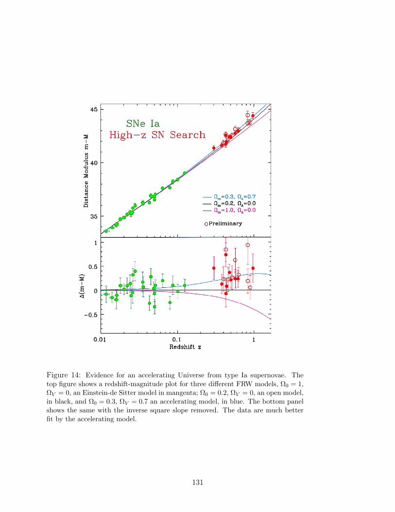
Figure 14: Evidence for an accelerating Universe from type Ia supernovae. Thetop figure shows a redshift-magnitude plot for three different FRW models, Ω0 = 1,ΩV = 0, an Einstein-de Sitter model in mangenta; Ω0 = 0.2, ΩV = 0, an open model,in black, and Ω0 = 0.3, ΩV = 0.7 an accelerating model, in blue. The bottom panelshows the same with the inverse square slope removed. The data are much betterfit by the accelerating model.

131

of establishing a truly standard candle via the type Ia supernovae, together the tehcnicalcapability of high receiver sensitivity and automated searches that allowed the programme(“The Supervova Cosmology Project”) to succeed.

Since the 1998/9 breakthrough, cosmologists have not been idle. The development ofextremely sensitive receivers and sophisticated modelling and simulation techniques haveturned the remnant radiation from the big bang itself into a vast treasure trove of information.In particular, the nature of the tiny fluctuations that are present in the radiation intensity—more specifically the radiation temperature—allow one to set very tight constraints on thethe large scale parameters of our Universe. Not only are these measurements completelyconsistent with the supernova data, the results of the missions known as WMAP and Planckrender them all but obsolete. Figure (12) speaks for itself.

8.9 The growth of density perturbations in an expanding universe

The Universe is expanding and the density of nonrelativistic matter decreasing as 1/R3.In such a background, as the raw material to form condensed objects is diminishing doquickly, does gravity even allow the sort of runaway collapse we think of when we envisiona star or a galaxy forming? Determining the fate of a small overdensity or underdensity ofnonrelativistic matter in an FRW universe is a problem that can be approached via (a nottoo difficult) analysis.

We require two equations. The first expresses the conservation of ordinary matter. Themass within a volume V ,

∫Vρ dV is changed only if matter flows in or out from the boundaries

of V . The flux of mass (mass per kg per square meter) is ρv. Hence

d

dt

∫V

ρ dV =

∫V

∂ρ

∂tdV = −

∫∂V

ρv · dA = −∫V

∇·(ρv) dV

where ∂V is the volume’s boundary and we have used the divergence. The volume V isarbitrary, so we much have

∂ρ

∂t+∇·(ρv) = 0 (563)

which is the equation of mass conservation. Newton’s equation of motion states that if a masselement of fluid ρdV is accelerating, then it is acted on by a gravitational force −ρdV∇Φ,where Φ is the associated potential function. In other words, the force equation reads aftercancellation of ρdV , [

∂

∂t+ (v · ∇)

]v = −∇Φ (564)

Note that the acceleration measured relative to a space-time coordinate background meansthat the “total time derivative” must be used, ∂t + vi∂i in index notation.

The local behaviour of the density is entirely Newtonian. The expansion of the universeis described by

v =R

Rr (565)

a familiar Hubble law. The mass equation then becomes

∂ρ

∂t+

1

r2∂

∂r

(r3ρ

R

R

)= 0 (566)

132

With the background ρ independent of position,

d ln ρ

dt+

3R

R= 0 (567)

whence ρR3 is a constant, as we know. As for the force equation, a straightforward calculationyields

∂v

∂t+ (v · ∇)v =

R

Rr (568)

and, as the discussion of §8.1.1 shows that R/R = −4πGρ/3, our solution for the backgroundexpansion is correct. The Poisson equation

∇2Φ = 4πGρ (569)

is likewise solved by our solution. (Try Φ = 2πGρr2/3).

We are interested in the behaviour of small disturbances δρ, δv and δΦ on top of thisbackground:

ρ→ ρ+ δρ, v → v + δv, Φ→ Φ + δΦ (570)

We replace our dynamical variables as shown, and because the δ-quantities are small, weretain them only through linear order, ignoring quadratic and higher order tems. The massequation is

∂δρ

∂t+∇·(ρδv) +∇·(vδρ) = 0 (571)

Noting that the gradient of ρ vanishes and that the equilibrium v satisfies∇·v = −∂t ln ρ, itis straightforward to show that the perturbed linearised mass conservation equation simplifiesto [

∂

∂t+ (v · ∇)

]δρ

ρ+∇·δv = 0 (572)

The linearised equation of motion[∂

∂t+ v · ∇

]δv + (δv · ∇)v = −∇δΦ (573)

becomes [∂

∂t+ v · ∇

]δv +

R

Rδv = −∇δΦ (574)

Now change to comoving coordinates. This is a simple task. Let r = R(t′)r′ and t = t′.Then r′ (or x′i in index notation) is a comoving spatial coordinate. The partial derivativetransformation is (sum over repeated i):

∂

∂t=∂

∂t′+∂x′i∂t

∂

∂x′i, ∇ =

1

R∇′, ∂x′i

∂t= − xi

R2R = −vi

R, (575)

so that∂

∂t+ (v · ∇) =

∂

∂t′, (576)

133

which is a time derivative following a fluid element of the unperturbed expansion. Then, ourtwo equations for mass conservation and dynamics are

∂

∂t′δρ

ρ+

1

R∇′·δv = 0 (577)

∂δv

∂t′+R

Rδv = − 1

R∇′δΦ (578)

Taking ∇′· of (578) and using (577) leads to

∂2

∂t′2δρ

ρ+

2R

R

∂

∂t′δρ

ρ=

1

R2∇′2δΦ = 4πGρ

(δρ

ρ

)(579)

where the last equality is the linearised Poisson equation ∇2δφ = 4πGδρ. For an Einstein-deSitter univese, recall that ρ = 1/6πGt2 and R/R = 2/3t, where we have dropped the primes.

Using the notation δ = δρ/ρ and a dot δ for a time derivative, our differential equation forthe growth of small perturbations in an Einstein de-Sitter universe takes on a very elegantform:

δ +4

3tδ − 2

3t2δ = 0 (580)

This differential equation has two very simple linearly independent solutions, one where δdecays as 1/t, the other where it grows as t2/3. (Show!) The important point is that itdisplays none of the explosive exponential growth typical of fluid instabilities in a staticbackground. The growing solution of the small perturbation is t2/3, growing no faster thanthe universe expands. This is a pretty torpid tempo. For the musically inclined, think ofsomething between larghissimo and adagio.

How our Universe grew both its large and small scale structures has long been a greatmystery, one that is remains far from understood. To make things grow in the barren soil ofthe Universe, you need to start out with very healthy-sized seeds. The questions of wherethose might come from and whether we can see their imprints in the cosmic backgroundradiation are the topics of the next section.

8.10 The Cosmic Microwave Background Radiation

8.10.1 Prologue

The Universe is expanding, and expanding systems cools adiabatically. That means if wefollow history backwards, the Universe was once extremely hot and dense. The frequency νof a photon scales as 1/R and the energy density as 1/R4 because the radiation temperatureTγ is an average of ν. The energy density of matter (dominated by rest mass) scales as 1/R3,so going back in time, the Universe must at some point have become radiation dominated.We will see that this occurred at a redshift of about 1000.

At redshifts larger than 1000, not only was radiation dominant, it was also well-coupledto matter and thus in a state of complete thermodynamic equilibrium: the radiation set thematter temperature. In thermodynamic equilibrium, the number density of photons is givenby the Planck function associated with a blackbody spectrum:

n(ν, T ) dν =(8πν2/c3)dν

exp(hν/kTγ)− 1(581)

134

At about the same epoch that the radiation became subdominant, it also lost couplingwith the matter and therefore was no longer maintained in themal equilibrium via collisions.Imagine an extreme, but realistic, situation in which the photons evolve with the expansion ofthe Universe and but are otherwise untouched. You might expect the shape of the spectrumto be maintained, but that the number density would perhaps be diluted below that of a trueblackbody (e.g. sunlight on earth). In fact, the number density and effective temperatureof the photons vary in exactly the right way to maintain a true blackbody distribution. Thedecreased number density is exactly correct for the cooling temperature.

To see this, start with the spectrum (581) at the time of “last scattering” at time t,which is the last moment of maintained thermal equilbrium, and let the group of photonswith frequency ν and disperson dν evolve with the Universe till time t′. The first thing tonote is that is the t′ number density n(ν ′, t′, T ′) is diluted by an overall normalisaton factor ofR3(t)/R3(t′) from the original time t blackbody. In addition, each t′ photon that we observeat frequency ν ′ must have come from a t frequency ν = R′/Rν ′ (R′ ≡ R(t′)), in the originalblackbody distribution. So, to get the more recent time t′ spectrum, simply take the originaltime t blackbody distribution, dilute it by R3/R′3, and replace ν everywhere in the formulaby R′ν ′/R:

n(ν ′, t′, T ′)dν ′ =R3

R′3(8π/c3)(R′ν ′/R)2d(ν ′R′/R)

exp(hR′ν ′/RkTγ)− 1=

8πν ′2 dν ′/c3

exp(hν ′/kT ′γ)− 1(582)

where T ′γ = TγR/R′, a cooler temperature. The point is that the distribution (582) is still

a blackbody at time t′, but with a new temperature T ′γ that has cooled in proportion to1/R with the expansion. This is remarkable because there is nothing maintaining thermalequilibrium. This scaling result follows mathematically for any number spectrum of theform ν2F (νp/T ) dν, where F is an arbitrary function and p is a real number. There is noreason why, as a matter of principle, the orginal photon spectrum has to be maintained as ablackbody, if other interaction physics takes place. For years there were arguments whetherthe spectrum was a true blackbody. These were based on observational results from rocket-borne instrumentation that were later retracted. (It turns out that rocket exhaust is nothelpful when hyper-accurate infrared sky measurements are required.) Moreover, as a matterof sensible physics, to change the radiation spectrum of the Universe takes a vast amountof energy! All doubts were erased in 1992 when the COBE (COsmic Background Explorer)satellite as launched. This satellite had sub mm detectors of unprecedented accuracy, showingthat the backgound radiation was an almost perfect blackbody at Tγ = 2.728K. Figure (15)summarises the data. The error bars are shown at 400 times their actual value, just in orderto be visible!

The photon distribution is not, however, absolutely exactly a blackbody, for two veryinteresting reasons. The first is that the earth is not at rest relative to the CMB frame.Why should it be? In fact the local group of galaxies seems to be moving at about 630 kms−1 relative to the CMG, a surprisingly large value. This corresponds to a measured radiationtemperature that is about 2 × 10−3K warmer in one direction and the same amount coolerin the oppostion direction.

The second reason is that matter has collapsed out of the expanding background, form-ing galaxies, stars, and great clusters. The seed for these structures could not have formedrecently; there isn’t enough time for them to have grown. They must have been presentduring the era when the Universe was radiation-dominated, and matter and radiation inter-acted strongly. This interaction would have left its imprint at the time of last scattering inthe form of fluctuations of the microwave background temperature. The relative fluctuation∆T/T would have had to have be, it would seem, at least ∼ 10−3 in order to be able to formnonlinear structures by the current epoch. Why? Because ∆Tγ/Tγ and ∆ρ/ρ in matter arecomparable and ∆ρ/ρ grows about in proportion to t2/3, the Einstein-de Sitter value, and

135

this means it is proportional to the scale factor R. R has grown be about a factor of 1500since the time of last scattering, whence ∆Tγ/Tγ ∼ 10−3.

The search for these fluctuations proved frustrating. There were no temperature fluctu-ations found at this level for many years. When COBE and later satellites did find them,starting in the early 1990’s, they were an order of magnitude smaller. So how does structureform in the Universe? The answer is that there is more to matter than the usual baryonswe know and love. The Universe is pervaded by what is known as “dark matter,” and thisleaves no imprint on the microwave background. More on the importance of dark matterlater.

8.10.2 An observable cosmic radiation signature: the Gamow argument

The idea that the Universe had a residual radiation field left over from its formation, and thatthis radiation is potentially observable, seems to have originated with George Gamow in the1940’s. Gamow was theoretical physicist with a brilliant common sense instinct that allowedhim to make contributions to a wide variety of problems, from the theory of radioactivity toDNA coding. He spent many years developing what became known as the Big Bang theory.

Gamow pointed out that Helium is about 25% of the Universe by mass. That is neitheroverwhelming nor negligible. It implies that at the time of nucelosynthesis—and Gamow wasconvinced that most of the Helium was made this way in the early Universe—the expansionrate and the nuclear reaction rate were comparable. Too rapid an expansion, no Helium.Too slow an expansion rate, all the protons get fused into Helium, and there is nothing leftover to make physcists. This turns out to be a remarkably constraining observation, leadingto a prediction that there should be a residual radiation field of about 10 K. Let’s see howit works.

At some point, the Universe passes downward through the temperature range of ∼ 109

K. When that happens, neutrons n and protons p can combine to form Deuterium nuclei.The reaction is

n+ p→ D + γ

where γ is a gamma ray. Helium synthesis then follows rapidly. Gamow took equal numbersof protons, neutrons and electrons. In order to get a 25% yield of Helium, the reaction rateand the age of the Universe (of order the expansion time) should be comparable. If the crosssection for Deuterium formation is σ (units of area), then the reaction rate per proton dueto an incoming flux nv of neutrons is nvσ (number per unit area per unit time). At time t,on average about one reaction per proton should have occured, because of the order unityfraction of Helium—that is the heart of the Gamow argument:

nvσt ∼ 1 (583)

The product σv is nearly independent of v (because the cross section σ depends on v) and,as Gamow knew from nuclear experiments, about 4.6× 10−26 m3 s−1. As for the time t, weare interested in the epoch when the temperature Tγ ∼ 109K. Using equation (558) for thedensity in relativistic particles, and following Gamow by assuming (not quite correctly, butlet it go) that this was all radiation, the time t is

t =c

T 2γ

(3

32πGa

)1/2

(584)

which amounts to 230 s for Tγ = 109K. This give n very close to 1023 m−3. Gamow estimateda present day average particle density of about 0.1 per cubic meter based on astronomical

136

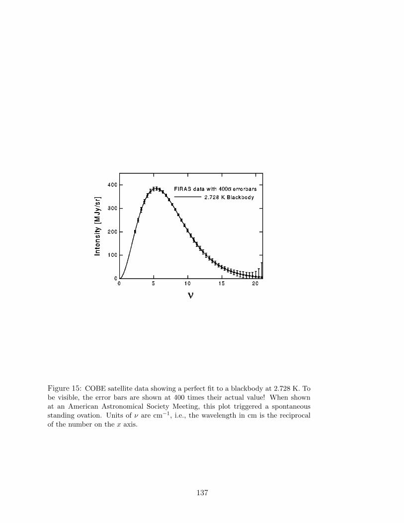
Figure 15: COBE satellite data showing a perfect fit to a blackbody at 2.728 K. Tobe visible, the error bars are shown at 400 times their actual value! When shownat an American Astronomical Society Meeting, this plot triggered a spontaneousstanding ovation. Units of ν are cm−1, i.e., the wavelength in cm is the reciprocalof the number on the x axis.

137

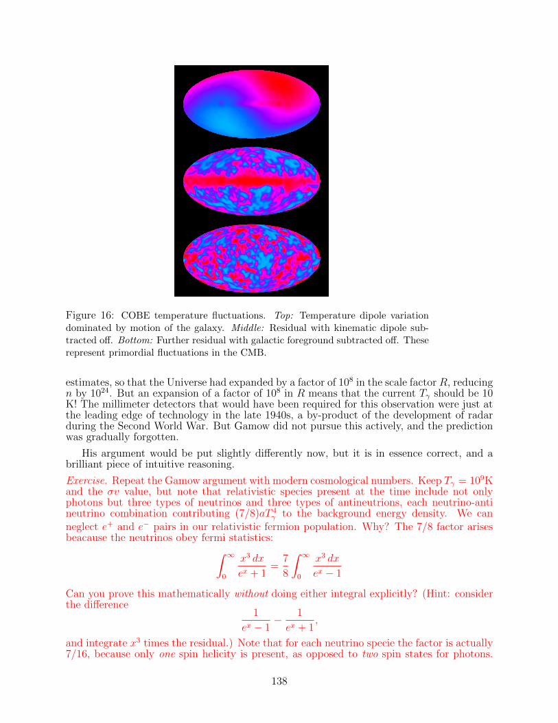
Figure 16: COBE temperature fluctuations. Top: Temperature dipole variationdominated by motion of the galaxy. Middle: Residual with kinematic dipole sub-tracted off. Bottom: Further residual with galactic foreground subtracted off. Theserepresent primordial fluctuations in the CMB.

estimates, so that the Universe had expanded by a factor of 108 in the scale factor R, reducingn by 1024. But an expansion of a factor of 108 in R means that the current Tγ should be 10K! The millimeter detectors that would have been required for this observation were just atthe leading edge of technology in the late 1940s, a by-product of the development of radarduring the Second World War. But Gamow did not pursue this actively, and the predictionwas gradually forgotten.

His argument would be put slightly differently now, but it is in essence correct, and abrilliant piece of intuitive reasoning.

Exercise. Repeat the Gamow argument with modern cosmological numbers. Keep Tγ = 109Kand the σv value, but note that relativistic species present at the time include not onlyphotons but three types of neutrinos and three types of antineutrions, each neutrino-antineutrino combination contributing (7/8)aT 4

γ to the background energy density. We canneglect e+ and e− pairs in our relativistic fermion population. Why? The 7/8 factor arisesbeacause the neutrinos obey fermi statistics:∫ ∞

0

x3 dx

ex + 1=

7

8

∫ ∞0

x3 dx

ex − 1

Can you prove this mathematically without doing either integral explicitly? (Hint: considerthe difference

1

ex − 1− 1

ex + 1,

and integrate x3 times the residual.) Note that for each neutrino specie the factor is actually7/16, because only one spin helicity is present, as opposed to two spin states for photons.

138

The neutrinos get back up to 7/8 with their antiparticles, which photons lack.) Take thecurrent density to be 5% of the critical density 3H2

0/8πG.

In 1965, the problem of determining Tγ0 attracted the attention of an able team ofphysicists at Princeton University. They rediscovered for themselves the Gamow argument.The senior investigator, Robert Dicke, a hugely talented physicist (both theoretical andexperimental), realised that there was likely to be a background radiation field that survivedto the present day. Moreover, it could be detected by an instrument, the Dicke radiometer,that he himself had invented twenty years before! (A Dicke radiometer is a device thatswitches 100 times per second between looking at the sky source and a calibrated thermalheat bath of liquid helium. This imparts a 100Hz fourier component to the desired signaland eliminates extraneous variability occuring on longer time scales.)

The A-Team assembled: Dicke, the scientific leader; J. Peebles, the brilliant young the-orist who would become the world’s leading cosmologist in the decades ahead, and P. Rolland D. Wilkinson, superb craftsmen who designed and built the contemporary Dicke ra-diometer. The were all set up to do the observation from the roof of their Princeton officebuliding, when a phone call came from nearby Bell Laboratories. Two radio engineers namedArno Penzias and Robert Wilson had found a nuisance extraneous signal in their detector,an instrument designed to receive signals relayed by some of the first commercial televisionsatellites. (The Telstar series.) They were trying to chase down all sources of backgoundconfusion. The “effective radiation temperature” of the unwanted diffuse signal was about3 K. Penzias and Wilson had no idea what to make of it, but were advised by a colleague togive the Dicke team at Princeton a call. Those guys are very clever you know, they mightjust be able to help.

The 1978 Nobel Prize in Physics went to Penzias and Wilson for the discovery of thecosmic microwave background radiation.

8.10.3 The cosmic microwave background (CMB): subsequent developments

The initial observations of the CMB were at one wavelength: 7 cm. Needless to say, asingle point does not establish a blackbody spectrum. The task of establishing the broaderspectrum was fraught with difficulties, with many disputed and ultimately withdrawn claimsof large deviations from a blackbody. In 1992 matters were finally laid to rest when the COBEsatellite returned its dramatically undramatic finding that the CMB is, very very nearly, butnot exactly, a blackbody. There are in fact small fluctuations in the temperature, the largestof which amount to a few parts in 104. This value, it turns out, is just of the order neededto account for the nonlinear structure in the Universe that we see today, provided that thereis a healthy component of dark matter that does not react with the radiation. This unseen,and unseeable, dark matter component had been invoked long before the COBE results toaccount for the large internal velocities measured in galaxies and within clusters of galaxies.These velocities are not maintainable without most of the mass of the galaxy (or cluster)being in the form of dark, non light-emitting or scattering, matter. Now the COBE resultsbecame another indication of the presence of dark matter in the Universe.

The next important result was the Wilkinson Microwave Anisotropy Probe, or WMAP.This is named for David Wilkinson, the Princeton Researcher who was instrumental inthe earliest CMB studies. With the launch of WMAP in 2003, cosmology truly became aprecision science. WMAP revealed the structure of the tmeperature fluctuations in suchexquisite detail in angular resolution on the sky, it became possible to determine the keyphysical parameters of the Universe: H0, Ω0, ΩV , t0 and many others, to several significantfigure accuracy. The Planck satellite was launched in 2009 and provided a further shrinkingof the error bars, higher angular resolution coverage of the CMB on the sky, better frequency

139

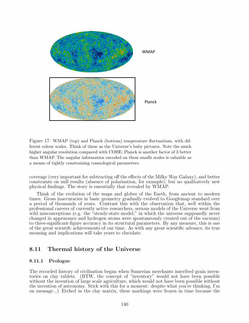
WMAP

Planck

Figure 17: WMAP (top) and Planck (bottom) temperature fluctuations, with dif-ferent colour scales. Think of these as the Universe’s baby pictures. Note the muchhigher angular resolution compared with COBE; Planck is another factor of 3 betterthan WMAP. The angular information encoded on these smalle scales is valuable asa means of tightly constraining cosmological parameters.

coverage (very important for subtracting off the effects of the Milky Way Galaxy), and betterconstraints on null results (absence of polarisation, for example), but no qualitatively newphysical findings. The story is essentially that revealed by WMAP.

Think of the evolution of the maps and globes of the Earth, from ancient to moderntimes. Gross inaccuracies in basic geometry gradually evolved to Googlemap standard overa period of thousands of years. Contrast this with the observation that, well within theprofessional careers of currently active researchers, serious models of the Universe went fromwild misconceptions (e.g. the “steady-state model,” in which the universe supposedly neverchanged in appearance and hydrogen atoms were spontaneously created out of the vacuum)to three-significant-figure accuracy in its structural parameters. By any measure, this is oneof the great scientifc achievements of our time. As with any great scientific advance, its truemeaning and implications will take years to elucidate.

8.11 Thermal history of the Universe

8.11.1 Prologue

The recorded history of civilisation began when Sumerian merchants inscribed grain inven-tories on clay tablets. (BTW, the concept of “inventory” would not have been possiblewithout the invention of large scale agriculture, which would not have been possible withoutthe invention of astronomy. Stick with this for a moment: despite what you’re thinking, I’mon message...) Etched in the clay matrix, these markings were frozen in time because the

140

background clay matrix, once dried, remained unaltered and intact. It turns out that theUniverse has its own gigantic clay tablet, which allowed “inscriptions” first to be imprinted,then to be preserved, effectively unaltered for 13.7 billion years. We know the inscriptionsas temperature fluctuations, and the clay tablet as the cosmic microwave background.

The temperature fluctuations are a tracer of the initial density fluctuations, which coupledto the radiation by electron scattering. (Also known as Thompson scattering.) While thiscoupling remained strong, the CMB dutifully recorded and re-recorded the evolving changesin the density. Then, when matter and radiation became decoupled, the pattern imprintedon the CMB abruptly stopped being recorded. The CMB instead retained only the patternimprinted on it at the time of the “last scattering.” It is this pattern that we receive,redshifted by the expansion of the Universe, in our detectors today. Think of this eitheras an ancient inscription passed on through the eons, or more congenially as the Universe’sbaby picture.

Exercise. Let σT be the Thompson cross section for a photon to collide with an electron,a constant number equal to 6.7 × 10−29 m2. When an electron has moved relative to thephoton gas a distance l such that the swept-out volume lσT captures a single photon, l issaid to be one mean free path (mfp): the average distance between scatterings.

Justify this definition, and show that the scattering rate per electron is nγcσ = c/l. (Andwhat is nγ here?) In a radiation-dominated Universe, show that the ratio of the photon

scattering mfp to the horizon size grows like√t; and the mfp relative to the scale factor R

grows like t. (t as usual is time.)

Exactly how to decipher the CMB inscriptions and turn them into a model of the Universeis a very complicated business, one that we will only be able to treat very superficially inthis course. We will go about this in two steps. In the first, we will describe what I willcall the “classical theory” of the thermal history of the Universe: how matter and radiationbehaved in each other’s presence from temperatures of 1012 K through 3000K, the time ofrecombination. In the second step, we will discuss the “modern theory” of the very earlyUniverse. This puts a premium on the notion of inflation, a period in the history of theUniverse in which it seems to have undergone a rapid exponential growth phase. Firstput forth in 1980, this idea has been the most important theoretical advance in moderncosmology in recent decades. There are very good theoretical reasons for invoking the processof inflation, even if the mechanism is not well-understood (not an unusual state of affairs inscience), for there is by now very good observational evidence for it. To my mind, the bestevidence there is for inflation is that we have in fact entered another inflationary stage ofthe Universe’s history. Inflation is real, full stop.

In what follows, we will have reason to consider physics on what is known as the “Planckscale.” These are fundamental values set by the three fundamental dimensional constantsNewton’s G, Planck’s h, and the speed of light c. There are unique dimensional combinationsto form a mass mP , a length lP and a time tP from these constants:

mP =

(hc

G

)1/2

= 5.456× 10−8 kg (585)

lP =

(hG

c3

)1/2

= 4.051× 10−35 m (586)

tP = lP/c =

(hG

c5

)1/2

= 1.351× 10−43 s (587)

These are, in some sense, the limits of our knowledge. It is on these scales that we mayexpect quantum gravity effects to be important, and on which we remain quite ignorant. We

141

cannot expect to have anything like a classical picture of the early Universe for time t < tP ,or horizon scales c/H < lP . The Planck mass may not, at first glance, appear remarkable,but remember the comparison is with elementary particle masses. A proton is close to 1GeV in rest energy; mP c

2 = 3.06× 1019 GeV.

8.11.2 Helium nucleosynthesis

Let us begin the story when the temperature of the Universe is just under 1012K. This isvery early on, about 10−4s after the big bang. In the next section we will go even before thisinterval, but this is a good place to begin for now. At this stage, the Universe consists of arelativistic cocktail of photons, neutrinos and their antiparticles, muons and their antipart-ciles and electrons and their antiparticles (positrons). This cocktail is well-mixed (shaken,not stirred) with all particles, even the neutrinos, in complete thermal equilibrium, freelycreated and destroyed.14 There is also a population of protons and neutrons, energeticallyunimportant at these temperatures. But keep track of them! They are going to make theUniverse we know and love, including us.

Once the temperature slips below 1012 K, the muons and antimuons annihilate, butwithout being able to maintain their populations from production by the other relativisticpopulations present. The energy from the photons and e+e− pairs produced in the annhi-lation are equilibrated amongst these populations, and everyone is heated, including theneutrinos.

The Universe continues to expand, the temperature falls. Now, neutrons and protons donot have the same mass. More precisely, with mp the proton mass and mn the neutron mass,

∆mc2 ≡ (mn −mp)c2 = 1.293 MeV = 2.072× 10−13 J. (588)

This is very small compared with either mnc2 or mpc

2. Except when we are specificallyconcerned with the mass difference or doing very accurate calculations, there is no needto distinguish mn for mp. Textbooks on statistical mechanics tells us that the ratio of theprobabilities for finding a system in state i or state j depends only on the energies Ei andEj of the states, and nothing else. In particular, the ratio of the probability of finding thesystem in i to the probability of finding it in j is given by the Boltzmann equation:

PiPj

=gigj

exp

[−(Ei − EjkT

)](589)

where the g’s are the statistical weights, basically how many distinct states there are withenergy Ei or Ej. (If you’ve forgotten this and don’t have a statistical mechanics textbookhandy, see the Exercise below for a quick justification.) Once we fall below 1011K, theso-called Boltzmann factor exp(−∆mc2/kT ) starts to differ noticeably from unity, and aswe approach 1010 it becomes small. Since neutrons are more massive than nprotons, theybecome more scarce at cooler temperatures. The temperature corresponding to kT = ∆mc2

is 1.5× 1010K. (By way of comparison, for electrons and positrons, mec2/k = 5.9× 109K.)

Exercise. Let the probability of finding a system in state i be f(Ei), where Ei is the energyof the state. The ratio of the probability of finding the system in state i versus j is thenf(Ei)/f(Ej). But this ratio must be a function only of the difference of the energies, becausea constant additive constant in energy can’t affect the physics! The potential energy is always

14By using the word “freely,” we ignore the electron and neutrino rest masses.

142

defined only up to such a constant. Hence

f(Ei)

f(Ej)= F (Ei − Ej)

If Ei = Ej + δ, show that if this equation is to hold even to first order in δ, that

f(E) ∝ exp(−βE)

where β is an as yet undetermined constant. We can determine β by physics, e.g. bydemanding that the ideal gas equation of state be satisfed, pressure P equals nkT , wheren is the number density and k is the Boltzmann constant and T the temperature. Then itfollows (show!) β = 1/kT .

The reactions that determine the neutron n proton p balance are

n+ ν ↔ p+ e

n+ e+ ↔ p+ ν

n↔ p+ e+ ν

The reaction rates for the two body processes are about 0.1 per second per nucleon atT = 1010K. However, the rate drops rapidly as the thermometer falls. Below 1010K, thereactions can’t keep up with the expansion rate of the Universe. When this occurs, whateverthe ratio of n/p is, it remains “frozen” with time, as the Universe is too cold to keep thereactions cooking! At T = 1010K, the Universe is about 1 s old. The n/p ratio at thistemperature is exp(−∆mc2/kT ) ' 0.2, and is frozen in.

Exercise. Show that the early Universe “temperature clock” is given conveniently by

t ' 1/T 210,

where t is the time in seconds and T10 the temperature in 1010K. Assume a Universe ofphotons, electrons and positrons, and three neutrinos and anti-neutrinos.

This figure of 20% is interesting, because it is neither close to unity nor tiny. Withoutfurther production of neutrons, they will decay in minutes by the third reaction channel.If all the neutrons had decayed into protons and electrons and antineutrinos, there wouldhave been no cosmological nucleosynthesis. But just as the neutrons start to slip away aswe approach 109K, the remaining neutrons are rescued from decay by being packed intostable 4He nuclei. The helium nuclei are perfectly safe radioactive containment vehicles.Here neutron decay is absolutely forbidden, in essence because the statistical phase spacewithin the nuclear potential is degenerate. When the neutrons are confined to the nuclearpotential, there are simply no available states to decay into. They are occupied by protons.It is rather like trying to use Oxford public transportation on a rainy day: SORRY, BUSFULL.

Back to our story. The neutrons are now scarfed up into He nuclei. This results in a firmprediction for the observed mass fraction of the Universe, since stellar nucleosynthesis doesnot change the number significantly. (By contrast, almost all of the much smaller heavierelement abundances are dominated by stellar nucelosynthesis.) From what we have just seen,the mass fraction in helium will be

4mp × (n/2)

mp(n+ p)=

2

1 + p/n' 0.33 (590)

143

Much more detailed, time-dependent calculations (pioneered by Peebles in 1965) give anumber close to 0.27, but the essential physis is captured by our very simple estimate.There is not very much wiggle room here. We cannot use the precise value of this number,say, to determine retrospectively what sort of Universe we must live in; it is essnetially thesame for any FRW model. The Big Bang Theory predicts 27% of the mass of the Universeis in the form of helium. And that, happily, turns out to be very close to what observationsreveal.

8.11.3 Neutrino and photon temperatures

As the temperature slides from 5×109 K to below 109, the electron positron pairs annihilateinto photons,

e+e− → 2γ

but because the temperature falls, the photons do not maintain an equilibrium populationof these e+e− pairs. In other words, there is a conversion of electrons and positrons intophotons. But in thermal equilibrium, the number of photons at a given temperature is fixed.If you add more of them via e+e− annihilation, the extra photons force a new equilibrium, oneat a higher temperature compatible with the increased photon number. The photons are, ineffect, heated. By contrast, the relativistic neutrinos that are present march blithely along,enjoying the expansion of the Universe without a care. They don’t care about anybody. Thismeans that they are cooler than the photons! The question is, by how much?

This turns out to be a relatively simple problem, because if we fix our attention on acomoving volume of the Universe, the entropy in this volume is conserved by the conversionof electron-positron pairs into photons. For photons or relativistic electrons/positrons, theentropy per unit volume is a function only of the temperature. It is most easily calculatedfrom a standard thermodynamic identity,

E + PV − TS +µN = 0,

for a gas with zero chemical potential µ. The latter is true of a relativistic gas that freelycreates and annihilates its own particles. So for the entropy per unit volume s,

s ≡ S

V=

E

V T+P

T(591)

With ρc2 denoting the energy per unit volume and P = ρc2/3 for a relativistic gas,

s =4ρc2

3T(592)

With a relativistic energy density always proportional to T 4, the entropy per unit volumeis proportional to T 3, and the entropy in a comoving volume R3 is proportional to (TR)3.It is conserved with the expansion, in essence because the entropy and particle number areproportional to one another, and particle number is conserved.

Before the e+e− annihilation, the entropy in volumeR3 in photons, electrons and positronsis

sR3 =4a(TR)3

3

(1 + 2× 7

8

)=

11a(TR)3before3

(593)

Afterwards, and after the reestablishment of thermal equilibrium, it is all photons:

sR3 =4a(TR)3after

3(594)

144

This entire process conserves entropy sR3: it conserves the total particles in photons pluse+e− pairs. It is therefore reversible: recompress the adiabatic expansion backwards toproduce the pairs. In other words,

4(TR)3after3

=11(TR)3before

3(595)

Now for an interesting point of physics. Whereas the muon-antimuon annihilation heated allrelativistic populations, because the cross sections permitted this at this earlier time whenthe Universe was much more dense, the e+e− population annihilation ignores the neutrinos.The density has now fallen to a level that the neutrinos pass through everything, so their TRdoes not increase. The electron-positron pair annihilation must therefore produce differentcosmic background photon and neutrino temperatures. The ratio of neutrino temperatureTν to photon temperature Tγ is

TνTγ

=

(4

11

)1/3

= 0.7138 (596)

This would correspond to a current value of Tν = 1.95 K — if the neutrinos remained aµ = 0 relativistic population for all time. Which we now know they did not. At one time,people wondered whether there was any possible way to measure this. But a temperature of1.95K corresponds to an energy kT of 1.7× 10−4 eV, whereas the average mass per neutrinospecie (the best we can measure at the current time) is about 0.1 eV, with a correspondingtemperature of 1160 K. Neutrinos thus became “cold” at a redshift of z ∼ 400. As we shallsee, this is well after hydrogen recombined, but probably before galaxies formed. Theseneutrinos are a part, but only a very small part, of the dark matter in galaxies. Even if ithad turned out that neutrinos had zero rest mass, it would have been impossible with presenttechnology to measure a 2K neutrino background! The physics of this problem remains isenlightening, and the formal difference in neutrino and photon temperatures surprising. Itmerits discussion.

8.11.4 Ionisation of Hydrogen

Between a few hundred seconds, the time of helium synthesis, and a few hundred thousandyears, almost nothing happens to change the character of the Universe. Radiation remainsthe dominant source of energy and pressure, and the Universe simply expands with R scalinglike t1/2. The matter and the radiation remain tightly coupled, so that density fluctuationsin the matter correspond also energy fluctuations in the radiation. But at some point, theUniverse cools enough that hydrogen recombines and the matter is no longer an ionsedplasma, but a neutral gas. At what temperature does this occur? To answer this question,we need to use an interesting sort of variation of the Boltzmann equation, know as the Sahaequation. It tells us the ionisation fraction as a function of T .

Recall the Boltzmann equation:

PiPj

=gigj

exp

(−Ei − Ej

kT

)(597)

For simplicity we will consider a gas of pure hydrogen, and interpret this equation as follows.State j is the ground state of hydrogen with one electron, the 1s state. Let’s set j to 0 so wethink of neutrality. State i is the ionised state with a bare proton and a free electron withkinetic energy between E and E+dE. Set j to 1. The electron has two spin states available

145

to it, whether bound or free, so this factor of 2 appears in both numerator and denominator,canceling in the process. Then g0 is unity. We think of g1 as the number of states availableto the electron with energy in the range dE. Do you remember how to do that? In terms ofmomentum p (a scalar magnitude here), the number of states per electron around a shell ofthickness dp in momentum space is

4πp2

neh3dp

where the factor 1/ne represents the volume per electron and h is Planck’s constant. Thisis derived in any standard text on statistical mechanics, but if this is not familiar, now isa good time to have a look at Blundell and Blundell, Concepts of Thermal Physics. Theconcept comes from the strategem of putting the electrons in big cube of volume V , countingthe eigenstates (now discrete because of the box walls) for each electron, and then noticingthat the artificial box appears in the calculation only as a volume per electron, which isjust 1/ne. Drawing these threads together, (597) becomes, upon adding up all possible freeelectron states,

nenpn0

= exp

(− Φ

kT

)4π

h3

∫ ∞0

p2 e−p2/2mekT dp (598)

where Φ is the ionisation potential of hydrogen, me the electron mass, ne the electron density,np the proton density and n0 the neutral hydrogen density. Note that we have interchangedthe ratio of densities of p and H for their relative probabilities. Now∫ ∞

0

p2 e−p2/2mekT dp = (2mekT )3/2

∫ ∞0

x2e−x2

dx = (2mekT )3/2 × π1/2

4(599)

The Saha equation becomes

nenpn0

=

(2πmekT

h2

)3/2

exp

(− Φ

kT

)(600)

The final step is to note that for pure hydrogen, ne = np and thus ne + n0 is the totalhydrogen density nH . This remains unchanged regardless of the ionisation state: if ne goesup by 1, n0 has gone down by 1. With x = ne/nH , our equation therefore becomes

x2

1− x=

1

nH

(2πmekT

h2

)3/2

exp

(− Φ

kT

)=

(2.415× 1021T 3/2

nH

)exp

(−1.578× 105

T

)(601)

in MKS units. The value x = 0.5 is attained at a redshift of about 1400, a temperature of3800 K. This is remarkable, because it is much less than the formal Boltzmann ionisationtemperature of 1.58×105K. At redshifts less than 1400, the Universe becomes transparent tophotons, the energy density is already dominated by matter. Interestingly, the intergalacticmedium seems to have been reionised shortly after galaxies were able to form at z ∼ 10,presumably by the very radiation produced by the accretion process that gave rise to thesegalaxies. To pursue this active area of current astrophysical research would take us toofar afield at this point. Now that we have a sense of the basics of helium nucleosynthesisand hydrogen recombination, we return to the very early Universe. It is there that we willlearn about what seems to have been a key process for creating the Universe as we know it:inflation.

146

8.11.5 Inflationary Models

We begin by posing two profound mysteries associated with classical FRW universes: thehorizon problem and the flatness problem.

We have already encountered the first, the horizon problem, on page (111). The CMB ishomogeneous to 1 part in 104 on all angular scales, yet the angular size of the horizon at theredshift of hydrogen recombination is of the order of the diameter of the full moon. How canwe possibly understand this degree of homogeneity between regions that have never been incausal contact?

The second problem is known as the flatness problem. Consider the dyanmical equationof motion in the form

1− 8πGρ

H2≡ 1− Ω2 =

2E

R2(602)

Now if E happens to be zero, Ω is unity for all time. Fair enough. But the measured valueof Ω, at least in terms of ordinary matter, was a number like 25%, including unseen darkmatter, and only 5% for ordinary baryons. A number that is smaller than unity but notinfinitesimally small. Now either Ω2 is very close to unity if E is small and R large, or Ω isvery small (proportional to 1/RR throughout most of the vast history of a matter dominateduniverse. But Ω passes though through the value “a number less than but not very differentfrom unity” during a tiny, fleeting moment of a universe’s history. And this is the period wejust so happen to be observing it? That certainly is a coincidence. We don’t like coincidenceslike that.

To see how the concept of inflation can resolve both of these problems, consider theintegral that is done on page (111) to calculate the horizon distance. The problem is thatthe horizon length at cosmic time t is very finite, of order c/H(t). Formally, this distance isproportional to ∫

dt′

R(t′)=

∫dR

RR(603)

Imagine that at very small R, the dominant behaviour of R is R ∼ Rp, where p is somenumber. If p ≥ 0, then the integral diverges like lnR or R−p at small R, and in this casedivergence is good: it is what we want. Then the the horizon problem goes away because thehorizon is unbounded! In essence a small patch of universe, small enough to communicatewith itself completely, can rapidly grow to encompass an arbitrarily large segment of sky.With p ≥ 0, R ≥ 0 at small R so that the universe would be accelerating (at at worst notdecelerating!). The problem with standard models is that they are radiation-dominated,p = −1, and highly decelerating. A matter-dominated universe, p = −1/2, is no help.

What instead appears to have happened is that the Universe, early in its history, wentthrough a phase of exponential expansion with R ∼ R, p = +1. As we have seen, the Universehas begun such an inflationary period recently, at redshifts of order unity. Exponentialexpansion is the hallmark of a vacuum energy density ρV , with a corresponding pressurePV = −ρV c2. This rapid expansion makes an entire Universe from a once very tiny regionthat was in complete causal self-contact15. The rapid large expansion also has the effect ofkilling off the 2E/R term in equation (622). In other words it resolves the flatness problem by,well, flattening the Universe! Think of being on patch of sphere and then having the radiusexpand by an enormous factor. The new surface would look very flat indeed. Dynamically,

15Note that the rest of the original universe is still hanging around! Inflationary models therefore leadnaturally to the concept of a “multiverse,” which in itself would help us to understand many otherwisemysterious cooperations between physical scales.

147

(622) shows us that Ω must then be equal to unity to great accuracy. This is just whatobservations show.

A nice story, but can we make a case for early inflation? If we are to understand thephysics of the vacuum quantitatively, we need to learn a little about quantum field theory,the domain of physics where the vacuum makes a starring appearance in a leading role.

Let us start easy, with spin 0 particles. Spin 0 particles, so-called scalar fields, satisfythe Klein-Gordon equation. In Minkowski spacetime, it looks like

2Φ− µ2Φ = 0, µ2 = (mc/~)2 (604)

where as usual 2 = ∂α∂α, m is the mass of the particle (the “quantum of the field”), and~ is Planck’s constant over 2π. Now when I solve the Einstein Field Equations, I need toknow what the stress energy tensor Tµν is. For ordinary stuff, this is not a problem:

T µν = Pgµν + (ρ+ P/c2)UµUν

The question is, what the heck is T µν for a field obeying equation (604)? What is the density?What is the pressure? We are not completely in the dark on this. Electrodynamics is alsoa field theory, and there is a perfectly good stress tensor for us. It is perfectly legitimateto put this stress tensor, like any other, into the right side of the Einstein Field Equations.With the help of our “4-potential” Aα (space components equal to the usual vector potentialA and time component equal to minus the electrostatic potential), we define the tensor Fαβ:

Fαβ =∂Aβ∂xα

− ∂Aα∂xβ

(605)

and

Tαβ = Fαγ F

βγ − 1

4ηαβFγδF

γδ (606)

(The texts of Jackson [1998] or W72 are good references if needed.) There is in fact onlyone conserved tensorial combination that is quadratic in the derivatives of the 4-potential.You’re looking at it. The overall normalisation constant can be determined by looking at theinteraction (the “work done”) between the fields and the particles via the Lorentz equationof motion.

With this as background, it is a surprisingly simple matter to find the Tαβ for the Klein-Gordon field, and even to pick out ρ and P . Multiply (604) by ∂βΦ. For ease of futuregenerality, let’s call the µ2 term dV (Φ)/dΦ, and refer to it as “the potential derivative”.For the K-G equation, V = µ2Φ2/2. We will shortly consider other forms. The equationbecomes:

∂Φ

∂xβ∂2Φ

∂xα∂xα=dV (Φ)

dΦ

∂Φ

∂xβ=∂V

∂xβ=∂(ηαβV )

∂xα(607)

Integrate the left side by parts:

∂Φ

∂xβ∂2Φ

∂xα∂xα=

∂

∂xα

(∂Φ

∂xα∂Φ

∂xβ

)− ∂Φ

∂xα∂2Φ

∂xβ∂xα(608)

But the final term of (608) is

− ∂Φ

∂xα∂2Φ

∂xβ∂xα= −1

2

∂

∂xα

(ηαβ

∂Φ

∂xγ∂Φ

∂xγ

)(609)

148

Putting the last three equations together:

∂Tαβ∂xα

= 0, where Tαβ = −ηαβ[

1

2

∂Φ

∂xγ∂Φ

∂xγ+ V (Φ)

]+

(∂Φ

∂xα∂Φ

∂xβ

)(610)

Notice that for T00, the rest frame energy density component (ρc2) is

T00 = ρc2 =1

2c2Φ2 +

1

2|∇Φ|2 + V (611)

which really does look like an energy density. The first term is a kinetic energy density(the dot means time derivative), the second the effective potential energy density from thespring-like coupling that produces the simple harmonic motion of Φ, and the final term is thepotential from an external driver. In textbooks on quantum fields, in Chapter 1 one beginsby examining the quantum mechanics of a collection of masses on springs, because thatproblem is not just similar to, but is practically identical with, the problem of the excitationof massless spin 0 particles. The Hamiltonian density used for this problem is precisely ourexpression (611) for ρc2.

To get the rest frame pressure P in terms of Φ, just read off Txx = P (or any otherCartesian component) assuming |∂xΦ|2 = |∇Φ|2/3 since there is no preferred direction:

P =1

2c2Φ2 − 1

6|∇Φ|2 − V (612)

As a check, note that in the massless boson V = 0 limit, (Φ/c)2 = |∇Φ|2 (from ω2/c2 = k2)and P = ρc2/3, which is the correct equation of state16. When Φ is a constant in space andtime, P = −ρc2, the vacuum equation of state.

The big idea now is to upgrade from ηαβ to gµν as per the usual GR prescription, and thenuse this form of Tµν in the cosmological equations during the earliest phase of the Universe.The the connection between Φ and “real life” is the classical limit. This consists of rapidlyoscillating Φ, both in space and time. We then get back to a uniform gas, since we averageover these rapid oscillations, just as we do in the classical limit of any quantum mechanicalproblem. But in the earliest Universe, we consider near vacuum conditions in which thisaveraging is not appropriate. Indeed, to a first approximation, we shall ignore any spatialstructure in Φ, allowing only temporal behaviour. The reason for explicitly identifying a ρand P from our stress tensor is that it is now an easy matter to solve the Field Equationswith our quantum field Tµν .

The fundamental dynamical equation in the absence of curvature is

H2 =8πGρ

3(613)

where H = R/R. We need a second equation to know how ρ and P depend upon R. Thisis the energy conservation equation, (522):

ρ+ 3H

(ρ+

P

c2

)= 0. (614)

16There is a discrepancy between these formulae (which agree with HEL06, and Kolb & Turner [1990])and those in Weinberg’s 2008 text Cosmology. Weinberg’s result P = ρc2 (from his equations B.66 and B.67,page 527) in the limit V = 0 seems incorrect to me. The discrepancy does not affect the discussion here,with ∇Φ = 0

149

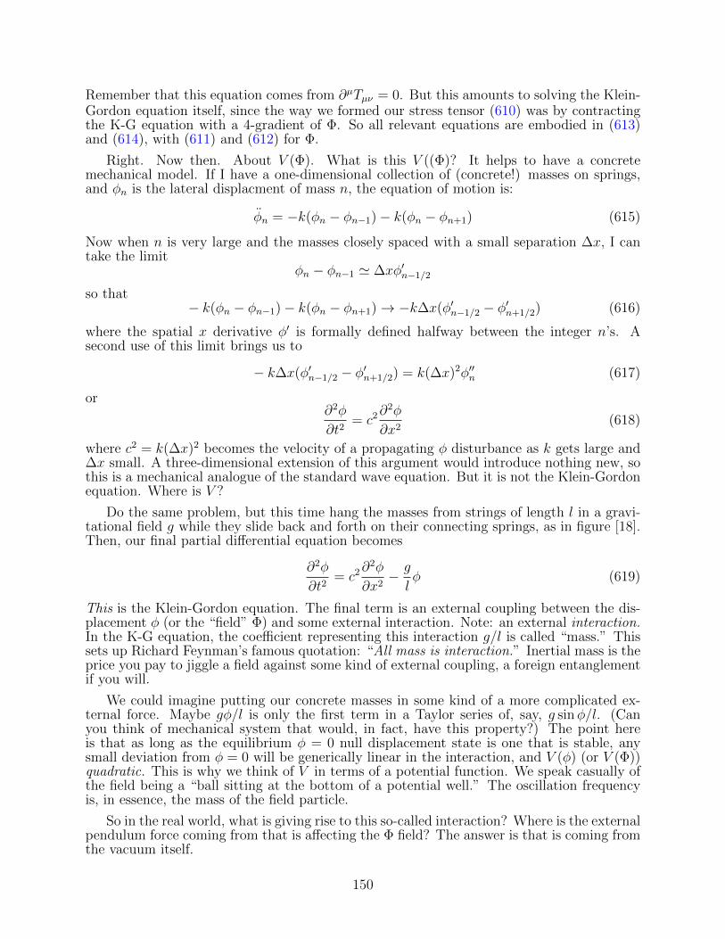
Remember that this equation comes from ∂µTµν = 0. But this amounts to solving the Klein-Gordon equation itself, since the way we formed our stress tensor (610) was by contractingthe K-G equation with a 4-gradient of Φ. So all relevant equations are embodied in (613)and (614), with (611) and (612) for Φ.

Right. Now then. About V (Φ). What is this V ((Φ)? It helps to have a concretemechanical model. If I have a one-dimensional collection of (concrete!) masses on springs,and φn is the lateral displacment of mass n, the equation of motion is:

φn = −k(φn − φn−1)− k(φn − φn+1) (615)

Now when n is very large and the masses closely spaced with a small separation ∆x, I cantake the limit

φn − φn−1 ' ∆xφ′n−1/2

so that− k(φn − φn−1)− k(φn − φn+1)→ −k∆x(φ′n−1/2 − φ′n+1/2) (616)

where the spatial x derivative φ′ is formally defined halfway between the integer n’s. Asecond use of this limit brings us to

− k∆x(φ′n−1/2 − φ′n+1/2) = k(∆x)2φ′′n (617)

or∂2φ

∂t2= c2

∂2φ

∂x2(618)

where c2 = k(∆x)2 becomes the velocity of a propagating φ disturbance as k gets large and∆x small. A three-dimensional extension of this argument would introduce nothing new, sothis is a mechanical analogue of the standard wave equation. But it is not the Klein-Gordonequation. Where is V ?

Do the same problem, but this time hang the masses from strings of length l in a gravi-tational field g while they slide back and forth on their connecting springs, as in figure [18].Then, our final partial differential equation becomes

∂2φ

∂t2= c2

∂2φ

∂x2− g

lφ (619)

This is the Klein-Gordon equation. The final term is an external coupling between the dis-placement φ (or the “field” Φ) and some external interaction. Note: an external interaction.In the K-G equation, the coefficient representing this interaction g/l is called “mass.” Thissets up Richard Feynman’s famous quotation: “All mass is interaction.” Inertial mass is theprice you pay to jiggle a field against some kind of external coupling, a foreign entanglementif you will.

We could imagine putting our concrete masses in some kind of a more complicated ex-ternal force. Maybe gφ/l is only the first term in a Taylor series of, say, g sinφ/l. (Canyou think of mechanical system that would, in fact, have this property?) The point hereis that as long as the equilibrium φ = 0 null displacement state is one that is stable, anysmall deviation from φ = 0 will be generically linear in the interaction, and V (φ) (or V (Φ))quadratic. This is why we think of V in terms of a potential function. We speak casually ofthe field being a “ball sitting at the bottom of a potential well.” The oscillation frequencyis, in essence, the mass of the field particle.

So in the real world, what is giving rise to this so-called interaction? Where is the externalpendulum force coming from that is affecting the Φ field? The answer is that is coming fromthe vacuum itself.

150

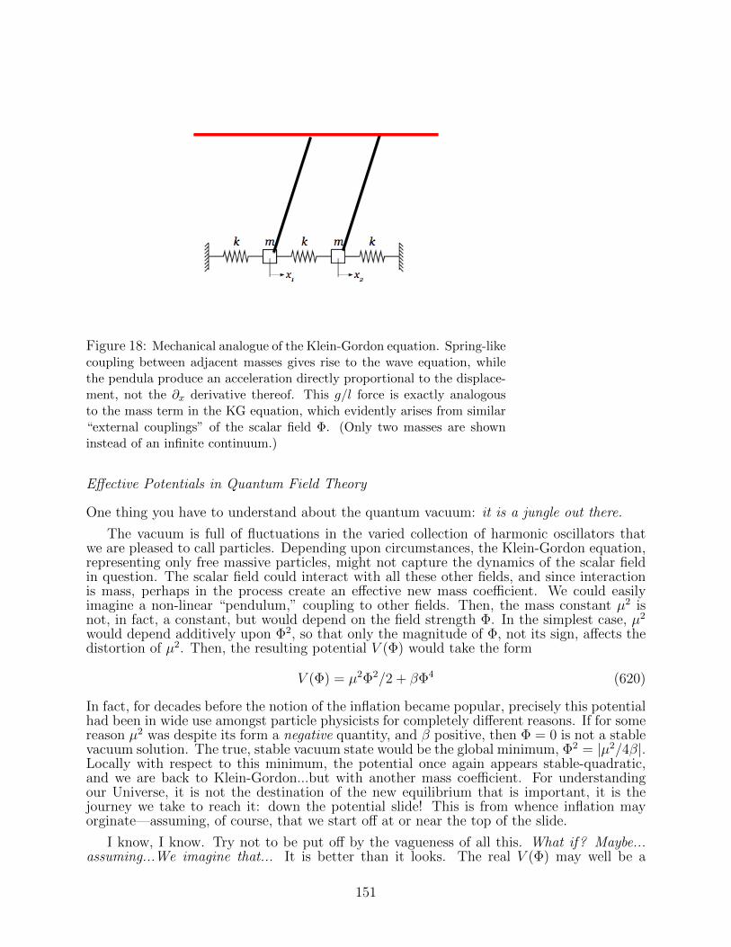
Figure 18: Mechanical analogue of the Klein-Gordon equation. Spring-likecoupling between adjacent masses gives rise to the wave equation, whilethe pendula produce an acceleration directly proportional to the displace-ment, not the ∂x derivative thereof. This g/l force is exactly analogousto the mass term in the KG equation, which evidently arises from similar“external couplings” of the scalar field Φ. (Only two masses are showninstead of an infinite continuum.)

Effective Potentials in Quantum Field Theory

One thing you have to understand about the quantum vacuum: it is a jungle out there.

The vacuum is full of fluctuations in the varied collection of harmonic oscillators thatwe are pleased to call particles. Depending upon circumstances, the Klein-Gordon equation,representing only free massive particles, might not capture the dynamics of the scalar fieldin question. The scalar field could interact with all these other fields, and since interactionis mass, perhaps in the process create an effective new mass coefficient. We could easilyimagine a non-linear “pendulum,” coupling to other fields. Then, the mass constant µ2 isnot, in fact, a constant, but would depend on the field strength Φ. In the simplest case, µ2

would depend additively upon Φ2, so that only the magnitude of Φ, not its sign, affects thedistortion of µ2. Then, the resulting potential V (Φ) would take the form

V (Φ) = µ2Φ2/2 + βΦ4 (620)

In fact, for decades before the notion of the inflation became popular, precisely this potentialhad been in wide use amongst particle physicists for completely different reasons. If for somereason µ2 was despite its form a negative quantity, and β positive, then Φ = 0 is not a stablevacuum solution. The true, stable vacuum state would be the global minimum, Φ2 = |µ2/4β|.Locally with respect to this minimum, the potential once again appears stable-quadratic,and we are back to Klein-Gordon...but with another mass coefficient. For understandingour Universe, it is not the destination of the new equilibrium that is important, it is thejourney we take to reach it: down the potential slide! This is from whence inflation mayorginate—assuming, of course, that we start off at or near the top of the slide.

I know, I know. Try not to be put off by the vagueness of all this. What if? Maybe...assuming...We imagine that... It is better than it looks. The real V (Φ) may well be a

151

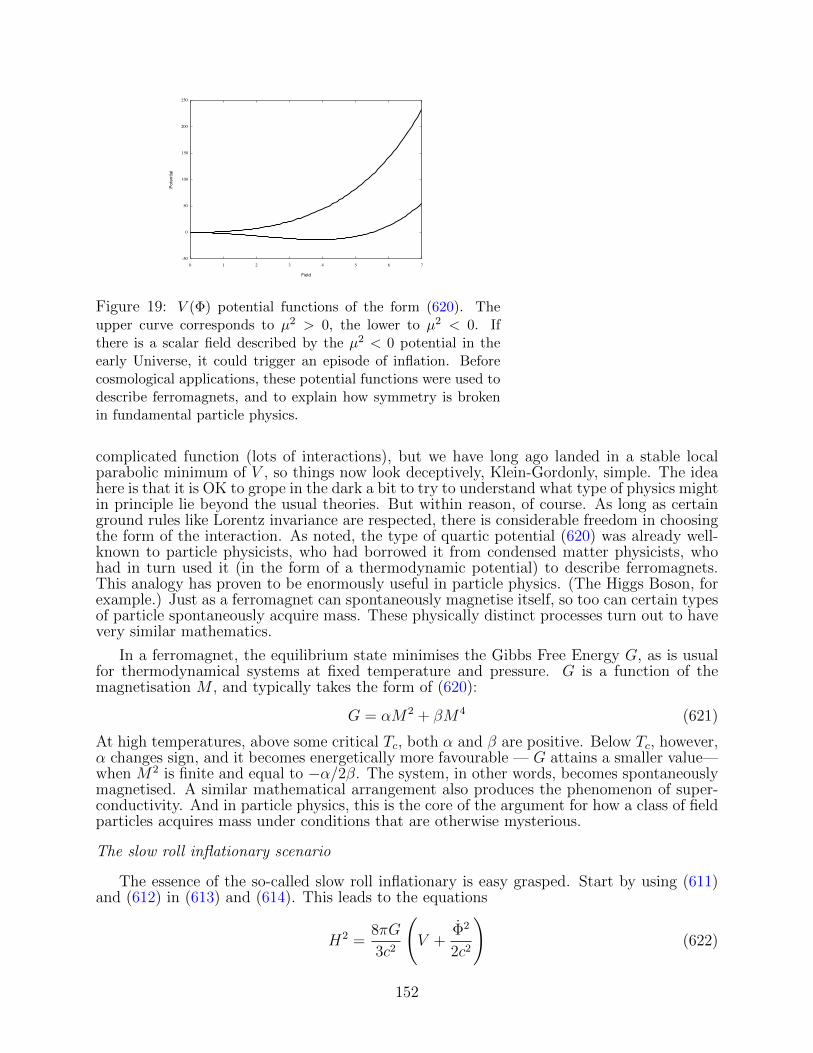
Figure 19: V (Φ) potential functions of the form (620). Theupper curve corresponds to µ2 > 0, the lower to µ2 < 0. Ifthere is a scalar field described by the µ2 < 0 potential in theearly Universe, it could trigger an episode of inflation. Beforecosmological applications, these potential functions were used todescribe ferromagnets, and to explain how symmetry is brokenin fundamental particle physics.

complicated function (lots of interactions), but we have long ago landed in a stable localparabolic minimum of V , so things now look deceptively, Klein-Gordonly, simple. The ideahere is that it is OK to grope in the dark a bit to try to understand what type of physics mightin principle lie beyond the usual theories. But within reason, of course. As long as certainground rules like Lorentz invariance are respected, there is considerable freedom in choosingthe form of the interaction. As noted, the type of quartic potential (620) was already well-known to particle physicists, who had borrowed it from condensed matter physicists, whohad in turn used it (in the form of a thermodynamic potential) to describe ferromagnets.This analogy has proven to be enormously useful in particle physics. (The Higgs Boson, forexample.) Just as a ferromagnet can spontaneously magnetise itself, so too can certain typesof particle spontaneously acquire mass. These physically distinct processes turn out to havevery similar mathematics.

In a ferromagnet, the equilibrium state minimises the Gibbs Free Energy G, as is usualfor thermodynamical systems at fixed temperature and pressure. G is a function of themagnetisation M , and typically takes the form of (620):

G = αM2 + βM4 (621)

At high temperatures, above some critical Tc, both α and β are positive. Below Tc, however,α changes sign, and it becomes energetically more favourable — G attains a smaller value—when M2 is finite and equal to −α/2β. The system, in other words, becomes spontaneouslymagnetised. A similar mathematical arrangement also produces the phenomenon of super-conductivity. And in particle physics, this is the core of the argument for how a class of fieldparticles acquires mass under conditions that are otherwise mysterious.

The slow roll inflationary scenario

The essence of the so-called slow roll inflationary is easy grasped. Start by using (611)and (612) in (613) and (614). This leads to the equations

H2 =8πG

3c2

(V +

Φ2

2c2

)(622)

152

and

Φ + 3HΦ + c2dV

dΦ= 0 (623)

The idea is that the gross form of the potential V (Φ) itself changes while the Universeexpands and cools, going from the top form of figure (19) early on to the bottom form asthings cool, much as a ferromagnet’s free energy does when the temperature changes fromT > Tc to T < Tc. Moreover, if V is very flat, so that dV/dΦ is small, then Φ is also smallby equation (623) and there is an extended period when (622) is simply

H =R

R'√

8πGV03c2

(624)

where V0 is the (approximately) constant of V (Φ). R grows exponentially,

R ∝ exp

(√8πGV0

3c2t

)(625)

and the Universe enters its inflationary phase. Φ meanwhile grows slowly, but it does grow,and eventually, after many e-foldings, the inflation stops when the minimum of V (Φ) isreached. It was Alan Guth, a particle physicist, who put together this picture in 1980,and brought to the fore the concept of inflation as a phase of the history of the earlyUniverse. In particular, he argued that the peculiar model potentials then in widespreaduse to understand ferromagnets and symmetry breaking in particle physics, might also berelevant to fundamental problems in cosmology.

Exercise. The slow-roll equations of inflationary cosmology, from (622) and (623), are

H2 =

(R

R

)2

=8πGV

3c2, Φ = −

(c5

24πGV

)1/2dV

dΦ.

What are the conditions for their validity? Next, try a potential of the form

V (Φ) = V0(1− ε2Φ2)2,

where ε is small and V0 constant. Plot V as a function of Φ. Show that this V satisfies theslow-roll constraints, and solve the above differential equations for R(t) and Φ(t) with nofurther approximations.

The theoretical arguments for the mechanism of inflation are not based on fundamentaltheory (at least not yet). They are what physicists call “phenomenological.” That meansthey are motivated by the existence of an as yet unexplained phenomenon, and rely on thedetailed mathematical exploration of a what-if theory to see how the ideas might lead tothe behaviour in question. Perhaps the theory, if framed carefully, will explain something itwasn’t specifically designed to do. That would be encouraging! Inflation models have thisproperty, which is why there are very attractive.

Here is an example. During the period of inflation, small fluctuations go through twotypes of behaviour in sequence. At first, they oscillate, like a sound wave. But as theUniverse rapidly expands, at some point the peak of a wave and the trough of a wave findthemselves outside of each other’s horizons. A wave can’t possibly oscillate coherently underthose conditions, so the disturbance remains “frozen.”

But the rapid inflation eventually stops while the Universe is still practically a newbornbaby. Then, the expansion no longer is accelerating, but decelerating, and enough time

153

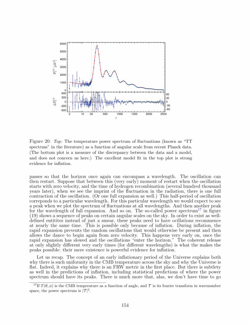
Figure 20: Top: The temperature power spectrum of fluctuations (known as “TTspectrum” in the literature) as a function of angular scale from recent Planck data.(The bottom plot is a measure of the discrepancy between the data and a model,and does not concern us here.) The excellent model fit in the top plot is strongevidence for inflation.

passes so that the horizon once again can encompass a wavelength. The oscillation canthen restart. Suppose that between this (very early) moment of restart when the oscillationstarts with zero velocity, and the time of hydrogen recombination (several hundred thousandyears later), when we see the imprint of the fluctuation in the radiation, there is one fullcontraction of the oscillation. (Or one full expansion as well.) This half-period of oscillationcorreponds to a particular wavelength. For this particular wavelength we would expect to seea peak when we plot the spectrum of fluctuations at all wavelengths. And then another peakfor the wavelength of full expansion. And so on. The so-called power spectrum17 in figure(19) shows a sequence of peaks on certain angular scales on the sky. In order to exist as well-defined entitites instead of just a smear, these peaks need to have ocillations recommenceat nearly the same time. This is possible only because of inflation. During inflation, therapid expansion prevents the random oscillations that would otherwise be present and thenallows the dance to begin again from zero velocity. This happens very early on, once therapid expansion has slowed and the oscillations “enter the horizon.” The coherent releaseat only slightly different very early times (for different wavelengths) is what the makes thepeaks possible: their mere existence is powerful evidence for inflation.

Let us recap. The concept of an early inflationary period of the Universe explains bothwhy there is such uniformity in the CMB temperature across the sky and why the Universe isflat. Indeed, it explains why there is an FRW metric in the first place. But there is subtletyas well in the predictions of inflation, including statistical predictions of where the powerspectrum should have its peaks. There is much more that, alas, we don’t have time to go

17If T (θ, φ) is the CMB temperature as a function of angle, and T is its fourier transform in wavenumberspace, the power spectrum is |T |2.

154

into in this course. There are firm predictions for how large scale structure in the Universeevolves—how galaxies cluster—from the intial seed fluctuations. These rely on the notionof Cold Dark Matter taking part in the gravitational response. Cold Dark Matter (CDM)is cold in the sense that it responds readily to gravitational perturbations, forming the bulkof the mass distribution in galaxies and clusters. Though we don’t know very much aboutCDM, there are reasons to think that it may be some kind of weakly interacting massiveparticle, and there are searches underway to try to detect such particles via their (perhaps)more easily found decay products. But it all must begin with some kind of inflationaryprocess. There really is no other explanation for how vast streches of the Universe couldeven have been in causual contact. Inflation is a powerful, unifying concept without whichwe can not make sense of even the most basic cosmological observations. And don’t forget:the Universe is inflating right now! We are living through mild inflation that will, with time,become much more dramatic.

But why? From whence? What is the underlying imperative? While there are somepromising ideas afoot, we still don’t really know how and why inflation occured. Maybesomebody reading these notes will settle the matter.18

8.11.6 A Final Word

Astrophysics can be a very a messy and speculative business. But every once and a while,something truly outstanding is accomplished. The development of stellar structure andevolution is one such triumph. This led to a new field of science: nuclear astrophysics, andultimately a precision theory for the origin of the chemical elements. We figured out whereatoms come from and even how to make them ourselves, a stunning achievement. Anothermilestone is the blossoming of the theory of black holes, brilliantly confirmed in the last yearby the LIGO detection of gravitational radiation from merging black hole binaries. Surelythe development of precision cosmology, the discovery and construction of a model of theUniverse must rank as one of the great advances in science, on a par with the Crick-WatsonDNA model, not just technical but transformative. We have taken the full measure of theentire Universe. What we thought of a generation ago as the stuff of the Universe is only 5%of the stuff of the Universe, and the concept of inflation suggests that a incomprehensiblyvast multiverse is a viable description of the true reality. To be sure, important questionsremain, and thank goodness for that. But we know the age, we know the dynamics, and weknow the gross history of the Universe. That is a breathtaking accomplishment, one thatwill happen only once in our existence as a species.

End of notes January 25, 2017.

18I’m quite serious: given the historical track record, when this problem is solved, it would not be at allsurprising to me that it is by someone who was an Oxford undergraduate.

155