optimizing limited solar roof access by exergy analysis of solar thermal, photovoltaic, and hybrid...
TRANSCRIPT
Pre-print: M.J.M. Pathak, P.G. Sanders, J. M. Pearce, Optimizing limited solar roof access by exergy analysis of solar thermal, photovoltaic, and hybrid photovoltaic thermal systems, Applied Energy, 120, pp. 115-124 (2014). DOI: http://dx.doi.org/10.1016/j.apenergy.2014.01.041
Optimizing Limited Solar Roof Access by Exergy Analysis of Solar Thermal, Photovoltaic, and Hybrid Photovoltaic Thermal Systems
M. J. M. Pathak1, P. G. Sanders2, J. M. Pearce2,3*
1. Department of Mechanical and Materials Engineering, Queen’s University, Kingston ON, Canada2. Department of Materials Science and Engineering, Michigan Technological University, Houghton, MI USA3. Department of Electrical & Computer Engineering, Michigan Technological University, Houghton, MI USA
* Corresponding author: 601 M&M Building1400 Townsend DriveHoughton, MI [email protected]
Abstract: An exergy analysis was performed to compare a conventional 1) two panel photovoltaic solar thermal hybrid (PVT x2) system, 2) side by side photovoltaic and thermal (PV +T) system, 3) two module photovoltaic (PV) system and 4) a two panel solar thermal (T x2) system with identical absorber areas to determine the superior technical solar energy systems for applications with a limited roof area. Three locations, Detroit, Denver and Phoenix, were simulated due to their differences in average monthly temperature and solar flux. The exergy analysis results show that PVT systems outperform the PV+T systems by 69% for all the locations, produce between 6.5-8.4% more exergy when matched against the purely PV systems and created 4 times as much exergy as the pure solar thermal system. The results clearly show that PVT systems, which are able to utilize all of the thermal and electrical energy generated, are superior in exergy performance to either PV+T or PV only systems. These results are discussed and future work is outlined to further geographically optimize PVT systems.
Keywords: exergy; PVT; solar energy; solar thermal; photovoltaic; photovoltaic thermal hybrid
1. Introduction
Fossil fuels cannot indefinitely sustain the energy needs of the earth’s growing human population due not only to finite supplies, but also the adverse effects of anthropogenic greenhouse gas emissions on global climate [1, 2]. It is therefore necessary to look for alternative renewable forms of energy [3-6] such as solar energy, which have previously been shown to be a sustainable solution to society's energy needs [7, 8]. Currently there are two common systems that utilize the sun’s energy for human use: 1) the solar photovoltaic (PV) cell, which converts sunlight directly into electricity and 2) the solar thermal (T) collector, which converts solar energy into thermal energy. As the levelized cost of PV has dropped quickly [9] to become competitive with conventional grid electricity in specific regions, available roof top space with open solar access tends to drop precipitously in those same regions as they are covered with PV. Thus, when attempting to meet all of a building’s internal electricity and heat loads with energy from the sun, roof area becomes a significant limiting factor [10]. A hybrid solar system, called a solar photovoltaic thermal hybrid system (PVT), provides a potential solution to this challenge [11-13]. PVT systems exploit the heat generated from the PV system, which is normally wasted, to produce useful thermal energy along with the electricity from the PV.
There have been several methods to compare PVT systems using economics, carbon dioxide emissions, energy produced and exergy efficiency [14-18]. Both Erdil et al. [19] and Kalogirou et al. [20] calculated the economic feasibility of a PVT system and concluded that their systems were cost effective. However, economic analysis is usually used to determine the cost viability of the system, but is limited because of the arbitrary nature of the current economic system [21, 22]. The proposal of using carbon dioxide (CO2) emissions, particularly the dynamic life-cycle emissions [4], as a way to rate energy systems is useful particularly in the context of stabilizing global CO2 concentrations. However, trying to make a system more energy efficient would reduce the CO2 emissions of the
Pre-print: M.J.M. Pathak, P.G. Sanders, J. M. Pearce, Optimizing limited solar roof access by exergy analysis of solar thermal, photovoltaic, and hybrid photovoltaic thermal systems, Applied Energy, 120, pp. 115-124 (2014). DOI: http://dx.doi.org/10.1016/j.apenergy.2014.01.041
system in a given location, which eventually reduces the complexities of varying geographic emission intensities due to fuel mix in a region [23]. Energy analysis has shown that PVT systems produce more energy than either a PV or thermal collector system per unit area [24]. Through this work, studies have tested using different flow rates, glazes and designs to determine if PVT systems are superior [25-28]. However, like the other two comparisons, energy lacks the ability to compare electrical energy and thermal energy since energy analysis only looks at the quantity of the energy and not the quality as well. Exergy, defined as the maximum useful energy in a specific reference state, typically the surroundings, analyzes both the quantity and quality. This further allows for an improved analysis and optimization of systems since exergy, unlike energy, is not conserved, but rather destroyed by irreversibilities in real processes [29].
There have been several studies comparing PV, T and PVT systems using exergy. However in these studies, the exergy analysis uses a simplified model by multiplying the Carnot cycle by the thermal energy efficiency [30, 31]. Other exergy analysis work has focused on specific systems to try to optimize operating settings [32-34]. A meticulous exergy analysis comparing PV, thermal and PVT systems has not been undertaken. Thus, this paper provides a more rigorous theoretical exergy model by building on previous detailed exergy models [32-34] but going further to compare a conventional two panels PVT (PVT x2) system to a side-by-side (PV + T) system, two modules PV (PV x2) only system, and a two panels T (T x2) only system to determine the technically superior system for applications with limited roof area. In this study all four solar energy systems were analyzed for the same total area to ensure an unbiased comparison in three locations with varying climatic conditions: Detroit, Denver and Phoenix.
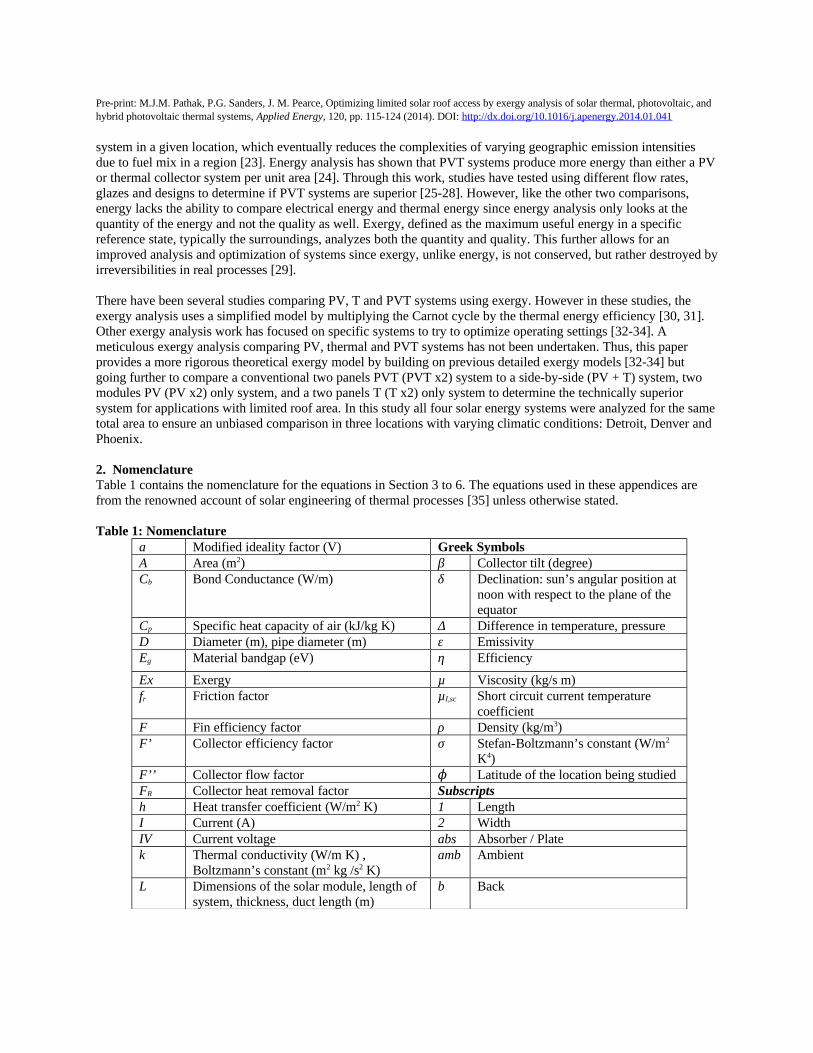
2. NomenclatureTable 1 contains the nomenclature for the equations in Section 3 to 6. The equations used in these appendices are from the renowned account of solar engineering of thermal processes [35] unless otherwise stated.
Table 1: Nomenclaturea Modified ideality factor (V) Greek SymbolsA Area (m2) β Collector tilt (degree)Cb Bond Conductance (W/m) δ Declination: sun’s angular position at
noon with respect to the plane of the equator
Cp Specific heat capacity of air (kJ/kg K) Δ Difference in temperature, pressureD Diameter (m), pipe diameter (m) ε Emissivity Eg Material bandgap (eV) η Efficiency
Ex Exergy µ Viscosity (kg/s m)fr Friction factor µI,sc Short circuit current temperature
coefficientF Fin efficiency factor ρ Density (kg/m3)F’ Collector efficiency factor σ Stefan-Boltzmann’s constant (W/m2
K4)F’’ Collector flow factor ϕ Latitude of the location being studiedFR Collector heat removal factor Subscriptsh Heat transfer coefficient (W/m2 K) 1 LengthI Current (A) 2 WidthIV Current voltage abs Absorber / Platek Thermal conductivity (W/m K) ,
Boltzmann’s constant (m2 kg /s2 K)amb Ambient
L Dimensions of the solar module, length of system, thickness, duct length (m)
b Back

Pre-print: M.J.M. Pathak, P.G. Sanders, J. M. Pearce, Optimizing limited solar roof access by exergy analysis of solar thermal, photovoltaic, and hybrid photovoltaic thermal systems, Applied Energy, 120, pp. 115-124 (2014). DOI: http://dx.doi.org/10.1016/j.apenergy.2014.01.041
m Air mass flow rate (Kg/s) cell CellN Number of glass covers f FluidNu Nusslet number g Glassp Flow pressure (Pa) h HydraulicP Perimeter (m) in Inlet PV Photovoltaic i Inner PV/T Photovoltaic solar thermal hybrid s L Loss, LightQu Useful gain (W) m MeanR Resistance (Ω) mp Maximum power pointRe Reynolds number o Reverse saturationS Solar radiation intensity (W/m2) oc Open circuit T Temperature (K) p PanelUb Overall back loss coefficient (W/m2 K) pv PhotovoltaicUe Overall edge loss coefficient (W/m2 K) pv/t Photovoltaic solar thermal systemUL Overall loss coefficient (W/m2 K) r RadiationUt Overall top loss coefficient (W/m2 K) ref ReferenceV Voltage (V) , Velocity (m/s) s SeriesW Distance between diameter of pipe (m) sc Short circuity Empirically determined coefficient
establishing the upper limit for module temperature at low wind speeds and high solar irradiance
sh Shunt
z Empirically determined coefficient establishing the rate at which module temperature drops as wind speed increases
th Thermal
w Windpm Mean Plate
3. Material and Methods
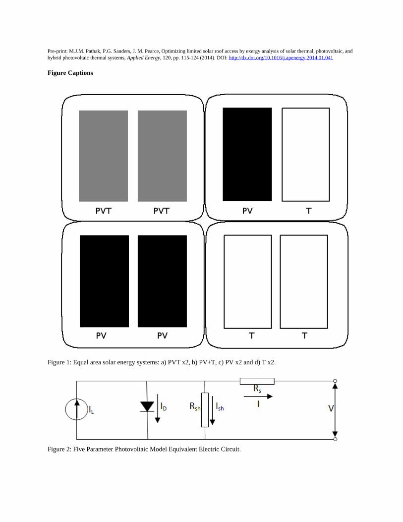
Models, detailed in the sections following, of the four solar energy systems (PVT x2, PV+T, PVx2, and Tx2) shown in Figure 1, were created and analyzed in Scilab, an open-source numerical simulation tool [36]. The National Renewable Energy Laboratory National Solar Radiation Data Base 1991-2005 update Typical Meteorological Year 3 (TMY 3) data was used for the three locations: Detroit City Airport (725375), Denver Intl AP (725650) and Phoenix Sky Harbor Intl AP (722780) [37].
All three locations are Class I data sets with the highest quality of solar modeled data with a complete data set. These three locations were chosen due to their distinct and representative average ambient temperatures and irradiance values, with Detroit representing both low temperatures and low solar flux (9.2 ºC and 3.63 kWh/m2/d), Denver presenting low temperatures and high solar flux (8.2 ºC and 4.58 kWh/m2/d), and Phoenix representing both high temperatures and high solar flux (16.9 ºC and 5.48 kWh/m2/d) [38]. The hourly air temperature, wind speed and solar irradiation were used in the simulation. The wind speed was recorded at ten meters off the ground and therefore the systems are assumed to be at that elevation. As shown in Figure 1 each individual system (PVT x2, PV+T, PV x2, and T x2) has the same total area. The following sub-sections describe the evolution of the models to analyze the systems. The PVT system was model as an air heater with a PV panel as the absorber since air systems are typically preferred due to the lower operating costs and minimal use of material [39]. The solar thermal system was modeled as a tube and sheet system but with air as the fluid to have the same medium as the PVT system for a more direct comparison.
Pre-print: M.J.M. Pathak, P.G. Sanders, J. M. Pearce, Optimizing limited solar roof access by exergy analysis of solar thermal, photovoltaic, and hybrid photovoltaic thermal systems, Applied Energy, 120, pp. 115-124 (2014). DOI: http://dx.doi.org/10.1016/j.apenergy.2014.01.041
4. PV Model
4.1 Solar Photovoltaic Cell Model
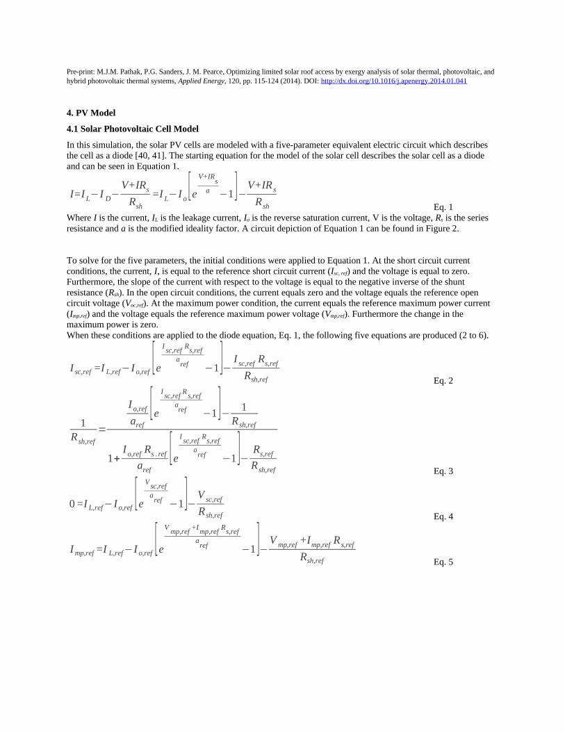
In this simulation, the solar PV cells are modeled with a five-parameter equivalent electric circuit which describes the cell as a diode [40, 41]. The starting equation for the model of the solar cell describes the solar cell as a diode and can be seen in Equation 1.
I=IL−I D−V+IRs
Rsh
=I L−I o[e
V+IRs
a −1]−V+IR s
R sh Eq. 1Where I is the current, IL is the leakage current, Io is the reverse saturation current, V is the voltage, Rs is the series resistance and a is the modified ideality factor. A circuit depiction of Equation 1 can be found in Figure 2.
To solve for the five parameters, the initial conditions were applied to Equation 1. At the short circuit current conditions, the current, I, is equal to the reference short circuit current (Isc, ref) and the voltage is equal to zero. Furthermore, the slope of the current with respect to the voltage is equal to the negative inverse of the shunt resistance (Rsh). In the open circuit conditions, the current equals zero and the voltage equals the reference open circuit voltage (Voc,ref). At the maximum power condition, the current equals the reference maximum power current (Imp,ref) and the voltage equals the reference maximum power voltage (Vmp,ref). Furthermore the change in the maximum power is zero.When these conditions are applied to the diode equation, Eq. 1, the following five equations are produced (2 to 6).
I sc,ref =I L,ref−I o,ref[e
Isc,ref
Rs,ref
aref −1]− I sc,ref Rs,ref
Rsh,ref Eq. 2
1R sh,ref
=
I o,ref
aref
[eIsc,ref
Rs,ref
aref −1]− 1
Rsh,ref
1+I o,ref Rs . ref
aref
[eIsc,ref
Rs,ref
aref −1]− Rs,ref
Rsh,ref Eq. 3
0=I L,ref−I o,ref[e
Vsc,refa
ref −1]−V sc,ref
Rsh,ref Eq. 4
I mp,ref =I L,ref−I o,ref[e
Vmp,ref
+Imp,ref
Rs,ref
aref −1]−V mp,ref +Imp,ref R s,ref
Rsh,ref Eq. 5
Pre-print: M.J.M. Pathak, P.G. Sanders, J. M. Pearce, Optimizing limited solar roof access by exergy analysis of solar thermal, photovoltaic, and hybrid photovoltaic thermal systems, Applied Energy, 120, pp. 115-124 (2014). DOI: http://dx.doi.org/10.1016/j.apenergy.2014.01.041
I mp,ref
V mp,ref
=
I o,ref
aref
[eV
mp,ref+I
mp,refR
s,refa
ref −1]− 1Rsh,ref
1+I o,ref Rs . ref
aref
[eV
mp,ref+I
mp,refR
s,refaref −1]− Rs,ref
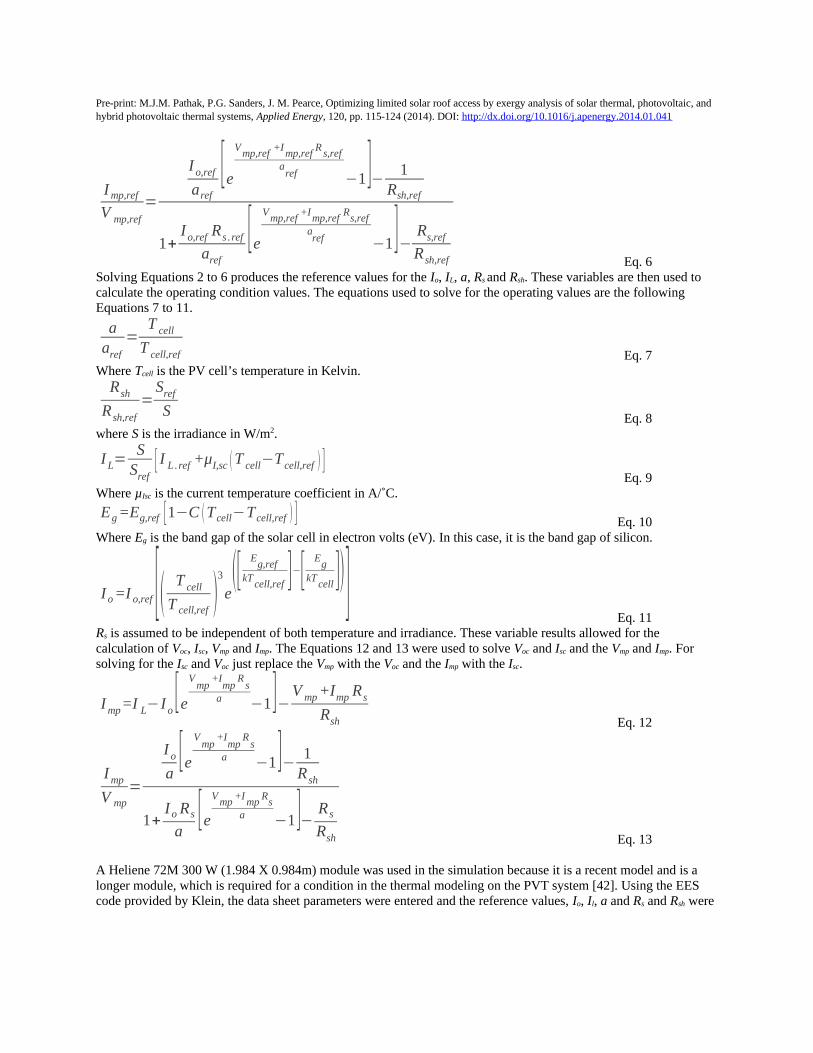
R sh,ref Eq. 6Solving Equations 2 to 6 produces the reference values for the Io, IL, a, Rs and Rsh. These variables are then used to calculate the operating condition values. The equations used to solve for the operating values are the following Equations 7 to 11.
aaref
=T cell
T cell,ref Eq. 7Where Tcell is the PV cell’s temperature in Kelvin.
Rsh
R sh,ref
=Sref
S Eq. 8where S is the irradiance in W/m2.
I L=S
Sref[ I L . ref +μI,sc (T cell−Tcell,ref ) ]
Eq. 9Where µIsc is the current temperature coefficient in A/˚C.
Eg =Eg,ref [1−C (Tcell−Tcell,ref ) ] Eq. 10Where Eg is the band gap of the solar cell in electron volts (eV). In this case, it is the band gap of silicon.
I o =I o,ref [( T cell
T cell,ref)3
e([
Eg,ref
kTcell,ref ]−[
Eg
kTcell ])]
Eq. 11Rs is assumed to be independent of both temperature and irradiance. These variable results allowed for the calculation of Voc, Isc, Vmp and Imp. The Equations 12 and 13 were used to solve Voc and Isc and the Vmp and Imp. For solving for the Isc and Voc just replace the Vmp with the Voc and the Imp with the Isc.
I mp=I L−I o[e
Vmp
+Imp
Rs
a −1]−V mp +Imp Rs
Rsh Eq. 12
I mp
V mp
=
I o
a[e
Vmp
+Imp
Rs
a −1]− 1R sh
1+I o Rs
a[e
Vmp
+Imp
Rs
a −1]− R s
Rsh Eq. 13
A Heliene 72M 300 W (1.984 X 0.984m) module was used in the simulation because it is a recent model and is a longer module, which is required for a condition in the thermal modeling on the PVT system [42]. Using the EES code provided by Klein, the data sheet parameters were entered and the reference values, Io, Il, a and Rs and Rsh were

Pre-print: M.J.M. Pathak, P.G. Sanders, J. M. Pearce, Optimizing limited solar roof access by exergy analysis of solar thermal, photovoltaic, and hybrid photovoltaic thermal systems, Applied Energy, 120, pp. 115-124 (2014). DOI: http://dx.doi.org/10.1016/j.apenergy.2014.01.041
calculated [41]. Using these reference values, the temperature and irradiance dependent Imp and Vmp were determined. Multiplying the Imp and Vmp produced the maximum power, which when divided by the total solar exergy (Exin) derived by Petela, produced the exergy efficiency for the solar panel [43, 44]. Equation 14 gives the efficiency of the PV panel.
ε pv=V mp Imp
E x in
Eq. 14
Where the Exin, Petela derived total solar exergy entering the system is given in Equation 15 [40].
E xin=(1−34
Tamb
T sun
+13 (
T amb
T sun)
4
)SA p
Eq. 15Where the Tamb and Tsun are the ambient and sun temperature in Kelvin.
4.2 Solar PV Panel Temperature
The temperature of the PV module was determined using the empirically derived equation from Sandia National Laboratories and was found to have ± 5oC accuracy in predicting the temperature of the panel, which is equivalent to a 3% error in the power output of the solar panel [45]. The system type chosen was glass/cell/polymer sheet on an open rack mount. The wind speeds used to determine the empirical coefficients were at the standard meteorological height of 10 m, which matches the wind speed input values for this simulation. The air properties were interpolated based off the average air temperature in the system [46, 47]. To determine the temperature of the back of the panel, Equation 16 was used [45].
T m=Sey+zV w +T amb Eq. 16
Where y is dimensionless and z is s/m, are the empirically determined coefficients with the values of -3.56 and -0.075 for the glass/cell/polymer sheet open rack module type and Vw is the wind velocity is m/s. To determine the temperature of the cell, Equation 17 was implemented [45].
T cell=Tm+S
Sref
ΔT Eq. 17
Where ΔT is the temperature difference between the panel’s back surface (Tm) and the cell’s temperature at an irradiance value of (Sref) 1000 W/m2. In the case of the module being considered, the temperature difference value is 3˚C.
5. Solar Thermal Model
5.1 Thermal Design
The solar thermal system was modeled using the Duffie and Beckman equations for a tube and sheet system [35]. The solar thermal model is modeled with eight 4 cm tubes running under the absorber. The coolant used is air with a flow rate for the system of 0.056 kg/s (100 kg/hr m2), which was chosen based off the ASHRAE standards for testing of solar air collectors [48]. This flow rate was chosen to be in the middle of the range of the ASHRAE flow rates of 0.01 to 0.03 m3/s m2. The inlet temperature is assumed to be the ambient temperature.
To determine the efficiency of the solar collector, the overall heat loss from the system is needed. The physical constants were calculated using interpolation from a physical constant table of values using the average temperature as the temperature the constants were at [46].The overall heat loss of the system was calculated using equations 18 to 24. Equation 18 was employed to calculate the top heat losses (Ut) as a starting temperature for the simulation.
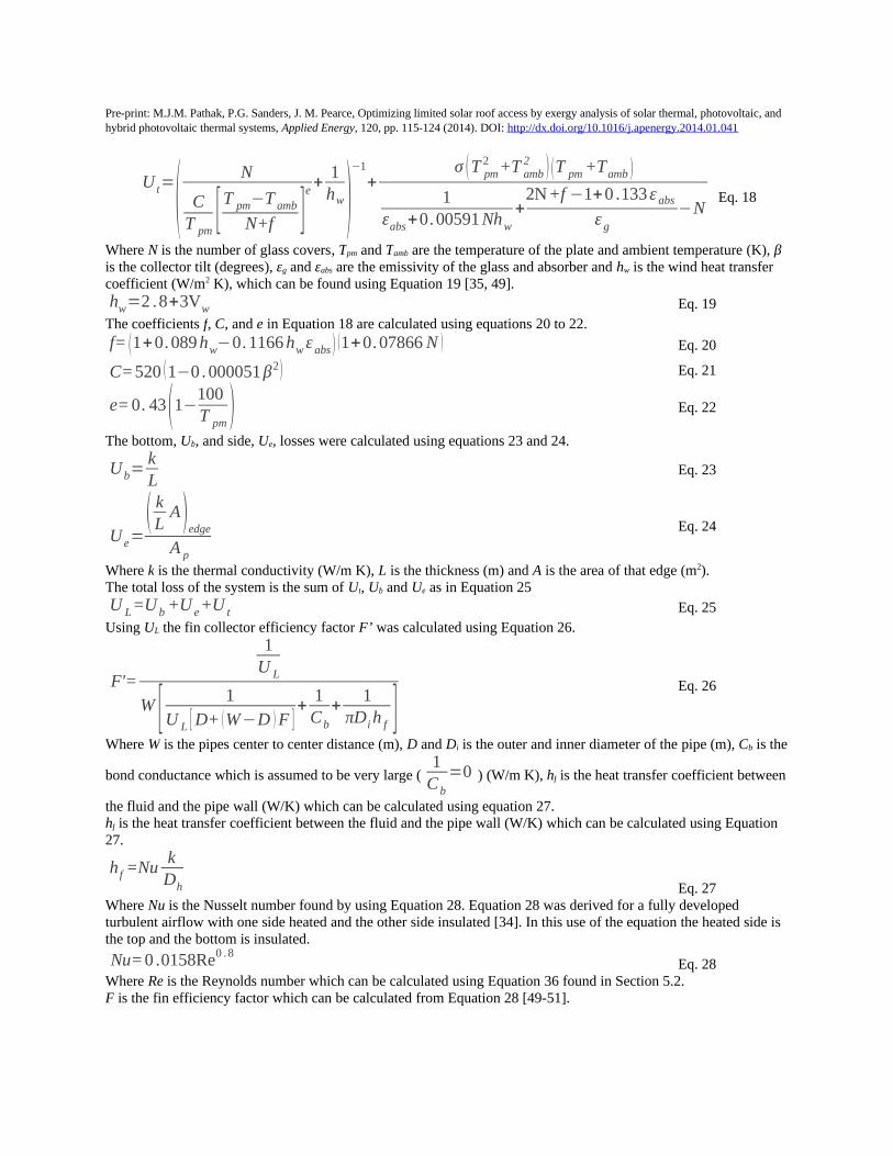
Pre-print: M.J.M. Pathak, P.G. Sanders, J. M. Pearce, Optimizing limited solar roof access by exergy analysis of solar thermal, photovoltaic, and hybrid photovoltaic thermal systems, Applied Energy, 120, pp. 115-124 (2014). DOI: http://dx.doi.org/10.1016/j.apenergy.2014.01.041
U t=(N
CT pm
[T pm−T amb
N+f ]e+
1hw )
−1
+σ (T pm
2 +T amb2 ) (T pm +Tamb )
1εabs+0.00591 Nhw
+2N+f −1+0 .133 ε abs
ε g
−N Eq. 18
Where N is the number of glass covers, Tpm and Tamb are the temperature of the plate and ambient temperature (K), β is the collector tilt (degrees), εg and εabs are the emissivity of the glass and absorber and hw is the wind heat transfer coefficient (W/m2 K), which can be found using Equation 19 [35, 49]. hw=2 .8+3Vw Eq. 19
The coefficients f, C, and e in Equation 18 are calculated using equations 20 to 22.f= (1+0.089 hw−0.1166 hw ε abs ) (1+0.07866 N ) Eq. 20
C=520 (1−0 . 000051 β2) Eq. 21
e= 0. 43(1−100T pm
) Eq. 22
The bottom, Ub, and side, Ue, losses were calculated using equations 23 and 24.
Ub=kL
Eq. 23
U e=( k
LA)
edge
A p
Eq. 24
Where k is the thermal conductivity (W/m K), L is the thickness (m) and A is the area of that edge (m2).The total loss of the system is the sum of Ut, Ub and Ue as in Equation 25U L=U b +U e+U t Eq. 25
Using UL the fin collector efficiency factor F’ was calculated using Equation 26.
F'=
1U L
W [ 1U L [ D+ (W−D ) F ]
+1Cb
+1
πDi h f ]Eq. 26
Where W is the pipes center to center distance (m), D and Di is the outer and inner diameter of the pipe (m), Cb is the
bond conductance which is assumed to be very large (1
Cb
=0 ) (W/m K), hf is the heat transfer coefficient between
the fluid and the pipe wall (W/K) which can be calculated using equation 27.hf is the heat transfer coefficient between the fluid and the pipe wall (W/K) which can be calculated using Equation 27.
h f =Nuk
Dh Eq. 27Where Nu is the Nusselt number found by using Equation 28. Equation 28 was derived for a fully developed turbulent airflow with one side heated and the other side insulated [34]. In this use of the equation the heated side is the top and the bottom is insulated.
Nu=0 .0158Re0 .8Eq. 28
Where Re is the Reynolds number which can be calculated using Equation 36 found in Section 5.2.F is the fin efficiency factor which can be calculated from Equation 28 [49-51].

Pre-print: M.J.M. Pathak, P.G. Sanders, J. M. Pearce, Optimizing limited solar roof access by exergy analysis of solar thermal, photovoltaic, and hybrid photovoltaic thermal systems, Applied Energy, 120, pp. 115-124 (2014). DOI: http://dx.doi.org/10.1016/j.apenergy.2014.01.041
F=tanh [m (W −D )/2 ]
m (W −D )/2Eq. 28
Where m can be calculated using Equation 29.
m=√U L
δk Eq. 29Where δ is the thickness of the plate (m) and k is the thermal conductivity of the plate (W/m K).Using the collector efficiency factor F’ found by Equation 26, the heat removal factor was determined from Equation 30 [49-51].
FR=mC p
A PU L
(1−e−
Ap
UL
F'
mCp ) Eq. 30
The actual useful energy gain Qu was then calculated using the Equation 31.
Qu =A p FR [ S−U L (T in−T amb )] Eq. 31
Using the Qu the mean temperature of the plate and the fluids outflow were calculated with Equations 32 and 33 [49-51].
T abs−m=T in+Qu/ Ap
U L F R(1−FR ) Eq. 32
T out =T in+Qu
mC p
Eq. 33
5.2 Exergy Model
The change in exergy (∆ E xth) for the thermal system is derived from the difference in the exergy of the flow at the inlet and outlet [32-34]. This is given by the Equation 33.
Δ E x th=mC p(T out−T in−T amb ln(T out
T in))−1. 5(
mT amb Δp
ρT in) Eq. 33
Where m is the mass flow rate (kg/s), Cp is the specific heat capacity (s/Kg K), Tout, Tin and Tamb are the outlet, inlet and ambient temperature (K) respectively, ρ is the density (kg/m3) and Δp is the frictional pressure drop (Pa). The 1.5 factor found in Eq. 33 is to account for the fan and motor efficiency losses (74% and 90% respectively) as derived in the paper by A. Hegazy [52]. The frictional pressure drop of the fluid Δp was calculated using Equation 34.
Δp=f r ρLV 2
2Dh Eq. 34Where L is the length of the duct (m), V is the velocity (m/s), Dh is the hydraulic diameter as seen in Equation 35.
Dh=4A f
P f Eq. 35Where Af is the cross sectional area (m2) and P is the wetted perimeter (m) and f is the friction which can be calculated using Equation 36.
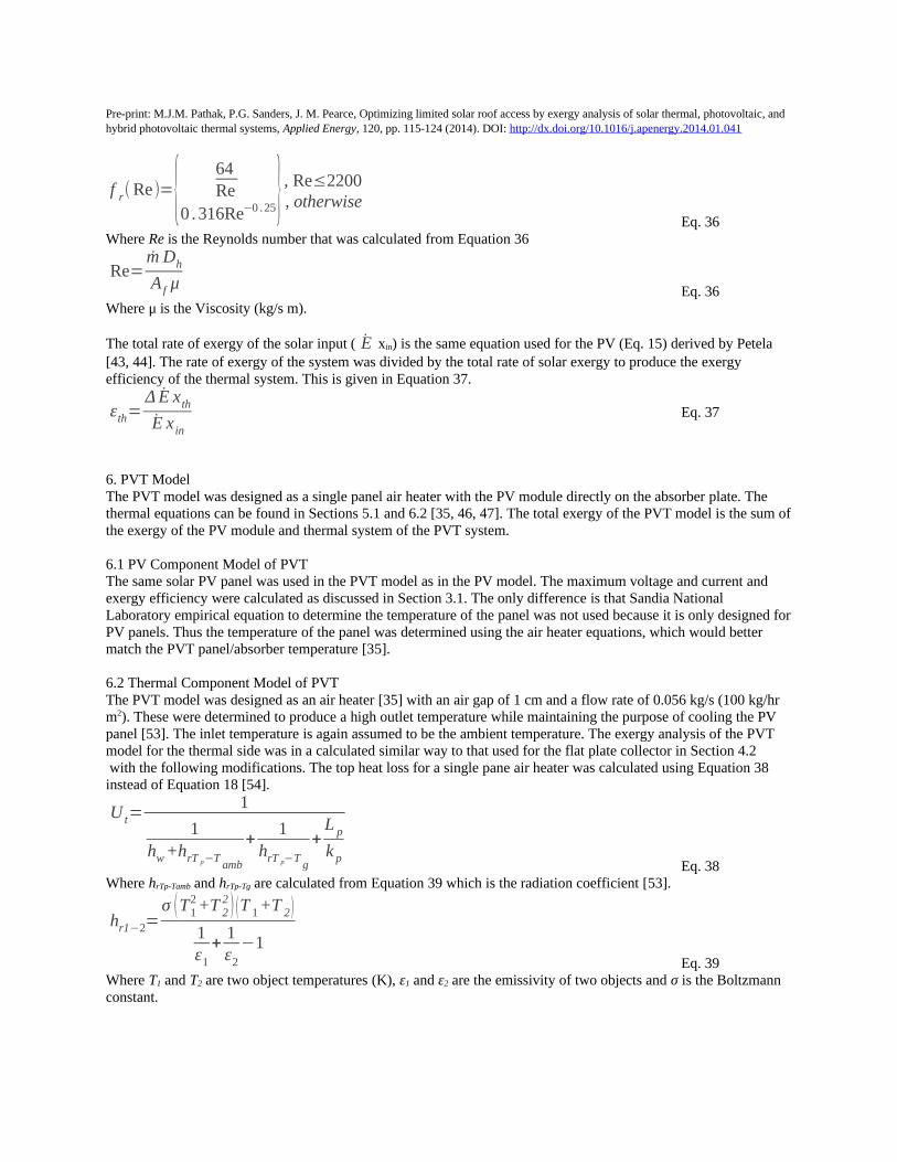
Pre-print: M.J.M. Pathak, P.G. Sanders, J. M. Pearce, Optimizing limited solar roof access by exergy analysis of solar thermal, photovoltaic, and hybrid photovoltaic thermal systems, Applied Energy, 120, pp. 115-124 (2014). DOI: http://dx.doi.org/10.1016/j.apenergy.2014.01.041
f r(Re)={64Re
0 .316Re−0 .25},,Re≤2200otherwise
Eq. 36Where Re is the Reynolds number that was calculated from Equation 36
Re=m Dh
A f μ Eq. 36Where μ is the Viscosity (kg/s m).
The total rate of exergy of the solar input ( E xin) is the same equation used for the PV (Eq. 15) derived by Petela [43, 44]. The rate of exergy of the system was divided by the total rate of solar exergy to produce the exergy efficiency of the thermal system. This is given in Equation 37.
εth=Δ E x th
E x in
Eq. 37
6. PVT ModelThe PVT model was designed as a single panel air heater with the PV module directly on the absorber plate. The thermal equations can be found in Sections 5.1 and 6.2 [35, 46, 47]. The total exergy of the PVT model is the sum of the exergy of the PV module and thermal system of the PVT system.
6.1 PV Component Model of PVTThe same solar PV panel was used in the PVT model as in the PV model. The maximum voltage and current and exergy efficiency were calculated as discussed in Section 3.1. The only difference is that Sandia National Laboratory empirical equation to determine the temperature of the panel was not used because it is only designed for PV panels. Thus the temperature of the panel was determined using the air heater equations, which would better match the PVT panel/absorber temperature [35].
6.2 Thermal Component Model of PVTThe PVT model was designed as an air heater [35] with an air gap of 1 cm and a flow rate of 0.056 kg/s (100 kg/hr m2). These were determined to produce a high outlet temperature while maintaining the purpose of cooling the PV panel [53]. The inlet temperature is again assumed to be the ambient temperature. The exergy analysis of the PVT model for the thermal side was in a calculated similar way to that used for the flat plate collector in Section 4.2 with the following modifications. The top heat loss for a single pane air heater was calculated using Equation 38 instead of Equation 18 [54].
U t=1
1hw +hrT p−T
amb
+1
hrT p−Tg
+L p
k pEq. 38
Where hrTp-Tamb and hrTp-Tg are calculated from Equation 39 which is the radiation coefficient [53].
hr1−2=σ (T1
2 +T 22 ) (T 1+T 2)
1ε1
+1ε2
−1Eq. 39
Where T1 and T2 are two object temperatures (K), ε1 and ε2 are the emissivity of two objects and σ is the Boltzmann constant.
Pre-print: M.J.M. Pathak, P.G. Sanders, J. M. Pearce, Optimizing limited solar roof access by exergy analysis of solar thermal, photovoltaic, and hybrid photovoltaic thermal systems, Applied Energy, 120, pp. 115-124 (2014). DOI: http://dx.doi.org/10.1016/j.apenergy.2014.01.041
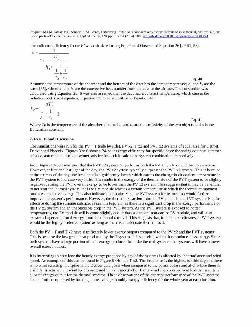
The collector efficiency factor F’ was calculated using Equation 40 instead of Equation 26 [49-51, 53].
F'=1
1+U L
h1+1
1h2
+1hr Eq. 40
Assuming the temperature of the absorber and the bottom of the duct has the same temperature; h1 and h2 are the same [35], where h1 and h2 are the convective heat transfer from the duct to the airflow. The convection was calculated using Equation 28. It was also assumed that the duct had a constant temperature, which causes the radiation coefficient equation, Equation 39, to be simplified to Equation 41.
hr=σT p
3
1ε1
+1ε2
−1 Eq. 41
Where Tp is the temperature of the absorber plate and ε1 and ε2 are the emissivity of the two objects and σ is the Boltzmann constant.
7. Results and Discussion
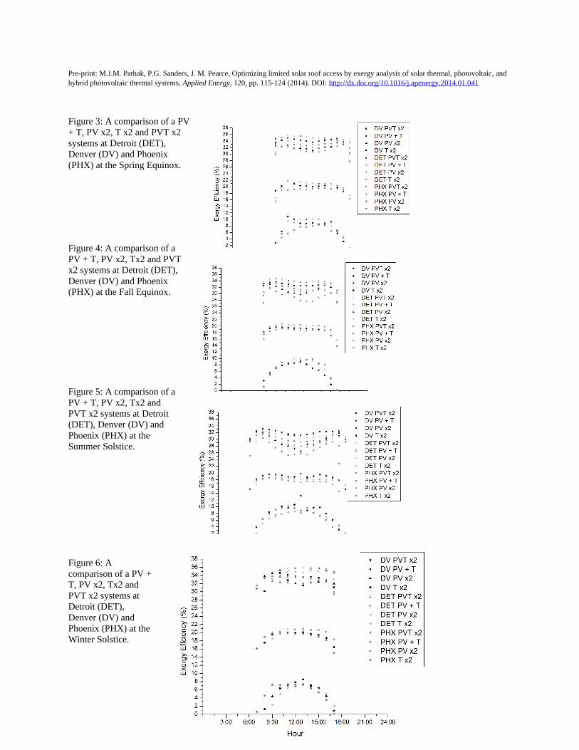
The simulations were run for the PV + T (side by side), PV x2, T x2 and PVT x2 systems of equal area for Detroit, Denver and Phoenix. Figures 3 to 6 show a 24-hour exergy efficiency for specific days: the spring equinox, summer solstice, autumn equinox and winter solstice for each location and system combination respectively.
From Figures 3-6, it was seen that the PVT x2 system outperforms both the PV + T, PV x2 and the T x2 systems. However, at first and last light of the day, the PV x2 system typically surpasses the PVT x2 system. This is because at these times of the day, the irradiance is significantly lower, which causes the change in air coolant temperature in the PVT system to increase very little. This results in the exergy of the thermal side of the PVT system to be slightly negative, causing the PVT overall exergy to be lower than the PV x2 system. This suggests that it may be beneficial to not start the thermal system until the PV module reaches a certain temperature at which the thermal component produces a positive exergy. This also indicates that optimizing the PVT system for its location would further improve the system’s performance. However, the thermal extraction from the PV panels in the PVT system is quite effective during the summer solstice, as seen in Figure 5, as there is a significant drop in the exergy performance of the PV x2 system and an unnoticeable drop in the PVT system. As the PVT system is exposed to hotter temperatures, the PV module will become slightly cooler than a standard non-cooled PV module, and will also extract a larger additional exergy from the thermal removal. This suggests that, in the hotter climates, a PVT system would be the highly preferred system as long as there is an adequate thermal load.
Both the PV + T and T x2 have significantly lower exergy outputs compared to the PV x2 and the PVT systems. This is because the low grade heat produced by the T systems is less useful, which thus produces less exergy. Since both systems have a large portion of their exergy produced from the thermal systems, the systems will have a lower overall exergy output.
It is interesting to note how the hourly exergy produced by any of the systems is affected by the irradiance and wind speed. An example of this can be found in Figure 5 with the T x2. The irradiance is the highest for this day and there is no wind resulting in a spike in the Denver data point when compared to the points before and after where there is a similar irradiance but wind speeds are 2 and 5 m/s respectively. Higher wind speeds cause heat loss that results in a lower exergy output for the thermal systems. These observations of the superior performance of the PVT systems can be further supported by looking at the average monthly exergy efficiency for the whole year at each location.
Pre-print: M.J.M. Pathak, P.G. Sanders, J. M. Pearce, Optimizing limited solar roof access by exergy analysis of solar thermal, photovoltaic, and hybrid photovoltaic thermal systems, Applied Energy, 120, pp. 115-124 (2014). DOI: http://dx.doi.org/10.1016/j.apenergy.2014.01.041
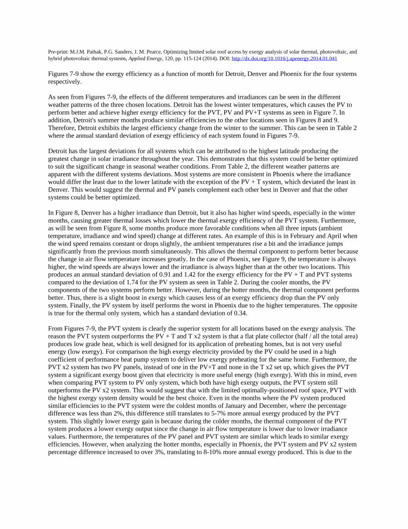
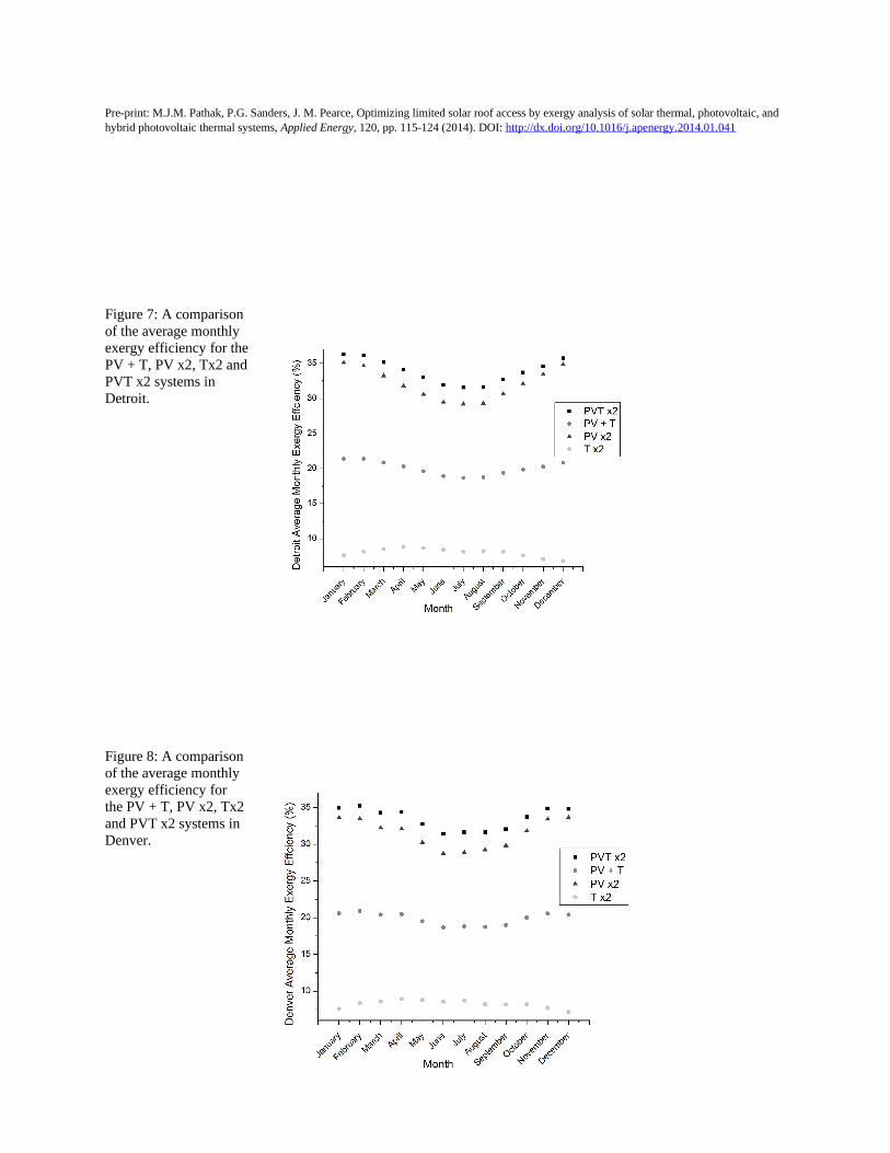
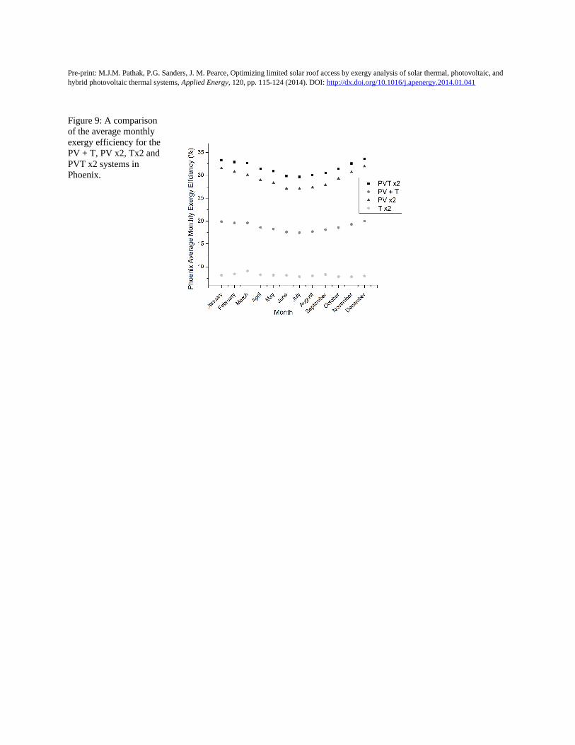
Figures 7-9 show the exergy efficiency as a function of month for Detroit, Denver and Phoenix for the four systems respectively.
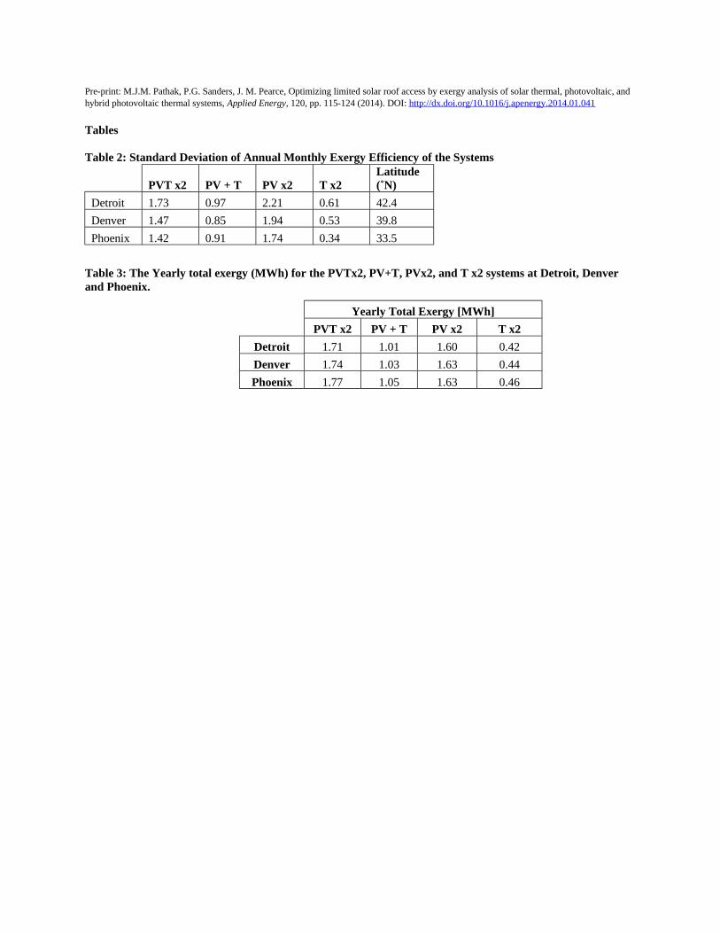
As seen from Figures 7-9, the effects of the different temperatures and irradiances can be seen in the different weather patterns of the three chosen locations. Detroit has the lowest winter temperatures, which causes the PV to perform better and achieve higher exergy efficiency for the PVT, PV and PV+T systems as seen in Figure 7. In addition, Detroit's summer months produce similar efficiencies to the other locations seen in Figures 8 and 9. Therefore, Detroit exhibits the largest efficiency change from the winter to the summer. This can be seen in Table 2 where the annual standard deviation of exergy efficiency of each system found in Figures 7-9.
Detroit has the largest deviations for all systems which can be attributed to the highest latitude producing the greatest change in solar irradiance throughout the year. This demonstrates that this system could be better optimized to suit the significant change in seasonal weather conditions. From Table 2, the different weather patterns are apparent with the different systems deviations. Most systems are more consistent in Phoenix where the irradiance would differ the least due to the lower latitude with the exception of the PV + T system, which deviated the least in Denver. This would suggest the thermal and PV panels complement each other best in Denver and that the other systems could be better optimized.
In Figure 8, Denver has a higher irradiance than Detroit, but it also has higher wind speeds, especially in the winter months, causing greater thermal losses which lower the thermal exergy efficiency of the PVT system. Furthermore, as will be seen from Figure 8, some months produce more favorable conditions when all three inputs (ambient temperature, irradiance and wind speed) change at different rates. An example of this is in February and April when the wind speed remains constant or drops slightly, the ambient temperatures rise a bit and the irradiance jumps significantly from the previous month simultaneously. This allows the thermal component to perform better because the change in air flow temperature increases greatly. In the case of Phoenix, see Figure 9, the temperature is always higher, the wind speeds are always lower and the irradiance is always higher than at the other two locations. This produces an annual standard deviation of 0.91 and 1.42 for the exergy efficiency for the PV + T and PVT systems compared to the deviation of 1.74 for the PV system as seen in Table 2. During the cooler months, the PV components of the two systems perform better. However, during the hotter months, the thermal component performs better. Thus, there is a slight boost in exergy which causes less of an exergy efficiency drop than the PV only system. Finally, the PV system by itself performs the worst in Phoenix due to the higher temperatures. The opposite is true for the thermal only system, which has a standard deviation of 0.34.
From Figures 7-9, the PVT system is clearly the superior system for all locations based on the exergy analysis. The reason the PVT system outperforms the PV + T and T x2 system is that a flat plate collector (half / all the total area) produces low grade heat, which is well designed for its application of preheating homes, but is not very useful energy (low exergy). For comparison the high exergy electricity provided by the PV could be used in a high coefficient of performance heat pump system to deliver low exergy preheating for the same home. Furthermore, the PVT x2 system has two PV panels, instead of one in the PV+T and none in the T x2 set up, which gives the PVT system a significant exergy boost given that electricity is more useful energy (high exergy). With this in mind, even when comparing PVT system to PV only system, which both have high exergy outputs, the PVT system still outperforms the PV x2 system. This would suggest that with the limited optimally-positioned roof space, PVT with the highest exergy system density would be the best choice. Even in the months where the PV system produced similar efficiencies to the PVT system were the coldest months of January and December, where the percentage difference was less than 2%, this difference still translates to 5-7% more annual exergy produced by the PVT system. This slightly lower exergy gain is because during the colder months, the thermal component of the PVT system produces a lower exergy output since the change in air flow temperature is lower due to lower irradiance values. Furthermore, the temperatures of the PV panel and PVT system are similar which leads to similar exergy efficiencies. However, when analyzing the hotter months, especially in Phoenix, the PVT system and PV x2 system percentage difference increased to over 3%, translating to 8-10% more annual exergy produced. This is due to the
Pre-print: M.J.M. Pathak, P.G. Sanders, J. M. Pearce, Optimizing limited solar roof access by exergy analysis of solar thermal, photovoltaic, and hybrid photovoltaic thermal systems, Applied Energy, 120, pp. 115-124 (2014). DOI: http://dx.doi.org/10.1016/j.apenergy.2014.01.041
exact opposite situation as described for the colder months. Table 3 displays the yearly amount of exergy produced by all four systems for the three locations.
From Table 3, it was seen that the PVT system produces almost twice as much exergy as the PV + T system and four times as much exergy as the T x2 over the course of the entire year for all three locations. In comparison with the PV x2 system, the PVT system produces 6.5%, 7.2% and 8.4% more exergy for the Detroit, Denver and Phoenix locations respectively. This further demonstrates that the PVT system should be chosen if there is limited optimal roof space to produce the maximum amount of exergy. It also suggests that there is a need to optimize the PVT system for each location: the Denver and Phoenix locations produce 2.1% and 3.7% more exergy than the Detroit due to the higher irradiance, but Detroit is more efficient. Such optimization might include changing the flow rates, reducing the thermal losses and using different PV materials to better suit higher operating temperatures.
8. Future Work
The primary limitation of this work is the assumption that all the exergy is used for the simulated systems. In solar thermal systems in particular this may not always be a valid assumption. Thus, it is left for future work to refine this base case to take into account primarily thermal loads, but also depending on electrical grid conditions, the electric loads. Such electrical grid conditions could include the use of battery storage either in the form of traditional batteries or utilizing the batteries in plug-in cars [55, 56]. For most rooftop constrained applications, the assumption of full consumption of the exergy produced may be reasonable. However, a practical optimization would require the matching of electrical and thermal loads for specific building usage. Depending on the loads, the optimal system could change substantially for a given application.
Another important consideration is the location, since it greatly affects the performance of the system. It would therefore be interesting to provide an exergy efficiency map of the PVT systems for all of North America or for other regions to determine efficiency patterns and location performance of the PVT system. Alongside location, possible building integrated PVT systems (BIPVT) instead of typical PVT panels should be analyzed to better understand the opportunities for PV to be utilized in the façade of a building [57].
PVT technology is at a relatively early stage of technological development. Optimizing the system’s components, such as the materials, could improve the performance for a given application. There have been many different studies on the PV material which could be harnessed to better optimize the system. Detailed work on the thermal and structural performance of a PV module and understand the spectral irradiance effect on the PV would assist in the design of the correct PVT for a specified location [58, 59]. Thin film PV panels such as hydrogenated amorphous silicon (a-Si:H) materials could be used in replacement of crystalline silicon (c-Si) in PVT systems since it offers a promising solution to PVT system integration [60]. a-Si:H can be deposited directly onto the absorber plate making an integral system [61], has a superior temperature coefficient (0.1%/ ˚C) [62] to c-Si-based PV and running the system at a higher operating temperature [63], which would have the added benefit of annealing the Staebler-Wronski Effect (SWE) defects and achieving a higher electrical performance. Preliminary studies of a-Si:H PV under PVT operating temperatures showed operating a-Si:H-based PV at 90˚C (i.e. a PVT operating temperature), with thicker i-layers than the cells currently used in commercial production, provided a greater power output compared to the thinner cells operating at either PV or PVT operating temperatures [64]. In addition, the solar thermal side of the PVT can be used to create high-temperature annealing pulses (spike annealing), which were found to provide a greater than 10% energy gain when compared to a cell that was only degraded under normal PV conditions [65]. These preliminary results showing the promise of a-Si:H as a PVT material should be followed up with an appropriate exergy analysis.
This could then be used to focus on optimizing the entire PVT system as an integrated optimized system, rather than the existing tradeoffs between the two sub-systems, and would clearly have an impact on the overall system exergy

Pre-print: M.J.M. Pathak, P.G. Sanders, J. M. Pearce, Optimizing limited solar roof access by exergy analysis of solar thermal, photovoltaic, and hybrid photovoltaic thermal systems, Applied Energy, 120, pp. 115-124 (2014). DOI: http://dx.doi.org/10.1016/j.apenergy.2014.01.041
efficiency. This would allow the thermal component to perform better than current designs whilst not hampering the PV performance [66].
9. Conclusions
This study found that for solar energy collecting systems with identical absorber areas, PVT hybrid systems surpassed the exergy efficiency of both PV+T (side by side) and purely PV systems in three representative regions in the U.S. The PVT system outperformed the PV + T system by 69% and the T x2 system by almost 400% in all the locations. Similarly, the PVT system performed 6.5%, 7.2% and 8.4% better than the PV only system for the Detroit, Denver and Phoenix locations respectively. It is clear that for applications with limited roof area PVT systems are superior choices. This research also suggests that greater optimization is required for PVT systems. To further improve the exergy performance of PVT systems, geographical optimization should be further investigated with potential improvements found in the PV material, flow rate and improved thermal loss reductions.
AcknowledgementsThis research was supported by the Natural Sciences and Engineering Research Council of Canada and the Solar Buildings Research Network. The authors would like to acknowledge helpful discussions with S.J. Harrison.
References
[1] Intergovernmental Panel on Climate Change (IPCC). Climate Change 2007: Synthesis Report.
Intergovernmental Panel on Climate Change. Cambridge University Press, Cambridge, United Kingdom.
[2] Stern N. The Economics of Climate Change: The Stern Review. Cambridge: Cambridge University Press;
2007.
[3] Hoffert MI, Caldeira K, Benford G, Criswell DR, Green C, Herzog, H,Jain AK, Kheshgi HS, Lackner KS,
Lewis JS, Lightfoot HD, Manheimer W, Mankins JC, Mauel ME, Perkins L J, Schlesinger ME, Volk T, Wigley TM L. Advanced Technology Paths to Global Climate Stability: Energy for a Greenhouse Planet. Science 2002; 298: 981-987.
[4] Kenny R, Law C, Pearce JM. Towards Real Energy Economics: Energy Policy Driven by Life-Cycle Carbon
Emission. Energ Policy 2010; 38: 1969-1978.
[5] Goswami DY. A review and future prospects of renewable energy in the global energy system. Advanced
Technology of Electrical Engineering and Energy 2008; 27: 55-62.
[6] Abbott D. Keeping the Energy Debate Clean: How Do We Supply the World's Energy Needs?. Proceedings
of the IEEE 2010; 98: 42–66.
[7] Pearce J, Photovoltaics - A Path to Sustainable Futures. Futures 2002; 34: 663-674.
[8] Shafiee S, Topal E. When will fossil fuel reserve be diminished? Energ Policy 2009; 37:181-189.
[9] Branker K, Pathak MJM, Pearce JM. A Review of Solar Photovoltaic Levelized Cost of Electricity. Renew
Sust Energ Rev 2011; 15:4470-4482.
Pre-print: M.J.M. Pathak, P.G. Sanders, J. M. Pearce, Optimizing limited solar roof access by exergy analysis of solar thermal, photovoltaic, and hybrid photovoltaic thermal systems, Applied Energy, 120, pp. 115-124 (2014). DOI: http://dx.doi.org/10.1016/j.apenergy.2014.01.041
[10] Anderson TN, Duke M, Morrison GL, Carson JK. Performance of a building integrated photovoltaic/thermal
(BIPVT) solar collector. Sol Energy 2009; 83: 445-455.
[11] Amori KE, Taqi Al-Najjar HM, Analysis of thermal and electrical performance of a hybrid (PV/T) air based
solar collector for Iraq, Appl Energy 2012; 98: 384-395
[12] Zogou O, Stapountzis H, Flow and heat transfer inside a PV/T collector for building application, Appl
Energy 2012; 91:103-115
[13] Sarhaddi F, Farahat S, Ajam H, Behzadmehr A, Mahdavi Adeli M, An improved thermal and electrical
model for a solar photovoltaic thermal (PV/T) air collector, Appl Energy 2010; 87:2328-2339
[14] Loir N, Zhang N. Energy, exergy, and second law performance criteria. Energy 2007; 32:445-455.
[15] Bakker M., Zondag HA, Elswijk MJ, Strootman KJ, Jong MJM. Performance and costs of a roof-sized
PV/thermal array combined with a ground coupled heat pump. Sol Energy 2003; 78: 331-339.
[16] van Helden W, van Zolingen R, Zondag HA. PV thermal systems: PV panels supplying renewable electricity
and heat. Prog Photovoltaics 2004; 12: 415-426.
[17] Tripanagnostopoulos Y, Souliotis M, Battisti R, Corrado A. Energy, cost and LCA results of PV and hybrid
PV/T solar systems. Prog Photovoltaics 2005; 13:235-250.
[18] Zondag HA. Flat-plate PV-Thermal collectors and systems: A review. Renew Sust Energ Rev 2008; 12:891-
959.
[19] Erdil E, Ilkan M, Egelioglu F. An Experimental study on energy generation with a photovoltaic (PV)-solar
thermal hybrid system. Energy 2008; 33:1241-1245.
[20] Kalogirou S, Tripanagnostopoulos Y. Industrial application of PV/T solar energy systems. Appl Therml Eng
2007; 27: 1259-1270.
[21] Costanza R. Embodied Energy and Economic Valuation. Science 1980; 210: 1219-1224.
[22] Burness S, Cummings R, Morris G, Paik I. Thermodynamic and Economic Concepts as Related to Resource-
Use Policies. Land Econ 1980; 56: 1-9.
[23] Kenny R, Law C, Pearce JM. Towards Real Energy Economics: Energy Policy Driven by Life-Cycle Carbon
Emission. Energ Policy 2010; 38: 1969–1978.
[24] Tiwari A, Sodha M, Chandra A, Joshi J. Performance evaluation of photovoltaic thermal solar air collector
for composite climate of India. Sol Energ Mat Sol C 2006; 90: 175-189.
[25] Sarhaddi F et al. An improved thermal and electrical model for a solar photovoltaic thermal (PV/T) air
collector. Appl Energy 2010; 87: 2328-2339.
Pre-print: M.J.M. Pathak, P.G. Sanders, J. M. Pearce, Optimizing limited solar roof access by exergy analysis of solar thermal, photovoltaic, and hybrid photovoltaic thermal systems, Applied Energy, 120, pp. 115-124 (2014). DOI: http://dx.doi.org/10.1016/j.apenergy.2014.01.041
[26] Fraisse G, Ménézo C, Johannes K. Energy performance of water hybrid PV/T collectors applied to
combisystems of Direct Solar Floor type G. Sol Energy 2007;81:1426-1438.
[27] Chow TT. A review on photovoltaic/thermal hybrid solar technology. Appl Energy 2010; 87: 365-379.
[28] Agrawal B, Tiwari G. Optimizing the energy and exergy of building integrated photovoltaic thermal (BIPVT)
systems under cold climate conditions. Appl Energy 2010; 87: 417-426.
[29] Rosen M.A., Bulucea C.A. Using Exergy to Understand and Improve the Efficiency of Electrical Power
Technologies. Entropy. 2009; 11(4):820-835.
[30] Chow T, Pei G, Fong K, Lin Z, Chan A, Ji J. Energy and exergy analysis of photovoltaic-thermal collector
with and without glass cover. Appl Energy 2009; 86: 310-316.
[31] Joshi A, Dincer I, Reddy B. Performance analysis of photovoltaic systems: a review. Renew Sust Energ Rev
2009; 13:1884-1897.
[32] Farahat S, Sarhaddi F, Ajam H. Exergetic optimization of flat plate solar collectors. Renew Energ 2009;
34:1169-1174.
[33] Kar A. Exergy efficiency and optimum operation of solar collectors. Appl Energy 1985; 21: 301-314.
[34] Suzuki A. General theory of exergy balance analysis and application to solar collectors. Energy 1988; 13:
153-160.
[35] Beckman W, Duffie J. Solar engineering of thermal processes. 3rd ed. New Jersery: John Wiley & Sons;
2006.
[36] Scilab Enterprises. Scilab. http://www.scilab.org/
[37] NREL. National Solar Radiadation Data Base, 1991-2005 Update: Typical Meteorological Year 3.
http://rredc.nrel.gov/solar/old_data/nsrdb/1991-2005/tmy3/by_state_and_city.html
[38] Surface meteorology and Solar Energy. A renewable energy resource web site (release 6.0). RETScreen
Data. NASA. Site Accessed Aug 28th 2011. http://eosweb.larc.nasa.gov/sse/RETScreen/
[39] Tonui JK, Tripanagnostopoulos Y, Air-cooled PV/T solar collectors with low cost performance
improvements, Sol Energy 2007; 81:498-511
[40] De Soto W. Improved and validation of a model for photovoltaic array performance. Solar Energy
Laboratory. University of Wisconsin-Madison. 2004.
[41] De Soto et al. PV 5-parameter model. University of Wisconsin-Madison. 2005.
http://sel.me.wisc.edu/software.shtml
[42] Heliene. Heliene 72 M. www.heliene.ca/Userfiles/Heliene72M.pdf
Pre-print: M.J.M. Pathak, P.G. Sanders, J. M. Pearce, Optimizing limited solar roof access by exergy analysis of solar thermal, photovoltaic, and hybrid photovoltaic thermal systems, Applied Energy, 120, pp. 115-124 (2014). DOI: http://dx.doi.org/10.1016/j.apenergy.2014.01.041
[43] Petela R. Exergy of undiluted thermal radiation. Sol Energy 2003; 74: 469-488.
[44] Bejan A. Advanced engineering thermodynamics. Toronto: John Wiley & Sons; 1988.
[45] King D, Boyson W, Kratochvil J. Photovoltaic array performance model. Sandia National Laboratories 2004:
SAND2004-3535
[46] Bergman T, Dewitt D, Incropera F, Lavine A. Fundamentals of heat and mass transfers. 6th ed. New Jersey:
John Wiley & Sons; 2007.
[47] Huesch W, Munson B, Okiishi T, Young D. Fundamentals of fluid mechanics. 6th ed. New Jersey: John
Wiley & Sons; 2009
[48] Solar Rating and Certification Corporation. “Solar Facts – Collector Ratings”. 2010. http://www.solar-
rating.org/facts/collector_ratings.html#FlowRates
[49] Klein SA. Calculation of flat-plate collector loss coefficients. Sol Energy 1975; 17: 79-80.
[50] Whillier A. Solar energy collection and its utilization for house heating. Sc.D. Thesis. MIT. 1953.
[51] Whillier A. Prediction of performance of solar collectors. Applications of solar energy for heating and
cooling of buildings. ASHRAE. New York. 1977.
[52] Hegazy AA, Comparative study of the performances of four photovoltaic/thermal solar air collectors, Energy
Conversion and Management 2000; 41: 861-881
[53] Hottel HC, Willier A. Evaluation of flat-plate collector performance. Trans. Conf. Use of Solar Energy 1958;
2: 74.
[54] Garg HP, Adhikari RS. Conventional hybrid photovoltaic/thermal (PV/T) air heating collectors: steady-state
simulation. Renew Energ 1997; 11: 363-385.
[55] Hill JE, Jenkins JP, Jones DE. Experimental verification of a standard test procedure for solar collectors.
National Bureau of Standards 1979; AT01-77CS36010.
[56] Zhao J, Kucuksari S, Mazhari E, Son Y., Integrated analysis of high-penetration PV and PHEV with energy
storage and demand response, Appl Energy 2003; 112:35-51
[57] Mulder G, Six D, Claessens B, Broes T, Omar N, Van Mierlo J, The dimensioning of PV-battery systems
depending on the incentive and selling price conditions, Appl Energy 2013; 111:1126-1135
[58] Zogou O, Stapountzis H, Energy analysis of an improved concept of integrated PV panels in an office
building in central Greece, Appl Energy 2011; 88:853-866
[59] Nofuentes G, García-Domingo B, Muñoz JV, Chenlo F, Analysis of the dependence of the spectral factor of
some PV technologies on the solar spectrum distribution, Appl Energy 2014; 113:302-309
Pre-print: M.J.M. Pathak, P.G. Sanders, J. M. Pearce, Optimizing limited solar roof access by exergy analysis of solar thermal, photovoltaic, and hybrid photovoltaic thermal systems, Applied Energy, 120, pp. 115-124 (2014). DOI: http://dx.doi.org/10.1016/j.apenergy.2014.01.041
[60] Siddiqui MU, Arif AFM, Electrical, thermal and structural performance of a cooled PV module: Transient
analysis using a multiphysics model, Appl Energy 2013; 112: 300-312
[61] Mahtani P, Kherani NP, Zukotynski S. The use of amorphous silicon in fabricating a photovoltaic-thermal
system. Proceedings of the 2nd Canadian Solar Buildings Conference 2007.
[62] Shah A, Torres P, Tscharner R, Wyrsch N, Keppner H. Photovoltaic technology: the case for thin-film solar
cells. Science 1999; 285:692-698.
[63] Platz R, Fischer D, Zufferey MA, Selvan JAA, Haller A, Shah A. Hybrid collectors using thin-film
technology. 26th IEEE Photovoltaic Specialists Conf Proc 1997; 1293-1296.
[64] Esen M, Esen, H. Experimental investigation of a two-phase closed thermosyphon solar water heater. Sol
Energy 2005; 79: 459-468.
[65] Pathak MJM, Girotra K, Harrison SJ, Pearce JM. The Effect of Hybrid Photovoltaic Thermal Device
Operating Conditions on Intrinsic Layer Thickness Optimization of Hydrogenated Amorphous Silicon Solar Cells. Sol Energy 2012; 86: 2673-2677
[66] Pathak MJM, Pearce JM and, Harrison SJ. Effects on Amorphous Silicon Photovoltaic Performance from
High-temperature Annealing Pulses in Photovoltaic Thermal Hybrid Devices. Sol Energ Mat Sol C 2012; 100: 199-203.
[67] Fraisse G, Menezo C, Johannes K. Energy performance of water hybrid PV/T collectors applied to
combisystems of Direct Solar Floor type. Sol Energy 2007; 81: 1426-1438.
Pre-print: M.J.M. Pathak, P.G. Sanders, J. M. Pearce, Optimizing limited solar roof access by exergy analysis of solar thermal, photovoltaic, and hybrid photovoltaic thermal systems, Applied Energy, 120, pp. 115-124 (2014). DOI: http://dx.doi.org/10.1016/j.apenergy.2014.01.041
Figure Captions
Figure 1: Equal area solar energy systems: a) PVT x2, b) PV+T, c) PV x2 and d) T x2.
Figure 2: Five Parameter Photovoltaic Model Equivalent Electric Circuit.
Pre-print: M.J.M. Pathak, P.G. Sanders, J. M. Pearce, Optimizing limited solar roof access by exergy analysis of solar thermal, photovoltaic, and hybrid photovoltaic thermal systems, Applied Energy, 120, pp. 115-124 (2014). DOI: http://dx.doi.org/10.1016/j.apenergy.2014.01.041
Figure 3: A comparison of a PV + T, PV x2, T x2 and PVT x2 systems at Detroit (DET), Denver (DV) and Phoenix (PHX) at the Spring Equinox.
Figure 4: A comparison of a PV + T, PV x2, Tx2 and PVT x2 systems at Detroit (DET), Denver (DV) and Phoenix (PHX) at the Fall Equinox.
Figure 5: A comparison of a PV + T, PV x2, Tx2 and PVT x2 systems at Detroit (DET), Denver (DV) and Phoenix (PHX) at the Summer Solstice.
Figure 6: A comparison of a PV + T, PV x2, Tx2 and PVT x2 systems at Detroit (DET), Denver (DV) and Phoenix (PHX) at the Winter Solstice.
Pre-print: M.J.M. Pathak, P.G. Sanders, J. M. Pearce, Optimizing limited solar roof access by exergy analysis of solar thermal, photovoltaic, and hybrid photovoltaic thermal systems, Applied Energy, 120, pp. 115-124 (2014). DOI: http://dx.doi.org/10.1016/j.apenergy.2014.01.041
Figure 7: A comparison of the average monthly exergy efficiency for the PV + T, PV x2, Tx2 and PVT x2 systems in Detroit.
Figure 8: A comparison of the average monthly exergy efficiency for the PV + T, PV x2, Tx2 and PVT x2 systems in Denver.
Pre-print: M.J.M. Pathak, P.G. Sanders, J. M. Pearce, Optimizing limited solar roof access by exergy analysis of solar thermal, photovoltaic, and hybrid photovoltaic thermal systems, Applied Energy, 120, pp. 115-124 (2014). DOI: http://dx.doi.org/10.1016/j.apenergy.2014.01.041
Figure 9: A comparison of the average monthly exergy efficiency for the PV + T, PV x2, Tx2 and PVT x2 systems in Phoenix.
Pre-print: M.J.M. Pathak, P.G. Sanders, J. M. Pearce, Optimizing limited solar roof access by exergy analysis of solar thermal, photovoltaic, and hybrid photovoltaic thermal systems, Applied Energy, 120, pp. 115-124 (2014). DOI: http://dx.doi.org/10.1016/j.apenergy.2014.01.041
Tables
Table 2: Standard Deviation of Annual Monthly Exergy Efficiency of the Systems
PVT x2 PV + T PV x2 T x2Latitude (˚N)
Detroit 1.73 0.97 2.21 0.61 42.4
Denver 1.47 0.85 1.94 0.53 39.8
Phoenix 1.42 0.91 1.74 0.34 33.5
Table 3: The Yearly total exergy (MWh) for the PVTx2, PV+T, PVx2, and T x2 systems at Detroit, Denver and Phoenix.
Yearly Total Exergy [MWh]
PVT x2 PV + T PV x2 T x2
Detroit 1.71 1.01 1.60 0.42
Denver 1.74 1.03 1.63 0.44
Phoenix 1.77 1.05 1.63 0.46