optimization of a 660 mwe supercritical power plant
TRANSCRIPT
energies
Article
Optimization of a 660 MWe Supercritical Power PlantPerformance—A Case of Industry 4.0 in theData-Driven Operational Management Part 1.Thermal Efficiency
Waqar Muhammad Ashraf 1,2, Ghulam Moeen Uddin 2, Syed Muhammad Arafat 2,3,Sher Afghan 4,5, Ahmad Hassan Kamal 1, Muhammad Asim 2, Muhammad Haider Khan 1,6,Muhammad Waqas Rafique 2, Uwe Naumann 4, Sajawal Gul Niazi 7,8, Hanan Jamil 1,2,Ahsaan Jamil 1, Nasir Hayat 2, Ashfaq Ahmad 2, Shao Changkai 1, Liu Bin Xiang 1,Ijaz Ahmad Chaudhary 9 and Jaroslaw Krzywanski 10,*
1 Huaneng Shandong Ruyi (Pakistan) Energy Pvt. Ltd. Sahiwal Coal Power Complex, Sahiwal,Punjab 57000, Pakistan; [email protected] (W.M.A.); [email protected] (A.H.K.);[email protected] (M.H.K.); [email protected] (H.J.); [email protected] (A.J.);[email protected] (S.C.); [email protected] (L.B.X.)
2 Department of Mechanical Engineering, University of Engineering & Technology, Lahore,Punjab 54890, Pakistan; [email protected] (G.M.U.);[email protected] (S.M.A.); [email protected] (M.A.);[email protected] (M.W.R.); [email protected] (N.H.); [email protected] (A.A.)
3 Department of Mechanical Engineering, Faculty of Engineering & Technology, The University of Lahore,Lahore 54000, Pakistan
4 Software and Tools for Computational Engineering, RWTH Aachen University, 52074 Aachen, Germany;[email protected] (S.A.); [email protected] (U.N.)
5 Department of Computer Science, Khawaja Fareed University of Engineering and Information Technology,Rahim Yar Khan, Punjab 64200, Pakistan
6 Institute of Energy & Environment Engineering, University of the Punjab, Lahore, Punjab 54000, Pakistan7 School of Mechanical and Electrical Engineering, University of Electronic Science and Technology of China,
Chengdu 611731, China; [email protected] Center for System Reliability and Safety, University of Electronic Science and Technology of China,
Chengdu 611731, China9 Department of Industrial Engineering, University of Management and Technology, Lahore,
Punjab 54770, Pakistan; [email protected] Faculty of Science and Technology, Jan Dlugosz University in Czestochowa, Armii Krajowej 13/15,
42-200 Czestochowa, Poland* Correspondence: [email protected]
Received: 27 September 2020; Accepted: 22 October 2020; Published: 26 October 2020�����������������
Abstract: This paper presents a comprehensive step-wise methodology for implementing industry4.0 in a functional coal power plant. The overall efficiency of a 660 MWe supercritical coal-firedplant using real operational data is considered in the study. Conventional and advanced AI-basedtechniques are used to present comprehensive data visualization. Monte-Carlo experimentation onartificial neural network (ANN) and least square support vector machine (LSSVM) process models andinterval adjoint significance analysis (IASA) are performed to eliminate insignificant control variables.Effective and validated ANN and LSSVM process models are developed and comprehensivelycompared. The ANN process model proved to be significantly more effective; especially, in termsof the capacity to be deployed as a robust and reliable AI model for industrial data analysis anddecision making. A detailed investigation of efficient power generation is presented under 50%, 75%,and 100% power plant unit load. Up to 7.20%, 6.85%, and 8.60% savings in heat input values are
Energies 2020, 13, 5592; doi:10.3390/en13215592 www.mdpi.com/journal/energies
Energies 2020, 13, 5592 2 of 33
identified at 50%, 75%, and 100% unit load, respectively, without compromising the power plant’soverall thermal efficiency.
Keywords: combustion; supercritical power plant; industry 4.0 for the power sector; artificialintelligence; thermal efficiency
1. Introduction
With the development of information and communication technology (ICT) in the last decade,the industrial sectors generate large volumes of data that possess an undiscovered source of information.The key challenges industries are facing today are data collection, storage, integration, processing,and analysis. The scientific literature addressing these problems is scarce [1,2]. The analysis of such rawindustrial data using advanced data analytics and AI algorithms can identify significant operationalsavings and suggest areas of useful technological improvements, i.e., the optimum industrial outputs,better product quality, and sustainable growth of the industries. Such an approach is truly in line withthe industrial revolution we live through that is recently being termed industry 4.0.
The growth rate of electricity consumption is a direct indicator of industrialization, economic growth,and a country’s gross domestic product. By the end of June 2019, Pakistan’s planned electricitygeneration capability was 26,887 MWe (electric power), while 63.96% of the electricity demand wasmet by thermal power plants [3,4]. The energy conversion efficiency, fuel consumption, and hazardousemissions from thermal power plants on the environment are critical issues of concern in research inindustrial and regulatory circles in the last decade [5–8]. Various retrofits, technology improvements,and state-of-the-art air pollution control devices are integrated at the power complexes to ensure cleanerenergy production with minimal emissions from the power plants that comply with various nationaland international standards [9–25].
A large number of operating parameters govern the ηthermal of a running coal power plant.The operating parameters have a non-linear, inter-dependent, and complex relationship with theηthermal [26]. An extensive set of assumptions should be made to help derive the analytical equationsfor such a complicated process analytically, and thereby, the correct response of the process cannot beaccurately described [27,28].
AI-based process models such as the least square support vector machine (LSSVM) and artificialneural network (ANN) are widely used to model such ill-defined and complex problems usingreal operational data of the process [29–34]. An extensive process of data of high quality, the datavisualization tests, and the validation of AI process models are essential for reliable AI utilization.Moreover, the response of a useful AI process model under certain operating conditions of an actualprocess establishes guidelines for optimizing the industrial performance without conducting the costlyhit and trial technological changes. The incorporation of real industrial data, computational softwaretools, and AI algorithms for the improved performance of industrial outputs help realize the realimplementation of industry 4.0.
Researchers have reported a novel Nelder-Mead approach for optimizing the objective functionof a complex process. Three different direct search approaches, i.e., Nelder-Mead, Rosenbrock,and Hooke-Jeeves, have represented the potential to locate the optimal objective function value againstthe influence of several decision variables [35–37]. The Nelder-Mead approach is primarily designedfor the un-constrained nature of the problem. The algorithm is computationally time-consuming toachieve the optimum results under the influence of many decision variables and the big volume of theprocess’s operation data [35]. However, AI process modeling techniques like ANN and LSSVM haveproved to be computationally inexpensive and efficient to model the complex process and find theoptimal solution of the objective function [38–40].
Energies 2020, 13, 5592 3 of 33
The new generation of artificial intelligence, called AI 2.0, had seen a rapid developmentworldwide, especially in smart energy and electric power systems (Smart EEPS) and fueling itsenormous applications in operation, optimization, control, and management of Smart EEPS [41,42].Moreover, a comprehensive review of machine learning tools for energy efficiency objectives waspresented based on the published forty-two research articles. Machine learning tools were potentiallyused for the energy utilization improvement demands of petrochemical industries, but limitedapplications were reported in other industries [43]. The process data analytics platform was builtaround the concept of industry 4.0 for studying the syngas heating values and flue gas temperaturesin waste to energy plants. A neural network-NARX model developed to evaluate the performanceof waste to the energy system well described the dynamic behavior of the system compared withconventional statistical techniques [1].
Complex data mining methods were utilized to minimize the net coal consumption rate (NCCR)of a 1000 MWe power generation. Such an approach allowed us to determine the benchmark valuesof the power plant’s key operation parameters. The proposed result served to adjust the criticaloperating parameters for an energy-efficient plant operation [44]. A cross-feature convolutional neuralnetwork was employed for generalizing the boiler load fluctuations behavior to ensure optimal energyutilization efficiency and ethylene production in the petrochemical industry. The average relativegeneralization error was reduced to 2.86%, and energy utilization efficiency was increased by 6.38% [45].LSSVM-based hybrid models were developed for forecasting the energy demand of the grid [46]as well as the energy consumption of complex industrial processes to ensure the efficient operationmanagement and control of the cement industry [47]. In other studies, ANN and LSSVM were used fordynamic optimization of a pilot-scale entrained flow gasifier operation [48]. They allow monitoringthe stability of a gas combustor [49], improving the energy conversion, optimization, and thermalefficiency of coal-fired utility boiler [50,51], gas turbine operation performance evaluation, and faultdiagnosis [52], and for predicting the boiler thermal efficiency of a 660 MWe ultra-supercritical coalpower plant [53].
Power generation from a power complex is governed by the demand and stability of the nationalgrid. The operating regimes of the key-controllable operation parameters are adjusted according to thevarious unit loads defined within the power generation capacity of the power complex offering anopportunity to optimize the controllable operating parameters for energy-efficient and techno-economicpower generation. The power plant’s efficient operation control can be assessed by the power plant’sηthermal. Since a power plant’s ηthermal is defined as the ratio of electric power produced (MWe)to the energy supplied (MW) by the fuel, the improved heat transfer to the heating surfaces andeffective operational control of the power plant offers optimal energy spent on the power production.Consequently, the power plant’s ηthermal can be simultaneously improved. The increase in thermalefficiency offers many benefits, i.e., reduced operation cost, optimal fuel consumption, and reducedpower plant emissions.
In this paper, operational data of the initially selected input control variables were taken from theSupervisory Information System (SIS) of the 660 MWe supercritical coal-fired power plant under thecontinuous power generation mode for developing the AI process models for ηthermal. A histogramand self-organizing feature map (SOFM) of control variables were constructed to visualize the data’shealth, distribution, and quality. Monte Carlo experiments on ANN and LSSVM and an intervaladjoint significance analysis (IASA) were performed to eliminate the insignificant variables from thelist of control variables. Effective and experimentally validated ANN and LSSVM process models weredeveloped, and the performance of the two models was compared comprehensively. The ANN processmodel proved to be significantly more effective; especially, in terms of the capacity to be deployed as arobust and reliable AI model for industrial data analysis and decision making. The 360 MWe, 495 MWe,
and 660 MWe that corresponded to 50%, 75%, and 100% unit load of the power plant were taken intoaccount in the study. Finally, some control variables that affected the power plant’s ηthermal at 50%,75%, and 100% unit loads were constructed with a 95% confidence interval. Extensive investigations of
Energies 2020, 13, 5592 4 of 33
the power plant’s various operational strategies were conducted using the ANN approach and theMonte Carlo technique.
Two fundamental objectives were considered: (a) the pursuit of minimum potential energiesspent (conveniently translatable in various useful measures like the monetary cost of power generationor fuel cost of power generation), and (b) achieving those above while maintaining or enhancingthe ηthermal of the power plant. The savings in heat input values at 50%, 75%, and 100% unit loadrelative to the power plant’s optimal ηthermal were calculated for the power plant’s energy-efficientoperation control.
Big data analytics, industrial internet of things, and simulation were the three technologiesprioritized and incorporated in the study to achieve the power plant’s operational excellence byembracing the industry 4.0 digital transformation approach. The process modeling based on processdata, process optimization, and data-driven strategy development for the improved process control leadto an increase in the thermal efficiency of the power plant that offers many benefits, i.e., reduced operatingcost and optimal fuel consumption. The utilization of advanced and sophisticated technologiesdedicated to the implementation of industry 4.0 in the industrial complexes for higher productivity andeffective operation control is in line with the objectives of the industry, innovation, and infrastructureprogram of the united nations sustainable development goals and the Paris agreement to fulfill thenations’ commitment for sustainable growth and environment [54,55].
2. Overview of a Coal Power Plant Operation
Power plants can be classified into sub-critical, critical, supercritical, and ultra-supercritical basedon the steam conditions [56]. At critical condition, water is directly converted to steam and no longerexists in separate phases. The critical state of water is defined at 22.1 MPa, and 374 ◦C. Steam conditionsin sub-critical power plants are generally around 16.5 MPa and 538 ◦C, while the steam parameters insupercritical power plants are generally maintained between 22.1 MPa to 28.9 MPa, and below 600 ◦C.There is no uniform definition for ultra-super-critical steam conditions. However, steam conditions of28.9 MPa or higher and 600 ◦C or higher are generally maintained in ultra-supercritical power plants.
Supercritical power plants have higher thermal efficiency, stable combustion, better fuel economy,reduced emissions, faster load following response than the sub-critical power plants, and are generallyemployed for electrical power generation systems [57].
The 660 MWe supercritical coal-fired boiler model # HG-2118/25.4-HM16 is manufactured byHarbin Boiler Plant Co., Ltd. at Harbin, China and installed at the Sahiwal Coal Power Plant, as shownin Figure 1. The modern and advanced design features of the boiler include a π-shaped structure,once-through technology (no steam drum), an intermediary reheating system, sliding pressure,balanced draft, wet bottom ash with a single furnace, ultra-sonic leakage detection system, full steelframe, full suspension structure arranged in the open air, and is also equipped with two rotary tri-sectorair preheaters (APH). The boiler’s sliding pressure ability allows it to continuously provide steamranging from 330 MWe to 660 MWe unit load.
The boiler furnace consists of diaphragm walls designed to improve the wall water tightnessand bear the high structural loads. The lower furnace water walls and hopper adopt spiral coils andhave enough cooling capacity under different boiler loads to effectively compensate for the thermaldeviation of furnace circumambient. Above the spiral tubes, vertical tubes are used to ensure theheat transfer for fast response characteristics. The intermediary mixing header used for the transitionbetween spiral tubes and vertical tubes also balances the pressure across four sides of water walls.
The furnace and fuel burners’ operation is synchronized to ensure the flame burning until burnout,higher combustion efficiency, and minimal NOx formation. The boiler’s burning system is equippedwith a medium-speed direct-fired pulverizing system with cold and hot primary air. Twenty-fourdirect-flow fuel burners are arranged, four at the corners in a layer, and a total of six layers for six coalmills. The fuel burner at the bottom of the furnace is provided with a micro oil gun system to save
Energies 2020, 13, 5592 5 of 33
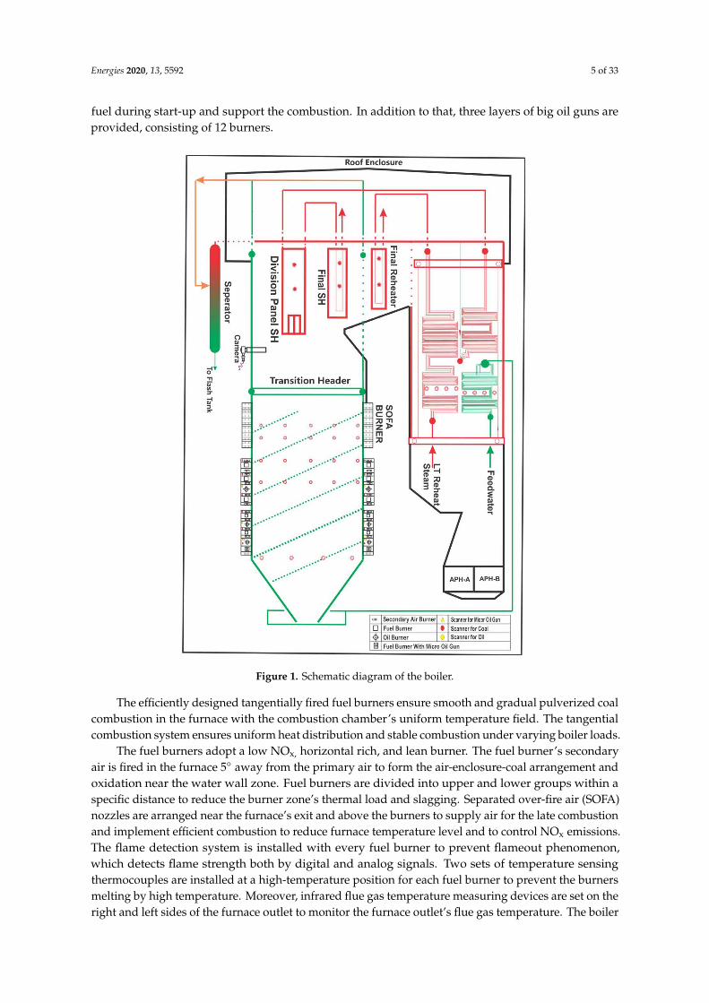
fuel during start-up and support the combustion. In addition to that, three layers of big oil guns areprovided, consisting of 12 burners.Energies 2020, 13, x FOR PEER REVIEW 5 of 35
Figure 1. Schematic diagram of the boiler.
The boiler furnace consists of diaphragm walls designed to improve the wall water tightness and bear the high structural loads. The lower furnace water walls and hopper adopt spiral coils and have enough cooling capacity under different boiler loads to effectively compensate for the thermal deviation of furnace circumambient. Above the spiral tubes, vertical tubes are used to ensure the heat transfer for fast response characteristics. The intermediary mixing header used for the transition between spiral tubes and vertical tubes also balances the pressure across four sides of water walls.
The furnace and fuel burners’ operation is synchronized to ensure the flame burning until burnout, higher combustion efficiency, and minimal NOx formation. The boiler’s burning system is equipped with a medium-speed direct-fired pulverizing system with cold and hot primary air. Twenty-four direct-flow fuel burners are arranged, four at the corners in a layer, and a total of six layers for six coal mills. The fuel burner at the bottom of the furnace is provided with a micro oil gun system to save fuel during start-up and support the combustion. In addition to that, three layers of big oil guns are provided, consisting of 12 burners.
The efficiently designed tangentially fired fuel burners ensure smooth and gradual pulverized coal combustion in the furnace with the combustion chamber’s uniform temperature field. The tangential combustion system ensures uniform heat distribution and stable combustion under varying boiler loads.
The fuel burners adopt a low NOx, horizontal rich, and lean burner. The fuel burner’s secondary air is fired in the furnace 5° away from the primary air to form the air-enclosure-coal arrangement
Figure 1. Schematic diagram of the boiler.
The efficiently designed tangentially fired fuel burners ensure smooth and gradual pulverized coalcombustion in the furnace with the combustion chamber’s uniform temperature field. The tangentialcombustion system ensures uniform heat distribution and stable combustion under varying boiler loads.
The fuel burners adopt a low NOx, horizontal rich, and lean burner. The fuel burner’s secondaryair is fired in the furnace 5◦ away from the primary air to form the air-enclosure-coal arrangement andoxidation near the water wall zone. Fuel burners are divided into upper and lower groups within aspecific distance to reduce the burner zone’s thermal load and slagging. Separated over-fire air (SOFA)nozzles are arranged near the furnace’s exit and above the burners to supply air for the late combustionand implement efficient combustion to reduce furnace temperature level and to control NOx emissions.The flame detection system is installed with every fuel burner to prevent flameout phenomenon,which detects flame strength both by digital and analog signals. Two sets of temperature sensingthermocouples are installed at a high-temperature position for each fuel burner to prevent the burnersmelting by high temperature. Moreover, infrared flue gas temperature measuring devices are set on theright and left sides of the furnace outlet to monitor the furnace outlet’s flue gas temperature. The boiler
Energies 2020, 13, 5592 6 of 33
is also equipped with the ultrasonic leakage detection system, and the flame observation cameras onboth sides of the boiler monitor the combustion. It is necessary to mention that the advanced andreliable combustion control systems installed at the power plant ensure the boiler’s stable and reliableoperation for the power generation. The manufacturer designed the boiler’s operating parameters atboiler maximum continuous rating (BMCR), listed in Table 1.
Table 1. Designed operating parameters of the boiler.
Parameters Unit BMCR Load
Superheated steam flow t/h 2118Superheater outlet steam pressure MPa 25.4
Superheater outlet steam temperature ◦C 571Reheat steam flow t/h 1752
Reheater steam inlet pressure MPa 5.6Reheater steam outlet pressure MPa 5.4
Reheater steam inlet temperature ◦C 345Reheater steam outlet temperature ◦C 569
Feed-water pressure MPa 29Feed-water temperature ◦C 300
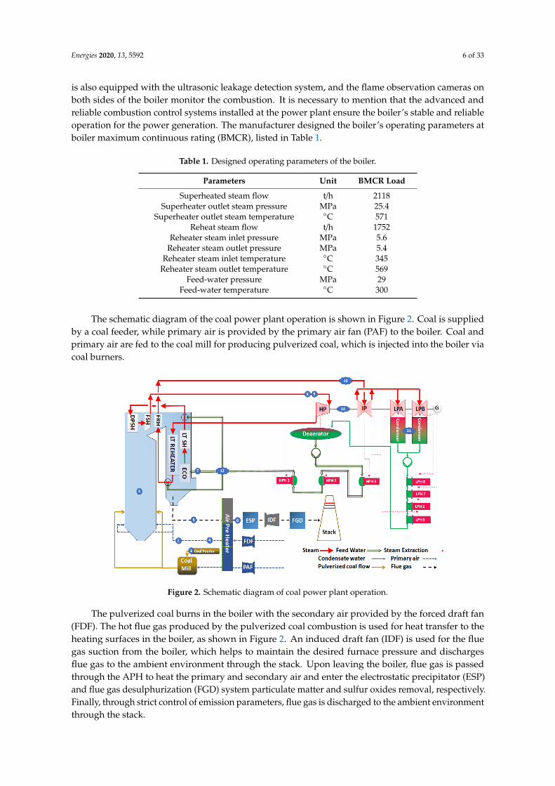
The schematic diagram of the coal power plant operation is shown in Figure 2. Coal is suppliedby a coal feeder, while primary air is provided by the primary air fan (PAF) to the boiler. Coal andprimary air are fed to the coal mill for producing pulverized coal, which is injected into the boiler viacoal burners.
Energies 2020, 13, x FOR PEER REVIEW 6 of 35
and oxidation near the water wall zone. Fuel burners are divided into upper and lower groups within a specific distance to reduce the burner zone’s thermal load and slagging. Separated over-fire air (SOFA) nozzles are arranged near the furnace’s exit and above the burners to supply air for the late combustion and implement efficient combustion to reduce furnace temperature level and to control NOx emissions. The flame detection system is installed with every fuel burner to prevent flameout phenomenon, which detects flame strength both by digital and analog signals. Two sets of temperature sensing thermocouples are installed at a high-temperature position for each fuel burner to prevent the burners melting by high temperature. Moreover, infrared flue gas temperature measuring devices are set on the right and left sides of the furnace outlet to monitor the furnace outlet’s flue gas temperature. The boiler is also equipped with the ultrasonic leakage detection system, and the flame observation cameras on both sides of the boiler monitor the combustion. It is necessary to mention that the advanced and reliable combustion control systems installed at the power plant ensure the boiler’s stable and reliable operation for the power generation. The manufacturer designed the boiler’s operating parameters at boiler maximum continuous rating (BMCR), listed in Table 1.
Table 1. Designed operating parameters of the boiler.
Parameters Unit BMCR Load Superheated steam flow t/h 2118
Superheater outlet steam pressure MPa 25.4 Superheater outlet steam temperature °C 571
Reheat steam flow t/h 1752 Reheater steam inlet pressure MPa 5.6
Reheater steam outlet pressure MPa 5.4 Reheater steam inlet temperature °C 345
Reheater steam outlet temperature °C 569 Feed-water pressure MPa 29
Feed-water temperature °C 300
The schematic diagram of the coal power plant operation is shown in Figure 2. Coal is supplied by a coal feeder, while primary air is provided by the primary air fan (PAF) to the boiler. Coal and primary air are fed to the coal mill for producing pulverized coal, which is injected into the boiler via coal burners.
Figure 2. Schematic diagram of coal power plant operation. Figure 2. Schematic diagram of coal power plant operation.
The pulverized coal burns in the boiler with the secondary air provided by the forced draft fan(FDF). The hot flue gas produced by the pulverized coal combustion is used for heat transfer to theheating surfaces in the boiler, as shown in Figure 2. An induced draft fan (IDF) is used for the fluegas suction from the boiler, which helps to maintain the desired furnace pressure and dischargesflue gas to the ambient environment through the stack. Upon leaving the boiler, flue gas is passedthrough the APH to heat the primary and secondary air and enter the electrostatic precipitator (ESP)and flue gas desulphurization (FGD) system particulate matter and sulfur oxides removal, respectively.Finally, through strict control of emission parameters, flue gas is discharged to the ambient environmentthrough the stack.
Energies 2020, 13, 5592 7 of 33
Feed-water can be considered the power plant’s blood and is converted to superheated steam inthe boiler. The condensate pump directs feed-water, now also called condensate water in the condenser,to the low-pressure heaters (LPH) for the feed-water heating. After passing through the LPH, feed-wateris passed through a deaerator where deoxygenation is applied to the feed-water. The feed-water pumpbuilds up the feed-water pressure and forces it to the series of high-pressure heaters (HPH) for furtherfeed-water heating. The steam extractions heat feed-water in the HPH and LPH from high-pressure(HP) and intermediate-pressure (IP) turbines. After passing through the HPH, feed-water passesthrough a series of heating surfaces like the economizer (ECO), low-temperature superheater (LTSH),division platen superheater (DPSH), and the final superheater (FSH), etc. for producing superheatedmain steam by the heat transfer from the flue gas. The superheated main steam is expanded in theHP turbine, where its temperature and pressure are dropped during expansion. After leaving theHP turbine, steam is directed to the low-temperature re-heater (LT REHEATER) and final re-heater(FRH) for reheating the steam. Attemperation water flow is used to control the temperature of themain steam and reheat steam. The reheat steam is expanded in the IP turbine and is directed to low-pressure (LP) turbines A and B for further expansion. The steam, after expanding in LPA and LPBturbines, is condensed to condensate water in the condenser, and the cycle continues. The expansion ofsuperheated and reheated steam in HP, IP, and LP turbines is used for the rotor rotation, coupled withthe generator (G) for electricity generation.
The Sahiwal coal power plant was commissioned in 2017 and has been operational and integratedwith the national grid since then. It is equipped with state-of-the-art measuring sensors as well asan SIS data storage system. All the sensors measuring the control variables involved in this studyare hard sensors measuring the power plant’s different operating parameters. The data generatedconstitute a large number of variables, with each variable having randomly distributed values. It hasbeen extensively reported in the literature that mining causal relationships out of such data is beyondthe capability of any type of multi-variate regression technique. AI-based data analytic techniquesperform significantly better for modeling such scenarios [39,58]. The sensors’ location for measuringthe power plant’s different operating parameters is shown with numbers in Figure 2. The sensorsmake and model numbers are mentioned in Table 2.
Table 2. Details of sensors measuring the control variables.
Sensors Make Model Number
Coal flow rate Vishay Precision Group (USA) 3410Air flow rate Siemens (Germany) 7MF4433-1BA22-2AB6-Z
Furnace pressure Siemens (Germany) 7MF4433-1DA22-2AB6APH air outlet temperature Anhui Tiankang (China) Thermocouple WRNR2 (K type)
% O2 in flue gas at boiler outlet Walsn (Canada) 0AM-800-RAPH outlet flue gas temperature Anhui Tiankang (China) Thermocouple WRNR2 (K type)
Feed-water temperature WIKAI (China) Thermocouple TC10-3(IEC 60584) (K type)Main steam pressure Siemens (Germany) 7MF4033-1GA50-2AB6-Z
Main steam temperature Anhui Tiankang (China) Thermocouple WRNK2 (K type)Reheat steam temperature Anhui Tiankang (China) Thermocouple WRNK2 (K type)
Condenser vacuumSiemens
STTRANS D PS III (Germany) 7MF4233-1GA50-2AB6-ZAttemperation water flow rate Siemens (Germany) 7MF4533-1FA32-2AB6-Z
Turbine speed Braun (Germany) A5S
3. AI-Based Data Visualization and Process Modeling
AI-based process models are developed to learn the complex, non-linear, and interactingrelationship between the system’s input and output variables [59–61]. ANN and LSSVM are consideredthe most efficient approximation tools of AI and can generalize the relationship between input andoutput variables. These AI tools also have the proven ability to mine the hidden details in the trainingdata, thereby ensure their reliable applications in real-world problems [40,62,63].
Energies 2020, 13, 5592 8 of 33
3.1. Variables Selection for AI Process Modeling
In this paper, thirteen control variables were initially selected to model the 660 MWe supercriticalcoal power plant’s ηthermal in Sahiwal, Pakistan. The variables were selected based upon therecommendation of experienced plant managers of the power plant and a comprehensive literaturereview [33,64–68]. Some control variables were controllable by the operator, e.g., the main steamtemperature (MST), reheat steam temperature (RST), and oxygen content in flue gas at the boiler outlet(O2). On the other hand, some control variables were uncontrollable during the power plant operation,e.g., turbine speed (N). The coal properties measured under the air-dried basis are listed in Table 3.
Table 3. Properties of coal (air-dried basis).
LHVMJ/kg Properties of Coal/wt.%
24.23Moisture Volatile Mater Ash Sulfur Fixed Carbon
2.5 23.73 16.6 0.55 57.66
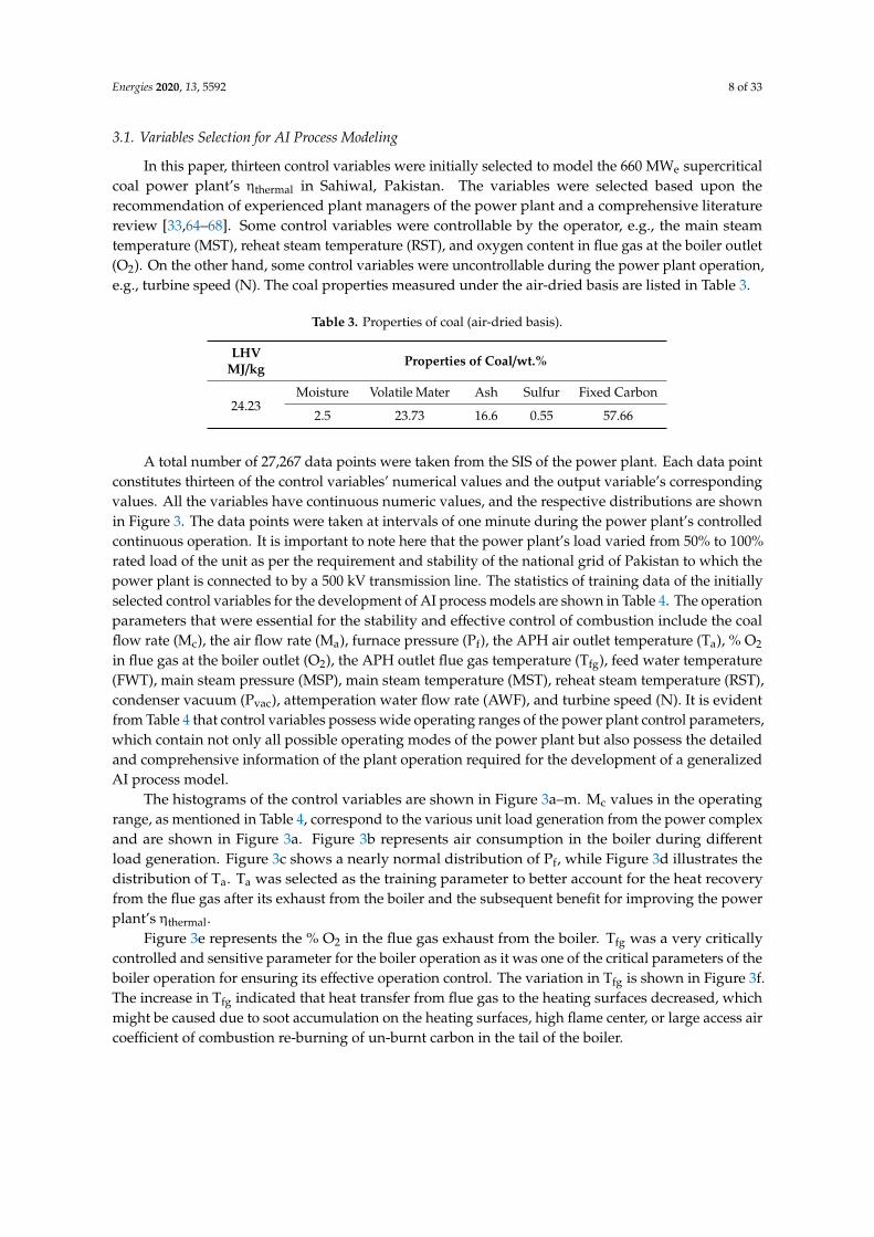
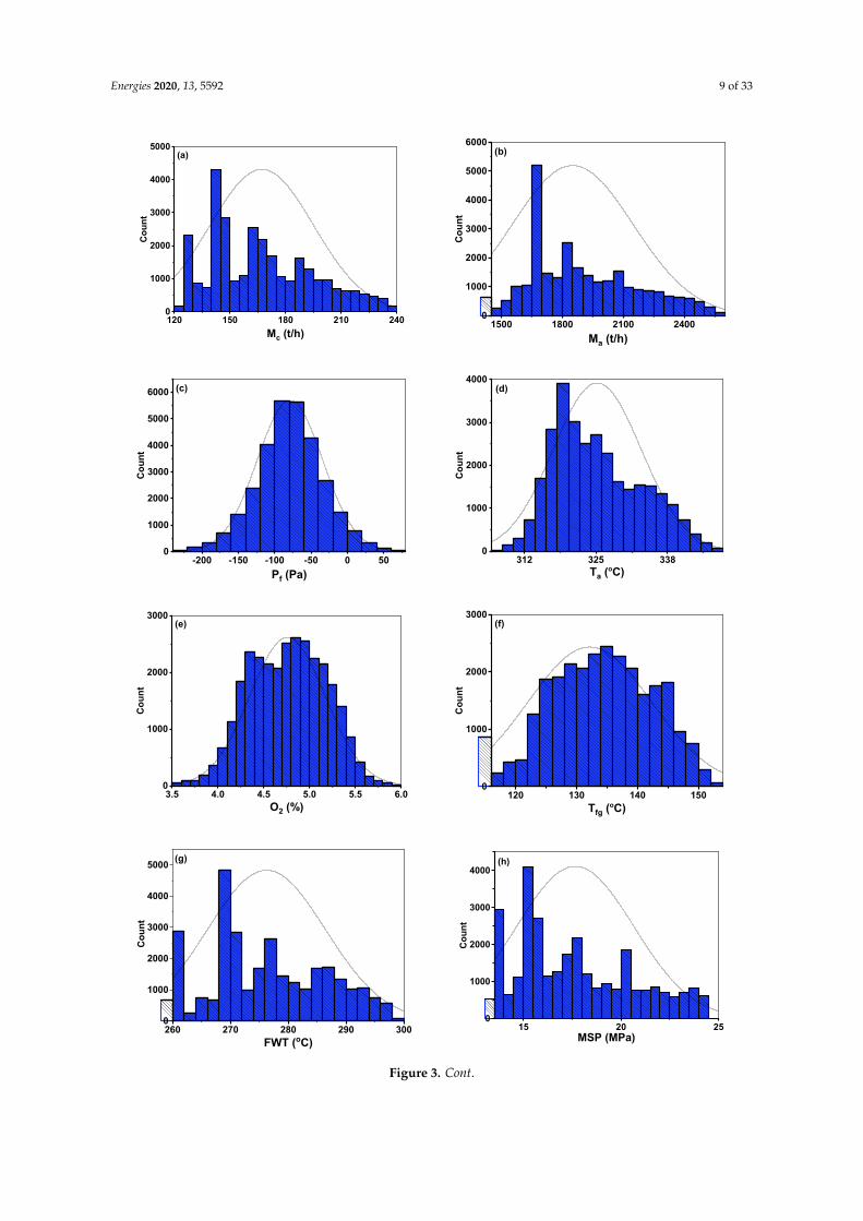
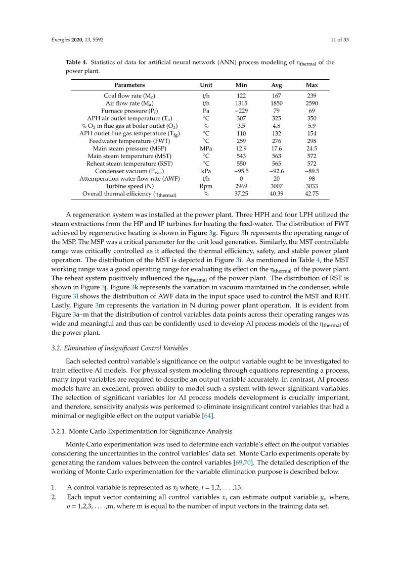
A total number of 27,267 data points were taken from the SIS of the power plant. Each data pointconstitutes thirteen of the control variables’ numerical values and the output variable’s correspondingvalues. All the variables have continuous numeric values, and the respective distributions are shownin Figure 3. The data points were taken at intervals of one minute during the power plant’s controlledcontinuous operation. It is important to note here that the power plant’s load varied from 50% to 100%rated load of the unit as per the requirement and stability of the national grid of Pakistan to which thepower plant is connected to by a 500 kV transmission line. The statistics of training data of the initiallyselected control variables for the development of AI process models are shown in Table 4. The operationparameters that were essential for the stability and effective control of combustion include the coalflow rate (Mc), the air flow rate (Ma), furnace pressure (Pf), the APH air outlet temperature (Ta), % O2
in flue gas at the boiler outlet (O2), the APH outlet flue gas temperature (Tfg), feed water temperature(FWT), main steam pressure (MSP), main steam temperature (MST), reheat steam temperature (RST),condenser vacuum (Pvac), attemperation water flow rate (AWF), and turbine speed (N). It is evidentfrom Table 4 that control variables possess wide operating ranges of the power plant control parameters,which contain not only all possible operating modes of the power plant but also possess the detailedand comprehensive information of the plant operation required for the development of a generalizedAI process model.
The histograms of the control variables are shown in Figure 3a–m. Mc values in the operatingrange, as mentioned in Table 4, correspond to the various unit load generation from the power complexand are shown in Figure 3a. Figure 3b represents air consumption in the boiler during differentload generation. Figure 3c shows a nearly normal distribution of Pf, while Figure 3d illustrates thedistribution of Ta. Ta was selected as the training parameter to better account for the heat recoveryfrom the flue gas after its exhaust from the boiler and the subsequent benefit for improving the powerplant’s ηthermal.
Figure 3e represents the % O2 in the flue gas exhaust from the boiler. Tfg was a very criticallycontrolled and sensitive parameter for the boiler operation as it was one of the critical parameters of theboiler operation for ensuring its effective operation control. The variation in Tfg is shown in Figure 3f.The increase in Tfg indicated that heat transfer from flue gas to the heating surfaces decreased, whichmight be caused due to soot accumulation on the heating surfaces, high flame center, or large access aircoefficient of combustion re-burning of un-burnt carbon in the tail of the boiler.
Energies 2020, 13, 5592 9 of 33Energies 2020, 13, x FOR PEER REVIEW 9 of 35
120 150 180 210 2400
1000
2000
3000
4000
5000(a)
C
ount
Mc (t/h)1500 1800 2100 2400
0
1000
2000
3000
4000
5000
6000(b)
Coun
t
Ma (t/h)
-200 -150 -100 -50 0 500
1000
2000
3000
4000
5000
6000
Cou
nt
Pf (Pa)
(c)
312 325 3380
1000
2000
3000
4000(d)
Cou
nt
Ta (oC)
3.5 4.0 4.5 5.0 5.5 6.00
1000
2000
3000(e)
Cou
nt
O2 (%)120 130 140 150
0
1000
2000
3000(f)
Cou
nt
Tfg (oC)
260 270 280 290 3000
1000
2000
3000
4000
5000 (g)
Cou
nt
FWT (oC)15 20 25
0
1000
2000
3000
4000(h)
Cou
nt
MSP (MPa)
Figure 3. Cont.
Energies 2020, 13, 5592 10 of 33Energies 2020, 13, x FOR PEER REVIEW 10 of 35
Figure 3. Histograms of initially selected control variables, (a) coal flow rate (Mc), (b) the air flow rate (Ma), (c) furnace pressure (Pf), (d) the APH air outlet temperature (Ta), (e) % O2 in flue gas at the boiler outlet (O2), (f) the APH outlet flue gas temperature (Tfg), (g) feed water temperature (FWT), (h) main steam pressure (MSP), (i) main steam temperature (MST), (j) reheat steam temperature (RST), (k) condenser vacuum (Pvac), (l) attemperation water flow rate (AWF), (m) turbine speed (N).
Table 4. Statistics of data for artificial neural network (ANN) process modeling of ηthermal of the power plant.
Parameters Unit Min Avg Max Coal flow rate (Mc) t/h 122 167 239 Air flow rate (Ma) t/h 1315 1850 2590
Furnace pressure (Pf) Pa −229 79 69 APH air outlet temperature (Ta) °C 307 325 350
% O2 in flue gas at boiler outlet (O2) % 3.5 4.8 5.9 APH outlet flue gas temperature (Tfg) °C 110 132 154
Feedwater temperature (FWT) °C 259 276 298
550 560 5700
2000
4000
6000
(i)
C
ount
MST (oC)552 558 564 570
0
1000
2000
3000
4000
5000(j)
Cou
nt
RST (oC)
-94 -93 -92 -91 -900
1000
2000
3000(k)
Cou
nt
Pvac (kPa) 0 15 30 45 60 75 900
2000
4000
6000
(l)
Cou
nt
AWF (t/h)
2970 2980 2990 3000 3010 3020 30300
1000
2000
3000
4000(m)
Cou
nt
N (Rpm)
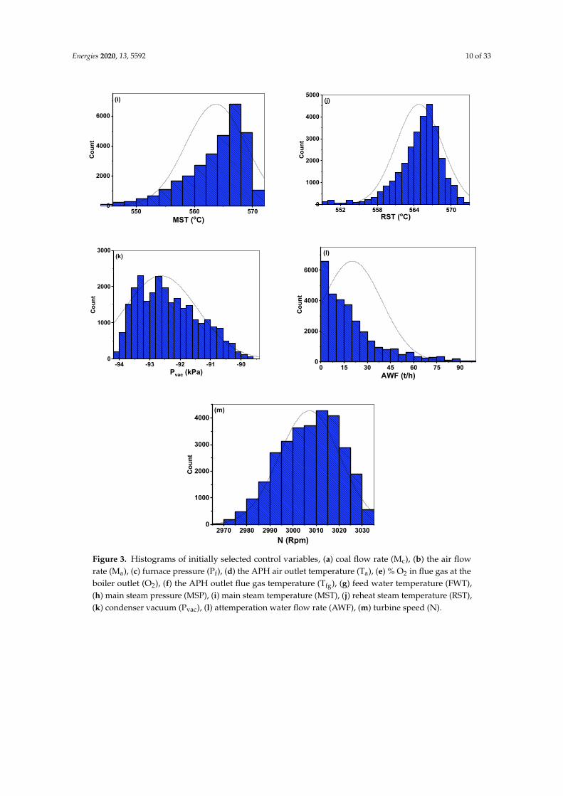
Figure 3. Histograms of initially selected control variables, (a) coal flow rate (Mc), (b) the air flowrate (Ma), (c) furnace pressure (Pf), (d) the APH air outlet temperature (Ta), (e) % O2 in flue gas at theboiler outlet (O2), (f) the APH outlet flue gas temperature (Tfg), (g) feed water temperature (FWT),(h) main steam pressure (MSP), (i) main steam temperature (MST), (j) reheat steam temperature (RST),(k) condenser vacuum (Pvac), (l) attemperation water flow rate (AWF), (m) turbine speed (N).
Energies 2020, 13, 5592 11 of 33
Table 4. Statistics of data for artificial neural network (ANN) process modeling of ηthermal of thepower plant.
Parameters Unit Min Avg Max
Coal flow rate (Mc) t/h 122 167 239Air flow rate (Ma) t/h 1315 1850 2590
Furnace pressure (Pf) Pa −229 79 69APH air outlet temperature (Ta) ◦C 307 325 350
% O2 in flue gas at boiler outlet (O2) % 3.5 4.8 5.9APH outlet flue gas temperature (Tfg) ◦C 110 132 154
Feedwater temperature (FWT) ◦C 259 276 298Main steam pressure (MSP) MPa 12.9 17.6 24.5
Main steam temperature (MST) ◦C 543 563 572Reheat steam temperature (RST) ◦C 550 565 572
Condenser vacuum (Pvac) kPa −95.5 −92.6 −89.5Attemperation water flow rate (AWF) t/h 0 20 98
Turbine speed (N) Rpm 2969 3007 3033Overall thermal efficiency (ηthermal) % 37.25 40.39 42.75
A regeneration system was installed at the power plant. Three HPH and four LPH utilized thesteam extractions from the HP and IP turbines for heating the feed-water. The distribution of FWTachieved by regenerative heating is shown in Figure 3g. Figure 3h represents the operating range ofthe MSP. The MSP was a critical parameter for the unit load generation. Similarly, the MST controllablerange was critically controlled as it affected the thermal efficiency, safety, and stable power plantoperation. The distribution of the MST is depicted in Figure 3i. As mentioned in Table 4, the MSTworking range was a good operating range for evaluating its effect on the ηthermal of the power plant.The reheat system positively influenced the ηthermal of the power plant. The distribution of RST isshown in Figure 3j. Figure 3k represents the variation in vacuum maintained in the condenser, whileFigure 3l shows the distribution of AWF data in the input space used to control the MST and RHT.Lastly, Figure 3m represents the variation in N during power plant operation. It is evident fromFigure 3a–m that the distribution of control variables data points across their operating ranges waswide and meaningful and thus can be confidently used to develop AI process models of the ηthermal ofthe power plant.
3.2. Elimination of Insignificant Control Variables
Each selected control variable’s significance on the output variable ought to be investigated totrain effective AI models. For physical system modeling through equations representing a process,many input variables are required to describe an output variable accurately. In contrast, AI processmodels have an excellent, proven ability to model such a system with fewer significant variables.The selection of significant variables for AI process models development is crucially important,and therefore, sensitivity analysis was performed to eliminate insignificant control variables that had aminimal or negligible effect on the output variable [64].
3.2.1. Monte Carlo Experimentation for Significance Analysis
Monte Carlo experimentation was used to determine each variable’s effect on the output variablesconsidering the uncertainties in the control variables’ data set. Monte Carlo experiments operate bygenerating the random values between the control variables [69,70]. The detailed description of theworking of Monte Carlo experimentation for the variable elimination purpose is described below.
1. A control variable is represented as xi where, i = 1,2, . . . ,13.2. Each input vector containing all control variables xi can estimate output variable yo where,
o = 1,2,3, . . . .,m, where m is equal to the number of input vectors in the training data set.
Energies 2020, 13, 5592 12 of 33
3. The Monte Carlo experimentation can be illustrated by considering a control variable xi andall other control variables as xj, were (i , j). As an example, let xi = x1 and xj = x2, . . . .., x13,where (i , j).
4. Create n equal divisions (k) for xi between its range (ximax–ximin) where, k = 1,2, . . . ,n.5. Generate M random values for each division k (k = 1,2, 3, . . . , n) by keeping xik, at a constant value.
All other input control variables for these M replications are generated so that the probability (P)of any value (u) between xjmin and xjmax is equal. The Mth input vector will be [x1kM, x2u, x3u, x4u. . . , x13u], and the corresponding output will be yokM.
6. The output value yokM is obtained by ANN and LSSVM prediction for the Mth input vector[x1kM, x2u, x3u, x4u, . . . , x13u]. Compute a mean value (µ) for each yokM having M replications,which will give yok for each xik.
7. Repeat step number iii to step number vi for all remaining control variables8. Compute ∆yi where ∆yi = yokmax − yokmin for all control variables xi and compute the summation
value Y for all ∆yi
Y =∑13
i=1∆yi (1)
9. Compute the percentage significance (ri) of each xi by dividing ∆yi with Y and multiplying itby 100
ri =
(∆yi
Y
)× 100 (2)
The least insignificant variables obtained from Monte Carlo experimentation performed on ANNand LSSVM are shown later in the paper. The elimination of insignificant control variables is essentialto develop a useful process model based on ANN and LSSVM. This elimination of insignificant controlvariables is usually obtained by coupling an algorithm (in our case, Monte Carlo experimentation)to ANN and LSSVM. Therefore, the significance of control variables obtained by Monte Carloexperimentation is confirmed with the Interval Adjoint Significance Analysis (IASA) method.
3.2.2. Interval Adjoint Significance Analysis (IASA)
The sensitivity-based method is advantageous in finding out the significance of control variablesin a given sample [71,72]. The deviation in output ∆y caused by the deviations in the input is definedas sensitivity [71]. By finding out the sensitivities of given control variables, we can find out theirsignificance. In this sub-section, intervals are represented by uppercase letters (e.g., A, B, C, . . .) andscalars are represented by lower case letters (e.g., a, b, c, . . .). The interval is defined as X =
[xl, xu
],
where l and u represent the lower and upper limit of the interval, respectively.Interval arithmetic (IA) [73] is used to evaluate a function f [X] in a given range over a domain
and it gives us a guaranteed enclosure f [X] ⊇{f [x]
∣∣∣x 3 [X]}
that contains all possible values of f (x)for x 3 [X]. Similarly, interval evaluation yield enclosures [Vi] for all intermediate variables Vi.Reverse mode (also; adjoint mode) of algorithmic differentiation (AD) [74,75] can be applied here toevaluate this interval function. Because reverse mode AD not only computes the primal values ofintermediate and output variables, but it also computes their derivatives ( δY
δXi, δYδVi
). Significance can
also be calculated here by taking the absolute maximum of first-order derivative max∣∣∣∇[xi]
[y]∣∣∣ of an
input interval Xi and multiplying it by the width w[Xi] = xui − xl
i of that interval [76].
SY(Xi) = w[Xi] ∗max∣∣∣∇[xi]
[y]∣∣∣ (3)
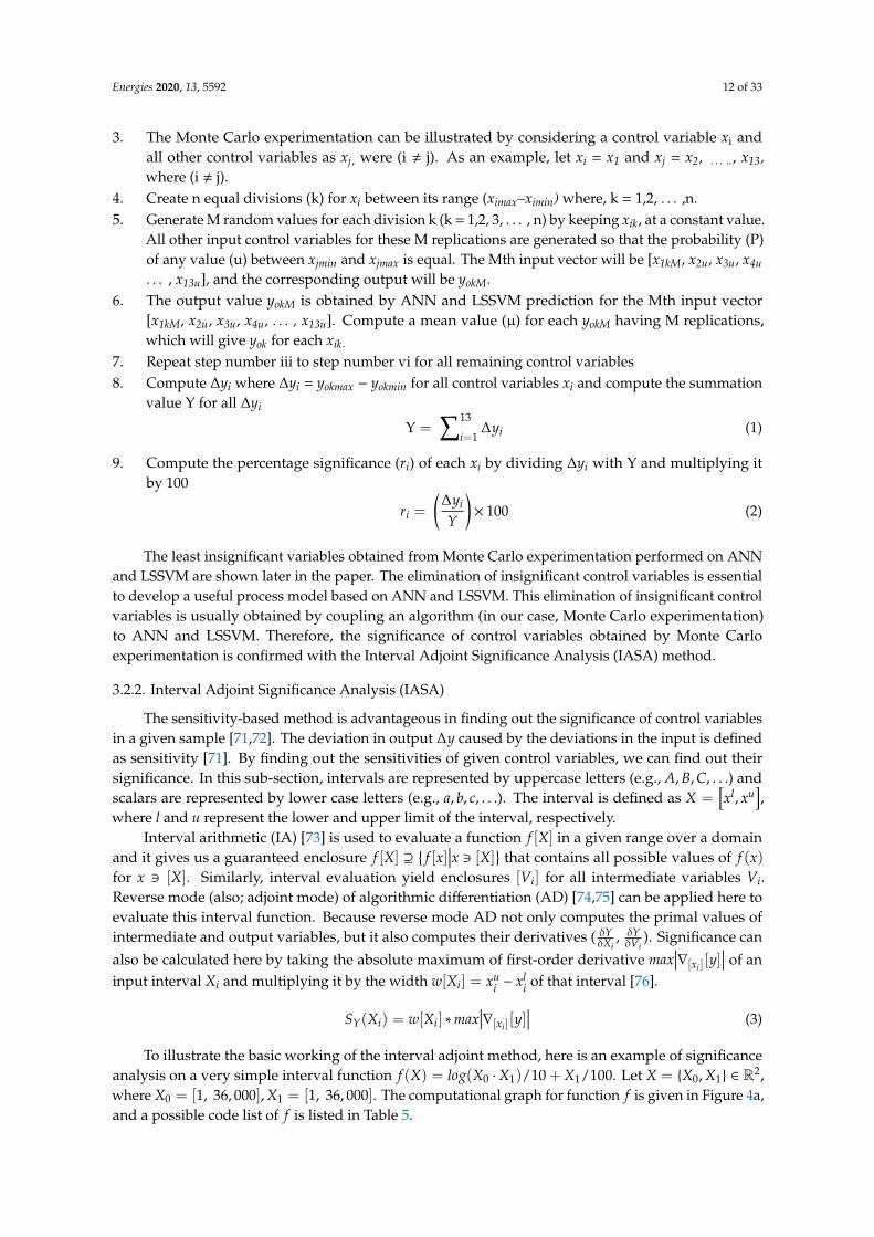
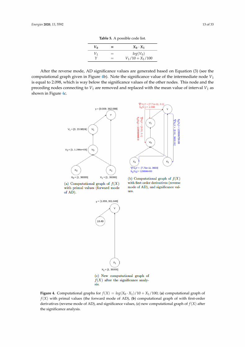
To illustrate the basic working of the interval adjoint method, here is an example of significanceanalysis on a very simple interval function f (X) = log(X0 ·X1)/10 + X1/100. Let X = {X0, X1} ∈ R2,where X0 = [1, 36, 000], X1 = [1, 36, 000]. The computational graph for function f is given in Figure 4a,and a possible code list of f is listed in Table 5.
Energies 2020, 13, 5592 13 of 33
Table 5. A possible code list.
V0 = X0 · X1
V1 = log(V0)Y = V1/10 + X1/100
After the reverse mode, AD significance values are generated based on Equation (3) (see thecomputational graph given in Figure 4b). Note the significance value of the intermediate node V1
is equal to 2.098, which is way below the significance values of the other nodes. This node and thepreceding nodes connecting to V1 are removed and replaced with the mean value of interval V1 asshown in Figure 4c.
Energies 2020, 13, x FOR PEER REVIEW 13 of 35
Table 5. A possible code list. = ⋅ = ( ) = /10 + /100
After the reverse mode, AD significance values are generated based on Equation (3) (see the computational graph given in Figure 4b). Note the significance value of the intermediate node is equal to 2.098, which is way below the significance values of the other nodes. This node and the preceding nodes connecting to are removed and replaced with the mean value of interval as shown in Figure 4c.
Figure 4. Computational graphs for ( ) = ( ⋅ )/10 + /100; (a) computational graph of ( )with primal values (the forward mode of AD), (b) computational graph of with first-order derivatives (reverse mode of AD), and significance values, (c) new computational graph of ( ) after the significance analysis.
Figure 4. Computational graphs for f (X) = log(X0 ·X1)/10 + X1/100; (a) computational graph off (X) with primal values (the forward mode of AD), (b) computational graph of with first-orderderivatives (reverse mode of AD), and significance values, (c) new computational graph of f (X) afterthe significance analysis.
Energies 2020, 13, 5592 14 of 33
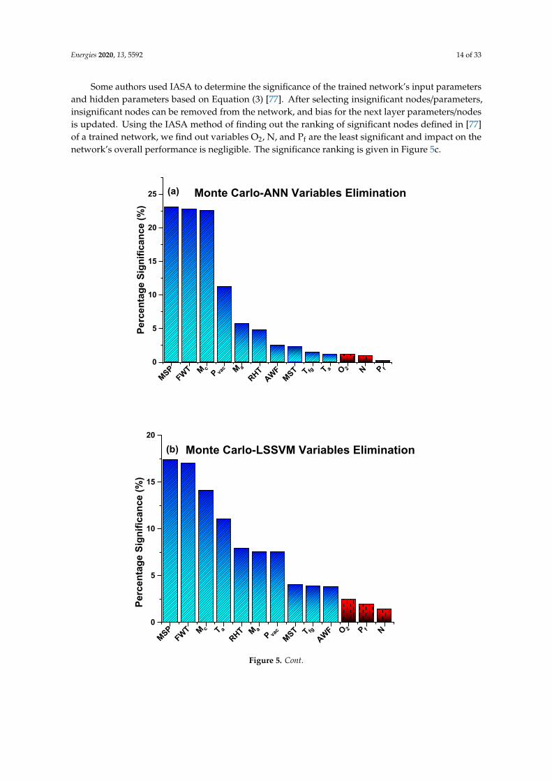
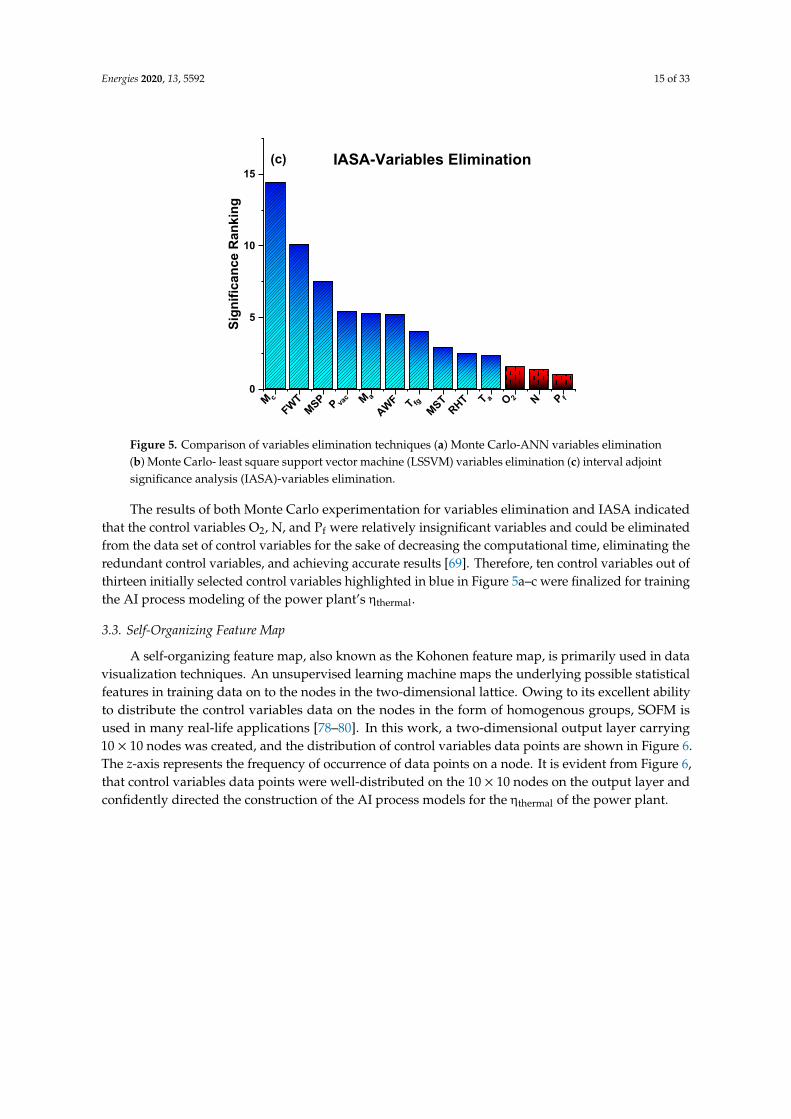
Some authors used IASA to determine the significance of the trained network’s input parametersand hidden parameters based on Equation (3) [77]. After selecting insignificant nodes/parameters,insignificant nodes can be removed from the network, and bias for the next layer parameters/nodesis updated. Using the IASA method of finding out the ranking of significant nodes defined in [77]of a trained network, we find out variables O2, N, and Pf are the least significant and impact on thenetwork’s overall performance is negligible. The significance ranking is given in Figure 5c.
Energies 2020, 13, x FOR PEER REVIEW 14 of 35
Some authors used IASA to determine the significance of the trained network’s input parameters and hidden parameters based on Equation (3) [77]. After selecting insignificant nodes/parameters, insignificant nodes can be removed from the network, and bias for the next layer parameters/nodes is updated. Using the IASA method of finding out the ranking of significant nodes defined in [77] of a trained network, we find out variables O2, N, and Pf are the least significant and impact on the network’s overall performance is negligible. The significance ranking is given in Figure 5c.
0
5
10
15
20
25
P fNO 2T aT fg
MSTAWF
RHTM aP va
cM c
FWT
Perc
enta
ge S
igni
fican
ce (%
)
MSP
Monte Carlo-ANN Variables Elimination(a)
0
5
10
15
20
Monte Carlo-LSSVM Variables Elimination
Perc
enta
ge S
igni
fican
ce (%
)
P f NO 2T a T fg
MSTAWF
RHT M aP va
cM c
FWTMSP
(b)
Figure 5. Cont.
Energies 2020, 13, 5592 15 of 33Energies 2020, 13, x FOR PEER REVIEW 15 of 35
Figure 5. Comparison of variables elimination techniques (a) Monte Carlo-ANN variables elimination (b) Monte Carlo- least square support vector machine (LSSVM) variables elimination (c) interval adjoint significance analysis (IASA)-variables elimination.
The results of both Monte Carlo experimentation for variables elimination and IASA indicated that the control variables O2, N, and Pf were relatively insignificant variables and could be eliminated from the data set of control variables for the sake of decreasing the computational time, eliminating the redundant control variables, and achieving accurate results [69]. Therefore, ten control variables out of thirteen initially selected control variables highlighted in blue in Figure 5a–c were finalized for training the AI process modeling of the power plant’s ηthermal.
3.3. Self-Organizing Feature Map
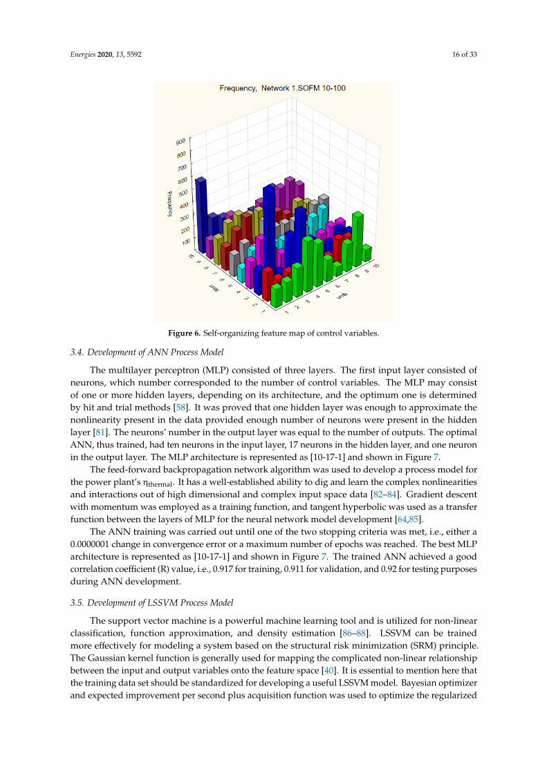
A self-organizing feature map, also known as the Kohonen feature map, is primarily used in data visualization techniques. An unsupervised learning machine maps the underlying possible statistical features in training data on to the nodes in the two-dimensional lattice. Owing to its excellent ability to distribute the control variables data on the nodes in the form of homogenous groups, SOFM is used in many real-life applications [78–80]. In this work, a two-dimensional output layer carrying 10 × 10 nodes was created, and the distribution of control variables data points are shown in Figure 6. The z-axis represents the frequency of occurrence of data points on a node. It is evident from Figure 6, that control variables data points were well-distributed on the 10 × 10 nodes on the output layer and confidently directed the construction of the AI process models for the ηthermal of the power plant.
0
5
10
15
P fNO 2T aT fgMST
AWFRHTM a
P vac
MSPFWT
Sign
ifica
nce
Ran
king
M c
IASA-Variables Elimination(c)
Figure 5. Comparison of variables elimination techniques (a) Monte Carlo-ANN variables elimination(b) Monte Carlo- least square support vector machine (LSSVM) variables elimination (c) interval adjointsignificance analysis (IASA)-variables elimination.
The results of both Monte Carlo experimentation for variables elimination and IASA indicatedthat the control variables O2, N, and Pf were relatively insignificant variables and could be eliminatedfrom the data set of control variables for the sake of decreasing the computational time, eliminating theredundant control variables, and achieving accurate results [69]. Therefore, ten control variables out ofthirteen initially selected control variables highlighted in blue in Figure 5a–c were finalized for trainingthe AI process modeling of the power plant’s ηthermal.
3.3. Self-Organizing Feature Map
A self-organizing feature map, also known as the Kohonen feature map, is primarily used in datavisualization techniques. An unsupervised learning machine maps the underlying possible statisticalfeatures in training data on to the nodes in the two-dimensional lattice. Owing to its excellent abilityto distribute the control variables data on the nodes in the form of homogenous groups, SOFM isused in many real-life applications [78–80]. In this work, a two-dimensional output layer carrying10 × 10 nodes was created, and the distribution of control variables data points are shown in Figure 6.The z-axis represents the frequency of occurrence of data points on a node. It is evident from Figure 6,that control variables data points were well-distributed on the 10 × 10 nodes on the output layer andconfidently directed the construction of the AI process models for the ηthermal of the power plant.
Energies 2020, 13, 5592 16 of 33Energies 2020, 13, x FOR PEER REVIEW 16 of 35
Figure 6. Self-organizing feature map of control variables.
3.4. Development of ANN Process Model
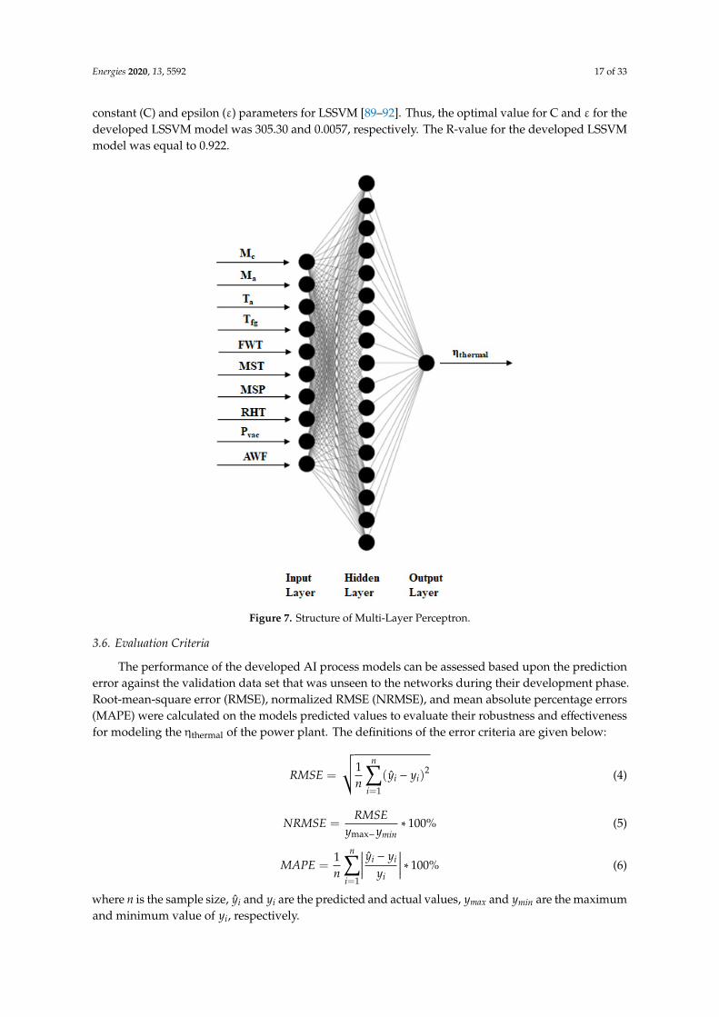
The multilayer perceptron (MLP) consisted of three layers. The first input layer consisted of neurons, which number corresponded to the number of control variables. The MLP may consist of one or more hidden layers, depending on its architecture, and the optimum one is determined by hit and trial methods [58]. It was proved that one hidden layer was enough to approximate the nonlinearity present in the data provided enough number of neurons were present in the hidden layer [81]. The neurons’ number in the output layer was equal to the number of outputs. The optimal ANN, thus trained, had ten neurons in the input layer, 17 neurons in the hidden layer, and one neuron in the output layer. The MLP architecture is represented as [10-17-1] and shown in Figure 7.
Figure 6. Self-organizing feature map of control variables.
3.4. Development of ANN Process Model
The multilayer perceptron (MLP) consisted of three layers. The first input layer consisted ofneurons, which number corresponded to the number of control variables. The MLP may consistof one or more hidden layers, depending on its architecture, and the optimum one is determinedby hit and trial methods [58]. It was proved that one hidden layer was enough to approximate thenonlinearity present in the data provided enough number of neurons were present in the hiddenlayer [81]. The neurons’ number in the output layer was equal to the number of outputs. The optimalANN, thus trained, had ten neurons in the input layer, 17 neurons in the hidden layer, and one neuronin the output layer. The MLP architecture is represented as [10-17-1] and shown in Figure 7.
The feed-forward backpropagation network algorithm was used to develop a process model forthe power plant’s ηthermal. It has a well-established ability to dig and learn the complex nonlinearitiesand interactions out of high dimensional and complex input space data [82–84]. Gradient descentwith momentum was employed as a training function, and tangent hyperbolic was used as a transferfunction between the layers of MLP for the neural network model development [64,85].
The ANN training was carried out until one of the two stopping criteria was met, i.e., either a0.0000001 change in convergence error or a maximum number of epochs was reached. The best MLParchitecture is represented as [10-17-1] and shown in Figure 7. The trained ANN achieved a goodcorrelation coefficient (R) value, i.e., 0.917 for training, 0.911 for validation, and 0.92 for testing purposesduring ANN development.
3.5. Development of LSSVM Process Model
The support vector machine is a powerful machine learning tool and is utilized for non-linearclassification, function approximation, and density estimation [86–88]. LSSVM can be trainedmore effectively for modeling a system based on the structural risk minimization (SRM) principle.The Gaussian kernel function is generally used for mapping the complicated non-linear relationshipbetween the input and output variables onto the feature space [40]. It is essential to mention here thatthe training data set should be standardized for developing a useful LSSVM model. Bayesian optimizerand expected improvement per second plus acquisition function was used to optimize the regularized
Energies 2020, 13, 5592 17 of 33
constant (C) and epsilon (ε) parameters for LSSVM [89–92]. Thus, the optimal value for C and ε for thedeveloped LSSVM model was 305.30 and 0.0057, respectively. The R-value for the developed LSSVMmodel was equal to 0.922.Energies 2020, 13, x FOR PEER REVIEW 17 of 35
Figure 7. Structure of Multi-Layer Perceptron.
The feed-forward backpropagation network algorithm was used to develop a process model for the power plant’s ηthermal. It has a well-established ability to dig and learn the complex nonlinearities and interactions out of high dimensional and complex input space data [82–84]. Gradient descent with momentum was employed as a training function, and tangent hyperbolic was used as a transfer function between the layers of MLP for the neural network model development [64,85].
The ANN training was carried out until one of the two stopping criteria was met, i.e., either a 0.0000001 change in convergence error or a maximum number of epochs was reached. The best MLP architecture is represented as [10-17-1] and shown in Figure 7. The trained ANN achieved a good correlation coefficient (R) value, i.e., 0.917 for training, 0.911 for validation, and 0.92 for testing purposes during ANN development.
3.5. Development of LSSVM Process Model
The support vector machine is a powerful machine learning tool and is utilized for non-linear classification, function approximation, and density estimation [86–88]. LSSVM can be trained more effectively for modeling a system based on the structural risk minimization (SRM) principle. The Gaussian kernel function is generally used for mapping the complicated non-linear relationship between the input and output variables onto the feature space [40]. It is essential to mention here that the training data set should be standardized for developing a useful LSSVM model. Bayesian optimizer and expected improvement per second plus acquisition function was used to optimize the regularized constant (C) and epsilon (ε) parameters for LSSVM [89–92]. Thus, the optimal value for C and ε for the developed LSSVM model was 305.30 and 0.0057, respectively. The R-value for the developed LSSVM model was equal to 0.922.
Figure 7. Structure of Multi-Layer Perceptron.
3.6. Evaluation Criteria
The performance of the developed AI process models can be assessed based upon the predictionerror against the validation data set that was unseen to the networks during their development phase.Root-mean-square error (RMSE), normalized RMSE (NRMSE), and mean absolute percentage errors(MAPE) were calculated on the models predicted values to evaluate their robustness and effectivenessfor modeling the ηthermal of the power plant. The definitions of the error criteria are given below:
RMSE =
√√1n
n∑i=1
(yi − yi)2 (4)
NRMSE =RMSE
ymax−ymin∗ 100% (5)
MAPE =1n
n∑i=1
∣∣∣∣∣ yi − yi
yi
∣∣∣∣∣ ∗ 100% (6)
where n is the sample size, yi and yi are the predicted and actual values, ymax and ymin are the maximumand minimum value of yi, respectively.
Energies 2020, 13, 5592 18 of 33
3.7. External Validation Case of Trained AI Process Models
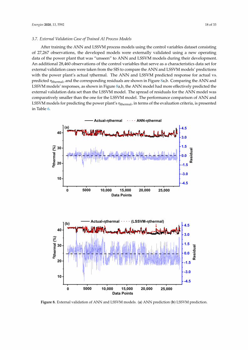
After training the ANN and LSSVM process models using the control variables dataset consistingof 27,267 observations, the developed models were externally validated using a new operatingdata of the power plant that was “unseen” to ANN and LSSVM models during their development.An additional 28,460 observations of the control variables that serve as a characteristics data set forexternal validation cases were taken from the SIS to compare the ANN and LSSVM models’ predictionswith the power plant’s actual ηthermal. The ANN and LSSVM predicted response for actual vs.predicted ηthermal, and the corresponding residuals are shown in Figure 8a,b. Comparing the ANN andLSSVM models’ responses, as shown in Figure 8a,b, the ANN model had more effectively predicted theexternal validation data set than the LSSVM model. The spread of residuals for the ANN model wascomparatively smaller than the one for the LSSVM model. The performance comparison of ANN andLSSVM models for predicting the power plant’s ηthermal, in terms of the evaluation criteria, is presentedin Table 6.
Energies 2020, 13, x FOR PEER REVIEW 19 of 35
Figure 8. External validation of ANN and LSSVM models. (a) ANN prediction (b) LSSVM prediction.
Table 6. Comparison of ANN and LSSVM model prediction performance.
Model RMSE NRMSE MAPE
(%) (%) (%) ANN 0.5051 8.2159 1.016
LSSVM 0.7164 11.6538 1.2819
It is clear from Table 6 that various error estimations, i.e., RMSE, NRMSE, and MAPE for the ANN predicted response was 0.5051%, 8.2159%, and 1.016% respectively, which was lower than the
10
20
30
40
25,00020,00015,00010,0005000
(a)
Res
idua
l
η the
rmal
(%)
Actual-ηthermal ANN-ηthermal
Data Points0
-4.5
-3.0
-1.5
0.0
1.5
3.0
4.5
10
20
30
40
Res
idua
l
η the
rmal
(%)
Actual-ηthermal (LSSVM-ηthermal)
Data Points25,00020,00015,00010,00050000
(b)
-4.5
-3.0
-1.5
0.0
1.5
3.0
4.5
Figure 8. External validation of ANN and LSSVM models. (a) ANN prediction (b) LSSVM prediction.
Energies 2020, 13, 5592 19 of 33
Table 6. Comparison of ANN and LSSVM model prediction performance.
ModelRMSE NRMSE MAPE
(%) (%) (%)
ANN 0.5051 8.2159 1.016LSSVM 0.7164 11.6538 1.2819
It is clear from Table 6 that various error estimations, i.e., RMSE, NRMSE, and MAPE for the ANNpredicted response was 0.5051%, 8.2159%, and 1.016% respectively, which was lower than the onesfor LSSVM model predictions, i.e., 0.7164%, 11.6538%, and 1.2819%, respectively. It confirmed thatthe ANN process model had effectively modeled the power plant’s ηthermal concerning the controlvariables compared to LSSVM. The ANN presented a good generalization ability to model the complexpower plant operation with better network robustness, confirming its superior efficacy for data analysisand decision making.
4. Results and Discussion
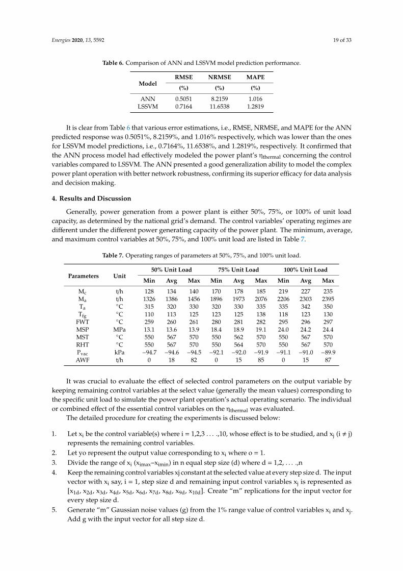
Generally, power generation from a power plant is either 50%, 75%, or 100% of unit loadcapacity, as determined by the national grid’s demand. The control variables’ operating regimes aredifferent under the different power generating capacity of the power plant. The minimum, average,and maximum control variables at 50%, 75%, and 100% unit load are listed in Table 7.
Table 7. Operating ranges of parameters at 50%, 75%, and 100% unit load.
Parameters Unit50% Unit Load 75% Unit Load 100% Unit Load
Min Avg Max Min Avg Max Min Avg Max
Mc t/h 128 134 140 170 178 185 219 227 235Ma t/h 1326 1386 1456 1896 1973 2076 2206 2303 2395Ta
◦C 315 320 330 320 330 335 335 342 350Tfg
◦C 110 113 125 123 125 138 118 123 130FWT ◦C 259 260 261 280 281 282 295 296 297MSP MPa 13.1 13.6 13.9 18.4 18.9 19.1 24.0 24.2 24.4MST ◦C 550 567 570 550 562 570 550 567 570RHT ◦C 550 567 570 550 564 570 550 567 570Pvac kPa −94.7 −94.6 −94.5 −92.1 −92.0 −91.9 −91.1 −91.0 −89.9AWF t/h 0 18 82 0 15 85 0 15 87
It was crucial to evaluate the effect of selected control parameters on the output variable bykeeping remaining control variables at the select value (generally the mean values) corresponding tothe specific unit load to simulate the power plant operation’s actual operating scenario. The individualor combined effect of the essential control variables on the ηthermal was evaluated.
The detailed procedure for creating the experiments is discussed below:
1. Let xi be the control variable(s) where i = 1,2,3 . . . .,10, whose effect is to be studied, and xj (i , j)represents the remaining control variables.
2. Let yo represent the output value corresponding to xi where o = 1.3. Divide the range of xi (ximax–ximin) in n equal step size (d) where d = 1,2, . . . .,n4. Keep the remaining control variables xj constant at the selected value at every step size d. The input
vector with xi say, i = 1, step size d and remaining input control variables xj is represented as[x1d, x2d, x3d, x4d, x5d, x6d, x7d, x8d, x9d, x10d]. Create “m” replications for the input vector forevery step size d.
5. Generate “m” Gaussian noise values (g) from the 1% range value of control variables xi and xj.Add g with the input vector for all step size d.
Energies 2020, 13, 5592 20 of 33
6. Predict the developed ANN process model from an input vector and compute mean (µ) andstandard deviation (σ) of the predicted values yod against xid input vector, which is representedas µyod and σyod relative to xid input vector, respectively.
7. Calculate upper control limit (UCL = µyod + 2* σyod) and lower control limit (LCL = µyod− 2* σyod)and plot mean, UCL and LCL against xi.
4.1. Effect of MST and RST on ηthermal of Power Plant
MST and RST are critically and simultaneously controlled power plant operating parameters.The power production was generally maintained at either 50%, 75%, or 100% unit load, which dependson the connected national grid’s demand and stability. MST and RST parameters under such anoperation scenario should be effectively controlled within the operating control limits to ensureeconomical, safe, and fuel-efficient power production from the power plant.
To evaluate the effect of MST and RST on the power plant’s ηthermal at 50%, 75%, and 100%unit load, MST and RST were varied from 550 to 570 ◦C. The remaining control parameters wereset at the corresponding average values at 50%, 75%, and 100% unit load, as mentioned in Table 7.Thus, the experiments were used to evaluate the combined effect of MST and RST on the powerplant’s ηthermal.
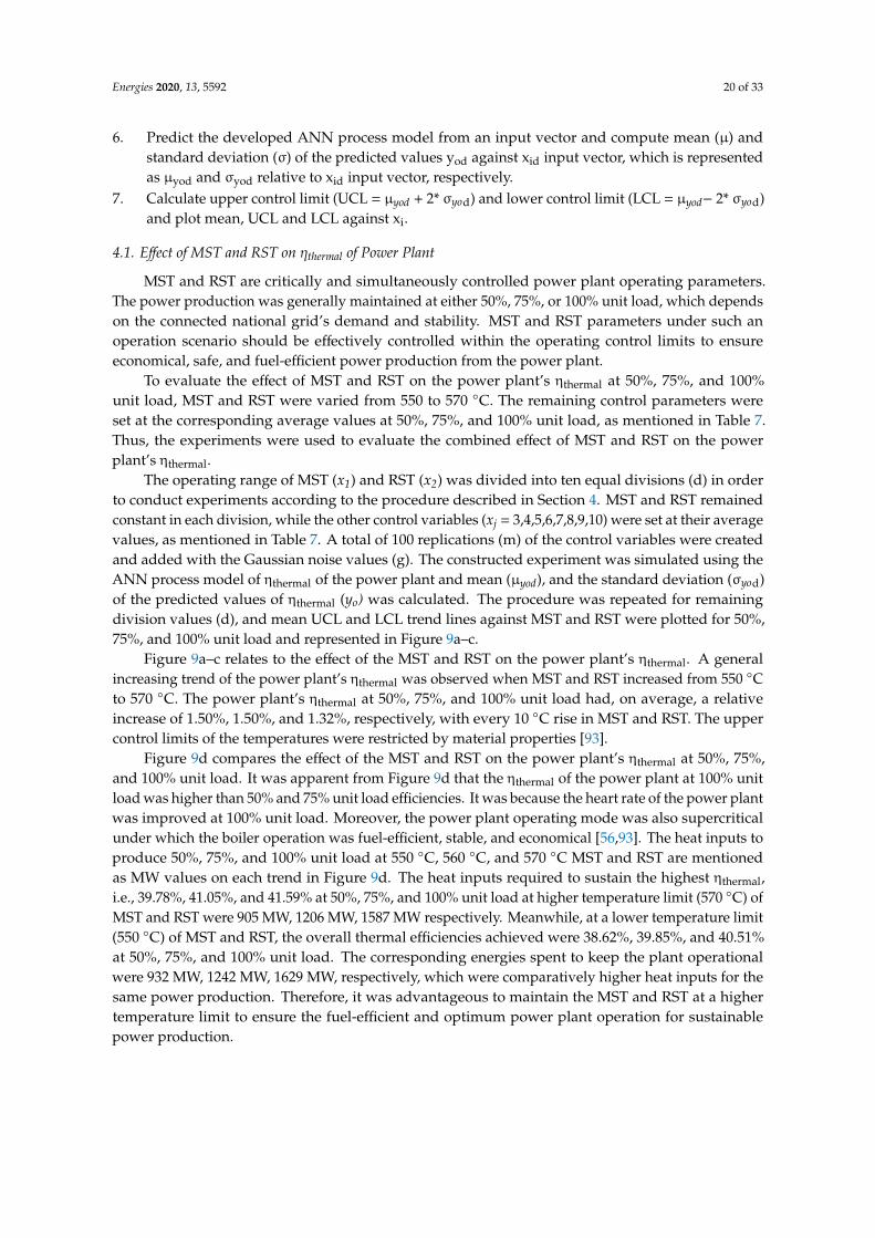
The operating range of MST (x1) and RST (x2) was divided into ten equal divisions (d) in orderto conduct experiments according to the procedure described in Section 4. MST and RST remainedconstant in each division, while the other control variables (xj = 3,4,5,6,7,8,9,10) were set at their averagevalues, as mentioned in Table 7. A total of 100 replications (m) of the control variables were createdand added with the Gaussian noise values (g). The constructed experiment was simulated using theANN process model of ηthermal of the power plant and mean (µyod), and the standard deviation (σyod)of the predicted values of ηthermal (yo) was calculated. The procedure was repeated for remainingdivision values (d), and mean UCL and LCL trend lines against MST and RST were plotted for 50%,75%, and 100% unit load and represented in Figure 9a–c.
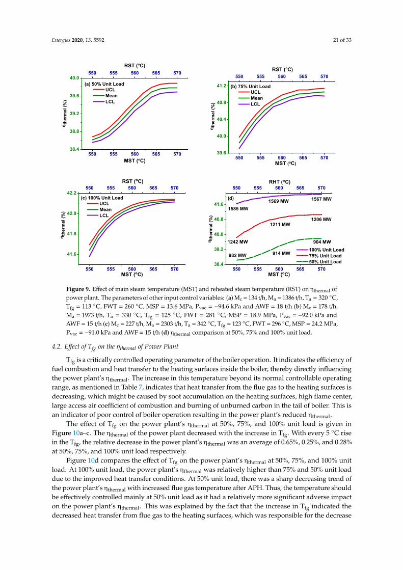
Figure 9a–c relates to the effect of the MST and RST on the power plant’s ηthermal. A generalincreasing trend of the power plant’s ηthermal was observed when MST and RST increased from 550 ◦Cto 570 ◦C. The power plant’s ηthermal at 50%, 75%, and 100% unit load had, on average, a relativeincrease of 1.50%, 1.50%, and 1.32%, respectively, with every 10 ◦C rise in MST and RST. The uppercontrol limits of the temperatures were restricted by material properties [93].
Figure 9d compares the effect of the MST and RST on the power plant’s ηthermal at 50%, 75%,and 100% unit load. It was apparent from Figure 9d that the ηthermal of the power plant at 100% unitload was higher than 50% and 75% unit load efficiencies. It was because the heart rate of the power plantwas improved at 100% unit load. Moreover, the power plant operating mode was also supercriticalunder which the boiler operation was fuel-efficient, stable, and economical [56,93]. The heat inputs toproduce 50%, 75%, and 100% unit load at 550 ◦C, 560 ◦C, and 570 ◦C MST and RST are mentionedas MW values on each trend in Figure 9d. The heat inputs required to sustain the highest ηthermal,i.e., 39.78%, 41.05%, and 41.59% at 50%, 75%, and 100% unit load at higher temperature limit (570 ◦C) ofMST and RST were 905 MW, 1206 MW, 1587 MW respectively. Meanwhile, at a lower temperature limit(550 ◦C) of MST and RST, the overall thermal efficiencies achieved were 38.62%, 39.85%, and 40.51%at 50%, 75%, and 100% unit load. The corresponding energies spent to keep the plant operationalwere 932 MW, 1242 MW, 1629 MW, respectively, which were comparatively higher heat inputs for thesame power production. Therefore, it was advantageous to maintain the MST and RST at a highertemperature limit to ensure the fuel-efficient and optimum power plant operation for sustainablepower production.
Energies 2020, 13, 5592 21 of 33
Energies 2020, 13, x FOR PEER REVIEW 21 of 35
an operation scenario should be effectively controlled within the operating control limits to ensure economical, safe, and fuel-efficient power production from the power plant.
To evaluate the effect of MST and RST on the power plant’s ηthermal at 50%, 75%, and 100% unit load, MST and RST were varied from 550 to 570 °C. The remaining control parameters were set at the corresponding average values at 50%, 75%, and 100% unit load, as mentioned in Table 7. Thus, the experiments were used to evaluate the combined effect of MST and RST on the power plant’s ηthermal.
The operating range of MST (x1) and RST (x2) was divided into ten equal divisions (d) in order to conduct experiments according to the procedure described in Section 4. MST and RST remained constant in each division, while the other control variables (xj = 3,4,5,6,7,8,9,10) were set at their average values, as mentioned in Table 7. A total of 100 replications (m) of the control variables were created and added with the Gaussian noise values (g). The constructed experiment was simulated using the ANN process model of ηthermal of the power plant and mean (μyod), and the standard deviation (σyod) of the predicted values of ηthermal (yo) was calculated. The procedure was repeated for remaining division values (d), and mean UCL and LCL trend lines against MST and RST were plotted for 50%, 75%, and 100% unit load and represented in Figure 9a–c.
Figure 9. Effect of main steam temperature (MST) and reheated steam temperature (RST) on ηthermal of power plant. The parameters of other input control variables: (a) Mc =134 t/h, Ma =1386 t/h, Ta = 320 °C, Tfg = 113 °C, FWT =260 °C, MSP = 13.6 MPa, Pvac = −94.6 kPa and AWF = 18 t/h (b) Mc = 178 t/h, Ma = 1973 t/h, Ta = 330 °C, Tfg = 125 °C, FWT = 281 °C, MSP = 18.9 MPa, Pvac = -92.0 kPa and AWF = 15 t/h (c) Mc =227 t/h, Ma = 2303 t/h, Ta = 342 °C, Tfg = 123 °C, FWT = 296 °C, MSP= 24.2 MPa, Pvac = −91.0 kPa and AWF = 15 t/h (d) ηthermal comparison at 50%, 75% and 100% unit load.
Figure 9a–c relates to the effect of the MST and RST on the power plant’s ηthermal. A general increasing trend of the power plant’s ηthermal was observed when MST and RST increased from 550 °C to 570 °C. The power plant’s ηthermal at 50%, 75%, and 100% unit load had, on average, a relative increase of 1.50%, 1.50%, and 1.32%, respectively, with every 10 °C rise in MST and RST. The upper control limits of the temperatures were restricted by material properties [93].
550 555 560 565 570
550 555 560 565 570
38.4
38.8
39.2
39.6
40.0
RST (oC)η t
herm
al (%
)
UCL Mean LCL
MST (oC)
(a) 50% Unit Load
550 555 560 565 570
550 555 560 565 570
39.6
40.0
40.4
40.8
41.2
MST (oC)
RST (oC)
UCL Mean LCL
(b) 75% Unit Load
η the
rmal
(%)
550 555 560 565 570
550 555 560 565 570
41.6
41.8
42.0
42.2
RST (oC)
MST (oC)
UCL Mean LCL
(c) 100% Unit Load
η the
rmal
(%)
550 555 560 565 570
550 555 560 565 570
38.4
39.2
40.0
40.8
41.6η t
herm
al (%
)
1569 MW
914 MW 100% Unit Load 75% Unit Load 50% Unit Load
RHT (oC)
MST (oC)
(d)
1585 MW
1567 MW
1206 MW1211 MW
1242 MW
932 MW
904 MW
Figure 9. Effect of main steam temperature (MST) and reheated steam temperature (RST) on ηthermal ofpower plant. The parameters of other input control variables: (a) Mc = 134 t/h, Ma = 1386 t/h, Ta = 320 ◦C,Tfg = 113 ◦C, FWT = 260 ◦C, MSP = 13.6 MPa, Pvac = −94.6 kPa and AWF = 18 t/h (b) Mc = 178 t/h,Ma = 1973 t/h, Ta = 330 ◦C, Tfg = 125 ◦C, FWT = 281 ◦C, MSP = 18.9 MPa, Pvac = −92.0 kPa andAWF = 15 t/h (c) Mc = 227 t/h, Ma = 2303 t/h, Ta = 342 ◦C, Tfg = 123 ◦C, FWT = 296 ◦C, MSP = 24.2 MPa,Pvac = −91.0 kPa and AWF = 15 t/h (d) ηthermal comparison at 50%, 75% and 100% unit load.
4.2. Effect of Tfg on the ηthermal of Power Plant
Tfg is a critically controlled operating parameter of the boiler operation. It indicates the efficiency offuel combustion and heat transfer to the heating surfaces inside the boiler, thereby directly influencingthe power plant’s ηthermal. The increase in this temperature beyond its normal controllable operatingrange, as mentioned in Table 7, indicates that heat transfer from the flue gas to the heating surfaces isdecreasing, which might be caused by soot accumulation on the heating surfaces, high flame center,large access air coefficient of combustion and burning of unburned carbon in the tail of boiler. This isan indicator of poor control of boiler operation resulting in the power plant’s reduced ηthermal.
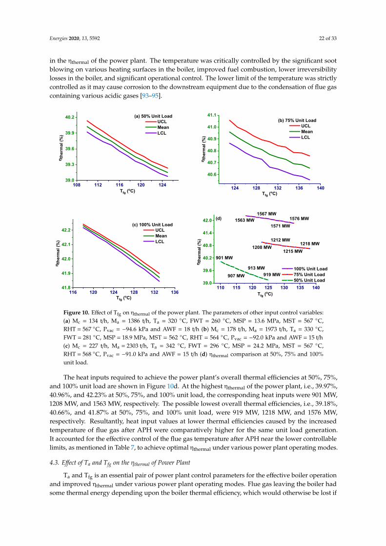
The effect of Tfg on the power plant’s ηthermal at 50%, 75%, and 100% unit load is given inFigure 10a–c. The ηthermal of the power plant decreased with the increase in Tfg. With every 5 ◦C risein the Tfg, the relative decrease in the power plant’s ηthermal was an average of 0.65%, 0.25%, and 0.28%at 50%, 75%, and 100% unit load respectively.
Figure 10d compares the effect of Tfg on the power plant’s ηthermal at 50%, 75%, and 100% unitload. At 100% unit load, the power plant’s ηthermal was relatively higher than 75% and 50% unit loaddue to the improved heat transfer conditions. At 50% unit load, there was a sharp decreasing trend ofthe power plant’s ηthermal with increased flue gas temperature after APH. Thus, the temperature shouldbe effectively controlled mainly at 50% unit load as it had a relatively more significant adverse impacton the power plant’s ηthermal. This was explained by the fact that the increase in Tfg indicated thedecreased heat transfer from flue gas to the heating surfaces, which was responsible for the decrease
Energies 2020, 13, 5592 22 of 33
in the ηthermal of the power plant. The temperature was critically controlled by the significant sootblowing on various heating surfaces in the boiler, improved fuel combustion, lower irreversibilitylosses in the boiler, and significant operational control. The lower limit of the temperature was strictlycontrolled as it may cause corrosion to the downstream equipment due to the condensation of flue gascontaining various acidic gases [93–95].
Energies 2020, 13, x FOR PEER REVIEW 22 of 35
Figure 9d compares the effect of the MST and RST on the power plant’s ηthermal at 50%, 75%, and 100% unit load. It was apparent from Figure 9d that the ηthermal of the power plant at 100% unit load was higher than 50% and 75% unit load efficiencies. It was because the heart rate of the power plant was improved at 100% unit load. Moreover, the power plant operating mode was also supercritical under which the boiler operation was fuel-efficient, stable, and economical [56,93]. The heat inputs to produce 50%, 75%, and 100% unit load at 550°C, 560 °C, and 570 °C MST and RST are mentioned as MW values on each trend in Figure 9d. The heat inputs required to sustain the highest ηthermal, i.e., 39.78%, 41.05%, and 41.59% at 50%, 75%, and 100% unit load at higher temperature limit (570 °C) of MST and RST were 905 MW, 1206 MW, 1587 MW respectively. Meanwhile, at a lower temperature limit (550 °C) of MST and RST, the overall thermal efficiencies achieved were 38.62%, 39.85%, and 40.51% at 50%, 75%, and 100% unit load. The corresponding energies spent to keep the plant operational were 932 MW, 1242 MW, 1629 MW, respectively, which were comparatively higher heat inputs for the same power production. Therefore, it was advantageous to maintain the MST and RST at a higher temperature limit to ensure the fuel-efficient and optimum power plant operation for sustainable power production.
4.2. Effect of Tfg on the ηthermal of Power Plant
Tfg is a critically controlled operating parameter of the boiler operation. It indicates the efficiency of fuel combustion and heat transfer to the heating surfaces inside the boiler, thereby directly influencing the power plant’s ηthermal. The increase in this temperature beyond its normal controllable operating range, as mentioned in Table 7, indicates that heat transfer from the flue gas to the heating surfaces is decreasing, which might be caused by soot accumulation on the heating surfaces, high flame center, large access air coefficient of combustion and burning of unburned carbon in the tail of boiler. This is an indicator of poor control of boiler operation resulting in the power plant’s reduced ηthermal.
The effect of Tfg on the power plant’s ηthermal at 50%, 75%, and 100% unit load is given in Figure 10a–c. The ηthermal of the power plant decreased with the increase in Tfg. With every 5 °C rise in the Tfg, the relative decrease in the power plant’s ηthermal was an average of 0.65%, 0.25%, and 0.28% at 50%, 75%, and 100% unit load respectively.
108 112 116 120 124
39.0
39.3
39.6
39.9
40.2
η the
rmal
(%)
Tfg (oC)
UCL Mean LCL
(a) 50% Unit Load
124 128 132 136 140
40.6
40.7
40.8
40.9
41.0
41.1
η the
rmal
(%)
Tfg (oC)
UCL Mean LCL
(b) 75% Unit Load
Energies 2020, 13, x FOR PEER REVIEW 23 of 35
Figure 10. Effect of Tfg on ηthermal of the power plant. The parameters of other input control variables: (a) Mc = 134 t/h, Ma = 1386 t/h, Ta = 320 °C, FWT = 260 °C, MSP = 13.6 MPa, MST = 567 °C, RHT = 567 °C, Pvac = −94.6 kPa and AWF = 18 t/h (b) Mc =178 t/h, Ma = 1973 t/h, Ta = 330 °C, FWT = 281 °C, MSP = 18.9 MPa, MST = 562 °C, RHT = 564 °C, Pvac = −92.0 kPa and AWF = 15 t/h (c) Mc =227 t/h, Ma = 2303 t/h, Ta= 342 °C, FWT = 296 °C, MSP = 24.2 MPa, MST = 567 °C, RHT = 568 °C, Pvac = −91.0 kPa and AWF = 15 t/h (d) ηthermal comparison at 50%, 75% and 100% unit load.
Figure 10d compares the effect of Tfg on the power plant’s ηthermal at 50%, 75%, and 100% unit load. At 100% unit load, the power plant’s ηthermal was relatively higher than 75% and 50% unit load due to the improved heat transfer conditions. At 50% unit load, there was a sharp decreasing trend of the power plant’s ηthermal with increased flue gas temperature after APH. Thus, the temperature should be effectively controlled mainly at 50% unit load as it had a relatively more significant adverse impact on the power plant’s ηthermal. This was explained by the fact that the increase in Tfg indicated the decreased heat transfer from flue gas to the heating surfaces, which was responsible for the decrease in the ηthermal of the power plant. The temperature was critically controlled by the significant soot blowing on various heating surfaces in the boiler, improved fuel combustion, lower irreversibility losses in the boiler, and significant operational control. The lower limit of the temperature was strictly controlled as it may cause corrosion to the downstream equipment due to the condensation of flue gas containing various acidic gases [93–95].
The heat inputs required to achieve the power plant’s overall thermal efficiencies at 50%, 75%, and 100% unit load are shown in Figure 10d. At the highest ηthermal of the power plant, i.e., 39.97%, 40.96%, and 42.23% at 50%, 75%, and 100% unit load, the corresponding heat inputs were 901 MW, 1208 MW, and 1563 MW, respectively. The possible lowest overall thermal efficiencies, i.e., 39.18%, 40.66%, and 41.87% at 50%, 75%, and 100% unit load, were 919 MW, 1218 MW, and 1576 MW, respectively. Resultantly, heat input values at lower thermal efficiencies caused by the increased temperature of flue gas after APH were comparatively higher for the same unit load generation. It accounted for the effective control of the flue gas temperature after APH near the lower controllable limits, as mentioned in Table 7, to achieve optimal ηthermal under various power plant operating modes.
4.3. Effect of Ta and Tfg on the ηthermal of Power Plant
Ta and Tfg is an essential pair of power plant control parameters for the effective boiler operation and improved ηthermal under various power plant operating modes. Flue gas leaving the boiler had some thermal energy depending upon the boiler thermal efficiency, which would otherwise be lost if not recovered and decrease the power plant’s ηthermal. A part of this energy was recovered by the air passing through the APH. Thus, the pre-heated air improved the power plant’s ηthermal and helped coal combustion at high air temperature for producing high-quality steam. The combined effect of rising Ta and falling Tfg represented the flue gas’s waste heat recovery system.
The operating ranges of two temperatures were divided into ten equal divisions to evaluate the combined effect of Ta and Tfg. Ta was varied systematically in the ascending order, while Tfg was decreasing systematically. The remaining operating parameters were kept at the average values
116 120 124 128 132 13641.8
41.9
42.0
42.1
42.2
η the
rmal
(%)
Tfg (oC)
UCL Mean LCL
(c) 100% Unit Load
110 115 120 125 130 135 14039.0
39.6
40.2
40.8
41.4
42.0 (d)
100% Unit Load 75% Unit Load 50% Unit Load
η the
rmal
(%)
Tfg (oC)
901 MW
919 MW913 MW
907 MW
1212 MW1208 MW
1215 MW1218 MW
1576 MW1571 MW
1567 MW1563 MW
Figure 10. Effect of Tfg on ηthermal of the power plant. The parameters of other input control variables:(a) Mc = 134 t/h, Ma = 1386 t/h, Ta = 320 ◦C, FWT = 260 ◦C, MSP = 13.6 MPa, MST = 567 ◦C,RHT = 567 ◦C, Pvac = −94.6 kPa and AWF = 18 t/h (b) Mc = 178 t/h, Ma = 1973 t/h, Ta = 330 ◦C,FWT = 281 ◦C, MSP = 18.9 MPa, MST = 562 ◦C, RHT = 564 ◦C, Pvac = −92.0 kPa and AWF = 15 t/h(c) Mc = 227 t/h, Ma = 2303 t/h, Ta = 342 ◦C, FWT = 296 ◦C, MSP = 24.2 MPa, MST = 567 ◦C,RHT = 568 ◦C, Pvac = −91.0 kPa and AWF = 15 t/h (d) ηthermal comparison at 50%, 75% and 100%unit load.
The heat inputs required to achieve the power plant’s overall thermal efficiencies at 50%, 75%,and 100% unit load are shown in Figure 10d. At the highest ηthermal of the power plant, i.e., 39.97%,40.96%, and 42.23% at 50%, 75%, and 100% unit load, the corresponding heat inputs were 901 MW,1208 MW, and 1563 MW, respectively. The possible lowest overall thermal efficiencies, i.e., 39.18%,40.66%, and 41.87% at 50%, 75%, and 100% unit load, were 919 MW, 1218 MW, and 1576 MW,respectively. Resultantly, heat input values at lower thermal efficiencies caused by the increasedtemperature of flue gas after APH were comparatively higher for the same unit load generation.It accounted for the effective control of the flue gas temperature after APH near the lower controllablelimits, as mentioned in Table 7, to achieve optimal ηthermal under various power plant operating modes.
4.3. Effect of Ta and Tfg on the ηthermal of Power Plant
Ta and Tfg is an essential pair of power plant control parameters for the effective boiler operationand improved ηthermal under various power plant operating modes. Flue gas leaving the boiler hadsome thermal energy depending upon the boiler thermal efficiency, which would otherwise be lost if
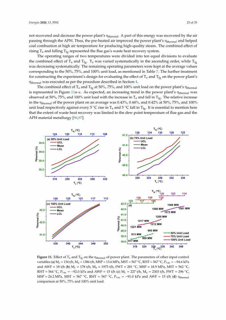
Energies 2020, 13, 5592 23 of 33
not recovered and decrease the power plant’s ηthermal. A part of this energy was recovered by the airpassing through the APH. Thus, the pre-heated air improved the power plant’s ηthermal and helpedcoal combustion at high air temperature for producing high-quality steam. The combined effect ofrising Ta and falling Tfg represented the flue gas’s waste heat recovery system.
The operating ranges of two temperatures were divided into ten equal divisions to evaluatethe combined effect of Ta and Tfg. Ta was varied systematically in the ascending order, while Tfg
was decreasing systematically. The remaining operating parameters were kept at the average valuescorresponding to the 50%, 75%, and 100% unit load, as mentioned in Table 7. The further treatmentfor constructing the experiment’s design for evaluating the effect of Ta and Tfg on the power plant’sηthermal was executed as per the procedure described in Section 4.
The combined effect of Ta and Tfg at 50%, 75%, and 100% unit load on the power plant’s ηthermal
is represented in Figure 11a–c. As expected, an increasing trend in the power plant’s ηthermal wasobserved at 50%, 75%, and 100% unit load with the increase in Ta and fall in Tfg. The relative increasein the ηthermal of the power plant on an average was 0.43%, 0.44%, and 0.42% at 50%, 75%, and 100%unit load respectively against every 5 ◦C rise in Ta and 5 ◦C fall in Tfg. It is essential to mention herethat the extent of waste heat recovery was limited to the dew point temperature of flue gas and theAPH material metallurgy [96,97].
Energies 2020, 13, x FOR PEER REVIEW 24 of 35
corresponding to the 50%, 75%, and 100% unit load, as mentioned in Table 7. The further treatment for constructing the experiment’s design for evaluating the effect of Ta and Tfg on the power plant’s ηthermal was executed as per the procedure described in Section 4.
The combined effect of Ta and Tfg at 50%, 75%, and 100% unit load on the power plant’s ηthermal is represented in Figure 11a–c. As expected, an increasing trend in the power plant’s ηthermal was observed at 50%, 75%, and 100% unit load with the increase in Ta and fall in Tfg. The relative increase in the ηthermal of the power plant on an average was 0.43%, 0.44%, and 0.42% at 50%, 75%, and 100% unit load respectively against every 5 °C rise in Ta and 5 °C fall in Tfg. It is essential to mention here that the extent of waste heat recovery was limited to the dew point temperature of flue gas and the APH material metallurgy [96,97].
Figure 11d compares the combined effect of Ta and Tfg on the power plant’s ηthermal at 50%, 75%, and 100% unit power generation capacity. At 100% unit power generation capacity, the power plant’s ηthermal was relatively higher than 50% and 75% unit power generation capacity because of its improved heat rate.
Figure 11. Effect of Ta and Tfg on the ηthermal of power plant. The parameters of other input control variables (a) Mc = 134 t/h, Ma = 1386 t/h, MSP = 13.6 MPa, MST = 567 °C, RHT = 567 °C, Pvac = −94.6 kPa and AWF = 18 t/h (b) Mc = 178 t/h, Ma = 1973 t/h, FWT = 281 °C, MSP = 18.9 MPa, MST = 562 °C, RHT = 564 °C, Pvac = −92.0 kPa and AWF = 15 t/h (c) Mc = 227 t/h, Ma = 2303 t/h, FWT = 296 °C, MSP = 24.2 MPa, MST = 567 °C, RHT = 567 °C, Pvac = −91.0 kPa and AWF = 15 t/h (d) ηthermal comparison at 50%, 75% and 100% unit load.
Trend lines in Figure 11d show the heat inputs to achieve the power plant’s thermal efficiency at 50%, 75%, and 100% unit load. At the highest ηthermal of the power plant, i.e., 39.77%, 41.08%, and 42.29% at 50%, 75%, and 100% unit load, the corresponding heat inputs were 905 MW, 1205 MW, and 1561 MW, respectively. The possible lowest overall thermal efficiencies at 50%, 75%, and 100% unit load would be 917 MW, 1221 MW, and 1580 MW, respectively. The lowest heat inputs corresponding
316 320 324 328 332
39.2
39.4
39.6
39.8
Tfg (oC)
Ta (oC)
108112116120
UCL Mean LCL
(a) 50% Unit Load
124
η the
rmal
(%)
320 324 328 332 33640.4
40.6
40.8
41.0
41.2122
UCL Mean LCL
Ta (oC)
(b) 75% Unit Load
Tfg (oC)126130134138
η the
rmal
(%)
336 340 344 348 352
41.8
42.0
42.2
η the
rmal
(%)
Ta (oC)
UCL Mean LCL
(c) 100% Unit Load
113Tfg (oC)
117121125129
318 324 330 336 342 348
39.0
39.5
40.0
40.5
41.0
41.5
42.0
42.5
Tfg (oC)
117122130138
109(d)
η the
rmal
(%)
1561 MW1566 MW
1572 MW
50% Unit Load 75% Unit Load 100% Unit Load
Ta (oC)
905 MW
909 MW913 MW
917 MW
1580 MW
1205 MW
1212 MW1217 MW
1221 MW
125
114122130
Figure 11. Effect of Ta and Tfg on the ηthermal of power plant. The parameters of other input controlvariables (a) Mc = 134 t/h, Ma = 1386 t/h, MSP = 13.6 MPa, MST = 567 ◦C, RHT = 567 ◦C, Pvac = −94.6 kPaand AWF = 18 t/h (b) Mc = 178 t/h, Ma = 1973 t/h, FWT = 281 ◦C, MSP = 18.9 MPa, MST = 562 ◦C,RHT = 564 ◦C, Pvac = −92.0 kPa and AWF = 15 t/h (c) Mc = 227 t/h, Ma = 2303 t/h, FWT = 296 ◦C,MSP = 24.2 MPa, MST = 567 ◦C, RHT = 567 ◦C, Pvac = −91.0 kPa and AWF = 15 t/h (d) ηthermal
comparison at 50%, 75% and 100% unit load.
Energies 2020, 13, 5592 24 of 33
Figure 11d compares the combined effect of Ta and Tfg on the power plant’s ηthermal at 50%,75%, and 100% unit power generation capacity. At 100% unit power generation capacity, the powerplant’s ηthermal was relatively higher than 50% and 75% unit power generation capacity because of itsimproved heat rate.
Trend lines in Figure 11d show the heat inputs to achieve the power plant’s thermal efficiencyat 50%, 75%, and 100% unit load. At the highest ηthermal of the power plant, i.e., 39.77%, 41.08%,and 42.29% at 50%, 75%, and 100% unit load, the corresponding heat inputs were 905 MW, 1205 MW,and 1561 MW, respectively. The possible lowest overall thermal efficiencies at 50%, 75%, and 100% unitload would be 917 MW, 1221 MW, and 1580 MW, respectively. The lowest heat inputs corresponding tothe power plant’s highest ηthermal at 50%, 75%, and 100% unit load was possible due to improved heatrecovery from the flue gas leaving the boiler. The effective operation control of Ta and Tfg promisedthe boiler’s efficient operation and the improved ηthermal of the power plant.
4.4. Effect of Change in All Control Variables on the ηthermal of Power Plant
In this sub-section, first, the power plant’s possible worst operating scenario during which overallthermal efficiencies of the power plant may drop to the lowest value at 50%, 75%, and 100% unit loadwas constructed. Further, in the Monte Carlo experiments, certain adjustments in operating parameterswere simulated to recover the power plant’s ηthermal. This strategy of adjusting operating parameterscan be practically implemented to achieve the maximum overall thermal efficiencies at various powerplant operation modes.
AWF controls the temperature of the MST and RST. Low adjustment of AWF, i.e., the exceptionallyhigh flow rate, may significantly drop the MST and RST. However, the MSP may have a little increasedepending upon the AWF and unit load. Moreover, MST and RST drop may also be linked withlower heat transfer to the boiler’s heating surfaces, indicated by higher Tfg. In such an operatingscenario, FWT would also drop, and the Pvac would be slightly increased. Meanwhile, the Mc, Ma,and AWF were adjusted to recover the plant operation to the stable operating conditions at any unitload. The operational ranges of all the control variables within which the corresponding variables’values were systematically changed at 50%, 75%, and 100% unit load are s mentioned in Table 7.
To conduct the experiments for optimizing the ηthermal of the power plant at 50%, 75%, and 100%unit load, Mc, Ma, Tfg, Ta, MSP, Pvac, and AWF were varied from maximum to average values asmentioned in Table 7. FWT was varied from minimum to average, while MST and RST were changedbetween the minimum and the maximum operating limits. The operating ranges of all variables weredivided into ten equal divisions. To evaluate the response of the power plant’s ηthermal under such anoperating scenario, we applied the procedure as described in Section 4.
The effect of changes in control variables (MST and RST are conveniently represented along thelower and upper x-axes while the operating range of remaining control variables is mentioned in thedescription of Figure 12) on the power plant’s ηthermal at 50%, 75%, and 100% unit load is shown inFigure 12a–c. At 50% unit load, the power plant’s ηthermal was initially stagnant (~550 ◦C ~555 ◦CMST), and then it started increasing. On the other hand, at 75% and 100% unit load, an increasingtrend of the power plant’s ηthermal was observed. For 550 ◦C to 560 ◦C and 560 ◦C to 570 ◦C of MSTand RST with the corresponding changes in remaining control parameters at 50%, 75%, and 100% unitload, the relative increase in the ηthermal of the power plant on an average was equal to 3.36%, 3.21%,and 4.29% respectively.
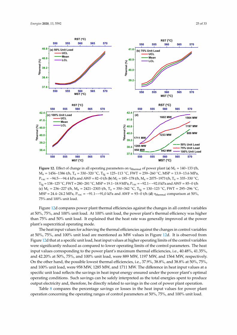
Energies 2020, 13, 5592 25 of 33
Energies 2020, 13, x FOR PEER REVIEW 25 of 35
to the power plant’s highest ηthermal at 50%, 75%, and 100% unit load was possible due to improved heat recovery from the flue gas leaving the boiler. The effective operation control of Ta and Tfg promised the boiler’s efficient operation and the improved ηthermal of the power plant.
4.4. Effect of Change in All Control Variables on the ηthermal of Power Plant
In this sub-section, first, the power plant’s possible worst operating scenario during which overall thermal efficiencies of the power plant may drop to the lowest value at 50%, 75%, and 100% unit load was constructed. Further, in the Monte Carlo experiments, certain adjustments in operating parameters were simulated to recover the power plant’s ηthermal. This strategy of adjusting operating parameters can be practically implemented to achieve the maximum overall thermal efficiencies at various power plant operation modes.
AWF controls the temperature of the MST and RST. Low adjustment of AWF, i.e., the exceptionally high flow rate, may significantly drop the MST and RST. However, the MSP may have a little increase depending upon the AWF and unit load. Moreover, MST and RST drop may also be linked with lower heat transfer to the boiler’s heating surfaces, indicated by higher Tfg. In such an operating scenario, FWT would also drop, and the Pvac would be slightly increased. Meanwhile, the Mc, Ma, and AWF were adjusted to recover the plant operation to the stable operating conditions at any unit load. The operational ranges of all the control variables within which the corresponding variables’ values were systematically changed at 50%, 75%, and 100% unit load are s mentioned in Table 7.
To conduct the experiments for optimizing the ηthermal of the power plant at 50%, 75%, and 100% unit load, Mc, Ma, Tfg, Ta, MSP, Pvac, and AWF were varied from maximum to average values as mentioned in Table 7. FWT was varied from minimum to average, while MST and RST were changed between the minimum and the maximum operating limits. The operating ranges of all variables were divided into ten equal divisions. To evaluate the response of the power plant’s ηthermal under such an operating scenario, we applied the procedure as described in Section 4.
The effect of changes in control variables (MST and RST are conveniently represented along the lower and upper x-axes while the operating range of remaining control variables is mentioned in the description of Figure 12) on the power plant’s ηthermal at 50%, 75%, and 100% unit load is shown in Figure 12a–c. At 50% unit load, the power plant’s ηthermal was initially stagnant (~550 °C ~555 °C MST), and then it started increasing. On the other hand, at 75% and 100% unit load, an increasing trend of the power plant’s ηthermal was observed. For 550 °C to 560 °C and 560 °C to 570 °C of MST and RST with the corresponding changes in remaining control parameters at 50%, 75%, and 100% unit load, the relative increase in the ηthermal of the power plant on an average was equal to 3.36%, 3.21%, and 4.29% respectively.
550 555 560 565 570
550 555 560 565 570
37.6
38.4
39.2
40.0
40.8
η the
rmal
(%)
(a) 50% Unit Load
RST (oC)
UCL Mean LCL
MST (oC) 550 555 560 565 570
550 555 560 565 570
39.2
40.0
40.8
41.6
η the
rmal
(%)
RST (oC)
MST (oC)
(b) 75% Unit Load UCL Mean LCL
Energies 2020, 13, x FOR PEER REVIEW 26 of 35
Figure 12. Effect of change in all operating parameters on ηthermal of power plant (a) Mc=140~133 t/h, Ma = 1456~1386 t/h, Ta = 330~320 °C, Tfg = 125~113 °C, FWT = 259~260 °C, MSP = 13.9~13.6 MPa, Pvac = −94.5~−94.4 kPa and AWF = 82~0 t/h (b) Mc = 185~178 t/h, Ma = 2075~1973 t/h, Ta = 335~330 °C, Tfg = 138~125 °C, FWT = 280~281 °C, MSP = 19.1~18.9 MPa, Pvac = −92.1~ −92.0 kPa and AWF = 85~0 t/h (c) Mc = 236~227 t/h, Ma = 2421~2303 t/h, Ta = 350~342 °C, Tfg = 130~123 °C, FWT = 295~296 °C, MSP = 24.4~24.2 MPa, Pvac = −91.1~−91,0 kPa and AWF = 93~0 t/h (d) ηthermal comparison at 50%, 75% and 100% unit load.
Figure 12d compares power plant thermal efficiencies against the changes in all control variables at 50%, 75%, and 100% unit load. At 100% unit load, the power plant’s thermal efficiency was higher than 75% and 50% unit load. It explained that the heat rate was generally improved at the power plant’s supercritical operating mode.
The heat input values for achieving the thermal efficiencies against the changes in control variables at 50%, 75%, and 100% unit load are mentioned as MW values in Figure 12d. It is observed from Figure 12d that at a specific unit load, heat input values at higher operating limits of the control variables were significantly reduced as compared to lower operating limits of the control parameters. The heat input values corresponding to the power plant’s maximum thermal efficiencies, i.e., 40.48%, 41.35%, and 42.20% at 50%, 75%, and 100% unit load, were 889 MW, 1197 MW, and 1564 MW, respectively. On the other hand, the possible lowest thermal efficiencies, i.e., 37.9%, 38.8%, and 38.8% at 50%, 75%, and 100% unit load, were 958 MW, 1285 MW, and 1711 MW. The difference in heat input values at a specific unit load reflects the savings in heat input energy ensured under the power plant’s optimal operating conditions. Such savings can be safely interpreted as the total energies spent to produce output electricity and, therefore, be directly related to savings in the cost of power plant operation.
Table 8 compares the percentage savings or losses in the heat input values for power plant operation concerning the operating ranges of control parameters at 50%, 75%, and 100% unit load.
550 555 560 565 570
550 555 560 565 570
38.4
39.2
40.0
40.8
41.6
42.4
η the
rmal
(%)
RST (oC)
MST (oC)
(c) 100% Unit Load UCL Mean LCL
550 555 560 565 570
550 555 560 565 570
37.6
38.4
39.2
40.0
40.8
41.6
42.4
1197 MW
1233 MW
1285 MW
1564 MW1602 MW
889 MW
942 MW
1711 MWη the
rmal
(%)
RST (oC)
MST (oC)
50% Unit Load 75% Unit Load 100% Unit Load958 MW
(d)
Figure 12. Effect of change in all operating parameters on ηthermal of power plant (a) Mc = 140~133 t/h,Ma = 1456~1386 t/h, Ta = 330~320 ◦C, Tfg = 125~113 ◦C, FWT = 259~260 ◦C, MSP = 13.9~13.6 MPa,Pvac = −94.5~−94.4 kPa and AWF = 82~0 t/h (b) Mc = 185~178 t/h, Ma = 2075~1973 t/h, Ta = 335~330 ◦C,Tfg = 138~125 ◦C, FWT = 280~281 ◦C, MSP = 19.1~18.9 MPa, Pvac =−92.1~−92.0 kPa and AWF = 85~0 t/h(c) Mc = 236~227 t/h, Ma = 2421~2303 t/h, Ta = 350~342 ◦C, Tfg = 130~123 ◦C, FWT = 295~296 ◦C,MSP = 24.4~24.2 MPa, Pvac = −91.1~−91,0 kPa and AWF = 93~0 t/h (d) ηthermal comparison at 50%,75% and 100% unit load.
Figure 12d compares power plant thermal efficiencies against the changes in all control variablesat 50%, 75%, and 100% unit load. At 100% unit load, the power plant’s thermal efficiency was higherthan 75% and 50% unit load. It explained that the heat rate was generally improved at the powerplant’s supercritical operating mode.
The heat input values for achieving the thermal efficiencies against the changes in control variablesat 50%, 75%, and 100% unit load are mentioned as MW values in Figure 12d. It is observed fromFigure 12d that at a specific unit load, heat input values at higher operating limits of the control variableswere significantly reduced as compared to lower operating limits of the control parameters. The heatinput values corresponding to the power plant’s maximum thermal efficiencies, i.e., 40.48%, 41.35%,and 42.20% at 50%, 75%, and 100% unit load, were 889 MW, 1197 MW, and 1564 MW, respectively.On the other hand, the possible lowest thermal efficiencies, i.e., 37.9%, 38.8%, and 38.8% at 50%, 75%,and 100% unit load, were 958 MW, 1285 MW, and 1711 MW. The difference in heat input values at aspecific unit load reflects the savings in heat input energy ensured under the power plant’s optimaloperating conditions. Such savings can be safely interpreted as the total energies spent to produceoutput electricity and, therefore, be directly related to savings in the cost of power plant operation.
Table 8 compares the percentage savings or losses in the heat input values for power plantoperation concerning the operating ranges of control parameters at 50%, 75%, and 100% unit load.

Energies 2020, 13, 5592 26 of 33
Table 8. Energy savings/losses in heat input values for power plant operation.
Parameters
50% Unit Load 75% Unit Load 100% Unit Load
OperatingRange
Heat InputRange
% EnergySavings/Losses
OperatingRange
Heat InputRange
% EnergySavings/Losses
OperatingRange
Heat InputRange
% EnergySavings/Losses
Unit ◦C MW % ◦C MW % ◦C MW %
MST and RST 550–570 934–907 2.94 550–570 1219–1183 2.95 550–570 1598–1557 1.16Tfg 110–125 903–921 −1.99 123–138 1186–1194 −0.75 118–133 1561–1567 −0.85
Ta and Tfg 315–330 919–907 1.27 320–335 1196–1183 1.31 335–350 1567–1554 1.24* All Control Variables 550–570 952–901 7.20 550–570 1252–1185 6.85 550–570 1643–1521 8.60
* All control variables are the operating parameters of the power plant, as mentioned in Table 7.
Energies 2020, 13, 5592 27 of 33
The energy savings were achievable by the effective operational control of the combustion thatultimately influenced power plant operation. The energy savings or energy losses were expressed in %of heat input values and were mentioned against the operating parameters, i.e., MST and RST, Tfg,Ta and Tfg, and all control variables, as discussed in Sections 4.1–4.4, respectively. The energy savingsor energy losses for any control variable at a specific unit load were calculated from the heat inputvalues corresponding to the control variable’s operating range, as mentioned in Figures 9d, 10d, 11dand 12d. (+) the sign indicates the % energy savings while the (−) sign indicates the % energy losses inheat input values against the control variable in its operating range. At 50%, 75%, and 100% unit load,MST and RST indicated energy savings in heat input values of 2.94%, 2.92%, and 2.59%. Ta and Tfg
noted energy savings of 1.27%, 1.31%, and 1.25%, respectively. All control variables showed significantenergy savings of 7.20%, 6.85%, and 8.60%, respectively, whereas, Tfg expressed energy losses of 1.99%,0.70%, and 0.35% in heat input values for the operation of the power plant.
5. Conclusions
In this work, industrial operation data, advanced data analytic tools, and AI algorithms areincorporated to formulate the step-wise methodology in the spirit of industry 4.0-data analytics tooptimize the power plant’s ηthermal for sustainable power generation from a power complex.
The quality of operation data is ensured by employing data visualization techniques like histogramsand SOFM. Monte-Carlo experiments on ANN and LSSVM process models and IASA were performedto eliminate insignificant variables from the list of initially selected control variables.
At 50%, 75%, and 100% unit load, for every 10 ◦C rise in MST and RST, the power plant’s ηthermal
on average had a relative increase of 1.50%, 1.50%, and 1.32%, respectively.For every 5 ◦C rise in Tfg, the relative decrease in the power plant’s ηthermal was an average of
0.65%, 0.25%, and 0.28%, respectively, under 50%, 75%, 100% unit load.For every 5 ◦C rise in Ta and 5 ◦C fall in Tfg, the relative increase in the ηthermal of the power plant
on average was 0.43%, 0.44%, and 0.42%, respectively, under 50%, 75%, and 100% unit load.From 550 ◦C to 560 ◦C and 560 ◦C to 570 ◦C MST and RST with the corresponding changes in
remaining control variables, the relative increase in the ηthermal of the power plant on an average was3.36%, 3.21%, and 4.29% respectively at 50%, 75%, and 100% unit load.
At 50%, 75%, and 100% unit load: the savings in heat inputs corresponding to the highest overallthermal efficiencies, for MST and RST were 2.94%, 2.92%, and 2.59% respectively, for Ta and Tfg are1.27%, 1.31%, and 1.25% respectively, for all control variables were 7.20%, 6.85%, and 8.60% respectively.Energy losses in heat inputs corresponding to the lowest overall thermal efficiencies at 50%, 75%,and 100% unit load, for Tfg were 1.99%, 0.70%, and 0.35%, respectively.
The true implementation of industry 4.0 built by the modern data analytics tools for powerplant operation ensured the increase in the power plant’s thermal efficiency and, therefore,the techno-economic benefits that offer reduced operation cost, optimal fuel consumption, and effectiveoperational control.
Big data analytics, industrial internet of things, and simulation were the three technologiesprioritized and incorporated in the study to achieve the power plant’s operational excellence byembracing the industry 4.0 digital transformation approach.
The process modeling based on process data, process optimization, and data-driven strategydevelopment for improved process control using sophisticated technologies dedicated to theimplementation of industry 4.0 in the industrial complexes for higher productivity and effectiveoperation control is in line with the objectives of the industry, innovation, and infrastructure programof the united nations for sustainable development and the Paris agreement allowing to fulfill thenations’ commitment to sustainable growth and the environment.
The effect of auxiliaries’ system operation, separately or combined, on the power plant’s ηthermal
needs to be evaluated in the future.
Energies 2020, 13, 5592 28 of 33
Author Contributions: Conceptualization, W.M.A., G.M.U., S.M.A., J.K.; methodology, S.A., A.H.K.; supervision,G.M.U., L.B.X., S.C.; validation, M.A., M.H.K., J.K.; data curation, W.M.A., A.J., A.A.; formal analysis, W.M.A.,S.A., M.W.R., U.N.; investigation, S.G.N., H.J.; writing—original draft, W.M.A., A.A.; writing—review and editing,G.M.U., L.B.X., S.C., J.K.; visualization, I.A.C., N.H., J.K.; project administration, W.M.A., G.M.U. All authors haveread and agreed to the published version of the manuscript.
Funding: This research received no external funding.
Acknowledgments: The research activity is based on the data collection from the Sahiwal Coal Power plant.The power plant is installed by Huaneng Shandong Ruyi Pakistan Energy Private limited- a joint venture of ChinaHuaneng Group and China Ruyi group. The author is obliged to the power plant management and professionalengineers to carry out the research activity for their support, supervision, and wisdom.
Conflicts of Interest: The author declares no conflict of interest concerning this work.
Nomenclature
AWF attemperation water flow rate (◦C)FWT Feed-water temperature (◦C)Ma air flow rate (t/h)Mc coal flow rate (t/h)MSP main steam pressure (MPa)MST main steam temperature (◦C)MW energy suppliedMWe electric powerN turbine speed (rpm)O2 % O2 in flue gas at boiler outlet (%)Pf furnace pressure (Pa)Pvac condenser vacuum (kPa)RST reheat steam temperature (◦C)Ta APH air outlet temperature (◦C)Tfg APH outlet flue gas temperature (◦C)ηthermal overall thermal efficiency (%)ε epsilon
Abbreviations
AD algorithmic differentiationAI Artificial IntelligenceANN Artificial Neural NetworkAPH air preheaterC regularized constantDPSH division platen superheaterECO economizerESP electrostatic precipitatorFDF forced draft fanFGD flue gas desulphurizationFRH final re-heaterFSH final superheaterG generatorHP high pressureHPH high-pressure heatersIA interval arithmeticIASA Interval Adjoint Significance AnalysisICT information and communication technologyIDF induced draft fanIP intermediate pressureLP low pressureLPA low-pressure turbine A
Energies 2020, 13, 5592 29 of 33
LPB low-pressure turbine BLPH low-pressure heatersLSSVM Least Square Support Vector MachineLT REHEATER low-temperature re-heaterLTSH low-temperature superheaterMAPE mean absolute percentage errorMLP multilayer perceptronNCCR the net coal consumption rateNRMSE normalized RMSEPAF primary air fanR correlation coefficientRMSE root mean square errorSIS Supervisory Information SystemSmart EEPS smart energy and electric power systemSOFM self-organizing feature mapSRM structural risk minimization
References
1. Kabugo, J.C.; Jämsä-Jounela, S.-L.; Schiemann, R.; Binder, C. Industry 4.0 based process data analyticsplatform: A waste-to-energy plant case study. Int. J. Electr. Power Energy Syst. 2020, 115, 105508. [CrossRef]
2. Santos, M.Y.; E Sá, J.O.; Costa, C.; Galvão, J.; Andrade, C.; Martinho, B.; Lima, F.V.; Costa, E. A big dataanalytics architecture for industry 4.0. In World Conference on Information Systems and Technologies; Springer:Cham, Switzerland, 2017; pp. 175–184.
3. NEPRA. State of Industry Report 2018; NEPRA: Islamabad, Pakistan, 2019. Available online: https://nepra.org.pk/publications/State%20of%20Industry%20Reports/State%20of%20Industry%20Report%202018.pdf(accessed on 10 July 2020).
4. NEPRA. State of Industry Report 2019; NEPRA: Islamabad, Pakistan, 2019; p. 201. Available online: https://nepra.org.pk/publications/Annual%20Reports/Annual%20Report%202018-19.pdf (accessed on 12 July 2020).
5. Bonilla-Alvarado, H.; Bryden, K.M.; Shadle, L.J.; Tucker, D.; Pezzini, P. Development of Real-Time SystemIdentification to Detect Abnormal Operations in a Gas Turbine Cycle. J. Energy Resour. Technol. 2020,142, 1–40. [CrossRef]
6. Gönül, H.I.; Bilen, M. Modeling Absorbers in WFGD System and Prediction of SO2 Removal Rate Based onSize Parameters. J. Energy Resour. Technol. 2020, 142, 1–27. [CrossRef]
7. Uguz, O.; Haykırı-Açma, H.; Yaman, S. Burning Resistance of Lignitic Coals Under Oxygen-EnrichedConditions. J. Energy Resour. Technol. 2020, 142, 1–23. [CrossRef]
8. Abad, A.; Gayán, P.; Pérez-Vega, R.; García-Labiano, F.; De Diego, L.; Mendiara, T.; Izquierdo, M.; Adánez, J.Evaluation of different strategies to improve the efficiency of coal conversion in a 50 kWth Chemical Loopingcombustion unit. Fuel 2020, 271, 117514. [CrossRef]
9. International Finance Corporation. Environmental, Health, and Safety Guidelines: Thermal Power Plants.2008, World Bank. Available online: https://www.ifc.org/wps/wcm/connect/f82a5f06-f3f7-4033-8ea6-b767523cda8e/FINAL_Thermal%2BPower.pdf?MOD=AJPERES&CVID=jqeD9Eg&id=1323162579734(accessed on 15 July 2020).
10. Askari, O.; Metghalchi, H.; Hannani, S.K.; Moghaddas, A.; Ebrahimi, R.; Hemmati, H. Fundamental Studyof Spray and Partially Premixed Combustion of Methane/Air Mixture. J. Energy Resour. Technol. 2012,135, 021001. [CrossRef]
11. Yu, G.; Askari, O.; Metghalchi, M. Theoretical Prediction of the Effect of Blending JP-8 with Syngas on theIgnition Delay Time and Laminar Burning Speed. J. Energy Resour. Technol. 2017, 140, 012204. [CrossRef]
12. Usman, M.; Farooq, M.; Naqvi, M.; Saleem, M.W.; Hussain, J.; Naqvi, S.R.; Jahangir, S.; Usama, H.M.J.;Idrees, S.; Anukam, A. Use of Gasoline, LPG and LPG-HHO Blend in SI Engine: A Comparative Performancefor Emission Control and Sustainable Environment. Processes 2020, 8, 74. [CrossRef]
13. Farooq, M.; Asim, M.; Imran, M.; Imran, S.; Ahmad, J.; Younis, M.R. Mapping past, current and future energyresearch trend in Pakistan: A scientometric assessment. Scientometrics 2018, 117, 1733–1753. [CrossRef]
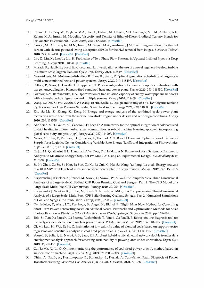
Energies 2020, 13, 5592 30 of 33
14. Razzaq, L.; Farooq, M.; Mujtaba, M.A.; Sher, F.; Farhan, M.; Hassan, M.T.; Soudagar, M.E.M.; Atabani, A.E.;Kalam, M.A.; Imran, M. Modeling Viscosity and Density of Ethanol-Diesel-Biodiesel Ternary Blends forSustainable Environment. Sustainability 2020, 12, 5186. [CrossRef]
15. Farooq, M.; Almustapha, M.N.; Imran, M.; Saeed, M.A.; Andresen, J.M. In-situ regeneration of activatedcarbon with electric potential swing desorption (EPSD) for the H2S removal from biogas. Bioresour. Technol.2018, 249, 125–131. [CrossRef] [PubMed]
16. Lin, Z.; Liu, X.; Lao, L.; Liu, H. Prediction of Two-Phase Flow Patterns in Upward Inclined Pipes via DeepLearning. Energy 2020, 118541. [CrossRef]
17. Moradi, R.; Habib, E.; Bocci, E.; Cioccolanti, L. Investigation on the use of a novel regenerative flow turbinein a micro-scale Organic Rankine Cycle unit. Energy 2020, 118519. [CrossRef]
18. Nazari-Heris, M.; Mohammadi-Ivatloo, B.; Zare, K.; Siano, P. Optimal generation scheduling of large-scalemulti-zone combined heat and power systems. Energy 2020, 210, 118497. [CrossRef]
19. Peltola, P.; Saari, J.; Tynjälä, T.; Hyppänen, T. Process integration of chemical looping combustion withoxygen uncoupling in a biomass-fired combined heat and power plant. Energy 2020, 210, 118550. [CrossRef]
20. Sokolov, D.V.; Barakhtenko, E.A. Optimization of transmission capacity of energy water pipeline networkswith a tree-shaped configuration and multiple sources. Energy 2020, 118469. [CrossRef]
21. Wang, D.; Dai, X.; Wu, Z.; Zhao, W.; Wang, P.; Hu, B.; Shi, L. Design and testing of a 340 kW Organic RankineCycle system for Low Pressure Saturated Steam heat source. Energy 2020, 210, 118380. [CrossRef]
22. Zhu, S.; Ma, Z.; Zhang, K.; Deng, K. Energy and exergy analysis of the combined cycle power plantrecovering waste heat from the marine two-stroke engine under design and off-design conditions. Energy2020, 210, 118558. [CrossRef]
23. AboKersh, M.H.; Vallès, M.; Cabeza, L.F.; Boer, D. A framework for the optimal integration of solar assisteddistrict heating in different urban sized communities: A robust machine learning approach incorporatingglobal sensitivity analysis. Appl. Energy 2020, 267, 114903. [CrossRef]
24. Naves, A.; Tulus, V.; Vazquez, E.G.; Jiménez, L.; Haddad, A.N.; Boer, D. Economic Optimization of the EnergySupply for a Logistics Center Considering Variable-Rate Energy Tariffs and Integration of Photovoltaics.Appl. Sci. 2019, 9, 4711. [CrossRef]
25. Najjar, M.; Qualharini, E.L.; Hammad, A.W.; Boer, D.; Haddad, A.N. Framework for a Systematic ParametricAnalysis to Maximize Energy Output of PV Modules Using an Experimental Design. Sustainability 2019,11, 2992. [CrossRef]
26. Si, N.; Zhao, Z.; Su, S.; Han, P.; Sun, Z.; Xu, J.; Cui, X.; Hu, S.; Wang, Y.; Jiang, L.; et al. Exergy analysisof a 1000 MW double reheat ultra-supercritical power plant. Energy Convers. Manag. 2017, 147, 155–165.[CrossRef]
27. Krzywanski, J.; Sztekler, K.; Szubel, M.; Siwek, T.; Nowak, W.; Mika, Ł. A Comprehensive Three-DimensionalAnalysis of a Large-Scale Multi-Fuel CFB Boiler Burning Coal and Syngas. Part 1. The CFD Model of aLarge-Scale Multi-Fuel CFB Combustion. Entropy 2020, 22, 964. [CrossRef]
28. Krzywanski, J.; Sztekler, K.; Szubel, M.; Siwek, T.; Nowak, W.; Mika, Ł. A Comprehensive, Three-DimensionalAnalysis of a Large-Scale, Multi-Fuel, CFB Boiler Burning Coal and Syngas. Part 2. Numerical Simulationsof Coal and Syngas Co-Combustion. Entropy 2020, 22, 856. [CrossRef]
29. Demirdelen, T.; Aksu, I.O.; Esenboga, B.; Aygul, K.; Ekinci, F.; Bilgili, M. A New Method for GeneratingShort-Term Power Forecasting Based on Artificial Neural Networks and Optimization Methods for SolarPhotovoltaic Power Plants. In Solar Photovoltaic Power Plants; Springer: Singapore, 2019; pp. 165–189.
30. Tolo, S.; Tian, X.; Bausch, N.; Becerra, V.; Santhosh, T.; Vinod, G.; Patelli, E. Robust on-line diagnosis tool forthe early accident detection in nuclear power plants. Reliab. Eng. Syst. Saf. 2019, 186, 110–119. [CrossRef]
31. Qi, M.; Luo, H.; Wei, P.; Fu, Z. Estimation of low calorific value of blended coals based on support vectorregression and sensitivity analysis in coal-fired power plants. Fuel 2019, 236, 1400–1407. [CrossRef]
32. Yousefi, S.; Soltani, R.; Naeini, A.B.; Saen, R.F. A robust hybrid artificial neural network double frontier dataenvelopment analysis approach for assessing sustainability of power plants under uncertainty. Expert Syst.2019, 36, e12435. [CrossRef]
33. Cai, J.; Ma, X.; Li, Q. On-line monitoring the performance of coal-fired power unit: A method based onsupport vector machine. Appl. Therm. Eng. 2009, 29, 2308–2319. [CrossRef]
34. Dhini, A.; Faqih, A.; Kusumoputro, B.; Surjandari, I.; Kusiak, A. Data-driven Fault Diagnosis of PowerTransformers using Dissolved Gas Analysis (DGA). Int. J. Technol. 2020, 11, 388. [CrossRef]
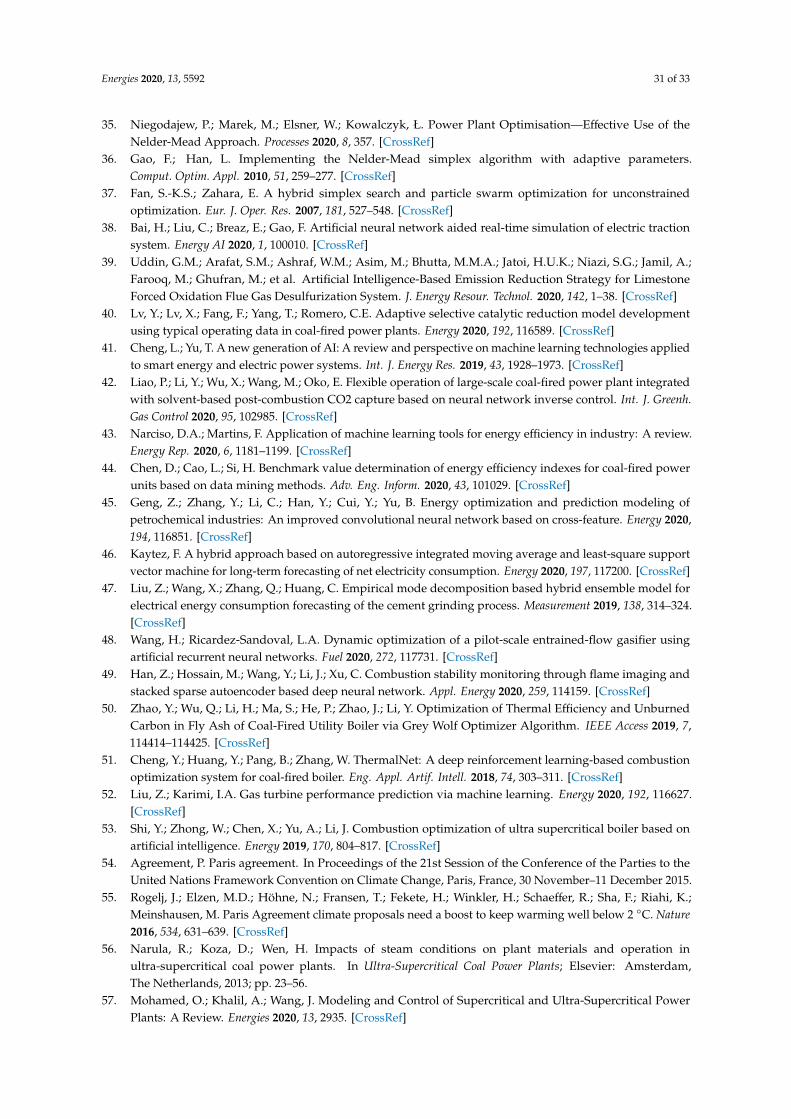
Energies 2020, 13, 5592 31 of 33
35. Niegodajew, P.; Marek, M.; Elsner, W.; Kowalczyk, Ł. Power Plant Optimisation—Effective Use of theNelder-Mead Approach. Processes 2020, 8, 357. [CrossRef]
36. Gao, F.; Han, L. Implementing the Nelder-Mead simplex algorithm with adaptive parameters.Comput. Optim. Appl. 2010, 51, 259–277. [CrossRef]
37. Fan, S.-K.S.; Zahara, E. A hybrid simplex search and particle swarm optimization for unconstrainedoptimization. Eur. J. Oper. Res. 2007, 181, 527–548. [CrossRef]
38. Bai, H.; Liu, C.; Breaz, E.; Gao, F. Artificial neural network aided real-time simulation of electric tractionsystem. Energy AI 2020, 1, 100010. [CrossRef]
39. Uddin, G.M.; Arafat, S.M.; Ashraf, W.M.; Asim, M.; Bhutta, M.M.A.; Jatoi, H.U.K.; Niazi, S.G.; Jamil, A.;Farooq, M.; Ghufran, M.; et al. Artificial Intelligence-Based Emission Reduction Strategy for LimestoneForced Oxidation Flue Gas Desulfurization System. J. Energy Resour. Technol. 2020, 142, 1–38. [CrossRef]
40. Lv, Y.; Lv, X.; Fang, F.; Yang, T.; Romero, C.E. Adaptive selective catalytic reduction model developmentusing typical operating data in coal-fired power plants. Energy 2020, 192, 116589. [CrossRef]
41. Cheng, L.; Yu, T. A new generation of AI: A review and perspective on machine learning technologies appliedto smart energy and electric power systems. Int. J. Energy Res. 2019, 43, 1928–1973. [CrossRef]
42. Liao, P.; Li, Y.; Wu, X.; Wang, M.; Oko, E. Flexible operation of large-scale coal-fired power plant integratedwith solvent-based post-combustion CO2 capture based on neural network inverse control. Int. J. Greenh.Gas Control 2020, 95, 102985. [CrossRef]
43. Narciso, D.A.; Martins, F. Application of machine learning tools for energy efficiency in industry: A review.Energy Rep. 2020, 6, 1181–1199. [CrossRef]
44. Chen, D.; Cao, L.; Si, H. Benchmark value determination of energy efficiency indexes for coal-fired powerunits based on data mining methods. Adv. Eng. Inform. 2020, 43, 101029. [CrossRef]
45. Geng, Z.; Zhang, Y.; Li, C.; Han, Y.; Cui, Y.; Yu, B. Energy optimization and prediction modeling ofpetrochemical industries: An improved convolutional neural network based on cross-feature. Energy 2020,194, 116851. [CrossRef]
46. Kaytez, F. A hybrid approach based on autoregressive integrated moving average and least-square supportvector machine for long-term forecasting of net electricity consumption. Energy 2020, 197, 117200. [CrossRef]
47. Liu, Z.; Wang, X.; Zhang, Q.; Huang, C. Empirical mode decomposition based hybrid ensemble model forelectrical energy consumption forecasting of the cement grinding process. Measurement 2019, 138, 314–324.[CrossRef]
48. Wang, H.; Ricardez-Sandoval, L.A. Dynamic optimization of a pilot-scale entrained-flow gasifier usingartificial recurrent neural networks. Fuel 2020, 272, 117731. [CrossRef]
49. Han, Z.; Hossain, M.; Wang, Y.; Li, J.; Xu, C. Combustion stability monitoring through flame imaging andstacked sparse autoencoder based deep neural network. Appl. Energy 2020, 259, 114159. [CrossRef]
50. Zhao, Y.; Wu, Q.; Li, H.; Ma, S.; He, P.; Zhao, J.; Li, Y. Optimization of Thermal Efficiency and UnburnedCarbon in Fly Ash of Coal-Fired Utility Boiler via Grey Wolf Optimizer Algorithm. IEEE Access 2019, 7,114414–114425. [CrossRef]
51. Cheng, Y.; Huang, Y.; Pang, B.; Zhang, W. ThermalNet: A deep reinforcement learning-based combustionoptimization system for coal-fired boiler. Eng. Appl. Artif. Intell. 2018, 74, 303–311. [CrossRef]
52. Liu, Z.; Karimi, I.A. Gas turbine performance prediction via machine learning. Energy 2020, 192, 116627.[CrossRef]
53. Shi, Y.; Zhong, W.; Chen, X.; Yu, A.; Li, J. Combustion optimization of ultra supercritical boiler based onartificial intelligence. Energy 2019, 170, 804–817. [CrossRef]
54. Agreement, P. Paris agreement. In Proceedings of the 21st Session of the Conference of the Parties to theUnited Nations Framework Convention on Climate Change, Paris, France, 30 November–11 December 2015.
55. Rogelj, J.; Elzen, M.D.; Höhne, N.; Fransen, T.; Fekete, H.; Winkler, H.; Schaeffer, R.; Sha, F.; Riahi, K.;Meinshausen, M. Paris Agreement climate proposals need a boost to keep warming well below 2 ◦C. Nature2016, 534, 631–639. [CrossRef]
56. Narula, R.; Koza, D.; Wen, H. Impacts of steam conditions on plant materials and operation inultra-supercritical coal power plants. In Ultra-Supercritical Coal Power Plants; Elsevier: Amsterdam,The Netherlands, 2013; pp. 23–56.
57. Mohamed, O.; Khalil, A.; Wang, J. Modeling and Control of Supercritical and Ultra-Supercritical PowerPlants: A Review. Energies 2020, 13, 2935. [CrossRef]
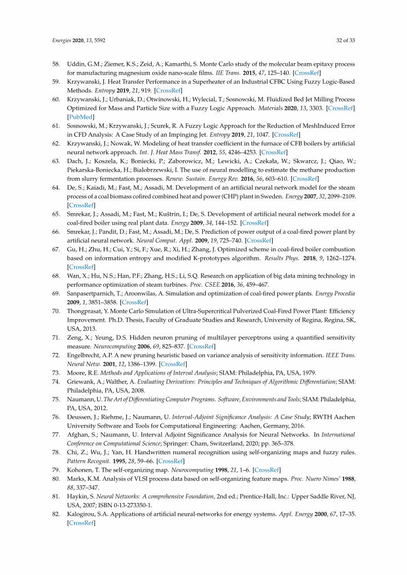
Energies 2020, 13, 5592 32 of 33
58. Uddin, G.M.; Ziemer, K.S.; Zeid, A.; Kamarthi, S. Monte Carlo study of the molecular beam epitaxy processfor manufacturing magnesium oxide nano-scale films. IIE Trans. 2015, 47, 125–140. [CrossRef]
59. Krzywanski, J. Heat Transfer Performance in a Superheater of an Industrial CFBC Using Fuzzy Logic-BasedMethods. Entropy 2019, 21, 919. [CrossRef]
60. Krzywanski, J.; Urbaniak, D.; Otwinowski, H.; Wylecial, T.; Sosnowski, M. Fluidized Bed Jet Milling ProcessOptimized for Mass and Particle Size with a Fuzzy Logic Approach. Materials 2020, 13, 3303. [CrossRef][PubMed]
61. Sosnowski, M.; Krzywanski, J.; Scurek, R. A Fuzzy Logic Approach for the Reduction of MeshInduced Errorin CFD Analysis: A Case Study of an Impinging Jet. Entropy 2019, 21, 1047. [CrossRef]
62. Krzywanski, J.; Nowak, W. Modeling of heat transfer coefficient in the furnace of CFB boilers by artificialneural network approach. Int. J. Heat Mass Transf. 2012, 55, 4246–4253. [CrossRef]
63. Dach, J.; Koszela, K.; Boniecki, P.; Zaborowicz, M.; Lewicki, A.; Czekała, W.; Skwarcz, J.; Qiao, W.;Piekarska-Boniecka, H.; Bialobrzewski, I. The use of neural modelling to estimate the methane productionfrom slurry fermentation processes. Renew. Sustain. Energy Rev. 2016, 56, 603–610. [CrossRef]
64. De, S.; Kaiadi, M.; Fast, M.; Assadi, M. Development of an artificial neural network model for the steamprocess of a coal biomass cofired combined heat and power (CHP) plant in Sweden. Energy 2007, 32, 2099–2109.[CrossRef]
65. Smrekar, J.; Assadi, M.; Fast, M.; Kuštrin, I.; De, S. Development of artificial neural network model for acoal-fired boiler using real plant data. Energy 2009, 34, 144–152. [CrossRef]
66. Smrekar, J.; Pandit, D.; Fast, M.; Assadi, M.; De, S. Prediction of power output of a coal-fired power plant byartificial neural network. Neural Comput. Appl. 2009, 19, 725–740. [CrossRef]
67. Gu, H.; Zhu, H.; Cui, Y.; Si, F.; Xue, R.; Xi, H.; Zhang, J. Optimized scheme in coal-fired boiler combustionbased on information entropy and modified K-prototypes algorithm. Results Phys. 2018, 9, 1262–1274.[CrossRef]
68. Wan, X.; Hu, N.S.; Han, P.F.; Zhang, H.S.; Li, S.Q. Research on application of big data mining technology inperformance optimization of steam turbines. Proc. CSEE 2016, 36, 459–467.
69. Sanpasertparnich, T.; Aroonwilas, A. Simulation and optimization of coal-fired power plants. Energy Procedia2009, 1, 3851–3858. [CrossRef]
70. Thongprasat, Y. Monte Carlo Simulation of Ultra-Supercritical Pulverized Coal-Fired Power Plant: EfficiencyImprovement. Ph.D. Thesis, Faculty of Graduate Studies and Research, University of Regina, Regina, SK,USA, 2013.
71. Zeng, X.; Yeung, D.S. Hidden neuron pruning of multilayer perceptrons using a quantified sensitivitymeasure. Neurocomputing 2006, 69, 825–837. [CrossRef]
72. Engelbrecht, A.P. A new pruning heuristic based on variance analysis of sensitivity information. IEEE Trans.Neural Netw. 2001, 12, 1386–1399. [CrossRef]
73. Moore, R.E. Methods and Applications of Interval Analysis; SIAM: Philadelphia, PA, USA, 1979.74. Griewank, A.; Walther, A. Evaluating Derivatives: Principles and Techniques of Algorithmic Differentiation; SIAM:
Philadelphia, PA, USA, 2008.75. Naumann, U. The Art of Differentiating Computer Programs. Software, Environments and Tools; SIAM: Philadelphia,
PA, USA, 2012.76. Deussen, J.; Riehme, J.; Naumann, U. Interval-Adjoint Significance Analysis: A Case Study; RWTH Aachen
University Software and Tools for Computational Engineering: Aachen, Germany, 2016.77. Afghan, S.; Naumann, U. Interval Adjoint Significance Analysis for Neural Networks. In International
Conference on Computational Science; Springer: Cham, Switzerland, 2020; pp. 365–378.78. Chi, Z.; Wu, J.; Yan, H. Handwritten numeral recognition using self-organizing maps and fuzzy rules.
Pattern Recognit. 1995, 28, 59–66. [CrossRef]79. Kohonen, T. The self-organizing map. Neurocomputing 1998, 21, 1–6. [CrossRef]80. Marks, K.M. Analysis of VLSI process data based on self-organizing feature maps. Proc. Nuero Nimes’ 1988,
88, 337–347.81. Haykin, S. Neural Networks: A comprehensive Foundation, 2nd ed.; Prentice-Hall, Inc.: Upper Saddle River, NJ,
USA, 2007; ISBN 0-13-273350-1.82. Kalogirou, S.A. Applications of artificial neural-networks for energy systems. Appl. Energy 2000, 67, 17–35.
[CrossRef]
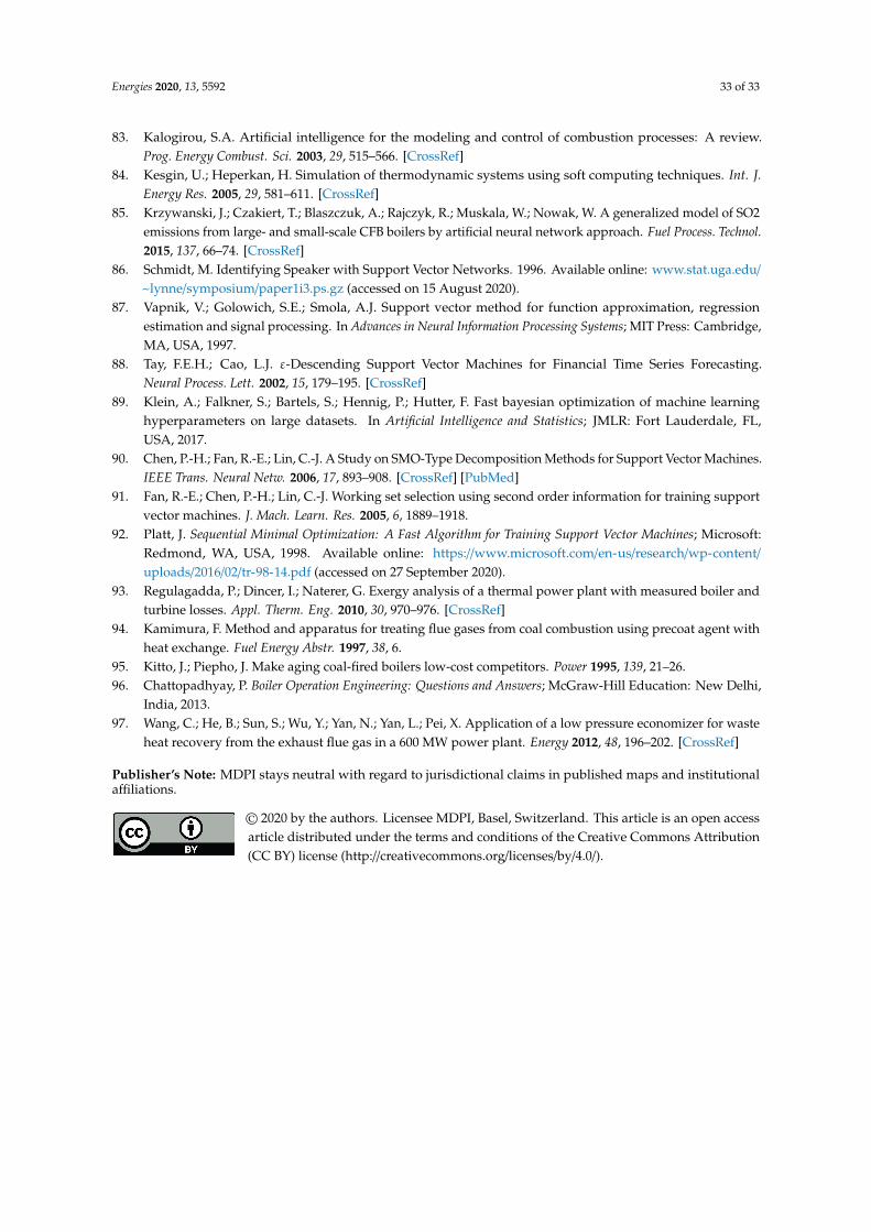
Energies 2020, 13, 5592 33 of 33
83. Kalogirou, S.A. Artificial intelligence for the modeling and control of combustion processes: A review.Prog. Energy Combust. Sci. 2003, 29, 515–566. [CrossRef]
84. Kesgin, U.; Heperkan, H. Simulation of thermodynamic systems using soft computing techniques. Int. J.Energy Res. 2005, 29, 581–611. [CrossRef]
85. Krzywanski, J.; Czakiert, T.; Blaszczuk, A.; Rajczyk, R.; Muskala, W.; Nowak, W. A generalized model of SO2emissions from large- and small-scale CFB boilers by artificial neural network approach. Fuel Process. Technol.2015, 137, 66–74. [CrossRef]
86. Schmidt, M. Identifying Speaker with Support Vector Networks. 1996. Available online: www.stat.uga.edu/
~lynne/symposium/paper1i3.ps.gz (accessed on 15 August 2020).87. Vapnik, V.; Golowich, S.E.; Smola, A.J. Support vector method for function approximation, regression
estimation and signal processing. In Advances in Neural Information Processing Systems; MIT Press: Cambridge,MA, USA, 1997.
88. Tay, F.E.H.; Cao, L.J. ε-Descending Support Vector Machines for Financial Time Series Forecasting.Neural Process. Lett. 2002, 15, 179–195. [CrossRef]
89. Klein, A.; Falkner, S.; Bartels, S.; Hennig, P.; Hutter, F. Fast bayesian optimization of machine learninghyperparameters on large datasets. In Artificial Intelligence and Statistics; JMLR: Fort Lauderdale, FL,USA, 2017.
90. Chen, P.-H.; Fan, R.-E.; Lin, C.-J. A Study on SMO-Type Decomposition Methods for Support Vector Machines.IEEE Trans. Neural Netw. 2006, 17, 893–908. [CrossRef] [PubMed]
91. Fan, R.-E.; Chen, P.-H.; Lin, C.-J. Working set selection using second order information for training supportvector machines. J. Mach. Learn. Res. 2005, 6, 1889–1918.
92. Platt, J. Sequential Minimal Optimization: A Fast Algorithm for Training Support Vector Machines; Microsoft:Redmond, WA, USA, 1998. Available online: https://www.microsoft.com/en-us/research/wp-content/uploads/2016/02/tr-98-14.pdf (accessed on 27 September 2020).
93. Regulagadda, P.; Dincer, I.; Naterer, G. Exergy analysis of a thermal power plant with measured boiler andturbine losses. Appl. Therm. Eng. 2010, 30, 970–976. [CrossRef]
94. Kamimura, F. Method and apparatus for treating flue gases from coal combustion using precoat agent withheat exchange. Fuel Energy Abstr. 1997, 38, 6.
95. Kitto, J.; Piepho, J. Make aging coal-fired boilers low-cost competitors. Power 1995, 139, 21–26.96. Chattopadhyay, P. Boiler Operation Engineering: Questions and Answers; McGraw-Hill Education: New Delhi,
India, 2013.97. Wang, C.; He, B.; Sun, S.; Wu, Y.; Yan, N.; Yan, L.; Pei, X. Application of a low pressure economizer for waste
heat recovery from the exhaust flue gas in a 600 MW power plant. Energy 2012, 48, 196–202. [CrossRef]
Publisher’s Note: MDPI stays neutral with regard to jurisdictional claims in published maps and institutionalaffiliations.
© 2020 by the authors. Licensee MDPI, Basel, Switzerland. This article is an open accessarticle distributed under the terms and conditions of the Creative Commons Attribution(CC BY) license (http://creativecommons.org/licenses/by/4.0/).