Optimization for Deep Learning

Tsz-Chiu Auchiu@unist.ac.kr

Acknowledgment: The content of this file is based on the textbook as well as the slides provided by Prof. Sung Ju Hwang.

Learning vs. Optimization

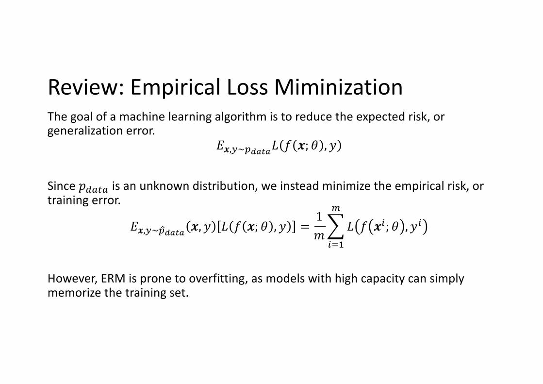
Review: Empirical Loss MiminizationThe goal of a machine learning algorithm is to reduce the expected risk, or generalization error.

!",$~&'()(* + "; - , .

Since /0121 is an unknown distribution, we instead minimize the empirical risk, or training error.

!",$~ 3&'()( ", . * + "; - , . = 167

89:

;* + "8; - , .8

However, ERM is prone to overfitting, as models with high capacity can simply memorize the training set.

Surrogate Loss FunctionsSometimes, the target loss function does not have useful gradients – e.g.) 0-1 loss

In such situations, one typically optimizes a surrogate loss function which act as a proxy but has advantages – e.g.) negative log-likelihood to estimate the conditional probability of a class, given the input.

In some cases, a surrogate loss function actually learns more than the original loss.- e.g.) When using log-likelihood surrogate, the test set 0-1 loss decreases for a long time after the training set 0-1 has reached 0, by pushing the classes further apart from each other.

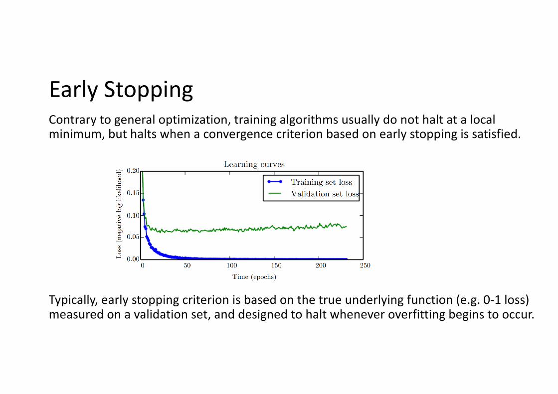
Early StoppingContrary to general optimization, training algorithms usually do not halt at a local minimum, but halts when a convergence criterion based on early stopping is satisfied.

Typically, early stopping criterion is based on the true underlying function (e.g. 0-1 loss) measured on a validation set, and designed to halt whenever overfitting begins to occur.

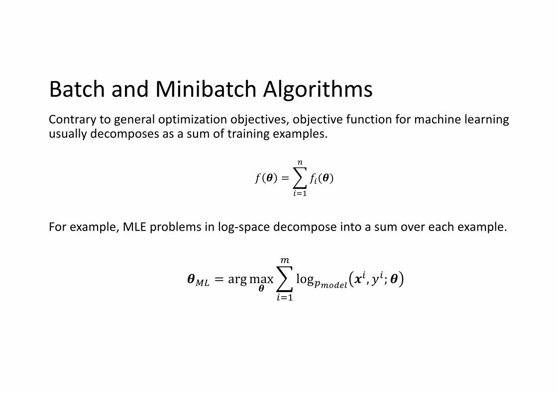
Batch and Minibatch AlgorithmsContrary to general optimization objectives, objective function for machine learning usually decomposes as a sum of training examples.

! " =$%&'

(!%(")

For example, MLE problems in log-space decompose into a sum over each example.

"+, = argmax"$%&'

2log56789: ;%, =%; "

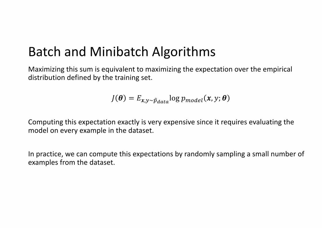
Batch and Minibatch AlgorithmsMaximizing this sum is equivalent to maximizing the expectation over the empirical distribution defined by the training set.

! " = $%,'~ )*+,-,log 123456 %, 7; "

Computing this expectation exactly is very expensive since it requires evaluating the model on every example in the dataset.

In practice, we can compute this expectations by randomly sampling a small number of examples from the dataset.

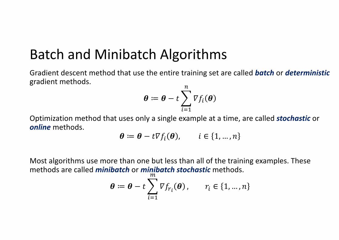
Batch and Minibatch AlgorithmsGradient descent method that use the entire training set are called batch or deterministicgradient methods.

! ≔ ! − $%&'(

)*+& !

Optimization method that uses only a single example at a time, are called stochastic or online methods.

! ≔ ! − $*+& ! , - ∈ 1, … , 1

Most algorithms use more than one but less than all of the training examples. These methods are called minibatch or minibatch stochastic methods.

! ≔ ! − $%&'(

2*+34 ! , 5& ∈ 1, … , 1

Batch and Minibatch AlgorithmsMinibatch sizes are generally decided by the following factors:

• Large batches provide a more accurate gradient estimate, but with less linear returns.

• Multicore architectures are usually underutilized by extremely small batches. In such cases, minibatch size can be increased until there is no reduction in processing time.

• Some kinds of hardware achieve better runtime with specific size of arrays – 2"

• Small batches can result in a regularizing effect, due to the noise they add in the learning process – generalization errors are often smallest with batch size = 1.

Challenges in Neural Network Optimization

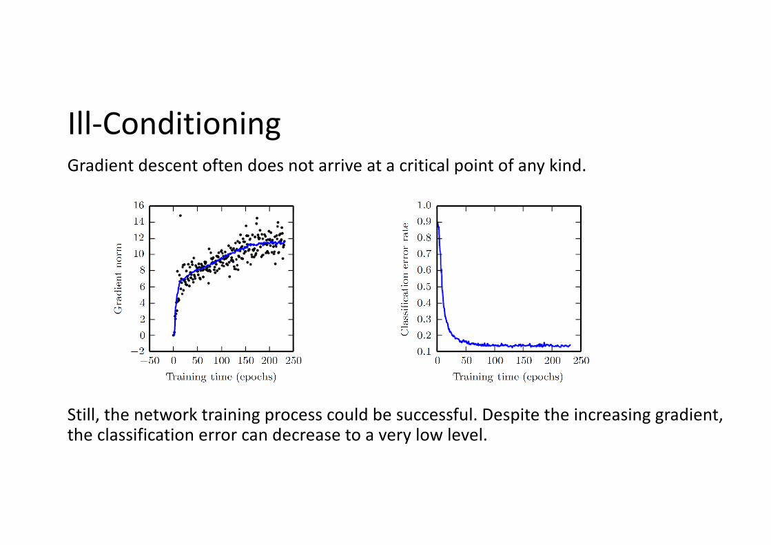
Ill-ConditioningGradient descent often does not arrive at a critical point of any kind.

Still, the network training process could be successful. Despite the increasing gradient, the classification error can decrease to a very low level.

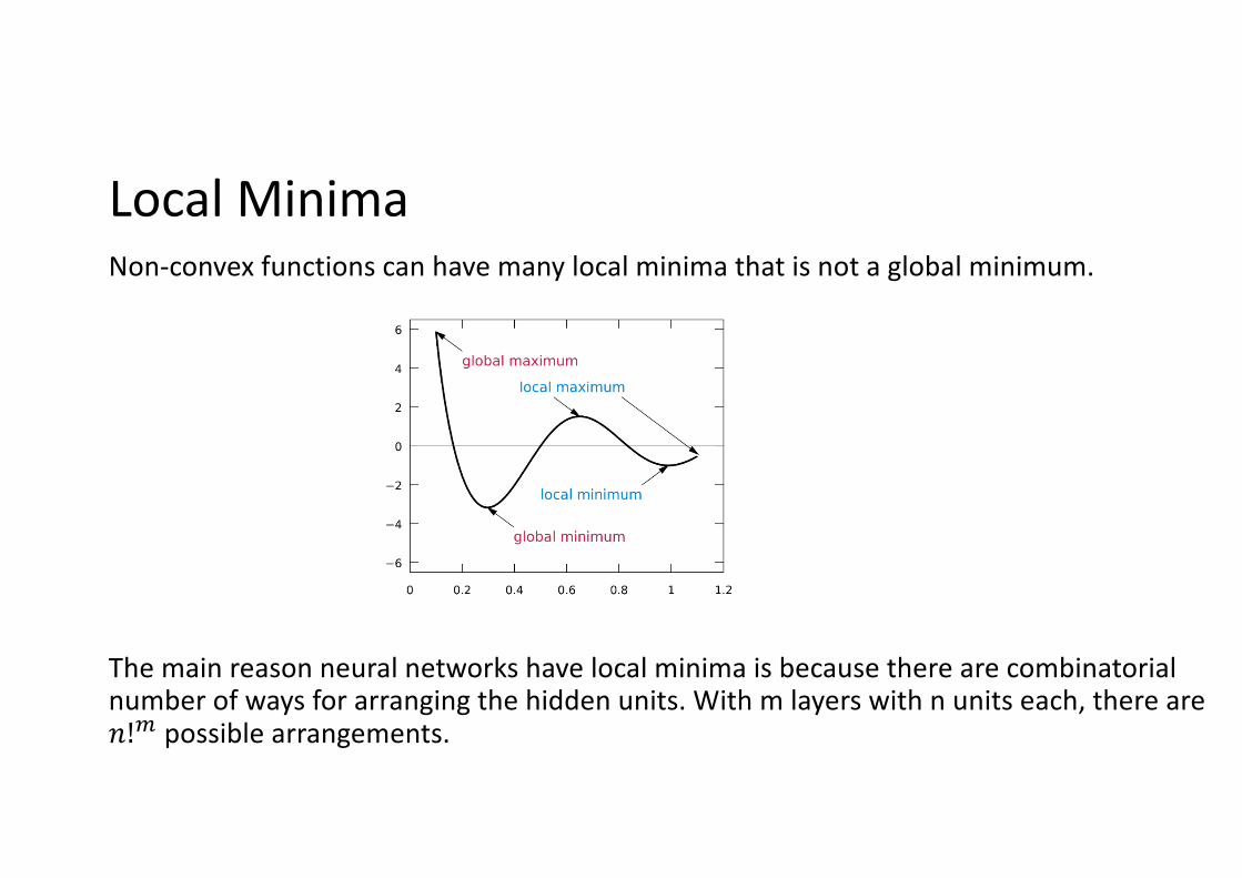
Local MinimaNon-convex functions can have many local minima that is not a global minimum.

The main reason neural networks have local minima is because there are combinatorial number of ways for arranging the hidden units. With m layers with n units each, there are !!# possible arrangements.

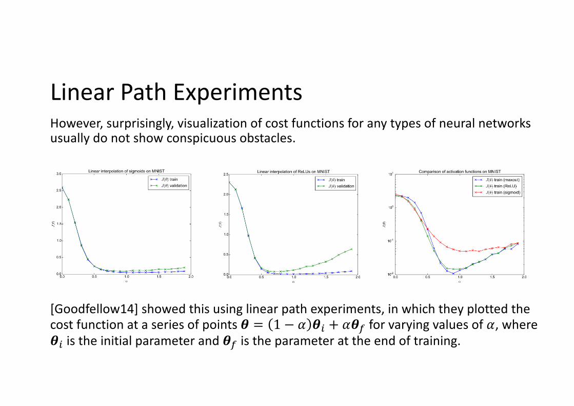
Linear Path ExperimentsHowever, surprisingly, visualization of cost functions for any types of neural networks usually do not show conspicuous obstacles.

[Goodfellow14] showed this using linear path experiments, in which they plotted the cost function at a series of points ! = 1 − % !& + %!( for varying values of %, where !& is the initial parameter and !( is the parameter at the end of training.

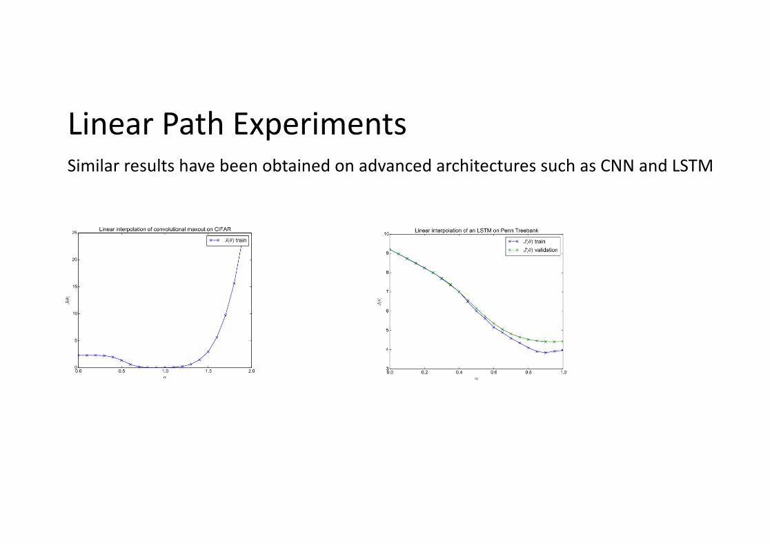
Linear Path ExperimentsSimilar results have been obtained on advanced architectures such as CNN and LSTM

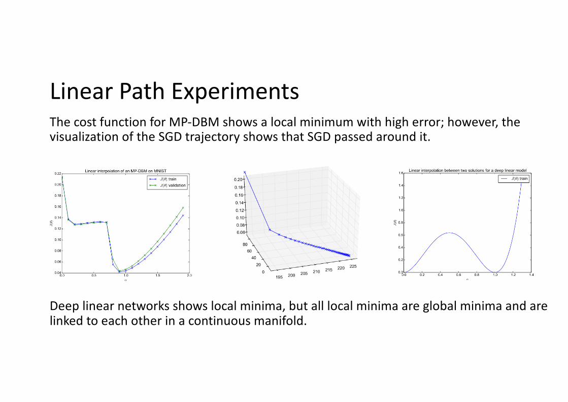
Linear Path ExperimentsThe cost function for MP-DBM shows a local minimum with high error; however, the visualization of the SGD trajectory shows that SGD passed around it.

Deep linear networks shows local minima, but all local minima are global minima and are linked to each other in a continuous manifold.

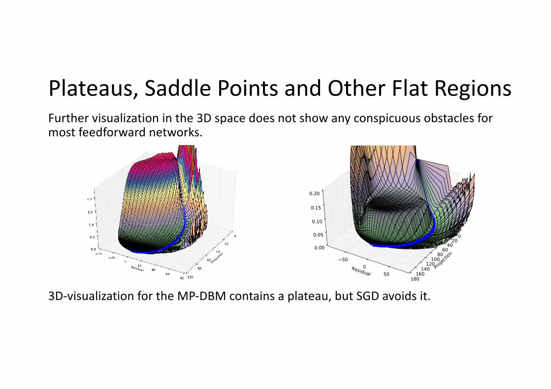
Plateaus, Saddle Points and Other Flat RegionsFurther visualization in the 3D space does not show any conspicuous obstacles for most feedforward networks.

3D-visualization for the MP-DBM contains a plateau, but SGD avoids it.

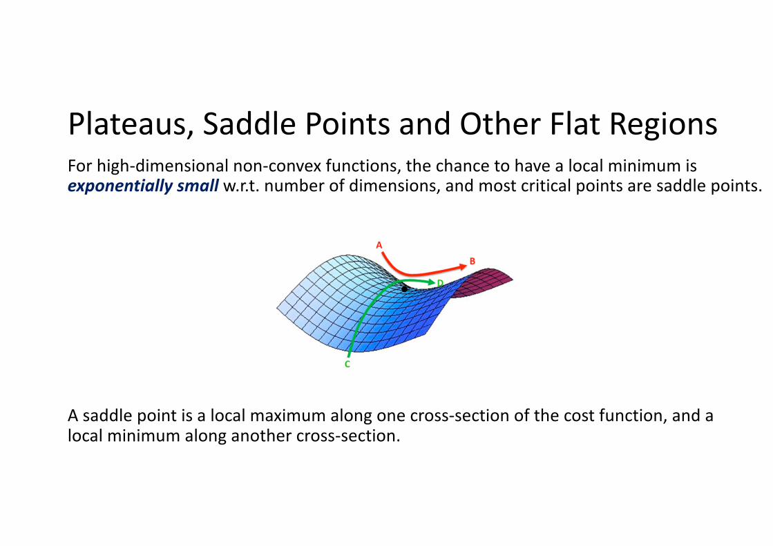
Plateaus, Saddle Points and Other Flat RegionsFor high-dimensional non-convex functions, the chance to have a local minimum is exponentially small w.r.t. number of dimensions, and most critical points are saddle points.

A saddle point is a local maximum along one cross-section of the cost function, and a local minimum along another cross-section.

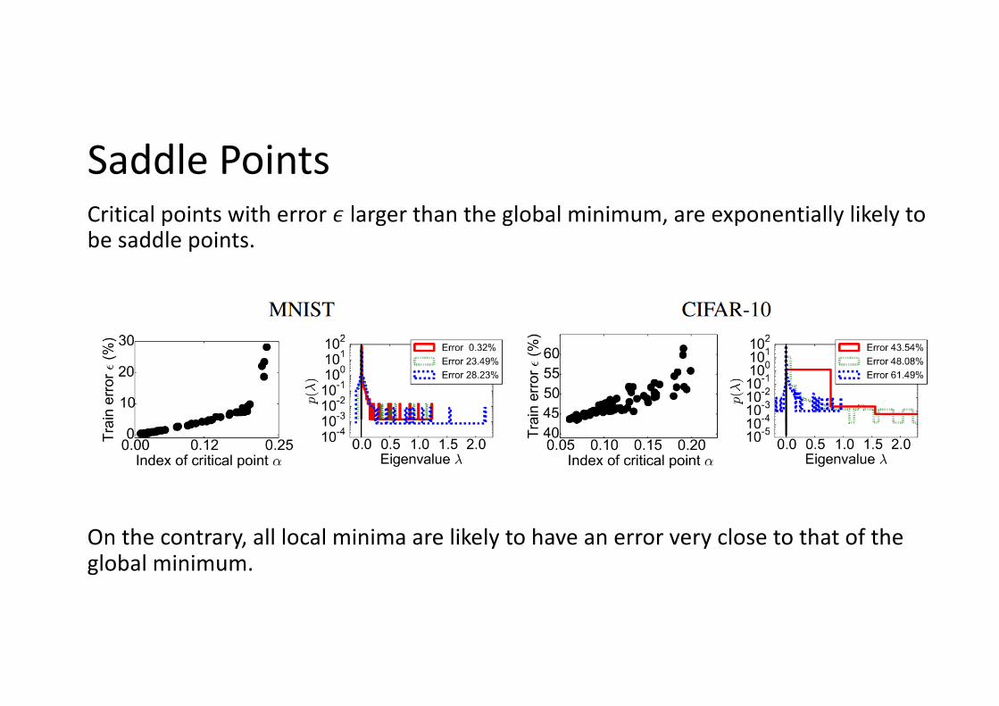
Saddle PointsCritical points with error ! larger than the global minimum, are exponentially likely to be saddle points.

On the contrary, all local minima are likely to have an error very close to that of the global minimum.

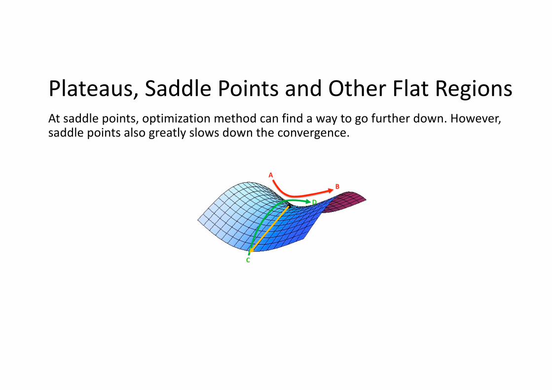
Plateaus, Saddle Points and Other Flat RegionsAt saddle points, optimization method can find a way to go further down. However, saddle points also greatly slows down the convergence.

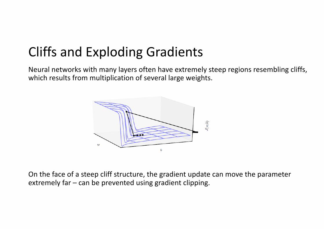
Cliffs and Exploding GradientsNeural networks with many layers often have extremely steep regions resembling cliffs, which results from multiplication of several large weights.

On the face of a steep cliff structure, the gradient update can move the parameter extremely far – can be prevented using gradient clipping.

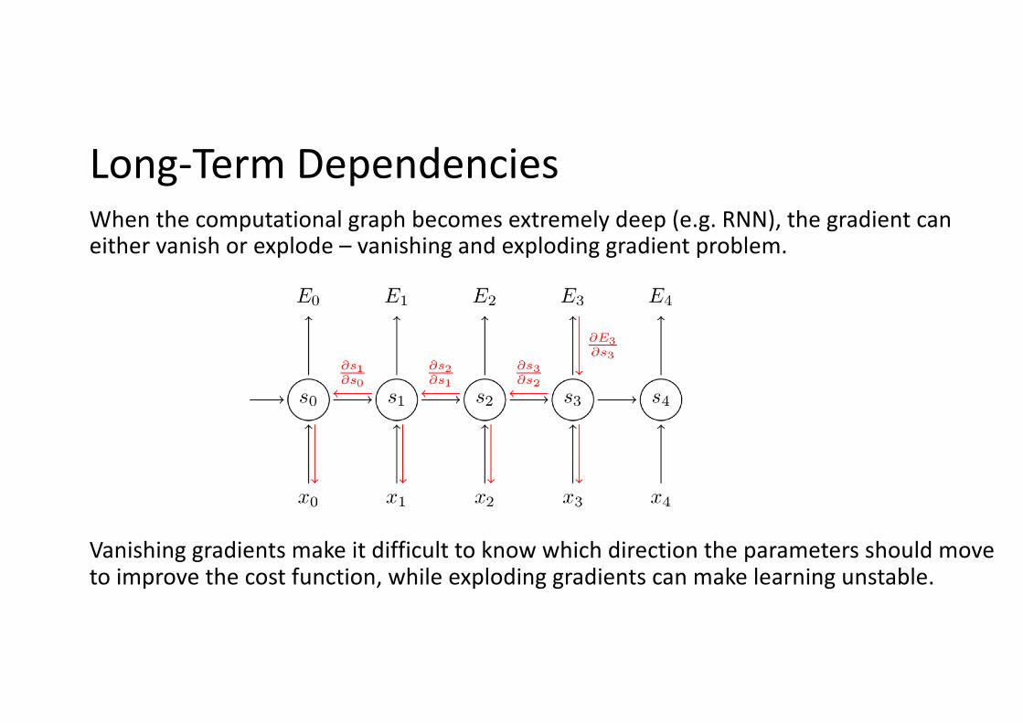
Long-Term DependenciesWhen the computational graph becomes extremely deep (e.g. RNN), the gradient can either vanish or explode – vanishing and exploding gradient problem.

Vanishing gradients make it difficult to know which direction the parameters should move to improve the cost function, while exploding gradients can make learning unstable.

Inexact GradientsWhile most optimization algorithms assume that we have exact knowledge of the gradient or Hessian, in reality we only have noisy or biased estimates.

Nearly all deep learning algorithms rely on sampling-based estimates such as using minibatch of training examples to compute the gradient.

In some other cases, the objective function we want to minimize is actually intractable, which makes the gradients to be intractable as well. In such cases, we can only approximate the gradient – e.g.) Boltzmann machine

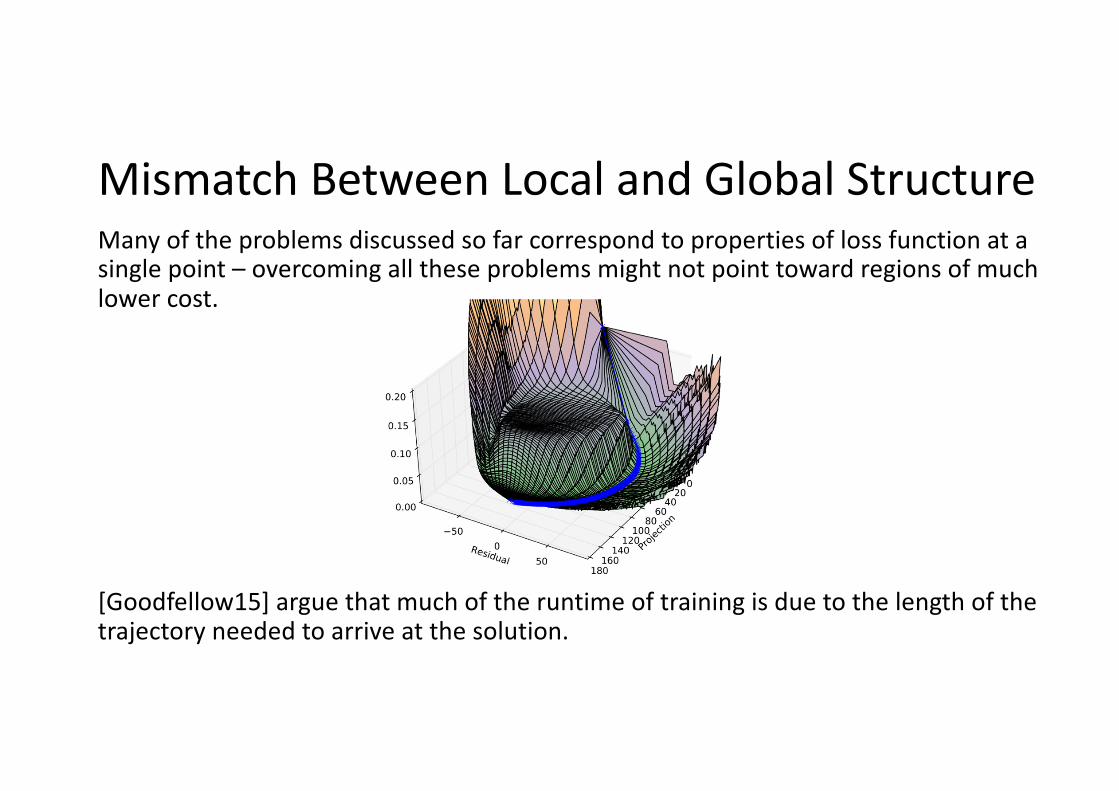
Mismatch Between Local and Global StructureMany of the problems discussed so far correspond to properties of loss function at a single point – overcoming all these problems might not point toward regions of much lower cost.

[Goodfellow15] argue that much of the runtime of training is due to the length of the trajectory needed to arrive at the solution.

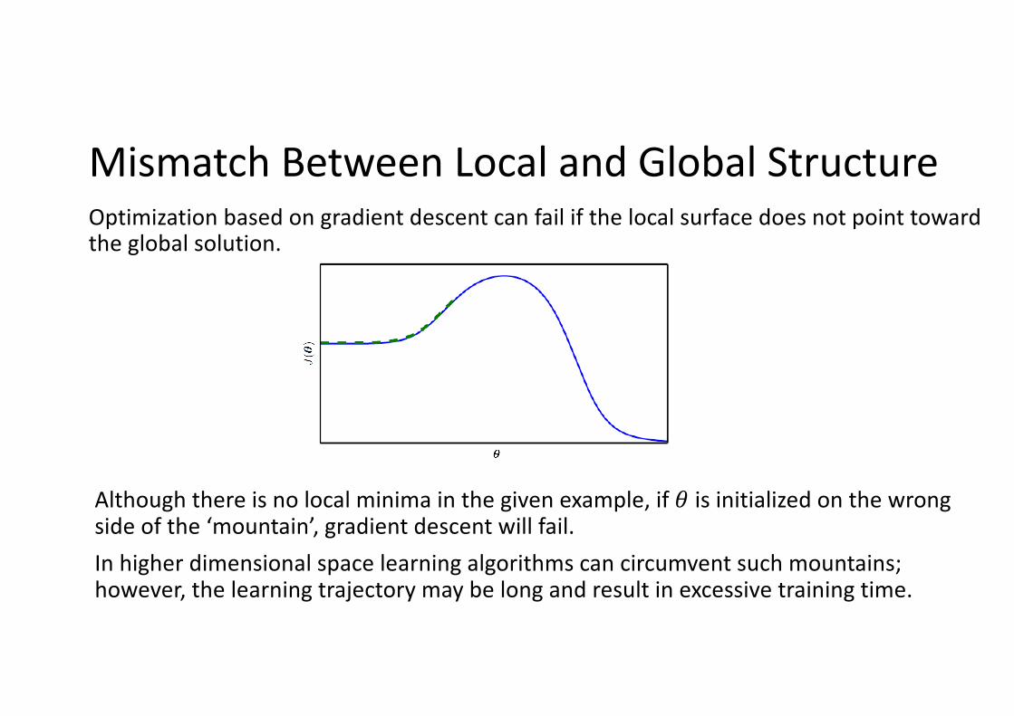
Mismatch Between Local and Global StructureOptimization based on gradient descent can fail if the local surface does not point toward the global solution.

Although there is no local minima in the given example, if ! is initialized on the wrong side of the ‘mountain’, gradient descent will fail. In higher dimensional space learning algorithms can circumvent such mountains; however, the learning trajectory may be long and result in excessive training time.

Stochastic Gradient Descent

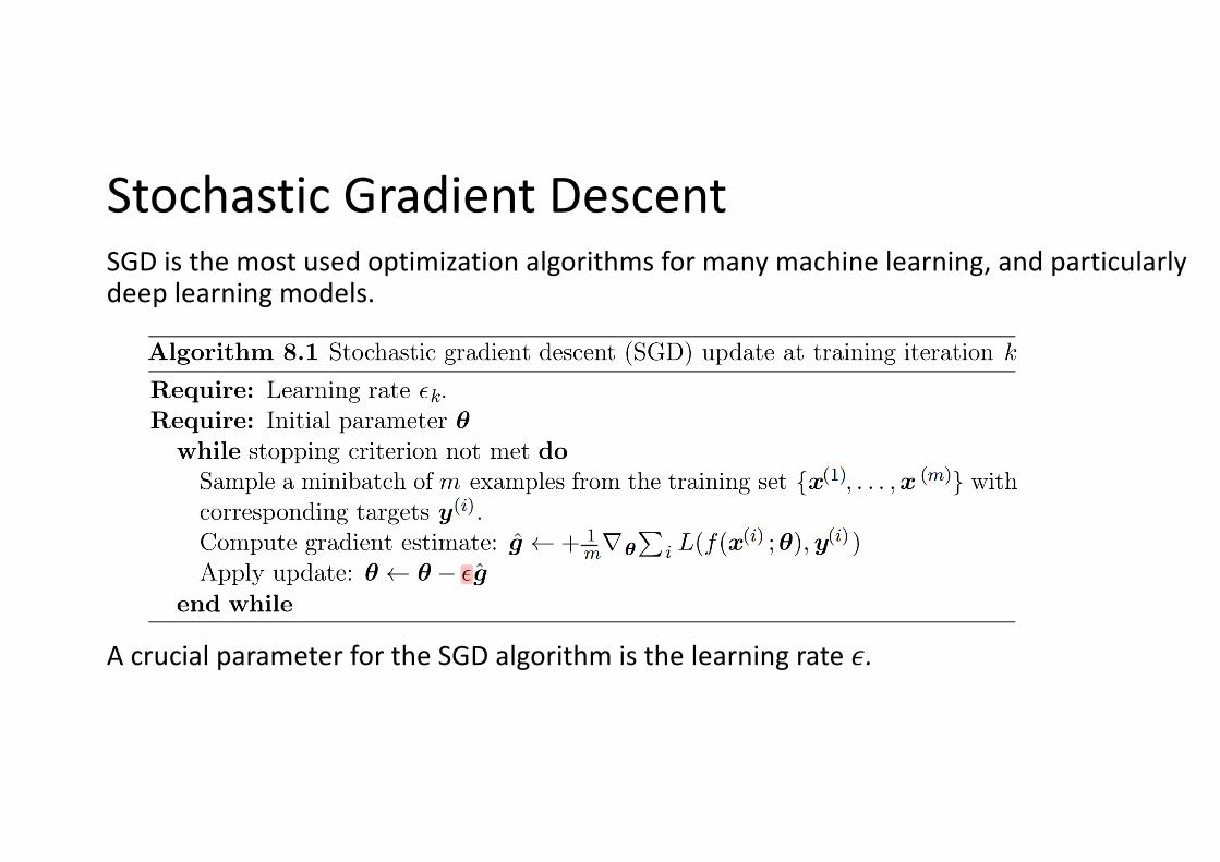
Stochastic Gradient DescentSGD is the most used optimization algorithms for many machine learning, and particularly deep learning models.

A crucial parameter for the SGD algorithm is the learning rate !.

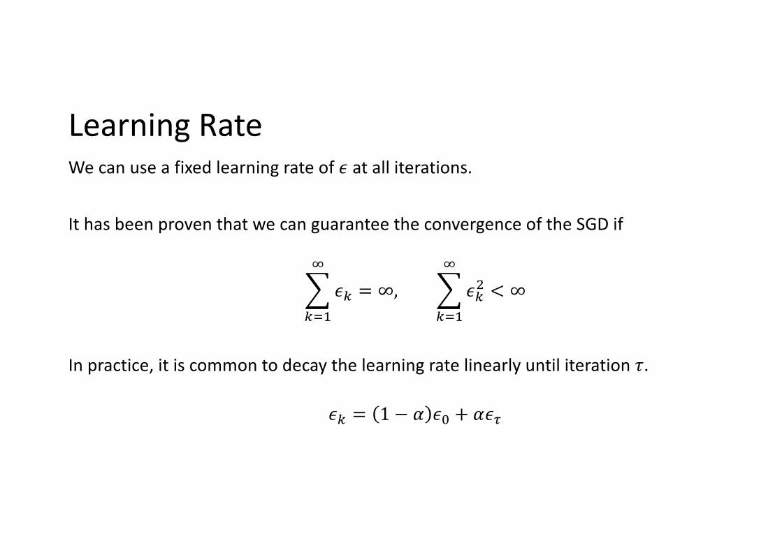
Learning RateWe can use a fixed learning rate of ! at all iterations.

It has been proven that we can guarantee the convergence of the SGD if

"#$%

&!# = ∞, "

#$%

&!#* < ∞

In practice, it is common to decay the learning rate linearly until iteration ,.

!# = 1 − / !0 + /!2

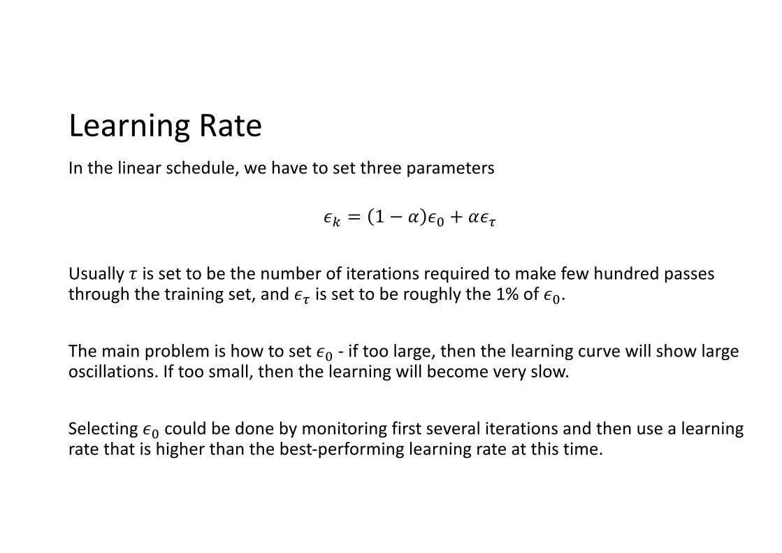
Learning RateIn the linear schedule, we have to set three parameters

!" = 1 − & !' + &!)

Usually * is set to be the number of iterations required to make few hundred passes through the training set, and !) is set to be roughly the 1% of !'.

The main problem is how to set !' - if too large, then the learning curve will show large oscillations. If too small, then the learning will become very slow.

Selecting !' could be done by monitoring first several iterations and then use a learning rate that is higher than the best-performing learning rate at this time.

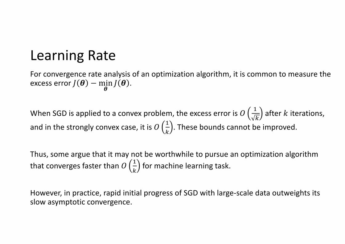
Learning RateFor convergence rate analysis of an optimization algorithm, it is common to measure the excess error ! " − min

"! " .

When SGD is applied to a convex problem, the excess error is ' () after * iterations,

and in the strongly convex case, it is ' () . These bounds cannot be improved.

Thus, some argue that it may not be worthwhile to pursue an optimization algorithm that converges faster than ' (

) for machine learning task.

However, in practice, rapid initial progress of SGD with large-scale data outweights its slow asymptotic convergence.

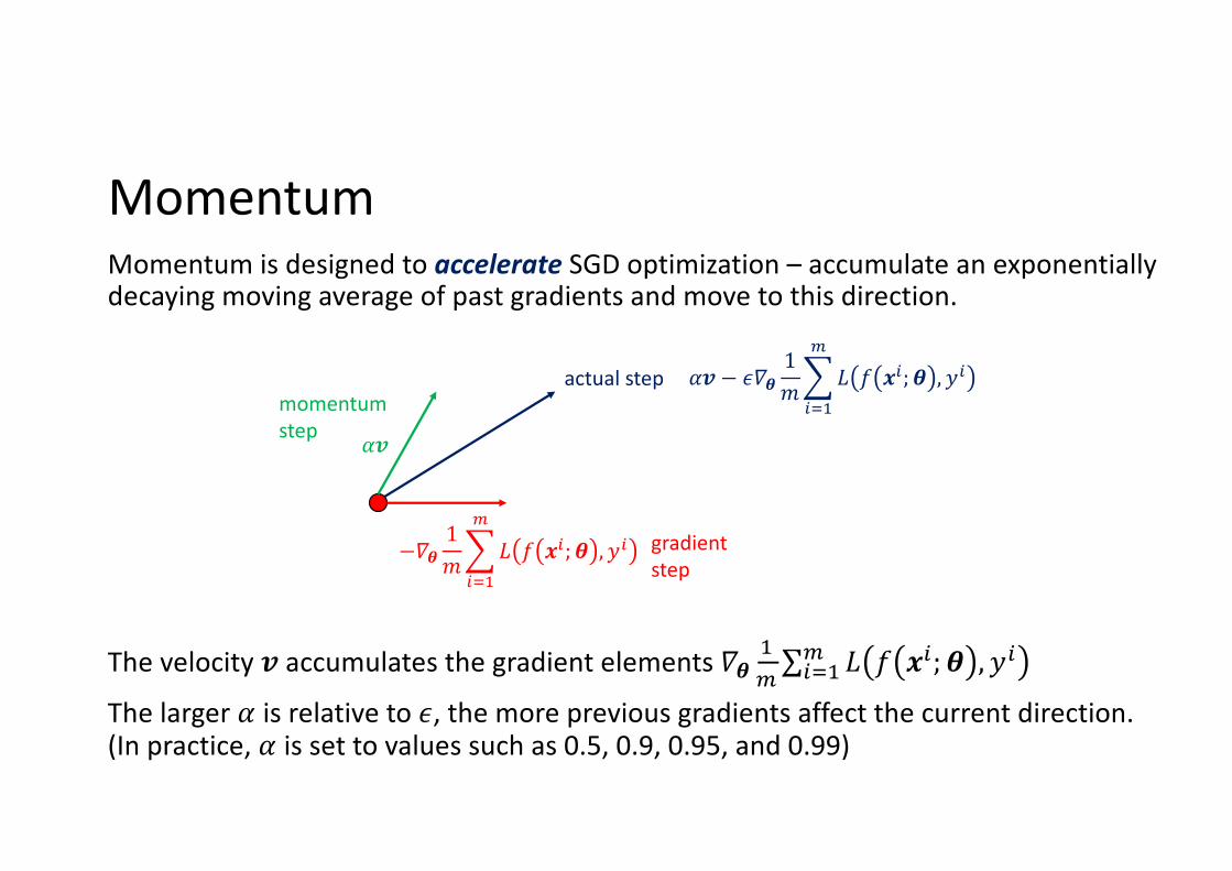
MomentumMomentum is designed to accelerate SGD optimization – accumulate an exponentially decaying moving average of past gradients and move to this direction.

The velocity ! accumulates the gradient elements "# $%∑'($

% ) * +'; # , .'The larger / is relative to 0, the more previous gradients affect the current direction. (In practice, / is set to values such as 0.5, 0.9, 0.95, and 0.99)

momentum step

gradient step

actual step

/!

−"#134

'($

%) * +'; # , .'

/! − 0"#134

'($

%) * +'; # , .'

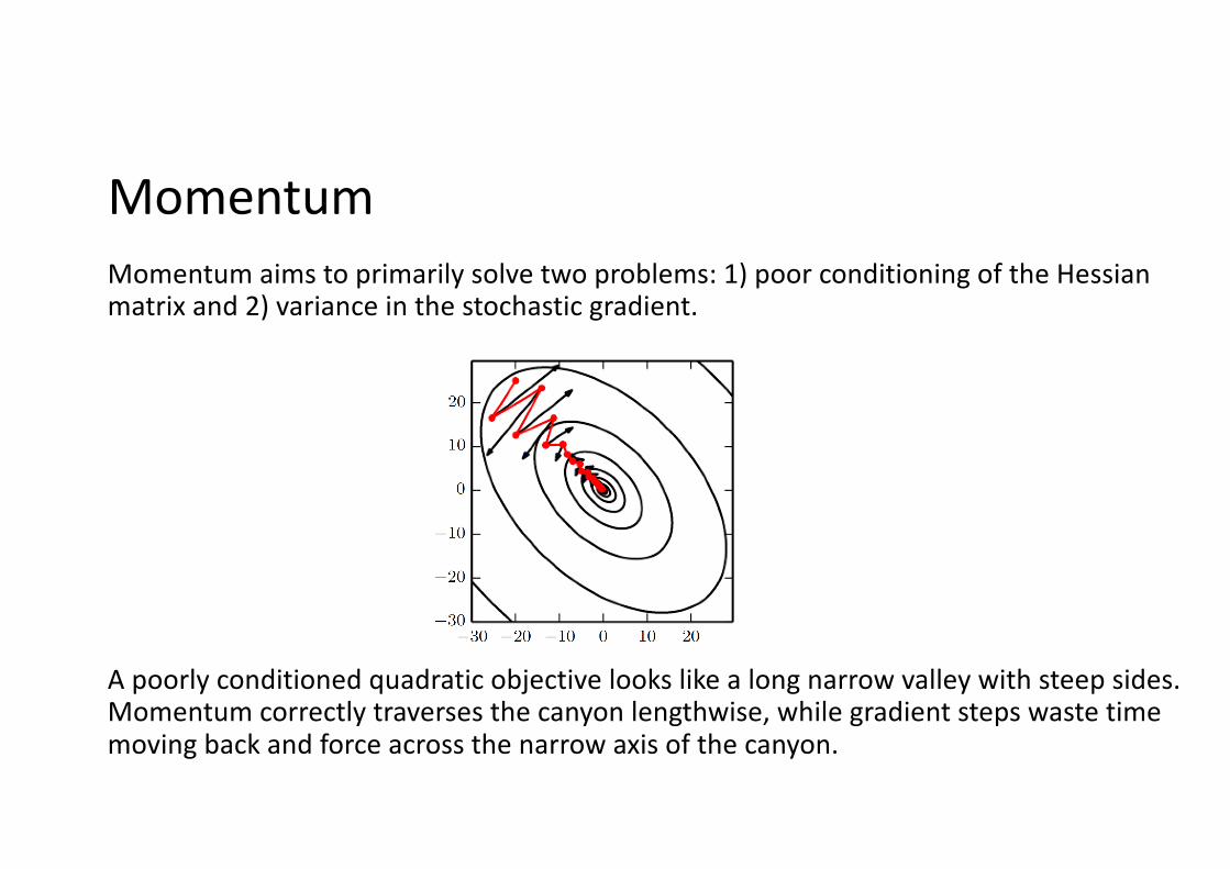
MomentumMomentum aims to primarily solve two problems: 1) poor conditioning of the Hessian matrix and 2) variance in the stochastic gradient.

A poorly conditioned quadratic objective looks like a long narrow valley with steep sides. Momentum correctly traverses the canyon lengthwise, while gradient steps waste time moving back and force across the narrow axis of the canyon.

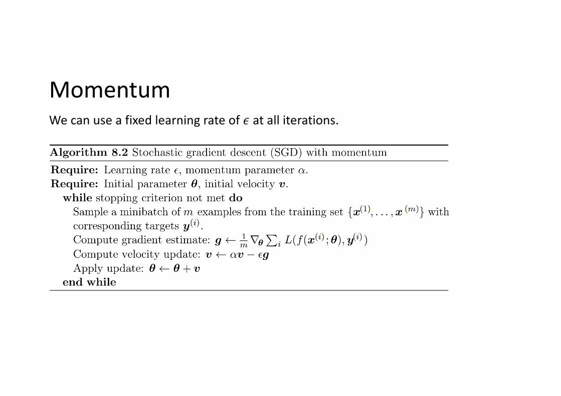
MomentumWe can use a fixed learning rate of ! at all iterations.

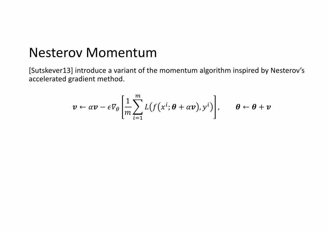
Nesterov Momentum[Sutskever13] introduce a variant of the momentum algorithm inspired by Nesterov’saccelerated gradient method.

! ← #! − %&'1)*

+,-

./ 0 1+; 3 + #! , 6+ , 3 ← 3 + !

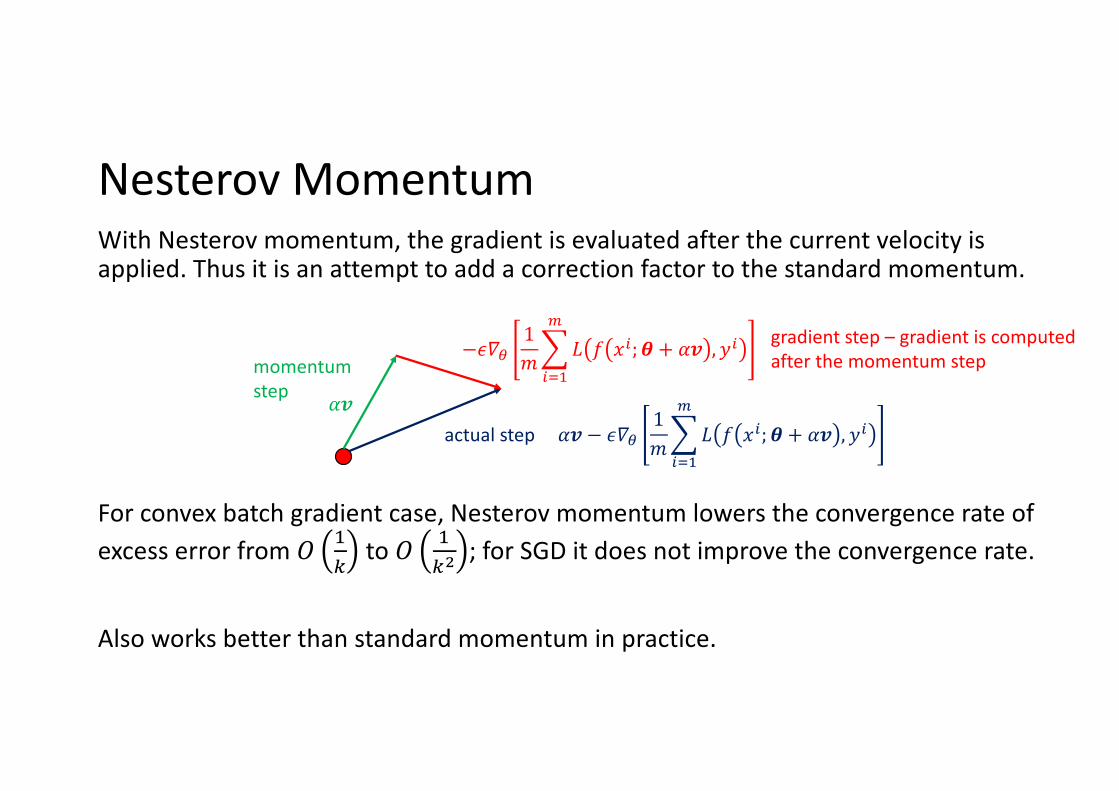
Nesterov MomentumWith Nesterov momentum, the gradient is evaluated after the current velocity is applied. Thus it is an attempt to add a correction factor to the standard momentum.

For convex batch gradient case, Nesterov momentum lowers the convergence rate of excess error from ! "

# to ! "#$ ; for SGD it does not improve the convergence rate.

Also works better than standard momentum in practice.

momentum step

gradient step – gradient is computed after the momentum step

actual step%&

%& − ()*1,-

./"

01 2 3.; 5 + %& , 8.

−()*1,-

./"

01 2 3.; 5 + %& , 8.

Strategies for Parameter InitializationTraining for deep learning gets largely affected by the choice of initialization.

Initial parameters need to break symmetry between different units, such that each unit evolves to compute a different function from all the other units.

In most cases, the weights are initialized as the values drawn randomly from a Gaussian or uniform distribution.

Here, the scale of the initial distribution is important - large initial weights will yield a stronger symmetry breaking effect.

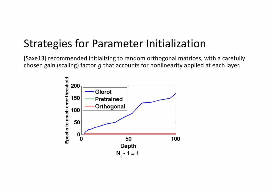
Strategies for Parameter Initialization[Saxe13] recommended initializing to random orthogonal matrices, with a carefully chosen gain (scaling) factor ! that accounts for nonlinearity applied at each layer.

Algorithms with Adaptive Learning Rates Among many hyperparameters, the learning rate is generally considered as the most difficult one to set, since it has a significant impact on model performance.

Normally, the cost function is highly sensitive to some directions in parameter spaces, and insensitive to others - thus some dimensions can allow large learning rate and for others the learning rate is best if kept small.

Solution - learn a separate learning rate for each parameter.

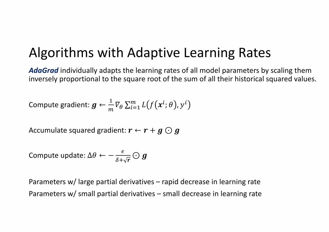
Algorithms with Adaptive Learning Rates AdaGrad individually adapts the learning rates of all model parameters by scaling them inversely proportional to the square root of the sum of all their historical squared values.

Compute gradient: ! ← #$%& ∑()#

$ * + ,(; . , 0(

Accumulate squared gradient: 1 ← 1 + !⊙ !

Compute update: Δ. ← − 678 1 ⊙ !

Parameters w/ large partial derivatives – rapid decrease in learning rateParameters w/ small partial derivatives – small decrease in learning rate

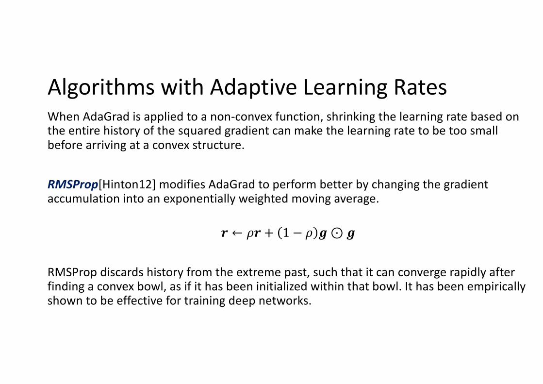
Algorithms with Adaptive Learning Rates When AdaGrad is applied to a non-convex function, shrinking the learning rate based on the entire history of the squared gradient can make the learning rate to be too small before arriving at a convex structure.

RMSProp[Hinton12] modifies AdaGrad to perform better by changing the gradient accumulation into an exponentially weighted moving average.

! ← #! + 1 − # '⊙ '

RMSProp discards history from the extreme past, such that it can converge rapidly after finding a convex bowl, as if it has been initialized within that bowl. It has been empirically shown to be effective for training deep networks.

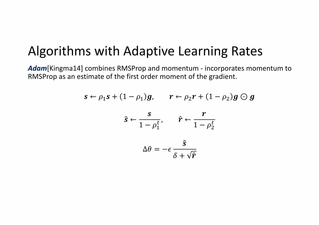
Algorithms with Adaptive Learning Rates Adam[Kingma14] combines RMSProp and momentum - incorporates momentum to RMSProp as an estimate of the first order moment of the gradient.

! ← #$! + 1 − #$ (, * ← #+* + 1 − #+ (⊙ (

-! ← !1 − #$.

, -* ← *1 − #+.

Δ0 = −2 -!3 + -*

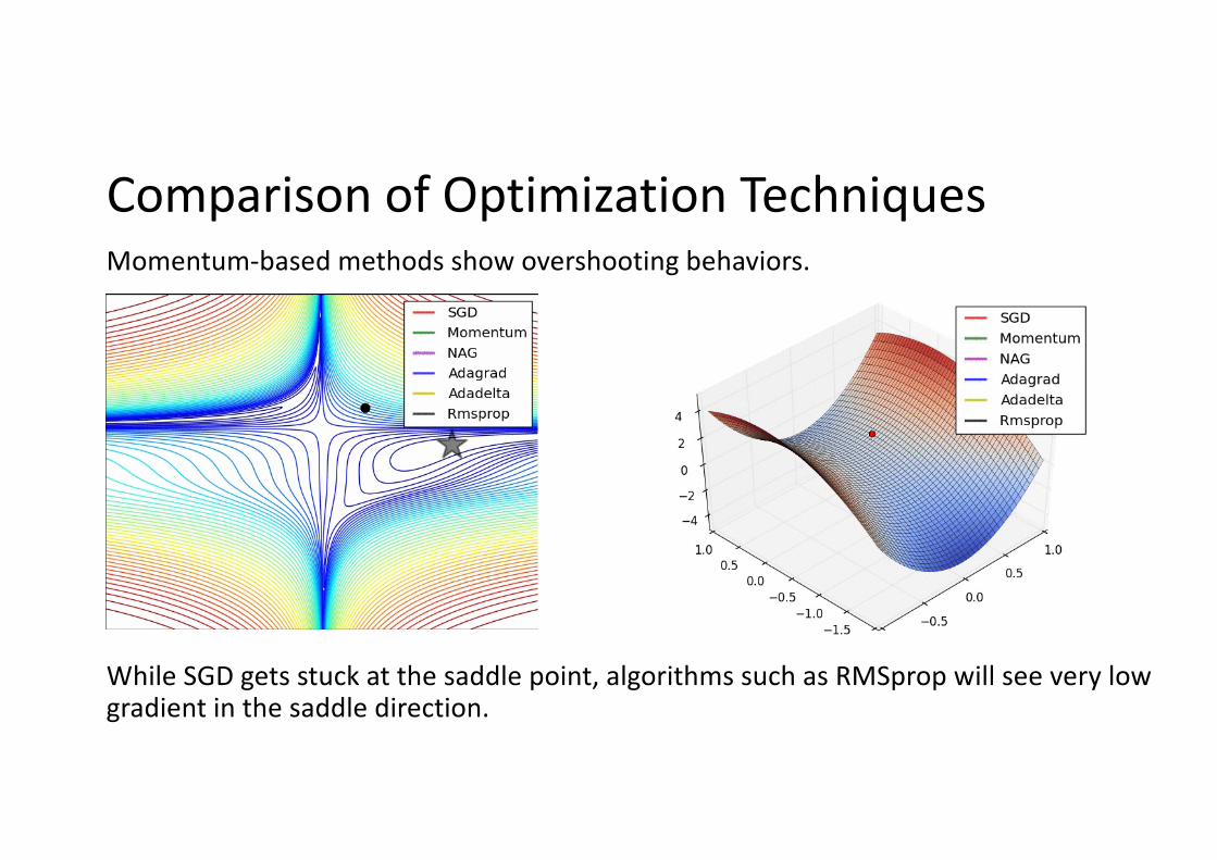
Comparison of Optimization TechniquesMomentum-based methods show overshooting behaviors.

While SGD gets stuck at the saddle point, algorithms such as RMSprop will see very low gradient in the saddle direction.

Approximate Second-Order Methods

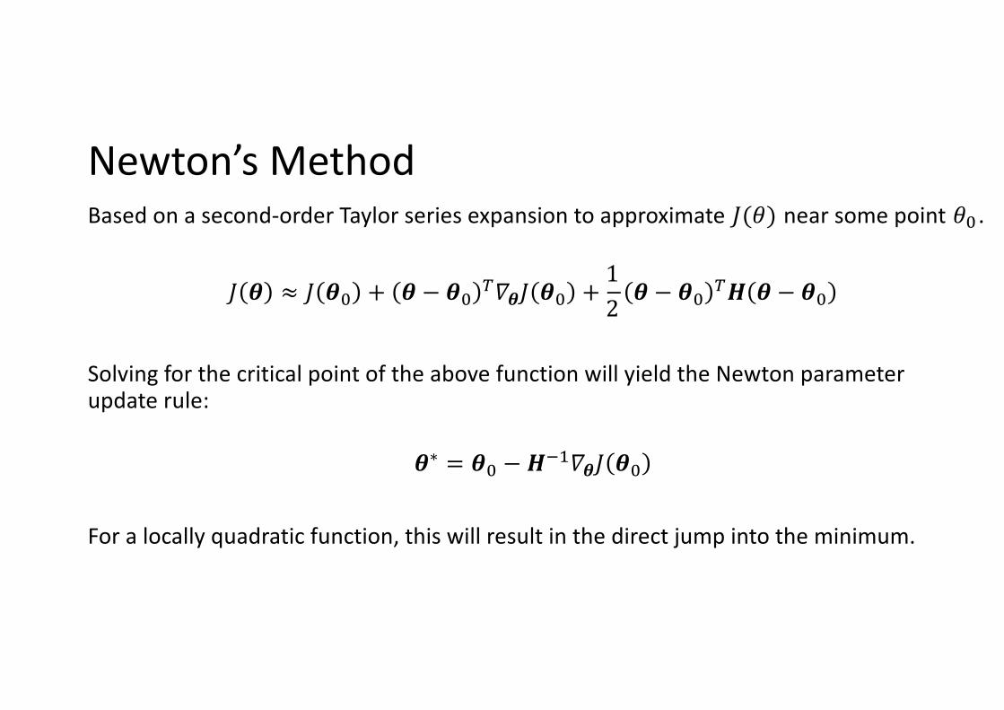
Newton’s MethodBased on a second-order Taylor series expansion to approximate !(#) near some point #% .

! & ≈ ! &% + & − &% *+&! &% + 12 & − &% *. & − &%

Solving for the critical point of the above function will yield the Newton parameter update rule:

&∗ = &% − .12+&! &%

For a locally quadratic function, this will result in the direct jump into the minimum.

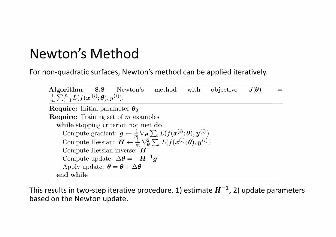
Newton’s MethodFor non-quadratic surfaces, Newton’s method can be applied iteratively.

This results in two-step iterative procedure. 1) estimate !"#, 2) update parameters based on the Newton update.

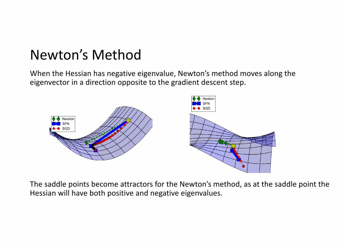
Newton’s MethodWhen the Hessian has negative eigenvalue, Newton’s method moves along the eigenvector in a direction opposite to the gradient descent step.

The saddle points become attractors for the Newton’s method, as at the saddle point the Hessian will have both positive and negative eigenvalues.

Attacking Saddle Point ProblemThis can be avoided by regularizing the Hessian by adding some positive constant !.

"∗ = "% − ' ( )% + !+ ,-./( "%

However, if the damping coefficient ! is set to high, then Newton’s method behaves similar to gradient descent, and loses the advantage of fast convergence.

Another way is to ignore the negative curvature. However, such algorithm cannot escape saddle points, as they ignore the directions of negative curvature that must be followed in order to escape.

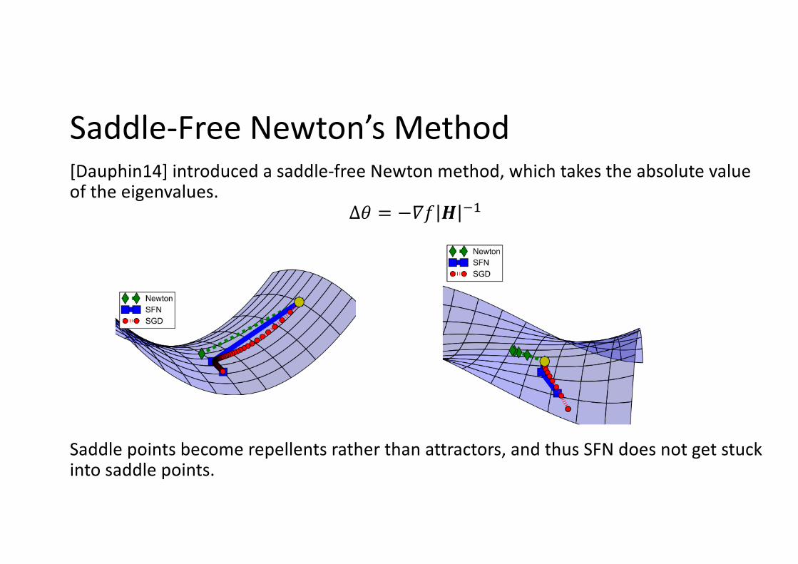
Saddle-Free Newton’s Method[Dauphin14] introduced a saddle-free Newton method, which takes the absolute value of the eigenvalues.

Δ" = −%& ' ()

Saddle points become repellents rather than attractors, and thus SFN does not get stuck into saddle points.

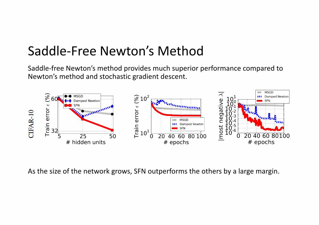
Saddle-Free Newton’s MethodSaddle-free Newton’s method provides much superior performance compared to Newton’s method and stochastic gradient descent.

As the size of the network grows, SFN outperforms the others by a large margin.

BFGSBroyden-Fletcher-Goldfarb-Shanno (BFGS) algorithm is an approximate Newton’s method with less computational burden.

Newton’s update is given by !∗ = !$ − &'()!* !$

which requires the computation of &'(, which has + ,- complexity (, = dim(!))

From this, we can see that the parameters at step 3 are related via the secant condition

!45( − !4 = −&'( )!* !45( − )!* !4

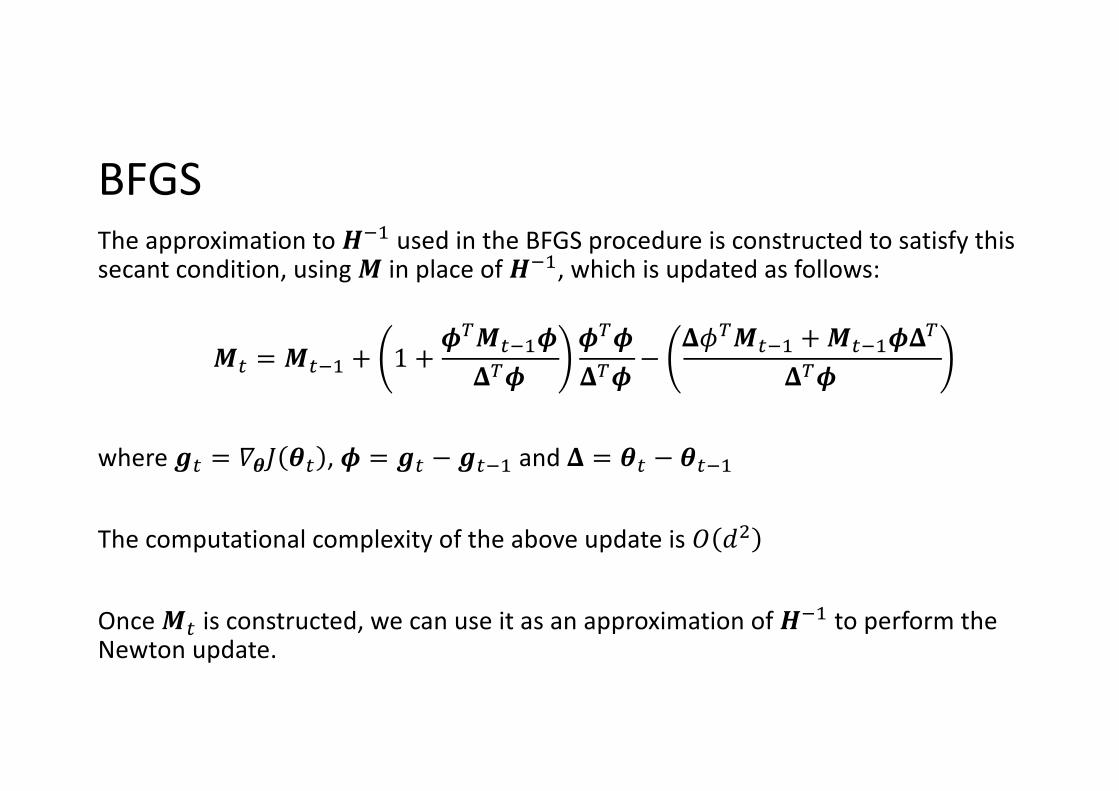
BFGSThe approximation to !"# used in the BFGS procedure is constructed to satisfy this secant condition, using $ in place of !"#, which is updated as follows:

$% = $%"# + 1 + )*$%"#)+*)

)*)+*) − +-*$%"# +$%"#)+*

+*)

where .% = /01 0% , ) = .% − .%"# and + = 0% − 0%"#

The computational complexity of the above update is 2 34

Once $% is constructed, we can use it as an approximation of !"# to perform the Newton update.

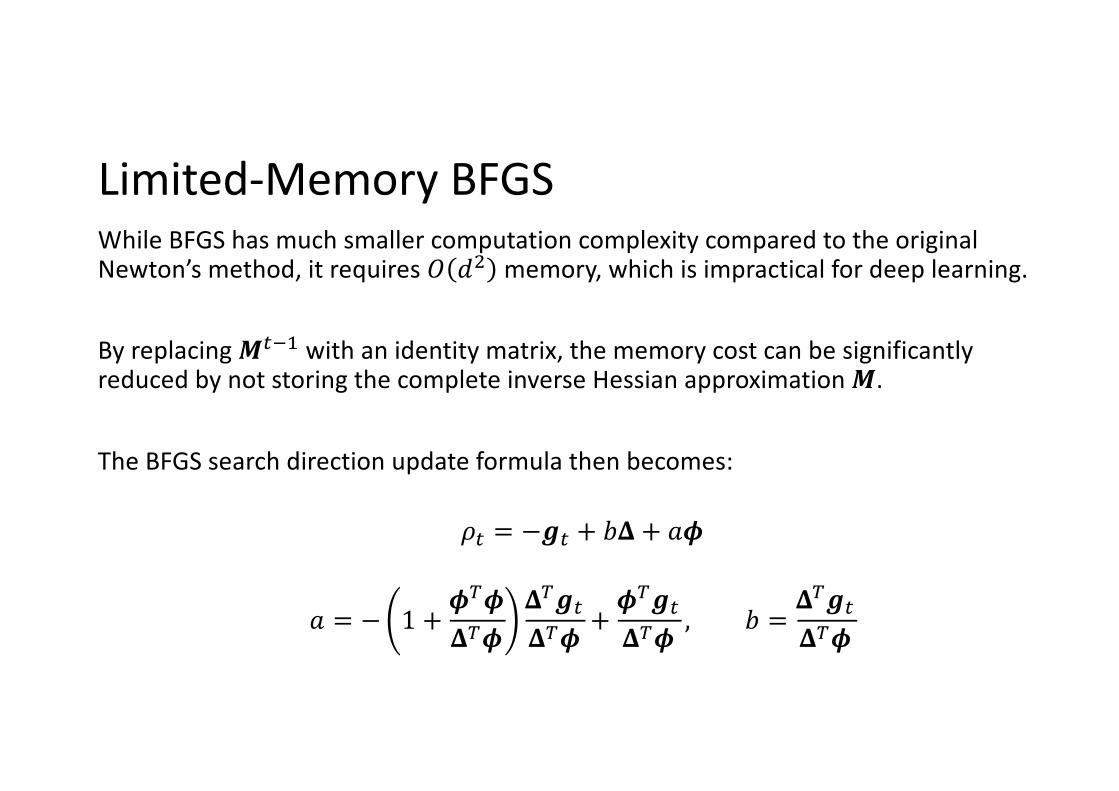
Limited-Memory BFGSWhile BFGS has much smaller computation complexity compared to the original Newton’s method, it requires ! "# memory, which is impractical for deep learning.

By replacing $%&' with an identity matrix, the memory cost can be significantly reduced by not storing the complete inverse Hessian approximation $.

The BFGS search direction update formula then becomes:

(% = −+% + -. + /0

/ = − 1 + 020

.20.2+%.20 + 0

2+%.20 , - = .2+%

.20

Optimization Strategies and Meta-Algorithms

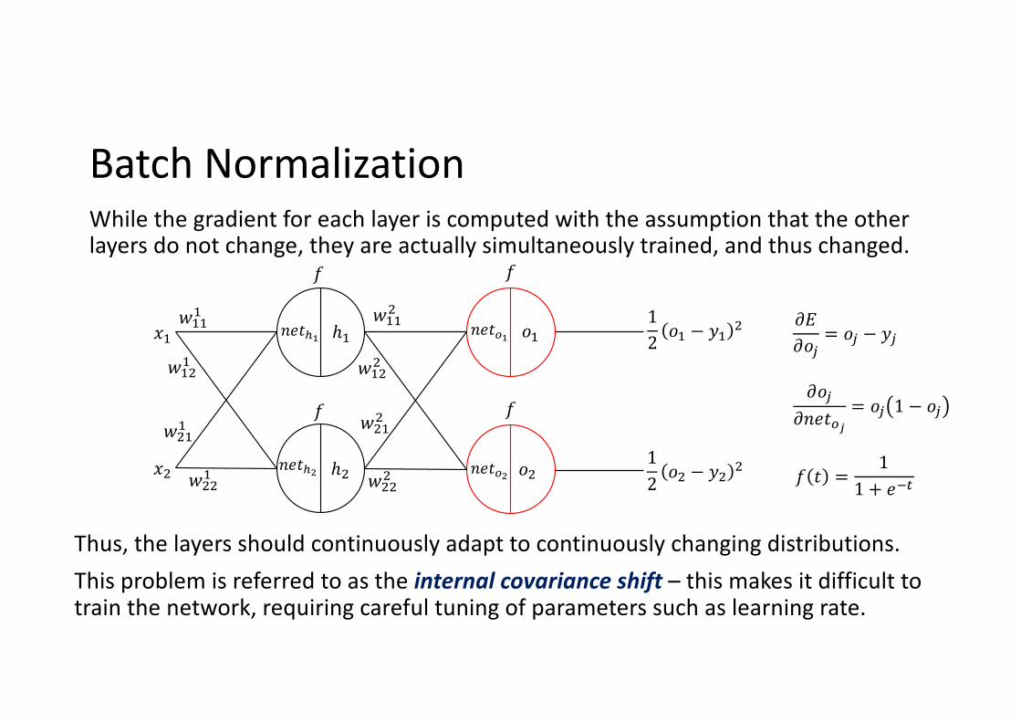
Batch NormalizationWhile the gradient for each layer is computed with the assumption that the other layers do not change, they are actually simultaneously trained, and thus changed.

Thus, the layers should continuously adapt to continuously changing distributions.This problem is referred to as the internal covariance shift – this makes it difficult to train the network, requiring careful tuning of parameters such as learning rate.

!"

#$!$%$$"

%$""

%"$"

%"""

ℎ$

ℎ" #"

%$$$

%$"$

%"$$

%""$

12 #$ − *$ "

+

+

+

+

,-,#.

= #. − *.

12 #" − *" "

,#.,01234

= #. 1 − #.

01256 01236

01257 01237 + 2 = 11 + 19:

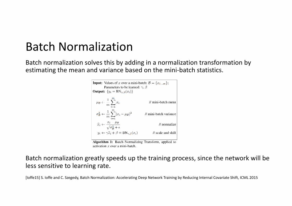
Batch NormalizationBatch normalization solves this by adding in a normalization transformation by estimating the mean and variance based on the mini-batch statistics.

Batch normalization greatly speeds up the training process, since the network will be less sensitive to learning rate.[Ioffe15] S. Ioffe and C. Szegedy, Batch Normalization: Accelerating Deep Network Training by Reducing Internal Covariate Shift, ICML 2015

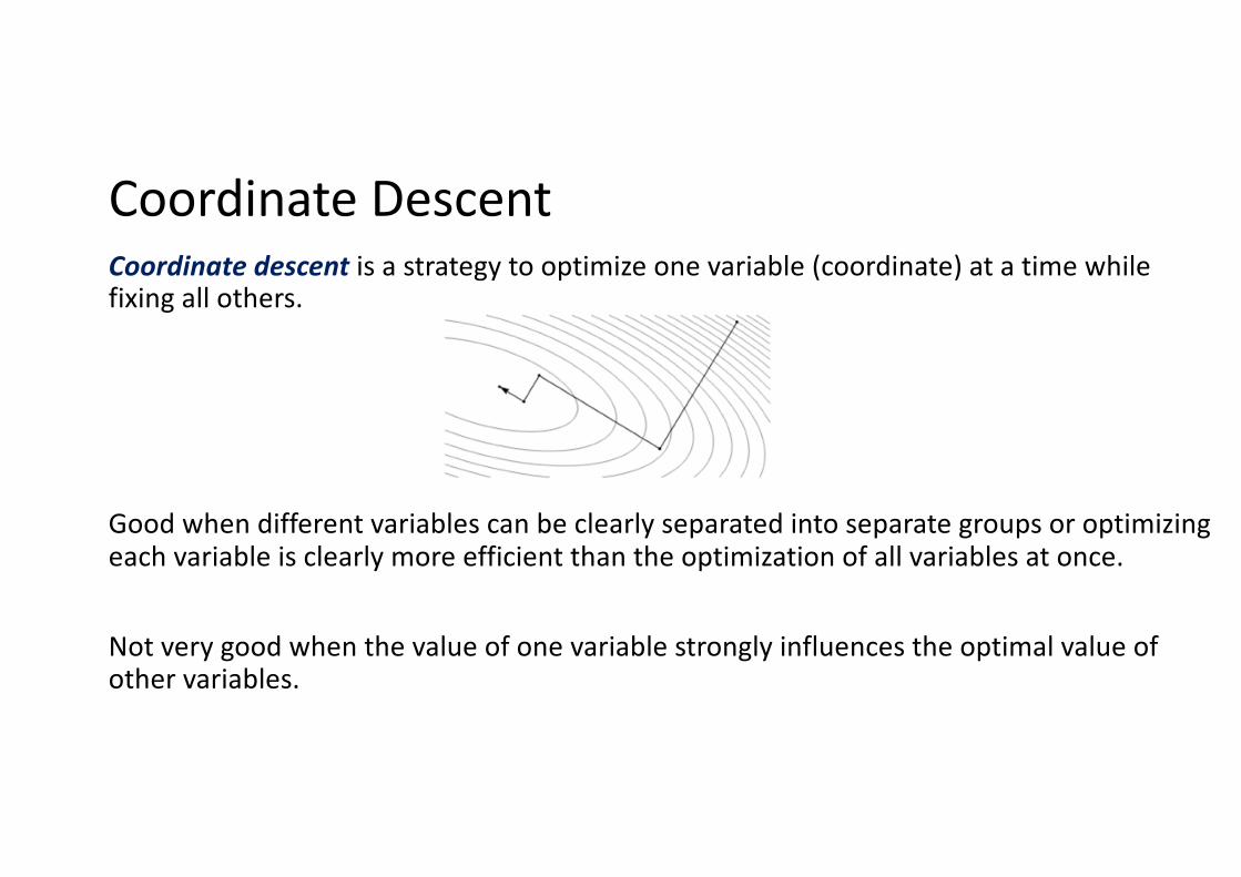
Coordinate DescentCoordinate descent is a strategy to optimize one variable (coordinate) at a time while fixing all others.

Good when different variables can be clearly separated into separate groups or optimizing each variable is clearly more efficient than the optimization of all variables at once.

Not very good when the value of one variable strongly influences the optimal value of other variables.

Polyak AveragingPolyak averaging averages several points in the parameter trajectory together.

If gradient descent visit points !", … , !%, then Polyak averaging outputs &!% = "% ∑) !).

On some problem classes, such as gradient descent applied to convex problems, this approach as strong convergence guarantees.

In non-convex problems, the path taken by the optimization trajectory can be complex and including points from the distant past separated by large barriers is not a good idea.

&!% = *&!%+" + 1 − * !%Thus, Polyak averaging for non-convex objectives uses exponentially decaying average.

Supervised PretrainingSometimes, directly training a model could be too ambitious if the model is complex, difficult to optimize, or the task is very difficult.

In such cases, it could be more effective to train a simpler model to solve the task, and then make the model more complex, or train the model to solve a simpler task and then move on to the final task.

These strategies are collectively known as pretraining.

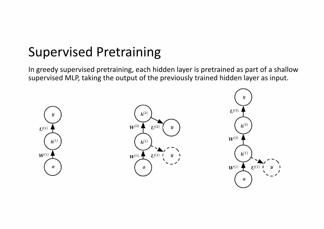
Supervised PretrainingIn greedy supervised pretraining, each hidden layer is pretrained as part of a shallow supervised MLP, taking the output of the previously trained hidden layer as input.

Designing Models to Aid OptimizationIn practice, it is more important to choose a model family that is easy to optimize, than to use a powerful optimization algorithm.

Most of the advances in neural network training has come from the change of the model family rather than optimization procedure - e.g.) Rectified linear units, maxout units, LSTM

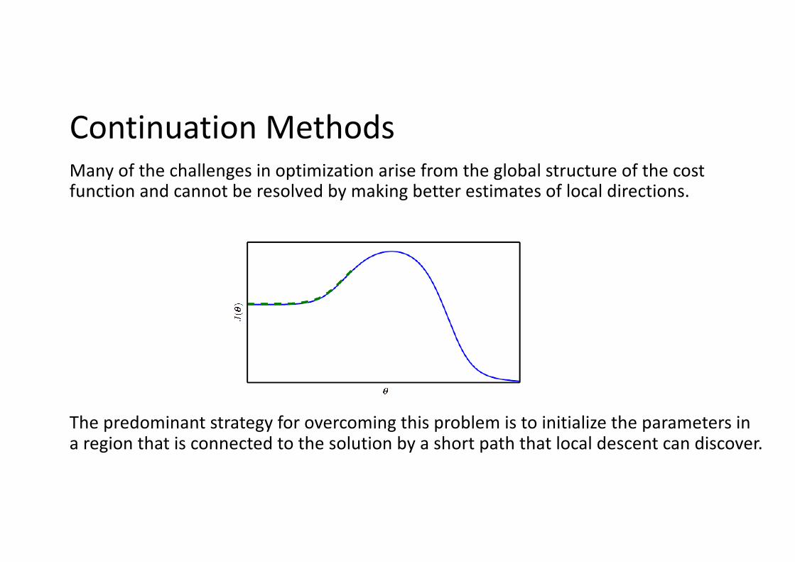
Continuation MethodsMany of the challenges in optimization arise from the global structure of the cost function and cannot be resolved by making better estimates of local directions.

The predominant strategy for overcoming this problem is to initialize the parameters in a region that is connected to the solution by a short path that local descent can discover.

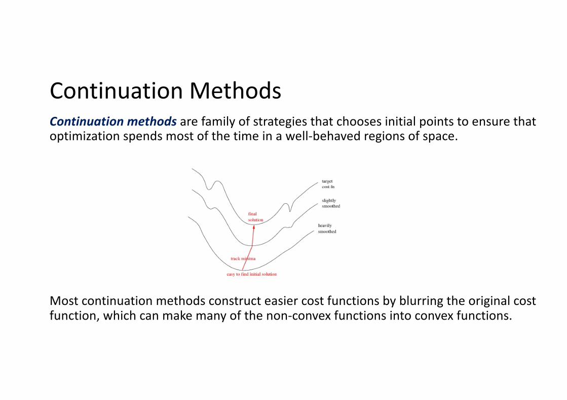
Continuation MethodsContinuation methods are family of strategies that chooses initial points to ensure that optimization spends most of the time in a well-behaved regions of space.

Most continuation methods construct easier cost functions by blurring the original cost function, which can make many of the non-convex functions into convex functions.

Curriculum LearningCurriculum learning, a kind of continuation method, is based on the concept of learning simple concepts and progress to learning more complex concepts that depend on them.

The cost function in this case is made easier by increasing the influence of simpler examples.

Curriculum learning has been successful on a wide range of AI tasks, including computer vision, natural language processing.

Also, curriculum learning was verified as being consistent with the way in which humans teach.

Any questions?Next class – Convolutional Neural Networks