optimizacion de márgenes de contribucion de servicios de alimentación usando modelos de demanda...
TRANSCRIPT
Revista Colombiana de Estadística
Edición para autor(es)
Optimization of food service contribution margins
by modeling independent component demand
Optimización de márgenes de contribución de servicios dealimentación modelando la demanda de componentes independientes
Fernando Rojas1,a, Víctor Leiva2,b, Peter Wanke3,c,
Carolina Marchant4,d
1Escuela de Nutrición y Alimentos, Universidad de Valparaíso, Chile
2Facultad de Ingeniería y Ciencias, Universidad Adolfo Ibáñez, Chile
3School of Business, Universidade Federal de Rio de Janeiro, Brazil
4Instituto de Estadística, Universidad de Valparaíso, Chile
Abstract
We propose a methodology useful for food services that allows contribu-tion margins to be optimized. The methodology is based on statistical tools,inventory models and financial indicators. Because there is a need to reducethe gap between theory and practice, we apply this methodology to the casestudy of a Chilean company to show its potential. We conduct a real-worlddemand data analysis for perishable and non-perishable components of itsinventory assortment. Then, we use suitable inventory models to optimizethe associated costs. Finally, we compare the proposed optimized systemand the non-optimized system employed by the company using financial in-dicators.
Key words: data analysis, demand, inventory, distributions.
Resumen
Proponemos una metodología útil para servicios de alimentación que per-mite optimizar sus márgenes de contribución. La metodología se basa enherramientas estadísticas, modelos de inventario e indicadores financieros.Debido a que hay una necesidad de reducir la brecha entre la teoría y lapráctica, aplicamos la metodología a un estudio de caso de una empresachilena para mostrar su potencial. Realizamos un análisis de datos realesde demanda para componentes perecederos y no perecederos del surtido in-ventario. Entonces, utilizamos modelos de inventarios adecuados para opti-mizar los costos asociados. Por último, comparamos los sistema optimizadopropuesto y el sistema no optimizado empleado por la empresa a través deindicadores financieros.
Palabras clave: análisis de datos, demanda, distribuciones, inventario.
aAssociate Professor. E-mail: [email protected]. Corresponding author: URL: www.victorleiva.cl. E-mail: [email protected] Professor. E-mail: [email protected] Professor. E-mail: [email protected]
1
2 Fernando Rojas, Víctor Leiva, Peter Wanke & Carolina Marchant
1. Acronyms
Table 1: acronyms used through the paper.
Anderson-Darling (AD) Kolmogorov-Smirnov (KS)
Birnbaum-Saunders (BS) lead time (LT)
BS-Student-t (BS-t) lognormal (LN)
coefficient of kurtosis (CK) maximum likelihood (ML)
coefficient of skewness (CS) ordering cost (OC)
coefficient of variation (CV) probability density function (PDF)
contribution margin (CM) purchasing cost (PC)
critical ratio (CR) quantile function (QF)
cumulative distribution function (CDF) random variable (RV)
cumulative percentage (CP) reorder point (ROP)
economic order quantity (EOQ) safety stock (SS)
empirical CDF (ECDF) safety factor (SF)
exploratory data analysis (EDA) storing cost (SC)
inverse Gaussian (IG) standard deviation (SD)
just in time (JIT) variable contribution margin (VCM)
2. Introducción
Systems of supply and inventory policies affect positively the logistics of thecompanies, minimizing the involved costs, and reducing inefficiencies in their man-agement. It is known that the total inventory cost is function of purchasing (PC),ordering (OC) and storing (SC) costs; see Hillier & Lieberman (2005). Severalauthors have discussed the importance of having optimal supply and inventorypolicies in a company and an efficient management of its logistics; see Gjerdrum,Samsatli, Shah & Papageorgiou (2005), Blankley, Khouja & Wiggins (2008) andKogan & Tell (2009). These aspects of logistics are also present in collective foodservice companies; see Ramirez (2013). Such services prepare portions of a foodmenu according to diverse specifications, including nutritional and sanitary issues,with respect to the different types of clients who consume this menu; see Maram-bio, Parker & Benavides (2005). The increase in the amount of food servicesis generating an important source of employment in the countries and providingmultiple market opportunities. This is attributed to the need that people have toeat outside of their homes due to their activity in businesses, factories, hospitals,schools and universities. Because of the diversity of the service, the complexity ofthis food industry has grown considerably, requiring a professional managementand a regulation from government agencies; see MINSAL (2004).
In Chile, collective food services are considered in the group of small andmedium enterprises. Many of these Chilean services are not optimizing their sup-ply of raw materials. These materials form the inventory assortment, which isdivided in perishable (as fruits, meats, vegetables) and non-perishable productswith greater storing capacity subject to shortage; see Grant, Karagianni & Li(2006). Such services rely the logistics of these raw materials on the monthlyplanning of the menu, guided by nutritional considerations. However, this man-
Revista Colombiana de Estadística, Edición para autor(es)
Optimizing contribution margins with demand models 3
agement can be improved by using inventory policies, allowing the contributionmargins (CMs) of the company to be increased; see Soman (2006) and McKinnon,Mendes & Nababteh (2007), and Nicolau (2009) for a case study in hotels. CMsare the gross profits of a company and summarizes the movements of income andcosts, which may be direct (variable costing) and indirect (absorption costing); seeZoller (2006). These margins vary depending on the sold units, unit costs of theproduct, ratio between its CM and its total costs, and of the fixed costs involved;see Ramanathan (2006).
An optimal inventory policy can be obtained choosing the most adequate inven-tory model, whose decision involves several aspects; see Botter & Fortuin (2000),Braglia, Eaves & Kingsman (2004a), Braglia, Grassi & Montanari (2004b), Gjer-drum et al. (2005), Wanke (2011) and Wanke (2008b). When considering non-perishable (multi-period) products, inventory models are classified in two types:pull and push, which range from the economic order quantity (EOQ) to the justin time (JIT) supply; see Wanke (2008a). The EOQ model is the cornerstoneof several software packages for inventory control and is widely used in practice;see Braglia & Gabbrielli (2001) and Nahmias (2001). The JIT method is usefulfor raw materials that can be supplied as timely as they are required, althoughit imposes conditions leading to logistics constraints that limits its use for sometypes of products in food services; see Carter, Carter, Monczka, Slaight & Swan(2000) and Wanke, Arkader & Rodrigues (2008). Chiu (2010) discussed models formulti-period products where shortage is not permitted, seeking to find the EOQand reorder point (ROP), which may be appropriate for groceries, often used byfood services. Considering lead time (LT) in the modeling makes the assumptionsof the model to be more adherent to real world settings; see Ben-Daya & Raouf(1994). The EOQ model is used altogether with the ROP in inventory controlto determine safety stocks (SS) under both random LT and demand, which ran-domness directly affect the operation of a logistics system; see Speh & Wagenheim(1978) and Wanke (2008a). Perishable (single-period) products can only be storedduring a limited period. These products correspond usually to fruits, meats andvegetables, which are key raw materials in a food service. When considering thistype of products, the model based on the critical ratio (CR) or service level isoften considered; see Hillier & Lieberman (2005, pp. 961-975).
Multiple and single period models must consider that the demanded quantityof a product cannot be predicted accurately due to several factors, making it tobe a random variable (RV) and, therefore, its behavior should be described by astatistical distribution (or probabilistic model); see Johnson, Kotz & Balakrishnan(1994). The Gaussian (or normal) distribution is often used for describing dataof three RVs involved in inventory models, which are demand, LT, and demandduring LT. It is known that this distribution is validly used for RVs that takenegative and positive values, so that quantities less than zero could be admittedin the modeling, which is not possible in practice for the three mentioned RVs;see Keaton (1995) and Nahmias (2001). Mentzer & Krishnan (1988) studied thenon-normality effect on the inventory control, indicating that demand for productsthat presents a normal distribution is found in few practical cases. This is becausedemand data often follow asymmetric distributions; see Moors & Strijbosch (1988).In any case, the normality assumption must be checked by goodness-of-fit methods;
Revista Colombiana de Estadística, Edición para autor(es)
4 Fernando Rojas, Víctor Leiva, Peter Wanke & Carolina Marchant
see Castro-Kuriss, Kelmansky, Leiva & Martinez (2010), Barros, Leiva, Ospina &Tsuyuguchi (2014) and Castro-Kuriss, Leiva & Athayde (2014). Thus, using thenormal distribution to model the demand and LT and to determine the ROPand SS can provoke wrong results, leading to stock shortage or excess. Non-normal distributions used for describing demand or LT in inventory models are thegamma or Erlang, inverse Gaussian (IG), lognormal (LN), uniform and Weibull;see Burgin (1975), Tadikamalla (1981), Lau (1989), Wanke (2008c) and Cobb,Rumí & Salmerón (2013).
A unimodal, two-parameter probability model with positive asymmetry that isreceiving considerable attention is the Birnbaum-Saunders (BS) distribution; seeJohnson et al. (1994, pp. 651-663). This is due to its good properties and its rela-tion with the normal distribution, which permits the BS distribution to be behavedas the LN distribution, but with properties that the LN does not have. Its appli-cations range diverse fields including business and industry; see Jin & Kawczak(2003), Bhatti (2010), Leiva, Soto, Cabrera & Cabrera (2011b), Sanhueza, Leiva& López-Kleine (2011), Leiva, Ponce, Marchant & Bustos (2012), Paula, Leiva,Barros & Liu (2012), Leiva, Santos-Neto, Cysneiros & Barros (2014c), Marchant,Bertin, Leiva & Saulo (2013), Leiva, Marchant, Saulo, Aslam & Rojas (2014a),Leiva, Rojas, Galea & Sanhueza (2014b) and Leiva, Saulo, Leao & Marchant(2014d). Although originally conceived as a count model, it includes the durationof the counting period (daily or weekly), which does unnecessary further data tobe collected, among other interesting properties, allowing the BS distribution tobe a good candidate for describing demand data; see Fox, Gavish & Semple (2008).
A good statistical modeling of the demand data and a scientific management ofinventories for collective food service companies can maximize their CMs, implyinga better competitiveness, efficiency and profitability of these companies. This canbe helpful in making optimal decisions.
The main objective of this paper is to propose a methodology useful for foodservices that allows their CMs to be optimized. This methodology is based on sta-tistical tools, inventory management models and financial indicators. Specifically,the methodology uses probabilistic models that describe the behavior of demanddata for raw materials employed by food services that prepare a daily menu. Here-after, we refer to these raw materials as components (or products) forming part ofa food menu. Then, the logistics process is optimized by using inventory modelsthat depends on the type of product from the corresponding assortment. Hence,the CMs of the company are measured by using absorption costing and improvedby means of logistics management. Such an improvement must be reached whencomparing the financial results obtained from the optimized system with respectto the non-optimized system used by the food service. Because some authorsstressed the need to conduct case studies that reduces the gap between theoryand practice and enables the researchers to increase their background (Wagner &Lindemann 2008), we apply this methodology to a case study of a food companythat serves the staff of a Chilean hospital.
This paper is organized as follows. In Section 3, we propose our methodology.In Section 4, we conduct a case study for a Chilean company. In Section 5, weprovide an illustration for one product from the inventory assortment. Finally, inSection 6, we discuss the conclusions of this study.
Revista Colombiana de Estadística, Edición para autor(es)
Optimizing contribution margins with demand models 5
3. Methodology
In this section, we provide a methodology for food services that allows CMs tobe optimized. First, we discuss assumptions and limitations of our methodology.Second, we mention how the demand data for components of a food menu shouldbe collected. Third, we present the statistical tools needed to fit a demand dataset to a suitable distribution. Fourth, we detail the inventory management modelsto be used for optimizing the supply system based on the selected distributions.Fifth, we describe the financial indicators of our methodology. An algorithm thatsummarizes this methodology is provided.
3.1. Assumptions and limitations
The main assumptions of our methodology are (i) random demand, (ii) demandtime series free of seasonality and trend, (iii) independent component demand, (iv)LT constant and (v) the need to ascertain managerial costing calculations. Somelimitations of our methodology are related to (i) additional research needed toimprove the results, especially introducing aspects to be more adherent to realworld settings, such as issues related to seasonality, trend and independent, and(ii) relevant costs of the operation characteristics.
Note that shortage costs for non-perishable products could be unavailable andthen they could not be incorporated in the analysis. Unlike situations proposalsby Silver, Pyke & Peterson (1998) and Zipkin (2000), in our methodology, there isno CMs or penalties that are imposed to a product with unsatisfied demand. Inpractice, for food companies, a product is replaced by another when it is missingand the customer continues making his(her) meals. We opt to set a target level ofservice based on a safety factor (SF), instead of the simultaneous optimization ofthe EOQ and SF. This is due to the eminently practical character of our study,which objective is, among others, to transfer knowledge and management of in-ventory policy over time to the company studied. Using the SF in an inventorypolicy necessarily requires the manager to think in terms of service level and inven-tory segmentation by levels of criticality with respect to shortage of items. Whenthe simultaneous optimization of EOQ and SF is carried out, these issues are lessexplicit for the manager.
3.2. Recording the data
We recommend to design and implement a record system for all the productsthat form the inventory assortment of raw materials of the food service company.This system must be based on identification code, unit PC, demanded quantity,price, date and time of entry and exit of products used in the preparation offood portions; see Harvey (2002) and Yajiong (2008). The record system must becarried out via individual identification using bar codes and developed for demandprofiles of the mentioned products, during the time period planned for the study.We recommend a period of six months (26 weeks). Initially, we considered 26weeks (half year) as a sample of convenience based on the project budget fordata collection. However, we could collect data for one week more, so that thisadditional week was considered to increase the sample size.
Revista Colombiana de Estadística, Edición para autor(es)
6 Fernando Rojas, Víctor Leiva, Peter Wanke & Carolina Marchant
3.3. Demand statistical distributions
Based on the record indicated in Subsection 3.2, the demand data needed tomodel the distribution of the demanded quantity for each product must be col-lected and then the demand distribution fitted. Until very recently, one of theproblems for using a demand distribution different from the normal model wasthe limitation of statistical software. However, today this is not a problem, firstbecause at present we have a number of statistical software that has implementedseveral statistical distributions and, second, the scientific community has at its dis-posal a non-commercial and open source software for statistics and graphs, namedR, which can be obtained at no cost from www.r-project.org. The statisticalsoftware R is being currently very popular in the international scientific commu-nity. Then, to perform a statistical analysis of demand data, we use the R softwareand also employ some software packages to carry out more specific statistical anal-ysis. As mentioned, the gamma, IG, LN, uniform and Weibull distributions haveused for modeling the demand or the LT in inventory problems and they are imple-mented in R software packages named gamlss and ig; see Stasinopoulos & Rigby(2007) and Leiva, Hernandez & Sanhueza (2008). Statistical analysis based onBS distributions, including a version known as the BS-Student-t (BS-t) distribu-tion, which has been proven to provide robust estimates of its parameters againstoutliers (Paula et al. 2012), can be conducted by means of an R software packagenamed gbs; see Barros, Paula & Leiva (2009). Next, we provide some useful resultsfor all of these distributions; see details in Johnson et al. (1994).
The BS distribution A RV D following the BS distribution with shape α > 0and scale β > 0 parameters is denoted by D ∼ BS(α, β), where “∼” means “dis-tributed as”. In this case, the probability density (PDF) and cumulative distribu-tion (CDF) functions of D are respectively
fD(d) =1√2π
exp
(−1
2ξ2(d/β)
)[d/β]−1/2 + [d/β]−3/2
2αβand
FD(d) = Φ (ξ(d/β)) , d > 0,
where ξ(y) =√y−
√1/y and Φ(·) is the standard normal CDF. The corresponding
quantile function (QF) is d(q) = F−1
D (q) = β[αz(q)/2 +√
(αz(q)/2)2 + 1]2, for0 < q < 1, where z(q) is the standard normal or N(0, 1) QF and F−1
D (·) is theinverse CDF. Note that d(0.5) = β, that is, β is also the median or 50th percentileof the distribution. The mean and variance of D are E[D] = β[1 + α2/2] andVar[D] = β2α2[1 + 5α2/4]. In addition, BS RVs (D) and standard normal (Z) arerelated by D = β[αZ/2 +
√(αZ/2)2 + 1]2 ∼ BS(α, β) and Z = [1/α]ξ(D/β) ∼
N(0, 1). Also, W = Z2 follows a chi-squared distribution with one degree offreedom, which is useful for goodness of fit. The BS distribution holds the scale andreciprocal properties, that is, cD ∼ BS(α, c β), with c > 0, and 1/D ∼ BS (α, 1/β),respectively.
The BS-t distribution A RV D following the BS-t distribution with shapeα > 0, ν > 0 and scale β > 0 parameters is denoted by D ∼ BS-t(α, β, ν). In this
Revista Colombiana de Estadística, Edición para autor(es)
Optimizing contribution margins with demand models 7
case, the PDF and CDF of D are
fD(d) =Γ(ν+1
2
)√ν π Γ
(ν2
)[1 +
ξ2(d/β)
ν
]− ν+12 [d/β]−1/2 + [d/β]−3/2
2αβ, t > 0, and
FD(d) =1
2
[1 + I ξ(d/β)
ξ(d/β)+ν
(1/2, ν/2)], d > 0,
where Ia(b, c) is the incomplete beta function ratio. The corresponding QF is againd(q) = F−1
D (q) = β[αz(q)/2 +√(αz(q)/2)2 + 1]2, for 0 < q < 1, but now z(q) is
the QF of the Student-t distribution with ν degrees of freedom. Note that β isagain the median or 50th percentile of the distribution. The mean and varianceof D are given by E[D] = β[1 + Aα2/2] and Var[D] = β2α2[A + 5Bα2/4], whereA = ν/[ν − 2], for ν > 2, and B = 3ν2/[(ν − 2)(ν − 4)], for ν > 4. Now, BS RVs(D) and Student-t (Z) are related by D = β[αZ/2+ (αZ/2)2+1]2 ∼ BS-t(α, β; ν)and Z = [1/α]ξ(D/β) ∼ t(ν). In this case, W = Z2 follows a Fisher distributionwith one degree of freedom in the numerator and ν degrees of freedom in thedenominator, which once again is useful for goodness of fit. Some properties are:cD ∼ BS-t(α, c β, ν), with c > 0, and 1/D ∼ BS-t(α, 1/β, ν).
The gamma distribution A RV D following the gamma distribution withshape α > 0 and scale β > 0 parameters is denoted by D ∼ Gamma(α, β). In thiscase, the PDF and CDF of D are
fD(d) =d1/α
2−1 exp(−d/α2β)
[α2β]1/α2Γ(1/α2)and FD(d) =
γ(1/α2, d/α2β)
Γ(1/α2), d > 0,
where Γ(·) and γ(·) denote the usual and incomplete gamma functions, respec-tively. The corresponding QF given by d(q) = F−1
D (q), for 0 < q < 1, must beobtained by solving this equation with an iterative numerical method. The meanand variance of D are E[D] = β and Var[T ] = α2 β2, respectively. The gammadistribution also shares the property cD ∼ Gamma(α, c β), with c > 0.
The inverse Gaussian distribution A RV D following the IG distributionwith mean λ > 0 and scale β > 0 parameters is denoted by D ∼ IG(λ, β). In thiscase, the PDF and CDF of D are
fD(d) =
√β
2πd3exp
(−β [d− λ]2
2dλ2
), d > 0, and
FD(d) = Φ(√
βλ ξ
(dλ
))+Φ
(√βλ
[√dλ +
√λd
])exp
(2βλ
), d > 0,
and once again the corresponding QF given by d(q) = F−1
D (q), for 0 < q < 1, mustbe obtained by solving this equation with an iterative numerical method. Themean and variance of D are given by E[D] = λ and Var[D] = λ3/β, respectively.The IG distribution also shares the scale property, that is, cD ∼ IG(c λ, c β), withc > 0.
Revista Colombiana de Estadística, Edición para autor(es)
8 Fernando Rojas, Víctor Leiva, Peter Wanke & Carolina Marchant
The lognormal distribution If Y = log(D) has a normal distribution withmean µ and variance α2, that is, Y = log(D) ∼ N(µ, α2), then the RV D followsthe LN distribution with shape α > 0 and scale β = exp(µ) > 0 parameters. Thenotation D ∼ LN(α, β) is used in this case. Thus, the PDF and CDF of D are,for d > 0,
fD(d) =1
dα√2π
exp
(− [log(d) − log(β)]2
2α2
)and FD(d) = Φ
(log(d)− log(β)
α
).
The corresponding QF is d(q) = F−1
D (q) = β exp(z(q)α), for 0 < q < 1, where z(q)is the standard normal QF. The mean and variance of D are E[D] = β exp(α2/2)and Var[D] = β2[exp(2α2)− exp(α2)], respectively.
The Weibull distribution A RV D following the Weibull distribution withshape α > 0 and scale β > 0 parameters is denoted by D ∼ Wei(α, β). In thiscase, the PDF and CDF of D are
fD(d) = αdα−1
βα exp(−[dβ
]α)and FD(t) = 1− exp
(−[dβ
]α), t > 0.
The QF of D is d(q) = β[− log(1−q)]1/α, for 0 < q < 1, and its mean and variance
E[D] = β Γ(α+1
α
)and Var[D] = β2
[Γ(α+2
α
)−{Γ(α+1
α
)}2].
Data analysis, parameter estimation and goodness-of-fit of distributionsAs mentioned, R is a free software environment for statistical computing andgraphics. Using this software (i) exploratory data analysis (EDA) can be conductedfor diagnosing the statistical features present in the demand data; (ii) estimation ofthe parameters of the BS, BS-t, gamma, IG, LN and Weibull distributions can becarried out by the popular maximum likelihood (ML) method, and (iii) goodness-of-fit of a distribution to a demand data set can be performed by Anderson-Darling(AD) and Kolmogorov-Smirnov (KS) tests and probability plots. Next, we describethe R commands of the gbs, ig and basics packages and briefly illustrate their use.
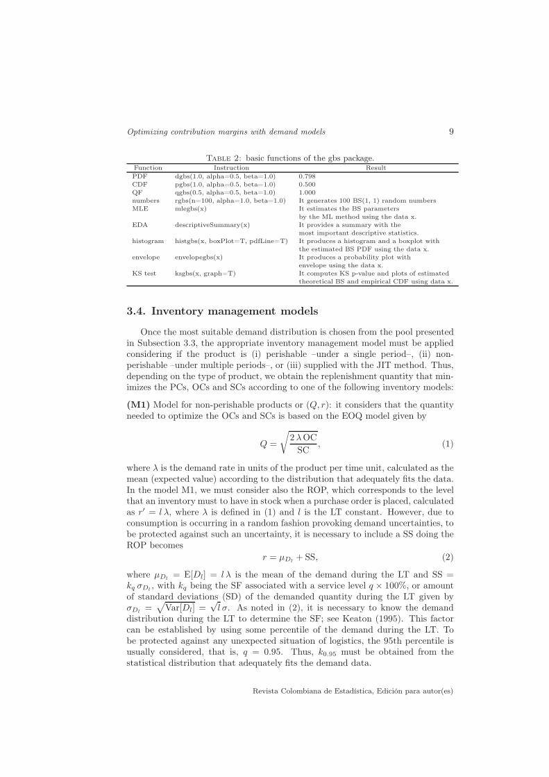
First, the R software must be downloaded from CRAN.r-project.org andinstalled as any other software. Second, the R software can be used in a simpleinteractive form with the R commander by installing the Rcmdr package. Third,the gbs and ig packages must be also installed. Data analyses based on the BSand BS-t distributions can be carried by the gbs package, for the IG distributionwith the ig package and for the gamma, LN and Weibull distributions with thebasics or gamlss packages. Thus, once these packages are installed, they must beloaded into the R software, for example, by the command library(gbs) typingthem at the R prompt of the R commander, or at any editor program that theuser is considering. Once all these instructions are ready, the data, for example,“product1” say, must be loaded as data(product1). The data can also be directlytyped by the R commander such as an Excel sheet or imported from text files,from other statistical software or from Excel. Table 2 provides examples of somecommands that allow us to work with the BS distribution, whereas analogousinstructions can be used for the other distributions; for more details about howusing the gbs package, see Barros et al. (2009).
Revista Colombiana de Estadística, Edición para autor(es)
Optimizing contribution margins with demand models 9
Table 2: basic functions of the gbs package.Function Instruction Result
PDF dgbs(1.0, alpha=0.5, beta=1.0) 0.798
CDF pgbs(1.0, alpha=0.5, beta=1.0) 0.500
QF qgbs(0.5, alpha=0.5, beta=1.0) 1.000
numbers rgbs(n=100, alpha=1.0, beta=1.0) It generates 100 BS(1, 1) random numbers
MLE mlegbs(x) It estimates the BS parameters
by the ML method using the data x.
EDA descriptiveSummary(x) It provides a summary with the
most important descriptive statistics.
histogram histgbs(x, boxPlot=T, pdfLine=T) It produces a histogram and a boxplot with
the estimated BS PDF using the data x.
envelope envelopegbs(x) It produces a probability plot with
envelope using the data x.
KS test ksgbs(x, graph=T) It computes KS p-value and plots of estimated
theoretical BS and empirical CDF using data x.
3.4. Inventory management models
Once the most suitable demand distribution is chosen from the pool presentedin Subsection 3.3, the appropriate inventory management model must be appliedconsidering if the product is (i) perishable –under a single period–, (ii) non-perishable –under multiple periods–, or (iii) supplied with the JIT method. Thus,depending on the type of product, we obtain the replenishment quantity that min-imizes the PCs, OCs and SCs according to one of the following inventory models:
(M1) Model for non-perishable products or (Q, r): it considers that the quantityneeded to optimize the OCs and SCs is based on the EOQ model given by
Q =
√2λOC
SC, (1)
where λ is the demand rate in units of the product per time unit, calculated as themean (expected value) according to the distribution that adequately fits the data.In the model M1, we must consider also the ROP, which corresponds to the levelthat an inventory must to have in stock when a purchase order is placed, calculatedas r′ = l λ, where λ is defined in (1) and l is the LT constant. However, due toconsumption is occurring in a random fashion provoking demand uncertainties, tobe protected against such an uncertainty, it is necessary to include a SS doing theROP becomes
r = µDl+ SS, (2)
where µDl= E[Dl] = l λ is the mean of the demand during the LT and SS =
kq σDl, with kq being the SF associated with a service level q × 100%, or amount
of standard deviations (SD) of the demanded quantity during the LT given byσDl
=√
Var[Dl] =√l σ. As noted in (2), it is necessary to know the demand
distribution during the LT to determine the SF; see Keaton (1995). This factorcan be established by using some percentile of the demand during the LT. Tobe protected against any unexpected situation of logistics, the 95th percentile isusually considered, that is, q = 0.95. Thus, k0.95 must be obtained from thestatistical distribution that adequately fits the demand data.
Revista Colombiana de Estadística, Edición para autor(es)
10 Fernando Rojas, Víctor Leiva, Peter Wanke & Carolina Marchant
Note that in the model M1 is not considered a shortage cost of the product,because, in case of occurring shortage, it is possible to produce a menu of emer-gency, so that no unsatisfied demand is generated for the final product (menu);see details about this model and it assumptions in Hillier & Lieberman (2005,pp. 956-961). Also, we recall no simultaneous optimization of Q and r is carriedout due to the practical nature of our methodology; see details in Subsection 3.2.
(M2) Model for perishable products: it considers the quantity needed to optimizethe cost of ordering one unit less (generating a temporary shortage), in contrastto ordering one unit more (generating a temporary overstock), based on the CRin this case given by CR = [UC − PC]/[UC + HC], where UC is the unit unsat-isfied demand shortage cost, that includes lost revenue and loss cost of customergoodwill, PC is expressed as a unit purchasing cost of the product, and HC isthe unit holding cost per day, that includes the SC minus a salvage value of aproduct unit. The numerator UC − PC results in the decrease in profit, due tonot ordering a unit that could have been sold during such a period, whereas thedenominator UC + HC results also in the decrease in profit, but due to orderinga unit that could not be sold during such a period. Thus, the single period modelfor perishable products allows us to obtain its optimum stored quantity from theoptimum service level given by
FD(d0) = CR, (3)
where FD(·) is the CDF of the demanded quantity and d0 the optimum quantityof ordered units; see details in Hillier & Lieberman (2005, pp. 961-975).
(M3) JIT model: it is the just quantity for production, does not consider storageand is used for specific products requested for completing the daily menu of thefood service company, using a Kanban type information system, which allows theavailability of the product to be harmonically coordinated; see Carter et al. (2000).
3.5. Determination of financial indicators
Once the appropriate inventory management model is chosen from M1, M2 orM3, (see Subsection 3.4), the CM for each of p products of the inventory assortmentused in the preparation of a food menu portion must be calculated, based on theincomes obtained during w weeks for the company corresponding to this menu.The quantities of each product used in the preparation of the menu (ingredients)are determined with its respective consumption measuring unit; see Table 14 inAppendix for an example about equivalence among these units for the products ofthe case study that we conduct in Section 4.
The prorated demand of the product i in the jth week can be obtained bymeans of the proportion that each product of the food portion holds weekly in themenu calculated according to
PDi,j = DQi,j/DQj , i = 1, . . . , p, j = 1, . . . , w, (4)
where DQi,j is the demanded quantity of the product i in the jth week and DQj
is the demanded quantity for all the products during that week. The income of
Revista Colombiana de Estadística, Edición para autor(es)
Optimizing contribution margins with demand models 11
the company for all the portions of the food menu sold during the jth week is
Ij = Nj Sj , j = 1, . . . , w, (5)
where Nj is the number of menus sold and Sj is the price of the food menu portion,both of them in the jth week. Thus, the prorated income due to the product iduring the jth week is obtained as
PIi,j = Ij PDi,j , i = 1, . . . , p, j = 1, . . . , w, (6)
where PDi,j and Ij are defined in (4) and (5), respectively. The PC for the producti in the jth week is
PCi,j = NCi,j PQi,j , i = 1, . . . , p, j = 1, . . . , w, (7)
where NCi,j and PQi,j are the unit net cost and the purchased quantity of theproduct i during the jth week, respectively. Note that, for the optimized systemwith the inventory model for non-perishable products, PQi,j must be estimatedfrom Q given in (1), whereas that, in the case of perishable products, PQi,j must beestimated from d0−Lj given in (3), with Lj being the stock level at the beginningof the jth week. For the non-optimized system, this value can be empiricallycalculated. Once financial indicators PIi,j and PCj defined in (6) and (7) areobtained, the variable contribution margin (VCM) of the product i during the jthweek must be computed as
VCMi,j = PIi,j − PCi,j , i = 1, . . . , p, j = 1, . . . , w. (8)
The OC for the product i during the jth week can be obtained as
OCi,j = OCi/52, i = 1, . . . , p, j = 1, . . . , w, (9)
where OCi is the annual OC of the product i given by OCi =∑3
h=1OCh
i OQi,
with OQi being the annual order quantity and OChi the cost of type h given
in Table 3, both for the product i. Note that, for the optimized system withthe inventory model for non-perishable products, OQi must be estimated from Qgiven in (1) using the expression λ/Q for each product (with λ being expressed as ademand rate per year), whereas that in the case of perishable products OQi = 52,for all i = 1, . . . , p. For the non-optimized system, this value can be empiricallycalculated.
Table 3: costs involved in generating a purchase order (OCh).
Cost Description
OC1 Administrative costs associated with the order movements (input and generalservice costs with respect to order generation).
OC2 Inspection and receiving costs (social security contributions andwarehouseman wages) of movements associated with an order.
OC3 Transportation costs related solely to order generation.
Source: generated by the authors based on Hernández-González (2011).
Revista Colombiana de Estadística, Edición para autor(es)
12 Fernando Rojas, Víctor Leiva, Peter Wanke & Carolina Marchant
The SC for the product i during the jth week is given by
SCi,j = [SCi/52] SQi,j , i = 1, . . . , p, j = 1, . . . , w, (10)
where SCi is the annual SC of the product i given by SCi =∑5
k=1SCk
i /SQi, with
SCki being the annual SC of type k defined in Table 4 and SQi =
∑52
j=1SQi,j the
annual stored quantity, both for the product i, and SQi,j is the stored quantity ofthe product i in the jth week. Note that, for the optimized system with the in-ventory management model for non-perishable products, SQi,j must be estimatedfrom SQ = Q/2 + SS, where Q and SS are given in (1) and (2), respectively,whereas that, in the case of perishable products, SQi,j must be estimated fromthe expected inventory level by single period. For the non-optimized system, thisvalue can be empirically calculated.
Table 4: annual costs involved in the storage of a product (SCk).
Cost Description
SC1 Annual cost of amortization of buildings and networks for air conditioning,handling equipment, information processing, receiving, storage mediaand weighing, among others.
SC2 Annual cost of damage, losses, obsolescence and product losses incurredin the storage period.
SC3 Annual cost of cleaning materials and storehouse, containers, packaging,and printed matter.
SC4 Annual cost of energy spent on the storehouse, including battery chargingnecessary for handling, data processing equipment and lighting.
SC5 Annual cost of rental of equipment and facilities, during insurance,storage and communications, and taxes.
Source: generated by the authors based on Morillo (2009).
We consider CMs as absorbable by the sales with respect to indirect costs,which are subtracted from the VCM given in (8) to obtain the total CM of theproduct i during the jth week as
CMi,j = VCMi,j − [OCi,j + SCi,j ], i = 1, . . . , p, j = 1, . . . , w, (11)
where VCMi,j , OCi,j and SCi,j are given in (8), (9) and (10), respectively. Thus,we collect a series of CMs for p products (one for each of them). Hence, the CMof all the products of the inventory assortment during the jth week is given byCMj =
∑pi=1
CMi,j , for j = 1 . . . , w, where CMi,j is given in (11). Therefore, thetotal CM of the inventory system is
CM =w∑
j=1
CMj . (12)
Note that the objective function to be maximized is the sum of CMi,j for theproduct i in the jth week, during all the period of study totalizing w weeks,for the menu composed by p components with independent demand. Here, the
Revista Colombiana de Estadística, Edición para autor(es)
Optimizing contribution margins with demand models 13
margins VCMi,j and costs OCj and SCi,j depend on the inventory model of thecomponent i. This function is expressed as
p∑
i=1
w∑
j=1
CMi,j =
p∑
i=1
w∑
j=1
{VCMi,j − OCi,j − SCi,j}.
Due to that our approach to calculating (i) CMs from the differential revenues and(ii) costs from the movements in and out of the inventory assortment is based onindependent components and not from the menu, the absorbable costs to store andsort are also calculated using the same criteria of independence and consideringthe spread of demand from the proportions of components used in the menu.This approach turns out to be more streamlined, because it does not considerthe correlations that could exist between the components of the menu, which is asource for future work; see Section 6.
3.6. Summary of the methodology
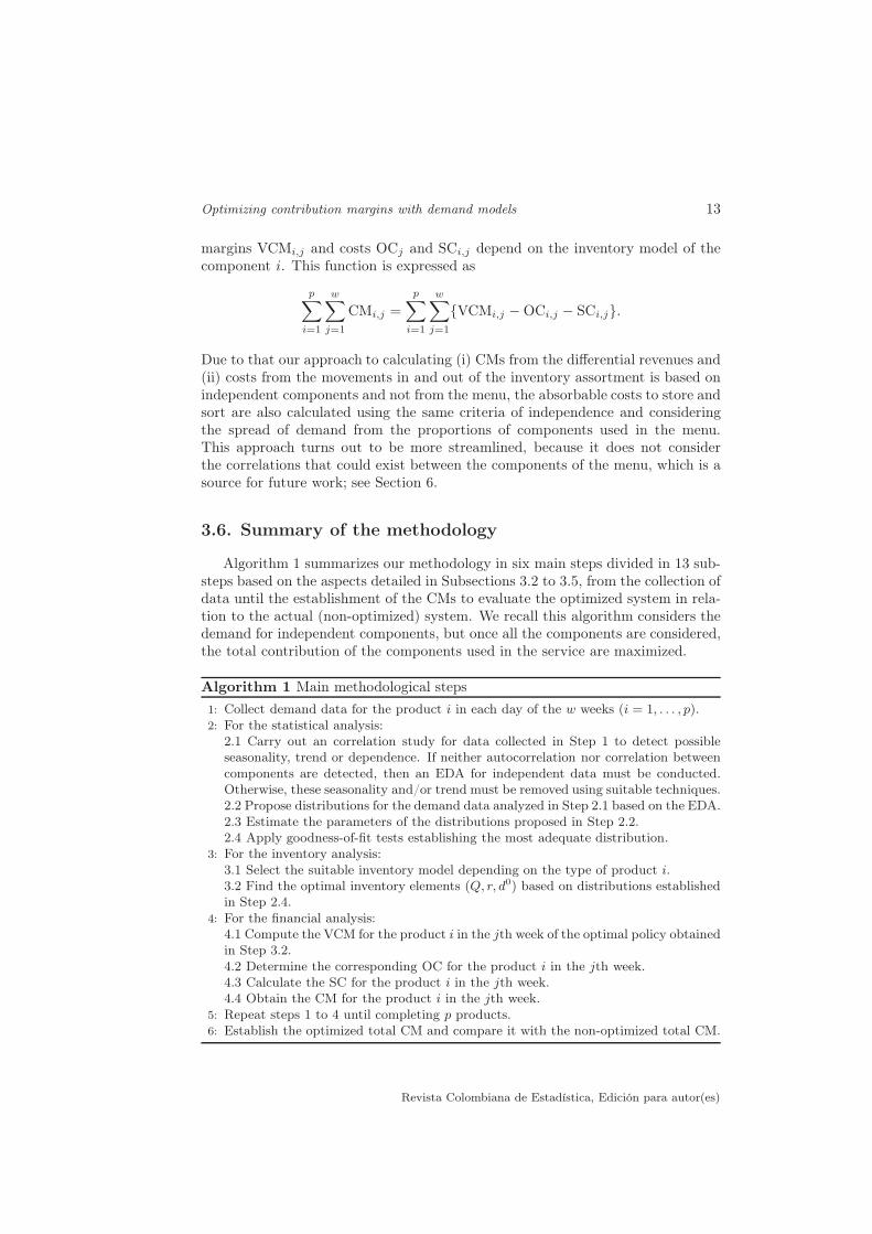
Algorithm 1 summarizes our methodology in six main steps divided in 13 sub-steps based on the aspects detailed in Subsections 3.2 to 3.5, from the collection ofdata until the establishment of the CMs to evaluate the optimized system in rela-tion to the actual (non-optimized) system. We recall this algorithm considers thedemand for independent components, but once all the components are considered,the total contribution of the components used in the service are maximized.
Algorithm 1 Main methodological steps
1: Collect demand data for the product i in each day of the w weeks (i = 1, . . . , p).2: For the statistical analysis:
2.1 Carry out an correlation study for data collected in Step 1 to detect possibleseasonality, trend or dependence. If neither autocorrelation nor correlation betweencomponents are detected, then an EDA for independent data must be conducted.Otherwise, these seasonality and/or trend must be removed using suitable techniques.2.2 Propose distributions for the demand data analyzed in Step 2.1 based on the EDA.2.3 Estimate the parameters of the distributions proposed in Step 2.2.2.4 Apply goodness-of-fit tests establishing the most adequate distribution.
3: For the inventory analysis:3.1 Select the suitable inventory model depending on the type of product i.3.2 Find the optimal inventory elements (Q, r, d0) based on distributions establishedin Step 2.4.
4: For the financial analysis:4.1 Compute the VCM for the product i in the jth week of the optimal policy obtainedin Step 3.2.4.2 Determine the corresponding OC for the product i in the jth week.4.3 Calculate the SC for the product i in the jth week.4.4 Obtain the CM for the product i in the jth week.
5: Repeat steps 1 to 4 until completing p products.6: Establish the optimized total CM and compare it with the non-optimized total CM.
Revista Colombiana de Estadística, Edición para autor(es)
14 Fernando Rojas, Víctor Leiva, Peter Wanke & Carolina Marchant
4. Case study
In this section, because there is a need to conduct case studies focusing on theirapplicability in firms to reduce the gap between theory and practice, we apply themethodology summarized in Algorithm 1 to an anonymous Chilean food company,which serves the staff of a hospital in the city of Valparaiso. This case study en-ables researchers to increase their practical knowledge given that aspects involvingunderstanding about environment’s complexity and the managerial efforts madeby firms become evident.
This study was leaded by Fernando Rojas and Victor Leiva in the Universityof Valparaiso-Chile (www.uv.cl) by means of the project grant DIUV 14/2009,during w = 27 weeks covering the period since 20-Nov-2011 to 26-May-2012 (189days). Details of p = 89 products of the inventory assortment considered in thisstudy are indicated in Table 14 with their respective equivalence units.
We recall that the unsatisfied demand shortage costs for non-perishable prod-ucts are unavailable to be incorporated in the analysis, because there is no CMsor penalties that are imposed for a product with unsatisfied demand. If a prod-uct is missing, it is replaced by similar another. In addition, due to the practicalcharacter of this study, for non-perishable products, we set a service level basedon a SF instead of simultaneously optimizing Q and r.
As mentioned, the data have been collected during the period indicated abovefollowing the record system mentioned in Subsection 3.2. Note that, in this typeof data that we analyze (food services for hospitals), seasonality or trend factorsusually are not present; see Step 2 of Algorithm 1. We have also explored thecorrelation between some products and only a small correlation but marginally notsignificant is detected, so that we discard this aspect. In any case, some commentsin this line are provided in the conclusions of this study. Moreover, demand dataare usually observed over time. Then, one must check whether these data havea dependence in the time or not. Autocorrelation graphical analysis providedthat the corresponding autocorrelations are very small, so that dependence inthe time could be discarded too. This graphical analysis can be corroborated bythe Durbin-Watson test and its bootstrapped p-value to examine independence inthese data.
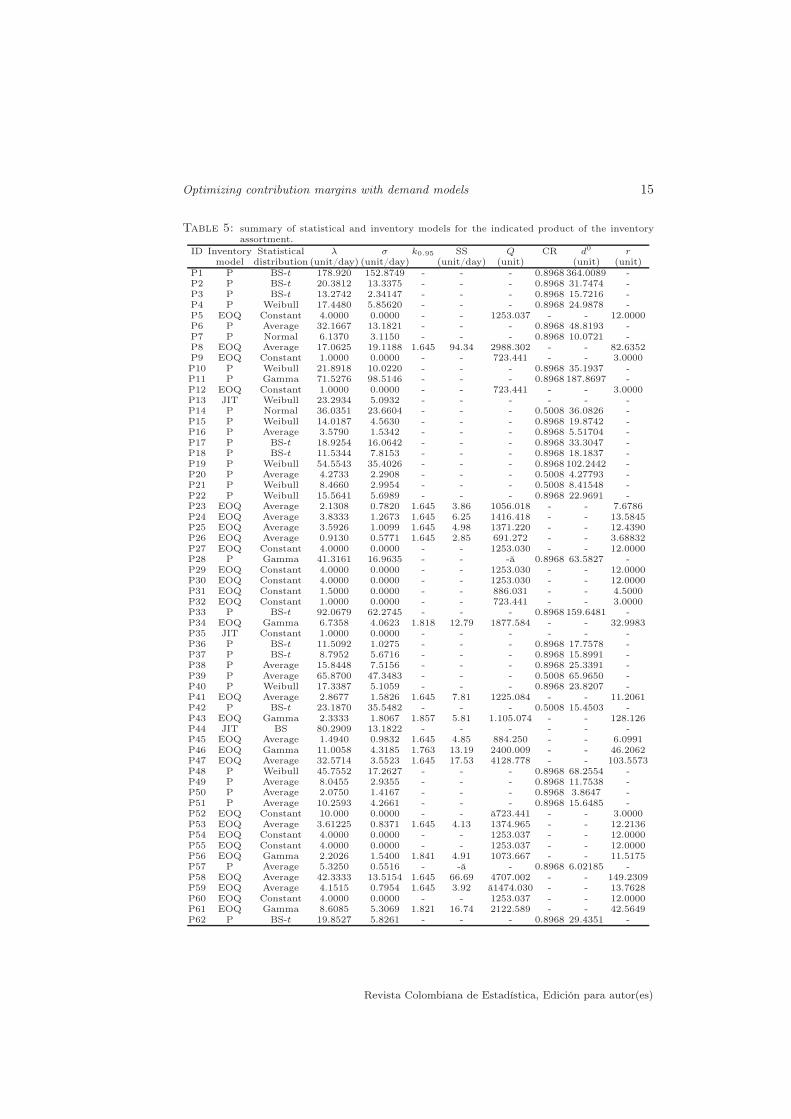
Second, we carry out the statistical analysis of these data from the EDA untilthe selection of the most appropriate distribution for the demand data of eachproduct under analysis, following Subsection 3.3. Tables 5-6 display a summary ofthe statistical results for 89 products of the inventory assortment of the Chileanfood service. This summary indicates, among other aspects, the statistical distri-bution that fits the demand data best for each product.
Third, once we have selected the most appropriate distribution to model thedemand data, we then use the adequate inventory management model to determinethe optimum level in stock to place an order of products, and the optimum quantityto order for minimizing the total cost of inventory, following Subsection 3.4. Tables5-6 also show the optimal quantity of replenishment and the ROP obtained byapplying the appropriate inventory management model.
Revista Colombiana de Estadística, Edición para autor(es)
Optimizing contribution margins with demand models 15
Table 5: summary of statistical and inventory models for the indicated product of the inventoryassortment.
ID Inventory Statistical λ σ k0.95 SS Q CR d0 rmodel distribution (unit/day) (unit/day) (unit/day) (unit) (unit) (unit)
P1 P BS-t 178.920 152.8749 - - - 0.8968 364.0089 -P2 P BS-t 20.3812 13.3375 - - - 0.8968 31.7474 -P3 P BS-t 13.2742 2.34147 - - - 0.8968 15.7216 -P4 P Weibull 17.4480 5.85620 - - - 0.8968 24.9878 -P5 EOQ Constant 4.0000 0.0000 - - 1253.037 - - 12.0000P6 P Average 32.1667 13.1821 - - - 0.8968 48.8193 -P7 P Normal 6.1370 3.1150 - - - 0.8968 10.0721 -P8 EOQ Average 17.0625 19.1188 1.645 94.34 2988.302 - - 82.6352P9 EOQ Constant 1.0000 0.0000 - - 723.441 - - 3.0000P10 P Weibull 21.8918 10.0220 - - - 0.8968 35.1937 -P11 P Gamma 71.5276 98.5146 - - - 0.8968 187.8697 -P12 EOQ Constant 1.0000 0.0000 - - 723.441 - - 3.0000P13 JIT Weibull 23.2934 5.0932 - - - - - -P14 P Normal 36.0351 23.6604 - - - 0.5008 36.0826 -P15 P Weibull 14.0187 4.5630 - - - 0.8968 19.8742 -P16 P Average 3.5790 1.5342 - - - 0.8968 5.51704 -P17 P BS-t 18.9254 16.0642 - - - 0.8968 33.3047 -P18 P BS-t 11.5344 7.8153 - - - 0.8968 18.1837 -P19 P Weibull 54.5543 35.4026 - - - 0.8968 102.2442 -P20 P Average 4.2733 2.2908 - - - 0.5008 4.27793 -P21 P Weibull 8.4660 2.9954 - - - 0.5008 8.41548 -P22 P Weibull 15.5641 5.6989 - - - 0.8968 22.9691 -P23 EOQ Average 2.1308 0.7820 1.645 3.86 1056.018 - - 7.6786P24 EOQ Average 3.8333 1.2673 1.645 6.25 1416.418 - - 13.5845P25 EOQ Average 3.5926 1.0099 1.645 4.98 1371.220 - - 12.4390P26 EOQ Average 0.9130 0.5771 1.645 2.85 691.272 - - 3.68832P27 EOQ Constant 4.0000 0.0000 - - 1253.030 - - 12.0000P28 P Gamma 41.3161 16.9635 - - -ă 0.8968 63.5827 -P29 EOQ Constant 4.0000 0.0000 - - 1253.030 - - 12.0000P30 EOQ Constant 4.0000 0.0000 - - 1253.030 - - 12.0000P31 EOQ Constant 1.5000 0.0000 - - 886.031 - - 4.5000P32 EOQ Constant 1.0000 0.0000 - - 723.441 - - 3.0000P33 P BS-t 92.0679 62.2745 - - - 0.8968 159.6481 -P34 EOQ Gamma 6.7358 4.0623 1.818 12.79 1877.584 - - 32.9983P35 JIT Constant 1.0000 0.0000 - - - - - -P36 P BS-t 11.5092 1.0275 - - - 0.8968 17.7578 -P37 P BS-t 8.7952 5.6716 - - - 0.8968 15.8991 -P38 P Average 15.8448 7.5156 - - - 0.8968 25.3391 -P39 P Average 65.8700 47.3483 - - - 0.5008 65.9650 -P40 P Weibull 17.3387 5.1059 - - - 0.8968 23.8207 -P41 EOQ Average 2.8677 1.5826 1.645 7.81 1225.084 - - 11.2061P42 P BS-t 23.1870 35.5482 - - - 0.5008 15.4503 -P43 EOQ Gamma 2.3333 1.8067 1.857 5.81 1.105.074 - - 128.126P44 JIT BS 80.2909 13.1822 - - - - - -P45 EOQ Average 1.4940 0.9832 1.645 4.85 884.250 - - 6.0991P46 EOQ Gamma 11.0058 4.3185 1.763 13.19 2400.009 - - 46.2062P47 EOQ Average 32.5714 3.5523 1.645 17.53 4128.778 - - 103.5573P48 P Weibull 45.7552 17.2627 - - - 0.8968 68.2554 -P49 P Average 8.0455 2.9355 - - - 0.8968 11.7538 -P50 P Average 2.0750 1.4167 - - - 0.8968 3.8647 -P51 P Average 10.2593 4.2661 - - - 0.8968 15.6485 -P52 EOQ Constant 10.000 0.0000 - - ă723.441 - - 3.0000P53 EOQ Average 3.61225 0.8371 1.645 4.13 1374.965 - - 12.2136P54 EOQ Constant 4.0000 0.0000 - - 1253.037 - - 12.0000P55 EOQ Constant 4.0000 0.0000 - - 1253.037 - - 12.0000P56 EOQ Gamma 2.2026 1.5400 1.841 4.91 1073.667 - - 11.5175P57 P Average 5.3250 0.5516 - -ă - 0.8968 6.02185 -P58 EOQ Average 42.3333 13.5154 1.645 66.69 4707.002 - - 149.2309P59 EOQ Average 4.1515 0.7954 1.645 3.92 ă1474.030 - - 13.7628P60 EOQ Constant 4.0000 0.0000 - - 1253.037 - - 12.0000P61 EOQ Gamma 8.6085 5.3069 1.821 16.74 2122.589 - - 42.5649P62 P BS-t 19.8527 5.8261 - - - 0.8968 29.4351 -
Revista Colombiana de Estadística, Edición para autor(es)
16 Fernando Rojas, Víctor Leiva, Peter Wanke & Carolina Marchant
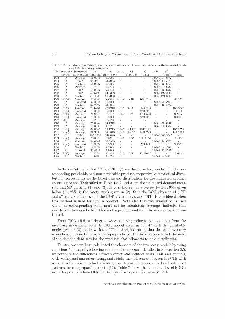
Table 6: (continuation Table 5) summary of statistical and inventory models for the indicated prod-uct of the inventory assortment.
ID Inventory Statistical λ σ k0.95 SS Q CR d0 rmodel distribution (unit/day) (unit/day) (unit/day) (unit) (unit) (unit)
P63 P Average 11.0061 3.0065 - - - 0.8968 14.8472 -P64 P BS-t 25.2673 13.2933 - - - 0.8968 37.5170 -P65 P Weibull 14.9037 5.4825 - - - 0.8968 22.0310 -P66 P Average 10.7543 2.7744 - - - 0.8968 14.2932 -P67 P BS-t 14.8657 2.7844 - - - 0.8968 22.3732 -P68 P BS-t 53.5429 64.6308 - - - 0.8968 127.0268 -P69 P Weibull 83.4886 66.2302 - - - 0.8968 171.6083 -P70 EOQ Gamma 3.1538 2.2651 1.845 7.24 1284.764 - - 16.7000P71 P Constant 3.0000 0.0000 - - - 0.8968 65.5800 -P72 P Weibull 22.7972 13.0891 - - - 0.8968 40.4072 -P73 EOQ Gamma 25.6761 27.1210 1.913 89.86 3665.788 - - 166.8877P74 EOQ Constant 1.0000 0.0000 - - ă723.441 - - 30000P75 EOQ Average 2.3501 0.7617 1.645 3.76 1106.560 - - 8.2717P76 EOQ Constant 1.0000 0.0000 - - ă723.441 - - 3.0000P77 JIT Average 1.6931 0.4624 - - - - - -P78 P Average 25.0652 14.7219 - - - 0.5008 25.0947 -P79 P Average 16.8333 1.1691 - - - 0.8968 18.3102 -P80 EOQ Average 34.3846 19.7718 1.645 97.56 4242.142 - - 135.6755P81 EOQ Average 37.3333 18.0870 1.645 89.25 4420.298 - - 141.7510P82 P BS-t 135.9223 142.046 - - - 0.8968 308.8345 -P83 EOQ Average 296.81 0.9211 1.645 4.55 1.246.354 - - 10.4193P84 P Gamma 34.6047 15.0383 - - - 0.8968 54.3573 -P85 EOQ Constant 1.0000 0.0000 - - 723.441 - - 3.0000P86 P Weibull 9.7969 4.7464 - - - 0.8968 16.1245 -P87 P Normal 23.4211 7.9465 - - - 0.8968 33.4597 -P88 EOQ Average 2.9364 1.1214 1.645 5.53 12.39687 - - 10.6538P89 P Weibull 4.8498 2.4073 - - - 0.8968 8.0645 -
In Tables 5-6, note that “P” and “EOQ” are the “inventory model” for the cor-responding perishable and non-perishable product, respectively; “statistical distri-bution” corresponds to the fitted demand distribution for the indicated productaccording to the ID detailed in Table 14; λ and σ are the estimated demand meanrate and SD given in (1) and (2); k0.95 is the SF for a service level of 95% givenbelow (2); “SS” is the safety stock given in (2); Q is the EOQ given in (1); CRand d0 are given in (3); r is the ROP given in (2); and “JIT” is considered whenthis method is used for such a product. Note also that the symbol “-” is usedwhen the corresponding value must not be calculated; “average” indicates thatany distribution can be fitted for such a product and then the normal distributionis used.
From Tables 5-6, we describe 38 of the 89 products (components) from theinventory assortment with the EOQ model given in (1), 47 with the perishablemodel given in (3), and 4 with the JIT method, indicating that the total inventoryis made up of mostly perishable type products. BS distributions fitted the mostof the demand data sets for the products that allows us to fit a distribution.
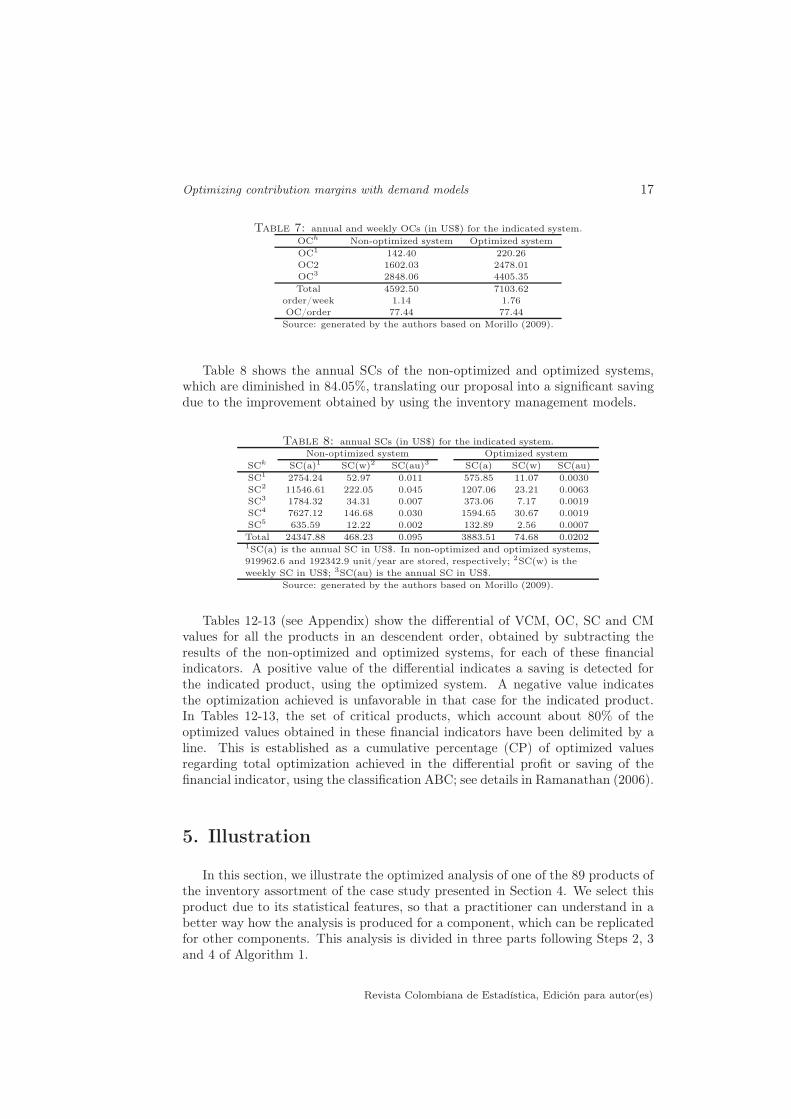
Fourth, once we have calculated the elements of the inventory models by usingequations (1) and (3), following the financial approach detailed in Subsection 3.5,we compute the differences between direct and indirect costs (unit and annual),with weekly and annual ordering, and obtain the differences between the CMs withrespect to the entire product inventory assortment of non-optimized and optimizedsystems, by using equations (4) to (12). Table 7 shows the annual and weekly OCsin both systems, where OCs for the optimized system increase 54.64%.
Revista Colombiana de Estadística, Edición para autor(es)
Optimizing contribution margins with demand models 17
Table 7: annual and weekly OCs (in US$) for the indicated system.
OCh Non-optimized system Optimized system
OC1 142.40 220.26
OC2 1602.03 2478.01
OC3 2848.06 4405.35
Total 4592.50 7103.62
order/week 1.14 1.76
OC/order 77.44 77.44
Source: generated by the authors based on Morillo (2009).
Table 8 shows the annual SCs of the non-optimized and optimized systems,which are diminished in 84.05%, translating our proposal into a significant savingdue to the improvement obtained by using the inventory management models.
Table 8: annual SCs (in US$) for the indicated system.
Non-optimized system Optimized system
SCk SC(a)1 SC(w)2 SC(au)3 SC(a) SC(w) SC(au)
SC1 2754.24 52.97 0.011 575.85 11.07 0.0030
SC2 11546.61 222.05 0.045 1207.06 23.21 0.0063
SC3 1784.32 34.31 0.007 373.06 7.17 0.0019
SC4 7627.12 146.68 0.030 1594.65 30.67 0.0019
SC5 635.59 12.22 0.002 132.89 2.56 0.0007
Total 24347.88 468.23 0.095 3883.51 74.68 0.02021SC(a) is the annual SC in US$. In non-optimized and optimized systems,
919962.6 and 192342.9 unit/year are stored, respectively; 2SC(w) is the
weekly SC in US$; 3SC(au) is the annual SC in US$.
Source: generated by the authors based on Morillo (2009).
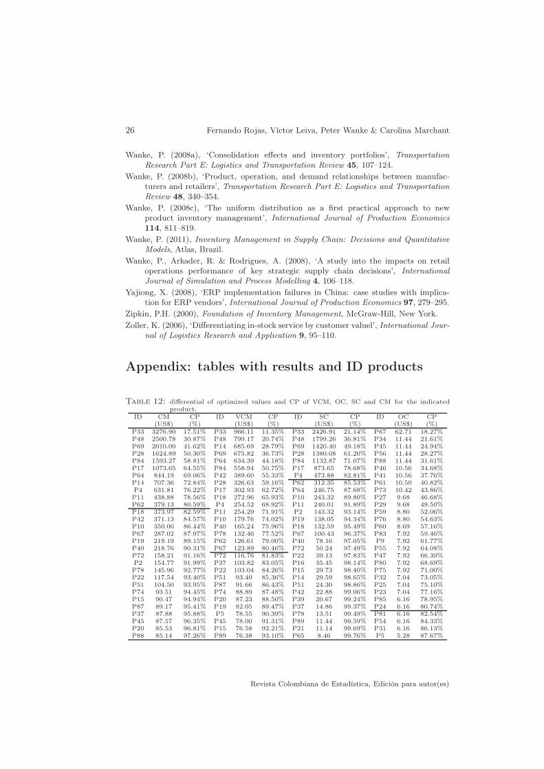
Tables 12-13 (see Appendix) show the differential of VCM, OC, SC and CMvalues for all the products in an descendent order, obtained by subtracting theresults of the non-optimized and optimized systems, for each of these financialindicators. A positive value of the differential indicates a saving is detected forthe indicated product, using the optimized system. A negative value indicatesthe optimization achieved is unfavorable in that case for the indicated product.In Tables 12-13, the set of critical products, which account about 80% of theoptimized values obtained in these financial indicators have been delimited by aline. This is established as a cumulative percentage (CP) of optimized valuesregarding total optimization achieved in the differential profit or saving of thefinancial indicator, using the classification ABC; see details in Ramanathan (2006).
5. Illustration
In this section, we illustrate the optimized analysis of one of the 89 products ofthe inventory assortment of the case study presented in Section 4. We select thisproduct due to its statistical features, so that a practitioner can understand in abetter way how the analysis is produced for a component, which can be replicatedfor other components. This analysis is divided in three parts following Steps 2, 3and 4 of Algorithm 1.
Revista Colombiana de Estadística, Edición para autor(es)
18 Fernando Rojas, Víctor Leiva, Peter Wanke & Carolina Marchant
First, we carry out the statistical analysis, describing the computational im-plementation of the methodology and providing details of this analysis for thedemand data set of the chosen product. Here, we perform an EDA and, basedon it, we propose statistical distributions to model such data. Then, by meansof goodness-of-fit methods, we detect which is the most appropriate distributionto model the demand data of the product under analysis. Second, by using theresults from the statistical analysis, we determinate the elements of the inventorymanagement model suitable for this product. Third, we carry out the financialanalysis of this illustration.
5.1. Statistical analysis
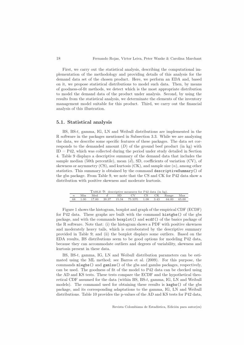
BS, BS-t, gamma, IG, LN and Weibull distributions are implemented in theR software in the packages mentioned in Subsection 3.3. While we are analyzingthe data, we describe some specific features of these packages. The data set cor-responds to the demanded amount (D) of the ground beef product (in kg) withID = P42, which was collected during the period under study detailed in Section4. Table 9 displays a descriptive summary of the demand data that includes thesample median (50th percentile), mean (d̄), SD, coefficients of variation (CV), ofskewness or asymmetry (CS), and kurtosis (CK), and sample size (n), among otherstatistics. This summary is obtained by the command descriptiveSummary() ofthe gbs package. From Table 9, we note that the CS and CK for P42 data show adistribution with positive skewness and moderate kurtosis.
Table 9: descriptive measures for P42 data (in kg).
n Min Med d̄ SD CV CS CK Range Max
68 1.00 17.00 20.37 15.34 75.33% 1.08 3.43 64.00 65.00
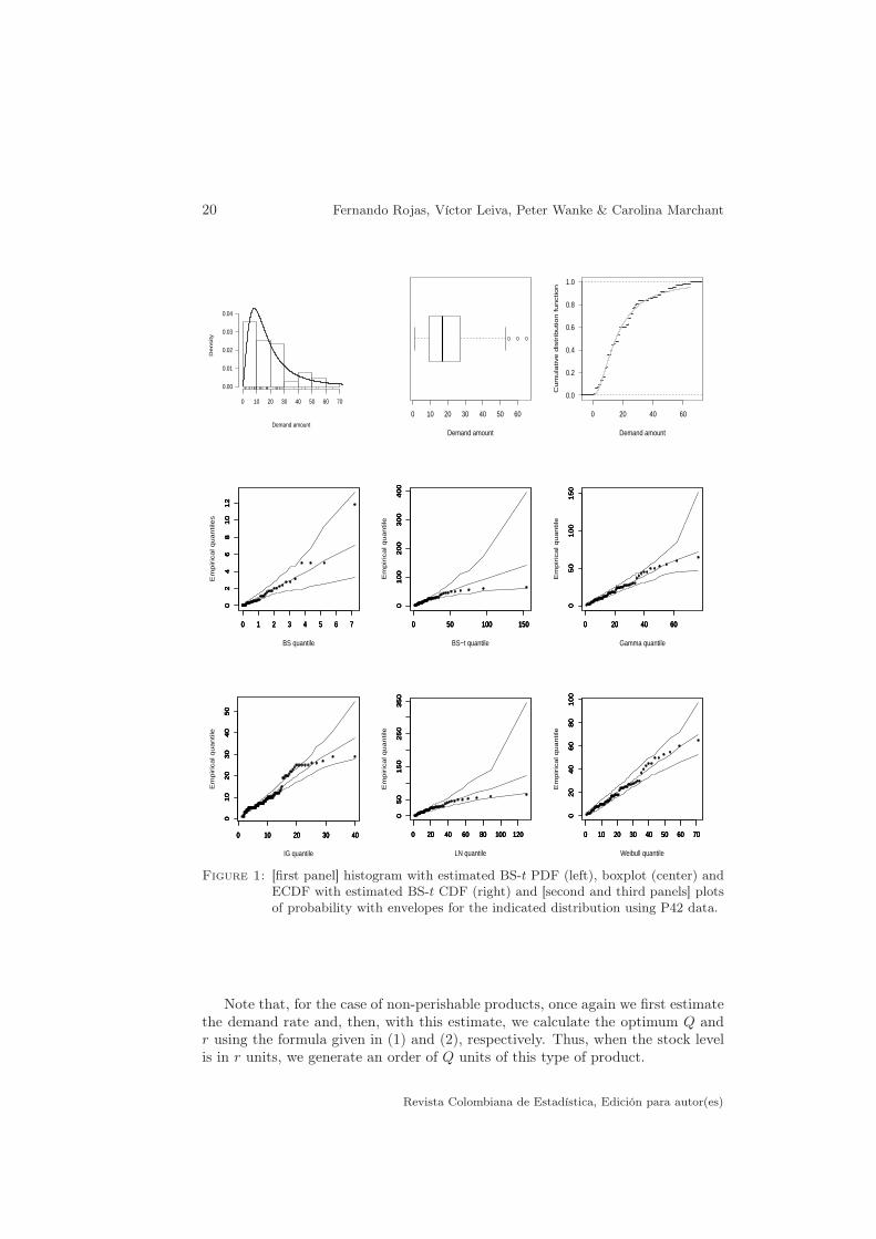
Figure 1 shows the histogram, boxplot and graph of the empirical CDF (ECDF)for P42 data. These graphs are built with the command histgbs() of the gbspackage, and with the commands boxplot() and ecdf() of the basics package ofthe R software. Note that: (i) the histogram shows a PDF with positive skewnessand moderately heavy tails, which is corroborated by the descriptive summaryprovided in Table 9; and (ii) the boxplot displays some outliers. Based on theEDA results, BS distributions seem to be good options for modeling P42 data,because they can accommodate outliers and degrees of variability, skewness andkurtosis present in these data.
BS, BS-t, gamma, IG, LN and Weibull distribution parameters can be esti-mated using the ML method; see Barros et al. (2009). For this purpose, thecommands mlegbs() and gamlss() of the gbs and gamlss packages, respectively,can be used. The goodness of fit of the model to P42 data can be checked usingthe AD and KS tests. These tests compare the ECDF and the hypothetical theo-retical CDF assumed for the data (within BS, BS-t, gamma, IG, LN and Weibullmodels). The command used for obtaining these results is ksgbs() of the gbspackage, and its corresponding adaptations to the gamma, IG, LN and Weibulldistributions. Table 10 provides the p-values of the AD and KS tests for P42 data,
Revista Colombiana de Estadística, Edición para autor(es)
Optimizing contribution margins with demand models 19
from which we note that almost all of these distributions seem to be reasonablemodels for these demand data. However, based on the AD test results, which ismore powerful than the KS test (Barros et al. 2014), only the BS, BS-t and LN fitthe data well at a p-value = 0.01.
Table 10: p-values of the indicated goodness-of-fit method and distribution for P42data.
Method BS BS-t Gamma GI LN Weibull
AD 0.0143 0.1214 < 0.001 < 0.001 0.0604 0.0022
KS 0.1668 0.7562 0.1525 0.0017 0.6165 0.2338
The fit of the model to P42 data is visually illustrated by three graphs shownin Figure 1, from where the ECDF (gray line) and the theoretical BS-t CDF (blackdots) are compared in Figure 1(right), whereas the histogram with the estimatedBS-t PDF is plotted in Figure 1(left). Probability plots with envelopes are shownin Figure 1, where “envelopes” are bands constructed by a simulation process fa-cilitating the display setting. In the case of BS distributions, these envelopes arebuilt using the formulas given in Subsection 3.3. For more details on probabilityplots with envelopes, see Leiva, Athayde, Azevedo & Marchant (2011a) and ref-erences therein. The commands used to obtain these graphs are envelopebs()
and envelopegbs() and their corresponding adaptations to the gamma, IG, LNand Weibull distributions. From these graphs, we note the appropriate fittingprovided by the six distributions that we propose to model P42 demand data.However, only the BS, BS-t, gamma, LN and Weibull models show plots with allthe point inside of their envelopes, which corroborates the results provided by thegoodness-of-fit methods given in Table 10. As can be seen from the boxplot givenFigure 1(center), there are some outliers that can introduce an adverse effect onthe ML estimates of the parameters of the distributions detected as suitable bythe goodness-of-fit methods. Nevertheless, as mentioned, only the BS-t distribu-tion has been proven to provide estimates robust to these outliers. Based on thisstatistical robustness, we choose the BS-t distribution as the most suitable withinthe distributions proposed for describing P42 demand data.
5.2. Inventory analysis
Once we have selected the most suitable distribution to model the quantitydemanded of P42, corresponding in this case to the BS-t distribution, we usethe adequate inventory management model to determine the optimum quantityto be ordered for minimizing the total cost of inventory. In this case, we usethe perishable product model for single period. First, we estimate the demandrate from the BS-t distribution as λ̂ = 23.19 kg/day. Then, with this value, we
determine the optimum replenishment quantity as d̂0 = 15.45 kg, by using theformula given in (3), whose value must be applied as refueling. We consider a LTconstant of l = 3 days, which is the same for all the products of the inventoryassortment. Thus, at the beginning of each week, the stock level must be checked,and then a quantity of (15.45− Lj) kg, for j = 1, . . . , 27, of the product must beordered.
Revista Colombiana de Estadística, Edición para autor(es)
20 Fernando Rojas, Víctor Leiva, Peter Wanke & Carolina Marchant
Demand amount
De
nsity
0 10 20 30 40 50 60 70
0.00
0.01
0.02
0.03
0.04
0 10 20 30 40 50 60
Demand amount
0 20 40 60
0.0
0.2
0.4
0.6
0.8
1.0
Demand amount
Cu
mu
lative
dis
trib
utio
n f
un
ctio
n
0 1 2 3 4 5 6 7
02
46
81
01
2
BS quantile
Em
pir
ica
l q
ua
ntile
s
0 1 2 3 4 5 6 7
02
46
81
01
2
0 1 2 3 4 5 6 7
02
46
81
01
2
0 1 2 3 4 5 6 7
02
46
81
01
2
0 50 100 150
01
00
20
03
00
40
0
BS−t quantile
Em
pir
ica
l q
ua
ntile
0 50 100 150
01
00
20
03
00
40
0
0 50 100 150
01
00
20
03
00
40
0
0 50 100 150
01
00
20
03
00
40
0
0 20 40 60
05
01
00
15
0
Gamma quantile
Em
pir
ica
l q
ua
ntile
0 20 40 60
05
01
00
15
0
0 20 40 60
05
01
00
15
0
0 20 40 60
05
01
00
15
0
0 10 20 30 40
01
02
03
04
05
0
IG quantile
Em
piric
al q
ua
ntile
0 10 20 30 40
01
02
03
04
05
0
0 10 20 30 40
01
02
03
04
05
0
0 10 20 30 40
01
02
03
04
05
0
0 20 40 60 80 100 120
05
01
50
25
03
50
LN quantile
Em
pir
ica
l q
ua
ntile
0 20 40 60 80 100 120
05
01
50
25
03
50
0 20 40 60 80 100 120
05
01
50
25
03
50
0 20 40 60 80 100 120
05
01
50
25
03
50
0 10 20 30 40 50 60 70
02
04
06
08
01
00
Weibull quantile
Em
pir
ica
l q
ua
ntile
0 10 20 30 40 50 60 70
02
04
06
08
01
00
0 10 20 30 40 50 60 70
02
04
06
08
01
00
0 10 20 30 40 50 60 70
02
04
06
08
01
00
Figure 1: [first panel] histogram with estimated BS-t PDF (left), boxplot (center) andECDF with estimated BS-t CDF (right) and [second and third panels] plotsof probability with envelopes for the indicated distribution using P42 data.
Note that, for the case of non-perishable products, once again we first estimatethe demand rate and, then, with this estimate, we calculate the optimum Q andr using the formula given in (1) and (2), respectively. Thus, when the stock levelis in r units, we generate an order of Q units of this type of product.
Revista Colombiana de Estadística, Edición para autor(es)
Optimizing contribution margins with demand models 21
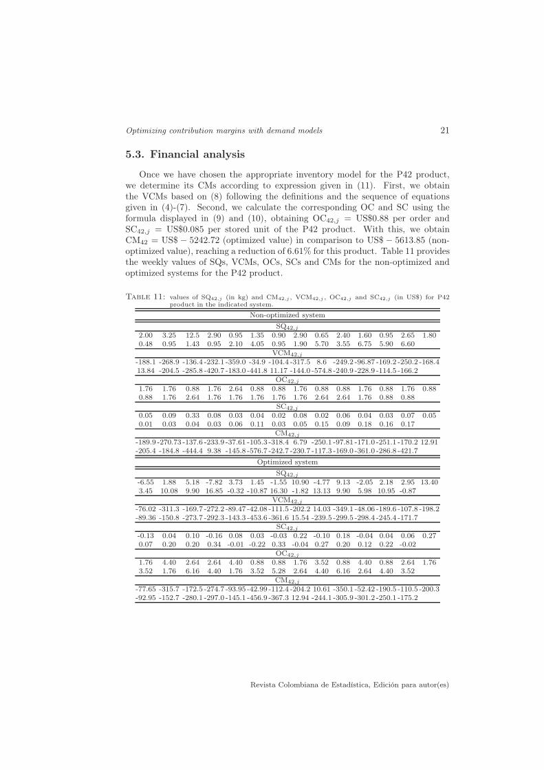
5.3. Financial analysis
Once we have chosen the appropriate inventory model for the P42 product,we determine its CMs according to expression given in (11). First, we obtainthe VCMs based on (8) following the definitions and the sequence of equationsgiven in (4)-(7). Second, we calculate the corresponding OC and SC using theformula displayed in (9) and (10), obtaining OC42,j = US$0.88 per order andSC42,j = US$0.085 per stored unit of the P42 product. With this, we obtainCM42 = US$ − 5242.72 (optimized value) in comparison to US$ − 5613.85 (non-optimized value), reaching a reduction of 6.61% for this product. Table 11 providesthe weekly values of SQs, VCMs, OCs, SCs and CMs for the non-optimized andoptimized systems for the P42 product.
Table 11: values of SQ42,j (in kg) and CM42,j , VCM42,j , OC42,j and SC42,j (in US$) for P42product in the indicated system.
Non-optimized system
SQ42,j
2.00 3.25 12.5 2.90 0.95 1.35 0.90 2.90 0.65 2.40 1.60 0.95 2.65 1.800.48 0.95 1.43 0.95 2.10 4.05 0.95 1.90 5.70 3.55 6.75 5.90 6.60
VCM42,j
-188.1 -268.9 -136.4 -232.1 -359.0 -34.9 -104.4 -317.5 8.6 -249.2 -96.87 -169.2 -250.2 -168.413.84 -204.5 -285.8 -420.7 -183.0 -441.8 11.17 -144.0 -574.8 -240.9 -228.9 -114.5 -166.2
OC42,j
1.76 1.76 0.88 1.76 2.64 0.88 0.88 1.76 0.88 0.88 1.76 0.88 1.76 0.880.88 1.76 2.64 1.76 1.76 1.76 1.76 1.76 2.64 2.64 1.76 0.88 0.88
SC42,j
0.05 0.09 0.33 0.08 0.03 0.04 0.02 0.08 0.02 0.06 0.04 0.03 0.07 0.050.01 0.03 0.04 0.03 0.06 0.11 0.03 0.05 0.15 0.09 0.18 0.16 0.17
CM42,j
-189.9 -270.73 -137.6 -233.9 -37.61 -105.3 -318.4 6.79 -250.1 -97.81 -171.0 -251.1 -170.2 12.91-205.4 -184.8 -444.4 9.38 -145.8 -576.7 -242.7 -230.7 -117.3 -169.0 -361.0 -286.8 -421.7
Optimized system
SQ42,j
-6.55 1.88 5.18 -7.82 3.73 1.45 -1.55 10.90 -4.77 9.13 -2.05 2.18 2.95 13.403.45 10.08 9.90 16.85 -0.32 -10.87 16.30 -1.82 13.13 9.90 5.98 10.95 -0.87
VCM42,j
-76.02 -311.3 -169.7 -272.2 -89.47 -42.08 -111.5 -202.2 14.03 -349.1 -48.06 -189.6 -107.8 -198.2-89.36 -150.8 -273.7 -292.3 -143.3 -453.6 -361.6 15.54 -239.5 -299.5 -298.4 -245.4 -171.7
SC42,j
-0.13 0.04 0.10 -0.16 0.08 0.03 -0.03 0.22 -0.10 0.18 -0.04 0.04 0.06 0.270.07 0.20 0.20 0.34 -0.01 -0.22 0.33 -0.04 0.27 0.20 0.12 0.22 -0.02
OC42,j
1.76 4.40 2.64 2.64 4.40 0.88 0.88 1.76 3.52 0.88 4.40 0.88 2.64 1.763.52 1.76 6.16 4.40 1.76 3.52 5.28 2.64 4.40 6.16 2.64 4.40 3.52
CM42,j
-77.65 -315.7 -172.5 -274.7 -93.95 -42.99 -112.4 -204.2 10.61 -350.1 -52.42 -190.5 -110.5 -200.3-92.95 -152.7 -280.1 -297.0 -145.1 -456.9 -367.3 12.94 -244.1 -305.9 -301.2 -250.1 -175.2
Revista Colombiana de Estadística, Edición para autor(es)
22 Fernando Rojas, Víctor Leiva, Peter Wanke & Carolina Marchant
6. Concluding remarks
We proposed a methodology useful for food service companies that allows theircontribution margins to be optimized. The methodology was based on statisticaltools, inventory management models and financial indicators. Its main steps weresynthesized in Algorithm 1. Because there is a need to conduct case studies focus-ing on their applicability in firms to reduce the gap between theory and practice,and to transfer knowledge to industry, we applied this methodology. Specifically,the case study was conducted to a Chilean food service company, which showed theimportance of considering inventory models and statistical aspects for improvingits supply and inventory policies, increasing its contribution margins. Inventorymanagement models for perishable products showed to adjust adequately the de-mand for fruits and vegetables, which have the greatest unit contribution margins,so that such products can be considered as critical in the inventory assortment.With respect to the non-perishable products, it is noteworthy that the EOQ modelfitted them considerably well. Such products can be stored indefinitely, withoutlosses occurring through maturity, which has been used to reduce ordering costs.Products fitted by the model for perishables presented an optimized quantity simi-lar to the demand rate, because such products have a shelf life so that they cannotbe stored for a long period. A small amount of products (about 5%) used a JITmethod. In summary, we validated improvements in logistics management ap-plying an appropriate inventory model, increasing the contribution margins of aChilean company. This result agrees with that reported by Ramanathan (2006),who linked inventory cost minimization and contribution margin maximizationin products of type A of the ABC classification. These products are responsiblearound 20% of the total of products of the inventory assortments and are responsi-ble for a proportion around 80% of the total contribution margin. It is noteworthythat, although we achieved an improvement of 10.47% in contribution margin forthe studied Chilean company, 1.8% in total variable contribution margin, 54.64%in ordering costs, and 84.05% in storing costs, using the proposed methodology,still some aspects can be improved. For example, it is possible to explore thestatistical dependence over time and among products. Seasonality and trend fac-tors, as well as dependence in the time of the demand, can be considered in themodeling by using time series models. The statistical dependence among productscan be analyzed by means of multivariate structures for the models considered inthis work. In fact, the authors of the paper will collect real-world data of thistype during 2014 for a future study. In addition, from the practical scope, anotherfuture study considering demand data for a menu instead of its components isbeing considered by the authors. Studies of this type have been presented in theliterature under names such as: assemble to order systems, inventory models withcorrelated demand, inventory models with multivariate demand, inventory modelswith multi-item demand, inventory models with multi-component demand and in-ventory models with component commonality, among others; see Lu & Song (2005)and Agraval & Cohen (2001). In any case, incorporating all of these elements inthe modeling can improve the precision of the results, but also can increase itsstatistical complexity.
Revista Colombiana de Estadística, Edición para autor(es)
Optimizing contribution margins with demand models 23
Acknowledgements
The authors thank the Editor-in-Chief, Dr. Leonardo Trujillo, and two anony-mous referees for their valuable comments on an earlier version of this manuscriptwhich resulted in this improved version. Also, the authors thank nutritionistsMelina Fuentes and Javiera Quijada for their help collecting the data used in thestudy. This research was supported by project grants DIUV 14/2009 from the Uni-versity of Valparaiso-Chile, FONDECYT 1120879 from the Chilean government,and by CAPES and FACEPE grants from the Brazil government.
References
Agrawal, M. &Cohen, M. (2001), ‘Optimal material control and performance evaluationin an assembly environment with component commonality’, Naval Research
Logistics 48, 409–429.
Barros, M., Leiva, V., Ospina, R. & Tsuyuguchi, A. (2014), ‘Goodness-of-fit tests for theBirnbaum-Saunders distribution with censored reliability data’, IEEE Transactions
on Reliability 63, 543–554.
Barros, M., Paula, G. & Leiva, V. (2009), ‘An R implementation for generalizedBirnbaum-Saunders distributions’, Computational Statistics and Data Analysis
53, 1511–1528.
Bhatti, C. (2010), ‘The Birnbaum-Saunders autoregressive conditional duration model’,Mathematics and Computers in Simulation 80, 2062–2078.
Ben-Daya, M. & Raouf, A. (1994), ‘Inventory models involving lead time as a decisionvariable’, Journal of the Operational Research Society 45, 579–582.
Blankley, A., Khouja, M. & Wiggins, C. (2008), ‘An investigation into the effect offull-scale supply chain management software adoptions on inventory balances andturns’, Journal of Business Logistics 29, 201–224.
Botter, R. & Fortuin, L. (2000), ‘Stocking strategy for service parts: a case study’,International Journal of Operations and Production Management 20, 656–674.
Braglia, M., Eaves, A. & Kingsman, B. (2004a), ‘Forecasting for the ordering and stock-holding of spare parts’, Journal of the Operational Research Society 55, 431–437.
Braglia, M. & Gabbrielli, R. (2001), ‘A genetic approach for setting parameters ofreorder point systems’, International Journal of Logistics Research and Application
4, 345–358.
Braglia, M., Grassi, A. & Montanari, R. (2004b), ‘Multi-attribute classification methodfor spare parts inventory management’, Journal of Quality in Maintenance
Engineering 10, 55–65.
Burgin, T. (1975), ‘The gamma distribution in inventory control’, Operations Research
Quarterly 26, 507–525.
Carter, P., Carter, J., Monczka, R., Slaight, T. & Swan, A. (2000), ‘The future ofpurchasing and supply: a ten-year forecast’, Journal of Supply Chain Management
36, 14–26.
Castro-Kuriss, C., Kelmansky, D., Leiva, V. & Martinez, E. (2010), ‘On a goodness-of-fittest for normality with unknown parameters and type-II censored data’, Journal of
Applied Statistics 37, 1193–1211.
Castro-Kuriss, C., Leiva, V. & Athayde, E. (2014), ‘Graphical tools to assess goodness-of-fit in non-location-scale distributions’, Colombian Journal of Statistics (in press).
Revista Colombiana de Estadística, Edición para autor(es)
24 Fernando Rojas, Víctor Leiva, Peter Wanke & Carolina Marchant
Chiu, Y. (2010), ‘Mathematical modelling for determining economic batch size andoptimal number of deliveries for EOQ model with quality assurance’, Mathematical
and Computer Modelling of Dynamical Systems 16, 373–388.
Cobb, B., Rumí, R. & Salmerón, A. (2013), ‘Inventory management with lognormaldemand per unit time’, Computers and Operations Research 40, 1842–1851.
Fox, E., Gavish, B. & Semple, J. (2008), ‘A general approximation to the distributionof count data with applications to inventory modeling’. Working Paper.
Gjerdrum, J., Samsatli, N., Shah, N. & Papageorgiou, L. (2005), ‘Optimisation ofpolicy parameters in supply chain applications’, International Journal of Logistics
Research and Application 8, 15–36.
Grant, D., Karagianni, C. & Li, M. (2006), ‘Forecasting and stock obsolescence in whiskyproduction’, International Journal of Logistics Research and Application 9, 319–334.
Harvey, W. (2002), ‘And then there were none’, Operations Research 50, 217–226.
Hernández-González, C. (2011), ‘Methodological proposal for the management ofthe refulling in the company Astilleros del Oriente’, Yearbook of the Faculty of
Ecomomical and Business Sciences 2, 53–60.
Hillier, F. & Lieberman, G. (2005), Introduction to Operational Research, McGraw Hill,New York.
Jin, X. & Kawczak, J. (2003), ‘Birnbaum-Saunders and lognormal kernel estimators formodelling durations in high frequency financial data’, Annals of Economics and
Finance 4, 103–124.
Johnson, N., Kotz, S. & Balakrishnan, N. (1994), Continuous Univariate Distributions,Vols. I and II, Wiley, New York.
Keaton, M. (1995), ‘Using the gamma distribution to model demand when lead time israndom’, Journal of Business Logistics 16, 107–131.
Kogan, K. & Tell, H. (2009), ‘Production smoothing by balancing capacity utilizationand advance orders’, Journal of Business Logistics 41, 223–231.
Lau, H. (1989), ‘Toward an inventory control system under non-normal demand andlead time uncertainty’, Journal of Business Logistics 10, 88–103.
Leiva, V., Athayde, E., Azevedo, C. & Marchant, C. (2011a), ‘Modeling wind energyflux by a Birnbaum-Saunders distribution with unknown shift parameter’, Journal
of Applied Statistics 38, 2819–2838.
Leiva, V., Hernandez, H. & Sanhueza, A. (2008), ‘An R package for a general class ofinverse Gaussian distributions’, Journal of Statistical Software 26, 1–16.
Leiva, V., Marchant, C., Saulo, H., Aslam, M. & Rojas, F. (2014a), ‘Capability indicesfor Birnbaum-Saunders processes applied to electronic and food industries’, Journal
of Applied Statistics 41, 1881–1902.
Leiva, V., Ponce, M., Marchant, C. & Bustos, O. (2012), ‘Fatigue statistical distribu-tions useful for modeling diameter and mortality of trees’, Colombian Journal of
Statistics 35, 349–367.
Leiva, V., Rojas, E., Galea, M. & Sanhueza, A. (2014b), ‘Diagnostics in Birnbaum-Saunders accelerated life models with an application to fatigue data’, Applied
Stochastic Models in Business and Industry 30, 115–131.
Leiva, V., Santos-Neto, M., Cysneiros, F. & Barros, M. (2014c), ‘Birnbaum-Saundersregression model: a new approach’, Statistical Modelling 14, 21–48.
Leiva, V., Saulo, E., Leao, J. & Marchant, C. (2014d), ‘A family of autoregressiveconditional duration models applied to financial data’, Computational Statistics
and Data Analysis 79, 175–191.
Revista Colombiana de Estadística, Edición para autor(es)

Optimizing contribution margins with demand models 25
Leiva, V., Soto, G., Cabrera, E. & Cabrera, G. (2011b), ‘New control charts based onthe Birnbaum-Saunders distribution and their implementation’, Colombian Journal
of Statistics 34, 147–176.
Lu, Y. & Song, J-S. (2005), ‘Order-based cost optimization in assemble to-order systems’,Operations Research 53, 151–169.
Marambio, M., Parker, M. & Benavides, X. (2005), Food and Nutrition Service:
Technical Guideline, Ministry of Health, Santiago, Chile.
Marchant, C., Bertin, K., Leiva, V. & Saulo, G. (2007), ‘Generalized Birnbaum-Saunderskernel density estimators and an analysis of financial data’, Computational Statis-
tics and Data Analysis 63, 1–15.
McKinnon, A., Mendes, D. & Nababteh, M. (2007), ‘In-store logistics: an analysis ofon-shelf availability and stockout responses for three product groups’, International
Journal of Logistics Research and Application 10, 251–268.
Mentzer, J. & Krishnan, R. (1988), ‘The effect of the assumption of normality oninventory control/customer service’, Journal of Business Logistics 6, 101–120.
MINSAL (2004), Agreement Hygienic for Food Services, Ministry of Health, Santiago,Chile.
Moors, J. & Strijbosch, L. (1988), ‘Exact fill rates for (R; s; S) inventory controlwith gamma distributed demand’, Journal of the Operational Research Society
53, 1268–1274.
Morillo, M. (2009), ‘Service costs for food and beverage in hostels’, Visión Gerencial
2, 304–327.
Nahmias, S. (2001), Production and Operations Analysis, McGraw Hill, New York.
Nicolau, J. (2009), ‘Leveraging profit from the fixed-variable cost ratio: the case of newhotels in Spain’, Tour Manager 26, 105–111.
Paula, G., Leiva, V., Barros, M. & Liu, S. (2012), ‘Robust statistical modeling using theBirnbaum-Saunders-t distribution applied to insurance’, Applied Stochastic Models
in Business and Industry 28, 16–34.
Ramanathan, R. (2006), ‘ABC inventory classification with multiple-criteria usingweighted linear optimization’, Computers and Operations Research 33, 695–700.
Ramirez, A. (2013), ‘A multi-stage almost ideal demand system: the case of beef demandin Colombia’, Colombian Journal of Statistics 36, 23–42.
Sanhueza, A., Leiva, V. & López-Kleine, L. (2011), ‘On the Student-t mixture inverseGaussian model with an application to protein production’, Colombian Journal of
Statistics 34, 177–195.
Silver, E.A., Pyke, D.F. & Peterson, R. (1998), Inventory Management and Production
Planning and Scheduling, Wiley, New York.
Soman, C. (2006), ‘Combined make-to-order make-to-stock in a food production system’,International Journal of Production Economics 90, 223–235.
Speh, T. & Wagenheim, G. (1978), ‘Demand and lead-time uncertainty: the impacts onphysical distribution performance and management’, Journal of Business Logistics
1, 95–113.
Stasinopoulos, D. & Rigby, R. (2007), ‘Generalized additive models for location, scaleand shape (GAMLSS)’, Journal of Statistical Software 23(7), December.
Tadikamalla, P. (1981), ‘The inverse Gaussian approximation to the lead time demandin inventory control’, International Journal of Production Research 19, 213–219.
Wagner, S. & Lindemann, E. (2008), ‘A case study-based analysis of spare parts man-agement in the engineering industry’, Production Planning and Control 19, 397–407.
Revista Colombiana de Estadística, Edición para autor(es)
26 Fernando Rojas, Víctor Leiva, Peter Wanke & Carolina Marchant
Wanke, P. (2008a), ‘Consolidation effects and inventory portfolios’, Transportation
Research Part E: Logistics and Transportation Review 45, 107–124.
Wanke, P. (2008b), ‘Product, operation, and demand relationships between manufac-turers and retailers’, Transportation Research Part E: Logistics and Transportation
Review 48, 340–354.
Wanke, P. (2008c), ‘The uniform distribution as a first practical approach to newproduct inventory management’, International Journal of Production Economics
114, 811–819.
Wanke, P. (2011), Inventory Management in Supply Chain: Decisions and Quantitative
Models, Atlas, Brazil.
Wanke, P., Arkader, R. & Rodrigues, A. (2008), ‘A study into the impacts on retailoperations performance of key strategic supply chain decisions’, International
Journal of Simulation and Process Modelling 4, 106–118.
Yajiong, X. (2008), ‘ERP implementation failures in China: case studies with implica-tion for ERP vendors’, International Journal of Production Economics 97, 279–295.
Zipkin, P.H. (2000), Foundation of Inventory Management, McGraw-Hill, New York.
Zoller, K. (2006), ‘Differentiating in-stock service by customer valuel’, International Jour-
nal of Logistics Research and Application 9, 95–110.
Appendix: tables with results and ID products
Table 12: differential of optimized values and CP of VCM, OC, SC and CM for the indicatedproduct.
ID CM CP ID VCM CP ID SC CP ID OC CP(US$) (%) (US$) (%) (US$) (%) (US$) (%)
P33 3276.90 17.51% P33 966.11 11.35% P33 2426.91 21.14% P67 62.71 18.27%P48 2500.78 30.87% P48 799.17 20.74% P48 1799.26 36.81% P34 11.44 21.61%P69 2010.00 41.62% P14 685.69 28.79% P69 1420.40 49.18% P45 11.44 24.94%P28 1624.89 50.30% P69 675.82 36.73% P28 1380.08 61.20% P56 11.44 28.27%P84 1593.27 58.81% P64 634.39 44.18% P84 1132.87 71.07% P88 11.44 31.61%P17 1073.65 64.55% P84 558.94 50.75% P17 873.65 78.68% P46 10.56 34.68%P64 844.19 69.06% P42 389.60 55.33% P4 473.88 82.81% P41 10.56 37.76%P14 707.36 72.84% P28 326.63 59.16% P62 312.35 85.53% P61 10.50 40.82%P4 631.81 76.22% P17 302.93 62.72% P64 246.75 87.68% P73 10.42 43.86%P11 438.88 78.56% P18 272.96 65.93% P10 243.32 89.80% P27 9.68 46.68%P62 379.13 80.59% P4 254.52 68.92% P11 240.01 91.89% P29 9.68 49.50%P18 373.97 82.59% P11 254.29 71.91% P2 143.32 93.14% P59 8.80 52.06%P42 371.13 84.57% P10 179.76 74.02% P19 138.05 94.34% P76 8.80 54.63%P10 350.00 86.44% P40 165.24 75.96% P18 132.59 95.49% P60 8.69 57.16%P67 287.02 87.97% P78 132.46 77.52% P67 100.43 96.37% P83 7.92 59.46%P19 219.19 89.15% P62 126.61 79.00% P40 78.16 97.05% P9 7.92 61.77%P40 218.76 90.31% P67 123.89 80.46% P72 50.24 97.49% P55 7.92 64.08%P72 158.21 91.16% P72 116.76 81.83% P22 39.13 97.83% P47 7.92 66.39%P2 154.77 91.99% P37 103.82 83.05% P16 35.45 98.14% P80 7.92 68.69%P78 145.96 92.77% P22 103.04 84.26% P15 29.73 98.40% P75 7.92 71.00%P22 117.54 93.40% P51 93.40 85.36% P14 29.59 98.65% P32 7.04 73.05%P51 104.50 93.95% P87 91.66 86.43% P51 24.30 98.86% P25 7.04 75.10%P74 93.51 94.45% P74 88.89 87.48% P42 22.88 99.06% P23 7.04 77.16%P15 90.47 94.94% P20 87.23 88.50% P39 20.67 99.24% P85 6.16 78.95%P87 89.17 95.41% P19 82.05 89.47% P37 14.86 99.37% P24 6.16 80.74%P37 87.88 95.88% P5 78.55 90.39% P78 13.51 99.49% P81 6.16 82.54%P45 87.57 96.35% P45 78.00 91.31% P89 11.44 99.59% P54 6.16 84.33%P20 85.53 96.81% P15 76.58 92.21% P21 11.14 99.69% P31 6.16 86.13%P88 85.14 97.26% P89 76.38 93.10% P65 8.46 99.76% P5 5.28 87.67%
Revista Colombiana de Estadística, Edición para autor(es)
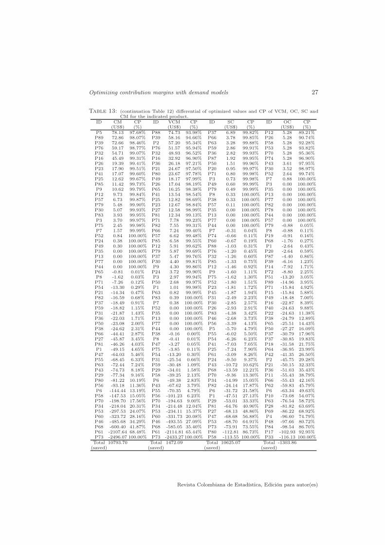
Optimizing contribution margins with demand models 27
Table 13: (continuation Table 12) differential of optimized values and CP of VCM, OC, SC andCM for the indicated product.
ID CM CP ID VCM CP ID SC CP ID OC CP(US$) (%) (US$) (%) (US$) (%) (US$) (%)
P5 78.13 97.68% P88 74.73 93.98% P37 6.89 99.82% P12 5.28 89.21%P89 72.86 98.07% P39 58.16 94.66% P66 3.78 99.85% P26 5.28 90.74%P39 72.66 98.46% P2 57.20 95.34% P63 3.28 99.88% P58 5.28 92.28%P76 59.17 98.77% P76 51.57 95.94% P59 2.86 99.91% P53 5.28 93.82%P32 54.71 99.07% P32 48.93 96.52% P36 2.82 99.93% P70 5.28 95.36%P16 45.49 99.31% P16 32.92 96.90% P87 1.92 99.95% P74 5.28 96.90%P26 19.39 99.41% P36 26.18 97.21% P50 1.51 99.96% P43 3.61 97.95%P23 17.90 99.51% P21 24.67 97.50% P20 0.95 99.97% P30 3.52 98.97%P41 17.07 99.60% P80 23.67 97.78% P71 0.80 99.98% P52 2.64 99.74%P25 12.62 99.67% P49 18.17 97.99% P3 0.73 99.98% P7 0.88 100.00%P85 11.42 99.73% P26 17.04 98.19% P49 0.60 99.99% P3 0.00 100.00%P9 10.62 99.79% P65 16.25 98.38% P79 0.49 99.99% P35 0.00 100.00%P12 9.73 99.84% P41 13.54 98.54% P8 0.33 100.00% P13 0.00 100.00%P57 6.73 99.87% P25 12.82 98.69% P38 0.33 100.00% P77 0.00 100.00%P79 5.48 99.90% P23 12.67 98.84% P57 0.11 100.00% P82 0.00 100.00%P30 5.07 99.93% P27 12.58 98.99% P35 0.00 100.00% P78 0.00 100.00%P83 3.93 99.95% P81 12.34 99.13% P13 0.00 100.00% P44 0.00 100.00%P3 3.70 99.97% P71 7.78 99.23% P77 0.00 100.00% P57 0.00 100.00%P75 2.45 99.98% P82 7.55 99.31% P44 0.00 100.00% P79 -0.88 0.05%P7 1.57 99.99% P66 7.24 99.40% P7 -0.31 0.04% P8 -0.88 0.11%P52 0.84 100.00% P57 6.62 99.48% P74 -0.66 0.11% P19 -0.91 0.16%P24 0.38 100.00% P85 6.58 99.55% P60 -0.67 0.19% P68 -1.76 0.27%P49 0.30 100.00% P12 5.91 99.62% P88 -1.03 0.31% P1 -2.64 0.43%P35 0.00 100.00% P79 5.87 99.69% P76 -1.20 0.45% P20 -2.64 0.59%P13 0.00 100.00% P37 5.47 99.76% P32 -1.26 0.60% P87 -4.40 0.86%P77 0.00 100.00% P30 4.40 99.81% P85 -1.33 0.75% P39 -6.16 1.23%P44 0.00 100.00% P9 4.30 99.86% P12 -1.46 0.92% P14 -7.92 1.71%P65 -0.81 0.01% P24 3.72 99.90% P9 -1.60 1.11% P72 -8.80 2.25%P8 -1.62 0.03% P3 2.97 99.94% P75 -1.62 1.30% P51 -13.20 3.05%P71 -7.26 0.12% P50 2.68 99.97% P52 -1.80 1.51% P89 -14.96 3.95%P54 -13.30 0.29% P1 1.01 99.98% P23 -1.81 1.72% P71 -15.84 4.92%P21 -14.34 0.47% P63 0.82 99.99% P45 -1.87 1.94% P15 -15.84 5.88%P82 -16.59 0.68% P83 0.39 100.00% P31 -2.49 2.23% P49 -18.48 7.00%P37 -18.49 0.91% P7 0.38 100.00% P30 -2.85 2.57% P16 -22.87 8.39%P59 -18.82 1.15% P52 0.00 100.00% P26 -2.93 2.91% P40 -24.63 9.88%P31 -21.87 1.43% P35 0.00 100.00% P83 -4.38 3.42% P22 -24.63 11.38%P36 -22.03 1.71% P13 0.00 100.00% P46 -2.68 3.73% P38 -24.79 12.89%P50 -23.08 2.00% P77 0.00 100.00% P56 -3.39 4.13% P65 -25.51 14.43%P38 -24.62 2.31% P44 0.00 100.00% P5 -5.70 4.79% P50 -27.27 16.09%P66 -44.41 2.87% P38 -0.16 0.00% P55 -6.02 5.50% P37 -30.79 17.96%P27 -45.87 3.45% P8 -0.41 0.01% P54 -6.26 6.23% P37 -30.85 19.83%P81 -46.26 4.03% P47 -3.27 0.05% P41 -7.03 7.05% P18 -31.58 21.75%P1 -49.15 4.65% P75 -3.85 0.11% P25 -7.24 7.90% P64 -36.95 23.99%P47 -64.03 5.46% P54 -13.20 0.30% P61 -3.09 8.26% P42 -41.35 26.50%P55 -68.45 6.33% P31 -25.54 0.66% P24 -9.50 9.37% P2 -45.75 29.28%P63 -72.44 7.24% P59 -30.48 1.09% P43 -10.72 10.62% P21 -50.15 32.33%P43 -74.73 8.18% P29 -34.01 1.58% P68 -13.59 12.21% P36 -51.03 35.43%P29 -77.34 9.16% P58 -39.25 2.13% P70 -9.36 13.30% P11 -55.43 38.79%P80 -81.22 10.19% P6 -49.38 2.83% P34 -14.99 15.05% P66 -55.43 42.16%P56 -93.18 11.36% P43 -67.62 3.79% P82 -24.14 17.87% P62 -59.83 45.79%P6 -144.44 13.19% P55 -70.35 4.79% P6 -31.72 21.58% P6 -63.34 49.63%P58 -147.53 15.05% P56 -101.23 6.23% P1 -47.51 27.13% P10 -73.08 54.07%P70 -198.70 17.56% P70 -194.63 9.00% P29 -53.01 33.33% P63 -76.54 58.72%P34 -218.04 20.31% P34 -214.48 12.04% P81 -64.76 40.90% P28 -81.82 63.69%P53 -297.53 24.07% P53 -234.11 15.37% P27 -68.13 48.86% P69 -86.22 68.92%P60 -323.72 28.16% P60 -331.73 20.08% P47 -68.68 56.88% P4 -96.60 74.79%P46 -485.68 34.29% P46 -493.55 27.09% P53 -68.70 64.91% P48 -97.66 80.72%P68 -600.40 41.87% P68 -585.05 35.40% P73 -73.91 73.55% P84 -98.54 86.70%P61 -2107.64 68.48% P61 -2114.81 65.44% P80 -112.81 86.73% P17 -102.93 92.95%P73 -2496.07 100.00% P73 -2433.27 100.00% P58 -113.55 100.00% P33 -116.13 100.00%Total 10793.70 Total 1472.09 Total 10625.07 Total -1303.86
(saved) (saved) (saved) (saved)
Revista Colombiana de Estadística, Edición para autor(es)
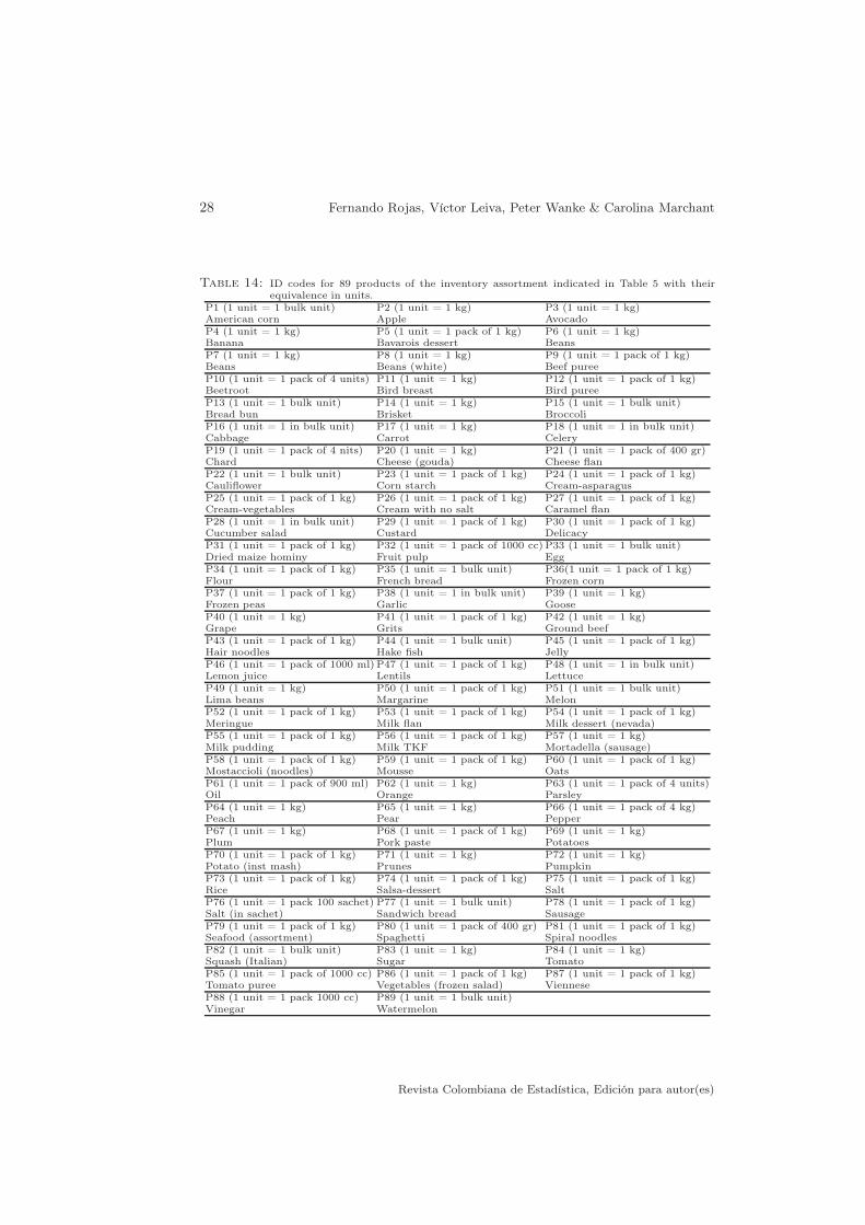
28 Fernando Rojas, Víctor Leiva, Peter Wanke & Carolina Marchant
Table 14: ID codes for 89 products of the inventory assortment indicated in Table 5 with theirequivalence in units.
P1 (1 unit = 1 bulk unit) P2 (1 unit = 1 kg) P3 (1 unit = 1 kg)American corn Apple AvocadoP4 (1 unit = 1 kg) P5 (1 unit = 1 pack of 1 kg) P6 (1 unit = 1 kg)Banana Bavarois dessert BeansP7 (1 unit = 1 kg) P8 (1 unit = 1 kg) P9 (1 unit = 1 pack of 1 kg)Beans Beans (white) Beef pureeP10 (1 unit = 1 pack of 4 units) P11 (1 unit = 1 kg) P12 (1 unit = 1 pack of 1 kg)Beetroot Bird breast Bird pureeP13 (1 unit = 1 bulk unit) P14 (1 unit = 1 kg) P15 (1 unit = 1 bulk unit)Bread bun Brisket BroccoliP16 (1 unit = 1 in bulk unit) P17 (1 unit = 1 kg) P18 (1 unit = 1 in bulk unit)Cabbage Carrot CeleryP19 (1 unit = 1 pack of 4 nits) P20 (1 unit = 1 kg) P21 (1 unit = 1 pack of 400 gr)Chard Cheese (gouda) Cheese flanP22 (1 unit = 1 bulk unit) P23 (1 unit = 1 pack of 1 kg) P24 (1 unit = 1 pack of 1 kg)Cauliflower Corn starch Cream-asparagusP25 (1 unit = 1 pack of 1 kg) P26 (1 unit = 1 pack of 1 kg) P27 (1 unit = 1 pack of 1 kg)Cream-vegetables Cream with no salt Caramel flanP28 (1 unit = 1 in bulk unit) P29 (1 unit = 1 pack of 1 kg) P30 (1 unit = 1 pack of 1 kg)Cucumber salad Custard DelicacyP31 (1 unit = 1 pack of 1 kg) P32 (1 unit = 1 pack of 1000 cc) P33 (1 unit = 1 bulk unit)Dried maize hominy Fruit pulp EggP34 (1 unit = 1 pack of 1 kg) P35 (1 unit = 1 bulk unit) P36(1 unit = 1 pack of 1 kg)Flour French bread Frozen cornP37 (1 unit = 1 pack of 1 kg) P38 (1 unit = 1 in bulk unit) P39 (1 unit = 1 kg)Frozen peas Garlic GooseP40 (1 unit = 1 kg) P41 (1 unit = 1 pack of 1 kg) P42 (1 unit = 1 kg)Grape Grits Ground beefP43 (1 unit = 1 pack of 1 kg) P44 (1 unit = 1 bulk unit) P45 (1 unit = 1 pack of 1 kg)Hair noodles Hake fish JellyP46 (1 unit = 1 pack of 1000 ml) P47 (1 unit = 1 pack of 1 kg) P48 (1 unit = 1 in bulk unit)Lemon juice Lentils LettuceP49 (1 unit = 1 kg) P50 (1 unit = 1 pack of 1 kg) P51 (1 unit = 1 bulk unit)Lima beans Margarine MelonP52 (1 unit = 1 pack of 1 kg) P53 (1 unit = 1 pack of 1 kg) P54 (1 unit = 1 pack of 1 kg)Meringue Milk flan Milk dessert (nevada)P55 (1 unit = 1 pack of 1 kg) P56 (1 unit = 1 pack of 1 kg) P57 (1 unit = 1 kg)Milk pudding Milk TKF Mortadella (sausage)P58 (1 unit = 1 pack of 1 kg) P59 (1 unit = 1 pack of 1 kg) P60 (1 unit = 1 pack of 1 kg)Mostaccioli (noodles) Mousse OatsP61 (1 unit = 1 pack of 900 ml) P62 (1 unit = 1 kg) P63 (1 unit = 1 pack of 4 units)Oil Orange ParsleyP64 (1 unit = 1 kg) P65 (1 unit = 1 kg) P66 (1 unit = 1 pack of 4 kg)Peach Pear PepperP67 (1 unit = 1 kg) P68 (1 unit = 1 pack of 1 kg) P69 (1 unit = 1 kg)Plum Pork paste PotatoesP70 (1 unit = 1 pack of 1 kg) P71 (1 unit = 1 kg) P72 (1 unit = 1 kg)Potato (inst mash) Prunes PumpkinP73 (1 unit = 1 pack of 1 kg) P74 (1 unit = 1 pack of 1 kg) P75 (1 unit = 1 pack of 1 kg)Rice Salsa-dessert SaltP76 (1 unit = 1 pack 100 sachet) P77 (1 unit = 1 bulk unit) P78 (1 unit = 1 pack of 1 kg)Salt (in sachet) Sandwich bread SausageP79 (1 unit = 1 pack of 1 kg) P80 (1 unit = 1 pack of 400 gr) P81 (1 unit = 1 pack of 1 kg)Seafood (assortment) Spaghetti Spiral noodlesP82 (1 unit = 1 bulk unit) P83 (1 unit = 1 kg) P84 (1 unit = 1 kg)Squash (Italian) Sugar TomatoP85 (1 unit = 1 pack of 1000 cc) P86 (1 unit = 1 pack of 1 kg) P87 (1 unit = 1 pack of 1 kg)Tomato puree Vegetables (frozen salad) VienneseP88 (1 unit = 1 pack 1000 cc) P89 (1 unit = 1 bulk unit)Vinegar Watermelon
Revista Colombiana de Estadística, Edición para autor(es)