optimism, pessimism, and realism in economic growth theory
TRANSCRIPT
ETH Library
Optimism, Pessimism, andRealism in Economic GrowthTheory
Doctoral Thesis
Author(s):Komarov, Evgenij
Publication date:2020
Permanent link:https://doi.org/10.3929/ethz-b-000455042
Rights / license:In Copyright - Non-Commercial Use Permitted
This page was generated automatically upon download from the ETH Zurich Research Collection.For more information, please consult the Terms of use.

Diss ETH No. 26788
Optimism, Pessimism, and Realismin Economic Growth Theory
A thesis submitted to attain the degree of
DOCTOR OF SCIENCES of ETH ZURICH
(Dr. sc. ETH Zurich)
presented by
EVGENIJ KOMAROV
M.Sc. in Economics, Humboldt-Universitat zu Berlin
born on 28.10.1990
Citizen of Germany
accepted on the recommendation of
Prof. Dr. Hans Gersbach (ETH Zurich), examiner
Prof. Dr. Lucas Bretschger (ETH Zurich), co-examiner
2020


Dl� moih roditele�


Acknowledgements
This dissertation was written during my time as a Doctoral Assistant at the Chair
of Macroeconomics: Innovation and Policy at ETH Zurich. Hence, I would like to
thank the head of the chair, Professor Dr. Hans Gersbach, and ETH Zurich for
allowing me to undertake the unique adventure of writing a dissertation.
I wish to express my deepest gratitude to Professor Hans Gersbach, who was also
my supervisor. Not only would I like to thank him for his continuous guidance,
but also for his trust in my abilities, enabling me to work quite independently. His
knowledge and skills were always impressive to me, and helped me to become a
better economist.
I am glad I had the chance of working with my co-author Professor Dr. Clive Bell,
and I would like to thank him for this opportunity. In my opinion, his eloquent
writing style is outstanding, and I learned a lot from him.
Of course, I am also indebted to my co-examiner Professor Dr. Lucas Bretschger
for his support and for his willingness to evaluate my thesis.
As a Doctoral Student, I got to know many colleagues. I want to thank them for all
the discussions and for the pleasant, yet intellectually stimulating, work environ-
ment they created. In particular, I would like to thank Afsoon, Akaki, Anastasia,
Christian, Ewelina, Fabio, Florian, Julia, Manvir, Marie, Margrit, Moritz, Oriol,
Philippe, Salomon, Stelios, Vincent, Volker, and Yulin.
Finally, I would like to thank my family and friends—for everything.
i


Abstract
This thesis analyzes non-standard issues in the context of economic growth, such
as optimism, war, and globalization. First, the introductory chapter provides a
motivation and an overview of the research.
In Chapter 2, we study the source and desirability of research bubbles. Research
bubbles are instances when decision-makers overestimate the productivity of re-
search, and thus, overinvest in it. We build an OLG model with endogenous growth
where growth stems from the accumulation of knowledge. In out setting, the pro-
ductivity of knowledge creation, which is research, is unknown. As a consequence
of this, the labor market equilibrium and the outcome of the economy depend on
the distribution and aggregation of beliefs. We find that under complete ratio-
nality of households, firms, and the government, research bubbles emerge. They
appear due to the self-selection of optimistic agents into research and the subse-
quent aggregation of beliefs by the government. Research bubbles typically fail
to implement the social optimum in a decentralized economy, but are welfare-
improving overall. We discuss institutional arrangements that can prevent such
bubbles from bursting and other mechanisms that move the economy closer to the
social planner solution, such as wage contracts and debt financing.
In Chapter 3, we study the effects of disease and war on the accumulation of human
and physical capital. In an OLG model with three generations, both types of
capital are prone to destruction. Altruistic young adults decide about investments
in schooling and reproducible capital. Schooling allows children to increase their
human capital. Also, it depends on the human capital stock of young adults,
iii

so that shocks to this stock have repercussions for future generations. We find
that, for a wide rage of parameter values, an economy cannot escape the state
of backwardness, and thus, finds itself in a poverty trap. However, altruism of
young adults can rule out the fall into such a trap. Moreover, if altruism is strong
enough, progress is the only steady state of the economy. We observe that there
are steady states between the two extremes of progress and backwardness. Some
of them are stationary. Finally, we demonstrate that the robustness of an economy
to stochastic shocks crucially depends on its initial endowment.
In Chapter 4, we present a unified framework that incorporates institutions, the
accumulation of human capital and international capital flows. The model that
we use is built around two countries that compete for international capital. We
can show that a small initial inequality in institutions can lead to substantial
differences between countries in the long-run. The reason is that a small difference
in institutions can lead to inflows of capital that set the accumulation of human
capital in motion.
Finally, in Chapter 5, we turn to the topic of artificial intelligence, and discuss the
impact of this technological development on growth. We provide an overview of
selected articles and describe which considerations might be important for future
research.
iv

Zusammenfassung
Diese Arbeit diskutiert und analysiert relevante Themen im Bereich des okonomischen
Wachstums, und zwar Optimismus, Krieg und Globalisierung. Wir beginnen
damit, in einem Einleitungskapitel, einen Uberblick uber unsere Forschung zu
geben und die Forschungsfragen gleichzeitig zu begrunden.
Danach, in Kapital 2, untersuchen wir die Ursache und Erwunschtheit von so-
genannten “research bubbles”. Research bubbles sind eine Art von Hochstim-
mungsphasen und sie entstehen in Situationen, wenn Entscheidungstrager die
Produktivitat von Forschung uberschatzen und daher zu viel in sie investieren.
Wir bauen ein overlapping generations (OLG) Modell mit endogenem Wachstum,
in welchem Wachstum durch die Akkumulation von Wissen entsteht. In diesem
Modell ist die Produktivitat der Forschung, also des Prozesses der Schaffung von
Wissen, unbekannt. Als Konsequenz hangt das Gleichgewicht des Arbeitsmarktes
sowie der gesamten Wirtschaft von der Verteilung und Aggregation von Vorstel-
lungen uber die besagte Produktivitat ab. Wir finden, dass, obwohl Haushalte,
Firmen und der Staat sich rational verhalten, research bubbles auftreten. Sie
entstehen wegen der Selbstselektion von Forschern in Forschung und wegen der
anschließenden Aggregation von Vorstellungen durch den Staat. In einer dezen-
tralen Okonomie erzielen research bubbles das soziale Optimum fur gewohnlich
nicht. Jedoch erhohen sie grundsatzlich die Wohlfahrt. Wir diskutieren institu-
tionelle Konstrukte, die das Platzen einer research bubble verhindern konnen, und
weitere Mechanismen, die die Okonomie naher an die Losung des sozialen Planers
bewegen, und zwar spezielle Lohnvertrage und Schuldenfinanzierung.
v

In Kapitel 3 untersuchen wir die Effekte von Krankheit und Krieg auf die Akkumu-
lation von Humankapital und in physisches Kapital. In einem OLG Modell mit drei
Generationen unterliegen beide Formen von Kapital dem Risiko, zerstort zu wer-
den. Altruistische junge Erwachsene entscheiden uber Investitionen in Ausbildung
und physischem Kapital. Ausbildung ermoglicht es Kindern, ihr menschliches Kap-
ital auszubauen. Daruber hinaus, hangt ihr menschliches Kapital von dem ihrer
Eltern ab, so dass negative Schocks gegen das elterliche Kapital langfristige Konse-
quenzen haben. Wir finden fur ein breites Spektrum an Parameterwerten, dass eine
Okonomie der Armutsfalle nicht entkommen kann und sich somit im Zustand der
Ruckstandigkeit befindet. Jedoch kann Altruismus den Abstieg in solch eine Falle
verhindern. Des Weiteren kann der Zustand des Fortschritts, welcher das Gegenteil
von Ruckstandigkeit ist, der einzige Wachstumspfad fur die Okonomie sein, falls
der Altruismus der Eltern stark genug ist. We finden, dass es auch Wachstumsp-
fade zwischen diesen beiden Extremen gibt, von denen einige stationar sind. Zum
Schluss zeigen wir, dass die Robustheit einer Okonomie gegenuber stochastischen
Schocks sehr stark von der anfanglichen Ausstattung der Wirtschaft mit beiden
Formen von Kapital abhangt.
In Kapitel 4 prasentieren wir ein Modell, das Institutionen, die Akkumulation von
Humankapital und internationale Kapitalstrome vereint. Dieses Modell beinhaltet
zwei Lander, welche um internationales Kapital konkurrieren. Wir konnen zeigen,
dass anfangliche kleine Unterschiede in der Qualitat der Institutionen, auf lange
Sicht, zu erheblichen Einkommensunterschieden zwischen Landern fuhren konnen.
Der Grund dafur ist, dass besagte kleine Unterschiede zum Zufluss von Kapital
fuhren konnen, welcher dann die Akkumulation von Humankapital in Gang setzt.
Letztlich, wenden wir uns in Kapitel 5 dem Thema der kunstlichen Intelligenz zu
und diskutieren die Auswirkungen dieses Phanomens auf wirtschaftliches Wachs-
vi

tum. Im Gegensatz zu den vorangehenden Kapital, verschaffen wir einen Uberblick
uber ausgewahlte Aufsatze und beschreiben, welche Uberlegungen in zukunftige
Forschung zu diesem Thema einfließen konnten.
vii


Contents
List of Figures xiii
List of Tables xv
1 Introduction 1
2 Research bubbles 7
2.1 Introduction . . . . . . . . . . . . . . . . . . . . . . . . . . . . . . . 7
2.2 A research economy . . . . . . . . . . . . . . . . . . . . . . . . . . . 12
2.2.1 Households . . . . . . . . . . . . . . . . . . . . . . . . . . . 13
2.2.2 Productive sector . . . . . . . . . . . . . . . . . . . . . . . . 15
2.2.3 Research sector . . . . . . . . . . . . . . . . . . . . . . . . . 16
2.2.4 Decentralized solution . . . . . . . . . . . . . . . . . . . . . 17
2.2.5 Social planner solution . . . . . . . . . . . . . . . . . . . . . 19
2.2.6 Implementing the socially optimal solution via research bub-
bles . . . . . . . . . . . . . . . . . . . . . . . . . . . . . . . . 23
2.3 Research with heterogeneous beliefs . . . . . . . . . . . . . . . . . . 24
2.3.1 Households . . . . . . . . . . . . . . . . . . . . . . . . . . . 24
2.3.2 Assessment of research productivity . . . . . . . . . . . . . . 27
2.3.3 The government’s problem . . . . . . . . . . . . . . . . . . . 28
2.3.4 Labor market equilibrium . . . . . . . . . . . . . . . . . . . 29
2.3.5 Social planner solution . . . . . . . . . . . . . . . . . . . . . 33
2.4 Implementing the socially optimal solution . . . . . . . . . . . . . . 35
ix

Contents
2.5 Bursting research bubbles and prevention . . . . . . . . . . . . . . . 38
2.5.1 Drawbacks . . . . . . . . . . . . . . . . . . . . . . . . . . . . 38
2.5.2 Institutional remedies . . . . . . . . . . . . . . . . . . . . . . 43
2.5.3 Debt financing . . . . . . . . . . . . . . . . . . . . . . . . . 43
2.6 Extensions . . . . . . . . . . . . . . . . . . . . . . . . . . . . . . . . 47
2.6.1 Effort in knowledge production . . . . . . . . . . . . . . . . 47
2.6.2 Linear utility . . . . . . . . . . . . . . . . . . . . . . . . . . 53
2.7 Conclusion . . . . . . . . . . . . . . . . . . . . . . . . . . . . . . . . 55
3 Untimely destruction: pestilence, war, and accumulation in the
long run 57
3.1 Introduction . . . . . . . . . . . . . . . . . . . . . . . . . . . . . . . 58
3.2 The model . . . . . . . . . . . . . . . . . . . . . . . . . . . . . . . . 65
3.2.1 Preferences and choices . . . . . . . . . . . . . . . . . . . . . 69
3.3 Steady states . . . . . . . . . . . . . . . . . . . . . . . . . . . . . . 71
3.3.1 Conditions for backwardness . . . . . . . . . . . . . . . . . . 74
3.3.2 Conditions for both a poverty trap and progress . . . . . . . 78
3.3.3 Numerical examples . . . . . . . . . . . . . . . . . . . . . . 82
3.3.4 The choice of schooling . . . . . . . . . . . . . . . . . . . . . 83
3.3.5 Stationary paths with incomplete schooling . . . . . . . . . . 85
3.4 A generalization: Isoelastic functions . . . . . . . . . . . . . . . . . 87
3.4.1 No altruism . . . . . . . . . . . . . . . . . . . . . . . . . . . 89
3.4.2 Altruism . . . . . . . . . . . . . . . . . . . . . . . . . . . . . 91
3.5 War and pestilence as stochastic events . . . . . . . . . . . . . . . . 95
3.5.1 The occurrence of war . . . . . . . . . . . . . . . . . . . . . 97
3.5.2 The probability of war . . . . . . . . . . . . . . . . . . . . . 100
3.6 Shocks and stability . . . . . . . . . . . . . . . . . . . . . . . . . . 102
x
Contents
3.7 Simulations . . . . . . . . . . . . . . . . . . . . . . . . . . . . . . . 106
3.8 Conclusions . . . . . . . . . . . . . . . . . . . . . . . . . . . . . . . 109
4 Capital flows and endogenous growth 111
4.1 Introduction . . . . . . . . . . . . . . . . . . . . . . . . . . . . . . . 111
4.2 Simple model . . . . . . . . . . . . . . . . . . . . . . . . . . . . . . 119
4.3 Institutions . . . . . . . . . . . . . . . . . . . . . . . . . . . . . . . 123
4.4 International capital flows . . . . . . . . . . . . . . . . . . . . . . . 125
4.5 The full model . . . . . . . . . . . . . . . . . . . . . . . . . . . . . . 127
4.6 Simulation . . . . . . . . . . . . . . . . . . . . . . . . . . . . . . . . 147
4.7 Conclusion . . . . . . . . . . . . . . . . . . . . . . . . . . . . . . . . 149
5 Artificial intelligence and growth 151
5.1 A rather optimistic perspective . . . . . . . . . . . . . . . . . . . . 151
5.2 A rather pessimistic perspective . . . . . . . . . . . . . . . . . . . . 155
5.3 An intermediate perspective . . . . . . . . . . . . . . . . . . . . . . 164
5.4 A short outlook . . . . . . . . . . . . . . . . . . . . . . . . . . . . . 167
6 Appendix 171
6.1 Appendix for Chapter 2 . . . . . . . . . . . . . . . . . . . . . . . . 171
6.1.1 Proof of Proposition 1 . . . . . . . . . . . . . . . . . . . . . 171
6.1.2 Steady state of the social planner solution . . . . . . . . . . 172
6.1.3 Critical belief . . . . . . . . . . . . . . . . . . . . . . . . . . 173
6.1.4 Stability analysis . . . . . . . . . . . . . . . . . . . . . . . . 177
6.1.5 Convergence under debt financing . . . . . . . . . . . . . . . 182
6.2 Appendix for Chapter 3 . . . . . . . . . . . . . . . . . . . . . . . . 184
6.2.1 Proof of Lemma 1 . . . . . . . . . . . . . . . . . . . . . . . . 185
6.2.2 Proof of Corollary 1 . . . . . . . . . . . . . . . . . . . . . . 187
xi
Contents
6.2.3 Derivation of Condition (3.20) . . . . . . . . . . . . . . . . . 188
6.2.4 Derivation of Equation (3.31) . . . . . . . . . . . . . . . . . 189
6.2.5 The extreme allocations of St(It) . . . . . . . . . . . . . . . 190
6.2.6 Convergence analysis . . . . . . . . . . . . . . . . . . . . . . 194
6.2.7 Analysis for the simulations . . . . . . . . . . . . . . . . . . 198
6.3 Appendix for Chapter 4 . . . . . . . . . . . . . . . . . . . . . . . . 199
6.3.1 Proof of Proposition 17 . . . . . . . . . . . . . . . . . . . . . 199
6.3.2 Policy function for capital . . . . . . . . . . . . . . . . . . . 200
Bibliography 201
CV 209
xii
List of Figures
2.1 Labor market and optimism equilibrium. . . . . . . . . . . . . . . . 30
2.2 Labor market and optimism equilibrium with overstatement. For
the purpose of illustration, we use the following parameter values:
β = 0.85, θl = 1, θh = 2, and LB = 0.5. . . . . . . . . . . . . . . . . 39
3.1 Sequence of events for the generation born in period t− 1. . . . . . 66
3.2 G(et, λt) and the optimal values of et(λt). . . . . . . . . . . . . . . . 86
3.3 Feasible sets of consumption and investment. . . . . . . . . . . . . . 98
3.4 Three consecutive periods of war followed by peace. . . . . . . . . . 109
4.1 Log GDP per capita, author’s own calculations. . . . . . . . . . . . 112
4.2 Relative GDP per capita of capital exporters and capital importers.
Source: Prasad et al. (2007). . . . . . . . . . . . . . . . . . . . . . . 113
4.3 Interaction of international capital with growth. Source: Author’s
design. . . . . . . . . . . . . . . . . . . . . . . . . . . . . . . . . . . 115
4.4 Sequence of events. . . . . . . . . . . . . . . . . . . . . . . . . . . . 126
4.5 Simulation for the case that country A improves its economic insti-
tutions. . . . . . . . . . . . . . . . . . . . . . . . . . . . . . . . . . 148
xiii
LIST OF FIGURES
5.1 The task space and a representation of the effect of introducing new
tasks (middle panel) and automating existing tasks (bottom panel)
(Source Acemoglu and Restrepo (2018b)). . . . . . . . . . . . . . . 158
5.2 Varieties of BGPs (Source Acemoglu and Restrepo (2018b)). . . . . 160
5.3 Transitional dynamics for baseline parameters (Source: Hemous and
Olsen (2014)). . . . . . . . . . . . . . . . . . . . . . . . . . . . . . . 163
5.4 Automation and asymptotic balanced growth (Source: Aghion et al.
(2017)). . . . . . . . . . . . . . . . . . . . . . . . . . . . . . . . . . 166
5.5 Capital share and robots 2000-2014 (Source: Aghion et al. (2017)). 168
6.1 Phase diagram for consumption and capital per effective labor. . . . 181
6.2 Set of initial allocations from which the economy converges to the
steady state. . . . . . . . . . . . . . . . . . . . . . . . . . . . . . . . 181
xiv

List of Tables
2.1 Parameter values. . . . . . . . . . . . . . . . . . . . . . . . . . . . . 33
2.2 Labor input in research for the social planner and government. . . . 33
3.1 Poverty traps and progress: A constellation of parameter values. . . 83
4.1 Parameter values. . . . . . . . . . . . . . . . . . . . . . . . . . . . . 147
xv


Chapter 1
Introduction
The importance of economic growth is indisputable. One central indicator of
economic growth—the level of gross domestic product per capita (or simply GDP
per capita)—is positively correlated with consumption per capita, life expectancy,
and personal happiness, as measured by the happiness index.12 GDP per capita
may not be an indicator of all economically relevant factors, as it ignores, for
instance, environmental and societal issues. However, its level and growth rate are
at the focus of political and academic attention.
Since the Solow-Swan-model, i.e. the neoclassical workhorse model, economists
have scrutinized the growth process, identified the driving factors of growth, and
partially rejected some of its core-assumptions. Neither do households always
save a constant fraction of their income, nor is technological progress completely
exogenous, i.e. independent of the economic environment and of agents’ actions.
Instead, households react to incentives and adjust their investment accordingly.
Also, technological progress is not a total black box anymore. It stems from the
actions of households and firms. On the one hand, households increase their human
1This chapter is single-authored.2The happiness index stems from the World Happiness Report, which defines itself as follows:
“The World Happiness Report is a landmark survey of the state of global happiness that ranks156 countries by how happy their citizens perceive themselves to be. This year’s World HappinessReport [2019] focuses on happiness and the community: how happiness has evolved over the pastdozen years, with a focus on the technologies, social norms, conflicts and government policiesthat have driven those changes.” (Source: https://worldhappiness.report/ed/2019/; accessed on19.03.20)
1

Chapter 1 Introduction
capital and perform basic research, creating new knowledge and patents. On the
other hand, firms strive to become monopolists, and thus buy patents and turn
knowledge into marketable products. They do this through the process of applied
research.
While in the last decades our understanding of the growth process has increased
tremendously3, a variety of important observations still awaits thorough examina-
tion. We address several of those issues in this study. The first observation is that
growth models usually assume rational and well-informed agents who know the re-
turn on their investments in advance, or, at least, have an idea of the distribution
of these returns. Yet, the particular field of basic research is especially prone to
uncertainty. The return to basic research only accrues with a substantial delay and
is notoriously difficult to measure, due to the heterogeneity of patent data and the
difficulty to distinguish basic from applied research. Because of this uncertainty,
society has frequently overestimated the value of new technologies. Hence, we
construct a growth model in the style of Romer (1990), and assign an important
role to the beliefs about the impact of research. In Chapter 2, we allow beliefs to
be either right or wrong, and show how the outcome of an economy can depend
on their distribution. Overoptimism emerges, resulting from the aggregation of
beliefs, and it crucially determines the state of the economy.
We build an overlapping generations model (OLG model) with endogenous growth
where growth stems from the accumulation of knowledge. Knowledge is created
through research, which is conducted by households. They decide whether to spend
their time in the research sector or in the production sector, and have heteroge-
neous beliefs about the productivity of research. This productivity is unknown to
3Seminal studies that contributed to our understanding are, of course, Romer (1990), Gross-man and Helpman (1991), and Aghion and Howitt (1992). There is also more recent work thatsheds light on the topic of economic growth, such as Schmassmann (2018).
2
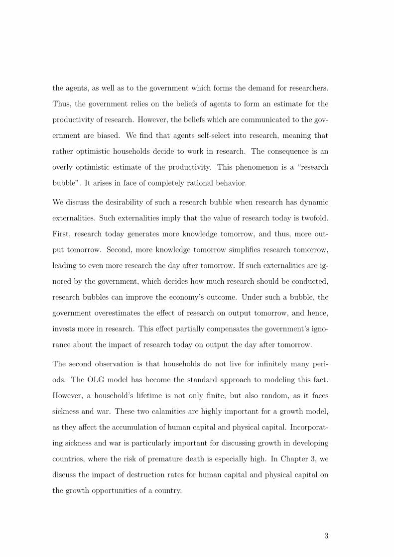
the agents, as well as to the government which forms the demand for researchers.
Thus, the government relies on the beliefs of agents to form an estimate for the
productivity of research. However, the beliefs which are communicated to the gov-
ernment are biased. We find that agents self-select into research, meaning that
rather optimistic households decide to work in research. The consequence is an
overly optimistic estimate of the productivity. This phenomenon is a “research
bubble”. It arises in face of completely rational behavior.
We discuss the desirability of such a research bubble when research has dynamic
externalities. Such externalities imply that the value of research today is twofold.
First, research today generates more knowledge tomorrow, and thus, more out-
put tomorrow. Second, more knowledge tomorrow simplifies research tomorrow,
leading to even more research the day after tomorrow. If such externalities are ig-
nored by the government, which decides how much research should be conducted,
research bubbles can improve the economy’s outcome. Under such a bubble, the
government overestimates the effect of research on output tomorrow, and hence,
invests more in research. This effect partially compensates the government’s igno-
rance about the impact of research today on output the day after tomorrow.
The second observation is that households do not live for infinitely many peri-
ods. The OLG model has become the standard approach to modeling this fact.
However, a household’s lifetime is not only finite, but also random, as it faces
sickness and war. These two calamities are highly important for a growth model,
as they affect the accumulation of human capital and physical capital. Incorporat-
ing sickness and war is particularly important for discussing growth in developing
countries, where the risk of premature death is especially high. In Chapter 3, we
discuss the impact of destruction rates for human capital and physical capital on
the growth opportunities of a country.
3

Chapter 1 Introduction
In an OLG model with three generations—children, young adults and the old—
output is produced through physical capital and human capital. Both are sup-
plied by young adults and children. While human capital is accumulated through
savings, human capital must be produced. Children are born with a fixed stock of
human capital which can be increased through schooling and their parents’ human
capital. Under such conditions, the untimely death of young adults has two neg-
ative implications. First, their human capital cannot be employed in production,
leading to less consumption for all generations. Second, they cannot contribute to
the education of their children. This effect has consequences that play out over
time, as less educated children will raise children that are even less educated, and
so on. In our model, we include social norms which govern how much each gener-
ation receives of total income, and consider altruism of parents to their children’s
education.
We find conditions for a path along which a country grows at a constant rate. This
is not guaranteed, in the economy that we model. Then, we show that a country
can find itself on one of two extreme paths. Along the first, it grows at a positive
rate—the state of progress. Along the second, it does not grow, but ends in what
we call a “poverty trap”. In such a poverty trap, investment is only able to offset
the destruction of capital, but not to accumulate capital. We also study whether
there are paths that lie between the extremes, and demonstrate that sufficiently
severe stochastic shocks can move an economy from the state of progress into a
poverty trap.
Third, agents in a specific country do not take their decisions in an economic
vacuum. Countries are integrated in the global economy, competing for scarce
resources. Over the last decades, we observe increasing inequality between coun-
tries. In addition, flows of capital from poorer to richer countries are triggered.
4

Such flows are called “uphill” capital flows, and we ask whether they can have
an impact on international inequality. Kose et al. (2009) suggest the following:
Inflows of capital do not impact the growth rate of a country directly. Instead,
they interact with other relevant factors of growth. In Chapter 4, we show how
the interaction of institutions, the accumulation of human capital, and the inflows
of capital can lead to long-term economic growth.
We model a world with two countries, with capital flowing between them. There
is no global financial market where countries can borrow as much as they want at
a constant rate. Instead, the rate of return is determined by the countries’ institu-
tions. The levels of institutions determine which country experiences inflows, and
which country experiences outflows of capital. If the change of institutions and
the inflow of capital increase the income of agents sufficiently, agents might begin
to invest in human capital. Hereby, human capital is the driving force of growth.
We find that a small initial difference in institutions can translate into substantial
differences in growth in the long-run. A country that extends its institutions can
find itself on a growth path with a positive rate, while another country remains
with the same output. We study conditions under which such a scenario occurs
and provide a simulation that reflects our theoretical findings.
Of course, many other issues are relevant in the context of economic growth, and it
is impossible to discuss them all in one thesis. However, we would like to mention
another phenomenon that emerged quite recently. This phenomenon is artificial
intelligence (AI). Its importance is drastically increasing, thanks partly to the
abundant data which is generated by social media. Hence, we study how AI can
contribute to economic growth. This question is particularly relevant, as economic
growth currently seems to slow down.
5

Chapter 1 Introduction
We review the literature on AI in Chapter 5.1. After providing the key insights
from existing studies, we shortly discuss possible avenues for future research.
6

Chapter 2
Research bubbles
Abstract
We develop a model to rationalize and examine so-called “research bubbles”, i.e.
research activities based on overoptimistic beliefs about the impact of this research
on the economy.1 Research bubbles occur when researchers self-select into research
activities and the government aggregates the assessment of active researchers on
the way advances in research may spur innovation and growth. In an overlapping
generations framework, we study the occurrence of research bubbles and show
that they tend to be welfare-improving. Particular forms can even implement the
socially optimal solution. However, research bubbles can collapse, and we discuss
institutional devices and the role of debt financing that ensure the sustainability
of such bubbles. Finally, we demonstrate that research bubbles emerge in various
extensions of our baseline model.
2.1 Introduction
Motivation
The world spends huge amounts of money on basic research and science in general.
1This chapter is joint work with Prof. Dr. Hans Gersbach.
7

Chapter 2 Research bubbles
In 2014, basic research accounted for nearly one-third (27.8 percent) of total R&D
expenditures in OECD countries (OECD (2016)), with total R&D equaling 2.4
percent of GDP. Basic research may lead to innovations that result in technological
progress and thus long-term material benefits. Historical examples are advances
in biology and medicine—from X-rays to DNA sequencing—and the introduction
of running water and sewer systems (see Gordon (2012) for many examples).
Nevertheless, the success of effort expended on basic research is highly uncertain,
and the value of research is often difficult to assess for the generation making the
investment. From 1991 to 1995, for example, only 12 percent of all university
patents were ready for commercial use once they were licensed, and whether man-
ufacturing would be feasible was known for only 8 percent (Jensen and Thursby
(2001)). Estimating the value of research is also difficult. HERG-OHE-Rand
(2008) find a return of 9 percent for medical research on physical health but state
that “[...] rates of return need to be treated with extreme caution. Most aspects
of the methods unavoidably involve considerable uncertainties.” Due to this un-
certainty, there are several examples where society has overestimated the value
of newly discovered technologies. Perez (2009) documents several examples of in-
vestment in new technologies, namely canal building in England, starting in 1771,
railway development in Great Britain, starting in 1829, and the establishment of
internet-related companies in the US, starting in 1971. With hindsight, these in-
stances displayed a concentration of investments, divorced from actual technology
needs in the real economy. Typically, these projects were fueled by great optimism
about potential real-world application. But, after an initial surge, investments
often slowed down or collapsed altogether.
There are also more recent examples of such occurrences, like the Apollo Pro-
gram (Gisler and Sornette (2009)) and the Human Genome Project (Gisler et al.
8
2.1 Introduction
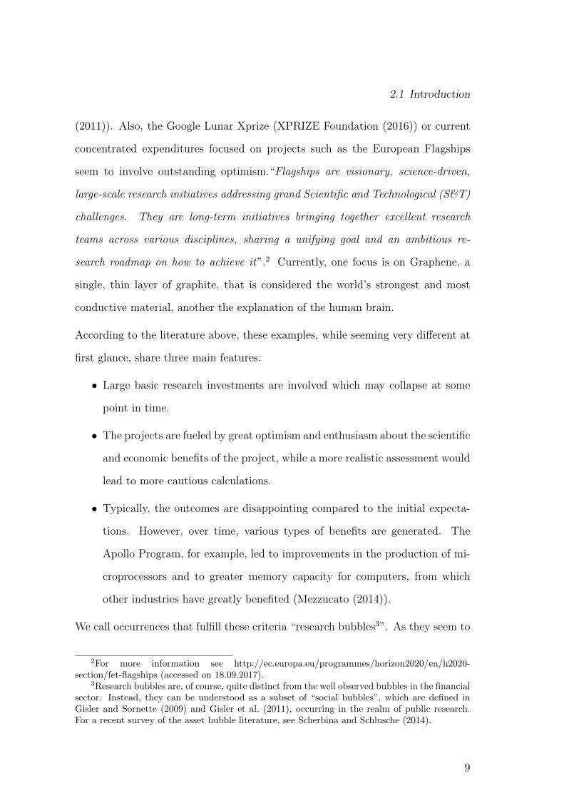
(2011)). Also, the Google Lunar Xprize (XPRIZE Foundation (2016)) or current
concentrated expenditures focused on projects such as the European Flagships
seem to involve outstanding optimism.“Flagships are visionary, science-driven,
large-scale research initiatives addressing grand Scientific and Technological (S&T)
challenges. They are long-term initiatives bringing together excellent research
teams across various disciplines, sharing a unifying goal and an ambitious re-
search roadmap on how to achieve it”.2 Currently, one focus is on Graphene, a
single, thin layer of graphite, that is considered the world’s strongest and most
conductive material, another the explanation of the human brain.
According to the literature above, these examples, while seeming very different at
first glance, share three main features:
• Large basic research investments are involved which may collapse at some
point in time.
• The projects are fueled by great optimism and enthusiasm about the scientific
and economic benefits of the project, while a more realistic assessment would
lead to more cautious calculations.
• Typically, the outcomes are disappointing compared to the initial expecta-
tions. However, over time, various types of benefits are generated. The
Apollo Program, for example, led to improvements in the production of mi-
croprocessors and to greater memory capacity for computers, from which
other industries have greatly benefited (Mezzucato (2014)).
We call occurrences that fulfill these criteria “research bubbles3”. As they seem to
2For more information see http://ec.europa.eu/programmes/horizon2020/en/h2020-section/fet-flagships (accessed on 18.09.2017).
3Research bubbles are, of course, quite distinct from the well observed bubbles in the financialsector. Instead, they can be understood as a subset of “social bubbles”, which are defined inGisler and Sornette (2009) and Gisler et al. (2011), occurring in the realm of public research.For a recent survey of the asset bubble literature, see Scherbina and Schlusche (2014).
9

Chapter 2 Research bubbles
be a pervasive feature in the discovery of knowledge, questions about the causes
and the desirability of such bubbles arise. This is the focus of this chapter.
One might suggest that such bubbles are the result of mere irrationality and since
agents overinvest, can only be detrimental to welfare. However, we suggest that
research bubbles are generated by the self-selection of researchers into research ac-
tivities and result from rational decisions on the part of governments as to whether
to embark on such adventures on the basis of the assessments by the researchers
involved.4 Moreover, while such bubbles may lead to disappointment and may
not benefit the current generation, they tend to be desirable from a long-term
perspective, taking the welfare of future generations into account. However, they
may also be excessive, even from a long-run perspective.
In classic innovation-driven growth theory and its extensions, research bubbles
do not figure at all (Aghion and Howitt (1992), Grossman and Helpman (1991),
Romer (1990)). Cozzi (2007) is an exception, presenting a model that allows
for self-fulfilling prophecies. In our model, research bubbles are not the result of
multiple equilibria, but arise from the government’s aggregation of heterogeneous
assessment by researchers who self-select into research activities. A related study
is Olivier (2000) where financial bubbles increase firms’ value and enables them
to attract more researchers. A positive effect on growth is the result. However,
we focus on instances when the allocation of researchers is the cause of a research
bubble, and not the consequence of a financial bubble.
Approach and results
More specifically, we develop a framework that rationalizes research bubbles in an
4The optimism bias in our study, which will be substantiated in the following sections isan aggregate phenomenon. Our definition differs from the standard explanation in psychologyand behavioral economics, where individuals overestimate the likelihood of positive events andunderestimate the likelihood of negative ones.
10
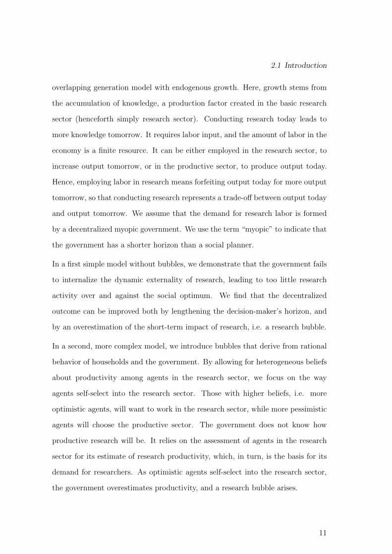
2.1 Introduction
overlapping generation model with endogenous growth. Here, growth stems from
the accumulation of knowledge, a production factor created in the basic research
sector (henceforth simply research sector). Conducting research today leads to
more knowledge tomorrow. It requires labor input, and the amount of labor in the
economy is a finite resource. It can be either employed in the research sector, to
increase output tomorrow, or in the productive sector, to produce output today.
Hence, employing labor in research means forfeiting output today for more output
tomorrow, so that conducting research represents a trade-off between output today
and output tomorrow. We assume that the demand for research labor is formed
by a decentralized myopic government. We use the term “myopic” to indicate that
the government has a shorter horizon than a social planner.
In a first simple model without bubbles, we demonstrate that the government fails
to internalize the dynamic externality of research, leading to too little research
activity over and against the social optimum. We find that the decentralized
outcome can be improved both by lengthening the decision-maker’s horizon, and
by an overestimation of the short-term impact of research, i.e. a research bubble.
In a second, more complex model, we introduce bubbles that derive from rational
behavior of households and the government. By allowing for heterogeneous beliefs
about productivity among agents in the research sector, we focus on the way
agents self-select into the research sector. Those with higher beliefs, i.e. more
optimistic agents, will want to work in the research sector, while more pessimistic
agents will choose the productive sector. The government does not know how
productive research will be. It relies on the assessment of agents in the research
sector for its estimate of research productivity, which, in turn, is the basis for its
demand for researchers. As optimistic agents self-select into the research sector,
the government overestimates productivity, and a research bubble arises.
11
Chapter 2 Research bubbles
When governments form average assessments of the technology potential from
research by listening to researchers, the emerging research bubble will typically fail
to reach the socially optimal level of research investments. But other aggregation
methods can produce research bubbles that generate socially optimal research
activities.
We further examine how research bubbles may burst and how such collapses can
be avoided through institutional remedies such as establishing constitutional rules
or giving optimistic researchers a big say in basic research investment. An alter-
native route is debt financing, where the amount of debt that the government can
borrow on international capital markets depends on the amount of research con-
ducted in the economy. Finally, we recast the occurrence of research bubbles in
variant models in which research success also depends on research effort decisions.
Models with alternative welfare functions of the government are also discussed.
Structure
The rest of the chapter is organized as follows: In the next section, we introduce
the baseline model describing our research economy. Section 2.3 presents the same
model, this time with research bubbles, and Section 2.4 studies the implemen-
tation of the social optimum in a decentralized economy. Section 2.5 discusses
the potential and the drawbacks of the decentralized solution. In Section 2.6, we
present possible extensions of the model. Section 2.7 concludes.
2.2 A research economy
Let us turn first to our baseline model without research bubbles. We use an OLG
model where endogenous growth results from an increasing stock of knowledge.
12

2.2 A research economy
Knowledge is created by basic research and research is conducted in the public
research sector, which competes with the production sector for skilled labor.
2.2.1 Households
Households live for two periods and at any point in time, two generations coexist.
An agent is labeled “young” in the first period and “old” in the second period.
Each generation is represented by a single household and possesses one unit of
time supplied inelastically in the market for labor. Hence, total labor endowment
L is normalized to 1. There is one physical commodity that can be either used
for consumption or as capital for production, while capital is fully depreciated in
each period. Consumption is the only source of utility. The life-time utility of a
household born in period t is
Ut = log(c1t)
+ β log(c2t+1
), (2.1)
where c1t denotes consumption of the physical good in the first period, c2t+1 in
the second, and the parameter β stands for the discount factor, with 0 < β <
1. When young, the agent makes decisions on saving and on how much time
to allocate to work in the research sector, and/or the productive sector. When
old, the household only consumes its savings. The variables LS,Rt and LS,Pt stand
for the time the agent supplies to the research sector and the productive sector,
respectively. Furthermore, st stands for savings, wPt for the wage in the productive
sector, wRt for the wage in the research sector, and rt+1 for the gross interest rate.
We assume that in order to finance research, wage income in the productive sector
is taxed at rate τt . Hence, when young and old, consumption for an agent born
13

Chapter 2 Research bubbles
in t are
c1t = wRt LS,Rt + (1− τt)wPt LS,Pt − st, (2.2)
c2t+1 = strt+1, and (2.3)
LS,Rt + LS,Pt = 1. (2.4)
We plug in these definitions and maximize utility with respect to LS,Rt and st to
obtain
LS,Pt =
0, if wRt > wPt (1− τt),
arbitrary, if wRt = wPt (1− τt),
1, if wRt < wPt (1− τt),
and
st =β
1 + β
(wRt L
S,Rt + (1− τt)wPt
(1− LS,Rt
)).
Throughout the chapter, we focus on constellations in which both sectors are
active, which in this section requires that wRt = wPt (1− τt). We denote this wage
by wt and obtain that savings are a constant share of income due to logarithmic
utility.
The tax rate balances the budget and fulfills the following condition:
wRt LRt = τtw
Pt (1− LRt ),
where LRt is the eventual market equilibrium. Hence, by the required equality of
14
2.2 A research economy
net wages, we have
(1− τt)wPt LRt = τtwPt (1− LRt )⇒ τt = LRt , (2.5)
implying that the tax rate on wage income from productive activity is equal to the
share of labor in the research sector.
2.2.2 Productive sector
A single firm produces output using knowledge Bt, capital Kt and labor LD,Pt , with
D,P indicating demand in the productive sector. The production function takes
the form
Yt = (LD,Pt Bt)1−αKα
t .
Labor is supplied by the young household, knowledge is created in the research
sector, as is described below, and capital is created from the household’s savings.
As capital depreciates fully within one generation, st = Kt+1 is the equilibrium
condition. Also, this implies that rt+1 is the net and gross interest rate. Knowledge
will be useful in production,5 and while the output of basic research can be used free
of charge, the other two production factors are rented by the firm and compensated
by wage wPt and interest rate rt. Hence, the profit of the firm reads
Πt = Yt − wPt LD,Pt − rtKt.
5Since basic research output is of no immediate commercial use, there is typically time lagbetween basic research and its use in production. Estimates of this time lag range between 6and 20 years on average (see Adams (1990)).
15

Chapter 2 Research bubbles
The firm takes all prices as given, so that optimal behavior is described by the
standard demand functions. Since both labor and capital are supplied inelastically,
we obtain the standard equilibrium condition for wages and the interest rate:
wPt = (1− α)Yt
LD,Pt
and rt = αYtKt
.
2.2.3 Research sector
We assume that the research sector is run by a government. It employs labor LD,Rt
to create new knowledge on the basis of the existing knowledge stock. From the
government’s perspective, the knowledge production function is
Bt+1 = (1 + θ · LD,Rt )Bt.
The function depends on labor demand in research LD,Rt and on the productivity
parameter θ.
Conducting research inhibits a fundamental trade-off: Increasing knowledge and
output tomorrow means forfeiting output today, as labor has to be reallocated
from the productive sector to the research sector. Thus, it is the government’s
task to decide how much labor should be employed in the research sector.
The economy allows for balanced growth paths. A steady state is characterized
by Proposition 1.
Proposition 1 A steady state of the economy for a given constant share of labor
invested in research in each period LR is uniquely characterized by a constant labor
input LP in the productive sector and a constant return to capital r. Consumption
of young and old agents, c1t and c2t , output Yt, capital Kt and the knowledge stock
Bt all grow at a constant rate g = θLR.
16
2.2 A research economy
The proof of Proposition 1 can be found in the Appendix for Chapter 2.
2.2.4 Decentralized solution
First, we look at a planner who is only concerned with the current generation. He
has preferences over output today and discounted output tomorrow, where both
depend on labor input in research. We call this the “government solution”
maxLD,Rt
log(Yt) + β log(Yt+1), or
maxLD,Rt
log(
((1− LD,Rt )Bt)1−αKα
t
)+ β log
(((1− LD,Rt+1 )Bt+1)
1−αKαt+1
),
where we assume that the government has the same logarithmic utility function
and discount factor β as the household. Maximizing with respect to LD,Rt yields
1
1− LD,Rt
=βθ
1 + θLD,Rt
for 0 ≤ LD,Rt < 1. (2.6)
The left hand side of (2.6) is the marginal product of labor and reflects the marginal
cost of one more unit of labor in research. The right hand side is the discounted
marginal product of research today on output tomorrow via an increase in the
knowledge stock.
Expression (2.6) only contains the contemporary value of LD,Rt but not LD,Rt+1 , so
that the government’s solution is static and takes the form
LD,R =1
1 + β
(β − 1
θ
)∀t, (2.7)
where LD,R only depends on the parameters β and θ. A condition for research to
occur in the decentralized economy is LD,R > 0↔ β > 1/θ. As we have assumed
17

Chapter 2 Research bubbles
that β is smaller than 1, the condition can be reduced to θ > 1. A more impatient
government with a lower discount factor β will invest less in research.
We can be certain that we have found a utility maximum, as the second derivative
of the objective function is simply
−(1− LD,Rt )−2 − βθ2(1 + θLD,Rt )−2 < 0 ∀LD,Rt ∈ (0, 1).
The static nature of the government’s solution results from two structural as-
sumptions: Logarithmic utility and a Cobb-Douglas production function. The
logarithmic utility causes Yt and Yt+1 to appear in the denominator of the deriva-
tive, and the production function causes them to appear in the numerator, so that
they cancel out.
To ensure that the household supplies the demanded share of labor, the government
sets the wage in the research sector
wRt = (1− τt)(1− α)Yt1− LRt
= (1− τt)wPt = wt, (2.8)
in each period. By doing this, the government can implement its demand as an
equilibrium, so that LD,R stands for the equilibrium value of labor in research LR.
Definition 1 We define an equilibrium of the economy as the paths of wt, rt, Yt, Kt
and Bt, given a sequence {LRt }∞t=0 that fulfill the following conditions: The house-
hold maximizes utility, the firm maximizes profits, the government maximizes its
own utility, and the market for capital clears as do the good and the labor market,
i.e. Equation (2.8) holds.
18
2.2 A research economy
2.2.5 Social planner solution
Next we turn to the social optimum for the economy. The maximization problem
of the social planner reads
max{c1t ,c2t+1,L
Rt ,Bt+1,Kt+1}∞t=0
W =∞∑
t=0
βts(log(c1t ) + β log(c2t+1)
)
s.t. ((1− LRt )Bt)1−αKα
t = c1t + c2t +Kt+1,
Bt+1 = (1 + θLRt )Bt,
where βs ∈ (0, 1) is the social planner’s discount factor and W denotes social
welfare. We define λt as the Lagrange Multiplier on the budget constraint and µt
as the multiplier on the knowledge-production function, and obtain the following
first order conditions:
∂L∂c1t
= βts
(1
c1t+ λt
)= 0,
∂L∂c2t+1,
= βts
(β
c2t+1
+ βsλt+1
)= 0,
∂L∂Kt+1
= λt − βsλt+1αYt+1
Kt+1
= 0,
∂L∂LRt
= λt(1− α)Yt
1− LRt+ µtθBt = 0,
∂L∂Bt+1
= −µt + βs(−λt+1(1− α)Yt+1
Bt+1
+ µt+1(1 + θLRt+1)) = 0,
where L is the Lagrange Function. The first three conditions are common, but the
last two deserve attention. To understand them, we interpret λt as the change in
the life-time utility of an agent born in t if one more unit of output Yt were available.
Analogously, we see µt as the change in the life-time utility of such an agent if one
more unit of knowledge Bt+1 were available tomorrow. With this, the derivative
with respect to LRt implies that the marginal loss from allocating one more unit of
19

Chapter 2 Research bubbles
labor to research, which is λt times the marginal product of labor, must be equal
to the benefit which results from having θBt more units of knowledge tomorrow.
In the derivative of the Lagrange Function with respect to Bt+1, µt stands for the
welfare loss associated with creating one more unit of Bt+1. The loss is equal to
the discounted sum of two different benefits. First, more knowledge tomorrow will
increase production by the marginal product (1 − α)Yt+1/Bt+1. Second, having
more knowledge tomorrow will reduce the necessity to conduct research tomorrow
and hence yields the benefit µt+1(1 + θLRt+1).
From the five first-order conditions we obtain two dynamic equations. The first is
the common Euler equation, and the second describes the dynamic allocation of
labor in research:
1
c1t=
βsαYt+1
Kt+1c2t+1
and (2.9)
Yt1− LRt
=Kt+1
αYt+1
(θYt+1
1 + θLRt+
Yt+1
1− LRt+1
1 + θLRt+1
1 + θLRt
). (2.10)
Together with the budget-constraint and the knowledge-production function, they
describe the model. If we assume βs = β, we obtain the following steady state
condition:
1
1− LR = β
(θ
1 + θLR+
1
1− LR)
and thus
LR = LO,R = β − 1− βθ
. (2.11)
For the derivation of the equation, see the Appendix for Chapter 2. We denote
the steady state value of labor input in research by LO,R and compare it to the
government’s demand for research LD,R = 11+β
(β − 1
θ
). We find three differences.
First, when θ goes to infinity, the social optimum converges to β in the limit, while
20
2.2 A research economy
the government solution converges to β/(1 + β) < β. Second, when θ increases,
the social planner will increase his demand less than the government:
∂LO,R
∂θ=
1− βθ2
<1
(1 + β)θ2=∂LD,R
∂θ,
which holds if and only if
(1−β)(1 +β) < 1⇔ β2 > 0. Third, the social planner always employs more labor
in research than the government:
LO,R = β − 1− βθ
>1
1 + β
(β − 1
θ
)= LD,R and thus 0 < β2(θ + 1),
which holds because we are assuming that β, θ > 0.
To explain this result, we compare (2.6) and (2.10). We rewrite (2.10) as
1
1− LRt=
Kt+1
αYt+1
Yt+1
Yt
(θ
1 + θLRt+
1 + θLRt+1
(1− LRt+1)(1 + θLRt )
)
and observe that the government and the social planner discount different bene-
fits, using different discount factors. The government only takes into consideration
the immediate benefit from research that arises in the next period and uses the
constant β to discount it. The social planner internalizes the additional intergen-
erational effects and uses Kt+1
αYt+1
Yt+1
Ytto scale the benefits occurring in the future.
Note that this factor is the product of two components: first, the inverse of the
marginal product of capital, which under complete depreciation is the economy’s
discount factor, and second, 1 plus the growth rate of output.
The social planner’s awareness of the long-term benefits of research explains why
the socially optimal steady state can be greater than the decentralized solution.
It also explains why the social planner solution is less sensitive to changes in θ.
21
Chapter 2 Research bubbles
The government only enjoys the benefits of a higher θ and increased productivity
in the next period. To capitalize on the increased productivity, the government
strongly raises labor input in research. The social planner, by contrast, is aware
that the benefits of a higher θ extend beyond the next period. Therefore he has
smaller incentives to increase labor input today
We prove that the difference between the social planner and the government solu-
tion arise only because of two differing decision horizons. For this, we show that
the government solution converges to the socially optimal solution with a rising
decision horizon. A government that is aware that research today has an impact
on all future generations faces the following problem of maximizing the sum of
all future output over investment today: maxLD,Rt
∑∞s=t β
s−t log(Ys), which due to
logarithmic utility can simply be written as
maxLD,Rt
log(1− LD,Rt ) +∞∑
s=t+1
βs−t log(1 + θLD,Rt ) or
maxLD,Rt
log(1− LD,Rt ) +β
1− β log(1 + θLD,Rt ),
which yields
(1 + θLD,Rt )(1− β) = βθ(1− LD,Rt ) and thus LD,R = β − 1− βθ
.
This expression precisely yields the social optimum. Thus, we obtain the following
proposition:
Proposition 2
For the decentralized government and the social planner, the steady state levels of
labor in research are given by (2.7) and (2.11). The social optimum implies more
research than the decentralized solution and has a higher upper bound but is less
22

2.2 A research economy
sensitive to changes in productivity.
2.2.6 Implementing the socially optimal solution via
research bubbles
The preceding analysis reveals that decentralized basic research investments can
yield lower social welfare. We note that a more optimistic government view, i.e.
the assumption that θ is higher than it actually is, would increase welfare. How-
ever, it would do so at the expense of generation t’s utility. In addition, if all
governments had a more optimistic view, i.e. if their assumption, θ, is greater
than the true value of θ, social welfare would be higher at the expense of the first
few generations. In particular, if the first generations could finance part of their
research expenditures by issuing debt, a combination of research bubbles and pub-
lic debt could implement the socially optimal solution and make everybody better
off compared to the decentralized solution. We define the following:
Definition 2 The economy exhibits a research bubble in a particular time frame
(0, T ] for some T ∈ R if the governments assume θ > θ when they decide on
investment in basic research.
In the following, we show that sufficient optimism in the decentralized economy
can implement the social optimum. Assume that the government does not know
the true value of θ but beliefs θ to be the true productivity. To achieve the socially
optimal outcome, this θ must fulfill
β − 1− βθ
=1
1 + β
(β − 1
θ
)and thus θ =
θ
1− β2(1 + θ). (2.12)
The implementation of the social optimum hinges on the relation between β and θ.
23
Chapter 2 Research bubbles
If 1/β2−1 > θ, then implementation is possible, otherwise it is not. This restriction
arises, because the decentralized solution has a lower upper bound than the social
planner solution, i.e. β1+β
< β.
Proposition 3 If there is optimism in the decentralized economy and the govern-
ment beliefs θ, given by (2.12), to be the true productivity, the economy will achieve
the social optimum if 1/β2 − 1 > θ.
In the next section, we derive a microfoundation for optimistic beliefs and sug-
gest that they are a natural outcome of decisions on basic research. Moreover,
we suggest an institutional arrangement that can implement the socially optimal
solution.
2.3 Research with heterogeneous beliefs
We next explore whether research bubbles arise naturally in scenarios where the
government does not know the true parameter θ. Also, we ask whether there are
institutional arrangements that support welfare-enhancing research bubbles.
We substitute the single household in each generation by a continuum of infinitely
many households of measure 1. A subset of these agents holds beliefs about the
parameter θ. The beliefs are heterogeneous and the government has to make an
estimate for θ based on the given beliefs.
2.3.1 Households
The economy is populated by infinitely many agents represented by the interval
[0, 1] and of mass 1. All agents possess one unit of time. Hence, the overall labor
endowment in the economy is 1, as before. A share LB of all agents is able to work
24

2.3 Research with heterogeneous beliefs
in the research sector and these agents hold beliefs about θ. The set of agents
with the capacity to work in the research sector is LB. We denote agent i ∈ LB’s
belief about θ as θi and allow it to lie in [θl, θh], with θl < θ < θh. Belief types are
uniformly distributed in [θl, θh], with density 1θh−θl , where the latter follows from
the assumption that households have mass 1.
The belief determines the sector in which an agent will want to work. If an agent
works in the productive sector, he earns a wage and consumes. If the agent works
in the research sector, additional considerations matter, since research has a strong
non-pecuniary utility component. We assume that a researcher derives utility from
research achievements and thus from knowledge creation, e.g. through intrinsic
means—satisfaction about achievements— or extrinsic means—such as status and
prestige. More specifically, utility derived from research depends on how efficient
the agent beliefs his research to be, θi, so that the utility function of a scientist
reads
URt,i = log(wRt − sRt,i) + (1 + β) log(1− θl + θi) + β log(rt+1s
Rt,i),
with i ∈ LB,
where we calibrate utility in such a way that the least optimistic agent, i.e. the
one who holds the belief θi = θl, receives no additional utility from working in
research. With this calibration we ensure that no agents receive negative utility
from working in research and hence require compensation. Also, we scale this
utility by 1 +β, as this simplifies later derivations. The utility of a worker is given
by
UPt,i = log((1− τt)wPt − sPt,i) + β log(rt+1s
Pt,i).
25

Chapter 2 Research bubbles
Since an individual has no impact on prices and aggregate variables, an agent takes
rt+1 as given and maximizes utility with respect to savings st,i. The solutions of
the worker problem the researcher problem are given by the expressions
sPt,i =β(1− τt)wPt
1 + βand sRt,i =
βwRt1 + β
. (2.13)
Plugging these results back into the utility function, we obtain
URt,i = log
(wRt
1 + β
)+ (1 + β) log(1− θl + θi) + β log
(βrt+1w
Rt
1 + β
)and
UPt,i = log
((1− τt)wPt
1 + β
)+ β log
(βrt+1(1− τt)wPt
1 + β
).
Setting both utilities equal yields Proposition 4.
Proposition 4
The critical value for researcher i’s belief is
θcrit,t =(1− τt)wPt
wRt− (1− θl). (2.14)
Hence, every household with a belief θi above this value θcrit,t will choose to work
in the research sector. Every household with a belief below θcrit,t will choose the
productive sector. The agent with θi = θcrit,t is indifferent and, by assumption, will
choose the research sector.6
We find that the critical belief is a linear function of the wage ratio. The greater
the wage in the productive sector, the greater an agent’s belief must be for him
to choose the research sector. Given some wage ratio, an agent will choose the
research sector if his belief θi lies between θcrit,t and θh, so that labor supply is
6For a more detailed derivation, see the Appendix for Chapter 2.
26
2.3 Research with heterogeneous beliefs
given by
LS,Rt = LBθh − θcrit,tθh − θl
, (2.15)
i.e. the product of the share of agents able to work in the research sector LB and
those who choose to do soθh−θcrit,tθh−θl .
2.3.2 Assessment of research productivity
Unlike before, the government does not know the parameter θ and has to form
an estimate. Hereby, the researchers’ beliefs are the only available source of in-
formation, and we assume that researchers truthfully signal their belief to the
government. Equipped with this set of beliefs, the government then makes the
following estimate:
θt = ηθh + (1− η)θcrit,t. (2.16)
The parameter η (0 < η < 1) is the weight that the government places on the most
optimistic researcher belief, and 1− η is the weight placed on the most pessimistic
counterpart. At this stage we do not specify how η is eventually determined. In
Section 5.3 we explore different institutional arrangements leading to particular
values of η.
Two remarks are in order. First, the expressed range of beliefs [θcrit,t, θh] is it-
self more optimistic than the range of beliefs [θl, θh] in the entire population of
researchers.
Second, at this stage we assume that researchers reveal their true beliefs to the gov-
ernment. In section 5.2 we discuss whether researchers do indeed have incentives
27
Chapter 2 Research bubbles
to reveal their true beliefs.
2.3.3 The government’s problem
The government relies on the following estimated production function to derive
research labor demand:
Bt+1 = (1 + θt · LD,Rt )Bt.
This demand differs from the previous one in two ways. First, it indicates the
amount of knowledge that the government believes to be available tomorrow, Bt+1.
Second, the parameter θ is replaced by the government’s estimate θt. To ease
notational complexity, LD,Rt again stands for the government’s demand for research
labor, but now for the case with heterogeneous beliefs. The maximization problem
for the government now reads
maxLD,Rt
log(
((1− LD,Rt )Bt)1−αKα
t
)+ β log
(((1− LD,Rt+1 )Bt(1 + θtL
D,Rt ))1−αKα
t+1
).
Maximizing with respect to LD,Rt yields
1
1− LD,Rt
=βθt
1 + θtLD,Rt
, with (2.17)
θt given by (2.16).
Equation (2.17) is analogous to Equation (2.6), but θ is now replaced by the
estimate θt. However, Equation (2.17) alone does not enable us to determine
LRt . It depends on θt, which in turn, depends on the labor supply to the research
sector. As labor is no longer supplied inelastically, it is necessary to determine labor
demand and supply for research labor simultaneously. We do this by examining
28

2.3 Research with heterogeneous beliefs
the labor market equilibrium in the next subsection.
2.3.4 Labor market equilibrium
To determine the labor market equilibrium, we solve (2.17) for LD,Rt
LD,Rt =1
1 + β
(β − 1
θt
). (2.18)
Using Definition (2.16) with η = 1/2 yields
LD,Rt =1
1 + β
(β − 2
(θh + θcrit,t)
).
Note that unlike before, LD,Rt is not a fixed value but a strictly concave function
of the variable θcrit,t. So is the labor supply from Equation (2.15). Thus, we have
two equations, labor supply and demand in two variables, research labor LRt , and
the critical belief θcrit,t. This means that labor demand and the critical belief are
interdependent. Labor supply depends on θcrit,t because every agent with a belief
higher than θcrit,t supplies his labor to the research sector. Hence, the supply
falls linearly with the critical value. Labor demand depends on θcrit,t because the
critical belief determines θt. Demand is an increasing function in θcrit,t: The more
optimistic the statement by researchers about the productivity of research, the
greater is, of course, the government’s demand.
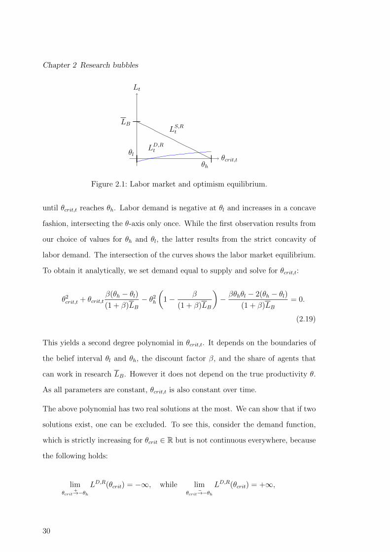
In Figure 2.1 we plot supply and demand as functions of θcrit,t for the purpose of
illustration with the values β = 0.85, θh = 2 and θl = 1. Labor supply by house-
holds is shown by the linear falling function and labor demand of the government
by the increasing one. Labor supply reaches its maximal value of LB when the
critical belief takes the smallest possible value. The supply decreases smoothly
29
Chapter 2 Research bubbles
θcrit,t
Lt
LS,Rt
LD,Rt
LB
θl
θh
Figure 2.1: Labor market and optimism equilibrium.
until θcrit,t reaches θh. Labor demand is negative at θl and increases in a concave
fashion, intersecting the θ-axis only once. While the first observation results from
our choice of values for θh and θl, the latter results from the strict concavity of
labor demand. The intersection of the curves shows the labor market equilibrium.
To obtain it analytically, we set demand equal to supply and solve for θcrit,t:
θ2crit,t + θcrit,tβ(θh − θl)(1 + β)LB
− θ2h(
1− β
(1 + β)LB
)− βθhθl − 2(θh − θl)
(1 + β)LB= 0.
(2.19)
This yields a second degree polynomial in θcrit,t. It depends on the boundaries of
the belief interval θl and θh, the discount factor β, and the share of agents that
can work in research LB. However it does not depend on the true productivity θ.
As all parameters are constant, θcrit,t is also constant over time.
The above polynomial has two real solutions at the most. We can show that if two
solutions exist, one can be excluded. To see this, consider the demand function,
which is strictly increasing for θcrit ∈ R but is not continuous everywhere, because
the following holds:
limθcrit
+→−θhLD,R(θcrit) = −∞, while lim
θcrit−→−θh
LD,R(θcrit) = +∞,
30

2.3 Research with heterogeneous beliefs
i.e. the limits to θcrit = −θh from left and right are not identical. Given that
demand is a strictly increasing function, we can conclude that the function becomes
infinitely large on the left of −θh, while it falls to −∞ on the right of it and then
increases with θcrit. This explains how two intersections are possible. One of them
has to lie to the left of −θh and is thus irrelevant.
With fixed LD,Rt , wPt is given and the government needs to set wRt according to
(2.14). By setting the wage in the research sector correctly, the government can
implement its demand as the market equilibrium so that, as before, LD,R = LR,H ,
where LR,H is the equilibrium value in the market for research labor in the steady
state. The superscript H stands for “heterogeneous beliefs”.
The economy reaches the described equilibrium in the following way: First, the
government hires a number of researchers and obtains the estimate θt. The ex-
pected productivity determines the government’s optimal labor demand. If the
optimal demand turns out to be greater, the government increases wRt , and hence
labor supply, to lower θcrit. By doing so, it hires additional, less optimistic agents
and obtains, in turn, a lower average for θ. This adjustment of labor demand
continues until the government hires exactly as many researchers as are justified
by their aggregated belief.
In this economy, the tax rate τt differs from the previous one, as wPt and wRt are
related by (2.14) and not simply (1 − τt)wPt = wRt . From labor supply, we know
that any market equilibrium LR,H implies the following critical belief:
θcrit = θh −(θh − θl)LR,H
LB.
31

Chapter 2 Research bubbles
Substituting this expression into (2.14) yields
θh −(θh − θl)LR,H
LB=
(1− τt)wPtwRt
− (1− θl),
or equivalently
wRt =(1− τt)wPt
1 + (θh − θl)(1− LR,H
LB). (2.20)
We find that, unlike before, researchers are now paid at a markdown. This follows,
of course, from the fact that researchers have their belief as an additional source
of utility and thus require less compensation for working in the research sector.
Additionally, we can see that market mechanisms determine this markdown. A
greater demand for research, expressed by bigger LR,H , will lower the markdown,
while a greater overall supply of researchers, expressed by a bigger LB, will increase
it. Hence, the tax rate now reads
τt =LR,H
1 + (θh − θl)(
1− LR,H
LB
)(1− LR,H)
,
which is obtained by substituting (2.20) into the government’s budget constraint,
LR,HwRt = τt(1− LR,H)wPt .
32

2.3 Research with heterogeneous beliefs
2.3.5 Social planner solution
To derive the social planner optimum for this economy, one would have to include
the following term in the previous welfare function W :
∞∑
t=0
βts
∫ θh
θcrit,t
log(1− θl + θi)di, with
θcrit,t = θh −(θh − θl)LRt
LB,
which captures the additional utility for those working in research. Note that θl <
θcrit,t, so that the integral is finite. If, however, the social planner communicates
the true parameter θ and it replaces the individual belief θi, then the integral is
zero and the problem collapses to the one studied above.
Next, we compare the socially optimal outcome to the decentralized outcomes in
economies with and without research bubbles. Table 2.1 provides the parameter
values that we use.
α β θ LB θl θh0.3 0.85 1.5 1 1 2
Table 2.1: Parameter values.
We derive research labor for the social planner, LO,R and the government, LR,H
under a research bubble, and the equilibrium without research bubbles, LR.
LR LR,H LO,R
0.0991 0.1767 0.75
Table 2.2: Labor input in research for the social planner and government.
Table 2.2 provides our findings, which we can summarize in one inequality: LR <
LR,H < LO,R. We find the following: First, there is a research bubble in the
decentralized economy, as can be seen in the first inequality. Although the true
33

Chapter 2 Research bubbles
productivity of research θ has remained the same, we find more labor dedicated
to knowledge production. Second, the research bubble moves the decentralized
amount of investment closer to the socially optimal one: We observe an increase
of roughly 8 percentage points, when comparing the two outcomes. Third, even
in the presence of a research bubble, the decentralized economy remains below
the optimal outcome, as can be seen in the second inequality. We summarize our
findings in Proposition 5.
Proposition 5
The steady state levels of the critical belief value θcrit and of research labor LR,H
in the decentralized economy are given by Equations (2.15), (2.18), and Equation
(2.19). Research labor LO,R in the social optimum is given by Equation (2.11) .
We observe a welfare-improving research bubble.
Several remarks are in order. The government is optimistic since θcrit,t > θl. Thus
its estimateθh+θcrit,t
2is higher than the true productivity. As described above, this
over-optimism and the ensuing research bubble are generated by two mechanisms,
self-selection of researchers and information aggregation by the government. By
self-selection we mean that agents decide themselves which sector they want to
work in. More optimistic agents are willing to work in research even if wRt is
small. Only with greater wRt does labor demand increase thus also attracting
less optimistic researchers . Consequently, researchers are hired, beginning at the
higher end of the belief distribution. The least optimistic ones are not hired, as
employing all agents in research is prohibitively costly. By information aggregation
we mean that the government forms an estimate about θ based only on the beliefs
of the agents hired. Hence, the estimate of the government does not yield the true
productivity and it demands more research than in the previous model. This is a
research bubble.
34

2.4 Implementing the socially optimal solution
If the government asked all agents about their respective beliefs, its estimate would
be exactly θ, as with θl = 1 and θh = 2, we have θ = 1.5 = θ. Yet the government
receives information from a non-representative sample of the population, as only
agents with θi ≥ θcrit work in research.
One can imagine the government as an econometrician tries to measure θ. It
faces random differences in the parameter because of the random distribution of
beliefs. Although the government’s methods are sophisticated, it overestimates
the parameter, because it does not take the self-selection bias into account.
2.4 Implementing the socially optimal solution
In this section, we explore how the socially optimal solution can be implemented
by the decentralized solution in the steady state.
First we focus on whether and how the decentralized solution can implement the
socially optimal solution through research bubbles. If the true productivity in the
economy is θ, then Equation (2.12) shows us the necessary size of the research
bubble. The equation also provides a necessary condition for the implementation
of the social optimum, given by 1/β2 − 1 > θ. It continues to hold. However, it is
not a sufficient condition, as θ = ηθh + (1− η)θcrit. Hence, we have
ηθh + (1− η)θcrit =θ
1− β2(1 + θ),
which implies that
θcrit =1
1− η
[1
1− β2(1 + θ)− ηθh
]and thus θ >
θh(1− β2)− 1
β2θh(2.21)
must hold for implementation. Expression (2.21) provides the sufficient condition
35
Chapter 2 Research bubbles
for a positive value of θcrit. Also, it yields the value θcrit which is the critical belief
that is socially optimal. This yields the following proposition:
Proposition 6 An optimistic view of the government θ = ηθh + (1 − η)θcrit can
implement the social optimum if 1/β2 − 1 > θ and Expression (2.21) are satisfied.
Note that the equilibrium θcrit of the decentralized economy does not have to
coincide with θcrit, even if the inequality from Expression (2.21) is fulfilled. The
mere possibility of implementation does not mean that the economy’s research
bubble will have precisely the optimal size. If θcrit < θcrit the economy’s research
bubble will be too large. In the opposite case it will be too small.
As a numerical example, consider the parameter values from Table 2.1 and the fact
that the government forms an average of the researchers’ beliefs, i.e. η = 1/2. In
this case implementation is not possible, as 1/β2− 1 > θ does not hold. However,
if we consider the following set of parameter values: θ = 0.3, θh = 4, β = 0.8, and
η = 0.5, we find that the necessary and sufficient conditions for implementation
are met. Under these parameter values we obtain θcrit = 1.9524.
However, if the government forms biased estimates of active researchers’ beliefs,
the socially optimal steady state can be implemented as a decentralized balanced
growth path, as we show next. For this purpose we consider the steady state
solution given in Equation (2.11).
Proposition 7 If LD,R(η = 12) < LO,R < β
1+β, i.e. if the social planner solution
lies between the government’s demand for research labor with η = 12
and the gov-
ernment’s maximal demand, β1+β
, there exists an η∗ > 12
and an associated research
bubble such that the decentralized solution can implement the social optimum. If
LO,R < LD,R(η = 12) < β
1+β, there exists an η∗ < 1
2that implements the social
optimum.
36

2.4 Implementing the socially optimal solution
We stress that the existence of such an η∗ hinges on the aforementioned condition.
If LO,R > β1+β
, no amount of optimism will elevate the government’s demand to
the socially optimal level.
But if such an η∗ exists, it can be found as follows: First, the implementation of
the social optimum as a market outcome requires LS,R = LD,R = LO,R. Hence, we
set research labor supply equal to the socially optimal level and solve for θcrit:
θcrit = θh −θh − θlLB
LO,R. (2.22)
Next we equate demand to LO,R and solve for η∗:
1
1 + β
(β − 2
(ηθh + (1− η)θcrit)
)= LO,R, (2.23)
which yields
η∗ =2
(θh − θcrit)(β − LO,R(1 + β))− θcritθh − θcrit
, (2.24)
where θcrit is given by (2.22). Note the factor (β−LO,R(1+β)) in the denominator
of the expression on the right hand side of (2.24). Slightly rewritten, it reads
β(
1− 1+ββLO,R
), meaning that η can only be positive if and only if LO,R is indeed
smaller than β1+β
. Note that this is a necessary but not a sufficient condition for
η∗ > 0.
Let us turn again to a numerical illustration under our baseline parametrization.
We already know from Table 2.2 that LO,R = 0.75 > β1+β
= 0.4595, so that
implementation is not possible. This is also reflected in the negative value of
η∗ = −0.664627. A simple way to achieve implementation is to assume a smaller
value for the true productivity θ. A decrease in θ will lower the socially optimal
37
Chapter 2 Research bubbles
level of research labor but will not affect the market equilibrium, as the latter
depends on the distribution of beliefs and on other model parameters, but not on
the actual research productivity. Setting θ = 0.3 instead of 1.5 reduces the socially
optimal solution to 0.35. It implies θcrit = 1.65 and η∗ = 25.044, meaning that
the market economy can achieve the social optimum given that the government is
more than twenty times as optimistic as the most optimistic researcher.
Another way of achieving implementation is to increase the government’s discount
factor. There is no reason why the government’s discount factor (call it βg) should
be equal to that of the social planner or the households. As the government
discounts only one future period, βg can even be greater than one. In qualitative
terms this possibility produces the same results as changing θ.
2.5 Bursting research bubbles and prevention
2.5.1 Drawbacks
In this subsection we explore two possible reasons why the implementation of the
socially optimal solution through research bubbles may fail.
38
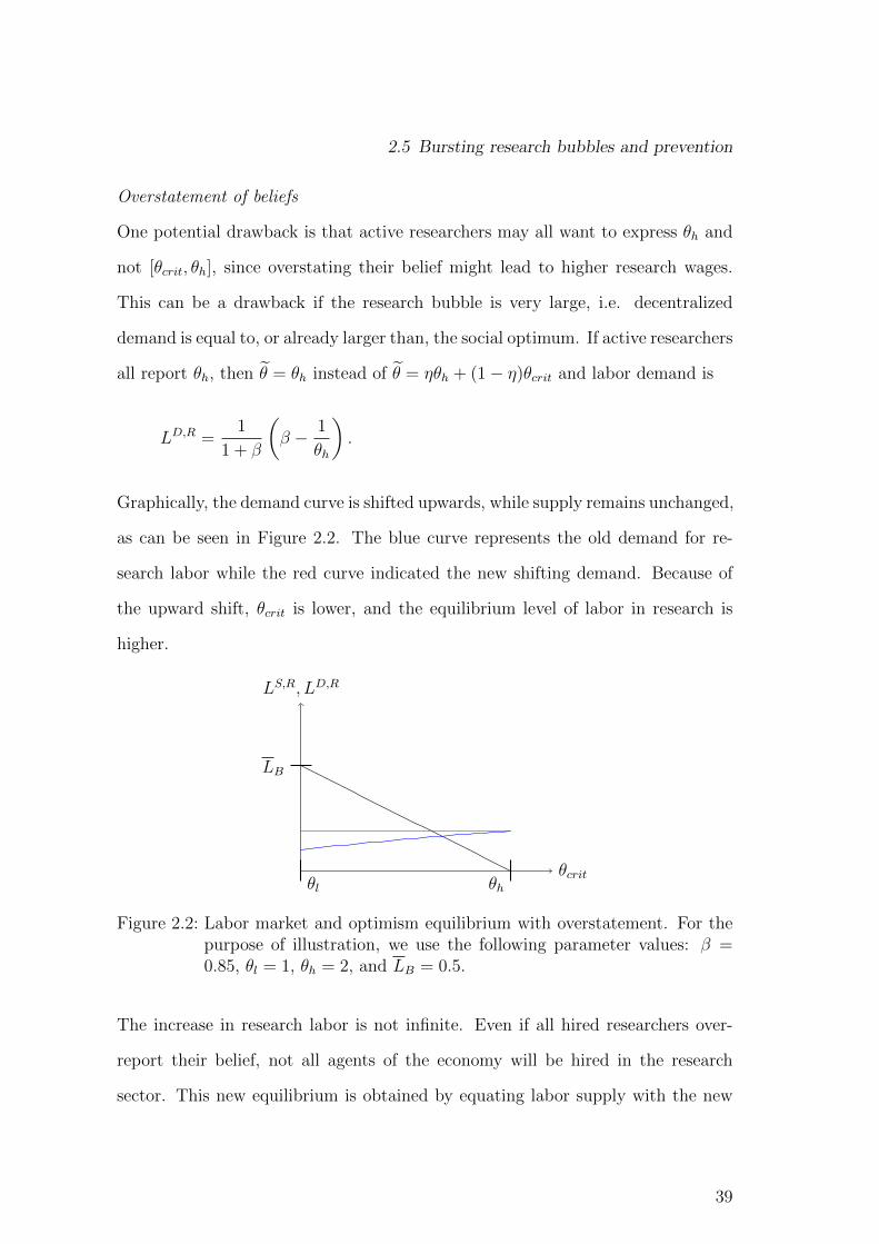
2.5 Bursting research bubbles and prevention
Overstatement of beliefs
One potential drawback is that active researchers may all want to express θh and
not [θcrit, θh], since overstating their belief might lead to higher research wages.
This can be a drawback if the research bubble is very large, i.e. decentralized
demand is equal to, or already larger than, the social optimum. If active researchers
all report θh, then θ = θh instead of θ = ηθh + (1− η)θcrit and labor demand is
LD,R =1
1 + β
(β − 1
θh
).
Graphically, the demand curve is shifted upwards, while supply remains unchanged,
as can be seen in Figure 2.2. The blue curve represents the old demand for re-
search labor while the red curve indicated the new shifting demand. Because of
the upward shift, θcrit is lower, and the equilibrium level of labor in research is
higher.
θcrit
LS,R, LD,R
LB
θl θh
Figure 2.2: Labor market and optimism equilibrium with overstatement. For thepurpose of illustration, we use the following parameter values: β =0.85, θl = 1, θh = 2, and LB = 0.5.
The increase in research labor is not infinite. Even if all hired researchers over-
report their belief, not all agents of the economy will be hired in the research
sector. This new equilibrium is obtained by equating labor supply with the new
39

Chapter 2 Research bubbles
labor demand:
θcrit = θh −(θh − θl)LB(1 + β)
(β − 1
θh
).
Collapse
Governments might learn that beliefs are too optimistic. This could happen from
observing past outcomes of basic research investments by previous governments
or—recognizing the selection of optimistic researchers into the research activities—
by discounting the assessment of researchers. While the first source of learning
might be difficult, since basic research activities are very different across time,7
the second source of learning is more plausible. Such learning might lead to a
collapse of the bubble, as we demonstrate next.
Assume a situation in which the social optimum has been achieved due to over-
optimism and the government’s η is equal to η∗. Now suppose a government
becomes less optimistic and lowers its η to η < η∗. We ask whether it will be
optimal for the government to lower its demand from LO,R to LD,R(η), which is the
labor demand associated to some η. Once its optimism decreases, the government
has two options. On the one hand, it can continue to demand LO,R, while η and
not η will enter its utility function. We assume that the government knows θ∗crit,
which implements the social optimum. The government can calculate its utility
from maintaining the social optimum. Another thing it can do is to reassess the
productivity, which will lead to a higher θcrit and a lower demand for research
labor. Doing this, the government does not internalize how a change in demand
7Moreover, if productivity is affected by macroeconomic shocks—and many varieties of suchshocks are discussed in the literature—inferring the impact of basic research on GDP may beinherently difficult or impossible.
40

2.5 Bursting research bubbles and prevention
for labor impacts θcrit. It will thus believe that, if it changes its demand, θcrit will
remain the same. This is a utility that the government expects to obtain. Clearly,
its choice will influence θcrit and influence the level of utility it actually achieves.
As the real productivity of research is always θ and not the believed value
ηθh + (1 − η)θcrit, we distinguish two different levels of utility. On the one hand,
there is the utility that the government active in period t expects to obtain, based
on the anticipated productivity. On the other, there is the actually realized utility,
based on the real productivity. If the government chooses to maintain the social
optimum, it will expect to obtain the following utility:
uG,Ot = log(1− LO,R) + β log(1 + (ηθh + (1− η)θ∗crit)L
O,R),
where θ∗crit is the critical value that implements the social optimum. The tilde in-
dicates the expected value, the superscript indicates the social optimum. Actually,
the government will achieve
uGt = log(1− LO,R) + β log(1 + θLO,R
).
If it chooses to deviate, it believes that its deviation will not influence θcrit, which
will remain at the level θ∗crit. Hence, the government maximizes the following
expression:
maxLD,Rt
uGt (LD,Rt ) = log(
1− LD,Rt
)+ β log
(1 + (ηθh + (1− η)θ∗crit)L
D,Rt
),
which yields
LD,R
t = LD,R
=1
1 + β
(β − 1
(ηθh + (1− η)θ∗crit)
).
41

Chapter 2 Research bubbles
Note that LD,R
is not a function but a specific value that the government believes
to be the market equilibrium.
In the next step we examine whether the government will deviate from the social
optimum. We have shown that the government’s maximization problem is strictly
concave over the domain of LD,R, so that a maximizer of the objective function
is unique and is also the global maximum. Therefore it remains to show that
LO,R 6= LD,R
. To see that this is indeed the case, recall that
LO,R = LD,R(η∗, θ∗crit), LD,R
= LD,R(η, θ∗crit), where
LD,R(η, θ∗crit) =1
1 + β
(β − 1
(ηθh + (1− η)θ∗crit)
)
⇔ ∂LD,R(η, θ∗crit)
∂η> 0,
so that LD,R
< LO,R, which concludes the proof. Note that we have assumed
β > 1/θ and that θh ≥ θ, so that β > 1/θh holds. We can be certain that the
government will deviate from the social optimum if it becomes less optimistic.
The government makes its decision believing that θcrit will not adjust. However,
we know that θcrit is likely to change. The reason is that lower optimism on the
part of the government, η, shifts the demand curve downwards and leads to a
larger θcrit. Therefore it is unlikely that LD,R
will be the new market equilibrium
LR(η) that is associated to η. Hence, the government will receive the following
utility:
uGt (η) = log(1− LR(η)
)+ β log
(1 + θLR(η)
),
which we write as a function of η because it determines the market clearing θcrit(η)
and the labor market equilibrium LR(η). Thus deviation will be profitable ex post
if uG,Ot < uGt (η), i.e. if the decentralized equilibrium provides higher utility than
the social optimum. This is the case, as the LR that maximizes the expression
42
2.5 Bursting research bubbles and prevention
uGt = log(1− LR
)+β log
(1 + θLR
)is, of course, the labor demand from the simple
model. Also, remember that uGt is a strictly concave function and thus is decreasing
on (LR, 1), so that LR < LR(η) < LO,R implies uGt (LR) > uGt (LR(η)) > uG,Ot .
Hence deviation is profitable ex post.
2.5.2 Institutional remedies
We have observed that governments may resort to more realistic assessments, thus
lowering basic research investments below socially optimal levels. Of course, it
is not the more realistic assessments of the impact of basic research that should
be prevented, but the lowering of basic research investments as a consequence.
There are three possible ways of preventing such attempts. First, one could give
optimistic researchers a strong say in decisions about basic research investments.
Of course, these views have to be balanced to prevent excessive basic research
investments. Second, one could allow the government to issue public debt the
amount of which is dependent on the level of research activities. This would
provide generations with more incentives to undertake the socially optimal amount
of research. We will explore this case in the next subsection. Third, attempts to
lower research investment could also be prevented by traditional constitutional
means making deviations from the social optimum difficult for a single generation.
This can be achieved, by say, committing to longer term funding plans that cannot
be rapidly changed by one individual generation.
2.5.3 Debt financing
We have shown that the decentralized solution implies less research than the social
optimum. The reason is straightforward. The decentralized government does not
43
Chapter 2 Research bubbles
internalize the marginal benefits of research for future generations. To increase the
the government’s labor demand, one could allow to issue debt. More precisely, our
goal is study whether there is some amount of debt dt enabling the steady state
social planner solution to be implemented in the decentralized case. We assume
that the government has access to financial markets and can borrow at the rate rt
without any frictions. Also, we assume that debt can be fully rolled over to the
next generation, i.e. if the government in period t borrows dt, in it can always
borrow at least rt+1dt in t+ 1.
We propose a debt contract made up of two parts. First, the government is allowed
to borrow an amount equal to the total debt level times interest in t . As described
above, this allows to roll over debt. Second, the government can borrow some
amount Dt(LD,Rt ), which depends on its demand for research labor. We can show
that if
Dt(LD,Rt ) =
(1
(1− LD,Rt )β(1−α)− 1
)Yt,
then the social optimum can be implemented in the market economy. To prove
this, we write the modified maximization problem of the government as
maxLD,Rt
log(Yt +Dt(L
D,Rt ) + rtdt−1 − rtdt−1
)+ β log (Yt+1 + rt+1dt − rt+1dt) ,
where dt = Dt(LD,Rt ) + dt−1rt is the accumulated debt stock, i.e. the sum of debt
taken over from the previous generation plus the additional debt from period t.
44
2.5 Bursting research bubbles and prevention
We can simplify the problem to
maxLD,Rt
log
(Yt
(1− LD,Rt )β(1−α)
)+ β log (Yt+1) =
maxLD,Rt
log
(((1− LD,Rt )Bt)
1−αKαt
(1− LD,Rt )β(1−α)
)+ β log
(((1− LD,Rt+1 )Bt(1 + θLD,Rt ))1−αKα
t+1
),
where as before, Kt and Bt are state variables in period t. In t, the government
perceives Lt+1 and Kt+1 as independent of its choice. Due to the logarithmic
utility function, the problem is a sum in which the components depending on the
aforementioned variables can be omitted. This enables us to reduce the problem
to
maxLD,Rt
(1− β) log(
1− LD,Rt
)+ β log
(1 + θLD,Rt
),
which yields
1− β1− LD,Rt
− βθ
1 + θLD,Rt
= 0
⇒ LD,Rt = β − 1− βθ
= LO,R.
It is thus possible to implement the socially optimal steady state as labor demand
in every period by allowing the government to issue debt. In the Appendix for
Chapter 2, we show that such a debt contract leads to a constant ratio of debt to
output if the interest rate satisfies r < 1 + θLO,R.
The socially optimal demand must be financed in order to become the new market
equilibrium. For this, we assume that all debt income is used to finance wages
in the research sector. At best, this would allow the government to lower income
taxes τt to zero and pay researchers the amount Dt(LO,R). We cannot however
45

Chapter 2 Research bubbles
be certain whether Dt(LO,R) will actually cover the government’s financing need,
which has increased, because the government wants to employ more researchers
than before. It may even be the case that the government will have to raise the
income tax rate. Therefore, when the government implements the optimal amount
LO,R and issues debt of magnitude Dt(LO,R), balancing the budget requires
LO,RwRt = τGt (1− LO,R)wPt +Dt(LO,R),
with τGt being the new tax rate. The right-hand side of this equation shows the
two sources of government income: Taxes and debt. Substituting wRt from (2.20)
and simplifying yields
wPt κ
LO,R
1 + (1− LO,R)(θh − θl)(
1− LO,R
LB
) − τGt
= Dt(L
O,R), with
κ :=
1 + (1− LO,R)(θh − θl)(
1− LO,R
LB
)
1 + (θh − θl)(
1− LO,R
LB
)
.
Note that the term
LO,R
1 + (1− LO,R)(θh − θl)(
1− LO,R
LB
)
is exactly the tax rate that would be required to finance the optimal labor demand
in the absence of debt. Thus, we call it τS and have
wPt κ(τS − τGt ) = Dt(LO,R).
By plugging in the definition of Dt(LO,R), and making use of wPt = (1−α)Yt/(1−
46

2.6 Extensions
LO,R), we arrive at
τS − τG =((1− LO,R)−β(1−α) − 1
) Yt(1− LO,R)
(1− α)κYt,
τG = τS − 1− LO,R(1− α)κ
((1− LO,R)−β(1−α) − 1
),
and find that the government does not have to increase the tax rate to τS thanks to
the presence of debt financing. However, it is not clear whether τG will be greater or
smaller than the previous τ . Their relative size depends on the difference between
the market and the social planner outcome and hence on parameter constellations.
2.6 Extensions
The model allows a number of extensions that shed further light on the role of
research bubbles.
2.6.1 Effort in knowledge production
In this extension, the output of the research sector depends not only on the number
of researchers but also on the effort they invest. The expected production function
for knowledge changes to
Bt+1 = Bt(1 + θtLD,Rt Et),
where, as before, Bt stands for the knowledge stock in t, Bt+1 for the expected
knowledge stock in t + 1, θt for the governments’ estimate of the productivity of
the research sector, given by θt = ηθh + (1− η)θcrit,t, and LD,Rt for the demand for
research labor. The new variable is Et, which is the aggregate effort of researchers,
47
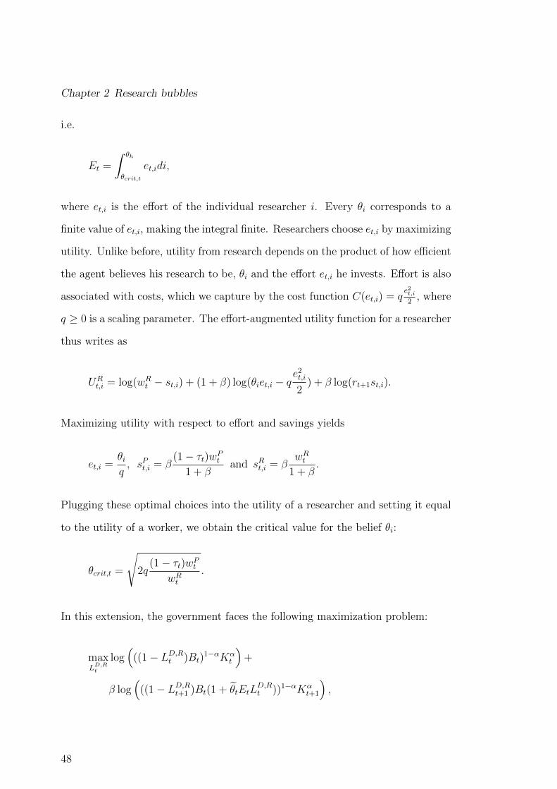
Chapter 2 Research bubbles
i.e.
Et =
∫ θh
θcrit,t
et,idi,
where et,i is the effort of the individual researcher i. Every θi corresponds to a
finite value of et,i, making the integral finite. Researchers choose et,i by maximizing
utility. Unlike before, utility from research depends on the product of how efficient
the agent believes his research to be, θi and the effort et,i he invests. Effort is also
associated with costs, which we capture by the cost function C(et,i) = qe2t,i2
, where
q ≥ 0 is a scaling parameter. The effort-augmented utility function for a researcher
thus writes as
URt,i = log(wRt − st,i) + (1 + β) log(θiet,i − q
e2t,i2
) + β log(rt+1st,i).
Maximizing utility with respect to effort and savings yields
et,i =θiq, sPt,i = β
(1− τt)wPt1 + β
and sRt,i = βwRt
1 + β.
Plugging these optimal choices into the utility of a researcher and setting it equal
to the utility of a worker, we obtain the critical value for the belief θi:
θcrit,t =
√2q
(1− τt)wPtwRt
.
In this extension, the government faces the following maximization problem:
maxLD,Rt
log(
((1− LD,Rt )Bt)1−αKα
t
)+
β log(
((1− LD,Rt+1 )Bt(1 + θtEtLD,Rt ))1−αKα
t+1
),
48

2.6 Extensions
where it takes Bt, Kt and Et as given and both Kt+1 and LD,Rt+1 as outside its sphere
of influence. Hence, the problem can be written as
maxLD,Rt
log(
1− LD,Rt
)+ β log
(1 + θtEtL
D,Rt
),
which gives the following demand function:
LD,Rt =1
1 + β
(β − 1
Etθt
), with (2.25)
Et =
∫ θh
θcrit,t
θiqdi =
θ2h − θ2crit,t2q
.
Plugging in the definitions of Et and θt, we can write demand as a function of
θcrit,t only:
LD,Rt =1
1 + β
(β − 4q
(θ2h − θ2crit,t)(θh + θcrit,t)
).
It is possible to show that this demand function is strictly concave in θcrit,t, which
yields two possible labor market equilibria, given that labor supply is the same lin-
ear function as in the previous model8. Moreover, we demonstrate that the market
equilibrium with greater labor in research LR is preferred by the government.
8Proofs for this claim, as well as for all others in this section, are available on request.
49

Chapter 2 Research bubbles
We also explore the solution of a social planner who knows the true value of θ:
maxc1t,i,c
2t+1,i,et,i,L
Rt ,Bt+1,Kt+1
W (c1t,i, c2t+1,i, et,i, L
Rt , Bt+1, Kt+1),
with
W =∞∑
t=0
βts
(∫ 1
0
log(c1t,i) + β log(c2t+1,i) di+
∫ 1
0
log(θet,i − qe2t,i2
) di
),
subject to
((1− LRt )Bt)1−αKα
t =
∫ 1
0
(c1t,i + c2t,i) di+Kt+1,
and
Bt+1 = (1 + θ ·∫ 1
0
et,i di · LRt )Bt.
For a symmetric equilibrium with et,i = Et and c1t,i = c1t = c2t,i = c2t ∀i, due to
βs = β, we find the following optimality conditions:
50

2.6 Extensions
1
c1t=
αβYt+1
Kt+1c2t+1
, (2.26)
Yt1− LRt
1
Et=
Kt+1
αYt+1
(θYt+1
(1 + θLRt Et)+
Yt+1
(1− LRt+1)Et+1
1 + θLRt+1Et+1
(1 + θLRt Et)
), (2.27)
and
EtLRt
θ − qEtθEt − qE
2t
2
= − 2(1− α)
(1− Kt+1
Yt)(1− LRt )
, (2.28)
which, in a steady state, yield
LR = β − 1− βθE
, and (2.29)
E2q
[(1− α)β
1− αβ + 1− β]− (1− β)
[1− 2(1− α)
1− αβ
](2.30)
− E[(1− β)
(θ − q
θ
)+
2(1− α)
1− αβ
(βθ +
(1− β)q
2θ
)]= 0.
We find that the socially optimal labor input equation, LR, is structurally equiv-
alent to what it was before, but that θ is replaced by θE. The same holds for the
decentralized labor demand. Hence, if θ and E were the same in the decentralized
economy and the social planner solution, LR would be too low in the decentralized
economy. However, if aggregate effort E was greater in the market equilibrium,
this could mitigate the government’s myopia. To investigate this possibility, we
compare the first order condition for the individual effort of some agent i in the
decentralized economy to that of the social planner:
θi − qet,iθiet,i − q
e2t,i2
+ 0 = 0, (2.31)
θ − qetθet − q e
2t
2
+2(1− α)Yt
etCt
LRt1− LRt
= 0. (2.32)
The first equation is the first-order condition in the decentralized equilibrium. We
obtain two differences. First, the individual agent bases his effort on his belief θi
51

Chapter 2 Research bubbles
and not on θ. Second, he does not internalize the positive externality of his effort
on knowledge production, which is captured by the second term in Equation (2.32).
Hence it is not clear whether an individual agent supplies more or less effort than
would be socially optimal. On the one hand, the individual belief might be greater
than θ, implying more effort, while on the other hand, the agent might not be
aware of the externality, implying less effort. It is likely, however, that the effort
externality is greater than the over-optimism, especially for more conservative
agents, so that aggregation of individual effort would provide an overall level of
effort that is too small compared to the social optimum.
With this finding, the implementation of the social optimum in the decentralized
economy cannot be achieved by introducing government debt alone, even when
the government knows θ. It is also necessary to create incentives for scientists to
provide the optimum amount of effort. Hence the following wage contracts must
be offered to a researcher with belief θi:
Proposition 8 The social optimum can be obtained in the decentralized economy
by offering researcher i with belief θi the wage
wRt,i = wtR
θet,i − q e
2t,i
2
θiet,i − qe2t,i2
11+β
eGtet,i1+β , with
wRt = wPt
(θet − q
e2t2
) −11+β
e−Gtet
1+β ,
et =θcrit − θlθh − θl
ESOC ,
and allowing the government to issue debt of magnitude
Yt(1− LD,R)β(1−α)
+ rtdt−1,
52

2.6 Extensions
where wRt is a fixed-wage component that is equal for all researchers. ESOC stands
for the social planner steady state levels of aggregate effort. Furthermore, θ =
θh−θlθh−θcrit θ and Gt = θh−θcrit
θh−θl Gt. θcrit corresponds to the steady state level of the
critical belief value that leads to the socially optimal supply of research labor. et is
individual effort, which is the same for all researchers.
The Appendix for Chapter 2 contains the proof that this payment scheme will
implement the social optimum. The intuition behind it is the following: First, we
want every researcher to base his effort decision on the true parameter and not on
his beliefs. Therefore wRt,i depends on θi and θ, i.e. on the individual belief and on
the scaled true parameter.9 Second, every researcher is supposed to internalize the
effect of his effort on research productivity. Therefore Gt is incorporated in the
wage scheme. Third, the government is supposed to increase its labor demand, so
that the debt it can issue depends on LD,Rt . The first of our measures simplifies the
task of implementing the social optimum. The second and third fulfill the task.
2.6.2 Linear utility
Another variant of the model is one with effort and a linear utility function for the
government. Accordingly, the government’s problem is
maxLD,Rt
((1− LD,Rt )Bt)1−αKα
t + β((1− LD,Rt+1 )Bt(1 + θtEtLD,Rt ))1−αKα
t+1.
In the following, we use Yt+1 to denote the output that the government believes
will be created, while Yt+1 is the true future output. Maximizing with respect to
9Why the true parameter needs to be scaled is set out in the Appendix for Chapter 2.
53

Chapter 2 Research bubbles
LD,Rt yields
Yt
1− LD,Rt
= βθtEtYt+1
1 + θtEtLD,Rt
, with (2.33)
Et =
∫ θh
θcrit,t
θiqdi =
θ2h − θ2crit,t2q
(2.34)
and θt given by (2.16).
Unlike before, the first order condition of the government is a dynamic equation in
LRt and does not yield a time-constant value for research labor demand. However,
a steady state with constant labor demand can be found
LD,R = 1− 1
βθE= 1− 4q
β(θ2h − θ2crit)(θh + θcrit).
In this case, it is possible that the government may demand more research labor
than is socially optimal. Furthermore, the demand function is not strictly increas-
ing in θcrit, as can be seen from plugging in θ and E. We can show that LD,R is
a concave function in θcrit, so that two market equilibria are possible. It can be
demonstrated, though, that one of them yields more utility for the government.10
The dynamic demand function allows for a convergence analysis. We find that
the decentralized market outcome is saddle-path stable. The implementation of
the social optimum steady state as a balanced growth path for the decentralized
economy is possible. However, this is only the case if the initial market allocation
implies a lower level of research labor. If that is so, then a combination of public
debt and wage contracts for researchers allows for implementation, as discussed
10By plugging in LD,R into the government’s utility function, one can analyze the governmentsutility as a function of θcrit. It turns out to be a concave function over the interval [θl, θh] witha local maximum. Hence, the desirability of the equilibria can be studied by their proximity tothe local maximum. This hold for parameter constellations under which the function behavesrather symmetrically around its maximum.
54

2.7 Conclusion
above.
2.7 Conclusion
We have developed a model that provides a rationale and a microfoundation for
research bubbles. Such research bubbles emerge when researchers self-select into
those activities they believe to be most promising, and when the assessments of
these researchers are aggregated by the government. Furthermore, bubbles can
implement socially desirable allocations. Thus specific forms of research bubbles
are desirable from a long-term welfare perspective. Numerous extensions require
further scrutiny, as they have the potential to shed further light on the emergence,
social desirability, and downside of research bubbles, which may be a key factor of
modern knowledge economies.
55


Chapter 3
Untimely destruction: pestilence, war,
and accumulation in the long run
Abstract
This chapter analyses the effects of disease and war on the accumulation of human
and physical capital.1 We employ an overlapping-generations framework in which
young adults, confronted with such hazards and motivated by old-age provision and
altruism, make decisions about investments in schooling and reproducible capital.
A poverty trap exists for a wide range of stationary war losses and premature
adult mortality. If parents are altruistic and their sub-utility function for own
consumption is more concave than that for the children’s human capital, the only
possible steady-state growth path involves full education. Otherwise, steady-state
paths with incompletely educated children may exist, some of them stationary
ones. We also examine, analytically and with numerical examples, a growing
economy’s robustness in a stochastic environment. The initial boundary conditions
have a strong influence on outcomes in response to a limited sequence of destructive
shocks.
1This chapter is joint work with Prof. Dr. Clive Bell and Prof. Dr. Hans Gersbach.
57

Chapter 3 Untimely destruction: pestilence, war, and accumulation in the long run
3.1 Introduction
Motivation
Durer’s woodcut, ‘The Four Horsemen of the Apocalypse’, is a terrifying vision of
the great scourges of humanity from time immemorial. This chapter deals with
three of them – pestilence, war and death, with their accompanying destruction of
human and physical capital. Its particular concern is how these calamities affect
the accumulation of capital, with special reference to the existence of growth paths
and poverty traps. The treatment is necessarily stylized, simple and, in contrast
to Durer’s masterpiece, desiccated.
In such a setting, the distinction between human and physical capital is vital. Not
only are they complementary in production, but they are also, in general, subject
to different, albeit not fully independent, hazard rates. The attendant risks are not,
moreover, equally insurable. These considerations weigh heavily in the decision
of how much to invest and in what form, with all the ensuing consequences for
material prosperity over the long run.
A few selected examples of such calamities will convey some flavor of the historical
dimensions of what is involved. The Black Death carried off about one-third of
the entire European population between 1347 and 1352. The so-called “Spanish
influenza” pandemic of 1918-1920 is estimated to have caused at least 50 million
deaths globally, with exceptionally high mortality among young adults. In recent
times, the AIDS pandemic, far slower in its course like the disease itself, still
threatens to rival that figure, despite the improved availability of anti-retroviral
therapies. Pestilence and war also ride together. Half a million died in an outbreak
of smallpox in the Franco-Prussian War of 1870-71 (Morgan (2002)). For every
British soldier killed in combat in the Crimean War (1854-56), another ten died
of dysentery, and in the Boer War (1899-1902), the ratio was still one to five.
58

3.1 Introduction
War losses in the 20th Century make for especially grim reading. Between 15
and 20 million people died in the First World War, the majority of them young
men. Almost two million French soldiers fell, including nearly 30 per cent of the
conscript classes of 1912-15. Joining this companionship of death were over 2
million Germans, including almost two of every five boys born between 1892 and
1895 (Keegan (1990a)), almost a million members of the British Empire’s armed
forces, and many millions more in those of Imperial Austria, Russia and Turkey. Its
continuation, the Second World War, was conducted, in every respect, on a much
vaster scale. Most estimates suggest that it resulted in at least 50 million deaths,
directly and indirectly. Among them were 15 million or more Soviet soldiers and
civilians, 6 million Poles (20 per cent of that country’s pre-war population) and
at least 4 million Germans (Keegan (1990b)). With these staggering human losses
went the razing of German and Japanese cities and massive destruction in the
western part of the Soviet Union as well as the states of Eastern Europe. The
catalog of conflicts in the second half of the 20th Century is also unbearably long,
with particularly appalling casualties in South-east Asia and Rwanda.
Great epidemics and wars capture the headlines and grip the imagination, but the
majority of those adults who die prematurely fall victim to low-level, ‘everyday’
causes, especially in poor countries: notable killers are endemic communicable dis-
eases, accidents, violence and childbirth. These are competing hazards—one dies
only once—, but their combined effect is not wholly negligible even in contempo-
rary O.E.C.D. countries. In many poorer ones, it is quite dismaying. According
to the W.H.O. (2007), those who had reached the age of 20 in the O.E.C.D. group
could expect to live, on average, another 60 years or so, their counterparts in China
and India another 50-55 years, and those in sub-Saharan Africa but 30-40. The
odds that a 20-year old in the O.E.C.D. group would not live to see his or her
59
Chapter 3 Untimely destruction: pestilence, war, and accumulation in the long run
40th birthday were 1 or 2 in a 100, rising to 2.5-5 in a 100 for the 50th birthday.
These odds were just a little worse for young Chinese, decidedly worse for young
Indians, and for young Africans much less favorable than those of Russian roulette
– in some countries where the AIDS epidemic was raging, indeed, scarcely better
than the toss of a fair coin.
Approach and results
The human and material losses so inflicted, whether they are caused by great
epidemics and wars, or endemic communicable diseases and low-level conflicts,
have long-run as well as immediate economic consequences. Taking as given agents’
preferences and the technologies for producing output and human capital in the
presence of these hazards, we address the following questions.
1. Under what conditions are steady-state growth paths outcomes in equilib-
rium?
2. Are such paths possible when parents are moved by altruism; and if so, is
stronger altruism conducive to faster steady-state growth?
3. If mortality and destruction rates do not vary over time, are both secular,
low-level stagnation and steady-state growth possible equilibria, thus estab-
lishing the existence of a poverty trap?
4. If mortality and destruction rates are stochastic, under what conditions
would the economy fall into such a trap when it would otherwise be growing?
The overlapping generations model (OLG) offers the natural framework within
which to analyze the long-run consequences of economic behavior in such environ-
ments. In the variant adopted here, there are children, young (working) adults
and the old. Young adults decide how much schooling the children will receive
60
3.1 Introduction
and how much to put aside to yield a stock of physical capital in the next period.
In doing so, they are bound by certain social norms, which govern the distribu-
tion of aggregate current consumption among the three generations. Untimely
destruction can undo these plans, however carefully laid. The children may die
prematurely at some point in young adulthood; and war can wreak havoc on the
newly formed capital stock. These losses, if they occur, will reduce the resources
available to satisfy claims on consumption in old age in the period that follows.
Parents may also be motivated by altruism towards their children, so that their
premature deaths will be felt as a distinct loss quite independently of the ensuing
reduction in old-age consumption under the prevailing social norms – and arguably
all the more keenly if the children have been well educated. The institutional form
within which all this takes place is assumed to be a very large extended family, in
which the surviving young adults raise all surviving children. Given such pooling,
the law of large numbers makes the level of consumption in old age – for those
who survive to enjoy it – virtually certain when mortality and war loss rates are
forecast unerringly, but even then, the idiosyncratic risk of dying earlier remains.
War losses are wholly uninsurable and operate much like cohort-specific mortality.
When these rates are stochastic, as is wholly plausible, they constitute unavoidable
systemic risks, with consequent effects on investment in both forms of capital.
Our main insights are as follows. Since balanced growth paths with endogenous
physical and human capital may not exist – as Uzawa (1961) pointed out in his
classic contribution – we first establish conditions for the existence of two extreme
steady states, namely, permanent backwardness with no education and unbounded
growth with a fully educated population, which we term ‘progress’. Without altru-
ism the well-known poverty trap always exists under standard conditions. More-
over, both backwardness and progress may both exist as equilibria for a wide range
61

Chapter 3 Untimely destruction: pestilence, war, and accumulation in the long run
of mortality and destruction rates. Parents’ altruism influences the set of balanced
growth paths in two ways. First, if sufficiently strong, it can rule out backwardness.
Yet with a robust numerical example, we show that even under quite strong altru-
ism, a poverty trap can exist. Second, in the presence of altruism, progress is the
only steady-state path other than backwardness if the sub-utility function for own
consumption is more strongly concave than that for parents’ evaluation of their
children’s human capital. If this latter condition is reversed, other steady-state
paths with incompletely educated children may exist, some of them stationary,
even if altruism is strong.
We also establish conditions for the local stability of a poverty trap. In some
settings, both extreme states may be locally stable equilibria, which contrasts
with results from corresponding models in which only human capital accumulation
matters. We also provide conditions for balanced growth paths with intermediate
levels of schooling.
Finally, we explore whether a growing economy can withstand an outbreak of war,
a severe epidemic, or a combination of both, as stochastic events; for such destruc-
tive events, even if temporary, may pitch a growing economy into backwardness.
We establish that these risks depress investment in both physical and human cap-
ital; and only extreme destruction of physical capital could induce an increase
in schooling. We also establish thresholds for human and physical capital above
which an economy can withstand a particular configuration of shocks. We show
with simulations that the duration of adverse events – wars or epidemics – is often
decisive in determining whether an economy can regain growth.
Relation to the literature
There is a substantial literature on the relationship between the health of popula-
62

3.1 Introduction
tions and aggregate economic activity. Notable is the general empirical observa-
tion that good health has a positive and statistically significant effect on aggregate
output (Barro and Sala-I-Martin (1995); Bloom and Canning (2000); Bloom et al.
(2001)). What is especially relevant for present purposes, however, is a body of
work on the macroeconomic effects of AIDS, in which there are varying points of
emphasis. Corrigan et al. (2005a,b), for example, adopt a two-generation OLG
framework in which the epidemic can affect schooling and the accumulation of
physical capital, but expectations about future losses play no role. In two con-
trasting studies of South Africa, Young (2005) uses a Solovian model to estimate
the epidemic’s impact on living standards through its effects on schooling and
fertility, with a constant savings rate; whereas Bell et al. (2006) apply a two-
generation OLG model with pooling through extended families and a vital role for
expectations, but no role for physical capital.
Closely related theoretical contributions include Chakraborty (2004), in whose
OLG framework endogenous mortality is at centre-stage. Better health promotes
growth by improving longevity, and investment in health emerges as a prerequisite
for sustained growth. Individual investment in health is also the prime mechanism
in Augier and Yaly (2013). Young adults, whose only income is wages, pay a fixed
fraction thereof as taxes into a fund managed by the government. This fund pro-
vides all capital for the next period, with the gross returns going to the survivors.
In Boucekkine and Laffargue‘s (2010) two-period framework with heterogeneous
levels of human capital, a rise in mortality among adults in the first period reduces
the proportion of young adults with low human capital in the second period be-
cause the mortality rate among children at the end of the first rises more sharply
in poor families. The number of orphans in the first period increases, however,
so that the proportion of young adults with low human capital in the second pe-
63
Chapter 3 Untimely destruction: pestilence, war, and accumulation in the long run
riod will increase if orphans go poorly educated. Bell and Gersbach (2013) analyze
growth paths and poverty traps when epidemics take the form of two-period shocks
to mortality, paying particular attention to their effects on inequality in nuclear
family systems, albeit without a place for physical capital.
A salient feature of these studies is the central importance, if only implicitly, of
premature adult mortality. Physical capital, when it does appear, is not subject
to similar hazards. Voigtlander and Voth (2013, 2009) take a Malthusian posi-
tion in explaining the rise of growth in early modern Europe. Disease and war
rode together, but ‘[war] destroyed human life quickly while not wreaking havoc
on infrastructure on a scale comparable to modern wars.’ (Voigtlander and Voth
(2013)). In contrast, the possibility of destruction on such a scale is an essen-
tial element of the present chapter, in which there are no fixed factors like land.
Furthermore, the second part of the chapter deals with the robustness of a grow-
ing economy to shocks: both destruction rates are stochastic. In this connection,
exponential depreciation at a constant rate in Solovian models does not lend it-
self to the task of representing the shocks of war losses. To our knowledge, no
other contribution addresses the possibilities of long-term growth and stagnation
when both forms of premature destruction are salient features of the environment
wherein agents make decisions about accumulation.
The chapter’s theme is also broadly related to the existence and relevance of ‘bal-
anced growth paths’. The classic problem examined by Uzawa (1961) is whether
such paths exist in neoclassical growth models with capital accumulation, popu-
lation growth and labor- or capital-augmenting technological progress. Grossman
et al. (2016) establish that balanced growth requires either an absence of capital-
augmenting technological change or a unitary elasticity of substitution between
physical and human capital, in which case the forms of factor-augmenting tech-
64
3.2 The model
nical change are all equivalent. In this connection, we explore a complementary
balanced growth problem: does balanced growth exist in an OLG framework with
endogenous physical and human capital accumulation, with or without altruism?
We establish conditions on the utility functions with respect to altruism and own
consumption that allow balanced growth without imposing very strong restrictions
on the production technology.
Structure
The plan of the chapter is as follows: Section 3.2 lays out the model and specifies
the general problem to be solved. There follows an analysis of steady states, which
necessarily involves unchanging mortality and destruction rates. Sections 3.3 and
3.4 not only establish the conditions for the existence of a stable, low-level equi-
librium in which all generations go uneducated, but also that these conditions and
those under which steady-state growth is also an equilibrium in the environment
in question can be satisfied simultaneously, thus establishing the existence of a
poverty trap. Settings in which the destruction rates are stochastic are treated in
Sections 3.5 to 3.7. Section 3.8 briefly draws together the chief conclusions.
3.2 The model
There are three overlapping generations: children, who split their time between
schooling and work; young adults, who work full time; and the old, who are active
neither economically nor in raising children. The timing of events within each
period t relates to a generation born in period t− 1, thus becoming young adults
at the start of period t. It is displayed in Figure 3.1. Those individuals who survive
into full old age in the following period t + 1 therefore live for the three periods
65

Chapter 3 Untimely destruction: pestilence, war, and accumulation in the long run
t− 1 to t+ 1.
Generation 𝑡𝑡 born in 𝑡𝑡 − 1,
childhood in 𝑡𝑡 − 1,𝑁𝑁𝑡𝑡−11 = 𝑛𝑛𝑡𝑡−1𝑁𝑁𝑡𝑡−12
children
𝑁𝑁𝑡𝑡2 = 𝑁𝑁𝑡𝑡−11 youngadults,
𝑁𝑁𝑡𝑡1 = 𝑛𝑛𝑡𝑡𝑁𝑁𝑡𝑡2 children
(1 − 𝑞𝑞𝑡𝑡2)𝑁𝑁𝑡𝑡2young adults
survive,1 − σ𝑡𝑡 𝑆𝑆𝑡𝑡−1
Capital destroyed
Young adultsdecide on
education 𝑒𝑒𝑡𝑡
Production
Young adultsdecide on savings𝑆𝑆𝑡𝑡 and hence
consumption 𝑐𝑐𝑡𝑡2
𝑁𝑁𝑡𝑡2(1 − 𝑞𝑞𝑡𝑡2)(1 − 𝑞𝑞𝑡𝑡+13 )reach full old age
Consumption 𝑐𝑐𝑡𝑡+13
𝑡𝑡 − 1 𝑡𝑡 𝑡𝑡 + 1
Figure 3.1: Sequence of events for the generation born in period t− 1.
All individuals belong to numerous, identical and very large extended families.
The number of young adults in each family at the beginning of period t is N2t .
They marry and have children at once. Mortality among children only occurs in
infancy, and any child who dies is replaced immediately. After such replacement
fertility, each couple within the extended family has 2nt children, all of whom
survive into adulthood in the next period. Thus, nt is the net reproduction rate
(NNR). Death then claims some young adults and some of those who have just
entered old age. The surviving young adults rear all children collectively and decide
how to allocate the children’s time between schooling and work, and the resulting
aggregate output between consumption and savings, whereby certain social rules
govern the claims of children and the old in relation to the consumption of young
adults. The numbers of young adults and their offspring who reach maturity are,
therefore,
N2t = nt−1N
2t−1 and N1
t = ntN2t ,
respectively. The numbers of young and old adults who make claims on output in
66

3.2 The model
period t are as follows:
(1− q2t )N2t young adults survive to raise all children, and
(1− q3t )N3t old adults survive to full old age, where N3
t = (1− q2t−1)N2t−1
and qat denotes the premature mortality rate among age group a(= 2, 3). All adults
who do reach full old age in period t die at the end of that period.
Two social rules govern consumption-sharing in the extended family:
(i) When each surviving young adult consumes c2t , each child consumes βc2t
(β < 1).
(ii) All surviving old adults receive the share ρ of the family’s current ‘full in-
come’, Yt, which is the level of output that would result if all children were
to work full time.2 Since the extended family is very large, each surviving
old adult will consume
c3t =ρYt
(1− q3t )N3t
. (3.1)
Output is produced under constant returns to scale by means of labor augmented
by human capital (that is, labor is measured in efficiency units) and physical
capital, which is made of the same stuff as output. All individuals are endowed
with one unit of time. The time the child spends in school in period t is denoted
by et ∈ [0, 1]. Each young adult possesses λt efficiency units of labor, each child γ
units. Each fully educated child (et = 1) requires w (< 1) young adults as teachers,
so that the direct cost of providing each child with schooling in the amount et is
wλtet, measured in units of human capital. The total endowment of the surviving
2The determination of β and ρ is discussed in Section 3.3.3. A variant of the rule governingold-age provision is discussed in Section 3.6.
67
Chapter 3 Untimely destruction: pestilence, war, and accumulation in the long run
young adults’ human capital is Λt ≡ (1−q2t )N2t λt; Lt ≡ Λt+γN
1t is the household’s
endowment of labor (measured in efficiency units) at time t; and the amount of
labor supplied to the production of the aggregate good is
Lt ≡ [(1− q2t − wntet)λt + ntγ(1− et)]N2t .
The aggregate savings of the previous period, St−1, like the cohort of children
entering adulthood, are also subject to losses early in the current one, and what
does remain has a lifetime of one period. The capital stock available for current
production is therefore Kt = σtSt−1, where σt ∈ (0, 1] is the survival rate in period
t. The current levels of aggregate output and full income are, respectively,
Yt = F (Lt, σtSt−1) (3.2)
and, putting et = 0,
Yt ≡ Yt(et = 0) = F (Λt + γN1t , σtSt−1),
where the function F is assumed to be monotonically increasing in both argu-
ments, continuously differentiable and homogeneous of degree 1, with both inputs
necessary in production.
Full income is available to finance the consumption of all three generations in
keeping with the social rules, savings to provide the capital stock in the next
period, and investment in the children’s education.
Ptc2t + St + ρYt = Yt, (3.3)
where Pt ≡ [1− q2t + βnt]N2t is effectively the price of one unit of a young adult’s
68
3.2 The model
consumption in terms of output, the numeraire.
The formation of human capital involves the contributions of parents’ human capi-
tal as well as formal education. The human capital attained by a child on reaching
adulthood is assumed to be given by
λt+1 = zth(et)λt + 1. (3.4)
The multiplier zt(> 0) represents the strength with which capacity is transmitted
across generations; and it may depend on the number of children each surviving
young adult must raise. The function h(·) may be thought of as representing the
educational technology, albeit with the fixed pupil-teacher ratio of 1/w. Let h(·) be
an increasing, differentiable function on [0, 1], with h(0) = 0 and lime→0+ h′(e) <
∞. The property h(0) = 0 implies that unschooled children attain, as adults, only
some basic level of human capital, which has been normalized to unity.
3.2.1 Preferences and choices
Young adults, who make all allocative decisions, have preferences over lotteries
involving current consumption, consumption in old age and, if they are altruistic,
the human capital attained by the children in their care. When deciding on an
allocation (c2t , et, St), young adults must forecast mortality and destruction rates
in the coming period. If these forecasts are unerring, as would be the case in a
steady state, those who survive into old age will obtain c3t+1, from (3.1), which the
law of large numbers renders virtually non-stochastic. The stochastic element in
the lotteries in question therefore only arises from the individual risks of failing
to reach old age and, where altruism towards the children is concerned, that the
latter will suffer the misfortune to die prematurely in young adulthood. In this
69

Chapter 3 Untimely destruction: pestilence, war, and accumulation in the long run
connection, let there be full altruism towards adopted children. If, in contrast, the
outbreaks of war and disease in the future are viewed as stochastic events, there
will be systemic risks. The analysis of such environments is deferred to Sections
3.5-3.7.
The surviving young adults’ preferences are assumed to be additively separable in
(c2t , c3t+1, λt+1) and von Neumann-Morgenstern in form:
Vt = u(c2t ) + δ(1− q3t+1)u(c3t+1) +b(1− q2t+1)
(1− q2t )ntv(λt+1), (3.5)
where δ is the pure impatience factor and b is a taste parameter for altruism.
The term 11−q2t
accounts for the children in the extended family whose parents have
died.3 The sub-utility functions u and v are assumed to be strictly concave, where
u satisfies limc→0
u′(.) = ∞. In view of the considerations they represent, there are
strong reasons to suppose that these functions are not the same.
The surviving young adults’ decision problem is as follows:
max(c2t ,et,St)
Vt s.t. (3.1)− (3.4), c2t ≥ 0, et ∈ [0, 1], St ≥ 0. (3.6)
When solving it, they note the current state variables,
(nt, zt, N1t , N
2t , N
3t , q
2t , q
3t , λt, Kt), and form beliefs about all relevant future levels.
Note that these decisions in period t are not influenced by their successors in
subsequent periods. Let (c20t , e0t , S
0t ) solve (3.6).
The evolution of the economy is governed by the following difference equations:
λ0t+1 = zth(e0t )λt + 1 and Kt+1 = σt+1S0t .
3If only natural children count, the ‘adjustment’ for adopted children 1/(1− q2t ) drops out.
70
3.3 Steady states
In what follows, the superscript ‘0’ will be dropped if no confusion would arise.
A preliminary step is to normalize the system by the size of the cohort N2t , ex-
ploiting the assumption that F is homogeneous of degree one. Let lt ≡ Lt/N2t and
st ≡ St/N2t , so that (3.1) and (3.3) can be written respectively as
c3t+1 =ρnt
(1− q3t+1)(1− q2t )· F[(1− q2t+1)λt+1(et) + nt+1γ,
σt+1stnt
](3.7)
and
[1− q2t + βnt]c2t + st + ρF
[(1− q2t )λt + ntγ,
σtst−1nt−1
]= F
(lt,σtst−1nt−1
). (3.8)
Normalized output is
yt ≡ F((1− q2t − wntet)λt + ntγ(1− et), σtst−1/nt−1
).
The analogous definition of normalized full income is yt ≡ F(lt, σtst−1/nt−1
),
where lt ≡ Lt/N2t denotes the normalized endowment of labor at time t. Closely
associated with these normalization is the ratio ζt ≡ λt/st−1, which arises from
investment decisions in the previous period.
Together with the constraints c2t ≥ 0, et ∈ [0, 1] and st ≥ 0, the budget identity
(3.8) defines the set of all feasible allocations (c2t , et, st). Upon substitution for c3t+1
from (3.7) into (3.5), it is seen that Vt is likewise defined in the same space.
3.3 Steady states
In a steady state, the levels of inputs, output and (dated) consumption all grow
at a constant rate. Thus, the parameters qt, nt, σt, and zt are constant, as is
71
Chapter 3 Untimely destruction: pestilence, war, and accumulation in the long run
the level of the children’s education et.4 A special case is that wherein all per
capita levels are constant, though population may be growing. In a slight abuse
of terminology, this will be called a stationary state, even if the population is not
constant. If all per capita levels are growing at the same, positive rate, the economy
is said to be on a steady-state growth path. There are two notable steady states,
which involve the extreme values of education. If a whole generation of children
goes uneducated (et = 0), so that λt+1 = 1, the state of backwardness is said
to rule in period t + 1. If such a state, once reached, becomes permanent, the
associated stationary equilibrium implies the existence of a poverty trap. If, at
the other extreme, children born in period t enjoy a full education (et = 1), and all
generations that follow them do likewise, this will be called the progressive state,
or simply ‘progress’. It may, under certain conditions to be explored below, be
an equilibrium which exhibits steady-state growth. A fundamental question to be
answered is whether permanent backwardness and a progressive growth path are
both possible equilibria of an economy of the kind treated here.
So much for the extremes, but are there also steady-state equilibria in which there
is some constant level of education short of a full one? If both backwardness and
progress are possible equilibria, considerations of continuity suggest that there
exists at least one stationary state with et = es ∈ (0, 1) ∀t. If, moreover, steady-
state growth with e0t = 1 is not an equilibrium path, are there such growth paths
with e0t constant and sufficiently close to 1?
It will be helpful to rewrite Vt as a function of the decision variables:
Vt = u(c2t ) + χtu
(ρntyt+1
(1− q3t+1)(1− q2t )
)+ νtv(zth(et)λt + 1), (3.9)
4Since λt+1 = zth(et)λt + 1, the latter property is implied by the former.
72

3.3 Steady states
where
χt ≡ δ(1− q3t+1) and νt ≡b(1− q2t+1)nt
(1− q2t ).
The budget constraint (3.8) can be expressed as yt = [1 − q2t + βnt]c2t + st + ρyt.
Hence, the associated Lagrangian is
Φt = Vt + µt[yt − [1− q2t + βnt]c2t − st − ρyt], (3.10)
whose multiplier is µt. Note that yt depends on the amount of child labor 1− et.
The assumptions on u (the Inada condition at c2t = 0) ensure that, at the optimum,
c2t > 0. By assumption, physical capital is necessary in production. Hence, if some
young adults are forecast to survive into full old age (q3t+1 < 1), so that χt > 0,
then s 0t > 0.
The associated f.o.c. are set out in the Appendix for Chapter 3. Those w.r.t. c2t
and st yield
u′(c2t )
u′(c3t+1)=σt+1δρ[(1− q2t ) + βnt]
(1− q2t )· F2
[lt+1,
σt+1stnt
], (3.11)
which holds for all et ∈ [0, 1]. Those with respect to c2t and et yield:
δρu′(c3t+1) · F1
[lt+1,
σt+1stnt
]zh′(et) + bv′(λt+1)zh
′(et) ≥
(1− q2t )(wλt + γ)u′(c2t )
(1− q2t+1)(1− q2t + βnt)λtF1
[lt,σtst−1nt−1
], e ≤ 1,
(3.12)
where the inequality holds in the other direction for e ≥ 0. Substituting from
73

Chapter 3 Untimely destruction: pestilence, war, and accumulation in the long run
(3.11) in (3.12), we obtain, for all interior solutions et ∈ (0, 1),
v′(λt+1)
u′(c2t )=
(w + γ
λt
)1−q2t
1−q2t+1F1
[lt,
σtst−1
nt−1
]− ((1− q2t )zh′(et)/σt+1)F1
[lt+1,
σt+1stnt
]/F2
[lt+1,
σt+1stnt
]
b(1− q2t + βnt)zh′(et).
(3.13)
3.3.1 Conditions for backwardness
Given stationary demographic conditions, output per head can increase only if
there is some form of technical progress. If time t does not appear as an ex-
plicit argument of F , the only possible form of technical progress in the present
framework is the labor-augmenting kind, which is expressed by an increase in the
average level of human capital possessed by those supplying labor to production.
The first question to be answered, therefore, is whether allocations in which no
generation receives any schooling can be equilibria, with the result that λt = 1 ∀t.
The second, related question is whether such a state is locally stable. If it is,
then backwardness – should it once occur – will persist: there will be a poverty
trap. The third question, which is of central importance, is whether, in a given
stationary setting, both backwardness and progress can be equilibria.
We examine young adults’ choice of et when they expect the next generation to
choose et+1 = 0. Given this expectation, λt = 1 ∀t will be a steady state of the
economy if, and only if, each and every generation’s optimal choice is et = 0. We
therefore seek to establish conditions that yield a steady-state path e0t = 0 ∀t.
Along such a path,
yt = yt(e0t = 0) = F
[(1− q2t ) + ntγ,
σtst−1nt−1
]∀t,
74

3.3 Steady states
since λt = zth(0)λt−1 + 1 = 1 ∀t.
Dropping the index t in Equation (3.11), we have
δρσ[1− q2 + βn]
(1− q2) F2
[(1− q2) + nγ,
σs
n
]u′(c3)− u′(c2) = 0.
The budget constraint (3.8) specializes to
[1− q2 + βn]c2 + s = (1− ρ)F [(1− q2) + γn, σs/n],
and (3.7) to
c3 =nρ
(1− q2)(1− q3) · F [(1− q2) + γn, σs/n].
Remark: F [(1− q2) + γn, σs/n] is the output per young adult at the start of each
period. Each of them has n children, but only the fraction (1− q2) of these adults
survive early adulthood. The deceased make no claims on full income in the fol-
lowing period.
Substituting for c2 and c3 in (3.11), we obtain an equation in s, given the con-
stellation (n, q2, q3, σ) and the parameters (ρ, β, γ, δ). Denote the smallest positive
value of s that satisfies this equation by sb = sb(n, q2, q3, σ).
The final step is to examine the counterpart of (3.13) when et = 0 ∀t. Rearranging
terms, we obtain
(γ + w)− 1− q2
σ· zh′(0)
F2
[l,σs
n
]
u′(c2)F1
[l,σs
n
]≥[(1− q2) + βn
]bv′(1)zh′(0),
(3.14)
where the derivatives are evaluated at the arguments ((1− q2) + γn, σsb/n).
75
Chapter 3 Untimely destruction: pestilence, war, and accumulation in the long run
If parents are at all altruistic, the r.h.s. of (3.14) will be positive, so the said
condition can hold as a strict inequality at the hypothesized e0t = 0 only if
(1− q2)zh′(0) < σ(γ + w) · F2
[(1− q2) + γn, σsb/n
]. (3.15)
A small investment in a child’s education will yield zh′(0) units of human capital,
over and above the basic endowment of unity, in the next period, with the fraction
1− q2 of all children surviving early adulthood, and so contributing to output.
The cost of this investment involves the sum of the opportunity and direct costs
of education at the margin, measured in units of human capital. When λt =
1, this combined direct cost is (γ + w) for each child, which is surely less than
unity. For a child is much less productive than an uneducated adult and w is
the teacher-pupil ratio, with some allowance for an administrative overhead. The
alternative is to invest in physical capital. The marginal product thereof, F2, is a
pure number, since capital is made of the same stuff as output. When adjusted
by the survival rate σ, it measures the yield of investing a little more in physical
capital, the proportional claim on future full income being ρ for both forms of
investment. Hence, σF2 is the opportunity cost of investing a little in education,
only considering making provision for one’s old age.
We make the following assumption, which will be relaxed in Section 3.4:
Assumption 1
u(ct) = ln ct and v(λt+1) = lnλt+1 .
Under Assumption 1, a sufficient condition for (3.15) to hold is derived as follows.
u′(c2t )
u′(c3t+1)=c3t+1
c2t=
[(1− q2) + βn]nρ
(1− q2)(1− q3)[(1− ρ)− sb/F ],
76

3.3 Steady states
where F is evaluated at the arguments ((1−q2)+γn, σsb/n). Recalling (3.11) and
noting that sb > 0, it is seen that (3.15) will hold if
n
δ(1− q2)(1− q3)(1− ρ)>zh′(0)
γ + w. (3.16)
The l.h.s. only depends on fertility and mortality rates, and the social norm and
preference parameters ρ and δ; the r.h.s. only on those representing the costs of
education and the associated marginal yield of human capital at et = 0. This
separation establishes the existence of a measurable subset of all these parameters
such that (3.15) will indeed hold. Since n ≥ 1, δ < 1 and both mortality rates
and ρ are positive, this is not a very exacting condition, even though γ + w < 1.
In particular, it creates some scope for z to exceed 1, and hence of fulfilling the
growth requirement zh(1) > 1.
In the absence of altruism (b = 0), condition (3.15) is also sufficient to ensure
the existence of a locally stable, steady-state equilibrium in which there is no
investment in human capital, children work full time, and output per head is
stationary. It does not, however, rule out zh(1) > 1, and hence the possible
existence of a steady-state path along which output per head grows without limit.
If condition (3.15) holds strongly, then by continuity, the same conclusions will also
hold if the altruism motive is sufficiently weak, since the latter implies that the
r.h.s of (3.14) will be small and hence that (3.14) will hold as a strict inequality.
If, however, altruism is strong, such a low-level equilibrium may well not exist. We
summarize our findings in Proposition 9.
Proposition 9
Under Assumption 1, conditions (3.14) and zh(1) > 1 are compatible, especially
if altruism is not too strong and the survival rates for investments in both forms
77
Chapter 3 Untimely destruction: pestilence, war, and accumulation in the long run
of capital are similar. If (3.14) holds as a strict inequality, backwardness will be
a locally stable state. If both conditions hold, an escape can be followed by an
asymptotic approach to a steady-state growth path along which output per head
increases without bound.
3.3.2 Conditions for both a poverty trap and progress
On any steady-state growth path, λt and st−1 will increase without bound, and
when they are sufficiently large, the contribution of γ in the relevant terms can be
neglected. The (asymptotic) rate of growth of λt and st at any fixed e, denoted
by g(e), is given by (3.4): 1 + g(e) = zh(e). A growth path with et = e is feasible,
therefore, only if the education technology and intergenerational transmission of
human capital satisfy the condition zh(e) > 1. Each path is effectively defined by
the value of e. The state of progress is a steady state with e = 1∀t.
The f.o.c for positive investment in education may be written as
δρu′(c3t+1)F1
[(1− q2)ζ, σ
n
]zh′(e) + bv′(λt+1)zh
′(e) ≥wu′(c2t )
1− q2 + βnF1
[(1− q2 − wne)ζ, σ
n
], e ≤ 1,
(3.17)
so that (3.13) becomes
v′(λt+1)
u′(c2t )≥ wF1
[lt,
σst−1
n
]− ((1− q2)zh′(e)/σ)F1
[lt+1,
σstn
]/F2
[lt+1,
σstn
]
b[(1− q2) + βn]zh′(e), e ≤ 1,
(3.18)
The following conditions must be satisfied if both states are to be equilibria.
(i) Condition (3.15), which must hold for backwardness (e0t = 0 ∀t) to be a
locally stable equilibrium.
78
3.3 Steady states
(ii) zh(1) > 1, so that unbounded growth results when et = 1∀t.
(iii) e0t = 1 along the steady-state path e = 1.
In order to ensure that Vt is concave over the feasible set, we also impose
(iv) Z(et) ≡ v(zh(et)λt + 1) is concave ∀et ∈ [0, 1].
This technical requirement is satisfied if h(e) is concave.5 We now examine whether
these conditions can be met simultaneously.
The social norms, as represented by the values of the parameters β and ρ, play
an important role. In the state of backwardness, λt = 1, and although a child’s
endowment of human capital, γ, is smaller, his or her potential contribution to
output will be relatively important. If β < γ, the (relative) claim on the common
pot is, in a sense, less than the child’s potential contribution, thus favoring child
labor over education. This consideration argues for keeping β fairly close to γ, n
being exogenous.
The old-age generation’s claim to the fraction ρ of current full income can be
regarded as stemming from its investments in the previous period. Under pure
individualism, with no family considerations other than pooling for insurance pur-
poses, this claim comprises the imputed share of physical capital in current output
and the return to investments in educating their children. In the state of back-
wardness, there are no investments in education, so that ρ would then be the said
imputed share. In the state of progress, the direct cost of educating each child is
wλt and full income is larger than output, the actual input of human capital being
(1−q2−wn)λt. Thus, ρ is a weighted average of physical capital’s imputed share in
current output and the combined imputed share of physical capital and, neglecting
the opportunity cost of the children’s endowment, wnλt units of human capital.
5This analytically convenient restriction on h is not easy to square with the fact that there isthe need to lay secure foundations early on in schooling in order to enable the rapid developmentof wider abilities later on.
79
Chapter 3 Untimely destruction: pestilence, war, and accumulation in the long run
Since wn is unlikely to be much greater than 0.1 and altruism enters through v,
this way of regarding the norm expressed by ρ argues for keeping its value fairly
close to physical capital’s imputed share of output in the state of progress. With
this preliminary settled, we turn to conditions (i)-(iii).
Condition (i). A sufficient condition for (3.15) to hold is (3.16), which is indepen-
dent of η, b, σ and F and only imposes a mild restriction on h(e), thereby leaving
considerable scope to satisfy conditions (ii) and (iii).
Condition (ii). To illustrate, let h = e, so that h′(e) = h(1) = 1 and z > 1 yields
g(1) > 0.
Condition (iii). Let us define ζ(1) as the constant ratio of λt and st−1 along the
state of progress with e = 1. Then in this state, F [(1 − q2 − wn)ζ(1), σ/n] is
obtained using (6.16), which is derived in the proof of Lemma 1 below (see the
Appendix for Chapter 3 ). When F is Cobb-Douglas, yt = A·l1−αt kαt , and u = ln ct,
this condition specializes to
Aζ(1)1−α(σ/n)α[(1− q2 − wn)1−α − ρ(1− q2)1−α] =
(1 +
1
(1− q3)αδ
)zh(1),
that is,
F [(1− q2 − wn)ζ(1), σ/n] =(1− q2 − wn)1−α
[(1− q2 − wn)1−α − ρ(1− q2)1−α]·
(1 +
1
(1− q3)αδ
)zh(1) ≡ F [·p], (3.19)
where it should be noted that the right-hand side is independent of the TFP-
parameter A.
It is proved in the Appendix for Chapter 3, that the condition for progress to be
80

3.3 Steady states
an equilibrium is
zh′(1) ≥ w(1− α)
(1− q2 − wn)· F [·p] ·
(b
(1− q3)αδ +1− αnα
)−1. (3.20)
In the absence of altruism (b = 0), (3.15) is both necessary and sufficient to
ensure the existence of backwardness as a stable equilibrium. Given u = ln ct and
h(e) = e, conditions (i), (ii) and (iii) will be satisfied if there exists a z > 1 such
that
n(γ + w)
δ(1− q2)(1− q3)(1− ρ)> z ≥ αnw
(1− q2 − wn)· F [(1− q2 − wn)ζ(1), σ/n],
(3.21)
whereby the weak inequality is also a necessary condition. The left-hand inequality
is readily satisfied by very large ranges of plausible parameter values, with z > 1.
The same holds for that on the right. For it is seen that although F [(1 − q2 −
wn)ζ(1), σ/n] > zh(1) > z, the term αnw takes values quite close to zero, plausibly
in the range [0.02, 0.07]. We summarize our findings in proposition 10.
Proposition 10
If u = ln ct and F is Cobb-Douglas, both backwardness and progress will be equilib-
ria if there exists an h and a z such that conditions (3.16) and (3.20) are satisfied,
whereby altruism is sufficiently weak. In the absence of altruism (b = 0), condition
(3.21) is both necessary and sufficient when h(e) = e.
The robust numerical examples that follow in Section 3.3.3 confirm that a poverty
trap, coupled with steady-state growth as an alternative equilibrium, will exist for
a wide range of functional forms and plausible parameter values. The function
h(e), for example, may be sufficiently weakly convex. If it is strictly convex for
81

Chapter 3 Untimely destruction: pestilence, war, and accumulation in the long run
all e close to zero, but weakly concave thereafter, it will restrict h′(0) without
necessarily making h′(1) too small. Technologies close to Cobb-Douglas will also
serve, as will sub-utility functions close to u = ln ct.
3.3.3 Numerical examples
Let h(e) = d1 · e− d2 · ed3 . Table 3.1 sets out the whole constellation of parameter
values: h(e) is fairly weakly concave (d3 = 1.5), with h(1) = 0.8, h′(0) = 1 and
h′(1) = 0.7. Long-run growth at a steady rate is feasible: zh(1) = 1 + g(1) = 1.2.
In the first variant, there is no altruism (b = 0). Backwardness is an equilibrium;
for
zh′(0) = 1.5 <n(γ + w)
δ(1− q2)(1− q3)(1− ρ)=
1.2(0.6 + 0.075)
0.85(1− 0.1)(1− 0.3)(1− 0.35)
= 2.327,
this inequality being itself a sufficient condition for (3.15) to hold. The progressive
state will also be an equilibrium if, and only if,
zh′(1) ≥ αnw
(1− q2 − wn)· F [(1− q2 − wn)ζ(1), σ/n].
Using the chosen parameter values, we have zh′(1) = 1.05, which substantially
exceeds
αnw
(1− q2 − wn)· F [(1− q2 − wn)ζ(1), σ/n]
=(1.2 · 0.075/3)
(1− 0.1− 0.09)
(1− 0.1− 0.09)2/3
(1− 0.1− 0.09)2/3 − 0.35(1− 0.1)2/3
·(
1 +3
(1− 0.3)0.85
)1.2 = 0.4300.
82

3.3 Steady states
Table 3.1: Poverty traps and progress: A constellation of parameter values.
Parameter Value Variablen 1.2 net reproduction rateq2 0.1 mortality rate at the start of young adulthoodq3 0.3 mortality rate at the close of young adulthoodσ 0.75 survival rate of physical capitalγ 0.6 a child’s endowment of human capitald1 1 a parameter of h(e)d2 0.2 a parameter of h(e)d3 1.5 a parameter of h(e)z 1.5 transmission factor for human capital formationw 0.075 teacher-pupil ratioA 1 TFP parameterα 1/3 elasticity of output w.r.t. physical capitalδ 0.85 pure impatience factorb (0, 0.1) taste parameter for altruismρ 0.35 share of current full income accruing to the oldβ 0.325 share parameter for a child’s consumption
The scope for substantial changes to this constellation of values, while satisfying
the conditions in question, is evidently large. Of particular interest is its robustness
to altruism. When b = 0.1, the said condition is easily satisfied: zh′(1) = 1.05 ≥
0.3301, whereby 0.3301 is smaller than the value 0.4300 when b = 0. We conclude
that even quite strong altruism is compatible with a poverty trap.
3.3.4 The choice of schooling
To establish whether there are also other, ‘intermediate’, equilibria, we now analyze
how the choice of the level of schooling depends on the stocks of human and
physical capital. The optimal level, e0t , depends on the state of the world today,
expectations about the state that will rule in the next period, and various state
variables, including λt and ζt.
Let F be Cobb-Douglas. Substituting (3.7) and (3.8) into (3.11) and recalling
83
Chapter 3 Untimely destruction: pestilence, war, and accumulation in the long run
Assumption 1, we obtain
ζt+1
ζαt=
(A
(1− q2 − wnet +
nγ(1− et)λt
)1−α− ρA
(1− q2 +
nγ
λt
)1−α)−1·
(zh(et) +
1
λt
)(1 +
1
αδ(1− q3)
)(nσ
)α
≡ ψ(et;λt; ·).
(3.22)
Likewise, we can use u(c2t ) from (3.11) and substitute it into (3.12). Using the
definition of c3t+1 then yields
ζt+1
ζαt=
(1− q2 − wnet +
nγ(1− et)λt
)α zh′(et)
αAδn(w + γ
λt
)(1− q3)
·
(δ(1− q3)(1− q2)1− q2 + nγ
λt+1(et,λt)
+bn
1− α
)(nσ
)α
≡ φ(et;λt; ·).
(3.23)
It is seen that this particular iso-elastic combination of preferences and technol-
ogy yields an optimal choice that only depends on the state variable λt and the
various parameters; for the optimum satisfies ψ(e0t ;λt; ·) = ψ(e0t ;λt; ·), which is
independent of the physical capital stock inherited from the decision st−1 (> 0).
The extreme values of et are covered by noting that if ψ(et; ·) = φ(et; ·) is satisfied
by e′t ≤ 0 or e′t ≥ 1, then e0t = 0 or e0t = 1, respectively. With e0t thus determined,
ψ(e0t ;λt; ·) = ζt+1/ζαt yields s0t .
To summarize these results precisely:
84

3.3 Steady states
Proposition 11
If u = ln(ct) and F is Cobb-Douglas, the functions ψ and φ yield the optimum
values of et and ζt+1 as follows:
(i) If et < 0 satisfies ψ(et; ·) = φ(et; ·), then e0t = 0 and ψ(0; ·) = ζ1t+1/ζαt yields
the value of ζt+1 (= λt+1(e0t = 0)/s0t = 1/s0t ).
(ii) If et ∈ (0, 1) satisfies ψ(et; ·) = φ(et; ·), then both (3.36) and (3.37) yield the
value of ζt+1.
(iii) If et > 1 satisfies ψ(et; ·) = φ(et; ·), then e0t = 1 and ψ(1; ·) = ζ1t+1/ζαt yields
the value of ζt+1.
In Figure 3.2, we illustrate the determination of e0t with the parameter values
given above. We plot the difference between ψ(et; ·) and φ(et; ·), which we call
G(et, λt), over the values of et ∈ [0, 1] for the values of λt ∈ {1, 2, 3, ..., 20}. An
increase in λt shifts G(et, λt) upwards, and so increases e0t , the value of et satisfying
G = 0. This explains how a poverty trap and a progressive state can coexist in our
model. A state with a low level of human capital implies a low level of education
and the opposite holds for a state with high values for λt. This means that once
one generation is schooled sufficiently for human capital to increase, the next
generation will receive even more schooling and the economy will converge to the
progressive state.
3.3.5 Stationary paths with incomplete schooling
The possibility of paths with stationary levels of st and λt is of particular interest.
If λt is stationary, (1− zh(et))λt = 1 ∀t, where zh(et) < 1. We seek an e∗ ∈ (0, 1)
such that et = e∗, λ∗ = 1/(1 − zh(e∗)) and s∗ = s0t (λ∗). Substituting for λ∗ in
85

Chapter 3 Untimely destruction: pestilence, war, and accumulation in the long run
Figure 3.2: G(et, λt) and the optimal values of et(λt).
(3.22) and rearranging, we obtain
(1
s∗
)1−α=
(A
(1− q2 − wne∗
1− zh(e∗)+ nγ(1− e∗)
)1−α− ρA
(1− q2
1− zh(e∗)+ nγ
)1−α)−1
(1 +
1
αδ(1− q3)
)(nσ
)α.
All pairs (e∗ ∈ (0, h−1(1/z)), s∗) satisfying this equation are stationary configura-
tions of the system. For any such pair to be an equilibrium, however, it must also
satisfy (3.13). In the absence of altruism, the latter becomes
(1− q2)zh′(et) =
(w +
γ
λt
)σF2
[lt+1,
σstn
]
F1
[lt+1,
σstn
] F1 [lt, σst−1/n] ,
where lt = [(1−q2−wne∗)/(1−zh(e∗))]+nγ(1−e∗), lt and st = s∗ are stationary.
It is seen that if the derivative h′(e∗) can be chosen independently of the level h(e∗),
there is considerable scope to satisfy both conditions. If, in contrast, h is linear
or nearly so, then it is far from clear that there exists an equilibrium path with
et = e∗ ∈ (0, 1). It appears, therefore, that some fairly strong restrictions must
be imposed on h to ensure the existence of such stationary paths, with or without
86
3.4 A generalization: Isoelastic functions
altruism.
3.4 A generalization: Isoelastic functions
We now relax the assumptions on u and F regarding the existence of steady state
paths with positive education. The state called progress is of central importance, so
the social norm represented by ρ should not make it infeasible. A (weak) necessary
condition for them to be compatible is yt(e = 1) > ρyt, or F[(1− q2 − wn)ζ, σ
n
]>
ρF[(1− q2)ζ, σ
n
].
We now turn to (3.18). The numerator on the r.h.s. of the left weak inequality
may be written as a function of e and ζ. Where the latter is also constant along
any such path:
D(e, ζ) ≡ wF1
[(1− q2 − wne)ζ, σ
n
]− (1− q2)zh′(e)
σ· F1
[(1− q2)ζ, σ
n
]
F2
[(1− q2)ζ, σ
n
] , (3.24)
and hence the ratio v′(λt+1)/u′(c2t ) must be likewise. Condition (3.11) specializes
to
u′(c2t )
u′(c3t+1)=σδρ[1− q2 + βn]
(1− q2) · F2
[(1− q2)ζ, σ
n
], (3.25)
so that u′(c3t+1)/u′(c2t ) must also be constant, a requirement that motivates the
following restriction on preferences:
Assumption 2
u(ct) = c1−ξt /(1− ξ).
87
Chapter 3 Untimely destruction: pestilence, war, and accumulation in the long run
Hence, (3.25) may be written
F2
[(1− q2)ζ, σ
n
]=
(1− q2)[(1 + g(e))(c3t/c2t )]
ξ
δρσ[(1− q2) + βn)]. (3.26)
The following lemma enables comparisons to be made across steady-state growth
paths.
Lemma 1
Let e vary parametrically to yield steady-state growth paths. Then ζ is increasing
in e for all F that are:
(i) Sufficiently close to Cobb-Douglas in form, provided ξ ≤ 1; or
(ii) Members of the CES family the absolute value of whose elasticity of substi-
tution, |(ε− 1)−1|, is at most 1, provided ξ + ε ≤ 1.
Proof. See the Appendix for Chapter 3 .
Remark : The condition ξ ≤ 1 in part (i) can be weakened to include values
exceeding, but sufficiently close to, 1. Regarding part (ii), if, for example, ε = −1,
the elasticity of substitution is −0.5, and the result holds for all ξ ≤ 2.
Corollary 1
If h(e) is concave or sufficiently weakly convex, D(e, ζ(e)) is increasing in e across
paths.
Proof. See the Appendix for Chapter 3.
The whole yield of human capital in the next period, zh(e), as well as the marginal
yield zh′(e) in optimization, plays a central role. Let ep denote the smallest value
of e satisfying zh(e) = 1, where ep > 0 in virtue of h(0) = 0. If ep ≥ 1, there will
exist no steady-state growth path. Corollary 1 yields:
88
3.4 A generalization: Isoelastic functions
Corollary 2
If h is strictly concave for all e ∈ [ep, 1] and D(ep, ζ(ep)) > 0, the expression
D(e, ζ(e))/[b[(1− q2) +βn]zh′(e)] on the r.h.s. of the left weak inequality in (3.18)
will be continuous, positive and increasing in e for all e ∈ (ep, 1].
Under the hypothesis that growth is occurring at a steady rate, the said expression
in (3.18) is a constant. If e < 1, the l.h.s. of the left weak inequality must be
likewise. If, however, (3.18) holds as a strict inequality at e = 1, the behavior of
v′(λt+1)/u′(c2t ) is not so restricted. That is to say, the requirement that c2t and λt
grow at the same rate imposes certain restrictions on both v and u.
Assumption 3
The sub-utility function v is iso-elastic: v(λ) = λ1−η/(1− η).
3.4.1 No altruism
A special case of particular interest is the absence of altruism (b = 0), wherein v
plays no role. Condition (3.17) then specializes to 0 ≥ D(e), e ≤ 1. Note that this
condition is completely independent of t so that once a generation has chosen the
level of e that fulfills this condition all future generations will chose the same value.
Hence, the choice of families will be sustained over time. In virtue of Corollary In
virtue of Corollary 1, this yields:
Proposition 12
If F satisfies the conditions in Lemma 1 and ep < 1, then in the absence of
altruism, there are just three possibilities when e is parametric:
(i) If D(ep) > 0, there exists no steady-state growth path.
(ii) If D(ep) ≤ 0 < D(1), there exists a unique, steady-state growth path such
89
Chapter 3 Untimely destruction: pestilence, war, and accumulation in the long run
that e ∈ (ep, 1).
(iii) If D(1) ≤ 0, the only such path is the progressive state.
(iv) The parametric growth paths defined by parts (ii) and (iii) will be sustained
by families’ optimal choices.
The direct costs of education, as represented by the parameter w, exert a strong
influence on which of these holds. If w is sufficiently close to zero, it follows from
(3.24) that D < 0, so that progress is the only possible outcome, a result which
accords with intuition. In fact, the educational system is a fairly heavy user of its
own output, so that the other outcomes are then distinctly possible.
Another way to show that families will choose to maintain the value of e everywhere
along the path in question is the following: Suppose the economy is on such a path.
The pairwise marginal rates of transformation among c2t , et and st are obtained
from the budget constraint (3.8). For any value of et ∈ [0, 1],
MRTce = − 1− q2 + βn
n(wλt + γ)F1
[lt,
σst−1
n
] , (3.27)
where F1
[lt,
σst−1
n
]is constant and terms involving γ can be neglected along the
hypothesized path.
Total differentiation of (3.9) yields the corresponding marginal rate of substitution:
MRSce =− u′(c2t )
n[δρF1
(lt+1,
σstn
)u′(c3t+1) + bv′(λt+1)
]zh′(et)λt
≡ − u′(c2t )
Qtzh′(et)λt≡ −Rt .
(3.28)
We now compare the levels of MRTce and MRSce along the path in question,
90

3.4 A generalization: Isoelastic functions
noting that et and F1
[lt,
σst−1
n
]are constant. A continuous approximation yields:
dst/st = dkt/kt = dλt/λt = dc2t/c2t = dc3t/c
3t = zh(et)− 1 = g(et). (3.29)
In the absence of altruism (b = 0), it is seen from Assumption 2 that λtRt is
constant, so that Rt is falling at the rate g(et). From (3.27), the same holds for
|MRTce|. Hence, if the optimality condition |MRTce| ≥ |MRSce|, et ≤ 1 is once
established, it will hold thereafter.
3.4.2 Altruism
Altruism introduces the additional term bv′(λt+1) into Qt.
Differentiating (3.28) totally and recalling (3.29) and Assumption 2, we obtain
dRt
Rt
= −(ξ +
dQt
dλt
λtQt
+ 1
)dλtλt
. (3.30)
It is shown in the Appendix for Chapter 3 that the elasticity of Qt w.r.t. λt can
be expressed in the form
dQt
dλt· λtQt
= −ξA+ ηb ·B(1 + g)−(η−ξ)t
A+ b ·B(1 + g)−(η−ξ)t, (3.31)
where A = δρF1
(lt+1,
σstn
)is constant along such a path and B is also a positive
constant.
The final step is to establish conditions under which the choice et = e, once
attained, remains optimal as λt grows without bound at the rate g(e). As noted
above from (3.27), |MRTce| falls at the rate g(e).
To maintain the optimality of et = e when e < 1, however, the |MRSce| (= Rt)
91
Chapter 3 Untimely destruction: pestilence, war, and accumulation in the long run
must fall at exactly the same rate. If, in any period t, |MRSce(e = 1)| <
|MRTce(e = 1)|, then e0t = 1, which will remain optimal thereafter if |MRSce(e =
1)| falls at least as fast as |MRTce(e = 1)|.
Rewriting (3.30) as
dRt
dλt
λtRt
= −ξ +ξA+ ηb ·B(1 + g(e))−(η−ξ)t
A+ b ·B(1 + g(e))−(η−ξ)t− 1,
we obtain:
Lemma 2
With altruism (b > 0), there exists a steady-state growth path with e0t = e if
1 ≥ A+ (η/ξ)b ·B(1 + g(e))−(η−ξ)t
A+ b ·B(1 + g(e))−(η−ξ)t, (3.32)
which must hold as an equality if e < 1.
If e < 1, (3.32) will hold iff ξ = η, whereas if e = 1, then η ≤ ξ. The reason is
that, when η ≤ ξ and t is large, the condition approaches 1 ≥ ηξ.
This leaves open what paths are possible if η > ξ. For if |MRSce(e = 1)| <
|MRTce(e = 1)| the former may still fall more slowly than the latter without
necessarily violating the condition itself. Suppose, therefore, that e0t = 1, with
growth proceeding at the steady rate g(1) > 0. For t sufficiently large, the child-
labor parameter γ can be neglected, and |MRSce(e = 1)| < |MRTce(e = 1)| if,
and only if,
1− q2 + βn
wF1
[lt,
σst−1
n
] > u′(c2t )[δρF1
(lt+1,
σstn
)u′(c3t+1) + bv′(λt+1)
]zh′(1)
.
By hypothesis, c2t , c3t and λt are all growing at the same steady rate, and the
derivatives F1(·) are constant. Thus the l.h.s. is constant. By Assumptions 2 and
92
3.4 A generalization: Isoelastic functions
3, the r.h.s. may be written A1/[B1 +b ·B2(1+g(1))(ξ−η)t]zh′(1), where A1, B1 and
B2 are positive constants. If η > ξ, then in the limit as t→∞, the r.h.s. goes to
A1/B1zh′(1): the altruism term b · B(1 + g(1))(ξ−η)t goes to zero. It then follows
from Propositions 12 that the postulated path of progress can hold if, and only if,
D(1) ≤ 0. The same argument holds if the postulated steady-state growth path is
such that et < 1, whereby D(ep) ≤ 0 < D(1) must now hold.
The only remaining possible steady states are stationary ones, wherein e0t =
e0t−1, λt = λt−1 and s0t = s0t−1 for all t. Denoting stationary values by a ∗, we
have λ∗ = 1/[1 − zh(e∗)]. In virtue of the assumption zh(1) > 1, there exists
an e∗ ∈ (0, 1) satisfying the latter condition. If such an equilibrium exists, then
MRSce(e∗) = MRTce(e
∗) and, from (3.13), D(e∗) > 0. The altruism term is now
operative for all t, and Qt = n[δρF1
(l∗, σs
∗n
)u′(c3∗) + bv′(λ∗)
]is constant. There
may exist more than one such e∗ ∈ (0, 1).
These results are summarized as:
Proposition 13
With iso-elastic preferences, the possible steady-state paths with positive education
are as follows.
(i) If u and v differ, with η < ξ, progress (e = 1) is the sole steady-state path
that can be supported by families’ optimizing decisions.
(ii) If η = ξ, there may exist steady-state growth paths with a less than fully
educated population (e < 1); but the state of progress is also possible as a
limiting case.
(iii) If η > ξ and D(1) ≤ 0, then progress is the sole steady-state path that can
be supported by families’ optimizing decisions. If D(1) > 0, progress is ruled
out. If D(ep) ≤ 0 < D(1), then by part (ii) of Proposition 12, steady-state
93

Chapter 3 Untimely destruction: pestilence, war, and accumulation in the long run
growth is possible with et < 1. If D(ep) > 0, there is no steady-state growth
path, but there may exist a stationary state wherein e > 0.
What is the intuition for these findings? If Rt is falling at the rate g(e) and e < 1,
both terms in Qt must fall at the same rate to preserve MRSce = MRTce, which
imposes ξ = η – a very strong restriction on preferences. In relaxing it, consider
the path e = 1, along which Rt may fall at a rate faster than g(1) without violating
the conditions for optimality. Investing in education provides both for old age and
the children’s well-being in adulthood, as expressed by the two terms comprising
Qt. Since λt+1 and c3t+1 are growing at the rate g(1), it suffices that v′(λt+1) fall no
faster than u′(c3t+1). That is to say, if v is less strongly concave than u, then steady-
state growth will be maintained. If parents are perfectly selfish, this consideration
does not arise.
If, however, u is less strongly concave than v (η > ξ), potential difficulties arise; for
along any postulated growth path, v′(λt+1) is falling faster than u′(c2t ) and u′(c3t+1).
With iso-elastic preferences, there is a common growth term in the numerator and
denominator of MRSce, but with different exponents. If η > ξ, then upon division,
the altruism term, which only appears in the denominator, goes asymptotically to
zero as t becomes arbitrarily large, and the results of Section 3.4.1 apply.
We have already established that altruism can rule out backwardness, which is not
surprising. It now emerges that it may also fail to yield steady-state growth when
u and v are iso-elastic and v is more concave than u.
For diminishing marginal returns then set in faster where the evaluation of the
children’s human capital is concerned than that of own consumption, and growth
renders altruism effectively inoperative over the long run.
With steady growth ruled out when the direct costs of education are so high that
94
3.5 War and pestilence as stochastic events
D(ep) > 0, the only remaining possible steady states are stationary ones.
3.5 War and pestilence as stochastic events
In reality, mortality and destruction rates are, in some degree, stochastic; for the
outbreak of war or a severe epidemic are events that cannot be forecast with
certainty. This fact rules out steady-state growth, and if there is a poverty trap,
such shocks may pitch a growing economy into backwardness. In order to analyze
this possibility, a preliminary step is needed, namely, to establish how such events
influence consumption and investment. We formulate the shock as the actual
outbreak of war, coupled with the (prior) probability of its occurrence. This prior
is assumed to be sharp.6
Let It ∈ {0, 1} denote the states of peace and war, respectively, in period t, and let
πt+1 = Pr(It+1 = 0) denote the probability of peace in period t+ 1. The survival
rate of physical capital is σt(It), where σt(1) < σt(0) ≤ 1. Mortality rates qt are
likewise dependent on It. It is almost surely the case that qat (1) > qat (0) (a = 2, 3),
and this much will be assumed. By assumption, It is known when decisions are
taken in period t. Consumption in old age, denoted by c3t+1(It+1) for those who
survive to enjoy it, now depends on the state ruling in period t + 1. The large
extended family cannot provide insurance against this particular risk, which does
not exist in a steady state.
The young adults’ preferences now not only involve the compound lottery arising
6For a vigorous argument that rational actors must have sharp priors, see Elga (2010).
95

Chapter 3 Untimely destruction: pestilence, war, and accumulation in the long run
from the future state It+1, but also the current realization of It if this affects q2t .
Vt(It) = u(c2t ) + δ[πt+1(1− q3t+1(0))u(c3t+1(0)) + (1− πt+1)(1− q3t+1(1))u(c3t+1(1))
]
+b[πt+1(1− q2t+1(0)) + (1− πt+1)(1− q2t+1(1))
]
(1− q2t (It))· nv(λt+1) , It = 0, 1.
(3.33)
Exploiting as before the assumption that F is homogeneous of degree one, we have
c3t+1(It+1; It) =ρn · F [(1− q2t+1(It+1))λt+1(et) + nγ, σt+1(It+1)st/n]
(1− q2t (It))(1− q3t+1(It+1)). (3.34)
The budget constraint becomes
[(1− q2t (It)) + βn]c2t + st + ρF
[(1− q2t (It))λt + nγ,
σt(It)st−1n
]
≤ F
[(1− q2t (It)− wnet)λt + nγ(1− et),
σt(It)st−1n
], It = 0, 1, (3.35)
where the dependence of current decision variables on the current realized state
can be (notationally) suppressed without ambiguity.
To analyze the economy’s behavior in the face of systemic shocks, we proceed
essentially as before, noting that the choices of st and et determine the productive
endowments in the next period and hence ζt+1. Let F be Cobb-Douglas. We
provide the generalized versions of (3.22) and (3.23) in a stochastic setting:
ζt+1
ζαt=
(A
(1− q2t (It)− wnet +
nγ(1− et)λt
)1−α− ρA
(1− q2t (It) +
nγ
λt
)1−α)−1·
(zh(et) +
1
λt
)(1
αδEt[1− q3t+1(It+1)]+ 1
)(σt(It)
n
)−α≡ ψ(et, It; ·)
(3.36)
96

3.5 War and pestilence as stochastic events
and, if et ∈ (0, 1),
ζt+1
ζαt=
(1− q2t (It)− wnet +
nγ(1− et)λt
)α zh′(et)
αAδn(w + γ
λt
)Et[1− q3t+1(It+1)]
(Et
[(1− q3t+1(It+1))(1− q2t+1(It+1))
1− q2t+1(It+1) + nγ/λt+1
]δ +
bn
1− α
)(n
σt(It)
)α= φ(et, It; ·),
(3.37)
where b = b · [πt+1(1− q2t+1(0)) + (1− πt+1)(1− q2t+1(1))]/(1− q2t (It)) = b · Et[1−
q2t+1]/1− q2t .
The forms of ψ and φ are highly complicated, even under the assumption that F
is Cobb-Douglas, so it would be as well to untangle their elements, relying rather
on intuition. We therefore discuss how the various factors in play influence the
final outcome, but without the said restriction on F .
3.5.1 The occurrence of war
The first step is to examine how It and q2t affect the set of current feasible choices,
which is independent of πt+1. This set is denoted by
S(It) = {c2t , et, st : (3.35), c2t ≥ 0, et ∈ [0, 1], st ≥ 0}.
It is seen that if the ratio of survival rates, σt(It)/(1 − q2t (It)), is independent of
the current state, then the outer frontier of the feasible set is only affected by the
mortality rate q2t (It), though the latter may certainly depend on the current state.
If the said ratio is indeed independent of It, an increase in q2t , whether associated
with war or not, also makes c2t cheaper relative to st.
The extreme allocations of S(It) ’s outer frontier, which are depicted as the points
97

Chapter 3 Untimely destruction: pestilence, war, and accumulation in the long run
st
et
c2t
C
C ′
AA′
BB′
DD′
G
Figure 3.3: Feasible sets of consumption and investment.
A, B, C and D, respectively, in Figure 3.3, are examined in the Appendix for
Chapter 3.
To summarize: A sufficient condition for (dc2t/dq2t (It)) et=st=0 < 0 ∀λt is β > γ,
which is not a very strong requirement. If the ratio of survival rates, σt(It)/(1 −
q2t (It)), is fixed for each current state It and β > γ, the outer frontier of the feasible
set S(It) will contract inwards everywhere as the mortality rate q2t (It) rises. If the
said ratio is the same for both states, the contraction from S(0) to S(1) represents
the effects of an outbreak of war.
To complete the argument, consider the case where et = 1 is infeasible for suffi-
ciently large values of q2t (It). Suppose that when q2t (It) = 0, the maximal values
of c2t and st, respectively, are both positive, as depicted in the figure when ABCD
corresponds to a zero level of such premature mortality. As q2t (It) progressively
increases, BD will shift towards G until the allocations B and D coincide at G
(et = 1, c2t = st = 0). Further increases in q2t (It) will reduce the maximal feasible
98

3.5 War and pestilence as stochastic events
level of et below one, with the associated allocation moving downwards along the
et-axis towards the origin O. Since AC also shifts progressively inwards towards
O, the outer frontier of S(It) contracts everywhere as q2t (It) increases.
The contraction of the feasible set established above points to unambiguous income
effects, c2t , et and st being all normal goods; but changes in survival rates also imply
changes in marginal rates of transformation, which are now examined. As noted
above, given the current state It, an increase in q2t (It) makes c2t cheaper relative
to st, as does an outbreak of war if this event leaves the ratio of survival rates
unchanged. Turning to the marginal rate of transformation between st and et, we
have
MRTse(It) = −(
[n(wλt+γ)]F1
[(1−q2t (It)−wnet)λt+nγ(1−et), σt(It)·
st−1n
])−1.
For any given It and et, an increase in q2t (It) will increase F1 and so reduce
|MRTse(It)|: st will be come cheaper relative to et, as intuition would suggest.
An outbreak of war, however, has ambiguous effects on MRTse(It). Since F1 is
homogeneous of degree zero, MRTse(It) can be expressed in the form
MRTse(It) = −(
[n(wλt + γ)]F1
[λt +
n[γ − (wλt + γ)et]
1− q2t (It),
σt(It)
1− q2t (It)· st−1n
])−1.
Suppose, as before, that the ratio of survival rates is independent of It, but with
q2t (1) > q2t (0). It is seen that the associated increase in mortality reduces, or
increases, the (normalized) input of human capital according as et>< γ/(γ +wλt).
For sufficiently large values of λt, the latter ratio will be very small, so that war in
the current period will make st cheaper relative to et for all values of et except those
very close to zero. The converse holds when λt is close to one; for γ/(γ + wλt) is
then close to one, and the n/(1−q2t (It)) children cared for by each surviving young
99

Chapter 3 Untimely destruction: pestilence, war, and accumulation in the long run
adult constitute a potentially large pool of labor, relatively speaking. The outbreak
of war reduces the opportunity cost of their labor and so makes investment in their
education more attractive relative to investment in physical capital. We summarize
our findings in Proposition 14:
Proposition 14
The contraction of the feasible set caused by war in the current period reduces both
current consumption and investment in both forms of capital. Consumption also
becomes cheaper relative to investment in physical capital. Investment in education
is likely to suffer especially when λt is large, but not when λt is small.
It seems rather unlikely that the associated changes in the marginal rates of trans-
formation will offset the reduction in investment in general arising from the adverse
income effect.
3.5.2 The probability of war
Intuition suggests that an increase in the prior probability of war in the future will
depress investment in the present. It will now be demonstrated that this is indeed
so in our framework provided an additional – and plausible – condition holds.
The feasible set in period t, as defined by (3.35), is independent of πt+1, so
that changes in the latter will affect decisions only through V (It). Inspection
of (3.33) reveals that the weight on the altruism term v is increasing in πt+1, since
q2t+1(1) > q2t+1(0). Where the terms involving old age are concerned, the probability
of surviving into full old age is increasing in the probability of peace, πt+1.
This does not, however, settle the matter; for the pay-off received by survivors
depends on the number of claimants as well as the size of the common pot. From
100
3.5 War and pestilence as stochastic events
(3.34), it is seen that for any given (et, st, It), c3t+1(It; 0) >
< c3t+1(It; 1) according as
F
[(1− q2t+1(0))λt+1(et) + nγ, σt+1(0)st
n
]
F
[(1− q2t+1(1))λt+1(et) + nγ, σt+1(1)st
n
] ><
1− q3t+1(0)
1− q3t+1(1).
The numerator on the l.h.s. is the level of full income in period t+ 1 when peace
prevails, the denominator is the corresponding level when war does so. The r.h.s.
is the corresponding ratio of survival rates into old age. Both ratios exceed 1,
but it is very likely that the former ratio is the larger; for war is likely to take a
proportionally heavier toll on young adults, and it will surely destroy some of the
capital stock. It is highly plausible, therefore, that the condition
F
[(1− q2t+1(0))λt+1(et) + nγ, σt+1(0)st
n
]
F
[(1− q2t+1(1))λt+1(et) + nγ, σt+1(1)st
n
] ≥ 1− q3t+1(0)
1− q3t+1(1)(3.38)
holds. This suffices to ensure that the second term on the r.h.s. of (3.33), which
may be expressed as EIt+1u[c3t+1(It; It+1)], is increasing in πt+1, It = 0, 1. Hence,
we have:
Proposition 15
If (3.38) holds, an increase in the (prior) probability that war will prevail in the
next period will depress investment in favor of consumption in the current one.
Consumption in old age depends on, inter alia, the savings made when young that
survive destruction at the start of old age. War and peace, respectively, affect the
second arguments of F in the denominator and numerator on the l.h.s of condition
(3.38). The prospect of heavy destruction of physical capital makes saving less
attractive when war in the next period has rather small effects on the survival rate
101

Chapter 3 Untimely destruction: pestilence, war, and accumulation in the long run
of those then entering old age, and hence on the number of such claimants. The
argument in Section 3.5.1 indicates that how the balance between et and st will be
affected thereby depends in a complicated way on the differences in survival rates
between the two states. The weight on the altruism term v(λt+1(et)) in (3.33) is
decreasing in the future mortality rate among young adults, and the stronger is
altruism, as represented by b, the larger will be the absolute size of the reduction in
the said weight. War would have to be extremely destructive of physical relative to
human capital such that substitution between the two forms of investment could
induce a net increase in et.
3.6 Shocks and stability
The system’s stability in the face of shocks will now be examined in some detail,
drawing upon the above findings. The argument proceeds in a series of taxonomic
steps. It rests on the claim that that the two extremes, i.e., backwardness with
et = 0 and the progressive state with et = 1 are both locally stable steady states.
Sufficient conditions for this claim to hold are given in the following proposition:
Proposition 16
If u = ln ct and F is Cobb-Douglas, both backwardness and the progressive state
are locally stable steady states if:
(i) 1− q2 > −αnγ;
(ii) the production function for human capital h(et) is concave or sufficiently
weakly convex;
(iii) 1− q2 > αwn.
Remark. In the light of Section 3.4, the assumptions on u and F can be weakened.
102

3.6 Shocks and stability
Condition (ii) has been discussed in Section 3.3.2. Condition (iii) is also easily
fulfilled, as the term αwn is close to zero for plausible values of w, whereas q2 is
not close to 1. It is clear that condition (i) is always fulfilled.
Suppose backwardness is a locally stable, long-run equilibrium, even when peace
always reigns (e0t = 0, It = 0 ∀t). Then once in backwardness, the economy is
perpetually trapped in that state, be there war or peace thereafter.
Suppose there also exists, when peace always reigns, a set of stationary states with
e0t ∈ (0, 1). Let e∗(0) denote the smallest such value of e0t , so that λt is stationary,
at λ∗(0), where λ∗(0) = zh(e∗(0))λ∗(0) + 1. Associated with e∗(0) there is a
stationary level of kt, denoted by k∗(0). Since the state of backwardness is locally
stable, the equilibrium (λ∗(0), k∗(0)) is unstable. If, at time t, the state variables
are such that (λt, kt) << (λ∗(0), k∗(0)),7 a descent into permanent backwardness
will certainly occur. This conclusion holds a fortiori if there is some chance of
war. For given any π < 1, it is established in Section 3.5.1 that an outbreak of
war in the current period will almost surely reduce current investment relative to
the state of peace, and in Section 3.5.2 that an increase in the hazard rate 1 − π
will do likewise, cet. par.
Taking a longer view where the economy’s capacity to withstand shocks is con-
cerned, a robust economy can be defined as one in which growth can occur even in
a state of perpetual war: e0t = e∗∗(1), It = 1∀t, where λt+1 = zh(e∗∗(1))λt+1 > λt.
This requires, inter alia, that (3.32) hold at qt = q(1), σt = σ(1). If steady growth
is possible in a state of perpetual war, growth will also be possible when peace
sometimes rules, but it will not be steady.
For any growth path to be attained, the starting values of the state variables must
7The inequality x << y indicates that each component of the vector y exceeds its counterpartin x.
103
Chapter 3 Untimely destruction: pestilence, war, and accumulation in the long run
be sufficiently favorable. The said values depend on the economy’s particular
history of war and peace. If, at time t′, the state variables (λt, kt) are such that,
should war become permanent, e0t ≥ e∗∗(1)∀t ≥ t′, then a sustained growth path
will be attained for all π.
Analogously to (λ∗(0), k∗(0)), suppose there is also a pair (λ∗(1), k∗(1)) in the
state of perpetual war. Since survival rates are higher in peace, (λ∗(0), k∗(0)) =
(λ∗(1), k∗(1)) cannot hold, and it is natural to conjecture that (λ∗(0), k∗(0)) <<
(λ∗(1), k∗(1)). If war and peace are both possible, i.e. π ∈ (0, 1), this conjecture
introduces chance into the final outcome in the long run if the initial conditions
satisfy
(λ∗(0), k∗(0)) << (λ0, k0) << (λ∗(1), k∗(1)).
For suppose (λ0, k0) exceeds, but lies close to, (λ∗(0), k∗(0)). With some positive
probability, the economy will enjoy an uninterrupted run of peace; and if long
enough, this run could yield state variables exceeding (λ∗(1), k∗(1)), and hence
ultimately, if the next stationary value of e0t is such that zh(e0t ) > 1, sustained
growth. Then again there is the grim possibility that (λ0, k0) falls short of, but
lies close to, (λ∗(1), k∗(1)), and that this initially tantalizing prospect recedes ever
farther away as the economy endures an unbroken run of wars, an event whose
probability of occurrence is also strictly positive. If long enough, such a run could
well yield state variables short of (λ∗(0), k∗(0)) and hence, ultimately, backward-
ness with certainty.
One consequence of the sharing rule for old-age provision, as specified by (3.7),
in a stochastic environment is that if war is more destructive of property than
life, then the aggregate payment to the old will fall disproportionately, though
war will also exact an additional toll on the numbers of those making a claim on
it. Consider, therefore, the variation in which all those who survive into old age
104

3.6 Shocks and stability
are allocated, not a fixed share of total full income at that time, but each one
of them a fixed proportion ρ′ of the full income of each surviving young adult:
c3t = ρ′Yt/(1 − q2t )N2t . It is seen that if mortality rates are varying over time and
sharply forecast, the difference in the respective denominators can yield different
incentives to invest. Under the alternative rule, we have, instead of (3.7),
c3t+1 =ρ′
(1− q2t+1)· F[(1− q2t+1)λt+1(et) + nγ, σt+1st/n
].
The arguments of F are formally identical, embodying the decision (et, st) in the
previous period. If the environment is stationary and non-stochastic, so that
steady-state equilibria may exist, choose ρ′ such that ρ′ = ρn/(1 − q3). The two
rules then yield identical allocations.
An unexpected outbreak of war in period t after an uninterrupted state of peace
will leave each of the surviving young adults less well equipped with physical
capital than their elders had intended, thus producing an adverse income effect
on both forms of investment in period t. The alternative sharing rule will relieve
the current loss by reducing the payment to each of the old-age survivors. If,
however, war takes a heavier toll on young adults than their elders, that rule will
not necessarily make the economy more robust to such asymmetric shocks to life
and property.
An unexpected outbreak of pestilence, such as the Black Death, is an asymmetric
shock of another kind, carrying off much of the population, but leaving the capital
stock untouched. This will be a windfall for the survivors, but it will avail them
little if physical and human capital are poor substitutes in production – indeed, not
at all if they are strict complements. If, in contrast, they are perfect substitutes,
then the windfall will yield a correspondingly large income effect, which may be
sufficiently strong to propel an economy out of backwardness onto a growth path,
105

Chapter 3 Untimely destruction: pestilence, war, and accumulation in the long run
even with perpetual, but not unduly destructive warfare.8
3.7 Simulations
Establishing more precisely whether an economy will withstand a particular shock
in the presence of a poverty trap involves some resort to simulations, whereby
the initial conditions need to be specified in a tractable form. Suppose, therefore,
that the economy has been proceeding along some steady-state growth path in the
state of peace, when it is suddenly hit by war out of the blue. Agents then form
some sharp prior 1−π that war will also occur in the next period, and make their
investment decisions accordingly.
If much time has elapsed along that path, both state variables will be very large
indeed, so that extremely heavy loss rates will have to occur in order to reduce the
normalized endowments to levels where even et = 1 will not be optimal, let alone
a certain collapse into backwardness. Suppose, therefore, that both state variables
are still relatively small.
Given the resulting normalized endowments and the (sharp) prior πt+1, the house-
holds will choose (e0t , s0t ). If the worst occurs again in period t + 1, the resulting
normalized endowments will be, suppressing the time subscripts for nt, σt and q2t ,
lt+1 = (1− q2(1))λt+1(e0t ) + nγ and kt+1 = σ(1)s0t/[(1− q2(1))n].
If peace is confidently expected in period t+ 2, (e0t+1, s0t+1) are chosen accordingly.
Since peace also actually rules, the resulting normalized endowments in period
8For an analysis of this potentially liberating stroke, see Bell and Gersbach (2013), in whichthere is only human capital. The assumption that both inputs are necessary in production leavesthe matter open.
106

3.7 Simulations
t+ 2 will be
lt+2 = (1− q2(0))λt+2(e0t+1) + nγ and kt+2 = σ(0)s0t+1/[(1− q2(0))n]. (3.39)
Given the values of the state variables in period t, (λt(e0t−1), s
0t−1), where these
conform to the ζ associated with the path under consideration, it can be checked
numerically whether the economy will recover from what are, in effect, the new
starting endowments under a regime of perpetual peace given by (3.39) or fail to
do so.
There remains the alternative possibility that peace, not war, rules in period t+1.
In that event, the normalized endowments will be
lt+1 = (1− q2(0))λt+2(e0t ) + nγ and kt+1 = σ(0)s0t/[(1− q2(0))n];
and the calculations for period t+ 2 then proceed as before.
A particular limitation of the two-period phase t and t + 1 during which war can
ever occur is that its influence on decisions ex ante is confined to period t. The
only possible sequences are war-war and war-peace, each followed by permanent
peace. Two consecutive adverse shocks are possible, but the certainty of peace
from t+ 2 onwards makes ultimate recovery more likely. It is desirable, therefore,
to extend the said phase to three periods, thus yielding an ex ante influence in
both periods t and t+ 1. The possible sequences are
{1, 1, 1}, {1, 1, 0}, {1, 0, 1}, {1, 0, 0}, {0, 1, 1}, {0, 1, 0}, {0, 0, 1}, {0, 0, 0},
with all outcomes preceded by development in the environment (q(0), σ(0)) up to
t = 0. We concentrate on the grimmest outcome: three consecutive periods of
107

Chapter 3 Untimely destruction: pestilence, war, and accumulation in the long run
war.
The constellation of parameter values in Table 3.1 must be extended to cover the
states of war and peace. Let those values hold in the state of peace, so there is
a poverty trap, even with unbroken peace, {0,0,0}, as the actual outcome. The
associated long-run value of ζt when ‘progress’ rules, ζt(0; e = 1), is 62. Let the
prior probability of war in periods 1 and 2, 1 − πt+1(t = 0, 1), be 0.5, and the
mortality rates in that state be q2t (1) = 0.25, q3t (1) = 0.35, with σt(1) = 0.4. As
noted above, the initial values of human and physical capital, λ0 and k0, which are
inherited from period t = −1, must be sufficiently small for a sequence of shocks
even as heavy as {1,1,1} to rule out any path to progress. Recalling Section 3.6, the
stationary (critical) values of λ∗ are now in play. Under perpetual peace, expected
as well as realized, λ∗(0) = 2.3738. With πt+1 = 0.5, the critical value of λ0 when
the realized sequence is indeed {0, 0, 0} is 2.5414, but 2.8939 when the outcome is
three periods of war, {1, 1, 1}. To complete the initial conditions, let ζ0 = 26; for
physical capital plausibly forms the greater part of the whole endowment in the
state of backwardness than that of progress.
The trajectories of λt and ζt for each of the values λ0 = 1, 2, 2.7, 3, 5 are depicted in
Figure 3.4. As intuition suggests, three periods of warfare generate an immediate
and sharp upward spike in ζt, even when backwardness is the ultimate outcome.
The two trajectories that closely bracket the critical value of λ0 = 2.8939, namely,
those for λ0 = 2.7 and 3, have more than one local extremum. The former follows
the spike by first undershooting, and then converging from below to the value un-
der backwardness; the latter goes on to attain a second local maximum, at t = 12,
before converging from above to the value under progress. These oscillations indi-
cate complex and long drawn-out transitional dynamics near critical values of the
boundary conditions, though these dynamics are less apparent in the trajectories
108
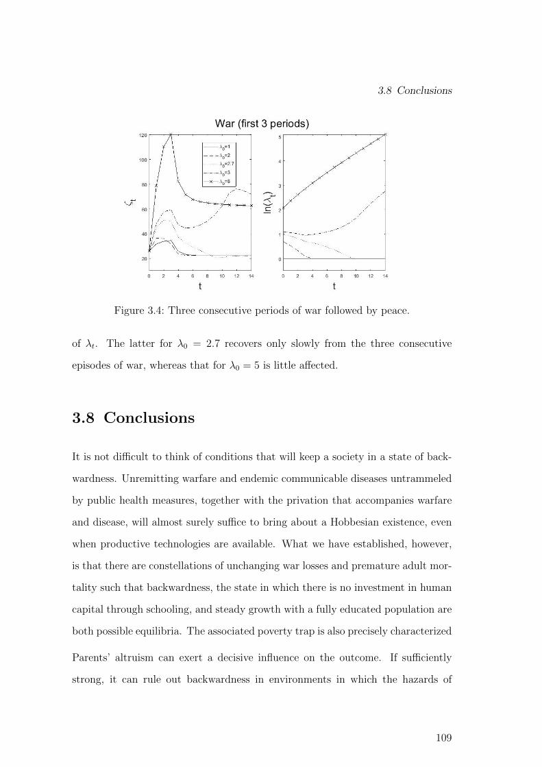
3.8 Conclusions
Figure 3.4: Three consecutive periods of war followed by peace.
of λt. The latter for λ0 = 2.7 recovers only slowly from the three consecutive
episodes of war, whereas that for λ0 = 5 is little affected.
3.8 Conclusions
It is not difficult to think of conditions that will keep a society in a state of back-
wardness. Unremitting warfare and endemic communicable diseases untrammeled
by public health measures, together with the privation that accompanies warfare
and disease, will almost surely suffice to bring about a Hobbesian existence, even
when productive technologies are available. What we have established, however,
is that there are constellations of unchanging war losses and premature adult mor-
tality such that backwardness, the state in which there is no investment in human
capital through schooling, and steady growth with a fully educated population are
both possible equilibria. The associated poverty trap is also precisely characterized
Parents’ altruism can exert a decisive influence on the outcome. If sufficiently
strong, it can rule out backwardness in environments in which the hazards of
109
Chapter 3 Untimely destruction: pestilence, war, and accumulation in the long run
destruction are such as to keep a selfish population in that condition for good. That
is no great surprise. Where attaining – and maintaining – steady-state growth is
concerned, however, altruism also comes into play in a different way. If parents’
preferences are such that the sub-utility functions for their own consumption and
their children’s well-being in adulthood differ – which is highly likely – and the
former is more concave than the latter, then the only steady-state path other than
backwardness is progress: There is growth with a fully educated population. If,
however, the sub-utility function for own consumption is less concave than that for
the children’s human capital, then steady-state growth paths with an incompletely
educated population may exist, as may stationary paths. The same holds if parents
are perfectly selfish, so that provision for old age is the sole motive for investment.
Thus, not only does altruism tend to promote growth as an outcome, as expected,
but it may also lead to permanently faster growth.
The fact that outbreaks of war and pestilence are stochastic events introduces
a central role for expectations. It also raises the question of whether a growing
economy is sufficiently robust to withstand a series of adverse shocks. Mature
economies that have experienced growth for long periods will have large per capita
stocks of human and physical capital. They will be correspondingly robust, unless
nuclear war destroys the environment itself. Economies at an earlier stage of
development are more vulnerable. Numerical simulations in which the realized
outcome is three consecutive periods of war followed by a confidently expected era
of perpetual peace reveal how the boundary conditions at the start have a decisive
influence on whether this series of shocks will pitch the economy into permanent
backwardness.
110
Chapter 4
Capital flows and endogenous growth
Abstract
So-called “uphill capital flows”, i.e. flows of physical capital from relatively poor
to rich countries, are a new phenomenon with yet unclear impact.1 We develop a
unified framework incorporating economic institutions, human capital and physical
capital to study the interaction of international capital flows and growth. Analyt-
ically, we study conditions under which a positive change of a country’s economic
institutions can attract inflows of physical capital from abroad, leading to long-
term growth via the accumulation of human capital. Our mechanism shows how a
small initial difference in the level of institutions can lead to substantial divergence
in income over time. We derive conditions under which a country receives inflows
of capital over time and increases its investment in human capital. Finally, we
provide simulations to illustrate our results.
4.1 Introduction
Motivation
Are international capital flows a cause for growth inequality between countries?
1This chapter is single-authored.
111
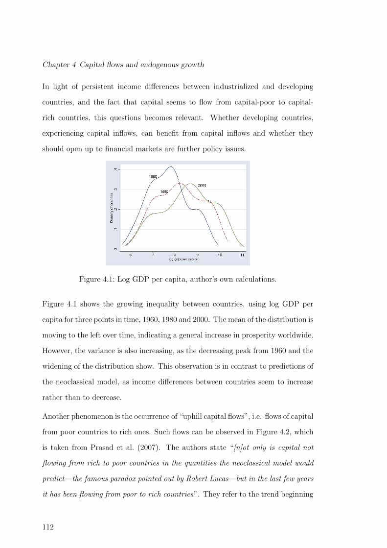
Chapter 4 Capital flows and endogenous growth
In light of persistent income differences between industrialized and developing
countries, and the fact that capital seems to flow from capital-poor to capital-
rich countries, this questions becomes relevant. Whether developing countries,
experiencing capital inflows, can benefit from capital inflows and whether they
should open up to financial markets are further policy issues.
Figure 4.1: Log GDP per capita, author’s own calculations.
Figure 4.1 shows the growing inequality between countries, using log GDP per
capita for three points in time, 1960, 1980 and 2000. The mean of the distribution is
moving to the left over time, indicating a general increase in prosperity worldwide.
However, the variance is also increasing, as the decreasing peak from 1960 and the
widening of the distribution show. This observation is in contrast to predictions of
the neoclassical model, as income differences between countries seem to increase
rather than to decrease.
Another phenomenon is the occurrence of “uphill capital flows”, i.e. flows of capital
from poor countries to rich ones. Such flows can be observed in Figure 4.2, which
is taken from Prasad et al. (2007). The authors state “[n]ot only is capital not
flowing from rich to poor countries in the quantities the neoclassical model would
predict—the famous paradox pointed out by Robert Lucas—but in the last few years
it has been flowing from poor to rich countries”. They refer to the trend beginning
112
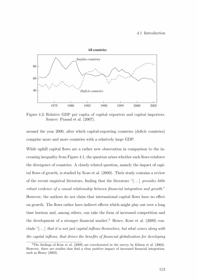
4.1 Introduction
All countries
40
60
80
1975
Excluding China and United States
Deficit countries
Surplus countries
Surplus countries
Deficit countries
200520001995199019851980
40
60
80
1975 200520001995199019851980
Figure 2. Relative GDP per Capita of Capital Exporters and Capital Importers,1970–2005a
10657-03a_Prasad.qxd 8/16/07 11:38 AM Page 155
Figure 4.2: Relative GDP per capita of capital exporters and capital importers.Source: Prasad et al. (2007).
around the year 2000, after which capital-exporting countries (deficit countries)
comprise more and more countries with a relatively large GDP.
While uphill capital flows are a rather new observation in comparison to the in-
creasing inequality from Figure 4.1, the question arises whether such flows reinforce
the divergence of countries. A closely related question, namely the impact of capi-
tal flows of growth, is studied by Kose et al. (2009). Their study contains a review
of the recent empirical literature, finding that the literature “[. . . ] provides little
robust evidence of a causal relationship between financial integration and growth.”
However, the authors do not claim that international capital flows have no effect
on growth. The flows rather have indirect effects which might play out over a long
time horizon and, among others, can take the form of increased competition and
the development of a stronger financial market.2 Hence, Kose et al. (2009) con-
clude “[. . . ] that it is not just capital inflows themselves, but what comes along with
the capital inflows, that drives the benefits of financial globalization for developing
2The findings of Kose et al. (2009) are corroborated in the survey by Edison et al. (2002).However, there are studies that find a clear positive impact of increased financial integration,such as Henry (2003).
113
Chapter 4 Capital flows and endogenous growth
countries.”
The possible interaction described by Kose et al. (2009) has not been modeled up
to now. Such a model is our goal in this chapter. We provide a framework where
international capital flows are related to and interact with well-known causes of
growth. This way, we describe some ideas concerning structures of international
capital flows and endogenous growth. We aim at providing a framework for future
empirical research. Following North and Thomas (1973), we assume that causes
of growth can be either proximate, such as accumulation of factors and technolog-
ical change, or fundamental, such as political and economic institutions. Hereby
“fundamental” means that without well designed institutions, no growth-driving
accumulation of factors is possible in an economy.3 We align those two causes of
growth with international capital flows in a unified framework. Our main idea is
that better economic institutions, which will be the fundamental cause for growth,
attract international capital flows. These, in turn, set the proximate causes in
motion. The proximate source of endogenous growth will be the accumulation of
human capital.
Our choice to combine economic institutions and human capital is based on the
idea shown in Figure 4.3. Since there is little direct impact of capital flows on
growth, we argue that capital can only have an impact via variables that interact
with growth themselves. Hence, our approach requires variables correlating with
international capital flows and growth.
There is a consensus that economic institutions and the accumulation of human
capital are paramount for economic growth4. Their correlation with international
3For a thorough discussion about the reasons and ways, in which institutions are a funda-mental cause for growth, see Acemoglu et al. (2004).
4There is an extensive literature, respectively, for the case of human capital and for the caseof institutions. For the former, some examples are work like Lucas (1989), Romer (1989), Barro(1991) and Mankiw et al. (1992). Pelinsecu (2014) provides a survey, including more recent work.For the latter, some examples are work like Acemoglu et al. (2001), Acemoglu et al. (2002), and
114

4.1 Introduction
capital flows has been demonstrated in several studies, for economic institutions
in work like Olsen et al. (2000), Alfaro et al. (2008) and Kose et al. (2009), and
for human capital in Lucas (1990) and Caselli and Feyrer (2007), for instance.5
Figure 4.3: Interaction of international capital with growth. Source: Author’sdesign.
After having chosen the variables that are relevant for our approach, the question
remains how these variables interact with each other. We build on the idea that
good economic institutions enable the accumulation of factors, such as physical
and human capital, or the raise of the technology level. In turn, the accumulation
of factors then leads to growth. We take this narrative and re-position it in an
international setting to formulate the following mechanism:
1. Better economic institutions allow agents to reap the benefits of their invest-
ment in physical capital. This interpretation is in line with Acemoglu et al.
(2004) that “[e]conomic institutions matter for economic growth because they
shape the incentives of key economic actors in society, in particular, they in-
fluence investments in physical and human capital [...]”.
2. The country with a larger return to capital will attract capital flows.
3. Capital inflows increase wages and hence agents have enough income to re-
duce labor supply and invest some time in the formation of human capital.
Hall and Jones (1999). Glaeser et al. (2004) provides a critical overview.5For an overview of other determinants of international capital flows, see Taylor and Sarno
(1997).
115
Chapter 4 Capital flows and endogenous growth
4. Human capital is not depreciated but accumulated, allowing for long-term
growth.
Approach and results
We use an OLG model with three generations, consisting of children, adults and
seniors. Children can either work or form human capital through schooling. Adults
work, save and decide whether to school their children. Seniors only consume. We
have two countries and a single good, produced with physical and human capital,
embodied in labor. Capital can move freely between the countries while labor
cannot. Both countries have economic institutions, determining the net return on
physical capital. Initially, arbitrage ensures that returns are equal across countries.
Then, a country experiences an improvement in its institutions and a subsequent
increase in its return to capital. Capital flows in and wages increase. We examine
whether the wage increase is sufficient for adults to send their children to school.
Schooling leads to the formation of human capital that can be used without costs
in the next period.
We demonstrate how a change in institutions, coupled with international capi-
tal, can generate differences in economic growth. While the country with better
economic institutions moves to a balanced growth path with increasing levels of
human capital, the other remains in a zero growth steady state. Furthermore, we
study the existence of different steady states and convergence to them.
Throughout our work, we interpret capital flows as private flows of foreign direct
investment (FDI). By doing this, our model can replicate the empirical findings
of Gourinchas and Jeanne (2013) and Alfaro et al. (2014), where the authors find
that public capital flows behave differently than private ones. Only private capital
flows to countries with higher growth rates. In a simulation, the country with
116

4.1 Introduction
increasing investment in education experiences increasing productivity growth,
attracting more capital. Hence, we establish a positive correlation between pro-
ductivity growth and inflows of capital.
Relation to the literature
Our work is closely related to studies that use the neoclassical growth model in an
international setting, such as Barro et al. (1992), Gourinchas and Jeanne (2006),
and Aguiar and Amador (2011). The authors study the impact of capital flows
on the convergence of an economy to a steady state. While Aguiar and Amador
(2011) focuse on explaining the behavior of governments, Barro et al. (1992) and
Gourinchas and Jeanne (2006) consider an economy where the steady state is a
balanced growth path with a constant growth rate. In both studies, the production
function accounts for human capital formation and growth is exogenous, driven
by technological progress. These studies show that inflows of capital have a rather
small effect on the convergence path. Our findings are consistent with this result.
However, our study differs in third crucial ways: First, we do not assume a constant
world rate of return. Instead, the flows of physical capital and the accumulation of
physical and human capital in a period will determine, whether a country can also
attract capital inflows in the next period. Second, we do not study the speed of
convergence, but we are interested in the question, whether a country can escape
a poverty trap and converge to a steady state with a constant rate. We provide
analytical conditions for such an escape. Third, we consider an exogenous growth
model in which growth stems from the accumulation of human capital.
Another study that analyzes a neoclassical growth model is Davenport (2018).
However, Davenport (2018) studies the importance of expectation formation for
international capital flows and growth. The authors are able to replicate sub-
117
Chapter 4 Capital flows and endogenous growth
stantial current account imbalances. However, she assumes an exogenous growth
process, where countries catch up to a technological frontier. We endogenize the
growth process and relate it to the structure of capital flows, making them inter-
dependent.
Howitt (2000) provides an alternative to the neoclassical model approach. He
constructs a multi-country model with elements of the Solow-Swan-model and
the Schmupeterian growth model to explain cross-country differences in growth.
Countries that invest in R&D will grow at a positive rate, while those who are
not able to do so, are stuck with the same output. Howitt (2000) abstracts,
however, from international capital flows, which are now incorporated in our work.
Furthermore, we highlight the importance of economic institutions and include
the accumulation of human capital instead of technological progress as the main
driving force of long-term growth.
Our study is also related to Bell et al. (2019), where the authors construct an
OLG model with endogenous growth. As in this work, growth is driven by the
accumulation of human capital through schooling and the effects of exogenous
shocks are studied in a closed economy. We take some of the central assumptions
and reassess them in an international setting with capital flows. Also, we include
a central role for institutions in our setting.
Finally, this chapter is related to other works about international capital flows
that, however, either focus on the international asset structure, such as Caballero
et al. (2008) and Cedric and Van Wincoop (2010), or on the international trade
structure, such as Jin (2012). While our model incorporates international assets,
it does it in a simple way, allowing us to focus on the interaction of capital flows
and growth and to show the causes for international inequality.
118
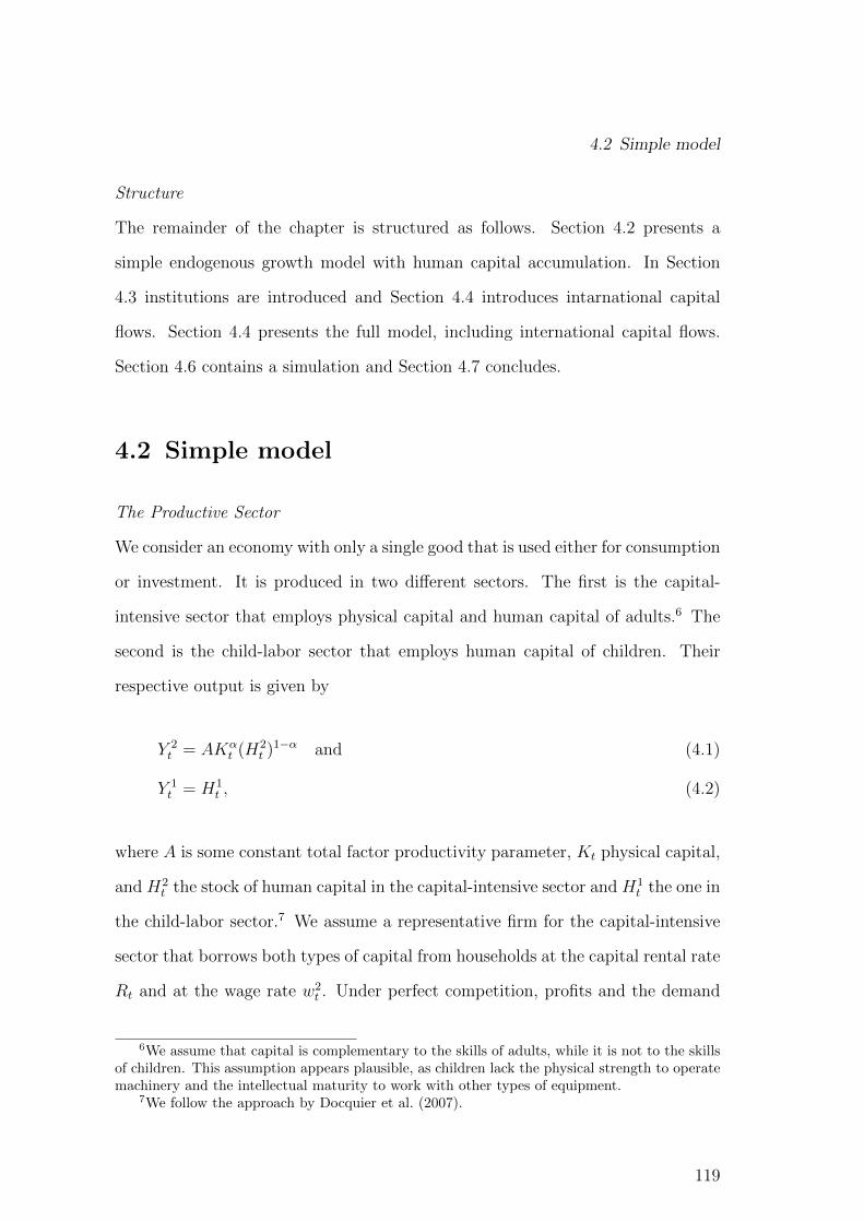
4.2 Simple model
Structure
The remainder of the chapter is structured as follows. Section 4.2 presents a
simple endogenous growth model with human capital accumulation. In Section
4.3 institutions are introduced and Section 4.4 introduces intarnational capital
flows. Section 4.4 presents the full model, including international capital flows.
Section 4.6 contains a simulation and Section 4.7 concludes.
4.2 Simple model
The Productive Sector
We consider an economy with only a single good that is used either for consumption
or investment. It is produced in two different sectors. The first is the capital-
intensive sector that employs physical capital and human capital of adults.6 The
second is the child-labor sector that employs human capital of children. Their
respective output is given by
Y 2t = AKα
t (H2t )1−α and (4.1)
Y 1t = H1
t , (4.2)
where A is some constant total factor productivity parameter, Kt physical capital,
and H2t the stock of human capital in the capital-intensive sector and H1
t the one in
the child-labor sector.7 We assume a representative firm for the capital-intensive
sector that borrows both types of capital from households at the capital rental rate
Rt and at the wage rate w2t . Under perfect competition, profits and the demand
6We assume that capital is complementary to the skills of adults, while it is not to the skillsof children. This assumption appears plausible, as children lack the physical strength to operatemachinery and the intellectual maturity to work with other types of equipment.
7We follow the approach by Docquier et al. (2007).
119
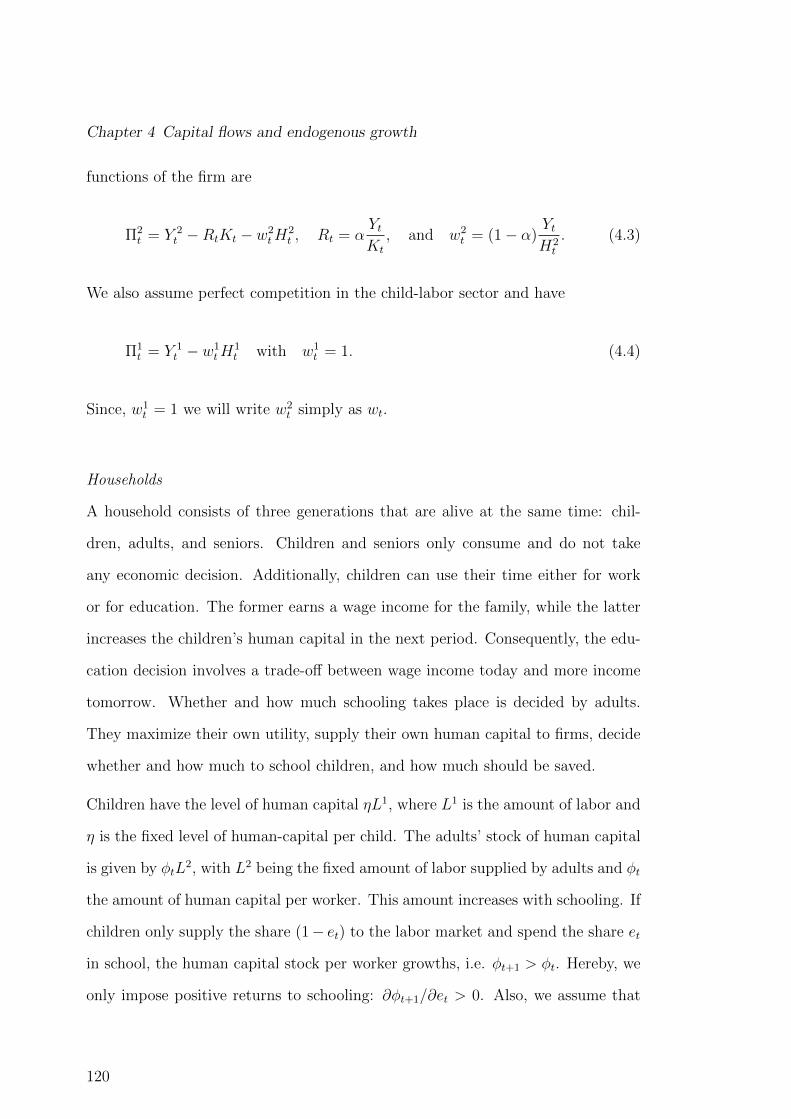
Chapter 4 Capital flows and endogenous growth
functions of the firm are
Π2t = Y 2
t −RtKt − w2tH
2t , Rt = α
YtKt
, and w2t = (1− α)
YtH2t
. (4.3)
We also assume perfect competition in the child-labor sector and have
Π1t = Y 1
t − w1tH
1t with w1
t = 1. (4.4)
Since, w1t = 1 we will write w2
t simply as wt.
Households
A household consists of three generations that are alive at the same time: chil-
dren, adults, and seniors. Children and seniors only consume and do not take
any economic decision. Additionally, children can use their time either for work
or for education. The former earns a wage income for the family, while the latter
increases the children’s human capital in the next period. Consequently, the edu-
cation decision involves a trade-off between wage income today and more income
tomorrow. Whether and how much schooling takes place is decided by adults.
They maximize their own utility, supply their own human capital to firms, decide
whether and how much to school children, and how much should be saved.
Children have the level of human capital ηL1, where L1 is the amount of labor and
η is the fixed level of human-capital per child. The adults’ stock of human capital
is given by φtL2, with L2 being the fixed amount of labor supplied by adults and φt
the amount of human capital per worker. This amount increases with schooling. If
children only supply the share (1− et) to the labor market and spend the share et
in school, the human capital stock per worker growths, i.e. φt+1 > φt. Hereby, we
only impose positive returns to schooling: ∂φt+1/∂et > 0. Also, we assume that
120
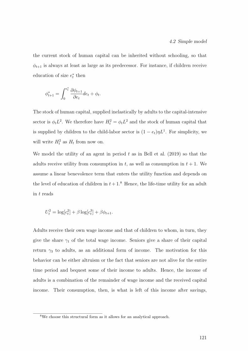
4.2 Simple model
the current stock of human capital can be inherited without schooling, so that
φt+1 is always at least as large as its predecessor. For instance, if children receive
education of size e∗t then
φ∗t+1 =
∫ e∗t
0
∂φt+1
∂etdet + φt.
The stock of human capital, supplied inelastically by adults to the capital-intensive
sector is φtL2. We therefore have H2
t = φtL2 and the stock of human capital that
is supplied by children to the child-labor sector is (1 − et)ηL1. For simplicity, we
will write H2t as Ht from now on.
We model the utility of an agent in period t as in Bell et al. (2019) so that the
adults receive utility from consumption in t, as well as consumption in t + 1. We
assume a linear benevolence term that enters the utility function and depends on
the level of education of children in t+ 1.8 Hence, the life-time utility for an adult
in t reads
U2t = log[c2t ] + β log[c3t ] + βφt+1.
Adults receive their own wage income and that of children to whom, in turn, they
give the share γ1 of the total wage income. Seniors give a share of their capital
return γ3 to adults, as an additional form of income. The motivation for this
behavior can be either altruism or the fact that seniors are not alive for the entire
time period and bequest some of their income to adults. Hence, the income of
adults is a combination of the remainder of wage income and the received capital
income. Their consumption, then, is what is left of this income after savings,
8We choose this structural form as it allows for an analytical approach.
121

Chapter 4 Capital flows and endogenous growth
leading to the following utility function:
U2t = log
[(1− γ1)(wtHt + (1− et)ηL1) + γ3KtRt − st
]
+ β log [(1− γ3)Rt+1st] + βφt+1.
(4.5)
We make an additional assumption, and say that the income that is paid to children
is only used for consumption and does not enter the savings decision. The rational
is that this assumption simplifies the analysis strongly. However, it can be argued
that parents only then send their children to work when it is necessary, i.e. when
the family goes hungry otherwise. They do not ask their children to work in order
to save and accumulate capital. In the following, we will refer to the income of
adults that accrues from capital and adult human capital as “income”, while the
sum of capital income, wage paid to adults, and wage paid to children will be
called “total income”. Hence, maximizing with respect to savings yields
∂U2t
∂st=
−1
(1− γ1)wtHt + γ3RtKt − st+β
st= 0, (4.6)
while maximizing with respect to education yields
∂U2t
∂et=
−(1− γ1)ηL1
(1− γ1)(wtHt + (1− et)ηL1) + γ3RtKt − st+ βφ′t+1 ≤ 0 for et ≥ 0,
(4.7)
∂U2t
∂et=
−(1− γ1)ηL1
(1− γ1)(wtHt + (1− et)ηL1) + γ3RtKt − st+ βφ′t+1 ≥ 0 for et ≤ 1,
(4.8)
Solving (4.6) for st, we obtain
st =β
1 + β((1− γ1)wtHt + γ3RtKt) .
122
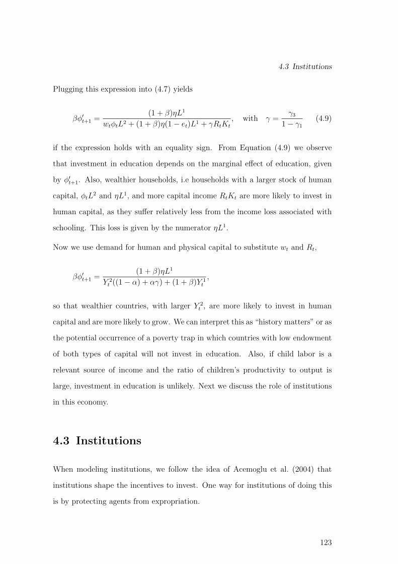
4.3 Institutions
Plugging this expression into (4.7) yields
βφ′t+1 =(1 + β)ηL1
wtφtL2 + (1 + β)η(1− et)L1 + γRtKt
, with γ =γ3
1− γ1(4.9)
if the expression holds with an equality sign. From Equation (4.9) we observe
that investment in education depends on the marginal effect of education, given
by φ′t+1. Also, wealthier households, i.e households with a larger stock of human
capital, φtL2 and ηL1, and more capital income RtKt are more likely to invest in
human capital, as they suffer relatively less from the income loss associated with
schooling. This loss is given by the numerator ηL1.
Now we use demand for human and physical capital to substitute wt and Rt,
βφ′t+1 =(1 + β)ηL1
Y 2t ((1− α) + αγ) + (1 + β)Y 1
t
,
so that wealthier countries, with larger Y 2t , are more likely to invest in human
capital and are more likely to grow. We can interpret this as “history matters” or as
the potential occurrence of a poverty trap in which countries with low endowment
of both types of capital will not invest in education. Also, if child labor is a
relevant source of income and the ratio of children’s productivity to output is
large, investment in education is unlikely. Next we discuss the role of institutions
in this economy.
4.3 Institutions
When modeling institutions, we follow the idea of Acemoglu et al. (2004) that
institutions shape the incentives to invest. One way for institutions of doing this
is by protecting agents from expropriation.
123
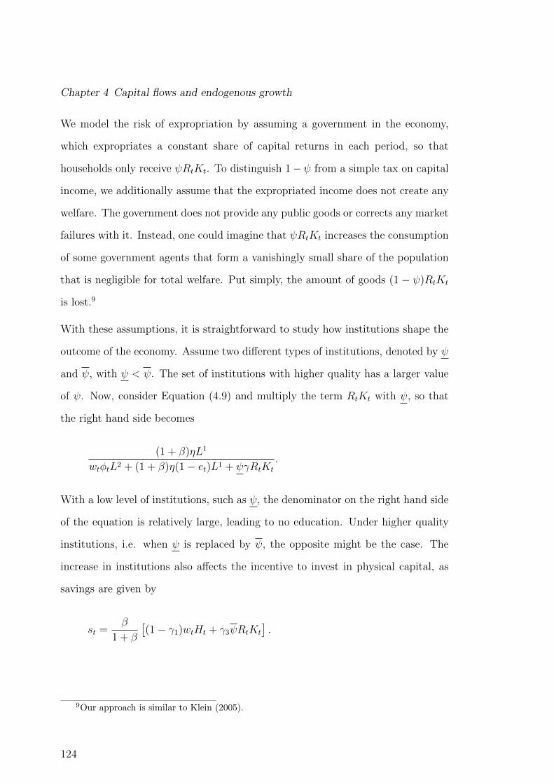
Chapter 4 Capital flows and endogenous growth
We model the risk of expropriation by assuming a government in the economy,
which expropriates a constant share of capital returns in each period, so that
households only receive ψRtKt. To distinguish 1−ψ from a simple tax on capital
income, we additionally assume that the expropriated income does not create any
welfare. The government does not provide any public goods or corrects any market
failures with it. Instead, one could imagine that ψRtKt increases the consumption
of some government agents that form a vanishingly small share of the population
that is negligible for total welfare. Put simply, the amount of goods (1− ψ)RtKt
is lost.9
With these assumptions, it is straightforward to study how institutions shape the
outcome of the economy. Assume two different types of institutions, denoted by ψ
and ψ, with ψ < ψ. The set of institutions with higher quality has a larger value
of ψ. Now, consider Equation (4.9) and multiply the term RtKt with ψ, so that
the right hand side becomes
(1 + β)ηL1
wtφtL2 + (1 + β)η(1− et)L1 + ψγRtKt
.
With a low level of institutions, such as ψ, the denominator on the right hand side
of the equation is relatively large, leading to no education. Under higher quality
institutions, i.e. when ψ is replaced by ψ, the opposite might be the case. The
increase in institutions also affects the incentive to invest in physical capital, as
savings are given by
st =β
1 + β
[(1− γ1)wtHt + γ3ψRtKt
].
9Our approach is similar to Klein (2005).
124
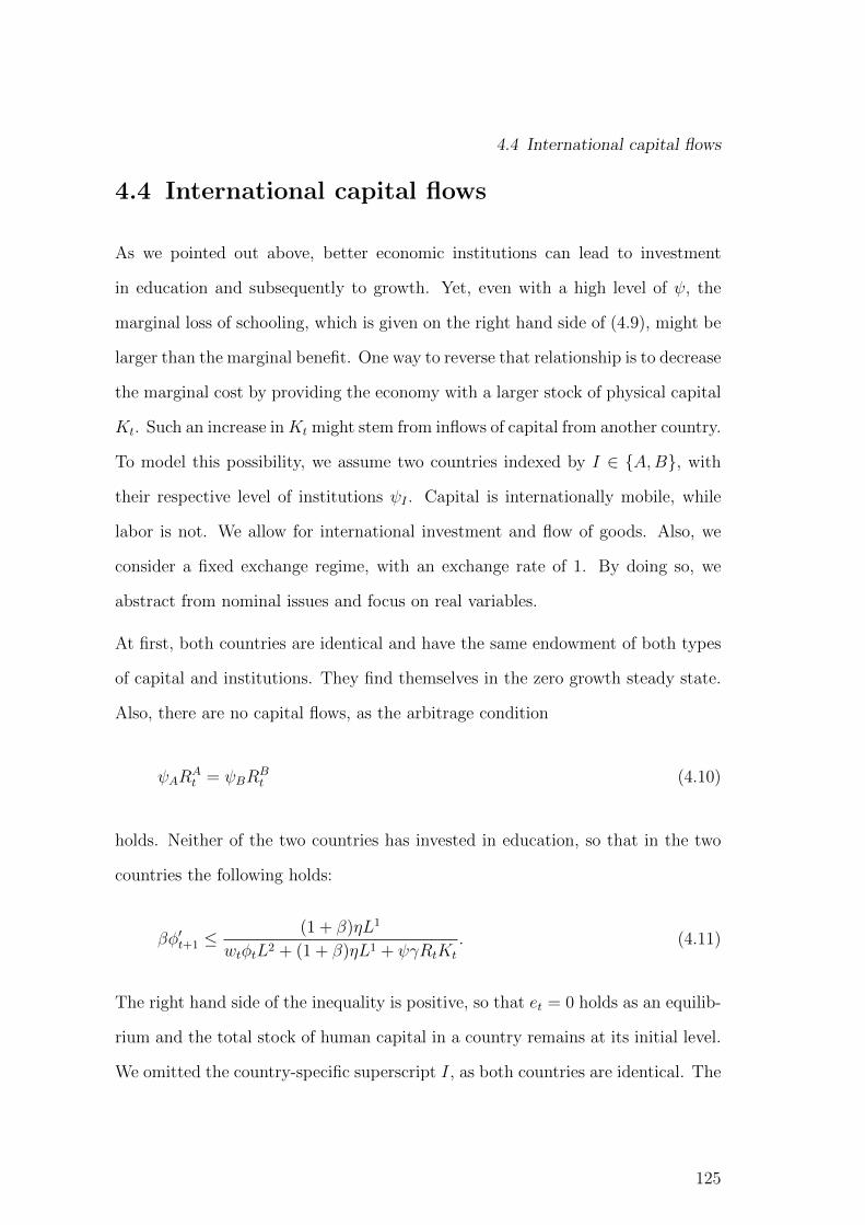
4.4 International capital flows
4.4 International capital flows
As we pointed out above, better economic institutions can lead to investment
in education and subsequently to growth. Yet, even with a high level of ψ, the
marginal loss of schooling, which is given on the right hand side of (4.9), might be
larger than the marginal benefit. One way to reverse that relationship is to decrease
the marginal cost by providing the economy with a larger stock of physical capital
Kt. Such an increase inKt might stem from inflows of capital from another country.
To model this possibility, we assume two countries indexed by I ∈ {A,B}, with
their respective level of institutions ψI . Capital is internationally mobile, while
labor is not. We allow for international investment and flow of goods. Also, we
consider a fixed exchange regime, with an exchange rate of 1. By doing so, we
abstract from nominal issues and focus on real variables.
At first, both countries are identical and have the same endowment of both types
of capital and institutions. They find themselves in the zero growth steady state.
Also, there are no capital flows, as the arbitrage condition
ψARAt = ψBR
Bt (4.10)
holds. Neither of the two countries has invested in education, so that in the two
countries the following holds:
βφ′t+1 ≤(1 + β)ηL1
wtφtL2 + (1 + β)ηL1 + ψγRtKt
. (4.11)
The right hand side of the inequality is positive, so that et = 0 holds as an equilib-
rium and the total stock of human capital in a country remains at its initial level.
We omitted the country-specific superscript I, as both countries are identical. The
125

Chapter 4 Capital flows and endogenous growth
stock of physical capital is fixed and is given by
K =
(βA
1 + β[(1− γ1)(1− α) + αψγ3]
) 11−α
H, (4.12)
where H is the initial stock of human capital of adults in the economy. Hence, we
define the zero growth steady state in the following way:
Definition 3 In a zero growth steady state, international capital flows are absent
and countries do not invest in education, i.e. (4.10) and (4.11) hold. Furthermore,
the stock of physical capital is constant and given by (4.12). Wages, interest rates,
profits and output are constant and given by (4.1)− (4.4).
Next, we allow for heterogeneous institutions across countries.
Change in institutions
In period t, before agents have decided about education, Institutions in country A
improve from ψA to ψA, so that we have ψARAt > ψBR
Bt . Hence, capital flows from
country B to A until returns are equalized again, affecting the education decision.
Let us turn to the sequence of events , which can be seen in Figure 4.4. Initially, we
Figure 4.4: Sequence of events.
have a positive change in the quality of institutions in country A. The improvement
126

4.5 The full model
leads to an inflow of capital and a change in income. Agents in both countries
now face their respective new income. As this is the income before adults decide
whether children should receive a positive amount of schooling, we call this income
their pre-education income. If agents decide to school children, the total supply
of human capital, given by Ht + (1− et)ηL1, decreases in the respective country.
4.5 The full model
Given that capital markets pay the marginal return of capital we have
ψA(KAt )α−1 = ψB(KB
t )α−1 ⇒ KAt =
(ψAψB
) 11−α
KBt , (4.13)
where KAt and KB
t are the capital stocks after capital movements from B to A.
We have KBt = KB
t − (KAt −KA
t ), where we assume that initially, KBt = KA
t , and
where we use the result for KAt to obtain
KBt = 2KB
t −(ψAψB
) 11−α
KBt ⇒ KB
t = 2
1 +
(ψAψB
) 11−α−1
KBt .
Intuitively, the new capital stock KBt depends on the ratio of institutions. The
number 2 on the right hand side stems from the assumption that initial capital
stocks are equal and the factor with exponent −1 shows how capital is allocated
between countries. Using (4.13), we obtain
KAt = 2
(ψAψB
) 11−α1 +
(ψAψB
) 11−α−1
KAt
127
Chapter 4 Capital flows and endogenous growth
for the new capital stock in A. One of the factors on the right hand side is increasing
in ψA, while the other is decreasing. The increasing part stems from the arbitrage
condition which yields that better economic institutions in A must increase the
capital stock in A compared to the one in B. The decreasing part stems from the
fact that better economic institutions in A mean that the final capital stock in B
is already smaller than it initially was, leaving less capital to flow to A. These two
forces offset each other in the limit, as
limψA→∞
KAt = 2KA
t ,
which is necessary, as the total initial endowment of capital is 2KAt . Of course, KA
t
is strictly increasing in the relative level of institutions, as one can see by slightly
rewriting the expression above,
KAt = 2
1 +
(ψAψB
) −11−α−1
KAt .
Income change
So far, a change in institutions triggers international capital flows. These flows
impact the income of households in both countries. For country A, we observe the
following: Before capital flows, its capital income was given by ψARAt K
At , after
capital flows, it is given by ψARAt K
At . We form the ratio of both
ψARAt K
At
ψARAt K
At
=ψBψA
2α−1
1 +
(ψAψB
) 11−α
1−α
.
This term can be either larger or smaller than one. Its size depends on three things:
First, on the improvement in institutions vis-a-vis the status quo ψA, second, on
the improvement relative to the institutions of country ψB and third, on the initial
128

4.5 The full model
allocation of capital, which is now represented by the number 2. These three issues
decide whether the improvement of institutions is so strong that the net return
rises although the marginal return to capital decreases in light of capital inflows.
Under our initial assumption that ψB = ψA, the income ratio is 1 if no change
occurs, i.e. ψA = ψB. If ψA > ψB then the income from capital increases above 1,
as the factor on the right hand side is a strictly increasing function in the ratio of
institutions ψAψB
.
Now let us study the relative change in labor income of adults, given by
wAt HAt
wAt HAt
=
(KAt
KAt
)α
= 2α
1 +
(ψAψB
) −11−α−α
.
We use wAt to denote the wage after capital flows and recall that there is no positive
level of education yet. We see that the ratio is 1 for ψA = ψB. For ψA > ψB, it
is larger than one because the expression on the right hand side is increasing in
ψA/ψB, as we have shown above.
Now let us turn to the income of agents in the capital-exporting country B. The
capital income of agents in B is the same as in A, and thus increases. The wage
income, however, decreases as the total local capital stock used in production in
B becomes smaller. This is reflected in the following ratio:
wBt HBt
wBt HBt
=
(KBt
KBt
)α
= 2α
1 +
(ψAψB
) 11−α−α
,
which is smaller than 1. With capital and wage income moving in opposite di-
rections, we study the net effect on income in B. The disposable income of adults
without earnings of their children, IBt = (1 − γ1)wBt H
Bt + ψBγ3R
Bt K
Bt , can be
129
Chapter 4 Capital flows and endogenous growth
written as
IBt =A(HBt )1−α(KB
t )α(
(1− α)(1− γ1) + αψBγ3(KBt )−1KB
t
)
=A(HBt )1−α(KB
t )α2α
1 +
(ψAψB
) 11−α−α
·
(1− α)(1− γ1) +
α
2ψBγ3
1 +
(ψAψB
) 11−α .
Taking the derivative of IBt with respect to ψA provides the first proposition.
Proposition 17 Given an initially symmetric allocation of capital between coun-
try A and B, the income in B decreases after capital flows if and only if
ψBγ
2<
1 +
(ψAψB
) 11−α−1
. (4.14)
The pre-education income in country A increases unambiguously.
We provide a short proof in the Appendix for Chapter 4. Proposition 17 implies
that the three factors, we encountered before, determine the change in income.
First, the relative increase in institutions is crucial, as can be seen from the right
hand side. Second, the initial level of institutions, represented by ψB on the right
hand side, is also important. Third, the number 2, on the left hand side of the
inequality, shows that the initial allocation of capital determines the outcome as
well. If we did not assume that the initial stocks of capital are equal, the number
2 would be replaced by the term KBt /(K
Bt +KA
t ).
To clarify, let us consider two examples. In the first, country B is relatively rich in
capital and has good institutions, i.e. ψB is relatively large. If country A strongly
improves its institutions with ψA significantly larger than ψB, then the income in
130

4.5 The full model
country B actually increases. Country B loses some wage income, though, because
it is rich in capital and can reap the benefits of investment. It is more than
compensated by the larger return on capital and larger capital income. In the
second example, Country B has a low share in world capital and comparatively
weak institutions. If, in this case, country A improves its institutions slightly,
country B will actually incur a decrease in income.
We also provide a more general approach to study the income change in B. For
this, we write the income in B after capital flows but before any education decision,
on the left hand side of the following inequality:
(1− γ1)wBt HBt + γ3ψBR
Bt K
Bt ≥ (1− γ1)wBt HB
t + γ3ψBRBt K
Bt .
The right hand side is the income before capital flows occur. Substituting wages
and interest rates before and after capital flows yields
G
(KBt
KBt
)≥ 1 with
G
(KBt
KBt
)=
(KBt
KBt
)α (1− α)(1− γ1) + αψBγ3KBt
KBt
(1− α)(1− γ1) + αψBγ3.
We define KBt /K
Bt as x, so that the above expression is 1 for x = 1, i.e. all local
capital is utilized in production. The derivative of G(x) is
α(1− α)xα−1(
1− γ1 −ψBγ3x
).
It has a global minimum at xmin = ψBγ3
1−γ1 and is strictly increasing to the left
and right of it, making G(x) strictly convex. If γ3 is similar to 1−γ1 the minimum
lies to the left of x = 1, with G(xmin) < 1. Due to the strict convexity and the
131
Chapter 4 Capital flows and endogenous growth
fact that limx→0
G(x) → ∞, there must be an x between [0, ψBγ], such that G(x) is
equal to 1. Hence, income in country B increases or decreases, depending on the
size of capital flows and the subsequent ratio of capital used in local production
to the total amount of initial capital. If capital outflows are very large, reducing
KBt strongly relative to KB
t , then country B will actually experience an increase
in its income. One determining factor is certainly the change in institutions in A.
The larger the change, the larger capital outflows from B will be, and the larger
capital outflows from B, the better the chances for B to benefit in net from it. Let
us assume for the following that income in B decreases.
Finally, we provide the income net of the earnings of children in A,
IAt =A(HAt )1−α(KA
t )α2α
1 +
(ψAψB
) −11−α−α
·
(1− γ1)(1− α) +
αψAγ32
1 +
(ψAψB
) −11−α .
(4.15)
We have established that wage and capital income in country A increase and con-
sequently lead to an increase of income. With larger income, savings in A also
increase.
Education decision
A change in wealth might alter the decision about schooling. To see this, consider
Equation (4.11), where we assumed that before capital flows, neither country in-
vests in education. The marginal benefits on the left hand side of the inequality
are equal to or smaller than the marginal income loss at zero education. The
marginal loss will be even larger if the country’s income has decreased. This is
what has happened in B. Thus, we are certain that country B does not invest into
132

4.5 The full model
education after the change in institutions in A.
We have seen that income increases in A. It enters the denominator of (4.11) allow-
ing the right hand side to be actually lower than φ′t+1(et = 0). If we additionally
assume that the marginal benefits of education are constant, there exists a value
for e∗t ∈ (0, 1] such that
βφ′t+1(e∗t ) =
(1 + β)(1− γ1)ηL1
A(φtL2)1−αKαt ΓAt + (1 + β)(1− γ1)(1− e∗t )ηL1
is fulfilled. We let ΓAt capture all remaining terms from Equation (4.15). Writing
the ratio ψAψB
as χ, we note that ΓAt increases in χ. To see this, recall the expression
for IAt from above. It is written as the product of income before capital flows,
A(HAt )1−α(KA
t )α, times the factor ΓAt . This factor must be larger than one, as we
have shown that income in A does increase due to capital inflows. Also, we have
shown that both components of income increase in χ, so that ΓAt must do this,
too. Alternatively, we can rewrite ΓAt as
2α(1− α)(1− γ1)(1 + χ−11−α )−α + α2α−1ψAγ3(1 + χ
−11−α )1−α,
noting that ψA = χψB. We see that both summands increase in χ. For further
analysis, it is useful to study whether households might choose a level of et that
lowers the family income below its initial level, i.e. the level that prevailed be-
fore the inflow of capital. This can occur, as investment in education reduces the
supply of human capital and also the earnings of children. We write the equation
from above as φ′t+1(e∗t ) = D(e∗t ,Γ
A), where D(.) is a function of the optimal value
of education and of the factor that scales output. Before capital flows, it held that
ΓA,0 = (1 − α)(1 − γ1) + αγ3ψA. In the initial steady state, we had φ′t+1(0) ≤
D(0,ΓA,0). After the inflow of capital, we assume that φ′t+1(0) > D(0,ΓAt ) holds.
133
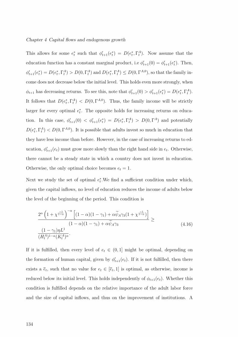
Chapter 4 Capital flows and endogenous growth
This allows for some e∗t such that φ′t+1(e∗t ) = D(e∗t ,Γ
At ). Now assume that the
education function has a constant marginal product, i.e φ′t+1(0) = φ′t+1(e∗t ). Then,
φ′t+1(e∗t ) = D(e∗t ,Γ
At ) > D(0,ΓAt ) and D(e∗t ,Γ
At ) ≤ D(0,ΓA,0), so that the family in-
come does not decrease below the initial level. This holds even more strongly, when
φt+1 has decreasing returns. To see this, note that φ′t+1(0) > φ′t+1(e∗t ) = D(e∗t ,Γ
At ).
It follows that D(e∗t ,ΓAt ) < D(0,ΓA,0). Thus, the family income will be strictly
larger for every optimal e∗t . The opposite holds for increasing returns on educa-
tion. In this case, φ′t+1(0) < φ′t+1(e∗t ) = D(e∗t ,Γ
At ) > D(0,ΓA) and potentially
D(e∗t ,ΓAt ) < D(0,ΓA,0). It is possible that adults invest so much in education that
they have less income than before. However, in the case of increasing returns to ed-
ucation, φ′t+1(et) must grow more slowly than the right hand side in et. Otherwise,
there cannot be a steady state in which a country does not invest in education.
Otherwise, the only optimal choice becomes et = 1.
Next we study the set of optimal e∗t .We find a sufficient condition under which,
given the capital inflows, no level of education reduces the income of adults below
the level of the beginning of the period. This condition is
2α(
1 + χ−11−α)−α [
(1− α)(1− γ1) + αψAγ3(1 + χ−11−α )
]
(1− α)(1− γ1) + αψAγ3≥
(1− γ1)ηL1
(HAt )1−α(KA
t )α.
(4.16)
If it is fulfilled, then every level of et ∈ (0, 1] might be optimal, depending on
the formation of human capital, given by φ′t+1(et). If it is not fulfilled, then there
exists a et, such that no value for et ∈ [et, 1] is optimal, as otherwise, income is
reduced below its initial level. This holds independently of φt+1(et). Whether this
condition is fulfilled depends on the relative importance of the adult labor force
and the size of capital inflows, and thus on the improvement of institutions. A
134
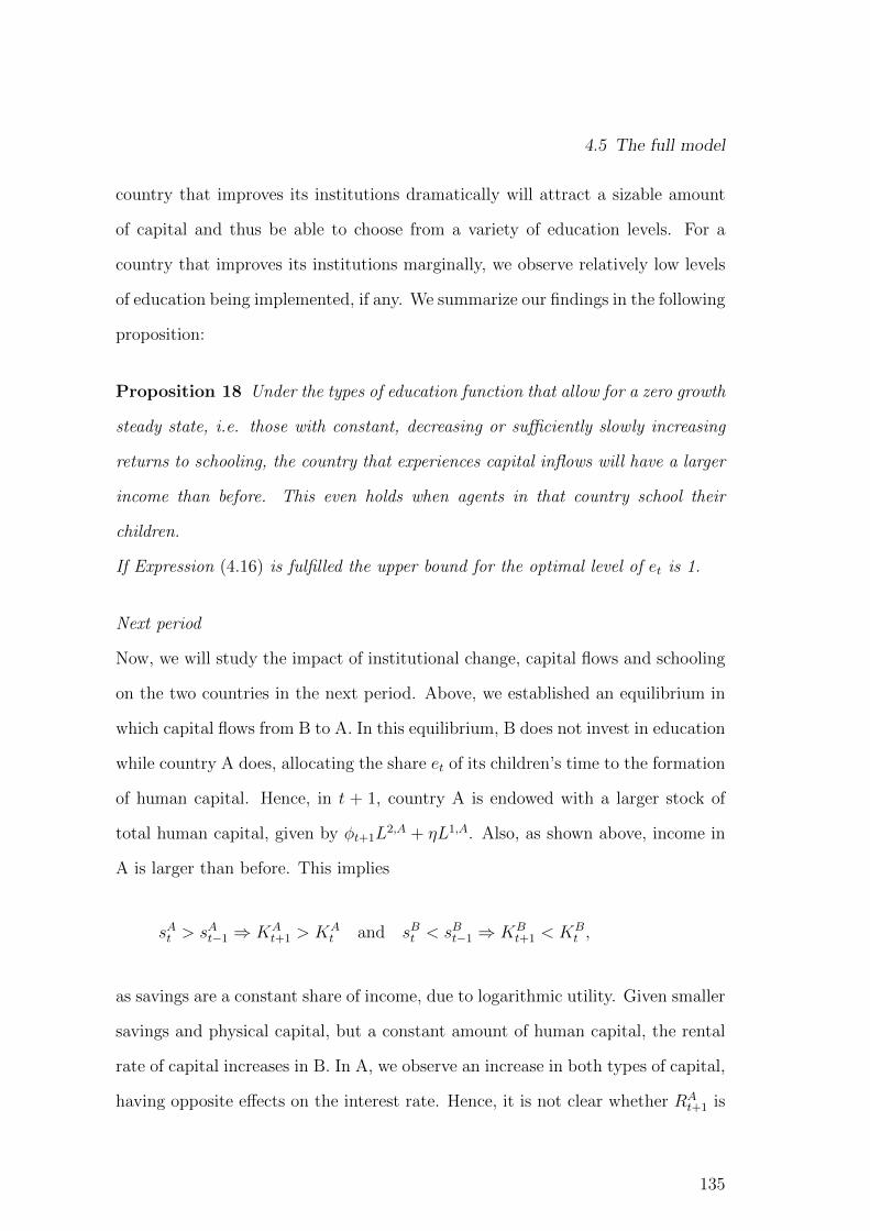
4.5 The full model
country that improves its institutions dramatically will attract a sizable amount
of capital and thus be able to choose from a variety of education levels. For a
country that improves its institutions marginally, we observe relatively low levels
of education being implemented, if any. We summarize our findings in the following
proposition:
Proposition 18 Under the types of education function that allow for a zero growth
steady state, i.e. those with constant, decreasing or sufficiently slowly increasing
returns to schooling, the country that experiences capital inflows will have a larger
income than before. This even holds when agents in that country school their
children.
If Expression (4.16) is fulfilled the upper bound for the optimal level of et is 1.
Next period
Now, we will study the impact of institutional change, capital flows and schooling
on the two countries in the next period. Above, we established an equilibrium in
which capital flows from B to A. In this equilibrium, B does not invest in education
while country A does, allocating the share et of its children’s time to the formation
of human capital. Hence, in t + 1, country A is endowed with a larger stock of
total human capital, given by φt+1L2,A + ηL1,A. Also, as shown above, income in
A is larger than before. This implies
sAt > sAt−1 ⇒ KAt+1 > KA
t and sBt < sBt−1 ⇒ KBt+1 < KB
t ,
as savings are a constant share of income, due to logarithmic utility. Given smaller
savings and physical capital, but a constant amount of human capital, the rental
rate of capital increases in B. In A, we observe an increase in both types of capital,
having opposite effects on the interest rate. Hence, it is not clear whether RAt+1 is
135
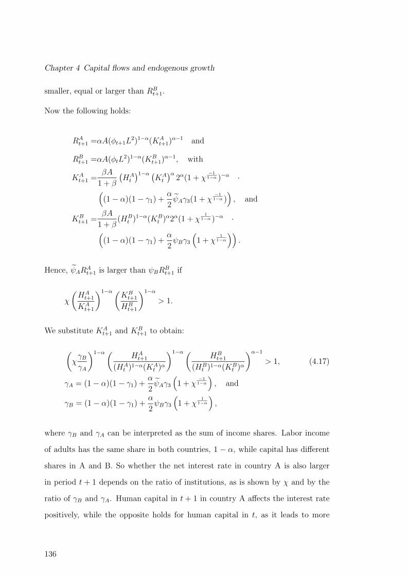
Chapter 4 Capital flows and endogenous growth
smaller, equal or larger than RBt+1.
Now the following holds:
RAt+1 =αA(φt+1L
2)1−α(KAt+1)
α−1 and
RBt+1 =αA(φtL
2)1−α(KBt+1)
α−1, with
KAt+1 =
βA
1 + β
(HAt
)1−α (KAt
)α2α(1 + χ
−11−α )−α ·
((1− α)(1− γ1) +
α
2ψAγ3(1 + χ
−11−α )
), and
KBt+1 =
βA
1 + β(HB
t )1−α(KBt )α2α(1 + χ
11−α )−α ·
((1− α)(1− γ1) +
α
2ψBγ3
(1 + χ
11−α))
.
Hence, ψARAt+1 is larger than ψBR
Bt+1 if
χ
(HAt+1
KAt+1
)1−α(KBt+1
HBt+1
)1−α> 1.
We substitute KAt+1 and KB
t+1 to obtain:
(χγBγA
)1−α( HAt+1
(HAt )1−α(KA
t )α
)1−α(HBt+1
(HBt )1−α(KB
t )α
)α−1> 1, (4.17)
γA = (1− α)(1− γ1) +α
2ψAγ3
(1 + χ
−11−α), and
γB = (1− α)(1− γ1) +α
2ψBγ3
(1 + χ
11−α),
where γB and γA can be interpreted as the sum of income shares. Labor income
of adults has the same share in both countries, 1 − α, while capital has different
shares in A and B. So whether the net interest rate in country A is also larger
in period t + 1 depends on the ratio of institutions, as is shown by χ and by the
ratio of γB and γA. Human capital in t + 1 in country A affects the interest rate
positively, while the opposite holds for human capital in t, as it leads to more
136
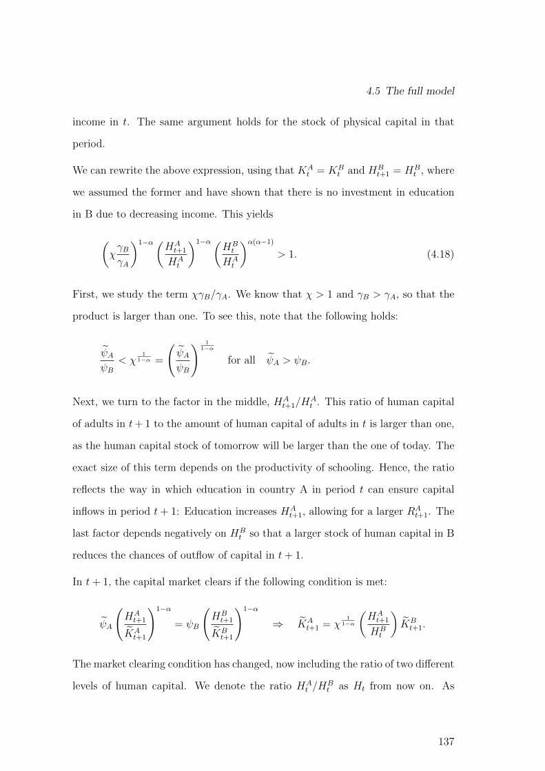
4.5 The full model
income in t. The same argument holds for the stock of physical capital in that
period.
We can rewrite the above expression, using that KAt = KB
t and HBt+1 = HB
t , where
we assumed the former and have shown that there is no investment in education
in B due to decreasing income. This yields
(χγBγA
)1−α(HAt+1
HAt
)1−α(HBt
HAt
)α(α−1)> 1. (4.18)
First, we study the term χγB/γA. We know that χ > 1 and γB > γA, so that the
product is larger than one. To see this, note that the following holds:
ψAψB
< χ1
1−α =
(ψAψB
) 11−α
for all ψA > ψB.
Next, we turn to the factor in the middle, HAt+1/H
At . This ratio of human capital
of adults in t+ 1 to the amount of human capital of adults in t is larger than one,
as the human capital stock of tomorrow will be larger than the one of today. The
exact size of this term depends on the productivity of schooling. Hence, the ratio
reflects the way in which education in country A in period t can ensure capital
inflows in period t+ 1: Education increases HAt+1, allowing for a larger RA
t+1. The
last factor depends negatively on HBt so that a larger stock of human capital in B
reduces the chances of outflow of capital in t+ 1.
In t+ 1, the capital market clears if the following condition is met:
ψA
(HAt+1
KAt+1
)1−α
= ψB
(HBt+1
KBt+1
)1−α
⇒ KAt+1 = χ
11−α
(HAt+1
HBt
)KBt+1.
The market clearing condition has changed, now including the ratio of two different
levels of human capital. We denote the ratio HAt /H
Bt as Ht from now on. As
137

Chapter 4 Capital flows and endogenous growth
country A has invested in education, we observe HAt+1 > HB
t . Country B has
not invested, remaining at the level of human capital HBt . While the difference
in institutions is still relevant, as shown by χ, the new ratio of human capital
Ht+1 =HAt+1
HBt
increases the difference between capital stocks in the two countries.
To solve for the post-flow capital stocks KAt+1 and KB
t+1, we note two things. First,
from the savings decision above, we know that
KAt+1 = KB
t+1
γAγBχ
α1−αH1−α
t wih Ht =HAt
HBt
. (4.19)
Second, the international sum of physical capital after flows must equal the sum
of physical capital after flows, implying
KBt+1 = KA
t+1 +KBt+1 − KA
t+1.
We substitute the market clearing condition and (4.19) to obtain
KBt+1 =
(1 +
γAγBχ
α1−α
)(1 + χ
11−αHt+1
)−1KBt+1 and
KAt+1 =
(1 +
γBγAχ−α1−α
)(1 + χ
−11−αH−1t+1
)−1KAt+1,
where we use that Ht = 1. In contrast to the equation that related KB and KBt ,
the number 2 is replaced by the left factor. This factor is smaller than 2 and thus
shows that, in period t + 1, country B has a smaller share of the global capital
stock than in t. This is due to γA/γB < 1 and the fact that Ht+1 > 1. While this
implies that KBt+1 < KB
t+1, it is not clear whether KBt+1/K
Bt+1 is larger or smaller
than KBt /K
Bt . Let us also consider the education decision for period t + 1. In
138

4.5 The full model
equilibrium, the optimal amount of schooling e∗t+1 must fulfill,
βφ′t+2(e∗t+1) =
(1 + β)ηL1
A(φt+1L2)1−α(KAt+1)
αΓAt+1 + (1 + β)(1− γ1)(1− e∗t+1)ηL1,
(4.20)
with
ΓAt+1 = (1− γ1)(
1 +γBγAχ−α1−α
)α (1 + χ
11−αHt+1
)−αχ
α1−α (HA
t+1)α·
[1− α + αψAt γ
(1 +
γBγAχ−α1−α
)−1 (1 + χ
11−αHA
t+1
)χ−11−α (Ht+1)
−1]. (4.21)
We know that the total endowment with both types of capital in A has increased,
i.e. φt < φt+1 and KAt < KA
t+1.
Next, we turn to ΓAt+1 which is structurally similar to ΓAt . However, the factor 2
is replaced by 1 + γBγAχ−α1−α , which is smaller than 2, and the term χ
11−α is replaced
by χ1
1−αHt+1, with Ht+1 > 1. This makes the derivative ∂ΓAt+1/∂χ not-trivial, as
the terms γB, γA, and Ht+1 depend on χ. We cannot say whether income in A, in
period t+ 1 before children are educated, is actually larger than the one in period
t. However, a condition, allowing for such a case, can be found in the following
way: First, we write income without the earnings of children in its general form,
IAt+1 = (1− α)(1− γ1)A(HAt+1)
1−α(KAt+1)
α + αψAγ3A(HAt+1)
1−α(KAt+1)
α−1KAt+1.
This expression holds for t + 1 and t. It is clear that It+1 increases in HAt+1 and
KAt . Forming the derivative with respect to KA
t+1, we find
∂IAt+1
∂KAt+1
= αA(KAt+1
)α−1 (HAt+1
)1−α[
(1− α)(1− γ1) + (α− 1)ψAγ3KAt+1
KAt+1
]> 0,
139

Chapter 4 Capital flows and endogenous growth
as ψA < 1, KAt /K
At < 1 due to capital inflows and that γ3 is unlikely too different
from 1 − γ1. We know that HAt < HA
t+1 and that KAt < KA
t+1. However, it is not
clear whether KAt < KA
t+1. KAt+1 can be written as a share of the total supply of
physical capital Kt+1
KAt+1 =
(1 +
1
χ1
1−αHt+1
)−1Kt+1. (4.22)
Country A obtains a larger share of total world capital. Yet, we have not estab-
lished whether the global total stock of physical capital has increased, i.e. whether
Kt < Kt+1. The opposite is also possible since in t, income increases in A, but
decreases in B. We examine whether A’s income increase compensates B’s income
decline. For this, we turn to ΓBt , given by
ΓBt = 2α(1 + χ1
1−α )−α(
(1− α)(1− γ1) +α
2ψBγ3(1 + χ
11−α )
),
which, as we know, decreases in χ. The marginal change is
2αα(1 + χ−11−α )−α
[− 1− γ1
1 + χ1
1−α+ψBγ3
2
].
Next, we study the derivative of ΓAt . It reads
2αα(
1 + χ−11−α)−α
χ−1(
1− γ11 + χ
11−α
+ψAγ3
2
).
140
4.5 The full model
It is larger than ∂ΓBt /∂χ in absolute terms if the following expression holds10:
γ31− γ1
ψA >χ− 1
1 + χ1
1−α. (4.23)
This inequality provides a lower bar for the value of ψA. However, it is easily
fulfilled if we consider small changes in institutions, so that χ is relatively close to
1.
With this, country A is richer after capital flows in t + 1 than after flows in t,
leading to a higher optimal level of education e∗t+1. Hence, the stock of human
capital will increase more strongly from t+ 1 to t+ 2 than it did from t to t+ 1.
We summarize in the following proposition:
Proposition 19 If Inequality (4.23) holds, then world income increases in t. This
is a sufficient condition for country A to increase its level of education in t+ 1.
More general discussion
So far, we have seen that in period t and t + 1, two relevant things occur. First,
capital flows from country B to A and second, A invests in education, and does
it in t + 1 even more than in t. We study now, whether this can also happen in
the following periods, i.e. whether there is a path where two conditions are met in
each period. First, country A experiences capital inflows and second, it increases
its level of education et, so that it converges to e∗T = 1, in some period T . The
first condition can only be met if
χ1
1−α
(HAt+2
HBt+2
)ΓBt+1
(HBt
)1−α(KB
t+1)α
ΓAt+1
(HAt+1
)1−α(KA
t+1)α> 1 (4.24)
10To be precise, this is the relevant condition if 1−γ11+χ
11−α
> ψBγ32 . In the opposite case,
∣∣∂ΓAt∂χ
∣∣ >∣∣∂ΓBt∂χ
∣∣ is always fulfilled, regardless of parameter values.
141
Chapter 4 Capital flows and endogenous growth
is fulfilled in t + 2 and in every following period. For this condition to hold, it is
important for country A to accumulate human capital sufficiently quickly, as KAt+1
is increasing due to country A’s larger wealth and KBt+1 is decreasing. Also the
factors ΓAt+1 and ΓBt+1 diverge, equalizing interest rates across the two countries.
A sufficient condition for country A to increase its education level is 1 < ΓAt < ΓAt+1.
It can be generalized for the following periods. If ΓAt+1 < ΓAt+2 and so on, then
e∗t+1 < e∗t+2 will hold, as can be seen from (4.20). The factor ΓAt+1 increases over
time if KAt+1 increases, which in turn, becomes larger over time if income rises more
quickly in A than income decreases in B, in a given period. This is expressed by
the following condition:
(HAt+1)
1−α(KAt+1)
αΓAt+1 − (HAt+1)
1−α(KAt+1)
αΓA,0t+1 ≥ (4.25)
∣∣(HBt+1)
1−α(KBt+1)
αΓB,0t+1 − (HBt+1)
1−α(KBt+1)
αΓBt+1
∣∣,
with ΓI,0t+1 = (1− α)(1− γ1) + αγ3ψI . Slightly rewritten, we have
Y 2,At+1
Y 2,Bt+1
(ΓAt+1 − ΓA,0t+1
)>∣∣ΓB,0t+1 − ΓBt+1
∣∣, (4.26)
which is a generalization of (4.23). Y 2,At+1 is country A’s potential output before
capital flows and education. We see that it is beneficial for A if country B is
relatively poor, i.e. Y 2,Bt+1 is rather small.
We summarize our findings in the following proposition:
Proposition 20 If returns to education are non-increasing or increase sufficiently
slowly and in every period and (4.24) and (4.26) are fulfilled, there exists a path
for country A along which it experiences inflows of capital in every period and
increases its level of education.
142
4.5 The full model
What happens, however, if (4.24) does not hold? To answer this question, let us
consider the following. From period t = 0 until some period T , capital has been
flowing from B to A, and A has been investing in education, without reaching the
state of full education, so that eT−1 < 1. Let us first assume, that in T , the return
on capital is equal in both countries, so that there are no capital flows in this period.
If capital inflows matter for country A, it might be the case that KAT−1 > KA
T, i.e.
country A had more capital available for production in the previous period than in
the current one, due to previous capital inflows. This might reduce the incentive to
invest in education in period T in comparison to T−1. However, we can exclude the
possibility that eT drops back to zero, as country A has been accumulating human
capital over the previous periods, which encourages investment in education. Also,
human capital is larger in the current period than in T−1, hindering any conclusion
about the relative size of eT compared to eT−1. If capital inflows are negligible in
comparison to country A’s capital stock, such considerations do not matter. As
before, country A will follow its path, increasing its stock of human capital. The
opposite will hold in B. The country does not invest in education, as it is poorer in
T than in the initial period t, where it already did not invest in education. Taken
together, these effects enable (4.24) to hold as an inequality.
Now assume, that the return in B is actually larger than in A and that capital
flows from A to B. It is more likely now that A invests less in education than in
the previous period with eT < eT−1, but it is quite unlikely that A will completely
stop investing, as the accumulation of human capital and physical capital has been
increasing wealth. If inflows in B are large, providing B with more capital than
it initially had, so that KBt < KB
T, B might begin to invest in education. Even if
it does, it will most likely invest less than country A, so that interest rates will
equalize in the following period. However, by investing in education, B might also
143
Chapter 4 Capital flows and endogenous growth
converge to the full education steady state.
Steady state
Let us turn to the existence of a balanced growth path. While the economy can
exhibit different steady states, we concentrate on the steady state in which country
A grows at the largest possible positive rate while country B does not. We define
such a state as follows:
Definition 4 Along a balanced growth path, human capital and physical capital
grow at the same rate. In country, A this rate is positive and as large as possible.
In B, it is zero. In the long run, the stocks of human capital and physical capital
become so large that agents in A neglect the effect of capital inflows from B and
the stock of children’s human capital in their decisions.
With this definition, we obtain for country A
KAt+1
HAt+1
= kAt+1 =βA((1− α)(1− γ1) + αγ3ψA)
(1 + β)Φ(kAt )α with Φ =
φt+1(1)
φt(1)∀t.
The constant ratio of the two forms of capital is kA = [βA((1−α)(1−γ1)+αγ3)/(1+
β)Φ]1/(1−α). For the derivation of this equation, see the Appendix for Chapter 4.
Additionally, we assume that the steady state defined above was reached along a
transition path, where country B never invested in education. This might be due
to country B’s rental rate always being smaller than A’s, i.e. Inequality (4.24)
always held along the convergence, or country B experienced capital inflows which
did not stimulate income sufficiently to ensure investment in education. Regardless
of the transition path, we show that there exists a steady state where country A
invests in education and country B does not.
Such a steady state cannot be one without capital flows, as country B has been
144

4.5 The full model
exporting capital and has seen a continuous reduction in income along the assumed
path. Hence, in some arbitrary period T , where A is already in its steady state,
B faces a capital stock that is smaller than its initial endowment. With KBT being
smaller than KBt and with a policy function for KB
t that is concave, as can be
seen from the savings decision, country B will accumulate capital in the absence
of international capital flows. This is not consistent with a steady state, and it is
not clear how this accumulation would affect the overall dynamics either.
Instead, we demonstrate the existences of a steady state with the following features.
At the beginning of every period, the market clearing condition is not fulfilled, so
that a time-independent amount of capital flows from B to A, clearing the arbitrage
condition. In every period, country B possesses the same amount of capital KB,
of which a constant fraction flows out. Furthermore, country B’s stock of capital
used in production is also constant, i.e. KB is fixed. Denoting the steady state
ratio of capital in A by kA, the rental rate in A is given by A(kA)α−1, which we
write as RA. Hence, KB and KB must fulfill
ψARA > ψB
(HB
KB
)1−α, ψAR
A = ψB
(HB
KB
)1−α, and
KB =βA
1 + β
[(1− α)(1− γ1)
(HB)1−α (
KB)α
+ αγ3ψARAKB
].
We solve for
KB = HB(χRA
) −11−α
and substitute this expression to obtain
KB =βA
1 + β
[(1− α)(1− γ1)HB
(χRA
) −α1−α](
1− αβγ3ψAA
1 + βRA
)−1. (4.27)
145
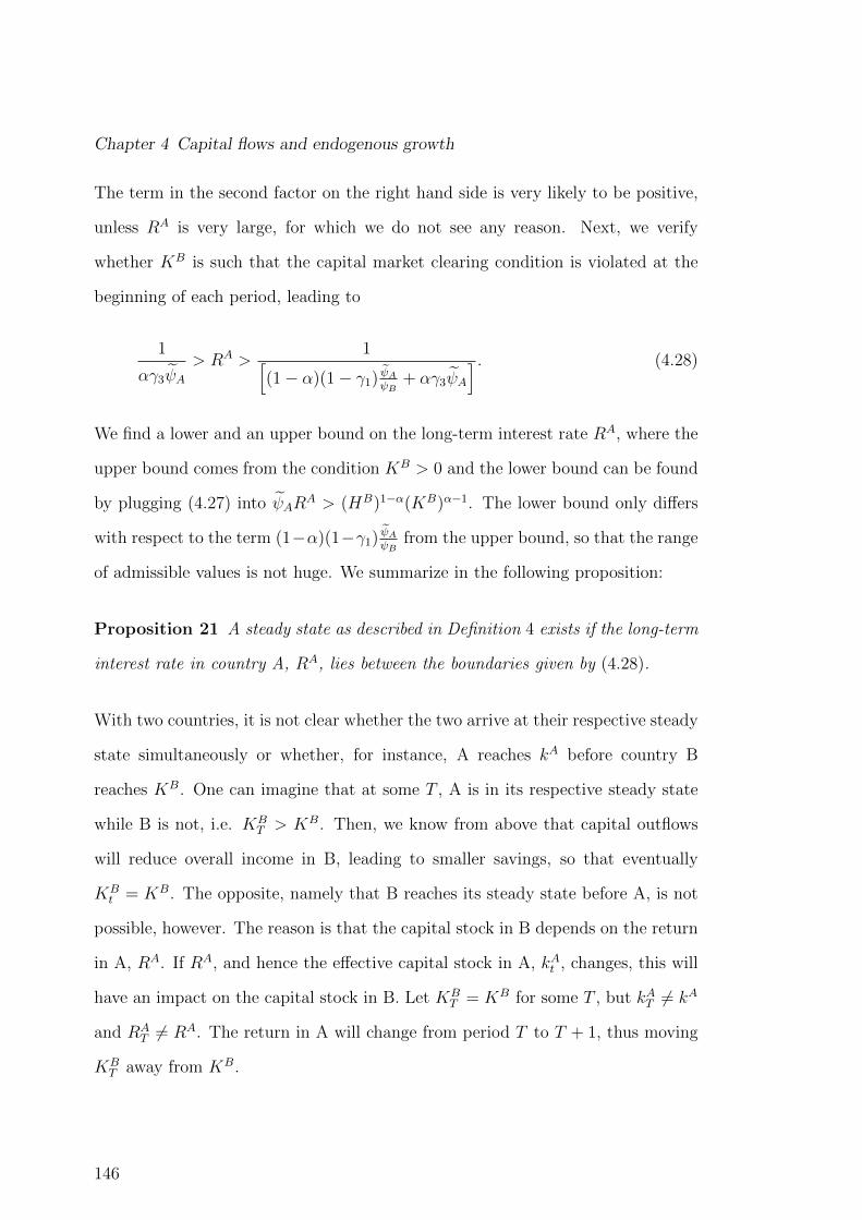
Chapter 4 Capital flows and endogenous growth
The term in the second factor on the right hand side is very likely to be positive,
unless RA is very large, for which we do not see any reason. Next, we verify
whether KB is such that the capital market clearing condition is violated at the
beginning of each period, leading to
1
αγ3ψA> RA >
1[(1− α)(1− γ1) ψAψB + αγ3ψA
] . (4.28)
We find a lower and an upper bound on the long-term interest rate RA, where the
upper bound comes from the condition KB > 0 and the lower bound can be found
by plugging (4.27) into ψARA > (HB)1−α(KB)α−1. The lower bound only differs
with respect to the term (1−α)(1−γ1) ψAψB from the upper bound, so that the range
of admissible values is not huge. We summarize in the following proposition:
Proposition 21 A steady state as described in Definition 4 exists if the long-term
interest rate in country A, RA, lies between the boundaries given by (4.28).
With two countries, it is not clear whether the two arrive at their respective steady
state simultaneously or whether, for instance, A reaches kA before country B
reaches KB. One can imagine that at some T , A is in its respective steady state
while B is not, i.e. KBT > KB. Then, we know from above that capital outflows
will reduce overall income in B, leading to smaller savings, so that eventually
KBt = KB. The opposite, namely that B reaches its steady state before A, is not
possible, however. The reason is that the capital stock in B depends on the return
in A, RA. If RA, and hence the effective capital stock in A, kAt , changes, this will
have an impact on the capital stock in B. Let KBT = KB for some T , but kAT 6= kA
and RAT 6= RA. The return in A will change from period T to T + 1, thus moving
KBT away from KB.
146
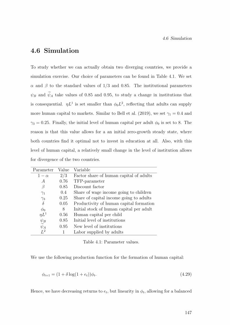
4.6 Simulation
4.6 Simulation
To study whether we can actually obtain two diverging countries, we provide a
simulation exercise. Our choice of parameters can be found in Table 4.1. We set
α and β to the standard values of 1/3 and 0.85. The institutional parameters
ψB and ψA take values of 0.85 and 0.95, to study a change in institutions that
is consequential. ηL1 is set smaller than φ0L2, reflecting that adults can supply
more human capital to markets. Similar to Bell et al. (2019), we set γ1 = 0.4 and
γ3 = 0.25. Finally, the initial level of human capital per adult φ0 is set to 8. The
reason is that this value allows for a an initial zero-growth steady state, where
both countries find it optimal not to invest in education at all. Also, with this
level of human capital, a relatively small change in the level of institution allows
for divergence of the two countries.
Parameter Value Variable1− α 2/3 Factor share of human capital of adultsA 0.76 TFP-parameterβ 0.85 Discount factorγ1 0.4 Share of wage income going to childrenγ3 0.25 Share of capital income going to adultsδ 0.05 Productivity of human capital formationφ0 8 Initial stock of human capital per adultηL1 0.56 Human capital per childψB 0.85 Initial level of institutions
ψA 0.95 New level of institutionsL2 1 Labor supplied by adults
Table 4.1: Parameter values.
We use the following production function for the formation of human capital:
φt+1 = (1 + δ log(1 + et))φt. (4.29)
Hence, we have decreasing returns to et, but linearity in φt, allowing for a balanced
147
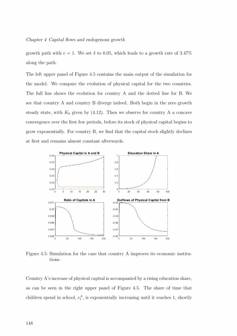
Chapter 4 Capital flows and endogenous growth
growth path with e = 1. We set δ to 0.05, which leads to a growth rate of 3.47%
along the path.
The left upper panel of Figure 4.5 contains the main output of the simulation for
the model. We compare the evolution of physical capital for the two countries.
The full line shows the evolution for country A and the dotted line for B. We
see that country A and country B diverge indeed. Both begin in the zero growth
steady state, with K0 given by (4.12). Then we observe for country A a concave
convergence over the first few periods, before its stock of physical capital begins to
grow exponentially. For country B, we find that the capital stock slightly declines
at first and remains almost constant afterwards.
Figure 4.5: Simulation for the case that country A improves its economic institu-tions.
Country A’s increase of physical capital is accompanied by a rising education share,
as can be seen in the right upper panel of Figure 4.5. The share of time that
children spend in school, eAt , is exponentially increasing until it reaches 1, shortly
148

4.7 Conclusion
after the 50th period. Thereafter, it remains constant at that value. Investment
in education in country B remains at eB = 0, and is not shown.
The dynamics of the ratio of capitals in A, KAt /φ
At can be seen in the left lower
panel of Figure 4.5. It reflects our previous findings. At first, the ratio of capital
increases, due to the strong accumulation of physical capital, which we observed
in the left upper panel. Then, country A accumulates human capital faster than
physical capital, decreasing the ratio. Finally, after country A has reached the
point in time, where eAt = 1, we see a convergence to the new steady state.
A theoretical prediction that we made was that country B converges to a steady
state where it exports the same amount of physical capital in every period. In
the right lower panel of Figure 4.5 we see that this indeed is the case. While
flows of physical capital to country B mirror the dynamics of KAt /φ
At , they are
always negative, indicating that B experiences outflows. The outflows decrease at
first, due to A’s fast accumulation of physical capital, which reduces A’s return.
However, outflows increase as A invests more in education. Furthermore, when
country A reaches the state of full education with eAt = 1, outflows continue to
increase but at a significantly lower rate, and start to converge. The convergence
is quite slow, going on for over 200 periods.
4.7 Conclusion
Institutions, human capital and flows of physical capital all seem to have an im-
pact on long-term growth. In this study, we provide a unified framework, where
these forces interact, and that might explain increasing inequality between coun-
tries. We propose the idea that better economic institutions attract international
capital, more physical capital increases households’ income and thus allows for the
149

Chapter 4 Capital flows and endogenous growth
formation of human capital. Human capital, then, drives growth. We analytically
provide conditions under which a country can undergo these steps towards long-
term growth and show that in our model endogenous separation between countries,
due to an initial difference in institutions, can occur. The country that was able
to improve its institutions benefits from inflows of capital and converges to a path
with a positive growth rate, while the other country remains at a zero growth
steady state.
There are different avenues that further research can take. First, we assume simple
sharing rules for family income and do not incorporate a pension system. Imple-
menting the latter might yield interesting insights. Second, one can extend the
model to incorporate more countries and a multitude of institutional parameters
to see which institutional changes are especially vital in enabling growth.
150
Chapter 5
Artificial intelligence and growth
Abstract
In the previous chapters, we analyzed several phenomena related to economic
growth.1 In this chapter, we turn to a trend that emerged very recently, but might
have a drastic impact on growth and other macroeconomic variables—artificial
intelligence (AI). By surveying a selected number of studies, we demonstrate the
authors’ mixed opinions about AI, and how AI can be modeled in the context of
growth models. To do this, authors rely on one of the following polar approaches:
On the hand, AI is considered as supporting human decision-making, thus increas-
ing the productivity of human labor. On the other hand, AI replaces humans in
the production process, since it is cheaper than conventional labor. After demon-
strating these ideas, we provide a small outlook for possible future models of AI.2
5.1 A rather optimistic perspective
The study by Agrawal et al. (2018) discusses the unique features of modern artifi-
cial intelligence, and examines how AI may help overcome the obstacles to growth
1This chapter is single-authored.2There is an increasing literature on the subject of AI in Economics. For a comprehensive,
non-theoretical survey see Abrardi et al. (2019). In contrast, Goldfarb et al. (2019) contains aseries of theoretical articles about the perspective of different economic fields on AI.
151

Chapter 5 Artificial intelligence and growth
at the technological frontier. The authors begin by describing the following prob-
lems of growth: First, empirical observations show that, at the technological fron-
tier, growth is indeed slowing down. This holds despite exponentially-increasing
numbers of researchers.3 Second, across different fields, researchers themselves ex-
perience a decline in their total factor productivity. These two observations reflect
well-known phenomena in the field of knowledge creation: the “fishing-out”- and
the “burden-of-knowledge”-problem. The former states that good ideas are be-
coming more and more difficult to find. The latter reveals that in order to create
new knowledge, researchers must already have an increasing stock of knowledge.
In the face of these problems, the authors take a somewhat optimistic stance:
“[O]ne reason to be hopeful about the future is the recent explosion in data avail-
ability under the rubric of ‘big data’ and computer-based advances in capabilities
to discover and process those data.” In particular, they argue that AI is becom-
ing increasingly helpful in “needle-in-a-haystack”-problems, i.e. situations where
knowledge is created by combining existing knowledge parts in a suitable way.
Their idea is that AI can impact growth by simplifying the research process, and
increasing the productivity of knowledge creation.
They propose two ways in which AI can support researchers. First, AI can help
in the process of search. It can find the relevant knowledge for a specific project,
easing the burden of knowledge. Examples are Metaα and BenchSci. Second, AI
can help in the process of prediction, by finding combinations of knowledge that
will yield useful new concepts. This may be a crucial feature of AI, as with more
existing knowledge, there is an combinatorial explosion of the ways that knowledge
can be put together. Examples for existing AI are Atomwise and DeepGenomics.
To model these ideas, the authors construct a growth model with a combinatorial
3Gordon (2012) is a seminal contribution that illustrates faltering growth.
152

5.1 A rather optimistic perspective
based knowledge production function. While their model is similar to the model
of Jones (1995) and Romer (1990), the production of knowledge differs crucially.
In Jones (1995) and Romer (1990), the research process consists of a single step, in
which scientist use existing knowledge to create new knowledge. In Agrawal et al.
(2018), however, research consists of two steps. First, scientists create all possible
combinations of existing knowledge. Second, all possible combinations are filtered
for those that are actually new and useful.
The details of Agrawal et al. (2018)’s model are as follows: Every research possesses
the amount of knowledge Aφ, where A is the global stock of knowledge, and φ lies
between 0 and 1. This parameter reflects the burden of knowledge, as Aφ−1 is
falling in A, and thus, the individual’s share of global knowledge is decreasing over
time. However, AI can increase φ, by assisting scientists in the search process.
Furthermore, the knowledge of an individual researcher can be combined. This
yields the following number of combinations:
Zi =Aφ∑
a=0
(Aφ
a
)= 2A
φ
,
where Zi grows exponentially in Aφ. As mentioned above, the combinations of
knowledge are then transformed into new knowledge, according to the following
function:
Ai = β
(Zθi − 1
θ
)= β
(2A
φ)θ− 1
θ
for 0 < θ ≤ 1.
The parameter β is a positive knowledge discovery parameter and not of significant
importance for the model—in contrast to θ. It stands for the elasticity of discovery
and thus, reflects the fishing-out problem. θ can be increased by AI, similar to φ.
153

Chapter 5 Artificial intelligence and growth
Unlike before, the relevant form of AI is the one helping with discovery and not
with search. Hence, the creation of knowledge is aggregated in the following way:
A = βLλA
(2A
φ)θ− 1
θ
,
where LA is the total amount of researchers in the economy and 0 ≤ λ ≤ 1. The
parameter λ implies that some researchers produce the same knowledge. This is
called the “standing-on-toes-effect”.
Above, we established that AI can increase θ. However, the authors argue that
such an increase can only be temporary, and that θ must depend negatively on
A. This feature reflects that even improved AI is overwhelmed by the number of
possible combinations, which arise from an increasing knowledge stock. Thus, the
authors assume the following:
limA→∞
θ(A) = 0,
so that in the limit, the knowledge production function becomes
A = β ln(2)LλAAφ,
which is a Romer/Jones-type function.
To study the steady state, Agrawal et al. (2018) use that the fact that in the limit,
their model is the same as in Jones (1995), and obtain the following growth rates
for knowledge, per capita output, per capita consumption, and capital per capita:
gA = gy = gc = gK =λn
1− φ,
154
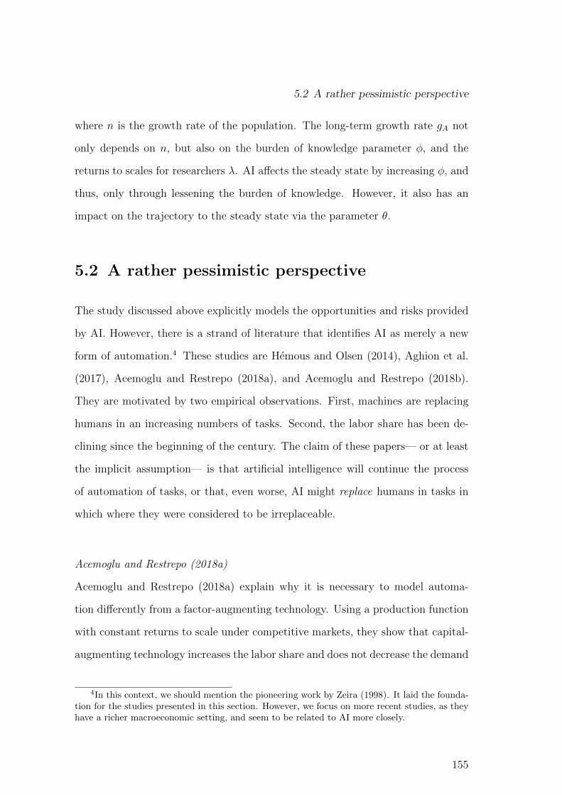
5.2 A rather pessimistic perspective
where n is the growth rate of the population. The long-term growth rate gA not
only depends on n, but also on the burden of knowledge parameter φ, and the
returns to scales for researchers λ. AI affects the steady state by increasing φ, and
thus, only through lessening the burden of knowledge. However, it also has an
impact on the trajectory to the steady state via the parameter θ.
5.2 A rather pessimistic perspective
The study discussed above explicitly models the opportunities and risks provided
by AI. However, there is a strand of literature that identifies AI as merely a new
form of automation.4 These studies are Hemous and Olsen (2014), Aghion et al.
(2017), Acemoglu and Restrepo (2018a), and Acemoglu and Restrepo (2018b).
They are motivated by two empirical observations. First, machines are replacing
humans in an increasing numbers of tasks. Second, the labor share has been de-
clining since the beginning of the century. The claim of these papers— or at least
the implicit assumption— is that artificial intelligence will continue the process
of automation of tasks, or that, even worse, AI might replace humans in tasks in
which where they were considered to be irreplaceable.
Acemoglu and Restrepo (2018a)
Acemoglu and Restrepo (2018a) explain why it is necessary to model automa-
tion differently from a factor-augmenting technology. Using a production function
with constant returns to scale under competitive markets, they show that capital-
augmenting technology increases the labor share and does not decrease the demand
4In this context, we should mention the pioneering work by Zeira (1998). It laid the founda-tion for the studies presented in this section. However, we focus on more recent studies, as theyhave a richer macroeconomic setting, and seem to be related to AI more closely.
155

Chapter 5 Artificial intelligence and growth
for labor, or its wage. Also, they demonstrate that labor-augmenting technology
decreases the labor share for realistic parameter values, but increases the demand
for labor and its wage. The production function they use is
Y = F (AKK,ALL),
where Y is aggregate output and AK , K, AL and L are the level of capital-
augmenting technology, the capital stock, the level of labor-augmenting technology
and labor, respectively. Hence, Acemoglu and Restrepo (2018a) state that the
findings above are not consistent with empirical observations, and propose a task-
based framework, which can be used instead. Here, the central assumption is that
output stems from combining different tasks. The production function takes the
form
Y =
(∫ N
N−1y(i)
σ−1σ di
) σσ−1
, (5.1)
with σ being the elasticity of substitution between tasks. y(i) is a distinct task,
and the measure of tasks is 1, as is reflected by the integration from N − 1 to N .
An individual task can be either non-automated or automated. In the first case,
it is produced using labor only, y(i) = γ(i)l(i). Here, γ(i) is the productivity of
labor l(i) in that task. In the second case, labor and capital can be used as perfect
substitutes in the production of the task, so that y(i) = η(i)k(i) + γ(i)l(i), with
η(i) reflecting the productivity of capital k(i) in that task. Furthermore, there
exists a task I ∈ [N −1, N ], such that every task with i > I is non-automated and
can only be produced with labor.
Before demonstrating the results in this framework, the authors make two as-
sumptions. First, tasks increase in complexity from N − 1 to N , and labor has
156

5.2 A rather pessimistic perspective
a comparative advantage for more complex tasks. Hence, γ(i)/η(i) increases with
i, which is an assumption that is strongly supported by empirical findings. The
second assumption is that, at task I, the following holds:
γ(I)
η(I)<W
R,
where W and R are the exogenously given wage and return to capital. Thus, all
tasks that can be produced with capital are being produced with capital only.
With these assumptions, the authors study automation, which is reflected by an
increase in I. They find the following: First, automation makes production less
labor-intensive and reduces the labor share. Second, automation increases produc-
tivity and output, since capital is cheaper than labor in the neighborhood of I.
Hence, using capital frees up resources and increases output. Third, automation
has an ambiguous net effect on the wage. On the one hand, automation increases
demand for labor, through increasing productivity (productivity effect). On the
other hand, capital replaces labor and reduces the wage (displacement effect).
Acemoglu and Restrepo (2018b)
The observations just mentioned are made in a simplified static model. To study
the relation between automation and growth, Acemoglu and Restrepo (2018b)
build an endogenous growth-model, using the task-framework as a starting point.
Hereby, the most important changes are the following: The share of automated
tasks is a dynamic variable. It depends not only the amount of automated tasks,
but also on new and more complex tasks, which are initially performed by labor.
Furthermore, savings are endogenous—as is the innovation process that drives
growth. We discuss these changes in turn.
Acemoglu and Restrepo (2018b) provide empirical evidence on the evolution of
157

Chapter 5 Artificial intelligence and growth
tasks. They show that while old tasks are automated, new tasks are created. The
way in which they incorporate this observations into their model is shown in Figure
5.1. An economy begins with the interval of tasks from N − 1 to N , among which
Figure 2: The task space and a representation of the effect of introducing new tasks (middle panel) and automating
existing tasks (bottom panel).
which we view as the less interesting case. This assumption is relaxed in the next two sections
where the capital stock is endogenous.
We next derive the demand for factors in terms of the (endogenous) threshold I∗ and the
technology parameter N . We choose the final good as the numeraire, which from equation (1) gives
the demand for task i as
y(i) = Bσ−1Y p(i)−σ. (7)
Let us define σ = σ(1− η) + ζη and B = Bσ−1σ−1 . Then, under Assumption 2, equations (2) and
(3) yield the demand for capital and labor in each task as
k(i) =
{Bσ−1(1− η)Y R−σ if i ≤ I∗,
0 if i > I∗.and l(i) =
0 if i ≤ I∗,
Bσ−1(1− η)Y1
γ(i)
(W
γ(i)
)−σ
if i > I∗.
We can now define a static equilibrium as follows. Given a range of tasks [N−1, N ], automation
technology I ∈ (N − 1, N ], and a capital stock K, a static equilibrium is summarized by a set of
factor prices, W and R, threshold tasks, I and I∗, and aggregate output, Y , such that:
• I is determined by equation (6) and I∗ = min{I, I};
• the capital and labor markets clear, so that
Bσ−1(1− η)Y (I∗ −N + 1)R−σ = K, (8)
Bσ−1(1− η)Y
∫ N
I∗
1
γ(i)
(W
γ(i)
)−σ
di = L; (9)
• factor prices satisfy the ideal price index condition,
(I∗ −N + 1)R1−σ +
∫ N
I∗
(W
γ(i)
)1−σ
di = B1−σ; (10)
9
Figure 5.1: The task space and a representation of the effect of introducing newtasks (middle panel) and automating existing tasks (bottom panel)(Source Acemoglu and Restrepo (2018b)).
tasks with i > I are performed by labor and the rest by capital. Research can
create new tasks and replace old tasks, at the same time. As a result, the task
interval is shifted to the right, so that the economy performs more complex tasks
than before. To be precise, the authors assume that the productivity of labor is
given by
γ(i) = eAi,
so that when N increases, the comparative advantage of labor in performing new
tasks also increases. Since some tasks were replaced, capital now performs a smaller
share of tasks. However, through further automation, this share can increase again.
We omit the discussion of model features that are quite standard, such as house-
hold behavior, and turn to the innovation process in the economy instead. The
158

5.2 A rather pessimistic perspective
aggregate production function is again a CES-function of tasks, as seen in Equation
(5.1). However, Acemoglu and Restrepo (2018b) change the production function
for tasks slightly. They introduce task-specific intermediates q(i), so that an au-
tomated task can be produces in the following way:
y(i) = B(ζ)[η
1ζ q(i)
ζ−1ζ + (1− η)
1ζ (k(i) + γ(i)l(i))
ζ−1ζ
] ζζ−1
,
where B(ζ) is just some scaling parameter. Whether the good is automated or not
is determined by the intermediate q(i), which is produced from final output. Hence,
if a (competitive) firm wants to produce a new task that was invented recently,
it must purchase the respective intermediate q(i) first. The same holds for a firm
producing a task that has been automated. In order to change its production
function and employ capital, it must purchase the relevant intermediate. These
intermediates can be purchased from so-called “technology monopolists”, who sell
at a mark-up over marginal costs. These monopolists can be replaced. New firms,
driven by the prospect of a positive profit, employ scientists that create new tasks
or automate existing tasks.5 They do this according to the following functions:
I(t) = κISI(t) and N = κNSN(t),
where κI and κN are the productivities of scientists in automation and the creation
of new tasks, respectively. SI(t) is the measure of scientists in automation, while
SN(t) is the measure of creation of new tasks. The sum of the two adds up to
some exogenous stock of scientists S.
5The actual model is slightly more complicated. The authors assume that the use of a newintermediate is a infringement on the patent of an existing intermediate. For instance, considerthe situation when a new monopolists emerges. It possesses the technology to produce a newtasks, and can sell it to a firm. However, the new task replaces some old task, so that the newmonopolist must compensate the old monopolist that held the right to the replaced task. Thus,the new monopolist makes a take-it-or-leave-it offer that depends on its income.
159
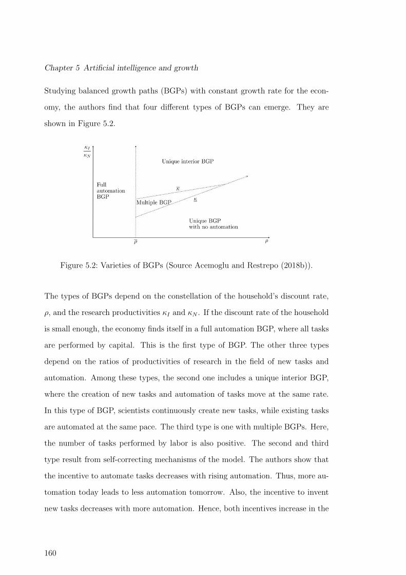
Chapter 5 Artificial intelligence and growth
Studying balanced growth paths (BGPs) with constant growth rate for the econ-
omy, the authors find that four different types of BGPs can emerge. They are
shown in Figure 5.2.
1 (Full automation) For ρ < ρ, there is a BGP in which n(t) = 0 and all tasks are produced
with capital.
For ρ > ρ, all BGPs feature n(t) = n > n(ρ). Moreover, there exist κ ≥ κ > 0 such that:
2 (Unique interior BGP) if κIκN
> κ there exists a unique BGP. In this BGP we have
n(t) = n ∈ (n(ρ), 1) and κNvN (n) = κIvI(n). If, in addition, θ = 0, then the equilibrium is
unique everywhere and the BGP is globally (saddle-path) stable. If θ > 0, then the equilibrium
is unique in the neighborhood of the BGP and is asymptotically (saddle-path) stable;
3 (Multiple BGPs) if κ > κIκN
> κ, there are multiple BGPs;
4 (No automation) If κ > κIκN
, there exists a unique BGP. In this BGP n(t) = 1 and all tasks
are produced with labor.
Proof. See Appendix A.
This proposition provides a complete characterization of different types of BGPs. Figure 7
shows visually how different BGPs arise in parts of the parameter space.
Figure 7: Varieties of BGPs.
Further intuition can be gained by studying the behavior κIvI(n) and κNvN (n), which we do
in Figure 8. Lemma A3 shows that, for S small, the normalized value functions can be written as
vI(n) =b((ρ+ δ + θg)ζ−σ − wI(n)
ζ−σ)
ρ+ (θ − 1)gvN (n) =
b(wN (n)ζ−σ − (ρ+ δ + θg)ζ−σ
)
ρ+ (θ − 1)g.
These expressions show that, asymptotically, the profitability of the two types of technologies
depend on the effective wages, wI(n) and wN (n). As n increases, so does wI(n) and it becomes
more expensive to produce the least complex tasks with labor, and this makes automation more
profitable and triggers further improvements in the automation technology. As a result, vI(n) is
increasing in n (recall that σ > ζ). However, vN (n) is also increasing in n because, as explained
26
Figure 5.2: Varieties of BGPs (Source Acemoglu and Restrepo (2018b)).
The types of BGPs depend on the constellation of the household’s discount rate,
ρ, and the research productivities κI and κN . If the discount rate of the household
is small enough, the economy finds itself in a full automation BGP, where all tasks
are performed by capital. This is the first type of BGP. The other three types
depend on the ratios of productivities of research in the field of new tasks and
automation. Among these types, the second one includes a unique interior BGP,
where the creation of new tasks and automation of tasks move at the same rate.
In this type of BGP, scientists continuously create new tasks, while existing tasks
are automated at the same pace. The third type is one with multiple BGPs. Here,
the number of tasks performed by labor is also positive. The second and third
type result from self-correcting mechanisms of the model. The authors show that
the incentive to automate tasks decreases with rising automation. Thus, more au-
tomation today leads to less automation tomorrow. Also, the incentive to invent
new tasks decreases with more automation. Hence, both incentives increase in the
160

5.2 A rather pessimistic perspective
number of tasks performed by labor. Since they do this at different rates, they
intersect eventually. In the third type, they intersect several types. The fourth
type is, of course, the opposite of the first case, and yields a BGP without au-
tomation. It is noteworthy that in the first type, the production function becomes
linear in capital, and thus, growth only stems from the accumulation of capital.
In the fourth type, the economy collapses to an Aghion and Howitt (1992)-type
endogenous growth model with quality improvements.
Hemous and Olsen (2014)
A closely related study is Hemous and Olsen (2014). The authors shift the focus
from studying the existence of a BGP to analyzing the relationship between au-
tomation and inequality. Besides the declining labor share mentioned above, their
study is motivated by the increasing skill premium that is observed in the U.S.
for college graduates. The authors use a slightly different aggregate production
function
Yt =
(∫ Nt
0
yt(i)σ−1σ di
) σσ−1
,
where σ > 1 is the elasticity of substitution and yt(i) is not seen as a task, but
simply as an intermediate input. The increase in the number of such inputs, shown
by Nt, is the driving force of growth. A noteworthy difference is the production
function, as it does not integrate over a fixed measure of tasks, but over an in-
creasing number of inputs. Also, new intermediates do not come with a higher
productivity for labor.
In order to study inequality, Hemous and Olsen (2014) formulate the following
161

Chapter 5 Artificial intelligence and growth
production function for an intermediate yt(i):
y(i) =[l(i)
ε−1ε + α(i)(φx(i))
ε−1ε
] εβε−1
h(i)1−β.
The four variables are l(i), α(i), x(i) and h(i). They respectively stand for the
amount of low-skill labor, an indicator function, showing whether the firm is au-
tomated (α = 1) or not (α = 0), the amount of capital used in production, and
the amount of high-skill labor. Hence, Hemous and Olsen (2014) distinguish be-
tween two types of labor, which are differently affected by automation. Low-skill
labor can be substituted by capital, whereas high-skill labor cannot. Instead, au-
tomation can even increase the marginal productivity of high-skill workers, and
thus, their wage. The parameters φ, ε and β are the productivity of capital, the
measure of substitutability between low-skill labor and capital, and the low-skill
factor share.
Hemous and Olsen (2014) provide an endogenous growth model with endogenous
capital accumulation and innovation. Hereby, innovation is twofold. First, research
can create new intermediates and thus, increase Nt. This process requires high-skill
workers, HDt , and has the Romer-type production function
Nt = γNtHDt ,
where γ is the productivity of research. The firm producing the intermediate is
a monopolist and initially, a non-automated firm. However, the monopolist can
decide to hire high-skill labor to conduct automation research. This is the second
type of innovation. Automation arrives at a Poisson process with the following
rate: ηGκt (Nth
At (i))κ, where Gt is the share of automated intermediate firms, and
η and κ describe the productivity of this type of research. Finally, κ stands for
162
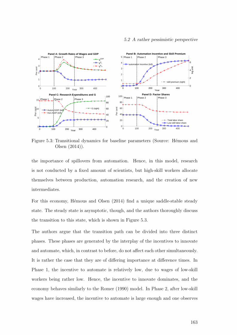
5.2 A rather pessimistic perspective
products Gt which eventually stabilizes at a level strictly below 1. There is no simple
one-to-one link between automation spending and rising inequality in our model: here,
automation spending is higher in Phase 3 than in Phase 2 (Panel C in figure 3), yet the
growth in the skill premium is slower.21
Panel A: Growth Rates of Wages and GDPPhase 1 Phase 2 Phase 3
0 100 200 300 400Year
0
1
2
3
4
Per
cen
t
gGDP
gwL
gwH
0 100 200 300 4000
1
2
3
4
5
automation incentive (left)
Panel B: Automation Incentive and Skill PremiumPhase 1 Phase 2 Phase 3
0 100 200 300 400Year
0
2
4
6
log
unit
skill premium (right)
0 100 200 300 4000
5
10
15
Per
cen
t
Autom./GDP (left)Hori./GDP (left)
Panel C: Research Expenditures and G
Phase 1 Phase 2 Phase 3
0 100 200 300 400Year
0
20
40
60
80
100
G (right)
Panel D: Factor SharesPhase 1 Phase 2 Phase 3
0 100 200 300 400Year
0
20
40
60
80
100
Per
cen
t
Total labor shareLow-skill labor share
Figure 3: Transitional Dynamics for baseline parameters. Panel A shows growth rates forGDP, low-skill wages (wL) and high-skill wages (wH), Panel B the incentive to au-tomate,
(V At − V Nt
)/ (wHt/Nt), and the skill premium, Panel C the total spending
on horizontal innovation and automation as well as the share of automated prod-ucts (G), and Panel D the wage share of GDP for total wages and low-skill wages.
As shown in Panel C, spending on horizontal innovation as a share of GDP declines
during Phase 2 and for any parameter values ends up being lower in Phase 3 than Phase
1. Despite this, the growth rate of GDP is roughly the same in Phases 1 and 3 because
the lower rate of horizontal innovation in Phase 3 is compensated by a higher elasticity of
GDP wrt. Nt (1/ [(σ − 1) (1− β)] instead of 1/ (σ − 1)). As a result, the phase of intense
automation—which also contributes to growth—is associated with a temporary boost
of growth. This is, however, specific to parameters (Appendix 7.7.2 gives a counter-
example). That intense automation need not be associated with a sharp increase in
growth is important because the lack of an acceleration in GDP growth in recent decades
has often been advanced in opposition to the hypothesis that a technological revolution
21Intuitively the elasticity of the skill-premium with respect to the skill-bias of technology is notconstant in our model, contrary to a CES framework with factor-augmenting technologies.
24
Figure 5.3: Transitional dynamics for baseline parameters (Source: Hemous andOlsen (2014)).
the importance of spillovers from automation. Hence, in this model, research
is not conducted by a fixed amount of scientists, but high-skill workers allocate
themselves between production, automation research, and the creation of new
intermediates.
For this economy, Hemous and Olsen (2014) find a unique saddle-stable steady
state. The steady state is asymptotic, though, and the authors thoroughly discuss
the transition to this state, which is shown in Figure 5.3.
The authors argue that the transition path can be divided into three distinct
phases. These phases are generated by the interplay of the incentives to innovate
and automate, which, in contrast to before, do not affect each other simultaneously.
It is rather the case that they are of differing importance at difference times. In
Phase 1, the incentive to automate is relatively low, due to wages of low-skill
workers being rather low. Hence, the incentive to innovate dominates, and the
economy behaves similarly to the Romer (1990) model. In Phase 2, after low-skill
wages have increased, the incentive to automate is large enough and one observes
163
Chapter 5 Artificial intelligence and growth
a rapid increase in the share of automated firms. Here, the growth rates of high-
and low-skill wages diverge, producing a positive skill premium which begins to
increase linearly. Finally, in Phase 3, the benefit from automation growths at the
same rate as its cost, leading to a constant share of automated firms Gt. The
economy begins to converge to the asymptotic steady state, where the economy
grows at a constant rate, but wages of high-skill workers grow faster than those of
low-skill ones.
5.3 An intermediate perspective
Finally, we turn to a study that not only considers the impact of AI on research,
as in Agrawal et al. (2018), but also takes into account the substitution of labor by
AI, similar to the studies discussed in the previous section. This study is Aghion
et al. (2017). As before, the authors rely on a CES-production function
Yt = At
(∫ 1
0
Xρitdi
) 1ρ
,
where At is the level of technology and Xit is some intermediate good, required
for the production in the final good sector. An intermediate can be produced
with a single unit of capital if it is automated, and with a single unit of labor
otherwise. The crucial difference to previous approaches is the parameter ρ, which
is assumed to be negative. This assumption reflects Baumol’s “cost-disease” (see
Baumol (1967)). It suggests that output is not bound by the most productive fac-
tors, but by the least productive ones. As a consequence, industries that increase
productivity might experience a decline in their share of output. An example of
this development is the agriculture sector.
The authors assume a symmetric allocation of capital and labor across goods, so
164

5.3 An intermediate perspective
that the production function can be written as
Yt = At
(βt
(Kt
βt
)ρ+ (1− βt)
(Lt
1− βt
)ρ) 1ρ
,
with βt being the share of automated goods. The ratio of the capital share and
the labor share becomes
αKtαLt
=
(βt
1− βt
)1−ρ(Kt
Lt
)ρ.
The authors find that an increase in automation, reflected by a larger βt, increases
the share of capital relatively. However, an increase in capital itself, which goes
hand in hand with automation, will decrease the price of capital, and thus, its
share. Aghion et al. (2017) argue that this opens up the possibility of constant
factor shares, even under continuous automation.
Furthermore, they interpret their production function as a special case of a neoclassical-
production function of the following form:
Yt = AtF (BtKt, CtLt) where Bt ≡ β1−ρρ
t and Ct ≡ (1− βt)1−ρρ .
As they assume that ρ < 0, they obtain the following: ↑ βt implies ↓ Bt and ↑ Ct.
This means that automation is not capital-augmenting but capital-depleting, as it
spreads a fixed amount of capital over a larger number of goods. The opposite holds
for labor, as automation reduces the range of goods for labor, concentrating it over
fewer tasks. Hence, the authors conclude that automation is labor-augmenting,
and find that it is possible to obtain asymptotically constant growth and constant
factor shares, even under complete automation. Figure 5.4 shows a model where
in each period, a constant share of goods is automated, implying constant growth
165
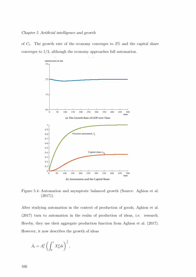
Chapter 5 Artificial intelligence and growth
of Ct. The growth rate of the economy converges to 2% and the capital share
converges to 1/3, although the economy approaches full automation.
12 P. AGHION, B. JONES, AND C. JONES
Figure 1: Automation and Asymptotic Balanced Growth
0 50 100 150 200 250 300 350 400 450 500
0%
1%
2%
3%
YEAR
GROWTH RATE OF GDP
(a) The Growth Rate of GDP over Time
0 50 100 150 200 250 300 350 400 450 5000
0.1
0.2
0.3
0.4
0.5
0.6
0.7
0.8
0.9
1
Fraction automated, t
Capital share K
YEAR
(b) Automation and the Capital Share
Note: This simulation assumes ρ < 0 and that a constant fraction of the tasks that have not yet
been automated become automated each year. Therefore Ct ≡ (1 − β)1−ρρ grows at a constant
exponential rate (2% per year in this example), leading to an asymptotic balanced growth path.The share of tasks that are automated approaches 100% in the limit. Interestingly, the capital shareof factor payments (and the share of automated goods in GDP) remains bounded, in this case ata value around 1/3. With a constant investment rate of s, the limiting value of the capital share is(
sgY +δ
)ρ.
Figure 5.4: Automation and asymptotic balanced growth (Source: Aghion et al.(2017)).
After studying automation in the context of production of goods, Aghion et al.
(2017) turn to automation in the realm of production of ideas, i.e. research.
Hereby, they use their aggregate production function from Aghion et al. (2017).
However, it now describes the growth of ideas
At = Aφt
(∫ 1
0
Xρtidi
) 1ρ
,
166
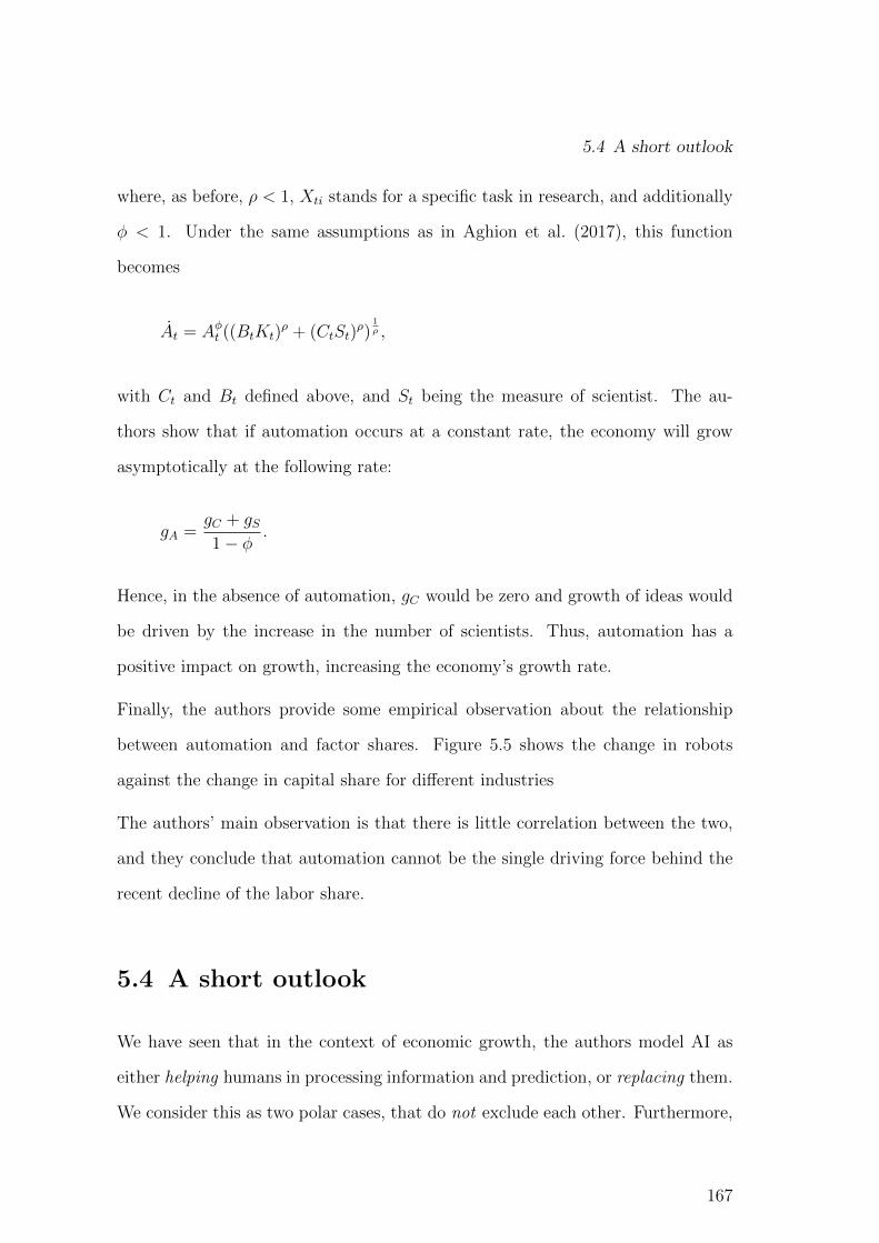
5.4 A short outlook
where, as before, ρ < 1, Xti stands for a specific task in research, and additionally
φ < 1. Under the same assumptions as in Aghion et al. (2017), this function
becomes
At = Aφt ((BtKt)ρ + (CtSt)
ρ)1ρ ,
with Ct and Bt defined above, and St being the measure of scientist. The au-
thors show that if automation occurs at a constant rate, the economy will grow
asymptotically at the following rate:
gA =gC + gS1− φ .
Hence, in the absence of automation, gC would be zero and growth of ideas would
be driven by the increase in the number of scientists. Thus, automation has a
positive impact on growth, increasing the economy’s growth rate.
Finally, the authors provide some empirical observation about the relationship
between automation and factor shares. Figure 5.5 shows the change in robots
against the change in capital share for different industries
The authors’ main observation is that there is little correlation between the two,
and they conclude that automation cannot be the single driving force behind the
recent decline of the labor share.
5.4 A short outlook
We have seen that in the context of economic growth, the authors model AI as
either helping humans in processing information and prediction, or replacing them.
We consider this as two polar cases, that do not exclude each other. Furthermore,
167
Chapter 5 Artificial intelligence and growth
ARTIFICIAL INTELLIGENCE AND ECONOMIC GROWTH 45
Figure 8: Capital Shares and Robots, 2004–2014
0 0.05 0.1 0.15 0.2 0.25 0.3 0.35-0.05
0
0.05
0.1
0.15
0.2
Utilities
Construction
Wood
Minerals Primary Metals
Fabricated Metals
Machinery
Computers
Appliances
Motor Vehicles
Other Transport Equipment
Misc Mfg
Food Mfg Textiles
Paper
Chemicals
Plastics
Education
CHANGE IN ROBOTS/VA
CHANGE IN CAPITAL SHARE
Note: The graph plots the change in the capital share from Jorgenson, Ho and Samuels (2017)against the change in the stock of robots relative to value-added using the robots data fromAcemoglu and Restrepo (2017).
industry level, this data is available for the decade 2004 to 2014. Figure 8 shows data on
the change in capital share by industry versus the change in the use of industrial robots.
Two main facts stand out from the figure. First, as noted earlier, the motor vehicles
industry is by far the largest adopter of industrial robots. For example, more than 56
percent of new industrial robots purchased in 2014 were installed in the motor vehicles
industry; the next highest share was under 12 percent in computers and electronic
products.
Second, there is little correlation between automation as measured by robots and
the change in the capital share between 2004 and 2014. The overall level of industrial
robot penetration is relatively small, and as we discussed earlier, other forces including
changes in market power, unionization, and composition effects are moving capital
shares around in a way that makes it hard for a simple data plot to disentangle.
Graetz and Michaels (2017) conduct a more formal econometric study using the EU-
KLEMS data and the International Federation of Robotics data from 1993 until 2007,
studying the effect of robot adoption on wages and productivity growth. Similar to
what we show in Figure 8, they find no systematic relationship between robot adoption
Figure 5.5: Capital share and robots 2000-2014 (Source: Aghion et al. (2017)).
while AI might further automate tasks and or jobs, it is important to distinguish
it from previous automation. AI is not driven by the accumulation of physical
capital. Instead, the so-called “AI-revolution”, that is observed recently, is fueled
by two other trends. On the one hand, there is an exponential rise in computational
power, and subsequent fall in the price paid for it. On the other hand, companies
have access to the huge amounts of data. Additionally, this data is generated by
households at zero costs for AI-companies and so-called “Tech Giants”, such as
Google and Facebook. Hence, we consider the following features to be relevant for
modeling AI in an endogenous growth model:
• AI interacts differently with certain labor types: While AI replaces some
low-skill labor type, it can increase the efficiency of some other type of
labor—in research and or production. Also, the AI sector offers employment
opportunities for a particularly high-skill type of labor. Potentially, this type
is even more productive in the AI-sector than in a more conventional sector.
• Physical capital and AI should be modeled as distinct variables. It is worth
including three different types of capital: physical capital, robots, and AI.
168

5.4 A short outlook
Hereby, AI should not stem from the accumulation of physical capital but
from the skill and effort of human labor.
• It is important not only to study AI as an intermediate in production but
also as a final good, sold to the consumer.
• AI relies on data generated by other sectors and households. This depen-
dency should be modeled, as the progress of AI might be halted by a mere
lack of usable data.
• The rise of Tech Giants certainly reshapes the market-place. Hence, a rise
of AI might change mark-ups and market-structure, potentially leading to
inefficiencies and distortions.
This list is, of course, not exhaustive in terms of features of AI that might be mod-
eled. In my view, these are conclusions we can infer from the literature presented.
169

Chapter 6
Appendix
6.1 Appendix for Chapter 2
6.1.1 Proof of Proposition 1
Assume there is a balanced growth path along which LRt = LR ∀t, where LR is
constant. The saving decision implies st =βwPt (1−τt)
1+β= Kt+1. Furthermore, we
have wPt = (1−α)Yt1−LRt
. Substituting wPt into the savings decision yields
Kt+1 =β(1− τt)(1 + β)
(1− α)Yt1− LRt
.
Recall that LRt = τt has to hold, so we have
Kt+1
Yt=β(1− α)
1 + β. (6.1)
As Kt+1
Ytis constant, Kt and Yt grow at the same rate. We show that this rate is
constant and equal to θLR. First, we take the logarithm of the production function
log(Yt) = (1− α) log(LPt ) + (1− α) log(Bt) + α log(Kt).
171

Chapter 6 Appendix
Then we write the analogous equation for the next period Yt+1 and subtract both
to obtain
gYt = (1− α)gLPt + (1− α)gBt + αgKt ,
where g(.) stands for the growth rate of the variable in the index. As in the steady
state, the labor share is constant in both sectors and it holds that gLPt = 0. We
have just found that gKt = gYt , even outside the steady state, so we obtain
gYt = gBt =Bt+1
Bt
− 1 = θLR.
Hence, the interest rate r is given by
r =αYt+1
Kt+1
=αYt+1YtYtKt+1
=α(1 + θLR)(1 + β)
β(1− α), (6.2)
because Yt+1/Yt = 1 + θLR.
6.1.2 Steady state of the social planner solution
For clarity we write down the Lagrange function of the social planner:
L =∞∑
t=0
βts[
log(c1t ) + β log(c2t+1)− λt(((1− LRt )Bt)
1−αKαt − c1t − c2t −Kt+1
)
− µt(Bt+1 − (1 + θLRt )Bt
) ],
where λt and µt are the Lagrange multiplier described in the main text. We derive
the steady state from Equations (2.9) and (2.10) in the following way: First, we
note that maximizing the Lagrangian with respect to c1t and c2t+1 yields c1t+1ββs
=
c2t+1. We assume β = βs, so that c1t = c2t and consequently, c1t = Ct/2, where Ct
172

6.1 Appendix for Chapter 2
stands for aggregate consumption in period t. We substitute this expression into
(2.9) and obtain
Ct+1
Ct=αβYt+1
Kt+1
, ⇔ Ct+1YtCtYt+1
=αβYtKt+1
.
In the steady state, aggregate consumption and output grow at the same rate, so
that the left-hand side is 1. Hence we find
Kt+1
αY t
= β,
where Kt+1 and Y t stand for the constantly growing values of capital and output.
Then we simplify (2.10) to
1
1− LR =Kt+1
αY t
(θ
1 + θLR+
1
1− LR1 + θLR
1 + θLR
),
where we can substitute Kt+1
αY tby β,
1 + θLR = β(θ − θLR + 1 + θLR),
θLR = βθ − (1− β).
6.1.3 Critical belief
Using our results from (2.13), we can write the utility of agent i if he is a researcher
as
URt,i = log
(wRt
1 + β
)+ (1 + β) log (1− θl + θi) + β log
(βrt+1w
Rt
1 + β
).
173

Chapter 6 Appendix
His utility as a worker is
UPt,i = log
((1− τt)wPt
1 + β
)+ β log
(βrt+1(1− τt)wPt
1 + β
).
The individual decision of agent i has no impact on the interest rate rt+1 so that the
respective interest rates are taken as equal in both cases. Hence we set URt,i = UP
t,i
for the agent with θi = θcrit,t
(1 + β) log(wRt ) + (1 + β) log (1− θl + θi) + β log (βrt+1)− (1 + β) log(1 + β)
=
(1 + β) log((1− τt)wPt
)+ β log(βrt+1)− (1 + β) log(1 + β),
⇔ log (1− θl + θi) = log
((1− τt)wPt
wRt
),
⇔ θcrit,t =(1− τt)wPt
wRt− (1− θl).
Proof of Proposition 8
After substituting the optimal savings decision, the utility function of a researcher
reads
URt,i = β log
(β
1 + β
)− log(1 + β) + log(wRt )(1 + β) + log
(θiet,i − q
e2t,i2
)+
β log(rt+1).
We want to alter the utility function of the researcher so that the derivative with
respect to effort will be identical to the first order condition of the social planner.
One way to do this is by setting wRt . Substituting wRt from Proposition 8 changes
174
6.1 Appendix for Chapter 2
the utility function to
URt,i = β log(
β
1 + β) + (1 + β) log(wt
R) + log(θet,i − qe2t,i2
) + Gtet,i + β log(rt+1),
(6.3)
with the derivative
∂URt,i
∂et,i=
θ − qet,iθet,i − q
e2t,i2
+ Gt = 0. (6.4)
Solving for et,i, which is the same for all i, yields
e2t −2
q
(θ − q
Gt
)et −
2θ
qGt
= 0, (6.5)
while the social planner FOC implies
eSOCt
2 − 2
q
(θ − q
Gt
)eSOCt − 2θ
qGt
= 0. (6.6)
Due to the definition of θ and Gt it holds that et = θh−θlθh−θcrit e
SOCt . To see this,
substitute et in Equation (6.5). This will yield Equation (6.6). In the decentralized
case we purposefully demand more effort from every researcher.
If eSOCt is the socially optimal individual and aggregate effort level, recall that the
mass of all agents is 1. Hence, in the steady state of the decentralized economy
we have for effort
ED =
∫ 1
θcrit−θlθh−θl
e di = eθh − θcritθh − θl
= eSOCθh − θlθcrit − θl
θcrit − θlθh − θl
= ESOC .
As mentioned, substituting e = θh−θlθh−θcritE
D in the steady state version of (6.5)
will yield the steady state version of Equation (6.6). Hence we have successfully
altered the researchers’ individual decisions to replicate one of the social planner’s
175
Chapter 6 Appendix
two optimality conditions.
Next we turn to the FOC of the decentralized government when it can issue debt,
1− β1− LD,R =
βθE
1 + θELD,R, (6.7)
which together with Equation (6.4) replicate the two equations of the social planner
problem and yield LSOC and ESOC as solutions.
Finally, we prove the definition of wtR. Under Proposition 8, we demonstrated
how optimal effort and labor demand can be established. Now we turn to labor
supply. As before, some agent i must be indifferent between working in research
and the productive sector. We show that, if wRt,i is defined as above, all agents are
indifferent. To see this, recall Equation (6.3). By construction, if the optimal et,i
is the same for all agents, URt,i is also the same. The following equality therefore
holds for all i
(1 + β) log(wtR) + log
(θet − q
e2t2
)+ Gtet = (1 + β) log(wPt ),
which yields
wtR = wPt
(θet − q
e2t2
) −11+β
e−Gtet1+β ,
as all researchers invest the same amount of effort. This concludes the proof.
Furthermore, note that in equilibrium, the following holds
wRt,i = wtR
θet,i − q e
2t,i
2
θiet,i − qe2t,i2
11+β
eGtet,i1+β , and
wRt,i =wPt
et(θi − q et2 )1
1+β
,
176

6.1 Appendix for Chapter 2
which means that researchers are paid the wage of the productive sector with a
mark-down depending on their preferences and optimal effort. This leaves agents
indifferent as to sector choice and exertion of socially optimal effort.
6.1.4 Stability analysis
In this section, we analyze the stability of the steady states of the decentralized
economy and the social planner solution in both models.
Decentralized solution without research bubbles
We have demonstrated that research labor is equal to the government’s demand,
given by
LRt = LD,R =1
1 + β
(β − 1
θ
).
It is therefore always constant and implies the following constant gross growth rate
of the knowledge stock: Bt+1/Bt = 1 + θLR. Note that savings are given by
st = Kt+1 =β(1− τt)wPt
1 + β,
so that substituting wPt = (1− α)Yt/(1− LRt ) yields
Kt+1 =(1− α)β(1− τt)
1 + β(1− LRt )−αB1−α
t Kαt ,
where τt = LRt = LR, as shown previously. We divide both sides by Bt+1,
Kt+1
Bt+1
=(1− α)β
(1 + β)(1− LR)1−α
(Kt
Bt
)αBt
Bt+1
.
177
Chapter 6 Appendix
We write capital in terms of the knowledge stock and define kt = Kt/Bt. Hence,
given the constant growth rate of Bt+1/Bt, we have
kt+1 =(1− α)β
(1 + β)(1− LR)α−1(1 + θLR)kαt ,
which is a simple convex policy-function in capital as the factor in front of kαt is a
mere constant.
Social planner solution
To study whether the economy converges to the socially optimal steady state, we
rewrite (2.10):
1 + θLRt1− LRt
=Kt+1
αYt+1
Yt+1
Yt
(θ +
1 + θLRt+1
1− LRt+1
), which implies
1 + θLRt1− LRt
=Kt+1
αYt+1
Yt+1
Yt
1 + θ
1− LRt+1
or simply
LPt+1 = 1− LRt+1 =Kt+1
αYt+1
Yt+1
Yt
1− LRt1 + θLRt
(1 + θ), (6.8)
so that the model dynamics are governed by (6.8), the knowledge production
function, and the following three equations:
Yt = Kαt (BtL
Pt )1−α,
Kt+1 = Yt − c1t − c2t ,
c2t+1 = βαYt+1
Kt+1
c1t .
We can rewrite aggregate consumption Ct = c1t + c2t , using the fact that the max-
imization of the Lagrangian with respect to c1t and c2t+1 yields c1t+1ββs
= c2t+1.
Assuming β = βs, we arrive at c1t = Ct/2. Next we express the four equations in
178

6.1 Appendix for Chapter 2
terms of effective labor BtLPt , defining gBt and gLt as the growth rate of knowledge
and of labor input in the productive sector in period t,
YtBtLPt
= yt = kαt ,
kt+1(1 + gBt)(1 + gLt) = yt − ct,
ct+1(1 + gBt)(1 + gLt) = βαkα−1t+1 ct,
where kt and ct without superscript indicate capital and aggregate consumption
per effective labor. Equation (2.10) becomes
LPt+1
LPt= 1 + gLt =
Kt+1
αYt+1
Yt+1
Yt
1
1 + θLRt(1 + θ).
By using 1 + gBt = 1 + θLRt from the knowledge production function we obtain
1 + gLt =1
α
kt+1
yt+1
yt+1
yt(1 + gBt)(1 + gLt)
(1 + θ)
1 + gBt,
1 =1 + θ
α
kt+1
kαt,
kt+1 =α
1 + θkαt . (6.9)
We arrive at a concave policy-function for capital per effective labor kt. Next we
turn to the Euler equation for consumption. By using the following relationships:
1 + gBt = 1 + θLRt ,
1 + gLt =Kt+1
αYt
1
1 + θLRt(1 + θ) =
Yt − CtαYt
1
1 + θLRt(1 + θ),
179
Chapter 6 Appendix
we obtain
ct+1
ct=
1
(1 + θ)βαkα−1t+1
αYtYt − Ct
,
ct+1
ct=
α2β
1 + θ
kα−1t+1 kαt
kαt − ct. (6.10)
Hence it is possible to express the system in the two Equations (6.9) and (6.10)
in two variables, consumption and capital per effective labor. The steady state
along which gBt and all variables in terms of effective labor, and equivalently the
amount of labor supplied to the productive sector are constant is given by
k =
(α
1 + θ
) 11−α
,
c = kα(1− α2β
1 + θkα−1) =
(α
1 + θ
) α1−α
(1− αβ) .
As the policy-function for capital is concave, we know that capital will converge
to the steady state. The convergence of consumption is not clear. We know that
for consumption to grow at a positive rate, it must hold that
ct+1
ct> 1⇒ ct > kαt − α2β
(α
1 + θ
)α−1kα
2
t . (6.11)
We use the phase diagram in Figure 6.1 to discuss the convergence of the model.
The black vertical line is the steady state condition for capital. The curved black
line shows the respective condition for consumption. The red line divides the space
into two sectors: The one above the red line indicates where consumption is grow-
ing, the one below the red line shows where consumption is decreasing. As we
know that capital converges to the steady state from both sides, we can draw the
appropriate arrows that indicate the movement of the variables.
The diagram shows that the model is saddle-path-stable, as convergence to the
180

6.1 Appendix for Chapter 2
kt
c t
Figure 6.1: Phase diagram for consumption and capital per effective labor.
steady state, which is the intersection of all three lines, does not occur from any
arbitrary initial allocation of ct and kt. For instance, convergence from an allo-
cation in the right upper corner, where consumption lies above the red line and
capital to the right of the vertical black line, is not possible. The economy would
move to kt = 0. In Figure 6.2, the space between the green lines shows all possi-
ble initial allocations of capital and consumption from which convergence to the
unique steady state occurs.
kt
c t
Figure 6.2: Set of initial allocations from which the economy converges to thesteady state.
We find further support for the saddle-path-stability of the system by linearizing
181

Chapter 6 Appendix
it around the steady state. The linearized versions of (6.9) and (6.10) are
kt+1
ct+1
=
α 0(α2ck− αckα−1
kα−c
) (1 + c
kα−c)
kt
ct
.
As the second entry of the first row is 0, the Eigenvalues of the matrix are given
by α = 0.3 < 1 and(1 + 1
kα−c)> 1. The first Eigenvalue is real and smaller in
absolute value than 1, while the second is real and larger than 1. To see this, note
that kα is aggregate production per effective labor, while c is the aggregate con-
sumption per effective labor. This difference is positive, so the second Eigenvalue
is at least one.
Government solution with research bubbles
As we have demonstrated, the research bubbles lead to a greater input of labor in
the research sector. Yet this value is constant over time, so that the dynamics of
the model do not change in comparison to the model without bubbles. Thus our
analysis from the section above carries over, the only difference being that LR is
greater.
6.1.5 Convergence under debt financing
We established above that it is theoretically possible to implement the socially
optimal steady state amount of research in the decentralized economy. In this
section, we investigate whether the model with heterogeneous beliefs converges
to its social optimum. If the optimal amount of research is implemented, i.e. if
182

6.1 Appendix for Chapter 2
LRt = LO,R ∀ t, we have
Kt+1 =β
1 + β(wRt L
O,R + (1− τG)wPt (1− LO,R)).
We substitute wRt to obtain
Kt+1
Bt+1
= kt+1 =β(1− α)(1− τG)
(1 + β)(1− LO,R)α−1
1 + (1− LO,R)(θh − θl)(
1− LO,R
LB
)
1 + (θh − θl)(
1− LO,R
LB
)
kαt .
Note that this expression is a concave policy-function for kt, as all terms in front
of kαt are constant. Next, under conditions on the parameter values, we show that
aggregate debt dt grows at the rate of output. We have defined Dt(LO,R) as the
additional debt issued in period t. Therefore we can write aggregate debt dt as
dt =1− γγ
Yt + rtdt−1,
where we write γ = (1− LO,R)β(1−α) for convenience. Hence,
dt =1− γγ
[Yt + rtYt−1 + rtrt−1Yt−2 + ...+
t∏
s=1
rsY0
]or
dt =1− γγ
[Yt + α
YtKt
Yt−1 + α2 YtKt
Yt−1Kt−1
Yt−2 + ...+ αtt∏
s=1
YsKs
Y0
].
From Equation (6.1) we know that Kt+1/Yt is constant for all t. This enables us
to write
dt =1− γγ
Yt
[1 +
α
δ+α2
δ2+ ...+
αt
δt
], with
δ =β(1− α)
1 + β.
183
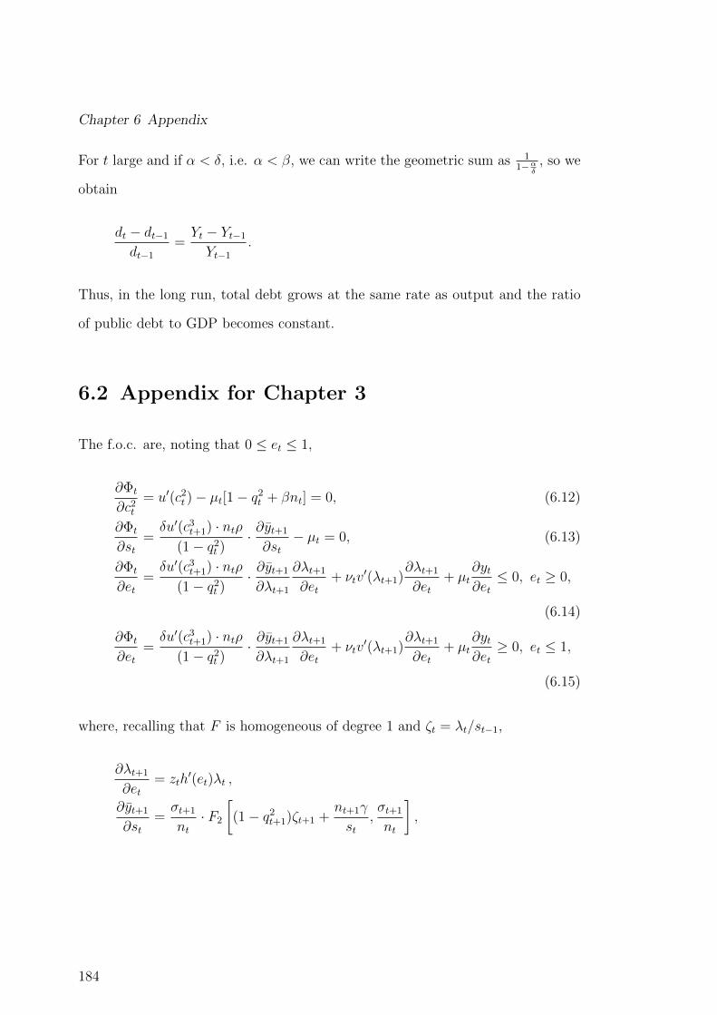
Chapter 6 Appendix
For t large and if α < δ, i.e. α < β, we can write the geometric sum as 11−α
δ, so we
obtain
dt − dt−1dt−1
=Yt − Yt−1Yt−1
.
Thus, in the long run, total debt grows at the same rate as output and the ratio
of public debt to GDP becomes constant.
6.2 Appendix for Chapter 3
The f.o.c. are, noting that 0 ≤ et ≤ 1,
∂Φt
∂c2t= u′(c2t )− µt[1− q2t + βnt] = 0, (6.12)
∂Φt
∂st=δu′(c3t+1) · ntρ
(1− q2t )· ∂yt+1
∂st− µt = 0, (6.13)
∂Φt
∂et=δu′(c3t+1) · ntρ
(1− q2t )· ∂yt+1
∂λt+1
∂λt+1
∂et+ νtv
′(λt+1)∂λt+1
∂et+ µt
∂yt∂et≤ 0, et ≥ 0,
(6.14)
∂Φt
∂et=δu′(c3t+1) · ntρ
(1− q2t )· ∂yt+1
∂λt+1
∂λt+1
∂et+ νtv
′(λt+1)∂λt+1
∂et+ µt
∂yt∂et≥ 0, et ≤ 1,
(6.15)
where, recalling that F is homogeneous of degree 1 and ζt = λt/st−1,
∂λt+1
∂et= zth
′(et)λt ,
∂yt+1
∂st=σt+1
nt· F2
[(1− q2t+1)ζt+1 +
nt+1γ
st,σt+1
nt
],
184

6.2 Appendix for Chapter 3
∂yt∂et
= −(γ + wλt)nt · F1
[(1− q2t − wntet)ζt +
ntγ(1− et)st−1
,σtnt−1
]and
∂yt+1
∂λt+1
= (1− q2t+1)F1
[(1− q2t+1)ζt+1 +
nt+1γ
st,σt+1
nt
].
6.2.1 Proof of Lemma 1
Since st and λt are growing at the steady rate g(e) = zh(e)− 1 > 0, we have
c2tc3t+1
=(1− q2)(1− q3)ρn(1− q2 + βn)
·(yt − styt+1
− ρ
zh(e)
),
where
yt − styt+1
− ρ
zh(e)=
1
zh(e)
(F [(1− q2 − wne)ζ, σ/n]− zh(e)
F [(1− q2)ζ, σ/n]− ρ),
which is a constant for any given e. Substituting for c2t/c3t+1 from (3.26), we obtain
ρδσ(1− q2 + βn)F2[(1− q2)ζ, σ/n]
1− q2
=
(ρn(1− q2 + βn)zh(e)F [(1− q2 − wne)ζ, σ/n]
(1− q2)(1− q3)[F [(1− q2 − wne)ζ, σ/n]− ρF [(1− q2)ζ, σ/n]− zh(e)]
)ξ,
which may be rearranged as
F [(1− q2 − wne)ζ, σ/n]− ρF [(1− q2)ζ, σ/n]
=
(1 +B′
F [(1− q2)ζ, σ/n]
(F2[(1− q2)ζ, σ/n])1/ξ
)zh(e), (6.16)
where
B′ ≡ n
(1− q3)(δσ)1/ξ
(ρ(1− q2 + βn)
1− q2)1−1/ξ
185
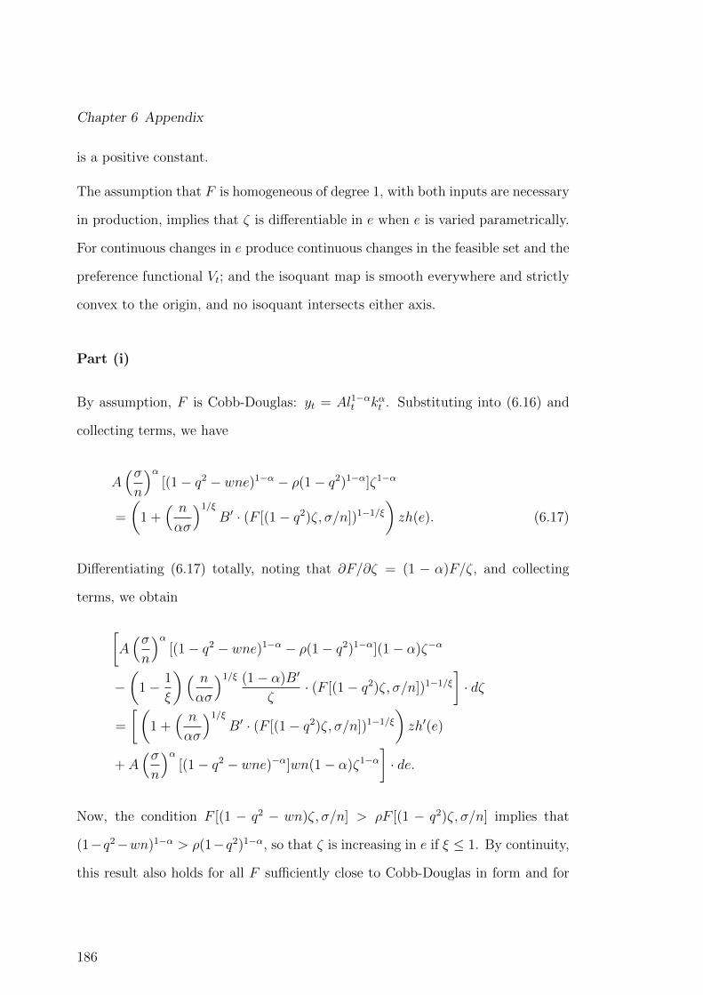
Chapter 6 Appendix
is a positive constant.
The assumption that F is homogeneous of degree 1, with both inputs are necessary
in production, implies that ζ is differentiable in e when e is varied parametrically.
For continuous changes in e produce continuous changes in the feasible set and the
preference functional Vt; and the isoquant map is smooth everywhere and strictly
convex to the origin, and no isoquant intersects either axis.
Part (i)
By assumption, F is Cobb-Douglas: yt = Al1−αt kαt . Substituting into (6.16) and
collecting terms, we have
A(σn
)α[(1− q2 − wne)1−α − ρ(1− q2)1−α]ζ1−α
=
(1 +
( n
ασ
)1/ξB′ · (F [(1− q2)ζ, σ/n])1−1/ξ
)zh(e). (6.17)
Differentiating (6.17) totally, noting that ∂F/∂ζ = (1 − α)F/ζ, and collecting
terms, we obtain
[A(σn
)α[(1− q2 − wne)1−α − ρ(1− q2)1−α](1− α)ζ−α
−(
1− 1
ξ
)( n
ασ
)1/ξ (1− α)B′
ζ· (F [(1− q2)ζ, σ/n])1−1/ξ
]· dζ
=
[(1 +
( n
ασ
)1/ξB′ · (F [(1− q2)ζ, σ/n])1−1/ξ
)zh′(e)
+ A(σn
)α[(1− q2 − wne)−α]wn(1− α)ζ1−α
]· de.
Now, the condition F [(1 − q2 − wn)ζ, σ/n] > ρF [(1 − q2)ζ, σ/n] implies that
(1−q2−wn)1−α > ρ(1−q2)1−α, so that ζ is increasing in e if ξ ≤ 1. By continuity,
this result also holds for all F sufficiently close to Cobb-Douglas in form and for
186

6.2 Appendix for Chapter 3
all ξ exceeding, but sufficiently close to, 1.
Part (ii)
By assumption, yt = A[b1lεt + b2k
ε]1/ε, ε ≤ 1: the elasticity of substitution is
(ε− 1)−1, where ε = 0 is Cobb-Douglas. Proceeding as before,
F [(1− q2)ζ, σ/n]
(F2[(1− q2)ζ, σ/n])1/ξ=
A[b1((1− q2)ζ)ε + b2(σ/n)ε]1/ε
[b2(σ/n)ε−1A[b1((1− q2)ζ)ε + b2(σ/n)ε]1/ε−1]1/ξ
= B1[b1((1− q2)ζ)ε + b2(σ/n)ε]ψ,
where ψ = (1/ε) + (1 − 1/ε)/ξ and B1 is a positive constant. Substituting into
(6.16), noting the derivative of [b1((1−q2)ζ)ε+b2(σ/n)ε]1/ψ w.r.t. ζ and rearranging
as before in part (i), there are two terms on the l.h.s. The first is the partial
derivative of {F [(1 − q2 − wne)ζ, σ/n] − ρF [(1 − q2)ζ, σ/n]} w.r.t. ζ, which is
positive if ε ≤ 0 and F [(1−q2−wn)ζ, σ/n] > ρF [(1−q2)ζ, σ/n]. The second term
has the sign of ψ · ε. Now, ψ · ε ≤ 0 iff ε + ξ ≤ 1. Since both inputs are assumed
to be necessary in production, ε ≤ 0, which yields the required result. Q.E.D.
6.2.2 Proof of Corollary 1
Recalling that both inputs are necessary in production, it follows that for all such
F , F1
[(1− q2)ζ, σ
n
]and F2
[(1− q2)ζ, σ
n
]are, respectively, decreasing and increas-
ing in e. Now, F1
[(1− q2 − wne)ζ, σ
n
]decreases more slowly than F1
[(1− q2)ζ, σ
n
]
as e increases. Hence, if h(e) is concave or sufficiently weakly convex, it is seen
that D is increasing in e across paths. Q.E.D.
187

Chapter 6 Appendix
6.2.3 Derivation of Condition (3.20)
We simplify (3.18) using
F1
[lt,σst−1n
]=
1− α(1− q2 − wn)ζ
F [(1− q2 − wn)ζ, σ/n], and
F1[lt+1,σstn
]
F2[lt+1,σstn
]=
1− αα· σn· 1
(1− q2)ζ .
Noting that (6.16) specializes to
F[(1− q2 − wn)ζ(1),
σ
n
]− ρF
[(1− q2)ζ(1),
σ
n
]=
(1 +
1
(1− q3)αδ
)zh(1),
we obtain
c2t = st−1
((1 +
1
(1− q3)αδ
)zh(1)− st
st−1
)1
1− q2 + βnand
c2t = st−11
(1− q3)αδ ·zh(1)
1− q2 + βn.
Substituting into (3.18) and rearranging terms, we have
λ−1t+1st−1zh(1)
(1− q3)αδ ≥(w(1− α)
(1− q2 − wn)ζ(1)F [·p]− zh′(1)(1− α)
ζ(1)nα
)· 1
bzh′(1),
Since ζt = λt/st−1 and λt+1/λt → zh(1) in the state of progress, a further rear-
rangement yields
zh′(1) ≥(
w(1− α)
(1− q2 − wn)F [·p]− zh′(1)(1− α)
nα
)· (1− q3)αδ
b,
188

6.2 Appendix for Chapter 3
so that
zh′(1) ≥ w(1− α)
(1− q2 − wn)F [·p] ·
(b
(1− q3)αδ +1− αnα
)−1.
6.2.4 Derivation of Equation (3.31)
Total differentiation of
Qt = n(δρF1
[lt+1,
σstn
]u′(c3t+1) + bv′(λt+1)
)
yields, noting (3.29) once more,
dQt = δρσF12
[lt+1,
σstn
]u′(c3t+1)dst + zh(e) dλt·
n
[δρ
((1− q2)F11
[lt+1,
σstn
]u′(c3t+1) +
u′′(c3t+1)c
3t+1
zh(e)λtF1
[lt+1,
σstn
])+ bv′′(λt+1)
]
≡ A′ · zh(e) · dλt + δρσF12
[lt+1,
σstn
]u′(c3t+1)dst . (6.18)
Next, we examine the expressiondQt
dλt· λtQt
on the r.h.s. of (3.30). From (6.18), we
have
dQt
dλt· λtQt
=A′zh(e) · λt + δρσF12
[lt+1,
σstn
]u′(c3t+1)st
n(δρF1
[lt+1,
σstn
]u′(c3t+1) + bv′(λt+1)
) .
Collecting terms in the numerator involving u′(c3t+1), the multiplicand is
J ≡ nδρ[(1− q2)λt+1F11
[lt+1,
σstn
]− ξF1
[lt+1,
σstn
]+σstnF12(lt+1,
σstn
)].
Since F1
[lt+1,
σstn
]and F2
[lt+1,
σstn
]are homogeneous of degree zero, it follows from
189

Chapter 6 Appendix
Euler’s Theorem that
[(1− q2)λt+1 + nγ]F11
[lt+1,
σstn
]+σstnF12
[lt+1,
σstn
]= 0,
so that for sufficiently large λt, J reduces to −nδρξF1
[lt+1,
σstn
]. Hence, recalling
that v is iso-elastic, we obtain the elasticity of Qt w.r.t. λt:
dQt
dλt
λtQt
=−ξδρF1
[lt+1,
σstn
]u′(c3t+1)− ηbv′(λt+1)
δρF1
[lt+1,
σstn
]u′(c3t+1) + bv′(λt+1)
.
By hypothesis, (λt, st) are growing at the rate g = zh(e)−1. Hence, this elasticity
can be expressed in the form
dQt
dλt· λtQt
= −ξA+ ηb ·B(1 + g)−(η−ξ)
A+ b ·B(1 + g)−(η−ξ),
where A = δρF1
[lt+1,
σstn
]and v′(λt+1)/u
′(c3t+1) are positive constants along the
path in question.
6.2.5 The extreme allocations of St(It)
In what follows, it will be useful to rewrite (3.35) in the form
[1 +
βn
1− q2t (It)
]c2t +
st1− q2t (It)
+ ρF
[λt +
γn
1− q2t (It),
σt(It)
1− q2t (It)· st−1n
]
≤ F
[(1− wnet
1− q2t (It)
)λt +
γn(1− et)1− q2t (It)
,σt(It)
1− q2t (It)· st−1n
], It = 0, 1. (6.19)
Allocation A: c2t = et = 0. Given It, st is maximal. From (3.35), we have st =
(1−ρ)F
[(1− q2t (It))λt + nγ,
σt(It)st−1n
], It = 0, 1. Given It, an increase in q2t (It)
will induce A to shift towards the origin O, as depicted by the point A′. Given that
q2t (1) > q2t (0), the allocations A and A ′ also represent those ruling under peace
190

6.2 Appendix for Chapter 3
and war, respectively, in period t.
Allocation B: c2t = 0, et = 1. Given It and maximum (full-time) investment in
education, st is maximal. We have, for It = 0, 1,
st = F
[(1− q2t (It)− wn)λt,
σt(It)st−1n
]− ρF
[(1− q2t (It))λt + nγ,
σt(It)st−1n
].
We begin by noting that the outer boundary of S(It) in the plane defined by c2t = 0,
AB, is strictly concave in virtue of the strict concavity of F in each argument.
We next establish conditions under which the said value of st is positive, i.e., B
lies to the right of G on the plane defined by et = 1. From (6.19), we have, for
It = 0, 1,
(1− q2t (It)− wn)−1st =F
[λt,
σt(It)
1− q2t (It)− wn· st−1n
]
− ρF[λt +
n(wλt + γ)
1− q2t (It)− wn,
σt(It)
1− q2t (It)− wn· st−1n
].
The input of human capital in the second term on the r.h.s. is larger in the
proportion n(w + γ/λt)/(1 − q2t (It) − wn). This proportion is maximal when
λt = 1. Since F is homogeneous of degree one, λt = 1 will therefore yield the
best chance that st < 0, as intuition would suggest. Now, w is fairly small, say
about 1/20, and γ would be about 0.6. In such a state of economic backwardness,
n = 3/2 and q2t = 0.2 are broadly plausible, so that the said proportion of inputs
of human capital would be about 4/3. Hence,
λt +n(wλt + γ)
1− q2t (It)− wn≤ 7λt/3, ∀λt.
Observe, however, that F is strictly concave in each argument alone and ρ is
unlikely to exceed 1/3. Comparing the two terms on the r.h.s., inputs of human
191
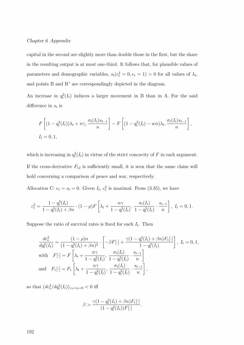
Chapter 6 Appendix
capital in the second are slightly more than double those in the first, but the share
in the resulting output is at most one-third. It follows that, for plausible values of
parameters and demographic variables, st(c2t = 0, et = 1) > 0 for all values of λt,
and points B and B ′ are correspondingly depicted in the diagram.
An increase in q2t (It) induces a larger movement in B than in A. For the said
difference in st is
F
[(1− q2t (It))λt + nγ,
σt(It)st−1n
]− F
[(1− q2t (It)− wn)λt,
σt(It)st−1n
],
It = 0, 1,
which is increasing in q2t (It) in virtue of the strict concavity of F in each argument.
If the cross-derivative F12 is sufficiently small, it is seen that the same claim will
hold concerning a comparison of peace and war, respectively.
Allocation C: et = st = 0. Given It, c2t is maximal. From (3.35), we have
c2t =1− q2t (It)
1− q2t (It) + βn· (1− ρ)F
[λt +
nγ
1− q2t (It),
σt(It)
1− q2t (It)· st−1n
], It = 0, 1.
Suppose the ratio of survival rates is fixed for each It. Then
dc2tdq2t (It)
=(1− ρ)n
(1− q2t (It) + βn)2·[−βF [·] +
γ(1− q2t (It) + βn)F1[·]1− q2t (It)
], It = 0, 1,
with F [·] = F
[λt +
nγ
1− q2t (It),
σt(It)
1− q2t (It)· st−1n
]
and F1[·] = F1
[λt +
nγ
1− q2t (It),
σt(It)
1− q2t (It)· st−1n
],
so that (dc2t/dq2t (It)) et=st=0 < 0 iff
β >γ(1− q2t (It) + βn)F1[·]
(1− q2t (It))F [·] .
192

6.2 Appendix for Chapter 3
The input of human capital is λt + nγ/(1− q2t (It)). Its imputed share in output is
1−α ≡ (λt+nγ(1−q2t (It))−1)F1[·]/F [·], so the foregoing inequality can be written
β >(1− α)γ(1− q2t (It) + βn)
(1− q2t (It))λt + γn,
which certainly holds for all sufficiently large λt. The denominator takes a mini-
mum under backwardness (λt = 1), when the inequality becomes
(β − (1− α)γ)(1− q2t (It)) + αβγn > 0.
Since both inputs are necessary in production, F is strictly concave in both ar-
guments and α ∈ (0, 1). It is plausible that α < 0.5, but n ≥ 1, so that the
inequality may hold even if β < γ, as in Table 3.1, for which constellation the
inequality holds.
Under the assumption that the ratio of survival rates is fixed for each It, we have
established that the points C and C ′ relate to each other as depicted in the figure,
which reveals that there is damage even under a mild mortality shock, given It.
If the ratio of survival rates is the same in both states, the points C and C ′ also
represent the respective allocations in peace and war.
Allocation D: et = 1, st = 0. Given It and maximum investment in (full-time)
education, c2t is maximal. Analogously to AB, the outer boundary of S in the
plane defined by s2t = 0, CD, is strictly concave in virtue of the strict concavity of
F in each argument.
Given et and It, all pairs (c2t , st) on the outer frontier of S are linearly related and
independent of et : dst = −(1− q2t (It) + βn) dc2t . Hence, AC is parallel to BD, and
A ′C ′ to B ′D ′. An increase in q2t (It) makes c2t cheaper relative to st; but since C ′
lies closer to O than does C, it follows that D ′ lies closer to G than does D. The
193

Chapter 6 Appendix
same holds when the ratio of survival rates is the same in both states.
6.2.6 Convergence analysis
Equations (3.22) and (3.23) provide our starting point. We take their total deriva-
tives, given that the right-hand sides depend on λt and et. We, then, equate the
left-hand sides and find the sign of det/dλt, that is, of the derivative ∂e0t/∂λt: it
turns out to be positive. Hence, it follows from (3.4) that a higher value of λt also
increases λt+1 through its indirect effect on the choice e0t . Two further statements
can be made. First, if an economy has reached the progressive state and is then
hit by a sufficiently small shock, e0t will fall, if at all, not much below 1, and the
economy will remain in, or return to, that state. Second, if λt is close to some
stationary level associated with e0t < 1 and the economy is hit by a sufficiently
adverse shock, there will be a descent into backwardness.
In the following, we take the derivatives of the aforementioned equations with
respect to et and λt. We then analyze their signs when (et, λt) = (0, 1) and et = 1
with λt large.
The derivative of the right hand side of (3.22) with respect to et is
[((1− q2 − wnet) +
nγ(1− et)λt
)1−α− ρ
(1− q2 +
nγ
λt
)1−α]−1·
{zh′(et) +
(zh(et) +
1
λt
)[(
1− q2 − wnet + nγ(1−et)λt
)1−α− ρ(1− q2 + nγ
λt)1−α
]−1
(1− q2 − wnet + nγ(1−et)
λt
)α ·
(1− α)
(w +
γ
λt
)n
}(nσ
)αA−1
(1 +
1
αδ(1− q3)
).
194

6.2 Appendix for Chapter 3
When et = 0 and λt = 1, this yields
[A(1− ρ)(1− q2 + nγ)1−α
]−1{zh′(0) +
(1− α)(w + γ)n
(1− ρ)(1− q2 + nγ)
}·
(nσ
)α(1 +
1
αδ(1− q3)
),
which is positive.
When et = 1 and λt is large, we have
(nσ
)α(1 +
1
αδ(1− q3)
)A−1
[(1− q2 − wn)1−α − ρ(1− q2 +
nγ
λt)1−α
]−1·
{(zh(1) +
1
λt
) [(1− q2 − wn)1−α − ρ(1− q2 + nγλt
)1−α]−1
(1− α)(w + γ
λt
)n
(1− q2 − wn)α+
zh′(1)
}
which is also positive.
The derivative of (3.22) with respect to λt is
[((1− q2 − wnet) +
nγ(1− et)λt
)1−α− ρ
(1− q2 +
nγ
λt
)1−α]−1·
{− 1 +
(1− q2 − wnet + nγ(1−et)
λt
)−α(1− et)− ρ
(1− q2 + nγ
λt
)−α
(1− q2 − wnet + nγ(1−et)
λt
)1−α− ρ
(1− q2 + nγ
λt
)1−α ·
(1− α)nγ
(zh(et) +
1
λt
)}(nσ
)α(1 +
1
αδ(1− q3)
)1
Aλ2t.
Evaluating this expression at et = 0 and λt = 1 gives
(nσ
)α(1 +
1
1 + αδ(1− q3)
)(A[(1− q2 + nγ)1−α(1− ρ)
])−1{−1 +
(1− α)nγ
1− q2 + nγ
},
which can be negative if 1− q2 > −αnγ.
195

Chapter 6 Appendix
When et = 1 and λt is large, we have
−(nσ
)α(1 +
1
αδ(1− q3)
)1
Aλ2t
[((1− q2 − wn) +
nγ
λt
)1−α− ρ
(1− q2 +
nγ
λt
)1−α]−1·
1 +
(zh(1) +
1
λt
) (1− α)ρnγ(
1− q2 + nγλt
)−α
(1− q2 − wn+ nγ
λt
)1−α− ρ
(1− q2 + nγ
λt
)1−α
,
which is clearly negative.
We repeat these steps in Equation (3.23). The derivative of the right hand side
with respect to et is
(nσ
)αzh′(et)
(1− q2 − wnet + nγ(1−et)
λt
)α
αAδn(1− q3)(w + γ
λt
)
δ(1− q3)(1− q2)(
1− q2 + nγλt+1
)2nγλtλ2t+1
zh′(et)
+
(δ(1− q3)(1− q2)
1− q2 + nγλt+1
+bn
1− α
)h′′(et)
h′(et)−
αn(w + γ
λt
)
1− q2 − wnet + nγ(1−et)λt
.
When et = 0 and λt = 1, we have
(nσ
)αzh′(0) (1− q2 + nγ)
α
αAδn(1− q3) (w + γ)
{δ(1− q3)(1− q2)nγzh′(0)
(1− q2 + nγ)2+
[h′′(0)
h′(0)− αn(w + γ)
1− q2 + nγ
]·
(δ(1− q3)(1− q2)
1− q2 + nγ+
bn
1− α
)}.
When et = 1 and λt is large, we have
(nσ
)αzh′(1)(1− q2 − wn)α
αAδn(1− q3)(w + γ
λt
){δ(1− q3)(1− q2)(
1− q2 + nγλt+1
)2nγλtzh
′(1)
λ2t+1
+
h′′(1)
h′(1)−αn(w + γ
λt
)
1− q2 − wn
(δ(1− q3)(1− q2)
1− q2 + nγλt+1
+bn
1− α
)}.
Both can be negative if h is concave or sufficiently weakly convex.
196

6.2 Appendix for Chapter 3
Finally, we examine the derivative of the right hand side of (3.23) with respect to
λt:
(nσ
)α (1− q2 − wnet + nγ(1−et)
λt
)αzh′(et)
(αAδn(1− q3))(w + γ
λt
)λ2t
{δ(1− q3)(1− q2)(
1− q2 + nγλt+1
)2nγλ2t zh
′(et)
λ2t+1
+
(δ(1− q3)(1− q2)
1− q2 + nγλt+1
+bn
1− α
)[γ
w + γλt
− αnγ(1− et)1− q2 − wnet + nγ(1−et)
λt
]}.
Plugging in et = 0 and λt = 1 yields
(nσ
)α(1− q2 + nγ)
αzh′(0)
(αAδn(1− q3)) (w + γ)
{(δ(1− q3)(1− q2)
1− q2 + nγ+
bn
1− α
)
[γ
w + γ− αnγ
1− q2 + nγ
]},
where 1− q2 > αwn is a necessary condition for the derivative to be positive.
When et = 1 and λt is large, the derivative is
δ(1− q3)(1− q2)(
1− q2 + nγλt+1
)2nγλ2t zh
′(1)
λ2t+1
+
(δ(1− q3)(1− q2)
1− q2 + nγλt+1
+bn
1− α
)γ
w + γλt
·
(nσ
)α(1− q2 − wn)
αzh(1)
(αAδn(1− q3))(w + γ
λt
)λ2t
,
which is positive.
In summary, we find that the derivative of (3.22) w.r.t. et is positive and that
w.r.t. λt is negative. The opposite holds for (3.23), given the previously stated
conditions. Equating the total derivatives yields
[+] · det + [−] · dλt = [−] · det + [+] · dλt,
197
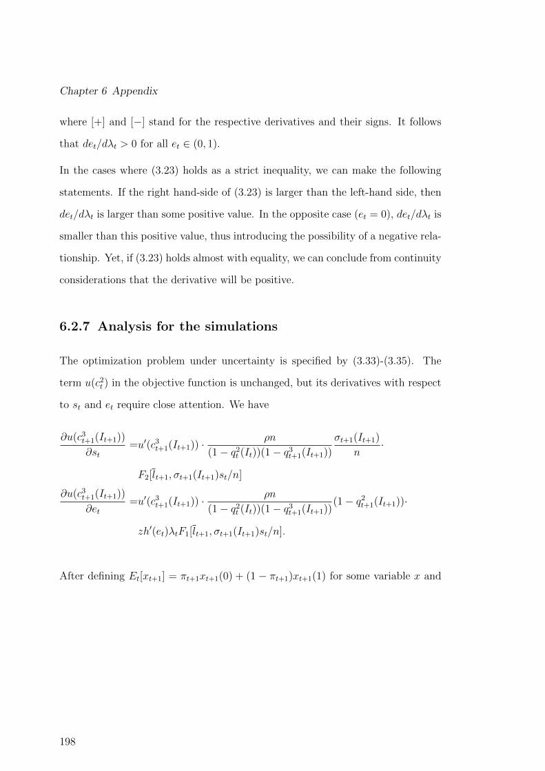
Chapter 6 Appendix
where [+] and [−] stand for the respective derivatives and their signs. It follows
that det/dλt > 0 for all et ∈ (0, 1).
In the cases where (3.23) holds as a strict inequality, we can make the following
statements. If the right hand-side of (3.23) is larger than the left-hand side, then
det/dλt is larger than some positive value. In the opposite case (et = 0), det/dλt is
smaller than this positive value, thus introducing the possibility of a negative rela-
tionship. Yet, if (3.23) holds almost with equality, we can conclude from continuity
considerations that the derivative will be positive.
6.2.7 Analysis for the simulations
The optimization problem under uncertainty is specified by (3.33)-(3.35). The
term u(c2t ) in the objective function is unchanged, but its derivatives with respect
to st and et require close attention. We have
∂u(c3t+1(It+1))
∂st=u′(c3t+1(It+1)) ·
ρn
(1− q2t (It))(1− q3t+1(It+1))
σt+1(It+1)
n·
F2[lt+1, σt+1(It+1)st/n]
∂u(c3t+1(It+1))
∂et=u′(c3t+1(It+1)) ·
ρn
(1− q2t (It))(1− q3t+1(It+1))(1− q2t+1(It+1))·
zh′(et)λtF1[lt+1, σt+1(It+1)st/n].
After defining Et[xt+1] = πt+1xt+1(0) + (1 − πt+1)xt+1(1) for some variable x and
198

6.3 Appendix for Chapter 4
substituting for the above derivatives, we obtain the following two equations:
δρ
1− q2t (It)Et[u′(c3t+1)σt+1(It+1)F2[lt+1, σt+1(It+1)st/n]
]=
u′(c2t )
1− q2t (It) + βn,
δEt
[u′(c3t+1)ρn(1− q2t+1(It+1))
1− q2t (It)F1[lt+1, σt+1(It+1)st/n]
]zh′(et)λt
+ bnv′(λt+1)zh′(et)λt =
u′(c2t )(wnλt + nγ)
(1− q2t (It) + βn)F1[lt, σt(It)st−1/n],
where b = bπt+1(1−q2t+1(0))+(1−πt+1)(1−q2t+1(1))
(1−q2t (It))= b · Et[1− q2t+1]/(1− q2t ).
In the next step, we substitute the following expressions into the two equations:
u′(c2t (It)) =
A(l1−αt − ρl1−αt )
(σt(It)st−1
n
)− st
1− q2t (It) + βn
−1
,
u′(c3t+1(It+1)) =
(ρn
(1− q2t (It))(1− q3t+1(It+1))F [lt+1, σt+1(It+1)st/n]
)−1.
This yields Equations (3.36) and (3.37).
6.3 Appendix for Chapter 4
6.3.1 Proof of Proposition 17
To see that the condition provided above is indeed necessary, consider the term
2
(1 +
(ψAψB
) 11−α)−1
. This term is smaller than one, as ψA > ψB by assumption.
This implies that the term
((1− γ1)(1− α) + α
2ψBγ3
(1 +
(ψAψB
) 11−α))
must be
larger than one, which is only possible if (4.14) holds.
199
Chapter 6 Appendix
6.3.2 Policy function for capital
The policy function for capital can be derived in two ways. We assume that only
A grows, so that KAt � KB
t and φtL2 � ηL1 for t → ∞. The inflow of capital
from B has virtually no effect on the overall income in A and the cost of sending
children to school becomes negligible. Hence we have KAt = KA
t .
The first way to derive the equation is by using this assumption and consider
country A as a closed economy, so that
KAt+1 =
βA
1 + β(HA
t )1−α(KAt )α
((1− α)(1− γ1) + αγ3ψA
),
where HAt = φtL
2. Dividing both sides by HAt+1 delivers the results.
The second way is to begin with the general savings equation, in some period,
where KAt 6= KB
t , i.e. the initial allocation of physical capital is not the same, but
it holds that KAt + KB
t = Kt = KAt + KB
t . With the stock of human capital also
differing across countries, we have
KAt+1 =
βA
1 + β(φtL
2)1−α(KAt )α
(1 + χ
−11−αH−1t
)−α·
[(1− α)(1− γ1) + αψAγ3
(1 + χ
−11−αH−1t
) KAt
Kt
].
As country A grows, it holds almost the entire share of international capital, so
that KAt ≈ Kt. Also, Ht becomes very large and the term Ht(1 + χ
11−αHt)
−1
converges to 1, yielding the policy function.
200

Bibliography
Abrardi, L., Cambini, C., and Rondi, L. (2019). The economics of artificial intelli-
gence: A survey. Robert Schuman Centre for Advanced Studies Research Paper
No. RSCAS, 58.
Acemoglu, D., Johnson, S., and Robinson, J. (2001). The colonial origins of com-
parative development: An empirical investigation. American economic review,
91(5):1369–1404.
Acemoglu, D., Johnson, S., and Robinson, J. (2002). Reversal of fortune: Geog-
raphy and institutions in the making of the modern world income distribution.
Quarterly Journal of Economics, 117(4):1231–1294.
Acemoglu, D., Johnson, S., and Robinson, J. (2004). Institutions as a fundamental
cause of long-run growth. NBER Working Paper, No. w10481.
Acemoglu, D. and Restrepo, P. (2018a). Modeling automation. AEA Papers and
Proceedings, 108:48–53.
Acemoglu, D. and Restrepo, P. (2018b). The race between man and machine:
Implications of technology for growth, factor shares, and employment. American
Economic Review, 108(6):1488–1542.
Adams, J. D. (1990). Fundamental stocks of knowledge and productivity growth.
Journal of Political Economy, 567(4):673–702.
Aghion, P. and Howitt, P. (1992). A model of growth through creative destruction.
Econometrica, 60(3):323–351.
201
BIBLIOGRAPHY
Aghion, P., Jones, B. F., and Jones, C. I. (2017). Artificial intelligence and eco-
nomic growth. NBER Working Paper, No. w23928.
Agrawal, A., McHale, J., and Oettl, A. (2018). Finding needles in haystacks: Arti-
ficial intelligence and recombinant growth. NBER Working Paper, No. w24541.
Aguiar, M. and Amador, M. (2011). Growth in the shadow of expropriation.
Quaterly Journal of Economics, 126(2):651–697.
Alfaro, L., Sebnem, K., and Volosovych, V. (2008). Why doesn’t capital flow from
rich to poor countries? An empirical investigation. Review of Economics and
Statistics, 90(2):347–368.
Alfaro, L., Sebnem, K., and Volosovych, V. (2014). Sovereigns, upstream capital
flows, and global imbalances. Journal of the European Economic Association,
12(5):1240–1284.
Augier, L. and Yaly, A. (2013). Economic growth and disease in the OLG model:
The HIV/AIDS case. Economic Modelling, 33:471–481.
Barro, R. and Sala-I-Martin, X. (1995). Economic Growth. McGraw-Hill, New
York, NY.
Barro, R. J. (1991). Economic growth in a cross section of countries. Quaterly
Journal of Economics, 106(2):407–443.
Barro, R. J., Mankiw, N., and Sala-i Martin, X. (1992). Capital mobility in
neoclassical models of growth. NBER Working Paper, No. w4206.
Baumol, W. J. (1967). Macroeconomics of unbalanced growth: The anatomy of
urban crisis. American Economic Review, 57(3):415–426.
202
BIBLIOGRAPHY
Bell, C., Devarajan, S., and Gersbach, H. (2006). The long-run economic costs
of AIDS: A model with an application to South Africa. World Bank Economic
Review, 20(1):55–89.
Bell, C. and Gersbach, H. (2013). Growth and enduring epidemic diseases. Journal
of Economic Dynamics and Control, 37(10):2083–2103.
Bell, C., Gersbach, H., and Komarov, E. (2019). Untimely destruction: Pestilence,
war and accumulation in the long run. IZA Discussion Paper, 12680.
Bloom, D. and Canning, D. (2000). Health and the wealth of nations. Science,
287:1207–9.
Bloom, D., Canning, D., and Sevilla, J. (2001). The effect of health on economic
growth: Theory and evidence. NBER Working Paper, No. w8587.
Boucekkine, R. and Laffargue, J. (2010). On the distributional consequences of
epidemics. Journal of Economic Dynamics and Control, 34(3):231–245.
Caballero, R. J., Farhi, E., and Gourinchas, P. O. (2008). An equilibrium model of
global imbalances and low interest rates. American Economic Review, 98(1):358–
93.
Caselli, F. and Feyrer, J. (2007). The marginal product of capital. Quarterly
Journal of Economics, 122(2):535–568.
Cedric, T. and Van Wincoop, E. (2010). International capital flows. Journal of
International Economics, 80(2):157–175.
Chakraborty, S. (2004). Endogenous lifetime and economic growth. Journal of
Economic Theory, 116(1):119–137.
203

BIBLIOGRAPHY
Corrigan, P., Glomm, G., and Mendez, F. (2005a). AIDS crisis and growth. Journal
of Development Economics, 77(1):107–124.
Corrigan, P., Glomm, G., and Mendez, F. (2005b). AIDS, human capital and
growth. mimeo, Indiana University, Bloomington, Indiana, USA.
Cozzi, G. (2007). Self-fulfilling prophecies in the quality ladder economy. Journal
of Development Economics, 46(1):445–464.
Davenport, M. (2018). On the Determinants of International Capital Flows. PhD
thesis, Universitat St. Gallen.
Docquier, F., Paddison, O., and Pestieau, P. (2007). Optimal accumulation in an
endogenous growth setting with human capital. Journal of Economic Theory,
134(1):361–378.
Edison, H. J., Klein, M. W., Ricci, L., and Sloek, T. (2002). Capital account
liberalization and economic performance: Survey and synthesis. NBER Working
Paper, No. w9100.
Elga, A. (2010). Subjective probabilities should be sharp. Philosopher’s Imprint,
10(5):1–11.
Gisler, M. and Sornette, D. (2009). Exhuberant innovations: The Apollo Program.
Society, 46(1):55–68.
Gisler, M., Sornette, D., and Woodard, R. (2011). Innovation as a social bubble:
The example of the Human Genome Project. Research Policy, 40(10):1412–1425.
Glaeser, E. L., La Porta, R., Lopez-de Silanes, F., and Shleifer, A. (2004). Do
institutions cause growth? Journal of Economic Growth, 9(3):271–303.
204

BIBLIOGRAPHY
Goldfarb, A., Gans, J., and Agrawal, A. (2019). The Economics of Artificial
Intelligence: An Agenda. University of Chicago Press, Chicago, IL.
Gordon, R. J. (2012). Is U.S. economic growth over? Faltering innovation confronts
the six headwinds. NBER Working Paper, No. w18315.
Gourinchas, P. and Jeanne, O. (2006). The elusive gains of financial integration.
Review of Economic Studies, 73(3):715–741.
Gourinchas, P. and Jeanne, O. (2013). Capital flows to developing countries: The
allocation puzzle. Review of Economic Studies, 80(4):1484–1515.
Grossman, G. M. and Helpman, E. (1991). Quality ladders in the theory of growth.
Review of Economic Studies, 58(1):43–61.
Grossman, G. M., Helpman, E., Oberfield, E., and Sampson, T. (2016). Balanced
growth despite Uzawa. NBER Working Paper, No. w21861.
Hall, R. E. and Jones, I. J. (1999). Why do some countries produce so much more
output per worker than others? Quaterly Journal of Economics, 114(1):83–116.
Hemous, D. and Olsen, M. (2014). The rise of the machines: Automation, horizon-
tal innovation and income inequality. CEPR Discussion Paper, No. DP10244.
Henry, P. B. (2003). Capital account liberalization, the cost of capital and economic
growth. American Economic Review, 93(2):91–96.
HERG-OHE-Rand (2008). Medical research: What’s it worth? Estimating the
economic benefits from medical research in the UK. Medical Research Council,
London.
Howitt, P. (2000). Endogenous growth and cross-country income differences.
American Economic Review, 90(4):829–846.
205

BIBLIOGRAPHY
Jensen, R. and Thursby, M. (2001). Proofs and prototypes for sale: The licensing
of university inventions. American Economic Review, 91(1):240–259.
Jin, K. (2012). Industrial structure and capital flows. American Economic Review,
102(5):2111–2146.
Jones, C. I. (1995). R&D- based models of economic growth. Journal of Political
Economy, 103(4):759–784.
Keegan, J. (1990a). The First World War. Knopf, New York.
Keegan, J. (1990b). The Second World War. Penguin, London.
Klein, M. W. (2005). Capital account liberalization, institutional quality and
economic growth: Theory and evidence. NBER Working Paper, No. 11112.
Kose, M. A., Prasad, E., Rogoff, K., and Wei, S. J. (2009). Financial globalization:
A reappraisal. NBER Working Paper, No. w12484.
Lucas, R. (1989). On the mechanics of economic development. NBER Working
Paper, No. R1176.
Lucas, R. (1990). Why doesn’t capital flow from rich to poor countries? American
Economic Review, 80(2):92–96.
Mankiw, N., Romer, D., and Weil, D. (1992). A contribution to the empirics of
economic growth. Quarterly Journal of Economic Growth, 107(2):407–437.
Mezzucato, M. (2014). Das Kapital des Staates: Eine andere Geschichte von
Innovation and Wachstum. Kunstmann, Munchen.
Morgan, E. S. (2002). The fastest killer. The New York Review of Books, February
14:22–24.
206
BIBLIOGRAPHY
North, D. and Thomas, R. (1973). A Rise of the Western World: A New Economic
History. Cambridge University Press, Cambridge.
OECD (2016). Main Science and Technology Indicators, Volume 2016 Issue 1.
Olivier, J. (2000). Growth-enhancing bubbles. International Economic Review,
41(1):133–152.
Olsen, M., Sarna, N., and Swarmy, A. (2000). Governance and growth: A simple
hypothesis explaining cross-country differences in productivity growth. Public
Choice, 102(3-4):314–364.
Pelinsecu, E. (2014). The impact of human capital on economic growth. Procedia
Economics and Finance, 22(1):184–190.
Perez, C. (2009). The double bubble at the turn of the century: Technological roots
and structural implications. Cambridge Journal of Economics, 33(4):779–805.
Prasad, E., Raghuram, G., and Subramanian, A. (2007). Foreign capital and
economic growth. NBER Working Paper, No. w13619.
Romer, P. M. (1989). Human capital and growth: Theory and evidence. NBER
Working Paper, No. w3173.
Romer, P. M. (1990). Endogenous technological change. Journal of Political Econ-
omy, 98(5):71–102.
Scherbina, A. and Schlusche, B. (2014). Asset price bubbles: A survey. Quantita-
tive Finance, 14(4):589–604.
Schmassmann, S. (2018). Basic Research, Complexity, and Wage inequality. PhD
thesis, ETH Zurich.
207
BIBLIOGRAPHY
Taylor, M. P. and Sarno, L. (1997). Capital flows to developing countries: Long-
and short-term determinants. World Bank Economic Review, 11(3):451–470.
Uzawa, H. (1961). Neutral inventions and the stability of growth equilibrium.
Review of Economic Studies, 28(2):117–124.
Voigtlander, N. and Voth, H. (2013). Gifts of Mars: War and Europe’s early rise
to riches. Journal of Economic Perspectives, 27(4):165–186.
Voigtlander, N. and Voth, H. J. (2009). Malthusian dynamism and the rise of
Europe: Make war, not love. American Economic Review, 99(2):248–54.
W.H.O. (2007). World Health Statistics. http://www.who.int/whosis/
database/life$_{-}$tables/life$_{-}$tables.cfm. Accessed on 18.02.20.
XPRIZE Foundation (2016). Google Lunar Xprize: Overview. https://lunar.
xprize.org/prizes/lunar. Accessed on 11.09.2018.
Young, A. (2005). The tragedy of AIDS and the welfare of future african genera-
tions. Quarterly Journal of Economics, 120(2):423–66.
Zeira, J. (1998). Workers, machines, and economic growth. Quaterly Journal of
Economics, 113(4):1091–1117.
208