JOURNAL OF CHEMOMETRICSJ. Chemometrics 2007; 21: 440–450Published online 11 September 2007 in Wiley InterScience

(www.interscience.wiley.com) DOI: 10.1002/cem.1043

Optimising production cost and end-product qualitywhen raw material quality is varying

Ingrid Mage1* and Tormod Næs2

1CAMO Software, Nedre Vollgate 8, 0158 Oslo, Norway2Matforsk Oslovein 1, 1430 As, Norway

Received 27 March 2007; Accepted 30 March 2007

*Correspo0158 OsloE-mail: im

This paper deals with the optimisation of production processes in a situation where the rawmaterial

varies. The objective is to minimise production costs for a given raw material quality, with

restrictions on the end-product quality. Three important issues are addressed. First, we discuss

the collection of data for response surface modelling. In full-scale production processes it is very

difficult to perform large experiments. We show that merging smaller designed experiments can be a

good alternative. Second, we illustrate the use of an approach for combining data obtained using an

experimental design with spectroscopic raw material measurements in a joint regression model.

Finally, we discuss some issues related to robustness and sensitivity in optimisation. We also show

how this optimisation can be used as a tool when purchasing raw materials. Copyright # 2007 John

Wiley & Sons, Ltd.

KEYWORDS: process optimisation; least cost; response surface; raw materials; process modelling; LS-PLS; S-PLS;

NIR; fish feed

1. INTRODUCTION

In all types of manufacturing, an important goal is to mini-

mise production cost in order to increase margins. Unfortu-

nately, decreasing costs often lead to reduced product

quality. An objective is therefore to minimise production cost

within an acceptable end-product quality range.

Product quality and cost are generally affected by both raw

material properties and processing. This means that chan-

ging the raw materials, raw material quality, recipe or

process factors such as temperature, pressure and rate of

throughput may alter the end-product quality. The cost can

in many cases be considered as a linear function of the

individual cost contributions, while the end-product quality

on the other hand may need a more complex non-linear

model to be described realistically. Non-linear programming

may therefore be needed to solve the optimisation problem.

An example of this kind of optimisation is given by Dingstad

et al. [1].

When the raw materials are complex substances, as for

instance biological materials, it is often not obvious what

aspects of the raw materials that influence the end-product

quality. In such cases, it may be natural to characterise them

by spectroscopic measurements and use thesemeasurements

ndence to: I. Mage, CAMO Software, Nedre Vollgate 8,, Norway.@camo.no

(for instance NIR) directly in the modelling. The newly

published method called LS-PLS is a method that is

developed for the particular purpose of combining designed

mixture or process variables with several sets of spectral

readings in a regression model [2]. It has been applied in

many cases with raw material variation, and it has shown to

have good modelling and prediction properties [2–7]. We

will here use a modification of LS-PLS, which is closely

related to the serial PLS (S-PLS) presented by Berglund and

Wold [8].

A cost model is usually accurate and easy to obtain, as for

instance a sum of contributions from the various ingredients.

The end-product quality model, on the other hand, is often

empirical and lots of data are needed to describe precisely

how the end-product is affected by raw materials and

processing. One important way of collecting such data is by

the use of designed response-surface experiments, where all

the decision variables are changed in a systematic way and

covers the relevant variable space adequately [9,10]. These

are sometimes quite large experiments and may therefore

become rather expensive, especially if they are to be run in a

large-scale production process. Another possibility is to use

historical data which have been collected from the ongoing

production process. The drawback with this approach is that

most of the data are collected at normal conditions, and

therefore only span a narrow range of the potential variation.

Very often, such data are also incomplete and collected in a

Copyright # 2007 John Wiley & Sons, Ltd.

Optimising production cost 441

rather unsystematic way. In this paper, we will focus on a

third possibility, namely a situation where historical data

from several designed experiments (with possibly very

different focus) are already available and one wants to

utilise the full potential in all data sets for optimisation

purposes. This is a very important and relevant situation in

practice since it is cheap. There are, however, also a number

of challenges with this approach that will be discussed

below.

The present study focuses on using this type of data for the

purpose of cost and quality optimisation of fish-feed

production at EWOS Innovation AS. First of all we will

discuss various aspects of merging data from different

experiments and constructing a quality model from these

data. Secondly, we use the models developed for optimis-

ation. The objective in the fish feed process is to minimise the

production cost given a certain raw material quality, with

restrictions on the physical quality of the fish feed pellets.

Finally, we will show how optimisation techniques can be

used for gaining insight about robustness and sensitivity of

the optimal solutions relative to for instance changes in raw

material prices.

2. THEORY

2.1. Combined mixture and process modelsThe combined mixture and process model expresses

the response as a function of the mixture’s blending

properties and effects of the process variables. The form of

the combined model depends on the complexity of both the

mixture and process effects, and is limited by the

experimental design.

Mixture design and modelling is thoroughly covered by

Cornell [10]. If there are Q mixture variables x1, x2,. . ., xQ, the

quadratic Scheffe mixture model is:

y ¼XQ

i¼1

bixiþXQ

i<j

Xbijxixj þ e (1)

Suppose also that there are p process variables, z1, z2, . . . ,

zp. A typical second order model from a two-level factorial

design in p process variables is:

y ¼ a0 þXp

i¼1

aizi þXp

i<j

Xaijzizj þ e (2)

The usual way of combining these mixture and process

models is to multiply them. Such crossed models often

contain a very high number of terms, and it is common

practice to reduce the models by removing higher order

interactions [10]. An example of a crossed model with three

mixture variables and two process variables is given in

Equation (3).

y ¼ ðb1x1 þ b2x2 þ b3x3 þ b12x1x2 þ b13x1x3 þ b23x2x3Þ

� ða0 þ a1z1 þ a2z2 þ a12z1z2Þ þ e (3)

The model (3) has 24 terms in total, and is very complex.

Twelve of the model terms are three- or four-factor

Copyright # 2007 John Wiley & Sons, Ltd.

interactions, and it will usually be natural to omit these

[10]. The model then becomes

y ¼ g1x1 þ g2x2 þ g3x3 þ g12x1x2 þ g13x1x3 þ g23x2x3

þ ’11x1z1 þ ’12x1z2 þ ’21x2z1 þ ’22x2z2 þ ’31x3z1

þ ’32x3z2 þ e (4)

2.2. Combining design and spectroscopicvariablesIn the present case, spectroscopic measurements of the raw

materials are taken and interest lies in combining the

mixture, process and spectral data in one regressionmodel of

the form:

y ¼ DbD þ XbX þ f (5)

where D is the model matrix consisting of design variables,

possibly combined with interactions and squared terms. If

the design is a crossed mixture and process design, the

columns in D can for instance correspond to the terms in

Equation (4). X is the matrix of spectral readings, bD and bX

contain regression coefficients and f is the residual vector.

Note that model (5) has no interactions between spectral

variables and the design variables. In principle such

interactions could be modelled [11], but for the present data

set they were found to be non-significant.

Various types of approaches could be envisioned for fitting

model (5). The use of regular PLS regression [12] onD and X

combined could be such an approach. A possible drawback

with regular PLS regression in this case is that the model will

be dependent on the relative scaling of the mixture/process-

and the spectral variables. The latent variables may also be

difficult to interpret because many components are often

needed, and they consist of contributions from both

mixture/process and wavelength variables [2,7]. In addition,

we are interested in modelling the data sequentially; the

design variables are considered to be the primary sources of

variation, and an interest lies in how much additional

information there is in the spectra.

Amethod which can be used to solve these problems is the

S-PLS method presented by Berglund and Wold in 1999 [8].

This is a method for modelling separate predictor blocks

serially. The method works by first fitting the response to the

first block by PLS regression. The residuals are then fitted to

the next block, and this solution is iterated until convergence.

When themaximum number of components is extracted in

a PLS model, it is well known that it equals the Least Squares

(LS) solution. Tests show that S-PLS with the maximum

number of components in the first block converges to the

same solution as LS-PLS [2], which is a method based on

fitting the design variables by LS regression and then using

the residuals for PLS regression. However, the iteration

processes differ and S-PLS tends to need somemore iteration

to reach convergence. In the present case, the variables in the

design matrix are collinear and a PLS regression of the first

block therefore seems more natural than LS. However,

empirical results indicate that the differences are small for

this data set and for the purpose of optimisation.

J. Chemometrics 2007; 21: 440–450DOI: 10.1002/cem

442 I. Mage and T. Næs

Note that S-PLS can be used on data matrices which are

orthogonalised with respect to each other in the same way as

done for LS-PLS in [3–7]. When doing this, there is no need

for iteration and the algorithm is less complicated. The space

spanned by D and X in model (5) is the same as the space

spanned byD and X orthogonalised with respect toD. Thus,

this represents no lack of generality in the basic regression

model. This approach will therefore be used here, and the

algorithm goes as follows:

1. F

Co

it y to D by PLS regression, and compute scores TD,

loading weights WD, D-loadings PD, y-loadings qD and

residuals fD for AD components.

2. O

rthogonalise X against TD: Xort¼X�TD(TTD TD)

�1 TTDX.

3. F

it the residuals fD to Xort by PLS regression, and compute

scores TX, loading weights WX, X-loadings PX and

y-loadings qX for AX components.

The resulting model can be written

y ¼ TDqD þ TXqX þ f (6)

which can be reformulated into model (5) by replacing TD

and TX by DWD(PTDWD)

�1 and XortWX(PTXWX)

�1 respect-

ively, and Xort as described in step 2 of the algorithm. The

regression coefficients qD and qX are the LS solution of TD

and TX regressed on y.

The number of PLS components in each block, AD and AX,

should be selected by some sort of validation method, for

example, cross-validation. The model for the second block

depends on howmany components that are used for the first

block and, cross-validations should therefore be performed

for all combinations of number of components. This results in

a matrix with cross-validated prediction errors, where the

rows and columns correspond to the number of components

for the first and second block respectively.

2.3. OptimisationThe objective of this work is to optimise production cost and

end-product quality. Several techniques for optimisation of

multiple responses exist [13–18]. In the present case, it is

more natural to use constrained optimisation, where the cost

function is minimised within a specified end-product quality

region. Such constrained optimisation problems can be

solved by mathematical programming [19].

Least cost optimisation is widely used in feed formulation

in order to find the least expensive recipe that satisfies the

nutritional requirements of the feed. These optimisations are

typically solved by linear programming methods, and the

single goal is to minimise the cost of the ration. Processing

costs are often not considered assuming that all recipes and

raw materials can be processed at the same cost.

A few approaches to the optimisation of both cost and

other end-product properties in the feed industry have

already been published [20–23]. However, quality properties

are usually not considered in practise. The reason for this is

that models for these properties are not always available and

because it complicates the optimisation procedure consider-

ably. Relationships between rawmaterial properties, process

settings and end-product properties are often non-linear, and

these optimisation problems must therefore be solved by

non-linear methods [24].

pyright # 2007 John Wiley & Sons, Ltd.

When doing a constrained optimisation, one needs to

decide on the objective function, decision variables and

constraints. The objective function is the actual function to

be optimised. In this paper, the objective function will be the

cost function. The decision variables are those variables that

can be changed in order to minimise the objective function.

Here, the decision variables are the amounts of the raw

materials and levels of the process settings. Constraints can

be set on any linear or non-linear functions of the decision

variables, and the restriction operators can be less than, greater

than, or equal to. The restrictions can for instance be low and

high limits of the decision variables (linear restrictions), and

lower limits for product quality (often non-linear).

The optimisation algorithm must also be provided with a

starting point, from where the algorithm starts to search for

the optimum. The starting point is crucial when solving

non-linear optimisation problems, as the algorithm is not

guaranteed to always find the global minimum of the

objective function. Sometimes it gets trapped in a local

minimum, especially if the models are complex. One way to

avoid this is to try a number of different starting points, and

choose the smallest minimum found. This approach will also

give a good indication of the complexity of the optimisation

problem and the number of local minima.

In the present paper, optimisationwill also be illustrated as

a tool for studying robustness of optimal settings and

sensitivity to raw material prices. The latter can be used to

help selecting the raw material with the most suitable

properties according to both cost and quality.

2.4. Collecting data for response surfacemodellingThe approach presented here uses data from several

designed experiments that have been performed earlier.

Each experiment may not be large enough or have enough

variable levels to fit a non-linear response surface, but several

experiments merged together may have the desired proper-

ties. It is, however, not a trivial task to merge data from

different designed experiments, and many issues have to be

considered.

First of all, it is crucial to have comprehensive information

about the experiments available. It is obviously important to

know the design variable levels, but when merging different

experiments it is equally important to know the levels of the

variables that were not varied in each design. This is

necessary because some variables may be varied in one

design but kept constant in another, and it is also helpful for

evaluating if the designs are run under equal conditions.

The variable ranges and levels must be compared between

designs. The levels should be overlapping in order to ensure

a continuous response surface. The response should also be

in the same range or overlapping for all experiments. If not,

this may be an indication that the process has not been run

under comparable conditions. An overall comparability can

for instance be evaluated by running principal component

analysis (PCA) and looking at the scores plot. If an

experiment is clearly separated from the others it is not

suited for merging.

J. Chemometrics 2007; 21: 440–450DOI: 10.1002/cem

Optimising production cost 443

2.4.1. Comparing quality of designsThere are several ways of evaluating a data set’s ability to

produce a good model. The easiest and most used ones are

based on LS estimation of the model. If the model matrix M

has columns that correspond to the model parameters,

ordinary LS estimates of the regression coefficients are given

by:

b ¼ ðMTMÞ�1MTy (7)

The response y for a new sample is predicted by:

y ¼ mb ¼ mðMTMÞ�1MTy (8)

where the elements in m contain values for the new sample

corresponding to the columns inM. If the residual variance is

s2, the variances of b and y are given by:

VarðbÞ ¼ ðMTMÞ�1s2 (9)

VarðyÞ ¼ mðMTMÞ�1mTs2 (10)

These variances are obviously dependent on the design

and the model form, that is, the rows and columns in M. A

design that minimises the variance of b (or more precisely

the volume of the joint confidence region) is called

D-optimal, and is obtained by maximising the determinant

ofMTM. The relative efficiency between two designsM1 and

M2 is given in Equation (11), where p is the number of model

coefficients [9].

Eff ¼ðMT

2M2�1���

���ðMT

1M1�1���

���

0B@

1CA

1=p

(11)

A design that minimises the average variance of y over a

set of candidate points is called V-optimal, and is obtained by

minimising:

traceðCðMTMÞ�1CTÞn

(12)

where C is a candidate set with n points [9]. For the situation

described in this paper, the model matrix M equals [TD TX]

(see Equation 6) where TD and TX are scores for pre-defined

numbers of components from D and X, respectively.

Both the D-optimal and V-optimal criteria can be used to

compare different designs. In the present paperwith focus on

merging previously performed experiments, these criteria

will be used for comparing merged data sets to a standard

response-surface design.

Table I. Overview of sizes, variable ranges and response ranges

Figure

Data set Number of samples

Mixture variables

A (%) B (%) C (

DS1 41 20–60 10–30 25–DS2 40 30–50 10–30 40DS3 40 52 15 33DS4 27 35–45 10–20 45–DS5 43 46–62 17 21–Total 191 20–62 10–30 21–

Copyright # 2007 John Wiley & Sons, Ltd.

3. CASE STUDY: OPTIMISATION OF AFISH FEED PRODUCTION PROCESS

We will here present a simple case study to illustrate how

earlier performed experiments can be used to fit response

surface models, and how these models can be used for

process optimisation. At EWOS Innovation AS, fish feed for

salmon farming is produced through an extrusion cooking

process. The main raw materials are fish meals, various

vegetable meals and oil. There are a number of different

end-product quality characteristics, connected to for

example, fish growth and physical quality of the feed. To

simplify, we will here focus on one quality parameter, which

we denote y.

A variety of rawmaterials are used in fish feed production,

and the ingredients change according to price, availability

and new knowledge. The ingredients are here grouped into

three categories: A, B and C. All the ingredients fall into one

of these categories, and because they form a mixture the sum

is always 100%. This means that the levels of A, B and C

cannot change independently.

One of the raw materials, A, has a large batch-to-batch

variation, which has shown to affect the end-product quality

significantly. This raw material is very complex, and it has

not been possible to single out specific properties that cause

these effects. However, NIR spectra seem to capture

important variation in A, and can be used to explain the

changes in end-product quality [3].

There are a number of process settings that can be changed

in order to manipulate the end-product quality. Earlier

experiments have identified two process variables that are

especially important, and we call them d and e.

3.1. Collection of dataSeveral designed experiments have been performed on the

fish feed process in the last couple of years. The scope of the

experiments has usually been to learn more about what

affects end-product quality, and to test new raw material

types or qualities.

We have collected five data sets from earlier experiments,

where the levels of ingredients A, B and C and process

variables d and e are known. Fifteen batches of rawmaterial A

have been used throughout the experiments, and we denote

them A1–A15. We name the data sets DS1, DS2, DS3, DS4 and

DS5, and an overview of size, variables and ranges are given

in Table I. Note that the response ranges are overlapping for

all data sets, although DS2 and DS5 have the widest ranges.

for the available data sets. The five designs are plotted in

1

Process variables

Quality of A Response y%) d e

55 18–24.5 0–3 A1 68–9418–24.5 0–3 A2–A5 58–9523–27 0–1 A6–A13 61–86

55 21.5–27 0 A14 77–9537 20–26 0 A15 59–9355 18–27 0–3 15 batches 58–95

J. Chemometrics 2007; 21: 440–450DOI: 10.1002/cem

Figure 1. Levels of mixture variables (left) and process variables (right) for the five data sets.

444 I. Mage and T. Næs

The sets DS1, DS2 and DS3 have also been presented in other

publications [3,6,25].

The left part of Figure 1 shows the mixture variable levels

for all the data sets. It is clear that DS1 covers the widest area

in mixture space, while DS2 and DS5 only have variation in

two of the components. DS3 has no variation (only one recipe

is used), while DS4 follows a standard axial design with a

relatively narrow variation range.

The right part of Figure 1 shows the process variable levels

for all the data sets. The variation in d is much better covered

than for e, mostly because DS4 and DS5 have no e variation.

DS1 and DS2 have equal process settings, apart from the

centre points which are shifted. DS3 is varied according to a

standard two-level factorial with one centre point, but the

variable ranges are narrower than for DS1 and DS2.

The quality of raw material A varies from batch-to-batch.

To characterise this variation, NIR reflectance spectra of each

Figure 2. NIR spectra of the 15 qualities of raw material

(right). The two first principal components explain 83.2% o

colour online at www.interscience.wiley.com/journal/cem

Copyright # 2007 John Wiley & Sons, Ltd.

batch were measured in the range 400–2500 nm using a

NIRSystems 6500 scanning spectrometer (FOSS NIRSystems,

Inc., Silver Spring, MD). The spectra were pre-processed

with extended multiplicative signal correction (EMSC) [26],

to remove random variation in physical effects such as

particle size and packing. This method is a modification of

the much-used multiplicative signal (or scatter) correction

(MSC), and EMSC removes linear and quadratic wave-

length-dependent effects in addition to the additive and

multiplicative effects removed by MSC. Figure 2 shows the

pre-processed NIR spectra and PCA scores of the first two

components. These two components explain 83.2% of the

total spectral variation.

The overall comparability between the experiments was

investigated by running a PCA on a matrix consisting of the

design variables, principal components of the NIR spectra

and the response. All variables were centred and UV-scaled.

A (left), and the two first principal component scores

f the total spectral variation. This figure is available in

J. Chemometrics 2007; 21: 440–450DOI: 10.1002/cem

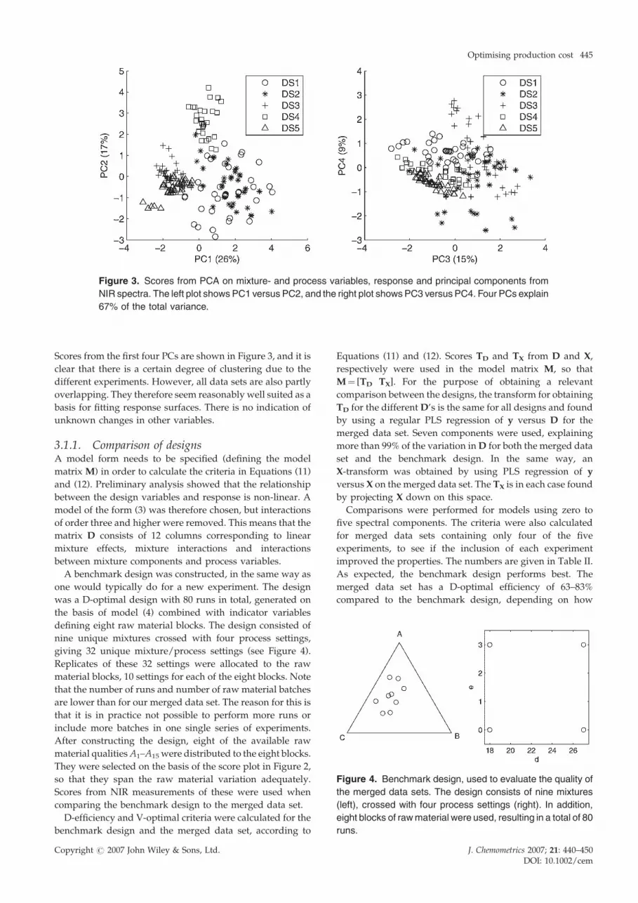
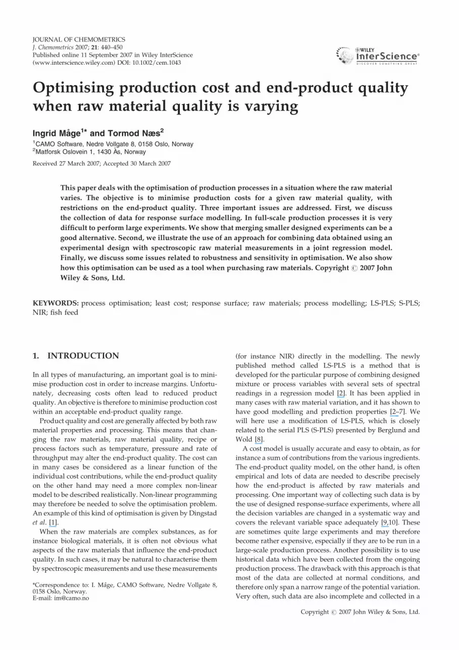
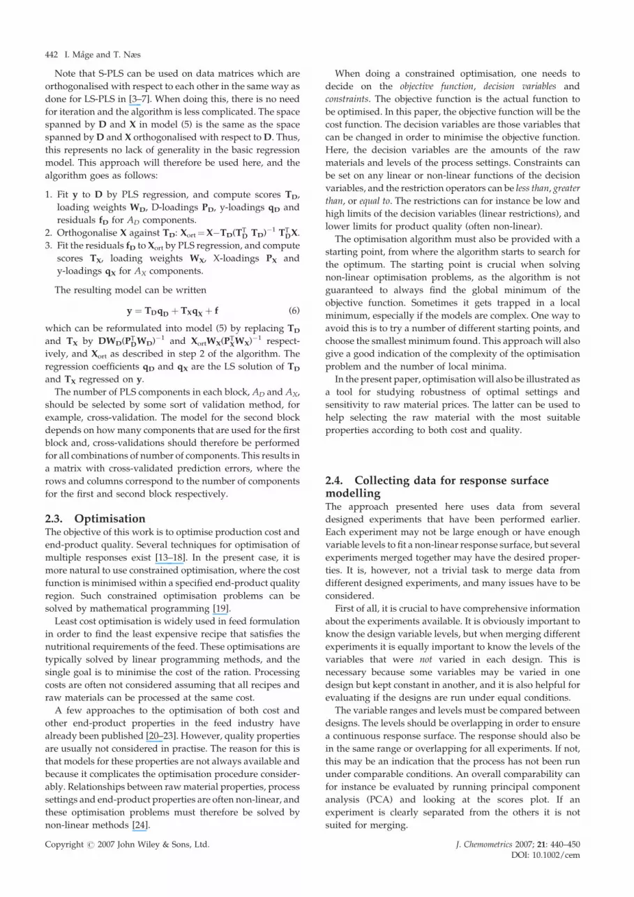
Figure 3. Scores from PCA on mixture- and process variables, response and principal components from

NIR spectra. The left plot shows PC1 versus PC2, and the right plot showsPC3 versus PC4. Four PCs explain

67% of the total variance.

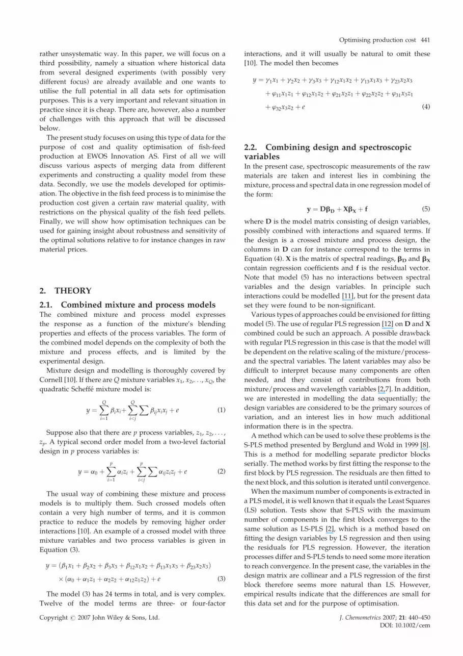
Figure 4. Benchmark design, used to evaluate the quality of

the merged data sets. The design consists of nine mixtures

(left), crossed with four process settings (right). In addition,

eight blocks of rawmaterial were used, resulting in a total of 80

runs.

Optimising production cost 445

Scores from the first four PCs are shown in Figure 3, and it is

clear that there is a certain degree of clustering due to the

different experiments. However, all data sets are also partly

overlapping. They therefore seem reasonably well suited as a

basis for fitting response surfaces. There is no indication of

unknown changes in other variables.

3.1.1. Comparison of designsA model form needs to be specified (defining the model

matrix M) in order to calculate the criteria in Equations (11)

and (12). Preliminary analysis showed that the relationship

between the design variables and response is non-linear. A

model of the form (3) was therefore chosen, but interactions

of order three and higher were removed. This means that the

matrix D consists of 12 columns corresponding to linear

mixture effects, mixture interactions and interactions

between mixture components and process variables.

A benchmark design was constructed, in the same way as

one would typically do for a new experiment. The design

was a D-optimal design with 80 runs in total, generated on

the basis of model (4) combined with indicator variables

defining eight raw material blocks. The design consisted of

nine unique mixtures crossed with four process settings,

giving 32 unique mixture/process settings (see Figure 4).

Replicates of these 32 settings were allocated to the raw

material blocks, 10 settings for each of the eight blocks. Note

that the number of runs and number of raw material batches

are lower than for our merged data set. The reason for this is

that it is in practice not possible to perform more runs or

include more batches in one single series of experiments.

After constructing the design, eight of the available raw

material qualities A1–A15 were distributed to the eight blocks.

They were selected on the basis of the score plot in Figure 2,

so that they span the raw material variation adequately.

Scores from NIR measurements of these were used when

comparing the benchmark design to the merged data set.

D-efficiency and V-optimal criteria were calculated for the

benchmark design and the merged data set, according to

Copyright # 2007 John Wiley & Sons, Ltd.

Equations (11) and (12). Scores TD and TX from D and X,

respectively were used in the model matrix M, so that

M¼ [TD TX]. For the purpose of obtaining a relevant

comparison between the designs, the transform for obtaining

TD for the differentD’s is the same for all designs and found

by using a regular PLS regression of y versus D for the

merged data set. Seven components were used, explaining

more than 99% of the variation inD for both the merged data

set and the benchmark design. In the same way, an

X-transform was obtained by using PLS regression of y

versus X on the merged data set. The TX is in each case found

by projecting X down on this space.

Comparisons were performed for models using zero to

five spectral components. The criteria were also calculated

for merged data sets containing only four of the five

experiments, to see if the inclusion of each experiment

improved the properties. The numbers are given in Table II.

As expected, the benchmark design performs best. The

merged data set has a D-optimal efficiency of 63–83%

compared to the benchmark design, depending on how

J. Chemometrics 2007; 21: 440–450DOI: 10.1002/cem

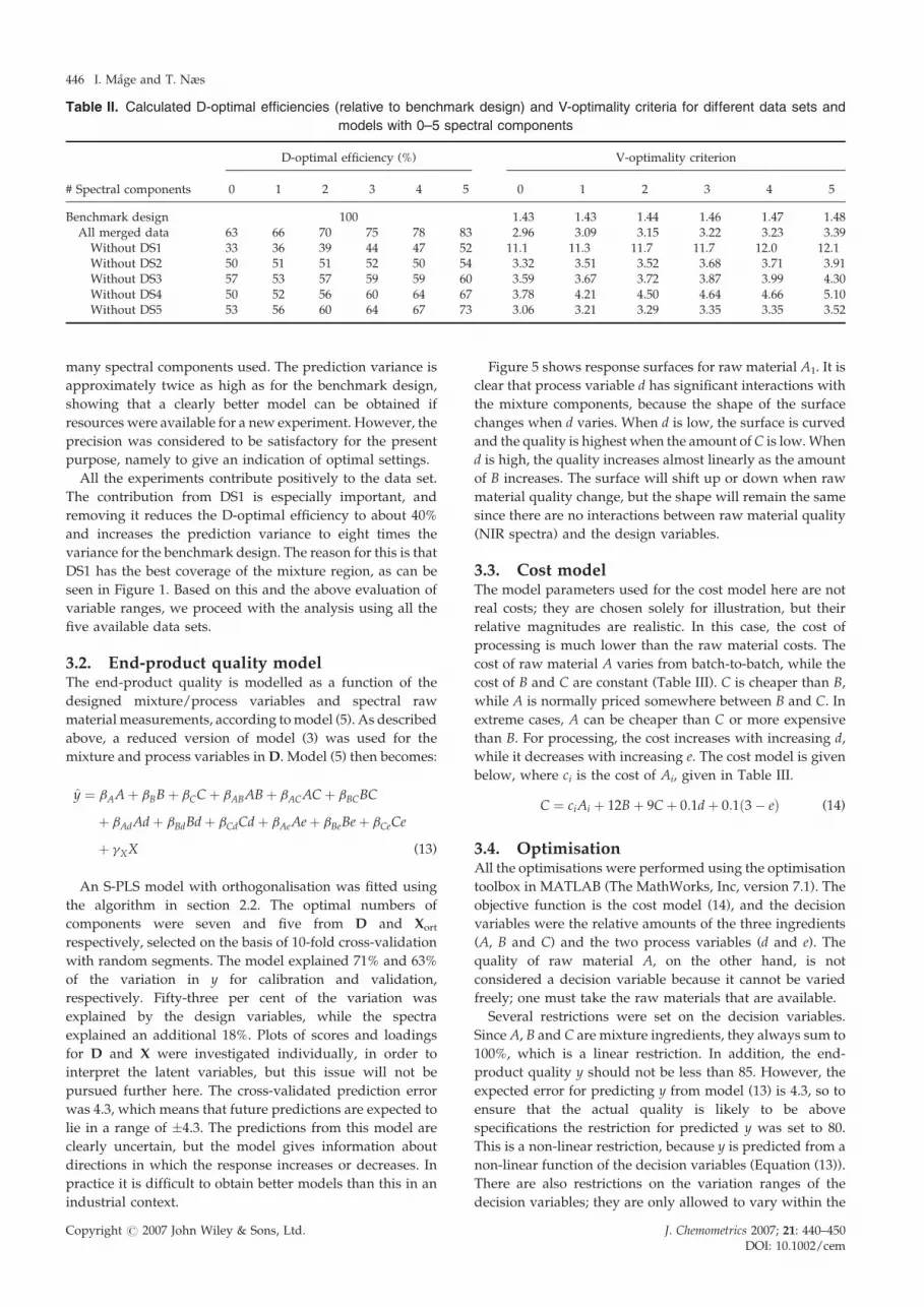
Table II. Calculated D-optimal efficiencies (relative to benchmark design) and V-optimality criteria for different data sets and

models with 0–5 spectral components

# Spectral components

D-optimal efficiency (%) V-optimality criterion

0 1 2 3 4 5 0 1 2 3 4 5

Benchmark design 100 1.43 1.43 1.44 1.46 1.47 1.48All merged data 63 66 70 75 78 83 2.96 3.09 3.15 3.22 3.23 3.39

Without DS1 33 36 39 44 47 52 11.1 11.3 11.7 11.7 12.0 12.1Without DS2 50 51 51 52 50 54 3.32 3.51 3.52 3.68 3.71 3.91Without DS3 57 53 57 59 59 60 3.59 3.67 3.72 3.87 3.99 4.30Without DS4 50 52 56 60 64 67 3.78 4.21 4.50 4.64 4.66 5.10Without DS5 53 56 60 64 67 73 3.06 3.21 3.29 3.35 3.35 3.52

446 I. Mage and T. Næs

many spectral components used. The prediction variance is

approximately twice as high as for the benchmark design,

showing that a clearly better model can be obtained if

resources were available for a new experiment. However, the

precision was considered to be satisfactory for the present

purpose, namely to give an indication of optimal settings.

All the experiments contribute positively to the data set.

The contribution from DS1 is especially important, and

removing it reduces the D-optimal efficiency to about 40%

and increases the prediction variance to eight times the

variance for the benchmark design. The reason for this is that

DS1 has the best coverage of the mixture region, as can be

seen in Figure 1. Based on this and the above evaluation of

variable ranges, we proceed with the analysis using all the

five available data sets.

3.2. End-product quality modelThe end-product quality is modelled as a function of the

designed mixture/process variables and spectral raw

material measurements, according tomodel (5). As described

above, a reduced version of model (3) was used for the

mixture and process variables inD. Model (5) then becomes:

y ¼ bAA þ bBB þ bCC þ bABAB þ bACAC þ bBCBC

þ bAdAd þ bBdBd þ bCdCd þ bAeAe þ bBeBe þ bCeCe

þ gXX (13)

An S-PLS model with orthogonalisation was fitted using

the algorithm in section 2.2. The optimal numbers of

components were seven and five from D and Xort

respectively, selected on the basis of 10-fold cross-validation

with random segments. The model explained 71% and 63%

of the variation in y for calibration and validation,

respectively. Fifty-three per cent of the variation was

explained by the design variables, while the spectra

explained an additional 18%. Plots of scores and loadings

for D and X were investigated individually, in order to

interpret the latent variables, but this issue will not be

pursued further here. The cross-validated prediction error

was 4.3, which means that future predictions are expected to

lie in a range of �4.3. The predictions from this model are

clearly uncertain, but the model gives information about

directions in which the response increases or decreases. In

practice it is difficult to obtain better models than this in an

industrial context.

Copyright # 2007 John Wiley & Sons, Ltd.

Figure 5 shows response surfaces for raw material A1. It is

clear that process variable d has significant interactions with

the mixture components, because the shape of the surface

changes when d varies. When d is low, the surface is curved

and the quality is highest when the amount of C is low.When

d is high, the quality increases almost linearly as the amount

of B increases. The surface will shift up or down when raw

material quality change, but the shape will remain the same

since there are no interactions between raw material quality

(NIR spectra) and the design variables.

3.3. Cost modelThe model parameters used for the cost model here are not

real costs; they are chosen solely for illustration, but their

relative magnitudes are realistic. In this case, the cost of

processing is much lower than the raw material costs. The

cost of raw material A varies from batch-to-batch, while the

cost of B and C are constant (Table III). C is cheaper than B,

while A is normally priced somewhere between B and C. In

extreme cases, A can be cheaper than C or more expensive

than B. For processing, the cost increases with increasing d,

while it decreases with increasing e. The cost model is given

below, where ci is the cost of Ai, given in Table III.

C ¼ ciAi þ 12B þ 9C þ 0:1d þ 0:1ð3� eÞ (14)

3.4. OptimisationAll the optimisations were performed using the optimisation

toolbox in MATLAB (The MathWorks, Inc, version 7.1). The

objective function is the cost model (14), and the decision

variables were the relative amounts of the three ingredients

(A, B and C) and the two process variables (d and e). The

quality of raw material A, on the other hand, is not

considered a decision variable because it cannot be varied

freely; one must take the raw materials that are available.

Several restrictions were set on the decision variables.

Since A, B and C are mixture ingredients, they always sum to

100%, which is a linear restriction. In addition, the end-

product quality y should not be less than 85. However, the

expected error for predicting y from model (13) is 4.3, so to

ensure that the actual quality is likely to be above

specifications the restriction for predicted y was set to 80.

This is a non-linear restriction, because y is predicted from a

non-linear function of the decision variables (Equation (13)).

There are also restrictions on the variation ranges of the

decision variables; they are only allowed to vary within the

J. Chemometrics 2007; 21: 440–450DOI: 10.1002/cem

Figure 5. Contour plots of the response surface for raw material A1. The response surface is clearly more

curved for low values of process variable d, and similarly shaped but a bit lower for high values of e. The

surface has the same shape but is shifted up or down when raw material quality vary.

Optimising production cost 447

region where the quality model is valid. To summarise, the

restrictions are:

y> 80

AþBþC¼ 100

20<A< 62

10<B< 30

21<C< 55

18< d< 27

0< e< 3

To avoid local minima, the optimisations were repeated

with a number of different starting points. The starting points

were generated by an experimental design; 7 evenly spread

mixture points were selected, and they were crossed with a

2-level factorial design with a centre point in the process

variables. This amounts to 35 different starting points.

The optimisation was performed for all the 15 rawmaterial

qualities available, A1–A15 (Table IV). The same minimum

cost was in each case found regardless of starting point. This

indicates that the optimisation problem is not too complex,

Table III. Raw ma

A

A1 A2 A3 A4 A5 A6 A7 A8 A9

12.5 11.8 8.8 7.8 9.8 9.5 8.7 10.8 12.5

The price of A varies from batch-to-batch, while the price of B and C are

Copyright # 2007 John Wiley & Sons, Ltd.

which is logical since there is only one non-linear constraint

involved. We see from Table IV that production costs vary

between raw material qualities. The predicted end-product

quality is always at the minimum level 80, which shows that

it costs more to produce a high quality product.

The optimal recipes and process variable settings are

plotted in Figure 6. Most of the recipes have a high inclusion

level of raw material C, which is one of the cheapest raw

materials (A is sometimes cheaper). The exception is A2 and

A5, which have a high inclusion of A and low C, even if the

cost of A is higher than C. This indicates that A2 and A5 have a

quality that need a high inclusion in order to yield a good

product. We also see from the score plot in Figure 2 that A2 is

rather different from the other raw materials. The process

settings are quite low for d and e for most of the raw material

qualities.

3.5. Selecting optimal settingsFor some rawmaterials, there are several recipes and process

settings that give the exact same cost and end-product

terial prices

B CA10 A11 A12 A13 A14 A15

9.2 8.7 9.7 11.2 8.5 8.0 12.0 9.0

constant.

J. Chemometrics 2007; 21: 440–450DOI: 10.1002/cem

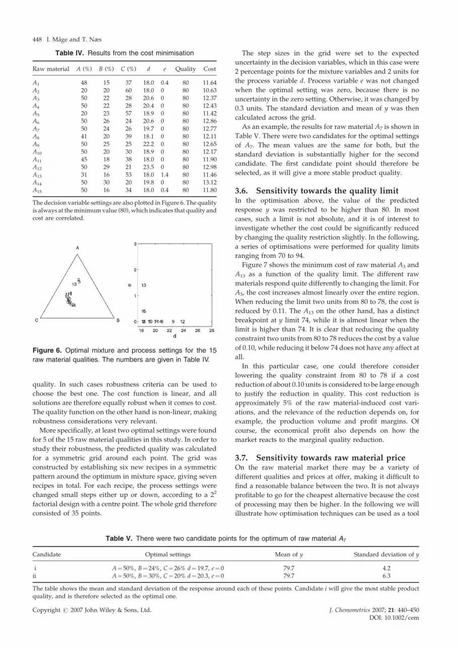
Table IV. Results from the cost minimisation

Raw material A (%) B (%) C (%) d e Quality Cost

A1 48 15 37 18.0 0.4 80 11.64A2 20 20 60 18.0 0 80 10.63A3 50 22 28 20.6 0 80 12.37A4 50 22 28 20.4 0 80 12.43A5 20 23 57 18.9 0 80 11.42A6 50 26 24 20.6 0 80 12.86A7 50 24 26 19.7 0 80 12.77A8 41 20 39 18.1 0 80 12.11A9 50 25 25 22.2 0 80 12.65A10 50 20 30 18.9 0 80 12.17A11 45 18 38 18.0 0 80 11.90A12 50 29 21 23.5 0 80 12.98A13 31 16 53 18.0 1.4 80 11.46A14 50 30 20 19.8 0 80 13.12A15 50 16 34 18.0 0.4 80 11.80

The decision variable settings are also plotted in Figure 6. The qualityis always at theminimumvalue (80), which indicates that quality andcost are correlated.

Figure 6. Optimal mixture and process settings for the 15

raw material qualities. The numbers are given in Table IV.

448 I. Mage and T. Næs

quality. In such cases robustness criteria can be used to

choose the best one. The cost function is linear, and all

solutions are therefore equally robust when it comes to cost.

The quality function on the other hand is non-linear, making

robustness considerations very relevant.

More specifically, at least two optimal settings were found

for 5 of the 15 raw material qualities in this study. In order to

study their robustness, the predicted quality was calculated

for a symmetric grid around each point. The grid was

constructed by establishing six new recipes in a symmetric

pattern around the optimum in mixture space, giving seven

recipes in total. For each recipe, the process settings were

changed small steps either up or down, according to a 22

factorial design with a centre point. The whole grid therefore

consisted of 35 points.

Table V. There were two candidate point

Candidate Optimal settings

i A¼ 50%, B¼ 24%, C¼ 26% d¼ 19.7, e¼ 0ii A¼ 50%, B¼ 30%, C¼ 20% d¼ 20.3, e¼ 0

The table shows the mean and standard deviation of the response aroundquality, and is therefore selected as the optimal one.

Copyright # 2007 John Wiley & Sons, Ltd.

The step sizes in the grid were set to the expected

uncertainty in the decision variables, which in this case were

2 percentage points for the mixture variables and 2 units for

the process variable d. Process variable e was not changed

when the optimal setting was zero, because there is no

uncertainty in the zero setting. Otherwise, it was changed by

0.3 units. The standard deviation and mean of y was then

calculated across the grid.

As an example, the results for raw material A7 is shown in

Table V. There were two candidates for the optimal settings

of A7. The mean values are the same for both, but the

standard deviation is substantially higher for the second

candidate. The first candidate point should therefore be

selected, as it will give a more stable product quality.

3.6. Sensitivity towards the quality limitIn the optimisation above, the value of the predicted

response y was restricted to be higher than 80. In most

cases, such a limit is not absolute, and it is of interest to

investigate whether the cost could be significantly reduced

by changing the quality restriction slightly. In the following,

a series of optimisations were performed for quality limits

ranging from 70 to 94.

Figure 7 shows the minimum cost of raw material A3 and

A13 as a function of the quality limit. The different raw

materials respond quite differently to changing the limit. For

A3, the cost increases almost linearly over the entire region.

When reducing the limit two units from 80 to 78, the cost is

reduced by 0.11. The A13 on the other hand, has a distinct

breakpoint at y limit 74, while it is almost linear when the

limit is higher than 74. It is clear that reducing the quality

constraint two units from 80 to 78 reduces the cost by a value

of 0.10, while reducing it below 74 does not have any affect at

all.

In this particular case, one could therefore consider

lowering the quality constraint from 80 to 78 if a cost

reduction of about 0.10 units is considered to be large enough

to justify the reduction in quality. This cost reduction is

approximately 5% of the raw material-induced cost vari-

ations, and the relevance of the reduction depends on, for

example, the production volume and profit margins. Of

course, the economical profit also depends on how the

market reacts to the marginal quality reduction.

3.7. Sensitivity towards raw material priceOn the raw material market there may be a variety of

different qualities and prices at offer, making it difficult to

find a reasonable balance between the two. It is not always

profitable to go for the cheapest alternative because the cost

of processing may then be higher. In the following we will

illustrate how optimisation techniques can be used as a tool

s for the optimum of raw material A7

Mean of y Standard deviation of y

79.7 4.279.7 6.3

each of these points. Candidate i will give the most stable product

J. Chemometrics 2007; 21: 440–450DOI: 10.1002/cem

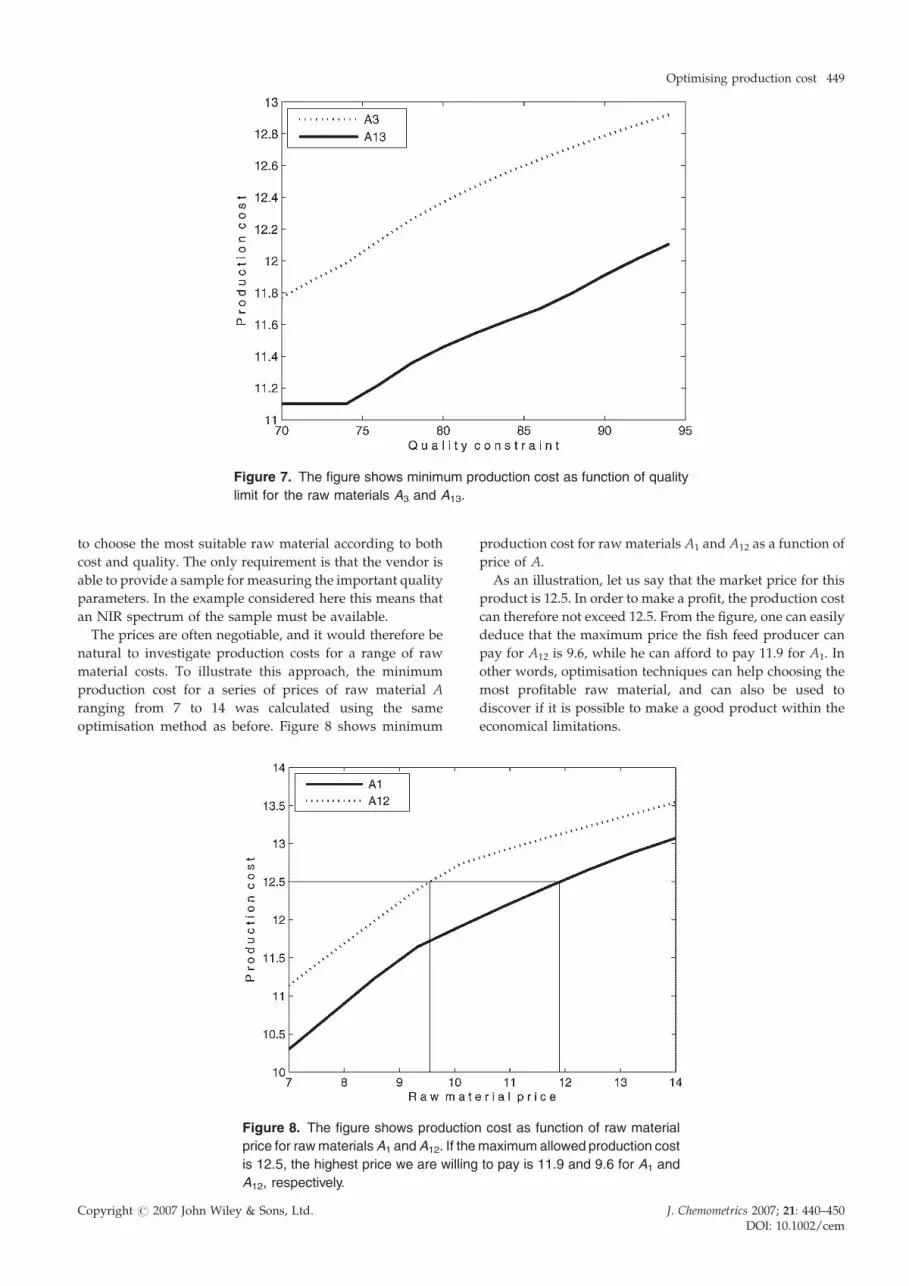
Figure 7. The figure shows minimum production cost as function of quality

limit for the raw materials A3 and A13.

Optimising production cost 449

to choose the most suitable raw material according to both

cost and quality. The only requirement is that the vendor is

able to provide a sample for measuring the important quality

parameters. In the example considered here this means that

an NIR spectrum of the sample must be available.

The prices are often negotiable, and it would therefore be

natural to investigate production costs for a range of raw

material costs. To illustrate this approach, the minimum

production cost for a series of prices of raw material A

ranging from 7 to 14 was calculated using the same

optimisation method as before. Figure 8 shows minimum

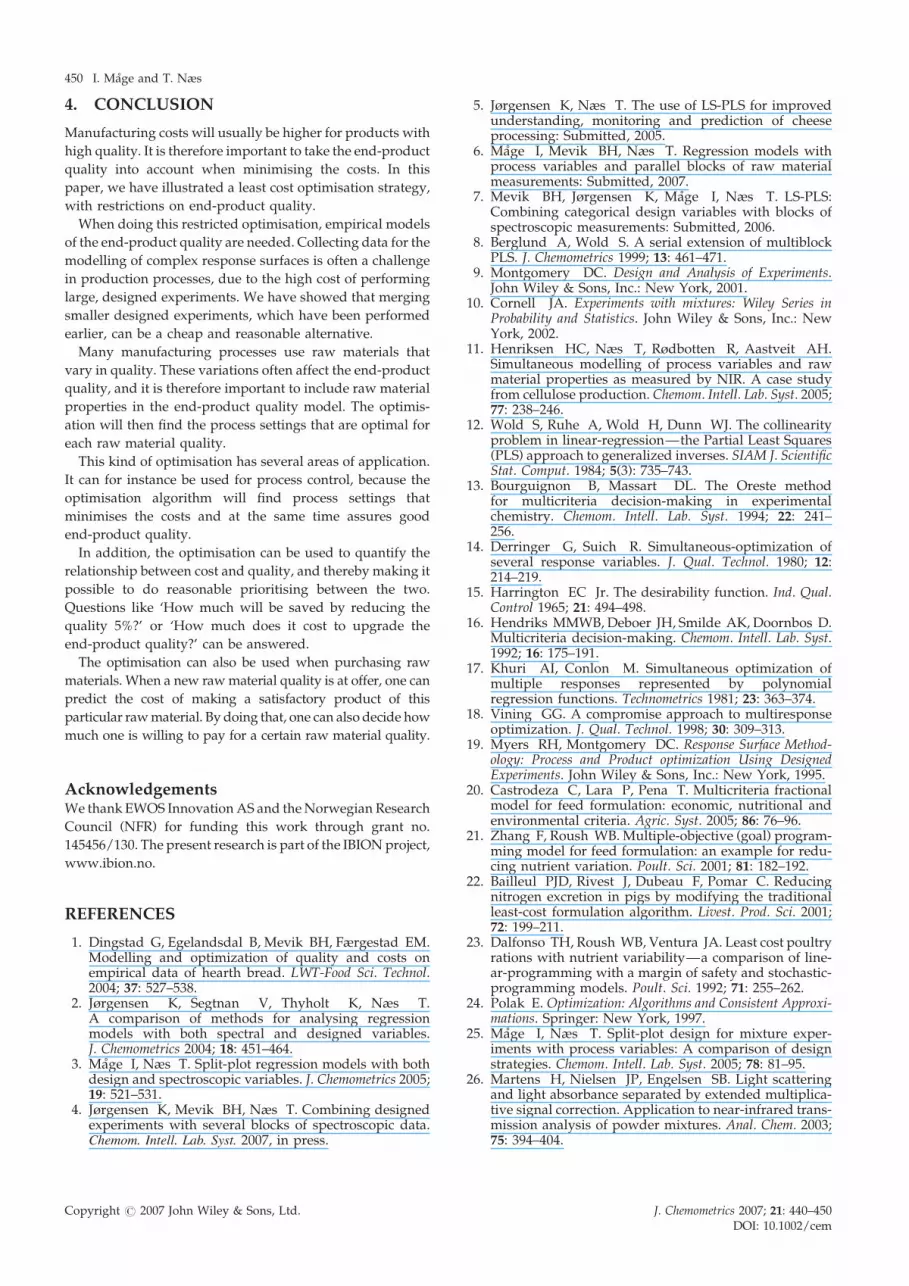
Figure 8. The figure shows production

price for rawmaterialsA1 andA12. If the

is 12.5, the highest price we are willing

A12, respectively.

Copyright # 2007 John Wiley & Sons, Ltd.

production cost for raw materials A1 and A12 as a function of

price of A.

As an illustration, let us say that the market price for this

product is 12.5. In order to make a profit, the production cost

can therefore not exceed 12.5. From the figure, one can easily

deduce that the maximum price the fish feed producer can

pay for A12 is 9.6, while he can afford to pay 11.9 for A1. In

other words, optimisation techniques can help choosing the

most profitable raw material, and can also be used to

discover if it is possible to make a good product within the

economical limitations.

cost as function of raw material

maximum allowed production cost

to pay is 11.9 and 9.6 for A1 and

J. Chemometrics 2007; 21: 440–450DOI: 10.1002/cem

450 I. Mage and T. Næs

4. CONCLUSION

Manufacturing costs will usually be higher for products with

high quality. It is therefore important to take the end-product

quality into account when minimising the costs. In this

paper, we have illustrated a least cost optimisation strategy,

with restrictions on end-product quality.

When doing this restricted optimisation, empirical models

of the end-product quality are needed. Collecting data for the

modelling of complex response surfaces is often a challenge

in production processes, due to the high cost of performing

large, designed experiments. We have showed that merging

smaller designed experiments, which have been performed

earlier, can be a cheap and reasonable alternative.

Many manufacturing processes use raw materials that

vary in quality. These variations often affect the end-product

quality, and it is therefore important to include raw material

properties in the end-product quality model. The optimis-

ation will then find the process settings that are optimal for

each raw material quality.

This kind of optimisation has several areas of application.

It can for instance be used for process control, because the

optimisation algorithm will find process settings that

minimises the costs and at the same time assures good

end-product quality.

In addition, the optimisation can be used to quantify the

relationship between cost and quality, and thereby making it

possible to do reasonable prioritising between the two.

Questions like ‘How much will be saved by reducing the

quality 5%?’ or ‘How much does it cost to upgrade the

end-product quality?’ can be answered.

The optimisation can also be used when purchasing raw

materials. When a new rawmaterial quality is at offer, one can

predict the cost of making a satisfactory product of this

particular rawmaterial. By doing that, one can also decide how

much one is willing to pay for a certain raw material quality.

AcknowledgementsWe thank EWOS InnovationAS and theNorwegian Research

Council (NFR) for funding this work through grant no.

145456/130. The present research is part of the IBIONproject,

www.ibion.no.

REFERENCES

1. Dingstad G, Egelandsdal B, Mevik BH, Færgestad EM.Modelling and optimization of quality and costs onempirical data of hearth bread. LWT-Food Sci. Technol.2004; 37: 527–538.

2. Jørgensen K, Segtnan V, Thyholt K, Næs T.A comparison of methods for analysing regressionmodels with both spectral and designed variables.J. Chemometrics 2004; 18: 451–464.

3. Mage I, Næs T. Split-plot regression models with bothdesign and spectroscopic variables. J. Chemometrics 2005;19: 521–531.

4. Jørgensen K, Mevik BH, Næs T. Combining designedexperiments with several blocks of spectroscopic data.Chemom. Intell. Lab. Syst. 2007, in press.

Copyright # 2007 John Wiley & Sons, Ltd.

5. Jørgensen K, Næs T. The use of LS-PLS for improvedunderstanding, monitoring and prediction of cheeseprocessing: Submitted, 2005.

6. Mage I, Mevik BH, Næs T. Regression models withprocess variables and parallel blocks of raw materialmeasurements: Submitted, 2007.

7. Mevik BH, Jørgensen K, Mage I, Næs T. LS-PLS:Combining categorical design variables with blocks ofspectroscopic measurements: Submitted, 2006.

8. Berglund A, Wold S. A serial extension of multiblockPLS. J. Chemometrics 1999; 13: 461–471.

9. Montgomery DC. Design and Analysis of Experiments.John Wiley & Sons, Inc.: New York, 2001.

10. Cornell JA. Experiments with mixtures: Wiley Series inProbability and Statistics. John Wiley & Sons, Inc.: NewYork, 2002.

11. Henriksen HC, Næs T, Rødbotten R, Aastveit AH.Simultaneous modelling of process variables and rawmaterial properties as measured by NIR. A case studyfrom cellulose production. Chemom. Intell. Lab. Syst. 2005;77: 238–246.

12. Wold S, Ruhe A, Wold H, Dunn WJ. The collinearityproblem in linear-regression—the Partial Least Squares(PLS) approach to generalized inverses. SIAM J. ScientificStat. Comput. 1984; 5(3): 735–743.

13. Bourguignon B, Massart DL. The Oreste methodfor multicriteria decision-making in experimentalchemistry. Chemom. Intell. Lab. Syst. 1994; 22: 241–256.

14. Derringer G, Suich R. Simultaneous-optimization ofseveral response variables. J. Qual. Technol. 1980; 12:214–219.

15. Harrington EC Jr. The desirability function. Ind. Qual.Control 1965; 21: 494–498.

16. Hendriks MMWB, Deboer JH, Smilde AK, Doornbos D.Multicriteria decision-making. Chemom. Intell. Lab. Syst.1992; 16: 175–191.

17. Khuri AI, Conlon M. Simultaneous optimization ofmultiple responses represented by polynomialregression functions. Technometrics 1981; 23: 363–374.

18. Vining GG. A compromise approach to multiresponseoptimization. J. Qual. Technol. 1998; 30: 309–313.

19. Myers RH, Montgomery DC. Response Surface Method-ology: Process and Product optimization Using DesignedExperiments. John Wiley & Sons, Inc.: New York, 1995.

20. Castrodeza C, Lara P, Pena T. Multicriteria fractionalmodel for feed formulation: economic, nutritional andenvironmental criteria. Agric. Syst. 2005; 86: 76–96.

21. Zhang F, Roush WB. Multiple-objective (goal) program-ming model for feed formulation: an example for redu-cing nutrient variation. Poult. Sci. 2001; 81: 182–192.

22. Bailleul PJD, Rivest J, Dubeau F, Pomar C. Reducingnitrogen excretion in pigs by modifying the traditionalleast-cost formulation algorithm. Livest. Prod. Sci. 2001;72: 199–211.

23. Dalfonso TH, Roush WB, Ventura JA. Least cost poultryrations with nutrient variability—a comparison of line-ar-programming with a margin of safety and stochastic-programming models. Poult. Sci. 1992; 71: 255–262.

24. Polak E. Optimization: Algorithms and Consistent Approxi-mations. Springer: New York, 1997.

25. Mage I, Næs T. Split-plot design for mixture exper-iments with process variables: A comparison of designstrategies. Chemom. Intell. Lab. Syst. 2005; 78: 81–95.

26. Martens H, Nielsen JP, Engelsen SB. Light scatteringand light absorbance separated by extended multiplica-tive signal correction. Application to near-infrared trans-mission analysis of powder mixtures. Anal. Chem. 2003;75: 394–404.

J. Chemometrics 2007; 21: 440–450DOI: 10.1002/cem