Article

Optimal Weed Control Strategies in Rice Productionunder Dynamic and Static Decision Rulesin South Korea

Woongchan Jeon 1 and Kwansoo Kim 1,2,*1 Department of Agricultural Economics and Rural Development, Seoul National University,

Seoul 08826, Republic of Korea; jwc0102@snu.ac.kr2 Research Institute of Agriculture and Life Sciences, Seoul National University,

Seoul 08826, Republic of Korea* Correspondence: kimk@snu.ac.kr; Tel.: +82-2-880-4727; Fax: +82-2-873-3565

Academic Editor: Vincenzo TorrettaReceived: 31 March 2017; Accepted: 31 May 2017; Published: 12 June 2017

Abstract: This paper analyzes optimal weed control management strategies under static and dynamicdecision rules. Seed bank is taken into account to introduce dynamics into the model. We presenta numerical example of controlling Sheathed Monochoria (Monochoria Vaginalis) in Korean rice paddyfields. Our results show that producers benefit from dynamic decision rules; higher income and morecontrol of weed density can be obtained with the same amount of herbicide. In order to illustratethe magnitude of differences between static and dynamic models, a numerical example is presentedusing a data set from Korean rice production. When it comes to controlling weed density, Koreanrice farmers are found to be better off under the dynamic model, and the magnitude of advantagesare found to be more sensitive to herbicide efficacy and less sensitive to initial seed banks andgermination rates in terms of weed density.

Keywords: optimal weed control, weed seed dynamics, Hamiltonian, maximum principle

1. Introduction

Herbicide is one of the major inputs in agricultural production, and has been credited withincreasing productivity. Empirical literature on production risk and risk preferences has increased ourknowledge on herbicide as an effective risk mitigation option, as it has been found to lower crop yieldvariability [1,2]. Pannell [3] argues that whether pesticide is a risk-reducing or a risk-increasing inputis an empirical issue. When some sources of uncertainty (e.g., pest density, pesticide effectiveness)are taken into account, pesticides and herbicides can be considered as risk reducing inputs. However,the inappropriate use of herbicides has been raising concerns that it might be harmful to humanhealth and the environment. Thus, it is important to establish optimal herbicide application rates andtiming in order to abate the production risk, but at the same time, to minimize the possible damageto humans and the environment. This is also particularly pertinent to climate change adaptation,as global warming can drive the success of invasive plants like weeds [4].

Finding an economically efficient level of herbicide dosage requires the modelling of yield damagecaused by weed crop competition. A rectangular hyperbola has been widely used to estimate the yieldloss from weed crop competition [5]. Logistic functional form has been commonly used to describea herbicide dose–response [6]. In crop science literature, research on farmers’ behavior of herbicidedosage has mostly focused on an economic threshold, deriving the herbicide dosage in order to keepcrop yield losses below a certain level [7].

In economics literature, much attention has been devoted to establishing economic principles andpolicy implications of optimal weed control analysis using estimated biological functions. Wu [8] used

Sustainability 2017, 9, 956; doi:10.3390/su9060956 www.mdpi.com/journal/sustainability

Sustainability 2017, 9, 956 2 of 11

seed bank as a state variable to develop a dynamic optimization model, and analyzed the differencesbetween static and dynamic weed control strategies using Iowa corn production data as a numericalexample. A discrete choice dynamic programming model was used to obtain the optimal compositionof weed control options [9]. An input–output analysis was applied to evaluate the impacts of weedson farm economy [10].

This study applies a dynamic programming model developed by Wu [8] to rice production datain South Korea, based on findings from crop science literature on rice (Oryza Sativa L.). Many studieson rice paddy weed control have mostly focused on the estimation of yield loss functionand dose–response curve [11,12]. A cost–benefit analysis of herbicide dosage was conducted forrice farmers, deriving a threshold level to attain a certain level of weed density [13]. However, theanalysis of the economic threshold ignores a profit maximization rule underlying producers’ behavior.In this regard, this paper tries to model a profit maximization principle in a dynamic setting andto provide an optimal level of herbicide dosage considering seed bank. We also compare the resultsfrom static and dynamic decision rules. Based on these efforts, this research attempts to develop policyimplications towards an optimal weed control strategy. It is expected that valuable policy implicationscan be drawn in the sense that rice farmers are expected to be better off under a dynamic model,thus contributing to a sustainable rice economy.

We first introduce dynamic programming and static optimization models proposed by Wu [8]in Section 2. We compare the results between two decision rules. Information on biological parametersand prices is presented in Section 3. Section 4 gives the simulation results, and Section 5 concludes.

2. Conceptual Framework

The following is a reformulation of a theoretical model suggested by Wu [8]. Assume that a typicalrice farmer experiences yield losses due to an annual weed infestation. He/she considers an applicationof herbicides to maximize the sum of present values over T periods. The biological life cycle of annualrice weeds is comprised of four stages: germination, growth, interference, and seed production [14].Some seeds buried in a rice paddy germinate in the spring, and the seedlings are exposed to somemortality factors such as frost, drought, herbivory, etc. Those who germinate after the first tillage growup and compete with rice unless herbicides are applied in the fields. The seed density (hereafter, seedbank) at the very beginning of the farming season in year t is denoted by St. Then, m portion of weedseeds are assumed to survive and compete with rice unless weed control measures are taken.

Farmers can control weeds in the fields by applying herbicides. The exponential functional formhas been commonly used to describe dose–response relations [15]. Let Ht denote herbicide dosage inyear t. Then, the weed density competing with rice can be explained by Wt = mSte−cHt , where c isa herbicide efficacy parameter taking a positive value depending on the weed species and herbicidesused and m is a germination rate. Rice farmers can sustain the optimal weed density by controllingthe herbicide dosage. Weeds that survive through some mortality factors can grow up, reproduce,and be spread by seeds, thereby completing a biological cycle. A new biological cycle begins againin the spring. Let k be the number of seeds that each weed produces. Then, a seed bank in the nextyear (St+1) can be calculated as St+1 = kWt = kmSte−cHt .

The hyperbolic function is widely used to estimate yield losses from weed infestation [16,17].Especially, an empirical model which is developed using rectangular hyperbola is most commonlyused to predict yield damage from weed-crop competition [5,11–13,18,19]. In addition, we assume thatyield losses take the form D(W) = βW

1+βW , where D(W) denotes the proportional yield losses givena certain level of weed density (W), and β is a parameter measuring the magnitudes of weed-cropcompetition. When the weed density is 1

β , the yield loss rate is one-half. The yield response can

be described as Yt = Y0t[1− D(mSte−cHt)], where Y0t denotes weed-free rice yield.In general, germination rate (m), herbicide efficacy (c), and weed-free crop (Y0t) are subject

to uncertainties such as temperature, rainfall, and other random factors. The role of uncertaintyon weed control has been extensively examined in the crop science literature [2,15,20]. However,

Sustainability 2017, 9, 956 3 of 11

in order to focus solely on how farmers benefit from dynamic decision rules, we assume that theseparameters are constant over time. Introducing uncertainty in this model would be a good topic fora future study.

Following Wu [8], profit maximization models under a dynamic setting can be written as

maxHt

T

∑t=1

ρt[

PtY0t[1− D(mSte−cHt)]−VtHt − C0t

](1)

s.t. St+1 − St = (mke−cHt − 1)St (2)

S1 = S01, (3)

where ρ is a discount factor, Pt is the rice price in year t, Vt is the herbicide price in year t, and C0tdenotes the cost of producing rice without considering the costs of herbicides. We assume that the statevariable (=seed bank, St) changes throughout the state transition Equation (2), and an initial valueof the state variable is given by (3).

The above discrete optimal control problem can be solved by Pontryagin’s maximum principle,which is widely used for finding an optimal path of control variables and corresponding state variablesthat maximize the objective function [21]. The associated Hamiltonian is given by Lt = ρt[PtY0t[1 − D(mSte−cHt)] − VtHt − C0t] + λt(mke−cHt − 1)St, where the Lagrange Multiplier λt denotesthe reduced value of maximized profit when one unit of seed bank increases. The first-order conditionsfor the Hamiltonian are given by

∂Lt

∂Ht= ρt[PtY0tD′(mSte−cHt)cmSte−cHt −Vt]− λtcmkSte−cHt = 0, ∀t, (4)

∂Lt

∂St= −ρtPtY0tD′(mSte−cHt)me−cHt + λt(mke−cHt − 1) = −(λt − λt−1), ∀t, (5)

∂Lt

∂λt= (mke−cHt − 1)St = St+1 − St, ∀t. (6)

To see the role of control variables in the dynamic equilibrium, Equation (4) can be rewritten as

ρtPt∂Yt

∂Ht+ λt

∂St+1

∂Ht= ρtVt, ∀t. (7)

There are two outcomes of an increase in herbicides: firstly, the level of yield can be positivelyinfluenced by herbicide dosage; and secondly, seed bank in year t + 1 decreases as weed densitydecreases in year t. The first term in Equation (7) denotes the discounted value of increased rice yield,and the second term reflects the decreased amount of seed banks in the next year multiplied by itsshadow value. On the other hand, the RHS (right-hand-side) of Equation (7) denotes the present valueof a unit price of herbicides. Thus, in a dynamic equilibrium, the marginal benefits of an extra unit ofapplied herbicide should be equal to its marginal cost, which is consistent with economic rationality inprofit maximization.

To see the role of state variables in the dynamic equilibrium, Equation (5) can be rewritten as

ρtPt∂Yt

∂St+ λt

∂St+1

∂St= λt−1. (8)

Changes in seed bank in year t has two outcomes: firstly, yield in year t decreases as weed densityin year t increases with St; secondly, seed bank in year t + 1 also increases by the state transitionEquation (2). The first term on the LHS (left-hand-side) of Equation (8) denotes the discounted damageof rice yields from increased seed bank in year t. The second term can be interpreted as an increased

Sustainability 2017, 9, 956 4 of 11

number of seed bank in year t + 1 multiplied by its shadow value. The RHS of Equation (8) denotesthe marginal cost of an extra unit of seed bank in year t− 1. Hence, in a dynamic equilibrium, the sumof discounted revenue reduction and the increased cost of seed bank in year t + 1 should be equal tothe marginal cost of the seed bank density of weeds in year t− 1.

Note that in order to derive the optimal path of weed density, Equation (4) can be rewritten asβ2W2

t + (2β− dt)Wt + 1 = 0, where dt = βcPtY0tVt−ρVt−1

. (If we multiply Equation (5) by cSt and add it

to Equation (4), then we can get λt = − ρt+1Vt+1cSt+1

. It follows from the rectangular hyperbola damage

function that D′(W) = β

(1+βW)2 . If we combine these with Equation (4), then we can get β2W2t + (2β−

βcPtY0tVt−ρVt−1

)Wt + 1 = 0). If dt ≥ 0 and (2β − dt)2 − 4β2 ≥ 0, then only the following solution meetsthe second order necessary condition:

W∗t =(dt − 2β)−

√(dt − 2β)2 − 4β2

2β2 . (9)

In the last period, T, rice farmers only take into account the present profit. The optimal weeddensity in T (W∗T) can be derived by inserting dT = βcPTY0T/VT into Equation (9). Then, the optimalpath of weed density can be obtained from Equation (9) and its corresponding seed bank. In this case,the optimal path of herbicide dosage can be derived as follows:

S∗t = kW∗t−1, ∀t = 2, · · · , T, (10)

H∗1 = −1c

ln

(W∗1mS0

1

), H∗t = −1

cln(

W∗tmS∗t

)= −1

cln

(W∗t

mkW∗t−1

), ∀t = 2, · · · , T. (11)

On the other hand, a model where farmers only consider the present profit can be alternativelywritten as maxHt PtY0t[1 − D(mSte−cHt)] − VtHt − C0t, and the first-order condition is given byPtY0tD′(mSte−cHt)cmSte−cHt − Vt = 0. The first-order condition can be rewritten as β2W2

t + (2β−d0

t )Wt + 1 = 0, where d0t = βcPtY0t/Vt. If d0

t ≥ 0 and (2β− d0t )

2 − 4β2 ≥ 0, only the following positivesolution meets the second-order necessary condition:

W0t =

(d0t − 2β)−

√(d0

t − 2β)2 − 4β2

2β2 . (12)

In this static world, the optimal path of weed density can be obtained, and its corresponding seedbank and herbicide dosage can be derived as follows:

S0t = kW0

t−1, ∀t = 2, · · · , T, (13)

H01 = −1

cln

(W0

1mS0

1

), H0

t = −1c

ln(

W0t

mS0t

)= −1

cln

(W0

tmkW0

t−1

), ∀t = 2, · · · , T. (14)

In addition, the optimal weed seed bank under the dynamic decision rule is less than that ofthe static rule for the whole time horizon excluding the last period (T); that is, W∗t = W(d∗t ) <

W(d0t ) = W0

t ∀t = 1, · · · , T − 1. W(dt, ·) is a decreasing function with respect to dt, and d∗t > d0t ∀t =

1, 2, · · · , T− 1. Additionally, it follows that the number of optimal weed seed banks under the dynamicdecision rule is smaller than that of the static decision (S∗t < S0

t ∀t = 2, · · · , T).The sum of the present value of optimal profits over T periods can be calculated. Farmers under

dynamic decision rules always get a weakly larger discounted sum of profits because they maximizenet present value over all periods. Let NPV∗ and NPV0 be the net present values under a dynamicdecision rule and a static decision rule, respectively. The differences between the two terms are given by

Sustainability 2017, 9, 956 5 of 11

NPV∗ − NPV0 =T

∑t=1

ρt [PtY0t[1− D(W∗t )]−VtH∗t − C0t]−T

∑t=1

ρt[

PtY0t[1− D(W0t )]−VtH0

t − C0t

]=

T

∑t=1

ρt[

PtY0t[D(W0t )− D(W∗t )] + Vt(H0

t − H∗t )]≥ 0.

(15)

3. Herbicide Application in Korean Rice Farming

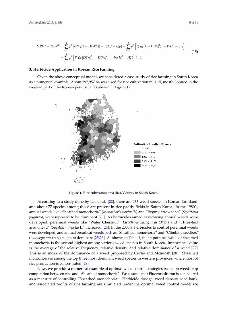
Given the above conceptual model, we considered a case study of rice farming in South Koreaas a numerical example. About 797,957 ha was used for rice cultivation in 2015, mostly located in thewestern part of the Korean peninsula (as shown in Figure 1).

Figure 1. Rice cultivation area (ha)/County in South Korea.

According to a study done by Lee et al. [22], there are 433 weed species in Korean farmland,and about 77 species among those are present in rice paddy fields in South Korea. In the 1980’s,annual weeds like “Sheathed monochoria” (Monochoria vaginalis) and “Pygmy arrowhead” (Sagittariapygmaea) were reported to be dominant [23]. As herbicides aimed at reducing annual weeds weredeveloped, perennial weeds like “Water Chestnut” (Eleocharis kuroguwai Ohwi) and “Three-leafarrowhead” (Sagittaria trifolia L.) increased [24]. In the 2000’s, herbicides to control perennial weedswere developed, and annual broadleaf weeds such as “Sheathed monochoria” and “Climbing seedbox”(Ludwigia prostrata) began to dominate [25,26]. As shown in Table 1, the importance value of Sheathedmonochoria is the second highest among various weed species in South Korea. Importance valueis the average of the relative frequency, relative density, and relative dominance of a weed [27].This is an index of the dominance of a weed proposed by Curtis and Mcintosh [28]. Sheathedmonochoria is among the top three most dominant weed species in western provinces, where most ofrice production is concentrated [29].

Now, we provide a numerical example of optimal weed control strategies based on weed-cropcompetition between rice and “Sheathed monochoria”. We assume that Flucetosulfuron is consideredas a measure of controlling “Sheathed monochoria”. Herbicide dosage, weed density, seed bank,and associated profits of rice farming are simulated under the optimal weed control model we

Sustainability 2017, 9, 956 6 of 11

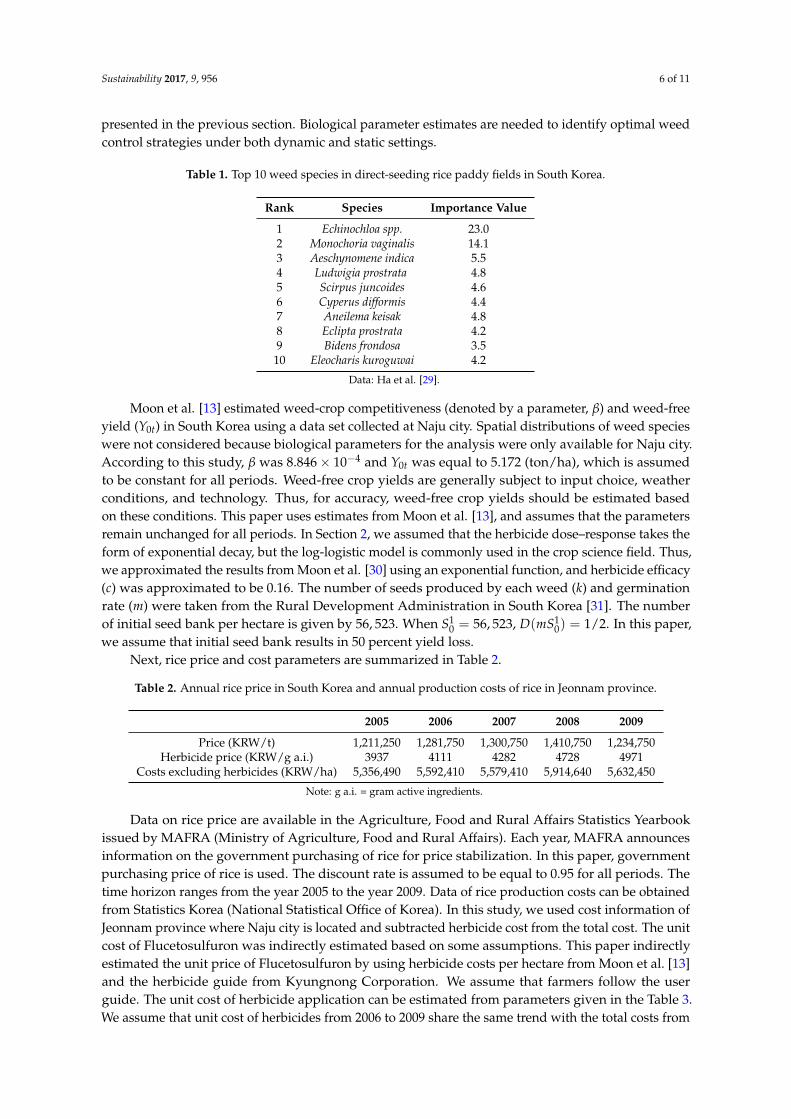
presented in the previous section. Biological parameter estimates are needed to identify optimal weedcontrol strategies under both dynamic and static settings.

Table 1. Top 10 weed species in direct-seeding rice paddy fields in South Korea.

Rank Species Importance Value

1 Echinochloa spp. 23.02 Monochoria vaginalis 14.13 Aeschynomene indica 5.54 Ludwigia prostrata 4.85 Scirpus juncoides 4.66 Cyperus difformis 4.47 Aneilema keisak 4.88 Eclipta prostrata 4.29 Bidens frondosa 3.510 Eleocharis kuroguwai 4.2

Data: Ha et al. [29].

Moon et al. [13] estimated weed-crop competitiveness (denoted by a parameter, β) and weed-freeyield (Y0t) in South Korea using a data set collected at Naju city. Spatial distributions of weed specieswere not considered because biological parameters for the analysis were only available for Naju city.According to this study, β was 8.846× 10−4 and Y0t was equal to 5.172 (ton/ha), which is assumedto be constant for all periods. Weed-free crop yields are generally subject to input choice, weatherconditions, and technology. Thus, for accuracy, weed-free crop yields should be estimated basedon these conditions. This paper uses estimates from Moon et al. [13], and assumes that the parametersremain unchanged for all periods. In Section 2, we assumed that the herbicide dose–response takes theform of exponential decay, but the log-logistic model is commonly used in the crop science field. Thus,we approximated the results from Moon et al. [30] using an exponential function, and herbicide efficacy(c) was approximated to be 0.16. The number of seeds produced by each weed (k) and germinationrate (m) were taken from the Rural Development Administration in South Korea [31]. The numberof initial seed bank per hectare is given by 56, 523. When S1

0 = 56, 523, D(mS10) = 1/2. In this paper,

we assume that initial seed bank results in 50 percent yield loss.Next, rice price and cost parameters are summarized in Table 2.

Table 2. Annual rice price in South Korea and annual production costs of rice in Jeonnam province.

2005 2006 2007 2008 2009

Price (KRW/t) 1,211,250 1,281,750 1,300,750 1,410,750 1,234,750Herbicide price (KRW/g a.i.) 3937 4111 4282 4728 4971

Costs excluding herbicides (KRW/ha) 5,356,490 5,592,410 5,579,410 5,914,640 5,632,450

Note: g a.i. = gram active ingredients.

Data on rice price are available in the Agriculture, Food and Rural Affairs Statistics Yearbookissued by MAFRA (Ministry of Agriculture, Food and Rural Affairs). Each year, MAFRA announcesinformation on the government purchasing of rice for price stabilization. In this paper, governmentpurchasing price of rice is used. The discount rate is assumed to be equal to 0.95 for all periods. Thetime horizon ranges from the year 2005 to the year 2009. Data of rice production costs can be obtainedfrom Statistics Korea (National Statistical Office of Korea). In this study, we used cost information ofJeonnam province where Naju city is located and subtracted herbicide cost from the total cost. The unitcost of Flucetosulfuron was indirectly estimated based on some assumptions. This paper indirectlyestimated the unit price of Flucetosulfuron by using herbicide costs per hectare from Moon et al. [13]and the herbicide guide from Kyungnong Corporation. We assume that farmers follow the userguide. The unit cost of herbicide application can be estimated from parameters given in the Table 3.We assume that unit cost of herbicides from 2006 to 2009 share the same trend with the total costs from

Sustainability 2017, 9, 956 7 of 11

the Agricultural Production Costs Survey from MAFRA (Republic of Korea) [32]. We also assume thatthere is no additional cost to applying herbicide in the fields.

Table 3. Unitary costs of applying Flucetosulfuron.

(A) (B) (C) (D)Herbicide Costs Exchange Rate in 2005 Recommended Dosage Unit Cost of Herbicide Application

($/10a) (KRW/$) (g a.i./10a) (KRW/g)

9.73 1011.6 2.5 3937

Source: (A)—Moon et al. [13] / (B)—Ministry of Strategy and Finance (Republic of Korea) [33] / (C)—Koreacrop protection association [34].

4. Simulation Results

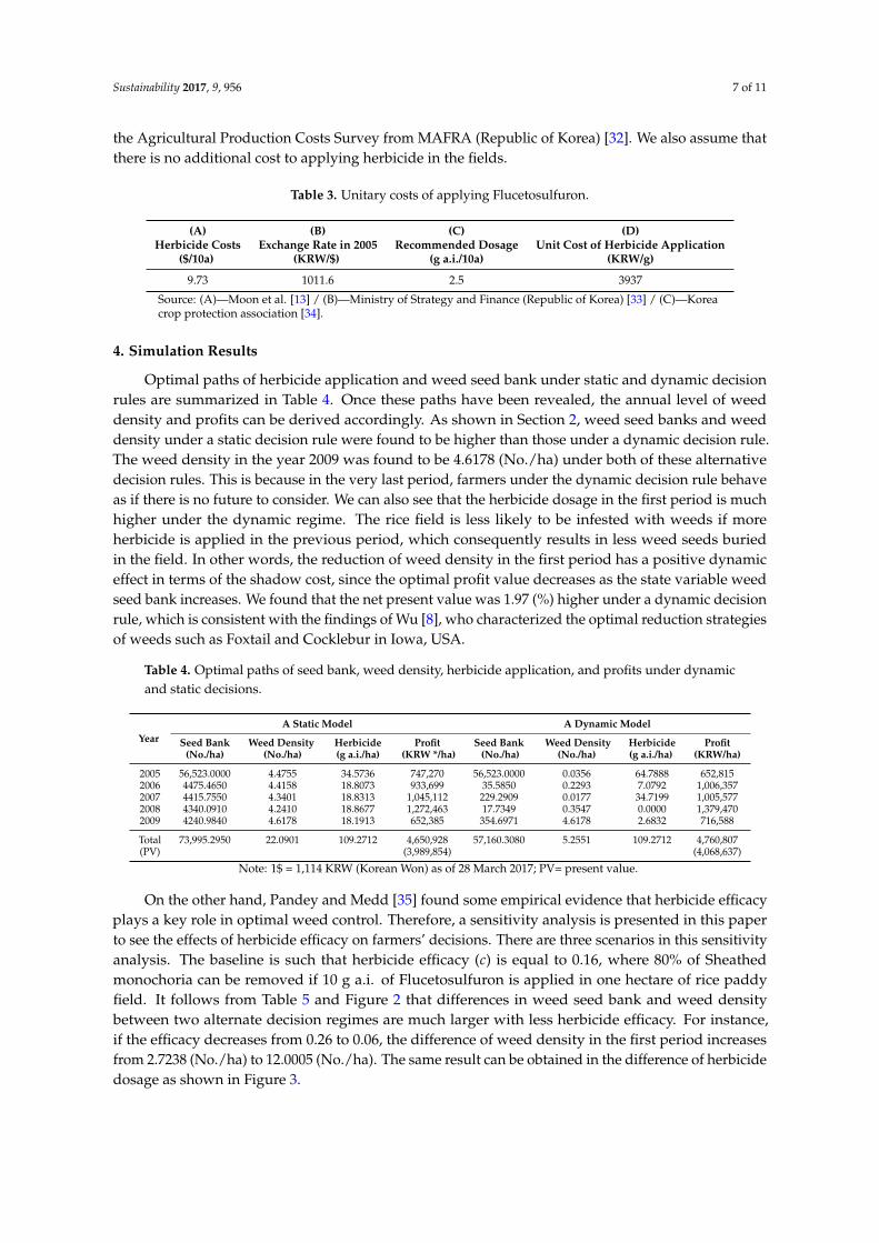
Optimal paths of herbicide application and weed seed bank under static and dynamic decisionrules are summarized in Table 4. Once these paths have been revealed, the annual level of weeddensity and profits can be derived accordingly. As shown in Section 2, weed seed banks and weeddensity under a static decision rule were found to be higher than those under a dynamic decision rule.The weed density in the year 2009 was found to be 4.6178 (No./ha) under both of these alternativedecision rules. This is because in the very last period, farmers under the dynamic decision rule behaveas if there is no future to consider. We can also see that the herbicide dosage in the first period is muchhigher under the dynamic regime. The rice field is less likely to be infested with weeds if moreherbicide is applied in the previous period, which consequently results in less weed seeds buriedin the field. In other words, the reduction of weed density in the first period has a positive dynamiceffect in terms of the shadow cost, since the optimal profit value decreases as the state variable weedseed bank increases. We found that the net present value was 1.97 (%) higher under a dynamic decisionrule, which is consistent with the findings of Wu [8], who characterized the optimal reduction strategiesof weeds such as Foxtail and Cocklebur in Iowa, USA.

Table 4. Optimal paths of seed bank, weed density, herbicide application, and profits under dynamicand static decisions.

YearA Static Model A Dynamic Model

Seed Bank Weed Density Herbicide Profit Seed Bank Weed Density Herbicide Profit(No./ha) (No./ha) (g a.i./ha) (KRW */ha) (No./ha) (No./ha) (g a.i./ha) (KRW/ha)

2005 56,523.0000 4.4755 34.5736 747,270 56,523.0000 0.0356 64.7888 652,8152006 4475.4650 4.4158 18.8073 933,699 35.5850 0.2293 7.0792 1,006,3572007 4415.7550 4.3401 18.8313 1,045,112 229.2909 0.0177 34.7199 1,005,5772008 4340.0910 4.2410 18.8677 1,272,463 17.7349 0.3547 0.0000 1,379,4702009 4240.9840 4.6178 18.1913 652,385 354.6971 4.6178 2.6832 716,588

Total 73,995.2950 22.0901 109.2712 4,650,928 57,160.3080 5.2551 109.2712 4,760,807(PV) (3,989,854) (4,068,637)

Note: 1$ = 1,114 KRW (Korean Won) as of 28 March 2017; PV= present value.

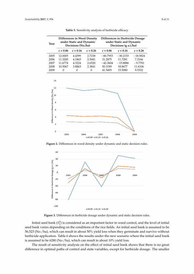
On the other hand, Pandey and Medd [35] found some empirical evidence that herbicide efficacyplays a key role in optimal weed control. Therefore, a sensitivity analysis is presented in this paperto see the effects of herbicide efficacy on farmers’ decisions. There are three scenarios in this sensitivityanalysis. The baseline is such that herbicide efficacy (c) is equal to 0.16, where 80% of Sheathedmonochoria can be removed if 10 g a.i. of Flucetosulfuron is applied in one hectare of rice paddyfield. It follows from Table 5 and Figure 2 that differences in weed seed bank and weed densitybetween two alternate decision regimes are much larger with less herbicide efficacy. For instance,if the efficacy decreases from 0.26 to 0.06, the difference of weed density in the first period increasesfrom 2.7238 (No./ha) to 12.0005 (No./ha). The same result can be obtained in the difference of herbicidedosage as shown in Figure 3.

Sustainability 2017, 9, 956 8 of 11

Table 5. Sensitivity analysis of herbicide efficacy.

Year

Differences in Weed Density Differences in Herbicide Dosageunder Static and Dynamic under Static and Dynamic

Decisions (No./ha) Decisions (g a.i./ha)

c = 0.06 c = 0.16 c = 0.26 c = 0.06 c = 0.16 c = 0.26

2005 12.0005 4.4399 2.7238 −80.7953 −30.2153 −18.58242006 11.3200 4.1865 2.5681 31.2875 11.7281 7.21662007 11.6774 4.3224 2.6520 −42.3604 −15.8886 −9.77812008 10.5067 3.8863 2.3841 50.3189 18.8677 11.61062009 0 0 0 41.5493 15.5080 9.5332

Figure 2. Differences in weed density under dynamic and static decision rules.

Figure 3. Differences in herbicide dosage under dynamic and static decision rules.

Initial seed bank (S01) is considered as an important factor in weed control, and the level of initial

seed bank varies depending on the conditions of the rice fields. An initial seed bank is assumed to be56,523 (No./ha), which can result in about 50% yield loss when they germinate and survive withoutherbicide application. Table 6 shows the results under the new scenario where the initial seed bankis assumed to be 6280 (No./ha), which can result in about 10% yield loss.

The result of sensitivity analysis on the effect of initial seed bank shows that there is no greatdifference in optimal paths of control and state variables, except for herbicide dosage. The smaller

Sustainability 2017, 9, 956 9 of 11

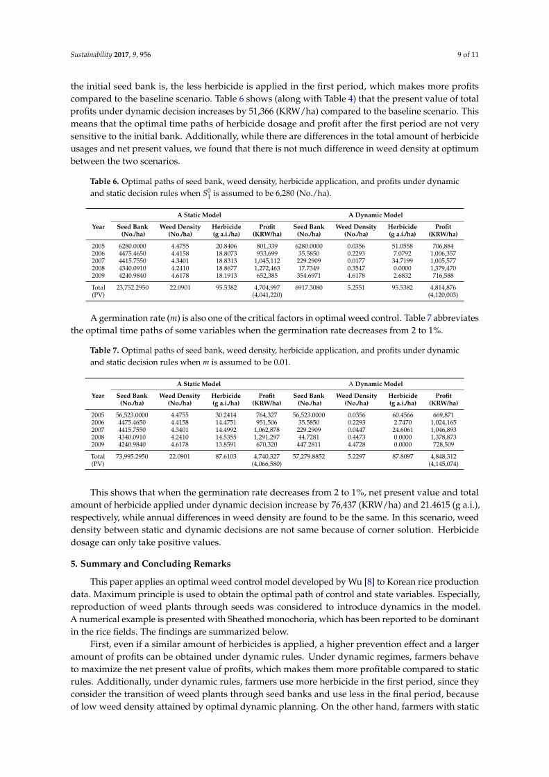
the initial seed bank is, the less herbicide is applied in the first period, which makes more profitscompared to the baseline scenario. Table 6 shows (along with Table 4) that the present value of totalprofits under dynamic decision increases by 51,366 (KRW/ha) compared to the baseline scenario. Thismeans that the optimal time paths of herbicide dosage and profit after the first period are not verysensitive to the initial bank. Additionally, while there are differences in the total amount of herbicideusages and net present values, we found that there is not much difference in weed density at optimumbetween the two scenarios.

Table 6. Optimal paths of seed bank, weed density, herbicide application, and profits under dynamicand static decision rules when S0

1 is assumed to be 6,280 (No./ha).

A Static Model A Dynamic Model

Year Seed Bank Weed Density Herbicide Profit Seed Bank Weed Density Herbicide Profit(No./ha) (No./ha) (g a.i./ha) (KRW/ha) (No./ha) (No./ha) (g a.i./ha) (KRW/ha)

2005 6280.0000 4.4755 20.8406 801,339 6280.0000 0.0356 51.0558 706,8842006 4475.4650 4.4158 18.8073 933,699 35.5850 0.2293 7.0792 1,006,3572007 4415.7550 4.3401 18.8313 1,045,112 229.2909 0.0177 34.7199 1,005,5772008 4340.0910 4.2410 18.8677 1,272,463 17.7349 0.3547 0.0000 1,379,4702009 4240.9840 4.6178 18.1913 652,385 354.6971 4.6178 2.6832 716,588

Total 23,752.2950 22.0901 95.5382 4,704,997 6917.3080 5.2551 95.5382 4,814,876(PV) (4,041,220) (4,120,003)

A germination rate (m) is also one of the critical factors in optimal weed control. Table 7 abbreviatesthe optimal time paths of some variables when the germination rate decreases from 2 to 1%.

Table 7. Optimal paths of seed bank, weed density, herbicide application, and profits under dynamicand static decision rules when m is assumed to be 0.01.

A Static Model A Dynamic Model

Year Seed Bank Weed Density Herbicide Profit Seed Bank Weed Density Herbicide Profit(No./ha) (No./ha) (g a.i./ha) (KRW/ha) (No./ha) (No./ha) (g a.i./ha) (KRW/ha)

2005 56,523.0000 4.4755 30.2414 764,327 56,523.0000 0.0356 60.4566 669,8712006 4475.4650 4.4158 14.4751 951,506 35.5850 0.2293 2.7470 1,024,1652007 4415.7550 4.3401 14.4992 1,062,878 229.2909 0.0447 24.6061 1,046,8932008 4340.0910 4.2410 14.5355 1,291,297 44.7281 0.4473 0.0000 1,378,8732009 4240.9840 4.6178 13.8591 670,320 447.2811 4.4728 0.0000 728,509

Total 73,995.2950 22.0901 87.6103 4,740,327 57,279.8852 5.2297 87.8097 4,848,312(PV) (4,066,580) (4,145,074)

This shows that when the germination rate decreases from 2 to 1%, net present value and totalamount of herbicide applied under dynamic decision increase by 76,437 (KRW/ha) and 21.4615 (g a.i.),respectively, while annual differences in weed density are found to be the same. In this scenario, weeddensity between static and dynamic decisions are not same because of corner solution. Herbicidedosage can only take positive values.

5. Summary and Concluding Remarks

This paper applies an optimal weed control model developed by Wu [8] to Korean rice productiondata. Maximum principle is used to obtain the optimal path of control and state variables. Especially,reproduction of weed plants through seeds was considered to introduce dynamics in the model.A numerical example is presented with Sheathed monochoria, which has been reported to be dominantin the rice fields. The findings are summarized below.

First, even if a similar amount of herbicides is applied, a higher prevention effect and a largeramount of profits can be obtained under dynamic rules. Under dynamic regimes, farmers behaveto maximize the net present value of profits, which makes them more profitable compared to staticrules. Additionally, under dynamic rules, farmers use more herbicide in the first period, since theyconsider the transition of weed plants through seed banks and use less in the final period, becauseof low weed density attained by optimal dynamic planning. On the other hand, farmers with static

Sustainability 2017, 9, 956 10 of 11

decision rules do not consider seed bank dynamics, and therefore, the total amount of herbicide usedwill be similar. However, the prevention effect will be much lower, since seed bank dynamics were notconsidered in the decision-making process.

Second, the annual difference in weed density and weed seed bank is larger for the lower herbicideefficacy. Therefore, farmers will be more likely to be better off under dynamic decision rules if herbicideefficacy is low. However, differences in those variables are not sensitive to the initial seed bank (S1

0)or germination rate (m).

Many studies have been carried out to describe yield loss from weed-crop competition andherbicide dose–response, which help us determine the optimal level of herbicide dosage [11,12,30].Additionally, much research on finding the threshold of herbicide application to attain a certain levelof weed density has been undertaken [13,18,19]. However, there is a huge research gap between thisthreshold analysis and reality because farmers do not take profit maximization principles into account.This paper attempted to analyze the optimal weed control under the profit maximization framework,incorporating research findings from crop science literature. In addition, gains from the dynamicdecision rules were investigated over the static rules. These gains can be viewed as effective incentivesfor achieving sustainable rice production in South Korea.

The analysis in this paper has the following limitations: First, we have concentrated mainly onthe effects of herbicide dosage on rice yields in both dynamic and static settings. Thus, price and yielduncertainties and farmers’ risk preferences were not incorporated into the model. Secondly, a spatialdistribution of weed seed bank was not considered due to data limitations. These issues are good areasfor future research.

Acknowledgments: This work was supported by the National Research Foundation of Korea-Grant funded bythe Korean Government (NRF-2014S1A3A2044459).

Author Contributions: Woongchan Jeon and Kwansoo Kim conceived and developed the model. WoongchanJeon and Kwansoo Kim analyzed results and wrote the manuscript. All authors have read and approved the final.

Conflicts of Interest: The authors declare no conflict of interest.

References

1. Carlson, G.A. Risk reducing inputs related to agricultural pests. In Risk Analysis of Agricultural Firms:Concepts, Information Requirements and Policy Issues; Proceedings of Regional Research Project S-180; Universityof Illinois: Champaign, IL, USA, 1984; pp. 164–175.

2. Feder, G. Pesticides, information, and pest management under uncertainty. Am. J. Agric. Econ. 1979, 61,97–103.

3. Pannell, D.J. Pests and pesticides, risk and risk aversion. Agric. Econ. 1991, 5, 361–383.4. Vila, M.; Corbin, J.D.; Dukes, J.S.; Pino, J.; Smith, S.D. Linking plant invasions to global environmental

change. In Terrestrial Ecosystems in a Changing World; Canadell, J.G., DPataki, D.E., Pitelka, L.F., Eds.;Springer: Heidelberg, Germany, 2007; pp. 93–102.

5. Cousens, R. A simple model relating yield loss to weed density. Ann. Appl. Biol. 1985, 107, 239–252.6. Streibig, J. Models for curve-fitting herbicide dose response data. Acta Agric. Scand. 1980, 30, 59–64.7. Kim, D.; Brain, P.; Marshall, E.; Caseley, J. Modelling herbicide dose and weed density effects on crop: Weed

competition. Weed Res. 2002, 42, 1–13.8. Wu, J. Optimal weed control under static and dynamic decision rules. Agric. Econ. 2000, 25, 119–130.9. Odom, D.I.; Cacho, O.J.; Sinden, J.; Griffith, G.R. Policies for the management of weeds in natural ecosystems:

The case of scotch broom (Cytisus scoparius L.) in an Australian national park. Ecol. Econ. 2003, 44, 119–135.10. Eiswerth, M.E.; Darden, T.D.; Johnson, W.S.; Agapoff, J.; Harris, T.R. Input–output modeling, outdoor

recreation, and the economic impacts of weeds. Weed Sci. 2005, 53, 130–137.11. Lee, S.-G.; Kim, D.-S.; Im, I.-B.; Pyon, J.-Y. Growth and yield of rice as affected by different densities

of perennial weeds and prediction of rice yield loss in paddy fields. Korean J. Weed Sci. 2005, 25, 295–303.12. Song, S.-B.; Hong, Y.-G.; Hwang, J.-B.; Park, S.-T.; Kim, H.-Y. Loss of rice growth and yield affected by weed

competition in machine transplanted rice cultivation. Korean J. Weed Sci. 2006, 26, 407–412.

Sustainability 2017, 9, 956 11 of 11

13. Moon, B.-C.; Kwon, O.-D.; Cho, S.-H.; Lee, S.-G.; Won, J.-G.; Lee, I.-Y.; Park, J.-E.; Kim, D.-S. Modeling theCompetition Effect of Sagittaria trifolia and Monochoria vaginalis Weed Density on Rice in TransplantedRice Cultivation. Korean J. Weed Sci. 2012, 32, 188–194.

14. Bauer, T.A.; Mortensen, D.A. A comparison of economic and economic optimum thresholds for two annualweeds in soybeans. Weed Technol. 1992, 6, 228–235.

15. Deen, W.; Weersink, A.; Turvey, C.; Weaver, S. Economics of weed control strategies under uncertainty.Rev. Agric. Econ. 1993, 15, 39–50.

16. Coble, H.D.; Mortensen, D.A. The threshold concept and its application to weed science. Weed Technol.1992, 6, 191–195.

17. Wilkerson, G.; Modena, S.; Coble, H. HERB: Decision model for postemergence weed control in soybean.Agron. J. 1991, 83, 413–417.

18. Al Mamun, M.A. Modelling rice-weed competition in direct-seeded rice cultivation. Agric. Res. 2014, 3,346–352.

19. Moon, B.-C.; Cho, S.-H.; Kwon, O.-D.; Lee, S.-G.; Lee, B.-W. Modelling rice competition with Echinochloacrus-galli and Eleocharis kuroguwai in transplanted rice cultivation. J. Crop Sci. Biotechnol. 2010, 13, 121–126.

20. Swinton, S.M.; King, R.P. The value of pest information in a dynamic setting: The case of weed control. Am. J.Agric. Econ. 1994, 76, 36–46.

21. Pontryagin, L.S. Mathematical Theory of Optimal Processes; Gordon and Breach Sceince Publishers S.A.:New York, NY, USA, 1986.

22. Lee, I.-Y.; Park, J.-E.; Kim, C.-S.; Oh, S.-M.; Chung-Kil, K.; Park, T.-S.; Cho, J.-R.; Moon, B.-C.; Kwon, O.-S.;Kim, K.-H.; et al. Characteristics of weed flora in arable land of Korea. Korean J. Weed Sci. 2007, 27, 1–21.

23. Oh, Y.; Ku, Y.; Lee, J.; Ham, Y. Distribution of weed population in the paddy field in Korea, 1981. Korean J.Weed Sci. 1981, 1, 21–29.

24. Park, K.; Oh, Y.; Ku, Y.; Kim, H.; Sa, J.; Park, J.; Kim, H.; Kwon, S.; Shin, H.; Kim, S. Changes of weedcommunity in lowland rice field [s] in Korea. Korean J. Weed Sci. 1995, 15, 254–261.

25. Park, J.-S.; Cho, Y.-C.; Han, S.-W.; Lim, G.J.; Lee, W.W.; Ju, Y.C.; Kim, Y.H. Weed population distribution andchange of dominant weed species on paddy field in Kyonggi region. Korean J. Weed Sci. 2001, 21, 320–326.

26. Park, J.-S.; Kim, H.-D.; Han, S.-W.; Lee, J.-H.; Jang, J.-H. Weed population distribution and change ofdominant weed species in paddy field of Gyeonggi region. Korean J. Weed Sci. 2007, 27, 56–65.

27. Kershaw, K.A. Quantitative and Dynamic Plant Ecology, 2nd ed.; American Elsevier Pub. Co.: New York,NY, USA, 1964.

28. Curtis, J.T.; McIntosh, R.P. The interrelations of certain analytic and synthetic phytosociological characters.Ecology 1950, 31, 434–455.

29. Ha, H.-Y.; Hwang, K.S.; Suh, S.J.; Lee, I.-Y.; Oh, Y.-J.; Park, J.; Choi, J.-K.; Kim, E.J.; Cho, S.H.; Kwon, O.-D.A survey of weed occurrence on paddy field in Korea. Weed Turfgrass Sci. 2014, 3, 71–77.

30. Moon, B.-C.; Kim, J.-W.; Cho, S.-H.; Park, J.-E.; Song, J.-S.; Kim, D.-S. Modelling the effects of herbicide doseand weed density on rice–weed competition. Weed Res. 2014, 54, 484–491.

31. Nongsaro. Available online: www.nongsaro.go.kr/portal/Main.ps?menuId=PS00001 (accessed on27 March 2017).

32. Korean Statistical Information Service (KOSIS). Available online: kosis.kr/statisticsList/statisticsList_01List.jsp?vwcd=MT_ZTITLE&parentIdF (accessed on 27 March 2017).

33. Korea National Index. Available online: www.index.go.kr/index.jsp?oid=N (accessed on 27 March 2017).34. Korea Crop Protection Association. Available online: koreacpa.org/index3/main.php (accessed on

27 March 2017).35. Pandey, S.; Medd, R.W. A stochastic dynamic programming framework for weed control decision making:

An application to Avena fatua L. Agric. Econ. 1991, 6, 115–128.

c© 2017 by the authors. Licensee MDPI, Basel, Switzerland. This article is an open accessarticle distributed under the terms and conditions of the Creative Commons Attribution(CC BY) license (http://creativecommons.org/licenses/by/4.0/).