optimal operation of industrial compressor stations in systems
TRANSCRIPT

Imperial College London
Department of Chemical Engineering
Optimal operation of industrial
compressor stations in systems with
large energy consumption
Dionysios P. Xenos
September 2015
Supervised by Professor Nina Thornhill
Co-Supervisor: Professor Ricardo Martinez-Botas
Submitted in part fulfilment of the requirements for the degree of
Doctor of Philosophy in Chemical Engineering of Imperial College London
and the Diploma of Imperial College London
1

Declaration of originality
I herewith certify that all material in this dissertation which is not my own work
has been properly acknowledged.
The copyright of this thesis rests with the author and is made available under
a Creative Commons Attribution Non-Commercial No Derivatives licence. Re-
searchers are free to copy, distribute or transmit the thesis on the condition that
they attribute it, that they do not use it for commercial purposes and that they do
not alter, transform or build upon it. For any reuse or redistribution, researchers
must make clear to others the licence terms of this work.
2

Abstract
The aim of the thesis is to study the optimal operation of compressor stations
in systems with large energy consumption such as process systems and natural
gas networks. Compressor stations include several compressors in parallel which
usually account for the major part of the total energy consumed in the system.
Therefore, the efficient operation and maintenance of the compressors could save
energy, and reduce operational costs.
The development of optimisation frameworks and optimisation models can de-
termine the decisions which lead to the minimisation of costs operating compressor
stations. The modelling of the behaviour of the compressors is also an important
topic of the current PhD study. Different types of models should be used according
to the level of optimisation level (online and real time, and offline), considering
the available resources such as compressor maps or process data.
The thesis developed a comprehensive real time optimisation framework which
can reduce the power consumption of compressor stations compared to the case
of operation with the existing industrial practices. The thesis also developed a
mixed integer linear programming multi-period optimisation model to minimise
total costs of the operation, for example electricity costs, and start up and shut
down costs. Another contribution of the thesis is the integration of operation
and maintenance of the compressors considering different types of maintenance
activities such as major overhauls and the washing of compressors. For example,
the proposed integrated framework can be used to generate the schedules of the
online and offline washing of the compressors compared to existing approaches
described by fixed periodical washing or washing when the degradation of the
condition of the compressors has reached unacceptable limits.
The optimisation frameworks was applied to two industrial case studies, namely
one air separation plant involving a network of air compressors in BASF, Lud-
wigshafen, Germany and one export natural gas compressor station operated by
Statoil in Norway. The final chapters of the thesis discuss the contributions and
assumptions of each method, and present potential new research areas deriving
from the PhD study.
3

Acknowledgements
Through the PhD journey, my main supervisor Professor Nina F. Thornhill
transfered to me all the basic principles for carrying out high quality scientific
research. Professor Thornhill showed me how to become objective in research,
how to use my critical and analytical thinking, how to be more conscious and
more efficient, and most importantly how to deal with the demanding world of
academia (and industry). I am deeply grateful and lucky that I had Professor
Nina as my PhD supervisor. My co-supervisor Professor Ricardo Martinez-Botas
helped me to understand technical concepts and supported me in difficult moments
throughout this journey. My colleague Matteo Cicciotti helped me in difficult
personal moments and he transferred to me work principles for example how to
notice small details which make the difference, how to work hard and how to be
professional at all levels of humans interactions. Dr. Georgios Kopanos is one of
the key contributors in my technical development as he guided me in modelling
and optimization methods. I would like to acknowledge my PhD colleagues, Sara
Budinis and Izzati Mohd Noor, and MSc student Mitra Matloubi who supported
me with fruitful discussions and helped in personal matters. Dr. Davide Fabozzi
transferred to me a way of thinking which I will always keep in my mind, in
brief “quality is the most important thing in academia”. I have to thank Dr.
Ala Bouaswaig and Dr. Olaf Kahrs from BASF, and Dr. Erling Lunde from
Statoil who provided me their technical knowledge and their experience about real
industrial case studies. Trond Haugen and Dr. Iiro Harjunkonski inspired me
to focus on the interactions between industry and academia. I would also like
to thank Imperial College London and Energy-SmartOps (European Commission
Marie Curie initial training network programme) which gave me the opportunity to
study and work as a researcher in one of the best universities worldwide. Without
this financial, infrastructure and human resource support I would not be able to
reach this personal development I have acquired so far. One of the most important
people of my life who helped me in this PhD journey is Inna. Without her I would
not have managed to finish my PhD studies. I would like to thank Toma who
supports me with her love and understanding. Without her I would not be able
to deliver this PhD thesis and at the same time to be able to keep a balance in
my life. I am grateful that I have met this angel. Finally I would like to thank
my family. I do not have words to express my gratefulness and feelings about my
family as with their love gave me and still giving me infinite fuel to attain my goals
and dreams.
4

“In today’s rush we all think too much, seek too much, want
too much and forget about the joy of just Being”
Eckhart Tolle
5

Contents
1 Introduction 25
1.1 Description of the chapter . . . . . . . . . . . . . . . . . . . . . . . 25
1.2 An introduction to the project: Energy SmartOps . . . . . . . . . 25
1.3 An introduction to the optimal operation of compressors . . . . . . 28
1.3.1 Compressed air . . . . . . . . . . . . . . . . . . . . . . . . . 28
1.3.2 Natural gas compression . . . . . . . . . . . . . . . . . . . . 30
1.4 Introduction to the case studies . . . . . . . . . . . . . . . . . . . . 31
1.4.1 BASF case study . . . . . . . . . . . . . . . . . . . . . . . . 32
1.4.2 Statoil case study . . . . . . . . . . . . . . . . . . . . . . . . 35
1.5 Scientific aim and objectives of the thesis . . . . . . . . . . . . . . 37
1.6 Contributions of the thesis . . . . . . . . . . . . . . . . . . . . . . . 39
1.6.1 Contribution to the real time optimisation of compressors . 39
1.6.2 Contribution to the scheduling of compressors for long periods 40
1.6.3 Contribution to the integration of operation and maintenance 40
1.7 Sponsors and acknowledgements . . . . . . . . . . . . . . . . . . . 41
1.8 Structure of the thesis . . . . . . . . . . . . . . . . . . . . . . . . . 42
2 Background of operation of compressor stations 44
2.1 Description of the chapter . . . . . . . . . . . . . . . . . . . . . . . 44
2.2 Industrial compressors . . . . . . . . . . . . . . . . . . . . . . . . . 44
2.2.1 Description of industrial centrifugal compressors . . . . . . 44
2.2.2 Operation of a compressor . . . . . . . . . . . . . . . . . . . 47
2.2.3 Maintenance of compressors . . . . . . . . . . . . . . . . . . 52
2.3 Compressors integrated with other systems . . . . . . . . . . . . . 53
2.3.1 Interactions between compressors and a downstream system 53
2.3.2 Control methods . . . . . . . . . . . . . . . . . . . . . . . . 55
2.4 Management of compressor stations . . . . . . . . . . . . . . . . . 56
2.4.1 Operational tasks of compressors . . . . . . . . . . . . . . . 56
2.4.2 Supervisory control: Real Time Optimisation (RTO) . . . . 57
2.4.3 Operational planning and scheduling . . . . . . . . . . . . . 59
2.5 Optimisation (mathematical programming) . . . . . . . . . . . . . 59
2.5.1 Definition of an optimisation problem . . . . . . . . . . . . 60
6

2.5.2 Classification of optimisation problems . . . . . . . . . . . . 63
2.5.3 Software and solvers . . . . . . . . . . . . . . . . . . . . . . 66
2.6 Summary of the chapter . . . . . . . . . . . . . . . . . . . . . . . . 67
3 Literature review on the optimal operation of compressor stations 68
3.1 Description of the chapter . . . . . . . . . . . . . . . . . . . . . . . 68
3.2 Classification of problems of optimal operation of compressors . . . 68
3.2.1 General overview . . . . . . . . . . . . . . . . . . . . . . . . 68
3.2.2 Optimisation of compressors regarding the application . . . 70
3.2.3 Optimisation of compressors regarding time horizon . . . . 71
3.3 Optimal load sharing . . . . . . . . . . . . . . . . . . . . . . . . . . 72
3.4 Scheduling and optimal selection of compressors . . . . . . . . . . . 74
3.4.1 Methodologies with similar formulation for other applica-
tions (e.g. utilities for process systems) . . . . . . . . . . . 75
3.4.2 Operational planning of air separation plants . . . . . . . . 76
3.5 Maintenance of compressors . . . . . . . . . . . . . . . . . . . . . . 78
3.6 Gaps of knowledge and contributions of the thesis . . . . . . . . . 81
3.7 Summary of the chapter . . . . . . . . . . . . . . . . . . . . . . . . 83
4 Real Time Optimisation (RTO) for online application 84
4.1 Description of the chapter . . . . . . . . . . . . . . . . . . . . . . . 84
4.2 General integrated optimisation framework for the optimisation of
compressor stations . . . . . . . . . . . . . . . . . . . . . . . . . . . 85
4.3 A Real Time Optimisation (RTO) framework using data-driven
models . . . . . . . . . . . . . . . . . . . . . . . . . . . . . . . . . . 87
4.3.1 Process data and measurements . . . . . . . . . . . . . . . . 88
4.3.2 Steady-state detection . . . . . . . . . . . . . . . . . . . . . 90
4.3.3 Development of models . . . . . . . . . . . . . . . . . . . . 92
4.3.4 Assessment of the accuracy of the prediction of the models 94
4.3.5 Optimisation model of the RTO . . . . . . . . . . . . . . . 95
4.4 Description of the industrial case study . . . . . . . . . . . . . . . 96
4.4.1 Practical challenges of the case study . . . . . . . . . . . . 98
4.5 Results . . . . . . . . . . . . . . . . . . . . . . . . . . . . . . . . . . 99
4.5.1 Models of compressors . . . . . . . . . . . . . . . . . . . . . 99
4.5.2 Illustrative example with industrial compressors . . . . . . 102
4.5.3 Demonstration of Real Time Optimisation (RTO) applica-
tion in parallel with real operation . . . . . . . . . . . . . . 103
4.6 Summary of the chapter . . . . . . . . . . . . . . . . . . . . . . . . 109
7
5 Multi-period optimisation of the operation of compressor stations110
5.1 Description of the chapter . . . . . . . . . . . . . . . . . . . . . . . 110
5.2 Description of the general methodology . . . . . . . . . . . . . . . 111
5.2.1 Description of a compressor station within a system . . . . 111
5.2.2 Examples of decisions . . . . . . . . . . . . . . . . . . . . . 114
5.2.3 Statement of the problem . . . . . . . . . . . . . . . . . . . 115
5.3 Minimum run and shutdown time . . . . . . . . . . . . . . . . . . . 118
5.4 Assignment of compressors to headers . . . . . . . . . . . . . . . . 118
5.5 Compressor-to-header assignment changes . . . . . . . . . . . . . . 119
5.6 Modelling of compressors with the use of process data . . . . . . . 120
5.6.1 Power consumption . . . . . . . . . . . . . . . . . . . . . . . 120
5.6.2 Feasible window of operation . . . . . . . . . . . . . . . . . 122
5.6.3 Feasible window of operation with tight constraints: Convex
hull application . . . . . . . . . . . . . . . . . . . . . . . . . 122
5.7 Modelling with the use of compressor maps . . . . . . . . . . . . . 125
5.7.1 Power consumption . . . . . . . . . . . . . . . . . . . . . . . 125
5.7.2 Feasible window of operation . . . . . . . . . . . . . . . . . 128
5.8 Other control methods . . . . . . . . . . . . . . . . . . . . . . . . . 129
5.8.1 Recycle model . . . . . . . . . . . . . . . . . . . . . . . . . 130
5.8.2 Blow-off valve model . . . . . . . . . . . . . . . . . . . . . . 130
5.9 Outlet pressure of compressors . . . . . . . . . . . . . . . . . . . . 131
5.10 Mass balances of air separation plant units . . . . . . . . . . . . . 131
5.10.1 Demand for compressed air utility . . . . . . . . . . . . . . 132
5.10.2 Air separation columns: mass flow rates for products . . . . 132
5.10.3 Storage tanks mass balances . . . . . . . . . . . . . . . . . . 133
5.11 Export gas operational constraints . . . . . . . . . . . . . . . . . . 134
5.12 Objective function . . . . . . . . . . . . . . . . . . . . . . . . . . . 135
5.13 Maintenance constraints - Given maintenance schedule . . . . . . . 136
5.14 Initial state of the network . . . . . . . . . . . . . . . . . . . . . . 137
5.15 Terminal constraints . . . . . . . . . . . . . . . . . . . . . . . . . . 139
5.16 Equal split and equal surge margin operation . . . . . . . . . . . . 140
5.16.1 Constraints of the equal split strategy . . . . . . . . . . . . 140
5.16.2 Constraints of the equal surge margin . . . . . . . . . . . . 142
5.17 Numerical application of the methodology . . . . . . . . . . . . . . 143
5.17.1 Description of the case study 1 (air separation plant) . . . . 143
5.17.2 Example 1-A: Illustrative example of the air separation plant 145
5.17.3 Example 1-B: Industrial example . . . . . . . . . . . . . . . 149
5.17.4 Example 2: Industrial example of an export gas compressor
station . . . . . . . . . . . . . . . . . . . . . . . . . . . . . . 152
8
5.18 Summary of the chapter . . . . . . . . . . . . . . . . . . . . . . . . 163
6 Integration of optimal operation and maintenance 166
6.1 Description of the chapter . . . . . . . . . . . . . . . . . . . . . . . 166
6.2 Basic model of integrated operation and maintenance . . . . . . . . 168
6.2.1 Basic maintenance constraints . . . . . . . . . . . . . . . . 168
6.2.2 Maintenance tasks restrictions . . . . . . . . . . . . . . . . 169
6.2.3 Integrated framework . . . . . . . . . . . . . . . . . . . . . 169
6.2.4 Example 3: Illustrative example . . . . . . . . . . . . . . . 170
6.2.5 Example 4: Industrial example . . . . . . . . . . . . . . . . 172
6.3 Basic maintenance model in a rolling time horizon framework (re-
active scheduling) . . . . . . . . . . . . . . . . . . . . . . . . . . . . 175
6.3.1 Model . . . . . . . . . . . . . . . . . . . . . . . . . . . . . . 175
6.3.2 Numerical example . . . . . . . . . . . . . . . . . . . . . . . 178
6.4 Maintenance model including major overhauls . . . . . . . . . . . . 183
6.4.1 Maintenance model . . . . . . . . . . . . . . . . . . . . . . . 183
6.4.2 Integrated framework with focus on major overhauls . . . . 186
6.4.3 Example 5: Industrial example . . . . . . . . . . . . . . . . 187
6.5 Condition based-based maintenance: washing of compressors . . . 193
6.5.1 Introduction . . . . . . . . . . . . . . . . . . . . . . . . . . 193
6.5.2 Model of offline washing maintenance . . . . . . . . . . . . 195
6.5.3 Model of online washing . . . . . . . . . . . . . . . . . . . . 200
6.5.4 Model of combined online and offline washing . . . . . . . . 202
6.5.5 Objective function . . . . . . . . . . . . . . . . . . . . . . . 204
6.5.6 Terminal constraints of maintenance model . . . . . . . . . 205
6.5.7 Description of numerical application . . . . . . . . . . . . . 205
6.5.8 Results and discusions . . . . . . . . . . . . . . . . . . . . . 208
6.5.9 Different degradation rates . . . . . . . . . . . . . . . . . . 212
6.5.10 Case with a less flexible system . . . . . . . . . . . . . . . . 216
6.6 Summary of the chapter . . . . . . . . . . . . . . . . . . . . . . . . 217
7 Critical evaluation and suggestions for future work 219
7.1 Description of the chapter . . . . . . . . . . . . . . . . . . . . . . . 219
7.2 Evaluation of the achievements of the objectives . . . . . . . . . . 219
7.2.1 Objective One . . . . . . . . . . . . . . . . . . . . . . . . . 219
7.2.2 Objective Two . . . . . . . . . . . . . . . . . . . . . . . . . 224
7.2.3 Objective Three . . . . . . . . . . . . . . . . . . . . . . . . 231
7.2.4 Summary of the contributions . . . . . . . . . . . . . . . . . 235
7.3 Latest outcomes of the thesis . . . . . . . . . . . . . . . . . . . . . 237
7.3.1 Impact of the research . . . . . . . . . . . . . . . . . . . . . 237
9
7.3.2 Further work on the optimal operation of compressors con-
sidering energy management . . . . . . . . . . . . . . . . . 238
7.4 Summary of the chapter . . . . . . . . . . . . . . . . . . . . . . . . 241
8 Conclusions 242
8.1 Statement and justification of objectives . . . . . . . . . . . . . . . 242
8.2 Conclusions of thesis for Objective One . . . . . . . . . . . . . . . 243
8.3 Conclusions of thesis for Objective Two . . . . . . . . . . . . . . . 243
8.4 Conclusion of thesis for Objective Three . . . . . . . . . . . . . . . 244
8.5 Future work . . . . . . . . . . . . . . . . . . . . . . . . . . . . . . . 244
8.6 Final comment . . . . . . . . . . . . . . . . . . . . . . . . . . . . . 245
10

List of Tables
1.1 Examples of uses of compressed air in industrial sector (U.S. De-
partment of Energy, 2003). . . . . . . . . . . . . . . . . . . . . . . 29
2.1 Operational and performance characteristics of positive displace-
ment, and axial and centrifugal compressors according to Boyce
(2003). . . . . . . . . . . . . . . . . . . . . . . . . . . . . . . . . . . 45
2.2 Planning and scheduling activities according to Edgar et al. (2001). 59
4.1 Statistics of the fitting and validation of the regression models. . . 99
4.2 Boundaries of mass flow rates and power consumptions. . . . . . . 101
4.3 First six coefficients of the regression models. . . . . . . . . . . . . 101
4.4 Last six coefficients of the regression models. . . . . . . . . . . . . 101
4.5 Three different cases of operation. . . . . . . . . . . . . . . . . . . 103
5.1 Normalised compressor operating bounds of outlet mass flow rates
and pressure (%). . . . . . . . . . . . . . . . . . . . . . . . . . . . . 143
5.2 Description of the examples of the air separation case study. . . . . 144
5.3 Example 1-A: Main parameters. . . . . . . . . . . . . . . . . . . . . 146
5.4 Computational results for all problem instances of the illustrative
Example 1-A. . . . . . . . . . . . . . . . . . . . . . . . . . . . . . 149
5.5 Example 1-B: initial condition (i.e. t = 0) for all compressors. . . . 150
5.6 Information of maintenance tasks of the compressors for Example
1-B. . . . . . . . . . . . . . . . . . . . . . . . . . . . . . . . . . . . 150
5.7 Initial state of the compressors. . . . . . . . . . . . . . . . . . . . . 152
5.8 Parameters of compressors. . . . . . . . . . . . . . . . . . . . . . . 153
5.9 Description of twelve problems for optimal operation of compres-
sors with different specifications, for example different methods for
sharing load, i.e. Optimal, Equal Split (ES), Equal Surge Margin
(ESM), and use of various number of large compressors. . . . . . . 156
5.10 Total costs and distribution of costs in EUR for Problem 2 (one
large compressor), Problem 9 (two large compressors) and Problem
10 (three large compressors). . . . . . . . . . . . . . . . . . . . . . 160
11

6.1 Example 3: Earliest and latest starting times for flexible mainte-
nance tasks (in Days). . . . . . . . . . . . . . . . . . . . . . . . . . 171
6.2 Information of maintenance tasks of the compressors. . . . . . . . . 172
6.3 Computational results for all instances of the industrial examples.
The Fixed Maint. case refers to the Example 1-B in Section 5.17.3. 172
6.4 Descriptions of maintenance tasks. . . . . . . . . . . . . . . . . . . 183
6.5 Values of start and finish of flexible windows. . . . . . . . . . . . . 187
6.6 Suggested operating conditions of i6 for five days. . . . . . . . . . . 191
6.7 Comparison between problem Instance 5.1 (baseline case) and In-
stance 5.2 (fixed maintenance case). . . . . . . . . . . . . . . . . . 192
6.8 Main parameters of operation and maintenance. . . . . . . . . . . . 206
6.9 Cost parameters of operation and maintenance. . . . . . . . . . . . 206
6.10 Initial state of the system. . . . . . . . . . . . . . . . . . . . . . . . 208
6.11 Problem specifications and values of the objective function for each
scenario. . . . . . . . . . . . . . . . . . . . . . . . . . . . . . . . . . 208
7.1 Description of sections of Chapter 6 with their respective optimisa-
tion models and types of maintenance. . . . . . . . . . . . . . . . . 232
7.2 Summary of the major topics for future work (IFOM stands for
Integrated Framework of Operation and Maintenance). . . . . . . . 236
12
List of Figures
1.1 Graphical description of the five Work Packages of the Energy Smar-
tOps (courtesy of Energy SmartOps consortium). . . . . . . . . . . 27
1.2 Applications of natural gas compression. . . . . . . . . . . . . . . . 30
1.3 Chemical complex of BASF in Ludwigshafen, Germany (Bertha
Benz Realschule Wiesloch, 2008). . . . . . . . . . . . . . . . . . . . 32
1.4 Topology of the operational units and gas streams in the air sepa-
ration plant similar to the plant of BASF, Germany. . . . . . . . . 33
1.5 BASF centrifugal multi-stage compressor with open body (a) and
top casing (b) (Cicciotti et al., 2015). . . . . . . . . . . . . . . . . . 34
1.6 Norwegian gas network (Ministry of Petroleum and Energy, 2014). 36
1.7 A schematic of the topology of the Kollsnes plant connected with a
downstream pipeline network. . . . . . . . . . . . . . . . . . . . . . 37
1.8 A schematic which illustrates the objectives of this thesis for achiev-
ing optimal operation of compressor stations. . . . . . . . . . . . . 39
2.1 Basic classification of compressors based on U.S. Department of
Energy (2003). . . . . . . . . . . . . . . . . . . . . . . . . . . . . . 45
2.2 An industrial multi-stage compressor (Gresh, 2001). . . . . . . . . 46
2.3 Operation of a two-stage (multi-stage) centrifugal compressor con-
nected with an upstream and a downstream system. . . . . . . . . 47
2.4 A typical compressor map of a single-stage centrifugal compressor
with different angles of IGVs. . . . . . . . . . . . . . . . . . . . . . 48
2.5 Enthalpy-entropy diagram which shows the isentropic and actual
compression of the gas through a compressor stage. . . . . . . . . 50
2.6 Power flow in the different components of a compressor. . . . . . . 51
2.7 Various types of load curves and an Operating Point (OP) of a
compressor connected with load curve A (a) and operating point
change OP1 to OP2 by increasing the position of the IGVs (b). . . 54
2.8 Decision pyramid of a plant according to the ANSI/ISA-95 (Har-
junkoski et al., 2009) (a) and the corresponding decision pyramid of
a compressor station (b). . . . . . . . . . . . . . . . . . . . . . . . . 56
13

2.9 A block diagram describing the implementation of RTO with regu-
latory feedback control in a process operation (Seborg et al., 2004). 58
2.10 A general classification of optimisation problems in process engi-
neering. . . . . . . . . . . . . . . . . . . . . . . . . . . . . . . . . . 63
3.1 Classification of optimisation of compressor stations. . . . . . . . . 69
3.2 Simplified structure of a cryogenic air separation process with oxy-
gen and nitrogen products. . . . . . . . . . . . . . . . . . . . . . . 77
4.1 Integrated framework for the optimisation of compressor stations. . 86
4.2 Detailed description of the structure of the components of the RTO. 87
4.3 General methodology of offline development of data-driven models. 88
4.4 Multi-stage centrifugal compressor with inlet and outlet measure-
ments. . . . . . . . . . . . . . . . . . . . . . . . . . . . . . . . . . . 90
4.5 Moving time data set window. . . . . . . . . . . . . . . . . . . . . . 91
4.6 Several process variables (normalised) of the operation of an indus-
trial centrifugal compressor over time. . . . . . . . . . . . . . . . . 92
4.7 Black box model which associates input with output variables. . . 93
4.8 The current implemented (a) and suggested (b) control scheme of
three parallel air multi-stage centrifugal compressors. . . . . . . . . 97
4.9 An operating point of the system defined by the intersection between
load curve and characteristic of the system (CS curve) (a) and the
feasible window of operation (i.e regression domain) of a compressor
with IGVs (b). . . . . . . . . . . . . . . . . . . . . . . . . . . . . . 98
4.10 Prediction versus actual values of power of compressors i1, i2 and
i3 in the validation set. . . . . . . . . . . . . . . . . . . . . . . . . 100
4.11 Example of the optimisation of two compressors in parallel. . . . . 102
4.12 The first sixteen steady-state episodes of the system of the compres-
sors, compressor i1 (green), compressor i2 (blue) and compressor i3
(red). . . . . . . . . . . . . . . . . . . . . . . . . . . . . . . . . . . 104
4.13 Normalised total power consumption during the periods of steady-
state operation of the three compressors from actual, equal split and
optimal operation. . . . . . . . . . . . . . . . . . . . . . . . . . . . 104
4.14 Compressor i1 normalised mass flow rate from three different cases. 105
4.15 Compressor i2 normalised mass flow rate from three different cases. 106
4.16 Compressor i3 normalised mass flow rate from three different cases. 106
4.17 Power consumption of compressors i1 and i2 from optimisation and
actual operation (equal split). . . . . . . . . . . . . . . . . . . . . . 107
4.18 Compressor i1 normalised mass flow rate from actual and optimal
operation. . . . . . . . . . . . . . . . . . . . . . . . . . . . . . . . . 108
14

4.19 Compressor i2 normalised mass flow rate from actual and optimal
operation. . . . . . . . . . . . . . . . . . . . . . . . . . . . . . . . . 108
5.1 Classification of type of application, actuator of compressors and
method of modelling of each case study. . . . . . . . . . . . . . . . 111
5.2 Components of a system which includes a compressor station. . . . 112
5.3 A typical compressor station. . . . . . . . . . . . . . . . . . . . . . 114
5.4 A uniform discretisation of the scheduling time horizon. . . . . . . 115
5.5 Modelling of header-changes for a compressor through constraints
(5.6). . . . . . . . . . . . . . . . . . . . . . . . . . . . . . . . . . . . 119
5.6 Convex hull problems with three process variables involved. . . . . 123
5.7 Characteristics of a gas compressor with VSD control. . . . . . . . 125
5.8 Power curves of a compressor with VSD control. . . . . . . . . . . 126
5.9 The gas flows of a compressor using recycling flow. . . . . . . . . . 130
5.10 Gas flows of an air compressor with the use of a blow-off valve. . . 130
5.11 Mass balances of the units of an air separation plant. . . . . . . . . 132
5.12 Export gas station diagram. . . . . . . . . . . . . . . . . . . . . . . 134
5.13 Carryover of past startup information to model minimum run time. 138
5.14 An example of three compressors and two headers. . . . . . . . . . 141
5.15 An example of two compressors working with equal surge margin. . 143
5.16 Example 1-A: Normalised demands for products. . . . . . . . . . . 145
5.17 Problem 1-A: schedules for all problem instances. . . . . . . . . . . 147
5.18 Optimal distribution of (normalised) load of compressors in Instance
1-A.1 . . . . . . . . . . . . . . . . . . . . . . . . . . . . . . . . . . . 148
5.19 Instance 1-A.1: (a) total compressed air supplied to each header,
and (b) production capacity ratio of column u1 and u2. . . . . . . 148
5.20 Normalised demand for products for Example 1-B. . . . . . . . . . 149
5.21 Optimal schedule for industrial Example 1-B. . . . . . . . . . . . . 151
5.22 Normalised load of compressors for industrial Example 1-B. . . . . 152
5.23 Input demand of flow rate and pressure of each delivery point for
headers j1 and j2. . . . . . . . . . . . . . . . . . . . . . . . . . . . 153
5.24 Upstream inlet pressure. . . . . . . . . . . . . . . . . . . . . . . . . 154
5.25 Specifications of the model of the scheduling with three different
methods for sharing the total load: Optimal, Equal Split (ES) and
Equal Surge Margin (ESM). . . . . . . . . . . . . . . . . . . . . . . 157
5.26 Total costs in EUR for thirty days optimisation for the twelve opti-
misation problems described in Table 5.9. . . . . . . . . . . . . . . 157
5.27 Example 2: computational time and nodes of the GAMS solutions. 158
5.28 Example 2: schedules for Problems 2, 9 and 10. . . . . . . . . . . . 160
5.29 Example 2: mass flow rates for Problem 10. . . . . . . . . . . . . . 162
15

5.30 Power consumption of the station (total all), of small compressors
(total i1− i3), of large compressors (total i4′ − i6) and power con-
sumption per header j1 and header j2 per each time period. . . . . 162
5.31 Power consumption absolute differences (in kW) between scheduling
with Optimal and other sharing methods (ESM/ES) per each day. 163
6.1 Example 3: Optimal schedule considering flexible maintenance policy.171
6.2 Example 3: Aggregated normalised objective value for fixed and
integrated approach cases (a), and normalised total cost breakdown
of fixed maintenance (two different CD) and integrated approach (b).172
6.3 Fixed maintenance (Example 1-B) and integrated approach (Exam-
ple 4: Instance 4.2): aggregated normalised objective value (a), and
normalised total cost breakdown (b). . . . . . . . . . . . . . . . . . 173
6.4 Optimal schedules of compressors. . . . . . . . . . . . . . . . . . . 174
6.5 Example of rolling horizon approach. . . . . . . . . . . . . . . . . . 176
6.6 A representative rolling horizon algorithm. . . . . . . . . . . . . . . 177
6.7 Normalised demand for products (deterministic values). . . . . . . 178
6.8 Computational CPU time in s for each iteration. . . . . . . . . . . 180
6.9 Schedule generation via rolling horizon. . . . . . . . . . . . . . . . 181
6.10 Normalised mass flow rates of small and large compressors. . . . . 182
6.11 Aggregated normalised objective value for the rolling horizon and
perfect information solution. . . . . . . . . . . . . . . . . . . . . . . 182
6.12 Input demand of flow rate and pressure of each delivery point for
headers j1 and j2 for 90d. . . . . . . . . . . . . . . . . . . . . . . . 188
6.13 Upstream inlet pressure. . . . . . . . . . . . . . . . . . . . . . . . . 188
6.14 Electricity cost and number of online compressors at each header. . 189
6.15 Schedule from optimisation of Instance 5.1. . . . . . . . . . . . . . 189
6.16 Optimal load distribution for Day 71. . . . . . . . . . . . . . . . . 190
6.17 Schedule from optimisation of case B. . . . . . . . . . . . . . . . . 192
6.18 Side and top view of a fouled impeller (Forsthoffer, 2011) . . . . . 193
6.19 The qualitative trend of the efficiency over time considering different
types of washing methods. . . . . . . . . . . . . . . . . . . . . . . . 194
6.20 Offline washing episode and binary variables explanation. . . . . . 195
6.21 Three different case scenarios of the status of a compressor: contin-
uous operation, maintenance and shut down. . . . . . . . . . . . . 198
6.22 Production targets of the air separation plant for thirty days. . . . 207
6.23 Gantt charts of the scheduling of the compressors for baseline case
with only offline washing (a) and both online and offline washing (b).209
6.24 Extra power consumption (scaled) over time. . . . . . . . . . . . . 211
16

6.25 Baseline case: total and electricity costs (a) and other costs (b) for
thirty days. . . . . . . . . . . . . . . . . . . . . . . . . . . . . . . . 212
6.26 Total cost and electricity costs (a) and other costs (b) for different
degradation rates when there is only online washing for thirty days. 213
6.27 Total cost and electricity costs (a) and other costs (b) for different
degradation rates when there is only offline washing for thirty days. 213
6.28 Total cost and electricity costs (a) and other costs (b) for different
degradation rates when both offline and online washing are consid-
ered for thirty days. . . . . . . . . . . . . . . . . . . . . . . . . . . 214
6.29 Scheduling of compressors with online and offline washing, and high
degradation rates. . . . . . . . . . . . . . . . . . . . . . . . . . . . 215
6.30 Extra power consumption of compressors with online and offline
washing, and high degradation rates. . . . . . . . . . . . . . . . . . 215
6.31 Comparison of total costs between a flexible system, Flexible System
(FS), and a Less Flexible System (LFS) . . . . . . . . . . . . . . . 216
7.1 Classification of different demand-side response schemes. . . . . . . 238
17
Nomenclature
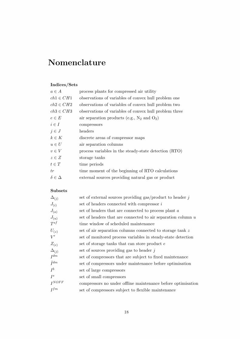
Indices/Sets
a ∈ A process plants for compressed air utility
ch1 ∈ CH1 observations of variables of convex hull problem one
ch2 ∈ CH2 observations of variables of convex hull problem two
ch3 ∈ CH3 observations of variables of convex hull problem three
e ∈ E air separation products (e.g., N2 and O2)
i ∈ I compressors
j ∈ J headers
k ∈ K discrete areas of compressor maps
u ∈ U air separation columns
v ∈ V process variables in the steady-state detection (RTO)
z ∈ Z storage tanks
t ∈ T time periods
tr time moment of the beginning of RTO calculations
δ ∈ ∆ external sources providing natural gas or product
Subsets
∆(j) set of external sources providing gas/product to header j
J(i) set of headers connected with compressor i
J(a) set of headers that are connected to process plant a
J(u) set of headers that are connected to air separation column u
T sf time window of scheduled maintenance
U(z) set of air separation columns connected to storage tank z
V ′ set of monitored process variables in steady-state detection
Z(e) set of storage tanks that can store product e
∆(j) set of sources providing gas to header j
Idm set of compressors that are subject to fixed maintenance
Idm set of compressors under maintenance before optimisation
Ib set of large compressors
Is set of small compressors
INOFF compressors no under offline maintenance before optimisation
Ifm set of compressors subject to flexible maintenance
18

IM set of compressors subject to maintenance
IM1 set of compressors subject to light maintenance
IM2 set of compressors subject to major overhaul
INM set of compressors not subject to maintenance
Subscripts
act actual conditions
act,s actual conditions at the inlet (suction) of a compressor
aux auxiliary variables
ch choke (stonewall)
cor corrected
d/out discharge/outlet (outlet position of compressor)
dem demand
el electrical
g gas
in/s inlet/suction (inlet position of compressor)
mech mechanical (refers to mechanical power)
meas measured variables
ref reference conditions
r.d regression domain
sur surge
std standard conditions
STP standard temperature and pressure
tot tot
Superscripts
* scaled parameters and variables in RTO optimisation model
fxd fixed maintenance
min minimum
max maximum
o initial conditions
out outlet (refers to outlet of tanks)
util utilities
Parameters
b/(b) estimated coefficients of regression model of Eq. (4.4) [ - ]
bch coefficients of expression for choke line [ - ]
bh coefficients of expression for head of a compressor [ - ]
bL coefficients of expression for minimum speed line [ - ]
19

bs coefficients of expression for surge line [ - ]
bU coefficients of expression for maximum speed line [ - ]
bw coefficients of expression for shaft power of a compressor [ - ]
bel coefficients of expression for electrical power consumption [ - ]
Cel electricity cost [EUR/kWh]
Cext purchase cost of product/gas from external sources [EUR/kg]
CD cost of header change [EUR/change]
Cf shutdown cost [EUR/shutdown]
cf,MolW ratio of actual and reference molecular weight [ - ]
cf,P ratio of actual and reference pressure [ - ]
cf,T ratio of actual and reference temperature [ - ]
Cst start up cost [EUR/startup]
Cof offline washing cost [EUR/wash]
Con online washing cost [EUR/wash]
cstd conversion factor from MMsm3/d to m3/h [ - ]
doof duration of offline washing before optimisation [d]
doon duration of online washing before optimisation [d]
dc conversion factor, equal to 24· 3600 [ - ]
h parameter of steady-state detection of RTO [ - ]
M∗ numbers for Big-M formulation [ - ]
M es Big-M numbers of equal split, Eqs. (5.71) – (5.72) [ - ]
M esm Big-M numbers of equal surge margin, Eqs. (5.75) – (5.76) [ - ]
M ext mass flow rate of gas/product from external sources [kg/s]
Mdem demand in mass flow rate [kg/s]
Min,x extreme points of inlet mass flow rate data-set [kg/s]
Mprod min/max boundaries of separation columns flows [kg/s]
Mr.d. min/max boundaries of mass flow rate of compressor [kg/s]
Mmaxrec maximum recycle flow rate [kg/s]
Mw mass flow rate of intercoolers[kg/s]
MolW molecular weight [mol/kg]
N min/max boundaries of rotational speed [RPM]
ns data included in a time window of a steady-state detection [ - ]
Pdem demand in pressure [bar A]
Pin pressure at the inlet of a compressor [bar A]
Pop operational pressure of downstream process [bar A]
Pout pressure at the outlet of a compressor [bar A]
Pd,x extreme points of discharge pressure data-set [bar A]
Qb/c volumetric flow rate boundaries of compressor maps [m3/h]
Qmaxch maximum volumetric flow rate at choke line [m3/h]
20

Qdem demand in volumetric flow rate [m3/h]
Qminsur minimum volumetric flow rate at surge line [m3/h]
Qstd demand in volumetric flow rate [MMsm3/d]
R ideal gas constant, equal to 8,314 [kJ/(mol·K)]
RF recovery factor of online washing model [ - ]
Rg gas constant [kJ/(kg·K)]
S number of data per step of the steady-state detection [ - ]
Td temperature of the gas at the delivery point [K]
Tin temperature at the inlet of a compressor [K]
Tin,x extreme points of inlet temperature data-set [K]
tS number of days before the end of the time horizon [d]
vstortnk initial inventory of products in storage tanks [kg]
vy variance used in steady-state detection algorithm [ - ]
Vdem demand of products for each period [kg]
Vtnk min/max storage capacity for products in storage tanks [kg]
Wmax maximum shaft power [kW]
x input measured variables of data-driven model (Eq. (4.4)) [ - ]
x mean value of input measured variables x
y output predicted variable of data-driven model (Eq. (4.4)) [ - ]
Yss defines steady-state status of a process variable [ - ]
Yss,system defines steady-state status of a system [ - ]
Z compressibility [ - ]
z input parameter vector of the RTO optimisation model
α0, α1 coefficients of load curve of headers [ - ]
γ∗ min. time period of two consecutive overhauls [d]
γ min. time between two consequent online washing events [d]
ε degradation rate of compressor [kW/d]
δSo initial cumulative hours of operation before optimisation [d]
η/ΛmaxC max. number of compressors to be maintained in a period [ - ]
η defines if a compressor is subject to fixed maintenance [ - ]
κ conversion factor of mass flow rate [ - ]
λoff/on max. number of offline/online washings per time period [ - ]
λk min. number of offline washing episodes [ - ]
ΛEl number of electrical maintenance actions [ - ]
ΛMe number of mechanical maintenance actions [ - ]
µ mean of a set of values [depends on parameter]
ν duration of maintenance (general case) [d]
νOV duration of major overhaul [d]
νfxd duration of fixed maintenance of compressors [d]
21
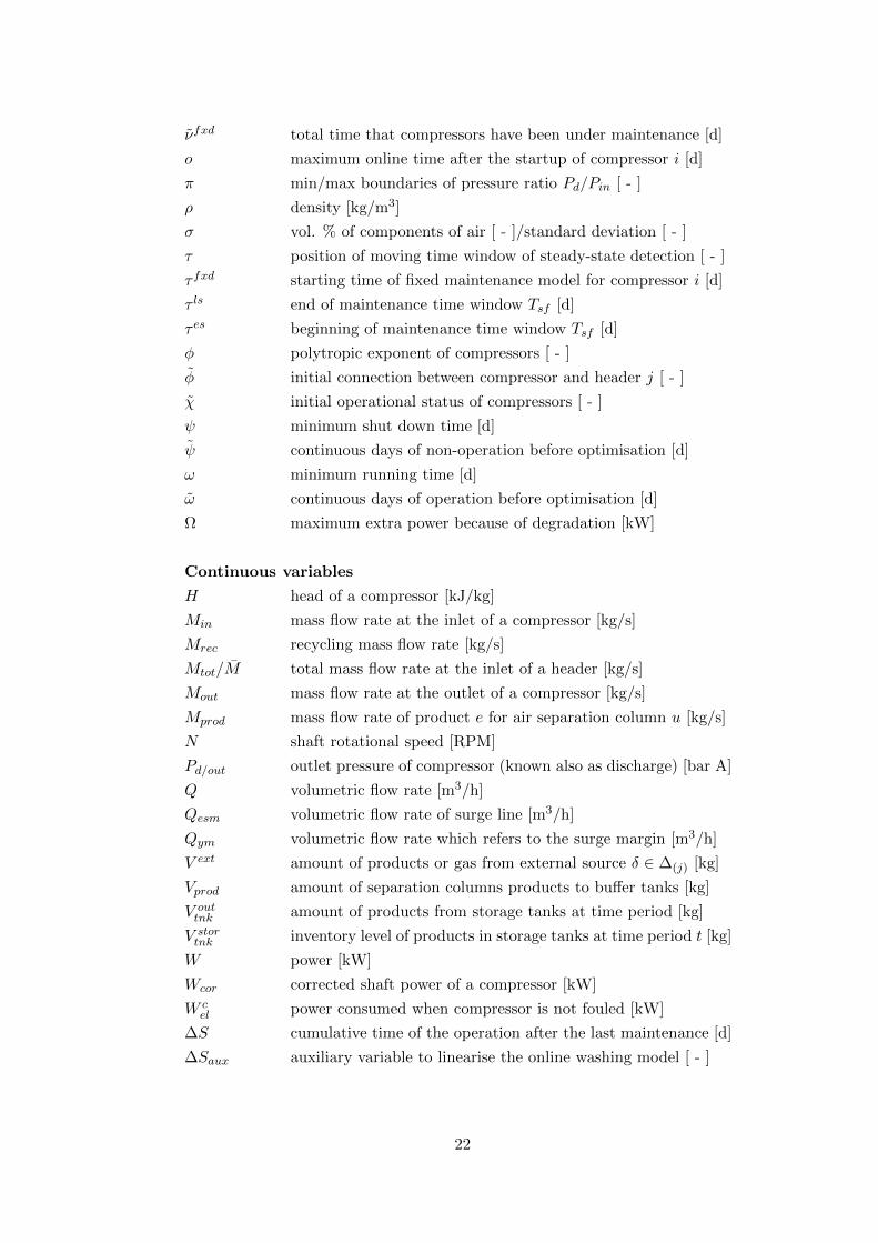
νfxd total time that compressors have been under maintenance [d]
o maximum online time after the startup of compressor i [d]
π min/max boundaries of pressure ratio Pd/Pin [ - ]
ρ density [kg/m3]
σ vol. % of components of air [ - ]/standard deviation [ - ]
τ position of moving time window of steady-state detection [ - ]
τ fxd starting time of fixed maintenance model for compressor i [d]
τ ls end of maintenance time window Tsf [d]
τ es beginning of maintenance time window Tsf [d]
φ polytropic exponent of compressors [ - ]
φ initial connection between compressor and header j [ - ]
χ initial operational status of compressors [ - ]
ψ minimum shut down time [d]
ψ continuous days of non-operation before optimisation [d]
ω minimum running time [d]
ω continuous days of operation before optimisation [d]
Ω maximum extra power because of degradation [kW]
Continuous variables
H head of a compressor [kJ/kg]
Min mass flow rate at the inlet of a compressor [kg/s]
Mrec recycling mass flow rate [kg/s]
Mtot/M total mass flow rate at the inlet of a header [kg/s]
Mout mass flow rate at the outlet of a compressor [kg/s]
Mprod mass flow rate of product e for air separation column u [kg/s]
N shaft rotational speed [RPM]
Pd/out outlet pressure of compressor (known also as discharge) [bar A]
Q volumetric flow rate [m3/h]
Qesm volumetric flow rate of surge line [m3/h]
Qym volumetric flow rate which refers to the surge margin [m3/h]
V ext amount of products or gas from external source δ ∈ ∆(j) [kg]
Vprod amount of separation columns products to buffer tanks [kg]
V outtnk amount of products from storage tanks at time period [kg]
V stortnk inventory level of products in storage tanks at time period t [kg]
W power [kW]
Wcor corrected shaft power of a compressor [kW]
W cel power consumed when compressor is not fouled [kW]
∆S cumulative time of the operation after the last maintenance [d]
∆Saux auxiliary variable to linearise the online washing model [ - ]
22
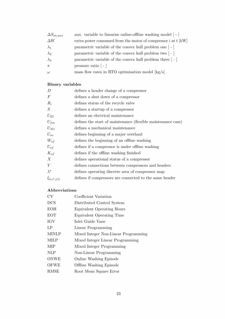
∆Son,aux aux. variable to linearise online-offline washing model [ - ]
∆W extra power consumed from the motor of compressor i at t [kW]
λ1 parametric variable of the convex hull problem one [ - ]
λ2 parametric variable of the convex hull problem two [ - ]
λ3 parametric variable of the convex hull problem three [ - ]
π pressure ratio [ - ]
ω mass flow rates in RTO optimisation model [kg/s]
Binary variables
D defines a header change of a compressor
F defines a shut down of a compressor
Rc defines status of the recycle valve
S defines a startup of a compressor
UEl defines an electrical maintenance
Ufm defines the start of maintenance (flexible maintenance case)
UMe defines a mechanical maintenance
Uov defines beginning of a major overhaul
Wof defines the beginning of an offline washing
Uof defines if a compressor is under offline washing
Kof defines if the offline washing finished
X defines operational status of a compressor
Y defines connections between compressors and headers
λ∗ defines operating discrete area of compressor map
ξ(i,i′,j,t) defines if compressors are connected to the same header
Abbreviations
CV Coefficient Variation
DCS Distributed Control System
EOH Equivalent Operating Hours
EOT Equivalent Operating Time
IGV Inlet Guide Vane
LP Linear Programming
MINLP Mixed Integer Non-Linear Programming
MILP Mixed Integer Linear Programming
MIP Mixed Integer Programming
NLP Non-Linear Programming
ONWE Online Washing Episode
OFWE Offline Washing Episode
RMSE Root Mean Square Error
23

RPM Rotations Per Minute
RSQ R Squared
RTO Real Time Optimisation
VSD Variable Speed Drive
m.u. Monetary units
n.u. Normalised units
r.d Regression domain
24
1 Introduction
1.1 Description of the chapter
The thesis elaborates on the optimal operation of compressor stations in process
systems and natural gas networks. Chapter 1 provides the overview of the thesis.
First, the description of the project Energy SmartOps is presented in Section 1.2,
as the PhD study on the optimal operation of compressors is part of the project.
Interactions with researchers of the project from different academic or technical
institutes, and visits in industrial sites are few of the highlights of this initial
training networking European project.
Section 1.3 introduces the research topic of the optimal operation of industrial
compressor stations with multiple parallel centrifugal compressors in large energy
systems. This section states the research problem and presents the key parameters
to be considered so as to define the scope of the thesis. Moreover, Section 1.3
answers the question why this problem is important to be studied.
Two industrial case studies are presented in Section 1.4. The process plants of
these two case studies include multi-stage centrifugal compressors which are con-
nected in a parallel configuration. The first case study involves an air separation
plant in BASF, Germany. This plant encompasses an air compressor station. The
second plant operated by Statoil, Norway, involves a natural gas export compres-
sor station which provides natural gas from Norway to Europe. Both compres-
sor stations include compressors with high power consumption. The developed
methodologies will be applied to these case studies.
Section 1.5 describes the aim and objectives of the thesis. This section explicitly
states the aims of the current study and presents the outline of the thesis by
describing the context and the interrelations among the chapters. Section 1.8
gives the structure of the thesis.
1.2 An introduction to the project: Energy SmartOps
The current study of the optimal operation of compressors is part of a European
project, namely Energy SmartOps. Energy SmartOps aims for (a) reducing energy
consumption in industrial applications and (b) training researchers through PhD
25
studies, networking and other activities. The project is funded by the European
Community via Marie Currie ITN People Actions under the FP7 program.
The project involves several partners such as universities, research organisations
of companies that supply technology, and end-user companies. The universities are
Imperial College London, which is the project coordinator, Cranfield University,
ETH Zurich, Politechnica Krakowska and Carnegie Mellon. Commercial organ-
isations such as ABB R&D in Norway, Poland and Germany, and international
technical training companies such as ESD Ltd are some of the partners. The end-
user companies participants of the project are BASF (Germany), ThyssenKrupp
(Italy) and Statoil (Norway).
There are fifteen European Early Stage Researchers, including the author of
the thesis, whose aim is to generate and test methods for energy savings in large
industrial sites. The developed methods will be applied to case studies provided
by the project. In addition, the project focuses on the technical training, e.g. PhD
studies, short technical courses, and personal development, e.g. soft skills courses,
industrial experience, of the researchers. The researchers based in universities
followed short-term placements in the industry (approximately three months) or
in the research centres of commercial organisations such as ABB, and vice versa.
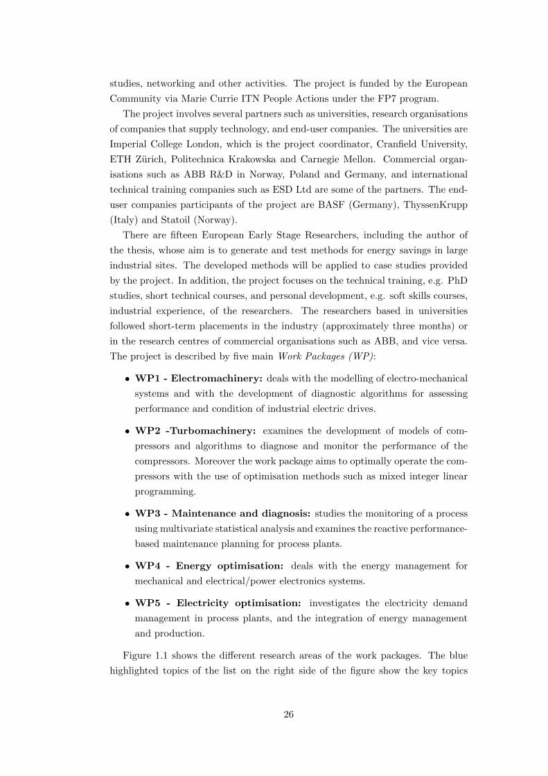
The project is described by five main Work Packages (WP):
• WP1 - Electromachinery: deals with the modelling of electro-mechanical
systems and with the development of diagnostic algorithms for assessing
performance and condition of industrial electric drives.
• WP2 -Turbomachinery: examines the development of models of com-
pressors and algorithms to diagnose and monitor the performance of the
compressors. Moreover the work package aims to optimally operate the com-
pressors with the use of optimisation methods such as mixed integer linear
programming.
• WP3 - Maintenance and diagnosis: studies the monitoring of a process
using multivariate statistical analysis and examines the reactive performance-
based maintenance planning for process plants.
• WP4 - Energy optimisation: deals with the energy management for
mechanical and electrical/power electronics systems.
• WP5 - Electricity optimisation: investigates the electricity demand
management in process plants, and the integration of energy management
and production.
Figure 1.1 shows the different research areas of the work packages. The blue
highlighted topics of the list on the right side of the figure show the key topics
26
with which the thesis is concerned. The topic of the thesis is related to WP2 -
Turbomachinery. The WP2 involves the modelling of the steady-state behaviour
of the compressors using two different approaches: data-driven models from pro-
cess data and polynomial models derived from compressor maps. The modelling
of the steady-state behaviour of a compressor describes its feasible window of op-
eration and its power consumption as a function of key process variables such as
temperature, mass flow rates and pressures.
The developed methods are applied to two different case studies. In the first
case study, when compressor maps are not available (these maps are explained in
Section 2.2.2), then process data have to be used to model power and the feasible
window of operation. In the second case compressor maps are used to model the
behaviour of the compressors. Optimisation formulations employ these models to
optimise the compressors. The role of the optimisation is to increase the total
efficiency of the compressor station, to reduce the total costs and decrease the
wear of the compressors while at the same time all the operational and other
constraints are satisfied. The diagnosis and management of faults is studied by
other researchers in the project.
Fault diagnosis
Equipment monitoring
Advanced control
Parameter identification
Online Optimisation
Maintenance
Scheduling
Systematic approach
Process industries
List of topics of interest
WP1
WP2
WP3
WP5
WP4
Figure 1.1: Graphical description of the five Work Packages of the Energy Smar-tOps (courtesy of Energy SmartOps consortium).
27

1.3 An introduction to the optimal operation of
compressors
Nowadays, the process, and oil and gas industries work on the improvement
of their operations. Government regulations, intense competition, changes in the
markets and requirements for more environmental-friendly applications are some
reasons which motivate the industries to improve their current practices. Each
equipment unit of a plant is highly integrated with the overall process, therefore
the consideration of the interactions among units, sub-systems and large systems
is essential to achieve increased total efficiency, reduced total costs and better
management of assets of a plant.
Many processes in these industries use compressors to achieve several objectives
for their operations. Compressors are mechanical machines which can provide air
for utilities (e.g. combustion or pneumatic tools), can recirculate fluids and can
convey gas through a pipe. In some cases, processes consume large amounts of
energy and the major part of this consumption comes from the operation of their
compressors. In addition, the maintenance costs of compressors are relatively
high. For these reasons, the efficient operation of compressors and their integrated
management could save energy and reduce operational costs. Energy-intense ap-
plications of compressors can be found in the chemical and natural gas industry.
1.3.1 Compressed air
U.S. Department of Energy (2003) has outlined a broad range of applications
of compressed air in industry. Table 1.1 shows examples of these applications.
Compressed air is also used in oxidation, cryogenics, refrigeration, dehydration and
aeration. According to Boyce (2003) typical applications in the process industry
are: (a) air blower for Fluid Catalytic Cracking (FCC) unit, (b) gas recovery unit
for FCC, (c) reformer recycle compressors, (d) ammonia plant nitric acid train, (e)
cryogenic expander, and (d) re-compression processing and refrigeration systems.
Compressed air is considered as the fourth utility, after electricity, natural gas
and water, in facilitating production activities according to Yuan et al. (2006). It
is one of the most expensive utilities in a facility. It accounts for more than 10% of
total industrial energy use for few selected countries as found in literature (Saidur
et al., 2010). In the review on compressed energy by Saidur et al. (2010), one of the
main remarks is that 70% to 90% of the total electricity bill of an air compressor
system comes from the annual operating usage of compressors and other related
components, such as air dryers and supporting equipment. Another remark is that
the operating cost of an air compressor system accounts for more than three times
than its maintenance and capital cost in the lifecycle of a compressor. Indeed,
28
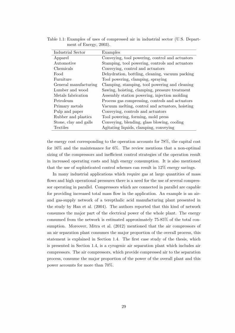
Table 1.1: Examples of uses of compressed air in industrial sector (U.S. Depart-ment of Energy, 2003).
Industrial Sector Examples
Apparel Conveying, tool powering, control and actuatorsAutomotive Stamping, tool powering, controls and actuatorsChemicals Conveying, control and actuatorsFood Dehydration, bottling, cleaning, vacuum packingFurniture Tool powering, clamping, sprayingGeneral manufacturing Clamping, stamping, tool powering and cleaningLumber and wood Sawing, hoisting, clamping, pressure treatmentMetals fabrication Assembly station powering, injection moldingPetroleum Process gas compressing, controls and actuatorsPrimary metals Vacuum melting, control and actuators, hoistingPulp and paper Conveying, controls and actuatorsRubber and plastics Tool powering, forming, mold pressStone, clay and galls Conveying, blending, glass blowing, coolingTextiles Agitating liquids, clamping, conveying
the energy cost corresponding to the operation accounts for 78%, the capital cost
for 16% and the maintenance for 6%. The review mentions that a non-optimal
sizing of the compressors and inefficient control strategies of the operation result
in increased operating costs and high energy consumption. It is also mentioned
that the use of sophisticated control schemes can result in 12% energy savings.
In many industrial applications which require gas at large quantities of mass
flows and high operational pressures there is a need for the use of several compres-
sor operating in parallel. Compressors which are connected in parallel are capable
for providing increased total mass flow in the application. An example is an air-
and gas-supply network of a terepthalic acid manufacturing plant presented in
the study by Han et al. (2004). The authors reported that this kind of network
consumes the major part of the electrical power of the whole plant. The energy
consumed from the network is estimated approximately 75-85% of the total con-
sumption. Moreover, Mitra et al. (2012) mentioned that the air compressors of
an air separation plant consumes the major proportion of the overall process, this
statement is explained in Section 1.4. The first case study of the thesis, which
is presented in Section 1.4, is a cyrogenic air separation plant which includes air
compressors. The air compressors, which provide compressed air to the separation
process, consume the major proportion of the power of the overall plant and this
power accounts for more than 70%.
29
1.3.2 Natural gas compression
Natural gas is one of the primary sources of energy which is used for heating,
cooking and generation of electricity in residential sector. Moreover industrial
plants use natural gas as a basic source of energy for heating and power generation.
A large natural gas network can provide several tens of billion std m3 of gas
annually (Nørstebø et al., 2008). Kurz and Brun (2012a) explained the operations
in the industrial oil and gas sector from the source, i.e. oil and gas fields, to the
end-users. Rich natural gas containing condensate is provided from wells to gas
processing plants which produce dry gas. The dry gas has to be transported to
industrial or domestic final customers.
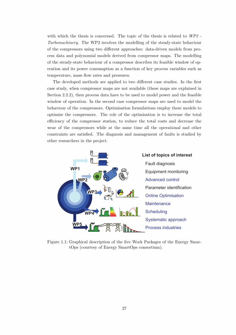
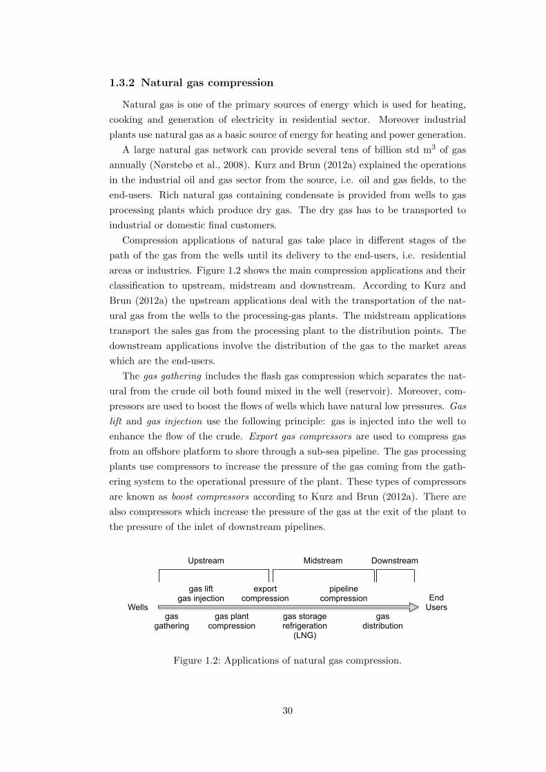
Compression applications of natural gas take place in different stages of the
path of the gas from the wells until its delivery to the end-users, i.e. residential
areas or industries. Figure 1.2 shows the main compression applications and their
classification to upstream, midstream and downstream. According to Kurz and
Brun (2012a) the upstream applications deal with the transportation of the nat-
ural gas from the wells to the processing-gas plants. The midstream applications
transport the sales gas from the processing plant to the distribution points. The
downstream applications involve the distribution of the gas to the market areas
which are the end-users.
The gas gathering includes the flash gas compression which separates the nat-
ural from the crude oil both found mixed in the well (reservoir). Moreover, com-
pressors are used to boost the flows of wells which have natural low pressures. Gas
lift and gas injection use the following principle: gas is injected into the well to
enhance the flow of the crude. Export gas compressors are used to compress gas
from an offshore platform to shore through a sub-sea pipeline. The gas processing
plants use compressors to increase the pressure of the gas coming from the gath-
ering system to the operational pressure of the plant. These types of compressors
are known as boost compressors according to Kurz and Brun (2012a). There are
also compressors which increase the pressure of the gas at the exit of the plant to
the pressure of the inlet of downstream pipelines.
Wellsgas
gathering
gas liftgas injection
gas plantcompression
export compression
pipelinecompression
gas storagerefrigeration
(LNG)
gas distribution
EndUsers
Upstream Midstream Downstream
Figure 1.2: Applications of natural gas compression.
30

The produced dry gas which is ready for use by the end-users is called sales
gas. Compressor stations are used to compress the sales gas from the exit of
the plant to the delivery points, in case of gas transportation through pipelines.
Schmidt et al. (2014) reports that this method of transportation is used when the
distances of transportation are up to 4,000 km over land and 2,000 km off-shore.
If the distances are greater than these, then the natural gas should be liquefied
(LNG process) and transported in ships. Therefore, the liquefaction of gas involves
a refrigeration process which has requirements in compression. Compressors are
also used to store gas in reservoirs to deal with the uncertainty in the demand of
the gas.
The pipeline transportation involves compressor stations in series to increase
the pressure of the gas in order to overcome the friction losses in pipes. A com-
pressor station can involve several compressor units which operate in parallel.
Typically, a large number of compressor stations can be found in a gas network
in different structures, for example a large network in US comprises several hun-
dreds of pipelines and tens of compressor stations distributed in a strategic way
(Rıos-Mercado and Borraz-Sanchez, 2015). However, there are gas networks which
employ a small number of compressor stations, but with great power and flow
capacity, to transport the gas through the long pipes of the gas network. One
example is the second case study of the thesis which considers an export gas com-
pressor station of Statoil which operates in the Norwegian gas network (Ministry
of Petroleum and Energy, 2014).
The electrical motor of a single compressor in a export gas compressor station
can consume up to 40 MW (Nørstebø et al., 2008). In the case where the drivers of
the compressors are gas turbines, the gas needed to provide the energy to operate
a natural gas network may reach up to 5% of the total volume of the transported
gas (Wu et al., 2000; DeMarco and Elias, 2011). The compressors driven by the
gas turbines are reported to consume 93% of this energy (DeMarco and Elias,
2011). In the long term, the operational costs outweigh the capital cost of the
purchase of a compressor. This fact enables researchers and industries to focus
on a more efficient operation considering the health condition of the compressors
(for instance, effective maintenance policies), and environmental and government
restrictions.
1.4 Introduction to the case studies
The project EnegySmartOps provided two case studies, an air separation plant
involving a network of air compressors in BASF, Germany, and one export natural
gas compressor station operated by Statoil in Norway.
31
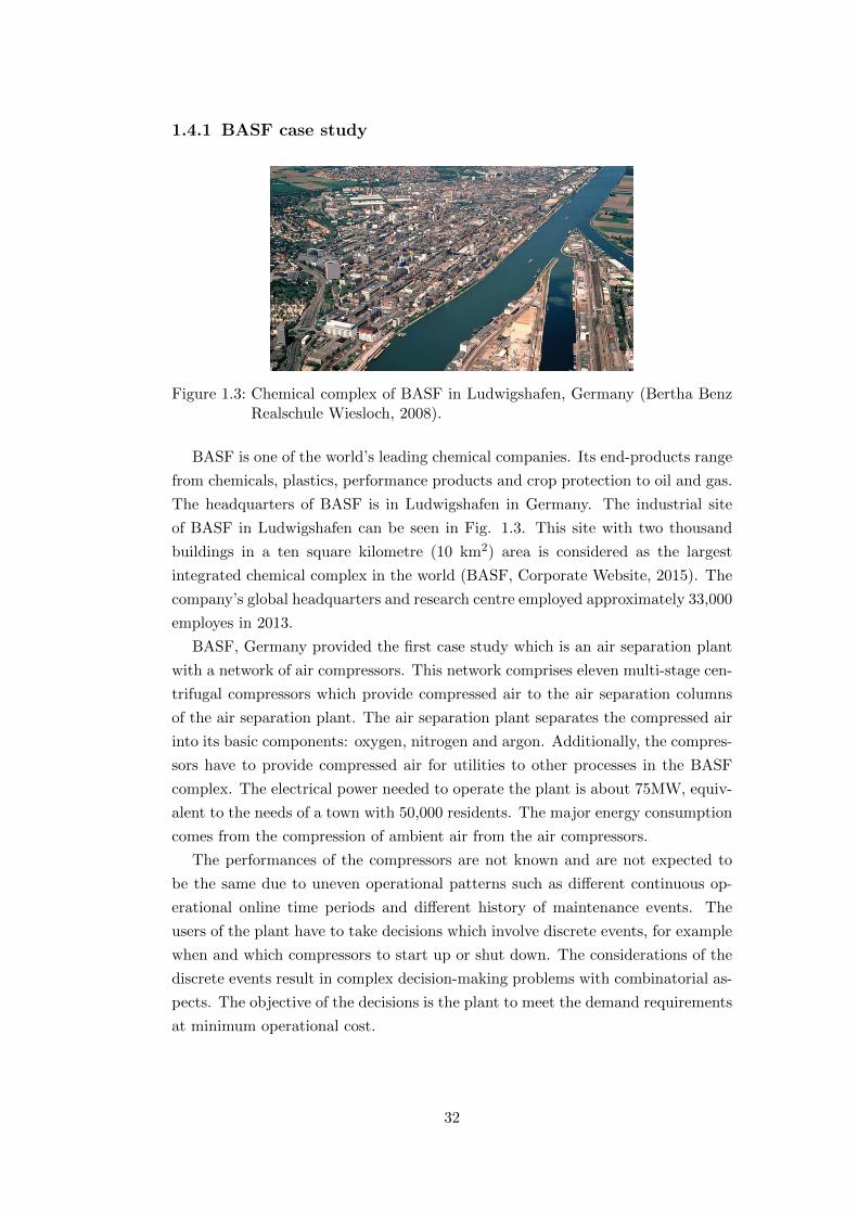
1.4.1 BASF case study
Figure 1.3: Chemical complex of BASF in Ludwigshafen, Germany (Bertha BenzRealschule Wiesloch, 2008).
BASF is one of the world’s leading chemical companies. Its end-products range
from chemicals, plastics, performance products and crop protection to oil and gas.
The headquarters of BASF is in Ludwigshafen in Germany. The industrial site
of BASF in Ludwigshafen can be seen in Fig. 1.3. This site with two thousand
buildings in a ten square kilometre (10 km2) area is considered as the largest
integrated chemical complex in the world (BASF, Corporate Website, 2015). The
company’s global headquarters and research centre employed approximately 33,000
employes in 2013.
BASF, Germany provided the first case study which is an air separation plant
with a network of air compressors. This network comprises eleven multi-stage cen-
trifugal compressors which provide compressed air to the air separation columns
of the air separation plant. The air separation plant separates the compressed air
into its basic components: oxygen, nitrogen and argon. Additionally, the compres-
sors have to provide compressed air for utilities to other processes in the BASF
complex. The electrical power needed to operate the plant is about 75MW, equiv-
alent to the needs of a town with 50,000 residents. The major energy consumption
comes from the compression of ambient air from the air compressors.
The performances of the compressors are not known and are not expected to
be the same due to uneven operational patterns such as different continuous op-
erational online time periods and different history of maintenance events. The
users of the plant have to take decisions which involve discrete events, for example
when and which compressors to start up or shut down. The considerations of the
discrete events result in complex decision-making problems with combinatorial as-
pects. The objective of the decisions is the plant to meet the demand requirements
at minimum operational cost.
32

i = 1
i = I
Process compressedair utility
Oxygen storage
1
Oxygendemand
Oxygen storage
2
Oxygen storage
3
Cryogenicprocess
Cryogenicprocess
i = 2
Nitrogenstorage
1
Nitrogendemand
M
M
M
Nitrogen lineOxygen lineAir line
Compressorstation with centrifugalcompressors
Air separation column 1
Air separation column 2
Headers
Figure 1.4: Topology of the operational units and gas streams in the air separationplant similar to the plant of BASF, Germany.
An air separation plant includes air separation units which are cryogenic sep-
aration columns integrated with heat exchangers, compressors, and expanders as
can be seen in Fig. 1.4. Storage tanks are used to store oxygen and nitrogen from
the cryogenic separation. The figure shows the cryogenic process after the com-
pressor station and before the cryogenic air separation columns. The cryogenic
process includes the purification of the compressed air, the main heat exchangers
and the expanders. A more detailed description of the air separation process can
be seen in Fig. 3.2.
The basic processes taking place in an air separation plant can be summarised
in six steps. In the first step, ambient air is drawn through filters at the inlet
of the plant. The filters remove dust and particles from the air. The filtered air
is compressed in the second step. Air compressors consume energy to increase
the pressure of the ambient air at a necessary pressure required from downstream
processes. The pressure is approximately from five to ten bar. The compression
of the air provides all the energy required for the refrigeration process which cools
the air to the operational cryogenic temperatures (cryogenic temperatures are
considered below -150oC). Moreover, modern air separation columns use expander
turbines of which main role is the cooling of the processed compressed air and
the turbines provide work to the air compressors, hence the overall efficiency is
increasing.
The fourth step involves the removal of substances such as water and CO2 from
the air to prevent their freezing in downstream processes with low temperatures.
33

(a) (b)
Figure 1.5: BASF centrifugal multi-stage compressor with open body (a) and topcasing (b) (Cicciotti et al., 2015).
According to Xu et al. (2011), filters such as molecular sieve adsorbers are used to
achieve this objective. Then in step five, the highly integrated expanders and heat
exchangers cool the processed compressed air to low temperature, approximately
to -180oC to liquefy the air. The principle of the operation of an air separation
plant is based on the refrigeration cycle and the throttling effect. The throttling
effect (or Joule-Thompson) is the change in the temperature of a gas (or liquid)
when it is expanded through a valve while at the same time heat is not exchanged in
the environment. Additionally, the main heat exchanger (MHE) cools the purified
compressed air to cryogenic temperatures with the use of streams of cold products
and waste cold streams.
The final step includes the cryogenic separation columns which vaporise the
liquid so as to selectively separate the air to its basic components at their differ-
ent boiling points. According to Messer Group (2015) oxygen becomes liquid at
temperature -183 oC and nitrogen at -196 oC. The exchange of mass and heat be-
tween the rising vapour and descending liquid causes continuous evaporation and
condensation. The result of this process is the production of oxygen at the bottom
and nitrogen at the top of the column. Argon can be separated with additional
process steps.
In the case of the air separation plant of BASF the products are exclusively
gases and they are stored in buffer tanks. The gaseous products are provided to
internal and external users through pipelines. An internal customer may be a
process plant on the same site which uses oxygen for its own processes.
As previously mentioned, the air compressors consume the majority of the total
energy of the plant. The air compressors of BASF air separation plant constitute a
network of compressors which are connected in parallel. There are eleven available
compressors comprising of groups with similar nominal specifications. However,
the groups of compressors differ in design, power rate, operating range, efficiency,
34

structure in terms of stages of compression and control method.
These air compressors are multi-stage centrifugal compressors with heat ex-
changers between each two sequential stages and an aftercooler after the exit of
the last stage of the compressor. They are driven by electrical motors at con-
stant speed. Figure 1.5 shows the open body of a multi-stage compressor of BASF
during maintenance operations.
The case study focuses on the optimal operation of the existing compressor units
without considering the purchase of new more efficient compressors. The plant
managers and operators aim to coordinate the individual operations of the com-
pressors to achieve the minimisation of the operational cost which mainly includes
the electricity consumption of the electrical motors which power the compressors.
The users of the plant deal with a decision-making problem which requires them
to identify the best set points and configuration of the compressors which result
in optimal operation. These decisions are related to the distribution of the load,
and the scheduling and maintenance of the compressors.
The compressors have been operating for more than fifty years and their per-
formance maps are not available, there is also a reduced number of available mea-
surements installed in most of the compressors, and therefore the development of
rigorous models of all the compressors which describe their performance is not
feasible.
1.4.2 Statoil case study
The second case study examines the operation of an export natural gas com-
pressor station in Norway. The compressor station is part of the Norwegian gas
transport network which comprises 7,800 km of pipelines and there are pipelines
which can reach up to 1,200 km length (Nørstebø, 2008). The operational pres-
sure in the pipes can reach up to 210 bar. The Norwegian gas transport network is
presented in Fig. 1.6. The blue nodes represent the main production wells of the
gas network which are related to Kollsnes gas processing plant, namely Visund,
Kvitebjørn and Troll fields. The red node represents the location of the export gas
compressor station of interest, which is part of the Kollsnes plant. The Kollsnes
plant supplies two offshore platforms Sleipner R and Draupener S/E represented
by the black nodes. These two offshore platforms distribute the sales gas to the
final terminals represented by the green nodes in the rest of Europe. Compared
to other conventional gas networks, which involve several compressor stations dis-
tributed in series along the pipes, the Norwegian gas network uses only a small
number of compressor stations which provide the necessary energy to the gas in
order to reach its final destination.
The Kollsnes plant is a gas processing plant which involves a compressor sta-
35
Figure 1.6: Norwegian gas network (Ministry of Petroleum and Energy, 2014).
tion with six large multi-stage centrifugal compressors operating in parallel. The
compressor station can handle 143 million standard cubic metres per day accord-
ing to the official website of Statoil (Statoil, 2015). A simplified schematic which
shows the topology of the plant can be seen in Fig. 1.7. The Troll, and Kvitebjørn
and Visund fields provide rich gas to the Dew Point Control (DPC) facilities and
Natural Gas Liquids plant which process the gas. Produced dry gas is delivered
through a common suction manifold to the inlets of the six multi-stage centrifugal
compressors. The exits of the compressors can be provide gas either to header
ZIIA or to header ZIIB towards to platforms Sleipner R (P-SLR) and Draupner
S/E (P-DPR). The first five compressors are nominally identical and the sixth
compressor has different characteristics compared to the other five compressors.
36
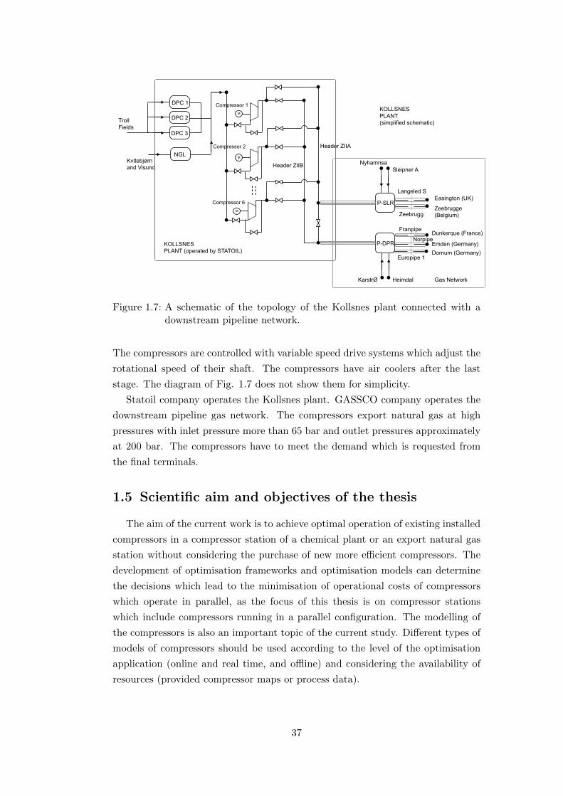
Compressor 6M
M
MKOLLSNES PLANT (simplified schematic)
DPC 1
DPC 2
DPC 3
NGL
Troll Fields
Kvitebjørnand Visund
P-SLR
P-DPR
Header ZIIA
Header ZIIB
Langeled S
Zeebrugg
Franpipe
Norpipe
Europipe 1
Sleipner A
KOLLSNES PLANT (operated by STATOIL)
Gas Network
Compressor 1
Compressor 2
KarstrØ Heimdal
Nyhamnsa
Easington (UK)
Zeebrugge (Belgium)
Dunkerque (France)
Emden (Germany)Dornum (Germany)
Figure 1.7: A schematic of the topology of the Kollsnes plant connected with adownstream pipeline network.
The compressors are controlled with variable speed drive systems which adjust the
rotational speed of their shaft. The compressors have air coolers after the last
stage. The diagram of Fig. 1.7 does not show them for simplicity.
Statoil company operates the Kollsnes plant. GASSCO company operates the
downstream pipeline gas network. The compressors export natural gas at high
pressures with inlet pressure more than 65 bar and outlet pressures approximately
at 200 bar. The compressors have to meet the demand which is requested from
the final terminals.
1.5 Scientific aim and objectives of the thesis
The aim of the current work is to achieve optimal operation of existing installed
compressors in a compressor station of a chemical plant or an export natural gas
station without considering the purchase of new more efficient compressors. The
development of optimisation frameworks and optimisation models can determine
the decisions which lead to the minimisation of operational costs of compressors
which operate in parallel, as the focus of this thesis is on compressor stations
which include compressors running in a parallel configuration. The modelling of
the compressors is also an important topic of the current study. Different types of
models of compressors should be used according to the level of the optimisation
application (online and real time, and offline) and considering the availability of
resources (provided compressor maps or process data).
37

Given the description of the aim, there are three major scientific objectives to
be achieved:
Objective One: is to develop a Real Time Optimisation (RTO) framework which
optimally shares the load among parallel compressors in real time to deal with short-
term changes in the operation. In practice and as found in the literature in Chapter
3, and as proved with the use of real industrial data in Chapter 4, a compressor
station usually involves dissimilar compressors. The problem of the optimal dis-
tribution of load aims to determine the loading of each compressor which results
in the minimum total power consumption while all the constraints are respected
including the satisfaction of the demand. The demand fluctuates over time and a
real time optimisation approach can deal with the uncertainty in parameters, such
as ambient conditions, model parameters, and demand profiles.
Objective Two: is to develop a multi-period optimisation framework to opti-
mally schedule the operations of compressors for long time periods. The users of a
compressor station have to take decisions which relate to discrete events such as
starting up a compressor. These decisions can be determined from a multi-period
optimisation framework which can optimise the operation for the total time peri-
ods under consideration. Therefore the solution, for example, of the first period
has considered the requirements of the following periods. The same applies for
the solutions of all the other time periods. The output of the framework is the
schedule of the compressors which provides the best decisions such as the selection
of the online compressors and the selection of stand-by compressors for each period.
Objective Three: is to implement maintenance activities into the operational
optimisation framework and achieve simultaneous optimal operation and mainte-
nance. The maintenance activities of a compressor station are, for example, the
repair of mechanical and electrical parts, and the washing of the inside of the
compressors with cleaning solutions. These activities improve the efficiency of the
compressors, however they have to be scheduled in accordance with the operation,
as maintenance activities require the shut down of compressors which influences
the total capacity and the total efficiency of the compressor station.
Figure 1.8 describes the three objectives and their interconnections to achieve
optimal operation of compressor stations. The Real Time Optimisation (RTO)
provides the set points of the loads of the compressors which minimise the power.
The selected compressors which should operate online are given from the output
of the scheduling. The scheduling also considers the load sharing problem but at
38
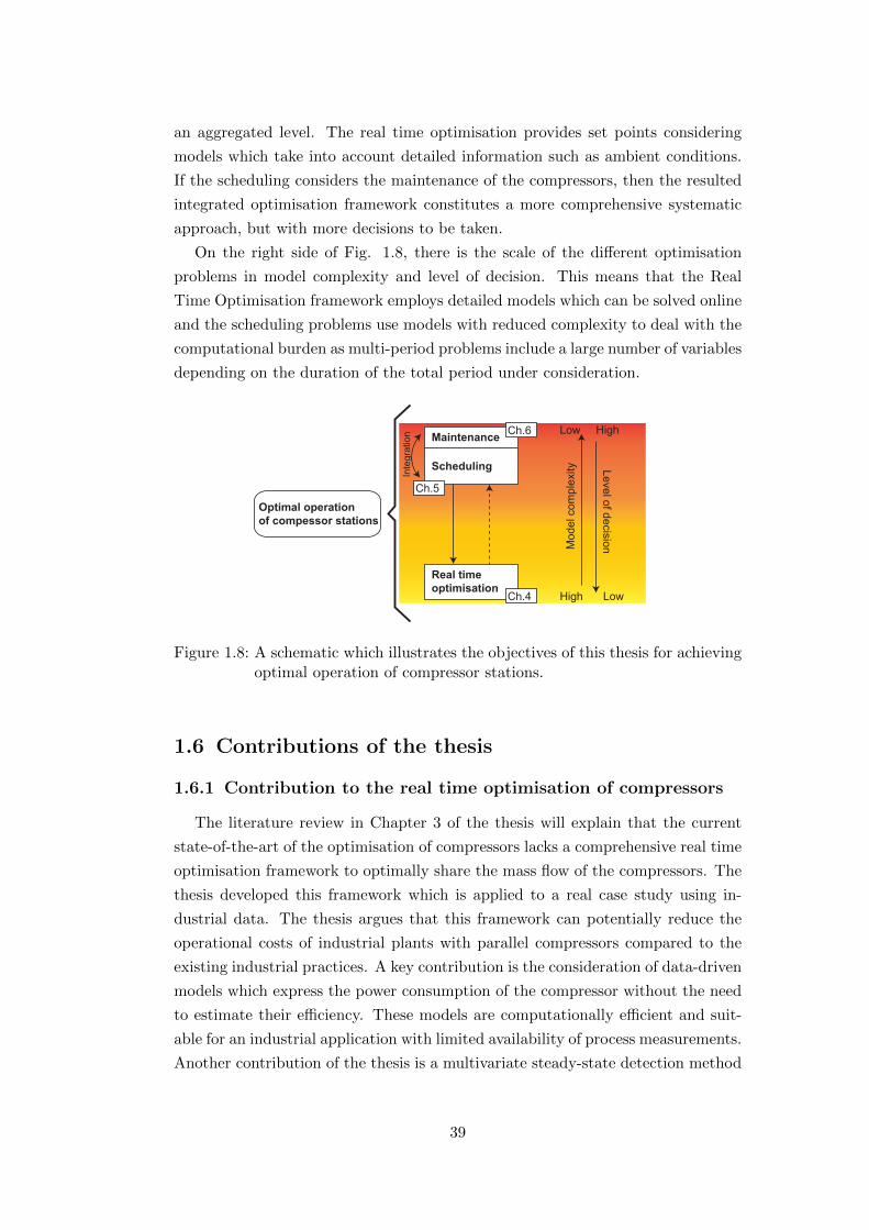
an aggregated level. The real time optimisation provides set points considering
models which take into account detailed information such as ambient conditions.
If the scheduling considers the maintenance of the compressors, then the resulted
integrated optimisation framework constitutes a more comprehensive systematic
approach, but with more decisions to be taken.
On the right side of Fig. 1.8, there is the scale of the different optimisation
problems in model complexity and level of decision. This means that the Real
Time Optimisation framework employs detailed models which can be solved online
and the scheduling problems use models with reduced complexity to deal with the
computational burden as multi-period problems include a large number of variables
depending on the duration of the total period under consideration.
Optimal operationof compessor stations
Scheduling
Maintenance
Real timeoptimisation
Inte
grat
ion
Mod
el c
ompl
exity Level of decision
Low
Low
High
HighCh.4
Ch.5
Ch.6
Figure 1.8: A schematic which illustrates the objectives of this thesis for achievingoptimal operation of compressor stations.
1.6 Contributions of the thesis
1.6.1 Contribution to the real time optimisation of compressors
The literature review in Chapter 3 of the thesis will explain that the current
state-of-the-art of the optimisation of compressors lacks a comprehensive real time
optimisation framework to optimally share the mass flow of the compressors. The
thesis developed this framework which is applied to a real case study using in-
dustrial data. The thesis argues that this framework can potentially reduce the
operational costs of industrial plants with parallel compressors compared to the
existing industrial practices. A key contribution is the consideration of data-driven
models which express the power consumption of the compressor without the need
to estimate their efficiency. These models are computationally efficient and suit-
able for an industrial application with limited availability of process measurements.
Another contribution of the thesis is a multivariate steady-state detection method
39
applied to a system of parallel compressors for the needs of the real time optimisa-
tion. Three papers have been published from this work, two in conferences (Xenos
et al., 2014a,b) and one in a journal (Xenos et al., 2015a).
1.6.2 Contribution to the scheduling of compressors for long
periods
Compressor stations in many industrial applications include several compressors
in parallel, however previous modelling approaches considered compressor stations
as a single entity neglecting the operational aspects of the individual compressors.
A breakthrough of the thesis is the development of mixed integer linear program-
ming optimisation model of compressor stations with individual models for each
compressor which can be used to minimise total costs of the stations, for example
electricity cost and shutdown costs. This generic optimisation model expands the
current state-of-the-art as:
• It can be used for different industrial applications which include compressors.
The model will be applied to two different cases, namely an air compressor
station of an air separation plant and an export natural gas station.
• It can employ data-driven models or models based on compressors maps to
describe the behaviour of the compressors. The reason for using different
modelling approaches is because a plant may not have sufficient instrumen-
tation to provide enough data for the building of the data-driven models.
Conversely, the compressor maps may not be known. Therefore, it is useful
to have both methods available.
• It can be used to compare the existing operation of compressors based on
typical industrial practices with the suggested optimal approach based on
the scheduling of compressors. The thesis will carry out this comparison in
the Statoil case study.
The work on the multi-period optimisation to optimally operate the compressors
for long periods is in preparation for publication in a journal article. This work
will present the results of the scheduling of compressors of the Statoil case study.
These results will be presented in Chapter 5.
1.6.3 Contribution to the integration of operation and
maintenance
The integration of operation and maintenance of compressors expands further
the state-of-the-art of the scheduling and maintenance of compressors. The lit-
erature review will support this statement as previous research focused on the
40
maintenance of a single compressor without considering the interconnections be-
tween the maintenance and operational tasks of more than one compressor. The
basic contributions are summarised below:
• The thesis provides a comprehensive framework for scheduling of compressors
considering different types of maintenance activities of compressors. The
maintenance activities refer to corrective mechanical and electrical repairs,
major overhauls to replace major parts of the compressors, and washing
of the compressors. The framework enables planning of maintenance tasks
according to the scheduling of the compressors.
• A breakthrough is that the suggested integrated framework can be used to
generate the schedules of the online and offline washing of the compressors.
Indeed, the existing approaches for washing a compressor are fixed periodical
washing or washing when the fouling has reached unacceptable levels.
• The thesis also presents further developments on the integration of mainte-
nance and operation. The thesis proposes a rolling horizon approach which
carries out the optimisation of the compressors as it would happen in reality.
The rolling horizon approach deals with uncertainty to some extent and this
is the first step for a future study on the optimisation of compressors under
uncertainty.
The work on the integration of operation and maintenance has been published
in two conference papers (Xenos et al., 2014c, 2015b) and in two journal articles
(Xenos et al., 2015c, 2016).
1.7 Sponsors and acknowledgements
The PhD studies started in September 2011 and included industrial second-
ments to BASF Ludwigshafen, Germany and Statoil in Norway. The group of
Automation Technology, Advanced Process Control in BASF hosted the author
for several months and supported the project with technical expertise related to
the BASF air separation case study. Dr Erling Lunde of Process Technology of
Upstream Rotating Equipment, Efficient Facilities, Research, Development and
Innovation (RDI) in Statoil, Norway hosted the author in an secondment in the
premises of Statoil. Dr Lunde provided industrial knowledge and support for the
natural gas case study of this thesis.
The PhD studies were fully funded from the Marie Curie FP7-ITN project “En-
ergy savings from smart operation of electrical, process and mechanical equiment
- ENERGY SMARTOPS”, Contract No: PITN-GA-2010-264940.
41
1.8 Structure of the thesis
This chapter has introduced the project and the aims of this thesis. The next
chapter, Chapter 2, explains the principles of the operation of a single industrial
multi-stage centrifugal compressor. It also explains the compressor map, feasible
window of operation, performance and power consumption, and control methods
of an industrial compressor. The interactions of multiple compressors attached
to an upstream and downstream system will be described. Moreover, the tasks
of the operational management of compressors will be classified and explained.
The current study deals with the supervisory control or real time optimisation,
and scheduling of compressors which will be explained within the context of the
operational management of industrial air and gas compressor stations.
Chapter 2 also defines the aspects of an optimisation problem using mathe-
matical programming to solve it. The classification of different types of optimisa-
tion problems will be presented. Techniques for solving linear programming, non-
linear programming, mixed integer programming optimisation problems will be
explained. These techniques are available in the software for optimisation GAMS
(McCarl et al., 2008).
The literature review in Chapter 3 presents the studies on the optimisation of
compressor stations from previous authors and determines the relevant state-of-
the-art. The study of the literature reveals the limitations of the current state-of-
the-art on the real time optimisation, scheduling and maintenance of compressors.
Chapter 3 mentions explicitly the gap of knowledge and the open questions which
this current study will try to answer.
Chapter 4 provides a methodology of real time optimisation for the optimal load
sharing of compressors online. The methodology explains how to use industrial
process data to develop data-driven models for the needs of a real time optimisation
application. Chapter 4 also demonstrates the application of the RTO to the BASF
case study, and after this the results are presented.
The scheduling of compressors can be examined with the formulation of a multi-
period optimisation problem as it is explained in Chapter 5. An optimisation
framework employing a Mixed Integer Linear Programming (MILP) model will
be presented using continuous and binary variables to represent continuous and
discrete operational aspects of the compressors respectively. Then, Chapter 5 will
present the application of the MILP model to compressor stations when compres-
sors maps are either known or not. The model will be applied to both BASF and
Statoil case studies.
Chapter 6 presents the integrated framework for optimal operation and mainte-
nance of compressor stations. First it begins with the description of a basic main-
tenance policy implemented into the operational model which is demonstrated in
42

Chapter 5. Then, the basic integrated model is implemented in a reactive schedul-
ing approach which updates the parameters of the model in an iterative way, and
in which the time horizon of the optimisation is moved by a step in each itera-
tion. The next topic is the extension of the basic integrated framework for optimal
operation and maintenance with the consideration of major overhauls of compres-
sors. This framework employs a longer time horizon compared to the basic case.
Then, Chapter 6 will present the optimal operation of compressors considering a
condition-based maintenance policy. The maintenance policy, here, involves dif-
ferent types of washings such as online, offline and their combination.
Chapter 7 evaluates the outcome from the research and justifies that the outputs
meet the requirements of the objectives presented in Chapter 1. Chapter 8 gives
the conclusions of this thesis and the references are given in the end.
43
2 Background of operation of
compressor stations
2.1 Description of the chapter
Chapter 2 provides the background knowledge which is necessary to understand
the developed methodologies for the optimal operation of compressor stations in
this current study. Therefore, the description of the principles of industrial cen-
trifugal compressors and their operational aspects are introduced in this chapter.
The focus of the study is on centrifugal compressors as this type of compressor is
usually used in process systems and natural gas applications. This chapter also
explains the major operational aspects of a compressor, namely characteristics,
performance, control methods and maintenance, of a single centrifugal compres-
sor. The systems known as compressor stations which include several compressors
in series and in parallel are also mentioned. Then, Chapter 2 elaborates on the
management of compressors and gives the definition of an automation pyramid of
a compressor station which illustrates the hierarchy of different decisions of the
operation of compressors. The chapter also explains the principles of mathemat-
ical programming, and computational tools are explained. Finally, optimisation
techniques and solvers of commercial platforms of optimisation such as GAMS are
reported.
2.2 Industrial compressors
2.2.1 Description of industrial centrifugal compressors
Classification of compressors
Industrial compressors can be classified into two main categories: positive dis-
placement and dynamic. According to Fig. 2.1, the first category involves rotary
compressors and reciprocating. Axial and centrifugal compressors constitute the
dynamic compressors. Dynamic compressors provide continuous flow and positive
displacement provide intermittent flow. The decision for selecting a suitable com-
pressor for an application depends on factors such as operational range, pressure
ratio, geometry, weight, power, efficiency, capital cost and availability in market.
44
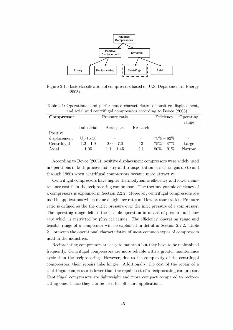
IndustrialCompressors
PositiveDisplacement Dynamic
Centrifugal AxialReciprocatingRotary
Figure 2.1: Basic classification of compressors based on U.S. Department of Energy(2003).
Table 2.1: Operational and performance characteristics of positive displacement,and axial and centrifugal compressors according to Boyce (2003).
Compressor Pressure ratio Efficiency Operatingrange
Industrial Aerospace ResearchPositivedisplacement Up to 30 - - 75% – 82% -Centrifugal 1.2 - 1.9 2.0 – 7.0 13 75% – 87% LargeAxial 1.05 1.1 – 1.45 2.1 80% – 91% Narrow
According to Boyce (2003), positive displacement compressors were widely used
in operations in both process industry and transportation of natural gas up to and
through 1960s when centrifugal compressors became more attractive.
Centrifugal compressors have higher thermodynamic efficiency and lower main-
tenance cost than the reciprocating compressors. The thermodynamic efficiency of
a compressors is explained in Section 2.2.2. Moreover, centrifugal compressors are
used in applications which request high flow rates and low pressure ratios. Pressure
ratio is defined as the the outlet pressure over the inlet pressure of a compressor.
The operating range defines the feasible operation in means of pressure and flow
rate which is restricted by physical causes. The efficiency, operating range and
feasible range of a compressor will be explained in detail in Section 2.2.2. Table
2.1 presents the operational characteristics of most common types of compressors
used in the industries.
Reciprocating compressors are easy to maintain but they have to be maintained
frequently. Centrifugal compressors are more reliable with a greater maintenance
cycle than the reciprocating. However, due to the complexity of the centrifugal
compressors, their repairs take longer. Additionally, the cost of the repair of a
centrifugal compressor is lower than the repair cost of a reciprocating compressor.
Centrifugal compressors are lightweight and more compact compared to recipro-
cating ones, hence they can be used for off-shore applications.
45
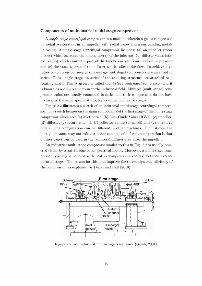
Components of an industrial multi-stage compressor
A single-stage centrifugal compressor is a machine wherein a gas is compressed
by radial acceleration in an impeller with radial vanes and a surrounding metal-
lic casing. A single-stage centrifugal compressor includes: (a) an impeller (rotor
blades) which increases the kinetic energy of the inlet gas, (b) diffuser vanes (sta-
tor blades) which convert a part of the kinetic energy to an increase in pressure
and (c) the vaneless area of the diffuser which collects the flow. To achieve high
ratios of compression, several single-stage centrifugal compressors are arranged in
series. These single stages in series of the resulting structure are attached to a
rotating shaft. This structure is called multi-stage centrifugal compressor and it
is known as a compressor train in the industrial field. Multiple (multi-stage) com-
pressor trains are usually connected in series and their compressors do not have
necessarily the same specifications, for example number of stages.
Figure 2.2 illustrates a sketch of an industrial multi-stage centrifugal compres-
sor. The sketch focuses on the main components of the first stage of the multi-stage
compressor which are: (a) inlet nozzle, (b) Inlet Guide Vanes (IGVs), (c) impeller,
(d) diffuser, (e) return channel, (f) collector volute (or scroll) and (g) discharge
nozzle. The configuration can be different in other machines. For instance, the
inlet guide vanes may not exist. Another example of different configuration is that
diffuser vanes can be used in the (vaneless) diffuser area after the impeller.
An industrial multi-stage compressor similar to this in Fig. 2.2 is usually pow-
ered either by a gas turbine or an electrical motor. Moreover, a multi-stage com-
pressor typically is coupled with heat exchangers (intercoolers) between two se-
quential stages. The reason for this is to improve the thermodynamic efficiency of
the compression as explained by Dixon and Hall (2010).
Dischargenozzle
Inletnozzle
IGVs
Impeller
Returnchannel
First stageDiffuser Volute
Figure 2.2: An industrial multi-stage compressor (Gresh, 2001).
46

2.2.2 Operation of a compressor
Definition of basic parameters of the operation
Figure 2.3 shows a compressor with two centrifugal compressor stages and an
intercooler placed in between them. The compressor is connected with a down-
stream and an upstream process. The compressor conveys a gas from the upstream
process with pressure, temperature and mass flow rate, Pin, Tin, Min, to the down-
stream process with gas specifications Pout, Tout, Mout. There is a driver which
provides power, Wmech, to the shaft of the compressor and the driver can be either
a gas turbine or an electrical motor. A steam turbine is also used in the same way
as the gas turbine to power a compressor, therefore when the text refers to gas
turbines as drivers of compressors, it is implied that steam turbines can also be
used instead of gas turbines.
The driver rotates the shaft with rotational speed N . This speed can be either
constant or variable in the case of a Variable Speed Drive (VSD). A variable speed
compressor is a compressor which employs this type of drive. Compressors can
also have adjustable blades, known as Inlet Guide Vanes (IGVs), at their inlet, i.e.
at the eye of the impeller. These blades are adjusted by an angle θ to change the
operating point of the compressor. The use of an intercooler can reduce the inlet
temperature, Tin,c, of the stream of gas which is coming from the exit of the first
stage, and therefore the reduction in inlet temperature can thermodynamically
improve the efficiency of the following stage (Dixon and Hall, 2010). The result is
the increase of the total efficiency of the multi-stage compressor.
The operation of a compressor can be identified from the studying of compres-
sor maps. Compressor maps provide information about the characteristics and
performance of compressors. These maps are used to identify the operating point
of a compressor and its efficiency at steady-state conditions, i.e. ambient tempera-
ture and pressure. The consideration of both the operating point, which describes
Stage 1 Stage 2
Intercooler
Wmech ,N
Driver
Upstreamprocess
Downstreamprocess
Compressortrain
Pout Tout Mout
Pin Tin Min
Τ out,c Pout,c
Pin,c Τin,c
θ
Figure 2.3: Operation of a two-stage (multi-stage) centrifugal compressor con-nected with an upstream and a downstream system.
47

pressure and flow rate, and the efficiency of the compressor can be used to estimate
the power consumed by the gas at specific conditions.
Compressor map: characteristics and thermodynamic efficiency
A standard graphical representation used to describe the operation of a com-
pressor is a compressor map which gives the characteristic curves of a variable
speed compressor or a compressor with inlet guide vanes. In the case of single
speed compressor without IGVs, there is only a single characteristic curve.
A typical corrected compressor map can be seen in Fig. 2.4. A general corrected
compressor map takes into account inlet conditions, pressure Pin and temperature
Tin and molecular weight MolW . For the sake of simplicity the MolW parameter
is omitted in this description, for example the compressor map of an air com-
pressor normally does not consider the MolW . The reason of considering the
inlet conditions is that a compressor map changes with respect to changes in inlet
temperature or pressure.
A single characteristic curve of a compressor describes the relationship between
pressure ratio π = Pout/Pin and the corrected mass flow rate Md = Min
√Tin/Pin
for a constant rotational speed N (Dixon and Hall, 2010). Figure 2.4 shows that
a compressor with characteristics with different angles of IGVs. According to the
manufacturer and the application, there are other descriptions of compressors maps
which may consider for example discharge pressure, or isentropic or polytropic head
on the vertical axis (Gresh, 2001). The horizontal axis in some compressor maps
describe volumetric flow rate.
surge limit
characteristics
choke limit
efficiency lines
maximumIGV opening
minimumIGV opening
0.75
10o
100o
0.85
0.90
60o
80o
Corrected mass flow rate
Pre
ssur
e ra
tio
Figure 2.4: A typical compressor map of a single-stage centrifugal compressor withdifferent angles of IGVs.
48
The operation between surge and choke for a constant speed curve (or a fixed
angle of Inlet Guide Vanes) defines the operational range of this characteristic
curve. The group of all the characteristics between minimum and maximum rota-
tional speed (or Inlet Guide Vanes) constitutes the operational domain or feasible
window of the operation of a compressor. The compressor cannot operate beyond
the limits of this window due to physical, safety, power and mechanical constraints.
Surge is a phenomenon of reverse flow in the compressor. This phenomenon oc-
curs when the machine compresses gas to high pressures at low flow rates. Helvoirt
(2007) reports that surge not only reduces both performance and efficiency, but it
can also cause damage to the compressor or other auxiliaries. Additionally, surge
causes vibrations due to the reversal of the flow which results in unacceptable noise
levels. Because of the undesired consequences of the effect of surge, compressors
have to operate at a reduced operational window. This operational window is
restricted by a left boundary, known as control surge line. This line is located to
the right of the surge line and both lines are separated by a safety margin.
Choke or stonewall region is located at the right region of a performance map.
A choke point is described as the operational point of a compressor which reaches
at the maximum flow rate and the minimum head for a fixed speed curve. Mach
number becomes equal to one, gas velocity has increased to acoustic velocity, and
the flow cannot increase further. Bloch (2006) reports that choke can cause serious
damage to the rotors and blades of multi-stage centrifugal or axial compressors.
However, the choke phenomenon does not damage single-stage compressors to a
great extent. Dixon and Hall (2010) explain the physical constraints of surge and
choke with the use of fundamental aerodynamic and thermodynamic equations.
The upper and lower bounds of the speed (or bounds of IGVs) of a compressor
map are defined by the specifications of the prime mover of the compressor, i.e.
electric motor or gas turbine.
Figure 2.4 illustrates that a compressor map also provides the efficiencies lines
which provide the efficiency of the compressor at every operating point on the map.
These lines give the thermodynamic isentropic or polytropic efficiency (ηis or ηp) of
a compressor. Isentropic and polytropic efficiencies are the most commonly used in
the literature of turbomachinery. The isentropic efficiency is defined as the ratio
of the useful energy input to fluid in unit time and the power input to the impeller
and this expression is given by Eq. (2.1). Figure 2.5 defines the actual work, i.e
power input to the impeller of one stage, and the isentropic work which is the
useful energy input to the fluid through this stage without considering losses. The
point A indicates the inlet of the stage of the compressor. The point B’ denotes
the outlet of the compressor with isentropic compression A-B’ and point B refers
to the actual compression A-B including losses.
49
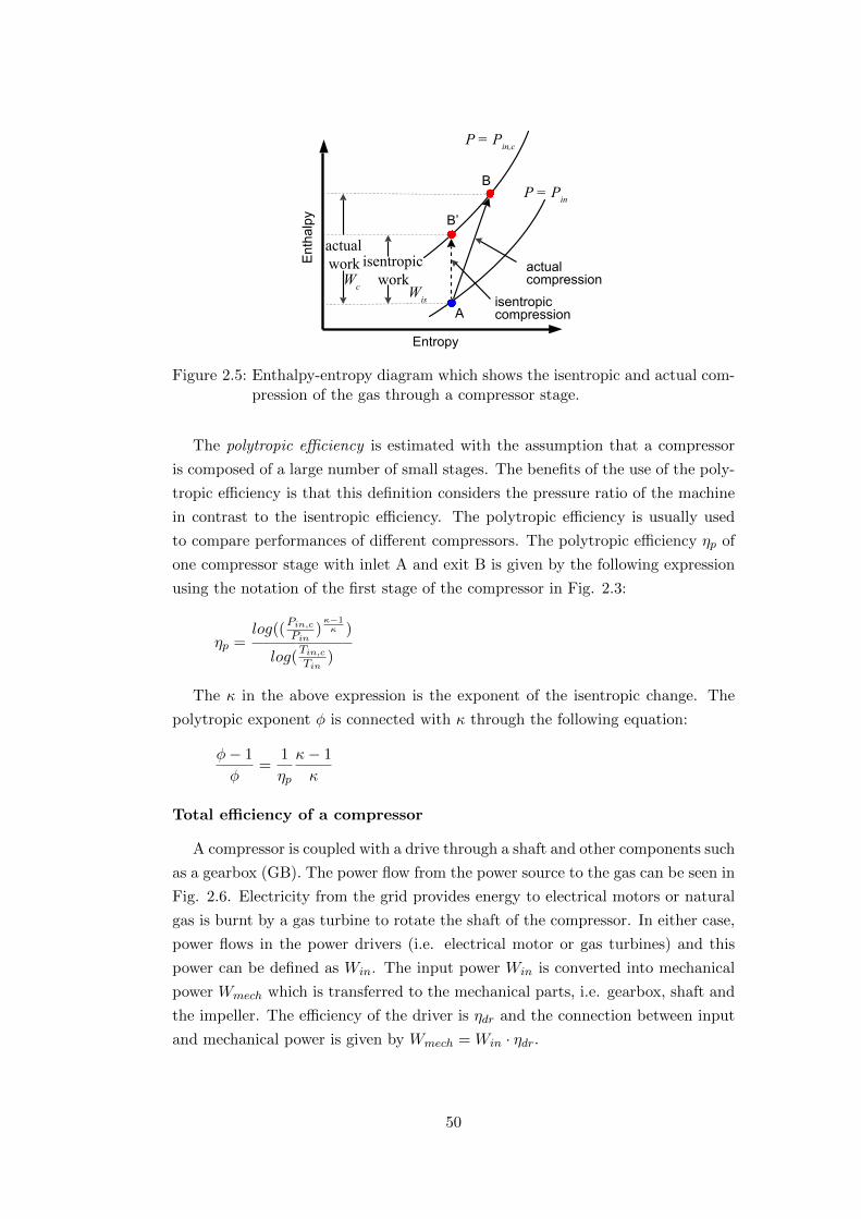
P = Pin
isentropicwork
actualwork
P = Pin,c
actual compression
isentropiccompression
Entropy
Ent
halp
y
Wc Wis
A
B’
B
Figure 2.5: Enthalpy-entropy diagram which shows the isentropic and actual com-pression of the gas through a compressor stage.
The polytropic efficiency is estimated with the assumption that a compressor
is composed of a large number of small stages. The benefits of the use of the poly-
tropic efficiency is that this definition considers the pressure ratio of the machine
in contrast to the isentropic efficiency. The polytropic efficiency is usually used
to compare performances of different compressors. The polytropic efficiency ηp of
one compressor stage with inlet A and exit B is given by the following expression
using the notation of the first stage of the compressor in Fig. 2.3:
ηp =log((
Pin,cPin
)κ−1κ )
log(Tin,cTin
)
The κ in the above expression is the exponent of the isentropic change. The
polytropic exponent φ is connected with κ through the following equation:
φ− 1
φ=
1
ηp
κ− 1
κ
Total efficiency of a compressor
A compressor is coupled with a drive through a shaft and other components such
as a gearbox (GB). The power flow from the power source to the gas can be seen in
Fig. 2.6. Electricity from the grid provides energy to electrical motors or natural
gas is burnt by a gas turbine to rotate the shaft of the compressor. In either case,
power flows in the power drivers (i.e. electrical motor or gas turbines) and this
power can be defined as Win. The input power Win is converted into mechanical
power Wmech which is transferred to the mechanical parts, i.e. gearbox, shaft and
the impeller. The efficiency of the driver is ηdr and the connection between input
and mechanical power is given by Wmech = Win · ηdr.
50
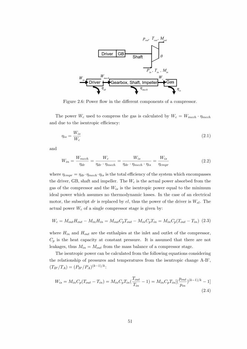
Win
Driver
Pin , Tin , Min
θ
pout, Tout , Mout
GB
DriverWmech
Gearbox, Shaft, Impeller
Shaft
Gasηis
ηmechηdr
Wc
Figure 2.6: Power flow in the different components of a compressor.
The power Wc used to compress the gas is calculated by Wc = Wmech · ηmechand due to the isentropic efficiency:
ηis =Wis
Wc(2.1)
and
Win =Wmech
ηdr=
Wc
ηdr · ηmech=
Wis
ηdr · ηmech · ηis=
Wis
ηcmpr(2.2)
where ηcmpr = ηdr ·ηmech ·ηis is the total efficiency of the system which encompasses
the driver, GB, shaft and impeller. The Wc is the actual power absorbed from the
gas of the compressor and the Wis is the isentropic power equal to the minimum
ideal power which assumes no thermodynamic losses. In the case of an electrical
motor, the subscript dr is replaced by el, thus the power of the driver is Wel. The
actual power Wc of a single compressor stage is given by:
Wc = MoutHout −MinHin = MoutCpTout −MinCpTin = MinCp(Tout − Tin) (2.3)
where Hin and Hout are the enthalpies at the inlet and outlet of the compressor,
Cp is the heat capacity at constant pressure. It is assumed that there are not
leakages, thus Min = Mout from the mass balance of a compressor stage.
The isentropic power can be calculated from the following equations considering
the relationship of pressures and temperatures from the isentropic change A-B’,
(TB′/TA) = (PB′/PA)(k−1)/k:
Wis = MinCp(Tout − Tin) = MinCpTin(ToutTin− 1) = MinCpTin[(
poutpin
)(k−1)/k − 1]
(2.4)
51

2.2.3 Maintenance of compressors
The maintenance of compressors is an essential factor of the general manage-
ment of a compressor station which will be explained in Section 2.4. The manage-
ment of the tasks of maintenance influences the availability and the reliability of
the production of the plants which include the compressors. The downtime of the
operation due to failures and unexpected breakdowns of compressors can lead to
unsatisfied demands and increased economic losses. Moreover, the unsatisfied tar-
gets can cause problems between the commercial relationships between plant and
its customers. This is because the plant would not be considered as reliable when
the agreed contracts between plant and customers are violated. The choice of the
best maintenance policy and the best maintenance plan of compressors has been
studied from many researchers as maintenance tasks may give rise to increased
maintenance and operational expenses if these tasks are not optimally scheduled.
Focusing on compressors and especially in industrial centrifugal compressors,
there are several maintenance policies of compressors to decide, namely corrective,
preventive and predictive. The corrective maintenance is related to the policy for
fixing a compressor after it has been broken. According to Thorp et al. (2014)
the mechanical components of a compressor with the most frequent failures are
bearings, seals, compressor blades, compressor discs and inlet air filters.
The restoration or the maintenance activity of a compressor which has not
failed at preselected intervals constitutes the preventive maintenance (Rao and
Naikan, 2008). A typical preventive maintenance approach includes the use of a
fixed schedule, optimised in advance for minimum cost according to Bohlin and
Warja (2010). However, unexpected failures may occur, and thus the users have to
re-plan the maintenance of the compressors. A preventive maintenance approach
involves inspections of the compressors which are performed to assess the condition
of the compressors.
The predictive maintenance uses real time analysis of data to assess the con-
dition of the compressors, therefore to decide the optimal moment to maintain
a compressor based on this acquired information and its analysis. The devel-
opment of advanced performance and condition monitoring tools based on the
condition of the oil and vibrations of mechanical and electrical components are
essential to achieve the application of predictive maintenance. The state-of-the-
art in performance monitoring of compressors which can estimate performance
and characteristics of a compressors is mentioned in the study by Cicciotti et al.
(2015). This study presents model-based approaches which exploit real time pro-
cess measurements, such as flow rates and pressures, to calculate the efficiency and
characteristics of the compressors online.
Bertolini and Bevilacqua (2006) reported that the development of advanced
52
techniques of maintenance requires managerial and technical skills of the mainte-
nance staff. The oldest and simplest method of maintenance, which is the cor-
rective, is to change to a more advanced maintenance but also more complex and
integrated policies such as a sophisticated preventive and predictive maintenance.
The management of advanced maintenance policies requires the considerations of
multiple components and multiple units which result in more complex methods
compared to those used in the corrective approach. These complex methods may
involve optimisation models which carry out an economic analysis to answer ques-
tions for example when the best moment to maintain a process unit is and what
maintenance policy should be applied to a particular system.
The maintenance of the compressors can also be classified into two categories:
(a) non-recoverable and (b) recoverable maintenance. The non-recoverable main-
tenance involves the repair (e.g. welding of material) or replacement of mechanical
or electrical parts of the compressors. The replacement of spare parts is defined
as a restoration action when a compressor has returned to perfect condition after
this restoration action. Replacements of spare parts take place in major overhauls
of the compressors which take longer compared to short shut downs to repair the
compressor. The cost of the repair per overhaul has been estimated between $472K
– $714K (Thorp et al., 2014).
The recoverable maintenance involves the washing of compressors to deal with
the problem of fouling. The fouling of compressor is caused from the deposition of
particles mainly on the blades of the compressors and annulus surfaces mainly due
to dust mixed with air. Fouling causes over-consumption of the power and drop of
full mass flow rate according to Martın-Aragon and Valdes (2014). The washing of
the compressors can occur online, i.e. a solution is injected while the compressor
operate online, or can occur offline, i.e. the compressor is washed with a solution
with additional treatments when it is in offline. Several washing schedules have
been suggested from Sanchez et al. (2009), Aretakis et al. (2012), Rao and Naikan
(2008) and Hovland and Antoine (2004). Chapter 6 will suggest a condition-based
maintenance approach which fall into the category of the predictive maintenance
studies. Martın-Aragon and Valdes (2014) mention that the cost of fouling of the
compressors has been estimated approximately 6.25 million per year and that an
improved maintenance schedule could save 200,000 EUR/year per gas turbine.
2.3 Compressors integrated with other systems
2.3.1 Interactions between compressors and a downstream system
An operating point of a compressor is the intersection of its characteristic curve
at a fixed rotational speed (or fixed angle of IGVs) and the characteristic curve of
53
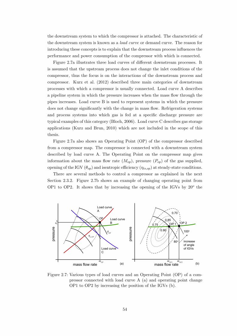
the downstream system to which the compressor is attached. The characteristic of
the downstream system is known as a load curve or demand curve. The reason for
introducing these concepts is to explain that the downstream process influences the
performance and power consumption of the compressor with which is connected.
Figure 2.7a illustrates three load curves of different downstream processes. It
is assumed that the upstream process does not change the inlet conditions of the
compressor, thus the focus is on the interactions of the downstream process and
compressor. Kurz et al. (2012) described three main categories of downstream
processes with which a compressor is usually connected. Load curve A describes
a pipeline system in which the pressure increases when the mass flow through the
pipes increases. Load curve B is used to represent systems in which the pressure
does not change significantly with the change in mass flow. Refrigeration systems
and process systems into which gas is fed at a specific discharge pressure are
typical examples of this category (Bloch, 2006). Load curve C describes gas storage
applications (Kurz and Brun, 2010) which are not included in the scope of this
thesis.
Figure 2.7a also shows an Operating Point (OP) of the compressor described
from a compressor map. The compressor is connected with a downstream system
described by load curve A. The Operating Point on the compressor map gives
information about the mass flow rate (Mop), pressure (Pop) of the gas supplied,
opening of the IGV (θop) and isentropic efficiency (ηis,op) at steady-state conditions.
There are several methods to control a compressor as explained in the next
Section 2.3.2. Figure 2.7b shows an example of changing operating point from
OP1 to OP2. It shows that by increasing the opening of the IGVs by 20o the
mass flow rate
pres
sure
Load curveA
Load curveC
Load curveBp O
P
mOP
100o
0.85
0.90
80o
mass flow rate
pres
sure
OP
OP 1 OP 2
0.70
mOP1 mOP2 (b)(a)
ηis,OP
θOP
0.75
increase of angleof IGVs
Figure 2.7: Various types of load curves and an Operating Point (OP) of a com-pressor connected with load curve A (a) and operating point changeOP1 to OP2 by increasing the position of the IGVs (b).
54

operating point changes. The compressor at OP2 provides higher mass flow rate
at a higher pressure than in the case of OP1, and moreover the efficiency of the
compressor drops to 0.7. This information, pressure, mass flow rate and efficiency
can be used to estimate the power consumed from the compressor (power in the
shaft). By using the efficiency of the shaft and gearbox, the power provided by
the driver can be computed.
2.3.2 Control methods
There are several control strategies to adjust the operating point of a compres-
sor, namely use of variable speed drives, suction and discharge throttling, inlet
guide vanes and recycling valve. More than one control strategy from the afore-
mentioned can be applied to a compressor to change its operating point. A brief
description of each control method is given below according to Liptak (2006) and
Kurz et al. (2012):
• Compressors can employ variable speed drives which can modify the values of
the rotational speed of the shaft. The drivers can be variable speed electrical
motors, steam or gas turbines. This control method is considered as one of
the most efficient.
• Suction throttling is mainly used for fixed speed compressors. The basic prin-
ciple of this method is that a throttling device, which is usually a butterfly
valve, varies the pressure of the inlet stream of gas at the inlet of the com-
pressor, and hence this results in changing the mass flow rate. A drawback
of this technique is that efficiency losses occur when the flow passes through
the valve.
• Discharge throttling works in the same way as in the case of the suction
throttling. In this case, throttle valve is located at the discharge side of the
compressor. The suction and discharge throttling are considered as the least
efficient methods to control a compressor.
• Inlet Guide Vanes (IGVs) are the actuators which modify the operating
range of a compressor. Indeed, IGVs consist of several blades placed at the
inlet of the compressor. In the instance of a multi-stage compressor, IGVs
can be found at the inlet of the first stage exclusively.
• The flow can be recycled to modify the operating point of a compressor.
However this method is used in a situation of emergency as this method of
control is inefficient. Indeed, compressed gas is recycled back to the inlet of
the compressor, therefore the energy to compress the gas is wasted.
55

• Multiple compressor units in parallel can be used to increase and decrease
the total capacity of the compressor station by switching on or off individual
compressors.
2.4 Management of compressor stations
2.4.1 Operational tasks of compressors
Figure 2.8a shows a pyramid of the typical decisions or control tasks of plant-
wide automation of a process plant according to the ANSI/ISA-95 standard (Har-
junkoski et al., 2009). The pyramid includes the Process Control System (PCS)
which involves real time set point control and real time monitoring of the process in
Level 0, 1 and 2. The time scale of Process Control System is seconds or fractions
of seconds. The Manufacturing Execution System (MES) of Level 3 deals with the
manufacturing operations and considers decisions for example the scheduling of the
units of the operations for the next days or hours. The Manufacturing Execution
System also considers the topic of the optimisation of the process by improving
its performance in real time. Indeed, the optimisation suggests the best set points
of the control system. On the top of the pyramid, in Level 4, is the Enterprise
Resource Planning (ERP) which considers business planning and logistics. The
high level decisions of the Enterprise Resource and Planning deals with markets,
production targets and sales.
Figure 2.8b presents a pyramid of decisions of the operations of a compressor
station. At the top of this pyramid, in Level 4, there are the targets of demand,
given from the Central Dispatch Department in the case of compressors in the
natural gas industries (Paparella et al., 2013). The targets of demand are the
input of Level 3 of the pyramid. Level 3 includes the scheduling and maintenance
ERPLevel 4
PCSLevel 0, 1, 2
MESLevel 3
Common actions Time scales
Supply chainDemand planningProduction planningSales and distribution
SchedulingProcess optimisationAdvanced controlAsset monitoring
Real time executionReal time monitoring
Months, weeks,days
Days, shifts, hours,minutes, seconds
Hours, minutes,seconds, less than a second.
ERPLevel 4
PCSLevel 0, 1, 2
CONTROL OF INDIVIDUAL COMPRESSORSMONITORING OF COMPRESSORS
OPTIMAL LOAD SHARING,UPDATE OF COMPRESSOR MAPS
MESLevel 3
OPTIMAL SCHEDULE AND MAINTENANCE
DEMAND
(a) (b)
Figure 2.8: Decision pyramid of a plant according to the ANSI/ISA-95 (Har-junkoski et al., 2009) (a) and the corresponding decision pyramid of acompressor station (b).
56
of compressors. The same level also deals with the optimal distribution of the load
among the compressors which provides set points, for example the set points of the
speeds of the motors of the compressors, to the controllers of the control system.
The lowest levels, Level 0, 1, 2, involve the control of the individual units and the
monitoring of the process. The role of the controllers is to deal with disturbances
with fast dynamics, thus to keep the given set points from the upper level constant.
The Real Time Optimisation and the scheduling of compressors are considered as
control tasks which belong in Level 3 of the decision pyramid in Fig. 2.8b.
2.4.2 Supervisory control: Real Time Optimisation (RTO)
According to Fig. 2.8a, Level 3 of the decision pyramid of a plant is concerned,
among other tasks, with the online calculation of the optimal set points of the
process operations of the plant. The calculation of the optimal set points can
be also carried out for combined units of a plant. This procedure is known as
Real Time Optimisation (RTO). According to Edgar et al. (2001), the application
of RTO in chemical industry started in the 1960s. Initially, a large mainframe
computer computed the optimal process set points which were subsequently sent
to analogue controllers to adjust the operating points of the operation. In the
1970s, real time optimisation was implemented into computer control systems with
a Distributed Control System (DCS). In this case the RTO was named supervisory
control.
The computation of the optimal set points of the process variables can be de-
termined from an optimisation problem. This optimisation problem, for which
general description will be explained in Section 2.5, aims to minimise (or max-
imise) a performance criterion while at the same time considers constraints of the
examined system including constraints derived from the steady-state modelling of
the processes. These process models can be derived from fundamental knowledge
(physics), experimental data or a combination of them. The set points, which
are determined every day, hour or minute, can be temperatures, pressures or flow
rates.
Furthermore, the performance criteria can be the increase of production rates,
the minimisation of energy consumption or the minimisation of the operational
cost. Seborg et al. (2004) defines the performance criterion as the operating profit.
The constraints of the operation can be design, safety or environmental boundaries.
For instance, the material of the blades of the compressor defines a maximum
temperature for the gas stream flowing into the compressor. Another example
is the flow rates boundaries which are dictated by geometrical restrictions of the
compressor.
The implementation of the RTO in a process operation using a traditional reg-
57
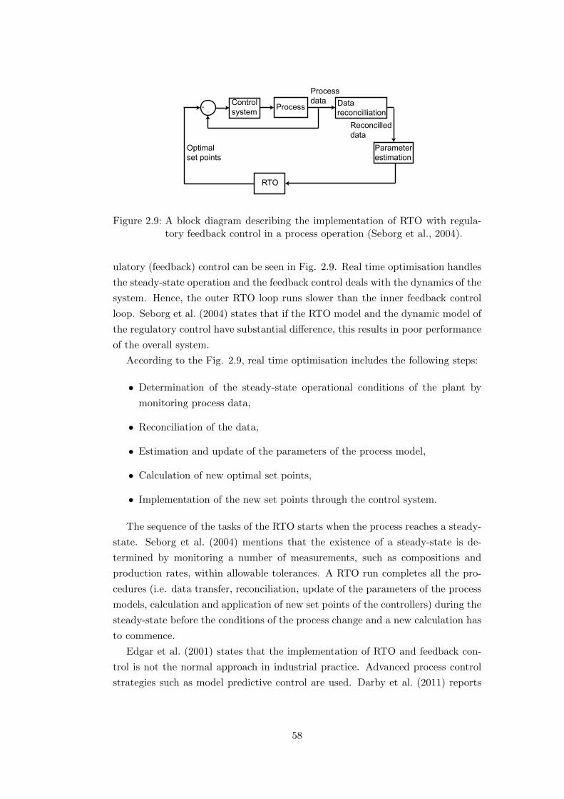
+-
Control system Process Data
reconcilliation
Processdata
Parameterestimation
Reconcilleddata
RTO
Optimalset points
Figure 2.9: A block diagram describing the implementation of RTO with regula-tory feedback control in a process operation (Seborg et al., 2004).
ulatory (feedback) control can be seen in Fig. 2.9. Real time optimisation handles
the steady-state operation and the feedback control deals with the dynamics of the
system. Hence, the outer RTO loop runs slower than the inner feedback control
loop. Seborg et al. (2004) states that if the RTO model and the dynamic model of
the regulatory control have substantial difference, this results in poor performance
of the overall system.
According to the Fig. 2.9, real time optimisation includes the following steps:
• Determination of the steady-state operational conditions of the plant by
monitoring process data,
• Reconciliation of the data,
• Estimation and update of the parameters of the process model,
• Calculation of new optimal set points,
• Implementation of the new set points through the control system.
The sequence of the tasks of the RTO starts when the process reaches a steady-
state. Seborg et al. (2004) mentions that the existence of a steady-state is de-
termined by monitoring a number of measurements, such as compositions and
production rates, within allowable tolerances. A RTO run completes all the pro-
cedures (i.e. data transfer, reconciliation, update of the parameters of the process
models, calculation and application of new set points of the controllers) during the
steady-state before the conditions of the process change and a new calculation has
to commence.
Edgar et al. (2001) states that the implementation of RTO and feedback con-
trol is not the normal approach in industrial practice. Advanced process control
strategies such as model predictive control are used. Darby et al. (2011) reports
58

that the basic structure of Real Time Optimisation in cascade with Model Pre-
dictive Control has become the standard approach for implementing steady-state
optimisation to improve the process which operates around nominal steady-states.
Edgar et al. (2001) and Darby et al. (2011) present the integration of RTO and
model predictive control in detail.
2.4.3 Operational planning and scheduling
Operational (or production) planning and scheduling are considered as sepa-
rated levels according to Fig. 2.8a. However, an overlap exists between these two
decision tasks in different levels in the pyramid in Fig. 2.8a. Edgar et al. (2001) re-
ports that planning focuses on broad classes of products and provision of adequate
manufacturing capacity at time horizons of years, months and days. Moreover,
scheduling focuses on details of material flow, manufacturing and production at
time horizons of weeks, days or hours. The activities of planning and scheduling
according to Edgar et al. (2001) are summarised in Table 2.2.
Table 2.2: Planning and scheduling activities according to Edgar et al. (2001).
Corporate operations planning
Allocate production requirements to plants.Balance facilitys capacity.Optimise materials and product movements (supply chain).
Plant operations planning
Determine production plans.Plan inventory strategy.Determine raw materials requirements.
Plant scheduling
Determine run lengths.Determine sequence of operations.Provide inventory for production runs.
2.5 Optimisation (mathematical programming)
A major current focus in lowering production costs has enabled engineers to em-
ploy rigorous methods and tools for decision-making, such as optimisation, which
is known as mathematical programming, to design and produce products both effi-
ciently and economically. Optimisation techniques are being used in a large range
of industries such as aerospace, chemical, electrical, construction and manufactur-
ing industries. Typical examples of optimisation problems are: (a) identification
59

of the minimum weight of an aircraft, (b) decision of optimal operating condi-
tions of a boiler in a process plant, (c) optimum design of electrical networks, (d)
selection of the best site to construct a plant, (e) plan of maintenance and replace-
ment of equipment to reduce operating costs in a manufacturing industry and (f)
evaluation of plant data to develop a model of a process.
A wide variety of problems in design, construction and operation of chemical
plants can be solved by optimisation. Focusing on operations of a plant, optimi-
sation provides several benefits such as improvement of the performance of the
processes, improved yields of the valuable products, reduced contaminants and
undesired emissions, and reduced energy consumptions. Additionally, the optimi-
sation of the operations results in reduced maintenance costs, longer times between
shutdowns of expensive equipment and less wear of the machines. The purpose of
Section 2.5 is to present the principles of optimisation theory and its application
for solving industrial problems.
2.5.1 Definition of an optimisation problem
According to Edgar et al. (2001), an engineering optimisation problem can be
described as follows: a process can be represented by some equations or experi-
mental data, and the goal of the optimisation is the identification of the values of
variables describing the process when the value of a single performance criterion
becomes maximum or minimum under given circumstances. Both the given restric-
tions and the model of the process constitute the constraints of the mathematical
problem.
General description
The statement of an optimisation problem is usually written in the following
form (Rao, 2009):
Find X = [x1 . . . xn]T which minimises f(X)
subject to the constraints:
gi(X) ≤ 0, i = 1, . . . ,m
hj(X) = 0, j = 1, . . . , p
Where:
• The X is a n-dimensional vector which describes the continuous variables
of the problem, these variables are known as design, decision, optimisation
variables or just variables of the optimisation problem.
60

• The f(X) is the objective function of the problem which represents the per-
formance criterion previously mentioned. In this case the objective function
is single equation but it is possible to have more than one objective function
to solve, i.e. multi-objective optimisation. The objective function can be
linear or non-linear.
• The gi are the inequality constraints which can be linear or non-linear.
• The hj are the equality constraints which can be linear or non-linear.
• The n denotes the number of the variables, the m denotes the number of
inequalities and the p is the number of the equalities of the optimisation
problem.
An optimisation problem is defined by an objective function and constraints.
Both the equalities and inequalities are the constraints. The constraints represent
the restrictions of the optimisation problem. The quantities which are found inside
the equations of both the objective function and the constraints can be classified
into the decision variables, which represent the variables of the optimisation prob-
lem, and the preassigned parameters. The preassigned parameters are fixed values
which cannot change during the procedure of optimisation and they are given as
input. The procedure to identify the objective function and constraints of the
problem is called modelling.
Constraints
All the values of the decision variables of the optimisation problem which satisfy
the constraints define a feasible solution. The set of all feasible solutions consti-
tutes the feasible region of the optimisation problem. Indeed, the combination
of the equalities and inequalities determine the feasible region of a constrained
optimisation problem.
Objective function
When there is more than one feasible solution of the optimisation problem, a
performance criterion is employed to choose the best feasible solution among all
of them. This performance criterion is called objective function. The choice of
the objective function depends on the nature of the problem. For example, in
a chemical plant the maximisation of the final product is the criterion preferred.
In an air separation plant, the minimisation of the energy consumption can be a
performance criterion.
61
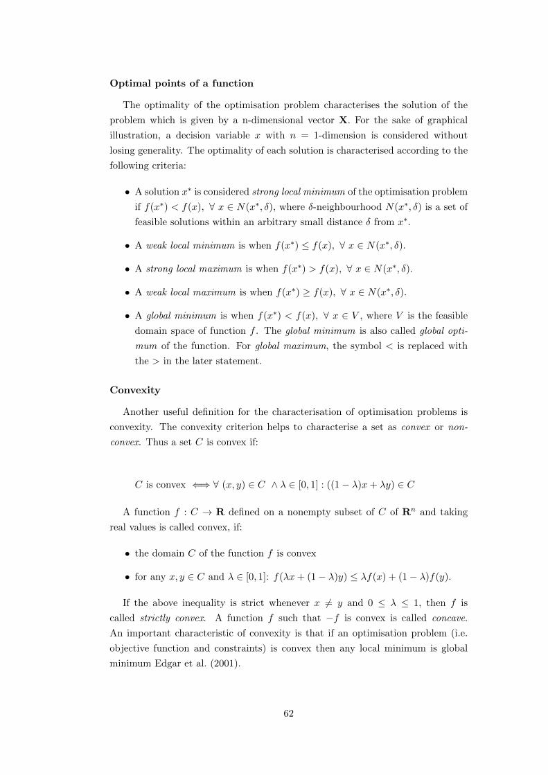
Optimal points of a function
The optimality of the optimisation problem characterises the solution of the
problem which is given by a n-dimensional vector X. For the sake of graphical
illustration, a decision variable x with n = 1-dimension is considered without
losing generality. The optimality of each solution is characterised according to the
following criteria:
• A solution x∗ is considered strong local minimum of the optimisation problem
if f(x∗) < f(x), ∀ x ∈ N(x∗, δ), where δ-neighbourhood N(x∗, δ) is a set of
feasible solutions within an arbitrary small distance δ from x∗.
• A weak local minimum is when f(x∗) ≤ f(x), ∀ x ∈ N(x∗, δ).
• A strong local maximum is when f(x∗) > f(x), ∀ x ∈ N(x∗, δ).
• A weak local maximum is when f(x∗) ≥ f(x), ∀ x ∈ N(x∗, δ).
• A global minimum is when f(x∗) < f(x), ∀ x ∈ V , where V is the feasible
domain space of function f . The global minimum is also called global opti-
mum of the function. For global maximum, the symbol < is replaced with
the > in the later statement.
Convexity
Another useful definition for the characterisation of optimisation problems is
convexity. The convexity criterion helps to characterise a set as convex or non-
convex. Thus a set C is convex if:
C is convex ⇐⇒ ∀ (x, y) ∈ C ∧ λ ∈ [0, 1] : ((1− λ)x+ λy) ∈ C
A function f : C → R defined on a nonempty subset of C of Rn and taking
real values is called convex, if:
• the domain C of the function f is convex
• for any x, y ∈ C and λ ∈ [0, 1]: f(λx+ (1− λ)y) ≤ λf(x) + (1− λ)f(y).
If the above inequality is strict whenever x 6= y and 0 ≤ λ ≤ 1, then f is
called strictly convex. A function f such that −f is convex is called concave.
An important characteristic of convexity is that if an optimisation problem (i.e.
objective function and constraints) is convex then any local minimum is global
minimum Edgar et al. (2001).
62

Optimisation in process engineering
Deterministic optimisation
DynamicSteady-state
Optimisation under uncertainty
Fuzzyprogramming
Stochasticprogramming
Discrete variableoptimisation
Continuous variableoptimisation
Linear Programming (LP)
Non-Linear Programming (NLP)
DerivativeFree Optmisation (DFO)
Mixed Integer(Non-) LinearProgramming (MIP)
Integer,Binary IntegerProgramming (IP,BIP)
Figure 2.10: A general classification of optimisation problems in process engineer-ing.
2.5.2 Classification of optimisation problems
Optimisation can be classified according to different criteria: for example the
types of the variables (continuous, integer or mixed) and the consideration of
uncertainty or not. Figure 2.10 illustrates a general overview of different types
of optimisation problems based on the studies of Edgar et al. (2001), Biegler and
Grossmann (2004), Sahinidis (2004) and Rao (2009).
Stochastic and deterministic optimisation
Depending on the nature of both variables and parameters of an optimisation
problem, the problem can be classified into deterministic or stochastic. Stochastic
optimisation deals with problems which involve uncertainty in the values of their
variables or their parameters. Prices of electricity, heat transfer coefficients, de-
mand of products, and ambient temperature and pressure are a few examples of
parameters which can involve uncertainty in optimisation problems of process sys-
tems. Deterministic optimisation does not consider uncertainty of variables and
parameters of the optimisation problems.
This PhD thesis will focus on the deterministic approach for modelling and
optimising operations of process systems and systems with large energy consump-
63
tion such as export gas compressor stations. Figure 2.10 shows that deterministic
optimisation problems are further classified into steady-state and dynamic optimi-
sation. Dynamic optimisation employs time-dependent models to determine the
optimal trajectory of a value of a process variable. Here, process operations are
modelled in dynamic conditions using Differential-Algebraic Equations (DAEs).
Typical examples of dynamic optimisation are optimisation of the scheduling of
batch processes (b) optimisation of processes with unstable conditions (c) evalu-
ation of control schemes (d) evaluation of safety studies and (d) identification of
the optimal behaviour of the system during start up, upset, shut down according
to Cervantes and Biegler (2009).
Deterministic steady-state optimisation solves algebraic equations and it does
not involve differential equations. As shown in Fig. 2.10, steady-state optimisation
can be further categorised into continuous or discrete optimisation depending on
the type of the variables of the problem, i.e continuous, integer or a combination of
them. In the case of the use of both continuous and discrete variables to describe an
objective function or/and constraints, then the optimisation problem is considered
as Mixed Integer Programming (MIP) problem.
Linear and Non-Linear Programming methods
Continuous variable optimisation involving only continuous variables can be di-
vided into Linear Programming (LP) and Non-Linear Programming (NLP). The
term of LP was given by George Dantzig in 1947 (Edgar et al., 2001). A Linear
Programming problem is the optimisation problem which uses both linear objec-
tive function and linear constraints. On the other hand, a non-linear programming
problem involves non-linear objective function or/and non-linear constraints. Lin-
ear programming problems have the generic form:
maximise f(X) = cTX : AX ≤ b, X ≥ 0
where f is the linear function to be maximised (or minimised in a minimisation
problem) and X is the vector of decision variables. The vectors of parameters
c, b and matrix of coefficients A are given. The objective is to estimate a feasible
solution (if there is any) which maximises (or minimises) the objective described
by the affine function f(X) which is equal to cTX in the general description. The
constraints given by a set of inequalities AX define a convex polytope on which the
optimisation problem has to search the optimal solution for the decision variables
X.
The main algorithms which solve LP problems are the Simplex and the Interior-
point algorithms. The Simplex algorithm is based on the search of the optimal
64
solution in the vertices of the polytope which defines the feasible region of the
optimisation problem. The algorithm moves from one vertex to the following one
until predefined criteria to be met. In contrast with the Simplex algorithm, an
Interior-point algorithm finds improved search directions strictly in the interior of
the feasible region.
The Non-Linear Programming method involves the optimisation of a problem
if one or more of the equations of the the objective function f , inequalities g and
equalities h is non-linear. The main challenge when dealing with NLP methods is
that when there are several optima and the aim is to estimate the global optimum
and not any local minimum. The main techniques to determine local solutions
are gradient-based search methods such as Newton’s method and steepest descent
approach (Edgar et al., 2001). Rao (2009) explains and presents in detail methods
for solving non-linear programming problems.
Mixed Integer Programming (MIP)
When an optimisation problem involves continuous, and integer and/or binary
variables the problem is called Mixed Integer Programming (MIP) which is further
classified to Mixed Integer Linear Non-Linear Programming (MILP and MINLP)
problems depending on the type of the objective function and the constraints. The
general mathematical formulation of the optimisation problem becomes:
Find X, Y which minimises f(X,Y)
subject to the constraints:
gi(X,Y) ≤ 0, i = 1, . . . ,m
hj(X,Y) = 0, j = 1, . . . , p
where vector X takes continuous and vector Y takes integer and/or binary values.
More specifically, the description of a MILP optimisation problem is given by the
following formulation:
maximise cTX + hY
subject to:
AX +GY ≤ b
X ≥ 0,Y ≥ 0 and integer or binary
where X is the vector of positive continuous variables and Y is the vector of integer
and/or binary variables. The vector coefficient c, b, h and matrices of coefficients
A, G are given in the optimisation problem.
65
The values of the binary variables Y represent decisions which refer to events
which should or should not occur. Therefore a variable Yλ takes value one if an
event λ should occur or value zero if this event should not occur. The event can
be an on/off mode of an operation, a logical condition, fixed cost or a piecewise
linear function decision.
The main algorithms used to solve Mixed Integer Programming Problems are
the cutting plane algorithm of Gomory (1960) and the branch-and-bound algo-
rithm of Land and Doig (1960). In addition, the algorithm of Balas Balas (1965)
can efficiently deal with binary problems according to Rao (2009). Kopanos (2010)
summarises other methods to solve mixed integer programming problems such as
the branch-and-cut method, which is a combination of branch-and-bound and cut-
ting plane algorithm, and disjunctive programming.
Other optimisation methods
Biegler and Grossmann (2004) reported optimisation techniques without deriva-
tives, namely genetic algorithms, simulated annealing and classical direct search
methods. These techniques have the advantage of easy implementation into a wide
spectrum of problems. They are used before applying any sophisticated optimisa-
tion methods. Moreover, most of these techniques derived from heuristics. This
type of optimisation is known as Derivative Free Optimisation (DFO) which is
presented in the study by Biegler and Grossmann (2004).
2.5.3 Software and solvers
Software for optimisation
The software platform for optimisation problems mainly to be used in this study
is GAMS (General Algebraic Modeling System). Software GAMS allows the user
to model and solve linear, non-linear, and mixed integer programming optimi-
sation problems. Since GAMS includes an integrated development environment,
this adheres the use of third-party developed optimisation solvers. Examples of the
most used solvers are CPLEX, CONOPT, DICOPT and BARON. The advantage
of the GAMS software is that it presents and models the equations in a concise,
human-readable algebraic description. Initially, GAMS was developed for appli-
cations related to economics and management science, however the researchers in
the process system engineering community use GAMS to solve relevant engineering
optimisation problems.
66

Solvers of GAMS
The most commonly used solver in GAMS is CPLEX or IBM ILOG CPLEX
Optimisation Studio (IBM, 2015). CPLEX took its name from the Simplex method
which is implemented in the C programming language at its original development
stage. The CPLEX solver can deal with integer programming problems, large scale
linear programming problems, and convex and non-convex quadratic programming
problems.
2.6 Summary of the chapter
This chapter classified industrial compressors according to their design and
principle of operation. The most common types of compressors used in the pro-
cess and natural gas industries are centrifugal compressors. The basic principles of
multi-stage centrifugal compressors were explained. Moreover, a compressor map
defines the operation of the compressors and provides the feasible region of oper-
ation and efficiency of the compressor. The maintenance of a compressor plays a
key role in its operation and lifecycle. The different types of strategies of mainte-
nance, namely corrective, preventive and predictive were explained. Furthermore,
the recoverable and non-recoverable maintenance of a compressor were mentioned.
This chapter also presented the management of the compressors with the use
of an automation pyramid of different decision tasks of a process plants tailored
to the specific tasks of a compressor station. The current study focuses on the
Real Time Optimisation (RTO), and Scheduling and maintenance of compressors.
These topics are related to the Level 3, Manufacturing Execution System, of the
pyramid of the decision tasks. Finally, the principles of mathematical programming
and the basic software tools to solve optimisation problems have been presented.
67

3 Literature review on the optimal
operation of compressor stations
3.1 Description of the chapter
Chapter 3 presents the literature review on the topic of the optimal operation of
compressor stations. Section 3.2 will classify the types of problems which deal with
the improvement of the operation of the compressors considering different applica-
tions, and considering steady-state analysis or multi-period approach. Moreover,
the optimisation problems which deal with optimal operation of compressors will
be classified based on the types of variables that are used in the mathematical for-
mulations. Binary variables are used to model decisions which deal with discrete
events, for example starting up or shutting down a machine. Continuous variables
represent flow rates and pressures.
Moreover, Chapter 3 focuses on studies from previous researchers on: (a) opti-
mal load sharing in Section 3.3, (b) scheduling in Section 3.4 and (c) maintenance
of compressors in Section 3.5. The presentation of the state-of-the-art in these
topics will show the need for developing optimisation frameworks to deal with
the optimal distribution of the load and with the scheduling of the compressors
considering maintenance tasks of the individual compressors. Therefore, Section
3.6 explicitly reports the gaps of knowledge considering the literature review and
justifies the contributions of the thesis.
3.2 Classification of problems of optimal operation of
compressors
3.2.1 General overview
The optimisation of compressor stations is a topic which many researchers have
studied in the recent years. Compressors are used in various applications where the
nature of each application influences the objectives and the constraints of the op-
timisation problem. For instance, problems examining natural gas systems which
transport gas through long pipes can consider the phenomenon of the linepack
(Kurz et al., 2012). The linepack is a time-dependent phenomenon which de-
68
Optimisation ofcompressor stations
Compressor stations innatural gas networks
Utilities (feed gas a process system)
Other applications (e.g. gas oil lifted wells)
Single-period optimisation
Optimal selection of compressors
Gas storageA
pplic
atio
ns
Con
tinuo
us
oper
atio
n,di
scre
te e
vent
s
Optimal loadsharing
Multi-period optimisation
Pipeline optimisation
Tim
e ho
rizon
Pipelineoptimisation
(Wu et al., 2000)
(Abbaspour et al., 2005)
(Abbaspour et al., 2007)
(Mahlkeet al., 2010)
(Carter et al., 2010)
(Han et al., 2004)
(Paparellaet al., 2013)
Nguyenet al., 2008)
(Camponogaraet al., 2012)
Optimal selection of compressors
Figure 3.1: Classification of optimisation of compressor stations.
scribes the inherent capability of a pipe to store gas. The stored gas can be used
for example when the operation cannot satisfy the demand due to an unexpected
failure of a compressor (Kurz and Brun, 2012a). On the other hand, a supply
compressor station of a chemical process provides gas at a constant pressure.
The optimal operation of gas compressors in different process systems has been
studied by many researchers, for example Han et al. (2004), Hasan et al. (2009)
and Sun and Ding (2014). These researchers employed a steady-state optimisation
analysis (solution for one set of operational conditions) compared to the scheduling
approach from van den Heever and Grossmann (2003) which used a multi-period
approach. The latter study focused on the pipeline network and not on the oper-
ational aspects of the compressors, such as shut down and start up actions. Other
studies focused on the optimal control of the compressors employed Model Pre-
dictive Control strategies, recent examples are the papers by Gopalakrishnan and
Biegler (2013), and Zavala (2014).
Figure 3.1 shows the main groups of optimisation problems regarding: (a) the
application, (b) the time horizon and (c) the consideration of continuous operation
or/and discrete events. The set points of the compressors refer to continuous
quantities. The selection of the compressors to operate online is modelled with
the use of binary variables which describe discrete events such as startups and
shutdowns.
69

3.2.2 Optimisation of compressors regarding the application
The top section of Figure 3.1 presents the classification of the optimisation of
compressor stations considering four main categories of applications, namely nat-
ural gas networks, utilities, gas storage and other applications. Many researchers,
for example Shaw (1994), Wu et al. (2000), Cobos-Zaleta and Rıos-Mercado (2002)
and Borraz-Sanchez (2010), have studied the optimisation of natural gas networks.
These studies focus on the solution of problems which involve complex networks
of pipelines and compressors. Due to the complexity and the large-scale of these
problems, a compressor station is modelled as a single compressor unit, even if a
compressor station consists of multiple compressors. The optimisation of this kind
of problem usually includes the basic storage modelling of the pipes, i.e. linepack.
The linepack of the pipe provides flexibility to the system, nevertheless the com-
pressors have to operate at higher pressures resulting in higher power consumption.
This trade-off between flexibility and increased power consumption is investigated
in these problems.
The second type of application refers to process systems which include utilities
in which compressors spend most of the energy consumption of these systems.
The compressors of utilities usually do not store the gas in the pipes, and thus
the analysis of these systems do not focus on detailed modelling of the pipes.
The reason is that the friction losses are not important compared to the previous
category of the natural gas networks where the length of the pipes are hundreds
of kilometres. A representative example of this type of application is the study by
Han et al. (2004) which examines the case of an air- and gas-supply compressor
station of a terephtalic acid manufacturing plant. The authors mentioned that such
compressor stations consume more than 75% of the total electric power consumed
in the plant. Widell and Eikevik (2010) studied the optimal operation of parallel
screw compressors in refrigeration systems. Compressors in refrigeration systems
consume large amounts of energy and can be used in oil and gas industry in a
number of cases as Kurz and Brun (2012a) reports cooling a compressed gas,
Liquefaction of Natural Gas (LNG) and removing liquids in a gas plant.
A typical example of the application of compressors for utilities is the first
case study of this thesis which deals with an air compressor station of an air
separation plant. This case study of the air compressors of an air separation plant
has been introduced in Section 1.4.1. The role of a process system which includes
a compressor station can be considered either as a utility or as a production plant.
The description of the end-user of the process system defines the process system
itself. For instance, if an air separation plant produces oxygen to sell to external
customers, then the plant is considered as production plant. On the other hand
if the downstream system of the plant is a major process which uses the oxygen
70
for producing the final products which are not oxygen or nitrogen, then the air
separation plant is considered as a utility. Agha et al. (2010) mention that a utility
is defined as any quantity containing energy and can be useful to an industrial
process in manufacturing the final product. Moreover, Section 3.4.1 will present
examples of the optimisation of utilities for steam production, articles in Chemical
Engineering refer to these kinds of problems as “utilities”.
The third type of application of compressors deals with the optimisation of com-
pressors in gas storage and it has been studied by Kurz and Brun (2010). Figure
3.1 shows that the fourth category considers applications such as lifting gas from
gas fields. Moreover, Kurz and Brun (2012a) reported that gas storage and gas
lifting from gas fields are considered as midstream applications of gas compression
in the oil and gas industry. Studies from Camponogara et al. (2012) and Silva
and Camponogara (2014) formulated a MINLP model that supports the real-time
decision-making problem in oil fields considering wells, reservoirs and compressors.
The current work does not study the optimal operation of compressors in these
types of applications.
3.2.3 Optimisation of compressors regarding time horizon
Many authors examined the optimisation of gas compressors in different ap-
plications considering different time horizons. According to Fig. 3.1, there is the
classification of single- and multi-period optimisation.
Single-period optimisation
The authors who have dealt with problems from the former category usually
do not explicitly name the optimisation problems as single-period. However, these
studies deal with steady-state analysis and consider information of one time pe-
riod. An example is when an optimisation problem uses a fixed set of values of
parameters which are related to the operation such as inlet ambient conditions
and demand.
Single-period optimisation can be further classified as (a) steady-state pipeline
optimisation (Wong and Larson, 1968; Wu et al., 2000; Borraz-Sanchez, 2010;
Carter et al., 2010), (b) optimal load sharing (Han et al., 2004; Abbaspour et al.,
2005; Paparella et al., 2013) and (c) optimal selection of compressors (Wright
et al., 1998; Cobos-Zaleta and Rıos-Mercado, 2002; Widell and Eikevik, 2010;
Camponogara et al., 2012; Paparella et al., 2013).
Steady-state pipeline optimisation examines the optimal operation of the fuel
cost minimisation problem (Borraz-Sanchez, 2010) considering information of one
period (Carter et al., 2010). Section 3.3 presents the optimal load sharing topic in
detail. Optimal selection of compressors is the third sub-category of single-period
71

optimisation. It involves discrete events in the formulation of the optimisation
problem, for example variables which represent which compressor stations should
operate (decision for online or offline mode) (Cobos-Zaleta and Rıos-Mercado,
2002) or binary variables for deciding assignments of gas-lift compressors to injec-
tion wells (Camponogara et al., 2012).
The binary variables represent decisions which are related to events which re-
sult in great changes in the system, for example switching on a compressor takes
considerable time compared to the change of its set point. In addition, the total
operational range of the system changes significantly after this change. Hence,
without knowledge of the following trends in demand, a decision which would be
optimal for the current moment, which is estimated from a steady-state analysis,
may be sub-optimal in the long term in the case of considering a longer time pe-
riod to optimise. Therefore a multi-period approach should consider binary events,
and therefore formulations such as MILP should be included in multi-period ap-
proaches.
Multi-period optimisation
Multi-period optimisation employs information about the future based on fore-
casting methods. The forecast of the demand and parameters of the constraints
are used in the optimisation model. The optimisation suggests decisions for the
current operation and these decisions are based on the forecasted information. An
example of a forecasted parameter is a scheduled maintenance of a compressor,
which might influence the decisions for the current operation.
Multi-period optimal operation of compressors, which considers long time hori-
zons, includes (a) pipeline optimisation with a fixed number of operating compres-
sors (Marques and Morari, 1988; Abbaspour et al., 2007; Carter et al., 2010) and
(b) optimal selection or scheduling of compressors (van den Heever and Grossmann,
2003; Nguyen et al., 2008; Mahlke et al., 2009). The current work will examine
the scientific area on the scheduling of compressors, thus Section 3.4 provides a
detailed literature review on the topic.
3.3 Optimal load sharing
Kurz et al. (2012) and Garcia-Hernandez and Brun (2012) reported that the
installation of spare stand-by compressors in a station increases its flexibility. Spare
compressors are used when the capacity of a station is not enough to satisfy the
demand which is requested due to changes in the demand side of the plant. These
changes are mainly caused because of changes in the markets (prices of products
and electricity) and changes in the internal production strategies of the company
72
such as products specifications and amount of production.
Many authors and practitioners reported that it is difficult or impossible for
different compressors in a compressor station to have identical characteristics and
efficiencies (Abbaspour et al., 2005; Liptak, 2006; Milum, 2012; Rolls Royce, 2014).
Moreover, these characteristics and efficiencies change over time due to fouling and
erosion (Kurz and Brun, 2012b), and non-uniform maintenance plans which result
in dissimilar compressor maps for the same compressor at different time periods
(Forsthoffer, 2011; Paparella et al., 2013; Cicciotti et al., 2014a). The use of
surrogate models and process data can predict the performance and characteristics
of the compressors according to the paper by Tirnovan et al. (2008).
Many strategies have been used to share the load between compressors. Kurz
et al. (2012) commented that if compressors have identical compressor maps, then
the load can be equally split or they can operate at the same surge margin. Surge
margin is the distance between operating point and surge. In the same work, it
was reported that if two compressors have different sizes or different efficiencies the
more efficient compressor should provide the base load and the second compressor,
the less efficient one, has to deal with the fluctuations of the load. On the other
hand Twohig (2011) reported that parallel compressors in a pharmaceutical fer-
mentation process were decided to operate so as the most aged (and less efficient)
compressor worked at its maximum flow rate (where its optimal point is) and the
more efficient compressors should vary their operation to cover the fluctuations
of the demand. Moreover, Liptak (2006) suggested a method in which the first
step is to estimate the performance of the compressors in units of flow per units
of power and the second is to load the units in order of their performance.
The approach of this thesis is to formulate an optimisation problem to distribute
the load among the compressors. A few researchers (Jenıcek and Kralık, 1995;
Han et al., 2004; Abbaspour et al., 2005) studied the optimal load sharing of
compressors operating in parallel in order to minimise the fuel consumed by the gas
turbines drivers. However, these works did not present an online application which
considers the practical aspects of the implementation of the actual optimisation,
for example update of the maps and steady-state detection. Paparella et al. (2013)
presented an online optimisation framework which updates the parameters of the
models of the compressors online. The optimisation framework applied to a gas
boosting station. The authors showed that surrogate models can be used to predict
the performance of the compressors for online applications.
73
3.4 Scheduling and optimal selection of compressors
The optimisation of natural gas networks involving compressor stations received
considerable attention in the last five decades (Sood et al., 1971; Marques and
Morari, 1988; Mahlke et al., 2009; Carter et al., 2010). Many studies have focused
on the optimisation of the overall network without zooming into the operational
complexity of the compressor stations of the gas network, examples of these works
are mentioned by Borraz-Sanchez (2010) and recently by MohamadiBaghmolaei
et al. (2014).
Most of the studies on natural gas networks emphasise the use of optimal con-
trol, usually by employing dynamic programming. However, the operational as-
pects such as startup and shutdown, timing constraints and maintenance of the
compressors are typically neither modelled explicitly nor optimised. The contribu-
tions from Uraikul et al. (2004) and Nguyen and Chan (2006) are some representa-
tive works that include a few operational decisions for the compressors. However,
both studies assumed that compressors operate at a single operating point (i.e.,
non-partial load operation), and therefore the mass flow of individual compressors
was not considered into the optimisation.
Compressor stations with parallel compressors are typically used to distribute
gas from an upstream process to other downstream processes. A few researchers
have addressed the optimisation of these systems. For example, van den Heever
and Grossmann (2003) proposed a mathematical programming approach for the
production planning and reactive scheduling problem of a hydrogen supply net-
work. Emphasis was placed on the modelling of the pipeline network and not
on the operation of the compressors. In particular, minimum run and shutdown
times and costs for compressors were ignored. Jiao et al. (2012) presented a similar
multi-period optimisation model for the scheduling of the operations of a hydro-
gen system involving multiple compressors. The authors considered the start up of
the compressors, however they used a simplified approach to represent the feasible
window of the operation of the compressors.
The work of Mahlke et al. (2009) used a mixed integer continuous variables
approach to include discrete events into an optimisation transient problem to deal
with optimal operation. However, the authors did not consider multiple com-
pressors in parallel within each compressor station and a short time horizon was
employed (24 hours). In a recent study by Paparella et al. (2013), the authors
studied the optimisation of a compressor station with parallel compressors. Al-
though this study used integer variables to represent the start up and shut down
of a compressor, a steady-state analysis accounted only for one time point. None
of the aforementioned studies included maintenance constraints.
74

A few studies considered discrete variables in their optimisation models, how-
ever the authors of these studies focused on the optimisation of a single time
point: Wu et al. (2000) presented a steady-state pipeline analysis, Abbaspour
et al. (2005) and Paparella et al. (2013) demonstrated the optimal load sharing of
multiple compressors, and Camponogara et al. (2012) studied the optimal selec-
tion of compressors for a single-period of the optimisation problem as mentioned
in Section 3.2.2.
3.4.1 Methodologies with similar formulation for other
applications (e.g. utilities for process systems)
There is significant research contribution in the operational optimisation of
utility systems for steam production or cogeneration (Iyer and Grossmann, 1997;
Kim and Han, 2001; Varbanov et al., 2004; Velasco-Garcia et al., 2011; Chen et al.,
2012; Luo et al., 2011, 2012). When a plant generates electricity and heat, this is
called cogeneration. The formulation of the optimisation problem in these works
involved the choice of the turbines to work online and the the estimation of the
optimal distribution of their load to minimise operational costs. Other similar
formulations can be seen in the publications by Kim et al. (2002), who studied the
optimisation of the operation after a failure of a unit, and by Agha et al. (2010),
who demonstrated the optimisation of the integration a production plant and a
utility system for minimising the operational cost of both systems simultaneously.
Iyer and Grossmann (1997) presented a multi-period approach to minimise the
operational costs of a utility system while at the same time the system satisfies
the demands for water, steam and power. A MILP optimisation model considered
discrete variables to represent the status of the units: on or off status. The output
of the optimisation model is the choice of the operation of the units for each period.
The formulation of the optimisation considered constraints for example for the
start up and shut down of the units, called changeovers. The objective function
included a term representing the purchase of utilities from external providers in
the case the plant could not meet the demand.
The main differences between the problems of the optimisation of utilities for
cogeneration of power and steam, and the optimisation of the gas compressors
are: (a) different physical processes, and (b) different functions which describe the
behaviour of their operating units, turbines in the case of utilities and compressors
in the other case. In the case of utilities, the steam is at high pressure at the inlet
of the turbines and at lower pressure at their exit. The compressors work in
the reverse way, they increase the pressure of the gas. The models of turbines,
which are well established as can be seen in Luo et al. (2011), are different from
the models of compressors in terms of the description of the feasible window of
75
operation and power consumption. Therefore, the optimisation models include
different constraints because turbines and compressors are described by different
physical processes.
However, these two categories of problem have similarities. For example, in
the cases which involve turbines users have to find the optimal trade-off between
expanding gas to different headers and generating electricity. The same princi-
ple can be seen in the case with compressors where users have to decide which
compressor to provide compressed gas to which header. In both cases, headers
connected with compressors (a) and output expansion levels of turbines (b) have
different pressures. Another common point is that the total load in both cases can
be controlled by starting up stand-by units or switching off the online ones. The
corresponding costs are included in both optimisation problems which employ a
multi-period approach.
Another application which demonstrates similar mathematical formulation to
the optimisation of compressors is the unit commitment problem (Raglend and
Padhy, 2008; Padhy, 2004). Operators of the electrical grid should optimally
schedule the operation of generators to satisfy the demand in electricity. The de-
cision variables are the choice of the generator units and their power outputs. The
objective is to minimise the total operational costs and a multi-period approach is
used.
There are other contributions in the literature describing process applications
with features similar to those found in the optimal operation of compressors.
Among them, Rong and Lahdelma (2005) presented a linear programming plan-
ning model and optimisation algorithm for trigeneration. Thorin et al. (2005)
proposed a mathematical programming model for the long-term planning of co-
generation systems in a competitive market environment. Kopanos et al. (2013)
presented an optimisation framework for the energy production planning of a net-
work of combined heat and power generators. Zhuan and Xia (2013) proposed a
dynamic programming algorithm for the operational scheduling of a pumping sta-
tion with multiple pumps. Recently, Kopanos and Pistikopoulos (2014) introduced
a reactive scheduling rolling horizon framework based on a state-space representa-
tion and multiparametric programming. The proposed approach was applied in a
network of combined heat and power units.
3.4.2 Operational planning of air separation plants
The process of the cryogenic air separation starts with the intake of atmospheric
air that is usually filtered to remove dust. This air is compressed and re-cooled with
the use of an aftercooler. Then, the compressed air is purified through molecular
sieves (molecular filters) so as to remove carbon dioxide, gaseous hydrocarbons and
76

water vapour. The compressed air is cooled to cryogenic temperatures through
the main heat exchanger and the expander. According to Zhu et al. (2011), the
compressed air is split into two streams, the main stream and a low pressure stream
after the expansion of the main stream through the expander. The two streams
enter an air separation column which separates the air to its basic components
of oxygen, nitrogen and argon. Figure 3.2 presents a simplified structure of a
cryogenic air separation process having oxygen and nitrogen as products. Gaseous
nitrogen collects in the top of the air separation column, and liquid oxygen collects
at the bottom of the air separation column. The oxygen at the bottom is vaporised
while nitrogen in liquid form is introduced at the top of the column. Flow rates,
temperatures and heat flows are designed so that the required purity is met.
The final products can be transferred via pipelines to inter-connected local in-
dustrial customers. For pipeline transfer, products should be vaporised into their
gaseous form. For other longer-distance customers, it is most practical and eco-
nomical to transfer them in a liquid form. In this case, the separated gaseous
products are passed through a liquefier and then placed into dedicated storage
tanks before their shipment by marine or land transportation modes. A liquefier
is the equipment which provides additional refrigeration (separately from this oc-
curring in the cryogenic air separation) for liquefaction. Liquefiers use the same
principle as the air separation process to cool a gas through compression, expansion
and heat exchange.
The cryogenic separation of air is a very energy-intensive process that requires
significant heat integration of heat exchangers and air separation columns, in order
to improve the energy efficiency of the overall process. Indeed, most previous
research has been dedicated to the heat integration of air separation plants. In
Pre-purificationcolumn
Molecularfilters
Heat exchanger 1
Low pressurecolumn
High pressurecolumn
Expander
Gaseous N2
Liquid O2 Gaseous O2
Liquid N2
Liquid O2
Compressedair
O2-rich liquid
Liquid N2
Heat exchanger 2
Liquefier
Condenser/Re-boiler
Low pressureair stream
High pressureair stream
Figure 3.2: Simplified structure of a cryogenic air separation process with oxygenand nitrogen products.
77

cryogenic air separation, the network of compressors and the liquefiers are the
main sources of power consumption.
There is a limited number of works concerning with the operational management
of air separation systems. Ierapetritou et al. (2002) presented a MIP optimisation
model which employed a black box model of the air separation plant. The objective
was to minimise the cost of the operation of the air separation units, the cost of
the liquefier and utility costs for lights and instruments. The model took into
account three different operational modes of the plant, regular, assisted operation
and shutdown. The resulting mixed integer linear programming model used binary
variables to model these different modes. This deterministic model was included
in a stochastic optimisation framework to consider uncertainty in the electricity
prices. The optimisation of Ierapetritou et al. (2002) can generate the schedule of
process operation modes and production rates.
Karwan and Keblis (2007) used a similar modeling approach to represent the
operation of an air separation plant with different operational modes. In this study,
the authors considered different electricity pricing contracts such as hourly based
pricing (called as real time pricing) and time of use. Karwan and Keblis (2007)
additionally considered product losses during configuration changes. Recently,
Mitra et al. (2012) presented a MIP optimisation framework for the minimization
of production, inventory and transition costs. The transition costs refer to the
changes from one operational mode of the plant to another. This study also
considered volatile electricity prices.
Following a different approach, Zhu et al. (2011) presented a NLP formulation
that has as constraints a process model for the air separation process that accounts
for mass and energy balances for the air separation columns, heat exchangers,
and the throttle valves. The above articles have focused on the planning of the
operational modes of the overall air separation plant, but did not address the
detailed scheduling of the components of the air separation plant such as the
compressors and the air separation columns.
3.5 Maintenance of compressors
Chapter 1 explained that the maintenance of a compressor may involve several
actions such as bearing and rotor repairs, coupling and gear box maintenance,
and inspections of the sealings and the motors. Moreover, the compressors which
are placed in process gas applications mainly suffer from fouling. Fouling is the
depositions of particles in the fluid to the airfoil. The depositions increase the
roughness of the surfaces of the internal mechanical components of the compressors
(e.g. impeller and diffuser area) and restrict the passage of the gas. Thus, the result
78

of the fouling is a decrease in performance and increase in power consumption for
the same load compared to a non-fouled compressor.
A rise in the number of startups of a compressor increases its Equivalent Op-
erating Hours (EOHs) (Bohlin and Warja, 2010). The increase in EOHs results
in decreasing the time between two consequent technical inspections and bringing
the compressor closer to a major overhaul (Aretakis et al., 2012). The fact that a
compressor is under a major overhaul results in reduced availability and flexibility
of the overall system. An example for taking the decision to switch off a compres-
sor is a case where the demand is low, thus it might be beneficial the compressor
to be shut down. However, there is a trade-off between the scenario of keeping
the compressor online working at lower capacity (but in less efficient operational
conditions) and the scenario of switching it off.
There is research on determining the optimal washing schedule of compressors.
However, most of the authors have focused on the examination of a single com-
pressor which is usually part of a gas turbine system, i.e. a compressor coupled
with a turbine. Moreover, most of the studies are focusing on advanced models
describing the performance of axial compressors. Rao and Naikan (2008) studied
the optimal washing schedule of a single compressor to determine the best intervals
for periodic online and offline washings. Indeed, the authors considered online and
offline washing costs, costs of inspections, cost of downtime and cost of random
failures. An optimisation algorithm with iterative steps was developed to minimise
the total cost.
Martın-Aragon and Valdes (2014) studied the optimal scheduling of offline
washing of gas turbine compressors with thermodynamic methods which connect
performance and operational aspects of compressors (e.g. efficiency and mass flow)
with the increase of the heat rate and the drop of the full load power of the com-
pressor. Similarly to the latter study, Sanchez et al. (2009) assessed the economic
influence of different offline washing programs of the compressor on the lost rev-
enue of a gas turbine. Fabbri et al. (2011) carried out a thermo-economic analysis
in order to compare online and offline washings of a gas turbine.
Aretakis et al. (2012) formulated a cost function which included costs for capi-
tal cost, fuel cost, offline washing cost, other maintenance cost (excluding washing
cost) and labour cost of a single compressor for one-year analysis. An optimisation
algorithm considered this cost function in conjunction with a generic performance
model of the compressor. The optimisation minimises the cost in an iterative way
according to minimisation criteria. The output of this optimisation framework is
the optimal washing intervals. The optimisation solver was the Simplex Down-hill
Method in Multi-dimensions which does not use derivatives. Another study from
Bohlin and Warja (2010) developed a mixed integer programming (MIP) optimi-
79
sation problem to deal with non-critical routine inspections and service tasks.
Boyce and Gonzalez (2007) carried out experimental trials for long time periods
to estimate the optimal scheduling of online and offline washing schedules. Basic
thermodynamic quantities such as isentropic efficiency and overall heat rate were
used to compare the performance of different schedules and different solutions for
injecting inside the compressor.
All the previous studies mainly focused on the maintenance of a single compres-
sor and most of them examined exclusively the maintenance without considering
how the partial operation of the compressors influences the maintenance and vice
versa. Although Boyce (2003) referred to a concept of integration between op-
eration and maintenance, the author called this integration Performance Based
Total Productive Maintenance, however this reference did not present a method
to achieve this integration.
There are also papers which studied the maintenance scheduling of single or
parallel units in other applications such as biopharmaceutical manufacturing (Liu
et al., 2014), wind turbine farms (Gustavsson et al., 2014), process plants (Sequeira
et al., 2001; Hazaras et al., 2012) and power plants with gas engines (Castro
et al., 2014). The article by Castro et al. (2014) deals with the maintenance
scheduling of parallel gas engines and the work demonstrates many similarities with
the topic of the current thesis. Castro et al. (2014) employed a mixed integer linear
programming model which considered shut downs and startups of the engines,
and constraints which involved industrial restrictions related to maintenance, for
example where there were limited maintenance resources. However, the model
considered an industrial case with identical engines and their power consumption
was independent of time and operational conditions.
Therefore, there is an open question to answer when examining a compres-
sor station which includes several compressors in operation, which is to optimally
maintain them and at the same time to consider an operation at high performance.
This framework should consider the state-of-the-art which is described by Li and
Nilkitsaranont (2009) who demonstrated a prognostic approach to estimate the
remaining time of a gas turbine until its next maintenance event. Moreover, con-
straints of the maintenance personnel should be implemented in this framework.
These constraints have been reported in the study by Castro et al. (2014). An
example is the consideration of limited personnel for the maintenance. Other con-
straints can be a maximum number of units than can be maintained at a given
time and there is a number of units which can be maintained simultaneously by
the same maintenance group.
80

3.6 Gaps of knowledge and contributions of the thesis
Gap of knowledge in optimal load sharing
Study of the literature revealed a lack of a systematic way to optimally share
the load of compressors online considering varying operational conditions, such as
atmospheric temperature and pressure, and demand requested from downstream
processes. One of the assumptions mainly used is that individual compressors
have the same characteristics and the same performance behaviour. Regarding
this assumption, the conventional practice is to distribute the load evenly among
the compressors or to apply other similar strategies described in Section 3.3. In
addition, a few works presented optimisation strategies to share the load, however
to the best of the author’s knowledge there is no approach which considers a
comprehensive online application with aspects such as update of maps and steady-
state detection. Therefore, there is a need for developing a Real Time Optimisation
(RTO) framework which optimally shares the load among parallel compressors in
real time to deal with short-term changes in operation. This is Objective One of
the thesis, as introduced in Section 1.5.
The current thesis will present a methodology for generating data-driven mod-
els of multi-stage centrifugal compressors with a water cooling system and IGVs,
which is not the most commonly studied case. Compressors with variable speed
drives and without IGVs is the most commonly studies case in the academic lit-
erature. Real industrial data are used to generate these data-driven models. The
data-driven models are implemented into an optimisation model which computes
the distribution of the load among the compressors in order to achieve reduced op-
erational costs. The proposed optimisation is formulated in a generic way and can
be applied to a compressor station with non-identical parallel single-or-multi-stage
compressors in utilities or in process systems when operational data are available.
Gap of knowledge in scheduling of compressors
The thesis suggests a comprehensive framework which deals with the optimi-
sation of the compressors in two different levels, long- and short-term optimisa-
tion. One of the contributions of the current study is to consider the schedule of
the compressors and the optimisation of the process in real-time. Previous au-
thors studied the scheduling of the compressors without taking into account the
constraints of the individual compressors of the station and most of the works
modelled the station as a single compressor, especially in studies for natural gas
networks optimisation. Therefore, the Objective Two focuses on the development
of a multi-period optimisation framework to optimally schedule the operations of
compressors for long time periods.
81

Gap of knowledge in simultaneous maintenance and operation
The articles presented in Section 3.4 offer a starting point for the work proposed
in the thesis on the scheduling of compressor stations. However, these articles do
not address the simultaneous optimisation of maintenance and operational tasks
of the compressors. The literature from one side examines the maintenance of
a single compressor considering its performance and on the other side it exam-
ines the optimisation of the operation of network of compressors neglecting their
maintenance tasks. Hence, the optimisation of a compressor station with multiple
(not necessarily similar) compressors in parallel considering the maintenance of
the individual units is still an open question. Objective Three will study the topic
of the implementation of maintenance activities into the operational optimisation
framework.
The current thesis will present a mathematical framework for the optimal oper-
ation considering condition-based maintenance which would be the state-of-the-art
in the optimal operation and maintenance of compressors. The framework includes
the basic operational constraints of the compressors considering operational as-
pects, for example the prediction of power consumption depending on operational
conditions, the extra power consumption due to degradation, and minimum run-
ning and minimum shut down times of the compressors. The model also includes
the constraints which describe the application of offline and online washing.
Moreover the account of the state-of-the-art suggests the multi-period optimi-
sation of integrated operation and maintenance of natural gas compressor stations
with multiple compressors in parallel. The maintenance model is related to major
overhauls for long time periods of several months. This kind of optimisation is still
an open question, therefore the thesis aims to develop and present an optimisation
framework which deals with this integration.
The thesis also demonstrates a method to linearise an industrial gas compressor
map using a Mixed Integer Linear Programming (MILP) formulation. The opti-
misation framework includes this formulation into a MILP model which considers
operational aspects of the compressors (e.g. shut downs) and a maintenance model.
The latter model includes major overhauls and minor maintenance activities, such
as corrective maintenance, inspections and electrical tests of the drives. The final
objective of the thesis is to demonstrate that the optimisation of the framework is
able to provide the best decisions in order to reduce operational costs and increased
flexibility and reliability.
82
3.7 Summary of the chapter
Chapter 3 presented the literature review on the topic of the optimal oper-
ation of compressor stations. The study of the state-of-the-art concludes that
there is a need to develop systematic approaches to optimise multiple dissimilar
industrial compressors in process systems and in natural gas networks. An online
optimisation framework for the optimal distribution of the load of compressors is
a solution for real-time applications. This method will be presented in the next
chapter. Moreover, there is not a systematic approach to schedule the compres-
sors for long time periods. Thus a multi-period optimisation approach should be
developed to fill this gap of knowledge in Chapter 5. The previous state-of-the-art
still has not presented a solution of the problem of the simultaneous maintenance
and operation of compressors. This integration is presented in Chapter 6.
83

4 Real Time Optimisation (RTO) for
online application
4.1 Description of the chapter
Chapter 4 presents a method to deal with the research topic of the thesis which
is the optimal distribution of the load among parallel compressors in real-time. The
proposed method is a Real Time Optimisation (RTO) framework. A compressor
station usually involves dissimilar compressors which are typically operated in a
way that the total load is evenly split or other load sharing strategies are applied.
These strategies have been explained in Chapter 3.
The current chapter explains a framework which estimates the load of each
individual compressor of the compressor station and the aim of the framework is
the minimisation of operational costs including the power used by the electrical
motors. The development of the models of compressors has to meet the require-
ments of an online application which runs calculations in real-time. Moreover, the
models should consider the industrial information which is available from the ex-
isting hardware and software, for example the available measurements of process
variables.
Section 4.3 presents the components of the RTO framework, namely monitoring
and collection of process variables, validation of data, development and parameter
estimation of data-driven models, optimisation and application of the optimal set
points via the control system. The industrial case of the air separation plant in
BASF which was introduced in Chapter 1 is explained in detail in Section 4.4.
Section 4.5 gives the results and the conclusions are given in Section 4.6. Finally,
the summary of the chapter is provided in the end.
The next Section 4.2 presents and explains a general integrated framework
which connects RTO and scheduling. After this description, every computational
step of the real time optimisation framework is explained. Chapter 4 involves
research which has been published in the following conferences and journals:
• The paper titled ‘Modeling and optimisation of industrial centrifugal com-
pressor stations employing data-driven methods’ (Xenos et al., 2014a) was
presented in the conference ASME Turbo 2014 and it introduced the method-
84
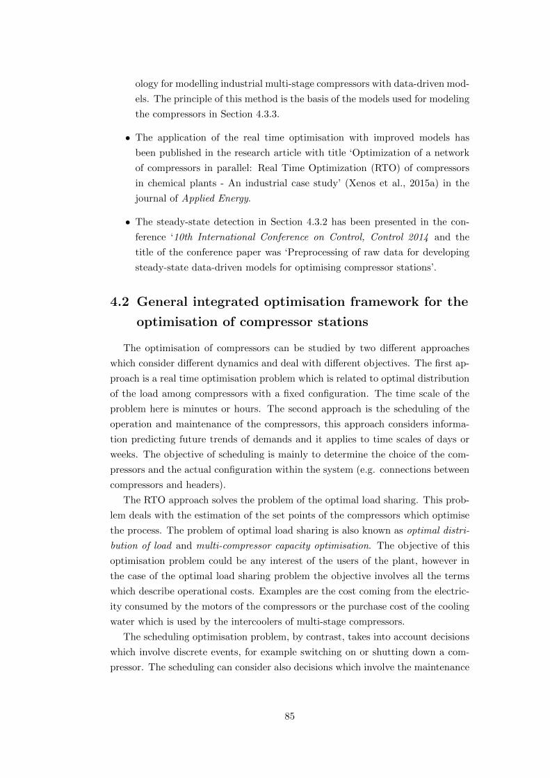
ology for modelling industrial multi-stage compressors with data-driven mod-
els. The principle of this method is the basis of the models used for modeling
the compressors in Section 4.3.3.
• The application of the real time optimisation with improved models has
been published in the research article with title ‘Optimization of a network
of compressors in parallel: Real Time Optimization (RTO) of compressors
in chemical plants - An industrial case study’ (Xenos et al., 2015a) in the
journal of Applied Energy.
• The steady-state detection in Section 4.3.2 has been presented in the con-
ference ‘10th International Conference on Control, Control 2014 and the
title of the conference paper was ‘Preprocessing of raw data for developing
steady-state data-driven models for optimising compressor stations’.
4.2 General integrated optimisation framework for the
optimisation of compressor stations
The optimisation of compressors can be studied by two different approaches
which consider different dynamics and deal with different objectives. The first ap-
proach is a real time optimisation problem which is related to optimal distribution
of the load among compressors with a fixed configuration. The time scale of the
problem here is minutes or hours. The second approach is the scheduling of the
operation and maintenance of the compressors, this approach considers informa-
tion predicting future trends of demands and it applies to time scales of days or
weeks. The objective of scheduling is mainly to determine the choice of the com-
pressors and the actual configuration within the system (e.g. connections between
compressors and headers).
The RTO approach solves the problem of the optimal load sharing. This prob-
lem deals with the estimation of the set points of the compressors which optimise
the process. The problem of optimal load sharing is also known as optimal distri-
bution of load and multi-compressor capacity optimisation. The objective of this
optimisation problem could be any interest of the users of the plant, however in
the case of the optimal load sharing problem the objective involves all the terms
which describe operational costs. Examples are the cost coming from the electric-
ity consumed by the motors of the compressors or the purchase cost of the cooling
water which is used by the intercoolers of multi-stage compressors.
The scheduling optimisation problem, by contrast, takes into account decisions
which involve discrete events, for example switching on or shutting down a com-
pressor. The scheduling can consider also decisions which involve the maintenance
85
Operation (compressors)
DataAnalysis
ModelsOptimisation
Optimisation
Control system/
operators
raw data
analyseddata
updated models
suggestedset points
set points
infeasible RTO optimisation problem
binary decisions
disturbances (ambient conditions,
demand)
costsdemand forecast
equipment availability
Real Time OptimisationScheduling
Figure 4.1: Integrated framework for the optimisation of compressor stations.
of the compressors. The objective of the scheduling includes cost terms which are
related to operational, maintenance, start up, and shut down costs. The opera-
tional costs in the scheduling are estimated in an aggregated way, however RTO
determines the operational costs in real time in a more refined way.
Although the two different approaches have different objectives, they are highly
integrated. Figure 4.1 shows a simplified graphical representation of the two frame-
works, of RTO and scheduling. The RTO uses the raw data of the measurements
from the operation to develop models. The data analysis examines the quality
of the data and cleans them from outliers. The optimisation uses the models to
suggest optimal set points to the control system. The control system under the
supervision of operators apply the set points to the compressors. This loop occurs
in a frequent basis in order to deal with changes in parameters. The parameters
change due to disturbances such as ambient conditions and demand.
When the actual demand given in the RTO is significantly different from that
which is predicted in the scheduling problem, then the RTO problem may become
infeasible. This is because the online compressors may not be able to meet the
requirements of the demand side. In this case, the scheduling problem updates its
models and a new schedule of the compressors is estimated. The new schedule gives
the new configuration of the system which can satisfy the demand, for instance by
bringing another compressor online. Another example is when compressors which
are online can satisfy the demand, but the demand could be satisfied by fewer
compressors, then, again, the scheduling problem has to be solved to estimate a
new set of compressors for optimal operation (it is also possible that the overall
analysis suggests keeping the same configuration). This integration will not be
studied in depth as it is not part of the scope of the thesis. However, discussions
86

on this topic will be presented in Chapter 7.
The framework in Fig. 4.1 connects several decisions tasks from Level 0, 1, 2
and 3 of the automation pyramid in Fig. 2.8b presented in Chapter 2, for example
optimal scheduling and maintenance, optimal load sharing and update of the maps,
and control and monitoring of the operation of compressors. The optimal load
sharing considers the updates of compressor maps which corresponds to the asset
monitoring in Level 3 in the manufacturing execution system of pyramid in Fig.
2.8a.
4.3 A Real Time Optimisation (RTO) framework
using data-driven models
Operation (compressors)
Validation ofdata
Parameter estimation
Optimisation(NLP)
Monitoring(sensors)
Raw data
Steady-state identification
Validated dataUpdated model
parameters
Set points
Applyset points
Input parameters
Disturbances (Ambient conditions,
demand)
Controlsystem/
operators
Figure 4.2: Detailed description of the structure of the components of the RTO.
A basic RTO scheme (Mansour and Ellis, 2008) can be tailored to the operation
of parallel compressors. Figure 4.2 presents the components of the RTO proposed
for compressors, and their relationships.
The sensors of the monitoring system collect process data of the operation
such as mass flow rates, pressures and temperatures. A steady-state identification
algorithm examines key process variables and identifies when the operation is in
steady-state. Thus, if the operation is in steady-state, then the collected data
should be validated (Prata et al., 2010; Mansour and Ellis, 2008). The next step
is to use the validated data to update the models of the online compressors.
A NLP optimisation model employs these data-driven models and estimates
87
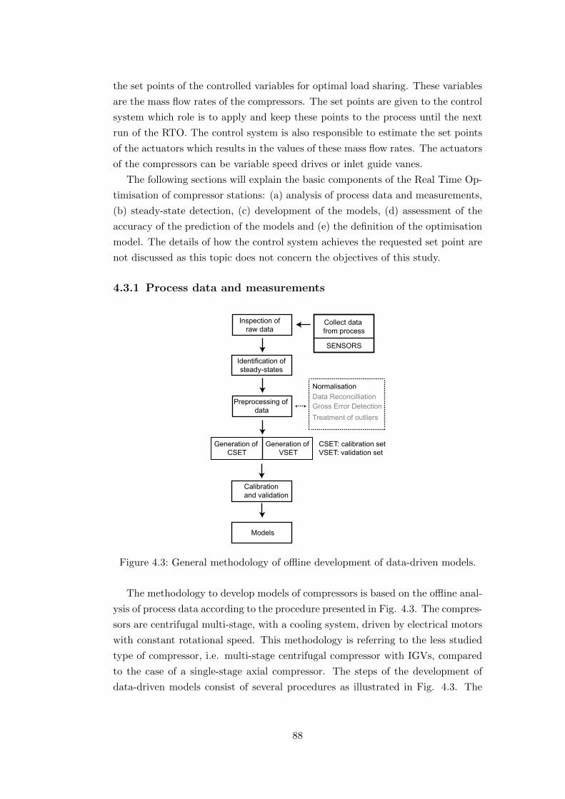
the set points of the controlled variables for optimal load sharing. These variables
are the mass flow rates of the compressors. The set points are given to the control
system which role is to apply and keep these points to the process until the next
run of the RTO. The control system is also responsible to estimate the set points
of the actuators which results in the values of these mass flow rates. The actuators
of the compressors can be variable speed drives or inlet guide vanes.
The following sections will explain the basic components of the Real Time Op-
timisation of compressor stations: (a) analysis of process data and measurements,
(b) steady-state detection, (c) development of the models, (d) assessment of the
accuracy of the prediction of the models and (e) the definition of the optimisation
model. The details of how the control system achieves the requested set point are
not discussed as this topic does not concern the objectives of this study.
4.3.1 Process data and measurements
Inspection ofraw data
Identification of steady-states
Preprocessing of data
Data ReconcilliationGross Error DetectionTreatment of outliers
Normalisation
Generation of CSET
CSET: calibration setVSET: validation set
Calibration and validation
Models
Generation of VSET
Collect data from process
SENSORS
Figure 4.3: General methodology of offline development of data-driven models.
The methodology to develop models of compressors is based on the offline anal-
ysis of process data according to the procedure presented in Fig. 4.3. The compres-
sors are centrifugal multi-stage, with a cooling system, driven by electrical motors
with constant rotational speed. This methodology is referring to the less studied
type of compressor, i.e. multi-stage centrifugal compressor with IGVs, compared
to the case of a single-stage axial compressor. The steps of the development of
data-driven models consist of several procedures as illustrated in Fig. 4.3. The
88

main steps in the procedure are the following:
Inspection of raw data: After the collection of the data from the operation, the
first step is to examine the values of the data set through observation and to gain a
general overview of its structure. Kadlec et al. (2009) mention the importance and
reasons of this step for developing regression models of data-driven soft sensors.
Identification of steady-state analysis and preprocessing of stationary
points: Steady-state regression models do not perform well when the collected
data are collected in transition. There are several methods in the literature to
estimate a steady-state of a process (Cao and Rhinehart, 1995; Jiang et al., 2003;
Kelly and Hedengren, 2013). Kim et al. (2008) suggested an algorithm, which is
simple to implement, to estimate the steady-states of a process. Section 4.3.2 will
present a multi-variate steady-state detection for compressor stations based on the
method proposed by Kim et al. (2008).
Preprocessing of data: Data have been normalised because different variables
have different units, for example power is measured in kW and pressure in bar. In
the current study, the maximum data point of the set is used to divide the set. The
normalised data, then, have to be preprocessed. Data reconciliation, gross error
detection and handling outliers constitute the procedure of the data preprocessing
(Prata et al., 2010). Indeed, it is common to find outliers in raw data. The outliers
can be ignored or to be replaced with predictions of the best value fit of the outlier
replaced.
Generation of the calibration and validation set of data: This step in-
volves the division of the total set of data into two smaller sets. The first set, the
calibration set, is used to estimate the parameters of the regression model while
the validation set examines if the generated model predicts well in a different set
than in the calibration one. The data set used to calibrate the model defines the
domain of validity of the model, which is called regression domain. Extrapola-
tion of the model outside its regression domain may give values which are not
true. Brooks et al. (1988) presented a study which characterises the domain of
regression models.
Calibration and validation of data: The next step is to decide the structure
of a model which describes the process. The process here is the compression of
ambient air from a multi-stage centrifugal compressor, presented in Fig. 4.4. The
89

Atmospheric air
Stage 1
Stage 2
Intercooler 1 Intercooler n
Stage n
AftercoolerWel
Pout
M: MotorGB: Gearbox
M GB
Min , Tin, pin
Compressed air
Figure 4.4: Multi-stage centrifugal compressor with inlet and outlet measurements.
model is calibrated and validated with the calibration and validation data sets
respectively.
The models are developed from historical data. The use of these data-driven
models allows the modelling of the multi-stage compressors with available mea-
surements only at the inlet of the first and at the exit of the last stage. A rigorous
model requires measurements between the stages of compression and analytical
models of the intercoolers. Moreover, the use of a data-driven model in the op-
timisation reduces the computational burden compared to the use of a rigorous
model which considers aerodynamics and thermodynamics of the fluid. The com-
putational time of the optimisation plays an important role in an online application
such as the RTO.
Figure 4.4 shows that the available process measurements can be found at the
inlet of the first stage and the exit of the outlet of the last stage. The measurements
at the inlet are the mass flow rate ma at standard conditions, TSTP = 273 K (0 oC)
and PSTP = 100 kPa (1 bar) (Wikipedia, 2015c). The specific gas constant of an
ideal gas, which is based on a mean molar mass for dry air of 28.97 g/mol, is
Rg = R/MolW = 287.1 J kg−1 K−1 (Wikipedia, 2015b). The electrical power of
the motor Wel is also given from measurements.
4.3.2 Steady-state detection
The purpose of the steady-state detection algorithm is to identify the steady-
states of the operation of the compressors to develop reliable data-driven models
of industrial compressors similar to this in Fig. 4.4. Data-driven models are black
boxes which hold a relationship between input and output variables. According to
Cao and Rhinehart (1995) and Kim et al. (2008), these input and output variables
should be close to steady-state to hold the validity of the mass and energy balances
implied in the black box
A steady-state detection algorithm based on a moving window was developed.
Figure 4.5 shows the application of the moving window to a data-set of a single
90

process variable. A moving data-set window is defined from a fixed number of data
points of the process variable, ns. The data included in the window are updated at
each step τ , recent data are added and old data are discarded. The window moves
every S number of data points. A process variable v has value x(i,v,t), where i ∈ I(I is the set of compressors), v ∈ V (V is the set of variables) and t ∈ T tot (T tot
is the set of data points which corresponds to the total sample time). Variable τ
corresponds to a window with data (t−ns + 1, t). The sample rate of the data set
(referring to the discretisation t ∈ T tot), the ns and the S are parameters which
have to be tuned for a desired function of the steady-state detection algorithm
relevant to the application.
At each step τ the data-set window moves to t′ = t + S and the standard
deviation of the included data points in the window, σ(i,v,τ), of compressor i and
variable v is calculated from:
σ(i,v,τ) =
√√√√ 1
ns
∑t′∈(t−ns+1,t)
(x(i,v,t′) − µ(i,v,τ))2(4.1)
where x(i,v,τ) is the mean of the data in the window:
x(i,v,τ) =1
ns
∑t′∈(t−ns+1,t)
x(i,u,t′) (4.2)
The steady-state algorithm detects a steady-state episode of a process variable
v when a particular condition holds true, for example if three times the standard
deviation 3σ(i,v,τ) is less than a predefined value h(i,v). This bound is chosen by
reference pointat τ = 2
data consideredat τ = 2
window τ =1window τ = 2
window τ = 3
t
SnS
proc
ess
varia
ble
Figure 4.5: Moving time data set window.
91

the users according to their engineering judgement as there are not standardised
values for this type of application.
The developed steady-state algorithm is multivariate and involves the exam-
ination of more than one variables to assess when the system is in steady-state.
According to Mansour and Ellis (2008) a system is in steady-state when all the con-
sidered variables are in steady-state. The system in this study is the compressors
which operate in parallel.
Hence, if a process variable v of compressor i is in steady-state at t then a
binary variable Yss(i,v,t) is equal to one, otherwise the variable takes the value
zero. Therefore, the steady-state of the system of i ∈ I compressors considering
v ∈ V ′ ⊆ V variables is estimated from the value of the variable Yss,system:
Yss,system =∏i∈I
∏v∈V ′
Yss(i,v,t) (4.3)
The output of the steady-state detection algorithm is a matrix of data with
J ′ rows (variables) and T ∗ columns (number of final steady-states of the system)
where T ∗ ⊆ T tot.
4.3.3 Development of models
0 1 2 3 4 5 6 7x 10⁵
0.2
0.4
0.6
0.8
1
Time (s)
angle of IGVs (θ)
air mass flow rate (Min)
ambient temperature (Tin)
Pro
cess
var
iabl
es (n
orm
alis
ed)
Figure 4.6: Several process variables (normalised) of the operation of an industrialcentrifugal compressor over time.
The development of a black box model of the compressor system of Fig. 4.4
includes: the multi-stage compressor, the cooling system, the rotating shaft, gear-
box and motor. According to the step tests in an industrial centrifugal compressor
of the air compressors in the air separation plant in BASF, it was shown that the
92

Χ = [ Min , pin , Tin , Pout ]
BLACKBOX
Input measured variables
Output predicted variable
Υ = Wel
Figure 4.7: Black box model which associates input with output variables.
power consumption of the motor mainly depends on the mass flow entering the
compressor, Min, the ambient conditions, Tin, Pin, and the pressure at the exit of
the compressor (discharge pressure), Pout.
In this test the compressor is disconnected from the downstream process and
receives different constant set points of the position of the IGVs for defined time
periods. The outlet conditions of the compressor are kept constant. These step
tests took place for one week and data with 10s sample interval, i.e 0.1Hz sample
rate, were collected. The investigation of the behaviour of the process variables of
the operation of this compressor helps to inspect which data should be taken into
account for the development of data-driven models and helps to identify upper
bounds for ideal steady-states.
Several measurements can be acquired from the Distributed Control System
(DCS), for example the mass flow at the exit of the compressor, the temperature
and pressure of the environment and the power consumed by the motors. Figure
4.6 shows three process variables, angle of the IGV (θ), mass flow rate (Min) and
ambient temperature (Tin), over time during the step tests. The values on the ver-
tical axis are normalised. All of these variables influence the power consumption.
Figure 4.6 shows that the mass flow rate is considerably influenced by the θ.
Indeed, the mass flow rate changes in a non-linear way with the change of the θ.
When the θ changes from 0.19 to 0.43 between 1 · 105 and 2 · 105 s, the mass flow
rate changes significantly compared to smaller changes in the mass flow rate from
larger changes of the θ between 2 · 105 and 3 · 105 s. Moreover, when θ is fixed,
the mass flow changes at a slow rate following inversely the change in the ambient
temperature.
Figure 4.7 shows the procedure for the development of the model of the opera-
tion of a multi-stage compressor. A black box is used to predict the power which
is consumed from the electrical driver Wel and this power is the output of the
model. The black box model represents the power as function of process variables
of the operation, Min(i,t), Tin, Pin, Pout. These variables represent the input of the
model. A polynomial regression model is used to develop the black box model
of each compressor i, by defining x(i,k,t) = [Min(i,t), T(in,t), P(t), Pout(t)] with k = 4
number of input variables and y(i,t) = Wel(i,t), then the following polynomial gives
93
the black box model of compressor i:
y∗(i,t) = b(i,0) + b(i,1) · x∗(i,1,t) + b(i,2) · x∗(i,2,t) + b(i,3) · x∗(i,3,t) + b(i,4) · x∗(i,4,t)+b(i,5) · x∗2(i,1,t) + b(i,6) · x∗2(i,2,t) + b(i,7) · x∗2(i,3,t) + b(i,8) · x∗2(i,4,t)+
b(i,9) · x∗(i,1,t) · x∗(i,2,t) + b(i,10) · x∗(i,1,t) · x
∗(i,3,t) + b(i,11) · x∗(i,1,t) · x
∗(i,4,t)
(4.4)
where y∗(i,t) = y(i,t)/ymax(i) , x∗(i,k,t) = x(i,k,t)/x
max(i,k) are the scaled variables of the
regression models of compressors i ∈ I. The xmax(i,k), ymax(i) are the maximum variables
of their respective calibration and validation sets. The parameters of the models,
b(i,m) with m = 0, 2, . . . , 11 are calculated with regression methods (Rosipal and
Kramer, 2006).
The black box model described by Eq. (4.4) has been derived based on the anal-
ysis of the available input data and the output data (power). The key variables
xk have been chosen based on the observation of data (plots of power against the
xk variables), examining the correlation between power and xk variables. Knowl-
edge also on the physical connections between power and other variables such as
temperatures and pressures has influenced the choice of the variables.
The choice of the form of the black box model and the terms of the polynomial
of the right hand side of the equation is based on several iterations until to reach
an acceptable level of accuracy of prediction, in other words reduced prediction
error for a validation set of data. The Matlab function stepwisefit (Matlab, 2014)
was employed to assess different regression models.
4.3.4 Assessment of the accuracy of the prediction of the models
To evaluate the accuracy of the prediction of the models the Coefficient of
Variation of the Root Mean Square Error, CV(RMSE) is used (Wikipedia, 2014):
CV(RMSE) =RMSE
y=
√(∑
t∈T ∗(ymeas(i,t) − y(i,t))2)/T ∗
y
and the coefficient of determination, known as R-squared (RSQ) expresses how
well the data fit the model (Matlab, 2014):
Sres = 1−(∑
t∈T ∗(ymeas(i,t) − y(i,t))2)
(T ∗ − 1) · vy
where y is the mean and vy is the variance of the predicted values of y, and ymeas
are the measured variables.
94

4.3.5 Optimisation model of the RTO
The offline steady-state identification algorithm, presented in Section 4.3.2 is
modified for online applications. The online steady-state identification examines
if the Yss,system is one at the current moment, tr, considering V ′ variables of each
compressor i at the window (tr − ns − 1, tr).
According to Fig. 4.3, raw data are collected from the operation after the
steady-state detection and they are validated through data reconciliation. The
validated data are used (a) to update the parameters of the models which are
used from an optimisation model and (b) to provide the input parameters of this
optimisation model. The set points of the mass flow rates, which are the output of
the optimisation model, are the input to the control system. The controller can be
a feedback controller. The controller deals with the application of the set points
and adjusts the position of the actuators (IGVs) to achieve the desired flows.
There is usually a mismatch between models and reality due to fitting errors and
performance changes due to fouling and erosion, as was also reported in (Paparella
et al., 2013). This mismatch influences the shape of the objective function of the
optimisation problem and consequently the estimation of the minimum of the total
power consumed. To reduce this influence, the mass flow rates of the compressors
were chosen as degrees of freedom of the optimisation problem. The position of the
IGVs can be then adjusted from the controllers. An analysis of the models showed
that the accuracy in prediction of the models does not improve significantly when
the position of the IGVs is considered as an input variable in the models.
Defining the mass flow rates ω∗(i,tr) as optimisation variables (degrees of freedom
or decision variables of the optimisation) and z∗ = [x∗(2,tr)x∗(3,tr)
x∗(4,tr)] as the input
parameter vector of the optimisation model (Fig. 4.2) , then the optimal load
distribution at a steady-state episode which starts at point t = tr is computed by
the following optimisation formulation:
minω∗∑i∈I
Wel(i,tr) (4.5)
subject to:
W ∗el(i,tr) = fi(z∗, ω∗(i,tr),b(i)), ∀i ∈ I (4.6)
Wel(i,tr) = W ∗el(i,tr) · ymax(i) , ∀i ∈ I (4.7)
Min(i,tr) = ω∗(i,tr) · xmax(i,1) , ∀i ∈ I (4.8)∑
i∈IMin(i,tr) = Mdem(tr) (4.9)
95

Mmin(i) ≤Min(i,tr), ∀i ∈ I (4.10)
Min(i,tr) ≤ xmax(i,1) , ∀i ∈ I (4.11)
Wminel(i) ≤Wel(i,tr), ∀i ∈ I (4.12)
Wel(i,tr) ≤ ymax(i) , ∀i ∈ I (4.13)
Equation (4.5) describes the objective function which is the minimisation of
the power consumption at steady-state which starts at t = tr, and Eq. (4.6)
describes the constraints which give the power of each compressor i as function of
the z∗ and normalised mass flow rates ω∗(i,tr). Equations (4.7) and (4.8) refer to
the normalisation of the powers and mass flow rates. Equation (4.9) provides the
mass balance between summation of the flows of the compressors and the demand,
Mdem(tr), requested. Finally, Eqs. (4.10) – (4.13) define the regression domain.
The above optimisation formulation was implemented in MatlabTM using the
optimisation function fmincon (Matlab, 2014b). The results from the optimisation
on a real industrial case study with compressors of a process plant will be presented
in Section 4.5.3. The description of the case study is given in the next section.
4.4 Description of the industrial case study
This section presents the application of the methodology of RTO to the air
compressor station of multi-stage compressors in parallel in BASF, Germany, which
distributes compressed air to different end-users. The end-users are air separation
columns and plant-site utilities for compressed air. The air compressor station
consumes the major part of the total energy in the air separation plant. Moreover,
the power rating of the plant is several tens of MW.
The case study to be examined has the following characteristics:
• The compressor station involves three air multi-stage centrifugal compressors
similar to the compressor depicted in Fig. 4.4.
• The compressors operate in parallel to supply an air separation column with
compressed air. The air separation column requests compressed air of mass
flow rate, Mdem, at a constant pressure, Pop.
• The three compressors are assumed to have the same specifications, which
are power rate, minimum and maximum capacity and efficiencies, at the
point of the commissioning of the plant. However, the compressors are not
in the same condition during the time period of the study as will be shown
in Section 4.5.
96
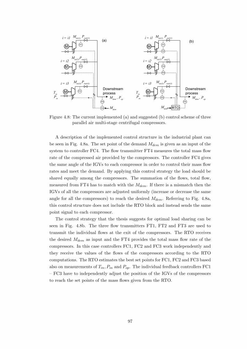
i = i1
i = i3
i = i2
Min(i1) Pout(i1)
Pout(i2)
Pin
Pout(i3)
Min(i2)
Min(i3)
Mdem , Pop
Tin
Downstreamprocess
FT1
FT2
FT3
Mdem
M
M
M
FC4
FT4
i = i1
i = i3
i = i2
Min(i1) Pout(i1)
Pout(i2)
Pin
Pout(i3)
Min(i2)
Min(i3)
Mdem , Pop
Tin
Downstreamprocess
FC1
FT1
FC2
FT2
FC3
FT3
RTOMdem
M
M
M
FT4
(a) (b)
Figure 4.8: The current implemented (a) and suggested (b) control scheme of threeparallel air multi-stage centrifugal compressors.
A description of the implemented control structure in the industrial plant can
be seen in Fig. 4.8a. The set point of the demand Mdem is given as an input of the
system to controller FC4. The flow transmitter FT4 measures the total mass flow
rate of the compressed air provided by the compressors. The controller FC4 gives
the same angle of the IGVs to each compressor in order to control their mass flow
rates and meet the demand. By applying this control strategy the load should be
shared equally among the compressors. The summation of the flows, total flow,
measured from FT4 has to match with the Mdem. If there is a mismatch then the
IGVs of all the compressors are adjusted uniformly (increase or decrease the same
angle for all the compressors) to reach the desired Mdem. Referring to Fig. 4.8a,
this control structure does not include the RTO block and instead sends the same
point signal to each compressor.
The control strategy that the thesis suggests for optimal load sharing can be
seen in Fig. 4.8b. The three flow transmitters FT1, FT2 and FT3 are used to
transmit the individual flows at the exit of the compressors. The RTO receives
the desired Mdem as input and the FT4 provides the total mass flow rate of the
compressors. In this case controllers FC1, FC2 and FC3 work independently and
they receive the values of the flows of the compressors according to the RTO
computations. The RTO estimates the best set points for FC1, FC2 and FC3 based
also on measurements of Tin, Pin and Pop. The individual feedback controllers FC1
– FC3 have to independently adjust the position of the IGVs of the compressors
to reach the set points of the mass flows given from the RTO.
97

4.4.1 Practical challenges of the case study
The case study of the industrial air separation process has revealed several
practical challenges which are summarised below. These challenges should be
considered in order to achieve a realistic approach of the proposed methodology.
The BASF operators did not operate the compressors over their full range in
the collected data set. Therefore, only a partial compressor map is captured in the
regression models. Hence, the feasible window of operation of the model used for
the optimisation is not defined from the actual physical limits of the compressor,
i.e. surge, choke, and minimum and maximum angles of IGVs. Instead, this
feasible operational window of the compressor is defined from the domain of the
regression model (Brooks et al., 1988). The regression domain is a part of the
actual operational window.
Figure 4.9a demonstrates that an operating point of the compressors comes
from the intersection of the Compressor System (CS) curve and the load curve of
the downstream process. The Compressor System curve is defined as the merged
individual compressor characteristics of the parallel compressors assuming that
the inlet conditions are the same of all compressors. The set of all the operating
points of the corresponding data set defines the regression domain of the model
of a compressor as can be seen in Fig. 4.9b. It is known from the plant that
the operators operated well within the physical limits (surge and choke) of the
compressors during the past operation.
A model is expected to be more accurate when the data set is collected over a
shorter time period, for example one week than a model derived from a data set of
several months because for longer period the compressor might have been in various
states during this period. For example, a compressor is efficient immediately after
Pre
ssur
e ra
tio
Flow of compressor
Characteristics of compressor for differernt IGVs openings
maximumcapacity
Chokeline
Surgeline
minimumcapacity Regression
domain
Pre
ssur
e
Flow of downstream process
(a) (b)
High demandload curve
Low demandload curve
Partial demandload curveOperating
point πr.d.(i)max
πr.d.(i)min
Mr.d.(i)min Mr.d.(i)
max
Figure 4.9: An operating point of the system defined by the intersection betweenload curve and characteristic of the system (CS curve) (a) and thefeasible window of operation (i.e regression domain) of a compressorwith IGVs (b).
98

maintenance and less efficient after many hours of operation. However, the range
of the regression domain of the model is smaller in the case of a more accurate
model. Moreover, for the purposes of the development of the models, the operators
should ideally run the compressors at different operating points through the day so
as to increase the range of the regression domain. However, such experimentation
is not practically feasible when the plant is operating for commercial production.
In the case that the compressor was operated close to the surge or choke line,
the regression domain cannot be assumed rectangular (see Fig. 4.9b) due to the
physical restrictions. There are two options to deal with this issue: (a) use a
convex hull for describing the regression domain, or (b) add an extra constraint
in the optimisation model described by Eqs. (4.6) – (4.13). The use of a convex
hull can be seen in Brooks et al. (1988) and in Mitra et al. (2012). The convex
hull ensures a more tight regression domain which increases the validity of the
model in its boundaries (Kahrs and Marquardt, 2007). The extra constraint can
be a regression black box model of the outlet pressure which relates the mass flow
rate and other parameters such as ambient temperature and pressure, Pout(i) =
gi(z,Min(i), c(i)), i ∈ I where ci is the vector of the fitted parameters of the new
regression model. The application of the convex hull is not used in the RTO
application, however it is explained in detail in the next Chapter 5.
The data reconciliation step requires redundant measurements, for example
extra measurements of the flow apart from these at the exit of the compressors.
Unfortunately the industrial case study did not have these measurements, and
hence the data reconciliation step could not be implemented.
4.5 Results
4.5.1 Models of compressors
Table 4.1: Statistics of the fitting and validation of the regression models.
Fitting Validation Validation
Compressors RSQ RSQ CV(RMSE)
i1 0.992 0.992 0.54i2 0.968 0.967 0.67i3 0.987 0.988 0.57
Data from fifteen days of operation were used to develop the models of the com-
pressors. The case study assumed that the performance of the models deteriorates
gradually and that there was no event which has caused a relatively high discon-
tinuous decrease in performance. Data of 129600 continuous operating points with
99

0.75 0.8 0.85 0.9 0.95 1
0. 8
0.85
0. 9
0.95
1
Normalised actual power (-)
Nor
mal
ised
pre
dict
ed p
ower
(-)
(a) Compressor i1
0.75 0.8 0.85 0.9 0.95 1
0. 8
0.85
0. 9
0.95
1
Normalised actual power (-)
Nor
mal
ised
pre
dict
ed p
ower
(-)
(b) Compressor i2
0.75 0.8 0.85 0.9 0.95 1
0. 8
0.85
0. 9
0.95
1
Normalised actual power (-)
Nor
mal
ised
pre
dict
ed p
ower
(-)
(c) Compressor i3
Figure 4.10: Prediction versus actual values of power of compressors i1, i2 and i3in the validation set.
10s sample interval (0.1 Hz sample rate) were collected. The steady-state algo-
rithm detected 7430 steady-state episodes in the examined data set for the system
of the compressors. Of these episodes, 80% were used for the fitting of the model
and the remaining 20% were used to validate the developed model.
Table 4.1 presents the statistics of the fitting, RSQ, and the validation, RSQ
and CV(RMSE), of the models of the three compressors. The standard function
LinearModel.fit of MatlabTM (Matlab, 2014) was used to fit the data into the poly-
nomial of Eq. (4.4). The computational time of the estimation of the coefficients is
a few seconds. Figure 4.10 shows the prediction of the normalised power consump-
tion of each compressor versus the measurements of the power. The axes present
normalised values of the power due to confidentiality restrictions. The normali-
sation of the power consumption of each compressor is calculated by dividing the
power with the ymaxi .
Compressor i1 shows the most accurate match between prediction and actual
measurements of the power. The fitting of the model has also higher RSQ value
100
than in the other cases. In the case of compressor i2 the accuracy of the prediction
is relatively less than of the other two compressors. The reason for this is that
the measurements of the mass flow and power of compressor i2 are relatively more
noisy than in the case the other two compressors. The CV(RMSE) of the models
ranges between 0.54% and 0.67%. By comparing the mean RMSE results with
other results from similar case studies (Han et al., 2004; Xenos et al., 2014b) these
models can be considered of high accuracy for predicting power consumption of
compressors.
Table 4.2 presents the minimum and maximum bounds of the mass flow rates
and powers of the three compressors. The values shown in Table 4.2 represent the
boundaries of mass flow rates and powers where they are divided by two scaling
factors to keep the confidentiality agreement with the provider of the case study.
In other words, the units are dimensionless and scaled. The table shows that
compressors have different regression domains with compressor i1 having a larger
feasible operational window than the other two. The values of the coefficients of
the regression models of the three compressors can be seen in Tables 4.3 and 4.4.
Table 4.2: Boundaries of mass flow rates and power consumptions.
Compressor Mminin(i) xmax(i,1) Wmin
el(i) ymax(i)
i1 0.670 0.924 0.304 0.406i2 0.676 0.836 0.295 0.365i3 0.624 0.842 0.286 0.374
Table 4.3: First six coefficients of the regression models.
Compressor b0 b1 b2 b3 b4 b5i1 -1.24 -0.24 -2.00 3.13 2.26 0.96i2 0.76 -20.61 5.98 23.84 -12.49 0.09i3 9.22 -2.58 -16.97 -0.69 1.73 0.97
Table 4.4: Last six coefficients of the regression models.
Compressor b6 b7 b8 b9 b10 b11
i1 1.27 -1.61 -0.99 -0.60 0.24 -0.16i2 -9.08 -8.86 -0.37 14.00 -7.22 15.00i3 9.20 -0.25 -1.52 -1.24 1.59 1.56
101
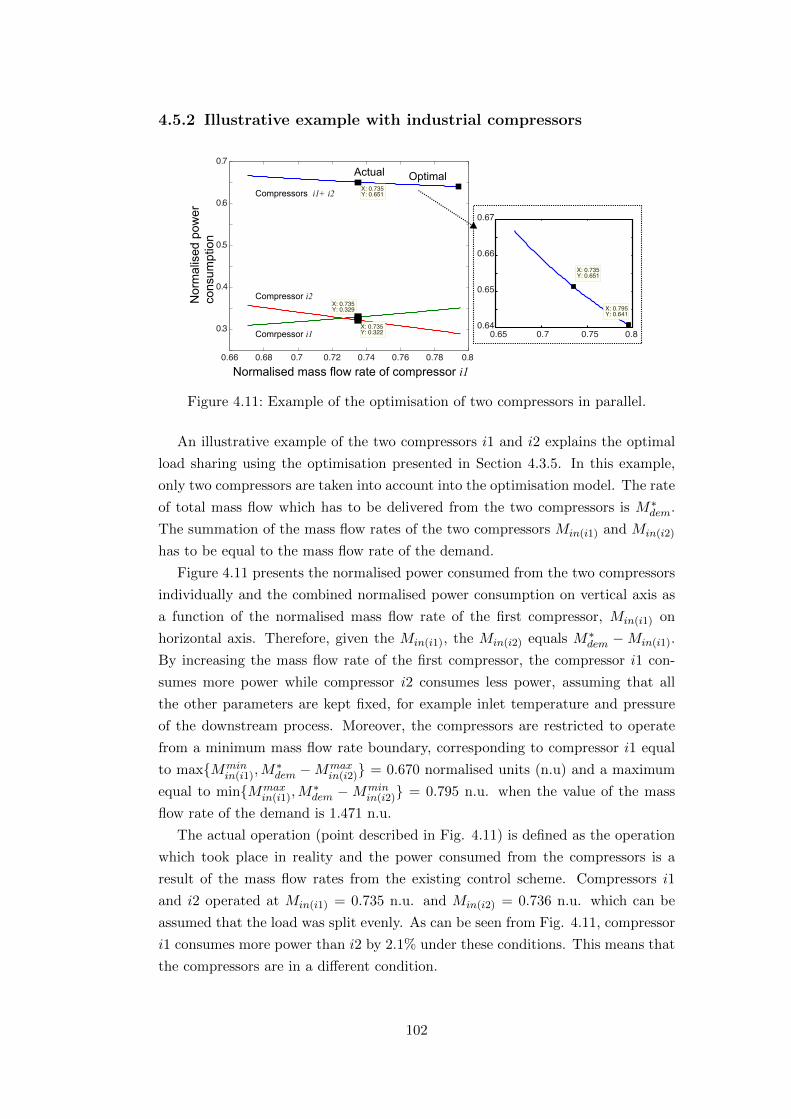
4.5.2 Illustrative example with industrial compressors
0.66 0.68 0.7 0.72 0.74 0.76 0.78 0.8
0.3
0.4
0.5
0.6
0.7
X: 0.735Y: 0.651
X: 0.735Y: 0.322
X: 0.735Y: 0.329
0.65 0.7 0.75 0.80.64
0.65
0.66
0.67
X: 0.735Y: 0.651
X: 0.795Y: 0.641
Nor
mal
ised
pow
erco
nsum
ptio
n
Normalised mass flow rate of compressor i1
Compressors i1+ i2
OptimalActual
Compressor i2
Comrpessor i1
Figure 4.11: Example of the optimisation of two compressors in parallel.
An illustrative example of the two compressors i1 and i2 explains the optimal
load sharing using the optimisation presented in Section 4.3.5. In this example,
only two compressors are taken into account into the optimisation model. The rate
of total mass flow which has to be delivered from the two compressors is M∗dem.
The summation of the mass flow rates of the two compressors Min(i1) and Min(i2)
has to be equal to the mass flow rate of the demand.
Figure 4.11 presents the normalised power consumed from the two compressors
individually and the combined normalised power consumption on vertical axis as
a function of the normalised mass flow rate of the first compressor, Min(i1) on
horizontal axis. Therefore, given the Min(i1), the Min(i2) equals M∗dem −Min(i1).
By increasing the mass flow rate of the first compressor, the compressor i1 con-
sumes more power while compressor i2 consumes less power, assuming that all
the other parameters are kept fixed, for example inlet temperature and pressure
of the downstream process. Moreover, the compressors are restricted to operate
from a minimum mass flow rate boundary, corresponding to compressor i1 equal
to maxMminin(i1),M
∗dem −Mmax
in(i2) = 0.670 normalised units (n.u) and a maximum
equal to minMmaxin(i1),M
∗dem −Mmin
in(i2) = 0.795 n.u. when the value of the mass
flow rate of the demand is 1.471 n.u.
The actual operation (point described in Fig. 4.11) is defined as the operation
which took place in reality and the power consumed from the compressors is a
result of the mass flow rates from the existing control scheme. Compressors i1
and i2 operated at Min(i1) = 0.735 n.u. and Min(i2) = 0.736 n.u. which can be
assumed that the load was split evenly. As can be seen from Fig. 4.11, compressor
i1 consumes more power than i2 by 2.1% under these conditions. This means that
the compressors are in a different condition.
102
From the combined curve (Compressors i1 + i2), it can be observed that in the
actual operation the mass flow rate of compressor i1 is Min(i1) = 0.735 n.u. In this
case, the total consumption is higher than operating at the point which compressor
i1 has mass flow rate Min(i1) = 0.795 n.u. The reduction in power is 1.54% in
this case. In other words, this observation demonstrates that compressor i1 is
more efficient than compressor i2 at these conditions. The more the compressor
i1 operates against compressor i2 the higher is the total power reduction in the
available search space. The upper boundary results due to the minimum mass flow
rate boundary of compressor i1.
The above analysis and graphical representation is feasible for two compressors
but if more than two compressors are involved in a compressor station, then opti-
misation deals with the estimation of the minimum value of the objective function
while ensuring that the constraints hold valid.
4.5.3 Demonstration of Real Time Optimisation (RTO)
application in parallel with real operation
Table 4.5: Three different cases of operation.
Case Mass flow rates to estimate power using Eq. (4.4)
Actual operation The mass flow rates are given from the real dataEqual split operation The demand is split to equal mass flow ratesOptimal operation The mass flow rates are given from the optimisation
Section 4.5.3 examines the application of the developed RTO methodology on
a simulation of real time operation. The historical data are simulated as if given
in real time and the RTO runs in parallel with the operation of the system which
is depicted in Fig. 4.8a. The RTO determines the conditions for the optimal load
sharing and the results coming from the computations of the RTO are compared
with the operation that took place in reality. The RTO methodology was applied
to the compressor system of the three parallel compressors for more than 12h.
The steady-state detection is configured to examine when the three compressors
are in steady-state simultaneously for 40s. The inputs of the optimisation are
collected during this period. After the RTO calculations, the system is examined
if it is still in steady-state and if this holds true the RTO results are given to
the proposed control system (see Fig. 4.8). The compressors would move to a
new steady state that is different from the one in the historical data. The current
approach examines each steady state of the historical data individually. The online
steady-state detection algorithm identified 50 steady-state episodes where the first
16 can be seen in Fig. 4.12.
103

7.7 7.72 7.74 7.76 7.78 7.8 7.82x 10⁵
0.72
0.73
0.74
0.75
0.76
0.77
0.78
0.79
0. 8
Comp.i1
Comp.i2
Comp.i3
Time (s)
Nor
mal
ised
pow
er c
onsu
mpt
ion
SteadyStates
1 6 9 13 148432 5 10
Past operation
Figure 4.12: The first sixteen steady-state episodes of the system of the compres-sors, compressor i1 (green), compressor i2 (blue) and compressor i3(red).
5 10 15 20 25 30 35 40 45 500.94
0.95
0.96
0.97
0.98
0.99
1
Number of steady-state episode
Nom
ralis
ed p
ower
con
sum
ptio
n
Actual operationEqual split operationOptimal operation
Figure 4.13: Normalised total power consumption during the periods of steady-state operation of the three compressors from actual, equal split andoptimal operation.
It was assumed that the compressor conditions do not change significantly dur-
ing the 15-day period of the collected data in Section 4.5.1 and the updated com-
pressor maps from the 15-day time window were used in the optimisation. Figure
4.13 shows the normalised power consumption of the three compressors in three
different cases for the examined 12 h: (a) actual operation, (b) equal split opera-
104

tion and (c) optimal operation. Table 4.5 shows these three case studies with the
assumptions considered to estimate the power consumption.
The power consumption in Fig. 4.13 is a calculated quantity whose errors
depend on errors in the quantities used in the calculation. The difference between
the actual operation and equal split operation might be attributed to random
variability in the data. However the power consumption for optimal operation
is systematically lower and the difference cannot be accounted for by random
statistical variation. The measurement error in the mass flow rate is less than
+/-0.005 on the normalised mass flow rate scale. This applies to the results in
Figs. 4.13 – 4.19.
Figure 4.13 shows that the actual operation and the equal split strategy do not
show an important difference in the total power consumed from the compressors.
Moreover, Figs. 4.14 – 4.16 show that the compressors are not equally split in the
actual operation. Especially in the case of compressor i3, it can be seen that there
is a difference between the mass flow rate from equal split operation and actual
operation. Although the values of the mass flow rates in the case of the equal split
are different from the mass flow rates from the actual operation, there is not much
difference in the total power consumption.
On the other hand, Fig. 4.13 shows that the optimisation achieves reduction
in the total power consumption in all 50 steady-state periods. Figure 4.14 shows
that compressor i1 should work at higher mass flows than in the case of the actual
and equal split operation and Fig. 4.15 shows that compressor i2 should work at
lower mass flows. Figure 4.16 demonstrates that the optimal operation suggests
that compressor i3 has to work at mass flow rates very close to the mass flows
the actual operation which took place. In other words, the optimisation estimated
5 10 15 20 25 30 35 40 45 500.65
0.7
0.75
0.8
0.85
0.9
Number of steady-state episode
Com
pres
sor i
1 no
rmal
ised
mas
s flo
w ra
te
Actual operationEqual split operation
Min/max boundariesOptimal operation
Figure 4.14: Compressor i1 normalised mass flow rate from three different cases.
105

that compressor i3 was operated well during the actual operation but compressor
i1 as more efficient should be loaded more than compressor i2 which is less efficient
under the current operational conditions.
It was observed that in actual operation compressor i1 and i2 were operated
with equal load and compressor i3 dealt with the remaining load. The RTO
method was applied exclusively to the two compressors i1 and i2 in the case
of the 50 steady-state episodes. This is because the previous results from the
optimisation showed that compressor i3 should not change operating point from
this of the actual operation, therefore the mass flow of compressor i3 does not have
any degree of freedom in the optimisation.
5 10 15 20 25 30 35 40 45 500.65
0.7
0.75
0.8
0.85
0.9
Number of steady-state episode
Com
pres
sor i
2 no
rmal
ised
mas
s flo
w ra
te Actual operation
Equal split operation
Min/max boundariesOptimal operation
Figure 4.15: Compressor i2 normalised mass flow rate from three different cases.
5 10 15 20 25 30 35 40 45 500.65
0.7
0.75
0.8
0.85
0.9
Number of steady-state episode
Com
pres
sor i
3 no
rmal
ised
mas
s flo
w ra
te
Actual operationEqual split operation
Min/max boundariesOptimal operation
Figure 4.16: Compressor i3 normalised mass flow rate from three different cases.
106
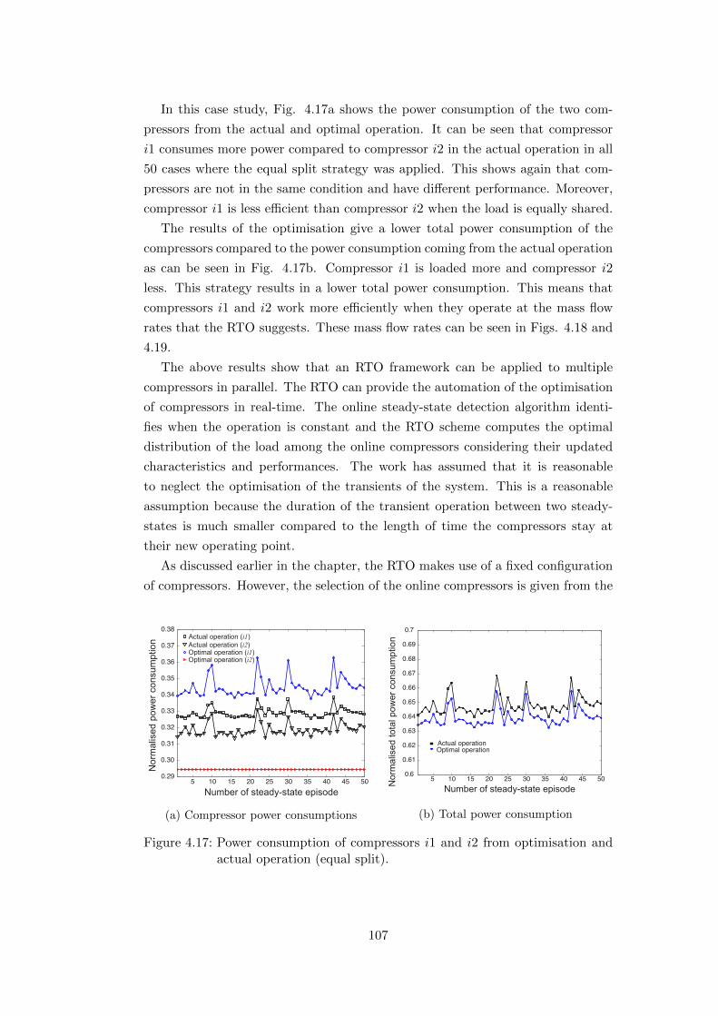
In this case study, Fig. 4.17a shows the power consumption of the two com-
pressors from the actual and optimal operation. It can be seen that compressor
i1 consumes more power compared to compressor i2 in the actual operation in all
50 cases where the equal split strategy was applied. This shows again that com-
pressors are not in the same condition and have different performance. Moreover,
compressor i1 is less efficient than compressor i2 when the load is equally shared.
The results of the optimisation give a lower total power consumption of the
compressors compared to the power consumption coming from the actual operation
as can be seen in Fig. 4.17b. Compressor i1 is loaded more and compressor i2
less. This strategy results in a lower total power consumption. This means that
compressors i1 and i2 work more efficiently when they operate at the mass flow
rates that the RTO suggests. These mass flow rates can be seen in Figs. 4.18 and
4.19.
The above results show that an RTO framework can be applied to multiple
compressors in parallel. The RTO can provide the automation of the optimisation
of compressors in real-time. The online steady-state detection algorithm identi-
fies when the operation is constant and the RTO scheme computes the optimal
distribution of the load among the online compressors considering their updated
characteristics and performances. The work has assumed that it is reasonable
to neglect the optimisation of the transients of the system. This is a reasonable
assumption because the duration of the transient operation between two steady-
states is much smaller compared to the length of time the compressors stay at
their new operating point.
As discussed earlier in the chapter, the RTO makes use of a fixed configuration
of compressors. However, the selection of the online compressors is given from the
5 10 15 20 25 30 35 40 45 500.29
0.30
0.31
0.32
0.33
0.34
0.35
0.36
0.37
0.38
Optimal operation (i2)Optimal operation (i1)Actual operation (i2)Actual operation (i1)
Nor
mal
ised
pow
er c
onsu
mpt
ion
Number of steady-state episode
(a) Compressor power consumptions
0.6
0.61
0.62
0.63
0.64
0.65
0.66
0.67
0.68
0.69
0.7
5 10 15 20 25 30 35 40 45 50Number of steady-state episodeN
orm
alis
ed to
tal p
ower
con
sum
ptio
n
Actual operationOptimal operation
(b) Total power consumption
Figure 4.17: Power consumption of compressors i1 and i2 from optimisation andactual operation (equal split).
107
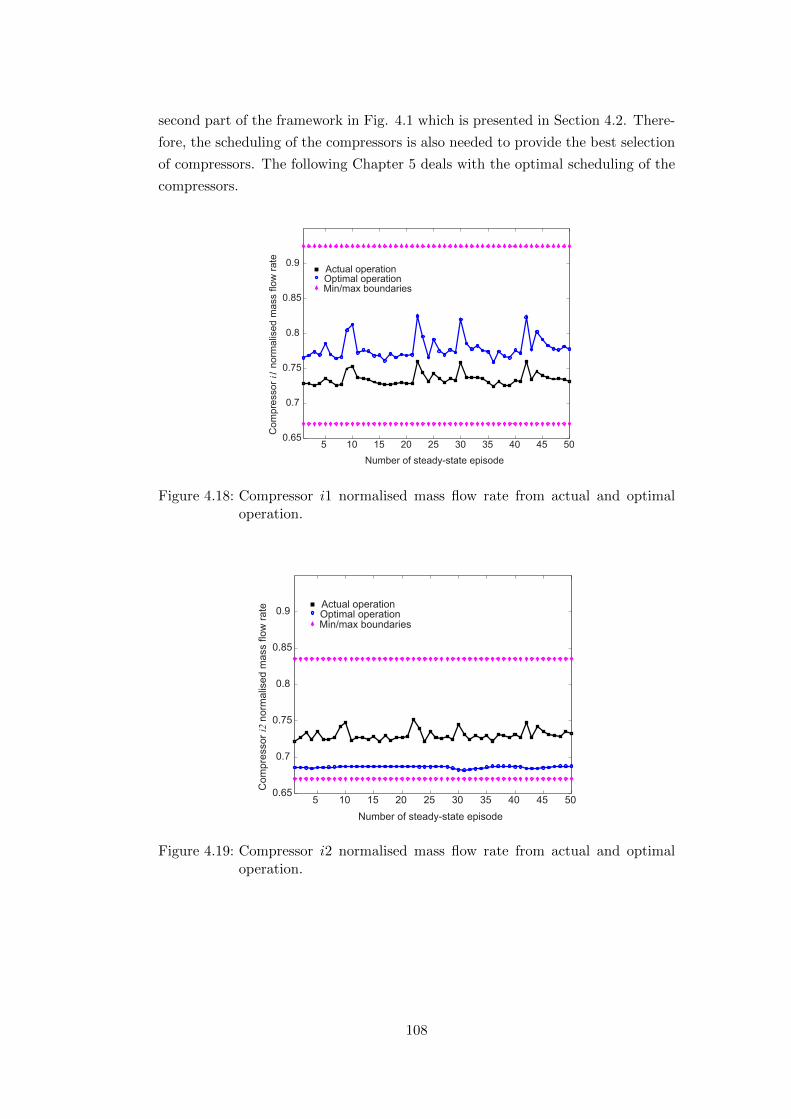
second part of the framework in Fig. 4.1 which is presented in Section 4.2. There-
fore, the scheduling of the compressors is also needed to provide the best selection
of compressors. The following Chapter 5 deals with the optimal scheduling of the
compressors.
5 10 15 20 25 30 35 40 45 500.65
0.7
0.75
0.8
0.85
0.9
Number of steady-state episode
Com
pres
sor i
1 no
rmal
ised
mas
s flo
w ra
te
Actual operation
Min/max boundariesOptimal operation
Figure 4.18: Compressor i1 normalised mass flow rate from actual and optimaloperation.
5 10 15 20 25 30 35 40 45 500.65
0.7
0.75
0.8
0.85
0.9
Number of steady-state episode
Com
pres
sor i
2 no
rmal
ised
mas
s flo
w ra
te Actual operation
Min/max boundariesOptimal operation
Figure 4.19: Compressor i2 normalised mass flow rate from actual and optimaloperation.
108
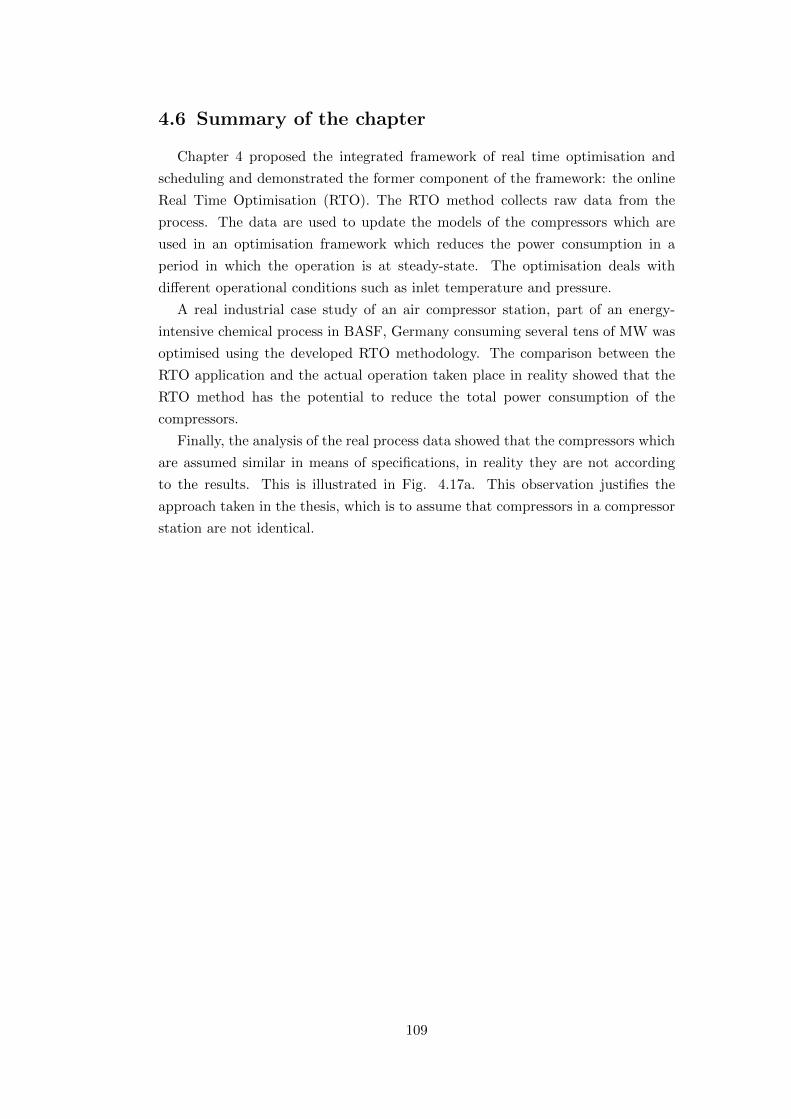
4.6 Summary of the chapter
Chapter 4 proposed the integrated framework of real time optimisation and
scheduling and demonstrated the former component of the framework: the online
Real Time Optimisation (RTO). The RTO method collects raw data from the
process. The data are used to update the models of the compressors which are
used in an optimisation framework which reduces the power consumption in a
period in which the operation is at steady-state. The optimisation deals with
different operational conditions such as inlet temperature and pressure.
A real industrial case study of an air compressor station, part of an energy-
intensive chemical process in BASF, Germany consuming several tens of MW was
optimised using the developed RTO methodology. The comparison between the
RTO application and the actual operation taken place in reality showed that the
RTO method has the potential to reduce the total power consumption of the
compressors.
Finally, the analysis of the real process data showed that the compressors which
are assumed similar in means of specifications, in reality they are not according
to the results. This is illustrated in Fig. 4.17a. This observation justifies the
approach taken in the thesis, which is to assume that compressors in a compressor
station are not identical.
109

5 Multi-period optimisation of the
operation of compressor stations
5.1 Description of the chapter
Chapter 5 presents the methodology for optimal selection of compressors for
long periods using a multi-period approach. The methodology is an optimisation
framework which uses continuous and binary variables to estimate the minimum
total costs of the operation of a compressor station while ensuring that the opera-
tional constraints of the compressors and the plant are satisfied. This framework
will also implement the maintenance model which is presented in the following
Chapter 6.
The problem of scheduling of compressors involves two different cases of mod-
elling. The first case assumes that the models of the compressors are data-driven.
The procedure of the building of these models is similar to that of the air com-
pressors of the case study of the BASF air compressors (presented in Chapter 4).
In the second case, the models of the compressors are represented by compressor
maps which provide both power and efficiency as functions of head, rotational
speed and volumetric flow rate. The compressor maps have been generated from
experiments under various operational conditions. Statoil provided the maps of
the gas natural compressors of the case study introduced in Section 1.4.2.
Mixed integer programming equations are used to describe the discrete oper-
ational functions of compressors and other process units of a plant. Examples of
discrete operations include the start up and shut down of a compressor, and the
assignment of online compressors to different downstream processes. A generic
multi-period optimisation model for the optimisation of a plant which includes the
compressor station involves these mixed integer programming equations and the
models of the power consumption. These models are either the data-driven poly-
nomial expressions or mixed integer programming formulations generated from
compressor maps. The resulting multi-period optimisation model is solved using
mathematical programming techniques, such as MILP.
A study was conducted to optimise the schedule of the BASF air separation
plant in a collaboration with the postdoctoral researcher Georgios Kopanos (now
lecturer at Cranfield University). The work with title ‘Operational planning of a
110
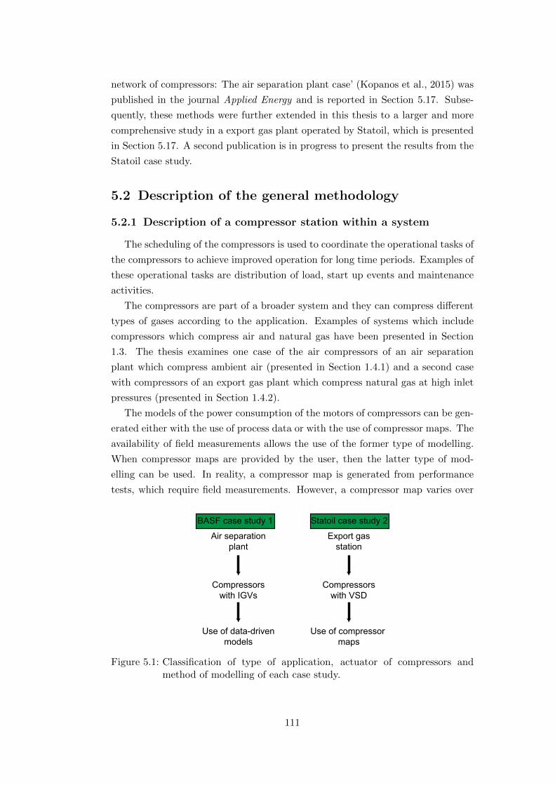
network of compressors: The air separation plant case’ (Kopanos et al., 2015) was
published in the journal Applied Energy and is reported in Section 5.17. Subse-
quently, these methods were further extended in this thesis to a larger and more
comprehensive study in a export gas plant operated by Statoil, which is presented
in Section 5.17. A second publication is in progress to present the results from the
Statoil case study.
5.2 Description of the general methodology
5.2.1 Description of a compressor station within a system
The scheduling of the compressors is used to coordinate the operational tasks of
the compressors to achieve improved operation for long time periods. Examples of
these operational tasks are distribution of load, start up events and maintenance
activities.
The compressors are part of a broader system and they can compress different
types of gases according to the application. Examples of systems which include
compressors which compress air and natural gas have been presented in Section
1.3. The thesis examines one case of the air compressors of an air separation
plant which compress ambient air (presented in Section 1.4.1) and a second case
with compressors of an export gas plant which compress natural gas at high inlet
pressures (presented in Section 1.4.2).
The models of the power consumption of the motors of compressors can be gen-
erated either with the use of process data or with the use of compressor maps. The
availability of field measurements allows the use of the former type of modelling.
When compressor maps are provided by the user, then the latter type of mod-
elling can be used. In reality, a compressor map is generated from performance
tests, which require field measurements. However, a compressor map varies over
Air separationplant
Compressorswith IGVs
Compressorswith VSD
Export gasstation
Use of data-drivenmodels
Use of compressor maps
BASF case study 1 Statoil case study 2
Figure 5.1: Classification of type of application, actuator of compressors andmethod of modelling of each case study.
111
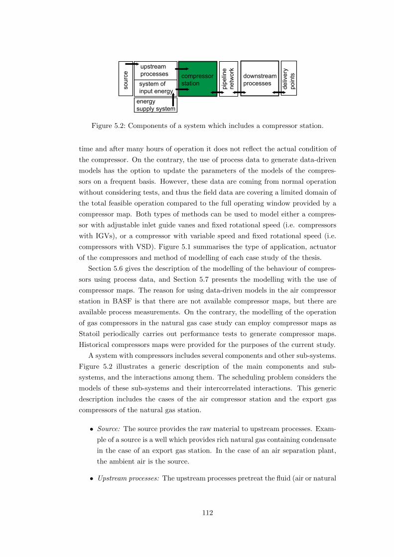
sour
ce
deliv
ery
poin
ts
pipe
line
netw
ork upstream
processessystem ofinput energy
energy supply system
compressorstation
downstreamprocesses
Figure 5.2: Components of a system which includes a compressor station.
time and after many hours of operation it does not reflect the actual condition of
the compressor. On the contrary, the use of process data to generate data-driven
models has the option to update the parameters of the models of the compres-
sors on a frequent basis. However, these data are coming from normal operation
without considering tests, and thus the field data are covering a limited domain of
the total feasible operation compared to the full operating window provided by a
compressor map. Both types of methods can be used to model either a compres-
sor with adjustable inlet guide vanes and fixed rotational speed (i.e. compressors
with IGVs), or a compressor with variable speed and fixed rotational speed (i.e.
compressors with VSD). Figure 5.1 summarises the type of application, actuator
of the compressors and method of modelling of each case study of the thesis.
Section 5.6 gives the description of the modelling of the behaviour of compres-
sors using process data, and Section 5.7 presents the modelling with the use of
compressor maps. The reason for using data-driven models in the air compressor
station in BASF is that there are not available compressor maps, but there are
available process measurements. On the contrary, the modelling of the operation
of gas compressors in the natural gas case study can employ compressor maps as
Statoil periodically carries out performance tests to generate compressor maps.
Historical compressors maps were provided for the purposes of the current study.
A system with compressors includes several components and other sub-systems.
Figure 5.2 illustrates a generic description of the main components and sub-
systems, and the interactions among them. The scheduling problem considers the
models of these sub-systems and their intercorrelated interactions. This generic
description includes the cases of the air compressor station and the export gas
compressors of the natural gas station.
• Source: The source provides the raw material to upstream processes. Exam-
ple of a source is a well which provides rich natural gas containing condensate
in the case of an export gas station. In the case of an air separation plant,
the ambient air is the source.
• Upstream processes: The upstream processes pretreat the fluid (air or natural
112
gas) coming from the source in order to purify it from undesired components,
for example dust from the ambient air in the case of air compressors. Gas
processing plants process rich gas and they produce dry natural gas.
• Input energy system: The compressors require energy to work. Gas turbines
or electrical motors power the compressors.
• Energy supply: The system of energy supply provides the energy to the
drivers of the compressors, for example the electrical grid supplies electricity
to the motors. Another example is a natural gas provider which provides
natural gas as a fuel to the gas turbines drives.
• Compressor station: The compressor station is the main focus of the schedul-
ing as most of the degrees of freedom are related to the operation of these
machines.
• Pipeline network: It includes the short pipes which connect the discharge
point of the compressors and the inlet of downstream processes. It also
includes the valves and other pipes which connect the main pipes among
them.
• Downstream processes: The downstream processes can be chemical processes
which post-treat the compressed air coming from the compressor station, in
the case of an air separation plant. In the case of the natural gas systems the
downstream processes are the long pipes which convey the dry gas to other
destinations. There is not treatment of the compressed gas, the “process”
considered here is the transportation of the gas. Moreover, the storage of
gas can be considered as downstream process.
• Delivery point: This sub-system includes the distribution of the final prod-
uct to the final users, these who define the amount and properties of the
final product. The demand of the compressor station is connected with the
demand of the final users of the overall system.
According to Nørstebø (2008) the optimisation of compressors should be exam-
ined as a system including all the components which affect the decisions related to
the operation of compressors. The consideration of a large-scale description of the
problem and the inclusion of more degrees of freedom can lead to a greater margin
of the improvement of the operation. However, the more components are included
into the optimisation model, the more difficult and more non-linear the problem
becomes. Moreover, the length of the time horizon influences the solution and
as a larger time horizon considers more information this leads to more accurate
decisions. On the other hand, the information coming from a long time horizon
113
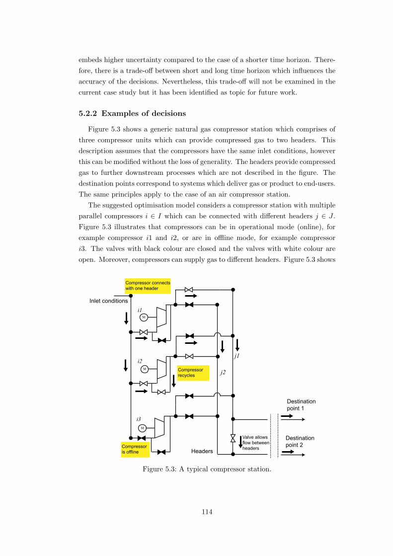
embeds higher uncertainty compared to the case of a shorter time horizon. There-
fore, there is a trade-off between short and long time horizon which influences the
accuracy of the decisions. Nevertheless, this trade-off will not be examined in the
current case study but it has been identified as topic for future work.
5.2.2 Examples of decisions
Figure 5.3 shows a generic natural gas compressor station which comprises of
three compressor units which can provide compressed gas to two headers. This
description assumes that the compressors have the same inlet conditions, however
this can be modified without the loss of generality. The headers provide compressed
gas to further downstream processes which are not described in the figure. The
destination points correspond to systems which deliver gas or product to end-users.
The same principles apply to the case of an air compressor station.
The suggested optimisation model considers a compressor station with multiple
parallel compressors i ∈ I which can be connected with different headers j ∈ J .
Figure 5.3 illustrates that compressors can be in operational mode (online), for
example compressor i1 and i2, or are in offline mode, for example compressor
i3. The valves with black colour are closed and the valves with white colour are
open. Moreover, compressors can supply gas to different headers. Figure 5.3 shows
i1
i3
i2
M
M
M
Headers
j1
j2
Inlet conditions
Destinationpoint 1
Destinationpoint 2
Valve allowsflow betweenheaders
Compressor connects with one header
Compressor recycles
Compressor is offline
Figure 5.3: A typical compressor station.
114
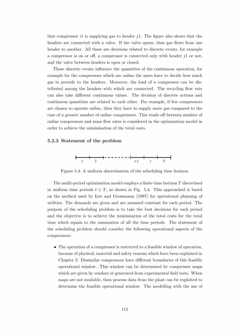
that compressor i1 is supplying gas to header j1. The figure also shows that the
headers are connected with a valve. If the valve opens, then gas flows from one
header to another. All these are decisions related to discrete events, for example
a compressor is on or off, a compressor is connected only with header j1 or not,
and the valve between headers is open or closed.
These discrete events influence the quantities of the continuous operation, for
example for the compressors which are online the users have to decide how much
gas to provide to the headers. Moreover, the load of a compressor can be dis-
tributed among the headers with which are connected. The recycling flow rate
can also take different continuous values. The decision of discrete actions and
continuous quantities are related to each other. For example, if few compressors
are chosen to operate online, then they have to supply more gas compared to the
case of a greater number of online compressors. This trade-off between number of
online compressors and mass flow rates is considered in the optimisation model in
order to achieve the minimisation of the total costs.
5.2.3 Statement of the problem
T1 2 t-1 t
Figure 5.4: A uniform discretisation of the scheduling time horizon.
The multi-period optimisation model employs a finite time horizon T discretised
in uniform time periods t ∈ T , as shown in Fig. 5.4. This approached is based
on the method used by Iyer and Grossmann (1997) for operational planning of
utilities. The demands are given and are assumed constant for each period. The
purpose of the scheduling problem is to take the best decisions for each period
and the objective is to achieve the minimisation of the total costs for the total
time which equals to the summation of all the time periods. The statement of
the scheduling problem should consider the following operational aspects of the
compressors:
• The operation of a compressor is restricted to a feasible window of operation,
because of physical, material and safety reasons which have been explained in
Chapter 2. Dissimilar compressors have different boundaries of this feasible
operational window. This window can be determined by compressor maps
which are given by vendors or generated from experimental field tests. When
maps are not available, then process data from the plant can be exploited to
determine the feasible operational window. The modelling with the use of
115

process data is presented in Section 5.6 and The modelling with the use of
compressor maps is explained in 5.7
• In reality, dissimilar compressors have different efficiencies. The efficiency of
a compressor is a function of head (or pressure) and mass flow rate. The
efficiency is known when a compressor map is given or when enough pro-
cess data are available to calculate the efficiency through thermodynamic
and aerodynamic equations (Dixon and Hall, 2010). The inclusion of the
efficiency in the optimisation problem adds non-linearities, thus instead of
the use of efficiency, the power consumption of the compressors is used in
the optimisation models. The use of the power leads to linear formulations
which is expected to significantly reduce the computational burden.
• A compressor can start up and shut down in a time period. It is assumed
that these events can happen only one time in the beginning of the period.
• A compressor can be connected with different header after each time period.
The change of the header incurs an operational cost, as will be explained
and modelled in Section 5.5.
The optimisation formulation includes the models of the compressors which
describe their power consumption and their feasible operational window. It also
includes the operational aspects of the compressors namely start up, shut down,
connection with and change of headers, and safety operational models of the com-
pressors. The safety operational models are the recycling gas and blow-off air
models. The BASF case study 1 considers a blow-off air model, and the natural
gas compressors of Statoil case study 2 consider a recycling gas model. The mass
balances in the headers, in other pipes and other process units are part of the
constraints of the optimisation formulation. The mass balances in the destination
points are also presented. The consideration of the initial state of the compressor
station, and the boundary constraints (or terminal) complete the mathematical
formulation of the framework.
The methodology employs binary and continuous variables in order to formulate
a Mixed Integer Linear Programming (MILP) model. The reason to use these two
types of variables is that the solution of the MILP model considers both continuous
operational aspects, such as flow distribution, and discrete events, for example the
selection of online compressors. As previously explained, both continuous and
discrete aspects influence each other, therefore it is essential to solve the problem
simultaneously.
The notation and explanation of the major binary and representative continu-
ous positive variables can be seen below:
116

Major binary variables
X(i,t) =
1, if compressor i ∈ I is in operation during time period t
0, otherwise
Y(i,j,t) =
1, if compressor i ∈ I serves header j ∈ J(i) in time period t
0, otherwise
S(i,t) =
1, if compressor i ∈ I starts up at the beginning of time period t
0, otherwise
F(i,t) =
1, if compressor i ∈ I shuts down at the beginning of time period t
0, otherwise
Representative positive continuous variables
Qcor(i,j,t) is the inlet corrected volumetric flow rate in m3/h
Hcor(i,j,t) is the corrected head in kJ/kg
Ncor(i,j,t) is the corrected speed in RPM
Wcor(i,j,t) is the corrected shaft power in kW
Min(i,j,t) is the inlet mass flow rate in kg/s
Pd(i,j,t) is the outlet pressure of the compressor in bar
of compressor i ∈ I connected with header j ∈ J(i) in period t ∈ T . The subset of
headers J(i) is related to the feasible connections between compressors i ∈ I and
headers j ∈ J . The inlet and outlet variables are referred to the inlet and outlet
of a compressor.
The inlet corrected volumetric flow rate Qcor and corrected head Hcor are used
for the description of the operation of natural gas compressors as can be seen
in Section 5.7. The reason is that conventional compressor maps for natural gas
are usually expressed in these quantities. Ambient conditions, compressibility
and molecular weight are the main factors which influence the feasible area and
performance of a natural gas compressors. On the other hand, inlet mass flow
rate Min and outlet pressure Pd are used for the description of air compressors.
The molecular weight and compressibility varies insignificantly in the case of air
compressors and the ambient conditions, such as temperature and pressure, are
considered in the data-driven models of these types of compressors, as can be seen
in Section 5.6.
The notation used describes variables, sets and parameters with the use of
117
subscripts and superscripts. The superscripts are used to specify the quantity,
for example to define an upper boundary of a variable X, then Xmax is used.
The subscript set-indices of variables, sets and parameters are in brackets. The
remaining letters are used to specify the quantities. In some cases through the
text, the subscript set-indices may be omitted for better readability. Lower case
letters (greek or latin) are used for parameters.
5.3 Minimum run and shutdown time
Constraints (5.1) and (5.2) define S(i,t) and F(i,t) binary variables through vari-
ables X(i,t). Parameters χ(i) denote the operating status, on or off, of compressor i
just before the beginning of the current scheduling horizon. Moreover, parameters
χ(i) can be calculated through parameters ϕ(i,j), which represent the active con-
nection of compressor i to header j before the beginning of the current schedul-
ing horizon. Both parameters χ(i) and ϕ(i,j) are connected through expression
χ(i) =∑
j∈J(i)ϕ(i,j), since a compressor can connect with at most one header at a
time.
S(i,t) − F(i,t) = X(i,t) − χ(i), ∀i ∈ I, t = 1
S(i,t) − F(i,t) = X(i,t) −X(i,t−1), ∀i ∈ I, t > 1(5.1)
S(i,t) + F(i,t) ≤ 1, ∀i ∈ I, t ∈ T (5.2)
Constraints (5.2) are omitted, if the costs of startup and shutdown are part of
the objective function. For every compressor i, constraints (5.3) and (5.4) model
the minimum run and shutdown time, respectively.
X(i,t) ≥t∑
t′=max1,t−ω(i)+1
S(i,t′), ∀i ∈ I, t ∈ T, ω(i) > 1 (5.3)
1−X(i,t) ≥t∑
t′=max1,t−ψ(i)+1
F(i,t′), ∀i ∈ I, t ∈ T, ψ(i) > 1 (5.4)
5.4 Assignment of compressors to headers
A compressor i can supply fluid to at most one header j ∈ J(i) at a time and
this is modelled through constraints (5.5). The reason for the exclusive opera-
tion between one compressor and a specific header is that headers have different
pressures. If a compressor was connected with more than one header, then back
118

flows would occur from headers with higher pressure towards to headers with lower
pressure.∑j∈J(i)
Y(i,j,t) = X(i,t), ∀i ∈ I, t ∈ T (5.5)
5.5 Compressor-to-header assignment changes
tt1 t2 t3 t4 t5
j1
X(i1,t2)=X(i1,t3)=X(i1,t4)=1
Compressori1 starts upS(i1,t2)=1
Y(j1,2)=Y(j1,3)=1
Y(j2,4)=1
Compressor i1 shuts downF(i1,t5)=1
D(i1,t2)
D(i1,t2)
≥Y(i1,j1,t2) − Y(i1,j1,t1)− S(i1,t2) D(i1,t2)≥ 0
≥ Y(i1,j2,t2) − Y(i1,j2,t1)−S(i1,t2) D(i1,t2)≥ − 1
D(i1,t3) ≥ Y(i1,j1,t3) − Y(i1,j1,t2)−S(i1,t3) D(i1,t3)≥ 0D(i1,t3)≥ Y(i1,j2,t3) − Y(i1,j2,t2)−S(i1,t3) D(i1,t3)≥ 0
D(i1,t4)≥ Y(i1,j1,t4) − Y(i1,j1,t3)−S(i1,t4) D(i1,t4)≥ −1
D(i1,t4)≥Y(i1,j2,t4) − Y(i1,j2,t3)−S(i1,t4) D(i1,t4)≥ 1
D(i1,t5)≥Y(i1,j1,t5) − Y(i1,j1,t4)−S(i1,t5) D(i1,t5)≥ 0D(i1,t5)≥Y(i1,j2,t5) − Y(i1,j2,t4)−S(i1,t5) D(i1,t5)≥ −1
D(i1,t2) ≥ 0
D(i1,t3) ≥ 0
D(i1,t4) = 1
D(i1,t5) ≥ 0
t = 2
t = 3
t = 4
t = 5
Headers
j2
Compressor i1 changes headerD(i1,t4)=1
Figure 5.5: Modelling of header-changes for a compressor through constraints(5.6).
Any compressor i during its operation can change headers from one time period
to another. The industrial practice concerns compressor-to-header re-assignments
to be typically achieved manually through valve opening or closing by the technical
personnel of the plant. For this reason, a small number of header-changes is
desirable so as to: (a) reduce the use of personnel, (b) decrease the probability
for potential human errors, (c) favour a more smooth operation (i.e. easier to
implement, control, and revise) of the overall network of compressors and (d)
avoid energy losses during the header-change due to venting of the fluid to the
atmosphere (in the case of air compressors). Hence, the total number of these
compressor-to-header changes is considered in the optimisation formulation which
incorporates an associated penalty cost term, CD, in the objective function as
showed in Section 5.12.
In order to model compressor-to-header changes, the following set of binary
decisions variables has been introduced:
D(i,t) =
1, if compressor i changes header from time period t− 1 to t
0, otherwise
119

The compressor-to-header changes are modelled by the following constraints:
D(i,t) ≥ Y(i,j,t) − ϕ(i,j) − S(i,t), ∀i ∈ I, j ∈ J(i), t = 1
D(i,t) ≥ Y(i,j,t) − Y(i,j,t−1) − S(i,t), ∀i ∈ I, j ∈ J(i), t > 1(5.6)
Figure 5.6 depicts an illustrative example of how constraints (5.6) work. Be-
cause of the introduction of a penalty cost for header-changes in the objective
function, the optimisation algorithm should try to force the binary variables D(i,t)
to become zero, in other words the optimisation will try to decrease the header-
changes to the minimum.
5.6 Modelling of compressors with the use of process
data
Air separationplant
Compressorswith IGVs
Compressorswith VSD
Export gasstation
Use of data-drivenmodels
Use of compressor maps
BASF case study 1 Statoil case study 2
Figure 5.1 describing the applications ofeach case study. Section 5.6 examines theuse of data-driven models.
The methodology which is used to
determine the power consumption and
feasible operational window of a multi-
stage centrifugal compressor for the
scheduling problem was described in
Chapter 4. A black box data-driven
model is used to model this behaviour.
This modelling approach will be used
only for the formulation of the opti-
misation model of the operation of air
compressors of the BASF case study, as
illustrated in Fig. 5.1. The use of com-
pressor maps to model the behaviour of
the compressors is used for the second
case study and this modelling approach is presented in the following Section 5.7.
5.6.1 Power consumption
The modelling of the power consumption of the motor of a multi-stage compres-
sor can be derived from process data. Chapter 4 presented a black box method to
represent the power consumption of the motor (Wel) as a function of: (a) process
variables such as mass flow rates (Min) and outlet pressures (Pd), and (b) param-
eters such as the inlet pressure (Pin). For the purposes of the scheduling problem
the output power of the electrical motor of a compressor can be calculated by the
following expression:
120
Wel(i,j,t) = bel(i,0)Y(i,j,t) + bel(i,1)Min(i,j,t) + bel(i,2)(Pd(i,j,t)/Pin(i,t))
+ bel(i,3)Mw(i,t)
(5.7)
whereMw(i,t) is the measured flow rate of the cooling water through the intercoolers
of a compressor i. The bel coefficients of this expression are calculated using data
fitting methods in MatlabTM. This expression is usually represented well by an
expression with quadratic and bilinear terms, however a more simple linear form
could be derived in some cases. The advantage of a linear objective function is
the significant reduced computational effort to reach optimality, however a higher
error in the results is usually expected.
This expression can describe compressors with Inlet Guide Vanes (IGVs) or
inlet throttling valves. With IGV, the operating point of the compressor changes
through the manipulation of the angle of the inlet guide vane that controls the
outlet pressure. In the latter case, the operating point of the compressor changes
by increasing the losses at the inlet of the compressor and in that way the inlet
pressure can be modified.
The industrial case of BASF includes air compressors which use either IGVs or
inlet throttling valves as actuators. However, the case study does not provide the
inlet pressure at the eye of the compressor. The measurement of the inlet pressure,
which is provided from the industrial partner, is at the filter of the inlet duct of
the compressors which is approximately one bar for all the compressors. This work
does not focus on the estimation of the manipulated variables, i.e. angles of IGVs
or angles of throttling valves. Therefore, the expression of Eq. (5.7) describes well
both cases of compressors for the purpose of scheduling, since the variable that is
taken into account in the optimisation is the outlet pressure Pd. The estimation
of the manipulated variables of the IGVs or angles of throttling valves should be
part of the analysis of lower automation levels such as control.
Chapter 4 demonstrated that two similar compressors consume different amounts
of energy at the same operating conditions. The efficiencies of the compressors and
motors are embedded in the power consumption expression of Eq. (5.7). The rea-
son to use this method is that the efficiencies cannot be explicitly modelled in this
case study because many measurements are not available. The measurements are
essential to carry out thermodynamic calculations to estimate the efficiency of a
compressor. As previously mentioned, the use of the efficiency adds non-linearities
in the models of the optimisation. Thus, the use of the power consumption of Eq.
(5.7) in the objective function of Eq. (5.61) helps to avoid non-linear formulations
which are hard to solve.
121
5.6.2 Feasible window of operation
The feasible window of operation of the compressor is defined from the domain
of the regression model (Brooks et al., 1988). The group of all the operating points
of a collected data set determines the regression domain of the model as can be
seen in Figure 4.9b which was described in the previous chapter. It is also known
from the plant that the operators of the compressors may not have operated the
compressors over their full operational range in the collected data set. Therefore,
a partial compressor map is captured in the regression models. This leads to a
solution in a confined space. The extrapolation of the models leads to inaccurate
results, as has been observed in a numerical study during the development of
the regression models. Nevertheless, the operation coming from the optimisation
using this operational space is expected to be more efficient than operation without
optimisation.
For any compressor i, constraints described by Eqs. (5.8) and (5.9) denote the
lower and upper bounds on the inlet compressed air mass flow rate and pressure
ratio that the compressor could operate. These bounds define the feasible win-
dow of operation. The extreme parameters Mminr.d.(i),M
maxr.d.(i), pi
minr.d.(i) and πmaxr.d.(i) are
estimated by the collected data set.
Mminr.d.(i) Y(i,j,t) ≤M(i,j,t) ≤Mmax
r.d.(i) Y(i,j,t), ∀i ∈ I, j ∈ J(i), t ∈ T (5.8)
πminr.d.(i) Y(i,j,t) ≤ Pd(i,j,t)/Pin(i,t) ≤ πmaxr.d.(i) Y(i,j,t), ∀i ∈ I, j ∈ J(i), t ∈ T (5.9)
From constraints (5.9), if Y(i,j,t) = 0, then Pd(i,j,t) = 0. This zero pressure
has no physical meaning, and is used for the calculation of the term of power
consumption cost in the objective function (Eq. (5.61)), which is related to the
power consumption given by Eq. (5.7).
5.6.3 Feasible window of operation with tight constraints:
Convex hull application
The operational behaviour of the electrical power consumption of the motors
of compressors can be formulated in a more detailed way that considers ambient
temperature. The inlet ambient pressure in the case of the air separation plant does
not change significantly, therefore it is not taken into account. This assumption
also simplifies the demonstration of the method described in this section. Hence,
the electrical power consumption of the motor of a compressor Wel(i,j,t) is given
by the following equation:
Wel(i,j,t) = bel(i,0)Y(i,j,t) + bel(i,1)Min(i,j,t) + bel(i,2)Pd(i,j,t) + bel(i,3)Tin(t) (5.10)
122

P d
Min
Problem one Problem two Problem three
extreme point (x)
interior operationalpoint
rectangular r.d.
Convex hull r.d.
T in
Min
P d
Tin
Figure 5.6: Convex hull problems with three process variables involved.
Equations (5.8) and (5.9) which describe the regression domain with a rect-
angular domain can be replaced by a domain based on the theory of the convex
hull presented in the study of Vecchietti et al. (2003). The use of a convex hull
provides more tight constraints of the regression domain (r.d.) compared to the
case of a rectangular domain. Indeed, the convex hull can ensure higher confidence
in the prediction of the power consumption compared to the case of a rectangular
regression domain. The reason is that the the extrapolation in the prediction is
minimised in the former case. The rectangular regression domain is defined by
minimum and maximum values of the observed operating points of the provided
data set, and thus this results in allowing Eq. (5.10) to take values which are
between the tight domain defined by the convex hull and the rectangular domain.
Figure 5.6 shows a graphical illustration of the constraints which define the
operational range of a compressor using rectangular and convex hull regression
domains. The convex hull regression domain is defined from the operating points
of the sets of the two variables Min and Pd and the parameter Tin. The devel-
opment of the constraints of each problem described by Eqs. (5.11) – (5.22) is
presented in the article by Danzer et al. (1963). Kahrs and Marquardt (2007)
discussed the validity of the model using the convex hull approach for data-driven
models, and Mitra et al. (2012) applied a convex hull approach to data-driven
models with mixed integer programming formulations.
Convex hull problem one involves variables Min and Pd:∑ch1∈CH1
λ1(i,j,ch1,t)Min,x(i,ch1) = Min(i,j,t), ∀i ∈ I, j ∈ J(i), t ∈ T (5.11)∑ch1∈CH1
λ1(i,j,ch1,t)Pd,x(i,ch1) = Pd(i,j,t), ∀i ∈ I, j ∈ J(i), t ∈ T (5.12)∑ch1∈CH1
λ1(i,j,ch1,t) = Y(i,j,t), ∀i ∈ I, j ∈ J(i), t ∈ T (5.13)
λ1(i,j,ch1,t) ≤ 1, ∀i ∈ I, ch1 ∈ CH1, j ∈ J(i), t ∈ T (5.14)
123

Convex hull problem two involves variables Min and Tin:∑ch2∈CH2
λ2(i,j,ch2,t)Min,x(i,ch2) = Min(i,j,t), ∀i ∈ I, j ∈ J(i), t ∈ T (5.15)∑ch2∈CH2
λ2(i,j,ch2,t)Tin,x(i,ch2) = Tin(t)Y(i,j,t), ∀i ∈ I, j ∈ J(i), t ∈ T (5.16)∑ch2∈CH2
λ2(i,j,ch2,t) = Y(i,j,t), ∀i ∈ I, j ∈ J(i), t ∈ T (5.17)
λ2(i,j,ch2,t) ≤ 1, ∀i ∈ I, ch2 ∈ CH2, j ∈ J(i), t ∈ T (5.18)
Convex hull problem three involves variables Pd and Tin:∑ch3∈CH3
λ3(i,j,ch3,t)Pd,x(i,ch3) = Pd(i,j,t), ∀i ∈ I, j ∈ J(i), t ∈ T (5.19)∑ch3∈CH3
λ3(i,j,ch3,t)Tin,x(i,ch3) = Tin(t)Y(i,j,t), ∀i ∈ I, j ∈ J(i), t ∈ T (5.20)∑ch3∈CH3
λ3(i,j,ch3,t) = Y(i,j,t), ∀i ∈ I, j ∈ J(i), t ∈ T (5.21)
λ3(i,j,ch3,t) ≤ 1, ∀i ∈ I, ch3 ∈ CH3, j ∈ J(i), t ∈ T (5.22)
The parameters Min,x(i,ch1), Pd,x(i,ch1) of convex hull problem one are the ex-
treme points of the sets of the observed operational points of mass flow rates and
pressures of compressors i ∈ I with observations ch1 ∈ CH1. The number of
observations of the variables of each compressor i can be different among them,
therefore the number of observations in the set CH1 represents the maximum
number of observations among all of the compressors i ∈ I. The extreme points
are estimated by the Matlab function convhull (Matlab, 2015). The parameter λ1
takes values between zero and one and it is used for the formulation of the convex
hull problem. Parameters λ1, λ2, λ3 do not have any physical meaning. The sets of
observations of pressures and mass flow rates of each compressor i for the convex
hull problem two and three are given by ch2 ∈ CH2 and ch3 ∈ CH3 respectively.
The equations of convex hull problem one, Eqs. (5.11) and (5.12), are satisfied
if the values of the variables Min(i,j,t), Pd(i,j,t) which represent an operating point
belong to the regression domain of the corresponding convex hull of problem one
in Fig. 5.6. Equations (5.11) and (5.12) are valid if there exists λ1(i,j,ch1,t) for
ch1 ∈ CH1 such that Eqs. (5.13) and (5.14) are satisfied. The summation of the
positive parameters λ1(i,j,ch1,t) for all ch1 ∈ CH1 has to be equal to one if the
compressor i is connected to header j at period t, thus Y(i,j,t) is equal to one as it
is described by Eq. (5.13). The other two convex hull problems are formulated in
the same way. Therefore Eqs. (5.11) – (5.22) define the regression domain of the
decision variables Min(i,j,t) and Pd(i,j,t) which consider the key parameter Tin(t).
124

5.7 Modelling with the use of compressor maps
Air separationplant
Compressorswith IGVs
Compressorswith VSD
Export gasstation
Use of data-drivenmodels
Use of compressor maps
BASF case study 1 Statoil case study 2
Figure 5.1 describing the applications ofeach case study. Section 5.7 examines theuse of compressor maps.
Section 5.7 presents the method-
ology for modelling the behaviour of
compressors using compressor maps.
The compressor maps in this section re-
fer to variable speed compressors work-
ing with natural gas. The second
industrial case study examines these
types of compressors as can be seen in
Fig. 5.1.
The compressors maps can be given
from the industry and they describe the
shaft power consumption, head, dis-
charge pressure, volumetric flow rate
and efficiency. The maps consider con-
stant reference conditions, i.e. reference temperature, Tref(i), reference pressure,
Pref(i), and reference molecular weight, MolWref(i). The volumetric flow rate,
speed, head, pressure and power are defined as corrected at these conditions as
can be seen in Eqs. (5.40) - (5.44).
5.7.1 Power consumption
Figure 5.7 shows a characteristic map which illustrates the feasible operational
window of an industrial compressor restricted by surge, choke, minimum and max-
imum speed line. Moreover, the power consumed from the shaft is given as a func-
tion of the speed and volumetric flow rate as can be seen in Fig. 5.8. Both sets
of curves are provided by the vendor, or by the user after conducting performance
tests. In the natural gas case study, the optimisation minimises the power of the
Poly
tropi
c he
ad
Inlet volumetric flow rate
Contro
l line
Surge line
H(Q,N) = bh1+ b
h2Q + bh3N
Min speed
Max speed
Area A2Area A1 Choke
Area A3
Qmin QmaxQcQbsur ch
Figure 5.7: Characteristics of a gas compressor with VSD control.
125

Qmin QmaxQcQbsur ch
Area A3
Area A2Area A1
Inlet volumetric flow rate
Sha
ft ab
sorb
ed p
ower
Figure 5.8: Power curves of a compressor with VSD control.
shaft of the compressors. Analysis of the losses of the gearbox of the industrial
compressors suggest that they are less than 1%. These losses have been ignored
for the purposes of the scheduling problem. For the same reason, the electrical
losses in the electrical motors for various operating points are not considered.
The power and head of the natural gas compressors are represented by the MILP
Eqs. (5.23) and (5.24) which include the auxiliary variables Waux, Haux, Naux
and Qaux, and a binary variable λ∗. The linearisation of the power and head of
the compressor involves the division of the maps into K areas. Figures 5.7 and
5.8 illustrate an example of the division of the polytropic head-volumetric flow
rate map and power curves into three areas with non-uniform segments. The
model becomes more accurate as the number of segments increases. However,
increasing the number of areas requires greater computational burden. The reason
for choosing three areas in this trade-off is that the modelling errors were of the
same order as the effects that have already been neglected (e.g. gearbox losses).
Waux(i,j,k,t) = bw1(k,i)λ∗(i,j,k,t) + bw2(k,i)Qaux(i,j,k,t)
+ bw3(k,i)Naux(i,j,k,t), ∀i ∈ I, j ∈ J(i), k ∈ K, t ∈ T (5.23)
Haux(i,j,k,t) = bh1(k,i)λ∗(i,j,k,t) + bh2(k,i)Qaux(i,j,k,t)
+ bh3(k,i)Naux(i,j,k,t), ∀i ∈ I, j ∈ J(i), k ∈ K, t ∈ T (5.24)
The following equations describe the constraints which include the binary vari-
able λ∗(i,j,k,t) used to linearise the characteristics (head-speed-volumetric flow rate)
and the power (work-speed-volumetric flow rate) curves:
126

∑k∈K
λ∗(i,j,k,t) = Y(i,j,t), ∀i ∈ I, j ∈ J(i), t ∈ T (5.25)
Wcor(i,j,t) =∑k∈K
Waux(i,j,k,t), ∀i ∈ I, j ∈ J(i), t ∈ T (5.26)
Hcor(i,j,t) =∑k∈K
Haux(i,j,k,t), ∀i ∈ I, j ∈ J(i), t ∈ T (5.27)
Ncor(i,j,t) =∑k∈K
Naux(i,j,k,t), ∀i ∈ I, j ∈ J(i), t ∈ T (5.28)
Qcor(i,j,t) =∑k∈K
Qaux(i,j,k,t), ∀i ∈ I, j ∈ J(i), t ∈ T (5.29)
Nmin(i) λ∗(i,j,k,t) ≤ Naux(i,j,k,t) ≤ Nmax
(i) λ∗(i,j,k,t),
∀i ∈ I, j ∈ J(i), k ∈ K, t ∈ T (5.30)
Qminsur(i)λ∗(i,j,k,t) ≤ Qaux(i,j,k,t) ≤ Qb(i)λ∗(i,j,k,t), k = 1, (5.31)
Qb(i)λ∗(i,j,k,t) ≤ Qaux(i,j,k,t) ≤ Qc(i)λ∗(i,j,k,t), k = 2, (5.32)
Qc(i)λ∗(i,j,k,t) ≤ Qaux(i,j,k,t) ≤ Qmaxch(i)λ
∗(i,j,k,t), k = 3, (5.33)
∀i ∈ I, j ∈ J(i), t ∈ T
where the Nmin(i) and Nmax
(i) are the minimum and maximum rotational speeds of
each compressor i. The volumetric flow rates Qminsur , Qb, Qc and Qmaxch are chosen
in such a way to divide the compressor map in three areas. The number of the
segments and their lengths are subject to users’ judgement.
For each area k ∈ K the power and head are estimated by various linear func-
tions of speed and volumetric flow rate. The auxiliary variables are associated with
each k area at which the compressor operates. The binary variable λ∗(i,j,k,t) defines
on which area a compressor i connected with header j operates in period t. If a
compressor i is not connected with any header, i.e. Y(i,j,t) = 0 and X(i,t) = 0, then
the λ∗(i,j,k,t) equals to zero. This means that the auxiliary variables take the value
zero and the corrected variables become zero, referring to Eqs. (5.23) - (5.33).
The linear expressions of power and head, functions of speed and volumetric
flow rate, are developed using data fitting methods in MatlabTM. The procedure
of the fitting of the data is similar to the methodology presented in Chapter 4. The
provided compressor maps from Statoil were digitalised and stored as a table as
has been explained by Abbaspour et al. (2005). The table provided the necessary
data for the fitting. Figure 5.7 shows an example of the linearisation of the head
curve, in area A2, using a linear function H(Q,N) = Haux(i,j,k,t)|k=2. The function
is a first order polynomial with input data the volumetric flow rate and rotational
speed, and output data the head for various operating points. Therefore, the
127

coefficients of Eqs. (5.23) and (5.24) are estimated from the fitting methods used
similarly in Chapter 4. The mathematical modelling of the power curves W (Q,N)
follows the same procedure as that of the head.
5.7.2 Feasible window of operation
The operative points are restricted to the area defined from the four red curves
defining the boundaries as can be seen in Fig. 5.7. Figure 5.7 illustrates that the
head has to be smaller than the head defined by the control surge line (known as
just control line) and the maximum speed line (Wu et al., 2000), these constraints
are modelled with Eqs. (5.34) and (5.35) respectively. Equations (5.36) and (5.37)
model the constraint which describes that the head has to be greater than the
choke and the head of the minimum speed line (Wu et al., 2000). The parameters
of the Eqs. (5.34) - (5.37), bs1(i), bs2(i), bU1(i), bU2(i), bch1(i), bch2(i), bL1(i), bL2(i), are
estimated with similar fitting methods as explained previously. The head of each
area k ∈ K has to respect these constraints.
Hcor(i,j,t) ≤ bs1(i)Qcor(i,j,t) + bs2(i)Y(i,j,t), (5.34)
Hcor(i,j,t) ≤ bU1(i)Y(i,j,t) + bU2(i)Qcor(i,j,t), (5.35)
Hcor(i,j,t) ≥ bch1(i)Qcor(i,j,t) + bch2(i)Y(i,j,t), (5.36)
Hcor(i,j,t) ≥ bL1(i)Y(i,j,t) + bL2(i)Qcor(i,j,t), (5.37)
∀i ∈ I, j ∈ J(i), t ∈ T
The mass flow rate Min provided at the inlet of the compressor is given by the
following equation:
Qact(i,j,t)ρ(i,t) = 3, 600Min(i,j,t), ∀i ∈ I, j ∈ J(i), t ∈ T (5.38)
with the density estimated by:
ρ(i,t) =104 Pact,s(t)
Rg(t) 103 Tact,s(i,t) Zact,s(t)(5.39)
The operating conditions (temperature Tact,s, pressure Pact,s, molecular weight
MolWact,s and compressibility Zact,s) are usually different from the reference condi-
tions. The different inlet conditions are called actual conditions. The calculations
to estimate the actual power consumption of the shaft of the compressor are done
using the actual conditions, because this variable is used in the objective function
to be minimised. The conversion between actual and corrected values is given from
equations Eqs. (5.40) - (5.44) (Boyce, 2003).
128
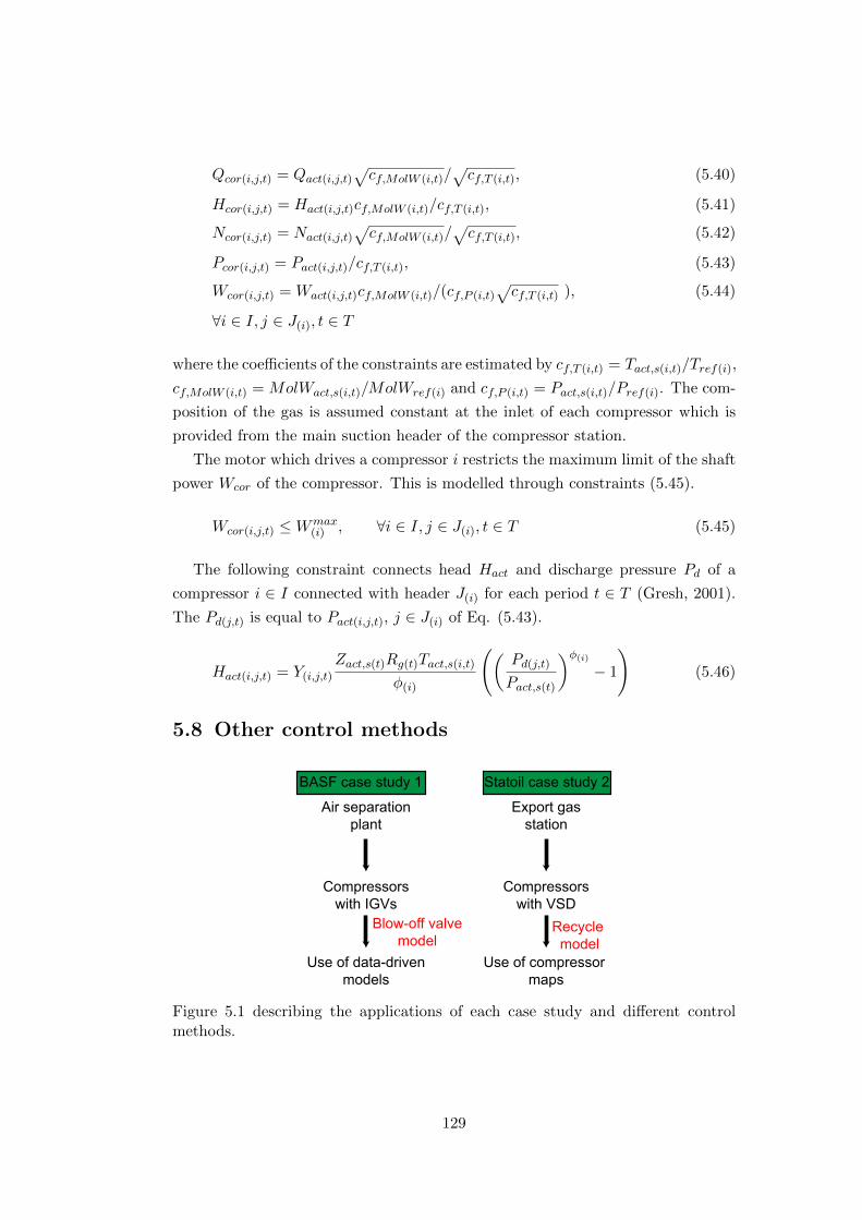
Qcor(i,j,t) = Qact(i,j,t)√cf,MolW (i,t)/
√cf,T (i,t), (5.40)
Hcor(i,j,t) = Hact(i,j,t)cf,MolW (i,t)/cf,T (i,t), (5.41)
Ncor(i,j,t) = Nact(i,j,t)√cf,MolW (i,t)/
√cf,T (i,t), (5.42)
Pcor(i,j,t) = Pact(i,j,t)/cf,T (i,t), (5.43)
Wcor(i,j,t) = Wact(i,j,t)cf,MolW (i,t)/(cf,P (i,t)√cf,T (i,t) ), (5.44)
∀i ∈ I, j ∈ J(i), t ∈ T
where the coefficients of the constraints are estimated by cf,T (i,t) = Tact,s(i,t)/Tref(i),
cf,MolW (i,t) = MolWact,s(i,t)/MolWref(i) and cf,P (i,t) = Pact,s(i,t)/Pref(i). The com-
position of the gas is assumed constant at the inlet of each compressor which is
provided from the main suction header of the compressor station.
The motor which drives a compressor i restricts the maximum limit of the shaft
power Wcor of the compressor. This is modelled through constraints (5.45).
Wcor(i,j,t) ≤Wmax(i) , ∀i ∈ I, j ∈ J(i), t ∈ T (5.45)
The following constraint connects head Hact and discharge pressure Pd of a
compressor i ∈ I connected with header J(i) for each period t ∈ T (Gresh, 2001).
The Pd(j,t) is equal to Pact(i,j,t), j ∈ J(i) of Eq. (5.43).
Hact(i,j,t) = Y(i,j,t)
Zact,s(t)Rg(t)Tact,s(i,t)
φ(i)
((Pd(j,t)
Pact,s(t)
)φ(i)− 1
)(5.46)
5.8 Other control methods
Air separationplant
Compressorswith IGVs
Compressorswith VSD
Export gasstation
Use of data-drivenmodels
Use of compressor maps
BASF case study 1 Statoil case study 2
Recycle model
Blow-off valvemodel
Figure 5.1 describing the applications of each case study and different controlmethods.
129

The previous methods presented the methodology of the operation of compres-
sors with the use of variable inlet guide vanes, inlet throttling valves and variables
speed drives. The first two cases are related to the air separation case study and
the case with the variable speed drives refers to the natural gas case study. Section
5.8 will present the modelling of the operation of natural gas compressors when
they are controlled with a recycle valve, and when compressed air is vent through
a blow-off valve in the case of air compressors.
5.8.1 Recycle model
M Mout
MinMrec
recycle valve
Figure 5.9: The gas flows of a compressor using recycling flow.
The mass balance of a single compressor which can use recycling of the gas is
shown in Fig. 5.9. This method to control the mass flow rate is usually used in
natural gas compressors, thus the following equations are related to the second
case study of the export gas station. The compressor maps consider the Min for
the head and power calculations. The Rc binary variable models the on-off status
of the recycle valve. The recycle flow control model is represented by the following
equations (van den Heever and Grossmann, 2003):
Min(i,j,t) = Mout(i,j,t) +Mrec(i,t), ∀i ∈ I, j ∈ J(i), t ∈ T (5.47)
Mrec(i,t) ≤Mmaxrec(i)Rc(i,t), ∀i ∈ I, t ∈ T (5.48)
Rc(i,t) ≤ X(i,t), ∀i ∈ I, t ∈ T (5.49)
5.8.2 Blow-off valve model
M Mout
Min
Mblow-off
atmosphere
downstreamprocess
Figure 5.10: Gas flows of an air compressor with the use of a blow-off valve.
130

When the fluid of a process can satisfy environmental requirements, then a
compressor can vent it into the atmosphere when it is necessary. In the case of
air compressors, Fig. 5.10 shows the mass balance when there is a blow-off valve
to vent the air. This mass balance Min = Mout + Mblow−off will be used in the
optimisation model of the BASF case study (Fig. 5.1). The excess of compressed
air produced is vented in the atmosphere. This may happen in the scenario of
keeping compressors online, and their total minimum flow rate due to control
surge line is higher than the demand.
5.9 Outlet pressure of compressors
The outlet pressure of a compressor is equal to the pressure of the header that
the compressor serves, and is given by the corresponding load curve:
Pd(i,j,t) = α0(j) M(i,j,t) + α1(j) Y(i,j,t), ∀i ∈ I, j ∈ J(i), t ∈ T (5.50)
Parameters α0(j) and α1(j) represent the coefficients of the load curve of header
j. In order to avoid non-linearities in the load curve constraints (5.50), auxiliary
variables M(i,j,t) have been introduced. These variables denote the total com-
pressed mass flow rate in the header j which is served by compressor i during time
period t. Non-negative variables M(i,j,t) are modelled through the following set of
big-M constraints (Vecchietti et al., 2003):
M(i,j,t) ≥∑i′∈Ij
M(i′,j,t) −M∗(j) (1− Y(i,j,t)), ∀i ∈ I, j ∈ J(i), t ∈ T
M(i,j,t) ≤∑i′∈Ij
M(i′,j,t) +M∗(j) (1− Y(i,j,t)), ∀i ∈ I, j ∈ J(i), t ∈ T
M(i,j,t) ≤M∗(j) Y(i,j,t), ∀i ∈ I, j ∈ J(i), t ∈ T
(5.51)
Parameters M∗(j) are problem-specific large numbers that can be usually calcu-
lated by considering the maximum capacity of header j. They do not have any
physical meaning, and they are used for the formulation of the big-M constraints.
5.10 Mass balances of air separation plant units
This section describes the constraints of the downstream processes of an air
separation plant which includes air compressors, as shown Fig. 5.11. The major
units are the air separation columns, the storage tanks of the products and the
system which includes the utilities for compressed air.
131
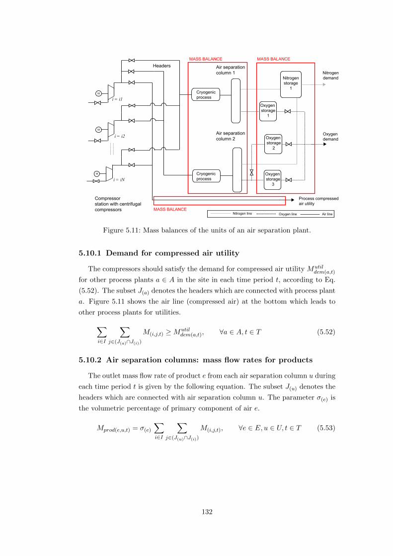
i = i1
i = iN
Process compressedair utility
Oxygen storage
1
OxygendemandOxygen
storage2
Oxygen storage
3
Cryogenicprocess
Cryogenicprocess
i = i2
Nitrogenstorage
1
Nitrogendemand
M
M
M
Nitrogen line Oxygen line Air line
Compressorstation with centrifugalcompressors
Air separation column 1
Air separation column 2
HeadersMASS BALANCE MASS BALANCE
MASS BALANCE
Figure 5.11: Mass balances of the units of an air separation plant.
5.10.1 Demand for compressed air utility
The compressors should satisfy the demand for compressed air utility Mutildem(a,t)
for other process plants a ∈ A in the site in each time period t, according to Eq.
(5.52). The subset J(a) denotes the headers which are connected with process plant
a. Figure 5.11 shows the air line (compressed air) at the bottom which leads to
other process plants for utilities.∑i∈I
∑j∈(J(a)∩J(i))
M(i,j,t) ≥Mutildem(a,t), ∀a ∈ A, t ∈ T (5.52)
5.10.2 Air separation columns: mass flow rates for products
The outlet mass flow rate of product e from each air separation column u during
each time period t is given by the following equation. The subset J(u) denotes the
headers which are connected with air separation column u. The parameter σ(e) is
the volumetric percentage of primary component of air e.
Mprod(e,u,t) = σ(e)
∑i∈I
∑j∈(J(u)∩J(i))
M(i,j,t), ∀e ∈ E, u ∈ U, t ∈ T (5.53)
132

Constraints (5.54) provide lower and upper bounds of the outlet mass flow rate
of product e from each air separation column.
Mminprod(e,u) ≤Mprod(e,u,t) ≤Mmax
prod(e,u), ∀e ∈ E, u ∈ U, t ∈ T (5.54)
5.10.3 Storage tanks mass balances
The total amount of products e from the air separation column u that is pro-
vided to each storage tank z ∈ Z(e) during time period t is represented by variables
Vprod(e,u,z,t), and is given by Eq. (5.55). The parameter κ(t) is a conversion factor
of mass flow rate to aggregated amount of mass flow.∑z∈Z(e)
Vprod(e,u,z,t) = κ(t)Mprod(e,u,t), ∀e ∈ E, u ∈ U, t ∈ T (5.55)
Hence, the demand for any product e in each time period t is met by extracting
the necessary amount of product, V outtnk(e,z,t), from the storage tanks z ∈ Z(e). The
products could be also acquired from external sources δ ∈ ∆(j) with amount of
provided flow V ext(e,t), if the demand Vdem(e,t) cannot be fully met by the internal
production network.∑z∈Z(e)
V outtnk(e,z,t) +
∑δ∈∆(j)
V ext(δ,e,t) = Vdem(e,t), ∀e ∈ E, t ∈ T (5.56)
Constraints (5.57) correspond to the mass balance in the product storage tanks
under the complete satisfaction of the demand for products. Variables V stortnk(e,z,t)
denote the amount of product e that is stored in storage tank z ∈ Z(e) at the end
of time period t. Parameter vstortnk(e,z) represents the initial inventory of product e
in storage tank z ∈ Z(e).
V stortnk(e,z,t) = vstortnk(e,z) +
∑u∈U(z)
Vprod(e,u,z,t) − V outtnk(e,z,t), ∀e ∈ E, z ∈ Z(e), t = 1
V stortnk(e,z,t) = V stor
tnk(e,z,t−1) +∑u∈U(z)
Vprod(e,u,z,t) − V outtnk(e,z,t), ∀e ∈ E, z ∈ Z(e), t > 1
(5.57)
Constraints (5.58) define the lower and the upper inventory bounds. The upper
inventory bound represents the storage capacity of the storage tank. Safety stocks
are represented by the lower inventory bound.
V mintnk(e,z) ≤ V
stortnk(e,z,t) ≤ V
maxtnk(e,z), ∀e ∈ E, z ∈ Z(e), t ∈ T (5.58)
133

5.11 Export gas operational constraints
M
M
M
Headers
Mout | i = i1, j = j2i = i1
i = i2
i = iN
Mout | i = i2, j = j1
Mout | i =iN, j = j2
MASS BALANCE
MASS BALANCE
Mout | i = i2, j = j1
Mtot | j = j1
Mtot | j = j2
M ext| δ = δ1
Termimals(platforms)
Figure 5.12: Export gas station diagram.
This section refers to the description of the operation of an export natural
gas compressor station which can be seen in Fig. 5.12. The summation of the
individual flows to each header is equal to the total mass flow rate at the inlet of
the header:
Mtot(j,t) =∑i∈I
Mout(i,j,t), ∀j ∈ J(i), t ∈ T (5.59)
The outlet pressure of each compressor has to be equal to the inlet pressure of
the header is connected with. The headers are connected with long pipes which
convey the compressed gas to platforms (Fig. 5.12).
The formulation of the optimisation problem considers the inlet of the pipes as
the delivery point of the export gas station. It assumed that the linepack (stored
amount of gas in the pipes) and the downstream pressures are given. Additionally,
the demand mass flow rate Mdem(j,t) of each pipe connected with each header j ∈ Jand pressure Pdem(j,t) are used in actual conditions as they are measured from the
plant. The mass balance at the delivery point, i.e. after the aftercooler of the
outlet of the compressors, can be seen in the following equation:
Mtot(j,t) +∑δ∈∆(j)
M ext(δ,t) ≥Mdem(j,t), ∀j ∈ J(i), t ∈ T (5.60)
134

where Mdem,g(j,t) is estimated from actual conditions using the following equations
for every header j ∈ J in every time period t ∈ T (Nørstebø, 2008):
Qdem,act(j,t) =Pstd
Pdem(j,t)·Td(t)
Tstd·Zd(t)
Zstd·Qstd · cstd
Mdem(j,t) =Qdem,act(j,t) · Pd(j,t) · 104
Rg(t) · Zact,s(t) · 3.6 · 104
where the standard conditions are given, Pstd = 1.01325 bar, Tstd = 288.15 K, and
Zstd = 1. The cstd stands for a conversion factor (=105/24) in order to convert
Qstd (given in MMsm3/d) into Qdem,act(j,t) (in m3/h).
The Td(t) is the temperature of the gas at the delivery point assumed constant
in this work and the Zd(t) equals to Zact,s(t) as compressibility (and composition)
of the gas are assumed constant. The gas constant is given by Rg(t) = R/MolW
where R = 8,314 kJ/(mol·K) is the ideal gas constant.
The variable M ext(δ,t) represents the mass flow rate of natural gas (in kg/s) pro-
vided from external sources δ ∈ ∆. In this work other external sources are not
considered, however in order to give a comprehensive description of this variable
is included in the presentation of the model.
5.12 Objective function
Considering both cases of air and natural gas compressors, the objective is to
minimise the electricity cost of the motors of the compressors, the start up and shut
down costs, the cost when a compressors changes header and the procurement costs
of gas/products from external sources. At the same time the constraints described
in Sections 5.3 - 5.11 related to each case study have to be respected. The general
form of the objective function is given by Eq. (5.61).
min
electricity cost︷ ︸︸ ︷∑t∈T
Cel(t)∑i∈I
∑j∈J(i)
dcWel(i,j,t) +
start up and shut down cost︷ ︸︸ ︷∑t∈T
∑i∈I
(Cst(i)S(i,t) + Cf(i)F(i,t)) +
change header cost︷ ︸︸ ︷∑t∈T
∑i∈I
CDD(i,t) +
purchase products/gas cost︷ ︸︸ ︷∑t∈T
∑e∈E
∑δ∈∆(j)
Cext(δ,e,t)dcMext(δ,e,t)
(5.61)
The first term of the objective function represents the total electricity cost of the
motors where the Cel(t) is the electricity cost in EUR/kWh and the dc is the factor
to convert electrical power consumption to energy used over the time period. The
electrical power consumption of the compressors W(el) in the objective function is
estimated from either Eq. (5.7) or (5.10) in the case of the air compressors. In
135

the case of the natural gas compressors, the power consumption is given by Eq.
(5.44). The binary variables S(i,t) and F(i,t) are equal to one if the compressor
starts up or shuts down respectively. The start up cost is Cst(i) and the shutdown
cost is Cf(i). The parameter CD corresponds to the cost which occurs when a
compressor changes header between period t−1 and t. The cost Cext(δ,e,t) refers to
the purchase price (in EUR/kg) of gas or product e from external sources δ ∈ ∆.
The formulated optimisation problem is a MILP model which minimises the
objective function of Eq. (5.61) subject to constraints described in Sections 5.3 -
5.11 considering the specific case study, for example the case of an air compres-
sor station in an air separation plant or an export gas compressor station. The
optimisation problem has been implemented in the optimisation platform GAMS
(McCarl et al., 2008). The optimisation determines the values of the optimisation
variables which minimise the objective function. These values describe the best
decisions the user of the plant should take to achieve optimal operation, the major
decisions can be seen below:
• Which compressors to operate in period t: X(i,t)
• Which header a compressor should connect with in period t: Y(i,j,t)
• When to start up a compressor: S(i,t)
• When to shut down a compressor: F(i,t)
• What is the optimal distribution of load: Min(i,j,t)
• What is the optimal purchase from external sources: M ext(δ,e,t)
5.13 Maintenance constraints - Given maintenance
schedule
The maintenance tasks of compressors are typically predefined before the op-
timisation of the production. The duration νfxd(i) of a maintenance task is given.
Two types of preventive maintenance tasks are considered in the basic operational
model: (a) maximum runtime-based, (b) and fixed. The first type of maintenance
is related to the maximum run time of the compressors. Fixed maintenance tasks
takes place in a predefined time horizon, such that the starting and completion
times of the maintenance tasks are known.
Maximum runtime-based maintenance tasks The performance of a com-
pressor depends on its current condition. Since the performance of the compressor
136

deteriorates during its utilisation, there is often a time limit on its continuous op-
eration. There is a maximum run time, o(i), after which the compressor should be
switched off, and maintenance takes place to prevent mechanical damage and the
energy-inefficient use of the compressor. The runtime-based maintenance policy
can be considered as a simplified case of the condition-based maintenance policy
(Li and Nilkitsaranont, 2009). For the sake of simplicity here, the duration of these
maintenance tasks is considered to be equal to the minimum shutdown time. For
every compressor, the maximum run time constraints are given by:
t∑t′=max1,t−o(i)
X(i,t′) ≤ o(i), ∀i ∈ I, t ∈ T (5.62)
If there is a maximum time that compressors could remain idle (i.e., maximum
shutdown time), similar types of constraints are derived.
Fixed maintenance tasks The starting times τ fxd(i) and the duration νfxd(i) of the
fixed maintenance tasks are known. For this reason, fixed maintenance tasks are
modelled by setting to zero (from the starting to the completion of the maintenance
task) the operating binary variables X(i,t) of compressors i ∈ Idm ⊆ I that are
subject to fixed maintenance:
X(i,t) = 0, ∀i ∈ Idm, t = τ fxd(i) , ..., (τ fxd(i) + νfxd(i) − 1) (5.63)
These constraints generally hold, since the maintenance duration is typically at
least equal to the minimum shutdown time.
5.14 Initial state of the network
The initial state of the network is partially described by the initial inventory
level of every storage tank vstortnk(e,z) and the initial operating status of every com-
pressor ϕ(i,j) (→ χ(i)). Variables vstortnk(e,z) are found in constraints (5.57), and bi-
nary variables ϕ(i,j) are found in (5.1). Also needed is information on the startup
and shutdown from the previous scheduling horizon. The following set of con-
straints allows past information regarding startup and shutdown to be carried
over at the beginning of the current scheduling horizon:
X(i,t) = 1, ∀ i ∈ I, t = 1, ..., (ω(i) − ω(i)) : 0 < ω(i) < ω(i) (5.64)
X(i,t) = 0, ∀ i ∈ I, t = 1, ..., (ψ(i) − ψ(i)) : 0 < ψ(i) < ψ(i) (5.65)
137

Parameter ω(i) denotes the total number of time periods at the end of the past
scheduling horizon that compressor i has been operating since its last startup.
Parameter ψ(i) denotes the total number of time periods at the end of the past
scheduling horizon that compressor i has not been operating since its last shut-
down. Figure 5.13 shows how the past startup information is captured from the
above constraints.
In the case of a compressor i which has been in operation at the end of the
previous scheduling horizon (i.e., ω(i) > 1), then the total run time from its last
startup of the past horizon should be carried over to the current scheduling horizon
so as to model successfully the maximum run time limits. Constraints (5.66)
describe the initial state of the network in respect of the maximum run time.
t∑t′=max1,t−(o(i)−ω(i))
X(i,t′) ≤ (o(i)−ω(i)), ∀i ∈ I, t ≤ (o(i)−ω(i)+1) : ω(i) > 1
(5.66)
Regarding fixed maintenance tasks, the initial maintenance state (i.e., under
maintenance or not) of every compressor should be carried over from the previous
scheduling horizon. To consider this properly, for the compressors i ∈ Idm that
are under maintenance at the beginning of the current scheduling horizon and
their maintenance tasks had already started in the previous scheduling horizon,
constraints (5.63) are modified as follows.
t1 2 3 4 5
Compressor: ω = 5
Past scheduling horizon Current scheduling horizon
X(i,t=1) = X(i,t=2) = X(i,t=3) = 1
Start up X(t) to be optimised for t > 3.
~ω = 2
Figure 5.13: Carryover of past startup information to model minimum run time.
138
η(i,t) = 1, ∀i ∈ (Idm \ Idm), t = τ fxd(i) , ..., (τ fxd(i) + νfxd(i) − 1)
X(i,t) = 1− η(i,t), ∀i ∈ (Idm \ Idm), t = τ fxd(i) , ..., (τ fxd(i) + νfxd(i) − 1)
η(i,t) = 1, ∀i ∈ Idm, t = 1, ..., (νfxd(i) − νfxd(i) )
X(i,t) = 1− η(i,t), ∀i ∈ Idm, t = 1, ..., (νfxd(i) − νfxd(i) )
(5.63′)
Parameter νfxd(i) denotes the total time that compressor i has been under mainte-
nance (since the start of the maintenance task) at the end of the previous schedul-
ing horizon. In other words, (νfxd(i) − νfxd(i) ) represents the remaining time that
compressor i has to be under maintenance in the current scheduling horizon. Pa-
rameter η(i,t) denotes if compressor i is under maintenance in time period t. For
η(i,t) = 1, the corresponding X(i,t) becomes zero. Equation (5.63′) refers to the set
of compressors i ∈ (Idm \ Idm) which defines these compressors which have to be
under maintenance but their maintenance have not started before the beginning
of the optimisation.
5.15 Terminal constraints
The optimisation determines a solution which minimises the total cost of the
operation of the plant and the solution applies only within the boundaries of
the optimisation problem. For instance, the solution for the optimal operation
for one month may suggest to work the compressors as long as possible without
maintaining them during the month to avoid the costs of shut down. However, the
current optimisation does not consider the requirements for a following scheduling
problem and it is possible to have an infeasible solution or a non-optimal solution
compared to the case where the two consequent scheduling problems have been
solved simultaneously.
Another example is the use of the storage tanks to reduce the production,
therefore the power consumption. However, the tanks would be empty at the end
of the scheduling horizon and the following optimisation problem would not have
the flexibility to utilise the tanks at the beginning of the new time horizon.
A practical issue for using a relatively short time horizon of one month is that
the uncertainty in the forecast of parameters, such as the production targets,
increases as the the length of the horizon becomes greater.
For these reasons, the optimisation has to consider boundary conditions at
the end of the time horizon. These boundary conditions can be called terminal
constraints. These boundary conditions take into account the requirements of
the following scheduling problem. Equation (5.67) ensures that the contents of
139
the tanks are full at the end of the time horizon, t = T , in the case of the air
separation plant.
V stortnk(e,z,t) = V max
tnk(e,z), ∀e ∈ E, z ∈ Z, t = T (5.67)
The terminal constraints have to be investigated using heuristics from historical
operation and literature. The decisions of these constraints are strongly related
with the particular configuration of the compressors of the plant.
5.16 Equal split and equal surge margin operation
The most common industrial strategies to share the loads of compressors are
the equal split and equal surge margin methods. The equal split method assumes
that the load of the compressors is split evenly among the compressors, and the
equal surge margin operation considers an equal distance between the operating
points of all the compressors and their respective control surge lines. The control
surge line or just control line is a limit on the right of the surge of a compressor
and it is known.
These strategies are less sophisticated than the optimal distribution of the load
this thesis is suggesting. The optimal distribution of the load is related to different
operating points of the individual compressors. In addition, the equal split and
equal surge margin strategies insert extra constraints into the optimisation model
and this increases the computational burden as shown in Section 5.17.4.
The following equations will be implemented in the optimisation formulation of
the natural gas compressors case study (the equations describing the equal split
strategy of Section 5.16.1 could be used also for the formulation of the optimisation
of the networks of compressors of the BASF case study). Section 5.16.2 presents
a formulation of equal surge margin strategy among parallel compressors which
require the use of compressor maps. The given compressor maps provide the
descriptions of the control surge lines.
5.16.1 Constraints of the equal split strategy
A binary variable ξ(i,i′,j,t) is defined for the equal split cases as follows:
ξ(i,i′,j,t) =
1, if compressors i and i′ are connected with header j in time period t
0, otherwise
140
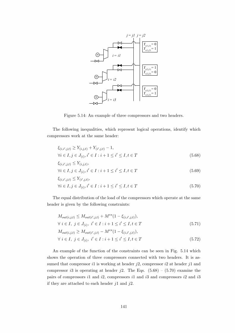
i = i2
j = j1 j = j2
i = i1M
M
i = i3
Y(i3,j1) = 0Y(i3,j2) = 1
Y(i2,j1) = 1Y(i2,j2) = 0
Y(i1,j1) = 0Y(i1,j2) = 1
M
Figure 5.14: An example of three compressors and two headers.
The following inequalities, which represent logical operations, identify which
compressors work at the same header:
ξ(i,i′,j,t) ≥ Y(i,j,t) + Y(i′,j,t) − 1,
∀i ∈ I, j ∈ J(i), i′ ∈ I : i+ 1 ≤ i′ ≤ I, t ∈ T (5.68)
ξ(i,i′,j,t) ≤ Y(i,j,t),
∀i ∈ I, j ∈ J(i), i′ ∈ I : i+ 1 ≤ i′ ≤ I, t ∈ T (5.69)
ξ(i,i′,j,t) ≤ Y(i′,j,t),
∀i ∈ I, j ∈ J(i), i′ ∈ I : i+ 1 ≤ i′ ≤ I, t ∈ T (5.70)
The equal distribution of the load of the compressors which operate at the same
header is given by the following constraints:
Mout(i,j,t) ≤Mout(i′,j,t) +M es(1− ξ(i,i′,j,t)),
∀ i ∈ I, j ∈ J(i), i′ ∈ I : i+ 1 ≤ i′ ≤ I, t ∈ T (5.71)
Mout(i,j,t) ≥Mout(i′,j,t) −M es(1− ξ(i,i′,j,t)),
∀ i ∈ I, j ∈ J(i), i′ ∈ I : i+ 1 ≤ i′ ≤ I, t ∈ T (5.72)
An example of the function of the constraints can be seen in Fig. 5.14 which
shows the operation of three compressors connected with two headers. It is as-
sumed that compressor i1 is working at header j2, compressor i2 at header j1 and
compressor i3 is operating at header j2. The Eqs. (5.68) – (5.70) examine the
pairs of compressors i1 and i2, compressors i1 and i3 and compressors i2 and i3
if they are attached to each header j1 and j2.
141
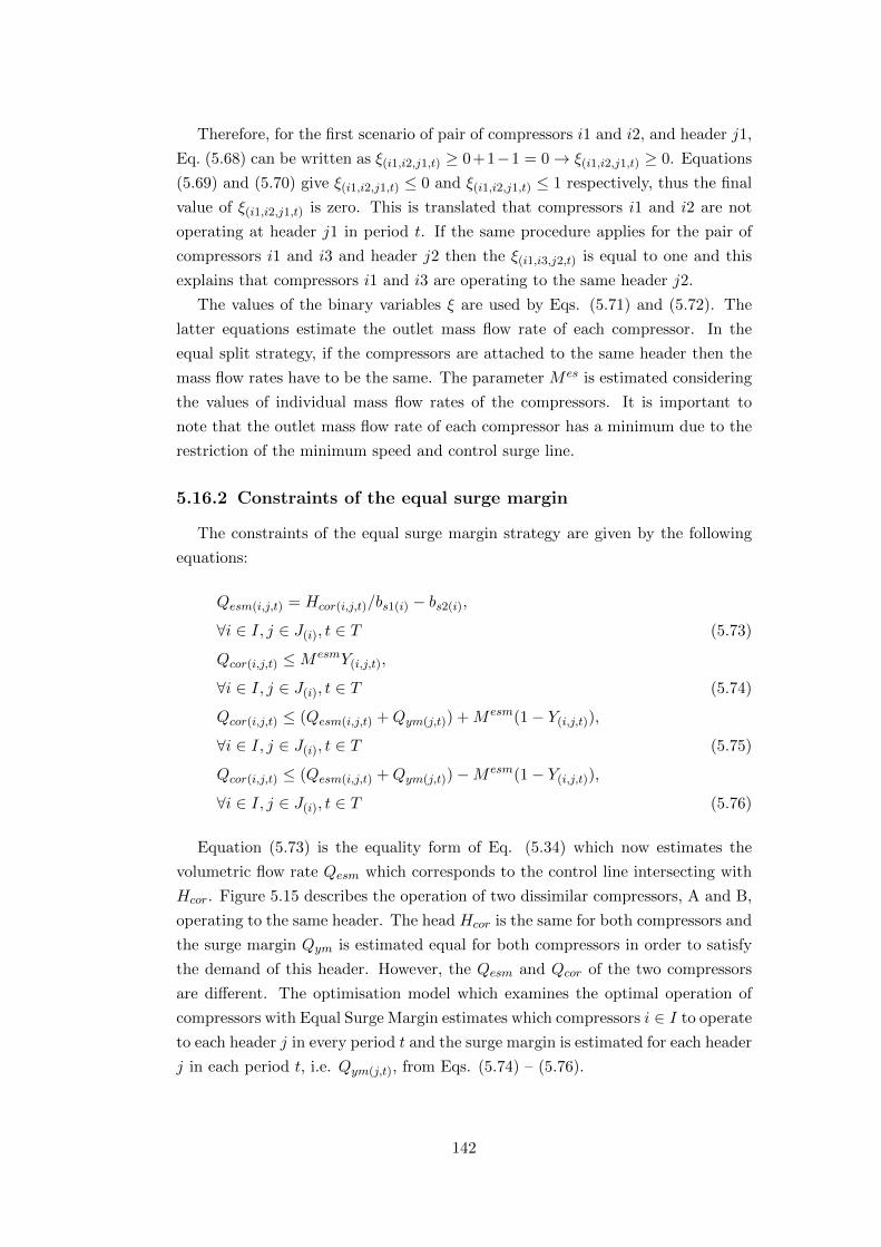
Therefore, for the first scenario of pair of compressors i1 and i2, and header j1,
Eq. (5.68) can be written as ξ(i1,i2,j1,t) ≥ 0+1−1 = 0→ ξ(i1,i2,j1,t) ≥ 0. Equations
(5.69) and (5.70) give ξ(i1,i2,j1,t) ≤ 0 and ξ(i1,i2,j1,t) ≤ 1 respectively, thus the final
value of ξ(i1,i2,j1,t) is zero. This is translated that compressors i1 and i2 are not
operating at header j1 in period t. If the same procedure applies for the pair of
compressors i1 and i3 and header j2 then the ξ(i1,i3,j2,t) is equal to one and this
explains that compressors i1 and i3 are operating to the same header j2.
The values of the binary variables ξ are used by Eqs. (5.71) and (5.72). The
latter equations estimate the outlet mass flow rate of each compressor. In the
equal split strategy, if the compressors are attached to the same header then the
mass flow rates have to be the same. The parameter M es is estimated considering
the values of individual mass flow rates of the compressors. It is important to
note that the outlet mass flow rate of each compressor has a minimum due to the
restriction of the minimum speed and control surge line.
5.16.2 Constraints of the equal surge margin
The constraints of the equal surge margin strategy are given by the following
equations:
Qesm(i,j,t) = Hcor(i,j,t)/bs1(i) − bs2(i),
∀i ∈ I, j ∈ J(i), t ∈ T (5.73)
Qcor(i,j,t) ≤M esmY(i,j,t),
∀i ∈ I, j ∈ J(i), t ∈ T (5.74)
Qcor(i,j,t) ≤ (Qesm(i,j,t) +Qym(j,t)) +M esm(1− Y(i,j,t)),
∀i ∈ I, j ∈ J(i), t ∈ T (5.75)
Qcor(i,j,t) ≤ (Qesm(i,j,t) +Qym(j,t))−M esm(1− Y(i,j,t)),
∀i ∈ I, j ∈ J(i), t ∈ T (5.76)
Equation (5.73) is the equality form of Eq. (5.34) which now estimates the
volumetric flow rate Qesm which corresponds to the control line intersecting with
Hcor. Figure 5.15 describes the operation of two dissimilar compressors, A and B,
operating to the same header. The head Hcor is the same for both compressors and
the surge margin Qym is estimated equal for both compressors in order to satisfy
the demand of this header. However, the Qesm and Qcor of the two compressors
are different. The optimisation model which examines the optimal operation of
compressors with Equal Surge Margin estimates which compressors i ∈ I to operate
to each header j in every period t and the surge margin is estimated for each header
j in each period t, i.e. Qym(j,t), from Eqs. (5.74) – (5.76).
142

surge limit
control linesurge limit
control line
HcorHcor
QB QBQA QAesm esmcor cor
QymQym
Volumetric flow rate Volumetric flow rate
COMPRESSOR BCOMPRESSOR A
Hea
d
Hea
d
Figure 5.15: An example of two compressors working with equal surge margin.
5.17 Numerical application of the methodology
5.17.1 Description of the case study 1 (air separation plant)
Section 5.17 considers the industrial air separation plant of BASF in Lud-
wigshafen, Germany (Fig. 1.4). There are five small compressors with throt-
tling valves, i ∈ Is = i1, i2, i3, i4, i5, and six large compressors with IGVs,
i ∈ Ib = i6, i7, i8, i9, i10, i11. There are three headers. The first header j1
collects the compressed air for utilities in the industrial complex of BASF. The
other two headers j2 and j3 are connected with two air separation columns u1
and u2, respectively. Oxygen and compressed air are the products of the indus-
trial plant. Table 5.1 gives the main operating data for the eleven compressors.
These data have been derived from the analysis of historical data of the industrial
air separation plant. The costs for startup and shutdown of the compressors are
estimated from Nguyen et al. (2008). These costs of the large compressors i6 – i11
are approximately 60% higher than those of the small compressors i1 – i5.
Section 5.17 examines two examples, which are defined in Table 5.2, to demon-
strate the optimisation framework for optimal operation of compressors. The first
Table 5.1: Normalised compressor operating bounds of outlet mass flow rates andpressure (%).
i1 i2 i3 i4 i5 i6 i7 i8 i9 i10 i11
Mminr.d.(i) 41.6 34.0 38.0 35.5 34.9 58.2 47.5 48.0 55.0 48.8 53.6
Mmaxr.d.(i) 58.5 55.7 55.2 55.8 56.5 88.4 87.6 83.7 83.4 87.0 87.7
πminr.d.(i) 52.6 44.2 49.5 50.3 48.4 53.7 46.3 50.1 52.1 45.7 47.4
πmaxr.d.(i) 68.9 64.8 70.0 59.8 62.6 64.9 69.3 69.3 66.5 69.2 69.8
143
Table 5.2: Description of the examples of the air separation case study.
Example Approach Brief description
Example 1-A Deterministic Simplified example of the industrial caseExample 1-B Deterministic Industrial case with deterministic demand
example is a modified version of the industrial problem to highlight the main fea-
tures of the proposed general optimisation framework. In comparison with the
original industrial problem, this illustrative example, Example 1-A, involves: (a) a
smaller number of compressors; (b) nitrogen as an additional product; (c) a storage
tank for nitrogen; (d) the possibility for purchasing the air separation products
from external sources; and (e) demand profiles with more fluctuations in compari-
son to the industrial data of BASF. The second example, Example 1-B, considers
the industrial problem of BASF under deterministic demand profiles for products.
A total scheduling horizon of 30 days, divided into one-day periods, is studied
in all examples. The optimisation model of the operation of the air separation
plant involves the following constraints:
• Constraints of the minimum run and shutdown time, described by Eqs. (5.1)
– (5.4).
• Constraints of the assignment of compressors to headers, described by Eq.
(5.5).
• Constraints of the changes of compressors to headers, described by Eq. (5.6)
in Section 5.5.
• Constraints which model the feasible window of operation of the compressors
with the use of a rectangular regression domain, described by Eqs. (5.8) and
(5.9).
• Constraints of the blow-off venting of the air, described in Section 5.8.2.
• Constraints which model the pressure of the headers with which the com-
pressors are connected. Equation (5.50) provides the relationship of pressure
and mass flow rate through a header and Eq. (5.51) is used to estimate the
total mass flow rate in the headers.
• Constraints of the mass balances of the air separation units, given by Eqs.
(5.52) – (5.58).
• Constraints of a given maintenance schedule including runtime-based main-
tenance constraints of Eq. (5.62), and given starting times and duration of
maintenance tasks described by Eq. (5.63) or (5.63′)
144

• Constraints of the initial state of the compressors, described by Eqs. (5.64),
(5.65) and (5.66).
• Constraints of the equal split strategy, described by Eqs. (5.68) – (5.72).
• Constraints of the equal surge margin strategy, described by Eqs. (5.73) –
(5.76).
The objective function for the case study of the air separation plant is given
by Eq. (5.61) in Section 5.12 with the power consumption of the motors of the
compressors to be given by Eq. (5.7). Equation (5.7) is used in conjunction with
the rectangular regression domain.
All given data and reported results are normalised and made dimensionless
due to confidentiality reasons. All optimisation problems have been solved in
GAMS/CPLEX 11.1, under default configurations, in an Intel(R) Core(TM) i7-
2600 CPU @3.4 GHz with 8 GB RAM. A zero optimality gap (OPTCR) has been
imposed in all problems instances.
The optimality gap represents the distance between the best integer solution,
which satisfies all the integer requirements so far, and the best estimate, which
is the bound of the best integer solution (McCarl et al., 2008). When CPLEX
finds a solution where the OPTCR is below, for this instance, 0.5%, then the
solver terminates the computational procedure and provides the solution to the
user. Problem instances have been solved to zero optimality gaps, if not otherwise
stated.
5.17.2 Example 1-A: Illustrative example of the air separation
plant
Dem
and
of p
rodu
cts
in k
g/s
air (
%)
Day
Figure 5.16: Example 1-A: Normalised demands for products.
This illustrative example considers a modified version of the industrial air sep-
aration plant described by Fig. 1.4. In this example, the air separation plant
consists of eight compressors I := i1− i4, i8− i11. There is no initial configura-
tion of the compressors as the history of the previous operation is not considered.
145
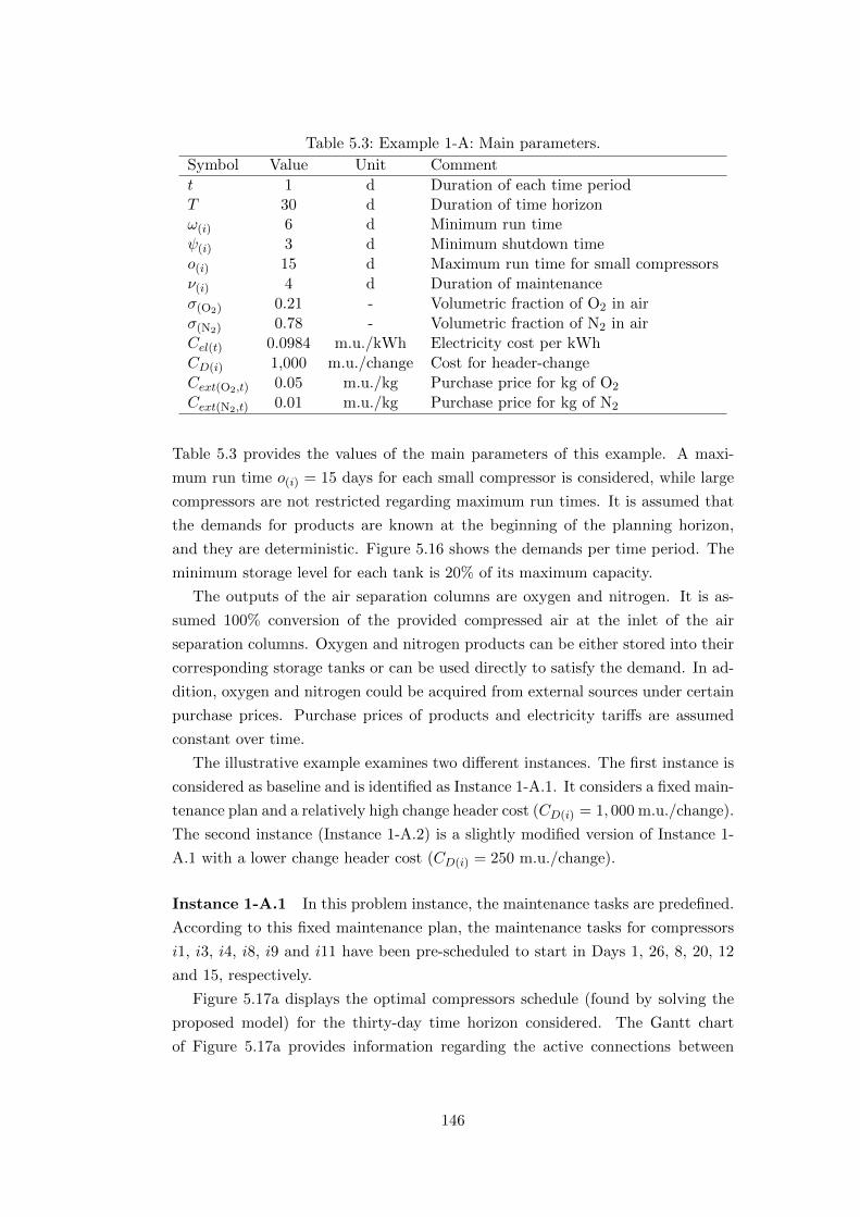
Table 5.3: Example 1-A: Main parameters.
Symbol Value Unit Comment
t 1 d Duration of each time periodT 30 d Duration of time horizonω(i) 6 d Minimum run time
ψ(i) 3 d Minimum shutdown time
o(i) 15 d Maximum run time for small compressors
ν(i) 4 d Duration of maintenance
σ(O2) 0.21 - Volumetric fraction of O2 in air
σ(N2) 0.78 - Volumetric fraction of N2 in air
Cel(t) 0.0984 m.u./kWh Electricity cost per kWh
CD(i) 1,000 m.u./change Cost for header-change
Cext(O2,t) 0.05 m.u./kg Purchase price for kg of O2
Cext(N2,t) 0.01 m.u./kg Purchase price for kg of N2
Table 5.3 provides the values of the main parameters of this example. A maxi-
mum run time o(i) = 15 days for each small compressor is considered, while large
compressors are not restricted regarding maximum run times. It is assumed that
the demands for products are known at the beginning of the planning horizon,
and they are deterministic. Figure 5.16 shows the demands per time period. The
minimum storage level for each tank is 20% of its maximum capacity.
The outputs of the air separation columns are oxygen and nitrogen. It is as-
sumed 100% conversion of the provided compressed air at the inlet of the air
separation columns. Oxygen and nitrogen products can be either stored into their
corresponding storage tanks or can be used directly to satisfy the demand. In ad-
dition, oxygen and nitrogen could be acquired from external sources under certain
purchase prices. Purchase prices of products and electricity tariffs are assumed
constant over time.
The illustrative example examines two different instances. The first instance is
considered as baseline and is identified as Instance 1-A.1. It considers a fixed main-
tenance plan and a relatively high change header cost (CD(i) = 1, 000 m.u./change).
The second instance (Instance 1-A.2) is a slightly modified version of Instance 1-
A.1 with a lower change header cost (CD(i) = 250 m.u./change).
Instance 1-A.1 In this problem instance, the maintenance tasks are predefined.
According to this fixed maintenance plan, the maintenance tasks for compressors
i1, i3, i4, i8, i9 and i11 have been pre-scheduled to start in Days 1, 26, 8, 20, 12
and 15, respectively.
Figure 5.17a displays the optimal compressors schedule (found by solving the
proposed model) for the thirty-day time horizon considered. The Gantt chart
of Figure 5.17a provides information regarding the active connections between
146
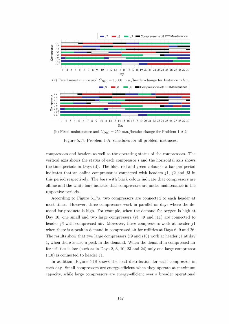
1 2 3 4 5 6 7 8 9 10 11 12 13 14 15 16 17 18 19 20 21 22 23 24 25 26 27 28 29 30
i 1i 2
i 4i 8
i 3
i 11
i 9i 10
J1
J1
J1J1
j1 j2 j3 MaintenanceCompressor is off
Day
Com
pres
sor
(a) Fixed maintenance and CD(i) = 1, 000 m.u./header-change for Instance 1-A.1.
1 2 3 4 5 6 7 8 9 10 11 12 13 14 15 16 17 18 19 20 21 22 23 24 25 26 27 28 29 30
i 1i 2
i 4i 8
i 3
i 11
i 9i 10
J1
J1
J1J1
Day
Com
rpes
sor
j1 j2 j3 MaintenanceCompressor is off
(b) Fixed maintenance and CD(i) = 250 m.u./header-change for Problem 1-A.2.
Figure 5.17: Problem 1-A: schedules for all problem instances.
compressors and headers as well as the operating status of the compressors. The
vertical axis shows the status of each compressor i and the horizontal axis shows
the time periods in Days (d). The blue, red and green colour of a bar per period
indicates that an online compressor is connected with headers j1, j2 and j3 in
this period respectively. The bars with black colour indicate that compressors are
offline and the white bars indicate that compressors are under maintenance in the
respective periods.
According to Figure 5.17a, two compressors are connected to each header at
most times. However, three compressors work in parallel on days where the de-
mand for products is high. For example, when the demand for oxygen is high at
Day 10, one small and two large compressors (i3, i9 and i11) are connected to
header j3 with compressed air. Moreover, three compressors work at header j1
when there is a peak in demand in compressed air for utilities at Days 6, 9 and 26.
The results show that two large compressors (i9 and i10) work at header j1 at day
1, when there is also a peak in the demand. When the demand in compressed air
for utilities is low (such as in Days 2, 3, 10, 23 and 24) only one large compressor
(i10) is connected to header j1.
In addition, Figure 5.18 shows the load distribution for each compressor in
each day. Small compressors are energy-efficient when they operate at maximum
capacity, while large compressors are energy-efficient over a broader operational
147

area. For these reasons, the large compressors accommodate the demand fluctua-
tions by adjusting their mass flow rates while small compressors tend to operate
at maximum capacity.
Figure 5.19a presents the total compressed air supplied to each header for each
time period. The mass flow rate of compressed air in header j1 is equal to the
compressed air for utilities as shown in Figure 5.16. Figure 5.19b shows the com-
pressed air load distribution proportion between the two air separation columns u1
and u2. As expected, column u2 produces more than column u1, due to the fact
that column u2 has a higher production capacity. Finally, purchase of nitrogen is
reported on Day 15. This is due to the fact that the demand for nitrogen cannot
be satisfied because two large compressors are under maintenance on this day.
i8i9 i11
i10
i1i2
i3i4
Sm
all c
ompr
esso
rsm
ass
flow
rate
s (%
)La
rge
com
pres
sors
mas
s flo
w ra
tes
(%)
Figure 5.18: Optimal distribution of (normalised) load of compressors in Instance1-A.1
(a)
(b)
j1 j2 j3
u1/u
2M
ass
flow
ra
tes
(%)
Figure 5.19: Instance 1-A.1: (a) total compressed air supplied to each header, and(b) production capacity ratio of column u1 and u2.
148
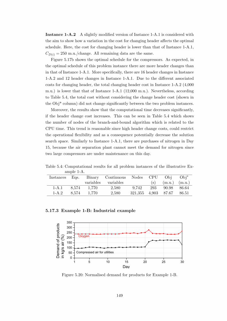
Instance 1-A.2 A slightly modified version of Instance 1-A.1 is considered with
the aim to show how a variation in the cost for changing header affects the optimal
schedule. Here, the cost for changing header is lower than that of Instance 1-A.1,
CD(i) = 250 m.u./change. All remaining data are the same.
Figure 5.17b shows the optimal schedule for the compressors. As expected, in
the optimal schedule of this problem instance there are more header changes than
in that of Instance 1-A.1. More specifically, there are 16 header changes in Instance
1-A.2 and 12 header changes in Instance 1-A.1. Due to the different associated
costs for changing header, the total changing header cost in Instance 1-A.2 (4,000
m.u.) is lower that that of Instance 1-A.1 (12,000 m.u.). Nevertheless, according
to Table 5.4, the total cost without considering the change header cost (shown in
the Obj* column) did not change significantly between the two problem instances.
Moreover, the results show that the computational time decreases significantly,
if the header change cost increases. This can be seen in Table 5.4 which shows
the number of nodes of the branch-and-bound algorithm which is related to the
CPU time. This trend is reasonable since high header change costs, could restrict
the operational flexibility and as a consequence potentially decrease the solution
search space. Similarly to Instance 1-A.1, there are purchases of nitrogen in Day
15, because the air separation plant cannot meet the demand for nitrogen since
two large compressors are under maintenance on this day.
Table 5.4: Computational results for all problem instances of the illustrative Ex-ample 1-A.
Instances Eqs. Binary Continuous Nodes CPU Obj Obj∗
variables variables (s) (m.u.) (m.u.)
1-A.1 8,574 1,770 2,580 9,742 293 90.98 86.641-A.2 8,574 1,770 2,580 321,355 4,903 87.67 86.51
5.17.3 Example 1-B: Industrial example
Day
Dem
and
of p
rodu
cts
in k
g/s
air (
%)
Figure 5.20: Normalised demand for products for Example 1-B.
149
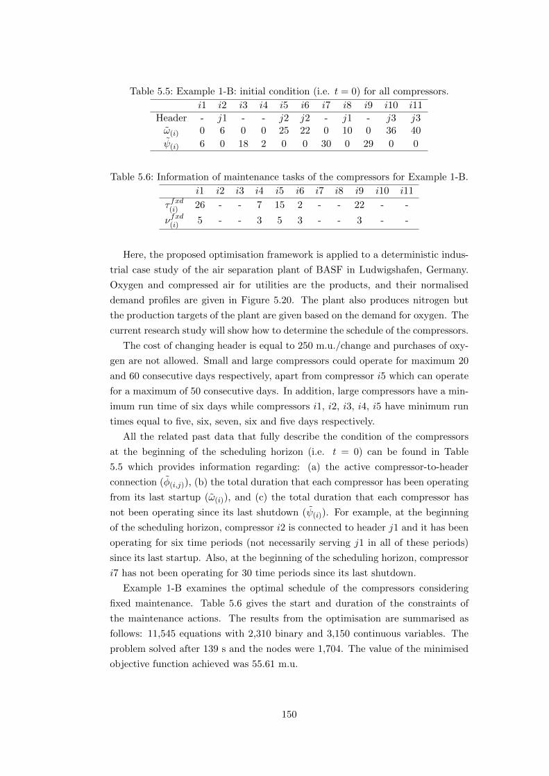
Table 5.5: Example 1-B: initial condition (i.e. t = 0) for all compressors.
i1 i2 i3 i4 i5 i6 i7 i8 i9 i10 i11
Header - j1 - - j2 j2 - j1 - j3 j3ω(i) 0 6 0 0 25 22 0 10 0 36 40
ψ(i) 6 0 18 2 0 0 30 0 29 0 0
Table 5.6: Information of maintenance tasks of the compressors for Example 1-B.
i1 i2 i3 i4 i5 i6 i7 i8 i9 i10 i11
τ fxd(i) 26 - - 7 15 2 - - 22 - -
νfxd(i) 5 - - 3 5 3 - - 3 - -
Here, the proposed optimisation framework is applied to a deterministic indus-
trial case study of the air separation plant of BASF in Ludwigshafen, Germany.
Oxygen and compressed air for utilities are the products, and their normalised
demand profiles are given in Figure 5.20. The plant also produces nitrogen but
the production targets of the plant are given based on the demand for oxygen. The
current research study will show how to determine the schedule of the compressors.
The cost of changing header is equal to 250 m.u./change and purchases of oxy-
gen are not allowed. Small and large compressors could operate for maximum 20
and 60 consecutive days respectively, apart from compressor i5 which can operate
for a maximum of 50 consecutive days. In addition, large compressors have a min-
imum run time of six days while compressors i1, i2, i3, i4, i5 have minimum run
times equal to five, six, seven, six and five days respectively.
All the related past data that fully describe the condition of the compressors
at the beginning of the scheduling horizon (i.e. t = 0) can be found in Table
5.5 which provides information regarding: (a) the active compressor-to-header
connection (φ(i,j)), (b) the total duration that each compressor has been operating
from its last startup (ω(i)), and (c) the total duration that each compressor has
not been operating since its last shutdown (ψ(i)). For example, at the beginning
of the scheduling horizon, compressor i2 is connected to header j1 and it has been
operating for six time periods (not necessarily serving j1 in all of these periods)
since its last startup. Also, at the beginning of the scheduling horizon, compressor
i7 has not been operating for 30 time periods since its last shutdown.
Example 1-B examines the optimal schedule of the compressors considering
fixed maintenance. Table 5.6 gives the start and duration of the constraints of
the maintenance actions. The results from the optimisation are summarised as
follows: 11,545 equations with 2,310 binary and 3,150 continuous variables. The
problem solved after 139 s and the nodes were 1,704. The value of the minimised
objective function achieved was 55.61 m.u.
150
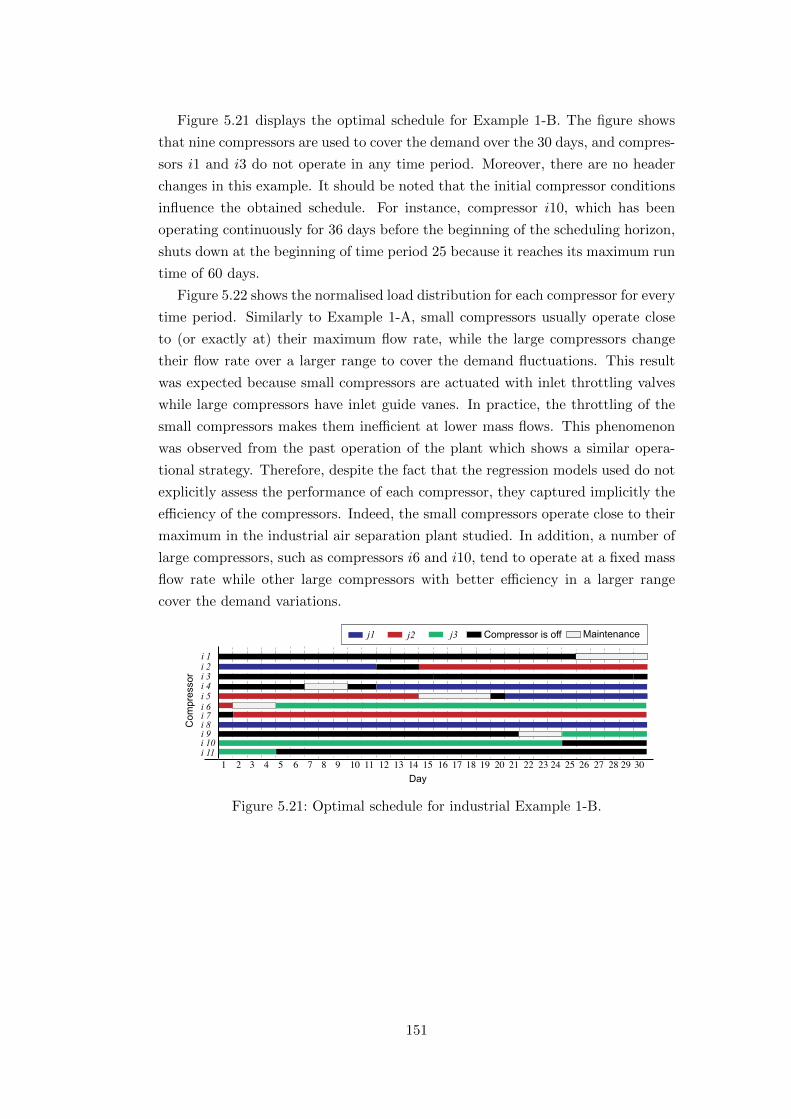
Figure 5.21 displays the optimal schedule for Example 1-B. The figure shows
that nine compressors are used to cover the demand over the 30 days, and compres-
sors i1 and i3 do not operate in any time period. Moreover, there are no header
changes in this example. It should be noted that the initial compressor conditions
influence the obtained schedule. For instance, compressor i10, which has been
operating continuously for 36 days before the beginning of the scheduling horizon,
shuts down at the beginning of time period 25 because it reaches its maximum run
time of 60 days.
Figure 5.22 shows the normalised load distribution for each compressor for every
time period. Similarly to Example 1-A, small compressors usually operate close
to (or exactly at) their maximum flow rate, while the large compressors change
their flow rate over a larger range to cover the demand fluctuations. This result
was expected because small compressors are actuated with inlet throttling valves
while large compressors have inlet guide vanes. In practice, the throttling of the
small compressors makes them inefficient at lower mass flows. This phenomenon
was observed from the past operation of the plant which shows a similar opera-
tional strategy. Therefore, despite the fact that the regression models used do not
explicitly assess the performance of each compressor, they captured implicitly the
efficiency of the compressors. Indeed, the small compressors operate close to their
maximum in the industrial air separation plant studied. In addition, a number of
large compressors, such as compressors i6 and i10, tend to operate at a fixed mass
flow rate while other large compressors with better efficiency in a larger range
cover the demand variations.
1 2 3 4 5 6 7 8 9 10 11 12 13 14 15 16 17 18 19 20 21 22 23 24 25 26 27 28 29 30
J1
Day
i 1i 2
i 4
i 8
i 3
i 11
i 9i 10
i 5i 6i 7
Com
pres
sor
j1 j2 j3 MaintenanceCompressor is off
Figure 5.21: Optimal schedule for industrial Example 1-B.
151

i2 i4
i6i7
i8 i10i11
i5
i9
Sm
all c
ompr
esso
rsm
ass
flow
rate
s (%
)La
rge
com
pres
sors
mas
s flo
w ra
tes
(%)
Figure 5.22: Normalised load of compressors for industrial Example 1-B.
5.17.4 Example 2: Industrial example of an export gas
compressor station
Description of case study 2 (Statoil export gas compressor station)
The methodology of the multi-period operational model of parallel compressors
is applied to an industrial example using data from Statoil. This example considers
a deterministic optimisation problem with a time horizon of thirty days with time
periods of one day each.
The industrial Example 2 considers Kollsnes export gas compressor station,
shown in Fig. 5.12, with six multi-stage centrifugal compressors. The range of
their nominal power is from 34 to 37 MW. The original case encompasses five small
compressors Is = i1, i2, i3, i4, i5 which have same characteristics and one large
compressor i6 ∈ Ib which has larger operating range and higher efficiency than the
other five small compressors. It is noted that the efficiency of a compressor varies
Table 5.7: Initial state of the compressors.
i1 i2 i3 i4 i5 i6
φ(i, j1) 1 1 0 0 0 0
φ(i, j2) 0 0 1 1 0 1ω(i) 50 20 55 14 0 20
ψ(i) 0 0 0 0 25 0
τ fxd(i) 15 18 - - 25 20
νfxd(i) 2 2 - - 2 2
152

Table 5.8: Parameters of compressors.
Tref Pref MolWref ω(i) ψ(i) o(i)
Is 273.15 75 17.3 5 3 65Ib 299.65 76.7 18.1 9 3 75
j1j2
Day
Dem
and
(MM
sm3 /d
)
(a) Given demand flow rate.
j1j2
Day
Pre
ssur
e (b
ar A
)(b) Given pressure.
Figure 5.23: Input demand of flow rate and pressure of each delivery point forheaders j1 and j2.
according to the volumetric flow rate and polytropic head for fixed conditions (i.e.
inlet pressure and temperature, compressibility and molecular weight).
Table 5.7 gives the initial connection of a compressor i with headers j1 and
j2, described by the binary parameter φ(i,j). The parameter ω(i) represents the
continuous days of operation of the online compressors before the beginning of the
optimisation. Parameter ψ(i) gives the continuous days of non-operation of the
compressors which have been shut down before the beginning of the optimisation.
Moreover, Table 5.7 provides the beginning τ(i) and duration ν(i) of the fixed main-
tenance of the compressors. Table 5.8 shows the values of the reference conditions
of each set of compressors. It also provides the minimum running time, ω(i), the
minimum shut down time, ψ(i), and the maximum running time, o(i).
It is assumed that the temperature of the delivery point is constant, Td(t) =
315.15 K. The composition and compressibility of the gas are assumed and given
constant over time, with molecular weight MolWact,s(t) = 17.3 and compressibility
Zact,s(t) = 0.809. The polytropic exponent in Eq. (5.46) is estimated from the
compressor maps φ(i) = 0.35 and the electricity price is assumed fixed for the
purposes of the scheduling problem with Cel(t) = 0.098 EUR/kWh (European
Commission, Eurostat, 2015).
Moreover, the start up cost is estimated equal to the energy spent to operate
a compressor for ten hours at its nominal rate is based on the experience of the
industry and analysis of historical data. The shut down cost was set equal to the
153

DayP
ress
ure
(bar
A)
Figure 5.24: Upstream inlet pressure.
half of the start-up cost. The inlet temperature of the gas is assumed constant
over time for different compressors. The temperature for the compressors i ∈ Is is
280 K and the temperature for compressors i ∈ Ib is 294 K.
Historical industrial data from past years are collected for formulating a case
study. Data from one summer month provided the demand in mass flow rate (Fig.
5.23a) and in pressure (Fig. 5.23b). The inlet pressure of the gas compressor
station is also given (Fig. 5.24) for this month.
The developed mathematical models which are applied to the Statoil export
gas compressor station involve the following constraints:
• Constraints of the minimum run and shutdown time, described by Eqs. (5.1)
– (5.4).
• Constraints of the assignment of compressors to headers, described by Eq.
(5.5).
• Constraints of the changes of compressors to headers, described by Eq. (5.6)
in Section 5.5.
• Constraints which model the power consumption and feasible window of
operation with the use of compressor maps. These constraints are described
by Eqs. (5.23) – (5.46).
• Constraints of the model of the recycle of the flow, described by Eqs. (5.47)
– (5.49).
• General constraints of the operation of an export gas compressor station
given by Eqs. (5.59), (5.60).
• Constraints of a given maintenance schedule including runtime-based main-
tenance constraints of Eq. (5.62), and given starting times and duration of
maintenance tasks described by Eq. (5.63).
154

• Constraints of the initial state of the compressors, described by Eqs. (5.64),
(5.65) and (5.66).
• Constraints of the equal split strategy, described by Eqs. (5.68) – (5.72).
• Constraints of the equal surge margin strategy, described by Eqs. (5.73) –
(5.76).
The objective function for the case study of the natural gas export station
is given by Eq. (5.61) in Section 5.12. Compressor maps are used to estimate
the power consumption through Eqs. (5.23), (5.26) and (5.44). As previously
mentioned, the motor and gearbox losses are not considered, thus Wel = Wact.
The constraints, objective function and the given input data were implemented
into the optimisation platform GAMS using the MILP solver CPLEX 1.1 in the
same system as in Example 1 with Intel(R) Core(TM) i7-2600 CPU @3.4GHz with
8GB RAM.
Twelve different optimisation problems have been developed to illustrate the
use of the mathematical model for optimal operation of export gas compressors.
Table 5.9 presents the description of the scheduling problems of which each con-
siders (a) different method for sharing the load, and (b) different number of large
compressors. The real configuration of the plant includes only one large compres-
sor installed. Problems 6 – 8 and 10 – 12 consider the hypothetical scenario of
the use of three large compressors. The reason to examine this case is that Sta-
toil considers to purchase large compressors in the next years. Finally, the twelve
problems examine different predefined values of the OPTCR criterion.
Therefore, the Optimal method for optimally sharing the load among the com-
pressors considers the operating set points of the compressors as decision variables
of the optimisation problem. The set points of the compressors are not correlated
through any constraint and they are free to take any value within their feasible
windows of operation. This method is proposed in this current research study and
it is compared with typical industrial policies such as equal split and equal surge
margin. The optimal method is part of the suggested optimisation framework of
this PhD thesis. The Equal Split (ES) method refers to a typical industrial method
which shares the total load evenly among the compressors and it was mathemati-
cally described in Section 5.16.1. An other common industrial policy to distribute
the total load is the one which refers to the operation with equal distance (margin)
between operation and surge of every compressor connecting to the same header,
namely Equal Surge Margin (ESM) method.
155
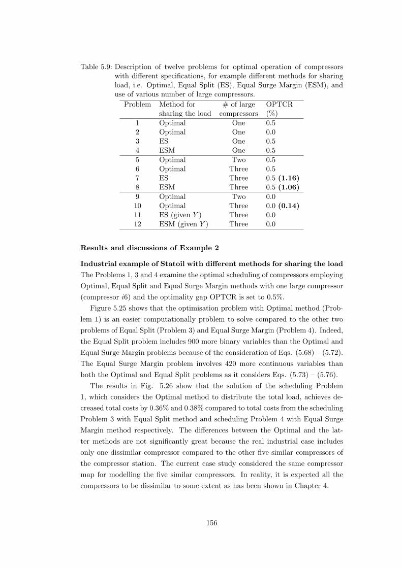
Table 5.9: Description of twelve problems for optimal operation of compressorswith different specifications, for example different methods for sharingload, i.e. Optimal, Equal Split (ES), Equal Surge Margin (ESM), anduse of various number of large compressors.
Problem Method for # of large OPTCRsharing the load compressors (%)
1 Optimal One 0.52 Optimal One 0.03 ES One 0.54 ESM One 0.5
5 Optimal Two 0.56 Optimal Three 0.57 ES Three 0.5 (1.16)8 ESM Three 0.5 (1.06)
9 Optimal Two 0.010 Optimal Three 0.0 (0.14)11 ES (given Y ) Three 0.012 ESM (given Y ) Three 0.0
Results and discussions of Example 2
Industrial example of Statoil with different methods for sharing the load
The Problems 1, 3 and 4 examine the optimal scheduling of compressors employing
Optimal, Equal Split and Equal Surge Margin methods with one large compressor
(compressor i6) and the optimality gap OPTCR is set to 0.5%.
Figure 5.25 shows that the optimisation problem with Optimal method (Prob-
lem 1) is an easier computationally problem to solve compared to the other two
problems of Equal Split (Problem 3) and Equal Surge Margin (Problem 4). Indeed,
the Equal Split problem includes 900 more binary variables than the Optimal and
Equal Surge Margin problems because of the consideration of Eqs. (5.68) – (5.72).
The Equal Surge Margin problem involves 420 more continuous variables than
both the Optimal and Equal Split problems as it considers Eqs. (5.73) – (5.76).
The results in Fig. 5.26 show that the solution of the scheduling Problem
1, which considers the Optimal method to distribute the total load, achieves de-
creased total costs by 0.36% and 0.38% compared to total costs from the scheduling
Problem 3 with Equal Split method and scheduling Problem 4 with Equal Surge
Margin method respectively. The differences between the Optimal and the lat-
ter methods are not significantly great because the real industrial case includes
only one dissimilar compressor compared to the other five similar compressors of
the compressor station. The current case study considered the same compressor
map for modelling the five similar compressors. In reality, it is expected all the
compressors to be dissimilar to some extent as has been shown in Chapter 4.
156

Continuous Variables Binary Variables
Equations
Method for sharing load
Qua
ntity
Figure 5.25: Specifications of the model of the scheduling with three different meth-ods for sharing the total load: Optimal, Equal Split (ES) and EqualSurge Margin (ESM).
Problem
Tota
l cos
t (E
UR
)
•106
•106
•106
•106
•106
•106
•106
•106 •1
06
•106 •1
06
•106
9.80
9.75
9.70
9.65
9.60
9.55
9.50
9.45
9.50
9.35
9.30
9.25
Figure 5.26: Total costs in EUR for thirty days optimisation for the twelve opti-misation problems described in Table 5.9.
The computational time for solving the scheduling problem with Equal Split
method is approximately 1534 times greater than the time needed to solve the
Optimal scheduling problem which computational time is only approximately 18
s as it is shown in Fig. 5.27a. The scheduling problem with the Equal Split
method has a large number of binary variables and this increases significantly the
computational time compared to the scheduling problem with the Equal Surge
Margin method with an increased number of continuous variables. Figure 5.27a
shows these computational times. The number of nodes of the branch-and-bound
tree (Section 2.5.2) of each optimisation problem can be seen in Fig. 5.27b.
The Problem 2 of Example 2 examines the scheduling with Optimal method
with predefined value of OPTCR equal to 0.00%. The solution of this problem
provides a reduced total cost by 0.28% compared to the total costs of Problem 1
157
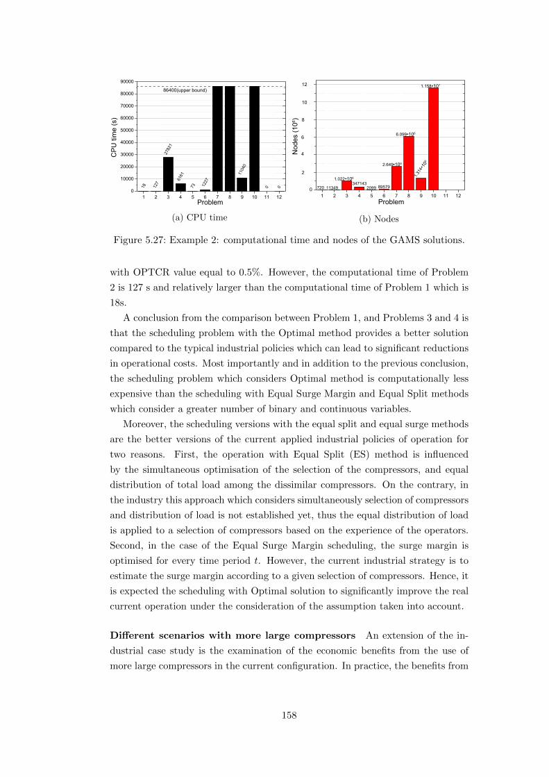
86400(upper bound)
Problem
CP
U ti
me
(s)
(a) CPU time
•106
•106
12
10
8
6
4
2
Problem
Nod
es (1
06 )
•106
•107
•106
(b) Nodes
Figure 5.27: Example 2: computational time and nodes of the GAMS solutions.
with OPTCR value equal to 0.5%. However, the computational time of Problem
2 is 127 s and relatively larger than the computational time of Problem 1 which is
18s.
A conclusion from the comparison between Problem 1, and Problems 3 and 4 is
that the scheduling problem with the Optimal method provides a better solution
compared to the typical industrial policies which can lead to significant reductions
in operational costs. Most importantly and in addition to the previous conclusion,
the scheduling problem which considers Optimal method is computationally less
expensive than the scheduling with Equal Surge Margin and Equal Split methods
which consider a greater number of binary and continuous variables.
Moreover, the scheduling versions with the equal split and equal surge methods
are the better versions of the current applied industrial policies of operation for
two reasons. First, the operation with Equal Split (ES) method is influenced
by the simultaneous optimisation of the selection of the compressors, and equal
distribution of total load among the dissimilar compressors. On the contrary, in
the industry this approach which considers simultaneously selection of compressors
and distribution of load is not established yet, thus the equal distribution of load
is applied to a selection of compressors based on the experience of the operators.
Second, in the case of the Equal Surge Margin scheduling, the surge margin is
optimised for every time period t. However, the current industrial strategy is to
estimate the surge margin according to a given selection of compressors. Hence, it
is expected the scheduling with Optimal solution to significantly improve the real
current operation under the consideration of the assumption taken into account.
Different scenarios with more large compressors An extension of the in-
dustrial case study is the examination of the economic benefits from the use of
more large compressors in the current configuration. In practice, the benefits from
158

the optimal distribution of load against typical load sharing strategies stem from
the fact that the compressors which operate in parallel are dissimilar. In an ideal
case in which all the compressors have the same specifications and conditions (i.e.
performance), then there would not be any significant improvement if the opti-
mal method is applied instead of the typical load sharing strategies. In practice
a compressor station involves dissimilar compressors due to uneven operation and
uneven maintenance of the compressors.
According to Table 5.9, Problems 5 and 6 examine the scheduling of compressors
with the following characteristics: (a) use of Optimal load sharing method, (b) use
of two and three large compressors with the same specifications as compressors i6
and (c) the value of the OPTCR is predefined to 0.5%. Problems 9 and 10 examine
similar cases to Problems 5 and 6 with two and three compressors respectively,
and the only difference is that the value of OPTCR is set to 0.0%. Therefore, the
sets of compressors with two large compressors for Problems 5 and 9 would be
Is = i1, i2, i3, i4 and Ib = i5′, i6, and the sets of compressors for Problems
6 and 10 are Is = i1, i2, i3 and Ib = i4′, i5′, i6 . Compressors i4′, i5′ are
assumed exactly the same as compressor i6.
Figure 5.26 shows that Problem 5 with two compressors achieves decreased total
operational costs compared to the Problem 1 with one large compressor by 1.11%.
Problem 6 with three large compressors achieves decreased total operational costs
compared to the Problem 1 by 2.05%. These calculations considered OPTCR
equal to 0.5%.
The comparison between Problems with one (i.e. Problem 2) , two (i.e. Prob-
lem 9) and three large compressors (Problem 10) with OPTCR = 0.0% shows
similar results. The Problem 9 achieves decreased total operational costs com-
pared to Problem 2 by 0.90% and the difference between Problem 10 with three
large compressors and Problem 2 is 1.91%. Indeed, in this representative industrial
example, the reduced operational costs for one month amounting to 88,857 EUR
if two large compressors are used, and to 182,707 EUR if three large compressors
are employed instead of only one large compressor in both cases. It is important
to notice that again the set with large compressors considers compressors which
have the same specifications.
From a computational point of view, the more large compressors are considered
in the optimisation problem, the longer it takes to find the optimal solution. Prob-
lem 10 reached the predefined time criterion of 24h (equal to 86,400 s) as can be
seen in Fig. 5.27a and the number of nodes of the computational tree are signif-
icantly greater than those of Problem 9. Furthermore, the solution of Problem 9
has a larger number of nodes than the solution of Problem 2. Problems 2 (with one
large compressor) and Problem 9 (with two large compressors) reached a solution
159
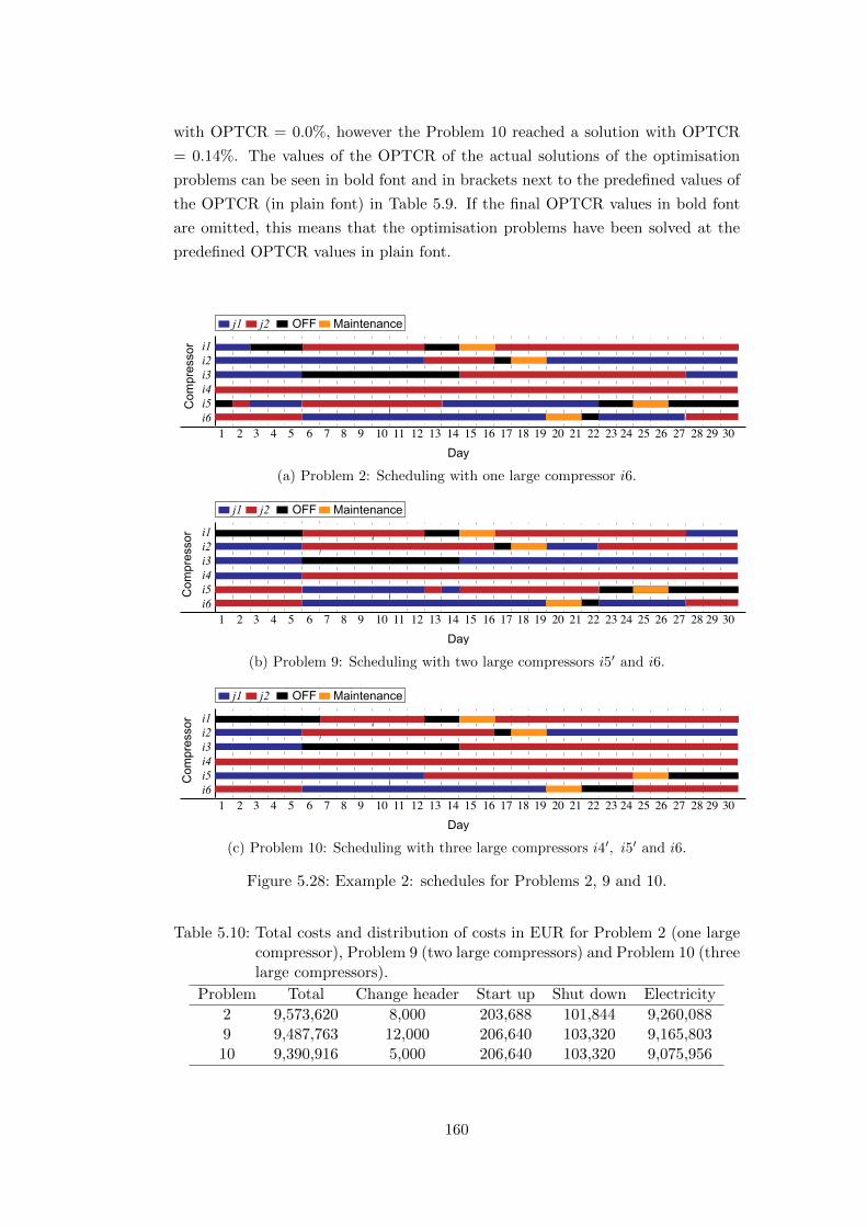
with OPTCR = 0.0%, however the Problem 10 reached a solution with OPTCR
= 0.14%. The values of the OPTCR of the actual solutions of the optimisation
problems can be seen in bold font and in brackets next to the predefined values of
the OPTCR (in plain font) in Table 5.9. If the final OPTCR values in bold font
are omitted, this means that the optimisation problems have been solved at the
predefined OPTCR values in plain font.
Com
pres
sor
1 2 3 4 5 6 7 8 9 10 11 12 13 14 15 16 17 18 19 20 21 22 23 24 25 26 27 28 29 30
i1i2
i4i5
i3
i6
Day
j1 j2 Maintenance OFF
(a) Problem 2: Scheduling with one large compressor i6.
Com
pres
sor
1 2 3 4 5 6 7 8 9 10 11 12 13 14 15 16 17 18 19 20 21 22 23 24 25 26 27 28 29 30
i1i2
i4i5
i3
i6
Day
j1 j2 Maintenance OFF
(b) Problem 9: Scheduling with two large compressors i5′ and i6.
Com
pres
sor
1 2 3 4 5 6 7 8 9 10 11 12 13 14 15 16 17 18 19 20 21 22 23 24 25 26 27 28 29 30
i1i2
i4i5
i3
i6
Day
j1 j2 Maintenance OFF
(c) Problem 10: Scheduling with three large compressors i4′, i5′ and i6.
Figure 5.28: Example 2: schedules for Problems 2, 9 and 10.
Table 5.10: Total costs and distribution of costs in EUR for Problem 2 (one largecompressor), Problem 9 (two large compressors) and Problem 10 (threelarge compressors).
Problem Total Change header Start up Shut down Electricity
2 9,573,620 8,000 203,688 101,844 9,260,0889 9,487,763 12,000 206,640 103,320 9,165,80310 9,390,916 5,000 206,640 103,320 9,075,956
160
Figure 5.28 provides the Gantt Chart of the scheduling of each problem with
one, two and three large compressors respectively. The first observation, is that
the number of the large compressors under consideration influences the number of
changes, and the number of startups and shutdowns of the compressors in each
problem according to Fig. 5.28 and Table 5.10. The problem with the greatest
number of large compressors, in Fig. 5.28c, shows that the operation involves
fewer changes and each compressor operates to one header for longer periods than
in the other two cases. It can be observed that in the first two problems there are
instances in which compressors operated to a head only for one time period, and
after the end of this period they changed connection, for instance compressor i5 on
Day 2 for Problem 2. Compressor i5 on Days 13 and 14 for Problem 9 is another
example. The initial condition influences the scheduling for all instances. For
instance, compressor i3 shuts down on Day 6 as it is close to reach its maximum
allowed continuous operational days and compressor i4 remains online mostly for
all time periods in all cases as it is the one which has been operated less than the
other compressors before the start of the optimisation.
In order to illustrate the benefits of the scheduling with the Optimal load sharing
approach compared to the Equal Split and Equal Surge Margin approaches when
three large compressors are installed, Problem 7 and Problem 8 dealt with the
Equal Split and Equal Surge Margin load sharing methods respectively. However,
both problems were computationally difficult to solve and the optimal solutions
found were these with OPTCR = 1.16% and 1.06% respectively after reaching the
maximum computational time limit. Figure 5.26 shows that the total costs from
Problems 7 (Equal Split) and 8 (Equal Surge Margin) are greater than the costs
of Problem 6 (Optimal), however, there is uncertainty in their relative respective
differences because Problems 7 and 8 have been solved for different OPTCR values.
The impact of different sharing load methods on the total costs of
scheduling The previous paragraph showed that the consideration of Equal
Split and Equal Surge Margin methods increases the complexity of the optimi-
sation problems and the optimal solution of the corresponding scheduling prob-
lems with three large compressors cannot be estimated at 0% OPTCR. For this
reason, this paragraph will examine the differences between scheduling problems
with Optimal and the other load typical sharing (i.e. Equal Split and Equal Surge
Margin) methods when the selection of the compressors is given in the case of the
scheduling with typical load sharing methods. The consideration of a given selec-
tion of compressors results in the simplification of the optimisation models as they
will not involve binary variables. The current industrial policy does not provide
a simultaneous solution of best selection of compressors and optimal distribution
161

Optimal operational range
Day
i1i2i3M
ass
flow
rate
s (k
g/s)
(a) Small compressors
i4’i5’i6
Day
Mas
s flo
w ra
tes
(kg/
s)
Optimal operational range
(b) Large compressors
Figure 5.29: Example 2: mass flow rates for Problem 10.
i4’-i6
Figure 5.30: Power consumption of the station (total all), of small compressors (to-tal i1−i3), of large compressors (total i4′−i6) and power consumptionper header j1 and header j2 per each time period.
of load. Hence the analysis in this paragraph will help to identify the benefits
of the scheduling of compressors with Optimal method compared to the typical
industrial methods.
Problems 11 and 12 consider the solution of the scheduling with Equal Split and
Equal Surge Margin method for sharing the load among the compressors with a
given selection of compressors for every day of the thirty day optimisation problem
described in the beginning in Section 5.17.4. Because there not any binary variables
included in the optimisation, then the computational time to solve both problems
is approximately 0.28s and therefore there are no nodes shown in Fig. 5.27b for
Problems 11 and 12. The optimal solution of Problem 10 with Optimal method
for sharing load achieves 0.88% and 1.03% reduced operational costs compared to
Equal Split and Equal Surge Margin methods.
Figure 5.29 illustrates the mass flow rates of small and large compressors per
162

(a) ESM against Optimal (b) ES against Optimal
Figure 5.31: Power consumption absolute differences (in kW) between schedulingwith Optimal and other sharing methods (ESM/ES) per each day.
time period for 30 days. As can be observed, there is not any pattern of operation
related to the flows of the compressors. Nevertheless, the operational range of
the small compressors is more narrow than that of the large compressors. More-
over, Fig. 5.30 displays the power consumption of the compressor station, of each
header and the groups of small and large compressors. From Day 20 and on-
wards the power consumption of small compressors become greater than that of
the large compressors. This is because two out of three large compressors have to
be maintained according to the given maintenance plan.
Figure 5.31 illustrates the absolute difference in power in kW between the
scheduling with Optimal method and the scheduling with Equal Surge Margin
(Fig. 5.31a) or Equal Split (Fig. 5.31a). The two latter methods are given the
selection of the compressors. In the first comparison the difference in power can
range from 54 kW up to more than 2 MW. Similarly in the second comparison
with the scheduling with Optimal and Equal Split method the difference can reach
the value of 5 MW. However, the total power difference for 30 days is greater in the
case of Optimal against Equal Surge Margin as mentioned previously. Neverthe-
less, this example shows the importance to consider the selection and distribution
of the compressors simultaneously.
5.18 Summary of the chapter
A general mathematical framework for the optimisation of the operational tasks
of multiple parallel compressors has been presented. The outputs of the framework
are the best decisions of the operation which result in reduced total costs. The
framework can be used for the optimisation of the operation of compressor stations
of systems with large energy consumption. The air compressors of an air separation
163
plant and the export natural gas compressor station of a gas network are two
examples of these systems.
The mathematical formulation of the suggested framework considered a MILP
multi-period approach with uniform discretised time periods. This mathematical
framework includes the modelling of compressors with the use of process data
or with the use of compressors maps. The mathematical framework with the
former modelling approach was applied to the industrial case of the air separation
plant and the latter modelling approach was applied to the export gas compressor
station.
The operative set points, startup, shutdown and change-header costs of the
compressors were determined for achieving optimal operation. Both continuous
and binary variables were used to model the operational constraints of the com-
pressors and the overall plant. Initial state of the system and terminal constraints
were defined and maintenance actions were given as input along with demands
and other parameters such as values of the costs. The resulting MILP model was
implemented in GAMS and the CPLEX solver was employed to find the optimal
solution.
The application of the framework to the case study of the air separation plant
demonstrated the outputs of the MILP model (e.g Gantt chart, set points of mass
flow rates) and validated the model by comparing the results of the scheduling
with industrial practices. An industrial example based on historical data showed
that the optimal schedule can provide insights and generic trends for improving the
operation. For instance, the small compressors should work at maximum capacity
and the large compressors to satisfy the remaining demand. Another example
is that compressors should operate with the minimum number of changes among
headers for the considered time period of optimisation.
The application of the framework to the case study of the export gas station
studied the following cases with the respective remarks:
• Comparison of scheduling cases with different load sharing methods for the
current industrial Statoil case (one large compressor under consideration):
The computational results showed that the optimisation problem with schedul-
ing with Equal Split and Equal Surge Margin methods are computationally
more demanding to solve compared to the scheduling with Optimal method.
Nevertheless, the scheduling with Optimal method achieves slightly better
results for the total costs of the operation. It was also observed that small
changes in the values of OPTCR affects the solution significantly.
• Investigation and quantification of the operational and economic impact of
different scenarios with more large compressors under consideration: The
164
more large compressors are used, the greater is the improvement in the oper-
ation. The use of two and three large compressors can reduce the operational
costs by approximately 1% and 2% respectively. However, the computational
time to solve the optimisation problem with more than one large compres-
sor increases with the number of the large compressors under consideration.
The optimisation problems with Equal Split and Equal Surge Margin shar-
ing methods reached solutions with OPTCR = 1.16% and 1.06% respectively
after 24 h computational time with the predefined OPTCR criterion was set
to 0.0% and the predefined time termination criterion was set to 24h.
• Examination of the impact of different sharing load methods on the total
costs of scheduling : the configuration of the compressors and connections of
compressors with headers are determined from the solution of the schedul-
ing problem with Optimal load sharing method. An example showed that
the latter scheduling problem achieves 0.88% and 1.03% reduced operational
costs compared to the cases with Equal Split and Equal Surge Margin meth-
ods respectively. The two latter cases used fixed configuration of compressors
and connections of compressors and headers from the solution of the former
scheduling problem.
165

6 Integration of optimal operation
and maintenance
6.1 Description of the chapter
The maintenance of centrifugal compressors is an important topic for the in-
dustry as the maintenance cost accounts for 6% of the total cost of the life cycle
of a compressor. Chapter 2 reported that the specifications of the maintenance
of centrifugal compressors, for example period of a cycle and cost of maintenance
service, differ compared to these of other types of compressors. Centrifugal com-
pressors have longer maintenance cycles but a maintenance repair lasts longer than
other types of compressors. Moreover, centrifugal compressors deal with the prob-
lem of fouling which causes erosion and corrosion. These two phenomena cause a
decrease in performance and therefore an increase in power consumption.
The aim of the maintenance of compressors is to reduce the number of unex-
pected breakdowns and failures. A failure of a compressor may affect other process
units which are connected with the compressor, and thus this failure can result
in downtime of the plant and lost production. The maintenance includes tasks
such as replacement of components (for instance bearings and blades of impeller),
inspection of mechanical and electrical parts, and cleaning of the surfaces of the
inside of the compressor.
Maintenance and operation seem to be highly dependent on each other. The
purpose of Chapter 6 is to develop methods for integrating maintenance and op-
eration, and prove this dependance and quantify it. Therefore, the integration of
operation and maintenance will be presented by mathematical models which deal
with different cases of maintenance of compressors, for example minor corrective
maintenance actions, major overhauls and different washing methods.
Section 6.2 presents a basic maintenance model which considers the start times
of the maintenance events as degrees of freedom in the optimisation model. In-
deed, the estimation of the start times of the maintenance events is restricted by a
given time window defined by the earliest and latest start time of the maintenance.
In addition, the compressors have maximum running time constraints, as a max-
imum runtime-based maintenance model is also taken into account (this model is
presented in Section 5.13).
166

The basic model can be adapted in a rolling time horizon framework which
is based on the principles of a model predictive control tool, but for scheduling
purposes. The time horizon of the multi-period optimisation problem is shifting
by a number of periods (one period will be used) and the parameters are updated
in every shift. Section 6.3 presents the algorithm of this rolling horizon approach
and gives the results from its application to the case of the air separation plant.
Section 6.4 presents the extension of the basic integration model considering
longer time periods and a larger set of maintenance constraints. This extended
model deals with the simultaneous optimisation of operation and maintenance
including major overhauls. This model also considers aspects of the maintenance
of compressors, for example different groups for mechanical and electrical repairs
and inspections, and restrictions for the maximum number of compressors that can
be repaired at the same period. These restrictions were mentioned in the study
by Castro et al. (2014).
Section 6.5 presents a model for condition-based maintenance for the optimi-
sation of the washing schedules of industrial centrifugal compressors. The as-
sumptions of the model are presented in detail and the model is applied to the
air compressors of the air separation plant of case study one. The comparison
between online, offline washing and their combination is presented. The frame-
work also examines scenarios of compressors with different degradation rates and
scenarios with different numbers of available compressors to operate.
Chapter 6 involves research which has been published in the following confer-
ences and journals:
• Results from the basic model of the integrated operation and maintenance of
Sections 6.2 and 6.3 have been published in the paper ‘Operational planning
of a network of compressors: The air separation plant case’ (Kopanos et al.,
2015) in the journal Applied Energy.
• The research in Section 6.4 initially was presented in the conference Turbo
Expo 2015 with title ‘Optimal operation and maintenance of gas compressor
stations: An integrated framework applied to a large-scale industrial case’
(Xenos et al., 2015b). The conference paper was recommended for journal
by the reviewers of the conference and therefore the original work with im-
provements was published in the Journal of Engineering for Gas Turbines
and Power (Xenos et al., 2015c).
• The work on the condition-based maintenance of compressor is published
in the journal Computers & Chemical Engineering with the title ‘Opera-
tional optimization of networks of compressors considering condition-based
maintenance’ (Xenos et al., 2016) and is presented in Section 6.5.
167

• A similar work titled as ‘Operational optimization of compressors in paral-
lel considering condition-based maintenance’ (Xenos et al., 2014c) was pub-
lished in the conference European Symposium on Computer Aided Process
Engineering (ESCAPE 24).
The application of the basic maintenance model (Section 6.2) and the rolling
time horizon framework (Section 6.3) considers the BASF case study 1 of the
air separation plant. The Section 6.4 consider the Statoil case study 2 of the
export natural gas compressor station. The Section 6.5 examines a condition-
based maintenance approach and is related to the case study 1. Chapter 6 will
present numerical examples related to the case studies for each optimisation model
after the end of the section which describes each model.
6.2 Basic model of integrated operation and
maintenance
6.2.1 Basic maintenance constraints
Section 6.2 focuses on activities of preventive maintenance such as repairs, re-
placements of mechanical and electrical parts, and inspections. These maintenance
tasks should take place within a predefined time window, and their exact starting
or completion times are additional decisions to be made in the optimal framework
which was presented in the previous Chapter 5. This approach is defined as flexible
maintenance. In order to model these types of maintenance tasks, the following
set of binary decisions variables is introduced:
Ufm(i,t) =
1, if the maintenance task of compressor i begins in time period t
0, otherwise
For compressors i ∈ Ifm ⊆ I that are subject to flexible maintenance, the
corresponding maintenance tasks should start within a given time window t ∈[τ es(i), τ
ls(i)] ⊆ T :
τ ls(i)∑
t=τes(i)
Ufm(i,t) = 1, ∀i ∈ Ifm (6.1)
The earliest and latest starting times of each compressor i are given by param-
eters τ es(i) and τ ls(i) respectively. The latest starting time plus the duration of the
maintenance task has to be lower or equal to the last time period of the scheduling
168

horizon of interest: (τ ls(i) + ν(i)) ≤ T . The reason is to ensure that the maintenance
task will be completed within the given scheduling horizon. Constraints (6.2)
ensure the unavailability of compressor i throughout the duration of the flexible
maintenance task ν(i).
X(i,t) +
minτ ls(i),t∑
t′=maxτes(i),t−ν(i)+1
Ufm(i,t′) ≤ 1, ∀i ∈ Ifm, t = τ es(i), . . . , (τls(i) +ν(i)−1)
(6.2)
The fixed maintenance tasks introduced in the previous chapter can be modelled
as flexible maintenance tasks, if they are included in the set Ifm, and the τ es(i) = τ fxd(i)
and τ ls(i) = (τ fxd(i) + ν(i) − 1) are defined. An incomplete flexible maintenance task
that started in the previous scheduling horizon, in the current scheduling horizon
is a fixed maintenance task that can be modelled by constraints (5.63′) found in
Chapter 5.
6.2.2 Maintenance tasks restrictions
Simultaneous maintenance of many compressors is undesirable. From a manage-
ment point of view, the maintenance of several compressors during the same time
limits the operational flexibility in the possibility of unexpected events. Moreover,
the maintenance manpower may be limited, and therefore a maximum number of
compressors (η(t)) could be maintained simultaneously in every time period. This
management aspect regarding maintenance tasks can be modelled by the following
constraints:
∑i∈(Idm∪Idm)
η(i,t) +∑i∈Ifm
τes(i)≤t≤(τ ls
(i)+ν(i)−1)
minτ ls(i),t∑
t′=maxτes(i),t−ν(i)+1
Ufm(i,t′) ≤ η(t), ∀t ∈ T
(6.3)
6.2.3 Integrated framework
The integrated model for operation and maintenance is given by the following
constraints:
• minimum run and shutdown time in Section 5.3,
• assignment of compressors to headers in Section 5.4,
• compressor-to-header assignment changes in Section 5.5,
169
• feasible operational window described by a rectangular regression domain in
Section 5.6,
• blow-off valve model in Section 5.8.2,
• outlet pressure of compressors in Section 5.9,
• mass balances of the units of air separation plant in Section 5.10,
• given maintenance tasks in Section 5.13,
• initial state of the network in Section 5.14,
• terminal constraints in Section 5.15,
• basic maintenance constraints in Section 6.2.1,
• maintenance task restrictions in Section 6.2.2.
The objective function is this of Eq. (5.61) using the data-driven model expres-
sion of power consumption of Eq. (5.7). An illustrative and industrial example
will be presented in the following sections to demonstrate the use of the integrated
approach compared to the optimal operation with pre-scheduled maintenance.
6.2.4 Example 3: Illustrative example
Example 3 is a development of Example 1-A that was explained in Section 5.17.2
on page 145. The description of the illustrative Example 3 of the air compressors
of an air separation plant has been explained in the description of Example 1-
A. Example 3 assumes that the header cost is 1,000 m.u/change and that the
maintenance tasks have not been pre-scheduled. Table 6.1 gives the values of the
earliest and latest starting times of the flexible window of maintenance of the
compressors. The aim of this example is to demonstrate that a better schedule
in terms of total costs can be obtained if maintenance and operational tasks for
compressors are simultaneously considered in the optimisation.
The number of equations are 8,695 with 1,894 binary and 2,580 continuous
variables. The nodes of the optimal solution are 139,173 and the CPU time solution
is 10,695 s. The objective value is 81.92 m.u. The value of the objective function
without considering the cost for changing header is 78.25 m.u.
Due to the inclusion of the degrees of freedom Ufm(i,t) of each compressor i,
there are 124 more binary variables in this example compared to the example with
fixed maintenance presented in the previous chapter in Section 5.17.2. This results
in an increase in the computational time. Figure 6.1 displays the optimal schedule
of the compressors. The maintenance plan is an output of the optimisation.
170
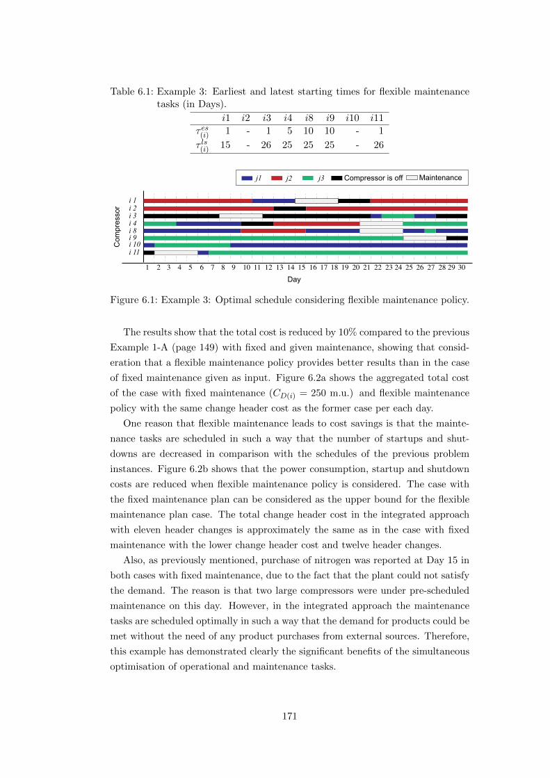
Table 6.1: Example 3: Earliest and latest starting times for flexible maintenancetasks (in Days).
i1 i2 i3 i4 i8 i9 i10 i11
τ es(i) 1 - 1 5 10 10 - 1
τ ls(i) 15 - 26 25 25 25 - 26
Com
pres
sor
1 2 3 4 5 6 7 8 9 10 11 12 13 14 15 16 17 18 19 20 21 22 23 24 25 26 27 28 29 30
i 1i 2
i 4i 8
i 3
i 11
i 9i 10
Day
j1 j2 j3 MaintenanceCompressor is off
Figure 6.1: Example 3: Optimal schedule considering flexible maintenance policy.
The results show that the total cost is reduced by 10% compared to the previous
Example 1-A (page 149) with fixed and given maintenance, showing that consid-
eration that a flexible maintenance policy provides better results than in the case
of fixed maintenance given as input. Figure 6.2a shows the aggregated total cost
of the case with fixed maintenance (CD(i) = 250 m.u.) and flexible maintenance
policy with the same change header cost as the former case per each day.
One reason that flexible maintenance leads to cost savings is that the mainte-
nance tasks are scheduled in such a way that the number of startups and shut-
downs are decreased in comparison with the schedules of the previous problem
instances. Figure 6.2b shows that the power consumption, startup and shutdown
costs are reduced when flexible maintenance policy is considered. The case with
the fixed maintenance plan can be considered as the upper bound for the flexible
maintenance plan case. The total change header cost in the integrated approach
with eleven header changes is approximately the same as in the case with fixed
maintenance with the lower change header cost and twelve header changes.
Also, as previously mentioned, purchase of nitrogen was reported at Day 15 in
both cases with fixed maintenance, due to the fact that the plant could not satisfy
the demand. The reason is that two large compressors were under pre-scheduled
maintenance on this day. However, in the integrated approach the maintenance
tasks are scheduled optimally in such a way that the demand for products could be
met without the need of any product purchases from external sources. Therefore,
this example has demonstrated clearly the significant benefits of the simultaneous
optimisation of operational and maintenance tasks.
171

Tota
l Cos
t
Ele
ctric
ityco
st
Sta
rt up
cost
Shu
t dow
nco
st
(a)
(b)
Fixed maintenance with CD = 250Integrated approach
Fixed maintenance with CD = 250Fixed maintenance with CD = 1000Integrated approach
Cha
ngin
ghe
ader
cos
t
(%)
(%)
(%)
(%)
(%)
(%)
Figure 6.2: Example 3: Aggregated normalised objective value for fixed and in-tegrated approach cases (a), and normalised total cost breakdown offixed maintenance (two different CD) and integrated approach (b).
6.2.5 Example 4: Industrial example
Example 4 builds on the Example 1-B that was presented in Section 5.17.3
on page 149. Section 6.2.5 presents two problem instances for Example 4 which
consider the integration of operation and maintenance. Instance 4.1 will present
the concept without including maintenance restrictions of manpower (explained in
Section 6.2.2) and Instance 4.2 will include these restrictions. Table 6.2 gives the
earliest and latest times of the maintenance tasks. The compressors which have
Table 6.2: Information of maintenance tasks of the compressors.
Instance Parameter i1 i2 i3 i4 i5 i6 i7 i8 i9 i10 i11
Instance 4.1 τ es(i) 1 - - 1 1 1 - - 1 - -
Instance 4.2 τ ls(i) 26 - - 28 25 28 - - 28 - -
Table 6.3: Computational results for all instances of the industrial examples. TheFixed Maint. case refers to the Example 1-B in Section 5.17.3.
Eqs. Binary Continuous Nodes CPU Objvariables variables (s) (m.u.)
Fixed Maint. 11,545 2,310 3,150 1,704 139 55.61Instance 4.1 11,683 2,444 3,150 58,626 7,721 54.65Instance 4.2 11,817 2,594 3,150 82,517 14,000 54.65
172
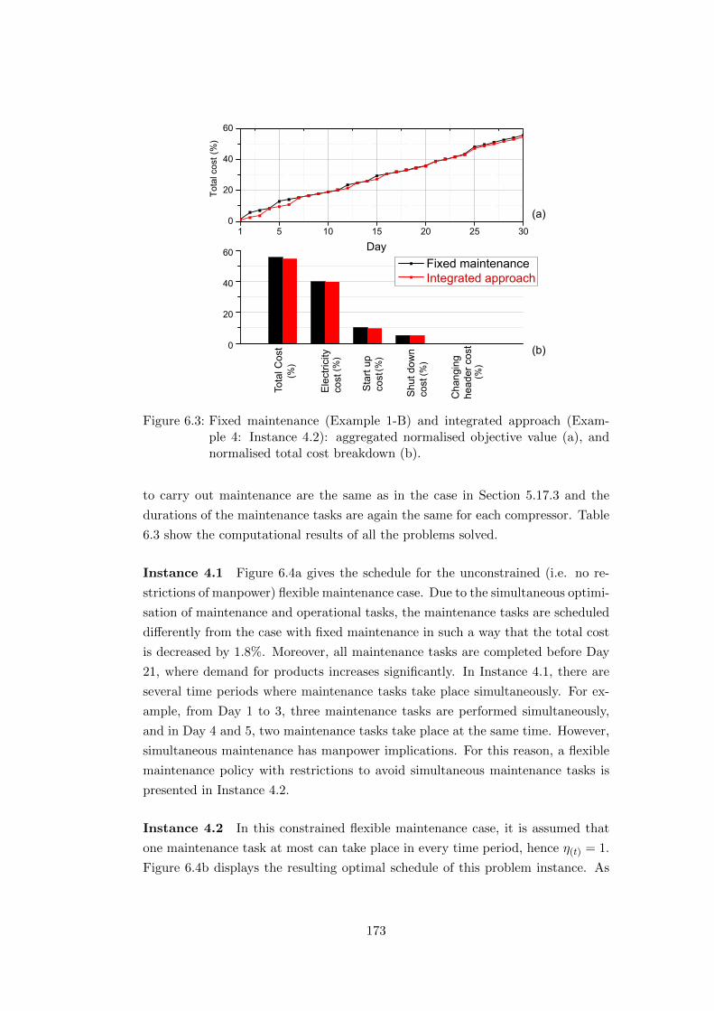
Fixed maintenanceIntegrated approach
Tota
l Cos
t
Ele
ctric
ityco
st
Sta
rt up
cost
Shu
t dow
nco
st
Cha
ngin
ghe
ader
cos
t
(a)
(b)
(%)
(%) (%
)
(%)
(%)
(%)
Figure 6.3: Fixed maintenance (Example 1-B) and integrated approach (Exam-ple 4: Instance 4.2): aggregated normalised objective value (a), andnormalised total cost breakdown (b).
to carry out maintenance are the same as in the case in Section 5.17.3 and the
durations of the maintenance tasks are again the same for each compressor. Table
6.3 show the computational results of all the problems solved.
Instance 4.1 Figure 6.4a gives the schedule for the unconstrained (i.e. no re-
strictions of manpower) flexible maintenance case. Due to the simultaneous optimi-
sation of maintenance and operational tasks, the maintenance tasks are scheduled
differently from the case with fixed maintenance in such a way that the total cost
is decreased by 1.8%. Moreover, all maintenance tasks are completed before Day
21, where demand for products increases significantly. In Instance 4.1, there are
several time periods where maintenance tasks take place simultaneously. For ex-
ample, from Day 1 to 3, three maintenance tasks are performed simultaneously,
and in Day 4 and 5, two maintenance tasks take place at the same time. However,
simultaneous maintenance has manpower implications. For this reason, a flexible
maintenance policy with restrictions to avoid simultaneous maintenance tasks is
presented in Instance 4.2.
Instance 4.2 In this constrained flexible maintenance case, it is assumed that
one maintenance task at most can take place in every time period, hence η(t) = 1.
Figure 6.4b displays the resulting optimal schedule of this problem instance. As
173

1 2 3 4 5 6 7 8 9 10 11 12 13 14 15 16 17 18 19 20 21 22 23 24 25 26 27 28 29 30
J1
Day
i 1i 2
i 4
i 8
i 3
i 11
i 9i 10
i 5i 6i 7
Com
pres
sor
j1 j2 j3 MaintenanceCompressor is off
(a) Instance 4.1
1 2 3 4 5 6 7 8 9 10 11 12 13 14 15 16 17 18 19 20 21 22 23 24 25 26 27 28 29 30
J1
Day
i 1i 2
i 4
i 8
i 3
i 11
i 9i 10
i 5i 6i 7
Com
pres
sor
j1 j2 j3 MaintenanceCompressor is off
(b) Instance 4.2 with restrictions and η(t) = 1.
Figure 6.4: Optimal schedules of compressors.
it can be seen from Table 6.3, the total cost of Instance 4.2 is the same with that
of Instance 4.1. The solution of Instance 4.1 is exactly the same with Instance
4.2 apart of the start times of the maintenance tasks. Indeed, in Instance 4.2 the
maintenance tasks of compressors i1 and i4 are shifted to the right so they do not
occur in the same time periods. Hence, these two changes do not affect the total
cost of Instance 4.1 since they do not add any cost in the objective function, and
the rest of the schedule is the same as that in Instance 4.1. Although Instance
4.1 and Instance 4.2 have the same total cost, Instance 4.2 gives a better schedule
(in terms of flexibility and management perspective), since maintenance tasks are
distributed more uniformly over the scheduling horizon of interest.
Figure 6.3a provides a comparison for the aggregated normalised total cost
between the fixed maintenance case of Example 1-B in Section 5.17.3 and the
integrated approach of Instance 4.2 (or Instance 4.1 as both have the same cost).
Figure 6.3b shows the normalised total cost breakdown for all problem instances.
Similarly to the results from the illustrative Example 3 of Section 6.2.4, it is
observed that the costs of startup and power consumption decrease under a flexible
maintenance policy (i.e., Instance 4.1 and Instance 4.2). In these cases, the cost
of power consumption has been reduced by 0.62%, and startup cost declines by
174

7.70% in comparison with those in the case with fixed maintenance.
Overall, it has been demonstrated that the simultaneous optimisation of main-
tenance and operational tasks could provide better solutions and decrease the total
cost compared to the case of optimal operation with given maintenance. As was
shown, the better coordination of the maintenance tasks helps to operate the com-
pressors more efficiently (a decrease in power consumption by 0.62% was observed)
and to reduce the startups of the compressors (reduction by 7.70%). The operation
with reduced number of startups increases the lifetime of the compressors.
6.3 Basic maintenance model in a rolling time horizon
framework (reactive scheduling)
6.3.1 Model
The basic model of integrated operation and maintenance of Section 6.2 is
formulated in such a way that it can be used within a rolling horizon framework
known as reactive scheduling. According to van den Heever and Grossmann (2003)
reactive scheduling is the problem which updates a schedule dynamically as the
constraints and parameters change over time. Focusing on the scheduling of com-
pressors, the initial state of the compressors (cumulative operating time or shut
down time) and the flows of demands are examples of parameters which change
over time. Moreover, an unexpected breakdown of a compressor is also considered
in the update of the constraints.
The rolling horizon concept is based on the principles of the model predictive
controller. According to Kopanos and Pistikopoulos (2014) the rolling horizon
framework solves an optimisation model for a scheduling horizon of certain length,
known as prediction horizon. A second time horizon, which is a subset of the
prediction horizon and known as control horizon, is used to apply the decisions
of the prediction horizon. This second time horizon usually has duration of one
time period. The optimisation problems are solved iteratively by moving forward
the prediction time horizon (consequently the control horizon moves along with
the prediction horizon) after each iteration. In each iteration, the solution of the
control horizon is applied. After each iteration, the optimisation problem receives
feedback, for instance updated demands and state of the system.
Figure 6.5 illustrates an example of the rolling horizon concept with a fixed
prediction horizon of three time periods and a control horizon of a single period.
The problem needs to be solved for five times periods, thus there are five iterations
(i.e. itertot = 5). In the first iteration, the initial state of the problem is known.
The optimisation problem is solved and the results of the optimisation are applied
only for the first time period. The output of the control horizon of the optimisation
175

t1 2 3 4 5
fixed duration
First iteration
t1 2 3 4 5
t1 2 3 4 5
Prediction horizon Δt = 3
Control horizon Δt = 1
Second iteration
Final iteration
itertot = 5
itertot+1 itertot+2
Initial state given
Initial state given from the end of control horizon of the first iteration
Solution applied fromprevious iteration
Figure 6.5: Example of rolling horizon approach.
problem of the first iteration are given as input to the second optimisation problem
for the second iteration. In the second iteration, the control horizon along with the
prediction horizon moved by one time period. After solving the problem iteratively
for five time periods, the solutions for the five periods have been applied.
Figure 6.6 displays a representative algorithm for rolling horizon optimisation
of the compressor station of the air separation plant. The algorithm is used to
demonstrate the implemented solutions after a predefined number of iterations
itertot. At the initialisation step for iter = 1, the prediction and control horizon,
and the initial state of the system are given. The prediction horizon is moving
by one time period and the parameters of the optimisation model are updated in
each iteration. For example, the initial connections of the compressors with the
headers for each optimisation problem in each iteration are given by Eqs. (6.4) –
(6.6). Equation (6.4) defines the parameter of the initial connections ϕ for the first
176
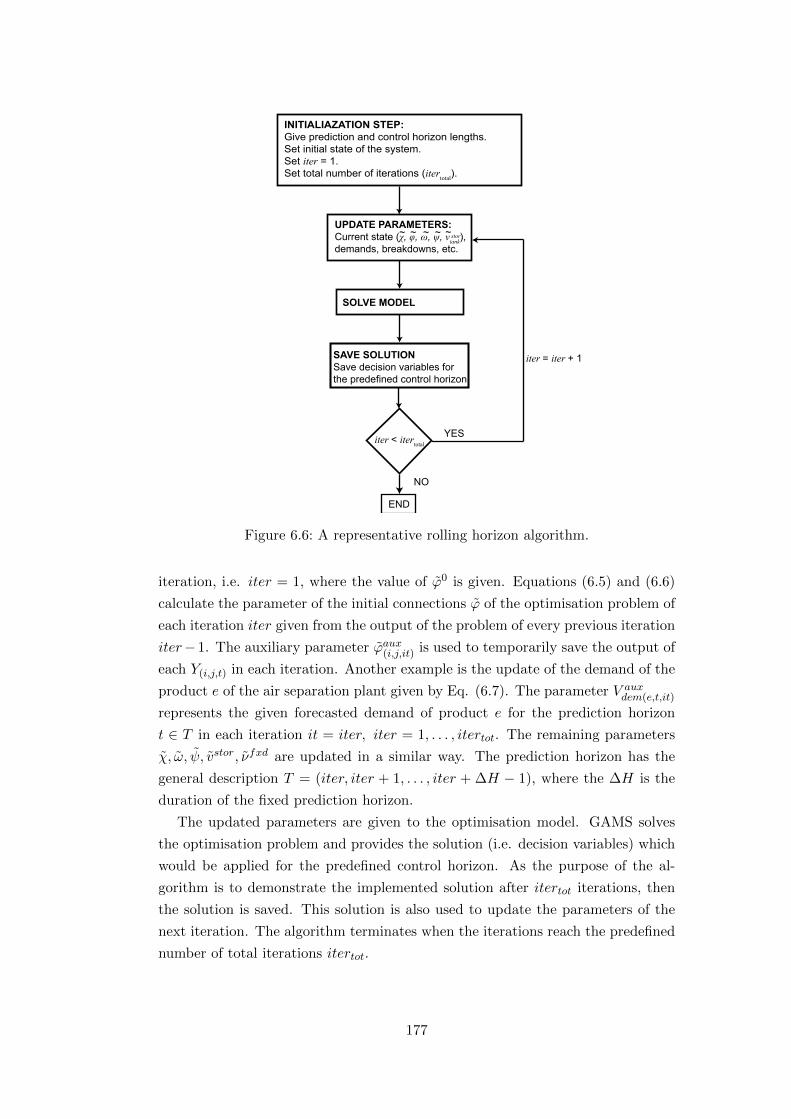
INITIALIAZATION STEP:Give prediction and control horizon lengths. Set initial state of the system.Set iter = 1.Set total number of iterations (itertotal).
SOLVE MODEL
UPDATE PARAMETERS: Current state (χ, φ, ω, ψ, vtank), demands, breakdowns, etc.
SAVE SOLUTIONSave decision variables forthe predefined control horizon
iter = iter + 1
YES
NO
END
~ ~ ~ ~ ~
iter < itertotal
stor
Figure 6.6: A representative rolling horizon algorithm.
iteration, i.e. iter = 1, where the value of ϕ0 is given. Equations (6.5) and (6.6)
calculate the parameter of the initial connections ϕ of the optimisation problem of
each iteration iter given from the output of the problem of every previous iteration
iter−1. The auxiliary parameter ϕaux(i,j,it) is used to temporarily save the output of
each Y(i,j,t) in each iteration. Another example is the update of the demand of the
product e of the air separation plant given by Eq. (6.7). The parameter V auxdem(e,t,it)
represents the given forecasted demand of product e for the prediction horizon
t ∈ T in each iteration it = iter, iter = 1, . . . , itertot. The remaining parameters
χ, ω, ψ, vstor, νfxd are updated in a similar way. The prediction horizon has the
general description T = (iter, iter + 1, . . . , iter + ∆H − 1), where the ∆H is the
duration of the fixed prediction horizon.
The updated parameters are given to the optimisation model. GAMS solves
the optimisation problem and provides the solution (i.e. decision variables) which
would be applied for the predefined control horizon. As the purpose of the al-
gorithm is to demonstrate the implemented solution after itertot iterations, then
the solution is saved. This solution is also used to update the parameters of the
next iteration. The algorithm terminates when the iterations reach the predefined
number of total iterations itertot.
177

ϕ(i,j) = ϕ0(i,j), ∀i ∈ I, j ∈ J(i), t = 1, iter = 1
(6.4)
ϕ(i,j) = ϕaux(i,j,it), ∀i ∈ I, j ∈ J(i), t > 1, it = iter − 1, iter = 2, . . . , itertot
(6.5)
ϕaux(i,j,it) = Y(i,j,t), ∀i ∈ I, j ∈ J(i), t = iter, it = iter, iter = 2, . . . , itertot
(6.6)
Vdem(e,t) = V auxdem(e,t,it) e ∈ E, t ∈ T, it = iter, iter = 1, . . . , itertot
(6.7)
6.3.2 Numerical example
Description of the example
Dem
and
of p
rodu
cts
in k
g/s
air (
%)
Day
Figure 6.7: Normalised demand for products (deterministic values).
The rolling time horizon framework is applied to the case study of the air separa-
tion plant in BASF. The aim is to show how the proposed integrated optimisation
framework can cope with a real-life case under the presence of uncertainty in de-
mand. The specifications of the optimisation problem are the following. Oxygen
and compressed air are the products of the plant, change header cost is equal to
250 m.u./change, and purchases of oxygen are not allowed.
The reactive scheduling problem will been solved via the rolling horizon ap-
proach displayed in Figure 6.6 for 30 days (i.e. there are 30 iterations). A time
period is equal to one day. A prediction horizon of 21 time periods, and a single-
period control horizon have been employed. In each iteration, a scheduling problem
for the next 21 time periods (i.e., the prediction horizon) is solved with updated
information regarding the current state of the overall system and the demand for
178

products. The solution of the first time period of the current prediction horizon is
only applied in the corresponding iteration, i.e. t = iter.
In this illustrative problem, demands for products are not deterministic but
instead may fluctuate over time. For this reason, the demand profiles are updated
after each iteration for a given prediction horizon. As the length of the control
horizon is one time period, then an iteration is carried out after one time period.
Figure 6.7 shows the actual normalised demand profile for oxygen and compressed
air for utilities for thirty days. Hence, the optimisation problem has to be updated
and solved for thirty iterations.
The adjective “actual” indicates that this normalised demand profile represents
the case in which the demand is known and is not expected to change over these
days (i.e. deterministic values of the demand). This is the case in which the
demand for products for all 30 days is known with certainty at the beginning of
the time horizon of each iteration and is called perfect information case. One
would solve a deterministic scheduling problem for the scheduling horizon of 30
days. The perfect information solution is the best solution that one could obtain.
However, in practice, it is impossible to find this solution due to the uncertainty
in the demand forecasting. In the real-life case the demand involves uncertainty.
Therefore in the rolling horizon approach a forecasted demand for the prediction
horizon is provided at each day. As the duration of the prediction horizon is
21 days, then there is a new demand prediction for the following 21 days after
every day. The forecasted demand for each prediction horizon at each day is not
presented in the Figure 6.7 for better readability.
The initial condition of the compressors is the same as in Table 5.5. It is
assumed that some compressors follow a fixed maintenance policy and others a
flexible maintenance policy to demonstrate the use of the framework for a general
scenario. Compressors i9 and i11 have been pre-scheduled for maintenance in Days
20 and 15 respectively. Compressors i2 and i6 are under flexible maintenance, and
their maintenance tasks must start in time window defined by earliest time start
τ es(i) = 1 (i.e. Day 1) and latest time start τ ls(i) = 15 (i.e. Day 15). The duration of
each maintenance task is three days. Maximum run times for compressors are the
same as in Example 4. Moreover, an unexpected breakdown of compressor i5 on
the second day is considered.
Results
A total number of 30 iterations has been solved. An iteration represents a
scheduling problem which employs a prediction horizon of 21 days and a time limit
of 1,800 s of the CPU time was set for each iteration. The computational time for
every iteration can be seen in Figure 6.8. On average, solutions are obtained in low
179

CP
U (s
)
Iteration
Figure 6.8: Computational CPU time in s for each iteration.
computational times. Negligible optimality gaps have been reported for iterations
20 to 22, where the imposed time limit was reached. As discussed by Kopanos
and Pistikopoulos (2014), longer prediction horizons result in bigger mathematical
model sizes, and as a consequence the necessary computational time will probably
increase too.
Figure 6.9 shows how the overall schedule was built through the solutions ob-
tained in each iteration. The last Gantt chart gives the implemented schedule.
The compressors that do not operate in any iteration are not included in Figure
6.9. In the third iteration, the schedule of the compressors for the first and second
day have been implemented, and the schedule for the third day is set fixed. The
schedule for Days 4,. . . ,23 will be re-evaluated in the next iterations considering
updated information (e.g. demands and state of compressors). As can be seen in
the Gantt chart of the implemented schedule, the schedule for Days 4 – 23 in the
third iteration is different from the final solution on these days.
Another example is that the schedule in the second iteration determined that
compressor i5 should operate at header j2 on Day 2. However, in the second
iteration, the updated information gives that compressor i5 must stay offline on
Day 2 due to an unexpected breakdown. Thus, the practical value of the reactive
scheduling approach can be seen here, as a new schedule is generated for Day 2
considering the updated information of the state of the compressors.
The normalised load distribution of each compressor is given in Figure 6.10.
The figure shows that compressors i3, i4, and i9 remain idle during the thirty-day
schedule. It should be noted here that it is known that compressor i3 is the least
energy-efficient compressor, and the results of all case studies give clear evidence
of it since they show that compressor i3 should stay offline or should operate at
limited capacity.
180

i1
1 2 3 4 5 6 7 8 9 10 11 12 13 14 15 16 17 18 19 20 21Day
Iteration 1
Iteration 2
Iteration 3
Iteration 30
i2
i7
i11
i8i10
i4i5i6
Com
pres
sor
Com
pres
sor
i1
1 2 3 4 5 6 7 8 9 10 11 12 13 14 15 16 17 18 19 20 21 22Day
i2
i7
i11
i8i10
i4i5i6
Com
pres
sor
i1i2
i7
i11
i8i10
i4i5i6
Com
pres
sor
i1i2
i7
i11
i8i10
i4i5i6
1 2 3 4 5 6 7 8 9 10 11 12 13 14 15 16 17 18 19 20 21 22 23Day
1 2 3 4 5 6 7 8 9 10 11 12 13 14 15 16 17 18 19 20 21 22 23 24 25 26 27 28 29 30Day
Fixed solution Prediction
PredictionPast operation
PredictionPast operation
Implemented schedule
.
.
.
.
.
.
.
.
.
.
.
.
.
.
.
.
Fixed solution
Fixed solution
Unexpected breakdown of compressor i5 on Day 2.
j1 j2 j3 MaintenanceCompressor is off
Fixed solution
Figure 6.9: Schedule generation via rolling horizon.
181

i1 i2 i5
i6i7i8
i10i11
Sm
all c
ompr
esso
rsm
ass
flow
rate
s (%
)La
rge
com
pres
sors
mas
s flo
w ra
tes
(%)
Figure 6.10: Normalised mass flow rates of small and large compressors.
Figure 6.11: Aggregated normalised objective value for the rolling horizon andperfect information solution.
182

The aggregated costs of the perfect information case and the solution derived by
the rolling horizon approach are shown in Figure 6.11. The results show that the
rolling horizon solution is 11% worse than that of the perfect information case. The
obtained solution could be improved, if the accuracy in the forecast of the demand
is improved and the length of the prediction horizon increases. However, in practice
as the length of the prediction horizon increases, the forecasting accuracy naturally
decreases. Overall, through this example it has been shown the applicability of
the basic integrated framework of operation and maintenance of compressors to
deal with relevant scheduling problems in dynamic production environments.
6.4 Maintenance model including major overhauls
6.4.1 Maintenance model
Table 6.4: Descriptions of maintenance tasks.
Maintenance Type Example Compressor Shutdownset duration
Overhaul Major Rotor replacement IM2 νOVMechanical Light Vibrational analysis IM1 1 dElectrical Light VSD inspection IM1 1 d
This section refers to an integrated model of operation and maintenance of
natural gas compressors and the Statoil export gas station will be considered for the
numerical applications. Section 6.4.1 demonstrates a comprehensive maintenance
model which considers different types of maintenance tasks: (a) major overhauls,
(b) mechanical maintenance and (c) electrical maintenance corrective tasks. A
major overhaul is a long term maintenance with duration νOV (i) days and the
compressor has to be off during this period.
A mechanical corrective maintenance involves minor mechanical repairs, leak
tests and vibrational analysis and it is assumed that it lasts for one day. Thus,
the compressor has to be off in this day. The electrical corrective maintenance
involves minor electrical repairs, inspection of the VSD drives of the motors of
the compressors and other types of inspections. It is assumed that the electrical
corrective maintenance also lasts for one day. The compressor also has to be off in
this day. Table 6.4 summarises the description of each maintenance. The following
assumptions of the maintenance model are taken into consideration:
• The cost of every type of maintenance is not involved in the objective function
as the cost of maintenance is assumed independent from the main variables
of operation.
183
• Two sets of compressors are considered for maintenance activities: compres-
sors i ∈ IM which are subject to maintenance and compressors i ∈ INM
which are not scheduled to be maintained.
• The industrial policy is that two different types of maintenance activities
cannot happen in the same time period. Only one maintenance group can
occupy the space for repairing a compressor in each day.
• There is a minimum time between two consequent major overhauls of two
different compressors. The reason is that a major overhaul includes replace-
ments of major spare parts of the compressor, for example the replacement
of the rotor. It takes time for the rotor to be repaired. When the rotor is
repaired, then a second compressor can have a major overhaul by replacing
its used rotor with the revamped one.
There are two different sets of compressors which are related respectively to
a major overhaul i ∈ IM2 ⊆ IM and to light maintenance i ∈ IM1 ⊆ IM . The
light maintenance includes mechanical, electrical repairs and inspections of the
equipment. The maintenance tasks have to be scheduled within a given time
window t ∈ T sf(i) = (τ es(i), τls(i)) ⊆ T . The maintenance model considers three sets of
binary variables:
Uov(i,t) =
1, if compressor i ∈ IM2 starts an overhaul maintenance in period t
0, otherwise
UMe(i,t) =
1, if compressor i ∈ IM1 shuts down for mechanical maintenance
actions in period t
0, otherwise
UEl(i,t) =
1, if compressor i ∈ IM1 shuts down for electrical maintenance
actions in period t
0, otherwise
When a mechanical or electrical maintenance episode takes place a compressor
should shut down and these constraints are modelled by Eqs. (6.8) and (6.9):
X(i,t) ≤ (1− UMe(i,t)), ∀i ∈ IM1, t ∈ T sf(i) (6.8)
X(i,t) ≤ (1− UEl(i,t)), ∀i ∈ IM1, t ∈ T sf(i) (6.9)
184

Equations (6.10) and (6.11) describe the constraints where a number of planned
mechanical or electrical maintenance episodes (ΛMe or ΛEl) have to take place
within the time period of the given time window T sf(i) .
∑t∈T
UMe(i,t) = ΛMe, ∀i ∈ IM1, t ∈ T sf(i) (6.10)∑t∈T
UEl(i,t) = ΛEl, ∀i ∈ IM1, t ∈ T sf(i) (6.11)
Equation (6.12) models the assumption that electrical and mechanical mainte-
nance tasks cannot happen for each compressor in the same period:
UMe(i,t) + UEl(i,t) ≤ 1, ∀i ∈ IM1, t ∈ T sf(i) (6.12)
Equations (6.13) and (6.14) consider a maximum number of mechanical (ΛmaxMe )
and electrical (ΛmaxEl ) maintenance tasks which can take place in a time period, by
considering limited maintenance manpower.∑i∈IM1
UMe(i,t) ≤ ΛmaxMe , ∀i ∈ IM1, t ∈ T sf(i) (6.13)
∑i∈IM1
UEl(i,t) ≤ ΛmaxEl , ∀i ∈ IM1, t ∈ T sf(i) (6.14)
In the case of a major overhaul, the binary variable Uov(i,t) takes the value
one when a compressor i ∈ IM2 starts the maintenance. The maintenance lasts
for νOV (i) days. Compressors i ∈ IM2 which are subject to major overhaul have
to start maintenance within a given time window T sf(i) according to Eq. (6.15).
Equation (6.16) models the unavailability of the compressors due to maintenance
for νOV (i) days similar to Eq. (6.2).∑t∈T sf
(i)
UOV (i,t) = 1, ∀i ∈ IM2 (6.15)
X(i,t) +
minτ ls(i),t∑
t′=maxτes(i),t−νOV (i)+1
UOV (i,t) ≤ 1,
∀i ∈ IM2, t = τ es(i), ..., (τls(i) + νOV (i) − 1)
(6.16)
Equation (6.17) assumes a maximum number of compressors ΛmaxC which can be
repaired at the same time period for each time period t ∈ T and Eq. (6.18) guar-
antees a minimum time γ∗ between two consequent beginnings of major overhauls
of different compressors due to the availability of a single spare rotor.
185

∑i∈IM2,
τes(i)≤t≤(τ ls
(i)+νOV (i)−1)
minτ ls(i),t∑
t′∈maxτes(i),t−νOV (i)+1
UOV (i,t′) ≤ ΛmaxC (6.17)
∑i∈IM2
t∑t′=max1,t−γ∗+1
UOV (i,t′) ≤ 1, ∀t ∈ T (6.18)
6.4.2 Integrated framework with focus on major overhauls
The objective is to minimise the electricity cost of the motors of the compressors,
the start up and shut down costs, and the change cost when a compressor changes
header while at the same time all the constraints of the integrated model have to
be respected. The objective function is Eq. (5.61) which is duplicated below.
min
electricity cost︷ ︸︸ ︷∑t∈T
Cel(t)∑i∈I
∑j∈J(i)
dcWel(i,j,t) +
start up and shut down cost︷ ︸︸ ︷∑t∈T
∑i∈I
(Cst(i)S(i,t) + Cf(i)F(i,t)) +
change header cost︷ ︸︸ ︷∑t∈T
∑i∈I
CDD(i,t) +
purchase products/gas cost︷ ︸︸ ︷∑t∈T
∑e∈E
∑δ∈∆(j)
Cext(δ,e,t)dcMext(δ,e,t)
(5.61)
The integrated operational and maintenance model is focused on major over-
hauls and maintenance tasks which are subject to limited maintenance manpower
and other constraints such as the constraint on the number of maintenance tasks
that can take place in the same time period. The integrated framework couples
the constraints of the operational model given by constraints of:
• minimum run and shutdown time in Section 5.3,
• assignment of compressors to headers in Section 5.4,
• compressor-to-header assignment changes in Section 5.5,
• power consumption and feasible operational window with the use of com-
pressor maps in Section 5.7,
• recycle model in Section 5.8.1,
• general operational constraints of the export gas station in Section 5.11,
• maximum run time constraints in 5.13,
• initial state of the network in Section 5.14, and
• the maintenance model described in Section 6.4.1.
186
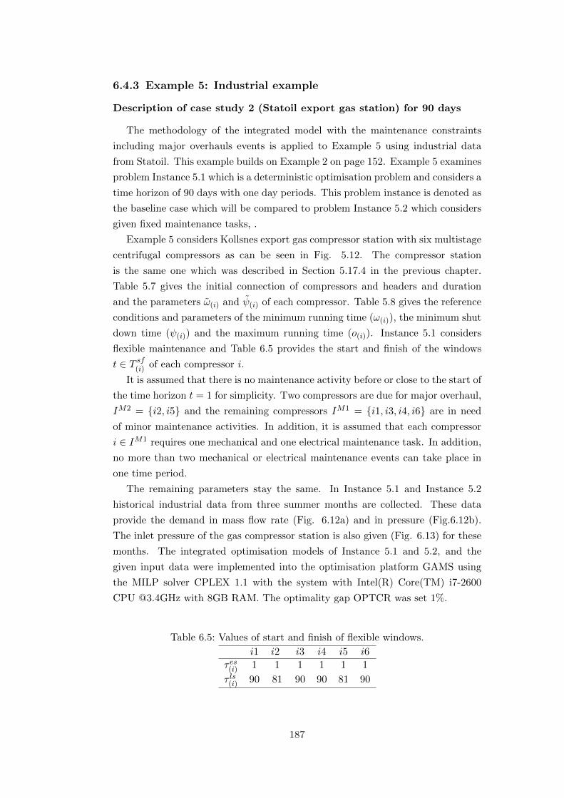
6.4.3 Example 5: Industrial example
Description of case study 2 (Statoil export gas station) for 90 days
The methodology of the integrated model with the maintenance constraints
including major overhauls events is applied to Example 5 using industrial data
from Statoil. This example builds on Example 2 on page 152. Example 5 examines
problem Instance 5.1 which is a deterministic optimisation problem and considers a
time horizon of 90 days with one day periods. This problem instance is denoted as
the baseline case which will be compared to problem Instance 5.2 which considers
given fixed maintenance tasks, .
Example 5 considers Kollsnes export gas compressor station with six multistage
centrifugal compressors as can be seen in Fig. 5.12. The compressor station
is the same one which was described in Section 5.17.4 in the previous chapter.
Table 5.7 gives the initial connection of compressors and headers and duration
and the parameters ω(i) and ψ(i) of each compressor. Table 5.8 gives the reference
conditions and parameters of the minimum running time (ω(i)), the minimum shut
down time (ψ(i)) and the maximum running time (o(i)). Instance 5.1 considers
flexible maintenance and Table 6.5 provides the start and finish of the windows
t ∈ T sf(i) of each compressor i.
It is assumed that there is no maintenance activity before or close to the start of
the time horizon t = 1 for simplicity. Two compressors are due for major overhaul,
IM2 = i2, i5 and the remaining compressors IM1 = i1, i3, i4, i6 are in need
of minor maintenance activities. In addition, it is assumed that each compressor
i ∈ IM1 requires one mechanical and one electrical maintenance task. In addition,
no more than two mechanical or electrical maintenance events can take place in
one time period.
The remaining parameters stay the same. In Instance 5.1 and Instance 5.2
historical industrial data from three summer months are collected. These data
provide the demand in mass flow rate (Fig. 6.12a) and in pressure (Fig.6.12b).
The inlet pressure of the gas compressor station is also given (Fig. 6.13) for these
months. The integrated optimisation models of Instance 5.1 and 5.2, and the
given input data were implemented into the optimisation platform GAMS using
the MILP solver CPLEX 1.1 with the system with Intel(R) Core(TM) i7-2600
CPU @3.4GHz with 8GB RAM. The optimality gap OPTCR was set 1%.
Table 6.5: Values of start and finish of flexible windows.
i1 i2 i3 i4 i5 i6
τ es(i) 1 1 1 1 1 1
τ ls(i) 90 81 90 90 81 90
187
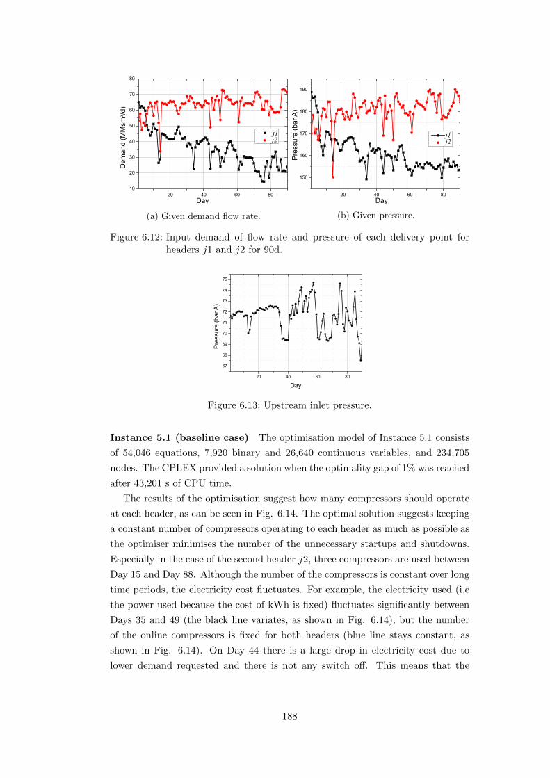
j1 j2
Day
Dem
and
(MM
sm3 /d
)
(a) Given demand flow rate.
j1 j2
Day
Pre
ssur
e (b
ar A
)
(b) Given pressure.
Figure 6.12: Input demand of flow rate and pressure of each delivery point forheaders j1 and j2 for 90d.
Day
Pre
ssur
e (b
ar A
)
Figure 6.13: Upstream inlet pressure.
Instance 5.1 (baseline case) The optimisation model of Instance 5.1 consists
of 54,046 equations, 7,920 binary and 26,640 continuous variables, and 234,705
nodes. The CPLEX provided a solution when the optimality gap of 1% was reached
after 43,201 s of CPU time.
The results of the optimisation suggest how many compressors should operate
at each header, as can be seen in Fig. 6.14. The optimal solution suggests keeping
a constant number of compressors operating to each header as much as possible as
the optimiser minimises the number of the unnecessary startups and shutdowns.
Especially in the case of the second header j2, three compressors are used between
Day 15 and Day 88. Although the number of the compressors is constant over long
time periods, the electricity cost fluctuates. For example, the electricity used (i.e
the power used because the cost of kWh is fixed) fluctuates significantly between
Days 35 and 49 (the black line variates, as shown in Fig. 6.14), but the number
of the online compressors is fixed for both headers (blue line stays constant, as
shown in Fig. 6.14). On Day 44 there is a large drop in electricity cost due to
lower demand requested and there is not any switch off. This means that the
188

j2j1
Ele
ctric
ity c
ost (
103 •
EU
R/d
)
Day
Figure 6.14: Electricity cost and number of online compressors at each header.
5 10 15 20 25 30 35 40 45 50 55 60 65 70 75 80 85 90
i1i2
i4i3
Day
Com
pres
sor
i6
i5
j1 j2 M2 OFF M1 me M1 el
Figure 6.15: Schedule from optimisation of Instance 5.1.
optimiser finds that it is more beneficial to reduce the capacity of a compressor
rather than switching it off.
The optimal scheduling resulting from the optimisation can be seen in Fig.
6.15. The schedule shows the status of the compressors, e.g. online and offline
status, header connection, maintenance activity, and the start and duration of
each operational task. According to Fig. 6.15, compressor i6 operates 97% of
the total examined time period. The other compressors operate less than this.
The reason for this is that compressor i6 is the most efficient. Therefore, keeping
efficient compressor i6 online for more time improves the overall efficiency of the
system. Moreover, compressor i6 changes headers more frequently than the other
compressors. The result is that the efficiency of the overall system increases against
the change-header costs of compressor i6. Another remark is that compressor i6
shuts down at Day 34 when the demand is low. Moreover, the power consumption
of the other compressors is relatively low on this day as can be seen in Fig. 6.14.
The maintenance tasks suggested from the optimisation have the flexibility to
be shifted within the period the compressors are off. This, mathematically, means
that there are multiple solutions as the shift of the timings of the maintenance
189
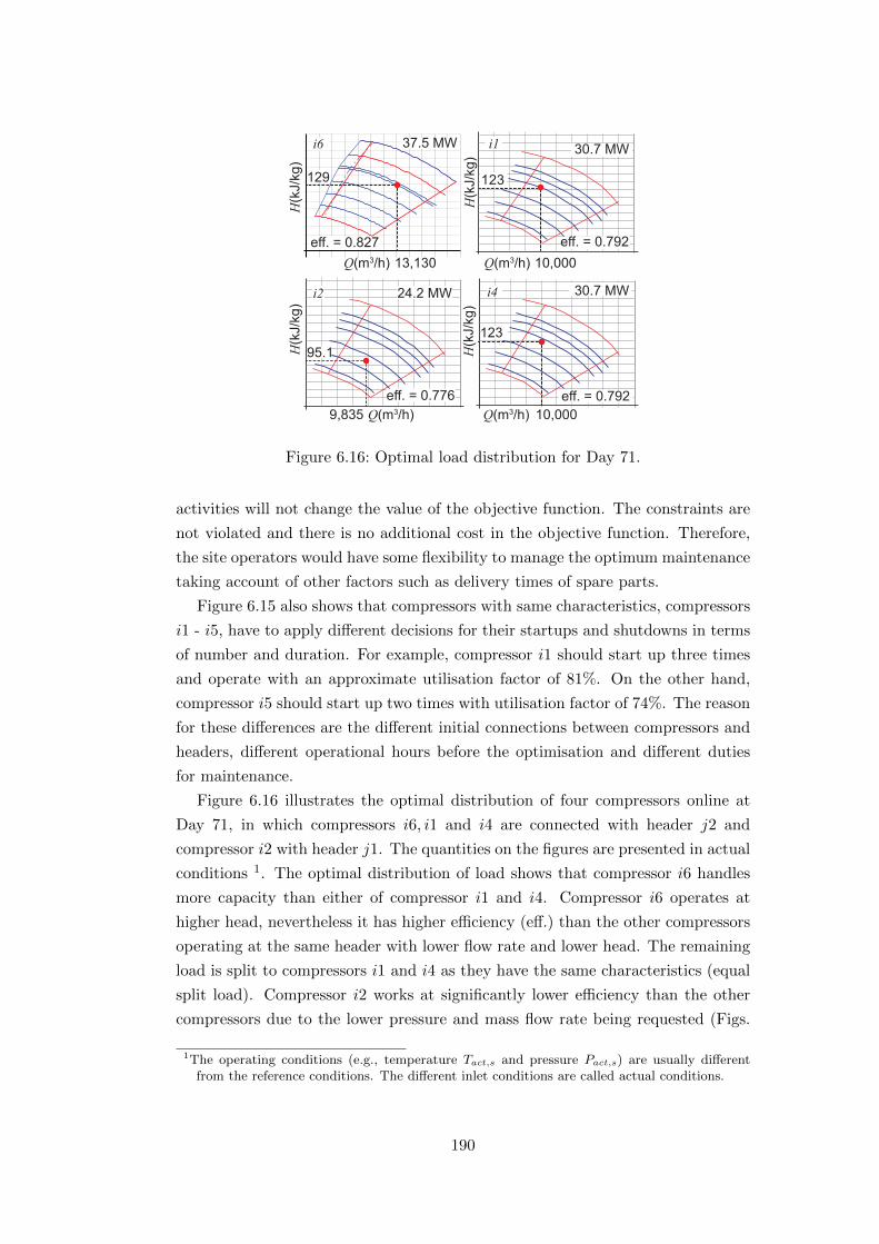
Po
lytr
op
ic H
ea
d
H(k
J/kg
)H
(kJ/
kg)
H(k
J/kg
)H
(kJ/
kg)
Q(m3/h) Q(m3/h)13,130 10,000
Q(m3/h) Q(m3/h)9,835 10,000
eff. = 0.827
37.5 MWi6
129
i2
95.1
eff. = 0.776
24.2 MW i4
eff. = 0.792
30.7 MW
123
eff. = 0.792
30.7 MW
123
i1
Figure 6.16: Optimal load distribution for Day 71.
activities will not change the value of the objective function. The constraints are
not violated and there is no additional cost in the objective function. Therefore,
the site operators would have some flexibility to manage the optimum maintenance
taking account of other factors such as delivery times of spare parts.
Figure 6.15 also shows that compressors with same characteristics, compressors
i1 - i5, have to apply different decisions for their startups and shutdowns in terms
of number and duration. For example, compressor i1 should start up three times
and operate with an approximate utilisation factor of 81%. On the other hand,
compressor i5 should start up two times with utilisation factor of 74%. The reason
for these differences are the different initial connections between compressors and
headers, different operational hours before the optimisation and different duties
for maintenance.
Figure 6.16 illustrates the optimal distribution of four compressors online at
Day 71, in which compressors i6, i1 and i4 are connected with header j2 and
compressor i2 with header j1. The quantities on the figures are presented in actual
conditions 1. The optimal distribution of load shows that compressor i6 handles
more capacity than either of compressor i1 and i4. Compressor i6 operates at
higher head, nevertheless it has higher efficiency (eff.) than the other compressors
operating at the same header with lower flow rate and lower head. The remaining
load is split to compressors i1 and i4 as they have the same characteristics (equal
split load). Compressor i2 works at significantly lower efficiency than the other
compressors due to the lower pressure and mass flow rate being requested (Figs.
1The operating conditions (e.g., temperature Tact,s and pressure Pact,s) are usually differentfrom the reference conditions. The different inlet conditions are called actual conditions.
190

5.23a and 5.23b).
Table 6.6 gives the details of the operational conditions suggested of the opti-
misation for five days (Days 71 - 75). The M(header) is the total mass flow rate
in the header in kg/s. As can be seen, there is a difference between actual and
corrected values. This is due to a change of inlet pressure. Compressor i6 han-
dles from 36.7% up to 39.1% of the mass flow provided from three compressors
in total to header j2. In Day 75, it operates alone providing 100% of the gas
requested. Figure 5.23a shows that the demand is very low in Day 75 where the
solver suggests that the best combination is compressor i6 to operate alone at the
header with the lower demand and the other three to the header with the higher
requested demand. Another solution could be to switch off a compressor, however
after two days after Day 75 the demand was forecast to become higher, and this
is the reason the optimiser did not choose this option.
Table 6.6: Suggested operating conditions of i6 for five days.
Day 71 72 73 74 75
Actual
M (kg/s) 232.1 238.6 225.6 212.2 137.1M/M(header)(%) 38.5 39.3 38.1 36.7 100
Q (m3/h) 13130 13574 12934 12000 7459H (kJ/kg) 128.8 130.3 129.7 128.0 92.0W (MW) 37.2 39.1 36.8 33.2 14.6
Corrected
Q (m3/h) 13303 13753 13105 12158 7557H (kJ/kg) 132.2 133.8 131.1 131.4 94.4W (MW) 36.1 37.7 35.2 32.2 14.7
Instance 5.2 (fixed maintenance case) In order to examine the importance
of the selection of the starting time points of the maintenance tasks into the optimi-
sation model, another optimisation problem with fixed maintenance is formulated.
This problem Instance 5.2 assumes that all the maintenance activities are placed
between days 59 and 90, and all the constraints of the maintenance model are
respected. Therefore, Eqs. (6.8) - (6.18) are not considered in the optimisation
model and the objective function is the same as in problem Instance 5.1.
Figure 6.17 shows the scheduling of the compressors for Instance 5.2. The
maintenance tasks have been arranged at the end of the time horizon. Comparing
the two schedules from Figs. 6.15 and 6.17, problem Instance 5.2 shows that
optimal operation is influenced greatly by the non-inclusion of the maintenance into
the optimisation. The decisions for the operation of compressors have significantly
191

5 10 15 20 25 30 35 40 45 50 55 60 65 70 75 80 85 90
i1i2
i4i3
j1 j2 M2 OFF M1 me M1 el
Day
Com
pres
sor
i6
i5
Figure 6.17: Schedule from optimisation of case B.
changed even at the beginning of the time horizon as can been seen for the case of
compressor i5. Another remark is that the fixed maintenance schedule reduces the
flexibility of the operation: for example compressor i6 is utilised approximately
93% over the total time of the optimisation in Instance 5.2. Thus, the overall
system is expected to be less profitable.
Table 6.7 compares the results from problem Instance 5.1 and Instance 5.2.
There is a significant difference in the start up, shut down and change header
costs, however the electricity cost does not increase significantly from Instance
5.1 to Instance 5.2. If this difference related to the electricity cost is translated
to absolute numbers, 54,000 EUR are saved in three months by considering the
selection of the times of the maintenance as a degree of freedom. The overall
savings are approximately 0.85% or 224,000 EUR in three months. The last column
of Table 6.7 gives the contribution of each cost to the total cost of the base case.
The electricity cost is the dominant one. Therefore, a small improvement in the
schedule of the compressors results in significant reduction in the overall savings.
Section 6.4.3 presented the scheduling of compressors for two cases, the baseline
with integrated operation and maintenance (Instance 5.1) and Instance 5.2 without
considering maintenance decisions in the optimisation. The proposed optimisation
deals with a difficult problem which includes many decisions to take which include
discrete events and continuous quantities. The scheduling approach deals with a
Table 6.7: Comparison between problem Instance 5.1 (baseline case) and Instance5.2 (fixed maintenance case).
Cost (103 EUR) Instance 5.1 Instance 5.2 % diff. % of total cost
Start Up 304.1 407.4 25.4 1.15Shut Down 152.0 203.7 25.4 0.56Change 23.0 38.0 39.5 0.09Electricity 25,974 26,028 0.21 98.20Total 26,453 26,677 0.84 100
192
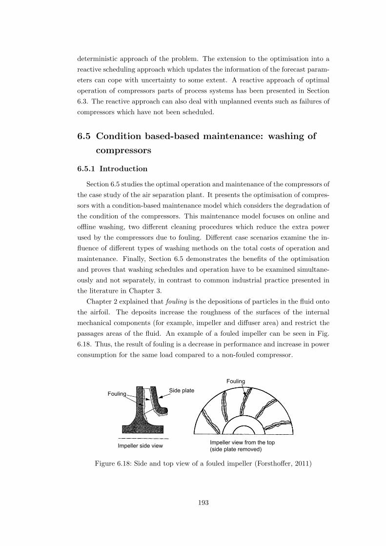
deterministic approach of the problem. The extension to the optimisation into a
reactive scheduling approach which updates the information of the forecast param-
eters can cope with uncertainty to some extent. A reactive approach of optimal
operation of compressors parts of process systems has been presented in Section
6.3. The reactive approach can also deal with unplanned events such as failures of
compressors which have not been scheduled.
6.5 Condition based-based maintenance: washing of
compressors
6.5.1 Introduction
Section 6.5 studies the optimal operation and maintenance of the compressors of
the case study of the air separation plant. It presents the optimisation of compres-
sors with a condition-based maintenance model which considers the degradation of
the condition of the compressors. This maintenance model focuses on online and
offline washing, two different cleaning procedures which reduce the extra power
used by the compressors due to fouling. Different case scenarios examine the in-
fluence of different types of washing methods on the total costs of operation and
maintenance. Finally, Section 6.5 demonstrates the benefits of the optimisation
and proves that washing schedules and operation have to be examined simultane-
ously and not separately, in contrast to common industrial practice presented in
the literature in Chapter 3.
Chapter 2 explained that fouling is the depositions of particles in the fluid onto
the airfoil. The deposits increase the roughness of the surfaces of the internal
mechanical components (for example, impeller and diffuser area) and restrict the
passages areas of the fluid. An example of a fouled impeller can be seen in Fig.
6.18. Thus, the result of fouling is a decrease in performance and increase in power
consumption for the same load compared to a non-fouled compressor.
Impeller side view Impeller view from the top (side plate removed)
Fouling
Fouling Side plate
Figure 6.18: Side and top view of a fouled impeller (Forsthoffer, 2011)
193

Time
Effi
cien
cy
Ideal maximum efficiency
no washing
only online washing
combined offline and onlinewashing
offline washingstarts
Figure 6.19: The qualitative trend of the efficiency over time considering differenttypes of washing methods.
There are two common strategies to deal with the problem of fouling, namely
offline and online washing. The offline washing takes place when a compressor
is not operating and the online washing cleans the compressor online without
interrupting its operation. An Offline Washing Episode (OFWE) is complete after
several cleaning steps when the compressor is in offline mode. The purpose of the
washing of these cleaning steps is to recover the efficiency of the compressor which
results in decreasing the extra power consumed. Fabbri et al. (2011) report that
supplementary maintenance tasks, such as mechanical inspections, can be included
during a typical OFWE, hence the total duration of this OFWE can be a few days.
Another method for improving the performance of a compressor is to inject a
cleaning solution inside the compressor while it is operating online, this procedure
is known as Online Washing Episode (ONWE). The advantage of this method
is that the efficiency improves without shutting down the compressor to wash.
However, the recovery of the performance is smaller than in the case of an offline
washing episode. Figure 6.19 shows the qualitative trends of the efficiencies when
a compressor (a) is not washed, (b) is washed online exclusively and (c) is cleaned
with a combination of offline and online washing. According to Fabbri et al. (2011),
an ONWE cannot take place if the ambient temperature is less than 14oC because
ice is created which can damage the blades of the compressor.
The following mathematical framework for the optimal operation of a compres-
sor station with multiple parallel compressors considers a condition-based main-
tenance approach focusing on preventing the effects from fouling. The framework
includes the basic operational model of the air separation plant which was pre-
sented in Section 6.2.3. The modelling includes the prediction of power consump-
tion depending on operational conditions, the extra power consumption due to
degradation, and offline and online washing maintenance which will be explained
in the following Sections 6.5.2 and 6.5.3.
194
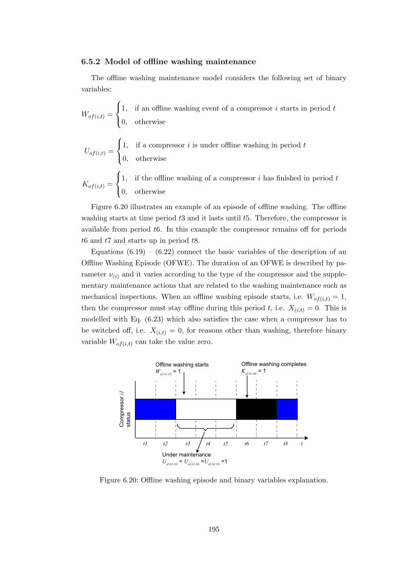
6.5.2 Model of offline washing maintenance
The offline washing maintenance model considers the following set of binary
variables:
Wof(i,t) =
1, if an offline washing event of a compressor i starts in period t
0, otherwise
Uof(i,t) =
1, if a compressor i is under offline washing in period t
0, otherwise
Kof(i,t) =
1, if the offline washing of a compressor i has finished in period t
0, otherwise
Figure 6.20 illustrates an example of an episode of offline washing. The offline
washing starts at time period t3 and it lasts until t5. Therefore, the compressor is
available from period t6. In this example the compressor remains off for periods
t6 and t7 and starts up in period t8.
Equations (6.19) – (6.22) connect the basic variables of the description of an
Offline Washing Episode (OFWE). The duration of an OFWE is described by pa-
rameter ν(i) and it varies according to the type of the compressor and the supple-
mentary maintenance actions that are related to the washing maintenance such as
mechanical inspections. When an offline washing episode starts, i.e. Wof(i,t) = 1,
then the compressor must stay offline during this period t, i.e. X(i,t) = 0. This is
modelled with Eq. (6.23) which also satisfies the case when a compressor has to
be switched off, i.e. X(i,t) = 0, for reasons other than washing, therefore binary
variable Wof(i,t) can take the value zero.
tt1 t2 t3 t4 t5
Com
pres
sor i
1 st
atus
t6 t7 t8
Offline washing startsWof (i1,t3) = 1
Offline washing completesKof (i1,t6) = 1
Under maintenance Uof (i1,t3) = Uof (i1,t4) =Uof (i1,t5) =1
Figure 6.20: Offline washing episode and binary variables explanation.
195

Wof(i,t) −Kof(i,t) = Uof(i,t) − Uof(i,t−1),
∀i ∈ I, (doof(i) > 0, (ν(i) − doof(i)) < t ≤ T ) ∨ (doof(i) = 0, t > 1) (6.19)
Wof(i,t) −Kof(i,t) = Uof(i,t),
∀i ∈ I, doof(i) = 0, t = 1 (6.20)
Wof(i,t) +Kof(i,t) ≤ 1,
∀i ∈ I, (doof(i) > 0, (ν(i) − doof(i)) < t ≤ T ) ∨ (doof(i) = 0, t ∈ T ) (6.21)
1− Uof(i,t) +t∑
t′=max1,t−ν(i)+1
Wof(i,t′) = 1,
∀i ∈ I, (doof(i) > 0, (ν(i) − doof(i)) < t ≤ T ) ∨ (doof(i) = 0, t ∈ T ) (6.22)
X(i,t) ≤ 1− Uof(i,t),
∀i ∈ I, t ∈ T (6.23)
Uof(i,t) = 1,
∀i ∈ I, d0of(i) > 0, 1 ≤ t ≤ (ν(i) − doof(i)) (6.24)
The optimisation model also considers OFWEs that occurred before the start
of the time window of the optimisation. This information is part of the input of
the model and describes the initial state of the system. The initial state of the
system influences significantly the optimisation results as has been demonstrated
in the work by Kopanos and Pistikopoulos (2014). The parameter doof(i) gives the
duration of a compressor which has already been in maintenance before the be-
ginning of the time horizon of the optimisation. If doof(i) > 0, then the compressor
has to continue being maintained up to the time period (ν(i) − doof(i)). Equation
(6.24) describes this constraint.
Equation (6.25) models the maximum number (λoff ) of maintenance events
which can take place in one time period. The simultaneous maintenance episodes
in one time period (e.g. in one day) may be restricted due to industrial policies.∑i∈I
Uof(i,t) ≤ λoff , ∀t ∈ T (6.25)
The constraints described by Eqs. (6.26) – (6.30) provide the models of the
degradation rate and recovery of the extra power consumption after an offline
washing episode. The main assumptions of the degradation and power recovery
model are summarised below:
• The degradation rate of a compressor depends on the type of the machine
196
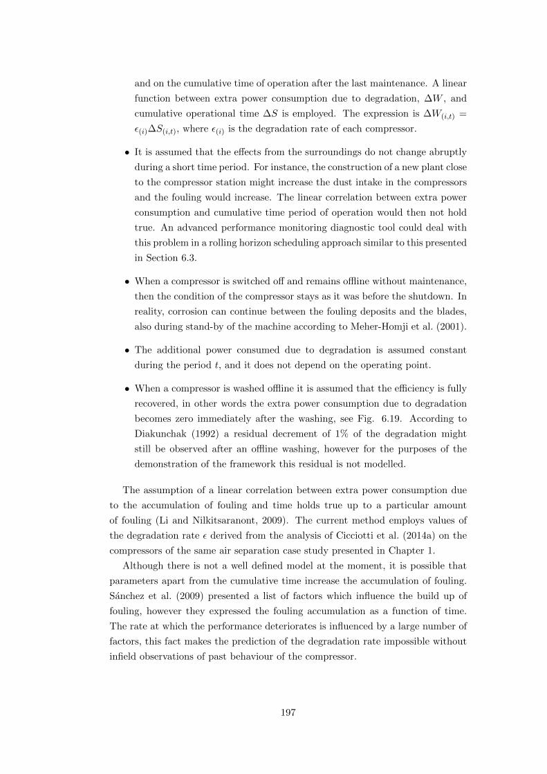
and on the cumulative time of operation after the last maintenance. A linear
function between extra power consumption due to degradation, ∆W , and
cumulative operational time ∆S is employed. The expression is ∆W(i,t) =
ε(i)∆S(i,t), where ε(i) is the degradation rate of each compressor.
• It is assumed that the effects from the surroundings do not change abruptly
during a short time period. For instance, the construction of a new plant close
to the compressor station might increase the dust intake in the compressors
and the fouling would increase. The linear correlation between extra power
consumption and cumulative time period of operation would then not hold
true. An advanced performance monitoring diagnostic tool could deal with
this problem in a rolling horizon scheduling approach similar to this presented
in Section 6.3.
• When a compressor is switched off and remains offline without maintenance,
then the condition of the compressor stays as it was before the shutdown. In
reality, corrosion can continue between the fouling deposits and the blades,
also during stand-by of the machine according to Meher-Homji et al. (2001).
• The additional power consumed due to degradation is assumed constant
during the period t, and it does not depend on the operating point.
• When a compressor is washed offline it is assumed that the efficiency is fully
recovered, in other words the extra power consumption due to degradation
becomes zero immediately after the washing, see Fig. 6.19. According to
Diakunchak (1992) a residual decrement of 1% of the degradation might
still be observed after an offline washing, however for the purposes of the
demonstration of the framework this residual is not modelled.
The assumption of a linear correlation between extra power consumption due
to the accumulation of fouling and time holds true up to a particular amount
of fouling (Li and Nilkitsaranont, 2009). The current method employs values of
the degradation rate ε derived from the analysis of Cicciotti et al. (2014a) on the
compressors of the same air separation case study presented in Chapter 1.
Although there is not a well defined model at the moment, it is possible that
parameters apart from the cumulative time increase the accumulation of fouling.
Sanchez et al. (2009) presented a list of factors which influence the build up of
fouling, however they expressed the fouling accumulation as a function of time.
The rate at which the performance deteriorates is influenced by a large number of
factors, this fact makes the prediction of the degradation rate impossible without
infield observations of past behaviour of the compressor.
197
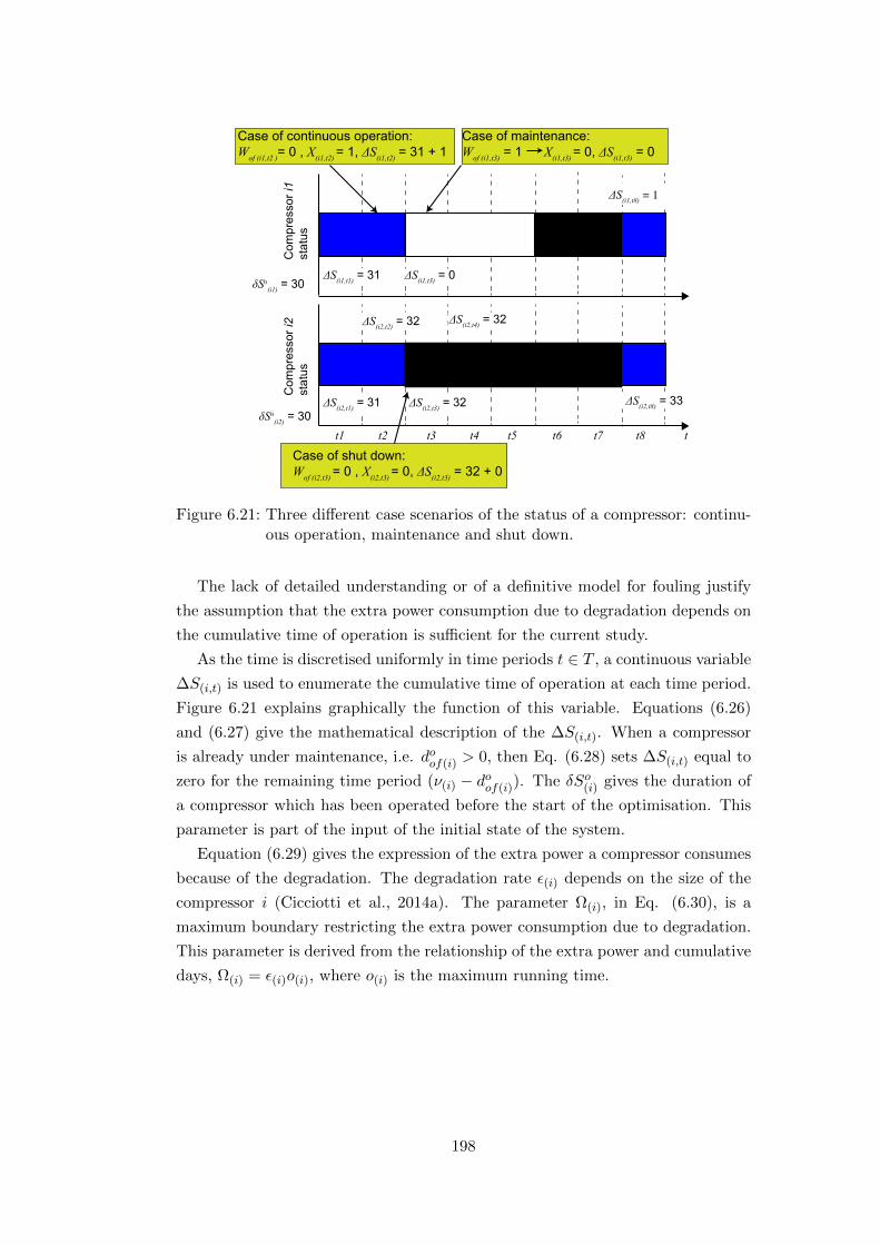
Com
pres
sor i
1 st
atus
Case of maintenance: Wof (i1,t3) = 1 X(i1,t3) = 0, ΔS(i1,t3) = 0
Case of continuous operation: Wof (i1,t2 )= 0 , X(i1,t2) = 1, ΔS(i1,t2) = 31 + 1
Case of shut down: Wof (i2,t3) = 0 , X(i2,t3) = 0, ΔS(i2,t3) = 32 + 0
Com
pres
sor i
2
stat
us
tt1 t2 t3 t4 t5 t6 t7 t8
δSo(i1) = 30
δSo(i2) = 30
ΔS(i1,t8) = 1
ΔS(i1,t3) = 0ΔS(i1,t1) = 31
ΔS(i2,t3) = 32ΔS(i2,t1) = 31 ΔS(i2,t8) = 33
ΔS(i2,t2) = 32 ΔS(i2,t4) = 32
Figure 6.21: Three different case scenarios of the status of a compressor: continu-ous operation, maintenance and shut down.
The lack of detailed understanding or of a definitive model for fouling justify
the assumption that the extra power consumption due to degradation depends on
the cumulative time of operation is sufficient for the current study.
As the time is discretised uniformly in time periods t ∈ T , a continuous variable
∆S(i,t) is used to enumerate the cumulative time of operation at each time period.
Figure 6.21 explains graphically the function of this variable. Equations (6.26)
and (6.27) give the mathematical description of the ∆S(i,t). When a compressor
is already under maintenance, i.e. doof(i) > 0, then Eq. (6.28) sets ∆S(i,t) equal to
zero for the remaining time period (ν(i) − doof(i)). The δSo(i) gives the duration of
a compressor which has been operated before the start of the optimisation. This
parameter is part of the input of the initial state of the system.
Equation (6.29) gives the expression of the extra power a compressor consumes
because of the degradation. The degradation rate ε(i) depends on the size of the
compressor i (Cicciotti et al., 2014a). The parameter Ω(i), in Eq. (6.30), is a
maximum boundary restricting the extra power consumption due to degradation.
This parameter is derived from the relationship of the extra power and cumulative
days, Ω(i) = ε(i)o(i), where o(i) is the maximum running time.
198
∆S(i,t) = (∆S(i,t−1) +X(i,t))(1−Wof(i,t)),
∀i ∈ I, (doof(i) > 0, (ν(i) − doof(i)) < t ≤ T ) ∨ (doof(i) = 0, t > 1) (6.26)
∆S(i,t) = (δSoi +X(i,t))(1−Wof(i,t)),
∀i ∈ I, doof(i) = 0, t = 1 (6.27)
∆S(i,t) = 0,
∀i ∈ I, doof(i) > 0 , 1 < t ≤ (ν(i) − doof(i)) (6.28)
∆W(i,t) = ε(i)∆S(i,t)X(i,t),
∀i ∈ I, t ∈ T (6.29)
∆W(i,t) ≤ Ω(i),
∀i ∈ I, t ∈ T (6.30)
Equations (6.26) and (6.27) involve bilinear terms some comprising multiplica-
tion of binary with binary variables and others the multiplication of binary with
continuous variables. Equations (6.31) – (6.36), which use the principles of the
Big-M formulation (Vecchietti et al., 2003), convert these non-linear constraints
into linear. The reason is to relax the optimisation problem and avoid to solve a
hard mixed integer non-linear programming optimisation model.
∆S(i,t) ≤ o(i)(1−Wof(i,t)),
∀i ∈ I, (doof(i) > 0, (ν(i) − doof(i)) < t ≤ T ) ∨ (doof(i) = 0, t ∈ T ) (6.31)
∆S(i,t) = 0,
∀i ∈ I, doof(i) > 0 , 1 ≤ t ≤ (ν(i) − doof(i)) (6.32)
∆S(i,t) ≤ δSoi +X(i,t) + o(i)Wof(i,t), ∀i ∈ I, doof(i) = 0, t = 1 (6.33)
δSoi +X(i,t) − o(i)Wof(i,t) ≤ ∆S(i,t), ∀i ∈ I, doof(i) = 0, t = 1 (6.34)
∆S(i,t) ≤ ∆S(i,t−1) +X(i,t) + o(i)Wof(i,t),
∀i ∈ I, (doof(i) > 0, (ν(i) − doof(i)) < t ≤ T ) ∨ (doof(i) = 0, t > 1) (6.35)
∆S(i,t−1) +X(i,t) − o(i)Wof(i,t) ≤ ∆S(i,t),
∀i ∈ I, (doof(i) > 0, (ν(i) − doof(i)) < t ≤ T ) ∨ (doof(i) = 0, t > 1) (6.36)
Moreover, Eq. (6.29) involves the multiplication of the continuous variable
∆S(i,t) with the binary variable X(i,t). The reason for this multiplication is that
199
the extra power due to degradation, ∆W(i,t), at a period t should not be added
into the objective function when the compressor i is offline but not washed. On the
other hand, the previous time periods in which the compressor has been operating
must be registered through ∆S(i,t) for each period t. This leads to a non-linear
equation, where the following formulation can convert the constraints into linear
constraints:
∆W(i,t) ≤ Ω(i)X(i,t), ∀i ∈ I, t ∈ T (6.37)
∆W(i,t) ≤ ε(i)∆S(i,t) + Ω(i)(1−X(i,t)), ∀i ∈ I, t ∈ T (6.38)
ε(i)∆S(i,t) − Ω(i)(1−X(i,t)) ≤ ∆W(i,t), ∀i ∈ I, t ∈ T (6.39)
As discussed in the assumptions, if the model considered the assumption of
Meher-Homji et al. (2001) that a compressor continues being fouled while it is
offline, then Eqs. (6.26) and (6.27) should exclude the X(i,t) in the first paren-
thesis. This would lead to an easier mathematical problem to solve. The current
optimisation problem considers the case that a compressor does not become fouled
during offline mode.
6.5.3 Model of online washing
The online washing maintenance model considers the following set of binary
variables:
Uon(i,t) =
1, if online washing of a compressor i occurs in time period t
0, otherwise
The injection of a cleaning solution into the compressor can have unwanted side
effects such as corrosion of the blades if done too frequently. For this reason, it is
assumed a minimum time period γ(i) of each compressor i between two consequent
Online Washing Episodes (ONWEs):
Uon(i,t) = 0,
∀i ∈ I, doon(i) < γ(i) , 1 ≤ t ≤ (γ(i) − doon(i)) (6.40)
t∑t′=maxt−γ(i)+1,1
Uon(i,t′) ≤ 1,
∀i ∈ I, (doon(i) ≥ γ(i), t ∈ T ) ∨ (doon(i) < γ(i), (γ(i) − doon(i)) < t ≤ T ) (6.41)
Equation (6.40) is valid when a compressor has been washed online for time
period doon(i) before the start of the optimisation and the doon(i) is smaller than the
γ(i). For any other case, Eq. (6.41) holds true.
200

Equation (6.42) describes the fact that there is also a maximum λon ONWEs of
different compressors that can take place in each time period of the time horizon.
The reason for considering this constraint is that it is possible the online wash-
ing infrastructure could not support simultaneous online washing as described by
Boyce and Gonzalez (2007). In any other case, this constraint can be omitted.∑i∈I
Uon(i,t) ≤ λon, ∀t ∈ T (6.42)
An online washing event cannot take place when the compressor is offline. Equa-
tion (6.43) describes that if a compressor i is online at period t, i.e. X(i,t) = 1,
then it has the option to be washed, i.e. Uon(i,t) = 1 or it can be decided to operate
without being washed, i.e. Uon(i,t) = 0. However, if the compressor is offline, i.e.
X(i,t) = 0, variable Uon(i,t) has to be equal to zero in this time period.
Uon(i,t) ≤ X(i,t), ∀i ∈ I, t ∈ T (6.43)
The recovery model for online washing, which is described in Eqs. (6.44) and
(6.45), assumes that ∆S(i,t) is reduced by a recovery factor RF . For instance, if the
recovery factor is RF = 0.2 and the operating period is ∆S(i,t) = 100 days, then
the final operating period after an online washing would be ∆S(i,t) · (1−RF ) = 80
days. Then the ∆W(i,t) is estimated based on the duration of this period. The
variable ∆S(i,t) represents the Equivalent Operating Time (EOT) presented by
de Backer (2000) and Bohrenkamper et al. (2000). The online washing model is
completed with the consideration of the degradation model, which is the same one
considered in the case of the offline washing in the previous Section 6.5.2 and it is
defined by Eqs. (6.29) and (6.30).
∆S(i,t) = (∆S(i,t−1) +X(i,t))(1−RF · Uon(i,t)), ∀i ∈ I, t > 1 (6.44)
∆S(i,t) = (δSoi +X(i,t))(1−RF · Uon(i,t)), ∀i ∈ I, t = 1 (6.45)
The formulation of the constraints in Eqs. (6.44) and (6.45) shows that the
multiplication of binary and continuous variables is more complicated compared
to the corresponding case of the offline washing. To overcome this complexity,
the linearisation of these constraints employs an auxiliary variable ∆Saux(i,t). The
linearised constraints of Eqs. (6.44) and (6.45) can be seen below:
201
∆S(i,t) = (δSoi +X(i,t))−∆Saux(i,t), ∀i ∈ I, t = 1 (6.46)
∆S(i,t) = (∆S(i,t−1) +X(i,t))−∆Saux(i,t), ∀i ∈ I, t > 1 (6.47)
∆Saux(i,t) = 0,
∀i ∈ I, doon(i) < γ(i), 1 ≤ t ≤ γ(i) − doon(i) (6.48)
∆Saux(i,t) ≤ o(i)Uon(i,t),
∀i ∈ I, (doon(i) ≥ γ(i), t ∈ T ) ∨ (doon(i) < γ(i), t > (γ(i) − doon(i))) (6.49)
∆Saux(i,t) ≤ (∆S(i,t−1) +X(i,t))RF + (1− Uon(i,t))o(i),
∀i ∈ I, (doon(i) ≥ γ(i), t > 1) ∨ (doon(i) < γ(i), t > γ(i) − doon(i)) (6.50)
(∆S(i,t−1) +X(i,t))RF − (1− Uon(i,t))o(i) ≤ ∆Saux(i,t),
∀i ∈ I, (doon(i) ≥ γ(i), t > 1) ∨ (doon(i) < γ(i), t > γ(i) − doon(i)) (6.51)
∆Saux(i,t) ≤ (δSoi +X(i,t))RF + (1− Uon(i,t))o(i),
∀i ∈ I, doon(i) ≥ γ(i), t = 1 (6.52)
(δSoi +X(i,t))RF − (1− Uon(i,t))o(i) ≤ ∆Saux(i,t),
∀i ∈ I, doon(i) ≥ γ(i), t = 1 (6.53)
The degradation model used in the online washing considers the linearisation
of the constraint of Eq. (6.29) which was described earlier when discussing Eqs.
(6.37) – (6.39) exactly as in the case of the offline washing degradation model.
6.5.4 Model of combined online and offline washing
Section 6.5.4 describes the scenarios when both offline and online washings are
available to clean the compressors. In this case, the optimisation model employs
all the binary variables Wof(i,t), Uof(i,t), Kof(i,t) and Uon(i,t). The optimisation
model includes the constraints in Eqs. (6.19) – (6.25) from the model of offline
washing in Section 6.5.2, and the constraints in Eqs. (6.40) – (6.43) from the
model of online washing in Section 6.5.3.
The degradation and recovery model is a combination of the two different wash-
ing models. This combined model is described by the constraints in the general
form in Eqs. (6.29) – (6.30) and the linearised form in Eqs. (6.37) – (6.39). The
recovery model in the combined online and offline washing scenario is given by
Eqs. (6.54) and (6.55).
202
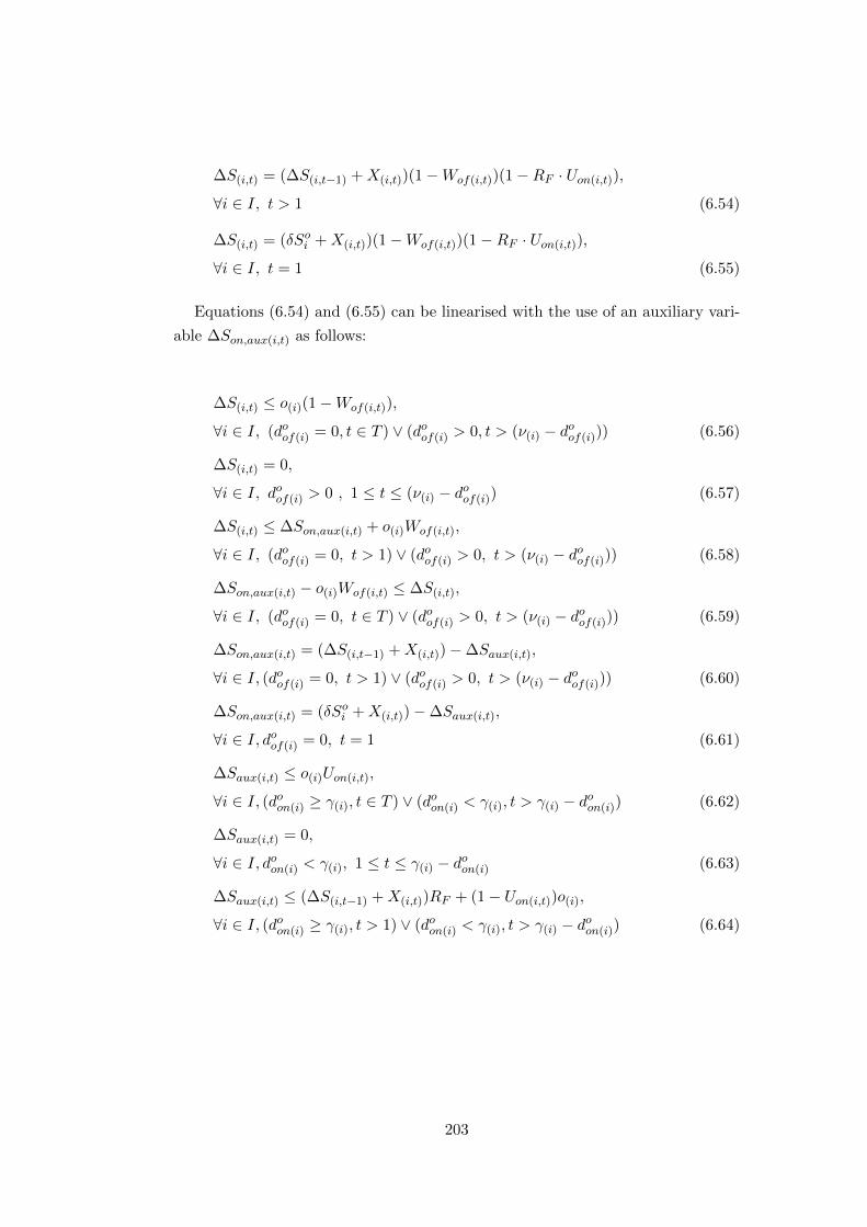
∆S(i,t) = (∆S(i,t−1) +X(i,t))(1−Wof(i,t))(1−RF · Uon(i,t)),
∀i ∈ I, t > 1 (6.54)
∆S(i,t) = (δSoi +X(i,t))(1−Wof(i,t))(1−RF · Uon(i,t)),
∀i ∈ I, t = 1 (6.55)
Equations (6.54) and (6.55) can be linearised with the use of an auxiliary vari-
able ∆Son,aux(i,t) as follows:
∆S(i,t) ≤ o(i)(1−Wof(i,t)),
∀i ∈ I, (doof(i) = 0, t ∈ T ) ∨ (doof(i) > 0, t > (ν(i) − doof(i))) (6.56)
∆S(i,t) = 0,
∀i ∈ I, doof(i) > 0 , 1 ≤ t ≤ (ν(i) − doof(i)) (6.57)
∆S(i,t) ≤ ∆Son,aux(i,t) + o(i)Wof(i,t),
∀i ∈ I, (doof(i) = 0, t > 1) ∨ (doof(i) > 0, t > (ν(i) − doof(i))) (6.58)
∆Son,aux(i,t) − o(i)Wof(i,t) ≤ ∆S(i,t),
∀i ∈ I, (doof(i) = 0, t ∈ T ) ∨ (doof(i) > 0, t > (ν(i) − doof(i))) (6.59)
∆Son,aux(i,t) = (∆S(i,t−1) +X(i,t))−∆Saux(i,t),
∀i ∈ I, (doof(i) = 0, t > 1) ∨ (doof(i) > 0, t > (ν(i) − doof(i))) (6.60)
∆Son,aux(i,t) = (δSoi +X(i,t))−∆Saux(i,t),
∀i ∈ I, doof(i) = 0, t = 1 (6.61)
∆Saux(i,t) ≤ o(i)Uon(i,t),
∀i ∈ I, (doon(i) ≥ γ(i), t ∈ T ) ∨ (doon(i) < γ(i), t > γ(i) − doon(i)) (6.62)
∆Saux(i,t) = 0,
∀i ∈ I, doon(i) < γ(i), 1 ≤ t ≤ γ(i) − doon(i) (6.63)
∆Saux(i,t) ≤ (∆S(i,t−1) +X(i,t))RF + (1− Uon(i,t))o(i),
∀i ∈ I, (doon(i) ≥ γ(i), t > 1) ∨ (doon(i) < γ(i), t > γ(i) − doon(i)) (6.64)
203
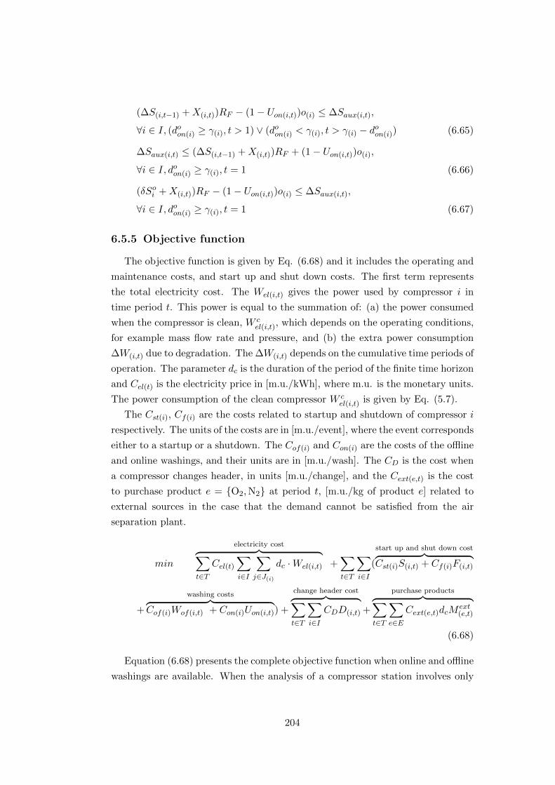
(∆S(i,t−1) +X(i,t))RF − (1− Uon(i,t))o(i) ≤ ∆Saux(i,t),
∀i ∈ I, (doon(i) ≥ γ(i), t > 1) ∨ (doon(i) < γ(i), t > γ(i) − doon(i)) (6.65)
∆Saux(i,t) ≤ (∆S(i,t−1) +X(i,t))RF + (1− Uon(i,t))o(i),
∀i ∈ I, doon(i) ≥ γ(i), t = 1 (6.66)
(δSoi +X(i,t))RF − (1− Uon(i,t))o(i) ≤ ∆Saux(i,t),
∀i ∈ I, doon(i) ≥ γ(i), t = 1 (6.67)
6.5.5 Objective function
The objective function is given by Eq. (6.68) and it includes the operating and
maintenance costs, and start up and shut down costs. The first term represents
the total electricity cost. The Wel(i,t) gives the power used by compressor i in
time period t. This power is equal to the summation of: (a) the power consumed
when the compressor is clean, W cel(i,t), which depends on the operating conditions,
for example mass flow rate and pressure, and (b) the extra power consumption
∆W(i,t) due to degradation. The ∆W(i,t) depends on the cumulative time periods of
operation. The parameter dc is the duration of the period of the finite time horizon
and Cel(t) is the electricity price in [m.u./kWh], where m.u. is the monetary units.
The power consumption of the clean compressor W cel(i,t) is given by Eq. (5.7).
The Cst(i), Cf(i) are the costs related to startup and shutdown of compressor i
respectively. The units of the costs are in [m.u./event], where the event corresponds
either to a startup or a shutdown. The Cof(i) and Con(i) are the costs of the offline
and online washings, and their units are in [m.u./wash]. The CD is the cost when
a compressor changes header, in units [m.u./change], and the Cext(e,t) is the cost
to purchase product e = O2,N2 at period t, [m.u./kg of product e] related to
external sources in the case that the demand cannot be satisfied from the air
separation plant.
min
electricity cost︷ ︸︸ ︷∑t∈T
Cel(t)∑i∈I
∑j∈J(i)
dc ·Wel(i,t) +∑t∈T
∑i∈I
(
start up and shut down cost︷ ︸︸ ︷Cst(i)S(i,t) + Cf(i)F(i,t)
+
washing costs︷ ︸︸ ︷Cof(i)Wof(i,t) + Con(i)Uon(i,t)) +
change header cost︷ ︸︸ ︷∑t∈T
∑i∈I
CDD(i,t) +
purchase products︷ ︸︸ ︷∑t∈T
∑e∈E
Cext(e,t)dcMext(e,t)
(6.68)
Equation (6.68) presents the complete objective function when online and offline
washings are available. When the analysis of a compressor station involves only
204
one type of washing then the objective function considers the respective terms of
costs. This objective function is an extension of the objective function used in the
Section 5.12.
6.5.6 Terminal constraints of maintenance model
Equations (6.69) and (6.70) give the constraint regarding the offline washing
of compressors. They describe that a minimum number of λk Offline Washing
Episodes (OFWEs) have to take place within the time period [T − t∗S , T ], where
t∗S = tS +maxν(i) and tS is a number of days before the end of the time horizon.
T∑t′=T−t∗S
∑i∈I
Kof(i,t′) = λk (6.69)
T∑t′=T−t∗S
Kof(i,t′) ≤ 1, ∀i ∈ INOFF (6.70)
The set INOFF ⊆ I involves all the compressors which have not been under of-
fline maintenance before the start of the optimisation. Equation (6.70) guarantees
that a compressor will be maintained only one time in the time period [T − t∗s, T ].
Moreover, the constraint described by Eq. (5.67) which ensures that the contents
of the storage tanks are full at the end of the time horizon is taken into account
in the optimisation formulation.
The terminal constraints have to be investigated using heuristics from historical
operation and literature. The decisions of these constraints are strongly related
with the particular configuration of the plant of the compressors in the plant.
6.5.7 Description of numerical application
The condition-based maintenance optimization is tested in the industrial air
separation plant of BASF in Ludwigshafen, Germany. This section considers
the eleven multi-stage centrifugal compressors of the plant. Again, the com-
pressors supply three headers with compressed air and there are five small com-
pressors, i ∈ Is = i1, i2, i3, i4, i5, driven by electrical motors with nominal
power rating of some MW, WNoel,s. Moreover, there are six large compressors,
i ∈ Ib = i6, i7, i8, i9, i10, i11 with power rate of more than ten MW each, WNoel,b ,
and WNoel,b = 2WNo
el,s. Table 5.1 gives the feasible region, i.e. boundaries of mass
flow rates and pressures, of the compressors derived from data analysis of past
operation.
The description of the plant has been described in Section 5.10 in which Fig.
5.11 gives the schematic of the plant. The first header, j1, collects the compressed
205
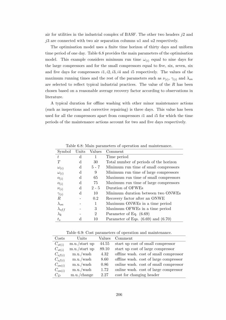
air for utilities in the industrial complex of BASF. The other two headers j2 and
j3 are connected with two air separation columns u1 and u2 respectively.
The optimisation model uses a finite time horizon of thirty days and uniform
time period of one day. Table 6.8 provides the main parameters of the optimisation
model. This example considers minimum run time ω(i) equal to nine days for
the large compressors and for the small compressors equal to five, six, seven, six
and five days for compressors i1, i2, i3, i4 and i5 respectively. The values of the
maximum running times and the rest of the parameters such as ν(i), γ(i) and λon
are selected to reflect typical industrial practices. The value of the R has been
chosen based on a reasonable average recovery factor according to observations in
literature.
A typical duration for offline washing with other minor maintenance actions
(such as inspections and corrective repairing) is three days. This value has been
used for all the compressors apart from compressors i1 and i5 for which the time
periods of the maintenance actions account for two and five days respectively.
Table 6.8: Main parameters of operation and maintenance.
Symbol Units Values Comment
t d 1 Time periodT d 30 Total number of periods of the horizonω(i) d 5 - 7 Minimum run time of small compressors
ω(i) d 9 Minimum run time of large compressors
o(i) d 65 Maximum run time of small compressors
o(i) d 75 Maximum run time of large compressors
ν(i) d 2 - 5 Duration of OFWEs
γ(i) d 10 Minimum duration between two ONWEs
R - 0.2 Recovery factor after an ONWEλon - 1 Maximum ONWEs in a time periodλoff - 3 Maximum OFWEs in a time periodλk - 2 Parameter of Eq. (6.69)ts d 10 Parameter of Eqs. (6.69) and (6.70)
Table 6.9: Cost parameters of operation and maintenance.
Costs Units Values Comment
Cst(i) m.u./start up 44.55 start up cost of small compressor
Cst(i) m.u./start up 89.10 start up cost of large compressor
Cof(i) m.u./wash 4.32 offline wash. cost of small compressor
Cof(i) m.u./wash 8.60 offline wash. cost of large compressor
Con(i) m.u./wash 0.86 online wash. cost of small compressor
Con(i) m.u./wash 1.72 online wash. cost of large compressor
CD m.u./change 2.27 cost for changing header
206

Dem
and
in k
g/s
air p
er d
ay (s
cale
d)
N2
O2
Figure 6.22: Production targets of the air separation plant for thirty days.
The ratio between extra power consumption and nominal power for one month,
∆W/WNoel is 4.5% and 3.3% of the small and large compressors respectively. These
values are based on the work from Cicciotti et al. (2014a) which used a detailed
first principles model of an industrial compressor to estimate the profile of the
degradation over time. The degradation rates are calculated based on monitoring
parameters (for example performance) of the compressor using a linear approxi-
mation.
Table 6.9 provides the values of all the major parameters of the costs of the
objective function. The start up costs for small and large compressors were as-
sumed equal to the energy consumed from the motors of the compressors for half
a day. In this example it is assumed that there is not a major energy consump-
tion for switching off a compressor, therefore this cost is zero. The washing costs
are estimated using the assumptions from Aretakis et al. (2012) and Fabbri et al.
(2011). Therefore, Table 6.9 gives the values of the costs of a washing episode in
this particular case study. The cost for changing header has been explained in
Chapter 5.
A baseline study is formulated to examine the optimal operation and mainte-
nance plan of compressors with different types of washings. This case uses the
information from Tables 5.8, 6.8 and 6.9. Moreover the information of the initial
state of the system is provided by Table 6.10. The base case employs modified
production targets for O2, N2 and compressed air for utilities from real industrial
data. Figure 6.22 gives the production targets for O2 and N2 in kg of compressed
air (scaled units).
207
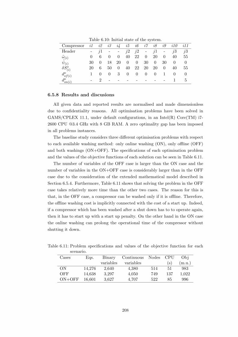
Table 6.10: Initial state of the system.
Compressor i1 i2 i3 i4 i5 i6 i7 i8 i9 i10 i11
Header - j1 - - j2 j2 - j1 - j3 j3ω(i) 0 6 0 0 40 22 0 20 0 40 55
ψ(i) 30 0 18 20 0 0 30 0 30 0 0
δSo(i) 20 6 50 0 40 22 20 20 0 40 55
doof(i) 1 0 0 3 0 0 0 0 1 0 0
doon(i) - 2 - - - - - - - 1 5
6.5.8 Results and discusions
All given data and reported results are normalised and made dimensionless
due to confidentiality reasons. All optimisation problems have been solved in
GAMS/CPLEX 11.1, under default configurations, in an Intel(R) Core(TM) i7-
2600 CPU @3.4 GHz with 8 GB RAM. A zero optimality gap has been imposed
in all problems instances.
The baseline study considers three different optimisation problems with respect
to each available washing method: only online washing (ON), only offline (OFF)
and both washings (ON+OFF). The specifications of each optimisation problem
and the values of the objective functions of each solution can be seen in Table 6.11.
The number of variables of the OFF case is larger than the ON case and the
number of variables in the ON+OFF case is considerably larger than in the OFF
case due to the consideration of the extended mathematical model described in
Section 6.5.4. Furthermore, Table 6.11 shows that solving the problem in the OFF
case takes relatively more time than the other two cases. The reason for this is
that, in the OFF case, a compressor can be washed only if it is offline. Therefore,
the offline washing cost is implicitly connected with the cost of a start up. Indeed,
if a compressor which has been washed after a shut down has to to operate again,
then it has to start up with a start up penalty. On the other hand in the ON case
the online washing can prolong the operational time of the compressor without
shutting it down.
Table 6.11: Problem specifications and values of the objective function for eachscenario.
Cases Eqs. Binary Continuous Nodes CPU Objvariables variables (s) (m.u.)
ON 14,276 2,640 4,380 514 51 983OFF 14,638 3,297 4,050 749 137 1,022ON+OFF 16,601 3,627 4,707 522 85 996
208
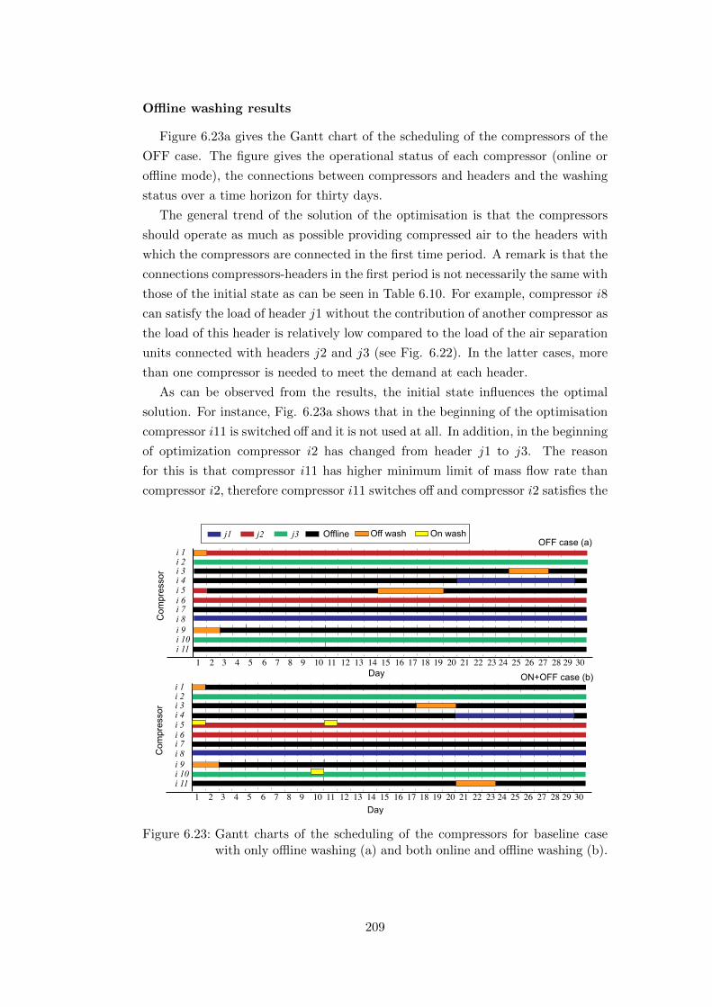
Offline washing results
Figure 6.23a gives the Gantt chart of the scheduling of the compressors of the
OFF case. The figure gives the operational status of each compressor (online or
offline mode), the connections between compressors and headers and the washing
status over a time horizon for thirty days.
The general trend of the solution of the optimisation is that the compressors
should operate as much as possible providing compressed air to the headers with
which the compressors are connected in the first time period. A remark is that the
connections compressors-headers in the first period is not necessarily the same with
those of the initial state as can be seen in Table 6.10. For example, compressor i8
can satisfy the load of header j1 without the contribution of another compressor as
the load of this header is relatively low compared to the load of the air separation
units connected with headers j2 and j3 (see Fig. 6.22). In the latter cases, more
than one compressor is needed to meet the demand at each header.
As can be observed from the results, the initial state influences the optimal
solution. For instance, Fig. 6.23a shows that in the beginning of the optimisation
compressor i11 is switched off and it is not used at all. In addition, in the beginning
of optimization compressor i2 has changed from header j1 to j3. The reason
for this is that compressor i11 has higher minimum limit of mass flow rate than
compressor i2, therefore compressor i11 switches off and compressor i2 satisfies the
1 2 3 4 5 6 7 8 9 10 11 12 13 14 15 16 17 18 19 20 21 22 23 24 25 26 27 28 29 30
i 1i 2
i 4
i 8
i 3
i 11
i 9i 10
j1 j2 j3 Off washOffline On wash
Com
pres
sor
i 6i 5
i 7
Day
OFF case (a)
ON+OFF case (b)
1 2 3 4 5 6 7 8 9 10 11 12 13 14 15 16 17 18 19 20 21 22 23 24 25 26 27 28 29 30
i 1i 2
i 4
i 8
i 3
i 11
i 9i 10
Day
Com
pres
sor
i 6i 5
i 7
Figure 6.23: Gantt charts of the scheduling of the compressors for baseline casewith only offline washing (a) and both online and offline washing (b).
209

load of header j3 along with compressor i10. These changes support the further
decisions which switch off compressor i5 at Day 2 and start up compressor i1
connecting to header j2.
The optimization suggests maintaining compressors i3 and i5 which have been
operated more than the others as can be seen from the values of δSo(i) in Table 6.10.
Hence, this decision leads to lower maintenance costs compared to the scenario
which could have decided the washing of a larger compressor such as compressor
i11. Table 6.9 shows that the offline washing cost of a small compressor is lower
than the cost of large compressor. In the section of the time horizon between Day
15 and Day 30, the two washing episodes of compressors i3 and i5 are derived
from the terminal constraints in Eqs. (6.69) and (6.70) with the consideration of
λk = 2, and t∗S = 15 d.
The previous statements show that there are many factors which influence the
best decisions for optimal operation of the compressors and these factors depend
on the knowledge of the future information such as forecast of the demand and the
decisions for the succeeding time periods. Moreover, the values of the parameters
of the problem influence these decisions and examples of these parameters are the
initial operating and shut down times, and the values of the penalty costs.
Thus, even the most well-trained and experienced team of managers and opera-
tors could find it difficult to take the best decisions without having a sophisticated
optimisation model based on the systematic use of the previous mentioned infor-
mation. The nature of the problem is combinatorial involving a large number of
scenarios, and therefore it is impractical and probably impossible to identify the
optimal patterns for the best decisions when there is not the use of optimisation.
Results from the combination of offline and online washing
Figure 6.23b illustrates the Gantt chart of the scheduling of the compressors
of the base case with available both online and offline washings, ON+OFF case.
The solution of the ON case results in the same Gantt chart as in the ON+OFF
case apart from the existence of offline washing episodes, therefore the ON Gantt
chart is not presented. Additionally, the numbers and times of the online washing
episodes (ONWEs) are the same in both cases.
The results from the schedule of the ON+OFF case show that online washing
is used along with offline. In this case compared to the OFF case, compressor i5
is not switched off but it is washed online. Hence, both schedules included clean-
ing of compressor i5, the OFF case with offline washing, but the ON+OFF with
online and keeping the compressor on. The reason is that this small compressor
is the second most fouled one after compressor i11. As the schedule of the OFF
case switched off compressor i11 the same can be observed in the schedule of the
210
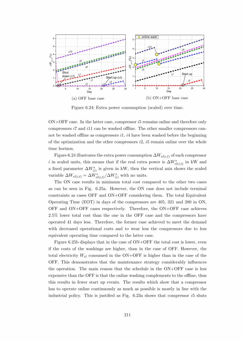
Day
i1
i8
i2
i6
i10
i5
ΔWel
(i,t)(
%)
Shut down (i5) Start up (i4)
i4
(a) OFF base case
i6
i5
i8i2
i4
i10
ΔWel
(i,t)(
%)
Start up
online wash
(b) ON+OFF base case
Figure 6.24: Extra power consumption (scaled) over time.
ON+OFF case. In the latter case, compressor i5 remains online and therefore only
compressors i7 and i11 can be washed offline. The other smaller compressors can-
not be washed offline as compressors i1, i4 have been washed before the beginning
of the optimization and the other compressors i2, i5 remain online over the whole
time horizon.
Figure 6.24 illustrates the extra power consumption ∆Wel(i,t) of each compressor
i in scaled units, this means that if the real extra power is ∆W ∗el(i,t) in kW and
a fixed parameter ∆W s(i) is given in kW, then the vertical axis shows the scaled
variable ∆Wel(i,t) = ∆W ∗el(i,t)/∆Ws(i) with no units.
The ON case results in minimum total cost compared to the other two cases
as can be seen in Fig. 6.25a. However, the ON case does not include terminal
constraints as cases OFF and ON+OFF considering them. The total Equivalent
Operating Time (EOT) in days of the compressors are 405, 321 and 280 in ON,
OFF and ON+OFF cases respectively. Therefore, the ON+OFF case achieves
2.5% lower total cost than the one in the OFF case and the compressors have
operated 41 days less. Therefore, the former case achieved to meet the demand
with decreased operational costs and to wear less the compressors due to less
equivalent operating time compared to the latter case.
Figure 6.25b displays that in the case of ON+OFF the total cost is lower, even
if the costs of the washings are higher, than in the case of OFF. However, the
total electricity Wel consumed in the ON+OFF is higher than in the case of the
OFF. This demonstrates that the maintenance strategy considerably influences
the operation. The main reason that the schedule in the ON+OFF case is less
expensive than the OFF is that the online washing complements to the offline, thus
this results in fewer start up events. The results which show that a compressor
has to operate online continuously as much as possible is mostly in line with the
industrial policy. This is justified as Fig. 6.23a shows that compressor i5 shuts
211
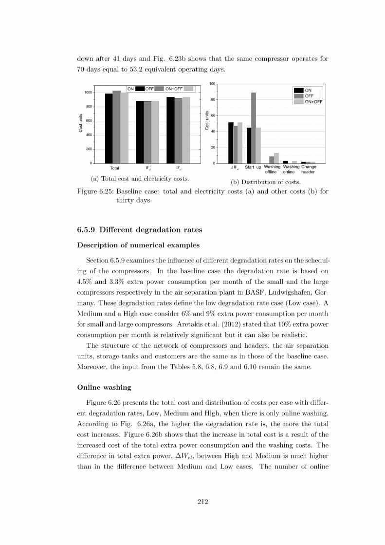
down after 41 days and Fig. 6.23b shows that the same compressor operates for
70 days equal to 53.2 equivalent operating days.
ON OFF ON+OFF
Cos
t uni
ts
Total Wel Welc
(a) Total cost and electricity costs.
ONOFFON+OFF
Cos
t uni
ts
ΔWelWashing offline
Washingonline
Changeheader
Start up
(b) Distribution of costs.
Figure 6.25: Baseline case: total and electricity costs (a) and other costs (b) forthirty days.
6.5.9 Different degradation rates
Description of numerical examples
Section 6.5.9 examines the influence of different degradation rates on the schedul-
ing of the compressors. In the baseline case the degradation rate is based on
4.5% and 3.3% extra power consumption per month of the small and the large
compressors respectively in the air separation plant in BASF, Ludwigshafen, Ger-
many. These degradation rates define the low degradation rate case (Low case). A
Medium and a High case consider 6% and 9% extra power consumption per month
for small and large compressors. Aretakis et al. (2012) stated that 10% extra power
consumption per month is relatively significant but it can also be realistic.
The structure of the network of compressors and headers, the air separation
units, storage tanks and customers are the same as in those of the baseline case.
Moreover, the input from the Tables 5.8, 6.8, 6.9 and 6.10 remain the same.
Online washing
Figure 6.26 presents the total cost and distribution of costs per case with differ-
ent degradation rates, Low, Medium and High, when there is only online washing.
According to Fig. 6.26a, the higher the degradation rate is, the more the total
cost increases. Figure 6.26b shows that the increase in total cost is a result of the
increased cost of the total extra power consumption and the washing costs. The
difference in total extra power, ∆Wel, between High and Medium is much higher
than in the difference between Medium and Low cases. The number of online
212
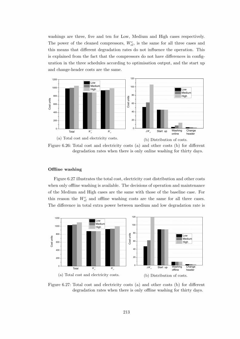
washings are three, five and ten for Low, Medium and High cases respectively.
The power of the cleaned compressors, W cel, is the same for all three cases and
this means that different degradation rates do not influence the operation. This
is explained from the fact that the compressors do not have differences in config-
uration in the three schedules according to optimisation output, and the start up
and change-header costs are the same.
Cos
t uni
ts
Total Wel Welc
LowMediumHigh
(a) Total cost and electricity costs.
Cos
t uni
tsΔWel
Washingonline
Changeheader
Start up
LowMediumHigh
(b) Distribution of costs.
Figure 6.26: Total cost and electricity costs (a) and other costs (b) for differentdegradation rates when there is only online washing for thirty days.
Offline washing
Figure 6.27 illustrates the total cost, electricity cost distribution and other costs
when only offline washing is available. The decisions of operation and maintenance
of the Medium and High cases are the same with those of the baseline case. For
this reason the W cel and offline washing costs are the same for all three cases.
The difference in total extra power between medium and low degradation rate is
Cos
t uni
ts
Total Wel Welc
LowMediumHigh
(a) Total cost and electricity costs.
Cos
t uni
ts
ΔWelWashingoffline
Changeheader
Start up
LowMediumHigh
(b) Distribution of costs.
Figure 6.27: Total cost and electricity costs (a) and other costs (b) for differentdegradation rates when there is only offline washing for thirty days.
213

31.3%, and the difference between high and medium is 91.6%. This results in
higher total cost in the High case. Moreover, the optimisation suggests keeping
the online compressors operating as much as possible to avoid start up costs or
possible change-header costs.
Both online and offline washing
Figure 6.28 shows that the combination of online and offline washings achieves
reduced total costs by 2.5%, 2.5% and 3.0% in each degradation rate case respec-
tively compared to the OFF case presented in the previous paragraph (Offline
washing). However, only in the High case the extra power ∆Wel cost is lower in
the case of the ON+OFF case than in the OFF case. The total cost of the OFF
case includes increased start up costs, on the other hand the ON+OFF case is
more flexible with lower total start up cost. The previous observations support
the use of both online and offline washing, especially when the Equivalent Operat-
ing Time (EOT) of the ON+OFF case is reduced by 35% compared to that of the
OFF case. This shows that the operation of compressors in the former case would
be more flexible for a following scheduling problem as the compressors have been
maintained in a more optimal way in the current scheduling problem.
Figure 6.29 shows the scheduling of the compressors and the online and offline
washing episodes timings in the case of the high degradation rate (High case). The
resulting schedule is different than the schedule when the degradation rate is lower,
as shown in the schedule of the base case in Fig. 6.23b. The optimisation does
not suggest washing a compressor after the minimum possible period, γ(i) days,
as can be seen in the case of compressor i2. This demonstrates that a periodic
fixed schedule, which is usually used in a typical industrial preventive maintenance
LowMediumHigh
Cos
t uni
ts
Total Wel Welc
(a) Total cost and electricity costs.
Cos
t uni
ts
ΔWelWashingoffline
Washingonline
Changeheader
Start up
LowMediumHigh
(b) Distribution of costs.
Figure 6.28: Total cost and electricity costs (a) and other costs (b) for differentdegradation rates when both offline and online washing are consideredfor thirty days.
214

1 2 3 4 5 6 7 8 9 10 11 12 13 14 15 16 17 18 19 20 21 22 23 24 25 26 27 28 29 30
i 1i 2
i 4
i 8
i 3
i 11
i 9i 10
Day
Com
pres
sor
i 6i 5
i 7
j1 j2 j3 Off washOffline On wash
Figure 6.29: Scheduling of compressors with online and offline washing, and highdegradation rates.
i2
i1
i5
i6i8
i10
ΔWel
(i,t)(
%)
online wash
Figure 6.30: Extra power consumption of compressors with online and offline wash-ing, and high degradation rates.
strategy, would increase the total costs if maintenance and operation had not been
integrated in the optimisation model. Figure 6.29 shows that compressor i5 should
be maintained in a periodic way. This does not apply to the maintenance frequency
of the other compressors according to the figure.
Figure 6.30 gives the profile of the extra power ∆Wel of each compressor over
the time horizon of the optimisation. The online washing model assumed that
the application of online washing recovers a fixed percentage of the extra power
of a compressor at the period the washing occurs. This means that for higher
values of extra power consumption, the effect of the washing becomes greater.
Moreover, Figure 6.29 shows that the optimisation suggests washing the more
fouled compressors (shown in Table 6.10), i5, i6, i8 and i10, with a high frequency.
Compressor i5 is the most fouled among the small compressors and it is washed
three times, which is the maximum possible number of washing episodes in the total
period of the optimisation. Compressor i2 is the least fouled, thus the optimisation
suggests only one washing as the fouling accumulation is not high.
215
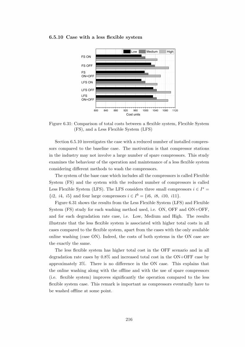
6.5.10 Case with a less flexible system
Cost units
LFS ON+OFF
FS ON+OFF
LFS OFF
FS OFF
LFS ON
FS ONLow Medium High
Figure 6.31: Comparison of total costs between a flexible system, Flexible System(FS), and a Less Flexible System (LFS)
Section 6.5.10 investigates the case with a reduced number of installed compres-
sors compared to the baseline case. The motivation is that compressor stations
in the industry may not involve a large number of spare compressors. This study
examines the behaviour of the operation and maintenance of a less flexible system
considering different methods to wash the compressors.
The system of the base case which includes all the compressors is called Flexible
System (FS) and the system with the reduced number of compressors is called
Less Flexible System (LFS). The LFS considers three small compressors i ∈ Is =
i2, i4, i5 and four large compressors i ∈ Ib = i6, i8, i10, i11.Figure 6.31 shows the results from the Less Flexible System (LFS) and Flexible
System (FS) study for each washing method used, i.e. ON, OFF and ON+OFF,
and for each degradation rate case, i.e. Low, Medium and High. The results
illustrate that the less flexible system is associated with higher total costs in all
cases compared to the flexible system, apart from the cases with the only available
online washing (case ON). Indeed, the costs of both systems in the ON case are
the exactly the same.
The less flexible system has higher total cost in the OFF scenario and in all
degradation rate cases by 0.8% and increased total cost in the ON+OFF case by
approximately 3%. There is no difference in the ON case. This explains that
the online washing along with the offline and with the use of spare compressors
(i.e. flexible system) improves significantly the operation compared to the less
flexible system case. This remark is important as compressors eventually have to
be washed offline at some point.
216
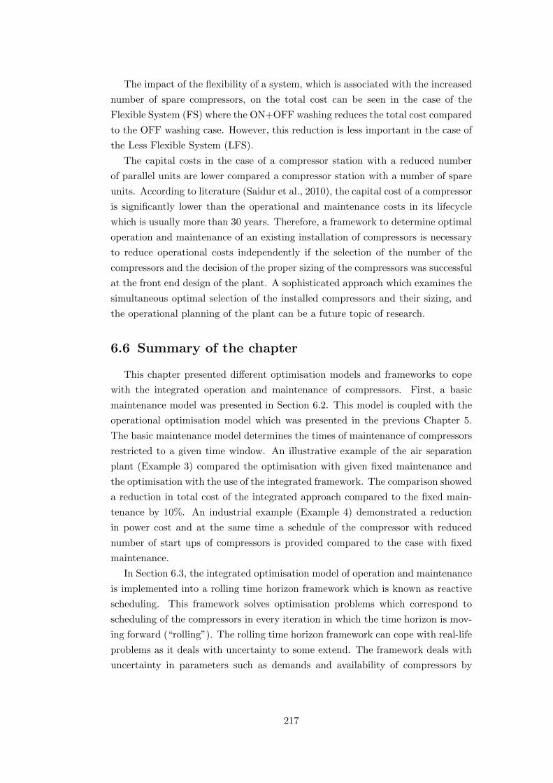
The impact of the flexibility of a system, which is associated with the increased
number of spare compressors, on the total cost can be seen in the case of the
Flexible System (FS) where the ON+OFF washing reduces the total cost compared
to the OFF washing case. However, this reduction is less important in the case of
the Less Flexible System (LFS).
The capital costs in the case of a compressor station with a reduced number
of parallel units are lower compared a compressor station with a number of spare
units. According to literature (Saidur et al., 2010), the capital cost of a compressor
is significantly lower than the operational and maintenance costs in its lifecycle
which is usually more than 30 years. Therefore, a framework to determine optimal
operation and maintenance of an existing installation of compressors is necessary
to reduce operational costs independently if the selection of the number of the
compressors and the decision of the proper sizing of the compressors was successful
at the front end design of the plant. A sophisticated approach which examines the
simultaneous optimal selection of the installed compressors and their sizing, and
the operational planning of the plant can be a future topic of research.
6.6 Summary of the chapter
This chapter presented different optimisation models and frameworks to cope
with the integrated operation and maintenance of compressors. First, a basic
maintenance model was presented in Section 6.2. This model is coupled with the
operational optimisation model which was presented in the previous Chapter 5.
The basic maintenance model determines the times of maintenance of compressors
restricted to a given time window. An illustrative example of the air separation
plant (Example 3) compared the optimisation with given fixed maintenance and
the optimisation with the use of the integrated framework. The comparison showed
a reduction in total cost of the integrated approach compared to the fixed main-
tenance by 10%. An industrial example (Example 4) demonstrated a reduction
in power cost and at the same time a schedule of the compressor with reduced
number of start ups of compressors is provided compared to the case with fixed
maintenance.
In Section 6.3, the integrated optimisation model of operation and maintenance
is implemented into a rolling time horizon framework which is known as reactive
scheduling. This framework solves optimisation problems which correspond to
scheduling of the compressors in every iteration in which the time horizon is mov-
ing forward (“rolling”). The rolling time horizon framework can cope with real-life
problems as it deals with uncertainty to some extend. The framework deals with
uncertainty in parameters such as demands and availability of compressors by
217

updating the parameters in every iteration. The application of the rolling time
horizon approach can be improved by estimating the best length of the time hori-
zon. There is a trade-off between length of the time horizon and accuracy in the
forecasting of the parameters. Moreover, the longer the time horizon the more
benefit is expected assuming that the forecasting error of parameters is constant
for different lengths of time horizons.
Section 6.4 presented a framework for integrated optimal operation and mainte-
nance of large compressors of an export gas compressor station of Statoil in Norway
for long periods. The framework receives input, for example the forecasted demand
in pressure and in flow, the upstream pressure of the gas and the initial state of the
configuration of the compressors. Industrial compressor maps were implemented
into a MILP model. Moreover, the MILP model considers the operational and
maintenance activities of the compressors. The framework uses the MILP model
to suggest the best decisions which minimise the total costs. The results of the
optimisation framework illustrated the best schedule of the operation and mainte-
nance of the compressors which would be a basis for an industrial tool to help the
users of the station to decrease costs, increase the lifecycle of the compressors and
guarantee flexibility of the overall system. A comparison with a case with fixed
maintenance schedule, showed that the integrated framework achieves savings of
224,000 EUR in three months (i.e. 0.84% improvement) from the optimal solution
of the case which does not consider the maintenance as a degree of freedom.
Finally, Section 6.5 presented an integrated optimisation framework which can
be used to optimise operation and maintenance of multiple compressors with dif-
ferent types of washings, namely offline and online, and their combination. This
method was tested in a numerical example of the BASF air separation plant. The
optimisation framework determines when and how often to wash the compressors
using each washing method. The results showed that the best maintenance strat-
egy to decrease the total costs and at the same time to minimise the wear of the
compressors is a combination of offline and online washing. In the case which a
compressor network involves spare compressors, the use of both washings decreases
the total costs and increases the availability of the compressor significantly. The
results have shown that the optimisation framework can provide enhanced decision
support leading to optimal operation and maintenance. By the modification of the
constraints of compressors and plant, the optimisation framework can be applied
to other systems which include large power rate compressors working in parallel.
218

7 Critical evaluation and suggestions
for future work
7.1 Description of the chapter
This chapter evaluates the outcomes of the research study on the optimisation
of compressor stations in different industrial applications. Chapter 1 defined the
objectives of the research study:
• Objective One was to develop a Real Time Optimisation (RTO) framework
to optimally share the load among parallel compressors in real time to deal
with short-term changes in the operation.
• Objective Two was to develop a multi-period optimisation framework to
optimally schedule the operations of compressors for long time periods.
• Objective Three was to implement maintenance activities into the opera-
tional optimisation framework and achieve simultaneous optimal operation
and maintenance.
Section 7.2 presents an evaluation of the achievements of the objectives. There
is a discussion on the research work for each objective, and the relevant scientific
contributions are identified. The strengths and assumptions of the methods used to
achieve each objective are examined, and the future work related to each objective
is reported. Finally, Section 7.3 highlights the recent outcomes and developments
following on from the research study of the thesis.
7.2 Evaluation of the achievements of the objectives
7.2.1 Objective One
Description of research work for Objective One
Chapter 4 focused on the first objective which was the development of the
Real Time Optimisation (RTO) of parallel compressors. The chapter presented a
comprehensive optimisation framework which can use raw industrial data in real
time to update process models used in an optimisation model. The operation of
219

the RTO can be see in Figure 4.2. The suggested optimisation model optimises
the compressors in means of minimum power consumption and provides the best
set points of the individual loads of the compressors to the control system. The
framework uses an online data detection algorithm to identify when the system
is in steady-state, so an RTO loop can initiate. This framework was applied to
the air compressors of the BASF air separation plant with the use of industrial
historical data provided by the industrial partner.
Contributions of the optimisation framework for Objective One
The major contributions related to the first objective are summarised below:
• The RTO framework employed data-driven models which update the models
for estimating power consumption and the feasible window of operation, so
as to represent the real-time conditions of the compressors at the point of
the optimisation. The PhD study demonstrated that the operational costs
are reduced with the use of the RTO compared to operation with industrial
strategies (Xenos et al., 2015a).
• The RTO framework is the state-of-the-art for optimising a network of com-
pressors, i.e. compressors connected in parallel configuration. This con-
tribution is considered novel as the RTO framework is applied to the air
compressor station in BASF which includes compressors which have been
operating for many years. The original motivation of this study to optimise
the operation of compressors was that compressors with similar nominal spec-
Operation (compressors)
Validation ofdata
Parameter estimation
Optimisation(NLP)
Monitoring(sensors)
Raw data
Steady-state identification
Validated dataUpdated model
parameters
Set points
Applyset points
Input parameters
Disturbances (Ambient conditions,
demand)
Controlsystem/
operators
Figure 4.2: Detailed description of the structure of the components of the RTO.
220

ifications (at the point of their purchase) have different power consumptions
and characteristics after many years of operation.
• The description of the integrated approach of the RTO (supervisory control)
and the upper automation level of scheduling highlighted the need to examine
the interactions among them. An example is that if the RTO problem is
infeasible, this means that a new configuration of the compressors has to be
chosen. The selection of the best compressors to operate online is one of the
outputs of the scheduling.
• The application of the RTO to a system of compressors demonstrated the de-
velopment of algorithms for offline and online steady-state detection using a
multivariate approach. The thesis showed which process variables should be
monitored by the algorithm. Moreover, the RTO algorithm optimises the op-
eration considering slow changes in the ambient conditions of the operation.
The thesis has presented a method suitable for detection of steady operation
of all compressors in a network of parallel compressors (Xenos et al., 2014b).
• Another contribution of the suggested RTO approach is that the data-driven
models of the compressors express the power consumption of the motors of
the compressors as an explicit function of basic process variables. Therefore,
there is no need to estimate efficiency. This is beneficial, because estimating
the efficiency on-line while the compressor is operating is a difficult problem.
For the needs of the RTO this is sufficient to estimate the optimal distribution
of the total load as the optimisation minimises the summation of the power
consumptions of the online compressors without the need to determine the
efficiencies. The efficiency of the system is not calculated but for the needs
of the optimisation its value is not necessary.
The reason is it difficult to estimate the efficiency of the compressors is
because of the lack of measurements of the multi-stage compressors. This
problem is common in industrial applications which involve multi-stage com-
pressors. For example, the compressors of Statoil did not have enough mea-
surements to calculate the efficiency with the use of process data. The use of
the efficiency in the objective function of the RTO adds non-linearities which
results in a harder optimisation problem to solve. The computational time to
solve the optimisation problem is an essential factor for online applications.
Therefore, the thesis describes a new way of thinking to model the behaviour
of compressors for the purposes of online optimisation and this method can
help to develop a practical industrial RTO implementation. This method
was presented in a conference paper (Xenos et al., 2014a), and the full work
in the journal article (Xenos et al., 2015a).
221

Assumptions and future work related to Objective One
The assumptions of the developed RTO approach are the following:
• As previously mentioned, measurements from a multi-stage compressor may
be limited, and therefore the development of a rigorous physical-based model
is not possible. Then, the use of a data-driven model is an attractive way to
represent the power consumption as a function of process variables. However,
there are some limitations by using a data-driven model. The data used to
generate the model define a regression domain and the model is valid within
the regression domain. Indeed, the regression domain is developed from
data of past operation. Therefore, if the operation is restricted to a small
operational range, then the model is reliable within a small region. However,
the optimal point may exist outside of this feasible region. The limitation
is that the optimisation could not find this point and most importantly the
user of the RTO application does not know if the operation can be improved
further.
• Local areas of the regression domain may involve only a few observations
or even no observations. The data-driven model is expected to predict with
lower accuracy in these areas compared to areas with many observations.
However, the boundaries of the regression domain define these areas as valid
areas of the model. Kahrs and Marquardt (2007) have discussed this topic
and the authors have suggested the use of a criterion which determines the
confidence of the prediction of the model for this part of the region. For the
objectives of the PhD and demonstration of the RTO framework, this thesis
did not investigate this topic of the local areas with sparse observations of
the regression domain. However, a future industrial implementation of the
RTO needs to consider the suggestion from Kahrs and Marquardt (2007).
• According to Romagnoli and Sanchez (2000), basic methods to reconcile
industrial data require redundancy in the system under consideration. The
reconciliation of the data can increase the accuracy of the data-driven models.
The redundant measurements will be used for mass and energy balances
calculations. The system of the case study 1 is an air compressor station
which involves several parallel air compressors. For example, for the mass
balance of the system, a redundant measurement would be a measurement at
the downstream header of the compressors which will provide the total mass
flow. However, the installation in the air compressor station in BASF does
not have extra measurements and the company cannot provide redundant
measurements, thus the reconciliation of data is impossible for this case.
222

The installation of new instrumentations to capture the necessary redundant
measurements requires a capital cost. An open question is if the benefit of
the extra installation can repay this investment. The influence of the data
reconciliation on the modelling of compressors and consequently on the load
sharing optimisation could be a topic for future work. The outcome of this
future work could suggest a method for data reconciliation of models of
compressors for the purpose of industrial implementation.
• The online application of the RTO did not study the transitional periods
from one steady-state before the application of the set points from the RTO
and the subsequent steady-state after the application of these set points.
The reason for this is that the dynamic behaviour of the compressor station
is out of the scope of the thesis. However, observations from industrial visits
and real tests showed that when the compressors change operating point,
they reach a new steady state in a relative short period and so the impact
of neglecting the transients is likely to be minimal. Further study needs
to investigate the actual application of the RTO to the plant through real
experiments or by developing a dynamic model. This has to be included in
the list of actions for the investigation of the practical implementation of
the RTO to the BASF air separation plant as presented in the next Section
7.3.1.
• A suggestion for future work is for the the data-driven models to use tighter
constraints. The general description of the convex hull was described in
Section 5.6.3, but MILP equations were used for the scheduling problem. The
implementation of the convex hull approach in the RTO model has to use
the algebraic form as it is presented in the paper by Kahrs and Marquardt
(2007). This implementation is expected to increase the accuracy of the
models of the RTO. The accuracy of the models is a critical topic for models
generated from process measurements. The first reason is that predictions
of the power consumption are not reliable outside of the domain defined by
the observations which fit the model of the power consumption. The second
reason is that the objective function of the model of RTO (shown on page 95)
depends on the power consumptions of the online compressors. Therefore,
the accuracy of the models influences the optimal solution related to the
selected set points. If the models are inaccurate, then the selected points
from the minimisation of the objective function cannot be trusted.
• The PhD thesis did not study the RTO with the use of first-principles models
as the necessary measurements were not available for all the online compres-
sors. One of the compressors in BASF had installed measurements and a
223
PhD student in the Department of Mechanical Engineering in Imperial Col-
lege London in the same European project which funded the current PhD
study developed a first-principles model of this compressor. This model is
based on a large set of non-linear thermodynamic, aerodynamic and mass
balance equations. This model can estimate the power consumption of the
BASF multistage centrifugal compressor for large range of operation and
for various operational conditions as the model is based on physical equa-
tions. Future work can investigate how to generate models for the other
compressors based on the developed model of the one compressor. Then,
a second investigation could use the developed models of the online parallel
compressors into the RTO framework replacing the data-driven models. This
investigation could examine if this approach is computationally efficient and
compare the results with the results from the RTO using data-driven models
of the same compressors.
• In the contribution of the first objective it was mentioned that the thesis
identified a need to investigate the interactions between RTO (supervisory
control) and the upper automation level of scheduling. This topic is not stud-
ied in the thesis due to the time restriction of the PhD studies. However, this
topic is essential as the real operation would need to deal with these inter-
actions in case both RTO and scheduling are implemented in a compressor
station. A remark here is that the RTO topic is responsible of the process
operation department of the compressor station, however the scheduling of
the compressor is part of the decisions of departments at a higher level of
plant hierarchy. The integration of RTO and scheduling will need to be a
joint effort between these departments.
7.2.2 Objective Two
Description of research work for Objective Two
Chapter 5 dealt with the second objective of the thesis and presented a general
mathematical framework which can estimate the schedule of parallel compressors
for long time periods. The mathematical framework develop a multi-period ap-
proach with a Mixed Integer Linear Programming (MILP) model including binary
and continuous decision variables. The continuous variables represent quantities
such as mass flow rates and pressures of compressors at each time period. The
binary variables model discrete events, for example a compressor starting up, shut-
ting down and changing header in each time period.
The output of the framework is a Gantt chart which shows the operational
mode of each compressor, i.e. online or offline mode, and the connection of each
224

compressor to each header per time period. Moreover, the aggregated mass flow
rates of the compressors are estimated. These decisions minimise the total costs
of the compressor station which include power consumption, shut down, start up
and change-header cost.
For the purposes of scheduling, the thesis examined one case with air compres-
sors of an air separation plant which compress ambient air (presented in Section
1.4.1) and a second case with compressors of an export gas plant which compress
natural gas at high inlet pressures (presented in Section 1.4.2). Figure 5.1 shows
that the scheduling problem of case 1 considered data-driven models for compres-
sors with inlet guide vanes and the problem of case 2 employed models based on
compressor maps for compressors with variable speed drives.
Contribution of the optimisation framework for Objective Two
The results of the scheduling of compressors on the air separation plant have
been published in collaboration with Dr Georgios Kopanos (Kopanos et al., 2015).
The scientific results of the scheduling of natural gas compressor station presented
in Section 5.17.4 is in preparation for publication. The major contributions of the
thesis related to the second objective are summarised below:
• The novelty of the research study on the scheduling of compressors stems
from the fact that the developed optimisation approach in this thesis em-
phasises the operation of individual non-identical compressor units. Previ-
ous authors such as Ierapetritou et al. (2002) and Mitra et al. (2012) who
worked on the optimisation of the operation of air separation plants consid-
ered the plant as a black box without considering the individual compressors
as degrees of freedom. Hence, there was no method to optimally operate the
individual compressors of the plant. Furthermore, in the case of the optimisa-
Air separationplant
Compressorswith IGVs
Compressorswith VSD
Export gasstation
Use of data-drivenmodels
Use of compressor maps
BASF case study 1 Statoil case study 2
Figure 5.1: Classification of type of application, actuator of compressors andmethod of modelling of each case study.
225
tion of natural gas networks, a compressor station with multiple compressors
in parallel was modelled as a single compressor unit assuming that all the
compressors of the station have similar characteristics and performances over
time.
In practice, the operators of a process plant or of a compressor station of
a natural gas network have to decide which compressors to operate online
and how much to load them. Indeed, these decisions influence the major
power consumption of the whole plant (in the case of the process plant) or
of the whole natural gas network. The PhD thesis developed a new method
which allows to take the best decisions to minimise the total costs of the
compressor station including the cost of the energy consumed. This new
method is a multi-period optimisation problem involving operational aspects
(such as startups and change-headers actions) and the power consumptions
of the individual compressors of the compressor station of the plant.
• Chapter 5 presented a generic systematic approach for modelling and op-
timisation of compressor stations. This means that this approach can be
used for different types of applications which involve compressors. The the-
sis presented the formulations of optimisation models for two cases, an air
compressor station and a natural export gas station (shown in Fig. 5.1).
The main operational aspects of compressors of various applications are the
same, for example constraints for minimum and maximum run or shut down
times.
Another remark is that the basic model for optimal operation of compressors
can be a extended for the use for other compressor applications. An exam-
ple is the optimisation model for integrated operation and maintenance of
compressors which was demonstrated in Chapter 6.
• The expression of the power consumption and the feasible window of op-
eration of compressors can be modelled with different methods. Chapter
5 demonstrated a data-driven method using process data (based on the
methodology in Chapter 4) and a method which uses compressors maps
provided by performance tests. Chapter 5 demonstrated how first to digitise
and store a compressor map as a table, and subsequently to use the table for
developing mixed integer linear programming equations which describe the
behaviour of the compressor.
• The use of data-driven models in the scheduling problem considered the
power consumptions of the compressors as functions of their basic process
variables. As explained in the contributions of the thesis in the RTO case
226

(page 221), the use of this type of data-driven model is beneficial because it
does not need to estimate the efficiencies of the compressors. The inclusion
of the efficiencies of the compressors would add non-linearities in the schedul-
ing problem and this would result in a hard MINLP model that would be
difficult to solve. It is important to notice that in the case of the natural gas
case study the industrial partner provided compressor maps including the
information of the efficiencies (in the case of the air separation plant the effi-
ciencies of the compressors were not given), however the scheduling problem
of the natural gas stations in Section 5.7.1 on page 125 considered only the
power consumptions and not the available efficiencies to avoid non-linearities
in the optimisation model.
• Chapter 5 also presented extended MILP models capturing typical industrial
approaches to the optimisation of export natural gas compressors. Compared
to the unconstrained distribution of load (Optimal method), these models
optimise the operation with different methods for distributing the load in-
cluding equal split and equal surge margin. The extended models can be
seen in Section 5.16 on page 140. The scheduling versions with the equal
split and equal surge methods are the better versions of the current applied
industrial policies of operation. The equal split and the equal surge margin
methods for sharing the load are influenced by the simultaneous optimisa-
tion of the selection of the compressors. On the contrary, in the industry
this approach which considers simultaneously selection of compressors and
distribution of load is not established yet, thus the equal distribution of load
and the equal surge margin are applied to a selection of compressors based on
the experience of the operators and this will result in increased total costs.
• The optimisation models which were developed for the cases of the air com-
pressors and the natural gas compressors can be used as a tool by their users
to examine “what if” scenarios. For example, the numerical Example 2 in
Section 5.17.4 examined the scenarios of the operation of different installa-
tion of compressors assuming that the plant replaced the small compressors
with larger ones.
Assumptions and future work related to Objective Two
The assumptions and future work suggestions related to Objective Two can be
seen below:
• The parameters of the costs of the change-header CD, shutdown Cf and
startup Cst of the objective function described by Eq. (5.61) on page 135
227
have to be estimated through experimental data and further studies. The
thesis used values for these coefficients based on the literature and on the
industrial experience of the users of the plants of BASF and Statoil. The
values of the cost coefficients influence the output of the optimisation (i.e.
values of decision variables and objective value) as they weight the cost
terms of the objective function. Thus, the accurate estimation for each case
study (air separation or natural gas compressors) is essential for a future
implementation of the technology on the plant.
• The electrical losses of the motors which depend on different operational
conditions are not included in the models which used compressor maps in
the natural gas case study. The implementation of this modelling aspect
would improve the accuracy of the optimisation results and it is important
for an industrial application. On the other hand, data-driven models consider
these losses, as explained in Section 4.3.3 on page 93.
• The solutions in the scheduling problem may be restricted because of the
restricted domain of the feasible window of operation of the the data-driven
models. It has been observed that the regression domain of a compressor
which has been exclusively operating at a specific header is influenced by the
past operation to this header. For instance, the range of the operational pres-
sure of this header is between 5.0 and 5.5 bar for a specific period. Therefore,
the model of the compressor operated at this header is defined based on this
pressure range. In reality, the compressor can run at higher pressures than
5.5 bar. For the optimisation calculations this compressor would not be able
to connect to another header with pressure more than 5.5 bar. Therefore, an
optimisation solution with a change of the compressor to this header would
be impossible as there are no past data for this pressure range.
The users of the plant operate the compressors in order to satisfy the re-
quested demand based on their experience. One solution to increase the
search space of the optimisation is to run online tests so as the compressors
and headers to operate within a larger range. The design of these tests can
be an interesting topic for research, as an online test implies direct costs
of the actual production operation, but if these tests help to carry out a
more effective scheduling then there would be an economic benefit for the
plant. This analysis can be new topic for future work. Moreover, these online
tests can be used for the improvement of the data-driven models in the RTO
approach.
In the case of the models which use compressor maps, the latter problem is
not observed as the compressor map provides a broader operational window.
228

In practice the compressor maps have been generated through performance
tests but not on a frequent basis.
• The optimisation framework for the air separation case study used a lin-
ear function for the data-driven model given by Eq. (5.7). The use of a
more complex function with quadratic and bilinear terms is expected to in-
crease the accuracy of the prediction of the power consumption, however the
scheduling model is expected to become more difficult to solve. The trade-off
between accuracy and computational time should be examined. Another in-
teresting study is to examine if the schedules from each method have major
differences. For the purposes of the demonstration of the optimisation frame-
work this thesis considered the linear functions, however, the implementation
of this approach in the industry needs to carry out an investigation for models
with the best trade-off between accuracy and computational power.
• In the case of the optimisation of the compressor station of the natural gas
case the outlet pressure of the compressors was given in the PhD study. This
means that the linepack 1 of the downstream pipes of the compressors was
not included in the optimisation as a degree of freedom. With the inclusion
of this decision variable, the optimisation model will be non-linear accord-
ing to basic flow equations (van den Heever and Grossmann, 2003) and the
resulting MILP model will be a MINLP. In the investigation of the linepack
optimisation, the optimisation should determine the values of the Pd(j,t) in
Eq. (5.46). In this case, the optimisation should take into account flow
and mass balance equations of the downstream pipes. The new optimisation
model will consider the trade-off between the stored amount of natural gas
in the pipes which influences the pressure at the outlet of the compressors
and the power consumption of the compressors which depends on this outlet
pressure too. The stored natural gas in the pipes provides flexibility desired
by the plant to deal with fluctuations in the demand during the day. More-
over, unexpected breakdowns of the compressors can be handled with the
help of the linepack.
The thesis did not consider the downstream pipes in the natural gas case
study to simplify the formulated optimisation model of the compressor sta-
tion for the needs of the current PhD study. However, an extension of the
PhD work can be very attractive for studying the whole gas network or part
of the gas network including compressor stations (there can be more than
one compressor station in the network) and pipes considering their linepack
1The linepack is a time-dependent phenomenon which describes the inherent capability of a pipeto store gas.
229

effects. This large-scale approach can be a new research topic which can
expand the category of the multi-period pipeline optimisation which was ex-
plained on page 72. One suggestion for a future step can be the consideration
of the single export gas station Kollsnes (from case study 2) with the inclu-
sion of its downstream pipes. The downstream pipes Zeepipe IIA and IIB
have approximately 300 km length and 1m diameter each, which means that
they can store great amount of gas per day.
• The formulation of the scheduling of the compressors using equal split and
equal surge margin (presented in Section 5.16) should be revisited as these
problems are difficult to solve even with the use of a MILP model. As was
discussed in Example 2 on page 161, Problems 7 and 8 could not find a
solution with 0% OPTCR after 86,400 s.
• In the natural gas case study, the compressibility of the delivery point of
the export gas station was assumed constant. This means that the com-
pressibility of the gas at the outlet of the compressor is assumed the same
as that of the inlet. The fact that the temperature at the delivery point is
assumed constant, and that also the pressure at the delivery point is also
known, then the compressibility can be estimated with the use of generalised
compressibility factor graphs (Wikipedia, 2015a). For academic purposes
this assumption does not influence the validity of the model of the thesis,
however, this assumption has to be investigated in the case of the industrial
implementation.
• The current study used different durations of the time horizons of the ex-
amined scheduling problems. All the formulations in Chapter 5 employed
four-week time horizons. However, the following Chapter 6 which studied
the integrated framework for operation and maintenance considered dura-
tions of three weeks in the case of the rolling horizon approach in Section
6.3, and three months in the case study of the natural gas compressor station
in Section 6.4.
The duration of the time horizon influences the solution of the scheduling
problem, as a larger time horizon which considers information for longer
periods will result in more accurate decisions (in the ideal case of determin-
istic information). On the other hand, the information coming from a long
time horizon embeds higher uncertainty compared to the case of a shorter
time horizon. Therefore, there is a trade-off between short and long time
horizon which influences the accuracy of the decisions. The investigation of
the trade-off between length of horizon and uncertainty is part of the future
work.
230
• The objective function for the case study of the air separation plant is given
by Eq. (5.61) on page 135 with the power consumption of the motors of
the compressors to be given by Eq. (5.7) on page 121. Equation (5.7) is
used in conjunction with the rectangular regression domain defined by the
contraints (5.8) and (5.9). The expression of power consumption of Eq.
(5.10) and the convex hull given by Eqs. (5.11) – (5.22) could be used
instead of the previous equations of power consumption and rectangular
regression domain. The resulting optimisation model is expected to increase
the accuracy of the predictions, however the computational problem would
be harder to solve. The thesis did not present results from the optimisation
model with implemented the convex hull due to time constraints of the PhD
studies. However, this approach is considered in the work under development
which is described in Section 7.3.2. This work is based on the optimisation
model of this thesis.
• In practice, the benefits from the optimal distribution of load against typical
load sharing strategies stem from the fact that the compressors which operate
in parallel are dissimilar. In an ideal case in which all the compressors have
the same specifications and conditions (i.e. performance), then there would
not be significant improvement if the optimal method is applied instead of
the typical load sharing strategies. In practice, a compressor station involves
dissimilar compressors due to uneven operation and uneven maintenance of
the compressors.
However, in Section 5.17.4 two different compressor maps were used to model
small and large compressors. Statoil provided the same map, which was
generated at a specific time point, for the five small compressors and a second
compressor map for the large compressor, which was generated at a different
time point. A next step is to carry out an analysis for optimal operation
of the natural gas compressor station after the industrial partner providing
industrial maps for all six compressors generated at the same time moment.
This can quantify the magnitude of the savings of the station with a better
accuracy.
7.2.3 Objective Three
Description of research work for Objective Three
Chapter 6 dealt with the third objective of the thesis. It presented optimisation
models and frameworks to cope with the integrated operation and maintenance
of compressors. The developed methodologies can deal with maintenance namely
minor corrective maintenance actions (for example repairs and replacements of
231

mechanical parts), major overhauls, and online and offline washing.
A basic maintenance model was presented in Section 6.2. This model is inte-
grated with the operational optimisation model which was presented in Chapter
5. The basic maintenance model determines the start times of maintenance of
compressors restricted to a given time window. In Section 6.3, the integrated op-
timisation model of operation and maintenance is implemented into a rolling hori-
zon framework. The rolling horizon framework can cope with real-life problems
as it deals with uncertainty to some extent. Section 6.4 presented a framework
for integrated optimal operation and maintenance of compressors of an export
gas compressor station for long periods. The integrated model includes different
types of maintenance tasks such as major overhauls, and mechanical and electrical
maintenance corrective tasks. Section 6.5 presented an integrated optimisation
framework which can be used to optimise operation and maintenance of multiple
compressors with different types of washings, namely offline and online, and their
combination. Table 7.1 summarises the sections of Chapter 6.
Contributions of the optimisation framework for Objective Three
The contributions of the thesis related to the third objective are summarised
below:
• The integrated approach of maintenance and operation can be a tool for
the operators and managers of industrial compressor stations to reduce their
energy consumption, to minimise the wear of the compressors with the min-
imisation of the number of startups and shutdowns, and to achieve a more
practical operation by reducing the number of changes of the headers. The
optimisation will find the best compromise among these costs.
• Chapter 6 demonstrated that maintenance and operation should be taken
into account simultaneously in the optimisation. The results showed that
the integration of maintenance and operation achieved reduced operational
costs compared to the case of optimal operation with fixed maintenance.
This was reported in Example 3 which studied the BASF air compressors in
Table 7.1: Description of sections of Chapter 6 with their respective optimisationmodels and types of maintenance.
Section Optimisation model Type of maintenance Case study
6.2 Basic Flexible maintenance BASF6.3 Basic in rolling horizon Flexible maintenance BASF6.4 Extended basic Major overhauls Statoil6.5 Extended basic Online, offline washing BASF
232

Section 6.2.4. By taking into account the integrated approach, the total cost
of the operation reduced by 10% compared to the case which neglected the
maintenance in the optimisation (Example 1-A). The industrial Example 4
also demonstrated a reduction in the total costs by 1.8% with the use of the
integrated approach compared to the case of given maintenance (Example
1-B). Example 5 demonstrated that a natural gas compressor station can
reduce its total costs with the use of the integrated operation and mainte-
nance. The estimated cost reduction was 224,000 EUR for a period of three
months.
• Chapter 6 presented that the integrated approach can deal with different
types of maintenance activities. Every industrial case has different policies
for maintenance and different resources, such as equipment and manpower.
The optimisation framework is flexible to include maintenance constraints
which are defined according to each specific industrial case.
• The demonstration of the basic integrated framework into the rolling hori-
zon framework shows that the application of the integrated model can deal
with uncertainty in parameters to an extent. In each iteration, parameters
and constraints are updated and unexpected failures can be also taken into
account.
• The methodology of the integrated approach which considered the wash-
ing of the compressors (e.g. online, offline) identified what are the model
requirements for the prediction of fouling of multi-stage centrifugal compres-
sors. When an accurate fouling model is developed, then the condition-based
maintenance approach can become a practical predictive maintenance strat-
egy in industry.
Assumptions and future work related to Objective Three
The integrated framework considers all the assumptions of the operational
model of the compressors in Chapter 5. Moreover, there are a few more assump-
tions and suggestions for future work regarding the integrated approach:
• In Section 6.5, the condition-based maintenance approach is based on as-
sumptions which are summarised in Section 6.5 on page 196.
• The non-linear equations of the model in Section 6.5 were linearised with
the use of Big-M formulation, for example Eqs. (6.26) and (6.27). The
model of this section has to be revisited as the resulting linear constraints
are not computationally efficient. During the PhD studies, it was observed
233

that the real industrial problem could not be solved (unacceptable computa-
tional time), thus the numerical application on page 205 considered reduced
demand which simplifies the optimisation problem.
• There is not a well defined model for predicting the accumulation of fouling
at the moment. It is expected that parameters in addition to the cumu-
lative time increase the accumulation of fouling. The rate at which the
performance deteriorates is influenced by a large number of factors, this fact
makes the prediction of the degradation rate impossible without infield ob-
servations of past behaviour of the compressor. The aim of Section 6.5 was
to show the practical use of the optimisation framework and its potential
use when advanced performance monitoring methods and explicit models of
the accumulation of the fouling are available in the future. Although the
assumption that the extra power consumption due to degradation depends
on the cumulative time of operation and is sufficient for the current study,
future work needs to examine the consideration of detailed models for foul-
ing. Another PhD student in the Department of the Mechanical Engineering
in Imperial College London in the same European project which funded the
current PhD study is studying the topic of the fouling of multistage centrifu-
gal compressors. Results from her work may be used to update the models
of the condition-based maintenance optimisation.
• Section 6.5 compared a flexible system with a great number of compressors
and a less flexible system with a smaller number of installed compressors.
The capital costs in the case of a compressor station with a reduced number
of parallel units are lower compared a compressor station with a number
of spare units. The developed framework in this thesis determines optimal
operation and maintenance of an existing installation of compressors. A
sophisticated approach which examines the simultaneous optimal selection
of the installed compressors and their sizing, and the operational planning
of the plant can be a future topic of research.
• In Section 6.5, the models of the extra power consumption have to be im-
proved to consider parameters such as mass flow rate and pressure. The
development of advanced performance monitoring techniques may improve
the prediction of the degradation with the update of the parameters of the
models. The implementation of these techniques with a reactive scheduling
approach similar to this used in Section 6.3 can lead to an effective real life
industrial solution. This is part of future work. Furthermore, the identifica-
tion of the terminal constraints of the integrated model (and the operational
model) is still an open question which depends on the particular industrial
234
case. This issue could be resolved by solving a larger problem with a longer
time horizon. The thesis focused on the academic aspects of this problem,
thus the industrial implementation needs to study further the topic of the
terminal constraints and their connections with the respective time horizon.
• If the integrated model is not implemented in a rolling horizon framework,
then the problem assumes that the parameters are deterministic. The consid-
eration of uncertainty in the parameters of the optimisation model, such as
demand, have been presented in Section 6.3. The optimisation models in the
other sections, for example the model considering the major overhauls for the
natural gas case study, and the model considering online and offline washings
for the air compressors can be implemented in a rolling horizon framework
and this is part of future work. Furthermore, the update of the models in
the rolling horizon framework has not been investigated. The thesis mainly
focused on the deterministic approach of the scheduling of compressor and
presented one case which can deal with uncertainty to some extend. More ro-
bust techniques to study the optimisation of compressors under uncertainty
can be the next development of the work of this PhD study.
7.2.4 Summary of the contributions
Table 7.2 summarises all the major suggestions and classifies them as immediate
improvements or as potential new research areas.
235
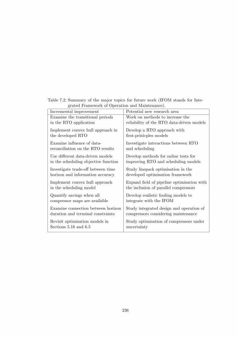
Table 7.2: Summary of the major topics for future work (IFOM stands for Inte-grated Framework of Operation and Maintenance).
Incremental improvement Potential new research area
Examine the transitional periods Work on methods to increase thein the RTO application reliability of the RTO data-driven models
Implement convex hull approach in Develop a RTO approach withthe developed RTO first-prinicples models
Examine influence of data- Investigate interactions between RTOreconciliation on the RTO results and scheduling
Use different data-driven models Develop methods for online tests forin the scheduling objective function improving RTO and scheduling models
Investigate trade-off between time Study linepack optimisation in thehorizon and information accuracy developed optimisation framework
Implement convex hull approach Expand field of pipeline optimisation within the scheduling model the inclusion of parallel compressors
Quantify savings when all Develop realistic fouling models tocompressor maps are available integrate with the IFOM
Examine connection between horizon Study integrated design and operation ofduration and terminal constraints compressors considering maintenance
Revisit optimisation models in Study optimisation of compressors underSections 5.16 and 6.5 uncertainty
236

7.3 Latest outcomes of the thesis
7.3.1 Impact of the research
The research work in this thesis has great potential for impact on real industrial
applications. In May 2015, the author of this thesis made a proposal and gained
funding for working on the development of the proof-of-concept of the RTO for
achieving energy savings in compressor stations in chemical plants. The funding is
provided by the EPSRC Impact Acceleration Awards 2015 through Imperial Col-
lege London. The author of the thesis is now employed at Imperial College London
on that project leading a study for proof of the RTO concept in an industrial con-
text and to provide quantified evidence for the savings that can be achieved. Real
experiments on the air separation plant of BASF have been planned to quantify
the savings. A comparison between operation with the application of the RTO
and typical operation without the use of RTO will estimate these savings.
One of the aims of the proposed project is to develop a pre-commercialisation
optimisation platform which can support the operators of a compressor station to
distribute the load of multiple compressors. The project will test the methodologies
developed and presented in this thesis and will identify the industrial considera-
tions which represent the real-life situation and lead to a proof-of-concept that the
optimisation platform can minimise the energy consumption in a real plant.
The project has to investigate that the energy savings are close to the values
presented in the thesis under the consideration of practical constraints. These
constraints can be the robustness of the optimization for various scenarios, the
consideration of uncertainty in the data, and the availability of data to develop
accurate models in every scenario. Moreover, the RTO will be tested online to
guarantee solutions with a high level of confidence within an optimisation loop.
The suggested platform has to also consider the available control structures and
be integrated with the existing installed hardware and software structures of the
plant.
BASF highlighted that the algorithms from the proposed project have the po-
tential to be implemented commercially for optimization of compressor stations in
BASF and in other plants. This means that the technology could be transferred to
other industrial areas of BASF. Moreover, Statoil and any other company which
operates compressor stations could potentially also use this state-of-the-art appli-
cation. Another important development step is that the optimization platform
should be fully automated. This development will follow after a period of its man-
ual use on the plant which will start to deliver the energy savings and build trust
in its decisions.
Finally, there may be potential for even broader interest. The work on real-
237

time optimization of compressors was presented at the launch of the Caterpillar
Innovation and Research Centre on February 24th 2015, at which the Provost
James Stirling signed the partnership between Imperial College and Caterpillar.
The industrial visitors from Caterpillar identified uses for the topics in the proposal
in a different sector, namely heavy automotive machinery.
7.3.2 Further work on the optimal operation of compressors
considering energy management
Introduction
This section describes research work which is under development in a different
but related area of the energy management of compressor stations. The reason
this work is presented here is that it was done during the PhD thesis and uses the
work on the optimisation of compressors as a foundation.
It is well established that industrial plants participate in electricity energy mar-
kets to take advantage of electricity price variations, for instance by increasing the
production when electricity is cheap. However, there is another electricity market
called reserve market, which could be of interest to the operators of industrial
sites. Therefore, industrial sites with large energy consumption can participate in
these markets through demand-side management whereby power producers and
consumers (i.e. the industrial sites which participating in the reserve markets)
communicate in a collaborative way to maintain stability in the electricity grid2.
Industrial plants consume large amounts of energy and their operation is easier to
control compared to the case of distributed residential users. The air separation
plant can be considered as an example of a large industrial plant.
The electricity consumers (for example an air separation plant) can participate
in different technologies of demand-side management which have been summarised
by Palensky and Dietrich (2011). The technologies of interest are Demand Re-
sponse (DR) programs which can be categorised into non-dispatchable programs
2The electricity grid delivers electricity from the generators to consumers via the transmissionand distribution grids.
DemandSide Response
Energy Markets(Non-Dispatchable
Programs)
Reserves Markets(Dispatchable
Programs)
Figure 7.1: Classification of different demand-side response schemes.
238
and dispatchable programs as can be seen in Fig. 7.1. The Non-Dispatchable
Programs which are related to energy markets allow the Transmission System Op-
erator3(TSO) to influence the power consumption in the demand side by giving
predefined electricity prices. Dispatchable Programs, which are related to reserve
markets enable the TSO to control the power consumption in the demand side
by giving instructions in accordance to the requirements of electricity grid. In
contrast to non-dispatchable programs, participants receive incentive payments
in terms of being successful in satisfying the requirements of the electricity grid
through orders given by the TSO.
An example of a dispatchable program is the demand offered by electrical con-
sumers by reducing their load when the demand-supply balance is threatened. The
reduced power which is offered by the consumer to the electrical grid is defined as
positive power reserve according to the definition given in Fabozzi et al. (2013).
Moreover, an electricity consumer can participate in a dispatchable program which
can request from the consumer to increase power consumption in some situations
when there is an excess of generation of electricity. In this case, the consumer
has to increase its power consumption and the extra power the plant consumes is
defined as negative power reserve.
However, the purpose of a plant is to produce products and not to provide
services to the electricity grid through the reserve markets. This means that there
is a need to assess the flexibility of a plant to provide services to the electricity
grid while at the same time ensuring that the plant meets the requirements of
its demand. This is the motivation to carry out an economic analysis of the
operation of an air separation plant which participates in demand-side management
schemes such as Demand Response (DR) programs. This analysis can quantify the
incentives of the air separation plant which should receive in order to participate
in these schemes.
Previous works and gap of knowledge
There are studies which focused on the scheduling of air separation plants with
the considerations of energy constraints. Chapter 3 mentioned the studies by Ier-
apetritou et al. (2002), Karwan and Keblis (2007) and Mitra et al. (2012) which
employed MIP models in an optimisation framework for the minimisation of pro-
duction costs considering electricity prices. These studies used binary variables
mainly to model the discrete operational modes of the operation of the plant, but
neglecting the operation of individual compressors. Another study which consid-
ered variable electricity prices in the optimization of the operating conditions of
3The TSO is a company that is responsible for operating, maintaining and developing the trans-mission system for a control area and its interconnections.
239

air separation plants is from Zhu et al. (2010) without considering discrete actions
such as startups and shutdowns of operational units.
The state-of-the-art of the participation of air separation plant in a dispatch-
able program has been recently presented by Zhang et al. (2015). The authors
considered the simultaneous considerations of non-dispatchable and dispatchable
programs. They also formulated a robust model for the uncertainty nature of the
reserve markets. This study, however, focused on the concept of the air separa-
tion plant as an electricity producer using the stored liquid products to power an
in-site cryogenic turbine providing electricity to the grid. Their model of the air
separation plant was based on Mitra et al. (2012) using the same discrete opera-
tional modes. At present, practically no industrial loads are collaborating with the
TSO of a grid through a dispatchable program, but the potential value of this col-
laboration for case studies such as an aluminium production have been examined
by ALCOA (Todd et al., 2009). The limited number of participants in dispatch-
able programs can be explained due to the lack of a well defined framework for
interaction between electricity grid and consumers. This is a question currently
being addressed in Europe by ENTSO-E (The European Network of Transmission
System Operators for Electricity)
Description of under development work
The work under development examines the participation of an air separation
plant in a demand side response scheme without any extra installation. The work
is based on the work presented in this thesis. The advantage of the suggested
method stems from the detailed modelling of the compressors and air separation
units which define the power consumption, capacity constraints and operational
aspects with discrete nature of each unit (i.e. compressor, air separation units),
for instance shutting down a compressor. An air separation column is rarely shut
down and only for maintenance reasons. The modelling of the suggested method
neglects the on or off modes of a column due to the short time horizon to be
considered. The modelling considers the operation of compressors which influence
the overall electricity costs of the air separation plant.
Performing a cost-benefit analysis is one method to ensure that the plant re-
mains profitable. Process operators require decision making tools to find the opti-
mal offer price so that the site can competitively participate in electricity markets,
while maintaining profitability. Hence, the work under development proposes an
optimisation framework to examine two case studies: (a) a non-dispatchable pro-
gram considering various contracts of day-ahead markets (e.g. variable hourly
electricity prices) with the simultaneous minimization of the operational costs of
the plant and (b) a dispatchable program which requests flexibility from the com-
240
pressors by means of the modification of the baseline operation of the plant to offer
power reserve to the TSO. Moreover, the work will propose how non-dispatchable
and dispatchable programs can be managed together in the same plant.
Preliminary results were presented in the poster session of the conference Eu-
ropean Symposium on Computer Aided Process Engineering (ESCAPE 25). The
full work is in preparation for publication in the journal of Applied Energy.
7.4 Summary of the chapter
Chapter 7 presented a critical evaluation of the achievements of the objec-
tives of the thesis. It summarised the description of each objective and for each
objective the chapter presented the respective contributions. Moreover, the chap-
ter described and critically discussed the assumptions used for the mathematical
frameworks presented in the thesis. Also, the topics for future work were classified
in cases of immediate improvement and of potential new research area. Table 7.2
summarised the major topics for future work for both cases. Section 7.3 presented
the impact of the research as the RTO will be studied further considering real life
constraints. The RTO methodology is planned to be tested in the air separation
plant of BASF and the results will be compared with the typical operation of the
BASF users. There is also academic work in progress which is based on the PhD
work on the optimisation of compressors. Section 7.3.2 introduces the work on the
energy management of compressor stations of chemical plants.
241

8 Conclusions
8.1 Statement and justification of objectives
Chapter 1 stated that the aim of the PhD thesis was to achieve optimal oper-
ation of existing installed compressors of systems with large energy consumption.
The thesis focused on two industrial systems, namely an air separation plant and
an export natural gas compressor station. The introduction of the thesis described
three objectives to achieve the above aim:
• Objective One was to develop a Real Time Optimisation (RTO) framework
which optimally shares the load among parallel compressors in real time to
deal with short-term changes in the operation.
• Objective Two was to develop a multi-period optimisation framework to
optimally schedule the operations of compressors for long time periods.
• Objective Three was to implement maintenance activities into the opera-
tional optimisation framework and achieve simultaneous optimal operation
and maintenance.
In Section 3, the literature review identified that there was a need to develop
a systematic online approach to optimally distribute the load among the parallel
compressors of the station. Chapter 4 dealt with the first objective of the thesis
and presented the development and application of a real time optimisation frame-
work for load sharing among compressors. The literature review identified that
previous authors neglected the operation of parallel non-identical compressors of a
compressor station. Thus, the second objective focused on this gap of knowledge
to develop a methodology to schedule the compressors of a system for long time
periods. Chapter 5 suggested a multi-period optimisation framework which was
applied to the air separation and to the natural gas station case studies. The
literature review also revealed the need to examine the simultaneous operation
and maintenance of compressors. Chapter 6 dealt with this third objective of the
thesis and presented the optimal operation compressors considering different types
of maintenance activities such as corrective maintenance actions, major overhauls
and washing of the compressors.
242
8.2 Conclusions of thesis for Objective One
The main evidence of achieving Objective One is the development of a com-
prehensive Real Time Optimisation framework which can optimally share the load
among parallel compressors in real time and deal with short-term changes in op-
eration. The description of the RTO framework was presented in Chapter 4. This
work made it possible to demonstrate reduced operational costs on a simulation
of real time operation of the industrial compressors of the air separation plant of
BASF using historical data. Until now, there was not a systematic way to optimally
share the load of compressors online considering varying operational conditions.
Strategies in common use are to share the load using equal split among compres-
sors, or running them with equal surge margin. The work of the PhD has shown
a way forward to use updated models of the compressor from process data and
estimate the best distribution of load among the compressors using optimisation.
Moreover, the work has shown that the new method of RTO can be applied at a
large scale relevant to the industry. Three papers have been published from this
work, two in conferences (Xenos et al., 2014a,b) and one in a journal (Xenos et al.,
2015a).
8.3 Conclusions of thesis for Objective Two
The main evidence of achieving Objective Two is the development of a multi-
period optimisation framework which can optimally schedule the operations of
compressors for long time periods. Chapter 5 presented the development of this
framework using a mixed integer linear programming multi-period model. This
work made it possible to generate the optimal schedule of compressors of the air
separation plant of BASF and the export natural gas station of Statoil. Until now,
compressor stations were treated as single units in natural gas optimisation prob-
lems. In previous work on the optimisation of air separation plants, the compressor
station was modelled as a black box along with the air separation units. The work
on the PhD study developed a method to schedule compressors which establishes
the current state-of-the-art of the topic of the optimisation of compressor stations
for long periods. The schedule can reduce the total costs of the operation, for ex-
ample electricity cost, start up and shut down cost. The application of the method
on the BASF industrial case study showed that the optimal schedule can improve
the operation for a horizon of one month. The application of the method on the
Statoil case study realised that the scheduling of compressors with the optimal
load sharing method can achieve 0.88% and 1.03% reduced operational costs com-
pared to the cases with equal split and equal surge margin methods respectively.
Developments of this work have been published in one journal paper (Kopanos
243

et al., 2015) and another journal paper with Xenos as first author is in progress.
8.4 Conclusion of thesis for Objective Three
The main evidence of achieving Objective Three is the implementation of main-
tenance activities into the operation optimisation framework which achieves op-
timal operation and maintenance as was presented in Chapter 6. Chapter 6 pre-
sented the integrated framework of operation and maintenance with different types
of maintenance activities such as major overhauls and washing of the compressors.
The framework was applied to the case of the BASF air separation plant to show
the benefits from the optimal operation with flexible maintenance compared to
operation disregarding decisions for maintenance activities. The framework also
made it possible to demonstrate the advantage of simultaneous optimisation and
maintenance including major overhauls in the case of the Statoil natural gas case
study for a three month time horizon. The literature examined the maintenance
of a single compressor considering its performance and it also examined the opti-
misation of the operation of network of compressors neglecting their maintenance
tasks. Therefore, the PhD study provides a new method for the optimisation of a
compressor station with multiple compressors in parallel considering their mainte-
nance. Four papers have been published from this work, two in conferences (Xenos
et al., 2014c, 2015b) and two in journals (Xenos et al., 2015c, 2016).
8.5 Future work
The PhD study presented methodologies and frameworks for optimising the
compressors of chemical plants and natural gas compressor stations. The previous
sections of this chapter justified that the work in the thesis met the objectives given
in the introduction. However during the PhD studies and after the achievement
of the objectives several topics related to the optimisation of compressors were
identified as future work:
• The RTO implementation in a plant needs to improve the robustness of
the data-driven models considering the real life operation and the practical
limitations related to the availability of process measurements.
• A new potential research area is to examine the use of first-principles models
in the RTO framework, as this research area needs to work on complex
physical models for online applications.
• The thesis identified the need to examine the interactions and possibly inte-
gration of automation levels of RTO and scheduling.
244

• The inclusion of the linepack effect and the modelling of the downstream
pipes in the optimisation problem of natural gas compressor stations would
result in a new research topic.
• The thesis studied optimal operation of an existing installation of compres-
sors. However, it identified that the design of the compressors and their
production planning of the compressors could be studied simultaneously.
• Furthermore, the current PhD study mainly focused on the deterministic
approach of the scheduling of compressors. Therefore, the scheduling of
compressors under uncertainty is another possible research area.
Immediate and other improvements for future work have been highlighted in
Section 7 and a summary of them is in Table 7.2. The current PhD work has
already launched two works which are under development, one work is the investi-
gation of the RTO implementation in the BASF plant and the second work is the
study of the participation of plants with compressor stations in electricity reserve
markets. Both works are based on the scientific work developed in this thesis.
8.6 Final comment
Compressors are essential components of the chemical and petroleum industry
and they consume large amounts of energy. The improvement of their operation
will result in an impact for the industry, the environment and the society. The
thesis has managed successfully to develop methods to potentially help the users of
real plants to efficiently operate their compressors. Furthermore, the work of this
thesis can be a foundation for further research on new areas such as the optimal
energy management of systems with large energy consumption. The penetration of
renewables in the conventional power generation system and the future increase in
electricity demand will require to examine both energy efficiency and new methods
to deal with these new circumstances and the optimal energy management of
compressor stations can be one of this methods.
245
Bibliography
Abbaspour, M., Chapman, K. S. and Krishnaswami, P. (2005), ‘Nonisothermal compres-
sor station optimisation’, Journal of Energy Resources Technology, Transactions of the
ASME 127, 131–141.
Abbaspour, M., Krishnaswami, P. and S., C. K. (2007), ‘Transient optimisation in natural
gas compressor stations for linepack operation’, Journal of Energy Resources Technol-
ogy, Transactions of the ASME 129, 314–324.
Agha, M. H., Thery, R., Hetreux, G., Hait, A. and Lann, J. M. L. (2010), ‘Integrated pro-
duction and utility system approach for optimizing industrial unit operations’, Energy
35(2), 611–627.
Aretakis, N., Roumeliotis, I., Doumouras, G. and Mathioudakis, K. (2012), ‘Compres-
sor washing economic analysis and optimization for power generation’, Applied Energy
95, 77–86.
Balas, E. (1965), ‘An additive algorithm for solving linear programs with zero–one vari-
ables’, Operations Research 13, 517–546.
BASF, Corporate Website (2015), Ludwigshafen-BASF.
available at: http://www.standort-ludwigshafen.basf.de
Bertha Benz Realschule Wiesloch (2008), Basf besuch.
available at: realschule-wiesloch.de/cms/jupgrade/index.php/schueler/schuelerbeitraege
/131-besuch-bei-der-basf (Accessed at 27 August 2015).
Bertolini, M. and Bevilacqua, M. (2006), ‘A combined goal programming - AHP approach
to maintenance selection problem’, Reliability Engineering and System Safety 91, 839–
848.
Biegler, L. T. and Grossmann, I. E. (2004), ‘Retrospective on optimization’, Computers
& Chemical Engineering 28(8), 1169–1192.
Bloch, H. P. (2006), A Practical Guide to Compressor Technology, John Wiley & Sons,
Inc., Hoboken, New Jersey, USA.
Bohlin, M. and Warja, M. (2010), ‘Optimizing maintenance for multi-unit industrial gas
turbine installations’, GT2010-23398, in ‘Proceedings of ASME Turbo Expo 2010 ’, June
14-18, Glasgow, UK.
246

Bohrenkamper, G., Bals, H., Wrede, U. and Umlauf, R. (2000), ‘Hot-gas-path life extension
options for the V94.2 gas turbine, 2000-GT-178’, ASME Tehcnical Paper: GT, American
Society of Mechanical Engineers, New York, USA.
Borraz-Sanchez, C. (2010), ‘Optimisation Methods for Pipeline Transportation of Natural
Gas’, PhD thesis, University of Bergen, Department of Informatics, Norway.
Boyce, M. P. and Gonzalez, F. (2007), ‘A study of on-line and off-line turbine washing to
optimize the operation of a gas turbine’, Journal of Engineering for Gas Turbines and
Power, Transactions of the ASME 129, 114–122.
Boyce, M. P. P. E. (2003), ‘Centrifugal Compressors: A Basic Guide’, Pen Well Corpora-
tion, Tulsa, Oklahoma, USA.
Brooks, D. G., Carroll, S. S. and Verdini, W. A. (1988), ‘Characterizing the domain of a
regression model’, The American Statician 42(3), 187–190.
Camponogara, E., Nazari, L. F. and N., M. C. (2012), ‘A revised model for compressor
design and scheduling in gas-lifted oil fields’, IIE Transactions 44(5), 342–351.
Cao, S. and Rhinehart, R. (1995), ‘An efficient method for on-line identification of steady
state’, Journal of Process Control 5(6), 363–374.
Carter, R., Reisner, M. and Sekirnjak, E. (2010), ‘Transient optimization - Examples and
directions’, PSIG 1011, in ‘PSIG Annual Meeting ’, 11-14 May, Florida, USA.
Castro, P. M., Grossmann, I. E., Veldhuizen, P. and Esplin, D. (2014), ‘Optimal main-
tenance scheduling of a gas engine power plant using generalized disjunctive program-
ming’, AIChE 60(6), 2083–2097.
Cervantes, A. and Biegler, L. T. (2009), ‘Encyclopedia of Optimisation, Optimisation
strategies for dynamic systems’, 2nd edn, Springer Science and Business Media, LCC,
New York, USA.
Chen, G., Shi, B. and Yan, L. (2012), ‘Multi-period optimal operational planning of boiler
steam system based on line-up competition algorithm’, Energy Procedia 14(0), 613–619.
Cicciotti, M., Xenos, D. P., Bouaswaig, A. E. F., Thornhill, N. F. and Martinez-Botas,
R. (2014a), ‘Online performance monitoring of industrial compressors using meanline
modelling’, GT2014-25088, in ‘Proceedings of ASME Turbo Expo 2014 ’, June 16-20,
Dusseldorf, Germany.
Cicciotti, M., Xenos, D. P., Bouaswaig, A. E. F., Thornhill, N. F. and Martinez-Botas,
R. F. (2015), ‘Physical modelling of industrial multistage centrifugal compressors for
monitoring and simulation’, Proceedings IMechE, Part C: Journal of Mechanical Engi-
neering Science 0, 1–16.
Cobos-Zaleta, D. and Rıos-Mercado, R. Z. (2002), ‘A MINLP model for minimizing fuel
consumption on natural gas pipeline networks’, in ‘Memorias del XI Congreso Latino
Iberoamericano de Investigacion de Operaciones (CLAIO)’, 27-31 October, Chile.
247

Danzer, L., Grunbaum, B. and Klee, V. (1963), ‘Helly’s theorem and its relatives’, Con-
vexity, Proc. Symp. Pure Math., American Mathematical Society 7, 101–180.
Darby, M. L., Nikolaou, M., Jones, J. and Nicholson, D. (2011), ‘RTO: An overview and
assessment of current practice’, Journal of Process Control 21(6), 874–884.
de Backer, W. (2000), ‘Modular uprating and upgrading solution in ABB ALSTOM
POWER gas turbines’, 2000-GT-306, in ‘ASME Turbo Expo 2000 ’, Vol. 3, Munich,
Germany, p. V003T02A014;13 pages.
DeMarco, F. C. G. and Elias, G. (2011), ‘Fuel consumption model on natural gas compres-
sion stations driven by two-shaft gas turbine’, PSIG 1107, in ‘PSIG Annual Meeting ’,
24-27 May, Napa Valley, California.
Diakunchak, I. S. (1992), ‘Performance deterioration in industrial gas turbines’, Journal
of Engineering for Gas Turbines and Power 114(2), 161–168.
Dixon, S. L. and Hall, C. A. (2010), Fluid Mechanics and Thermodynamics of Turboma-
chinery, 6th edn, Elsevier, Oxford, UK.
Edgar, T. F., Himmelblau, D. M. and Lasdon, L. S. (2001), ‘Optimization of Chemical
Processes’, Chemical Engineering Series, 2nd edn, McGraw-Hill International Edition,
New York, NY.
European Commission, Eurostat (2015), Energy price statistics.
available at: ec.europa.eu/eurostat/statistics-explained/index.php/Energy price statistics
(Accessed at 26 August 2015).
Fabbri, A., Traverso, A. and Cafaro, S. (2011), ‘Compressor performance recovery system:
which solution and when’, in ‘Proceedings of the Institution of Mechanical Engineers,
Part A: Journal of Power and Energy ’, Vol. 225, pp. 457–466.
Fabozzi, D., Thornhill, N. and Pal, B. (2013), Frequency restoration reserve control
scheme with participation of industrial loads, in ‘PowerTech (POWERTECH), 2013
IEEE Grenoble’, pp. 1–6.
Forsthoffer, W. E. (2011), ‘Forsthoffer’s Best Practice Handbook for Rotating Machinery’,
Butterworth-Heinemann, Oxford, UK.
Garcia-Hernandez, A. and Brun, K. (2012), ‘Energy usage in natural gas pipeline appli-
cations’, ASME Journal of Engineering for Gas Turbines and Power 134, 022402–1:9.
Gomory, R. E. (1960), ‘An algorithm for the Mixed Integer Problem’, Rand Report R.M.
25797.
Gopalakrishnan, A. and Biegler, L. T. (2013), ‘Economic nonlinear model predictive con-
trol for periodic optimal operation of gas pipeline networks’, Computers & Chemical
Engineering 52, 90–99.
Gresh, T. (2001), ‘Compressor Performance, Aerodynamics for the User’, 2nd edn, Else-
vier Science & Technology Books, Woburn, Massachusetts, USA.
248

Gustavsson, E., Patriksson, M., Stromberg, A.-B., Wojciechowski, A. and Onnheim, M.
(2014), ‘Preventive maintenance scheduling of multi-component systems with interval
costs’, Computers and Industrial Engineering 76, 390–400.
Hadera, H., Harjunkoski, I., Sand, G., Grossmann, I. E. and Engell, S. (2015), ‘Opti-
mization of steel production scheduling with complex time-sensitive electricity cost’,
Computers & Chemical Engineering 76, 117–136.
Han, I. S., Han, C. and Chung, C. B. (2004), ‘Optimisation of the air-and gas-supply net-
work of a chemical plant’, Chemical Engineering Research and Design, Trans IChemE
82(A10), 1337–1343.
Harjunkoski, I., Nystrom, R. and Horch, A. (2009), ‘Integration of scheduling and control
- theory and practice’, Computers & Chemical Engineering 33, 1909–1918.
Hasan, M. M. F., Razib, M. S. and Karimi, I. A. (2009), ‘Optimization of compressor
networks in LNG operations’, in ‘10th International Symposium on Process Systems
Engineering - PSE2009 ’, pp. 1767–1772.
Hazaras, M. J., Swartz, C. L. E. and Marlin, T. E. (2012), ‘Flexible maintenance within
a continuous-time state-task network framework’, Computers & Chemical Engineering
46, 167–177.
Helvoirt, J. (2007), ‘Centrifugal Compressor Surge, Modeling and Identification for Con-
trol ’, PhD thesis, Technische Universiteit Eindhoven.
Hovland, G. and Antoine, M. (2004), ‘Economic optimisation of gas turbine compres-
sor washing’, in ‘Australasian Universities Power Engineering Conference’, September,
Brisbane, Australia.
IBM (2015), IBM ILOG CPLEX Optimization Studio.
available at: www-03.ibm.com/software/products/en/ibmilogcpleoptistud/ (Accessed at
26 August 2015).
Ierapetritou, M. G., Wu, D., Vin, J., Sweeney, P. and Chigirinskiy, M. (2002), ‘Cost min-
imization in an energy-intensive plant using mathematical programming approaches’,
Industrial and Engineering Chemistry Research 41(21), 5262–5277.
Iyer, R. R. and Grossmann, I. E. (1997), ‘Optimal multiperiod operational planning for
utility systems’, Computers & Chemical Engineering 21(8), 787 – 800.
Jenıcek, T. and Kralık, J. (1995), ‘Optimized control of generalized compressor station’,
in ‘27th Annual Meeting Pipeline Simulation Interest Group (PSIG)’, October 18-20,
Albuquerque, New Mexico.
Jiang, T., Chen, B., He, X. and Stuart, P. (2003), ‘Application of steady-state detection
method based on wavelet transform’, Computers & Chemical Engineering 27(4), 569–
578.
249
Jiao, Y., Su, H., Hou, W. and Liao, Z. (2012), ‘A multiperiod optimization model for
hydrogen system scheduling in refinery’, Industrial & Engineering Chemistry Research
51(17), 6085–6098.
Kadlec, P., Gabrys, B. and Strandt, S. (2009), ‘Data-driven soft sensors in the process
industry’, Computers & Chemical Engineering 33(4), 795–814.
Kahrs, O. and Marquardt, W. (2007), ‘The validity domain of hybrid models and its
application in process optimization’, Chemical Engineering and Processing 46, 1054–
1066.
Karwan, M. H. and Keblis, M. F. (2007), ‘Operations planning with real time pricing of a
primary input’, Computers and Operations Research 34(13), 848–867.
Kelly, J. D. and Hedengren, J. D. (2013), ‘A steady-state detection (SSD) algorithm to
detect non-stationary drifts in processes’, Journal of Process Control 23(3), 326–331.
Kim, J. H. and Han, C. (2001), ‘Short-term multiperiod optimal planning of utility sys-
tems using heuristics and dynamic programming’, Industrial & Engineering Chemistry
Research 40(8), 1928–1938.
Kim, J. H., Ju, S., Yi, H.-S., Han, I.-S. and Han, C. (2002), ‘Preventive optimization frame-
work for unexpected equipment failures in the utility system with quantitative emer-
gency handling constraints’, Industrial & Engineering Chemistry Research 41(24), 6070–
6081.
Kim, M., Yoon, S. H., Domanski, P. A. and Payne, W. V. (2008), ‘Design of a steady-state
detector for fault detection and diagnosis of a residential air conditioner’, International
Journal of Refrigeration 31, 790–799.
Kopanos, G. M. (2010), ‘Techniques for the Efficient Solution of Large-scale Production
Scheduling & Planning Problems in the Process Industries’, PhD thesis, Escola Tecnica
Superior d’Enginyeria Industrial de Barcelona Universitat Politecnica de Catalunya.
Kopanos, G. M., Georgiadis, M. C. and Pistikopoulos, E. N. (2013), ‘Energy production
planning of a network of micro combined heat and power generators’, Applied Energy
102, 1522–1534.
Kopanos, G. M. and Pistikopoulos, E. N. (2014), ‘Reactive scheduling by a multiparametric
programming rolling horizon framework: a case of a network of combined heat and power
units’, Industrial and Engineering Chemistry Research 53(11), 4366–4386.
Kopanos, G. M., Xenos, D. P., Cicciotti, M., Pistikopoulos, E. F. and Thornhill, N. F.
(2015), ‘Operational planning of a network of compressors: The air separation plant
case’, Applied Energy .
Kurz, R. and Brun, K. (2010), ‘Assessment of compressors in gas storage applications’,
Journal of Engineering for Gas Turbines and Power 132, 062402–1:7.
250
Kurz, R. and Brun, K. (2012a), ‘Upstream and midstream compression applications - Part
1: Applications’, GT2012-68005, in ‘Proceedings of ASME Turbo Expo 2012 ’, June 11-
15, Copenhagen, Denmark.
Kurz, R. and Brun, K. (2012b), ‘Fouling mechanisms in axial compressors’, Journal of
Engineering for Gas Turbines and Power 134, 032401–1:9.
Kurz, R., Lubomirsky, M. and Brun, K. (2012), ‘Gas compressor station economic opti-
mization’, International Journal of Rotating Machinery 12, 1–9.
Land, A. H. and Doig, A. (1960), ‘An automatic method of solving discrete programming
problems’, Econometrica 28, 497–520.
Li, Y. G. and Nilkitsaranont, P. (2009), ‘Gas turbine performance prognostic for condition-
based maintenance’, Applied Energy 86, 2152–2161.
Liptak, B. G. (2006), ‘Instrument Engineer’s Handbook, Process Control and Optimiza-
tion’, Vol. 2, 4th edn, Taylor & Francis Group, Florida, USA, pp. 1763–1792.
Liu, S., Yahia, A. and Papageorgiou, L. G. (2014), ‘Optimal production and maintenance
planning of biopharmaceutical manufacturing under performance decay’, Industrial and
Engineering Chemistry Research 53(44), 17075–17091.
Luo, X., Zhang, B., Chen, Y. and Mo, S. (2011), ‘Modeling and optimization of a utility
system containing multiple extractions steam turbines’, Energy 36(5), 3501–3512.
Luo, X., Zhang, B., Chen, Y. and Mo, S. (2012), ‘Operational planning optimization of
steam power plants considering equipment failure in petrochemical complex’, Applied
Energy 11, 1247–1264.
Mahlke, D., Martin, A. and Moritz, S. (2009), ‘A mixed integer approach for time-
dependent gas network optimization’, Optimisation Methods and Software 25(4), 625–
644.
Mansour, M. and Ellis, J. E. (2008), ‘Methodology of on-line optimisation applied to a
chemical reactor’, Applied Mathematical Modelling 32, 170–184.
Marques, D. and Morari, M. (1988), ‘On-line optimisation of gas pipeline networks’, Au-
tomatica 24(4), 455–469.
Martın-Aragon, J. and Valdes, M. (2014), ‘A method to determine the economic cost of
fouling of gas turbine compressors’, Applied Thermal Engineering 69(1-2), 261–266.
Matlab (2014), Linear Regression.
available at: mathworks.co.uk/help/matlab/data analysis/linear-regression.html (Ac-
cessed at 25 April 2014).
Matlab (2014b), Optimization Toolbox.
available at: mathworks.co.uk/help/optim/ug/fmincon.html (Accessed at 25 April
2014).
251
Matlab (2015), Computational Geometry.
available at: uk.mathworks.com/help/matlab/ref/convhull.html (Accessed at 21 Febru-
ary 2015).
McCarl, B. A., Meeraus, A., Eijk, P., Bussieck, M., Dirkse, S., Steacy, P. and Nelissen,
F. (2008), ‘McCarl Expanded GAMS User Guide, Version 22.9’, GAMS Development
Corporation, Washington, DC, USA.
Meher-Homji, C. B., Chaker, M. and Motiwalla, H. (2001), ‘Gas turbine performance
deterioration’, in ‘Proceedings of the 30th Turbomachinery Symposium’, September 17-
20, Houston, Texas.
Messer Group (2015), Air separation.
available at: www.messergroup.com/de/Produkte und Loesungen/luftzerlegung (Ac-
cessed at 9 February 2015).
Milum, R. (2012), ‘Multi-compressor capacity optimization’, in ‘7th Pipeline Technology
Conference 2012 ’, 28-30 March, Hannover, Germany.
Ministry of Petroleum and Energy (2014), ‘Facts, The Norwegian Petroleum Sector ’, Nor-
way, Oslo.
Mitra, S., Grossmann, I. E., Pinto, J. M. and Arora, N. (2012), ‘Optimal production plan-
ning under time-sensitive electricity prices for continuous power-intensive processes’,
Computers & Chemical Engineering 38(0), 171–184.
MohamadiBaghmolaei, M., Mahmoudy, M., Jafari, D., MohamadiBaghmolaei, R. and
Tabkhi, F. (2014), ‘Assessing and optimization of pipeline system performance using
intelligent systems’, Journal of Natural Gas Science and Engineering 18, 64–76.
Nguyen, H. H. and Chan, C. W. (2006), ‘Applications of artificial intelligence for opti-
mization of compressor scheduling’, Engineering Applications of Artificial Intelligence
19(2), 113–126.
Nguyen, H. H., Uraikul, V., Chan, C. W. and Tontiwachwuthikul, P. (2008), ‘A compar-
ison of automation techniques for optimization of compressor scheduling’, Advances in
Engineering Software 39, 178–188.
Nørstebø, V. S. (2008), ‘Optimum Operation of Gas Export Systems’, PhD thesis, Nor-
wegian University of Science and Technology, Department of Energy and Process Engi-
neering, Norway.
Nørstebø, V. S., Bakken, L. E. and Dahl, H. J. (2008), ‘Energy-efficient operation of gas
export systems’, SPE 123132, in ‘International Petroleum Technology Conference’, 4-6
December, Dubai.
Padhy, N. P. (2004), ‘Unit commitment - a bibliographical survey’, IEEE Transactions on
power systems 19(2), 1196–1205.
252

Palensky, P. and Dietrich, D. (2011), ‘Demand side management: Demand response, intel-
ligent energy systems, and smart loads’, IEEE Transactions on industrial informatics
7(3), 381–388.
Paparella, F., Domınguez, L., Cortinovis, A., Mercangoz, M., Pareschi, D. and Bittanti,
S. (2013), ‘Load sharing optimization of parallel compressors’, in ‘European Control
Conference (ECC)’, July 17-19, Zurich, Switzerland.
Prata, D. M., Schwaab, M., Lima, E. L. and Pinto, J. C. (2010), ‘Simultaneous robust
data reconciliation and gross error detection through particle swarm optimization for
an industrial polypropylene reactor’, Chemical Engineering Science 65(17), 4943–4954.
Raglend, I. J. and Padhy, N. P. (2008), ‘Comparison of practical unit commitment prob-
lem’, Electric power components and systems 36(8), 844–863.
Rao, P. N. and Naikan, V. N. (2008), ‘An optimal maintenance policy for compressor
of a gas turbine power plant’, Journal of Engineering for Gas Turbines and Power
130(2), 021801–1:5.
Rao, S. S. (2009), Engineering Optimisation, Theory and Practice, 4th edn, John Wiley
& Sons, Inc., USA.
Rıos-Mercado, R. Z. and Borraz-Sanchez, C. (2015), ‘Optimization problems in natural
gas transportation systems: A state-of-the-art review’, Applied Energy 145(0), 536–55.
Rolls Royce (2014).
available at: www.rolls-royce.com/energy/energy products/ (Accessed at 6 February
2014).
Romagnoli, J. A. and Sanchez, M. C. (2000), Data Processing and Reconciliation for
Chemical Process Operations, Vol. Volume 2 (Process Systems Engineering), Academic
Press, California, USA.
Rong, A. and Lahdelma, R. (2005), ‘An efficient linear programming model and optimiza-
tion algorithm for trigeneration’, Applied Energy 82(1), 40–63.
Rosipal, R. and Kramer, N. (2006), ‘Overview and recent advances in partial least squares,
Subspace’, in ‘Revised Selected Papers (Lecture Notes in Computer Science 3940)’, Sub-
space, Latent Structure and Feature Selection: Statistical and Optimization Perspec-
tives Workshop (SLSFS 2005), Springer-Verlag, Berlin, Germany, pp. 34–51.
Sahinidis, N. V. (2004), ‘Optimization under uncertainty: state-of-the-art and opportuni-
ties’, Computers & Chemical Engineering 28(6-7), 971–983.
Saidur, R., Rahim, N. A. and Hasanuzzaman, M. (2010), ‘A review on compressed-air
energy use and energy savings’, Renewable and Sustainable Energy Reviews 14(4), 1135–
1153.
Sanchez, D., Chacartegui, R., Becerra, J. A. and Sanchez, T. (2009), ‘Determining com-
pressor wash programmes for fouled gas turbines’, Power and Energy, Proceedings
IMechE Part A 223, 467–476.
253

Schmidt, M., Steinbach, M. C. and Willert, B. M. (2014), ‘High detail stationary opti-
mization models for gas networks’, Optimization and Engineering pp. 1–34.
Seborg, E. S., Edgar, T. F. and Mellichamp, D. A. (2004), Process Dynamics and Control,
2nd edn, John Wiley & Sons, Inc., New Jersey, USA.
Sequeira, S. E., Graells, M. and Puigjaner, L. (2001), ‘Decision-making framework for
the scheduling of cleaning/maintenance tasks in continuous parallel lines with time-
decreasing performance’, European Symposium on Computer Aided Process Engineering
- 11, Computer Aided Chemical Engineering 9, 913–918.
Shaw, D. C. (1994), ‘Pipeline system optimization: A tutorial’, Technical report, Scientific
Software-Intercomp, Houston, USA.
Silva, T. L. and Camponogara, E. (2014), ‘A computational analysis of multidimensional
piecewise-linear models with applications to oil production optimization’, European
Journal of Operational Research 232(3), 630–642.
Sood, A. K., Funk, G. L. and Delmastro, A. C. (1971), ‘Dynamic optimization of a nat-
ural gas pipeline using a gradient search technique’, International Journal of Control
14(6), 1149–1157.
Statoil (2015), Kollsnes gas processing plant.
available at: www.statoil.com/en/ouroperations/terminalsrefining/processcomplexkollsnes
(Accessed at 27 September 2015).
Sun, H. and Ding, H. (2014), ‘Plant simulation and operation optimization of SMR plant
with different adjustment methods under part-load conditions’, Computers & Chemical
Engineering 68, 107–113.
Thorin, E., Brand, H. and Weber, C. (2005), ‘Long-term optimization of cogeneration
systems in a competitive market environment’, Applied Energy 81(2), 152–169.
Thorp, J., Khan, F., Brun, K., Strobel, M. and Khalifa, M. (2014), ‘Risk based assessment
of gas turbines in pipeline service’, GT2014-27312, in ‘ASME Turbo Expo 2014 ’, Vol.
Volume 3B, Dusseldorf, Germany.
Tirnovan, R., Giurgea, S., Miraoui, A. and Cirrincione, M. (2008), ‘Surrogate modelling
of compressor characteristics for fuel-cell applications’, Applied Energy 85, 394–403.
Todd, D., Caufield, M., Helms, B., Starke, M., Kirby, B., and Kueck, J. (2009), ‘Providing
reliability services through demand response: A preliminary evaluation of the demand
response capabilities of alcoa inc.’, http://certs.lbl.gov/pdf/dralcoa.pdf.
Twohig, D. (2011), ‘Utility optimization: Driving economic performance through the uti-
lization of automation technologies’, in ‘ISA Publications, InTech Magazine’.
available at: https://www.isa.org/standards-and-publications/isa-publications/intech-
magazine/2011/october/process-automation-utility-optimization/ (Accessed at 25 Au-
gust 2015).
254

Uraikul, V., Chan, C. W. and Tontiwachwuthikul, P. (2004), ‘A mixed-integer optimiza-
tion model for compressor selection in natural gas pipeline network system operations’,
Journal of Environmental Informatics 3(1), 33–41.
U.S. Department of Energy (2003), ‘Improving Compressed Air System Performance’, U.S.
Department of Energy, Energy Efficiency and Renewable Energy.
van den Heever, S. A. and Grossmann, I. E. (2003), ‘A strategy for the integration of
production planning and reactive scheduling in the optimisation of a hydrogen supply
network’, Computers & Chemical Engineering 27(12), 1813–1839.
Varbanov, P. S., Doyle, S. and Smith, R. (2004), ‘Modeling and optimization of utility
systems’, Chemical Engineering Research and Design, Trans IChemE 82(A5), 561–578.
Vecchietti, A., Sangbum, L. and Grossmann, I. E. (2003), ‘Modeling of discrete/continuous
optimization problems: characterization and formulation of disjunctions and their re-
laxations’, Computers and Chemical Engineering 27, 433–448.
Velasco-Garcia, P., Varbanov, P. S., Arellano-Garcia, H. and Wozny, G. (2011), ‘Utility
systems operation: Optimisation-based decision making’, Applied Thermal Engineering
31(16), 3196–3205.
Widell, K. N. and Eikevik, T. (2010), ‘Reducing power consumption in multi-compressor
refrigeration systems’, International Journal of Refrigeration 33, 88–94.
Wikipedia (2014), Root-mean-square deviation.
available at: en.wikipedia.org/wiki/Root-mean-square deviation (Accessed at 25 April
2014).
Wikipedia (2015a), Compressibility factor.
available at: wikipedia.org/wiki/Compressibility factor (Accessed at 11 May 2015).
Wikipedia (2015b), Gas constant.
available at: en.wikipedia.org/wiki/Gas constant (Accessed at 18 February 2015).
Wikipedia (2015c), Standard Temperature Pressure.
available at: en.wikipedia.org/wiki/Standard conditions for temperature and pressure
(Accessed at 18 February 2015).
Wong, J. P. and Larson, E. R. (1968), ‘Optimisation of tree-structured natural-gas trans-
mission networks’, Journal of Mathematical Analysis and Applications 24, 613–626.
Wright, S., Somani, M. and Ditzel, C. (1998), ‘Compressor station optimization’, in
‘Pipeline Simulation Interest Group (PSIG)’, October 28-30, Denver, Colorado.
Wu, S., Rios-Mercado, R. Z., Boydm, E. A. and R, S. L. (2000), ‘Model relaxations for
the fuel cost minimization of steady-state gas pipeline networks’, Mathematical and
Computer Modelling 31, 197–220.
255
Xenos, D. P., Cicciotti, M., Bouaswaig, A. E. F. and Thornhill, N. F. (2014b), ‘Pre-
processing of raw data for developing steady-state data-driven models for optimizing
compressor stations’, in ‘10th International Conference on Control, Control 2014 ’, July
8-11, Loughborough, UK.
Xenos, D. P., Cicciotti, M., Bouaswaig, A. E. F., Thornhill, N. F. and Martinez-Botas,
R. (2014a), ‘Modeling and optimization of industrial centrifugal compressor stations
employing data-driven methods’, GT2014-25089, in ‘Proceedings of ASME Turbo Expo
2014 ’, June 16-20, Dusseldorf, Germany.
Xenos, D. P., Cicciotti, M., Kopanos, M. G., Bouaswaig, A. E. F., Kahrs, O., Martinez-
Botas, R. and Thornhill, N. F. (2015a), ‘Optimization of a network of compressors
in parallel: Real Time Optimizatio (RTO) of compressors in chemical plants - An
indsustrial case study’, Applied Energy .
Xenos, D. P., Kopanos, G. M., Cicciiotti, M., Pistikopoulos, E. N. and Thornhill, N. F.
(2014c), ‘Operational optimization of compressors in parallel considering condition-
based maintenance’, in ‘European Symposium on Computer Aided Process Engineering
(ESCAPE 24)’, June 15-18, Budapest, Hungary.
Xenos, D. P., Kopanos, G. M., Cicciotti, M. and Thornhill, N. F. (2016), ‘Operational op-
timization of networks of compressors considering condition-based maintenance’, Com-
puters & Chemical Engineering 84, 117–131.
Xenos, D. P., Lunde, E. and Thornhill, N. F. (2015b), ‘Optimal operation and maintenance
of gas compressor stations: An integrated framework applied to a large-scale industrial
case’, GT2015-44002, in ‘Proceedings of ASME Turbo Expo 2015’, Montreal, Canada.
Xenos, D. P., Lunde, E. and Thornhill, N. F. (2015c), ‘Optimal operation and maintenance
of gas compressor stations: An integrated framework applied to a large-scale industrial
case’, ASME Journal of Engineering for Gas Turbines and Power .
Xu, Z., Zhao, J., Chen, X., Shao, Z., Qian, J., Zhu, L., Zhou, Z. and Qin, H. (2011),
‘Automatic load change system of cryogenic air separation process’, Separation and
Purification Technology 81(3), 451–465.
Yuan, C. Y., Zhang, T., Rangarajan, A., Dornfeld, D., Ziemba, B. and Whitbeck, R.
(2006), ‘A decision-based analysis of compressed air usage patterns in automotive man-
ufacturing’, Journal of Manufacturing Systems 25(4), 293–300.
Zavala, V. M. (2014), ‘Stohastic optimal control model for natural gas networks’, Com-
puters and Chemical Engineering 64, 103–113.
Zhang, Q., Grossmann, I. E., Heuberger, C. F., Sundaramoorthy, A. and Pinto, J. M.
(2015), ‘Air separation with cryogenic energy storage: Optimal scheduling considering
electric energy and reserve markets’, AIChE Journal 61(5), 1547–1558.
Zhu, Y., Legg, S. and Laird, C. D. (2010), ‘A multiperiod nonlinear programming approach
for operation of air seperation plants with variable power pricing’, AIChE 57(9), 2421–
2430.
256

Zhu, Y., Legg, S. and Laird, C. D. (2011), ‘Optimal operation of cryogenic air separation
systems with demand uncertainty and contractual obligations’, Chemical Engineering
Science 66(5), 953–963.
Zhuan, X. and Xia, X. (2013), ‘Optimal operation scheduling of a pumping station with
multiple pumps’, Applied Energy 104(0), 250–257.
257