NBER WORKING PAPER SERIES

OPTIMAL INTEGRATION STRATEGIESFOR THE MULTINATIONAL FIRM

Gene M. GrossmanElhanan Helpman

Adam Szeidl

Working Paper 10189http://www.nber.org/papers/w10189

NATIONAL BUREAU OF ECONOMIC RESEARCH1050 Massachusetts Avenue

Cambridge, MA 02138December 2003

We acknowledge with thanks the support of the National Science Foundation (SES 9904480 and SES0211748) and the US-Israel Binational Science Foundation (2002132). The views expressed herein are thoseof the authors and not necessarily those of the National Bureau of Economic Research.

©2003 by Gene M. Grossman, Elhanan Helpman, and Adam Szeidl. All rights reserved. Short sections oftext, not to exceed two paragraphs, may be quoted without explicit permission provided that full credit,including © notice, is given to the source.

Optimal Integration Strategies for the Multinational FirmGene M. Grossman, Elhanan Helpman, and Adam SzeidlNBER Working Paper No. 10189December 2003JEL No. F23, F12, L22

ABSTRACT

We examine integration strategies of multinational firms that face a rich array of choices of

international organization. Each firm in an industry must provide headquarter services from its home

country, produce intermediate inputs, and assemble the intermediate goods into final products. Both

production of intermediate goods and assembly can be performed at home, in another “Northern”

country, in the low-wage “South,” or in several of these locations. We study the equilibrium choices

of firms that differ in productivity (and thus size), focusing on the role of industry characteristics

such as the fixed costs of foreign subsidiaries, the cost of transporting intermediate and final goods,

and the share of the consumer market that resides in the South in determining optimal integration

strategies.

Gene M. GrossmanDepartment of Economics300 Fisher HallPrinceton UniversityPrinceton, NJ 08544and NBERgrossman@princeton.edu

Elhanan HelpmanDepartment of EconomicsLittauer CenterHarvard UniversityCambridge, MA 02138and NBERehelpman@harvard.edu

Adam SzeidlDepartment of EconomicsLittauer CenterHarvard UniversityCambridge, MA 02138szeidl@fas.harvard.edu

1 Introduction

The globalization process of recent years has been expressed in the growth of many types

of international transactions, but few more salient than the expansion in the activity of

multinational firms. The growth rate of sales by foreign affiliates of multinational corporations

outpaced the growth of exports of goods and non-factor services by almost seven percent per

year from 1990 to 2001. Gross product by all foreign affiliates accounted for an estimated

eleven percent of world GDP in 2001, while exports by these affiliates represented an estimated

35 percent of total world trade (UNCTAD, 2002).

Multinational firms have pursued a multitude of strategies for international expansion,

as described in the World Investment Report (UNCTAD, 1998) and cited by Yeaple (2003).

Firms have opened foreign affiliates to perform activities ranging from R&D to after-sales

service, and including production of parts and components, assembly, and wholesale and retail

distribution, among others. Some firms procure parts from subsidiaries in many countries and

assemble them in a single location. Others concentrate production of parts in one place and

assemble final products in several plants located close to their customers. Still others erect

an integrated plant in a low-wage country and use it to serve consumers around the globe.

The motives for foreign direct investment (FDI) are similarly diverse, but the potential for

factor-cost savings, for transportation-cost and trading-cost savings, and for the realization

of economies of scale seem to be among the primary inducements.

The theory of international trade and foreign direct investment traditionally has distin-

guished two forms of multinational activity based on alternative reasons why a firm might opt

to locate production or other activities abroad (see, for example, Markusen [2002, pp.17-20]).

Vertical multinationals are firms that geographically separate various stages of production.

Such fragmentation of the production process typically is motivated by cost considerations

arising from cross-country differences in technologies or factor prices. For example, Helpman

(1984) and Helpman and Krugman (1985) model multinational firms that maintain their

headquarters in one country but manufacture output in another in order to conserve on

production costs. In contrast, horizontal multinationals are firms that replicate most or all

of the production process in several locations. These multi-plant firms often are motivated

by potential savings of transport and trading costs. In the models developed by Markusen

(1984), Brainard (1997) and Markusen and Venables (1998, 2000), for example, firms with

headquarters in a home country produce final output in plants that serve consumers in each

of two national markets.

The distinction between vertical and horizontal FDI is clear enough when there are two

countries and two production activities, namely headquarter operations and “manufacturing.”

But with more countries and more stages of production, some organizational forms do not fit

neatly into either of these categories. For example, a multinational firm might manufacture

goods in a foreign subsidiary and sell the output primarily in third-country markets; Ekholm

2

et al. (2003) term such activity “export-platform FDI.” Or a firm might perform intermediate

stages of production in one country to save on production costs and subsequent stages in

several plants to conserve on transport costs. Yeaple (2003) follows the World Investment

Report in referring to this as a “complex integration strategy.” Feinberg and Keane (2003)

report that, in their sample of U.S. multinationals with affiliates in Canada, only 12 percent

of the firms have negligible intra-firm flows of intermediate goods and thus can be considered

to be purely horizontal multinationals, while only 19 percent of the firms have intra-firm

flows of intermediate goods in only one direction, which would make them purely vertical

multinationals. The remaining 69 percent of firms are what they call “hybrids”; i.e., firms

that are pursuing more complex integration strategies. Similarly, Hanson et al. (2001)

describe the rich patterns of FDI they find in their data pertaining to operations by U.S.

multinationals and their foreign affiliates. They document and analyze the roles played by

foreign affiliates as export platforms, as producers adding value to inputs acquired from their

U.S. parents, and as wholesale distributors in foreign markets. Based on their analysis of data

for the 1990’s, Hanson et al. conclude that “the literature’s benchmark distinction between

horizontal and vertical FDI does not capture the range of strategies that multinationals use.”

Both Yeaple (2003) and Ekholm et al. (2003) examine theoretically the determinants of

firms’ choices among a limited set of integration strategies that includes an option for FDI

that is neither purely horizontal nor purely vertical. Yeaple studies a model with two identical

“Northern” countries and a third, “Southern” country in which firms headquartered in one of

the Northern countries need two produced inputs to assemble differentiated final goods. One

component can be produced more cheaply in the North, the other in the South. Shipping

entails an “iceberg” transport cost that is a similar proportion of output for intermediate

goods as for final goods. All consumption of the differentiated final goods takes place in the

North. In this context, Yeaple compares the profitability of four integration strategies: (i) a

“national firm” that produces both of the components in the same Northern country as where

its headquarters are located; (ii) a “vertical multinational” that produces one component in

the South and the other in the firm’s home country; (ii) a “horizontal multinational” that

maintains integrated production facilities (that produce both components) in both Northern

countries, and (iv) a “complex multinational” that produces one component in the South and

the other in both Northern countries. In Yeaple’s model of symmetric producers, all firms

adopt the same integration strategy in equilibrium. Yeaple shows how the viability of the

four different organizational forms depends on factor-price differentials, shipping costs, and

the fixed costs of establishing subsidiaries in the North and South.

Ekholm et al. (2003) also study a setting with two similar Northern countries and a single

Southern country. Theirs is a duopoly model, with one firm headquartered in each country in

the North. Each of these firms must produce an intermediate good in its home country but

may assemble their final output in one or more plants located in any or all of the countries.

3

Thus, each firm chooses among four options: (i) a national firm that conducts all activities at

home, (ii) a purely horizontal multinational that assembles in both Northern countries; (iii)

a pure export platform, with all assembly in the South; and (iv) a hybrid multinational, with

assembly in both the home country and the South. Like Yeaple, Ekholm at al. examine how

the organizational choices reflect transport costs, the relative cost advantage of the South,

and the fixed costs associated with foreign investment.

Our concerns in this paper are somewhat similar to those of Yeaple (2003) and Ekholm et

al. (2003), but we aim to shed light on the determinants of integration strategy when firms

face a richer array of choices. Our goal is to provide a reasonably general analysis in which a

variety of different complex integration strategies can emerge in equilibrium. In our model,

as with the others, there are three countries; namely, two, symmetric Northern countries

that we call “East” and “West” and a low-wage country that we call “South.” In contrast

to the earlier papers, we allow for consumption of the differentiated products produced by

integrated firms in all three locations. Thus, the relative size of the Southern market becomes

an important parameter in our analysis. The firms that produce differentiated products must

perform two production activities besides their headquarter services; they first must produce

intermediate goods and then must assemble the intermediates into a final product. Either

production of intermediate goods, or assembly, or both may be separated geographically from

a firm’s headquarters, and a firm may perform these activities in one or several locations.

As in Yeaple (2003), there are interesting complementarities that link the location decisions.

We assume in our analysis that the prospective labor costs of producing intermediate

goods and assembling them are lower in the South than in the North. A firm must bear a

fixed cost for each plant it operates abroad to produce intermediate goods and a (possibly

different) fixed cost for each foreign subsidiary that assembles final goods. Both intermediate

goods and final goods may be costly to trade, and the cost of transporting the two types

of goods (relative to the value of output) need not be the same. The key parameters that

we use to describe an industry are the sizes of the transport costs for intermediate and final

goods, the relative size of the fixed costs for different types of subsidiaries, and the share of

the consumer market that resides in the South.

We also allow for heterogeneity among the firms in an industry. Following Melitz (2002)

and Helpman et al. (2003), we assume that each entrant into an industry draws a productivity

level from a known distribution. By the time that firms make their decisions about integration

strategy, they have learned about their own potential productivity levels. In equilibrium,

firms with different productivity levels may make different choices about their organizational

form. Thus, our model can account for the coexistence of a variety of forms in the same

industry, in keeping with the evidence reported by Hanson et al. (2001) and Feinberg and

Keane (2003). Moreover, our analysis draws a link between the size of a firm and its

equilibrium integration strategy. In principal, these predictions can be subjected to empirical

4

scrutiny.

The remainder of this paper is organized as follows. In Section 2, we develop our model

of firms that must choose where to produce intermediate goods and where to assemble final

products. The firms in an industry share similar fixed costs of opening foreign subsidiaries,

similar costs of shipping components, and similar costs of shipping final goods. They face

symmetric demands but differ in their potential productivity. In Section 3, we analyze

the equilibrium integration strategies that emerge in the absence of transport costs. In this

simple case we are able to develop intuition about the sorting of firms by productivity level

and show how the parameters describing fixed costs and the relative size of the South affect

the choices of organizational form. In Section 4, we introduce transportation costs for final

goods and consider the full range of possible costs from low to high. Again we examine how

different parameters describing industry conditions color the equilibrium choices by firms

with different productivity levels. Section 5 contains a discussion of some interesting cases

that arise when intermediate goods too are costly to transport. Section 6 concludes.

2 The Model

We seek a simple setting in which firms face a choice between performing activities at home

and engaging in foreign direct investment (FDI) to conserve on either production costs or

trading costs. We also need to distinguish between “assembly activities”–those that result

in a finished product ready for sale to consumers –and “intermediate activities”–those that

can be performed in any location so long as the output later is transported to the place of

assembly. For this, we develop a model with three countries and two stages of production.

Following Ekholm et al. (2003) and Yeaple (2003), we assume that one of the countries

(‘South’) has low production costs and a relatively small market for the goods produced by

the integrated firms, while the other two (‘East’ and ‘West’, together comprising the ‘North’)

have larger markets, higher wages, and are fully symmetric.

Households consume goods produced by J +1 industries. One industry supplies a homo-

geneous good under competitive conditions. The others manufacture differentiated products.

Consumers share similar preferences that can be represented by the utility function

U = x0 +JXj=1

1

µjααjj

Xµjj , 0 < µj < 1, (1)

where x0 is consumption of the homogeneous good and Xj is an index of consumption of the

differentiated outputs of industry j ∈ {1, . . . , J}. The consumption index for industry j is a

CES aggregate of the amounts consumed of the different varieties. That is,

Xj =

·Z nj

0xj(i)

αjdi

¸1/αj, 0 < αj < 1, (2)

5

where xj(i) is consumption of the ith variety of industry j and nj is the measure (number)

of varieties in that industry. With this utility function, the elasticity of substitution between

any pair of goods produced by industry j is 1/(1 − αj). We assume that αj > µj , so that

the brands in a given industry substitute more closely for one another than they do for the

outputs of a different industry.

We distinguish the countries in several ways. First, firms in the North are more productive

than those in the South in producing the homogeneous good. This creates a gap between

Northern and Southern equilibrium wages. We assume that one unit of labor is needed to

produce one unit of the homogenous good in East or West, but that 1/w > 1 units of labor are

needed to produce one unit of the good in South. We also assume that the homogeneous good

is produced in the equilibrium in all three countries and take this good to be the numeraire.

Then wE = wW = 1 > wS = w, where w is the wage in country . Second, the sizes of the

markets for differentiated products may differ; we denote by M the number of households

in country who consume differentiated products, and assume that ME = MW = MN .1

Finally, we assume that firms can enter as producers of differentiated products only in the

Northern countries and that these firms must locate their headquarters in their country of

origin.

Entry into industry j requires hj units of local labor in East or West. With this fee,

entrants acquire the design for a differentiated product and learn their productivity level,

θ. Productivity levels in industry j are independent draws from a cumulative distribution

function, Gj(θ). A firm in industry j with productivity θ produces final output according

to the production function θFj(m,a), where m is the quantity of a specialized, intermediate

input and a is the level of assembly activity. The intermediate goods can be produced apart

from the assembly activity, but if so, the intermediates must be shipped to the place of

assembly before a final good can be produced. The location of assembly determines the

(pre-shipment) location of the final good.

We take Fj(·) to be an increasing and concave function with constant returns to scaleand an elasticity of substitution between m and a no greater than one. Let cj(pm, pa) denote

the unit cost function dual to Fj(m,a), where pi is the effective price of input i in the place

of assembly (including delivery costs). Then cj(pm, pa)/θ is the per-unit variable cost of

production in this location for a firm with productivity θ.

A firm in industry j that separates the production of intermediate inputs from the location

of its headquarters bears an extra (fixed) cost of gj units of home labor for communication

and governance. These costs are the same for a firm that produces the intermediates in the

other Northern country as for one that produces them in the South. Similarly, a firm that

engages in FDI in assembly incurs an extra fixed cost of fj units of home labor no matter

1We do not necessarily associate the number of consumers of differentiated products with the size of acountry’s population. There may be some consumer who lack sufficient income to consume these productsand who instead concentrate their purchases on the homogeneous good.

6

where the assembly takes place. Iceberg transportation costs may exist for both intermediate

inputs and final goods. Specifically, a firm in industry j must ship τ j ≥ 1 units of the

intermediate good to deliver one unit of the good to a distant place of assembly and tj ≥ 1units of the final good to deliver one unit of the good to a distant place of consumption.

We assume that the manufacture of one unit of an intermediate good requires one unit

of local labor in the place of production and that one unit of assembly activity requires one

unit of local labor in the place of assembly. With these assumptions, the South enjoys a

comparative advantage both in assembly and in production of intermediate goods relative to

production of the homogeneous good x0.2

It is now straightforward to calculate the variable cost to a firm in industry j of delivering

one unit of the final good to a given market by means of alternative integration strategies.

Consider for example a firm in East with productivity θ that wishes to deliver final goods to

consumers in West. Such a firm would pay tjcj(1, 1)/θ per unit to produce and assemble the

good at home (including the cost of shipping to West), whereas it would pay tjcj(w,w)/θ

per unit to conduct all production and assembly activity in South. Still another possibility

would be to produce intermediates in South and perform assembly in West, thereby avoiding

the transport cost for final goods. The variable cost associated with this strategy would be

cj(τ jw, 1)/θ per unit, considering the cost of shipping the intermediates from South to West.

3 Zero Transport Costs

We begin with the case in which intermediate and final goods can be shipped between coun-

tries at zero cost. It is helpful to examine this simple case first, because it highlights the

trade-off between the fixed costs of FDI and the variable-cost savings that can be achieved

by performing certain activities in the low-wage South (as in Helpman et al. [2003]), as well

as the complementarities between FDI decisions for different stages of development (as in

Yeaple [2003]).

In what follows, we consider firms in a particular industry j and omit the subscript j from

the variables and parameters of interest. We focus on the variation across firms in productivity

levels, as indexed by θ. The firms under consideration may have their headquarters in East

or West. Since these two countries are fully symmetric, it is more convenient to refer to

H, the home country of the firm in question, and R, the “other” Northern country in which

the firm will sell its output. This means, of course, that if H = E, R = W ; and if H = W ,

R = E.

With zero transport costs, the integrated firm never opts to produce its intermediate goods

2We have also examined situations with different production structures that admit a comparative advantagefor the South in one of the activities undertaken by the integrated firms. For small comparative advantage inone of these activities, our results are unaffected. Larger degrees of comparative advantage modify our resultin fairly intuitive ways.

7

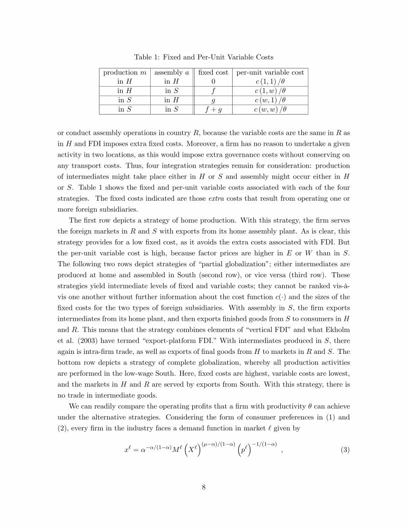
Table 1: Fixed and Per-Unit Variable Costs

production m assembly a fixed cost per-unit variable costin H in H 0 c (1, 1) /θ

in H in S f c (1, w) /θ

in S in H g c (w, 1) /θ

in S in S f + g c (w,w) /θ

or conduct assembly operations in country R, because the variable costs are the same in R as

in H and FDI imposes extra fixed costs. Moreover, a firm has no reason to undertake a given

activity in two locations, as this would impose extra governance costs without conserving on

any transport costs. Thus, four integration strategies remain for consideration: production

of intermediates might take place either in H or S and assembly might occur either in H

or S. Table 1 shows the fixed and per-unit variable costs associated with each of the four

strategies. The fixed costs indicated are those extra costs that result from operating one or

more foreign subsidiaries.

The first row depicts a strategy of home production. With this strategy, the firm serves

the foreign markets in R and S with exports from its home assembly plant. As is clear, this

strategy provides for a low fixed cost, as it avoids the extra costs associated with FDI. But

the per-unit variable cost is high, because factor prices are higher in E or W than in S.

The following two rows depict strategies of “partial globalization”; either intermediates are

produced at home and assembled in South (second row), or vice versa (third row). These

strategies yield intermediate levels of fixed and variable costs; they cannot be ranked vis-à-

vis one another without further information about the cost function c(·) and the sizes of thefixed costs for the two types of foreign subsidiaries. With assembly in S, the firm exports

intermediates from its home plant, and then exports finished goods from S to consumers in H

and R. This means that the strategy combines elements of “vertical FDI” and what Ekholm

et al. (2003) have termed “export-platform FDI.” With intermediates produced in S, there

again is intra-firm trade, as well as exports of final goods from H to markets in R and S. The

bottom row depicts a strategy of complete globalization, whereby all production activities

are performed in the low-wage South. Here, fixed costs are highest, variable costs are lowest,

and the markets in H and R are served by exports from South. With this strategy, there is

no trade in intermediate goods.

We can readily compare the operating profits that a firm with productivity θ can achieve

under the alternative strategies. Considering the form of consumer preferences in (1) and

(2), every firm in the industry faces a demand function in market given by

x = α−α/(1−α)M³X´(µ−α)/(1−α) ³

p´−1/(1−α)

, (3)

8

0

)( gf +−

SS ,π

Θ),( SSHHΘ

HH ,π

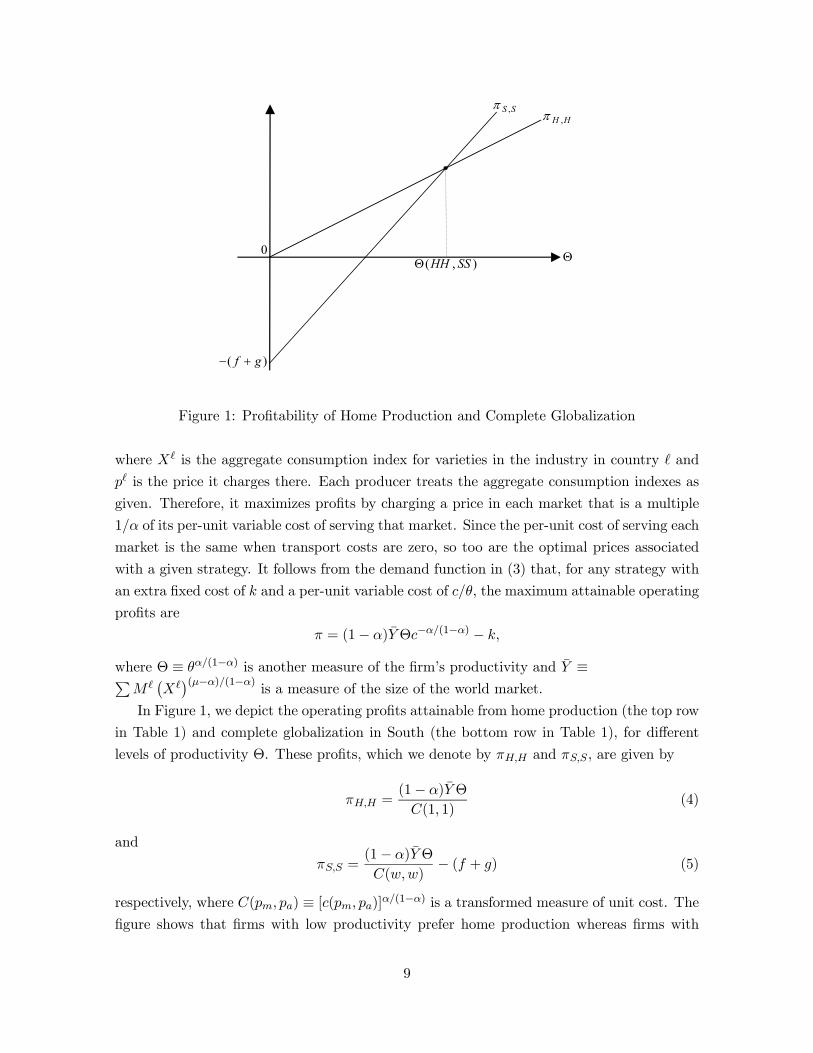
Figure 1: Profitability of Home Production and Complete Globalization

where X is the aggregate consumption index for varieties in the industry in country and

p is the price it charges there. Each producer treats the aggregate consumption indexes as

given. Therefore, it maximizes profits by charging a price in each market that is a multiple

1/α of its per-unit variable cost of serving that market. Since the per-unit cost of serving each

market is the same when transport costs are zero, so too are the optimal prices associated

with a given strategy. It follows from the demand function in (3) that, for any strategy with

an extra fixed cost of k and a per-unit variable cost of c/θ, the maximum attainable operating

profits are

π = (1− α)YΘc−α/(1−α) − k,

where Θ ≡ θα/(1−α) is another measure of the firm’s productivity and Y ≡PM

¡X¢(µ−α)/(1−α)

is a measure of the size of the world market.

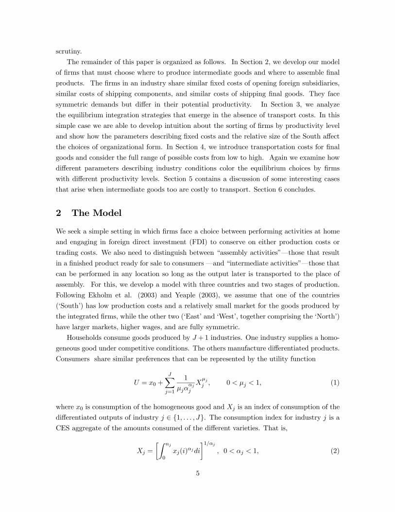
In Figure 1, we depict the operating profits attainable from home production (the top row

in Table 1) and complete globalization in South (the bottom row in Table 1), for different

levels of productivity Θ. These profits, which we denote by πH,H and πS,S, are given by

πH,H =(1− α)YΘ

C(1, 1)(4)

and

πS,S =(1− α)YΘ

C(w,w)− (f + g) (5)

respectively, where C(pm, pa) ≡ [c(pm, pa)]α/(1−α) is a transformed measure of unit cost. Thefigure shows that firms with low productivity prefer home production whereas firms with

9

high productivity prefer FDI, in keeping with the findings of Helpman et al. (2003). The

reason, of course, is that FDI offers the prospect of lower per-unit costs and higher fixed

costs, and the potential to save on variable cost is most valuable to highly productive firms

that anticipate producing high volumes of output.

Next consider the firm’s option to locate only assembly operations in South, while pro-

ducing intermediate goods in the home country. The potential operating profits from this

integration strategy for a firm with productivity Θ are

πH,S =(1− α)YΘ

C(1, w)− f . (6)

If we were to add πH,S to Figure 1, it would have an intercept between those of πH,H and πS,Sand a slope steeper than πH,H but less steep than πS,S . Thus, if locating only assembly in

South is to be viable at any productivity level, this strategy must be at least as profitable as

concentrating both activities in either location at the productivity level labelled Θ(HH,SS)

in the figure. But this requires3

g

f≥ C(1, 1)

C(w,w)

·C(1, w)−C(w,w)

C(1, 1)−C(1, w)

¸. (7)

Leaving this strategy aside for a moment, the firm also has the option to produce inter-

mediate goods in South and assemble final goods at home. This strategy offers a firm with

productivity Θ operating profits of

πS,H =(1− α)YΘ

C(w, 1)− g . (8)

Again, the intercept and slope are intermediate between those for the two lines shown in

Figure 1, and viability of the strategy requires that it be at least as profitable as the other

two at Θ = Θ(HH,SS). This in turn requires

g

f≤ C(w,w)

C(1, 1)

·C(1, 1)−C(w, 1)

C(w, 1)−C(w,w)

¸. (9)

From (7) and (9) we conclude that no firm will separate the production of its intermediate

goods from its assembly operations when

C(w,w)

C(1, 1)

·C(1, 1)−C(w, 1)

C(w, 1)−C(w,w)

¸<

g

f<

C(1, 1)

C(w,w)

·C(1, w)− C(w,w)

C(1, 1)− C(1, w)

¸.

Our assumption that the elasticity of substitution between intermediates and assembly in

the production of final goods is no greater than one ensures that the upper limit in this

3To derive this condition, we calculate Θ(HH,SS) as the value of Θ that equates πH,H and πS,S , and thencompare πH,S and πH,H at Θ = Θ(HH,SS).

10

string of inequalities exceeds the lower limit.4 It follows that there always exist a range of

values of g/f for which neither assembly in South and production of intermediates at home,

nor production of intermediates in South with assembly at home is optimal for any firm,

regardless of its productivity level.

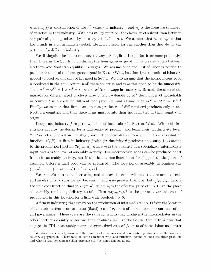
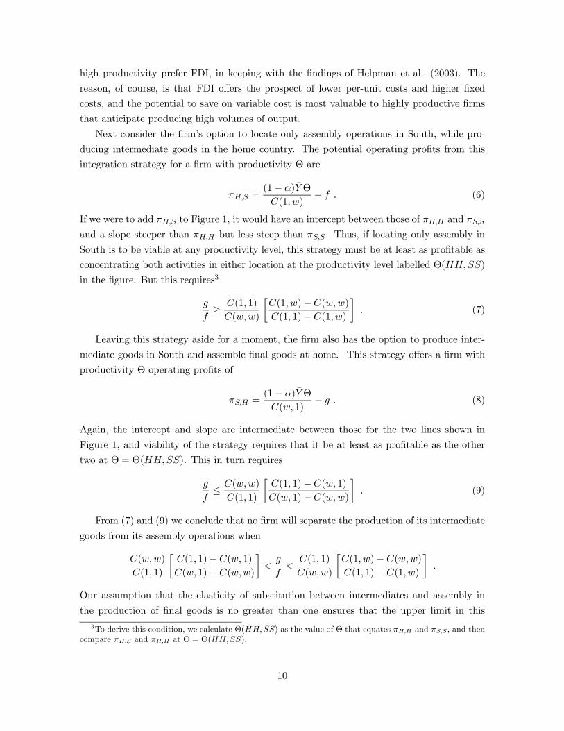
Suppose now that the fixed costs of operating a foreign assembly operation are small

relative to the fixed costs of operating a foreign plant to manufacture intermediate goods;

i.e., g/f is large enough so that (7) is satisfied. Then a firm with productivity level at or near

Θ(HH,SS) prefers to locate its assembly in South and manufacture intermediates at home to

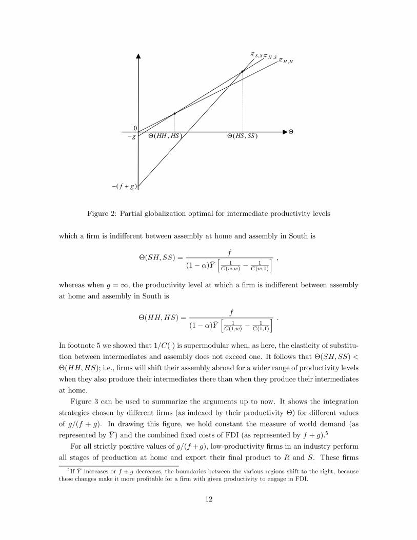
any other integration strategy. Figure 2 shows the operating profits πH,S (as well as πH,H and

πS,S) for this case. Clearly, firms with low productivity below Θ(HH,HS) conduct all oper-

ations at home, firms with intermediate productivity between Θ(HH,HS) and Θ(HS,SS)

conduct only their assembly operations in South, and firms with high productivity above

Θ(HS,SS) perform all of their production activities in South.

The case when the fixed cost of FDI in assembly is large relative to the fixed cost of FDI

in intermediates is qualitatively similar. With g/f small enough so that (9) is satisfied, the

line representing πS,H will cut πH,H at some relatively low productivity level Θ(HH,SH)

that is to the left of Θ(HH,SS) in Figure 1, and will cut πS,S at some relatively high

productivity level Θ(SH,SS) to the right of Θ(HH,SS) in the figure. Then firms with

productivity between Θ(HH,SH) and Θ(SH,SS) will choose to produce their intermediates

in the low-wage South while conducting assembly at home.

Our analysis can be used to highlight one form of complementarity that exists between a

firm’s decision to invest abroad at different stages of production. Compare, for example, a

firm’s decision whether to conduct assembly in South when g = 0 and g =∞. In the first case,the fixed cost of FDI in intermediate goods is nil and so all firms produce their intermediates

in South. In the second case, the cost of FDI for the production of intermediates is prohibitive

and all firms produce their intermediates at home. When g = 0, the productivity level at

4 It can be shown that

C(1, 1)

C(w,w)

C(1, w)− C(w,w)

C(1, 1)− C(1, w)>

C(w,w)

C(1, 1)

C(1, 1)− C(w, 1)

C(w, 1)− C(1, 1)

if and only if1

C(w,w)+

1

C(1, 1)>

1

C(w, 1)+

1

C(1, w);

i.e., if and only if the function 1/C(·) is supermodular. But 1/C(pm, pa) ≡ [c(pm, pa)]α/(1−α) is supermodularif it is twice differentiable and

c(pm, pa) ∂2c(pm, pa)/∂pm∂pa

[∂c(pm, pa)/∂pm][∂c(pm, pa)/∂pa]<

1

1− α.

The left-hand side of this inequality is the elasticity of substitution between m and a in the production of finalgoods, which is no greater than one by assumption. Therefore, the inequality holds for all positive values ofα.

11

0

)( gf +−

Θ),( SSHSΘ

SH ,π

),( HSHHΘg−

SS ,πHH ,π

Figure 2: Partial globalization optimal for intermediate productivity levels

which a firm is indifferent between assembly at home and assembly in South is

Θ(SH,SS) =f

(1− α)Yh

1C(w,w) − 1

C(w,1)

i ,whereas when g =∞, the productivity level at which a firm is indifferent between assembly

at home and assembly in South is

Θ(HH,HS) =f

(1− α)Yh

1C(1,w) − 1

C(1,1)

i .In footnote 5 we showed that 1/C(·) is supermodular when, as here, the elasticity of substitu-tion between intermediates and assembly does not exceed one. It follows that Θ(SH,SS) <

Θ(HH,HS); i.e., firms will shift their assembly abroad for a wider range of productivity levels

when they also produce their intermediates there than when they produce their intermediates

at home.

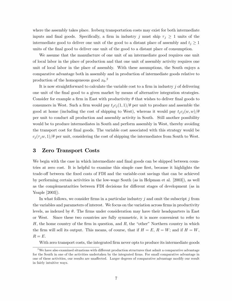
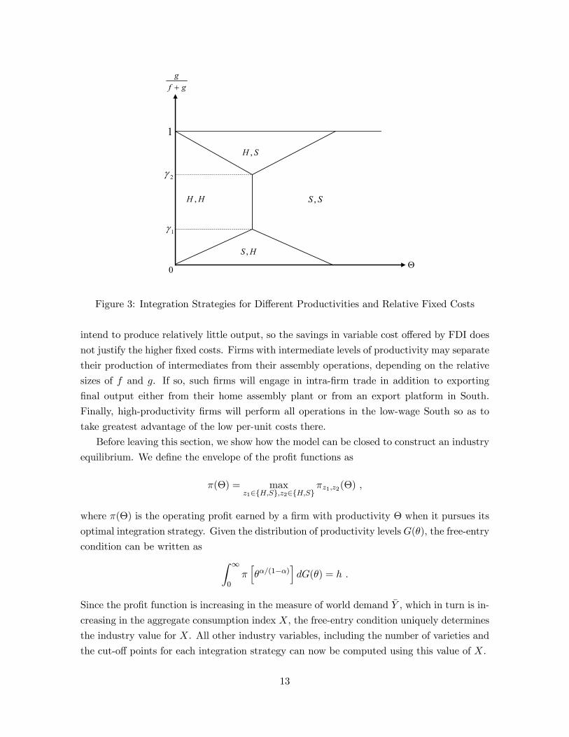
Figure 3 can be used to summarize the arguments up to now. It shows the integration

strategies chosen by different firms (as indexed by their productivity Θ) for different values

of g/(f + g). In drawing this figure, we hold constant the measure of world demand (as

represented by Y ) and the combined fixed costs of FDI (as represented by f + g).5

For all strictly positive values of g/(f + g), low-productivity firms in an industry perform

all stages of production at home and export their final product to R and S. These firms

5 If Y increases or f + g decreases, the boundaries between the various regions shift to the right, becausethese changes make it more profitable for a firm with given productivity to engage in FDI.

12

Θ

gf g+

HH , SS ,

,S H

,H S

2γ

1γ

0

1

Figure 3: Integration Strategies for Different Productivities and Relative Fixed Costs

intend to produce relatively little output, so the savings in variable cost offered by FDI does

not justify the higher fixed costs. Firms with intermediate levels of productivity may separate

their production of intermediates from their assembly operations, depending on the relative

sizes of f and g. If so, such firms will engage in intra-firm trade in addition to exporting

final output either from their home assembly plant or from an export platform in South.

Finally, high-productivity firms will perform all operations in the low-wage South so as to

take greatest advantage of the low per-unit costs there.

Before leaving this section, we show how the model can be closed to construct an industry

equilibrium. We define the envelope of the profit functions as

π(Θ) = maxz1∈{H,S},z2∈{H,S}

πz1,z2(Θ) ,

where π(Θ) is the operating profit earned by a firm with productivity Θ when it pursues its

optimal integration strategy. Given the distribution of productivity levelsG(θ), the free-entry

condition can be written as Z ∞

0πhθα/(1−α)

idG(θ) = h .

Since the profit function is increasing in the measure of world demand Y , which in turn is in-

creasing in the aggregate consumption index X, the free-entry condition uniquely determines

the industry value for X. All other industry variables, including the number of varieties and

the cut-off points for each integration strategy can now be computed using this value of X.

13

4 Transport Costs for Final Goods

In this section, we allow for costly transport of final goods, while maintaining the assumption

that intermediates can be shipped costlessly. For example, the intermediates may represent

services that can be performed remotely and then moved electronically. This assumption

implies that intermediates goods are only produced in one location.

When the transport of final goods is costly, relative market size may affect the location

of assembly operations. Moreover, firms may engage in “horizontal FDI,” by, for example,

assembling goods in more than one location. We focus here on the interaction between market

size and FDI costs in determining a firm’s optimal integration strategy.

4.1 Low Transport Costs

The viable integration strategies vary with the size of transport costs. We begin with a case

in which transport costs for final goods are reasonably small; in particular, we assume that

1 < t <c(1, 1)

c(1, w). (10)

When inequality (10) is satisfied, the variable cost of serving any market is minimized by

assembly in South, no matter where the intermediate goods are produced. To see this,

observe first that if the intermediates are produced in H or R, the cost of serving any market

from an assembly plant in the North is at least c(1, 1). But this exceeds the cost of serving the

same market from the South, which is at most tc(1, w). Next observe that if intermediates are

produced in South, the per-unit variable cost of serving any market from an assembly plant

in the North is at least c(w, 1), while the per-unit cost of serving the same market from a

plant in South is at most tc(w,w). However, c(w, 1)/c(w,w) > c(1, 1)/c(1, w),6 so inequality

(10) ensures that c(w, 1) > tc(w,w) as well.

Under the circumstances, a firm with headquarters in H will not conduct any activity

in R. Intermediate goods are no less costly to produce in R than in H and can be shipped

costlessly from one to the other. By producing these goods in R, the firm would needlessly

incur an extra fixed cost of FDI. And if assembly is to be conducted outside of H, the

delivered cost of serving any market from S are lower than the cost of serving the market

from R, while the fixed cost of an assembly plant is the same in the two locations.

We can also rule out any integration strategy in which a given activity is performed in more

than one location. If it is worthwhile for the firm to bear the fixed cost of opening a facility

to manufacture intermediate goods in South, the firm produces all of its intermediates there

to take full advantage of the low production costs. The same is true for assembly, considering

6Note that c(1, 1)/c(1, w) < c(1, w)/c(w,w) if and only if log c(1, 1)+ log c(w,w) < log c(1, w)+ log c(w, 1);i.e., if and only if log c(pm, pa) is submodular. But log c(pm, pa) indeed is submodular when the elasticity ofsubstitution between m and a is less than one, because ∂2 log c(pm, pa)/∂pm∂pa < 1.

14

the reasonably low cost of shipping goods. It follows that each firm chooses one of four

integration strategies; these are the same set of strategies that we considered in Section 3.

A firm’s decision calculus is similar to that described in Section 3, except that now it must

take into account the relative size of the market in South when deciding whether to open

facilities there. We define Y ≡M (X )(µ−α)/(1−α) as a measure of market size in countryand σ ≡ Y S/Y as the share of the South in world demand for industry output.

We begin, as before, by comparing the profitability of performing all production activities

at home with the profitability of performing all stages in South. Again, firms with low

productivity prefer home production while those with high productivity prefer FDI in South.

The productivity level Θ(HH,SS) at which a firm earns equal operating profits under the

alternative integration strategies depends, as before, on the size of the fixed costs, f + g,

and on the relative wage, w. Now it depends too on the shipping cost and on the relative

size of South. If the typical market in the North is larger than the market in South (i.e., if

Y E = YW = Y N > Y S), then a larger shipping cost t diminishes the relative profitability of

production in South, because the shipments from S to H and S to R, under this strategy are

larger respectively than those from H to S and from H to R under the alternative strategy

of home production. It follows that the larger is t, the greater is the productivity level that

makes a firm indifferent between production in home and complete globalization in South.7

On the other hand, the larger is σ, the smaller is Θ(HH,SS), because the relative profitability

of producing in South increases with the size of the market there due to the transport costs.

Again, as was the case with zero transport costs, a strategy of producing intermediate

goods at home with assembly in South can be optimal for some firms only if the fixed cost of

FDI in intermediate-good production is high relative to the fixed cost of a foreign assembly

operation. And a strategy of producing intermediate goods in South with assembly at home

can be optimal for some firms only if the fixed cost of FDI in intermediate-good production

is relatively low compared to that for a foreign assembly operation. For intermediate values

of g/f , all low-productivity firms produce their intermediates and conduct assembly at home

while all high-productivity firms produce their intermediates and conduct assembly in South.

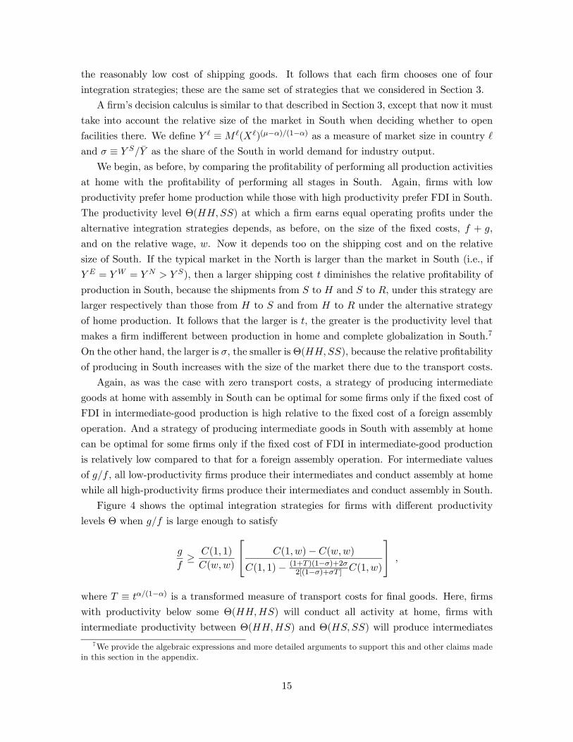
Figure 4 shows the optimal integration strategies for firms with different productivity

levels Θ when g/f is large enough to satisfy

g

f≥ C(1, 1)

C(w,w)

C(1, w)−C(w,w)

C(1, 1)− (1+T )(1−σ)+2σ2[(1−σ)+σT ] C(1, w)

,

where T ≡ tα/(1−α) is a transformed measure of transport costs for final goods. Here, firmswith productivity below some Θ(HH,HS) will conduct all activity at home, firms with

intermediate productivity between Θ(HH,HS) and Θ(HS,SS) will produce intermediates

7We provide the algebraic expressions and more detailed arguments to support this and other claims madein this section in the appendix.

15

Θ

σ

HH , ,H S

0

1

SS ,

( , )HH HSΘ ( , )HS SSΘ

Figure 4: Optimal integration strategies when t is small and g/f is large

at home and assemble in South, and firms with productivity above Θ(HS,SS) will perform all

production activities in South. The figure shows that Θ(HH,HS) is a decreasing function

of σ, inasmuch as assembly in the South is more profitable when the Southern market is

relatively large. Also, Θ(HS,SS) is a decreasing function of σ for reasons that are a bit more

subtle. Comparing a strategy that has only assembly performed in South with a strategy that

has all production in South, the latter provides lower unit costs and therefore larger volumes

of output. With larger volumes, the transport cost savings from assembling in South are

larger the greater is the share of South in the world market. Therefore, the break-even point

between a strategy of performing only assembly in South and a strategy of performing all

production activity in South will come at a lower productivity level when the market share

of the South is larger.

When the fixed cost of producing intermediate goods in South is small relative to the

fixed cost of foreign assembly, an integration strategy with production of intermediates in

South and assembly at home will be optimal for firms with intermediate productivity levels.

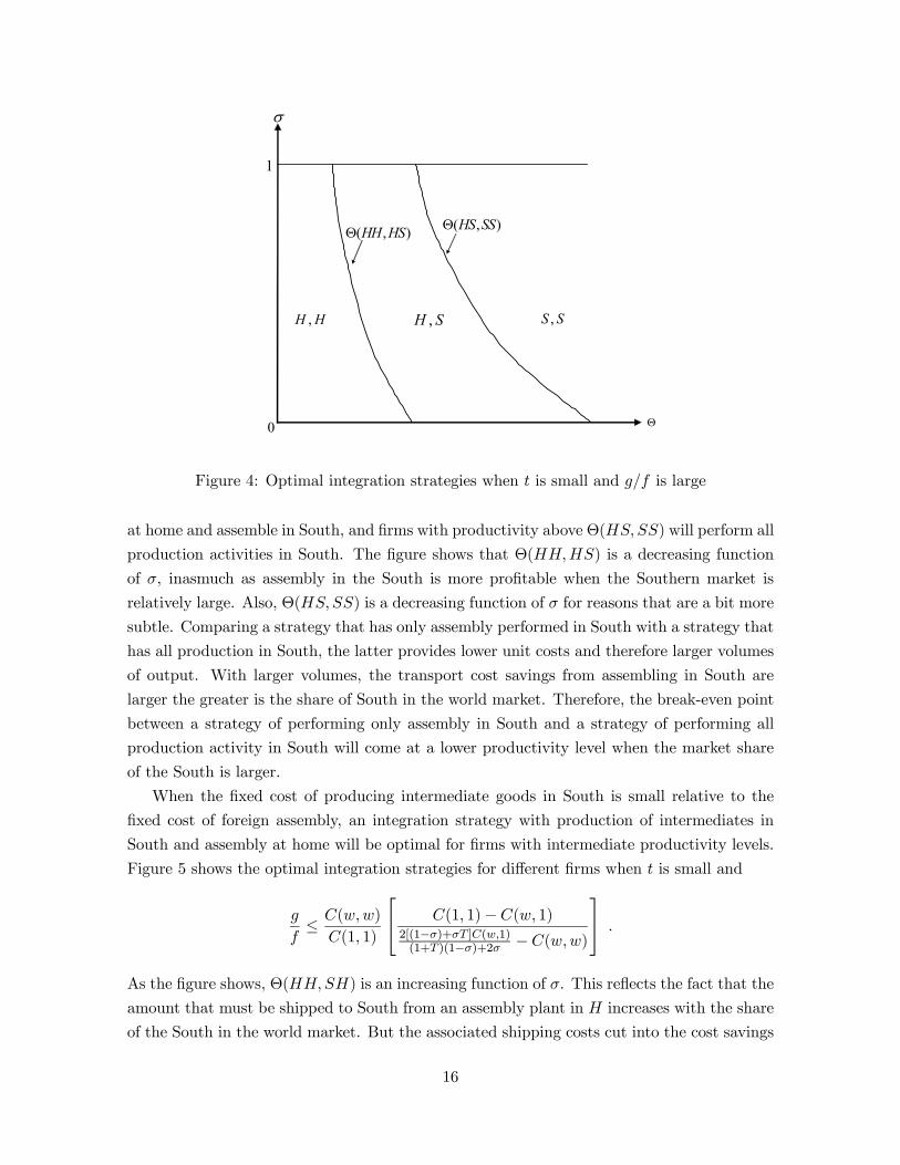
Figure 5 shows the optimal integration strategies for different firms when t is small and

g

f≤ C(w,w)

C(1, 1)

C(1, 1)−C(w, 1)2[(1−σ)+σT ]C(w,1)(1+T )(1−σ)+2σ − C(w,w)

.

As the figure shows, Θ(HH,SH) is an increasing function of σ. This reflects the fact that the

amount that must be shipped to South from an assembly plant in H increases with the share

of the South in the world market. But the associated shipping costs cut into the cost savings

16

Θ

σ

HH , ,S H

0

1

SS ,

( , )HH SHΘ ( , )SH SSΘ

Figure 5: Optimal integration strategiess when t is small and g/f is small

generated by a strategy of foreign production of intermediates, and so a higher productivity

level is needed to justify the higher fixed costs of this strategy.

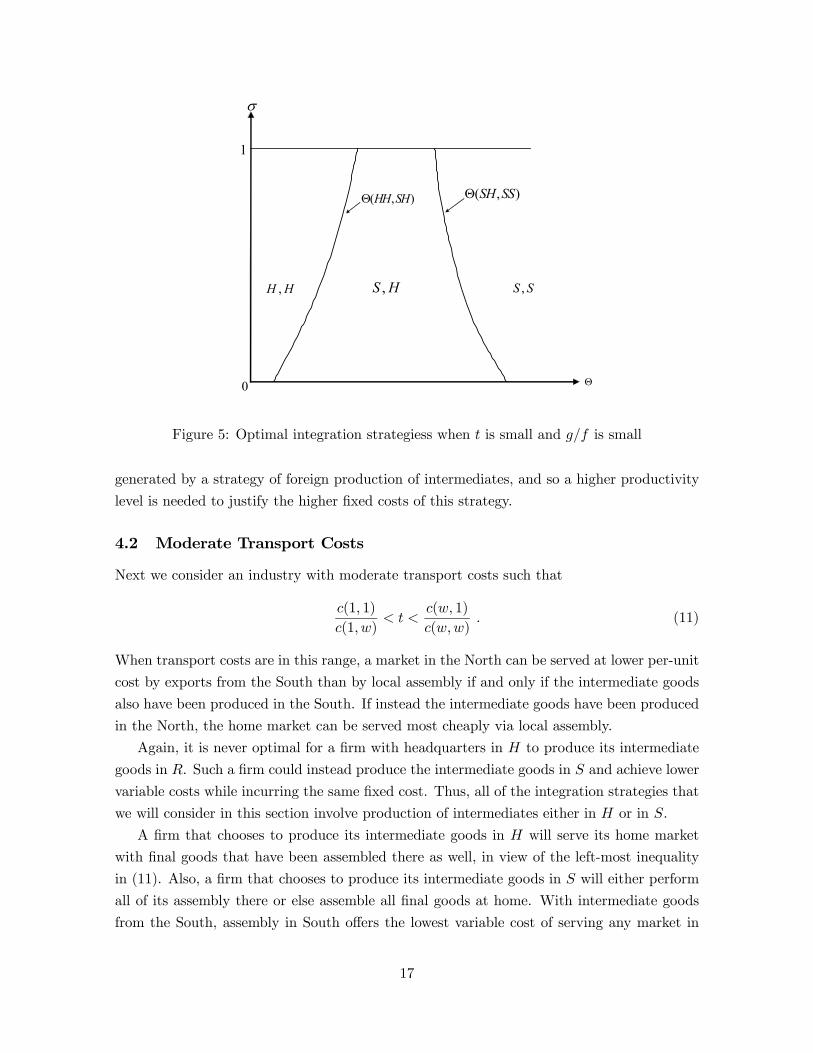
4.2 Moderate Transport Costs

Next we consider an industry with moderate transport costs such that

c(1, 1)

c(1, w)< t <

c(w, 1)

c(w,w). (11)

When transport costs are in this range, a market in the North can be served at lower per-unit

cost by exports from the South than by local assembly if and only if the intermediate goods

also have been produced in the South. If instead the intermediate goods have been produced

in the North, the home market can be served most cheaply via local assembly.

Again, it is never optimal for a firm with headquarters in H to produce its intermediate

goods in R. Such a firm could instead produce the intermediate goods in S and achieve lower

variable costs while incurring the same fixed cost. Thus, all of the integration strategies that

we will consider in this section involve production of intermediates either in H or in S.

A firm that chooses to produce its intermediate goods in H will serve its home market

with final goods that have been assembled there as well, in view of the left-most inequality

in (11). Also, a firm that chooses to produce its intermediate goods in S will either perform

all of its assembly there or else assemble all final goods at home. With intermediate goods

from the South, assembly in South offers the lowest variable cost of serving any market in

17

view of the right-most inequality in (11). Thus, a firm that elects to bear the fixed cost

of FDI in assembly will serve all markets from there. But a firm may choose to avoid the

fixed cost of FDI in assembly by performing its assembly at home. We are left with six

integration strategies to consider when transport costs are moderate: Southern production

of intermediate goods with assembly either in H or in S; or home production of intermediate

goods with assembly in H, in H and S, in H and R, or in H,S and R.

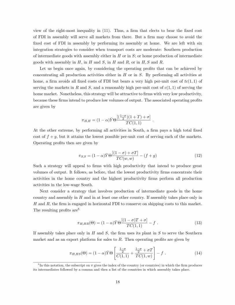
Let us begin once again, by considering the operating profits that can be achieved by

concentrating all production activities either in H or in S. By performing all activities at

home, a firm avoids all fixed costs of FDI but bears a very high per-unit cost of tc(1, 1) of

serving the markets in R and S, and a reasonably high per-unit cost of c(1, 1) of serving the

home market. Nonetheless, this strategy will be attractive to firms with very low productivity,

because these firms intend to produce low volumes of output. The associated operating profits

are given by

πH,H = (1− α)YΘ[(1−σ2 )(1 + T ) + σ]

TC(1, 1).

At the other extreme, by performing all activities in South, a firm pays a high total fixed

cost of f + g, but it attains the lowest possible per-unit cost of serving each of the markets.

Operating profits then are given by

πS,S = (1− α)YΘ[(1− σ) + σT ]

TC(w,w)− (f + g) (12)

Such a strategy will appeal to firms with high productivity that intend to produce great

volumes of output. It follows, as before, that the lowest productivity firms concentrate their

activities in the home country and the highest productivity firms perform all production

activities in the low-wage South.

Next consider a strategy that involves production of intermediate goods in the home

country and assembly in H and in at least one other country. If assembly takes place only in

H and R, the firm is engaged in horizontal FDI to conserve on shipping costs to this market.

The resulting profits are8

πH,HR(Θ) = (1− α)YΘ[(1− σ)T + σ]

TC(1, 1)− f . (13)

If assembly takes place only in H and S, the firm uses its plant in S to serve the Southern

market and as an export platform for sales to R. Then operating profits are given by

πH,HS(Θ) = (1− α)YΘ

"1−σ2

C(1, 1)+

1−σ2 + σT

TC(1, w)

#− f . (14)

8 In this notation, the subscript on π gives the index of the country (or countries) in which the firm producesits intermediates followed by a comma and then a list of the countries in which assembly takes place.

18

0

Θ),( HRSHSΘ

f−

,H HRSπ,H HSπ

f2−

,H HRπ

Figure 6: Assembly in multiple plants with moderate transport costs

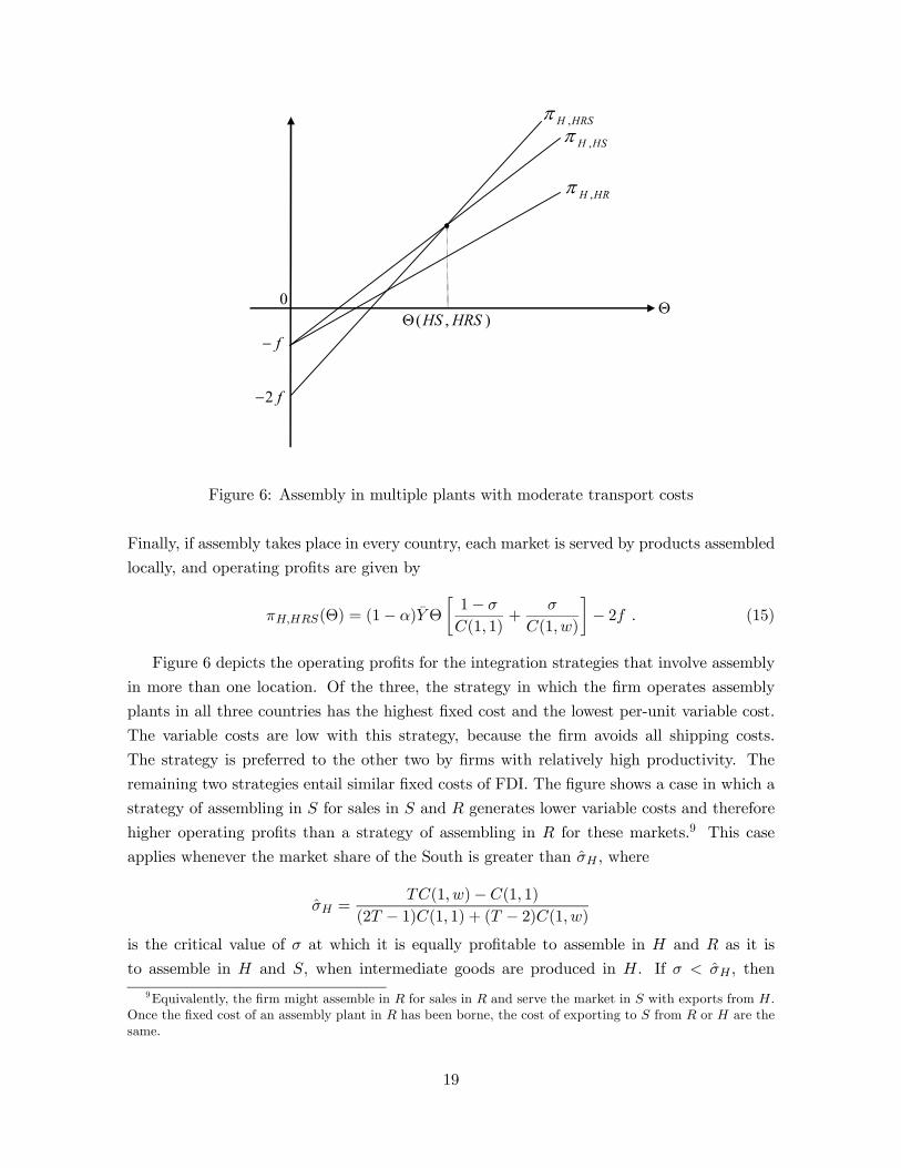
Finally, if assembly takes place in every country, each market is served by products assembled

locally, and operating profits are given by

πH,HRS(Θ) = (1− α)YΘ

·1− σ

C(1, 1)+

σ

C(1, w)

¸− 2f . (15)

Figure 6 depicts the operating profits for the integration strategies that involve assembly

in more than one location. Of the three, the strategy in which the firm operates assembly

plants in all three countries has the highest fixed cost and the lowest per-unit variable cost.

The variable costs are low with this strategy, because the firm avoids all shipping costs.

The strategy is preferred to the other two by firms with relatively high productivity. The

remaining two strategies entail similar fixed costs of FDI. The figure shows a case in which a

strategy of assembling in S for sales in S and R generates lower variable costs and therefore

higher operating profits than a strategy of assembling in R for these markets.9 This case

applies whenever the market share of the South is greater than σH , where

σH =TC(1, w)− C(1, 1)

(2T − 1)C(1, 1) + (T − 2)C(1, w)is the critical value of σ at which it is equally profitable to assemble in H and R as it is

to assemble in H and S, when intermediate goods are produced in H. If σ < σH , then

9Equivalently, the firm might assemble in R for sales in R and serve the market in S with exports from H.Once the fixed cost of an assembly plant in R has been borne, the cost of exporting to S from R or H are thesame.

19

0

Θ

f−

,H HRSπ,H HSπ

f2−

HH ,π

A

B

SS ,π

C

)( gf +−

Figure 7: Moderate transport costs, σ > σH , and g/f large

πH,HR > πH,HS for all Θ.

If the profit line for πH,H were added to Figure 6, it would be apparent how firms that

might choose to produce intermediates at home would locate their assembly operations. Those

with low productivity prefer a single assembly plant at home, while those with high produc-

tivity prefer to have assembly plants in all three countries. The firms with intermediate levels

of productivity prefer to have an assembly operation at home and in one other country; in

the South if σ is large, and in R otherwise.

Now we consider a firm’s option to produce its intermediates in the South and then

assemble final goods in either H or S. If assembly takes place at home, operating profits are

πS,H = (1− α)YΘ

·(1− σ)(1 + T ) + 2σ

2TC(w, 1)

¸− g,

whereas if assembly takes place in S, the profits are given in (12). Among these two strategies,

firms with low productivity prefer the former and firms with high productivity prefer the

latter.

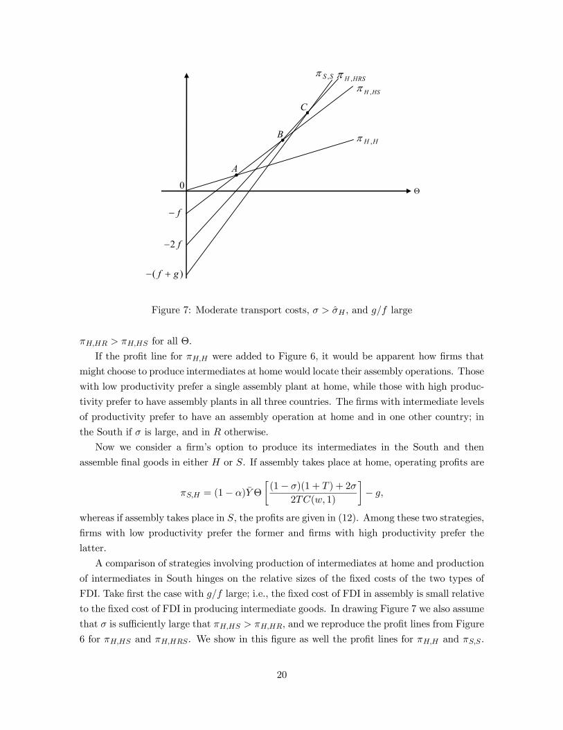
A comparison of strategies involving production of intermediates at home and production

of intermediates in South hinges on the relative sizes of the fixed costs of the two types of

FDI. Take first the case with g/f large; i.e., the fixed cost of FDI in assembly is small relative

to the fixed cost of FDI in producing intermediate goods. In drawing Figure 7 we also assume

that σ is sufficiently large that πH,HS > πH,HR, and we reproduce the profit lines from Figure

6 for πH,HS and πH,HRS . We show in this figure as well the profit lines for πH,H and πS,S .

20

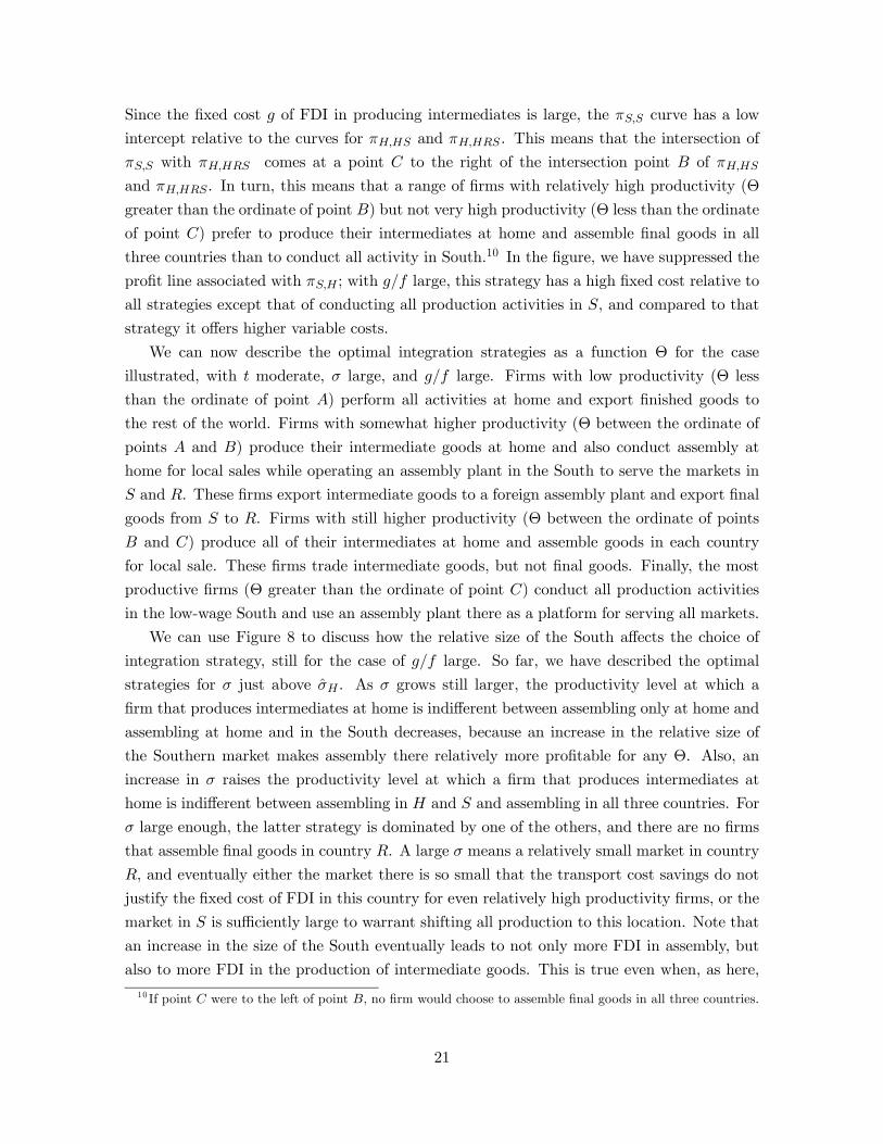
Since the fixed cost g of FDI in producing intermediates is large, the πS,S curve has a low

intercept relative to the curves for πH,HS and πH,HRS . This means that the intersection of

πS,S with πH,HRS comes at a point C to the right of the intersection point B of πH,HS

and πH,HRS. In turn, this means that a range of firms with relatively high productivity (Θ

greater than the ordinate of point B) but not very high productivity (Θ less than the ordinate

of point C) prefer to produce their intermediates at home and assemble final goods in all

three countries than to conduct all activity in South.10 In the figure, we have suppressed the

profit line associated with πS,H ; with g/f large, this strategy has a high fixed cost relative to

all strategies except that of conducting all production activities in S, and compared to that

strategy it offers higher variable costs.

We can now describe the optimal integration strategies as a function Θ for the case

illustrated, with t moderate, σ large, and g/f large. Firms with low productivity (Θ less

than the ordinate of point A) perform all activities at home and export finished goods to

the rest of the world. Firms with somewhat higher productivity (Θ between the ordinate of

points A and B) produce their intermediate goods at home and also conduct assembly at

home for local sales while operating an assembly plant in the South to serve the markets in

S and R. These firms export intermediate goods to a foreign assembly plant and export final

goods from S to R. Firms with still higher productivity (Θ between the ordinate of points

B and C) produce all of their intermediates at home and assemble goods in each country

for local sale. These firms trade intermediate goods, but not final goods. Finally, the most

productive firms (Θ greater than the ordinate of point C) conduct all production activities

in the low-wage South and use an assembly plant there as a platform for serving all markets.

We can use Figure 8 to discuss how the relative size of the South affects the choice of

integration strategy, still for the case of g/f large. So far, we have described the optimal

strategies for σ just above σH . As σ grows still larger, the productivity level at which a

firm that produces intermediates at home is indifferent between assembling only at home and

assembling at home and in the South decreases, because an increase in the relative size of

the Southern market makes assembly there relatively more profitable for any Θ. Also, an

increase in σ raises the productivity level at which a firm that produces intermediates at

home is indifferent between assembling in H and S and assembling in all three countries. For

σ large enough, the latter strategy is dominated by one of the others, and there are no firms

that assemble final goods in country R. A large σ means a relatively small market in country

R, and eventually either the market there is so small that the transport cost savings do not

justify the fixed cost of FDI in this country for even relatively high productivity firms, or the

market in S is sufficiently large to warrant shifting all production to this location. Note that

an increase in the size of the South eventually leads to not only more FDI in assembly, but

also to more FDI in the production of intermediate goods. This is true even when, as here,

10 If point C were to the left of point B, no firm would choose to assemble final goods in all three countries.

21

0 Θ

σ

HH ,

,H HR

,H HS

SS ,,H HRS

1

Hσ

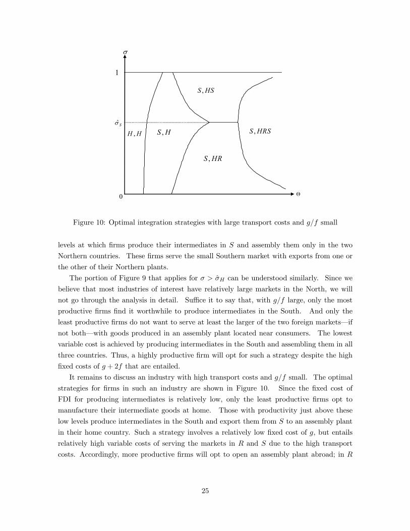
Figure 8: Optimal integration strategies with moderate transport costs and g/f large

the intermediate goods can be shipped costlessly. The two types of FDI are complementary,

because when assembly takes place in the South, a larger σ spells lower average transport costs

and thus greater volumes of output at a given productivity level. With more output being

produced, the cost savings promised by the South’s low wages justify FDI in intermediate

goods at lower levels of productivity.

Now consider a Southern market share σ just below σH . For all σ < σH , a strategy with

production of intermediate goods at home and assembly in H and S is dominated by one with

production of intermediate goods at home and assembly in H and R. For σ slightly less than

σH , the choice of integration strategies is similar to those for σ just above σH , except that

some firms with intermediate productivity levels choose to assemble in H and R, rather than

in H and S. As σ shrinks further, there are fewer firms that choose to assemble in all three

countries, and for σ below some level, no firms find this to be an optimal strategy. Moreover,

the smaller is the South, the greater is the productivity level needed before a firm opts to

move all production activity there. The market share of the South also affects the decision of

firms that manufacture intermediates at home and are choosing between assembling only in

H and assembling in H and in R. As σ shrinks for given Y , the size of the markets in H and

R grow. The growth in the size of the home market has no affect on the relative profitability

of these two strategies, but the growth in the size of the market in R favors the strategy with

assembly there. Accordingly, the productivity level at which a firm is indifferent between

assembly in H and R and assembling only in H falls as σ shrinks to zero.

Let us consider briefly an industry with moderate transport costs and g/f small. In this

22

case, the fixed cost of FDI for producing intermediate goods is much smaller than that for

FDI in assembly. Since intermediate goods also are costless to ship, all firms except those

with very low levels of productivity will find it optimal to produce their intermediate goods

in the South. In particular, with g/f small, any strategy with production of intermediate

goods at home and assembly in South or in multiple locations is dominated by a strategy

with all production activities concentrated at home or all production activities concentrated

in the South. And any strategy with production of intermediates in the South and assembly

in multiple locations is dominated by one with assembly only at home or only in the South.

It follows that all firms choose one of three integration strategies: either all activity is

concentrated at home, all activity is concentrated in South, or intermediates are manufactured

in the South and assembled at home. It should be clear by now how firms with different

productivity levels divide among these three alternatives. Those with very low productivity

opt to minimize their fixed costs by conducting all production activities at home. Those with

very high productivity minimize their variable costs by performing all production activities

in the low-wage South. And those with intermediate levels of productivity produce their

intermediate goods in the South and assemble them at home. Compared to the option of

conducting all activity in the South, such firms accept the relatively high variable cost of

sales to all three markets in order to avoid the relatively large fixed costs of FDI in assembly.

4.3 High Transport Costs

Finally, we consider an industry in which shipping final goods is quite costly, so that

t >c(w, 1)

c(w,w). (16)

In such circumstances, the lowest variable cost of serving any market is achieved by local

assembly near to consumers.11

Suppose first that g/f is large; i.e., the fixed cost of FDI in producing intermediate goods

is large compared to the fixed cost of FDI in assembly. Then it will not be optimal for any

firm to produce intermediates in a foreign subsidiary in South and conduct assembly only

at home. Such a strategy is dominated either by producing the intermediates in South and

conducting assembly in every country or by performing all production activities at home. The

same two strategies together dominate one of producing intermediates in S and performing

assembly in H and S, unless σ is close to one. Similarly, no firm will choose to assemble in

H and R intermediate goods produced in S unless σ is quite small. And, as before, there

exists a critical value of σ (that we have denoted by σH) at which a strategy of producing

intermediates at home and performing assembly in H and R yields the same operating profits

11Recall that an elasticity of substitution between intermediates and assembly of no more than one ensuresc(w, 1)/c(w,w) > c(1, 1)/c(1.w). Therefore, when (16) is satisfied, tc(1, w) > c(1, 1).

23

0 Θ

σ

HH ,

,H HR

,H HS

,S HRS,H HRS

1

,S HR

,S HS

Hσ

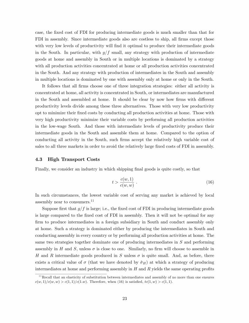
Figure 9: Optimal integration strategies with large transport costs and g/f large

as one of producing intermediates at home and performing assembly in H and S.

Consider σ slightly below σH and refer to Figure 9. As usual, firms with low productivity

can minimize fixed costs by conducting all activities at home. The next lowest fixed cost is

achieved by adding a single assembly plant. Since σ < σH , every firm prefers to add such

a plant in R rather than in S. By doing so, it can save on the variable costs of serving the

market in R at the relatively-low fixed cost of f . This strategy will be chosen by firms that

have productivity levels that are low but not quite as low as those that choose to stay entirely

at home. Still more productive firms will add an assembly plant in S so as to reduce the

variable costs of serving that country’s market. Finally, the most productive firms are willing

to pay the high fixed cost g of opening a subsidiary to produce intermediate goods in South.

These firms assemble the intermediates from S in separate plants located near consumers,

thereby minimizing the variable cost of serving every market.

Now let us reduce the relative size of the market in S. Since we maintain the assumption

that the two Northern countries are symmetric, a fall in σ increases the size of R. Accordingly,

the productivity level at which a firm is willing to open an assembly operation in R falls. Also,

as σ falls, so does the profitability of operating an assembly plant in S. The productivity

level at which a firm that produces its intermediates in H is indifferent between performing

assembly only in H and R and doing so also in S rises, until eventually a value of σ is reached

such that no firm that produces intermediates inH assembles final goods in the South. When

σ is quite small, even a firm that produces intermediates in S will not opt to assemble there

unless θ is very large. Rather, for σ small, there exists a range of quite high productivity

24

0 Θ

σ

HH , ,S H ,S HRS

,S HR

,S HS

1

Sσ

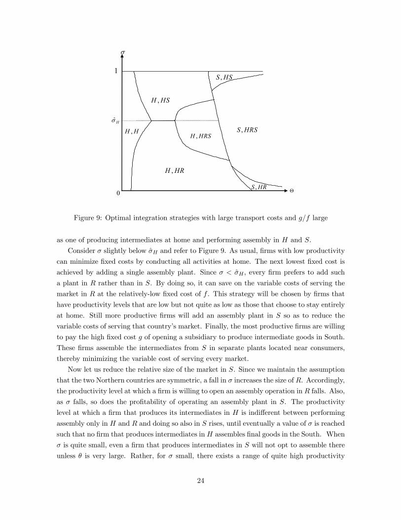
Figure 10: Optimal integration strategies with large transport costs and g/f small

levels at which firms produce their intermediates in S and assembly them only in the two

Northern countries. These firms serve the small Southern market with exports from one or

the other of their Northern plants.

The portion of Figure 9 that applies for σ > σH can be understood similarly. Since we

believe that most industries of interest have relatively large markets in the North, we will

not go through the analysis in detail. Suffice it to say that, with g/f large, only the most

productive firms find it worthwhile to produce intermediates in the South. And only the

least productive firms do not want to serve at least the larger of the two foreign markets–if

not both–with goods produced in an assembly plant located near consumers. The lowest

variable cost is achieved by producing intermediates in the South and assembling them in all

three countries. Thus, a highly productive firm will opt for such a strategy despite the high

fixed costs of g + 2f that are entailed.

It remains to discuss an industry with high transport costs and g/f small. The optimal

strategies for firms in such an industry are shown in Figure 10. Since the fixed cost of

FDI for producing intermediates is relatively low, only the least productive firms opt to

manufacture their intermediate goods at home. Those with productivity just above these

low levels produce intermediates in the South and export them from S to an assembly plant

in their home country. Such a strategy involves a relatively low fixed cost of g, but entails

relatively high variable costs of serving the markets in R and S due to the high transport

costs. Accordingly, more productive firms will opt to open an assembly plant abroad; in R

25

if σ < σS and in S otherwise.12 Finally, the most productive firms operate assembly plants

in both R and S. These firms export intermediate goods from S to H and to R, but do not

trade any of their final products.

The slopes of the various boundary lines in the figure are easy to understand in the

light of the previous discussion. For example, the boundary between (S,H) and (S,HS)

is downward sloping in the region with σ > σS, because the profitability of an assembly

plant in S increases with an increase in South’s market share. Similarly, for σ < σS, the

boundary between (S,H) and (S,HR) slopes upward, because an increase in σ corresponds

to a decrease in the relative size of R and so firms require a higher level of productivity to

justify placing an assembly plant there. The slopes of the boundaries between (S,HS) and

(S,HRS) and between (S,HR) and (S,HRS) have analogous explanations.

4.4 Transport Costs and FDI When the South is Small

In this section, we highlight the relationship between the cost of transporting final goods and

the integration strategies chosen by multinational firms in situations where the market in the

South is small. Specifically, we focus on the case where σ = 0 and review systematically how

changes in t affect the relative prevalence of different organizational forms.

We consider first the case in which g/f is large; i.e., the fixed cost of FDI in intermediate

production is large relative to the fixed cost of FDI in assembly. When transport costs are

small and σ = 0, the optimal integration strategies for firms with different productivity levels

are shown along the horizontal axis of Figure 4. We see that firms with low productivity

conduct all activity at home, firms with intermediate productivity produce intermediate

goods in H and assemble final goods in S, while firms with high productivity conduct all

production activity in the South. As the cost of transport rises but still remains in the range

where t < tm ≡ c(1, 1)/c(1, w), the boundary Θ(HH,HS) at which the first two of these

strategies are equally profitable shifts to the right, as does the boundary Θ(HS,SS) at which

the last two strategies are equally profitable. An increase in transport cost favors assembly at

home relative to assembly in the South, because the Southern market is small and shipments

from South to Home become more expensive as t rises. Thus, equal profitability occurs at

a higher productivity level when t is a bit larger compared to when t is close to one. The

rightward shift of Θ(HS,SS) reflects that output of final goods is larger when intermediate

goods are produced in the South as compared to when they are produced in the higher-cost

North. Therefore, an increase in transport costs for final goods has a larger impact on the

profitability of a firm that conducts all of its production activities in the South than it does

on one that only performs assembly there.

We use γi,j to denote the fraction of firms that produce intermediate goods in country

12We use σS to denote the critical value of σ at which it is equally profitable to assemble in H and R as itis to assemble in H and S, when intermediate goods are produced in the South.

26

mtt

HH ,γ

)( apanel

mtt

SH ,γ

mtt

HRH ,γ

)( cpanel )( dpanel

mtt

SS ,γHRS ,γ

)( bpanelht

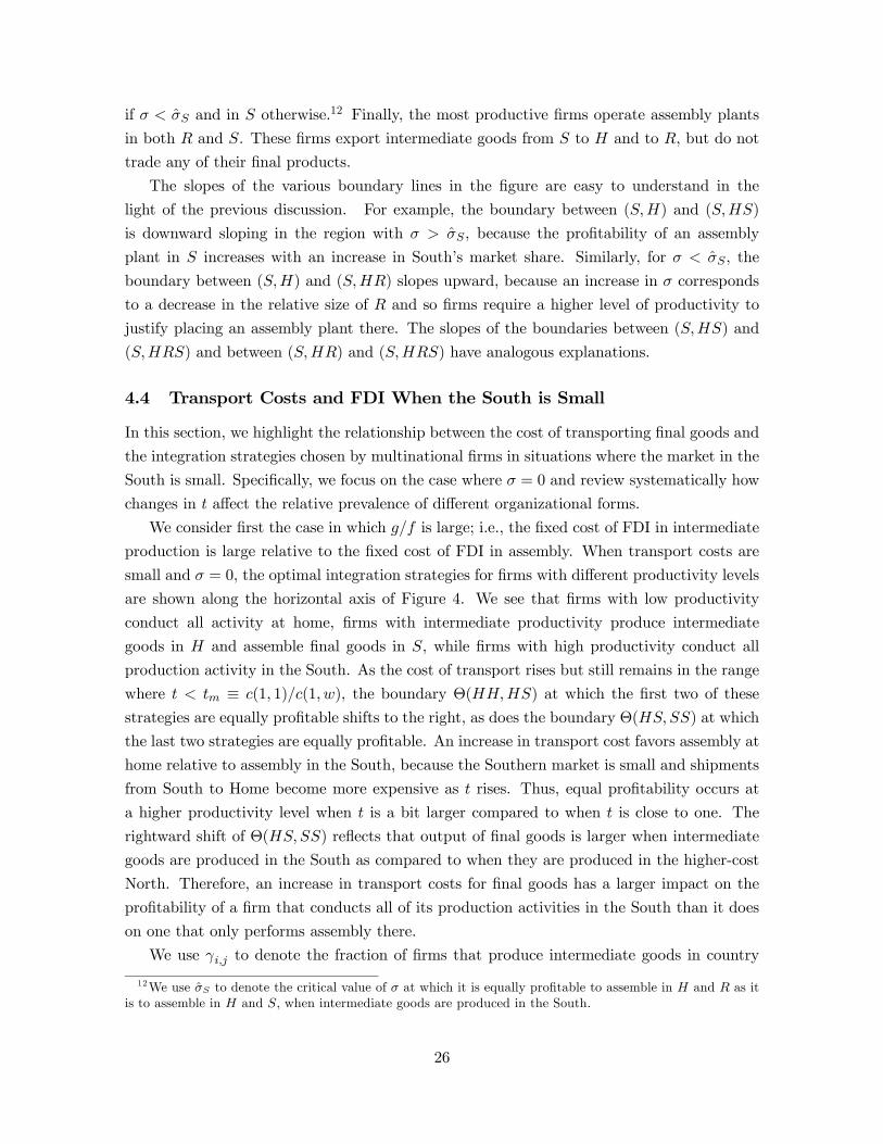
Figure 11: Relative prevalence of organizational forms when σ = 0 and g/f is large

i and assemble final goods in the set of countries {j}. Evidently, a rise in t increases γH,H

for t < tm, as shown in panel (a) of Figure 11. Also, γS,S falls, as shown by the broken

curve in panel (b). The fraction of firms that produce intermediate goods in the North and

assemble in the South can rise or fall, since this organizational form gains at the expense

of integrated production in the South but loses at the expense of integrated production in

the North. However, it can readily be shown that γH,S must fall as t rises when the size

distribution of productivity levels is characterized by a Pareto distribution.13 This is shown

in panel (c).

Next suppose that t rises above tm. For t ≥ tm, a firm that produces its intermediate

goods in H can earn higher profits by performing assembly in H and R than by performing

assembly in S. The integration strategies used by firms with different productivity levels

are shown along the horizontal axis of Figure 8. Firms with low productivity conduct all

activity at home, firms with intermediate productivity produce intermediate goods at home

and assemble in H and R, and firms with high productivity conduct all production activity

in the South. Further increases in t for tm < t ≤ th ≡ c(w, 1)/c(w,w) cause a contraction in

the fraction of firms with all production activities in H or S, and an expansion in the fraction

of firms that assemble in both H and R. Thus, γH,H and γS,S fall while γH,HR rises with

13With a Pareto distribution of θ, the fraction of firms that have productivity less than θ is given byG(θ) = 1 − (b/θ)k for θ ≥ b > 0 and k > 1. We show in the appendix that with this distribution the shareγH,S is a declining function of transport costs when g/f is large.The Pareto distribution is commonly used to describe the size distribution of productivity levels. Axtell

(2001) provides evidence that such a distribution fits well the data on the distribution of sales by U.S. firms.Helpman et al. (2003) show that a Pareto distribution of firm sizes emerges from a Pareto distribution ofproductivity measures.

27

)( apanel

)( cpanel

t

HH ,γ

)( bpanelht

t

SS ,γHRS ,γ

t

HS ,γ

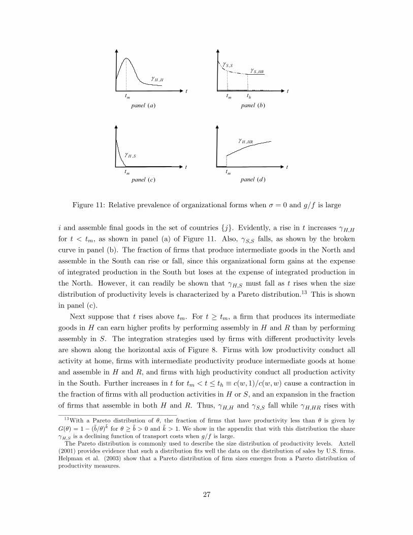
Figure 12: Relative prevalence of organizational forms when σ = 0 and g/f is small

increases in transport costs in this range, as shown in panels (a), (b) and (d) of Figure 8.

Finally, for high transport costs such that t > th, the optimal integration strategies are

shown in Figure 9. For t ≥ th, no assembly is performed in the South. Now, even the firms

with high productivity that produce intermediates in S find it more profitable to assemble

their final goods close to consumers. The low productivity firms perform all activities at

home, the firms with intermediate productivity manufacture intermediate goods at home and

assemble them in H and R, and the high productivity firms produce intermediate goods in

the South and assemble in H and R. Further increases in transport costs continue to shrink

the range of productivities for which it is most profitable to have a fully integrated facility

in the home country and serve R by exports. However, the productivity level at which it is

equally profitable to produce intermediates in H or S, with assembly in each case in H and

R, is unaffected by changes in t, inasmuch as neither of these strategies involves any trade in

final goods. Figure 8 shows γH,H falling, γS,HR flat, and γH,HR rising for t ≥ th.

Overall, increases in transport costs for final goods cause production activities to shift

away from the South. Assembly operations in the South are replaced by assembly operations

closer to consumers. And production of intermediate goods in the South contracts in favor

of production at home, inasmuch as the strategies that involve intermediate production in

the South also involve high volumes of output and so are especially vulnerable to increases

in the cost of transporting final goods.

We turn briefly to the case of g/f small. When the fixed cost of FDI in assembly

is relatively large, the same three integration strategies are observed in equilibrium for all

t < th; firms with low productivity conduct all activities at home, firms with intermediate

productivity produce intermediate goods in a subsidiary in the South but perform assembly

28

at home, and firms with high productivity perform all production activities in the South. An

increase in t for t < th causes both Θ(HH,SH) and Θ(SH,SS) to shift to the right. The

range of firms that performs all activity at home expands, because a firm that manufactures its

intermediate goods in the South will choose to produce more output than one with similarly

productivity that manufactures these goods at home, so the rise in the cost of transporting

final goods from H to R will impact more strongly the multinational firms. A strategy of

integrated production in the South becomes less profitable, because this strategy involves

the transport of final goods to markets in both H and R. Thus, as t grows, γH,H rises and

γS,S falls, as shown in panels (a) and (b) of Figure 12. The fraction of firms that produces

intermediate goods in the South and assembles them at home may rise or fall with an arbitrary

distribution of productivity levels; but it must decline if θ has a Pareto distribution, as shown

in panel (c) of Figure 12.14

For t > th, any strategy with assembly in the South is dominated by one with assembly in

H and R. Thus, for transport costs in this range, firms with low productivity concentrate all

activity at home, firms with intermediate productivity produce intermediates in the South

and assemble at home, and firms with high productivity manufacture intermediate goods in

the South and conduct assembly near to their markets in H and R. A further increase in t

expands the range of productivity levels for which firms concentrate all activities at home, as

well as that for which assembly in H and R is optimal; thus, γH,H and γS,HR increase with t,

while γS,H declines, as shown in Figure 12. As t rises, the fraction of multinational firms falls

monotonically, as production of intermediate goods in South gives way to production of these

goods at home, and assembly in the South gives way to assembly at home and ultimately to

assembly in both Northern markets.

5 Transport Costs for Intermediate Goods

Up until now, we have assumed that intermediate goods can be moved costlessly to any place

of assembly. This simplifying assumption allowed us to examine how variations in the cost

of transporting final goods, in relative market size, and in the relative fixed costs of FDI in

different activities affect firms’ decisions about global integration. We have seen that, with

variations in productivity in an industry, rich patterns of trade and FDI are possible.

In this section, we introduce a cost of trading intermediate inputs. To avoid a detailed

taxonomy, however, we explore only cases in which the cost of transporting intermediates

goods is high. Such costs give firms an incentive to locate the production of intermediate

goods near to where they intend to perform their assembly activities. We also assume that

the South is negligible in size (σ = 0), so that firms are not motivated to locate their assembly

operations in S in order to serve the Southern market. Rather, if a firm opens an assembly

14See the appendix for a derivation of this result.

29

plant in the South, it is because it wishes to use such a plant as an export platform.

Recall that τ captures the cost of shipping intermediate goods; τ > 1 units of the good

must be shipped from a production facility in some country to deliver one unit of the good to

an assembly plant in another country. The sense in which we assume that τ is large is that

wc(τ , 1) > c(1, 1) . (17)

This restriction implies that τw > 1; i.e., it is more costly to produce the intermediate good

in South and ship it to the North than it is to manufacture the good in East or West.15 Also,

it implies that c(τ ,w) > c(1, 1); i.e., a final good assembled in S with intermediates imported

from the North has a greater per-unit cost than one produced and assembled entirely in a

single Northern country.16

With high costs of transporting intermediate goods and a small market in the South, many

integration strategies can be ruled out. First, no firm with its headquarters in H will have a

sole assembly plant in country R. Any such strategy is dominated by an alternative one with

all production activities undertaken at home.17 Second, no firm will maintain assembly plants

in all three countries, inasmuch as the plant in the South would then serve only the negligible

Southern market and thus would not cover its fixed costs. Third, if a firm has assembly

plants in H and R, it will not produce intermediates only in R. Instead, it could produce

intermediates only in H, achieve the same total variable costs and conserve on fixed costs.

Fourth, a firm with assembly plants in H and R will not produce any intermediate goods

in S, because delivery from S involves higher costs than local production near an assembly

plant and entails fixed costs that are at least as large. Taken together, these observations

imply that any firm with an assembly operation in R will also have one in H, and that such

a firm will produce intermediate goods either only in H or in H and R. The resulting profits

are πH,HR or πHR,HR, as the case may be.

Four other strategies seem viable at this point. First, a firm may assemble only in S.

But then it will produce its intermediates in S as well, because a strategy with intermediates

produced in H or R and assembled in S is dominated by one with all production activities

in H, inasmuch as (17) implies c(τ , w) > c(1, 1). Second, a firm may assemble only in H.

Then it will produce its intermediate goods in H as well, to conserve on both shipping costs

and fixed costs. Finally, a firm may operate assembly plants in H and S, the former to serve

the home market and the latter to serve the market in R. If so, it will produce intermediates

15Note that wc(τ, 1) = c(τw,w). Then c(τw,w) > c(1, 1) and w < 1 implies τw > 1.16Note that c(τ ,w) > c(τw,w) = wc(τ , 1).17 If the sole assembly plant is in R, there would be no reason to have multiple plants producing intermediate

goods. Then a strategy of producing intermediates in S and assembling in R is dominated by one with allproduction activities in R, because τw > 1. And a strategy with all production in R or one with productionof intermediates in H and assembly in R is dominated by one with all production in H; the latter strategyyields variable costs that are no higher (in view of the symmetry of the two countries) and conserves on fixedcosts of FDI.

30

either in S only, or in H and S.18 The four strategies that do not involve assembly in R yield

potential profits of πS,S , πH,H , πS,HS , and πHS,HS , respectively.

The optimal choices among the remaining strategies will depend on the sizes of the fixed

costs of FDI in intermediates and assembly, the cost of transporting final goods, and the

productivity of the firm. Consider first an industry with a low cost of transporting final

goods such that

t <1

w. (18)

This implies tc(w,w) < c(1, 1) or that the variable cost of serving any Northern market from

an integrated production and assembly plant in the South is less than the cost of serving

the same market from an assembly plant in the North.19 Thus, πS,S(θ) > πHS,HS(θ) >

πHR,HR(θ) and πS,S(θ) > πS,HS(θ)for all θ. Moreover, (17) and (18) together imply tc(1, 1) <

c(τ , 1), so that πH,H(θ) > πH,HR(θ). In other words, the only viable integration strategies

when t is small are ones with all production activities concentrated either in South or at home.

Relatively productive firms will prefer the former strategy with its lower variable costs, while

less productive firms prefer the latter strategy with its lower fixed costs. Evidently, the high

cost of transporting intermediate goods dictates the optimal strategy for integration, which

must involve production of intermediate goods and assembly in the same location.

Next consider intermediate costs of shipping final goods such that

1

w< t <

c(τ , 1)

c(1, 1). (19)

With t > 1/w, a strategy of integrated production and assembly in both H and R offers

higher profits to any firm than one of concentrating all production in the South, operating

integrated production and assembly operations in bothH and S, and producing intermediates

in S with assembly in H and S. This is so, because all of these strategies entail the same fixed

cost f + g and with relatively costly transport of intermediate and final goods it is better to

assemble output near to consumers than to ship output from the South.

The right-most inequality in (19) implies that the variable cost of supplying the market

in R with goods produced entirely in H is less than the variable cost of serving that market

with goods assembled there with intermediates imported from H. This in turn implies that

πH,H(θ) > πH,HR(θ), since concentrating production in H also conserves on fixed costs.

Thus, the only viable strategies when t satisfies (19) are ones with an integrated production

and assembly operation only in H or with such integrated operations both in H and in R.

18 If assembly is peformed in H and S, a strategy with production of intermediates only in R or in R and Sis dominated by one with production only in H or in H and S, respectively. A strategy with intermediatesproduced in H and R is dominated by one with intermediates produced in H and S. And no firm will chooseto produce intermediates only in H and assemble in H or S, because with intermediates eminating only fromH the firm could earn higher profits by serving the market in R from an assembly plant located there.19The variable cost of serving a Northern market from an assembly plant located in that market is at least

c(1, 1).

31

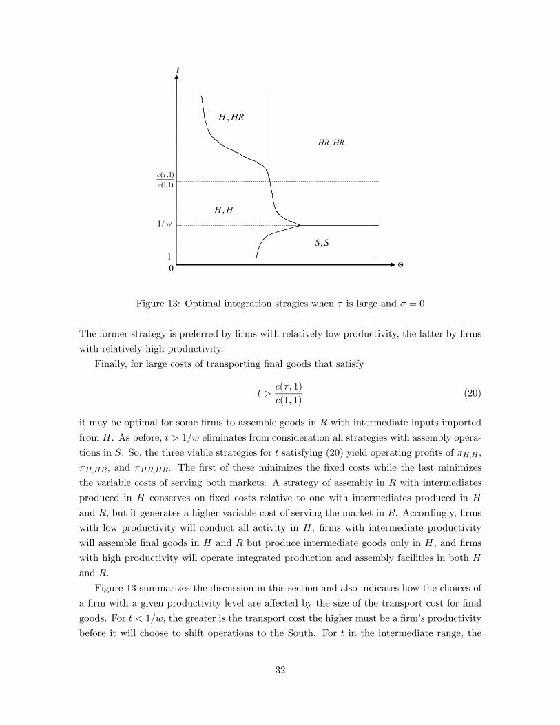
0 Θ1

t

HH ,

,H HR

,S S

,HR HR

1/w

( ,1)(1,1)ccτ

Figure 13: Optimal integration stragies when τ is large and σ = 0

The former strategy is preferred by firms with relatively low productivity, the latter by firms

with relatively high productivity.

Finally, for large costs of transporting final goods that satisfy

t >c(τ , 1)

c(1, 1)(20)

it may be optimal for some firms to assemble goods in R with intermediate inputs imported

from H. As before, t > 1/w eliminates from consideration all strategies with assembly opera-

tions in S. So, the three viable strategies for t satisfying (20) yield operating profits of πH,H ,

πH,HR, and πHR,HR. The first of these minimizes the fixed costs while the last minimizes

the variable costs of serving both markets. A strategy of assembly in R with intermediates

produced in H conserves on fixed costs relative to one with intermediates produced in H

and R, but it generates a higher variable cost of serving the market in R. Accordingly, firms

with low productivity will conduct all activity in H, firms with intermediate productivity

will assemble final goods in H and R but produce intermediate goods only in H, and firms

with high productivity will operate integrated production and assembly facilities in both H

and R.

Figure 13 summarizes the discussion in this section and also indicates how the choices of

a firm with a given productivity level are affected by the size of the transport cost for final

goods. For t < 1/w, the greater is the transport cost the higher must be a firm’s productivity

before it will choose to shift operations to the South. For t in the intermediate range, the

32

greater are transport costs the lower is the productivity level at which a firm will open an

integrated production facility in R. And finally, for t large, the greater are transport costs, the

lower is the productivity level at which a firm is indifferent between maintaining an assembly

plant in R and not in H. The cost of shipping final goods has no bearing on firms’ decision

whether to produce intermediate goods in H only, or in H and R, since this decision applies

to firms that are not trading final goods in any case.

6 Concluding Remarks

In this paper, we have examined the joint determination of international trade and foreign

direct investment in a setting in which firms may choose among a rich array of integration

strategies. In our analysis, firms that are headquartered in a Northern country supply

differentiated final goods to two national markets in the North and one in the South. Each

such firm must produce an intermediate input and conduct assembly activities in order to

generate a final product. The firms may produce intermediate goods in their home country,

in the other Northern country, or in the South. Similarly, assembly may take place in

any of the three locations. And firms may choose to maintain plants for either or both

stages of production in multiple locations. Accordingly, there are many possible choices of

organizational forms available to firms. Each such choice has implications for the pattern of

trade in intermediate and final goods.

We characterized industries by the size of the fixed costs of maintaining a foreign sub-

sidiary for production of intermediate goods and for assembly, the cost of transporting in-

termediate and final goods internationally, and the fraction of the consumer demand that

resides in the low-wage South. For each industry, we derived the equilibrium organizational

forms of heterogeneous firms that differ in their productivity.

In an industry in which transportation of intermediate and final goods is costless, the rel-

ative size of fixed costs for foreign investment in intermediate goods and assembly determines

the set of organizational firms that are observed in equilibrium. Here, the relative sizes of

the markets have no bearing on the equilibrium choices, and there is no intra-industry FDI.

Firms with low productivity choose an integration strategy that minimize the fixed cost of

operation, whereas firms with high productivity seek to minimize variable costs of serving

the various markets.

When final goods are costly to transport, relative country size plays a role in determining

the viable multinational strategies. Generally, the larger is the consumer market in the South,

the greater is the fraction of firms that maintain subsidiaries there, not only for performing

assembly but also for producing intermediate goods. Also, the higher are transport costs

for final goods, the greater is the fraction of firms that performs assembly in two or more

locations. Finally, costly transport of intermediate goods can make it attractive for a firm to

33

produce intermediate goods in multiple locations. In all cases, the attractiveness of alternative

locations for each stage of production depends upon the choices contemplated for the other.

One limitation of our analysis in this paper is that we take the boundaries of the firm

as given. That is, we have simply assumed that firms must produce their own intermedi-

ate goods and perform assembly in-house. In other recent work (Grossman and Helpman,

2002, 2003, 2004) two of us have studied how contracting problems interact with factor-price

differentials and transport costs to determine which activities are outsourced and which per-

formed within a firms’ corporate boundaries. In those papers, the range of strategies open

to the multinational firm was substantially narrower than here. Ultimately, we would like

a theory that simultaneously explains the make-or-buy decision and the organization of the

multinational firm. Such a theory could help explain the broad range of corporate strategies

that are found in the firm-level data.

34

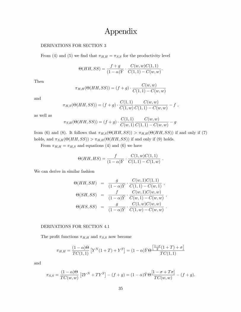
Appendix

DERIVATIONS FOR SECTION 3

From (4) and (5) we find that πH,H = πS,S for the productivity level

Θ(HH,SS) =f + g

(1− α)Y· C(w,w)C(1, 1)

C(1, 1)− C(w,w).

Then

πH,H(Θ(HH,SS)) = (f + g) · C(w,w)

C(1, 1)− C(w,w)

and

πH,S(Θ(HH,SS)) = (f + g) · C(1, 1)C(1, w)

C(w,w)

C(1, 1)− C(w,w)− f ,

as well as

πS,H(Θ(HH,SS)) = (f + g) · C(1, 1)C(w, 1)

C(w,w)

C(1, 1)− C(w,w)− g

from (6) and (8). It follows that πH,S(Θ(HH,SS)) > πH,H(Θ(HH,SS)) if and only if (7)

holds, and πS,H(Θ(HH,SS)) > πH,H(Θ(HH,SS)) if and only if (9) holds.

From πH,H = πH,S and equations (4) and (6) we have

Θ(HH,HS) =f

(1− α)Y· C(1, w)C(1, 1)

C(1, 1)− C(1, w).

We can derive in similar fashion

Θ(HH,SH) =g

(1− α)Y· C(w, 1)C(1, 1)

C(1, 1)− C(w, 1),

Θ(SH,SS) =f

(1− α)Y· C(w, 1)C(w,w)

C(w, 1)− C(w,w),

Θ(HS,SS) =g

(1− α)Y· C(1, w)C(w,w)

C(1, w)− C(w,w).

DERIVATIONS FOR SECTION 4.1

The profit functions πH,H and πS,S now become

πH,H =(1− α)Θ

TC(1, 1)

£Y N (1 + T ) + Y S

¤= (1− α)YΘ

£1−σ2 (1 + T ) + σ

¤TC(1, 1)

and

πS,S =(1− α)Θ

TC(w,w)

£2Y N + TY S

¤− (f + g) = (1− α)YΘ[1− σ + Tσ]

TC(w,w)− (f + g).

35

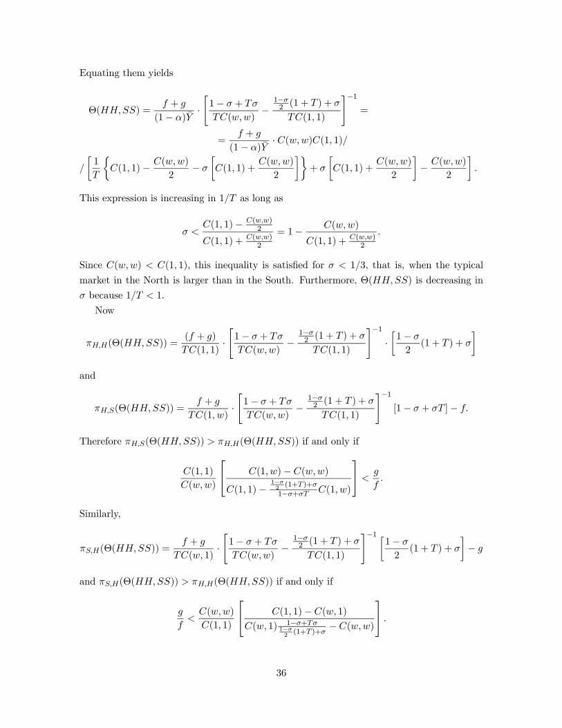
Equating them yields

Θ(HH,SS) =f + g

(1− α)Y·"1− σ + Tσ

TC(w,w)−

1−σ2 (1 + T ) + σ

TC(1, 1)

#−1=

=f + g

(1− α)Y· C(w,w)C(1, 1)/

/

·1

T

½C(1, 1)− C(w,w)

2− σ

·C(1, 1) +

C(w,w)

2

¸¾+ σ

·C(1, 1) +

C(w,w)

2

¸− C(w,w)

2

¸.

This expression is increasing in 1/T as long as

σ <C(1, 1)− C(w,w)

2

C(1, 1) + C(w,w)2

= 1− C(w,w)

C(1, 1) + C(w,w)2

.

Since C(w,w) < C(1, 1), this inequality is satisfied for σ < 1/3, that is, when the typical

market in the North is larger than in the South. Furthermore, Θ(HH,SS) is decreasing in

σ because 1/T < 1.

Now

πH,H(Θ(HH,SS)) =(f + g)

TC(1, 1)·"1− σ + Tσ

TC(w,w)−

1−σ2 (1 + T ) + σ

TC(1, 1)

#−1··1− σ

2(1 + T ) + σ

¸and

πH,S(Θ(HH,SS)) =f + g

TC(1, w)·"1− σ + Tσ

TC(w,w)−

1−σ2 (1 + T ) + σ

TC(1, 1)

#−1[1− σ + σT ]− f.

Therefore πH,S(Θ(HH,SS)) > πH,H(Θ(HH,SS)) if and only if

C(1, 1)

C(w,w)

C(1, w)− C(w,w)

C(1, 1)−1−σ2(1+T )+σ

1−σ+σT C(1, w)

<g

f.

Similarly,

πS,H(Θ(HH,SS)) =f + g

TC(w, 1)·"1− σ + Tσ

TC(w,w)−

1−σ2 (1 + T ) + σ

TC(1, 1)

#−1 ·1− σ

2(1 + T ) + σ

¸− g

and πS,H(Θ(HH,SS)) > πH,H(Θ(HH,SS)) if and only if

g

f<

C(w,w)

C(1, 1)

C(1, 1)− C(w, 1)

C(w, 1) 1−σ+Tσ1−σ2(1+T )+σ

− C(w,w)

.

36

We can derive Θ(HH,HS) from πH,H = πH,S, which yields

Θ(HH,HS) =f

(1− α)Y·"1− σ + σT

TC(1, w)−

1−σ2 (1 + T ) + σ

TC(1, 1)

#−1.

The expression for σ in the last term is

σ =T − 1

TC(1, w)+

T − 12TC(1, 1)

,

implying that Θ(HH,HS) is decreasing in σ. Similarly, we find that Θ(HS,SS) is

Θ(HS,SS) =g

(1− α)Y· 1

1− σ + Tσ··

1

TC(w,w)− 1

TC(1, w)

¸−1,

which is decreasing in σ.

DERIVATIONS FOR SECTION 4.2

Equating πH,HR and πH,HS we obtain

(1− α)YΘ[(1− σ)T + σ]

TC(1, 1)− f = (1− α)YΘ

"1−σ2

C(1, 1)+[1−σ2 + Tσ

TC(1, w)

#− f ,

or equivalently,

σH =TC(1, w)−C(1, 1)

(2T − 1)C(1, 1) + (T − 2)C(1, w) .

Similarly, equating πS,HR and πS,HS yields

(1− α)YΘ[(1− σ)T + σ]

TC(w, 1)− (f + g) = (1− α)YΘ

"1−σ2

C(w, 1)+[1−σ2 + Tσ

TC(w,w)

#− (f + g) ,

or

σS =C(w, 1)− TC(w,w)

(2− T )C(w,w) + (1− 2T )C(w, 1) .

DERIVATIONS FOR SECTION 4.4

When the productivity draws θ have a Pareto distribution, the distribution of produc-

tivity among the population of firms who remain in the market is also Pareto, and so is the

distribution of Θ among these firms. Let the distribution of Θ be 1 − (b/Θ)k, where Θ ≥ b

37

and k > 1. Then for the case in which g/f is large,

γH,S = bk·

1

Θ(HH,HS)k− 1

Θ(HS,SS)k

¸=

·b(1− α)Y

T

¸k "1

fk··

1

C(1, w)− 1 + T

2C(1, 1)

¸k− 1

gk··

1

C(w,w)− 1

C(1, w)

¸k#.

This expression is decreasing in T .

When g/f is small, we have

γS,H = bk·

1

Θ(HH,SH)k− 1

Θ(SH,SS)k

¸

=£b(1− α)Y

¤k 1gk

µ1

2T+1

2

¶k

··

1

C(w, 1)− 1

C(1, 1)

¸k− 1

fk·"

1

TC(w,w)−

12T +

12

C(w, 1)

#k .

The derivative of this expression with respect to T is

∂γS,H∂T

=− £b(1− α)Y

¤kgk

k

µ1

2T+1

2

¶k−1 1

2T 2··

1

C(w, 1)− 1

C(1, 1)

¸k−£b(1− α)Y

¤kfk

· k"

1

TC(w,w)−

12T +

12

C(w, 1)

#k−1 · −1T 2C(w,w)

+1

2T 2C(w, 1)

¸

=£b(1− α)Y

¤k k

T 21

fk··

1

TC(w,w)− 1 + T

2TC(w, 1)

¸k−1 · 1

C(w,w)− 1

2C(w, 1)

¸− £b(1− α)Y

¤k k

T 21

gk

µT + 1

2T

¶k−1 12

·1

C(w, 1)− 1

C(1, 1)

¸k,

which is negative as long as

1

gk

µT + 1

2T

¶k−1 12

·1

C(w, 1)− 1

C(1, 1)

¸k>1

fk··

1

TC(w,w)− 1 + T

2TC(w, 1)

¸k−1 · 1

C(w,w)− 1

2C(w, 1)

¸,

or equivalently,121/k

¡T+12T

¢ k−1k

h1

C(w,1) − 1C(1,1)

ih

1TC(w,w) − 1+T

2TC(w,1)

ik−1kh

1C(w,w) − 1

2C(w,1)

i 1k

>g

f.

The left hand side is bounded away from zero and infinity as long as T ≤ C(w,1)C(w,w) . This

range includes the moderate transport cost region. It follows that for g/f small enough the

derivative is negative.

38

References

[1] Axtell, Robert L. (2001), “Zipf Distribution of U.S. Firm Sizes,” Science, 293, 1818-1820.

[2] Brainard, Lael S. (1997) “An Empirical Assessment of the Proximity-Concentration

Trade-off between Multinational Sales and Trade,” American Economic Review, 87, 520-

544.

[3] Ekholm, Karolina, Forslid, Rikard and Markusen, James (2003) “Export Platform For-

eign Direct Investment” NBER Working Paper No. 9517.

[4] Feinberg, Susan E. and Keane, Michael P. (2003) “Accounting for the Growth of MNC-

Based Trade Using a Structural Model of U.S. MNCs” University of Maryland, manu-

script.

[5] Grossman Gene M. and Helpman, Elhanan (2002), “Outsourcing in the Global Econ-

omy,” NBER Working Paper No. 8728, forthcoming in the Review of Economic Studies.

[6] Grossman, Gene M, and Helpman, Elhanan (2003), “Outsourcing versus FDI in Industry

Equilibrium,” Journal of the European Economic Association, 1, 317-327.

[7] Grossman Gene M. and Helpman, Elhanan (2004), “Managerial Incentives and the In-

ternational Organization of Production,” forthcoming in the Journal of International

Economics.

[8] Hanson, Gordon H., Mataloni, Raymond J. and Slaughter, Matthew J. (2001), “Ex-

pansion Strategies of U.S. Multinational Corporations,” Brookings Trade Forum 2001,

245-294.

[9] Helpman, Elhanan (1984) “A Simple Theory of International Trade with Multinational

Corporations,” Journal of Political Economy, 92, 451-471.

[10] Helpman, Elhanan and Krugman, Paul (1985) Market Structure and Foreign Trade,

Cambridge, MA, The MIT Press.

[11] Helpman, Elhanan, Melitz, Marc and Yeaple, Stephen (2003). “Export versus FDI with

Heterogenous Firms,” forthcoming in the American Economic Review.

[12] Markusen, James R. (1984) “Multinationals, Multi-Plant Economies, and the Gains from

Trade,” Journal of International Economics, 16, 205-226.

[13] Markusen, James R. (2002) Multinational Firms and the Theory of International Trade,

Cambridge, MA and London, UK: The MIT Press.

[14] Markusen, James R. and Venables, Anthony J. (1998) “Multinational Firms and the

New Trade Theory,” Journal of International Economics, 46, 183-203.

39

[15] Markusen, James R. and Venables, Anthony J. (2000) “The Theory of Endowment,

Intra-Industry, and Multinational Trade,” Journal of International Economics, 52, 209—

234.

[16] Melitz, Marc (2002) “The Impact of Trade on Intra-Industry Reallocations on Aggregate

Industry Productivity,” NBER Working Paper No. 8881, forthcoming in Econometrica.

[17] UNCTAD (1998) World Investment Report: Trends and Determinants, New York and

Geneva: United Nations Conference on Trade and Development.

[18] UNCTAD (2002) World Investment Report: Transnational Corporations and Export

Competitiveness, New York and Geneva: United Nations Conference on Trade and De-

velopment.

[19] Yeaple, Stephen R. (2003), “The Complex Integration Strategies of Multinationals and

Cross Country Dependencies in the Structure of Foreign Direct Investment,” Journal of

International Economics, 60, 293-314.

40