online rescheduling of multiple picking agents for warehouse management
TRANSCRIPT

1
Online Rescheduling of Multiple Picking Agents for Warehouse
Management
Jose I.U. Rubrico,1 Toshimitu Higashi,2 Hirofumi Tamura,3 and Jun Ota4
1Department of Precision Engineering, The University of Tokyo, 7-3-1 Hongo, Bunkyo-ku, Tokyo 113-8656,
Japan
2Murata Machinery, Ltd., 2 Nakajima, Hashizume, Inuyama-shi, Aichi 484-0076, Japan
3Murata Systems, Ltd., 3 Minamiochiai-cho, Kisshoin, Minami-ku, Kyoto 601-8326, Japan
4 Research into Artifacts, Center for Engineering (RACE), The University of Tokyo, 5-1-5 Kashiwanoha,
Kashiwa, Chiba 277-8568, Japan
Abstract
In this paper, we present a solution for a dynamic rescheduling problem involving new orders arriving
randomly while static orders have been given in advance in warehouse environments. We propose two
variations of an incremental static scheduling scheme: one based on the steepest descent insertion, called
OR1, and the other, on multistage rescheduling, called OR2. Both techniques are enhanced by a local
search procedure specifically designed for the problem at hand. We also implemented several existing
online algorithms to our problem for evaluative purposes. Extensive statistical experiments based on real
picking data indicate that the proposed methodologies are competitive with existing online schedulers and
show that load-balancing algorithms, such as OR1, yield the best results on the average and that OR2 is
effective in reducing the picking time when dynamism is low to moderate.
Keywords: dynamic scheduling, warehouse management, on-line algorithm

2
1. Introduction
The problem of picking customer orders from warehouse storage to the packing/delivery area, i.e.,
order picking, is one of the most important activities in a warehouse due to its high operational cost.
Studies have shown that order picking can amount to 60% of the total costs of warehouse operations [1].
Traditionally, due to the high percentage of travel time in an order picker’s activity [2], order picking has
been treated as a distance-minimization problem. Optimization of a single picking route may be found in
Refs.[3-7], among others.
For multiple routes and order pickers, exact methods are presented in Refs. [8-9], while heuristics for
the cluster-then-route approach are investigated in Ref. [10]. In a series of works, Rubrico et al. [11-14]
solve a more complicated form of the order-picking problem with multiple pickers (agents), in which each
agent may be assigned more than one trip (route) to accomplish and delays due to congestion or queuing
are considered. The objectives are to minimize an agent’s idle time by minimizing the travel distance and
delays as well as maintain the balance of the load among the agents. They adapt a hierarchical
decomposition and solve each subdivision using heuristics to achieve good schedules quickly for
realistically sized problems.
The works reported above address a static order-picking problem in which all orders to be picked are
known beforehand. Purely online versions of a picking problem in which all orders are not known
beforehand and arrive at random are addressed in Refs. [15-16], where stochastic distributions are assumed
for the order parameters and the problem is solved using methods related to the queuing theory. The online
picking problem can be seen as an instance of the general online scheduling problem, in which the agents
retrieving the orders correspond to machines that process jobs. A description of the online scheduling
problem and its variants, as well as surveys of eminent online algorithms, may be found in Refs. [17-20].
Online scheduling on uniform machines (i.e., a given job may be processed on any machine at the same
cost) has been relatively well studied [21-25]. However, such a straightforward representation cannot be
directly applied to the online picking problem because the cost incurred by the agent as a result of a random
order will depend on the agent’s current load and is further complicated by the occurrence of delays. A
more appropriate representation of the online picking problem is the scheduling of unrelated machines, in
which the cost of processing a given job may differ arbitrarily from one machine to another. Literature on

3
this difficult variation of the online scheduling problem remains relatively sparse[26-27]. In one study [26],
Aspnes et al. investigate the characteristics of a post-greedy variation of Graham’s algorithm (originally
intended for scheduling on uniform machines [21]) and propose a procedure that attains the best possible
worst-case behavior (according to competitive analysis [28-29]) for the online scheduling of jobs on
unrelated machines.
Another problem closely related to the online picking problem is the dynamic vehicle routing problem
(DVRP). Typical dynamic events include: a) customer additions/deletions, b) changing path costs (e.g.,
road traffic status), and c) contingencies, such as vehicle breakdowns and recovery. These dynamic
parameters can cause re-planning of routes and rescheduling of vehicles as well as the addition of vehicles
for dispatching to meet strict due dates. Their correspondence with the online picking problem is apparent,
and, in it, the addition of customers corresponds to the random arrival of new orders. A survey of the
classifications, variants, and methodologies for the DVRP may be found in Ref. [30]. In Ref. [31], a
parallel tabu search is used incrementally to improve a solution between dynamic events (e.g., order of
arrivals). A generalization of this approach is discussed in Ref. [32] as the Multiple Plan Approach (MPA),
which keeps multiple plans each time an event occurs to allow for greater flexibility in the solution choice
as time progresses. The MPA is a framework that is independent of the search procedure. In the same paper,
the authors also introduce an enhancement of the MPA that includes the forecasting capability. This
approach is referred to as the Multiple Scenario Approach, in which the solutions kept include predicted
demands incorporated with existing ones. In Ref. [33], a reactive architecture based on constraint
programming is proposed to deal with dynamic changes in real time, while, in Ref. [34], a software
prototype is presented that demonstrates the capabilities of reactive vehicle routing.
In this paper, we are interested in solving the dynamic problem of new orders arriving randomly while
the static orders are in the process of being picked. This problem is referred to here as the online
rescheduling problem because it involves modifying the existing agent schedules in order to effectively
incorporate the new orders along with the old ones, which are yet unpicked. The arrival of new orders is
considered in this study because it is the primary cause of dynamicity in a real picking operation. The
rescheduling problem differs from strict online scheduling, in which all orders arrive randomly. The
methods for online scheduling are somewhat limited for the rescheduling problem because they are unable

4
to modify the existing schedule by redistributing existing trips among the agents. On the other hand, the
DVRP with stochastic demands is more similar to the problem presented in this paper. However, because
of the metropolitan scales of distances in the DVRP, a calculation time of approximately one minute is
acceptable from the methodologies reported in the preceding paragraphs. Such times are too slow for the
picking problem and will severely delay operations. Thus, there is a need for faster rescheduling methods
for our problem which, nonetheless, yield good and robust schedules.
The objective of the study is to investigate the performance of two variants of an incremental static
scheduler that resolves the total schedule every time a new order arrives by comparing it to existing online
schedulers in the literature and in general practice. The incremental static framework is adapted because of
its speed and low resource overhead as compared to more elaborate methods, such as those in Refs. [31-32].
The rest of the paper proceeds as follows. In Section 2, the online rescheduling problem is described.
In Section 3, the proposed and reference methodologies are described. In Section 4, results from evaluative
experiments are presented, and Section 5 is the conclusion.
2. Problem
The online rescheduling problem is a dynamic extension of the warehouse picking problem (WPP)
preliminarily described in Ref. [11]. In the static version, a set of customer orders must be retrieved from
warehouse storage shelves by a group of picking agents and transferred to a common packing shed. In the
online problem, new orders randomly arrive and are added to the list of orders to be picked even while the
static orders are being retrieved. Figure 1 illustrates an input (order list) and output (agent picking schedule)
example. For the static problem, the order list remains unchanged in time until picking is completed,
whereas, for the dynamic WPP (DWPP), the order list continually grows in a random manner as time
passes until some terminating condition is satisfied. Some assumptions on the dynamic problem are
enumerated below:
Static and dynamic orders have the same priority
All static and dynamic orders must be picked
A dynamic order cannot be inserted into a trip currently being traversed by an agent
Only order additions are considered (i.e., no cancellations)

5
A newly arrived order is composed of one type of product only
Stochastic Orders
The parameters that characterize the random orders are a) arrival rate λ (orders per unit time), b)
product information, i.e., storage quantity prand and required quantity drand, and c) total item ratio with static
orders, γ = Drand/Dstatic, where Drand is the total quantity of random orders picked and Dstatic is the total
number of static orders.
The arrival of new orders is taken to be exponentially distributed. A transformation can be made to
express the inter-arrival time in terms of the uniform distribution, as given in (1) below. The term U
denotes a uniform distribution of random variates within interval (0,1), while τarr is the inter-arrival time,
i.e., the time interval between order arrivals.
)ln(Uarr
(1)
As each new order arrives, the quantity of a product that it requires is assumed to be uniformly
distributed within the range of [1,Q], where Q is the capacity of an agent. Similarly, the location,
represented by the storage shelf, is also uniformly distributed in the warehouse.
The γ parameter is generally a characteristic of a specific warehouse and may change with market
seasons and other factors. In some warehouses, this parameter may be used as a decision variable (e.g., how
many picking agents to use). For the industry partner of this research, a common value is γ = 0.5, indicating
that almost a third of the products picked from their warehouses are stochastic in nature. In (1) above, if τarr
is taken to be the total picking time horizon T, then τarrλ = Tλ = nx, where n is the total number of orders
picked, x is the ratio of random orders to the total orders picked, and, hence, nx is the number of random
orders that arrived after time T elapsed. Note that varying either γ or the arrival rate λ affects the dynamicity
of the system.
Objective and Time Constraint

6
The objective of the online rescheduling problem is to minimize the makespan, i.e., the picking time,
of the total schedule. This makespan is necessarily dynamic because the schedule does not remain fixed but
is constantly modified as new orders are added. Due to the stochastic nature of the orders, only partial
information is available regarding the total input, and a global solution to the dynamic problem is not
possible. An alternative objective, then, is to optimize the schedule makespan each time a new order arrives,
subject to computational time restrictions. Although this does not guarantee the arrival at a global optimum,
it does assure that a good schedule is used every time a new order arrives.
Online rescheduling is to be done in real time, i.e., computational times must be limited to several
seconds at most. In the worst case, an agent that has just finished loading at the shed will wait for its new
trip assignment for a time not less than that required to recalculate the schedule. Thus, it is important to
keep the effect of this delay low to minimize on warehouse throughput.
Schedule Regeneration
Figure 2 illustrates the interaction between the static and dynamic aspects of the picking problem.
Initially, the offline scheduler supplies the picking agents with a schedule derived from the static orders. As
new orders arrive, the online scheduler modifies the current schedule to incorporate the new additions and
output the changes to the agents. This continues until new orders cease to arrive. Here, the modifiable
elements of an agent’s schedule are taken to mean all the trips that are not currently being traversed or have
not yet been traversed. In contrast to dispatching policies that are basically open-loop, the online scheduler
uses a feedback mechanism in which the state of the current schedule partly determines the recalculated
schedule.
3. Methodology
Incremental Static Rescheduling
The proposed online schedulers are presented here. Because of strict time considerations, the
schedulers are designed to be fast without sacrificing effectiveness. A global rescheduling strategy is
adopted in which a complete schedule is recalculated each time the input changes. An advantage of this

7
approach is that fast and efficient heuristics can be used to derive good schedules for the updated set of
orders in real time.
3.1.1 Steepest Descent Insertion
Figure 3 shows the flowchart of the proposed OR1 (Online Rescheduler 1). Assuming that picking is
still allowed in the warehouse, the scheduler waits for the arrival of a random order. When there is such an
order, it is immediately routed using a VRP heuristic (e.g., savings heuristic [35]). The resulting trip TN is
then assigned to the agent that is estimated to have the shortest makespan. A set of untraversed trips, ST, is
then created. TN is not included in ST. If the set is empty, then the schedule is left as it is. However, if the set
is not empty, then it means that it is still possible for the schedule to be improved by relocating demands. A
fast local search heuristic is used to implement the improvements.
Before elaborating more on the OR1, the basic operators and local search procedure used to minimize
the schedule makespan are first presented.
Basic Operators
Three types of demand relocation operators are considered. A demand refers to the items that need to
be picked from a given shelf location; hence, a demand relocation refers to the transfer or exchange of
demands between agents or within an agent (i.e., between trips of an agent), as illustrated in Figure 4. Here,
each segment corresponds to a trip (i.e., a picking cycle subject to an agent’s capacity). The numbers
correspond to the shelf identifications (0 designates the shed), while those in parentheses refer to the
number of items to be picked from the corresponding shelf.
Let s1 be a shelf that is visited by agent a1, and let d1 be the demand to be picked by a1 from s1. A
demand transfer (M1) is a move that transfers d1 items of s1 from a1 to another agent, a2. A new trip is
constructed to serve s1 and then assigned to a2. Thus, a2 will have one extra trip after the transfer. Note
that a demand transfer is only allowed if a1 will have at least one remaining shelf to visit after the demand
of s1 is removed from it.
The next operator is the demand exchange (M2), wherein the d1 items from shelf s1 currently assigned
to agent a1 are relocated to another agent, a2. Similarly, d2 items from shelf s2 currently assigned to a2 are
relocated to a1. After the exchange, a1 and a2 will each have one extra trip containing the demands of s1
and s2, respectively.

8
The splitting demand transfer (M3) is an extension of the M1 operator that allows partial relocation of
a shelf’s demands from one agent to another provided that such a transfer improves the balance of the
agents’ makespans. Figure 5 illustrates such an instance.
For any shelf s with total demand d currently assigned to agent a1, we can estimate the amount of items d*
of s to be moved from a1 to another agent, a2, so that their makespans are balanced:
1 2( ) ( )*
2a a s
LOAD
MK MK Td
T
(2)
MKa1 and MKa2 are the makespans of a1 and a2, respectively, before demand d* is relocated, Ts is the travel
time for the new trip assigned to a2 containing d* items of s, and TLOAD is the loading time for a single item.
In the event that the agents’ makespans cannot be balanced by a partial relocation of p, the value of d* will
be less than or equal to zero. On the other hand, if d* is greater than or equal to d, then more than d items
are needed to balance the agents’ makespans.
Local Search Procedure
In previous studies, the introduction of direct trips serving the relocated demands may result in a)
suboptimal travel distance for each of the affected agents, resulting in longer makespans and b) large delays
caused by loading queues that may occur after modifying the schedule unchecked. The local search (LS)
procedure (Figure 6) is applied after every basic move operation to minimize the undesirable effects
mentioned. This figure corresponds to the rectangle “Improve Schedule Using Local Search” in Figure 3.
The first problem is to determine how to best incorporate the transferred demand in the schedule of the
receiving agent. This problem is non-trivial and involves solving a VRP for every demand transfer.
Because such a task needs to be repeated numerous times in the search, a fast heuristic is employed. The
DLGIA procedure in Ref. [36] is utilized for this purpose, although any other “good” VRP improvement
procedure will suffice. Figure 7 explicitly illustrates the demand insertion procedure utilizing the VRP
procedure. Here, the demand from shelf 13 is moved from agent a1 to agent a2. The VRP representation of
each agent’s pallets changes accordingly from the original (Step 1) to the intermediate state (Step 2). The
final frame (Step 3) shows the improvement trips for each agent after the VRP heuristics have been applied.

9
After the trips of the agents involved in the demand transfer/exchange have been improved, the next
step is to determine whether the new schedule has queuing delays. The NoLQ2 procedure shown in Figures
6 and 11, diagrammed as Figure 8, is applied to minimize the reported delays. In the figure,
numLQ – number of queues in the current schedule
maxLQ –maximum queue delay in the current schedule
mkmaxNumLQ – number of queues for the agent with the maximum makespan
curLQ – the current queue being minimized
The parameters above are estimated using a fast, variable time-step schedule simulator embedded in
the improvement loop. The simulator is run each time the schedule is modified to obtain the estimates.
The RESEQUENCE procedure will reassign the dispatch sequence of a trip assigned to an agent if
doing so minimizes or eliminates loading queue delays, as shown in Figure 9, while the INVERT
procedures reverse the traversal sequence of a trip if this minimizes or eliminates loading queues, as shown
in Figure 10.
In the following figures, tLQ refers to the trip(s) containing the products at the shelf pLQ that cause
the queuing delay. The function f1() returns the makespan.
3.1.2 Online Multistage Rescheduling
The second online rescheduler is referred to as OR2. For this variant, whenever a new order arrives, a
VRP improvement procedure is applied to all currently unserved routes plus the direct trip serving the new
order. The resulting routes are then reassigned to the agents using the load-balancing techniques presented
in Ref. [11] and a queue-minimization procedure similar to that described in Section 3.1.1. This procedure
minimizes the makespan by reducing the idle time associated with the agents, i.e., the travel time and
queuing delays. The logical diagram of the OR2 and its listing are given in Figure 11.
3.2 Other Algorithms for Comparison
Among the variants of the online scheduling problem, the one most similar to our problem is that of
scheduling unrelated machines. This variation is the most general and involves machines with arbitrary
processing speeds.

10
As far as we know, there are only two algorithms on the said scheduling problem that have been
formally investigated [26]. We implement both as a basis of comparison for the proposed methods. They
are selected because they solve a similar problem to ours and are considerably fast.
The first one is the G66 Listing algorithm that is an extension of Graham’s List scheduling [21] to the
DWPP. The main idea of this algorithm is to balance the load among the agents by assigning a new order to
the agent that will increase its makespan the least if the new order is added to it.
The second one is an extension of Aspnes’93 algorithm [4] to the DWPP. This algorithm tends to create
a load imbalance if the agents’ makespans are roughly the same instead of always maintaining the load
balance.
3.3 Reference Online Scheduler
The reference is an online extension to a widely practiced procedure to schedule picking agents.
Initially, trips are generated according to the S-Shaped heuristic [21] and then assigned sequentially to each
agent. An agent is assigned a new trip as soon as it reaches the shed and becomes idle. This goes on until
all the orders are picked.
The logic of the online reference scheduler is diagramed in the flowchart in Figure 12. Assuming that
picking is still allowed in the warehouse, the scheduler continually checks for the presence of an idle agent
in the shed. If there is such an agent, then it is assigned the next available trip generated from the offline
orders. However, if all offline trips have already been assigned, then the warehouse order queue is checked
for pending (i.e., random) orders. If there are any, the orders are routed, and the resulting trip is assigned to
the idle agent. A waiting loop is entered while there are no idle agents in the shed or no pending orders to
be routed.
4 Experiments
4.1 Simulation Setup
The experiments are done on a set of real data instances. A summary of the base static instances is
given in Table 1. For every shelf distribution, there are two different item densities (i.e., the average
number of items picked per active shelf) with one density higher (“a” suffix) than the other (“o” suffix).
The agent capacity Q is taken to be 60 items. The instances generally have irregular shelf distributions with
some small clusters in a number of aisles. The warehouse is large with 1,000 storage shelves. The aisles of

11
the warehouse are wide enough so that two picking agents can pick side by side with room to spare for
maneuvers. Such characteristics reflect the kind of setup used in the real system considered here.
Initial solutions are first generated for the base instances. Then, while the orders are being picked, new
orders are allowed to arrive randomly. For each static data, 10 online instances are generated (i.e., using
different random number generator seeds). In the experiments, γ = 0.2, 0.5, 0.8, and m = 8 agents to
correspond to the common situations in the warehouse of the industry partner. To investigate the sensitivity
of the online reschedulers to the inter-arrival times of the random orders, the experiments are run on λ =
0.0025, 0.005, 0.01, 0.025, 0.05, and 0.1. Thus, for each online algorithm tested, 6*10*3*6 = 1,080
simulations are done, resulting in 5,400 total simulations run for the five procedures evaluated.
Except for the reference scheduler, all other schedulers use the same initial static schedule (for a given
base instance), in which each agent is already assigned the complete list of trips that it must complete at the
start of the picking process. In contrast to the S-Shaped heuristic used by the reference, all other schedulers
generate their trips using the parallel savings heuristic [37].
4.2 Results
The comparative results of the experiments are presented here. The evaluation is done on the basis of a
makespan. In the discussions that follow, the term “scheduler” is used in place of “rescheduler” for
convenience.
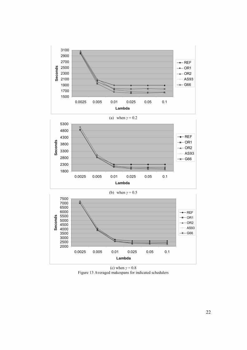
Figure 13 shows the makespans obtained using the schedulers tested. The values correspond to the
average taken over 60 data instances (6 base instances*10 online instances per base instance) for a given λ
and γ. For a fixed γ, uncertainty increases as λ decreases because random orders will arrive more slowly and
the system degenerates into a first-come-first-served (FCFS) queue in which planning becomes
meaningless. As λ increases, random orders arrive quickly enough so that they can be rescheduled with
most of the yet unpicked static orders, thus reducing the uncertainty in the system. On the other hand, for a
fixed λ, dynamicity increases with γ since it would mean an increased ratio of random orders.
The percent improvement of OR1, OR2, AS93, and G66 against the reference (REF) scheduler is
tabulated in Table 2. A negative improvement indicates that the solution of the corresponding scheduler is
worse than that of the reference.
The following observations can be made from the makespan results:

12
All schedulers tend to perform equivalently as dynamicity increases (i.e., small λ and large γ). This
is apparent in the way the makespan values converge as λ decreases.
OR1 performs significantly better than the reference except in the most dynamic cases tested, in
which its performance is equivalent to the reference. Its improvements tend to increase as
dynamism decreases, as expected from an incremental static scheduler. This results in the best
average improvement of 8.31% over the reference.
OR2 performs significantly better than the reference when dynamism is low to moderate. However,
when uncertainty is high, it tends to perform worse than the reference. This results in both the
highest (15.53%) and the lowest (-4.96%) improvement. This suggests that distance optimization
is more effective in minimizing the makespan when sufficient planning is applicable (i.e., many
orders are still available to be rescheduled jointly). When the system becomes more dynamic,
random orders arrive piecemeal in an FCFS fashion, and minimizing the travel time does not
necessarily minimize the picking time. OR2 shows an average improvement of 6.17% over the
reference.
AS93 performs as well as the reference when dynamism is high and provides slight to moderate
improvements as the system becomes more static. Its average improvement is 1.83%.
The G66 algorithm performs as well as the reference when dynamism is high. It performs
significantly better when dynamism is decreased. This is interesting in that the greedy algorithm
theoretically has a much larger worst-case margin than the AS93 (optimal worst-case margin). On
the average, it shows improvement of 5.29% over the reference.
All recalculation times are real time and do not exceed 5 seconds.
The first observation results from the characteristic breakdown of any scheduler into an FCFS policy
when the remaining random inputs continue to arrive long after all static and early random orders have
been picked. In this state, the makespans of different schedules level out as the agents remain idle and
simply wait for the arrival of the next order. The second and third observations are consistent with the fact
that, when dynamism is low to moderate, redistributing trips among agents is beneficial because of the
more global consideration in improving the makespan than the restricted approach adopted by the reference
and online schedulers (G66, AS93). It also indicates that minimizing the average makespan by reducing the

13
idle travel time (OR2) does not necessarily minimize the maximum makespan when randomness is high
because there will be fewer available trips that OR2 can reroute. On the other hand, OR1 reduces to a load
balancing scheduler under such circumstances and performs well, not unlike G66, which also strives to
achieve makespan balance. The AS93 is unable to remain competitive with the other schedulers because it
sacrifices balance to minimize the worst-case performance. Thus, unless a degenerative instance is being
scheduled, it often underperforms.
5. Conclusion
In this paper, we address a problem of online rescheduling in which new orders arrive randomly while
static orders are still being picked. Two real-time incremental static reschedulers are proposed: OR1, which
is based on a steepest descent insertion scheme, and OR2, which is based on a multistage optimization
procedure (distance minimization, load balancing, and queuing delay minimization).
Extensive statistical experiments on real data instances reveal that load-balancing algorithms, such as
OR1 and G66, yield the best results on the average. They are consistent, either matching the performance
of the reference (within 1%) or improving it significantly (by 6% or more). On the other hand, the tests
show that algorithms possessing desirable worst-case margins (AS93) do not necessarily perform well on
the average. It is also evident that incremental distance minimization (OR2) is effective in reducing the
picking time when dynamism is low to moderate. However, it performs badly when dynamism is high.
These results show that the proposed online reschedulers are competitive against existing online
methods when uncertainty in the system is low to moderate. These are the levels of dynamism often
encountered in real picking systems that tend to restrict the incorporation of random orders with existing
ones for accountability and due-date concerns. Thus, OR1 and OR2 can provide significant improvements
in real picking systems that have a mix of static and stochastic inputs.
There are several limitations of the proposed algorithms. One is that we only assume the situation in
which a new order is coming. However, in real working environments, many other disturbances may occur,
such as a disorder of some apparatus or delay in the completion of a certain operation. We need to take
such effects into account. Another important issue is that agents are heterogeneous and can change
dynamically in real environments. In that case, it is not easy to measure the performance of each agent

14
precisely, and it may introduce bad performance in rescheduling. We need to deal with the problem as a
future work.
References
[1] J. Drury, “Towards more efficient order picking,” IMM Monograph No. 1, The Institute of Materials
Management, Cranfield, U.K., 1988.
[2] J. A. Tompkins, et al., Facilities Planning, John Wiley & Sons, New York, 1996.
[3] H. D. Ratliff and A. S. Rosenthal, “Order-picking in a rectangular warehouse: A solvable case for
the traveling salesman problem,” Op. Res. 31(3) (1983), pp. 507-521.
[4] K. J. Roodbergen and R. De Koster, “Routing methods for warehouses with multiple cross-aisles,”
Int. J. Prod. Res. 39(9) (2001), pp. 1865-1883.
[5] K. J. Roodbergen and R. De Koster, “Routing order-pickers in a warehouse with a middle aisle,”
European J. Op. Res. 133 (2001), pp. 32-43.
[6] M. B. De Koster, E. S. Van Der Poort, and M. Wolters, “Efficient orderbatching methods in a
warehouse,” Int. J. Prod. Res. 37(7) (1999), pp. 1479-1504.
[7] R. W. Hall, “Distance approximations for routing manual pickers in a warehouse,” IIE Trans. 25(4)
(1993), pp. 76-87.
[8] A. J. R. M. Gademann, J. P. Van Den Berg, and H. H. Van Der Hoff, “An order batching algorithm
for wave picking in a parallel-aisle warehouse,” IIE Trans. 33(5) (2001), pp. 385-398.
[9] A. J. R. M. Gademann and S. van de Velde, “Order batching to minimize total travel time in a
parallel-aisle warehouse,” IIE Trans. 37(1) (2005), pp. 63-75.
[10] M. B. Rosenwein, “An application of cluster analysis to the problem of locating items within a
warehouse,” IIE Trans. 26(1) (1994), pp. 101-103.
[11] J. I. U. Rubrico, J. Ota, T. Higashi, H. Tamura, and M. Akiyoshi, “Route generation for warehouse
management using fast heuristics,” IEEE/RSJ Int. Conf. on Intelligent Robots and Systems, Sendai,
(2004), pp. 2093-2098.
[12] J. I. U. Rubrico, J. Ota, T. Higashi, and H. Tamura, “Route assignment heuristics for picking
products in a warehouse,” Human and Artificial Intelligence Systems: From Control to Autonomy,

15
Proc. 4th Int. Symp. on Human and Artificial Intelligence Systems, K. Murase, L. Jain, K. Sekiyama,
T. Asakura, Eds., Advanced Knowledge International, (2004), pp. 341-346.
[13] J. I. U. Rubrico, J. Ota, T. Higashi, H. Tamura, and M. Akiyoshi, “Multi-agent scheduling in a
warehouse,” Int. Conf. on Instrumentation, Control and Information Technology (SICE 2005),
Okayama, (2005), pp. 3243-3247.
[14] J. I. U. Rubrico, J. Ota, T. Higashi, and H. Tamura, “Scheduling multiple agents for picking products
in a warehouse,” Int. Conf. on Robotics and Automation (ICRA 2006), Orlando, (2006), pp. 1438-
1443.
[15] E. P. Chew and L. C. Tang, “Travel time analysis for general item location assignment in a
rectangular warehouse,” European J. Op. Res. 112(3) (1999), pp. 582-597.
[16] T. Le-Duc, “Design and Control of Efficient Order Pickling Processes,” PhD Thesis, Erasmus
University Rotterdam, The Netherlands, (2005).
[17] S. Albers, “Competitive online algorithms,” BRICS Lecture Series LS96-2, Department of
Computer Science, University of Aarhus, (1996).
[18] J. Sgall, “Online Scheduling,” Developments from a June 1996 seminar on Online Algorithms: The
State of the Art, A. Fiat and G. Woeginger, Eds., Springer LNCS 1442 (1998), pp. 196-231.
[19] Y. Azar, “On-line load balancing,” Developments from a June 1996 seminar on Online Algorithms:
The State of the Art, A. Fiat and G. Woeginger, Eds., Springer LNCS 1442 (1998), pp. 178-195.
[20] T. Winter and U. T. Zimmermann, “Discrete online and real-time optimization,” Proc. 15th IFIP
World Computer Congress, Budapest/Vienna, (1998), pp.31-48.
[21] R. L. Graham, “Bounds for certain multi-processing anomalies,” Bell System Technical Journal 45
(1966), pp. 1563-1581.
[22] Y. Bartal, H. Karloff, and Y. Rabani, “A better lower bound for on-line scheduling,” Information
Processing Letters 50(3)(1994), pp. 113-116.
[23] Y. Bartal, A. Fiat, H. Karloff, and R. Vohra, “New algorithms for an ancient scheduling problem,”
Journal of Computer and System Sciences 51(3) (1995), pp. 359-366.
[24] D. Karger, S. Phillips, and E. Tong, “A better algorithm for an ancient scheduling problem,” Proc.
5th ACM-SIAM Symp. on Discrete Algorithms (1994) pp. 132-140.

16
[25] S. Albers, “Better bounds for online scheduling,” SIAM J. Comp. 29 (1999), pp. 459-473.
[26] J. Aspnes, Y. Azar, A. Fiat, S. Plotkin, and O. Waarts, “On-line load balancing with applications to
machine scheduling and virtual circuit routing,” Proc. 25th ACM Annual Symp. on the Theory of
Computing (1993), pp. 623-631.
[27] I. Caragiannis, “Better bounds for online load balancing on unrelated machines,” Proc. 19th annual
ACM-SIAM Symp. Discrete Algorithms, (2008), pp.972-981
[28] D. D. Sleator and R. E. Tarjan, “Amortized efficiency of list update and paging rules,”
Communication of the ACM 28(2) (1985), pp. 202-208.
[29] A. Karlin, M. Manasse, L. Rudolph, and D. D. Sleator, “Competitive snoopy caching,” Algorithmica
3(1-4)(1988), pp. 79-119.
[30] M. Gendreau and J. Potvin, Dynamic Vehicle Routing and Dispatching, Fleet Management and
Logistics, T. Crainic and G. Laporte, Eds., Kluwer (1998) pp. 115-126.
[31] M. Gendreau, F. Guertin, J. Y. Potvin, and E. Taillard, “Parallel tabu search for real-time vehicle
routing and dispatching,” Trans. Sci. 33(4) (1999), pp. 381-390.
[32] R. Bent and P. Van Hentenryck, “Dynamic vehicle routing with stochastic requests,” Int. Joint Conf.
on Artificial Intelligence (IJCAI), Acapulco, Mexico( 2003), pp. 1362-1363.
[33] K. Zhu and K. Ong, “A reactive method for real time dynamic vehicle routing problems,” Proc. 12th
IEEE Int. Conf. on Tools with Artificial Intelligence (ICTAI), Vancouver, BC, Canada (2000), pp.
176-180.
[34] H. C. Lau and D. Seah, “An efficient technique for routing of vehicles reactively,” Proc. 8th ITSA
Annual Meeting and Exposition, Detroit, Michigan (1998)
[35] G. Clarke and J. W. Wright, “Scheduling of vehicles from a central depot to a number of delivery
points,” Op. Res. 12(4) (1964), pp. 568-581.
[36] M. Dror and L. Levy, “A vehicle routing improvement algorithm: Comparison of “greedy” and a
“matching” implementation for inventory routing,” Comp. Op. Res. 13(1) (1986), pp. 33-45.
[37] K. Altinkemer and B. Gavish, "Parallel savings based heuristic for the delivery problem," Op. Res.
39(3) (1991), pp. 456-469.

17
ORDERS
PRODUCT SHELF # QTY
AAAGBX::EFEZ:
1750::110130:
105260::545:
WPP
SOLVER
AGENT SCHEDULE
AGENT SHELF SEQUENCE
A1 7,1,4,0; 2,13,0;40;43;47,0; 8,0;
A2 6,9,7,0; 21,23,5,0;60;72;75,0; 91,0;48,49,50,0; 100,0;:
A8 112,115,110,0;14,20,40,7,0; 3,0;
:
:
ORDERS
PRODUCT SHELF # QTY
AAAGBX::EFEZ:
1750::110130:
105260::545:
WPP
SOLVER
AGENT SCHEDULE
AGENT SHELF SEQUENCE
A1 7,1,4,0; 2,13,0;40;43;47,0; 8,0;
A2 6,9,7,0; 21,23,5,0;60;72;75,0; 91,0;48,49,50,0; 100,0;:
A8 112,115,110,0;14,20,40,7,0; 3,0;
:
:
Figure 1 Input and output of the picking problem
Figure 2 Static and dynamic aspects of the WPP
Randomorder?
START
Create a set ofuntraversed trips ST
Create a trip TN containingthe new order
ST
empty?
Assign TN to agent withminimum makespan
Improve schedule usinglocal search
Y
Y
N
N
Figure 3 Diagram for OR1 procedure

18
a1: 10 (25) 73 (20)0 131 (40) 1 (20)0
a2: 154 (50)0 18 (30) 89 (5)0
local relocation
non-local relocations
a1: 10 (25) 73 (20)0 131 (40) 1 (20)0
a2: 154 (50)0 18 (30) 89 (5)0
local relocation
non-local relocations
Figure 4 Agent schedule and demand relocation
a1: 10 (60)0 14(60)0
a2: 101 (60)0
a1: 10 (60)0 14(30)0
a2: 101 (60)0 14(30)0
Splitting for betterbalance
a1: 10 (60)0 14(60)0
a2: 101 (60)0
a1: 10 (60)0 14(30)0
a2: 101 (60)0 14(30)0
Splitting for betterbalance
Figure 5 The optimal non-splitting solution vs. the splitting solution
Local Search
Operators
BEGINcurrent iteration
Demandexchange?
Y
Remove d2 from andadd to a1 as a direct trip
Solve a VRP withthe nodes beingthe shelves of
Remove d1 from andadd to as a direct trip
N
Solve a VRP withthe nodes being
Use a scheduling procedure,NoLQ2 to minimize delays of
the resulting schedule
Determine operator and itsinputs a1, d1, a2, (d2)
Decide whether or not toaccept new schedule
ENDcurrent iteration
the shelves of
a2
a2a1
a1a2
Figure 6 Local search used in conjunction with operators

19
START
numLQ > 0
curLQ = mkmaxNumLQ curLQ = maxLQ
RESEQUENCE
IMPRV?
mkmaxNumLQ > 0
INVERT
IMPRV?
STOP
Y N
NY
Y N
Y N
Agent schedule aftermove ope rator and
VRP heu ristics are appl ied
Agent scheduleafter delay
management
NoLQ2
Figure 8 Diagram of the NoLQ2 procedure
Step 3. VRP Solutions
a1: 10 (25) 23 (20)0 7 (40) 13 (20)0
a2: 4 (50)0 8 (30) 9 (5)0
0
13
a1: 10 (25) 23 (20)0 7 (40)
13 (20)
0
a2: 4 (50)0 8 (30) 9 (5)0
7 10
23
4
8 9
0
move 0
0
7 10
23
4
8 9
0
13
direct trip
Q = 60 Q = 60 Q = 60 Q = 60
move
a1 Trips a2 Trips a1 Trips a2 Trips
a1: 10 (25)23 (20)0 7 (40)
13 (20)
0
a2: 4 (50)0 8 (30) 9 (5)0
0
7 10
23
4
8 9
0
13
regroupings
Q = 60 Q = 60
a1 Trips a2 Trips
Step 1. Original State Step 2. Move Operator
directtrip
Figure 7 Illustrating the VRP procedure as part of the local search

20
aLQt1 t6 t10
aLQt1 t6 t10
Original Trip Sequence of aLQ (Load Queues not shown)
Reinsertions of tLQ in aLQ (Load Queues not shown)
tLQ
tLQ
aLQtLQt1 t6 t10
aLQtLQt1 t6 t10
aLQtLQt1 t6 t10
Figure 9 Trip reinsertion, RESEQUENCE
aLQ1
t1 t6 t10
aLQ2
t2 t8 t3
Trips of agents sharing a pallet, pLQ, causing a load queue
Possible Inversions of tLQs to avoid loading queues
tLQ1
tLQ2
pLQ p12
pLQ
p14
p15
overlap
aLQ1
t1 t6 t10
aLQ2
t2 t8 t3
tLQ1
tLQ2
pLQp12
pLQ
p14
p15
aLQ1
t1 t6 t10
aLQ2
t2 t8 t3
tLQ1
tLQ2
pLQ p12
pLQ
p14
p15
Figure 10 Trip inversion, INVERT

21
RandomOrder?
START
Y
Y
N
create a trip TN containingthe new order
Assign TN to agent withminimum makespan
NY
“Improve routes”procedure
UntraversedRoutes?
“Reassign routes to agents” procedure
“NoLQ2(s)”procedure
RandomOrder?
START
Y
Y
N
create a trip TN containingthe new order
Assign TN to agent withminimum makespan
NY
“Improve routes”procedure
UntraversedRoutes?
“Reassign routes to agents” procedure
“NoLQ2(s)”procedure
Figure 11 Diagram for the OR2 procedure
OfflineTrips?
Assign next offlinetrip in sequence to
agent
Route orders usingS-Shape
RandomOrders?
Y
Y N
N
N
START
agent atshed?
Y
Assign newtrip to agent
Figure 12 Online reference scheduler
22
150017001900210023002500270029003100
0.0025 0.005 0.01 0.025 0.05 0.1
Lambda
Se
co
nd
s
REFOR1OR2AS93G66
(a) when γ = 0.2
1800
2300
2800
3300
3800
4300
4800
5300
0.0025 0.005 0.01 0.025 0.05 0.1
Lambda
Se
co
nd
s
REFOR1OR2AS93G66
(b) when γ = 0.5
200025003000350040004500500055006000650070007500
0.0025 0.005 0.01 0.025 0.05 0.1
Lambda
Se
co
nd
s
REFOR1OR2AS93G66
(c) when γ = 0.8
Figure 13 Averaged makespans for indicated schedulers

23
Table 1 Characteristics of the static base instances, Q = 60
0.2667Irregular30480MDAT3a
0.13Irregular30234MDAT3o
0.3556Irregular45960MDAT2a
0.2807Irregular45758MDAT2o
0.2524Irregular751136MDAT1a
0.1731Irregular75779MDAT1o
AverageItem Density
ShelfDistribution
Shelves
ItemsInstance
0.2667Irregular30480MDAT3a
0.13Irregular30234MDAT3o
0.3556Irregular45960MDAT2a
0.2807Irregular45758MDAT2o
0.2524Irregular751136MDAT1a
0.1731Irregular75779MDAT1o
AverageItem Density
ShelfDistribution
Shelves
ItemsInstance
Table 2 % Improvement of indicated schedulers over the reference
4.84%6.82%6.61%6.90%7.35%1.44%-0.08%0.8
6.08%8.98%9.13%8.98%7.12%2.10%0.20%0.5
4.96%6.74%6.44%6.71%6.49%2.53%0.83%0.2
G66
3.01%4.00%4.00%4.03%5.03%1.11%-0.12%0.8
3.63%5.13%5.13%4.95%5.90%0.55%0.14%0.5
-1.15%-1.55%-1.55%-1.55%-0.83%-1.35%-0.05%0.2
AS93
5.38%13.16%12.81%11.57%3.18%-4.96%-3.46%0.8
6.32%15.53%14.73%13.70%3.24%-4.97%-4.31%0.5
6.81%12.74%12.12%11.52%7.78%-1.88%-1.40%0.2
OR2
6.51%9.81%10.32%9.94%7.64%1.41%-0.08%0.8
8.20%13.77%12.07%13.15%8.33%1.44%0.46%0.5
10.20%13.14%14.04%14.29%12.16%6.01%1.59%0.2
OR1
AVE0.10.050.0250.010.0050.0025
Arrival Rate, λScheduler and γ