on the trade balance effects of free trade agreements between the eu15 and the ceec-4 countries

THE WILLIAM DAVIDSON INSTITUTE AT THE UNIVERSITY OF MICHIGAN

ON THE TRADE BALANCE EFFECTS

OF FREE TRADE AGREEMENTS BETWEEN THE EU-15 AND THE CEEC-4 COUNTRIES

By: Guglielmo Maria Caporale, Christophe Rault, Robert Sova and Ana Maria Sova

William Davidson Institute Working Paper Number 912 March 2008

ON THE TRADE BALANCE EFFECTS OF FREE TRADE AGREEMENTS

BETWEEN THE EU-15 AND THE CEEC-4 COUNTRIES

Guglielmo Maria CAPORALE, Centre for Empirical Finance, Brunel University, London1

Christophe RAULT,

Université d’Orléans, LEO, CNRS, UMR 6221, France; IZA, Germany; and William Davidson Institute at the University of Michigan, Ann Arbor,Michigan, United States;

web-site: http://membres.lycos.fr/chrault/2

Robert SOVA, CES, Sorbonne University, A.S.E and EBRC3

Ana Maria SOVA,

CES, Sorbonne University and EBRC4

Abstract

The expansion of regionalism has spawned an extensive theoretical literature analysing the effects of Free Trade Agreements (FTAs) on trade flows. In this paper we focus on FTAs (also called European agreements) between the European Union (EU-15) and the Central and Eastern European countries (CEEC-4, i.e. Bulgaria, Hungary, Poland and Romania) and model their effects on trade flows by treating the agreement variable as endogenous. Our theoretical framework is the gravity model, and the econometric method used to isolate and eliminate the potential endogeneity bias of the agreement variable is the fixed effect vector decomposition (FEVD) technique. Our estimation results indicate a positive and significant impact of FTAs on trade flows. However, exports and imports are affected differently, leading to some disparity in trade flow performance between countries. Therefore, there is an asymmetric impact on the trade balance, the agreement variable resulting in a trade balance deficit in the CEEC.

Keywords: Regionalisation, European integration, Panel data methods. JEL Classification: E61, F13, F15, C25.

1 Brunel University, Uxbridge, Middlesex UB8 3PH, UK. Tel.: +44 (0)1895 266713. Fax: +44 (0)1895 269770. Email: [email protected]. 2 Rue de Blois-B.P.6739, 45067 Orléans Cedex 2.E-mail : [email protected], web-site: http://membres.lycos.fr/chrault/index.html (corresponding author). 3 Center of Economics Studies Paris I, 106-112 bd. de L'Hôpital, 75647 Paris Cedex 13, France, and Academy of Economic Studies, Bucharest, Romania, E-mail: [email protected]. 4 Center of Economics Studies Paris I, 106-112 bd. de L'Hôpital, 75647 Paris Cedex 13, France, and Economic &Business Research Center, E-mail: [email protected].

2

Non-Technical Summary

This paper analyse the impact of association agreements on trade flows between the EU-

15 and CEEC-4 countries (i.e. Bulgaria, Hungary, Poland and Romania) treating the

agreement variable as endogenous and using appropriate panel methods to estimate a

gravity equation. The most relevant estimates are those provided by the FEVD estimation

method which is the most appropriate for our purposes. This method permits to obtain

unbiased coefficients and to capture the effects of time-invariant variables. As theory

suggests, association agreements were found to have a positive and significant impact on

trade flows between the participant countries. However, such effects appear to be

asymmetric, the estimated coefficient being higher for imports (0.36) than for exports

(0.21), which suggests trade asymmetry. In particular, the agreements resulted in

increased trade deficits for the CEEC-4 countries (net importers), which is not desirable

for economies still trying to catch up with the other EU states. Convergent or divergent

dynamics of imports and exports are the main cause of trade balance changes. The

evolution of exports, imports as well as of trade balance over the estimation period for all

CEEC-4 highlights the persistence and the deepening of the trade deficit.

The lower impact of the agreement on CEEC-4 exports can be interpreted in terms of low

EU demand for CEEC products reflecting their lack of attractiveness for European

consumers, despite their price competitiveness based on comparative advantages due to

lower labour costs. Trade liberalisation did not lead to a restructuring of exports and to a

development of the most innovative sectors of the economy. Instead, CEEC-4 exports are

still represented mainly by labour-intensive products with lower added value.

Higher trade openness and the progressive liberalisation of the capital flows resulting

from the trade agreement have strongly influenced the behaviour of multinationals firms.

Vertical FDI in the CEEC-4 countries has instead increased. This type of investment

consists in the fragmentation of the various operations of the production process to

implement them in countries offering lower costs. The production location which results

from it inevitably entails a rise of intermediate and equipments good imports of these

3

countries from the investor’s countries. Thus, in the case of the CEEC-4 countries

vertical FDI has induced a significant increase of intermediate and equipments good (and

hence of total imports): these now represent more than half of the CEEC-4 countries total

imports from the EU. In order to reduce their trade deficit and to have a sustainable trade

balance, the CEEC-4 countries would need instead more intra-branch trade with high

added value products so as to increase their export competitiveness towards the EU and

to attract horizontal FDI, thereby achieving real convergence.

4

1. Introduction Following the new wave of regionalisation in the eighties, regional integration has again

been extensively investigated both in the theoretical and empirical literature. Recent

analyses are based on Viner’s (1950) framework but also include theoretical ideas from

the new trade theory and economic geography, being concerned with the impact of

integration on global welfare. The innovation compared to the first wave studies consists

in taking into account the dynamic effects of geographical size, non-economic gains,

industrial localisation, and economies of scale.

The enlargement of the European Union (EU) to 27 countries which was proposed during

the nineties was unprecedented in terms of the number of countries and the changes

which were implied, hence representing a challenge for both EU member countries and

Central and Eastern European countries (CEEC). It was a very important development for

the future of the European continent. From a political point of view, it ensured stability

after the troubled years of the Cold War. From an economic point of view, because of the

size and the population of the countries involved and the development gap relative to the

EU, the transition towards a market economy has not been without difficulties for the

CEEC.

There exists already an extensive literature analyzing the effects of regional free trade

agreements (FTAs) on trade flows and stressing the role of regionalisation. However, the

evidence is mixed. Most studies assume that the FTA formation (i.e. the choice of partner

countries) is exogenous, but some papers highlight the potential endogeneity bias in

estimating the effects of FTAs on trade volumes (Magee, 2003; Baier and Bergstrand,

2004). Regional agreements require the assent of two governments. According to

Grossman and Helpman (1995) a FTA assumes a relative balance in the potential trade

between the partner countries.

In this paper we focus on association agreements between four Central and Eastern

European countries (CEEC-4, i.e. Bulgaria, Hungary, Poland and Romania) and

5

European Union member states (EU-15, i.e. Austria, Belgium-Luxemburg, Denmark,

England, Finland, France, Germany, Greece, Holland, Ireland, Italy, Portugal, Spain,

Sweden) in the context of EU enlargement towards the East. Our econometric analysis is

based on the gravity model and tries to determine the effects of association agreements on

trade flows treating FTAs as endogenous. We are particularly interested in whether such

European agreements have increased trade flows between their members and, if so, by

how much and how; in particular, we investigate whether their impact is symmetric or

not. To address these issues, we examine the links between exports and imports volume

introducing a dummy variable which represents the association agreement. Further, we

use panel data techniques to isolate and eliminate the potential endogeneity bias of the

agreement variable.

The remainder of the paper is organised as follows. In Section 3 we discuss briefly

European agreements and the issue of endogeneity in regional agreements. In Section 3

we outline the theoretical framework, i.e. the gravity model. In sections 4 we discuss

alternative econometric methods to estimate gravity models, whilst the empirical analysis

is presented in Section 5. Section 6 summarises the main findings and offers some

concluding remarks.

2. European Agreements and the Endogeneity Issue

EU enlargement is not a new phenomenon, as the EU has already been enlarged several

times since its creation: the year 1973 marked the accession of Denmark, the United

Kingdom and Ireland; 1981, of Greece; 1986, of Spain and Portugal; 1995, of Austria,

Sweden and Finland. However, EU enlargement towards the East is different both

politically and economically, as it is the first time that countries belonging to the old

communist bloc have applied for EU membership, and on this occasion integration has

increased by as much as a third the EU population and territory (and to a lesser extent its

wealth).

6

The EU proposed two basic strategic objectives for enlargement. Firstly, the creation of a

Europe which guarantees peace, stability, democracy and respect of the human rights of

minorities. Secondly, the creation of an open and competitive market able to improve the

standard of living in the CEEC, gradually achieving real convergence. As a first step, in

the early nineties all candidate countries signed bilateral “European Agreements” or

“Association Agreements” with the EU creating preferential trade relationships.5 These

included a time schedule for trade liberalisation between the signatories, with the EU

agreeing to reduce barriers more quickly than the CEEC. However, initially tariff and

non-tariff barriers were not dismantled for sensitive sectors such as agriculture and

textiles.

The expansion of regionalism has spawned an extensive literature on the effects of FTAs

on trade flows and the choice of countries to form a preferential trade agreement. This

literature provides some motivations based on welfare-enhancing and political arguments

to explain association agreements. Since Viner (1950) most studies have analysed the

welfare gains or losses from FTAs for member countries. FTAs have a positive impact on

welfare if trade creation exceeds trade diversion. Factors accounting for the probability

that two countries sign a regional agreement can be divided in three groups: (i) geography

factors, (ii) intra-industry trade determinants, (iii) inter-industry trade determinants. In

brief, two countries are more likely to sign an agreement if they are closer

geographically, similar in size and differ in terms of factor endowment ratios:

i) The net welfare gain is higher the closer the two countries are, because of trade

creation. Several studies (see Frankel, Stein and Wei, 1996; Frankel and Wei, 1998)

include geographical proximity in their analysis of a FTA formation. The rationale is the

existence of transport costs (Helpman and Krugman, 1985), leading to the concept of

"natural trade partners" based on geographical distance. Krugman (1991b) shows that in

the case of agreements between geographically close countries trade creation is sizable

(see also Wonnacot and Lutz, 1989), but the concept of “natural” partners has attracted

5 Hungary (1991), Poland (1991), Romania (1993), Czech Republic (1993), Slovakia (1993), Bulgaria

(1993), Latvia (1995), Estonia (1995), Lithuania (1995), Slovenia (1995).

7

criticism, on the grounds that geographical proximity and initially high trade volumes do

not necessarily ensure trade creation (see Bhagwati and Panagaryia, 1996).

(ii) The larger and more similar in economic size the two countries signing a trade

agreement are, the higher the welfare gains from trade creation, which are achieved by

exploiting economies of scale in the presence of differentiated products.

(iii) The greater the difference in endowment ratios between two countries, the higher

the potential welfare gains from trade creation reflecting traditional comparative

advantages.

Consequently, countries which sign a regional agreement tend to have similar economic

characteristics, which leads to trade creation and welfare gains.

Non-economic objectives can also be behind regional agreements (Johnson 1965b,

Cooper and Massell (1965), Wonnacott and Lutz, 1989, Magee, 2003, Baier and

Bergstrand, 2004). In particular, better political decision-making, a guarantee of policy

irreversibility, and bigger negotiating power with third parties could also explain such

agreements (especially when the agreement takes the form of a customs union with a

common exterior tariff – see Schiff and Winters, 1998). Also, democratic countries are

more interested in consumers’ welfare and more likely to sign agreements with other

democratic partners. Further, De Melo et al. (1993) showed that regional agreements

make the implementation of policies more effective owing to a dilution effect of

preferences: the lobby capacity of interest groups is lower in a regional as opposed ot

national framework. Finally, such agreements make domestic policy reforms irreversible

(Fernandez et Portes, 1998).

The first empirical studies analysing the trade effects of a FTA included a FTA dummy

variable in a gravity model. Most of them treated FTA formation (choice of partner

countries) as exogenous. The evidence was mixed. For instance, some studies found a

significant impact of EC (European Community) agreements on trade flows between

members (Aitken, 1973), whilst others concluded that this effect was insignificant

(Bergstrand, 1985) or even negative (Frankel, 1997). This highlighted the potential

8

endogeneity bias affecting the preferential agreement variable, and subsequently a few

studies tried to address the endogeneity issue by considering the role of economic factors,

democratic freedom, and transport costs in the decision to conclude a regional agreement.

Baier and Bergstrand (2004) found that pairs of countries that sign an agreement tend to

share common economic characteristics, which results in net trade creation and welfare

growth. Magee (2003) measured the effects of preferential agreements on trade volumes

treating FTAs as endogenous, estimating a system of simultaneous equations with 2SLS.

He found that it is likely that two countries will sign an agreement if they are closer

geographically, are similar in size and are both democracies.

Ghosh and Yamarik (2004) tried to test the robustness of the regional agreement effect by

using cross-section data. They concluded that its effect may be over- or underestimated

owing to the potential endogeneity of this variable. These findings were confirmed by

Baier and Bergstrand (2007), who pointed out that the regional agreement variable is not

exogenous and the estimation of a gravity model using cross-section data for

investigating the quantitative effect of this variable on trade flows can be biased because

of unobservable heterogeneity or/and omitted variables. The bias resulting from not

considering this variable as endogenous is an important issue; it can be the consequence

of omitted variables that can be correlated with the regional agreement variable. Panel

data (fixed effects) methods were shown to be suitable to take endogeneity into account.

3. Trade Flow Effects of FTAs: The Gravity Model

Our theoretical framework to examine the trade flows effects of FTAs (treating

association agreements as endogenous) is the gravity model 6, in which trade flows from

country i to country j are a function of the supply of the exporter country and of the

demand of the importer country and trade barriers. In other words, national incomes of

two countries, transport costs (transaction costs) and regional agreements are the basic

determinants of trade. 6 The popularity of the gravity model is highlighted by Eichengreen and Irwin (1995) who consider it “the workhorse for empirical studies of regional integration”.

9

Initially inspired by Newton’s gravity law, gravity models have become essential tools in

the analysis of the effects of regional agreements on trade flows. The first applications

were rather intuitive, without great theoretical claims. These included the contributions of

Tinbergen (1962) and Pöyhönen (1963). But these studies were criticised for their lack of

robust theoretical foundations. Subsequently, new international trade theory provided

theoretical justifications for these models in terms of increasing returns of scale,

imperfect competition and geography (transport costs).

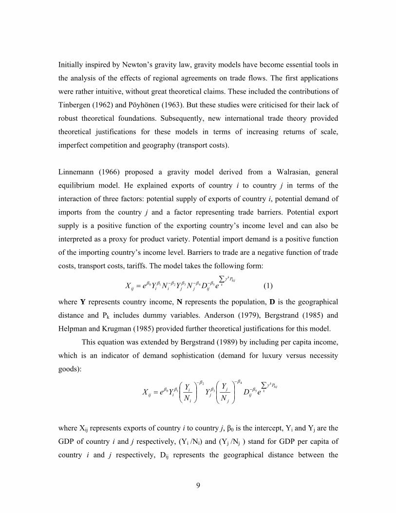
Linnemann (1966) proposed a gravity model derived from a Walrasian, general

equilibrium model. He explained exports of country i to country j in terms of the

interaction of three factors: potential supply of exports of country i, potential demand of

imports from the country j and a factor representing trade barriers. Potential export

supply is a positive function of the exporting country’s income level and can also be

interpreted as a proxy for product variety. Potential import demand is a positive function

of the importing country’s income level. Barriers to trade are a negative function of trade

costs, transport costs, tariffs. The model takes the following form:

∑= −−− k

kijk P

ijjjiiij eDNYNYeXγ

ββββββ 543210 (1)

where Y represents country income, N represents the population, D is the geographical

distance and Pk includes dummy variables. Anderson (1979), Bergstrand (1985) and

Helpman and Krugman (1985) provided further theoretical justifications for this model.

This equation was extended by Bergstrand (1989) by including per capita income,

which is an indicator of demand sophistication (demand for luxury versus necessity

goods):

∑⎟⎟⎠

⎞⎜⎜⎝

⎛⎟⎟⎠

⎞⎜⎜⎝

⎛= −

−−

kkij

k P

ijj

jj

i

iiij eD

NY

YNYYeX

γβ

β

ββ

ββ 5

4

3

2

10

where Xij represents exports of country i to country j, β0 is the intercept, Yi and Yj are the

GDP of country i and j respectively, (Yi /Ni) and (Yj /Nj ) stand for GDP per capita of

country i and j respectively, Dij represents the geographical distance between the

10

economic centers of two partners, Pkij stands for other variables such as common

language and historical bonds.

4. Econometric Issues

The regionalism issue was most frequently examined using a gravity model including a

dummy variable for regional agreements7. Most studies estimating a gravity model

applied the ordinary least square (OLS) method to cross-section data. Recently several

papers have argued that standard cross-section methods lead to biased results because

they do not account for heterogeneity. For instance, the impact of historical, cultural and

linguistic links on trade flows is difficult to quantify. On the other hand, the potential

sources of endogeneity bias in gravity model estimations fall under three categories:

omitted variables, simultaneity, and measurement error (see Wooldrige, 2002).

Matyas (1997) points out that the cross-section approach is affected by misspecification

and suggests that the gravity model should be specified as a “three – way model” with

exporter, importer and time effects (random or fixed ones). Egger (2000) argues that

panel data methods are the most appropriate for disentangling time-invariant and country-

specific effects. Egger and Pfaffermayr (2003) underline that the omission of specific

effects for country pairs can bias the estimated coefficients. An alternative solution is to

use an estimator to control bilateral specific effects as in a fixed effect model (FEM) or in

a random effect model (REM). The advantage of the former is that it allows for

unobserved or misspecified factors that simultaneously explain the trade volume between

two countries and lead to unbiased and efficient results8. The choice of the method (FEM

or REM) is determined by economic and econometric considerations. From an economic

point of view, there are unobservable time-invariant random variables, difficult to be

quantified, which may simultaneously influence some explanatory variables and trade

volume. From an econometric point of view, the inclusion of fixed effects is preferable to

random effects because the rejection of the null assumption of no correlation between the

7 Baldwin (1994), Frankel (1997), Soloaga et Winters (2001), Glick et Rose (2002), Carrere (2006). 8 Egger (2000), Egger (2002)

11

unobservable characteristics and explanatory variables is less plausible (see Baier and

Bergstrand 2007).

Another method which has gained considerable acceptance among economists (see Egger

and Pfaffermayr, 2004) is the Hausman-Taylor's panel one incorporating time-invariant

variables correlated with bilateral specific effects (see, for instance, Hausman-Taylor,

1981; Wooldrige, 2002; Hsiao, 2003). Plümper and Troeger (2004) have proposed a more

efficient method called “the fixed effect vector decomposition (FEVD)” to accommodate

time-invariant variables. Using Monte Carlo simulations they compared the performance

of the FEVD method to some other existing techniques, such as the fixed effects, or

random effects, or Hausman-Taylor method. Their results indicate that the most reliable

technique for small samples is FEVD if time-invariant variables and the other variables

are correlated with specific effects, which is likely to be the case in our study.

Consequently, we use this technique for the empirical analysis.

Next we provide more details of the alternative methods mentioned above, i.e. random

effect estimator (REM), fixed effect estimator (FEM) and fixed effect vector

decomposition (FEVD).

4.1 Within Estimator and Random Estimator (FEM and REM)

In the presence of correlation of the unobserved characteristics with some of the

explanatory variables the random effect estimator leads to biased and inconsistent

estimates of the parameters. To eliminate this correlation it is possible to use a traditional

method called “within estimator or fixed effect estimator” which consists in transforming

the data into deviations from individual means. In this case, even if there is correlation

between unobserved characteristics and some explanatory variables, the within estimator

provides unbiased and consistent results.

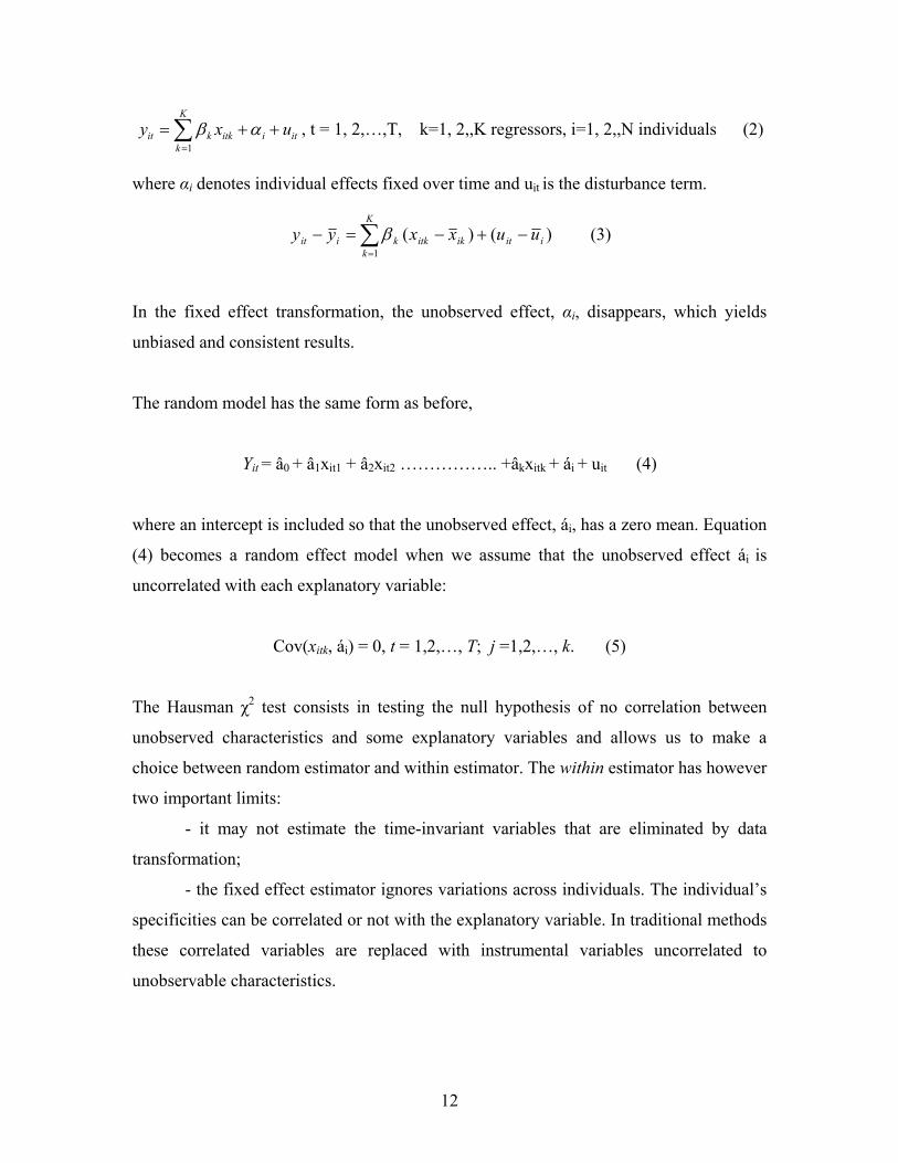
The fixed effect model can be written as

12

iti

K

kitkkit uxy ++= ∑

=

αβ1

, t = 1, 2,…,T, k=1, 2,,K regressors, i=1, 2,,N individuals (2)

where αi denotes individual effects fixed over time and uit is the disturbance term.

)()(1

iitikitk

K

kkiit uuxxyy −+−=− ∑

=

β (3)

In the fixed effect transformation, the unobserved effect, αi, disappears, which yields

unbiased and consistent results.

The random model has the same form as before,

Yit = â0 + â1xit1 + â2xit2 …………….. +âkxitk + ái + uit (4)

where an intercept is included so that the unobserved effect, ái, has a zero mean. Equation

(4) becomes a random effect model when we assume that the unobserved effect ái is

uncorrelated with each explanatory variable:

Cov(xitk, ái) = 0, t = 1,2,…, T; j =1,2,…, k. (5)

The Hausman χ2 test consists in testing the null hypothesis of no correlation between

unobserved characteristics and some explanatory variables and allows us to make a

choice between random estimator and within estimator. The within estimator has however

two important limits:

- it may not estimate the time-invariant variables that are eliminated by data

transformation;

- the fixed effect estimator ignores variations across individuals. The individual’s

specificities can be correlated or not with the explanatory variable. In traditional methods

these correlated variables are replaced with instrumental variables uncorrelated to

unobservable characteristics.

13

4.2. Fixed Effect Vector Decomposition (FEVD)

Plümper and Troeger (2004) suggest an alternative to the estimation of time-invariant

variables in the presence of unit effects. The alternative is the model discussed in Hsiao

(2003). It is known that unit fixed effects are a vector of the mean effect of omitted

variables, including the effect of time-invariant variables. It is therefore possible to

regress the unit effects on the time-invariant variables to obtain approximate estimates for

invariant variables. Plümper and Troeger (2004) propose a three-stage estimator, where

the second stage only aims at the identification of the unobserved parts of the unit effects,

and then uses the unexplained part to obtain unbiased pooled OLS (POLS) estimates of

the time-varying and time-invariant variables only in the third stage. The unit effect

vector is decomposed into two parts: a part explained by time-invariant variables and an

unexplainable part (the error term). The model proposed by Plümper and Troeger (2004)

yields unbiased and consistent estimates of the effect of time-varying variable and

unbiased for time-invariant variables if the unexplained part of unit effects is uncorrelated

with time-invariant variables.

This model has the robustness of fixed effect model and allows for the correlation

between the time-variant explanatory variables and the unobserved individual effects. In

brief, the fixed effect vector decomposition (FEVD) proposed by Plümper and Troeger

(2004) involves the three following steps:

estimation of the unit fixed effects by the FEM excluding the time-invariant

explanatory variables;

regression of the fixed effect vector on the time-invariant variables of the original

model (by OLS);

re-estimation of the original model by POLS, including all time-variant

explanatory variables, time-invariant variables and the unexplained part of the fixed

effect vector. The third stage is required to control for multicollinearity and to adjust the

degrees of freedom9.

9 The program STATA proposed (ado-file) by the authors executes all three steps and adjusts the variance-covariance matrix. Options like AR (1) error-correction and robust variance-covariance matrix are allowed.

14

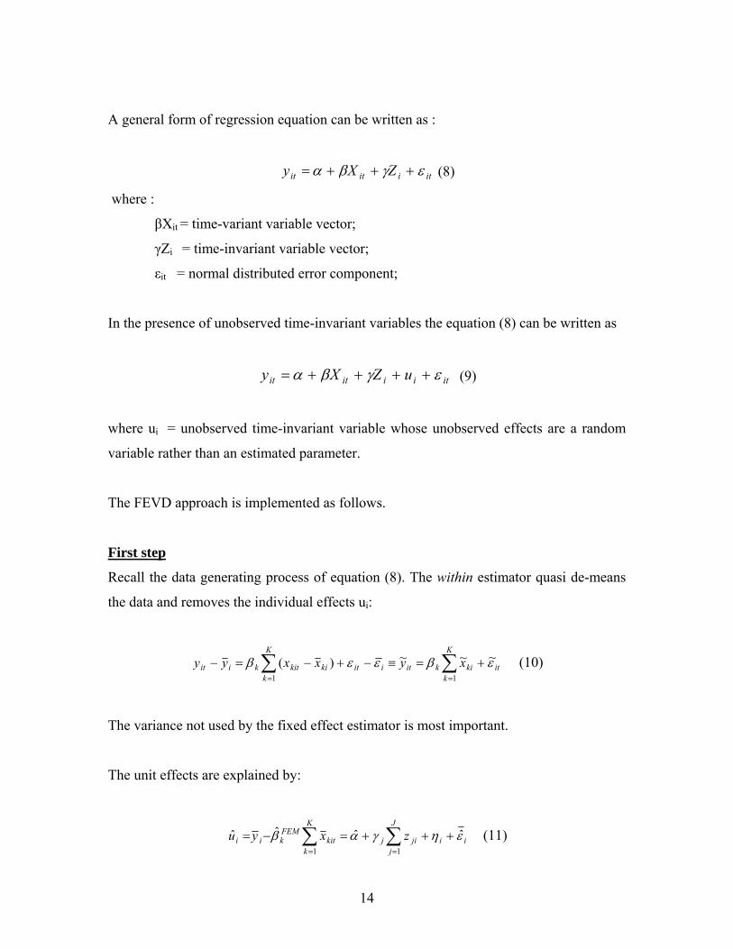
A general form of regression equation can be written as :

itiitit ZXy εγβα +++= (8)

where :

βXit = time-variant variable vector;

γZi = time-invariant variable vector;

εit = normal distributed error component;

In the presence of unobserved time-invariant variables the equation (8) can be written as

itiiitit uZXy εγβα ++++= (9)

where ui = unobserved time-invariant variable whose unobserved effects are a random

variable rather than an estimated parameter.

The FEVD approach is implemented as follows.

First step

Recall the data generating process of equation (8). The within estimator quasi de-means

the data and removes the individual effects ui:

∑∑==

+=≡−+−=−K

kitkikit

K

kiitkikitkiit xyxxyy

11

~~~)( εβεεβ (10)

The variance not used by the fixed effect estimator is most important.

The unit effects are explained by:

ii

J

jjij

K

kkit

FEMkii zxyu εηγαβ ˆˆˆˆ

11

+++=−= ∑∑==

(11)

15

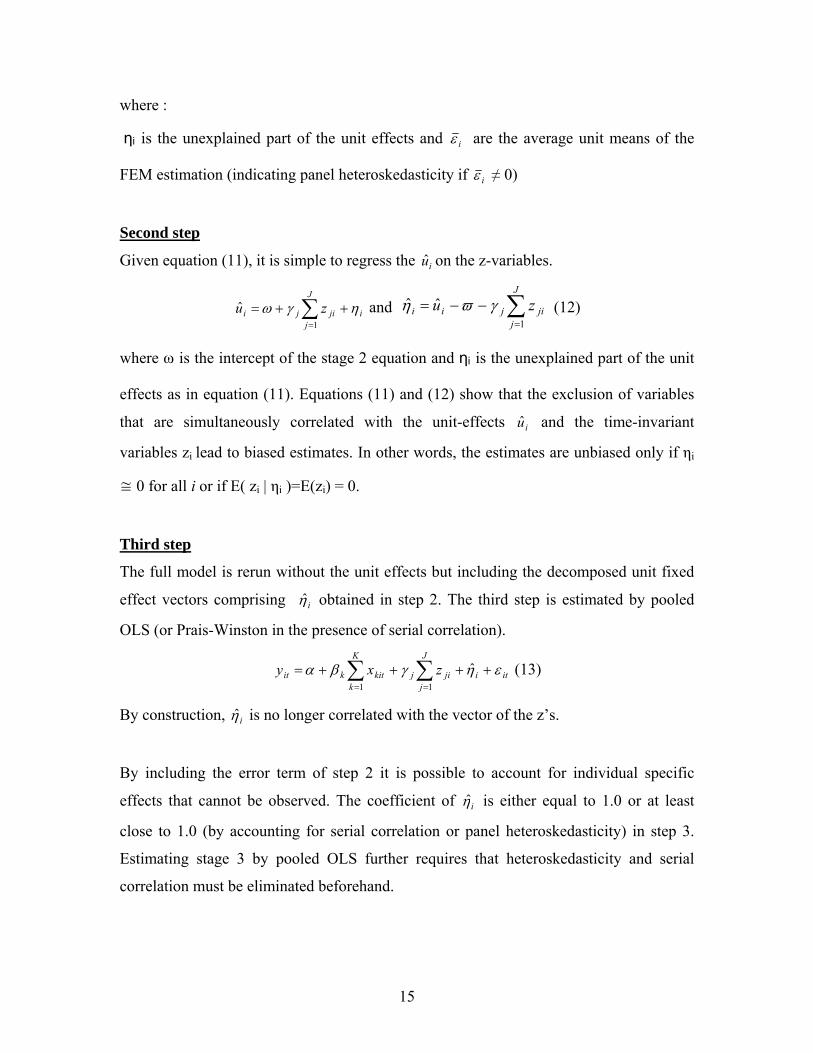
where :

ηi is the unexplained part of the unit effects and iε are the average unit means of the

FEM estimation (indicating panel heteroskedasticity if iε ≠ 0)

Second step

Given equation (11), it is simple to regress the iu on the z-variables.

i

J

jjiji zu ηγω ++= ∑

=1

ˆ and ∑=

−−=J

jjijii zu

1

ˆˆ γϖη (12)

where ω is the intercept of the stage 2 equation and ηi is the unexplained part of the unit

effects as in equation (11). Equations (11) and (12) show that the exclusion of variables

that are simultaneously correlated with the unit-effects iu and the time-invariant

variables zi lead to biased estimates. In other words, the estimates are unbiased only if ηi

≅ 0 for all i or if E( zi | ηi )=E(zi) = 0.

Third step

The full model is rerun without the unit effects but including the decomposed unit fixed

effect vectors comprising iη obtained in step 2. The third step is estimated by pooled

OLS (or Prais-Winston in the presence of serial correlation).

iti

J

jji

K

kjkitkit zxy εηγβα ++++= ∑∑

==

ˆ11

(13)

By construction, iη is no longer correlated with the vector of the z’s.

By including the error term of step 2 it is possible to account for individual specific

effects that cannot be observed. The coefficient of iη is either equal to 1.0 or at least

close to 1.0 (by accounting for serial correlation or panel heteroskedasticity) in step 3.

Estimating stage 3 by pooled OLS further requires that heteroskedasticity and serial

correlation must be eliminated beforehand.

16

At least in theory this method has three obvious advantages (see Plümper and Troeger, 2004): a) the fixed effect vector decomposition does not require prior knowledge of the

correlation between time-variant explanatory variables and unit specific effects,

b) the estimator relies on the robustness of the within-transformation and does not need to

meet the orthogonality assumptions (for time-variant variables) of random effects,

c) FEVD estimator maintains the efficiency of POLS.

Essentially FEVD produces unbiased estimates of time-varying variables, regardless of

whether they are correlated with unit effects or not, and unbiased estimates of time-

invariant variables that are not correlated. The estimated coefficients of the time-

invariable variables correlated with unit effects, however, suffer from omitted variable

bias. To summarise, FEVD produces less biased and more efficient coefficients. The

main advantages of FEVD come from its lack of bias in estimating the coefficients of

time-variant variables that are correlated with unit-effects.

5. Empirical Analysis

5.1 The Econometric Model

The econometric model we adopt in order to identify and to quantify the impact of the

association agreement on trade flows between the EU-15 and CEEC-4 countries was

chosen taking into account our sample data, the potential endogeneity of variable, the

existence of unobservable bilateral characteristics which might or might not be correlated

with the explanatory variables, and multicollinearity.

Our econometric specification is the following:

),......1;,......1()log(

)log()log()log()log()log(

65

43210

TtNiuAccTchr

DistDGDPCGDPGDPY

ijttijijtijt

ijijtjtitijt

==++++

+++++=

εθαα

ααααα (1)

In this specification, the bilateral trade (Yijt) is the dependent variable. The explanatory

variables used are the gross domestic product of the two partners (GDPit), (GDPjt),

17

geographic distance (Distij), the difference in development level (DGDPCijt), the real

exchange rate (Tchrijt), the dichotomous variable association agreement (Accijt).

The notation is the following:

• Yijt denotes the bilateral trade between countries i and j at time t with i ≠ j

(millions of dollars);

• αo is the intercept;

• GDPit, GDPjt represents the Gross Domestic Product of country i and country j

(millions of dollars);

• DGDPCijt is the difference in GDP per capita between partners and is a proxy of economic distance or of comparative advantage intensity,

jt

jt

it

itijt N

GDPN

GDPDGDPC −=

where Ni(j) is the population ; • Distij represents the distance between country i and country j (kilometers); • Tchrijt is the real exchange rate which indicates price competitiveness;

jt

itijtijt P

PxTcnTchr =

where : Tcnijt is the nominal exchange rate;

Pi (j) is the consumer price index;

• Accijt is a dummy variable that is equal to 1 if country i and country j have signed

a regional agreement, and zero otherwise;

• uij is a bilateral specific effect (i = 1,2,…,N, j = 1,2,…,M) ;

• θt is a time specific effect (t = 1,…..T);

• εijt is the disturbance term, which is assumed to be normally distributed with a

zero mean and a constant variance for all observations and to be uncorrelated.

The source of data is the CHELEM – French CEPII data base for GDP, GDP/capita,

nominal exchange rate and population; the CEPII data base for geographic distance; and

the World Bank – World Tables for the consumer index price. The estimation period goes

18

from 1987 to 2005, i.e. 19 years for a sample of EU-1510 and 4 CEEC countries11. We

construct a panel with two dimensions: country pairs, and years.

5.2 Estimation Results

This section summarises the results from the estimation of the gravity model. We used

panel data techniques for eliminating the endogeneity bias, and applied different panel

data econometric methods such Fixed Effect Model (FEM), Random Effect Model

(REM) and Fixed Effects Vector Decomposition (FEVD) in order to check the robustness

of our estimates (see Table 1, 2, 3).

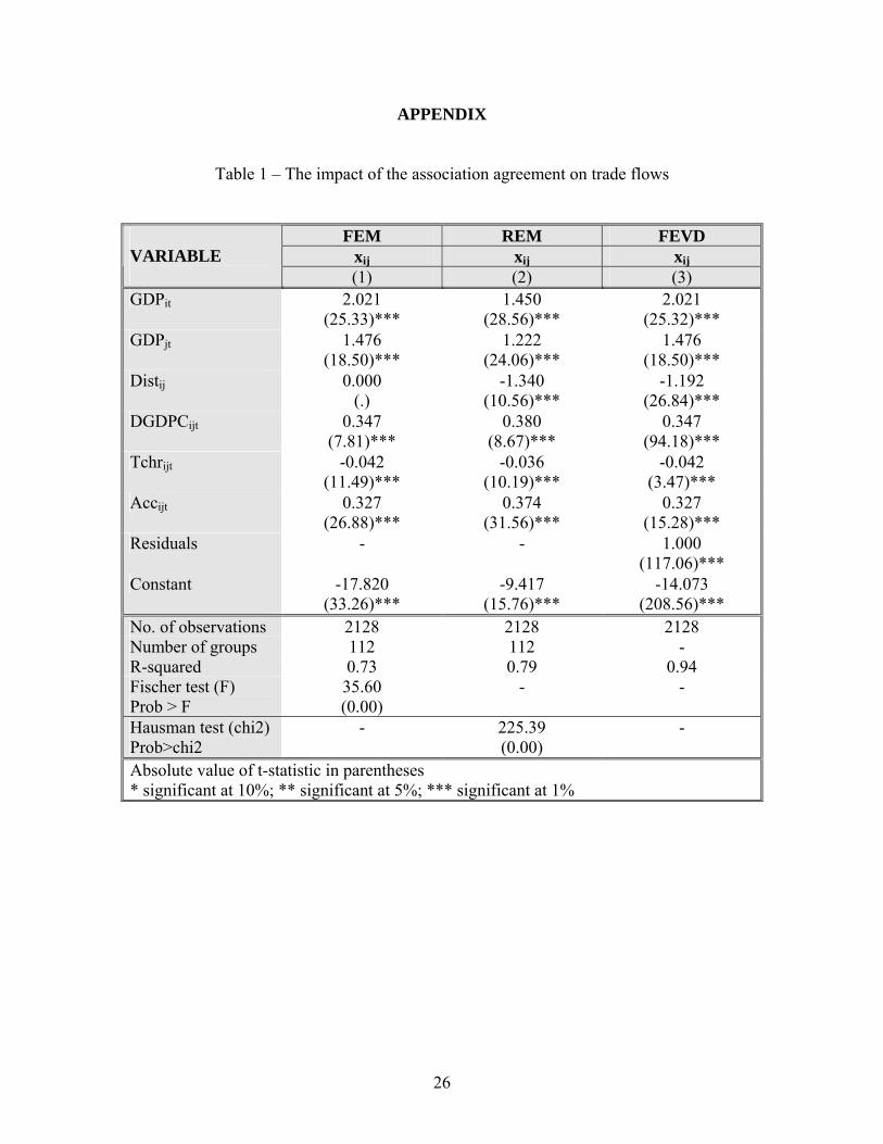
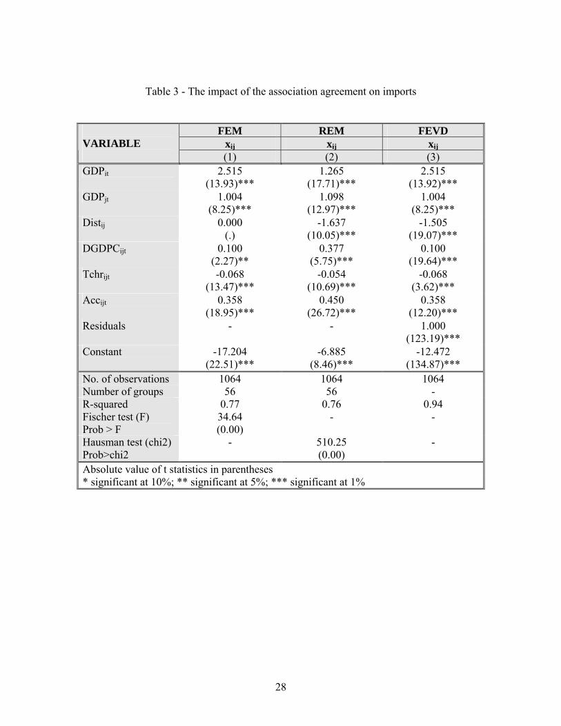
Table 1 shows the impact of FTAs on trade flows. To establish whether the effect on the

trade balance is symmetric or asymmetric, we estimate separately the effects on exports

(Table 2) and imports (Table 3). The aggregate estimation indicates a positive effect of

the association agreement variable on trade flows, in accordance with previous studies12.

The coefficients are statistically significant and have the expected signs consistently with

the gravity model: a positive effect on trade flows of country size and association

agreement, and a negative impact of geographical distance and of real exchange rate.

Moreover, the positive effect of the association agreement is found to be stronger after

eliminating the endogeneity bias, the estimated coefficient being now close to 0.33 (see

column 3, Table 1). The coefficient of the European agreement variable decreases from

0.37 (random effects model) to 0.33 in the fixed effects and FEVD model. Thus, there is

clear evidence that the agreement has increased trade volume between EU-15 and CEEC-

4 countries.

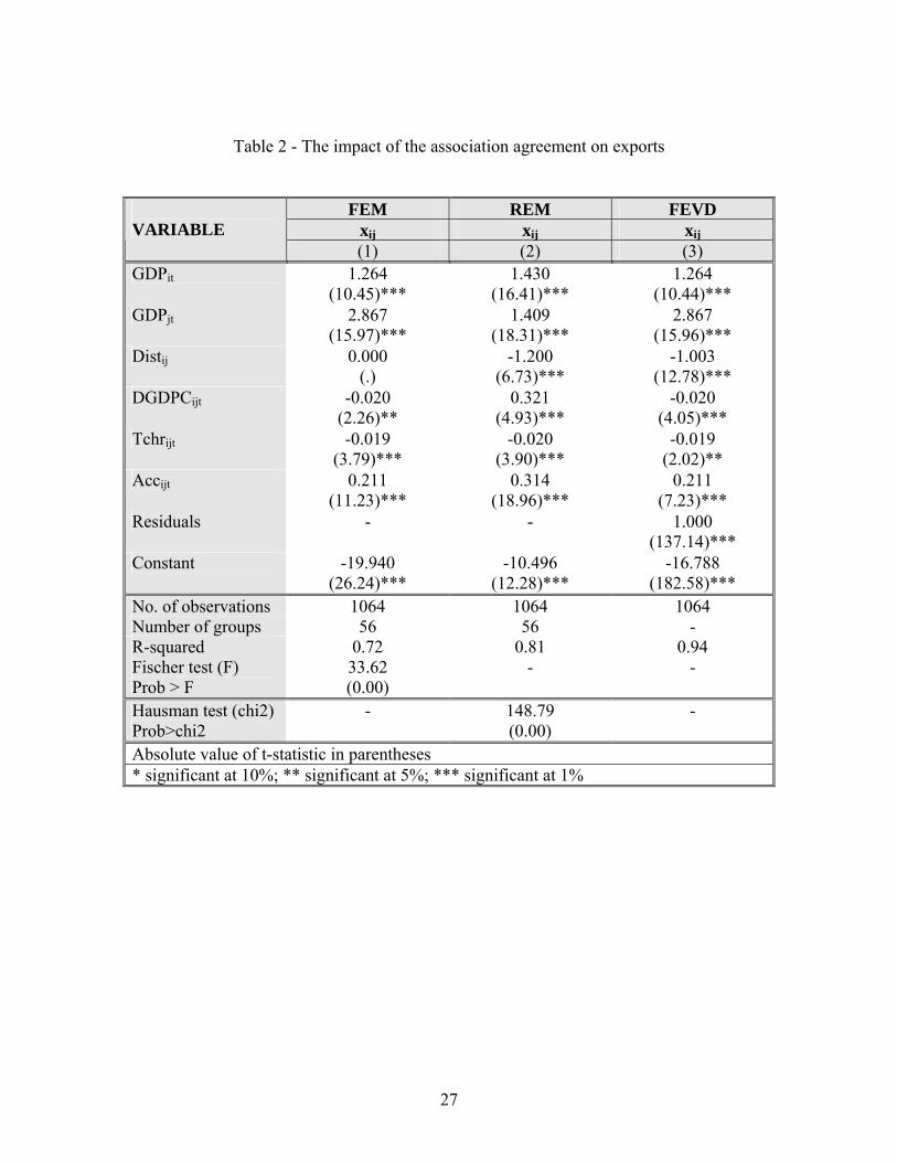
The association agreement appears to have had a positive but different impact on the

CEEC-4 exports and imports towards the EU-15 countries. The coefficients are higher for

imports (0.36) than for exports (0.21), indicating asymmetry. Concerning the trade

10 EU-15: Austria, Belgium-Luxemburg, Denmark, England, Finland, France, Germany, Greece, Holland, Ireland, Italy, Portugal, Spain, Sweden. 11 Bulgaria, Hungary, Poland, Romania. 12 See for instance, Soloaga and Winters (2001), Carrère (2006), Cheng and Wall (2004), Rault and Sova (2007).

19

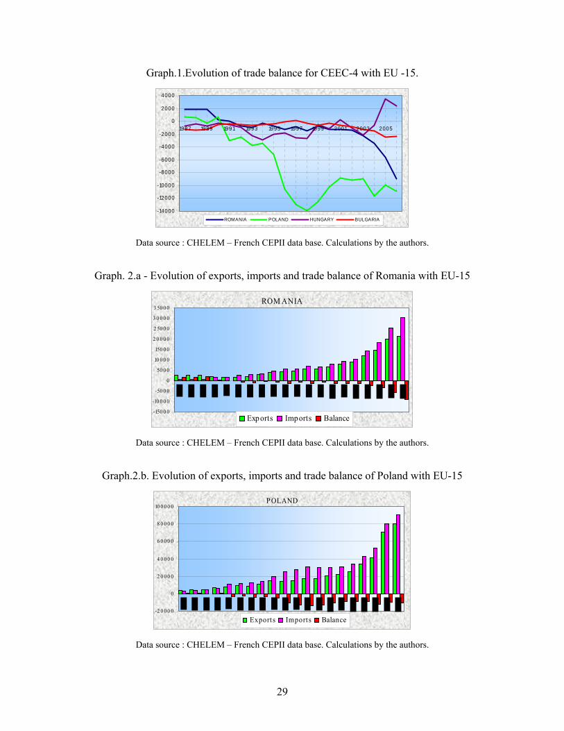
balance, we note that association leads to a trade deficit for the CEEC-4 with respect to

the EU-15. Moreover, movements of the trade balance over time reveal that imports

increase more quickly than exports (see Graph 1). Some potential explanations are: (i) the

lack of product competitiveness in the European market, (ii) the increasing vertical FDI,

importing intermediate goods necessary for their production process; (iii) a greater

preference of consumers for products from the EU.

Concerning robustness, the estimated coefficients are similar for FEM and FEVD;

however, the latter not only enables us to isolate the endogeneity of the association

agreement variable and to obtain unbiased coefficients, but also captures the effects of

time-invariant variables on trade flows.

The Fisher test suggests the introduction of effects (fixed or random) to improve the

estimation results. The estimated coefficients of the FEM are different from those

obtained with the REM (for instance, association agreement) which can be explained by

the existence of a correlation between some explanatory variables and the bilateral

specific effect. Moreover, the Hausman test rejects the null assumption of no correlation

between the individual effects and some explanatory variables for all estimations. This

implies endogeneity bias, and therefore the fixed effects model is preferred. The

Davidson-MacKinnon test of exogeneity (F=160.26, P-value = 0.00), confirm the

endogeneity of the FTA. We also calculate the variance inflation factor (VIF) to ensure

that multicollinearity does not affect the quality of estimates. In our all estimates, VIF did

not exceed the threshold of 10, indicating that there is no multicollinearity13.

Overall, the agreement variable coefficient indicates a positive and significant impact on

trade flows but an asymmetric effect on exports and imports.

13 A variance inflation factor value higher than 10 reveals the presence of multicollinearity requiring specific corrections (see Gujarati, 1995).

20

6. Conclusions

This paper has analysed the impact of association agreements on trade flows between the

EU-15 and CEEC-4 countries treating the agreement variable as endogenous and using

appropriate panel methods to estimate a gravity equation. The most relevant estimates are

those provided by the FEVD estimation method which is the most appropriate for our

purposes. This method permits to obtain unbiased coefficients and to capture the effects

of time-invariant variables. As theory suggests, association agreements were found to

have a positive and significant impact on trade flows between the participant countries.

However, such effects appear to be asymmetric, the estimated coefficient being higher for

imports (0.36) than for exports (0.21), which suggests trade asymmetry. In particular, the

agreements resulted in increased trade deficits for the CEEC-4 countries (net importers),

which is not desirable for economies still trying to catch up with the other EU states14.

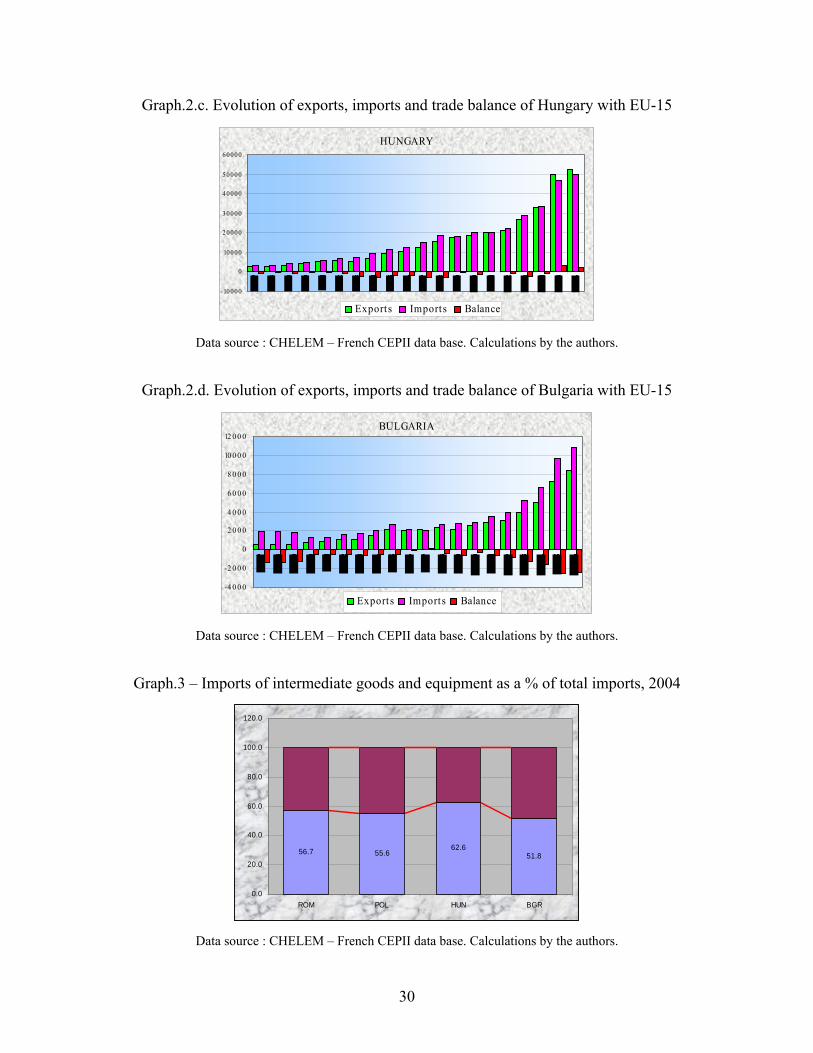
Convergent or divergent dynamics of imports and exports are the main cause of trade

balance changes. The evolution of exports, imports as well as of trade balance over the

estimation period for all CEEC-4 highlights the persistence and the deepening of the

trade deficit (see Graphs 1 and 2).

The lower impact of the agreement on CEEC-4 exports can be interpreted in terms of low

EU demand for CEEC products reflecting their lack of attractiveness for European

consumers, despite their price competitiveness based on comparative advantages due to

lower labour costs. Trade liberalisation did not lead to a restructuring of exports and to a

development of the most innovative sectors of the economy. Instead, CEEC-4 exports are

still represented mainly by labour-intensive products with lower added value.15

Higher trade openness and the progressive liberalisation of the capital flows resulting

from the trade agreement have strongly influenced the behaviour of multinationals firms.

Vertical FDI in the CEEC-4 countries has instead increased. This type of investment

consists in the fragmentation of the various operations of the production process to

14 The trade balance is a component of GDP: a surplus increases GDP and a deficit reduces it. 15 See Rault et al. (2007)

21

implement them in countries offering lower costs. The production location which results

from it inevitably entails a rise of intermediate and equipments good imports of these

countries from the investor’s countries. Thus, in the case of the CEEC-4 countries

vertical FDI has induced a significant increase of intermediate and equipments good (and

hence of total imports): these now represent more than half of the CEEC-4 countries total

imports from the EU (see Graph 3). In order to reduce their trade deficit and to have a

sustainable trade balance, the CEEC-4 countries would need instead more intra-branch

trade with high added value products so as to increase their export competitiveness

towards the EU and to attract horizontal FDI, thereby achieving real convergence.

In conclusion, our estimation results indicate a positive and significant impact of FTAs

on trade flows. However, exports and imports are affected differently, leading to some

disparity in trade flow performance between countries. Therefore, there is an asymmetric

impact on the trade balance, the agreement variable resulting in a trade balance deficit in

the CEEC-4.

22

References

[1] Aitken, N., “The effect of the EEC and EFTA on European trade: a temporal cross-

section analysis “, American Economic Review, 63(5), 1973.

[2] Anderson E. J. “A Theoretical Foundation for the Gravity Equation”, American

Economique Review, No 69, pp 106-116, 1979.

[3] Baier S.L. and Bergstrand J., “Economic determinants of free-trade agreements “,

Journal of International Economics, 64(1), 29-63, 2004.

[4] Baier, S.L. and Bergstrand, J. H., "Do free trade agreements actually increase

members' international trade?", Journal of International Economics, Elsevier, vol. 71(1),

pages 72-95,2007.

[5] Baldwin R.E., “Towards an Integrated Europe”, London, CEPR, 1994.

[6] Bergstrand J.H., “The Gravity Equation in International Trade: some Microeconomic

Foundations and Empirical Evidence”, The Review of Economics and Statistics, Vol. 67,

No 3, August, pp. 474-481, 1985.

[7] Bergstrand J.H., “The Generalized Gravity Equation, Monopolistic Competition, and

the Factor-Proportions Theory in International Trade”, The Review of Economics and

Statistics, Vol.71, No 1, February, pp. 143-153, 1989.

[8] Bhagwati, J., Panagariya, “The theory of preferential trade agreements: historical

evolution and current trends “, American EconomicReview, 86(2), 82-87, 1996.

[9] Carrere C.,“Revisiting the Effects of Regional Trading Agreements on Trade Flows

with Proper Specification of Gravity Model”, European Economic Review vol. 50, 223-

247, 2006.

[10] Cheng I.-H.,Wall, H. “Controlling for heterogeneity in gravity models of trade and

integration”, Working Papers 1999-010, Federal Reserve Bank of St. Louis, 2004.

[11] Cooper, C. and Massell B., A New Look at Customs Unions Theory, The Economic

Journal, Vol. 75, pp. 742-7, 1965.

[12] De Melo J. et al., “The new Regionalism a Country Perspective “, Cambridge

University Press, New York, 1993.

[13] Egger P., “A note on the Proper Econometric Specification of the Gravity Equation”,

Economics Letters, Vol. 66, pp.25-31, 2000.

23

[14] Egger,P., "An Econometric View on the Estimation of Gravity Models and the

Calculation of Trade Potentials", The World Economy 25 (2), 297 – 312, 2002

[15] Egger P. and M. Pfaffermayr, “The proper panel econometric specification of the

gravity equation : a three-way model with bilateral interaction effects”, Empirical

Economics, 28, 571-580, 2003.

[16] Egger P. et Pfaffermayr M. ,”Distance, trade and FDI : a SUR Hausman-Taylor

approach”, Journal of Applied Econometrics, 19(2), 227-46,2004.

[17] Eichengreen, B. and Irwin, D. A., “Trade blocs, currency blocs and the reorientation

of world trade in the 1930s," Journal of International Economics, Elsevier, vol. 38(1-2),

pages 1-24, 1995.

[18] Fernandez R. et Portes J., “Returns to regionalism: an analysis of non traditional

gains from regional trade agreements “, World Bank Economic Review, 12(2), 197-220,

1998.

[19] Frankel, J. A. & Stein, E. and Wei, S-J, "Regional Trading Arrangements: Natural or

Supernatural," American Economic Review, American Economic Association, vol. 86(2),

pages 52-56, 1996.

[20] Frankel, J., “Regional trading blocs in the world economic system”, Institute for

International Economics, Washington, 1997.

[21 ] Frankel, J.A., Wei S-J., "Open Regionalism in a World of Continental Trade Blocs,"

IMF Staff Papers, International Monetary Fund, vol. 45(3), pages 2, 1998.

[22] Ghosh S., Yamarik S., “Are Regional Trading Arrangements Trade Creating?: An

Aplication of Extreme Bounds Analysis.”, Journal of International Economics 63, no.2:

369-395, 2004.

[23] Glick R. et Rose A. ,” Does a currency union affect trade ? The time series evidence

“, European Economic Review, 46(6), 1125-151, 2002.

[24] Grossman, G. M. and Helpman, E.,”The Politics of Free-Trade Agreements.”

American Economic Review, 85(4), pp. 667-690, 1995.

[25 ] Gujarati, D. N., “Basic Econometrics “,McGraw-Hill College, Edition 3, 1995.

[26] Hausman J.A. and Taylor,W.E., “Panel Data and Unobservable Individual

Effects”,Économetrica, 49, pp. 1377-1398,1981.

24

[27] Helpman, E., and Krugman P.R., “Market Structure and Foreign Trade: Increasing

Returns, Imperfect Competition, and the International Economy”, Cambridge/Mass.: MIT

Press, 1985.

[28] Hsiao C., “Analysis of Panel Data”, 2nd edition, Cambridge University Press, Ch.

4,1-4.6, 2003.

[29] Johnson, H., “An Economic Theory of Protectionism, Tariff Bargaining and the

Formation of Customs Unions”, Journal of Political Economy 73(3), 256-83, 1965.

[30] Krugman, P., “Geography and Trade”, Cambridge (Mass.), MIT Press, 1991.

[31] Linnemann, H., “An Econometric Study of International Trade Flows”, North

Holland Publishing Company, Amsterdam, 1966.

[32] Magee, C. “Endogenous Preferential Trade Agreements: An Empirical Analysis.”

Contributions to Economic Analysis and Policy 2, no. 1. Berkeley Electronic Press, 2003.

[33] Matyas, L., “Proper Econometric Specification of the Gravity Model”, The World

Economie, 20 (3), 363-368, 1997.

[34] Plumper, T. and V. Troeger, “The Estimation of Time-Invariant Variables in Panel

Analysis with Unit Fixed Effects,” Konstanz University, mimeo, 2004

[35] Pöyhönen, P., “A tentative model for the flows of trade between countries”,

Welwirtschftliches Archiv, 90, 93-100, 1963.

[36] Rault C., Sova, R. and Sova, A, "The Role of Association Agreements Within

European Union Enlargement to Central and Eastern European Countries", IZA

Discussion Paper No. 2769, 2007.

[37] Rault, C., Sova A. and Sova, R., "The Endogeneity of Association Agreements and

their Impact on Trade for Eastern Countries: Empirical Evidence for Romania", William

Davidson Institute Working Paper No. 868, 2007.

[38] Schiff M. and L. A.Winters, “Regional Integration as Diplomacy.”, World Bank

Economic Review, vol. 12, no. 2, 1998.

[39 ] Soloaga I. et Winters A., "Regionalism in the nineties: what effect on trade?," The

North American Journal of Economics and Finance, Elsevier, vol. 12(1), pages 1-29,

2001.

[40] Tinbergen J., “Shaping the World Economy: Suggestions for an International

Economic Policy”, Twentieth Century Fund, New York, 1962.

25

[41] Viner, J., The Customs Union Issue, New York, Carnegie Endowment for

International Peace, 1950.

[42] Wonnacott P. and Lutz, M., “Is There a Case for Free Trade Areas ?”, in Schott, J.

ed., Free Trade Areas and US Trade Policy, Washington, D.C., Institute for International

Economics,1989.

[43] Wooldrige, J.H., “Econometric Analysis of Cross Section and Panel Data 2rd

Edition”: Books: The MIT Press Cambridge, Massachusetts London, England, 2002.

26

APPENDIX

Table 1 – The impact of the association agreement on trade flows

FEM REM FEVD xij xij xij

VARIABLE (1) (2) (3) GDPit 2.021

(25.33)*** 1.450

(28.56)*** 2.021

(25.32)*** GDPjt 1.476

(18.50)*** 1.222

(24.06)*** 1.476

(18.50)*** Distij 0.000

(.) -1.340

(10.56)*** -1.192

(26.84)*** DGDPCijt 0.347

(7.81)*** 0.380

(8.67)*** 0.347

(94.18)*** Tchrijt -0.042

(11.49)*** -0.036

(10.19)*** -0.042

(3.47)*** Accijt 0.327

(26.88)*** 0.374

(31.56)*** 0.327

(15.28)*** Residuals -

-

1.000 (117.06)***

Constant -17.820 (33.26)***

-9.417 (15.76)***

-14.073 (208.56)***

No. of observations 2128 2128 2128 Number of groups 112 112 - R-squared 0.73 0.79 0.94 Fischer test (F) Prob > F

35.60 (0.00)

- -

Hausman test (chi2) Prob>chi2

- 225.39 (0.00)

-

Absolute value of t-statistic in parentheses * significant at 10%; ** significant at 5%; *** significant at 1%

27

Table 2 - The impact of the association agreement on exports


VARIABLE

(1) (2) (3) GDPit 1.264

(10.45)*** 1.430

(16.41)*** 1.264

(10.44)*** GDPjt 2.867

(15.97)*** 1.409

(18.31)*** 2.867

(15.96)*** Distij 0.000

(.) -1.200

(6.73)*** -1.003

(12.78)*** DGDPCijt -0.020

(2.26)** 0.321

(4.93)*** -0.020

(4.05)*** Tchrijt -0.019

(3.79)*** -0.020

(3.90)*** -0.019

(2.02)** Accijt 0.211

(11.23)*** 0.314

(18.96)*** 0.211


-

1.000 (137.14)***

Constant -19.940 (26.24)***

-10.496 (12.28)***

-16.788 (182.58)***


33.62 (0.00)

- -


- 148.79 (0.00)

-

Absolute value of t-statistic in parentheses * significant at 10%; ** significant at 5%; *** significant at 1%

28

Table 3 - The impact of the association agreement on imports


VARIABLE (1) (2) (3) GDPit 2.515

(13.93)*** 1.265

(17.71)*** 2.515

(13.92)*** GDPjt 1.004

(8.25)*** 1.098

(12.97)*** 1.004

(8.25)*** Distij 0.000

(.) -1.637

(10.05)*** -1.505

(19.07)*** DGDPCijt 0.100

(2.27)** 0.377

(5.75)*** 0.100

(19.64)*** Tchrijt -0.068

(13.47)*** -0.054

(10.69)*** -0.068

(3.62)*** Accijt 0.358

(18.95)*** 0.450

(26.72)*** 0.358


-

1.000 (123.19)***

Constant -17.204 (22.51)***

-6.885 (8.46)***

-12.472 (134.87)***


34.64 (0.00)

- -


- 510.25 (0.00)

-

Absolute value of t statistics in parentheses * significant at 10%; ** significant at 5%; *** significant at 1%

29

Graph.1.Evolution of trade balance for CEEC-4 with EU -15.

-14000

-12000

-10000

-8000

-6000

-4000

-2000

0

2000

4000

1987 1989 1991 1993 1995 1997 1999 2001 2003 2005

ROMANIA POLAND HUNGARY BULGARIA

Data source : CHELEM – French CEPII data base. Calculations by the authors.

Graph. 2.a - Evolution of exports, imports and trade balance of Romania with EU-15

ROM ANIA

-150 0 0

-10 0 0 0

-50 0 0

0

50 0 0

10 0 0 0

150 0 0

2 0 0 0 0

2 50 0 0

3 0 0 0 0

3 50 0 0

Exp orts Imports Balance


Graph.2.b. Evolution of exports, imports and trade balance of Poland with EU-15

POLAND

-2 0 0 0 0

0

2 0 0 0 0

4 0 0 0 0

6 0 0 0 0

8 0 0 0 0

10 0 0 0 0

Exports Imports Balance


30

Graph.2.c. Evolution of exports, imports and trade balance of Hungary with EU-15

HUNGARY

- 10000

0

10000

20000

30000

40000

50000

60000



Graph.2.d. Evolution of exports, imports and trade balance of Bulgaria with EU-15

BULGARIA

-4 0 0 0

-2 0 0 0

0

2 0 0 0

4 0 0 0

6 0 0 0

8 0 0 0

10 0 0 0

12 0 0 0



Graph.3 – Imports of intermediate goods and equipment as a % of total imports, 2004

56.7 55.662.6

51.8

0.0

20.0

40.0

60.0

80.0

100.0

120.0

ROM POL HUN BGR


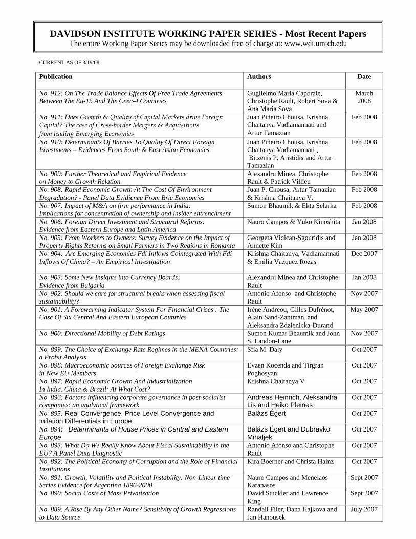
DAVIDSON INSTITUTE WORKING PAPER SERIES - Most Recent Papers The entire Working Paper Series may be downloaded free of charge at: www.wdi.umich.edu

CURRENT AS OF 3/19/08 Publication Authors Date

No. 912: On The Trade Balance Effects Of Free Trade Agreements Between The Eu-15 And The Ceec-4 Countries

Guglielmo Maria Caporale, Christophe Rault, Robert Sova & Ana Maria Sova

March 2008

No. 911: Does Growth & Quality of Capital Markets drive Foreign Capital? The case of Cross-border Mergers & Acquisitions from leading Emerging Economies

Juan Piñeiro Chousa, Krishna Chaitanya Vadlamannati and Artur Tamazian

Feb 2008

No. 910: Determinants Of Barries To Quality Of Direct Foreign Investments – Evidences From South & East Asian Economies

Juan Piñeiro Chousa, Krishna Chaitanya Vadlamannati , Bitzenis P. Aristidis and Artur Tamazian

Feb 2008

No. 909: Further Theoretical and Empirical Evidence on Money to Growth Relation

Alexandru Minea, Christophe Rault & Patrick Villieu

Feb 2008

No. 908: Rapid Economic Growth At The Cost Of Environment Degradation? - Panel Data Evidience From Bric Economies

Juan P. Chousa, Artur Tamazian & Krishna Chaitanya V.

Feb 2008

No. 907: Impact of M&A on firm performance in India: Implications for concentration of ownership and insider entrenchment

Sumon Bhaumik & Ekta Selarka Feb 2008

No. 906: Foreign Direct Investment and Structural Reforms: Evidence from Eastern Europe and Latin America

Nauro Campos & Yuko Kinoshita Jan 2008

No. 905: From Workers to Owners: Survey Evidence on the Impact of Property Rights Reforms on Small Farmers in Two Regions in Romania

Georgeta Vidican-Sgouridis and Annette Kim

Jan 2008

No. 904: Are Emerging Economies Fdi Inflows Cointegrated With Fdi Inflows Of China? – An Empirical Investigation

Krishna Chaitanya, Vadlamannati & Emilia Vazquez Rozas

Dec 2007

No. 903: Some New Insights into Currency Boards: Evidence from Bulgaria

Alexandru Minea and Christophe Rault

Jan 2008

No. 902: Should we care for structural breaks when assessing fiscal sustainability?

António Afonso and Christophe Rault

Nov 2007

No. 901: A Forewarning Indicator System For Financial Crises : The Case Of Six Central And Eastern European Countries

Irène Andreou, Gilles Dufrénot, Alain Sand-Zantman, and Aleksandra Zdzienicka-Durand

May 2007

No. 900: Directional Mobility of Debt Ratings Sumon Kumar Bhaumik and John S. Landon-Lane

Nov 2007

No. 899: The Choice of Exchange Rate Regimes in the MENA Countries: a Probit Analysis

Sfia M. Daly Oct 2007

No. 898: Macroeconomic Sources of Foreign Exchange Risk in New EU Members

Evzen Kocenda and Tirgran Poghosyan

Oct 2007

No. 897: Rapid Economic Growth And Industrialization In India, China & Brazil: At What Cost?

Krishna Chaitanya.V

Oct 2007

No. 896: Factors influencing corporate governance in post-socialist companies: an analytical framework

Andreas Heinrich, Aleksandra Lis and Heiko Pleines

Oct 2007

No. 895: Real Convergence, Price Level Convergence and Inflation Differentials in Europe

Balázs Égert

Oct 2007

No. 894: Determinants of House Prices in Central and Eastern Europe

Balázs Égert and Dubravko Mihaljek

Oct 2007

No. 893: What Do We Really Know About Fiscal Sustainability in the EU? A Panel Data Diagnostic

António Afonso and Christophe Rault

Oct 2007

No. 892: The Political Economy of Corruption and the Role of Financial Institutions

Kira Boerner and Christa Hainz Oct 2007

No. 891: Growth, Volatility and Political Instability: Non-Linear time Series Evidence for Argentina 1896-2000

Nauro Campos and Menelaos Karanasos

Sept 2007

No. 890: Social Costs of Mass Privatization David Stuckler and Lawrence King

Sept 2007

No. 889: A Rise By Any Other Name? Sensitivity of Growth Regressions to Data Source

Randall Filer, Dana Hajkova and Jan Hanousek

July 2007

on the trade balance effects of free trade agreements between the eu15 and the ceec-4 countries

Documents