HAL Id: hal-00833556https://hal.archives-ouvertes.fr/hal-00833556

Submitted on 23 Jun 2018

HAL is a multi-disciplinary open accessarchive for the deposit and dissemination of sci-entific research documents, whether they are pub-lished or not. The documents may come fromteaching and research institutions in France orabroad, or from public or private research centers.

L’archive ouverte pluridisciplinaire HAL, estdestinée au dépôt et à la diffusion de documentsscientifiques de niveau recherche, publiés ou non,émanant des établissements d’enseignement et derecherche français ou étrangers, des laboratoirespublics ou privés.

On the modeling of aircraft tireAnge Kongo-Kondé, Iulian Rosu, Frédéric Lebon, Olivier Brardo, Bernard

Devésa

To cite this version:Ange Kongo-Kondé, Iulian Rosu, Frédéric Lebon, Olivier Brardo, Bernard Devésa. On themodeling of aircraft tire. Aerospace Science and Technology, Elsevier, 2013, 27 (1), pp.67-75.�10.1016/j.ast.2012.06.008�. �hal-00833556�

a AIRBUS, 316 route de Bayonne, 31060 Toulouse cedex 03, Franceb LMA-CNRS, Aix-Marseille Univ., 31 chemin Joseph-Aiguier, 13402 Marseille cedex 20, France

A method is presented here for modeling and predicting the rolling and yaw behavior of an aircraft tirewhich is subjected to a strong inflation pressure and a concentrated load on the axle, in contact witha flat, rigid surface. Finite element methods were used to model and simulate the aircraft tire/groundinteractions. The incompressibility of the material, the large transformations and the unilateral contactwith Coulomb friction law were all taken into account. Imaging methods were used to examine thecomplex structure of the tire cross-section. Comparisons are made between the data obtained with themodel, the experimental data and those provided by the manufacturer. The tire response predictionswere found to depend considerably on the material and the geometrical characteristics of the tire.

On the modeling of aircraft tire

A. Kongo Kondéa,b, I. Rosub, F.Lebonb, O.Brardoa, B.Devésaa

1. Introduction

Modeling the geometry of tires and predicting their behaviorare complex tasks. The loading, which can be either quasi-static ordynamic, also involves severe contact conditions.

1.1. Review of the literature

Most studies on tires have been performed on automobile tires[4]. Several authors [9,4,13,15] have focused on truck tires, espe-cially those used on military trucks, and the motion of vehicles hasbeen simulated on various types of soil (dry, wet, muddy), whereassome authors have dealt with bike tires [17].

In the aerospatial and aeronautical field, the first studies onthese lines were conducted by NASA [16,11,3]. These studies weremostly experimental and dealt with the thermal aspects (the in-fluence of the temperature on tires dynamic responses, its distri-bution within the tire thickness, and the evolution of the frictioncoefficient in tire/ground contact).

In recent studies [14], numerical tools have been used to simu-late the behavior of aircraft tires, and some modeling aspects stillcause engineers and researchers major problems because there aretoo many non-linear phenomena involved.

Under operating conditions, tire’s behavior is highly non-lineardue to their constituents, their geometry and shape, the loadingconditions, contact with friction and many other interconnectedparameters.

* Corresponding author.E-mail address: rosu@lma.cnrs-mrs.fr (I. Rosu).

The operating conditions and the structure of aircraft tires arevery different from those of automobiles. For example, automo-bile tires are inflated at a pressure of 2 bars, whereas the nominalinflation pressure of aircraft tires is around 15 bars. The verticalloads are also extremely different: 1 to 6 tonnes in the case of au-tomobiles and trucks, as compared with about 20 tonnes in that ofaircraft [14].

Developing a fine, efficient mesh is difficult and requires lotsof resources and it is necessary to simplify the geometry of nu-merical models (the grooves, asperities, etc.). The challenge is howto find a compromise between material models, geometrical mod-els and the quality of the expected results. Finite Element Analysis(FEA) is now being used routinely to analyze and predict the var-ious aspects of tire behavior. For these predictions to be success-ful, accurate 3-D tire models are essential. Another fundamentalrequirement for tire-modeling is the need for accurate, relevantinformation about the tire cross-section, especially as regards thelayout of the composite structure.

1.2. Aims of the study

In this study, a numerical model for a smooth tire (without anygrooves) is developed for static and dynamic aircraft tire simula-tions. A method of accurately modeling aircraft tires is presented.Based on experiments performed on samples taken from each ofthe layers in the tire, three models are developed: an orthotropicelastic model, an isotropic hyper elastic model and a compositemodel involving embedded elements called the “Rebar” model [1].The mesh is obtained by rotating the axisymmetric 2-D sectionabout the axle of the rim. The grooves are not included in this ge-ometric model, for reasons shown previously in [6]. The grooves

1

Fig. 1. Aircraft tires components.

are not essential because this study focused on the overall behav-ior of the tire.

Sensitivity studies will be performed in order to determine theinfluence of geometrical and material parameters on the responseof the tire. For reasons of confidentiality, the figures presented herewill show only general numerical results.

2. Tire simulation using finite element methods

In this study, finite element analyses were performed in sev-eral stages. In the first stage, the tire was modeled under inflationpressure using an axisymmetric model 2-D. A 3-D model was thendeveloped for performing static vertical loading simulations (i.e. inthe footprint stage). To study the lateral, torsional and longitudi-nal stiffness of the tire, a quasi-static analysis was performed afterthe static analysis. The thermal effects due to contact with frictionwere not taken into account in this study.

2.1. Tire structure

Modern pneumatic tires consist of a specific combination ofrubber compounds, cord and steel belts (see Fig. 1). The main partsof a modern pneumatic tire are its body, sidewalls, beads, andtread. The body is made of rubberized fabric layers called plies,that give the tire its strength and flexibility. The fabric used israyon, nylon, or polyester cord. The sidewalls and tread are madeof chemically treated rubber. Embedded in the two inner edgesof the tire are steel loops called beads, supporting the rim of thetire. The rubber components have different characteristics depend-ing on their functional role. The tread, for example, comes intodirect contact with the ground and has to be much harder thanthe sidewalls.

2.2. Tire geometry

Some imaging methods developed for inspection purposes arenow being used by researchers to acquire the geometric data whenno CAD tire geometry data are available. These methods includethose based on charge-coupled devices (CDD), cameras, X-ray to-mography devices and laser holography equipment, on both themicro and macro scales.

Scanned images give an accurate description of the perimeter oftire cross-section and the locations of the ply lines and cord ends.

The tire cross-section was cut in this study using a water-jet, asshown in Fig. 2. This method gives a highly accurate cutting planeand a very detailed image of all inner layers of the tire, as shownin Fig. 3.

Fig. 2. Water-cutting process.

Fig. 3. Layout of the composite structure.

Fig. 4. Discretized tire structure.

Image processing methods, were used to discretize the cross-sectional image is order to obtain the real 2-D tire structure, asshown in Fig. 4.

2.3. Constitutive models for tire materials

Since rubber is a highly extensible material, small-strain elas-ticity theory is not suitable for describing the responses of tires tolarge strains. A useful means of measuring the response consists

2

in using the mechanical energy W stored in the unit volume bydeformation.

In tire applications, rubber compounds are often assumed tobe isotropic, and cord/rubber composites are assumed to be or-thotropic. These components combined can withstand the struc-tural and thermal working conditions to which tires are exposed.In this section we will briefly describe the hyperelastic models andthe linear orthotropic properties used so far to define the mechani-cal characteristics of the rubber, the belt and the ply layers. In thisstudy, the material behavior will not be taken to depend on thetemperature, as established experimentally in [7].1

Orthotropic elastic properties have often been used in numer-ical modeling studies based on methods such as FEA and closed-form methods. Since a tire undergoes large deformations, the over-all structural problem is non-linear. However, the stiffness pre-dictions obtained in the framework of linear orthotropic elasticityare useful for design purposes. In addition, when these predictionsare combined with non-linear FEA methods, a good approximationof the tire’s structural response is obtained. The model developedhere for composite lamina and laminates was based on those pre-sented in [5] and [18].

2.3.1. Hyperelastic constitutive models for rubbersIn tire modeling studies, the incompressible Mooney–Rivlin

model is commonly and widely used [4,8,14,15,20].The stresses for hyperelastic materials can be obtained from the

partial derivatives of the strain energy functions [10]. It is wellknown that in the case of pure stress state like uniaxial tension,biaxial tension and planar tension, the stress can simply be de-scribed in terms of stretch ratios.

Under uniaxial tensile stress conditions, we have:

λ1 = λ, λ2 = λ3 = λ− 12 , λ = 1 + ε (1)

where λi are the principal stretch ratios, λ is the stretch ratio andε is the strain.

The two first deviatoric strain invariants are

I1 = λ2 + 2λ−1, I2 = λ−2 + 2λ (2)

The principle of virtual work and the material incompressibility(D = ∞) are used to obtain the nominal stress–strain relationship,

δU = T δλ = ∂U

∂λδλ (3)

and it follows that

T = ∂U

∂λ= ∂U

∂ I1· ∂ I1

∂λ+ ∂U

∂ I2· ∂ I2

∂λ

= 2(1 − λ−3)(λ

∂U

∂ I1+ ∂U

∂ I2

)(4)

where U is the strain energy function of incompressible hyperelas-tic materials and T is the stress. Based on experimental data, thecoefficients of the constitutive function can be determined for eachrubber by performing curve fitting.

Since the Mooney–Rivlin model is widely used in tire model-ing studies, this model will be compared with Neo-Hookean andYeoh models in terms of their predictive power and their accuracy.The criterion on which the choice of models was based was thedeformation rate reached (35 to 50%) in aircraft applications [12].

The strain energy used in the three models is:

1 In this experiment, it was established that the temperature variations are re-stricted to the tread zone.

Neo-Hookean: U = C10( I1 − 3) (5)

Mooney–Rivlin: U = C10( I1 − 3) + C01( I2 − 3) (6)

Yeoh: U = C10 + C20( I1 − 3)1 + C30( I1 − 3)2 (7)

As regards the predictive validity of these models, we used onlythe uniaxial tension test data to identify all the coefficients byperforming curve fitting before comparing the three models. Theresults are presented in the next section.

2.3.2. Mechanical behavior of composite cord/rubber materialsComposite materials consist of at least two different con-

stituents or components that are bonded together, giving a struc-ture that meets specific thermo-mechanical requirements. Thecomposite materials used for structural applications often includeeither continuous or chopped fibers embedded in a softer matrix.

The geometric complexity of tires makes it difficult to cutsamples for performing classical experimental tests. Samples weretherefore cut here in the radial and circumferential directions, butnot in that of the thickness.

The reinforcement of a tire can be modeled in three ways:

1. Orthotropic elastic properties (O): When reinforced rubber ismodeled using the orthotropic elastic approach, the reinforce-ment (steel cords, nylon cords, etc.) is taken to be a homo-geneous component. This means cord/rubber composites suchas belts and carcass and bead reinforcements are modeled inthe form of orthotropic elastic components for which all theelastic modules are determined by performing tension tests onvarious samples in the radial and/or circumferential directions.The shear modulus and the elastic modulus in the thicknessare computed using numerical samples, and the Poisson co-efficients are determined by applying the following stabilityconditions ((10) and (11))

⎡⎢⎢⎢⎢⎢⎢⎢⎣

ε1

ε2

ε3

γ1

γ2

γ3

⎤⎥⎥⎥⎥⎥⎥⎥⎦

=

⎛⎜⎜⎜⎜⎜⎜⎜⎜⎜⎝

1E1

−υ21E2

−υ31E3

0 0 0−υ12

E1

1E2

−υ32E3

0 0 0−υ13

E1

−υ23E2

1E3

0 0 0

0 0 0 1G12

0 0

0 0 0 0 1G23

0

0 0 0 0 0 1G31

⎞⎟⎟⎟⎟⎟⎟⎟⎟⎟⎠

⎡⎢⎢⎢⎢⎢⎢⎢⎣

σ1

σ2

σ3

τ1

τ2

τ3

⎤⎥⎥⎥⎥⎥⎥⎥⎦

(8)

The stability of an orthotropic material also requires that [S]must be positive-definite, which results in the criteria:

E1, E2, E3, G12, G23, G31 > 0 (9)

|νi j| <(

Ei

E j

) 12

i, j = 1,2,3 (10)

1 − ν12ν13 − ν13ν23 − ν12ν23 − 2ν12ν13ν23 < 0 (11)

2. Isotropic Hyperelastic model (H): Reinforced rubber is modeledusing the hyperelastic Yeoh model, and by performing simpletension tests on radially and circumferentially reinforced spec-imens.

3. Rebar approach (R): With the Rebar approach, the reinforce-ment is treated like a one-dimensional element [1] (see Fig. 5).The Rebar properties depend on the elastic modulus, which isdetermined performing a simple tension test. The viscosity ofthe rubber is not taken into account. The rubber is assumed tobe purely hyperelastic.The properties of Rebar components differ from those of theunderlying component, and their orientation can be definedrelative to the local coordinate system as shown in Fig. 5. To

3

define the Rebar reinforcement, one must specify the cross-sectional area A of each Rebar component, the spacing S be-tween two consecutive cords, and the orientation angle θ ofthe Rebar cord in the local frame.

2.3.3. Experimental determination of the properties of rubberTo determine the properties of the tire material studied, uni-

axial tension tests were performed on each rubber material, thesteel beads and the reinforcement cords. Fig. 6 shows the speci-mens used in the tire rubber tests.

Fig. 5. Rebar components defined relative to the local coordinate system.

2.4. Experimental results on tire specimens

Uniaxial tension tests were carried out with an INSTRON 10KNTesting Machine with a large deformation extensometer. Fig. 7gives the stress–strain curve obtained on the tread rubber in sev-eral tests.

Comparisons between the various predictions obtained on treadrubber materials are made in Fig. 8. These comparisons show that:

• The Mooney–Rivlin and Neo-Hookean models were satisfactoryup to 50% of the strain rate. Beyond this point, these modelsconsiderably underestimated the behavior of the material.

• The Yeoh model predictions matched the experimental testdata exactly, although a small error occurred at small defor-mations.

The Yeoh model was therefore chosen to describe the hypere-lastic behavior of tire rubber.

2.5. Interactions

2.5.1. Tire/rim contactThe contact of the tire with the rim was simplified by making

the assumption that the tire sticks to the rim.

Fig. 6. Samples: CE stands for the belt and FF for the carcass. C and R (circumferential or radial) denote the direction in which the sample was cut.

Fig. 7. Stress–strain curve obtained on tread rubber.

4

Fig. 8. Behavior of rubber.

Fig. 9. 2-D axisymmetric finite element model.

2.5.2. Coulomb friction at tire/ground contactThe tire/ground contact complicates the finite element model,

since contact and friction problems are highly non-linear. How-ever, these effects cannot be ignored. The contact problem wasdescribed in the FEM model using a “soft” contact approach withexponential regularization [1]. The Coulomb friction was modeledusing a stiffness method. The stiffness method used for friction inABAQUS/Standard is a penalty method that permits some relativemotion of the surfaces [2].

3. Finite element analysis

All the finite element calculations were carried out using ABA-QUS/Standard Version 9-EF on an HP server with two Xeon quad-core processors cadenced at 3 GHz, using the parallel code version.

3.1. Static analysis

The first step in studying the tire’s behavior consisted in per-forming a 2-D inflation analysis. The second step consisted in de-termining the footprint, which is the static deformed shape of thepressurized tire produced by a vertical dead load (corresponding tothe weight of an airplane). A three-dimensional model is requiredfor this analysis. The finite element mesh used with this modelis obtained by revolving the axisymmetric cross-section about theaxle of the rim.

3.1.1. Inflation analysisInflation analysis (see Fig. 9) is mainly performed on the ax-

isymmetric model in order to check the integrity of the model,to determine the deformed shape of the inflated tire, to locatethe stresses in the carcass, belts and rubber components and toset the basis for the 3-D FE model. The group element CGAX4(H)and CGAX3(H) from the ABAQUS element library was selected torepresent all the rubber parts. These are four- and three-noddedelements with twist and constant pressure accounting for the in-compressibility of the rubber material. The reinforcement materialswere modeled in three ways:

• with CGAX4(H) and CGAX3(H) elements for orthotropic elasticmodel;

• with CGAX4(H) and CGAX3(H) elements for isotropic hypere-lastic model;

• with SFMGAX1 for Rebar elements (two-nodded linear axisym-metric surface element with twist).

The three models inflated at the nominal pressure are pre-sented in Fig. 9. The deformation of the belt zone given by theorthotropic and hyperelastic models does not correspond to thephysical shape of the inflated tire as the Rebar model does.

3.1.2. Analysis of a vertically loaded tireThe inflation analysis of the axisymmetric model was followed

by a static 3-D analysis of a vertically loaded tire. This analysisconsisted of three steps:

Fig. 10. Loaded and unloaded half-tire geometry given by the Rebar model.

Fig. 11. Lateral, longitudinal and torsional loadings.

• In the first step, the 3-D model was created by rotating theaxisymmetric model around the tire axis.

• In the second step, the 3-D tire was inflated and the groundsurface was gradually moved towards the tire axis until a pre-scribed ground displacement value was reached.

• In the third step, the prescribed ground displacement valuewas replaced by a constant force acting as the airplane weight.This step served as the basis for the subsequent quasi-staticand/or dynamic analyses. The results of the vertically loadedtire analysis are shown in Fig. 10.

3.2. Quasi-static analysis

In the first validation step, the numerical vertical and horizontaldeflections and the footprint shape and area were compared withthe manufacturer’s data.

Next, three types of loading simulations were performed in or-der to compare the lateral, longitudinal and torsional stiffnessesobtained with the three models tested with the manufacturer’sdata (see Fig. 11).

5

4. Results

Simulations were performed under static vertical loads F z rang-ing from 0.125 to 0.75 of f0. The inflation pressure p0 was17.2 bars and the static friction coefficient μs was 0.65. p0 andf0 stand for the references values of the pressure and the ver-tical load respectively. The orthotropic and hyperelastic modelsinvolve about 100 000 degrees of freedom (DOF), while the Rebarmodel has about 210 000 DOF. Total run time for a complete analy-sis, including inflation, footprint, lateral, longitudinal and torsionalanalyses was about 6000 seconds in the case of the most complexRebar model.

Fig. 12. Load/deflection curves.

Fig. 13. Contact area curves.

4.1. Static results

4.1.1. Load–deflection curvesFig. 12 shows the load–deflection curves obtained with the

three material models, in comparison with the manufacturer’s dataand the experimental results.

It can be seen from these comparisons that there was a goodagreement between the reference data (manufacturer’s data andexperimental results) and the values obtained with the (R) model.However, the results obtained with the (H) and (O) models differedconsiderably from the reference data. This means that the (H) and(O) models are much stiffer than the real tire stiffness measuredin the vertical loading direction.

4.1.2. Contact areaFig. 13 gives the contact area vs. loading curves obtained with

the three tire models, in comparison with the manufacturer’sdata and the experimental results. These comparisons show that,with all 3 models (H, O, R), the contact areas predicted werelarger than those corresponding to the experimental and manu-facturer’s data, mainly because we did not take the tire groovesinto account. The contact area was about 35% larger without thegrooves.

The next two figures (Figs. 14 and 15) give the evolution of thecontact area depending on the loading force and the shape of thecontact area predicted using a grooved model.

As we can see here, the contact area could only be predicted bymodeling a grooved tire.

Fig. 14. Evolution of the contact area in the case of a grooved tire.

Fig. 15. Experimental and numerical footprints at 0.44 f0.

6

Table 1Changes in sidewall geometry during inflation.

Inflationpressure

Leftsidewall

Tiretread

Rightsidewall

Experimental p0 1 1 1Orthotropic model p0 0.98 9.48 0.98Hyperelastic model p0 0.97 9.59 0.97Rebar model p0 0.89 1.08 0.89

Table 2Lateral deflection.

Vertical load Lateral deflection

Experimental f1 1Orthotropic model f1 0.87Hyperelastic model f1 0.89Rebar model f1 0.95

Fig. 16. Sidewall profiles for 0.15p0 and p0.

Fig. 17. Lateral deflection at f1.

4.1.3. Changes in the tire sidewall deflection during inflation andloading

These experimental tests were conducted with several inflationpressures and vertical loads.

In Table 1 comparisons are made between the experimen-tal data and the three models tested, in terms of the changesin the sidewall geometry at a pressure p0 and a vertical loadFz = 0.585 f0 (see Fig. 16).

Table 2 presents the lateral deflection of the tire measured atthe extreme points of the sidewall (Fig. 17) during vertical loadingwith a force f1 = 0.585 f0.

These comparisons show that the Rebar model gives the mostaccurate aircraft tire predictions.

In the next section, we will present the results obtained usingthe Rebar model alone. As explained above, the definition of Rebarelements in shells and surface elements is based on three geomet-ric properties: the cross-sectional area (A) of each individual Rebarelement, the spacing (S) between the elements and their orien-tation (θ ) with respect to the local coordinate system. Since, theproperties of Rebar elements depend on the elastic modulus (E),we focused here on the effects of these geometrical and materialproperties on the lateral, longitudinal and torsional responses ofthe tires simulated.

4.2. Geometrical effects

4.2.1. Carcass orientation effectsFour carcass angles θ (0◦,±4◦,±7◦ and ±12◦) were selected as

design variables for investigating the effects of the carcass angle onthe tire’s lateral, longitudinal and torsional stiffness. This sensitiv-ity study was performed to determine the exact orientation of thefibers in the tire because these orientations cannot be measureddirectly.

Fig. 18(a) gives the lateral force as a function of the lateral dis-placement. In this figure, the slope gives the lateral stiffness kY ofthe tire (the force is applied to the center of the rim). It can beseen from this figure that the stiffness increases with θ .

Fig. 18(b) gives the longitudinal force as a function of the longi-tudinal displacement. In this figure, the slope gives the longitudinalstiffness kX of the tire. Regardless of the orientation, the stiffnesspredicted by the model was always greater than the manufac-turer.

Fig. 19 gives the torsional moment as a function of the rota-tional displacement. In this figure, the curves give the torsionalstiffness kMz of the tire. No strong dependence on θ can be ob-served, and the values predicted were always greater than themanufacturer’s.

The values θ = ±7◦ gave the most accurate lateral behavior kY .

Fig. 18. Effects of θ on kY and kX tire stiffness.

7

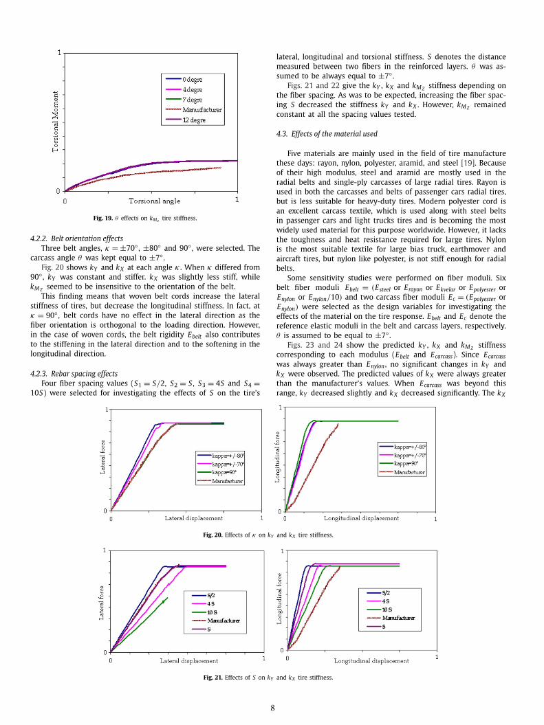
Fig. 19. θ effects on kMz tire stiffness.

4.2.2. Belt orientation effectsThree belt angles, κ = ±70◦ , ±80◦ and 90◦ , were selected. The

carcass angle θ was kept equal to ±7◦ .Fig. 20 shows kY and kX at each angle κ . When κ differed from

90◦ , kY was constant and stiffer. kX was slightly less stiff, whilekM Z seemed to be insensitive to the orientation of the belt.

This finding means that woven belt cords increase the lateralstiffness of tires, but decrease the longitudinal stiffness. In fact, atκ = 90◦ , belt cords have no effect in the lateral direction as thefiber orientation is orthogonal to the loading direction. However,in the case of woven cords, the belt rigidity Ebelt also contributesto the stiffening in the lateral direction and to the softening in thelongitudinal direction.

4.2.3. Rebar spacing effectsFour fiber spacing values (S1 = S/2, S2 = S , S3 = 4S and S4 =

10S) were selected for investigating the effects of S on the tire’s

lateral, longitudinal and torsional stiffness. S denotes the distancemeasured between two fibers in the reinforced layers. θ was as-sumed to be always equal to ±7◦ .

Figs. 21 and 22 give the kY , kX and kM Z stiffness depending onthe fiber spacing. As was to be expected, increasing the fiber spac-ing S decreased the stiffness kY and kX . However, kM Z remainedconstant at all the spacing values tested.

4.3. Effects of the material used

Five materials are mainly used in the field of tire manufacturethese days: rayon, nylon, polyester, aramid, and steel [19]. Becauseof their high modulus, steel and aramid are mostly used in theradial belts and single-ply carcasses of large radial tires. Rayon isused in both the carcasses and belts of passenger cars radial tires,but is less suitable for heavy-duty tires. Modern polyester cord isan excellent carcass textile, which is used along with steel beltsin passenger cars and light trucks tires and is becoming the mostwidely used material for this purpose worldwide. However, it lacksthe toughness and heat resistance required for large tires. Nylonis the most suitable textile for large bias truck, earthmover andaircraft tires, but nylon like polyester, is not stiff enough for radialbelts.

Some sensitivity studies were performed on fiber moduli. Sixbelt fiber moduli Ebelt = (Esteel or Erayon or Ekvelar or Epolyester orEnylon or Enylon/10) and two carcass fiber moduli Ec = (Epolyester orEnylon) were selected as the design variables for investigating theeffects of the material on the tire response. Ebelt and Ec denote thereference elastic moduli in the belt and carcass layers, respectively.θ is assumed to be equal to ±7◦ .

Figs. 23 and 24 show the predicted kY , kX and kM Z stiffnesscorresponding to each modulus (Ebelt and Ecarcass). Since Ecarcass

was always greater than Enylon , no significant changes in kY andkX were observed. The predicted values of kX were always greaterthan the manufacturer’s values. When Ecarcass was beyond thisrange, kY decreased slightly and kX decreased significantly. The kX

Fig. 20. Effects of κ on kY and kX tire stiffness.

Fig. 21. Effects of S on kY and kX tire stiffness.

8

Fig. 22. S effects on kMz tire stiffness.

Fig. 23. Effects of the fiber modulus on kY and kX tire stiffness.

Fig. 24. Effects of the fiber on the tire stiffness kMz .

predicted by the Rebar model was therefore very similar to thevalue specified by the manufacturer. The steel–polyester materialshowed the greatest lateral stiffness (see Fig. 23).

The tire response seems to be more sensitive to the carcassmoduli. Most carcass layers of aircraft tires are presumably madeof polyester, as stated in [19].

9

These sensitivity studies show that the kY depends on the mod-ulus of the carcass Ecarcass while kX depends on Ebelt . kY and kX

seem to be strongly coupled. Although many configurations andsimulations were performed, it is difficult, however, to determineexactly how are correlated the lateral and longitudinal stiffness.

5. Conclusion

In this paper is presented a method for modeling an aircrafttire under severe operating conditions using finite element tools.The Rebar model proved to be the most accurate mean of mod-eling tire behavior under static and quasi-static loading conditionswith a view to dynamic simulations. The Rebar modeling of the re-inforced zones also gave the most realistic results. After the manysensitivity studies performed here, the next challenge is to eluci-date the strong coupling which seems to exist between the lateraland longitudinal stiffness.

References

[1] ABAQUS/Standard, Theory Manual and Example Problems Manual, Release 6.9,2010.

[2] ABAQUS/Standard, Abaqus Analysis User’S Manual, Release 6.9, 2010.[3] S.K. Clark, R.N. Dogde, Heat generation in aircraft tires under free rolling con-

ditions, NASA contractor report 3629, 1982.[4] M.H. Ghoreish Reza, Finite element analysis of steel-belted radial tyre with

tread pattern under contact load, Iranian Polymer Journal 15 (8) (2006) 667–674.

[5] R.M. Jones, Mechanics of Composite Materials, 2nd edition, Taylor & Francis,1999.

[6] A. Kongo Kondé, I. Rosu, F. Lebon, O. Brardo, B. Devésa, Etude du comportementen roulement d’un pneu d’avion, Colloque National de Calcul de Structures,Giens 1 (2009) 699–704 (in French).

[7] A. Kongo Kondé, Modélisation du roulement d’un pneumatique d’avion, PhDthesis, Aix-Marseille University, 2011, p. 232 (in French).

[8] N. Korunovic, M. Trajanovic, M. Stojkovic, Finite element model for steady staterolling tire analysis, Journal of the Serbian Society for Computational Mechan-ics 1 (1) (2007) 63–79.

[9] J. Lacombe, Tire model for simulations of vehicle motion on high and low fric-tion road surfaces, in: Proceedings of the Winter 2000 Simulation Conference,vol. 1, Hanover, 2000, pp. 1025–1034.

[10] N. Lahellec, F. Mazerolle, J.C. Michel, Second-order estimate of the macroscopicbehaviour of periodic hyperelastic composites: theory and experimental vali-dation, Journal of the Mechanics and Physics of Solids 52 (2004) 27–49.

[11] J.L. McCarthy, J.A. Tanner, Temperature distribution in a aircraft tire at lowground speed, NASA technical paper 2195, 1983.

[12] Michelin dans le Benelux, Performances de haut niveau pour le décollage etl’atterrissage, http://www.michelin.be (in French).

[13] K.V. Narasimha Rao, R. Krishna Kumar, P.C. Bohara, R. Mukhopadhyay, A finiteelement algorithm for the prediction of steady-state temperatures of rollingtires, Tire Science and Technology, TSTCA 34 (3) (2006) 195–214.

[14] J.P. Navarro, Contribution la modélisation du pneumatique de l’Avion, Thèse,Université Toulouse III–Paul Sabatier, 2003 (in French).

[15] O.A. Olatunbosum, E.O. Bolarinwa, Finite element simulation of the tyre bursttest, in: Proceedings of the Institution of Mechanical Engineers, vol. 218, 2006,pp. 1251–1258.

[16] J.A. Tanner, R.C. Dreher, S.M. Strubb, E.G. Smith, Tire tread temperatures duringantiskid braking and “cornering” on a dry runway, NASA technical paper 2009,1982.

[17] W.D. Versteden, Improving a tire for motorcycle simulation, Thesis, EindhovenUniversity of Technology, 2005.

[18] J.D. Walter, H.P. Patel, Approximate expressions for the elastic constants ofcord–rubber laminates, Rubber Chemistry and Technology 52 (1979) 710–724.

[19] J.D. Walter, A.N. Gent, The pneumatic tire, National Highway Traffic Safety Ad-ministration, US Department of Transportation, Washington DC 20590, DOTContract DTNH22-02-P-07210, August 2005.

[20] G. Yanjin, Z. Guoqun, C. Gang, Influence of belt cord angle on radial tire underdifferent rolling states, Journal of Reinforced Plastics and Composites 25 (10)(2006) 1059–1077.