modeling and analysis of off-road tire cornering

Modeling and Analysis of Off-Road Tire Cornering Characteristics

by

Fatemeh Gheshlaghi

A thesis submitted to the

School of Graduate and Postdoctoral Studies in partial

fulfillment of the requirements for the degree of

Master of Applied Science in Mechanical Engineering

Faculty of Engineering and Applied Science

University of Ontario Institute of Technology (Ontario Tech University)

Oshawa, Ontario, Canada

May 2022

© Fatemeh Gheshlaghi, 2022

THESIS EXAMINATION INFORMATION

Submitted by: Fatemeh Gheshlaghi

Master of Applied Science in Mechanical Engineering

Thesis title: Modeling and Analysis of Off-Road Tire Cornering Characteristics

An oral defense of this thesis took place on April 28, 2022 in front of the following

examining committee:

Examining Committee:

Chair of Examining Committee

Dr. Martin Agelin-Chaab

Research Supervisor

Dr. Moustafa El-Gindy

Research Co-supervisor

Dr. Subhash Rakheja

Examining Committee Member

Dr. Zeinab El-Sayegh

Thesis Examiner

Dr. Jaho Seo

The above committee determined that the thesis is acceptable in form and content and

that a satisfactory knowledge of the field covered by the thesis was demonstrated by the

candidate during an oral examination. A signed copy of the Certificate of Approval is

available from the School of Graduate and Postdoctoral Studies.

ii

ABSTRACT

Cornering performance characteristics of wheeled vehicles substantially rely on the

forces/moments generated from interactions between pneumatic tires and terrains.

Accurate models are thus required to predict these forces/moments to be employed in

vehicle simulations for development and design. The goal of this dissertation research is to

provide a virtual testing environment in Pam-Crash software as an alternative to actual tests

for Finite Element Analysis (FEA) and Smoothed Particle Hydrodynamics (SPH) analysis

of rolling tire interactions on deformable terrains. SPH method and hydrodynamics-elastic

plastic material were used to simulate different soil types that are often utilized in vehicle-

terrain interactions. Two pressure-sinkage and shear-strength experiments were used to

calibrate the terrains. The simulation findings were compared with the measured data that

showed good agreements.

Furthermore, a detailed analysis of the rolling resistance coefficient and cornering

properties of the tire over various terrains is presented, as well as the development of

Genetic Algorithms (GA) to determine the mathematical relations for the cornering force,

self-aligning moment, and overturning moment as functions of important operating factors.

Cornering tests were performed for the RHD tire operating over the mud soil to examine

the validity of the GA-based cornering force, self-aligning moment, and overturning

moment relationships. It was concluded that the identified mathematical relations could

provide very good estimations of the cornering characteristics under a broad range of

operating conditions and soils.

Keywords: Tire modeling; Terrain calibration; Tire-terrain interaction; Smoothed-Particle

Hydrodynamics; Finite Element Analysis; Cornering Characteristics; Rolling resistance

iii

AUTHOR'S DECLARATION

I hereby declare that this thesis consists of original work of which I have authored. This is

a true copy of the thesis, including any required final revisions, as accepted by my

examiners.

I authorize the University of Ontario Institute of Technology to lend this thesis to other

institutions or individuals for the purpose of scholarly research. I further authorize the

University of Ontario Institute of Technology to reproduce this thesis by photocopying or

by other means, in total or in part, at the request of other institutions or individuals for the

purpose of scholarly research. I understand that my thesis will be made electronically

available to the public.

FATEMEH GHESHLAGHI

iv

STATEMENT OF CONTRIBUTIONS

Part of the work described in Chapter 2 will be submitted as:

Gheshlaghi, F., Rakheja, S., El-Gindy, M., “Tire-Terrain Interaction Modeling and

Analysis: Literature Survey” Int. J. Vehicle Systems Modelling and Testing, (To be

submitted).

Part of the work described in Chapter 3 has been published as:

Gheshlaghi F., El-Sayegh Z., El- Gindy M et al. 'Prediction and validation of

terramechanics models for estimation of tire rolling resistance coefficient". Int. J. Vehicle

Systems Modelling and Testing, 14, no. 3-4 (2020) 1-12.

Part of the work described in Chapter 4 has been published as:

Gheshlaghi, F., El-Sayegh, Z., El-Gindy, M., Oijer, F. et al., "Advanced Analytical Truck

Tires-Terrain Interaction Model," SAE Technical Paper No. 2021-01-0329, April 13- 15,

Detroit Michigan, USA, (2021), https://doi.org/10.4271/2021-01-0329.

Part of the work described in Chapters 5 and 6 has been published as:




Gheshlaghi, F., El-Sayegh, Z., El-Gindy, M., Oijer, F. et al., “Analysis of off-road tire

cornering characteristics using advanced analytical techniques” Tire Society Journal, Oct

2021, USA, (Under review).

https://doi.org/10.4271/2021-01-0329

https://doi.org/10.4271/2021-01-0329

v

CONTENTS

ABSTRACT ................................................................................................................... ii

AUTHOR'S DECLARATION ....................................................................................... iii

STATEMENT OF CONTRIBUTIONS ........................................................................ iv

CONTENTS ................................................................................................................... v

LIST OF FIGURES ......................................................................................................... ix

LIST OF TABLES ......................................................................................................... xvi

NOMENCLATURE ...................................................................................................... xvii

ACKNOWLEDGEMENTS .......................................................................................... xix

CHAPTER 1 MOTIVATION AND OBJECTIVES .................................................... 1

1.1 MOTIVATION .................................................................................................... 1

1.2 OBJECTIVES AND SCOPE ............................................................................... 2

1.3 OUTLINE OF THESIS ........................................................................................ 3

CHAPTER 2 LITERATURE REVIEW ....................................................................... 5

2.1 Tire modeling ....................................................................................................... 6

2.1.1 FEA tire modeling ......................................................................................... 9

2.2 Tire model validations ........................................................................................ 14

2.2.1 Multi-axis stiffness tests ............................................................................. 14

2.2.2 Dynamic validation tests ............................................................................. 20

Drum-cleat test ...................................................................................................... 21

Yaw Oscillation test: .............................................................................................. 22

Cornering test ......................................................................................................... 23

2.3 Terrain modeling methods ................................................................................. 24

2.4 Terrain models calibrations ................................................................................ 29

2.4.1 Soil penetration tests ................................................................................... 29

vi

2.4.2 Pressure-sinkage tests .............................................................................. 31

2.4.3 Shear strength test ................................................................................... 32

2.5 Tire-terrain interaction modeling ....................................................................... 33

2.5.1 Rolling resistance analysis .......................................................................... 33

2.5.2 Cornering characteristic analysis ................................................................ 36

2.5.3 Soil behavior analysis ................................................................................. 38

2.6 Summary ............................................................................................................ 40

CHAPTER 3 TIRE MODELING AND MODEL VALIDATIONS ........................ 42

3.1 Tire model validations ........................................................................................ 45

3.1.1 Vertical stiffness test ................................................................................... 45

3.1.2 Footprint test ............................................................................................... 47

3.1.3 Drum-cleat test ............................................................................................ 49

3.2 Summary ............................................................................................................ 52

CHAPTER 4 SOIL MODELING ................................................................................ 54

4.1 Experimental characterization of a clay loam soil ............................................. 54

4.2 SPH soil modeling .............................................................................................. 56

4.3 SPH sensitivity analysis ..................................................................................... 57

Displacement speed in the shear-strength test ............................................................... 57

Equation of state coefficients ........................................................................................ 59

Yield stress .................................................................................................................... 60

Tangent modulus ........................................................................................................... 61

4.4 SPH soil model calibrations ............................................................................... 62

4.4.1 Pressure-sinkage test ................................................................................... 63

4.4.2 Shear strength test ....................................................................................... 64

4.5 Soil model characteristics ................................................................................... 66

vii

4.6 Summary ............................................................................................................ 69

CHAPTER 5 TIRE-TERRAIN INTERACTIONS ANALYSIS: ROLLING

RESISTANCE 70

5.1 Introduction ........................................................................................................ 70

5.2 Simulation model setup for tire rolling resistance analyses ............................... 71

5.3 Rolling resistance analyses ................................................................................. 74

5.3.1 Effect of vertical load .................................................................................. 75

5.3.2 Effect of inflation pressure .......................................................................... 76

5.3.3 Effect of soil compaction ............................................................................ 80

5.3.4 Effect of speed ............................................................................................ 81

5.4 The development of rolling resistance relationship using genetic algorithm ..... 82

5.5 Summary ............................................................................................................ 87

CHAPTER 6 TIRE-TERRAIN INTERACTIONS ANALYSIS: CORNERING

CHARACTERISTICS .................................................................................................... 89

6.1 Introduction ........................................................................................................ 89

6.2 Simulation model setup ...................................................................................... 90

6.3 Cornering characteristics analyses ..................................................................... 92

6.3.1 Effect of side-slip angle .............................................................................. 92

6.3.2 Effect of vertical load .................................................................................. 97

6.3.3 Effect of inflation pressure ........................................................................ 102

6.3.4 Effect of rolling speed ............................................................................... 107

6.3.5 Effect of soil internal friction angle .......................................................... 111

6.3.6 Effect of soil compaction .......................................................................... 115

6.4 The development and validation of cornering characteristics relationships using

genetic algorithm ......................................................................................................... 119

6.5 Summary .......................................................................................................... 123

viii

CHAPTER 7: MAJOR CONCLUSIONS AND CONTRIBUTIONS ...................... 125

7.1 Major contributions of the thesis ...................................................................... 125

7.2 Major conclusions ............................................................................................ 125

7.3 Future works ..................................................................................................... 128

7.4 Publications ...................................................................................................... 129

REFERENCES .............................................................................................................. 130

ix

LIST OF FIGURES

FIGURE 2.1. DYNAMICS TIRE MODELS ..................................................................... 7

FIGURE 2.2. RIGID RING TIRE MODEL [SCHMEITZ, 2004] ..................................... 8

FIGURE 2.3. TIRE MODEL WITH CONSTANT SHEAR STRESS IN RIM CONTACT

REGION [ZHANG ET AL., 2001] ........................................................................... 10

FIGURE 2.4. TIRE COMPONENTS [ZHANG ET AL., 2001] ...................................... 11

FIGURE 2.5. (A) CONSTITUENTS OF 295/75R22.5 TRUCK TIRE

(GOODYEAR.COM); AND (B) FEA TRUCK TIRE MODEL [CHAE, 2006] ..... 12

FIGURE 2.6. THE FEA MODEL OF AN AGRICULTURAL VEHICLE TIRE [EL-

SAYEGH ET AL., 2019] .......................................................................................... 13

FIGURE 2.7. FEA MODEL OF A HIGH-LUG FARM SERVICE VEHICLE TIRE [XU

ET AL., 2020] ........................................................................................................... 14

FIGURE 2.8. TIRE VERTICAL STIFFNESS TESTING MACHINE [JAFARI, 2018] . 16

FIGURE 2.9. FEA HLFS TIRE SIZE 220/80-B16 VERTICAL STIFFNESS TEST [EL-

SAYEGH ET AL., 2019] .......................................................................................... 16

FIGURE 2.10. COMPARISONS OF VERTICAL FORCE-DEFLECTION

CHARACTERISTICS OBTAINED FROM THE FEA MODEL OF A HLFS TIRE

WITH THE MEASURED DATA [EL-SAYEGH ET AL., 2019] ........................... 17

FIGURE 2.11. MEASURED TRUCK TIRE FOOTPRINT UNDER DIFFERENT

VERTICAL LOADS AND INFLATION PRESSURES [XIONG ET AL., 2015] .. 18

FIGURE 2.12. COMPARISON OF CONTACT AREA RESPONSES OF A HLFS TIRE

MODEL WITH THE MEASURED DATA UNDER DIFFERENT TIRE LOADS

[GHESHLAGHI, 2020] ............................................................................................ 19

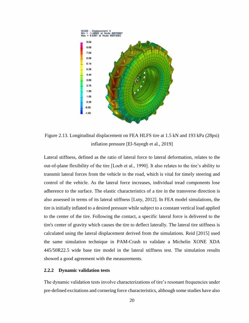
FIGURE 2.13. LONGITUDINAL DISPLACEMENT ON FEA HLFS TIRE AT 1.5 KN

AND 193 KPA (28PSI) INFLATION PRESSURE [EL-SAYEGH ET AL., 2019] 20

FIGURE 2.14. THE VERTICAL FIRST MODE OF VIBRATION OF FEA WIDE-

BASED TIRE AT 45.4 KN VERTICAL LOAD AND 827 KPA (120 PSI)

INFLATION PRESSURE [MARJANI, 2016] ......................................................... 22

FIGURE 2.15. (A) YAW OSCILLATION TESTING MACHINE; AND (B) FEA YAW

OSCILLATION TEST MODEL [CHE, 2006] ......................................................... 23

FIGURE 2.16. CORNERING FORCE VALIDATION USING EXPERIMENTAL

DATA [CHAE, 2006] ............................................................................................... 24

FIGURE 2.17. SELF-ALIGNING MOMENT VALIDATION USING

EXPERIMENTAL DATA [CHAE, 2006] ............................................................... 24

FIGURE 2.18. PARTICLE INTERPOLATION UTILIZING PARTICLES INSIDE THE

SMOOTHING FUNCTIONS DOMAIN [BUI ET AL., 2007] ................................ 27

FIGURE 2.19. BEVAMETER SCHEMATIC [WONG, 2008] ....................................... 31

FIGURE 2.20. THE FEA PRESSURE-SINKAGE TEST FOR 17% MOIST CLAY

LOAM SOIL [GHESHLAGHI AND MARDANI, 2020] ........................................ 32

FIGURE 2.21. THE FEA SHEAR-STRENGTH TEST FOR 17% MOIST CLAY LOAM

SOIL; AND [GHESHLAGHI AND MARDANI, 2020] .......................................... 33

x

FIGURE 2.22. (A) VERTICAL, (B) LONGITUDINAL, AND (C) TRANSVERSE

CONTACT STRESS DISTRIBUTION OF A FREE-ROLLING TIRE WITH A 32.5

KN LOAD [GUO ET AL., 2020] ............................................................................. 39

FIGURE 2.23. TERRAIN MAPPING DURING THE MULTI-PASS SIMULATION OF

A DRIVEN TIRE (A) SOIL CONSECUTIVE LOADING-UNLOADING (B)

CONTOUR OF TERRAIN SINKAGE [SANDU ET AL., 2019] ............................ 40

FIGURE 3.1. FEA TIRE BASIC DIMENSIONS [CHAE, 2006] .................................... 43

FIGURE 3.2. RHD TIRE SECTION [SLADE, 2009] ..................................................... 44

FIGURE 3.3. THE RAMP VERTICAL LOAD APPLIED TO THE RIM OF THE TIRE

MODEL .................................................................................................................... 46

FIGURE 3.4. VERTICAL STIFFNESS SIMULATION TEST OF THE TIRE MODEL 46

FIGURE 3.5. LOAD-DEFLECTION RESPONSES OF THE RHD TRUCK TIRE

MODEL UNDER DIFFERENT INFLATION PRESSURES .................................. 47

FIGURE 3.6. VON MISES STRESS DISTRIBUTION OVER THE CONTACT AREA

OF THE TIRE MODEL (40 KN VERTICAL LOAD AND 758 KPA (110 PSI)

INFLATION PRESSURE) ....................................................................................... 48

FIGURE 3.7. COMPARISON OF CONTACT AREAS OBTAINED FROM THE TIRE

MODEL WITH THOSE REPORTED FOR THE GOODYEAR TIRE (CHAE,

2006) FOR DIFFERENT VERTICAL LOADS (INFLATION PRESSURE:758

KPA (110 PSI)) ......................................................................................................... 49

FIGURE 3.8. FEA RHD TRUCK TIRE MODEL UNDER THE DRUM-CLEAT TEST

................................................................................................................................... 50

FIGURE 3.9. FREQUENCY SPECTRUM OF VERTICAL AND LONGITUDINAL

FREE VIBRATION OF THE TIRE MODEL OBTAINED FROM THE DRUM-

CLEAT TEST (TIRE LOAD: 40 KN; INFLATION PRESSURE: 586 KPA (85

PSI)) .......................................................................................................................... 51




PSI)) .......................................................................................................................... 52




PSI)) .......................................................................................................................... 52

FIGURE 4.1. PLATE PENETRATION TESTER AND SHEAR TEST BOX USED FOR

THE MEASUREMENT OF SOIL ........................................................................... 56

FIGURE 4.2. CONVERTING FEA ELEMENTS TO SPH PARTICLES ....................... 57

FIGURE 4.3. SPH SOIL SHEAR-STRENGTH AT DIFFERENT SPEEDS VERSUS

MEASUREMENTS FOR CLAY LOAM SOIL ...................................................... 58

FIGURE 4.4. SPH SOIL PRESSURE-SINKAGE AT DIFFERENT C1 COEFFICIENTS

VERSUS MEASUREMENTS FOR CLAY LOAM SOIL ...................................... 59

FIGURE 4.5. SPH SOIL SHEAR-STRENGTH AT DIFFERENT SPEEDS VERSUS

MEASUREMENTS FOR CLAY LOAM SOIL ....................................................... 60

xi

FIGURE 4.6. SPH SOIL PRESSURE-SINKAGE AT DIFFERENT YIELD STRESSES


FIGURE 4.7. SPH SOIL SHEAR-STRENGTH AT DIFFERENT TANGENT MODULI


FIGURE 4.8. SPH SOIL PRESSURE-SINKAGE TEST ................................................. 63

FIGURE 4.9. SPH SOIL PRESSURE-SINKAGE VERSUS MEASUREMENTS FOR

CLAY LOAM SOIL ................................................................................................. 64

FIGURE 4.10. SPH SOIL SHEAR STRENGTH TEST .................................................. 65

FIGURE 4.11. SPH SOIL SHEAR-STRENGTH TEST VERSUS MEASUREMENTS

FOR THE CLAY LOAM SOIL ............................................................................... 66

FIGURE 4.12. SIMULATED PRESSURE-SINKAGE TESTS FOR DIFFERENT SOILS

................................................................................................................................... 68

FIGURE 5.1. SCHEMATIC OF THE VOLVO F-SERIES MEDIUM 8*4 TRUCK ...... 71

FIGURE 5.2. MODEL USED TO SIMULATE TIRE’S INTERACTIONS WITH A

SOFT SOIL (CLAY LOAM) .................................................................................... 73

FIGURE 5.3. MULTI-PASS TIRE-TERRAIN INTERACTION MODEL

CONSIDERING THE FOUR TIRES OF A SINGLE VEHICLE TRACK ............. 73

FIGURE 5.4. INFLUENCE OF VERTICAL LOAD ON ROLLING RESISTANCE

COEFFICIENT OF THE TIRE ROLLING FREELY ON DIFFERENT SOILS: (A)

CLAY LOAM; (B) DENSE SAND; AND (C) CLAYEY SOIL (FORWARD

SPEED = 10KM/H) .................................................................................................. 76

FIGURE 5.5. EFFECT OF INFLATION PRESSURE ON ROLLING RESISTANCE

COEFFICIENT OF A DRIVEN TIRE SUBJECT TO DIFFERENT DRIVE

TORQUES OVER THE CLAY LOAM SOIL (FORWARD SPEED: 10 KM/H;

WHEEL LOAD: 40 KN). ......................................................................................... 78

FIGURE 5.6. INFLUENCE OF INFLATION PRESSURE ON ROLLING

RESISTANCE COEFFICIENT OF THE TIRE ROLLING FREELY ON

DIFFERENT SOILS: (A) CLAY LOAM; (B) DENSE SAND; AND (C) CLAYEY

SOIL (FORWARD SPEED = 10KM/H) .................................................................. 79

FIGURE 5.7. ROLLING RESISTANCE COEFFICIENT AS A FUNCTION OF SOIL

DEPTH AT DIFFERENT SOILS ............................................................................. 81

FIGURE 5.8. EFFECT OF FORWARD SPEED ON THE ROLLING RESISTANCE

COEFFICIENT OF THE TIRE OPERATING ON THE CLAY SOIL FOR

DIFFERENT VERTICAL LOADS (INFLATION PRESSURE: 758KPA (110 PSI))

................................................................................................................................... 82

FIGURE 5.9. THE FLOWCHART OF THE PROPOSED GENETIC ALGORITHM

[ABE, 2004] .............................................................................................................. 84

FIGURE 5.10. PREDICTED VERSUS SIMULATED ROLLING RESISTANCE

COEFFICIENT ......................................................................................................... 87

FIGURE 6.1. TIRE-TERRAIN INTERACTION MODEL CONSIDERING SIDE-SLIP

OF TIRES OF A FOUR-AXLE TRUCK ................................................................. 91

FIGURE 6.2. FORCES AND MOMENTS ACTING ON A STEERED TIRE ............... 91

xii

FIGURE 6.3. SELF-ALIGNING MOMENT AS A FUNCTION OF SIDE-SLIP ANGLE

FOR THE FREE-ROLLING TIRES OVER THE SANDY LOAM AT DIFFERENT

AXLES (SPEED:15 KM/H; INFLATION PRESSURE: 758 KPA (110 PSI) ;

VERTICAL LOAD: 40 KN) .................................................................................... 93

FIGURE 6.4. CORNERING FORCE AS A FUNCTION OF SIDE-SLIP ANGLE FOR

THE FREE-ROLLING TIRES OVER THE SANDY LOAM AT DIFFERENT

AXLES (SPEED:15 KM/H; INFLATION PRESSURE: 758 KPA (110 PSI);

VERTICAL LOAD: 40 KN) .................................................................................... 94

FIGURE 6.5. SELF-ALIGNING MOMENT AS A FUNCTION OF SIDE-SLIP ANGLE

FOR THE DRIVEN TIRES OVER THE SANDY LOAM AT DIFFERENT AXLES

(SPEED:15 KM/H; INFLATION PRESSURE: 758 KPA (110 PSI); VERTICAL

LOAD: 40 KN) ......................................................................................................... 95

FIGURE 6.6. CORNERING FORCE AS A FUNCTION OF SIDE-SLIP ANGLE FOR

THE DRIVEN TIRES OVER THE SANDY LOAM AT DIFFERENT AXLES

(SPEED:15 KM/H; INFLATION PRESSURE: 758 KPA (110 PSI); VERTICAL

LOAD: 40 KN) ......................................................................................................... 96

FIGURE 6.7. OVERTURNING MOMENT AS A FUNCTION OF SIDE-SLIP ANGLE

FOR THE FREE-ROLLING TIRES OVER THE SANDY LOAM AT DIFFERENT

AXLES (SPEED:15 KM/H; INFLATION PRESSURE: 758 KPA (110 PSI);

VERTICAL LOAD: 40 KN) .................................................................................... 97

FIGURE 6.8. INFLUENCE OF VERTICAL WHEEL LOAD ON THE SELF-

ALIGNING MOMENT OF THE FREE-ROLLING TIRE OPERATING ON 25%

MOIST SANDY SOIL FOR DIFFERENT INFLATION PRESSURES (SLIP

ANGLE: 6 DEG; SPEED: 15 KM/H)....................................................................... 98

FIGURE 6.9. INFLUENCE OF VERTICAL WHEEL LOAD ON THE CORNERING

FORCE OF THE FREE-ROLLING TIRE OPERATING ON 25% MOIST SANDY

SOIL FOR DIFFERENT INFLATION PRESSURES (SLIP ANGLE: 6 DEG;

SPEED: 15 KM/H) ................................................................................................... 99

FIGURE 6.10. INFLUENCE OF VERTICAL WHEEL LOAD ON THE SELF-

ALIGNING MOMENT OF THE DRIVEN TIRE OPERATING ON 25% MOIST

SANDY SOIL FOR DIFFERENT INFLATION PRESSURES (SLIP ANGLE: 6

DEG; SPEED: 15 KM/H) ....................................................................................... 100

FIGURE 6.11. INFLUENCE OF VERTICAL WHEEL LOAD ON THE CORNERING

FORCE OF THE DRIVEN TIRE OPERATING ON 25% MOIST SANDY SOIL

FOR DIFFERENT INFLATION PRESSURES (SLIP ANGLE: 6 DEG; SPEED: 15

KM/H) ..................................................................................................................... 101

FIGURE 6.12. INFLUENCE OF VERTICAL WHEEL LOAD ON THE

OVERTURNING MOMENT OF THE FREE-ROLLING TIRE OPERATING ON

25% MOIST SANDY SOIL FOR DIFFERENT INFLATION PRESSURES (SLIP

ANGLE: 6 DEG; SPEED: 15 KM/H)..................................................................... 102

FIGURE 6.13. INFLUENCE OF INFLATION PRESSURE ON SELF-ALIGNING

MOMENT OF THE TIRE ROLLING FREELY ON THE 25% MOIST SANDY

xiii

SOIL FOR TWO DIFFERENT SLIP ANGLES (VERTICAL LOAD: 40 KN;

SPEED: 15 KM/H) ................................................................................................ 103

FIGURE 6.14. INFLUENCE OF INFLATION PRESSURE ON CORNERING FORCE

OF THE TIRE ROLLING FREELY ON THE 25% MOIST SANDY SOIL FOR

TWO DIFFERENT SLIP ANGLES (VERTICAL LOAD: 40 KN; SPEED: 15

KM/H) ..................................................................................................................... 104

FIGURE 6.15. INFLUENCE OF INFLATION PRESSURE ON SELF-ALIGNING

MOMENT OF THE DRIVEN TIRE ON THE 25% MOIST SANDY SOIL FOR

TWO DIFFERENT SLIP ANGLES (VERTICAL LOAD: 40 KN; SPEED: 15

KM/H) ..................................................................................................................... 105

FIGURE 6.16. INFLUENCE OF INFLATION PRESSURE ON CORNERING FORCE

OF THE DRIVEN TIRE ON THE 25% MOIST SANDY SOIL FOR TWO

DIFFERENT SLIP ANGLES (VERTICAL LOAD: 40 KN; SPEED: 15 KM/H) 106

FIGURE 6.17. INFLUENCE OF INFLATION PRESSURE ON OVERTURNING

MOMENT OF THE TIRE ROLLING FREELY ON THE 25% MOIST SANDY

SOIL FOR DIFFERENT SLIP ANGLES (VERTICAL LOAD: 40 KN; SPEED: 15

KM/H) ..................................................................................................................... 106

FIGURE 6.18. INFLUENCE OF FORWARD SPEED ON THE SELF-ALIGNING

MOMENT OF FREE-ROLLING TIRES OF THE FOUR-AXLE VEHICLE

MODEL OPERATING ON THE DRY SANDY LOAM SOIL (SLIP ANGLE: 6

DEG; INFLATION PRESSURE: 758 KPA (110 PSI); VERTICAL LOAD: 40 KN)

................................................................................................................................. 108

FIGURE 6.19. INFLUENCE OF FORWARD SPEED ON THE CORNERING FORCE

OF FREE-ROLLING TIRES OF THE FOUR-AXLE VEHICLE MODEL

OPERATING ON THE DRY SANDY LOAM SOIL (SLIP ANGLE: 6 DEG;

INFLATION PRESSURE: 758 KPA (110 PSI); VERTICAL LOAD: 40 KN) ..... 108

FIGURE 6.20. INFLUENCE OF FORWARD SPEED ON THE OVERTURNING

MOMENT OF FREE-ROLLING TIRES OF THE FOUR-AXLE VEHICLE

MODEL OPERATING ON THE DRY SANDY LOAM SOIL (SLIP ANGLE: 6

DEG; INFLATION PRESSURE: 758 KPA (110 PSI); VERTICAL LOAD: 40 KN)

................................................................................................................................. 109

FIGURE 6.21. INFLUENCE OF FORWARD SPEED ON THE SELF-ALIGNING

MOMENT OF DRIVEN TIRES OF THE FOUR-AXLE VEHICLE MODEL

OPERATING ON THE DRY SANDY LOAM SOIL (SLIP ANGLE: 6 DEG;

INFLATION PRESSURE: 758 KPA (110 PSI); VERTICAL LOAD: 40 KN) ..... 110

FIGURE 6.22. INFLUENCE OF FORWARD SPEED ON THE CORNERING FORCE

OF DRIVEN TIRES OF THE FOUR-AXLE VEHICLE MODEL OPERATING ON

THE DRY SANDY LOAM SOIL (SLIP ANGLE: 6 DEG; INFLATION

PRESSURE: 758 KPA (110 PSI); VERTICAL LOAD: 40 KN) ........................... 111

FIGURE 6.23. INFLUENCE OF SOIL INTERNAL FRICTION ANGLE ON THE

SELF-ALIGNING MOMENT DEVELOPED BY THE FREE-ROLLING TIRE

FOR TWO DIFFERENT SLIP ANGLES (INFLATION PRESSURE: 758 KPA

(110 PSI); VERTICAL LOAD: 40 KN; SPEED: 15 KM/H) ................................. 112

xiv


CORNERING FORCE DEVELOPED BY THE FREE-ROLLING TIRE FOR TWO

DIFFERENT SLIP ANGLES (INFLATION PRESSURE: 758 KPA (110 PSI);

VERTICAL LOAD: 40 KN; SPEED: 15 KM/H) ................................................... 113


OVERTURNING MOMENT DEVELOPED BY THE FREE-ROLLING TIRE FOR




SELF-ALIGNING MOMENT DEVELOPED BY THE DRIVEN TIRE FOR TWO




CORNERING FORCE DEVELOPED BY THE DRIVEN TIRE FOR TWO



FIGURE 6.28. INFLUENCE OF SOIL SINKAGE ON THE SELF-ALIGNING

MOMENT OF THE FREE-ROLLING TIRE OPERATING ON THE DRY SANDY

LOAM SOIL AT 15 KM/H SPEED, 758 KPA (110 PSI) INFLATION PRESSURE,

AND 40 KN VERTICAL LOAD ........................................................................... 116

FIGURE 6.29. INFLUENCE OF SOIL SINKAGE ON THE SELF-ALIGNING

MOMENT OF THE DRIVEN TIRE OPERATING ON THE DRY SANDY LOAM

SOIL AT 15 KM/H SPEED, 758 KPA (110 PSI) INFLATION PRESSURE, AND

40 KN VERTICAL LOAD ..................................................................................... 116

FIGURE 6.30. INFLUENCE OF SOIL SINKAGE ON THE CORNERING FORCE OF

THE FREE-ROLLING TIRE OPERATING ON THE DRY SANDY LOAM SOIL

AT 15 KM/H SPEED, 758 KPA (110 PSI) INFLATION PRESSURE, AND 40 KN

VERTICAL LOAD ................................................................................................. 117

FIGURE 6.31. INFLUENCE OF SOIL SINKAGE ON THE CORNERING FORCE OF

THE DRIVEN TIRE OPERATING ON THE DRY SANDY LOAM SOIL AT 15

KM/H SPEED, 758 KPA (110 PSI) INFLATION PRESSURE, AND 40 KN

VERTICAL LOAD ................................................................................................. 118

FIGURE 6.32. INFLUENCE OF SOIL SINKAGE ON THE OVERTURNING

MOMENT OF THE FREE-ROLLING TIRE OPERATING ON THE DRY SANDY

LOAM SOIL AT 15 KM/H SPEED, 758 KPA (110 PSI) INFLATION PRESSURE,

AND 40 KN VERTICAL LOAD ........................................................................... 118

FIGURE 6.33. CORRELATIONS OF THE CORNERING FORCE PREDICTED FROM

THE IDENTIFIED MATHEMATICAL RELATIONS WITH THOSE PREDICTED

FROM THE FE-SPH SIMULATION MODEL. .................................................... 122

FIGURE 6.34. CORRELATIONS OF THE SELF-ALIGNING MOMENT PREDICTED

FROM THE IDENTIFIED MATHEMATICAL RELATIONS WITH THOSE

PREDICTED FROM THE FE-SPH SIMULATION MODEL. ............................. 123

xv

FIGURE 6.35. CORRELATIONS OF THE OVERTURNING MOMENT PREDICTED

FROM THE IDENTIFIED MATHEMATICAL RELATIONS WITH THOSE

PREDICTED FROM THE FE-SPH SIMULATION MODEL. ............................. 123

xvi

LIST OF TABLES

TABLE 3.1. RHD TIRE SPECIFICATIONS [CHAE, 2006] .......................................... 43

TABLE 3.2. COMPARISONS OF MODEL-PREDICTED VERTICAL STIFFNESS OF

THE TIRE MODEL WITH THE REPORTED DATA [HIROMA ET AL.,1997]

FOR DIFFERENT INFLATION PRESSURES ....................................................... 47

TABLE 3.3. FUNDAMENTAL VERTICAL AND LONGITUDINAL MODE

FREQUENCIES OF THE TIRE MODEL FOR DIFFERENT INFLATION

PRESSURES (VERTICAL LOAD: 40KN) ............................................................. 52

TABLE 4.1. SHEAR-STRENGTH TEST PARAMETERS OF SPH SOILS AT

DIFFERENT SPEEDS AND MEASUREMENTS .................................................. 58

TABLE 4.2. MATERIAL PROPERTIES OF SPH SOILS [GHESHLAGHI ET AL.,

2020; EL-SAYEGH, 2020] ....................................................................................... 63

TABLE 4.3. PREDICTED AND MEASURED SHEAR PROPERTIES OF CLAY

LOAM SOIL PARAMETERS ................................................................................. 66

TABLE 4.4. MATERIAL PROPERTIES OF SPH MUD SOIL [COLLINGS ET AL.,

2021] ......................................................................................................................... 68

TABLE 4.5. SIMULATED SOIL CHARACTERISTICS. .............................................. 68

TABLE 5.1. VEHICLE SPECIFICATIONS .................................................................... 72

TABLE 5.2. SENSITIVITY ANALYSIS OF GA EQUATION PARAMETERS ON THE

ROLLING RESISTANCE COEFFICIENT ............................................................. 86

TABLE 6.1. SENSITIVITY ANALYSIS OF GA EQUATION PARAMETERS ON THE

CORNERING CHARACTERISTICS .................................................................... 121

xvii

NOMENCLATURE

Symbol Parameter Units

φ Angle of internal shearing resistance

deg

Et Tangentail modulus

MPa

𝜏max Maximum shear strength MPa

𝜏 shear stress

MPa

b Plate width

m

kφ Pressure-sinkage parameter

kN/mn+2

kc Pressure-sinkage parameter

kN/mn+1

𝜉 Damping ratio

-

ωy Yaw oscillation frequency

Rad/s

G Shear modulus of the terrain

MPa

P Tire inflation pressure

kPa, Psi

k Bulk modulus of the terrain

MPa

kcx Longitudinal tread stiffness

kN/m

kf Cornering stiffness

kN/rad

kk Longitudinal slip stiffness KN/slip unit

kl Lateral slip stiffness

kN/m

kM Self-aligning moment stiffness

kN.m/rad

ktot Tire total vertical stiffness

kN/m

kvr Residual vertical stiffness

kN/m

ma Wheel rim mass

kg

mb Tire belt mass

kg

mtot Mass of the tire and rim (ma + mb)

kg

mtread Mass of the tread of the tire only kg

Mx Overturning moment

kN/m

My Rolling resistance moment

kN/m

Mz Vertical or aligning moment

kN/m

n Exponent from terrain values

-

R Radius of the inflated tire before loading

m

Re Effective rolling radius

m

xviii

Rdrum Drum radius

m

v, vtire Tire speed

m/s

vdrum Drum speed

m/s

𝜎 Yield stress of the soil

MPa

z Sinkage of disk in Bekker equation

m

α Slip angle

rad

𝛿 Log decrement

-

γ Amplitude ratio of the yaw oscillation output

-

θss Steady state angle value for rotation

rad

c Cohesion constant of terrain kPa

cc Critical damping constant kNs/m

cvr Residual damping constant

kNs/m

d Tire deflection due to loading

m

E Youngs modulus of the terrain

MPa

fr, RR

Rolling resistance coefficient -

Fx Longitudinal (tractive) force

kN

Fy Lateral force

kN

Fz, F Vertical force

kN

ρ Density of terrain

Kg/m3

ω Wheel angular speed

Rad/s

h Smoothing length m

Ci (i=0 to 6) Material constants -

µ Density factor -

n Soil parameter -

xix

ACKNOWLEDGEMENTS

I would like to express my appreciation to my research supervisors, Dr. Moustafa El-Gindy

and Dr. Subhash Rakheja, for their continuous guidance and valuable criticism throughout

the course of my MASc. Their determination and passion for perfection always inspired

me to work hard and I will be eternally grateful to them. I am also grateful to the financial

support that provided to me during the course of my study from Dr. Subhash Rakheja of

Concordia University. I extend thanks to Dr. El-Sayegh for providing me with requisite

materials regarding my research.

I would also like to express my appreciation to NSERC Discovery Grant for their funding

of this research work and allowing me to contribute to the state-of-the-art research for tire

terrain interaction. I also wish to express my gratitude to Volvo Group Trucks Technology

for providing me the opportunity to perform this research project and partially funding my

research work.

I am extremely grateful to my parents and family for their endless support and abiding my

ignorance during my abroad studies. Finally, I owe thanks to my dear husband, for his

unconditional love, support and patience during my MASc studies.

1

MOTIVATION AND OBJECTIVES

1.1 MOTIVATION

The tire is one of the most important components affecting nearly all aspects of vehicle

dynamics. In particular, tire’s cornering characteristics have a key role in determining

vehicle handling, directional control and stability. Cornering force developed by a tire is

related to many design and operating factors such as slip angle, inflation pressure, vertical

load, speed, driving condition, tire construction, tread pattern and more, in a highly

complex manner. Apart from these, the tire’s interactions with deformable soils in an off-

road environment constitutes another complexity. The cornering characteristics of an off-

road tire thus also depend on soil-related factors such as cohesion, internal friction angle,

and moisture content.

The cornering properties of tires have been widely investigated using phenomenological

and semi-empirical models [Choi and GIM, 2000; Svendenius, J. and Gäfvert, M., 2004],

which are mostly applicable to non-deformable terrains. A vast number of multi-layer

structural models employing numerical approaches such as the Finite Element (FE)

methods have also been developed for design and development of pneumatic tires [El-

Sayegh et al., 2019; Marjani, 2016]. The cornering properties of tires operating on

deformable terrains, however, have been investigated in relatively fewer studies. The soil

models formulated based on pressure-sinkage and shear tests, are integrated to the FE tire

models to evaluate their cornering properties [Tang et al., 2019]. Unlike the

phenomenological models, these permit accurate modeling of tire-soil interactions with a

focus on physical properties of both the pneumatic tire and the soil as deformable

structures. The FE methods, however, have shown limitations for modeling soft soils,

which are mostly due to the mesh-based nature of the FE method [Tagar et al., 2015;

Carbonell et al., 2022]. Alternatively, mesh-less methods such as the Smoothed Particle

Hydrodynamics (SPH) techniques have been used to overcome the mesh-related

limitations of the FE methods [Gheshlaghi et al, 2020a; 2021; Lardner, 2017]. The mesh-

less SPH methods can provide more realistic soil flow behavior than the traditional FE

2

methods, particularly when large deformations and fragmentations of soil materials are

encountered [Niroumand et al., 2016]. The SPH methods could thus enable more realistic

analyses of tires’ interactions with deformable terrains and help limit the need for physical

testing of the tires over different terrains. The SPH methods, however, have been

implemented in a relatively fewer studies for investigating cornering properties of tires

operating on soft soils. Moreover, these have been applied to a limited number of soil- and

tire-design factors and operating conditions.

This study is primarily motivated to seek an efficient simulation method for accurate

analysis of off-road tire cornering characteristics on deformable terrains considering

important operation conditions. An off-road tire is modeled using the Finite Element

Analysis (FEA) technique considering tire’s interactions with deformable terrain and its

validity is examined using the available measured data that were obtained from physical

tests. Smoothed-Particle Hydrodynamic (SPH) technique is subsequently used to model

different soils. The SPH models are calibrated for a number of soils, such as clay, moist

sand, and sandy loam using the pressure-sinkage and shear stress data. A relatively large

sample of terrains is considered to determine the mesh size, plot size and edge constraints

to achieve improved simulation efficiency and convergence. The key motivation of the

present study arises from the desire for a reliable tire cornering force model coupled with

the SPH soil with reasonable computing demand for relatively higher speed operations in

the off-road sectors.

1.2 OBJECTIVES AND SCOPE

The primary objective of the thesis research is to develop a simulation model for predicting

cornering characteristics of off-road tires running over different types of deformable

terrains. The specific goals of the study include:

• Develop a reliable tire cornering force model coupled with the SPH models of

different soils such as such as clayey soil, dry sand, dense sand, moist sand, and

sandy loam.

• Conduct soil models’ calibrations and examine validity of the tire-soil models using

the available measured data.

3

• Investigate influences of important operating parameters on the cornering

properties of the tire.

• Develop novel relationships for predicting cornering characteristics tires under

different soils and operating conditions for implementation in the full vehicle

models using advanced algorithms involving testing, training and validations.

The development of a cornering force relationship with the operating conditions constitutes

the novel goal of this study. These relations will permit simulations of directional analyses

of full vehicle models coupled with deformable soils in a computationally efficient manner.

The relationships are formulated considering different operating conditions, namely, speed,

inflation pressure, traffic, drive torque, vertical load, longitudinal and lateral slip and

steering angle in addition to the soil characteristics such as cohesion and angle of

resistance. Such relations are intended for possible implementation in the Volvo

Transportation Model (VTM) by replacing the rigid ring tire model.

1.3 OUTLINE OF THESIS

This dissertation is organized into 7 chapters describing the systematic developments in

the simulation model, parametrization, validations and cornering force analyses. Chapter 2

presents a review of recent studies focused on off-road tire-terrain interactions. The

reported studies are systematically grouped with regard to tire, terrain and tire-terrain

interaction modeling techniques. Moreover, the studies reporting applications of tire-

terrain interaction simulations for analyzing the rolling resistance, cornering

characteristics, and soil behavior under different operating conditions are reviewed and

discussed.

The FEA technique used for tire modeling is presented in Chapter 3 together with the

validation techniques. The tire model validation techniques are further described in terms

of the vertical stiffness, footprint and drum-cleat tests. The soil modeling and calibration

methodologies are subsequently presented in Chapter 4. Pressure-sinkage and shear

strength tests as calibration methods for the soil model are explained in details. The terrain

calibration results are presented and compared with experimental and/or terramechanics

data.

4

The rolling resistance coefficient of an off-road truck tire is evaluated in Chapter 5

considering different operating conditions. The simulation model for evaluating tire rolling

resistance is presented and the simulation results are discussed to illustrate the effects of

vertical load, inflation pressure, speed and terrain properties. The chapter further explores

the relationship for the rolling resistance with the operating conditions using the genetic

algorithm. The chapter presents the genetic algorithm modeling technique in addition to

the development of the relationship for the rolling resistance coefficient. The validation

process of the relationship derived using the GA algorithm for a different soil model is then

described.

The cornering characteristics of off-road truck tires running over different terrains are

analyzed in Chapter 6. After illustrating the simulation model for the tire cornering, the

effects of different parameters such as vertical load, inflation pressure, speed, soil friction

angle, soil cohesion and soil compaction on the cornering characteristics are discussed. The

chapter further explores the relationship for the cornering characteristics with the operating

conditions using the genetic algorithm. The chapter presents the genetic algorithm

modeling technique in addition to the development of the relationship for the cornering

force, self-aligning moment and overturning moment. The validation process of the

relationship derived using the GA algorithm for a different soil model is then described.

The major conclusions of the research work along with major contributions are summarized

in Chapter 7 together with some suggestions for further works.

5

LITERATURE REVIEW

The study of tire-terrain interactions is vital for the design and performance analyses of

off-road vehicles. The study of tire-ground interaction encompasses many complex

challenges and it involves highly nonlinear dependence on a wide range of parameters such

as soil compaction, soil stresses, traction, rolling resistance and cornering characteristics.

The development of an accurate analysis method for tire-terrain interactions can facilitate

understanding of the tire performance under different operating conditions and the design

of a suitable powertrain for different terrain conditions.

The reported studies on wheel-soil interactions can be classified into three groups

based on their methodology, namely, experimental, semi-analytical and

analytical/numerical. Experimental methods are generally based on the dimensionless

parameter of wheel number, which depends on the soil penetration resistance, vertical load

and geometric features of the tire [Taheri et al., 2015]. The semi-analytical methods involve

measurements of mechanical properties of soils such as cohesion and internal friction

[Bekker, 1969]. Both, the experimental and semi-analytical methods, however, tend to

oversimplify the dynamic interactions of the tire with the soils, and cannot accurately

capture the tire performance with varying soil properties. The analytical or numerical

methods such as finite element and discrete element methods can accurately simulate the

tire-terrain interactions without relying on numerous simplifying assumptions, while

considering impenetrability and dynamic traction conditions at the contact surface. These

methods describe the tire as a flexible body using a finite strain hyperplastic material

model.

In this chapter, the reported analyses methods are reviewed to gain essential knowledge

and to formulate the scope of the thesis research. The study of tire-terrain interactions

encompasses modeling of the tire and the soils, and models’ refinements and validations.

The reported studies are thus organized to describe these aspects systematically. Section

2.1 describes different methods of tire modeling, while section 2.2 reviews different

techniques used for model validations. Terrain modeling and validation techniques are

6

reviewed in sections 2.3 and 2.4, respectively. Applications of analytical tire-terrain

interaction models for analyzing rolling resistance, cornering characteristics, soil stress,

and soil compaction under different operating conditions such as inflation pressure, vertical

load, speed, multi-pass, and soil characteristics are presented in Section 2.5. A brief chapter

summary is presented in section 2.6.

2.1 Tire modeling

Since the performance of a vehicle strongly relies on the forces and moments developed at

the tire-terrain interface, several tire models have been developed for predicting tire forces

/moments as functions of various design and operating parameters. The developments in

advanced electronic stability and directional control systems, and autonomous vehicles

have emphasized the need for more efficient and accurate tire models. Reported tire models

range from physics-based simplistic models to highly complex finite element models

capable of predicting tire behavior accurately. Tire models may be categorized into steady-

state, transient, and dynamic models based on the rate of loading of the tire.

Steady-state tire models may yield considerable errors in the presence of transient loads

such as those encountered during lane shift maneuvers on rough road surfaces or the

oscillatory cycling effects of ABS braking and steering conditions [Lugner et al., 2005].

This is because the force generated in the tire contact area does not follow slip variations

in real-time. The transient tire models can yield more accurate predictions of tire forces

under transient maneuvers but are limited to lower frequencies [Lugner et al., 2005]. The

dynamic tire models, on the other hand, incorporate the inertial effects under high-speed

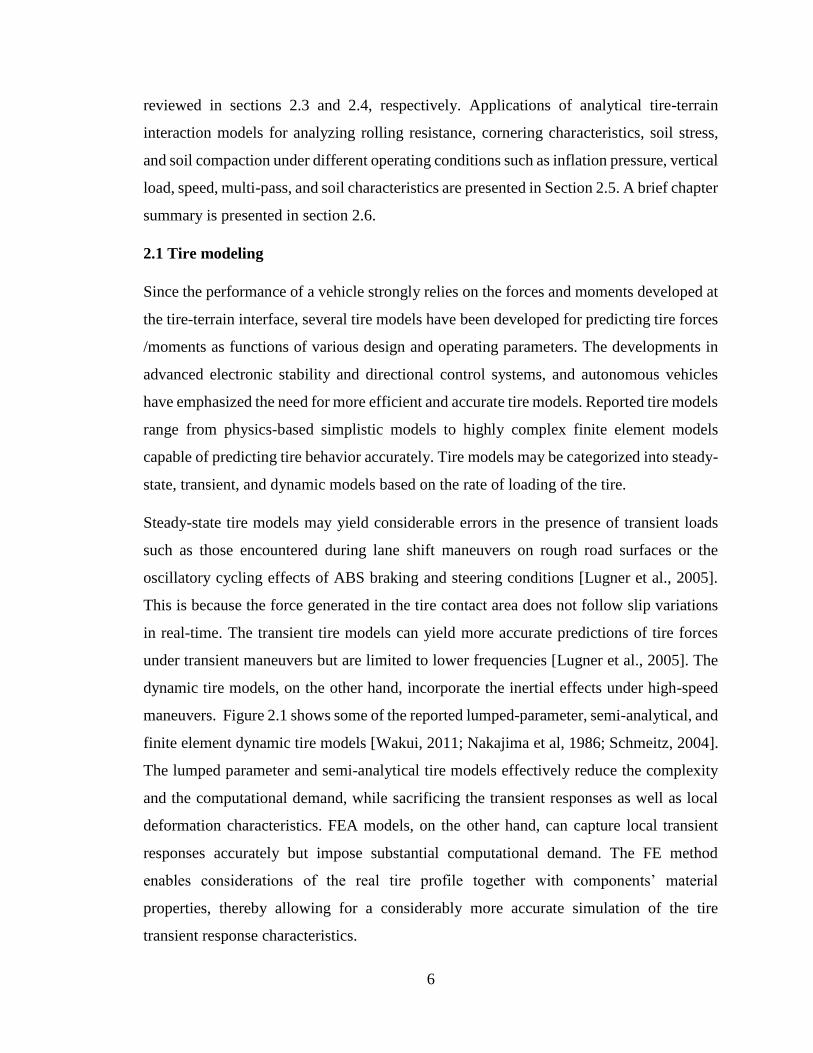
maneuvers. Figure 2.1 shows some of the reported lumped-parameter, semi-analytical, and

finite element dynamic tire models [Wakui, 2011; Nakajima et al, 1986; Schmeitz, 2004].

The lumped parameter and semi-analytical tire models effectively reduce the complexity

and the computational demand, while sacrificing the transient responses as well as local

deformation characteristics. FEA models, on the other hand, can capture local transient

responses accurately but impose substantial computational demand. The FE method

enables considerations of the real tire profile together with components’ material

properties, thereby allowing for a considerably more accurate simulation of the tire

transient response characteristics.

7

A. Lumped-parameter

model [Wakui, 2011]

B. Semi analytical

model [Nakajima et

al, 1986]

C. Finite Element Analysis

model [Schmeitz, 2004]

Figure 2.1. Dynamics tire models

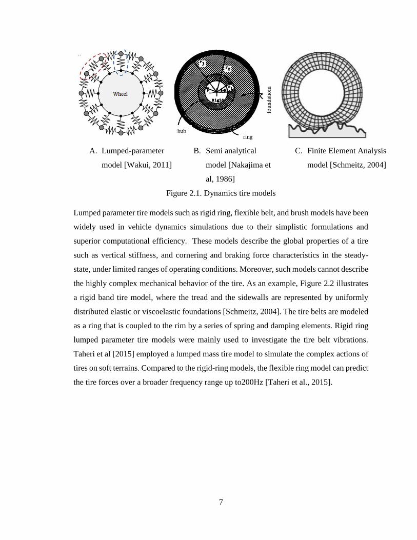
Lumped parameter tire models such as rigid ring, flexible belt, and brush models have been

widely used in vehicle dynamics simulations due to their simplistic formulations and

superior computational efficiency. These models describe the global properties of a tire

such as vertical stiffness, and cornering and braking force characteristics in the steady-

state, under limited ranges of operating conditions. Moreover, such models cannot describe

the highly complex mechanical behavior of the tire. As an example, Figure 2.2 illustrates

a rigid band tire model, where the tread and the sidewalls are represented by uniformly

distributed elastic or viscoelastic foundations [Schmeitz, 2004]. The tire belts are modeled

as a ring that is coupled to the rim by a series of spring and damping elements. Rigid ring

lumped parameter tire models were mainly used to investigate the tire belt vibrations.

Taheri et al [2015] employed a lumped mass tire model to simulate the complex actions of

tires on soft terrains. Compared to the rigid-ring models, the flexible ring model can predict

the tire forces over a broader frequency range up to200Hz [Taheri et al., 2015].

8

Figure 2.2. Rigid ring tire model [Schmeitz, 2004]

Semi-analytical models have been developed for predicting the forces developed at the tire-

ground interface considering the physical phenomenon of tire-ground interactions. Such

models can predict tire forces in the steady as well as transient states, while adequately

considering mechanical properties of the tire, road friction, and operating conditions

[Hirschberg et al., 2010]. Such models combine the lumped-parameter analytical methods

to depict tire motion together with discrete element models to focus on individual areas or

points of interest. Semi-analytical models, also termed as semi-FE or hybrid models, are

considered to represent a compromise between the simplistic lumped-parameter and

comprehensive FE models. These models, however, are also simplistic to investigate

localized deformations of the tire constituents.

Mastinu et al. [1997] developed a semi-analytical tire model for enhanced vehicle

dynamics simulations in the steady-state and transient conditions. The physical processes

involved in tire-ground interactions were described using mathematical models of some

tire components. The tire model yielded forces generated in the tire-terrain contact area in

both steady and transient conditions, while considering the mechanical properties of the

tire, friction coefficient, and a range of operating conditions. In another study, Chan and

Sandu [2008] developed a semi-analytical technique to model a tire that could be applied

to both on- and off-road conditions. The tractive force developed by the tire was evaluated

9

through the integration of the shear stresses developed at the tire contact interface. The

experiments revealed that the tire model reverts to a rigid wheel when the soils deform

much more than the tire.

2.1.1 FEA tire modeling

The Finite Element Analysis (FEA) techniques have been most widely used to develop,

design, and analyze pneumatic tires [Chen et al., 2021; Zumrat et al., 2021; Jung et al.,

2018]. In FEA methods, the element types used in the model and meshing constitute the

most important aspects for achieving accurate results. The FEA tire models may employ

one-, two- or three-dimensional elements with different aspect ratios. Padovan [1977] used

a thin shell element model with an asymmetrical axial 2-D curve to investigate the energy

dissipation and heat losses of steady-state rolling tires. The phase of the curve function was

considered in this model and the simulation results were compared with the analytical

results. Noor and Anderson [1982] stated that Padovan’s thin shell element model ignored

the crosswise shear stresses, and reported a FEA tire model using 2-D thick curved shell

elements. The model enabled simulation of multilayer tire structure considering the

anisotropic materials, crosswise shear stresses, inflation pressure, and response of the

thermo-viscoelastic materials. Other studies [e.g., Crmn et al., 1988; Chen, 1988] have

proposed novel approaches to model a two-dimensional tire. Young’s modulus for the tire

model was estimated from the readily accessible generalized deflection chart (GDC), while

the Poisson’s ratio was taken as 0.5. These tire models provided more accurate predictions

of the tire-terrain contact geometry when compared to the previously reported approaches.

Later, Wang [1990] used a general-purpose FEA tool, referred to as ASGARD, to develop

a three-dimensional tire model. The tire was modeled as a toroid filled with pressurized air,

while the tire material was considered to be homogenous, and its Young's modulus was

calculated from the load-deflection curve obtained from the tire manufacturer's GDC. The

tire model could predict the load-deflection relationship accurately, while the relationships

between the tire deflection and contact width, contact length or contact area showed

significant deviations from the measured data provided by the tire manufacturer in the

GDC. The observed discrepancies were attributed to the assumption of homogenous tire

material. Nakashima and Wong [1993] reported an improved three-dimensional FEA tire

10

model considering different material properties for the tire tread and sidewall. Young's

moduli for the sidewall and the tread were derived from the load-deflection and deflection-

contact patch relationships provided in the GDC for a certain tire. The Poisson’s ratios for

the tread and sidewall were assumed to be close to 0.5, assuming that the volume of tire

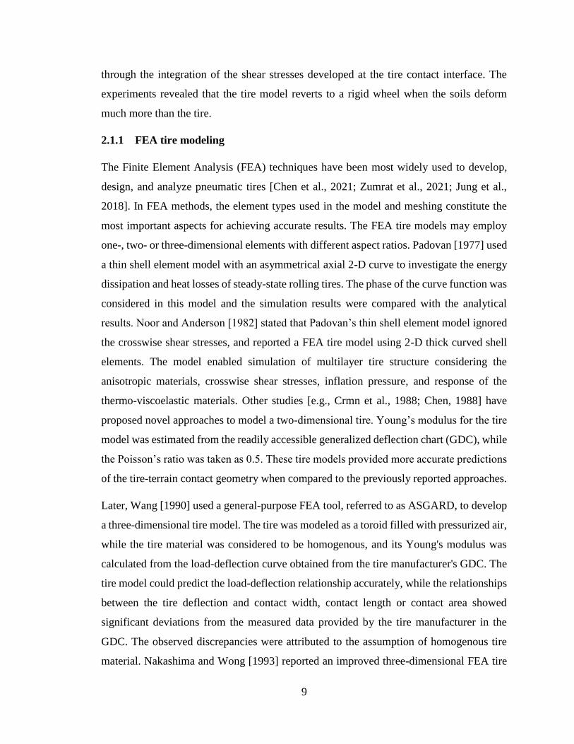
materials remains constant during deformation. Similarly, Zhang et al. [2001] designed a

3-D nonlinear FEA 12.5R22.5 truck tire model using hyper-elastic solid elements, shown

in Figure 2.3, to predict tire contact pressure distribution on the terrain under different

inflation pressures and vertical loads. The model considered four layers of steel belts under

the treads, as shown in Figure 2.4, and a linear combination of alternating rubber and belt

layers. This model assumed clamped boundary constraints at the rim contact regions,

thereby no-slip condition, while neglecting the beads. The pressure distributions obtained

under different vertical loads agreed well with the measured data.

Figure 2.3. Tire model with constant shear stress in rim contact region [Zhang et al.,

2001]

A number of studies have reported FEA models of the rolling tires. For instance, Yan

[2003] reported a 9.00R20 truck tire model using the FEA technique to study the maximum

contact area and reaction force under different speeds and vertical loads. Tire materials

were handled as incompressible solid components using the Lagrangian multiplier

approach. The Mooney-Rivlin material model was used to simulate the non-linear

mechanical characteristics of elastomers, while the model constants were identified from

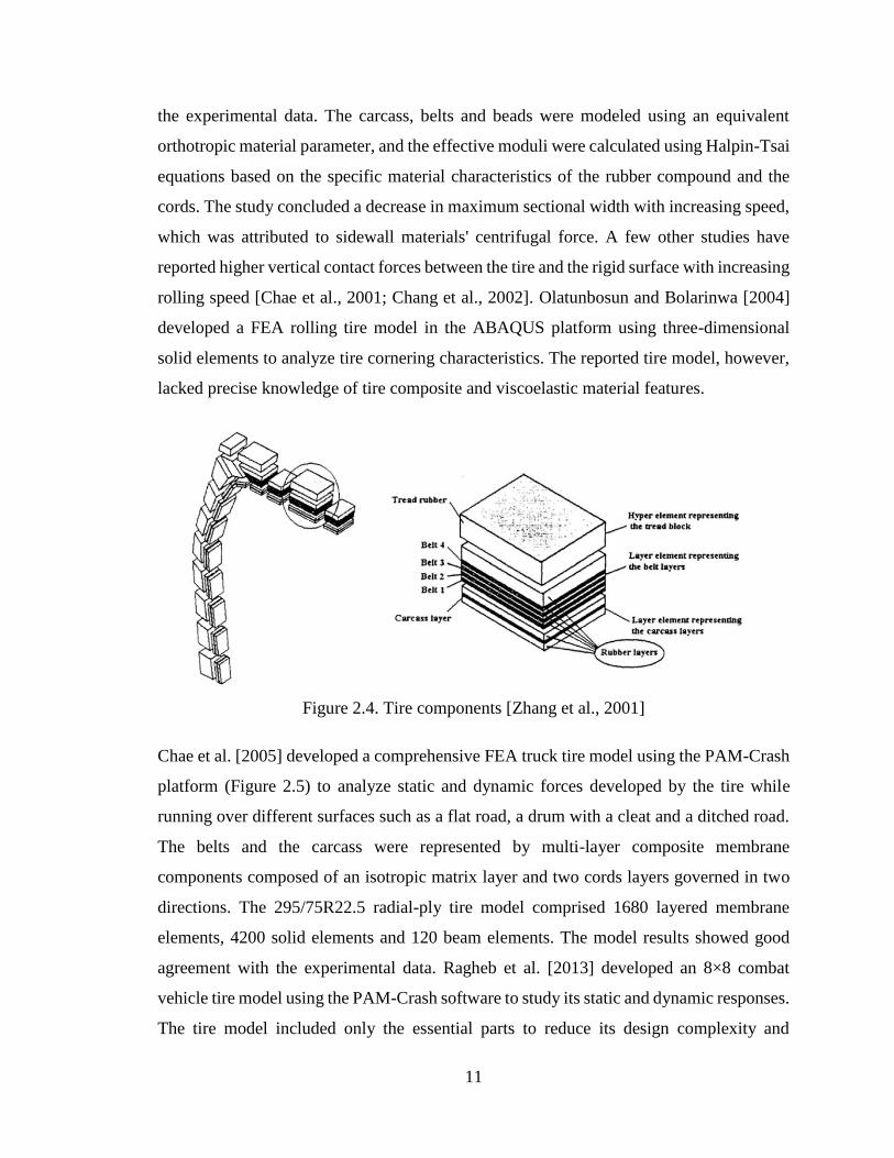
11

the experimental data. The carcass, belts and beads were modeled using an equivalent

orthotropic material parameter, and the effective moduli were calculated using Halpin-Tsai

equations based on the specific material characteristics of the rubber compound and the

cords. The study concluded a decrease in maximum sectional width with increasing speed,

which was attributed to sidewall materials' centrifugal force. A few other studies have

reported higher vertical contact forces between the tire and the rigid surface with increasing

rolling speed [Chae et al., 2001; Chang et al., 2002]. Olatunbosun and Bolarinwa [2004]

developed a FEA rolling tire model in the ABAQUS platform using three-dimensional

solid elements to analyze tire cornering characteristics. The reported tire model, however,

lacked precise knowledge of tire composite and viscoelastic material features.

Figure 2.4. Tire components [Zhang et al., 2001]

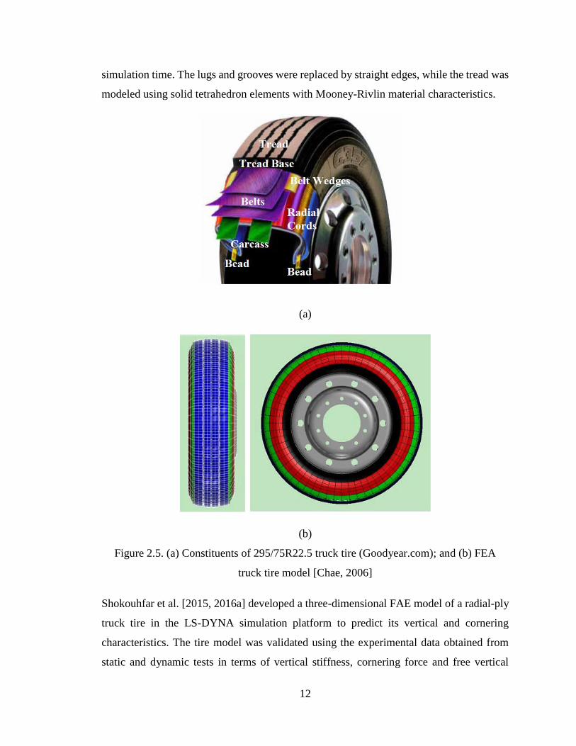
Chae et al. [2005] developed a comprehensive FEA truck tire model using the PAM-Crash

platform (Figure 2.5) to analyze static and dynamic forces developed by the tire while

running over different surfaces such as a flat road, a drum with a cleat and a ditched road.

The belts and the carcass were represented by multi-layer composite membrane

components composed of an isotropic matrix layer and two cords layers governed in two

directions. The 295/75R22.5 radial-ply tire model comprised 1680 layered membrane

elements, 4200 solid elements and 120 beam elements. The model results showed good

agreement with the experimental data. Ragheb et al. [2013] developed an 8×8 combat

vehicle tire model using the PAM-Crash software to study its static and dynamic responses.

The tire model included only the essential parts to reduce its design complexity and

12

simulation time. The lugs and grooves were replaced by straight edges, while the tread was

modeled using solid tetrahedron elements with Mooney-Rivlin material characteristics.

(a)

(b)

Figure 2.5. (a) Constituents of 295/75R22.5 truck tire (Goodyear.com); and (b) FEA

truck tire model [Chae, 2006]

Shokouhfar et al. [2015, 2016a] developed a three-dimensional FAE model of a radial-ply

truck tire in the LS-DYNA simulation platform to predict its vertical and cornering

characteristics. The tire model was validated using the experimental data obtained from

static and dynamic tests in terms of vertical stiffness, cornering force and free vertical

13

vibration response [Shokouhfar et al., 2016b]. The FEA tire model behaved well up to 100

km/h rolling speeds. The validated tire model was subsequently used to investigate the

influences of multiple operational factors on tires’ vertical and cornering characteristics.

The study suggested that the detailed model could serve as a virtual tool for investigating

the impacts of multiple operating and design factors on tire dynamic properties. Owing to

the high computational demand of the model, the authors further developed a reduced

model using the Part-Composite approach, where the multiple structural layers were

represented by a single composite element with a layered arrangement [Shokouhfar et al.,

2016c]. This approach resulted in a considerable decrease in the total number of elements

in the model with a significant increase in computing efficiency.

El-Sayegh et al. [2019] developed a high lug farm service (HLFS) vehicle off-road tire

(220/70B16) model using the FEA technique in PAM-Crash to study tire interactions with

a SPH model of the clayey loam soil. The model, shown in Figure 2.6, employed hyper-

elastic Mooney-Rivlin material elements with 42 lugs for the tread pattern. The HLFS tire

model comprised 21 parts including the rim, tread, under the tread, sidewalls, and belts.

Quad shell elements were used to model the rim, while solid elements were chosen to

represent the lugs, the shoulder and under treads. Lastly, beam elements were used to model

the beads. The cross-section of the HLFS tire was constructed using these materials and

then rotated about the tire axis to develop the full tire model. The tire model was used to

predict the tire's interactions with the soil in terms of rolling resistance force under different

inflation pressures and vertical loads, which agreed well with the measured data.

Figure 2.6. The FEA model of an agricultural vehicle tire [El-Sayegh et al., 2019]

14

(1: Tread, 2: Under tread, 3: Shoulder, 4, 5, 6: Sidewall, 7: Plies, 8: Beads, 9: Rim)

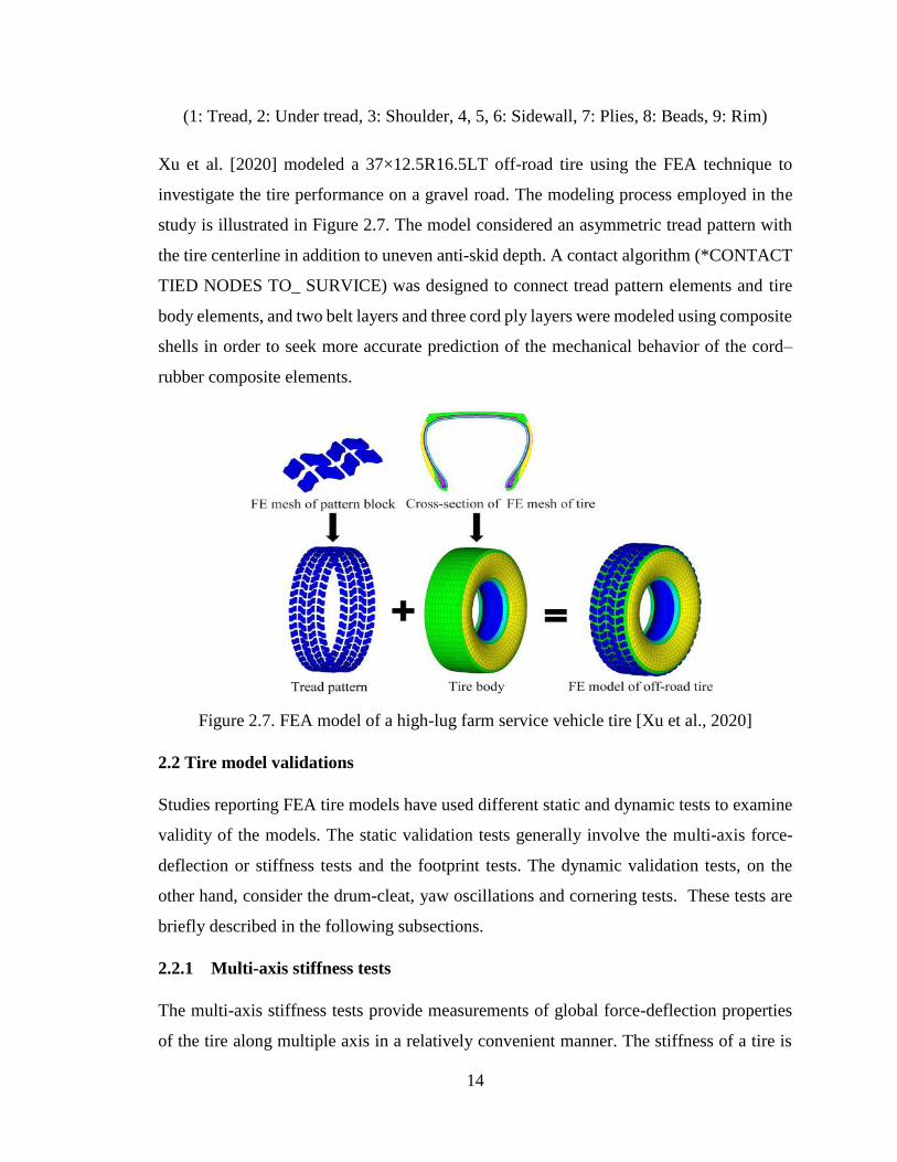
Xu et al. [2020] modeled a 37×12.5R16.5LT off-road tire using the FEA technique to

investigate the tire performance on a gravel road. The modeling process employed in the

study is illustrated in Figure 2.7. The model considered an asymmetric tread pattern with

the tire centerline in addition to uneven anti-skid depth. A contact algorithm (*CONTACT

TIED NODES TO_ SURVICE) was designed to connect tread pattern elements and tire

body elements, and two belt layers and three cord ply layers were modeled using composite

shells in order to seek more accurate prediction of the mechanical behavior of the cord–

rubber composite elements.

Figure 2.7. FEA model of a high-lug farm service vehicle tire [Xu et al., 2020]

2.2 Tire model validations

Studies reporting FEA tire models have used different static and dynamic tests to examine

validity of the models. The static validation tests generally involve the multi-axis force-

deflection or stiffness tests and the footprint tests. The dynamic validation tests, on the

other hand, consider the drum-cleat, yaw oscillations and cornering tests. These tests are

briefly described in the following subsections.

2.2.1 Multi-axis stiffness tests

The multi-axis stiffness tests provide measurements of global force-deflection properties

of the tire along multiple axis in a relatively convenient manner. The stiffness of a tire is

15

affected by a number of tire design factors apart from the normal load and inflation

pressure. Although the tire stiffness is generally characterized along the vertical or radial,

lateral, longitudinal and torsional axis under different normal loads, the vertical stiffness

tests have been most widely used to examine validity of FEA tire models. Figure 2.8 shows

a vertical stiffness tester used to characterize the vertical force-deflection properties of a

tire. The tire vertical stiffness is defined as the rate of change of normal force with respect

to overall vertical deflection of the tire. The vertical stiffness of a tire is an important

measure that directly affects the tire deflection, load-carrying capacity and vehicle ride

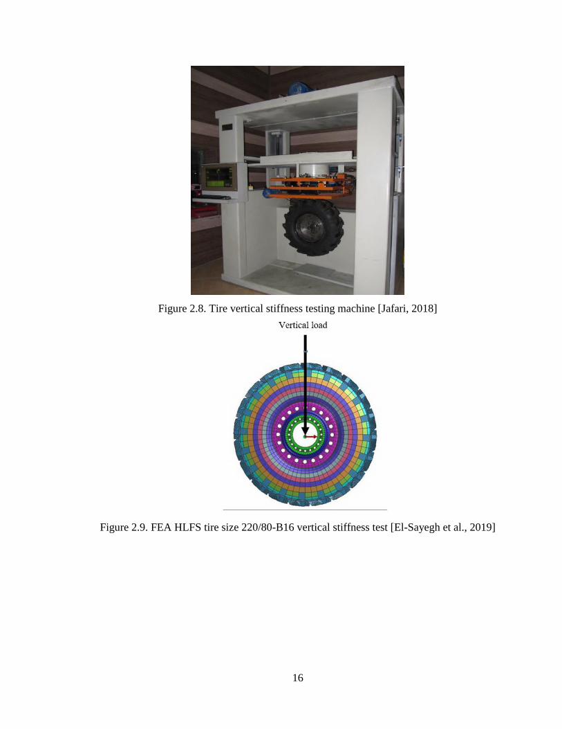
property. The force-deflection properties of a tire can be conveniently evaluated from the

FEA tire model by applying vertical load or deflection in an incremental manner. As an

example, Figure 2.9 shows the vertical stiffness test simulation results obtained from a FEA

tire model in PAM-Crash visual environment [El-Sayegh et al., 2019]. The results were

obtained for a HLFS 220/80-B16 tire subject to an increasing normal load in a ramp

manner. In the simulation, the FEA tire model, positioned on a rigid surface, was inflated

to the desired internal pressure. The vertical load is applied to the rim center in a ramp

manner, as shown in Figure 2.9. The figure illustrates variation in the applied force with

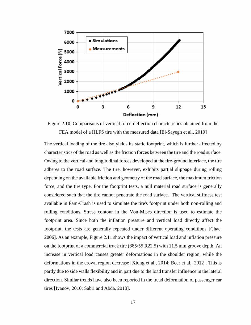
the resulting vertical deflection of the tire. Figure 2.10 shows the vertical force versus

deflection of the HLFS tire during the vertical stiffness test. It can be noticed that there is

a good agreement between measurements and simulations up to about 6 mm deflection.

The simulation model shows highly nonlinear stiffness characteristics beyond 6 mm

deflection, while the measured data is nearly linear since the measured vertical force is

plotted approximately versus deflection using limited number of points provided by the tire

manufacturer. Although the FEA tire model showed good behavior under regular operating

settings, the authors suggested further investigations under different working conditions.

Marjani [Marjani, 2016], Chae [Chae, 2006], and Slade [Slade, 2009] used the same FEA

technique to validate the tire models statically.

16

Figure 2.8. Tire vertical stiffness testing machine [Jafari, 2018]

Figure 2.9. FEA HLFS tire size 220/80-B16 vertical stiffness test [El-Sayegh et al., 2019]

17

Figure 2.10. Comparisons of vertical force-deflection characteristics obtained from the

FEA model of a HLFS tire with the measured data [El-Sayegh et al., 2019]

The vertical loading of the tire also yields its static footprint, which is further affected by

characteristics of the road as well as the friction forces between the tire and the road surface.

Owing to the vertical and longitudinal forces developed at the tire-ground interface, the tire

adheres to the road surface. The tire, however, exhibits partial slippage during rolling

depending on the available friction and geometry of the road surface, the maximum friction

force, and the tire type. For the footprint tests, a null material road surface is generally

considered such that the tire cannot penetrate the road surface. The vertical stiffness test

available in Pam-Crash is used to simulate the tire's footprint under both non-rolling and

rolling conditions. Stress contour in the Von-Mises direction is used to estimate the

footprint area. Since both the inflation pressure and vertical load directly affect the

footprint, the tests are generally repeated under different operating conditions [Chae,

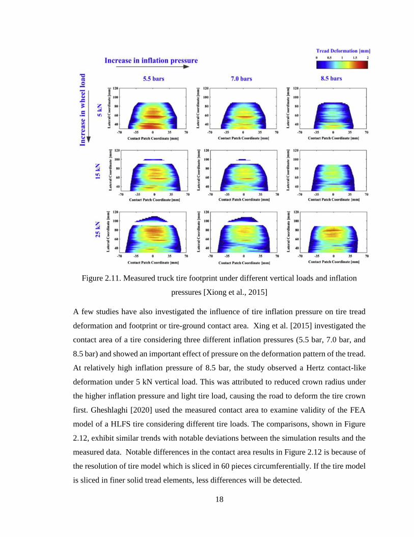
2006]. As an example, Figure 2.11 shows the impact of vertical load and inflation pressure

on the footprint of a commercial truck tire (385/55 R22.5) with 11.5 mm groove depth. An

increase in vertical load causes greater deformations in the shoulder region, while the

deformations in the crown region decrease [Xiong et al., 2014; Beer et al., 2012]. This is

partly due to side walls flexibility and in part due to the load transfer influence in the lateral

direction. Similar trends have also been reported in the tread deformation of passenger car

tires [Ivanov, 2010; Sabri and Abda, 2018].

18

Figure 2.11. Measured truck tire footprint under different vertical loads and inflation

pressures [Xiong et al., 2015]

A few studies have also investigated the influence of tire inflation pressure on tire tread

deformation and footprint or tire-ground contact area. Xing et al. [2015] investigated the

contact area of a tire considering three different inflation pressures (5.5 bar, 7.0 bar, and

8.5 bar) and showed an important effect of pressure on the deformation pattern of the tread.

At relatively high inflation pressure of 8.5 bar, the study observed a Hertz contact-like

deformation under 5 kN vertical load. This was attributed to reduced crown radius under

the higher inflation pressure and light tire load, causing the road to deform the tire crown

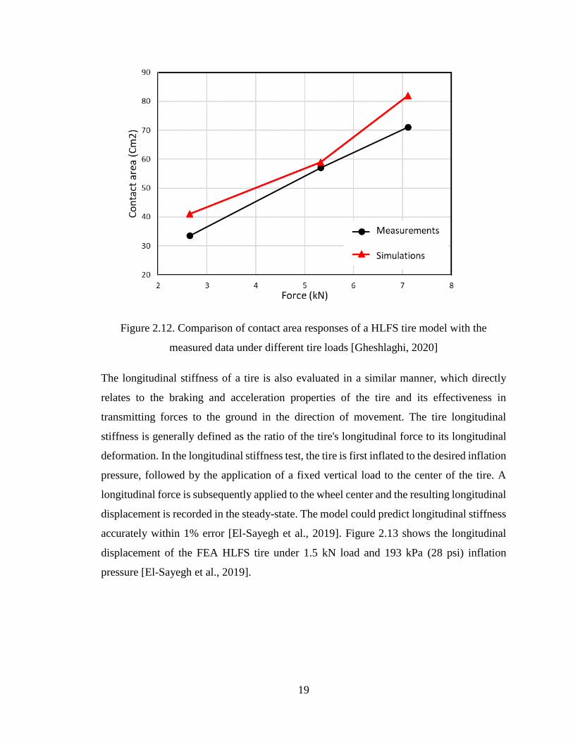
first. Gheshlaghi [2020] used the measured contact area to examine validity of the FEA

model of a HLFS tire considering different tire loads. The comparisons, shown in Figure

2.12, exhibit similar trends with notable deviations between the simulation results and the

measured data. Notable differences in the contact area results in Figure 2.12 is because of

the resolution of tire model which is sliced in 60 pieces circumferentially. If the tire model

is sliced in finer solid tread elements, less differences will be detected.

19

Figure 2.12. Comparison of contact area responses of a HLFS tire model with the

measured data under different tire loads [Gheshlaghi, 2020]

The longitudinal stiffness of a tire is also evaluated in a similar manner, which directly

relates to the braking and acceleration properties of the tire and its effectiveness in

transmitting forces to the ground in the direction of movement. The tire longitudinal

stiffness is generally defined as the ratio of the tire's longitudinal force to its longitudinal

deformation. In the longitudinal stiffness test, the tire is first inflated to the desired inflation

pressure, followed by the application of a fixed vertical load to the center of the tire. A

longitudinal force is subsequently applied to the wheel center and the resulting longitudinal

displacement is recorded in the steady-state. The model could predict longitudinal stiffness

accurately within 1% error [El-Sayegh et al., 2019]. Figure 2.13 shows the longitudinal

displacement of the FEA HLFS tire under 1.5 kN load and 193 kPa (28 psi) inflation

pressure [El-Sayegh et al., 2019].

20

Figure 2.13. Longitudinal displacement on FEA HLFS tire at 1.5 kN and 193 kPa (28psi)

inflation pressure [El-Sayegh et al., 2019]

Lateral stiffness, defined as the ratio of lateral force to lateral deformation, relates to the

out-of-plane flexibility of the tire [Loeb et al., 1990]. It also relates to the tire’s ability to

transmit lateral forces from the vehicle to the road, which is vital for timely steering and

control of the vehicle. As the lateral force increases, individual tread components lose

adherence to the surface. The elastic characteristics of a tire in the transverse direction is

also assessed in terms of its lateral stiffness [Luty, 2012]. In FEA model simulations, the

tire is initially inflated to a desired pressure while subject to a constant vertical load applied

to the center of the tire. Following the contact, a specific lateral force is delivered to the

tire's center of gravity which causes the tire to deflect laterally. The lateral tire stiffness is

calculated using the lateral displacement derived from the simulations. Reid [2015] used

the same simulation technique in PAM-Crash to validate a Michelin XONE XDA

445/50R22.5 wide base tire model in the lateral stiffness test. The simulation results

showed a good agreement with the measurements.

2.2.2 Dynamic validation tests

The dynamic validation tests involve characterizations of tire’s resonant frequencies under

pre-defined excitations and cornering force characteristics, although some studies have also

21

employed longitudinal force-slip characteristics of tires. The experimental and simulation

methods employed for dynamic validations tests are briefly described below.

Drum-cleat test:

The drum-cleat test is performed to identify dominant natural frequencies of a tire rolling

on a drum, where a semicircular cleat serves as an excitation to the tire. This test generally

focuses on the fundamental mode of vertical vibration of the tire [El-Sayegh, 2019]. The

FEA tire models also employ similar excitation to examine models’ validity in terms of the

fundamental frequency, which is strongly affected by material features, inflation pressure

and normal load of the tire. In FEA models’ simulations, the tire is loaded to a desired level

after applying the target inflation pressure. An angular velocity is subsequently applied and

the tire is permitted to roll freely, while the tire spindle is constrained in all translational

directions. The drum center is also constrained in all translational directions with the

exception of the rotational degree-of-freedom. The cleat located on the rolling drum surface

excites the tire vertically. The vertical and longitudinal force responses at the tire center

are extracted and a frequency spectrum of vibration is obtained using the Fast Fourier

Transformation (FFT) algorithm. The spectra of vibration permit identifications of

fundamental frequencies of vertical and longitudinal vibrations of the tire under different

operating conditions. As an example, Figure 2.14 shows the frequency spectrum of vertical

vibration response of a wide-based truck tire, which exhibits a distinct peak near 74 Hz,

considered as the fundamental mode of vertical vibration. The spectrum also exhibits a

dominant peak near 2 Hz, which corresponds to rolling speed of the drum. The Fourier

spectrum of contact force suggests force magnitude of 500 N at 0 Hz. Since the mean of

the force has been adjusted to zero prior to performing the FFT, the large magnitude at zero

frequency is related to the vibrations that happen at 0 Hz because of inflating and loading

the tire to the specific values. The measured data have also been used to estimate tire

sidewall damping factor 𝜶 [Chae, 2006; Marjani, 2016]:

𝛼 = 2𝜉𝜔 = 2𝜉(2𝜋𝑓) (2.1)

Where 𝜔 is the fundamental mode frequency in rad/s and 𝜉 is the damping ratio, which is

generally considered to be 5% [Chae, 2006]. El-Sayegh [2019], Chae [2006], and Slade

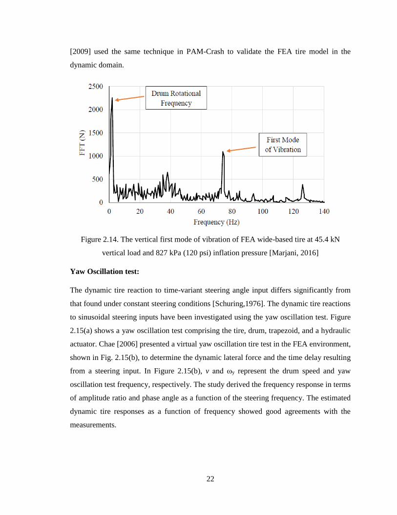
22

[2009] used the same technique in PAM-Crash to validate the FEA tire model in the

dynamic domain.

Figure 2.14. The vertical first mode of vibration of FEA wide-based tire at 45.4 kN

vertical load and 827 kPa (120 psi) inflation pressure [Marjani, 2016]

Yaw Oscillation test:

The dynamic tire reaction to time-variant steering angle input differs significantly from

that found under constant steering conditions [Schuring,1976]. The dynamic tire reactions

to sinusoidal steering inputs have been investigated using the yaw oscillation test. Figure

2.15(a) shows a yaw oscillation test comprising the tire, drum, trapezoid, and a hydraulic

actuator. Chae [2006] presented a virtual yaw oscillation tire test in the FEA environment,

shown in Fig. 2.15(b), to determine the dynamic lateral force and the time delay resulting

from a steering input. In Figure 2.15(b), v and ωy represent the drum speed and yaw

oscillation test frequency, respectively. The study derived the frequency response in terms

of amplitude ratio and phase angle as a function of the steering frequency. The estimated

dynamic tire responses as a function of frequency showed good agreements with the

measurements.

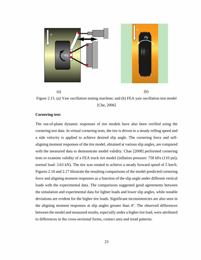
23

(a) (b)

Figure 2.15. (a) Yaw oscillation testing machine; and (b) FEA yaw oscillation test model

[Che, 2006]

Cornering test:

The out-of-plane dynamic responses of tire models have also been verified using the

cornering test data. In virtual cornering tests, the tire is driven to a steady rolling speed and

a side velocity is applied to achieve desired slip angle. The cornering force and self-

aligning moment responses of the tire model, obtained at various slip angles, are compared

with the measured data to demonstrate model validity. Chae [2008] performed cornering

tests to examine validity of a FEA truck tire model (inflation pressure: 758 kPa (110 psi);

normal load: 3.63 kN). The tire was rotated to achieve a steady forward speed of 5 km/h.

Figures 2.16 and 2.17 illustrate the resulting comparisons of the model-predicted cornering

force and aligning moment responses as a function of the slip angle under different vertical

loads with the experimental data. The comparisons suggested good agreements between

the simulation and experimental data for lighter loads and lower slip angles, while notable

deviations are evident for the higher tire loads. Significant inconsistencies are also seen in

the aligning moment responses at slip angles greater than 4°. The observed differences

between the model and measured results, especially under a higher tire load, were attributed

to differences in the cross-sectional forms, contact area and tread patterns.

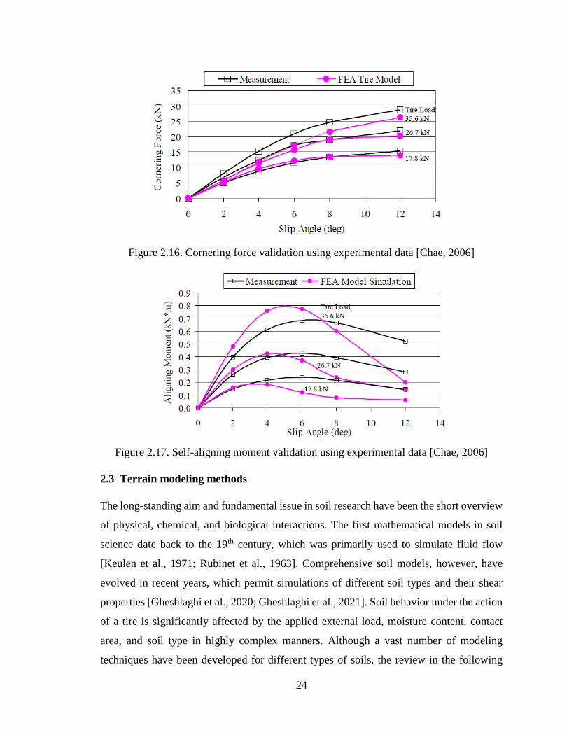
24

Figure 2.16. Cornering force validation using experimental data [Chae, 2006]

Figure 2.17. Self-aligning moment validation using experimental data [Chae, 2006]

2.3 Terrain modeling methods

The long-standing aim and fundamental issue in soil research have been the short overview

of physical, chemical, and biological interactions. The first mathematical models in soil

science date back to the 19th century, which was primarily used to simulate fluid flow

[Keulen et al., 1971; Rubinet et al., 1963]. Comprehensive soil models, however, have

evolved in recent years, which permit simulations of different soil types and their shear

properties [Gheshlaghi et al., 2020; Gheshlaghi et al., 2021]. Soil behavior under the action

of a tire is significantly affected by the applied external load, moisture content, contact

area, and soil type in highly complex manners. Although a vast number of modeling

techniques have been developed for different types of soils, the review in the following

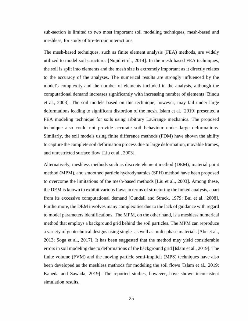
25

sub-section is limited to two most important soil modeling techniques, mesh-based and

meshless, for study of tire-terrain interactions.

The mesh-based techniques, such as finite element analysis (FEA) methods, are widely

utilized to model soil structures [Nujid et el., 2014]. In the mesh-based FEA techniques,

the soil is split into elements and the mesh size is extremely important as it directly relates

to the accuracy of the analyses. The numerical results are strongly influenced by the

model's complexity and the number of elements included in the analysis, although the

computational demand increases significantly with increasing number of elements [Bindu

et al., 2008]. The soil models based on this technique, however, may fail under large

deformations leading to significant distortion of the mesh. Islam et al. [2019] presented a

FEA modeling technique for soils using arbitrary LaGrange mechanics. The proposed

technique also could not provide accurate soil behaviour under large deformations.

Similarly, the soil models using finite difference methods (FDM) have shown the ability

to capture the complete soil deformation process due to large deformation, movable frames,

and unrestricted surface flow [Liu et al., 2003].

Alternatively, meshless methods such as discrete element method (DEM), material point

method (MPM), and smoothed particle hydrodynamics (SPH) method have been proposed

to overcome the limitations of the mesh-based methods [Liu et al., 2003]. Among these,

the DEM is known to exhibit various flaws in terms of structuring the linked analysis, apart

from its excessive computational demand [Cundall and Strack, 1979; Bui et al., 2008].

Furthermore, the DEM involves many complexities due to the lack of guidance with regard

to model parameters identifications. The MPM, on the other hand, is a meshless numerical

method that employs a background grid behind the soil particles. The MPM can reproduce

a variety of geotechnical designs using single- as well as multi-phase materials [Abe et al.,

2013; Soga et al., 2017]. It has been suggested that the method may yield considerable

errors in soil modeling due to deformations of the background grid [Islam et al., 2019]. The

finite volume (FVM) and the moving particle semi-implicit (MPS) techniques have also

been developed as the meshless methods for modeling the soil flows [Islam et al., 2019;

Kaneda and Sawada, 2019]. The reported studies, however, have shown inconsistent

simulation results.

26

The smoothed particle hydrodynamics (SPH) technique has been employed in recent years

to capture the soil flows more accurately. The SPH technique was developed in the 1970s

to address astrophysical modeling challenges [Gingold et al., 1977]. The SPH method is

considered superior over the other meshless methods since it permits consideration of the

real particle structure with no connection, while it involves relatively simpler formulations

and solution methods [Rahman and Konagai, 2017; Gholami et al., 2018]. The resolution

of this approach can be adjusted for different application domains such as solid mechanics

and fluid flow because of its capacity to handle boundary particles and its Lagrangian

character in addition to the essential soil factors such as density [Akbari, 2017; Ran et al.,

2015; Ghaitanellis et al., 2018]. In the SPH method, each particle is considered with its

unique features, such as mass, density, and velocity, which are adjusted using a smoothing

kernel from those of the nearby particles within a defined domain. The simulation process

is continued until the required time or velocity is attained, followed by numerical

integration to adjust each particle's location [Islam et al., 2019]. The basic step in SPH is

the integral form of a function, which describes the function at a location r, such that:

A(r) = ∫𝐴(𝑟′)𝑊(𝑟 − 𝑟′, ℎ)𝑑𝑟′ (2.2)

Where, h is the smoothing length defining the influence domain A, r and r′ are covered in

the integration domain A(r′) [Larry et al., 1993]. Function W, commonly known as the

smoothing function, is an interpolating kernel that must meet three characteristics. The first

characteristic relates to normalization condition of W, which must satisfy:

∫𝑊(𝑟 − 𝑟′, ℎ)𝑑𝑟′ = 1 (2.3)

limℎ→0

∫𝑊(𝑟 − 𝑟′, ℎ)𝑑𝑟′ = 𝛿(𝑟 − 𝑟′) (2.4)

𝑊(𝑟 − 𝑟′, ℎ) = 0 𝑤ℎ𝑒𝑛 |𝑟 − 𝑟′| > 𝑘ℎ (2.5)

Where k describes the domain of A(r) and is a constant associated with the smoothing

function for a point at r, as shown in Figure 2.18. The second characteristic represents

smoothing function (𝑊(𝑟 − 𝑟′, ℎ)), when h approaches zero. The third characteristic

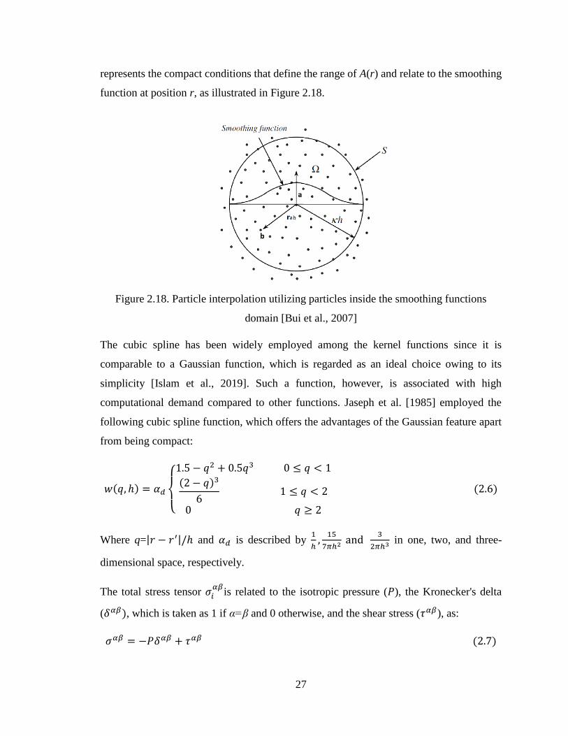
27

represents the compact conditions that define the range of A(r) and relate to the smoothing

function at position r, as illustrated in Figure 2.18.

Figure 2.18. Particle interpolation utilizing particles inside the smoothing functions

domain [Bui et al., 2007]

The cubic spline has been widely employed among the kernel functions since it is

comparable to a Gaussian function, which is regarded as an ideal choice owing to its

simplicity [Islam et al., 2019]. Such a function, however, is associated with high

computational demand compared to other functions. Jaseph et al. [1985] employed the

following cubic spline function, which offers the advantages of the Gaussian feature apart

from being compact:

𝑤(𝑞, ℎ) = 𝛼𝑑

{

1.5 − 𝑞2 + 0.5𝑞3 0 ≤ 𝑞 < 1

(2 − 𝑞)3

6 1 ≤ 𝑞 < 2

0 𝑞 ≥ 2

(2.6)

Where q=|𝑟 − 𝑟′|/ℎ and 𝛼𝑑 is described by 1

ℎ,15

7𝜋ℎ2 and

3

2𝜋ℎ3 in one, two, and three-

dimensional space, respectively.

The total stress tensor 𝜎𝑖𝛼𝛽

is related to the isotropic pressure (𝑃), the Kronecker's delta

(𝛿𝛼𝛽), which is taken as 1 if α=β and 0 otherwise, and the shear stress (𝜏𝛼𝛽), as:

𝜎𝛼𝛽 = −𝑃𝛿𝛼𝛽 + 𝜏𝛼𝛽 (2.7)

28

The pressure P in the above formulation is obtained from the “equation of state”

considering the material density and internal energy [ESI group, 2014]:

𝑃 = 𝐶0 + 𝐶1𝜇 + 𝐶2𝜇2 + 𝐶3𝜇

3 + (𝐶4 + 𝐶5𝜇 + 𝐶6𝜇2)𝐸𝑖 (2.8)

The above formulation has been used for hydrodynamic elastic-plastic materials, where Ci

(i=0 to 6) are material constants, µ = ρ/ρ0 -1 is the density factor, and Ei is the internal

energy. The shear stress rate, 𝜏 ̇𝛼𝛽, is subsequently obtained as a function of the rate of the

strain tensor 휀 ̇, as:

𝜏 ̇𝛼𝛽 = 2𝐺 (휀 ̇ 𝛼𝛽 −1

3𝛿𝛼𝛽휀 ̇ 𝛾𝛾) (2.9)

Where G is the shear modulus. The shear stress factors should be restricted to the surface

failure that occurs when plastic flow begins. The plastic flow area is estimated using the

Mohr-Coulomb relation [Wong, 2008].

𝜏𝑚𝑎𝑥 = 𝑐 + 𝑃 tan𝜑 (2.10)

Where c is soil cohesion constant, P is applied pressure, and 𝜑 is the internal friction angle.

El-Gindy et al. [2011] used FEA and SPH techniques to model the soil and investigate the

tire-soil interaction process. The soil was modeled as an elastic-plastic material in both the

techniques and the results showed that the SPH soil deforms like the real soil in the shear-

strength test. Dhillon [2013] studied the sensitivity analysis of the SPH technique in the

PAM-Crash environment for modeling different soils. The impact of soil model

characteristics such as geometry and contact model on the behavior of soft soil was

investigated. The predicted soil parameters were compared to the experimental data to

verify the models [Dhillon, 2013].

Marjani [2017] used SPH and FEA techniques to model dry sand and investigate the

computational efficiency of the tire-soil interaction process using different types of soil

models such as full FEA, full SPH, hybrid half SPH/FEA, and hybrid quarter SPH/FEA.

Pressure-sinkage and shear strength tests wre used for the soil model calibration, which

ensured more accurate representation of dry sand. In terms of the pressure-sinkage test, the

simulation results obtained from both modeling methods agreed reasonably with the

measurements. Due to a lack of penetration in the FEA model, a sponge-like effect was

29

detected, which was accomplished using the SPH modeling method. The shear strength

test was found to be applicable only for the SPH soil model. Using a rigid tire-soil

interaction model, the computational efficiency of each soil model was investigated and

compared. It was discovered that the quarter SPH soil model is the most efficient soil model

under the same operating conditions. Compared to full SPH, the hybrid quarter SPH soil

model reduced computation time by 45.67 percent.

Zhao et al [2022] studied slope collapse under large deformations using the SIMSAND

critical state sand model in conjunction with the smoothed particle hydrodynamics (SPH)

method and discrete element method (DEM). As benchmarks, a series of slope collapse

studies utilizing the discrete element method (DEM) with different particle forms

(spherical, tetrahedral, and elongated) and different initial densities (dense and loose) were

used. Comparisons showed that the SIMSAND-SPH technique could recreate the main

characteristics of slope collapse, qualitatively and quantitatively, such as the free surface,

final deposit configurations, and final runout distance. In comparison to DEM, the

proposed SIMSAND-SPH technique showed better computing efficiency while keeping

the same computational accuracy.

2.4 Terrain models’ calibrations

The soil models are generally calibrated by identifying essential model parameters using

the measured data. The studies have reported different test techniques to measure soil

strength and shear properties. These include the bevameter, the cone penetrometer, the

triaxial instrument, and classic civil engineering procedures, which are briefly discussed in

the following sub-sections.

2.4.1 Soil penetration tests

Soil penetration tests are performed to characterize soil strength and pressure-sinkage

relationship using the bevameter and cone penetrometer. The measured data have been

used to predict off-road vehicle mobility and tire traction and provide guidance on the

tillage tools designs [Taghavifar and Mardani, 2017; Ogbeche and Idowu, 2016]. The apex

angle and the penetration rate are the significant factors that impact the penetration force.

Studies reporting empirical and DEM soil models have shown that model calibrations on

30

the basis of a basic penetration test, such as a cone penetrometer test, necessitate a deeper

understanding of the particle size to cone penetrometer ratio apart from the geometry

scaling ratio [Syed et al., 2017]. The level of cone penetration resistance is affected by the

size of the virtual container in which the cone penetrometer test is done. Bolton and Gui

[1993] showed that cone penetration resistance is insensitive to the soil box diameter when

it is more than 80 times the cone base diameter. Bolton [1993] suggested a DEM virtual

container with a radius of 250.6 mm for the cone penetrometer simulation. The box size

effects, however, are strongly related to the DEM particle size, stiffness, and friction.

Another study suggested that the minimum number of DEM particles contacting the cone

should be 13 or more [Jiang and Yu, 2006].

Although the cone penetrometer is easy to use on-site, the measurements differ

considerably depending on the operators’ skill level [Kim et al., 2021]. The cone index also

represents the link between compression and shear characteristics, which cannot be

separated. As a result, Kim et al. [2021] suggested some limitations of this method for the

study of tire-terrain interactions focusing on developments in off-road vehicles.

Alternatively, the bevameter test was proposed to overcome limitations of cone

penetrometers. The bevameters have been used to perform pressure-sinkage and shear

strength tests for characterizing mechanical properties of soils [Bekker, 1969]. Figure 2.19

illustrates a soil test system using bevameter. Wong [2010] performed penetration tests for

different soils and concluded that the bevameter is the most accurate representation of

interactions between the soil and a tire, although the measurement method is more difficult

and time-consuming than the cone penetrometer. Massah and Noorolahi [2010] constructed

a tractor-mounted bevameter for analyzing the characteristics of snow using circular,

elliptical, and rectangular plates, and found that the form of the plate had an important

effect on the measured properties. Kim et al. [2021] introduced a new bevameter to

determine parameters that influence the bevameter's performance. The pressure-sinkage

test was carried out using circular plates of various sizes, and the findings revealed reduced

pressure-sinkage parameters with increasing plate size. The study also considered a normal

pressure via a dead load applied to the shear-test equipment in order to prevent normal-

pressure changes with displacement and speed. In addition, a spline was added to top of

31

the shaft attached to the shear ring to evaluate slide sinkage during the shear tests. The

pressure–sinkage and shear stress–slip displacement relationships, rather than the

pressure–sinkage alone was found to be more accurate predictors of sinkage.

Figure 2.19. Bevameter schematic [Wong, 2008]

2.4.2 Pressure-sinkage tests

The pressure-sinkage testing of a soil is performed by placing a penetrating plate on the

soil surface, while measuring the resulting normal tension. This test is used to measure soil

sinkage under different vertical loads and the data is used to identify parameters of the

pressure-sinkage relationship [Wong, 2008]:

𝑃 = (𝑘𝑐𝑏+ 𝑘𝜑)𝑍

𝑛 (2.11)

Where Kc, Kφ, and n are soil parameters and b is smaller dimension of the penetrating plate.

The FEA methods have also been used to obtain the pressure-sinkage behaviours of soils

in a virtual manner. As an example, Figure 2.20 shows a FEA test box filled with SPH soil

and water particles [Gheshlaghi and Mardani, 2020]. In the virtual test, the plate sinkage is

measured and compared to the experimental data under different normal pressures in order

32

to calibrate the soil models. Marjani [2015] and Slade [2009] used a similar FEA technique

to calibrate different soil models.

Figure 2.20. The FEA pressure-sinkage test for 17% moist clay loam soil [Gheshlaghi

and Mardani, 2020]

2.4.3 Shear strength test

The shear-strength test is performed by twisting a toothed plate into the soil while

measuring the resulting shear stress [Chu et al., 2005]. Figure 2.21(b) illustrates a typical

shear test setup for soils. The test data are used to identify shear stress relationship constants

such as cohesion coefficient c and internal friction angle 𝜑 [Wong, 2008]:

𝜏 = 𝑐 + 𝑃 𝑡𝑎𝑛𝜑 (2.12)

Figure 2.21shows the FEA shear strength test setup for a moist clay loam soil. The test is

done using a box made up of three parts. The top and middle plates are subjected to a

vertical load and horizontal velocity of 10mm/s, respectively, while the lower plate is fixed.

The shear stress values are then extracted after 100 mm displacement. The shear stress

response obtained from the model is compared with the measured data for calibrating the

soil model [Gheshlaghi and Mardani, 2020]. El-Gindy et al. [2011] and Marjani [2016]

used a similar shear-strength test method to evaluate relative effectiveness of FEA and SPH

soil models.

33

Figure 2.21. The FEA shear-strength test for 17% moist clay loam soil; and [Gheshlaghi

and Mardani, 2020]

2.5 Tire-terrain interaction modeling

The performance of off-road tires on soft terrains is increasingly being investigated using

FEA methods, where the continuum objects such as tire and soil models are idealized via

the finite number of two-dimensional and three-dimensional elements. The FEA tire

models in conjunction FEA or SPH soil models have been used to study tire-terrain

interactions focusing on rolling resistance, traction forces and cornering properties of the

tires in addition to the soil responses. The reported studies on these aspects are briefly

summarized below.

2.5.1 Rolling resistance analysis

The rolling resistance of a pneumatic tire is affected by a variety of factors including the

tire structure, materials, terrain features, inflation pressure, speed, vertical load, and

temperature. Bias-ply tires exhibit considerably higher rolling resistance than the radial-

ply tires for a given rated load and inflation pressure [Chae, 2006]. This is attributed to

relatively higher hysteresis losses associated with the cross-ply structure of the bias-ply

tires. The thicker treads and sidewalls together with a higher number of carcass plies also

contribute to increased rolling resistance of the tire. The tires comprising synthetic rubber

compounds also exhibit higher rolling resistance when compared to those made of natural

rubber [Chae, 2006]. A number of studies have used FEA tire models to investigate rolling

resistance of tires on rigid as well as deformable terrains under different operating

34

conditions. Some of these are summarized in Table 2.1 together with the operating

conditions considered.

Table 2.1. Recent research on tire-soil interaction with FEA techniques to evaluate tire

rolling resistance

Author Model specification Operating

conditions

Modeling technique Evaluation

method

Model Features

Tire Terrain Tire model Terrain

model

Shoop,

2001

Truck Snow,

Sand

Terrain

depth

3D FEA FEA Experiments An accurate FEA tire

model, new material for

fresh snow, modal

analysis tire model on

snow

Grujicic

et al,

2010

Goodyear

Wrangler

HT

235/75

R15

Sand Inflation

pressure,

vertical load,

slip

FEA with 8-

node and

rebar

elements

FEA with 8-

node solid

elements

Published data

(063,064)

Simulation of tire-sand

interactions with FEA

results and Pacejka magic

formula combination

Li, 2013 Radial

truck tire

soil Load,

inflation

pressure

2D and 3D

FEA

FEA Measurements An accurate 3-D non-

linear tire model, pressure

measurements with a 3D

kinetic scanner in the lab,

with experimental

validation

Sandu et

al, 2019

Michelin

LTX

235/85R1

6

Rigid

terrain

Vertical

load, Slip

ratio

lumped-mass

discretized

model using

Kelvin-Voigt

material

elements

FEA Published data

(Pacejka and

Bakker, 1992)

Minimizing the error

between predictions and

measurements using a 3D

distributed brush model

for contact algorithm and

a LuGre friction model

for maneuvers

Gheshla

ghi et al,

2020

HLFS tire Clay-

loam

Vertical

load- multi-

pass

FEA SPH Measurements The superiority of FEA

technique over Bekker

and Wismer-Luth model

The tire model reported by Yong and Fattah [1976] was among the first FEA-based models

developed to predict subsoil response behavior and rolling resistance of tires running over

uneven terrain. The tire was modeled as a semi-flexible ring with plane strain and the soil

was modeled using the stress-strain test and the yield criterion. The tire-soil contact area

and subsoil reaction have to be predicted as part of the method. The analytical model used

in the study was designed to mimic the physical motion of the wheel as nearly as possible

35

by accounting for the loading/unloading soil response beneath the wheel. The particle path

representing the soil displacement is determined considering the wheel geometry and

degree of slip. Correlations with performance measures were used to validate the

theoretical specification's applicability. Moreover, the FEA models have been used to

evaluate tire-soil interactions in terms of tire deformation, energy losses, and contact area

changes considering the wheel loading and slip, boundary conditions, and soil

deformations [Yong et al., 1978]. The results showed superior ability of the analytical

technique for the semi-flexible tire model operating on soft clay. The study however did

not address the effects of variations in operating parameters such as speed, inflation

pressure, multi-pass, and terrain characteristics.

Marjani et al. [2017] implemented the SPH technique to simulate dry sand together with a

FEA truck tire model to investigate rolling resistance of a wide base tire operating on dry

sand. The soil model was calibrated using pressure-sinkage and shear-displacement tests.

The effects of load and inflation pressure variations on the tire rolling resistance were

studied, which showed good agreements with the measured data. The study, however, did

not address the effects of some of the important operating conditions such as rolling speed,

multi-pass, slip, and terrain features. Farhadi et al. [2019] modeled the interaction between

a treaded tire and moist clayey loam soil using the FEA technique to evaluate rolling

resistance, contact area, and contact volume. The moist soil was modeled using the

Drucker-Prager model in the Abaqus software considering three different levels of

moisture contents and the tire was modeled using FEM. The simulation results for rolling

resistance, contact volume, and the contact area showed a good agreement with the

measurements. As in the case of above-mentioned studies, the important parameters

affecting the tire-terrain interaction were not considered, namely, the tire speed, slip, and

multi-pass. Guo et al. [2020] analyzed the rolling resistance of a truck tire under various

operating conditions using a three-dimensional tire–pavement model. The results were

used to formulate a rolling resistance relationship with the operating speed and inflation

pressure, as:

𝑅𝑅 = (0.13153 − 0.00211𝑉 + 0.00001𝑉2)𝐹1.13258 ⋅ 𝑃−0.28753 (2.13)

36

Where RR refers to rolling resistance coefficient, V is forward speed, P is inflation pressure

and F is the tire load. The applicability of the proposed relationship, however, is limited

since the contributions of many important factors, such as multi-pass, terrain properties and

slip were not considered.

2.5.2 Cornering characteristic analysis

Cornering force is a function of the tire characteristics such as side-slip angle, inflation

pressure, vertical load, speed, driving condition in addition to the soil parameters such as

cohesion, internal friction angle and moisture content. The cornering properties of tires,

however, have been investigated in relatively fewer studies using experimental as well as

numerical methods. The reported studies have used FEA models of tires together with

terrain models to determine cornering properties under slected operating conditions. Table

2.2 summarizes some of the recent studies on analysis of cornering characteristics of off-

road tires using FEA tire models. Gengenbach [1986] conducted an experimental

investigation on the cornering performance of various tires operating over a wet surface.

The study observed increase in the cornering force with increase in the inflation pressure

under a given constant tire load. Grosch and Maycock [1968], however, reported a reduced

cornering coefficient with increasing speed. Goran et al. [2013] determined cornering

stiffness through integration of a mathematical model and real vehicle exploration

parameters. The study involved the analysis of a tire mathematical model, identification of

key real exploitation parameters, and integration of a mechatronic system for tire load

monitoring. Measurements of tire load and subsequent integration of measured values into

the developed software modules provided determination of cornering stiffness for the given

vehicle and road contact patch conditions.

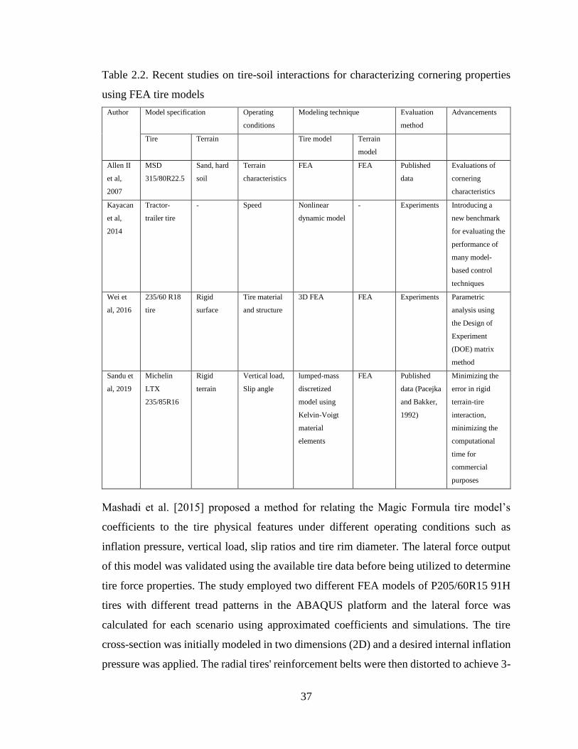
37

Table 2.2. Recent studies on tire-soil interactions for characterizing cornering properties

using FEA tire models

Author Model specification Operating

conditions

Modeling technique Evaluation

method

Advancements

Tire Terrain Tire model Terrain

model

Allen II

et al,

2007

MSD

315/80R22.5

Sand, hard

soil

Terrain

characteristics

FEA FEA Published

data

Evaluations of

cornering

characteristics

Kayacan

et al,

2014

Tractor-

trailer tire

- Speed Nonlinear

dynamic model

- Experiments Introducing a

new benchmark

for evaluating the

performance of

many model-

based control

techniques

Wei et

al, 2016

235/60 R18

tire

Rigid

surface

Tire material

and structure

3D FEA FEA Experiments Parametric

analysis using

the Design of

Experiment

(DOE) matrix

method

Sandu et

al, 2019

Michelin

LTX

235/85R16

Rigid

terrain

Vertical load,

Slip angle

lumped-mass

discretized

model using

Kelvin-Voigt

material

elements

FEA Published

data (Pacejka

and Bakker,

1992)

Minimizing the

error in rigid

terrain-tire

interaction,

minimizing the

computational

time for

commercial

purposes

Mashadi et al. [2015] proposed a method for relating the Magic Formula tire model’s

coefficients to the tire physical features under different operating conditions such as

inflation pressure, vertical load, slip ratios and tire rim diameter. The lateral force output

of this model was validated using the available tire data before being utilized to determine

tire force properties. The study employed two different FEA models of P205/60R15 91H

tires with different tread patterns in the ABAQUS platform and the lateral force was

calculated for each scenario using approximated coefficients and simulations. The tire

cross-section was initially modeled in two dimensions (2D) and a desired internal inflation

pressure was applied. The radial tires' reinforcement belts were then distorted to achieve 3-

38

D representations. It was demonstrated that using this approach, the MF tire model

coefficients could be estimated in terms of tire load and physical attributes. El-Sayegh and

El-Gindy [2018] evaluated cornering characteristics of a wide base truck tire

(445/50R22.5) operating on a wet surface considering variations in different operating

conditions such as inflation pressure, wheel loads, and water depth. The water was modeled

using smoothed-particle hydrodynamics, while the wide base truck tire was modeled using

FEA. The lateral force, rolling resistance, cornering stiffness, and self-aligning moment

were among the cornering parameters studied. The simulation results showed good

agreements with the experimental data.

The reported studies have mostly neglected the important effects of operating speed, tire

slip, inflation pressure and multi pass condition, which are known to strongly affect the

tire-terrain interactions. Moreover, the studies were mostly limited to a particular tire and

terrain such as water covered pavement or dry or moist sand or clay. The knowledge of tire

interactions with different soils or soil properties thus remains limited.

2.5.3 Soil behavior analysis

Soil compaction due to rolling tire operation is an unavoidable event. The soil compaction

due to contact pressure caused by the heavy vehicle mobility and loads strongly affects the

off-road vehicle traction efficiency, although this raises many concerns with regard to soil

erosion, runoffs, hardpan formations, energy loss, and environmental-related damages

[Gheshlaghi and Mardani, 2021]. The soil compaction has been studied extensively using

analytical and FEA tire models. Many analytical models have also been developed to

describe the process of changes in the soil characteristics considering multiple tire passes.

Liu et al. [1996, 1999] analyzed sand-tire interactions using the finite element program

MARC that included a modified Cam–Clay critical-state soil model as well as a nonlinear

elastic law. The study included a soil model in a large strain framework considering

substantial soil deformations resulting from plastic deformations and localized failures.

Guo et al [2020] investigated soil compaction in terms of contact stress distributions under

various operating conditions using a three-dimensional tire–pavement model. Figure 2.22

illustrates the contact stress distribution under the tire. The longitudinal contact stress was

symmetrically distributed in the longitudinal direction, as shown in Figure 2.22b, while the

39

lateral contact stress was virtually anti-symmetrically distributed in longitudinal direction,

as shown in Figure 2.22(c). The longitudinal contact stress was negative at the leading

portion of the contact region and positive at the trailing end. The contact region with

negative stress distribution, however, was considerably smaller than that of the positive

stress distribution.

Figure 2.22. (a) vertical, (b) longitudinal, and (c) transverse contact stress distribution of

a free-rolling tire with a 32.5 kN load [Guo et al., 2020]

Sandu et al. [2019] developed a Hybrid Soft Soil Tire Model (HSSTM) to evaluate the tire-

terrain interactions. The main goal was to describe the soil deformations in the vertical and

longitudinal directions under different operating conditions. A visualization environment

was created to show the behavior of the user-defined terrain, such as plastic deformations

and stress distributions. Figure 2.23 depicts snapshots of the terrain viewing environment

under multi-pass conditions. Owing to the nonlinearities of the HSSTM, the study

presented the responses under a variety of normal and tangential loads. The simulation

results revealed unequal permanent plastic deformation of the ground following the tire

passing. The study further revealed that positive shear forces continue to drive the tire

forward when it is traveling on a deformable terrain under an applied torque, while the

negative ground forces oppose the tire motion.

40

Figure 2.23. Terrain mapping during the multi-pass simulation of a driven tire (a) soil

consecutive loading-unloading (b) Contour of terrain sinkage [Sandu et al., 2019]

Gheshlaghi et al. [2021] investigated the soil stress distribution under an off-road tire using

the SPH-FEA model under different operating conditions. Tire-moist soil experiments

were also conducted utilizing a single wheel tester in a large soil storage area. A bevameter

and a shear-strength box were used to estimate soil model parameters. From the

comparisons of simulation results with the experimental data, it was concluded that the

FEA-SPH model could accurately predict the soil stress distribution. In another study,

Gheshlaghi et al [2020a] used the same simulation technique to study soil density and

sinkage effects that are directly related to changes in soil compaction. With a particular

user-distinguished kernel function, the SPH technique predicted the local density

reasonably well.

2.6 Summary

This chapter presented a review of available published works related to tire-terrain

interaction modeling and testing. Depending on whether the vehicle is used off-road or on-

road, the terrain on which it operates could range from a hard surface to deformable

surfaces, such as soils and snow. It is well known that soft terrain characteristics have a

significant impact on off-road vehicle performance, development of a reliable and robust

tire-terrain interaction model is vital. The tire modeling techniques as well as the modeling

and validation methods used for developing FEA) tire models were discussed in details.

The techniques used for soil modeling and calibrations such as FEA and Smoothed Particle

41

Hydrodynamics (SPH) were also discussed. In addition, the tire-terrain contact algorithm,

the tire performance analyses under different operating conditions were further discussed.

From the review of reported studies, it is concluded that the cornering characteristics of

tires operating on soft soils have not been comprehensively studied. The effects of

variations in important operating parameters, in particular, have not been adequately

addressed. Considering that compressive FEA tire models and SPH modeling techniques

for soils have been well developed, these could be applied to gain insight into the roles of

important operating conditions and soil properties. These include the rolling speed, inflation

pressure, wheel load, and tire slip angle, in addition to soil characteristics such as cohesion,

angle of internal friction, and sinkage. The implementations of these models in total vehicle

performance analyses, however, have been limited due to the associated excessive

computational demands. It is thus desirable to formulate relationships for cornering force and

rolling resistance as functions of the operating parameters, which would permit vehicle

performance analyses considering tires’ interactions with different soils. Formulations of such

relationships constitutes the primary motivation for this study, which are developed using an

advanced algorithm involving testing, training and validations. Moreover, the relations

describing the important effects of many operating conditions such as free-rolling or driven,

multi-pass, and soil compaction, would be highly desirable.

42

TIRE MODELING AND MODEL VALIDATIONS

The studies reporting tire-terrain interactions generally focus on static and dynamic

responses for limited ranges of design and operating factors. This is mostly due to the need

for remodeling and in-part due to large computational demand. Furthermore, the

performance assessments and designs of tires involve repeated field and/or laboratory tests,

which are extremely costly and demanding on human resources. In recent years, the need

to develop a virtual tire test platform has been broadly emphasized [El-Sayegh et al., 2019;

Farhadi et al., 2019], which would permit performance assessments and initial stage

designs in a cost-effective manner. Advancements in computing hardware and software

have facilitated developments in a new generation of tire modeling techniques that could

serve as the virtual test platform, and permit design and analyses of tire structure in a cost-

effective manner. Furthermore, these would allow the effects of various structure- and

material-related factors on static and dynamic properties of tires and the soils. The design

of an effective virtual test platform tires operating on soft soils involves the development

of a comprehensive FEA tire model and its integration with the SPH model of the soil.

This chapter describes the FEA model of a truck tire (Goodyear RHD 315/80R22.5), which

is implemented to the SPH soil model (Chapter 5) to investigate tire-terrain interactions

under varying operating conditions and soil types. A comprehensive FEA model of a truck

tire, developed by Slade [2009] in the Pam-Crash visual environment, has been adopted in

this study for its integration to the soil models. The model validity, however, is thoroughly

examined prior to its integration. This chapter describes different static and dynamic tests

used for model verification. These include the vertical stiffness, footprint, and drum-cleat

tests. The model validity is demonstrated by comparing the static and dynamic responses

of the model with the available measured data for the same tire under different inflation

pressures and vertical loads.

43

3.1 FEA truck tire modeling

A truck tire (Goodyear RHD 315/80R22.5) is considered for developing the FEA model.

This particular tire was selected for the study due to the fact that the experimental data were

accessible for examining model validity. The tire model was developed using the essential

geometric and material data obtained from the manufacturer, as reported in [Slade, 2009;

Chae, 2006], which are presented in Figure 3.1 and Table 3.1.

Figure 3.1. FEA tire basic dimensions [Chae, 2006]

Table 3.1. RHD tire specifications [Chae, 2006]

Tread Depth 27 mm

Rim Width 229 mm

Rim mass (ma) 34.8 kg

Tire mass 72 kg

Mass of the wheel 106.8 kg

Mass of Belt (mb) 43.4406 kg

Overall Width 315 mm

Overall Diameter 1092 mm

Static Loaded Radius 505 mm

Speed Rating 120 km/h

Rated Inflation Pressure 848 kPa (123 psi)

44

The tire is modeled in a visual environment called PAM-Crash that enables the modeling

of complex geometry by offering different structural and continuum elements such as

beams, shells, membranes and solids. Figure 3.2 shows half of the 3-dimensional tire cross-

section that was generated in PATRAN. To produce a complete cross-section, this half

model was mirrored about the tire's longitudinal axis. The cross-section was then rotated

in 6 degree increments about the tire axle axis to form the entire tire with 60 identical

sectors [Slade, 2009]. The tire carcass is made up of layered membrane components, while

the bead fillers, shoulder region, tread, and under tread are made up of Mooney-Rivlin

elements. Three separate layers of the layered membrane elements in the same component

were considered that altered the material characteristics and orientations. The tire carcass

structure in this case comprised rubber tire carcass as well as steel belts and steel wires,

which extended radially from bead to bead within the carcass. The tire bead is represented

as a circular beam element with a specific cross-sectional area and steel characteristics.

Figure 3.2. RHD tire section [Slade, 2009]

The RHD truck tire is made up of 21 parts, which are connected with each other and having

31 different material characteristics. The tire model has 4200 solid elements, 1680

membrane elements and 120 beam elements. The RHD tire has an asymmetric tread

pattern that helps to keep gravel out of the tread. The tread design was reduced to include

only the essential parts while reducing modeling complexities and computational demand.

45

The tread, under-tread, shoulders, and bead fillers are all represented as solid elements.

Three-dimensional solid elements are used to represent these components since these are

composed of rather thick rubber and are subjected to shear loads and abrupt changes in

curvature during operation.

3.1 Tire model validations

There are several critical tire properties that must be precisely matched in order to produce

the desired tire responses. The sidewall thickness (h), the modulus of elasticity (E) of the

sidewalls and under-tread, and the Mooney-Rivlin coefficients of the rubber compounds of

the tread and under-tread were all taken as reported by Slade [2009], which showed

acceptable vertical stiffness compared to the published data [Lardner, 2017]. The vertical

stiffness and contact patch area are among the static parameters utilized for calibration and

validation in this case. The vertical and horizontal vibration mode frequencies are

considered for validating the tire model in terms of its dynamic behaviour.

3.1.1 Vertical stiffness test

The vertical stiffness test is initially used to fine-tune the tire model to fit the measured

load-deflection curves. The RHD tire model is positioned on a rigid surface and constrained

along the lateral, longitudinal and all rotational directions. The tire is then inflated to a

desired inflation pressure and a vertical load is applied to the rim in a ramp manner, as

shown in Figures 3.3 and 3.4, until the target load of 40 kN is achieved. The tests were

performed for three different inflation pressures, namely, 586, 758 and 896 kPa (85, 110

and 130 psi). Figure 3.5 shows the static load-deflection responses of the model for the

three different inflation pressures. The results suggest linear vertical stiffness, defined as

the slope of the force-deflection curve. Table 0.2 summarizes the vertical stiffness of the

FEA tire model under the selected inflation pressures, which are also compared with those

reported for a Goodyear truck tire by Hiroma et al. [1997]. The comparisons suggest

reasonably good agreements between the model-predicted and reported vertical stiffness

data. The peak difference between the two was observed to be in the order of is 2.3% for

586 kPa (85 psi) inflation pressure and 3.1% for 758 kPa (110 psi) and 896 kPa (130 psi)

inflation pressures.

46

Figure 3.3. The ramp vertical load applied to the rim of the tire model

Figure 3.4. Vertical stiffness simulation test of the tire model

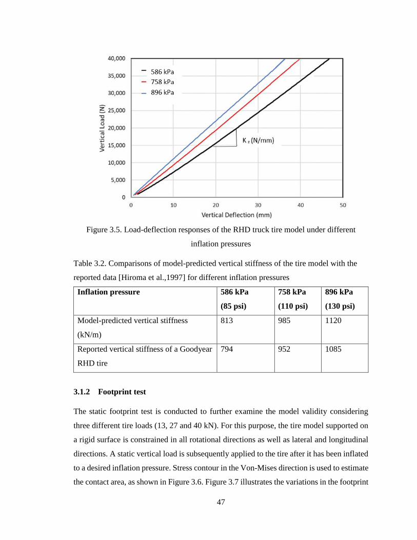
47

Figure 3.5. Load-deflection responses of the RHD truck tire model under different

inflation pressures

Table 3.2. Comparisons of model-predicted vertical stiffness of the tire model with the

reported data [Hiroma et al.,1997] for different inflation pressures

Inflation pressure 586 kPa

(85 psi)

758 kPa

(110 psi)

896 kPa

(130 psi)

Model-predicted vertical stiffness

(kN/m)

813 985 1120

Reported vertical stiffness of a Goodyear

RHD tire

794 952 1085

3.1.2 Footprint test

The static footprint test is conducted to further examine the model validity considering

three different tire loads (13, 27 and 40 kN). For this purpose, the tire model supported on

a rigid surface is constrained in all rotational directions as well as lateral and longitudinal

directions. A static vertical load is subsequently applied to the tire after it has been inflated

to a desired inflation pressure. Stress contour in the Von-Mises direction is used to estimate

the contact area, as shown in Figure 3.6. Figure 3.7 illustrates the variations in the footprint

48

area of the tire model for the three tire loads and constant inflation pressure of 758 kPa

(110 psi). The model responses are also compared with the measured data obtained from

the Goodyear Tire & Rubber Co. [Chae, 2006]. The results show comparable trends but

notable differences between the simulation results and measured data. The peak difference

between the model and measured results is observed for the higher tire load (40 kN). The

model results revealed contact area of about 540 mm2 under the 40kN, which is 7% lower

than the measured contact area. This is likely due to low resolution of the model, which

was realized considering 60 circumferential sectors. The prediction error could be reduced

by formulating a more refined model with 120 or 180 circumferential sectors.

Figure 3.6. Von Mises stress distribution over the contact area of the tire model (40 kN

vertical load and 758 kPa (110 psi) inflation pressure)

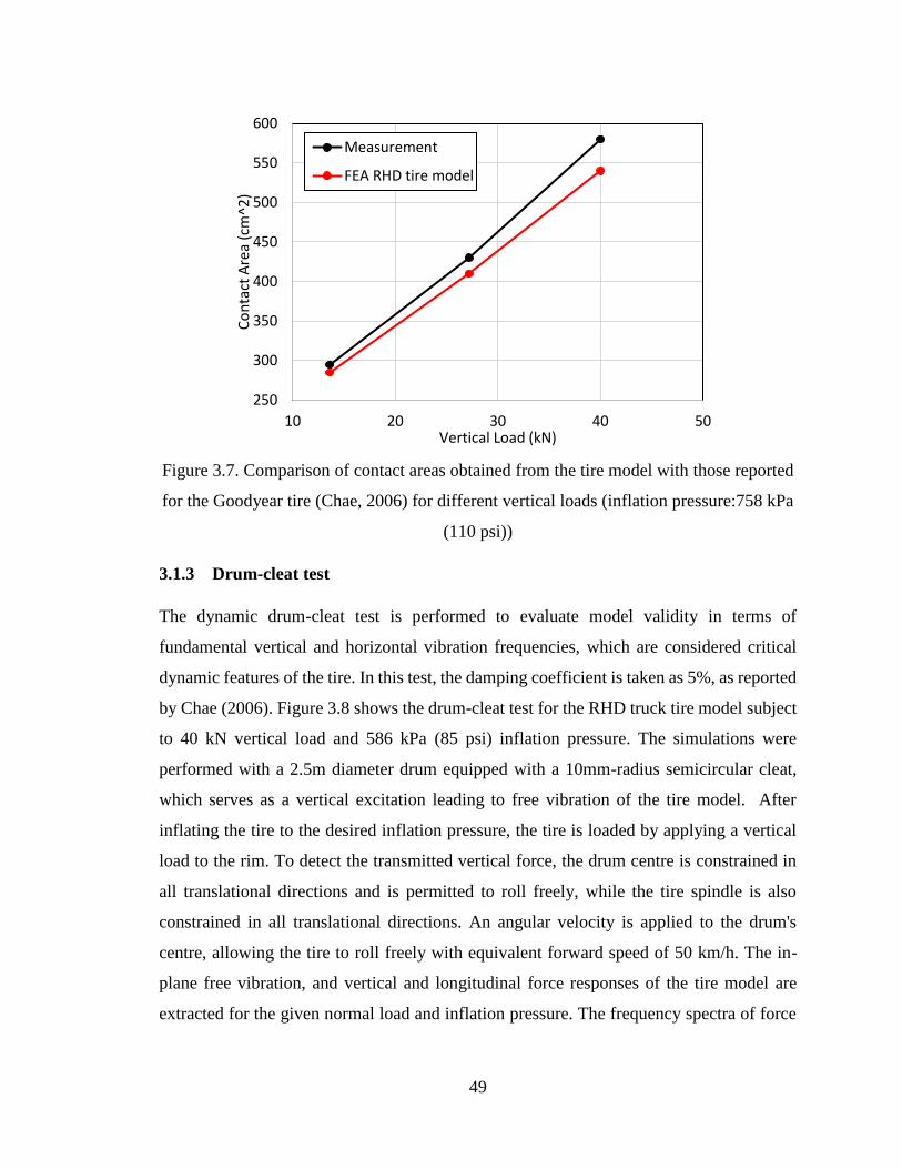
49

Figure 3.7. Comparison of contact areas obtained from the tire model with those reported

for the Goodyear tire (Chae, 2006) for different vertical loads (inflation pressure:758 kPa

(110 psi))

3.1.3 Drum-cleat test

The dynamic drum-cleat test is performed to evaluate model validity in terms of

fundamental vertical and horizontal vibration frequencies, which are considered critical

dynamic features of the tire. In this test, the damping coefficient is taken as 5%, as reported

by Chae (2006). Figure 3.8 shows the drum-cleat test for the RHD truck tire model subject

to 40 kN vertical load and 586 kPa (85 psi) inflation pressure. The simulations were

performed with a 2.5m diameter drum equipped with a 10mm-radius semicircular cleat,

which serves as a vertical excitation leading to free vibration of the tire model. After

inflating the tire to the desired inflation pressure, the tire is loaded by applying a vertical

load to the rim. To detect the transmitted vertical force, the drum centre is constrained in

all translational directions and is permitted to roll freely, while the tire spindle is also

constrained in all translational directions. An angular velocity is applied to the drum's

centre, allowing the tire to roll freely with equivalent forward speed of 50 km/h. The in-

plane free vibration, and vertical and longitudinal force responses of the tire model are

extracted for the given normal load and inflation pressure. The frequency spectra of force

250

300

350

400

450

500

550

600

10 20 30 40 50

Co

nta

ct A

rea

(cm

^2)

Vertical Load (kN)

Measurement

FEA RHD tire model

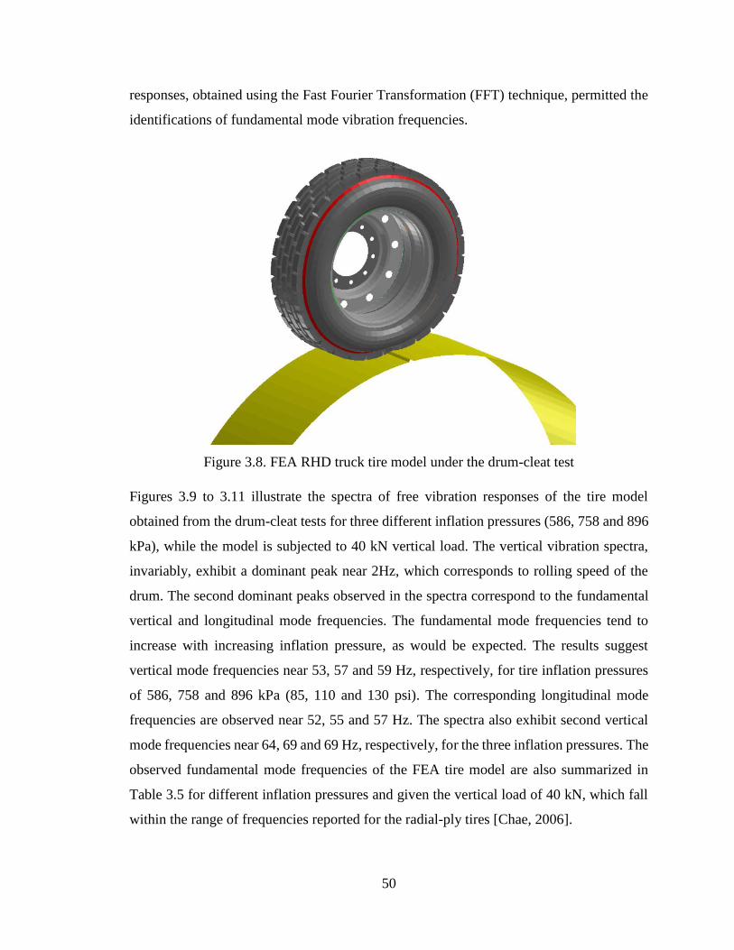
50

responses, obtained using the Fast Fourier Transformation (FFT) technique, permitted the

identifications of fundamental mode vibration frequencies.

Figure 3.8. FEA RHD truck tire model under the drum-cleat test

Figures 3.9 to 3.11 illustrate the spectra of free vibration responses of the tire model

obtained from the drum-cleat tests for three different inflation pressures (586, 758 and 896

kPa), while the model is subjected to 40 kN vertical load. The vertical vibration spectra,

invariably, exhibit a dominant peak near 2Hz, which corresponds to rolling speed of the

drum. The second dominant peaks observed in the spectra correspond to the fundamental

vertical and longitudinal mode frequencies. The fundamental mode frequencies tend to

increase with increasing inflation pressure, as would be expected. The results suggest

vertical mode frequencies near 53, 57 and 59 Hz, respectively, for tire inflation pressures

of 586, 758 and 896 kPa (85, 110 and 130 psi). The corresponding longitudinal mode

frequencies are observed near 52, 55 and 57 Hz. The spectra also exhibit second vertical

mode frequencies near 64, 69 and 69 Hz, respectively, for the three inflation pressures. The

observed fundamental mode frequencies of the FEA tire model are also summarized in

Table 3.5 for different inflation pressures and given the vertical load of 40 kN, which fall

within the range of frequencies reported for the radial-ply tires [Chae, 2006].

51

Figure 3.9. Frequency spectrum of vertical and longitudinal free vibration of the tire

model obtained from the drum-cleat test (Tire load: 40 kN; inflation pressure: 586 kPa

(85 psi))

52



(110 psi))



(130 psi))

Table 3.3. Fundamental vertical and longitudinal mode frequencies of the tire model for

different inflation pressures (vertical load: 40kN)

Inflation pressure 586 kPa

(85 psi)

758 kPa

(110 psi)

896 kPa

(130 psi)

Vertical mode frequency (Hz) 53 57 59

Longitudinal mode frequency (Hz) 52 55 57

3.2 Summary

• A FEA model of a truck tire is formulated and its validity is demonstrated through

different static and dynamic tests, namely, the vertical stiffness, footprint and the

drum-cleat tests. The static and dynamic responses obtained from the simulation

53

tests are compared with the available data of the same tire considering different

inflation pressures and normal loads. It is shown that the model can predict the

static and dynamic responses reasonably well for the ranges of inflation pressure

and normal load considered. From the results, it is deduced that: the tire vertical

stiffness increases as the inflation pressure increases. The vertical stiffness

increased from 784 kN/m to 1244 kN/m, when the inflation pressure was varied

from 586 kPa (85 psi) to 896 kPa (130 psi).

• The fundamental mode of vertical vibration of the tire model occurred in the 53-59

Hz frequency range with inflation pressure ranging from 586 (85 psi) to 896 kPa

(130 psi).

• The fundamental mode of longitudinal vibration occurred at a slightly lower

frequency and it increased from 52 and 57 Hz when inflation pressure was increased

from 586 kPa (85 psi) to 896 kPa (130 psi).

• The fundamental vertical and longitudinal mode frequencies increased with the tire

inflation pressure.

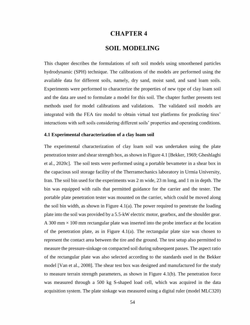
54

SOIL MODELING

This chapter describes the formulations of soft soil models using smoothened particles

hydrodynamic (SPH) technique. The calibrations of the models are performed using the

available data for different soils, namely, dry sand, moist sand, and sand loam soils.

Experiments were performed to characterize the properties of new type of clay loam soil

and the data are used to formulate a model for this soil. The chapter further presents test

methods used for model calibrations and validations. The validated soil models are

integrated with the FEA tire model to obtain virtual test platforms for predicting tires’

interactions with soft soils considering different soils’ properties and operating conditions.

4.1 Experimental characterization of a clay loam soil

The experimental characterization of clay loam soil was undertaken using the plate

penetration tester and shear strength box, as shown in Figure 4.1 [Bekker, 1969; Gheshlaghi

et al., 2020c]. The soil tests were performed using a portable bevameter in a shear box in

the capacious soil storage facility of the Therramechanics laboratory in Urmia University,

Iran. The soil bin used for the experiments was 2 m wide, 23 m long, and 1 m in depth. The

bin was equipped with rails that permitted guidance for the carrier and the tester. The

portable plate penetration tester was mounted on the carrier, which could be moved along

the soil bin width, as shown in Figure 4.1(a). The power required to penetrate the loading

plate into the soil was provided by a 5.5-kW electric motor, gearbox, and the shoulder gear.

A 300 mm × 100 mm rectangular plate was inserted into the probe interface at the location

of the penetration plate, as in Figure 4.1(a). The rectangular plate size was chosen to

represent the contact area between the tire and the ground. The test setup also permitted to

measure the pressure-sinkage on compacted soil during subsequent passes. The aspect ratio

of the rectangular plate was also selected according to the standards used in the Bekker

model [Van et al., 2008]. The shear test box was designed and manufactured for the study

to measure terrain strength parameters, as shown in Figure 4.1(b). The penetration force

was measured through a 500 kg S-shaped load cell, which was acquired in the data

acquisition system. The plate sinkage was measured using a digital ruler (model MLC320)

55

with a ± 1-pulse reproducibility accuracy that was attached to the driven part of the device.

The shear plate was pulled by the carrier at a constant speed of 0.2 m/s and the pulling

force was measured by the load cell. The penetration force, the pull force and displacement

signals were acquired in a data acquisition system. The vertical force acting on the shear

box was varied by changing the weight and the shear strength parameters were

subsequently using the Mohr-Coulomb criterion [Wong, 2008]. The experimental pressure-

sinkage and shear-strength curves are shown in Figures 4.4 and 4.5.

a. Plate penetration tester [Gheshlaghi et al., 2020c]

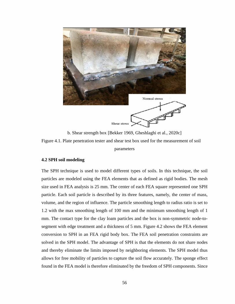
56

b. Shear strength box [Bekker 1969, Gheshlaghi et al., 2020c]

Figure 4.1. Plate penetration tester and shear test box used for the measurement of soil

parameters

4.2 SPH soil modeling

The SPH technique is used to model different types of soils. In this technique, the soil

particles are modeled using the FEA elements that as defined as rigid bodies. The mesh

size used in FEA analysis is 25 mm. The center of each FEA square represented one SPH

particle. Each soil particle is described by its three features, namely, the center of mass,

volume, and the region of influence. The particle smoothing length to radius ratio is set to

1.2 with the max smoothing length of 100 mm and the minimum smoothing length of 1

mm. The contact type for the clay loam particles and the box is non-symmetric node-to-

segment with edge treatment and a thickness of 5 mm. Figure 4.2 shows the FEA element

conversion to SPH in an FEA rigid body box. The FEA soil penetration constraints are

solved in the SPH model. The advantage of SPH is that the elements do not share nodes

and thereby eliminate the limits imposed by neighboring elements. The SPH model thus

allows for free mobility of particles to capture the soil flow accurately. The sponge effect

found in the FEA model is therefore eliminated by the freedom of SPH components. Since

57

SPH, unlike FEA, enables penetration, it yields a more accurate portrayal of soil behaviour

under pressure.

Figure 4.2. Converting FEA elements to SPH Particles

4.3 SPH sensitivity analysis

The SPH terrain behaviour is significantly impacted by the material characteristics

employed. The material characteristics impact the property change in the pressure-sinkage

and shear strength relationships. This section presents the sensitivity analysis performed

for various parameters. The displacement speed in the shear-strength test, tangent modulus,

yield stress, and the coefficient of the pressure-volume equation of state are among the

parameters investigated.

Displacement speed in the shear-strength test

The displacement speed refers to how quickly the shear box is being dragged. It determines

how rapidly the SPH particles move and react to a change in speed. Under constant material

circumstances and SPH control parameters, three different speeds are examined to evaluate

the effect of speed on soil behavior. To complete this test, a total movement of 10 mm is

necessary. Thus, the box with a 10 mm/s speed moved for 1 second, the box with a 5 mm/s

speed moved for 2 seconds, and the box with a 1 mm/s speed moved for 10 seconds.

Figure 4.3 shows the simulation results for the three boxes with three different speeds and

measurements. Table 4.1 summarizes the parameters obtained from the simulation of the

shear strength test at different speeds and experimental tests. The results show that the

speed of the box has a minor impact on the shear strength relationship. Because the speed

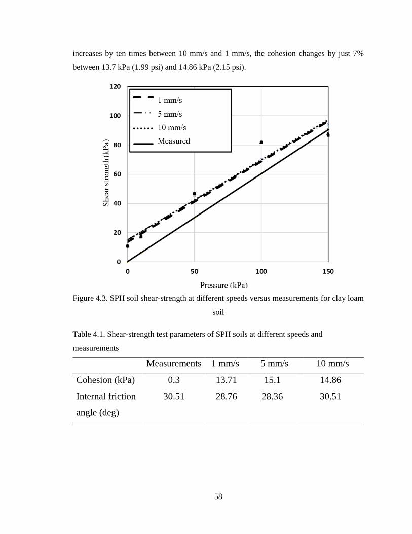
58

increases by ten times between 10 mm/s and 1 mm/s, the cohesion changes by just 7%

between 13.7 kPa (1.99 psi) and 14.86 kPa (2.15 psi).

Figure 4.3. SPH soil shear-strength at different speeds versus measurements for clay loam

soil

Table 4.1. Shear-strength test parameters of SPH soils at different speeds and

measurements

10 mm/s 5 mm/s 1 mm/s Measurements

14.86 15.1 13.71 0.3 Cohesion (kPa)

30.51 28.36 28.76 30.51 Internal friction

angle (deg)

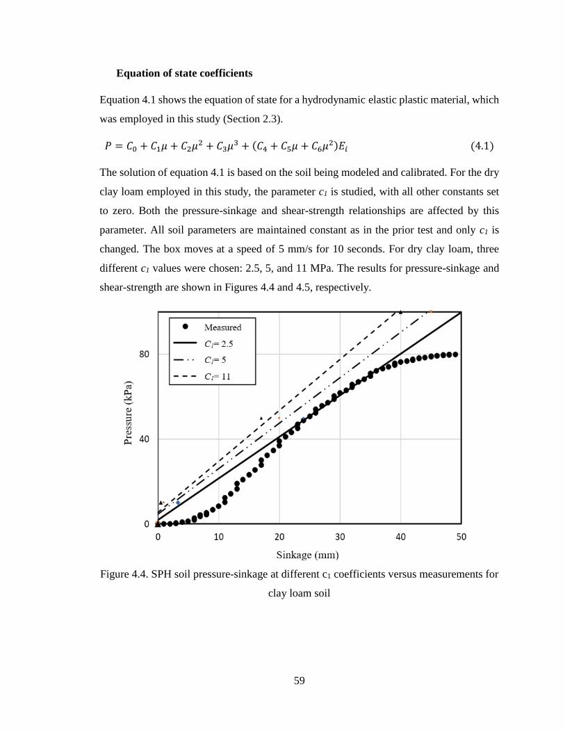
59

Equation of state coefficients

Equation 4.1 shows the equation of state for a hydrodynamic elastic plastic material, which

was employed in this study (Section 2.3).

𝑃 = 𝐶0 + 𝐶1𝜇 + 𝐶2𝜇2 + 𝐶3𝜇

3 + (𝐶4 + 𝐶5𝜇 + 𝐶6𝜇2)𝐸𝑖 (4.1)

The solution of equation 4.1 is based on the soil being modeled and calibrated. For the dry

clay loam employed in this study, the parameter c1 is studied, with all other constants set

to zero. Both the pressure-sinkage and shear-strength relationships are affected by this

parameter. All soil parameters are maintained constant as in the prior test and only c1 is

changed. The box moves at a speed of 5 mm/s for 10 seconds. For dry clay loam, three

different c1 values were chosen: 2.5, 5, and 11 MPa. The results for pressure-sinkage and

shear-strength are shown in Figures 4.4 and 4.5, respectively.

Figure 4.4. SPH soil pressure-sinkage at different c1 coefficients versus measurements for

clay loam soil

60

Figure 4.5. SPH soil shear-strength at different speeds versus measurements for clay loam

soil

The results show that the value of c1 has a significant impact on the sinkage of the soil.

Sinkage reduces between 50 mm and 40 mm when c1 increases from 2.5 MPa to 11 MPa.

The internal friction angle increases between 28.36 and 34.1 degrees as c1 increases

between 2.5 and 11 MPa. c1 affects the stiffness of the material. For example; a lower

number of results in a softer material, which sinks more. 2.5 MPa is chosen as the optimal

value of c1 that results in pressure-sinkage and shear-strength curves near the measurement

curves.

Yield stress

Yield stress is the stress that corresponds to the yield point at which the material begins to

bend plastically. Since it reflects the top limit of forces that may be applied without causing

permanent deformation, the yield stress is commonly employed to estimate the maximum

permitted load in a mechanical component. The yield stress has a minor effect on the shear-

strength relationship, according to many simulations performed using the shear box test.

The pressure-sinkage relationship, however, is significantly affected. The yield stress was

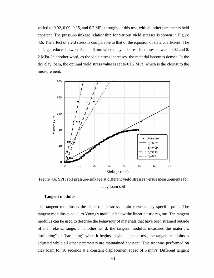
61

varied to 0.02, 0.09, 0.15, and 0.2 MPa throughout this test, with all other parameters held

constant. The pressure-sinkage relationship for various yield stresses is shown in Figure

4.6. The effect of yield stress is comparable to that of the equation of state coefficient. The

sinkage reduces between 52 and 6 mm when the yield stress increases between 0.02 and 0.

2 MPa. In another word, as the yield stress increases, the material becomes denser. In the

dry clay loam, the optimal yield stress value is set to 0.02 MPa, which is the closest to the

measurement.

Figure 4.6. SPH soil pressure-sinkage at different yield stresses versus measurements for

clay loam soil

Tangent modulus

The tangent modulus is the slope of the stress–strain curve at any specific point. The

tangent modulus is equal to Young's modulus below the linear elastic regime. The tangent

modulus can be used to describe the behaviour of materials that have been strained outside

of their elastic range. In another word, the tangent modulus measures the material's

"softening" or "hardening" when it begins to yield. In this test, the tangent modulus is

adjusted while all other parameters are maintained constant. This test was performed on

clay loam for 10 seconds at a constant displacement speed of 5 mm/s. Different tangent

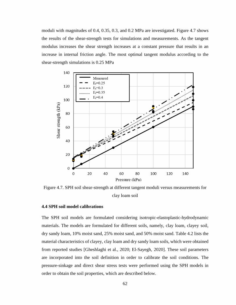
62

moduli with magnitudes of 0.4, 0.35, 0.3, and 0.2 MPa are investigated. Figure 4.7 shows

the results of the shear-strength tests for simulations and measurements. As the tangent

modulus increases the shear strength increases at a constant pressure that results in an

increase in internal friction angle. The most optimal tangent modulus according to the

shear-strength simulations is 0.25 MPa

Figure 4.7. SPH soil shear-strength at different tangent moduli versus measurements for

clay loam soil

4.4 SPH soil model calibrations

The SPH soil models are formulated considering isotropic-elastoplastic-hydrodynamic

materials. The models are formulated for different soils, namely, clay loam, clayey soil,

dry sandy loam, 10% moist sand, 25% moist sand, and 50% moist sand. Table 4.2 lists the

material characteristics of clayey, clay loam and dry sandy loam soils, which were obtained

from reported studies [Gheshlaghi et al., 2020; El-Sayegh, 2020]. These soil parameters

are incorporated into the soil definition in order to calibrate the soil conditions. The

pressure-sinkage and direct shear stress tests were performed using the SPH models in

order to obtain the soil properties, which are described below.

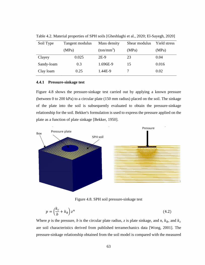
63

Table 4.2. Material properties of SPH soils [Gheshlaghi et al., 2020; El-Sayegh, 2020]

Soil Type Tangent modulus

(MPa)

Mass density

(ton/mm3)

Shear modulus

(MPa)

Yield stress

(MPa)

Clayey 0.025 2E-9 23 0.04

Sandy-loam 0.3 1.696E-9 15 0.016

Clay loam 0.25 1.44E-9 7 0.02

4.4.1 Pressure-sinkage test

Figure 4.8 shows the pressure-sinkage test carried out by applying a known pressure

(between 0 to 200 kPa) to a circular plate (150 mm radius) placed on the soil. The sinkage

of the plate into the soil is subsequently evaluated to obtain the pressure-sinkage

relationship for the soil. Bekker's formulation is used to express the pressure applied on the

plate as a function of plate sinkage [Bekker, 1950].

Figure 4.8. SPH soil pressure-sinkage test

𝑝 = (𝑘𝑐𝑏+ 𝑘∅) 𝑧

𝑛 (4.2)

Where p is the pressure, b is the circular plate radius, z is plate sinkage, and n, 𝑘∅, and 𝑘𝑐

are soil characteristics derived from published terramechanics data [Wong, 2001]. The

pressure-sinkage relationship obtained from the soil model is compared with the measured

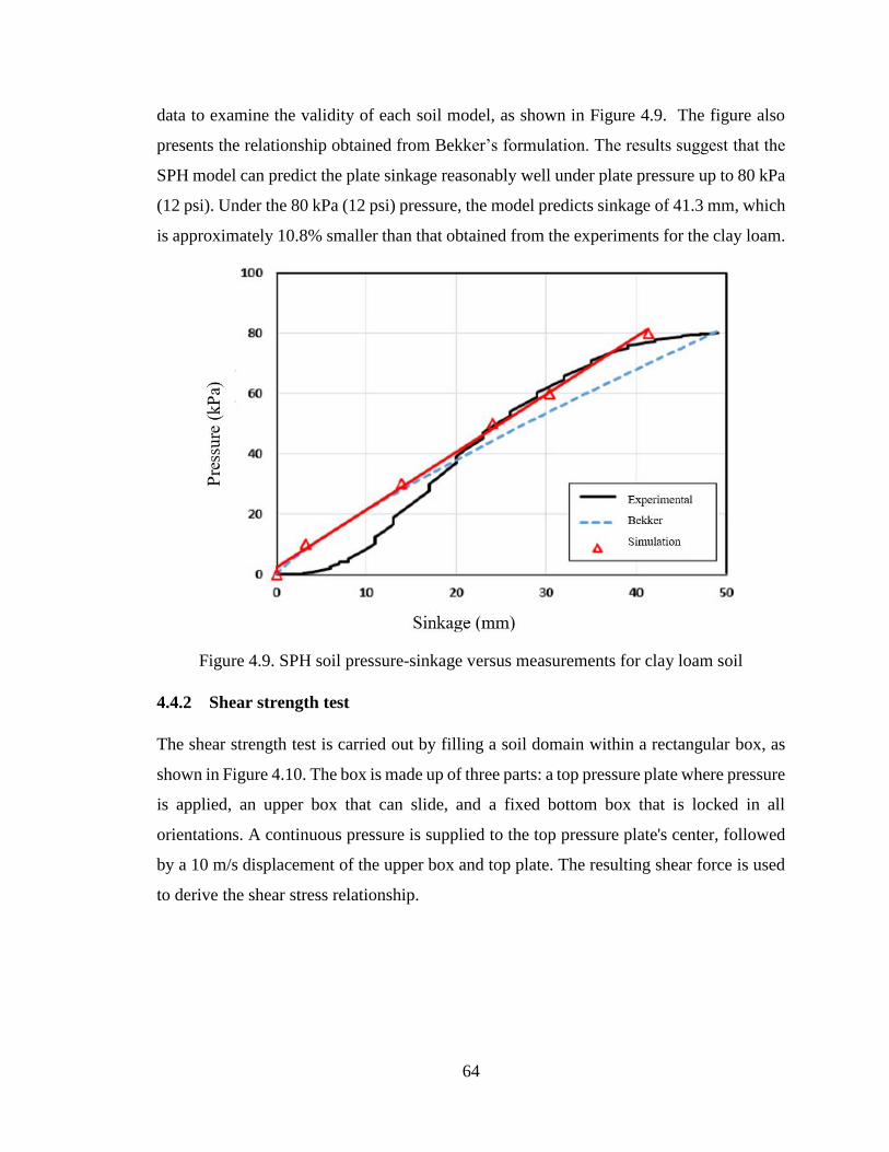
64

data to examine the validity of each soil model, as shown in Figure 4.9. The figure also

presents the relationship obtained from Bekker’s formulation. The results suggest that the

SPH model can predict the plate sinkage reasonably well under plate pressure up to 80 kPa

(12 psi). Under the 80 kPa (12 psi) pressure, the model predicts sinkage of 41.3 mm, which

is approximately 10.8% smaller than that obtained from the experiments for the clay loam.

Figure 4.9. SPH soil pressure-sinkage versus measurements for clay loam soil

4.4.2 Shear strength test

The shear strength test is carried out by filling a soil domain within a rectangular box, as

shown in Figure 4.10. The box is made up of three parts: a top pressure plate where pressure

is applied, an upper box that can slide, and a fixed bottom box that is locked in all

orientations. A continuous pressure is supplied to the top pressure plate's center, followed

by a 10 m/s displacement of the upper box and top plate. The resulting shear force is used

to derive the shear stress relationship.

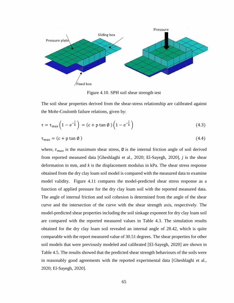
65

Figure 4.10. SPH soil shear strength test

The soil shear properties derived from the shear-stress relationship are calibrated against

the Mohr-Coulomb failure relations, given by:

τ = τmax (1 − e−j

k ) = (c + p tan ∅ ) (1 − e−j

k ) (4.3)

τmax = (c + p tan ∅ ) (4.4)

where, 𝜏𝑚𝑎𝑥 is the maximum shear stress, ∅ is the internal friction angle of soil derived

from reported measured data [Gheshlaghi et al., 2020; El-Sayegh, 2020], j is the shear

deformation in mm, and k is the displacement modulus in kPa. The shear stress response

obtained from the dry clay loam soil model is compared with the measured data to examine

model validity. Figure 4.11 compares the model-predicted shear stress response as a

function of applied pressure for the dry clay loam soil with the reported measured data.

The angle of internal friction and soil cohesion is determined from the angle of the shear

curve and the intersection of the curve with the shear strength axis, respectively. The

model-predicted shear properties including the soil sinkage exponent for dry clay loam soil

are compared with the reported measured values in Table 4.3. The simulation results

obtained for the dry clay loam soil revealed an internal angle of 28.42, which is quite

comparable with the report measured value of 30.51 degrees. The shear properties for other

soil models that were previously modeled and calibrated [El-Sayegh, 2020] are shown in

Table 4.5. The results showed that the predicted shear strength behaviours of the soils were

in reasonably good agreements with the reported experimental data [Gheshlaghi et al.,

2020; El-Sayegh, 2020].

66

In addition to the similarity of the behavior and characteristics of the tested soil and the

calibrated soil shown in Figure 4.11, more detailed results in Table 4.3 demonstrate that

the SPH technique holds the reasonable capacity to predict soil parameters.

Figure 4.11. SPH soil shear-strength test versus measurements for the clay loam soil

Table 4.3. Predicted and measured shear properties of clay loam soil parameters

Clay loam

soil

Cohesion

(kPa)

Internal

friction angle

(deg)

Soil sinkage

exponent

Simulation 1.143 28.42 0.86

Measured

[Gheshlaghi et al.,

2020]

0.3 30.51 0.84

4.5 Soil model characteristics

The calibrations were formed for the SPH models formulated for different soils. These

included the models for relationships for the tire-soil interaction dry clay loam, clayey soil,

dry sandy loam, 10% moist sand, 25% moist sand, and 50% moist sand. The soil models

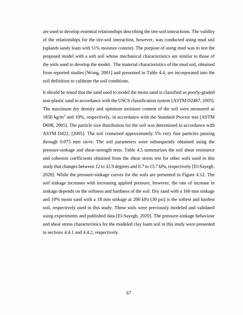
67

are used to develop essential relationships describing the tire-soil interactions. The validity

of the relationships for the tire-soil interaction, however, was conducted using mud soil

(uplands sandy loam with 51% moisture content). The purpose of using mud was to test the

proposed model with a soft soil whose mechanical characteristics are similar to those of

the soils used to develop the model. The material characteristics of the mud soil, obtained

from reported studies [Wong, 2001] and presented in Table 4.4, are incorporated into the

soil definition to calibrate the soil conditions.

It should be noted that the sand used to model the moist sand is classified as poorly-graded

non-plastic sand in accordance with the USCS classification system [ASTM D2487, 2005].

The maximum dry density and optimum moisture content of the soil were measured as

1850 kg/m3 and 10%, respectively, in accordance with the Standard Proctor test [ASTM

D698, 2005]. The particle size distribution for the soil was determined in accordance with

ASTM D422, [2005]. The soil contained approximately 5% very fine particles passing

through 0.075 mm sieve. The soil parameters were subsequently obtained using the

pressure-sinkage and shear-strength tests. Table 4.5 summarizes the soil shear resistance

and cohesion coefficients obtained from the shear stress test for other soils used in this

study that changes between 12 to 32.9 degrees and 0.7 to 15.7 kPa, respectively [El-Sayegh,

2020]. While the pressure-sinkage curves for the soils are presented in Figure 4.12. The

soil sinkage increases with increasing applied pressure, however, the rate of increase in

sinkage depends on the softness and hardness of the soil. Dry sand with a 160 mm sinkage

and 10% moist sand with a 18 mm sinkage at 200 kPa (30 psi) is the softest and hardest

soil, respectively used in this study. These soils were previously modeled and validated

using experiments and published data [El-Sayegh, 2020]. The pressure-sinkage behaviour

and shear stress characteristics for the modeled clay loam soil in this study were presented

in sections 4.4.1 and 4.4.2, respectively.

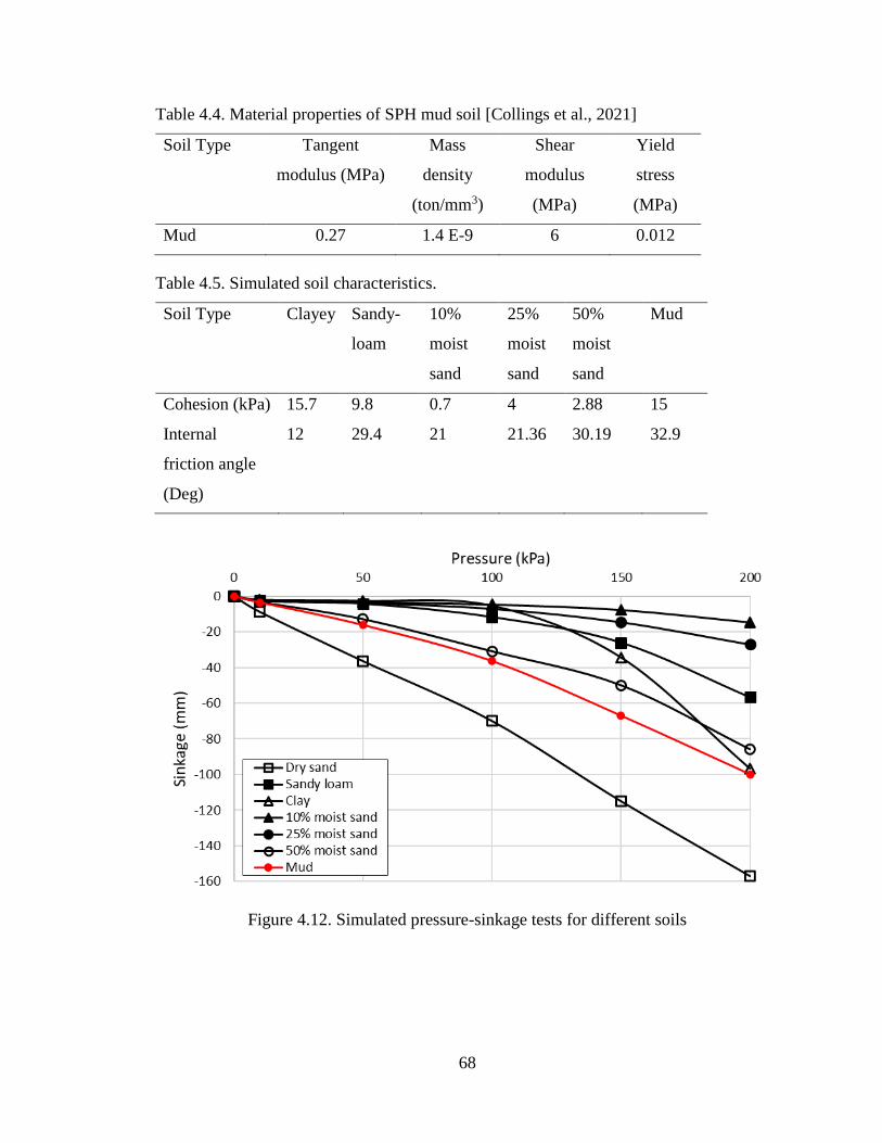
68

Table 4.4. Material properties of SPH mud soil [Collings et al., 2021]

Soil Type Tangent

modulus (MPa)

Mass

density

(ton/mm3)

Shear

modulus

(MPa)

Yield

stress

(MPa)

Mud 0.27 1.4 E-9 6 0.012

Table 4.5. Simulated soil characteristics.

Soil Type Clayey Sandy-

loam

10%

moist

sand

25%

moist

sand

50%

moist

sand

Mud

Cohesion (kPa) 15.7 9.8 0.7 4 2.88 15

Internal

friction angle

(Deg)

12 29.4 21 21.36 30.19 32.9

Figure 4.12. Simulated pressure-sinkage tests for different soils

69

4.6 Summary

This chapter described the primary features of soft terrain modeling and calibration

techniques. Different soil types that are often utilized in the vehicle-terrain interactions

were calibrated, which included clay loam, sand-loam, clayey soil, and moist sands. SPH

method and hydrodynamics-elastic plastic material were used to simulate the soils. Two

pressure-sinkage and shear-strength experiments were used to calibrate the terrains. The

simulation findings were compared with the reported terramechanics measured data. Using

Mohr-Columb failure criteria, the cohesion and angle of shear resistance were estimated

and evaluated against published physical terramechanics parameters. The SPH soil models

were found to be in good agreement with the measurements. The soil models are used to

develop essential relationships for describing tire-soil interactions, while the mud soil is

used to validate the developed relationships.

70

TIRE-TERRAIN INTERACTIONS ANALYSIS: ROLLING

RESISTANCE

5.1 Introduction

A rolling tire exhibits considerable rolling resistance, which contributes to substantial

energy loss. Rolling resistance of a tire is primarily caused by hysteresis of the rubber tread

and carcass that is encountered as the tire rolls through its footprint. The rolling resistance

of a tire rolling on an undeformable pavement is strongly affected by the material hysteresis

and orientations of the high modulus cords in the layered carcass and belt structure, in

addition to various operating factors such as rolling speed, normal load, inflation pressure

and tread depth. Soil compression and shearing further contribute to the rolling resistance

in a highly complex manner when the tire rolls on deformable terrains [Contreras et al.,

2013]. For tires operating on non-deformable pavements, the tire's flexibility accounts for

the majority of the rolling resistance. During soft soils operations, the soil deformations in

both vertical and horizontal directions are the important contributory factors. The designs

of tires and development operating practices leading to low rolling resistance have been

widely emphasized for preserving the fuel economy of vehicles [Taghavifar and Mardani,

2013].

In this chapter, integrating the FEA tire model and the SPH soil model is used to evaluate

rolling resistance of the tire. The results are employed to develop relationships for the

rolling resistance using the genetic algorithm (GA), which is implemented to analyze

rolling resistance of a vehicle. The first part of the chapter focuses on the analysis of rolling

resistance under different operating conditions such as inflation pressure, vertical load,

speed, torque, in addition to the soil characteristics. The second part of this chapter includes

the development of a genetic algorithm model to derive a relationship describing the rolling

resistance coefficient as a function of various operating conditions. These include the

multi-pass, longitudinal speed, vertical load, inflation pressure, and soil characteristics. An

experiment was designed to characterize rolling resistance of a RHD tire operating on mud

soil. The tests were done with four different tires (one steered, two driven, and one push)

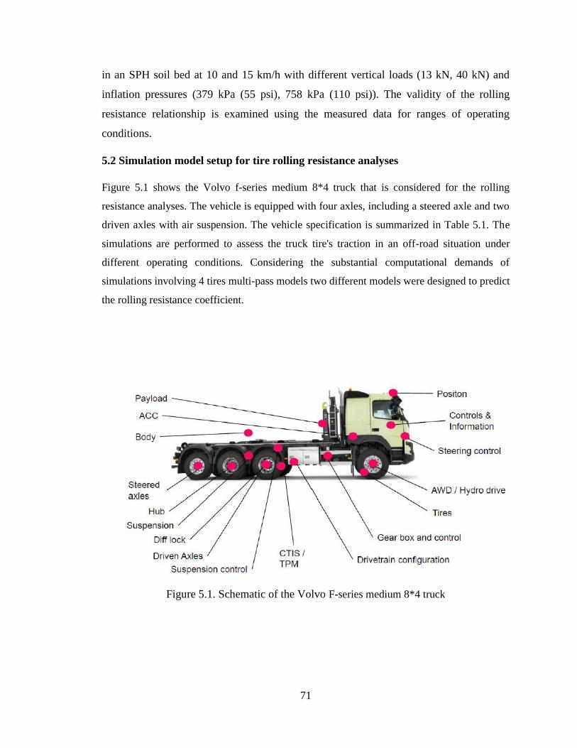
71

in an SPH soil bed at 10 and 15 km/h with different vertical loads (13 kN, 40 kN) and

inflation pressures (379 kPa (55 psi), 758 kPa (110 psi)). The validity of the rolling

resistance relationship is examined using the measured data for ranges of operating

conditions.

5.2 Simulation model setup for tire rolling resistance analyses

Figure 5.1 shows the Volvo f-series medium 8*4 truck that is considered for the rolling

resistance analyses. The vehicle is equipped with four axles, including a steered axle and two

driven axles with air suspension. The vehicle specification is summarized in Table 5.1. The

simulations are performed to assess the truck tire's traction in an off-road situation under

different operating conditions. Considering the substantial computational demands of

simulations involving 4 tires multi-pass models two different models were designed to predict

the rolling resistance coefficient.

Figure 5.1. Schematic of the Volvo F-series medium 8*4 truck

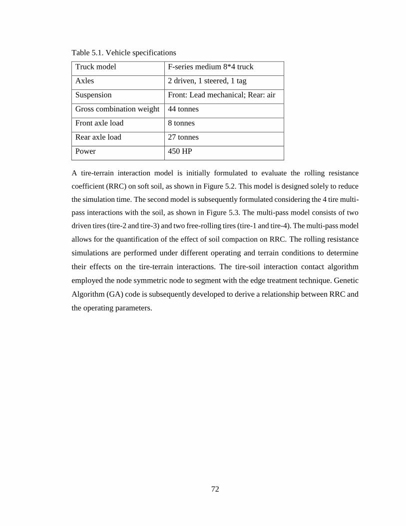
72

Table 5.1. Vehicle specifications

Truck model F-series medium 8*4 truck

Axles 2 driven, 1 steered, 1 tag

Suspension Front: Lead mechanical; Rear: air

Gross combination weight 44 tonnes

Front axle load 8 tonnes

Rear axle load 27 tonnes

Power 450 HP

A tire-terrain interaction model is initially formulated to evaluate the rolling resistance

coefficient (RRC) on soft soil, as shown in Figure 5.2. This model is designed solely to reduce

the simulation time. The second model is subsequently formulated considering the 4 tire multi-

pass interactions with the soil, as shown in Figure 5.3. The multi-pass model consists of two

driven tires (tire-2 and tire-3) and two free-rolling tires (tire-1 and tire-4). The multi-pass model

allows for the quantification of the effect of soil compaction on RRC. The rolling resistance

simulations are performed under different operating and terrain conditions to determine

their effects on the tire-terrain interactions. The tire-soil interaction contact algorithm

employed the node symmetric node to segment with the edge treatment technique. Genetic

Algorithm (GA) code is subsequently developed to derive a relationship between RRC and

the operating parameters.

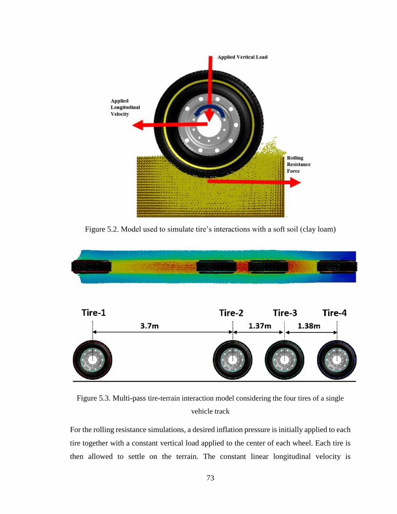
73

Figure 5.2. Model used to simulate tire’s interactions with a soft soil (clay loam)

Figure 5.3. Multi-pass tire-terrain interaction model considering the four tires of a single

vehicle track

For the rolling resistance simulations, a desired inflation pressure is initially applied to each

tire together with a constant vertical load applied to the center of each wheel. Each tire is

then allowed to settle on the terrain. The constant linear longitudinal velocity is

74

subsequently applied to the center of the free-rolling tire. An angular velocity is

simultaneously applied to the center of each driven tire. The tires are then allowed to roll

over the terrain for about 1.5 seconds to obtain steady motion at the tire-terrain contact

patch. It should be noted that the simulation model consists of four tires running in a single

run.

It should be noted that the total rolling resistance of an off-road tire comprises both the

internal and external rolling resistances. The internal rolling resistance arises from the loss

of energy attributed to deformations of the tire, while the external rolling resistance is due

to energy loss associated with the deformation of the soil. In this study, the rolling

resistance of the tire is evaluated in terms of the longitudinal force opposing the tire motion

due to the deformation of the soil, which does not include the energy losses due to

hysteresis and the thermal losses due to tire deformation.

To validate the simulation model, physical testing on gravelly soil was previously carried

out at Volvo Group's Truck Technology center in Gothenburg, Sweden in 2018 [Zeinab,

2020]. The measurements included response and acceleration from the ground through the

axle, as well as soil compaction and changes in ground properties after successive driving.

The response parameters extracted from the simulation model to determine the RRC

include the vertical load applied on the tire and the contact force between the tire and terrain

in the tire’s forward direction. The results showed that the tire-soil interaction model

simulation is in good agreement with experiments [Zeinab, 2020].

5.3 Rolling resistance analyses

The simulations of different terrains include dry and moist sands, a clayey soil, and a dense

sand. The simulations are also repeated for different operating conditions. These included

three different inflation pressures (379 kPa (85 psi), 586 kPa (110 psi), and 758 kPa (130

psi)), three different vertical loads (13 kN, 27 kN, and 40 kN), and three different

longitudinal speeds (5 km/h, 10 km/h and 15 km/h). The simulation results are presented

below and discussed to highlight the impacts of variations in the vertical load, inflation

pressure, soil compaction, and soil mechanical properties on the rolling resistance. RRC is

subsequently evaluated by normalizing the resisting force to the wheel load.

75

5.3.1 Effect of vertical load

Figures 5.4(a), 5.4(b), and 5.4(c) show the effects of variations in vertical load on the

rolling resistance coefficient of the free rolling tire model coupled with the models of clay

loam, dense sand, and clayey soil, respectively. The results are presented for a constant

forward speed of 10 km/h and three different inflation pressures. The results suggest a

nearly linear increase in RRC with an increase in vertical load, irrespective of the inflation

pressure. This is due to greater sinkage of the wheel into the soil and higher tire-soil contact

area under the higher wheel load. The interactions of the tire with clayey soil, however,

yield slightly nonlinear effects of normal load on the resulting RRC. This is evident in

Figure 5.4(c) for the higher inflation pressure.

The results exhibit significant effects of the soil on the RRC and its rate of change with the

vertical load. The operation on the clay loam soil yields an almost linear increase in RRC

with the vertical load, irrespective of the inflation pressure. The rate of change of RRC

with the vertical load, however, tends to be considerably lower for the low inflation

pressure of 380 kPa (55 psi). Lower inflation pressure also yields notably lower RRC for

all the vertical loads considered, which is attributable to relatively lower wheel sinkage

under the lower inflation pressure. The results suggest the lowest RRC of 0.226

corresponding to the 13 kN wheel load and 380 kPa (55 psi) inflation pressure, while the

highest RRC of 0.269 is observed under the 40 KN load and 758 kPa (110 psi) inflation

pressure. Similar trends in RRC are also observed for the tire’s interactions with the dense

sand and clayey soil, as seen in Figures 5.4(b) and 5.4(c). The RRC of the free rolling tire,

however, is significantly higher during operation on the clayey soil. For the higher inflation

pressure of 758 kPa (110 psi), the RRC increases from about 0.32 to 0.75, when the wheel

load is increased from 13 kN to 40 kN. The results thus suggest that the tire’s interactions

with the clayey soil are far more sensitive to wheel load when compared to those with clay

loam and dense sand which is due to the softness of the soil. The results also show that the

rolling resistance coefficient changes linearly with regard to the vertical load regardless of

the soil characteristics. Many published researchers consider the relationship of rolling

resistance versus load as linear [Gheshlaghi et al., 2020] while Michelin [2013] reported

slight nonlinearity with an exponent of 0.85.

76

(a) Clay loam (b) Dense sand

(c) Clayey soil

Figure 5.4. Influence of vertical load on rolling resistance coefficient of the tire rolling

freely on different soils: (a) clay loam; (b) dense sand; and (c) clayey soil (forward speed

= 10km/h)

5.3.2 Effect of inflation pressure

The sinkage of the wheel and thus the RRC is also strongly affected by the inflation

pressure. The results in Fig. 5.4 suggest that the higher inflation pressure yields relatively

higher RRC, while the effect of pressure on RRC is highly nonlinear. Furthermore, the

application of a driving torque may also contribute to greater shearing of the soil and

thereby higher external rolling resistance. Figure 5.5 shows the effect of inflation pressure

on the RRC of the driven leading axle tire over the clay loam soil. The results are presented

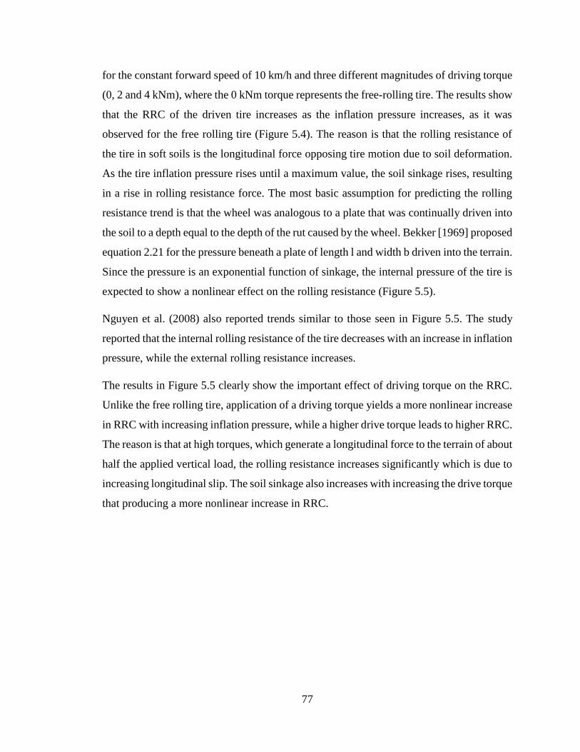
77

for the constant forward speed of 10 km/h and three different magnitudes of driving torque

(0, 2 and 4 kNm), where the 0 kNm torque represents the free-rolling tire. The results show

that the RRC of the driven tire increases as the inflation pressure increases, as it was

observed for the free rolling tire (Figure 5.4). The reason is that the rolling resistance of

the tire in soft soils is the longitudinal force opposing tire motion due to soil deformation.

As the tire inflation pressure rises until a maximum value, the soil sinkage rises, resulting

in a rise in rolling resistance force. The most basic assumption for predicting the rolling

resistance trend is that the wheel was analogous to a plate that was continually driven into

the soil to a depth equal to the depth of the rut caused by the wheel. Bekker [1969] proposed

equation 2.21 for the pressure beneath a plate of length l and width b driven into the terrain.

Since the pressure is an exponential function of sinkage, the internal pressure of the tire is

expected to show a nonlinear effect on the rolling resistance (Figure 5.5).

Nguyen et al. (2008) also reported trends similar to those seen in Figure 5.5. The study

reported that the internal rolling resistance of the tire decreases with an increase in inflation

pressure, while the external rolling resistance increases.

The results in Figure 5.5 clearly show the important effect of driving torque on the RRC.

Unlike the free rolling tire, application of a driving torque yields a more nonlinear increase

in RRC with increasing inflation pressure, while a higher drive torque leads to higher RRC.

The reason is that at high torques, which generate a longitudinal force to the terrain of about

half the applied vertical load, the rolling resistance increases significantly which is due to

increasing longitudinal slip. The soil sinkage also increases with increasing the drive torque

that producing a more nonlinear increase in RRC.

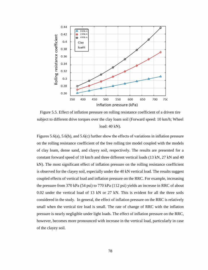
78

Figure 5.5. Effect of inflation pressure on rolling resistance coefficient of a driven tire

subject to different drive torques over the clay loam soil (Forward speed: 10 km/h; Wheel

load: 40 kN).

Figures 5.6(a), 5.6(b), and 5.6(c) further show the effects of variations in inflation pressure

on the rolling resistance coefficient of the free rolling tire model coupled with the models

of clay loam, dense sand, and clayey soil, respectively. The results are presented for a

constant forward speed of 10 km/h and three different vertical loads (13 kN, 27 kN and 40

kN). The most significant effect of inflation pressure on the rolling resistance coefficient

is observed for the clayey soil, especially under the 40 kN vertical load. The results suggest

coupled effects of vertical load and inflation pressure on the RRC. For example, increasing

the pressure from 370 kPa (54 psi) to 770 kPa (112 psi) yields an increase in RRC of about

0.02 under the vertical load of 13 kN or 27 kN. This is evident for all the three soils

considered in the study. In general, the effect of inflation pressure on the RRC is relatively

small when the vertical tire load is small. The rate of change of RRC with the inflation

pressure is nearly negligible under light loads. The effect of inflation pressure on the RRC,

however, becomes more pronounced with increase in the vertical load, particularly in case

of the clayey soil.

79

(a) Clay loam (b) Dense sand

(c) Clayey soil

Figure 5.6. Influence of inflation pressure on rolling resistance coefficient of the tire

rolling freely on different soils: (a) clay loam; (b) dense sand; and (c) clayey soil (forward

speed = 10km/h)

Tire operation on clayey soil yields substantially higher RRC compared to those observed

for the clay loam and dense sand, as seen in Figure 5.6(c). Under the 40 kN vertical load,

the RRC of tire operating on the clayey soil increases from 0.63 to 0.75, when the inflation

pressure is increased from 370 kPa (54 psi) to 770 kPa (112 psi). The results show that the

external resistance of the tire is far more sensitive to both inflation pressure and load when

compared to clay loam and dense sand soils. This is due to the softness of the soil, which

causes the soil to deform more under pressure and vertical load and causes more rolling

resistance.

80

5.3.3 Effect of soil compaction

The tire’s interactions with a deformable terrain strongly depend on soil compaction, which

tends to alter soil density and thereby sinkage or soil depth and the tire-soil contact

footprint. Variations in soil compaction, observed especially during the passage of multiple

wheels, may thus exhibit notable effects on RRC. The multi-pass model, described in

Figure 5.3, is used to simulate the multi-pass effect of rolling tires on deformable soils. The

simulations are performed for sandy soils with different moisture contents of 0%, 10% and

25%. The lead axle (axle 1), drive axles (axles 2 and 3) and the trailing axle (axle 4) are all

subjected to vertical loads of 40 kN, 758 kPa (110 psi) inflation pressure and 10 km/h

speed. These tests were performed on sandy soils with different moisture contents because

they are a better representative of changes in rolling resistance to sinkage as they offer a

wider range of internal soil friction. Data collection for these soils along with optimizing

the time of all tests was another reason. It is noted that scattered tests for the multi-axle

model with different pressures, loads and speeds in clay, clay loam and dense sand soils

were also performed.

The passage of wheels on the soils causes soil compaction and thereby reductions in soil

depth. The RRC is computed for the tire on each axle, which revealed notable effects of

soil depth. Figure 5.7 shows the variations in RRC of different axle tire as a function of the

corresponding soil depth. The soil depth after passing the first axle is 0.585 m, after passing

the second axle is 0.575 m, after passing the third and fourth axles is 0.565 m. The same

depth of the third and the fourth axle is due to the nature of the fourth tag axle. As shown

in figure 5.7, the rolling resistance coefficient increases with the increase of soil depth. In

another word, the highest rolling resistance force has been yielded at the highest soil depth

after passing the first axle (0.585 m). It is due to the highest sinkage happening after passing

the first axle on fresh soil. Since the second axle moves on compacted soil, it naturally

sinks less in the soil and shows less rolling resistance than the first axle. This result is

similar for the third and fourth axes. Furthermore, the rolling resistance coefficient

decreases with increasing the soil moisture content which is due to an increase in the

internal friction angle or in other words, increasing the ability of a unit of soil to withstand

shear stress.

81

Figure 5.7. Rolling resistance coefficient as a function of soil depth at different soils

5.3.4 Effect of speed

The important effects of rolling speed of the tire on internal resistance of the tires operating

on non-deformable terrains have been widely reported [Shakiba et al., 2016; Suyabodha et

al., 2017]. Only limited knowledge, however, exits on the effect of rolling speed on the

external resistance of the tires operating on deformable soils. In this study, the RRC of the

tire operating on soft soils is investigated considering different speeds, ranging from 5 to

20 km/h. As an example, Figure 5.8 shows the variations in RRC of the tire rolling on the

clay soil as a function of the longitudinal speed. The results were obtained considering 758

kPa (110 psi) inflation pressure and different vertical loads. The RRC increases

considerably with the vertical load, as it was seen in Figure 5.4. The results, in general,

show an increase in RRC with the forward speed. The rate of increase of RRC, however,

depends on the vertical load. The RRC increases by approximately 25% when the speed is

increased from 5 km/h to 20 km/h under the load of 13 kN. The corresponding increase in

RRC is in the order of only 8% under the higher load of 40 kN. Similar tests were performed

on clay loam soil at 758 kPa (110 psi) inflation pressure and different vertical loads. The

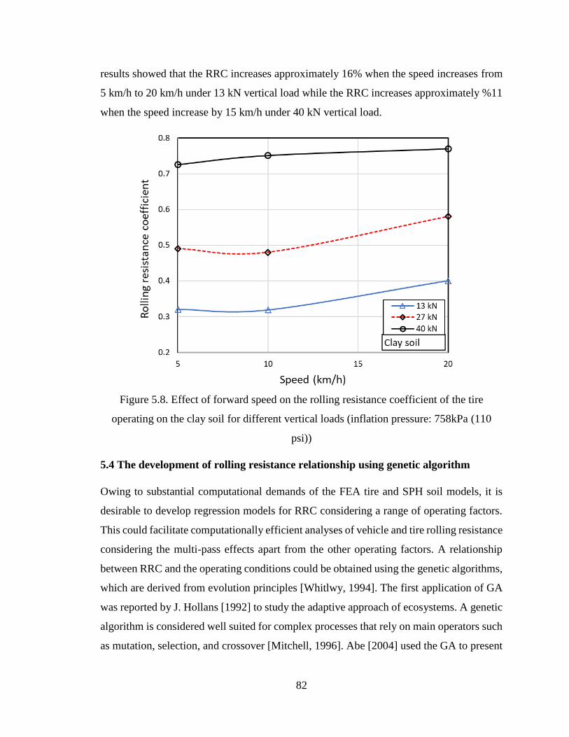
82

results showed that the RRC increases approximately 16% when the speed increases from

5 km/h to 20 km/h under 13 kN vertical load while the RRC increases approximately %11

when the speed increase by 15 km/h under 40 kN vertical load.

Figure 5.8. Effect of forward speed on the rolling resistance coefficient of the tire

operating on the clay soil for different vertical loads (inflation pressure: 758kPa (110

psi))

5.4 The development of rolling resistance relationship using genetic algorithm

Owing to substantial computational demands of the FEA tire and SPH soil models, it is

desirable to develop regression models for RRC considering a range of operating factors.

This could facilitate computationally efficient analyses of vehicle and tire rolling resistance

considering the multi-pass effects apart from the other operating factors. A relationship

between RRC and the operating conditions could be obtained using the genetic algorithms,

which are derived from evolution principles [Whitlwy, 1994]. The first application of GA

was reported by J. Hollans [1992] to study the adaptive approach of ecosystems. A genetic

algorithm is considered well suited for complex processes that rely on main operators such

as mutation, selection, and crossover [Mitchell, 1996]. Abe [2004] used the GA to present

83

an optimum tire construction by considering many variables such as belt angle, belt

topology, and belt materials. The optimized GA model was confirmed to enhance the

cornering stiffness by more than 15% by comparing the control construction in an indoor

drum test [Abe, 2004]. Taghavifar et al. [2015] developed a GA model to predict the power

required for the driven tires of off-road vehicles. The data to generate the GA model were

provided by a single-wheel tester in a soil bin facility under different vertical load, slip,

and speed conditions. The model with a 0.022 mean square error showed a high-quality

solution for predicting the power provided by the driven tire.

The genetic algorithm is the computational technique that can present the complex process

of tire-soil interaction in the form of a mathematical relationship. Figure 5.9 shows the

flowchart of the modeling technique used in this study to identify a GA mathematical

relationship for RRC of the tire. It starts with an initial population considered as a random

solution. Each population comprises a set of problem-solving candidates, called

chromosomes. The chromosome evolution is based on the evaluation of fitness function

through successive generations. The subsequent generation is made up of children in the

current population. The algorithm creates parents by selecting a group of chromosomes

that have the highest fitness in the current population. Three main operators (crossover,

mutation, and selection) in the GA work together to guide the algorithm towards a

successful solution. The user-defined crossover is used to generate a new offspring by

combining the genetic information of two parents, while the mutation operator is activated

to modify a chromosome for the next generation. The high-quality solutions are subjected

to preferred weightings by choosing individual genomes for the subsequent breeding using

the selection operator. Finally, after producing a successive population, the algorithm

converges to the best chromosomes, which provide the optimal solution to the problem

[Abe, 2004].

The Eureqa modeling engine is utilized in this study to develop a relationship between

RRC and the essential operating conditions considering different soil environments. Eureqa

software employs evolutionary search to anticipate a mathematical relationship between

the input and output data points. The chromosome evolution is based on the evaluation of

fitness function. The Eureqa training is internal and it produces different equations with

84

different accuracy. The operating conditions such as vertical load, speed, tire inflation

pressure, soil depth, soil internal friction angle, and soil cohesion were considered as the

inputs. While the rolling resistance was incorporated in the output. In order to study the

multi-pass effect, which involved stacking of four FEA tire models to examine variations

in rolling resistance with varying levels of soil compaction, the soil sinkage induced by

each axle was regarded as the input reflecting the soil axle location.

Figure 5.9. The flowchart of the proposed genetic algorithm [Abe, 2004]

The rolling resistance data collected from the FEA_SPH tire-soil simulation models were

utilized to develop the relationships for the rolling resistance as a function of various

operating conditions. The resulting GA rolling resistance relationship is subsequently

implemented into the full vehicle model, denoted as the Volvo Transportation Model

(VTM). The VTM is a MATLAB/Simulink code that predicts the full vehicle motions and

responses during different maneuvers. The VTM model originally included the PAC2002

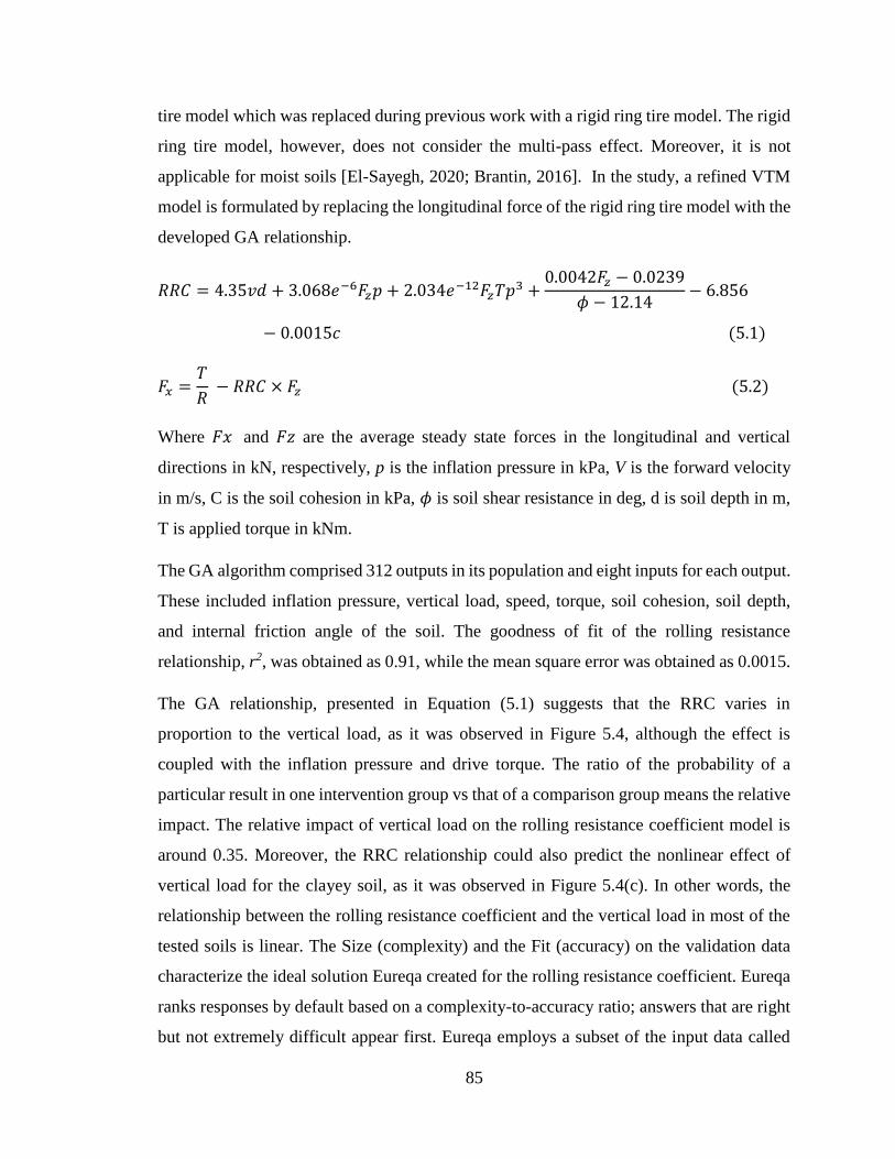
85

tire model which was replaced during previous work with a rigid ring tire model. The rigid

ring tire model, however, does not consider the multi-pass effect. Moreover, it is not

applicable for moist soils [El-Sayegh, 2020; Brantin, 2016]. In the study, a refined VTM

model is formulated by replacing the longitudinal force of the rigid ring tire model with the

developed GA relationship.

𝑅𝑅𝐶 = 4.35𝑣𝑑 + 3.068𝑒−6𝐹𝑧𝑝 + 2.034𝑒−12𝐹𝑧𝑇𝑝

3 +0.0042𝐹𝑧 − 0.0239

𝜙 − 12.14− 6.856

− 0.0015𝑐 (5.1)

𝐹𝑥 =𝑇

𝑅 − 𝑅𝑅𝐶 × 𝐹𝑧 (5.2)

Where 𝐹𝑥 and 𝐹𝑧 are the average steady state forces in the longitudinal and vertical

directions in kN, respectively, p is the inflation pressure in kPa, V is the forward velocity

in m/s, C is the soil cohesion in kPa, 𝜙 is soil shear resistance in deg, d is soil depth in m,

T is applied torque in kNm.

The GA algorithm comprised 312 outputs in its population and eight inputs for each output.

These included inflation pressure, vertical load, speed, torque, soil cohesion, soil depth,

and internal friction angle of the soil. The goodness of fit of the rolling resistance

relationship, r2, was obtained as 0.91, while the mean square error was obtained as 0.0015.

The GA relationship, presented in Equation (5.1) suggests that the RRC varies in

proportion to the vertical load, as it was observed in Figure 5.4, although the effect is

coupled with the inflation pressure and drive torque. The ratio of the probability of a

particular result in one intervention group vs that of a comparison group means the relative

impact. The relative impact of vertical load on the rolling resistance coefficient model is

around 0.35. Moreover, the RRC relationship could also predict the nonlinear effect of

vertical load for the clayey soil, as it was observed in Figure 5.4(c). In other words, the

relationship between the rolling resistance coefficient and the vertical load in most of the

tested soils is linear. The Size (complexity) and the Fit (accuracy) on the validation data

characterize the ideal solution Eureqa created for the rolling resistance coefficient. Eureqa

ranks responses by default based on a complexity-to-accuracy ratio; answers that are right

but not extremely difficult appear first. Eureqa employs a subset of the input data called

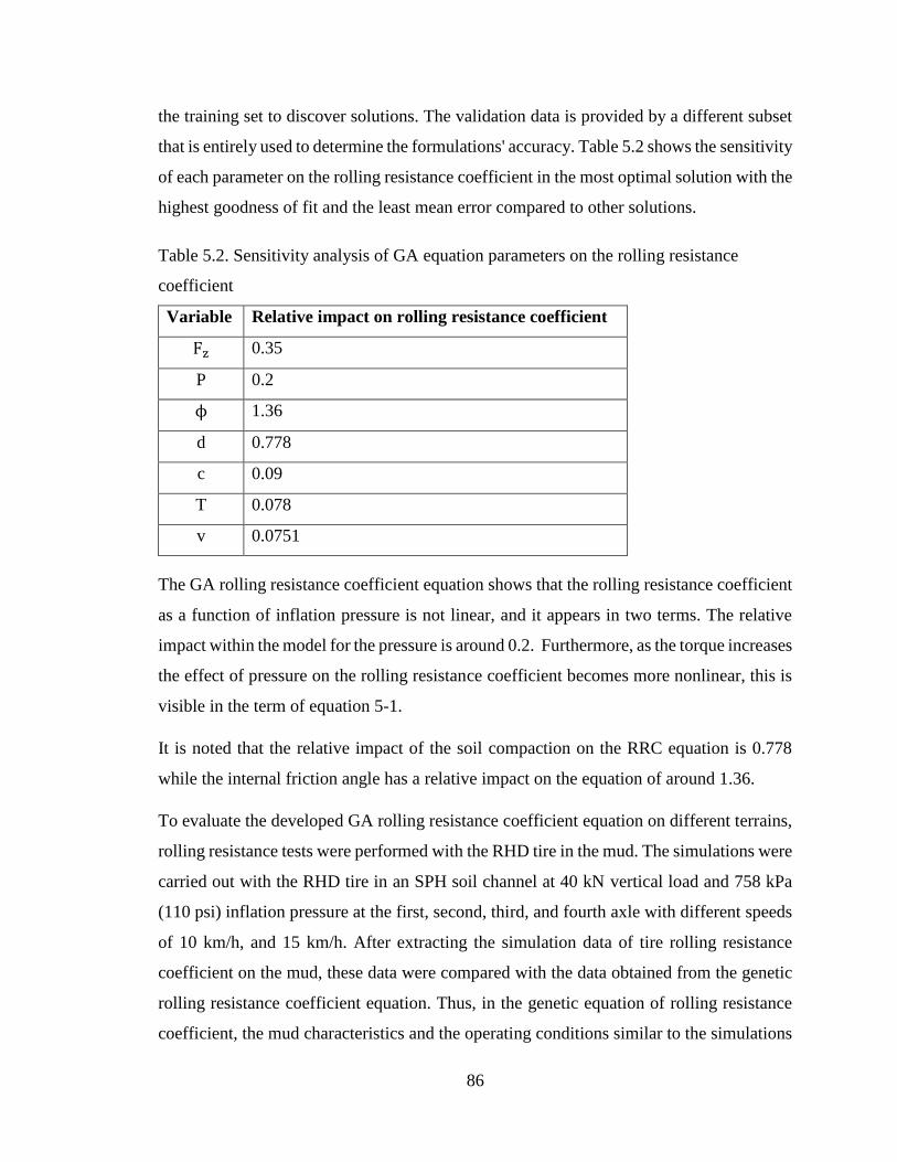
86

the training set to discover solutions. The validation data is provided by a different subset

that is entirely used to determine the formulations' accuracy. Table 5.2 shows the sensitivity

of each parameter on the rolling resistance coefficient in the most optimal solution with the

highest goodness of fit and the least mean error compared to other solutions.

Table 5.2. Sensitivity analysis of GA equation parameters on the rolling resistance

coefficient

Variable Relative impact on rolling resistance coefficient

Fz 0.35

P 0.2

ϕ 1.36

d 0.778

c 0.09

T 0.078

v 0.0751

The GA rolling resistance coefficient equation shows that the rolling resistance coefficient

as a function of inflation pressure is not linear, and it appears in two terms. The relative

impact within the model for the pressure is around 0.2. Furthermore, as the torque increases

the effect of pressure on the rolling resistance coefficient becomes more nonlinear, this is

visible in the term of equation 5-1.

It is noted that the relative impact of the soil compaction on the RRC equation is 0.778

while the internal friction angle has a relative impact on the equation of around 1.36.

To evaluate the developed GA rolling resistance coefficient equation on different terrains,

rolling resistance tests were performed with the RHD tire in the mud. The simulations were

carried out with the RHD tire in an SPH soil channel at 40 kN vertical load and 758 kPa

(110 psi) inflation pressure at the first, second, third, and fourth axle with different speeds

of 10 km/h, and 15 km/h. After extracting the simulation data of tire rolling resistance

coefficient on the mud, these data were compared with the data obtained from the genetic

rolling resistance coefficient equation. Thus, in the genetic equation of rolling resistance

coefficient, the mud characteristics and the operating conditions similar to the simulations

87

were used. Figure 5.10 shows the simulated and GA rolling resistance coefficient with R2

goodness of 0.907 which shows the capability of the GA RRC model to predict the rolling

resistance coefficient of the tire on the mud.

Figure 5.10. Predicted versus simulated rolling resistance coefficient

5.5 Summary

The rolling resistance for the RHD truck tire size 315/ 80R22.5 was analyzed under various

terrains. The SPH approach was used to model and calibrate the soils, and the findings

were given in Chapter 4. This chapter focuses on estimating, analyzing and validating the

rolling resistance coefficient equation for a truck tire running over various soils under

various operating conditions, such as tire inflation pressure, vertical load, and speed.

The rolling resistance coefficient was found to be highly dependent on the applied vertical

load. The tire inflation pressure, on the other hand, has less impact on the rolling resistance

coefficient at low vertical loads and a larger impact at high vertical loads. Concerning a

truck tire traversing various terrains, the truck tire was found to have the greatest rolling

88

resistance coefficient at a lower internal friction angle. As a result, if a truck is driving

through clayey terrain, it will use more gasoline than if it is driving on clay loam.

The RRC data from this chapter was then utilized to establish an equation between the RRC

and the operating conditions. Cohesion, internal friction angle, and soil sinkage were used

to create the operating conditions in addition to tire operating conditions such as inflation

pressure, vertical load, and speed. An equation that relates the rolling resistance coefficient

with several operating conditions was developed using advanced algorithm techniques

through training and testing using Pam-Crash simulation results. It was concluded that the

equation can predict the rolling resistance coefficient at different operating and soil

conditions. The developed equation has an R-square fitness of 0.91 (91.1%), the mean

square error is 0.0015 and the mean average error is 0.022.

89

TIRE-TERRAIN INTERACTIONS ANALYSIS:

CORNERING CHARACTERISTICS

6.1 Introduction

The cornering property of a tire is most critical for adequate vehicle handling and

directional stability. The cornering characteristics of tires are strongly affected by many

designs and operating factors such as tire construction and material properties, tire load,

inflation pressure and rolling speed [El-Razaz et al., 1988; Bolarinwa et al., 2004]. In an

off-road environment, the properties of the soil further affect the cornering properties in a

highly complex manner. In this chapter, the tire-terrain interaction models, integrating the

FEA tire model and the SPH soil models, are used to derive the cornering properties of the

tire under different operating conditions including different soils. Owing to the excessive

computational demands of the tire-terrain interaction models, the simulation results

attained for selected operating conditions are used to develop a mathematical relationship

between the cornering property and the operating factors.

The first part of the chapter presents a tire-terrain interaction model setup using a

combination of FEA and SPH techniques for calculating tire cornering characteristics for

different operating conditions. The operating conditions include the longitudinal speed,

applied torque, inflation pressure, vertical load, and slip angle. The soil characteristics such

as cohesion, angle of internal friction and sinkage are considered in the setup. The second

part of the chapter includes the analysis of cornering characteristics under different

operating and soil factors. In the final section, the simulation results are used to develop

regression relationships for the cornering force, self-aligning moment, and overturning

moment as functions of the operating factors. The relationships are developed using

advanced algorithm techniques through testing, training and validations while taking into

consideration the multi-pass effect, soil compaction, and the free-rolling and the driven

tire. The validity of the proposed mathematical relations is demonstrated in the final section

considering different operating conditions. For this purpose, the cornering tests of the RHD

tires were performed while operating over the mud soil.

90

6.2 Simulation model setup

Two different model simulation schemes were designed to determine the tire cornering

characteristics. In the first scheme, a single tire-terrain interaction model is used to evaluate

tire’s cornering characteristics on different soils to reduce the simulation time. The second

scheme employs a 4 tires multi-pass interaction model to study the multi-pass and soil

compaction effects. The model, shown in Figure 6.1, represents a four-axle Volvo truck.

The numerical tests are carried out for both driven and free-rolling tires.

After inflating each tire to the desired inflation pressure, the selected vertical load is applied

to the center of the rim. The tire is subsequently pre-steered to various slip angles, ranging

from 0° to 12°, to investigate the cornering force and aligning moment as a function of the

side-slip angle. In the case of the free-rolling tires, each tire is permitted to roll so as to

achieve a desired forward speed. The simulations are performed for three different forward

speeds (5 km/h, 10 km/h and 15 km/h). In the case of driven tires, an angular velocity is

applied to the center of each driven tire. The force responses within the contact area

between the tires and the soil are extracted to obtain the cornering force and aligning

moment for each given side-slip angle. Apart from the aligning moment (Mz) about the

vertical axis of the tire, the shift in the vertical force center is considered to derive the

overturning moment (Mx) of the tire, as shown in Figure 6.2. The overturning moment is

predominantly caused by two factors. These include the horizontal deformations of the tire

carcass induced by the lateral force. and the effective carcass camber caused by the tire

camber and the lateral force.

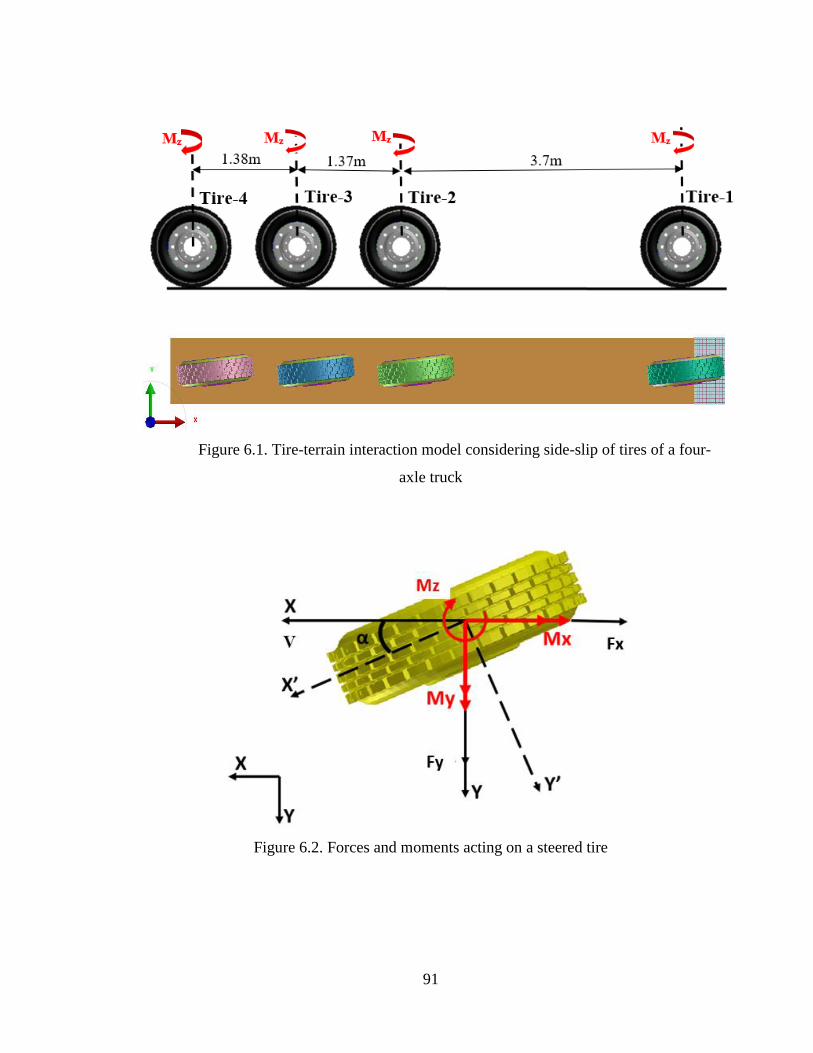
91

Figure 6.1. Tire-terrain interaction model considering side-slip of tires of a four-

axle truck

Figure 6.2. Forces and moments acting on a steered tire

92

6.3 Cornering characteristics analyses

The tire-soil interaction model simulations were performed considering different operating

conditions and soils. The operating factors included four levels of forward speed (5, 10,

15, and 20 km/h), three levels of inflation pressure (379.21(55 psi), 586.05 (110 psi) and

758.42 kPa (130 psi)), three levels of vertical load (13, 27, and 40 kN) and four different

side-slip angles (0, 2, 4, 6, and 12 degrees). The soil models included those of clay, sandy

loam, clay loam, 10% moist sand, 25% moist sand and 50% moist sand. The simulation

results obtained for both the schemes are discussed in the following sub-sections.

6.3.1 Effect of side-slip angle

Figures 6.3 and 6.4 illustrate the variations in the self-aligning moment and cornering force

developed by each free-rolling tire as a function of the slip angle, respectively. The

simulation setup, in this case, includes the four wheels model to investigate the multi-pass

effect on the cornering characteristics. The simulation results are presented for the sandy

loam soil (cohesion 9.8 kPa and internal friction angle 29.4 degrees), as an example,

considering the constant forward speed of 15 km/h speed, 758 kPa (110 psi) inflation

pressure, and 40 kN vertical load. The results show that the self-aligning moment increases

with an increase in the slip angle and it is more significant under a higher level of soil

compaction. In other words, the self-aligning moment increases as the soil undergoes

compaction. It is noted that the cornering force and self-aligning moment reach saturation

on the hard surface only at a larger slip angle, but on soft soil, they don't [El-Razaz, 1988;

Schwanghart, 1981]. It is because the lateral force generated by an off-road tire is a function

of the tire's lateral deformation and the soil shear-induced lateral deformation. The lateral

deformation of a tire refers to a force at the soil-tire contact caused by a displacement of

the tire tread or carcass, and it is the most important characteristic for determining the

lateral force of tires on hard surfaces. The lateral displacement of soil due to soil shearing

which is characterized by Equation 2.20 is the more important parameter on the lateral

force of tires on deformable terrains. Since the soil shearing behavior shows a linear

relationship based on Equation 2.20, a linear trend is also expected for the cornering force

and self-aligning moment versus slip angle on deformable terrain.

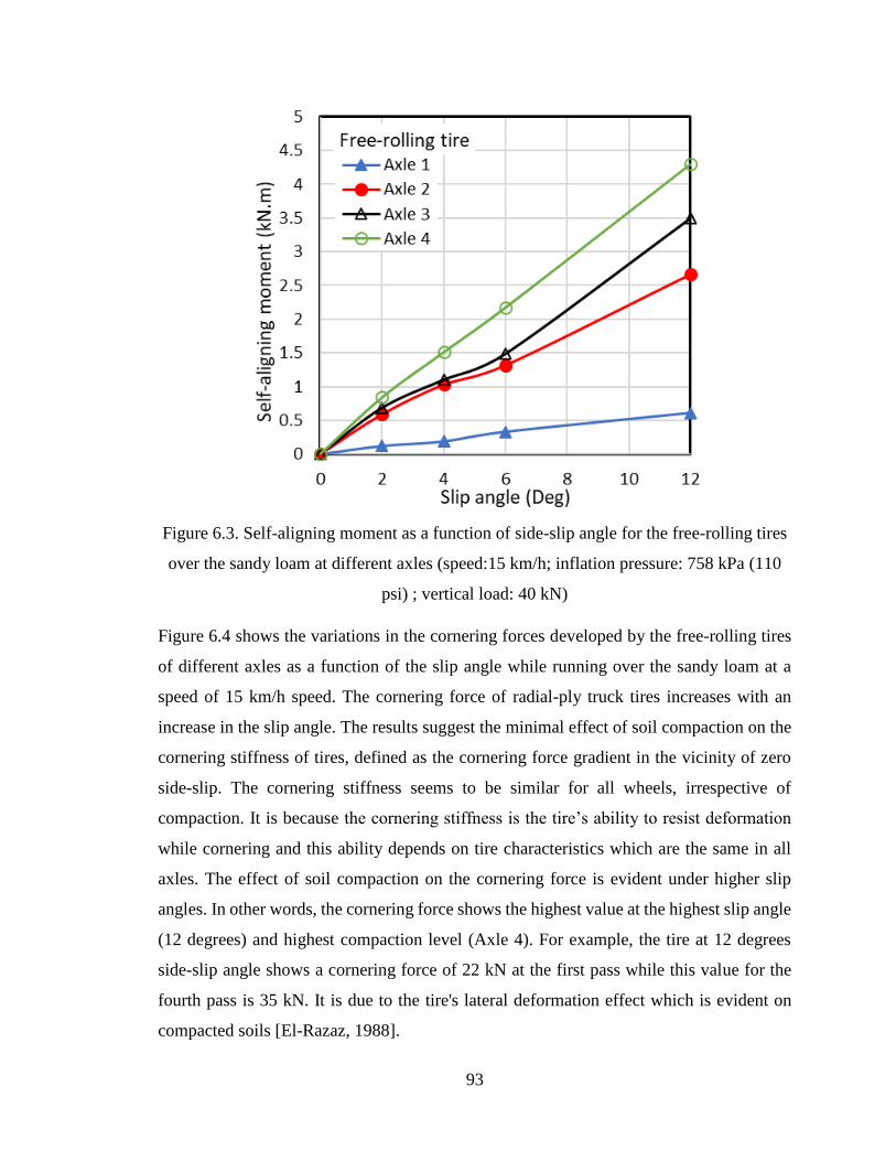
93

Figure 6.3. Self-aligning moment as a function of side-slip angle for the free-rolling tires

over the sandy loam at different axles (speed:15 km/h; inflation pressure: 758 kPa (110

psi) ; vertical load: 40 kN)

Figure 6.4 shows the variations in the cornering forces developed by the free-rolling tires

of different axles as a function of the slip angle while running over the sandy loam at a

speed of 15 km/h speed. The cornering force of radial-ply truck tires increases with an

increase in the slip angle. The results suggest the minimal effect of soil compaction on the

cornering stiffness of tires, defined as the cornering force gradient in the vicinity of zero

side-slip. The cornering stiffness seems to be similar for all wheels, irrespective of

compaction. It is because the cornering stiffness is the tire’s ability to resist deformation

while cornering and this ability depends on tire characteristics which are the same in all

axles. The effect of soil compaction on the cornering force is evident under higher slip

angles. In other words, the cornering force shows the highest value at the highest slip angle

(12 degrees) and highest compaction level (Axle 4). For example, the tire at 12 degrees

side-slip angle shows a cornering force of 22 kN at the first pass while this value for the

fourth pass is 35 kN. It is due to the tire's lateral deformation effect which is evident on

compacted soils [El-Razaz, 1988].

94

Figure 6.4. Cornering force as a function of side-slip angle for the free-rolling tires over

the sandy loam at different axles (speed:15 km/h; inflation pressure: 758 kPa (110 psi);

vertical load: 40 kN)

The cornering properties of the tires are further investigated in the presence of drive torque.

Figures 6.5 and 6.6 show the self-aligning moment and cornering force characteristics,

respectively, of the driven tires as a function of slip angle. The results are obtained

considering the angular velocity of 8.25 rad/s (equal to 15 km/h forward speed) applied to

all axle tires, while the cornering responses are obtained at the forward speed of 15 km/h,

758 kPa (110 psi) inflation pressure, and 40 kN vertical load. It is noted that the variation

of the angular velocity at constant linear longitudinal velocity will result in longitudinal

slip which indicates that the cornering force is calculated at a driven rolling tire. The self-

aligning moment increases with side-slip angle and it becomes more significant with

increasing level of soil compaction. The tires’ multi-pass effect on the self-aligning

moment is clearly evident in Figure 6.5. At a 6° side-slip angle, the self-aligning moment

developed by the second axle tire is nearly twice that of the leading axle tire, which is

attributable to soil compaction by the leading axle tire. Tires of the subsequent axles’ tires,

however, exhibit a relatively smaller increase in the aligning moment, suggesting the

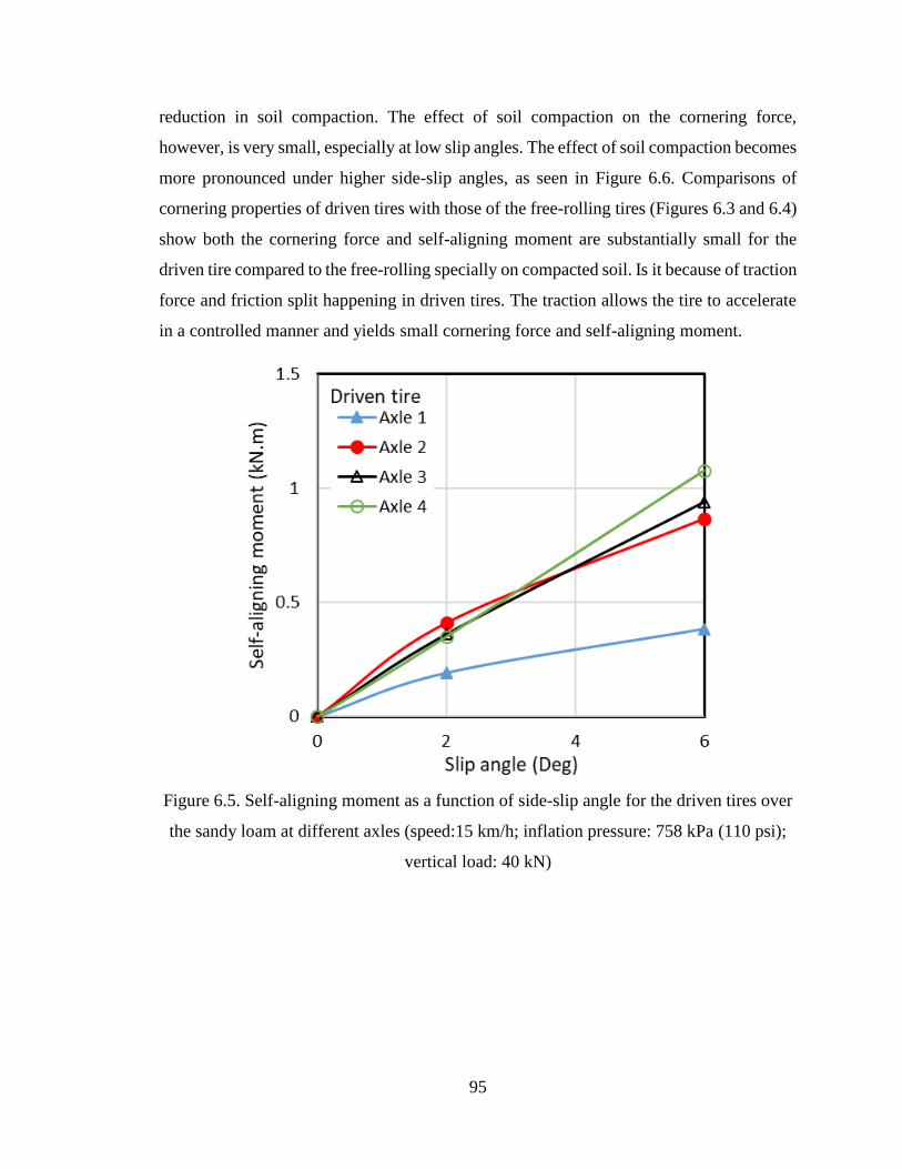
95

reduction in soil compaction. The effect of soil compaction on the cornering force,

however, is very small, especially at low slip angles. The effect of soil compaction becomes

more pronounced under higher side-slip angles, as seen in Figure 6.6. Comparisons of

cornering properties of driven tires with those of the free-rolling tires (Figures 6.3 and 6.4)

show both the cornering force and self-aligning moment are substantially small for the

driven tire compared to the free-rolling specially on compacted soil. Is it because of traction

force and friction split happening in driven tires. The traction allows the tire to accelerate

in a controlled manner and yields small cornering force and self-aligning moment.

Figure 6.5. Self-aligning moment as a function of side-slip angle for the driven tires over

the sandy loam at different axles (speed:15 km/h; inflation pressure: 758 kPa (110 psi);


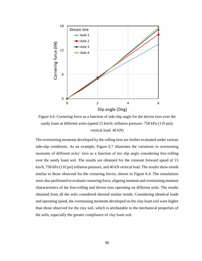
96

Figure 6.6. Cornering force as a function of side-slip angle for the driven tires over the

sandy loam at different axles (speed:15 km/h; inflation pressure: 758 kPa (110 psi);


The overturning moments developed by the rolling tires are further evaluated under various

side-slip conditions. As an example, Figure 6.7 illustrates the variations in overturning

moments of different axles’ tires as a function of tire slip angle considering free-rolling

over the sandy loam soil. The results are obtained for the constant forward speed of 15

km/h, 758 kPa (110 psi) inflation pressure, and 40 kN vertical load. The results show trends

similar to those observed for the cornering forces, shown in Figure 6.4. The simulations

were also performed to evaluate cornering force, aligning moment and overturning moment

characteristics of the free-rolling and driven tires operating on different soils. The results

obtained from all the soils considered showed similar trends. Considering identical loads

and operating speed, the overturning moments developed on the clay loam soil were higher

than those observed for the clay soil, which is attributable to the mechanical properties of

the soils, especially the greater compliance of clay loam soil.

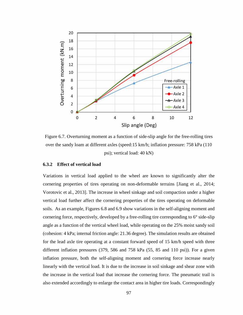
97

Figure 6.7. Overturning moment as a function of side-slip angle for the free-rolling tires

over the sandy loam at different axles (speed:15 km/h; inflation pressure: 758 kPa (110

psi); vertical load: 40 kN)

6.3.2 Effect of vertical load

Variations in vertical load applied to the wheel are known to significantly alter the

cornering properties of tires operating on non-deformable terrains [Jiang et al., 2014;

Vorotovic et al., 2013]. The increase in wheel sinkage and soil compaction under a higher

vertical load further affect the cornering properties of the tires operating on deformable

soils. As an example, Figures 6.8 and 6.9 show variations in the self-aligning moment and

cornering force, respectively, developed by a free-rolling tire corresponding to 6° side-slip

angle as a function of the vertical wheel load, while operating on the 25% moist sandy soil

(cohesion: 4 kPa; internal friction angle: 21.36 degree). The simulation results are obtained

for the lead axle tire operating at a constant forward speed of 15 km/h speed with three

different inflation pressures (379, 586 and 758 kPa (55, 85 and 110 psi)). For a given

inflation pressure, both the self-aligning moment and cornering force increase nearly

linearly with the vertical load. It is due to the increase in soil sinkage and shear zone with

the increase in the vertical load that increase the cornering force. The pneumatic trail is

also extended accordingly to enlarge the contact area in higher tire loads. Correspondingly

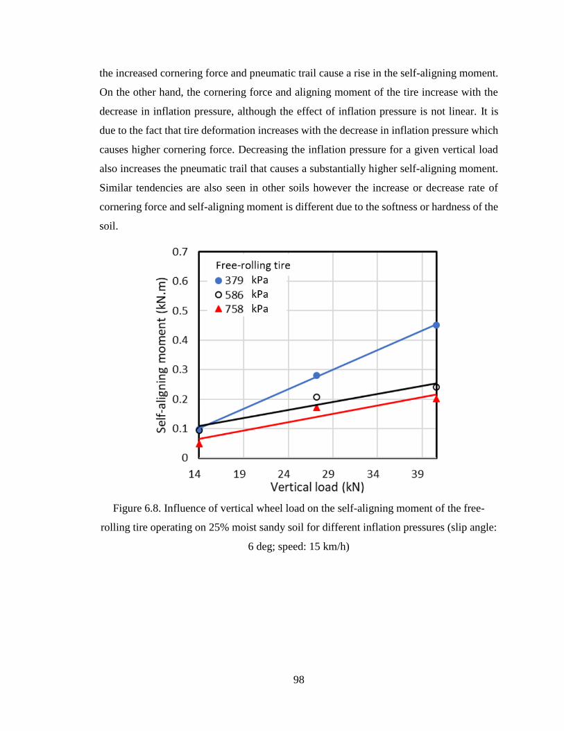
98

the increased cornering force and pneumatic trail cause a rise in the self-aligning moment.

On the other hand, the cornering force and aligning moment of the tire increase with the

decrease in inflation pressure, although the effect of inflation pressure is not linear. It is

due to the fact that tire deformation increases with the decrease in inflation pressure which

causes higher cornering force. Decreasing the inflation pressure for a given vertical load

also increases the pneumatic trail that causes a substantially higher self-aligning moment.

Similar tendencies are also seen in other soils however the increase or decrease rate of

cornering force and self-aligning moment is different due to the softness or hardness of the

soil.

Figure 6.8. Influence of vertical wheel load on the self-aligning moment of the free-

rolling tire operating on 25% moist sandy soil for different inflation pressures (slip angle:

6 deg; speed: 15 km/h)

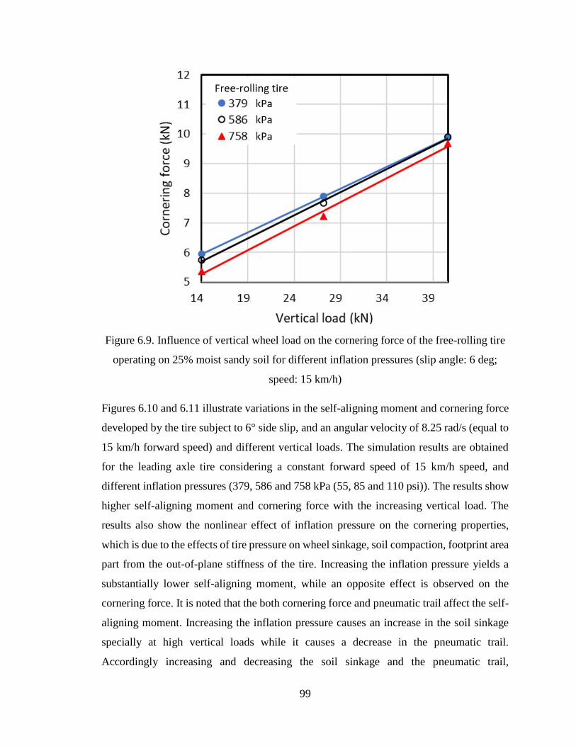
99

Figure 6.9. Influence of vertical wheel load on the cornering force of the free-rolling tire

operating on 25% moist sandy soil for different inflation pressures (slip angle: 6 deg;

speed: 15 km/h)

Figures 6.10 and 6.11 illustrate variations in the self-aligning moment and cornering force

developed by the tire subject to 6° side slip, and an angular velocity of 8.25 rad/s (equal to

15 km/h forward speed) and different vertical loads. The simulation results are obtained

for the leading axle tire considering a constant forward speed of 15 km/h speed, and

different inflation pressures (379, 586 and 758 kPa (55, 85 and 110 psi)). The results show

higher self-aligning moment and cornering force with the increasing vertical load. The

results also show the nonlinear effect of inflation pressure on the cornering properties,

which is due to the effects of tire pressure on wheel sinkage, soil compaction, footprint area

part from the out-of-plane stiffness of the tire. Increasing the inflation pressure yields a

substantially lower self-aligning moment, while an opposite effect is observed on the

cornering force. It is noted that the both cornering force and pneumatic trail affect the self-

aligning moment. Increasing the inflation pressure causes an increase in the soil sinkage

specially at high vertical loads while it causes a decrease in the pneumatic trail.

Accordingly increasing and decreasing the soil sinkage and the pneumatic trail,

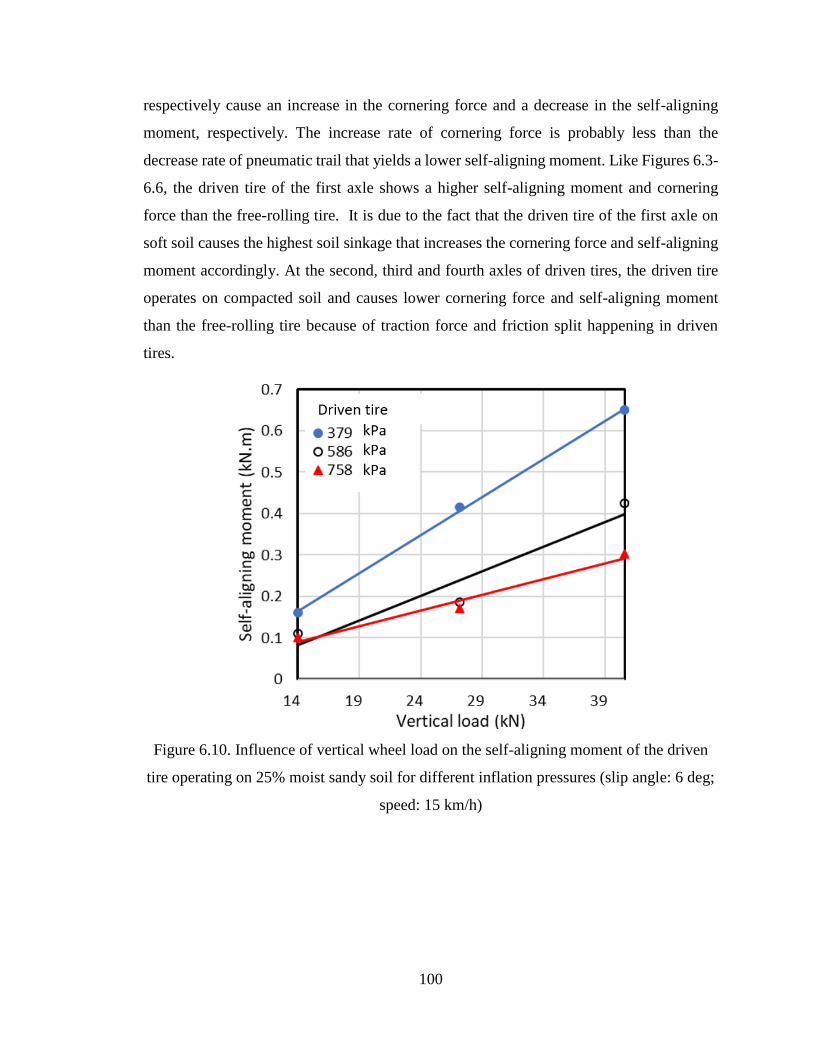
100

respectively cause an increase in the cornering force and a decrease in the self-aligning

moment, respectively. The increase rate of cornering force is probably less than the

decrease rate of pneumatic trail that yields a lower self-aligning moment. Like Figures 6.3-

6.6, the driven tire of the first axle shows a higher self-aligning moment and cornering

force than the free-rolling tire. It is due to the fact that the driven tire of the first axle on

soft soil causes the highest soil sinkage that increases the cornering force and self-aligning

moment accordingly. At the second, third and fourth axles of driven tires, the driven tire

operates on compacted soil and causes lower cornering force and self-aligning moment

than the free-rolling tire because of traction force and friction split happening in driven

tires.

Figure 6.10. Influence of vertical wheel load on the self-aligning moment of the driven

tire operating on 25% moist sandy soil for different inflation pressures (slip angle: 6 deg;

speed: 15 km/h)

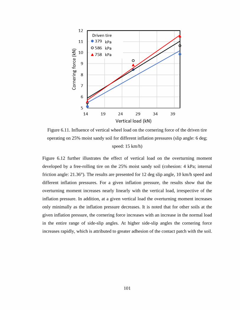
101

Figure 6.11. Influence of vertical wheel load on the cornering force of the driven tire

operating on 25% moist sandy soil for different inflation pressures (slip angle: 6 deg;

speed: 15 km/h)

Figure 6.12 further illustrates the effect of vertical load on the overturning moment

developed by a free-rolling tire on the 25% moist sandy soil (cohesion: 4 kPa; internal

friction angle: 21.36°). The results are presented for 12 deg slip angle, 10 km/h speed and

different inflation pressures. For a given inflation pressure, the results show that the

overturning moment increases nearly linearly with the vertical load, irrespective of the

inflation pressure. In addition, at a given vertical load the overturning moment increases

only minimally as the inflation pressure decreases. It is noted that for other soils at the

given inflation pressure, the cornering force increases with an increase in the normal load

in the entire range of side-slip angles. At higher side-slip angles the cornering force

increases rapidly, which is attributed to greater adhesion of the contact patch with the soil.

102

Figure 6.12. Influence of vertical wheel load on the overturning moment of the free-

rolling tire operating on 25% moist sandy soil for different inflation pressures (slip angle:

6 deg; speed: 15 km/h)

6.3.3 Effect of inflation pressure

Figures 6.13 and 6.14 show the influence of tire inflation pressure on the self-aligning

moment and cornering force, respectively, of the tire rolling freely over the 25% moist sand

(cohesion: 4 kPa; internal friction angle: 21.36°). Simulation results are obtained

considering 40 kN vertical load and 15 km/h forward speed. The results are also presented

for two different side slip angles: 2° and 6°. As the inflation pressure increases, the self-

aligning moment decreases and this decrement is more visible at 6° slip angle. Higher side

slip angle means higher side velocity and therefore lateral shearing that makes a higher

cornering force. The results suggest the effect of pressure on the aligning moment is

nonlinearly coupled with the side-slip angle and thus the side velocity. The effect of

pressure on the aligning moment is very small under lower side-slip angles, while it

becomes more pronounced for higher slip angles. Increasing the inflation pressure causes

a considerable reduction in the aligning moment under the higher side-slip of 6°, as seen

in Fig. 6.13, which may be attributed to the lower pneumatic trail. The moment comes from

103

cornering force and shift in the center of force (trail effect). In this case, since the cornering

force is almost constant, the change in the pneumatic trail is the predominant factor

affecting the self-aligning moment variation. The effects of tire pressure variations on the

cornering force, however, is considerably small, irrespective of the side-slip angle, as seen

in Figure 6.14. Other studies reporting the effect of inflation pressure on cornering force

developed by a tire operating on non-deformable as well as deformable surfaces have also

reported similar trends [El-Razaz et al., 1988; Shokouhfar, 2017].

Figure 6.13. Influence of inflation pressure on self-aligning moment of the tire rolling

freely on the 25% moist sandy soil for two different slip angles (vertical load: 40 kN;

speed: 15 km/h)

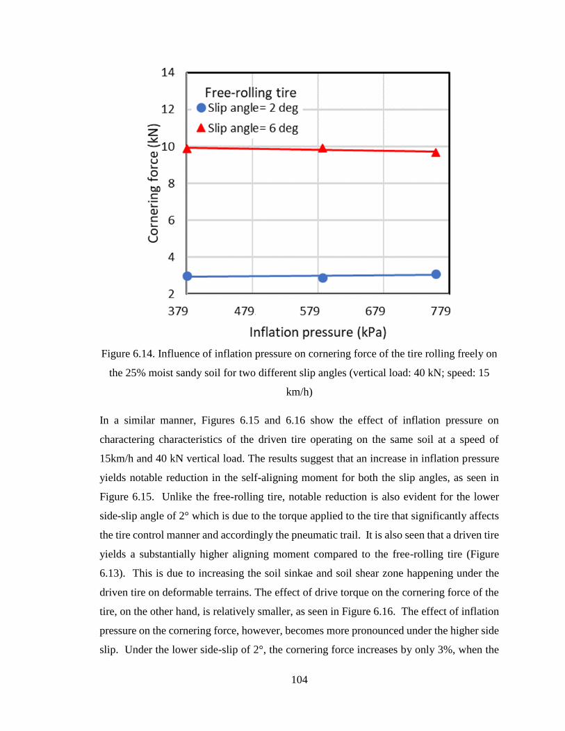
104

Figure 6.14. Influence of inflation pressure on cornering force of the tire rolling freely on

the 25% moist sandy soil for two different slip angles (vertical load: 40 kN; speed: 15

km/h)

In a similar manner, Figures 6.15 and 6.16 show the effect of inflation pressure on

charactering characteristics of the driven tire operating on the same soil at a speed of

15km/h and 40 kN vertical load. The results suggest that an increase in inflation pressure

yields notable reduction in the self-aligning moment for both the slip angles, as seen in

Figure 6.15. Unlike the free-rolling tire, notable reduction is also evident for the lower

side-slip angle of 2° which is due to the torque applied to the tire that significantly affects

the tire control manner and accordingly the pneumatic trail. It is also seen that a driven tire

yields a substantially higher aligning moment compared to the free-rolling tire (Figure

6.13). This is due to increasing the soil sinkae and soil shear zone happening under the

driven tire on deformable terrains. The effect of drive torque on the cornering force of the

tire, on the other hand, is relatively smaller, as seen in Figure 6.16. The effect of inflation

pressure on the cornering force, however, becomes more pronounced under the higher side

slip. Under the lower side-slip of 2°, the cornering force increases by only 3%, when the

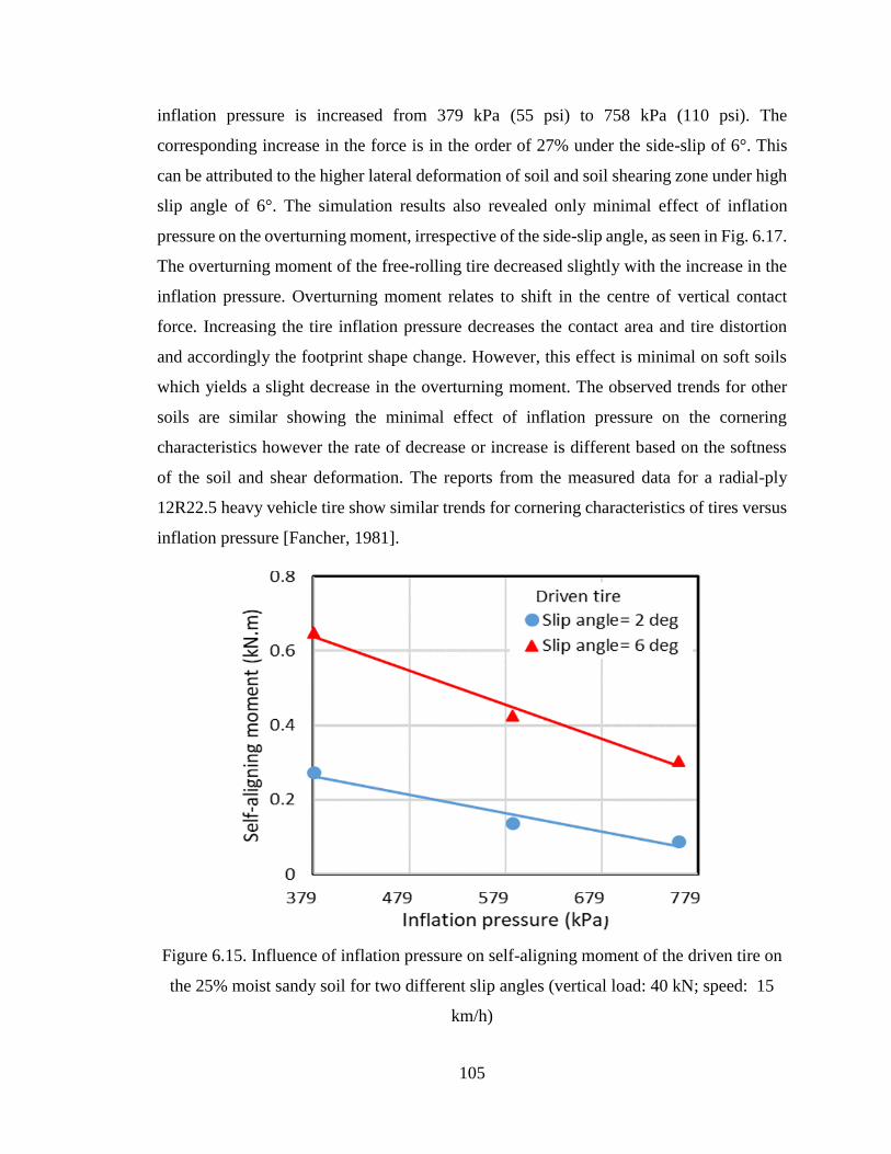
105

inflation pressure is increased from 379 kPa (55 psi) to 758 kPa (110 psi). The

corresponding increase in the force is in the order of 27% under the side-slip of 6°. This

can be attributed to the higher lateral deformation of soil and soil shearing zone under high

slip angle of 6°. The simulation results also revealed only minimal effect of inflation

pressure on the overturning moment, irrespective of the side-slip angle, as seen in Fig. 6.17.

The overturning moment of the free-rolling tire decreased slightly with the increase in the

inflation pressure. Overturning moment relates to shift in the centre of vertical contact

force. Increasing the tire inflation pressure decreases the contact area and tire distortion

and accordingly the footprint shape change. However, this effect is minimal on soft soils

which yields a slight decrease in the overturning moment. The observed trends for other

soils are similar showing the minimal effect of inflation pressure on the cornering

characteristics however the rate of decrease or increase is different based on the softness

of the soil and shear deformation. The reports from the measured data for a radial-ply

12R22.5 heavy vehicle tire show similar trends for cornering characteristics of tires versus

inflation pressure [Fancher, 1981].

Figure 6.15. Influence of inflation pressure on self-aligning moment of the driven tire on

the 25% moist sandy soil for two different slip angles (vertical load: 40 kN; speed: 15

km/h)

106

Figure 6.16. Influence of inflation pressure on cornering force of the driven tire on the

25% moist sandy soil for two different slip angles (vertical load: 40 kN; speed: 15 km/h)

Figure 6.17. Influence of inflation pressure on overturning moment of the tire rolling

freely on the 25% moist sandy soil for different slip angles (vertical load: 40 kN; speed:

15 km/h)

107

6.3.4 Effect of rolling speed

Studies reporting cornering properties of tires operating on non-deformable terrains have,

invariably, shown minimal effect of speed on the cornering force developed by the tire

[Shokouhfar, 2017; Longhouse, 1972]. The tire’s interactions with deformable soils,

however, are strongly affected by the mechanical properties of the soil, soil compaction

and the speed. The effect of rolling speed on the resulting cornering properties of free-

rolling as well as driven tires operating on deformable soils are thus investigated

considering the soil compaction effect. For this purpose, the simulations are performed

considering tires of the four axles vehicle. As an example, Figure 6.18 shows the effects

of forward speed on variations in the self-aligning moments developed by the free-rolling

tires of four axles operating on the sandy loam soil corresponding to 6 deg slip angle. Each

tire in the simulation model is subjected to 40 kN vertical load and 758 kPa (110 psi)

inflation pressure, and simulations are performed considering three different speeds (5, 10

and 15 km/h). The self-aligning moment developed by each tire generally increases with

an increase in the forward speed. Tires of different axles, however, exhibit substantial

differences in their aligning moment, which clearly show the effect of increasing soil

compaction. The tire rolling speed affects the relative slip between the tire contact patch

and the terrain, which could affect the tire cornering force and trail pneumatic, particularly

under large side-slip angles and compacted soils. Since the cornering force shows a

minimal change versus rolling speed in Figure 6.19, the pneumatic trail is the vital factor

that is affected by rolling speed and changes the aligning moment accordingly.

108

Figure 6.18. Influence of forward speed on the self-aligning moment of free-rolling tires

of the four-axle vehicle model operating on the dry sandy loam soil (slip angle: 6 deg;

inflation pressure: 758 kPa (110 psi); vertical load: 40 kN)

Figure 6.19. Influence of forward speed on the cornering force of free-rolling tires of the

four-axle vehicle model operating on the dry sandy loam soil (slip angle: 6 deg; inflation

pressure: 758 kPa (110 psi); vertical load: 40 kN)

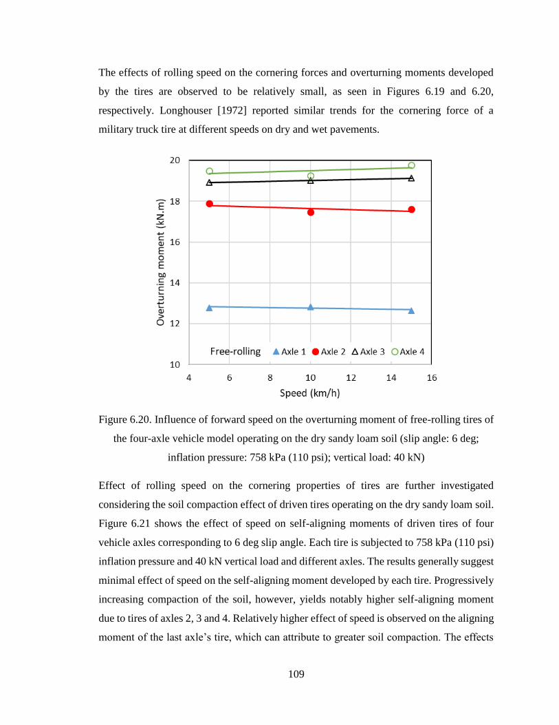
109

The effects of rolling speed on the cornering forces and overturning moments developed

by the tires are observed to be relatively small, as seen in Figures 6.19 and 6.20,

respectively. Longhouser [1972] reported similar trends for the cornering force of a

military truck tire at different speeds on dry and wet pavements.

Figure 6.20. Influence of forward speed on the overturning moment of free-rolling tires of

the four-axle vehicle model operating on the dry sandy loam soil (slip angle: 6 deg;

inflation pressure: 758 kPa (110 psi); vertical load: 40 kN)

Effect of rolling speed on the cornering properties of tires are further investigated

considering the soil compaction effect of driven tires operating on the dry sandy loam soil.

Figure 6.21 shows the effect of speed on self-aligning moments of driven tires of four

vehicle axles corresponding to 6 deg slip angle. Each tire is subjected to 758 kPa (110 psi)

inflation pressure and 40 kN vertical load and different axles. The results generally suggest

minimal effect of speed on the self-aligning moment developed by each tire. Progressively

increasing compaction of the soil, however, yields notably higher self-aligning moment

due to tires of axles 2, 3 and 4. Relatively higher effect of speed is observed on the aligning

moment of the last axle’s tire, which can attribute to greater soil compaction. The effects

110

of longitudinal speed on the self-aligning moments of the free-rolling tires, shown in Figure

6.18, are more significant than those of the driven tires. It could attribute to the effect of

torque on the relative slip between tire and terrain. Figure 6.22 shows similar effects of

speed on the cornering forces developed by the driven tires on the dry sandy loam soil.

The cornering force due to the last axle tire increases with increase in vehicle speed due to

greater soil compaction. The effect of speed on the cornering force developed by the other

axles’ tires are relatively small, as it is observed for the free-rolling tires (Figure 6.19). The

results are obtained for other soils show the similar trends for cornering characteristics of

free-rolling and driven tires versus rolling speed.

Figure 6.21. Influence of forward speed on the self-aligning moment of driven tires of the

four-axle vehicle model operating on the dry sandy loam soil (slip angle: 6 deg; inflation


111

Figure 6.22. Influence of forward speed on the cornering force of driven tires of the four-

axle vehicle model operating on the dry sandy loam soil (slip angle: 6 deg; inflation


6.3.5 Effect of soil internal friction angle

The cornering properties of tires operating on soft soils are strongly affected by mechanical

properties of the soil such as cohesion coefficient and internal friction angle. In this study,

the effect of internal friction angle of the soil is evaluated on the cornering as well as

overturning moment characteristics of the free-rolling and driven tires. The internal friction

angle relates to the moisture content of the soil. A higher internal friction angle represents

higher moisture content of the soil. Simulations are performed for three different internal

friction angles of the soil, namely, 21, 21.36 and 29.4 degrees. Figures 6.23 and 6.24 show

the effect of internal friction angle on self-aligning moment and cornering force,

respectively, developed by the free-rolling tire for two different side-slip angles, namely,

2° and 6°. The results are obtained for the tire running at a speed of 15 km/h with 758 kPa

(110 psi) inflation pressure and 40 kN vertical load. The results show both the cornering

force and self-aligning moment increase with increase in the friction angle for both the

side-slip conditions considered. For the 6°angle, the self-aligning moment and cornering

112

force increase by nearly 88% and 50%, respectively, when the internal friction angle is

increased from 21 degrees to 29.4 degrees. This is attributable to greater wheel sinkage and

compression of the soil with higher internal friction angle, which contributes to higher

cornering force and thereby higher self-aligning moment. The overturning moment

developed by the free-rolling tire also increases with increase in the internal friction angle,

as shown in Figure 6.25. The figure shows variations in overturning moment as a function

of the internal friction angle for three different side-slip angles (2°, 6° and 12°). Higher

slip angle yields more significant increases in the cornering force, self-aligning moment

and the overturning moment, which can be attributed higher side velocity of the freerolling

tire.

Figure 6.23. Influence of soil internal friction angle on the self-aligning moment

developed by the free-rolling tire for two different slip angles (inflation pressure: 758 kPa

(110 psi); vertical load: 40 kN; speed: 15 km/h)

113

Figure 6.24. Influence of soil internal friction angle on the cornering force developed by

the free-rolling tire for two different slip angles (inflation pressure: 758 kPa (110 psi);

vertical load: 40 kN; speed: 15 km/h)

Figure 6.25. Influence of soil internal friction angle on the overturning moment

developed by the free-rolling tire for different slip angles (inflation pressure: 758 kPa

(110 psi); vertical load: 40 kN; speed: 15 km/h)

114

Figures 6.26 and 6.27 show the effect of internal friction angle on self-aligning moment

and cornering force, respectively, developed by the driven-rolling tire for two different

side-slip angles, namely, 2° and 6°. The results are obtained for the tire running at a speed

of 15 km/h with 758 kPa (110 psi) inflation pressure and 40 kN vertical load, and the soil

internal friction ranging from 21° to 30.19°. The self-aligning moment increases with

increase in the soil internal friction angle, as seen in Figure 6.26, as it was observed for the

free-rolling tire. This is due to additional friction of the soil with greater internal friction

angle. The cornering force also increases with the internal friction angle, as seen in Figure

6.27. The observed trends in the cornering force and aligning moment, however, differ

from those of the free-rolling tire (Figures 6.23 and 6.24), which is due to greater sinkage

of the wheel in the soil in the presence of the drive torque.

Figure 6.26. Influence of soil internal friction angle on the self-aligning moment

developed by the driven tire for two different slip angles (inflation pressure: 758 kPa (110

psi); vertical load: 40 kN; speed: 15 km/h)

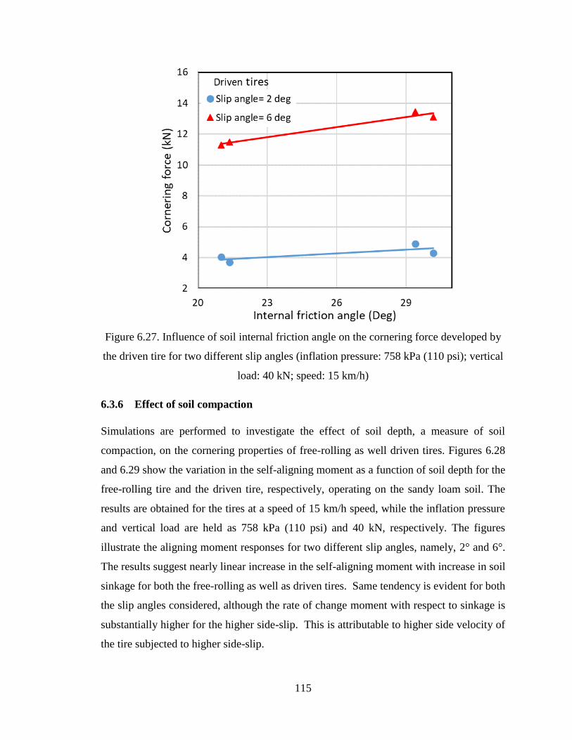
115

Figure 6.27. Influence of soil internal friction angle on the cornering force developed by

the driven tire for two different slip angles (inflation pressure: 758 kPa (110 psi); vertical

load: 40 kN; speed: 15 km/h)

6.3.6 Effect of soil compaction

Simulations are performed to investigate the effect of soil depth, a measure of soil

compaction, on the cornering properties of free-rolling as well driven tires. Figures 6.28

and 6.29 show the variation in the self-aligning moment as a function of soil depth for the

free-rolling tire and the driven tire, respectively, operating on the sandy loam soil. The

results are obtained for the tires at a speed of 15 km/h speed, while the inflation pressure

and vertical load are held as 758 kPa (110 psi) and 40 kN, respectively. The figures

illustrate the aligning moment responses for two different slip angles, namely, 2° and 6°.

The results suggest nearly linear increase in the self-aligning moment with increase in soil

sinkage for both the free-rolling as well as driven tires. Same tendency is evident for both

the slip angles considered, although the rate of change moment with respect to sinkage is

substantially higher for the higher side-slip. This is attributable to higher side velocity of

the tire subjected to higher side-slip.

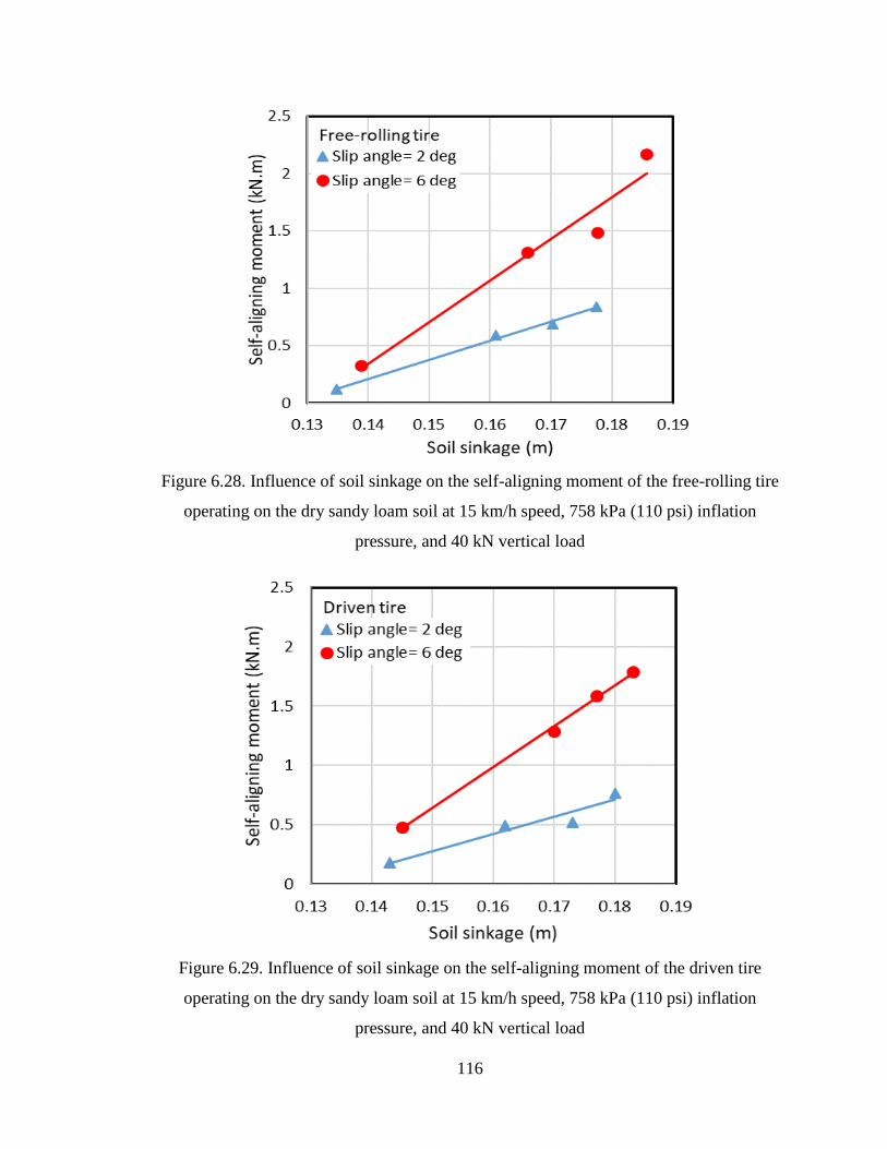
116

Figure 6.28. Influence of soil sinkage on the self-aligning moment of the free-rolling tire

operating on the dry sandy loam soil at 15 km/h speed, 758 kPa (110 psi) inflation

pressure, and 40 kN vertical load

Figure 6.29. Influence of soil sinkage on the self-aligning moment of the driven tire



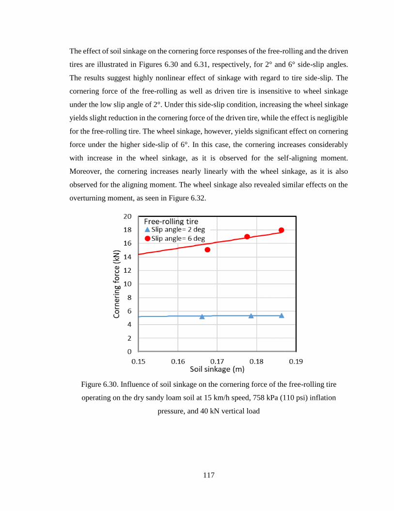
117

The effect of soil sinkage on the cornering force responses of the free-rolling and the driven

tires are illustrated in Figures 6.30 and 6.31, respectively, for 2° and 6° side-slip angles.

The results suggest highly nonlinear effect of sinkage with regard to tire side-slip. The

cornering force of the free-rolling as well as driven tire is insensitive to wheel sinkage

under the low slip angle of 2°. Under this side-slip condition, increasing the wheel sinkage

yields slight reduction in the cornering force of the driven tire, while the effect is negligible

for the free-rolling tire. The wheel sinkage, however, yields significant effect on cornering

force under the higher side-slip of 6°. In this case, the cornering increases considerably

with increase in the wheel sinkage, as it is observed for the self-aligning moment.

Moreover, the cornering increases nearly linearly with the wheel sinkage, as it is also

observed for the aligning moment. The wheel sinkage also revealed similar effects on the

overturning moment, as seen in Figure 6.32.

Figure 6.30. Influence of soil sinkage on the cornering force of the free-rolling tire



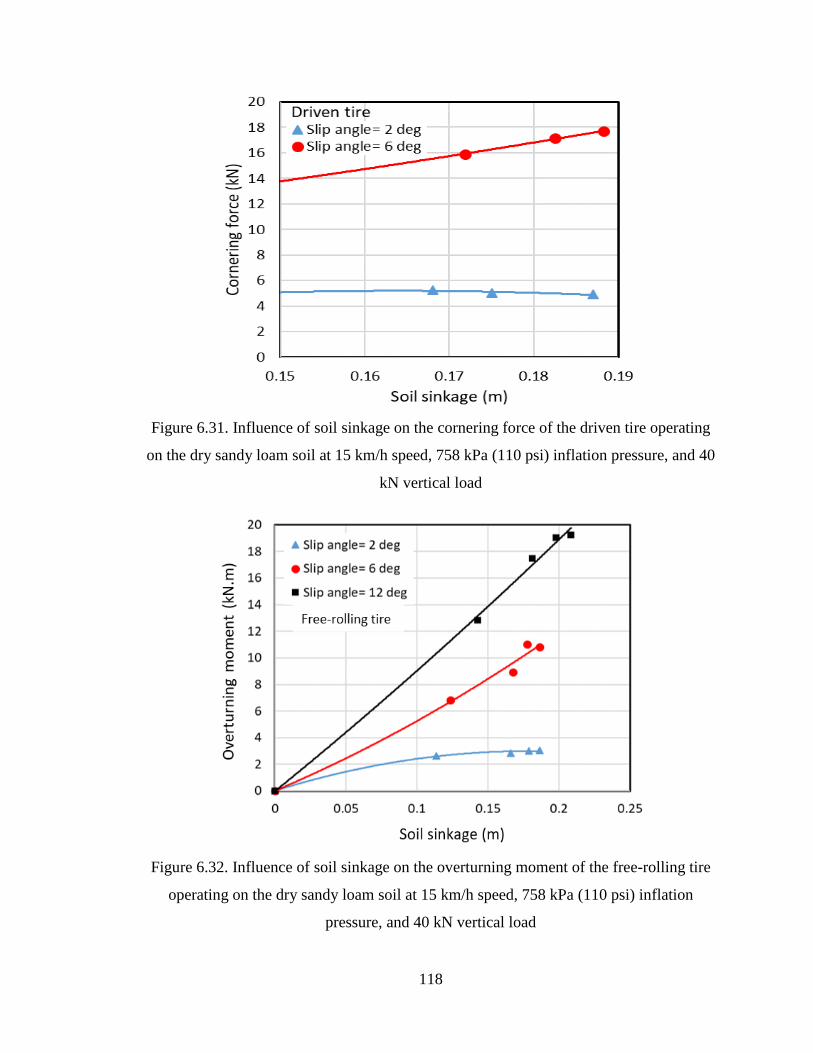
118

Figure 6.31. Influence of soil sinkage on the cornering force of the driven tire operating

on the dry sandy loam soil at 15 km/h speed, 758 kPa (110 psi) inflation pressure, and 40

kN vertical load

Figure 6.32. Influence of soil sinkage on the overturning moment of the free-rolling tire



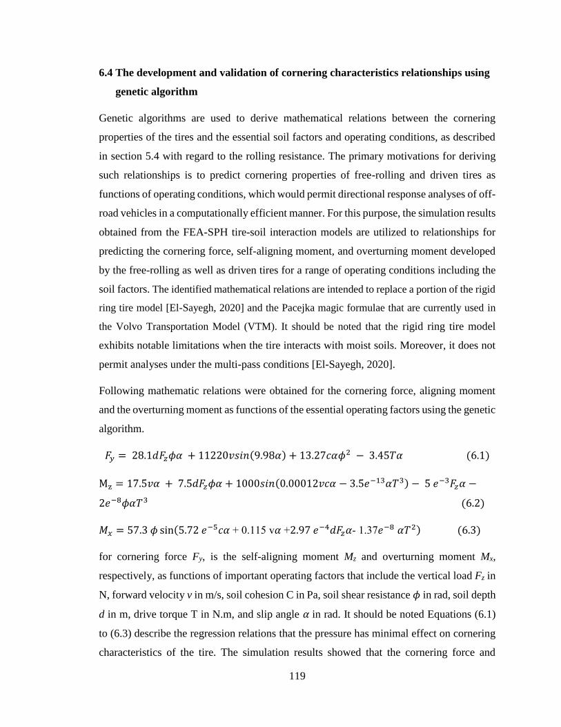
119

6.4 The development and validation of cornering characteristics relationships using

genetic algorithm

Genetic algorithms are used to derive mathematical relations between the cornering

properties of the tires and the essential soil factors and operating conditions, as described

in section 5.4 with regard to the rolling resistance. The primary motivations for deriving

such relationships is to predict cornering properties of free-rolling and driven tires as

functions of operating conditions, which would permit directional response analyses of off-

road vehicles in a computationally efficient manner. For this purpose, the simulation results

obtained from the FEA-SPH tire-soil interaction models are utilized to relationships for

predicting the cornering force, self-aligning moment, and overturning moment developed

by the free-rolling as well as driven tires for a range of operating conditions including the

soil factors. The identified mathematical relations are intended to replace a portion of the rigid

ring tire model [El-Sayegh, 2020] and the Pacejka magic formulae that are currently used in

the Volvo Transportation Model (VTM). It should be noted that the rigid ring tire model

exhibits notable limitations when the tire interacts with moist soils. Moreover, it does not

permit analyses under the multi-pass conditions [El-Sayegh, 2020].

Following mathematic relations were obtained for the cornering force, aligning moment

and the overturning moment as functions of the essential operating factors using the genetic

algorithm.

𝐹𝑦 = 28.1𝑑𝐹𝑧𝜙𝛼 + 11220𝑣𝑠𝑖𝑛(9.98𝛼) + 13.27𝑐𝛼𝜙2 − 3.45𝑇𝛼 (6.1)

Mz = 17.5𝑣𝛼 + 7.5𝑑𝐹𝑧𝜙𝛼 + 1000𝑠𝑖𝑛(0.00012𝑣𝑐𝛼 − 3.5𝑒−13𝛼𝑇3) − 5 𝑒−3𝐹𝑧𝛼 −

2𝑒−8𝜙𝛼𝑇3 (6.2)

𝑀𝑥 = 57.3 𝜙 sin(5.72 𝑒−5𝑐𝛼 + 0.115 v𝛼 +2.97 𝑒−4𝑑𝐹𝑧𝛼- 1.37𝑒−8 𝛼𝑇2) (6.3)

for cornering force Fy, is the self-aligning moment Mz and overturning moment Mx,

respectively, as functions of important operating factors that include the vertical load Fz in

N, forward velocity v in m/s, soil cohesion C in Pa, soil shear resistance 𝜙 in rad, soil depth

d in m, drive torque T in N.m, and slip angle 𝛼 in rad. It should be noted Equations (6.1)

to (6.3) describe the regression relations that the pressure has minimal effect on cornering

characteristics of the tire. The simulation results showed that the cornering force and

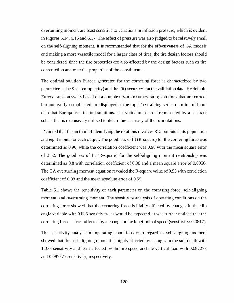
120

overturning moment are least sensitive to variations in inflation pressure, which is evident

in Figures 6.14, 6.16 and 6.17. The effect of pressure was also judged to be relatively small

on the self-aligning moment. It is recommended that for the effectiveness of GA models

and making a more versatile model for a larger class of tires, the tire design factors should

be considered since the tire properties are also affected by the design factors such as tire

construction and material properties of the constituents.

The optimal solution Eureqa generated for the cornering force is characterized by two

parameters: The Size (complexity) and the Fit (accuracy) on the validation data. By default,

Eureqa ranks answers based on a complexity-to-accuracy ratio; solutions that are correct

but not overly complicated are displayed at the top. The training set is a portion of input

data that Eureqa uses to find solutions. The validation data is represented by a separate

subset that is exclusively utilized to determine accuracy of the formulations.

It's noted that the method of identifying the relations involves 312 outputs in its population

and eight inputs for each output. The goodness of fit (R-square) for the cornering force was

determined as 0.96, while the correlation coefficient was 0.98 with the mean square error

of 2.52. The goodness of fit (R-square) for the self-aligning moment relationship was

determined as 0.8 with correlation coefficient of 0.98 and a mean square error of 0.0056.

The GA overturning moment equation revealed the R-square value of 0.93 with correlation

coefficient of 0.98 and the mean absolute error of 0.55.

Table 6.1 shows the sensitivity of each parameter on the cornering force, self-aligning

moment, and overturning moment. The sensitivity analysis of operating conditions on the

cornering force showed that the cornering force is highly affected by changes in the slip

angle variable with 0.835 sensitivity, as would be expected. It was further noticed that the

cornering force is least affected by a change in the longitudinal speed (sensitivity: 0.0817).

The sensitivity analysis of operating conditions with regard to self-aligning moment

showed that the self-aligning moment is highly affected by changes in the soil depth with

1.075 sensitivity and least affected by the tire speed and the vertical load with 0.097278

and 0.097275 sensitivity, respectively.

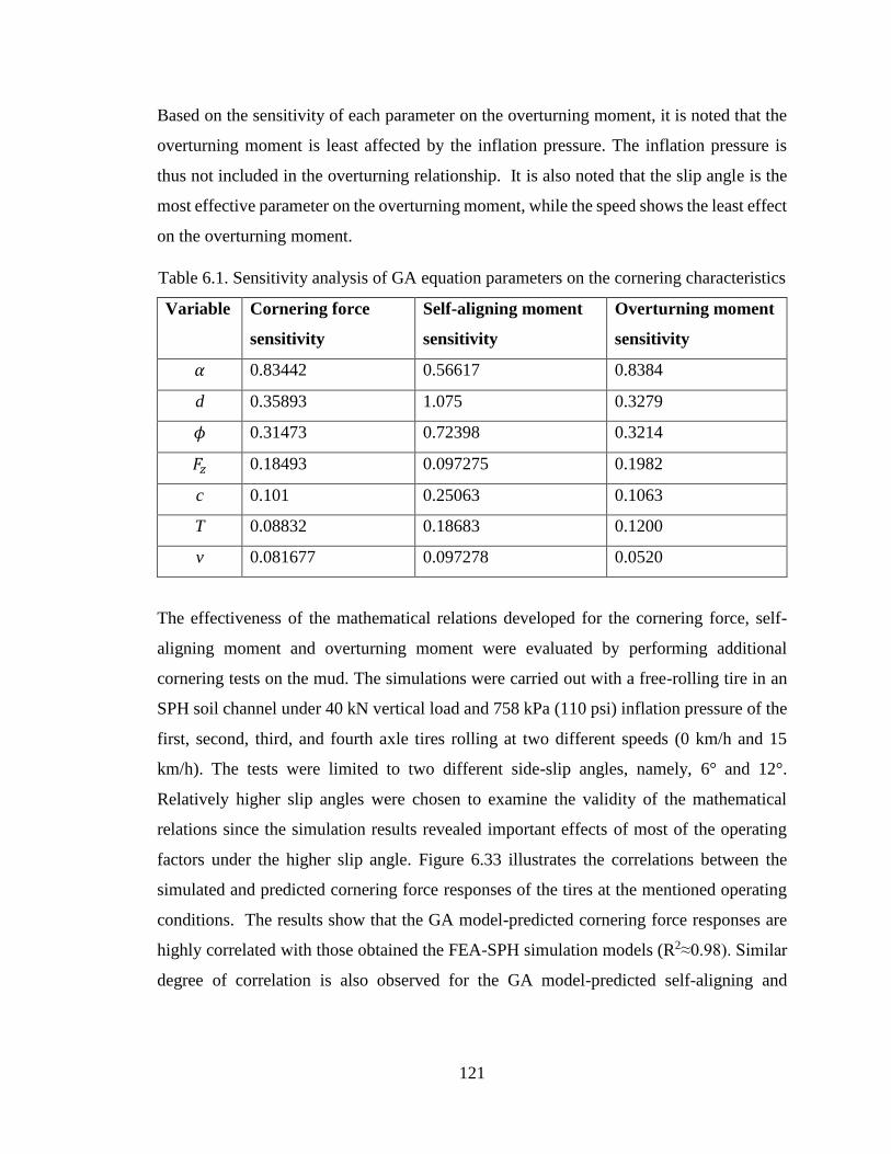
121

Based on the sensitivity of each parameter on the overturning moment, it is noted that the

overturning moment is least affected by the inflation pressure. The inflation pressure is

thus not included in the overturning relationship. It is also noted that the slip angle is the

most effective parameter on the overturning moment, while the speed shows the least effect

on the overturning moment.

Table 6.1. Sensitivity analysis of GA equation parameters on the cornering characteristics

Variable Cornering force

sensitivity

Self-aligning moment

sensitivity

Overturning moment

sensitivity

𝛼 0.83442 0.56617 0.8384

d 0.35893 1.075 0.3279

𝜙 0.31473 0.72398 0.3214

𝐹𝑧 0.18493 0.097275 0.1982

c 0.101 0.25063 0.1063

T 0.08832 0.18683 0.1200

v 0.081677 0.097278 0.0520

The effectiveness of the mathematical relations developed for the cornering force, self-

aligning moment and overturning moment were evaluated by performing additional

cornering tests on the mud. The simulations were carried out with a free-rolling tire in an

SPH soil channel under 40 kN vertical load and 758 kPa (110 psi) inflation pressure of the

first, second, third, and fourth axle tires rolling at two different speeds (0 km/h and 15

km/h). The tests were limited to two different side-slip angles, namely, 6° and 12°.

Relatively higher slip angles were chosen to examine the validity of the mathematical

relations since the simulation results revealed important effects of most of the operating

factors under the higher slip angle. Figure 6.33 illustrates the correlations between the

simulated and predicted cornering force responses of the tires at the mentioned operating

conditions. The results show that the GA model-predicted cornering force responses are

highly correlated with those obtained the FEA-SPH simulation models (R2≈0.98). Similar

degree of correlation is also observed for the GA model-predicted self-aligning and

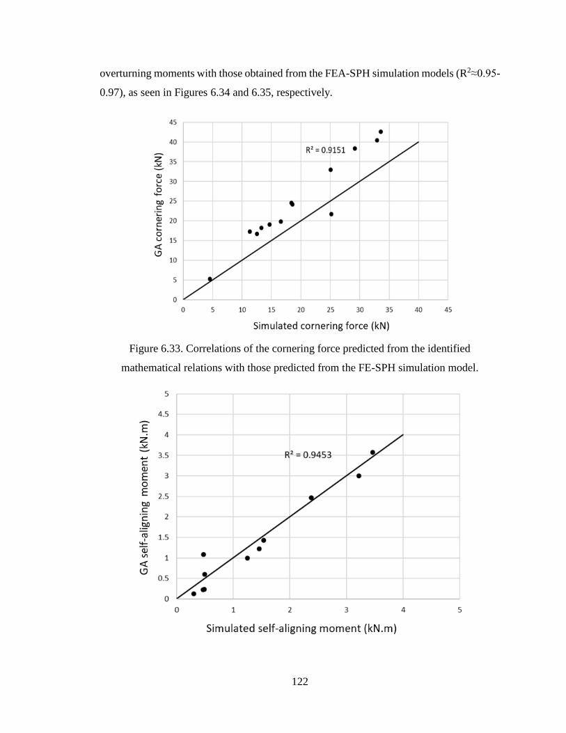
122

overturning moments with those obtained from the FEA-SPH simulation models (R2≈0.95-

0.97), as seen in Figures 6.34 and 6.35, respectively.

Figure 6.33. Correlations of the cornering force predicted from the identified

mathematical relations with those predicted from the FE-SPH simulation model.

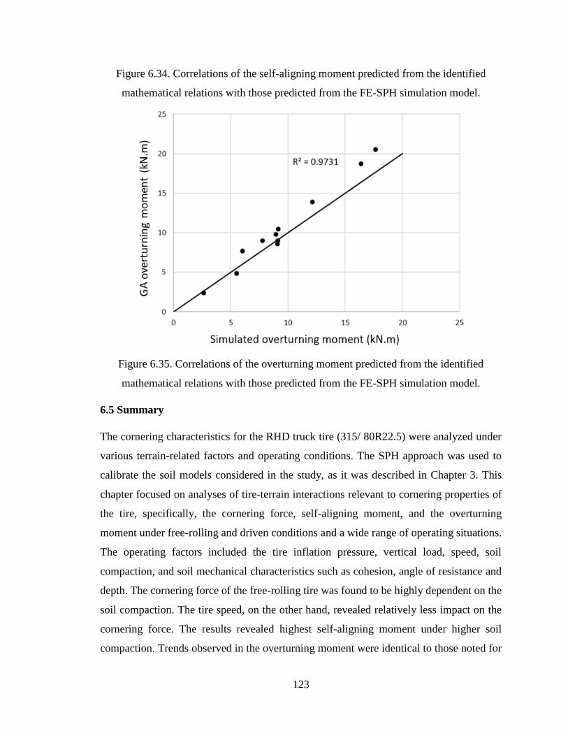
123

Figure 6.34. Correlations of the self-aligning moment predicted from the identified


Figure 6.35. Correlations of the overturning moment predicted from the identified


6.5 Summary

The cornering characteristics for the RHD truck tire (315/ 80R22.5) were analyzed under

various terrain-related factors and operating conditions. The SPH approach was used to

calibrate the soil models considered in the study, as it was described in Chapter 3. This

chapter focused on analyses of tire-terrain interactions relevant to cornering properties of

the tire, specifically, the cornering force, self-aligning moment, and the overturning

moment under free-rolling and driven conditions and a wide range of operating situations.

The operating factors included the tire inflation pressure, vertical load, speed, soil

compaction, and soil mechanical characteristics such as cohesion, angle of resistance and

depth. The cornering force of the free-rolling tire was found to be highly dependent on the

soil compaction. The tire speed, on the other hand, revealed relatively less impact on the

cornering force. The results revealed highest self-aligning moment under higher soil

compaction. Trends observed in the overturning moment were identical to those noted for

124

the cornering force over the entire ranges of operating conditions considered in the study.

The tire overturning moment was observed to be highly dependent on soil compaction,

while the tire speed had a minimal impact on the overturning moment.

The simulation results were used to develop mathematical relations for the cornering force,

self-aligning moment, and overturning moment as functions of important operating factors

using advanced algorithm techniques through training, testing and validations in the Pam-

Crash simulation platform. Cornering tests were performed for the RHD tire operating over

the mud soil to examine the validity of the GA-based cornering force, self-aligning

moment, and overturning moment relationships. It was concluded that the identified

mathematical relations could provide very good estimations of the cornering characteristics

under a broad range of operating conditions and soils (R2≈ 0.95-0.98).

125

MAJOR CONCLUSIONS AND CONTRIBUTIONS

7.1 Major contributions of the thesis

The thesis research focused on the development of a comprehensive dynamic tire-soil

interactions model for investigating tires’ interactions with deformable soils considering a

wide range of operating and soil factors. The major contributions of the study are

summarized below:

Owing to the excessive computational demands posed by the FEA-SPH tire-soil models,

the thesis proposed a unique mathematical relationship for estimating the rolling resistance

coefficient of the free-rolling as well driven truck tires in an efficient manner. A

methodology based on genetic algorithms is employed to derive the relationship

considering different soil properties and a broad range of operational factors. The soils

included the clay loam, dense sand, clayey soil, sandy, moist sand with varying moisture

content (10%, 25%, and 50%). The operating conditions included the inflation pressure,

vertical load, speed, torque, and multi-pass effect. The effectiveness of the proposed rolling

resistance coefficient relationship is also demonstrated under different operating

conditions. The proposed relationship could be implemented to the total vehicle model for

assessing rolling resistance under different operating conditions in a computationally

efficient manner.

The methodology based on genetic algorithms is further applied to develop novel relations

for predicting cornering characteristics of the tire operating on different types of soils. The

relationships are derived for predicting cornering force, self-aligning moment and

overturning moment of free-rolling as well as driven tires as functions of the side-slip

angle. The validity of the proposed relations is examined for a range of operating conditions,

such as vertical load, speed, torque, the multi-pass effects, and soils, namely, clay loam, dense

sand, clayey soil, sandy, moist sand with varying moisture content (10%, 25%, and 50%).

126

7.2 Major conclusions

In this study, the tire-soil interaction model was developed by integrating the

comprehensive FEA model of a truck tire with SPH models of different soils. The validity

of the FEA tire model was examined by performing different static and dynamic tests, such

as the drum-cleat, vertical stiffness, and footprint tests. The validity of the model was

demonstrated by comparing the simulation results with the published data. The

comparisons generally showed good agreements between the model-predicted static and

dynamic responses with the available data. For the static vertical stiffness, comparisons

revealed a maximum deviation of about 2.3%, which was observed under 586 kPa (85 psi)

inflation pressure. The peak errors for the 758 kPa (110 psi) and 896 kPa (130 psi) inflation

pressure were in the order of 3.1%. The results obtained from the footprint tests of the FEA

model also showed reasonably good agreements with the available data for the same tire.

The results obtained from the drum-cleat tests of the RHD tire model revealed that

fundamental vertical mode frequency ranges from 53 Hz to 59 Hz for the range of inflation

pressure considered in the study. The corresponding fundamental horizontal mode

frequency ranged from 52 Hz to 57 Hz. The model-predicted fundamental vertical and

horizontal modes frequencies were observed to lie within the ranges of frequencies reported

in earlier studies. The simulation results also showed higher vertical tire stiffness and thus

the fundamental vibration mode frequencies with increasing inflation pressure. It also

showed a slight non-linear relationship between the vertical load and deflection that can be

considered a linear trend.

The soil was modeled using the Smoothed-Particle Hydrodynamics technique. The models

for different soils were subsequently formulated through calibrations involving pressure-

sinkage and shear-strength tests. The model calibrations were conducted for a number of

soils that are often encountered during off-road driving. These included the clay loam,

dense sand, and clayey soil. The validity of the calibrated models was examined using the

available terramechanics data. Experiments were designed and performed for calibration

and validations of the clay loam soil model. The experiments were performed using a

portable bevameter and a shear box in a soil bin in the terramechanics laboratory of Urmia

University in Iran. The comparisons of the measured pressure-sinkage and shear strength

127

test data with the simulation results showed that the SPH soil model was successfully

calibrated.

The FEA tire model and the SPH soil model were utilized to predict and analyze the rolling

resistance coefficient and cornering characteristics of free-rolling as well as driven tires

under different operating conditions. The predicted cornering force, self-aligning moment,

and overturning moment simulation data were then used to develop relationships using

genetic algorithms through training and testing. The input parameters were the longitudinal

speed, torque, inflation pressure, vertical load, and slip angle; in addition to the terrain

characteristics such as cohesion, friction angle, and depth.

The simulation results showed that the vertical load has a significant impact on the rolling

resistance coefficient. The rolling resistance coefficient is less affected by tire inflation

pressure at low vertical loads and more affected by it at high vertical loads. The truck tire

was found to have the greatest rolling resistance coefficient at a lower internal friction

angle when operating over different terrains. It was also discovered that the free-rolling

tire's cornering force was highly dependent on soil compaction. The influence of tire speed

on the cornering force, on the other hand, was rather minor. The results demonstrated that

increased soil compaction resulted in the highest self-aligning moment. Under all operating

conditions evaluated in the study, the overturning moment followed the same trends as the

cornering force. The overturning moment of a tire was shown to be highly dependent on

soil compaction, while tire speed had only a minor influence.

It was concluded that the GA cornering characteristics equations were able to predict the

cornering characteristics at different operating and terrain conditions with an R-square

fitness of greater than 0.8. It was also found that there is a minimal effect of the inflation

pressure on the cornering characteristics. Hence, the inflation pressure parameter didn’t

appear in the GA equations. The most effective parameter on the cornering force and the

overturning moment was the slip angle, as expected, while soil depth was the most effective

parameter on the self-aligning moment. As the tire sinkage increased the cornering force,

self-aligning moment, and the overturning moment all increased at a given operating

condition.

128

It was also found that for the RRC relationship the R-square goodness of fit is 0.911, the

mean error is 0.201, the mean square error is 0.0015 and the mean average error is 0.022.

It was concluded that the rolling resistance coefficient varies linearly concerning vertical

load, as the vertical load increase the rolling resistance coefficient increases as well. The

same observation was found for the cornering force as a function of vertical load.

Furthermore, the inflation pressure was concluded to have a greater effect on the rolling

resistance than the cornering force. As for the effect of the tire multi-pass described by the

tire sinkage, it was noticed that as the tire sinkage increases the rolling resistance

coefficient increases.

7.3 Future works

The work done to achieve the aims of this thesis includes a wide range of engineering and

science topics. The greatest effort has been put in a certain amount of time in order to

simulate each test as accurately as feasible. The techniques, modeling and testing setup,

and actual experiments, on the other hand, may continually be improved and modified.

Tire modeling and evaluation is a factor that can be considered to improve the tire-terrain

interaction results. For this purpose, it is suggested that tire evaluation tests be performed

experimentally to provide a more accurate reference for evaluating the tire model. Tire

material is another parameter that has not been accessible. The materials used for the tire

model were the result of experiments by previous researchers, which were used with

optimization methods for the most accurate modeling. Access to tire materials provides a

more realistic and accurate model of the tire.

It is recommended that experimental pressure-sinkage and shear-strength tests of 10%

moist sand, 25% moist sand, and 50% moist sand, such as tests performed for clay loam

soil, be performed to provide more accurate calibration of the test soils. For soil modeling,

it is also suggested to study the particle layering method to cover a wide range of soils. For

example, clay loam soil can be modeled according to the percentage of its components.

It is recommended that the developed equations for cornering force, self-aligning moment,

and overturning moment should be validated using physical testing since the equations are

mainly based on simulation results.

129

It is recommended for future work to investigate the effect of slip angle on the longitudinal

force. This will allow for better modeling of the longitudinal force during the cornering

maneuver.

Regarding the developed genetic equations, it is suggested that the tire design parameters

such as tire size, tire tread, etc. be considered in order to extend the equation to more

comprehensive conditions. Therefore, it is recommended that all cornering and rolling

resistance tests performed on the RHD truck tire be performed on another tire with different

design characteristics. Cornering tests on other terrains such as snow, flooded surface, and

mud can also help to integrate the GA equations.

7.4 Publications




Gheshlaghi, F., El-Sayegh, Z., El-Gindy, M., Oijer, F. et al., “Analysis of off-road tire

cornering characteristics using advanced analytical techniques” Tire Society Journal, Oct

2021, USA, (Under review).

Gheshlaghi F., El-Sayegh Z., El- Gindy M et al. 'Prediction and validation of

terramechanics models for estimation of tyre rolling resistance coefficient". Int. J.

Vehicle Systems Modelling and Testing, 14, no. 3-4 (2020) 1-12.

Gheshlaghi, F., Rakheja, S., El-Gindy, M., “Tire-Terrain Interaction Modeling and

Analysis: Literature Survey” Int. J. Vehicle Systems Modelling and Testing, (To be

submitted).

https://doi.org/10.4271/2021-01-0329

130

REFERENCES

1. Goodyear, C. (1853) “Gum-Elastic and its Varieties: With a Detailed Account of its Applications

and Uses and of the Discovery of Vulcanization”, Vol. 2, Harvard University, Published for the

author.

2. https://www.treadwright.com/blogs/treadwright-blog/the-history-of-tires

3. Gheshlaghi F., Mardani A., Mohebi A. (2020) “Investigating the effects of off-road vehicles on soil

compaction using FEA-SPH simulation”. Int. J. of Heavy Vehicle Systems, 14 N1:1-10 (DOI:

10.1504/IJHVS.2020.10027405)

4. Slade et al., (2009) “Off-road Tire-Soil Modeling using Finitie Element Analysis Technique”,

ASME International Design Engineering Technical Conference, August 30, 2009, San Diego,

California.

5. Schmeitz, A. (2004) “Semi-Empirical Three-Dimensional Model of the Pneumatic Tyre Rolling

over Arbitrarily Uneven Road Surfaces”. PhD thesis, Delft University of Technology, 2004.

6. Lugner, P. and Plochl, M. (2005) “Tyre model performance test: first experiences and results,”

Vehicle System Dynamics, vol. 43, no. suppl, pp. 48 – 62.

7. Padovan, J., (1977), “Numerical Simulation of Rolling Tires,” Tire rolling losses and fuel economy,

an R & D Planning Workshop, October 19-20, series SAE conference proceedings P-74. pp. 87-94.

8. Olatunbosun, O.A., Bolarinwa, E.O., (2004) “FE Simulation of the Effect of Tire Design Parameters

on Lateral Forces and Moments”. Tire Science and Technology, TSTCA, 2004. 32(3): p. 146-163.

9. Bolarinwa, E.O., Olatunbosun, O.A., and Burnett, M. (2004) “A Study of Tyre Cornering Behaviour

using a Finite Element Model, in Computational Mechanics”, WCCM VI in conjunction with

APCOM'04. 2004: Beijing, China.

10. El-Sayegh Z., Gheshlaghi F., Sharifi M., and Mardani A. (2019) “Development of an HLFS

agricultural tire model using FEA technique”. SN Applied Sciences 1, no. 11: 1454.

11. Gheshlaghi F., Mardani A. (2021) “Prediction of soil vertical stress under the off-road tire using

smoothed-particle hydrodynamics”. Journal of Terramechanics, Volume 95, Pages 7-14.

12. Dhillon, R.S. (2013) “Development of Truck Tire-Terrain Finite Element Analysis Models”, PhD

thesis, University of Ontario Institute of Technology.

13. Vehicle Dynamics Terminology, SAE J670e, Society of Automotive Engineers, 1978.

14. Bekker, M. G. (1950). “Relationship between soil and a vehicle.” Society of Automotive Engineers,

4(3), 381-396

15. Gheshlaghi, F., El-Sayegh, Z., Sharifi, M., and El-Gindy, M., (2020) “Prediction and Validation of

Terramechanics Models for Estimation of Tyre Rolling Resistance Coefficient,” Int. J. Vehicle

Systems Modelling and Testing 14(3-4):1-12.

https://www.treadwright.com/blogs/treadwright-blog/the-history-of-tires

https://www.researchgate.net/publication/339722810_Investigating_the_effects_of_off-road_vehicles_on_soil_compaction_using_FEA-SPH_simulation



131

16. Fancher, S. Ervin, R.D., Winkler, C.B., and Gillespie, T.D. (1986) “A Fact Book of the Mechanical

Properties of the Components for Single-unit and Articulated Heavy Trucks,” Report No. DOT HS

807 125, National Highway Traffic Safety Administration, U.S. Department of Transportation.

17. Luty, W. (2011) “An analysis of tire relaxation in conditions of the wheel side cornering angle

oscillations”, Journal of Kones 18 (1): 325–332.

18. Pacejka, Hans B. (2006) “Tyre and vehicle dynamics (2nd ed.)” SAE International.

p. 22. ISBN 978-0-7680-1702-1.

19. Lu, D., Guo, K., Wu, H., Moschus, N., Lu, X.-P. & Chen, S.-K. (2006) “Modelling of tire

overturning moment and loaded radius”, Vehicle System Dynamics, 44:sup1, 104-114.

20. Liu, C.H., and Wong, J.Y. (1996) “Numerical Simulations of Tire–Soil Interaction Based on Critical

State Soil Mechanics,” Journal of Terramechanics, vol. 33, no. 5.

21. Liu, C.H., Wong, J.Y., and Mang, H.A. (1999) “Large Strain Finite Element Analysis of Sand:

Model, Algorithm and Application to Numerical Simulation of Tire–Sand Interaction” Computers

and Structures, vol. 74, no. 3.

22. Hiroma, T., Wanjii, S., Kataoka, T. and Ota, Y. (1997) “Stress analysis using fem on stress

distribution under a wheel considering friction with adhesion between a wheel and soil”, Journal of

Terramechanics, Vol. 34, No. 4, pp.225–233.

23. PAM System International (2000) Pam-Shock User Manual.

24. Chen Liang, Zhi Gao, Shengkang Hong, Guolin Wang, Bentil Mawunya Kwaku Asafo-Duho, Jieyu

Ren, (2021) "A Fatigue Evaluation Method for Radial Tire Based on Strain Energy Density

Gradient", Advances in Materials Science and Engineering, vol. 2021, Article ID 8534954, 12

pages. https://doi.org/10.1155/2021/8534954

25. Zumrat Usmanova, Emin Sunbuloglu. (2021) “Finite element method estimation of temperature

distribution of automotive tire using one-way-coupled method”, Proc IMechE Part D: J Automobile

Engineering 1–12, IMechE, DOI: 10.1177/09544070211008757.

26. Jung, H., Park, W. and Jeong, K. (2018) “Finite Element Analysis of Tire Traction Using a Rubber-

Ice Friction Model”. Open Journal of Applied Sciences, 8, 495-505.

doi: 10.4236/ojapps.2018.811040.

27. CrmN, S. T. and Wong, J. Y. (1988) “an approach to improving the prediction of pneumatic tire

performance over unprepared terrain”. Proc. 2nd Asia-Pacific Conf. ISTVS, pp. 293-302.

28. Chen, S. T. (1988) “Study of tire-terrain interaction using the finite element method”. Unpublished

Master of Engineering Thesis, Carleton University, Ottawa, Canada.

29. Wang, L. (1990) “Tire modelling using a three-dimensional finite element method”. Unpublished

Master of Engineering Thesis, Carleton University, Ottawa, Canada.

30. Nakashima, H., and Wong, J.Y. (1993) “A Three-dimensional Tire Model by the Finite Element

Method,” Journal of Terramechanics, vol. 30, no. 1.

https://en.wikipedia.org/wiki/Hans_B._Pacejka

https://en.wikipedia.org/wiki/ISBN_(identifier)

https://en.wikipedia.org/wiki/Special:BookSources/978-0-7680-1702-1

https://doi.org/10.1155/2021/8534954

https://journals.sagepub.com/action/doSearch?target=default&ContribAuthorStored=Usmanova%2C+Zumrat

https://journals.sagepub.com/action/doSearch?target=default&ContribAuthorStored=Sunbuloglu%2C+Emin

https://doi.org/10.4236/ojapps.2018.811040

132

31. Zhang, X., Rakheja, S., and Ganesan, R., (2001), “Estimation of tire-road contact pressure

distribution based on nonlinear finite element analysis”, Heavy Vehicle Systems, Series B,

International Journal of Vehicle Dynamics, Vol. 8 No.3/4, pp. 197-217.

32. Yan, X., (2003), “Nonlinear Three-Dimensional Finite Element Analysis of Steady Rolling Radial

Tires,” Journal of Reinforced Plastics and Composites, Vol. 22, No.8. pp. 733-750.

33. Wu, G. Z., and He X. M., (1992), “Effects of Aspect Ratio on the Stresses and Deformations of

Radial Passenger Tires,” Tire Science and Technology, TSTCA, Vol. 20, No. 2, pp. 74-82.

34. Chae, S., Chang, Y. P., El-Gindy, M., Streit, D. A., (2001), “Standing Wave Prediction of a Racing

Car Tire,” CSME-MDE-2001, November 21-22, Montreal, Canada.

35. Chang, Y. P., El-Gindy, M., and Streit, D. A., (2002), “Influence of Tire Loading and Inflation

Pressure on Standing Waves Phenomena using PAM-SHOCK,” a special issue on “New

Development in Heavy Vehicle Simulation,” International Journal of Heavy Vehicle Systems.

36. Chae, S. (2006) “Nonlinear Finite Element Modeling and Analysis of a Truck Tire”, PhD thesis,

The Pennsylvania State University.

37. Marjani, M. (2016) “Development of FEA Wide-Base Truck Tire and Soil Interaction Models”,

PhD thesis.

38. El-Sayegh Z., Gheshlaghi F., Sharifi M., and Mardani A. (2019) “Development of an HLFS

agricultural tire model using FEA technique”. SN Applied Sciences 1, no. 11:1454.

39. Jafari, S. (2018) “Transient In-plane Analysis of Lug Tire Traversing Rigid Obstacles and

Validation of Finite Element Modeling by Experimental Tests”. Doctoral dissertation. (In Persian).

40. Xiong, Y., and Tuononen, A. (2015) “Rolling deformation of truck tires: Measurement and analysis

using a tire sensing approach”, Journal of Terramechanics 61: 33–42, ISSN 0022-4898.

41. Xiong, Y., Tuononen, A.J., (2014) “A laser-based sensor system for tire tread deformation

measurement” Meas. Sci. Technol. 25 (11), 115103.

42. De Beer, M., Maina, J.W., van Rensburg, Y., Greben, J.M. (2012) “Towardusing tire-road contact

stresses in pavement design and analysis”. TireSci. Technol., 246–271.

43. Van Keulen, H., and C.G.E.M. Van Beek. (1971) “Water movement in layered soils a simulation

model”. Neth. J. Agric. Sci. 19:138–153.

44. Rubin, J., and R. Steinhardt. (1963) “Soil water relations during rainfall infiltration: I. Theory”.

Soil Sci. Soc. Am. Proc. 27:247–251.

45. Nujid, M. and Raihan Taha Professor, M. (2017) “A Review of Bearing Capacity of Shallow

Foundation on Clay Layered Soils Using Numerical Method”. Available at:

http://www.ejge.com/2014/Ppr2014.072mar.pdf (Accessed: 17 March 2017).

46. T. More, S. and Bindu, D. R. S. (2017) “Effects of mesh size on finite element analysis of plate

structure”, Certified International Journal of Engineering Science and Innovative Technology,

9001(3), pp. 2319–5967. Available at: http://www.ijesit.com/Volume 4/Issue

3/IJESIT201503_24.pdf (Accessed: 17 March 2017).

133

47. Gingold, R.A., Monaghan, J.J., (1977) “Smoothed particle hydrodynamics: theory and application

to non-spherical stars”. Mon. Not. R. Astron. Soc. 181 (3), 375–89. Bibcode:1977MNRAS.

181..375G. http://doi.org/10.1093/mnras/181.3.375.

48. Liu GR, Liu MB (2003) “Smoothed particle hydrodynamics a meshfree particle method”. World

Scientific Publishing, Singapore

49. Islam, N., Hawlader, B., Wang, C., Soga, K. (2019) “Large deformation finite-element modelling

of earthquake-induced landslides considering strain-softening behavior of sensitive clay”. Can

Geotech J 56:1003–1018.

50. Abe, K., Soga, K., Bandara, S. (2013) “Material point method for coupled hydromechanical

problems”. J Geotech Environmental Eng 140:04013033. https ://doi.org/10.1061/(asce)gt.1943-

5606.00010 11

51. Soga, K, Alonso, E., Yerro, A. et al. (2017) “Trends in large-deformation analysis of landslide mass

movements with particular emphasis on the material point method”. Géotechnique 68:457–458.

https://doi.org/10.1680/jgeot .16. d.004.

52. Akbari, H. (2017) “Simulation of wave overtopping using an improved SPH method”. Coast Eng

126:51–68. https ://doi.org/10.1016/j.coast aleng .2017.04.010

53. Ran, Q., Tong, J., Shao, S. et al (2015) “Advances in water resources incompressible SPH scour

model for movable bed dam break flows”. Adv Water Resour 82:39–50. https

://doi.org/10.1016/j.advwa tres.2015.04.009

54. Ghaïtanellis, A., Violeau D, Ferrand M et al (2018) “A SPH elasticviscoplastic model for granular

flows and bed-load transport”. Adv Water Resour 111:156–173. https ://doi.org/10.1016/j.advwa

tres.2017.11.007.

55. Joseph, J., Monaghan and John C Lattanzio. (1985) “A refined particle method for astrophysical

problems”. Astronomy and astrophysics, 149:135-143.

56. PAM System International. Pam-crash user manual version 2014. ESI Group,2014.

57. Wong, Jo Yung. (2008) “Theory of ground vehicles”. John Wiley & Sons.

58. El-Gindy, M., Lescoe, R., Öijer, F., Johansson, I. & Trivedi, M. (2011) “Soil Modelling Using FEA

and SPH Techniques for a Tire-Soil Interaction”. ASME International Design Engineering

Technical Conference, 28 August 2011.

59. Reese, L., Qiu, T., Linzell, D., & Rado, Z. (2016) “Field-Scale Testing and Numerical Investigation

of Soil-Boulder Interaction under Vehicular Impact Using FEM and Coupled FEM-SPH

Formulations”. Civil Engineering Faculty Publications, 7(1) 77–99.

60. Gheshlaghi, F., Mardani, A. & Mohebi, A. (2020a) “Investigating the effects of off-road vehicles

on soil compaction using FEA-SPH simulation”. Int. J. Heavy Vehicle Systems, DOI:

10.1504/IJHVS.2020.10027405.

61. Gheshlaghi, F., and Mardani, A., (2021) “Prediction of soil vertical stress under off-road tire using

smoothed-particle hydrodynamics”, Journal of Terramechanics 95 (2021) 7–14.

http://doi.org/10.1093/mnras/181.3.375

134

62. Aubel, T. (1993) “FEM simulation of the interaction between elastic tire and soft soil”. In

Proceedings, 11th International Conference of the ISTVS, Lake Tahoe, Nevada.

63. Fervers, C. W. (1994) “FE simulations of tire-profile effects on traction on soft soil”. In Proceedings,

6th European Conference of the ISTVS, Vienna, Austria, 1994.

64. Fervers, C. W. (1997) “Effects of traction and slip, investigations with FEM”. In Proceedings, 7th

European Conference of the ISTVS, Ferrara, Italy.

65. Gentaro, H., Susan, F., A State, Chris, L., and Henry, F. (2001) “An implicit finite element method

for elastic solids in contact”. In Computer Animation, 2001. The Fourteenth Conference on

Computer Animation. Proceedings, pages 136{254. IEEE, 2001.

66. Thiyahuddin, MI., Yuan Tong Gu, RB Gover, and DP Thambiratnam. (2014) “Fluid-structure

interaction analysis of full-scale vehicle-barrier impact using coupled sph-fea”. Engineering

Analysis with Boundary Elements, 42:26-36.

67. Hermange, C., Oger, G. and Touzfe D. (2016) “Development of a coupling strategy between

smoothed particle hydrodynamics and finite element method for violent fluid-structure interaction

problems”. In 3rd International Conference on Violent Flows 2016.

68. Aimin, Y., Jinze, L., Hengheng, Q., Yuhang, P., Yanhong, K., and Yuzhu, Z. (2016) “Numerical

simulation of hypervelocity impact fem-sph algorithm based on large deformation of material”.

69. Hallquist, J. Goudreau, G., and Benson, D. (1985) “Sliding interfaces with contact impact in large-

scale lagrangian computations”. Computer methods in applied mechanics and engineering, 51(1-

3):107-137.

70. Onafeko, O. (1964) “Instrumentation for measuring radial and tangential stresses beneath rigid

wheels”. Journal of Terramechanics, 1(3):61-68.

71. Onafeko, O., and Reece, AR. (1967) “Soil stresses and deformations beneath rigid wheels”. Journal

of Terramechanics, 4(1):59-80.

72. Wong, Jo-Yung and Reece, AR. (1967) “Prediction of rigid wheel performance based on the

analysis of soil-wheel stresses part I”. performance of driven rigid wheels. Journal of

Terramechanics, 4(1):81-98.

73. Wong, Jo-Yung and Reece, AR. (1967) “Prediction of rigid wheel performance based on the

analysis of soil-wheel stresses: Part II”. performance of towed rigid wheels. Journal of

Terramechanics, 4(2):7-25.

74. Chu, Lok-Man and Yin, Jian-Hua. (2005) “Comparison of interface shear strength of soil nails

measured by both direct shear box tests and pullout tests”. Journal of geotechnical and geo-

environmental engineering, 131(9):1097-1107.

75. Larry, D., Libersky, Albert G Petschek, Theodore C Carney, Jim R Hipp, and Firooz a Allahdadi.

(1993) "High strain lagrangian hydrodynamics: a three-dimensional sph code for dynamic material

response”. Journal of computational physics, 109(1):67-75.

135

76. Shokouhfar, S., Rakheja, S., and El-Gindy, M. (2016a) “Development of a rolling truck tire model

using an automatic model regeneration algorithm” International J. of Vehicle Systems Modelling

and Testing, 11(1); 68-95.

77. Shokouhfar, S., Rakheja, S., and El-Gindy, M. (2016b) “Modal analysis of a rolling truck tire

subjected to inflation pressure and vertical deflection” International J. of Vehicle Systems Modelling

and Testing, 11(2):116.

78. Shokouhfar, S., Rakheja, S., and El-Gindy, M. (2015) “Verification of the Part-Composite Approach

for modeling the multi-layered structure of a rolling truck tire” 10th European LS-DYNA

Conference 2015, Würzburg, GermanyAt: Würzburg, Germany, DOI:10.13140/RG.2.1.2453.1048.

79. Shokouhfar, S., Rakheja, S., and El-Gindy, M. (2016c) “Development of a computationally efficient

rolling truck tire model using part-composite approach and its verification” International J. of

Vehicle Systems Modelling and Testing, 11(2):142. DOI: 10.1504/IJVSMT.2016.077929.

80. Lardner, K., (2017), “Prediction of the off-road rigid-ring model parameters for truck tire and soft

soil interatcions’, MASc thesis, University of Ontario Tech.

81. Hiroma, T., Wanjii, S. Kataoka, T., and Ota, (1997), "Stress analysis using fem on stress distribution

under a wheel considering friction with adhesion between a wheel and soil," Journal of

Terramechanics, vol. 34, no. 4, pp. 255-233, October 1997.

82. Takayama, M., and Yamagishi, K., (1984), "Simulation Model of Tire Vibration," Tire Science and

Technology, vol. 1, no. No. 1, pp. 38-49.

83. Loo, M., (1985), "A Model Analysis of Tire Behavior Under Vertical Loading and Straight-Line

Free Rolling," Tire Science and Technology, vol. 13, no. 2, pp. 67-90.

84. Taheri, S., Sandu, C., Taheri, S., Pinto, E. and Gorsich, D. (2015) ‘A technical survey on

terramechanics models for tire-terrain interaction used in modeling and simulation of wheeled

vehicles’, J. Terramechanics, Vol. 57, pp.1–22, ISSN 0022-4898, pp.1–22.

85. Bekker, M.G. (1969) ‘Part I: The terrain’, ‘Part II: The vehicle’, Introduction to Terrain-Vehicle

Systems, University of Michigan, Ann Arbor, Michigan.

86. Wakui F, Terumichi Y. (2011) “Numerical simulation of tire behavior on

soft ground”. J Syst Des Dyn 2011; 5(3): 486–500.

87. Nakajima, Y., and Padovan, J., (1986), “Numerical Simulation of Tire Sliding Events Involving

Impacts with Holes and Bumps,” Tire Science and Technology, Vol. 14, No. 2, pp. 125-136.

88. Chan, B.J., and Sandu, C., (2008), “A semi-analytical approach to off-road tire modeling for vehicle

dynamics simulations” International Society for Terrain Vehicle Systems, January 2008.

89. MASTINU, G et al. (1997), “A Semi-Analytical Tyre Model for Steady- and Transient-State

Simulations.” Vehicle system dynamics 27.sup001 1997: 2–21. Web.

90. Xu, W., Zeng, H., Yang, P., and Zang, M. (2020), “Numerical analysis on tractive performance of

off-road tire on gravel road using a calibrated finite element method–discrete element method model

136

and experimental validation”, Proc IMechE Part D: J Automobile Engineering, Vol. 234(14) 3440–

3457.

91. El-Gindy, M, Lescoe, R, O¨ijer, F, Johansson, I, & Trivedi, M. (2011), "Soil Modeling Using FEA

and SPH Techniques for a Tire-Soil Interaction." Proceedings of the ASME 2011 International

Design Engineering Technical Conferences and Computers and Information in Engineering

Conference. Washington, DC, USA. August 28–31, 2011. pp. 793-802. ASME.

92. Dhillon, R, El-Gindy, M, Ali, R, Philipps, D, Öijer, F, & Johansson, I. (2013), "Sensitivity Analysis

of Smoothed Particle Hydrodynamics in PAM-CRASH for Modeling of Soft Soils." Proceedings of

the ASME 2013 International Design Engineering Technical Conferences and Computers and

Information in Engineering Conference. USA. August 4–7, 2013. V001T01A015. ASME.

https://doi.org/10.1115/DETC2013-12024.

93. Kim, J.-T.; Im, D.-U; Choi, H.-J.; Oh, J.-W.; Park, Y.-J. (2021), “Development and Performance

Evaluation of a Bevameter for Measuring Soil Strength”. Sensors 2021, 21, 1541.

94. Syed, Z., Tekeste, M., and Way, T. (2017), “Discrete element modeling of cone penetration testing

on soil with varying relative soil density”, 2017 ASABE Annual International Meeting Sponsored

by ASABE Spokane, Washington, July 16-19, 2017.

95. Jiang, M. J., H-S Yu, and D. Harris. (2006), "Discrete element modelling of deep penetration in

granular soils." International Journal for Numerical and Analytical Methods in Geomechanics 30

(4):335-361.

96. Bolton, M. D., and M. W. Gui. (1993), “The study of relative density and boundary effects for cone

penetration tests in centrifuge”: University of Cambridge, Department of Engineering.

97. Wong, J.Y, (2010). Terramechanics and Off-Road Vehicle Engineering, 2nd ed.; Butterworth-

Heinemann: Oxford, UK.

98. Okello, J.A., Watany, M., Crolla, D.A. (1998), “A theoretical and experimental investigation of

rubber track performance models”, J. Agric.Eng. Res. 1998, 69, 15–24.

99. Massah, J., Noorolahi, S. (2010), “Design, development and performance evaluation of a tractor-

mounted bevameter”. Soil Tillage Res. 2010, 110, 161–166.

100. Guo, M., Li, X., Ran, M., Z, X., and Yan, Y. (2020), “Analysis of contact stresses and rolling

resostance of truck-bus tires under different working condition”, Sustainability 2020, 12, 10603;

doi:10.3390/su122410603.

101. Yong, R, Fattah, E. (1976) “Prediction of wheel–soil interaction and performance using the finite

element method”. J Terramech; 13(4):227–40.

102. Yong, R., Fattah E. and Boosinsuk, P. (1978), Analysis and Prediction of Tyre-Soil Interaction and

Performance using Finite Elements, J. Terramechanics 15, 43-63

103. Mashadi, B., Mousavi, H., and Montazeri, M. (2015) “Obtaining Relations between the Magic

Formula Coefficients and Tire Physical Properties”, International Journal of Automotive

Engineering; 5(1): 911-922.

https://doi.org/10.1115/DETC2013-12024

137

104. Farhadi, P., Golmohammadi, A., Sharifi Malvajerdi, A., Shahgholi, G. (2019) ‘Finite element

modeling of the interaction of a treaded tire with clay-loam soil’, Journal of Computers and

Electronics in Agriculture; 162: 793-806.

105. Gaertig, T., Schack-Kirchner, H., Hildebrand, E.E., von Wilpert, K., (2002), “The impact of soil

aeration on oak decline in southwestern Germany”, Forest Ecol. Manag.159, 15–25.

106. Pacejka, H.B., Bakker, E., 1992. The magic formula tyre model. Veh. Syst. Dyn. 21(001), 1–18.

107. Li H, Schindler C. Analysis of soil compaction and tire mobility with finite element method. Proc

Inst Mech Eng K 2013.

108. Grujicic M et al. A finite element analysis of pneumatic-tire/sand interactions during off-road

vehicle travel. Multi. Model. Mater. Struct. 2009;6(2):284–308.

109. Shoop SA. Finite element modeling of tire–terrain interaction. Hanover, NH: US Army Corps of

Engineers; 2001.

110. Sandu, C. et al. (2019), “Hybrid Soft Soil Tire Model (HSSTM). Part II: Tire-terrain interaction,

Journal of Terramechanics 86 (2019) 15–29

111. Gheshlaghi, F., El-Sayegh, Z., Sharifi, M., and El-Gindy, M. (2020), “Prediction and validation of

tire rolling resistane coefficient, Int. J. Vehicle Systems Modelling and Testing, Vol. 14, No. 1,

2020.

112. W Gengenbach. (1968), “Experimantelle untersuchung von reifen auf nasser fahrbahn

(experimental investigation of tires on wet tracks)”. Automobiltechnische Zeitschrift, Yol, 70:310-

316, 1968.

113. El-Sayegh, Z., and El-Gindy, M., (2018), “Cornering characteristics of a truck tire on wet surface

using finite element analysis and smoothed-particle hydrodynamics”, International Journal of

Dynamics and Control (2018) 6:1567–1576

114. KA Grosch and G Maycock. (1968), “Inuence of test conditions on wet skid resistance of tire tread

compounds”. Rubber Chemistry and Technology, 41(2):477-494, 1968.

115. Tonuk, E. Unlusoy, Y. S., (2001), “Prediction of Automobile Tire Cornering Force Characteristics

by Finite Element Modeling and Analysis”, Computers and Structures.

116. G. S. Vorotovic, B. B. Rakicevic, S. R. Mitic and D. D. Stamenkovic. (2013), “Determination of

Cornering Stiffness Through Integration of a Mathematical Model and Real Vehicle Exploitation

Parameters”. FME Transactions, 41, 66-71, 2013.

117. Wei, C., Olatunbosun, O.A. (2016), “the effects of tire material and structure properties on

relaxation length using finite element method” Materials and Design 102 (2016) 14–20.

118. Allen II, J., et al., (2007), “Predictions of tire-reeain interaction using finite element analysis

models”, Proceedings of DETC’07, 2007 ASME International Design Engineering Technical

Conference, September 4-7, 2007, Las Vegas, Nevada.

138

119. Kayacan, E., Kayacan, E., Ramon, H., and Saeys, W. (2014), “Nonlinear modeling and

identification of an autonomous tractor–trailer System”, Computers and Electronics in Agriculture

106 (2014) 1–10.

120. Hirschberg, W., Rill, G., Weinfurter, H. (2010), “User-appropriate tyre-modelling for vehicle

dynamics in standard and limit situations”. Veh. Sys. Dyn. 2010, 38, 103–12.

121. Bui, H.H., Sako, K. and Fukagawa, R. (2007), “Numerical simulation of soil–water interaction using

smoothed particle hydrodynamics (sph) method”, Journal of Terramechanics, Vol. 44, No. 5,

pp.339–346.

122. P. S. Fancher. (1981), “Descriptive parameters used in analyzing the braking and handling of heavy

trucks - measurements of the longitudinal and lateral traction properties of truck tires”, data volume

iii. Tech. Rep. UM-HSRI-81-19-3-4, University of Michigan,Highway Safety Research Institute,

1981.

123. Ragheb, H., El-Gindy, M., and Kishawy, H., (2013), “Development of a Combat Vehicle FEA Tire

Model for Off-Road Applications,” SAE Technical Paper 2013-01-0632, 2013,

https://doi.org/10.4271/2013-01-0632.

124. El-Sayegh, Z. (2020), “Modeling and Analysis of Truck Tire-Terrain Interaction,” Doctoral

dissertation, 2020.

125. Choi Y., and GIM G.H., (2000), “Improved UA tire model as a semi-empirical model” 2000 FISITA

World Automotive Congress At: Seoul, Korea.

126. Svendenius, J. and Gäfvert, M., (2004), "A Brush-Model Based Semi-Empirical Tire-Model for

Combined Slips," SAE Technical Paper 2004-01-1064, 2004, https://doi.org/10.4271/2004-01-

1064.

127. Tang S, Yuan S, Li X, Zhou J. (2020), “Dynamic modeling and experimental validation of skid-

steered wheeled vehicles with low-pressure pneumatic tires on soft terrain”. Proceedings of the

Institution of Mechanical Engineers, Part D: Journal of Automobile Engineering. 2020;234(2-

3):840-856. doi:10.1177/0954407019847302.

128. Carbonell, J., Monforte L., Ciantia M., et al, (2022), “Geotechnical particle finite element method

for modeling of soil-structure interaction under large deformation conditions”, Journal of Rock

Mechanics and Geotechnical Engineering, 2022, ISSN 1674-7755.

129. Nirouman H., Mehrizi M., and Saaly M., (2016), “Application of mesh-free smoothed particle

hydrodynamics (SPH) for study of soil behavior”, July 2016, Geomechanics and Engineering

11(1):1-39.

130. Ivanov, V. (2010), "Analysis of Tire Contact Parameters Using Visual Processing", Advances in

Tribology, vol. 2010, Article ID 491723, 11 pages, 2010. https://doi.org/10.1155/2010/491723.

131. Sabri M. and Abda S., (2018), “Grip Analysis of Road Surface and Tire Footprint Using FEM”, IOP

Conf. Ser.: Mater. Sci. Eng. 308 012018.

https://doi.org/10.4271/2013-01-0632

https://doi.org/10.4271/2004-01-1064

https://doi.org/10.4271/2004-01-1064

https://doi.org/10.1177/0954407019847302

https://www.researchgate.net/journal/Geomechanics-and-Engineering-2005-307X

https://doi.org/10.1155/2010/491723

139

132. Loeb, J. S., Guenther, D. A. and Chen, H. F. (1990), "Lateral Stiffness, Cornering Stiffness and

Relaxation Length of the Pneumatic Tire," SAE Paper 900129, February 1990.

133. Reid, A (2015), "Development and Optimization of a Wide Base FEA Truck Tire Model for

Prediction of Tire-Road Interactions," University of Ontario Institue of Technology, Oshawa.

134. Cundall PA, Strack ODL. (1979), “A discrete numerical model for granular assemblies:,

Geotechnique 29:47–65. https ://doi.org/10.1680/geot.1979.29.1.47.

135. Bui HH, Fukagawa R, Sako K, Ohno S. (2008), “Lagrangian meshfree particles method (SPH) for

large deformation and failure flows of geomaterial using elastic–plastic soil constitutive model”. Int

J Numer Anal Methods Geomech 32:1537–1570. https ://doi.org/10.1002/nag.

136. Kaneda K., and Sawada T., (2019), “GRANULAR FLOW ANALYSIS CONSIDERING SOIL

STRENGTH USING MOVING PARTICLE SIMULATION METHOD” VI International

Conference on Particle-based Methods – Fundamentals and Applications PARTICLES 2019.

137. Rahman MA, Konagai K. (2017), “Substantiation of debris flow velocity from super-elevation: a

numerical approach”. Landslides 14:633–647. https ://doi.org/10.1007/s1034 6-016-0725-3.

138. Gholami Korzani M, Galindo-Torres SA, Scheuermann A, Williams DJ. (2018), “SPH approach for

simulating hydromechanical processes with large deformations and variable permeabilities”. Acta

Geotech 13:303–316. https ://doi.org/10.1007/s1144 0-017-0610-9.

139. Zhao Lu, Zhuang Jin, Panagiotis Kotronis, (2021), “Numerical analysis of slope collapse using SPH

and the SIMSAND critical state model”, Journal of Rock Mechanics and Geotechnical Engineering,

Volume 14, Issue 1, 2022, Pages 169-179, ISSN 1674-7755,

https://doi.org/10.1016/j.jrmge.2021.03.009.

140. Ogbeche O., and Idowu M., (2016), “Design steps of narrow tillage tools for draught reduction and

increased soil disruption-a review” March, 2016 AgricEngInt: CIGR Journal Open access at

http://www.cigrjournal.org Vol. 18, No. 1 P: 91-102.

141. Collings, W., El-Sayegh, Z., and El-Gindy, M. (2021), “Phase XIX Task 3 Progress Report:

Development of terramechanics mud characteristics for tire-terrain interaction”, Volvo Group

Trucks Technology, Göteborg, Sweden, XVIII-1, Aug. 30 2021.

142. Contreras, U. Li, G., Foster, C.D. Shabana, A.A. Jayakumar, P. and Letherwood, M.D., (2013), "Soil

Models and Vehicle System Dynamics", Applied Mechanics Reviews, vol. 65,040802-1.

143. El-Razaz, A., (1988), “Lateral tire forces on off-road surfaces” PhD thesis, Septemeber 1988.

144. Brantin, A., (2016), “Implementation of the Rigid Ring Tyre Model and Accompanying Soil Model

in a Complete Vehicle Simulation Tool for Trucks” Master’s Thesis, 2016.

145. Shakiba, M., Ozer, H., Ziyadi, M. et al. (2016), “Mechanics based model for predicting structure-

induced rolling resistance (SRR) of the tire-pavement system”, Mech Time-Depend Mater 20, 579–

600 (2016).

https://doi.org/10.1016/j.jrmge.2021.03.009

140

146. Suyabodha, Apiwat; Abdul Amir, H.F , Khiew, P.S, (2017), “A Relationship between Tyre Pressure

and Rolling Resistance Force under Different Vehicle Speed” MATEC web of conferences, 2017,

Vol.108, p.12004.

147. Jiang k, Pavelescu A, Victorino A, Charara A. (2014), “Estimation of vehicle’s vertical and lateral

tire forces considering road angle and road irregularity”, 17th International IEEE Conference on

Intelligent Transportation Systems (ITSC 2014), Oct 2014, Qingdao, China. pp.342-

347, 10.1109/ITSC.2014.6957714.

148. Schwanghart, H. (1981), "Measurements of forces on steered towed wheels". Proc. of the 7th Int.

Conf. I. S. T. V. S. Calgary, Vol. 1, pp (335-356).

149. Longhouser, J.E. (1972), “Investigation of the cornering dynamics of a military tire”. Tech. Rep.

SIT-DL-72-1609, Davidson Lab, Stevens Institute of Technology, Hoboken, New Jersey, 1972.

https://ocul-it.primo.exlibrisgroup.com/discovery/fulldisplay?docid=cdi_doaj_primary_oai_doaj_org_article_7111af7029d740ab9d9b959e9359f6eb&context=PC&vid=01OCUL_IT:UO&lang=en&adaptor=Primo%20Central&tab=ONTECHLIBS&query=any%2Ccontains%2Con-road%20tire%20rolling%20resistance%20analysis%20at%20different%20speed&offset=0

https://ocul-it.primo.exlibrisgroup.com/discovery/fulldisplay?docid=cdi_doaj_primary_oai_doaj_org_article_7111af7029d740ab9d9b959e9359f6eb&context=PC&vid=01OCUL_IT:UO&lang=en&adaptor=Primo%20Central&tab=ONTECHLIBS&query=any%2Ccontains%2Con-road%20tire%20rolling%20resistance%20analysis%20at%20different%20speed&offset=0

modeling and analysis of off-road tire cornering

Documents