on the interpretation of responses to contingent valuation surveys

On the Interpretation of Responses to Contingent Valuation Surveys

by

Glenn W. Harrison and Bengt Kriström†

Published in P.O. Johansson, B. Kriström and K.G. Mäler (eds.),Current Issues in Environmental Economics (Manchester: Manchester University Press, 1995)

ABSTRACT

We discuss the interpretation of responses to contingent valuation surveys of environmentalbenefits. Our examples are drawn from two recent surveys, one assessing damages of US$2.8billion from the Exxon Valdez oil spill and another assessing damages of A$647 million fromproposed mining activity in the Kakadu Conservation Zone of Australia. The first issue is whetherthe mean or the median of the sample should be used for computing aggregate damages: we arguethat there is no clearly stated rationale behind the exclusive use of a median when the goal is toassess aggregate damages to a population. The second issue is the appropriate monetary value toascribe to any respondent. We argue that there is a natural monetary value to use for thispurpose in dichotomous choice surveys: the tax-price offered to the subject. Current practiceinfers a value which will exceed this tax-price with some probability. Apart from the considerablearithmetic and econometric simplicity that comes from our interpretation, we believe that astrong case can be made that it is the "minimal legal willingness to pay" that can be attributed tothe subject. This interpretation is particularly compelling if one views the response of the subjectas representing an implicit contract between the surveyor and the respondent. The third issue isthe need for consistency in survey responses before one proceeds to use them to determineaggregate damages.

† Dewey H. Johnson Professor of Economics, Department of Economics, College of BusinessAdministration, University of South Carolina, Columbia, SC 29208, U.S.A., and AssistantProfessor, Department of Economics, Stockholm School of Economics, Box 6501, S-113 83Stockholm, Sweden. Harrison is grateful to Resources for the Future for financial support.

TABLE OF CONTENTS

1. Mean or Median? . . . . . . . . . . . . . . . . . . . . . . . . . . . . . . . . . . . . . . . . . . . . . . . . . . . . - 3 -The Valdez Argument . . . . . . . . . . . . . . . . . . . . . . . . . . . . . . . . . . . . . . . . . . . . . . - 4 -The Kakadu Argument . . . . . . . . . . . . . . . . . . . . . . . . . . . . . . . . . . . . . . . . . . . . . - 6 -An Assessment . . . . . . . . . . . . . . . . . . . . . . . . . . . . . . . . . . . . . . . . . . . . . . . . . . . - 8 -

2. Are WTP Responses an Implicit Contract? . . . . . . . . . . . . . . . . . . . . . . . . . . . . . . . . . - 9 -

3. What if WTP Responses are Inconsistent? . . . . . . . . . . . . . . . . . . . . . . . . . . . . . . . . - 13 -Logical Restrictions and Survey Context . . . . . . . . . . . . . . . . . . . . . . . . . . . . . . - 14 -Double-Bounded Questions . . . . . . . . . . . . . . . . . . . . . . . . . . . . . . . . . . . . . . . . - 16 -

4. Conclusions . . . . . . . . . . . . . . . . . . . . . . . . . . . . . . . . . . . . . . . . . . . . . . . . . . . . . . . . - 21 -

References . . . . . . . . . . . . . . . . . . . . . . . . . . . . . . . . . . . . . . . . . . . . . . . . . . . . . . . . . . . - 23 -

Appendix A: Consistency of Response . . . . . . . . . . . . . . . . . . . . . . . . . . . . . . . . . . . . . . - 27 -

Appendix B: The Kakadu Data . . . . . . . . . . . . . . . . . . . . . . . . . . . . . . . . . . . . . . . . . . . - 34 -

LIST OF TABLES

Table 1: WTP Intervals in the Valdez Design . . . . . . . . . . . . . . . . . . . . . . . . . . . . . . . . . . . . . . . . . . . . . . . . . . . - 25 -Table 2: Raw Responses to the Valdez Valuation Questions . . . . . . . . . . . . . . . . . . . . . . . . . . . . . . . . . . . . . . . - 25 -Table 3: Minimal Legal WTP for the Valdez Case . . . . . . . . . . . . . . . . . . . . . . . . . . . . . . . . . . . . . . . . . . . . . . . - 25 -Table 4: Minimal Legal WTP in the Kakadu Case (Major Impact) . . . . . . . . . . . . . . . . . . . . . . . . . . . . . . . . . . - 26 -Table 5: Raw Responses in the Kakadu Study (Major Impact; National Sample) . . . . . . . . . . . . . . . . . . . . . . . - 26 -Table 6: Turnbull-Kaplan-Meir Adjusted Responses to the Valdez Survey . . . . . . . . . . . . . . . . . . . . . . . . . . . . - 26 -Table 7: Initial LIMDEP commands . . . . . . . . . . . . . . . . . . . . . . . . . . . . . . . . . . . . . . . . . . . . . . . . . . . . . . . . . . - 37 -Table 8: Secondary LIMDEP commands . . . . . . . . . . . . . . . . . . . . . . . . . . . . . . . . . . . . . . . . . . . . . . . . . . . . . . - 38 -Table 9: Tertiary LIMDEP Commands . . . . . . . . . . . . . . . . . . . . . . . . . . . . . . . . . . . . . . . . . . . . . . . . . . . . . . . . - 39 -Table 10: LIMDEP Commands to Estimate Weibull Models . . . . . . . . . . . . . . . . . . . . . . . . . . . . . . . . . . . . . . - 39 -Table 11: LIMDEP Commands to Integrate Weibull Models . . . . . . . . . . . . . . . . . . . . . . . . . . . . . . . . . . . . . . - 40 -Table 12: LIMDEP Commands to Estimate Interval-Censored Logit Models . . . . . . . . . . . . . . . . . . . . . . . . . . - 41 -

The term "tax-price" is not meant to imply that taxes are the only payment vehicle used. It is a term1

employed more generally in public economics. Many of these issues also relate to the use of open-ended contingent valuation surveys, but we focus here2

only on the DC format for simplicity.

Environmental benefits are often assessed using responses to hypothetical surveys.

These surveys are increasingly elaborate, and have become controversial with their use in

litigation over the damages arising from environmental injury. One study concluded with a

"conservative" estimate of $2.8 billion in damages arising from the 1989 oil spill of the

Exxon Valdez. Another study assessed damages of A$647 million from proposed mining

activity in the Kakadu Conservation Zone of Australia. We review the way in which the

responses to these surveys were interpreted, and make a number of suggestions which

simplify the task of interpretation.

Our main goal is to make the results of such surveys more transparent, so that critics

and proponents of their use can join the debate over their validity. One of us (Kriström) is a

supporter of the use of contingent valuation surveys, while the other (Harrison) is a critic.

Each of us, however, believes that it is possible to resolve many of the secondary issues in

interpretation so as to allow a more productive debate on the validity of results from such

surveys. Our review is intended to facilitate such a debate.

It is becoming popular in environmental damage assessments to use the dichotomous

choice (DC) or "referendum" approach in hypothetical surveys. Essentially, the respondent is

asked if he or she is willing to pay a fixed amount of money towards a public good (an

environmental improvement). Different subject are typically asked the same valuation

question but with different tax-prices. Each respondent may also be asked their willingness1

to pay (WTP) a different amount, depending on their response to the first question. A

respondent saying "yes" to a $15 question might then be asked a $30 question, while a "no"

might generate a $5 question.

There are three aspects of the interpretation of DC responses that concern us. In2

each case we illustrate the issue by reference to two recent surveys of some importance. One

is the study undertaken by Carson, Mitchell, Hanemann, Kopp, Presser and Ruud [1992]

for the Attorney General of the State of Alaska to assess damages resulting from the Exxon

Valdez oil spill of 1989. The other is the study undertaken by Imber, Stevenson and Wilks

- 2 -

[1991] for the Resource Assessment Commission of the Australian Government to assess

damages from proposed mining activity in the Kakadu Conservation Zone. We refer to these

as the Valdez and Kakadu studies.

The first issue is whether the mean or the median of the sample should be used for

computing aggregate damages. We argue that there is virtually no rationale behind the

exclusive use of the median when the goal is to assess aggregate damages to a population.

Since these data are invariably right-skewed, with the mean being larger than the median,

this suggests that damage assessments using the median may have understated damages.

The second issue is the appropriate monetary value to ascribe to any respondent. We

argue that there is a natural monetary value to use for this purpose in DC surveys: the tax-

price offered to the subject. Current practice ascribes, or infers, a value for any individual

subject which will exceed this tax-price with some probability. Apart from the considerable

arithmetic simplicity that comes from our interpretation, we believe that a strong case can be

made that it is the "minimally legal WTP" that can be attributed to the subject. This

interpretation is particularly compelling if one views the response of the subject as

representing an implicit contract between the surveyor and the respondent. Such a

contractual interpretation is the only one that makes sense when eliciting a legally binding

response that will lead to a real economic commitment, as in a laboratory or field

experiment. It is arguably the interpretation that is sought in a hypothetical survey, at least

in the minds of subjects if they are to view the valuation question as if it were a legally

binding financial commitment.

The third issue is the need for consistency in DC responses before one proceeds to

use them to determine aggregate damages. Here there are two schools of thought, which we

believe should be made more explicit as alternatives. One could just leave the raw responses

alone, arguing that any consistency adjustments "break faith" with the implicit contract

underlying the survey. On the other hand, one could undertake minimal adjustments to the

raw responses to ensure that basic consistency requirements are met. We discuss how these

adjustments could be made, and contrast that to how they are in fact made in standard

statistical analyses. We argue that the use of double-bounded DC questions substantially

The "population" refers to those individuals that have legal standing in the matter. Typically this will be the3

adult citizens of one country. It could also be defined on a household basis. The same sort of comparison can be made for the Kakadu study. Their preferred median estimate (p. 75) for4

the Minor impact was $52.80 per person per year for ten years (p. 76), resulting in an aggregate annual damageestimate of A$647 million. This point estimate of the median, however, is derived by linear interpolation of anon-parametrically estimated interval, and has little to recommend it statistically (Carson [1991b; p. 46]). Usingthe preferred parametric estimates using the Weibull duration model (p.87), one obtains a median point estimate

- 3 -

increases the estimates of WTP, contrary to claims in the Valdez and Kakadu studies.

1. Mean or Median?

The goal of most environmental damage assessment exercises is to assess aggregate

damages resulting from some environmental insult, such as an oil spill or mining activity.

This measure of aggregate damage to the population could be used to assess a fine against3

some liable party (such as Exxon in the Valdez case) or to assess gross benefits in a cost-

benefit analysis for some government agency (such as the Resource Assessment Commission

in the Kakadu case).

In order to assess aggregate damages, without having to sample the entire population,

one can proceed by generating an estimate of the population mean WTP. This estimate may

then be used to infer aggregate damages by just multiplying it by the number of households

or individuals in the population.

For skewed distributions, the median and the mean will typically differ. In the case of

WTP responses in CVM surveys, the problem is one of right-skewness, with a large number

of people being willing to pay small amounts of money and some saying that they are willing

to pay a very large amount of money. In such a setting the median is invariably much

smaller than the mean.

In the Valdez study, for example, the preferred estimation procedure generated a

median WTP of $31 and a mean WTP of $94 (Table 5.8, p. 99, using the Weibull

distribution). Multiplying the median by the number of English-speaking households,

estimated in the study to be 90.838 million (p. 77-78), one obtains the preferred estimate of

aggregate damages of $2.816 billion (p. 123). If the mean had been used instead, this

aggregate damage estimate would have been $8.539 billion. A big difference, particularly if4

of $80.30 (p. 76) and a mean point estimate of $1931.46 (p. 86). These result in annual damage estimates of$985 million and $23,682 million, respectively. We offer alternative estimates from these data later.Nonetheless, the issue of the use of mean or median is obviously an important one for the Kakadu study to havecorrectly resolved. The location parameter is just the mean of the distribution, and the scale parameter the variance.5

- 4 -

you are the one writing the check!

How, then, is the exclusive use of the median justified? The arguments in the Valdez

and Kakadu studies are slightly different in this respect.

The Valdez Argument

The argument in the Valdez report is that the median is to be preferred (i) since "...

the mean can not be reliably estimated and the median can be reliably estimated" (p. 101),

and (ii) the median is a "... lower bound for the damage estimate" (p. 11) since the median is

smaller than the mean. Consider each argument in turn.

The argument that the mean cannot be reliably estimated runs as follows. Using four

alternative distributional assumptions, a regression model is developed to explain WTP

responses as a function of a "location parameter" and a "scale parameter." No covariates,5

reflecting the effect of explanatory variables such as respondent age or sex, are used. The

model is estimated by maximum-likelihood procedures, and the resulting means and

medians from the estimated model are tabulated. For the Weibull, Exponential, Log-Normal,

and Log-Logistic, the medians are found to be $31, $46, $27 and $29, and the means to be

$94, $67, $220 and infinity, respectively (Table 5.8, p. 99).

It is possible to discriminate between these distributions statistically. For example,

the Exponential is a special case of the Weibull. This leads (p. 100) to the rejection of the

Exponential distribution using standard tests. Although the Log-Logistic and Log-Normal are

not special cases of the Weibull, a non-nested test leads to the rejection of the Log-Logistic

in favor of the Weibull (p. 101, fn. 85). It was not possible to discriminate, however,

between the Weibull and Log-Normal distributions using this non-nested test. The argument

for using the Weibull distribution as the preferred alternative between the two "survivors"

seems to be that it is the most popular (p. 97) and is flexible with respect to the

- 5 -

representation of WTP responses (p. 98).

The estimate of the mean is then deemed unreliable since "... the shape of the right

tail of the chosen distribution, rather than the actual data, is the primary determinant of the

estimate of the mean." (p. 101, footnote omitted). This is illustrated by the variability of the

mean estimates listed above over the four alternative distributions. However, the previous

argument has just eliminated all but two of these distributions on statistical grounds: only

the Weibull and Log-Normal remain as viable candidates. Hence there are just two

alternative estimates of the mean to be considered, one at $94 and the other at $220 (the

latter resulting in an aggregate damage amount of $20.711 billion). Moreover, the informal

grounds for preferring the Weibull over the Log-Normal should apply here as well,

suggesting that there is some basis for just preferring one distributional assumption, the

Weibull, and its estimates of median and mean.

Thus there appears to be no consistent statistical basis in this line of argument for

eliminating the mean from consideration. The arguments advanced for eliminating all but

the Weibull distribution with respect to the use of the median apply equally to the use of

the mean, since they were not couched with reference to the use of the median or the mean.

Consider now the argument that the median is to be preferred since it is smaller than

the mean, and hence provides a more "conservative" measure of aggregate damages. This line

of argument is becoming very popular, and appears in the findings of the CVM Panel of the

National Oceanic and Atmospheric Administration [1993; p.4608] as follows:

Generally, when aspects of the survey design and the analysis of the responses are ambiguous, theoption that tends to underestimate willingness to pay is preferred. A conservative design increasesthe reliability of the estimate by eliminating extreme responses that can enlarge estimated valueswildly and implausibly.

The same argument appears throughout the Valdez report (e.g., pp. 11, 30, 33, 112-117).

The problem with this argument is that it begs the reason that we want to bias the

estimates in the first place. It is obvious that the reason that the Valdez study wants to do so

is to be able to justify a fine of at least $2.8 billion. The authors of that report clearly want

the reader to come away with the impression that the true level of aggregate damages is

above that figure, and that there is very little chance of the true level of aggregate damages

- 6 -

being less. Nonetheless, the argument for a "conservative" lower-bound choice of the median

would only appear to hold water when there is some ambiguity as to whether the mean or

the median should be used. No such ambiguity has been articulated in the Valdez report,

suggesting that their application of the "be conservative" guideline is actually inappropriate

in this instance.

The Kakadu Argument

The Kakadu study recognizes that the mean is the logically correct estimate for use in

cost-benefit analysis (p. 82-83), but opts for the median on two grounds. The first is that it

ignores distributional considerations, and the second is a variant on the "statistical

reliability" argument discussed above.

The discussion of distributional concerns does point the way to a proper conceptual

basis for discriminating between mean and median due to Johansson, Kriström, and Mäler

[1989] and Hanemann [1989]. The report begins by arguing that the mean has the "...

disadvantage that the distributional consequences of the policy in question are not addressed

by use of the mean. The result is that a benefit-cost analysis will be weighted towards the

relative valuations of the wealthy." (p. 82) On the other hand, the DC approach "... can take

account of the distributional desires of the electorate by eliciting the tax payment that half

of the electorate is prepared to make. The most useful policy interpretation of the results of

this survey is therefore likely to be to use the median result in a referendum framework. This

prevents the result from being too strongly influenced one way or another by the desires of a

few." (p. 82).

These arguments do not make much sense. Consider a project that generates gross

benefits of $1 to each of two people and $100 to a third. If the gross cost of the project is

$3, then social welfare depends on how the costs are distributed and on what social welfare

function (SWF) is adopted.

If the costs are distributed equally between the three, then a Rawlsian SWF would

judge this project as not being worth pursuing since at least one member of society is made

worse off (in fact, two are). Similarly, a Majority Rule SWF would decide against it. On the

The only other place is in reference to the use of DC questions: "... if dichotomous valuation questions are6

used (e.g., hypothetical referenda), separate valuation amounts must be asked of random sub-samples and theseresponses must be unscrambled econometrically to estimate the underlying population mean or median." (p.4611). Kanninen and Kriström [1993] demonstrate how the SWF that is adopted can dramatically change the7

conclusions from a CVM study, implying that one ought to ensure that data is generated that permits thearguments of such SWFs to be evaluated (e.g, it might not be adequate just to report mean population WTP, butinstead one might need mean WTP for different income levels of households).

- 7 -

other hand, a Utilitarian SWF would judge this project as being worthy since the sum of the

net benefits to society are positive. Assuming away any general equilibrium effects from

redistribution, the same conclusion would obtain from the joint use of a Kaldor-Hicks SWF

and the Pareto Criterion (assuming hypothetical sidepayments), or directly from the Pareto

Criterion viewed as a SWF (assuming actual sidepayments).

The issue then becomes the relative plausibility of these alternative SWF

assumptions. If the Majority Rule SWF is deemed appropriate, then the median will tell us

what we need to know since it will be the median voter who decides the issue in a single-

dimension case such as considered here. If the Kaldor-Hicks SWF or the Pareto SWF are

deemed appropriate, then the mean will tell us what we need to know.

There is no basis for asserting the primacy of one SWF over another in all

circumstances. As Hanemann [1991; p. 188] notes, "I personally find the Kaldor-Hicks

criterion unattractive in many cases, and I don't believe that it automatically governs all

cost-benefit exercises." This suggests that he would opt for the median. On the other hand,

we find the Pareto SWF, assuming actual sidepayments such that real income is no lower for

any household than before, to be attractive, and would opt for the mean. The NOAA [1993]

Panel is silent on this issue, although in virtually the only place that it mentions either of6

the words "median" or "mean", it claims that a "... CVM study seeks to find the average

willingness to pay for a specific environmental improvement." (p. 4606; emphasis added).

This suggests the implicit adoption of the Kaldor-Hicks or Pareto SWF, or perhaps even the

Utilitarian SWF. Existing CVM studies do not elicit the preferred form of the SWF,

although it could readily be done.7

If one adopts a SWF such that the median WTP is the relevant thing to measure,

does it follow that one should then aggregate median WTP by the total number of

One is unlikely to see this argument advanced by a critic of the CVM hired by a defendant, since it might be8

seen as arguing for a higher damage estimate. We believe that this is unfortunate and myopic of the CVM critics,since it arguably points to deeper concerns with the validity of the CVM (as discussed in the text). Mead [1992]does present a version of this Laugh Test, but in such an unfair and snide manner as to not warrant furtherscholarly attention.

- 8 -

households (or individuals)? The answer is "yes" if indeed the median WTP was the tax-price

that was offered to subjects in the DC format. The reason is that this represents the minimal

aggregate WTP for this population that would be agreed to by the population using a voting

rule such as Simple Majority.

An Assessment

One concern that appears to underlie the arguments in favor of the median in these

two reports is a fear that the mean just will not pass the Laugh Test. In other words, the

values for the population mean implied by the way WTP responses are modelled are just too

high to be plausible. Rather than being ad hoc, this line of argument is eminently sensible8

and reflects the use of a priori beliefs about the process being studied. What is necessary,

however, is that one not apply incorrect arguments to defend this proper Bayesian exercise.

Instead, we argue that the confusion over "mean versus median" reflects two more

fundamental sources of discomfort with the results of CVM studies, and that one ought to

address these issues first and foremost instead of dancing around them.

The first issue is the appropriate way to view the tax-price that is offered in a CVM.

We argue in the next section that it should be viewed as defining an implicit contract

between two agents, typically the government and the population. This has an important

implication for how DC responses ought to be interpreted in statistical analyses, as we shall

see.

The second issue is the validity of using a hypothetical WTP to effect real economic

payments, either in the form of fines or in the form of allocated resources for some project

(that passes a cost-benefit test that uses the CVM). We believe that CVM researchers ought

to focus considerable effort on this issue. We return to this point in section 5.

This assumes that WTP is non-negative. A negative WTP would not be plausible a priori for the Valdez oil9

spill, but it could be a concern in the Kakadu case if subjects factor in the net employment benefits of the newmining activity (despite being asked not to in the questionnaire). We do not take into account the possibility that these differences are attributable to sampling error. The10

samples in each cell are relatively large, since each survey version had several hundred respondents, so this is notlikely to be a major factor.

- 9 -

2. Are WTP Responses an Implicit Contract?

The Valdez and Kakadu surveys have a common design, in which four versions of the

survey are administered. Each version has different WTP prices. In the case of the Valdez

survey, the A version starts with a price of $10. If the subject says "no" to that he is then

asked if he is willing to pay $5; if he says "yes" to the initial $10 question he is asked a $30

question. The B version starts with a price of $30 and then offers $10 or $60. The C (D)

version starts with a price of $60 ($120) and then offers $30 ($60) or $120 ($250).

These four versions result in an expressed WTP for an individual that falls into one

of several intervals, at least according to the customary interpretation. Table 1 shows the9

intervals implied by the Valdez design. The raw data from the Valdez survey (Table 5.5, p.

95) are presented in Table 2 in rounded percentage form. Focussing on the column of YY

responses, we see that 45% of the version A sample said "yes" and "yes" to the two questions,

implying that their WTP was $30 or higher. Similarly, focussing on the YN column, we see

that 23% of these version A subjects said "yes" to $10 but then said "no" to $30. Thus we can

infer that the percentage of version A subjects that said "yes" to the initial DC question of

$10 was the sum of these two: 68% = 45% + 23%.

A potential problem arises because of the use of four versions of the survey.

Respondents to version A might have a probability of being willing to pay a given interval

that differs from the probability that version B respondents express of being willing to pay

the same interval. For example, the response YN (NY) in version A (B) implies a WTP of

between $10 and $30. But the raw probability of such a response is very different in the two

versions. The data in Table 2 indicates that it is 0.23 in version A and only 0.12 in version

B. There are many other such comparisons possible, as inspection of Table 1 suggests.10

How should we deal with these inconsistencies? One solution is to "minimally" adjust

the responses so as to ensure consistency between the four versions. This solution is implicit

Bishop and Heberlein [1979] adopted the same procedure for their analysis, "chopping off" the right hand11

tail of the distribution at the highest DC price. They did not apply this method for the other tax-price values,however.

- 10 -

in attempts to apply parametric and semiparametric models to these data, in an attempt to

cull out a consistent demand curve for the public good. The problem is that one seeks to

make these adjustments in a minimal way, and there are many ways to effect such

adjustments. We discuss these alternatives in the next section.

Another solution, which has much to commend it, is to do nothing! In a legal sense,

the referendum questions posed to the individuals in different versions are just different

(implicit) contracts, the terms of which ought to be respected. Thus one would not attempt

to adjust these data as illustrated in the next section, since this would not "keep faith" with

the raw responses elicited from respondents. As noted correctly by Carson [1991a; p.139],

"In the discrete-choice framework, the commitment is to pay the specified amount".

This interpretation of DC responses as resulting from an implicit contract is one that

applies even when the raw results are consistent. Imagine for a moment that one is actually

going to use the results of the CVM survey to effect compensation in real terms, and that

the amount determined from the survey was $31 (the preferred median from the Valdez

study). If one returned to the respondent that said YN in version B, it would not be

appropriate to "demand" to be given $31. Even though the subject knew that this was a "real

response" that had been asked of him, he did not say "yes" to $31: he said "yes" to $30.

There is, of course, some probability that this particular respondent might be willing to pay

$31, perhaps with a bit of a grumble, but it is clear that the minimal legal WTP implied by

the CVM contract here is only $30.

The same argument applies to all of the other groups of respondents. Thus the

minimal legal WTP for each respondent is the lower bound of the valuation interval shown

in Table 1. This interpretation of the DC response permits a remarkably simple calculation

of mean WTP, or indeed median WTP.11

To see how such a calculation can be made, consider only the responses to the first

DC question. We extend the calculation in a moment to both DC questions, but there is

There are some slight discrepancies between the results reports in Table 5.4 and Table 5.5 of the study.12

The expected WTP differs considerably for each of the four versions. For versions A, B, C and D it is $6.7413

(= 0.6742 × $10), $15.51, $30.35 and $41.09, respectively. These would be the expected WTP if only thatversion had been asked. Instead, the actual survey can be viewed as a lottery in which there were four equi-probable states of nature. See Appendix A (available on request).14

- 11 -

some advantage in just examining the first set of responses. This calculation illustrates

another advantage of our minimal legal WTP interpretation of DC responses: it greatly

facilitates "back of the envelope" calculations of total damages, enhancing the transparency

of damage estimates.

Table 3 spells out the arithmetic involved. Each survey is assumed to have had an

equal chance of being used; the report does not say what the completed response rates were,

but one can assume that they are each about the same. Thus there is a probability of 0.25 of

being asked each version of the survey. The probability of a "yes" response is taken directly

from the Valdez study (Table 5.4, p. 94) , with "not sure" responses being interpreted as not12

saying "yes". Such an interpretation, apart from being standard, is also consistent with our

minimal legal WTP interpretation of the DC response. The final piece of data is the minimal

legal WTP implied by a "yes" response: these are the actual DC prices asked in the survey

questions, and are the lower bounds of the intervals listed in Table 1.

By simply taking the product of these three columns of data, we obtain the expected

WTP as shown in the far right column. The sum of these is $23.423, and represents the

expected minimal legal WTP from these survey question. In other words, if we randomly

asked the sample the question posed in each of the four versions, and we received the same

response rate as in the survey, we could expect to receive $23.423. This average, when13

multiplied by 90.838 million households, generates an aggregate damage estimate of $2.128

billion, which is quite close to the median-based estimate of $2.8 billion from the Valdez

study.

It is a straightforward matter to extend this type of calculation to include the second

valuation question. This generates an aggregate WTP of $3.456 billion. It is apparent that14

the inclusion of the second question must increase this aggregate damage estimate. By

allowing the subject that says "yes" to the first question to say "yes" to a higher valuation, it

The raw response data is collated in Table 8.2, page 77.15

The valuation question asked for payments over ten years, but we follow the official study by reporting the16

amount on an annual basis. These would be the total damages if the valuation questions were interpreted asasking for a lump-sum payment, but should otherwise be scaled up by a factor of ten if we ignore timediscounting.

- 12 -

allows some probability mass to be moved up from being assigned to the first valuation

amount (the minimal legal WTP for the first question) to the second, higher valuation

amount (the minimal legal WTP for the second question). Similarly, the double-bounded

DC question allows some of the probability mass implicitly assigned to $0 as the result of a

"no" or "not sure" answer to the first question to be assigned to the lower, but positive,

valuation amount on the second question.

The same calculation can be performed for the National sample of the Kakadu

study. In Table 4 we see that the expected WTP for the Major impact version is15

A$29.477, resulting in an aggregate damage estimate of A$361 million when multiplied by

the 12.261455 million households used for this calculation in the original study. The16

results for the Minor impact are remarkably similar, resulting in an aggregate damage

estimate of exactly $300 million. These values compare with the official estimates from the

Kakadu study for the Major (Minor) impact of $1.518 billion ($0.647 billion) using non-

parametric methods and $1.756 billion ($0.985 billion) using parametric methods (Table

8.5, p. 81).

If one undertakes the calculation for the Kakadu study using the double-bounded DC

responses, the aggregate damage estimates for the Major (Minor) impact are $745 million

($658 million), which is just over double those found with the single DC responses. The

reason for this large difference is the extremely high YY response rate found in the Kakadu

study. The detailed responses for the National sample are tabulated in Table 5. The YY

responses indicate subjects who said that they would be willing to pay $20, $50, $100 and

$250, respectively.

One further advantage of the minimal legal WTP interpretation that we propose is

that it facilitates the econometric analysis of these data. Rather than using interval-censored

methods, one can use familiar methods which assume that the precise WTP is known. We

- 13 -

illustrate this in section 4.

There is no reason to expect our interpretation of the DC responses as representing a

minimal legal WTP to generate the same estimates of damages as alternative interpretations

that have been used in the literature (e.g., the interval-censored models used in the Valdez

and Kakadu studies). It is clear by construction that the contract interpretation we advocate

will converge, with larger samples, to the expected amount of money we would receive from

the sample. No such claim can be made for the alternative interpretations. Our

interpretation is also likely to generate damage estimates that are lower than those found in

the literature, which implies that the latter estimates are generally going to overestimate the

expected amount of money to be paid by the sample.

3. What if WTP Responses are Inconsistent?

The standard way of interpreting DC responses entails some attempt to impose

consistency on them. Although the attempt to impose such consistency requirements is

arguable, we see some merit in imposing certain minimal "rationality" restrictions on the

results of such surveys. The argument has been well put by the NOAA [1993; p. 4604]

Panel:

It could be asked whether rationality is indeed needed. Why not take the values found as given?There are two answers. One is that we do not know yet how to reason about values without someassumption of rationality, if indeed it is possible at all. Rationality requirements impose aconstraint on possible values, without which damage estimates would be arbitrary. A secondanswer is that ... it is difficult to find objective counterparts to verify the values obtained in theresponse to questionnaires. Therefore, some form of internal consistency is the least we wouldneed to feel some confidence that the verbal answers corresponded to some reality.

The issue, then, is what rationality restrictions to impose?

There are two classes of consistency restrictions which follow from considerations of

subject rationality. The first has to do with different responses when randomly selected

subjects are presented with valuation questions that are logically the same, even if the context

might differ. The second has to do with the use of double-bounded DC questions rather

than single DC questions, and the effects that this has on the incentives that a subject has to

rationally respond truthfully. We consider each of these types of restrictions in turn.

Kriström [1990] considers the relatively simple case of ensuring consistency (weak monotonicity) for DC17

responses to a single survey, employing an estimator due to Ayer et al. [1955]. One could extend these rationality restrictions to indirect comparisons by making some assumptions about18

how to apportion responses for intervals that are not directly observed. For example, in version A we know fromthe raw responses that a respondent will say that he is willing to pay $30 or more with probability 0.45 (see theYY column of Table 2 for version A). Can we impute a probability that this person will be willing to pay $60 ormore? Under some assumptions one can. These assumptions typically take the form of using the implied data onthe conditional probability of such a response. In the above example, we can infer the conditional probabilityneeded from the YY responses of version B, the YN and YY responses of version C, and the NY, YN and YYresponses of version D. Of course, this rests on the untested assumption that subjects in version A respond justlike subjects in surveys B, C and D in terms of their conditional probabilities of such events. We prefer to restrictthe data only in terms of direct comparisons, although we note that the TKM estimator does make indirectcomparisons of this kind. This accounts for differences between our balanced responses and those implied by theTKM estimator.

- 14 -

Logical Restrictions and Survey Context

The semiparametric method of estimating "survival tables" that is used in the Valdez

report is a variant of the Kaplan-Meier algorithm. This variant handles interval-censored

data, and is referred to in the report as the Turnbull-Kaplan-Meier (TKM) estimator

following Turnbull [1974] and Kaplan and Meier [1958]. Table 6 illustrates how the use of

this estimator ensures consistency between the responses of the four versions: note how the

probability of a WTP between $10 and $30 is now 0.16 for both version A and version B.

The TKM estimator per se does not ensure consistency across versions of the survey. This

only comes about because the data from different versions are pooled prior to the use of the

estimator.17

It is nonetheless possible to undertake a re-balancing of the raw response data making

the least possible assumptions involving imputed values. The result is a set of responses that

ensures that any direct comparisons between different versions of the survey are18

deterministically consistent. These consistency requirements involve equality constraints

between the probability masses assigned to identical WTP intervals in different survey

versions, equality constraints to ensure that the probabilities in any given version sum to

one, and inequality constraints that ensure that the probability mass assigned to a given

WTP interval be no less than any WTP interval that is strictly smaller than it. The objective

function is constructed so as to keep the data as close as possible to the raw responses;

formally, we take the sum of the squared deviations of the old data to the new data as our

This problem is easily represented in GAMS as a non-linear programming problem (the objective function is19

the only non-linear part of the system). The GAMS code is listed in Appendix A (available on request). GAMS isdocumented in Brooke, Kendrick and Meeraus [1988]. The extension to consider stochastic consistency wouldinvolve stochastic programming methods, which are beyond the scope of the present application. See Appendix A (available on request).20

- 15 -

objective, and minimize it.19

The Valdez report presents the TKM estimates, but then only uses them to identify

the median interval as being between $30 and $60. This is because the probability of having

a WTP greater than $30, according to the TKM estimator, is just over 0.50 (0.504 in fact),

but the probability of having a WTP response greater than $60 is 0.38. The report states

that the TKM "... technique can not estimate mean willingness to pay...", since, to "... get a

point estimate of the mean or median, WTP must be assumed to have a particular

underlying distribution." (p. 97). Although this is true, there does exist a simple way of

making a simple estimate of the mean WTP from the raw responses we have, using the

minimum legal WTP interpretation proposed earlier. Doing so, we obtain a mean WTP

from the TKM estimator of $34.36, resulting in an aggregate damage estimate of $3.121

billion. This is slightly less than the $3.456 billion implied by the raw data, unadjusted for

consistency.

Applying the consistency requirements mentioned above, and re-balancing the raw

responses so as to ensure that these requirements are satisfied, we generate an aggregate

damage estimate for the Valdez study of $3.124, virtually identical to that implied by the

TKM estimator. On the other hand, the adjusted responses themselves are quite different in

some cases from those generated by the TKM estimator. This suggests that there might be20

some reason to investigate explicitly the restrictions imposed in the TKM algorithm, to

ensure that they are indeed desirable restrictions to impose from the perspective of economic

rationality.

Similar results, using our re-balancing algorithm, can be generated for the Kakadu

responses. We find an aggregate damage estimate for the Major (Minor) impact of $723

million ($652 million), virtually identical to the estimates obtained for the raw response

These results should be contrasted with those reported in the Kakadu report. Their method of generating a21

point estimate for the median from the "non-parametric" TKM method is debatable (viz., interpolating aroundthe median). But they do calculate a simple minimum legal WTP measure exactly as we do here, by assumingthat the WTP for any interval is the lower bound (see p. 84, fn.2). Their estimates are $1.311 billion and $1.165billion, respectively, for the Major and Minor impacts. These are nearly double the values implied by our method,again suggesting that it would be useful to examine the implicit consistency requirements imposed in the TKMalgorithm.

- 16 -

data.21

We do not claim that the consistency requirements imposed in the TKM estimator,

or any parametric estimator for that matter, are invalid. Rather, by making the rationality

restrictions explicit in a simple programming problem, we seek to better understand how

they are affecting the aggregate damage estimates. We only caution against mindless

application of one or other algorithm for ensuring consistency of DC response without

verifying the contents of the black box.

Double-Bounded Questions

It has become popular to use the double-bounded format for asking DC questions, on

the grounds that it enhances the amount of information gleaned from any given subject. It

follows, rather trivially in fact, that double-bounded responses will generate better estimators

of population statistics, providing there is no effect from the order in which the valuation question is

asked.

The crucial issue is whether or not the extra question has any effect on subject

responses. Consider initially the incentives faced by subjects when asked the first DC

question. The NOAA [1993] Panel begs this question by presuming (p. 4606) that the single

DC format solves the incentives problem, since it is incentive compatible (i.e., it encourages

truthful reports). If the DC format is a real one, in which the subject actually perceives some

probability of reaping the consequences of his response, then it is indeed incentive

compatible. But we are talking about the incentive compatibility of the hypothetical DC

format here, and that is another beast altogether. Subjects in such a setting have no

incentive to lie or to tell the truth: they simply have no incentives at all.

As a matter of modeling convenience, theorists often choose to assume that subjects

The same is true, incidentally, of CVM questions stated in an open-ended manner: see Neill, Cummings,22

Ganderton, Harrison and McGucken [1994].

- 17 -

would then decide to tell the truth, but this is just a matter of assumption. There is clearly

no positive incentive to tell the truth. The term "incentive compatible" formally includes the

case of indifference just referred to, but it debases the language and confounds the issue to

simply assert, as in the NOAA [1993] Panel report and the Valdez and Kakadu studies, that

the DC format is incentive compatible without clarifying the weak and formal sense in

which this is true.

This point is all the more important given that experimental evidence from the

laboratory dramatically shows that the responses to hypothetical DC questions can overstate

WTP for simple private goods (see Cummings, Harrison and Rutström [1995]). Why22

should the hypothetical CVM be expected to behave any differently for more exotic

environmental goods?

Turning now to the second question in the double-bounded DC format, even more

serious problems arise than for the single DC format. Assume that the question is real, in the

sense described above that renders the single DC question incentive compatible. If the

subject perceives that his final economic commitment depends on his "yes" or "no" response,

then an obvious incentive builds to misrepresent true preferences.

Consider the subject that said "no" to the first valuation question, and then received

the second valuation question. The subject perceived that by saying "no" the tax-price is

lowered. A plausible conjecture, then, would be to keep saying "no" in order to lower the tax-

price even further and thereby increase expected consumer surplus. Of course, if the subject

was convinced that these were independent tax-prices, which is what the language of the

Valdez and Kakadu surveys attempts to do, this would not be a problem.

A similar incentive to misrepresent arises for the subject saying "yes" to the first tax-

price. In this case the subject received a higher tax-price, and might perceive that further

signs of approval might generate even higher tax-prices. Thus an incentive appears to say

"no" when the true preference might be to say "yes".

These considerations aside, there is a simple way to check for the effects of the extra

The comparison in Hanemann, Loomis and Kanninen [1991] is between responses to a single DC question23

collected by a mail survey and responses to a double-bounded DC format in which the second DC question wasasked in a follow-up telephone survey of the respondents to the initial mail survey (p. 1258). Their econometricresults on the differences in responses could, therefore, be due to the use of mixed survey methods in the double-bounded context. It is possible to estimate a parametric model of binary response using the Weibull distributional assumption:24

see Greene [1992; pp. 435-437] for an illustration.

- 18 -

question: just see what the data says if one ignores it. This is the tack adopted in the23

Valdez report (p. 116-117) and by Carson [1991b; p. 44] when defending the use of double-

bounded responses.

The argument in each case is identical. The claim is that the use of the second

valuation question introduces a "small downward bias" in the resulting damage estimates, but

generates a significant improvement in the confidence bounds that attach to those estimates.

The problem seems to be that this conclusion compares econometric specifications that are

quite different, apart from the use of different valuation responses, and the latter is the issue

of concern. Specifically, the estimate from the double-bounded responses is the median

prediction and confidence interval generated by using the interval-censored duration model

employing the preferred Weibull distribution. The logical thing to compare this to would be

the same model, with the same distributional assumption, but using only the intervals

implied by the first DC valuation question.

Instead, the comparison is to the median prediction and confidence intervals drawn

from a probit model. The probit model adopts a distributional assumption about responses

that is completely different from the Weibull distributional assumption.24

The result that is obtained by this comparison is that the median from the probit

equation estimated using single DC responses is higher than the median from the Weibull

duration model using double-bounded DC responses. Moreover, the confidence interval of

the former is quite a bit larger than the latter. Hence the basis, such as it is, of the

conclusion that the effect of asking the second question is to shift the median estimate

down, but with a much smaller standard error.

It is a simple matter to make the conceptually correct comparison using the same

For example, see Hanemann, Loomis and Kanninen [1991]. They draw the same conclusions as those noted25

in the Valdez and Kakadu studies, but use the same (log-logistic or logistic) distributional assumptions. It is notclear if their results are contaminated by the use of different survey procedures in eliciting the first and secondDC response, as noted earlier. It might be argued that although this comparison does use the single and double-bounded DC data in the26

same econometric model, it is the wrong model and hence our conclusions might be driven by that. This is alegitimate concern, particularly for the double-bounded data, but not one that is crucial to our present goal ofevaluating the published studies. One important extension involves recognizing that the responses to the secondquestion in the double-bounded DC format might be correlated with the responses to the first question (seeHanemann [1991; p. 189-190] and Cameron and Quiggin [1992]). One reason for possible correlation is thatthe sample of respondents to the lower and higher WTP amount are selected according to their response to thefirst question, posing a standard sample selection problem in estimation. It is a straightforward matter to allowfor this possibility using bivariate probit estimation procedures (e.g., Greene [1992; ch. 39]). Another way tomodel this hierarchical dependence would be to use nested logit estimation procedures (e.g., Greene [1992; ch.36]). Appendix B (available on request) details the exact specifications used. All data used here are available on27

request from Harrison.

- 19 -

distributional assumptions. Although there are a number of ways to specify the valuation25

function econometrically, we employ the same econometric model as used in the Valdez and

Kakadu studies. We use the Kakadu database for this purpose, since it is the only one of the26

two currently in the public domain.

Following the Valdez and Kakadu studies, we employ the Weibull duration model.

Given our interpretation of DC responses as a minimal legal WTP, we do not use the

interval-censored version of this model, but instead just take the lower bound of the WTP

interval as the observed WTP for the subject. We adopt the same assumptions for both the

single DC responses and the double-bounded DC responses. In the first case we just assume

that a "no" implies a WTP of $0, and a "yes" implies a WTP equal to the first tax-price

offered. In the second case we just take the WTP of the interval corresponding to the

subjects responses (see Table 1, for example). In each case we estimate the duration model

using only the positive WTP responses.

As explanatory variables we employ a large number of socio-demographic variables as

well as the attitudinal variables employed by Carson [1991a][1991b][1992] in his preferred

valuation function. It would be possible to estimate models that employ no covariates, as for

the models used to generate the estimates referred to in the above comparisons, but there

seems little point in doing so (moreover, likelihood ratio tests confirm the joint significance

of the covariates used).27

The standard errors of these estimates are so small as to make it very unlikely that they are statistically the28

same. For example, the 95% confidence interval around the estimate of the double-bounded median is ($27.26,$32.14), and the 95% confidence interval around the estimate of the single-question median is ($56.18,$65.25). In the absence of covariates we obtain the same qualitative results, and indeed similar quantitative results.29

The median (mean) damage estimate from the Weibull model and the double-bounded DC responses is $61.04($82.59), whereas it is only $29.94 ($40.76) for the same model and the single DC responses. Again, the 95%confidence intervals on the median estimates do not overlap: they are ($56.42, $65.65) and ($27.47, $32.41),respectively. The results are less clear if one adopts the interval-censored interpretation. Using the logistic distributional30

assumption and no covariates, following Hanemann, Loomis and Kanninen [1991; p. 1260], we obtain meanestimates from the single DC Kakadu data which are slightly greater than those obtained from the double-boundedKakadu data.

- 20 -

The results are astonishing, at least in relation to the conclusions drawn above. We

find that the damages implied by the model estimated with double-bounded DC responses

are much higher than the damages implied by the same model estimated with single DC

responses. Consider the estimates for the Minor impact using the National sample (the

qualitative point being made does not depend on these selections). The median WTP using

the double-bounded DC responses is A$60.72 per household, implying an aggregate damage

estimate of $745 million. By contrast, the median WTP using the single DC responses is

just $29.70 per household, implying an aggregate damage estimate of $364 million. The28

means implied by these two models are $107.02 (double-bounded DC) and $41.06 (single

DC), for aggregate damage estimates of $1,312 million and $504 million.29

These results suggest, to us, that one should be wary of the effects of using the

second DC response in assessing damages. On theoretical grounds, one is courting possible

misrepresentation unless subjects can be convinced of the independence of the first and

second tax-prices. On empirical grounds, there is an evident tendency in the Kakadu data for

the second valuation question to generate much larger damage estimates. This effect is not

particularly surprising, given our earlier discussion as to the effect of the second valuation

question on the probability mass of behavioral responses. In other words, it cannot lower

damage estimates if one adopts the minimal legal WTP interpretation of responses.30

- 21 -

4. Conclusions

Our review of issues in the interpretation of DC responses to contingent valuation

surveys leads us to the following conclusions.

First, the reasons advanced for focussing exclusively on the median WTP rather than

the mean WTP are inadequate. Either one has in mind an explicit social welfare function

which implies that the median is the proper measure, or else one should use the mean.

Claims that the median is the "conservative" way to measure WTP rest on hidden,

asymmetric loss functions that ought to be made explicit. Once one does so, it is far from

obvious that the median should be used since those loss functions are not particularly

attractive.

Second, there does exist a simple "back of the envelope" procedure for estimating

mean WTP. This procedure rests on the interpretation of a subject's DC response as

representing the agreement (or not) to an implicit contract defining the conditions under

which the public good will be provided. Such an interpretation is needed if one is to hope to

compare the responses of a CVM with real economic commitments, which always entail

some or other implied contract. In laboratory experiments, such as those conducted by

Cumming, Harrison and Rutström [1995] and Neill et al. [1994], one must necessarily

make the contract very explicit. In fact, it is difficult to conceive of any way of interpreting

the CVM response consistently without some such contractual notion.

So viewed, the WTP value that should be attributed to a specific subject's response is

precisely the valuation amount of the survey question, and not some higher amount. Using

this legal minimum WTP as the basis for evaluating subject responses, we show how one can

transparently generate mean WTP estimates using the raw DC response data or data which

has been massaged to ensure consistency with a set of minimal rationality requirements.

Third, we argue that if one is to make changes to the raw response data so as to

ensure rationality requirements, then it is important to be explicit about the way in which

those requirements are imposed. With respect to rationality restrictions implied by the

logical equivalence of certain valuation responses, some sizeable discrepancies are obtained,

using the Kakadu data, between the consistent DC responses generated by our explicit

Such evidence could be readily generated by simple extensions of the laboratory experimental design in31

Cummings, Harrison, and Rutström [1995].

- 22 -

algorithm and the consistent DC responses generated by a popular estimation algorithm.

Further scrutiny of the latter is therefore suggested, to ensure that it is not imposing

unwarranted restrictions.

With respect to rationality restrictions implied by the use of double-bounded DC

questionnaire formats, instead of single DC formats, we have theoretical and empirical

reservations. On the theoretical side, the incentive compatibility properties of single DC

questions (under ideal conditions in which a real economic commitment is elicited) do not

carry over to the double-bounded context. On the empirical side, while we do not have direct

evidence on the behavioral tendency to misrepresent for double-bounded DC questions,31

the evidence that has been presented in the Kakadu and Valdez studies is flawed. The

evidence actually shows that there is a sizeable upward bias from the use of double-bounded

formats, contrary to the claims in the literature. For both of these reasons we would strongly

recommend against use of the current double-bounded format in future surveys.

The upshot of our re-interpretation is to make the analysis of DC responses more

transparent than has been the case. This transparency can be an advantage for proponents

and critics of the CVM alike, as it makes it clear where the "big numbers" are coming from.

They do not come from mysterious acts of "econometric unscrambling," to paraphrase the

technical jargon of the NOAA [1993; p. 4611] Panel. Rather, the big numbers come from

the probabilities that subjects state when faced with a hypothetical valuation question. The

brute simplicity of the arithmetic in Table 3 for the Valdez study and in Table 4 for the

Kakadu study are, to us, compelling as to where the big numbers come from.

The credibility of these big numbers in turn rests on the belief that the raw

behavioral responses represent real WTP rather than a biased estimate of real WTP.

Cummings and Harrison [1994], Cummings, Harrison and Rutström [1995] and Blackburn,

Harrison and Rutström [1994] have argued that this must be the primary focus of attention

in any attempts to validate or calibrate the CVM, and we trust that our suggestions will spur

that endeavor.

- 23 -

References

Bishop, Richard C. and Thomas A. Heberlein, "Measuring Values of Extramarket Goods: Are Indirect MeasuresBiased?" American Journal of Agricultural Economics, 61, December 1979, 926-930.

Australian Bureau of Agricultural and Resource Economics, Valuing Conservation in the Kakadu Conservation Zone(Canberra, Australia: Australian Government Publishing Service, April 1991).

Ayer, M.; Brunk, H.D.; Ewing, G.M.; Reid, W.T.; and Silverman, E., "An Empirical Distribution Function forSampling with Incomplete Information", Annals of Mathematical Statistics, 26, December 1955, 641-647.

Blackburn, McKinley; Harrison, Glenn W., and Rutström, E.E., "Statistical Bias Functions and InformativeHypothetical Surveys", American Journal of Agricultural Economics, 76, December 1994, forthcoming.

Brooke, Anthony; Kendrick, David, and Meeraus, Alexander, GAMS: A User's Guide (Redwood City, CA: TheScientific Press, 1988).

Cameron, Trudy Ann, "A New Paradigm for Valuing Non-Market Goods Using Referendum Data: MaximumLikelihood Estimation by Censored Logistic Regression", Journal of Environmental Economics and Management,15, 1988, 355-379.

Cameron, Trudy Ann, "Cameron's Censored Logistic Regression Model: Reply", Journal of Environmental Economicsand Management, 20, May 1991, 303-304.

Cameron, Trudy Ann, and Quiggin, John, "Estimation Using Contingent Valuation Data From a 'DichotomousChoice With Follow-Up' Questionnaire", Unpublished Manuscript, Department of Economics, UCLA,March 1992.

Carson, Richard T., "Constructed Markets," in J.B. Braden and C.K. Kolstad (eds.), Measuring the Demand forEnvironmental Quality (Amsterdam: North-Holland, 1991a).

Carson, Richard T., "The RAC Kakadu Conservation Zone Contingent Valuation Study: Remarks on the Brunton,Stone, and Tasman Institute Critiques", in Resource Assessment Commission (eds.), Commentaries on theResource Assessment Commission's Contingent Valuation Survey of the Kakadu Conservation Zone (Canberra,Australia: Resource Assessment Commision, June 1991b).

Carson, Richard T., "Memo Regarding the ABARE Submission", in Resource Assessment Commission (eds.),Commentaries on the Resource Assessment Commission's Contingent Valuation Survey of the Kakadu ConservationZone (Canberra, Australia: Resource Assessment Commision, June 1991c).

Carson, Richard T., "Kakadu Conservation Zone", in K.M. Ward and J.W. Duffield (eds.), Natural ResourceDamages: Law and Economics (New York: John Wiley, 1992).

Carson, Richard T.; Mitchell, Robert C.; Hanemann, W. Michael; Kopp, Raymond J.; Presser, Stanley; and Ruud,Paul A., A Contingent Valuation Study of Lost Passive Use Values Resulting From the Exxon Valdez Oil Spill(Anchorage: Attorney General of the State of Alaska, November 1992).

Cummings, Ronald G., and Harrison, Glenn W., "Was the Ohio Court Well Informed in Their Assessment of theAccuracy of the Contingent Valuation Method?", Natural Resources Journal, 34, 1994, forthcoming.

Cummings, Ronald G.; Harrison, Glenn W., and Rutström, E.E., "Homegrown Values and Hypothetical Surveys: Isthe Dichotomous Choice Approach Incentive Compatible?", American Economic Review, 85, 1995,forthcoming.

- 24 -

Greene, William H., Econometric Analysis (New York: Macmillan, 1991).

Greene, William H., LIMDEP Version 6.0: User's Manual and Reference Guide (Bellport, NY: Econometric Software,Inc., 1992).

Hanemann, Michael, "Welfare Evaluations in Contingent Valuation Experiments with Discrete Responses,"American Journal of Agricultural Economics, 66, 1984, 332-341.

Hanemann, W. Michael, "Welfare Evaluations in Contingent Valuation Experiments with Discrete Response Data:Reply," American Journal of Agricultural Economics, 71, November 1989, 1057-1061.

Hanemann, W. Michael, "Review of 'A Contingent Valuation Survey of the Kakadu Conservation Zone'", in D.Imber, G. Stevenson, and L. Wilks, A Contingent Valuation Survey of the Kakadu Conservation Zone (Canberra:Australian Government Publishing Service for the Resource Assessment Commission, February 1991).

Hanemann, Michael; Loomis, John; and Kanninen, Barbara, "Statistical Efficiency of Double-BoundedDichotomous Choice Contingent Valuation", American Journal of Agricultural Economics, 73, November1991, 1255-1263.

Imber, David; Stevenson, Gay; and Wilks, Leanne, A Contingent Valuation Survey of the Kakadu Conservation Zone(Canberra: Australian Government Publishing Service for the Resource Assessment Commission, February1991).

Johansson, Per-Olov; Kriström, Bengt; and Mäler, Karl-Göran, "Welfare Evaluations in Contingent ValuationExperiments with Discrete Response Data: Comment," American Journal of Agricultural Economics, 71,November 1989, 1054-1056.

Kanninen, Barbara J., and Kriström, Bengt, "Welfare Benefit Estimation and Income Distribution", Working Paper#21, Beijer Institute, Royal Academy of Sciences, Stockholm, 1993.

Kaplan, E.L., and Meier, P., "Nonparametric Estimation from Incomplete Observations", Journal of the AmericanStatistical Association, 53, June 1958, 457-481.

Kriström, Bengt, "A Non-Parametric Approach to the Estimation of Welfare Measures in Discrete responseValuation Studies", Land Economics, 66, May 1990, 135-139.

Mead, Walter J., "Review and Analysis of Recent State-of-the-Art Contingent Valuation Studies", in Hausman, J.(ed.), Contingent Valuation: A Critical Appraisal (Cambridge, MA: Cambridge Economics, Inc., 1992).

Mitchell, Robert C., and Carson, Richard T., Using Surveys to Value Public Goods: The Contingent Valuation Method(Baltimore: Johns Hopkins Press, 1989).

National Oceanic and Atmospheric Administration, "Report of the NOAA Panel on Contingent Valuation", FederalRegister, v.58, no.10, January 11, 1993, 4602-4614.

Neill, Helen R.; Cummings, Ronald G.; Ganderton, Philip T.; Harrison, Glenn W.; and McGuckin, Thomas,"Hypothetical Surveys and Real Economic Commitments", Land Economics, 70(2), May 1994, 145-154.

Segersted, Bo, and Nyquist, Hans, "On the Conditioning Problem in Generalized Linear Models", Journal of AppliedStatistics, 19(4), 1992, 513-526.

Turnbull, Bruce W., "Nonparametric Estimation of a Survivorship Function with Doubly Censored Data", Journal ofthe American Statistical Association, 69, March 1974, 169-173.

- 25 -

Possible responses to the first and second questions

Survey Version NN NY YN YY

A $0-5 $5-10 $10-30 $30-4

B 0-10 10-30 30-60 60-4

C 0-30 30-60 60-120 120-4

D 0-60 60-120 120-250 250-4

Table 1: WTP Intervals in the Valdez Design


Survey Version NN NY YN YY All

A 30% 3 23 45 100

B 37 12 26 26 100

C 40 10 29 21 100

D 54 12 21 14 100

Table 2: Raw Responses to the Valdez Valuation Questions

SurveyVersion

Probability of Asking

× Probabilityof "yes"

× MinimalLegal WTP

= ExpectedWTP

A 0.25 0.6742 $10 $1.6855

B 0.25 0.5169 $30 $3.8768

C 0.25 0.5059 $60 $7.5885

D 0.25 0.3424 $120 $10.272

Sum 1.00 $23.423

Table 3: Minimal Legal WTP for the Valdez Case

- 26 -

SurveyVersion

Probability of Asking

× Probabilityof "yes"

× MinimalLegal WTP

= ExpectedWTP

A 0.25 0.784 $5 $0.98

B 0.252 0.669 $20 $3.372

C 0.245 0.690 $50 $8.453

D 0.253 0.659 $100 $16.673

Sum 1.00 $29.477

Table 4: Minimal Legal WTP in the Kakadu Case (Major Impact)



A 30% 1 8 71 100

B 27 6 10 57 100

C 27 4 12 57 100

D 31 3 23 43 100

Table 5: Raw Responses in the Kakadu Study (Major Impact; National Sample)



A 30% 4 16 50 100

B 34 16 12 38 100

C 50 12 15 23 100

D 62 15 12 11 100

Table 6: Turnbull-Kaplan-Meir Adjusted Responses to the Valdez Survey

- 27 -

Appendix A: Consistency of Response

We employ a GAMS program to solve the non-linear programming problems

described in the text. The code is relatively self-explanatory, since GAMS is defined in

largely symbolic terms. The first program sets up the Valdez consistency problem, and then

"includes" the generic code called BALDC.GMS to actually solve the DC balancing problem:* VALDEZ.GMS rebalances DC responses for the Valdez CVM survey

SET SURVEYS Versions of the survey /A, B, C, D/;SET RESPONSES Types of responses /NN, NY, YN, YY/;

ALIAS (RR, RESPONSES);

PARAMETER WTPOLD Conservative estimate of WTP using old data ($b);PARAMETER WTPTKM Conservative estimate of WTP using TKM estimates ($b);PARAMETER WTPNEW Conservative estimate of WTP using new data ($b);PARAMETER VADJ1(SURVEYS, RESPONSES) Ratio adjustments of new to old;PARAMETER VADJ2(SURVEYS, RESPONSES) Ratio adjustments of new to TKM;PARAMETER WEIGHTS(SURVEYS) Weights on each survey;

SCALAR NHHDS Number of households (millions) /90.838/;

WEIGHTS(SURVEYS) = 1/4;

TABLE V(SURVEYS, RESPONSES) Observed data (Table 5.5)

NN NY YN YY

A 29.55 3.03 23.35 45.08B 36.7 11.61 25.84 25.84C 39.7 9.84 29.13 21.26D 54.09 11.67 20.62 13.62;

TABLE VTKM(SURVEYS, RESPONSES) Implied TKM estimates (Table 5.6)

NN NY YN YY

A .304 .036 .157 .504B .34 .157 .119 .384C .497 .119 .148 .236D .616 .148 .125 .111;

TABLE WTP(SURVEYS, RESPONSES) Minimum WTP

NN NY YN YY

A 0 5 10 30B 0 10 30 60C 0 30 60 120D 0 60 120 250;

V(SURVEYS,RESPONSES) = V(SURVEYS, RESPONSES) /100;

$INCLUDE BALDC.GMS

VADJ1(SURVEYS, RESPONSES) = VNEW.L(SURVEYS, RESPONSES) /V(SURVEYS, RESPONSES);

VADJ2(SURVEYS, RESPONSES) = VNEW.L(SURVEYS, RESPONSES) /VTKM(SURVEYS, RESPONSES);

WTPNEW = NHHDS * SUM((SURVEYS, RESPONSES), WEIGHTS(SURVEYS) *VNEW.L(SURVEYS, RESPONSES) *WTP(SURVEYS, RESPONSES) ) / 1000;

WTPOLD = NHHDS * SUM((SURVEYS, RESPONSES), WEIGHTS(SURVEYS) *V(SURVEYS, RESPONSES) *WTP(SURVEYS, RESPONSES) ) / 1000;

WTPTKM = NHHDS * SUM((SURVEYS, RESPONSES), WEIGHTS(SURVEYS) *

- 28 -

VTKM(SURVEYS, RESPONSES) *WTP(SURVEYS, RESPONSES) ) / 1000;

DISPLAY V, VTKM, VNEW.L, VADJ1, VADJ2, WTPOLD, WTPTKM, WTPNEW;

The next piece of code is the generic programming part, used in all of the subsequent

applications as well:* BALDC.GMS contains the generic DC balancing code

* SET UP SYSTEM OF EQUATIONS FOR ENSURING DIRECT CONSISTENCY:

VARIABLE

OBJ Value of the objective,VNEW(SURVEYS, RESPONSES) Consistent Valdez Responses;

EQUATION

OBJDEF Objective (close as possible to the original),FIX1 Fix an inconsistency,FIX2 Fix an inconsistency,FIX3 Fix an inconsistency,FIX4 Fix an inconsistency,FIX5 Fix an inconsistency,FIX6 Fix an inconsistency,FIX7 Fix an inconsistency,FIX8 Fix an inconsistency,FIX9 Fix an inconsistency,SUMUP(SURVEYS) Ensure that the probabilities sum to 1,ORD1 Ensure ordered responses,ORD2 Ensure ordered responses,ORD3 Ensure ordered responses;

POSITIVE VARIABLE

VNEW, VNEW2;

FIX1..

VNEW("A","YN") =E= VNEW("B","NY");

FIX2..

VNEW("B","YN") =E= VNEW("C","NY");

FIX3..

VNEW("C","YN") =E= VNEW("D","NY");

FIX4..

VNEW("A","NN") + VNEW("A","NY") =E= VNEW("B","NN");

FIX5..

VNEW("B","NN") + VNEW("B","NY") =E= VNEW("C","NN");

FIX6..

VNEW("C","NN") + VNEW("C","NY") =E= VNEW("D","NN");

FIX7..

VNEW("A","YY") =E= VNEW("B","YN") + VNEW("B","YY");

FIX8..

VNEW("B","YY") =E= VNEW("C","YN") + VNEW("C","YY");

FIX9..

VNEW("C","YY") =E= VNEW("D","YN") + VNEW("D","YY");

SUMUP(SURVEYS)..

SUM(RR, VNEW(SURVEYS,RR)) =E= 1;

- 29 -

ORD1..

VNEW("A","YN") + VNEW("A","YY") =G= VNEW("B","YN") + VNEW("B","YY");

ORD2..

VNEW("B","YN") + VNEW("B","YY") =G= VNEW("C","YN") + VNEW("C","YY");

ORD3..

VNEW("C","YN") + VNEW("C","YY") =G= VNEW("D","YN") + VNEW("D","YY");

OBJDEF..OBJ =E= SUM((SURVEYS, RESPONSES), (V(SURVEYS, RESPONSES)-VNEW(SURVEYS, RESPONSES))**2 );

MODEL BALANCED /FIX1, FIX2, FIX3, FIX4, FIX5, FIX6, FIX7, FIX8, FIX9, SUMUP, ORD1, ORD2, ORD3, OBJDEF/;

SOLVE BALANCED MINIMIZING OBJ USING NLP;

The results of running the above program are as follows. First we have a listing of the raw

and balanced responses, and then some matrices showing how much adjustment has

occurred in order to satisfy the constraints. Finally, we list the implied aggregate damage

estimates:

---- 163 PARAMETER V Observed data (Table 5.5)

NN NY YN YY

A 0.295 0.030 0.233 0.451B 0.367 0.116 0.258 0.258C 0.397 0.098 0.291 0.213D 0.541 0.117 0.206 0.136

---- 163 PARAMETER VTKM Implied TKM estimates (Table 5.6)

NN NY YN YY

A 0.304 0.036 0.157 0.504B 0.340 0.157 0.119 0.384C 0.497 0.119 0.148 0.236D 0.616 0.148 0.125 0.111

---- 163 VARIABLE VNEW.L Consistent Valdez Responses

NN NY YN YY

A 0.155 0.033 0.155 0.657B 0.188 0.155 0.188 0.469C 0.343 0.188 0.343 0.127D 0.531 0.343 0.098 0.028

---- 163 PARAMETER VADJ1 Ratio adjustments of new to old

NN NY YN YY

A 0.524 1.098 0.663 1.458B 0.512 1.333 0.728 1.816C 0.863 1.911 1.177 0.595D 0.981 2.937 0.477 0.207

---- 163 PARAMETER VADJ2 Ratio adjustments of new to TKM

NN NY YN YY

A 0.509 0.924 0.986 1.304

- 30 -

B 0.553 0.986 1.580 1.222C 0.690 1.580 2.316 0.536D 0.862 2.316 0.786 0.255

---- 163 PARAMETER WTPOLD = 3.456 Conservative estimate of WTP using old data ($b) PARAMETER WTPTKM = 3.121 Conservative estimate of WTP using TKM estimates ($b) PARAMETER WTPNEW = 3.124 Conservative estimate of WTP using new data ($b)

Essentially the same code is used for the Kakadu balancing problems, although the

raw data input is obviously different:* KAKMAJ.GMS rebalances DC responses for the Kakadu study (major impact)

* For the major impact, A is Lilac, B is Buff, C is Grey, and D is Yellow.* A similar correspondence applies to the minor impact.



PARAMETER WTPOLD Conservative estimate of WTP using old data ($b);PARAMETER WTPNEW Conservative estimate of WTP using new data ($b);PARAMETER V(SURVEYS, RESPONSES) Holds raw response data for NLP;PARAMETER VADJ(SURVEYS, RESPONSES) Ratio adjustments of new to old;PARAMETER WEIGHTS(SURVEYS) Weights on each survey;


* Install weights now for the major impact.

WEIGHTS("A") = 254/1018;WEIGHTS("B") = 257/1018;WEIGHTS("C") = 249/1018;WEIGHTS("D") = 258/1018;

TABLE VMAJ(SURVEYS, RESPONSES) Observed major impact data (Table 8.2)

NN NY YN YY

A 20.9 0.8 7.5 70.9B 26.8 6.2 9.7 57.2C 26.5 4.4 11.6 57.4D 30.6 3.5 22.5 43.4;

TABLE VMIN(SURVEYS, RESPONSES) Observed minor impact data (Table 8.2)

NN NY YN YY

A 31.3 2.8 6.7 59.1B 33.3 4.3 7.8 53.3C 36.9 5.9 9.1 49.2D 39.7 6.7 11.9 41.7;


NN NY YN YY

A 0 2 5 20B 0 5 20 50C 0 20 50 100D 0 50 100 250;

* Install the major impact values.

V(SURVEYS,RESPONSES) = VMAJ(SURVEYS, RESPONSES) /100;

$INCLUDE BALDC.GMS

- 31 -

VADJ(SURVEYS, RESPONSES) = VNEW.L(SURVEYS, RESPONSES) /V(SURVEYS, RESPONSES);



DISPLAY WEIGHTS, V, VNEW.L, VADJ, WTPOLD, WTPNEW;

---- 169 PARAMETER WEIGHTS Weights on each survey

A 0.250, B 0.252, C 0.245, D 0.253

---- 169 PARAMETER V Holds raw response data for NLP

NN NY YN YY

A 0.209 0.008 0.075 0.709B 0.268 0.062 0.097 0.572C 0.265 0.044 0.116 0.574D 0.306 0.035 0.225 0.434


NN NY YN YY

A 0.081 0.023 0.081 0.814B 0.104 0.081 0.104 0.710C 0.186 0.104 0.186 0.524D 0.290 0.186 0.158 0.367

---- 169 PARAMETER VADJ Ratio adjustments of new to old

NN NY YN YY

A 0.389 2.883 1.085 1.148B 0.390 1.312 1.076 1.241C 0.701 2.373 1.601 0.913D 0.948 5.307 0.700 0.845

---- 169 PARAMETER WTPOLD = 0.745 Conservative estimate of WTP using old data ($b) PARAMETER WTPNEW = 0.723 Conservative estimate of WTP using new data ($b)

* KAKMIN.GMS rebalances DC responses for the Kakadu study (minor impact)

* For the major impact, A is Lilac, B is Buff, C is Grey, and D is Yellow.* A similar correspondence applies to the minor impact.



PARAMETER WTPOLD Conservative estimate of WTP using old data ($b);PARAMETER WTPNEW Conservative estimate of WTP using new data ($b);PARAMETER V(SURVEYS, RESPONSES) Holds raw response data for NLP;PARAMETER VADJ(SURVEYS, RESPONSES) Ratio adjustments of new to old;PARAMETER WEIGHTS(SURVEYS) Weights on each survey;


* Install weights now for the major impact.

WEIGHTS("A") = 252/1011;WEIGHTS("B") = 255/1011;WEIGHTS("C") = 252/1011;WEIGHTS("D") = 252/1011;

- 32 -

TABLE VMAJ(SURVEYS, RESPONSES) Observed major impact data (Table 8.2)

NN NY YN YY

A 20.9 0.8 7.5 70.9B 26.8 6.2 9.7 57.2C 26.5 4.4 11.6 57.4D 30.6 3.5 22.5 43.4;

TABLE VMIN(SURVEYS, RESPONSES) Observed minor impact data (Table 8.2)

NN NY YN YY

A 31.3 2.8 6.7 59.1B 33.3 4.3 7.8 53.3C 36.9 5.9 9.1 49.2D 39.7 6.7 11.9 41.7;


NN NY YN YY

A 0 2 5 20B 0 5 20 50C 0 20 50 100D 0 50 100 250;

* Install the minor impact values.

V(SURVEYS,RESPONSES) = VMIN(SURVEYS, RESPONSES) /100;

$INCLUDE BALDC.GMS

VADJ(SURVEYS, RESPONSES) = VNEW.L(SURVEYS, RESPONSES) /V(SURVEYS, RESPONSES);



DISPLAY WEIGHTS, V, VNEW.L, VADJ, WTPOLD, WTPNEW;

---- 169 PARAMETER WEIGHTS Weights on each survey

A 0.249, B 0.252, C 0.249, D 0.249

---- 169 PARAMETER V Holds raw response data for NLP

NN NY YN YY

A 0.313 0.028 0.067 0.591B 0.333 0.043 0.078 0.533C 0.369 0.059 0.091 0.492D 0.397 0.067 0.119 0.417


NN NY YN YY

A 0.103 0.023 0.103 0.770B 0.126 0.103 0.126 0.644C 0.230 0.126 0.230 0.414D 0.356 0.230 0.058 0.356

---- 169 PARAMETER VADJ Ratio adjustments of new to old

NN NY YN YY

A 0.330 0.829 1.541 1.303B 0.380 2.401 1.621 1.208C 0.622 2.143 2.524 0.842

- 33 -

D 0.897 3.428 0.488 0.854

---- 169 PARAMETER WTPOLD = 0.658 Conservative estimate of WTP using old data ($b) PARAMETER WTPNEW = 0.652 Conservative estimate of WTP using new data ($b)

- 34 -

Appendix B: The Kakadu Data

The Kakadu data were kindly provided by the Resource Assessment Commission of

Australia. These notes describe how they were accessed and processed, to facilitate any

attempt to replicate or extend our statistical analysis. Machine-readable copies of all data,

and the programs written by us to process it, are available on request from Harrison.

The original data from the Resource Assessment Commission of Australia come in a

floppy disk in the form of Microsoft Excel worksheets. These can be read directly into

version 3 of Lotus. From there they may be saved as Lotus worksheets, allowing them to be

directly read into LIMDEP using a command such as: read; file=nat1.wk1;format=wks$.

From LIMDEP the data were printed to a file in standard ASCII, with missing values being

listed explicitly (rather than as blank fields as in the worksheets). These files are called

NAT1.RAW, NAT2.RAW and NT.RAW.

NAT1 and NAT2 contain the National sample, broken into two blocks given the size

of the overall dataset. NT contains the entire National Territory sample. The NAT1 and

NAT2 files are not, unfortunately, in the same "order", in that corresponding rows can refer

to different respondents. A common ID variable is provided, however, to facilitate matching

them up, and a QuickBASIC program (KAKGET.BAS) was written to do so. The end result

is a new ASCII file called NAT.RAW, containing the National sample of 2034 subjects and

data on 80 variables. Another program, KAKNT.BAS, was written to translate the LIMDEP

output file NT.RAW into an ASCII form compatible with NAT.RAW: this file is called

NT.ADD when generated by the program. The final result is a file called KAK.RAW, which

is just NAT.RAW followed by NT.RAW. A variable identifies which of the samples the data

was collected from, facilitating later analysis.

Once the data is in this form, we undertake a number of simple transformation

within LIMDEP to make it easier to use. These are contained in Table 7, Table 8, and

Table 9, and simply generate a file KAK.SAV which can be re-read into LIMDEP without

any waste in time. The relevant data is recoded in a way to make it easier to interpret in

regression models.

- 35 -

There are 80 variables in the final dataset, initially labelled X1 through X80.

Referring to the survey reprinted in Imber, Stevenson and Wilks [1991; p.104-118], these

relate to the original questions as follows:

C X1 is the subject's internal ID number;

C X2 is the color of the survey, which identifies the scenario adopted and the dollar values

adopted, as indicated in the re-coding shown in Table 8 (see p.118 of the survey);

C X3 through X6 refer to question 1;

C X7 refers to question 2;

C X8 through X15 refer to question 3 (note that the original spreadsheet for the Northern

Territory sample did not have as many entries for this question as the National

sample);


C X17, X18, and X19 refer to questions 5a, 5b and 5c;

C X20 through X27 refer to question 6 (again, note that a disparity between the national and

Northern Territory samples existed);


C X29, X30, X31 refer to questions 8a, 8b and 8c (X30 is the higher dollar value, and X31

the lower dollar value);

C X32 through X36 refers to question 9a, and X37 through X41 to question 9b;

C X42 through X51 refer to questions 10 through 19, respectively;

C X52 refers to question 20a;

C X53 through X59 refers to question 20b;

C X60 through X67 refer to questions 21 through 28, respectively;

C X68 refers to questions 68, and X69 to question 29b;

C X70 refers to the coded value of the answer to question 30b;

C X71 refers to the coded value of the answer to question 31;


C X73 refers to the postcode (the Australian zip code);

C X74 refers to the day of the interview, and X75 to the month;

- 36 -

C X76 refers to the state of the interview;

C X77 refers to the "metro" or "non-metro" location of the interview;

C X78 refers to the Northern Territory sample or the National sample;

C X79 refers to question 33; and

C X80 refers to question 34.

These data, and codings, are the same for the Northern Territory and National samples,

albeit after some fiddling with the former.

It is a simple matter to generate variables that permit the analysis of the double-

bounded DC responses. Table 10 lists these commands, as well as the command to

undertake the Weibull estimation referred to in the text. Note that these responses do not

involve the interval interpretation of WTP, as in the Kakadu study. Instead, each WTP is

defined in terms of the minimal legal WTP interpretation offered in the text.

Once the Weibull model has been estimated we generate the mean WTP by

integrating the estimated function (evaluated at sample means) with respect to probabilities,

as shown in Table 11. The output from the LIMDEP SURVIVAL procedure automatically

displays the estimated median and 95% confidence intervals for each model.

It is a simple matter to modify the commands in Table 10 and Table 11 to estimate

and integrate the Weibull duration model with no covariates. In this case the only variable

on the "right hand side" is the variable ONE.

Finally, in Table 12 we list the commands required to estimate the interval-censored

version of the logit model with no covariates. In the single-bounded DC case the estimation

is identical to using regular logit regression, so we use the "canned" LOGIT procedure within

LIMDEP as a check on our calculations using the explicit MINIMIZE procedure (the same

- 37 -

read; file=kak.raw;nobs=2536;nvar=80$rename; x2=color; x42=q10;x43=q11;x44=q12;x45=q13;x46=q14;x47=q15;x48=q16;x49=q17;x50=q18; x29=wtp;x30=wtphi;x31=wtplo; x64=sex;x65=age;x66=educ;x67=income;x68=wstatus; x72=immig;x74=wend;x76=state;x77=city;x78=ntsamp$create; major=color;v=color;vhi=color;vlo=color; if (x60=1 & x61=1) envconsm=1; (else) envconsm=0; if (x62=1) envtv=1; (else) envtv=0; if (x63=1) conmem=1; (else) conmem=0; if (x16=1) visparks=1; (else) visparks=0; if (x19=1) vkakadu=1; (else) vkakadu=0; unemp=wstatus;pension=wstatus;home=wstatus; nsw=state;vic=state;qld=state;sa=state;wa=state;tas=state;act=state; nt=state$

Table 7: Initial LIMDEP commands

results are obtained).

- 38 -

recode; sex;1=0;2=1$recode; wtp;2=0$recode; wtphi;2=0$recode; wtplo;2=0$recode; major;2,4,1,8=0; 6,3,5,7=1$recode; immig;800=0;*=1$recode; v;6,2=100;3,4=50;5,1=20;7,8=5$recode; vhi;6,2=250;3,4=100;5,1=50;7,8=20$recode; vlo;6,2=50;3,4=20;5,1=5;7,8=2$recode; unemp;1=0;2=1;*=0$recode; pension;1=0;3,4=1;*=0$recode; home;1=0;6=1;*=0$recode; wend;1,2,8,9,15,16,22,23=1;*=0$recode; city;2=0$recode; nsw;2/8=0$recode; vic;1=0;3/8=0;2=1$recode; qld;1/2=0;3=1;*=0$recode; sa;1/3=0;4=1;*=0$recode; wa;1/4=0;5=1;*=0$recode; tas;1/5=0;6=1;*=0$recode; act;1/6=0;7=1;*=0$recode; nt;1/7=0;8=1$recode; ntsamp;2=0$create; inc=income$recode; inc;0=1$recode; income; 1=2.5;2=8.5;3=16;4=25;5=35;6=45;7=60;8=85;9=125;*=-999.0$recode; educ;8=-999.0$skip$

Table 8: Secondary LIMDEP commands

- 39 -

namelist; socio=sex,age,educ,income,unemp,pension,home,immig$namelist; demog=sex,age,educ,income$namelist; geog=nsw,qld,sa,wa,tas,act,nt,city$namelist; region=tas,nt,city$namelist; survey=major,wend$namelist; w=wtp,wtphi,wtplo$namelist; soft=q10,q11,q12,q13,q14,q15,q16,q17,q18,envconsm,envtv,conmem, visparks,vkakadu$dstat; rhs=w,socio,geog,survey,soft,ntsamp$save; file=kak.sav$

Table 9: Tertiary LIMDEP Commands

load;file=kak.sav$

? get the minor impact data and the national samplereject;

major=1$reject;

ntsamp=1$create;

vdb=v;if (wtp=1 & wtphi=1) vdb=vhi;if (wtp=0 & wtplo=1) vdb=vlo;if (wtp=0 & wtplo=0) vdb=0.001;if (wtp=1) vsingle=v; (else) vsingle=0.001;lwtp = log(vdb);lswtp= log(vsingle)$

namelist;z=one,socio,geog,wend,soft$

? only estimate on the positive responsesreject;

vdb=0.001$? estimate the double-bounded versionsurvival;

lhs=lwtp;rhs=z;model=weibull$

? save the results of the double-bounded versionmatrix;

bdouble=b;sdouble=s$

reject;vsingle=0.001$

? estimate the single versionsurvival;

lhs=lswtp;rhs=z;model=weibull$

? save the results of the single versionmatrix;

bsingle=b;ssingle=s$

Table 10: LIMDEP Commands to Estimate Weibull Models

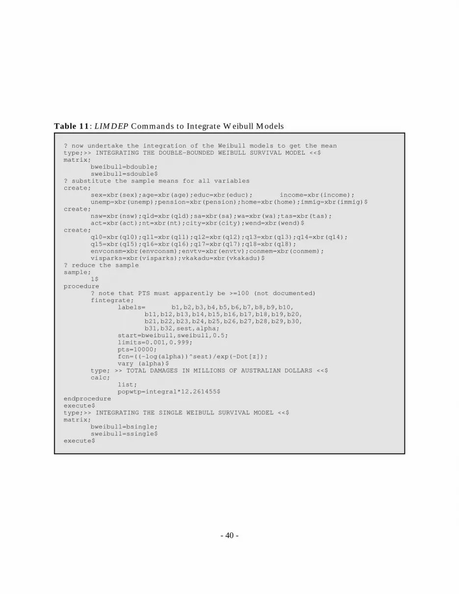
- 40 -

? now undertake the integration of the Weibull models to get the meantype;>> INTEGRATING THE DOUBLE-BOUNDED WEIBULL SURVIVAL MODEL <<$matrix;

bweibull=bdouble;sweibull=sdouble$

? substitute the sample means for all variablescreate;

sex=xbr(sex);age=xbr(age);educ=xbr(educ); income=xbr(income);unemp=xbr(unemp);pension=xbr(pension);home=xbr(home);immig=xbr(immig)$

create;nsw=xbr(nsw);qld=xbr(qld);sa=xbr(sa);wa=xbr(wa);tas=xbr(tas);act=xbr(act);nt=xbr(nt);city=xbr(city);wend=xbr(wend)$

create;q10=xbr(q10);q11=xbr(q11);q12=xbr(q12);q13=xbr(q13);q14=xbr(q14);q15=xbr(q15);q16=xbr(q16);q17=xbr(q17);q18=xbr(q18);envconsm=xbr(envconsm);envtv=xbr(envtv);conmem=xbr(conmem);visparks=xbr(visparks);vkakadu=xbr(vkakadu)$

? reduce the samplesample;

1$procedure

? note that PTS must apparently be >=100 (not documented)fintegrate;

labels= b1,b2,b3,b4,b5,b6,b7,b8,b9,b10,b11,b12,b13,b14,b15,b16,b17,b18,b19,b20,b21,b22,b23,b24,b25,b26,b27,b28,b29,b30,b31,b32,sest,alpha;

start=bweibull,sweibull,0.5;limits=0.001,0.999;pts=10000;fcn=((-log(alpha))^sest)/exp(-Dot[z]);vary (alpha)$

type; >> TOTAL DAMAGES IN MILLIONS OF AUSTRALIAN DOLLARS <<$calc;

list;popwtp=integral*12.261455$

endprocedureexecute$type;>> INTEGRATING THE SINGLE WEIBULL SURVIVAL MODEL <<$matrix;

bweibull=bsingle;sweibull=ssingle$

execute$

Table 11: LIMDEP Commands to Integrate Weibull Models

- 41 -

title; >>> ESTIMATE INTERVAL-CENSORED LOGIT MODELS (NO COVARIATES) <<<$load;

file=kak.sav$? get the minor impact and national samplereject;

major=1$reject;

ntsamp=1$title; >>> ESTIMATE THE INTERVAL-CENSORED DOUBLE-BOUNDED LOGIT <<<$? generate the indicator variablescreate;

yy=0;yn=0;nn=0;ny=0;if (wtp=1 & wtphi=1) yy=1;if (wtp=1 & wtphi=0) yn=1;if (wtp=0 & wtplo=1) ny=1;if (wtp=0 & wtplo=0) nn=1$

? scale values for MINIMIZEcreate;

v=v/100;vlo=vlo/100;vhi=vhi/100$

namelist;first=one,v$

namelist;high=one,vhi$

namelist;low=one,vlo$

? LGP() is the logistic CDF, showing the probability of a NOminimize;

labels=a,c;start=1,1;fcn= - ( yy * log(1-lgp(dot[high]))

+ yn * log(lgp(dot[high])-lgp(dot[first]))+ ny * log(lgp(dot[first])-lgp(dot[low]))+ nn * log(lgp(dot[low])) )$

calc;list;avedb=100*(-(b(1)/b(2)));damdb=avedb*12.261455$

title; >>> ESTIMATE THE INTERVAL-CENSORED SINGLE-BOUNDED LOGIT <<<$create;

yes=0;no=0;if (wtp=1) yes=1;(else) no=1$

minimize;labels=a,c;start=1,1;fcn= - ( yes * log(1-lgp(dot[first]))

+ no * log(lgp(dot[first])) )$calc;

list;avesb=100*(-(b(1)/b(2)));damsb=avesb*12.261455$

? now do this directly as a checklogit;

lhs=yes;rhs=one,v$

calc;list;avesb=100*(-(b(1)/b(2)));damsb=avesb*12.261455$

Table 12: LIMDEP Commands to Estimate Interval-Censored Logit Models

on the interpretation of responses to contingent valuation surveys

Documents