on the influence of weather forecast errors in short-term load forecasting models

IEEE TRANSACTIONS ON POWER SYSTEMS, VOL. 25, NO. 3, AUGUST 2010 1751

On the Influence of Weather Forecast Errorsin Short-Term Load Forecasting Models

Damien Fay and John V. Ringwood, Senior Member, IEEE

Abstract—Weather information is an important factor in loadforecasting models. Typically, load forecasting models are con-structed and tested using actual weather readings. However,online operation of load forecasting models requires the use ofweather forecasts, with associated weather forecast errors. Theseweather forecast errors inevitably lead to a degradation in modelperformance. This is an important factor in load forecasting buthas not been widely examined in the literature. The main aimof this paper is to present a novel technique for minimizing theconsequences of this degradation. In addition, a supplementarytechnique is proposed to model weather forecast errors to reflectcurrent accuracy.

The proposed technique utilizes a combination of forecasts fromseveral load forecasting models (sub-models). The parameter esti-mation may thus be split into two parts: sub-model and combina-tion parameter estimation. It is shown that the lowest PMSE corre-sponds to training the sub-models with actual weather but trainingthe combiner with forecast weather.

Index Terms—Load forecasting, model combination, neural net-works, weather forecast errors.

I. INTRODUCTION

S HORT-TERM load forecasting (STLF) refers to forecastsof electricity demand (or load), on an hourly basis, from

one to several days ahead. The amount of excess electricity pro-duction (or spinning reserve) required to guarantee supply, in theevent of an underestimation, is determined by the accuracy ofthese forecasts. Conversely, overestimation of the load leads tosub-optimal scheduling (in terms of production costs) of powerplants (known as unit commitment). In addition, a deregulatedmarket structure exists in Ireland in which load forecasts play acentral role. As indicated above, STLF is an important area andthis is reflected in the literature by the many techniques that havebeen applied, including neural networks [1], fuzzy logic [2] andstatistical techniques [3], to mention but a few. In many elec-tricity grid systems, the prevailing weather has a significant ef-fect on the load and it has been found that including weather in-formation can improve a load forecast [3]. However, in order touse weather information for future load forecasts, weather fore-casts must be utilized and these have associated weather forecast

Manuscript received November 30, 2007; revised July 29, 2009. First pub-lished February 02, 2010; current version published July 21, 2010. Paper no.TPWRS-00917-2007.

D. Fay is with the University of Cambridge, Cambridge, U.K. (e-mail:[email protected]).

J. V. Ringwood is with the National University of Ireland, Maynooth, Ireland(e-mail: [email protected]).

Color versions of one or more of the figures in this paper are available onlineat http://ieeexplore.ieee.org.

Digital Object Identifier 10.1109/TPWRS.2009.2038704

errors. Although system dependent, weather forecast errors canbe significant [4] and have been attributed as the cause of 17%[5] to 60% [6] of load forecast errors.

Load forecasting models are usually trained using actualpast weather readings as opposed to past weather forecasts [7].This is based on the assumption that to use the latter essentiallyadds forecast noise to the training data which can lead to biasedparameter estimation [8]. Often weather forecasts are unavail-able for the entire training period and/or can be subject toincreasing accuracy of meteorological models, as mathematicalweather models are constantly improved. Therefore, trainingload models with actual weather can be justified [7]. However,when weather forecast errors not present in the training setare presented, they can have a disproportionate influence onload models [9]. Changing the load model parameters to ac-count for this can be impossible in many conventional modelsonce training is completed. Douglas et al. [5] approached thisproblem by use of a Bayesian framework, but restricted analysisto the use of dynamic linear models. In spite of the importanceof weather forecast errors with respect to load forecasting, theliterature is sparse [10], [11].

The main contribution of this paper is the combination of sev-eral models (called sub-models), or model fusion, as a techniquefor minimizing the effect of weather forecast errors in load fore-casting models. Model fusion is particularly suited to STLF asthe sub-models may be trained with actual weather informationand the effect of weather forecast errors taken into account whencombining the models. While the concept of model fusion iswell known in the general field of forecasting and was pioneeredmainly in [12], its use to deal with forecasting errors in causalvariables is new. For example, a linear combiner is used in [13]to combine ARIMA models, with weights updated iterativelyfollowing each additional observation, based on model stabilitymeasures. In [14] the short-term load forecasting problem is ad-dressed using a combination of forecasts, where weather inputsare considered using a “factor vector”, though autoregressivemodels are used for the individual forecasts. The weights of thelinear combiner are updated at each time step using a forecastingperformance measure and errors in weather forecasts are notconsidered. Similar approaches may be found in [15] and [16].

Fused forecasts are theoretically more accurate than any ofthe individual model forecasts [17], [18], though there are someresults which show little benefit under certain circumstances[19], in particular where an unweighted mean of forecasts isused to model an autoregressive time series. Nevertheless, dif-ferent models are often better at modeling different aspects ofan underlying process and combining the models appropriately(i.e., by taking weather forecast errors into account) thus gives

0885-8950/$26.00 © 2010 IEEE

Authorized licensed use limited to: The Library NUI Maynooth. Downloaded on August 05,2010 at 17:02:32 UTC from IEEE Xplore. Restrictions apply.

1752 IEEE TRANSACTIONS ON POWER SYSTEMS, VOL. 25, NO. 3, AUGUST 2010

TABLE IDATA TIME SCALE AND RANGE

TABLE IIWEATHER DATA TIME-SCALE AND RANGE

TABLE IIIDIVISION OF DATA SET

a better forecast. In addition, a single model incorporating allaspects of an underlying process may be more complex and dif-ficult to train than combining individual models [17]. However,it should be noted that a fusion model is not a universal ap-proximator as information may be lost by the sub-models whichcannot be recovered by the fusion model.

II. DATA SETS

The range and time-scale of the available electrical demanddata is given in Table I. Two categories of historical weather dataare available from the Meteorological Office of Ireland (MOI):readings (or actual weather) and forecasts. Both sets of data arefor Dublin airport, the closest and most relevant weather stationto Dublin (Table II). The readings and forecasts are for dry bulbtemperature, cloud cover, wind speed and wind direction.

The data is subdivided into three sets in order to train, validateand test the load forecasting models (Table III). The training setis used to estimate model parameters, the validation set is usedto aid in model structure determination and the novelty set isused to evaluate model performance.

Data between Monday and Friday in the months January toMarch (known as the late winter working day day-type) is se-lected so as to avoid the exceptions associated with weekend,Christmas and changes due to the daylight saving hour.

The relatively long data record used permits the data to bedisaggregated according to hour-of-day and day type and pro-vides sufficient data to obtain reliable statistics on training, val-idation and novelty sets. The potential issues of data “currency”and nonstationarity associated with a relatively long dataset aredealt with by:

• the use of a Kalman filter to determine the underlying sea-sonal and IRW components; and

• the use of a heterogeneity transform (4) to deal with in-creasing variance.

III. MODELING WEATHER FORECAST ERRORS

Due to the sparseness of weather forecast data available tous (Table II) it is necessary to model the weather forecast error

Fig. 1. Actual and forecast temperature (February 6–15, 2000).

to produce pseudo-weather forecasts for the entire data set. In-deed, even given a long database of weather forecasts, modelingthe error is desirable. This is because the quality of weatherforecasts is changing over time due to improved forecastingtechniques and climate change [20]. Previous approaches inSTLF have modeled the weather forecast error simply as anIID Gaussian random variable [21], [22]. However, as seen inFig. 1 this is not an accurate representation of the statistics ofthe weather forecast errors in Ireland. Rather, the forecast errordisplays serial correlation, i.e., it is either above or below theactual for prolonged periods (i.e., the errors are not identicallydistributed, Fig. 1). Typically some form of aggregate weathervariables are normally used in STLF models (e.g., average dailytemperature). Serial correlation can introduce large deviationsin the sample mean and so an IID noise process is not a goodmodel for weather forecast errors.

The weather in Ireland is dominated by Atlantic weather sys-tems. When a weather system or front reaches Ireland there isa shift in the level of the temperature and other weather vari-ables (Fig. 1) (a similar situation is noted in [3]). This shift isalso a factor that the Irish Meteorological Office must forecast.The weather forecast error is thus assumed to have the followingstructure:

• turning points (Fig. 1) which represent the arrival of aweather front;

• a level error, , which is the average of the weather forecasterror between turning points;

• a shape error, , which is the standard deviation of theweather forecast error between turning points; and

• a random error, which accounts for the remaining error ifand are removed.

In order to detect the turning points the following simplealgorithm was found to suffice. The weather variable is firstsmoothed by means of a state space model based on an inte-grated random walk:

(1)


FAY AND RINGWOOD: ON THE INFLUENCE OF WEATHER FORECAST ERRORS IN SHORT-TERM LOAD FORECASTING MODELS 1753

Fig. 2. Sample of the turning points calculated for temperature.

where is the state vector at time and is the processnoise. The temperature is then extracted from the state vector bymeans of the measurement equation:

(2)

where is the filtered weather variable and is themeasurement noise. The state vector is estimated using theKalman filter (Note: the a-posteriori state vector estimate isused in (2) as a smoothed version of the original is desired[23]). The turning points are then defined as the maxima andminima within a rolling window of length 5:

(3)

where is the set of turning points and denotes greateror less than. A sample of the turning points detected by thisalgorithm is shown in Fig. 2.

Fig. 3 shows the histograms, fitted Gaussian distributionsand the Sample AutoCorrelation Function (SACF) for the levelshape and random error of the temperature forecasts. The shapeand level errors of the four weather variables are found to becross correlated, suggesting that they may not be independent.In order to generate pseudo-weather forecast errors, the turningpoints in the actual weather variables are first identified. Then,a multivariate Gaussian pseudo-random number generator isused to generate the random errors for each of the weathervariables jointly. Fig. 4 shows the SACF of the temperatureforecast errors and the pseudo-temperature forecast errors.As can be seen, the SACF for both are similar, showing thatthe pseudo-forecast errors have captured the auto-correlationevident in the temperature forecast errors. A similar situationwas found with the other weather variables.

IV. FUSION MODEL

A. Preliminary Auto-Regressive (AR) Linear Model

It was previously found by these authors [24] that decom-posing load data into 24 parallel series, one for each hour ofthe day, is advantageous, as the parallel series are not interde-pendent. The parallel series for hour on day , , hasa low frequency trend, , which is first removed using aBasic Structural Model (BSM) [25], via an integrated randomwalk, leaving a residual, (Fig. 5), which is composed of

Fig. 3. Distributions and SACF for temperature forecasts.

Fig. 4. SACF of forecast and pseudo-forecast temperature errors.

Fig. 5. Preliminary AR linear model overview.

weather, nonlinear auto-regressive and white noise components[24].

B. Sub-Models

Three sub-models were chosen which have different types ofinputs. These are chosen so that forecast errors can be attributedto particular inputs. A fourth sub-model is included using all theavailable inputs to capture any nonlinear relationships betweenthe inputs and the residual. The sub-models are named after their



Fig. 6. Data fusion model overview.

input types as shown in Fig. 4. The fusion technique combinesthe forecasts of the sub-models, , to givea fused forecast, of the residual for series on day(Fig. 6). It should be noted that all of the sub-models are trainedon actual, rather than forecast data. The consideration of fore-cast errors takes place in the fusion algorithm, as detailed inSection IV-C.

The sub-models all use feed forward neural networks, al-though it should be noted that the choice of modeling techniqueis not central to this paper. Initially, the traditional back-prop-agation algorithm using Levenberg-Marquadt with cross vali-dation was used to train the networks. Each of the networkshas two hidden layers and a single output. To determine a suit-able structure for the network (i.e., the number of nodes in eachlayer), different network structures were trained (ranging froma 1 1 to a 7 7 network) and their prediction mean squarederrors (PMSE) compared over the validation set. The best struc-ture was then selected for further evaluation. Given these initialmodels, the residuals where then examined for homogeneity ofvariance and it was concluded that the time series possessednonconstant variance. The most likely cause for the noncon-stant variance lies in the considerable growth experienced inIrish electricity demand over the period of the data set. Withthe increase in electricity demand a corresponding increase inforecasting error (and thus variance) would be expected. Thestandard approach in this case is to presume that the varianceis proportional to the level of the time series squared, specifi-cally , and then to scale the errors using weighted leastsquares (see [26, Section 8.3]). During training with the back-propagation algorithm the target errors are thus scaled prior tobeing propagated backwards as

......

. . ....

(4)

where is vector of target errors and is the adjusted vector. Itwas found that this improved the prediction performance of themodels in all cases. The Temperature Model (TM) input, ,is a vector of the current and previous 71 h of temperature fromhour on day . Similarly the other Weather Model (WM)uses vectors of wind speed, , cloud cover, , andwind direction, containing current and previous 71 h ofweather. The Non-Linear Auto-Regressive model (NLAR) usesthe previous two days of residual, and .The Non-Linear Model (NLM) uses all the available inputs.

C. Fusion Algorithm

The data fusion algorithm described in [27] seeks to minimizethe variance of the fused forecast based on the covariance ma-trix of the sub-model forecasts. In this way, the load forecast er-rors, due to weather forecast errors, are taken into account. Thecross-covariance of the forecasts is considered and the distribu-tion of the forecast error noise is not restricted to Gaussian butmerely required to be unbiased. A combined forecast, ,of the load is created using a weighted average of the individualforecasts, [27]:

(5)

where is the weight applied to the forecast from sub-model for hour ,1 and is derived from the error covariancematrices of as

(6)where , , and are auxiliaryvariables derived from the sample error covariance of

:

(7)where is the error covariance of sub-model with sub-model for hour , and is the number of samples used. Theauxiliary variables are then defined as

(8)

and

(9)

1Although it is assumed that the variance is proportional to � �� , an ad-justment for heteroskedasticity is not necessary here as multiplying � �� bya scaling factor will not change the weights.



TABLE IVCROSS-COVARIANCE MATRIX OF SUB-MODEL LOAD

FORECAST ERRORS (CASE I�CASE II)

where

(10)The final weight is determined using the constraint that

is unbiased:

(11)

Finally the fused load forecast, , is estimated by reintro-ducing the trend:

(12)

V. RESULTS

The results are here analyzed for three cases. The first exam-ines the behavior of the fusion model without pseudo-weatherforecasts and the second and third examines the behavior withthem. Case II is the most relevant case with the others includedfor comparison:

Case I: The sub-model parameters are estimated using ac-tual weather inputs. The error covariance matrices of thesub-models (7) are then estimated using actual weather in-puts. The weights, , are then calculated using theseerror covariance matrices (as in Section IV-C).Case II: The sub-model parameters are estimated usingactual weather inputs (as in Case I). The error covari-ance matrices of the sub-models (7) are then estimatedusing pseudo-weather forecast inputs (unlike Case I). Theweights, , are then calculated using these (new)error covariance matrices (as in Section IV-C). Modelsare trained and evaluated using pseudo-weather forecastinputs.Case III: The sub-model parameters and are calcu-lated as in Case I (i.e., based on actual weather). However,in this case the models are evaluated using pseudo-weatherforecasts as input (thus a comparison can be drawn withCase II).

As an example, the cross-covariance matrix of sub-modelforecast errors is shown in Table IV for the midday series

. The difference between Cases I and II is indicated by anarrow. As can be seen the covariance of sub-models 2 to 4 in-creases when pseudo-weather forecasts are used. This increase

TABLE VEXAMPLE OF FUSION WEIGHTS (ACTUAL WEATHER INPUTS)

Fig. 7. MAPE as a function of hour of the day for fusion and sub-models (notes:novelty set, actual weather used).

TABLE VIMODEL PERFORMANCE USING ACTUAL WEATHER INPUTS

indicates the degradation of the models due to (pseudo) weatherforecast error.

The corresponding values of are shown in Table V.Note that the weights change significantly in the presence ofpseudo-weather forecasts.

Fig. 7. shows the mean absolute percentage error (MAPE) forthe sub-models and the fusion model in Case I. As can be seen,the fusion model performs best for each hour of the day.

Table VI, summarizes the results in the training, validationand novelty data sets.

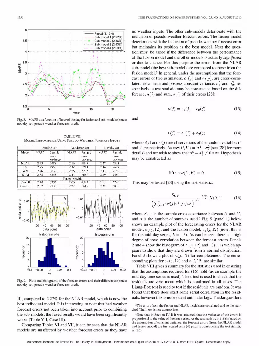
Fig. 8 shows the MAPE for the sub-models and the fusionmodel using pseudo-forecast weather inputs in the novelty set(Case II). As can be seen the fusion model again performs bestfor each hour of the day.

Tables VI and VII enumerate the benefit of the fusion model.Table VI is included for reference, corresponding to the case ofno weather forecast errors. There is a modest improvement ofthe fusion model MAPE over the best individualmodel (TM and NLM, with MAPE ) for the noveltyset. However, in Table VII, a more significant improvement isrecorded, with a MAPE of 2.15% for the fusion model (Case



Fig. 8. MAPE as a function of hour of the day for fusion and sub-models (notes:novelty set, pseudo-weather forecasts used).

TABLE VIIMODEL PERFORMANCE USING PSEUDO-WEATHER FORECAST INPUTS

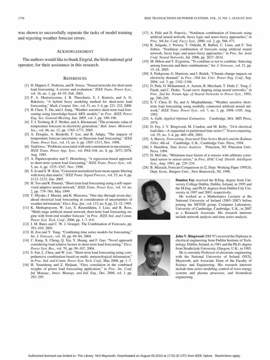
Fig. 9. Plots and histograms of the forecast errors and their differences (notes:novelty set, pseudo-weather forecasts used).

II), compared to 2.27% for the NLAR model, which is now thebest individual model. It is interesting to note that had weatherforecast errors not been taken into account prior to combiningthe sub-models, the fused results would have been significantlyworse (Table VII, Case III).

Comparing Tables VI and VII, it can be seen that the NLARmodels are unaffected by weather forecast errors as they have

no weather inputs. The other sub-models deteriorate with theinclusion of pseudo-weather forecast errors. The fusion modeldeteriorates with the inclusion of pseudo-weather forecast errorbut maintains its position as the best model. Next the ques-tion must be asked if the difference between the performanceof the fusion model and the other models is actually significantor due to chance. For this purpose the errors from the NLARsub-model (the best sub-model) are compared to those from thefusion model.2 In general, under the assumptions that the fore-cast errors of two estimators, and , are cross-corre-lated, zero mean and possess constant variance, and , re-spectively; a test statistic may be constructed based on the dif-ference, and sum, of their errors [28]:

(13)

and

(14)

where and are observations of the random variablesand , respectively. As (see [28] for moredetails) and we wish to show that a null hypothesismay be constructed as

(15)

This may be tested [28] using the test statistic:

(16)

where is the sample cross covariance between and ,and is the number of samples used.3 Fig. 9 (panel 1) belowshows an example plot of the forecasting errors for the NLARmodel, , and the fusion model, (note: this isfor the mid-day series, ). As can be seen there is a highdegree of cross-correlation between the forecast errors. Panels2 and 4 show the histogram of and which ap-pears to show that they are drawn from a normal distribution.Panel 3 shows a plot of for completeness. The corre-sponding plots for and are similar.

Table VIII gives a summary for the statistics used in ensuringthat the assumptions required for (16) hold (as an example themid-day time series is used). The t-test is used to check that theresiduals are zero mean which is confirmed in all cases. TheLjung-Box test is used to test if the residuals are random. It wasfound that there does exist some serial correlation in the resid-uals, however this is not evident until later lags. The Jarque-Bera

2The errors from the fusion and NLAR models are correlated and so the stan-dard Theil test is not appropriate.

3Note that in Section IV-B it was assumed that the variance of the errors isproportional to the value of the time series. As the test statistic in (16) is based onthe assumption of constant variance, the forecast errors (from the NLAR modeland fusion model) are first scaled as in (4) prior to constructing the test statisticin (16)



TABLE VIIISUMMARY OF FORECAST ERROR STATISTICS ��

Fig. 10. P-values for each hour of the day (notes: novelty set, pseudo-weatherforecasts used).

test is used to test for normality. It is found that the hypothesisof normality is rejected. On further examination this is due toseveral outliers on the right tail of the distribution. These arecaused by the large error which occurs between the transitionsfrom year to year in the late winter working day day-type. Giventhis limitation the hypothesis (15) is tested.

Fig. 10 shows the p-value for the testing the hypothesis thatthe variance of the residuals from the two models are statisticallydifferent. As there are 24 h, 24 tests are conducted. The resultsshow that the hypothesis is accepted at the 1% confidence levelfor most of the hours, at the 5% confidence level for all but oneof the hours where the p-value is 0.83. Thus empirical evidencewould seem to show that the fusion model is indeed a bettermodel than the NLAR model.

A final comment relates to the length of the training setused. There is a trade off between more data (which reducesparameter estimate variance) and irrelevant (older) data which

Fig. 11. Effect of training data record length on prediction accuracy (start yearof dataset shown).

increases the variance. In order to examine the effect of datarecord length on the result, the fusion model and sub-modelswere evaluated for training data length of two years (from 1995)to ten years (from 1987). The MAPE achieved in the novelty setfor record lengths of two to ten years is shown in Fig. 11, whichshows that there is a marked decrease in model performance asthe training data record length reduces to three years. There isrelatively little variation in MAPE for record lengths greaterthan four years using pseudo-weather inputs, with some minorlocal minima in MAPE at six and eight years, using actualand pseudo-weather inputs, respectively. Given the results inFig. 11, a training data record of seven years, beginning in 1990,was employed, which was seen as a reasonable compromisebetween actual and pseudo-weather MAPE indicators.

VI. CONCLUSION

This paper examined the effect of weather forecast errors inload forecasting models. In Section III, the distribution of theweather forecast errors was examined and it was found that aGaussian distribution was not appropriate in this case. Rather,a structure exists which means that the weather forecast errorwill have a large effect on any aggregate weather variables. Thestructure of the weather forecast errors was then used to producepseudo-weather forecast errors from 1986 to 2000 which havethe accuracy of current weather forecasts. This is important as,for example, weather forecasts from 1986 are less accurate thancurrent weather forecasts and thus of no relevance in predictingfuture loads.

It was argued that splitting parameter estimation into twophases; one weather forecast error dependent and the other in-dependent was appropriate and advantageous. A model fusiontechnique was employed for this task. In general weather fore-cast error causes approximately 1% deterioration in load fore-casts of all models used here. This figure, though important, isnot as high as suggested by [5] and [6], for their systems. How-ever, the fusion model was capable of adjusting the weightingof the sub-models to reflect that the weather based sub-modelsdeteriorated relative to the AR model. Finally, the fusion model



was shown to successfully separate the tasks of model trainingand rejecting weather forecast errors.

ACKNOWLEDGMENT

The authors would like to thank Eirgrid, the Irish national gridoperator, for their assistance in this research.

REFERENCES

[1] H. Hippert, C. Pedreira, and R. Souza, “Neural networks for short-termload forecasting: A review and evaluation,” IEEE Trans. Power Syst.,vol. 16, no. 1, pp. 44–55, Feb. 2001.

[2] P. A. Mastorocostas, J. B. Theocharis, S. J. Kiartzis, and A. G.Bakirtzis, “A hybrid fuzzy modeling method for short-term loadforecasting,” Math. Comput. Sim., vol. 51, no. 3–4, pp. 221–232, 2000.

[3] H. Chen, Y. Du, and J. Jiang, “Weather sensitive short-term load fore-casting using knowledge-based ARX models,” in Proc. IEEE PowerEng. Soc. General Meeting, Jun. 2005, vol. 1, pp. 190–196.

[4] T. J. Teisberg, R. F. Weiher, and A. Khotanzad, “The economic value oftemperature forecasts in electricity generation,” Bull. Amer. Meteorol.Soc., vol. 86, no. 12, pp. 1765–1771, 2005.

[5] A. Douglas, A. Breipohl, F. Lee, and R. Adapa, “The impacts oftemperature forecast uncertainty on Bayesian load forecasting,” IEEETrans. Power Syst., vol. 13, no. 4, pp. 1507–1513, Nov. 1998.

[6] Taskforce, “Problems associated with unit commitment in uncertainty,”IEEE Trans. Power App. Syst., vol. PAS-104, no. 8, pp. 2072–2078,Aug. 1985.

[7] A. Papalexopoulos and T. Hesterberg, “A regression-based approachto short-term system load forecasting,” IEEE Trans. Power Syst., vol.5, no. 4, pp. 1535–1547, Nov. 1990.

[8] S. Jo and S. W. Kim, “Consistent normalized least mean square filteringwith noisy data matrix,” IEEE Trans. Signal Process., vol. 53, no. 6, pp.2112–2123, Jun. 2005.

[9] H. Yoo and R. Pimmel, “Short term load forecasting using a self-super-vised adaptive neural network,” IEEE Trans. Power Syst., vol. 14, no.2, pp. 779–784, May 1999.

[10] T. Miyake, J. Murata, and K. Hirasawa, “One-day-through seven-day-ahead electrical load forecasting in consideration of uncertainties ofweather information,” Elect. Eng. Jpn., vol. 115, no. 8, pp. 22–32, 1995.

[11] K. Methaprayoon, W. Lee, S. Rasmiddatta, J. Liao, and R. Ross,“Multi-stage artificial neural network short-term load forecasting en-gine with front-end weather forecast,” in Proc. IEEE Ind. and Comm.Power Syst. Tech. Conf., 2006, pp. 1–7, 0-0.

[12] J. M. Bates and C. W. J. Granger, The Combination of Forecasts, pp.391–410, 2001.

[13] H. Zou and Y. Yang, “Combining time series models for forecasting,”Int. J. Forecast., vol. 20, pp. 69–84, 2004.

[14] C. Kang, X. Cheng, Q. Xia, Y. Huang, and F. Gao, “Novel approachconsidering load-relative factors in short-term load forecasting,” Elect.Power Syst. Res., vol. 70, pp. 99–107, 2004.

[15] S. Fan, L. Chen, and W. Lee, “Short-term load forecasting using com-prehensive combination based on multi- meteorological information,”in Proc. Ind. and Comm. Power Syst. Tech. Conf., May 2008, pp. 1–7.

[16] H. Yuansheng and Z. Huijuan, “Grey correlation in the combinedweights of power load forecasting application,” in Proc. Int. Conf.Inf. Manage., Innov. Manage. and Ind. Eng., Dec. 2008, vol. 1, pp.292–295.

[17] A. Palit and D. Popovic, “Nonlinear combination of forecasts usingartificial neural network, fuzzy logic and neuro-fuzzy approaches,” inProc. 9th Int. Conf. Fuzzy Syst., 2000, vol. 2, pp. 566–571.

[18] R. Salgado, J. Periera, T. Oshishi, R. Ballini, C. Lima, and F. VonZuben, “Nonlinear combination of forecasts using artificial neuralnetwork, fuzzy logic and neuro-fuzzy approaches,” in Proc. Int. JointConf. Neural Networks, Jul. 2006, pp. 2627–2634.

[19] M. Hibon and T. Evgeniou, “To combine or not to combine: Selectingamong forecasts and their combinations,” Int. J. Forecast., vol. 21, pp.15–24, 2005.

[20] S. Parkpoom, G. Harrison, and J. Bialek, “Climate change impacts onelectricity demand,” in Proc. 39th Int. Univ. Power Eng. Conf., Sep.2004, vol. 3, pp. 1342–1346.

[21] D. Park, O. Mohammed, A. Azeem, R. Merchant, T. Dinh, C. Tong, J.Farah, and C. Drake, “Load curve shaping using neural networks,” inProc. 2nd Int. Forum App. of Neural Networks to Power Syst., 1993,pp. 290–295.

[22] S.-T. Chen, D. Yu, and A. Moghaddamjo, “Weather sensitive short-term load forecasting using nonfully connected artificial neural net-work,” IEEE Trans. Power Syst., vol. 7, no. 3, pp. 1098–1105, Aug.1992.

[23] A. Gelb, Applied Optimal Estimation. Cambridge, MA: MIT Press,1974.

[24] D. Fay, J. V. Ringwood, M. Condon, and M. Kelly, “24-h electricalload data—A sequential or partitioned time series?,” Neurocomputing,vol. 55, no. 3–4, pp. 469–498, 2003.

[25] A. Harvey, Forecasting, Structural Time Series Models and the KalmanFilter, 4th ed. Cambridge, U.K.: Cambridge Univ. Press, 1994.

[26] J. Hamilton, Time Series Analysis. Princeton, NJ: Princeton Univ.Press, 1994.

[27] H. McCabe, “Minimum trace fusion of n sensors with arbitrary corre-lated sensor to sensor errors,” in Proc. IFAC Conf. Distrib. IntelligentSyst., Aug. 1991, pp. 229–234.

[28] B. Mizrach, Forecast Comparison in l2, Dept. Working Paper 199524,Dept. Econ., Rutgers Univ., New Brunswick, NJ, 1996.

Damien Fay received the B.Eng. degree from Uni-versity College Dublin, Dublin, Ireland, in 1995 andthe M.Eng. and Ph.D. degrees from Dublin City Uni-versity in 1997 and 2003, respectively.

He worked as a Mathematics Lecturer at theNational University of Ireland (2003–2007) beforejoining the NETOS group, Computer Laboratory,University of Cambridge, Cambridge, U.K., in 2007as a Research Associate. His research interestsinclude network analysis and time series analysis.

John V. Ringwood (SM’97) received the Diploma inelectrical engineering from Dublin Institute of Tech-nology, Dublin, Ireland, in 1981 and the Ph.D. degreefrom Strathclyde University, Glasgow, U.K., in 1985.

He is currently Professor of electronic engineeringwith the National University of Ireland (NUI),Maynooth, and Associate Dean of the Faculty ofScience and Engineering. His research interestsinclude time series modeling, control of wave energysystems and plasma processes, and biomedicalengineering.


on the influence of weather forecast errors in short-term load forecasting models

Documents