on the dynamics of pressure relief valves with external pilot for ice lubrication

1 Copyright © 2014 by ASME

On the Dynamics of Pressure Relief Valves with External Pilot for ICE Lubrication

Proceedings of the ASME 2014 International Mechanical Engineering Congress & ExpositionIMECE2014

November 14-20, 2014, Montreal, Quebec, Canada

IMECE2014-37973

Massimo RundoPolitecnico di Torino

Department of EnergyTorino, 10129, Italy

[email protected]

ABSTRACT

The paper analyzes the influence on the stability of theremote pilot in pressure relief valves used for enginelubrication. Such valves are mainly used to discharge theexcess flow generated by a fixed displacement pump,moreover they can also be used as pilot stage to control thedisplacement in the new generation of vane pumps. In thepaper the transfer function that relates the pressure in the maingallery with the valve spool position is determined. It wasfound that, when the valve is provided with an external pilot,the interaction between the hydraulic inductance of the pilotpipe and the spool decreases by many times the mechanicalfrequency of the valve, leading to a reduction of the stability.The experimental procedure used to measure the frequencyresponse of the valve is also described. The test rig wasprovided with a servovalve used to generate a sinusoidalexcitation pressure with variable frequency. The valvefrequency response was evaluated by means of two pressuretransducers at the two ends of the pilot channel. Finally theinfluence on the stability of some geometric parameters isanalyzed by means of a simulation model in the AMESimenvironment.

NOMENCLATURE

A surface of influence of the valveAp cross section of the pilot pipe

c viscous friction coefficientCd discharge coefficient

dp diameter of the pilot pipe

ds spool diameter

k stiffness of the valve spring

lp length of the pilot pipe

moil mass of oil in the pilot pipe

m spool massp1 pressure at the inlet of the pilot pipe

p2 pressure at the end of the pilot pipe

p* valve cracking pressureQ flow rate through the pilot pipev spool velocityVc pilot chamber volume

V0 circuit volume

Vp pipe volume

x spool position fluid bulk modulus fluid dynamic viscosity fluid density jet angle

INTRODUCTION

In the lubricating circuit of internal combustion engines,the oil flow rate is generated by a gear pump driven with afixed transmission ratio by the crankshaft. The pumpdisplacement is dimensioned in order to satisfy the enginerequirements in the hot idling conditions, namely at minimumspeed and maximum oil temperature. Since the pump flow rateis proportional to the engine speed and the circuit permeabilityis highly dependent on the oil temperature, it is evident that, inmost operating conditions, the flow rate generated by the pumpdoes not match the engine requirements. Therefore the excessflow must be recirculated through a pressure relief valve. Inrecent years, to improve the fuel saving, variable displacementvane pumps are progressively substituting the fixed


displacement gear pumps. However a pressure relief valve canbe still used as pilot stage to control the pump displacement. Inboth cases the pressure relief valve can be piloted remotelythrough a channel connected directly with the engine maingallery. With respect to the internal pilot design, such solutionallows to guarantee in the main gallery a more constantpressure level, since it is not influenced by the variablepressure drop in the oil filter. However the use of the externalpilot can lead to the instability of the valve or of the pumpdisplacement control.Many studies are available in the open literature about thestability of pressure relief valves. Among the others Johnstonet al. [1] studied the stability of a cartridge valve using thesecondary source method and they discussed the effect ofdifferent parameters.In [2] Alirand et al. determined a simplified 3rd transferfunction suitable to study the stability of pressure relief andpressure reducing valves.In [3] Pohl et al. focused on the stability of a pressure reliefvalve for engine lubrication. The authors proposed amodification of the valve with the pressurization of the springchamber. With the new design the mechanical frequency wasreplaced by a much higher hydraulic frequency leading to asignificant improving of the stability.In this paper it is demonstrated that the use of an external pilotdecreases dramatically the mechanical frequency of the valveleading to a drastic reduction of the stability. The worsening ofthe valve behaviour can be amplified by low values of theeffective oil bulk modulus due to the presence of separated air.

SYSTEM DESCRIPTION

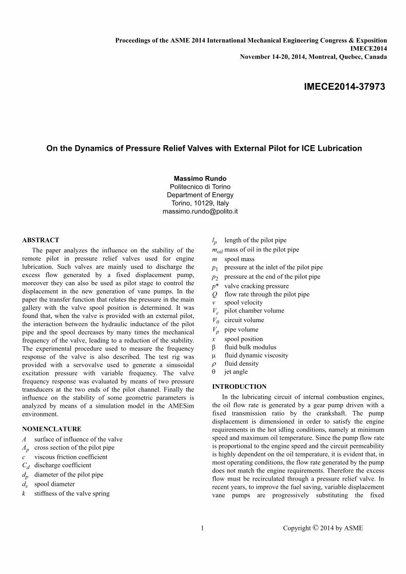
In Fig. 1 a schematic of a direct acting pressure relief valvewith remote pilot is reported with the indication of the mainparameters. The valve is represented in regulating conditions.The P port is connected to the pump outlet, while the right endof the pilot channel is connected with the engine main gallery.

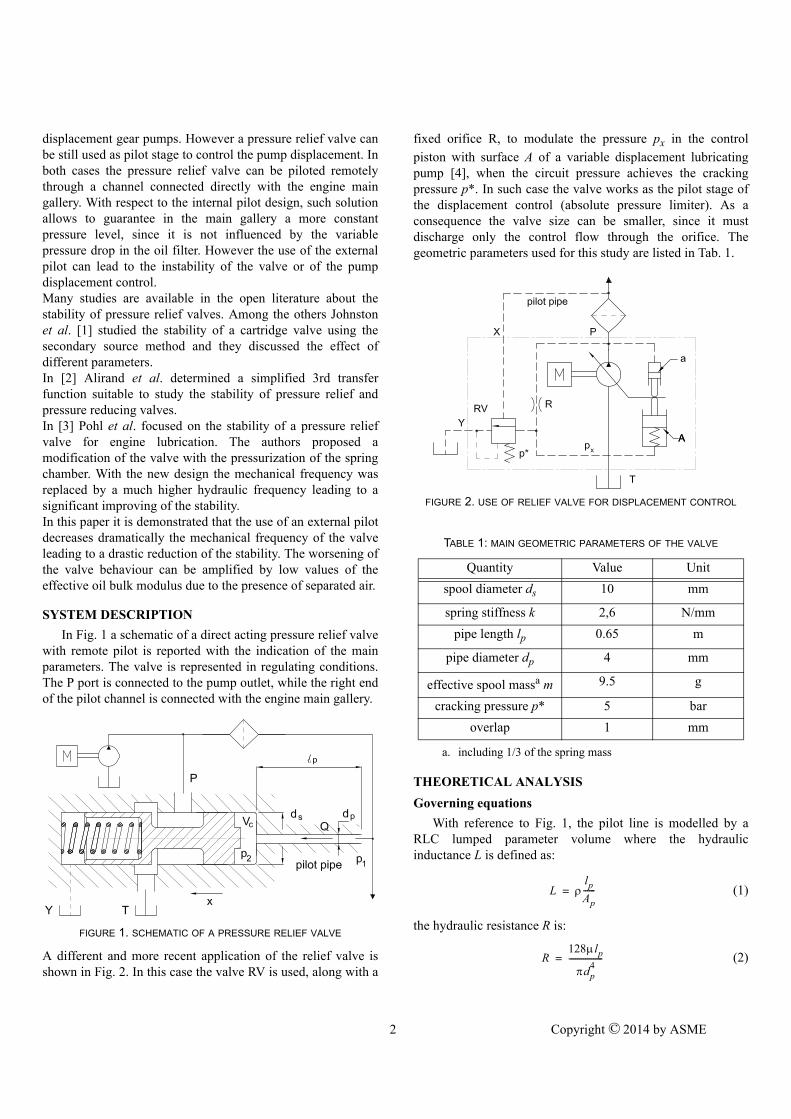
A different and more recent application of the relief valve isshown in Fig. 2. In this case the valve RV is used, along with a

FIGURE 1. SCHEMATIC OF A PRESSURE RELIEF VALVE

fixed orifice R, to modulate the pressure px in the control

piston with surface A of a variable displacement lubricatingpump [4], when the circuit pressure achieves the crackingpressure p*. In such case the valve works as the pilot stage ofthe displacement control (absolute pressure limiter). As aconsequence the valve size can be smaller, since it mustdischarge only the control flow through the orifice. Thegeometric parameters used for this study are listed in Tab. 1.

THEORETICAL ANALYSIS

Governing equations

With reference to Fig. 1, the pilot line is modelled by aRLC lumped parameter volume where the hydraulicinductance L is defined as:

(1)

the hydraulic resistance R is:

(2)

FIGURE 2. USE OF RELIEF VALVE FOR DISPLACEMENT CONTROL

TABLE 1: MAIN GEOMETRIC PARAMETERS OF THE VALVE

Quantity Value Unit

spool diameter ds 10 mm

spring stiffness k 2,6 N/mm

pipe length lp 0.65 m

pipe diameter dp 4 mm

effective spool massa m

a. including 1/3 of the spring mass

9.5 g

cracking pressure p* 5 bar

overlap 1 mm

L lp

Ap------=

R128lp

dp4

-----------------=


and the hydraulic capacitance C is expressed as:

(3)

In this first analysis the dynamic orifice, normally presentbetween the pilot chamber and the end of the pipe, is notconsidered. In this case the volumes of the pipe and of thechamber can be gathered into a single hydraulic capacity. Theinfluence of the damping orifice can be taken into account byusing an equivalent viscous friction coefficient c between thespool valve and the seat, as also demonstrated in [2].The system variables are the spool position x, the pressure inthe pilot chamber p2, the pressure at the inlet of the pilot pipe

p1 and the flow rate through the pipe Q.

It is possible to write the following equations:• the spool equilibrium:

(4)

• the equilibrium of the fluid in the pipe:

(5)

• the continuity equation:

(6)

To take into account the steady-state term of the flow force, thespring stiffness can be substituted by an equivalent coefficientkeq [3], defined as:

(7)

The flow force can be neglected if the valve is used as a pilotstage in the displacement control.The equations (4), (5) and (6) can also be written using thefollowing matrix form:

(8)

where x is the state vector, u is the controlled variable and y isthe observed variable. In this case the pressure p1 and the

position x are selected respectively as the controlled and theobserved variables. In fact the aim of the study is to observe thevariation of the spool position when a variation of the pressurein the circuit occurs. The system of equations (8) becomes:

(9)

CVp

------=

mx·· cx· kx p2A–+ + 0=

p1 p2– LQ· RQ+=

p2· 1

C---- Q Av– =

keq k 2Cddsp cos+=

x· Ax Bu+=

y CTx=

v·

x·

p2·

Q·

cm----– k

m----–

Am---- 0

1 0 0 0

AC----– 0 0

1C----

0 0 1L---–

RL---

v

x

p2

Q

0

0

0

1L---

p1+= y 0 1 0 0

v

x

p2

Q

=

The eigenvalues of the matrix A can be calculated by solvingthe characteristic equation (10):

(10)

and the following 4th order polynomial equation is obtained:

(11)

If the natural frequency and the damping ratio of themechanical system:

(12)

and the natural frequency and the damping ratio of thehydraulic system:

(13)

are defined, the Eq. (11) can be written as:

(14)

where:

(15)

As alternative the Eq. (11) can be also rearranged as:

(16)

where it is possible to observe that, with A = 0, the uncoupledsolutions of the mass-spring system and the RLC pipe areobtained:

(17)

If the dissipative terms c e R are neglected, the naturalfrequencies are given by the Eq. (18):

(18)

For the valve under study with the parameters reported in theTab. 1, the values of frequency are and

det A I– 0=

4 cm---- R

L---+

3 km---- cR

mL-------- 1

LC------- A

2

mC--------+ + +

2+ + +

RkmL-------- c

mLC------------ A

2R

mLC------------+ +

kmLC------------+ 0=+

mkm----= m

c

2 mk--------------=

h1

LC-------= h

R2--- C

L----=

4a3

3a2

2a1 a0+ + + + 0=

a3 2 mm hh+ =

a2 m2 h

24mhmh

A2

mC--------+ + +=

a1 2 hhm2 mmh

2 hhA

2

mC--------+ +

=

a0 m2 h

2=

22hh h

2+ + 2

2mm m2

+ + +

2hh+ A2

mC--------+ 0=

1 2 mm– jm 1 m– =

3 4 hh– jh 1 h– =

n1 n212--- h

2 m2 A

2

Cm--------+ +

14--- h

2 m2 A

2

Cm--------+ +

2

m2 h

2–=

n1 15.2 Hz=


. Therefore the main frequency is more than 5

times lower than the mechanical frequency of the valve( ).

Transfer functions

The system of differential equations (9) can be rewrittenusing the Laplace transforms:

(19)

From the first two equations it is possible to obtain the transferfunction that relates the spool position with the pressure in thepilot chamber:

(20)

while from the last two equations the transfer function thatrelates the two pressures p1 and p2:

(21)

The Eq. (21) can also be written using the coefficients (15):

(22)

The transfer function has two complex conjugate zeros

in correspondence of the poles of the function and four

poles given by the solutions of the characteristic equation (14).Therefore the transfer function between the pressure in theengine main gallery and the spool position is:

(23)

Simplification of the transfer function

Since the natural frequency is two orders of magnitude

higher than the frequency , the equation (23) can be

simplified into a 2nd order transfer function. In fact the terms

s4 and s3 can be neglected, moreover the first term of the

n2 1284 Hz=

m 83 Hz=

svcm----v–

km----x–

Am----p2+=

sx v=

sp2AC----v–

1C----Q+=

sQ1L---p2–

RL---Q–

1L---p1+=

F1 s x

p2

----- A

ms2

cs k+ + -----------------------------------

Am----

s2

2mms m2

+ + --------------------------------------------------= = =

F2 s p2

p1

-----s

2 cm----s k

m----+ +

sC sL R+ 1+ s2 c

m----s k

m----+ +

s sL R+ A2

m------+

------------------------------------------------------------------------------------------------------------------= =

F2 s h

2s

22mms m

2+ +

s4

a3s3

a2s2

a1s a0+ + + +-----------------------------------------------------------------=

F2 s

F1 s

F s F1 s F2 s x

p1

-----h

2 Am----

s4

a3s3

a2s2

a1s a0+ + + +-----------------------------------------------------------------= = =

n2

n1

coefficient a1 is two orders of magnitude smaller with respect

to the other two. Finally the first three terms of the coefficienta2 are at least two orders of magnitudes smaller than the fourth,

therefore the function (23) can be simplified as:

(24)

The equation (24) can be rearranged as:

(25)

where it is evident that the mass of the spool is increased by the

term , while the viscous friction coefficient is incremented

by the term .Accordingly the equation (21) can be simplified as:

(26)

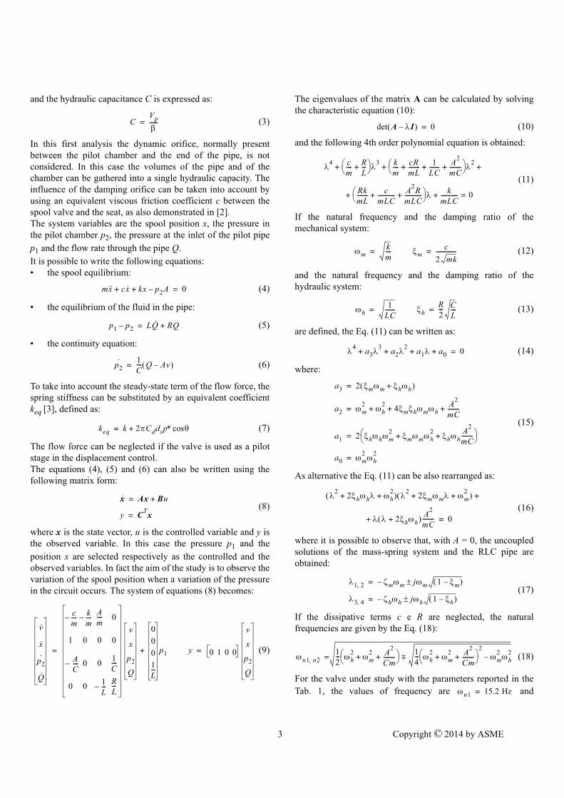
In Fig. 3 the comparison between the 4th order function

and the simplified 2nd order function is shown in terms

of amplitude and phase. The two functions are almostcoincident up to about 500 Hz.

The graphs shown in Fig. 3 have been obtained using thegeometric parameters listed in the Tab. 1 and the fluidproperties in Tab. 2. The value of the bulk modulus reported inTab. 2 comes from the experience on other experimental tests.A similar value was also found by Johnston [1].The friction coefficient has been determined experimentallythrough the procedure described hereinafter.

FIGURE 3. COMPARISON BETWEEN 4TH AND 2ND ORDER TRANSFER FUNCTIONS

Fs s x

p1

-----

1LA-------

s2

2mC

A2

--------mmh2 hh+

smC

A2

--------m2 h

2+ +

-------------------------------------------------------------------------------------------------------= =

Fs s A

m LA2

+ s2

c RA2

+ s k+ +-------------------------------------------------------------------------=

LA2

RA2

Fs2 s p2

p1

----- ms2

cs k+ +

m LA2

+ s2

c RA2

+ s k+ +-------------------------------------------------------------------------= =

F s

Fs s

160

140

120

100

80

60

40

20

0

50

40

30

20

10

0

10

20

phase(degree)

amplitud

e(dB)

2nd order

4th order

200

180

160

70

60

1 10 100 1000frequency (Hz)


Equivalent spool mass

It is possible to define an equivalent spool mass that takesinto account the hydraulic inductance of the pilot pipe. Withreference to the equations (6) and (7), if the dissipative termsare neglected, it is possible to write:

(27)

Since the flow rate variation through the pipe due to the spoolacceleration is:

(28)

the Eq. (27) becomes:

(29)

and therefore the system is equivalent to a single concentratedmass meq. If the definition of hydraulic inductance is applied:

(30)

the equivalent mass becomes:

(31)

It can be observed that if the pipe diameter is the same as thespool diameter, then the equivalent mass is simply the sum ofthe mass of the spool and the mass of the oil in the pipe,otherwise the mass of the oil is hugely amplified. In this casethe oil mass in the pilot line is 7 g, but since the ratio betweenthe spool diameter and the pipe diameter is 2.5, the equivalentmass of the oil is 274 g, being amplified by 39 times.

EXPERIMENTAL TESTS

Test rig description

The pressure relief valve was tested to determineexperimentally the frequency response of the systemconstituted by the pilot line and the spool. The results of thetest were used to validate the simplification of the transferfunction and to determine the viscous friction coefficient. Thevalve was mounted on a test bench used to measure thedynamic characteristics of servovalves. For the specific test the

TABLE 2: FLUID AND FRICTION PARAMETERS

Quantity Value Unit

density 860 kg/m3

dynamic viscosity 0.04

bulk modulus 1000 MPa

viscous friction coefficient c 7 N/(m/s)

Pa s

mx·· kx+ p1A LAQ·–=

Q· x··A=

m LA2

+ x·· kx+ p1A meqx·· kx+= =

LA2 lp

Ap------- A

2 moilA

2

Ap2

------ moil

ds

dp-----

4= = =

meq m moil

ds

dp-----

4+=

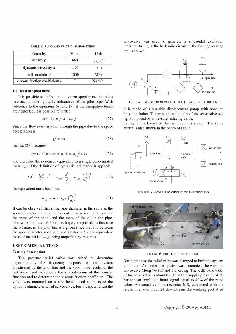
servovalve was used to generate a sinusoidal excitationpressure. In Fig. 4 the hydraulic circuit of the flow generatingunit is shown.

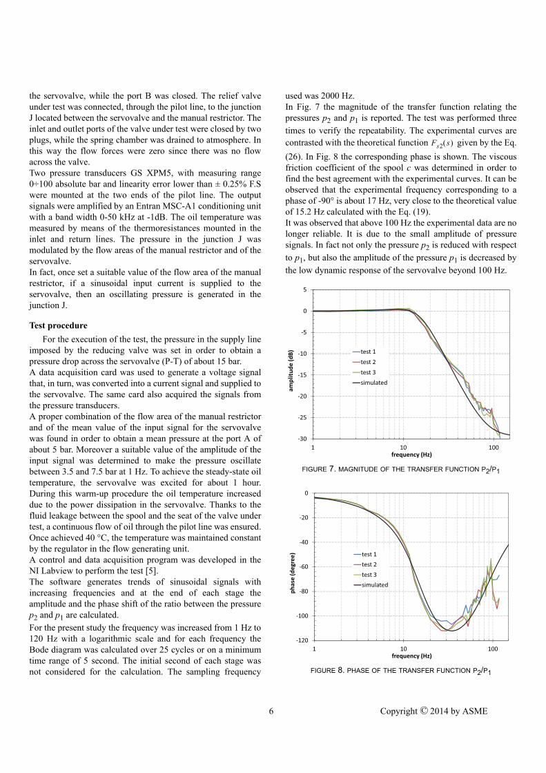
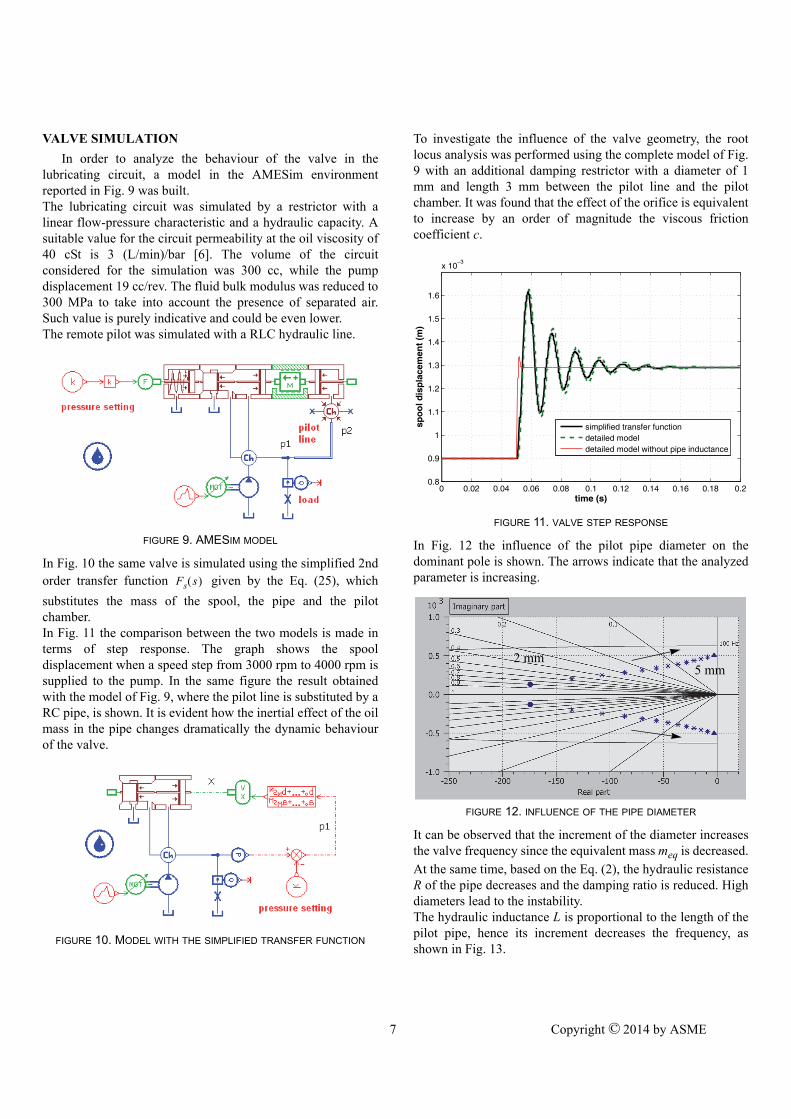
It is made of a variable displacement pump with absolutepressure limiter. The pressure at the inlet of the servovalve testrig is imposed by a pressure reducing valve.In Fig. 5 the layout of the test circuit is shown. The samecircuit is also shown in the photo of Fig. 6.

During the test the relief valve was clamped to limit the systemvibration. An interface plate was mounted between aservovalve Moog 76-103 and the test rig. The -3dB bandwidthof the servovalve is about 85 Hz with a supply pressure of 70bar and an amplitude input signal equal to 40% of the ratedvalue. A manual variable restrictor MR, connected with thereturn line, was mounted downstream the working port A of

FIGURE 4. HYDRAULIC CIRCUIT OF THE FLOW GENERATING UNIT

FIGURE 5. HYDRAULIC CIRCUIT OF THE TEST RIG

FIGURE 6. PHOTO OF THE TEST RIG

pilot line

servovalve

valve under test

P2

P1

MR


the servovalve, while the port B was closed. The relief valveunder test was connected, through the pilot line, to the junctionJ located between the servovalve and the manual restrictor. Theinlet and outlet ports of the valve under test were closed by twoplugs, while the spring chamber was drained to atmosphere. Inthis way the flow forces were zero since there was no flowacross the valve.Two pressure transducers GS XPM5, with measuring range0÷100 absolute bar and linearity error lower than ± 0.25% F.Swere mounted at the two ends of the pilot line. The outputsignals were amplified by an Entran MSC-A1 conditioning unitwith a band width 0-50 kHz at -1dB. The oil temperature wasmeasured by means of the thermoresistances mounted in theinlet and return lines. The pressure in the junction J wasmodulated by the flow areas of the manual restrictor and of theservovalve.In fact, once set a suitable value of the flow area of the manualrestrictor, if a sinusoidal input current is supplied to theservovalve, then an oscillating pressure is generated in thejunction J.

Test procedure

For the execution of the test, the pressure in the supply lineimposed by the reducing valve was set in order to obtain apressure drop across the servovalve (P-T) of about 15 bar.A data acquisition card was used to generate a voltage signalthat, in turn, was converted into a current signal and supplied tothe servovalve. The same card also acquired the signals fromthe pressure transducers.A proper combination of the flow area of the manual restrictorand of the mean value of the input signal for the servovalvewas found in order to obtain a mean pressure at the port A ofabout 5 bar. Moreover a suitable value of the amplitude of theinput signal was determined to make the pressure oscillatebetween 3.5 and 7.5 bar at 1 Hz. To achieve the steady-state oiltemperature, the servovalve was excited for about 1 hour.During this warm-up procedure the oil temperature increaseddue to the power dissipation in the servovalve. Thanks to thefluid leakage between the spool and the seat of the valve undertest, a continuous flow of oil through the pilot line was ensured.Once achieved 40 °C, the temperature was maintained constantby the regulator in the flow generating unit.A control and data acquisition program was developed in theNI Labview to perform the test [5].The software generates trends of sinusoidal signals withincreasing frequencies and at the end of each stage theamplitude and the phase shift of the ratio between the pressurep2 and p1 are calculated.

For the present study the frequency was increased from 1 Hz to120 Hz with a logarithmic scale and for each frequency theBode diagram was calculated over 25 cycles or on a minimumtime range of 5 second. The initial second of each stage wasnot considered for the calculation. The sampling frequency

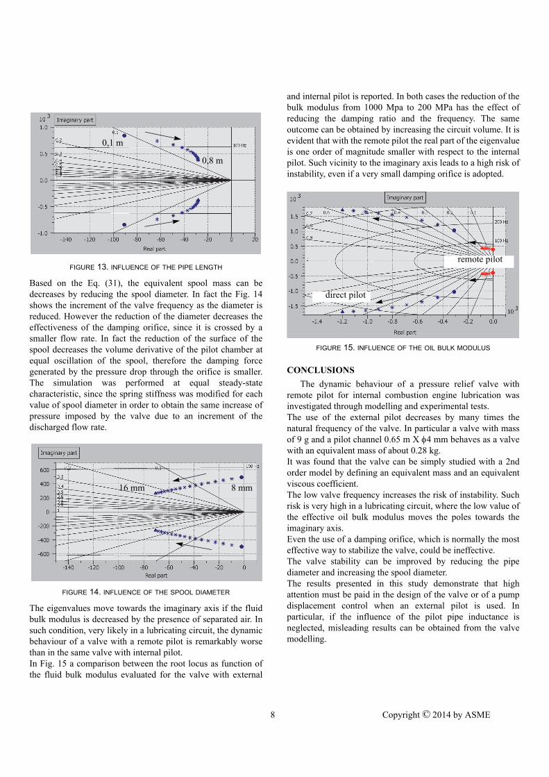
used was 2000 Hz.In Fig. 7 the magnitude of the transfer function relating thepressures p2 and p1 is reported. The test was performed three

times to verify the repeatability. The experimental curves arecontrasted with the theoretical function given by the Eq.

(26). In Fig. 8 the corresponding phase is shown. The viscousfriction coefficient of the spool c was determined in order tofind the best agreement with the experimental curves. It can beobserved that the experimental frequency corresponding to aphase of -90° is about 17 Hz, very close to the theoretical valueof 15.2 Hz calculated with the Eq. (19). It was observed that above 100 Hz the experimental data are nolonger reliable. It is due to the small amplitude of pressuresignals. In fact not only the pressure p2 is reduced with respect

to p1, but also the amplitude of the pressure p1 is decreased by

the low dynamic response of the servovalve beyond 100 Hz.

FIGURE 7. MAGNITUDE OF THE TRANSFER FUNCTION P2/P1

FIGURE 8. PHASE OF THE TRANSFER FUNCTION P2/P1

Fs2 s

15

10

5

0

5plitud

e(dB) test 1

test 2

test 3

simulated

30

25

20

1 10 100

am

frequency (Hz)

simulated

60

40

20

0

ase(degree) test 1

test 2

test 3

simulated

120

100

80

1 10 100

pha

frequency (Hz)

simulated


VALVE SIMULATION

In order to analyze the behaviour of the valve in thelubricating circuit, a model in the AMESim environmentreported in Fig. 9 was built.The lubricating circuit was simulated by a restrictor with alinear flow-pressure characteristic and a hydraulic capacity. Asuitable value for the circuit permeability at the oil viscosity of40 cSt is 3 (L/min)/bar [6]. The volume of the circuitconsidered for the simulation was 300 cc, while the pumpdisplacement 19 cc/rev. The fluid bulk modulus was reduced to300 MPa to take into account the presence of separated air.Such value is purely indicative and could be even lower.The remote pilot was simulated with a RLC hydraulic line.

In Fig. 10 the same valve is simulated using the simplified 2ndorder transfer function given by the Eq. (25), which

substitutes the mass of the spool, the pipe and the pilotchamber.In Fig. 11 the comparison between the two models is made interms of step response. The graph shows the spooldisplacement when a speed step from 3000 rpm to 4000 rpm issupplied to the pump. In the same figure the result obtainedwith the model of Fig. 9, where the pilot line is substituted by aRC pipe, is shown. It is evident how the inertial effect of the oilmass in the pipe changes dramatically the dynamic behaviourof the valve.

FIGURE 9. AMESIM MODEL

FIGURE 10. MODEL WITH THE SIMPLIFIED TRANSFER FUNCTION

Fs s

To investigate the influence of the valve geometry, the rootlocus analysis was performed using the complete model of Fig.9 with an additional damping restrictor with a diameter of 1mm and length 3 mm between the pilot line and the pilotchamber. It was found that the effect of the orifice is equivalentto increase by an order of magnitude the viscous frictioncoefficient c.

In Fig. 12 the influence of the pilot pipe diameter on thedominant pole is shown. The arrows indicate that the analyzedparameter is increasing.

It can be observed that the increment of the diameter increasesthe valve frequency since the equivalent mass meq is decreased.

At the same time, based on the Eq. (2), the hydraulic resistanceR of the pipe decreases and the damping ratio is reduced. Highdiameters lead to the instability.The hydraulic inductance L is proportional to the length of thepilot pipe, hence its increment decreases the frequency, asshown in Fig. 13.

FIGURE 11. VALVE STEP RESPONSE

FIGURE 12. INFLUENCE OF THE PIPE DIAMETER

0 0.02 0.04 0.06 0.08 0.1 0.12 0.14 0.16 0.18 0.20.8

0.9

1

1.1

1.2

1.3

1.4

1.5

1.6

x 103

time (s)

spo

ol d

isp

lace

men

t (m

)

simplified transfer functiondetailed modeldetailed model without pipe inductance

2 mm5 mm


Based on the Eq. (31), the equivalent spool mass can bedecreases by reducing the spool diameter. In fact the Fig. 14shows the increment of the valve frequency as the diameter isreduced. However the reduction of the diameter decreases theeffectiveness of the damping orifice, since it is crossed by asmaller flow rate. In fact the reduction of the surface of thespool decreases the volume derivative of the pilot chamber atequal oscillation of the spool, therefore the damping forcegenerated by the pressure drop through the orifice is smaller.The simulation was performed at equal steady-statecharacteristic, since the spring stiffness was modified for eachvalue of spool diameter in order to obtain the same increase ofpressure imposed by the valve due to an increment of thedischarged flow rate.

The eigenvalues move towards the imaginary axis if the fluidbulk modulus is decreased by the presence of separated air. Insuch condition, very likely in a lubricating circuit, the dynamicbehaviour of a valve with a remote pilot is remarkably worsethan in the same valve with internal pilot.In Fig. 15 a comparison between the root locus as function ofthe fluid bulk modulus evaluated for the valve with external

FIGURE 13. INFLUENCE OF THE PIPE LENGTH

FIGURE 14. INFLUENCE OF THE SPOOL DIAMETER

0,1 m

0,8 m

8 mm16 mm

and internal pilot is reported. In both cases the reduction of thebulk modulus from 1000 Mpa to 200 MPa has the effect ofreducing the damping ratio and the frequency. The sameoutcome can be obtained by increasing the circuit volume. It isevident that with the remote pilot the real part of the eigenvalueis one order of magnitude smaller with respect to the internalpilot. Such vicinity to the imaginary axis leads to a high risk ofinstability, even if a very small damping orifice is adopted.

CONCLUSIONS

The dynamic behaviour of a pressure relief valve withremote pilot for internal combustion engine lubrication wasinvestigated through modelling and experimental tests. The use of the external pilot decreases by many times thenatural frequency of the valve. In particular a valve with massof 9 g and a pilot channel 0.65 m X 4 mm behaves as a valvewith an equivalent mass of about 0.28 kg. It was found that the valve can be simply studied with a 2ndorder model by defining an equivalent mass and an equivalentviscous coefficient.The low valve frequency increases the risk of instability. Suchrisk is very high in a lubricating circuit, where the low value ofthe effective oil bulk modulus moves the poles towards theimaginary axis.Even the use of a damping orifice, which is normally the mosteffective way to stabilize the valve, could be ineffective.The valve stability can be improved by reducing the pipediameter and increasing the spool diameter.The results presented in this study demonstrate that highattention must be paid in the design of the valve or of a pumpdisplacement control when an external pilot is used. Inparticular, if the influence of the pilot pipe inductance isneglected, misleading results can be obtained from the valvemodelling.

FIGURE 15. INFLUENCE OF THE OIL BULK MODULUS

direct pilot

remote pilot


REFERENCES

[1] Johnston, D.N., Edge, K.A., Brunelli, M., 2002.“Impedance and stability characteristic of a relief valve”.Proc IMechE, Vol 216, Part I: Journal of Systems andControl Engineering.

[2] Alirand, M., Favennec, G., Lebrun, M., 2002. “Pressurecomponents stability analysis: a revised approach”.International Journal of Fluid Power, 3(1), pp. 33-46.

[3] Pohl, J., Krus, P., Palmberg, J.O., 1999. “Design of aPressure Relief Valve for the Lubrication System of anInternal Combustion Engine”. 4th JHPS InternationalSymposium.

[4] Rundo, M., 2010. “Piloted Displacement Controls for ICELubricating Vane Pumps”. SAE Int. Journal of Fuels andLubricants 2(2), pp. 176-184.

[5] Barberis, D., 2002. “Determinazione teorica esperimentale della risposta in frequenza delle lineeidrauliche”. M.Sc. Thesis, Politecnico di Torino.

[6] Rundo, M., Squarcini, R., 2009. “Experimental Procedurefor Measuring the Energy Consumption of IC EngineLubricating Pumps during a NEDC Driving Cycle”. SAEInt. Journal of Engines 2(1), pp. 1690-1700.

on the dynamics of pressure relief valves with external pilot for ice lubrication

Documents