Statistics & Probability Letters 44 (1999) 309–318www.elsevier.nl/locate/stapro

On improving standard estimators via linear empiricalBayes methods

Francisco J. Samaniego ∗, Eric Vestrup 1

Division of Statistics, University of California, Davis, CA 95616-8705, USA

Received June 1998; received in revised form November 1998

Abstract

Suppose one wishes to estimate the parameter � in a current experiment when one also has in hand data from kpast experiments satisfying empirical Bayes sampling assumptions. It has long been known that, for a variety of models,empirical Bayes estimators tend to outperform, asymptotically, standard estimators based on the current experiment alone.Much less is known about the superiority of empirical Bayes estimators over standard estimators when k is �xed; what isknown in that regard is largely the product of Monte Carlo studies. Conditions are given here under which certain linearempirical Bayes estimators are superior to the standard estimator for arbitrary k¿1. c© 1999 Elsevier Science B.V. Allrights reserved

Keywords: Empirical Bayes; Bayes risk; Linear decision rules; Parametric empirical Bayes problems

1. Introduction

The empirical Bayes (EB) framework, as introduced by Robbins (1955), presumes the existence of asequence of independent but similar experiments. More precisely, it is assumed that the parameter valuesgoverning these experiments may vary, with that assumption quanti�ed as

�1; : : : ; �k ; �k+1i:i:d:∼ G; (1)

where the prior distribution G is unknown. It is further assumed that

Xi|�i ∼ F�i ; i = 1; : : : ; k + 1; (2)

where, typically, F�i is assumed to be a member of some �xed parametric family. The independence of therandom pairs (Xi; �i) and (Xj; �j) for all i 6= j is tacitly assumed. Robbins’ stated goal, and ours, is that of

∗ Corresponding author.E-mail address: fjsamaniego@ucdavis.edu (F.J. Samaniego)1 Now with Dept. of Mathematics, De Paul University, Chicago, IL 60614, USA.

0167-7152/99/$ - see front matter c© 1999 Elsevier Science B.V. All rights reservedPII: S0167 -7152(99)00022 -X

310 F.J. Samaniego, E. Vestrup / Statistics & Probability Letters 44 (1999) 309–318

estimating the parameter value �k+1 in the current experiment based on the current datum Xk+1 and, possibly,on data X1; : : : ; Xk from past experiments.Following Robbins, we will restrict attention to squared error as a loss criterion, and employ the (expected)

Bayes risk r(G; d) of a rule d relative to the true prior G, that is,

r(G; d) = E�∼EX | �∼

(d(X)− �k+1)2; (3)

as our measure of its performance. Since the “true prior” G is unknown, the Bayes rule dG for estimating�k+1, that is, the rule which minimizes r(G; ·) in Eq. (3), is unavailable as an estimator of �k+1. Robbinsnoted that one could e�ectively approximate dG using data from past experiments. For example, when F� isthe Poisson model, dG may be expressed as

dG(x) =(x + 1)pG(x + 1)

pG(x); (4)

where pG(·) is the marginal probability mass function (pmf) of X , so that one might utilize the decision rule

dk(xk+1) =(xk+1 + 1)pk(xk+1 + 1)

pk(xk+1)(5)

as an EB estimator of �k+1, where pk(·) is the empirical pmf based on X1; : : : ; Xk . It is clear from Eqs.(4) and (5) that, for all integers x¿0; dk(x)→dG(x) as k→∞. Johns (1956) showed that dk was indeed“asymptotically optimal”, i.e. that

r(G; dk)→ r(G; dG) (6)

as k→∞, provided that the prior G has �nite second moment.Aside from demonstrations of the asymptotic optimality of EB rules in various settings, there has been rather

little analytical work on the comparative performance of EB rules. One issue that has generated considerableinterest, but no de�nitive results, is the comparison of various EB rules based on a �xed number of pastexperiments with a standard estimator (the MLE or UMVUE, e.g.) based on the current experiment alone.What is generally known is that most “reasonable” EB rules outperform the standard rule if k is su�cientlylarge. If d∗ represents the standard estimator, with dk representing an EB rule of interest, then the questionwe wish to shed light on here pertains to the nature of the set K= {k : r(G; dk) 6 r(G; d∗)}.Let k∗ be the smallest member of the set K, i.e., let k∗ be the smallest number of past experiments needed

for dk to dominate the standard rule. What is presently known about k∗ has been derived, primarily, fromsimulation studies. Maritz and Lwin (1989), e.g. compared the performance of seven EB rules in the problemof estimating a Poisson parameter �51 in the current (51st) experiment when the true prior was modeledas a speci�c gamma distribution. They found that Robbins’ estimator d50 in Eq. (5) performed very poorlyrelative to the MLE d∗(x51)= x51, but that certain other EB rules, especially those involving some smoothing,performed better than the MLE. In that particular study, it is evident that, for the right EB estimator, k∗ issubstantially smaller than 50. In other comparative simulation studies, Canavos (1973) and Bennett (1977)showed that, for certain classes of prior distributions, smooth EB estimators of exponential or Weibull failurerates were generally superior to the MLE in the (k + 1)st experiment when k was quite small. To ourknowledge, however, there have been no theoretical results which characterize or bound the threshold valuek∗. Indeed, Maritz and Lwin (1989, p. 87) state: “Obtaining analytical results for rk(G;EB), where EB herestands for any empirical Bayes estimator : : : seems virtually impossible, except as approximations for large k”.In this paper, we study the performance of a certain class of convex empirical Bayes estimators (CEBEs)

of �k+1, and demonstrate that, in the context studied, there is always a subclass of such estimators whoseperformance is superior to that of “the standard estimator” of �k+1 based on the current experiment alone.While, in general, the best convex empirical Bayes estimator (BCEBE) depends formally on the �rst twomoments of the true prior G, examples are given of parametric empirical Bayes problems in which the

F.J. Samaniego, E. Vestrup / Statistics & Probability Letters 44 (1999) 309–318 311

BCEBE can be computed explicitly. In such problems, we are thus able to derive a most satisfying answerto the question: what is the value of the constant k∗? In Section 2, we identify a class of problems in whichk∗ = 1. Thus, even with only one past experiment, there are EB rules of a very speci�c form that dominatethe standard rule based solely on the current experiment. In Section 3, we treat the general empirical Bayesproblem, showing that, for arbitrary values of k, a certain class of EB rules provides uniform improvementover the standard rule.

2. The case of one past experiment

We proceed directly to our main result. The subscripts on the expectations below will be subsumedwhen clarity is not compromised thereby; variances will be denoted by V . A bold E represents expecta-tion with respect to the joint distribution of the random vectors X and �. The empirical Bayes framework inEqs. (1) and (2) is broadened slightly in the theorem below; the model for the conditional distribution of Xis permitted to vary from one experiment to the next.

Theorem 1. Let (�1; X1) and (�2; X2) be independent random pairs satisfying

�1; �2i:i:d:∼ G (7)

and

Xi|�i ∼ F (i)�i ; i = 1; 2; (8)

where G and F (i)�i are distributions having �nite second moments. If Xi is an unbiased estimator of �i fori = 1; 2; then r(G; cX1 + (1− c)X2)¡r(G; X2) for any constant c satisfying

0¡c¡2EV (X2|�2)

EV (X1|�1) + EV (X2|�2) + 2V (�) ; (9)

where � is a generic random variable having distribution G.

Proof. We may write

r(c) = r(G; cX1 + (1− c)X2)=E(�2 − cX1 − (1− c)X2)2 (10)

= E(c(�2 − X1) + (1− c) (�2 − X2))2 (11)

= c2E(X1 − �2)2 + (1− c)2E(X2 − �2)2; (12)

since the cross product term obtained in expanding the quadratic in Eq. (11) vanishes on account of theunbiasedness of X2. The Bayes risk in Eq. (12), being quadratic in c, is uniquely minimized by the positivevalue

c∗ =E(X2 − �2)2

E(X1 − �2)2 + E(X2 − �2)2 ; (13)

and, in fact, r(c)¡r(0) for any c∈ (0; 2c∗). We complete the proof by showing that 2c∗ may be rewritten asthe right-hand side of Eq. (9). Clearly,

E(X2 − �2)2 = E�2EX2|�2 (X2 − �2)2 (14)

= EV (X2|�2); (15)

312 F.J. Samaniego, E. Vestrup / Statistics & Probability Letters 44 (1999) 309–318

while, by the unbiasedness of X1, we obtain

E(X1 − �2)2 = E�∼EX| �∼(X1 − �1)2 + E�∼

EX| �∼(�1 − �2)2 (16)

= EV (X1|�1) + V (�1 − �2) (17)

= EV (X1|�1) + 2V (�): (18)

Substituting Eqs. (15) and (18) into Eq. (13) yields the desired expression in (9).

The inequality in Eq. (9) provides information about the mixing constant c in a readily interpretable form.It indicates, for example, that only in the case that X2 is degenerate at �2 is it impossible to improve uponX2 as an estimator of �2. Further, it indicates that the size of c, that is, the weight one would wish to placeon the past datum X1, depends on the variability of X1; X2 and �. One should place substantial weight on X1when(i) � is not highly variable, and(ii) X2 is much more variable than X1.These observations, extracted quite easily from Eq. (9), agree with one’s native intuition on this problem

since, together, conditions (i) and (ii) imply that �1 and �2 are close, so that the past experiment does provideuseful information about the current parameter, and that, under such a circumstance, a precise estimate of �1is more useful as an estimator of �2 than an imprecise estimator of �2.Note that since

EV (Xi|�i) = V (Xi)− V (�i) for i = 1; 2; (19)

the constant c∗ in Eq. (13) may be rewritten as

c∗ =V (X2)− VG(�)V (X1) + V (X2)

: (20)

When VG(�) = 0, that is, when G is degenerate at the (unknown) point �0, and the model F� is the same ineach experiment (as in Eq. (2)), then c∗ in Eq. (20) reduces to the familiar c∗ = 1=2. When VG(�) is large,borrowing strength from the past is still bene�cial, but the weight assigned to X1 in the convex combinationcX1 + (1− c)X2 should be suitably small.In many problems of interest, a rough upper bound for c may be obtained by examining plausible priors

in some parametric class. It should be noted that a conservative choice of c, smaller than an approximatedoptimal value c∗, might be reasonable when one’s intuition about the variability of � is a bit fuzzy. As ithappens, there are situations in which the optimal EB rule of the form cX1 + (1 − c)X2 may be identi�edexplicitly. We give two examples of such situations below, both in the context of empirical Bayes estimationwith parametric, but not completely speci�ed, priors. See Morris (1983) for a detailed discussion of theparametric empirical Bayes approach.

Example 1. Consider a “parametric Empirical Bayes” treatment of Robbins’ Poisson problem. Assume that,for i = 1; 2; Xi|�i ∼ P(�i) and �1; �2 i:i:d:∼ �(�; 1); where �(�; 1) is the gamma distribution with density

f(�|�) = 1�(�)

��−1e−�I(0;∞) (�):

The posterior distribution of �2, given X2 = x2, is the �(� + x2; 1=2) distribution, so that the Bayes estimateof �2, were � known, would be

dG(x2) = 12 (�+ x2):

F.J. Samaniego, E. Vestrup / Statistics & Probability Letters 44 (1999) 309–318 313

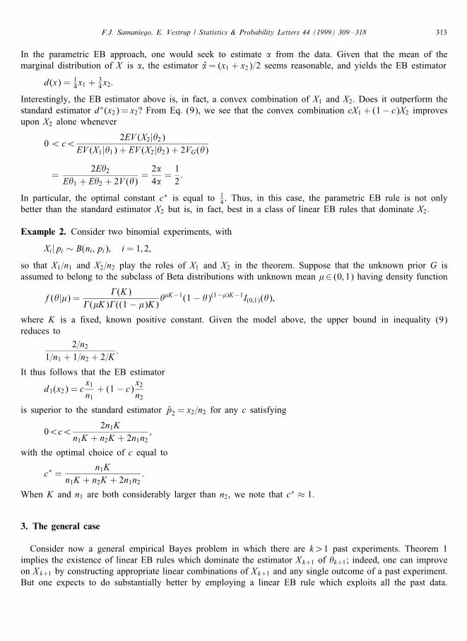
In the parametric EB approach, one would seek to estimate � from the data. Given that the mean of themarginal distribution of X is �, the estimator �̂= (x1 + x2)=2 seems reasonable, and yields the EB estimator

d(x) = 14x1 +

34x2:

Interestingly, the EB estimator above is, in fact, a convex combination of X1 and X2. Does it outperform thestandard estimator d∗(x2) = x2? From Eq. (9), we see that the convex combination cX1 + (1− c)X2 improvesupon X2 alone whenever

0¡c¡2EV (X2|�2)

EV (X1|�1) + EV (X2|�2) + 2VG(�)

=2E�2

E�1 + E�2 + 2V (�)=2�4�=12:

In particular, the optimal constant c∗ is equal to 14 . Thus, in this case, the parametric EB rule is not only

better than the standard estimator X2 but is, in fact, best in a class of linear EB rules that dominate X2.

Example 2. Consider two binomial experiments, with

Xi|pi ∼ B(ni; pi); i = 1; 2;

so that X1=n1 and X2=n2 play the roles of X1 and X2 in the theorem. Suppose that the unknown prior G isassumed to belong to the subclass of Beta distributions with unknown mean �∈ (0; 1) having density function

f(�|�) = �(K)�(�K)�((1− �)K)�

�K−1(1− �)(1−�)K−1I(0;1)(�);

where K is a �xed, known positive constant. Given the model above, the upper bound in inequality (9)reduces to

2=n21=n1 + 1=n2 + 2=K

:

It thus follows that the EB estimator

d1(x2) = cx1n1+ (1− c) x2

n2is superior to the standard estimator p̂2 = x2=n2 for any c satisfying

0¡c¡2n1K

n1K + n2K + 2n1n2;

with the optimal choice of c equal to

c∗ =n1K

n1K + n2K + 2n1n2:

When K and n1 are both considerably larger than n2, we note that c∗ ≈ 1.

3. The general case

Consider now a general empirical Bayes problem in which there are k¿1 past experiments. Theorem 1implies the existence of linear EB rules which dominate the estimator Xk+1 of �k+1; indeed, one can improveon Xk+1 by constructing appropriate linear combinations of Xk+1 and any single outcome of a past experiment.But one expects to do substantially better by employing a linear EB rule which exploits all the past data.

314 F.J. Samaniego, E. Vestrup / Statistics & Probability Letters 44 (1999) 309–318

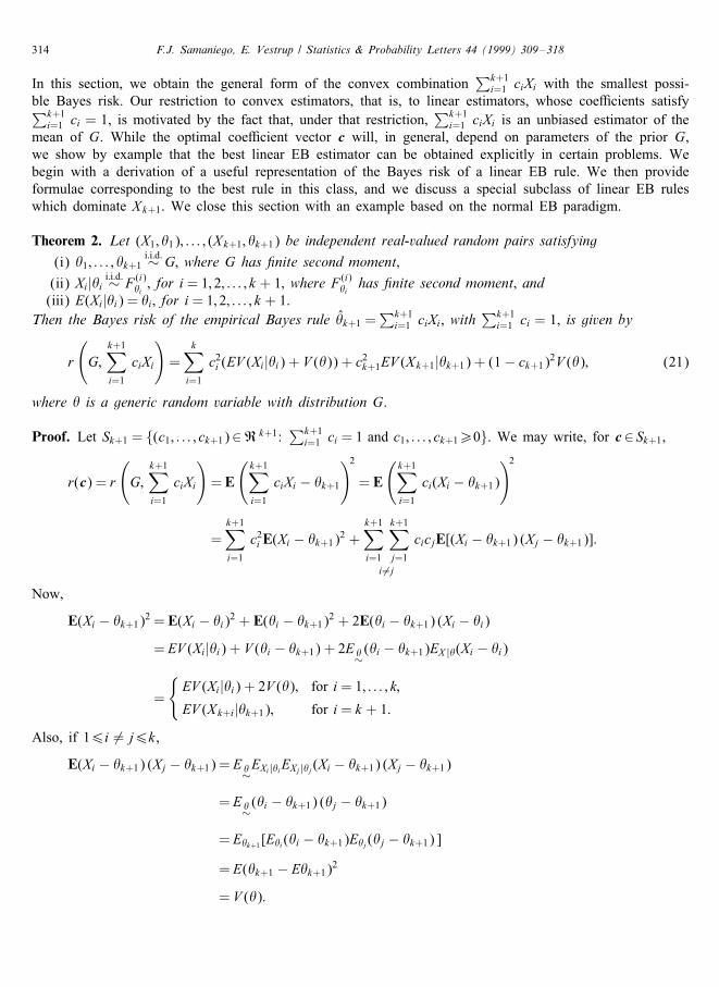
In this section, we obtain the general form of the convex combination∑k+1

i=1 ciXi with the smallest possi-ble Bayes risk. Our restriction to convex estimators, that is, to linear estimators, whose coe�cients satisfy∑k+1

i=1 ci = 1, is motivated by the fact that, under that restriction,∑k+1

i=1 ciXi is an unbiased estimator of themean of G. While the optimal coe�cient vector c will, in general, depend on parameters of the prior G,we show by example that the best linear EB estimator can be obtained explicitly in certain problems. Webegin with a derivation of a useful representation of the Bayes risk of a linear EB rule. We then provideformulae corresponding to the best rule in this class, and we discuss a special subclass of linear EB ruleswhich dominate Xk+1. We close this section with an example based on the normal EB paradigm.

Theorem 2. Let (X1; �1); : : : ; (Xk+1; �k+1) be independent real-valued random pairs satisfying(i) �1; : : : ; �k+1

i:i:d:∼ G; where G has �nite second moment;(ii) Xi|�i i:i:d:∼ F (i)�i ; for i = 1; 2; : : : ; k + 1; where F

(i)�ihas �nite second moment; and

(iii) E(Xi|�i) = �i; for i = 1; 2; : : : ; k + 1.Then the Bayes risk of the empirical Bayes rule �̂k+1 =

∑k+1i=1 ciXi, with

∑k+1i=1 ci = 1, is given by

r

(G;

k+1∑i=1

ciXi

)=

k∑i=1

c2i (EV (Xi|�i) + V (�)) + c2k+1EV (Xk+1|�k+1) + (1− ck+1)2V (�); (21)

where � is a generic random variable with distribution G.

Proof. Let Sk+1 = {(c1; : : : ; ck+1)∈R k+1:∑k+1

i=1 ci = 1 and c1; : : : ; ck+1¿0}. We may write, for c ∈ Sk+1,

r(c) = r

(G;

k+1∑i=1

ciXi

)=E

(k+1∑i=1

ciXi − �k+1)2= E

(k+1∑i=1

ci(Xi − �k+1))2

=k+1∑i=1

c2i E(Xi − �k+1)2 +k+1∑i=1

k+1∑j=1

i 6=j

cicjE[(Xi − �k+1) (Xj − �k+1)]:

Now,

E(Xi − �k+1)2 =E(Xi − �i)2 + E(�i − �k+1)2 + 2E(�i − �k+1) (Xi − �i)= EV (Xi|�i) + V (�i − �k+1) + 2E�∼(�i − �k+1)EX |�(Xi − �i)

=

{EV (Xi|�i) + 2V (�); for i = 1; : : : ; k;EV (Xk+i|�k+1); for i = k + 1:

Also, if 16i 6= j6k,E(Xi − �k+1) (Xj − �k+1) = E�∼EXi|�iEXj|�j (Xi − �k+1) (Xj − �k+1)

= E�∼(�i − �k+1) (�j − �k+1)

= E�k+1 [E�i(�i − �k+1)E�j (�j − �k+1) ]= E(�k+1 − E�k+1)2

= V (�):

F.J. Samaniego, E. Vestrup / Statistics & Probability Letters 44 (1999) 309–318 315

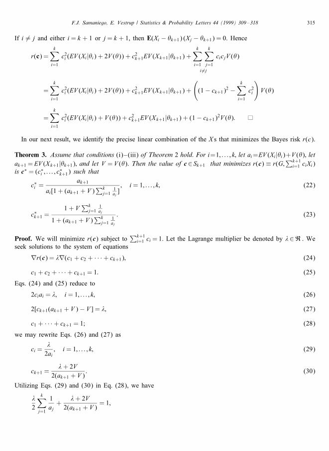
If i 6= j and either i = k + 1 or j = k + 1, then E(Xi − �k+1) (Xj − �k+1) = 0. Hence

r(c) =k∑i=1

c2i (EV (Xi|�i) + 2V (�)) + c2k+1EV (Xk+1|�k+1) +k∑i=1

k∑j=1

i 6=j

cicjV (�)

=k∑i=1

c2i (EV (Xi|�i) + 2V (�)) + c2k+1EV (Xk+1|�k+1) +((1− ck+1)2 −

k∑i=1

c2i

)V (�)

=k∑i=1

c2i (EV (Xi|�i) + V (�)) + c2k+1EV (Xk+1|�k+1) + (1− ck+1)2V (�):

In our next result, we identify the precise linear combination of the X s that minimizes the Bayes risk r(c).

Theorem 3. Assume that conditions (i)–(iii) of Theorem 2 hold. For i=1; : : : ; k; let ai=EV (Xi|�i)+V (�); letak+1 = EV (Xk+1|�k+1); and let V = V (�). Then the value of c ∈ Sk+1 that minimizes r(c) ≡ r(G;∑k+1

i=1 ciXi)is c∗ = (c∗i ; : : : ; c

∗k+1) such that

c∗i =ak+1

ai[1 + (ak+1 + V )∑k

j=11aj]; i = 1; : : : ; k; (22)

c∗k+1 =1 + V

∑kj=1

1aj

1 + (ak+1 + V )∑k

j=11aj

: (23)

Proof. We will minimize r(c) subject to∑k+1

i=1 ci =1. Let the Lagrange multiplier be denoted by �∈R . Weseek solutions to the system of equations

∇r(c) = �∇(c1 + c2 + · · ·+ ck+1); (24)

c1 + c2 + · · ·+ ck+1 = 1: (25)

Eqs. (24) and (25) reduce to

2ciai = �; i = 1; : : : ; k; (26)

2[ck+1(ak+1 + V )− V ] = �; (27)

c1 + · · ·+ ck+1 = 1; (28)

we may rewrite Eqs. (26) and (27) as

ci =�2ai; i = 1; : : : ; k; (29)

ck+1 =�+ 2V

2(ak+1 + V ): (30)

Utilizing Eqs. (29) and (30) in Eq. (28), we have

�2

k∑j=1

1aj+

�+ 2V2(ak+1 + V )

= 1;

316 F.J. Samaniego, E. Vestrup / Statistics & Probability Letters 44 (1999) 309–318

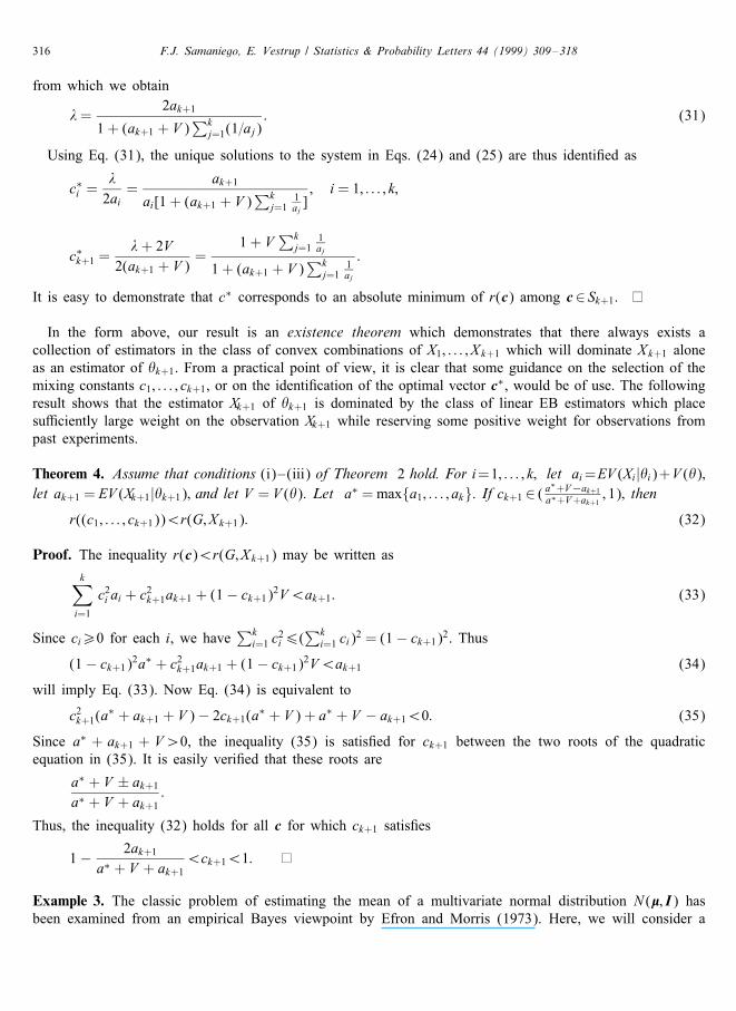
from which we obtain

�=2ak+1

1 + (ak+1 + V )∑k

j=1(1=aj): (31)

Using Eq. (31), the unique solutions to the system in Eqs. (24) and (25) are thus identi�ed as

c∗i =�2ai

=ak+1

ai[1 + (ak+1 + V )∑k

j=11aj]; i = 1; : : : ; k;

c∗k+1 =�+ 2V

2(ak+1 + V )=

1 + V∑k

j=11aj

1 + (ak+1 + V )∑k

j=11aj

:

It is easy to demonstrate that c∗ corresponds to an absolute minimum of r(c) among c ∈ Sk+1.

In the form above, our result is an existence theorem which demonstrates that there always exists acollection of estimators in the class of convex combinations of X1; : : : ; Xk+1 which will dominate Xk+1 aloneas an estimator of �k+1. From a practical point of view, it is clear that some guidance on the selection of themixing constants c1; : : : ; ck+1, or on the identi�cation of the optimal vector c∗, would be of use. The followingresult shows that the estimator Xk+1 of �k+1 is dominated by the class of linear EB estimators which placesu�ciently large weight on the observation Xk+1 while reserving some positive weight for observations frompast experiments.

Theorem 4. Assume that conditions (i)–(iii) of Theorem 2 hold. For i=1; : : : ; k; let ai=EV (Xi|�i)+V (�);let ak+1 = EV (Xk+1|�k+1); and let V = V (�). Let a∗ =max{a1; : : : ; ak}. If ck+1 ∈ ( a

∗+V−ak+1a∗+V+ak+1

; 1); then

r((c1; : : : ; ck+1))¡r(G; Xk+1): (32)

Proof. The inequality r(c)¡r(G; Xk+1) may be written ask∑i=1

c2i ai + c2k+1ak+1 + (1− ck+1)2V¡ak+1: (33)

Since ci¿0 for each i, we have∑k

i=1 c2i6(

∑ki=1 ci)

2 = (1− ck+1)2. Thus(1− ck+1)2a∗ + c2k+1ak+1 + (1− ck+1)2V¡ak+1 (34)

will imply Eq. (33). Now Eq. (34) is equivalent to

c2k+1(a∗ + ak+1 + V )− 2ck+1(a∗ + V ) + a∗ + V − ak+1¡0: (35)

Since a∗ + ak+1 + V¿0, the inequality (35) is satis�ed for ck+1 between the two roots of the quadraticequation in (35). It is easily veri�ed that these roots are

a∗ + V ± ak+1a∗ + V + ak+1

:

Thus, the inequality (32) holds for all c for which ck+1 satis�es

1− 2ak+1a∗ + V + ak+1

¡ck+1¡1:

Example 3. The classic problem of estimating the mean of a multivariate normal distribution N (�; I) hasbeen examined from an empirical Bayes viewpoint by Efron and Morris (1973). Here, we will consider a

F.J. Samaniego, E. Vestrup / Statistics & Probability Letters 44 (1999) 309–318 317

related problem, that of estimating a single component �k+1 of a (k + 1) dimensional mean vector, takingthe view that the information on the other components of � as data from k past experiments. Speci�cally,suppose that the (k + 1) random pairs (Xi; �i), are independent, with

�1; �2; : : : ; �k ; �k+1i:i:d:∼ N (�0; 1);

Xi|�i ∼ N (�i; 1); for i = 1; : : : ; k + 1:

Using the notation of Theorem 3, we have, V = V (�) = 1 and

ai = EV (Xi|�i) + V (�) = E(1) + 1 = 2; for i = 1; : : : ; k

ak+1 = EV (Xk+1|�k+1) = 1:It follows that the best convex EB estimator (BCEBE) of �k+1 is given by

�̂k+1 =k+1∑i=1

c∗i Xi;

where

c∗i =1

2[1 + 2∑k

1(12 ) ]

=1

2k + 2;

c∗k+1 =1 + 1

∑k1(12 )

1 + 2∑k

112

=k + 22k + 2

:

Thus, the BCEBE in this problem is the estimator

�̂k+1 =k

2k + 2Xk +

k + 22k + 2

Xk+1;

where

Xk =1k

k∑i=1

Xi:

In the case of one past experiment, that is, when k = 1, the best linear EB rule places weight 3=4 on thecurrent observation and weight 1=4 on the past observation.

4. Discussion

The primary domain of application of these results is to problems in which the standard estimator in thecurrent experiment is unbiased. This tends to be the case in many common problems involving exponentialfamilies, and includes the problems of estimating a Binomial proportion or the mean of a Poisson, normalor exponential distribution. It must be borne in mind, of course, that the empirical Bayes assumptions areessential and are stringent enough to eliminate many settings in which combining data from disparate sourcesmight be contemplated. As is well recognized, Robbins’ empirical Bayes approach is a frequentist theory ofinference which utilizes no prior modeling regarding unknown parameters. Bayes empirical Bayes methodshave been treated by, among others, Deely and Lindley (1981) and Walter and Hamedani (1991). For ananalysis complementary to the present one which compares Bayes estimators in an empirical Bayes setting,see Samaniego and Neath (1996).

318 F.J. Samaniego, E. Vestrup / Statistics & Probability Letters 44 (1999) 309–318

References

Bennett, G.K., 1977. Basic concepts of empirical Bayes methods with some results for the Weibull distribution. In: Tsokos, C., Shimi,I.N. (Eds.), The Theory and Applications of Reliability, vol. II. Academic Press, New York, pp. 181–202.

Canavos, G.C., 1973. An empirical Bayes approach for the Poisson life distribution. IEEE Trans. Reliab. R-22, 91–96.Deely, J., Lindley, D., 1981. Bayes empirical Bayes. J. Amer. Statist. Assoc. 76, 833–841.Efron, B., Morris, C., 1973. Stein’s estimation rule and its competitors – an empirical Bayes approach. J. Amer. Statist. Assoc.68, 117–130.

Johns, M.V. Jr., 1956. Contributions to the theory of non-parametric empirical Bayes procedures in statistics. Unpublished Ph.D.Dissertation, Columbia University.

Maritz, J.S., Lwin, T., 1989. Empirical Bayes Methods. Chapman and Hall, London.Morris, C., 1983. Parametric empirical Bayes inference: theory and applications. J. Amer. Statist. Assoc. 78, 47–65 (with discussion).Robbins, H., 1955. An empirical Bayes approach to statistics. Proc. 3rd Berkeley Symp. on Mathematical Statistics and Probability. UCPress, Berkeley.

Samaniego, F.J., Neath, A.A., 1996. How to be a better Bayesian. J. Amer. Statist. Assoc. 91, 733–742.Walter, G., Hamedani, G., 1991. Bayes empirical Bayes estimation for natural exponential families with quadratic variance functions.Ann. Statist. 19, 1191–1224.