This is a free offprint provided to the author by the publisher. Copyright restrictions may apply.

QUARTERLY OF APPLIED MATHEMATICS

VOLUME LXVIII, NUMBER 3

SEPTEMBER 2010, PAGES 591–606

S 0033-569X(2010)01174-3

Article electronically published on May 19, 2010

ON DIFFUSIVE SLOWDOWN

IN THREE-LAYER HELE-SHAW FLOWS

By

PRABIR DARIPA (Department of Mathematics, Texas A&M University, College Station, Texas77843 )

and

GELU PASA (Institute of Mathematics “Simion Stoillow” of Romanian Academy, Bucharest,Romania 70700 )

Abstract. In a recently published article of Daripa and Pasa [Transp. Porous Media

(2007) 70:11-23], the stabilizing effect of diffusion in three-layer Hele-Shaw flows was

proved using an exact analysis of normal modes. In particular, this was established from

an upper bound on the growth rate of instabilities which was derived from analyzing

stability equations. However, the method used there is not constructive in the sense that

the upper bound derived from actual numerical discretization of the problem could be

significantly different from the exact one reported depending on the scheme used. In

this paper, a numerical approach to solve the stability equations using a finite difference

scheme is presented and analyzed. An upper bound on the growth rate is derived from

numerical analysis of the discrete system which also shows the diffusive slowdown of

instabilities. Upper bounds obtained by this numerical approach and by the analytical

approach are compared. The present approach is constructive and directly leads to

the implementation of the numerical approach to obtain approximate solutions in the

presence of diffusion. The contributions of the paper are the novelty of the approach and

a bound on the growth rates that does not depend on the solution itself.

1. Introduction. The subject of multi-layer (more than two-layer) multi-phase flows

has received much less attention than similar two-layer flows, partly because of the level

of difficulty associated with studies of such flows. Such flows are usually richer in com-

plexity and involve many parameters and variables whose control and manipulations in

innovative ways can prove to be useful technologically. To make theoretical and com-

putational advances in this direction, the mathematical formulation of such problems is

the first necessary step. One such problem that has received some attention ([11], [3]),

partly motivated by industrial applications ([14], [17], [23], [25], [28]), involves three-layer

Received February 1, 2009.2000 Mathematics Subject Classification. Primary 76E17, 76T30, 76R50, 65F99, 65Q05.E-mail address: daripa@math.tamu.eduE-mail address: Gelu.Pasa@imar.ro

c©2010 Brown UniversityReverts to public domain 28 years from publication

591

This is a free offprint provided to the author by the publisher. Copyright restrictions may apply.

592 PRABIR DARIPA AND GELU PASA

immiscible flows in Hele-Shaw cells involving two sharp interfaces initially. The physical

setup of the problem involves three layers of fluid in a Hele-Shaw cell with the least vis-

cous fluid such as water displacing an intermediate layer of fluid having variable viscosity.

This layer in turn displaces the most viscous fluid such as oil. The fluid in the interme-

diate layer is an aqueous phase consisting of a polymer in water. Pointwise viscosity of

this aqueous phase (to be called ‘poly-solution’ henceforth) in this intermediate layer de-

pends on the local concentration of the polymer. In our model, the polymer is passively

advected by the fluid and therefore, the viscosity profile of the middle layer dynamically

evolves with the velocity field in this region. The simplest nontrivial admissible solution

of the underlying equations is the uniform motion of all three layers having two planar

interfaces separating these three layers. The stability of this system has been addressed

earlier (see [3], [5]) for arbitrary viscosity profiles in the intermediate layer.

In this paper, our model allows diffusion of the polymer in the above problem setup.

In a recent paper, Daripa and Pasa ([6]) first mathematically formulated this problem

incorporating diffusion of the polymer in the middle layer. In that paper, stability

equations were derived in a form suitable for classical analysis using normal modes. The

resulting eigenvalue problem was then analyzed using weak formulation in order to obtain

quantitative results about the effect of diffusion on flow instability. Such results were

obtained in the form of upper bounds on the growth rate. The present paper develops a

constructive method to obtain similar bounds as in Daripa and Pasa [6] using numerical

analysis. The method is constructive in the sense that the bounds are obtained by first

developing a numerical scheme to solve the stability equations whose implementation and

subsequent mining of numerical data to obtain approximate solutions will be taken up in

the future. An interesting possibility is that there could be transient growth, because the

original problem is not selfadjoint. This might change the conclusion that the polymeric

diffusivity stabilizes the flow. A reference to transient growth and its applications is the

book of Henningson and Schmidt.

In most fluid flows, molecular diffusion slows down the growth of instabilities except

for some flows such as parallel shear flows. Such cannot be said, without analytical

justification, of the role of polymer diffusion in this problem since its role is somewhat

different from that of molecular diffusion in fluid flows. In the middle layer, instabilities

create nonuniformities in polymer concentration, which in turn drives diffusion of the

polymer, an effect neglected thus far in the literature. This diffusion of the polymer

dynamically changes the local viscosity gradients in the middle layer and the magnitudes

of jumps in viscosities across the interfaces which respectively drive the growth rates of

instabilities in the middle layer and on two interfaces. The extent to which the growth of

these instabilities is affected depends on the diffusion coefficient. Quantifying this effect

in terms of the diffusion coefficient can be useful in providing an insight into the rough

effect of diffusion on the flow. In this paper, we investigate these issues using numerical

discretization of the underlying stability equations.

We obtain bounds on the growth rate using numerical analysis of the stability equa-

tions. The diffusion coefficient dependent bound obtained numerically clearly shows

diffusive slowdown of instabilities which supports our results reported recently in Daripa

and Pasa [6]. Since the method presented here relies on first developing a numerical

This is a free offprint provided to the author by the publisher. Copyright restrictions may apply.

DIFFUSIVE SLOWDOWN IN HELE-SHAW FLOWS 593

scheme to solve the stability equations, the numerical scheme given here can be imple-

mented, if so desired, to construct approximate solutions. This will allow one to explore

numerically the effects of diffusion on the modal growth rates and eigenfunctions of the

normal modes. We must stress that these numerical implementation issues are not the

subject of this paper, though we intend to undertake this task in the future.

It is important to emphasize here that the purpose of the numerical analysis of the

specific scheme carried out here is not so much as to just obtain a bound on a physical

quantity (i.e., the maximal growth rate) but to ensure that the numerical scheme pro-

posed for solving the stability equations has some desirable properties of the continuum

equations that are useful to have before using the scheme to construct approximate solu-

tions. Numerically estimating the bound and assuring that it compares reasonably well

with the exact bound, which has been done in this paper, precisely serves that purpose.

This scheme then should be useful in computing the early stages of evolution of initial

disturbances. The evolution of interfacial disturbances based on this scheme during ini-

tial stages then can be used as a benchmark for the purpose of validating any numerical

calculation for the full initial value problem from which linear stability equations are

derived. This is another motivation for the work carried out in this paper.

Since three-layer Hele-Shaw flows with diffusion partly build upon two-layer Hele-

Shaw flows, it is appropriate to add some relevant literature on various pertinent aspects

of such two-layer flows, which we do next in this paragraph. There have been extensive

experimental, theoretical and numerical works on two-layer immiscible as well as miscible

Hele-Shaw flows. The literature is huge, and we can cite only a few here. The earliest

theoretical works on viscosity-jump driven interfacial instability of such two-layer immis-

cible flows date back to the late fifties (see [21], [19] for Hele-Shaw flows and [2] for flows

in permeable media). Subsequently, there have been many studies on such two-layer flows

such as exact nontrivial solutions in the form of fingers with and without surface tension

([7], [27], [12], [29]), singularity formation (see [18]), numerical and perturbation studies

([1], [16]), etc. For more exhaustive references on various numerical, experimental, and

theoretical works, the review articles of Saffman (see [20]) and Kessler et al. (see [13]) are

worth mentioning. Towards this end, works of Hickernell and Yortsos (see [8]), Yortsos

and Zeybek (see [30]), Loggia et al. (see [15]), and Shariati and Yortsos (see [24]) on

two-layer miscible flows should also be cited.

In closing this section, we comment on how this work on Hele-Shaw flows relates to

porous media. In porous media, transport of reactive as well as nonreactive species occurs

in a myriad of processes either naturally and/or artificially by design, e.g., transport

of contaminants, transport of biomass and solutes, transport of various species during

various oil recovery processes, just to mention a few. In modeling such porous media flow

processes involving a variety of species, diffusion of species naturally plays a significant

role. Therefore, assessing the effect of species diffusion on various flow processes including

hydrodynamic stability is important. This is what we do in this paper for immiscible

flows using the Hele-Shaw model as opposed to the more appropriate Buckley-Leverett

model, but this compromise has an insignificant effect on the basic problem of diffusive

slowdown we are addressing here. For example, the displacement of oil by water in

porous media by the Buckley-Leverett model allows shock waves and rarefaction waves

This is a free offprint provided to the author by the publisher. Copyright restrictions may apply.

594 PRABIR DARIPA AND GELU PASA

in saturation. A shock wave creates a jump in mobility across it, whereas the saturation

waves behind the shock wave create a mobility gradient behind the shock. To a large

extent, this is very well modeled using Hele-Shaw models instead with a sharp jump in

viscosity (mobility) across the interface separating displaced and displacing fluids and a

viscous profile behind the interface modeling the effect of rarefaction waves. The Hele-

Shaw model that we consider below has all these properties.

2. Preliminaries.

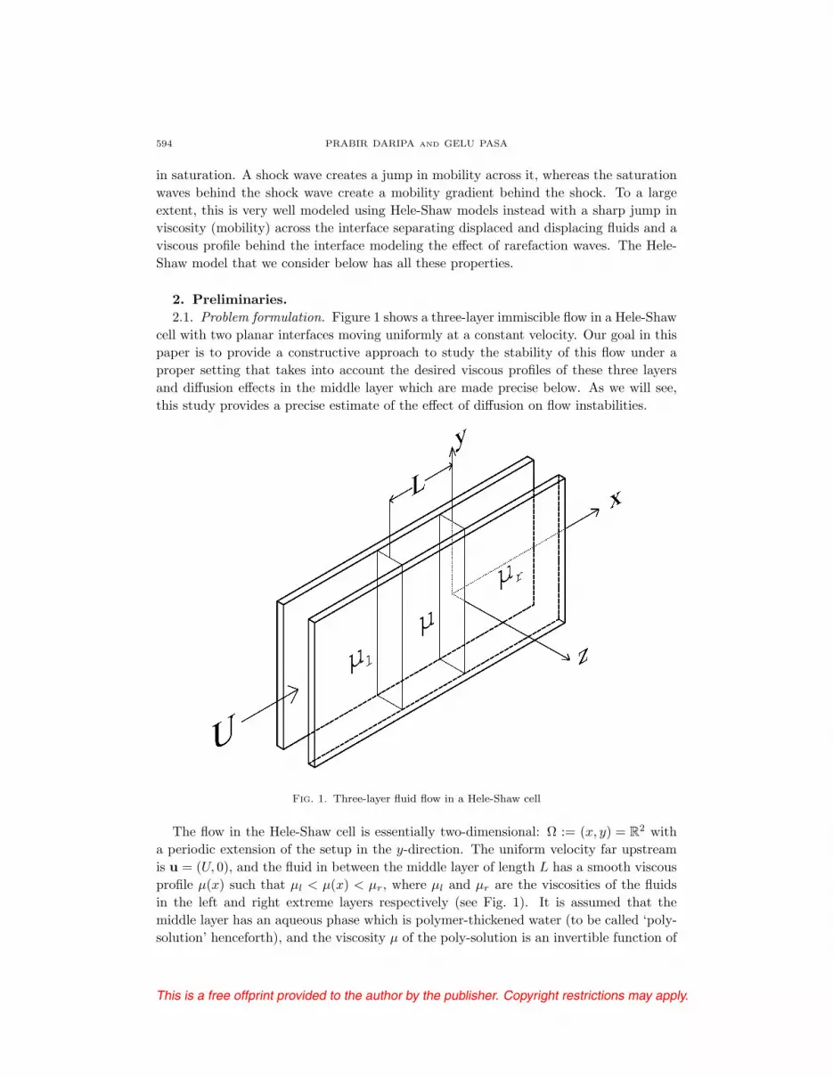
2.1. Problem formulation. Figure 1 shows a three-layer immiscible flow in a Hele-Shaw

cell with two planar interfaces moving uniformly at a constant velocity. Our goal in this

paper is to provide a constructive approach to study the stability of this flow under a

proper setting that takes into account the desired viscous profiles of these three layers

and diffusion effects in the middle layer which are made precise below. As we will see,

this study provides a precise estimate of the effect of diffusion on flow instabilities.

Fig. 1. Three-layer fluid flow in a Hele-Shaw cell

The flow in the Hele-Shaw cell is essentially two-dimensional: Ω := (x, y) = R2 with

a periodic extension of the setup in the y-direction. The uniform velocity far upstream

is u = (U, 0), and the fluid in between the middle layer of length L has a smooth viscous

profile μ(x) such that μl < μ(x) < μr, where μl and μr are the viscosities of the fluids

in the left and right extreme layers respectively (see Fig. 1). It is assumed that the

middle layer has an aqueous phase which is polymer-thickened water (to be called ‘poly-

solution’ henceforth), and the viscosity μ of the poly-solution is an invertible function of

This is a free offprint provided to the author by the publisher. Copyright restrictions may apply.

DIFFUSIVE SLOWDOWN IN HELE-SHAW FLOWS 595

the polymer concentration c. The polymer concentration profile c(x)(−L < x < L) of

the middle layer determines the viscous profile μ(x) of this layer.

The case of passive advection of the polymer by the fluid in the middle layer has been

addressed earlier by several authors (see [11], [3]). Thus, in this model, the viscosity of

every fluid element in the poly-solution is a constant of motion. In this paper, we break

this invariance property by also allowing diffusion of the polymer in the middle layer,

which is more realistic. Hitherto, this diffusion effect has not been addressed in this

three-layer flow. The advection-diffusion equation of the polymer in the middle layer is

governed by∂c

∂t+ u ·∇c = η� c,

where η, the diffusion coefficient, is a constant. Since the viscosity μ is an invertible

function of the concentration c, the same equation holds true in the middle layer for

viscosity μ(x) in the middle layer. Therefore, the governing equations in each layer are

∇·u = 0, (2.1)

∇ p = −μ u, (2.2)

∂μ

∂t+ u ·∇μ = η�μ, (2.3)

where p is the pressure, ∇ =(

∂∂x ,

∂∂y

), and � is the Laplacian in the plane. The first

equation (2.1) is the continuity equation for incompressible flow, the second equation

(2.2) is Darcy’s law (Darcy (1856)), and the third equation (2.3) is the advection-diffusion

equation for viscosity. Modeling such flows using Darcy’s law (2.2) has been the practice

in the literature for a long time, including the article of Taylor and Saffman (see [21])

which originally appeared in the journal: Proceedings of Royal Society. In using such

a model, averaging is first done in the vertical direction in the original configuration

shown in Fig. 1 and then the motion of the fluid is assumed to evolve as per the equation

resulting from averaging, i.e. Darcy’s law. Thus the parabolic profile in the z-direction

separating two fluids does not arise, which is acceptable since the fluid on the walls is

moving with the average velocity in the z-direction, which is not the physical velocity.

This model has been accepted in thousands of articles starting with the experiments

of Taylor. Taylor showed in physical experiments the development of fingers, which

were also obtained theoretically using Darcy’s law within a very good approximation by

Saffman and Taylor [21]. There is a rich history to it in fluid mechanics. For example,

see Saffman [20], Homsy [9], Tanveer [26] and Howison [10] just to mention a few. In

short, this model does not include the structure of displacement in the gap between the

plates.

The setup shown in Fig. 1 and discussed at the beginning of this section is a basic

solution of the above system with the following qualifications: the extreme layer viscosi-

ties μl and μr are constants and the viscous profile of the middle layer is linear, with

viscosity increasing in the direction of flow in this layer. The pressure corresponding to

this basic solution can be obtained by integrating (2.2). It is convenient to work in a

moving frame with velocity (U, 0) so that the basic solution is stationary in this moving

frame. Henceforth, our discussion including equations will be in the moving frame, unless

This is a free offprint provided to the author by the publisher. Copyright restrictions may apply.

596 PRABIR DARIPA AND GELU PASA

otherwise mentioned. Here and below, with a slight abuse of notation, the same variable

x is used to refer to the x-coordinate in the moving reference frame.

2.2. Stability equations. In the moving frame, the basic state is (u = 0, v = 0, p0(x),

μ(x)), where the basic viscous profile μ(x) of the middle layer (−L < x < L) is linear,

namely μ(x) = ax+ b, with viscosity increasing in the direction of flow from μ(−L) > μl

to μ(0) < μr in this layer. If this basic state is perturbed by (εu, εv, εp, εμ), where ε is a

small parameter and the perturbed state (εu, εv, p0(x)+εp, μ(x)+εμ) is then substituted

in the moving frame version of the equations (2.1) through (2.3), then we obtain the

following linearized equations for u = (u, v), p, and μ at the order O(ε):

∇·u = 0, x, y ∈ R, (2.4)

∇ p = −μ u− μ (U, 0), x, y ∈ R, (2.5)

∂μ

∂t+ u

dμ

dx= η �μ, −L < x < 0. (2.6)

The above equations are studied by the method of normal modes in which a typical

wave disturbance has the form

(u, v, p, μ) = (f(x), ψ(x), φ(x), h(x)) e(i k y+σt), (2.7)

where k is a real axial wavenumber and σ is the growth rate, which could be complex.

Substitution of (2.7) in (2.4) through (2.6) results in equations involving f(x), ψ(x), φ(x),

and h(x) whose manipulation then leads to two coupled equations (see equations (2.8)1and (2.8)2 below) involving f(x) and h(x). These are subject to boundary conditions

resulting from the linearization of the kinematic and the dynamic boundary conditions

at two interfaces as derived in Daripa and Pasa [4] for the zero-diffusion case. These

boundary conditions are independent of the diffusion process in the middle layer. Thus,

in this model, where the viscosity is advected as well as diffused by the fluid in the middle

layer, the evolution of linearized disturbances is governed by the following problem:

− (μ fx)x + k2μf = −k2Uh, x ∈ (−L, 0),

ηhxx − (σ + ηk2)h = af, a > 0, x ∈ (−L, 0),

fx(0) = (λP + q)f(0), fx(−L) = (λr + s)f(−L),

h(0) = h(−L) = 0,

⎫⎪⎪⎬⎪⎪⎭ (2.8)

where λ = 1/σ, a = (μ(0)− μ(−L))/L > 0, η > 0, and P, q, r, s are defined by

P = {[μ]r Uk2 − Tk4}/μ(0), q = −μrk/μ(0) ≤ 0,

r = {−[μ]l Uk2 + Sk4}/μ(−L), s = μlk/μ(−L) ≥ 0,

}(2.9)

where [μ]r = (μr − μ(0)) and [μ]l = (μ(−L)− μl). It is worth noting that

P ≥ 0 for k2 ≤ k21 = [μ]r U/T, and r ≤ 0 for k2 ≤ k22 = [μ]l U/S. (2.10)

All these equations are in dimensional form. In (2.9), T is the surface tension at the

interface x = 0 and S is the surface tension at the interface x = −L. Note that the

formulation here allows jumps in viscosities across the interfaces.

This is a free offprint provided to the author by the publisher. Copyright restrictions may apply.

DIFFUSIVE SLOWDOWN IN HELE-SHAW FLOWS 597

3. Numerical approximation. The problem (2.8) is one-dimensional involving only

the independent variable x. We use a finite difference discretization of system (2.8) on

(M−1) equidistant interior points in the segment [−L, 0]: xM = −L < xM−1 < xM−2 <

· · · < x1 < x0 = 0 and let d = (xi − xi+1). Then we have the unknowns f0, f1, f2, ...., fMand h1, h2, ...., hM−1, where fi = f(xi) and hi = h(xi).

Using first-order approximation for derivatives at the end points in the boundary

conditions (2.8)3 and (2.8)4, we obtain after some simplifications,(1

dP − q

P

)f0 −

1

dP f1 = λf0, (3.1)

1

drfM−1 −

(1

dr+

s

r

)fM = λfM . (3.2)

For interior points we use the central finite difference approximations to the derivatives

such as

hx(x) =h(x+ d/2)− h(x− d/2)

d, hxx(x) =

h(x+ d)− 2h(x) + h(x− d)

d2.

Using the above finite difference approximations, the discretized form of the system (2.8)

becomes

A00f0 +A01f1 = λf0, (3.3)

Aijfj = −k2Uhi, ∀ i ∈ [1,M − 1], ∀ j ∈ [0,M ], (3.4)

AM,M−1fM−1 +AMMfM = λfM , (3.5)

{ηBim − (σ + k2η)δim}hm = afi, ∀ i,m ∈ [1,M − 1]. (3.6)

This system is overall first-order accurate due to first-order approximations (3.1) and (3.2)

at the boundary. This makes the analysis and the results that we obtain below possible.

In the above expressions, Aij and Bij are the conventional notation for the entries of the

tridiagonal matrices A ∈ R(M+1)×(M+1) and B ∈ R

(M−1)×(M−1), respectively, which are

given below. Above and below, Ai,i−1 means the entry Aij when j = i − 1. A similar

result holds for the entries of the matrix B:

A00 =

(1

dP − q

P

), A01 = − 1

dP , A0j = 0, ∀j ∈ [2,M ], (3.7)

Ai,i−1 = −μi−1/2

d2, Aii = μik

2 +μi−1/2 + μi+1/2

d2, Ai,i+1 = −

μi+1/2

d2, 1 ≤ i ≤ M − 1,

(3.8)

AMj = 0, ∀j < M − 1, AM,M−1 =1

dr, AMM = −

(1

dr+

s

r

), (3.9)

Aij = Bi,j = 0 ∀ j /∈ [i− 1, i+ 1], 1 ≤ i ≤ M − 1, (3.10)

Bii = − 2

d2, Bi−1,i = Bi,i+1 =

1

d2, 1 ≤ i ≤ M − 1. (3.11)

We obtain only one relation from (3.4) and (3.6) as follows. From (3.6) we have:

hi = − a

σ + k2ηfi +

η

σ + k2ηBimhm, ∀ i ∈ [1,M − 1]. (3.12)

This is a free offprint provided to the author by the publisher. Copyright restrictions may apply.

598 PRABIR DARIPA AND GELU PASA

We use the above expression in (3.4) and get

Aijfj = −k2Uhi = (−k2U)

{−a

σ + k2ηfi +

η

σ + k2ηBimhm

}, ∀ i ∈ [1,M − 1], (3.13)

where Einstein summation is implied for the subscripts m ∈ [1,M − 1] and j ∈ [0,M ].

We replace again hm by the expression (3.12) obtained from (3.4), in the last term of

the right-hand side of the above formula (3.13). The final form of our discretized system

(3.3)-(3.6) is given by the following set of equations:

A00f0 +A01f1 = λf0, (3.14)

Aijfj =ak2U

σ + k2ηfi +

η

σ + k2ηBimAmjfj , (3.15)

AM,M−1fM−1 +AMMfM = λfM , (3.16)

where we recall that 1 ≤ i,m ≤ (M − 1) and 0 ≤ j ≤ M for the system (3.15).

4. Approximate estimate of the growth rate. We let σ = σR + iσI and λ =

λR + iλI , σR, σI , λR, λI ∈ R. Below, we obtain an estimate for the real part (σR) of the

growth rate. We consider (3.15) in the form (Einstein summation in (3.15) is replaced

by conventional summation sign)

(σ + k2η)

M∑j=0

Aijfj = (ak2U)fi + η

M−1∑m=1

Bim

M∑j=0

Amjfj ; i = 1, ...,M − 1. (4.1)

We use the following notation (with the slight abuse of notation because y below has

nothing to do with the y-coordinate of the setup (see Fig. 1)):

yi =

j=M∑j=0

Aijfj , for i = 1, . . . , (M − 1). (4.2)

Therefore, the system (4.1) becomes

(σ + k2η)yi = ak2Ufi + η

M−1∑m=1

Bimym. (4.3)

Let y∗ = max{|yi|, i = 1, 2, ..., (M − 1)}. The following possibilities exist:

y∗ = |y1| ⇒ |σ + k2η − ηB11| ≤ ak2U|f1||y1|

+ η|B12|; (4.4)

y∗ = |yj |, 1 < j < (M − 1) ⇒ |σ + k2η − ηBjj | ≤ ak2U|fj ||yj |

+ η(|Bj,j−1|+ |Bj,j+1|);

(4.5)

y∗ = |yn|, n = (M − 1) ⇒ |σ + k2η − ηBnn| ≤ ak2U|fn||yn|

+ η|Bn,n−1|. (4.6)

We recall that k, B, η are real numbers. Then we have the following inequality:

σR + k2η − ηBmm ≤ |σ + k2η − ηBmm|.

This is a free offprint provided to the author by the publisher. Copyright restrictions may apply.

DIFFUSIVE SLOWDOWN IN HELE-SHAW FLOWS 599

In the relations (4.4), (4.5), and (4.6) we use the following relations:

B11 + |B12| = −2/d2 + 1/d2 ≤ 0,

Bjj + |Bj,j−1|+ |Bj,j+1| = −2/d2 + 1/d2 + 1/d2 = 0, 1 < j < M − 1,

BM−1,M−1 + |BM−1,M−2| = −2/d2 + 1/d2 ≤ 0.

From these inequalities and the relations (4.4)-(4.6), it follows that there exists an integer

p, 1 ≤ p ≤ (M − 1), such that |yp| = maxj

{|yj |, 1 ≤ j ≤ M − 1} (see (4.2)) for which

σR + k2η ≤ ak2U|fp||yp|

. (4.7)

In the following, we obtain an estimate of the ratio |fp|/|yp|. For this, we first need

to rewrite the system (3.4) in a suitable form because the matrix with entries Aij , i =

1, ..., (M − 1); j = 0, 1, ...,M of the system (3.4) is not a square matrix and hence not

invertible. The following subsection discusses how to convert system (3.4) into a well-

posed system. In particular, below we convert the nonsquare matrix associated with

system (3.4) into a square matrix and then prove that this square matrix is invertible.

4.1. A well-posed system. In order to have only (M−1) unknowns in the new system,

we need to first express f0 in terms of f1, f2 and express fM in terms of fM−1, fM−2.

Below we use the boundary condition (2.8)5 for h and the equation (2.8)1 to obtain a

new form of the system (3.4) where only the unknowns f1, f2, ..., fM−1 appear. Then we

prove that the matrix of this new system is invertible.

The functions h and f are smooth, and we consider that (2.8)1 holds also for x = 0

and x = xM . Then we have

−(μfx)x (x)|x=0 + k2μ(0)f(0) = 0, (4.8)

−(μfx)x (x)|x=xM+ k2μ(xM )f(xM ) = 0. (4.9)

We approximate the derivatives in (4.8) by a finite-difference formula:

(μfx)x(0) ≈ {(μfx)(x0)− (μfx)(x1)}/d,fx(xi) ≈ {f(xi)− f(xi+1)}/d.

Then from (4.8) we obtain

f0 = − μ0 + μ1

μ0(k2d2 − 1)f1 +

μ1

μ0(k2d2 − 1)f2. (4.10)

Similar expressions are used to approximate the derivatives in (4.9). Below we use the

notation n = M − 1 for ease of presentation and obtain

fn+1 =μn + μn+1

μn+1(1− d2k2)fn − μn

μn+1(1− d2k2)fn−1. (4.11)

We consider the first equation of the system (3.4) which after using (3.7) becomes

A10f0 +A11f1 +A12f2 = −k2Uh1.

This is a free offprint provided to the author by the publisher. Copyright restrictions may apply.

600 PRABIR DARIPA AND GELU PASA

Substituting (4.10) for f0 and the values of the coefficients A10, A11 and A12 from (3.8)

in the above equation, we obtain after some simplification{ −μ1/2

d2(1− k2d2)

(1 +

μ1

μ0

)+

μ1/2 + μ3/2

d2+ k2μ1

}f1

+

{μ1/2μ1

d2μ0(1− k2d2)−

μ3/2

d2

}f2 = −k2Uh1.

(4.12)

We consider also the last equation of the system (3.4):

An,n−1fn−1 +An,nfn +An,n+1fn+1 = −k2Uhn, n = M − 1.

We use (4.11) to replace fn+1 in the above system in terms of fn, fn−1 and obtain{μn−1/2 + μn+1/2

d2+ k2μn −

μn+1/2

d2(1− k2d2)(1 +

μn

μn+1)

}fn

+

{−μn−1/2

d2+

μn μn+1/2

d2μn+1(1− k2d2)

}fn−1 = −k2Uhn. (4.13)

If we let k d � 1, then

(1− k2 d2) ≈ 1. (4.14)

Therefore the denominators in the formula (4.12)-(4.13) are not zero and the expressions

(4.12) and (4.13) simplify to{−μ1/2μ1 + μ0μ3/2

d2μ0+ k2μ1

}f1 +

{μ1/2μ1 − μ0μ3/2

d2μ0

}f2 = −k2Uh1 (4.15)

and{μn+1/2μn − μn+1μn−1/2

d2μn+1

}fn−1 +

{μn+1μn−1/2 − μn+1/2μn

d2μn+1+ k2μn

}fn = −k2Uhn.

(4.16)

Once the first and the last equations of the system (3.4) are replaced by (4.15) and

(4.16), the linear system (3.4) contains only the unknowns f1, f2, ..., fM−1 and have a

square matrix whose entries, now denoted by A′ij , i, j = 1, 2, ..., (M − 1), are given by

A′11=

−μ1/2μ1 + μ0μ3/2

d2μ0+ k2μ1, A′

12=μ1/2μ1 − μ0μ3/2

d2μ0, A′

1j=A1j , j = 3, . . . ,M − 1,

(4.17)

A′ij = Ai,j , i = 2, . . . ,M − 2, j = 1, . . . ,M − 1, (4.18)

(4.19)

A′nn =

μn+1μn−1/2 − μn+1/2μn

d2μn+1+ k2μn, n = M − 1,

A′n,n−1 =

μn+1/2μn − μn+1μn−1/2

d2μn+1, n = M − 1,

A′M−1,j = AM−1,j , j = 1, . . . , M − 3. (4.20)

Note that the equations corresponding to i = 2, . . . ,M − 2 of the initial system (3.4)

remain the same.

This is a free offprint provided to the author by the publisher. Copyright restrictions may apply.

DIFFUSIVE SLOWDOWN IN HELE-SHAW FLOWS 601

It is easily verified that |A′ii| >

∑j �=i

|A′ij | for each i ∈ [2, (M − 2)]. If we have the same

relation also for i = 1 and i = M − 1, then we can conclude that matrix A′ with entries

A′ij , i, j = 1, 2, ...,M − 1 is diagonally dominant and hence A′ is an invertible matrix.

Therefore we have to prove that |A′11| > |A′

12| and |A′M−1,M−1| > |A′

M−1,M−2|, wherethe elements of A′ are defined in (4.17) and (4.20). That means we need to prove∣∣∣∣−μ1/2μ1 + μ0μ3/2

d2μ0+ k2μ1

∣∣∣∣ >∣∣∣∣μ1/2μ1 − μ0μ3/2

d2μ0

∣∣∣∣ (4.21)

and ∣∣∣∣μn+1μn−1/2 − μn+1/2μn

d2μn+1+ k2μn

∣∣∣∣ >∣∣∣∣μn+1/2μn − μn+1μn−1/2

d2μn+1

∣∣∣∣ . (4.22)

Recall that μ(x) = ax+ b, which defines a = [μ0 − μ(−L)]/L, b = μ0. Hence

μ1/2 = b− ad/2, μ1 = b− ad, μ3/2 = b− 3ad/2,

μn = axn + b, μn+1 = axn+1 + b, μn−1/2 = axn−1/2 + b, μn+1/2 = axn+1/2 + b.

Therefore−μ1/2μ1 + μ0μ3/2

d2μ0= − a2

2μ0

andμn+1μn−1/2 − μn+1/2μn

d2μn+1= − a2

2μn+1.

We consider in (4.21) and (4.22) a large value of k and a small value of a to have

k2μ1 −a2

2μ0> 0, k2μn − a2

2μn+1> 0.

Consequently, the inequalities (4.21) and (4.22) are equivalent with

k2μ1 >a2

μ0, k2μn >

a2

μn+1. (4.23)

The above inequalities hold for large enough l and k. Then we obtain |A′11| > |A′

12|,|A′

M−1,M−1| > |A′M−1,M−2| and the matrix A′ given by (4.17), (4.18) and (4.20) becomes

invertible.

4.2. Diffusion enhanced stability bounds on the growth rate. We will be using the

inequality (4.7) to obtain a reasonable bound on the growth rate. For this, we first

rewrite yi, defined in terms of the entries of the matrix A in (4.2), in terms of the matrix

A′, which is

yi =m=M−1∑

m=1

A′imfm, fi =

j=M−1∑j=1

(A′−1

)ijyj , i = 1, . . . ,M − 1, (4.24)

where(A′−1

)is the inverse of matrix A′. Using (4.24) in the inequality (4.7), it follows

that

σR + k2η ≤ ak2U|fp||yp|

= ak2U1

|yp|

M−1∑j=1

∣∣∣∣(A′−1)pjyj

∣∣∣∣ ≤ ak2U

M−1∑j=1

∣∣∣∣(A′−1)pj

∣∣∣∣ |yj ||yp|.

This is a free offprint provided to the author by the publisher. Copyright restrictions may apply.

602 PRABIR DARIPA AND GELU PASA

We recall (see the line preceding (4.7)) that |yp| = maxj

{|yj |, 1 ≤ j ≤ (M − 1)}. Usingthis in the above inequality for the estimate of the growth rate, we obtain the following

estimate:

σR + k2η ≤ ak2UM−1∑j=1

∣∣∣∣(A′−1)pj

∣∣∣∣ . (4.25)

The matrix A′ does not depend on η. Moreover we have A′−1 ≈ O(d2) and A′−1 ≈O(1/k2) because A′ ≈ O(1/d2) and A′ ≈ O(k2). Then from (4.25) we obtain the

following conclusion: the real part of the growth rate is negative with strong diffusion.

In the case of very small wavenumbers k, we approximate the system (3.15) after

neglecting k2 as k is very small. Then we obtain from (4.1),

(σ/η)

j=M∑j=0

Aijfj =

M−1∑m=1

Bim

M∑j=0

Amjfj , i = 1, . . . ,M − 1,

and (σ/η) is an eigenvalue of the matrix Bim, with eigenvectors

j=M∑j=0

Amjfj . In this case,

we do not need a new system and the initial matrix with entries Aij does not depend on

k and η. Recall the definition (3.11) of the matrix B. The sum of the elements of each

line of B is negative, and hence we obtain σ/η ≤ 0. This shows diffusive (diffusion of

polymer) slowdown of instabilities.

The matrix A′ does not depend on the surface tensions T and S (see relations (4.17),

(4.18), (4.20)). Therefore, the upper bound on σ given by (4.25) does not depend on

T and S. This implies that very large values of η can stabilize the flow regardless of

the values of the surface tensions. Note that this result appears to be stronger than the

one obtained analytically by Daripa and Pasa (see [6]), because the term in the bound

there responsible for slowdown due to diffusion depends on surface tensions through the

functions f and h (see [6]). However, a careful inspection of the results in [6] shows that

the results presented in this paper are consistent with the results of [6].

5. Comparison. An estimate of the upper bound similar to the one given above

by (4.7) can be derived from the results we have obtained in [6] using exact (weak

formulation) analysis of the exact system (2.8). To see this, recall the following estimates

from [6]:

σR ≤ aF1∫ 0

−L|h|2 dx

− k2η ≤ a|F1|∫ 0

−L|h|2 dx

− k2η,

where σR = real(σ) and F1 is the real part of the inner product∫ 0

−Lf (−h)∗ dx (see

Daripa and Pasa [6]). Since

|F1| ≤

√(∫ 0

−L

|f |2 dx) (∫ 0

−L

|h|2 dx)

,

This is a free offprint provided to the author by the publisher. Copyright restrictions may apply.

DIFFUSIVE SLOWDOWN IN HELE-SHAW FLOWS 603

which follows from the Cauchy-Schwarz inequality, we get

σR ≤ a

√√√√∫ 0

−L|f |2 dx∫ 0

−L|h|2 dx

− k2η. (5.1)

We use the rectangle rule to approximate the two integrals appearing in (5.1). We have∫ 0

−L

|f |2 dx ≈ |f1|2d+ |f2|2d+ |f3|2d+ · · ·+ |fM−1|2d,∫ 0

−L

|h|2 dx ≈ |h1|2d+ |h2|2d+ |h3|2d+ · · ·+ |hM−1|2d,

where d is the discretization step used in section 3. Therefore we get∫ 0

−L|f |2 dx∫ 0

−L|h|2 dx

≈ |f1|2d+ |f2|2d+ |f3|2d+ · · ·+ |fM−1|2d|h1|2d+ |h2|2d+ |h3|2d+ · · ·+ |hM−1|2d

≤ maxi

{|fi|2|hi|2

}, 1 ≤ i ≤ M − 1.

From the relations (4.2) and (3.4) we have hi = −yi/(k2U). Therefore, from the above

formula, it follows that

σR ≤ ak2U maxi

|fi||yi|

− k2η. (5.2)

This bound, obtained from numerical approximation of the exact formulae of the upper

bound derived in [6], is also implied by (4.7). This is shown below. Since |yp| = maxj

|yj |in (4.7) (see the line before inequality (4.7)), it follows that

|fp||yp|

≤ maxi

|fi||yi|

,

and hence inequality (4.7) reduces to (5.2). Thus we see that both procedures give the

same formula and, in this sense, the presented numerical method of this paper is also

convergent.

We want to emphasize that in Daripa and Pasa [6], using a variational formulation,

we obtained an exact formula for the upper bound from which we obtain the above

estimate (5.2), which is the same estimate derived in this paper using numerical analysis

of the discrete approximation of the underlying scheme. Thus the presented numerical

scheme is a reasonable candidate for use in the construction of approximate solutions.

However, since this estimate is not exclusively in terms of the data of the problem but

also depends on the eigenfunction f , this formula (5.2) is not very useful for computing

exact numerical values of modal upper bounds a priori. In contrast, in addition to the

estimate (5.2) or equivalently (4.7), we have another explicit estimate (4.25) which is in

terms of the data of the problem. The unknown ratio |fi|/|yl| does not appear any more

in the formula (4.25). From this, we also see that a large value of the diffusion coefficient

has the potential to completely stabilize the flow, a conclusion also reached in Daripa

and Pasa [6].

Exact computation of the upper bound from (5.2) is not possible in the context of

this paper since the estimate (5.2) depends on the eigenfunction f , which is not known

This is a free offprint provided to the author by the publisher. Copyright restrictions may apply.

604 PRABIR DARIPA AND GELU PASA

until the differential equations modeling this problem are solved computationally, which

falls outside the scope of this work. The present work, as stated early in the abstract, is

about the establishment of the stabilizing role of diffusion on hydrodynamic instability

using a constructive approach, which has been accomplished in this paper. The bound

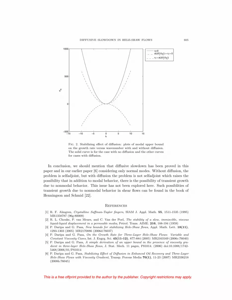
(5.2) on the growth rate is for individual waves due to dependency of the estimate on

the wavenumber k. We can compute values of the modal upper bound for individual

waves from (5.2) (which is implied by (4.7)) provided we assume, for the purpose of

exposition of the effect of diffusion on stability, the value of mini

|fi|/|yi|, where the

minimum is taken over all i. We plot the modal upper bound against the wavenumber

k taking mini

|fi|/|yi| = 10/(aU) and η = 4 (recall that a is the slope of the basic profile

of the viscosity and η is the viscosity coefficient). There is no specific reason behind

these numbers. Any other choice will do as well to reveal the qualitative nature of the

plots in Fig. 2. Figure 2 shows plots of the upper bound for individual waves against

the wavenumber for three cases: (i) the solid curve is for the case with no diffusion;

(ii) the dash-and-dotted curve is for the case with diffusion for modest values of the

diffusion coefficient η (specifically when aU |fi||yl| > η); (iii) the dashed curve is also for

the case with diffusion but for very large values of the diffusion coefficient (specifically

when aU |fi||yl| < η). These figures show qualitatively the nature of the stabilizing effect

of diffusion and in the extreme situation (the dashed curve), the flow can be completely

stabilized. In reality, qualitatively in some finite neighborhood of the point (0,0), Fig.

2 should compare well with similar plots obtained from an exact computation of the

differential equations.

6. Conclusion. The constructive approach of this paper (see section 4) and the weak

formulation approach of Daripa and Pasa (2007) provide similar estimates (4.7) and (5.2),

respectively, for the real part of the growth rate. Moreover, the formula (4.25) in this

paper and Theorem 1 in Daripa and Pasa (2007) clearly show that species diffusion

suppresses instability. For appropriate values of the parameters of our model, a large

enough diffusion coefficient can reverse the instability process. As a function of the

wavenumbers, the growth rate is bounded by a parabola with a maximum point (with

the leading term −η) given by the estimate (4.25). Since the proposed numerical scheme

in this paper provides a bound comparable to the exact one, the proposed scheme should

be useful to numerically construct approximate solutions and thereby explore the effect

of diffusion.

The technique used in this paper is of general interest and very constructive, which

leads to implementation of the algorithm. Furthermore, the technique presented here

should be applicable in principle to multi-layer Hele-Shaw flows (more than three-layer)

and other multi-layer flows involving species diffusion. Such problems are usually gov-

erned by a system of advection-diffusion equations, similar to the system of equations

(1)-(3). Since such problems are abundant in all areas of classical physics and biomedi-

cal sciences, to name just a few, the technique used here should be applicable to many

applied problems involving species diffusion.

This is a free offprint provided to the author by the publisher. Copyright restrictions may apply.

DIFFUSIVE SLOWDOWN IN HELE-SHAW FLOWS 605

−15 −10 −5 0 5 10 15−500

0

500

1000

k

σ R

η=0aU(|f

i|/|y

l|) > η > 0

η > aU(|fi|/|y

l|)

Fig. 2. Stabilizing effect of diffusion: plots of modal upper boundon the growth rate versus wavenumber with and without diffusion.The solid curve is for the case with no diffusion and the other curvesfor cases with diffusion.

In conclusion, we should mention that diffusive slowdown has been proved in this

paper and in our earlier paper [6] considering only normal modes. Without diffusion, the

problem is selfadjoint, but with diffusion the problem is not selfadjoint which raises the

possibility that in addition to modal behavior, there is the possibility of transient growth

due to nonmodal behavior. This issue has not been explored here. Such possiblities of

transient growth due to nonmodal behavior in shear flows can be found in the book of

Henningson and Schmid [22].

References

[1] R. F. Almgren, Crystalline Saffman-Taylor fingers, SIAM J. Appl. Math. 55, 1511-1535 (1995)MR1358787 (96g:80009)

[2] R. L. Chouke, P. van Meurs, and C. Van der Poel, The stability of a slow, immiscible, viscousliquid-liquid displacement in a permeable media, Petrol. Trans. AIME. 216, 188-194 (1959)

[3] P. Daripa and G. Pasa, New bounds for stabilizing Hele-Shaw flows, Appl. Math. Lett. 18(11),1293-1303 (2005) MR2170886 (2006d:76037)

[4] P. Daripa and G. Pasa, On the Growth Rate for Three-Layer Hele-Shaw Flows: Variable andConstant Viscosity Cases, Int. J. Engrg. Sci. 43(11-12), 877-884 (2005) MR2163169 (2006c:76040)

[5] P. Daripa and G. Pasa, A simple derivation of an upper bound in the presence of viscosity gra-dient in three-layer Hele-Shaw flows, J. Stat. Mech. 11 pages, P01014. (2006) doi:10.1088/1742-5468/2006/01/P01014

[6] P. Daripa and G. Pasa, Stabilizing Effect of Diffusion in Enhanced Oil Recovery and Three-LayerHele-Shaw Flows with Viscosity Gradient, Transp. Porous Media 70(1), 11-23 (2007) MR2336218

(2008h:76045)

This is a free offprint provided to the author by the publisher. Copyright restrictions may apply.

606 PRABIR DARIPA AND GELU PASA

[7] J. Escher and G. Simonett, On Hele-Shaw models with surface tension, Math. Res. Lett. 3, 467-474(1996) MR1406012 (97i:35145)

[8] F. J. Hickernell and Y. C. Yortsos, Linear stability of miscible displacement processes in porousmedia in the absence of dispersion, Stud. Appl. Math. 74, 93-115 (1986) MR836292 (87e:76073)

[9] G. M. Homsy, Viscous fingering in porous media, Ann. Rev. Fluid Mech. 19, 271-311 (1987)[10] S. D. Howison, Complex variable methods in Hele-Shaw moving boundary problems, Eur. J. Appl.

Math. 3, 209-224 (1992) MR1182213 (94f:76025)[11] S. B. Gorell and G. M. Homsy, A theory of the optimal policy of oil recovery by the secondary

displacement process, SIAM J. Appl. Math. 43, 79-98 (1983) MR687791 (84b:76073)[12] L. P. Kadanoff, Exact Solutions for the Saffman-Taylor Problem with Surface Tension, Phys. Rev.

Letts. 65, 2986-2988 (1990)[13] D. A. Kessler, J. Koplik, and H. Levine, Pattern selection in fingered growth phenomena, Adv. in

Phys. 37, 255-329 (1998)[14] W. Littman, Polymer Flooding: Developments in Petroleum Science. 24 Elsevier, Amsterdam

(1988)[15] D. Loggia, N. Rakotomalala, D. Salin, and Y. C. Yortsos, The effect of mobility gradients on viscous

instabilities in miscible flows in porous media, Phys. Fluids. 11(3), 740-742 (1999)[16] J. W. McLean and P. G. Saffman, The effect of surface tension on the shape of fingers in a Hele-

Shaw cell, J. Fluid Mech. 102, 445-469 (1981)[17] R. B. Needham and P. H. Doe, Polymer flooding review, J. Pet. Technol. 12, 1503-1507 (1987)[18] Q. Nie and F. R. Tian, Singularities in Hele-Shaw flows, SIAM J. Appl. Math. 58, 34-54 (1998)

MR1610037 (2000c:76023)[19] P. G. Saffman, Exact solutions for the growth of fingers from a flat interface between two fluids in

a porous medium or Hele-Shaw cell, Quart. J. Mech. Appl. Math. 12, 146-155 (1959) MR0104422(21:3177)

[20] P. G. Saffman, Viscous Fingering in Hele-Shaw Cells, J. Fluid Mech. 173, 73-94 (1986) MR877015(87m:76062)

[21] P. G. Saffman and G. I. Taylor, The penetration of a fluid in a porous medium or Hele-Shaw cellcontaining a more viscous fluid, Proc. Roy. Soc. A., 245, 312-329 (1958) MR0097227 (20:3697)

[22] P. J. Schmid and D. S. Henningson, Stability and Transition in Shear Flows, Springer-Verlag, NewYork (2001) MR1801992 (2001j:76039)

[23] D. Shah and R. Schecter, Improved Oil Recovery by Surfactants and Polymer Flooding, AcademicPress, New York, 1977

[24] M. Shariati and Y. C. Yortsos, Stability of miscible displacements across stratified porous media,Phys. Fluids 13(8) 2245-2257 (2001)

[25] K. S. Sorbie, Polymer-Improved Oil Recovery. CRC Press, Boca Raton, Florida, 1991[26] S. Tanveer, Surprises in viscous fingering, J. Fluid Mech. 409, 273-308 (2000) MR1756392

(2002a:76059)

[27] F. R. Tian, A Cauchy integral approach to Hele-Shaw problems with a free boundary: the case ofzero surface tension, Arch. Ration. Mech. Anal. 135, 175-196 (1996) MR1418464 (97j:35167)

[28] A. C. Uzoigwe, F. C. Scanlon, and R. L. Jewett, Improvement in polymer flooding: The programmedslug and the polymer-conserving agent, J. Petrol. Tech. 26, 33-41 (1974)

[29] G. L. Vasconceles and L. P. Kadanoff, Stationary solutions for the Saffman-Taylor problem withsurface tension Phys. Rev. A. 44, 6490-6495 (1991)

[30] Y. C. Yortsos and M. Zeybek, Dispersion driven instability in miscible displacement in porous-media, Phys. Fluids 31, 3511-3518 (1988)