SIAM J. MATH. ANAL. c© 2014 Society for Industrial and Applied MathematicsVol. 46, No. 6, pp. 3761–3781

ON A TWO SPECIES CHEMOTAXIS MODEL WITH SLOWCHEMICAL DIFFUSION∗

MIHAELA NEGREANU† AND J. IGNACIO TELLO‡

Abstract. In this paper we consider a system of three parabolic equations modeling the behaviorof two biological species moving attracted by a chemical factor. The chemical substance verifies aparabolic equation with slow diffusion. The system contains second order terms in the first twoequations modeling the chemotactic effects. We apply an iterative method to obtain the globalexistence of solutions using that the total mass of the biological species is conserved. The stability ofthe homogeneous steady states is studied by using an energy method. A final example is presentedto illustrate the theoretical results.

Key words. chemotaxis, global existence, Moser–Alikakos iteration, asymptotic behavior, sta-bility

AMS subject classifications. 35A01, 35B40, 35B35, 35K57, 95D25

DOI. 10.1137/140971853

1. Introduction. Chemotaxis is the capacity of organisms to move along achemical gradient. Such movement, maybe towards or away from a higher concentra-tion of the chemical substance, has been investigated by different authors, not onlyfrom a biological point of view but also from mathematical, physical, or chemicalperspectives, among others. In particular, in the early 1970s, Keller and Segel, pro-posed a mathematical model of two parabolic equations to describe the aggregation ofDictyostelium discoideum, a soil-living amoeba. Chemotactic abilities are crucial inmany biological phenomena, such as immune system response, embryo development,tumor growth, etc. Recent studies also describe macroscopic processes in terms ofchemotaxis, such as population dynamics or gravitational collapse, among others.

After the pioneering works of Keller and Segel, mathematical models of chemo-taxis have been used to model the mentioned phenomena where one or several speciesrespond to chemical stimuli. Among the mathematical challenges that the problempresents, the blowing up and the global existence of solutions, have attracted the at-tention of the mathematical community. The system describing the evolution of onebiological species where the chemical is modeled by a second order elliptic equationhas been largely studied, as the fully parabolic system; see, for instance, the reviewby Horstmann [12] and reference therein.

Motivated by empirical biological data, multispecies chemotaxis systems havebeen proposed over the last 30 years; see, for instance, Alt [1], Fasano, Mancini, andPrimicerio [10], Wolansky [26], or Horstmann [13].

Parabolic-parabolic-elliptic systems, where the evolution of two biological speciesis described by parabolic equations and an elliptic equation models the behavior ofthe chemoattractant substance, have been recently analyzed by several authors. In

∗Received by the editors June 6, 2014; accepted for publication (in revised form) August 22, 2014;published electronically November 13, 2014. This work was supported by Project MTM2013-42907DIGISP Spain.

http://www.siam.org/journals/sima/46-6/97185.html†Departamento de Matematica Aplicada, Universidad Complutense de Madrid, 28040 Madrid,

Spain (negreanu@mat.ucm.es).‡Departamento de Matematica Aplicada, E.U.I. Universidad Politecnica de Madrid, 28031

Madrid, Spain (j.tello@upm.es).

3761

3762 MIHAELA NEGREANU AND J. IGNACIO TELLO

Tello and Winkler [22] and Stinner, Tello, and Winkler [20] global asymptotic stabilityof homogeneous steady states is studied under the effects of competition between thespecies. The blow-up phenomenon in a bounded domain, when the interaction be-tween the biological species is reduced to the chemical production, has been consideredin Espejo, Stevens, and Velazquez [7] and [8] for simultaneous and nonsimultaneousblow-up in R

2. See also Biler, Espejo, and Guerra [3], Biler and Guerra [4] for boundeddomains and Conca and Espejo [5], and Conca, Espejo, and Vilches [6] for the two-dimensional case in the whole space (see also Espejo and Wolanski [9] for more detailsand cases).

The one species fully parabolic system with signal-dependent chemotactic sensi-tivities has been already researched in the literature. In Biler [2], the two-dimensionalcase was studied, the author proving global existence of solutions for χ(w) = 1/w withinitial data satisfying ∇u0 ∈ [L2(ω)]2. In Winkler [24] and [25], the global existenceis obtained for arbitrary dimension n ≥ 2 for χ(w) = χ0/w with a positive constantχ0 <

√2/n. In [21], Stinner and Winkler investigated the existence of week solutions

for arbitrary large chemotactic sensitivity χ0.Signal dependent chemotactic sensitivities appear in many other PDE systems,

such as the parabolic-elliptic case, systems coupled with Stokes or Navier–Stokesequations modeling different biological phenomena (see, for instance, [14] and [15]).

The parabolic-parabolic-ODE problem, has been recently studied in Negreanuand Tello [18], where the rectangles method used in Friedman and Tello [11] (see also[17]) for the parabolic-ODE problem cannot be applied due to the second componentof the species. In Negreanu and Tello [16], the logistic growth term drives the solutionto the unique positive constant stationary state under some structural restrictions inthe chemical stimuli.

In this paper we focus on the fully parabolic problem, where the diffusion coeffi-cient of the chemical substance is strictly less than 1. The system has been previouslyconsidered by Horstmann [13] where the linear stability is studied for a range ofparameters with constant chemoattractant sensitivity and linear chemical production.

We denote the densities of the species by u(x, t) and v(x, t), the concentration ofthe chemoattractant by w(x, t), Ω is a bounded and regular domain of Rn for n ≥ 1.The fully parabolic system is given by the following system of equations:

(1.1)

⎧⎪⎪⎪⎨⎪⎪⎪⎩

ut = Δu−∇ · (uχ1(w)∇w), x ∈ Ω, t > 0,

vt = Δv −∇ · (vχ2(w)∇w), x ∈ Ω, t > 0,

wt = εΔw + h(u, v, w), x ∈ Ω, t > 0,

∇u · ν = ∇v · ν = ∇w · ν = 0, x ∈ ∂Ω, t > 0

for ε > 0, and initial data

(1.2) u(x, 0) = u0(x), v(x, 0) = v0(x), w(0, x) = w(x), x ∈ Ω.

In (1.1), h(u, v, w) denotes the balance between the production and degradation ofthe chemical which depends explicitly on the living organisms. The chemotacticsensitivity coefficients χ1 and χ2 are assumed to be positive and regular, i.e.,

(1.3) χi ∈ W 1,∞loc (R+) ∩C1(R+), χi > 0 for i = 1, 2.

For technical reasons we also assume that

(1.4) χ′i +

1

1− εχ2i ≤ 0 for i = 1, 2.

ON A TWO SPECIES CHEMOTAXIS MODEL 3763

We consider that the balance between production and degradation of a chemical is aregular function

(1.5) h ∈ W 1,∞(R3+) ∩ C1(R3

+),

monotone increasing in u and v and monotone decreasing in w, i.e.,

∂h

∂u≥ εu > 0 and

∂h

∂v≥ εv > 0,(1.6)

∂h

∂w≤ −εw < 0(1.7)

for some positive constants εu, εv, and εw.We denote by u∗ and v∗ the positive constants defined as

(1.8)

u∗ :=1

|Ω|∫Ω

u0(x)dx =1

|Ω|∫Ω

u(x, t)dx,

v∗ :=1

|Ω|∫Ω

v0(x)dx =1

|Ω|∫Ω

v(x, t)dx.

Thanks to assumption (1.7) and the implicit function theorem we may deduce theexistence of a unique constant w∗ satisfying

(1.9) h(u∗, v∗, w∗) = 0.

In section 2 we study the global existence of solutions to (1.1)–(1.2) and obtainglobal uniform boundedness of the solutions under the following constrains in h andχi (for i = 1, 2):

- There exist two constants w and w verifying

(1.10) 0 ≤ w < w0 < w, w < w∗ < w.

- There exist some positive constants k1 and k2 such that

(1.11) −h(0, 0, w) ≤ kiχi(w)

for i = 1, 2 and w ≤ w ≤ w.

- There exist k01 and k02 positive constants such that

(1.12) 0 < k0i ≤ χi(w)e∫

ww

χi(s)ds for i = 1, 2 and w ≥ w.

- We also assume

(1.13) h(u, v, w) ≥ 0, h(u, v, w) < 0 for 0 ≤ u ≤ u, 0 ≤ v ≤ v,

where

(1.14) u := f1∞(w)max{k1 (εuk01(1− ε))

−1, ‖u0‖L∞(Ω)

}and

(1.15) v := f2∞(w)max{k2 (εvk02(1− ε))−1 , ‖v0‖L∞(Ω)

}for f1∞ and f2∞ defined by

(1.16) fi∞(w) = exp

{1

1− ε

∫ w

w

χi(s)ds

}for i = 1, 2.

3764 MIHAELA NEGREANU AND J. IGNACIO TELLO

Under assumptions (1.11)–(1.16) we have the uniform boundedness of the solutions,more precisely, we obtain the bounds

0 ≤ u(x, t) ≤ u, 0 ≤ v(x, t) ≤ v, and w ≤ w(x, t) ≤ w for t > 0, x ∈ Ω.

That result, together with the existence of solutions is enclosed in Theorem 3.1. Toachieve the uniform bounds we implement an iterative method based on the Lp-normof the solutions inspired by the Moser–Alikakos iteration.

In section 3 without loss of generality we analyze the stability of the system fora linear profile h defined by

h(u, v, w) = au+ v − 2μw for a, μ > 0.

By using an energy method, in Theorem 4.1 we prove the asymptotic stability ofthe homogeneous steady state (u∗, v∗, w∗) defined by (1.8), (1.9) under the additionalrestrictions

(1.17) uχ1(w)∂h

∂u+vχ2(w)

∂h

∂v+

∂h

∂w< 0, 0 ≤ u ≤ u, 0 ≤ v ≤ v, w ≤ w ≤ w,

and

C(Ω)max{(χ1(w)u)

2, (χ2(w)v)2}max{1, a2} < 2με,

where C(Ω) is the smallest positive constant satisfying∫Ω

u2dx ≤ C(Ω)

∫Ω

|∇u|2dx

for any u ∈ H1(Ω), such that∫Ωu(x)dx = 0.

In the last section we illustrate the results obtained in the previous sections witha particular example, where the chemosensitivity functions are χi = αi/(βi + w) forsome positive values αi, βi (i = 1, 2).

A simple case of the above example is given for the parameters

a = μ = 1, ε :=1

2, α1 = α2 =

1

2, β1 = β2 =

1

16,

i.e.,

h(u, v, w) = u+ v − 2w, χ1(w) = χ2 =8

16w + 1

with

w = 0, w <1

8.

Hypothesis (1.11) is verified taking

k1 = k2 = 1,

and (1.12) is reduced to

k01 = k02 =2

(1 + 16w)12

.

ON A TWO SPECIES CHEMOTAXIS MODEL 3765

The rest of the assumptions are simple computations. Then, for any initial data(u0, v0, w0) satisfying

‖u0‖L∞(Ω) ≤ w

( 116 + w)

13

, ‖v0‖L∞(Ω) ≤ w

( 116 + w)

13

, ‖w0‖L∞(Ω) ≤ w,

the solution is uniformly bounded in (0,∞) and

limt→∞

∫Ω

|u− u∗|2dx = limt→∞

∫Ω

|v − v∗|2dx = limt→∞

∫Ω

|w − w∗|2dx = 0,

where the stationary solution of system (1.1) is

(u∗, v∗, w∗) :=(∫

Ω

u0(x)dx,

∫Ω

v0(x)dx,

∫Ω

(u0 + v0)dx

2

).

For the sake of simplicity we assume thorough the article that |Ω| = 1 and denoteby ΩT = Ω× (0, T ), Ω∞ = Ω× (0,∞).

2. Steady states. The steady states of problem (1.1) satisfy the system

(2.1)

⎧⎪⎪⎪⎨⎪⎪⎪⎩

0 = Δu−∇ · (uχ1(w)∇w), x ∈ Ω, t > 0,

0 = Δv −∇ · (vχ2(w)∇w), x ∈ Ω, t > 0,

0 = εΔw + h(u, v, w), x ∈ Ω, t > 0,

∇u · ν = ∇v · ν = ∇w · ν = 0, x ∈ ∂Ω.

The biological meaningful solutions should be positive, hence we only consider non-negative bounded steady states.

Lemma 2.1. Under assumptions (1.3), (1.5)–(1.17), for every ε > 0, any non-negative bounded solutions of (2.1) are constant.

Proof. We introduce the change of variables u and v defined by

(2.2) u = u exp

{∫ w

w

χ1(s)ds

}, v = v exp

{∫ w

w

χ2(s)ds

}.

Since

∇u = (χ1(w)u∇w +∇u) exp

{∫ w

w

χ1(s)ds

}

and

Δu = ∇(χ1(w)u∇w + exp

{∫ w

w

χ1(s)ds

}∇u

),

the first equation in (2.1) becomes

−∇ ·(exp

{∫ w

w

χ1(s)ds

}∇u

)= 0, x ∈ Ω,

and the boundary condition

∇u · ν = 0

implies that u is a constant. In the same way we obtain that v is also a constant.

3766 MIHAELA NEGREANU AND J. IGNACIO TELLO

Since ε > 0, we have that w satisfies

(2.3) −εΔw = h

(u exp

{∫ w

w

χ1(s)ds

}, v exp

{∫ w

w

χ2(s)ds

}, w

),

where u and v are constant. Thanks to assumption (1.17), we obtain that

d

dwh(uf1(w), vf2(w), w) = uχ1(w)hu + vχ2(w)hv + hw < 0

which proves the existence of, at most one solution of (2.3). By the implicit functiontheorem, there exists a constant w∗ satisfying h(u∗, v∗, w∗) = 0, which ends theproof.

3. Global existence. In this section we study the global existence of solutionsand we obtain global uniform bounds in L∞(Ω). The result is enclosed in the followingTheorem.

Theorem 3.1. Under (1.3)–(1.17), (1.11)–(1.16) for any initial data (u0, v0, w0)∈ (C1(Ω))3 satisfying Neumann boundary conditions and u0 ≥ 0, v0 ≥ 0, there existsa unique solution to (1.1)–(1.2)

u, v, w ∈ [Lp(0, T : W 2,p(Ω)) ∩W 1,p(0, T : Lp(Ω))]3

for p > n such that

‖u‖L∞(Ω) + ‖v‖L∞(Ω) + ‖w‖L∞(Ω) ≤ C < ∞.

We divide the proof of the theorem into several steps. To obtain some a prioribounds, we need some technical lemmas.

Lemma 3.2. Under assumption (1.5), any solution to (1.1)–(1.2) satisfies∫Ω

udx =

∫Ω

u0dx,

∫Ω

vdx =

∫Ω

v0dx,∫Ω

wdx ≤ C

(‖h‖W 1,∞(R3

+), εw,

∫Ω

u0dx,

∫Ω

v0dx,

∫Ω

w0dx, w∗).

Proof. We integrate the first two equation in (1.1) to obtain the mass conservationof the species, i.e.,

d

dt

∫Ω

udx = 0,d

dt

∫Ω

vdx = 0

which prove∫Ωudx =

∫Ωu0dx and

∫Ωvdx =

∫Ωv0dx. Integrating the third equation

of (1.1) we obtain

d

dt

∫Ω

wdx =

∫Ω

h(u, v, w)dx;

by the mean value theorem, we have that

h(u, v, w) =∂h

∂u

∣∣∣∣u=ξ1

(u − u∗) +∂h

∂v

∣∣∣∣v=ξ2

(v − v∗) +∂h

∂w

∣∣∣∣w=ξ3

(w − w∗)

ON A TWO SPECIES CHEMOTAXIS MODEL 3767

and thanks to (1.6) and (1.7)∫Ω

h(u, v, w)dx ≤ ‖h‖W 1,∞(R3+)

∫Ω

(u+ v + w∗)dx− εw

∫Ω

wdx

and then

d

dt

∫Ω

wdx + εw

∫Ω

wdx ≤ ‖h‖W 1,∞(R3+)

∫Ω

(u+ v + w∗)dx.

Applying the maximum principle we achieve the results.Lemma 3.3. Given (u0, v0, w0) ∈ [C1(Ω)]3 positive initial data, under assump-

tions (1.3)–(1.5) for ε > 0, there exists T > 0 small enough and a unique solution(u, v, w) to (1.1) in ΩT satisfying

u, v, w ∈ [Lp(0, T : W 2,p(Ω)) ∩W 1,p(0, T : Lp(Ω))]3

for p > n. Moreover we have

u ≥ 0, v ≥ 0, w ≥ w.

Proof. We introduce the following functions:

(3.1) f1∞(w) = e1

1−ε

∫ww

χ1(s)ds, f2∞(w) = e1

1−ε

∫ww

χ2(s)ds,

and the new variables u and v given by

(3.2) u = f1∞(w)u, v = f2∞(w)v.

Operating, we have

ut = f ′1∞(w)wtu+ f1∞(w)ut, vt = f ′

2∞(w)wtv + f2∞(w)vt,

∇u = f ′1∞(w)u∇w + f1∞(w)∇u, ∇v = f ′

2∞(w)v∇w + f2∞(w)∇v,

Δu = f ′′1∞u|∇w|2 + f ′

1∞(w)∇u∇w + f ′1∞(w)uΔw +∇ · (f1∞(w)∇u),

Δv = f ′′2∞v|∇w|2 + f ′

2∞(w)∇v∇w + f ′2∞(w)vΔw +∇ · (f2∞(w)∇v),

∇ · (uχ1(w)∇w) = uf1∞(w)χ1(w)Δw + u(f ′1∞(w)χ1(w) + f1∞(w)χ′

1(w))|∇w|2+ f1∞(w)χ1(w)∇u∇w,

∇ · (vχ2(w)∇w) = vf2∞(w)χ2(w)Δw + v(f ′2∞(w)χ2(w) + f2∞(w)χ′

2(w))|∇w|2+ f2∞(w)χ2(w)∇v∇w,

where

f ′i∞(w) =

1

1− εfi∞(w)χi(w), f ′′

i∞(w) =fi∞(w)

(1 − ε)2(χ2

i (w) + (1− ε)χ′i(w)), i = 1, 2.

Considering the following operators

L1(w)u = ut −Δu− 1 + ε

1− εχ1(w)∇w∇u,

L2(w)v = vt −Δv − 1 + ε

1− εχ2(w)∇w∇v,

gi(u, v, w) = − 1

1− εfi∞(w)χi(w)h(f1∞(w)u, f2∞(w)v, w),

3768 MIHAELA NEGREANU AND J. IGNACIO TELLO

system (1.1) becomes

(3.3)

⎧⎪⎨⎪⎩

L1(w)u = ug1(u, v, w) + uε f1(w)(1−ε)2 (χ

21(w) + (1− ε)χ′

1(w))|∇w|2,L2(w)u = vg2(u, v, w) + vε f2(w)

(1−ε)2 (χ22(w) + (1 − ε)χ′

2(w))|∇w|2 ,wt = εΔw + h(f1∞(w)u, f2∞(w)v, w), x ∈ Ω, t > 0.

Considering a fixed point argument in [Lp(0, T : W 2,p(Ω))∩W 1,p(0, T : Lp(Ω))]2 (forp > n), we take w ∈ C(0, T : C1(Ω)) satisfying w ∈ (w,w) and |∇w| < C and defineu, v as the unique solution to{

L1(w)u = ug1(u, v, w) + uε f1(w)(1−ε)2 (χ

21(w) + (1 − ε)χ′

1(w))|∇w|2,L2(w)u = vg2(u, v, w) + vε f2(w)

(1−ε)2 (χ22(w) + (1− ε)χ′

2(w))|∇w|2 ,

(for more details see Quittner and Souplet [19, Remark 48.3]). Nonnegativity of uand v is a consequence of the multiplicative terms u and v on the right-hand side partof (3.3). Notice also that u and v are regular functions satisfying

(3.4) L1(w)u ≤ ug1(u, v, w), L2(w)v ≤ vg2(u, v, w).

Thanks to (3.4) we may construct supersolutions u and v such that

0 ≤ u ≤ u, 0 ≤ v ≤ v for t < T,

for T small enough. We apply Theorem 2.1 of Negreanu and Tello [18] to obtain asolution in (0, T ). For w we solve the parabolic equation

wt = εΔw + h(f1∞(w)u, f2∞(w)v, w).

Applying the Schauder fixed point theorem, thanks to the parabolic regularity and thecompact embeddings, we get the local existence of the solutions. Standard technicsused in parabolic equations assert uniqueness of solutions.

To see that w ≥ w we consider the equation

wt − εΔw = h(u, v, w) ≥ h(0, 0, w),

where h satisfies (1.7) and (1.13) which implies

h(0, 0, w) ≥ 0 and∂h

∂w

∣∣∣∣u=v=0,w=w

≤ −εw.

Thanks to the maximum principle and (1.10) we obtain that w ≥ w and the proofends.

The solution is extended to the interval (0, Tmax), where Tmax has the property

(3.5) lim supt→Tmax

‖u‖L∞(Ω) + ‖v‖L∞(Ω) + ‖w‖L∞(Ω) + t = ∞.

To finish the proof, we need to introduce new notation f1p and f2p,

(3.6) f1p = e1

1−εp−1p

∫ww

χ1(s)ds

, f2p(w) = e1

1−εp−1p

∫ww

χ2(s)ds

ON A TWO SPECIES CHEMOTAXIS MODEL 3769

with

d

dwf1p =

1

1− ε p−1p

χ1(w)f1p andd

dwf2p =

1

1− ε p−1p

χ2(w)f2p.

Lemma 3.4. Let p > 1 and fip (for i = 1, 2) defined in (3.6). Then, underassumptions (1.3)–(1.16), the following hold:

(3.7)1

p− 1

d

dt

∫Ω

upf1−p1p dx ≤ − 1

1− ε p−1p

∫Ω

upχ1(w)f1−p1p h(u, v, w)dx

and

(3.8)1

p− 1

d

dt

∫Ω

vpf1−p2p dx ≤ − 1

1− ε p−1p

∫Ω

vpχ2(w)f1−p2p h(u, v, w)dx.

Proof. For p > 1

d

dt

∫Ω

upf1−p1p dx

= p

∫Ω

up−1utf1−p1p dx +

∫Ω

up[f1−p1p ]′(εΔw + h(u, v, w))dx

= p

∫Ω

up−1utf1−p1p dx +

1− p

1− ε p−1p

∫Ω

upf1−p1p χ1(w)(εΔw + h(u, v, w))dx

= p

∫Ω

up−1f1−p1p

[Δu −∇ · (uχ1(w)∇w) +

1− p

p− ε(p− 1)uχ1(w)εΔw

]dx

+1− p

1− ε p−1p

∫Ω

upχ1(w)f1−p1p h(u, v, w)dx.

(3.9)

Taking into account that

uχ1(w)Δw = ∇ · (uχ1(w)∇w) − χ1(w)∇u∇w − uχ′1|∇w|2

it gives

p

∫Ω

up−1f1−p1p

[Δu−∇ · (uχ1(w)∇w) +

(1 − p)ε

p− ε(p− 1)uχ1(w)Δw

]dx

= p

∫Ω

up−1f1−p1p

[Δu−∇ · (uχ1(w)∇w) +

(1− p)ε

p− ε(p− 1)∇(uχ1(w)∇w)

]

+ p

∫Ω

up−1f1−p1p

[− (1 − p)ε

p− ε(p− 1)(χ1(w)∇u∇w + uχ′

1|∇w|2)]dx.

Since

Δu−∇ · (uχ1(w)∇w) +(1− p)ε

p− ε(p− 1)∇(uχ1(w)∇w) = ∇

(f1p∇ u

f1p

)

3770 MIHAELA NEGREANU AND J. IGNACIO TELLO

we have

I :=

∫Ω

up−1

f1−p1p

[pΔu− p∇ · (uχ1(w)∇w) +

(1 − p)ε

1− ε p−1p

uχ1(w)Δw

]dx

=

∫Ω

up−1

f1−p1p

[pΔu− pχ1∇u∇w − puχ′

1(w)|∇w|2 +(

(1− p)ε

1− ε p−1p

− p

)uχ1(w)Δw

]dx

= p

∫Ω

up−1

fp−11p

[∇(f1p∇ u

f1p

)− 1− p

p− ε(p− 1)ε(χ1(w)∇u∇w + uχ′

1|∇w|2)]dx

= p

∫Ω

up−1

fp−11p

[∇(f1p∇ u

f1p

)− 1− p

p− ε(p− 1)ε(χ1(w)∇u∇w + uχ′

1|∇w|2)]dx

= p(p− 1)

∫Ω

up−2

fp−21p

[−f1p

∣∣∣∣∇ u

f1p

∣∣∣∣2

+uε(χ1(w)∇u∇w + uχ′

1|∇w|2)f1p(p− ε(p− 1))

]dx.

We denote by I1, I2, and I3 the terms on the right-hand side of the previous equation,i.e.,

I1 := −p(p− 1)

∫Ω

up−2f3−p1p

∣∣∣∣∇ u

f1p

∣∣∣∣2

dx

I2 :=p(p− 1)ε

p− ε(p− 1)

∫Ω

up−1f1−p1p χ1(w)∇u∇wdx

and

I3 :=p(p− 1)ε

p− ε(p− 1)

∫Ω

up−1f1−p1p uχ′

1|∇w|2dx.

We consider now I2. Since

∇u = f1p∇ u

f1p+

f ′1p

f1pu∇w = f1p∇ u

f1p+

1

1− ε p−1p

χ1(w)u∇w

it gives ∫Ω

up−1f1−p1p χ1(w)∇u∇wdx

=

∫Ω

up−1f1−p1p χ1(w)

[f1p∇ u

f1p+

1

1− ε p−1p

χ1(w)u∇w

]∇wdx

which implies

I2 =(p− 1)pε

p− ε(p− 1)

∫Ω

up−1f2−p1p χ1(w)∇ u

f1p∇w

+(p− 1)p2ε

(p− ε(p− 1))2

∫Ω

up−1f1−p1p χ2

1(w)u|∇w|2dx

≤ p(p− 1)

∫Ω

up−2f3−p1p

∣∣∣∣∇ u

f1p

∣∣∣∣2

+ε2p(p− 1)

(p− ε(p− 1))2

∫Ω

upf1−p1p χ2

1(w)|∇w|2dx

+(p− 1)p2ε

(p− ε(p− 1))2

∫Ω

upf1−p1p χ2

1(w)|∇w|2dx.

ON A TWO SPECIES CHEMOTAXIS MODEL 3771

For I2 we have the following bound:

I2 ≤ p(p− 1)

∫Ω

up−2f3−p1p |∇ u

f1p|2

+

[ε2p(p− 1)

(p− ε(p− 1))2+

(p− 1)p2ε

(p− ε(p− 1))2

] ∫Ω

upf1−p1p χ2

1(w)|∇w|2dx.

Recalling, I := I1 + I2 + I3, with I1, I2, and I3 defined above, it satisfies

(3.10) I ≤ p(p− 1)ε

p− ε(p− 1)

∫Ω

upf1−p1p |∇w|2

[χ′1 +

ε+ p

p− ε(p− 1)χ21

]dx.

Due to the function

gε(p) :=ε+ p

p− ε(p− 1)

being monotone increasing in p for p ≥ 1, we have that

ε+ p

p− ε(p− 1)≤ 1

1− εfor p ≥ 1

and thanks to (1.4)

I ≤ 0 for any p > 1.

As a consequence of (3.9) we prove the first inequality (3.7). In the same way weobtain (3.8) and the proof in done.

In order to prove the global boundedness of the solution, we proceed in severalsteps: First, we see that, as far as ‖w(x, t)‖L∞(Ω) ≤ w we have that u and v areuniformly bounded by u and v, respectively (Lemma 3.6). To that purpose we considerT ∗ defined by

(3.11) T ∗ :=

{Tmax if w ≤ w in (0, Tmax),

Tw if ‖w‖L∞(ΩTmax )> w,

where Tw < Tmax satisfies that ‖w‖L∞(ΩTw ) ≤ w and ‖w‖L∞(ΩTw+δ) > w for anyδ > 0, if ‖w‖L∞(ΩTmax )

> w.Notice that since w ∈ C(0, Tmax : C1(Ω)) and thanks to (1.10) we have that

T ∗ > 0.Lemma 3.5. We assume (1.3)–(1.16) and consider p > 1 and fip (for i = 1, 2)

as in (3.6). Then, for any t < T ∗, the solutions to the problem satisfy

1

p− 1

d

dt

∫Ω

upf1−p1p dx ≤ −εuk01

∫Ω

up+1f−p1p dx+

k11− ε

∫Ω

upf1−p1p dx

and

1

p− 1

d

dt

∫Ω

vpf1−p2p dx ≤ −εvk02

∫Ω

vp+1f−p2p dx +

k21− ε

∫Ω

vpf1−p2p dx

for ki, k0i, εu, and εv given by (1.11), (1.12), and (1.6).

3772 MIHAELA NEGREANU AND J. IGNACIO TELLO

Proof. We split h into several terms in the following way:

h(u, v, w) = h(u, v, w)− h(0, v, w) + h(0, v, w)− h(0, 0, w) + h(0, 0, w),

and thanks to (1.3), the mean value theorem, and assumptions (1.6), (1.7), and (1.11)it gives

−h(u, v, w) ≤ −εuu− εvv − h(0, 0, w) ≤ −εuu+k1

χ1(w).

Then, the term containing h in Lemma 3.4 is bounded in the following sense:

(3.12)

−∫Ω

upχ1(w)f1−p1p h(u, v, w)dx

≤ −εu

∫Ω

up+1χ1(w)f1−p1p dx+ k1

∫Ω

upf1−p1p dx

≤ −εuk01

∫Ω

up+1f−p1p dx+ k1

∫Ω

upf1−p1p dx.

Notice that in the previous inequality we have used the fact that

k0i ≤ χi(w)exp

{∫ w

w

χi(s)ds

}≤ χi(w)fip(w).

We replace (3.12) in Lemma 3.4 and due to

1 ≤ 1

1− ε p−1p

≤ 1

1− ε,

we achieve

1

p− 1

d

dt

∫Ω

upf1−p1p dx ≤ − εuk01

1− ε p−1p

∫Ω

up+1f−p1p dx+

k1

1− ε p−1p

∫Ω

upf1−p1p dx

≤ −εuk01

∫Ω

up+1f−p1p dx +

k11− ε

∫Ω

upf1−p1p dx.

Repeating the process for v, the proof ends.Lemma 3.6. Under assumptions (1.3)–(1.16), the solutions to (1.1)–(1.2) satisfy

‖u‖L∞(Ω) ≤ exp

{1

1− ε

∫ w

w

χ1(s)ds

}max

{k1 (εuk01(1− ε))

−1, ‖u0‖L∞(Ω)

},

‖v‖L∞(Ω) ≤ exp

{1

1− ε

∫ w

w

χ2(s)ds

}max

{k2 (εvk02(1− ε))

−1, ‖v0‖L∞(Ω)

}

for any t < T ∗.Proof. The proof of the lemma is based on an iterative method for the function

Xp =

∫Ω

upf1−p1p

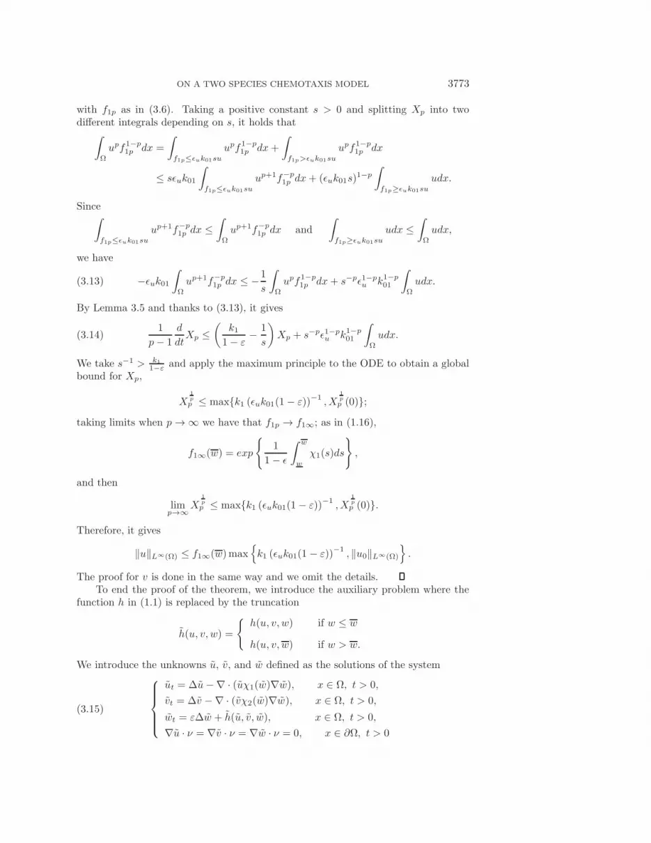
ON A TWO SPECIES CHEMOTAXIS MODEL 3773

with f1p as in (3.6). Taking a positive constant s > 0 and splitting Xp into twodifferent integrals depending on s, it holds that∫

Ω

upf1−p1p dx =

∫f1p≤εuk01su

upf1−p1p dx+

∫f1p>εuk01su

upf1−p1p dx

≤ sεuk01

∫f1p≤εuk01su

up+1f−p1p dx+ (εuk01s)

1−p

∫f1p≥εuk01su

udx.

Since∫f1p≤εuk01su

up+1f−p1p dx ≤

∫Ω

up+1f−p1p dx and

∫f1p≥εuk01su

udx ≤∫Ω

udx,

we have

(3.13) −εuk01

∫Ω

up+1f−p1p dx ≤ −1

s

∫Ω

upf1−p1p dx + s−pε1−p

u k1−p01

∫Ω

udx.

By Lemma 3.5 and thanks to (3.13), it gives

(3.14)1

p− 1

d

dtXp ≤

(k1

1− ε− 1

s

)Xp + s−pε1−p

u k1−p01

∫Ω

udx.

We take s−1 > k1

1−ε and apply the maximum principle to the ODE to obtain a globalbound for Xp,

X1pp ≤ max{k1 (εuk01(1− ε))

−1, X

1pp (0)};

taking limits when p → ∞ we have that f1p → f1∞; as in (1.16),

f1∞(w) = exp

{1

1− ε

∫ w

w

χ1(s)ds

},

and then

limp→∞X

1pp ≤ max{k1 (εuk01(1− ε))

−1, X

1pp (0)}.

Therefore, it gives

‖u‖L∞(Ω) ≤ f1∞(w)max{k1 (εuk01(1 − ε))

−1, ‖u0‖L∞(Ω)

}.

The proof for v is done in the same way and we omit the details.To end the proof of the theorem, we introduce the auxiliary problem where the

function h in (1.1) is replaced by the truncation

h(u, v, w) =

{h(u, v, w) if w ≤ w

h(u, v, w) if w > w.

We introduce the unknowns u, v, and w defined as the solutions of the system

(3.15)

⎧⎪⎪⎪⎨⎪⎪⎪⎩

ut = Δu−∇ · (uχ1(w)∇w), x ∈ Ω, t > 0,

vt = Δv −∇ · (vχ2(w)∇w), x ∈ Ω, t > 0,

wt = εΔw + h(u, v, w), x ∈ Ω, t > 0,

∇u · ν = ∇v · ν = ∇w · ν = 0, x ∈ ∂Ω, t > 0

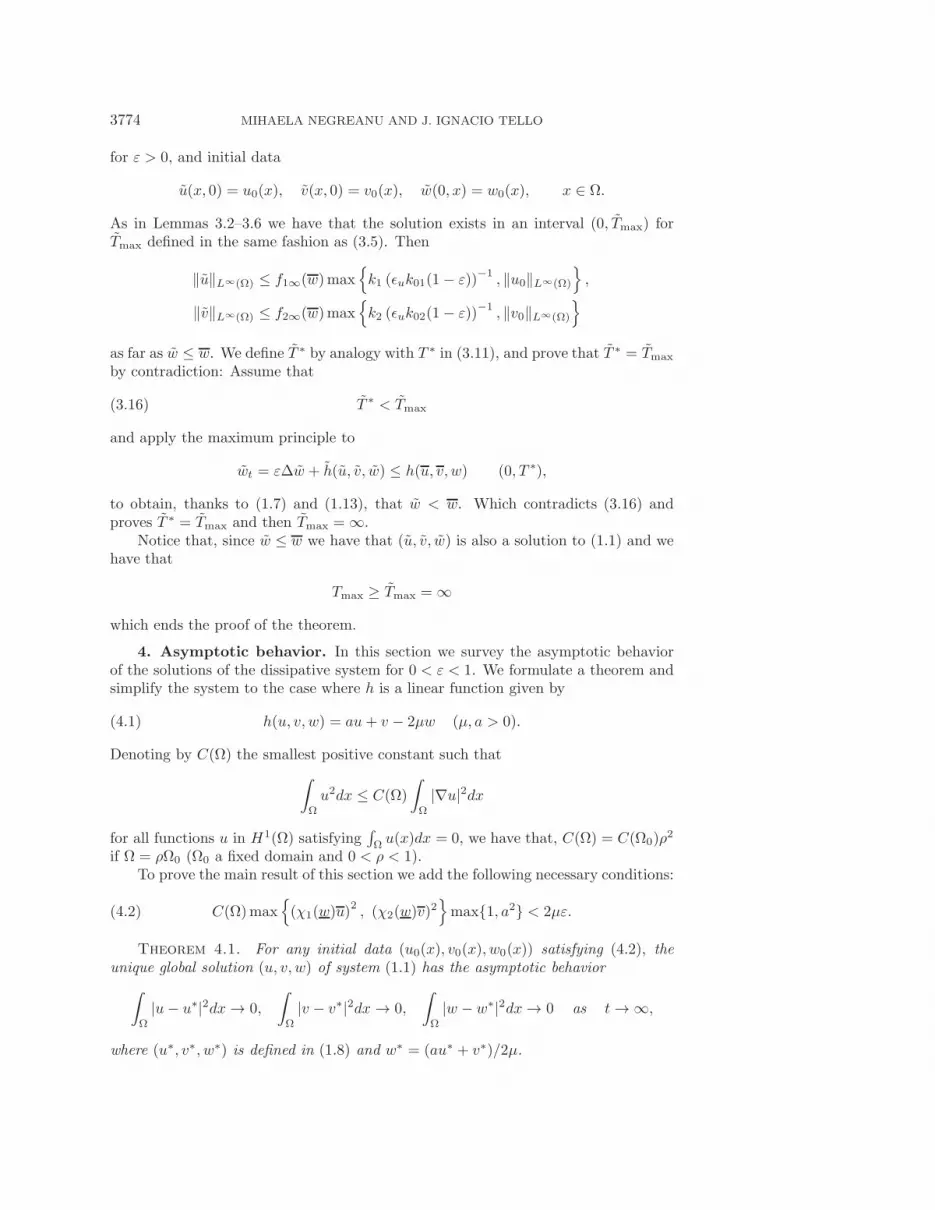
3774 MIHAELA NEGREANU AND J. IGNACIO TELLO

for ε > 0, and initial data

u(x, 0) = u0(x), v(x, 0) = v0(x), w(0, x) = w0(x), x ∈ Ω.

As in Lemmas 3.2–3.6 we have that the solution exists in an interval (0, Tmax) forTmax defined in the same fashion as (3.5). Then

‖u‖L∞(Ω) ≤ f1∞(w)max{k1 (εuk01(1− ε))

−1, ‖u0‖L∞(Ω)

},

‖v‖L∞(Ω) ≤ f2∞(w)max{k2 (εuk02(1− ε))

−1, ‖v0‖L∞(Ω)

}as far as w ≤ w. We define T ∗ by analogy with T ∗ in (3.11), and prove that T ∗ = Tmax

by contradiction: Assume that

(3.16) T ∗ < Tmax

and apply the maximum principle to

wt = εΔw + h(u, v, w) ≤ h(u, v, w) (0, T ∗),

to obtain, thanks to (1.7) and (1.13), that w < w. Which contradicts (3.16) andproves T ∗ = Tmax and then Tmax = ∞.

Notice that, since w ≤ w we have that (u, v, w) is also a solution to (1.1) and wehave that

Tmax ≥ Tmax = ∞which ends the proof of the theorem.

4. Asymptotic behavior. In this section we survey the asymptotic behaviorof the solutions of the dissipative system for 0 < ε < 1. We formulate a theorem andsimplify the system to the case where h is a linear function given by

(4.1) h(u, v, w) = au+ v − 2μw (μ, a > 0).

Denoting by C(Ω) the smallest positive constant such that∫Ω

u2dx ≤ C(Ω)

∫Ω

|∇u|2dx

for all functions u in H1(Ω) satisfying∫Ω u(x)dx = 0, we have that, C(Ω) = C(Ω0)ρ

2

if Ω = ρΩ0 (Ω0 a fixed domain and 0 < ρ < 1).To prove the main result of this section we add the following necessary conditions:

(4.2) C(Ω)max{(χ1(w)u)

2, (χ2(w)v)

2}max{1, a2} < 2με.

Theorem 4.1. For any initial data (u0(x), v0(x), w0(x)) satisfying (4.2), theunique global solution (u, v, w) of system (1.1) has the asymptotic behavior∫

Ω

|u− u∗|2dx → 0,

∫Ω

|v − v∗|2dx → 0,

∫Ω

|w − w∗|2dx → 0 as t → ∞,

where (u∗, v∗, w∗) is defined in (1.8) and w∗ = (au∗ + v∗)/2μ.

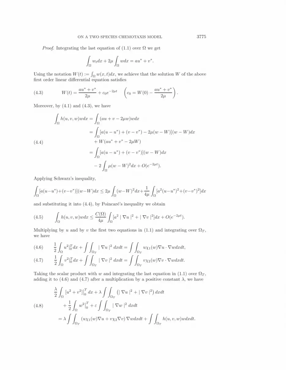
ON A TWO SPECIES CHEMOTAXIS MODEL 3775

Proof. Integrating the last equation of (1.1) over Ω we get∫Ω

wtdx+ 2μ

∫Ω

wdx = au∗ + v∗.

Using the notation W (t) :=∫Ωw(x, t)dx, we achieve that the solution W of the above

first order linear differential equation satisfies

(4.3) W (t) =au∗ + v∗

2μ+ c0e

−2μt

(c0 = W (0)− au∗ + v∗

2μ

).

Moreover, by (4.1) and (4.3), we have

(4.4)

∫Ω

h(u, v, w)wdx =

∫Ω

(au+ v − 2μw)wdx

=

∫Ω

[a(u− u∗) + (v − v∗)− 2μ(w −W )](w −W )dx

+ W (au∗ + v∗ − 2μW )

=

∫Ω

[a(u− u∗) + (v − v∗)](w −W )dx

− 2

∫Ω

μ(w −W )2dx+O(e−2μt).

Applying Schwarz’s inequality,∫Ω

[a(u−u∗)+(v−v∗)](w−W )dx ≤ 2μ

∫Ω

(w−W )2dx+1

4μ

∫Ω

[a2(u−u∗)2+(v−v∗)2]dx

and substituting it into (4.4), by Poincare’s inequality we obtain

(4.5)

∫Ω

h(u, v, w)wdx ≤ C(Ω)

4μ

∫Ω

[a2 | ∇u |2 + | ∇v |2]dx+O(e−2μt).

Multiplying by u and by v the first two equations in (1.1) and integrating over ΩT ,we have

1

2

∫Ω

u2|T0 dx +

∫ ∫ΩT

| ∇u |2 dxdt =

∫ ∫ΩT

uχ1(w)∇u · ∇wdxdt,(4.6)

1

2

∫Ω

v2|T0 dx+

∫ ∫ΩT

| ∇v |2 dxdt =

∫ ∫ΩT

vχ2(w)∇v · ∇wdxdt.(4.7)

Taking the scalar product with w and integrating the last equation in (1.1) over ΩT ,adding it to (4.6) and (4.7) after a multiplication by a positive constant λ, we have

(4.8)

λ

2

∫Ω

[u2 + v2]∣∣T0dx+ λ

∫ ∫ΩT

(| ∇u |2 + | ∇v |2) dxdt+

1

2

∫Ω

w2∣∣T0+ ε

∫ ∫ΩT

| ∇w |2 dxdt

= λ

∫ ∫ΩT

(uχ1(w)∇u + vχ2∇v)∇wdxdt +

∫ ∫ΩT

h(u, v, w)wdxdt.

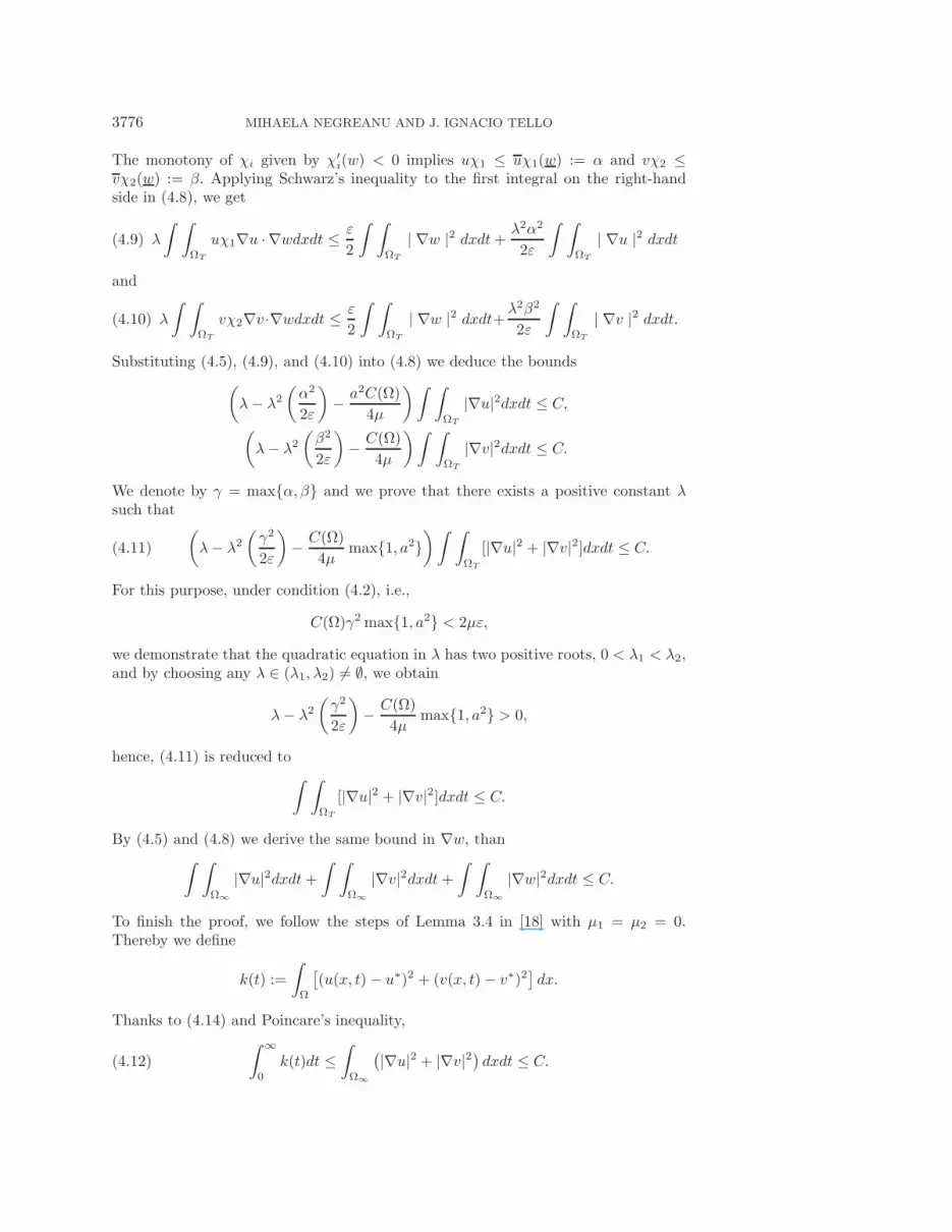
3776 MIHAELA NEGREANU AND J. IGNACIO TELLO

The monotony of χi given by χ′i(w) < 0 implies uχ1 ≤ uχ1(w) := α and vχ2 ≤

vχ2(w) := β. Applying Schwarz’s inequality to the first integral on the right-handside in (4.8), we get

(4.9) λ

∫ ∫ΩT

uχ1∇u · ∇wdxdt ≤ ε

2

∫ ∫ΩT

| ∇w |2 dxdt+λ2α2

2ε

∫ ∫ΩT

| ∇u |2 dxdt

and

(4.10) λ

∫ ∫ΩT

vχ2∇v·∇wdxdt ≤ ε

2

∫ ∫ΩT

| ∇w |2 dxdt+λ2β2

2ε

∫ ∫ΩT

| ∇v |2 dxdt.

Substituting (4.5), (4.9), and (4.10) into (4.8) we deduce the bounds(λ− λ2

(α2

2ε

)− a2C(Ω)

4μ

)∫ ∫ΩT

|∇u|2dxdt ≤ C,(λ− λ2

(β2

2ε

)− C(Ω)

4μ

)∫ ∫ΩT

|∇v|2dxdt ≤ C.

We denote by γ = max{α, β} and we prove that there exists a positive constant λsuch that

(4.11)

(λ− λ2

(γ2

2ε

)− C(Ω)

4μmax{1, a2}

)∫ ∫ΩT

[|∇u|2 + |∇v|2]dxdt ≤ C.

For this purpose, under condition (4.2), i.e.,

C(Ω)γ2 max{1, a2} < 2με,

we demonstrate that the quadratic equation in λ has two positive roots, 0 < λ1 < λ2,and by choosing any λ ∈ (λ1, λ2) = ∅, we obtain

λ− λ2

(γ2

2ε

)− C(Ω)

4μmax{1, a2} > 0,

hence, (4.11) is reduced to∫ ∫ΩT

[|∇u|2 + |∇v|2]dxdt ≤ C.

By (4.5) and (4.8) we derive the same bound in ∇w, than∫ ∫Ω∞

|∇u|2dxdt+∫ ∫

Ω∞|∇v|2dxdt+

∫ ∫Ω∞

|∇w|2dxdt ≤ C.

To finish the proof, we follow the steps of Lemma 3.4 in [18] with μ1 = μ2 = 0.Thereby we define

k(t) :=

∫Ω

[(u(x, t)− u∗)2 + (v(x, t)− v∗)2

]dx.

Thanks to (4.14) and Poincare’s inequality,

(4.12)

∫ ∞

0

k(t)dt ≤∫Ω∞

(|∇u|2 + |∇v|2) dxdt ≤ C.

ON A TWO SPECIES CHEMOTAXIS MODEL 3777

In order to have the limit k(t) → 0, as t → ∞, we apply Lemma 5.1 (ii) of [11] andwe need to prove that

(4.13) |k(t+ s)− k(t)| ≤ ε(t) for all s > 0, where ε(t) → 0 as t → ∞.

Notice that∫Ω

[(u(x, t+ s)− u∗)2 − (u(x, t)− u∗)2]dx

=

∫Ω

[u2(x, t+ s) + (u∗)2 − 2u∗u(x, t+ s)− u2(x, t) − (u∗)2 + 2u∗u(x, t)]dx

and ∫Ω

u∗u(x, t+ s)dx =

∫Ω

u∗u(x, t)dx = (u∗)2

and therefore∫Ω

[(u(x, t+ s)− u∗)2 − (u(x, t)− u∗)2]dx =

∫Ω

[u2(x, t+ s)− u2(x, t)]dx.

Since

(4.14) k(t+ s)− k(t) =

∫ t+s

t

k′(τ)dτ

and

k′(t) = 2

∫Ω

(u− u∗)utdx+ 2

∫Ω

(v − v∗)vtdx = 2

∫Ω

uutdx+ 2

∫Ω

vvtdx,

multiplying the first equation in (1.1) by u we have that∫Ω

uutdx =

∫Ω

|∇u|2dx+

∫Ω

χ1(w)u∇u∇wdx.

By the inequalities∫Ω

χ1(w)u∇u∇wdx ≤ ‖u‖L∞(Ω∞)χ1(w)

∫Ω

[|∇u|2 + |∇w|2] dx,∫Ω

χ2(w)v∇v∇wdx ≤ ‖v‖L∞(Ω∞)χ2(w)

∫Ω

[|∇v|2 + |∇w|2] dx,we obtain

(4.15) |k′(t)| ≤ C

∫Ω

[|∇u|2 + |∇v|2 + |∇w|2] dxand therefore, thanks to (4.14) and (4.15), we get

|k(t+ s)− k(t)| ≤ C

∫ t+s

t

∫Ω

(| ∇u(x, τ) |2 + | ∇v(x, τ) |2 + | ∇w(x, τ) |2)dxdτ.

Therefore ε(t) → 0 as t → ∞. We now apply Lemma 5.1 (ii) in [11] to obtain k(t) → 0as t → ∞.

3778 MIHAELA NEGREANU AND J. IGNACIO TELLO

For the limit ∫Ω

|w − w∗|2dx → 0 as t → ∞,

consider W defined in (4.3) and define the function

q(t) =

∫Ω

(w(x, t) −W (t))2dx.

To obtain q(t) → 0 as t → ∞, we recall again Lemma 5.1 (ii) in [11]. We have toprove that ∫ ∞

0

q(t)dt < ∞ and |q(t+ s)− q(t)| ≤ ε(t) → 0 as t → ∞.

To obtain the first inequality we consider the equation

wt −Wt − εΔ(w −W ) + 2μ(w −W ) = a(u− u∗) + v − v∗.

Multiplying by w −W , integrating in time, and thanks to (4.12) we obtain∫ ∞

0

q(t)dt < C.

The second inequality is proven in the same way as u and v. Thereby, we infer that∫Ω

|w(x, t) −W (t)|2dx → 0 as t → ∞,

and thanks to (4.3) the proof ends.Remark 4.1. Since any stationary solution (u∗, v∗, w∗) of (1.1), with w < w∗(x) <

w, 0 < u∗(x) < u, 0 < v∗(x) < v satisfies the estimate∫ ∫Ω∞

|∇u|2dxdt+∫ ∫

Ω∞|∇v|2dxdt+

∫ ∫Ω∞

|∇w|2dxdt ≤ C,

it follows that such solutions are necessarily constant.

5. Applications. In this section we apply the theoretical results obtained in theprevious section to the case where the chemotactic sensitivities of the species χi aredefined by

χi = αi/(βi + w) and h = au+ v − 2μw,

with positive constants a, μ, αi, and βi (for i = 1, 2) such that

αi ≤ 1− ε for i = 1, 2,(5.1)

βi <αi

αi + 1for i = 1, 2.(5.2)

With αi as in (5.1), the chemotactic sensitivities χi satisfy (1.4) for every 0 < ε < 1with i = 1, 2.

In order to obtain the global existence of the solutions of (1.1) and to prove thatany solution is asymptotically stable, we have to verify that assumptions (1.6), (1.17),(1.11)–(1.13), and (4.2) are fulfilled.

ON A TWO SPECIES CHEMOTAXIS MODEL 3779

1. We have hu = a > 0, hv = 1, and hw = −2μ < 0, so assumptions (1.6) and(1.7) are satisfied for εu = a, εv = 1, and εw = 2μ.

2. Relation (1.11) is equivalent to

(5.3) 2μαiw

βi + w≤ ki.

For

ki := 2μαiw

βi + w,

(5.3) holds, where the upper bound w is to be defined latter. Moreover,observe that it is enough to consider ki = 2μαi, i = 1, 2.

3. Computing in (1.12), we take positive constants such that

k0i :=αi

(βi + w)1−αi, i = 1, 2.

4. Notice that h(0, 0, 0) = 0 and

h(u, v, w) = au+ v − 2μw.

Looking upon the lower bound w = 0, for any upper bound w, by expressions(1.14)–(1.16), the second inequality in (1.13) is equivalent to

(5.4) (β1 + w)

α1ε

1− ε + (β2 + w)

α2ε

1− ε < 1− ε.

For every w and βi verifying (5.4) with αi as in (5.1), we have h(u, v, w) < 0.5. It remains to be studied what conditions are necessary to fulfill (1.17). Sim-

plifying and operating, we found that (1.17) is reduced to

(5.5) (β1 + w)

α1ε

1 − εwα1

β1 + w+ (β2 + w)

α2ε

1 − εwα2

β2 + w≤ 1− ε,

and looking back to (5.4), if we request

(5.6) w <βi

αi, i = 1, 2,

then (5.5) is verified.For the stability, assumption (4.2) is reduced to

(5.7) C(Ω)

(αi

βi

)(βi + w)

2αiε

1 − ε max{1, a2} < 2με(1− ε)2.

Therefore, for every w as in (5.5) and (5.6), for all initial data (u0, v0, w0) of (1.1)satisfying

||u0||L∞ ≤ 2μw

a(β1 + w)2−ε(1 − ε), ||v0||L∞ ≤ 2μw

(β2 + w)2−ε(1− ε), and 0 ≤ w0 ≤ w

such that

u0 ≡ 0 and v0 ≡ 0,

3780 MIHAELA NEGREANU AND J. IGNACIO TELLO

all the required hypotheses are verified and we can apply Theorems 3.1 and 4.1, i.e.,the solution (u, v, w) of (1.1) is globally uniformly bounded and

limt→∞

∫Ω

|u− u∗|2dx = limt→∞

∫Ω

|v − v∗|2dx = limt→∞

∫Ω

|w − w∗|2dx = 0,

where the stationary solution of system (1.1) is

(u∗, v∗, w∗) :=(∫

Ω

u0(x)dx,

∫Ω

v0(x)dx,

∫Ω

(au0 + v0)dx

2μ

).

REFERENCES

[1] W. Alt, Orientation of cells migrating in a chemotactic gradient, in Biological Growth andSpread, Lecture Notes in Biomath. 38, Springer-Verlag, New York, 1980, pp. 353–366

[2] P. Biler, Global solutions to some parabolic-elliptic systems of chemotaxis, Adv. Math. Sci.Appl., 9 (1999), pp. 347–359.

[3] P. Biler, E.E. Espejo, and I. Guerra, Blowup in higher dimensional two species chemotacticsystems, Commun. Pure Appl. Anal., 12 (2013), pp. 89–98.

[4] P. Biler and I. Guerra, Blowup and self-similar solutions for two-component drift-diffusionsystems, Nonlinear Anal., 75 (2012), pp. 5186–5193.

[5] C. Conca and E.E. Espejo, Threshold condition for global existence and blow-up to a radiallysymmetric drift-diffusion system, Appl. Math. Lett., 25 (2012), pp. 352–356.

[6] C. Conca, E.E. Espejo, and K. Vilches, Remarks on the blowup and global existence for atwo species chemotactic Keller-Segel system in R2, European J. Appl. Math., 22 (2011),pp. 553–580.

[7] E.E. Espejo, A. Stevens, and J.J.L. Velazquez, Simultaneous finite time blow-up in a two-species model for chemotaxis, Analysis, 29 (2009), pp. 317–338.

[8] E.E. Espejo, A. Stevens, and J.J.L. Velazquez, A note on non-simultaneous blow-up for adrift-diffusion model, Differential Integral Equations, 23 (2010), pp. 451–462.

[9] E.E. Espejo and G. Wolansky, The Patlak-Keller-Segel model of chemotaxis on with singulardrift and mortality rate, Nonlinearity, 26 (2013), pp. 2315–2331.

[10] A. Fasano, A. Mancini, and M. Primicerio, Equilibrium of two populations subjected tochemotaxis, Math. Models Methods Appl. Sci., 14 (2004), pp. 503–533.

[11] A. Friedman and J.I. Tello, Stability of solutions of chemotaxis equations in reinforcedrandom walks, J. Math. Anal. Appl., 272 (2002), pp. 138–163.

[12] D. Horstmann, From 1970 until present: The Keller-Segel model in chemotaxis and its con-sequences, Jahresber. Deutsch. Math.-Verein., 105 (2003), pp. 103–165.

[13] D. Horstmann, Generalizing the Keller-Segel model: Lyapunov functionals, steady state anal-ysis, and blow-up results for multi-species chemotaxis models in the presence of attractionand repulsion between competitive interacting species, J. Nonlinear Sci., 21 (2011), pp. 231–270.

[14] C. Morales-Rodrigo and J.I. Tello, Global existence and asymptotic behavior of a tumorangiogenesis model with chemotaxis and naptotaxis, Math. Models Methods Appl. Sci., 24(2014), pp. 427–464.

[15] C. Morales-Rodrigo, On some models describing cellular movement: The macroscopic scale,Bol. Soc. Espanola Mat. Apl., 48 (2009), pp. 85–111.

[16] M. Negreanu and J.I. Tello, On a competitive system under chemotactic effects with non-local terms, Nonlinearity, 26 (2013), pp. 1086–1103.

[17] M. Negreanu and J.I. Tello, On a comparison method to reaction-diffusion systems and itsapplications to chemotaxis, Discrete Contin. Dynam. Systems, 18 (2013), pp. 2669–2688.

[18] M. Negreanu and J.I. Tello, Asymptotic stability of a two species chemotaxis system withnon-diffusive chemoattractant, J. Differential Equations, to appear.

[19] P. Quittner and P. Souplet, Superlinear Parabolic Problems: Blow-up, Global Existenceand Steady States, Birkhauser Adv. Texts, Birkhauser, Basel, 2007.

[20] C. Stinner, J.I. Tello, and M. Winkler, Competitive exclusion in a two species chemotaxismodel, J. Math. Biol., 68 (2014), pp. 1607–1626.

[21] C. Stinner and M. Winkler, Global weak solutions in a chemotaxis system with large singularsensitivity, Nonlinear Anal. Real World Appl., 12 (2011), pp. 3727–3740.

[22] J.I. Tello and M. Winkler, Stabilization in a two-species chemotaxis system with logisticsource, Nonlinearity, 25 (2012), pp. 1413–1425.

ON A TWO SPECIES CHEMOTAXIS MODEL 3781

[23] J.J.L. Velazquez, Stability of some mechanisms of chemotactic aggregation, SIAM J. Appl.Math., 62 (2002), pp. 1581–1633.

[24] M. Winkler, Absence of collapse in a parabolic chemotaxis system with signal-dependent sen-sitivity, Math. Nachr., 283 (2010), pp. 1664–1673.

[25] M. Winkler, Global solutions in a fully parabolic chemotaxis system with singular sensitivity,Math. Methods Appl. Sci., 34 (2011), pp. 176–190.

[26] G. Wolansky, Multi-components chemotactic system in absence of conflicts, European J.Appl. Math., 13 (2002), pp. 641–661.