offshore stereo measurements of gravity waves
TRANSCRIPT
Coastal Engineering 64 (2012) 127–138
Contents lists available at SciVerse ScienceDirect
Coastal Engineering
j ourna l homepage: www.e lsev ie r .com/ locate /coasta leng
Offshore stereo measurements of gravity waves
A. Benetazzo a,⁎, F. Fedele b, G. Gallego c, P.-C. Shih d, A. Yezzi d
a Institute of Marine Science, National Research Council, Venice, Italyb School of Civil and Environmental Engineering and School of Electrical and Computer Engineering, Georgia Institute of Technology, Atlanta Georgia, 30332, USAc Grupo de Tratamiento de Imágenes, Universidad Politécnica de Madrid, E-28040 Madrid, Spain.d School of Electrical and Computer Engineering, Georgia Institute of Technology, Atlanta, Georgia, 30332, USA
⁎ Corresponding author. Tel.: +39 041 2407952.E-mail addresses: [email protected] (A
[email protected] (F. Fedele), [email protected] (G. G(A. Yezzi).
0378-3839/$ – see front matter © 2012 Elsevier B.V. Alldoi:10.1016/j.coastaleng.2012.01.007
a b s t r a c t
a r t i c l e i n f oArticle history:Received 4 June 2011Received in revised form 25 January 2012Accepted 27 January 2012Available online 21 February 2012
Keywords:Stereo measurementWASSWavenumber-frequency spectrumWave statisticsCurrent vertical profile
Stereo video techniques are effective for estimating the space-time wave dynamics over an area of the ocean.Indeed, a stereo camera view allows retrieval of both spatial and temporal data whose statistical content isricher than that of time series data retrieved from point wave probes. To prove this, we consider an applica-tion of the Wave Acquisition Stereo System (WASS) for the analysis of offshore video measurements of grav-ity waves in the Northern Adriatic Sea. In particular, we deployed WASS at the oceanographic platform AcquaAlta, off the Venice coast, Italy. Three experimental studies were performed, and the overlapping field of viewof the acquired stereo images covered an area of approximately 1100 m2. Analysis of the WASS measure-ments show that the sea surface can be accurately estimated in space and time together, yielding associateddirectional spectra and wave statistics that agree well with theoretical models. From the observedwavenumber-frequency spectrum one can also predict the vertical profile of the current flow underneaththe wave surface. Finally, future improvements of WASS and applications are discussed.
© 2012 Elsevier B.V. All rights reserved.
1. Introduction
The statistics and spectral properties of ocean waves are typicallyinferred from time series measurements of the wave surface displace-ments retrieved from wave gauges, ultrasonic instruments or buoysat a fixed point P of the ocean. However, the limited informationcontent of point measurements does not accurately predict thespace-time wave dynamics over an area centered at P, especially themaximum surface elevation over the same area, which is generallylarger than that observed in time at P (Fedele et al., 2011; Forristall,2006, 2007). Synthetic Aperture Radar (SAR) or Interferometric SAR(INSAR) remote sensing provide sufficient resolution for measuringwaves only at large spatial scales longer than 100 m (see, e.g.,Marom et al., 1990, 1991; Dankert et al., 2003). However, they are in-sufficient to estimate spectral properties at smaller scales. Presently,at such scales, field measurements for estimating directional wavespectra are challenging or inaccurate even if one could employ linearor two-dimensional wave probe-type arrays, which are expensive toinstall and maintain (Allender et al., 1989; O'Reilly et al., 1996).
Stereo video techniques can be effective for such precise measure-ments which are beneficial for many applications, such as the valida-tion of remote sensing data, the estimation of dissipation rates, andgathering statistics of breakingwaves for the correct parameterization
. Benetazzo),allego), [email protected]
rights reserved.
of numerical wave models. Indeed, a stereo camera view providesboth spatial and temporal data whose statistical content is richerthan that of time series retrieved from wave gauges (Benetazzo,2006; Fedele et al, 2012, 2011; Gallego et al., 2011). Since the watersurface is a specular object in rapid movement, it is convenient to ac-quire stereo-pairs simultaneously, and the geometry of the stereo sys-tem is designed to minimize errors due to sea surface specularities(Jahne, 1993). Further, prior art has based the reconstruction of thewater surface on epipolar techniques (Benetazzo, 2006), which findpixel correspondences in the two synchronized images via pixel-by-pixel based searches that are computationally expensive. Only in thelast two decades or so, has this traditional approach to stereo imagingbecome suitable for applications in oceanography thanks to theadvent of high performance computer processors. For example,Shemdin et al. (1988) and Banner et al. (1989) estimated directionalspectra of short gravity waves, and Benetazzo (2006) proposed andoptimized a Wave Acquisition Stereo System (WASS) for field mea-surements at the coast. More recently, Bechle and Wu (2011) havestudied coastal waves over areas of ~3 m2 using a trinocular system(Wanek and Wu, 2006), de Vries et al. (2011) have presented stereomeasurements of waves in the surf zone over an area of ~1000 m2,and Kosnik and Dulov (2011) have estimated sea roughness from ste-reo images.
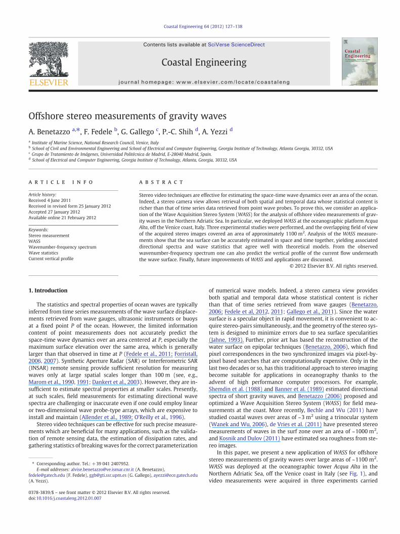
In this paper, we present a new application of WASS for offshorestereo measurements of gravity waves over large areas of ~1100 m2.WASS was deployed at the oceanographic tower Acqua Alta in theNorthern Adriatic Sea, off the Venice coast in Italy (see Fig. 1), andvideo measurements were acquired in three experiments carried
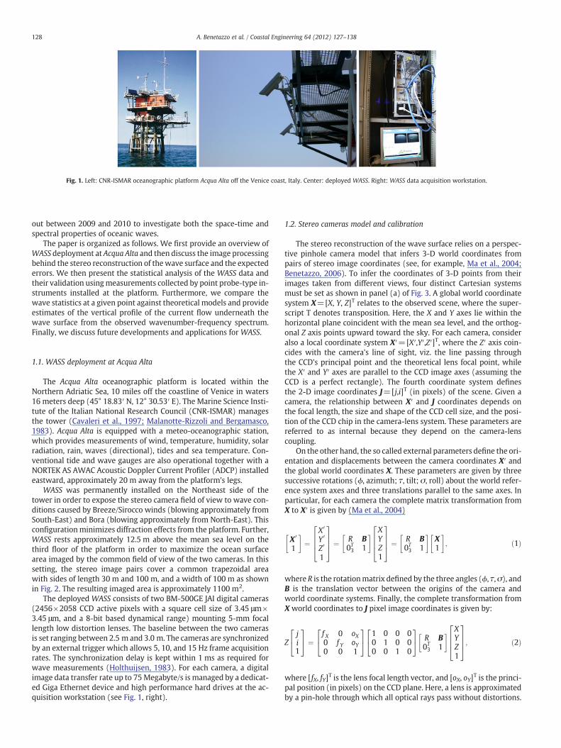
Fig. 1. Left: CNR-ISMAR oceanographic platform Acqua Alta off the Venice coast, Italy. Center: deployed WASS. Right: WASS data acquisition workstation.
128 A. Benetazzo et al. / Coastal Engineering 64 (2012) 127–138
out between 2009 and 2010 to investigate both the space-time andspectral properties of oceanic waves.
The paper is organized as follows. We first provide an overview ofWASS deployment at Acqua Alta and then discuss the image processingbehind the stereo reconstruction of thewave surface and the expectederrors. We then present the statistical analysis of the WASS data andtheir validation usingmeasurements collected by point probe-type in-struments installed at the platform. Furthermore, we compare thewave statistics at a given point against theoretical models and provideestimates of the vertical profile of the current flow underneath thewave surface from the observed wavenumber-frequency spectrum.Finally, we discuss future developments and applications for WASS.
1.1. WASS deployment at Acqua Alta
The Acqua Alta oceanographic platform is located within theNorthern Adriatic Sea, 10 miles off the coastline of Venice in waters16 meters deep (45° 18.83′ N, 12° 30.53′ E). The Marine Science Insti-tute of the Italian National Research Council (CNR-ISMAR) managesthe tower (Cavaleri et al., 1997; Malanotte-Rizzoli and Bergamasco,1983). Acqua Alta is equipped with a meteo-oceanographic station,which provides measurements of wind, temperature, humidity, solarradiation, rain, waves (directional), tides and sea temperature. Con-ventional tide and wave gauges are also operational together with aNORTEK AS AWAC Acoustic Doppler Current Profiler (ADCP) installedeastward, approximately 20 m away from the platform's legs.
WASS was permanently installed on the Northeast side of thetower in order to expose the stereo camera field of view to wave con-ditions caused by Breeze/Sirocco winds (blowing approximately fromSouth-East) and Bora (blowing approximately from North-East). Thisconfigurationminimizes diffraction effects from the platform. Further,WASS rests approximately 12.5 m above the mean sea level on thethird floor of the platform in order to maximize the ocean surfacearea imaged by the common field of view of the two cameras. In thissetting, the stereo image pairs cover a common trapezoidal areawith sides of length 30 m and 100 m, and a width of 100 m as shownin Fig. 2. The resulting imaged area is approximately 1100 m2.
The deployed WASS consists of two BM-500GE JAI digital cameras(2456×2058 CCD active pixels with a square cell size of 3.45 μm×3.45 μm, and a 8-bit based dynamical range) mounting 5-mm focallength low distortion lenses. The baseline between the two camerasis set ranging between 2.5 m and 3.0 m. The cameras are synchronizedby an external trigger which allows 5, 10, and 15 Hz frame acquisitionrates. The synchronization delay is kept within 1 ms as required forwave measurements (Holthuijsen, 1983). For each camera, a digitalimage data transfer rate up to 75Megabyte/s is managed by a dedicat-ed Giga Ethernet device and high performance hard drives at the ac-quisition workstation (see Fig. 1, right).
1.2. Stereo cameras model and calibration
The stereo reconstruction of the wave surface relies on a perspec-tive pinhole camera model that infers 3-D world coordinates frompairs of stereo image coordinates (see, for example, Ma et al., 2004;Benetazzo, 2006). To infer the coordinates of 3-D points from theirimages taken from different views, four distinct Cartesian systemsmust be set as shown in panel (a) of Fig. 3. A global world coordinatesystem X=[X, Y, Z]T relates to the observed scene, where the super-script T denotes transposition. Here, the X and Y axes lie within thehorizontal plane coincident with the mean sea level, and the orthog-onal Z axis points upward toward the sky. For each camera, consideralso a local coordinate system X′=[X′,Y′,Z′]T, where the Z′ axis coin-cides with the camera's line of sight, viz. the line passing throughthe CCD's principal point and the theoretical lens focal point, whilethe X′ and Y′ axes are parallel to the CCD image axes (assuming theCCD is a perfect rectangle). The fourth coordinate system definesthe 2-D image coordinates J=[j,i]T (in pixels) of the scene. Given acamera, the relationship between X′ and J coordinates depends onthe focal length, the size and shape of the CCD cell size, and the posi-tion of the CCD chip in the camera-lens system. These parameters arereferred to as internal because they depend on the camera-lenscoupling.
On the other hand, the so called external parameters define the ori-entation and displacements between the camera coordinates X′ andthe global world coordinates X. These parameters are given by threesuccessive rotations (ϕ, azimuth; τ, tilt; σ, roll) about the world refer-ence system axes and three translations parallel to the same axes. Inparticular, for each camera the complete matrix transformation fromX to X′ is given by (Ma et al., 2004)
X 0
1
� �¼
X0
Y 0
Z0
1
2664
3775 ¼ R B
0T3 1
� � XYZ1
2664
3775 ¼ R B
0T3 1
� �X1
� �; ð1Þ
where R is the rotationmatrix defined by the three angles (ϕ, τ,σ), andB is the translation vector between the origins of the camera andworld coordinate systems. Finally, the complete transformation fromX world coordinates to J pixel image coordinates is given by:
Zji1
24
35 ¼
f X 0 oX0 f Y oY0 0 1
24
35 1 0 0 0
0 1 0 00 0 1 0
24
35 R B
0T3 1
� � XYZ1
2664
3775; ð2Þ
where [fX, fY]T is the lens focal length vector, and [oX, oY]T is the princi-pal position (in pixels) on the CCD plane. Here, a lens is approximatedby a pin-hole through which all optical rays pass without distortions.
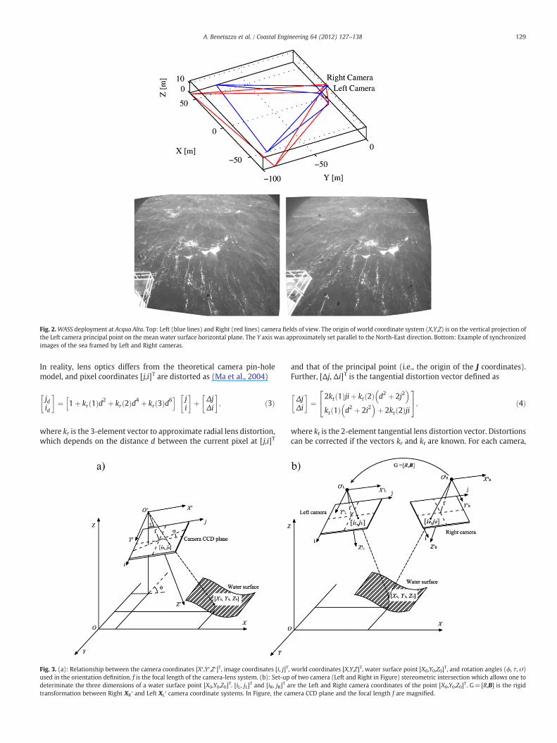
Fig. 2.WASS deployment at Acqua Alta. Top: Left (blue lines) and Right (red lines) camera fields of view. The origin of world coordinate system (X,Y,Z) is on the vertical projection ofthe Left camera principal point on the mean water surface horizontal plane. The Y axis was approximately set parallel to the North-East direction. Bottom: Example of synchronizedimages of the sea framed by Left and Right cameras.
129A. Benetazzo et al. / Coastal Engineering 64 (2012) 127–138
In reality, lens optics differs from the theoretical camera pin-holemodel, and pixel coordinates [j,i]T are distorted as (Ma et al., 2004)
jdid
� �¼ 1þ kr 1ð Þd2 þ kr 2ð Þd4 þ kr 3ð Þd6h i j
i
� �þ Δj
Δi
� �; ð3Þ
where kr is the 3-element vector to approximate radial lens distortion,which depends on the distance d between the current pixel at [j,i]T
Fig. 3. (a): Relationship between the camera coordinates [X′,Y′,Z′]T, image coordinates [i, j]T,used in the orientation definition. f is the focal length of the camera-lens system. (b): Set-updeterminate the three dimensions of a water surface point [X0,Y0,Z0]T. [iL, jL]T and [iR, jR]T atransformation between Right XR′ and Left XL′ camera coordinate systems. In Figure, the ca
and that of the principal point (i.e., the origin of the J coordinates).Further, [Δj, Δi]T is the tangential distortion vector defined as
ΔjΔi
� �¼
2kt 1ð Þjiþ kt 2ð Þ d2 þ 2j2� �
kt 1ð Þ d2 þ 2i2� �
þ 2kt 2ð Þji
24
35; ð4Þ
where kt is the 2-element tangential lens distortion vector. Distortionscan be corrected if the vectors kr and kt are known. For each camera,
world coordinates [X,Y,Z]T, water surface point [X0,Y0,Z0]T, and rotation angles (ϕ, τ, σ)of two camera (Left and Right in Figure) stereometric intersection which allows one tore the Left and Right camera coordinates of the point [X0,Y0,Z0]T. G=[R,B] is the rigidmera CCD plane and the focal length f are magnified.
130 A. Benetazzo et al. / Coastal Engineering 64 (2012) 127–138
the intrinsic calibration (Heikkila and Silven, 1997; Ma et al., 2004;Zhang, 2000) is the procedure that allows the user to estimate the in-ternal parameters needed in Eqs. (2)–(4), viz. the lens focal lengthvector [fX, fY]T, the principal point image coordinates [oX, oY]T on theCCD plane, and the distortion vectors kr and kt. These parameters aresummarized in Table 1 for the WASS cameras installed at Acqua Alta.
Given the two camera pixel positions JL and JR, one can infer the 3-D coordinates of the associated world point X0 given the two 3-D rigidtransformations from the world reference system to Left and Rightcamera reference systems, respectively. Consequently, such a geomet-ric constraint, viz. the rigid motion between Left and Right camera ref-erence systems, is used to triangulate image coordinates with respectto one of two image coordinates as shown in panel (b) of Fig. 3. The sixdegrees of freedom (three consecutive rotations and three orthogonaltranslations) of the 3-D rigid motion between the Left and Right cam-eras coordinate systems can be estimated via an extrinsic calibrationprocedure.
Finally, to infer the 3-D rigid motion in Eq. (2) between, say, theLeft camera and the world coordinates system we assume that thetime average of the mean level of the water surface elevation is aplane orthogonal to the direction of gravity, viz. Z. Benetazzo (2006)validated such assumption, which allows operating WASS withoutground control points. Rigid motion is estimated by fitting the 3-Dreconstructed surface with a mean plane aX′+bY′+cZ′+e=0 inthe camera reference system. Such a plane is then rotated and trans-lated to the world camera system according to the rotation matrix RWand the translation vector tw given, respectively, by
RW ¼1− 1−cð Þa2
a2 þ b2− 1−cð Þab
a2 þ b2−a
− 1−cð Þaba2 þ b2
1− 1−cð Þb2a2 þ b2
−b
a b c
2666664
3777775 ð5Þ
tw ¼ 0; 0; e½ �T ð6Þ
where a, b, c, and e are the mean plane parameters. The estimation ismade robust by averaging several thousand mean planes calculatedfrom all the stereo snapshots within the given time sequence. As anexample, Fig. 4 shows a time sequence of images (snapshots) takenbyWASS and the associated elevationmaps of the wave surface recon-structed by stereo-matching of pixels within the red box.
1.3. Image processing and expected errors
The epipolar algorithm herein proposed is a local method sinceeach pixel correspondence is processed independently from theother pairs. Consequently, the resulting reconstructed wave surfaceis a collection of 3-D scattered points, and proper interpolation en-forces spatial and temporal continuity (Benetazzo, 2006). The keyissue in such methods is the optimal selection of both the AggregationSupportWindow (ASW) and Search Area (SA) for pixel matchingwithrespect to the 2-D image coordinates [i,j]T (Tombari et al., 2008). Sincethe camera parameters are known, epipolar geometry reduces the 2-Dsearch to a sequence of 1-D searches along epipolar lines (or a band toaccount for uncertainties). For example, choose the pixel (point)
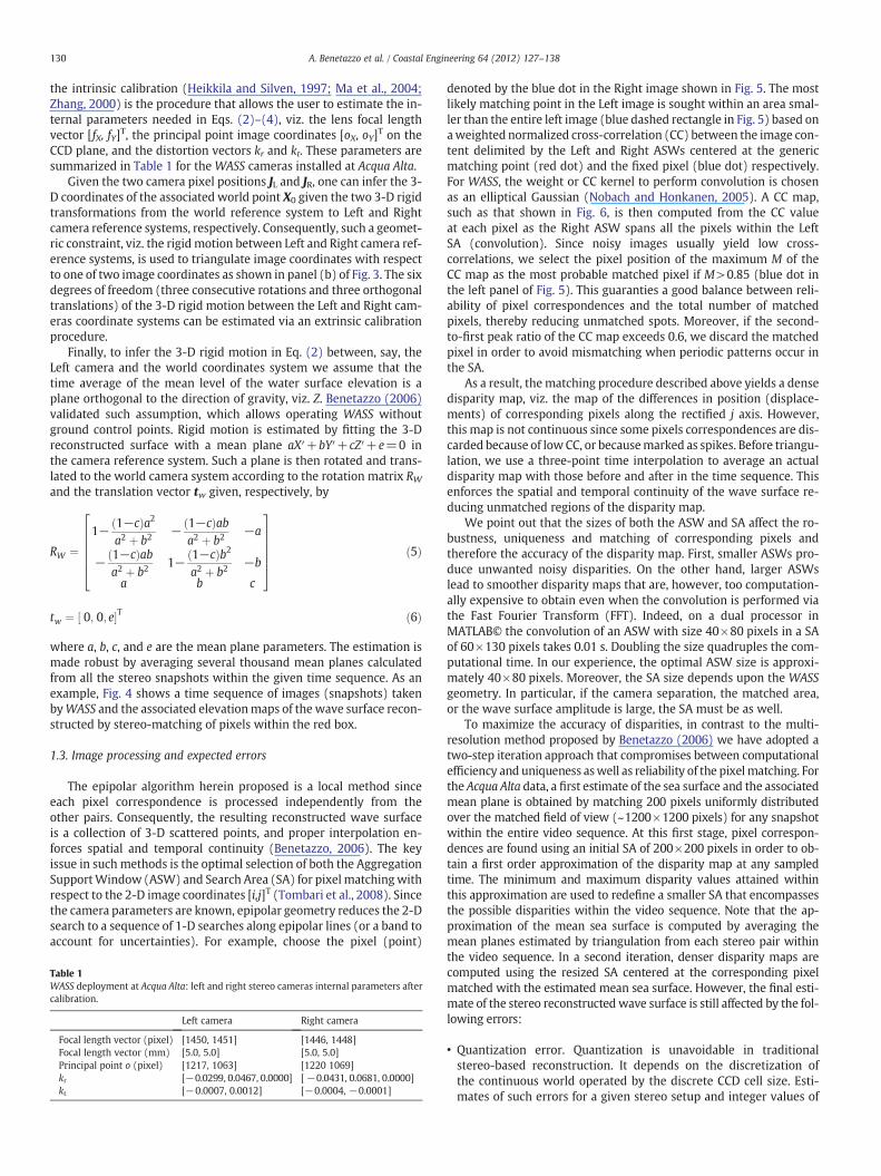
Table 1WASS deployment at Acqua Alta: left and right stereo cameras internal parameters aftercalibration.
Left camera Right camera
Focal length vector (pixel) [1450, 1451] [1446, 1448]Focal length vector (mm) [5.0, 5.0] [5.0, 5.0]Principal point o (pixel) [1217, 1063] [1220 1069]kr [−0.0299, 0.0467, 0.0000] [−0.0431, 0.0681, 0.0000]kt [−0.0007, 0.0012] [−0.0004, −0.0001]
denoted by the blue dot in the Right image shown in Fig. 5. The mostlikely matching point in the Left image is sought within an area smal-ler than the entire left image (blue dashed rectangle in Fig. 5) based onaweighted normalized cross-correlation (CC) between the image con-tent delimited by the Left and Right ASWs centered at the genericmatching point (red dot) and the fixed pixel (blue dot) respectively.For WASS, the weight or CC kernel to perform convolution is chosenas an elliptical Gaussian (Nobach and Honkanen, 2005). A CC map,such as that shown in Fig. 6, is then computed from the CC valueat each pixel as the Right ASW spans all the pixels within the LeftSA (convolution). Since noisy images usually yield low cross-correlations, we select the pixel position of the maximum M of theCC map as the most probable matched pixel if M>0.85 (blue dot inthe left panel of Fig. 5). This guaranties a good balance between reli-ability of pixel correspondences and the total number of matchedpixels, thereby reducing unmatched spots. Moreover, if the second-to-first peak ratio of the CC map exceeds 0.6, we discard the matchedpixel in order to avoid mismatching when periodic patterns occur inthe SA.
As a result, the matching procedure described above yields a densedisparity map, viz. the map of the differences in position (displace-ments) of corresponding pixels along the rectified j axis. However,this map is not continuous since some pixels correspondences are dis-carded because of low CC, or becausemarked as spikes. Before triangu-lation, we use a three-point time interpolation to average an actualdisparity map with those before and after in the time sequence. Thisenforces the spatial and temporal continuity of the wave surface re-ducing unmatched regions of the disparity map.
We point out that the sizes of both the ASW and SA affect the ro-bustness, uniqueness and matching of corresponding pixels andtherefore the accuracy of the disparity map. First, smaller ASWs pro-duce unwanted noisy disparities. On the other hand, larger ASWslead to smoother disparity maps that are, however, too computation-ally expensive to obtain even when the convolution is performed viathe Fast Fourier Transform (FFT). Indeed, on a dual processor inMATLAB© the convolution of an ASW with size 40×80 pixels in a SAof 60×130 pixels takes 0.01 s. Doubling the size quadruples the com-putational time. In our experience, the optimal ASW size is approxi-mately 40×80 pixels. Moreover, the SA size depends upon the WASSgeometry. In particular, if the camera separation, the matched area,or the wave surface amplitude is large, the SA must be as well.
To maximize the accuracy of disparities, in contrast to the multi-resolution method proposed by Benetazzo (2006) we have adopted atwo-step iteration approach that compromises between computationalefficiency and uniqueness aswell as reliability of the pixelmatching. Forthe Acqua Alta data, a first estimate of the sea surface and the associatedmean plane is obtained by matching 200 pixels uniformly distributedover the matched field of view (~1200×1200 pixels) for any snapshotwithin the entire video sequence. At this first stage, pixel correspon-dences are found using an initial SA of 200×200 pixels in order to ob-tain a first order approximation of the disparity map at any sampledtime. The minimum and maximum disparity values attained withinthis approximation are used to redefine a smaller SA that encompassesthe possible disparities within the video sequence. Note that the ap-proximation of the mean sea surface is computed by averaging themean planes estimated by triangulation from each stereo pair withinthe video sequence. In a second iteration, denser disparity maps arecomputed using the resized SA centered at the corresponding pixelmatched with the estimated mean sea surface. However, the final esti-mate of the stereo reconstructedwave surface is still affected by the fol-lowing errors:
• Quantization error. Quantization is unavoidable in traditionalstereo-based reconstruction. It depends on the discretization ofthe continuous world operated by the discrete CCD cell size. Esti-mates of such errors for a given stereo setup and integer values of
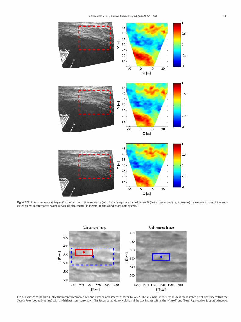
Fig. 4. WASS measurements at Acqua Alta: (left column) time sequence (Δt=2 s) of snapshots framed by WASS (Left camera), and (right column) the elevation maps of the asso-ciated stereo reconstructed water surface displacements (in meters) in the world coordinate system.
Fig. 5. Corresponding pixels (blue) between synchronous Left and Right camera images as taken byWASS. The blue point in the Left image is the matched pixel identified within theSearch Area (dotted blue line) with the highest cross-correlation. This is computed via convolution of the two images within the left (red) and (blue) Aggregation Support Windows.
131A. Benetazzo et al. / Coastal Engineering 64 (2012) 127–138
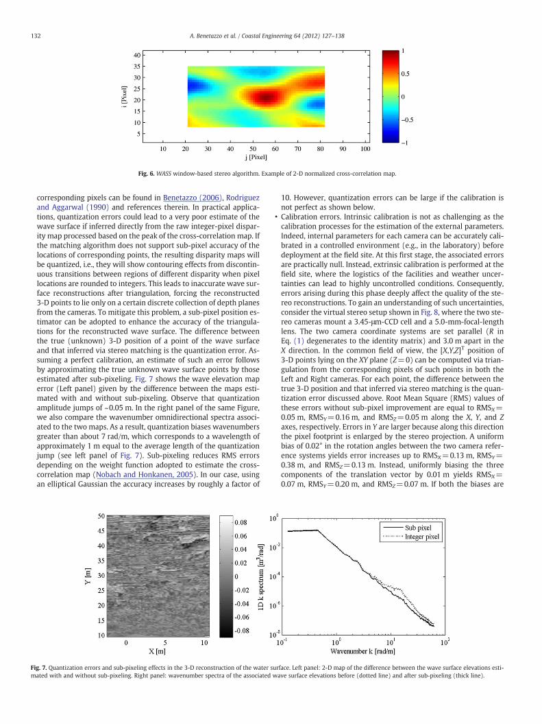
Fig. 6. WASS window-based stereo algorithm. Example of 2-D normalized cross-correlation map.
132 A. Benetazzo et al. / Coastal Engineering 64 (2012) 127–138
corresponding pixels can be found in Benetazzo (2006), Rodriguezand Aggarwal (1990) and references therein. In practical applica-tions, quantization errors could lead to a very poor estimate of thewave surface if inferred directly from the raw integer-pixel dispar-ity map processed based on the peak of the cross-correlation map. Ifthe matching algorithm does not support sub-pixel accuracy of thelocations of corresponding points, the resulting disparity maps willbe quantized, i.e., they will show contouring effects from discontin-uous transitions between regions of different disparity when pixellocations are rounded to integers. This leads to inaccurate wave sur-face reconstructions after triangulation, forcing the reconstructed3-D points to lie only on a certain discrete collection of depth planesfrom the cameras. To mitigate this problem, a sub-pixel position es-timator can be adopted to enhance the accuracy of the triangula-tions for the reconstructed wave surface. The difference betweenthe true (unknown) 3-D position of a point of the wave surfaceand that inferred via stereo matching is the quantization error. As-suming a perfect calibration, an estimate of such an error followsby approximating the true unknown wave surface points by thoseestimated after sub-pixeling. Fig. 7 shows the wave elevation maperror (Left panel) given by the difference between the maps esti-mated with and without sub-pixeling. Observe that quantizationamplitude jumps of ~0.05 m. In the right panel of the same Figure,we also compare the wavenumber omnidirectional spectra associ-ated to the two maps. As a result, quantization biases wavenumbersgreater than about 7 rad/m, which corresponds to a wavelength ofapproximately 1 m equal to the average length of the quantizationjump (see left panel of Fig. 7). Sub-pixeling reduces RMS errorsdepending on the weight function adopted to estimate the cross-correlation map (Nobach and Honkanen, 2005). In our case, usingan elliptical Gaussian the accuracy increases by roughly a factor of
Fig. 7. Quantization errors and sub-pixeling effects in the 3-D reconstruction of the water smated with and without sub-pixeling. Right panel: wavenumber spectra of the associated
10. However, quantization errors can be large if the calibration isnot perfect as shown below.
• Calibration errors. Intrinsic calibration is not as challenging as thecalibration processes for the estimation of the external parameters.Indeed, internal parameters for each camera can be accurately cali-brated in a controlled environment (e.g., in the laboratory) beforedeployment at the field site. At this first stage, the associated errorsare practically null. Instead, extrinsic calibration is performed at thefield site, where the logistics of the facilities and weather uncer-tainties can lead to highly uncontrolled conditions. Consequently,errors arising during this phase deeply affect the quality of the ste-reo reconstructions. To gain an understanding of such uncertainties,consider the virtual stereo setup shown in Fig. 8, where the two ste-reo cameras mount a 3.45-μm-CCD cell and a 5.0-mm-focal-lengthlens. The two camera coordinate systems are set parallel (R inEq. (1) degenerates to the identity matrix) and 3.0 m apart in theX direction. In the common field of view, the [X,Y,Z]T position of3-D points lying on the XY plane (Z=0) can be computed via trian-gulation from the corresponding pixels of such points in both theLeft and Right cameras. For each point, the difference between thetrue 3-D position and that inferred via stereo matching is the quan-tization error discussed above. Root Mean Square (RMS) values ofthese errors without sub-pixel improvement are equal to RMSX=0.05 m, RMSY=0.16 m, and RMSZ=0.05 m along the X, Y, and Zaxes, respectively. Errors in Y are larger because along this directionthe pixel footprint is enlarged by the stereo projection. A uniformbias of 0.02° in the rotation angles between the two camera refer-ence systems yields error increases up to RMSX=0.13 m, RMSY=0.38 m, and RMSZ=0.13 m. Instead, uniformly biasing the threecomponents of the translation vector by 0.01 m yields RMSX=0.07 m, RMSY=0.20 m, and RMSZ=0.07 m. If both the biases are
urface. Left panel: 2-D map of the difference between the wave surface elevations esti-wave surface elevations before (dotted line) and after sub-pixeling (thick line).
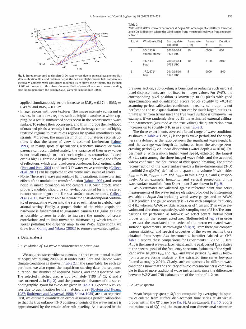
Fig. 8. Stereo setup used to simulate 3-D shape errors due to external parameters biasafter calibration. Blue and red lines depict the Left and Right camera fields of view re-spectively. Cameras were considered mounted 15 m above the XY plane, and inclinedof 40° with respect to this plane. Common Field of view allows one to correspondingpixel up to 80 m from the camera CCDs. Cameras separation is 3.0 m.
Table 22009–2010 WASS stereo experiments at Acqua Alta oceanographic platform. Directionangle Dir is direction where the wind comes from, measured clockwise from geograph-ic North.
Exp # Wind [m/s, Dir] Starting dateand hour
Frame rate[Hz]
Frames#
Duration[s]
1 6.5, 133.0Sirocco Breeze
2009/06/051428 UTC
10 6000 600
2 9.6, 51.2Bora
2009/10/140755 UTC
10 21000 2100
3 17.9, 67.5Bora
2010/03/091120 UTC
5 9000 1800
133A. Benetazzo et al. / Coastal Engineering 64 (2012) 127–138
applied simultaneously, errors increase to RMSX=0.17 m, RMSY=0.49 m, and RMSZ=0.18 m.
• Image regions with poor textures. The image intensity constraint isuseless in textureless regions, such as bright areas due to white cap-ping. As a result, unmatched spots occur in the reconstructed wavesurface. To reduce their occurrence, and thus improve the likelihoodof matched pixels, a remedy is to diffuse the image content of highlytextured regions to textureless regions by spatial smoothness con-straints. Moreover, the main assumption in our stereo reconstruc-tions is that the scene of view is assumed Lambertian (Jahne,1993). In reality, spots of specularities, reflective surfaces, or trans-parency can occur. Unfortunately, the variance of their gray valuesis not small enough to mark such regions as textureless. Indeed,even a high CC threshold in pixel matching will not avoid the effectsof reflections, which alter pixel correspondences. Local optimal paths(Park and Park, 2001) and local 3-D water wave continuity (Gallegoet al., 2011) can be exploited to overcome such source of errors.
• Noise. There are always unavoidable light variations, image blurring,effects of themodulation transfer function (Jahne, 1993), and sensornoise in image formation on the camera CCD. Such effects whenproperly modeled should be somewhat accounted for in the stereoreconstruction algorithm. For sea surface measurements, Gallegoet al. (2011) have been able to include the spatial-temporal continu-ity of propagating waves into the stereo estimation in a global vari-ational setting. Finally, a proper choice of the video acquisitionhardware is fundamental to guarantee camera CCD gains as closeas possible to zero in order to increase the number of cross-correlations and to limit unwanted mismatching which results inspikes polluting the disparity map. In our WASS applications, wedraw from Goring and Nikora (2002) to remove unwanted spikes.
2. Data analysis
2.1. Validation of 3-d wave measurements at Acqua Alta
We acquired stereo video sequences in three experimental studiesat Acqua Alta during 2009–2010 under both Bora and Sirocco waveclimate conditions as shown in Table 2. In the same Table, for each ex-periment, we also report the acquisition starting date, the sequenceduration, the number of acquired frames, and the associated rate.The selected matched area is approximately 1100 m2 (X, Y, and Zaxes oriented as in Fig. 2), and the geometrical features of the stereophotographic layout for WASS are given in Table 3. Expected RMS er-rors due to quantization for the matched area (Blostein and Huang,1987; Rodriguez and Aggarwal, 1990; Solina, 1985) are also reported.First, we estimate quantization errors assuming a perfect calibration,so that the true unknown 3-D position of points of the wave surface isapproximated by the results after sub-pixeling. As discussed in the
previous section, sub-pixeling is beneficial in reducing such errors ifpixel displacements are not fixed to integer values. For WASS, thecorresponding pixel position is known up to 0.1 pixels with goodapproximation and quantization errors reduce roughly to ~0.01 massuming perfect calibration conditions. In reality, calibration is notperfect and the true quantization error can be much larger, but its es-timate is far from trivial since the true wave surface is unknown. Forexample, if we randomly alter by 3% the estimated external calibra-tion parameters (assumed as the true values) the quantization errorincreases up to roughly 0.16 m as shown Table 3.
The three experiments covered a broad range of wave conditionsas shown in Table 4. Here, Tp is the peak wave period, and the steep-ness ε is defined as the ratio between the significant wave height Hs
and the average wavelength Lm estimated from the average zero-crossing period Tz via linear dispersion (water depth d=16 m). Ex-periment 3, with a much higher wind speed, exhibited the largestHs / Lm ratio among the three imaged wave fields, and the acquiredvideos confirmed the occurrence of widespread breaking. The stereoreconstruction of the wave surface yields a three-dimensional (3-D)manifold Z=η(X,Y;t) defined on a space-time volume V with sidesXmax=35 m, Ymax=35 m and tmax~30 min along X,Y and t, respec-tively. As an example, horizontal and vertical projections of thewave surface manifold from Experiment 2 are shown in Fig. 9.
WASS estimates are validated against reference point time seriesmeasurements of the wave surface elevation provided by instrumentsavailable at Acqua Alta including wired wave gauges and an AWACADCP profiler. The gauge accuracy is ~1 cm with sampling frequencyof 4 Hz, whereas AWAC exhibits accuracies of 1 cm and 2° in wave ele-vation and direction, respectively, with sampling rate of 2 Hz. The com-parisons are performed as follows: we select several virtual pointprobes within the reconstructed area (Bottom-left of Fig. 9) in orderto extract the associated time series of the stereo-estimated wavesurface displacements (Bottom-right of Fig. 9). From these, we comparevarious statistical and spectral properties of the waves against thoseobtained from Acqua Alta instruments, hereafter labeled as CNR.Table 5 reports these comparisons for Experiments 1, 2 and 3. Here,Hmax is the largestwave surface height, and the peak period Tp is relativeto the spectral peak of the frequency spectrum. Estimates of the signif-icant wave heights Hmo and H1/3, and wave periods Tm and Tz followfrom a zero-crossing analysis of the extracted time series low-passfiltered at roughly 2.0 Hz. Clearly, such comparisons for different waveconditions show that the accuracy of WASS measurements is compara-ble to that of more traditional wave instruments since the differencesbetweenWASS and CNR estimates are of the order of 1–2 cm.
2.2. Wave spectra
Mean frequency spectra S(f) are computed by averaging the spec-tra calculated from surface displacement time series at 40 virtualprobes within the XY plane (see Fig. 9). As an example, Fig. 10 reportsthe estimates of S(f) and the associated non-dimensional saturation
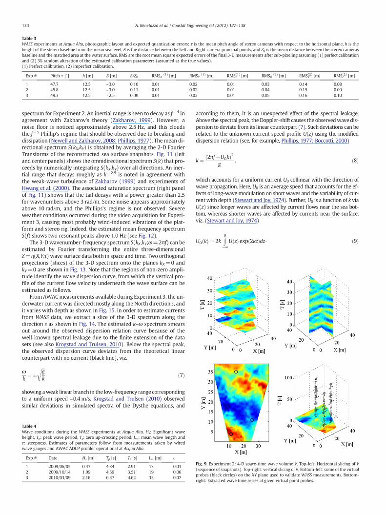
Table 3WASS experiments at Acqua Alta, photographic layout and expected quantization errors: τ is the mean pitch angle of stereo cameras with respect to the horizontal plane, h is theheight of the stereo baseline from the mean sea level, B is the distance between the Left and Right camera principal points, and Z0 is the mean distance between the stereo camerasbaseline and the matched area at the water surface. RMS are the root mean square expected errors of the final 3-D measurements after sub-pixeling assuming (1) perfect calibrationand (2) 3% random alteration of the estimated calibration parameters (assumed as the true values).(1) Perfect calibration, (2) imperfect calibration.
Exp # Pitch τ [°] h [m] B [m] B/Z0 RMSX (1) [m] RMSY (1) [m] RMSZ(1) [m] RMSX (2) [m] RMSY(2) [m] RMSZ(2) [m]
1 47.7 12.5 ~3.0 0.10 0.01 0.02 0.01 0.03 0.14 0.082 45.8 12.5 ~3.0 0.11 0.01 0.02 0.01 0.04 0.15 0.093 49.3 12.5 ~2.5 0.09 0.01 0.02 0.01 0.05 0.16 0.10
134 A. Benetazzo et al. / Coastal Engineering 64 (2012) 127–138
spectrum for Experiment 2. An inertial range is seen to decay as f−4 inagreement with Zakharov's theory (Zakharov, 1999). However, anoise floor is noticed approximately above 2.5 Hz, and this cloudsthe f−5 Phillip's regime that should be observed due to breaking anddissipation (Newell and Zakharov, 2008; Phillips, 1977). The mean di-rectional spectrum S(kX,kY) is obtained by averaging the 2-D FourierTransforms of the reconstructed sea surface snapshots. Fig. 11 (leftand center panels) shows the omnidirectional spectrum S(k) that pro-ceeds by numerically integrating S(kX,kY) over all directions. An iner-tial range that decays roughly as k−2.5 is noted in agreement withthe weak-wave turbulence of Zakharov (1999) and experiments ofHwang et al. (2000). The associated saturation spectrum (right panelof Fig. 11) shows that the tail decays with a power greater than 2.5for wavenumbers above 3 rad/m. Some noise appears approximatelyabove 10 rad/m, and the Phillips's regime is not observed. Severeweather conditions occurred during the video acquisition for Experi-ment 3, causing most probably wind-induced vibrations of the plat-form and stereo rig. Indeed, the estimated mean frequency spectrumS(f) shows two resonant peaks above 1.0 Hz (see Fig. 12).
The 3-D wavenumber-frequency spectrum S(kX,kY;ω=2πf) can beestimated by Fourier transforming the entire three-dimensionalZ=η(X,Y;t) wave surface data both in space and time. Two orthogonalprojections (slices) of the 3-D spectrum onto the planes kX=0 andkY=0 are shown in Fig. 13. Note that the regions of non-zero ampli-tude identify the wave dispersion curve, from which the vertical pro-file of the current flow velocity underneath the wave surface can beestimated as follows.
From AWACmeasurements available during Experiment 3, the un-derwater current was directedmostly along the North direction s, andit varies with depth as shown in Fig. 15. In order to estimate currentsfrom WASS data, we extract a slice of the 3-D spectrum along thedirection s as shown in Fig. 14. The estimated k–ω spectrum smearsout around the observed dispersion relation curve because of thewell-known spectral leakage due to the finite extension of the datasets (see also Krogstad and Trulsen, 2010). Below the spectral peak,the observed dispersion curve deviates from the theoretical linearcounterpart with no current (black line), viz.
ωk¼ �
ffiffiffigk
rð7Þ
showing aweak linear branch in the low-frequency range correspondingto a uniform speed ~0.4 m/s. Krogstad and Trulsen (2010) observedsimilar deviations in simulated spectra of the Dysthe equations, and
Table 4Wave conditions during the WASS experiments at Acqua Alta. Hs: Significant waveheight, Tp: peak wave period, Tz: zero up-crossing period, Lm: mean wave length andε: steepness. Estimates of parameters follow from measurements taken by wiredwave gauges and AWAC ADCP profiler operational at Acqua Alta.
Exp # Date Hs [m] Tp [s] Tz [s] Lm [m] ε
1 2009/06/05 0.47 4.34 2.91 13 0.032 2009/10/14 1.09 4.59 3.51 19 0.063 2010/03/09 2.16 6.37 4.62 33 0.07
according to them, it is an unexpected effect of the spectral leakage.Above the spectral peak, the Doppler-shift causes the observedwave dis-persion to deviate from its linear counterpart (7). Such deviations can berelated to the unknown current speed profile U(z) using the modifieddispersion relation (see, for example, Phillips, 1977; Boccotti, 2000)
k ¼ 2πf−U0kð Þ2g
; ð8Þ
which accounts for a uniform current U0 collinear with the direction ofwave propagation. Here, U0 is an average speed that accounts for the ef-fects of long-wave modulation on short waves and the variability of cur-rent with depth (Stewart and Joy, 1974). Further, U0 is a function of k viaU(z) since longer waves are affected by current flows near the sea bot-tom, whereas shorter waves are affected by currents near the surface,viz. (Stewart and Joy, 1974)
U0 kð Þ ¼ 2k ∫0
−∞U zð Þ exp 2kzð Þdz⋅ ð9Þ
Fig. 9. Experiment 2: 4-D space-time wave volume V. Top-left: Horizontal slicing of V(sequence of snapshots). Top-right: vertical slicing of V. Bottom-left: some of the virtualprobes (black circles) on the XY plane used to validate WASS measurements, Bottom-right: Extracted wave time series at given virtual point probes.
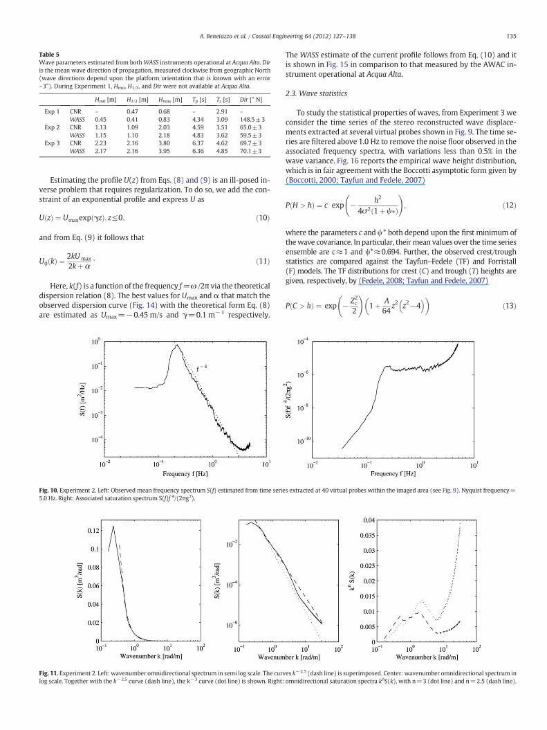
Table 5Wave parameters estimated from bothWASS instruments operational at Acqua Alta. Diris the mean wave direction of propagation, measured clockwise from geographic North(wave directions depend upon the platform orientation that is known with an error~3°). During Experiment 1, Hmo, H1/3, and Dir were not available at Acqua Alta.
Hm0 [m] H1/3 [m] Hmax [m] Tp [s] Tz [s] Dir [° N]
Exp 1 CNR – 0.47 0.68 – 2.91 –
WASS 0.45 0.41 0.83 4.34 3.09 148.5±3Exp 2 CNR 1.13 1.09 2.03 4.59 3.51 65.0±3
WASS 1.15 1.10 2.18 4.83 3.62 59.5±3Exp 3 CNR 2.23 2.16 3.80 6.37 4.62 69.7±3
WASS 2.17 2.16 3.95 6.36 4.85 70.1±3
135A. Benetazzo et al. / Coastal Engineering 64 (2012) 127–138
Estimating the profile U(z) from Eqs. (8) and (9) is an ill-posed in-verse problem that requires regularization. To do so, we add the con-straint of an exponential profile and express U as
U zð Þ ¼ Umaxexp γzð Þ; z≤0; ð10Þ
and from Eq. (9) it follows that
U0 kð Þ ¼ 2kUmax
2kþ α⋅ ð11Þ
Here, k(f) is a function of the frequency f=ω /2π via the theoreticaldispersion relation (8). The best values for Umax and α that match theobserved dispersion curve (Fig. 14) with the theoretical form Eq. (8)are estimated as Umax=−0.45 m/s and γ=0.1 m−1 respectively.
Fig. 10. Experiment 2. Left: Observed mean frequency spectrum S(f) estimated from time serie5.0 Hz. Right: Associated saturation spectrum S(f)f 4/(2πg2).
Fig. 11. Experiment 2. Left: wavenumber omnidirectional spectrum in semi log scale. The curvlog scale. Together with the k−2.5 curve (dash line), the k−3 curve (dot line) is shown. Right:
The WASS estimate of the current profile follows from Eq. (10) and itis shown in Fig. 15 in comparison to that measured by the AWAC in-strument operational at Acqua Alta.
2.3. Wave statistics
To study the statistical properties of waves, from Experiment 3 weconsider the time series of the stereo reconstructed wave displace-ments extracted at several virtual probes shown in Fig. 9. The time se-ries are filtered above 1.0 Hz to remove the noise floor observed in theassociated frequency spectra, with variations less than 0.5% in thewave variance. Fig. 16 reports the empirical wave height distribution,which is in fair agreement with the Boccotti asymptotic form given by(Boccotti, 2000; Tayfun and Fedele, 2007)
P H > hð Þ ¼ c exp − h2
4σ2 1þ ψ�ð Þ
!; ð12Þ
where the parameters c and ψ* both depend upon the first minimum ofthewave covariance. In particular, theirmean values over the time seriesensemble are c≈1 and ψ*≈0.694. Further, the observed crest/troughstatistics are compared against the Tayfun–Fedele (TF) and Forristall(F) models. The TF distributions for crest (C) and trough (T) heights aregiven, respectively, by (Fedele, 2008; Tayfun and Fedele, 2007)
P C > hð Þ ¼ exp − Z2c
2
!1þ Λ
64z2 z2−4� �� �
ð13Þ
s extracted at 40 virtual probes within the imaged area (see Fig. 9). Nyquist frequency=
es k−2.5 (dash line) is superimposed. Center: wavenumber omnidirectional spectrum inomnidirectional saturation spectra knS(k), with n=3 (dot line) and n=2.5 (dash line).
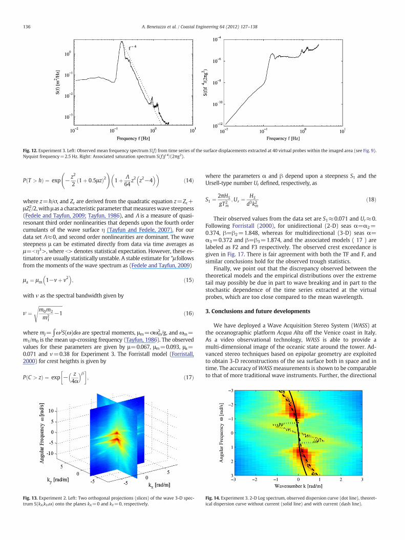
Fig. 12. Experiment 3. Left: Observed mean frequency spectrum S(f) from time series of the surface displacements extracted at 40 virtual probes within the imaged area (see Fig. 9).Nyquist frequency=2.5 Hz. Right: Associated saturation spectrum S(f)f 4/(2πg2).
136 A. Benetazzo et al. / Coastal Engineering 64 (2012) 127–138
P T > hð Þ ¼ exp − z2
21þ 0:5μzð Þ2
!1þ Λ
64z2 z2−4� �� �
ð14Þ
where z=h/σ, and Zc are derived from the quadratic equation z=Zc+μZc2/2,with μ as a characteristic parameter thatmeasureswave steepness(Fedele and Tayfun, 2009; Tayfun, 1986), and Λ is a measure of quasi-resonant third order nonlinearities that depends upon the fourth ordercumulants of the wave surface η (Tayfun and Fedele, 2007). For ourdata set Λ≈0, and second order nonlinearities are dominant. The wavesteepness μ can be estimated directly from data via time averages asμ=bη3>, where b> denotes statistical expectation. However, these es-timators are usually statistically unstable. A stable estimate for "μ followsfrom the moments of the wave spectrum as (Fedele and Tayfun, 2009)
μa ¼ μm 1−vþ v2� �
; ð15Þ
with ν as the spectral bandwidth given by
ν ¼ffiffiffiffiffiffiffiffiffiffiffiffiffiffiffiffiffiffiffiffiffim0m2
m21
−1
sð16Þ
where mj=∫ω jS(ω)dω are spectral moments, μm=σωm2 /g, and ωm=
m1/m0 is the mean up-crossing frequency (Tayfun, 1986). The observedvalues for these parameters are given by μ=0.067, μm=0.093, μa=0.071 and ν=0.38 for Experiment 3. The Forristall model (Forristall,2000) for crest heigthts is given by
P C > zð Þ ¼ exp − z4α
� �β� �; ð17Þ
Fig. 13. Experiment 2. Left: Two orthogonal projections (slices) of the wave 3-D spec-trum S(kX,kY,ω) onto the planes kX=0 and kY=0, respectively.
where the parameters α and β depend upon a steepness S1 and theUrsell-type number Ur defined, respectively, as
S1 ¼ 2πHS
gT2m
;Ur ¼HS
d3k2mð18Þ
Their observed values from the data set are S1≈0.071 and Ur≈0.Following Forristall (2000), for unidirectional (2-D) seas α=α2=0.374, β=β2=1.848, whereas for multidirectional (3-D) seas α=α3=0.372 and β=β3=1.874, and the associated models ( 17 ) arelabeled as F2 and F3 respectively. The observed crest exceedance isgiven in Fig. 17. There is fair agreement with both the TF and F, andsimilar conclusions hold for the observed trough statistics.
Finally, we point out that the discrepancy observed between thetheoretical models and the empirical distributions over the extremetail may possibly be due in part to wave breaking and in part to thestochastic dependence of the time series extracted at the virtualprobes, which are too close compared to the mean wavelength.
3. Conclusions and future developments
We have deployed a Wave Acquisition Stereo System (WASS) atthe oceanographic platform Acqua Alta off the Venice coast in Italy.As a video observational technology, WASS is able to provide amulti-dimensional image of the oceanic state around the tower. Ad-vanced stereo techniques based on epipolar geometry are exploitedto obtain 3-D reconstructions of the sea surface both in space and intime. The accuracy ofWASSmeasurements is shown to be comparableto that of more traditional wave instruments. Further, the directional
Fig. 14. Experiment 3. 2-D Log spectrum, observed dispersion curve (dot line), theoret-ical dispersion curve without current (solid line) and with current (dash line).
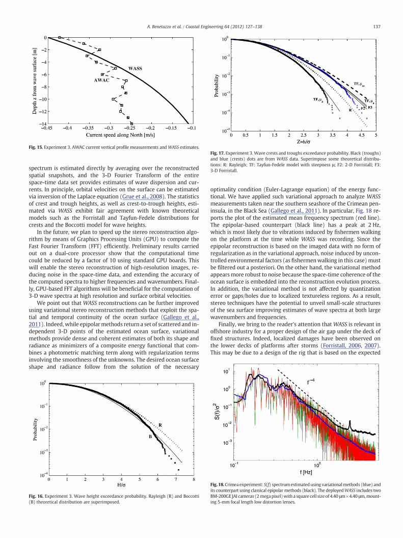
Fig. 15. Experiment 3. AWAC current vertical profile measurements and WASS estimates.Fig. 17. Experiment 3. Wave crests and troughs exceedance probability. Black (troughs)and blue (crests) dots are from WASS data. Superimpose some theoretical distribu-tions: R: Rayleigh; TF: Tayfun-Fedele model with steepness μ; F2: 2-D Forristall; F3:3-D Forristall.
137A. Benetazzo et al. / Coastal Engineering 64 (2012) 127–138
spectrum is estimated directly by averaging over the reconstructedspatial snapshots, and the 3-D Fourier Transform of the entirespace-time data set provides estimates of wave dispersion and cur-rents. In principle, orbital velocities on the surface can be estimatedvia inversion of the Laplace equation (Grue et al., 2008). The statisticsof crest and trough heights, as well as crest-to-trough heights, esti-mated via WASS exhibit fair agreement with known theoreticalmodels such as the Forristall and Tayfun-Fedele distributions forcrests and the Boccotti model for wave heights.
In the future, we plan to speed up the stereo reconstruction algo-rithm by means of Graphics Processing Units (GPU) to compute theFast Fourier Transform (FFT) efficiently. Preliminary results carriedout on a dual-core processor show that the computational timecould be reduced by a factor of 10 using standard GPU boards. Thiswill enable the stereo reconstruction of high-resolution images, re-ducing noise in the space-time data, and extending the accuracy ofthe computed spectra to higher frequencies and wavenumbers. Final-ly, GPU-based FFT algorithms will be beneficial for the computation of3-D wave spectra at high resolution and surface orbital velocities.
We point out that WASS reconstructions can be further improvedusing variational stereo reconstruction methods that exploit the spa-tial and temporal continuity of the ocean surface (Gallego et al.,2011). Indeed,while epipolarmethods return a set of scattered and in-dependent 3-D points of the estimated ocean surface, variationalmethods provide dense and coherent estimates of both its shape andradiance as minimizers of a composite energy functional that com-bines a photometric matching term along with regularization termsinvolving the smoothness of the unknowns. The desired ocean surfaceshape and radiance follow from the solution of the necessary
Fig. 16. Experiment 3. Wave height exceedance probability. Rayleigh (R) and Boccotti(B) theoretical distribution are superimposed.
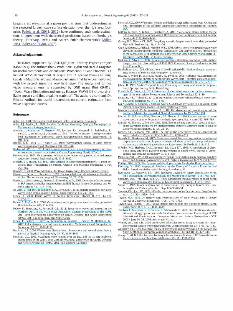
optimality condition (Euler-Lagrange equation) of the energy func-tional. We have applied such variational approach to analyze WASSmeasurements taken near the southern seashore of the Crimean pen-insula, in the Black Sea (Gallego et al., 2011). In particular, Fig. 18 re-ports the plot of the estimated mean frequency spectrum (red line).The epipolar-based counterpart (black line) has a peak at 2 Hz,which is most likely due to vibrations induced by fishermen walkingon the platform at the time while WASS was recording. Since theepipolar reconstruction is based on the imaged data with no form ofregularization as in the variational approach, noise induced by uncon-trolled environmental factors (as fishermenwalking in this case)mustbe filtered out a posteriori. On the other hand, the variational methodappears more robust to noise because the space-time coherence of theocean surface is embedded into the reconstruction evolution process.In addition, the variational method is not affected by quantizationerror or gaps/holes due to localized textureless regions. As a result,stereo techniques have the potential to unveil small-scale structuresof the sea surface improving estimates of wave spectra at both largewavenumbers and frequencies.
Finally, we bring to the reader's attention that WASS is relevant inoffshore industry for a proper design of the air gap under the deck offixed structures. Indeed, localized damages have been observed onthe lower decks of platforms after storms (Forristall, 2006, 2007).This may be due to a design of the rig that is based on the expected
Fig. 18.Crimea experiment: S(f) spectrumestimatedusing variationalmethods (blue) andits counterpart using classical epipolar methods (black). The deployedWASS includes twoBM-200GE JAI cameras (2 megapixel)with a square cell size of 4.40 μm×4.40 μm,mount-ing 5-mm focal length low distortion lenses.
138 A. Benetazzo et al. / Coastal Engineering 64 (2012) 127–138
largest crest elevation at a given point in time that underestimatesthe expected largest wave surface elevation over the rig's area foot-print. Fedele et al. (2011, 2012) have confirmed such underestima-tion, in agreement with theoretical predictions based on Piterbarg'stheory (Piterbarg, 1996) and Adler's Euler characteristics (Adler,1981; Adler and Taylor, 2007).
Acknowledgements
Research supported by CASE-EJIP Joint Industry Project (project#4545093). The authors thank Profs. Aziz Tayfun and Harald Krogstadfor useful comments and discussions. Protecno S.r.l. and Phoenix S.r.l.helped WASS deployment at Acqua Alta. A special thanks to LuigiCavaleri, Mauro Sclavo and Mauro Bastianini that have been involvedwith the project since the very first stage. The analysis of Crimeavideo measurements is supported by ONR grant BAA 09-012:“OceanWave Dissipation and energy Balance (WAVE-DB): toward re-liable spectra and first breaking statistics”. The authors also thank Dr.Fabrice Ardhuin for useful discussions on current estimation fromwave dispersion curves.
References
Adler, R.J., 1981. The Geometry of Random Fields. John Wiley, New York.Adler, R.J., Taylor, J.E., 2007. Random Fields and Geometry. Springer Monographs in
Mathematics Springer, New York.Allender, J., Audunson, T., Barstow, S.F., Bjerken, S.H., Krogstad, E., Steinbakke, P.,
Vartdal, L., Borgman, L.E., Graham, C., 1989. The WADIC project: a comprehensivefield evaluation of directional wave instrumentation. Ocean Engineering 16,505–536.
Banner, M.L., Jones, S.F., Trinder, J.C., 1989. Wavenumber spectra of short gravitywaves. Journal of Fluid Mechanics 198, 321–344.
Bechle, A.J., Wu, C.H., 2011. Virtual wave gauges based upon stereo imaging for mea-suring surface wave characteristics. Coastal Engineering 58 (4), 305–316.
Benetazzo, A., 2006. Measurements of short water waves using stereo matched imagesequences. Coastal Engineering 53, 1013–1032.
Blostein, S.D., Huang, T.S., 1987. Error analysis in stereo determination of 3-D point po-sitions. IEEE Transactions on Pattern Analysis and Machine Intelligence 9 (6),752–765.
Boccotti, P., 2000. Wave Mechanics for Ocean Engineering. Elsevier Science, Oxford.Cavaleri, L., Bertotti, L., Tescaro, N., 1997. The modelled wind climatology of the Adria-
tic Sea. Theoretical and Applied Climatology 56, 231–254.Dankert, H., Horstmann, J., Lehner, S., Rosenthal, W.G., 2003. Detection of wave groups
in SAR images and radar image sequences. IEEE Transactionson Geoscience and Re-mote Sensing 41, 1437–1446.
de Vries, S., Hill, D.F., de Schipper, M.A., Stive, M.J.F., 2011. Remote sensing of surf zonewaves using stereo imaging. Coastal Engineering 58 (3), 239–250.
Fedele, F., 2008. Rogue waves in oceanic turbulence. Physica D 237 (14–17),2127–2131.
Fedele, F., Tayfun, M.A., 2009. On nonlinear wave groups and crest statistics. Journal ofFluid Mechanics 620, 221–239.
Fedele, F., Benetazzo, A., Forristall, G.Z., 2011. Space-time waves and spectra in theNorthern Adriatic Sea via a Wave Acquisition System. Proceedings of the ASME2011 30th International Conference on Ocean, Offshore and Arctic Engineering(OMAE 2011) in Rotterdam, The Netherlands.
Fedele, F., Gallego, G., Yezzi, A., Benetazzo, A., Cavaleri, L., Sclavo, M., Bastianini, M.,2012. Euler characteristics of oceanic sea states. Mathematics and Computers inSimulation 82 (6), 1102–1111.
Forristall, G.Z., 2000. Wave crests distributions: observations and second order theory.Journal of Physical Oceanography 38 (8), 1931–1943.
Forristall, G.Z., 2006. Maximum wave heights over an area and the air gap problem.Proceedings of the ASME 2006 25th International Conference on Ocean, Offshoreand Arctic Engineering (OMAE 2006) in Hamburg, Germany.
Forristall, G.Z., 2007. Wave crest heights and deck damage in Hurricanes Ivan, Katrina andRita. Proceedings of the Offshore Technology Conference Proceedings in Houston,USA.
Gallego, G., Yezzi, A., Fedele, F., Benetazzo, A., 2011. A variational stereo method for the3-D reconstruction of ocean waves. IEEE Transactions of Geosciences and RemoteSensing 49 (11), 4445–4457.
Goring, D.G., Nikora, V.I., 2002. Despiking acoustic doppler velocimeter data. Journal ofHydraulic Engineering 128, 117–126.
Grue, J., Romero, L., Kleiss, J., Melville, W.K., 2008. Orbital velocity in spatial ocean waveelevation measurement: nonlinear computation and approximation. Proceedingsof the ASME 2008 27th International Conference on Ocean, Offshore and Arctic En-gineering (OMAE 2008) in Estoril, Portugal.
Heikkila, J., Silven, O., 1997. A four-step camera calibration procedure with implicitimage correction. Proceedings of 1997 IEEE Computer Society Conference in SanJuan, Puerto Rico.
Holthuijsen, L.H., 1983. Observations of the directional distribution of ocean wave en-ergy. Journal of Physical Oceanography 13, 816–827.
Hwang, P., Wang, D., Walsh, E., Krabill, W., Swift, R., 2000. Airborne measurements ofthe wavenumber spectra of ocean surface waves, part I: spectral slope and dimen-sionless spectral coefficient. Journal of Physical Oceanography 30, 2753–2767.
Jahne, B., 1993. Spatio-Temporal Image Processing — Theory and Scientific Applica-tions. Springer-Verlag Berlin Heidelberg.
Kosnik, M.V., Dulov, V.A., 2011. Extraction of short wind wave spectra from stereo im-ages of the sea surface. Measurement Science and Technology 22, 1–10.
Krogstad, H.E., Trulsen, K., 2010. Interpretations and observations of ocean wave spec-tra. Ocean Dynamics 60 (4), 973–991.
Ma, Y., Soatto, S., Kosecka, J., Shankar Sastry, S., 2004. An invitation to 3-D vision: fromimages to geometric models. Springer-Verlag New York.
Malanotte-Rizzoli, P., Bergamasco, A., 1983. The dynamics of coastal region of thenorthern Adriatic Sea. Journal of Physical Oceanography 13, 1105–1130.
Marom, M., Goldstein, R.M., Thornton, E.B., Shemer, L., 1990. Remote sensing of oceanwave spectra by interferometric synthetic aperture radar. Nature 345, 793–795.
Marom, M., Shemer, L., Thornton, E.B., 1991. Energy density directional spectra of near-shore wavefield measured by interferometric synthetic aperture radar. Journal ofGeophysical Research 96, 22125–22134.
Newell, A.C., Zakharov, V.E., 2008. The role of the generalized Phillip's spectrum inwave turbulence. Physics Letters A 372 (23), 4230–4233.
Nobach, H., Honkanen, M., 2005. Two-dimensional Gaussian regression for sub-pixeldisplacement estimation in particle image velocimetry and particle position esti-mation in particle tracking velocimetry. Experiments in Fluids 38, 511–515.
O'Reilly, W.C., Herbers, T.H.C., Seymour, R.J., Guza, R.T., 1996. A comparison of direc-tional buoy and fixed platform measurements of Pacific swell. Journal of Atmo-spheric and Oceanic Technology 13, 231–238.
Park, C.S., Park, H.W., 2001. A robust stereo disparity estimation using adaptive windowsearch and dynamic programming search. Pattern Recognition 34 (12), 2573–2576.
Phillips, O.M., 1977. The Dynamics of the Upper Ocean. Cambridge University Press.Piterbarg, V., 1996. Asymptotic Methods in the Theory of Gaussian Processes and
Fields. American Mathematical Society, Providence, RI.Rodriguez, J.J., Aggarwal, J.K., 1990. Stochastic analysis of stereo quantization error.
IEEE Transactions on Pattern Analysis and Machine Intelligence 12 (5), 467–470.Shemdin, O.H., Tran, H.M., Wu, S.C., 1988. Directional measurements of short ocean
waves with stereography. Journal of Geophysical Research 93, 13891–13901.Solina, F., 1985. Errors in stereo due to quantization. Dep. Comput. Inform. Sci., Univ.
Pennsylvania, Philadelphia, Tech. Rep. MS-CIS-85-34.Stewart, R.H., Joy, J.W., 1974. HF radio measurements of surface currents. Deep Sea Re-
search 21 (12), 1039–1049.Tayfun, M.A., 1986. On narrow-band representation of ocean waves. Part I: Theory
Journal of Geophysical Research 1 (C6), 7743–7752.Tayfun, M.A., Fedele, F., 2007. Wave-height distributions and nonlinear effects. Ocean
Engineering 34 (11–12), 1631–1649.Tombari, F., Mattoccia, S., Di Stefano, L., Addimanda, E., 2008. Classification and evalu-
ation of cost aggregation methods for stereo correspondence. Proceedings of IEEEInternational Conference on Computer Vision and Pattern Recognition (CVPR2008), June 24–26, 2008, Anchorage, Alaska.
Wanek, J.M., Wu, C.H., 2006. Automated trinocular stereo imaging system for three-dimensional surface wave measurements. Ocean Engineering 33 (5–6), 723–747.
Zakharov, V.E., 1999. Statistical theory of gravity and capillary waves on the surface of afinite-depth fluid. European Journal of Mechanics - B/Fluid 18 (3), 327–344.
Zhang, Z., 2000. A flexible new technique for camera calibration. IEEE Transactions onPattern Analysis and Machine Intelligence 22 (11), 1330–1334.