Contents lists available at ScienceDirect

Journal of Quantitative Spectroscopy &Radiative Transfer

Journal of Quantitative Spectroscopy & Radiative Transfer 174 (2016) 39–55

http://d0022-40

n CorrE-m

baptiste

journal homepage: www.elsevier.com/locate/jqsrt

SMARTIES: User-friendly codes for fast and accurate calculationsof light scattering by spheroids

W.R.C. Somerville, B. Auguié, E.C. Le Ru n

The MacDiarmid Institute for Advanced Materials and Nanotechnology, School of Chemical and Physical Sciences,Victoria University of Wellington, PO Box 600, Wellington 6140, New Zealand

a r t i c l e i n f o

Article history:Received 3 November 2015Received in revised form5 January 2016Accepted 5 January 2016Available online 20 January 2016

Keywords:Electromagnetic scatteringSpheroidsT-matrixNumerical simulations

x.doi.org/10.1016/j.jqsrt.2016.01.00573/& 2016 Elsevier Ltd. All rights reserved.

esponding author.ail addresses: wrcsomerville@gmail.com (W..auguie@gmail.com (B. Auguié), eric.leru@vu

a b s t r a c t

We provide a detailed user guide for SMARTIES, a suite of MATLAB codes for the calculation ofthe optical properties of oblate and prolate spheroidal particles, with comparable cap-abilities and ease-of-use as Mie theory for spheres. SMARTIES is a MATLAB implementation ofan improved T-matrix algorithm for the theoretical modelling of electromagnetic scat-tering by particles of spheroidal shape. The theory behind the improvements in numericalaccuracy and convergence is briefly summarized, with reference to the original publica-tions. Instructions of use, and a detailed description of the code structure, its range ofapplicability, as well as guidelines for further developments by advanced users are dis-cussed in separate sections of this user guide. The code may be useful to researchersseeking a fast, accurate and reliable tool to simulate the near-field and far-field opticalproperties of elongated particles, but will also appeal to other developers of light-scattering software seeking a reliable benchmark for non-spherical particles with achallenging aspect ratio and/or refractive index contrast.

& 2016 Elsevier Ltd. All rights reserved.

1. Introduction

We present a user guide and description of SMARTIES, anumerically stable and highly accurate implementation ofthe T-matrix/Extended Boundary-Condition Method(EBCM) for light-scattering by spheroids, based on ourrecent work [1–3]. The complete package can be down-loaded freely from http://www.victoria.ac.nz/scps/research/research-groups/raman-lab/numerical-tools, see Section 1.4for licensing information. The name of the program standsfor Spheroids Modelled Accurately with a Robust T-matrixImplementation for Electromagnetic Scattering, and is also anod to the well-known colorful candy of oblate shape.

R.C. Somerville),w.ac.nz (E.C. Le Ru).

1.1. Description and overview

This package contains a suite of MATLAB codes to simulatethe light scattering properties of spheroidal particles, fol-lowing the general T-matrix framework [4]. The scatterershould be homogeneous, and described by a local, isotropicand linear dielectric response (this includes metals, but notperfect conductors). Magnetic, non-linear, and opticallyactive materials are not considered. The surrounding med-ium is described by a lossless, homogeneous and isotropicdielectric medium extending to infinity.

SMARTIES specifically implements recently developedalgorithms for numerically accurate and stable calculations.The general EBCM/T-matrix method is described in detail inRef. [4], while the underlying theory and relevant formulasfor our specific improvements are described in Ref. [2], withadditional information found in [1,3]. The relevant equa-tions and sections from both Refs. [2,4] are referenced whenpossible as “inline comments” to the code.

W.R.C. Somerville et al. / Journal of Quantitative Spectroscopy & Radiative Transfer 174 (2016) 39–5540

The package includes detailed examples and can alsobe used by a non-specialist with an application-orientedperspective, requiring no specific knowledge of theunderlying theory.

The package contains:

� Six ready-to-run example scripts to calculate standardoptical properties, namely fixed-orientation and orien-tation-averaged far-field cross-sections, near fields, T-matrix elements, and scattering matrix elements. Examplesalso cover the simulation of wavelength-dependent spectraof surface-field and far-field properties.

� Two tutorial scripts where such simulations are furtherdetailed with step-by-step instructions, exposing thelower-level calculations of intermediate quantities.

� Additional high-level and post-processing functions,which can be used by users to write new scripts tailoredto their specific needs.

� A number of low-level functions, which are used by thecode and might be adapted by advanced users.

� Dielectric functions for a few materials such as gold andsilver, implemented via analytic expressions [5,6] orsilicon, interpolated from tabulated values.

1.2. Relation to other codes

Standard T-matrix/EBCM codes in FORTRAN have alreadybeen developed [7,8], with those by Mishchenko andTravis [9] arguably the most popular. These freely availablecodes provide a wide range of capabilities (including forexample different particle shapes) and have been widelyused and tested. The standard EBCM method howeversuffers from a number of numerical problems andinstabilities for large multipole orders, which are neces-sary for either high precision, large particles, elongatedparticles, near-field calculations, or any combination of theabove. This can result in inaccurate results and in somecases in complete loss of convergence. This unreliablebehavior for numerically challenging simulations canmake the method difficult to use for non-experts, whomay find it hard to “tune” the parameters that ensureaccuracy and convergence. It also impedes the theoreticalstudy of the intrinsic convergence properties of the T-matrix method, obfuscated by (implementation-depen-dent) numerical loss of precision [3].

Recently, we have identified the primary causes fornumerical instabilities in the special (but important) caseof spheroidal particles [1] and proposed a new algorithmto overcome them [2]. Thanks to those improvements,high accuracy and reliable convergence can be obtainedover a wider range of parameters, especially towards highaspect-ratio (elongated) particles where the standardEBCM implementation would fail [3]. This document aimsto present and discuss a publicly available MATLAB imple-mentation of these recent developments. Our packageshould complement, rather than replace, existing T-matrixcodes such as those of Mishchenko and Travis [9]. Thepresent code offers a number of advantages:

� Thanks to the improvements in accuracy and con-vergence, we believe this code will be readily accessible

to non-expert users and allow the routine calculation ofoptical properties of spheroids as easily as with Mietheory for spheres. An example is provided in Section 2.7as a demonstration.

� We also provide specific routines to compute near fieldsand surface fields, which will be beneficial to theexploitation of this powerful method in areas such asnanophotonics, optical trapping, plasmonics, etc., wherethe T-matrix/EBCM method has not been widelyapplied.

� MATLAB provides an easy-access, interactive environmentto carry out a broad range of numerical simulations, andplot/export the results conveniently.

� The accuracy of the obtained results can be easily esti-mated for any type of calculation, owing to the well-behaved convergence of the improved algorithm.

� A wider range of parameters can be simulated, espe-cially scatterers with large aspect ratios.

A number of limitations should be also be noted:

� These codes are limited to spheroidal particles, forwhich we identified and circumvented numerical pro-blems that are very specific to this geometrical shape.

� MATLAB is inherently slow compared to compiled lan-guages such as C or FORTRAN, which may be an issue forintensive calculations (for example the simulation ofpolydisperse samples, with particles varying in size andshape). We envisage that this implementation couldserve as a template for a future port of this new algo-rithm to a more efficient language.

� The calculation of some derived properties, e.g. thescattering matrix, has not been optimized and could beparticularly slow.

� Although the range of parameters that may be simu-lated with reasonable accuracy has been extendedtowards larger aspect ratios, the method is still limitedto moderate particle sizes; and even small sizes only forparticles with a large relative refractive index. In thiscase, the matrix inversion step is the limiting factor andextended-precision arithmetic as implemented in [9]would be required to overcome it.

1.3. Aims of this manual

This document was written with two types of users inmind:

� Researchers interested in simulating electromagneticscattering by nonspherical particles for practical appli-cations, and seeking an efficient and (relatively) fool-proof program with ease of use comparable to Mietheory.

� Other developers of electromagnetic scattering softwareinterested in benchmarking calculations against ahighly accurate reference.

With this dual perspective, we have divided the sourcecode into low-level and high-level functions, includingcomplete scripts for specific calculations, but also docu-mented how to access intermediate quantities such as the

W.R.C. Somerville et al. / Journal of Quantitative Spectroscopy & Radiative Transfer 174 (2016) 39–55 41

T-matrix elements. This user guide is also divided intosections that reflect these two complementary objectives,with Sections 3 and 4 focusing on more theoretical aspectsand in-depth description of the code implementation.

1.4. Licensing

SMARTIES is licensed under the Creative CommonsAttribution-NonCommercial 4.0 International License. Toview a copy of this license, visit http://creativecommons.org/licenses/by-nc/4.0/. The package including all its filesand content are under the following copyright: 2015Walter Somerville, Baptiste Auguié, and Eric Le Ru. Thepackage may be used freely for research, teaching, orpersonal use. The unmodified complete package may bere-distributed and freely exchanged for academic researchor government use, but cannot be commercialized or usedfor commercial purposes. The theory and code should beappropriately referenced by citing this user-guide in anypresentation of results obtained using this package (or anyother code using it).

1.5. Disclaimer

These codes have been developed and tested withMATLAB 7.14 (R2012a) [10], GNU Octave 4.0.0 [11] (open-source software) and MATLAB 8.5 (R2015a) on a PC runningMicrosoft Windows 7 x64. The code is also known to rununder MacOS X (10.10) and Linux (Ubuntu 15.04). Slightchanges may be necessary to run them on older (ornewer!) versions of MATLAB/Octave.

Although every effort has been made to get rid of bugs(programming bugs, or incorrect physical formulas) and totest the code against existing ones, some issues may stillbe present. We hope the users will help us identify themand we will try to update the code when necessary.

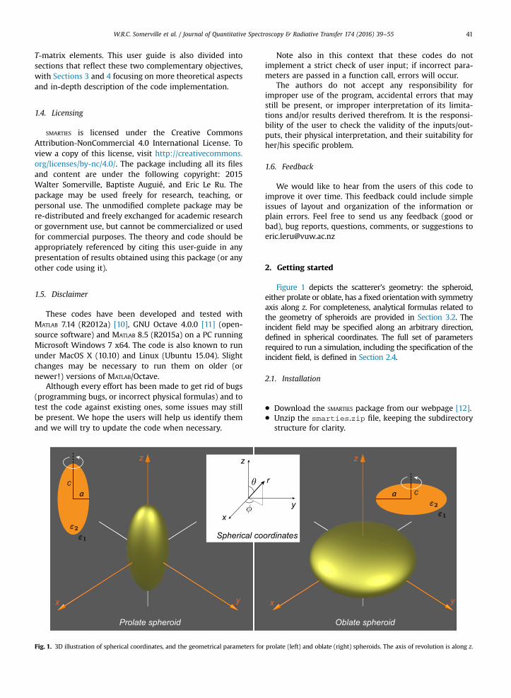
z

x y

c

Prolate spheroid

x

z

Spherical co

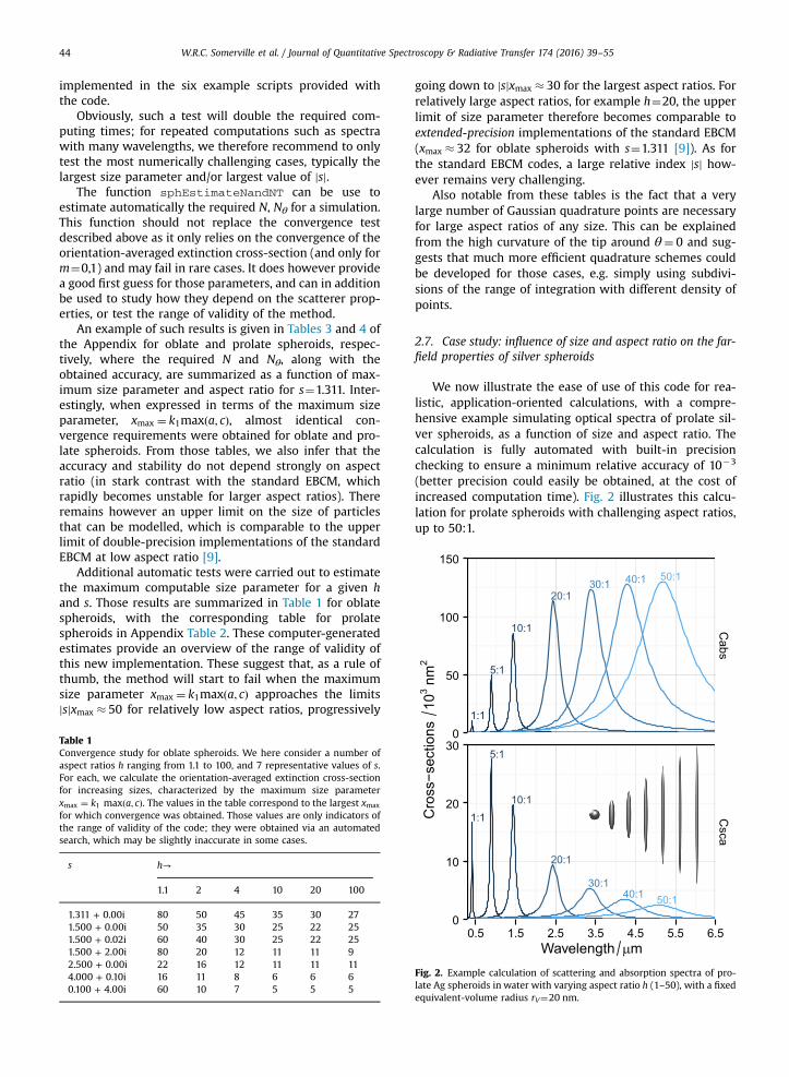
Fig. 1. 3D illustration of spherical coordinates, and the geometrical parameters for

Note also in this context that these codes do notimplement a strict check of user input; if incorrect para-meters are passed in a function call, errors will occur.

The authors do not accept any responsibility forimproper use of the program, accidental errors that maystill be present, or improper interpretation of its limita-tions and/or results derived therefrom. It is the responsi-bility of the user to check the validity of the inputs/out-puts, their physical interpretation, and their suitability forher/his specific problem.

1.6. Feedback

We would like to hear from the users of this code toimprove it over time. This feedback could include simpleissues of layout and organization of the information orplain errors. Feel free to send us any feedback (good orbad), bug reports, questions, comments, or suggestions toeric.leru@vuw.ac.nz

2. Getting started

Figure 1 depicts the scatterer's geometry: the spheroid,either prolate or oblate, has a fixed orientationwith symmetryaxis along z. For completeness, analytical formulas related tothe geometry of spheroids are provided in Section 3.2. Theincident field may be specified along an arbitrary direction,defined in spherical coordinates. The full set of parametersrequired to run a simulation, including the specification of theincident field, is defined in Section 2.4.

2.1. Installation

� Download the SMARTIES package from our webpage [12].� Unzip the smarties.zip file, keeping the subdirectory

structure for clarity.

z

x y

Oblate spheroid

cy

r

ordinates

prolate (left) and oblate (right) spheroids. The axis of revolution is along z.

W.R.C. Somerville et al. / Journal of Quantitative Spectroscopy & Radiative Transfer 174 (2016) 39–5542

� Set your MATLAB current directory to smarties and runthe InitPath.m function once in MATLAB toadd all the subdirectories to your MATLAB search path.All the functions and scripts are then accessible fromthe MATLAB command line. This allows all codes to runand communicate with each other irrespective of thecurrent directory.

Note that you must run InitPath.m each time yourestart MATLAB. To avoid this step, you may add all smar-ties folders to your MATLAB path permanently or edit thestartup.m file to do that (check MATLAB's help for details).

2.2. Octave users

Octave is an open-source alternative to MATLAB.Although our codes were mostly developed and tested forMATLAB, we have tried to ensure their compatibility withOctave. Most scripts should therefore run as-is withOctave, although they were typically slower in our tests.The numerical accuracy may also differ, as well as therendering of graphics.

2.3. Initial steps

The easiest way to get started is to run one of theexample files in the Scripts folder (those starting withScriptSolve) and change the parameters as needed.These scripts provide a direct example of how to call anumber of high-level functions designed to solve specificproblems of interest. These are

� ScriptSolveForT: Calculates the T-matrix, scatteringmatrix, and orientation-averaged properties for a singlewavelength.

� ScriptSolveForFixed: Calculates the field expansioncoefficients and the corresponding far-field cross-sec-tions for a fixed-orientation, for a single wavelength.

� ScriptSolveForSurfaceField: Calculates the fieldexpansion coefficients and the corresponding far-fieldcross-sections and surface fields for a fixed-orientation.

� ScriptSolveForTSpectrum: Calculates the T-matrixand the orientation-averaged properties for multiplewavelengths.

� ScriptSolveForFixedSpectrum: Calculates the fieldexpansion coefficients and the corresponding far-fieldcross-sections for a fixed-orientation, as a function ofwavelength.

� ScriptSolveForSurfaceFieldSpectrum: Calculatesthe field expansion coefficients and the correspondingfar-field cross-sections and surface fields for a fixed-orientation, as a function of wavelength.

Those scripts define the parameters of the simulation,call the corresponding high-level functions to perform thecalculations, and output the most important results in theMATLAB console and/or as interactive graphics. Convergencetests are also performed as part of the calculations, andaccuracy estimates for the results are included in thedisplays.

In order to understand in more detail how the codeoperates, we also provide two example scripts, ScriptTu-torial and ScriptTutorialSpectrum, where all themain steps in the calculation are listed explicitly withextensive comments about the meaning of the variousparameters. We recommend copying and editing theseexample scripts to solve user-specific problems and/orimplement custom extensions to the current code.

Most functions start with a detailed help and are com-mented within the code. Typing help FunctionName willdisplay the corresponding help information.

The information below summarizes and complementsthe inline comments included in the six example scriptsScriptSolve…. It provides the most important technicaldetails of the implementation, for users wishing to writeadditional custom routines.

2.4. Definition of the parameters

For the calculation of the T-matrix and orientation-averaged cross-sections, only four parameters are neededto define the scatterer properties:

� a: semi-axis along x; y.� c: semi-axis along z (axis of rotational symmetry).� k1: wavevector in embedding medium (possibly a

wavelength-dependent vector).� s: relative refractive index s (possibly a wavelength-

dependent vector).

Note that consistent units must be used for a, c, and k1,e.g. a and c in nm and k1 in nm�1.

k1 denotes the wavevector outside the particle, wherethe refractive index is n1 ¼

ffiffiffiffiffiε1

p(assumed real positive):

k1 ¼ωcffiffiffiffiffiε1

p ¼ 2πλ

ffiffiffiffiffiε1

p: ð1Þ

The relative refractive index (adimensional) is defined as

s¼ffiffiffiffiffiε2

pffiffiffiffiffiε1

p : ð2Þ

Both s and ε2 may be complex (for absorbing and/or con-ducting particles).

The P;Q ; T ;R-matrices computation requires the fol-lowing parameters:

� N: Number of multipoles N requested for the T-matrix(and R-matrix).

� nNbTheta: Number of angles θ used in Gaussianquadratures for the evaluation of P- and Q-matrixintegrals.

The function sphEstimateNandNT may be used to auto-matically estimate those latter two parameters for bestconvergence, but we nevertheless recommend that theconvergence of the calculations be checked to ensurereliable results.

For convenience those six parameters may be collated ina structure (a MATLAB object akin to a list, called stParams inour example scripts), which is passed to the high-level(slv…) functions.

W.R.C. Somerville et al. / Journal of Quantitative Spectroscopy & Radiative Transfer 174 (2016) 39–55 43

Additionally, one of the following two parameters isneeded if the field expansion coefficients and/or the cross-sections for a given fixed orientation are sought:

� sIncType: String defining the type of incident planewave, e.g. “KxEz” for a wave incident along x and line-arly polarized along z. This shorthand notation is onlydefined for a few standard combinations, namely KxEz,

KxEy, KyEz, KyEx, KzEx, KzEy. In other cases, usestIncPar.

� stIncPar: Structure defining a linearly polarized inci-dent plane wave excitation via three Euler angles.It can be obtained from calling vshMakeIncident

Parameters.

For field calculations (such as surface fields), furtherparameters are required:

� nNbThetaPst: Number of angles θ for post-processing(should typically be larger than nNbTheta for accuratesurface averaging).

� lambda: Wavelength (in free space) [in the same unit asa, c, k�1

1 ].� epsilon2: Dielectric function ε2 of scatterer (possibly

complex).� epsilon1: Relative dielectric constant ε1 of embedding

medium (real positive).

Note that the latter three are not independent of k1 and sthat have already been defined. Those additional para-meters should also be included in stParams.

Finally a number of optional settings can also bedefined in a structure stOptions:

� bGetR: Boolean (default: false). If false, the R-matrixand internal field coefficients are not calculated. Thedefault value will be overridden by functions requiringR.

� Delta: Number of extra multipoles for P- andQ- matrices, i.e. NQ ¼NþΔ. Default is Δ¼ 0. IfDelta¼-1, then the code tries to estimate it from theconvergence of T22;m ¼ 1

11 (see [3] for details), by callingsphEstimateDelta.

� NB: Number of multipoles to compute the Bessel func-tions in the improved algorithm ðNBZNQ Þ. If NB¼0,then NB is estimated by calling sphEstimateNB, whichis the case by default.

� absmvec: Vector containing the values of jmj for whichT is to be computed. These values are limited to0r jmjrN. To compute all m (most cases of interest),simply use absmvec¼0:N (which is the default value).

� bGetSymmetricT: Boolean (default: false). If true, Tis symmetrized as described in Section 3.8.

� bOutput: Boolean (default: true). If false, suppressessome of the output printed in the MATLAB console, whichis a better option for example in calculations of spectrawith many wavelengths.

2.5. Minimal example

The following script is set up to simulate the far-fieldcross-sections of a gold prolate spheroid in air, at a singlewavelength λ¼ 650 nm. The simulation parameters arestored in a structure stParams for convenience. Only oneoptional parameter is defined in stOptions (for theothers, default values will be used). These two structuresare passed to the high-level slvForFixed function thatimplements the calculation of the expansion coefficientsand cross-sections for a fixed orientation.

Minimalist script showing how to set up a simulation

This general structure is followed by all the examples, withvarying levels of complexity, and the high-level functionssuch as slvForFixed performing the actual calculationsare grouped in the Solve directory.

2.6. Convergence, accuracy, and range of validity

One of the problems of the conventional T-matrix/EBCM method is to study its convergence and accuracy.This is because the method becomes unstable with mul-tipoles of high order, which may occur before the resultshave fully converged. Many of those issues have beensolved in the present method, as discussed in Ref. [3]. Ref.[3] also provides a detailed discussion of the parametersaffecting convergence and accuracy.

Thanks to the improved stability, we propose a simpleand reliable convergence and accuracy test that will workin most cases. It consists in repeating the same calcula-tions with a larger number of multipoles N and quadraturepoints Nθ, for example: N0 ¼Nþ5 and N0

θ ¼Nθþ5. Ifsurface-averaged properties are calculated, the number ofquadrature points used in post-processing should also bechecked independently.

In our experience, this simple convergence test pro-vides a reliable estimate of the accuracy of the results. It is

1:1

5:1

10:1

20:130:1 40:1 50:1

50

100

150

Cabs

103 n

m2

W.R.C. Somerville et al. / Journal of Quantitative Spectroscopy & Radiative Transfer 174 (2016) 39–5544

implemented in the six example scripts provided withthe code.

Obviously, such a test will double the required com-puting times; for repeated computations such as spectrawith many wavelengths, we therefore recommend to onlytest the most numerically challenging cases, typically thelargest size parameter and/or largest value of jsj.

The function sphEstimateNandNT can be use toestimate automatically the required N, Nθ for a simulation.This function should not replace the convergence testdescribed above as it only relies on the convergence of theorientation-averaged extinction cross-section (and only form¼0,1) and may fail in rare cases. It does however providea good first guess for those parameters, and can in additionbe used to study how they depend on the scatterer prop-erties, or test the range of validity of the method.

An example of such results is given in Tables 3 and 4 ofthe Appendix for oblate and prolate spheroids, respec-tively, where the required N and Nθ, along with theobtained accuracy, are summarized as a function of max-imum size parameter and aspect ratio for s¼1.311. Inter-estingly, when expressed in terms of the maximum sizeparameter, xmax ¼ k1maxða; cÞ, almost identical con-vergence requirements were obtained for oblate and pro-late spheroids. From those tables, we also infer that theaccuracy and stability do not depend strongly on aspectratio (in stark contrast with the standard EBCM, whichrapidly becomes unstable for larger aspect ratios). Thereremains however an upper limit on the size of particlesthat can be modelled, which is comparable to the upperlimit of double-precision implementations of the standardEBCM at low aspect ratio [9].

Additional automatic tests were carried out to estimatethe maximum computable size parameter for a given hand s. Those results are summarized in Table 1 for oblatespheroids, with the corresponding table for prolatespheroids in Appendix Table 2. These computer-generatedestimates provide an overview of the range of validity ofthis new implementation. These suggest that, as a rule ofthumb, the method will start to fail when the maximumsize parameter xmax ¼ k1maxða; cÞ approaches the limitsjsjxmax � 50 for relatively low aspect ratios, progressively

Table 1Convergence study for oblate spheroids. We here consider a number ofaspect ratios h ranging from 1.1 to 100, and 7 representative values of s.For each, we calculate the orientation-averaged extinction cross-sectionfor increasing sizes, characterized by the maximum size parameterxmax ¼ k1 maxða; cÞ. The values in the table correspond to the largest xmax

for which convergence was obtained. Those values are only indicators ofthe range of validity of the code; they were obtained via an automatedsearch, which may be slightly inaccurate in some cases.

s h→

1.1 2 4 10 20 100

1.311 + 0.00i 80 50 45 35 30 271.500 + 0.00i 50 35 30 25 22 251.500 + 0.02i 60 40 30 25 22 251.500 + 2.00i 80 20 12 11 11 92.500 + 0.00i 22 16 12 11 11 114.000 + 0.10i 16 11 8 6 6 60.100 + 4.00i 60 10 7 5 5 5

going down to jsjxmax � 30 for the largest aspect ratios. Forrelatively large aspect ratios, for example h¼20, the upperlimit of size parameter therefore becomes comparable toextended-precision implementations of the standard EBCM(xmax � 32 for oblate spheroids with s¼1.311 [9]). As forthe standard EBCM codes, a large relative index jsj how-ever remains very challenging.

Also notable from these tables is the fact that a verylarge number of Gaussian quadrature points are necessaryfor large aspect ratios of any size. This can be explainedfrom the high curvature of the tip around θ¼ 0 and sug-gests that much more efficient quadrature schemes couldbe developed for those cases, e.g. simply using subdivi-sions of the range of integration with different density ofpoints.

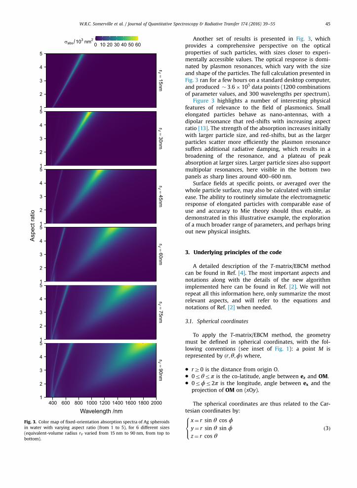
2.7. Case study: influence of size and aspect ratio on the far-field properties of silver spheroids

We now illustrate the ease of use of this code for rea-listic, application-oriented calculations, with a compre-hensive example simulating optical spectra of prolate sil-ver spheroids, as a function of size and aspect ratio. Thecalculation is fully automated with built-in precisionchecking to ensure a minimum relative accuracy of 10�3

(better precision could easily be obtained, at the cost ofincreased computation time). Fig. 2 illustrates this calcu-lation for prolate spheroids with challenging aspect ratios,up to 50:1.

1:1

5:1

10:1

20:1

30:140:1 50:1

0

0

10

20

30

Csca

0.5 1.5 2.5 3.5 4.5 5.5 6.5Wavelength μm

Cro

ss−s

ectio

ns

Fig. 2. Example calculation of scattering and absorption spectra of pro-late Ag spheroids in water with varying aspect ratio h (1–50), with a fixedequivalent-volume radius rV¼20 nm.

1

2

3

4

5

1

2

3

4

5

1

2

3

4

5

1

2

3

4

5

1

2

3

4

5

1

2

3

4

5

rV=

15n mrV

=30n m

rV=

45 nmrV

=60n m

rV=

75nmrV

=90n m

400 600 800 1000 1200 1400 1600 1800 2000

Wavelength /nm

Asp

ect r

atio

0 10 20 30 40 50 60σabs 103 nm2

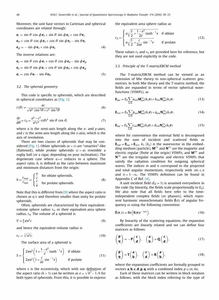
Fig. 3. Color map of fixed-orientation absorption spectra of Ag spheroidsin water with varying aspect ratio (from 1 to 5), for 6 different sizes(equivalent-volume radius rV varied from 15 nm to 90 nm, from top tobottom).

W.R.C. Somerville et al. / Journal of Quantitative Spectroscopy & Radiative Transfer 174 (2016) 39–55 45

Another set of results is presented in Fig. 3, whichprovides a comprehensive perspective on the opticalproperties of such particles, with sizes closer to experi-mentally accessible values. The optical response is domi-nated by plasmon resonances, which vary with the sizeand shape of the particles. The full calculation presented inFig. 3 ran for a few hours on a standard desktop computer,and produced � 3:6� 105 data points (1200 combinationsof parameter values, and 300 wavelengths per spectrum).

Figure 3 highlights a number of interesting physicalfeatures of relevance to the field of plasmonics. Smallelongated particles behave as nano-antennas, with adipolar resonance that red-shifts with increasing aspectratio [13]. The strength of the absorption increases initiallywith larger particle size, and red-shifts, but as the largerparticles scatter more efficiently the plasmon resonancesuffers additional radiative damping, which results in abroadening of the resonance, and a plateau of peakabsorption at larger sizes. Larger particle sizes also supportmultipolar resonances, here visible in the bottom twopanels as sharp lines around 400–600 nm.

Surface fields at specific points, or averaged over thewhole particle surface, may also be calculated with similarease. The ability to routinely simulate the electromagneticresponse of elongated particles with comparable ease ofuse and accuracy to Mie theory should thus enable, asdemonstrated in this illustrative example, the explorationof a much broader range of parameters, and perhaps bringout new physical insights.

3. Underlying principles of the code

A detailed description of the T-matrix/EBCM methodcan be found in Ref. [4]. The most important aspects andnotations along with the details of the new algorithmimplemented here can be found in Ref. [2]. We will notrepeat all this information here, only summarize the mostrelevant aspects, and will refer to the equations andnotations of Ref. [2] when needed.

3.1. Spherical coordinates

To apply the T-matrix/EBCM method, the geometrymust be defined in spherical coordinates, with the fol-lowing conventions (see inset of Fig. 1): a point M isrepresented by ðr;θ;ϕÞ where,

� rZ0 is the distance from origin O.� 0rθrπ is the co-latitude, angle between ez and OM.� 0rϕr2π is the longitude, angle between ex and the

projection of OM on (xOy).

The spherical coordinates are thus related to the Car-tesian coordinates by:

x¼ r sin θ cos ϕy¼ r sin θ sin ϕz¼ r cos θ

8><>: ð3Þ

W.R.C. Somerville et al. / Journal of Quantitative Spectroscopy & Radiative Transfer 174 (2016) 39–5546

Moreover, the unit base vectors in Cartesian and sphericalcoordinates are related through:

er ¼ sin θ cos ϕ exþ sin θ sin ϕeyþ cos θ ez

eθ ¼ cos θ cos ϕ exþ cos θ sin ϕ ey� sin θ ez

eϕ ¼ � sin ϕ exþ cos ϕ ey ð4Þ

The inverse relations are:

ex ¼ sin θ cos ϕ erþ cos θ cos ϕ eθ� sin ϕ eϕ

ey ¼ sin θ sin ϕ erþ cos θ sin ϕ eθþ cos ϕ eϕ

ez ¼ cos θ er� sin θ eθ ð5Þ

3.2. The spheroid geometry

This code is specific to spheroids, which are describedin spherical coordinates as (Fig. 1):

r θ� �¼ acffiffiffiffiffiffiffiffiffiffiffiffiffiffiffiffiffiffiffiffiffiffiffiffiffiffiffiffiffiffiffiffiffiffiffiffiffiffiffiffiffiffiffiffi

a2 cos 2θþc2 sin 2θp ð6Þ

drdθ

¼ rθ ¼a2�c2

a2c2rðθÞ3 sin θ cos θ; ð7Þ

where a is the semi-axis length along the x- and y-axes,and c is the semi-axis length along the z-axis, which is theaxis of revolution.

There are two classes of spheroids that may be con-sidered (Fig. 1). Oblate spheroids ða4cÞ are “smarties”-like(flattened), while prolate spheroids ðc4aÞ resemble arugby ball (or a cigar, depending on your inclination). Thedegenerate case where a¼c reduces to a sphere. Theaspect ratio, h, is defined as the ratio between maximumand minimum distances from the origin:

h¼ rmax

rmin¼

ac

for oblate spheroids;

ca

for prolate spheroids:

8><>: ð8Þ

Note that this is different from [9] where the aspect ratio ischosen as a=c and therefore smaller than unity for prolatespheroids.

Often, spheroids are characterized by their equivalent-volume sphere radius rV, or their equivalent-area sphereradius, rA. The volume of a spheroid is

V ¼ 43 πa

2c ð9Þ

and hence the equivalent-volume radius is

rV ¼ffiffiffiffiffiffiffia2c3

p: ð10Þ

The surface area of a spheroid is

S¼2πa2 1þ1�e2

etanh�1e

� �if oblate

2πa2 1þ cae

sin �1e� �

if prolate

8>><>>: ð11Þ

where e is the eccentricity, which with our definition ofthe aspect ratio ðh41Þ can be written as e¼

ffiffiffiffiffiffiffiffiffiffiffiffiffih2�1

p=h for

both types of spheroids. From this, it is possible to express

the equivalent-area sphere radius as

rA ¼a

ffiffiffiffiffiffiffiffiffiffiffiffiffiffiffiffiffiffiffiffiffiffiffiffiffiffiffiffiffiffiffiffiffiffiffiffiffiffiffiffi12þ1�e2

2etanh�1e

rif oblate

a

ffiffiffiffiffiffiffiffiffiffiffiffiffiffiffiffiffiffiffiffiffiffiffiffiffiffiffiffiffiffiffiffiffiffi12þ c2ae

sin �1e

rif prolate:

8>>><>>>:

ð12Þ

These values rV and rA are provided here for reference, butthey are not used explicitly in the code.

3.3. Principle of the T-matrix/EBCM method

The T-matrix/EBCM method can be viewed as anextension of Mie theory to non-spherical scatterer geo-metries. In both Mie theory and the T-matrix method, thefields are expanded in terms of vector spherical wave-functions (VSWFs), as

Einc ¼ E0Xn;m

anmMð1Þnm k1rð ÞþbnmNð1Þ

nm k1rð Þ ð13Þ

Esca ¼ E0Xn;m

pnmMð3Þnm k1rð ÞþqnmN

ð3Þnm k1rð Þ ð14Þ

Eint ¼ E0Xn;m

cnmMð1Þnm k2rð ÞþdnmNð1Þ

nm k2rð Þ ð15Þ

where for convenience the external field is decomposedinto the sum of incident and scattered fields asEout ¼ EincþEsca. k1 (k2) is the wavevector in the embed-ding medium (particle), Mð1Þ and Nð1Þ are the magnetic andelectric regular (finite at the origin) VSWFs, and Mð3Þ andNð3Þ are the irregular magnetic and electric VSWFs thatsatisfy the radiation condition for outgoing sphericalwaves. The indices m and n correspond to the projectedand total angular momentum, respectively with jmjrnand n¼ 1⋯1. The VSWFs definition can be found inAppendix C of Ref. [4].

A unit incident field ðE0 ¼ 1Þ is assumed everywhere inthe code (by linearity, the fields scale proportionally to E0).We also note that all fields here refer to the time-independent complex fields (or phasors), which repre-sent harmonic monochromatic fields ~EðtÞ of angular fre-quency ω using the following convention:

~Eðr; tÞ ¼ Re EðrÞe� iωt� �

: ð16Þ

By linearity of the scattering equations, the expansioncoefficients are linearly related and we can define fourmatrices as follows:

pq

!¼ �P

cd

� �;

ab

� �¼Q

cd

� �; ð17Þ

pq

!¼ T

ab

� �;

cd

� �¼ R

ab

� �; ð18Þ

where the expansions coefficients are formally grouped invectors a;b; c;d;p;q with a combined index p� ðn;mÞ.

Each of these matrices can be written in block notationas follows, with the block index referring to the type of

W.R.C. Somerville et al. / Journal of Quantitative Spectroscopy & Radiative Transfer 174 (2016) 39–55 47

multipole (electric or magnetic):

Q ¼ Q11 Q 12

Q21 Q 22

!: ð19Þ

Each block is an infinite square matrix, which is in practicetruncated to only include elements acting on multipoleorders up to a maximum order N. Taking into accountjmjrn, each block in the matrix has dimensionsNðNþ2Þ � NðNþ2Þ. The most common method to calcu-late those matrices is the Extended Boundary-ConditionMethod (EBCM) also called the Null-Field Method, wherethe matrix elements of P;Q are obtained as surface inte-grals on the particle as derived for example in Ref. [4,Section 5.8].

In practice, the expansion coefficients of the incidentfield ða;bÞ are known, and the scattered field can beobtained from T, while the internal field results from R.From the above equations, those two matrices can becomputed from P and Q as:

T¼ �PQ �1; R¼Q �1: ð20ÞThe matrix T contains all information about the scat-

terer. It allows in particular for analytical averaging over allorientations [9,14–17] or solving multiple scattering pro-blems by an ensemble of particles [16-18].

3.4. Additional simplifications for spheroids

For particles with symmetry of revolution, such asspheroids, expansion coefficients with different m valuesare entirely decoupled, and one can therefore solve theproblem for each value of m, where m can be viewed as afixed parameter (which will be implicit in most of ournotations). This means that each large 2NðNþ2Þ �2NðNþ2Þ matrix can be decoupled into 2Nþ1 indepen-dent matrices with m¼ �N⋯N, each of size 2ðN�mþ1Þ �2ðN�mþ1Þ (or 2N � 2N for m¼0). Moreover, we have:

T11n;kj�m ¼ T11

n;kjm; T12n;kj�m ¼ �T21

n;kjm;

T21n;kj�m ¼ �T12

n;kjm; T22n;kj�m ¼ T22

n;kjm: ð21Þ

and therefore only mZ0 values need to be considered inthe calculation of T.

Furthermore, the surface integrals reduce to line inte-grals, for which we have recently proposed a number ofsimplified expressions [19].

Reflection symmetry with respect to the equatorialplane also results in a number of additional simplifications(see Section 5.2.2 of Ref. [4] and Section 2.3 of Ref. [2]).Half of the matrix entries are zero because of the sym-metry in changing θ-π�θ and the other integrals aresimply twice the integrals evaluated over the half-range0 to π=2. Explicitly, we have

P11nk ¼ P22

nk ¼Q11nk ¼ Q22

nk ¼ 0 if nþk odd;

P12nk ¼ P21

nk ¼Q12nk ¼ Q21

nk ¼ 0 if nþk even; ð22Þand identical relations for T and R. From the point of viewof numerical implementation, it means that only half theelements need to be computed and stored. More impor-tantly, it also implies that we can rewrite Eqs. (17) and (18)as two independent sets of equations [2]. Explicitly, we

define

ae ¼a2a4⋮

0B@

1CA; bo ¼

b1b3⋮

0B@

1CA; ao ¼

a1a3⋮

0B@

1CA; be ¼

b2b4⋮

0B@

1CA;

ð23Þand similarly for c, d, p, q. We also define the matrices Qeoand Qoe from Q as:

Qeo ¼Q 11

ee Q 12eo

Q 21oe Q 22

oo

!; Qoe ¼

Q11oo Q 12

oe

Q21eo Q 22

ee

!; ð24Þ

where Q12eo denotes the submatrix of Q12 with even row

indices and odd column indices, and similarly for theothers. One can see that Qeo and Qoe contain all the non-zero elements of Q and exclude all the elements that mustbe zero by reflection symmetry, so this is an equivalentdescription of the Q-matrix.

The equations relating the expansion coefficients thendecouple into two sets of independent equations, forexample

aebo

!¼Qeo

cedo

!;

aobe

!¼Qoe

code

!; ð25Þ

and similar expressions deduced from Eqs. (17) and (18)for P, T, and R. As a result, the problem of finding the2ðN�mþ1Þ � 2ðN�mþ1Þ T- (or R-) matrix up to multi-pole order N reduces to finding the two decoupled T-matrices Teo and Toe, each of size ðN�mþ1Þ � ðN�mþ1Þ,namely:

Teo ¼ �Peo Qeo� ��1

; Toe ¼ �Poe Qoe� ��1

: ð26ÞThese symmetries and the definitions of this section are

used in the code to compute and store the matrices.

3.5. Angular functions

The T-matrix integrals and many of the physical prop-erties are expressed in terms of angular (θ-dependent)functions, which are derived from the associated Legendrefunctions Pm

n ðxÞ. We here summarize the most importantdefinitions. The associated Legendre functions may bewritten in terms of the Legendre polynomials as (formZ0)

Pmn xð Þ ¼ ð�1Þm 1�x2

� �m=2 dm

dxmPn xð Þ ð27Þ

where the polynomial is given by the expression

Pn xð Þ ¼ 12nn!

dn

dxnx2�1� �n

: ð28Þ

The factor ð�1Þm in the definition of Eq. (27) is known asthe Condon–Shortley phase. In the case of negative m, theexpression for the associated Legendre function is

P�mn xð Þ ¼ ð�1Þmðn�mÞ!

ðnþmÞ!Pmn xð Þ: ð29Þ

Following Ref. [4], we do not use the associatedLegendre functions directly, but rather some functionsobtained from them, which have more favorable numericalproperties. We notably use a special case of the Wigner d-

W.R.C. Somerville et al. / Journal of Quantitative Spectroscopy & Radiative Transfer 174 (2016) 39–5548

functions:

dnm θ� �� dn0m θ

� �¼ ð�1Þmffiffiffiffiffiffiffiffiffiffiffiffiffiffiffiffiffiðn�mÞ!ðnþmÞ!

sPmn cos θ� � ð30Þ

where we make use of the simpler dnmðθÞ notation. Wewill also use the functions πnmðθÞ and τnmðθÞ, derived fromthem as (Eqs. (5.16) and (5.17) of [4]):

πnm θ� �¼mdnmðθÞ

sin θ;

τnm θ� �¼ d

dθdnm θ

� �: ð31Þ

The function πnmðθÞ is generated for m40 using therecursion relation (derived from Eq. (B.22) in [4], see also[20]):

πn;m θð Þ ¼ 1ffiffiffiffiffiffiffiffiffiffiffiffiffiffiffiffiffiffin2 �m2

p 2n� 1ð Þ cos θπn�1;m θð Þ� ��

ffiffiffiffiffiffiffiffiffiffiffiffiffiffiffiffiffiffiffiffiffiffiffiffiffiffiffiffiffiffiðn� 1Þ2 �m2

qπn�2;m θð Þ; ð32Þ

applied for nZmþ1 with the initial conditions

πm�1;mðθÞ ¼ 0

πm;mðθÞ ¼mAmð sin θÞm�1 ð33Þ

with Am defined recursively as

A0 ¼ 1

Amþ1 ¼ Am

ffiffiffiffiffiffiffiffiffiffiffiffiffiffiffiffiffiffi2mþ12ðmþ1Þ

s: ð34Þ

τnm is then calculated as

τnm θð Þ ¼ �1m

ffiffiffiffiffiffiffiffiffiffiffiffiffiffiffiffin2�m2

pπn�1;m θð Þþ n

mcos θπnm θð Þ: ð35Þ

For mo0, the following relations are used:

πn;�mðθÞ ¼ ð�1Þmþ1πnmðθÞ;τn;�mðθÞ ¼ ð�1ÞmτnmðθÞ: ð36Þ

Finally, for m¼0, we have

πn;0ðθÞ ¼ 0

τn;0ðθÞ ¼ � sin θP0nð cos θÞ: ð37Þ

When dnmðθÞ is needed, it is calculated as:

dn;m θ� �¼ 1

msin θπn;m θ

� �if ma0

dn;0ðθÞ ¼ Pnð cos θÞ if m¼ 0

8<: ð38Þ

In those latter expressions, dn;0 and τn;0 are obtained bystandard recursion for the Legendre polynomials and theirderivatives. For nZ1:

dn;0 ¼2n�1

ncos θ dn�1;0�

n�1n

dn�2;0

τn;0 ¼ cos θ τn�1;0�n sinθ τn�2;0

d�1;0 ¼ 0; d0;0 ¼ 1

τ�1;0 ¼ 0; τ0;0 ¼ � sin θ: ð39Þ

The function vshPinmTaunm computes the requiredangular functions using the above formulas, which arenumerically stable and efficient [4].

3.6. Integral quadratures

All T-matrix integrals can be written as integrals overthe variable cos ðθÞ. The integrals are numerically com-puted using a standard Gauss–Legendre quadraturescheme with Nθ points,

Z π

0f ðθÞ sin θ dθ¼

Z 1

�1f ðθÞ dð cos θÞ �

XNθ

p ¼ 1

wpf ðθpÞ; ð40Þ

where θp and wp are the nodes and weights of the quad-rature. The same procedure is also used for calculatingsurface-averaged field properties, but may require a dif-ferent number of integration points.

The function auxInitLegendreQuad calculates thesenodes and weights for any number Nθ and uses the algo-rithm developed by Greg von Winckel available from theMATLAB Central website [21] (where it is called lgwt.m). Forconvenience the file Utils/quadTable.mat stores pre-calculated nodes and weights by steps of 5 from 50 up to2000, which can reduce the calculation time.

For spheroids, the T-matrix integrals can be reduced toa half-interval by symmetry, so the nodes and weights arecomputed for quadrature order 2Nθ and only the positivenodes θp40 are used (giving Nθ quadrature points).

We note that alternative quadrature schemes couldeasily be used, and may perform better for these types ofintegrands (requiring fewer function evaluations). Unfor-tunately, in order to make the best use of vectorized cal-culations, paramount for efficient MATLAB code, the imple-mentation of adaptive quadrature (with internal accuracyestimate) appears challenging and would require animportant refactoring of those functions performingnumerical integrations.

3.7. Computation of the P and Q matrices

The formulas used for the computation of the integralsof the P and Q matrices are given in Section 2.2 of Ref. [2].Explicitly, we use the following equations from Ref. [2]:

P12; Q 12: Eqs: ð11Þ and ð15ÞP21; Q 21: Eqs: ð12Þ and ð16ÞP11; Q 11: Eqs: ð17Þ and ð18ÞP22; Q 22: Eqs: ð19Þ–ð22Þ

8>>>><>>>>:

ð41Þ

The diagonal terms are treated separately and we use:

P11nn; Q

11nn: Eqs: ð23Þ; ð25Þ; and ð65Þ

P22nn; Q

22nn: Eqs: ð24Þ; ð26Þ; and ð27Þ

(ð42Þ

The algorithm used to avoid numerical cancellationswas described in detail in [2] and summarized in Section4.4 of [2]. All the technical details of the implementationcan be found in Ref. [2], in particular in the Appendix.Comments in the code also explain the most importantsteps, using the same notation and referring to equationsand sections of Ref. [2].

The function sphCalculatePQ handles all those cal-culations and returns the two matrices.

W.R.C. Somerville et al. / Journal of Quantitative Spectroscopy & Radiative Transfer 174 (2016) 39–55 49

The functions sphGetModifiedBesselProducts,sphGetXiPsi, and sphGetFpovx are used specifically toimplement the new algorithm.

One important parameter of the new algorithm is thenumber of multipoles, NB, used to estimate the modifiedBessel products. For large size parameters, it may benecessary to use NB4NQ to obtain accurate results.Whether this precaution is necessary can be easily checkedbefore carrying out the bulk of the calculations. Thefunction sphEstimateNB can be called to provide such anestimate for NB. It calculates the modified Bessel productsðF þ =xÞ for the maximum size parameter and the smallestand largest s (if λ-dependent) for increasing NB until allresults up to n¼NQ have converged (within a specifiedrelative accuracy, the default value is 10�13).

3.8. Matrix inversion for T and R matrices

The inversion of the linear systems for T and R is per-formed using block inversion as detailed in Section 4.5 of[2]. Specifically, the inversion is carried out with the fol-lowing steps (Eq. (70) of [2]):

F1 ¼ Q11� ��1

;

G1 ¼ P11F1; G3 ¼ P21F1; G5 ¼Q 21F1:

F2 ¼ Q 22�G5Q12

h i�1;

G2 ¼ P22F2; G4 ¼ P12F2; G6 ¼Q 12F2:

T12 ¼ G1G6�G4; T22 ¼ G3G6�G2;

T11 ¼ G1�T12G5; T21 ¼G3�T22G5: ð43ÞThis is carried out separately for Teo and Toe.

Two matrix inversions are needed in those steps (tocompute F1 and F2). Because of the often near-singularnature of the matrices, the choice of the inversion algo-rithm can have dramatic consequences on the numericalstability of the calculations. A number of options havebeen proposed and studied in the literature. In [22], amethod based on a LU factorization with partial rowpivoting (equivalent to A/B in MATLAB to get AB�1) wasproposed. In [2], we observed that (B.'⧹A.’).’ appeared to bemore numerically stable. This amounts to a LU factoriza-tion with partial column pivoting (as opposed to rowpivoting as suggested in [22]). Although not explicitlystated as such, we believe this is equivalent to theimproved algorithm proposed in [23] and based onGaussian elimination with back-substitution.

In SMARTIES, we implement the inversion algorithmexplicitly to avoid using the ⧹ operator, which has a dif-ferent behavior in MATLAB and Octave for near-singularmatrices. The steps are as follows. The function lu is calledon the transpose of the matrix, BT , to enforce columnpivoting instead of rows, i.e. we obtain lower and uppertriangular matrices L and U and a permutation matrix Psuch that

LU¼ PBT: ð44ÞThe solution of XB¼A is then obtained by successivelysolving the following two triangular linear systems and

transposing the result, i.e.

LZ¼ PAT ð45Þ

UY¼ Z ð46Þ

X¼ YT ð47Þ

F1 and F2 are calculated with this algorithm by settingA¼ I. Note that with this algorithm, we have not noticedany difference in accuracy when calculating T directlyfrom solving TQ ¼ �P as opposed to calculating R firstfrom RQ ¼ I and then deducing T from T¼ �PR.

The function rvhGetTRfromPQ calculates T (andoptionally R).

Note that, as explained in detail in Ref. [3], the elementsof the T-matrix are not accurate up to multipole n¼NQ

even when P and Q are. If an accurate T-matrix up tomultipole N is required, it is therefore necessary to calcu-late P and Q with NQ ¼NþΔ multipoles, and then trun-cate the obtained T-matrix down to N multipoles (see [3]for full details). In such cases, the function sphEstima-

teDelta can be used to estimate Δ and the functionrvhTruncateMatrices is then used to truncate T downto N multipoles.

In principle, the T-matrix should satisfy general sym-metry relations arising from optical reciprocity [3,4],namely:

T11nk ¼ T11

kn ; T21nk ¼ �T12

kn ;

T12nk ¼ �T21

kn ; T22nk ¼ T22

kn : ð48Þ

It was suggested in [3,24] that the upper triangular part ofthe T-matrix is more accurate in challenging cases than thelower triangular part. Using the function rvhGetSymme-

tricMat, one can use these symmetry relations to deducethe lower parts from the upper parts. This can slightlyincrease the range of validity of the method.

As pointed out in [3], these precautions are not neces-sary in many cases, and it is sufficient to check that thedesired physical properties have converged (see con-vergence tests in Section 2.6).

3.9. Orientation-averaged properties

One of the advantages of the T-matrix formalism is thatthe optical properties for any orientation can in principlebe derived from a single computation of the scatterer T-matrix. In particular, once the T-matrix has been calcu-lated, it is possible to calculate analytically the opticalproperties of a (non-interacting) collection of randomlyoriented scatterers. Such orientation-averaged far-fieldcross-sections are evaluated as detailed in Ref. [4]. Wehave in particular (Eqs. (5.107) and (5.141) of [4]):

⟨Cext⟩¼�2π

k21

Xn;m

Re T11nnjmþT22

nnjm� �

;

¼ �2π

k21

Xn ¼ 1…1m ¼ 0…n

2�δm;0� �

Re T11nnjmþT22

nnjm� �

ð49Þ

W.R.C. Somerville et al. / Journal of Quantitative Spectroscopy & Radiative Transfer 174 (2016) 39–5550

⟨Csca⟩¼2π

k21

Xn ¼ 1…1k ¼ 1…1

m ¼ 0…minðn;kÞ

2�δm;0� �� T11

nkjm 2þ T12

nkjm 2þ T21

nkjm 2þ T22

nkjm 2� �

ð50Þ

⟨Cabs⟩¼ ⟨Cext⟩� ⟨Csca⟩: ð51ÞThe function rvhGetAverageCrossSections calcu-

lates those cross-sections from a previously obtained T-matrix.

3.10. Scattering matrix for random orientation

The T-matrix formalism can also be used to efficientlyand accurately compute the scattering matrix for ran-domly oriented scatterers. The full details of such calcu-lations are described in Section 5.5 of Ref. [4] and thecorresponding algorithm has been implemented in stan-dard T-matrix codes [9]. For convenience, we here providea function pstScatteringMatrixOA to calculate thisscattering matrix and output the results in the same for-mat as in Ref. [9]. This function (and the subroutines ituses) is a direct port of those FORTRAN routines into MATLAB

and are here provided for convenience with permissionfrom M. Mishchenko. Because no attempt was made tooptimize them for MATLAB, they are much slower than thecorresponding FORTRAN routines. For any intensive scatter-ing matrix calculations, it is therefore recommended toexport the T-matrix obtained from MATLAB and run thecalculations in FORTRAN using the code of Ref. [9].

3.11. Incident field

For scatterers with a fixed orientation, one first needsto define the incident field through its correspondingexpansion coefficients anm and bnm (Eq. (13)). Only incidentplane waves with linear polarization are currently imple-mented in the code. For a general incident plane wave,those are given in Eqs. (C.56)–(C59) of Ref. [4]. Explicitly,the field is:

EðrÞ ¼ E0 exp ik1 � rð Þ ð52Þand we define the incident k-vector direction with its twoangles from spherical coordinates θp, ϕp, i.e.:

k1 ¼ k1erp

¼ k1 sin θp cos ϕpexþ sin θp sin ϕpeyþ cos θpez� �

: ð53Þ

The incident field polarization, which must be perpendi-cular to k1 is then defined by one angle αp as:

E0 ¼ E0 cos αp eθp þ sin αp eϕp

� �¼ E0 cos αp cos θp cos ϕp� sin αp sin ϕp

� �ex

hþ cos αp cos θp sin ϕpþ sin αp cos ϕp

� �ey

� cos αp sin θp ez ð54Þ

With those defined, the expansion coefficients are thenobtained from:

anm ¼ dnm i cos αpπnmðθpÞþ sin αpτnmðθpÞ�

bnm ¼ dnm i cos αpτnmðθpÞþ sin αpπnmðθpÞ� ð55Þ

where

dnm ¼ ð�1Þmþ1 exp � imϕp

� �� in

ffiffiffiffiffiffiffiffiffiffiffiffiffiffiffiffiffiffiffiffiffiffiffi4πð2nþ1Þnðnþ1Þ

s: ð56Þ

Note that if the incident field is incident along the zdirection, then only jmj ¼ 1 terms are non-zero.

Here are a few examples of common configurations:

KzEx: θp ¼ 0; ϕp ¼ 0; αp ¼ 0 ð57Þ

KzEy: θp ¼ 0; ϕp ¼ 0; αp ¼ π=2 ð58Þ

KxEz: θp ¼ π=2; ϕp ¼ 0; αp ¼ π ð59Þ

KxEy: θp ¼ π=2; ϕp ¼ 0; αp ¼ π=2 ð60Þ

The function vshMakeIncidentParameters can be usedto define these parameters, and vshGetInci-

dentCoefficients to get the incidentfield coefficients. We note that these definitions werechosen for linear polarization, but elliptic polarizationcould be easily accommodated by amending the functionvshGetIncidentCoefficients.

3.12. Expansion coefficients of scattered and internal fieldsand fixed-orientation cross-sections

Once the incident field expansion coefficients aredefined, it is straightforward to obtain those of the scat-tered and internal fields from Eq. (18). The functionrvhGetExpansionCoefficients will carry out this task.The internal fields coefficients are only computed if thematrix R was calculated.

Once the expansion coefficients of the scattered fieldare known, the extinction, scattering, and absorptioncross-sections are simply obtained from similar expres-sions as for standard Mie theory (Eq. (5.18) of [4]):

Csca ¼1

k21

Xn;m

cnmj j2þ dnm 2� �

ð61Þ

Cext ¼�1

k21

Xn;m

cnmanmþdnmbnm� � ð62Þ

Cabs ¼ Cext�Csca: ð63Þ

3.13. Surface fields

T-matrix calculations have been mostly applied to far-field properties but for many applications in plasmonics,nanophotonics, optical forces, etc., the near-field proper-ties are also needed.

The applicability of the T-matrix method to near-fieldcalculations is still debated; a particular point of concern isto avoid reliance on the Rayleigh hypothesis, which isgenerally not valid. This implies that the scattered fieldexpansion (Eq. (14)) is no longer valid for fields near thescatterer surface (but it can be shown that it is valid atleast outside the circumscribing sphere of the scatterer[4]).

W.R.C. Somerville et al. / Journal of Quantitative Spectroscopy & Radiative Transfer 174 (2016) 39–55 51

To circumvent this limitation, we here use an alter-native approach relying on the internal field expansion(Eq. (15)), which remains valid everywhere at the surface(at least in the case of spheroids). This expansion allows usto calculate the internal field everywhere on the surface(but inside) of the particle, E

in. In order to calculate fields

Eout

immediately outside the surface, we apply the stan-dard boundary conditions:

Eint�E

out� �

� n¼ 0

εinEint�εoutE

out� �

� n¼ 0 ð64Þ

where the normal is

n¼ nrerþnθeθ

¼ rffiffiffiffiffiffiffiffiffiffiffiffiffiffir2þr2θ

q er� rθffiffiffiffiffiffiffiffiffiffiffiffiffiffir2þr2θ

q eθ : ð65Þ

Explicitly, we have (using s2 ¼ ε2=ε1)

Eoutr ¼ 1þðs2�1Þn2

r

� Einr þ s2�1

� nrnθE

inθ

Eoutθ ¼ s2�1

� nrnθE

inr þ 1þðs2�1Þn2

θ

� Einθ

Eoutϕ ¼ E

inϕ ð66Þ

The function pstSurfaceFields uses this method tocalculate the surface electric field along with a number ofsurface-averaged properties relevant to plasmonics andother near-field applications. Note that the ϕ-dependenceof all quantities is relatively simple, since they can all beexpressed as:

Aðr;θ;ϕÞ ¼Xm ¼ þN

m ¼ �N

Amðr;θÞ expðimϕÞ: ð67Þ

Our code therefore calculates the 2Nþ1 variables Amðr;θÞand the ϕ-dependence can then be trivially re-introduced.

3.14. Near fields

This method of calculating surface fields, however,cannot be used to obtain the near-field except exactly atthe surface. For points sufficiently far from the particle, thescattered field may be obtained from Eq. (14). However, forparticles deviating from a sphere, the series may notconverge for points close to the particle (failure of theRayleigh hypothesis). To test whether a point converges,an indicative test is to increase the number of multipolesconsidered, and confirm that the calculated field convergesto some value. If it fails to converge, either insufficientmultipoles were considered, or the point is in a regionwhere convergence will never be obtained. We haverecently studied these aspects and developed an alter-native method of computing near-fields, which will bediscussed in detail elsewhere [25]. We only here give abrief overview of the method, which is implemented in thefunction pstGetNearField.

As originally suggested in Ref. [26], we make use of thesurface integral equation (Eq. (5.168) of [4]), which

expresses the scattered field in terms of the surface fields:

Escaðr0Þ ¼ZSdS iωμ0 n�HðrÞ½ � G

2

ðr; r0Þþ n� EðrÞ½ �

� ∇� G2

ðr; r0Þ ��

; ð68Þ

where G2

is the free-space Green's function. The surfacefields E;H can be calculated accurately as described earlierand the integral is then performed using a double quad-rature on θ and ϕ (with the same number of nodes forsimplicity). As a result, this method is slower than theother methods for calculating the scattered field (whereapplicable), but will exhibit much better convergencebehavior for points near the particle [25]. An example ofits use is given in ScriptTutorial.

4. Additional implementation details

4.1. File naming conventions and organization

The first three letters of each function are used toclassify functions depending on their roles:

� slv: High-level functions solving a specific class ofproblems.

� pst: High-level functions used for post-processing.� vsh: Mostly low-level functions handling the calcula-

tions of quantities related to vector sphericalwavefunctions.

� rvh: T-matrix related functions specific to particleswith mirror-reflection symmetry.

� sph: T-matrix related functions specific to spheroidalparticles.

� aux: Auxiliary functions (low-level).

Each m-file is also located in a specific folder with thefollowing classification:

� High-Level: T-matrix related functions most likely tobe called directly by the user.

� Low-Level: T-matrix related functions used by thehigh-level functions.

� Materials: Includes dielectric functions of gold (Au)and silver (Ag) for plasmonics applications, as well as anexample dielectric function interpolated from tabulatedvalues for silicon (Si).

� Post-processing: Functions to calculate opticalproperties.

� Scripts: Contains example and tutorial scripts.� Solve: Contains the slv functions used to solve a

specific class of problems.� Utils: Includes miscellaneous utility functions, notably

to export the T-matrix, test whether the code is runningin Octave or MATLAB, or generate quadrature nodes andweights.

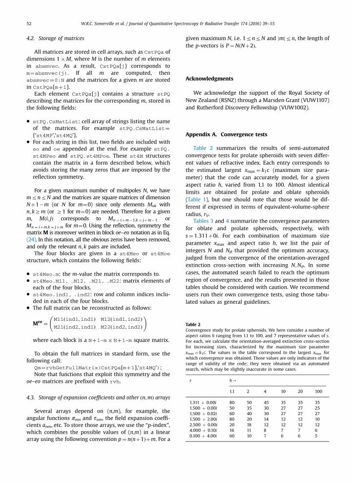
Table 2Convergence study for prolate spheroids. We here consider a number ofaspect ratios h ranging from 1.1 to 100, and 7 representative values of s.For each, we calculate the orientation-averaged extinction cross-sectionfor increasing sizes, characterized by the maximum size parameterxmax ¼ k1c. The values in the table correspond to the largest xmax forwhich convergence was obtained. Those values are only indicators of therange of validity of the code; they were obtained via an automatedsearch, which may be slightly inaccurate in some cases.

s h-

1.1 2 4 10 20 100

1.311 þ 0.00i 80 50 45 35 35 351.500 þ 0.00i 50 35 30 27 27 251.500 þ 0.02i 60 40 30 27 27 271.500 þ 2.00i 80 20 14 12 12 102.500 þ 0.00i 20 18 12 12 12 124.000 þ 0.10i 16 11 8 7 7 60.100 þ 4.00i 60 10 7 6 6 5

W.R.C. Somerville et al. / Journal of Quantitative Spectroscopy & Radiative Transfer 174 (2016) 39–5552

4.2. Storage of matrices

All matrices are stored in cell arrays, such as CstPQa ofdimensions 1�M, where M is the number of m elementsin absmvec. As a result, CstPQa{j} corresponds tom¼absmvec(j). If all m are computed, thenabsmvec¼0:N and the matrices for a given m are storedin CstPQa{mþ1}.

Each element CstPQa{j} contains a structure stPQ

describing the matrices for the corresponding m, stored inthe following fields:

� stPQ.CsMatList: cell array of strings listing the nameof the matrices. For example stPQ.CsMatList¼{‘st4MP’,‘st4MQ’}.

� For each string in this list, two fields are included witheo and oe appended at the end. For example stPQ.

st4MPeo and stPQ.st4MPoe. These st4M structurescontain the matrix in a form described below, whichavoids storing the many zeros that are imposed by thereflection symmetry.

For a given maximum number of multipoles N, we havemrnrN and the matrices are square matrices of dimensionNþ1�m (or N for m¼0) since only elements Mnk withn; kZm (or Z1 for m¼0) are needed. Therefore for a givenm, Mði; jÞ corresponds to Mn ¼ iþm�1;k ¼ jþm�1 orMn ¼ iþm;k ¼ jþm for m¼0. Using the reflection, symmetry thematrixM is moreover written in block oe–eo notation as in Eq.(24). In this notation, all the obvious zeros have been removed,and only the relevant n; k pairs are included.

The four blocks are given in a st4Meo or st4Moe

structure, which contains the following fields:

� st4Meo.m: the m-value the matrix corresponds to.� st4Meo.M11, .M12, .M21, .M22: matrix elements of

each of the four blocks.� st4Meo.ind1, .ind2: row and column indices inclu-

ded in each of the four blocks.� The full matrix can be reconstructed as follows:

Meo ¼M11ðind1;ind1Þ M12ðind1;ind2ÞM21ðind2;ind1Þ M22ðind2;ind2Þ

!

where each block is a Nþ1-m x Nþ1-m square matrix.

To obtain the full matrices in standard form, use thefollowing call:

Qm¼rvhGetFullMatrix(CstPQa{mþ1},‘st4MQ’);Note that functions that exploit this symmetry and the

oe–eo matrices are prefixed with rvh.

4.3. Storage of expansion coefficients and other ðn;mÞ arrays

Several arrays depend on (n,m), for example, theangular functions πnm and τnm, the field expansion coeffi-cients anm, etc. To store those arrays, we use the “p-index”,which combines the possible values of (n,m) in a lineararray using the following convention p¼ nðnþ1Þþm. For a

given maximum N, i.e. 1rnrN and jmjrn, the length ofthe p-vectors is P ¼NðNþ2Þ.

Acknowledgments

We acknowledge the support of the Royal Society ofNew Zealand (RSNZ) through a Marsden Grant (VUW1107)and Rutherford Discovery Fellowship (VUW1002).

Appendix A. Convergence tests

Table 2 summarizes the results of semi-automatedconvergence tests for prolate spheroids with seven differ-ent values of refractive index. Each entry corresponds tothe estimated largest xmax ¼ k1c (maximum size para-meter) that the code can accurately model, for a givenaspect ratio h, varied from 1.1 to 100. Almost identicallimits are obtained for prolate and oblate spheroids(Table 1), but one should note that those would be dif-ferent if expressed in terms of equivalent-volume-sphereradius, rV.

Tables 3 and 4 summarize the convergence parametersfor oblate and prolate spheroids, respectively, withs¼ 1:311þ0i. For each combination of maximum sizeparameter xmax and aspect ratio h, we list the pair ofintegers N and Nθ that provided the optimum accuracy,judged from the convergence of the orientation-averagedextinction cross-section with increasing N;Nθ . In somecases, the automated search failed to reach the optimumregion of convergence, and the results presented in thosetables should be considered with caution. We recommendusers run their own convergence tests, using those tabu-lated values as general guidelines.

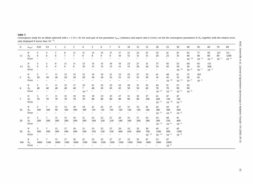
Table 3Convergence study for an oblate spheroid with s¼ 1:311þ0i. For each pair of size parameter xmax (columns) and aspect ratio h (rows), we list the convergence parameters N;Nθ , together with the relative error,

only displayed if worse than 10�13.

h: xmax: 0.01 0.1 1 2 3 4 5 6 7 8 10 12 15 20 25 30 40 50 60 70 80

N 5 5 7 9 11 11 13 15 17 17 21 23 27 35 41 47 63 77 95 127 1111.1 Nθ 6 6 6 7 7 8 8 9 9 10 15 15 15 20 25 35 40 40 80 80 1200

Error – – – – – – – – – – – – – – – – 10�12 10�11 10�9 10�7 10�4

N 5 5 9 11 11 13 15 15 19 19 23 27 31 37 45 53 69 93 1151.3 Nθ 9 9 9 9 9 10 15 15 15 15 15 20 20 25 45 30 50 45 500

Error – – – – – – – – – – – – – – – 10�12 10�9 10�7 10�3

N 5 7 11 13 15 15 19 19 21 23 25 27 33 41 49 61 75 1032 Nθ 20 20 20 20 20 20 20 20 25 25 25 25 30 35 45 35 50 45

Error – – – – – – – – – – – – – – 10�12 10�11 10�7 10�4

N 5 7 11 15 17 19 21 23 23 25 29 31 35 45 51 57 594 Nθ 40 40 40 40 40 7 40 45 45 45 50 50 60 70 70 90 90

Error – – – – – 10�3 – – – – – – – 10�13 10�11 10�9 10�4

N 5 7 11 15 19 19 19 23 25 27 31 35 37 41 47 477 Nθ 70 70 70 70 70 70 80 80 80 80 90 90 100 200 130 130

Error – – – – – – – – – – – – – 10�11 10�10 10�6

N 5 7 13 15 19 19 21 25 27 27 31 33 41 45 43 4710 Nθ 100 100 90 100 100 100 110 110 110 120 120 130 140 180 180 200

Error – – – – – – – – – – – – – 10�11 10�8 10�6

N 5 7 13 15 19 21 23 23 27 29 33 37 43 43 49 4120 Nθ 200 200 200 200 200 200 200 220 220 240 260 260 280 300 550 400

Error – – – – – – – – – – – – – 10�12 10�8 10�4

N 5 7 13 17 19 21 23 25 27 29 33 35 39 45 47 4550 Nθ 500 500 500 500 500 500 550 550 550 600 650 800 700 1100 900 1200

Error – – – – – – – – – – – – 10�13 10�12 10�9 10�6

N 5 7 13 17 19 21 23 25 27 27 33 35 47 53 47100 Nθ 1000 1100 1000 1100 1000 1100 1100 1100 1100 1100 1300 1500 1400 1600 2000

Error – – – – – – – – – – – – – – 10�9

W.R.C.Som

ervilleet

al./Journal

ofQuantitative

Spectroscopy&

Radiative

Transfer174

(2016)39

–5553

Table 4Convergence study for a prolate spheroid with s¼ 1:311þ0i. For each pair of size parameter xmax (columns) and aspect ratio h (rows), we list the convergence parameters N;Nθ , together with the relative error, only

displayed if worse than 10�13.

h: xmax: 0.01 0.1 1 2 3 4 5 6 7 8 10 12 15 20 25 30 40 50 60 70 80

N 5 5 7 9 11 11 13 15 17 17 21 23 27 35 41 47 67 79 97 87 1091.1 Nθ 6 6 6 7 7 8 8 9 10 10 15 15 15 20 25 25 40 60 45 70 120

Error – – – – – – – – – – – – – – – – 10�12 10�10 10�9 10�7 10�4

N 5 5 9 11 11 13 15 15 19 19 23 27 31 37 45 53 73 95 1171.3 Nθ 9 9 9 9 9 10 15 15 15 15 15 20 20 25 25 30 40 45 180

Error – – – – – – – – – – – – – – – 10�12 10�10 10�7 10�4

N 5 7 11 13 15 15 19 19 21 23 25 27 33 41 49 61 89 1132 Nθ 20 20 20 20 20 20 20 20 20 25 25 25 30 30 45 45 40 50

Error – – – – – – – – – – – – – – 10�12 10�10 10�7 10�4

N 5 7 11 15 17 19 19 23 23 25 27 31 35 43 49 49 594 Nθ 40 40 40 40 40 40 40 40 45 45 45 50 60 90 70 100 110

Error – – – – – – – – – – – – – 10�12 10�9 10�6

N 5 7 11 15 17 19 21 23 25 27 31 33 37 43 43 477 Nθ 80 80 80 70 70 70 70 80 80 80 80 90 90 120 120 130

Error – – – – – – – – – – – – – 10�13 10�10 10�8

N 5 7 11 15 17 21 21 23 27 27 31 33 37 45 45 4510 Nθ 120 120 120 120 120 100 120 120 120 120 120 120 140 160 160 200

Error – – – – – – – – – – – – – – 10�10 10�8

N 5 7 11 15 19 21 21 25 27 27 31 29 39 47 49 4520 Nθ 220 220 220 260 220 220 220 220 220 260 260 260 280 300 350 350

Error 10�13 10�13 10�13 – – – – – – – – 10�12 – 10�13 10�10 10�7

N 5 7 11 15 19 21 21 25 27 29 31 33 39 45 53 4550 Nθ 650 650 650 400 500 500 500 500 650 700 600 700 700 900 1100 1200

Error 10�12 10�12 10�12 10�12 – – – – – – – – – 10�12 10�11 10�7

N 5 7 11 15 19 21 21 25 27 29 31 33 39 45 47 47100 Nθ 800 800 800 800 800 1000 1000 1000 1000 1400 1400 1200 1600 1800 2000 2000

Error 10�12 10�12 10�12 10�12 10�12 10�12 10�13 10�13 10�13 – – – – 10�12 10�11 10�8

W.R.C.Som

ervilleet

al./Journal

ofQuantitative

Spectroscopy&

Radiative

Transfer174

(2016)39

–5554

W.R.C. Somerville et al. / Journal of Quantitative Spectroscopy & Radiative Transfer 174 (2016) 39–55 55

References

[1] Somerville WRC, Auguié B, Le Ru EC. Severe loss of precision incalculations of T-matrix integrals. J Quant Spectrosc Radiat Transf2012;113(7):524–35.

[2] Somerville WRC, Auguié B, Le Ru EC. A new numerically stableimplementation of the T-matrix method for electromagnetic scat-tering by spheroidal particles. J Quant Spectrosc Rad Transf2013;123:153–68.

[3] Somerville WRC, Auguié B, Le Ru EC. Accurate and convergent T-matrix calculations of light scattering by spheroids. J Quant Spec-trosc Rad Transf 2015;160:29–35.

[4] Mishchenko MI, Travis LD, Lacis AA. Scattering, absorption andemission of light by small particles. 3rd ed.Cambridge: CambridgeUniversity Press; 2002.

[5] Etchegoin PG, Le Ru EC, Meyer M. An analytic model for the opticalproperties of gold. J Chem Phys 2006;125:164705.

[6] Le Ru EC, Etchegoin PG. Principles of surface enhanced ramanspectroscopy and related plasmonic effects.Amsterdam: Elsevier;2009.

[7] Barber PW, Hill SC. Light scattering by particles: computationalmethods.Singapore: World Scientific; 1990.

[8] Quirantes A. A T-matrix method and computer code for randomlyoriented, axially symmetric coated scatterers. J Quant Spectrosc RadTransf 2005;92(3):373–81.

[9] Mishchenko MI, Travis LD. Capabilities and limitations of a currentFORTRAN implementation of the T-matrix method for randomlyoriented, rotationally symmetric scatterers. J Quant Spectrosc RadTransfer 1998;60:309–24.

[10] MATLAB, version 7.14 (R2012a). The MathWorks Inc. Natick, Mas-sachusetts; 2012.

[11] John W. Eaton, David Bateman, Søren Hauberg, Rik Wehbring (2015).GNU Octave version 4.0.0 manual: a high-level interactive languagefor numerical computations. URL http://www.gnu.org/software/octave/doc/interpreter/.

[12] Somerville WRC, Auguié B, Le Ru EC. [link] URL ⟨http://www.victoria.ac.nz/scps/research/research-groups/raman-lab/numerical-tools⟩;2015.

[13] Boyack R, Le Ru EC. Investigation of particle shape and size effects inSERS using T-matrix calculations. Phys Chem Chem Phys 2009;11:7398–405.

[14] Mishchenko MI. Light scattering by randomly oriented axiallysymmetric particles. J Opt Soc Am A 1991;8(6):871–82.

[15] Khlebtsov NG. Orientational averaging of light-scattering obser-vables in the T-matrix approach. Appl Opt 1992;31:5359–65. http://dx.doi.org/10.1364/AO.31.005359.

[16] Mishchenko M. Light scattering by size-shape distributions of ran-domly oriented axially symmetric particles of a size comparable to awavelength. Appl Opt 1993;32(24):4652–66.

[17] Mackowski DW, Mishchenko MI. Calculation of the T-matrix and thescattering matrix for ensembles of spheres. J Opt Soc Am A 1996;13:2266–78. http://dx.doi.org/10.1364/JOSAA.13.002266.

[18] Peterson B, Ström S. T-matrix for electromagnetic scattering from anarbitrary number of scatterers and representations of E(3). Phys RevD 1973;8(10):3661–78.

[19] Somerville WRC, Auguié B, Le Ru EC. Simplified expressions of the T-matrix integrals for electromagnetic scattering. Opt Lett 2011;36(17):3482–4.

[20] Mishchenko MI. Calculation of the amplitude matrix for a non-spherical particle in a fixed orientation. Appl Opt 2000;39(6):1026–31.

[21] von Winckel G., Legendre–Gauss quadrature weights and nodes.MATLAB central file exchange, 2004.

[22] Wielaard D, Mishchenko M, Macke A, Carlson B. Improved T-matrixcomputations for large, nonabsorbing and weakly absorbing non-spherical particles and comparison with geometrical-opticsapproximation. Appl Opt 1997;36(18):4305–13.

[23] Moroz A. Improvement of Mishchenko's T-matrix code for absorbingparticles. Appl Opt 2005;44(17):3604–9.

[24] Volkov SN, Samokhvalov IV, Kim D. Assessing and improving theaccuracy of T-matrix calculation of homogeneous particles withpoint-group symmetries. J Quant Spectrosc Rad Transf 2013;123:169–75.

[25] Le Ru EC, Roache S, Somerville WRC, Auguié B. Numerical investi-gations into the Rayleigh hypothesis for the T-matrix method.Manuscript in preparation.

[26] Doicu A, Wriedt T. Near-field computation using the null-fieldmethod. J Quant Spectrosc Rad Transf 2010;111(3):466–73.