observation et modélisation du déferlement des vagues
TRANSCRIPT
THÈSE DE DOCTORAT
UNIVERSITÉ DE BRETAGNE OCCIDENTALE
sous le sceau de l’Université européenne de Bretagne
pour obtenir le titre de
DOCTEUR DE L’UNIVERSITÉ DE BRETAGNE OCCIDENTALE
Mention : océanographie physique
École Doctorale des Sciences de la Mer
présentée par
Fabien Leckler Préparée à l'IFREMER
Observation et modélisation du
déferlement des vagues
Thèse soutenue le 18 Décembre 2013 devant le jury composé de :
Xavier CARTON Professeur, Université de Bretagne Occidentale
Président de jury
Philippe FORGET Directeur de recherche, Université du Toulon
Rapporteur
Alain WEILL Directeur de recherche, Université Pierre et Marie Curie
Rapporteur
Danièle HAUSER Directrice de recherche, Université Pierre et Marie Curie
Examinatrice
Alvise BENETAZZO Chercheur, CNR-ISMAR, Venezia, Italia
Examinateur
Fabrice ARDHUIN Chercheur, IFREMER
Directeur de thèse

Resume
Les recentes parametrisations utilisees dans les modeles spectraux de vagues offrentdes resultats interessants en termes de prevision et rejeux des etats de mer. Cependant,de nombreux phenomenes physiques presents dans ces modeles sont encore mal compriset donc mal modelises, notamment le terme de dissipation lie au deferlement des vagues.Le travail presente dans cette these vise dans un premier temps a analyser et critiquer lesparametrisations existantes de la dissipation, au travers de la modelisation explicite desproprietes du deferlement sous-jacentes. Du constat de l’echec de ces parametrisationsa reproduire les observations in situ et satellite du deferlement, une nouvelle methoded’observation et d’analyse des deferlements est proposee a l’aide de systemes de stereovideo. Cette methode permet l’observation des deferlements sur des surfaces de mer re-construites a haute resolution par stereo triangulation. Ainsi, une methode completede reconstruction des surfaces de mer en presence de vagues deferlantes est proposee etvalidee. La detection des vagues deferlantes sur les images et leur reprojection sur les sur-faces reconstruites est egalement discutee. Bien que peu d’acquisitions soient disponibles,les differents parametres observables grace a l’utilisation de la stereo video sont mis enavant. Ce travail montre l’interet des systemes video stereo pour une meilleure observationet comprehension du deferlement des vagues, pour le developpement des parametrisationsde la dissipation dans les modeles spectraux de vague.
1

Abstract
The recent parameterizations used in spectral wave models provide today interestingresults in terms of forecast and hindcast of the sea states. Nevertheless, many physicalphenomena present in these models are still poorly understood and therefore poorly mod-eled, in particular the dissipation source term due to breaking. First, the work presentedin this thesis is aimed at analyzing and criticizing the existing parameterizations of thedissipation through the explicit modeling of the underlying properties of breaking. Thefinding of the failure of these parameterizations to reproduce the in situ and satelliteobservations, a new method for the observation and the analysis of breaking is proposedusing stereo video systems . This method allows the observation of breaking waves on thehigh-resolution stereo-reconstructed sea surfaces. Therefore, a complete method for recon-struction of the sea surfaces in the presence of breaking waves is proposed and validated.The detection of breaking waves on the images and their reprojection on reconstructedsurface is also discussed. Although too few acquisitions are available to draw firm results,an overview of the various observable parameters through the use of stereo video is given.This work shows the importance of stereo video systems to a better observation and un-derstanding of the breaking waves, required in order to improve dissipation source termin spectral wave models.
3

Acknowledgments
Je souhaite, avant de vous presenter mes travaux de these, presenter mes remerciementsa bon nombre de personnes dont l’aide et le soutien, tant professionnel que personnel, ontfait de mes trois ans de doctorat une experience de travail, de rencontres et de vie que jen’oublierai jamais. Ceux qui sont passes par la le savent, la these est un moment difficile,qui demande beaucoup d’investissement et de travail de l’etudiant, mais dont le succesne peut etre attribue uniquement a celui-ci. En effet, ce succes depend egalement pourbeaucoup d’un grand nombre personnes, qui parfois sans le savoir, jouent un role essentiel.Ces quelques lignes leur sont dediees.
Tout d’abord, je souhaiterais remercier mon directeur de recherche, Fabrice Ardhuin,non pas car il en est de coutume, mais car il a ete le pilier essentiel, non seulement de mestravaux, mais aussi de mon moral et de ma motivation. Plus qu’un chercheur brillant,Fabrice a fait preuve d’une grande patience et d’un soutien sans faille dans les momentsdifficiles. Sa motivation, sa perseverance et sa determination ont ete pour moi une sourced’inspiration constante. Toutes ses qualites, tant scientifiques qu’humaines, ont fait deces trois annees de travail intense a ses cotes, une experience tres agreable.
Je presente egalement mes chaleureux remerciements a l’ensemble de mes colleguesdu Laboratoire d’Oceanographie Spatiale, tout particulierement Bertrand Chapron, di-recteur du laboratoire, pour son encadrement et ses remarques et conseils avises. Mickael,plus que d’avoir m’assurer un soutien informatique indispensable, nos pauses cafe et nos”experimentations in situ” au Minou, Dalbos et Deolen ont ete de tres bons moments. Jeremercie egalement Alexei pour ces remarques toujours sinceres et justes. Severine, mercipour les nombreuses relectures d’anglais, nos discussions et notre amitie (sans oublier lesmaccarons au pot de ma soutenance). Ma gratitude se tourne aussi vers tous ceux que jen’ai pas cite, mais qui se reconnaitront, pour avoir ete des collegues attentionnes, voirepour nombres d’entre eux d’etre devenus de bons amis.
J’adresse aussi mes remerciements aux personnels de l’ecole doctorale, tout parti-culierement Elisabeth Bondu, pour sa tolerance lorsque les deadlines venaient a etreallegrement depassees, mais aussi et surtout pour son soutien technique pour les tachesadministratives et la preparation de ma soutenance.
Je sais gre a mes rapporteurs, Alain Weill et Philippe Forget, ainsi qu’aux membres dujury, Xavier Carton, Daniele Hauser et Alvise Benetazzo pour la lecture consciencieuse et
5
attentionnee de mon manuscrit et leurs remarques pertinentes et constructives sur montravail. Merci a eux egalement de s’etre deplaces peu avant Noel pour ma soutenance etainsi de m’avoir permis de passer des fetes de fins d’annees plus sereinement.
Õî÷ó âûðàçèòü áëàãîäàðíîñòü êîìàíäå Ìîðñêîãî �èäðî�èçè÷åñêîãî Èíñòèòóòà
Â.Â. Ìàëèíîâñêîìó, Â.À. Äóëîâó, Â.Å. Ñìîëîâó, À.Ñ. Ìèðîíîâó, Ì.Â. Þðîâñêîé,
Þ.Þ. Þðîâñêîìó è À.Å. Êîðèíåíêî çà íàó÷íî-òåõíè÷åñêóþ ïîääåðæó âî âðåìÿ
ïðîâåäåíèÿ ýêñïåðèìåíòîâ íà ïëàò�îðìå. Ñïàñèáî çà ïîìîùü â îðãàíèçàöèè áûòà
è ïèòàíèÿ, âêëþ÷àÿ ñóï èç ñâåæåâûëîâëåííîé ðûáû â ñîïðîâîæäåíèè ìåñòíûõ íà-
ïèòêîâ. Ýòîò íåçàáûâàåìûé îïûò îñòàíåòñÿ ñî ìíîé íàâñåãäà.
Vorrei ringraziare i team italiani di ISMAR/CNR e di PROTECNO per il loro supportotecnico, per l’installazione di WASS e per l’elaborazione dei dati stereo. Un ringraziamentoparticolare va ad Alvise Benetazzo e a sua moglie, per il contributo significativo nellosviluppare gli algoritmi di elaborazione dei dati stereo e per l’accoglienza che ho ricevutoa Venezia: una splendida visita della citta ed un risotto squisito!
I warmly thank Johannes Gemmrich, Mickael Banner and Russel Morison for providingbreaking wave and wave spectra data from the FAIRS experiment.
I also thank Magdalena Anguelova and Ferris Webster for sharing their global whitecapdatabase.
Merci aussi a tous mes amis, de Brest, des Landes et d’ailleurs, pour leur soutien,pour les soirees musique (ou autres), pour les vacances passees avec eux, ..., pour tous cesmoments qui m’ont permis de decompresser, d’oublier mes erreurs de compilation, mesproblemes de deadline souvent bien trop courtes, ou encore, pour votre presence a masoutenance.
Enfin, je remercie beaucoup ma compagne, Carine, pour son soutien quotidien indefec-tible et son optimisme contagieux vis a vis de mon travail. Sa patience sans faille et sonecoute attentive ont ete les garants de mon moral dans les moments de doutes. Je souligneegalement son indulgence et sa bienveillance envers moi surtout durant les derniers moislorsque le manque de sommeil a severement erode ma delicatesse et ma gentillesse : ildevrait exister un diplome pour les compagnes de doctorant ! A defaut, je lui dedicace cemanuscrit.
Ces remerciement ne peuvent bien evidemment pas s’achever sans une douce penseepour mes parents et ma sœur. Malgre l’eloignement geographique, votre amour et vosencouragements m’ont accompagne tout au long de ma vie, pour faire de moi la personneque je suis aujourd’hui, et ont joue un role significatif dans la reussite de ce projet.
This work was supported by a FP7-ERC young investigator grant number 240009for the IOWAGA project, the U.S. National Ocean Partnership Program, under grantU.S. Office of Naval Research grant N00014-10-1-0383. Additional support from ESA and
6

CNES for the Globwave project is gratefully acknowledged.
7

Contents
Resume 1
Abstract 3
Acknowledgments 5
Table of content 9
List of figures 11
1 Introduction 19
2 Wave breaking modeling 332.1 Introduction . . . . . . . . . . . . . . . . . . . . . . . . . . . . . . . . . . . 332.2 Investigated dissipation parameterizations . . . . . . . . . . . . . . . . . . 36
2.2.1 Description of the parameterizations . . . . . . . . . . . . . . . . . 372.2.2 Correction of swell dissipation . . . . . . . . . . . . . . . . . . . . . 412.2.3 Adaptation of TEST500 into TEST570 . . . . . . . . . . . . . . . . 412.2.4 Model settings for the different parameterizations . . . . . . . . . . 50
2.3 Dissipation source terms and breaking crest length densities . . . . . . . . 502.3.1 Academic case: Uniform infinite deep ocean . . . . . . . . . . . . . 502.3.2 Wave-breaking experiment: FAIRS hindcast . . . . . . . . . . . . . 55
2.4 Whitecap coverage and mean foam thickness at the global scale . . . . . . 572.5 Conclusion and Perspectives . . . . . . . . . . . . . . . . . . . . . . . . . . 63
3 Sea surface reconstruction 653.1 Introduction . . . . . . . . . . . . . . . . . . . . . . . . . . . . . . . . . . . 653.2 Experiment description . . . . . . . . . . . . . . . . . . . . . . . . . . . . . 663.3 Theoretical background . . . . . . . . . . . . . . . . . . . . . . . . . . . . . 68
3.3.1 Pinhole camera model . . . . . . . . . . . . . . . . . . . . . . . . . 683.3.2 From 3D coordinates to 2D pixel coordinates . . . . . . . . . . . . . 723.3.3 Epipolar geometry and stereo triangulation . . . . . . . . . . . . . . 77
3.4 Camera calibration and image rectification . . . . . . . . . . . . . . . . . . 783.4.1 Short historical of camera calibrations . . . . . . . . . . . . . . . . 783.4.2 Camera intrinsic calibration . . . . . . . . . . . . . . . . . . . . . . 803.4.3 Camera extrinsic calibration . . . . . . . . . . . . . . . . . . . . . . 92
9
CONTENTS
3.4.4 Image rectification . . . . . . . . . . . . . . . . . . . . . . . . . . . 943.5 Sea surface reconstruction . . . . . . . . . . . . . . . . . . . . . . . . . . . 95
3.5.1 Point matching processing . . . . . . . . . . . . . . . . . . . . . . . 963.5.2 Triangulation processing . . . . . . . . . . . . . . . . . . . . . . . . 1033.5.3 Mean surface plane definition . . . . . . . . . . . . . . . . . . . . . 1073.5.4 Surfaces in world reference system . . . . . . . . . . . . . . . . . . . 1083.5.5 Correction for the asymmetric projection . . . . . . . . . . . . . . . 1083.5.6 Griding and smoothing of the surfaces . . . . . . . . . . . . . . . . 110
3.6 Analyses of sea surface reconstructions . . . . . . . . . . . . . . . . . . . . 1103.6.1 Probability density function of the elevation . . . . . . . . . . . . . 1103.6.2 Non directional frequency spectra . . . . . . . . . . . . . . . . . . . 1113.6.3 Frequency-wavenumber directional spectra . . . . . . . . . . . . . . 1113.6.4 Wavenumber spectra . . . . . . . . . . . . . . . . . . . . . . . . . . 1113.6.5 Mean Square Slopes of elevation maps . . . . . . . . . . . . . . . . 123
3.7 Conclusion . . . . . . . . . . . . . . . . . . . . . . . . . . . . . . . . . . . . 123
4 Breaking Observation 1274.1 Introduction . . . . . . . . . . . . . . . . . . . . . . . . . . . . . . . . . . . 1274.2 Automatic detection of breaking events . . . . . . . . . . . . . . . . . . . . 130
4.2.1 Image binarization . . . . . . . . . . . . . . . . . . . . . . . . . . . 1314.2.2 Event filtering method . . . . . . . . . . . . . . . . . . . . . . . . . 135
4.3 Crest length density . . . . . . . . . . . . . . . . . . . . . . . . . . . . . . 1414.4 Breaking probabilities . . . . . . . . . . . . . . . . . . . . . . . . . . . . . 1434.5 Wave scale analysis . . . . . . . . . . . . . . . . . . . . . . . . . . . . . . . 1474.6 Saturation spectrum . . . . . . . . . . . . . . . . . . . . . . . . . . . . . . 1484.7 Conclusion . . . . . . . . . . . . . . . . . . . . . . . . . . . . . . . . . . . . 150
5 Conclusion 153
Bibliography 157
10
List of Figures
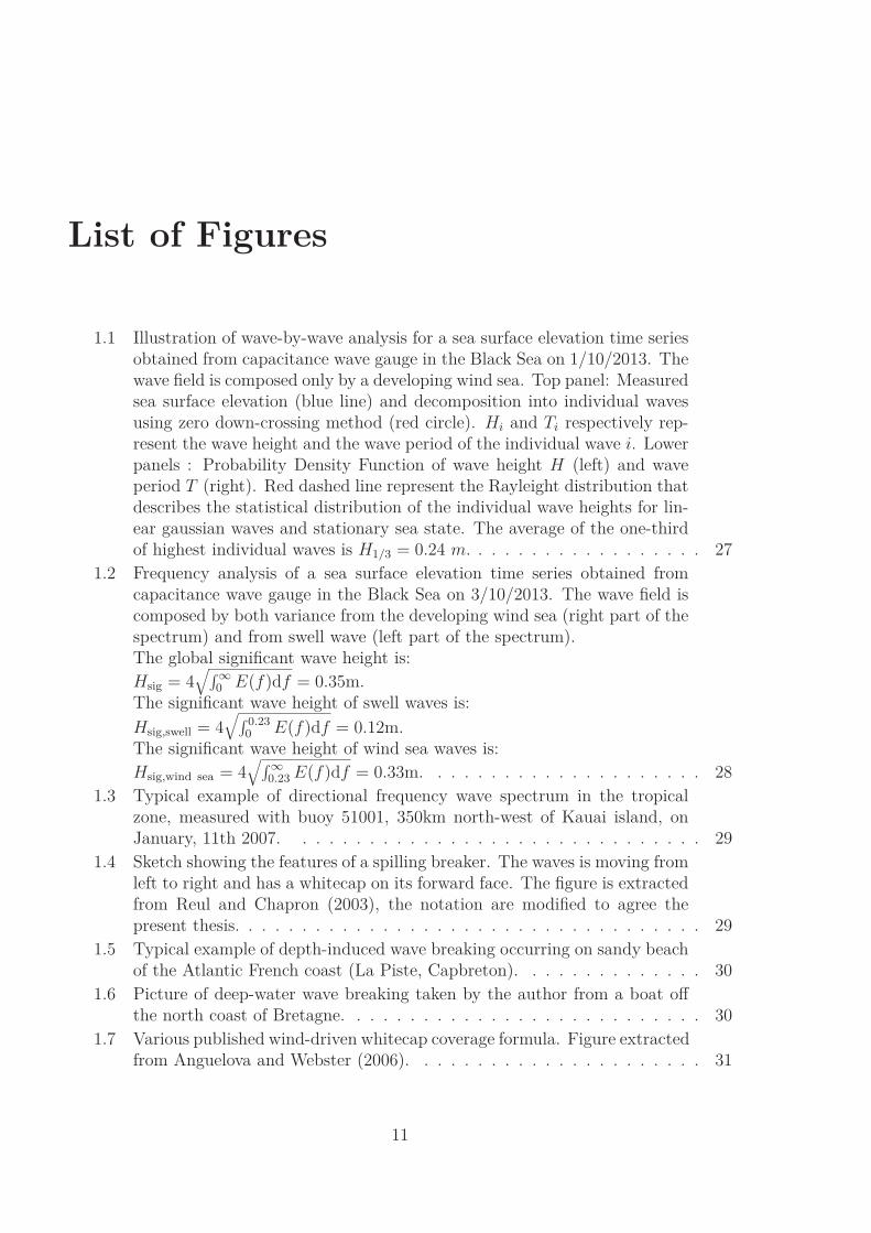
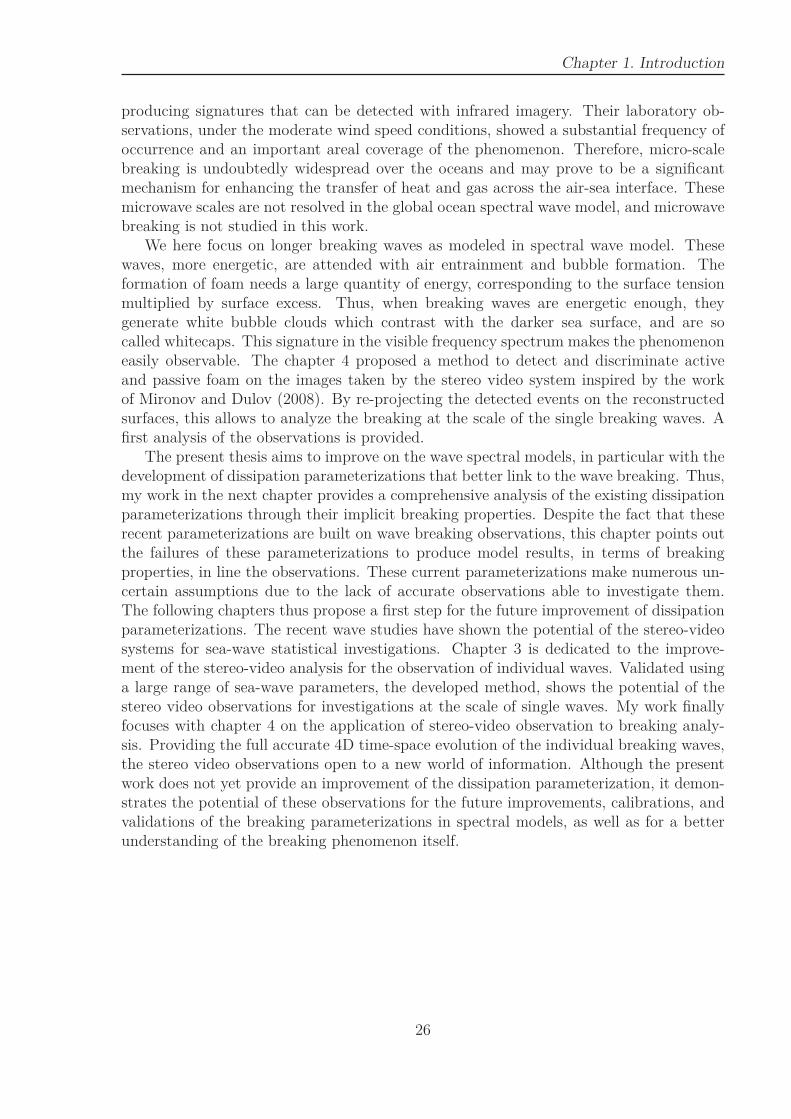
1.1 Illustration of wave-by-wave analysis for a sea surface elevation time seriesobtained from capacitance wave gauge in the Black Sea on 1/10/2013. Thewave field is composed only by a developing wind sea. Top panel: Measuredsea surface elevation (blue line) and decomposition into individual wavesusing zero down-crossing method (red circle). Hi and Ti respectively rep-resent the wave height and the wave period of the individual wave i. Lowerpanels : Probability Density Function of wave height H (left) and waveperiod T (right). Red dashed line represent the Rayleight distribution thatdescribes the statistical distribution of the individual wave heights for lin-ear gaussian waves and stationary sea state. The average of the one-thirdof highest individual waves is H1/3 = 0.24 m. . . . . . . . . . . . . . . . . . 27
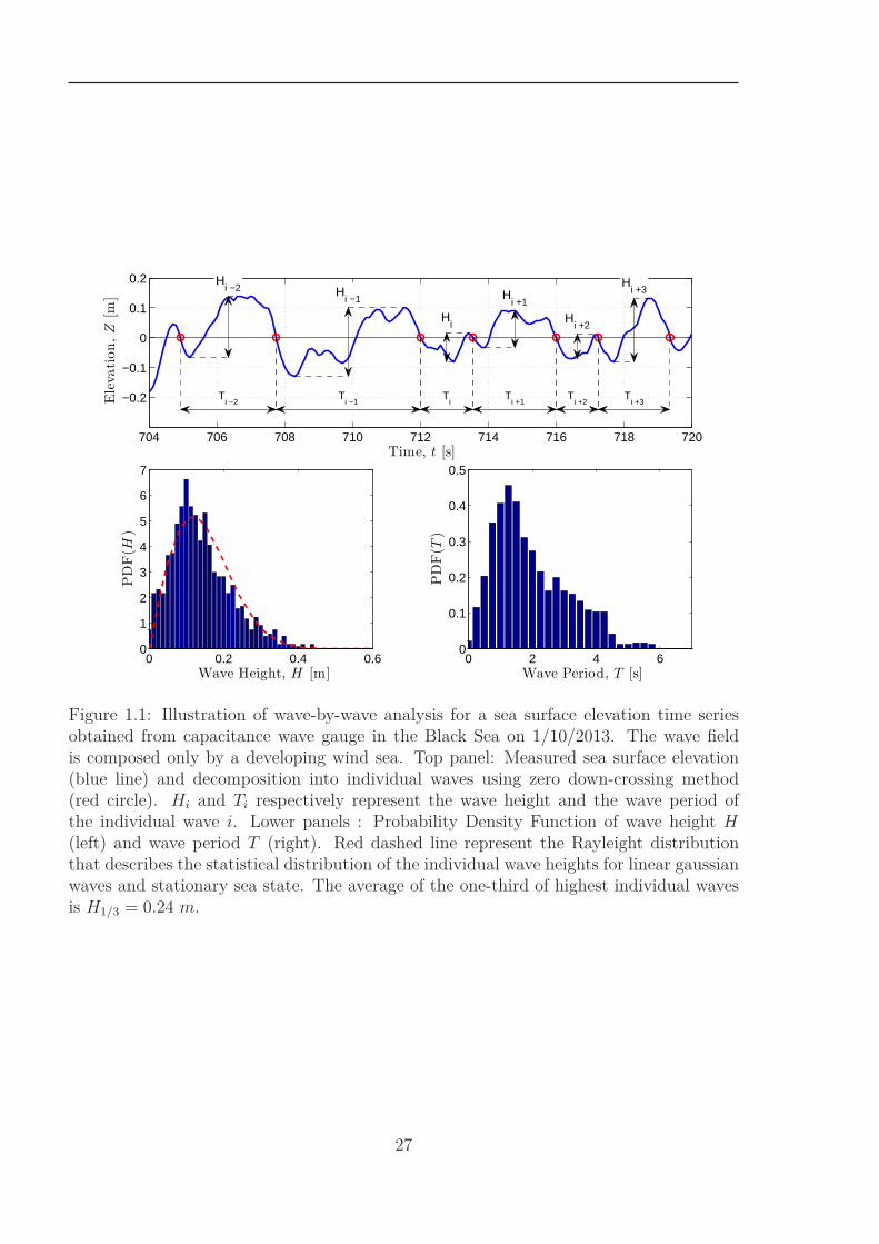
1.2 Frequency analysis of a sea surface elevation time series obtained fromcapacitance wave gauge in the Black Sea on 3/10/2013. The wave field iscomposed by both variance from the developing wind sea (right part of thespectrum) and from swell wave (left part of the spectrum).The global significant wave height is:
Hsig = 4√
∫
∞
0 E(f)df = 0.35m.The significant wave height of swell waves is:
Hsig,swell = 4√
∫ 0.230 E(f)df = 0.12m.
The significant wave height of wind sea waves is:
Hsig,wind sea = 4√
∫
∞
0.23 E(f)df = 0.33m. . . . . . . . . . . . . . . . . . . . . 28
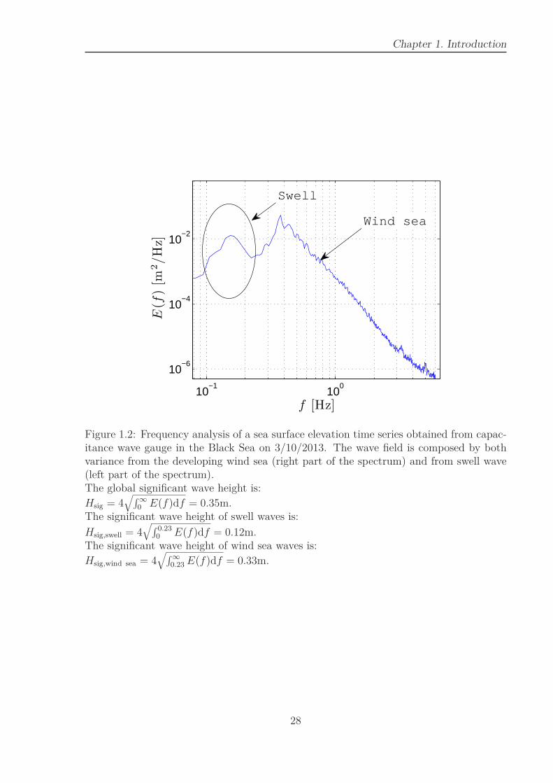
1.3 Typical example of directional frequency wave spectrum in the tropicalzone, measured with buoy 51001, 350km north-west of Kauai island, onJanuary, 11th 2007. . . . . . . . . . . . . . . . . . . . . . . . . . . . . . . 29
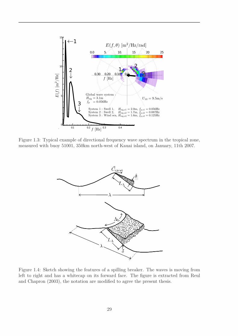
1.4 Sketch showing the features of a spilling breaker. The waves is moving fromleft to right and has a whitecap on its forward face. The figure is extractedfrom Reul and Chapron (2003), the notation are modified to agree thepresent thesis. . . . . . . . . . . . . . . . . . . . . . . . . . . . . . . . . . . 29
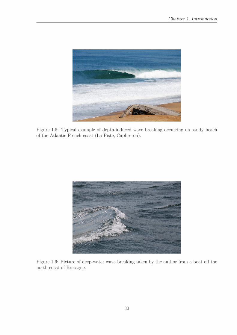
1.5 Typical example of depth-induced wave breaking occurring on sandy beachof the Atlantic French coast (La Piste, Capbreton). . . . . . . . . . . . . . 30
1.6 Picture of deep-water wave breaking taken by the author from a boat offthe north coast of Bretagne. . . . . . . . . . . . . . . . . . . . . . . . . . . 30
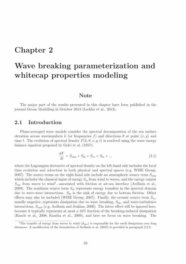
1.7 Various published wind-driven whitecap coverage formula. Figure extractedfrom Anguelova and Webster (2006). . . . . . . . . . . . . . . . . . . . . . 31
11

LIST OF FIGURES
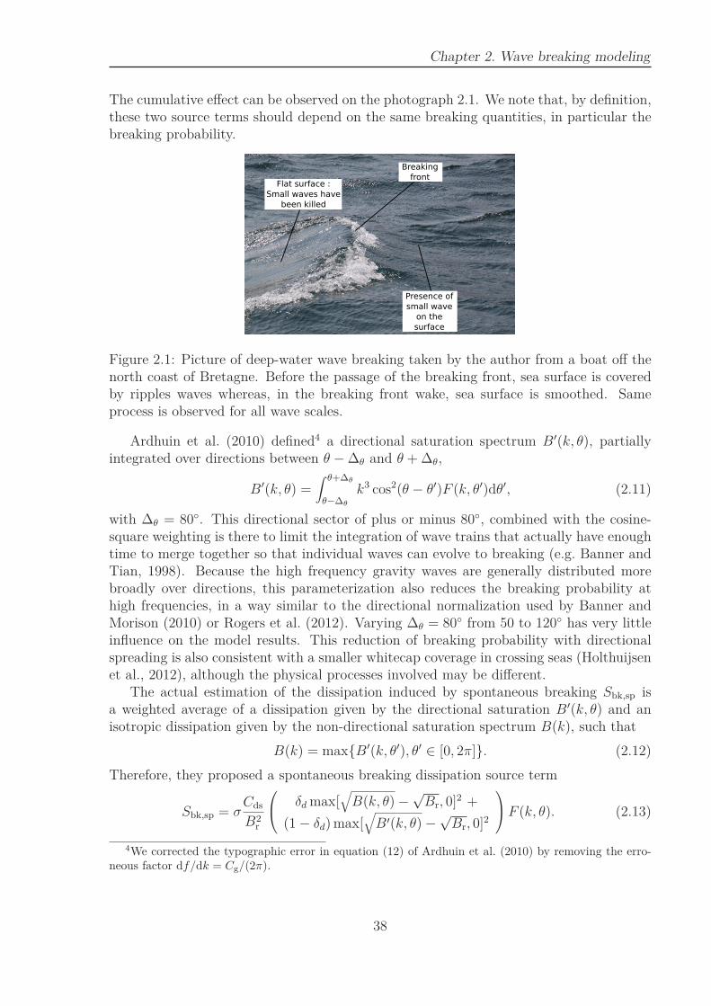
2.1 Picture of deep-water wave breaking taken by the author from a boat offthe north coast of Bretagne. Before the passage of the breaking front, seasurface is covered by ripples waves whereas, in the breaking front wake, seasurface is smoothed. Same process is observed for all wave scales. . . . . . 38
2.2 Top: Global NRMS Error for parameterizations TEST441b (left) and TEST451(right). Middle: Comparison of PDF of wave heights (left) and Normal-ized bias vs wave height (right). Bottom: Comparison of Normalized RMSError (left) and Scatter Index vs wave height (right). . . . . . . . . . . . . 42
2.3 Top: Rectangular filtering windows Wfi(colors) over integrated spectrum
(black line). Bottom: Breaking probabilities Pb,fiobtained for each wave
scale fi (colors) and breaking probability Pb(k) obtained with averaging(Black line). . . . . . . . . . . . . . . . . . . . . . . . . . . . . . . . . . . . 43
2.4 Normalized RMS Error for new parameterization TEST570 compared toTEST451 (Ardhuin et al., 2010) and BJA (Bidlot et al., 2005) parame-terizations for whole 2006 year. In all three cases the model is driven byECMWF operational wind analyses. . . . . . . . . . . . . . . . . . . . . . . 45
2.5 Normalized Bias, RMS Error and Scatter Index on Hs for new parameter-ization TEST570 compared to TEST451 and BJA parameterizations. . . . 46
2.6 Mean values of mssku binned as a function of Hs (x-axis) and U10 (y-axis)for TEST570 and TEST451 parameterizations and satellite observations. . 47
2.7 Wave spectra (top panels), mean direction (middle panels) and directionalspread (bottom panels) on 3 November 1999 at buoy X2 and X4, averagedover the time window 12:00-17:00 EST, from observations and model runswith T451 , TEST510 and T570 parameterizations. The swell is excludeddue to the frequency range used in the figure. . . . . . . . . . . . . . . . . 49
2.8 Breaking probabilities and associated dissipations obtained for a fully de-veloped sea state (3 days of simulation) for TEST570 (left) and TEST451(right). . . . . . . . . . . . . . . . . . . . . . . . . . . . . . . . . . . . . . . 51
2.9 Source terms for TEST570, TEST451 and BJA parameterizations usingDIA for non-linear interactions after 8 hours of run. The considered modelis a uniform infinite deep ocean with a uniform 10 ms−1 wind, starting fromrest. . . . . . . . . . . . . . . . . . . . . . . . . . . . . . . . . . . . . . . . 53
2.10 Source terms after 8 hours of run for TEST570X, TEST451X and BJAXparameterizations using XNL for non-linear interactions. The consideredmodel is a uniform infinite deep ocean with a uniform 10 ms−1 wind, start-ing from rest. . . . . . . . . . . . . . . . . . . . . . . . . . . . . . . . . . . 54
2.11 Spectra (left) and direction-integrated breaking crest length distribution(right) obtained with TEST570 and TEST451 parameterizations for a uni-form infinite deep ocean after 3 days of run, when Cp/U10 > 1.2, withU10 = 5, 10, and 15 m s−1. Energy peaks are marked by circles. . . . . . . 55
2.12 Top: Evolution of spectra (left) and direction-integrated breaking crestlength distribution (right) for TEST570 (XNL) with increasing wave age(colors), for U10 = 12 m s−1. Bottom: Evolution of Λ(Cp) as function ofCp/U10, with TEST570 and TEST451 parameterizations . . . . . . . . . . 56
12

LIST OF FIGURES
2.13 Direction-integrated Breaking Crest Length Distribution Λ(C) from BWHDintegration (TEST570,red) and from directional saturation spectrum (TEST451,blue) extracted from hindcast of FAIRS experiment. Squares are observedΛ(C) by Gemmrich et al. (2008). . . . . . . . . . . . . . . . . . . . . . . . 58
2.14 Mean values of W binned under the WindSat track as a function of U10 fornew parameterization (TEST570) and modified Ardhuin et al. (2010)’s pa-rameterization (TEST451) compared to March 2006 satellite observationsby Anguelova et al. (2009). Wind used for binning is the collocated CFSRdata, which is independent of the WindSat data until September 2008. Redbars represent minimum and maximum values, black bars are the standarddeviations and the blue line represents the empirical fit by Monahan andWoolf (1989). . . . . . . . . . . . . . . . . . . . . . . . . . . . . . . . . . . 60
2.15 Q-Q plot of WCC given by TEST570 and TEST451 and satellite obser-vations (Anguelova et al., 2009) on March 2006. Compared values arecollocated under WindSat swath. Colors give the values of log(Nval). . . . . 61
2.16 Mean values of mean foam thickness (∆) binned as a function of U10 fornew parameterization (TEST570) and modified Ardhuin et al. (2010)’s pa-rameterization (TEST451). Wind used for binning is the collocated CFSRdata, which is independent of the WindSat data until September 2008. Redbars represent minimum and maximum values, black bars are the standarddeviations. . . . . . . . . . . . . . . . . . . . . . . . . . . . . . . . . . . . . 62
3.1 Platform of Katsiveli, Crimea, Ukraine. Location of anemometer, wavegauge array and Wave Acquisition Stereo System (WASS). . . . . . . . . . 67
3.2 Top: Waterproof camera case. Bottom, left: 5-mm focal length low distor-tion lens. Bottom, right: 5 Megapixel BM-500GE JAI cameras. . . . . . . 69
3.3 Evolution of wind and wave conditions during the experiment. Acquisitionswere done for wind direction established to West-South-West, with speedup to 10m/s. . . . . . . . . . . . . . . . . . . . . . . . . . . . . . . . . . . 70
3.4 Schema of the pinhole camera model. . . . . . . . . . . . . . . . . . . . . . 73
3.5 Schema of the links between 3D points of the scene and their projection onundistorted bit-mapped image. . . . . . . . . . . . . . . . . . . . . . . . . . 74
3.6 Illustration of epipolar geometry for a pair of cameras. The points C1 andC2 are the center of projection. The image points e1 and e2 are epipolarpoints. The epipolar plane corresponding to scene point P is represented inyellow. The intersection between the epipolar plane and the image planesdefined the epipolar line. . . . . . . . . . . . . . . . . . . . . . . . . . . . . 79
3.7 Example of images using for left intrinsic camera calibration. Green crossesrepresent corner detected on the images whereas blue circle are reprojec-tions of 3D points using with calibrated intrinsic and extrinsic parameters.On upper-left panel, red lines represent definition of the world coordinatesystem. Chessboard square size is 30mm on the four upper images, and80mm on the two lower ones. . . . . . . . . . . . . . . . . . . . . . . . . . 81
3.8 Chessboard and image planes seen as projective planes, so linked by ahomography matrix H. . . . . . . . . . . . . . . . . . . . . . . . . . . . . . 85
13
LIST OF FIGURES
3.9 Deviation of pixels from rectilinear projection due to distortion for rightcamera. . . . . . . . . . . . . . . . . . . . . . . . . . . . . . . . . . . . . . 89
3.10 Error of reprojection (residual after optimization) for the right camera :ru = u − up and rv = v − vp. Upper-left panel shows that some reprojec-tions are far from observed corner, nevertheless, these points have smallinfluence on global calibration results, given large number of calibrationpoints. Upper-right panel shows disparity in reprojection errors in both uand v pixel axis. Lower panel gives disparity in reprojection errors for eachaxis. We note that assumption of error assimilated to a white Gaussiannoise looks fine. Directional RMS errors of reprojection are (0.28, 0.20) forleft camera and (0.26, 0.18) for right one. . . . . . . . . . . . . . . . . . . . 90
3.11 Distribution of intrinsic calibration chessboards in camera reference systemfor right camera. . . . . . . . . . . . . . . . . . . . . . . . . . . . . . . . . 91
3.12 Main steps of stereo reconstruction processing: Top panels show set ofcorresponding points returnd by matching point processing. Bottom leftpanel corresponds to the stereo-triangulation processing. Finally, bottom-right panel represents the sea surface obtained in world coordinate system.Figure presented here shows results obtained for first image pair of the 4th
acquisition. . . . . . . . . . . . . . . . . . . . . . . . . . . . . . . . . . . . 97
3.13 Example of bad point matching due to foam patch. Size of correlationtemplates is purposefully increased to 121 × 61 pixels to exaggerate thisphenomenon. Left panels: Matching points obtained between left (top)and right (bottom) images. Color of points are correlation coefficient ofmatching (top) and standard deviation of pixel values in right correlationwindow. Green point matching is not disturbed by foam patch whereas redpoint matching if fully driven by small part of foam patch in correlationwindow. Top-right: resulting surface after stereo triangulation (§3.5.2) androtation to world coordinates (§3.5.4). Green point falls on reconstructionin back of wave crest whereas images show that it is in front of the crest.Bad matching leads to unrealistic step around foam patch. Bottom-right:histogram of pixel vertical coordinates disparity between left and rightimages, with abnormal peak observed around pixel value 101 due to badmatching. . . . . . . . . . . . . . . . . . . . . . . . . . . . . . . . . . . . . 99
3.14 Same figure as 3.13, but matched points are now obtained with decreasingcorrelation template size, pixel histogram equalization, and left image recti-fication. Sizes of correlation templates are 121×61 pixels, 41×41 pixels, and21 × 21 pixels in subsequent searching steps. Left panels: Matching pointsobtained between left (top) and right (bottom) images. The point colorsrepresent correlation coefficient of matching (top) and standard deviationof pixel values in right correlation window. Top-right: resulting surface af-ter stereo triangulation (§3.5.2) and rotation to world coordinates (§3.5.4).Bottom-right: histogram of pixel vertical coordinates disparity between leftand right images. The abnormal peak observed around pixel value 79 infigure 3.13 is not present here. . . . . . . . . . . . . . . . . . . . . . . . . . 101
14
LIST OF FIGURES
3.15 Same figure as 3.15, after the smoothing of the disparity map with a 10×10point (i.e. 20 × 20 pixel) median filter. Top-right: resulting surface afterstereo triangulation (§3.5.2) and rotation to world coordinates (§3.5.4).Bottom-right: histogram of pixel vertical coordinates disparity betweenleft and right images. . . . . . . . . . . . . . . . . . . . . . . . . . . . . . . 102
3.16 Reconstruction zone in which matching processing is done. Results areapproximatively rectangular reconstructed sea surface. . . . . . . . . . . . 104
3.17 Mean vertical (left) and horizontal (right) disparity maps obtained fromthe average of the 21576 disparity maps of the 4th acquisition. . . . . . . . 105
3.18 Triangulated point deviation due to correction for asymmetric projection,applied on the mean disparity map of acquisition 4 (Fig. 3.17) . . . . . . . 109
3.19 Probability Density Function (PDF) of the surface elevation. Black linescorrespond to the PDF obtained with wave gauges time series. The bluelines correspond to the PDF of the reconstructions obtained with the newprocessing, including both equalization of pixel intensity histogram anddecreasing correlation template size in the matching point processing, andthe correction for asymmetric projection. . . . . . . . . . . . . . . . . . . . 112
3.20 Frequency Spectra (FS) of the surface elevation. Black lines correspondto the PDF obtained with wave gauges time series. The blue lines corre-spond to the FS of the reconstructions obtained with the new processing,including both equalization of pixel intensity histogram and decreasing cor-relation template size in the matching point processing, and the correctionfor asymmetric projection. . . . . . . . . . . . . . . . . . . . . . . . . . . . 113
3.21 Wave spectrum over wavenumbers and frequencies (i.e. 3D spectrum in-tegrated over directions) on the left panel and cross-sections in the 3Dfrequency-wavenumber-direction spectrum at fixed frequencies on right pan-els, for acquisition 1 (U23 = 11.5 m/s, Hs = 0.30 m, fp = 0.33 Hz). Thewhite arrow indicates the wind direction. . . . . . . . . . . . . . . . . . . . 114
3.22 Same figure as Fig. 3.21 for acquisition 2 (U23 = 10.9 m/s, Hs = 0.36 m,fp = 0.38 Hz). . . . . . . . . . . . . . . . . . . . . . . . . . . . . . . . . . . 115
3.23 Same figure as Fig. 3.21 for acquisition 3 (U23 = 13.2 m/s, Hs = 0.45 m,fp = 0.33 Hz). . . . . . . . . . . . . . . . . . . . . . . . . . . . . . . . . . . 116
3.24 Same figure as Fig. 3.21 for acquisition 4 (U23 = 13.9 m/s, Hs = 0.55 m,fp = 0.27 Hz). . . . . . . . . . . . . . . . . . . . . . . . . . . . . . . . . . . 117
3.25 Non directional wavenumber spectra E(k) for the 4 acquisition. The blackdashed line is the k−3 asymptote. . . . . . . . . . . . . . . . . . . . . . . . 119
3.26 Saturated directional wavenumber spectra S(k) = E(k)k3 for the 4 acqui-sition. . . . . . . . . . . . . . . . . . . . . . . . . . . . . . . . . . . . . . . 120
3.27 Wavenumber spectra obtained with the integration over positive frequen-cies of the 3D spectra presented on the figures 3.21-3.24. The obtainedwavenumber spectrum E(k, θ) is so unambiguous in direction. . . . . . . . 121
3.28 Directional spreading (Eq. 3.6.4) computed from the spectra presented infigure 3.27. . . . . . . . . . . . . . . . . . . . . . . . . . . . . . . . . . . . . 122
3.29 Spreading integral (Eq. 3.85) computed from the directional spreadingpresented in figure 3.28. . . . . . . . . . . . . . . . . . . . . . . . . . . . . 125
15
LIST OF FIGURES
3.30 Mean Square Slope given by waves longer than 1m computed over the wholeset of images for the 4 acquisitions. mss>1m is the global slope variance(left panels), mss>1m is the slope variance along x-axis (center panels) andmss>1m is the slope variance along y-axis (right panels). . . . . . . . . . . 126
4.1 A) Image 001028 of acquisition 4 (I). B) Long-lasting brightness compo-nent (Iavg) resulting from background conditions. C) Instant brightness(Ig = I − Iavg) due to surface slope. D) Binarized Images (Ig > T ). . . . . 134
4.2 Brightness variance distribution and probability function obtained for the4 acquisitions. The blue solid thin line corresponds to the observed p(I)function. The green solid thick line is its corresponding F (I) function. Thered dashed line corresponds to F0(I). The computed threshold value IT ismarked with a blue cross. . . . . . . . . . . . . . . . . . . . . . . . . . . . 134
4.3 Example 1: 1st detected active breaking event on acquisition 1. The bluecontours are white patches detected by threshold method. The red contouris the filtered active breaking. . . . . . . . . . . . . . . . . . . . . . . . . . 137
4.4 Example 1: 1st detected active breaking event on acquisition 1. The blackpoints correspond to the projection of the active foam points (red contourof the figure 4.3) on 3D surfaces. Black contours are the footprint of theimages shown on figure 4.3. . . . . . . . . . . . . . . . . . . . . . . . . . . 138
4.5 Example 2: 54th detected active breaking event on acquisition 4. The bluecontours are white patches detected by threshold method. The red contouris the filtered active breaking. . . . . . . . . . . . . . . . . . . . . . . . . . 139
4.6 Example 2: 54th detected active breaking event on acquisition 4. The blackpoints correspond to the projection of the active foam points (red contourof the figure 4.5) on 3D surfaces. Black contours are the footprint of theimages shown on figure 4.5. . . . . . . . . . . . . . . . . . . . . . . . . . . 140
4.7 Probability density function of breaking to breaking speeds for the 4 ac-quisitions. . . . . . . . . . . . . . . . . . . . . . . . . . . . . . . . . . . . . 142
4.8 Probability density function of breaking direction relative to the wind di-rection for the 4 acquisitions. . . . . . . . . . . . . . . . . . . . . . . . . . 143
4.9 Probability density function of breaking to breaking speeds and directionsfor the 4 acquisitions. The black arrows give the wing direction. . . . . . . 144
4.10 Frequency-filtered surfaces (left panels) and the wavenumber-frequency-filtered surfaces (right panels) for λc = 1m (top), 3m (middle) and 5m(bottom). The black points are detected to be wave crest points. . . . . . . 145
4.11 Crest length densities for the four acquisitions. Black line represents thecrest length densities for monochromatic unidirectional waves. . . . . . . . 146
4.12 Breaking probabilities as ratio of breaking crest length to total crest length,breaking or not (triangles, dashed-line) and as ratio of number of breakingwaves to total number of waves, breaking or not (square, full line). Numberof waves is defined using a wave-by-wave analysis applied on the time seriesget from each point of the surface. . . . . . . . . . . . . . . . . . . . . . . . 147
4.13 Directional distribution of the breaking probabilities in each wave scale forthe four acquisitions. . . . . . . . . . . . . . . . . . . . . . . . . . . . . . . 148
16

LIST OF FIGURES
4.14 Left panel: frequency spectra obtained from wave gauges. Right panel :comparison of the observed unidirectional breaking probabilities with themodeled probabilities of Filipot et al. (2010) computed using the wavegauge frequency spectra. . . . . . . . . . . . . . . . . . . . . . . . . . . . . 149
4.15 Saturation spectra (left axis, full lines) and corresponding breaking PDF(right axis, dashed lines) as function of wavenumbers (left panel) and fre-quencies (right panel). . . . . . . . . . . . . . . . . . . . . . . . . . . . . . 149
4.16 Comparison of the direction-wavenumber PDF of the detected breaking(left panels) compared to the wavenumber saturation spectra B(k, θ) (mid-dle panels) and partially integrated wavenumber saturation spectra B′(k, θ)as defined by equation 2.11 for each acquisition. . . . . . . . . . . . . . . . 151
17

Chapter 1
Introduction
The breaking of surface gravity waves is an obvious phenomenon at the air-sea in-terface. The main part of the energy transfered from the wind to surface waves is thendissipated by wave breaking. Wave breaking therefore plays a major role in the limita-tion of the wave height. The present thesis envisages breaking waves in the context ofwave dissipation, particularly with the objective to improve the accuracy of spectral wavemodels used today for marine meteorology and other geophysical applications. After an-alyzing the actual parameterizations of breaking-induced dissipation, the work presentedhere aims to propose a comprehensive method for the observation of the breaking wavewith stereo-video systems, as well as highlight its potential contribution to future im-provements, calibrations, and validations of the breaking parameterizations. We notethat wave breaking also draws attention from scientists as it has profound impacts onother marine and meteorological applications. It mixes the water surface layer by the in-duced near-surface turbulence (Agrawal et al., 1992; Craig and Banner, 1994; Gemmrichand Farmer, 2004), generates marine aerosols (Smith et al., 1993), enhances gases andheat transfers (Chanson and Cummings, 1992; Melville, 1994), increases the drag of thewing (Banner and Melville, 1976; Kudryavtsev and Makin, 2001) and strongly affects theremote sensing of ocean properties (Reul and Chapron, 2003).
Two approaches can then be used to analyze the evolution of the random waves. Thesimplest approach is the wave-by-wave analysis, generally applied on sea surface elevationtime series on which individual waves are defined by two consecutive zero up-crossingsor down-crossings. Then, the height, H, and the period, T (or the wavelength, λ) canbe extracted for each individual wave (see Fig. 1.1). The individual wave steepness isthen defined with Hλ. This method is very largely used and numerous statistics can befound in the literature. It takes note in particular that wave height distribution followsa well-know Rayleigh distribution. Using wave-by-wave analysis, the global wave height,H1/3, is usually defined as the average of the one-third of the highest individual waves.The evolution of H1/3 depends on both the 10m-height wind speed, U10, (or wind stress,u⋆, which is the shear stress exerted by the wind on the surface) and the wind fetch, D,which is the distance, in the wind direction, that indicates how far the wind affects thesea surface (i.e. the wind fetch is the distance over which waves are still growing underwind action). We nevertheless note that, by construction, this method is not adapted tothe study of smaller waves riding over bigger ones, and should be restricted to the study
19
Chapter 1. Introduction
of the dominant waves.We note here that the Airy wave theory, usually referred to as the linear wave theory,
links the pulsation ω = 2π/T = 2πf to the wavenumber k = 2π/λ with the dispersionrelation
ω2 = gk tanh(kD), (1.1)
where g is the gravity and D is the water. Then, the phase speed is given with
C =ω
k, (1.2)
and the group speed, which describes the energy propagation in space, is given by
C =dω
dk. (1.3)
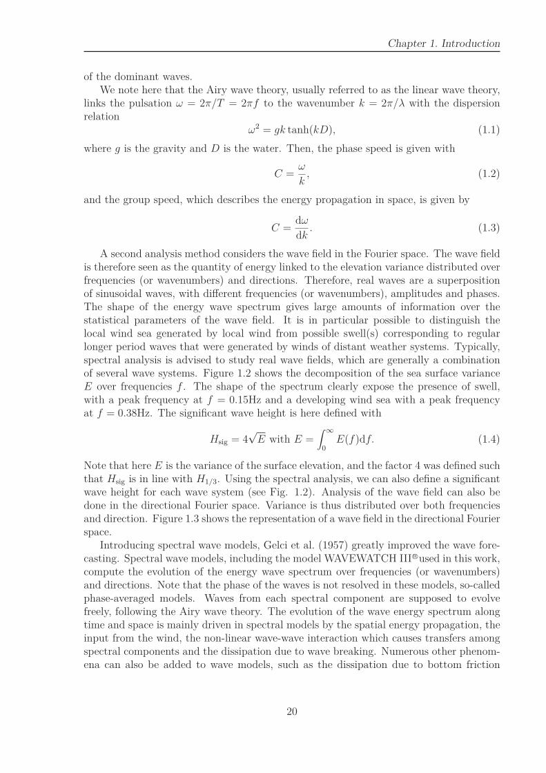
A second analysis method considers the wave field in the Fourier space. The wave fieldis therefore seen as the quantity of energy linked to the elevation variance distributed overfrequencies (or wavenumbers) and directions. Therefore, real waves are a superpositionof sinusoidal waves, with different frequencies (or wavenumbers), amplitudes and phases.The shape of the energy wave spectrum gives large amounts of information over thestatistical parameters of the wave field. It is in particular possible to distinguish thelocal wind sea generated by local wind from possible swell(s) corresponding to regularlonger period waves that were generated by winds of distant weather systems. Typically,spectral analysis is advised to study real wave fields, which are generally a combinationof several wave systems. Figure 1.2 shows the decomposition of the sea surface varianceE over frequencies f . The shape of the spectrum clearly expose the presence of swell,with a peak frequency at f = 0.15Hz and a developing wind sea with a peak frequencyat f = 0.38Hz. The significant wave height is here defined with
Hsig = 4√E with E =
∫
∞
0E(f)df. (1.4)
Note that here E is the variance of the surface elevation, and the factor 4 was defined suchthat Hsig is in line with H1/3. Using the spectral analysis, we can also define a significantwave height for each wave system (see Fig. 1.2). Analysis of the wave field can also bedone in the directional Fourier space. Variance is thus distributed over both frequenciesand direction. Figure 1.3 shows the representation of a wave field in the directional Fourierspace.
Introducing spectral wave models, Gelci et al. (1957) greatly improved the wave fore-casting. Spectral wave models, including the model WAVEWATCH III R©used in this work,compute the evolution of the energy wave spectrum over frequencies (or wavenumbers)and directions. Note that the phase of the waves is not resolved in these models, so-calledphase-averaged models. Waves from each spectral component are supposed to evolvefreely, following the Airy wave theory. The evolution of the wave energy spectrum alongtime and space is mainly driven in spectral models by the spatial energy propagation, theinput from the wind, the non-linear wave-wave interaction which causes transfers amongspectral components and the dissipation due to wave breaking. Numerous other phenom-ena can also be added to wave models, such as the dissipation due to bottom friction
20
or refraction due to the coast. Some of these additional phenomena are discussed in thechapter 2.
Considering free wave evolving, spectral wave models are well suited to represent thewave energy propagation, which well follows the Airy wave theory. Nevertheless, wenote that real waves are not linear, and wave field evolution is largely driven by non-linear phenomena. Wave-wave interactions are weakly non-linear phenomena and can beresolved in spectral wave models. Nevertheless, the phase-averaged models are not welladapted to resolve highly non-linear phenomena such as wave growing and wave breaking.These essential terms must therefore be statistically parametrized.
When wind blows over a flat water surface, friction at the air-water interface exertsforces on the surface, resulting in its deformation. Thus, the excess of free surface tensioncaused by the sea surface deformation compensates the wind induced forces. Wind beingstrongly turbulent, the pressure field (i.e. the force field) is not uniform over the flatsea surface and random capillarity waves, also called ripples, appears on the sea surface.With wavelengths of few millimeters, these ripples are fully driven by the effects of thesurface tension. If the wind stops, they quickly die, their energy being absorbed by viscousdissipation. On the contrary, if the wind is still blowing, a resonant interaction betweenwaves and ripples develops, resulting in the growth of ripples. The mechanism of wavegrowing is still misunderstood, particularly at small scale. It is evident that in the air-sea boundary layer, air flow and sea surface influence each other permanently, resultingin a strongly non-linear system. Many theories were however proposed to explain thewave generation by the wind (Jeffreys, 1925; Belcher and Hunt, 1993; Miles, 1957, 1962;Phillips, 1957), but no details are given in this work.
Then non-linear phenomena occur. The first phenomenon explains the displacementof the spectral energy to the highest frequency such that wind can create waves withphase speed Cp, higher than its own speed. In simple words, two wave trains can interactand create a third one. This phenomenon was confirmed by experimental results andtwo main theories were proposed by Hasselmann (1960, 1962) and Zakharov (1968), butnot yet fully validated. Details are not given in this work, but we note, however, thatthese nonlinear effects imply perpetual energy transfers between spectral components. Nodetails will be given in this work.
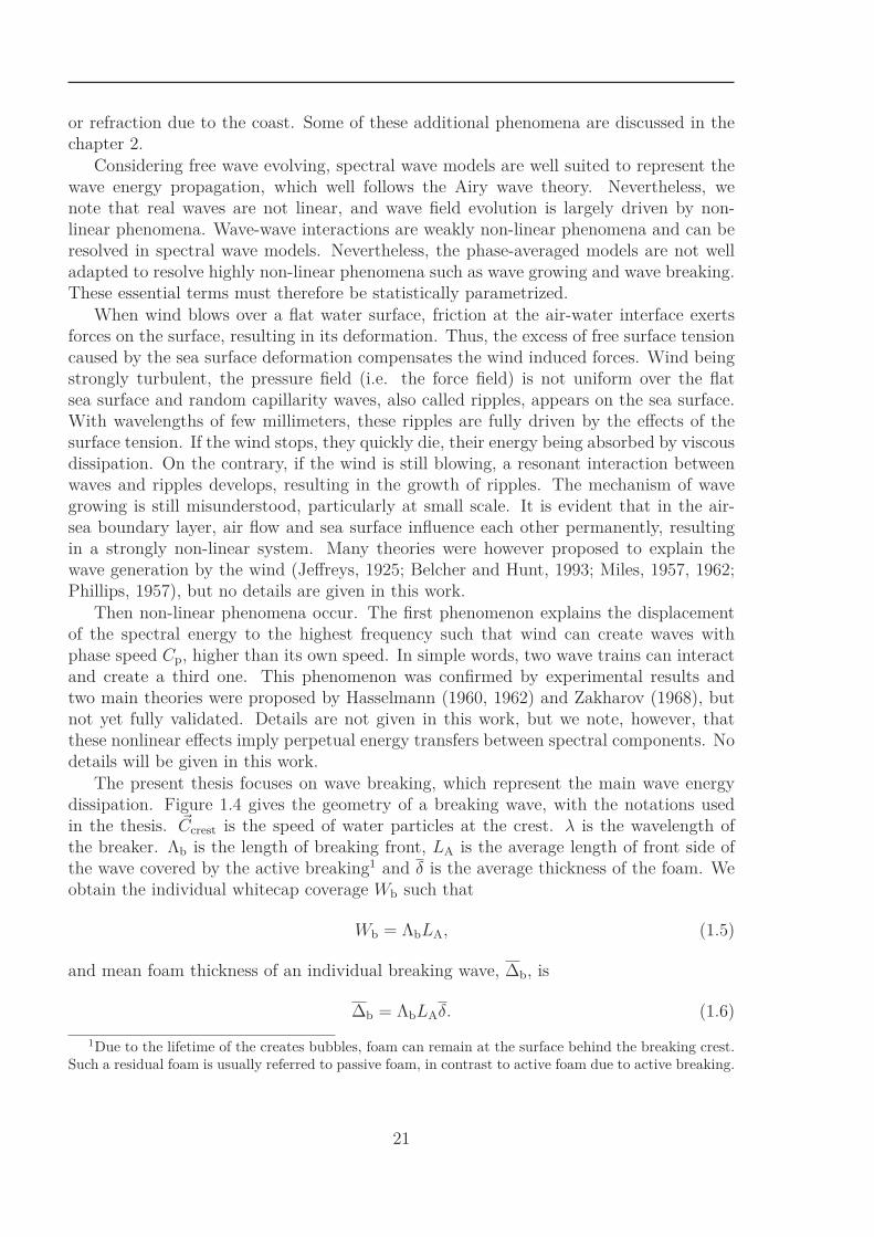
The present thesis focuses on wave breaking, which represent the main wave energydissipation. Figure 1.4 gives the geometry of a breaking wave, with the notations usedin the thesis. ~Ccrest is the speed of water particles at the crest. λ is the wavelength ofthe breaker. Λb is the length of breaking front, LA is the average length of front side ofthe wave covered by the active breaking1 and δ is the average thickness of the foam. Weobtain the individual whitecap coverage Wb such that
Wb = ΛbLA, (1.5)
and mean foam thickness of an individual breaking wave, ∆b, is
∆b = ΛbLAδ. (1.6)
1Due to the lifetime of the creates bubbles, foam can remain at the surface behind the breaking crest.Such a residual foam is usually referred to passive foam, in contrast to active foam due to active breaking.
21
Chapter 1. Introduction
Subsequently, we will use the density Λ (breaking crest length density), W (whitecapcoverage), ∆ (mean foam thickness), which represents the total quantities (sum over allwaves) per unit area such that
Λ =1
S
Nb∑
1
Λb (1.7)
W =1
S
Nb∑
1
Wb (1.8)
∆ =1
S
Nb∑
1
∆b (1.9)
where Nb are the number of breaking waves in the surface S.Generally, in people’s minds, wave breaking is associated with the depth-induced
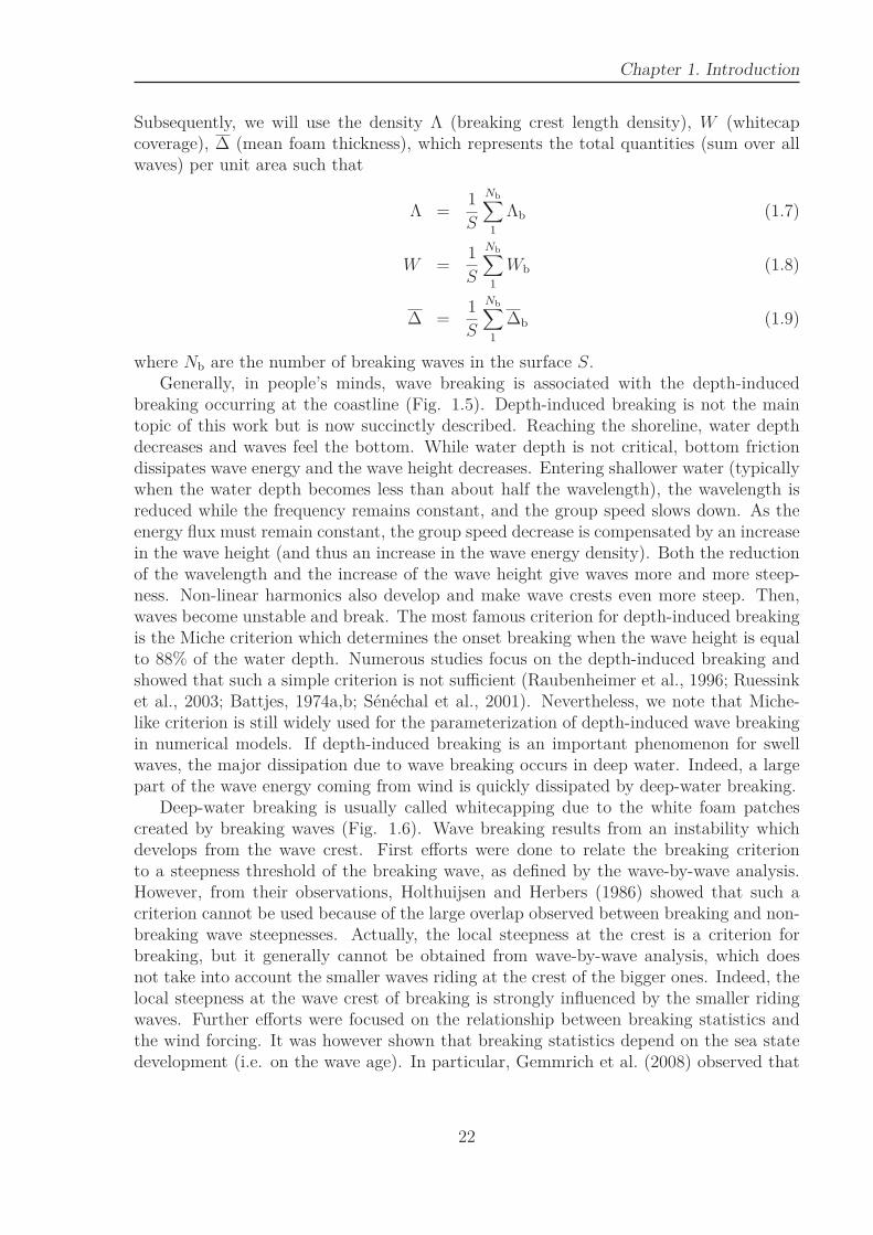
breaking occurring at the coastline (Fig. 1.5). Depth-induced breaking is not the maintopic of this work but is now succinctly described. Reaching the shoreline, water depthdecreases and waves feel the bottom. While water depth is not critical, bottom frictiondissipates wave energy and the wave height decreases. Entering shallower water (typicallywhen the water depth becomes less than about half the wavelength), the wavelength isreduced while the frequency remains constant, and the group speed slows down. As theenergy flux must remain constant, the group speed decrease is compensated by an increasein the wave height (and thus an increase in the wave energy density). Both the reductionof the wavelength and the increase of the wave height give waves more and more steep-ness. Non-linear harmonics also develop and make wave crests even more steep. Then,waves become unstable and break. The most famous criterion for depth-induced breakingis the Miche criterion which determines the onset breaking when the wave height is equalto 88% of the water depth. Numerous studies focus on the depth-induced breaking andshowed that such a simple criterion is not sufficient (Raubenheimer et al., 1996; Ruessinket al., 2003; Battjes, 1974a,b; Senechal et al., 2001). Nevertheless, we note that Miche-like criterion is still widely used for the parameterization of depth-induced wave breakingin numerical models. If depth-induced breaking is an important phenomenon for swellwaves, the major dissipation due to wave breaking occurs in deep water. Indeed, a largepart of the wave energy coming from wind is quickly dissipated by deep-water breaking.
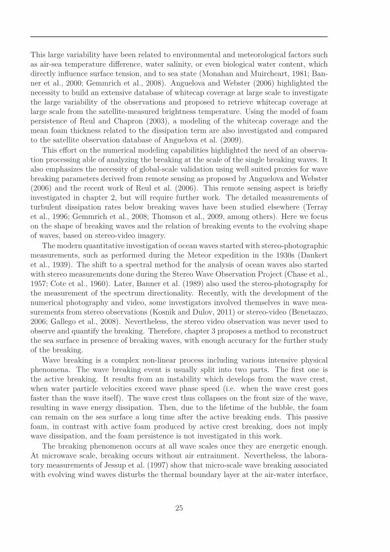
Deep-water breaking is usually called whitecapping due to the white foam patchescreated by breaking waves (Fig. 1.6). Wave breaking results from an instability whichdevelops from the wave crest. First efforts were done to relate the breaking criterionto a steepness threshold of the breaking wave, as defined by the wave-by-wave analysis.However, from their observations, Holthuijsen and Herbers (1986) showed that such acriterion cannot be used because of the large overlap observed between breaking and non-breaking wave steepnesses. Actually, the local steepness at the crest is a criterion forbreaking, but it generally cannot be obtained from wave-by-wave analysis, which doesnot take into account the smaller waves riding at the crest of the bigger ones. Indeed, thelocal steepness at the wave crest of breaking is strongly influenced by the smaller ridingwaves. Further efforts were focused on the relationship between breaking statistics andthe wind forcing. It was however shown that breaking statistics depend on the sea statedevelopment (i.e. on the wave age). In particular, Gemmrich et al. (2008) observed that
22

breaking concerns a large range of phase speed, from dominant waves to smaller wave scalein young wind sea whereas it concerns only waves with phase speed less than half of thephase speed of dominant waves for well developed wind sea. Moreover, Banner et al. (2000)showed that wind effects can become secondary for dominant waves in developed wavefields. Further, the kinematic criterion was also investigated to explain wave breaking.Wave breaking occurs when water particle velocity at the wave crest ucrest becomes higherthan the wave phase speed C. Furthermore, Stansell and MacFarlane (2002) showed thatwaves become instable and inevitably evolve towards breaking for crest particle speeducrest below C. Therefore, wave stability criterion is exceeded before irreversible breakingprocess yet starts (Babanin et al., 2007). The major advantage of a kinematic criterion isthe consideration of the growing non-linearities which cause the wave instability (Tanaka,1983). Numerous authors have also displayed interest in the the non-linear effects of thelong waves on the breaking of the shorter ones. Indeed, the passage of long wave underthe smaller ones induces hydrodynamical modulations, resulting in the acceleration ofsmaller riding waves which may evolve to breaking (Unna, 1947; Stewart, 1960; Longuet-Higgins, 1978; Dulov et al., 2002, among others). The role of non-linear features, resultingtypically in wave asymmetry and wave skewness, in the emergence of crest instability wasalso highlighted by Caulliez (2002).
From an energetic point of view, sea surface assimilates wind energy increasing itssurfaces (i.e. generating waves) until the exceeding energy is released by breaking waves(Newell and Zakharov, 1992). We note that breaking waves are local phenomena and canso be related to local energy exceedings. This effect is particularly highlighted by thecorrelation observed between wave groupiness and wave breaking (Donelan et al., 1972;Holthuijsen and Herbers, 1986). Breaking is observed at the crest of the highest wavesof the group, where the energies from the different spectral components converge. Thisenergy convergence was further inquired as the main predictor of breaking (Banner andTian, 1998; Tulin and Waseda, 1999; Song and Banner, 2002; Banner and Song, 2002).We note that, in laboratories, investigators can create waves that converge and break ina predicted location.
The thesis opens with the chapter 2 dedicated to a discussion and the adjustmentof the parameterizations for the spectral evolution associated with wave breaking. Wehighlight that breaking waves are highly non-linear phenomena where phase relationsbetween spectral components play a major role. This is difficult to reconcile with phase-average wave models, and observations of individual breaking are difficult to link to thespectral dissipation due to wave breaking needed in spectral wave models. Hence, earlyconcepts, such as proposed by Hasselmann (1974), have little relation with measurablequantities. Nevertheless, despite the fact that breaking waves are small local phenomena,a-priori non predictive, their statistics averaged over time and space should be relatedto wave spectrum. This link between spectra and time-averaged observable propertiesof breaking waves followed the analysis of Phillips (1984). He proposed the idea of alinearized dissipation rate, and gave a theoretical framework built around a measurablequantity: the length of breaking wave fronts and their distributions across displacementvelocities. Then, Melville and Matusov (2002) proposed wave breaking measurementsusing aerial imaging, and provided a statistical description of related sea-surface processes.They found that the distribution of the breaking front lengths per unit area on the sea
23

Chapter 1. Introduction
surface is proportional to the cube of the wind speed. They also showed that the fraction ofthe ocean surface mixed by breaking waves is dominated by wave breaking at low velocitiesand short wavelengths, consistently with the Phillips (1984)’s theory. Furthermore, thevideo observations of Gemmrich et al. (2008) showed that the distribution of breakingcrest length density peaks at intermediate wave scales and drops off sharply at largerand smaller scales. Similar distribution were found in other observations (Gemmrich andFarmer, 2004; Mironov and Dulov, 2008; Thomson and Jessup, 2008). This drop off atsmall scale is not explained by the Phillips (1984)’s theory which proposes an increasingdissipation at smaller scale.
Simultaneously, the breaking-induced dissipation of wave energy was studied with anumerical approach in spectral wave models (Alves et al., 2003; van der Westhuysen et al.,2005; Ardhuin et al., 2009; Banner and Morison, 2010; Rogers et al., 2012). These modeldevelopments, discussed in the introduction of the chapter 2, showed the increasing needof dissipation with smaller wave scales. Supported by the observations of Banner et al.(1989), these developments lead to the idea that the dissipation of wave energy at a givenscale was not only related to the breaking of these same waves, but also to the breakingof waves at larger scales. This so-called ”cumulative effect” is necessary to reproduce theobserved shapes of spectra (Banner and Morison, 2010).
My work takes up the work developed by Filipot and Ardhuin (2012) who initiateda seamless treatment of wave breaking from deep to shallow water. In particular, I haveinvestigated the modification of their parameterization to make the breaking probabili-ties used for the dissipation term linked to the breakers themselves consistent with theassociated cumulative term. The parameterization of Filipot and Ardhuin (2012), usedoperationally at NOAA/NCEP for the Great Lakes since 2013 because of its better per-formance at short fetches is analyzed and compared to the parameterization of Ardhuinet al. (2010), used for operational ocean wave forecasting at NOAA/NCEP since May2012 for the global ocean. In these recent parameterizations, whitecap occurrence hasbeen related to the steepness of the waves, respectively through the unidirectional wavescale analysis of Filipot et al. (2010) and the observations on saturation spectra of Banneret al. (2000) and Banner et al. (2002). Banner and Morison (2010) showed that an ex-plicit modeling of whitecap properties provides a new constraint on the model dissipationsource terms. Nevertheless, there parameterizations have seldom been verified in terms ofwhitecap properties. In this work, an explicit modeling of the breaking wave front lengthdistribution over phase speed is proposed and compared to the in situ observations ofGemmrich and Farmer (2004).
Because of its strong influence on electromagnetic measurements and air-sea gas ex-changes, the whitecap coverage was also investigated in many studies (Monahan andWoolf, 1989; Hanson and Phillips, 1999; Reul and Chapron, 2003, among others). Manyinvestigations have resulted in relationships between the whitecap coverage and the windspeed at 10m above the sea surface. This relationship was used more than one centurybefore with the famous Beaufort scale which evaluates the wind speed from whitecapcoverage for higher degrees. We note that most of the whitecap coverage used for thecorrection of the satellite measurements are still today only estimated from the windspeed despite of the large disparity between the published empirical relationships fittedon different observations (see Fig. 1.7, extracted from Anguelova and Webster (2006)).
24
This large variability have been related to environmental and meteorological factors suchas air-sea temperature difference, water salinity, or even biological water content, whichdirectly influence surface tension, and to sea state (Monahan and Muircheart, 1981; Ban-ner et al., 2000; Gemmrich et al., 2008). Anguelova and Webster (2006) highlighted thenecessity to build an extensive database of whitecap coverage at large scale to investigatethe large variability of the observations and proposed to retrieve whitecap coverage atlarge scale from the satellite-measured brightness temperature. Using the model of foampersistence of Reul and Chapron (2003), a modeling of the whitecap coverage and themean foam thickness related to the dissipation term are also investigated and comparedto the satellite observation database of Anguelova et al. (2009).
This effort on the numerical modeling capabilities highlighted the need of an observa-tion processing able of analyzing the breaking at the scale of the single breaking waves. Italso emphasizes the necessity of global-scale validation using well suited proxies for wavebreaking parameters derived from remote sensing as proposed by Anguelova and Webster(2006) and the recent work of Reul et al. (2006). This remote sensing aspect is brieflyinvestigated in chapter 2, but will require further work. The detailed measurements ofturbulent dissipation rates below breaking waves have been studied elsewhere (Terrayet al., 1996; Gemmrich et al., 2008; Thomson et al., 2009, among others). Here we focuson the shape of breaking waves and the relation of breaking events to the evolving shapeof waves, based on stereo-video imagery.
The modern quantitative investigation of ocean waves started with stereo-photographicmeasurements, such as performed during the Meteor expedition in the 1930s (Dankertet al., 1939). The shift to a spectral method for the analysis of ocean waves also startedwith stereo measurements done during the Stereo Wave Observation Project (Chase et al.,1957; Cote et al., 1960). Later, Banner et al. (1989) also used the stereo-photography forthe measurement of the spectrum directionality. Recently, with the development of thenumerical photography and video, some investigators involved themselves in wave mea-surements from stereo observations (Kosnik and Dulov, 2011) or stereo-video (Benetazzo,2006; Gallego et al., 2008). Nevertheless, the stereo video observation was never used toobserve and quantify the breaking. Therefore, chapter 3 proposes a method to reconstructthe sea surface in presence of breaking waves, with enough accuracy for the further studyof the breaking.
Wave breaking is a complex non-linear process including various intensive physicalphenomena. The wave breaking event is usually split into two parts. The first one isthe active breaking. It results from an instability which develops from the wave crest,when water particle velocities exceed wave phase speed (i.e. when the wave crest goesfaster than the wave itself). The wave crest thus collapses on the front size of the wave,resulting in wave energy dissipation. Then, due to the lifetime of the bubble, the foamcan remain on the sea surface a long time after the active breaking ends. This passivefoam, in contrast with active foam produced by active crest breaking, does not implywave dissipation, and the foam persistence is not investigated in this work.
The breaking phenomenon occurs at all wave scales once they are energetic enough.At microwave scale, breaking occurs without air entrainment. Nevertheless, the labora-tory measurements of Jessup et al. (1997) show that micro-scale wave breaking associatedwith evolving wind waves disturbs the thermal boundary layer at the air-water interface,
25
Chapter 1. Introduction
producing signatures that can be detected with infrared imagery. Their laboratory ob-servations, under the moderate wind speed conditions, showed a substantial frequency ofoccurrence and an important areal coverage of the phenomenon. Therefore, micro-scalebreaking is undoubtedly widespread over the oceans and may prove to be a significantmechanism for enhancing the transfer of heat and gas across the air-sea interface. Thesemicrowave scales are not resolved in the global ocean spectral wave model, and microwavebreaking is not studied in this work.
We here focus on longer breaking waves as modeled in spectral wave model. Thesewaves, more energetic, are attended with air entrainment and bubble formation. Theformation of foam needs a large quantity of energy, corresponding to the surface tensionmultiplied by surface excess. Thus, when breaking waves are energetic enough, theygenerate white bubble clouds which contrast with the darker sea surface, and are socalled whitecaps. This signature in the visible frequency spectrum makes the phenomenoneasily observable. The chapter 4 proposed a method to detect and discriminate activeand passive foam on the images taken by the stereo video system inspired by the workof Mironov and Dulov (2008). By re-projecting the detected events on the reconstructedsurfaces, this allows to analyze the breaking at the scale of the single breaking waves. Afirst analysis of the observations is provided.
The present thesis aims to improve on the wave spectral models, in particular with thedevelopment of dissipation parameterizations that better link to the wave breaking. Thus,my work in the next chapter provides a comprehensive analysis of the existing dissipationparameterizations through their implicit breaking properties. Despite the fact that theserecent parameterizations are built on wave breaking observations, this chapter points outthe failures of these parameterizations to produce model results, in terms of breakingproperties, in line the observations. These current parameterizations make numerous un-certain assumptions due to the lack of accurate observations able to investigate them.The following chapters thus propose a first step for the future improvement of dissipationparameterizations. The recent wave studies have shown the potential of the stereo-videosystems for sea-wave statistical investigations. Chapter 3 is dedicated to the improve-ment of the stereo-video analysis for the observation of individual waves. Validated usinga large range of sea-wave parameters, the developed method, shows the potential of thestereo video observations for investigations at the scale of single waves. My work finallyfocuses with chapter 4 on the application of stereo-video observation to breaking analy-sis. Providing the full accurate 4D time-space evolution of the individual breaking waves,the stereo video observations open to a new world of information. Although the presentwork does not yet provide an improvement of the dissipation parameterization, it demon-strates the potential of these observations for the future improvements, calibrations, andvalidations of the breaking parameterizations in spectral models, as well as for a betterunderstanding of the breaking phenomenon itself.
26
704 706 708 710 712 714 716 718 720
−0.2
−0.1
0
0.1
0.2
Time, t [s]
Ele
vati
on,Z
[m]
Ti −2
Hi −2
Ti −1
Hi −1
Ti
Hi
Ti +1
Hi +1
Ti +2
Hi +2
Ti +3
Hi +3
0 0.2 0.4 0.60
1
2
3
4
5
6
7
Wave Height, H [m]
PD
F(H
)
0 2 4 60
0.1
0.2
0.3
0.4
0.5
Wave Period, T [s]
PD
F(T
)
Figure 1.1: Illustration of wave-by-wave analysis for a sea surface elevation time seriesobtained from capacitance wave gauge in the Black Sea on 1/10/2013. The wave fieldis composed only by a developing wind sea. Top panel: Measured sea surface elevation(blue line) and decomposition into individual waves using zero down-crossing method(red circle). Hi and Ti respectively represent the wave height and the wave period ofthe individual wave i. Lower panels : Probability Density Function of wave height H(left) and wave period T (right). Red dashed line represent the Rayleight distributionthat describes the statistical distribution of the individual wave heights for linear gaussianwaves and stationary sea state. The average of the one-third of highest individual wavesis H1/3 = 0.24 m.
27
Chapter 1. Introduction
10−1
100
10−6
10−4
10−2
f [Hz]
E(f
)[m
2/H
z]
Swell
Wind sea
Figure 1.2: Frequency analysis of a sea surface elevation time series obtained from capac-itance wave gauge in the Black Sea on 3/10/2013. The wave field is composed by bothvariance from the developing wind sea (right part of the spectrum) and from swell wave(left part of the spectrum).The global significant wave height is:
Hsig = 4√
∫
∞
0 E(f)df = 0.35m.The significant wave height of swell waves is:
Hsig,swell = 4√
∫ 0.230 E(f)df = 0.12m.
The significant wave height of wind sea waves is:
Hsig,wind sea = 4√
∫
∞
0.23 E(f)df = 0.33m.
28
0.1 0.2 0.3 0.4
0
5
10
15
0.00.100.200.30
0.0 5. 10. 15 20 25
3
212
1
3
Figure 1.3: Typical example of directional frequency wave spectrum in the tropical zone,measured with buoy 51001, 350km north-west of Kauai island, on January, 11th 2007.
Figure 1.4: Sketch showing the features of a spilling breaker. The waves is moving fromleft to right and has a whitecap on its forward face. The figure is extracted from Reuland Chapron (2003), the notation are modified to agree the present thesis.
29
Chapter 1. Introduction
Figure 1.5: Typical example of depth-induced wave breaking occurring on sandy beachof the Atlantic French coast (La Piste, Capbreton).
Figure 1.6: Picture of deep-water wave breaking taken by the author from a boat off thenorth coast of Bretagne.
30
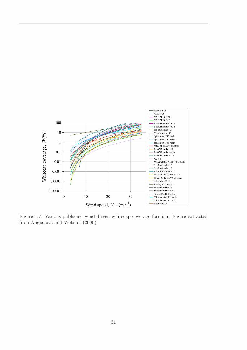
Figure 1.7: Various published wind-driven whitecap coverage formula. Figure extractedfrom Anguelova and Webster (2006).
31

Chapter 2
Wave breaking parameterization andwhitecap properties modeling
Note
The major part of the results presented in this chapter have been published in thejournal Ocean Modelling in October 2013 (Leckler et al., 2013).
2.1 Introduction
Phase-averaged wave models consider the spectral decomposition of the sea surfaceelevation across wavenumbers k (or frequencies f) and directions θ at point (x, y) andtime t. The evolution of spectral density F (k, θ, x, y, t) is resolved using the wave energybalance equation proposed by Gelci et al. (1957):
dF
dt= Satm + Snl + Soc + Sbt + ... (2.1)
where the Lagrangian derivative of spectral density on the left-hand side includes the localtime evolution and advection in both physical and spectral spaces (e.g. WISE Group,2007). The source terms on the right-hand side include an atmospheric source term Satm
which includes the classical input of energy Sin from wind to waves, and the energy outputSout from waves to wind1, associated with friction at air-sea interface (Ardhuin et al.,2009). The nonlinear source term Snl represents energy transfers in the spectral domaindue to wave-wave interactions. Sbt is the sink of energy due to bottom friction. Othereffects may also be included (WISE Group, 2007). Finally, the oceanic source term Soc,usually negative, represents dissipation due to wave breaking, Sbk, and wave-turbulenceinteractions, Sturb (e.g. Ardhuin and Jenkins, 2006). The latter effect will be ignored here,because it typically represents at most a 10% fraction of the breaking-induced dissipation(Rascle et al., 2008; Kantha et al., 2009), and here we focus on wave breaking. The
1The transfer of energy from waves to wind (Sout) is responsible for the swell dissipation over longdistances. A modification of the formulation of Ardhuin et al. (2010) is provided in paragraph 2.2.2.
33
Chapter 2. Wave breaking modeling
goal of the present chapter is to evaluate the ability of the breaking-induced dissipationparameterization to model the associated whitecap properties.
Early parameterizations of dissipation were adjusted to close the energy balance ofwaves, with no explicit link to breaking and dissipation observations. This, in particular,was the basis of the parameterizations of Komen et al. (1984). Following Hasselmann(1974), they proposed a dissipation quasi-linear in the wave spectrum adjusted on Pierson-Moskowitz spectrum (Pierson and Moskowitz, 1964) such that
Soc(k, θ) = Sds(k, θ) = −ψd(k)F (k, θ), (2.2)
with ψd depends only on the wavenumber and integrated parameters. Various forms hadbeen proposed for the quasi-linear coefficient ψd. One of the most successful forms of ψd,used for a long time as dissipation source term in WAM, was proposed by Komen et al.(1994)
ψd(k) = −Cds
(
α
αPM
)m
(1 − δ)k
k+ δ
(
k
k
)n/2
ω
, (2.3)
where α = Etotk2
is an integral steepness parameter, αPM = 4.57 10−3 is the integratedsteepness of a fully developed Pierson–Moskowitz spectrum (Pierson and Moskowitz,1964), k is the mean wavenumber, ω is the mean angular frequency, δ is a weightingfactor that controls the magnitude of linear and quadratic functions of the ratio k/k andEtot is the total wave energy obtained by integrating the directional wavenumber spec-trum F (k, θ). δ, n and m are tuning parameters. We note that this dissipation aims toproduce spectra close to the empirical Pierson–Moskowitz spectrum, and not to reproducedissipation due to wave breaking.
Thereafter, following Phillips (1984)’s analysis, breaking probabilities have been re-lated to the nondimensionals saturation spectrum B,
B(k) = k3 F (k) = k3∫ π
−πF (k, θ)dθ. (2.4)
This approach was extended to the parametrization of breaking probabilities for dominantwaves (Banner et al., 2000). In particular, it was found that breaking probabilities becomesignificant when the saturation exceeds a constant threshold Br. A similar threshold mayalso be applied to waves shorter than the dominant waves (Banner et al., 2002).
A preliminary modeling effort based on these observations was made by Alves andBanner (2003) who modified the Komen et al. (1994) dissipation to include a furtherdependence on the ratio B(k, θ)/Br, such that
Sds(k, θ) = −Cds
[
B(k)
Br
]p/2(
Etotk2p
)m(
k
k
)n
ωF (k, θ), (2.5)
where B(k) is the local saturation parameter defined by equation 2.4, (Etotk2p) is an
integral spectral steepness parameter, with kp is the peak wavenumber. Following Banneret al. (2002), wave breaking occurs when B(k) > Br, and whitecapping dissipation shouldbecome negligible. Nevertheless, to take in account for the other dissipation processes
34
2.1 Introduction
(straining of shorter waves and wave–turbulence interactions), they assumed that term[B(k)/Br]
p/2 asymptotically approaches unity instead of zero with
p =p0
2+p0
2tanh
10
[
B(k)
Br
]1/2
− 1
(2.6)
Therefore, we note that the primary dissipation mechanism is supplemented with twomultiplication factorsA = (Etotk
2p)m andB = (k/k)n, inherited from Komen et al. (1994)’s
parameterisation, in order to represent dissipation due to general background turbulence.The threshold saturation level Br and the coefficient Cds and p0, m and n are constantsdetermined numerically to provide modeled spectra which match the observations. Fromnumerical tuning, they obtained Br about double of the thershold saturation found fromobservations by Banner et al. (2002). Furthermore, numerically found high value of p0implies a dependence of dissipation on the variance density of up to a power of 5, difficultto reconsile with the conventional wind input expression (van der Westhuysen et al., 2007).
Considering this, van der Westhuysen et al. (2007) built another parameterization,implemented in SWAN, where the dissipation rate is a function of B(k, θ)/Br to a powerthat varies with the wave age. They also remove removed the multiplication factors A andB considering that general background turbulence cannot be simplified to a simple multi-plication factor but must be considered as an independent additional source term. Theyproposed a whitecapping dissipation in frequency space2, except for saturation parameterB kept in wavenumber space, such that
Sds(σ, θ) = −Cds
[
B(k)
Br
]p/2
σE(σ, θ), (2.7)
where exponent p is a function of the wave age which scales it from 4 to 2, taking intoconsideration the balance with the wind input (see details on appendix A in van derWesthuysen et al. (2007)).
That type of dependency to wave age was then abandoned in the recent parameteri-zations by Banner and Morison (2010), Ardhuin et al. (2010), and Babanin et al. (2010).Ardhuin et al. (2010) introduced a directional dependence of the dissipation rate, withmuch strong dissipation in the mean direction, consistent with observed higher proba-bilities of breaking waves propagating in the mean direction (Mironov and Dulov, 2008).Conversly, the parameterization by Babanin et al. (2010) assumes a stronger dissipation inoblique directions. More importantly these last three parameterizations also include somesuppression of the short wave energy due to the breaking of longer waves. This so-calledcumulative effect is consistent with many observations (Banner et al., 1989; Melville et al.,2002; Young and Babanin, 2006).
In his analysis, Phillips (1984) had warned that the use of the saturation spectrum wasonly meaningful if the spectrum was relatively smooth. Indeed, monochromatic waves ofvery small amplitude have an infinite saturation level but do not produce any breaking.The saturation-based parameterization of Ardhuin et al. (2010), hereinafter referred to as
2The model SWAN resolves the wave energy balance equation (Eq. 2.1) in frequency space.
35
Chapter 2. Wave breaking modeling
TEST4513, does not use a smoothed saturation spectrum. In practice the wave spectrumis most saturated at the peak of the wind sea. As a result, that parameterization givesan abnormal lower dissipation rate on frequencies just above the peak, which is difficultto reconcile with the relatively broad spectral signature expected from the short lifetimeof each breaking event. For this reason, Banner and Morison (2010) use a smoothedsaturation spectrum.
A different smoothing procedure is used in the parameterization by Filipot and Ard-huin (2012), hereinafter referred to as TEST500. They defined wave steepnesses fordifferent scales based on a moving-window integration of the spectrum. This parame-terization has two benefits. Firstly, it allows the estimation of breaking probabilities fordifferent scales, in a way consistent with observations (Filipot et al., 2010). Secondly, itprovides a natural way of combining deep and shallow water breaking in a single formu-lation, extending the work of Thornton and Guza (1983) and Chawla and Kirby (2002).One inconsistency of TEST500 is that it uses the cumulative effect of Ardhuin et al.(2010) which is based on different breaking probabilities. For this reason a modificationof TEST500 is proposed. Parameters for all parameterizations discussed in this chapterare given in table 2.1 in paragraph 2.2.4.
Furthermore, mixing air into water, breaking waves form clouds of bubbles beneaththe sea surface and foamy patches on the surface. This surface signature makes breakingeasily observable with simple visible video or photo camera (Mironov and Dulov, 2008;Thomson and Jessup, 2008; Kleiss and Melville, 2011). The video observations collectedat small scales, traditionally from research platforms, ships, or aircraft give informationabout breaking probability and breaking crest length density as functions of wavenumber(or wave scale). Another source of whitecap measurement is given by the very clearsignature of bubbles and foam on the emissivity and brightness of sea surface temperature(Droppleman, 1970). This property was particularly exploited by Anguelova and Webster(2006). Using satellite radiometric measurements, they gave the first global dataset ofwhitecap coverage.
Many investigations have resulted in relationships between the whitecap coverage andthe wind speed at 10m above the sea surface, U10. These relationships exhibit a largevariability which cannot be predicted only with the wind speed. Although the measure-ment conditions, in particular the view geometry and lighting conditions are an inherentsource of scatter in video measurements, there are also environmental and meteorologi-cal factors besides the wind speed that may explain some of this scatter. These includeair-sea temperature difference ∆T , water salinity, but also sea state parameters such asthe significant wave height Hs or wave age (Monahan and Muircheart, 1981). Indeed,Hanson and Phillips (1999) found that observed wave age explained a large part of thescatter in the whitecap coverage measurements that they analyzed. Recent measurementcampaigns have focused on the estimation of the spectral distribution of breaking crestlengths, introduced by Phillips (1985). Banner and Morison (2010) have shown that theirparameterization of wave dissipation was indeed able of reproducing the variability indominant breaking wave crest lengths. In order to investigate the general applicability
3Compared to the version TEST441b described in that paper, we have introduced a minor swelldissipation modification described in paragraph 2.2.2. This modification has no impact on the breakingstatistics.
36
2.2 Investigated dissipation parameterizations
of our wave model for such a task, we confront here our model to the global radiometricdata of Anguelova et al. (2009).
In section 2.2 the two parameterizations by Ardhuin et al. (2010) and Filipot andArdhuin (2012) are fully described, with a minor update to the latter to make the cumu-lative effect consistent. This updated parameterization is called TEST570. The resultingdissipation and breaking crest length density are analyzed in section 2.3 with an academictest case and an hindcast of the SHOWEX experiment. In the next section, we interpretwhitecap coverage W and mean foam thickness ∆ compared to radiometer data over theworld ocean. Conclusions and perspectives follow in section 2.5.
2.2 Investigated dissipation parameterizations
From now on, we focus the investigation on the parameterizations by Ardhuin et al.(2010), used for operational ocean wave forecasting at NOAA/NCEP since May 2012,and the parameterizations by Filipot and Ardhuin (2012), now used operationally atNOAA/NCEP for the Great Lakes since 2013, because of their better performance atshort fetches. Results with the parameterization of Bidlot et al. (2005) (hereinafter BJA)are given as references, because this parameterization has been used operationally atEuropean Center for Medium-Range Weather Forecasts (hereinafter ECMWF) since 2005,with a few minor adjustments (Bidlot, 2012). However, this parameterization is notinvestigated because of its poor link to breaking and dissipation observations.
2.2.1 Description of the parameterizations
The two parameterizations by Ardhuin et al. (2010) and Filipot and Ardhuin (2012)here investigated split the swell dissipation and the dissipation of the wind-sea into in-dependant negative source terms, Sout and Sbk. As stated in the introduction, the swelldissipation due to air-sea friction is add to the wind input in the atmospheric source termsuch that
Satm = Sin + Sout (2.8)
and the oceanic source term includes the dissipation due to wave breaking and wave-turbulence interactions, such that
Soc = Sbk + Sturb. (2.9)
Following observations by Banner et al. (1989), Melville et al. (2002), and Young andBabanin (2006), both parameterizations split the wave breaking dissipation source termSbk into a spontaneous dissipation source term Sbk,sp due to wave crest collapsing andanother source term Sbk,cu which represents the dissipation of the shorter underlyingwaves wiped out by the larger breaking waves (cumulative effect). Therefore, the wavebreaking source terms is
Sbk = Sbk,sp + Sbk,cu. (2.10)
37
Chapter 2. Wave breaking modeling
The cumulative effect can be observed on the photograph 2.1. We note that, by definition,these two source terms should depend on the same breaking quantities, in particular thebreaking probability.
Flat surface :
Small waves have
been killed
Breaking
front
Presence of
small wave
on the
surface
Figure 2.1: Picture of deep-water wave breaking taken by the author from a boat off thenorth coast of Bretagne. Before the passage of the breaking front, sea surface is coveredby ripples waves whereas, in the breaking front wake, sea surface is smoothed. Sameprocess is observed for all wave scales.
Ardhuin et al. (2010) defined4 a directional saturation spectrum B′(k, θ), partiallyintegrated over directions between θ − ∆θ and θ + ∆θ,
B′(k, θ) =∫ θ+∆θ
θ−∆θ
k3 cos2(θ − θ′)F (k, θ′)dθ′, (2.11)
with ∆θ = 80◦. This directional sector of plus or minus 80◦, combined with the cosine-square weighting is there to limit the integration of wave trains that actually have enoughtime to merge together so that individual waves can evolve to breaking (e.g. Banner andTian, 1998). Because the high frequency gravity waves are generally distributed morebroadly over directions, this parameterization also reduces the breaking probability athigh frequencies, in a way similar to the directional normalization used by Banner andMorison (2010) or Rogers et al. (2012). Varying ∆θ = 80◦ from 50 to 120◦ has very littleinfluence on the model results. This reduction of breaking probability with directionalspreading is also consistent with a smaller whitecap coverage in crossing seas (Holthuijsenet al., 2012), although the physical processes involved may be different.
The actual estimation of the dissipation induced by spontaneous breaking Sbk,sp isa weighted average of a dissipation given by the directional saturation B′(k, θ) and anisotropic dissipation given by the non-directional saturation spectrum B(k), such that
B(k) = max{B′(k, θ′), θ′ ∈ [0, 2π]}. (2.12)
Therefore, they proposed a spontaneous breaking dissipation source term
Sbk,sp = σCds
B2r
δd max[√
B(k, θ) −√Br, 0]2 +
(1 − δd) max[√
B′(k, θ) −√Br, 0]2
F (k, θ). (2.13)
4We corrected the typographic error in equation (12) of Ardhuin et al. (2010) by removing the erro-neous factor df/dk = Cg/(2π).
38

2.2 Investigated dissipation parameterizations
This combination of B′(k, θ) and B(k) allowed a control of the dissipation direction-ality. δd was adjusted to reproduce observed directional spreads, and also provided goodestimates of the energy levels in opposing wave directions (Ardhuin and Roland, 2012).
For the cumulative dissipation, the breaking probability is estimated from the direc-tional saturation spectrum B′, extrapolating the empirical expression given by Banneret al. (2000) for dominant waves on the entire spectrum, and assuming that for the dom-inant waves the steepness is given by B′/1.6. This gives a spectral breaking probabilityPb
Pb(k, θ) = 28.4 max[√
B′(k, θ) −√
Br, 0]2. (2.14)
For each breaking wave with phase speed Cb, relative crest velocities of underlyingshort waves are defined by ∆C = |C − Cb|. Then, the dissipation rate due to cumulativeeffect is simply defined by the rate of passage of the long breaking waves over the shortunderlying waves ∆C Λ(C) dC where Λ(C) dC is the breaking crests length density ofwave with phase speed in range [C,C + dC] introduced by Phillips (1985). Λ(k, θ) dk dθis estimated using the length density of crest (breaking or not) l(k, θ) ≃ 1/(2π2) (definedby Ardhuin et al., 2010) with
Λ(k, θ) = Pb(k, θ) l(k, θ). (2.15)
This yields the cumulative dissipation
Sbk,cu(k, θ) = CcuF (k, θ)∫
k′<r2cuk
∫ 2π
0∆CΛ(k′, θ)dθdk′, (2.16)
where rcu defines the maximum ratio between the frequency of the underlying waves wipedout by the breaker and the breaker frequency. This whitecapping dissipation added tothe wind-wave generation and swell dissipation is called TEST441b and is fully describedby Ardhuin et al. (2010). A minor adjustment of the swell dissipation is described inparagraph 2.2.2, giving a parameterization TEST451.
The parameterization of Filipot and Ardhuin (2012) is built on the Breaking WaveHeight Distribution (hereinafter BWHD) per wave scale, as parameterized by Filipot et al.(2010). As stated in the introduction, Filipot and Ardhuin (2012) filtered the spectrumE(k) with a sliding rectangular windows Rfi
, similar to the range used used by Banneret al. (2000), such that
Rfi(f) =
1 if 0.7fi < f < 1.3fi
0 elsewhere.(2.17)
Then for each wave scale fi, wave steepness is defined from representative wave heightHfi
and mean wavenumber kfi, with
Hfi=
4√2
√
Efi(2.18)
and
kfi=
∫
∞
0 Rfi(f)k(f)E(f)df
Efi
, (2.19)
39
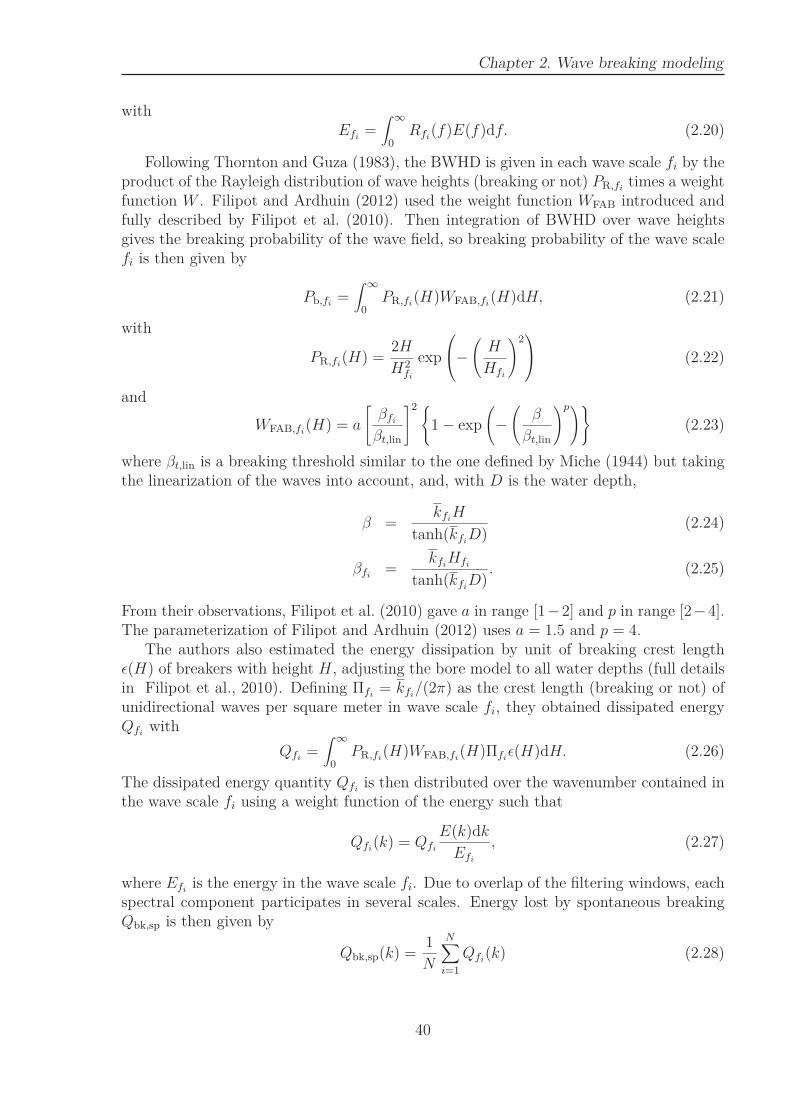
Chapter 2. Wave breaking modeling
withEfi
=∫
∞
0Rfi
(f)E(f)df. (2.20)
Following Thornton and Guza (1983), the BWHD is given in each wave scale fi by theproduct of the Rayleigh distribution of wave heights (breaking or not) PR,fi
times a weightfunction W . Filipot and Ardhuin (2012) used the weight function WFAB introduced andfully described by Filipot et al. (2010). Then integration of BWHD over wave heightsgives the breaking probability of the wave field, so breaking probability of the wave scalefi is then given by
Pb,fi=∫
∞
0PR,fi
(H)WFAB,fi(H)dH, (2.21)
with
PR,fi(H) =
2H
H2fi
exp
−(
H
Hfi
)2
(2.22)
and
WFAB,fi(H) = a
[
βfi
βt,lin
]2 {
1 − exp
(
−(
β
βt,lin
)p)}
(2.23)
where βt,lin is a breaking threshold similar to the one defined by Miche (1944) but takingthe linearization of the waves into account, and, with D is the water depth,
β =kfiH
tanh(kfiD)
(2.24)
βfi=
kfiHfi
tanh(kfiD)
. (2.25)
From their observations, Filipot et al. (2010) gave a in range [1−2] and p in range [2−4].The parameterization of Filipot and Ardhuin (2012) uses a = 1.5 and p = 4.
The authors also estimated the energy dissipation by unit of breaking crest lengthǫ(H) of breakers with height H, adjusting the bore model to all water depths (full detailsin Filipot et al., 2010). Defining Πfi
= kfi/(2π) as the crest length (breaking or not) of
unidirectional waves per square meter in wave scale fi, they obtained dissipated energyQfi
with
Qfi=∫
∞
0PR,fi
(H)WFAB,fi(H)Πfi
ǫ(H)dH. (2.26)
The dissipated energy quantity Qfiis then distributed over the wavenumber contained in
the wave scale fi using a weight function of the energy such that
Qfi(k) = Qfi
E(k)dk
Efi
, (2.27)
where Efiis the energy in the wave scale fi. Due to overlap of the filtering windows, each
spectral component participates in several scales. Energy lost by spontaneous breakingQbk,sp is then given by
Qbk,sp(k) =1
N
N∑
i=1
Qfi(k) (2.28)
40
2.2 Investigated dissipation parameterizations
where fi∈[1,N ] are the wave scales involving k.Qbk,sp(k) is then distributed over direction with
Qbk,sp(k, θ) = Qbk,sp(k)E(k, θ)dθ
E(k), (2.29)
Finally, dissipation Sbk,sp is given by Sbk,sp(k, θ)dkdθ = Qbk,sp(k, θ). Compared to theoriginal algorithm, we now compute Pb,fi
by extrapolating the wave spectrum to unre-solved high frequencies, assuming a f−5 roll-off of the energy spectrum. The bottom panelof figure 2.3 shows the breaking probabilities obtained with this spectral extrapolation.
Because there may be inconsistencies in combining breaking probabilities derived fromsaturation spectrum (Ardhuin et al., 2010) for cumulative dissipation, and breaking prob-abilities derived from wave scale analysis (Filipot and Ardhuin, 2012) for spontaneousdissipation, a consistent combination, resulting in TEST570 parameterization, is pre-sented and validated in paragraph 2.2.3. Despite the fact that this new parameterizationdoes not clearly provide better results, the inconsistency of the dissipation term Sbk inTEST500 does not allow the modelisation and the investigation of the breaking propertieswhich are derived from it.
2.2.2 Correction of swell dissipation
The essence of that modification is a smoothing of the swell dissipation function aroundthe threshold for transition between laminar and turbulent conditions. This was doneby introducing a weighted average of the laminar Sout,l (f, θ) and turbulent Sout,t (f, θ)dissipation source terms respectively given by equations (8) and (9) of Ardhuin et al.(2010),
Sout (f, θ) = (0.5 + α)Sout,l (f, θ) + (0.5 − α)Sout,t (f, θ) (2.30)
where the smoothing parameter is defined by,
α = 0.5 tanh[
(πH3s/(4νTm0,2) − s4)/s7
]
, (2.31)
where ν = 1.4 × 10⁻⁵ m2 s−1 is the air viscosity, Tm0,2 is the mean wave period ands4 = 105 m and s7 = 2.3 × 10⁵ m are fitting parameters.
The new parameterization of swell dissipation reduced the global errors on wave heightby 4% on average (Fig. 2.2). More importantly it corrected the abnormal distribution ofsignificant wave heights. Implemented in both TEST441b and TEST500, parameteriza-tions are respectively renamed TEST451 and TEST510.
2.2.3 Adaptation of TEST500 into TEST570
The parameterization TEST500 by Filipot and Ardhuin (2012) is now modified byincluding both a correction of swell dissipation described above, and a cumulative effectnow consistent with the spontaneous breaking dissipation term. These aspects are im-plemented in WAVEWATCH III R©(hereinafter WWATCH), and we refer to the modifiedparameterization as TEST570.
41
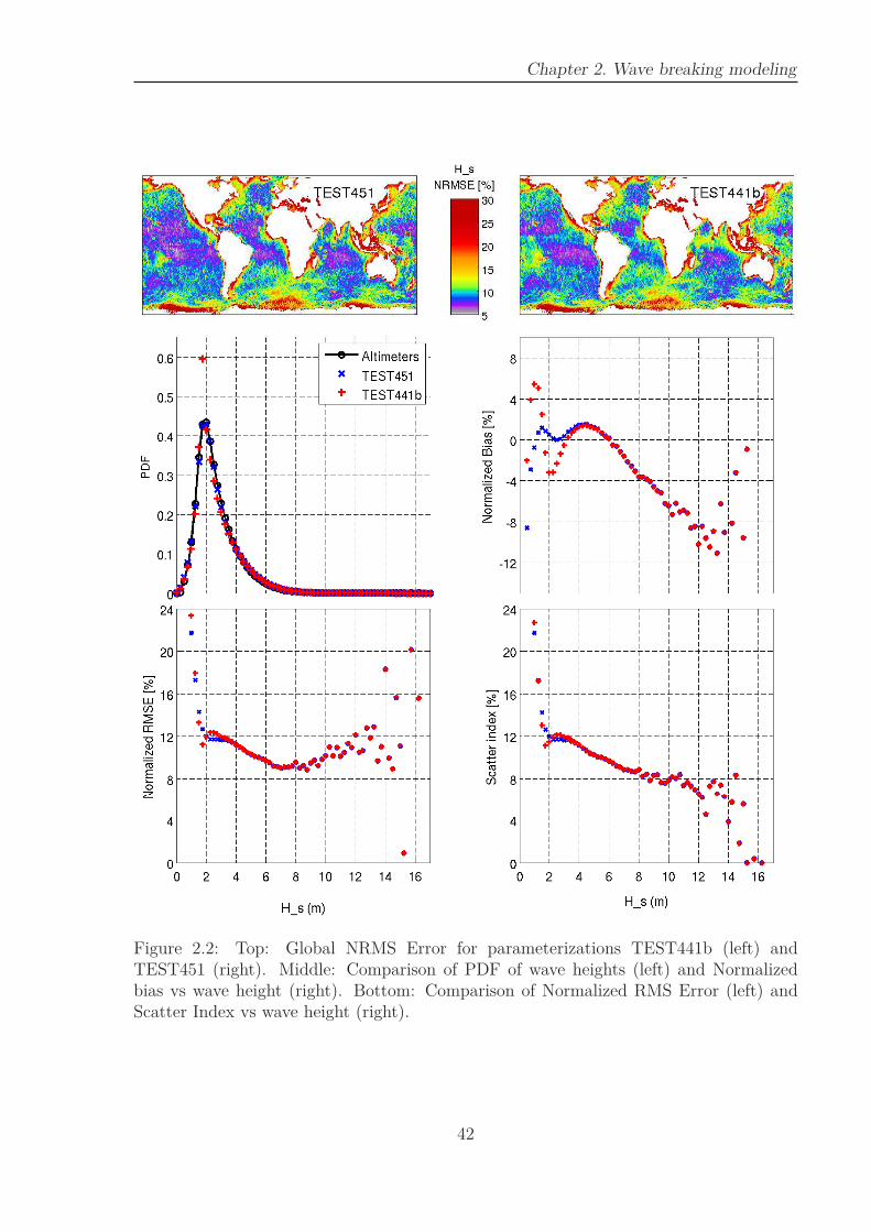
Chapter 2. Wave breaking modeling
Figure 2.2: Top: Global NRMS Error for parameterizations TEST441b (left) andTEST451 (right). Middle: Comparison of PDF of wave heights (left) and Normalizedbias vs wave height (right). Bottom: Comparison of Normalized RMS Error (left) andScatter Index vs wave height (right).
42
2.2 Investigated dissipation parameterizations
From breaking probabilities Pb,fiestimated by equation (2.21), breaking probabilities
Pb(k) at wave wavenumber k is then estimated averaging the Pb,fiof the N wave scales
fi∈[1,N ] involving k,
Pb(k) =1
N
N∑
i=1
Pb,fi. (2.32)
The breaking probability is distributed over different directions proportionally to thespectral energy
Pb(k, θ) = Pb(k)E(k, θ)
∫ 2π0 E(k, θ)dθ
. (2.33)
Then, Λ(k, θ) is obtained with equation (2.15) and is now used in equation (2.16) toprovide the cumulative dissipation.
The parameters for spontaneous dissipation are kept equal to those proposed by Filipotand Ardhuin (2012) and parameters for cumulative effect dissipation, rcu and Ccu inequation (2.16) are kept equal to those proposed by Ardhuin et al. (2010) (see §2.2.4).As a result, the only differences with TEST500 are the breaking probabilities used in thecumulative term.
We note that Ccu = 0.6 is kept whereas it is expected to be close to 1 (Ardhuin et al.,2010). There can be two explanations. First, the crest lengths of all waves, breaking ornot, is larger by a factor of two in Ardhuin et al. (2010) compared to Banner and Morison(2010). Using the expression in Banner and Morison (2010), we would arrive at the samemodel results with Ccu = 1.2. Second, it appears likely that the wind input for theshortest waves is underestimated in the parameterizations described here (see Rascle andArdhuin, A global wave parameter database for geophysical applications. Part 2: modelvalidation with improved source term parameterization, submitted to Ocean Modelling).This low input requires an underestimation of the dissipation rate to produce a correctspectral level. Calibration of the new parameterization leads us to reduce the global swelldissipation factor from 0.70 to 0.65. The wind input coefficient βmax is also decreasedfrom 1.52 to 1.50 (see 2.2.4 for further details).
Validation of the updated (TEST570) parameterization
Global validation for all of 2006 The model performance in terms of significantwave height Hs and mean square slope (mss) is now given. The model uses a 0.5-degreeregular resolution in longitude and latitude. ECMWF operational analyses for the windand sea ice concentration are used as forcing fields, with the addition of sub-grid blockingof waves by small icebergs in the Southern Ocean, using the method and iceberg datasetdescribed by Ardhuin et al. (2011b). The validation uses altimeter data from ERS2,ENVISAT, Jason-1 and GFO-Sat, assembled in the Globwave database (Queffeulou andCroize-Fillon, 2010). The model results from three-hourly gridded output are interpolatedon the satellite track position every second. Both model and satellite data are thenaveraged over 1 degree in latitude along the track. These averaged parameters are thenbinned geographically or according to the wind speed and wave height.
Figure 2.4 shows the similar biases and random errors of the TEST570 and TEST451parameterizations. These are also close to the results of TEST500 (not shown, see Filipot
43

Chapter 2. Wave breaking modeling
0
0.2
0.4
0.6
0.8
1N
orm
aliz
ed E
(k)
10−2
10−1
100
101
0
5
10
15
20
25
30
k [m−1]
Pfi a
nd P
(k)
[%]
Figure 2.3: Top: Rectangular filtering windows Wfi(colors) over integrated spectrum
(black line). Bottom: Breaking probabilities Pb,fiobtained for each wave scale fi (colors)
and breaking probability Pb(k) obtained with averaging (Black line).
and Ardhuin 2012). These results contrast with the very different error pattern obtainedwith the BJA parameterization by Bidlot et al. (2005), which is shown for reference. BJAproduces larger normalized errors, with large biases for low wave heights, due to an under-estimation of swell dissipation, in particular in the Pacific Ocean. That effect is generallywell corrected in the operational ECMWF by the assimilation of altimeter data. Otheraspects of these differences are discussed by Ardhuin et al. (2010). TEST570 generally
44
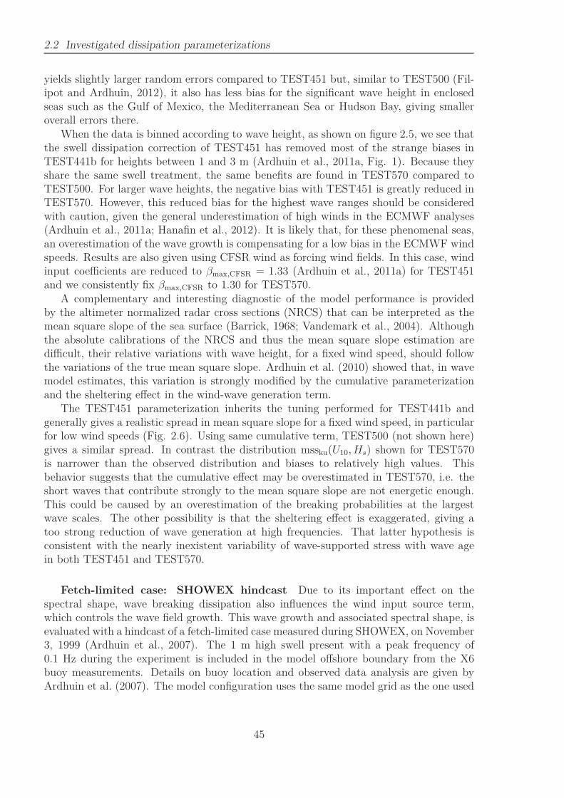
2.2 Investigated dissipation parameterizations
yields slightly larger random errors compared to TEST451 but, similar to TEST500 (Fil-ipot and Ardhuin, 2012), it also has less bias for the significant wave height in enclosedseas such as the Gulf of Mexico, the Mediterranean Sea or Hudson Bay, giving smalleroverall errors there.
When the data is binned according to wave height, as shown on figure 2.5, we see thatthe swell dissipation correction of TEST451 has removed most of the strange biases inTEST441b for heights between 1 and 3 m (Ardhuin et al., 2011a, Fig. 1). Because theyshare the same swell treatment, the same benefits are found in TEST570 compared toTEST500. For larger wave heights, the negative bias with TEST451 is greatly reduced inTEST570. However, this reduced bias for the highest wave ranges should be consideredwith caution, given the general underestimation of high winds in the ECMWF analyses(Ardhuin et al., 2011a; Hanafin et al., 2012). It is likely that, for these phenomenal seas,an overestimation of the wave growth is compensating for a low bias in the ECMWF windspeeds. Results are also given using CFSR wind as forcing wind fields. In this case, windinput coefficients are reduced to βmax,CFSR = 1.33 (Ardhuin et al., 2011a) for TEST451and we consistently fix βmax,CFSR to 1.30 for TEST570.
A complementary and interesting diagnostic of the model performance is providedby the altimeter normalized radar cross sections (NRCS) that can be interpreted as themean square slope of the sea surface (Barrick, 1968; Vandemark et al., 2004). Althoughthe absolute calibrations of the NRCS and thus the mean square slope estimation aredifficult, their relative variations with wave height, for a fixed wind speed, should followthe variations of the true mean square slope. Ardhuin et al. (2010) showed that, in wavemodel estimates, this variation is strongly modified by the cumulative parameterizationand the sheltering effect in the wind-wave generation term.
The TEST451 parameterization inherits the tuning performed for TEST441b andgenerally gives a realistic spread in mean square slope for a fixed wind speed, in particularfor low wind speeds (Fig. 2.6). Using same cumulative term, TEST500 (not shown here)gives a similar spread. In contrast the distribution mssku(U10, Hs) shown for TEST570is narrower than the observed distribution and biases to relatively high values. Thisbehavior suggests that the cumulative effect may be overestimated in TEST570, i.e. theshort waves that contribute strongly to the mean square slope are not energetic enough.This could be caused by an overestimation of the breaking probabilities at the largestwave scales. The other possibility is that the sheltering effect is exaggerated, giving atoo strong reduction of wave generation at high frequencies. That latter hypothesis isconsistent with the nearly inexistent variability of wave-supported stress with wave agein both TEST451 and TEST570.
Fetch-limited case: SHOWEX hindcast Due to its important effect on thespectral shape, wave breaking dissipation also influences the wind input source term,which controls the wave field growth. This wave growth and associated spectral shape, isevaluated with a hindcast of a fetch-limited case measured during SHOWEX, on November3, 1999 (Ardhuin et al., 2007). The 1 m high swell present with a peak frequency of0.1 Hz during the experiment is included in the model offshore boundary from the X6buoy measurements. Details on buoy location and observed data analysis are given byArdhuin et al. (2007). The model configuration uses the same model grid as the one used
45
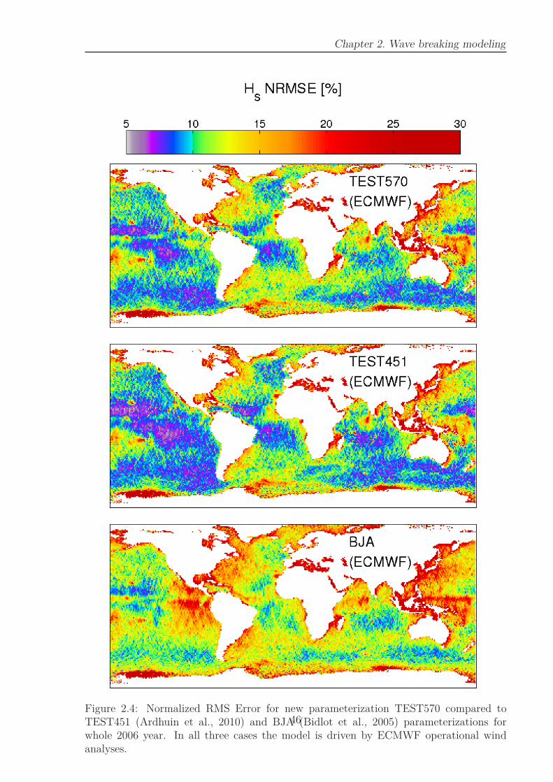
Chapter 2. Wave breaking modeling
Figure 2.4: Normalized RMS Error for new parameterization TEST570 compared toTEST451 (Ardhuin et al., 2010) and BJA (Bidlot et al., 2005) parameterizations forwhole 2006 year. In all three cases the model is driven by ECMWF operational windanalyses.
46
2.2 Investigated dissipation parameterizations
Figure 2.5: Normalized Bias, RMS Error and Scatter Index on Hs for new parameteriza-tion TEST570 compared to TEST451 and BJA parameterizations.
47

Chapter 2. Wave breaking modeling
Figure 2.6: Mean values of mssku binned as a function of Hs (x-axis) and U10 (y-axis) forTEST570 and TEST451 parameterizations and satellite observations.
48
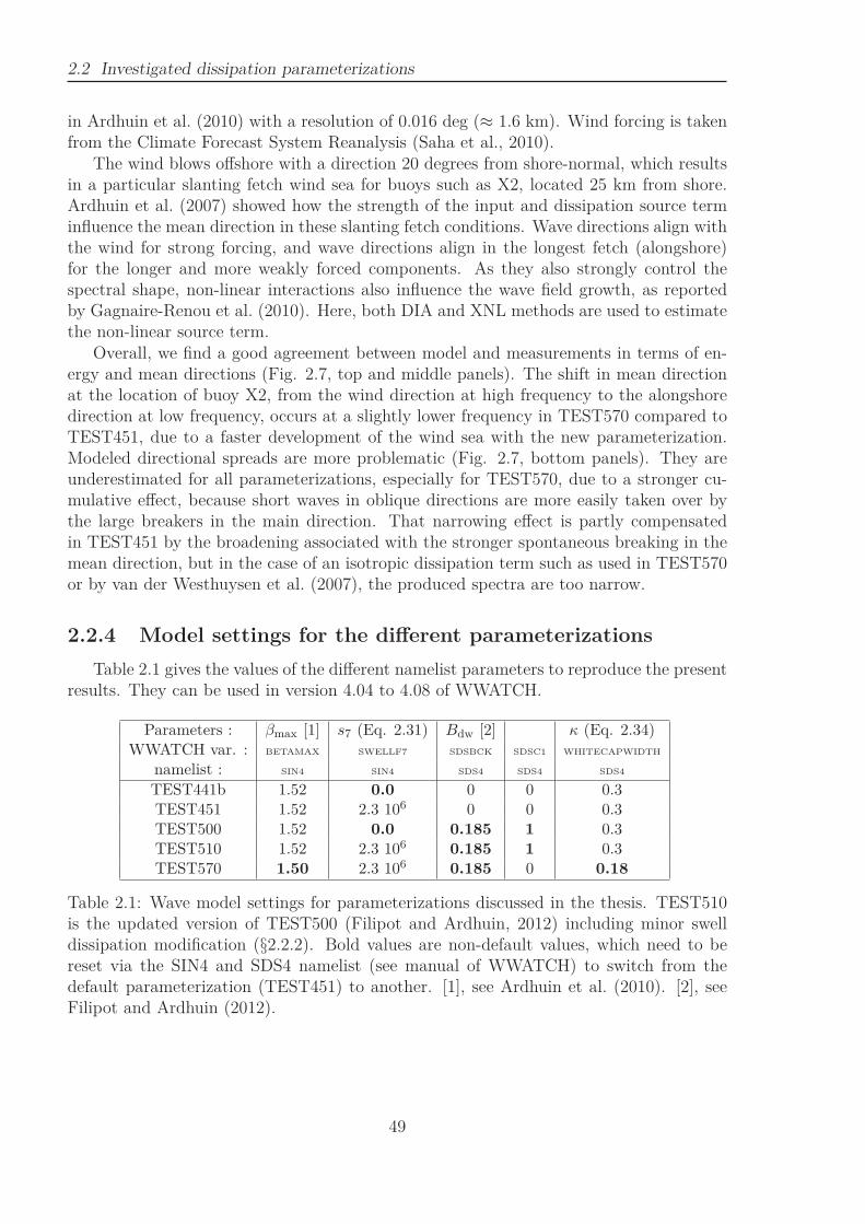
2.2 Investigated dissipation parameterizations
in Ardhuin et al. (2010) with a resolution of 0.016 deg (≈ 1.6 km). Wind forcing is takenfrom the Climate Forecast System Reanalysis (Saha et al., 2010).
The wind blows offshore with a direction 20 degrees from shore-normal, which resultsin a particular slanting fetch wind sea for buoys such as X2, located 25 km from shore.Ardhuin et al. (2007) showed how the strength of the input and dissipation source terminfluence the mean direction in these slanting fetch conditions. Wave directions align withthe wind for strong forcing, and wave directions align in the longest fetch (alongshore)for the longer and more weakly forced components. As they also strongly control thespectral shape, non-linear interactions also influence the wave field growth, as reportedby Gagnaire-Renou et al. (2010). Here, both DIA and XNL methods are used to estimatethe non-linear source term.
Overall, we find a good agreement between model and measurements in terms of en-ergy and mean directions (Fig. 2.7, top and middle panels). The shift in mean directionat the location of buoy X2, from the wind direction at high frequency to the alongshoredirection at low frequency, occurs at a slightly lower frequency in TEST570 compared toTEST451, due to a faster development of the wind sea with the new parameterization.Modeled directional spreads are more problematic (Fig. 2.7, bottom panels). They areunderestimated for all parameterizations, especially for TEST570, due to a stronger cu-mulative effect, because short waves in oblique directions are more easily taken over bythe large breakers in the main direction. That narrowing effect is partly compensatedin TEST451 by the broadening associated with the stronger spontaneous breaking in themean direction, but in the case of an isotropic dissipation term such as used in TEST570or by van der Westhuysen et al. (2007), the produced spectra are too narrow.
2.2.4 Model settings for the different parameterizations
Table 2.1 gives the values of the different namelist parameters to reproduce the presentresults. They can be used in version 4.04 to 4.08 of WWATCH.
Parameters : βmax [1] s7 (Eq. 2.31) Bdw [2] κ (Eq. 2.34)WWATCH var. : BETAMAX SWELLF7 SDSBCK SDSC1 WHITECAPWIDTH
namelist : SIN4 SIN4 SDS4 SDS4 SDS4
TEST441b 1.52 0.0 0 0 0.3TEST451 1.52 2.3 106 0 0 0.3TEST500 1.52 0.0 0.185 1 0.3TEST510 1.52 2.3 106
0.185 1 0.3TEST570 1.50 2.3 106
0.185 0 0.18
Table 2.1: Wave model settings for parameterizations discussed in the thesis. TEST510is the updated version of TEST500 (Filipot and Ardhuin, 2012) including minor swelldissipation modification (§2.2.2). Bold values are non-default values, which need to bereset via the SIN4 and SDS4 namelist (see manual of WWATCH) to switch from thedefault parameterization (TEST451) to another. [1], see Ardhuin et al. (2010). [2], seeFilipot and Ardhuin (2012).
49
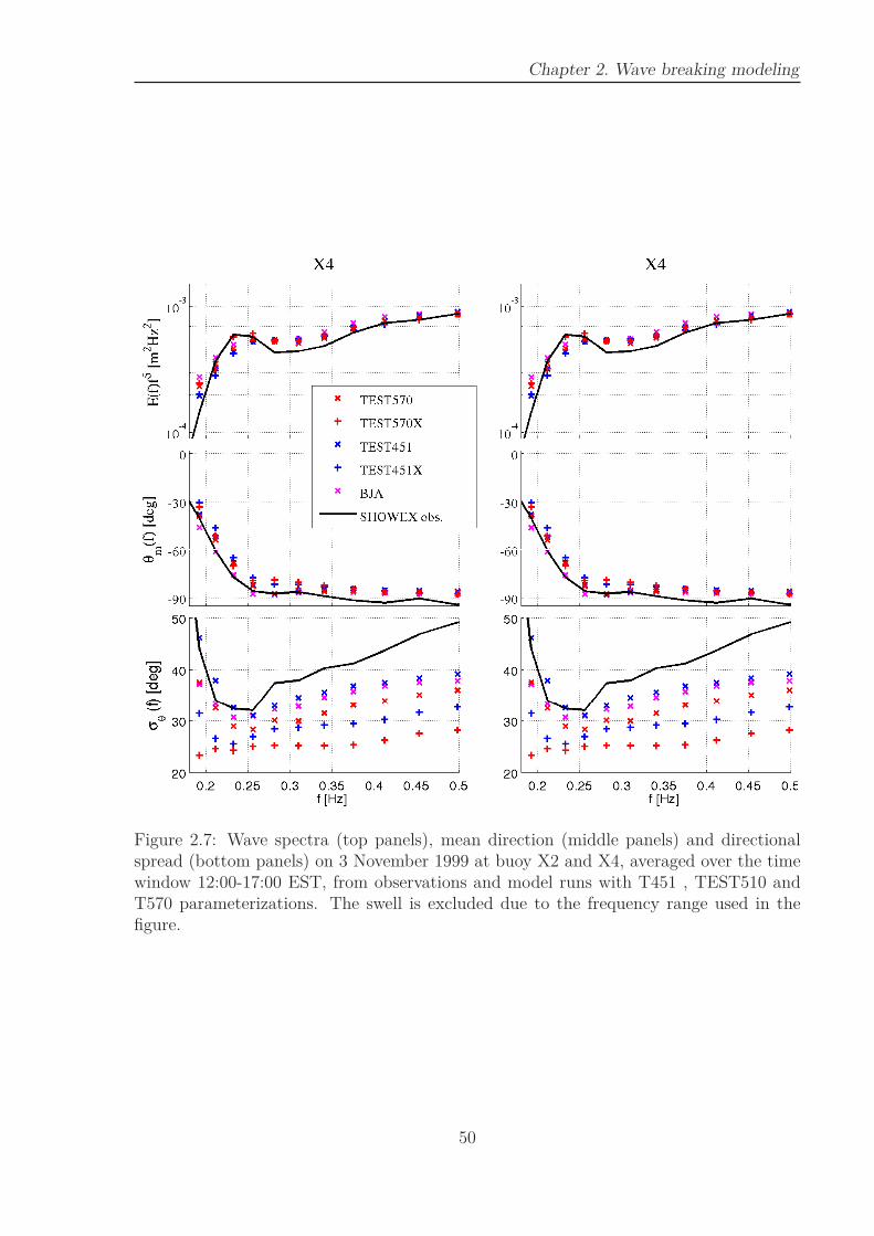
Chapter 2. Wave breaking modeling
Figure 2.7: Wave spectra (top panels), mean direction (middle panels) and directionalspread (bottom panels) on 3 November 1999 at buoy X2 and X4, averaged over the timewindow 12:00-17:00 EST, from observations and model runs with T451 , TEST510 andT570 parameterizations. The swell is excluded due to the frequency range used in thefigure.
50
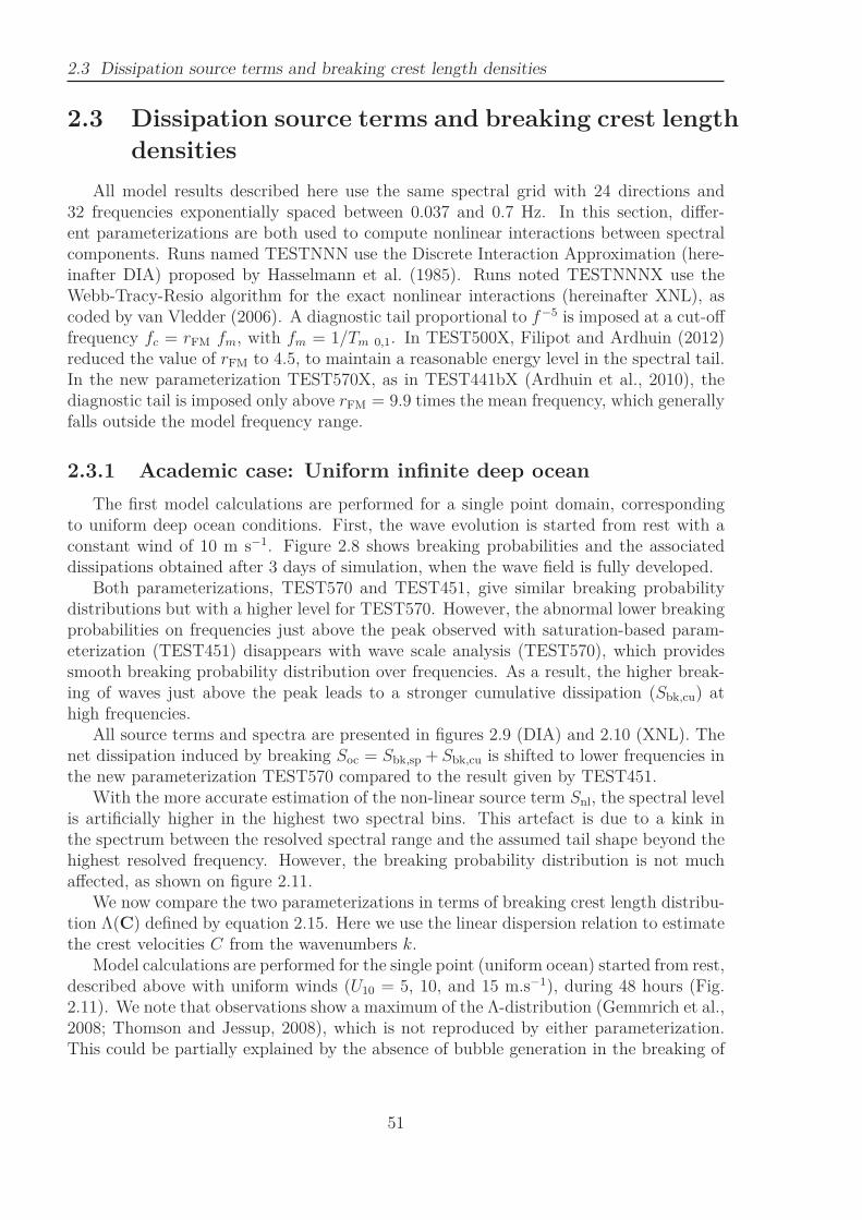
2.3 Dissipation source terms and breaking crest length densities
2.3 Dissipation source terms and breaking crest length
densities
All model results described here use the same spectral grid with 24 directions and32 frequencies exponentially spaced between 0.037 and 0.7 Hz. In this section, differ-ent parameterizations are both used to compute nonlinear interactions between spectralcomponents. Runs named TESTNNN use the Discrete Interaction Approximation (here-inafter DIA) proposed by Hasselmann et al. (1985). Runs noted TESTNNNX use theWebb-Tracy-Resio algorithm for the exact nonlinear interactions (hereinafter XNL), ascoded by van Vledder (2006). A diagnostic tail proportional to f−5 is imposed at a cut-offfrequency fc = rFM fm, with fm = 1/Tm 0,1. In TEST500X, Filipot and Ardhuin (2012)reduced the value of rFM to 4.5, to maintain a reasonable energy level in the spectral tail.In the new parameterization TEST570X, as in TEST441bX (Ardhuin et al., 2010), thediagnostic tail is imposed only above rFM = 9.9 times the mean frequency, which generallyfalls outside the model frequency range.
2.3.1 Academic case: Uniform infinite deep ocean
The first model calculations are performed for a single point domain, correspondingto uniform deep ocean conditions. First, the wave evolution is started from rest with aconstant wind of 10 m s−1. Figure 2.8 shows breaking probabilities and the associateddissipations obtained after 3 days of simulation, when the wave field is fully developed.
Both parameterizations, TEST570 and TEST451, give similar breaking probabilitydistributions but with a higher level for TEST570. However, the abnormal lower breakingprobabilities on frequencies just above the peak observed with saturation-based param-eterization (TEST451) disappears with wave scale analysis (TEST570), which providessmooth breaking probability distribution over frequencies. As a result, the higher break-ing of waves just above the peak leads to a stronger cumulative dissipation (Sbk,cu) athigh frequencies.
All source terms and spectra are presented in figures 2.9 (DIA) and 2.10 (XNL). Thenet dissipation induced by breaking Soc = Sbk,sp + Sbk,cu is shifted to lower frequencies inthe new parameterization TEST570 compared to the result given by TEST451.
With the more accurate estimation of the non-linear source term Snl, the spectral levelis artificially higher in the highest two spectral bins. This artefact is due to a kink inthe spectrum between the resolved spectral range and the assumed tail shape beyond thehighest resolved frequency. However, the breaking probability distribution is not muchaffected, as shown on figure 2.11.
We now compare the two parameterizations in terms of breaking crest length distribu-tion Λ(C) defined by equation 2.15. Here we use the linear dispersion relation to estimatethe crest velocities C from the wavenumbers k.
Model calculations are performed for the single point (uniform ocean) started from rest,described above with uniform winds (U10 = 5, 10, and 15 m.s−1), during 48 hours (Fig.2.11). We note that observations show a maximum of the Λ-distribution (Gemmrich et al.,2008; Thomson and Jessup, 2008), which is not reproduced by either parameterization.This could be partially explained by the absence of bubble generation in the breaking of
51
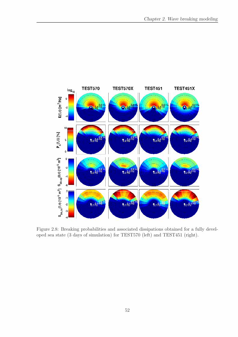
Chapter 2. Wave breaking modeling
Figure 2.8: Breaking probabilities and associated dissipations obtained for a fully devel-oped sea state (3 days of simulation) for TEST570 (left) and TEST451 (right).
52
2.3 Dissipation source terms and breaking crest length densities
0
0.5
1
1.5
2
Sat
m(f
) [1
0−4 m
2 ]
−1.5
−1
−0.5
0
0.5
1
Snl
(f)
[10−
4 m2 ]
−1.5
−1
−0.5
0
Soc
(f)
[10−
4 m2 ]
−0.5
0
Sbk
,sp(f
) [1
0−4 m
2 ]
−8−7−6−5−4−3−2−1
0
f [Hz]
Sbk
,cu(f
) [1
0−5 m
2 ]
0.1
0.2
0.3
0.50.7
1
2
f [Hz]
f5 E(f
) [1
0−3 m
2 Hz4 ]
TEST570
TEST451
BJA
Figure 2.9: Source terms for TEST570, TEST451 and BJA parameterizations using DIAfor non-linear interactions after 8 hours of run. The considered model is a uniform infinitedeep ocean with a uniform 10 ms−1 wind, starting from rest.
53
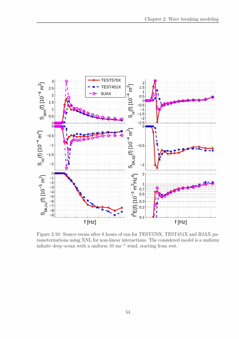
Chapter 2. Wave breaking modeling
0
0.5
1
1.5
2
2.5
3
Sat
m(f
) [1
0−4 m
2 ]
−2.5−2
−1.5−1
−0.50
0.51
1.52
Snl
(f)
[10−
4 m2 ]
−2
−1.5
−1
−0.5
0
Soc
(f)
[10−
4 m2 ]
−1
−0.5
0S
bk,s
p(f)
[10−
4 m2 ]
−9−8−7−6−5−4−3−2−1
0
f [Hz]
Sbk
,cu(f
) [1
0−5 m
2 ]
0.1
0.2
0.3
0.50.7
1
2
f [Hz]
f5 E(f
) [1
0−3 m
2 Hz4 ]
TEST570X
TEST451X
BJAX
Figure 2.10: Source terms after 8 hours of run for TEST570X, TEST451X and BJAX pa-rameterizations using XNL for non-linear interactions. The considered model is a uniforminfinite deep ocean with a uniform 10 ms−1 wind, starting from rest.
54
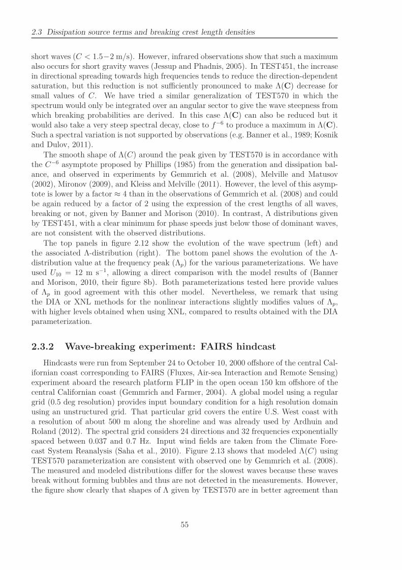
2.3 Dissipation source terms and breaking crest length densities
short waves (C < 1.5−2 m/s). However, infrared observations show that such a maximumalso occurs for short gravity waves (Jessup and Phadnis, 2005). In TEST451, the increasein directional spreading towards high frequencies tends to reduce the direction-dependentsaturation, but this reduction is not sufficiently pronounced to make Λ(C) decrease forsmall values of C. We have tried a similar generalization of TEST570 in which thespectrum would only be integrated over an angular sector to give the wave steepness fromwhich breaking probabilities are derived. In this case Λ(C) can also be reduced but itwould also take a very steep spectral decay, close to f−6 to produce a maximum in Λ(C).Such a spectral variation is not supported by observations (e.g. Banner et al., 1989; Kosnikand Dulov, 2011).
The smooth shape of Λ(C) around the peak given by TEST570 is in accordance withthe C−6 asymptote proposed by Phillips (1985) from the generation and dissipation bal-ance, and observed in experiments by Gemmrich et al. (2008), Melville and Matusov(2002), Mironov (2009), and Kleiss and Melville (2011). However, the level of this asymp-tote is lower by a factor ≈ 4 than in the observations of Gemmrich et al. (2008) and couldbe again reduced by a factor of 2 using the expression of the crest lengths of all waves,breaking or not, given by Banner and Morison (2010). In contrast, Λ distributions givenby TEST451, with a clear minimum for phase speeds just below those of dominant waves,are not consistent with the observed distributions.
The top panels in figure 2.12 show the evolution of the wave spectrum (left) andthe associated Λ-distribution (right). The bottom panel shows the evolution of the Λ-distribution value at the frequency peak (Λp) for the various parameterizations. We haveused U10 = 12 m s−1, allowing a direct comparison with the model results of (Bannerand Morison, 2010, their figure 8b). Both parameterizations tested here provide valuesof Λp in good agreement with this other model. Nevertheless, we remark that usingthe DIA or XNL methods for the nonlinear interactions slightly modifies values of Λp,with higher levels obtained when using XNL, compared to results obtained with the DIAparameterization.
2.3.2 Wave-breaking experiment: FAIRS hindcast
Hindcasts were run from September 24 to October 10, 2000 offshore of the central Cal-ifornian coast corresponding to FAIRS (Fluxes, Air-sea Interaction and Remote Sensing)experiment aboard the research platform FLIP in the open ocean 150 km offshore of thecentral Californian coast (Gemmrich and Farmer, 2004). A global model using a regulargrid (0.5 deg resolution) provides input boundary condition for a high resolution domainusing an unstructured grid. That particular grid covers the entire U.S. West coast witha resolution of about 500 m along the shoreline and was already used by Ardhuin andRoland (2012). The spectral grid considers 24 directions and 32 frequencies exponentiallyspaced between 0.037 and 0.7 Hz. Input wind fields are taken from the Climate Fore-cast System Reanalysis (Saha et al., 2010). Figure 2.13 shows that modeled Λ(C) usingTEST570 parameterization are consistent with observed one by Gemmrich et al. (2008).The measured and modeled distributions differ for the slowest waves because these wavesbreak without forming bubbles and thus are not detected in the measurements. However,the figure show clearly that shapes of Λ given by TEST570 are in better agreement than
55
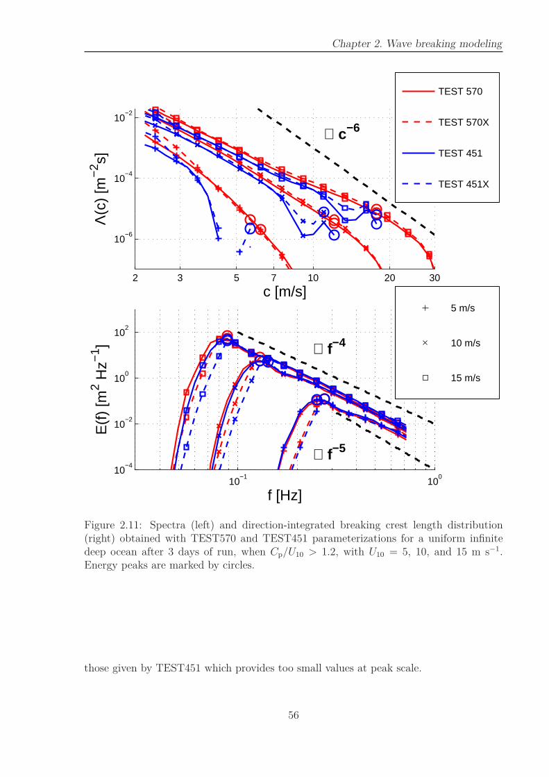
Chapter 2. Wave breaking modeling
10−1
100
10−4
10−2
100
102
f [Hz]
E(f
) [m
2 Hz−
1 ] ∝ f−4
∝ f−5
2 3 5 7 10 20 30
10−6
10−4
10−2
c [m/s]
Λ(c
) [m
−2 s]
∝ c−6
TEST 570
TEST 570X
TEST 451
TEST 451X
5 m/s
10 m/s
15 m/s
Figure 2.11: Spectra (left) and direction-integrated breaking crest length distribution(right) obtained with TEST570 and TEST451 parameterizations for a uniform infinitedeep ocean after 3 days of run, when Cp/U10 > 1.2, with U10 = 5, 10, and 15 m s−1.Energy peaks are marked by circles.
those given by TEST451 which provides too small values at peak scale.
56
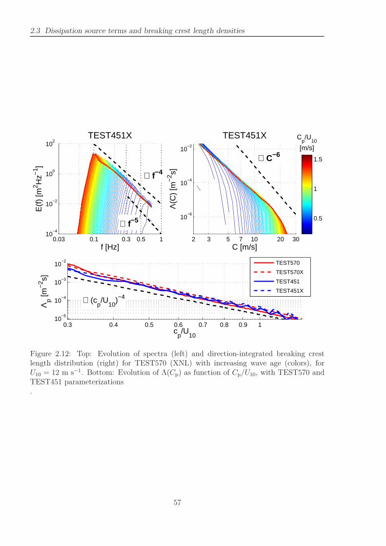
2.3 Dissipation source terms and breaking crest length densities
0.03 0.1 0.3 0.5 110
−4
10−2
100
102
∝ f−4
∝ f−5
TEST451X
f [Hz]
E(f
) [m
2 Hz−
1 ]
2 3 5 7 10 20 30
10−6
10−4
10−2
∝ C−6
C [m/s]
Λ(C
) [m
−2 s]
TEST451X
0.3 0.4 0.5 0.6 0.7 0.8 0.9 110
−5
10−4
10−3
10−2
cp/U
10
Λp [m
−2 s]
∝ (cp/U
10)−4
Cp/U
10
[m/s]
0.5
1
1.5
TEST570
TEST570X
TEST451
TEST451X
Figure 2.12: Top: Evolution of spectra (left) and direction-integrated breaking crestlength distribution (right) for TEST570 (XNL) with increasing wave age (colors), forU10 = 12 m s−1. Bottom: Evolution of Λ(Cp) as function of Cp/U10, with TEST570 andTEST451 parameterizations.
57
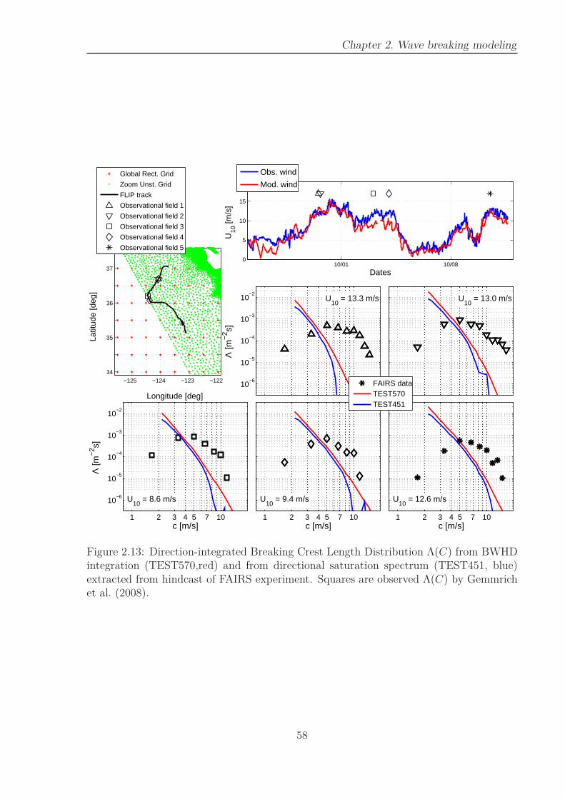
Chapter 2. Wave breaking modeling
10/01 10/080
5
10
15
20
Dates
U10
[m/s
]
−125 −124 −123 −12234
35
36
37
Longitude [deg]
Latit
ude
[deg
]
10−6
10−5
10−4
10−3
10−2
U10
= 13.3 m/s
Λ [m
−2 s]
U10
= 13.0 m/s
1 2 3 4 5 7 10
10−6
10−5
10−4
10−3
10−2
U10
= 8.6 m/s
c [m/s]
Λ [m
−2 s]
1 2 3 4 5 7 10
U10
= 9.4 m/s
c [m/s]1 2 3 4 5 7 10
U10
= 12.6 m/s
c [m/s]
Obs. wind
Mod. windGlobal Rect. Grid
Zoom Unst. Grid
FLIP track
Observational field 1
Observational field 2
Observational field 3
Observational field 4
Observational field 5
FAIRS dataTEST570TEST451
Figure 2.13: Direction-integrated Breaking Crest Length Distribution Λ(C) from BWHDintegration (TEST570,red) and from directional saturation spectrum (TEST451, blue)extracted from hindcast of FAIRS experiment. Squares are observed Λ(C) by Gemmrichet al. (2008).
58

2.4 Whitecap coverage and mean foam thickness at the global scale
2.4 Whitecap coverage and mean foam thickness at
the global scale
In this section, we consider the global hindcast of the year 2006, for which we obtainedthe WindSat radiometer data interpreted by Anguelova and Webster (2006). The modeluses the same 0.5-degree regular resolution in longitude and latitude, ECMWF opera-tional analyses for the wind and sea ice and iceberg concentrations than used in previousdescribed global validation of the TEST570 parameterization. The non-linear source termis now computed using only the DIA (Hasselmann et al., 1985). This same model is val-idated in terms of wave height and mean square slope in 2.2.3. The low error levels forboth parameters, typically 10% of the observed RMS values, indicate a generally goodrepresentation of the frequency spectrum. We now consider our estimations of whitecapcoverage in relation to the radiometer data of Anguelova et al. (2009).
In order to be consistent with radiometer data, we define the whitecap coverage (WCC)as the fraction of sea surface covered by both active breaking (stage A) and residual foam(stage B). Although stage A is more closely related to breaking fronts, which is whatwe model, these two stages are difficult to separate in microwave radiometric data. Thiscombination with stage B introduces a large variability due to other factors, such as watertemperature and salinity, which we have not introduced in our model.
For a single breaker, the area covered by foam is obtained by multiplying the breakingcrest length by a mean whitecap width parameterized as the constant fraction κ = κA+κB
of breaker wavelength λ. Mironov (2009) has found that the geometry of phase A iswell represented by ellipses of almost constant eccentricity with breaking crest lengthsdistributed as a power-law. These observations are consistent with the use of a constantκA. Reul and Chapron (2003) also proposed a κA constant to represent stage A. Basedon laboratory observations of Duncan (1981), they used κA = 0.3. Our parameterizationfor both stages A and B is based on the fact that, for constant environmental parameters,stage B is related to stage A.
The whitecap coverage, corresponding to the fraction of sea surface covered by bothstages, is here estimated as
W =∫
∞
0κ λC Λ(C) dC, (2.34)
where λC is the wavelength of breaking waves with phase speed C. In deep water, thewavelength is proportional to the squared phase speed (λC = 2πC2/g). Therefore, white-cap coverage from breaking wave with velocities in range C to C + dC in deep wateris proportional to the second moment of λC (Reul and Chapron, 2003) and the totalwhitecap coverage, in deep water, is given by
W =∫
∞
0κ2π.
C2
gΛ(C)dC. (2.35)
We have adjusted the constant κ for each parameterization, to provide whitecap cov-erage consistent with empirical wind-driven fit by Monahan and Woolf (1989) and theglobal whitecap coverage database of Anguelova et al. (2009). κ is adjusted to 0.30 forTEST451 and 0.18 for TEST570.
59
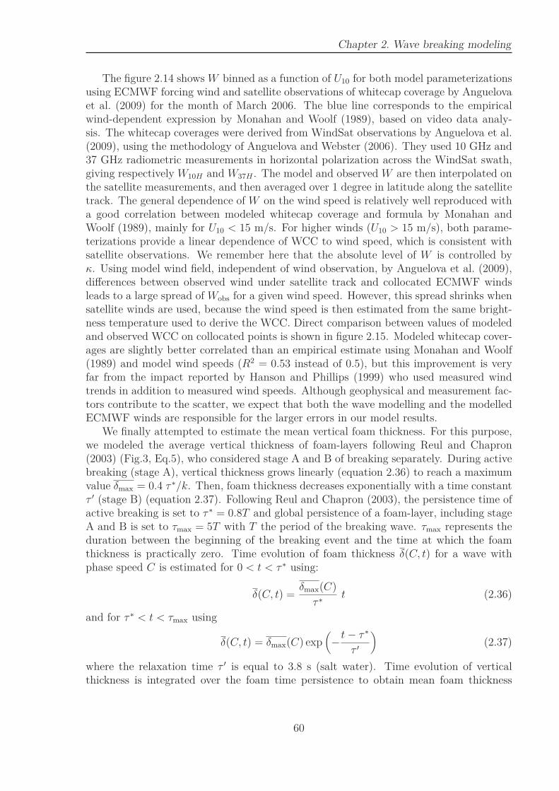
Chapter 2. Wave breaking modeling
The figure 2.14 shows W binned as a function of U10 for both model parameterizationsusing ECMWF forcing wind and satellite observations of whitecap coverage by Anguelovaet al. (2009) for the month of March 2006. The blue line corresponds to the empiricalwind-dependent expression by Monahan and Woolf (1989), based on video data analy-sis. The whitecap coverages were derived from WindSat observations by Anguelova et al.(2009), using the methodology of Anguelova and Webster (2006). They used 10 GHz and37 GHz radiometric measurements in horizontal polarization across the WindSat swath,giving respectively W10H and W37H . The model and observed W are then interpolated onthe satellite measurements, and then averaged over 1 degree in latitude along the satellitetrack. The general dependence of W on the wind speed is relatively well reproduced witha good correlation between modeled whitecap coverage and formula by Monahan andWoolf (1989), mainly for U10 < 15 m/s. For higher winds (U10 > 15 m/s), both parame-terizations provide a linear dependence of WCC to wind speed, which is consistent withsatellite observations. We remember here that the absolute level of W is controlled byκ. Using model wind field, independent of wind observation, by Anguelova et al. (2009),differences between observed wind under satellite track and collocated ECMWF windsleads to a large spread of Wobs for a given wind speed. However, this spread shrinks whensatellite winds are used, because the wind speed is then estimated from the same bright-ness temperature used to derive the WCC. Direct comparison between values of modeledand observed WCC on collocated points is shown in figure 2.15. Modeled whitecap cover-ages are slightly better correlated than an empirical estimate using Monahan and Woolf(1989) and model wind speeds (R2 = 0.53 instead of 0.5), but this improvement is veryfar from the impact reported by Hanson and Phillips (1999) who used measured windtrends in addition to measured wind speeds. Although geophysical and measurement fac-tors contribute to the scatter, we expect that both the wave modelling and the modelledECMWF winds are responsible for the larger errors in our model results.
We finally attempted to estimate the mean vertical foam thickness. For this purpose,we modeled the average vertical thickness of foam-layers following Reul and Chapron(2003) (Fig.3, Eq.5), who considered stage A and B of breaking separately. During activebreaking (stage A), vertical thickness grows linearly (equation 2.36) to reach a maximumvalue δmax = 0.4 τ ∗/k. Then, foam thickness decreases exponentially with a time constantτ ′ (stage B) (equation 2.37). Following Reul and Chapron (2003), the persistence time ofactive breaking is set to τ ∗ = 0.8T and global persistence of a foam-layer, including stageA and B is set to τmax = 5T with T the period of the breaking wave. τmax represents theduration between the beginning of the breaking event and the time at which the foamthickness is practically zero. Time evolution of foam thickness δ(C, t) for a wave withphase speed C is estimated for 0 < t < τ ∗ using:
δ(C, t) =δmax(C)
τ ∗t (2.36)
and for τ ∗ < t < τmax using
δ(C, t) = δmax(C) exp(
−t− τ ∗
τ ′
)
(2.37)
where the relaxation time τ ′ is equal to 3.8 s (salt water). Time evolution of verticalthickness is integrated over the foam time persistence to obtain mean foam thickness
60
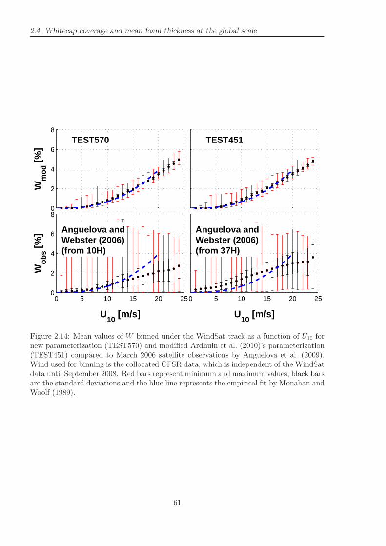
2.4 Whitecap coverage and mean foam thickness at the global scale
0 5 10 15 20 250
2
4
6
8
Anguelova andWebster (2006)(from 10H)
U10
[m/s]
Wob
s [%
]
0 5 10 15 20 25
Anguelova andWebster (2006)(from 37H)
U10
[m/s]
0
2
4
6
8
Wm
od [%
]
TEST570 TEST451
Figure 2.14: Mean values of W binned under the WindSat track as a function of U10 fornew parameterization (TEST570) and modified Ardhuin et al. (2010)’s parameterization(TEST451) compared to March 2006 satellite observations by Anguelova et al. (2009).Wind used for binning is the collocated CFSR data, which is independent of the WindSatdata until September 2008. Red bars represent minimum and maximum values, black barsare the standard deviations and the blue line represents the empirical fit by Monahan andWoolf (1989).
61
Chapter 2. Wave breaking modeling
Figure 2.15: Q-Q plot of WCC given by TEST570 and TEST451 and satellite observations(Anguelova et al., 2009) on March 2006. Compared values are collocated under WindSatswath. Colors give the values of log(Nval).
62

2.4 Whitecap coverage and mean foam thickness at the global scale
∆(C) of individual breaking events:
∆(C) =δmax(C)
τmax
(
1
2+ 3.8
(
1 − exp(
−τmax − τ ∗
3.8
)))
(2.38)
Integration of the whitecap coverage produced by each scale times its mean foam thicknessover all wave scales gives a global mean foam thickness
∆ =∫
∞
0∆(C)κλ(C)Λ(C)dC, (2.39)
The figure 2.16 shows the dependence between the mean foam thickness and the windspeed for the two parameterizations. Higher breaking probabilities just above the peak inTEST570 than ones in TEST451 lead to a slightly higher level of mean foam thickness.This difference increases with wind speed due to displacement of the peak to longer waveswhich produce higher foam layers. More importantly, for a fixed wind speed, the relativevariability of foam thickness is much larger than the variability observed in whitecapcoverage values. This suggests that radiometric data at larger wavelengths, which aremore sensitive to foam thickness, may be a good indicator of breaking activity beyondthe usual wind-whitecap coverage relation of which the Beaufort scale for wind speeds isa perfect example.
Figure 2.16: Mean values of mean foam thickness (∆) binned as a function of U10 fornew parameterization (TEST570) and modified Ardhuin et al. (2010)’s parameterization(TEST451). Wind used for binning is the collocated CFSR data, which is independentof the WindSat data until September 2008. Red bars represent minimum and maximumvalues, black bars are the standard deviations.
63
Chapter 2. Wave breaking modeling
2.5 Conclusion and Perspectives
The TEST570 parameterization presented here accounts for the physical relationshipthat intrinsically links spontaneous breaking dissipation and dissipation induced by break-ing waves (cumulative term) and thereby extends the work of Filipot and Ardhuin (2012).The cumulative dissipation term was adjusted so that the model could reproduce observedspectral evolution and global wave heights distributions. It is found that this TEST570parameterization produces breaking crest lengths distributions that are in better quali-tative agreement with observations, contrary to TEST451 which fails to produce smoothΛ-distributions. This difference is clearly associated with the integration over frequenciesin TEST570 compared to the local saturation used in TEST451. Banner and Morison(2010) have shown that estimating breaking parameters after smoothing the local satu-rations over frequencies has the same effect.
Overall, as already shown by Banner and Morison (2010), an explicit modeling ofwhitecap properties provides a new constraint on the model dissipation source terms, anda more detailed use of global observations from satellite radiometers, such as interpretedby Anguelova and Webster (2006), can be used for this. In particular, we find that jointestimates of the whitecap coverage and foam thickness could be an interesting way todiscriminate between different sea states or parameterizations. This can be achieved bycombining radiometric measurements from different bands. Recent results by Reul et al.(2006) with L-band radiometric measurements in Hurricanes using the Soil Moisture andOcean Salinity space mission can be combined with the Ku and X band data to providethe necessary information.
Further work on the parameterization remains, in particular on the method to at-tribute breaking probabilities and dissipation rates to different directions, and in thephysical processes represented in the cumulative term. Indeed, the cumulative effect pa-rameterization of Ardhuin et al. (2010) used with isotropic breaking probability tendsto reduce the width of the directional spectrum. All the parameterizations tested hereproduce directional spectra which are too narrow at high frequencies (f > 0.6 Hz intypical oceanic conditions). We attribute this deficiency to a lack of physical processesin the model. In particular the splash of breakers has been shown to transfer energy tohigh frequencies by creating small waves (Rozenberg and Ritter, 2005, e.g.), and shortwaves are known to break mostly at the crest of longer waves, due to hydrodynamic andaerodynamic modulations (e.g. Smith, 1986).
The analysis of the recent wave breaking dissipation parameterizations provided inthis chapter showed that such parameterizations are able to provide an energy dissipationthat properly equilibrate the wave energy balance equation providing spectra in goodagreement with observation in terms of shape and energy level, but without guaranteefor the underlying physics. In particular, we showed that modeled breaking crest lengthdensities are inconsistent with observations. Moreover, models are currently not able toreproduce the large disparity in observations. We also note that the parameterizations
64

2.5 Conclusion and Perspectives
combine results from different studies, from different areas, from both laboratory and fieldexperiments. The large sensibility of the results the a misunderstood number of externalparameters, makes the combination of these studies uncertain.
We here highlights the need of observations that provide in same time information onwave spectrum, directional breaking parameters and directional breaking dissipation. Inthe next chapter, we propose a field experiment using stereo video system to observe time-space evolution of sea surface wave evolving towards breaking or not. Such observationsprovide simultaneously directional breaking parameters and directional wave spectrumincluding non-linear contributions. These observation can also be used to observe theevolution of the wave shapes induced by breaking, and thus, to estimate dissipation in-duced by breaking.
65


Chapter 3
Reconstruction of 3D oceanic surfacewaves
3.1 Introduction
Water wave elevations can be measured with different methods. Usually, 1-D elevationis obtained using a pressure sensor in the water or a capacitive wave gauge crossing thesurface. By multiplying the number of instruments, several 1-D surface elevations canbe obtained and 2-D surfaces can be approached. Direct 2-D surface elevation can alsobe obtained using 2-D radar-based systems installed on either fixed positions (Dankertet al., 2003) and aircrafts (Hwang et al., 2000) or using stereo video systems. These lastsystems provide 3-D elevation maps of water waves by using a spatial-widespread andnon-intrusive optical system. Video imagery has another significant advantage with alow-cost system in both installation and maintenance (Holland et al., 1997; Holland andHolman, 1997). A stereo camera view provides spatial and temporal data whose statisticalcontent is richer than that of a time series retrieved from a buoy, which is expensive toinstall and maintain (Benetazzo, 2006; Gallego et al., 2008). Moreover, extending imageprocessing from static individual images to image sequences of stereo-pairs opens a newworld of information. Indeed, stereo image sequences contain both the temporal andspatial structure of the phenomena observed. Except for limitations in resolution in timeand space and the size of the images, image sequences capture the events as completelyas possible.
Stereoscopy regroups all the methods which reproduce relief effect from a pair of 2Dimages. Long before its application to recent computer vision, humans have exploited theability of their brain to create a 3D illusion starting from a pair of 2D images. Therefore,in 1550’s, painter Jacopo Chimenti made two drawings representing a slightly differentpoint of view of a same scene to produce a relief effect within the brain of viewer. Thefirst stereoscopic camera appeared in the 1850’s, soon after the first simple camera andtheir evolution is still underway. Taken with a spacing of a few centimeters, pairs ofphotographs present a slightly different image to each eye and reproduce the relief ofthe scene. A rich literature on the subject exists on the subject. Stereoscopy appeared inscientific literature from the middle of the 18th century (Wheatstone, 1853; Claudet, 1856,1857, and many others.) with large scope of application, such as for example, topography
67
Chapter 3. Sea surface reconstruction
(Galton and Galton, 1865) or medicine (Mach, 1896). Nevertheless, 3D reconstruction ofthe scene was only a brain process, and no quantitative access to the 3rd dimension waspossible.
Further, the development of the epipolar geometry (see §3.3.3) sets the basis of therecent computer vision, where the shape of the scene can be extracted from the stereopairs of photographs. In spite of the relatively simple procedures involved by the stereovision, its application to oceanic surface waves is rather limited. Therefore, before the1950’s, only one published study used it (Dankert et al., 1939). In the early 1950’s,the desirability of obtaining the two-dimensional sea spectra appeared in the literature(Pierson, 1952; St Denis and Pierson Jr, 1953). The stereo-photography of the wavysurface for determining the vertical displacement of the water surface was initiated byMarks (1954) to determine the wave number spectrum. By taking photographs from abridge, he was able to get useful data on the two-dimensional wave spectrum, but on amuch reduced scale. Moreover, Cruset (1953) also showed feasibility of photogrammetricmeasurements of the sea swell from synchronized cameras driven by separated aircrafts.These two studies among others motivated the launching of the Stereo Wave ObservationProject (Chase et al., 1957; Cote et al., 1960). Latter, Banner et al. (1989) also used thestereo-photography for the measurement of the spectrum directionality. Recently, withthe development of the numerical photography, some investigators concerned themselveswith wave measurements from stereo photography (Kosnik and Dulov, 2011) or stereo-video (Benetazzo, 2006; Gallego et al., 2008).
In this chapter, the first section gives a description of the experiment. Then, the section3.3 deals with the theoretical background and the mathematical definitions of the relationsbetween a 3D scene and its camera image projection. The epipolar geometry describingthe relations existing between the projection of a same scene on multiple camera images isalso considered. Then, the section 3.5 describes methodology of the stereo reconstructionof sea surfaces. Finally the section 3.6 deals with the validation of reconstructed surfacesand the analysis of their corresponding spectra.
3.2 Experiment description
The experiment was conducted on September and October 2011 from the researchplatform of the Marine Hydrophysical Institute of the Academy of Sciences of Ukraine.The platform is located 500 meters off the coast next to Katsiveli in the Black Sea. Thedepth at the observation area is at least 30m. The measurements consider synchronizedacquisition of wind speed and direction, sea surface elevation and stereo video acquisitions.The positions of the instruments are shown in the figure 3.1. The wind measurements,speed and direction, are obtained using a 23 meter height anemometer. The sea surfaceelevation is measured at a 10Hz sampling frequency and 2mm accuracy with an arrayof six wave gauges. Finally, the Wave Acquisition Stereo System (hereinafter WASS)acquires image sequences of the sea surface.
The WASS is a couple of synchronized 5 Megapixel BM-500GE JAI cameras encap-sulated in waterproof cases (Fig. 3.2) with the following specifications
• Sensor 2/3” progressive scan CCD (8 bit)
68
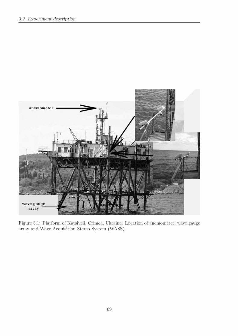
3.2 Experiment description
Figure 3.1: Platform of Katsiveli, Crimea, Ukraine. Location of anemometer, wave gaugearray and Wave Acquisition Stereo System (WASS).
69
Chapter 3. Sea surface reconstruction
• Pixel Clock 60 MHz
• Active area 8.45 (h) x 7.07 (v)
• Cell size 3.45 (h) x 3.45 (v)
• Active pixels 2456 (h) x 2058 (v). (Cell size = 3.45µm x 3.45µm)
• Read-out modes
• GigE Vision interface with 12, 10 or 8-bit output
Each camera was coupled to a 5-mm focal length low distortion lens and linked to theworkstation with RJ45 Ethernet cable for data transfer and a power cable, also used fortrigger, ensuring synchronization of pictures taken by each camera. Due to the hard diskwriting speed limitation, the maximum frame rate is 15 frames per second. In addition toensure trigger and picture storage, the software allows parameterization of the exposuretime of each camera by the user before acquisition and an automatic adjustment of the gainis done by the system during the acquisition to compensate for the brightness variations.For all the acquisitions described further, the exposure time is set for the both camerasto 6000µs. Such a large value is set to keep a small analogical gain, but it implies someblurring on the image borders.
The acquisitions were done for wind direction established to West-South-West, withspeed up to 10m/s. The figure 3.3 and the table 3.1 resume the wind and wave conditionsduring the 4 video acquisitions selected for this study. The wind speeds and directionsare averaged over the duration of the record. The significant wave heights and the windsea peak frequencies are get from wave gauge records.
3.3 Theoretical background
The video cameras capture the light reflected from the objects on the observed sceneusing a Charge-Coupled Device (CCD). During the exposure time, each cell of the CCDmeasures the received light quantity. Then, this quantity is discretized to give the value ofthe corresponding pixel. The number of possible discretized values is the image depth. Tomaintain the values between the range of the possible values, an analogical gain is generallyapplied on the measured raw light quantities before discretization. Repeating the processat high frequency, the result is a N frame-per-second (fps) sequence of pictures capturingthe evolution of the scene, with a resolution (i.e. a number of pixels) given by the numberof CCD cells. The aim of the camera calibration is to find the parameters which link a 3Dobject to its projection on the bit-mapped image. Usually used in computer vision, thepinhole camera model, described in paragraph 3.3.1, provides this link. Nevertheless, thissimple model does not take in account that the coordinates are generally expressed in areference system independent of camera position and orientation nor the discretization ofthe image plane into pixels and the distortion induced by the optical lenses. The completeequations that relates a 3D point to its projection are discussed in the paragraphs 3.3.2.Finally, the last paragraph 3.3.2 describes the epipolar geometry which links the twopinhole cameras.
70
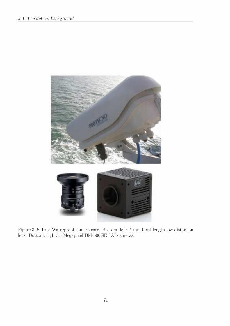
3.3 Theoretical background
Figure 3.2: Top: Waterproof camera case. Bottom, left: 5-mm focal length low distortionlens. Bottom, right: 5 Megapixel BM-500GE JAI cameras.
71
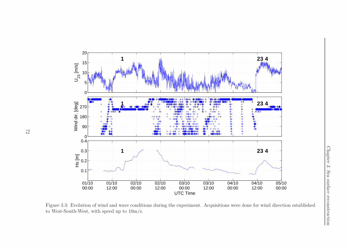
Chapter
3.
Sea
surfa
cereco
nstru
ction
0
5
10
15
20
U23
[m/s
]
1 23 4
0
90
180
270
Win
d di
r. [d
eg] 1 23 4
0.1
0.2
0.3
0.4
01/1000:00
01/1012:00
02/1000:00
02/1012:00
03/1000:00
03/1012:00
04/1000:00
04/1012:00
05/1000:00
UTC Time
Hs
[m] 1 23 4
Figure 3.3: Evolution of wind and wave conditions during the experiment. Acquisitions were done for wind direction establishedto West-South-West, with speed up to 10m/s.
72
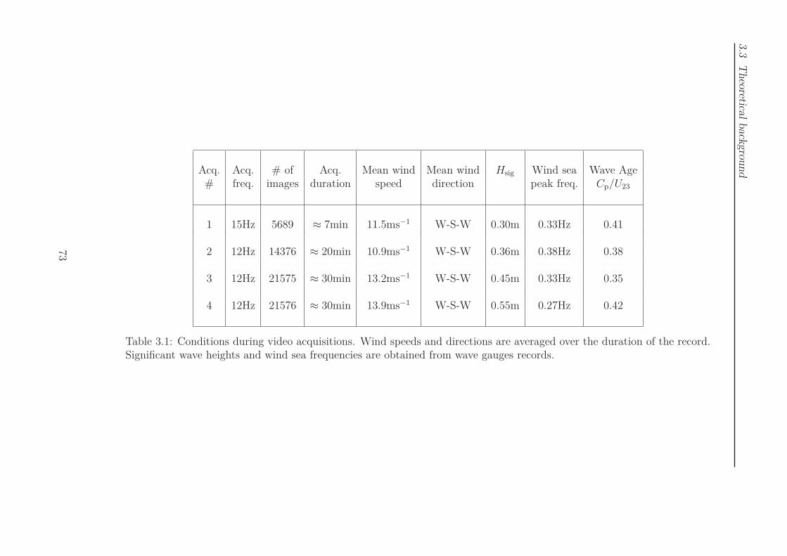
3.3
Theo
retical
back
gro
undAcq. Acq. # of Acq. Mean wind Mean wind Hsig Wind sea Wave Age
# freq. images duration speed direction peak freq. Cp/U23
1 15Hz 5689 ≈ 7min 11.5ms−1 W-S-W 0.30m 0.33Hz 0.41
2 12Hz 14376 ≈ 20min 10.9ms−1 W-S-W 0.36m 0.38Hz 0.38
3 12Hz 21575 ≈ 30min 13.2ms−1 W-S-W 0.45m 0.33Hz 0.35
4 12Hz 21576 ≈ 30min 13.9ms−1 W-S-W 0.55m 0.27Hz 0.42
Table 3.1: Conditions during video acquisitions. Wind speeds and directions are averaged over the duration of the record.Significant wave heights and wind sea frequencies are obtained from wave gauges records.
73

Chapter 3. Sea surface reconstruction
3.3.1 Pinhole camera model
The pinhole camera model is the simplest model which relates a point of the sceneto its projection on the image plane. It assumes a rectilinear projection in which thestraight lines in a scene are projected into straight lines in the image. In other worlds, itassumes that all rays from the 3D scene straightly crosses the image plane and focus onthe projection center, at a distance f , so-called the focal length, such as shown on figure3.4. A metric image coordinate system is defined such that origin o is the intersectionbetween the optical axis and the image plane and the vectors ~u′ and ~v′ are orthogonal andparallel to the image plane. The camera coordinate system is defined such that the originOc is the projection center, the axis ~Zc is collinear to the optical axis and the vectors ~Xc
and ~Yc are respectively collinear to ~u′ and ~v′. Therefore, a 3D point P (Xc, Yc, Zc) of thescene is related to its projection point p(u′, v′) on image plane with
[
u′
v′
]
=f
Zc
[
Xc
Yc
]
. (3.1)
3.3.2 From 3D coordinates to 2D pixel coordinates
This paragraph, illustrated by the figure 3.5, describes links between a 3D point Pof the scene expressed in 3D world reference and its projection in the undistorted bit-mapped image. Generally, the coordinates of the 3D point P in the scene are not knownin the camera reference system (Oc, ~Xc, ~Yc, ~Zc), but in an external system, usually called
world system, (Ow, ~Xw, ~Yw, ~Zw). Assuming that both the camera axes and the world axesare orthogonal and isotropic, the unique Euclidean 3D transformation between the twocoordinate systems can be defined by a 3 × 3 rotation matrix R and a 3-dimensionaltranslation vector T , such that
Xc
Yc
Zc
= R ∗
Xw
Yw
Zw
+ T, (3.2)
where R transforms axes ( ~Xw, ~Yw, ~Zw) into axes ( ~Xc, ~Yc, ~Zc) and T moves origin from Ow
to Oc. We note that the rotation matrix R is related to the 3 angles parameters, theroll θ (counterclockwise rotation of the camera around X-axis), the pitch φ (Y -axis), andthe yaw ψ (Z-axis). These three angles with the three components of T are called theextrinsic (or external) camera parameters.
We now define two different coordinate systems on the image plane. The first one isthe metric system defined by the camera pinhole model which the origin is the intersectionof the optical axis with the image plane and the axis (~u′, ~v′) are collinear to the camerareference system (see Fig. 3.4). The second system, called pixel coordinates system,is defined such that the origin is the center of the upper-left pixel and the axis (~u,~v)respectively follow rows and columns of the pixel matrix, such as shown on figure 3.5. Wenote here that due to the manufacturing defects on camera sensor, these axis are generallynot perfectly orthogonal.
74

3.3
Theo
retical
back
gro
und
optical axis
Projection center
(optical center)
Image plane
Principal point
(center point)
Figure 3.4: Schema of the pinhole camera model.
75

Chapter
3.
Sea
surfa
cereco
nstru
ction
Image plane
Projection center
(optical center)
pixel
Principal point
(center point)
optical axis
Figure 3.5: Schema of the links between 3D points of the scene and their projection on undistorted bit-mapped image.
76

3.3 Theoretical background
Many transformations can be found in the literature, implying different parametersadapted to type and quality of the sensor. Consistently with calibration described further,and accordingly with the used CCD sensor, the set of intrinsic (or internal) parametersused to link point coordinates expressed in camera reference system to pixel coordinatesof its projections on bit-mapped image consists of :
• the focal length f as defined in pinhole camera model,
• the distortion coefficient, Kn and Pn, which correct for the optical lens distortion,
• the pixel coordinates of the principal (or center) point, (uc, vc)
• the coefficients, Du and Dv , which change metric into values to pixel (Stated oth-erwise 1/Du and 1/Dv are the center-to-center distance between two consecutiveCCD cells in respectively u and v axis.),
• an uncertainty scale factor on u-axis, su (Typically, such an uncertainty scale factoralso exist on v-axis. However, one of these uncertainty factors can be absorbed byfocal length. Calibration used for this work, as usually done in the literature, keepssu and adapt focal length to obtain sv = 1),
• and the skew coefficient, γ, which corrects for error on the orthogonality of CCDcells.
All these internal parameters are linked to the use of a given optical lens with a givenCCD in a given configuration, so they generally differ from left to right camera. Thecalibration of these parameters is discussed in section 3.4.
We note that the projection of the 3D scene on an image plane reduces the dimensionsfrom three to two. Following the pinhole camera model, the coordinates (u′, v′) of theprojection on the image plane of a given 3D scene point expressed in camera referencesystem by (Xc, Yc, Zc) is fully determined by the equation 3.1. On the contrary, giventhe image projection coordinates, the position of the scene point is only defined with anignoring factor. Indeed, the ensemble of the possible coordinates of the scene point is aline, called line of slight or ray. Following the 3D camera geometry given by the pinholecamera model, the orientation vector r of the ray is defined such that
r ∼
u′
v′
f
(3.3)
Usually, the orientation vector r is normalized such that its third component is the unity.Therefore
r = [u′
f,v′
f, 1]T = [u′, v′, 1]T, (3.4)
where (u′, v′) are normalized metric image coordinates.The pinhole camera model considers the rectilinear projection. Nevertheless, the use
of real optical lens entails distortion, which corresponds to a deviation from the rectilin-ear projection. Indeed, seen through optical lens the straight lines can appear curved.
77
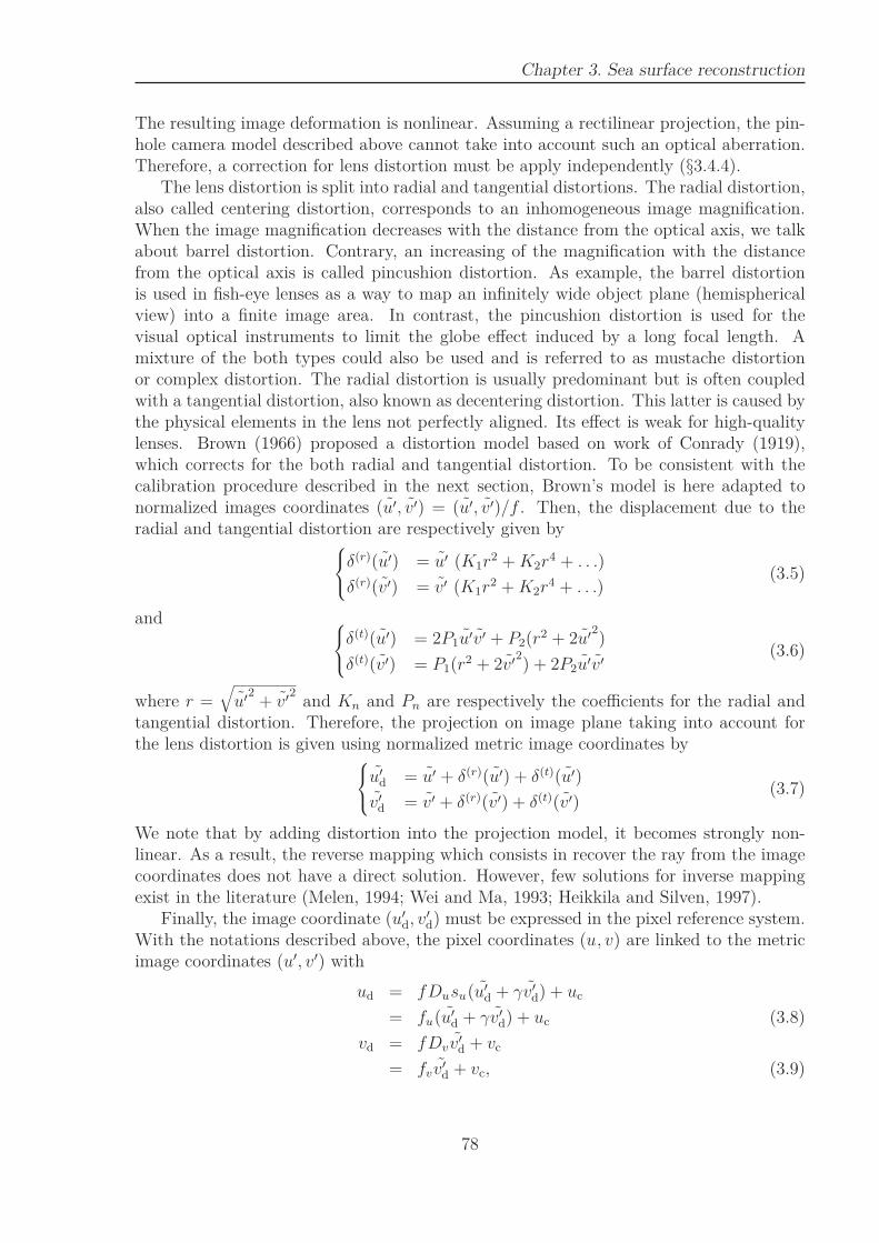
Chapter 3. Sea surface reconstruction
The resulting image deformation is nonlinear. Assuming a rectilinear projection, the pin-hole camera model described above cannot take into account such an optical aberration.Therefore, a correction for lens distortion must be apply independently (§3.4.4).
The lens distortion is split into radial and tangential distortions. The radial distortion,also called centering distortion, corresponds to an inhomogeneous image magnification.When the image magnification decreases with the distance from the optical axis, we talkabout barrel distortion. Contrary, an increasing of the magnification with the distancefrom the optical axis is called pincushion distortion. As example, the barrel distortionis used in fish-eye lenses as a way to map an infinitely wide object plane (hemisphericalview) into a finite image area. In contrast, the pincushion distortion is used for thevisual optical instruments to limit the globe effect induced by a long focal length. Amixture of the both types could also be used and is referred to as mustache distortionor complex distortion. The radial distortion is usually predominant but is often coupledwith a tangential distortion, also known as decentering distortion. This latter is caused bythe physical elements in the lens not perfectly aligned. Its effect is weak for high-qualitylenses. Brown (1966) proposed a distortion model based on work of Conrady (1919),which corrects for the both radial and tangential distortion. To be consistent with thecalibration procedure described in the next section, Brown’s model is here adapted tonormalized images coordinates (u′, v′) = (u′, v′)/f . Then, the displacement due to theradial and tangential distortion are respectively given by
δ(r)(u′) = u′ (K1r2 +K2r
4 + . . .)
δ(r)(v′) = v′ (K1r2 +K2r
4 + . . .)(3.5)
and
δ(t)(u′) = 2P1u′v′ + P2(r2 + 2u′
2)
δ(t)(v′) = P1(r2 + 2v′
2) + 2P2u′v′
(3.6)
where r =√
u′2
+ v′2
and Kn and Pn are respectively the coefficients for the radial andtangential distortion. Therefore, the projection on image plane taking into account forthe lens distortion is given using normalized metric image coordinates by
u′
d = u′ + δ(r)(u′) + δ(t)(u′)
v′
d = v′ + δ(r)(v′) + δ(t)(v′)(3.7)
We note that by adding distortion into the projection model, it becomes strongly non-linear. As a result, the reverse mapping which consists in recover the ray from the imagecoordinates does not have a direct solution. However, few solutions for inverse mappingexist in the literature (Melen, 1994; Wei and Ma, 1993; Heikkila and Silven, 1997).
Finally, the image coordinate (u′
d, v′
d) must be expressed in the pixel reference system.With the notations described above, the pixel coordinates (u, v) are linked to the metricimage coordinates (u′, v′) with
ud = fDusu(u′
d + γv′
d) + uc
= fu(u′
d + γv′
d) + uc (3.8)
vd = fDv v′
d + vc
= fv v′
d + vc, (3.9)
78
3.3 Theoretical background
where fu = Dusuf and fv = Dvf are the unique focal metric distance f expressed interm of pixels in each direction. When the pixels in the CCD sensor are not perfectlysquare, the aspect ratio, Dv/(suDu) = fv/fu , differs from 1. Nevertheless, the recent highquality CCD manufacturing leads to an aspect ratio close to 1 (fu and fv are usually verysimilar). Moreover, the high quality manufacturing also leads to skew factor close to 0.
The computer vision science usually used the homogeneous coordinates, which con-sists in the expression of the coordinates with an additional dimension, such that thehomogeneous 3D points coordinates in world reference system (resp. in camera referencesystem) are given by vector [Xw, Yw, Zw, 1]T (resp. [Xc, Yc, Zc, 1]T). Then, neglecting thedistortion, the projection of a scene points into the bit-mapped image can be representedwith a 3 × 4 matrix C, called the camera matrix such that
Zc
uv1
= C ∗
Xw
Yw
Zw
1
= A[
R T]
Xw
Yw
Zw
1
(3.10)
where R and T are the external parameters (see Eq. 3.2) and A is the matrix containingthe intrinsic parameters such that
Zc
uv1
= A
Xc
Yc
Zc
, (3.11)
with
A =
Dusuf Dusufγ uc
0 Dvf vc
0 0 1
=
fu fuγ uc
0 fv vc
0 0 1
, (3.12)
As previously discussed, the coordinates of a points, given coordinates of its projection,are given by
Xc
Yc
Zc
= α C−1
uv1
. (3.13)
We note that the ray where are all the possible positions of the point is then given byvarying α, and coordinates of the 3D point are given by α = Zc, which is generallyunknown. The equation 3.13 is the linear solution for the inverse mapping usually used incomputer vision. Nevertheless, as noted, by including distortion, the projection becomesnon-linear (C = C(u, v)). As a result, the camera matrix C cannot be inversed and theequation 3.13 cannot be applied. A way around the problem is to use the equation on arectified image corrected for the lens distortion (see §3.4.4).
3.3.3 Epipolar geometry and stereo triangulation
Given two (or more) cameras with distinct projection centers, the epipolar geometrydescribes geometric constraints existing between the cameras. This geometry is based onthe pinhole camera model, so the distortion must be neglected or previously corrected
79
Chapter 3. Sea surface reconstruction
(see §3.4.4). The example for two cameras is shown on the figure 3.6, where the centers ofprojection of the cameras are the points C1 and C2. We suppose the external parameters(R1, T1) and (R2, T2). We note that the world reference system can be defined as equalto the reference system of the first camera. Therefore, R1 = I3 and T1 = [0, 0, 0]T, and(R2, T2) represent the relative positions of the cameras. We define the epipolar points (e1,e2) as the intersection of the line (C1C2) with the image planes. These epipolar pointsgenerally fall out of the bit-mapped image. For each point P of the scene, the correspond-ing epipolar plane is defined by the three points (C1, C2, P ). This plane intersects the leftand right image planes in lines, called epipolar lines.
Projecting on the first image plane onto p1, the corresponding scene point P must beon the ray (C1, p1). Therefore, its projection on the second image must be on the epipolarline, which corresponds to the projection of the ray. This property is used in the pointmatching step of the reconstruction processing, described further, to reduce search areaof the corresponding points (see §3.5.1). Inversely, given p1 and p2 the projections of asame scene points P into the image 1 and 2 respectively, the 3D location of the point P isfully determined by the intersection of the rays (C1, p1) and (C2, p2). The determinationof the 3D coordinates of a point from its projections onto two images is called stereotriangulation (see §3.5.2).
3.4 Camera calibration and image rectification
The aim of the camera calibration is to compute the intrinsic and extrinsic cameraparameters disused in paragraph 3.3. The performances of the WASS are inevitablyrelated to the camera calibration accuracy which is described in this paragraph. Aftera short history on the evolution of calibration methods, a detailed description of thecalibration procedures, for the intrinsic and extrinsic calibration, used in this work forWASS calibration are given.
3.4.1 Short historical of camera calibrations
Throughout the years, many authors proposed many methods following the growingneed of accuracy and image sensor evolution. We must note the strong influence of theworks of Tsai (1987) on the recent camera calibration methods. The previous methodscould be simply classified into two categories. The first category involves full scale nonlin-ear optimization, allowing easy adaptation of any arbitrarily complex model for imaging,including obviously the lens distortion. Nevertheless, this adaptability is made at thecost of a large set of non-physical implicit parameters. Moreover, these implicit methodsrequire a good initial guess to start computing. In contrast, the second category regroupsthe computationally efficient explicit methods that solve only linear equations related tophysical parameters. These methods have generally a number of unknowns much largerthan the degrees of freedom. Moreover, no nonlinear search entails that the effect of thelens distortion cannot be considered. These linear solutions do not provide as good resultsas nonlinear minimization.
Mixing these two approaches, Tsai (1987) proposed an autonomous, accurate, reason-
80
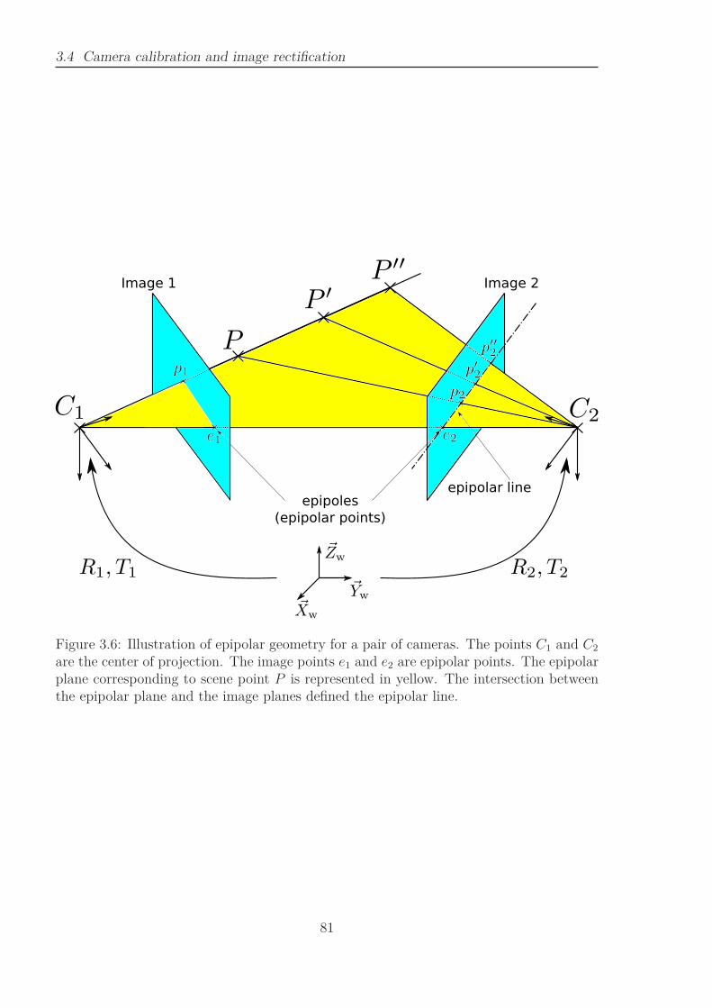
3.4 Camera calibration and image rectification
epipolar lineepipoles
(epipolar points)
Image 1 Image 2
Figure 3.6: Illustration of epipolar geometry for a pair of cameras. The points C1 and C2
are the center of projection. The image points e1 and e2 are epipolar points. The epipolarplane corresponding to scene point P is represented in yellow. The intersection betweenthe epipolar plane and the image planes defined the epipolar line.
81
Chapter 3. Sea surface reconstruction
ably efficient and versatile two-step method applicable to any type of camera, whereasmost of previous methods require professional cameras and processing equipment. Ap-proximating the intrinsic parameters to the manufacturing given values, the first stageconsists in a linear approximation of the parameters. In the second stage, the optimizedsolution is computed with a standard optimization scheme, using as guess null distortion(K1 = 0) and the parameter approximations previously computed in the first step. Even ifa reduction of the lens effect to this first radial component limits the method accuracy, thiskind of two-step method (the linear approximation is the guess for the nonlinear optimiza-tion) still today the groundwork of most of the recent calibration procedures. Heikkilaand Silven (1997) further improved calibration by including the asymmetric projectioncorrection. We note that the historical development of camera calibration techniques withan exhaustive literature survey can be found in Clarke and Fryer (1998).
Numerous calibration tools are available today (Heikkila and Silven, 1997; Vezhnevets,2005; Strobl et al., 2006; Scaramuzza et al., 2006; Stoyanov, 2010, and many others). Forthis work, the WASS calibration was done using the Camera Calibration Toolbox forMatlab R© written by Jean-Yves Bouguet which proposes interesting additional tools, suchas corner extraction and visual check routines. As the overall accuracy of the surfacereconstruction is interconnected with the accuracy of the camera calibration, the detailson both operator procedure and calibration code as written by Jean-Yves Bouguet aregiven.
3.4.2 Camera intrinsic calibration
The intrinsic parameters, which link a 3D point in the camera reference system to itsprojection in the bit-mapped image reference system, must be firstly defined. Driven bythe association of a given Charge-Coupled Device (CCD) with a given lens, the intrinsiccalibration is done independently for each camera with an identical processing. A large setof calibration images containing a square-chessboard at various distances are taken (seeFig. 3.7). Precisely, more than 1000 images are selected for each camera. Two chessboardswith 30mm and 80mm square size were used. We note that chessboard corners correspondto a coplanar set of points.
Since the coordinates of the chessboards are not initially known in the camera referencesystem, the extrinsic parameters must be also estimated. The intrinsic parameters do notdepend on the extrinsic ones. This allows us to define an independent world coordinatesystem for each image. Conveniently, the world systems are fixed such that the Xw-axis and Yw-axis are collinear to the square sides of the chessboard and the origin is thecenter of the up-left corner (see Fig. 3.7, up-left panel). Therefore, the corner worldcoordinates are well known in its corresponding reference system and depend only on thechessboard square size, dX. In a second step, the coordinates of the corner projectionsmust be extracted from images. The human influence on the processing is limited to arough estimation of the four extreme corners of the chessboard. An automatic mechanismthen counts squares in each direction and deduces approximate locations of the projectedcorners. Finally, the sub-pixel corner coordinates are computed using gradients. A visualcheck is done by the operator. At the end, for each image, a set of coplanar 3D points andtheir projection on the images are stored. Following the previous notations, a corner point
82
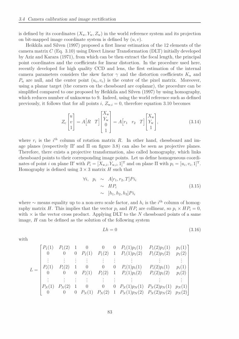
3.4 Camera calibration and image rectification
is defined by its coordinates (Xw, Yw, Zw) in the world reference system and its projectionon bit-mapped image coordinate system is defined by (u, v).
Heikkila and Silven (1997) proposed a first linear estimation of the 12 elements of thecamera matrix C (Eq. 3.10) using Direct Linear Transformation (DLT) initially developedby Aziz and Karara (1971), from which can be then extract the focal length, the principalpoint coordinates and the coefficients for linear distortion. In the procedure used here,recently developed for high quality CCD and lens, the first estimation of the internalcamera parameters considers the skew factor γ and the distortion coefficients Kn andPn are null, and the center point (uc, vc) is the center of the pixel matrix. Moreover,using a planar target (the corners on the chessboard are coplanar), the procedure can besimplified compared to one proposed by Heikkila and Silven (1997) by using homography,which reduces number of unknowns to 9. Indeed, using the world reference such as definedpreviously, it follows that for all points i, Zw,i = 0, therefore equation 3.10 becomes
Zc
uv1
= A[
R T]
Xw
Yw
01
= A[
r1 r2 T]
Xw
Yw
1
, (3.14)
where ri is the ith column of rotation matrix R. In other hand, chessboard and im-age planes (respectively Π′ and Π on figure 3.8) can also be seen as projective planes.Therefore, there exists a projective transformation, also called homography, which linkschessboard points to their corresponding image points. Let us define homogeneous coordi-nates of point i on plane Π′ with Pi = [Xw,i, Yw,i, 1]T and on plane Π with pi = [ui, vi, 1]T.Homography is defined using 3 × 3 matrix H such that
∀i, pi ∼ A[r1, r2, T ]Pii
∼ HPi (3.15)
∼ [h1, h2, h3]Pii
where ∼ means equality up to a non-zero scale factor, and hi is the ith column of homog-raphy matrix H. This implies that the vector pi and HPi are collinear, so pi ×HPi = 0,with × is the vector cross product. Applying DLT to the N chessboard points of a sameimage, H can be defined as the solution of the following system
Lh = 0 (3.16)
with
L =
P1(1) P1(2) 1 0 0 0 P1(1)p1(1) P1(2)p1(1) p1(1)0 0 0 P1(1) P1(2) 1 P1(1)p1(2) P1(2)p1(2) p1(2)...
......
......
......
......
Pi(1) Pi(2) 1 0 0 0 Pi(1)pi(1) Pi(2)pi(1) pi(1)0 0 0 Pi(1) Pi(2) 1 Pi(1)pi(2) Pi(2)pi(2) pi(2)...
......
......
......
......
PN(1) PN(2) 1 0 0 0 PN(1)pN(1) PN(2)pN(1) pN(1)0 0 0 PN(1) PN(2) 1 PN(1)pN(2) PN(2)pN(2) pN(2)
83
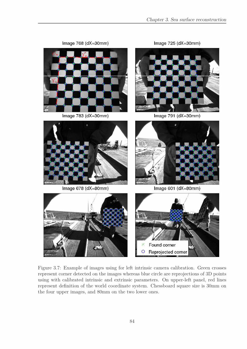
Chapter 3. Sea surface reconstruction
Figure 3.7: Example of images using for left intrinsic camera calibration. Green crossesrepresent corner detected on the images whereas blue circle are reprojections of 3D pointsusing with calibrated intrinsic and extrinsic parameters. On upper-left panel, red linesrepresent definition of the world coordinate system. Chessboard square size is 30mm onthe four upper images, and 80mm on the two lower ones.
84
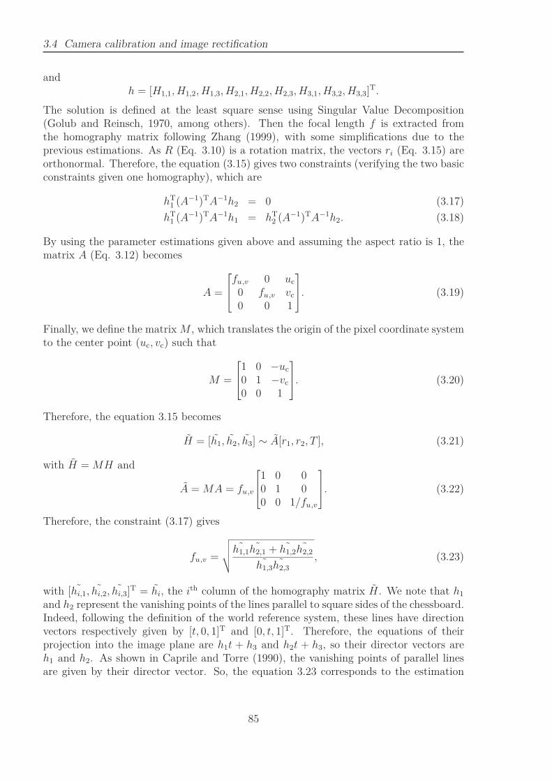
3.4 Camera calibration and image rectification
andh = [H1,1, H1,2, H1,3, H2,1, H2,2, H2,3, H3,1, H3,2, H3,3]T.
The solution is defined at the least square sense using Singular Value Decomposition(Golub and Reinsch, 1970, among others). Then the focal length f is extracted fromthe homography matrix following Zhang (1999), with some simplifications due to theprevious estimations. As R (Eq. 3.10) is a rotation matrix, the vectors ri (Eq. 3.15) areorthonormal. Therefore, the equation (3.15) gives two constraints (verifying the two basicconstraints given one homography), which are
hT1 (A−1)TA−1h2 = 0 (3.17)
hT1 (A−1)TA−1h1 = hT
2 (A−1)TA−1h2. (3.18)
By using the parameter estimations given above and assuming the aspect ratio is 1, thematrix A (Eq. 3.12) becomes
A =
fu,v 0 uc
0 fu,v vc
0 0 1
. (3.19)
Finally, we define the matrix M , which translates the origin of the pixel coordinate systemto the center point (uc, vc) such that
M =
1 0 −uc
0 1 −vc
0 0 1
. (3.20)
Therefore, the equation 3.15 becomes
H = [h1, h2, h3] ∼ A[r1, r2, T ], (3.21)
with H = MH and
A = MA = fu,v
1 0 00 1 00 0 1/fu,v
. (3.22)
Therefore, the constraint (3.17) gives
fu,v =
√
√
√
√
˜h1,1˜h2,1 + ˜h1,2
˜h2,2
˜h1,3˜h2,3
, (3.23)
with [hi,1, hi,2, hi,3]T = hi, the ith column of the homography matrix H. We note that h1
and h2 represent the vanishing points of the lines parallel to square sides of the chessboard.Indeed, following the definition of the world reference system, these lines have directionvectors respectively given by [t, 0, 1]T and [0, t, 1]T. Therefore, the equations of theirprojection into the image plane are h1t + h3 and h2t + h3, so their director vectors areh1 and h2. As shown in Caprile and Torre (1990), the vanishing points of parallel linesare given by their director vector. So, the equation 3.23 corresponds to the estimation
85
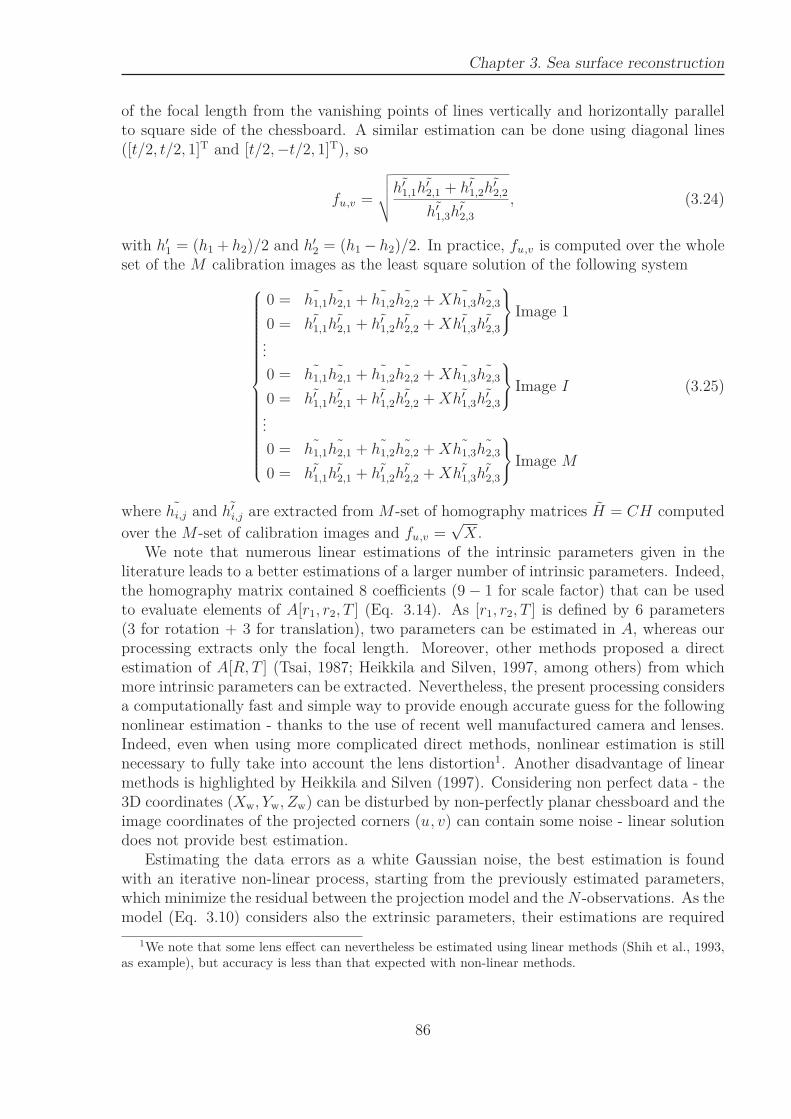
Chapter 3. Sea surface reconstruction
of the focal length from the vanishing points of lines vertically and horizontally parallelto square side of the chessboard. A similar estimation can be done using diagonal lines([t/2, t/2, 1]T and [t/2,−t/2, 1]T), so
fu,v =
√
√
√
√
˜h′
1,1˜h′
2,1 + ˜h′
1,2˜h′
2,2
˜h′
1,3˜h′
2,3
, (3.24)
with h′
1 = (h1 + h2)/2 and h′
2 = (h1 − h2)/2. In practice, fu,v is computed over the wholeset of the M calibration images as the least square solution of the following system
0 = ˜h1,1˜h2,1 + ˜h1,2
˜h2,2 +X ˜h1,3˜h2,3
0 = ˜h′
1,1˜h′
2,1 + ˜h′
1,2˜h′
2,2 +X ˜h′
1,3˜h′
2,3
Image 1
...
0 = ˜h1,1˜h2,1 + ˜h1,2
˜h2,2 +X ˜h1,3˜h2,3
0 = ˜h′
1,1˜h′
2,1 + ˜h′
1,2˜h′
2,2 +X ˜h′
1,3˜h′
2,3
Image I
...
0 = ˜h1,1˜h2,1 + ˜h1,2
˜h2,2 +X ˜h1,3˜h2,3
0 = ˜h′
1,1˜h′
2,1 + ˜h′
1,2˜h′
2,2 +X ˜h′
1,3˜h′
2,3
Image M
(3.25)
where hi,j and h′
i,j are extracted from M -set of homography matrices H = CH computed
over the M -set of calibration images and fu,v =√X.
We note that numerous linear estimations of the intrinsic parameters given in theliterature leads to a better estimations of a larger number of intrinsic parameters. Indeed,the homography matrix contained 8 coefficients (9 − 1 for scale factor) that can be usedto evaluate elements of A[r1, r2, T ] (Eq. 3.14). As [r1, r2, T ] is defined by 6 parameters(3 for rotation + 3 for translation), two parameters can be estimated in A, whereas ourprocessing extracts only the focal length. Moreover, other methods proposed a directestimation of A[R, T ] (Tsai, 1987; Heikkila and Silven, 1997, among others) from whichmore intrinsic parameters can be extracted. Nevertheless, the present processing considersa computationally fast and simple way to provide enough accurate guess for the followingnonlinear estimation - thanks to the use of recent well manufactured camera and lenses.Indeed, even when using more complicated direct methods, nonlinear estimation is stillnecessary to fully take into account the lens distortion1. Another disadvantage of linearmethods is highlighted by Heikkila and Silven (1997). Considering non perfect data - the3D coordinates (Xw, Yw, Zw) can be disturbed by non-perfectly planar chessboard and theimage coordinates of the projected corners (u, v) can contain some noise - linear solutiondoes not provide best estimation.
Estimating the data errors as a white Gaussian noise, the best estimation is foundwith an iterative non-linear process, starting from the previously estimated parameters,which minimize the residual between the projection model and the N -observations. As themodel (Eq. 3.10) considers also the extrinsic parameters, their estimations are required
1We note that some lens effect can nevertheless be estimated using linear methods (Shih et al., 1993,as example), but accuracy is less than that expected with non-linear methods.
86
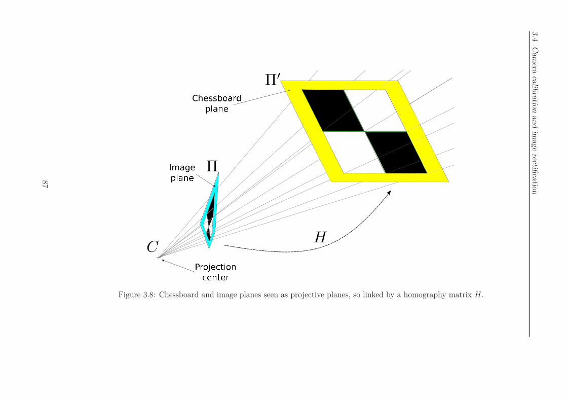
3.4
Cam
eraca
libra
tion
and
image
rectifica
tion
Image
Chess
Figure 3.8: Chessboard and image planes seen as projective planes, so linked by a homography matrix H.
87

Chapter 3. Sea surface reconstruction
to start the non-linear error minimization. The extrinsic parameters differs between thecalibration images (world system depends on chessboard position), and so are estimatedindependently for each image. As the intrinsic parameters are now estimated, the imagecoordinates can be normalized with
u′ = (u − uc)/fu,v
v′ = (v − vc)/fu,v .(3.26)
The origin of the world coordinate system is translated to the barycenter of points with
Xw = Xw −Xw
Yw = Yw − Yw
Zw = Zw = 0.
(3.27)
Then the homography H between normalized coordinates is computed using same methodas previously. Using the normalized pixel coordinates, the equation 3.15 becomes αH =[r1, r2, T ], with α an ignoring factor. An approximation of this factor is given by α =1/2(||r1|| + ||r2||) where ||X|| means the norm of the column vector X. Therefore, theapproximated extrinsic parameters R and T are get using
r1 = αh1 (3.28)
r1 = r1/||r1|| (3.29)
r2 = h2 − (r1 · h2)r1 (ensures orthogonality) (3.30)
r2 = r2/||r2|| (3.31)
r3 = r1 × r2 (r3 finishes orthonormal basis). (3.32)
R = [r1, r2, r3] (3.33)
T = h3 (3.34)
where · and × are respectively vector dot and cross product. Theses estimations beingvery poor due to poor approximation of factor α, a refinement is done using minimizationof the reprojection error. The iterative non-linear least square optimization processing isnow described in detail using the external parameter refinements as example. A similarprocessing will be used further for the intrinsic parameter refinements. Remember that therotation matrix is defined by the 3 angles: θ (roll), φ (pitch), ψ (yaw) and T = [t1, t2, t3]
T.From the world coordinates (Xw,i, Yw,i, Zw,i) of each point i, the coordinates (up,i, vp,i) ofthe corresponding projection are computed using equation 3.10. So, the residual (error) rcan be estimated for each point i with ri = (ui − up,i, vi − vp,i). The solution in the leastsquares sense, is the set of n parameters βj=1,...,n (here there are n parameters: θ, φ, ψ,t1, t2, t3) which minimize the sum S of the squares residuals,
S =N∑
i=1
||ri||. (3.35)
The minimum value of S occurs when all its partial derivatives with respect to the 6external parameters are zero: ∀i ∈ [1, n],
∂S
∂βj= 2
N∑
i=1
ri∂ri∂βj
= 0 (3.36)
88
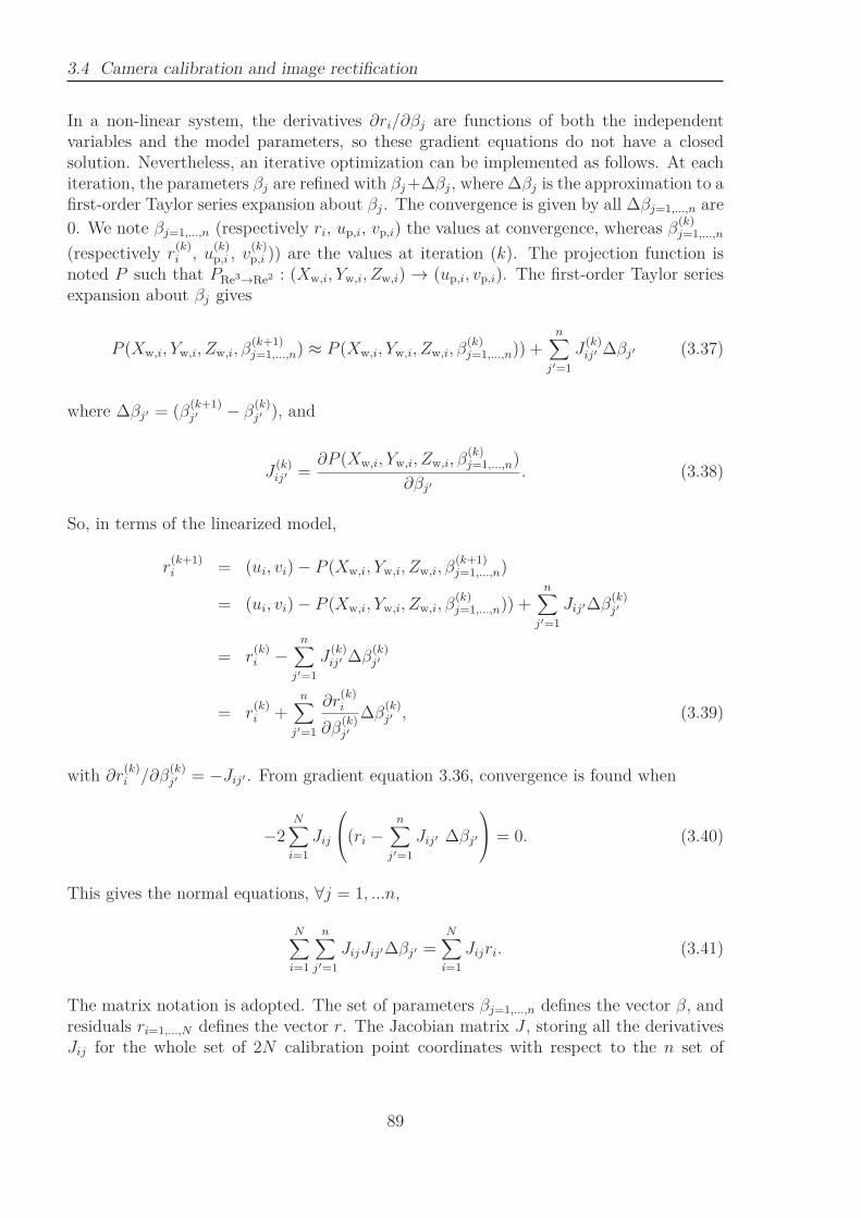
3.4 Camera calibration and image rectification
In a non-linear system, the derivatives ∂ri/∂βj are functions of both the independentvariables and the model parameters, so these gradient equations do not have a closedsolution. Nevertheless, an iterative optimization can be implemented as follows. At eachiteration, the parameters βj are refined with βj+∆βj, where ∆βj is the approximation to afirst-order Taylor series expansion about βj. The convergence is given by all ∆βj=1,...,n are
0. We note βj=1,...,n (respectively ri, up,i, vp,i) the values at convergence, whereas β(k)j=1,...,n
(respectively r(k)i , u
(k)p,i , v
(k)p,i )) are the values at iteration (k). The projection function is
noted P such that PRe3→Re2 : (Xw,i, Yw,i, Zw,i) → (up,i, vp,i). The first-order Taylor series
expansion about βj gives
P (Xw,i, Yw,i, Zw,i, β(k+1)j=1,...,n) ≈ P (Xw,i, Yw,i, Zw,i, β
(k)j=1,...,n)) +
n∑
j′=1
J(k)ij′ ∆βj′ (3.37)
where ∆βj′ = (β(k+1)j′ − β
(k)j′ ), and
J(k)ij′ =
∂P (Xw,i, Yw,i, Zw,i, β(k)j=1,...,n)
∂βj′
. (3.38)
So, in terms of the linearized model,
r(k+1)i = (ui, vi) − P (Xw,i, Yw,i, Zw,i, β
(k+1)j=1,...,n)
= (ui, vi) − P (Xw,i, Yw,i, Zw,i, β(k)j=1,...,n)) +
n∑
j′=1
Jij′∆β(k)j′
= r(k)i −
n∑
j′=1
J(k)ij′ ∆β
(k)j′
= r(k)i +
n∑
j′=1
∂r(k)i
∂β(k)j′
∆β(k)j′ , (3.39)
with ∂r(k)i /∂β
(k)j′ = −Jij′ . From gradient equation 3.36, convergence is found when
−2N∑
i=1
Jij
(ri −n∑
j′=1
Jij′ ∆βj′
= 0. (3.40)
This gives the normal equations, ∀j = 1, ...n,
N∑
i=1
n∑
j′=1
JijJij′∆βj′ =N∑
i=1
Jijri. (3.41)
The matrix notation is adopted. The set of parameters βj=1,...,n defines the vector β, andresiduals ri=1,...,N defines the vector r. The Jacobian matrix J , storing all the derivativesJij for the whole set of 2N calibration point coordinates with respect to the n set of
89
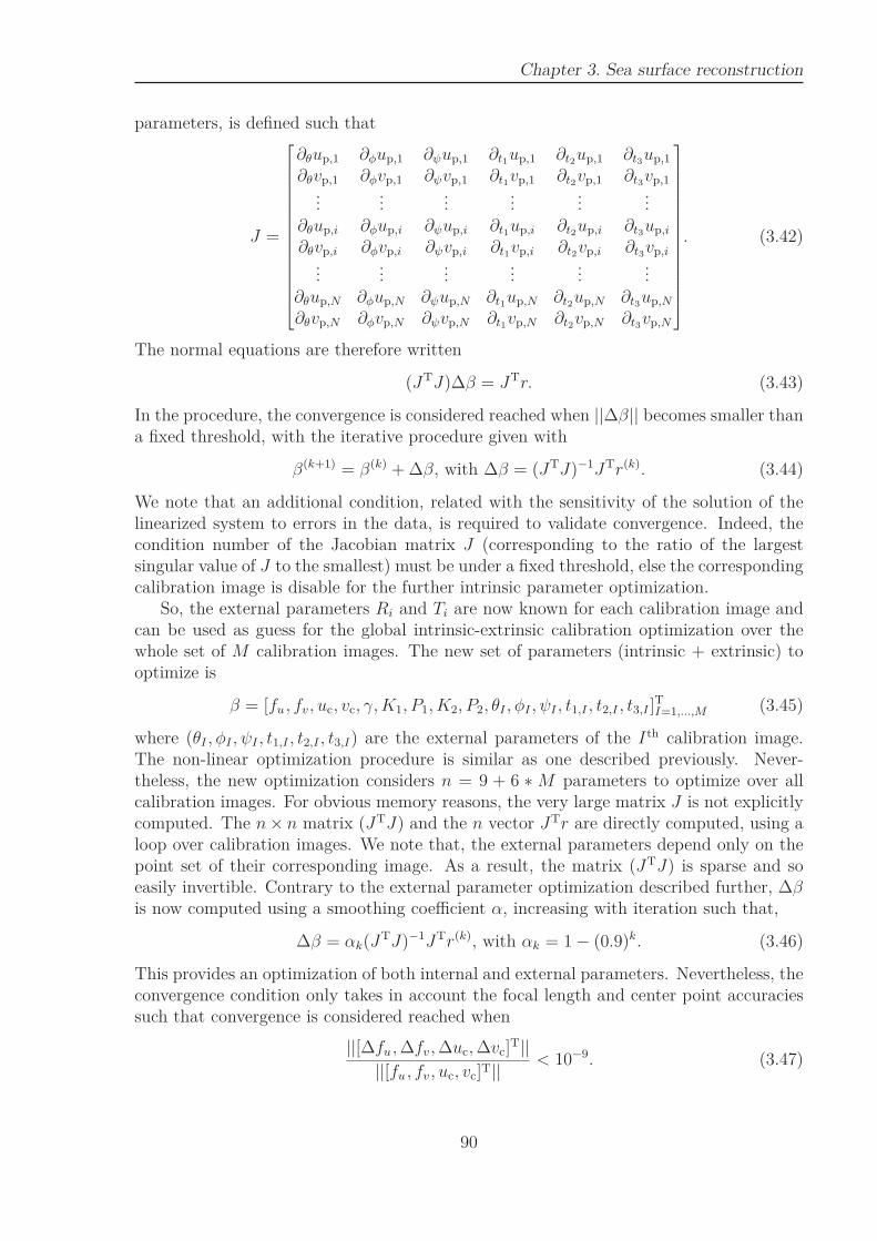
Chapter 3. Sea surface reconstruction
parameters, is defined such that
J =
∂θup,1 ∂φup,1 ∂ψup,1 ∂t1up,1 ∂t2up,1 ∂t3up,1
∂θvp,1 ∂φvp,1 ∂ψvp,1 ∂t1vp,1 ∂t2vp,1 ∂t3vp,1...
......
......
...∂θup,i ∂φup,i ∂ψup,i ∂t1up,i ∂t2up,i ∂t3up,i
∂θvp,i ∂φvp,i ∂ψvp,i ∂t1vp,i ∂t2vp,i ∂t3vp,i...
......
......
...∂θup,N ∂φup,N ∂ψup,N ∂t1up,N ∂t2up,N ∂t3up,N
∂θvp,N ∂φvp,N ∂ψvp,N ∂t1vp,N ∂t2vp,N ∂t3vp,N
. (3.42)
The normal equations are therefore written
(JTJ)∆β = JTr. (3.43)
In the procedure, the convergence is considered reached when ||∆β|| becomes smaller thana fixed threshold, with the iterative procedure given with
β(k+1) = β(k) + ∆β, with ∆β = (JTJ)−1JTr(k). (3.44)
We note that an additional condition, related with the sensitivity of the solution of thelinearized system to errors in the data, is required to validate convergence. Indeed, thecondition number of the Jacobian matrix J (corresponding to the ratio of the largestsingular value of J to the smallest) must be under a fixed threshold, else the correspondingcalibration image is disable for the further intrinsic parameter optimization.
So, the external parameters Ri and Ti are now known for each calibration image andcan be used as guess for the global intrinsic-extrinsic calibration optimization over thewhole set of M calibration images. The new set of parameters (intrinsic + extrinsic) tooptimize is
β = [fu , fv , uc, vc, γ,K1, P1, K2, P2, θI , φI , ψI , t1,I , t2,I , t3,I ]TI=1,...,M (3.45)
where (θI , φI , ψI , t1,I , t2,I , t3,I) are the external parameters of the Ith calibration image.The non-linear optimization procedure is similar as one described previously. Never-theless, the new optimization considers n = 9 + 6 ∗ M parameters to optimize over allcalibration images. For obvious memory reasons, the very large matrix J is not explicitlycomputed. The n× n matrix (JTJ) and the n vector JTr are directly computed, using aloop over calibration images. We note that, the external parameters depend only on thepoint set of their corresponding image. As a result, the matrix (JTJ) is sparse and soeasily invertible. Contrary to the external parameter optimization described further, ∆βis now computed using a smoothing coefficient α, increasing with iteration such that,
∆β = αk(JTJ)−1JTr(k), with αk = 1 − (0.9)k. (3.46)
This provides an optimization of both internal and external parameters. Nevertheless, theconvergence condition only takes in account the focal length and center point accuraciessuch that convergence is considered reached when
||[∆fu ,∆fv ,∆uc,∆vc]T||
||[fu , fv , uc, vc]T|| < 10−9. (3.47)
90
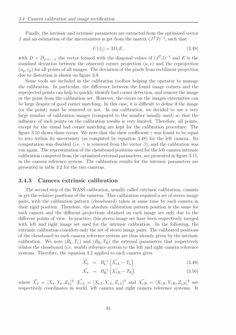
3.4 Camera calibration and image rectification
Finally, the intrinsic and extrinsic parameters are extracted from the optimized vectorβ and an estimation of the uncertainties is get from the matrix (JTJ)−1, such that
U(βj) = 3DjE, (3.48)
with D = Dj=1,...,n the vector formed with the diagonal values of (JTJ)−1 and E is thestandard deviation between the observed corner projection (u, v) and the reprojection(up, vp) for all points of all images. The deviation of the pixels from rectilinear projectiondue to distortion is shown on figure 3.9.
Some tools are included in the calibration toolbox helping the operator to managethe calibration. In particular, the difference between the found image corners and thereprojected points can help to quickly identify bad corner detection, and remove the imageor the point from the calibration set. However, the errors on the images extremities canbe large despite of good corner matching. In this case, it is difficult to define if the image(or the point) must be removed or not. In our calibration, we decided to use a verylarge number of calibration images (compared to the number usually used) so that theinfluence of such points on the calibration results is very limited. Therefore, all points,except for the visual bad corner matching are kept for the calibration procedure. Thefigure 3.10 shows these errors. We note that the skew coefficient γ was found to be equalto zero within its uncertainty (as computed by equation 3.48) for the left camera. Itscomputation was disabled (i.e. γ is removed from the vector β), and the calibration wasrun again. The representation of the chessboard positions used for the left camera intrinsiccalibration computed from the optimized external parameters, are presented in figure 3.11,in the camera reference system. The calibration results for the intrinsic parameters arepresented in table 3.2 for the two cameras.
3.4.3 Camera extrinsic calibration
The second step of the WASS calibration, usually called extrinsic calibration, consistsin get the relative positions of the cameras. This calibration required a set of stereo imagepairs, with the calibration pattern (chessboard) taken at same time by each camera intheir rigid position. Therefore, the absolute calibration pattern position is the same foreach camera and the different projections obtained on each image are only due to thedifferent points of view. In practice, this stereo image set have been respectively mergedwith left and right image set used for the intrinsic calibration. In the following, theextrinsic calibration considers only the set of stereo image pairs. The calibrated positionsof the chessboard in each camera reference system are thus already given by the intrinsiccalibration. We note (RL, TL) and (RR, TR) the external parameters that respectivelyrelates the chessboard (i.e. world) reference system to the left and right camera referencesystems. Therefore, the equation 3.2 applied to each camera gives
~Xw = R−1L
(
~Xc,L − TL
)
(3.49)
~Xw = R−1R
(
~Xc,R − TR
)
(3.50)
where ~Xw = [Xw, Yw, Zw]T ~Xc,L = [Xc,L, Yc,L, Zc,L]T and ~Xc,R = [Xc,R, Yc,R, Zc,R]T arerespectively coordinates in world, left camera and right camera reference systems. It
91
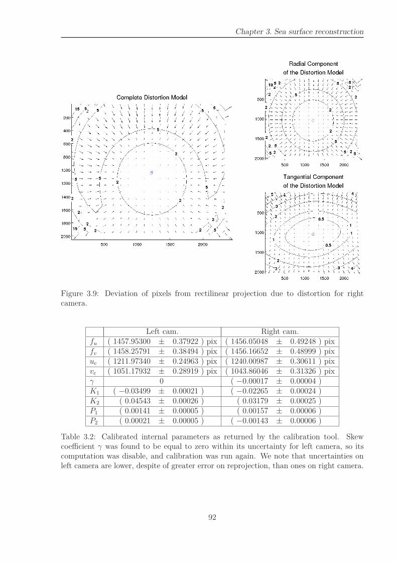
Chapter 3. Sea surface reconstruction
Figure 3.9: Deviation of pixels from rectilinear projection due to distortion for rightcamera.
Left cam. Right cam.fu ( 1457.95300 ± 0.37922 ) pix ( 1456.05048 ± 0.49248 ) pixfv ( 1458.25791 ± 0.38494 ) pix ( 1456.16652 ± 0.48999 ) pixuc ( 1211.97340 ± 0.24963 ) pix ( 1240.00987 ± 0.30611 ) pixvc ( 1051.17932 ± 0.28919 ) pix ( 1043.86046 ± 0.31326 ) pixγ 0 ( −0.00017 ± 0.00004 )K1 ( −0.03499 ± 0.00021 ) ( −0.02265 ± 0.00024 )K2 ( 0.04543 ± 0.00026 ) ( 0.03179 ± 0.00025 )P1 ( 0.00141 ± 0.00005 ) ( 0.00157 ± 0.00006 )P2 ( 0.00021 ± 0.00005 ) ( −0.00143 ± 0.00006 )
Table 3.2: Calibrated internal parameters as returned by the calibration tool. Skewcoefficient γ was found to be equal to zero within its uncertainty for left camera, so itscomputation was disable, and calibration was run again. We note that uncertainties onleft camera are lower, despite of greater error on reprojection, than ones on right camera.
92
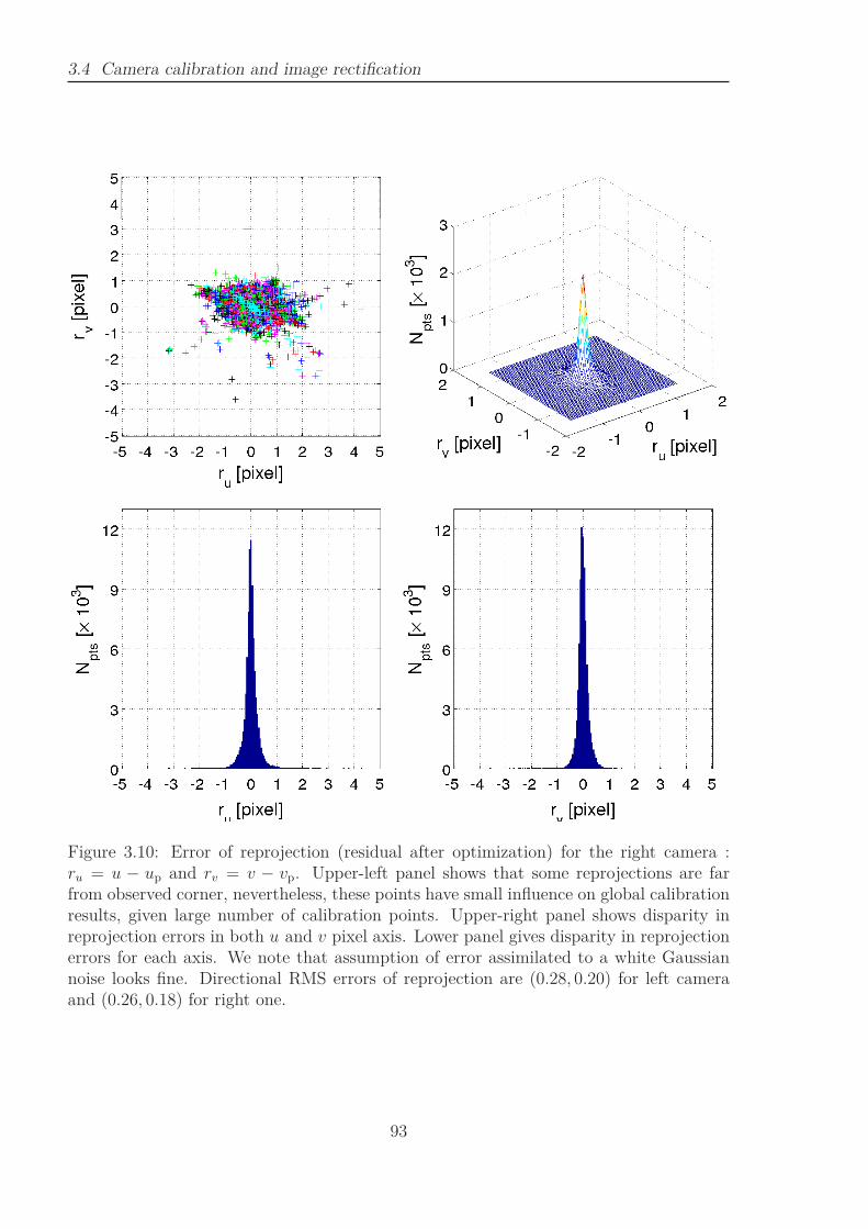
3.4 Camera calibration and image rectification
Figure 3.10: Error of reprojection (residual after optimization) for the right camera :ru = u − up and rv = v − vp. Upper-left panel shows that some reprojections are farfrom observed corner, nevertheless, these points have small influence on global calibrationresults, given large number of calibration points. Upper-right panel shows disparity inreprojection errors in both u and v pixel axis. Lower panel gives disparity in reprojectionerrors for each axis. We note that assumption of error assimilated to a white Gaussiannoise looks fine. Directional RMS errors of reprojection are (0.28, 0.20) for left cameraand (0.26, 0.18) for right one.
93
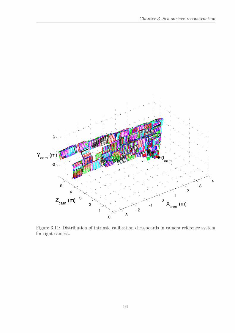
Chapter 3. Sea surface reconstruction
Figure 3.11: Distribution of intrinsic calibration chessboards in camera reference systemfor right camera.
94
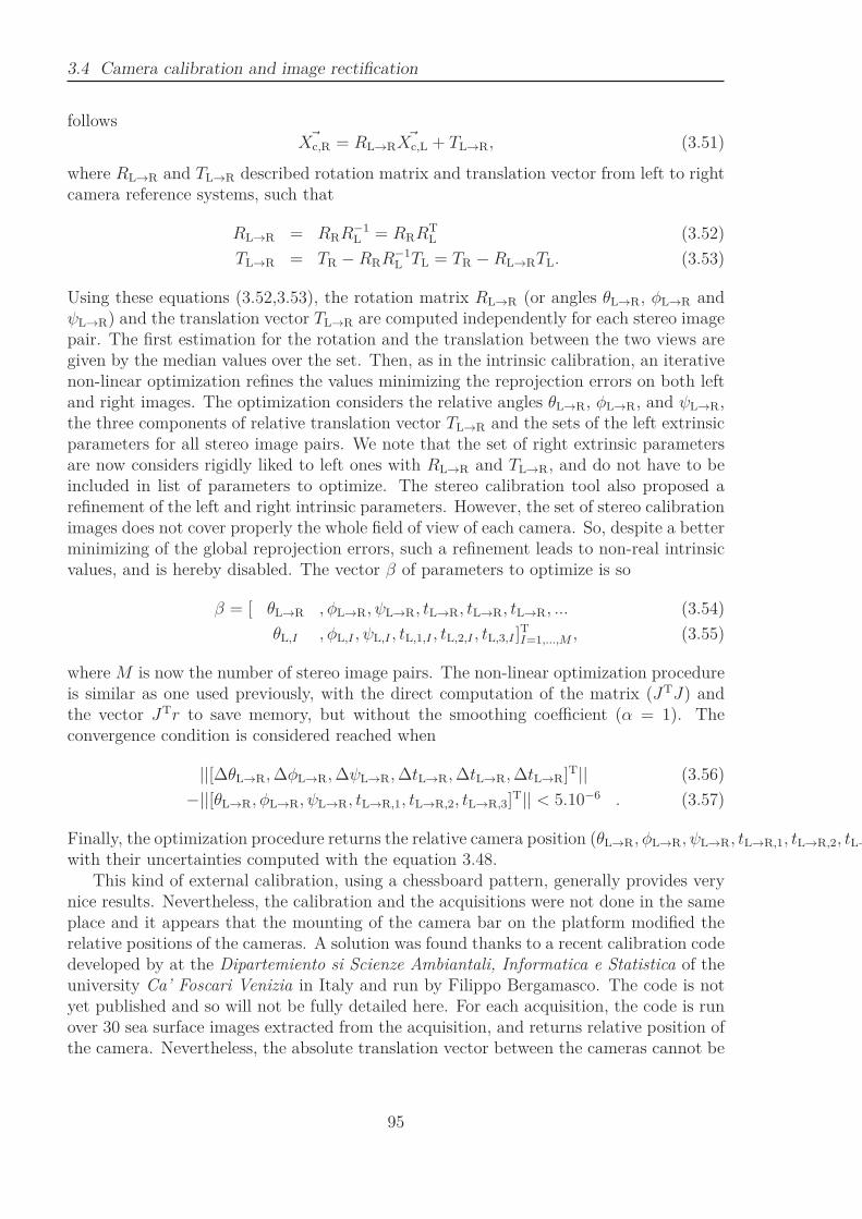
3.4 Camera calibration and image rectification
follows~Xc,R = RL→R
~Xc,L + TL→R, (3.51)
where RL→R and TL→R described rotation matrix and translation vector from left to rightcamera reference systems, such that
RL→R = RRR−1L = RRR
TL (3.52)
TL→R = TR −RRR−1L TL = TR −RL→RTL. (3.53)
Using these equations (3.52,3.53), the rotation matrix RL→R (or angles θL→R, φL→R andψL→R) and the translation vector TL→R are computed independently for each stereo imagepair. The first estimation for the rotation and the translation between the two views aregiven by the median values over the set. Then, as in the intrinsic calibration, an iterativenon-linear optimization refines the values minimizing the reprojection errors on both leftand right images. The optimization considers the relative angles θL→R, φL→R, and ψL→R,the three components of relative translation vector TL→R and the sets of the left extrinsicparameters for all stereo image pairs. We note that the set of right extrinsic parametersare now considers rigidly liked to left ones with RL→R and TL→R, and do not have to beincluded in list of parameters to optimize. The stereo calibration tool also proposed arefinement of the left and right intrinsic parameters. However, the set of stereo calibrationimages does not cover properly the whole field of view of each camera. So, despite a betterminimizing of the global reprojection errors, such a refinement leads to non-real intrinsicvalues, and is hereby disabled. The vector β of parameters to optimize is so
β = [ θL→R , φL→R, ψL→R, tL→R, tL→R, tL→R, ... (3.54)
θL,I , φL,I , ψL,I , tL,1,I , tL,2,I , tL,3,I ]TI=1,...,M , (3.55)
where M is now the number of stereo image pairs. The non-linear optimization procedureis similar as one used previously, with the direct computation of the matrix (JTJ) andthe vector JTr to save memory, but without the smoothing coefficient (α = 1). Theconvergence condition is considered reached when
||[∆θL→R,∆φL→R,∆ψL→R,∆tL→R,∆tL→R,∆tL→R]T|| (3.56)
−||[θL→R, φL→R, ψL→R, tL→R,1, tL→R,2, tL→R,3]T|| < 5.10−6 . (3.57)
Finally, the optimization procedure returns the relative camera position (θL→R, φL→R, ψL→R, tL→R,1, tL→R,2, tL→
with their uncertainties computed with the equation 3.48.This kind of external calibration, using a chessboard pattern, generally provides very
nice results. Nevertheless, the calibration and the acquisitions were not done in the sameplace and it appears that the mounting of the camera bar on the platform modified therelative positions of the cameras. A solution was found thanks to a recent calibration codedeveloped by at the Dipartemiento si Scienze Ambiantali, Informatica e Statistica of theuniversity Ca’ Foscari Venizia in Italy and run by Filippo Bergamasco. The code is notyet published and so will not be fully detailed here. For each acquisition, the code is runover 30 sea surface images extracted from the acquisition, and returns relative position ofthe camera. Nevertheless, the absolute translation vector between the cameras cannot be
95

Chapter 3. Sea surface reconstruction
extracted from sea surface images, and is returned normalized by the absolute distancebetween camera. Compared to the results obtained with the chessboard calibration, therelative rotation (around Xc,L) between the cameras is increased by a few degrees. Thesefew degrees have a strong influence on the final results, providing a magnification of the3-dimensions by a factor about 2. Nevertheless, they do not significantly affect distancebetween the cameras. The distance between the cameras is obtained by the chessboardcalibration and is the applied to the normalized translation vector to obtain the absolutetranslation vector later used for reconstruction.
96
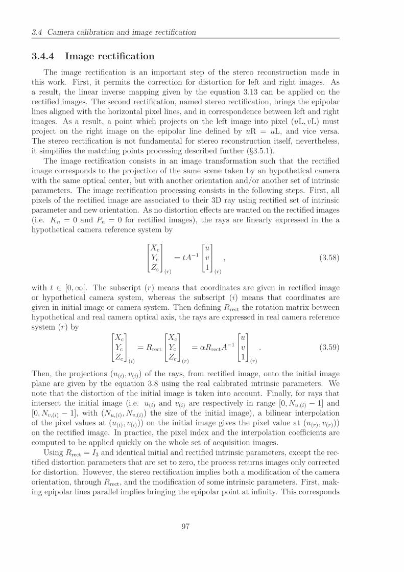
3.4 Camera calibration and image rectification
3.4.4 Image rectification
The image rectification is an important step of the stereo reconstruction made inthis work. First, it permits the correction for distortion for left and right images. Asa result, the linear inverse mapping given by the equation 3.13 can be applied on therectified images. The second rectification, named stereo rectification, brings the epipolarlines aligned with the horizontal pixel lines, and in correspondence between left and rightimages. As a result, a point which projects on the left image into pixel (uL, vL) mustproject on the right image on the epipolar line defined by uR = uL, and vice versa.The stereo rectification is not fundamental for stereo reconstruction itself, nevertheless,it simplifies the matching points processing described further (§3.5.1).
The image rectification consists in an image transformation such that the rectifiedimage corresponds to the projection of the same scene taken by an hypothetical camerawith the same optical center, but with another orientation and/or another set of intrinsicparameters. The image rectification processing consists in the following steps. First, allpixels of the rectified image are associated to their 3D ray using rectified set of intrinsicparameter and new orientation. As no distortion effects are wanted on the rectified images(i.e. Kn = 0 and Pn = 0 for rectified images), the rays are linearly expressed in the ahypothetical camera reference system by
Xc
Yc
Zc
(r)
= tA−1
uv1
(r)
, (3.58)
with t ∈ [0,∞[. The subscript (r) means that coordinates are given in rectified imageor hypothetical camera system, whereas the subscript (i) means that coordinates aregiven in initial image or camera system. Then defining Rrect the rotation matrix betweenhypothetical and real camera optical axis, the rays are expressed in real camera referencesystem (r) by
Xc
Yc
Zc
(i)
= Rrect
Xc
Yc
Zc
(r)
= αRrectA−1
uv1
(r)
. (3.59)
Then, the projections (u(i), v(i)) of the rays, from rectified image, onto the initial imageplane are given by the equation 3.8 using the real calibrated intrinsic parameters. Wenote that the distortion of the initial image is taken into account. Finally, for rays thatintersect the initial image (i.e. u(i) and v(i) are respectively in range [0, Nu,(i) − 1] and[0, Nv,(i) − 1], with (Nu,(i), Nv,(i)) the size of the initial image), a bilinear interpolationof the pixel values at (u(i), v(i))) on the initial image gives the pixel value at (u(r), v(r)))on the rectified image. In practice, the pixel index and the interpolation coefficients arecomputed to be applied quickly on the whole set of acquisition images.
Using Rrect = I3 and identical initial and rectified intrinsic parameters, except the rec-tified distortion parameters that are set to zero, the process returns images only correctedfor distortion. However, the stereo rectification implies both a modification of the cameraorientation, through Rrect, and the modification of some intrinsic parameters. First, mak-ing epipolar lines parallel implies bringing the epipolar point at infinity. This corresponds
97

Chapter 3. Sea surface reconstruction
to parallel left and right image planes, and so parallel optical axis (RL → R = I3). Thisis obtained by rotating each camera minimally such that
R1,L = Frodrigues(−θL→R/2,−φL→R/2,−ψL→R/2) = R−1L = RT
L (3.60)
R1,R = Frodrigues(θL→R/2, φL→R/2, ψL→R/2) = R−1R = RT
R. (3.61)
where Frodrigues returns the rotation matrix corresponding to roll, pitch, and yaw angles(Rodrigues formula). This implies that the new translation vector between the camerasis T1 = R1,RT . Then, the epipolar lines aligned with the horizontal pixel lines are givenby the rotation R2 which makes the horizontal pixel lines parallel to T1. Finally, therotations to be applied to each camera are
Rrect,L = R2R1,L (3.62)
Rrect,R = R2R1,R. (3.63)
The rectified set of external parameters that links left to right camera is
Rrect,L→R = I3
Trect,L→R = Rrect,RT. (3.64)
Finally, epipolar lines in correspondence are obtained by coplanar left and right imageplanes and a same vertical pixel discretization (fv,rect identical for both each image). Inorder to retain the maximum information from initial image (i.e. a maximum of raysfrom the rectified image intersect the initial image), the common rectified focal length isdefined such that
frect,v = min(f1, f2) (3.65)
where
f1 = fv,L[
1 + P1,L(N2u +N2
v )/(4P 22,L)
]
(3.66)
f2 = fv,R[
1 + P1,R(N2u +N2
v )/(4P 22,R)
]
(3.67)
Therefore, the rectified set of intrinsic parameters for each camera is only modified bysetting distortion parameters to zero and vertical pixel focal length to fv,rect and therectified relative position of the cameras are given by equations 3.64
3.5 Sea surface reconstruction
The stereo analysis to obtain the 3-D shape of a scene is one of the first and mostpopular problems in Computer Vision. As discussed above in paragraph 3.3.3, using twoprojections of the same scene from different points of view restores the third dimensionlost by single projection. Thanks to the camera calibration described in the previousparagraph 3.4, links between 3D scene and each projection are now well-known. Moreover,using rectified images (with rectified camera parameters), the inverse mapping has now asimple linear solution given by equation 3.13. For the continuation of the chapter, onlyrectified images with their rectified intrinsic and extrinsic parameters are now considered
98
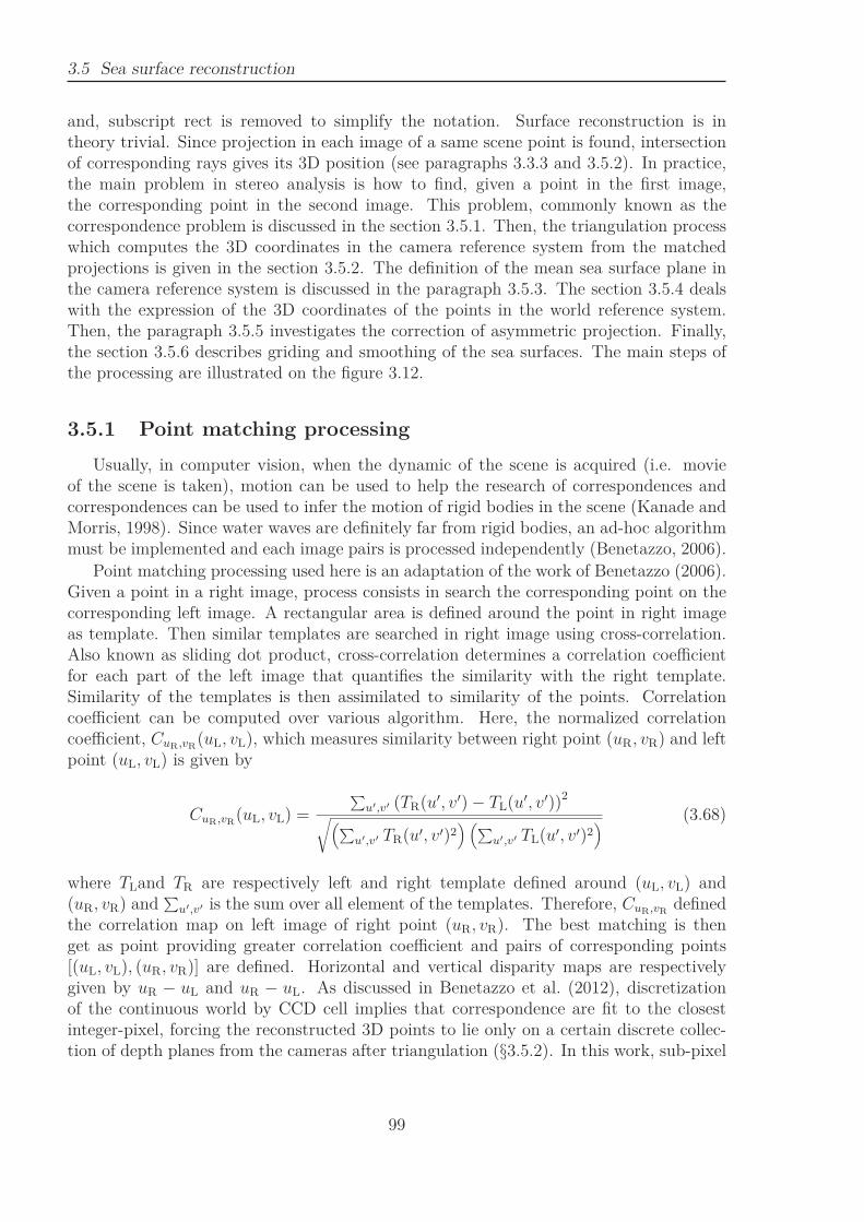
3.5 Sea surface reconstruction
and, subscript rect is removed to simplify the notation. Surface reconstruction is intheory trivial. Since projection in each image of a same scene point is found, intersectionof corresponding rays gives its 3D position (see paragraphs 3.3.3 and 3.5.2). In practice,the main problem in stereo analysis is how to find, given a point in the first image,the corresponding point in the second image. This problem, commonly known as thecorrespondence problem is discussed in the section 3.5.1. Then, the triangulation processwhich computes the 3D coordinates in the camera reference system from the matchedprojections is given in the section 3.5.2. The definition of the mean sea surface plane inthe camera reference system is discussed in the paragraph 3.5.3. The section 3.5.4 dealswith the expression of the 3D coordinates of the points in the world reference system.Then, the paragraph 3.5.5 investigates the correction of asymmetric projection. Finally,the section 3.5.6 describes griding and smoothing of the sea surfaces. The main steps ofthe processing are illustrated on the figure 3.12.
3.5.1 Point matching processing
Usually, in computer vision, when the dynamic of the scene is acquired (i.e. movieof the scene is taken), motion can be used to help the research of correspondences andcorrespondences can be used to infer the motion of rigid bodies in the scene (Kanade andMorris, 1998). Since water waves are definitely far from rigid bodies, an ad-hoc algorithmmust be implemented and each image pairs is processed independently (Benetazzo, 2006).
Point matching processing used here is an adaptation of the work of Benetazzo (2006).Given a point in a right image, process consists in search the corresponding point on thecorresponding left image. A rectangular area is defined around the point in right imageas template. Then similar templates are searched in right image using cross-correlation.Also known as sliding dot product, cross-correlation determines a correlation coefficientfor each part of the left image that quantifies the similarity with the right template.Similarity of the templates is then assimilated to similarity of the points. Correlationcoefficient can be computed over various algorithm. Here, the normalized correlationcoefficient, CuR,vR
(uL, vL), which measures similarity between right point (uR, vR) and leftpoint (uL, vL) is given by
CuR,vR(uL, vL) =
∑
u′,v′ (TR(u′, v′) − TL(u′, v′))2
√
(
∑
u′,v′ TR(u′, v′)2) (
∑
u′,v′ TL(u′, v′)2)
(3.68)
where TLand TR are respectively left and right template defined around (uL, vL) and(uR, vR) and
∑
u′,v′ is the sum over all element of the templates. Therefore, CuR,vRdefined
the correlation map on left image of right point (uR, vR). The best matching is thenget as point providing greater correlation coefficient and pairs of corresponding points[(uL, vL), (uR, vR)] are defined. Horizontal and vertical disparity maps are respectivelygiven by uR − uL and uR − uL. As discussed in Benetazzo et al. (2012), discretizationof the continuous world by CCD cell implies that correspondence are fit to the closestinteger-pixel, forcing the reconstructed 3D points to lie only on a certain discrete collec-tion of depth planes from the cameras after triangulation (§3.5.2). In this work, sub-pixel
99
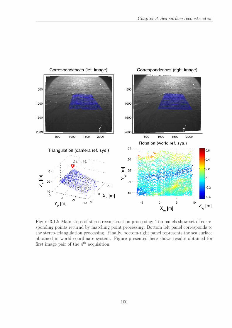
Chapter 3. Sea surface reconstruction
Figure 3.12: Main steps of stereo reconstruction processing: Top panels show set of corre-sponding points returnd by matching point processing. Bottom left panel corresponds tothe stereo-triangulation processing. Finally, bottom-right panel represents the sea surfaceobtained in world coordinate system. Figure presented here shows results obtained forfirst image pair of the 4th acquisition.
100
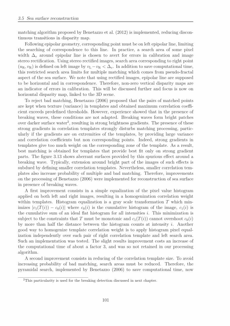
3.5 Sea surface reconstruction
matching algorithm proposed by Benetazzo et al. (2012) is implemented, reducing discon-tinuous transitions in disparity map.
Following epipolar geometry, corresponding point must be on left epipolar line, limitingthe searching of correspondence to this line. In practice, a search area of some pixelwidth ∆v around epipolar line is chosen to avert for errors in calibration and imagestereo rectification. Using stereo rectified images, search area corresponding to right point(uR, vR) is defined on left image by vL −vR < ∆v. In addition to save computational time,this restricted search area limits for multiple matching which comes from pseudo-fractalaspect of the sea surface. We note that using rectified images, epipolar line are supposedto be horizontal and in correspondence. Therefore, non-zero vertical disparity maps arean indicator of errors in calibration. This will be discussed further and focus is now onhorizontal disparity map, linked to the 3D scene.
To reject bad matching, Benetazzo (2006) proposed that the pairs of matched pointsare kept when texture (variance) in templates and obtained maximum correlation coeffi-cient exceeds predefined thresholds. However, experience showed that in the presence ofbreaking waves, these conditions are not adapted. Breaking waves form bright patchesover darker surface water2, resulting in strong brightness gradients. The presence of thesestrong gradients in correlation templates strongly disturbs matching processing, partic-ularly if the gradients are on extremities of the templates, by providing large varianceand correlation coefficients but non corresponding points. Indeed, strong gradients intemplates give too much weight on the corresponding zone of the template. As a result,best matching is obtained for templates that provide best fit only on strong gradientparts. The figure 3.13 shows aberrant surfaces provided by this spurious effect around abreaking wave. Typically, extension around bright part of the images of such effects issubdued by defining smaller correlation templates. Nevertheless, smaller correlation tem-plates also increase probability of multiple and bad matching. Therefore, improvementson the processing of Benetazzo (2006) were implemented for reconstruction of sea surfacein presence of breaking waves.
A first improvement consists in a simple equalization of the pixel value histogramapplied on both left and right images, resulting in a homogenization correlation weightwithin templates. Histogram equalization is a gray scale transformation T which min-imizes |c1(T (i)) − c0(i)| where c0(i) is the cumulative histogram of the image, c1(i) isthe cumulative sum of an ideal flat histogram for all intensities i. This minimization issubject to the constraints that T must be monotonic and c1(T (i)) cannot overshoot c0(i)by more than half the distance between the histogram counts at intensity i. Anothergood way to homogenize template correlation weight is to apply histogram pixel equal-ization independently over each pair of right correlation template and left search area.Such an implementation was tested. The slight results improvement costs an increase ofthe computational time of about a factor 3, and was so not retained in our processingalgorithm.
A second improvement consists in reducing of the correlation template size. To avoidincreasing probability of bad matching, search areas must be reduced. Therefore, thepyramidal search, implemented by Benetazzo (2006) to save computational time, now
2This particularity is used for the breaking detection discussed in next chapter.
101

Chapter 3. Sea surface reconstruction
Figure 3.13: Example of bad point matching due to foam patch. Size of correlationtemplates is purposefully increased to 121 × 61 pixels to exaggerate this phenomenon.Left panels: Matching points obtained between left (top) and right (bottom) images.Color of points are correlation coefficient of matching (top) and standard deviation ofpixel values in right correlation window. Green point matching is not disturbed by foampatch whereas red point matching if fully driven by small part of foam patch in correlationwindow. Top-right: resulting surface after stereo triangulation (§3.5.2) and rotation toworld coordinates (§3.5.4). Green point falls on reconstruction in back of wave crestwhereas images show that it is in front of the crest. Bad matching leads to unrealisticstep around foam patch. Bottom-right: histogram of pixel vertical coordinates disparitybetween left and right images, with abnormal peak observed around pixel value 101 dueto bad matching.
102

3.5 Sea surface reconstruction
includes a decreasing of correlation template size with increasing iterations. A 3-stepcorresponding point search is implemented. In the first step, we get disparity map corre-sponding to the mean surface plane. A few number of corresponding points distributedover reconstruction area are given by highest correlation coefficient computed using a largecorrelation template (121×61 pixels), which increases the probability of good matching. Asimple standard deviation filtering rejects uncertain matching. Then, 2D linear functionsare fit at the least square sense on kept correspondence, such that
uL = AuuR +BuvR + Cu (3.69)
vL = AvuR +BvvR + Cv. (3.70)
These functions are then assimilated at pixel displacement between right and left corre-sponding point, due to mean sea surface plane of the considered area. Then, second stepis to approximate disparity map due to long signal waves in images. A denser grid isdefined on the right image and corresponding left points are searched using smaller corre-lation template(41 × 41 pixels). Estimating location of corresponding left points thanksto linear functions 3.69 and 3.70, search areas can be reduced and bad matching proba-bility decreased. A standard deviation filtering is then applied on the difference betweenpredicted and found left points to rejects uncertain matching. Finally, the last step is tofind a very dense set of corresponding points, with a 2 × 2 pixel resolution grid definedon the right image. Once again, predictive locations of correspondences on left image areestimated using linear interpolation of the previous results. Finally, a fine disparity mapis obtained using a small correlation template (21 × 21 pixels), and sub-pixel fit. Again, astandard deviation filtering is then applied on the difference between predicted and foundleft points.
We note that due to the projective transformation between left and right images, therectangular template in the right image must corresponds to a parallelogram on the leftimage. Therefore, the processing is slightly modified by taking into account for this fact.Following methods of Kosnik and Dulov (2011), results at each step are now used totransform the left image, such that disparity map computed over transformed image isnull. In a similar way as described above, a projective transformation fitted on the firststep filtered results is applied on the left image. The rectified left image is used in thesecond step search, where predictive positions of correspondences are (uL, vL) = (uR, vR).Reverse transformation then recover correspondences in the initial left image. A piecewiselinear transformed image is computed by these results and used in the last step search.Reverse transformation gives fine disparity map. Correlation template sizes are kept equal.We note that with this method variant, matching should be better, because rectanglepattern in right image correspond to rectangular pattern in transformed left one. Wenote that image transformation also induces a smoothing of pixel values, so a loss oftexture in the images, which slightly increases the number of unmatched points.
Experience shows that direct triangulation of these results leads to spiky surfaces.Therefore, the disparity map is smoothed using a 10×10 point (i.e. 20×20 pixel) medianfilter, resulting in the figure 3.15. The figure 3.14 shows corresponding points obtainedwith this modified matching processing.
We note that Benetazzo (2006) proposed to approximate locally the water surfaceby a planar surface to limit the possible location of the corresponding points on the
103
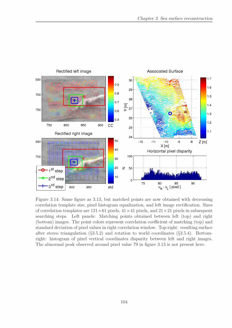
Chapter 3. Sea surface reconstruction
Figure 3.14: Same figure as 3.13, but matched points are now obtained with decreasingcorrelation template size, pixel histogram equalization, and left image rectification. Sizesof correlation templates are 121×61 pixels, 41×41 pixels, and 21×21 pixels in subsequentsearching steps. Left panels: Matching points obtained between left (top) and right(bottom) images. The point colors represent correlation coefficient of matching (top) andstandard deviation of pixel values in right correlation window. Top-right: resulting surfaceafter stereo triangulation (§3.5.2) and rotation to world coordinates (§3.5.4). Bottom-right: histogram of pixel vertical coordinates disparity between left and right images.The abnormal peak observed around pixel value 79 in figure 3.13 is not present here.
104
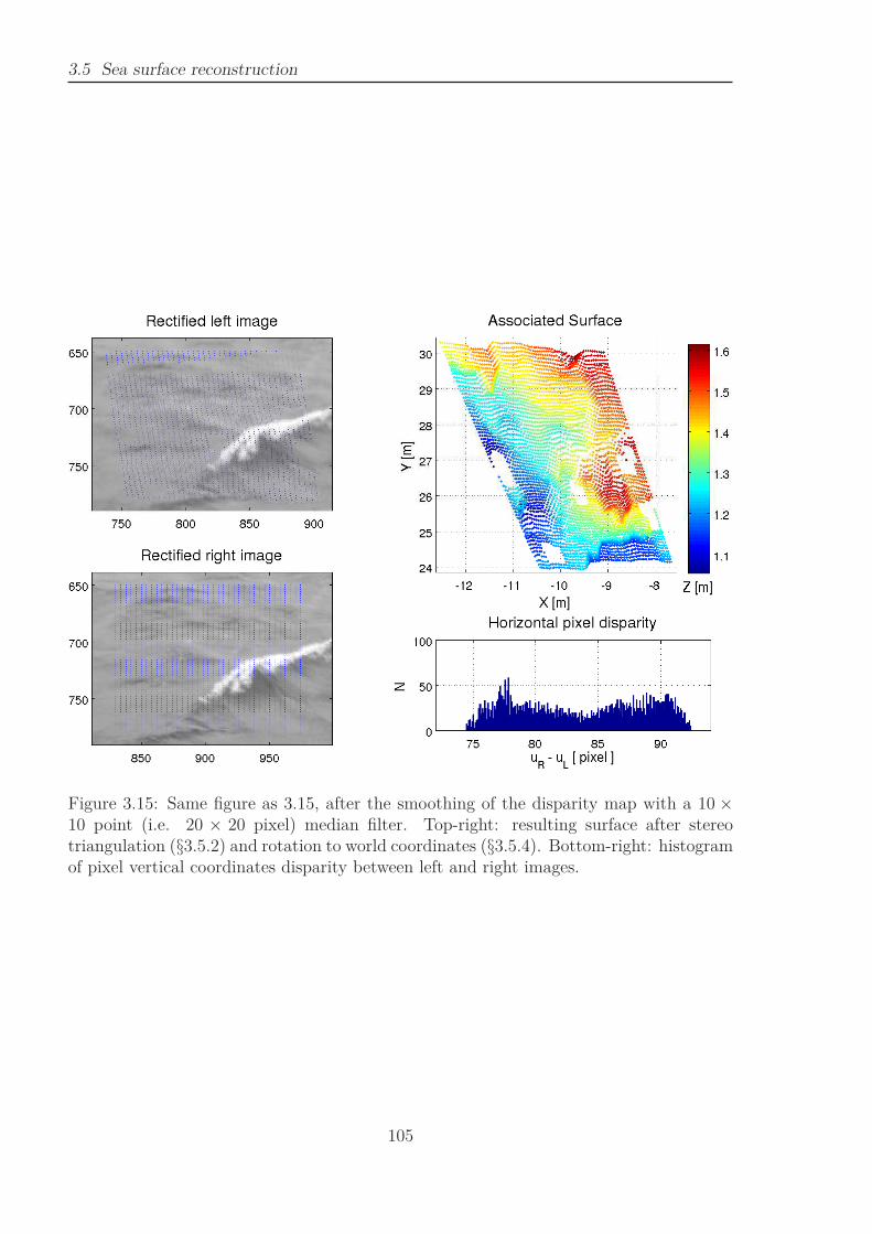
3.5 Sea surface reconstruction
Figure 3.15: Same figure as 3.15, after the smoothing of the disparity map with a 10 ×10 point (i.e. 20 × 20 pixel) median filter. Top-right: resulting surface after stereotriangulation (§3.5.2) and rotation to world coordinates (§3.5.4). Bottom-right: histogramof pixel vertical coordinates disparity between left and right images.
105

Chapter 3. Sea surface reconstruction
epipolar line in subsequent steps. Here, the reasoning is different. Indeed, Benetazzo(2006) use a same correlation template size for all its steps, and so subsequent steps onlysearch for new correspondences, with the aim of refining the disparity map. Therefore, anon-iterative search should lead to the same disparity map, and iterative-processing onlysaves computational time. In the method described here, the previous steps predict theapproximative locations of the correspondences and so reduces the search areas in thenext step. This helps to reduce the correlation template size, with a limited increase inthe probability of bad matching. Therefore, each step refines correspondences location.
The size of the correlation template footprints on the sea surface greatly increase awayfrom the cameras. Therefore, the use of a fixed template size over the whole image mustbe interpreted with care. Indeed, on upper part of images, disparity is obtained over seasurface areas of a few square meters whereas disparity on the lower part of the imagesis obtained over sea surface areas of a few square centimeters. At this stage, absoluteposition and orientation of cameras are not known3. Nevertheless, they can be estimatedfrom triangulation (see §3.5.2) of the points taken in the first step. Therefore, an adaptivecorrelation template size can be implemented to keep a constant footprint on the seasurface. Such processing should leads to more homogeneous disparity map. However,in a same way, informations on small waves far from cameras (i.e. in the upper part ofthe images) is lost due to the larger footprints of pixels. Because the correspondencesearch needs enough texture within the correlation templates, such a processing was notimplemented.
The figure 3.16 show the zone on images selected for reconstruction. The zone shapesare computed using an approximation of the mean sea surface plane to provide recon-structed surfaces approximatevely rectangular.
Figure 3.17 shows the time-mean horizontal and vertical disparity maps obtained forthe acquisition 4. The non-null vertical disparity map means that correspondences werefound out of calibrated epipolar lines, and so reveals errors in calibration results. Never-theless, we note that the vertical disparity maps are typically less than one pixel. Thisindicates that the intrinsic and extrinsic camera parameters are correct and can be usedfor next reconstruction steps.
The matching process is the more expensive process of reconstruction in term of com-putational time. Matching process takes more than 6 minutes to search for the about100000 correspondence, corresponding to previous shown figures. As reference, the fixedcorrelation template size (61 × 41 pixels) process takes about 30% more time, and reject-ing process applying pixel histogram to each correlation template and search areas takesmore than 300% more time for same reconstruction area. Written in Matlab R©, codes werecompiled and matching processes, independent for each image pairs, were then distributedin a few hundred parallel jobs.
3.5.2 Triangulation processing
Following the epipolar geometry discussed in paragraph 3.3.3, the triangulation pro-vides the 3D coordinates of the intersection of rays corresponding to left and right corre-
3Only relative positions and orientations of camera compared to each other are given by calibration.
106
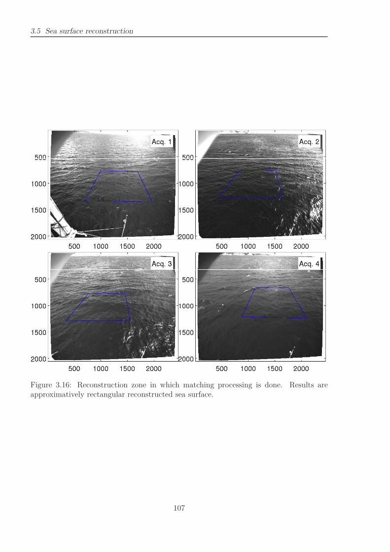
3.5 Sea surface reconstruction
Figure 3.16: Reconstruction zone in which matching processing is done. Results areapproximatively rectangular reconstructed sea surface.
107
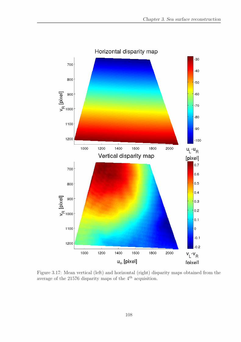
Chapter 3. Sea surface reconstruction
Figure 3.17: Mean vertical (left) and horizontal (right) disparity maps obtained from theaverage of the 21576 disparity maps of the 4th acquisition.
108
3.5 Sea surface reconstruction
sponding points using equation (3.13),
Xc
Yc
Zc
= αL C−1L
uL
vL
1
= αR C−1R
uR
vR
1
. (3.71)
As the earth system is not defined at this stage, the world system is defined as the leftcamera system. Then, using relative camera position (Eq. 3.51) with intrinsic cameramatrix (Eq. 3.12), triangulation searches for αL and αR which are solution of
Xc
Yc
Zc
= αL A−1L
uL
vL
1
= αR RA−1R
uR
vR
1
+ T, (3.72)
where R = RL→R and T = TL→R, such as defined by external camera calibration. Asundistorted images are used, v′
L = v′
R = v′ and [u′, v′, 1]T = A−1[u, v, 1]T, with α[u′, v′, 1]T
is equation of the 3D ray corresponding to pixel (u, v). Moreover, the stereo rectificationof images implies R = I3 and T = [d, 0, 0]T. Therefore, equation 3.72 can be written
αL
u′
L
v′
1
= αR
u′
R
v′
1
+
d00
. (3.73)
Then, the equation 3.73 gives
Zc = Zc,L = Zc,R = d/(
u′
R − u′
L
)
Yc = Yc,L = Yc,R = Zcv′
Xc,L = Zcu′
L = Xc,R + d
Xc,R = Zcu′
R = Xc,L − d
(3.74)
This verifies definition of image stereo rectification, with third dimension fully given byhorizontal disparity map. Nevertheless, in practice, calibration errors and non-perfectaccuracy of matching points lead to vL 6= vR. As a result, left and right rays computed byequation 3.13 do not intersect in the 3D space. The problem, then, is to find a 3D pointwhich optimally fits the measured image points. Literature proposes multiple methodsto define this optimal point. Based on different optimality criteria, the various methodsproduce different estimates when noise (error) is involved. A description of triangulationprocessing used in this work is now given. Usually called mid-point method, the algorithmfirst computes independently the point [X ′
L, Y′
L, Z′
L]T = αL[u′
L, v′
L, 1]T on left ray closestto right ray and inversely, the point [X ′
R, Y′
R, Z′
R]T = αR[u′
R, v′
R, 1]T on right ray closest toleft ray with
αL =1
D
[
(rR · (RrL))(rR · T ) − ||rR||2(RrL · T )]
(3.75)
αR =1
D
[
||rL||2(rR · T ) − (RrL · T )(rR ·RrL)]
(3.76)
109
Chapter 3. Sea surface reconstruction
where (x · y) means dot product of vectors x and y, rL = [u′
L, v′
L, 1]T, rR = [u′
R, v′
R, 1]T arerespectively left and right rays, and
D = ||rL||2||rR||2 − (RrL · rR)2. (3.77)
Obviously, if the left and right rays intersect, these two points are directly linked by rigidtransformation between camera. In general case, the two different points are expressed inthe same reference system (here left camera one) and mid-point is computed, in both leftand right camera reference system with
XL
YL
ZL
=1
2
X ′
L
Y ′
L
Z ′
L
+R−1
X ′
R
Y ′
R
Z ′
R
− T
, (3.78)
and
XR
YR
ZR
= R
XL
YL
ZL
+ T. (3.79)
We note that the following triangulation algorithm does not need image stereo rectifi-cation. Nevertheless, it is implicitly assumed that a previous correction of images fordistortion was done, which allows a linear link between pixel p = (u, v) to its correspond-ing ray [u′, v′, 1]T. From each stereo image pair, triangulation returns a scattered set of3D surface point positions expressed in left and right camera reference system. Bottomleft panel of figure 3.12 shows an example of 3D surface point coordinates returned bytriangulation processing, expressed in right camera reference system.
3.5.3 Mean surface plane definition
This process consists in the expression of the scattered surface points in world coordi-nate system, where axis ~Xw and ~Yw are horizontal and ~Zw is aligned with gravity, lookingup. As position of cameras in such a reference system is not known, information mustbe extracted from the set of 3D points. Only right coordinates are now used, but similarprocess can be done over left ones. Following Benetazzo (2006), gravity direction in rightcamera reference system is obtained using time-averaged water surface elevation. Indeed,considering a long period, the time-average surface is assumed to be a horizontal plane.Benetazzo (2006) proposed to fit a plane (aXc + bYc + cZc + d = 0, with a2 + b2 + c2 = 1and c ≥ 0) over all scattered points using a least square solution. In practice, solution canbe found directly over the whole set of 4D (space + time) scattered points. Therefore, themean plane is obtained by averaging all the a, b, c, and d parameters of planes fitted foreach stereo image pairs. We note here that triangulation applied on time-mean disparitymap gives 3D positions of 3D scattered points on mean sea surface plane. Mean plane canthen be extracted directly from this set of points. The two methods were implemented,and they give similar results. The effect on final reconstruction is negligible.
110
3.5 Sea surface reconstruction
3.5.4 Surfaces in world reference system
The rigid transformation between right camera reference system and world systemis defined by consecutive rotation Rc→w which makes the mean surface plane horizontaland vertical translation Tc→w which moves mean sea surface plane to Zw = 0. In otherwords, the world system is defined by ~Zw is aligned with gravity, looking upwards, andthe origin is on mean sea surface plane, vertically below right camera. We define the unitnormal vector of plane ~np = [−a,−b,−c]T, looking out water (camera looks down andplane parameters are defined such that c ≥ 0). Rotation must transform ~np into [0, 0, 1]T.Therefore, Rc→w = [~u,~v, ~np]T with (~u,~v, ~np) forms an orthonormal basis, here definedwith
~u =[b,−a, 0]T√a2 + b2
(3.80)
~v = ~np × ~u. (3.81)
where × means cross product. We note that any couple of vectors (~u,~v) which form
orthonormal basis with ~np makes mean sea surface plane horizontal with ~Zw looking up.
Nevertheless, defining the third component of ~u null, the obtained ~Yw is aligned withcamera reference (i.e. rotation around Z-axis (yaw) is null). The proper direction of~u then gives positive values of Yw. Finally, translation vector is simply defined withTc→w = [0, 0,−d]T. Therefore, coordinates of surface points in world coordinates are
Xw
Yw
Zw
= Rc→w
Xc
Yc
Zc
+ Tc→w. (3.82)
3.5.5 Correction for the asymmetric projection
Inspired from works of Heikkila and Silven (1997) (§2.3), a correction for the asymmet-ric projection was implemented. In our experimentation, image and sea surface planes arenot parallel. So, projective geometry does not preserve shape. In other words, the imagerectangular correlation template projects on the mean sea surface plane in a quadrilat-eral polygon. Considering a real sea surface deformed by waves, projection is a complexsurface. Generally, the barycenter of this surface does not project on center of the cor-responding image template. This problem is commonly called asymmetric projection.Using a five-step iterative processing, template corners of each left and right cameraare projected on sea surface plane, as defined in the previous paragraph. The templatebarycenter is then reprojected on left and right images respectively, giving a new disparitymap. A new triangulation is done, giving a new mean plane. The process is reiterated toobtain both the mean plane and a set of triangulated points corrected for the asymmetricprojection. We note that this processing does not take in account the local sea surfaceslope due to waves. Nevertheless, experience shows that such a correction provides aminor modification of the results. Figure 3.18 shows deviation of triangulated points dueto correction for the asymmetric projection.
111
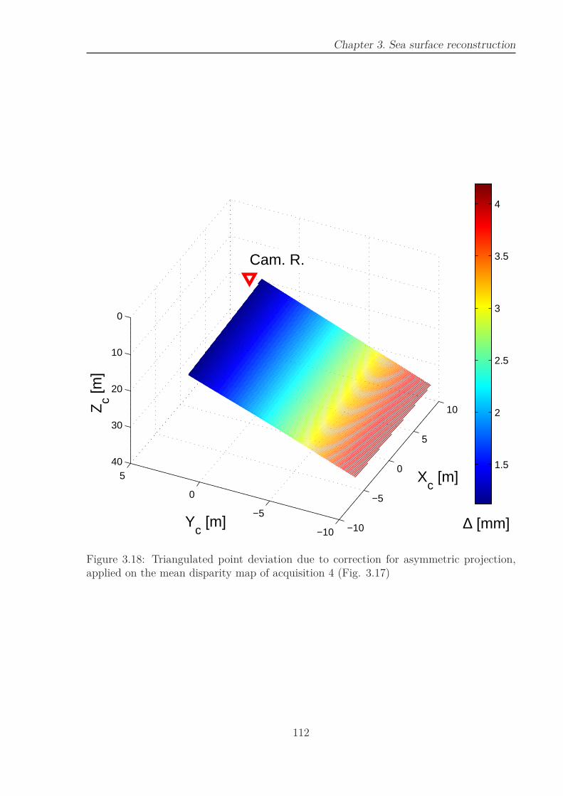
Chapter 3. Sea surface reconstruction
−10
−5
0
5
10
−10
−5
0
5
0
10
20
30
40
Xc [m]
Cam. R.
Yc [m]
Zc [m
]
∆ [mm]
1.5
2
2.5
3
3.5
4
Figure 3.18: Triangulated point deviation due to correction for asymmetric projection,applied on the mean disparity map of acquisition 4 (Fig. 3.17)
112
3.6 Analyses of sea surface reconstructions
3.5.6 Griding and smoothing of the surfaces
As scattered point sets are difficult to manipulate, the surface at each time step (i.e.for each stereo image pair) is then gridded, using a bi-linear interpolation. Three differentgrids are defined. First, two grids, shown in blue and red on figure 3.16, are used forthe 3D spectra (frequency-wavenumber) described in the next section. A third large grid,shown in black on the figure is used in next chapter to analyze breaking events.
To reduce noise in the data, a slight smoothing is applied on the gridded surface, usinga time-space low-pass filter. The 2D space filter is defined by the matrix Fs such that
Fs =1
16
1 2 12 4 21 2 1
, (3.83)
and the time filter is a 5-point hann window. This time-space filtering reduces noise forfrequencies up to 1Hz.
3.6 Analyses of sea surface reconstructions
The reconstruction results here analyzed correspond to the matching processing includ-ing both equalization of pixel intensity histogram and decreasing correlation template sizeas discussed in paragraph 3.5.1, with the correction for asymmetric projection describedin paragraph 3.5.5. If it is not specified, the smoothed surfaces are analyzed (see §3.5.6).After the reconstruction processing and the data griding, the time-evolving elevation mapare Z(x, y, t) for a regular x, y grid.
Unfortunately, the wave elevation could not be measured in the reconstruction areas.Indeed, the above-water part of the capacitance wave gauges would have affected theimages, making reconstruction impossible and due to the water depth (30m), the pressuresensors could not measure the short waves. Nevertheless, the capacitance wave gaugeswere about 20-30 meters away from reconstruction areas. At this distance, wave shapesare strongly disturbed, and the direct comparison of water elevation cannot be done,however, the wave statistics are comparable. Therefore, Probability Density Function(PDF) of elevation and the frequency spectra obtained with reconstruction are comparedto those obtained with wave gauges in the respective sections 3.6.1 and 3.6.2. Another wayto validate our reconstruction is the 3D wavenumber-frequency-direction spectra discussedin the section 3.6.3. The directional wavenumber spectra are then analyzed in the section3.6.4. Finally, the mean square slopes (mss) are compared to the observations of Cox andMunk (1954) in the section 3.6.5.
3.6.1 Probability density function of the elevation
For each acquisition, the Probability Density Function (hereinafter PDF) of the eleva-tion is computed over the whole set of 3D reconstructed surfaces. The PDF are comparedto those those obtained with the wave gauges time series on the figure 3.19. The ob-tained PDF are in line with the wave gauge observations. Nevertheless, we note that the
113
Chapter 3. Sea surface reconstruction
reconstruction for the fourth acquisition disagree with wave gauges data. Same disagree-ment is observed on the comparison of frequency spectra given further. We also note anunrealistic step in the PDF obtained with the wave gauges around Z = −0.5m.
3.6.2 Non directional frequency spectra
For each (x, y) of the grid, the time series of surface elevations, Zx,y(t), are exacted.For each time series, the frequency spectra are computed in the sliding sub-time seriesof 1024 elevation, and averaged. We note that no spatial variation of spectra on thegrid appears up to 2Hz. The same processing is applied on the 6 wave gauges timeseries. For both reconstruction and wave gauge data, all the frequency spectra obtainedin different location are finally averaged and plotted on figure 3.20. The spectra from thereconstructions are globally in line with wave gauges observations, and well followed theexpecting f−5 decreasing asymptote. We note however that a bad fit is observed for thesmall swell present during the first acquisition. This bad fit could be relied to the shorttime-series observations for the first acquisition, in which statistics on longer waves cannot be well represented.
3.6.3 Frequency-wavenumber directional spectra
For the acquisition 1 (resp. 2, 3 and 4), 11 (resp 28, 42 and 42) elevation matrixZ(x, y, t) with size 128×128×1024 (resp. 200×200×1024, 240×240×1024 and 256×256×1024) are extracted from smoothed surfaces, and the corresponding 3D spectra E(kx, ky, f)are computed and averaged. Hann-windows are applied in each axis (x, y and t), beforethe spectrum calculation. We note that an ambiguity in direction of 180˚on the 2Dwavenumber spectra cannot be resolved using an individual elevation map. Nevertheless,the time evolution of the elevation maps resolves this direction ambiguity through the3D frequency-wavenumber spectra. Therefore, the spectrum part corresponding to thenegative frequencies is removed. Due to the symmetry of the Fourier spectrum, theenergy is conserved with a multiplication of the energy spectrum part corresponding tothe positive frequencies by 2. The 3D spectra E(kx, ky, f) are converted to frequency-wavenumber-direction spectra E(k, θ, f) and respectively plotted on the figures 3.21-3.24,for the 4 acquisitions.
The figures show that the energy integrated over directions follows the dispersionrelation up to 1.6Hz. We however note that the phase speeds of the small waves is sightlygreater than ones expected by the dispersion relation. The small wave are modulatedand drifted by the longer underlying wave orbital velocity, resulting in absolute greaterapparent phase speed. We note also the presence of the energy corresponding to thesecond order. The directional energy spreading is discussed in the next paragraph.
3.6.4 Wavenumber spectra
The wavenumber spectrum considers the spatial Fourier analysis. From a square sub-area is extracted from each elevation map, the wavenumber spectra E(kx, ky) can becomputed, then averaged over the whole set of images. As stated before, this Fourier
114
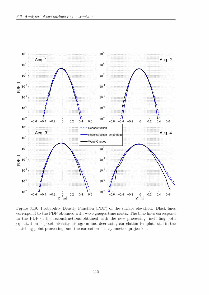
3.6 Analyses of sea surface reconstructions
−0.6 −0.4 −0.2 0 0.2 0.4 0.610
−4
10−3
10−2
10−1
100
101
102
PD
F[1
]
Acq. 1Acq. 1Acq. 1Acq. 1
−0.6 −0.4 −0.2 0 0.2 0.4 0.610
−4
10−3
10−2
10−1
100
101
102
Acq. 2Acq. 2Acq. 2Acq. 2
−0.6 −0.4 −0.2 0 0.2 0.4 0.610
−4
10−3
10−2
10−1
100
101
102
Z [m]
PD
F[1
]
Acq. 3Acq. 3Acq. 3Acq. 3
−0.6 −0.4 −0.2 0 0.2 0.4 0.610
−4
10−3
10−2
10−1
100
101
102
Z [m]
Acq. 4Acq. 4Acq. 4Acq. 4Reconstruction
Reconstruction (smoothed)
Wage Gauges
Figure 3.19: Probability Density Function (PDF) of the surface elevation. Black linescorrespond to the PDF obtained with wave gauges time series. The blue lines correspondto the PDF of the reconstructions obtained with the new processing, including bothequalization of pixel intensity histogram and decreasing correlation template size in thematching point processing, and the correction for asymmetric projection.
115

Chapter 3. Sea surface reconstruction
10−1
100
10−4
10−3
10−2
10−1
100
E(f
)[m
2/H
z]
Acq. 1Acq. 1Acq. 1Acq. 1
10−1
100
10−4
10−3
10−2
10−1
100
Acq. 2Acq. 2Acq. 2Acq. 2
10−1
100
10−4
10−3
10−2
10−1
100
f [Hz]
E(f
)[m
2/H
z]
Acq. 3Acq. 3Acq. 3Acq. 3
10−1
100
10−4
10−3
10−2
10−1
100
f [Hz]
Acq. 4Acq. 4Acq. 4Acq. 4Reconstruction
Reconstruction (smoothed)
Wage Gauges
Figure 3.20: Frequency Spectra (FS) of the surface elevation. Black lines correspond tothe PDF obtained with wave gauges time series. The blue lines correspond to the FSof the reconstructions obtained with the new processing, including both equalization ofpixel intensity histogram and decreasing correlation template size in the matching pointprocessing, and the correction for asymmetric projection.
116
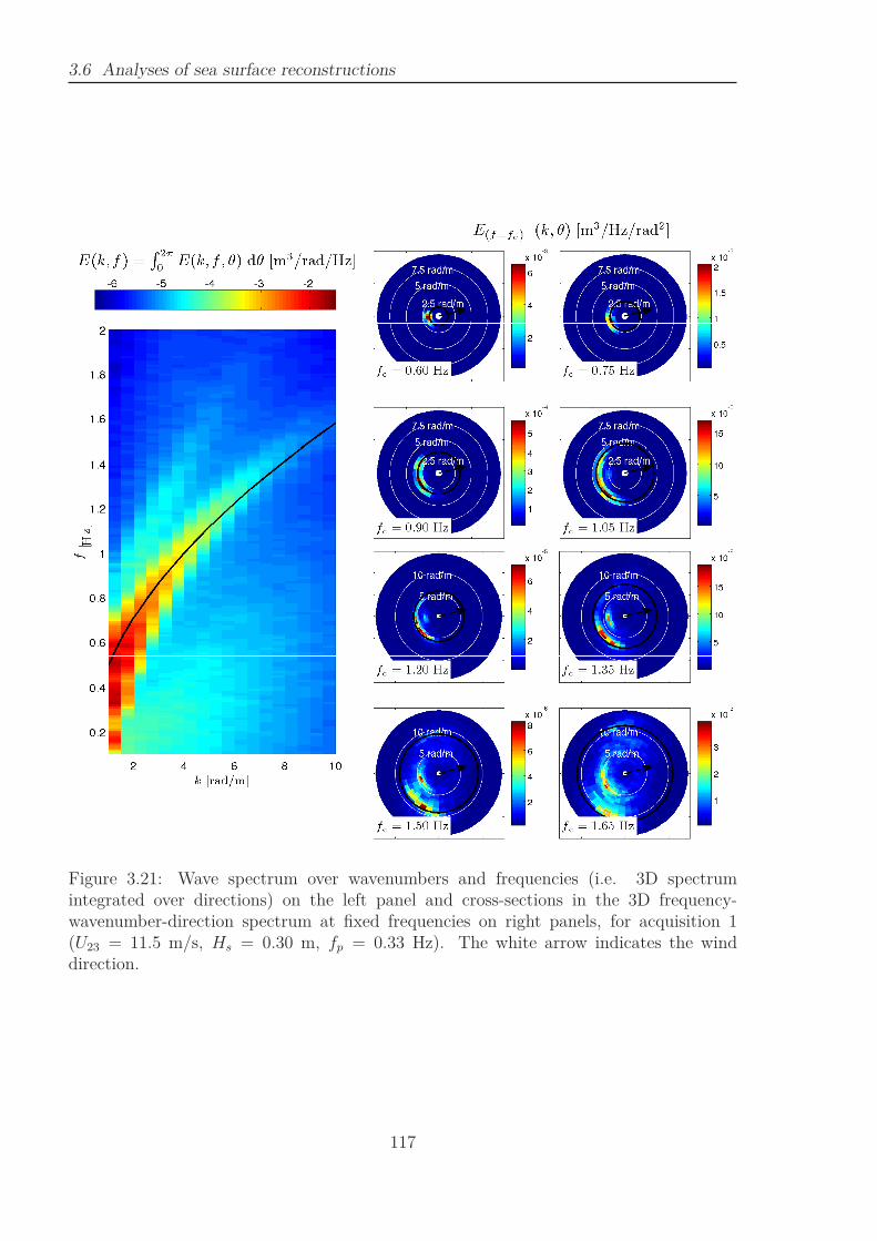
3.6 Analyses of sea surface reconstructions
Figure 3.21: Wave spectrum over wavenumbers and frequencies (i.e. 3D spectrumintegrated over directions) on the left panel and cross-sections in the 3D frequency-wavenumber-direction spectrum at fixed frequencies on right panels, for acquisition 1(U23 = 11.5 m/s, Hs = 0.30 m, fp = 0.33 Hz). The white arrow indicates the winddirection.
117
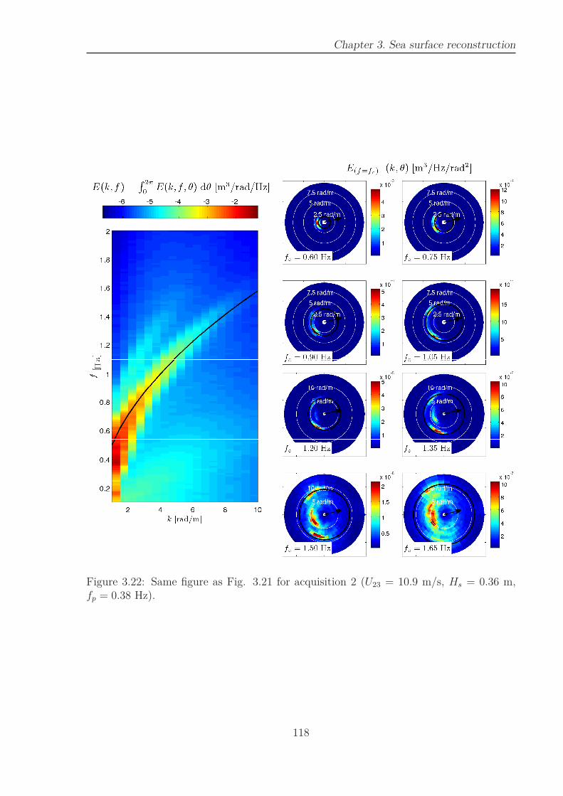
Chapter 3. Sea surface reconstruction
Figure 3.22: Same figure as Fig. 3.21 for acquisition 2 (U23 = 10.9 m/s, Hs = 0.36 m,fp = 0.38 Hz).
118
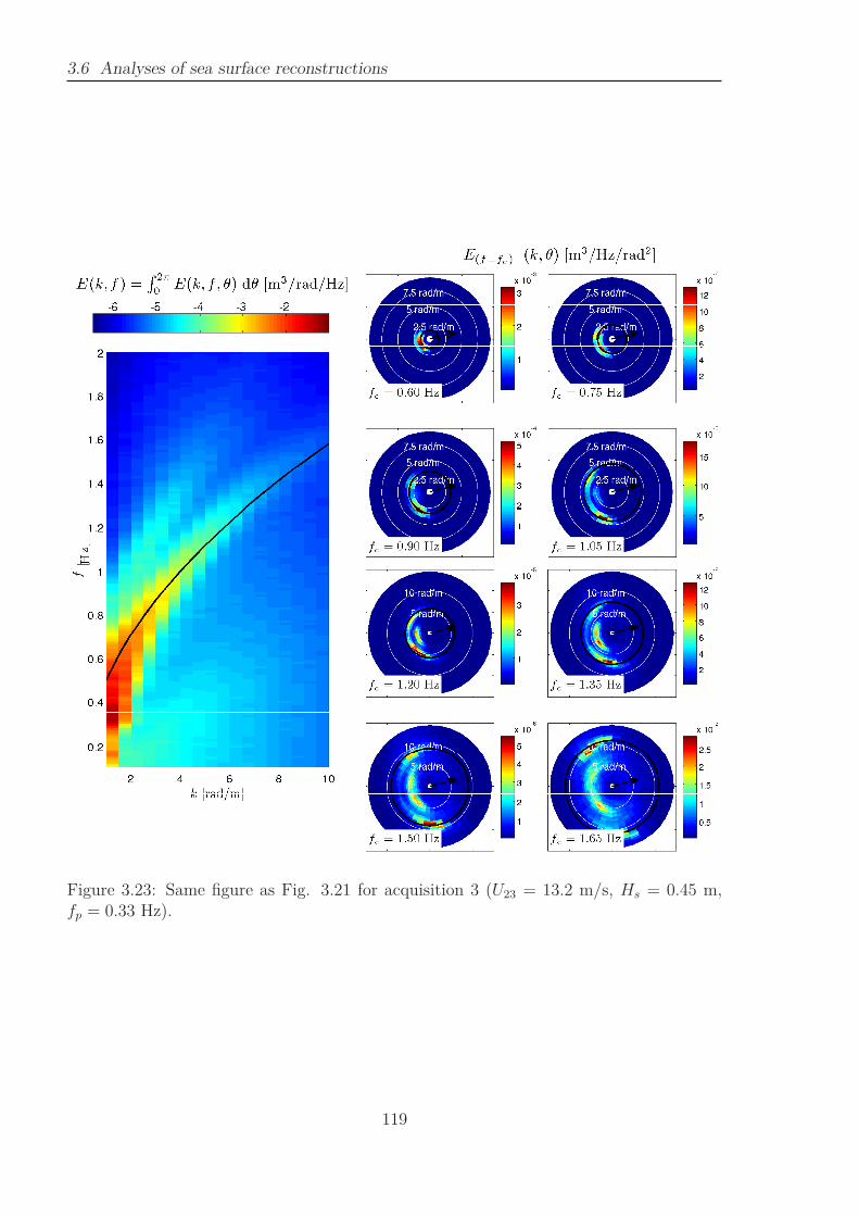
3.6 Analyses of sea surface reconstructions
Figure 3.23: Same figure as Fig. 3.21 for acquisition 3 (U23 = 13.2 m/s, Hs = 0.45 m,fp = 0.33 Hz).
119
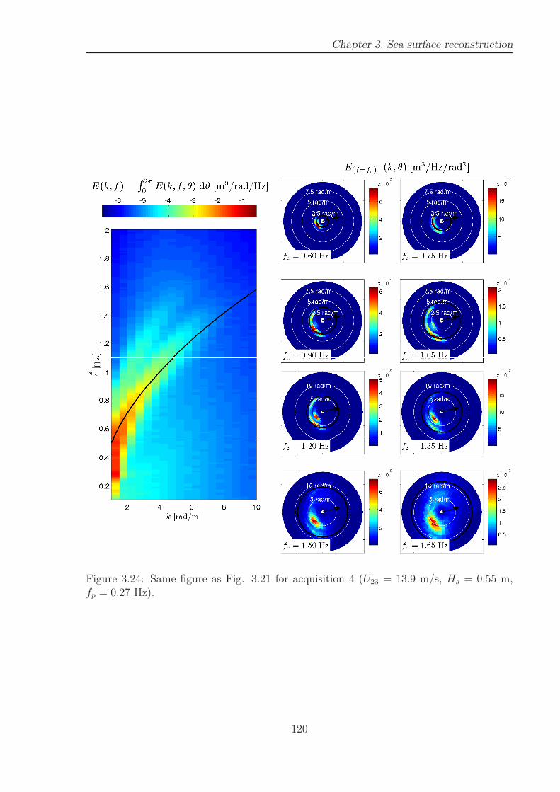
Chapter 3. Sea surface reconstruction
Figure 3.24: Same figure as Fig. 3.21 for acquisition 4 (U23 = 13.9 m/s, Hs = 0.55 m,fp = 0.27 Hz).
120
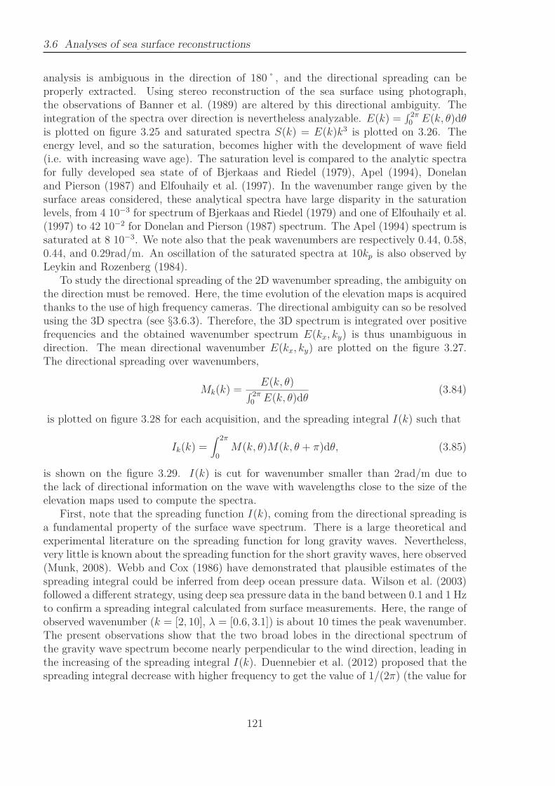
3.6 Analyses of sea surface reconstructions
analysis is ambiguous in the direction of 180˚, and the directional spreading can beproperly extracted. Using stereo reconstruction of the sea surface using photograph,the observations of Banner et al. (1989) are altered by this directional ambiguity. Theintegration of the spectra over direction is nevertheless analyzable. E(k) =
∫ 2π0 E(k, θ)dθ
is plotted on figure 3.25 and saturated spectra S(k) = E(k)k3 is plotted on 3.26. Theenergy level, and so the saturation, becomes higher with the development of wave field(i.e. with increasing wave age). The saturation level is compared to the analytic spectrafor fully developed sea state of of Bjerkaas and Riedel (1979), Apel (1994), Donelanand Pierson (1987) and Elfouhaily et al. (1997). In the wavenumber range given by thesurface areas considered, these analytical spectra have large disparity in the saturationlevels, from 4 10−3 for spectrum of Bjerkaas and Riedel (1979) and one of Elfouhaily et al.(1997) to 42 10−2 for Donelan and Pierson (1987) spectrum. The Apel (1994) spectrum issaturated at 8 10−3. We note also that the peak wavenumbers are respectively 0.44, 0.58,0.44, and 0.29rad/m. An oscillation of the saturated spectra at 10kp is also observed byLeykin and Rozenberg (1984).
To study the directional spreading of the 2D wavenumber spreading, the ambiguity onthe direction must be removed. Here, the time evolution of the elevation maps is acquiredthanks to the use of high frequency cameras. The directional ambiguity can so be resolvedusing the 3D spectra (see §3.6.3). Therefore, the 3D spectrum is integrated over positivefrequencies and the obtained wavenumber spectrum E(kx, ky) is thus unambiguous indirection. The mean directional wavenumber E(kx, ky) are plotted on the figure 3.27.The directional spreading over wavenumbers,
Mk(k) =E(k, θ)
∫ 2π0 E(k, θ)dθ
(3.84)
is plotted on figure 3.28 for each acquisition, and the spreading integral I(k) such that
Ik(k) =∫ 2π
0M(k, θ)M(k, θ + π)dθ, (3.85)
is shown on the figure 3.29. I(k) is cut for wavenumber smaller than 2rad/m due tothe lack of directional information on the wave with wavelengths close to the size of theelevation maps used to compute the spectra.
First, note that the spreading function I(k), coming from the directional spreading isa fundamental property of the surface wave spectrum. There is a large theoretical andexperimental literature on the spreading function for long gravity waves. Nevertheless,very little is known about the spreading function for the short gravity waves, here observed(Munk, 2008). Webb and Cox (1986) have demonstrated that plausible estimates of thespreading integral could be inferred from deep ocean pressure data. Wilson et al. (2003)followed a different strategy, using deep sea pressure data in the band between 0.1 and 1 Hzto confirm a spreading integral calculated from surface measurements. Here, the range ofobserved wavenumber (k = [2, 10], λ = [0.6, 3.1]) is about 10 times the peak wavenumber.The present observations show that the two broad lobes in the directional spectrum ofthe gravity wave spectrum become nearly perpendicular to the wind direction, leading inthe increasing of the spreading integral I(k). Duennebier et al. (2012) proposed that thespreading integral decrease with higher frequency to get the value of 1/(2π) (the value for
121
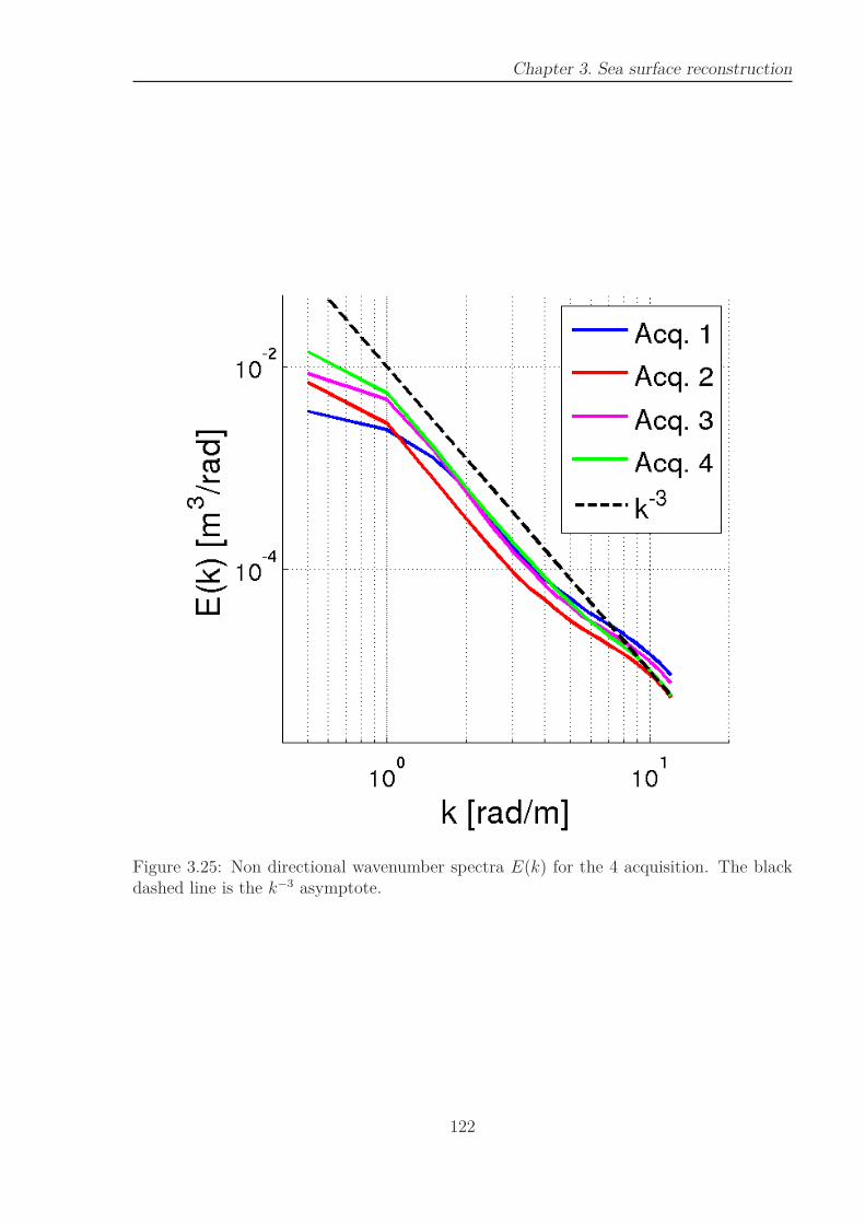
Chapter 3. Sea surface reconstruction
Figure 3.25: Non directional wavenumber spectra E(k) for the 4 acquisition. The blackdashed line is the k−3 asymptote.
122
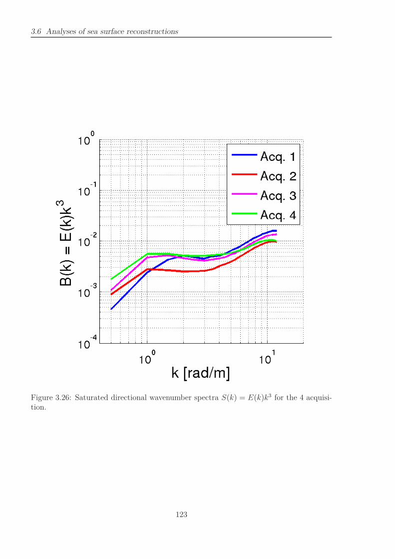
3.6 Analyses of sea surface reconstructions
Figure 3.26: Saturated directional wavenumber spectra S(k) = E(k)k3 for the 4 acquisi-tion.
123

Chapter 3. Sea surface reconstruction
Figure 3.27: Wavenumber spectra obtained with the integration over positive frequenciesof the 3D spectra presented on the figures 3.21-3.24. The obtained wavenumber spectrumE(k, θ) is so unambiguous in direction.
124
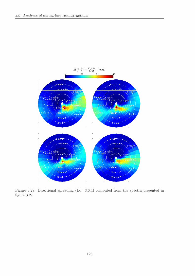
3.6 Analyses of sea surface reconstructions
Figure 3.28: Directional spreading (Eq. 3.6.4) computed from the spectra presented infigure 3.27.
125
Chapter 3. Sea surface reconstruction
a near isotropic spreading) at the wave frequency of 1Hz. Our observations clearly showa non isotropic spreading up to 1.6Hz.
3.6.5 Mean Square Slopes of elevation maps
Another interesting parameter generally observed is the Mean Square Slopes (here-inafter mss). As the whole range of wave scale is not given by the reconstruction, thestandard comparison with the mss computed from sunlight reflection by Cox and Munk(1954) cannot be done directly. However, Vandemark et al. (2004) proposed to add themss<1m = 0.019ln(U10) to 1m-mss. At each point (x, y, t) of the elevation maps, the slopesx and sy are computed mssx and mssy are so computed with
sx,>1m(x, y, t) = (Z(x− 0.5, y, t) − Z(x+ 0.5, y, t)) /1 (3.86)
sy,>1m(x, y, t) = (Z(x, y − 0.5, t) − Z(x, y + 0.5, t)) /1. (3.87)
Therefore, 1m-mss is given with
mssx,>1m(x, y) =1
T
∫ T
0s2x(x, y, t)dt (3.88)
mssy,>1m(x, y) =1
T
∫ T
0s2y(x, y, t)dt (3.89)
mss>1m(x, y) = mssx(x, y) +mssy(x, y) (3.90)
The figure 3.30 shows the slope variance mss1m (left panels), and the slope variance alongx-axis, mssx,1m (center panels) and y-axis, mssy,1m (rigth panels) for each acquisition.We note that the spatial disparity of the mss over the reconstructed area does not havea physical sense. In particular, the inhomogenous mssy obtained for acquisition 4 islinked to the errors in the matching processing due to inhomogeneous illumination of thesea surface. The spatial-averaged mss1m are respectively 0.65%, 0.55%, 0.84% and 0.97for the four acquisitions. Then, the mss given by the smaller scales than 1m are addedfollowing Vandemark et al. (2004) with mss = mss>1m + mss<1m. To a fonction of thewind speed, 11.5m/s, 10.9m/s, 13.2m/s and 13.9m/s, the mss are 5.29%, 5.09%, 5.74.%and 5.87%, where Cox and Munk (1954)’s formula gives respectively 6.19%, 5.88%, 7.06%and 7.42%, with a standard deviation estimated to 0.004. Our mss are strongly under theCox and Munk (1954)’s ones. However, note that the acquisitions correspond to youngwave field, and Vandemark et al. (2004) show that mss given by wave scale greater that1m wavelength, here not fully developed, strongly influence the global mss.
3.7 Conclusion
The existing methods of sea surface reconstruction provide good results in term ofsea elevation statistics and spectra. Nevertheless, it was shown that the presence of foampatches on the sea surface strongly disturbs the local shape of the surface. Particularly,these methods provide unrealistic breaking wave shapes. In this chapter, a completemethod for the reconstruction of sea surface in presence of foam patches is proposed
126
3.7 Conclusion
and validated. Compared to the existing reconstruction methods, the main improvementconcerns the matching point processing. The implementation of an iterative correspondingpoint search with a correlation template which size decreases with increasing iterationgreatly increases the accuracy of the reconstructed surface, particularly in the presenceof foam patches. A correction for the asymmetric projection is also proposed.
Four stereo video acquisitions are investigated. A first validation of the reconstructedsurfaces obtained with the improved method is given by comparison with wave gaugedata. Then the observation of the 3D direction-wavenumber-frequency spectra obtainedfrom the time-space evolution of the surface shows the coherence of the surfaces up tof = 1.6Hz (λ ≈ 60cm). The observed directional wavenumber spectra directly computedover the elevation maps and the directional frequency spectra computed over extractionof several times series are also discussed. Finally, the mean square slope are computedand compared to the classical observations by Cox and Munk (1954). After the validationprovided, the reconstructed sea surfaces are considered accurate enough to be used in thebreaking wave study proposed in the next chapter.
127

Chapter 3. Sea surface reconstruction
Figure 3.29: Spreading integral (Eq. 3.85) computed from the directional spreadingpresented in figure 3.28.
128

3.7 Conclusion
Figure 3.30: Mean Square Slope given by waves longer than 1m computed over the wholeset of images for the 4 acquisitions. mss>1m is the global slope variance (left panels),mss>1m is the slope variance along x-axis (center panels) and mss>1m is the slope variancealong y-axis (right panels).
129

Chapter 4
Observation of breaking waves
4.1 Introduction
Breaking waves occur everywhere on the world’s oceans and affect almost all seasurfaces. Today, the breaking phenomena are still misunderstood. Nevertheless, it isclear that breaking is the dominant process for wind wave energy dissipation. Therefore,a good understanding of wave breaking is necessary to understand wave energy balancesand wave spectra characteristics. Moreover, breaking waves also influence many processes.Inducing a turbulence increasing in the upper sea layer and an active air entrainment intowater, they play an important role in air-sea gas transfers and biochemical processes.Wave breaking process is also associated to the production of sea sprays. In addition, thebreaking-induced foam strongly influences many ocean electromagnetic measurements. Inparticular, whitecaps increase surface reflectance in visible frequencies and strongly impacton radar backscattered signal and brightness temperatures measured by radiometers, suchas those used on Windsat, SMOS and Aquarius. Thus, the whitecap coverage variabilitymust be taken into consideration for the sea surface albedo or ocean color estimations,but also for retrieving sea surface properties. These electromagnetic properties are usedin this work to detect breaking wave in visible spectrum range. Indeed, generated whitefoam areas contrast with a dark sea surface, and are easily observable signatures of thebreaking waves.
Wave breaking is a complex non-linear process with various intense physical phenom-ena in it. Different terminology can be found in the literature to describe evolution ofbreaking waves. Wave breaking event is usually decomposed into two parts. The firstone is the active breaking usually called stage A (Bondur and Sharkov, 1982; Monahanand Woolf, 1989). It results from an instability which develops from the wave crest, whenwater particle velocities approach the wave phase speed (Longuet-Higgins, 1978; Longuet-Higgins and Fox, 1978; Tanaka, 1983, 1985). The wave crest thus collapses on the frontsize of the wave, resulting in wave energy dissipation. The breaking phenomenon occursat all wave scales once they are energetic enough.
For waves shorter than one meter in wavelength, breaking occurs without air entrain-ment, and so without signature in the visible spectrum range. Nevertheless, laboratorymeasurements of Jessup et al. (1997) show that microscale wave breaking associatedwith evolving wind waves disturbs the thermal boundary layer at the air-water interface,
131

Chapter 4. Breaking Observation
producing signatures that can be detected with infrared imagery. Their laboratory ob-servations, under the moderate wind speed conditions, showed a substantial frequency ofoccurrence and an important areal coverage of the phenomenon. Therefore, microscalebreaking is undoubtedly widespread over the oceans and may prove to be a significantmechanism for enhancing the transfer of heat and gas across the air-sea interface (Jessupand Phadnis, 2005; Sutherland and Melville, 2013). These microwave scales are not re-solved in the global ocean spectral wave model, and microwave breaking is not studied inthis work.
The present thesis focuses on longer breaking waves as modeled in spectral wave mod-els. These waves, more energetic, are attended with air entrainment and bubble formation.Formation of foam needs a large quantity of energy, corresponding to the surface tensionmultiplied with surface excess. Thus, when breaking waves are energetic enough, theygenerate white bubble clouds which form whitecaps that contrast with the darker seasurface. This signature in the visible frequency spectrum makes the phenomenon easilyobservable.
Persistence of the foam on sea surface in the wake of the breaking wave is usuallyreferred as stage B of the breaking, also called passive breaking. Passive foam, in contrastwith active foam produced by active crest breaking, does not imply wave dissipation.Nevertheless, the lifetime of the foam persistence is of interest to many investigators dueto the previously discussed strong influence on electromagnetic measurements and air-sea gas exchanges. Foam lifetime has been related to environmental and meteorologicalparameters, including air-sea temperature difference, salinity or even biological content,which directly influence surface tension. Focusing on whitecap dissipation, this work doesnot investigate the passive breaking.
Despite wave breaking being an important phenomenon with many authors interestedin this subject, it is still misunderstood for many reasons. Wave breaking is generallystudied with laboratory or field measurements. Laboratory measurement provides veryinteresting and complete data. Indeed, experimental tanks are manageable environmentwhere a complete instrumentation can be easily deployed. Moreover, laboratory experi-ments allow a quasi complete control of the various factors which influence wave breaking,and thus provide reproducible experiments in well defined conditions. Numerous labo-ratory experiments have quantified the breaking occurrence and the wave dissipation.However, these experiments fail to reproduce all the conditions observed in situ. Indeed,wave age have a strong influence on breaking ; for young wind-sea, intensive breaking isobserved around a spectral peak whereas breaking seems to be absent at the peak wavescale for mature sea (Cp/U10 ≃ 1), and whitecaps are observed on smaller wave scales.Tank experiments succeed in reproducing very young wind sea (with wave age Cp/U10
less than 0.15), but fail to reproduce more developed sea due to limited fetches (Donelanet al., 1993). However, in situ measurements sample a wave age from 0.2 for young seato 0.83 for fully developed wave field. These considerations make the results obtainedin laboratory difficult to apply in the wave models. In contrast, field measurements dealwith real external conditions. But such investigations also have their limits. Firstly, thedeployment of complex measuring equipment is difficult in real sea condition. Secondly,the large number of non manageable external parameters makes experiments non repro-ducible and results difficult to analyze. Here again, application of observation results to
132
4.1 Introduction
model parameterization seems difficult, due to dependence of results to very particularconditions.
Two approaches are usually used to study breaking in field measurements. Generatedwhite foam areas contrasting with the dark sea surface, breaking wave can be easilydetected on photo (Monahan et al., 1983; Stramska and Petelski, 2003; Callaghan et al.,2008) or on image sequences from video camera (Melville and Matusov, 2002; Mironov andDulov, 2008). Various acoustic methods can also be used to measure breaking intensity.On one hand, breaking wave characteristics can be retrieved from reflection of the acousticsonar signal on breaking wave (Loewen and Melville, 1991). On the other hand, soundproduced by breaker crest collapsing can be measured using hydrophones (Babanin et al.,2001). This last method provides direct information on the occurrence and intensity ofbreaking, but is not able to define neither precise location of the breaking nor breakingdirection. In contrast, optical methods based on breaking foam detection at sea surface,are generally used to investigate shape, speed, direction and other characteristics of thebreaking waves. Nevertheless results are strongly dependent on the threshold used forfoam patch detection and on the discrimination of stage A and B.
In this study, an optical system is used. As in majority of the optical methods pub-lished in the literature, foam patches of breaking waves are here detected using a thresholdmethod. In large number of studies, the threshold is defined by the investigator. Thesemethods have two main disadvantages. Firstly, results depend on the investigator sub-jectivity. Secondly, these methods are difficult to apply automatically on different datasets. Discrimination of phases A (active breaking) and stage B (passive foam) is alsoproblematic. Many studies proposed a discrimination using to different thresholds. Ac-tive breaking entrains air into water, and so actively produce new bubbles, associatedwith brighter foam. Passive foam corresponds to the decreasing of the foam density andis related to darker foam. Therefore, high level selects bright whitecaps and marks themas active breaking, whereas a lower value discriminates passive foam. Results of whitecapmeasurements vary in different works; often, the problem of threshold selection is amongthe causes of such variations (Mironov and Dulov, 2008).
Mironov and Dulov (2008) developed a processing algorithm to define threshold anddiscriminates stage A and B based on physical prerequisites and statistical properties ofthe studied phenomenon that maximally eliminates human influence, and so that can beapplied in a same way on different data sets. They applied their processing on large dataset, providing very interesting speed and direction distribution. Nevertheless, their studydoes not include the elevation of the surface and shape of breaking waves. Indeed, usingonly one camera, they linked pixel coordinates to sea surface coordinates by a simpleprojection on the mean sea plane, losing sea surface elevation information. Originality ofthe present work is that, using surface stereo reconstruction discussed in previous chapter,the breaking waves are observed together with sea surface elevation maps, providing analternative source of information.
The vast majority of the wave breaking studies discuss the breaking probability. Onthe classical 1D studies, the breaking probability Pb is defined with
Pb =Nb
Nw
, (4.1)
133
Chapter 4. Breaking Observation
where Nb is the number of breaking waves and Nw is the total number of waves. Inan elevation time series, the individual waves are generally defined between successivepoints where the water surface crosses downwards (zero down-crossing) or upwards (zeroup-crossing) the mean water level. For each individual wave, the period is the time lagseparating the two zero down-crossing (or up-crossing) and the height is the differencebetween minimum and maximum elevation. This wave-by-wave analysis is applied forthe study of the dominant wave breaking (Banner et al., 1989). By construction, thisanalysis can be applied to the study of the smaller waves, which may be riding on thecrest of the large waves (Banner et al., 2002). Nevertheless, this wave counting methodcan be applied to frequency filtered elevation time-series to analyze breaking of smallerwave scales (Banner et al., 2000; Babanin et al., 2001; Filipot et al., 2010). The difficultyis to choose a frequency bandwidth narrow enough in order to discriminate the energyof waves with different frequencies but also large enough so that the filtered surfacehas a representative steepness. Indeed, the narrower bandwidth, reduced to a uniquefrequency would lead to a small monochromatic wave not representative of the observedsurface elevation. Banner et al. (2000) and Babanin et al. (2001) assumed that thecomponents contributing to the dominant waves were contained between (1−δBBY)fp and(1 + δBBY)fp, with δBBY = 0.3. For deep water waves, this frequency interval correspondsto wavenumbers from 0.5kp to 1.7kp. Further, Filipot et al. (2010) re-use this frequencybandwidth for their wave-scaled analysis of breaking.
As disused in the chapter 2, these breaking probabilities were then related to thespectrum saturation (Banner et al., 2002), leading to the breaking parameterization ofArdhuin et al. (2010) (TEST451) or to the wave steepness (Filipot et al., 2010), leadingto the breaking parameterization of Filipot and Ardhuin (2012) (TEST500), improved toTEST570 (see chapter 2). The work presented here proposed a comparison of our obser-vations with these two parameterization of breaking probability and a critical analysis ofthe assumptions used in the breaking parameterizations. Indeed, it must be noted thatin the wave model, the assumption is made for the length of crest calculation, and sofor the cumulative effect estimation, that the breaking probability thus calculated can beapplied on the wave crest (breaking or not) length density to obtain the breaking crestlength density. Another severe assumption is made for the definition of the wave crestlength density.
The breaking detection processing used in this work, greatly inspired from the algo-rithm of Mironov and Dulov (2008), is described in the section 4.2, with a description ofthe results in terms of speed and direction distributions of the detected breaking. Thenext section (4.3) discussed a definition of the crest length density. Then, observed break-ing probabilities are shown in section 4.4. These observations are compared to the modelof Filipot et al. (2010) used in the parameterization of Filipot and Ardhuin (2012) in thesection 4.5, then rely to the partially integrated saturation spectrum used in the param-eterization of Ardhuin et al. (2010) in the section 4.6. The conclusion follows in the lastsection.
134

4.2 Automatic detection of breaking events
4.2 Automatic detection of breaking events
Detection of breaking events used for this study is now described. The processedimage parts of the 4 records correspond to the reconstruction areas shown on figure 3.16.The process is split into two steps. First step consists in removing of all unnecessaryinformation not connected with breaking wave properties, to simplify processing. Anevident way of such simplification is binarization of whitecaps from the sea surface videorecords using brightness threshold criterion (Mironov and Dulov, 2008). A binary dataarray with only whitecap information is the result of this procedure. The main difficulty ofthis step is the selection of the threshold which discriminates foam patches. The methodof Mironov and Dulov (2008) is used here, as described in section 4.2.1. Second stepconsists in the discrimination of the binarized foam patches into active and passive foam.This second step is also adapted from works of Mironov and Dulov (2008). Using physicalproperties, the binarized data are then discriminated into active and passive foam. Thediscrimination is described in section 4.2.2. The automatic detection of breaking eventsis applied to the four acquisition already described in the chapter 3 (see §3.2, Tab. 3.1).
4.2.1 Image binarization
Pixel brightness arises from various parameters. Basically, brightness levels dependon the position of the Sun and sea surface slope. Nevertheless, many other parameterscan strongly influence it: the presence of clouds, the sky reflection and air scattering andabsorption (which is a problem in airborne imagery. Note that in our case, there canalso be a strong reflection from the coastal mountains. Moreover, the automatic gainadjustment also affects pixel brightness. Finally, the presence of foam on the sea surfacealso strongly increases brightness level. The aim of the present algorithm is to define athreshold which discriminates high pixel brightness level due to presence of foam.
Long-lasting brightness removing
Mironov and Dulov (2008) proposed an algorithm, independent of human influenceand based on physical principles of brightness field formation, which ensures satisfactorythreshold for such a wide range of conditions. Brightness variance at a fixed point of seasurface, I, is the sum of an instant brightness, Ig, due to surface slope and of a long-lastingbrightness component, Iavg, resulting from background conditions. Generally, the valuesof Iavg widely vary on the frame, making the selection of a common threshold impossible.The first step so consists in the removing of this brightness trend. This trend is evaluatedby averaging a sequence of consecutive images. In this work, average is done over 2000images, corresponding to about 2.2 min sequence for the 15 Hz acquisition 1 and 2.7 minsequence for the 12 Hz acquisitions 2, 3, and 4. The evolution of the automatic gain issmoothed, and the gain is assumed constant during the averaged image sequence. Spatialbrightness distribution permanently evolves along the frame (sun displacement, cloudmoving, ...) and Iavg is computed for every 2000 image sequence of the record. Then, allbrightness trends and heterogeneity can be removed by the subtraction of the calculatedIavg values from each frame of the processed video record.
135
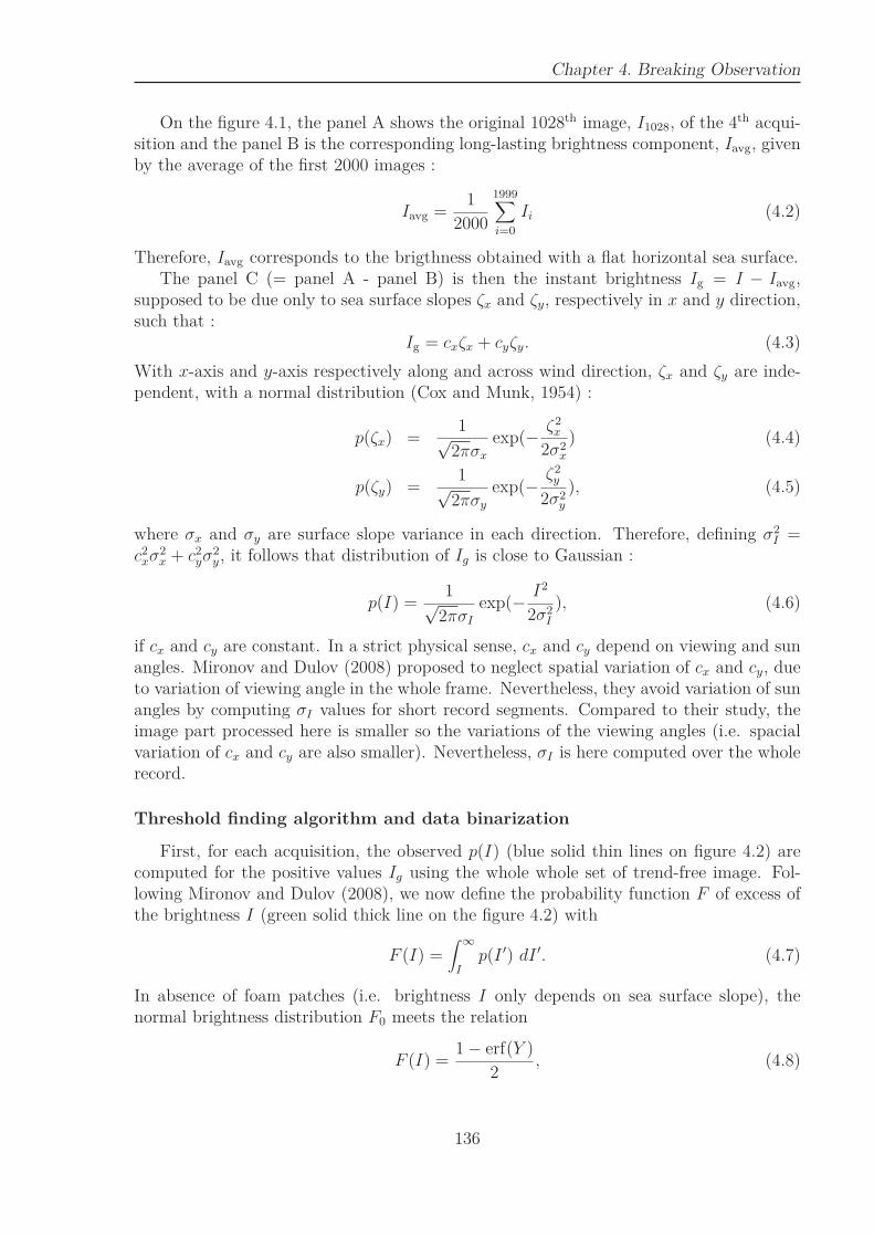
Chapter 4. Breaking Observation
On the figure 4.1, the panel A shows the original 1028th image, I1028, of the 4th acqui-sition and the panel B is the corresponding long-lasting brightness component, Iavg, givenby the average of the first 2000 images :
Iavg =1
2000
1999∑
i=0
Ii (4.2)
Therefore, Iavg corresponds to the brigthness obtained with a flat horizontal sea surface.The panel C (= panel A - panel B) is then the instant brightness Ig = I − Iavg,
supposed to be due only to sea surface slopes ζx and ζy, respectively in x and y direction,such that :
Ig = cxζx + cyζy. (4.3)
With x-axis and y-axis respectively along and across wind direction, ζx and ζy are inde-pendent, with a normal distribution (Cox and Munk, 1954) :
p(ζx) =1√
2πσxexp(− ζ2
x
2σ2x
) (4.4)
p(ζy) =1√
2πσyexp(− ζ2
y
2σ2y
), (4.5)
where σx and σy are surface slope variance in each direction. Therefore, defining σ2I =
c2xσ
2x + c2
yσ2y , it follows that distribution of Ig is close to Gaussian :
p(I) =1√
2πσIexp(− I2
2σ2I
), (4.6)
if cx and cy are constant. In a strict physical sense, cx and cy depend on viewing and sunangles. Mironov and Dulov (2008) proposed to neglect spatial variation of cx and cy, dueto variation of viewing angle in the whole frame. Nevertheless, they avoid variation of sunangles by computing σI values for short record segments. Compared to their study, theimage part processed here is smaller so the variations of the viewing angles (i.e. spacialvariation of cx and cy are also smaller). Nevertheless, σI is here computed over the wholerecord.
Threshold finding algorithm and data binarization
First, for each acquisition, the observed p(I) (blue solid thin lines on figure 4.2) arecomputed for the positive values Ig using the whole whole set of trend-free image. Fol-lowing Mironov and Dulov (2008), we now define the probability function F of excess ofthe brightness I (green solid thick line on the figure 4.2) with
F (I) =∫
∞
Ip(I ′) dI ′. (4.7)
In absence of foam patches (i.e. brightness I only depends on sea surface slope), thenormal brightness distribution F0 meets the relation
F (I) =1 − erf(Y )
2, (4.8)
136
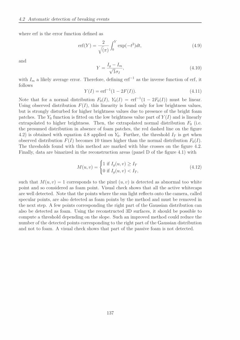
4.2 Automatic detection of breaking events
where erf is the error function defined as
erf(Y ) =2
√
(π)
∫ Y
0exp(−t2)dt, (4.9)
and
Y =Ig − Im√
1σI, (4.10)
with Im a likely average error. Therefore, defining erf−1 as the inverse function of erf, itfollows
Y (I) = erf−1(1 − 2F (I)). (4.11)
Note that for a normal distribution F0(I), Y0(I) = erf−1(1 − 2F0(I)) must be linear.Using observed distribution F (I), this linearity is found only for low brightness values,but is strongly disturbed for higher brightness values due to presence of the bright foampatches. The Y0 function is fitted on the low brightness value part of Y (I) and is linearlyextrapolated to higher brightness. Then, the extrapolated normal distribution F0 (i.e.the presumed distribution in absence of foam patches, the red dashed line on the figure4.2) is obtained with equation 4.8 applied on Y0. Further, the threshold IT is get whenobserved distribution F (I) becomes 10 times higher than the normal distribution F0(I).The thresholds found with this method are marked with blue crosses on the figure 4.2.Finally, data are binarized in the reconstruction areas (panel D of the figure 4.1) with
M(u, v) =
1 if Ig(u, v) ≥ IT
0 if Ig(u, v) < IT ,(4.12)
such that M(u, v) = 1 corresponds to the pixel (u, v) is detected as abnormal too whitepoint and so considered as foam point. Visual check shows that all the active whitecapsare well detected. Note that the points where the sun light reflects onto the camera, calledspecular points, are also detected as foam points by the method and must be removed inthe next step. A few points corresponding the right part of the Gaussian distribution canalso be detected as foam. Using the reconstructed 3D surfaces, it should be possible tocompute a threshold depending on the slope. Such an improved method could reduce thenumber of the detected points corresponding to the right part of the Gaussian distributionand not to foam. A visual check shows that part of the passive foam is not detected.
137
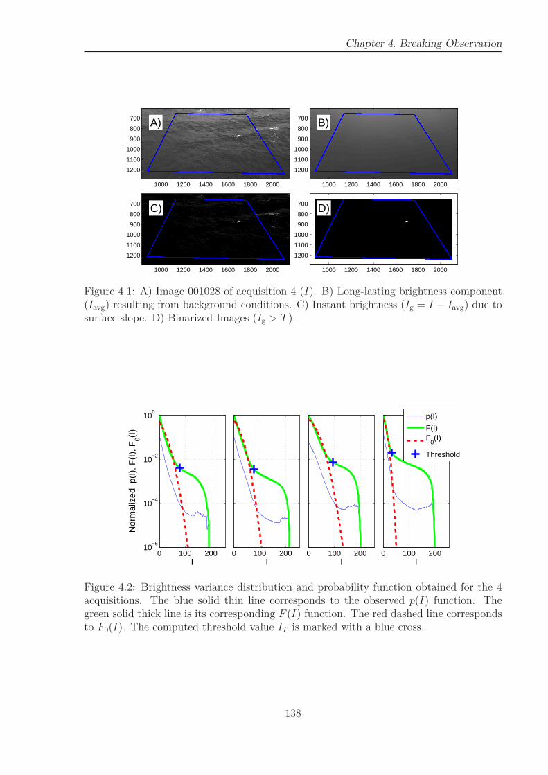
Chapter 4. Breaking Observation
A)
1000 1200 1400 1600 1800 2000
700
800
900
1000
1100
1200
B)
1000 1200 1400 1600 1800 2000
700
800
900
1000
1100
1200
C)
1000 1200 1400 1600 1800 2000
700
800
900
1000
1100
1200
D)
1000 1200 1400 1600 1800 2000
700
800
900
1000
1100
1200
Figure 4.1: A) Image 001028 of acquisition 4 (I). B) Long-lasting brightness component(Iavg) resulting from background conditions. C) Instant brightness (Ig = I − Iavg) due tosurface slope. D) Binarized Images (Ig > T ).
0 100 20010
−6
10−4
10−2
100
I
Nor
mal
ized
p(I
), F
(I),
F0(I
)
0 100 200I
0 100 200I
0 100 200I
p(I)
F(I)F
0(I)
Threshold
Figure 4.2: Brightness variance distribution and probability function obtained for the 4acquisitions. The blue solid thin line corresponds to the observed p(I) function. Thegreen solid thick line is its corresponding F (I) function. The red dashed line correspondsto F0(I). The computed threshold value IT is marked with a blue cross.
138
4.2 Automatic detection of breaking events
4.2.2 Event filtering method
For each acquisition, binarized data are organized in a large 3D binary matrix M =M(u, v, f) where u and v are pixel coordinates in reconstruction area and f is the framenumber. The foam points directly connected in time and connected in space within alength of 10 pixels are grouped. Generally, the set of foam points in each group in-cludes active and passive foam, but also mirror points which must be discriminated. Highsunglint on wave crest can also imply additional white point detection. This problemis difficult to resolve because corresponding detected white points follow the wave evo-lution and so have dynamic properties very close to breaking detected white points. Toavoid this problem, the processed image areas have been chosen in the image part darkenough to visually distinguish the breaking. However, specular points can appear in thereconstruction areas. These points have short lifetime and a small area. The acquisitiontime was chosen so that most of the specular points are in the lower part of the image,where they disturb only small number of connected pixel. These points are removed by afiltering of smallest white point groups in time and space. Typically, groups which containless than 200 white points, or which time duration is less than 0.4 seconds are removed.All non-removed white points are now called foam points. Note that this filtering alsoremoved small breaking event. Nevertheless, the reconstructed surface resolution is alsonot adapted, due to insufficient pixel resolution, to study the small events. Higher pixelresolution and/or using of zoom lenses should allow for smaller breaking event study.
As stated in the introduction, many investigators discriminate active foam by brighterpixels. In this work, a discrimination algorithm based on physical properties, inspiredfrom work of Mironov and Dulov (2008), is implemented. Focusing on active breakingand wave dissipation, the present algorithm is adjusted to mainly detect the start of thebreaking event, and as far as possible the complete active breaking. Each foam pointgroup is the analyzed separately.
The group is first analyzed in the pixel-frame reference system. Let’s note Mi(u, v, f)the binary sub-matrix containing the foam points of group i. The time evolution ofnumber of foam points Ni(f) is first computed with
Ni(f) =∑
u
∑
v
Mi(u, v, f). (4.13)
The sea surface footprint of pixels depends on both surface shape and coordinates ofthe pixel on the image. Nevertheless, foam pixels of a same group stretch on a smalland localized image part. Therefore, the time evolution of pixel number Ni(f) is in firstapproximation assimilated to the time evolution of foam patch surface. Active breakingactively produces new bubbles, faster than passive foam disappears. Typically, Ni(f)increases to a maximum during active wave breaking and then decreases as a function ofthe foam lifetime. However, a new active breaking can occur in the same zone, beforethe residual foam of the previous one completely disappears. In this case, the two activebreaking events are contained in the same group, and must be split. If the second breakingwave is not too small compared to the first one, it implies a second increase of Ni(f) andso can be detected. In practice, each group is split into independent events such thatprevious an event ends when its number of foam points N becomes smaller than 25% ofits maximum and a new event starts further if N becomes higher by 25% of the previous
139
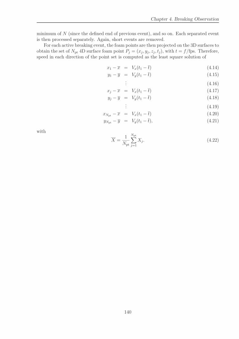
Chapter 4. Breaking Observation
minimum of N (since the defined end of previous event), and so on. Each separated eventis then processed separately. Again, short events are removed.
For each active breaking event, the foam points are then projected on the 3D surfaces toobtain the set of Npt 4D surface foam point Pj = (xj, yj, zj, tj), with t = f/fps. Therefore,speed in each direction of the point set is computed as the least square solution of
x1 − x = Vx(t1 − t) (4.14)
y1 − y = Vy(t1 − t) (4.15)... (4.16)
xj − x = Vx(t1 − t) (4.17)
yj − y = Vy(t1 − t) (4.18)... (4.19)
xNpt− x = Vx(t1 − t) (4.20)
yNpt− y = Vy(t1 − t), (4.21)
with
X =1
Npt
Npt∑
j=1
Xj. (4.22)
140
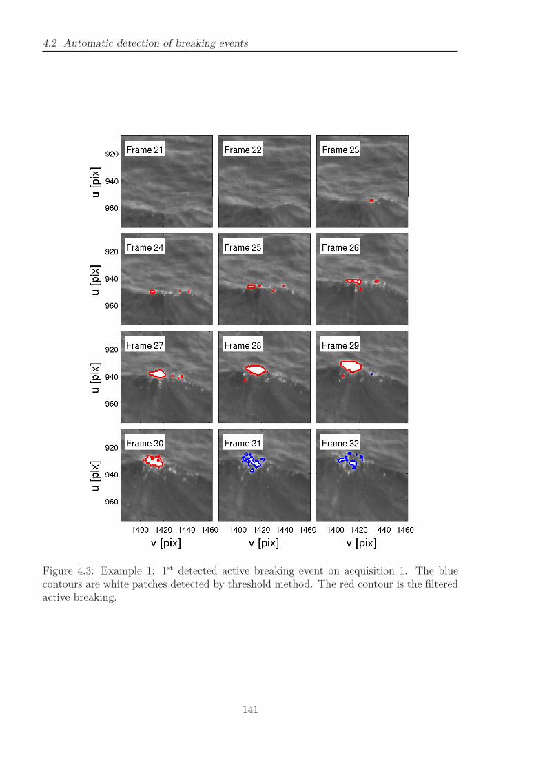
4.2 Automatic detection of breaking events
Figure 4.3: Example 1: 1st detected active breaking event on acquisition 1. The bluecontours are white patches detected by threshold method. The red contour is the filteredactive breaking.
141
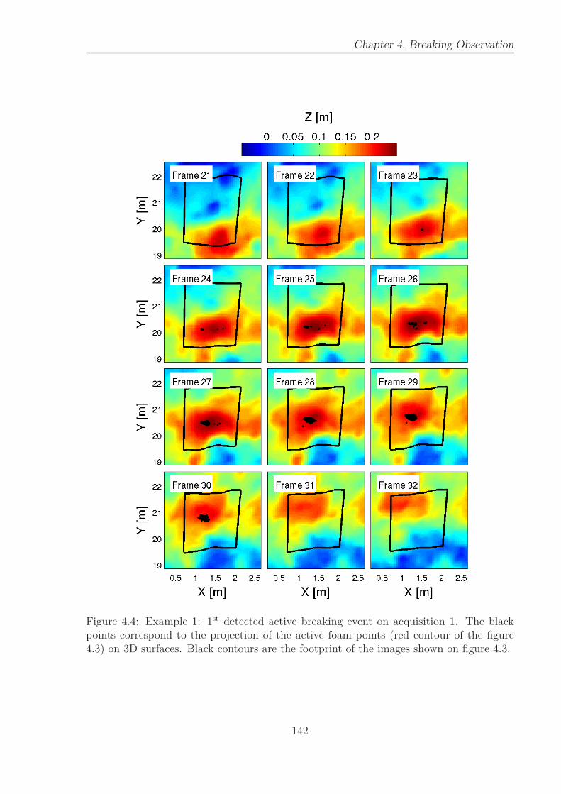
Chapter 4. Breaking Observation
Figure 4.4: Example 1: 1st detected active breaking event on acquisition 1. The blackpoints correspond to the projection of the active foam points (red contour of the figure4.3) on 3D surfaces. Black contours are the footprint of the images shown on figure 4.3.
142
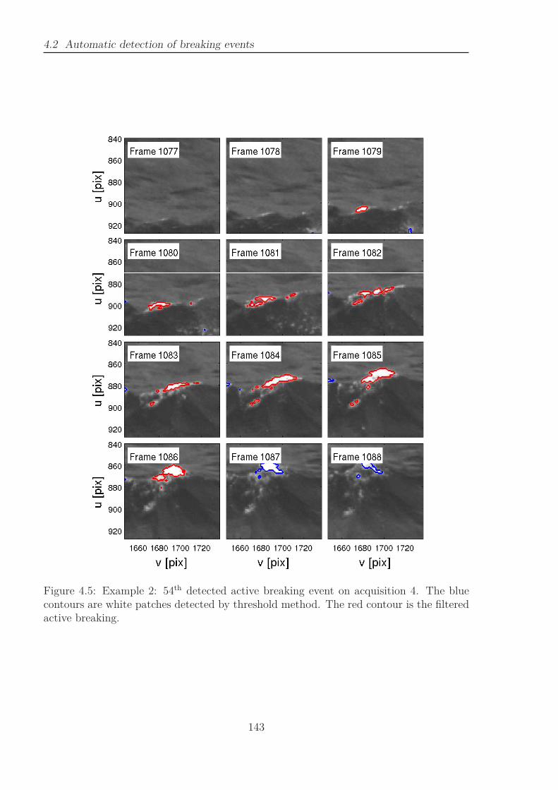
4.2 Automatic detection of breaking events
Figure 4.5: Example 2: 54th detected active breaking event on acquisition 4. The bluecontours are white patches detected by threshold method. The red contour is the filteredactive breaking.
143
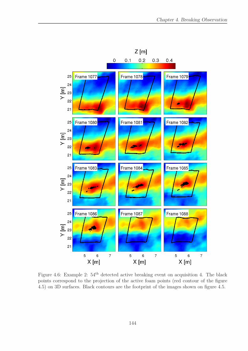
Chapter 4. Breaking Observation
Figure 4.6: Example 2: 54th detected active breaking event on acquisition 4. The blackpoints correspond to the projection of the active foam points (red contour of the figure4.5) on 3D surfaces. Black contours are the footprint of the images shown on figure 4.5.
144
4.3 Crest length density
Therefore, absolute speed and direction are
Vb =√
V 2x + V 2
y (4.23)
θb = arctan(VyVx
). (4.24)
Visual observations of breaking waves show that active breaking foam move around themain direction of wind surface waves and passive foam drift on a sea surface with ratherslow velocity modulated by orbital velocities of the surface waves. Therefore, all eventswith computed speed less than 1m/s are assimilated to small events or passive foam andare removed. The figures 4.3 and 4.5 show two examples of detected active breakingevents on images. The figure 4.4 and 4.6 show their respective projection on 3D surfaces.
With this algorithm, 276, 795, 1669 and 1390 active breaking events are respectivelyfound for the 4 acquisitions. The probability density functions of breaking waves tobreaking speed and directions are respectively shown on the figures 4.7 and 4.8. Theobservations show a maximum in the breaking speed distribution, which could be relatedto the maximum of the Λ-distribution observed by Gemmrich et al. (2008) and Thomsonand Jessup (2008). The maximum seems to move to the higher breaking speeds with windspeed increasing. The breaking wave direction distribution show a Gaussian centered onthe wind direction, in line with the observations of Mironov and Dulov (2008). The 2Dprobability density function of breaking to breaking speeds and directions is given onfigure 4.9.
4.3 Crest length density
We define wave crest as the locations where one slope component is zero, with anegative curvature. In other words, the crests are defined by the points such that (dz/dx =0 and d2z/d2x < 0) or (dz/dy = 0 and d2z/d2y < 0). Note that this method also considersthe crests corresponding to the smaller riding waves, generally not taken into account bywave-by-wave zero-crossing analysis. Consecutive points in the elevation map matrix aregrouped to form the wave crests. Finally the crest length is measured and divided by thesea surface area to obtained the crest length density of the waves, breaking or not, for theconsidered wave scale fc. Note that the obtained crest length densities are linked to thefrequency bandwidth ∆k = 2δBBYk = 0.6k.
Following Filipot et al. (2010), the crest are detected on frequency-filtered surfaces, atvarious scales, with frequency filter defined by a 2δ wide Hann window Ufc
(f), centeredat fc such that
Ufc(f) = 0.5 − 0.5 cos
[
π
δ
(
f
fc− 1 − δ
)]
, (4.25)
with δ = δBBY = 0.3. The 3D spectra presented on the figures 3.21-3.24 in the chapter3 show that the frequency-filtered surfaces also contain energy associated with nonlinearharmonics of other wave scales. As the wave models only takes into account linear wavesenergy, Filipot et al. (2010) proposed to remove the nonlinear contribution using aniterative removing of the harmonic coming from the other wave scales estimated using the
145
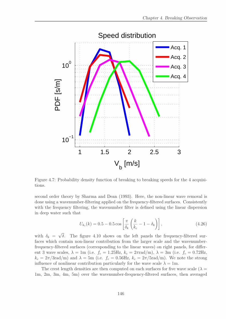
Chapter 4. Breaking Observation
1 1.5 2 2.5 3
10−1
100
Vb [m/s]
PD
F [s
/m]
Speed distribution
Acq. 1
Acq. 2
Acq. 3
Acq. 4
Figure 4.7: Probability density function of breaking to breaking speeds for the 4 acquisi-tions.
second order theory by Sharma and Dean (1993). Here, the non-linear wave removal isdone using a wavenumber-filtering applied on the frequency-filtered surfaces. Consistentlywith the frequency filtering, the wavenumber filter is defined using the linear dispersionin deep water such that
Ukc(k) = 0.5 − 0.5 cos
[
π
δk
(
k
kc− 1 − δk
)]
, (4.26)
with δk =√δ. The figure 4.10 shows on the left panels the frequency-filtered sur-
faces which contain non-linear contribution from the larger scale and the wavenumber-frequency-filtered surfaces (corresponding to the linear waves) on right panels, for differ-ent 3 wave scales, λ = 1m (i.e. fc = 1.25Hz, kc = 2πrad/m), λ = 3m (i.e. fc = 0.72Hz,kc = 2π/3rad/m) and λ = 5m (i.e. fc = 0.56Hz, kc = 2π/5rad/m). We note the stronginfluence of nonlinear contribution particularly for the wave scale λ = 1m.
The crest length densities are then computed on each surfaces for five wave scale (λ =1m, 2m, 3m, 4m, 5m) over the wavenumber-frequency-filtered surfaces, then averaged
146
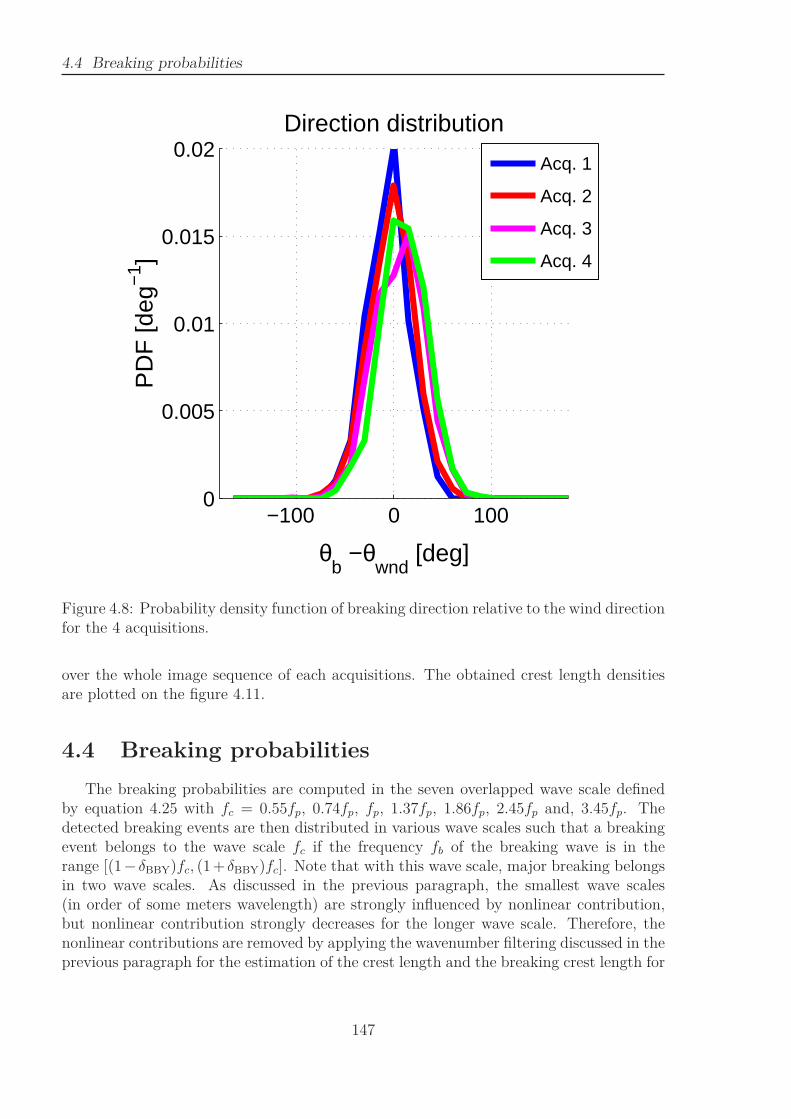
4.4 Breaking probabilities
−100 0 1000
0.005
0.01
0.015
0.02
θb −θ
wnd [deg]
PD
F [d
eg−
1 ]Direction distribution
Acq. 1
Acq. 2
Acq. 3
Acq. 4
Figure 4.8: Probability density function of breaking direction relative to the wind directionfor the 4 acquisitions.
over the whole image sequence of each acquisitions. The obtained crest length densitiesare plotted on the figure 4.11.
4.4 Breaking probabilities
The breaking probabilities are computed in the seven overlapped wave scale definedby equation 4.25 with fc = 0.55fp, 0.74fp, fp, 1.37fp, 1.86fp, 2.45fp and, 3.45fp. Thedetected breaking events are then distributed in various wave scales such that a breakingevent belongs to the wave scale fc if the frequency fb of the breaking wave is in therange [(1− δBBY)fc, (1+ δBBY)fc]. Note that with this wave scale, major breaking belongsin two wave scales. As discussed in the previous paragraph, the smallest wave scales(in order of some meters wavelength) are strongly influenced by nonlinear contribution,but nonlinear contribution strongly decreases for the longer wave scale. Therefore, thenonlinear contributions are removed by applying the wavenumber filtering discussed in theprevious paragraph for the estimation of the crest length and the breaking crest length for
147

Chapter 4. Breaking Observation
1 m/s
1 m/s
2 m/s
2 m/s2 m/s
3 m/s 3 m/s
3 m/s
3 m/s
Acq. 1, U10
= 11.5 m/s
1 m/s
1 m/s
2 m/s
2 m/s2 m/s
3 m/s 3 m/s
3 m/s
3 m/s
Acq. 2, U10
= 10.9 m/s
1 m/s
2 m/s
2 m/s
3 m/s
3 m/s3 m/s
Acq. 3, U10
= 13.2 m/s
1 m/s
1 m/s
2 m/s
2 m/s2 m/s
3 m/s 3 m/s
3 m/s
3 m/s
Acq. 4, U10
= 13.9 m/s
PDF [s/m/deg]1e−4 1e−3 1e−2
Figure 4.9: Probability density function of breaking to breaking speeds and directions forthe 4 acquisitions. The black arrows give the wing direction.
the wave scale in which the wavelengths are included in the surface areas and are neglectedfor the other wave scales. Moreover, with the reconstructed surface areas greater than thehalf size of the peak wavelength, the non-linear contribution is only neglected in the wavescale fc = 0.55fp, 0.74fp, fp, 1.37fp, in which non-linear contribution from the harmonicsof the peak waves do not have strong influence.
As stated in the introduction, the breaking probability is generally the ratio betweenthe number of breaking waves and the total number of waves (breaking or not). Thenumber of waves is generally computed using a zero up-crossing (or zero down-crossing)processing of the elevation time series. On a 2D real sea surface, the definition of anindividual wave is more difficult. Therefore, two methods for the probability estimation
148
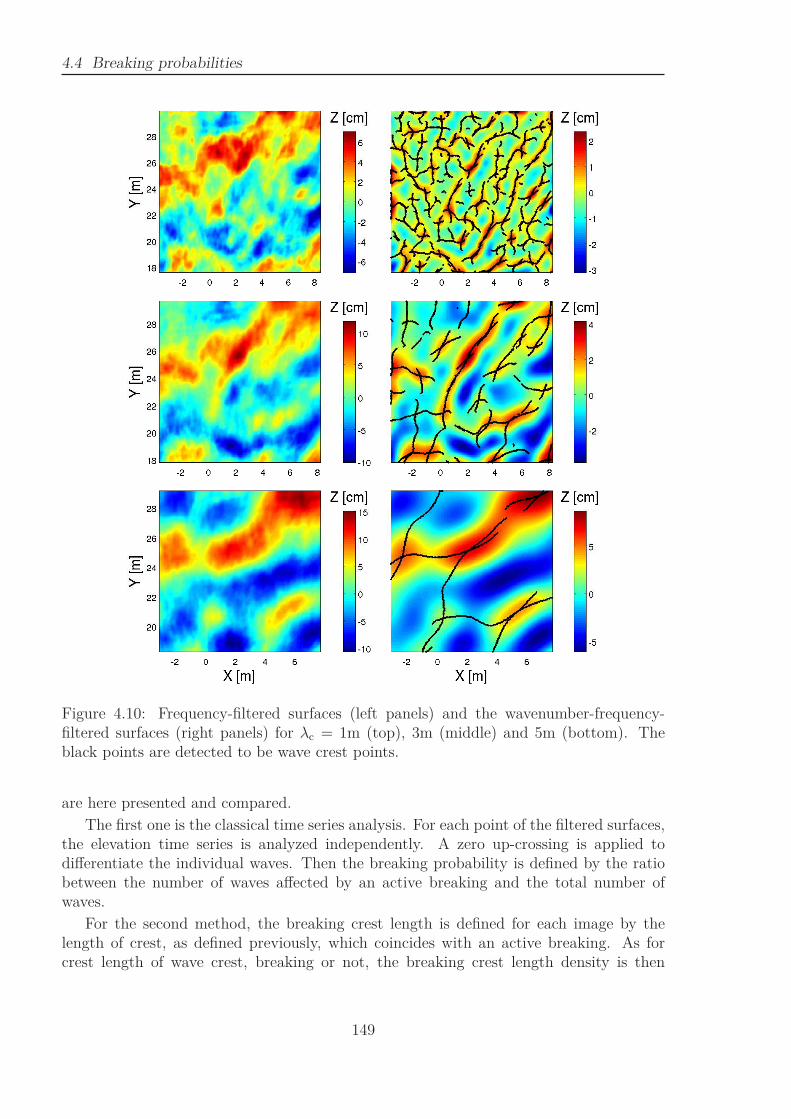
4.4 Breaking probabilities
Figure 4.10: Frequency-filtered surfaces (left panels) and the wavenumber-frequency-filtered surfaces (right panels) for λc = 1m (top), 3m (middle) and 5m (bottom). Theblack points are detected to be wave crest points.
are here presented and compared.
The first one is the classical time series analysis. For each point of the filtered surfaces,the elevation time series is analyzed independently. A zero up-crossing is applied todifferentiate the individual waves. Then the breaking probability is defined by the ratiobetween the number of waves affected by an active breaking and the total number ofwaves.
For the second method, the breaking crest length is defined for each image by thelength of crest, as defined previously, which coincides with an active breaking. As forcrest length of wave crest, breaking or not, the breaking crest length density is then
149
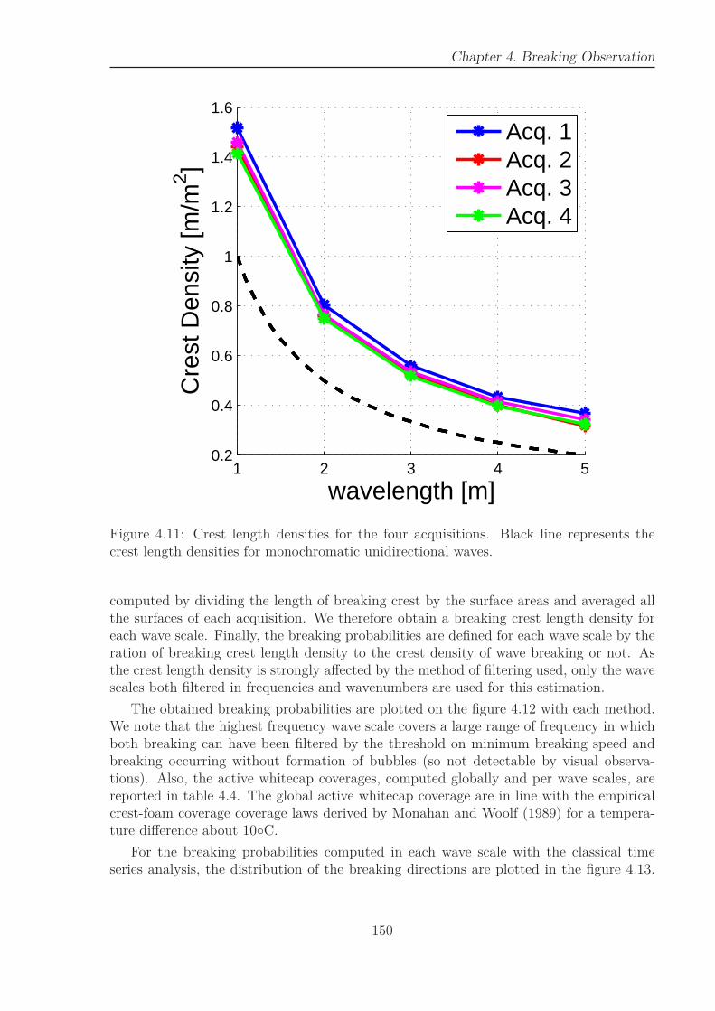
Chapter 4. Breaking Observation
1 2 3 4 50.2
0.4
0.6
0.8
1
1.2
1.4
1.6
wavelength [m]
Cre
st D
ensi
ty [m
/m2 ]
Acq. 1Acq. 2Acq. 3Acq. 4
Figure 4.11: Crest length densities for the four acquisitions. Black line represents thecrest length densities for monochromatic unidirectional waves.
computed by dividing the length of breaking crest by the surface areas and averaged allthe surfaces of each acquisition. We therefore obtain a breaking crest length density foreach wave scale. Finally, the breaking probabilities are defined for each wave scale by theration of breaking crest length density to the crest density of wave breaking or not. Asthe crest length density is strongly affected by the method of filtering used, only the wavescales both filtered in frequencies and wavenumbers are used for this estimation.
The obtained breaking probabilities are plotted on the figure 4.12 with each method.We note that the highest frequency wave scale covers a large range of frequency in whichboth breaking can have been filtered by the threshold on minimum breaking speed andbreaking occurring without formation of bubbles (so not detectable by visual observa-tions). Also, the active whitecap coverages, computed globally and per wave scales, arereported in table 4.4. The global active whitecap coverage are in line with the empiricalcrest-foam coverage coverage laws derived by Monahan and Woolf (1989) for a tempera-ture difference about 10◦C.
For the breaking probabilities computed in each wave scale with the classical timeseries analysis, the distribution of the breaking directions are plotted in the figure 4.13.
150
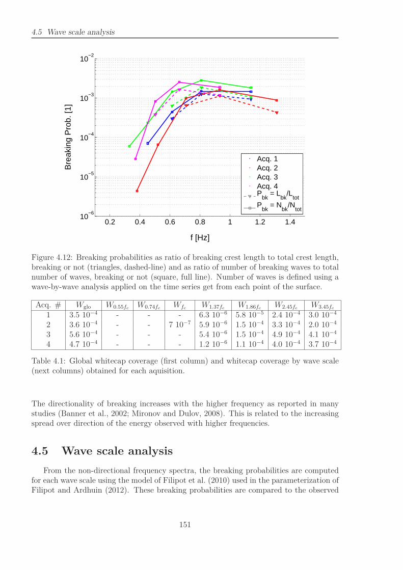
4.5 Wave scale analysis
0.2 0.4 0.6 0.8 1 1.2 1.410
−6
10−5
10−4
10−3
10−2
f [Hz]
Bre
akin
g P
rob.
[1]
Acq. 1Acq. 2Acq. 3Acq. 4P
bk = L
bk/L
totP
bk = N
bk/N
tot
Figure 4.12: Breaking probabilities as ratio of breaking crest length to total crest length,breaking or not (triangles, dashed-line) and as ratio of number of breaking waves to totalnumber of waves, breaking or not (square, full line). Number of waves is defined using awave-by-wave analysis applied on the time series get from each point of the surface.
Acq. # Wglo W0.55fcW0.74fc
WfcW1.37fc
W1.86fcW2.45fc
W3.45fc
1 3.5 10−4 - - - 6.3 10−6 5.8 10−5 2.4 10−4 3.0 10−4
2 3.6 10−4 - - 7 10−7 5.9 10−6 1.5 10−4 3.3 10−4 2.0 10−4
3 5.6 10−4 - - - 5.4 10−6 1.5 10−4 4.9 10−4 4.1 10−4
4 4.7 10−4 - - - 1.2 10−6 1.1 10−4 4.0 10−4 3.7 10−4
Table 4.1: Global whitecap coverage (first column) and whitecap coverage by wave scale(next columns) obtained for each aquisition.
The directionality of breaking increases with the higher frequency as reported in manystudies (Banner et al., 2002; Mironov and Dulov, 2008). This is related to the increasingspread over direction of the energy observed with higher frequencies.
4.5 Wave scale analysis
From the non-directional frequency spectra, the breaking probabilities are computedfor each wave scale using the model of Filipot et al. (2010) used in the parameterization ofFilipot and Ardhuin (2012). These breaking probabilities are compared to the observed
151
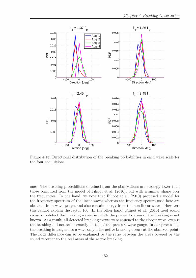
Chapter 4. Breaking Observation
−100 0 1000
0.005
0.01
0.015
0.02
0.025
0.03
0.035
f c
= 1.37 f p
Direction [deg]
PD
F
−100 0 1000
0.005
0.01
0.015
0.02
0.025
f c
= 1.86 f p
Direction [deg]
PD
F
−100 0 1000
0.005
0.01
0.015
0.02
f c
= 2.45 f p
Direction [deg]
PD
F
−100 0 1000
0.002
0.004
0.006
0.008
0.01
0.012
0.014
0.016
f c
= 3.45 f p
Direction [deg]
PD
F
Acq. 1Acq. 2Acq. 3Acq. 4
Figure 4.13: Directional distribution of the breaking probabilities in each wave scale forthe four acquisitions.
ones. The breaking probabilities obtained from the observations are strongly lower thanthose computed from the model of Filipot et al. (2010), but with a similar shape overthe frequencies. In one hand, we note that Filipot et al. (2010) proposed a model forthe frequency spectrum of the linear waves whereas the frequency spectra used here areobtained from wave gauges and also contain energy from the non-linear waves. However,this cannot explain the factor 100. In the other hand, Filipot et al. (2010) used soundrecords to detect the breaking waves, in which the precise location of the breaking is notknown. As a result, all detected breaking events were assigned to the closest wave, even isthe breaking did not occur exactly on top of the pressure wave gauge. In our processing,the breaking is assigned to a wave only if the active breaking occurs at the observed point.The large difference can so be explained by the ratio between the areas covered by thesound recorder to the real areas of the active breaking.
152
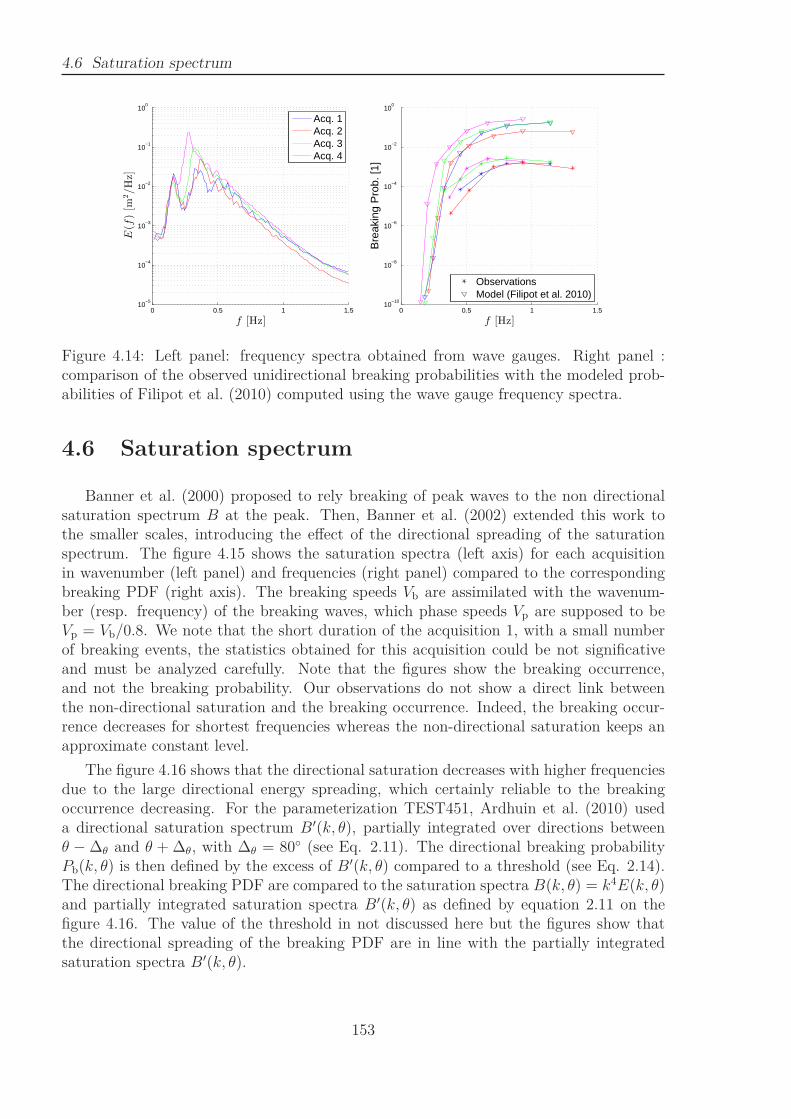
4.6 Saturation spectrum
0 0.5 1 1.510
−5
10−4
10−3
10−2
10−1
100
f [Hz]
E(f)[m
2/Hz]
0 0.5 1 1.510
−10
10−8
10−6
10−4
10−2
100
f [Hz]
Bre
akin
g P
rob.
[1]
Acq. 1Acq. 2Acq. 3Acq. 4
ObservationsModel (Filipot et al. 2010)
Figure 4.14: Left panel: frequency spectra obtained from wave gauges. Right panel :comparison of the observed unidirectional breaking probabilities with the modeled prob-abilities of Filipot et al. (2010) computed using the wave gauge frequency spectra.
4.6 Saturation spectrum
Banner et al. (2000) proposed to rely breaking of peak waves to the non directionalsaturation spectrum B at the peak. Then, Banner et al. (2002) extended this work tothe smaller scales, introducing the effect of the directional spreading of the saturationspectrum. The figure 4.15 shows the saturation spectra (left axis) for each acquisitionin wavenumber (left panel) and frequencies (right panel) compared to the correspondingbreaking PDF (right axis). The breaking speeds Vb are assimilated with the wavenum-ber (resp. frequency) of the breaking waves, which phase speeds Vp are supposed to beVp = Vb/0.8. We note that the short duration of the acquisition 1, with a small numberof breaking events, the statistics obtained for this acquisition could be not significativeand must be analyzed carefully. Note that the figures show the breaking occurrence,and not the breaking probability. Our observations do not show a direct link betweenthe non-directional saturation and the breaking occurrence. Indeed, the breaking occur-rence decreases for shortest frequencies whereas the non-directional saturation keeps anapproximate constant level.
The figure 4.16 shows that the directional saturation decreases with higher frequenciesdue to the large directional energy spreading, which certainly reliable to the breakingoccurrence decreasing. For the parameterization TEST451, Ardhuin et al. (2010) useda directional saturation spectrum B′(k, θ), partially integrated over directions betweenθ − ∆θ and θ + ∆θ, with ∆θ = 80◦ (see Eq. 2.11). The directional breaking probabilityPb(k, θ) is then defined by the excess of B′(k, θ) compared to a threshold (see Eq. 2.14).The directional breaking PDF are compared to the saturation spectra B(k, θ) = k4E(k, θ)and partially integrated saturation spectra B′(k, θ) as defined by equation 2.11 on thefigure 4.16. The value of the threshold in not discussed here but the figures show thatthe directional spreading of the breaking PDF are in line with the partially integratedsaturation spectra B′(k, θ).
153
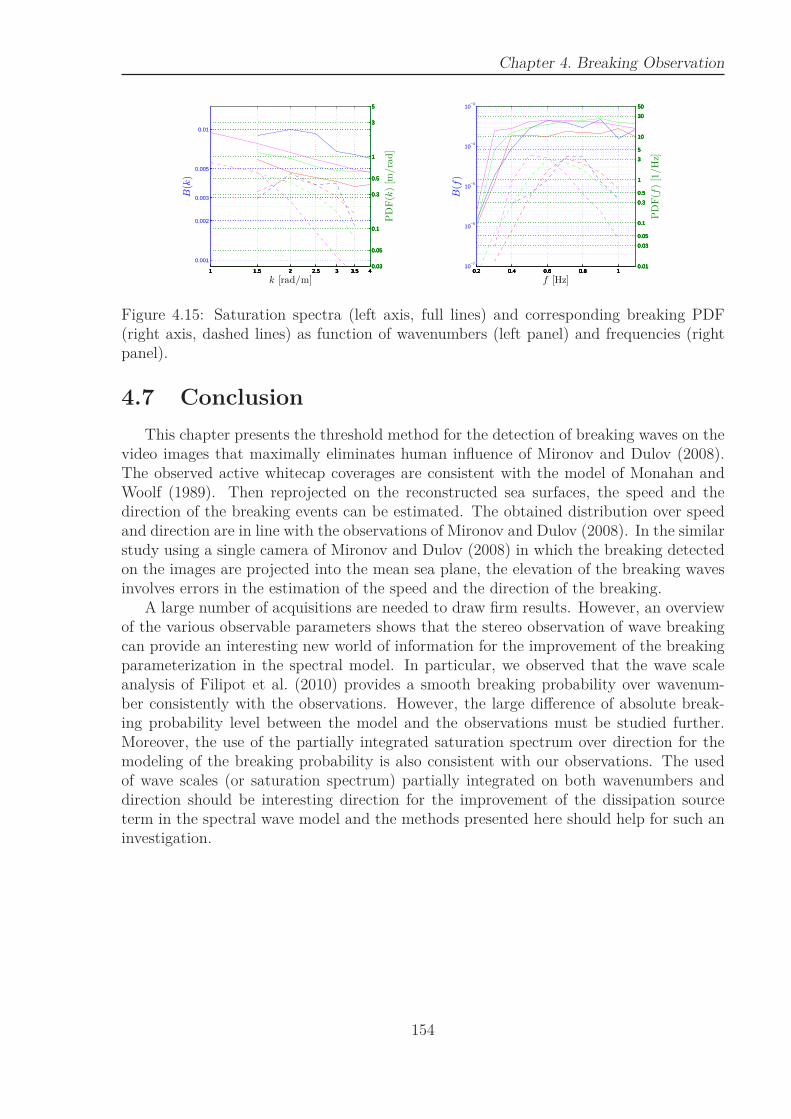
Chapter 4. Breaking Observation
1 1.5 2 2.5 3 3.5 4
0.001
0.002
0.003
0.005
0.01
k [rad/m]
B(k)
0.2 0.4 0.6 0.8 110
−7
10−6
10−5
10−4
10−3
f [Hz]
B(f)
1 1.5 2 2.5 3 3.5 40.03
0.05
0.1
0.3
0.5
1
3
5
PDF(k)[m
/rad]
0.2 0.4 0.6 0.8 10.01
0.03
0.05
0.1
0.3
0.5
1
3
5
10
30
50
PDF(f)[1/Hz]
1 1.5 2 2.5 3 3.5 40.03
0.05
0.1
0.3
0.5
1
3
5
0.2 0.4 0.6 0.8 10.01
0.03
0.05
0.1
0.3
0.5
1
3
5
10
30
50
1 1.5 2 2.5 3 3.5 40.03
0.05
0.1
0.3
0.5
1
3
5
0.2 0.4 0.6 0.8 10.01
0.03
0.05
0.1
0.3
0.5
1
3
5
10
30
50
1 1.5 2 2.5 3 3.5 40.03
0.05
0.1
0.3
0.5
1
3
5
0.2 0.4 0.6 0.8 10.01
0.03
0.05
0.1
0.3
0.5
1
3
5
10
30
50
Figure 4.15: Saturation spectra (left axis, full lines) and corresponding breaking PDF(right axis, dashed lines) as function of wavenumbers (left panel) and frequencies (rightpanel).
4.7 Conclusion
This chapter presents the threshold method for the detection of breaking waves on thevideo images that maximally eliminates human influence of Mironov and Dulov (2008).The observed active whitecap coverages are consistent with the model of Monahan andWoolf (1989). Then reprojected on the reconstructed sea surfaces, the speed and thedirection of the breaking events can be estimated. The obtained distribution over speedand direction are in line with the observations of Mironov and Dulov (2008). In the similarstudy using a single camera of Mironov and Dulov (2008) in which the breaking detectedon the images are projected into the mean sea plane, the elevation of the breaking wavesinvolves errors in the estimation of the speed and the direction of the breaking.
A large number of acquisitions are needed to draw firm results. However, an overviewof the various observable parameters shows that the stereo observation of wave breakingcan provide an interesting new world of information for the improvement of the breakingparameterization in the spectral model. In particular, we observed that the wave scaleanalysis of Filipot et al. (2010) provides a smooth breaking probability over wavenum-ber consistently with the observations. However, the large difference of absolute break-ing probability level between the model and the observations must be studied further.Moreover, the use of the partially integrated saturation spectrum over direction for themodeling of the breaking probability is also consistent with our observations. The usedof wave scales (or saturation spectrum) partially integrated on both wavenumbers anddirection should be interesting direction for the improvement of the dissipation sourceterm in the spectral wave model and the methods presented here should help for such aninvestigation.
154
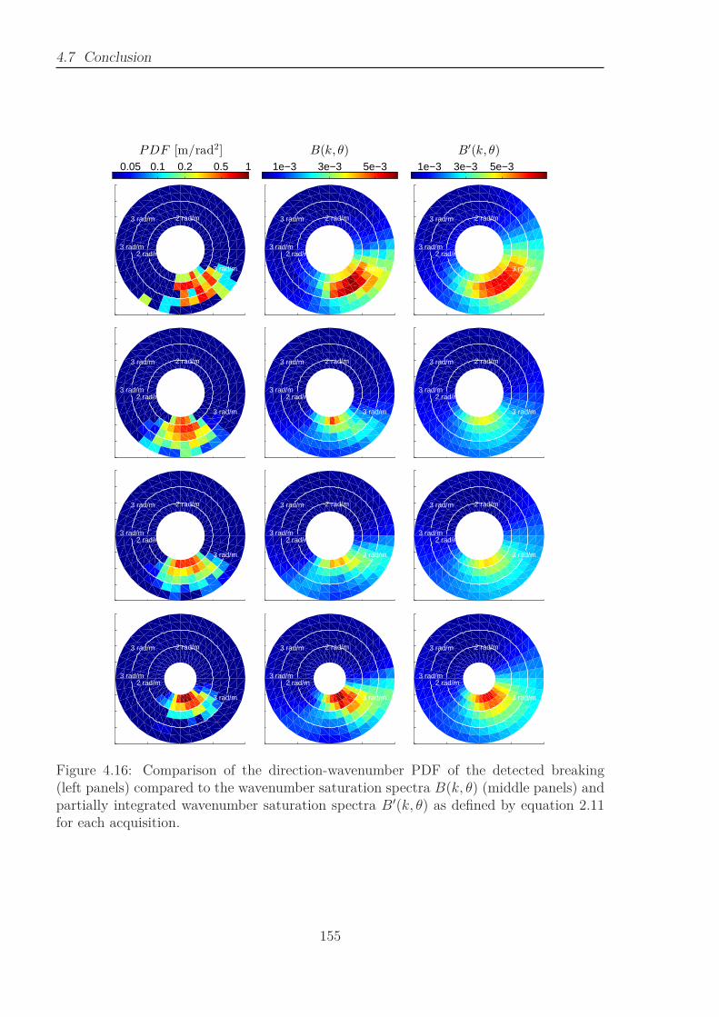
4.7 Conclusion
2 rad/m
2 rad/m
3 rad/m
3 rad/m
3 rad/m
2 rad/m
2 rad/m
3 rad/m
3 rad/m
3 rad/m
2 rad/m
2 rad/m
3 rad/m
3 rad/m
3 rad/m
2 rad/m
2 rad/m
3 rad/m
3 rad/m
3 rad/m
2 rad/m
2 rad/m
3 rad/m
3 rad/m
3 rad/m
2 rad/m
2 rad/m
3 rad/m
3 rad/m
3 rad/m
2 rad/m
2 rad/m
3 rad/m
3 rad/m
3 rad/m
2 rad/m
2 rad/m
3 rad/m
3 rad/m
3 rad/m
2 rad/m
2 rad/m
3 rad/m
3 rad/m
3 rad/m
2 rad/m
2 rad/m
3 rad/m
3 rad/m
3 rad/m
2 rad/m
2 rad/m
3 rad/m
3 rad/m
3 rad/m
2 rad/m
2 rad/m
3 rad/m
3 rad/m
3 rad/m
PDF [m/rad2]
0.05 0.1 0.2 0.5 1
B(k, θ)
1e−3 3e−3 5e−3
B′(k, θ)
1e−3 3e−3 5e−3
Figure 4.16: Comparison of the direction-wavenumber PDF of the detected breaking(left panels) compared to the wavenumber saturation spectra B(k, θ) (middle panels) andpartially integrated wavenumber saturation spectra B′(k, θ) as defined by equation 2.11for each acquisition.
155

Chapter 5
Conclusion
Starting from an analysis of the capability of spectral wave models to reproduce theevolution of the sea state, this work first focus on the dissipation source term associatedto wave breaking in the energy balance equation. This source term have been for longtime used as tuning knob balancing the other better understand source terms, but recentefforts have been done to make it closer than the physical processes involved by the wavebreaking. Two recent wave breaking parameterizations based on observations were a ma-jor focus of the first chapter. The model accuracy is generally evaluated through its abilityto reproduce observed wave heights and spectral evolution. Nevertheless, considering onlythe integration of the whole set of source terms, these validations fails to validate inde-pendently each one. Although the explicit modeling of whitecap properties is a constrainton the model dissipation source terms, these recent dissipation parameterizations haveseldom been verified in these terms. Therefore, the breaking crest lengths distributions,the whitecap coverage and the foam thickness are extracted from the parameterizationsof the wave breaking dissipation and compared to observations.
The two recent parameterizations investigated in this work are the directional satura-tion based parameterization of Ardhuin et al. (2010) and the parameterization of Filipotand Ardhuin (2012), based on the non directional observations of breaking probabilitiesper wave scale of Filipot et al. (2010). These parameterizations have been first slightmodified in terms of swell dissipation and the physical relationship that intrinsically linksspontaneous breaking dissipation and dissipation induced by breaking waves have beenmade self consistent in the second one. Validated using the classical ways, these slightmodifications improve the global accuracy of the models. Nevertheless, these modifica-tions do not influence on the breaking statistics, which are the main purpose of this work.It is found that the breaking parameterization by Filipot and Ardhuin (2012) producesbreaking crest length distributions that are in better qualitative agreement with obser-vations, contrary to the parameterization of Ardhuin et al. (2010) which fails to producesmooth Λ-distributions. This difference is clearly associated with the breaking probabil-ities computed over wave scales compared to those linked the local saturation. The esti-mation of the breaking parameters after smoothing the local saturations over frequenciescould lead to better Λ-distributions (Banner and Morison, 2010). Inversely, the isotropicdistribution of the breaking probabilities over frequency afflicting the parameterization ofFilipot and Ardhuin (2012) compared to the directional distribution of the breaking done
157
Chapter 5. Conclusion
in the parameterization by Ardhuin et al. (2010), linked to the partial integration overdirections of the directional saturation spectra. Indeed, combined with the cumulativeeffect parameterization, the isotropic distribution of breaking, moreover not observed,tends to reduce the width of the directional spectrum. Inversely, despite producing unre-alistic unsmoothed crest lengths distributions, the directional breaking distribution of theparameterization by Ardhuin et al. (2010), linked to the directional saturation spectra,provides spectra directional spreading more in line with the observations. A combinationof these two approaches, using directional wave scales or directional saturation partiallyintegrated over both directions and frequencies should leads to better distribution of thebreaking.
Comparing the modeled global whitecap coverage to the observations observationsfrom satellite radiometers interpreted by Anguelova and Webster (2006), it is shown thatany parameterization reproduce the large variability of the observations. Nevertheless,it is find that joint estimates of the whitecap coverage and foam thickness could be aninteresting way to discriminate between different sea states or parameterizations. Recentresults by Reul et al. (2006) with L-band radiometric measurements in Hurricanes usingthe Soil Moisture and Ocean Salinity space mission, combined with radiometric measure-ments from different bands should provide information on the distribution of the breakingfoam and should be a interesting way to even more constraint the dissipation source termsin the spectral wave models. This deficiency is both attributed to the bad modeling of thebreaking in the model, but also to the lack of physical process and external parametersin the model which strongly influence on the quantity of created foam by breaking waveand its lifetime.
The analysis of the existing parameterization shows the need of the synchronizedobservations of wave spectra and breaking wave distributions. These two parameterscan be observed using the stereo observation of the sea. Indeed, recent method weredeveloped to reconstruct accurate wavy sea surface from the standard stereo triangulationwell known in computer vision. Moreover the breaking waves which produce white foampatches over the darker water surface are easily detectable, providing the new world ofinformation combining the observation of the breaking wave and the time-space evolutionof the underlying sea surface.
The existing methods of sea surface reconstruction provide good results in term of seaelevation statistics and spectra. Nevertheless, it is shown in this work that the presenceof foam patches on the sea surface strongly disturbs the local shape of the surface. Thefirst effort was to improved the existing reconstruction methods to provide realistic seasurface shape around the foam patches. Four stereo video acquisitions are investigatedand a validation of the reconstructed surfaces obtained with the improved method is givenby comparison with wave gauge data. The observation of the 3D direction-wavenumber-frequency spectra obtained from the time-space evolution of the surface shows that thereconstructed surfaces shows the coherence of the surfaces up to f = 1.6Hz (λ ≈ 60cm).
Then, the breaking waves are detected on the images using the threshold method ofMironov and Dulov (2008) that maximally eliminates human influence, then reprojectedon the reconstructed sea surfaces. The speed and the direction of the breaking eventsare computed. The obtained distribution over speed and direction are in line with theobservations of Mironov and Dulov (2008). We highlight that the access to the sea surface
158
elevation in this work allows a better calculation of the breaking speed and direction thanin the single camera observations of Mironov and Dulov (2008) in which the breakingdetected on the images are projected into the mean sea plane, involving errors related tothe elevation of the breaking waves.
In addition to the quantification of the breaking and its precise distributions overwave scales and directions, it was shown that the stereo observation allows the analysisthe breaking at the scale of the single breaking waves and thus opens a new world ofinformation about the space-time evolution of the breaking waves for large range of wavescales. Despite these aspects were not addressed in this work, the stereo observationprovides the necessary information to study the dissipation of the breaking waves andthe quantification of the possibly associated cumulative effect observed by (Banner et al.,1989). A large number of acquisitions is needed to draw firm results, however the providedoverview of the various observable parameters shows that the method developed herecan provide large information for the validation and the improvement of the breakingparameterization in the spectral model. Moreover, the stereo observations at microwavescale with high resolution camera of Yurovskaya et al. (2013) should also be used toquantify the generation of short waves in all directons from the breaking of long waves.This generation of short waves, also detected on the acoustic measurements of Duennebieret al. (2012), could have a important effect on the transfer of the energy from the windto the waves.
Finally, a new experiment was done on September 2013 from the scientific platform ofKatsively in Ukraine, with a larger range of wind and wave conditions. Two synchronizedstereo video systems were deployed with different lenses to observe different wave scales.In addition to the wind and wave measurements also available for the present study, jointmeasurement have been done with Ka-band radar and stereo-photo. The processing ofthe data is in progress. Interesting informations over a larger range of wave scales areexpected in terms of distribution of wave breaking but also on the relationship of thebreaking with the spectrum shape.
159

Bibliography
Agrawal, Y., E. Terray, M. Donelan, P. Hwang, A. Williams, W. Drennan, K. Kahma,and S. Krtaigorodskii, 1992: Enhanced dissipation of kinetic energy beneath surfacewaves.
Alves, J. H. G. M. and M. L. Banner, 2003: Performance of a saturation-based dissipation-rate source term in modeling the fetch-limited evolution of wind waves. J. Phys.Oceanogr., 33, 1274–1298.
Alves, J. H. G. M., M. L. Banner, and I. R. Young, 2003: Revisiting the Pierson-Moskowitzasymptotic limits for fully developed wind waves. J. Phys. Oceanogr., 33, 1301–1323.
Anguelova, M. D., J. P. Bobak, W. E. Asher, D. J. Dowgiallo, B. I. Moat, R. W. Pascal,and M. J. Yelland, 2009: Validation of satellite-based estimates of whitecap coverage:Approaches and initial results. 16th Air-Sea Interaction conference, AMS, Phoenix,Arizona.
Anguelova, M. D. and F. W. Webster, 2006: Whitecap coverage from satellite measure-ments: a first step toward modeling the variability of oceanic whitecaps. J. Geophys.Res., 111, C03017.
Apel, J., 1994: An improved model of the ocean surface wave vector spectrum and itseffects on radar backscatter. J. Geophys. Res., 99, 16269–16291.
Ardhuin, F., B. Chapron, and F. Collard, 2009: Observation of swell dissipation acrossoceans. Geophys. Res. Lett., 36, L06607.
Ardhuin, F., J. Hanafin, Y. Quilfen, B. Chapron, P. Queffeulou, M. Obrebski,J. Sienkiewicz, and D. Vandemark, 2011a: calibration of the IOWAGA global wavehindcast (1991–2011)using ECMWF and CFSR winds. Proceedings, 12th Int. Workshop of Wave Hindcastingand Forecasting, Hawaii.
Ardhuin, F., T. H. C. Herbers, K. P. Watts, G. P. van Vledder, R. Jensen, and H. Graber,2007: Swell and slanting fetch effects on wind wave growth. J. Phys. Oceanogr., 37,908–931.
Ardhuin, F. and A. D. Jenkins, 2006: On the interaction of surface waves and upper oceanturbulence. J. Phys. Oceanogr., 36, 551–557.
161
BIBLIOGRAPHY
Ardhuin, F., E. Rogers, A. Babanin, J.-F. Filipot, R. Magne, A. Roland, A. van der West-huysen, P. Queffeulou, J.-M. Lefevre, L. Aouf, and F. Collard, 2010: Semi-empiricaldissipation source functions for wind-wave models: part I, definition, calibration andvalidation. J. Phys. Oceanogr., 40, 1917–1941.
Ardhuin, F. and A. Roland, 2012: Coastal wave reflection, directional spreading, andseismo-acoustic noise sources. J. Geophys. Res., 117, in press.
Ardhuin, F., J. Tournadre, P. Queffelou, and F. Girard-Ardhuin, 2011b: Observation andparameterization of small icebergs: drifting breakwaters in the southern ocean. OceanModelling, 39, 405–410.
Aziz, A. Y. I. and H. M. Karara, 1971: Direct linear transformation into object spacecoordinates in close-range photogrammetry. Proc. of the Symposium on Close-RangePhotogrammetry, Urbana, Illinois, 1–18.
Babanin, A., D. Chalikov, I. Young, and I. Savelyev, 2007: Predicting the breaking onsetof surface water waves. Geophys. Res. Lett., 34, L07605.
Babanin, A., I. Young, and M. Banner, 2001: Breaking probabilities for dominant surfacewaves on water of finite depth. J. Geophys. Res., 106, 11659–11676.
Babanin, A. V., K. N. Tsagareli, I. R. Young, and D. J. Walker, 2010: Numerical inves-tigation of spectral evolution of wind waves. part II: Dissipation term and evolutiontests. J. Phys. Oceanogr., 40, 667–683.
Banner, M. and W. Melville, 1976: On the separation of air flow over water waves. Journalof Fluid Mechanics, 77, 825–842.
Banner, M. L., A. V. Babanin, and I. R. Young, 2000: Breaking probability for dominantwaves on the sea surface. J. Phys. Oceanogr., 30, 3145–3160.
Banner, M. L., J. R. Gemmrich, and D. M. Farmer, 2002: Multiscale measurement ofocean wave breaking probability. J. Phys. Oceanogr., 32, 3364–3374.
Banner, M. L., I. S. F. Jones, and J. C. Trinder, 1989: Wavenumber spectra of shortgravity waves. J. Fluid Mech., 198, 321–344.
Banner, M. L. and R. P. Morison, 2010: Refined source terms in wind wave models withexplicit wave breaking prediction. part I: Model framework and validation against fielddata. Ocean Modelling, 33, 177–189.
Banner, M. L. and J.-B. Song, 2002: On determining the onset and strength of breakingfor deep water waves. part ii: Influence of wind forcing and surface shear. Journal ofphysical oceanography, 32, 2559–2570.
Banner, M. L. and X. Tian, 1998: On the determination of the onset of breaking formodulating surface gravity water waves. J. Fluid Mech., 367, 107–137.
162
BIBLIOGRAPHY
Barrick, D. E., 1968: Rough surface scattering based on the specular point theory. IEEETrans. Antennas Propagat., AP-14, 449–454.
Battjes, J., 1974a: Computations of set-up, longshore currents, run-up and overtoppingdue to wind-generated waves. Ph.D. thesis, Delft University of Technology, The Nether-lands.
Battjes, J. A., 1974b: Surf similarity. Proceedings of the 14th international conference oncoastal engineering, ASCE, 466–480.
Belcher, S. and J. Hunt, 1993: Turbulent shear flow over slowly moving waves. Journalof Fluid Mechanics, 251, 109–148.
Benetazzo, A., 2006: Measurements of short water waves using stereo matched imagesequences. Coastal engineering, 53, 1013–1032.
Benetazzo, A., F. Fedele, G. Gallego, P.-C. Shih, and A. Yezzi, 2012: Offshore stereomeasurements of gravity waves. Coastal Engineering, 64, 127 – 138.
Bidlot, J., S. Abdalla, and P. Janssen, 2005: A revised formulation for ocean wave dissi-pation in CY25R1. Technical Report Memorandum R60.9/JB/0516, Research Depart-ment, ECMWF, Reading, U. K.
Bidlot, J.-R., 2012: Present status of wave forecasting at e.c.m.w.f. Workshop on OceanWaves, ECMWF .
Bjerkaas, A. and F. Riedel, 1979: Proposed model for the elevation spectrum of a wind-roughened sea surface. Technical report, DTIC Document.
Bondur, V. and E. Sharkov, 1982: Statistical properties of whitecaps on a rough sea.Oceanology, 22, 274–279.
Brown, D. C., 1966: Decentering distortion of lenses. Photometric Engineering, 32, 444–462.
Callaghan, A., G. de Leeuw, L. Cohen, and C. D. O’Dowd, 2008: Relationship of oceanicwhitecap coverage to wind speed and wind history. Geophysical Research Letters, 35,n/a–n/a.
Caprile, B. and V. Torre, 1990: Using vanishing points for camera calibration. Interna-tional journal of computer vision, 4, 127–139.
Caulliez, G., 2002: Self-similarity of near-breaking short gravity wind waves. Physics ofFluids, 14, 2917.
Chanson, H. and P. D. Cummings, 1992: Aeration of the ocean due to plunging breakingwaves. Technical report.
163
BIBLIOGRAPHY
Chase, J., L. J. Cote, W. Marks, E. Mehr, W. J. Pierson, J. F. C. Ronne, G. Stephenson,R. C. Vetter, and R. G. Walden, 1957: The directional spectrum of a wind generatedsea as determined from data obtained by the Stereo Wave Observation Project. NewYork University, College of Engineering, Research Division, Dept. of Meteorology andOceanography and Engineering STatistics Group.
Chawla, A. and J. T. Kirby, 2002: Monochromatic and random wave breaking at blockingpoints. J. Geophys. Res., 107, 3067.
Clarke, T. A. and J. G. Fryer, 1998: The development of camera calibration methods andmodels. The Photogrammetric Record, 16, 51–66.
Claudet, A., 1856: On various phenomena of refraction through semi-lenses or prisms,producing anomalies in the illusion of stereoscopic images.[abstract]. Proceedings of theRoyal Society of London, 8, 104–110.
— 1857: On the stereomonoscope, a new instrument by which an apparently single pictureproduces the stereoscopic illusion. Proceedings of the Royal Society of London, 9, 194–196.
Conrady, A. E., 1919: Lens-systems, decentered. Monthly notices of the royal astronomicalsociety, 79, 384–390.
Cote, L. J., J. O. Davis, W. Marks, R. J. McGough, E. Mehr, W. Pierson, J. Ropek,G. Stephenson, and R. C. Vetter, 1960: The directional spectrum of a wind generatedsea as determined from data obtained by the {Stereo Wave Observation Project}. 2,758–766.
Cox, C. and W. Munk, 1954: Measurement of the roughness of the sea surface fromphotographs of the sun’s glitter. J. Opt. Soc. Am., 44, 838–850.
Craig, P. D. and M. L. Banner, 1994: Modeling wave-enhanced turbulence in the oceansurface layer. Journal of Physical Oceanography, 24, 2546–2559.
Cruset, J., 1953: Photogrammetric measurement of the sea swell. Photogrammetria, 9,122 – 125.
Dankert, H., J. Horstmann, S. Lehner, and W. Rosenthal, 1939: Stereophotogram-metrische wellenaufrahmen. (stereophotogrammetric wave photos.). VerrnessungsschiffMeteor , 7.
— 2003: Detection of wave groups in SAR images and radar-image sequences. IEEETrans. on Geosci. and Remote Sensing, 41, 1437–1441.
Donelan, M., M. S. Longuet-Higgins, and J. Turner, 1972: Periodicity in whitecaps.
Donelan, M. A., F. W. Dobson, S. D. Smith, and R. J. Anderson, 1993: On the dependenceof sea surface roughness on wave development. J. Phys. Oceanogr., 23, 2143–2149.
164
BIBLIOGRAPHY
Donelan, M. A. and W. J. Pierson, Jr., 1987: Radar scattering and equilibrium ranges inwind-generated waves with application to scatterometry. J. Geophys. Res., 92, 4971–5029.
Droppleman, J. D., 1970: Apparent microwave emissivity of sea foam. J. Geophys. Res.,75(3), 696–698.
Duennebier, F. K., R. Lukas, E.-M. Nosal, J. Aucan, and R. A. Weller, 2012: Wind,waves, and acoustic background levels at station aloha. J. Geophys. Res., 117, in press.
Dulov, V., V. Kudryavtsev, and A. Bolshakov, 2002: A field study of white caps coverageand its modulations by energy containing wave. Gas Transfer at the Water Surface,Geophysical Monographs 127 , M. A. D. et al., ed., American Geophysical Union, pages187–192.
Duncan, J. H., 1981: An experimental investigation of breaking waves produced by atowed hydrofoil. Proc. Roy. Soc. Lond. A, 377, 331–348.
Elfouhaily, T., B. Chapron, K. Katsaros, and D. Vandemark, 1997: A unified directionalspectrum for long and short wind-driven waves. Journal of Geophysical Research, 102,15781–15.
Filipot, J.-F. and F. Ardhuin, 2012: A unified spectral parameterization for wave breaking:from the deep ocean to the surf zone. J. Geophys. Res., 116.
Filipot, J.-F., F. Ardhuin, and A. Babanin, 2010: A unified deep-to-shallow-water wave-breaking probability parameterization. J. Geophys. Res., 115, C04022.
Gagnaire-Renou, E., M. Benoit, and P. Forget, 2010: Ocean wave spectrum properties asderived from quasi-exact computations of nonlinear wave-wave interactions. J. Geophys.Res., 115, C12058.
Gallego, G., A. Benetazzo, A. Yezzi, and F. Fedele, 2008: Wave statistics and spectra viaa variational wave acquisition stereo system. 27th Int. Conf. Offshore Mechanics ArcticEngineering (OMAE), Lisbon, Portugal.
Galton, F. and R. C. Galton, 1865: On stereoscopic maps, taken from models of moun-tainous countries. Journal of the Royal Geographical Society of London, 35, 99–106.
Gelci, R., H. Cazale, and J. Vassal, 1957: Prevision de la houle. La methode des densitesspectroangulaires. Bulletin d’information du Comite d’Oceanographie et d’Etude desCotes, 9, 416–435.
Gemmrich, J. R., M. L. Banner, and C. Garrett, 2008: Spectrally resolved energy dissi-pation rate and momentum flux of breaking waves. J. Phys. Oceanogr., 38, 1296–1312.
Gemmrich, J. R. and D. M. Farmer, 2004: Near-surface turbulence in the presence ofbreaking waves. J. Phys. Oceanogr., 34, 1067–1086.
165
BIBLIOGRAPHY
Golub, G. H. and C. Reinsch, 1970: Singular value decomposition and least squaressolutions. Numerische Mathematik, 14, 403–420.
Hanafin, J., Y. Quilfen, F. Ardhuin, D. Vandemark, B. Chapron, H. Feng, J. Sienkiewicz,P. Queffeulou, M. Obrebski, B. Chapron, N. Reul, F. Collard, D. Cormand, E. B.de Azevedo, D. Vandemark, and E. Stutzmann, 2012: Phenomenal sea states and swellradiation: a comprehensive analysis of the 12-16 February 2011 North Atlantic storms.Bull. Amer. Meterol. Soc., in press.
Hanson, J. L. and O. M. Phillips, 1999: Wind sea growth and dissipation in the openocean. J. Phys. Oceanogr., 29, 1633–1648.
Hasselmann, K., 1960: Grundgleichugen der seegangsvorhersage. Schifftechnik, 7, 191–195.
— 1962: On the non-linear energy transfer in a gravity wave spectrum, part 1: generaltheory. J. Fluid Mech., 12, 481–501.
— 1974: On the spectral dissipation of ocean waves due to white capping. Boundary-LayerMeteorol., 6, 107–127.
Hasselmann, S., K. Hasselmann, J. Allender, and T. Barnett, 1985: Computation andparameterizations of the nonlinear energy transfer in a gravity-wave spectrum. Part II:Parameterizations of the nonlinear energy transfer for application in wave models. J.Phys. Oceanogr., 15, 1378–1391.
Heikkila, J. and O. Silven, 1997: A four-step camera calibration procedure with implicitimage correction. Computer Vision and Pattern Recognition, 1997. Proceedings., 1997IEEE Computer Society Conference on, 1106–1112.
Holland, K. T. and R. A. Holman, 1997: Video estimation of foreshore topography usingtrinocular stereo. Journal of Coastal Research, 13, 81–87.
Holland, K. T., R. A. Holman, T. C. Lippmann, J. Stanley, and N. Plant, 1997: Practicaluse of video imagery in nearshore oceanographic field studies. IEEE J. Oceanic Eng.,22, 81–92.
Holthuijsen, L. and T. Herbers, 1986: Statistics of breaking waves observed as whitecapsin the open sea. Journal of Physical Oceanography, 16, 290–297.
Holthuijsen, L. H., M. D. Powell, and J. D. Pietrzak, 2012: Wind and waves in extremehurricanes. J. Geophys. Res., 117, C09003.
Hwang, P. A., D. W. Wang, E. J. Walsh, W. B. Krabill, and R. N. Swift, 2000: Airbornemeasurements of the wavenumber spectra of ocean surface waves. part i: Spectral slopeand dimensionless spectral coefficient*. Journal of Physical Oceanography, 30, 2753–2767.
Jeffreys, H., 1925: On the formation of water waves by wind. Proceedings of the RoyalSociety of London. Series A, 107, 189–206.
166
BIBLIOGRAPHY
Jessup, A., C. Zappa, and H. Yeh, 1997: Defining and quantifying microscale wave break-ing with infrared imagery. Journal of Geophysical Research, 102, 23145–23.
Jessup, A. T. and K. R. Phadnis, 2005: Measurement of the geometric and kinematicproperties of microscale breaking waves from infrared imagery using a PIV algorithm.Meas. Sci. Technol., 16, 1961–1969.
Kanade, T. and D. D. Morris, 1998: Factorization methods for structure from motion.Philosophical Transactions of the Royal Society of London. Series A: Mathematical,Physical and Engineering Sciences, 356, 1153–1173.
Kantha, L., P. Wittmann, M. Sclavo, and S. Carniel, 2009: A preliminary estimate of thestokes dissipation of wave energy in the global ocean. Geophys. Res. Lett., 36, L02605.
Kleiss, J. M. and W. K. Melville, 2011: The analysis of sea surface imagery for whitecapkinematics. J. Atmos. Ocean Technol., 28, 219–243.
Komen, G., L. Cavaleri, M. Donelan, K. Hasselmann, and S. Hasselmann, 1994: Janssenpaem. dynamics and modeling of ocean waves.
Komen, G. J., K. Hasselmann, and S. Hasselmann, 1984: On the existence of a fullydeveloped windsea spectrum. J. Phys. Oceanogr., 14, 1271–1285.
Kosnik, M. V. and V. A. Dulov, 2011: Extraction of short wind wave spectra from stereoimages of the sea surface. Measurement Science and Technology, 22, 015504.
Kudryavtsev, V. and V. Makin, 2001: The impact of air-flow separation on the drag ofthe sea surface. Boundary-layer meteorology, 98, 155–171.
Leckler, F., F. Ardhuin, J.-F. Filipot, and A. Mironov, 2013: Dissipation source termsand whitecap statistics. Ocean Modelling, 70, 62 – 74.
Leykin, I. A. and A. D. Rozenberg, 1984: Sea-tower measurements of wind-wave spectrain the Caspian Sea. J. Phys. Oceanogr., 14, 168–176.
Loewen, M. R. and W. K. Melville, 1991: Microwave backscatter and acoustic radiationfrom breaking waves. J. Fluid Mech., 224, 601–623.
Longuet-Higgins, M. and M. Fox, 1978: Theory of the almost-highest wave. part 2. match-ing and analytic extension. Journal of Fluid Mechanics, 85, 769–786.
Longuet-Higgins, M. S., 1978: The instabilities of gravity waves of finite amplitude in deepwater. i. superharmonics. Proceedings of the Royal Society of London. A. Mathematicaland Physical Sciences, 360, 471–488.
Mach, E., 1896: On the stereoscopic application of roentgen’s rays. The Monist, 6, 321–323.
Marks, W., 1954: The use of a filter to sort out directions in a short-crested gaussian seasurface. Transactions, American Geophysical Union, 35, 758–766.
167

BIBLIOGRAPHY
Melen, T., 1994: Geometrical modelling and calibration of video cameras for underwa-ter navigation. Institutt for Teknisk Kybernetikk, Universitetet i Trondheim, NorgesTekniske Høgskole.
Melville, K. W., 1994: Energy dissipation by breaking waves. Journal of Physical Oceanog-raphy, 24, 2041–2049.
Melville, W. K. and P. Matusov, 2002: Distribution of breaking waves at the ocean surface.Nature, 417, 58–63.
Melville, W. K., F. Verron, and C. J. White, 2002: The velocity field under breakingwaves: coherent structures and turbulence. J. Fluid Mech., 454, 203–233.
Miche, A., 1944: Mouvements ondulatoires de la mer en profondeur croissante oudecroissante. forme limite de la houle lors de son deferlement. application auxdigues maritimes. deuxieme partie. mouvements ondulatoires periodiques en profondeurregulierement decroissante. Annales des Ponts et Chaussees, Tome 114, 131–164,270–292.
Miles, J. W., 1957: On the generation of surface waves by shear flows. Journal of FluidMechanics, 3.
— 1962: On the generation of surface waves by shear flows. part 4. J. Fluid Mech, 13,433–448.
Mironov, A. S., 2009: Experimental investigation of statistical and kinematical propertiesof breaking wind waves. Ph.D. thesis, Marine Hydrophysics Institue, Sebastopol, inRussian.
Mironov, A. S. and V. A. Dulov, 2008: Detection of wave breaking using sea surface videorecords. Meas. Sci. Technol., 19, 015405.
Monahan, E. C., C. W. Fairall, K. L. Davidson, and P. J. Boyle, 1983: Observed inter-relations between 10m winds, ocean whitecaps and marine aerosols. Quarterly Journalof the Royal Meteorological Society, 109, 379–392.
Monahan, E. C. and I. O. Muircheart, 1981: Optimal power-law description of oceanicwhitecap coverage dependence on wind speed. J. Phys. Oceanogr., 10, 2094–2099.
Monahan, E. C. and D. K. Woolf, 1989: Comments on ”variations of whitecap coveragewith wind stress and water temperature”. J. Phys. Oceanogr., 19, 706–709.
Munk, W., 2008: An inconvenient sea truth: Spread, steepness, and skewness of surfaceslopes. Annual review of marine science, 1, 377–415.
Newell, A. C. and V. E. Zakharov, 1992: Rough sea foam. Physical review letters, 69,1149.
Phillips, O. M., 1957: On the generation of waves by turbulent wind. J. Fluid Mech., 2,415–417.
168
BIBLIOGRAPHY
— 1984: On the response of short ocean wave components at a fixed wavenumber toocean current variations. J. Phys. Oceanogr., 14, 1425–1433.
— 1985: Spectral and statistical properties of the equilibrium range in wind-generatedgravity waves. J. Fluid Mech., 156, 505–531.
Pierson, W. J., 1952: A unified mathematical theory for the analysis, propagation andrefraction of storm generated ocean surface waves, parts {I} and {II}.
Pierson, W. J., Jr and L. Moskowitz, 1964: A proposed spectral form for fully developedwind seas based on the similarity theory of S. A. Kitaigorodskii. J. Geophys. Res., 69,5,181–5,190.
Queffeulou, P. and D. Croize-Fillon, 2010: Global altimeter SWH data set, version 7, may2010. Technical report, Ifremer.
Rascle, N., F. Ardhuin, P. Queffeulou, and D. Croize-Fillon, 2008: A global wave param-eter database for geophysical applications. part 1: wave-current-turbulence interactionparameters for the open ocean based on traditional parameterizations. Ocean Modelling,25, 154–171, doi:10.1016/j.ocemod.2008.07.006.
Raubenheimer, B., R. Guza, and S. Elgar, 1996: Wave transformation across the innersurf zone. Journal of geophysical research, 101, 25589–25.
Reul, N. and B. Chapron, 2003: A model of sea-foam thickness distributionfor passive microwave remote sensing applications. J. Geophys. Res., 108, 3321,doi:10.1029/2003JC001887.
Reul, N., J. Tenerelli, B. Chapron, D. Vandemark, Y. Quilfen, and Y. Kerr, 2006: Smossatellite l-band radiometer: A new capability for ocean surface remote sensing in hur-ricanes. J. Geophys. Res., 117, C02006.
Rogers, W. E., A. V. Babanin, and D. W. Wang, 2012: Observation-consistent input andwhitecapping dissipation in a model for wind-generated surface waves: Description andsimple calculations. J. Atmos. Ocean Technol., 29, 1329–1346.
Rozenberg, A. and M. Ritter, 2005: Laboratory study of the fine structure of shortsurface waves due to breaking: Two-directional wave propagation. J. Geophys. Res.,110, C02011.
Ruessink, B. G., D. J. R. Walstra, and H. N. Southgate, 2003: Calibration and verificationof a parametric wave model on barred beaches. Coastal Eng., 48, 139–149.
Saha, S., S. Moorthi, H.-L. Pan, X. Wu, J. Wang, S. Nadiga, P. Tripp, R. Kistler,J. Woollen, D. Behringer, H. Liu, D. Stokes, R. Grumbine, G. Gayno, J. Wang, Y.-T.Hou, H. ya Chuang, H.-M. H. a. J. S. Juang, M. Iredell, R. Treadon, D. Kleist, P. V.Delst, D. Keyser, J. Derber, M. Ek, J. Meng, H. Wei, R. Yang, S. Lord, H. van denDool, A. Kumar, W. Wang, C. Long, M. Chelliah, Y. Xue, B. Huang, J.-K. Schemm,W. Ebisuzaki, R. Lin, P. Xie, M. Chen, S. Zhou, W. Higgins, C.-Z. Zou, Q. Liu, Y. Chen,
169

BIBLIOGRAPHY
Y. Han, L. Cucurull, R. W. Reynolds, G. Rutledge, and M. Goldberg, 2010: The NCEPClimate Forecast System Reanalysis. Bull. Amer. Meterol. Soc., 91, 1015–1057.
Scaramuzza, D., A. Martinelli, and R. Siegwart, 2006: A flexible technique for accu-rate omnidirectional camera calibration and structure from motion. Computer VisionSystems, 2006 ICVS ’06. IEEE International Conference on, 45–45.
Senechal, N., H. Dupuis, P. Bonneton, H. Howa, and R. Pedreros, 2001: Observation ofirregular wave transformation in the surf zone over a gently sloping sandy beach on thefrench atlantic coastline. Oceanol. Acta, 24, 545–556.
Sharma, J. N. and R. G. Dean, 1993: Second order directional wave kinematics in shallowwater. Ocean wave measurement and analysis, Proc. WAVES’93 Conf., 165–179.
Shih, S.-W., Y.-P. Hung, and W.-S. Lin, 1993: Accurate linear technique for cameracalibration considering lens distortion by solving an eigenvalue problem. Optical Engi-neering, 32, 138–149.
Smith, J., 1986: Short surface waves with growth and dissipation. J. Geophys. Res., 91,2616–2632.
Smith, M., P. Park, and I. Consterdine, 1993: Marine aerosol concentrations and esti-mated fluxes over the sea. Quarterly Journal of the Royal Meteorological Society, 119,809–824.
Song, J.-B. and M. L. Banner, 2002: On determining the onset and strength of breakingfor deep water waves. Part I: Unforced irrotational wave groups. J. Phys. Oceanogr.,32, 2541–2558.
St Denis, M. and W. J. Pierson Jr, 1953: On the motions of ships in confused seas.Technical report, DTIC Document.
Stansell, P. and C. MacFarlane, 2002: Experimental investigation of wave breaking criteriabased on wave phase speeds. J. Phys. Oceanogr., 32, 1269–1283.
Stewart, R., 1960: Changes in the form of short gravity waves on long waves and tidalcurrents. J. Fluid Mech, 8, 565–585.
Stoyanov, D., 2010: Camera calibration toolbox for matlab. Royal Society/Wolfson Foun-dation Medical Image Computing Laboratory, Imperial College London, UK .
Stramska, M. and T. Petelski, 2003: Observations of oceanic whitecaps in the north polarwaters of the atlantic. Journal of Geophysical Research: Oceans, 108.
Strobl, K., W. Sepp, S. Fuchs, C. Paredes, and K. Arbter, 2006: Camera calibrationtoolbox for matlab. Pasadena, CA.
Sutherland, P. and W. K. Melville, 2013: Field measurements and scaling of ocean surfacewave-breaking statistics. Geophysical Research Letters.
170

BIBLIOGRAPHY
Tanaka, M., 1983: The stability of steep gravity waves. J. Phys. Soc. Japan, 52, 3047–3055.
— 1985: The stability of steep gravity waves. Part 2. J. Fluid Mech., 156, 281–289.
Terray, E., M. Donelan, Y. Agrawal, W. Drennan, K. Kahma, A. Williams, P. Hwang, andS. Kitaigorodskii, 1996: Estimates of kinetic energy dissipation under breaking waves.Journal of Physical Oceanography, 26, 792–807.
Thomson, J., J. R. Gemmrich, and A. T. Jessup, 2009: Energy dissipation and the spectraldistribution of whitecaps. Geophysical Research Letters, 36, L11601.
Thomson, J. and A. T. Jessup, 2008: A fourier-based method for the distribution ofbreaking crests from video observations. J. Atmos. Ocean Technol., 26, 1663–1671.
Thornton, E. B. and R. T. Guza, 1983: Transformation of wave height distribution. J.Geophys. Res., 88, 5,925–5,938.
Tsai, R., 1987: A versatile camera calibration technique for high-accuracy 3d machinevision metrology using off-the-shelf tv cameras and lenses. Robotics and Automation,IEEE Journal of , 3, 323–344.
Tulin, M. P. and T. Waseda, 1999: Laboratory observations of wave group evolution,including breaking effects. Journal of Fluid Mechanics, 378, 197–232.
Unna, P., 1947: Sea waves. Nature, 159, 239–242.
van der Westhuysen, A. J., M. Zijlema, and J. A. Battjes, 2005: Implementation of localsaturation-based dissipation in SWAN. Proceedings of the 5th International SymposiumOcean Wave Measurement and Analysis, Madrid, june 2005 , ASCE.
— 2007: Saturation-based whitecapping dissipation in SWAN for deep and shallow water.Coastal Eng., 54, 151–170.
van Vledder, G. P., 2006: The WRT method for the computation of non-linear four-waveinteractions in discrete spectral wave models. Coastal Eng., 53, 223–242.
Vandemark, D., B. Chapron, J. Sun, G. H. Crescenti, and H. C. Graber, 2004: Ocean waveslope observations using radar backscatter and laser altimeters. J. Phys. Oceanogr., 34,2825–2842.
Vezhnevets, V., 2005: Gml matlab camera calibration toolbox.
Webb, S. and C. Cox, 1986: Observations and modeling of seafloor microseisms. Journalof Geophysical Research: Solid Earth (1978–2012), 91, 7343–7358.
Wei, G.-Q. and S. Ma, 1993: A complete two-plane camera calibration method and ex-perimental comparisons. Computer Vision, 1993. Proceedings., Fourth InternationalConference on, IEEE, 439–446.
171
BIBLIOGRAPHY
Wheatstone, C., 1853: On the binocular microscope, and on stereoscopic pictures ofmicroscopic objects. Transactions of The Microscopical Society & Journal, 1, 99–102.
Wilson, D. K., G. V. Frisk, T. E. Lindstrom, and C. J. Sellers, 2003: Measurementand prediction of ultralow frequency ocean ambient noise off the eastern u.s. coast. J.Acoust. Soc. Am., 113, 3117.
WISE Group, 2007: Wave modelling - the state of the art. Progress in Oceanography, 75,603–674.
Young, I. R. and A. V. Babanin, 2006: Spectral distribution of energy dissipation of wind-generated waves due to dominant wave breaking. J. Phys. Oceanogr., 36, 376–394.
Yurovskaya, M. V., V. A. Dulov, B. Chapron, and V. N. Kudryavtsev, 2013: Directionalshort wind wave spectra derived from the sea surface photography. J. Geophys. Res.,in press.
Zakharov, V. E., 1968: Stability of periodic waves of finite amplitude on the surface of adeep fluid. J. Appl. Mech. Tech. Phys., 2, 190–194.
Zhang, Z., 1999: Flexible camera calibration by viewing a plane from unknown orien-tations. Computer Vision, 1999. The Proceedings of the Seventh IEEE InternationalConference on, volume 1, 666–673 vol.1.
172