andau–tizationoth arebounded

or

Applied Numerical Mathematics 46 (2003) 95–111www.elsevier.com/locate/apnum

Numerical study of nonlinear ferromagnetic materials

Marián Slodicka∗, Ivan Cimrák

Department of Mathematical Analysis, Faculty of Engineering, Ghent University, Galglaan 2, B-9000 Ghent, Belgium

Abstract

We consider Maxwell’s equations together with a nonlinear dissipative magnetic law described by LLifshitz–Gilbert equation. We suggest two new numerical schemes (linear and nonlinear) for a time discreof the nonlinear equations describing a quasi-static electromagnetic field in a ferromagnetic material. Bdesigned in such a way that they conserve the quantities natural for the continuous model. Assuming amagnetic field we derive the error estimates for both approximation algorithms. 2003 IMACS. Published by Elsevier Science B.V. All rights reserved.

Keywords: Ferromagnetism; Maxwell–Landau–Lifshitz–Gilbert system; Quasi-static electromagnetic field

1. Introduction

Consider an open bounded domainΩ ⊂ R3 (with a Lipschitz boundaryΓ ), which is occupied by a

ferromagnetic material. The electromagnetic field inΩ can be described by the following four vectfields

• B—the magnetic induction,• H—the magnetic field,• M—the magnetization,• E—the electric field,

which depend on a position and time. The magnetic variables are related as follows

B =µ0(H +M), (1)

whereµ0 denotes the magnetic permeability of free space.

* Corresponding author.E-mail addresses: marian.slodicka@rug.ac.be (M. Slodicka), ivan.cimrak@rug.ac.be (I. Cimrák).URLs: http://cage.rug.ac.be/~ms/, http://cage.rug.ac.be/~cimo/.

0168-9274/03/$30.00 2003 IMACS. Published by Elsevier Science B.V. All rights reserved.doi:10.1016/S0168-9274(03)00010-2

96 M. Slodicka, I. Cimrák / Applied Numerical Mathematics 46 (2003) 95–111

We consider quasi-static Maxwell equations of the form

endingby thison a

ed

thetization

ssion of

r

se that

∇ ×H = σE + J 0, ∂tB + ∇ ×E = 0, (2)

whereJ 0 is the current density andσ > 0 denotes the conductivity of a medium.A ferromagnetic material, which temperature is below a critical value (Curie’s temperature dep

on the material), breaks up into small uniformly magnetized regions (Weiß domains), separatedtransition layers (Bloch walls)—see Weiss [24], Landau and Lifshitz [15,16]. The magnetizationmicroscopic scale has a prescribed modulus|M| =M and variable orientation. The evolution is governby Landau–Lifshitz–Gilbert (LLG) equation

∂tM = |γ |1+ α2

(H T (H ,M)×M + α

M

|M| × (H T (H ,M)×M

))= f (H ,M), (3)

whereα is a damping constant andγ is the gyromagnetic factor. The vectorH T (H ,M) represents thetotal magnetic field in the ferromagnet

H T (H ,M)=H +H s +KP(M), (4)

whereH s is a given static field. The constantK is a constant characterizing the material. We discusscase of a ferromagnetic crystal with one distinguished axis, which is the axis of easiest magnerepresented by a unit vectorp, |p| = 1. The symbolP(M) denote the projection ofM onp, i.e.,

P(M)= (p ·M)p. (5)

Let us note that we have neglected the exchange magnetic field in (4). For a more complete discuthe model see, e.g., [1,7,8,21,22].

The first term in the right side of (3) causes a precession ofM aroundH T (H ,M) and it is notdissipative, while the second term is dissipative.

A scalar multiplication of (3) byM gives

∂tM ·M = 1

2∂t |M|2 = 0,

which after the time integration implies the conservation of length ofM for any timet > 0∣∣M(t)∣∣= ∣∣M(0)

∣∣. (6)

EliminatingB andE in (2), we get the following Maxwell–LLG system

µ0∂tH + σ−1∇ × ∇ ×H = σ−1∇ × J 0 −µ0∂tM, ∂tM = f (H ,M). (7)

The boundaryΓ of Ω is split into two non-overlapping partsΓD andΓN . For simplicity, we considehomogeneous boundary conditions (BCs) forH of the type

H = 0 onΓD, ν ×H = 0 onΓN, (8)

whereν stands for the outward unit normal vector on the boundary.We assume that the fieldsH andM are specified at timet = 0, i.e.,H (0)=H 0 andM(0)=M0. We

tacitly presume that they are sufficiently smooth for our purposes. For physical reasons we suppo

∇ · (H 0 +M0)= 0 inΩ,

which ensures thatB is divergence free.

M. Slodicka, I. Cimrák / Applied Numerical Mathematics 46 (2003) 95–111 97

A single LLG equation has been intensively studied by many authors, e.g., [4–6,17,23,25]. One-dimensional Maxwell–LLG problem has been considered, for example, in [9,12,13].

shownll–LLG

]agnetic

od was

xwell–oblem.

tizationction 4)

forded,tion 5 we

f

undary

ity

epen-

The Maxwell–LLG system has been discussed by Joly and Vacus [14], Joly et al. [10,11]. It isthere how a certain class of finite element methods can be used to approximate the Maxweequations while preserving energy decay and the modulus of magnetizationM . Monk and Vacus [18derived the error estimates for the space discretization assuming a sufficiently smooth electromfield. For the time discretization a finite difference scheme was used. The stability of the methproved, but no error estimates have been established.

Monk and Vacus [19] proposed a family of mass-lumped finite element schemes for the MaLLG problem and they proved the existence of a class of Liapunov functions for the continuous prAdditional references can be found in Prohl [20].

The main purpose of this paper is to present two new approximation schemes for the time discreof a quasi-static Maxwell–LLG system. We design a linear (see Section 3) and a nonlinear (see Senumerical algorithm for the computation of the vector fieldM . Both schemes conserve the length ofM .We derive exact formulas for the approximation ofM , see Lemmas 2 and 6. We use Rothe’s methodthe time discretization forH . Assuming that the exact solution of a Maxwell–LLG system is bounwe derive the error estimates for the proposed numerical schemes, cf. Theorems 5 and 7. In Secpresent numerical examples in order to demonstrate suggested algorithms.

2. Preliminaries

For ease of exposition we putσ = µ0 = α =K = 1, γ = 2 andJ 0 =H s = 0 in the theoretical part othe paper, but not in the numerical one.

We denote by(w,z) the usualL2-scalar product of any real or vector-valued functionsw andz in Ω ,i.e., (w,z)= ∫

Ωw · z and‖w‖ = √

(w,w). For short we denoteW = (L2(Ω))3. We use the notation

H (curl;Ω)= w ∈W ; ∇ ×w ∈W .Let us introduce the following space of test vector-functions

V = φ ∈H (curl;Ω); (ν × φ)× ν = 0 onΓD, ν × φ = 0 onΓN

.

Throughout the rest of the paper we assume the following regularity of an exact solution to the bovalue problem (7), (8)

∂tH ∈ L2((0, T ),W

), H ∈ L∞

((0, T ),H (curl;Ω)

) ∩L∞((0, T )×Ω

),

∂tM ∈L∞((0, T ),W

), M ∈ L∞

((0, T )×Ω

).

(9)

Let us note that the assumptionH ∈ L∞((0, T )×Ω) together with (6) guarantee the Lipschitz continuof the right sidef of (3) (see [18, Lemma 2.2], thus also the uniqueness of a solution.

The variational formulation of (7) reads as

(∂tH ,ϕ)+ (∇ ×H ,∇ × ϕ)= −(∂tM,ϕ), (∂tM,ψ)= (f (H ,M),ψ

)(10)

for anyϕ ∈ V and anyψ ∈W .

Remark 1. C,ε,Cε denote generic positive constants (i.e., they can differ from place to place) inddent of the time stepτ (ε is small andCε = C(ε−1) is large).

98 M. Slodicka, I. Cimrák / Applied Numerical Mathematics 46 (2003) 95–111

3. Linear approximation scheme

l

We divide the time interval[0, T ] into n equidistant subintervals[ti−1, ti] for ti = iτ , whereτ = T /n

for anyn ∈ N. We introduce the following notation

zi = z(ti), δzi = zi − zi−1

τ

for any functionz.We suggest the following recurrent linear approximation scheme fori = 1, . . . , n:

Algorithm 1 (Linear).

(1) We start fromhi−1 andmi−1 taking into accounth0 =H 0 andm0 =M0.(2) We solve the linear ordinary differential equation (ODE) with an unknownm(t) on the subinterva

[ti−1, ti]∂tm= [

hi−1 +P(mi−1)]×m+ m

|mi−1| × ([hi−1 + P(mi−1)

]×mi−1). (11)

(3) We setmi :=m(ti).(4) We solve the partial differential equation (PDE) forhi

(δhi ,ϕ)+ (∇ × hi ,∇ × ϕ)= −(∂tm(ti),ϕ) for ϕ ∈ V . (12)

Suppose thathi−1 andmi−1 are given. A scalar multiplication of (11) bym implies

∂tm ·m= 1

2∂t |m|2 = 0.

The time integration over[ti−1, ti] immediately gives

|mi−1| =∣∣m(t)∣∣ for t ∈ [ti−1, ti].

Thusm preserves its modulus. Further, Eq. (11) admits a unique solution for anyx ∈ Ω which is givenby the following lemma foru0 =mi−1 anda = hi−1 + P(mi−1)− [

hi−1 +P(mi−1)]× mi−1

|mi−1| .

Lemma 2. Let a and u0 be any vectors in R3. Then the unique solution of

∂tu(t)= a × u(t) t > 0, u(0)= u0, (13)

is given by

u(t)= u‖0 + u⊥

0 cos(|a|t)+ a

|a| × u⊥0 sin

(|a|t),where u0 = u⊥

0 + u‖0, u‖

0 is parallel to a, and u⊥0 is perpendicular to a. Moreover, the vector field u(t)

preserves its modulus, i.e., |u(t)| = |u0| for any time t > 0.

Proof. The assertion of Lemma 2 fora = 0 is trivial. Now, we suppose thata = 0. Let us introduce thenotation for anyk ∈ N

a0 × u0 := u0, ak × u0 := a × (ak−1 × u0

).

M. Slodicka, I. Cimrák / Applied Numerical Mathematics 46 (2003) 95–111 99

stimates

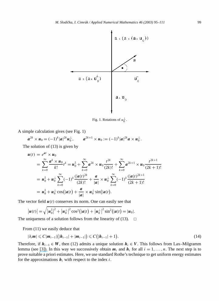
Fig. 1. Rotations ofu⊥0 .

A simple calculation gives (see Fig. 1)

a2k × u0 = (−1)k|a|2ku⊥0 , a2k+1 × u0 := (−1)k|a|2ka × u⊥

0 .

The solution of (13) is given by

u(t) = eat × u0

=∞∑k=0

ak × u0

k! tk = u‖0 +

∞∑k=0

a2k × u0t2k

(2k)! +∞∑k=0

a2k+1 × u0t2k+1

(2k + 1)!

= u‖0 + u⊥

0

∞∑k=0

(−1)k(|a|t)2k(2k)! + a

|a| × u⊥0

∞∑k=0

(−1)k(|a|t)2k+1

(2k + 1)!= u

‖0 + u⊥

0 cos(|a|t)+ a

|a| × u⊥0 sin

(|a|t).The vector fieldu(t) conserves its norm. One can easily see that∣∣u(t)∣∣=√∣∣u‖

0

∣∣2 + ∣∣u⊥0

∣∣2 cos2(|a|t)+ ∣∣u⊥

0

∣∣2 sin2(|a|t)= |u0|.

The uniqueness of a solution follows from the linearity of (13).From (11) we easily deduce that

|∂tm| C|mi−1|(|hi−1| + |mi−1|

)C

(|hi−1| + 1). (14)

Therefore, ifhi−1 ∈W , then (12) admits a unique solutionhi ∈ V . This follows from Lax–Milgrammlemma (see [3]). In this way we successively obtainmi andhi for all i = 1, . . . , n. The next step is toprove suitable a priori estimates. Here, we use standard Rothe’s technique to get uniform energy efor the approximationshi with respect to the indexi.

100 M. Slodicka, I. Cimrák / Applied Numerical Mathematics 46 (2003) 95–111

Lemma 3. Let j ∈ 1, . . . , n. Then there exists a positive constant C such that

j j

tes.

btain

‖hj‖2 +∑i=1

‖hi − hi−1‖2 +∑i=1

‖∇ × hi‖2τ C.

Proof. We setϕ = hiτ in (12) and sum the equation fori = 1, . . . , j . We have

j∑i=1

(hi − hi−1,hi)+j∑

i=1

‖∇ × hi‖2τ = −j∑

i=1

(∂tm(ti),hi

)τ. (15)

The first term on the left can be written asj∑

i=1

(hi − hi−1,hi)= 1

2

(‖hj‖2 − ‖h0‖2 +

j∑i=1

‖hi − hi−1‖2

).

For the right side of (15) we use Cauchy’s and Young’s inequalities and (14). We get∣∣∣∣∣j∑i=1

(∂tm(ti),hi

)τ

∣∣∣∣∣C

j∑i=1

(1+ ‖hi−1‖

)‖hi‖τ C

(1+

j∑i=1

‖hi‖2τ

).

Summarizing all estimates we get

‖hj‖2 +j∑

i=1

‖hi − hi−1‖2 +j∑

i=1

‖∇ × hi‖2τ C

(1+

j∑i=1

‖hi‖2τ

).

The desired result follows from Gronwall’s lemma.We have neededH 0 ∈W in Lemma 3. WhenH 0 ∈ V , then we are able to get better a priori estima

Lemma 4. Let j ∈ 1, . . . , n and H 0 ∈ V . Then there exists a positive constant C such thatj∑

i=1

‖δhi‖2τ + ‖∇ × hj‖2 +j∑

i=1

∥∥∇ × [hi − hi−1]∥∥2 C.

Proof. Settingϕ = hi − hi−1 in (12) and summing up fori = 1, . . . , j we getj∑

i=1

‖δhi‖2τ +j∑

i=1

(∇ × hi ,∇ × [hi − hi−1])= −

j∑i=1

(∂tm(ti), δhi

)τ. (16)

The second term on the left can be written asj∑

i=1

(∇ × hi ,∇ × [hi − hi−1])= 1

2

(‖∇ × hj‖2 − ‖∇ × h0‖2)+ 1

2

j∑i=1

∥∥∇ × [hi − hi−1]∥∥2.

For the right side of (16) we use Cauchy’s inequality, (14), Lemma 3 and Young’s inequality. We o∣∣∣∣∣j∑i=1

(∂tm(ti), δhi

)τ

∣∣∣∣∣C

j∑i=1

(1+ ‖hi−1‖

)‖δhi‖τ C

j∑i=1

‖δhi‖τ Cε + ε

j∑i=1

‖δhi‖2τ.

M. Slodicka, I. Cimrák / Applied Numerical Mathematics 46 (2003) 95–111 101

Choosing a sufficiently small positiveε and collecting all estimates, we arrive atj j

r our

), (12).ling of

∑i=1

‖δhi‖2τ + ‖∇ × hj‖2 +∑i=1

∥∥∇ × [hi − hi−1]∥∥2 C,

which concludes the proof.Now, let us introduce the following piecewise linear in time vector fieldhn (i = 1, . . . , n)

hn(0) =H 0,

hn(t) = hi−1 + (t − ti−1)δhi for t ∈ (ti−1, ti],and the step vector fieldshn,mn and∂tmn

hn(0)=H 0, hn(t)= hi ,

mn(0)=M0, mn(t)=mi ,

∂tmn(0)= ∂tM(0), ∂tmn(t)= ∂tm(ti) for t ∈ (ti−1, ti].Further we define the vector fieldmn as follows

mn(t)=m(t) for t ∈ [ti−1, ti],and for alli = 1, . . . , n.

Using the new notation we rewrite (12) into the following form, which is more convenient fopurposes

(∂thn,ϕ)+ (∇ × hn,∇ × ϕ)= −(∂tmn,ϕ

), (17)

for anyϕ ∈ V .Now, we are in a position to derive the error estimates for the linear approximation scheme (11

We use the standard proof-technique for parabolic equations. The only difficulty will be the handthe right side.

Theorem 5. There exist positive constants C and τ0 such that

(i) maxt∈[0,T ]

∥∥H (t)− hn(t)∥∥2 +

T∫0

∥∥∇ × [H − hn

]∥∥2 Cτ,

(ii) maxt∈[0,T ]

∥∥M(t)−mn(t)∥∥2 +

T∫0

‖∂tM − ∂tmn‖2 Cτ,

hold for any 0< τ < τ0.

Proof. (i) Using the definitions of the vector fieldsM andmn we can write for any timet

∂tM(t)− ∂tmn(t) = [H (t)+ P

(M(t)

)]×M(t)

+ M(t)

|M(t)| × ([H (t)+P

(M(t)

)]×M(t))

102 M. Slodicka, I. Cimrák / Applied Numerical Mathematics 46 (2003) 95–111

− [hn(t − τ)+ P

(mn(t − τ)

)]×mn(t)

m (t) ([ ( )] )

− n

|mn(t)| × hn(t − τ)+ P mn(t − τ) ×mn(t − τ)

= R1 +R2 +R3 +R4 +R5, (18)

where

R1 = [H (t)+ P

(M(t)

)]× (M(t)−mn(t)

),

R2 = ([H (t)+P

(M(t)

)]− [hn(t − τ)+P

(mn(t − τ)

)])×mn(t),

R3 = M(t)

|M(t)| × ([H (t)+ P

(M(t)

)]× [M(t)−mn(t − τ)

]),

R4 = M(t)−mn(t)

|M(t)| × ([H (t)+ P

(M(t)

)]×mn(t − τ)),

R5 = mn(t)

|M(t)| × ([H (t)+ P

(M(t)

)]×mn(t − τ))

− mn(t)

|M(t)| × ([hn(t − τ)+P

(mn(t − τ)

)]×mn(t − τ)).

Taking into account the fact that bothH and M are bounded inL∞((0, T ) × Ω), we get in astraightforward way∣∣∂tM(t)− ∂tmn(t)

∣∣C

(∣∣H (t)− hn(t − τ)∣∣+ ∣∣M(t)−mn(t)

∣∣+ ∣∣M(t)−mn(t − τ)∣∣)

C(∣∣H (t)− hn(t)

∣∣+ ∣∣hn(t)− hn(t − τ)∣∣+ ∣∣M(t)−mn(t)

∣∣+ ∣∣mn(t)−mn(t − τ)∣∣).

(19)

The fieldsmn andM are continuous in time and they start from the same initial datumM0. Therefore

M(t)−mn(t)=t∫

0

∂tM − ∂tmn.

In virtue of (19) and Lemma 4 we can write

∥∥M(t)−mn(t)∥∥

t∫0

‖∂tM − ∂tmn‖ C

t∫0

(τ + ‖H − hn‖ + τ‖∂thn‖ + ‖M −mn‖

)

C

(τ +

t∫0

(‖H − hn‖ + ‖M −mn‖)),

because of the inequality

∥∥mn(t)−mn(t − τ)∥∥

t∫t−τ

‖∂tmn‖ Cτ.

M. Slodicka, I. Cimrák / Applied Numerical Mathematics 46 (2003) 95–111 103

Gronwall’s argument implies( t )

val

a 4 as

ption

∥∥M(t)−mn(t)∥∥ C τ +

∫0

‖H − hn‖ . (20)

This together with (19) give

t∫0

‖∂tM − ∂tmn‖2 C

(τ 2 +

t∫0

‖H − hn‖2

). (21)

Now, we subtract (17) from (10a), setϕ =H − hn and integrate the equation over the time inter(0, t). We get

1

2

∥∥H (t)− hn(t)∥∥2 +

t∫0

∥∥∇ × (H − hn

)∥∥2

=t∫

0

(∇ × (H − hn

),∇ × (

hn − hn))+

t∫0

(∂tmn − ∂tM,H − hn

). (22)

We estimate the first term on the right side using Cauchy’s and Young’s inequalities and Lemmfollows

t∫0

(∇ × (H − hn

),∇ × (

hn − hn))

t∫

0

∥∥∇ × (H − hn

)∥∥∥∥∇ × (hn − hn

)∥∥ ε

t∫0

∥∥∇ × (H − hn

)∥∥2 +Cε

t∫0

∥∥∇ × (hn − hn

)∥∥2 ε

t∫0

∥∥∇ × (H − hn

)∥∥2 +Cετ. (23)

For anyt ∈ [ti−1, ti] we can write∥∥∂tmn(t)− ∂tM(t)∥∥

∥∥∂tmn(ti)− ∂tM(ti)∥∥+ ∥∥∂tM(ti)− ∂tM(t)

∥∥. (24)

The difference∂tM(ti) − ∂tM(t) can be estimated using [18, Lemma 2.2] due to the assumH ∈ L∞((0, T )×Ω), namely,∥∥∂tM(ti)− ∂tM(t)

∥∥C

(∥∥M(ti)−M(t)∥∥+ ∥∥H (ti)−H (t)

∥∥) C

(τ +

ti∫ti−1

‖∂tH‖).

For the term∂tmn(ti)− ∂tM(ti) we apply (19), triangle inequality and (20)∥∥∂tmn(ti)− ∂tM(ti)∥∥

C(∥∥H (ti)− hn(ti−1)

∥∥+ ∥∥M(ti)−mn(ti)∥∥+ ∥∥M(ti)−mn(ti−1)

∥∥)

104 M. Slodicka, I. Cimrák / Applied Numerical Mathematics 46 (2003) 95–111

C

(∥∥H (t)− hn(t)∥∥+ ∥∥M(ti)−mn(ti)

∥∥+ τ +ti∫

‖∂tH‖ +ti∫

‖∂thn‖)

e for

ti−1 ti−1

C

(∥∥H (t)− hn(t)∥∥+

t∫0

‖H − hn‖ + τ +ti∫

ti−1

‖∂tH‖ +ti∫

ti−1

‖∂thn‖).

Taking the second power in (24) and integrating over the time, we deducet∫

0

∥∥∂tmn − ∂tM∥∥2 C

(τ 2 +

t∫0

‖H − hn‖2

).

For the last term on the right in (22) we deduce using Cauchy’s and Young’s inequalities∣∣∣∣∣t∫

0

(∂tmn − ∂tM,H − hn

)∣∣∣∣∣

t∫0

∥∥∂tmn − ∂tM∥∥2 +

t∫0

‖H − hn‖2 C

(τ 2 +

t∫0

‖H − hn‖2

). (25)

Summarizing (22), (23), (25) and choosing a sufficiently small positiveε, we arrive at (τ < τ0 1)

∥∥H (t)− hn(t)∥∥2 +

t∫0

∥∥∇ × (H − hn

)∥∥2 C

(τ +

t∫0

‖H − hn‖2

).

Applying the Gronwall lemma, we conclude the proof.(ii) The assertion immediately follows from the just proved part (i) and the relations (20), (21).

4. Nonlinear approximation scheme

As a second possibility, we design the following recurrent nonlinear approximation schemi = 1, . . . , n:

Algorithm 2 (Nonlinear).

(1) We start fromhi−1 andmi−1 taking into accounth0 =H 0 andm0 =M0.(2) We solve the quadratic ODE with an unknownm(t) on the subinterval[ti−1, ti]

∂tm= [hi−1 +P(mi−1)

]×m+ m

|m| × ([hi−1 + P(mi−1)

]×m). (26)

(3) We setmi :=m(ti).(4) We solve the PDE forhi

(δhi ,ϕ)+ (∇ × hi ,∇ × ϕ)= −(∂tm(ti),ϕ) for ϕ ∈ V . (27)

M. Slodicka, I. Cimrák / Applied Numerical Mathematics 46 (2003) 95–111 105

The approximation ofM is now nonlinear (compare with (11)). The conservation of the modulus form can be proved exactly in the same way as it has been done for the linear algorithm.

tor

et

Let u(t) be the solution of

∂tu= a× u+ cu× (a × u) t > 0, u(0)= u0. (28)

Due to the properties of any rotationR we have the identity

R(x × y)= Rx × Ry,

which is valid for any vectorsx andy. Therefore, we can write

∂tRu= Ra × Ru+ cRu× (Ra × Ru) t > 0

along withRu(0) = Ru0. Hence we see that it is enough to study the solvability of (28) for a vecabeing parallel to(1,0,0)T.

Let us fix anyx ∈ Ω . The existence ofm on [ti−1, ti] follows from the next lemma. First, we su0 =mi−1, a = hi−1 + P(mi−1) andc = 1/|m|, then we perform a rotationR of the coordinate systemin such a way thata := R(a)= |a|(1,0,0). Then we denoteu0 := R(u0) anda = |a|.Lemma 6. Let a, c ∈ R, u0 = (x0, y0, z0)

T be any vector in R3. Then the solution u(t)= (x(t), y(t), z(t))T

of (28) for a = a(1,0,0)T is given by

x(t)= |u0|eact |u0|(|u0| + x0)− e−act |u0|(|u0| − x0)

eact |u0|(|u0| + x0)+ e−act |u0|(|u0| − x0),

y(t)= 2|u0| y0 cos(at)− z0 sin(at)

eact |u0|(|u0| + x0)+ e−act |u0|(|u0| − x0),

z(t)= 2|u0| y0 sin(at)+ z0 cos(at)

eact |u0|(|u0| + x0)+ e−act |u0|(|u0| − x0).

Proof. Let us denote byR = |u0| =√x2

0 + y20 + z2

0. A scalar multiplication of (28) byu(t) gives

∂tu(t) · u(t)= 1

2∂t∣∣u(t)∣∣2 = 0,

which after the time integration yields|u(t)| =R for all t > 0.Further, a simple computation implies

a× u= (a,0,0)T × (x, y, z)T = a(0,−z, y)T

and

u× (a× u)= a(y2 + z2,−xy,−xz

)T.

Therefore, (28) for thex-coordinate reads as

∂tx = ac(y2 + z2)= ac

(R2 − x2), x(0)= x0.

This ordinary differential equation can be explicitly solved. We demonstrate it for|x| < R. The case|x| =R is trivial. Thus, we can write

∂tx

(1

R − x+ 1

R + x

)= 2acR.

106 M. Slodicka, I. Cimrák / Applied Numerical Mathematics 46 (2003) 95–111

We integrate this equation over(0, t) and get

tial

ich

f alleorem

lnR + x(t)

R − x(t)= ln

R + x0

R − x0+ 2acRt,

or an equivalent form

R + x(t)

R − x(t)= R + x0

R − x0e2acRt .

The solution of this algebraic equation is

x(t)=ReacRt(R + x0)− e−acRt (R − x0)

eacRt(R + x0)+ e−acRt (R − x0).

Once we have the formula for thex-coordinate, we have to solve the system of ordinary differenequations for they- andz-coordinate, which has the form

∂ty = −az− acxy, ∂tz= ay − acxz,

along with the starting data(y0, z0). This system can also be explicitly solved, e.g., by MAPLE, whgives the solution of the form

y(t)= 2Ry0 cos(at)− z0 sin(at)

eacRt(R + x0)+ e−acRt (R − x0),

z(t)= 2Ry0 sin(at)+ z0 cos(at)

eacRt (R + x0)+ e−acRt (R − x0).

Further we follow the same way as we did for the linear algorithm. We can show the existence ohifor i = 1, . . . , n and we can get the same a priori estimates as in Lemmas 3 and 4. The following thderives the error estimates for the nonlinear algorithm.

Theorem 7. There exist positive constants C and τ0 such that

(i) maxt∈[0,T ]

∥∥H (t)− hn(t)∥∥2 +

T∫0

∥∥∇ × [H − hn

]∥∥2 Cτ,

(ii) maxt∈[0,T ]

∥∥M(t)−mn(t)∥∥2 +

T∫0

‖∂tM − ∂tmn‖2 Cτ,

hold for any 0< τ < τ0.

Proof. We use the definitions of the vector fieldsM andmn and we write for any timet

∂tM(t)− ∂tmn(t)

= [H (t)+ P

(M(t)

)]×M(t)+ M(t)

|M(t)| × ([H (t)+P

(M(t)

)]×M(t))

− [hn(t − τ)+ P

(mn(t − τ)

)]×mn(t)

M. Slodicka, I. Cimrák / Applied Numerical Mathematics 46 (2003) 95–111 107

− mn(t)

|mn(t)| × ([hn(t − τ)+ P

(mn(t − τ)

)]×mn(t))

ion, buttes the

hen

= R1 + R2 + R3 + R4 + R5, (29)

where

R1 = [H (t)+ P

(M(t)

)]× (M(t)−mn(t)

),

R2 = ([H (t)+P

(M(t)

)]− [hn(t − τ)+P

(mn(t − τ)

)])×mn(t),

R3 = M(t)

|M(t)| × ([H (t)+ P

(M(t)

)]× [M(t)−mn(t)

]),

R4 = M(t)−mn(t)

|M(t)| × ([H (t)+ P

(M(t)

)]×mn(t)),

R5 = mn(t)

|M(t)| × ([H (t)+ P

(M(t)

)]×mn(t))

− mn(t)

|M(t)| × ([hn(t − τ)+P

(mn(t − τ)

)]×mn(t)).

Further we follow exactly the same line as in the proof of Theorem 5, therefore we omit the rest.

5. Numerical experiments

In this section we present two numerical examples. The first one simulates an applied situathere no exact solution is known. The second example (with a prescribed solution) demonstraconvergence rates.

5.1. Example 1

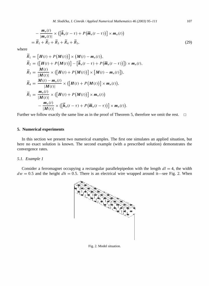
Consider a ferromagnet occupying a rectangular parallelepipedon with the lengthdl = 4, the widthdw = 0.5 and the heightdh = 0.5. There is an electrical wire wrapped around it—see Fig. 2. W

Fig. 2. Model situation.

108 M. Slodicka, I. Cimrák / Applied Numerical Mathematics 46 (2003) 95–111

the electrical current starts to flow through the wire, the induced electromagnetic field influences themagnetizationM . We apply the nonlinear algorithm in order to simulate the evolution ofM andH .

eye step

zef

t

opn a short

First, we split the domain into small blocks with-x = 0.25 and-y = -z = 0.5/6. Then we divideeach block into 6 tetrahedrons. For the approximation of the magnetic fieldH we use Whitney’s edgelements, cf. Bossavit [2], Cessenat [3]. Recall that the approximation ofM can be determined at anpoint x from the approximation of the LLG equation—see (26). For computations we use the timτ = 0.02.

The material constants appearing in the problem setting areµ= σ = 1, α = 0.3, γ = 1.5,K = 10 andthe easy magnetization axis is given byp = (1,0,0)T. The static magnetic fieldH s vanishes andJ 0 = 0.Further we setf = 0.5 andHamp= 50.

We consider the following boundary conditions forHΓD: H (t) = (H(t),0,0)T for H(t) = Hampcos(2πf t) on the long boundary parts (with the si

dl × dw and dl × dh). This boundary condition can be interpreted asν × CH × ν = 0 because o(ν × φ) · (∇ ×H )= [ν × (ν × φ)] · [ν × (∇ ×H )] = φ · [(∇ ×H )× ν].

ΓN : ν ×H = 0 on the small boundary parts (with the sizedh× dw).Thus, the BCs are periodical with the periodTper = 2. Initial data areH 0 = (Hamp,0,0)T and

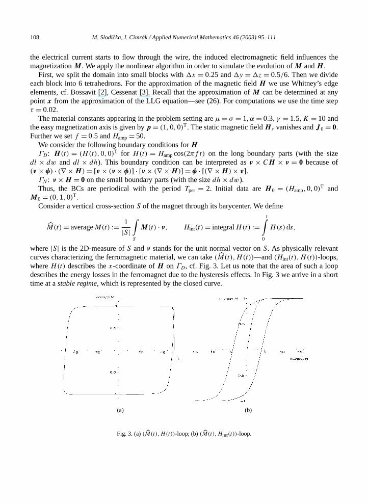
M0 = (0,1,0)T.Consider a vertical cross-sectionS of the magnet through its barycenter. We define

M(t)= averageM(t) := 1

|S|∫S

M(t) · ν, Hint(t)= integralH(t) :=t∫

0

H(s)ds,

where|S| is the 2D-measure ofS andν stands for the unit normal vector onS. As physically relevancurves characterizing the ferromagnetic material, we can take(M(t),H(t))—and(Hint(t),H(t))-loops,whereH(t) describes thex-coordinate ofH on ΓD, cf. Fig. 3. Let us note that the area of such a lodescribes the energy losses in the ferromagnet due to the hysteresis effects. In Fig. 3 we arrive itime at astable regime, which is represented by the closed curve.

(a) (b)

Fig. 3. (a)(M(t),H(t))-loop; (b)(M(t),Hint(t))-loop.

M. Slodicka, I. Cimrák / Applied Numerical Mathematics 46 (2003) 95–111 109

The

hich is

mputed

tion

hitney

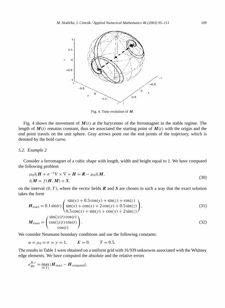
Fig. 4. Time evolution ofM .

Fig. 4 shows the movement ofM(t) at the barycenter of the ferromagnet in the stable regime.length ofM(t) remains constant, thus we associated the starting point ofM(t) with the origin and theend point travels on the unit sphere. Gray arrows point out the end points of the trajectory, wdenoted by the bold curve.

5.2. Example 2

Consider a ferromagnet of a cubic shape with length, width and height equal to 1. We have cothe following problem

µ0∂tH + σ−1∇ × ∇ ×H =R−µ0∂tM,

∂tM = f (H ,M)+ S,(30)

on the interval(0, T ), where the vector fieldsR andS are chosen in such a way that the exact solutakes the form

H exact= 0.1sin(t)

( sin(x)+ 0.5cos(y)+ sin(z)+ cos(z)sin(x)+ cos(x)+ 2cos(y)+ 0.5sin(z)0.5cos(x)+ sin(y)+ cos(y)+ 2sin(z)

), (31)

Mexact=( sin(|x|t)cos(t)

cos(|x|t)cos(t)cos(t)

). (32)

We consider Neumann boundary conditions and use the following constants:

α = µ0 = σ = γ = 1, K = 0, T = 0.5.

The results in Table 1 were obtained on a uniform grid with 16 939 unknowns associated with the Wedge elements. We have computed the absolute and the relative errors

eH,τabs = max

[0,T ]|H exact−H computed|,

110 M. Slodicka, I. Cimrák / Applied Numerical Mathematics 46 (2003) 95–111

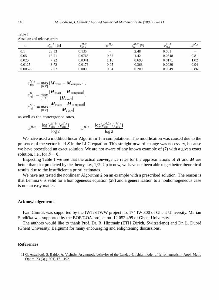
Table 1Absolute and relative errors

to thecausen exact

tical

ason isous case

arián

upré

ath.

τ eH,τrel [%] e

H,τabs ωH,τ e

M,τrel [%] e

M,τabs ωM,τ

0.1 28.53 0.135 – 2.48 0.061 –0.05 16.21 0.0763 0.82 1.42 0.0348 0.810.025 7.22 0.0341 1.16 0.698 0.0171 1.020.0125 3.72 0.0176 0.95 0.363 0.0089 0.940.00625 2.07 0.0098 0.84 0.200 0.0049 0.86

eM,τabs = max

[0,T ]|Mexact−Mcomputed|,

eH,τrel = max

[0,T ]|H exact−H computed|

|H exact| ,

eM,τrel = max

[0,T ]|Mexact−Mcomputed|

|Mexact|as well as the convergence rates

ωH,τ = log[eH,2τabs /e

H,τabs ]

log 2, ωM,τ = log[eM,2τ

abs /eM,τabs ]

log 2.

We have used a modified linear Algorithm 1 in computations. The modification was caused duepresence of the vector fieldS in the LLG equation. This straightforward change was necessary, bewe have prescribed an exact solution. We are not aware of any known example of (7) with a givesolution, i.e., forS = 0.

Inspecting Table 1 we see that the actual convergence rates for the approximations ofH andM arebetter than that predicted by the theory, i.e., 1/2. Up to now, we have not been able to get better theoreresults due to the insufficient a priori estimates.

We have not tested the nonlinear Algorithm 2 on an example with a prescribed solution. The rethat Lemma 6 is valid for a homogeneous equation (28) and a generalization to a nonhomogeneis not an easy matter.

Acknowledgements

Ivan Cimrák was supported by the IWT/STWW project no. 174 IW 300 of Ghent University. MSlodicka was supported by the BOF/GOA-project no. 12 052 499 of Ghent University.

The authors would like to thank Prof. Dr. R. Hiptmair (ETH Zürich, Switzerland) and Dr. L. D(Ghent University, Belgium) for many encouraging and enlightening discussions.

References

[1] G. Anzellotti, S. Baldo, A. Visintin, Asymptotic behavior of the Landau–Lifshitz model of ferromagnetism, Appl. MOptim. 23 (3) (1991) 171–192.

M. Slodicka, I. Cimrák / Applied Numerical Mathematics 46 (2003) 95–111 111

[2] A. Bossavit, Computational Electromagnetism, Variational Formulations, Complementarity, Edge Elements, in: Electro-magnetism, Vol. 18, Academic Press, Orlando, FL, 1998.

. Appl.

(1–2)

nlinear

–1665.h. Ser.

h. Anal.

IAM J.

Proc. 3

Henri

, SIAM

olutions,

. Anal.

hys. Z.

d from

th. 151

l. 36 (3)

Mech.

Partial

Comput.

3–847.

[3] M. Cessenat, Mathematical Methods in Electromagnetism—Linear Theory and Applications, in: Ser. Adv. MathSci., Vol. 41, World Scientific, Singapore, 1996.

[4] Y. Chen, Dirichlet boundary value problems of Landau–Lifshitz equation, Comm. Partial Differential Equations 25(2000) 101–124.

[5] Y. Chen, Existence and singularities for the Dirichlet boundary value problems of Landau–Lifshitz equations, NoAnal. Theory Methods Appl. A 48 (3) (2002) 411–426.

[6] W. E, X.-P. Wang, Numerical methods for the Landau–Lifshitz equation, SIAM J. Numer. Anal. 38 (5) (2000) 1647[7] B. Guo, S. Ding, Neumann problem for the Landau–Lifshitz–Maxwell system in two dimensions, Chin. Ann. Mat

B 22 (4) (2001) 529–540.[8] B. Guo, F. Su, Global weak solution for the Landau–Lifshitz–Maxwell equation in three space dimensions, J. Mat

Appl. 211 (1) (1997) 326–346.[9] H. Haddar, P. Joly, Effective boundary conditions for thin ferromagnetic layers: The one-dimensional model, S

Appl. Math. 61 (4) (2001) 1386–1417.[10] J.L. Joly, G. Métivier, J. Rauch, Electromagnetic wave propagation in presence of a ferromagnetic material, ESAIM

(1998) 85–99.[11] J.L. Joly, G. Métivier, J. Rauch, Global solutions to Maxwell equations in a ferromagnetic medium, Ann.

Poincaré 1 (2) (2000) 307–340.[12] P. Joly, A. Komech, O. Vacus, On transitions to stationary states in a Maxwell–Landau–Lifschitz–Gilbert system

J. Math. Anal. 31 (2) (2000) 346–374.[13] P. Joly, O. Vacus, Maxwell’s equations in a 1D ferromagnetic medium: Existence and uniqueness of strong s

INRIA, Technical Report No. 3052, 1996.[14] P. Joly, O. Vacus, Mathematical and numerical studies of nonlinear ferromagnetic materials, Modél Math

Numér 33 (3) (1999) 593–626.[15] L.D. Landau, E.M. Lifshitz, On the theory of the dispersion of magnetic permeability in ferromagnetic bodies, P

Sowjetunion 8 (1935) 153–169.[16] L.D. Landau, E.M. Lifshitz, Electrodynamics of Continuous Media, Pergamon Press, New York, 1960, (translate

the Russian by J.B. Sykes and J.S. Bell).[17] D. Lewis, N. Nigam, Geometric integration on spheres and some interesting applications, J. Comput. Appl. Ma

(2003) 141–170.[18] P.B. Monk, O. Vacus, Error estimates for a numerical scheme for ferromagnetic problems, SIAM J. Numer. Ana

(1998) 696–718.[19] P.B. Monk, O. Vacus, Accurate discretization of a nonlinear micromagnetic problem, Comput. Methods Appl.

Engrg. 190 (40–41) (2001) 5243–5269.[20] A. Prohl, Computational Micromagnetism, in: Adv. Numer. Math., Vol. 16, Teubner, Leipzig, 2001.[21] F. Su, B. Guo, The global smooth solution for Landau–Lifshitz–Maxwell equation without dissipation, J.

Differential Equations 11 (3) (1998) 193–208.[22] A. Visintin, On Landau–Lifshitz’ equations for ferromagnetism, Japan J. Appl. Math. 2 (1985) 69–84.[23] X.-P. Wang, C.J. García-Cervera, W. E, A Gauss–Seidel projection method for micromagnetics simulations, J.

Phys. 171 (2001) 357–372.[24] P. Weiss, L’hypothèse du champ moléculaire et la proprièté ferromagnetique, J. Phys. 6 (1907) 661–690.[25] J. Zhai, Existence and behavior of solutions to the Landau–Lifshitz equation, SIAM J. Math. Anal. 30 (4) (1999) 83