numerical simulations of drag-reducing devices for ground
TRANSCRIPT
Numerical Simulations of Drag-Reducing Devices for Ground Vehicles
by
Walid Ibrahim Mazyan
A Thesis Presented to the Faculty of the
American University of Sharjah
College of Engineering
in Partial Fulfillment
of the Requirements
for the Degree of
Master of Science in
Mechanical Engineering
Sharjah, United Arab Emirates
January 2013

© 2013 Walid Ibrahim Mazyan. All rights reserved.
Approval Signatures
We, the undersigned, approve the Master’s Thesis of Walid Ibrahim Mazyan.
Thesis Title: Numerical Simulations of Drag-Reducing Devices for Ground Vehicles.
Signatures Date of Signatures
_________________________ _______________
Dr. Essam Wahba
Associate Professor, Department of Mechanical Engineering
Thesis Advisor
_________________________ _______________
Dr. Mohamed Gadalla
Professor, Department of Mechanical Engineering
Thesis Committee Member
_________________________ _______________
Dr. Rami Haweeleh
Associate Professor, Department of Civil Engineering
Thesis Committee Member
_________________________ _______________
Dr. Ibrahim Deiab
Head, Department of Mechanical Engineering
_________________________ _______________
Dr. Hani El Kadi
Associate Dean, College of Engineering
_________________________ _______________
Dr. Hany El Kadi
Acting Dean, College of Engineering
_________________________ _______________
Dr. Khalid Assaleh
Director of Graduate Studies

Acknowledgments
I would like to express my gratitude to my advisor, Dr. Essam Wahba, whose unrivaled
guidance at every stage of this thesis ensured a richer, deeper understanding of the results
achieved in this research.
I would like to thank my committee members, Dr. Mohammad Gadalla and Dr. Rami
Haweeleh for their highly constructive feedback on this research.
My heartfelt gratitude also goes to my beloved family who supported me in every way
possible way to achieve this Master Degree.
Last but not least, I would like to thank my beloved friends, Asif Javaid, Ayman Helal,
Farah El Amin, Shadi Kalash, Matthew El Jamal and Mohammad Tibi for their continuous
support throughout the Masters program.

To My Beloved Mother, Father and Sisters
I wouldn’t have made it without your love and support.
6
Abstract
The aim of the present study is to reduce the aerodynamic drag coefficient of ground
vehicles. With the application of efficient drag reducing devices, aerodynamic drag is
significantly reduced. This study analyzes numerically the effect of applying drag reducing
devices on a sedan, sports utility vehicle (SUV) and a tractor trailer model to improve the fuel
consumption of the vehicle. Both RANS (Reynolds-averaged Navier–Stokes equations) and LES
(Large Eddy Simulations) are used to analyze the percent drag reduction due to the use of
different drag reducing devices. The numerical procedure is first validated against the
experimental data for the tractor-trailer model with no drag reducing devices installed. Following
the validation, simulations are carried out to investigate the percent drag reduction by installing a
modified front head to help the flow transition from the tractor to the trailer, and inventive rear
wings that direct the air flow towards the rear of the vehicle where low pressure exists. The
tractor trailer results showed a total drag reduction of around 21% when the front and rear drag
reducing devices were installed. Vortex generators are also numerically simulated and results
show that they reduce drag by 1.6%. The SUV model showed a drag reduction of 4.2 % and the
Ahmed car model showed a drag reduction of 10 %. Results showed that the LES model
provides the most accurate prediction of all turbulence models as compared to the experimental
value of the drag coefficient.
Keywords: Aerodynamics, Large Eddy Simulation, Reynolds-Averaged Navier-Stokes
equations, Drag, Ground Vehicles.
7
Table of Contents
Abstract ....................................................................................................................................... 6
Chapter 1: Introduction ............................................................................................................. 13
1.1. Background ................................................................................................................... 13
1.2. Research Significance ................................................................................................... 14
1.3. Research Objectives ...................................................................................................... 15
Chapter 2: Literature Review .................................................................................................... 16
2.1. Ground Vehicle Aerodynamics ..................................................................................... 16
2.2. Drag Reducing Devices for Ground Vehicles ............................................................... 16
Chapter 3: Numerical Models and Schemes ............................................................................. 23
3.1. Reynolds averaged Navier Stokes Equations (RANS) ................................................. 23
3.1.1. k-ε Model .......................................................................................................... 23
3.1.2. Re-Normalization Group (RNG) k-ε ................................................................ 25
3.2. Large Eddy Simulation ................................................................................................. 28
3.2.1. Filter Implementation ........................................................................................ 29
Chapter 4: Ground Vehicle Models .......................................................................................... 34
4.1. Tractor-Trailer Configurations ...................................................................................... 34
4.1.1. Tractor Trailer with No Drag-Reducing Devices...................................................... 34
4.1.2. Tractor Trailer with Rear Drag Reducing Devices ................................................... 35
4.1.3. Tractor Trailer with Front Drag Reducing Devices .................................................. 36
4.1.4. Tractor Trailer with Front and Rear Drag Reducing Devices ................................... 37
4.1.5. Tractor Trailer with Vortex Generators .................................................................... 38
4.2. Sports Utility Vehicle Configurations........................................................................... 40
4.2.1. Hummer H2 with no Drag Reducing Devices .......................................................... 40
4.2.2. Hummer H2 with Directing Vanes ........................................................................... 40
4.3. Sedan Vehicle Configurations ...................................................................................... 41
4.3.1. Ahmed Car Model with no Drag Reducing Devices ................................................ 42
4.3.2. Ahmed Car Model with Rear Wing .......................................................................... 42
Chapter 5: Grid Generation ....................................................................................................... 44
5.1. Tractor-Trailer Grid Generation .................................................................................... 44
5.1.1. Tractor Trailer Grid Generation with Rear Drag Reducing Devices ........................ 44
5.1.2. Tractor Trailer Grid Generation with Front Drag Reducing Devices ....................... 45
5.1.3. Tractor Trailer Grid Generation with Front and Rear Drag Reducing Devices ........ 46
5.1.4. Tractor Trailer Grid Generation with Vortex Generators ......................................... 46
8
5.2. SUV Grid Generation ................................................................................................... 47
5.2.1. SUV Grid Generation with No Drag Reducing Devices .......................................... 47
5.2.2. SUV Grid Generation with Rear Directing Vanes .................................................... 47
5.3. Sedan Vehicle Grid Generation .................................................................................... 48
5.3.1. Sedan Vehicle Grid Generation with No Drag Reducing Devices ........................... 48
5.3.2. Sedan Vehicle Grid Generation with Drag Reducing Devices ................................. 49
Chapter 6: Numerical Results ................................................................................................... 50
6.1. Tractor-Trailer Numerical Results ................................................................................ 50
6.1.1. Tractor Trailer with No Drag Reducing Devices ...................................................... 50
6.1.2. Tractor Trailer with Rear Drag Reducing Devices ................................................... 53
6.1.3. Tractor Trailer with Front Drag Reducing Devices .................................................. 57
6.1.4. Tractor Trailer with Front and Rear Drag Reducing Devices ................................... 62
6.1.5. Tractor Trailer with Vortex Generators .................................................................... 66
6.2. SUV Numerical Results ................................................................................................ 69
6.2.1. SUV with No Drag Reducing Devices ..................................................................... 69
6.2.2. SUV with Directing Vanes ....................................................................................... 71
6.3. Ahmed Car Model Results ............................................................................................ 74
6.3.1. Ahmed Car Model with No Drag Reducing Devices................................................ 74
6.3.2. Ahmed Car Model with Rear Wing .......................................................................... 75
Chapter 7: Results and Validation ............................................................................................ 78
7.1. Grid Independence Tests ............................................................................................... 78
7.2. Results Validation ......................................................................................................... 78
7.2.1. Tractor Trailer ........................................................................................................... 78
7.2.2. Sports Utility Vehicle ............................................................................................... 79
7.2.3. Ahmed Car Model ..................................................................................................... 79
Chapter 8: Summary and Conclusion ....................................................................................... 82
References ................................................................................................................................. 85
9
List of Figures
Figure 1: TrailerTail of ATDynamics. [6] ................................................................................ 17
Figure 2: Different drag-reducing devices on heavy vehicles. [6] ............................................ 17
Figure 3: View of the rear roof of SDR [7]............................................................................... 18
Figure 4: View of the SDR rear spoiler. [7] .............................................................................. 18
Figure 5: Front drag-reducing device.[8] .................................................................................. 18
Figure 6: Controlled vortices on a wing.[9] .............................................................................. 19
Figure 7: Velocity profile on top of a surface.[11] ................................................................... 20
Figure 8: Bump-shaped VG.[5] ................................................................................................ 20
Figure 9: Delta wing VG.[5] ..................................................................................................... 21
Figure 10: Vortex generator types.[5] ....................................................................................... 21
Figure 11: Rear vortices on a vehicle.[12] ................................................................................ 21
Figure 12: Vehicle Platoon. [15] ............................................................................................... 22
Figure 13: Side Skirt.[15] ......................................................................................................... 22
Figure 14: Sample tractor trailer. .............................................................................................. 34
Figure 15: Wind tunnel dimensions. ......................................................................................... 35
Figure 16: Geometric model with wind tunnel with rear DRDs attached. ................................ 35
Figure 17: A magnified snapshot with rear DRDs on tractor trailer. ........................................ 36
Figure 18: Wind tunnel geometric model with front DRDs. .................................................... 36
Figure 19: A magnified snapshot at the geometric model with front DRDs attached. ............. 37
Figure 20: Upper view of the tractor trailer with front DRDs attached. ................................... 37
Figure 21: Geometric model with full DRDs attached. ............................................................ 38
Figure 22: A magnified snapshot at the tractor trailer with full DRDs attached. ..................... 38
Figure 23: Geometric model with vortex generators attached. ................................................. 39
Figure 24: Magnified snapshot at the geometric model with vortex generators attached. ........ 39
Figure 25: Geometry of each vortex generator. ........................................................................ 39
Figure 26: Geometric model of Hummer H2. ........................................................................... 40
Figure 27: Hummer H2 geometric model with directing vanes. ............................................... 41
Figure 28: Ahmed car model general dimensions. ................................................................... 41
Figure 29: Ahmed Car Geometric Model inside the wind tunnel. ............................................ 42
Figure 30: Magnified snapshot of the Geometric Model of Ahmed Car With No Rear Wing. 42
Figure 31: Geometric model of Ahmed car with rear wing and wind tunnel. .......................... 42
Figure 32: Geometric model of Ahmed car model with rear wing. .......................................... 43
Figure 33: Wind tunnel meshing grid of tractor trailer. ............................................................ 44
Figure 34: A magnified snapshot of the tractor trailer mesh with rear DRDs. ......................... 45
Figure 35: Grid of the wind tunnel with front DRDs. ............................................................... 45
Figure 36: Magnified snapshot at the model mesh with front DRDs attached. ........................ 45
Figure 37: Wind tunnel meshing grid. ...................................................................................... 46
Figure 38: A magnified snapshot at the tractor trailer with full DRDs attached. ..................... 46
Figure 39: Grid with vortex generators attached. ..................................................................... 47
Figure 40: Grid of the Hummer with no vanes. ........................................................................ 47
Figure 41: Grid of the Hummer with directing vanes. .............................................................. 48
Figure 42: Grid of the Ahmed car model with no wing. ........................................................... 48
Figure 43: Grid of Ahmed car model with rear wing................................................................ 49
10
Figure 44: Velocity vectors of tractor trailer with no DRDs. ................................................... 52
Figure 45: A magnified snapshot of velocity vectors of tractor trailer with no DRDs. ............ 52
Figure 46: Velocity vectors of tractor trailer with no DRDs—top view. .................................. 53
Figure 47: Velocity Vectors of tractor trailer with rear DRDs. ................................................ 54
Figure 48: Velocity Vectors at rear of the tractor trailer with DRDs. ....................................... 54
Figure 49: Velocity Vectors of top rear of the trailer with rear DRDs. .................................... 55
Figure 50: Velocity Vectors of rear bottom of the trailer with rear DRDs. .............................. 55
Figure 51: Velocity Vectors of rear bottom of the tractor with rear DRDs. ............................. 56
Figure 52: Pressure contours on Tractor trailer with rear DRD’s ............................................. 56
Figure 53: Velocity Vectors at the rear of the trailer with rear DRDs attached. ....................... 57
Figure 54: Velocity vectors around the tractor with front DRDs attached. .............................. 58
Figure 55: A magnified picture of the velocity vectors at the front DRD. ............................... 58
Figure 56: Velocity vector at the front DRD (top view). .......................................................... 59
Figure 57: A magnified look at the rear of the trailer with front DRDs attached. .................... 59
Figure 58: Velocity vectors with front DRDs attached (top view). .......................................... 60
Figure 59: Velocity vectors at the rear of the tractor with front DRDs attached. ..................... 60
Figure 60: Pressure contours around the tractor trailer with front DRD’s ................................ 61
Figure 61: Velocity vector with full DRDs attached. ............................................................... 62
Figure 62: Velocity vectors at the rear bottom of the tractor with full DRDs attached. ........... 63
Figure 63: Velocity vectors at the tractor's side with full DRDs attached. ............................... 63
Figure 64: Velocity vector at the top of the tractor with full DRDs attached. .......................... 64
Figure 65: Velocity vectors at the front with full DRDs attached (top view). .......................... 64
Figure 66: Velocity vectors around the tractor trailer with full DRDs attached (top view). .... 65
Figure 67: Pressure contours around the tractor trailer with full DRD’s .................................. 65
Figure 68: Velocity vectors with vortex generators attached.................................................... 66
Figure 69: Pressure contours around the tractor trailer with VG .............................................. 67
Figure 70: A magnified snapshot of pressure contours around VG .......................................... 67
Figure 71: Drag coefficients of different solvers histogram ..................................................... 69
Figure 72: Velocity vectors around Hummer with no directing vanes. .................................... 69
Figure 73: A magnified snapshot of velocity vectors at the rear of the Hummer with no
directing vanes. ......................................................................................................................... 70
Figure 74: Velocity vectors around the Hummer (top view). ................................................... 70
Figure 75: Pressure contours around SUV with no DRD ......................................................... 71
Figure 76: Velocity vectors at the Hummer with directing vanes (top view). .......................... 71
Figure 77: Magnified snapshot of the airflow at the rear of SUV ............................................ 72
Figure 78: Pressure contours around the SUV with rear directing vanes ................................. 72
Figure 79: Drag coefficient of SUV with and without DRD using LES .................................. 73
Figure 80: Velocity vectors around the sedan car with no DRD .............................................. 74
Figure 81: Pressure contours at the rear of the Ahmed car model with no rear wing. .............. 74
Figure 82: Velocity vectors of Ahmed car with rear wing. ...................................................... 75
Figure 83: Pressure contours of the sedan vehicle with rear wing ............................................ 76
Figure 84: Drag coefficient summary histogram of the sedan model ....................................... 77
Figure 85: Velocity plots vs. height at 38, 88 and 138 mm behind The Ahmed car model. ..... 80
Figure 86: Fuel consumption pie charts of ground vehicles before and after adding the DRD 82
11
List of Tables
Table 1: Market dimensions of trailers. .................................................................................... 34
Table 2: RANS Drag Coefficient Summary ............................................................................. 50
Table 3: LES drag results. ......................................................................................................... 51
Table 4: Drag coefficient summary of tractor trailer (rear DRD). ............................................ 57
Table 5: Drag coefficient summary of tractor trailer (front DRD). .......................................... 61
Table 6: Drag coefficient summary of tractor trailer (full DRD). ............................................. 66
Table 7: Drag coefficient summary of tractor trailer (vortex generator). ................................. 68
Table 8: Percentage Summary. ................................................................................................. 68
Table 9: Drag coefficient summary of the Hummer model—vanes and no vanes. .................. 72
Table 10: Drag coefficient summary of Ahmed car model (no vanes). .................................... 75
Table 11: Drag coefficient summary of Ahmed car model (vane). .......................................... 76
Table 12: RANS drag error with experimental results. ............................................................ 78
Table 13: LES drag error with experimental results. ................................................................ 79
Table 14: RANS drag error with LES paper results. ................................................................ 79
Table 15: LES drag error with LES paper results. .................................................................... 79
12
List of Abbreviations
Cd: Drag Coefficient
A: Area
F: Drag Force
DRD: Drag-reducing device
ρ: Air Density
RANS: Reynolds Averaged Navier-Stokes
LES: Large Eddy Simulation
13
Chapter 1: Introduction
1.1. Background
Energy resources scarcity remains one of the most researched topics in academia due
to increased consumption of the energy resources caused by staggering population and
pollution spikes. The main energy source consumed since the 1900’s is fossil fuel which
sustain virtually all factories and machines produced today. These resources are depleting
rapidly thus prompting the need for newer, more efficient energy sources and—more
importantly—a means to conserve these fuels as much as possible. It is for this reason that
major manufacturers today have built research and development centers dedicated to
improving the engine’s efficiency in order to make maximum power with minimal fuel
consumption a possibility. Additionally, the aerodynamics of the vehicles is quickly becoming
an area of focus. This rising interest in improving vehicle efficiently is chiefly the result of
inflation of fuel prices and the need of reducing the emission of greenhouse gases [1].
Losses in the vehicles arise in the engine, aerodynamics and the interaction with the
surroundings. For example, ground vehicles acquire losses due to traction friction between the
wheels and the ground, by the transmission system and finally by the aerodynamic drag.
Reducing this aerodynamic drag, thus, accounts for a major improvement in the fuel
consumption. According to Daimler [2], every 0.01 reduction in the Cd figure can cut fuel
consumption by up to 0.4-litres/100km at 130km/h. Teddy Woll [2] states: "the currency of
aerodynamics is drag counts, which is 1/1,000th of a Cd, so from 0.29 to 0.25 is 40 drag
counts in 25 years of sedan development". He goes on to state, "Now we've gone from 0.30 in
the outgoing B-Class to 0.26 which is a leap frog in seven years. And we have an optimum
eco package with a lot of measures which then reaches 0.24—a phenomenal drag factor for
such a relatively boxy car." [2]
As oil prices continue to fluctuate dramatically, improving the aerodynamics of
vehicles to reduce fuel consumption has become a necessity. In 1997, the fuel consumption of
the Class 8 trucks reached 18 billion gallons in which 65% of this fuel consumption was
wasted to overcome the aerodynamic drag [3].
Heavy vehicles are aerodynamically inefficient compared to other ground vehicles due
to a large frontal area and bulky frames. A forty ton truck traveling at 60mph consumes about
34 liter of fuel alone to overcome the aerodynamic drag. In contrast, an average-sized vehicle
14
consumes a quarter of what tractor trailers consume. As testament to this fact, it should be
noted that 22% of energy consumed in the United Kingdom is by heavy vehicles [4].
The drag coefficient is a significant constant that automotive industry highly
concentrates on. The drag coefficient is a factor that evaluates the aerodynamic efficiency of
the road vehicle in addition to its maneuverability. Reducing the drag coefficient means
reducing the fuel consumption of the vehicle. To find the drag coefficient of a vehicle, a wind
tunnel test is applied on the vehicle in which inlet airflow is blown on the vehicle and the total
difference in pressure in front and behind the vehicle is measured. The difference in the
pressure is a proportional to the drag coefficient.
However, in actuality time-varying forces are acting on the vehicles, where a part of
these time varying forces and moments is the effect of overtaking of the vehicles and cross
winds. These forces need to be studied as they also have an effect on the vehicle’s
performance and stability [5].
To improve the stability of the vehicle, spoilers/wings are employed, which serve to
push the vehicle downwards when travelling at high speeds. One main disadvantage of having
a spoiler/wing, however, is that it increases the total drag and the rolling resistance of the
vehicle. Drag forces are dependent on the velocity of the vehicle. The higher the velocity
facing the vehicle, the more aerodynamic forces are applied on the vehicle and hence, the
more power the vehicle needs to overcome these frictional forces.
Increase in drag causes an increase in fuel consumption which is why when it comes to
reducing a vehicle’s fuel consumption, drag coefficient reduction is one of the main methods
to do so. Spoilers and drag-reducing devices should also be used in order to reduce the drag
on tractor trailers. Drag-reduction on trucks, in particular, saves millions of dollars by
reducing the fuel consumption. On top of this, it was necessary for the manufacturers to
design the vehicles as more “aerodynamically friendly” by reducing the sharp edges, small
gaps and add the drag-reducing devices.
1.2. Research Significance
This research uses mechanical devices such as diffusers, rear and side spoilers to
reduce aerodynamic drag for ground vehicles. These drag-reducing devices can also be
applied on regular vehicles to improve the efficiency and reduce drag.
15
This study also allows for a comparison to be drawn between the different RANS
simulation models compared to LES models which is significant in showing how accurate
LES is as opposed to RANS.
1.3. Research Objectives
The present research aims to shed new light on the global problem of increased fuel
consumption by heavy vehicles. The major objectives of this research are:
1. Numerical simulations with Reynolds Averaged Navier-Stokes equations on a Tractor
trailer, a sports utility vehicle represented by Hummer H2 and a sedan vehicle
represented by Ahmed car model.
2. Numerical simulations using Large Eddy Simulation on the tractor trailer, Hummer H2
and Ahmed car models.
3. Validation against available experimental results.
4. Identification of the optimum configuration of drag-reducing devices for improved
aerodynamic performance.
16
Chapter 2: Literature Review
2.1. Ground Vehicle Aerodynamics
For an average-size car to travel on a highway, it expends vast amounts of energy to
displace the air. Studies show that at 70 miles per hour (110km/hr), as much as 65% of the
fuel is spent in overcoming air-resistance. This is even a bigger problem for heavy vehicles
which attain a boxy shape that is aerodynamically inefficient.
Following the fuel crises in 1970, the US government commenced an intensive
research on reducing fuel consumption of vehicles, which constitutes to 28% of the total
energy consumed by USA. Particular interest was cast upon heavy vehicles due to their high
fuel-consumption and long travel frequency. The U.S. Department of Energy has requested
numerous national laboratories to discover possible methods on reducing the fuel
consumption of tractor-trailers. The methods put forth were based on the enhancement of the
aerodynamics, power-train and engine-combustion efficiency.
2.2. Drag Reducing Devices for Ground Vehicles
In 2010, national laboratories such as Livermore Laboratory, aimed to reduce the
aerodynamic drag of the tractor trailers by at least 25% by the year of 2015, which represents
a 12% improvement in fuel economy at highway speeds. This is equivalent to the annual oil
stored in 130 mid-size tankers.
Other companies such as ATDynamics aimed even higher in their quest for a better
fuel economy. This company collaborated with national laboratories as well as universities in
order to reduce the aerodynamic drag on a tractor trailers by 50%. One of the technologies
that ATDynamics utilized was adding the TrailerTail to the rear of the trailer where low
pressure suction occurs. These flaps at the rear delayed the separation of the air thus reducing
the aerodynamic drag. ATDynamics claimed that the TrailerTail can potentially reduce the
fuel consumption by $20 billion over the next decade. As per ATDynamics’ claim, the trailer-
tail technology is projected to reduce fuel consumption by as much as the entire US electric
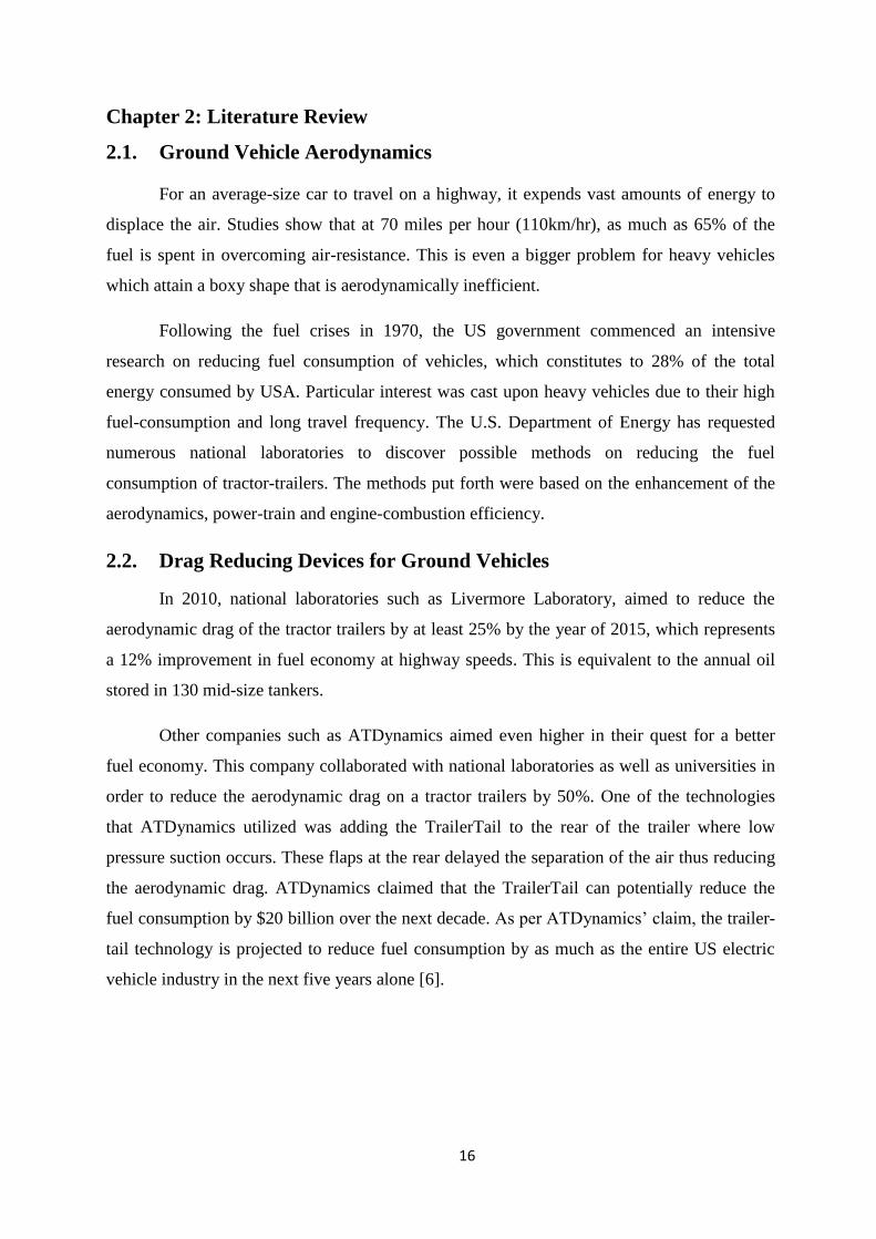
vehicle industry in the next five years alone [6].
17
Figure 1: TrailerTail of ATDynamics. [6]
Numerous TrailerTails have been employed by the US trucking industry, operating
over 300 million miles on the U.S. highways. This has in turn has saved the U.S. trucking
business two million gallons of diesel that would normally go to waste in overcoming
aerodynamic drag. As ATDynamics summarizes these results, each tail saves 6% of fuel
consumption [6]. Also, each tail omits the effect of fuel consumption of a whole passenger
car.
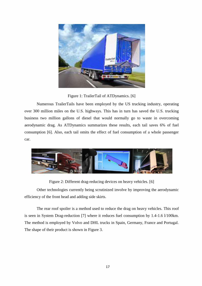
Figure 2: Different drag-reducing devices on heavy vehicles. [6]
Other technologies currently being scrutinized involve by improving the aerodynamic
efficiency of the front head and adding side skirts.
The rear roof spoiler is a method used to reduce the drag on heavy vehicles. This roof
is seen in System Drag-reduction [7] where it reduces fuel consumption by 1.4-1.6 l/100km.
The method is employed by Volvo and DHL trucks in Spain, Germany, France and Portugal.
The shape of their product is shown in Figure 3.
18
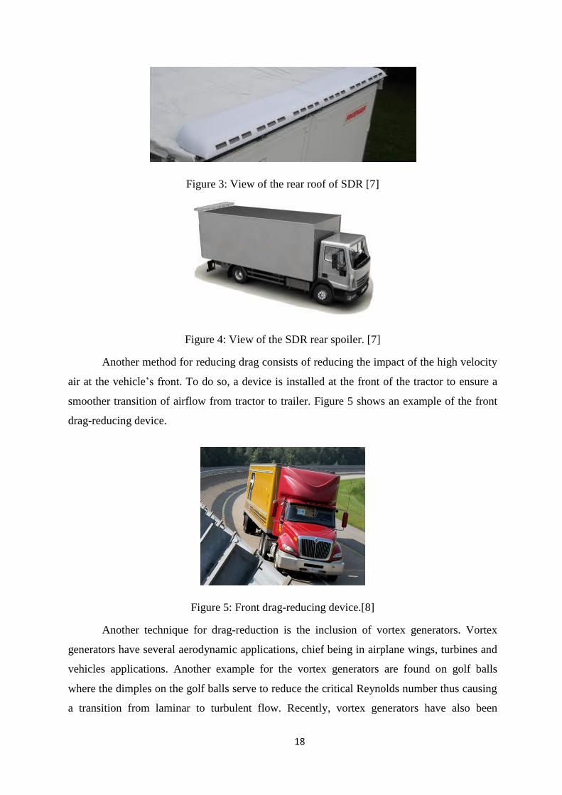
Figure 3: View of the rear roof of SDR [7]
Figure 4: View of the SDR rear spoiler. [7]
Another method for reducing drag consists of reducing the impact of the high velocity
air at the vehicle’s front. To do so, a device is installed at the front of the tractor to ensure a
smoother transition of airflow from tractor to trailer. Figure 5 shows an example of the front
drag-reducing device.
Figure 5: Front drag-reducing device.[8]
Another technique for drag-reduction is the inclusion of vortex generators. Vortex
generators have several aerodynamic applications, chief being in airplane wings, turbines and
vehicles applications. Another example for the vortex generators are found on golf balls
where the dimples on the golf balls serve to reduce the critical Reynolds number thus causing
a transition from laminar to turbulent flow. Recently, vortex generators have also been
19
introduced by the automotive industry to decrease drag via reduction in fuel consumption or
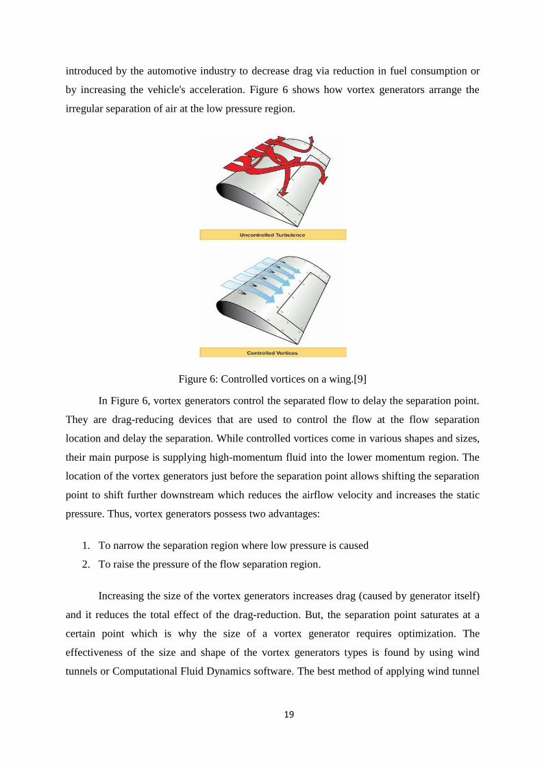
by increasing the vehicle's acceleration. Figure 6 shows how vortex generators arrange the
irregular separation of air at the low pressure region.
Figure 6: Controlled vortices on a wing.[9]
In Figure 6, vortex generators control the separated flow to delay the separation point.
They are drag-reducing devices that are used to control the flow at the flow separation
location and delay the separation. While controlled vortices come in various shapes and sizes,
their main purpose is supplying high-momentum fluid into the lower momentum region. The
location of the vortex generators just before the separation point allows shifting the separation
point to shift further downstream which reduces the airflow velocity and increases the static
pressure. Thus, vortex generators possess two advantages:
1. To narrow the separation region where low pressure is caused
2. To raise the pressure of the flow separation region.
Increasing the size of the vortex generators increases drag (caused by generator itself)
and it reduces the total effect of the drag-reduction. But, the separation point saturates at a
certain point which is why the size of a vortex generator requires optimization. The
effectiveness of the size and shape of the vortex generators types is found by using wind
tunnels or Computational Fluid Dynamics software. The best method of applying wind tunnel
20
tests on ground vehicles through a simultaneous application of wheel rotation and airflow on
the vehicle. The rotation of the wheels will contribute in the flow turbulence behind it [10].
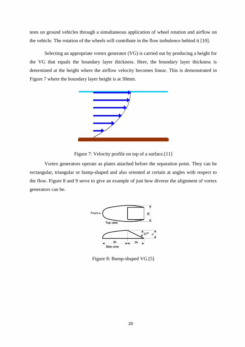
Selecting an appropriate vortex generator (VG) is carried out by producing a height for
the VG that equals the boundary layer thickness. Here, the boundary layer thickness is
determined at the height where the airflow velocity becomes linear. This is demonstrated in
Figure 7 where the boundary layer height is at 30mm.
Figure 7: Velocity profile on top of a surface.[11]
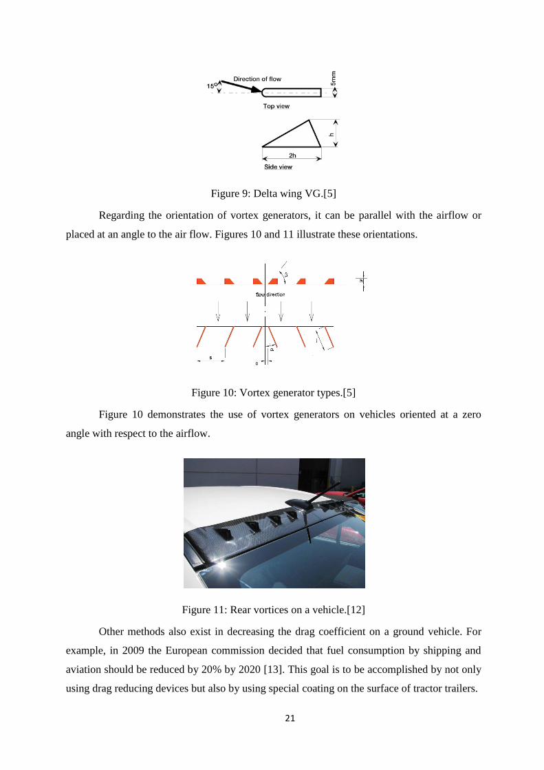
Vortex generators operate as plates attached before the separation point. They can be
rectangular, triangular or bump-shaped and also oriented at certain at angles with respect to
the flow. Figure 8 and 9 serve to give an example of just how diverse the alignment of vortex
generators can be.
Figure 8: Bump-shaped VG.[5]
21
Figure 9: Delta wing VG.[5]
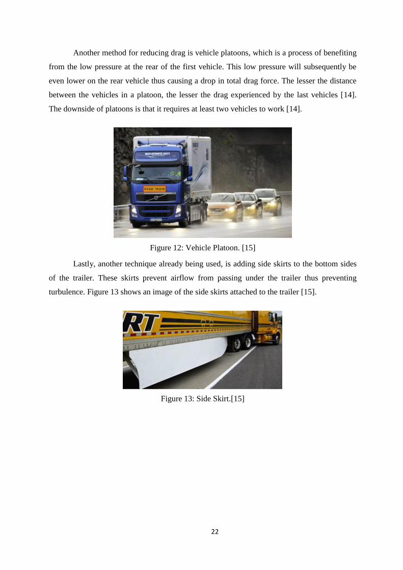
Regarding the orientation of vortex generators, it can be parallel with the airflow or
placed at an angle to the air flow. Figures 10 and 11 illustrate these orientations.
Figure 10: Vortex generator types.[5]
Figure 10 demonstrates the use of vortex generators on vehicles oriented at a zero
angle with respect to the airflow.
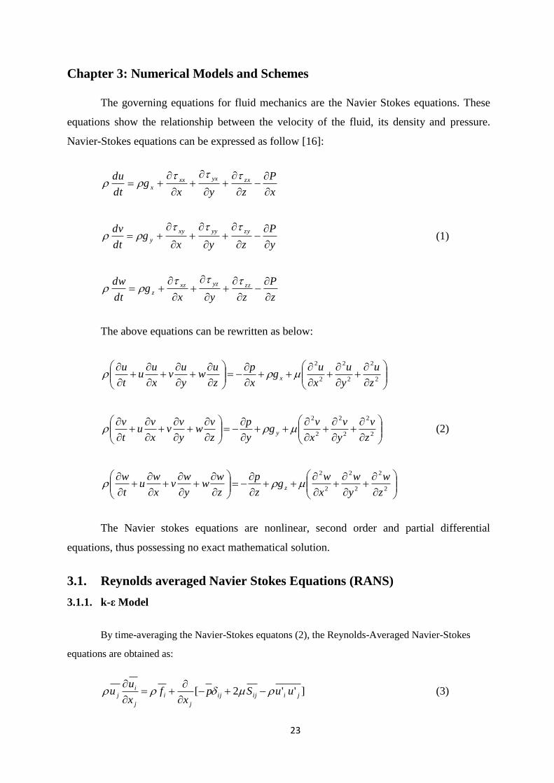
Figure 11: Rear vortices on a vehicle.[12]
Other methods also exist in decreasing the drag coefficient on a ground vehicle. For
example, in 2009 the European commission decided that fuel consumption by shipping and
aviation should be reduced by 20% by 2020 [13]. This goal is to be accomplished by not only
using drag reducing devices but also by using special coating on the surface of tractor trailers.
22
Another method for reducing drag is vehicle platoons, which is a process of benefiting
from the low pressure at the rear of the first vehicle. This low pressure will subsequently be
even lower on the rear vehicle thus causing a drop in total drag force. The lesser the distance
between the vehicles in a platoon, the lesser the drag experienced by the last vehicles [14].
The downside of platoons is that it requires at least two vehicles to work [14].
Figure 12: Vehicle Platoon. [15]
Lastly, another technique already being used, is adding side skirts to the bottom sides
of the trailer. These skirts prevent airflow from passing under the trailer thus preventing
turbulence. Figure 13 shows an image of the side skirts attached to the trailer [15].
Figure 13: Side Skirt.[15]
23
Chapter 3: Numerical Models and Schemes
The governing equations for fluid mechanics are the Navier Stokes equations. These
equations show the relationship between the velocity of the fluid, its density and pressure.
Navier-Stokes equations can be expressed as follow [16]:
x
P
zyxg
dt
du zxyxxx
x
y
P
zyxg
dt
dv zyyyxy
y
(1)
z
P
zyxg
dt
dw zzyzxz
z
The above equations can be rewritten as below:
2
2
2
2
2
2
z
u
y
u
x
ug
x
p
z
uw
y
uv
x
uu
t
ux
2
2
2
2
2
2
z
v
y
v
x
vg
y
p
z
vw
y
vv
x
vu
t
vy (2)
2
2
2
2
2
2
z
w
y
w
x
wg
z
p
z
ww
y
wv
x
wu
t
wz
The Navier stokes equations are nonlinear, second order and partial differential
equations, thus possessing no exact mathematical solution.
3.1. Reynolds averaged Navier Stokes Equations (RANS)
3.1.1. k-ε Model
By time-averaging the Navier-Stokes equatons (2), the Reynolds-Averaged Navier-Stokes
equations are obtained as:
]''2[ jiijij
j
i
j
ij uuSp
xf
x
uu
(3)
24
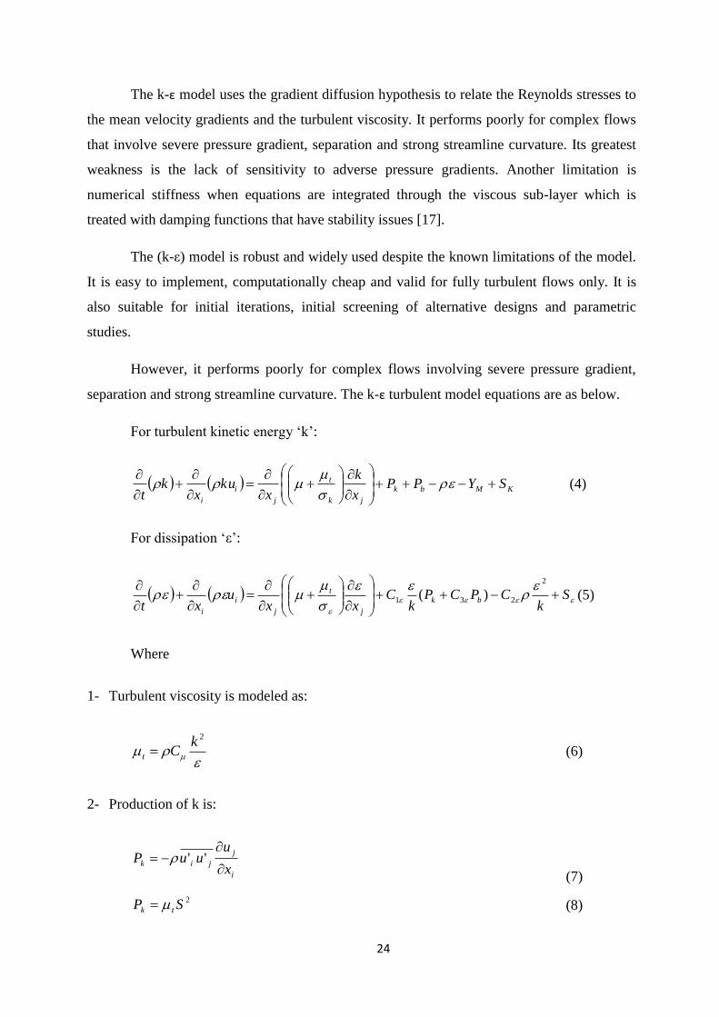
The k-ε model uses the gradient diffusion hypothesis to relate the Reynolds stresses to
the mean velocity gradients and the turbulent viscosity. It performs poorly for complex flows
that involve severe pressure gradient, separation and strong streamline curvature. Its greatest
weakness is the lack of sensitivity to adverse pressure gradients. Another limitation is
numerical stiffness when equations are integrated through the viscous sub-layer which is
treated with damping functions that have stability issues [17].
The (k-ε) model is robust and widely used despite the known limitations of the model.
It is easy to implement, computationally cheap and valid for fully turbulent flows only. It is
also suitable for initial iterations, initial screening of alternative designs and parametric
studies.
However, it performs poorly for complex flows involving severe pressure gradient,
separation and strong streamline curvature. The k-ε turbulent model equations are as below.
For turbulent kinetic energy ‘k’:
KMbk
jk
t
j
i
i
SYPPx
k
xku
xk
t
(4)
For dissipation ‘ε’:
S
kCPCP
kC
xxu
xtbk
j
t
j
i
i
2
231 )( (5)
Where
1- Turbulent viscosity is modeled as:
2k
Ct (6)
2- Production of k is:
i
j
jikx
uuuP
''
(7)
2SP tk (8)
25
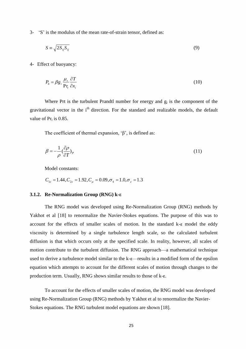
3- ‘S’ is the modulus of the mean rate-of-strain tensor, defined as:
ijijSSS 2 (9)
4- Effect of buoyancy:
it
tib
x
TgP
Pr
(10)
Where Prt is the turbulent Prandtl number for energy and gi is the component of the
gravitational vector in the ith
direction. For the standard and realizable models, the default
value of Prt is 0.85.
The coefficient of thermal expansion, ‘β’, is defined as:
PT
)(1
(11)
Model constants:
3.1,0.1,09.0,92.1,44.1 21 kCCC
3.1.2. Re-Normalization Group (RNG) k-ε
The RNG model was developed using Re-Normalization Group (RNG) methods by
Yakhot et al [18] to renormalize the Navier-Stokes equations. The purpose of this was to
account for the effects of smaller scales of motion. In the standard k-ε model the eddy
viscosity is determined by a single turbulence length scale, so the calculated turbulent
diffusion is that which occurs only at the specified scale. In reality, however, all scales of
motion contribute to the turbulent diffusion. The RNG approach—a mathematical technique
used to derive a turbulence model similar to the k-ε—results in a modified form of the epsilon
equation which attempts to account for the different scales of motion through changes to the
production term. Usually, RNG shows similar results to those of k-ε.
To account for the effects of smaller scales of motion, the RNG model was developed
using Re-Normalization Group (RNG) methods by Yakhot et al to renormalize the Navier-
Stokes equations. The RNG turbulent model equations are shown [18].
26
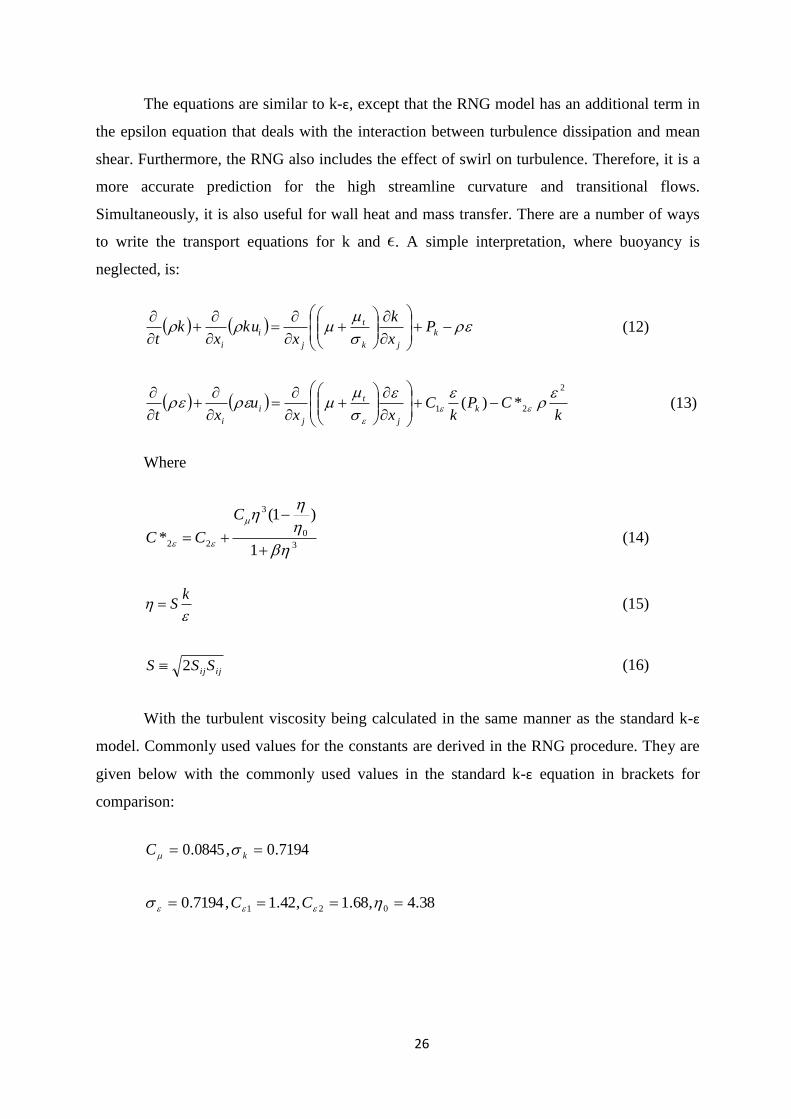
The equations are similar to k-ε, except that the RNG model has an additional term in
the epsilon equation that deals with the interaction between turbulence dissipation and mean
shear. Furthermore, the RNG also includes the effect of swirl on turbulence. Therefore, it is a
more accurate prediction for the high streamline curvature and transitional flows.
Simultaneously, it is also useful for wall heat and mass transfer. There are a number of ways
to write the transport equations for k and . A simple interpretation, where buoyancy is
neglected, is:
k
jk
t
j
i
i
Px
k
xku
xk
t (12)
k
CPk
Cxx
uxt
k
j
t
j
i
i
2
21 *)(
(13)
Where
3
0
3
221
)1(
*
C
CC (14)
kS (15)
ijijSSS 2 (16)
With the turbulent viscosity being calculated in the same manner as the standard k-ε
model. Commonly used values for the constants are derived in the RNG procedure. They are
given below with the commonly used values in the standard k-ε equation in brackets for
comparison:
7194.0,0845.0 kC
38.4,68.1,42.1,7194.0 021 CC
27
3.1.3. Shear Stress Transport (SST)
Shear Stress Transport (SST) is a variant of the standard k–ω model, combining the
original Wilcox k-ε model for use near walls and the standard k–ε model away from walls. It
does so using a blending function. The eddy viscosity formulation is modified to account for
the transport effects of the principle turbulent shear stress. It also bars out compressibility.
It offers similar benefits as the standard k–ω. The SST model accounts for the
transport of turbulent shear stress and gives highly accurate predictions of the onset and the
amount of flow separation under adverse pressure gradients. SST is recommended for high
accuracy boundary layer simulations.
On the other hand, the (SST) model depends on wall distance which makes this less
suitable for free shear flows compared to standard k-ε which requires mesh resolution near the
wall. A Reynolds Stress model may be more appropriate for flows with sudden alterations in
strain rate or rotating flows while the SST model may be more appropriate for separated
flows.
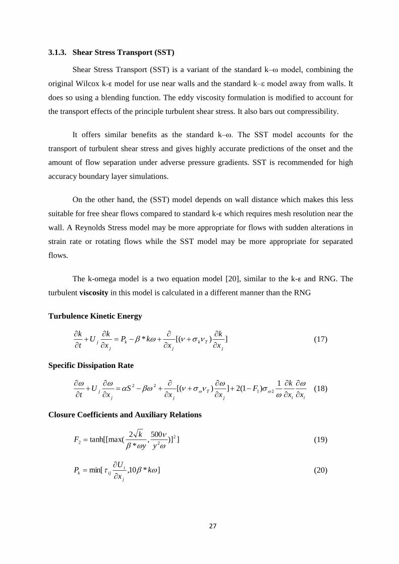
The k-omega model is a two equation model [20], similar to the k-ε and RNG. The
turbulent viscosity in this model is calculated in a different manner than the RNG
Turbulence Kinetic Energy
])[(*j
Tk
j
k
j
jx
k
xkP
x
kU
t
k
(17)
Specific Dissipation Rate
iij
T
jj
jxx
kF
xxS
xU
t
1)1(2])[( 21
22 (18)
Closure Coefficients and Auxiliary Relations
])]500
,*
2tanh[[max(
2
22
yy
kF (19)
]*10,min[ kx
UP
j
iijk
(20)
28
]]]4
),500
,*
max(tanh[[min[4
2
2
21yCD
k
yy
kF
k
(21)
)10,1
2max(10
2
ii
kxx
kCD
(22)
)1( 1211 FF (23)
,1,85.0,100
9*,0828.0,
40
3,44.0,
9
5212121 kk
856.0,5.0 21
3.2. Large Eddy Simulation
Large eddy simulation (LES) is a mathematical model used for t flow in numerical
simulations in fluid dynamics. Initially, it was proposed by Joseph Smagorinsky in 1963 to
simulate the atmospheric air currents. Many of the issues that are unique to LES were first
discovered by Deardorff in 1970. LES grew fast and now, it is applied in a wide variety of
engineering applications such as combustion, acoustics, and simulations of the atmospheric
boundary layer. LES operates on the Navier-Stokes equations and reduces the range of length
scales of the turbulence in the solution, which reduces the computational cost. [22]
The principal operation in large eddy simulation is low-pass filtering, an operation
applied to the Navier-Stokes equations in order to eliminate small scales of the solution. The
result is a decrease in computational cost. The governing equations are transformed resulting
in a filtered velocity field.
Large eddy simulation resolves large scales of the flow field solution, allowing better
dependability than alternative approaches such as Reynolds-averaged Navier-Stokes (RANS)
methods. It also models the smallest scales of the solution, rather than resolving them like
direct numerical simulation (DNS). This makes the computational cost for practical
engineering systems with complex geometry or flow configurations (such as turbulent jets,
pumps, vehicles, and landing gear) attainable using supercomputers. In contrast, direct
numerical simulation, which resolves every scale of the solution, is too expensive for nearly
all systems with complex geometry or flow configurations.
29
Large eddy simulation serves as the solution to the discrete filtered governing
equations, using computational fluid dynamics. Moreover, this requires either high-order
numerical schemes or fine grid resolution (if low-order numerical schemes are used). While
even-order schemes have truncation error, they are non-dissipative. Additionally, as subfilter
scale models are dissipative, even-order schemes will not affect the subfilter scale model
contributions as strongly as dissipative schemes.
3.2.1. Filter Implementation
The filtering operation in LES can be implicit or explicit. Implicit filtering recognizes
that the sub filter scale model dissipates in a similar fashion as many numerical schemes. With
this, the grid or the numerical discretization scheme can be assumed to be the LES low-pass
filter. This takes advantage of the grid resolution and eliminates the computational cost of
calculating a sub filter scale model term. However, it is difficult to determine the shape of the
LES filter that is associated with certain numerical issues. Additionally, truncation error is a
potential issue in this method. In explicit filtering, an LES filter is applied to the discretized
Navier-Stokes equations, providing a well-defined filter shape while reducing the truncation
error. However, explicit filtering requires a finer grid than implicit filtering. Computational
cost also increase with the power of 4.
Other researchers have numerically investigated the flow around passenger trains to
obtain a better understanding of the flow behavior. To do so, Reynolds-Averaged Navier–
Stokes (RANS) equations, time varying RANS (URANS), detached-eddy simulation (DES)
and large-eddy simulation (LES) have been employed.
These have also been employed to investigate the flow around road vehicles subjected
to side winds, as the stability of the vehicles is vital, more so for heavy vehicles due to their
greater height [23]. Furthermore, in the last two decades, significant efforts have been devoted
to understanding the flow behavior around simplified bluff bodies (such as the simplified
Ahmed car model body and cylinders). Although these bodies are simplified, studies revealed
that flows around them are highly unsteady and three-dimensional.
Unfortunately, despite countless, innovative experimentations carried out on unsteady
aerodynamic response caused by ambient turbulence and wind gusts, only a limited
knowledge has been acquired. This is owing to the difficulty of capturing the unsteady
aerodynamic forces and the restricted physical values to be measured. Moreover, additional
30
experimental setups for unsteady aerodynamics analyses are costly and unsuitable for the
industrial development process.
Computational fluid dynamics (CFD) serves as an attractive approach for such
problems as it provides a large amount of transient data and detailed three-dimensional
information about the flow field. This data potentially elucidates the comprehensive
mechanisms of the unsteady aerodynamics of road vehicles.
However, the conventional Reynolds-averaged Navier–Stokes (RANS) simulation is
not suitable for transient analysis, more so in cases where the fluctuating incoming flow
interacts with the vehicles wake turbulence. And even for the simplified vehicle called the
Ahmed car model, the wake flow is completely unsteady and three-dimensional, exhibiting
separation at the roof’s trailing edge and reattachment depending on the vehicle’s rear slant
angle. The recirculation bubbles above the slant deck and their interaction with the wake
vortices produce large elongated trailing vortices, causing a high induced drag. Reproduction
of these complicated unsteady flows is indeed challenging for turbulence simulations, and
only limited success has been achieved so far using RANS approaches.
A promising candidate for this purpose is Large Eddy Simulation (LES), in which
larger eddies are solved directly while smaller and universal eddies are only modeled. Thus,
the physical mechanism of the transient aerodynamic response caused by unsteady three
dimensional eddies can be explained by means of the method. Therefore, the objective of the
present study is to develop a numerical method based on LES and to study the transient
aerodynamic response caused by ambient turbulence and wind gusts.
Recently attempts have been made to apply LES to the Ahmed car flow (e.g.,
Krajnovic´ and Davidson, 2005a,b). Fares (2006) chose to use the lattice Boltzmann method
instead of the spatially filtered Navier–Stokes approach and demonstrated the validity of the
unsteady flow simulation. Minguez et al. (2008) proposed a high order LES based on a multi-
domain spectral Chebyshev–Fourier approach.
In this study, we focused on a real production vehicle as a typical engineering
application. The difficulty of the target lied in the fact that, owing to the complicated
geometry compared with the Ahmed car model, only a limited numerical approach such as a
fully unstructured finite volume/element or voxel mesh could be applied. Thus, the fully
31
unstructured finite volume method was employed in this study. The ambient turbulence was
simplified to a sinusoidal transversal velocity imposed on the main inlet, and, as a result, the
relative yaw angle with respect to the incoming flow changed transiently. Similarly, the
crosswind gust was represented by the simple stepwise transversal velocity imposed on the
main flow.
Flow around tractor trailer and the subsequent drag was crucial in determining the fuel
consumption of the tractor trailer. The reduction of the drag force by 1% had a major impact
in the fuel consumption reduction along the whole driving distance.
RANS has many models that were used such as the k-ε, k-w & SST. These models
determine the drag force applied on the tractor trailer within an error tolerance. RANS are
time averaged equations of motion for fluid flow.
Mathematically, separating the velocity field into a resolved and sub-grid part was
considered to be effective. The resolved part of the field represent the “large” eddies, while
the sub grid part of the velocity represent the "small scales" whose effect on the resolved field
was included through the sub grid-scale model. Therefore, filtering as the convolution of a
function with a filtering kernel ‘G’ would be as follow:
duxGxui )()()( (24)
This yields the following equation:
iii uuu ' (25)
Where ui is the resolvable scale is part and ui is the sub grid-scale part. However, most
practical and commercial implementations of LES use the grid itself as the filter and perform
no explicit filtering.
The filtered equations are developed from the incompressible Navier-Stokes equations
of motion:
)()(1
j
i
jij
i
j
i
x
u
xx
p
x
uu
t
u
(26)
32
Substituting in the decomposition iii uuu ' and iii ppp ' and then filtering the
resulting equation provides the equations of motion for the resolved field as:
)(1
)()(1
j
ij
j
i
jij
ij
i
xx
u
xx
p
x
uu
t
u
(27)
Here, it was assumed that the filtering operation and the differentiation operation
commute, which is not generally the case. The errors associated with this assumption were
believed to be usually small, although filters that commute with differentiation have been
developed. The extra term j
ji
x
, arises from the non-linear advection terms, due to the fact
that:
j
ij
j
ij
x
uu
x
uu
(28)
Hence, the viscous stresses represented by ij can be written as:
jijiij uuuu (29)
Similar equations can be derived for the sub grid-scale field (i.e. the residual field).
Sub grid-scale turbulence models usually employ the Boussinesq hypothesis, and seek
to calculate (the deviatoric part of) the SGS stress using:
ijtijkkij S 23
1 (30)
Where ‘Sij’ is the rate-of-strain tensor for the resolved scale defined by:
)(2
1
i
j
j
iij
x
u
x
uS
(31)
νt is the sub grid-scale turbulent viscosity. Substituting into the filtered Navier-Stokes
equations, we then have:
33
)]([(1
j
i
t
jij
ij
i
x
u
xx
p
x
uu
t
u
(32)
34
Chapter 4: Ground Vehicle Models
4.1. Tractor-Trailer Configurations
While tractor trailers are available in diverse shapes and sizes, they generally consume
a huge amount of fuel due to their high distance travels throughout the year.
Different sizes and dimensions are available in the market for the tractor-trailers.
Standard dimensions for the trailer are shown in Table 1.
Table 1: Market dimensions of trailers.
Overall Dimensions
Length Width Height
45' 96" 13' 6"
48' 102" 13' 6"
53' 102" 13' 6"
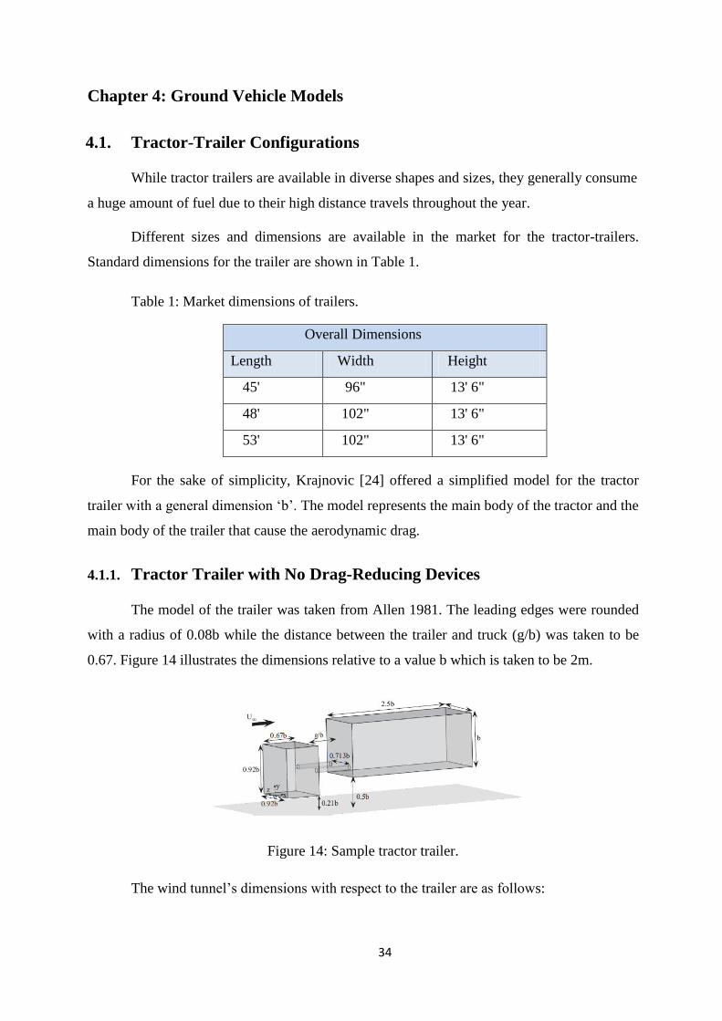
For the sake of simplicity, Krajnovic [24] offered a simplified model for the tractor
trailer with a general dimension ‘b’. The model represents the main body of the tractor and the
main body of the trailer that cause the aerodynamic drag.
4.1.1. Tractor Trailer with No Drag-Reducing Devices
The model of the trailer was taken from Allen 1981. The leading edges were rounded
with a radius of 0.08b while the distance between the trailer and truck (g/b) was taken to be
0.67. Figure 14 illustrates the dimensions relative to a value b which is taken to be 2m.
Figure 14: Sample tractor trailer.
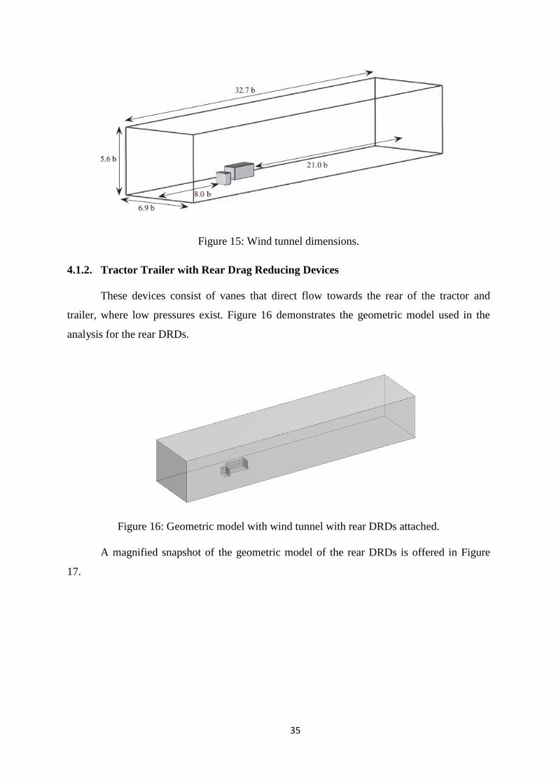
The wind tunnel’s dimensions with respect to the trailer are as follows:
35
Figure 15: Wind tunnel dimensions.
4.1.2. Tractor Trailer with Rear Drag Reducing Devices
These devices consist of vanes that direct flow towards the rear of the tractor and
trailer, where low pressures exist. Figure 16 demonstrates the geometric model used in the
analysis for the rear DRDs.
Figure 16: Geometric model with wind tunnel with rear DRDs attached.
A magnified snapshot of the geometric model of the rear DRDs is offered in Figure
17.
36
Figure 17: A magnified snapshot with rear DRDs on tractor trailer.
The rear directing wings were designed such that the leading angle is at 0 degrees and
they curve at 26 degrees to the horizontal.
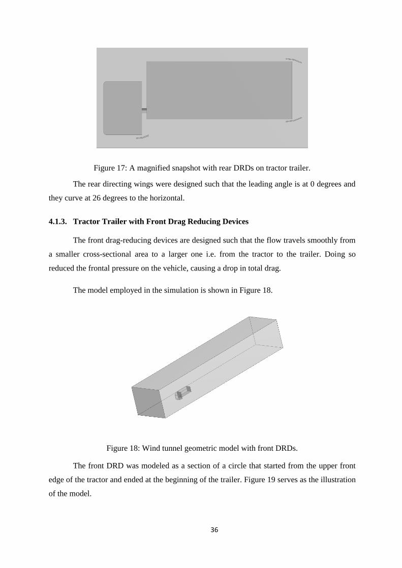
4.1.3. Tractor Trailer with Front Drag Reducing Devices
The front drag-reducing devices are designed such that the flow travels smoothly from
a smaller cross-sectional area to a larger one i.e. from the tractor to the trailer. Doing so
reduced the frontal pressure on the vehicle, causing a drop in total drag.
The model employed in the simulation is shown in Figure 18.
Figure 18: Wind tunnel geometric model with front DRDs.
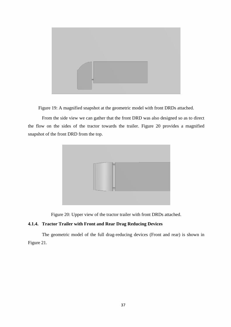
The front DRD was modeled as a section of a circle that started from the upper front
edge of the tractor and ended at the beginning of the trailer. Figure 19 serves as the illustration
of the model.
37
Figure 19: A magnified snapshot at the geometric model with front DRDs attached.
From the side view we can gather that the front DRD was also designed so as to direct
the flow on the sides of the tractor towards the trailer. Figure 20 provides a magnified
snapshot of the front DRD from the top.
Figure 20: Upper view of the tractor trailer with front DRDs attached.
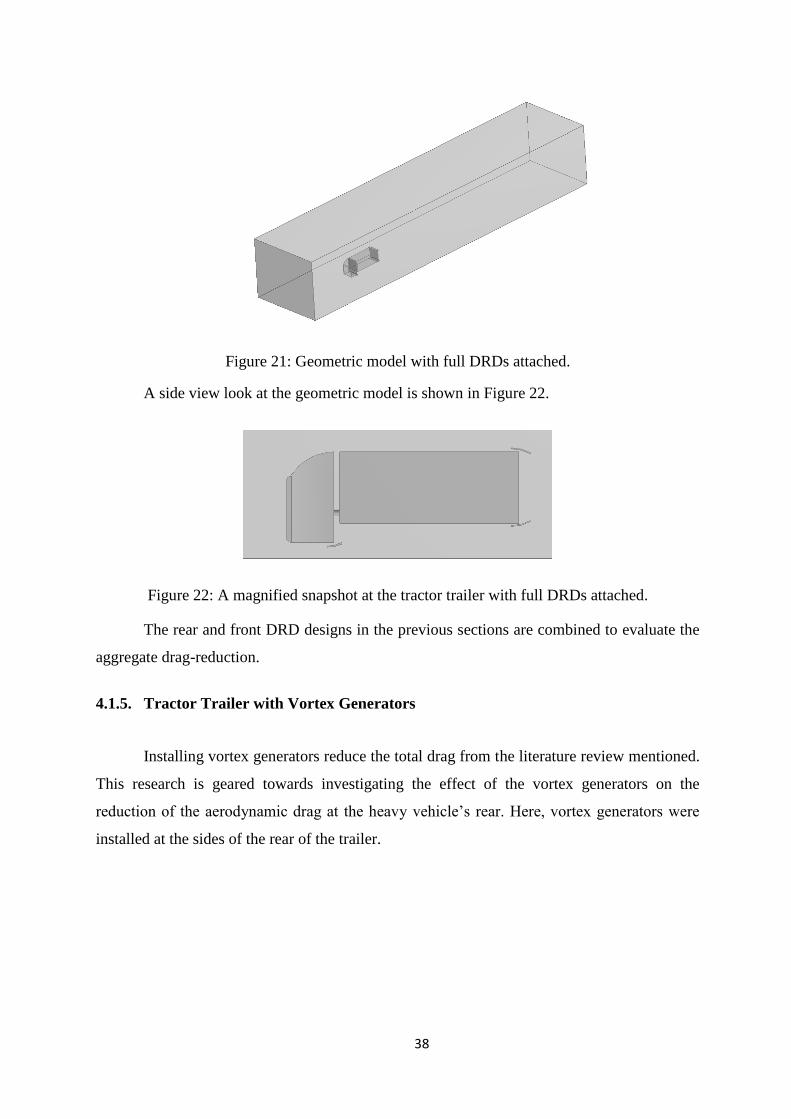
4.1.4. Tractor Trailer with Front and Rear Drag Reducing Devices
The geometric model of the full drag-reducing devices (Front and rear) is shown in
Figure 21.
38
Figure 21: Geometric model with full DRDs attached.
A side view look at the geometric model is shown in Figure 22.
Figure 22: A magnified snapshot at the tractor trailer with full DRDs attached.
The rear and front DRD designs in the previous sections are combined to evaluate the
aggregate drag-reduction.
4.1.5. Tractor Trailer with Vortex Generators
Installing vortex generators reduce the total drag from the literature review mentioned.
This research is geared towards investigating the effect of the vortex generators on the
reduction of the aerodynamic drag at the heavy vehicle’s rear. Here, vortex generators were
installed at the sides of the rear of the trailer.
39
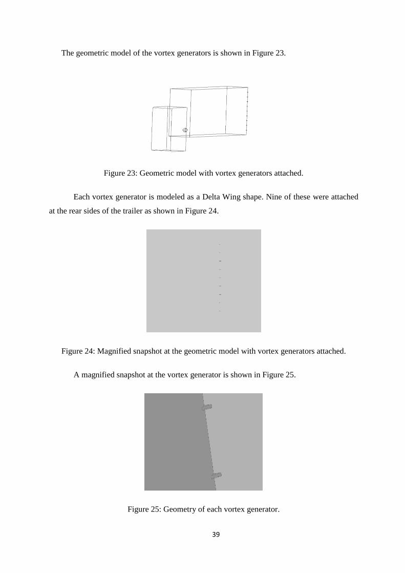
The geometric model of the vortex generators is shown in Figure 23.
Figure 23: Geometric model with vortex generators attached.
Each vortex generator is modeled as a Delta Wing shape. Nine of these were attached
at the rear sides of the trailer as shown in Figure 24.
Figure 24: Magnified snapshot at the geometric model with vortex generators attached.
A magnified snapshot at the vortex generator is shown in Figure 25.
Figure 25: Geometry of each vortex generator.
40
Vortex generators, shown in the literature review, possess the ability to control the
flow separation on the vehicle. Their peak efficiency is when the flow is partially separated.
This way the vortex generators direct the flow to reduce the impact of turbulence on the rear
of the vehicle. In cases where the separation of the air flow is sudden and not partial, the
effectiveness of the vortex generators is compromised.
4.2. Sports Utility Vehicle Configurations
The sports utility vehicle (SUV) is represented by a Hummer vehicle in this research.
The geometric model is first built with a CAD program by Bachelors students at the American
University of Sharjah during their senior year.
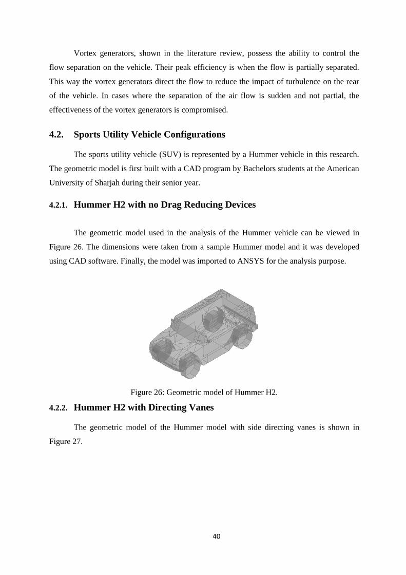
4.2.1. Hummer H2 with no Drag Reducing Devices
The geometric model used in the analysis of the Hummer vehicle can be viewed in
Figure 26. The dimensions were taken from a sample Hummer model and it was developed
using CAD software. Finally, the model was imported to ANSYS for the analysis purpose.
Figure 26: Geometric model of Hummer H2.
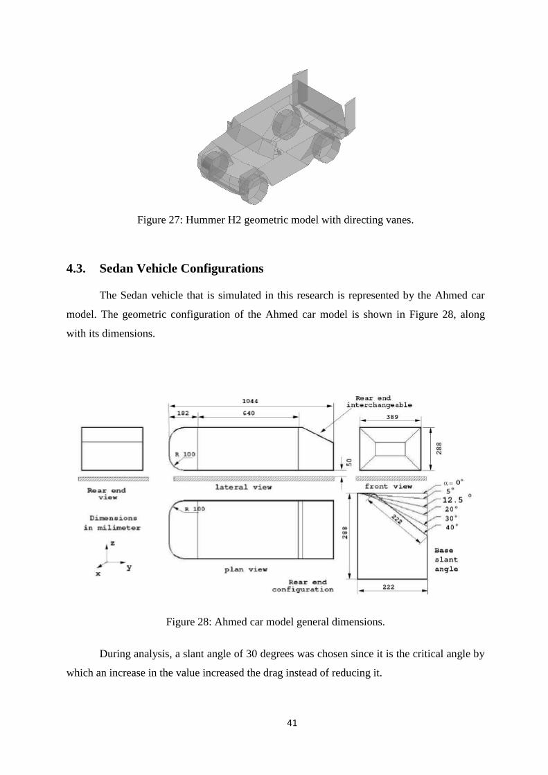
4.2.2. Hummer H2 with Directing Vanes
The geometric model of the Hummer model with side directing vanes is shown in
Figure 27.
41
Figure 27: Hummer H2 geometric model with directing vanes.
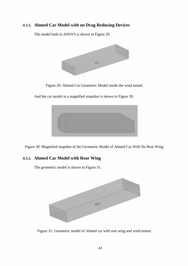
4.3. Sedan Vehicle Configurations
The Sedan vehicle that is simulated in this research is represented by the Ahmed car
model. The geometric configuration of the Ahmed car model is shown in Figure 28, along
with its dimensions.
Figure 28: Ahmed car model general dimensions.
During analysis, a slant angle of 30 degrees was chosen since it is the critical angle by
which an increase in the value increased the drag instead of reducing it.
42
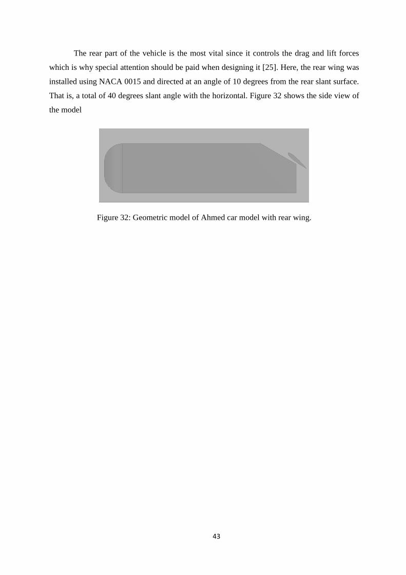
4.3.1. Ahmed Car Model with no Drag Reducing Devices
The model built in ANSYS is shown in Figure 29.
Figure 29: Ahmed Car Geometric Model inside the wind tunnel.
And the car model at a magnified snapshot is shown in Figure 30.
Figure 30: Magnified snapshot of the Geometric Model of Ahmed Car With No Rear Wing.
4.3.2. Ahmed Car Model with Rear Wing
The geometric model is shown in Figure 31.
Figure 31: Geometric model of Ahmed car with rear wing and wind tunnel.
43
The rear part of the vehicle is the most vital since it controls the drag and lift forces
which is why special attention should be paid when designing it [25]. Here, the rear wing was
installed using NACA 0015 and directed at an angle of 10 degrees from the rear slant surface.
That is, a total of 40 degrees slant angle with the horizontal. Figure 32 shows the side view of
the model
Figure 32: Geometric model of Ahmed car model with rear wing.
44
Chapter 5: Grid Generation
Discretization of all the geometric models was done using the tetrahedral meshing
elements that are easy to fit in small corners and are efficient enough to give accurate results.
The meshing grids were divided into coarse, medium and fine meshing grids. The coarse
meshing grid consisted of 1,300,000 elements; whereas the medium meshing grid consisted of
1,600,000 meshing elements, and the fine meshing grid consisted of 1,800,000 meshing
elements. The optimum number of meshing elements that can be achieved during the
numerical analysis and using the available ANSYS license is 2,000,000 meshing elements.
5.1. Tractor-Trailer Grid Generation
5.1.1. Tractor Trailer Grid Generation with Rear Drag Reducing Devices
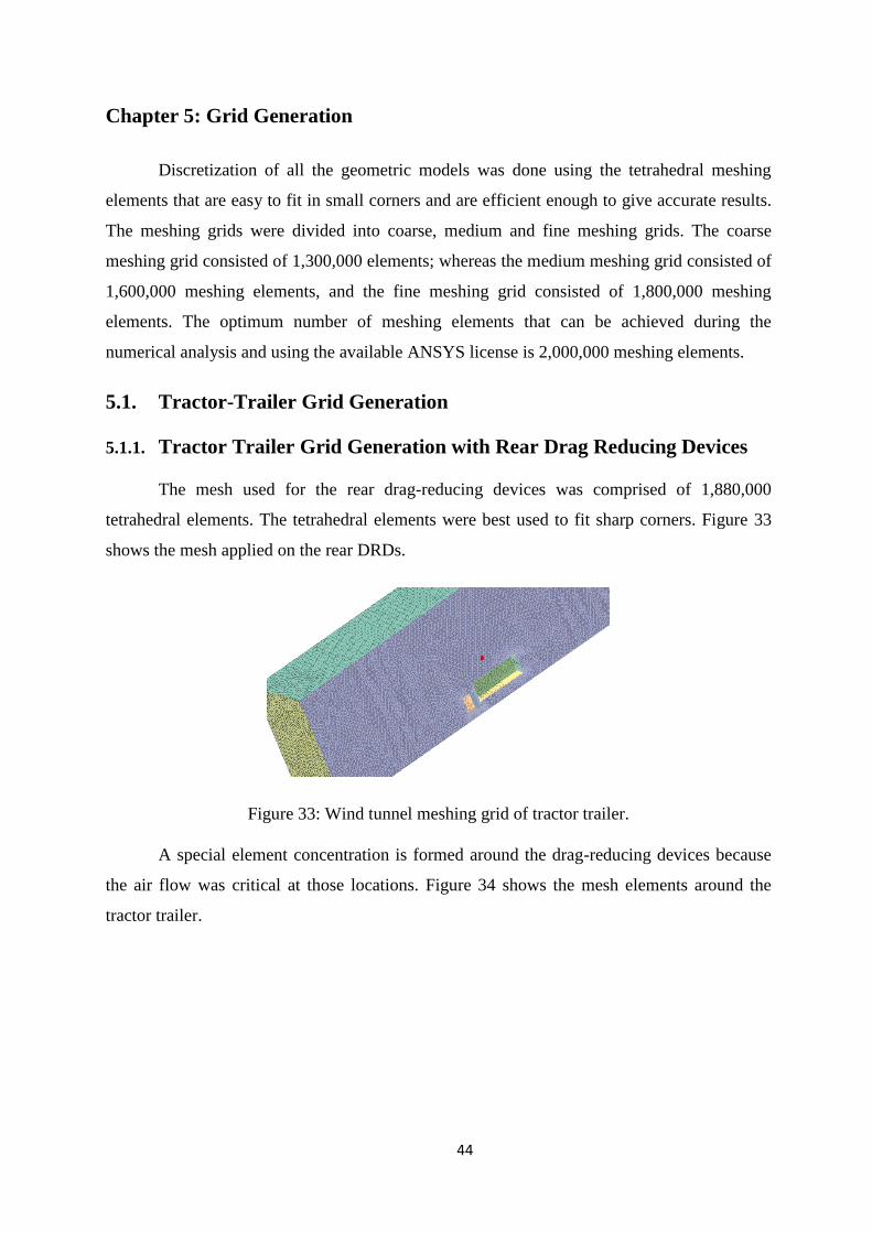
The mesh used for the rear drag-reducing devices was comprised of 1,880,000
tetrahedral elements. The tetrahedral elements were best used to fit sharp corners. Figure 33
shows the mesh applied on the rear DRDs.
Figure 33: Wind tunnel meshing grid of tractor trailer.
A special element concentration is formed around the drag-reducing devices because
the air flow was critical at those locations. Figure 34 shows the mesh elements around the
tractor trailer.
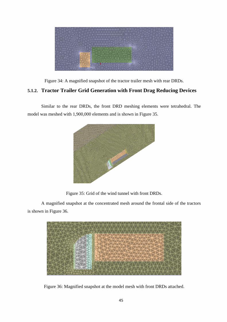
45
Figure 34: A magnified snapshot of the tractor trailer mesh with rear DRDs.
5.1.2. Tractor Trailer Grid Generation with Front Drag Reducing Devices
Similar to the rear DRDs, the front DRD meshing elements were tetrahedral. The
model was meshed with 1,900,000 elements and is shown in Figure 35.
Figure 35: Grid of the wind tunnel with front DRDs.
A magnified snapshot at the concentrated mesh around the frontal side of the tractors
is shown in Figure 36.
Figure 36: Magnified snapshot at the model mesh with front DRDs attached.
46
5.1.3. Tractor Trailer Grid Generation with Front and Rear Drag Reducing
Devices
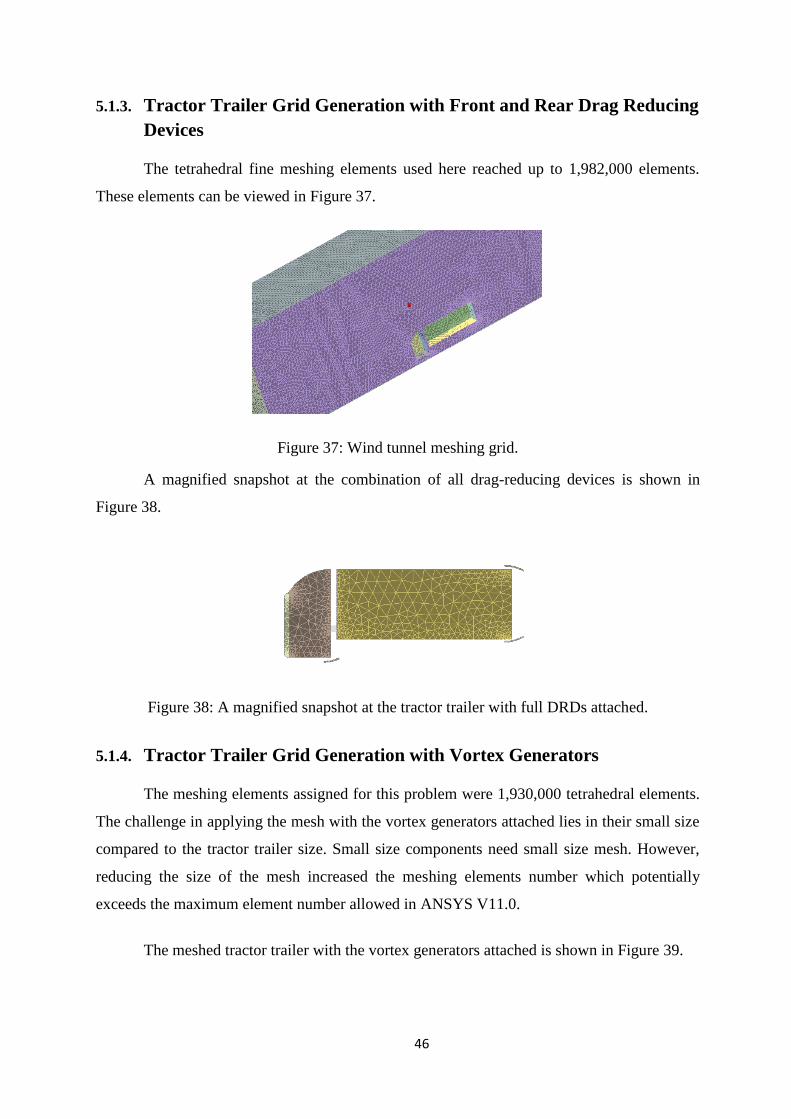
The tetrahedral fine meshing elements used here reached up to 1,982,000 elements.
These elements can be viewed in Figure 37.
Figure 37: Wind tunnel meshing grid.
A magnified snapshot at the combination of all drag-reducing devices is shown in
Figure 38.
Figure 38: A magnified snapshot at the tractor trailer with full DRDs attached.
5.1.4. Tractor Trailer Grid Generation with Vortex Generators
The meshing elements assigned for this problem were 1,930,000 tetrahedral elements.
The challenge in applying the mesh with the vortex generators attached lies in their small size
compared to the tractor trailer size. Small size components need small size mesh. However,
reducing the size of the mesh increased the meshing elements number which potentially
exceeds the maximum element number allowed in ANSYS V11.0.
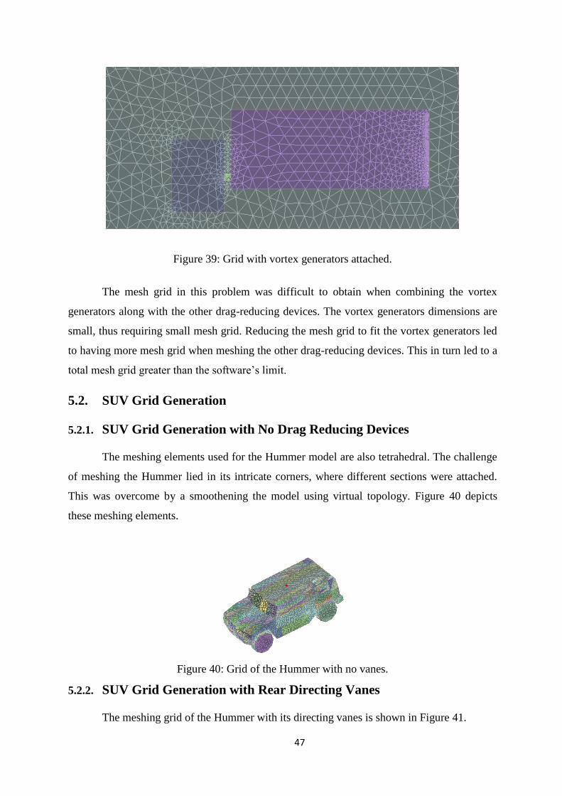
The meshed tractor trailer with the vortex generators attached is shown in Figure 39.
47
Figure 39: Grid with vortex generators attached.
The mesh grid in this problem was difficult to obtain when combining the vortex
generators along with the other drag-reducing devices. The vortex generators dimensions are
small, thus requiring small mesh grid. Reducing the mesh grid to fit the vortex generators led
to having more mesh grid when meshing the other drag-reducing devices. This in turn led to a
total mesh grid greater than the software’s limit.
5.2. SUV Grid Generation
5.2.1. SUV Grid Generation with No Drag Reducing Devices
The meshing elements used for the Hummer model are also tetrahedral. The challenge
of meshing the Hummer lied in its intricate corners, where different sections were attached.
This was overcome by a smoothening the model using virtual topology. Figure 40 depicts
these meshing elements.
Figure 40: Grid of the Hummer with no vanes.
5.2.2. SUV Grid Generation with Rear Directing Vanes
The meshing grid of the Hummer with its directing vanes is shown in Figure 41.
48
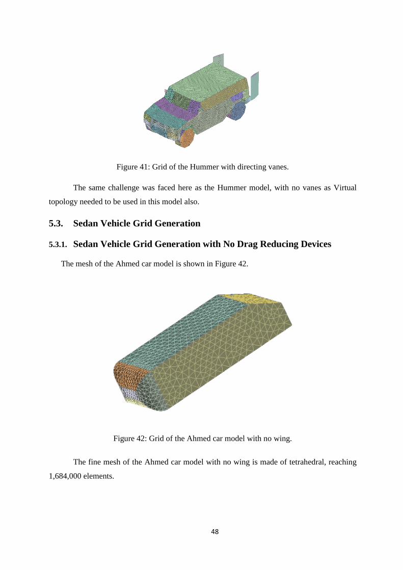
Figure 41: Grid of the Hummer with directing vanes.
The same challenge was faced here as the Hummer model, with no vanes as Virtual
topology needed to be used in this model also.
5.3. Sedan Vehicle Grid Generation
5.3.1. Sedan Vehicle Grid Generation with No Drag Reducing Devices
The mesh of the Ahmed car model is shown in Figure 42.
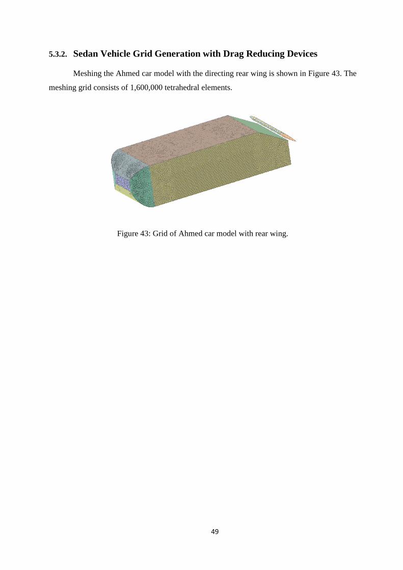
Figure 42: Grid of the Ahmed car model with no wing.
The fine mesh of the Ahmed car model with no wing is made of tetrahedral, reaching
1,684,000 elements.
49
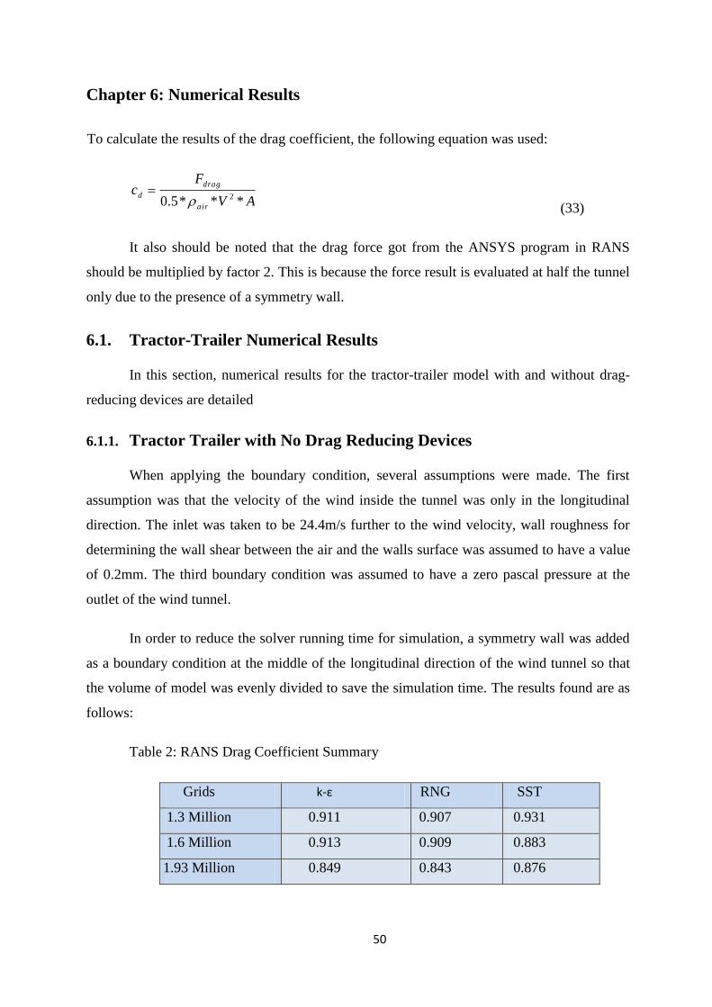
5.3.2. Sedan Vehicle Grid Generation with Drag Reducing Devices
Meshing the Ahmed car model with the directing rear wing is shown in Figure 43. The
meshing grid consists of 1,600,000 tetrahedral elements.
Figure 43: Grid of Ahmed car model with rear wing.
50
Chapter 6: Numerical Results
To calculate the results of the drag coefficient, the following equation was used:
AV
Fc
air
drag
d***5.0
2
(33)
It also should be noted that the drag force got from the ANSYS program in RANS
should be multiplied by factor 2. This is because the force result is evaluated at half the tunnel
only due to the presence of a symmetry wall.
6.1. Tractor-Trailer Numerical Results
In this section, numerical results for the tractor-trailer model with and without drag-
reducing devices are detailed
6.1.1. Tractor Trailer with No Drag Reducing Devices
When applying the boundary condition, several assumptions were made. The first
assumption was that the velocity of the wind inside the tunnel was only in the longitudinal
direction. The inlet was taken to be 24.4m/s further to the wind velocity, wall roughness for
determining the wall shear between the air and the walls surface was assumed to have a value
of 0.2mm. The third boundary condition was assumed to have a zero pascal pressure at the
outlet of the wind tunnel.
In order to reduce the solver running time for simulation, a symmetry wall was added
as a boundary condition at the middle of the longitudinal direction of the wind tunnel so that
the volume of model was evenly divided to save the simulation time. The results found are as
follows:
Table 2: RANS Drag Coefficient Summary
Grids k-ε RNG SST
1.3 Million 0.911 0.907 0.931
1.6 Million 0.913 0.909 0.883
1.93 Million 0.849 0.843 0.876
51
The velocity contours play a major role in determining where the drag-reducing
devices should be added. Those devices will all be added to reduce the eddies found along the
velocity contours (where the disruption of velocity appears clearly at the back of the truck and
trailer). Also, a sudden change in velocity is shown before the trailer. Therefore, drag-
reducing devices should be added here and studied. Finally, the distance between the trailer
and tractor causes drag where air flow is disturbed. This location too requires drag reduction.
Two runs were performed using Large Eddy Simulations, a coarse mesh analysis and a
fine mesh analysis. The coarse mesh analysis consisted of a mesh grid with 140,000 meshing
elements. The average drag force calculated from the coarse mesh was 1180N and hence the
drag coefficient from that force was found to be 0.83. The courant number (CFL) which
represents how fast the calculation of the LES is, was very low and reached a value of 0.01.
The main reason for this was the time chosen for each element calculation in the LES being
0.0001s. Increasing the average time per calculation from 0.0001s to 0.001s increased the
CFL number to 0.11, which was more acceptable. In finite element analysis, CFL number
should be less than 1 to give accurate LES results. Otherwise, the LES simulation will
diverge.
The fine mesh used for the LES analysis consisted of 1.7 Million meshing elements
and it resulted in a drag force equals 1166N. This drag force showed a drag coefficient of
0.816. A summary of the LES results is shown in table 3.
Table 3: LES drag results.
Mesh # LES
0.140 Million 0.83
1.7 Million 0.81
52
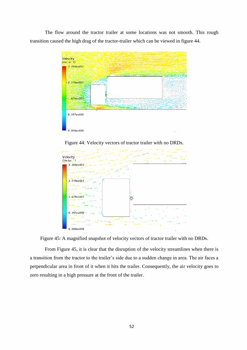
The flow around the tractor trailer at some locations was not smooth. This rough
transition caused the high drag of the tractor-trailer which can be viewed in figure 44.
Figure 44: Velocity vectors of tractor trailer with no DRDs.
Figure 45: A magnified snapshot of velocity vectors of tractor trailer with no DRDs.
From Figure 45, it is clear that the disruption of the velocity streamlines when there is
a transition from the tractor to the trailer’s side due to a sudden change in area. The air faces a
perpendicular area in front of it when it hits the trailer. Consequently, the air velocity goes to
zero resulting in a high pressure at the front of the trailer.
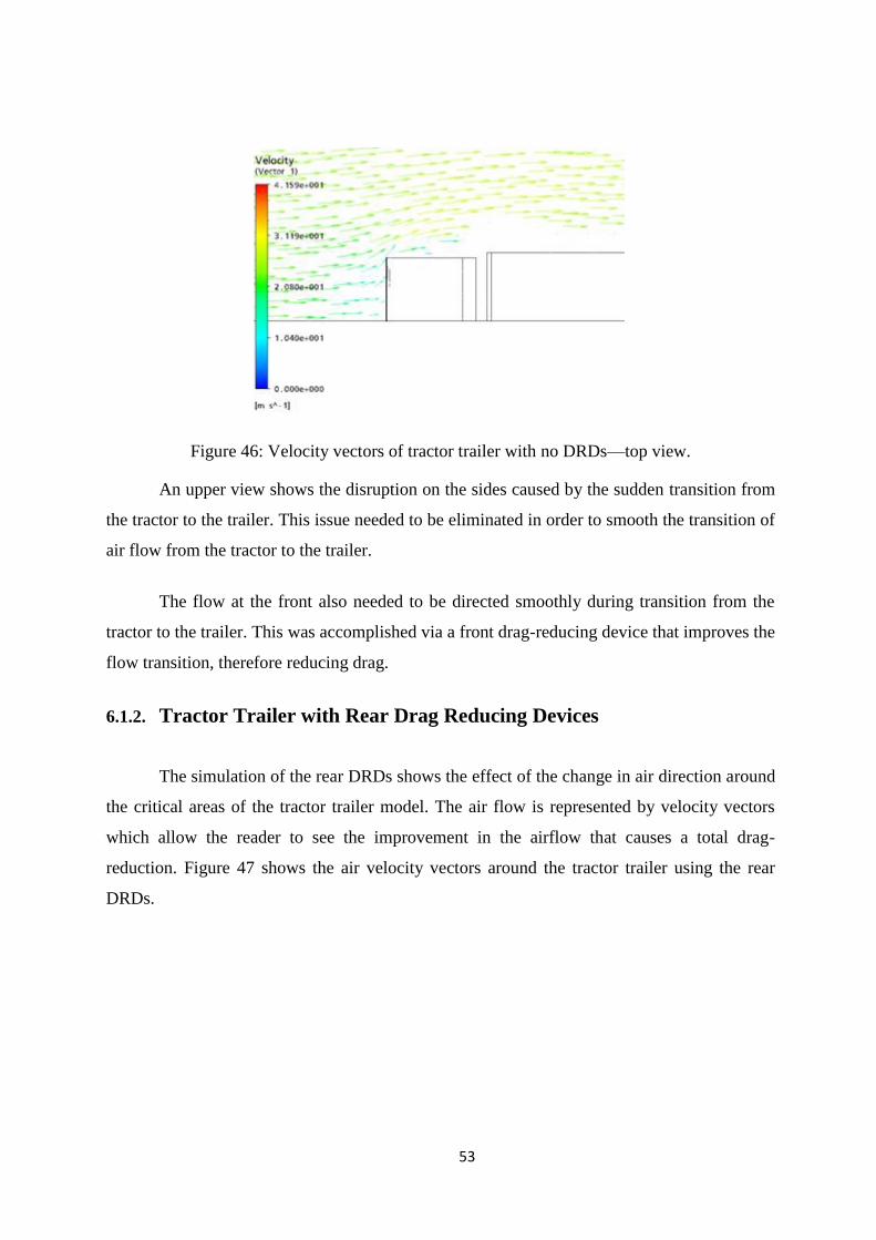
53
Figure 46: Velocity vectors of tractor trailer with no DRDs—top view.
An upper view shows the disruption on the sides caused by the sudden transition from
the tractor to the trailer. This issue needed to be eliminated in order to smooth the transition of
air flow from the tractor to the trailer.
The flow at the front also needed to be directed smoothly during transition from the
tractor to the trailer. This was accomplished via a front drag-reducing device that improves the
flow transition, therefore reducing drag.
6.1.2. Tractor Trailer with Rear Drag Reducing Devices
The simulation of the rear DRDs shows the effect of the change in air direction around
the critical areas of the tractor trailer model. The air flow is represented by velocity vectors
which allow the reader to see the improvement in the airflow that causes a total drag-
reduction. Figure 47 shows the air velocity vectors around the tractor trailer using the rear
DRDs.
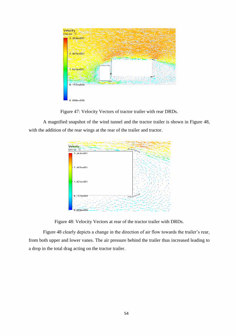
54
Figure 47: Velocity Vectors of tractor trailer with rear DRDs.
A magnified snapshot of the wind tunnel and the tractor trailer is shown in Figure 48,
with the addition of the rear wings at the rear of the trailer and tractor.
Figure 48: Velocity Vectors at rear of the tractor trailer with DRDs.
Figure 48 clearly depicts a change in the direction of air flow towards the trailer’s rear,
from both upper and lower vanes. The air pressure behind the trailer thus increased leading to
a drop in the total drag acting on the tractor trailer.
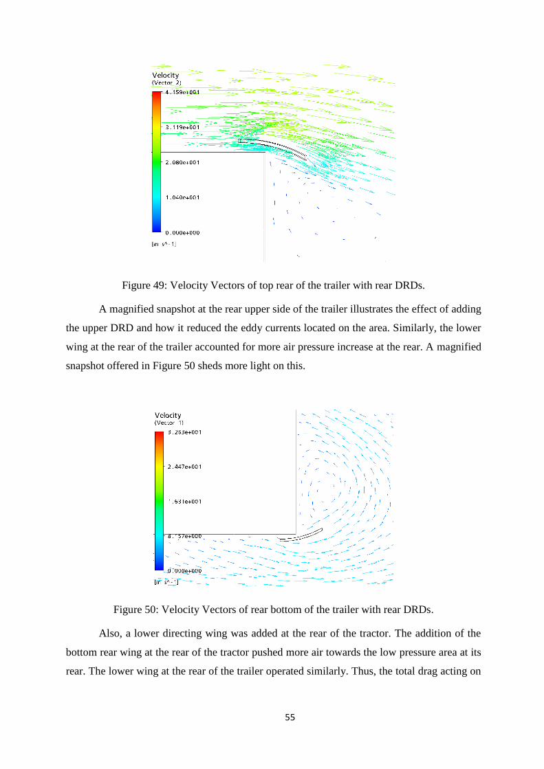
55
Figure 49: Velocity Vectors of top rear of the trailer with rear DRDs.
A magnified snapshot at the rear upper side of the trailer illustrates the effect of adding
the upper DRD and how it reduced the eddy currents located on the area. Similarly, the lower
wing at the rear of the trailer accounted for more air pressure increase at the rear. A magnified
snapshot offered in Figure 50 sheds more light on this.
Figure 50: Velocity Vectors of rear bottom of the trailer with rear DRDs.
Also, a lower directing wing was added at the rear of the tractor. The addition of the
bottom rear wing at the rear of the tractor pushed more air towards the low pressure area at its
rear. The lower wing at the rear of the trailer operated similarly. Thus, the total drag acting on
56
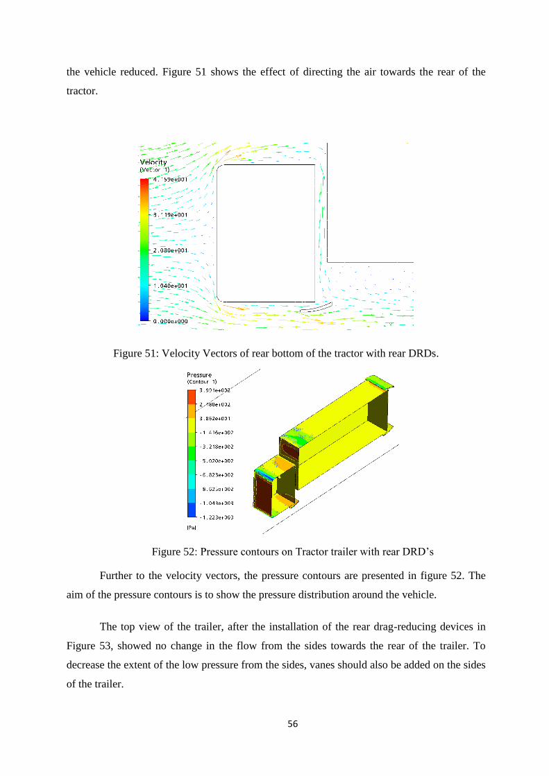
the vehicle reduced. Figure 51 shows the effect of directing the air towards the rear of the
tractor.
Figure 51: Velocity Vectors of rear bottom of the tractor with rear DRDs.
Figure 52: Pressure contours on Tractor trailer with rear DRD’s
Further to the velocity vectors, the pressure contours are presented in figure 52. The
aim of the pressure contours is to show the pressure distribution around the vehicle.
The top view of the trailer, after the installation of the rear drag-reducing devices in
Figure 53, showed no change in the flow from the sides towards the rear of the trailer. To
decrease the extent of the low pressure from the sides, vanes should also be added on the sides
of the trailer.
57
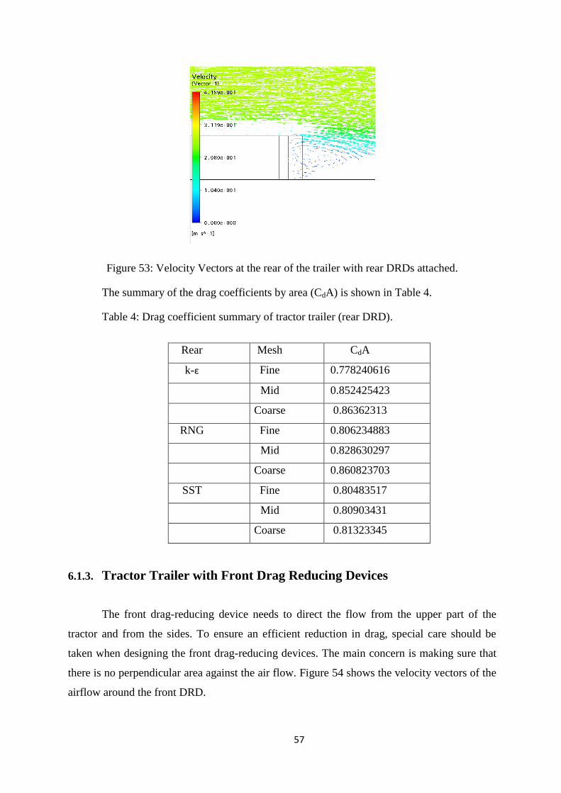
Figure 53: Velocity Vectors at the rear of the trailer with rear DRDs attached.
The summary of the drag coefficients by area (CdA) is shown in Table 4.
Table 4: Drag coefficient summary of tractor trailer (rear DRD).
Rear Mesh CdA
k-ε Fine 0.778240616
Mid 0.852425423
Coarse 0.86362313
RNG Fine 0.806234883
Mid 0.828630297
Coarse 0.860823703
SST Fine 0.80483517
Mid 0.80903431
Coarse 0.81323345
6.1.3. Tractor Trailer with Front Drag Reducing Devices
The front drag-reducing device needs to direct the flow from the upper part of the
tractor and from the sides. To ensure an efficient reduction in drag, special care should be
taken when designing the front drag-reducing devices. The main concern is making sure that
there is no perpendicular area against the air flow. Figure 54 shows the velocity vectors of the
airflow around the front DRD.
58
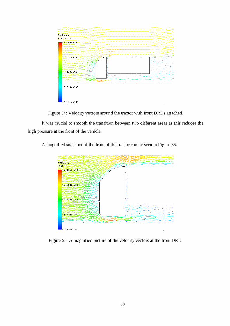
Figure 54: Velocity vectors around the tractor with front DRDs attached.
It was crucial to smooth the transition between two different areas as this reduces the
high pressure at the front of the vehicle.
A magnified snapshot of the front of the tractor can be seen in Figure 55.
Figure 55: A magnified picture of the velocity vectors at the front DRD.
59
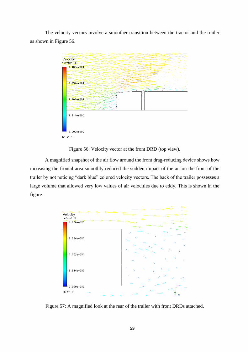
The velocity vectors involve a smoother transition between the tractor and the trailer
as shown in Figure 56.
Figure 56: Velocity vector at the front DRD (top view).
A magnified snapshot of the air flow around the front drag-reducing device shows how
increasing the frontal area smoothly reduced the sudden impact of the air on the front of the
trailer by not noticing “dark blue” colored velocity vectors. The back of the trailer possesses a
large volume that allowed very low values of air velocities due to eddy. This is shown in the
figure.
Figure 57: A magnified look at the rear of the trailer with front DRDs attached.
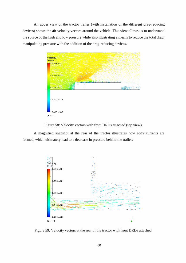
60
An upper view of the tractor trailer (with installation of the different drag-reducing
devices) shows the air velocity vectors around the vehicle. This view allows us to understand
the source of the high and low pressure while also illustrating a means to reduce the total drag:
manipulating pressure with the addition of the drag-reducing devices.
Figure 58: Velocity vectors with front DRDs attached (top view).
A magnified snapshot at the rear of the tractor illustrates how eddy currents are
formed, which ultimately lead to a decrease in pressure behind the trailer.
Figure 59: Velocity vectors at the rear of the tractor with front DRDs attached.
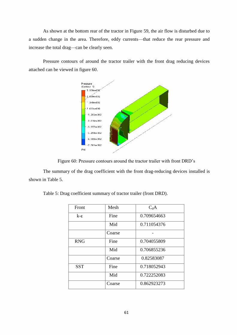
61
As shown at the bottom rear of the tractor in Figure 59, the air flow is disturbed due to
a sudden change in the area. Therefore, eddy currents—that reduce the rear pressure and
increase the total drag—can be clearly seen.
Pressure contours of around the tractor trailer with the front drag reducing devices
attached can be viewed in figure 60.
Figure 60: Pressure contours around the tractor trailer with front DRD’s
The summary of the drag coefficient with the front drag-reducing devices installed is
shown in Table 5.
Table 5: Drag coefficient summary of tractor trailer (front DRD).
Front Mesh CdA
k-ε Fine 0.709654663
Mid 0.711054376
Coarse -
RNG Fine 0.704055809
Mid 0.706855236
Coarse 0.82583087
SST Fine 0.718052943
Mid 0.722252083
Coarse 0.862923273
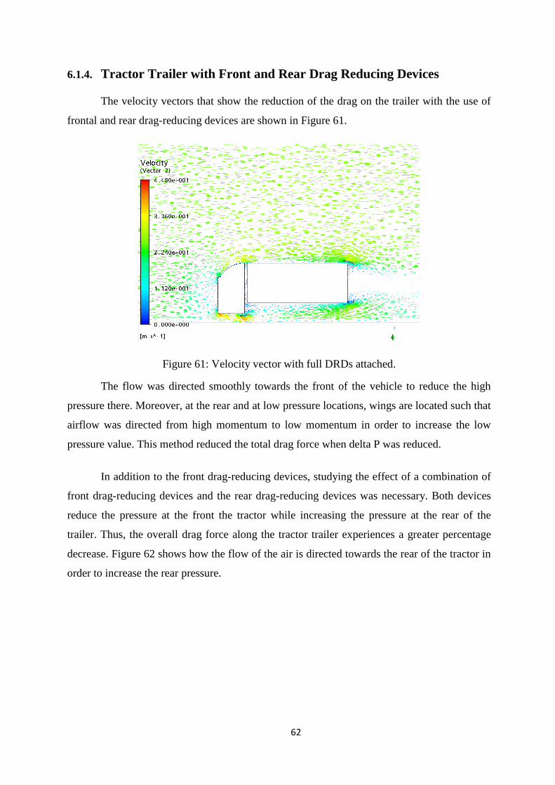
62
6.1.4. Tractor Trailer with Front and Rear Drag Reducing Devices
The velocity vectors that show the reduction of the drag on the trailer with the use of
frontal and rear drag-reducing devices are shown in Figure 61.
Figure 61: Velocity vector with full DRDs attached.
The flow was directed smoothly towards the front of the vehicle to reduce the high
pressure there. Moreover, at the rear and at low pressure locations, wings are located such that
airflow was directed from high momentum to low momentum in order to increase the low
pressure value. This method reduced the total drag force when delta P was reduced.
In addition to the front drag-reducing devices, studying the effect of a combination of
front drag-reducing devices and the rear drag-reducing devices was necessary. Both devices
reduce the pressure at the front the tractor while increasing the pressure at the rear of the
trailer. Thus, the overall drag force along the tractor trailer experiences a greater percentage
decrease. Figure 62 shows how the flow of the air is directed towards the rear of the tractor in
order to increase the rear pressure.
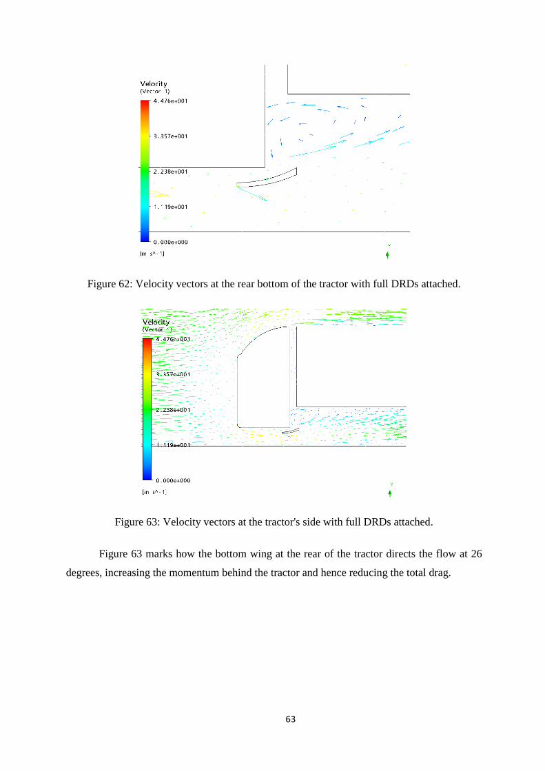
63
Figure 62: Velocity vectors at the rear bottom of the tractor with full DRDs attached.
Figure 63: Velocity vectors at the tractor's side with full DRDs attached.
Figure 63 marks how the bottom wing at the rear of the tractor directs the flow at 26
degrees, increasing the momentum behind the tractor and hence reducing the total drag.
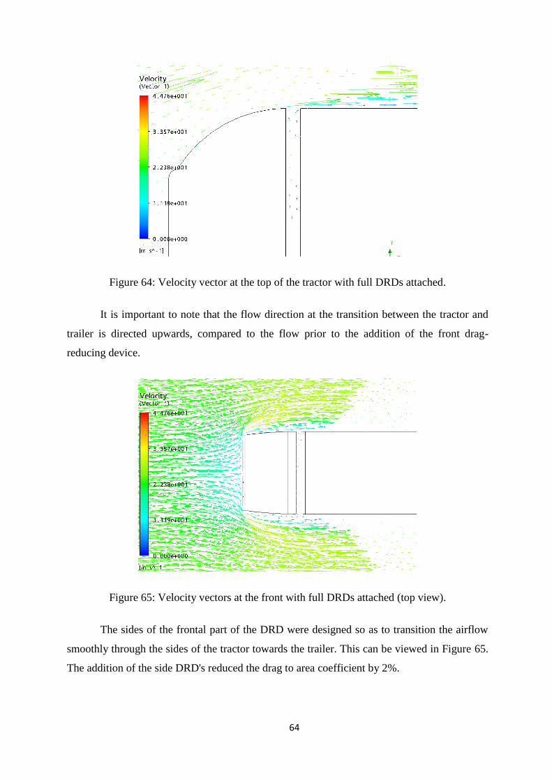
64
Figure 64: Velocity vector at the top of the tractor with full DRDs attached.
It is important to note that the flow direction at the transition between the tractor and
trailer is directed upwards, compared to the flow prior to the addition of the front drag-
reducing device.
Figure 65: Velocity vectors at the front with full DRDs attached (top view).
The sides of the frontal part of the DRD were designed so as to transition the airflow
smoothly through the sides of the tractor towards the trailer. This can be viewed in Figure 65.
The addition of the side DRD's reduced the drag to area coefficient by 2%.
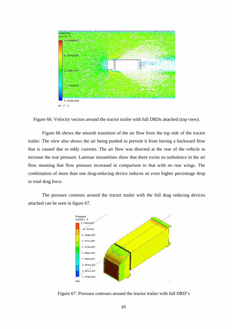
65
Figure 66: Velocity vectors around the tractor trailer with full DRDs attached (top view).
Figure 66 shows the smooth transition of the air flow from the top side of the tractor
trailer. The view also shows the air being pushed to prevent it from having a backward flow
that is caused due to eddy currents. The air flow was directed at the rear of the vehicle to
increase the rear pressure. Laminar streamlines show that there exists no turbulence in the air
flow meaning that flow pressure increased in comparison to that with no rear wings. The
combination of more than one drag-reducing device induces an even higher percentage drop
in total drag force.
The pressure contours around the tractor trailer with the full drag reducing devices
attached can be seen in figure 67.
Figure 67: Pressure contours around the tractor trailer with full DRD’s
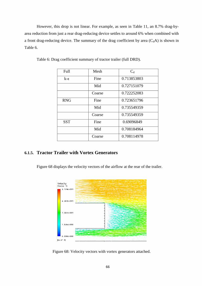
66
However, this drop is not linear. For example, as seen in Table 11, an 8.7% drag-by-
area reduction from just a rear drag-reducing device settles to around 6% when combined with
a front drag-reducing device. The summary of the drag coefficient by area (CdA) is shown in
Table 6.
Table 6: Drag coefficient summary of tractor trailer (full DRD).
Full Mesh Cd
k-ε Fine 0.713853803
Mid 0.727151079
Coarse 0.722252083
RNG Fine 0.723651796
Mid 0.735549359
Coarse 0.735549359
SST Fine 0.69096849
Mid 0.708184964
Coarse 0.708114978
6.1.5. Tractor Trailer with Vortex Generators
Figure 68 displays the velocity vectors of the airflow at the rear of the trailer.
Figure 68: Velocity vectors with vortex generators attached.
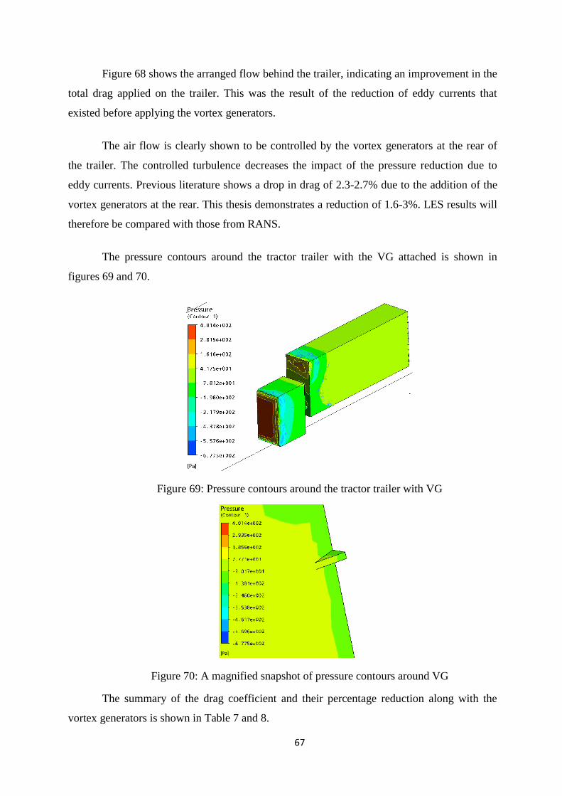
67
Figure 68 shows the arranged flow behind the trailer, indicating an improvement in the
total drag applied on the trailer. This was the result of the reduction of eddy currents that
existed before applying the vortex generators.
The air flow is clearly shown to be controlled by the vortex generators at the rear of
the trailer. The controlled turbulence decreases the impact of the pressure reduction due to
eddy currents. Previous literature shows a drop in drag of 2.3-2.7% due to the addition of the
vortex generators at the rear. This thesis demonstrates a reduction of 1.6-3%. LES results will
therefore be compared with those from RANS.
The pressure contours around the tractor trailer with the VG attached is shown in
figures 69 and 70.
Figure 69: Pressure contours around the tractor trailer with VG
Figure 70: A magnified snapshot of pressure contours around VG
The summary of the drag coefficient and their percentage reduction along with the
vortex generators is shown in Table 7 and 8.
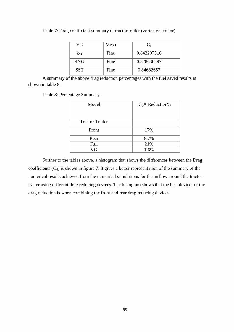
68
Table 7: Drag coefficient summary of tractor trailer (vortex generator).
VG Mesh Cd
k-ε Fine 0.842207516
RNG Fine 0.828630297
SST Fine 0.84682657
A summary of the above drag reduction percentages with the fuel saved results is
shown in table 8.
Table 8: Percentage Summary.
Model CdA Reduction%
Tractor Trailer
Front 17%
Rear 8.7%
Full 21%
VG 1.6%
Further to the tables above, a histogram that shows the differences between the Drag
coefficients (Cd) is shown in figure 7. It gives a better representation of the summary of the
numerical results achieved from the numerical simulations for the airflow around the tractor
trailer using different drag reducing devices. The histogram shows that the best device for the
drag reduction is when combining the front and rear drag reducing devices.
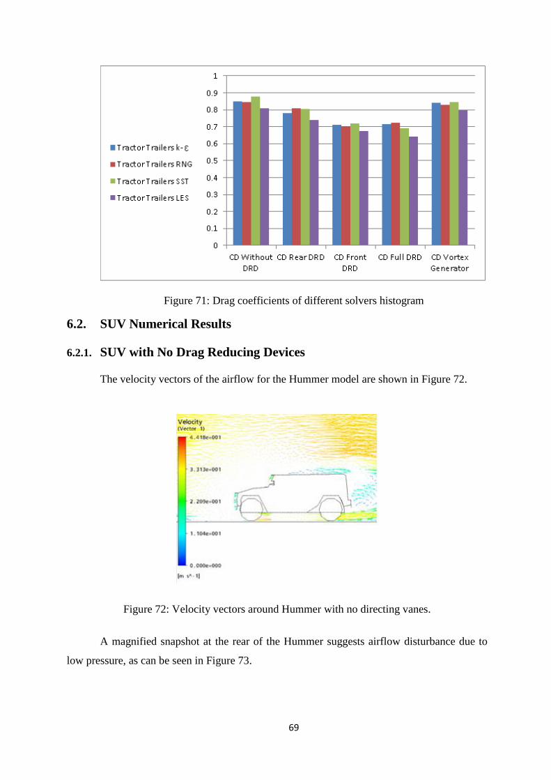
69
Figure 71: Drag coefficients of different solvers histogram
6.2. SUV Numerical Results
6.2.1. SUV with No Drag Reducing Devices
The velocity vectors of the airflow for the Hummer model are shown in Figure 72.
Figure 72: Velocity vectors around Hummer with no directing vanes.
A magnified snapshot at the rear of the Hummer suggests airflow disturbance due to
low pressure, as can be seen in Figure 73.
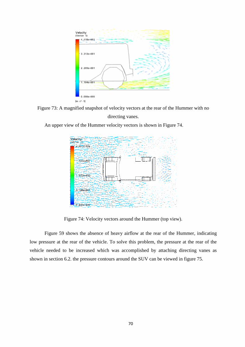
70
Figure 73: A magnified snapshot of velocity vectors at the rear of the Hummer with no
directing vanes.
An upper view of the Hummer velocity vectors is shown in Figure 74.
Figure 74: Velocity vectors around the Hummer (top view).
Figure 59 shows the absence of heavy airflow at the rear of the Hummer, indicating
low pressure at the rear of the vehicle. To solve this problem, the pressure at the rear of the
vehicle needed to be increased which was accomplished by attaching directing vanes as
shown in section 6.2. the pressure contours around the SUV can be viewed in figure 75.
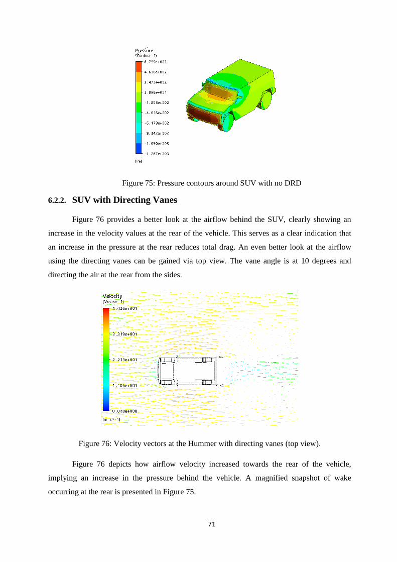
71
Figure 75: Pressure contours around SUV with no DRD
6.2.2. SUV with Directing Vanes
Figure 76 provides a better look at the airflow behind the SUV, clearly showing an
increase in the velocity values at the rear of the vehicle. This serves as a clear indication that
an increase in the pressure at the rear reduces total drag. An even better look at the airflow
using the directing vanes can be gained via top view. The vane angle is at 10 degrees and
directing the air at the rear from the sides.
Figure 76: Velocity vectors at the Hummer with directing vanes (top view).
Figure 76 depicts how airflow velocity increased towards the rear of the vehicle,
implying an increase in the pressure behind the vehicle. A magnified snapshot of wake
occurring at the rear is presented in Figure 75.
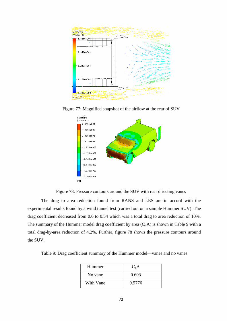
72
Figure 77: Magnified snapshot of the airflow at the rear of SUV
Figure 78: Pressure contours around the SUV with rear directing vanes
The drag to area reduction found from RANS and LES are in accord with the
experimental results found by a wind tunnel test (carried out on a sample Hummer SUV). The
drag coefficient decreased from 0.6 to 0.54 which was a total drag to area reduction of 10%.
The summary of the Hummer model drag coefficient by area (CdA) is shown in Table 9 with a
total drag-by-area reduction of 4.2%. Further, figure 78 shows the pressure contours around
the SUV.
Table 9: Drag coefficient summary of the Hummer model—vanes and no vanes.
Hummer CdA
No vane 0.603
With Vane 0.5776
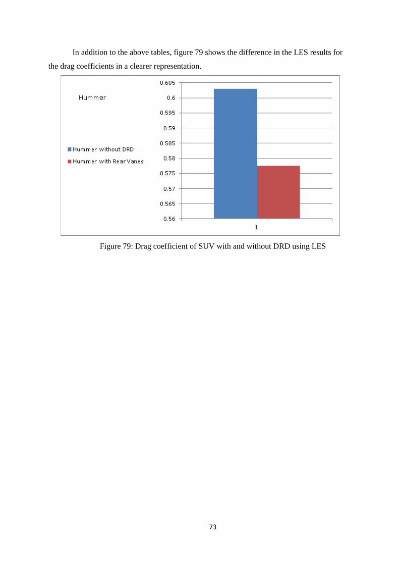
73
In addition to the above tables, figure 79 shows the difference in the LES results for
the drag coefficients in a clearer representation.
Figure 79: Drag coefficient of SUV with and without DRD using LES
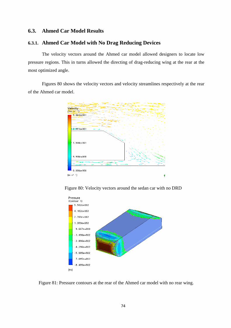
74
6.3. Ahmed Car Model Results
6.3.1. Ahmed Car Model with No Drag Reducing Devices
The velocity vectors around the Ahmed car model allowed designers to locate low
pressure regions. This in turns allowed the directing of drag-reducing wing at the rear at the
most optimized angle.
Figures 80 shows the velocity vectors and velocity streamlines respectively at the rear
of the Ahmed car model.
Figure 80: Velocity vectors around the sedan car with no DRD
Figure 81: Pressure contours at the rear of the Ahmed car model with no rear wing.
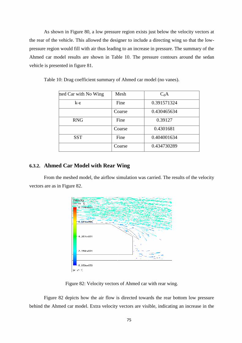
75
As shown in Figure 80, a low pressure region exists just below the velocity vectors at
the rear of the vehicle. This allowed the designer to include a directing wing so that the low-
pressure region would fill with air thus leading to an increase in pressure. The summary of the
Ahmed car model results are shown in Table 10. The pressure contours around the sedan
vehicle is presented in figure 81.
Table 10: Drag coefficient summary of Ahmed car model (no vanes).
Ahmed Car with No Wing Mesh CdA
k-ε Fine 0.391571324
Coarse 0.430465634
RNG Fine 0.39127
Coarse 0.4301681
SST Fine 0.404001634
Coarse 0.434730289
6.3.2. Ahmed Car Model with Rear Wing
From the meshed model, the airflow simulation was carried. The results of the velocity
vectors are as in Figure 82.
Figure 82: Velocity vectors of Ahmed car with rear wing.
Figure 82 depicts how the air flow is directed towards the rear bottom low pressure
behind the Ahmed car model. Extra velocity vectors are visible, indicating an increase in the
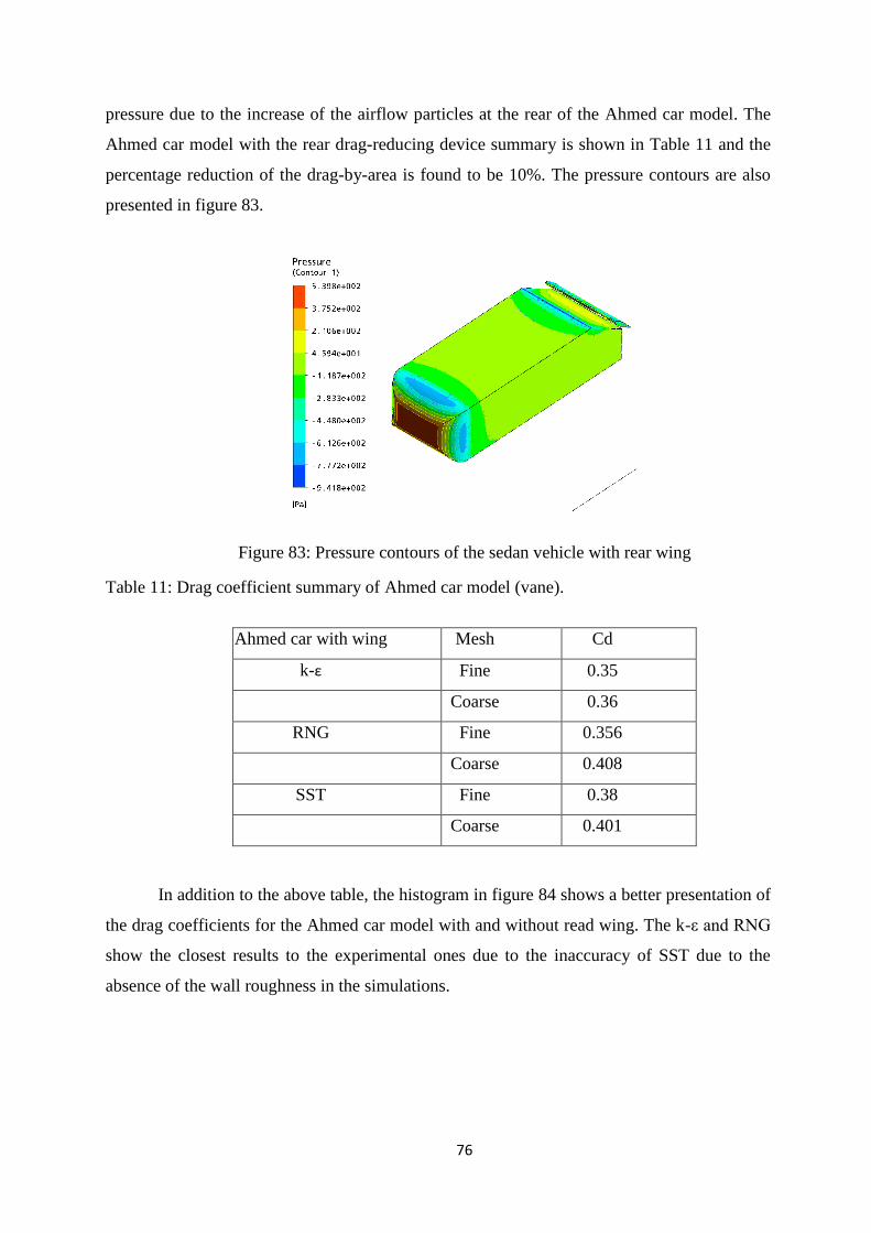
76
pressure due to the increase of the airflow particles at the rear of the Ahmed car model. The
Ahmed car model with the rear drag-reducing device summary is shown in Table 11 and the
percentage reduction of the drag-by-area is found to be 10%. The pressure contours are also
presented in figure 83.
Figure 83: Pressure contours of the sedan vehicle with rear wing
Table 11: Drag coefficient summary of Ahmed car model (vane).
Ahmed car with wing Mesh Cd
k-ε Fine 0.35
Coarse 0.36
RNG Fine 0.356
Coarse 0.408
SST Fine 0.38
Coarse 0.401
In addition to the above table, the histogram in figure 84 shows a better presentation of
the drag coefficients for the Ahmed car model with and without read wing. The k-ε and RNG
show the closest results to the experimental ones due to the inaccuracy of SST due to the
absence of the wall roughness in the simulations.
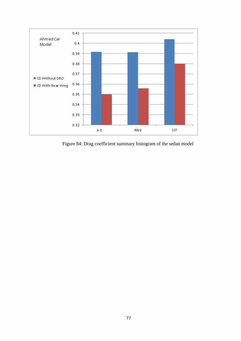
77
Figure 84: Drag coefficient summary histogram of the sedan model
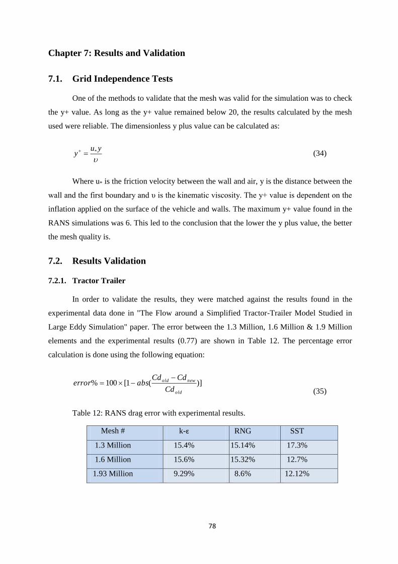
78
Chapter 7: Results and Validation
7.1. Grid Independence Tests
One of the methods to validate that the mesh was valid for the simulation was to check
the y+ value. As long as the y+ value remained below 20, the results calculated by the mesh
used were reliable. The dimensionless y plus value can be calculated as:
yuy * (34)
Where u* is the friction velocity between the wall and air, y is the distance between the
wall and the first boundary and υ is the kinematic viscosity. The y+ value is dependent on the
inflation applied on the surface of the vehicle and walls. The maximum y+ value found in the
RANS simulations was 6. This led to the conclusion that the lower the y plus value, the better
the mesh quality is.
7.2. Results Validation
7.2.1. Tractor Trailer
In order to validate the results, they were matched against the results found in the
experimental data done in "The Flow around a Simplified Tractor-Trailer Model Studied in
Large Eddy Simulation" paper. The error between the 1.3 Million, 1.6 Million & 1.9 Million
elements and the experimental results (0.77) are shown in Table 12. The percentage error
calculation is done using the following equation:
)](1[100%old
newold
Cd
CdCdabserror
(35)
Table 12: RANS drag error with experimental results.
Mesh # k-ε RNG SST
1.3 Million 15.4% 15.14% 17.3%
1.6 Million 15.6% 15.32% 12.7%
1.93 Million 9.29% 8.6% 12.12%
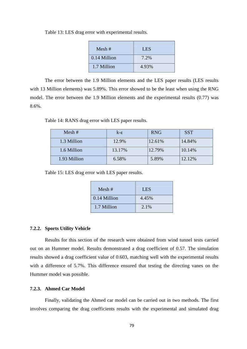
79
Table 13: LES drag error with experimental results.
Mesh # LES
0.14 Million 7.2%
1.7 Million 4.93%
The error between the 1.9 Million elements and the LES paper results (LES results
with 13 Million elements) was 5.89%. This error showed to be the least when using the RNG
model. The error between the 1.9 Million elements and the experimental results (0.77) was
8.6%.
Table 14: RANS drag error with LES paper results.
Mesh # k-ε RNG SST
1.3 Million 12.9% 12.61% 14.84%
1.6 Million 13.17% 12.79% 10.14%
1.93 Million 6.58% 5.89% 12.12%
Table 15: LES drag error with LES paper results.
Mesh # LES
0.14 Million 4.45%
1.7 Million 2.1%
7.2.2. Sports Utility Vehicle
Results for this section of the research were obtained from wind tunnel tests carried
out on an Hummer model. Results demonstrated a drag coefficient of 0.57. The simulation
results showed a drag coefficient value of 0.603, matching well with the experimental results
with a difference of 5.7%. This difference ensured that testing the directing vanes on the
Hummer model was possible.
7.2.3. Ahmed Car Model
Finally, validating the Ahmed car model can be carried out in two methods. The first
involves comparing the drag coefficients results with the experimental and simulated drag
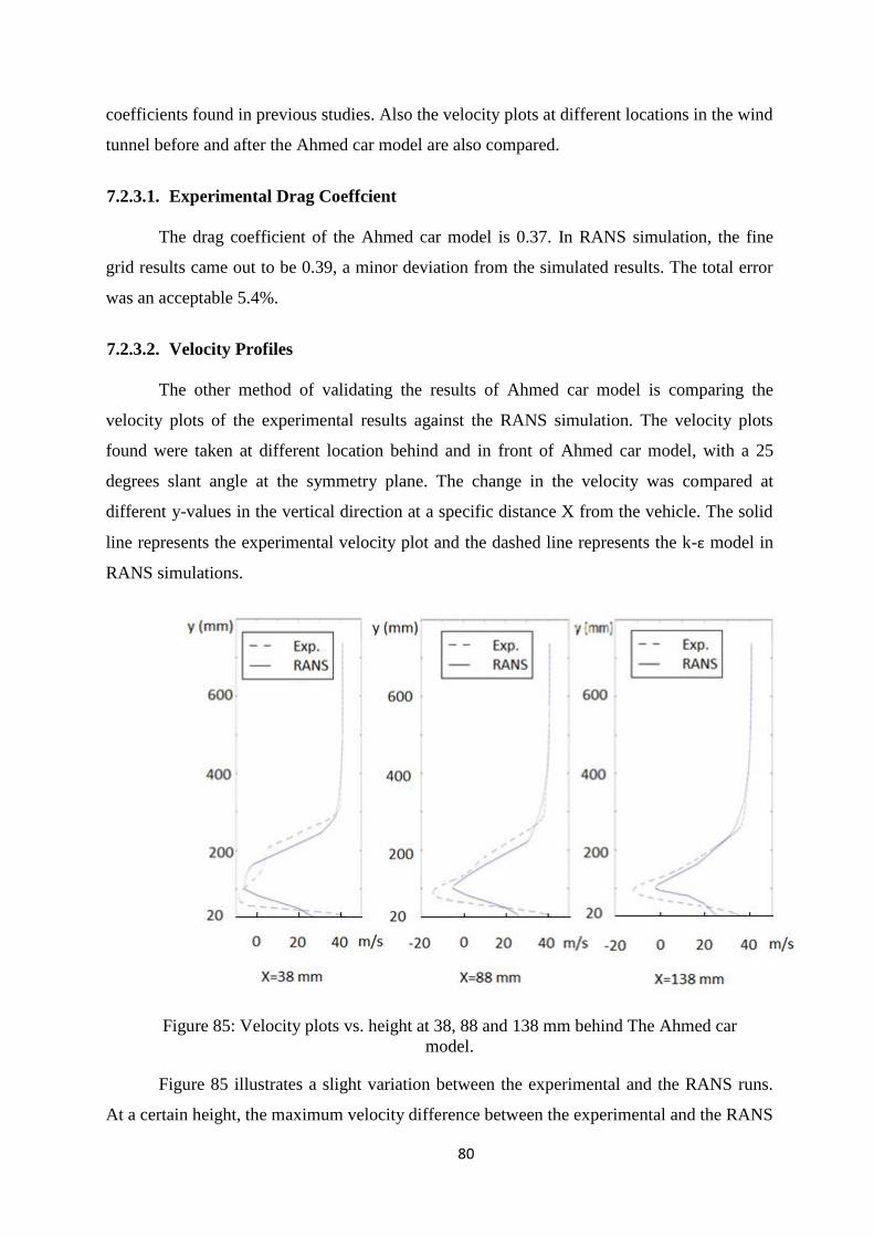
80
coefficients found in previous studies. Also the velocity plots at different locations in the wind
tunnel before and after the Ahmed car model are also compared.
7.2.3.1. Experimental Drag Coeffcient
The drag coefficient of the Ahmed car model is 0.37. In RANS simulation, the fine
grid results came out to be 0.39, a minor deviation from the simulated results. The total error
was an acceptable 5.4%.
7.2.3.2. Velocity Profiles
The other method of validating the results of Ahmed car model is comparing the
velocity plots of the experimental results against the RANS simulation. The velocity plots
found were taken at different location behind and in front of Ahmed car model, with a 25
degrees slant angle at the symmetry plane. The change in the velocity was compared at
different y-values in the vertical direction at a specific distance X from the vehicle. The solid
line represents the experimental velocity plot and the dashed line represents the k-ε model in
RANS simulations.
Figure 85: Velocity plots vs. height at 38, 88 and 138 mm behind The Ahmed car
model.
Figure 85 illustrates a slight variation between the experimental and the RANS runs.
At a certain height, the maximum velocity difference between the experimental and the RANS
81
was a 15% error. Although the error is above 10%, the velocity plots are in harmony with the
experimental velocity plots. Therefore, the tests of the Ahmed car model with the directing
wing could be proceeded with.
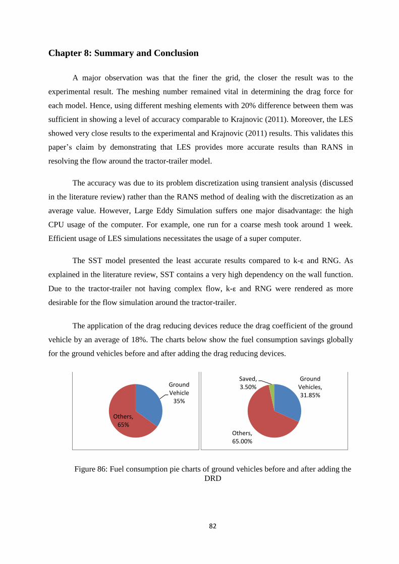
82
Chapter 8: Summary and Conclusion
A major observation was that the finer the grid, the closer the result was to the
experimental result. The meshing number remained vital in determining the drag force for
each model. Hence, using different meshing elements with 20% difference between them was
sufficient in showing a level of accuracy comparable to Krajnovic (2011). Moreover, the LES
showed very close results to the experimental and Krajnovic (2011) results. This validates this
paper’s claim by demonstrating that LES provides more accurate results than RANS in
resolving the flow around the tractor-trailer model.
The accuracy was due to its problem discretization using transient analysis (discussed
in the literature review) rather than the RANS method of dealing with the discretization as an
average value. However, Large Eddy Simulation suffers one major disadvantage: the high
CPU usage of the computer. For example, one run for a coarse mesh took around 1 week.
Efficient usage of LES simulations necessitates the usage of a super computer.
The SST model presented the least accurate results compared to k-ε and RNG. As
explained in the literature review, SST contains a very high dependency on the wall function.
Due to the tractor-trailer not having complex flow, k-ε and RNG were rendered as more
desirable for the flow simulation around the tractor-trailer.
The application of the drag reducing devices reduce the drag coefficient of the ground
vehicle by an average of 18%. The charts below show the fuel consumption savings globally
for the ground vehicles before and after adding the drag reducing devices.
Figure 86: Fuel consumption pie charts of ground vehicles before and after adding the
DRD
Ground Vehicle
35%
Others, 65%
Ground Vehicles, 31.85%
Others, 65.00%
Saved, 3.50%
83
To conclude, millions of dollars can be saved by reducing the aerodynamic drag on
ground vehicles. The impact of the scarcity of the fuel resources has pushed major
manufacturers towards research and development in order to yield higher efficiency. Special
attention is directed towards the reduction of the aerodynamic drag on the vehicles which was
achieved by utilizing various drag-reducing devices installed on ground vehicles. Moreover,
some of these devices can be combined with present drag-reducing devices in order to further
reduce the drag coefficient further.
The results clearly infer that installing mechanical drag-reducing devices on heavy
vehicles reduced the aerodynamic drag-by-area (CdA) by 21%, which was achieved by the
addition of the front and rear drag-reducing devices. This reduction occurred due to the
combination of decreasing the frontal impact pressure and by increasing the rear pressure
found at the rear of the vehicle. The drag reduction of the tractor trailer with the installation of
each of the drag reducing devices is:
1. The rear drag-reducing devices reduced the drag-by-area (CdA) by 8.7% by directing
the high-momentum airflow towards the rear of the trailer and tractor where the
pressure was low.
2. The front drag-reducing devices smooth the airflow from the tractor with a smaller
area to the trailer that has a larger frontal area. This resulted in a 17% reduction in the
drag-by-area (CdA).
3. The vortex generators caused airflow separation at the rear of the trailer to be laminar,
causing a reduced turbulent separation of the flow. The addition of the vortex
generators reduced the drag-by-area by around 1.6%.
4. The combination of the front and rear drag reducing devices reduced the drag by area
ratio by a total of 21%.
This research also studied the effect of drag-reducing devices on an SUV model
represented by a Hummer model. The addition of directing side vanes at the rear of the
vehicle making a 10 degrees angle with the vertical plane lowered the drag-by-area by 4.2%.
This decrease was accomplished by directing high momentum airflow towards the rear of the
Hummer.
For the completion of this research, in addition to heavy vehicles and SUV’s, the
application of drag-reducing devices on a sedan sample vehicle represented by the famous
84
Ahmed car model was also conducted. A rear wing modeled by NACA 0015 was attached at
10 degrees from the rear slant angle which lowered the drag-by-area of the Ahmed car model
by 10%.
All results were compared against experimental results. Tractor trailer RANS results
showed an error of 12% while LES results showed an error of 4.9% in comparison with the
paper’s results [26]. The SUV model showed an error of 5.7% in comparison with the
experimental results for a small scale Hummer model in a wind tunnel.
Furthermore, the Ahmed car model validation was justified in two ways:
1. The first method involved comparing the drag coefficient of the simulation by the
experimental results of the drag coefficient in a wind tunnel. This yielded an error of
5.1%.
2. The second method of validating the results of the Ahmed car model was derived by
comparing the velocity plots of the experimental results of the Ahmed car model (at a
30 degrees slant angle). This gave an error of 5.4%.
These comparisons demonstrate a strong parallel between the two types of results for
all models, thus, providing us ample grounds to consider the drag-reduction percentages as
reasonable results. Drag-reduction, therefore, serves as a leading method for reducing fuel
consumption in ground vehicles and thus, for preserving energy resources.
85
References
[1] B. Khalighia. "Aerodynamic flow around a sport utility vehicle—Computational
and experimental investigation." Journal of Wind Engineering and Industrial
Aerodynamics, vol.107-108, pp. 140–148, Aug.–Sep. 2012.
[2] S. Bickerstaffe. "Mercedes B Class Sets Aerodynamic Benchmark." Automotive
Engineer Magazine, 2011.
[3] D. G. Hyams. "Computational simulation of model and full scale Class 8 trucks
with drag-reduction devices. "Computers & Fluids, vol. 41, pp. 27–40, Feb.
2011.
[4] Z. Kassim. "Fuel savings on a heavy vehicle via aerodynamic drag-reduction."
Transportation Research Part D, vol. 15, pp. 275–284, Jul. 2010.
[5] S.Y. Cheng. " A numerical analysis of transient flow past road vehicles
subjected to pitching oscillation." Journal of Wind Engineering and Industrial
Aerodynamics, vol. 99, pp. 511–522, May 2011.
[6] T. Dills. "Explorations of ATDynamics' TrailerTail." Overdrive Magazine, Mar.
2012.
[7] B. Tinham. "System Drag Reduction device cuts trailer turbulence by 50%."
Transport Engineer Magazine, Nov. 2012.
[8] Freight Wing. "Tractor Aerodynamics." Transport Canada, Feb. 2012.
[9] S. Williams. "Vortex Generator." Aviation Glossary, Jan. 2013.
[10] S. Krajnovic. "Numerical Simulation of the Flow Around a simplified Vehicle
Model With Active Flow Control." International Journal of Heat and Fluid Flow,
vol.32, pp. 192-200, Jul. 2010.
[11] F. White. Fluid Mechanics. New York, NY: McGraw-Hill, 2003, p. 607.
[12] D. Lengani. "Turbulent boundary layer separation control and loss evaluation
86
of low profile vortex generators." Experimental Thermal and Fluid Science, vol.
35, pp. 1505-1513, Nov. 2011.
[13] V. Stenzela. "Drag-reducing paints for the reduction of fuel consumption in
aviation and shipping." Progress in Organic Coatings, vol.70, pp. 224-229, Apr.
2011.
[14] S. Watkins. "The effect of vehicle spacing on the aerodynamics of a
representative car shape." Journal of Wind Engineering and Industrial
Aerodynamics, vol. 96, pp. 1232–1239, Jun.–Jul. 2008.
[15] L. Tsuei. "Transient aerodynamics of vehicle platoons during in-line
oscillations." Journal of Wind Engineering and Industrial Aerodynamics, vol. 89,
pp. 1085–1111, Oct. 2001.
[16] M. Y. Okiishi. Fundementals of Fluid Mechanics. New York, NY: John Wiley &
Sons, 1998, pp. 360-361.
[17] D. Wilcox. Turbulence Modeling for CFD. California: DCW Industries, 2000, pp.
123-127.
[18] V. Yakhot."Renormalization group analysis of turbulence." Journal of Scientific
Computing, vol. 1, p.3, 1986.
[19] Y. Zhou. "Renormalization group theory for fluid and plasma turbulence."
Physics Reports, vol. 488, pp. 1-49, 2010.
[20] D. Wilcox. Turbulence Modeling for CFD. California: DCW Industries, 2000, pp.
119-122
[21] W. C. Basford. "Aerodynamic combination for improved base drag reduction."
U.S. Patent 6959958, Nov. 2005.
[22] G. Chen. "Remarks on large eddy simulation." Communications in Nonlinear
Science and Numerical Simulation, vol. 5, pp. 85-90, Sept. 2000.
[23] T. Nakashima. " Coupled analysis of unsteady aerodynamics and vehicle
87
motion of a road vehicle in windy conditions." Computers & Fluids, Nov. 2012.
[24] S. Krajnovic. "The Flow around a trailer-truck model studied by Large Eddy
Simulation." Journal of Wind Engineering and Industrial Aerodynamics, vol.
102, pp. 36-47, Jan. 2011.
[25] E.M. Wahba, H. Al-Marzooqi, M. Shaath, M. Shahin and T. El-Dhmashawy.
"Aerodynamic Drag Reduction for Ground Vehicles using Lateral Guide Vanes."
CFD Letters, vol. 4, pp. 68-79, Jun. 2012.
[26] H. Fukuda. "Improvement of vehicle aerodynamics by wake control." JSAE
Review, vol. 16, pp. 151–155, Apr. 1995.
[27] A. Gilkson. "An Experimental and Computational Study of the Aerodynamic
and Passive Ventilation Charecteristics of Small Livestock Trailers." Journal of
Wind Engineering and Industrial Aerodynamics, vol. 97, pp. 415-425, Aug.
2009.
[28] A. Al Garni. "Experimental Study of a Pickup truck Near Wake." Journal of Wind
Engineering and Industrial Aerodynamics, vol. 98, pp. 100-112, Oct. 2009.
[29] J.Bettle. " A Computational Study of the Aerodynamic Forces acting on a
tractor trailer vehicle on a bridge in cross-wind." University of New Brunswick,
vol. 91, pp. 573-592, Nov. 2002.
[30] A. Hafez. "Numerical investigation of the fully developed turbulent flow over a
moving wavy wall using k–ε turbulence model." Alexandria Engineering
Journal, vol. 50, pp. 145–162, 2011.
[31] M. Tsubokura. " Large Eddy Simulation on the Unsteady aerodynamic response
of a road vehicle in Transient Crosswinds." International Journal of Heat and
Fluid Flow, vol. 31, pp. 1075-1086, Jul. 2010.
[32] W. Mazyan. "The Dynamic Positive Lift Spoiler." United Arab Emirates. Patent
Application: W-403-821-UAE-IPPAT, 2010.
[33] M. Mahbubar Rahman. "Numerical Investigation of Unsteady Flow Past A
Circular Cylinder 2-D-Finite Volume Method." Journal of Naval Architecture
88
and Marine Engineering, vol. 4, pp. 27-42, 2007.
[34] R. Menter. "Zonal Two Equation k-epsilon Turbulence Models for Aerodynamic
Flows." in 24th Fluid Dynamics Conference, 1993.
[35] P. Moin. "Advances in Large Eddy Simulation Methodology for Complex
Flows." International Journal of Heat and Fluid Flow, vol. 23, pp. 710-720,
2002.
[36] QI Xia. "Experimental and Numerical Studies of Aerodynamic Performance of
Trucks." Journal of Hydrodynamics, vol. 23, pp. 752-758, Jul. 2011.
[37] S. Becker. "Flow and Turbulence Structures in the Wake of a Simplified Car
Model." SAE Technical Paper, 2003.
[38] S. Krajnović. "Influence of floor motions in wind tunnels on the aerodynamics
of road vehicles." Journal of Wind Engineering and Industrial Aerodynamics,
vol. 93, pp. 677–696, Sep. 2005.
[39] F. Grosche. "Research at DLR Gottingen on bluff body aerodynamics, drag
reduction by wake ventilation and active flow control." Journal of Wind
Engineering, vol. 89, pp. 1201-1218, 2001.
[40] M. Baker. "Drag reducing device for land vehicles." U.S. Patent 5348366, Sep.
1994.
89
Vita
Walid Ibrahim Mazyan was born on the 18th
of February, 1986, in Kuwait and lived in
Beirut, Lebanon. His educational journey started in Al Maqasid School in Beirut, Lebanon.
He received his Bachelor of Science in Mechanical Engineering from the American
University of Sharjah, UAE, in the summer of 2009. After graduation, he worked in Petrofac
International Limited, Sharjah, where he worked as a Static Mechanical Engineer on diverse
oil and gas equipment. In January 2011, he joined the American University of Sharjah as a
part time student to earn his Master of Science in Mechanical Engineering, with an emphasis
on Fluid Mechanics. He applied for a patent on a new design of a rear wing on sports cars that
reduces the drag in 2010. He eventually graduated with a Master of Science in Mechanical
Engineering Degree in the fall of 2013.