micromixing devices
TRANSCRIPT

129
4
Micromixing Devices
4.1
Role of Mixing for the Performance of Chemical Reactors
Mixing is one of the basic unit operations involved in chemical transformations.
The problems associated with badmixingmay have a decisive impact on the prod-
uct distribution and the performance of a chemical reactor. Mixing is a general
definition applied for different physical processes. It can be subdivided into two
main classes:
1) Microscopic mixing: mixing of individual molecules, like homogenization of
two miscible fluids, or dissolution of a solid in a liquid without the formation
of any concentration (temperature) gradients.
2) Macroscopic mixing: mixing of groups or aggregates of molecules, such as
a. Suspension of a solid in a liquid or slurry formation
b. Dispersion (or emulsification) of two immiscible liquids
c. Dispersion of a gas in a liquid (or foam formation).
In general, good mixing at the macroscopic scale can be easily attained, but
it is much more difficult to obtain an intimate mixing on the molecular scale.
Nonuniform reactant concentrations on themolecular scalemay have a significant
influence on the effective transformation rate and the product distribution, espe-
cially when complex and rapid chemical reactions are involved. In this chapter we
mainly consider the microscopic mixing between miscible fluids.This means that
two completely miscible reacting fluids are brought together. If the characteristic
mixing time defined as the time required for two fluids to become homogenous on
the molecular scale is in the same order of magnitude as the characteristic reac-
tion time or even longer, the product distribution is strongly affected, especially in
the case of complex networks with parallel and/or consecutive reactions [1, 2]. To
avoid the negative effect on reactor productivity and yield of the desired product
(often an intermediate in a complex reaction network), the characteristic mixing
time should be at least 10-fold shorter than the characteristic reaction time.
To describe themixing process and its influence on the performance of chemical
reactors, differentmodelswere developed [3, 4]. Hereinwe discuss the influence of
the micromixing process using the concept of segregation as proposed by Baldyga
Microstructured Devices for Chemical Processing, First Edition.Madhvanand N. Kashid, Albert Renken and Lioubov Kiwi-Minsker.© 2015 Wiley-VCH Verlag GmbH & Co. KGaA. Published 2015 by Wiley-VCH Verlag GmbH & Co. KGaA.
130 4 Micromixing Devices
[5]. In addition, we restrict the discussion to ideal tubular reactors supposing plug
flow behavior.
The concept of segregation in chemical reactors was first introduced by Danck-
werts in 1953 [6]. He defined an intensity of segregation, Is, varying between one
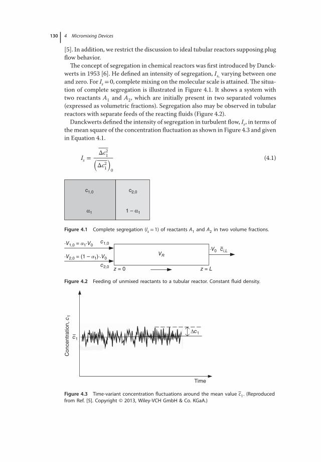
and zero. For Is = 0, complete mixing on the molecular scale is attained.The situa-
tion of complete segregation is illustrated in Figure 4.1. It shows a system with
two reactants A1 and A2, which are initially present in two separated volumes
(expressed as volumetric fractions). Segregation also may be observed in tubular
reactors with separate feeds of the reacting fluids (Figure 4.2).
Danckwerts defined the intensity of segregation in turbulent flow, Is, in terms of
the mean square of the concentration fluctuation as shown in Figure 4.3 and given
in Equation 4.1.
Is =Δc2
1(Δc2
1
)0
(4.1)
c1,0 c2,0
α1 1 – α1
Figure 4.1 Complete segregation (Is = 1) of reactants A1 and A2 in two volume fractions.
·V1,0 = α1·V0·V0
VR·V2,0 = (1 – α1)··V0
c1,0
ci,L
c2,0 z = 0 z = L
Figure 4.2 Feeding of unmixed reactants to a tubular reactor. Constant fluid density.
Time
Con
ce
ntr
atio
n,
c 1
c1
Δc1
Figure 4.3 Time-variant concentration fluctuations around the mean value c1. (Reproduced
from Ref. [5]. Copyright © 2013, Wiley-VCH GmbH & Co. KGaA.)
4.1 Role of Mixing for the Performance of Chemical Reactors 131
where (Δc21)0 corresponds to the initialmean square of concentration fluctuations.
The mean square of the concentration variations is given in Equation 4.2
Δc21= (c1 − c1)2 (4.2)
For the situation shown in Figure 4.1 the initial mean square fluctuations are given
by
(Δc21)0 = c21,0 ⋅ 𝛼1(1 − 𝛼1) (4.3)
For separate feed to a continuously operated reactor, the volume fraction 𝛼1 cor-
responds to the volumetric flow containing A1 referred to the total inlet flow.
α1 =V1,0
V1,0 + V2,0
=V1
V0
(4.4)
Depending on the mixing intensity in the reactor, the segregation will diminish
with increasing residence time. The rate of decay of the concentration variance
can be supposed to be a first order process as indicated in Equation 4.5
rd = −bs ⋅ Δc21 = − 1
tmx
⋅ Δc21
(4.5)
The parameter bs is equivalent to the inverse mixing time, tmx, and is a function
of the power dissipation per volume and the geometry of the mixing device.
In plug flow reactors (PFRs) under steady state, the segregation intensity will
decay with the distance from the reactor inlet, respectively, with the residence
time, 𝜏 .
Δc21(
Δc21
)0
= Is = exp(−bs𝜏) = exp(−bs𝜏PFRZ)
with 𝜏PFR = VR∕V0; Z = V∕VR = z∕L (constant diameter) (4.6)
The transformation rate of an irreversible second order reaction in a partially
segregated fluid can be expressed in terms of the mean concentrations and the
concentration fluctuations of the reactants [7].
R1 = −k ⋅ c1c2 = −k ⋅ (c1 ⋅ c2 + Δc1Δc2)dc1d𝜏
= R1 = −k ⋅ (c1 ⋅ c2 − Isc1,0 ⋅ c2,0)
with ∶ Δc1Δc2 = −Is(c1,0 ⋅ c2,0) (4.7)
With the following dimensionless variables:
M = c2,0∕c1,0, fi = ci∕c1,0, c2,0 = c2,0 ⋅ (1 − 𝛼1); c1,0 = c1,0 ⋅ 𝛼1, DaI =kc1,0𝜏PFRThematerial balance for the reactantA1 can be expressed in dimensionless form
as follows:
df1dZ
= −DaI ⋅ [f1 ⋅ (f1 +M − 1) − IsM] (4.8)
132 4 Micromixing Devices
For given reaction conditions and residence time in a PFR, the axial concentration
profile and the outlet conversion depends strongly on the ratio between mixing
time and characteristic reaction time. This ratio can be interpreted as a second
Damköhler number for mixing DaIImx.
DaIImx =tmx
tr= k ⋅ c1,0 ⋅ tmx (second order reaction) (4.9)
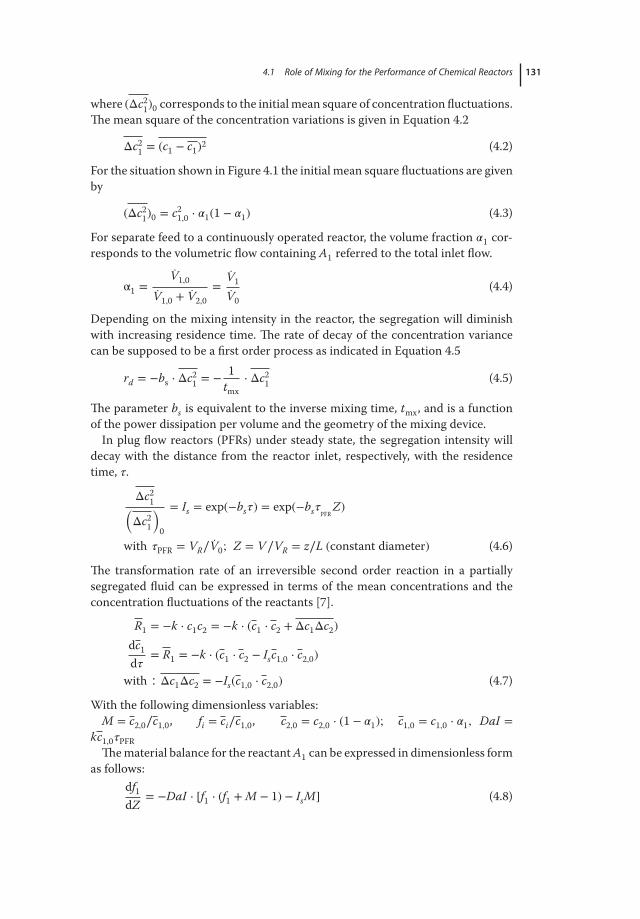
This is shown in Figure 4.4, where the residual concentration of A1 is plotted as
function of the reactor length for different values of DaIImx and constant DaI
and equimolar reactant feed (M= 1). Whereas for immediate mixing of the reac-
tants at the reactor entrance (DaIImx =>0) the conversion of A1 corresponds to
X = 0.833 (f 1 = 0.167) atDaI = 5, the conversion drops toX = 0.345 (f 1 = 0.655) for
DaIImx = 5. A roughly four times higher residence time in the reactor is needed to
get the same conversion as for DaIImx = 0. In general, long mixing times as com-
pared to the characteristic reaction time diminish the reactor performance for
reactions with positive reaction orders (n> 0). This leads to the increased reactor
size in order to attain the same degree of conversion.
Even more important is the influence of slow mixing on the performance of
complex reactions. If the reaction between two fluids takes place to an appre-
ciable extent before the homogeneity is attained, segregation can affect product
distribution. This is discussed for consecutive competing reactions represented
by Equation 4.10.
A1 + A2
k1−−→A3
A3 + A2
k2−−→A4 (4.10)
Reactor length, Z = z/L
0.0 0.2 0.4 0.6 0.8 1.0
Re
sid
ua
l co
nce
ntr
atio
n o
f A
1,
f 1 =
1 –
X
0.0
0.2
0.4
0.6
0.8
1.0
Final concentration for Dallmx = 0
Dallmx = 0
Dallmx = 5.0
2.01.00.50.2
Figure 4.4 Estimated residual concentration of A1 as function of reactor length for differ-
ent DaIImx. DaI= 5; M= 1.
4.1 Role of Mixing for the Performance of Chemical Reactors 133
Examples of such consecutive competing reactions are chlorination, nitration of
hydrocarbons, or the addition of alkene oxides (e.g., ethylene oxide) to amines or
alcohols. If the mixing is fast enough, so that the reacting fluid is homogenous
before the reaction takes place, the maximum yield of the desired intermediate
A3 will be controlled by the ratio of k2/k1. Let us suppose irreversible second
order reactions, so the following relations describe the transformation rates of
the involved reactants.
R1 = −k1 ⋅ c1c2R2 = −k1 ⋅ c1c2 − k2 ⋅ c2c3R3 = k1 ⋅ c1c2 − k2 ⋅ c2c3R4 = k2 ⋅ c2c3 (4.11)
In batch or ideal PFR the concentration of the intermediate product A3 will first
increase with increasing residence time, pass through a maximum, and finally
disappear at long residence times, if the initial reaction partners are fed in stoi-
chiometric ratios. For the simple reaction scheme shown by Equation 4.10, M =c2,0∕c1,0 must beM= 2 for complete transformation of A1 and A2. The concentra-
tion profiles can be calculated by solving the corresponding mass balances. For a
PFR the following mass balances are obtained:
−dc1d𝜏
= k1 ⋅ c1c2
−dc2d𝜏
= k1 ⋅ c1c2 + k2c2c3
dc3d𝜏
= k1 ⋅ c1c2 − k2c2c3
dc4d𝜏
= k2c2c3 (4.12)
Initial conditions: 𝜏 = 0 ∶ c1 = c1,0; c2 = c2,0; c3 = c4 = 0
By dividing the third equation by the first one, the residence time can be elimi-
nated and we get a relationship between the reactant concentrations.
−dc3dc1
= 1 −k2k1
⋅c3c1
(4.13)
After integration, a relation between the yield of the intermediateA3 and the con-
version of the key component A1 is obtained.
Y3,1 =(1 − X)𝜅 − (1 − X)
1 − 𝜅; 𝜅 =
k2k1
≠ 1
Y3,1 = (X − 1) ⋅ ln(1 − X); 𝜅 =k2k1
= 1 (4.14)
134 4 Micromixing Devices
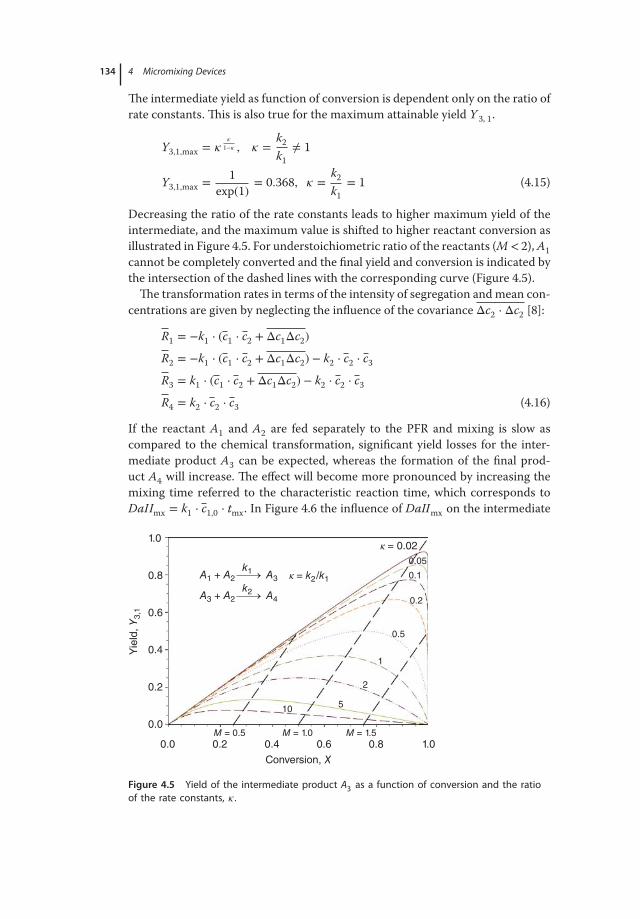
The intermediate yield as function of conversion is dependent only on the ratio of
rate constants. This is also true for the maximum attainable yield Y 3, 1.
Y3,1,max = 𝜅𝜅
1−𝜅 , 𝜅 =k2k1
≠ 1
Y3,1,max =1
exp(1)= 0.368, 𝜅 =
k2k1
= 1 (4.15)
Decreasing the ratio of the rate constants leads to higher maximum yield of the
intermediate, and the maximum value is shifted to higher reactant conversion as
illustrated in Figure 4.5. For understoichiometric ratio of the reactants (M< 2),A1
cannot be completely converted and the final yield and conversion is indicated by
the intersection of the dashed lines with the corresponding curve (Figure 4.5).
The transformation rates in terms of the intensity of segregation andmean con-
centrations are given by neglecting the influence of the covariance Δc2 ⋅ Δc2 [8]:
R1 = −k1 ⋅ (c1 ⋅ c2 + Δc1Δc2)
R2 = −k1 ⋅ (c1 ⋅ c2 + Δc1Δc2) − k2 ⋅ c2 ⋅ c3
R3 = k1 ⋅ (c1 ⋅ c2 + Δc1Δc2) − k2 ⋅ c2 ⋅ c3
R4 = k2 ⋅ c2 ⋅ c3 (4.16)
If the reactant A1 and A2 are fed separately to the PFR and mixing is slow as
compared to the chemical transformation, significant yield losses for the inter-
mediate product A3 can be expected, whereas the formation of the final prod-
uct A4 will increase. The effect will become more pronounced by increasing the
mixing time referred to the characteristic reaction time, which corresponds to
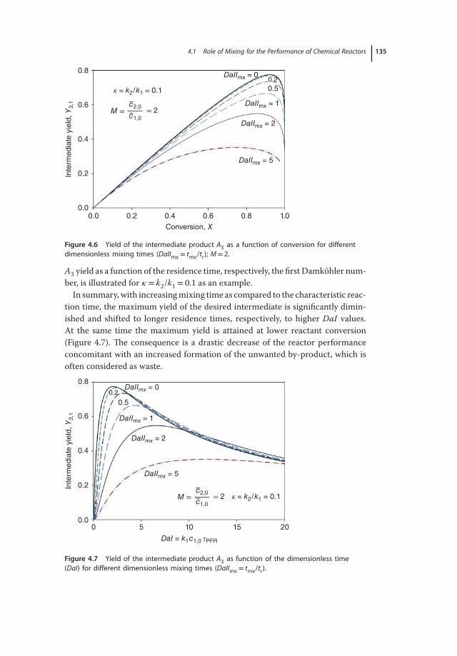
DaIImx = k1 ⋅ c1,0 ⋅ tmx. In Figure 4.6 the influence of DaIImx on the intermediate
Conversion, X
0.0 0.2 0.4 0.6 0.8 1.0
Yie
ld, Y
3,1
0.0
0.2
0.4
0.6
0.8 A1 + A2 A3
1.0κ = 0.02
κ = k2/k1 0.1
0.5
0.2
2
1
5
0.05
10
M = 0.5 M = 1.0 M = 1.5
k1
A3 + A2 A4
k2
Figure 4.5 Yield of the intermediate product A3 as a function of conversion and the ratio
of the rate constants, 𝜅.
4.1 Role of Mixing for the Performance of Chemical Reactors 135
Conversion, X
0.00.0
0.2
0.2
0.4
0.4
0.6
0.6
0.8
0.8
1.0
Inte
rmedia
te y
ield
, Y
3,1
DaIImx = 5
DaIImx = 2
DaIImx = 1
DaIImx = 0
0.5
0.2
κ = k2/k1 = 0.1
c2,0
c1,0M = = 2
Figure 4.6 Yield of the intermediate product A3 as a function of conversion for different
dimensionless mixing times (DaIImx = tmx/tr); M= 2.
A3 yield as a function of the residence time, respectively, the first Damköhler num-
ber, is illustrated for 𝜅 = k2/k1 = 0.1 as an example.
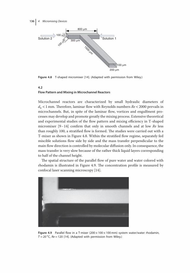
In summary,with increasingmixing time as compared to the characteristic reac-
tion time, the maximum yield of the desired intermediate is significantly dimin-
ished and shifted to longer residence times, respectively, to higher DaI values.
At the same time the maximum yield is attained at lower reactant conversion
(Figure 4.7). The consequence is a drastic decrease of the reactor performance
concomitant with an increased formation of the unwanted by-product, which is
often considered as waste.
DaI = k1c1,0 τPFR
0 5 10 15 20
Inte
rme
dia
te y
ield
, Y
3,1
0.0
0.2
0.4
0.6
0.8
DaIImx = 5
DaIImx = 2
DaIImx = 1
DaIImx = 0
0.5
0.2
κ = k2/k1 = 0.1c2,0
c1,0M = = 2
Figure 4.7 Yield of the intermediate product A3 as function of the dimensionless time
(DaI) for different dimensionless mixing times (DaIImx = tmx/tr).
136 4 Micromixing Devices
Solution 1Solution 2
200 μm
1500 μm
100 μm
800 μm
300 μm
100 μm
100 μm
Figure 4.8 T-shaped micromixer [14]. (Adapted with permission from Wiley.)
4.2
Flow Pattern andMixing in Microchannel Reactors
Microchannel reactors are characterized by small hydraulic diameters of
dh < 1mm. Therefore, laminar flow with Reynolds numbers Re< 2000 prevails in
microchannels. But, in spite of the laminar flow, vortices and engulfment pro-
cesses may develop and promote greatly the mixing process. Extensive theoretical
and experimental studies of the flow pattern and mixing efficiency in T-shaped
micromixer [9–14] confirm that only in smooth channels and at low Re less
than roughly 100, a stratified flow is formed. The studies were carried out with a
T-mixer as shown in Figure 4.8. Within the stratified flow regime, separately fed
miscible solutions flow side by side and the mass transfer perpendicular to the
main flow direction is controlled by molecular diffusion only. In consequence, the
mass transfer is very slow because of the rather thick liquid layers corresponding
to half of the channel height.
The spatial structure of the parallel flow of pure water and water colored with
rhodamin is illustrated in Figure 4.9. The concentration profile is measured by
confocal laser scanning microscopy [14].
Figure 4.9 Parallel flow in a T-mixer (200× 100× 100mm) system water/water rhodamin,
T = 20 ∘C, Re= 120 [14]. (Adapted with permission from Wiley.)
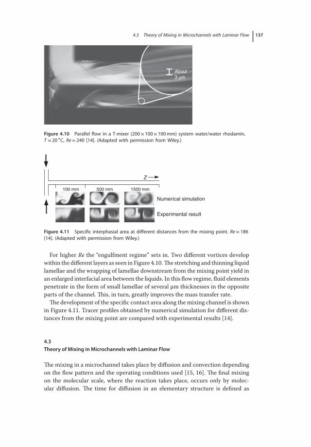
4.3 Theory of Mixing in Microchannels with Laminar Flow 137
About3 μm
Figure 4.10 Parallel flow in a T-mixer (200× 100× 100mm) system water/water rhodamin,
T = 20 ∘C, Re= 240 [14]. (Adapted with permission from Wiley.)
Z
Numerical simulation
Experimental result
100 mm 500 mm 1500 mm
Figure 4.11 Specific interphasial area at different distances from the mixing point. Re= 186
[14]. (Adapted with permission from Wiley.)
For higher Re the “engulfment regime” sets in. Two different vortices develop
within the different layers as seen in Figure 4.10.The stretching and thinning liquid
lamellae and the wrapping of lamellae downstream from the mixing point yield in
an enlarged interfacial area between the liquids. In this flow regime, fluid elements
penetrate in the form of small lamellae of several μm thicknesses in the opposite
parts of the channel. This, in turn, greatly improves the mass transfer rate.
The development of the specific contact area along themixing channel is shown
in Figure 4.11. Tracer profiles obtained by numerical simulation for different dis-
tances from the mixing point are compared with experimental results [14].
4.3
Theory of Mixing in Microchannels with Laminar Flow
Themixing in a microchannel takes place by diffusion and convection depending
on the flow pattern and the operating conditions used [15, 16]. The final mixing
on the molecular scale, where the reaction takes place, occurs only by molec-
ular diffusion. The time for diffusion in an elementary structure is defined as
138 4 Micromixing Devices
follows [3]:
tD = A′
(l
2
)2
Dm
(4.17)
with l the thickness of the aggregate,Dm – themolecular diffusion coefficient, and
A′ – a shape factor.
A′ = 1
(p + 1)(p + 3); p = 0(slab), p = 1 (cylinder), p = 2 (sphere) (4.18)
In liquids, the value of molecular diffusion coefficient is ∼Dm = 10−9 m2 s−1. In
consequence, mixing by diffusion in liquids is a very slow process.
In the case of very low Re (<100), a segregated flow is observed in smooth
microchannels and mixing occurs by molecular diffusion. In microchannels with
stratified flow and diameters of dh = 100 μm, the characteristic time of diffusion is
in the order of a second, which is by far too long for fast chemical reactions with
characteristic reaction times less than a second.
Under these conditions the mixing process can be promoted only by the reduc-
tion of the diffusion distances.Thus, the characteristic dimension (the diameter of
the channel) directly influences the micromixing time, that is, the time necessary
to achieve mixing on a molecular level by diffusion (Equation 4.17).
Equation 4.17 enables one to estimate themixing time.The choice of the charac-
teristic dimension in more complex geometry is rather difficult because of multi-
ple laminar vertices, which deform the layers along the three dimensions of space
[17]. However, in the case of single-channel micromixers without any complex
internal structures, the characteristic dimension can be assumed to be equal to
its diameter (l= dh). Mixing in T-mixers at low Re-numbers with stratified flow is
discussed in Example 4.1 and 4.2.
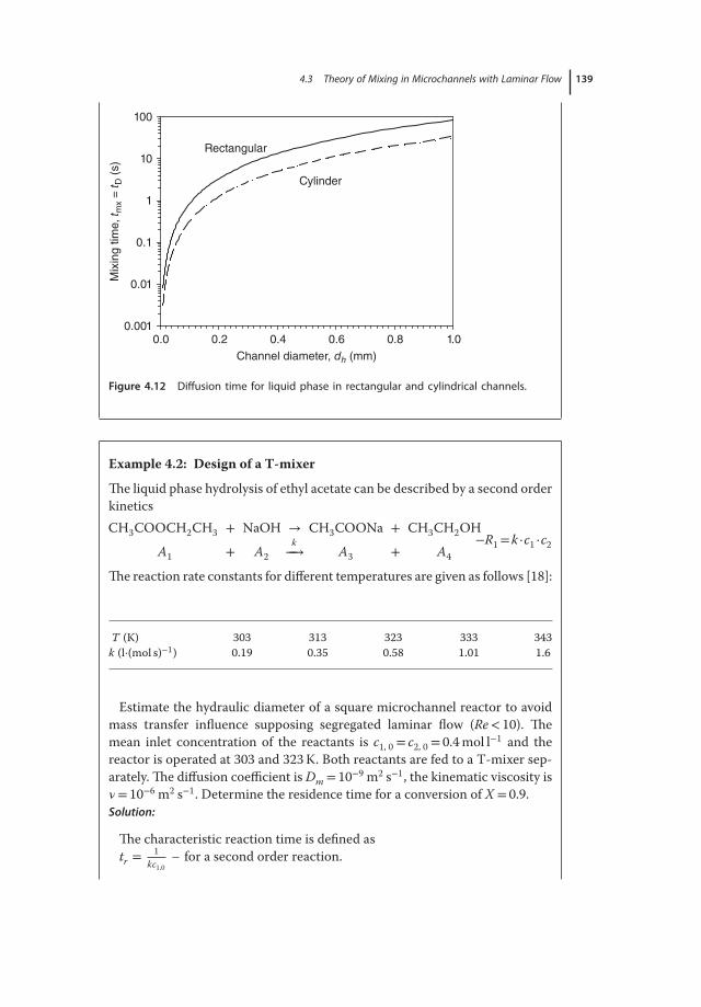
Example 4.1: Mixing in stratified laminar flow.
Investigate and plot the mixing time as a function of micromixer diameters
in the range of 10–1000 μm considering rectangular and cylindrical shapes
assuming stratified flow. The diffusion coefficient in the liquid is assumed to
be Dm = 10−9 m2 s−1.
Answer:
Themixing time is estimated based on Equations 4.17 and 4.18 (Figure 4.12):
Rectangular channel ∶ tmx = tD = A′ (dh∕2)2
Dm
;A′ = 1
3(rectangular channel)
4.3 Theory of Mixing in Microchannels with Laminar Flow 139
Channel diameter, dh (mm)
0.0 0.2 0.4 0.6 0.8 1.0
Mix
ing tim
e,
t mx =
t D (
s)
0.001
0.01
0.1
1
10
100
Cylinder
Rectangular
Figure 4.12 Diffusion time for liquid phase in rectangular and cylindrical channels.
Example 4.2: Design of a T-mixer
The liquid phase hydrolysis of ethyl acetate can be described by a second order
kinetics
CH3COOCH2CH3 + NaOH → CH3COONa + CH3CH2OH
A1 + A2
k−−→ A3 + A4
−R1=k ⋅c1 ⋅c2
The reaction rate constants for different temperatures are given as follows [18]:
T (K) 303 313 323 333 343k (l⋅(mol s)−1) 0.19 0.35 0.58 1.01 1.6
Estimate the hydraulic diameter of a square microchannel reactor to avoid
mass transfer influence supposing segregated laminar flow (Re< 10). The
mean inlet concentration of the reactants is c1, 0 = c2, 0 = 0.4mol l−1 and the
reactor is operated at 303 and 323K. Both reactants are fed to a T-mixer sep-
arately. The diffusion coefficient isDm = 10−9 m2 s−1, the kinematic viscosity is
𝜈 = 10−6 m2 s−1. Determine the residence time for a conversion of X = 0.9.
Solution:
The characteristic reaction time is defined as
tr =1
kc1,0– for a second order reaction.

140 4 Micromixing Devices
On the basis of the rate constants measured, the following characteristic
reaction times result:
T (K) 303 313 323 333 343tr (s) 13.2 7.14 4.31 2.48 1.56
To avoid the influence of mixing on the reaction kinetics, the mixing
time should be at least 10-fold shorter than the characteristic reaction time
(DaIImx ≤ 0.1).
Reaction temperature T = 303K:
tmx = 1.3 s. With A′ = 1/3 we obtain with Equation 4.17 dh = 125 μm.
Supposing plug flow pattern within the microchannel, for the conversion of
0.9, the residence time can be calculated: X = DaI
1+DaI= 0.9;DaI = 𝜏PFR
tr= 10 ⇒
𝜏PFR = 132s.
Reaction temperature T = 323K: tmx = 0.43 s; dh = 70 μm; 𝜏PFR = 43 s.
Reaction temperature T = 343K: tmx = 0.16 s; dh = 44 μm; 𝜏PFR = 16 s.
In laminar shear flow at Re> ca. 100 the dimension of the characteristic fluid
structure decreases in the direction orthogonal to the elongation as discussed in
Section 4.2. Therefore, diffusion and convection contribute simultaneously to the
mixing process. As diffusion is slow, convection is the dominant process for large
structures, and diffusion becomes the controlling step of mixing at small scale.
To estimate the overall mixing time, tmx, of intertwined lamellae the following
relation is proposed [19]:
tmx = tD+shear =1
2��arcsinh
(0.76 ⋅ �� ⋅ 2δ2
0
Dm
)(4.19)
where 𝛿0 is the original thickness of the lamella and �� is the shear rate.
Themean shear rate in laminar flow depends on the kinematic viscosity, 𝜈 of the
fluid, and the specific power dissipation, 𝜀, expressed in Wkg−1:
�� =(
𝜀
2ν
) 1
2(4.20)
The specific power dissipation is proportional to the flow rate and the pressure
drop. The pressure drop through open channels with laminar flow is given by the
Hagen-Poiseuille equation [20]:
Δp = 32𝜁𝜇u
d2t
Lt (4.21)
where 𝜁 is a geometric factor, which is 1 for circular tubes and it depends on
the height (H) to width (W ) ratio for rectangular channels. The correction fac-
tor becomes 0.89 for quadratic channels and assumes the asymptotic value 1.5
4.3 Theory of Mixing in Microchannels with Laminar Flow 141
when the ratio goes to zero, which corresponds to parallel plates. An empirical
correlation is given by the following expression [21]:
𝜁 = 0.8735 + 0.6265 exp(−3.636 H
W
)(4.22)
It follows for the specific power dissipation:
𝜀 =V ⋅ Δp𝜌 ⋅ V
= 32 ⋅ ν ⋅ u2
d2t
(circular channel) (4.23)
If the thickness of the lamella corresponds initially to the half diameter of the
microchannel, we obtain the following relationship for the characteristic mixing
time [17]:
tmx =dt8 ⋅ u
arcsinh(0.76 ⋅ Pe) =d2t ∕Dm
8 ⋅ Pearcsinh(0.76 ⋅ Pe)
with the Péclet number ∶ Pe = Re ⋅ Sc =u ⋅ dtDm
(4.24)
For Pe> 20 the arcsinh (0.76⋅Pe) can be replaced by ln (1.52 ⋅Pe) and Equation 4.24becomes:
tmx =d2t ∕Dm
8 ⋅ Peln(1.52 ⋅ Pe) = 1√
2
( ν𝜀
) 1
2ln(1.52 ⋅ Pe) (4.25)
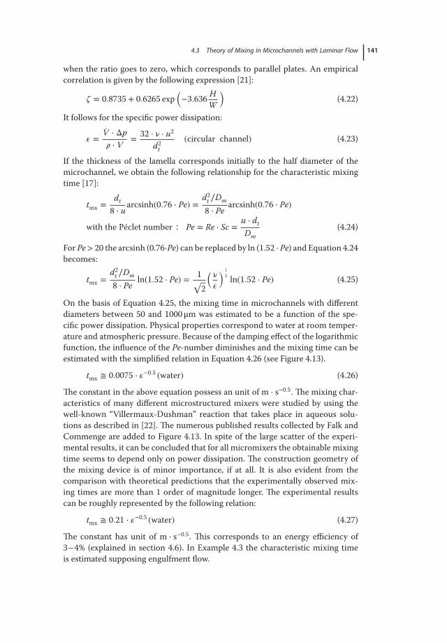
On the basis of Equation 4.25, the mixing time in microchannels with different
diameters between 50 and 1000 μm was estimated to be a function of the spe-
cific power dissipation. Physical properties correspond to water at room temper-
ature and atmospheric pressure. Because of the damping effect of the logarithmic
function, the influence of the Pe-number diminishes and the mixing time can be
estimated with the simplified relation in Equation 4.26 (see Figure 4.13).
tmx ≅ 0.0075 ⋅ 𝜀−0.5 (water) (4.26)
The constant in the above equation possess an unit of m ⋅ s−0.5. The mixing char-
acteristics of many different microstructured mixers were studied by using the
well-known “Villermaux-Dushman” reaction that takes place in aqueous solu-
tions as described in [22]. The numerous published results collected by Falk and
Commenge are added to Figure 4.13. In spite of the large scatter of the experi-
mental results, it can be concluded that for all micromixers the obtainable mixing
time seems to depend only on power dissipation. The construction geometry of
the mixing device is of minor importance, if at all. It is also evident from the
comparison with theoretical predictions that the experimentally observed mix-
ing times are more than 1 order of magnitude longer. The experimental results
can be roughly represented by the following relation:
tmx ≅ 0.21 ⋅ 𝜀−0.5 (water) (4.27)
The constant has unit of m ⋅ s−0.5. This corresponds to an energy efficiency of
3–4% (explained in section 4.6). In Example 4.3 the characteristic mixing time
is estimated supposing engulfment flow.
142 4 Micromixing Devices
Triangular
Mikroglas
Tangential
IMTEK
Caterpillar
IMM
Starlam
IMMT-mixer
100
10–1
10–2
10–3
10–4
10–5
100 101
Specific power dissipation, ε (W kg–1)
Mix
ing
tim
e,
t mx (
s)
102 103
Predicted
Experimental
104
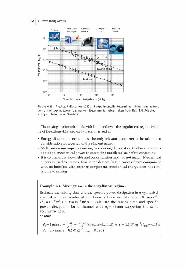
Figure 4.13 Predicted (Equation 4.25) and experimentally determined mixing time as func-
tion of the specific power dissipation. (Experimental values taken from Ref. [15]. Adapted
with permission from Elsevier.)
Themixing inmicrochannelswith laminar flow in the engulfment regime (valid-
ity of Equations 4.19 and 4.24) is summarized as
• Energy dissipation seems to be the only relevant parameter to be taken into
consideration for a design of the efficient mixer.
• Multilamination improves mixing by reducing the striation thickness, requires
additional mechanical power to create fine multilamellae before contacting.
• It is common that flow fields and concentration fields do notmatch.Mechanical
energy is used to create a flow in the devices, but in zones of pure component
with no interface with another component, mechanical energy does not con-
tribute to mixing.
Example 4.3: Mixing time in the engulfment regime.
Estimate the mixing time and the specific power dissipation in a cylindrical
channel with a diameter of dt = 1mm, a linear velocity of u = 0.2m ⋅ s−1.Dm = 10−9 m2 s−1, 𝜈 = 10−6 m2 s−1. Calculate the mixing time and specific
power dissipation for a channel with dt = 0.5mm supposing the same
volumetric flow.
Solution:
dt = 1mm: 𝜀 = V ⋅Δp𝜌⋅V
= 32⋅ν⋅u2
d2t(circularchannel) ⇒ 𝜀 = 1.3Wkg−1; tmx = 0.18 s
dt = 0.5mm: 𝜀= 82Wkg−1; tmx = 0.023 s.

4.4 Types of Micromixers and Mixing Principles 143
4.4
Types of Micromixers and Mixing Principles
As presented before, short radial diffusion lengths decrease the mixing time in
microchannels even at low flow rates in the laminar flow regime.Themixing time
can further be reduced using convectivemixing by creating eddies.The convective
diffusion enhancement is commonly employed in mixing devices using various
methods. A lot of efforts have been made to develop efficient micromixers, and
differentmixer concepts have been proposed [23, 24]. In general, two types ofmix-
ers can be distinguished: passive and active mixers. The former works essentially
with energy provided by pumping while the latter uses an external energy source
such as acoustic fields, electric fields (electrokinetic instability), ormicroimpellers.
Compared with active micromixers, passive mixers have the advantages of low
cost, and easy integration in the microfluidic systems, no complex control units,
and no additional power input.
For chemical reactions, micromixers are mounted in front of a residence time
unit that provides the required residence time for the reaction to complete. The
choice of the micromixer to be used depends on the characteristic reaction time.
The mixing time should be at least 10 times shorter compared to the reaction
time to avoid losses in reactor performance and product selectivity as discussed
in Section 4.1. Besides mixing efficiency, heat transfer potential is an important
issue for fast exothermic reaction as is discussed in Chapter 5.
A series of micromixers with different types of mixing elements have been
developed using different mixing principles as listed in Table 4.1 and depicted in
Figure 4.14. In the case of passive mixing, the flow that is caused by pumping or
hydrostatic potential is restructured in order to get faster mixing. Thin lamellae
are created in special feed arrangements, termed interdigital. A commonly used
method to enhance passive mixing in microchannels is to distribute the flow
into compartments and reduce diffusion paths beyond the geometric dimensions
of the mixing microchannel. For instance, splitting and recombining the feed
streams or the injection of substreams via a special microstructure can break
the laminar profile and better mixing can be achieved [25]. Chaotic mixing
Table 4.1 Passive and active mixing techniques used in micromixers.
Passive mixing Active mixing
Interdigital multilamellae arrangements UltrasoundSplit-and-recombine concepts (SAR) Acoustically induced vibrationsChaotic mixing by eddy formation and folding Electrokinetic instabilitiesDroplet binding in two-phase environment Periodical variation of pressure fieldNozzle injection in flow Electrowetting-induced joint of dropletsSpecialties, e.g., Coanda effect Magnetohydrodynamic action
Small impellersPiecoelectrically vibrating membraneIntegrated micro valves/pumps
144 4 Micromixing Devices
Splitting andrecombination
Forced masstransport
Periodic injection
High energy collision Contacting
Injection of substreams to a main stream
Decrease ofdiffusion path
Injection of substreams
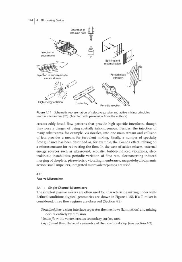
Figure 4.14 Schematic representation of selective passive and active mixing principles
used in micromixers [26]. (Adapted with permission from the authors.)
creates eddy-based flow patterns that provide high specific interfaces, though
they pose a danger of being spatially inhomogenous. Besides, the injection of
many substreams, for example, via nozzles, into one main stream and collision
of jets provides a means for turbulent mixing. Finally, a number of specialty
flow guidance has been described as, for example, the Coanda effect, relying on
a microstructure for redirecting the flow. In the case of active mixers, external
energy sources such as ultrasound, acoustic, bubble-induced vibrations, elec-
trokinetic instabilities, periodic variation of flow rate, electrowetting-induced
merging of droplets, piezoelectric vibrating membranes, magnetohydrodynamic
action, small impellers, integrated microvalves/pumps are used.
4.4.1
Passive Micromixer
4.4.1.1 Single-Channel Micromixers
The simplest passive mixers are often used for characterizing mixing under well-
defined conditions (typical geometries are shown in Figure 4.15). If a T-mixer is
considered, three flow regimes are observed (Section 4.2):
Stratified flow: a clear interface separates the two flows (lamination) andmixing
occurs entirely by diffusion
Vortex flow: the vortex creates secondary surface area
Engulfment flow: the axial symmetry of the flow breaks up (see Section 4.2).
4.4 Types of Micromixers and Mixing Principles 145
(b) (c)(a)
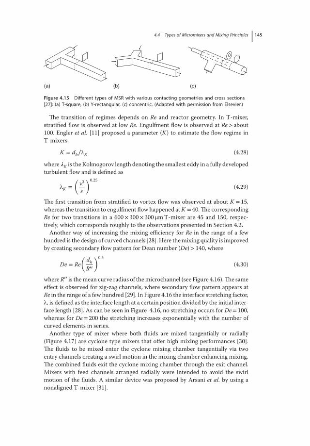
Figure 4.15 Different types of MSR with various contacting geometries and cross sections
[27]: (a) T-square, (b) Y-rectangular, (c) concentric. (Adapted with permission from Elsevier.)
The transition of regimes depends on Re and reactor geometry. In T-mixer,
stratified flow is observed at low Re. Engulfment flow is observed at Re> about
100. Engler et al. [11] proposed a parameter (K ) to estimate the flow regime in
T-mixers.
K = dh∕λK (4.28)
where 𝜆K is the Kolmogorov length denoting the smallest eddy in a fully developed
turbulent flow and is defined as
λK =(ν3𝜀
)0.25
(4.29)
The first transition from stratified to vortex flow was observed at about K = 15,
whereas the transition to engulfment flow happened atK = 40.The corresponding
Re for two transitions in a 600× 300× 300 μmT-mixer are 45 and 150, respec-
tively, which corresponds roughly to the observations presented in Section 4.2.
Another way of increasing the mixing efficiency for Re in the range of a few
hundred is the design of curved channels [28]. Here themixing quality is improved
by creating secondary flow pattern for Dean number (De)> 140, where
De = Re
(dhR′′
)0.5
(4.30)
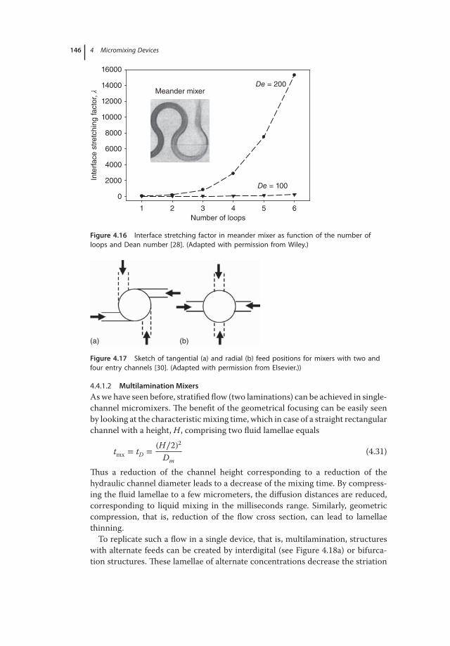
whereR′′ is themean curve radius of themicrochannel (see Figure 4.16).The same
effect is observed for zig-zag channels, where secondary flow pattern appears at
Re in the range of a few hundred [29]. In Figure 4.16 the interface stretching factor,
λ, is defined as the interface length at a certain position divided by the initial inter-face length [28]. As can be seen in Figure 4.16, no stretching occurs for De= 100,
whereas for De= 200 the stretching increases exponentially with the number of
curved elements in series.
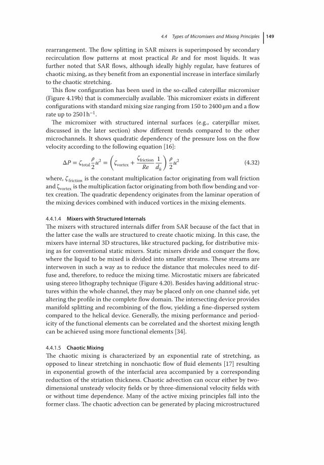
Another type of mixer where both fluids are mixed tangentially or radially
(Figure 4.17) are cyclone type mixers that offer high mixing performances [30].
The fluids to be mixed enter the cyclone mixing chamber tangentially via two
entry channels creating a swirl motion in the mixing chamber enhancing mixing.
The combined fluids exit the cyclone mixing chamber through the exit channel.
Mixers with feed channels arranged radially were intended to avoid the swirl
motion of the fluids. A similar device was proposed by Arsani et al. by using a
nonaligned T-mixer [31].
146 4 Micromixing Devices
Number of loops
1 2 3 4 5 6
Inte
rface s
tretc
hin
g facto
r, λ
0
2000
4000
6000
8000
10000
12000
14000
16000
De = 200
De = 100
Meander mixer
Figure 4.16 Interface stretching factor in meander mixer as function of the number of
loops and Dean number [28]. (Adapted with permission from Wiley.)
(a) (b)
Figure 4.17 Sketch of tangential (a) and radial (b) feed positions for mixers with two and
four entry channels [30]. (Adapted with permission from Elsevier.))
4.4.1.2 Multilamination Mixers
Aswe have seen before, stratified flow (two laminations) can be achieved in single-
channel micromixers. The benefit of the geometrical focusing can be easily seen
by looking at the characteristicmixing time, which in case of a straight rectangular
channel with a height, H , comprising two fluid lamellae equals
tmx = tD =(H∕2)2
Dm
(4.31)
Thus a reduction of the channel height corresponding to a reduction of the
hydraulic channel diameter leads to a decrease of the mixing time. By compress-
ing the fluid lamellae to a few micrometers, the diffusion distances are reduced,
corresponding to liquid mixing in the milliseconds range. Similarly, geometric
compression, that is, reduction of the flow cross section, can lead to lamellae
thinning.
To replicate such a flow in a single device, that is, multilamination, structures
with alternate feeds can be created by interdigital (see Figure 4.18a) or bifurca-
tion structures. These lamellae of alternate concentrations decrease the striation

4.4 Types of Micromixers and Mixing Principles 147
(a) Slit-type interdigital micromixer (b) Superfocus micromixer
(c) Flow pattern in a cyclone micromixer (d) Star lamination micromixer
Flow distribution zone
Mixing channel for
generation of multi-
lamellae
500 μm
Figure 4.18 Different types of multil-
amination micromixers. (a) liquid flows
10–1000ml h−1, (b) 138 microchannels flow:
350 l h−1 at 3.5 bar, (c) 20ml h−1, and (d)
snapshot of mixer for throughput <300 l h−1,pressure drop 7.6 bar [32]. (Adapted with per-
mission from Elsevier.)
thickness resulting in low diffusion time. Multilaminating flow configurations can
be realized by different types of feed arrangements. Bifurcation-type feeds create
an alternate arrangement of feeds. Such a laminated feed stream passes into an
inverse bifurcation structure and a subsequent folded delay-loop channel where
mixing takes place. The channel width of the feeds of most interdigital arrange-
ments is chosen in a way that the width of the corresponding liquid lamellae is
rather thick (e.g., 100 μm), that is, diffusion is not very effective. Therefore, a sec-
ondmomentum for speeding upmixing is employed. In analogy to thewell-known
hydrodynamic focusing concept (for a single streamor for two streams), themulti-
laminated flows are focused by posing geometric constraints (typically a triangular
focusing chamber), thereby compressing the lamellae.
Theflowpatterns in liquids can be confirmedusing photographic analysis before
and after focusing. These lamellae can tilt and, at high Re, spirally wind and form
recirculations, if the focusing angle is set too large. In the case of gas mixing in
an interdigital microstructured mixer, similar periodic multilamination patterns
were determined by a tiny gas-collecting nozzle that wasmoved within themixing
chamber of interdigital mixers. At high velocities of the gas streams, anomalously
high mixing efficiencies were found at a certain axial distance along the mixing
chamber. This observed faster mixing was explained with additional turbulent
mixing because of the collision of gas streams owing to the tilted injection via

148 4 Micromixing Devices
the interdigital feed. It was found that the mixing energy of these microstructured
mixers normalized by the volume for a given mixing task is lower than that of an
industrially employed jet mixer.
A special liquid focusing interdigital mixer with parallel feed flows, termed
SuperFocus, was optimized by semianalytical calculations and first realized as
a glass version with 128 nozzles (8 h−1 at 3.5 bar) and later as a steel version
(350 h−1 at 10 bar) with 138 nozzles. Both versions yield 4 μm thin liquid lamellae.
A mixing time (for 95% completion of mixing) of 4ms, excluding the time needed
for passing the focusing chamber, can be obtained by photometric measurement
for the SuperFocus mixer, corresponding to some centimeter mixing length
at most practical throughputs. Different cross sections are used to optimize
the focusing chamber to reduce the residence time within this flow passage to
shorten the overall mixing time.
The cyclone mixer is another micromixer that can also be multilaminated. In
the high-throughput Star laminators (Figure 4.18d), the fluid feed resembles an
alternating (interdigital) flow injection. Owing to the large internal opening and
the typically applied large volume flows, the flow regime, however, is turbulent
so that a prelayered flow is consecutively mixed by eddy formation. As the plates
can be manufactured at low cost and a large number of plates, for example, sev-
eral hundred, can be stacked, extremely large throughputs can be achieved already
for devices of small external volume (StarLam300 – 1000 l h−1 (3 bar) and Star-
Lam3000 – 5m3 h−1 (about 3 bar)). The determined mixing efficiencies reach the
limits that are usually attributed to good mixing in macro- and microstructured
mixers.
4.4.1.3 Split-and-Recombine (SAR) Flow Configurations
Unlike commonly applied interdigital multilamination approach, split-and-
recombine (SAR) mixing relies on a multistep procedure. According to its name,
the basic operations are the splitting of a bi- or multilayered stream perpendicular
to the lamella orientation into substreams and their subsequent recombination
[33]. This concept is schematically represented in Figure 4.19a. For this purpose,
basically three steps are required: flow splitting, flow recombination, and flow
(a) (b)
Figure 4.19 Caterpillar mixer. (a) Schematic of SAR showing structured walls. (b) Snap-
shot of the 600 μm size caterpillar mixer. The size is defined for entrance channel. Courtesy
Fraunhofer ICT-IMM, Germany.
4.4 Types of Micromixers and Mixing Principles 149
rearrangement. The flow splitting in SAR mixers is superimposed by secondary
recirculation flow patterns at most practical Re and for most liquids. It was
further noted that SAR flows, although ideally highly regular, have features of
chaotic mixing, as they benefit from an exponential increase in interface similarly
to the chaotic stretching.
This flow configuration has been used in the so-called caterpillar micromixer
(Figure 4.19b) that is commercially available. This micromixer exists in different
configurations with standard mixing size ranging from 150 to 2400 μm and a flow
rate up to 250 l h−1.
The micromixer with structured internal surfaces (e.g., caterpillar mixer,
discussed in the later section) show different trends compared to the other
microchannels. It shows quadratic dependency of the pressure loss on the flow
velocity according to the following equation [16]:
ΔP = 𝜁total𝜌
2u2 =
(𝜁vortex +
𝜁friction
Re
1
dh
)𝜌
2u2 (4.32)
where, 𝜁 friction is the constant multiplication factor originating from wall friction
and ζvortex is themultiplication factor originating from both flow bending and vor-
tex creation. The quadratic dependency originates from the laminar operation of
the mixing devices combined with induced vortices in the mixing elements.
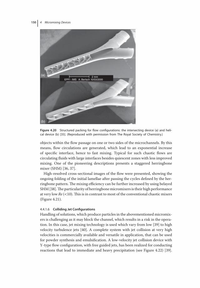
4.4.1.4 Mixers with Structured Internals
The mixers with structured internals differ from SAR because of the fact that in
the latter case the walls are structured to create chaotic mixing. In this case, the
mixers have internal 3D structures, like structured packing, for distributive mix-
ing as for conventional static mixers. Static mixers divide and conquer the flow,
where the liquid to be mixed is divided into smaller streams. These streams are
interwoven in such a way as to reduce the distance that molecules need to dif-
fuse and, therefore, to reduce the mixing time. Microstatic mixers are fabricated
using stereo lithography technique (Figure 4.20). Besides having additional struc-
tures within the whole channel, they may be placed only on one channel side, yet
altering the profile in the complete flow domain.The intersecting device provides
manifold splitting and recombining of the flow, yielding a fine-dispersed system
compared to the helical device. Generally, the mixing performance and period-
icity of the functional elements can be correlated and the shortest mixing length
can be achieved using more functional elements [34].
4.4.1.5 Chaotic Mixing
The chaotic mixing is characterized by an exponential rate of stretching, as
opposed to linear stretching in nonchaotic flow of fluid elements [17] resulting
in exponential growth of the interfacial area accompanied by a corresponding
reduction of the striation thickness. Chaotic advection can occur either by two-
dimensional unsteady velocity fields or by three-dimensional velocity fields with
or without time dependence. Many of the active mixing principles fall into the
former class. The chaotic advection can be generated by placing microstructured
150 4 Micromixing Devices
(a)
(b)
2 mmEPFl - IMS A. Bertsch 10/03/2000
Figure 4.20 Structured packing for flow configurations: the intersecting device (a) and heli-
cal device (b) [35]. (Reproduced with permission from The Royal Society of Chemistry.)
objects within the flow passage on one or two sides of the microchannels. By this
means, flow circulations are generated, which lead to an exponential increase
of specific interface, hence to fast mixing. Typical for such chaotic flows are
circulating fluids with large interfaces besides quiescent zones with less improved
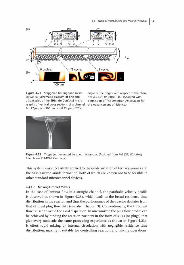
mixing. One of the pioneering descriptions presents a staggered herringbone
mixer (SHM) [36, 37].
High-resolved cross-sectional images of the flow were presented, showing the
ongoing folding of the initial lamellae after passing the cycles defined by the her-
ringbone pattern.Themixing efficiency can be further increased by using belayed
SHM[38].Theparticularity of herringbonemicromixers is their high performance
at very low Re (<10).This is in contrast to most of the conventional chaotic mixers
(Figure 4.21).
4.4.1.6 Colliding Jet Configurations
Handling of solutions, which produce particles in the abovementionedmicromix-
ers is challenging as it may block the channel, which results in a risk in the opera-
tion. In this case, jet mixing technology is used which vary from low [39] to high
velocity turbulence jets [40]. A complete system with jet collision at very high
velocities is commercially available and versatile in application, that can be used
for powder synthesis and emulsification. A low-velocity jet collision device with
Y-type flow configuration, with free guided jets, has been realized for conducting
reactions that lead to immediate and heavy precipitation (see Figure 4.22) [39].
4.4 Types of Micromixers and Mixing Principles 151
x
(a)
(b)
w
h
0 cycles: 1/2 cycle: 1 cycle:
αh2π/q
100 μm
z
x
z
u u
h h
c c
pw
d u u
xy
z
c c
pw
d
Δϕm
Δϕm
Δϕm
Figure 4.21 Staggered herringbone mixer
(SHM). (a) Schematic diagram of one-and-
a-halfcycles of the SHM. (b) Confocal micro-
graphs of vertical cross sections of a channel.
h= 77 μm, w= 200 μm, 𝛼 = 0.23, pw= 2/3w,
angle of the ridges with respect to the chan-
nel, 𝜃 = 45∘ , Re< 0.01 [36]. (Adapted with
permission of The American Association for
the Advancement of Science.)
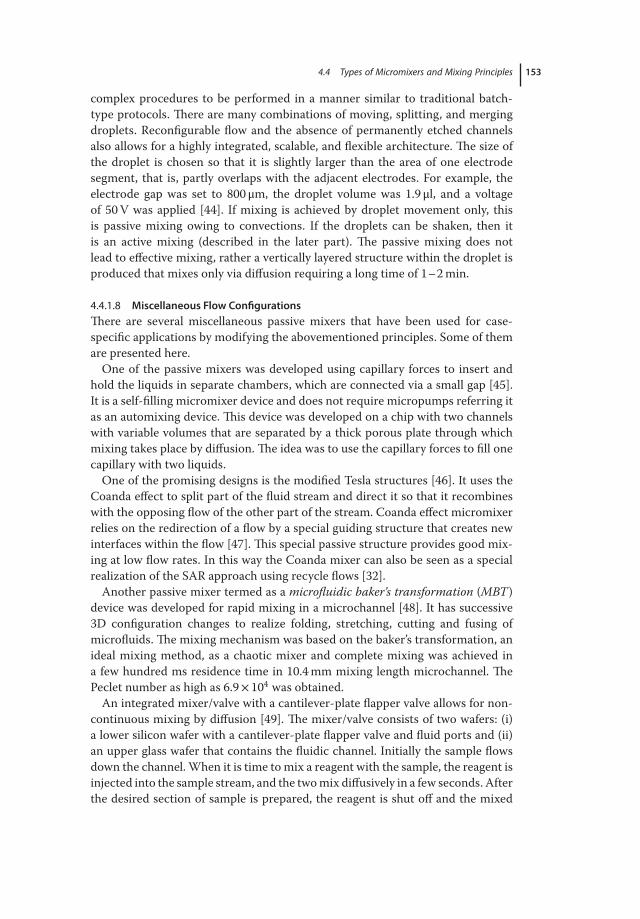
Figure 4.22 Y-type jet generated by a jet micromixer. (Adapted from Ref. [39] (Courtesy
Fraunhofer ICT-IMM, Germany.)
This system was successfully applied to the quaternization of ternary amines and
the base-assisted amide formation, both of which are known not to be feasible in
other standard microchannel devices.
4.4.1.7 Moving Droplet Mixers
In the case of laminar flow in a straight channel, the parabolic velocity profile
is observed as shown in Figure 4.23a, which leads to the broad residence time
distribution in the reactor, and thus the performance of the reactor deviates from
that of ideal plug flow [41] (see also Chapter 3). Conventionally, the turbulent
flow is used to avoid the axial dispersion. In micromixer, the plug flow profile can
be achieved by binding the reaction partners in the form of slugs (or plugs) that
give every molecule the same processing experience as shown in Figure 4.23b.
It offers rapid mixing by internal circulation with negligible residence time
distribution, making it suitable for controlling reaction and mixing operations.

152 4 Micromixing Devices
(b)(a)
A
AB
AB
B C+ →
A B C+ → A B C+ → A B C+ →Carrier
Figure 4.23 Moving droplet mixers (schematic): (a) typical laminar profile, (b) homoge-
neous mixing in biphasic mode.
Different arrangements, axial and radial arrangements of reactants within slugs,
can be achieved with the former arrangement of reactants giving higher mixing
performances than the radial arrangement at the same Peclet number [42].
Besides, bending the microchannels in different angles mixing in the slugs can be
altered as shown in Figure 4.24.
This concept is also used for kinetics study of fast homogenous reactions with
characteristic reaction times in the range of milliseconds. Further examples are
precipitations and the reactions that use reagents in the nanoliter scale.
Another method of droplet-based mixing is via electrowetting, which is based
on the change of surface energies by applying electric fields [44]. This technique
differs from continuous flow systems in which discrete droplets are manipulated
rather than continuous liquid streams and possess a number of advantages over
the latter such as the ability to control each droplet independently, enabling
REORIENT
(a)
(c)
(b)
StretchAND fold
Flow within plugs
(i)
Smooth turns
(i) (ii)
50 μm 50 μm
(ii)
Sharp turns
Figure 4.24 Chaotic mixing in droplets
[43]. (a) Schematic of straight portions of the
channel performs stretching and folding, and
turns allow for reorientation. (b) Schematic of
recirculating flow in plugs moving through
smooth and sharp turns. (c) Snapshots of
the microfluidic network in which flow pat-
terns inside plugs in different positions in
the microchannel demonstrate flow patterns.
(Adapted with permission from The Royal
Society.)
4.4 Types of Micromixers and Mixing Principles 153
complex procedures to be performed in a manner similar to traditional batch-
type protocols. There are many combinations of moving, splitting, and merging
droplets. Reconfigurable flow and the absence of permanently etched channels
also allows for a highly integrated, scalable, and flexible architecture. The size of
the droplet is chosen so that it is slightly larger than the area of one electrode
segment, that is, partly overlaps with the adjacent electrodes. For example, the
electrode gap was set to 800 μm, the droplet volume was 1.9 μl, and a voltage
of 50V was applied [44]. If mixing is achieved by droplet movement only, this
is passive mixing owing to convections. If the droplets can be shaken, then it
is an active mixing (described in the later part). The passive mixing does not
lead to effective mixing, rather a vertically layered structure within the droplet is
produced that mixes only via diffusion requiring a long time of 1–2min.
4.4.1.8 Miscellaneous Flow Configurations
There are several miscellaneous passive mixers that have been used for case-
specific applications by modifying the abovementioned principles. Some of them
are presented here.
One of the passive mixers was developed using capillary forces to insert and
hold the liquids in separate chambers, which are connected via a small gap [45].
It is a self-filling micromixer device and does not require micropumps referring it
as an automixing device. This device was developed on a chip with two channels
with variable volumes that are separated by a thick porous plate through which
mixing takes place by diffusion. The idea was to use the capillary forces to fill one
capillary with two liquids.
One of the promising designs is the modified Tesla structures [46]. It uses the
Coanda effect to split part of the fluid stream and direct it so that it recombines
with the opposing flow of the other part of the stream. Coanda effect micromixer
relies on the redirection of a flow by a special guiding structure that creates new
interfaces within the flow [47]. This special passive structure provides good mix-
ing at low flow rates. In this way the Coanda mixer can also be seen as a special
realization of the SAR approach using recycle flows [32].
Another passive mixer termed as a microfluidic baker’s transformation (MBT)
device was developed for rapid mixing in a microchannel [48]. It has successive
3D configuration changes to realize folding, stretching, cutting and fusing of
microfluids. The mixing mechanism was based on the baker’s transformation, an
ideal mixing method, as a chaotic mixer and complete mixing was achieved in
a few hundred ms residence time in 10.4mm mixing length microchannel. The
Peclet number as high as 6.9× 10⁴ was obtained.
An integrated mixer/valve with a cantilever-plate flapper valve allows for non-
continuous mixing by diffusion [49]. The mixer/valve consists of two wafers: (i)
a lower silicon wafer with a cantilever-plate flapper valve and fluid ports and (ii)
an upper glass wafer that contains the fluidic channel. Initially the sample flows
down the channel. When it is time tomix a reagent with the sample, the reagent is
injected into the sample stream, and the twomix diffusively in a few seconds. After
the desired section of sample is prepared, the reagent is shut off and the mixed
154 4 Micromixing Devices
sample and reagent flow down the channel and out of the mixer/valve. The liquid
mixer/valve is controlled by varying the reagent and sample flow rates. The rela-
tive flow rates in turn determine the mixing ratio and the pressures at the reagent
and sample ports; the cantilever plate aligns itself accordingly.
4.4.2
Active Micromixers
In contrast to the presented passive mixers, active micromixers rely on exter-
nal power input to introduce perturbations within the laminar flow to accelerate
mixing. A selection of different external perturbation sources are summarized in
Table 4.1 and are discussed briefed here.
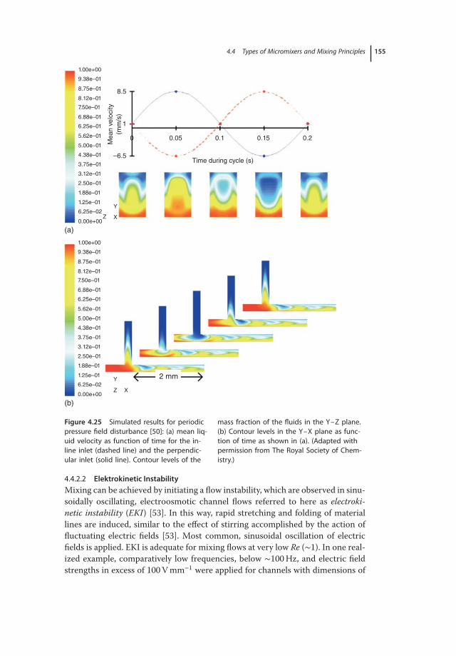
4.4.2.1 Pressure Induced Disturbances
Mixing in stratified laminar flow relies on molecular diffusion. Therefore, mixing
time for liquids is in the order of seconds in microchannels with diameters in the
range of about 100 μm. A very simple method to disturb the fluid flow consists in
superimposing a pulsating flow in the inlet of the channels. Glasgow and Aubry
[50] used a simple T-shaped mixer to demonstrate the effective flow disturbance
at very low Re (≥0.3) by varying the inlet flow in a sine wave fashion.
Time pulsing of one inlet flow rate distorts the interface to an asymmetrically
curved shape, which changes with time-influencing material transport and thus
the mixing. The periodicity and the number of pulsing streams have a notable
influence of the mixing efficiency. The best results are reported for two pulsed
inlet flows having a phase difference of 180∘ with amplitude and frequency being
the same [50].The simulated results are reproduced in Figure 4.25 for a mean flow
velocity of 1mms−1 and a perturbation frequency of 5Hz. Besides, the bending
of the fluid interface along the channel cross section and the respective stretching
and folding in the direction of the flow increases the mixing further. This concept
can be extended to the multiple, pulsing injection of flows into one microchannel;
such devices are so far hypothetical and certainly would require a complex control
system [51]. By these means, chaotic advection can be generated.
For electroosmotic-driven flow, periodic flow switching can be achieved in a
similar way, now by using nonuniform 𝜉 potentials along the conduits walls to
induce chaotic advection [52]. Both spatial and temporal control of the 𝜉 poten-
tial can be achieved by imposing an electric field perpendicular to the solid–liquid
interface. The nonuniformity of the 𝜉 potentials induces complex flow patterns
in the conduit. By appropriate time modulation of the 𝜉 potential, one can alter-
nate among two or more flow patterns and induce chaotic advection and effi-
cient stirring in the conduit. There are many choices for possible flow patterns.
The selection of combinations that lead to the most efficient stirring process is
an interesting optimization problem. Such a method is particularly beneficial for
microfluidic systems where incorporation of moving components is difficult.
4.4 Types of Micromixers and Mixing Principles 155
1.00e+00
9.38e–01
8.75e–01
8.12e–01
7.50e–01
6.88e–01
6.25e–01
5.62e–01
5.00e–01
4.38e–01 –6.5
1
0 0.05 0.1
Time during cycle (s)
0.15 0.2
Mean v
elo
city
(mm
/s)
8.5
3.75e–01
3.12e–01
2.50e–01
1.88e–01
1.25e–01
6.25e–02X
Y
Z
X
2 mmY
Z
0.00e+00
(a)
(b)
1.00e+00
9.38e–01
8.75e–01
8.12e–01
7.50e–01
6.88e–01
6.25e–01
5.62e–01
5.00e–01
4.38e–01
3.75e–01
3.12e–01
2.50e–01
1.88e–01
1.25e–01
6.25e–02
0.00e+00
Figure 4.25 Simulated results for periodic
pressure field disturbance [50]: (a) mean liq-
uid velocity as function of time for the in-
line inlet (dashed line) and the perpendic-
ular inlet (solid line). Contour levels of the
mass fraction of the fluids in the Y–Z plane.
(b) Contour levels in the Y–X plane as func-
tion of time as shown in (a). (Adapted with
permission from The Royal Society of Chem-
istry.)
4.4.2.2 Elektrokinetic Instability
Mixing can be achieved by initiating a flow instability, which are observed in sinu-
soidally oscillating, electroosmotic channel flows referred to here as electroki-
netic instability (EKI) [53]. In this way, rapid stretching and folding of material
lines are induced, similar to the effect of stirring accomplished by the action of
fluctuating electric fields [53]. Most common, sinusoidal oscillation of electric
fields is applied. EKI is adequate for mixing flows at very low Re (∼1). In one real-
ized example, comparatively low frequencies, below ∼100Hz, and electric field
strengths in excess of 100Vmm−1 were applied for channels with dimensions of
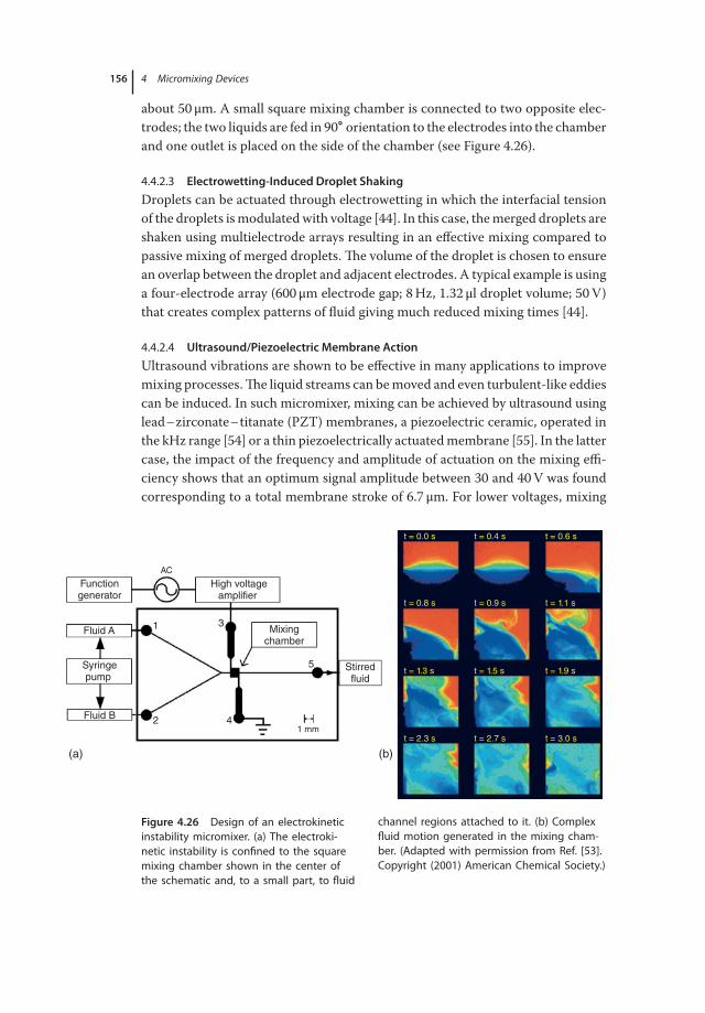
156 4 Micromixing Devices
about 50 μm. A small square mixing chamber is connected to two opposite elec-
trodes; the two liquids are fed in 90∘ orientation to the electrodes into the chamber
and one outlet is placed on the side of the chamber (see Figure 4.26).
4.4.2.3 Electrowetting-Induced Droplet Shaking
Droplets can be actuated through electrowetting in which the interfacial tension
of the droplets ismodulatedwith voltage [44]. In this case, themerged droplets are
shaken using multielectrode arrays resulting in an effective mixing compared to
passive mixing of merged droplets. The volume of the droplet is chosen to ensure
an overlap between the droplet and adjacent electrodes. A typical example is using
a four-electrode array (600 μm electrode gap; 8Hz, 1.32 μl droplet volume; 50V)
that creates complex patterns of fluid giving much reduced mixing times [44].
4.4.2.4 Ultrasound/Piezoelectric Membrane Action
Ultrasound vibrations are shown to be effective in many applications to improve
mixing processes.The liquid streams can bemoved and even turbulent-like eddies
can be induced. In such micromixer, mixing can be achieved by ultrasound using
lead–zirconate–titanate (PZT) membranes, a piezoelectric ceramic, operated in
the kHz range [54] or a thin piezoelectrically actuatedmembrane [55]. In the latter
case, the impact of the frequency and amplitude of actuation on the mixing effi-
ciency shows that an optimum signal amplitude between 30 and 40V was found
corresponding to a total membrane stroke of 6.7 μm. For lower voltages, mixing
AC
Functiongenerator
Fluid A1 3
2 4
5
1 mm
Fluid B
High voltageamplifier
Syringepump
Mixingchamber
Stirredfluid
(a) (b)
t = 0.0 s t = 0.4 s t = 0.6 s
t = 0.8 s t = 0.9 s t = 1.1 s
t = 1.3 s t = 1.5 s t = 1.9 s
t = 2.3 s t = 2.7 s t = 3.0 s
Figure 4.26 Design of an electrokinetic
instability micromixer. (a) The electroki-
netic instability is confined to the square
mixing chamber shown in the center of
the schematic and, to a small part, to fluid
channel regions attached to it. (b) Complex
fluid motion generated in the mixing cham-
ber. (Adapted with permission from Ref. [53].
Copyright (2001) American Chemical Society.)
4.4 Types of Micromixers and Mixing Principles 157
is incomplete. At higher amplitude, no further improvement was noted. Owing to
the very small mixing chamber, fast changes of mixing can be induced.
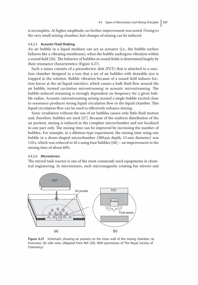
4.4.2.5 Acoustic Fluid Shaking
An air bubble in a liquid medium can act as actuator (i.e., the bubble surface
behaves like a vibrating membrane), when the bubble undergoes vibration within
a sound field [56].The behavior of bubbles in sound fields is determined largely by
their resonance characteristics (Figure 4.27).
Such a mixer consists of a piezoelectric disk (PZT) that is attached to a reac-
tion chamber designed in a way that a set of air bubbles with desirable size is
trapped in the solution. Bubble vibration because of a sound field induces fric-
tion forces at the air/liquid interface, which causes a bulk fluid flow around the
air bubble, termed cavitation microstreaming or acoustic microstreaming. The
bubble-induced streaming is strongly dependent on frequency for a given bub-
ble radius. Acoustic microstreaming arising around a single bubble excited close
to resonance produces strong liquid circulation flow in the liquid chamber. This
liquid circulation flow can be used to effectively enhance mixing.
Sonic irradiation without the use of air bubbles causes only little fluid motion
and, therefore, bubbles are used [57]. Because of the uniform distribution of the
air pockets, mixing is induced in the complete microchamber and not localized
to one part only. The mixing time can be improved by increasing the number of
bubbles. For example, in a dilution-type experiment, the mixing time using one
bubble in a drum-shaped microchamber (300 μm depth; 15mm diameter) was
110 s, which was reduced to 45 s using four bubbles [56] – an improvement in the
mixing time of about 60%.
4.4.2.6 Microstirrers
The stirred tank reactor is one of the most commonly used equipments in chem-
ical engineering. In micromixers, such micromagnetic rotating bar stirrers and
PZT
Bubble
Air pocket
Fluid stream
PZT
(a) (b)
Figure 4.27 Schematic showing air pockets on the inner wall of the mixing chamber. (a)
Overview; (b) side view. (Adapted from Ref. [56]. With permission of The Royal Society of
Chemistry.)
158 4 Micromixing Devices
arrays have been designed using the principles of macroscopic mixers [58]. The
centerpiece of the mixer is a rotating bar (rotor) made of a ferromagnetic material
consisting of a cap, hub, and two rotary blades. The new mixing principle offers
several advantages like rapid mixing that can be realized within the characteristic
length of a stirrer bar and externally applied magnetic actuation, which requires
no wires and reduces complexity.
Themixer can be used for a wide variety of fluids with different electrochemical
characteristics.
4.4.2.7 Miscellaneous Active Micromixers
A special micromixer has been designed for cyclic reaction using alternating
current (AC) magnetohydrodynamic (MHD) actuation [59]. It utilizes arrays of
electrodes deposited on the walls of a microchannel. The experimental apparatus
comprised an AC power source connected in series to the MHD chip and an
electromagnet. Through alternate potential differences across pairs of electrodes,
currents in various directions of the mixing volume are generated. By coupling
an electric and a magnetic field, forces are exerted on the fluid. The MHD
actuation is favored for applications involving strong electrolytes or even ionic
liquids, where pumping methods such as electroosmotic flow are compromised.
Annular MHD reactors are one of the examples of systems for conducting
architecture-controlled chemistry, meaning the chemistry that requires careful
consideration of channel design, material choice, and actuation technique.
4.5
Experimental Characterization of Mixing Efficiency
For the proper design of a chemical reactor, the mixing time for the separated fed
reactants must be adapted to the reaction kinetics and the characteristic reaction
time (see Section 4.1). A variety of different experimental methods are developed
and used to characterize themixing process.Thesemethods can be broadly classi-
fied as physical and chemical methods.The application of these methods depends
on the size of mixer, optical characteristics of the wall material, that is, transpar-
ent or opaque, flow throughput, and the precision of mixing quality needed for a
given application of mixer. The mixing quality is defined either in terms of degree
of segregation (no mixing) or intensity of mixing.
Danckwerts defined the intensity of segregation in turbulent flow, Is, in terms
of the mean square of the concentration fluctuation as shown in Figure 4.3 and
defined in Equations 4.1–4.4. The efficiency of mixing is in the range between 1
and 0.
4.5.1
Physical Methods
Physical methods to characterize the mixing efficiency are based on the use of an
inert tracer, which differs in color, conductivity, or optical density from the main
4.5 Experimental Characterization of Mixing Efficiency 159
fluid.The tracer concentration ismonitored bymeasuring the color, electrical con-
ductivity, pH, and so on as function of time. One of the prerequisites for the use
of optical method is that the micromixer should be transparent to track the color
change ofmixed solutionswith a reasonable spatial resolution. Visualization of the
color spreading along the channel of a continuous mixer using a high-resolution
photographic system gives information about the mixing process.
In a more precise method of investigation, the local concentration in a con-
trolled volume is considered. This allows determining the concentration fluctua-
tions referred to the mean.
It is evident that the degree of mixing measured experimentally will depend on
the spatial resolution of the probe used to estimate the local concentration in the
mixture. Depending on the kind of application, a decrease in the length scales
on which these variations are present or reduction in their amplitude or both are
desired.
There are several limitations to optical techniques as described in the following:
• The visualization is done usually perpendicularly to the flow direction, and
therefore, the analyzed image gives color intensity value over a mixer depth
meaning that the visually uniform color concentration may be interpreted
either as a complete mixing or as a regular multilamellae flow of various
concentrations. This results in inappropriate investigation of mixing time.
• Besides, even in the case of transparent device, the analysis can be done only for
very simple microchannel geometry without internal structures.
• Finally, if the sampling volume is larger than the smallest segregation scale, then
it is difficult to determine whether the two fluids are mixed or not within the
measurement resolution.
4.5.2
Chemical Methods
As explained before, physical methods possess severe limitations and, therefore,
chemical methods have been developed to characterize the mixing efficiency. In
this case, very fast reactions that are strongly influenced by mixing are used and
the amount of product formed represents the mixing quality in the mixer. How-
ever, if a single reaction is used, it requires the onlinemeasurement of local species
concentration along the flow.With such systems, one experiences the main draw-
back of physical methods with the difficulty of local measurement and the influ-
ence of the probe size on the mixing quality estimation. Therefore, offline mea-
surement is warranted. These methods are described in the following.
4.5.2.1 Competitive Chemical Reactions
The principle of competitive chemical reactions is based on the fact that when the
characteristic mixing time and characteristic reaction time are of the same order
of magnitude, two processes will compete resulting in lower consumption rate of
160 4 Micromixing Devices
reactants than the intrinsic reaction rate. Using themodels that couplemixing and
reaction kinetics, the mixing time can be estimated.
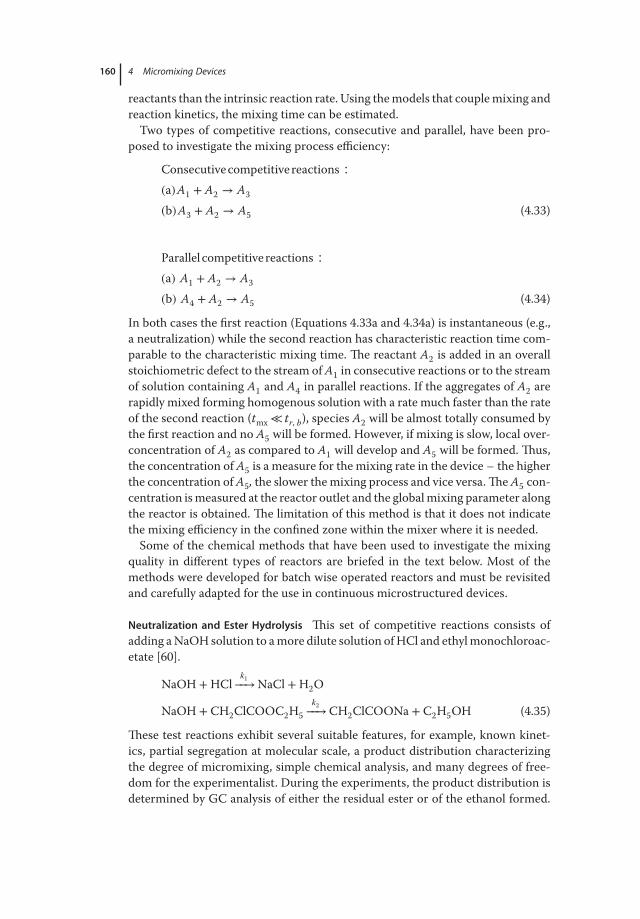
Two types of competitive reactions, consecutive and parallel, have been pro-
posed to investigate the mixing process efficiency:
Consecutivecompetitivereactions ∶(a)A1 + A2 → A3
(b)A3 + A2 → A5 (4.33)
Parallel competitivereactions ∶(a) A1 + A2 → A3
(b) A4 + A2 → A5 (4.34)
In both cases the first reaction (Equations 4.33a and 4.34a) is instantaneous (e.g.,
a neutralization) while the second reaction has characteristic reaction time com-
parable to the characteristic mixing time. The reactant A2 is added in an overall
stoichiometric defect to the stream ofA1 in consecutive reactions or to the stream
of solution containing A1 and A4 in parallel reactions. If the aggregates of A2 are
rapidly mixed forming homogenous solution with a rate much faster than the rate
of the second reaction (tmx ≪ tr, b), species A2 will be almost totally consumed by
the first reaction and no A5 will be formed. However, if mixing is slow, local over-
concentration of A2 as compared to A1 will develop and A5 will be formed. Thus,
the concentration of A5 is a measure for the mixing rate in the device – the higher
the concentration ofA5, the slower themixing process and vice versa.TheA5 con-
centration ismeasured at the reactor outlet and the globalmixing parameter along
the reactor is obtained. The limitation of this method is that it does not indicate
the mixing efficiency in the confined zone within the mixer where it is needed.
Some of the chemical methods that have been used to investigate the mixing
quality in different types of reactors are briefed in the text below. Most of the
methods were developed for batch wise operated reactors and must be revisited
and carefully adapted for the use in continuous microstructured devices.
Neutralization and Ester Hydrolysis This set of competitive reactions consists of
adding aNaOH solution to amore dilute solution ofHCl and ethylmonochloroac-
etate [60].
NaOH +HClk1−−→NaCl +H2O
NaOH + CH2ClCOOC2H5
k2−−→CH2ClCOONa + C2H5OH (4.35)
These test reactions exhibit several suitable features, for example, known kinet-
ics, partial segregation at molecular scale, a product distribution characterizing
the degree of micromixing, simple chemical analysis, and many degrees of free-
dom for the experimentalist. During the experiments, the product distribution is
determined by GC analysis of either the residual ester or of the ethanol formed.
4.5 Experimental Characterization of Mixing Efficiency 161
Further hydrolysis of the acidic sample before GC analysis is almost negligible as
the non-catalyzed hydrolysis is very slow.
When studying the influence of micromixing on the product distribution
of three parallel reactions, the alkaline hydrolysis of methyl chloroacetate is
employed as the third reaction supplementing the existing ones:
NaOH + CH2ClCOOCH3
k2−−→CH2ClCOONa + CH3OH (4.36)
The alkaline hydrolysis of themethyl ester (Equation 4.36) is faster than that of the
ethyl ester (Equation 4.35).
Diazo Coupling The diazo coupling between 1-naphthol and diazotized sulfanilic
acid is a competitive-consecutive reaction that gives two primary couplings to
produce isomeric mono-azo dyes (para and ortho) and their secondary coupling
to give finally one bisazo dye [61]. The product distribution between mono- and
bisazo dyes is sensitive to mixing and can be used to determine the rate of mixing
in the reaction zone.
The reaction is exothermic (ΔHr =−100 kJmol−1) and the activation energy is
39 kJmol−1. Therefore, lower concentrations are used to minimize the tempera-
ture rise.The product distribution, after the limiting reagent (diazotized sulfanilic
acid) has been fully consumed, is considered to characterize the mixing quality.
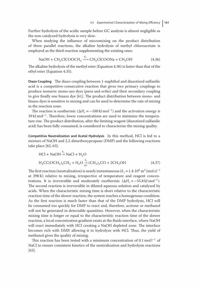
Competitive Neutralization and Acetal Hydrolysis In this method, HCl is fed to a
mixture of NaOH and 2,2-dimethoxypropane (DMP) and the following reactions
take place [62, 63]:
HCl +NaOHk1→NaCl +H2O
H3CC(OCH3)2CH3 +H2Ok2→H+
(CH3)2CO + 2CH3OH (4.37)
Thefirst reaction (neutralization) is nearly instantaneous (k1=1.4⋅108 m3 (mol s)−1
at 298K) relative to mixing, irrespective of temperature and reagent concen-
trations. It is irreversible and moderately exothermic (ΔHr =−55.8 kJmol−1).
The second reaction is irreversible in diluted aqueous solution and catalyzed by
acids. When the characteristic mixing time is short relative to the characteristic
reaction time of the slower reaction, the system reaches a homogenous condition.
As the first reaction is much faster than that of the DMP hydrolysis, HCl will
be consumed too quickly for DMP to react and, therefore, acetone or methanol
will not be generated in detectable quantities. However, when the characteristic
mixing time is longer or equal to the characteristic reaction time of the slower
reaction, a local concentration gradient exists at the fluids interface, where NaOH
will react immediately with HCl creating a NaOH depleted zone. The interface
becomes rich with DMP, allowing it to hydrolyze with HCl. Thus, the yield of
methanol gives the quality of mixing.
This reaction has been tested with a minimum concentration of 0.1mol l−1 of
NaCl to ensure consistent kinetics of the neutralization and hydrolysis reactions
[63].
162 4 Micromixing Devices
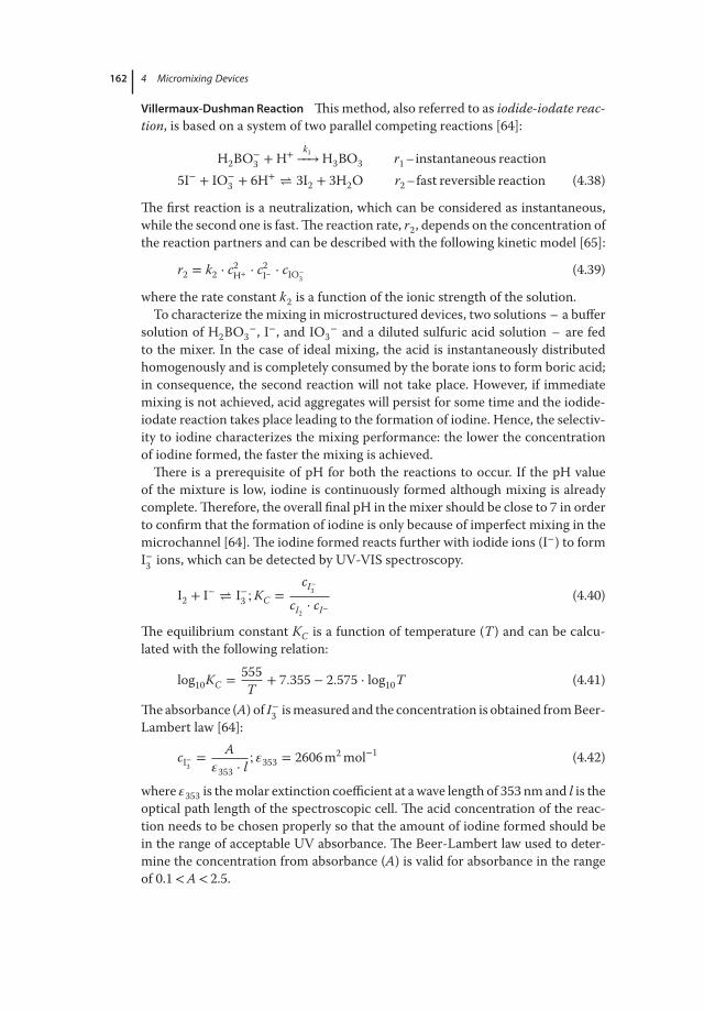
Villermaux-Dushman Reaction Thismethod, also referred to as iodide-iodate reac-
tion, is based on a system of two parallel competing reactions [64]:
H2BO−3 +H+ k1−−→H3BO3 r1–instantaneous reaction
5I− + IO−3 + 6H+ ⇌ 3I2 + 3H2O r2–fast reversible reaction (4.38)
The first reaction is a neutralization, which can be considered as instantaneous,
while the second one is fast.The reaction rate, r2, depends on the concentration of
the reaction partners and can be described with the following kinetic model [65]:
r2 = k2 ⋅ c2H+ ⋅ c2I− ⋅ cIO−
3(4.39)
where the rate constant k2 is a function of the ionic strength of the solution.
To characterize the mixing in microstructured devices, two solutions – a buffer
solution of H2BO3−, I−, and IO3
− and a diluted sulfuric acid solution – are fed
to the mixer. In the case of ideal mixing, the acid is instantaneously distributed
homogenously and is completely consumed by the borate ions to form boric acid;
in consequence, the second reaction will not take place. However, if immediate
mixing is not achieved, acid aggregates will persist for some time and the iodide-
iodate reaction takes place leading to the formation of iodine. Hence, the selectiv-
ity to iodine characterizes the mixing performance: the lower the concentration
of iodine formed, the faster the mixing is achieved.
There is a prerequisite of pH for both the reactions to occur. If the pH value
of the mixture is low, iodine is continuously formed although mixing is already
complete.Therefore, the overall final pH in the mixer should be close to 7 in order
to confirm that the formation of iodine is only because of imperfect mixing in the
microchannel [64].The iodine formed reacts further with iodide ions (I−) to form
I−3ions, which can be detected by UV-VIS spectroscopy.
I2 + I− ⇌ I−3 ;KC =cI−
3
cI2 ⋅ cI−(4.40)
The equilibrium constant KC is a function of temperature (T) and can be calcu-
lated with the following relation:
log10KC = 555
T+ 7.355 − 2.575 ⋅ log10T (4.41)
Theabsorbance (A) of I−3ismeasured and the concentration is obtained fromBeer-
Lambert law [64]:
cI−3= A
𝜀353 ⋅ l; 𝜀353 = 2606m2mol−1 (4.42)
where 𝜀353 is themolar extinction coefficient at awave length of 353 nmand l is the
optical path length of the spectroscopic cell. The acid concentration of the reac-
tion needs to be chosen properly so that the amount of iodine formed should be
in the range of acceptable UV absorbance. The Beer-Lambert law used to deter-
mine the concentration from absorbance (A) is valid for absorbance in the range
of 0.1<A< 2.5.

4.5 Experimental Characterization of Mixing Efficiency 163
Themass balance for the iodine atoms yields the following expression [64]:
cI− = cI− ,0 −5
3⋅ (cI2 + cI−
3) − cI−
3(4.43)
With the known equilibrium constant, the iodine concentration can be deter-
mined:
−5
3⋅ c2
I2+(cI− ,0 −
8
3⋅ cI−
3
)⋅ cI2 −
cI−3
KC
= 0 (4.44)
The mixing quality can be expressed in terms of a segregation index (XS) defined
in Equation 4.45, which lies between 0 and 1. XS = 1 corresponds to complete seg-
regation and the segregation XS = 0 is obtained for ideal molecular mixing.
XS =Y
YCS
(4.45)
where Y denotes the ratio of the quantity of acid moles consumed by the second
reaction (Equation 4.38) and the total amount of acid fed to the system. Y cs is the
value for complete segregation. For a continuous mixer with equal flow rates of
both solutions, the equations for Y and YCS can be written as
Y =4 ⋅ (cI2 + cI−
3)
cH+,0
(4.46)
YCS =6 ⋅ cIO−
3,0
6 ⋅ cIO−3,0 + cH2BO
−3,0
(4.47)
where subscript 0 denotes the inlet concentrations of the component in the
respective solutions.The use of the Villermaux-Dushman Reaction for estimating
the segregation in microtubes is demonstrated in Example 4.4.
Example 4.4: Characterization of mixing in microchannel reactors.
Estimate the segregation index using the method based on Villermaux-
Dushman reaction to characterize mixing in a continuous flow circular tube
with a diameter of dt = 500 μm. The experimental set-up used is depicted in
Figure 4.28. It consists of two continuously operating high-precision pumps
to introduce the two miscible solutions to a microchannel. The connections of
the microchannel with pumps and sample collector are made of transparent
PTFE capillaries. To determine the pressure loss in the micromixer, pressure
transducers aremounted at different locations including one on each upstream
capillary and one on the downstream capillary. The downstream capillary
is further attached to an online spectroscopic analysis system comprising a
cuvette, a UV-VIS spectrometer, a light source, and a laptop.

164 4 Micromixing Devices
Solution 1
Solution 2Pressuresensor
Microchannel
UVspectrometer
Cuvette
Tank
Laptop
UVLight source
a
Figure 4.28 Experimental set-up for characterizing mixing in microchannels.
Table 4.2 Proposed concentration sets to be used to characterize micromixers working
with two equal inlet flow rates [22].
c (kmolm−3) Set 1a Set 1b Set 1c Set 2a Set 2b Set 2c
[H+] 0.03 0.06 0.04 0.015 0.03 0.02 Solution 1[KI] 0.032 0.032 0.032 0.016 0.016 0.016 Solution 2[KIO3] 0.006 0.006 0.006 0.003 0.003 0.003[NaOH] 0.09 0.09 0.09 0.045 0.045 0.045[H3BO3] 0.09 0.09 0.09 0.045 0.045 0.045
Preparation of the solutions:Acid solutions: Sulfuric acid solution is prepared from commercial concen-
trated solutions.
Iodide, iodate, borate solutions: First the KI and KIO3 solutions and the
H3BO3/NaOH buffer solutions are prepared separately. Then the iodide
and iodate solutions are added to the buffer. As iodide/iodate can coex-
ist only in basic solution; the sequence of the preparation is important to
prevent the formation of iodine. In addition, oxygen should be stripped
with nitrogen before use. It is also advised to prepare the solution just
before the experiments.
Experimental procedure:The two solutions are added continuously to the microchannel with identical
flow rates. The formed tri-iodide is measured continuously with a UV/VIS
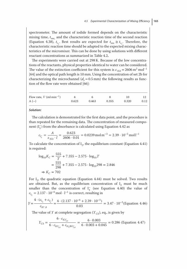
4.5 Experimental Characterization of Mixing Efficiency 165
spectrometer. The amount of iodide formed depends on the characteristic
mixing time, tmx, and the characteristic reaction time of the second reaction
(Equation 4.38), tr2 . Best results are expected for tmx ≅ tr2 . Therefore, the
characteristic reaction time should be adapted to the expected mixing charac-
teristics of the micromixer. This can be done by using solutions with different
reactant concentrations as summarized in Table 4.2.
The experiments were carried out at 298K. Because of the low concentra-
tions of the reactants, physical properties identical to water can be considered.
The value of the extinction coefficient for this system is 𝜀353 = 2606m2 mol−1
[64] and the optical path length is 10mm. Using the concentration of set 2b for
characterizing the microchannel (dt = 0.5mm) the following results as func-
tion of the flow rate were obtained [66]:
Flow rate, V (mlmin−1) 4 6 8 10 12A (−) 0.623 0.463 0.355 0.320 0.12
Solution:
The calculation is demonstrated for the first data point, and the procedure is
than repeated for the remaining data. The concentration of measured compo-
nent (I−3) from the absorbance is calculated using Equation 4.42 as
cI−3= A
𝜀353 ⋅ l= 0.623
2606 ⋅ 0.01= 0.0239molm−3 = 2.39 ⋅ 10−5mol l−1
To calculate the concentration of I2, the equilibrium constant (Equation 4.41)
is required:
log10KC = 555
T+ 7.355 − 2.575 ⋅ log10T
= 555
298+ 7.355 − 2.575 ⋅ log10298 = 2.846
⇒ KC = 702
For I2, the quadratic equation (Equation 4.44) must be solved. Two results
are obtained. But, as the equilibrium concentration of I2 must be much
smaller than the concentration of I−3
(see Equation 4.40) the value of
cI2 = 2.137 ⋅ 10−6mol ⋅ l−1 is correct, resulting in
Y=4 ⋅ (cI2 + cI−
3)
cH+,0
= 4 ⋅ (2.137 ⋅ 10−6 + 2.39 ⋅ 10−5)0.03
= 3.47 ⋅ 10−3(Equation 4.46)
The value of Y at complete segregation (YCS), eq., is given by
YCS =6 ⋅ cIO−
3,0
6 ⋅ cIO−3,0+ cH2BO
−3,0
= 6 ⋅ 0.0036 ⋅ 0.003 + 0.045
= 0.286 (Equation 4.47)
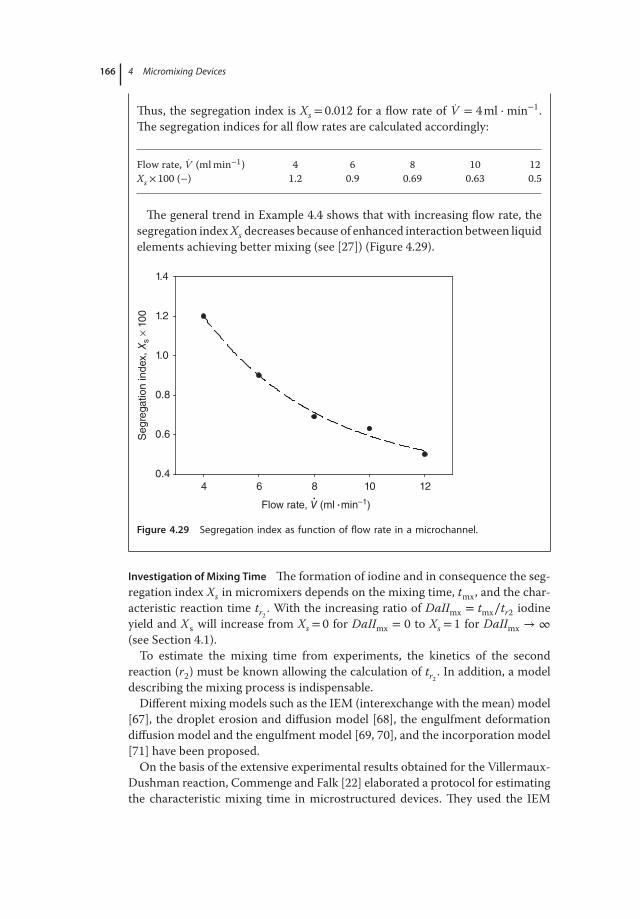
166 4 Micromixing Devices
Thus, the segregation index is Xs = 0.012 for a flow rate of V = 4ml ⋅min−1.
The segregation indices for all flow rates are calculated accordingly:
Flow rate, V (mlmin−1) 4 6 8 10 12Xs × 100 (−) 1.2 0.9 0.69 0.63 0.5
The general trend in Example 4.4 shows that with increasing flow rate, the
segregation indexXs decreases because of enhanced interaction between liquid
elements achieving better mixing (see [27]) (Figure 4.29).
4 6 8 10 12
Segre
gation index, X
s ×
100
0.4
0.6
0.8
1.0
1.2
1.4
Flow rate, V (ml • min–1)•
Figure 4.29 Segregation index as function of flow rate in a microchannel.
Investigation of Mixing Time The formation of iodine and in consequence the seg-
regation index Xs in micromixers depends on the mixing time, tmx, and the char-
acteristic reaction time tr2 . With the increasing ratio of DaIImx = tmx∕tr2 iodine
yield and Xs will increase from Xs = 0 for DaIImx = 0 to Xs = 1 for DaIImx → ∞(see Section 4.1).
To estimate the mixing time from experiments, the kinetics of the second
reaction (r2) must be known allowing the calculation of tr2 . In addition, a model
describing the mixing process is indispensable.
Different mixing models such as the IEM (interexchange with the mean) model
[67], the droplet erosion and diffusion model [68], the engulfment deformation
diffusion model and the engulfment model [69, 70], and the incorporation model
[71] have been proposed.
On the basis of the extensive experimental results obtained for the Villermaux-
Dushman reaction, Commenge and Falk [22] elaborated a protocol for estimating
the characteristic mixing time in microstructured devices. They used the IEM
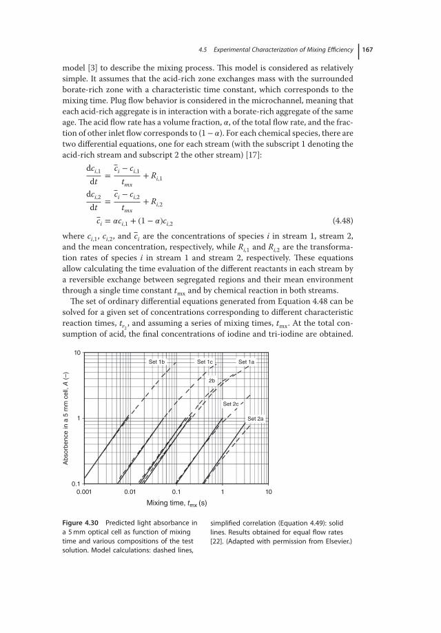
4.5 Experimental Characterization of Mixing Efficiency 167
model [3] to describe the mixing process. This model is considered as relatively
simple. It assumes that the acid-rich zone exchanges mass with the surrounded
borate-rich zone with a characteristic time constant, which corresponds to the
mixing time. Plug flow behavior is considered in the microchannel, meaning that
each acid-rich aggregate is in interaction with a borate-rich aggregate of the same
age.The acid flow rate has a volume fraction, 𝛼, of the total flow rate, and the frac-
tion of other inlet flow corresponds to (1− 𝛼). For each chemical species, there are
two differential equations, one for each stream (with the subscript 1 denoting the
acid-rich stream and subscript 2 the other stream) [17]:
dci,1
dt=
ci − ci,1
tmx
+ Ri,1
dci,2
dt=
ci − ci,2
tmx
+ Ri,2
ci = 𝛼ci,1 + (1 − 𝛼)ci,2 (4.48)
where ci,1, ci,2, and ci are the concentrations of species i in stream 1, stream 2,
and the mean concentration, respectively, while Ri,1 and Ri,2 are the transforma-
tion rates of species i in stream 1 and stream 2, respectively. These equations
allow calculating the time evaluation of the different reactants in each stream by
a reversible exchange between segregated regions and their mean environment
through a single time constant tmx and by chemical reaction in both streams.
The set of ordinary differential equations generated from Equation 4.48 can be
solved for a given set of concentrations corresponding to different characteristic
reaction times, tr2 , and assuming a series of mixing times, tmx. At the total con-
sumption of acid, the final concentrations of iodine and tri-iodine are obtained.
0.001
0.1
1
Set 1b Set 1c
2b
Set 1a
Set 2c
Set 2a
10
Ab
so
rbe
nce
in
a 5
mm
ce
ll, A
(–
)
0.01 0.1 1 10
Mixing time, tmx (s)
Figure 4.30 Predicted light absorbance in
a 5mm optical cell as function of mixing
time and various compositions of the test
solution. Model calculations: dashed lines,
simplified correlation (Equation 4.49): solid
lines. Results obtained for equal flow rates
[22]. (Adapted with permission from Elsevier.)
168 4 Micromixing Devices
This in turn can be used to calculate the light absorbance within a spectroscopic
cell. The results obtained for the concentration sets summarized in Table 4.2 are
plotted in Figure 4.30.
The mixing time can also be estimated with a simplified relation given in
Equation 4.49.
tmx = 0.33A′ ⋅ c−4.55H+,0
⋅ c−1.5I− ,0
⋅ c5.8IO−
3,0⋅ c−2
NaOH,0⋅ c−2
H3BO3,0
A′ ∶ absorbance for an optical path length of l = 1mm (4.49)
The use of the presented relations for estimating the mixing time based on
experimental data is illustrated in Example 4.5 and 4.6.
Example4.5: Estimationof the characteristicmixing time inmicrochannel
reactors.
Estimate the mixing time as function of the flow rate for the experiments
shown in Example 4.4 and plot the mixing time as function of the power dis-
sipation in the microchannel.
Solution:
The mixing time can be investigated using the correlation proposed in
Equation 4.49. For the case of V = 4mlmin−1 the absorbance in a cell
with 10mm optical path was found to be A= 0.623, which corresponds to
A′ = 0.0623 (1mm optical path). With the concentrations of set 2b (Table 4.2)
we obtain:
tmx = 0.33A′ ⋅ c−4.55H+,0
⋅ c−1.5I− ,0
⋅ c5.8IO−
3,0⋅ c−2
NaOH,0⋅ c−2
H3BO3 ,0
= A′ ⋅ 0.33 ⋅ 0.03−4.55 ⋅ 0.016−1.5 ⋅ 0.0035.8 ⋅ 0.045−2 × 0.045−2
= A′ ⋅ 0.7868 = 0.049s
Flow rate, V (mlmin−1) 4 6 8 10 12tmx (s) 0.049 0.0365 0.0279 0.0252 0.0.0203
The specific power dissipation in a channel is given by
𝜀 =V ⋅ Δp𝜌 ⋅ V
(W ⋅ kg−1)
The pressure drop in channels with laminar flow can be calculated with the
Hagen-Poiseuille law: Δp = 32𝜁μ ud2h
Lt (Equation 4.22)
It follows for the specific power dissipation in circular tubes:
𝜀 =V ⋅ Δp𝜌 ⋅ V
=u ⋅ Δp𝜌 ⋅ Lt
=u ⋅ 32 ⋅ μ ⋅ u ⋅ Lt
𝜌 ⋅ Lt ⋅ d2h
= 32 ⋅ ν ⋅ u2
d2t
(circularchannel)
(4.23)

4.5 Experimental Characterization of Mixing Efficiency 169
With 𝜈 = 10−6 m2 s−1, dt = 0.5mm we obtain:
Flow rate, V (mlmin−1) 4 6 8 10 12𝜀 (Wkg−1) 14.77 33.34 59.08 92.32 132.94
Themixing time in themicrochannel as a function of the specific power dissi-
pation is shown in Figure 4.31.Theexperimental results are in good agreement
with the empirical relation (Equation 4.27) shown in Figure 4.13.
Power dissipation, ε (W kg–1)
1 10 100 1000
Mix
ing tim
e, t m
x (
s)
0.01
0.1
0.005
0.05
Figure 4.31 Mixing time as function of specific power dissipation. Experimental results
taken from Example 4.4. Solid line: prediction with Equation 4.27.
Example 4.6: Estimationofmixing timeandexperimentalmeasurements.
Commenge and Falk [22] studied a T-mixer with square channels and 90∘bends. A scheme of the used mixer is shown in Figure 4.32.
10 mm
30 m
m
Figure 4.32 Design of the T-mixer with 10-bends.
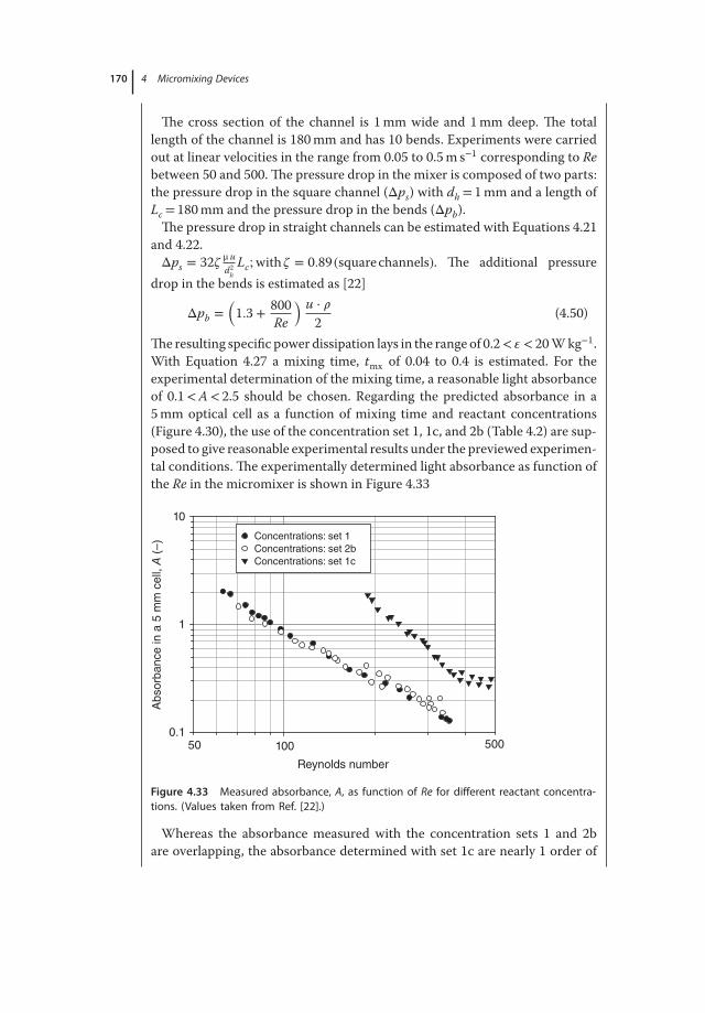
170 4 Micromixing Devices
The cross section of the channel is 1mm wide and 1mm deep. The total
length of the channel is 180mm and has 10 bends. Experiments were carried
out at linear velocities in the range from 0.05 to 0.5m s−1 corresponding to Re
between 50 and 500.The pressure drop in the mixer is composed of two parts:
the pressure drop in the square channel (Δps) with dh = 1mm and a length of
Lc = 180mm and the pressure drop in the bends (Δpb).The pressure drop in straight channels can be estimated with Equations 4.21
and 4.22.
Δps = 32𝜁μ ud2h
Lc;with𝜁 = 0.89 (squarechannels). The additional pressure
drop in the bends is estimated as [22]
Δpb =(1.3 + 800
Re
) u ⋅ 𝜌2
(4.50)
The resulting specific power dissipation lays in the range of 0.2<𝜀< 20Wkg−1.
With Equation 4.27 a mixing time, tmx of 0.04 to 0.4 is estimated. For the
experimental determination of the mixing time, a reasonable light absorbance
of 0.1<A< 2.5 should be chosen. Regarding the predicted absorbance in a
5mm optical cell as a function of mixing time and reactant concentrations
(Figure 4.30), the use of the concentration set 1, 1c, and 2b (Table 4.2) are sup-
posed to give reasonable experimental results under the previewed experimen-
tal conditions. The experimentally determined light absorbance as function of
the Re in the micromixer is shown in Figure 4.33
Reynolds number
100
Absorb
ance in a
5 m
m c
ell,
A (
–)
0.1
1
10
Concentrations: set 1
Concentrations: set 2b
Concentrations: set 1c
50050
Figure 4.33 Measured absorbance, A, as function of Re for different reactant concentra-
tions. (Values taken from Ref. [22].)
Whereas the absorbance measured with the concentration sets 1 and 2b
are overlapping, the absorbance determined with set 1c are nearly 1 order of
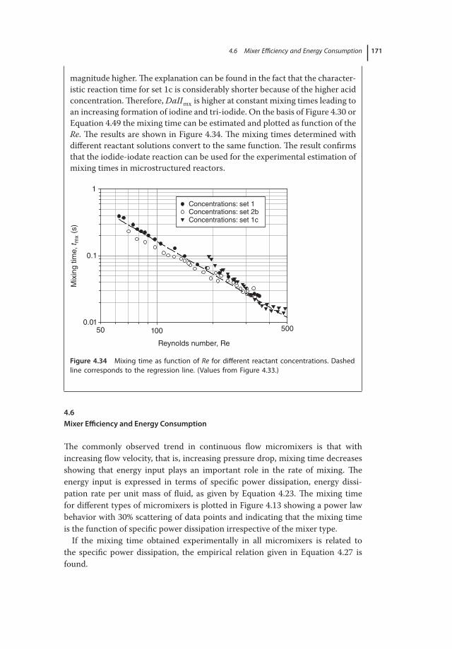
4.6 Mixer Efficiency and Energy Consumption 171
magnitude higher.The explanation can be found in the fact that the character-
istic reaction time for set 1c is considerably shorter because of the higher acid
concentration.Therefore,DaIImx is higher at constant mixing times leading to
an increasing formation of iodine and tri-iodide. On the basis of Figure 4.30 or
Equation 4.49 the mixing time can be estimated and plotted as function of the
Re. The results are shown in Figure 4.34. The mixing times determined with
different reactant solutions convert to the same function. The result confirms
that the iodide-iodate reaction can be used for the experimental estimation of
mixing times in microstructured reactors.
Reynolds number, Re
100
Mix
ing
tim
e, t m
x (
s)
0.01
0.1
1
Concentrations: set 1 Concentrations: set 2b Concentrations: set 1c
50050
Figure 4.34 Mixing time as function of Re for different reactant concentrations. Dashed
line corresponds to the regression line. (Values from Figure 4.33.)
4.6
Mixer Efficiency and Energy Consumption
The commonly observed trend in continuous flow micromixers is that with
increasing flow velocity, that is, increasing pressure drop, mixing time decreases
showing that energy input plays an important role in the rate of mixing. The
energy input is expressed in terms of specific power dissipation, energy dissi-
pation rate per unit mass of fluid, as given by Equation 4.23. The mixing time
for different types of micromixers is plotted in Figure 4.13 showing a power law
behavior with 30% scattering of data points and indicating that the mixing time
is the function of specific power dissipation irrespective of the mixer type.
If the mixing time obtained experimentally in all micromixers is related to
the specific power dissipation, the empirical relation given in Equation 4.27 is
found.
172 4 Micromixing Devices
By comparing it with the theoretical mixing time, the energetic efficiency of
mixing (𝜂mx) can be defined as the ratio between shear rate effectively used for
mixing and total shear rate used for the flow:
𝜂mx =��
��max
= ��√𝜀∕(2ν)
(4.51)
It is impossible to determine theoretically the value of the energetic efficiency
of mixing and, therefore, the comparison of the experimental correlation
(Equation 4.27) with the theoretical relation (Equation 4.26) can be used for its
evaluation:
𝜂mx =��
��max
≈tm,theory
tm,exp t.
≈ 0.0075𝜀−0.5
0.21𝜀−0.5≈ 0.036 (4.52)
It is observed that the mixing efficiency in microchannels is about 3–4%.The effi-
ciency is even lower in conventional reactors, for example, <1% in twin-screw
extruders [72]. As the mixing time is inversely proportional to the efficiency, an
increase of the energetic mixing efficiency, say by a factor 3 (from 3–10%), has
the same influence on the mixing time as an increase of 1 order of magnitude
(10 times) power dissipation.
The reason behind such a low energetic efficiency is the mismatch of flow
fields and concentration fields. The mechanical energy provided to the mixer
is used to achieve the flow in device, but in zones of pure component with no
interface with another component, this energy does not contribute in mixing.
In the case of micromixers, multilamination improves mixing by reducing the
striation thickness, but it requires additional mechanical power to create fine
multilamellae before contacting.
4.7
Summary
In this chapter, theories of homogenous mixing, types of micromixers, and meth-
ods to determine characteristicmixing time have been presented. Amethod based
on Villermaux-Dushman reaction is widely used for the efficiency characteriza-
tion of different types of mixers. The wide variety of micromixers shows that the
mixing can be tuned for a given chemical system using different geometries and
flow rates. The choice of the device is always governed by the tradeoff between
characteristic mixing time (defined by the chemical system and its intrinsic kinet-
ics), on the one hand, and the energy consumption, on the other, indicating that
energy dissipation seems to be the only relevant parameter to design an efficient
mixer.
From the geometric point of view, the mixing in single-channel micromixers is
not sufficient for fast reactions and, therefore, it needs to be improved further. In
multilamination micromixers, the lamination improves mixing by reducing the
striation thickness; however, it requires additional mechanical power to create
References 173
fine multilamellae before contacting. Besides, the zone of different concentration
should be effectively contacted, so that the major part of mechanical energy sup-
plied to the micromixer can be utilized for mixing.
4.8
List of Symbols
A, A′ Absorbance, absorbance at l= 1mm —A′ Shape factor —bs Inverse mixing time s−1ci,ci,L Mean concentration species i, at length L molm−3
Is Intensity of segregation —K Flow regime parameter (= dh/𝜆k) —l Thickness of the aggregate, optical path length of
the spectroscopic cellm
M Ratio of initial concentration —rd Rate of decay mol2 m−6 s−1Ri Overall reaction/transformation rate of partially
segregated flowmolm−3 s−1
R′′ Mean curve radius of the micro-channel mtD+shear Diffusion and shearing flow mixing time sXS Segregation index —Y , Y cs Ratio of the quantity of acid moles consumed by
Villermaux–Dushman reaction, value of Y atcomplete segregation
—
𝛼i Volume fraction of phase i —𝛥c2
1Mean square of concentration fluctuations mol2 m−6
𝜀i Molar extinction coefficient at a wavelength i m2 mol−1𝜆 Interface stretching factor —𝜆K Kolmogorov length m𝜁 friction,ζvortex
Factor originating from wall friction, factororiginating from both flow bending and vortexcreation
—
𝛿 Thickness of the lamella m𝜅 Ratio of reaction rate constants Variable𝜂mx Energetic efficiency of mixing/mixer —�� Shear rate s−1
References
1. Bourne, J.R. (1997) Mixing and the
selectivity of fast chemical reactions,
in Handbook of Batch Process Design
(ed P.N. Sharratt), Blackie Academic &
Professional.
2. Renken, A. (2006) in Chemische Reak-
toren und deren reaktionstechnische
Modellierung in Technische Chemie
(eds M. Baerns, A. Behr, A. Brehm, J.
Gmehling, H. Hofmann, U. Onken, and
A. Renken), Wiley-VCH Verlag GmbH,
Weinheim, pp. 145–194.
3. Villermaux, J. (1986) Micromix-
ing phenomena in stirred reactors,
in Encyclopedia of Fluid Mechanics
174 4 Micromixing Devices
(eds K. Ando et al.), Gulf Publishing,
Houston, TX.
4. Baldyga, J. and Bourne, J.R. (1999) Tur-
bulent Mixing and Chemical Reactions,
John Wiley & Sons, Ltd, Chichester etc.
5. Baldyga, J. (2000) Mixing and segrega-
tion in chemical reactors, in Chemical
Engineering Dynamics (eds J. Ingham,
I.J. Dunn, E. Heinzle, and J.E. Prenosil),
Wiley-VCH Verlag GmbH, Weinheim.
6. Danckwerts, P.V. (1951) The def-
initionand measurement of some
characteristics of mixing. Appl. Sci.
Res., Sect. A, 3, 279–296.
7. Toor, H.L. (1969) Turbulent mixing of
two species with and without chemical
reactions. Ind. Eng. Chem. Fundam., 8
(4), 655–659.
8. Bourne, J.R. and Toor, H.L. (1977) Sim-
ple criteria for mixing effects in complex
reactions. AIChE J., 23 (4), 602–604.
9. Bothe, D., Stemich, C., and Warnecke,
H.-J. (2006) Fluid mixing in a T-shaped
micro-mixer. Chem. Eng. Sci., 61 (9),
2950–2958.
10. Bothe, D., Stemich, C., and Warnecke,
H.J. (2004) Theoretische und exper-
imentelle Untersuchungen der
Mischvorgänge in T-förmigen Mikrore-
aktoren – Teil 1: Numerische Simulation
und Beurteilung des Strömungsmis-
chens. Chem. Ing. Tech., 76 (10),
1480–1484.
11. Engler, M., Kockmann, N., Kiefer, T.,
and Woias, P. (2004) Numerical and
experimental investigations on liquid
mixing in static micromixers. Chem. Eng.
J., 101 (1-3), 315–322.
12. Hoffmann, M., Schlüter, M., and N.R.
(2006) Experimental investigation of
liquid-liquid mixing in T-shaped micro-
mixers using [mu]-LIF and [mu]-PIV.
Chem. Eng. Sci., 61 (9), 2968–2976.
13. Hoffmann, M., Schlüter, M., and
Räbiger, N. (2007) Study of the mix-
ing processes in microreactors by use of
micro laser induced fluorescence (LIF)
and micro particle imaging velocime-
try (PIV). Chem. Ing. Tech., 79 (7),
1067–1075.
14. Schlüter, M., Hoffmann, M., and
Räbiger, N. (2004) Theoretische und
experimentelle Untersuchungen
der Mischvorgänge in T-förmigen
Mikroreaktoren-Teil 1 Experimentelle
Untersuchung des Strömungsmischens.
Chem. Ing. Tech., 76 (11), 1682–1688.
15. Falk, L. and Commenge, J.M. (2010) Per-
formance comparison of micromixers.
Chem. Eng. Sci., 65 (1), 405–411.
16. Kockmann, N., Kiefer, T., Engler, M.,
and Woias, P. (2006) Convective mixing
and chemical reactions in microchannels
with high flow rates. Sens. Actuators B,
117 (2), 495–508.
17. Falk, L. and Commenge, J.-M. (2009)
in Micro Process Engineering: A Com-
prehensive Handbook (eds V. Hessel, A.
Renken, J.C. Schouten, and J.I. Yoshida),
Wiley-VCH Verlag GmbH, Weinheim,
pp. 147–173.
18. Schneider, M.A., Maeder, T., Ryser, P.,
and Stoessel, F. (2004) A microreactor-
based system for the study of fast
exothermic reactions in liquid phase:
characterization of the system. Chem.
Eng. J., 101 (1-3), 241–250.
19. Baldyga, J. and Bourne, J.R. (1984) Mix-
ing and fast chemical reaction-VIII:
initial deformation of material elements
in isotropic, homogeneous turbulence.
Chem. Eng. Sci., 39 (2), 329–334.
20. (2002) VDI-Wärmeatlas, 9 edn, Verein
Deutscher Ingenieure: Springer, Berlin,
Heidelberg, New York.
21. Kiwi-Minsker, L. and Renken, A. (2008)
in Handbook of Heterogeneous Catalysis
(eds G. Ertl, H. Knözinger, F. Schüth,
and J. Weitkamp), Wiley-VCH Verlag
GmbH, Weinheim, pp. 2248–2264.
22. Commenge, J.M. and Falk, L. (2011)
Villermaux-Dushman protocol for exper-
imental characterization of micromixers.
Chem. Eng. Proc., 50, 979–990.
23. Capretto, L., W.C. , Hill, M., and Zhang,
X. (2011) Micromixing within microflu-
idic devices. Top. Curr. Chem., 304,
27–68.
24. Kumar, V., Paraschivoiu, M., and Nigam,
K.D.P. (2011) Single-phase fluid flow and
mixing in microchannels. Chem. Eng.
Sci., 66, 1329–1373.
25. Hessel, V., Hofmann, C., Löwe, H.,
Meudt, A., Scherer, S., Schönfeld,
F., and Werner, B. (2004) Selectiv-
ity gains and energy savings for the
industrial phenyl boronic acid process
References 175
using micromixer/tubular reactors. Org.
Process Res. Dev., 8 (3), 511–523.
26. Löwe, H., Ehrfeld, W., Hessel, V.,
Richter, T., and Schiewe, J. (2000)
Micromixing technology. 4th Inter-
national Conference on Microreaction
Technology (IMRET4), Atlanta, GA,
2000, pp. 31–47.
27. Kashid, M., Renken, A., and
Kiwi-Minsker, L. (2011) Mixing effi-
ciency and energy consumption for five
generic microchannel designs. Chem.
Eng. J., 167 (2-3), 436–443.
28. Jiang, F., Drese, K.S., S.H. , Kupper, M.,
and Schonfeld, F. (2004) Helical flows
and chaotic mixing in curved micro
channels. AIChE J., 50 (9), 2297–2305.
29. Mengeaud, V., Josserand, J., and Girault,
H.H. (2002) Mixing processes in a zigzag
microchannel: finite element simulations
and optical study. Anal. Chem., 74 (16),
4279–4286.
30. Kölbl, A., Kraut, M., and Wenka, A.
(2011) Design parameter studies on
cyclone type mixers. Chem. Eng. J., 167
(2-3), 444–454.
31. Ansari, M.A., Kim, K.-Y., Anwar, K., and
Kim, S.M. (2012) Vortex micro T-mixer
with non-aligned inputs. Chem. Eng. J.,
181–182, 846–850.
32. Hessel, V., Lowe, H., and Schonfeld, F.
(2005) Micromixers – a review on pas-
sive and active mixing principles. Chem.
Eng. Sci., 60 (8-9), 2479–2501.
33. Schönfeld, F., Hessel, V., and Hofmann,
C. (2004) An optimised split-and-
recombine micro-mixer with uniform
‘chaotic’ mixing. Lab Chip, 4 (1), 65–69.
34. Jen, C.-P., Wu, C.-Y., Lin, Y.-C., and Wu,
C.-Y. (2003) Design and simulation of
the micromixer with chaotic advection
in twisted microchannels. Lab Chip, 3
(2), 77–81.
35. Bertsch, A., Heimgartner, S., Cousseau,
P., and Renaud, P. (2001) Static
micromixers based on large-scale indus-
trial mixer geometry. Lab Chip, 1 (1),
56–60.
36. Stroock, A.D., Dertinger, S.K.W.,
Ajdari, A., Mezic, I., Stone, H.A., and
Whitesides, G.M. (2002) Chaotic mixer
for microchannels. Science, 295 (5555),
647–651.
37. Stroock, A.D. and McGraw, G.J. (2004)
Investigation of the staggered herring-
bone mixer with a simple analytical
model. Philos. Trans. R. Soc. London, Ser.
A, 362 (1818), 971–986.
38. Choudhary, R., Bhakat, T., Singh, R.K.,
Ghubade, A., Mandal, S., Ghosh, A.,
Rammohan, A., Sharma, A., and
Bhattacharya, S. (2011) Bilayer stag-
gered herringbone micro-mixers with
symmetric and asymmetric geometries.
Microfluid. Nanofluid., 10 (2), 271–286.
39. Werner, B., Donnet, M., Hessel, V.,
Hofmann, C., Jongen, N., Lowe, H.,
Schenk, R., and Ziogas, A. (2002) Spe-
cially suited micromixers for process
involving strong fouling. 6th Interna-
tional Conference on Microreaction
Technology, IMRET 6, AIChE, New
Orleans, 2002, pp. 168–183.
40. Penth, B. (2001) Method and device
for carrying out chemical and physical
processes. WO Patent 2000061275 A3.
41. Song, H., Tice, J.D., and Ismagilov, R.F.
(2003) A microfluidic system for control-
ling reaction networks in time. Angew.
Chem. Int. Ed., 42 (7), 768–772.
42. Matsuyama, K., Tanthapanichakoon, W.,
Aoki, N., and Mae, K. (2007) Operation
of microfluidic liquid slug formation and
slug design for kinetics measurement.
Chem. Eng. Sci., 62 (Special Issue 18-20),
5133–5136.
43. Bringer, M.R., Gerdts, C.J., Song, H.,
Tice, J.D., and Ismagilov, R.F. (2004)
Microfluidic systems for chemical
kinetics that rely on chaotic mixing in
droplets. Philos. Trans. R. Soc. London,
Ser. A, 362 (1818), 1087–1104.
44. Paik, P., Pamula, V.K., and Fair, R.B.
(2003) Rapid droplet mixers for digital
microfluidic systems. Lab Chip, 3 (4),
253–259.
45. Seidel, R.U., Sim, D.Y., W.M. , and
Esashi, M. (2000) Third International
Conference on Microreaction Technology.
IMRET 3, Springer, Berlin, pp. 189–197.
46. Hong, C.-C., Choi, J.-W., and Ahn,
C.H. (2004) A novel in-plane passive
microfluidic mixer with modified tesla
structures. Lab Chip, 4 (2), 109–113.
47. Hong, C.-C., Choi, J.-W., and Ahn, C.H.
(2001) in Micro Total Analysis Systems
(eds J.M. Ramsey and A. van den Berg),
176 4 Micromixing Devices
Kluwer Academic Publishers, Dordrecht,
pp. 31–33.
48. Yasui, T., Omoto, Y., Osato, K., Kaji,
N., Suzuki, N., Naito, T., Watanabe, M.,
Okamoto, Y., Tokeshi, M., Shamoto,
E., and Baba, Y. (2011) Microfluidic
baker’s transformation device for three-
dimensional rapid mixing. Lab Chip, 11
(19), 3356–3360.
49. Voldman, J., Gray, M.L., and Schmidt,
M.A. (1998) in Micro Total Analysis
Systems (eds J. Harrison and A. van den
Berg), Kluwer Academic Publishers,
Dordrecht, pp. 181–184.
50. Glasgow, I. and N.A. (2003) Enhance-
ment of microfluidic mixing using time
pulsing. Lab Chip, 3 (2), 114–120.
51. Niu, X.Z. and Lee, Y.K. (2003) Effi-
cient spatial-temporal chaotic mixing in
microchannels. J. Micromech. Microeng.,
13 (3), 454–462.
52. Qian, S.Z. and Bau, H.H. (2002) A
chaotic electroosmotic stirrer. Anal.
Chem., 74 (15), 3616–3625.
53. Oddy, M.H., Santiago, J.G., and
Mikkelsen, J.C. (2001) Electrokinetic
instability micromixing. Anal. Chem., 73
(24), 5822–5832.
54. Yang, Z., Goto, H., Matsumoto, M., and
Maeda, R. (2000) Active micromixer
for microfluidic systems using lead-
zirconate-titanate(PZT)-generated
ultrasonic vibration. Electrophoresis,
21 (1), 116–119.
55. Woias, P., Hauser, K., and
Yacoub-George, E. (2000) in Micro Total
Analysis Systems (eds A. van den Berg,
W.O. , and P. Bergveld), Kluwer Aca-
demic Publishers, Dordrecht, pp.
277–282.
56. Liu, R.H., Yang, J., Pindera, M.Z.,
Athavale, M., and Grodzinski, P. (2002)
Bubble-induced acoustic micromixing.
Lab Chip, 2 (3), 151–157.
57. Liu, R.H., Lenigk, R., Druyor-Sanchez,
R.L., Yang, J., and Grodzinski, P. (2003)
Hybridization enhancement using cavi-
tation microstreaming. Anal. Chem., 75
(8), 1911–1917.
58. Lu, L.-H., Ryu, K.S., and Liu, C. (2000)
A magnetic microstirrer and array for
microfluidic mixing. J. Microelectromech.
Syst., 11 (5), 462–469.
59. West, J., Karamata, B., Lillis, B., Gleeson,
J.P., Alderman, J., Collins, J.K., Lane, W.,
Mathewson, A., and Berney, H. (2002)
Application of magnetohydrodynamic
actuation to continuous flow chemistry.
Lab Chip, 2 (4), 224–230.
60. Bourne, J.R. and Yu, S. (1994) Investi-
gation of micromixing in stirred tank
reactors using parallel reactions. Ind.
Eng. Chem. Fundam., 33 (1), 41–55.
61. Bourne, J.R., Kut, O.M., Lenzner, J., and
Maire, H. (1990) Kinetics of the diazo
coupling between 1-naphthol and dia-
zotized sulfanilic acid. Ind. Eng. Chem.
Fundam., 29 (9), 1761–1765.
62. Baldyga, J., Bourne, J.R., and Walker, B.
(1998) Non-isothermal micromixing in
turbulent liquids: theory and experiment.
Can. J. Chem. Eng., 76 (3), 641–649.
63. Holvey, C.P., Roberge, D.M., Gottsponer,
M., N.K. , and Macchi, A. (2011) Pres-
sure drop and mixing in single phase
microreactors: simplified designs of
micromixers. Chem. Eng. Proc., 50 (10),
1069–1075.
64. Guichardon, P. and Falk, L. (2000) Char-
acterisation of micromixing efficiency by
the iodide-iodate reaction system. Part I:
Experimental procedure. Chem. Eng. Sci.,
55 (19), 4233–4243.
65. Guichardon, P. and Falk, L. (2000) Char-
acterisation of micromixing efficiency by
the iodide-iodate reaction system. Part
II:kinetic study. Chem. Eng. Sci., 55 (19),
4245–4253.
66. Kumar, A. (2012) Characterization of
Hot Spots in Microstructured Reactors
for Fast and Exothermic Reactions in
Mixing Regime, Ecole Polytechnique
Fédérale de Lausanne, EPFL, Lausanne.
67. Villermaux, J. and Devillon, J.C. (1972)
Représentation de la coalescence et de
la redispersion des domaines de ségré-
gation dans un fluide par un modéle
d’interaction phénoménologique. 2nd
International Symposium on Chemical
Reaction Engineering, Amsterdam, The
Netherlands, 1972.
68. Ou, J.J. and Ranz, W.E. (1983) Mix-
ing and chemical reactions. Chemical
selectivities. Chem. Eng. Sci., 38 (7),
1015–1019.
69. Baldyga, J. and Bourne, J.R. (1990)
Comparison of the engulfment and the
References 177
interaction-by-exchange-with-the-mean
micromixing models. Chem. Eng. J., 45
(1), 25–31.
70. Baldyga, J. and Bourne, J.R. (1989) Sim-
plification of micromixing calculations.
I. Derivation and application of new
model. Chem. Eng. J., 42 (2), 83–92.
71. Fournier, M.C., Falk, L., and Villermaux,
J. (1996) A new parallel competing reac-
tion system for assessing micromixing
efficiency-determination of micromixing
time by a sample mixing model. Chem.
Eng. Sci., 51 (23), 5187–5192.
72. Baldyga, J., Rozen, A., and Mostert, F.
(1998) A model of laminar micromixing
with application to parallel chemical
reactions. Chem. Eng. J., 69 (1), 7–20.