2ND　INTERNATlONAl　WORKSHOP　ON

THE　INTEGRITY　OF

NUCLEAR　COMPONENTS

April20121，1998

主催 社団法人目本溶接協会原子力研究委員会The　Japan　Welding　Engineeing　Society

Atomic　Energy　Reseach　Committee

Sa血ty　and　Structural　Integrity　Research　Center，

Sung　Kyun　Kwan　University

Program of the Workshop

Session I

Design and Analysis

I- 1 Concept of Advanced Design Standards for DFBR

Masahiro Ueta, JAPC, Japan

CONCEPT OF ADVANCED DESIGN STANDARDS FOR DFBR

Masahiro UETA

THE JAPAN ATOMIC POWER COMPANY 1-6-1, Ohtemachi, Chiyoda-ku, Tokyo 100, JAPAN

Phone : 3-3201-6631 Fax : 3-3285-0542

E-mail : masahiro-ueta@japc.co.jp

Abstract

The Japan Atomic Power Company (JAPC) has been developing the demonstration fast breeder reactor (DFBR) under the sponsorship of nine

Japanese electric companies and the Electric Power Development Co.Ltd since 1986. JAPC has drafted the structural design guide for the DFBR at

elevated temperatures (DDS) based on that for the prototype FBR MONJU.

However, in the last December the round-table committee, established in the

Atomic Energy Commission, published the report that the construction of the

DFBR should be projected based on experiences of operation and maintenance of MONJU and reflecting latest R&D achievement. As the result the DFBR project may be somewhat postponed. Meanwhile, the requirement to the DFBR are becoming more and more strict toward higher

economy consistent with reliability. To cope with the requirement, JAPC has

started drastic revision of the DDS. The main issues in the revision are

rearrangement of code systems and inrprovement of estimation method of

load conditions, accumulated strains by ratchetting and creep-fatigue damage. This paper describes the concept of the advanced DDS.

1 . Introduction

Worldwide energy demand has been increasing with population increase and economic development especially in developing countries,

although many countries are making efforts to save energy consumption. If

the consumption of fossil energy increase with energy demand, energy resources, such as oil and natural gas, may be run out of in the middle of the

-1-

next century. And it is also forced to limit consump~tion of fossil energy from

the view point of protecting global environment from greenhouse effect and

acid rain caused by exhausted gas like carbon dioxide and other oxidant

gases from fossil power plants. Nuclear power generation is the most promising and effective measures to cope with both energy demand and

environment protection. Nuclear people convince that nuclear power generation will play the essential role in energy supply in the next century.

Fast breeder reactors (FBRS) have the potential to utilize uranium

resources much more effectively than light water reactors (LWRs) by more

than 50 times, and so it is expected that FBRs can secure worldwide energy

supply for more than thousands of years. FBRs also have fascinating potential to be able to incinerate minor actinides which are radioactive

wastes of ultra-long half-lives originated from nuclear power plants.

Therefore, Japanese government and utilities have been promoting the development of FBR since the initial stage of nuclear energy development.

The Japan Atomic Power Company (JAPC) has been developing the demonstration fast breeder reactor (DFBR) following the prototype FBR

MONJU under the auspices of nine Japanese electric power companies and

the Electric Power Development Co.Ltd. since 1986. Main specifications of

the DFBR were settled in January 1994. In December 1995, the sodium leak

incident occurred in MONJU. It showed that it is essentially important for

FBRs to prevent sodium fire which may result in long-term plant outage and

lower plant availability of FBRs. And deregulation in electric power industries forces nuclear industries to reduce power generation cost as fossil

power generation of which cost is drastically reduced recently. Therefore,

JAPC has been conducting the conceptual design study of the DFBR aiming

at eliminating anxiety of sodium fire and reducing construction cost of the

DFBR far below 1.5 times that of LWRs on the 1000MWe basis. In this study

the DFBR would be provided with comprehensive countermeasures against

sodium leak and fire to eliminate instrumentation well through sodium boundaries, to enclose whole sodium piping by guard pipes, and to install

auxiliary sodium systems as purification systems into vessels.

The MONJU incident induced nationwide discussion on FBR development in Japan, and the round-table committee was established in the

Atomic Energy Commission. This committee reported in December 1997 that

FBR is one of the promising options of future energy resources, that MONJU

-2-

should be restarted for research and development (R&D) of FBR, and that

the DFBR should be projected reflecting experience obtained in operation

and maintenance of MONJU and incorporating latest R&D achievements. Therefore, sufficient time is kept until construction of the DFBR enough to

achieve innovative R&Ds for improving economy of the DFBR drastically.

The current structural design guide for the DFBR at elevated temperatures (DDS) was drafted based on that for MONJU and incorporating

R&D achievements after MONJU. It has been applied as the design standard to

design studies of the DFBR. However, it is required to improve accuracy of

design evaluation for realizing economical design consistent with reliability.

Therefore, JAPC has started the long-range study for the advanced DDS as a

typical embodiment of innovative R&Ds.

This paper describes the policy to revise the DDS.

2. Policy to Improve DFBR Design

2.1 Reducing Uncertainty in Design

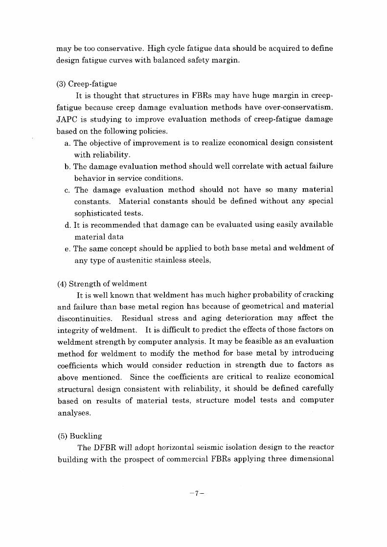
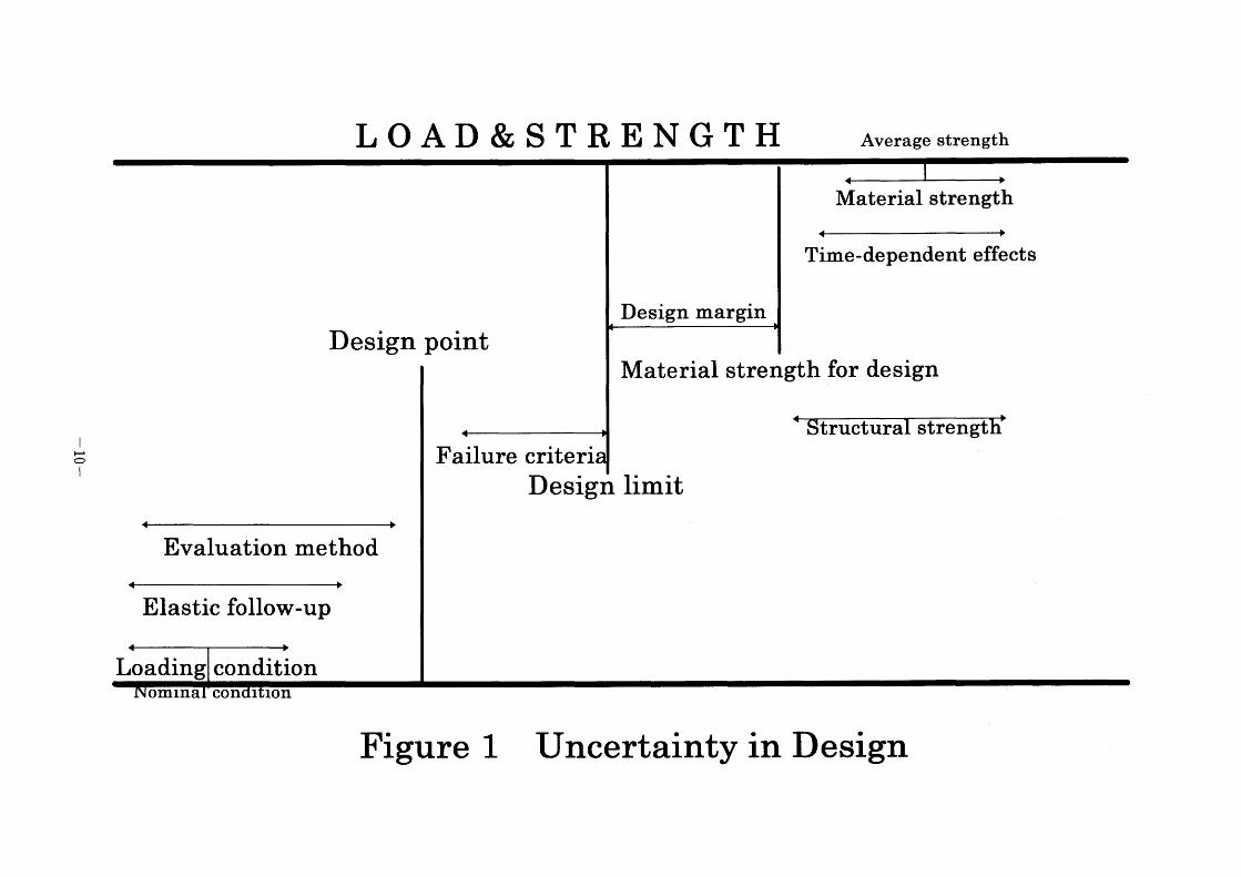
The nuclear steam supply system (NSSS) of the DFBR should have reliability prior to others, because sufficient experiences have not been

accumulated in FBR operation and maintenance. Economy improvement compatible with reliability can be realized by reducing uncertainty in whole

design process as shown in Fig. 1. The policies to reduce uncertainty are as

follows.

(1) Material

To reduce scattering of material strength, chemical compositions and

heat treatment conditions should be specified rigorously as far as material

cost does not increase significantly.

To reduce inaccuracy in extrapolation of material strength, data of

10ng-term creep rupture, ultra-high cycle fatigue and creep-fatigue in low

strain range should be acquired.

To improve prediction of time-dependent effects, data of long-term

aging effect at elevated temperatures, neutron irradiation effect and sodium

environment effect on material strength should be acquired.

-3-

(2) Structure

To reduce deviation of strength from normal value and to eliminate

unforeseen trouble, requirements on quality assurance should be imposed on

design, fabrication, construction, installation and inspection considering cost

imp act.

To reduce uncertainty of structural strength caused by worker's skill

and discontinuities in material or geometry, simple and robust design should

be aimed at.

(3) Loading condition

Thermal transient load is critical in assuring structural integrity of

FBR components since it is much more difficult to predict thermal transient

10ad than pressure load. Improvement of thermal load prediction will

contribute to economical design consistent with reliability. Thermal hydraulic model tests are useful to understand thermal hydraulic behaviors,

to improve accuracy of thermal load prediction and to verify computer codes

for design analysis.

Usually thermal stresses are classified into the secondary stress, but

they may act as the primary stress in case elastic follow-up is significant at

elevated temperatures. Therefore, strain intensification due to elastic

follow-up should be evaluated carefully in elevated temperature design. The

current method employed in the DDS has shown to be too conservative in

many cases, To realize economical design consistent with reliability, new

concept considering the mechanism of elastic follow-up should be introduced

into the advanced DDS.

(4) Design criteria of failure

Design criteria of failure should be well correlating with actual failure

modes and should conservatively envelope actual failure limits as close as

possible. Creep damage evaluation is the key toward well-correlated design

criteria. The current method applies time fraction concept for creep damage

evaluation. To realize economical design consistent with reliability, creep

damage evaluation method should be improved through discussions taking

suffrcient time to reach consensus among the related specialists and engineers. New methods as ductility exhaustion concept will be investigated

in addition to modifying the current time fraction concept.

~4-

2.2 Safety Margin

Design margins should be kept sufficiently in design criteria in DDS,

for example, 20 of number of cycles and 2 of strain range in fatigue design.

Different margins should be defined dependent upon frequencies and significance of failure events.

Evaluation methods applied in design should envelope failure limits on

a conservative side, but as close to the limits as possible. In other word,

design margin should not be shared to inaccuracy of evaluation method,

while additional margin is not expected in evaluation methods.

2.3 Inelastic analysis

Computer analysis is making great advance in recent years. Inelastic

analysis will be employed widely to DFBR design to realize economical design consistent with reliability. JAPC will employ inelastic analysis to

estimate ratchetting strain in design, to find optimized design by numerical

experiments in place of model tests, to define appropriate elastic follow-up

parameters, and to confirm that sufficient design margin is kept.

The guideline of inelastic analysis should be prepared to assure conservatism and to attain licensability of designs employing inelastic

analysis.

3. Policies for Advanced DDS

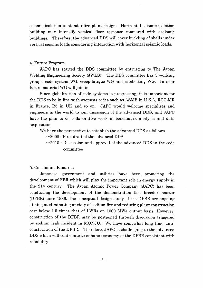
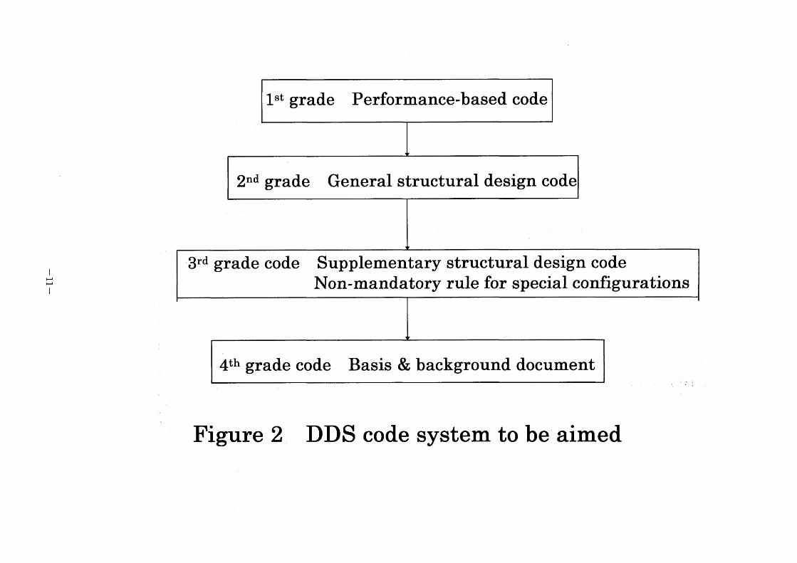
3.1 General The advanced DDS will adopt the graded code ,system as shown in Fig.2.

The discussion has started to introduce the graded code system into the

design of plants in non-nuclear fields with future prospect of introducing that

system also into nuclear fields.

The first grade is a performance-based code, such as MITI ordinance No.

62, which specifies only requirements from the view point of safety and

reliability. The second grade is a general structural design code which provides the limits of load, stress, strain, damage and other parameters from

the viewpoint of assuring structural integrity. The third grade is a supplemental code which would provide local rules, for instance, seismic

design guideline under a site-dependent earthquake condition. Non-

-5-

mandatory rules for special configurations such as tube plates are also

included in the third grade. The guideline of inelastic analysis may be

classified into the third grade. The fourth grade is the document to explain

the basis and background of codes and standards. The document would include data of tests, experiments and analyses to validate the code.

The advanced DDS will aim at the code which has merit to do detailed

design analysis. For this purpose the advanced DDS will be composed of

screening rules using simplified analysis, standard rules using detailed

elastic analysis, and general rules in which it would be permitted to validate

the design by experiment and detailed inelastic analysis.

3.2 Main items to be revised

(1) Accumulated inelastic strain

While current codes provide constant values of accumulated inelastic

strain limit independent of material, the advanced DDS would define the

limit values material by material to take advantage of improved ductility.

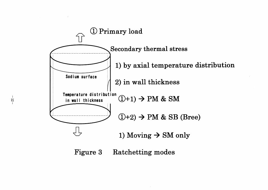
Several modes of ratchetting may occur under the combination of primary loads and secondary thermal loads as shown in Fig.3. It is not easy

to estimate inelastic strain due to all ratchetting modes using elastic

analysis. On the contrary, inelastic analysis can conservatively estimate

whole ratchetting behaviors by one calculation using appropriate model and

considering all loading conditions. Therefore, the advanced DDS would adopt

design using inelastic analysis to ratchetting as a standard method. The

guideline of inelastic analysis should be prepared to provide the procedure to

ensure conservatism of analysis results.

(2) Fatigue

High cycle fatigue is a important cause of cracking and failure of

structures in FBR, because sodium flow with high velocity at different

temperatures may occur flow-induced vibration and thermal fluctuation. The

key issue is to establish the method to estimate loading conditions as forces,

stresses and frequencies. The guideline should be prepared for high cycle

fatigue design to enhance reliability.

Since ultra-high cycle fatigue data are very limited at elevated

temperatures, current elevated temperature fatigue curves are drawn by

linear extrapolation to ultra-high cycles without fatigue limit, although it

-6-

may be too conservative. High cycle fatigue data should be acquired to define

design fatigue curves with balanced safety margin.

(3) Creep-fatigue

It is thought that structures in FBRs may have huge margin in creep-

fatigue because creep damage evaluation methods have over-conservatism.

JAPC is studying to improve evaluation methods of creep-fatigue damage

based on the following policies.

a. The objective of improvement is to realize economical design consistent

with reliability.

b. The damage evaluation method should well correlate with actual failure

behavior in service conditions.

c. The damage evaluation method should not have so many material constants. Material constants should be defined without any special

sophisticated tests.

d. It is recommended that damage can be evaluated using easily available

material data

e. The same concept should be applied to both base metal and weldment of

any type of austenitic stainless steels,

(4) Strength of weldment It is well known that weldment has much higher probability of cracking

and failure than base metal region has because of geometrical and material

discontinuities. Residual stress and aging deterioration may affect the integrity of weldment. It is difficult to predict the effects of those factors on

weldment strength by computer analysis. It may be feasible as an evaluation

method for weldment to modify the method for base metal by introducing

coefficients which would consider reduction in strength due to factors as

above mentioned. Since the coefficients are critical to realize economical

structural design consistent with reliability, it should be defmed carefully

based on results of material tests, structure model tests and computer

analyses.

(5) Buckling

The DFBR will adopt horizontal seismic isolation design to the reactor

building with the prospect of commercial FBRs applying three dimensional

-7-

seismic isolation to standardize plant design. Horizontal seismic isolation

building may intensify vertical floor response compared with aseismic buildings. Therefore, the advanced DDS will cover buckling of shells under

vertical seismic loads considering interaction with horizontal seismic loads.

4. Future Program

JAPC has started the DDS committee by entrusting to The Japan Welding Engineering Society (JWES). The DDS committee has 3 working groups, code system WG, creep-fatigue WG and ratchetting WG. In near future material WG will join in.

Since globalization of code systems is progressing, it is important for

the DDS to be in line with overseas codes such as ASME in U.S.A, RCC-MR

in France, R5 in UK and so on. JAPC would welcome specialists and engineers in the world to join discussion of the advanced DDS, and JAPC

have the plan to do collaborative work in benchmark analysis and data acquisition.

We have the perspective to establish the advanced DDS as follows.

-2005 : First draft ofthe advanced DDS

-2010 : Discussion and approval of the advanced DDS in the code

committee

5. Concluding Remarks

Japanese government and utilities have been promoting the development of FBR which will play the important role in energy supply in

the 2lst century. The Japan Atomic Power Company (JAPC) has been conducting the development of the demonstration fast breeder reactor

(DFBR) since 1986. The conceptual design study of the DFBR are ongoing aiming at eliminating anxiety of sodium fire and reducing plant construction

cost below 1.5 times that of LWRs on 1000 MWe output basis. However, construction of the DFBR may be postponed through discussion triggered

by sodium leak incident in MONJU. We have somewhat long ti_me until construction of the DFBR. Therefore, JAPC is challenging to the advanced

DDS which will contribute to enhance economy of the DFBR consistent with reliability.

-8-

The key issues in the advanced DDS are to reduce uncertainty in strength of materials and structures, to correlate design criteria well with

actual failure behaviors, and to improve accuracy of evaluation methods

especially of ratchetting, high cycle fatigue and creep-fatigue.

JAPC has started the DDS committee to draft the advanced DDS by

entrusting to The Japan Welding Engineering Society (JWES). The advanced DDS will be embodied around 2010.

-9-

!~ l

Average strength

Material strength

Time-dependent effects

Design margin Design point

Material strength for design

tructura strengt Failure criteri

Design limit

Evaluation method

Elastic follow-up

Loading condition Omlna COn I lOn

Figure 1 Uncertainty in Design

H H' I

Frgure 2 DDS code system to be aimed

l

~. N)

i

l~ ~) Pnmary load

Secondary thermal stress

l) by axial temperature distribution

sodium surtace ~ 2) in wall thickness

Temperature distributiOn R+1) ~ pM & SM in wall thickness

------ ~)+2) ~ PM & SB (Bree)

Figure 3 Ratchetting modes

I-2 A Study of the Helical Effect on the Connection by Three

Dimensional FEM Stress Analyses

Jien-Jong Chen &Yan-Shin Shih, Institute of Nuclear Energy Research Atomic

Energy Council, Taiwan, Republic of China

A study of the helical effect on the thread connection

by three dimensional finite element analysis

Jien-Jong Chen~b and Yan-Shin Shihb

'Nuclear Division, Institute ofNuclear Energy Research, P. O. Box 3-3,

Lung-Tan, Taoyuan, Taiwan, ROC

b Department of Mechanical Engineering, Chung-Yuan Christian University,

Chung-Li,32023 Taiwan. ROC

Abstract

The three dimensional finite element analysis of the bolted joints with finite sliding

deformable contact has been studied, and the helical and fiiction effect on the load

distnbution of each thread is analyzed. It shows the analyiical analysis by

Yamamoto's method reaches a lower value of load ratio than the finite element analysis

at the first thread. The load distribution on each thread between axisynunetrical model

and three dimensional model are provided. HenGe, although increasing the coefficient

of friction and decreasing of the lead angle may improve the load distribution slightly,

for I "-16UNF bolt joints, the error of load ratio at the first thread in axisymmetrical

finite element model is 1 20/0 with respect to three dimensional analysis.

I. Introduction

The bolted joint is a typieal counection that is widely used for the construction of

stuctural Gomponents. Owing to the easy replacement and installation, the bolted

joint has been applied to many components of nuclear power plants. However, two

problems of bolted joints connection should be concemed. The first one is the

-13-

functionality of the joints which threaded end olosure is still kept, and the second is the

load bearing fraotion on each thread of. the bolt and nut. In the recent year, many

authors (Chaaban et. al. 1992, Grosse et. al. 1990, Wileman et. al 1991, Lehnhoff et. al

1 996) have focused on the study of threaded end olosure of the bolted j oint. But the

load distribution analysis has bcen seldom mentioned durirmg last few decades. The

investigation of the load distribution in the threaded couneetion has been studied since

l 940's. The Sopwith theory (Sopwith 1 948) for predicting the load distribution of the

threaded fasteners is a well known analyiical model. The action of a number of strains

is formuated by the axial extension of the bolt and eompression of the nut in Sopwith

theory. These strains include the bending defleetion of the thread, an axial recession

due to radial compression of the threads, and an axial reeession due to axial contraction

of the bolt and expansion of the nut caused by radial pressure of the joints.

Altematively, Yamamoto (Yamamoto 1 980) proposed a procedure for calculating the

defleotion due to bending moment, shear loading and radial contraction and expansion

on the bolt and nut. The assumption ofplane strain has also been made by Yamamoto

for dealing with thread region. Hence, the three dimensional bolt-nut assembly can bc

simply analyzed by axisymmetrical model to caleulate the load distribution along the

axial direction ofbolt. The analyiical and axisymmetrical fmite element analysis have

been studied in the literature (Chaaban et. al, 1 992, Grosse et. al. 1 990, Wileman et. al

1991, Lehnhoff et. al 1996). However, the lead angle due to helical effect can not be

modeled by axisymmetrical model, such that, the helical effeet to the load distribution is

still lacking on the literature. Due to the progress ofthe modem fmite element method,

modeling of the fmite sliding, and deformable to deformable contact problem becomes

possible by usmg ABAQUS code( Hibbitt et.al 1 998). The cunosrty rs nsen for

- 14 -

exploring the differenee among theoretioal, axisymmetrical and three dimensional fmite

element models, and that is the purpose of the present study.

II. Modeling and Assumption.

A standard one ineh bolt (8UNC) and two fine threaded bolt (12UNF and 1 6UNF) are

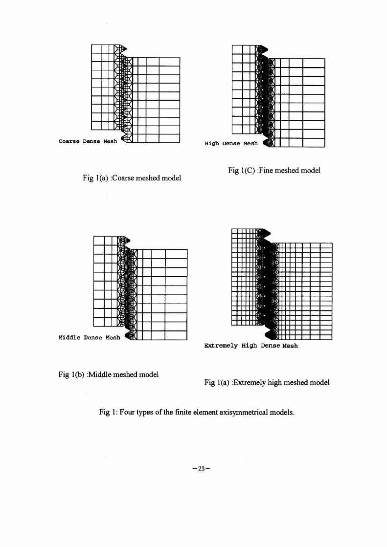
used to study the helical effect ofthe bolts. Four axisymmetrical finite element models

with the different mesh on the threads are shown in Figure I . In the axisymmetrical

model, the radial symmetric is assumed on the center line of bolt. The three

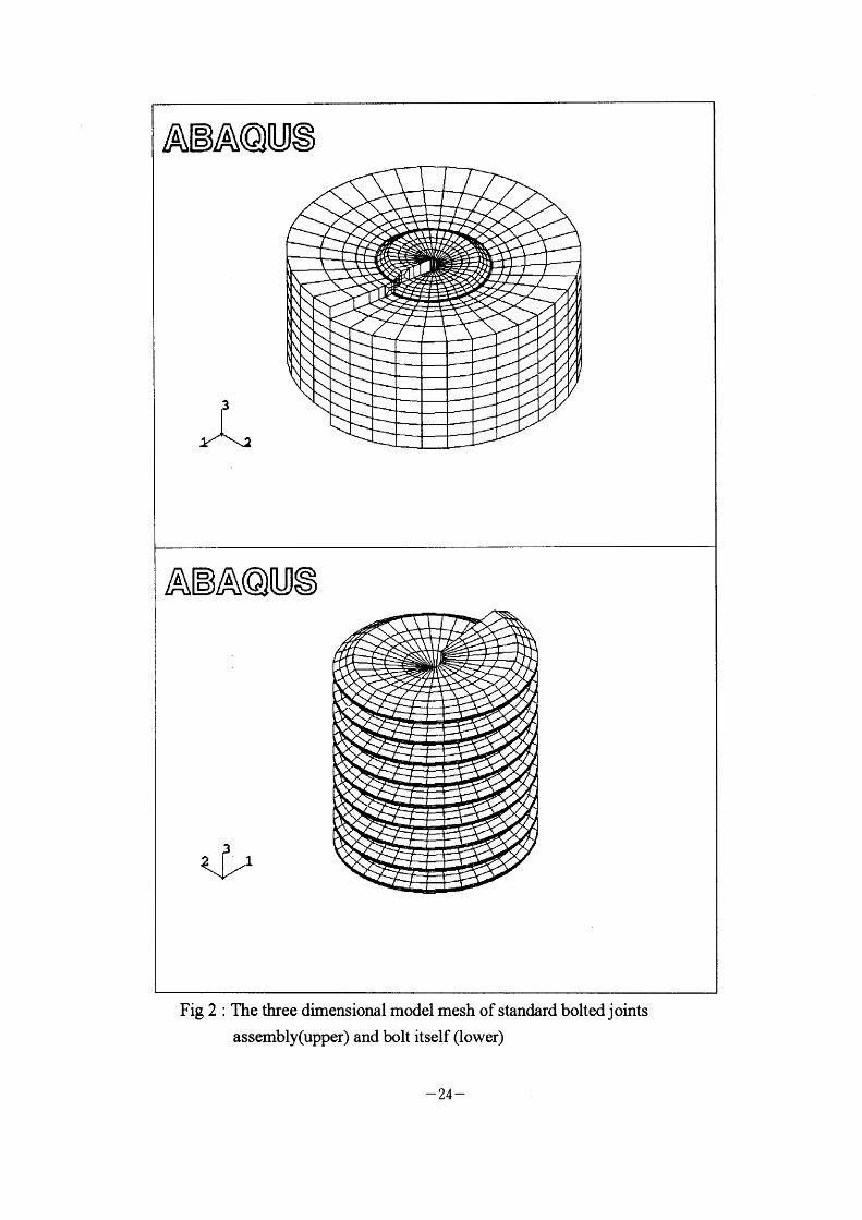
dimensional model ofthe standard bolt assembly is shown in Figure 2, and the model of

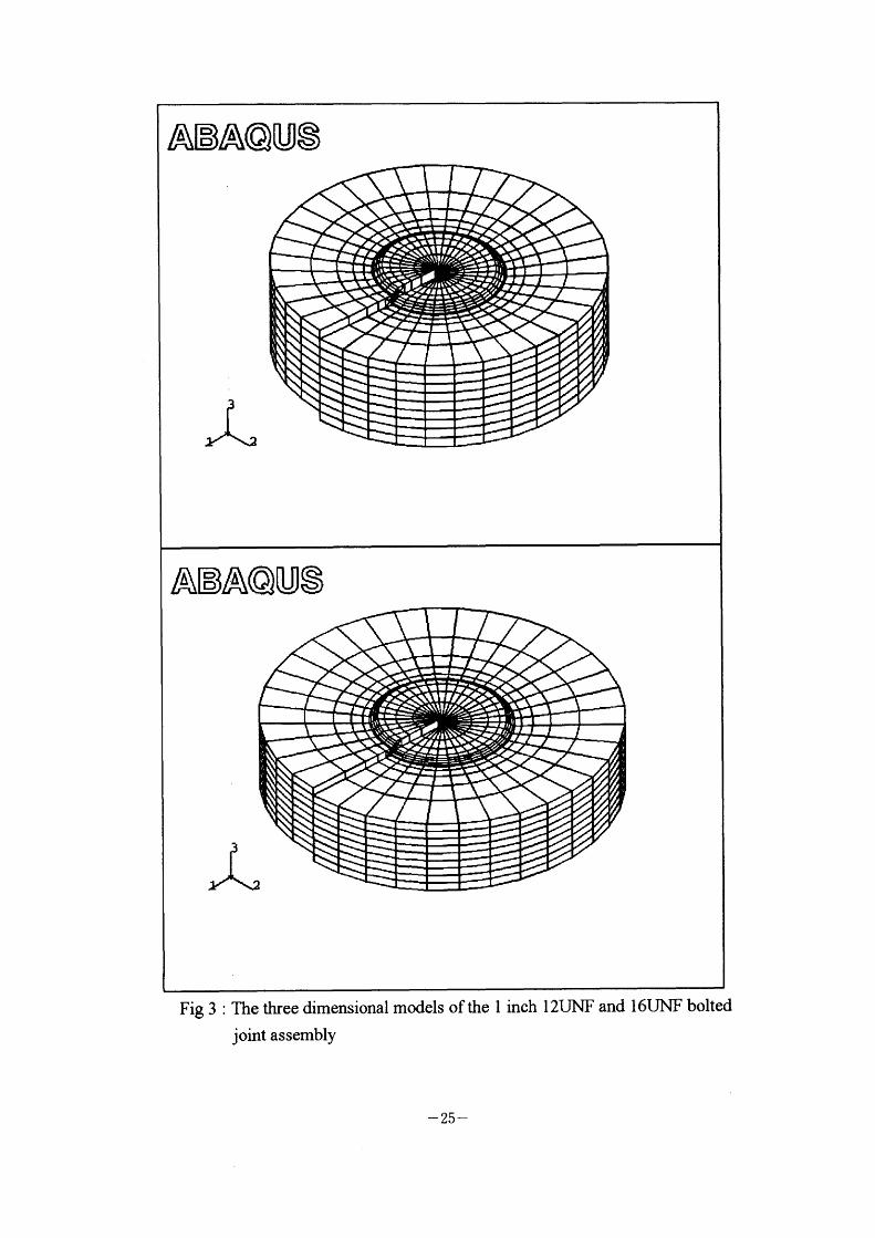
the fine thread bolt is shown in Figure 3 . Due to the difficulty ofthe three dimensional

modeling, a small hole is assumed at the center of the bolt, this will slightly reduces the

area of the applied load. The elastie material is used through out this work, where the

Young's modulus(F) is assumed as 30E+6 psi, Poisson ratio( v) as 0.3, and the

coeffieient of friction( p) as 0.1 in this analysis. The uniform pressure loading (p=

l OOOO psi) is applied on the top root surface of the bolt in this study.

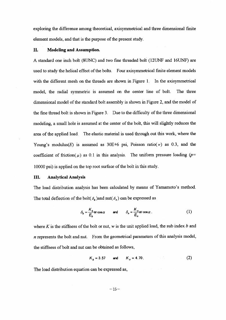
III. Analytical Analysis

The load disinbution analysis has been calculated by means of Yamamoto's method.

The total defleetion of the bolt( 6b )and nut( 6~ ) can be expressed as

6;b = Kbwoosa 5 = K~wc06a (1) and

where K is the stiffness of the bolt or nut, w is the unit applied load, the sub index b and

n represents the bolt and nut. From the geometrieal parameters of this analysis model,

the stifiness of bolt and nut can be obtained as follows,

Kb = 3.57 and K 4 70 (2) The load distribution equation can be expressed as,

- 15 -

F = F dd,(Ax) (3) b dnb(AL) '

where Fb is the load on the flfSt thread of the bolt. L is the engaged length of the bolted

joints, and ;t is a Gharacteristic length and expressed as

1 l + ;t= AbEb A.E. _ (4) 0.0847 ~ Kb K) [ : + tanP Eb E

where A is the crossseGtion area, p is the lead angle Hence the result of the load

disinbution on eaGh thread can be shown on Table I .

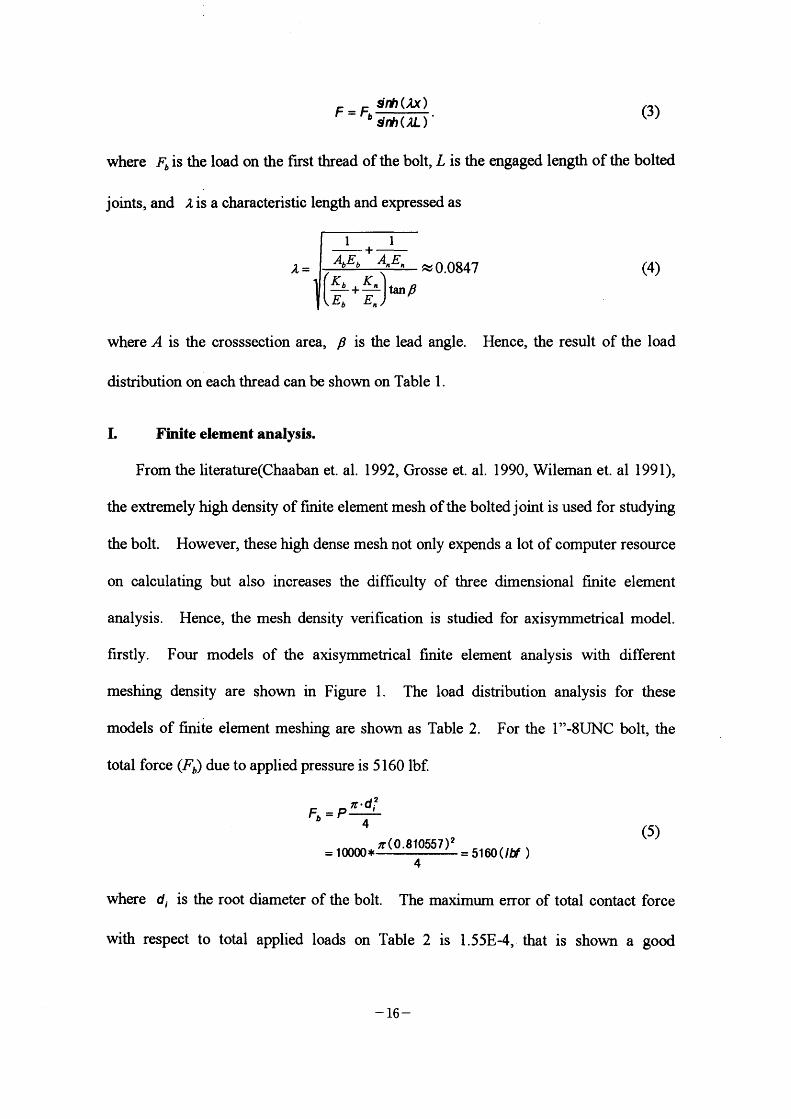
I. Finite clement analysis.

From the literature(Chaaban et. al. 1 992, Grosse et. al. 1 990, Wileman et. al 1 991),

the extremely high density of fmite element mesh of the bolted j oint is used for studying

the bolt. However, these high dense mesh not only expends a lot of computer resouree

on calculating but also increases the difficulty of three dimensional fmite element

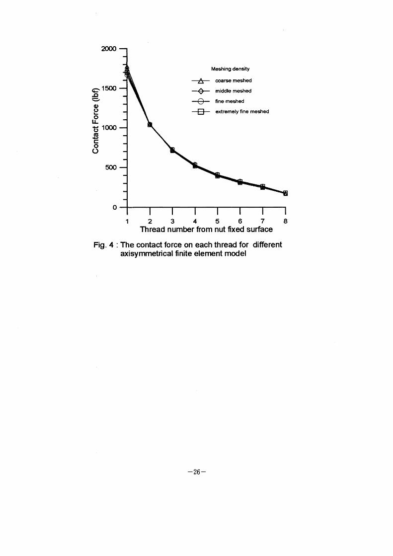
analysis. Hence, the mesh density verifioation is studied for axisymmeincal model.

firstly. Four models of the axisymmeincal finite element analysis with different

meshing density are shown in Figure I . The load distribution analysis for these

models of fmite element meshing are shown as Table 2. For the I "-8UNC bolt, the

total force (Fb) due to applied pressure is 5 1 60 Ibf.

F =P;T'di2

loooo*'r(0.8ro557)2 5leo(Il/ )

4 -where di is the root diameter of the bolt. The maximum error of total contaot forGe

with respect to total applied loads on Table 2 is I .55E-4, that is shown a good

-16-

agreement with four types of axisymmetrical meshed model. From the Figure 4, the

maximum deviation is happened at frrst thread of the bolted j oints, and the maximum

differential is 60/0 between GOarse mesh model and fine mesh model. Therefore, the

coarse meshed model used in this study can be proposed for studying helical and

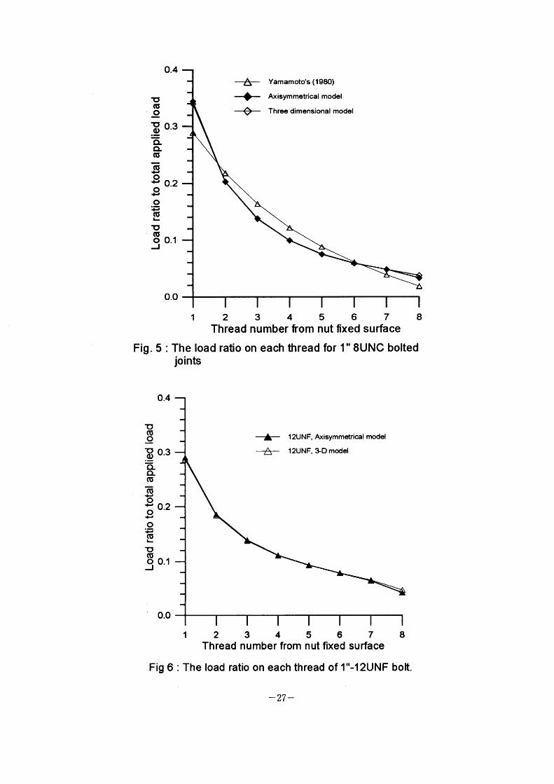
friction effects on the three dimensional fmite element analysis. Figure 5 shows the

load distribution of analytical, coarse meshed axisymmetrical and three dimensional

finite element analysis results. The load distribution with analytiGal prediction has

shown somewhat lower than the result of fmite element analysis.

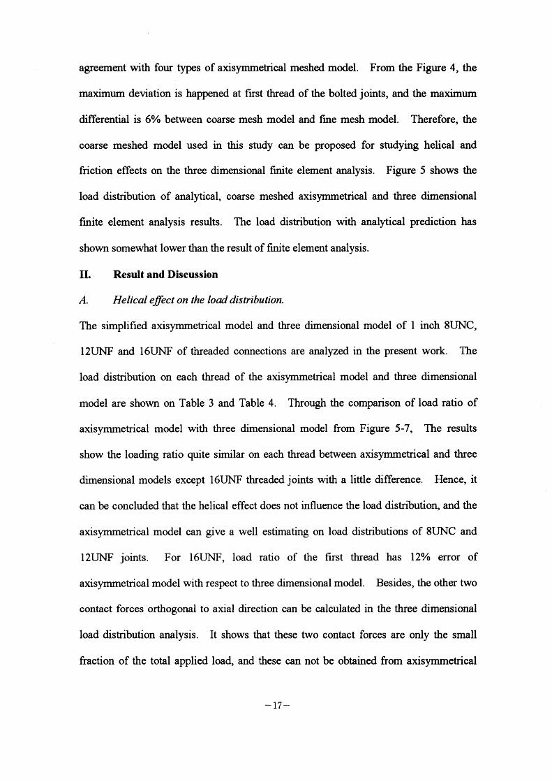
II. Result and Discussion

A. Helical effect on the loed distribution.

The simplified axisymmetrical model and three dimensional model of I inch 8UNC,

l 2UNF and 1 6UNF of threaded connections are analyzed in the present work. The

load disinbution on each thread of the axisymmetrical model and three dimensional

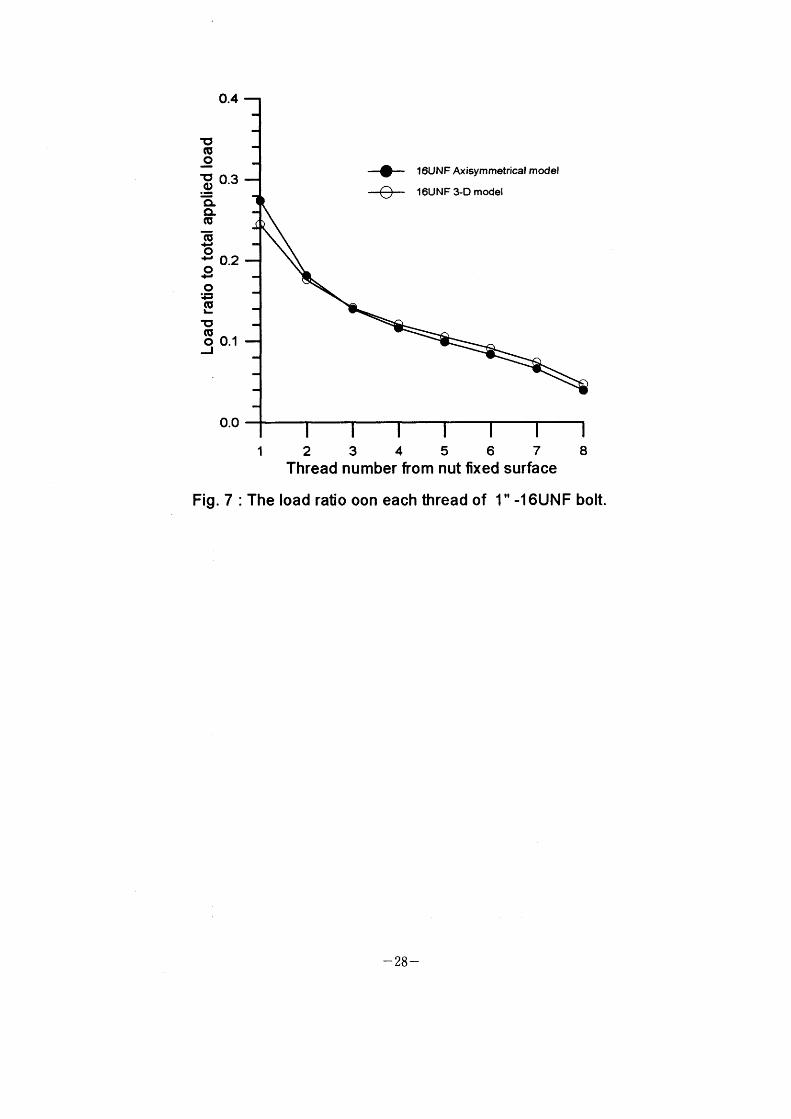
model are shown on Table 3 and Table 4. Through the comparison of load ratio of

axisymmeincal model with three dimensional model from Figure 5-7, The results

show the loading ratio quite similar on eaoh thread between axisymmetrical and three

dimensional models exGept 1 6UNF threaded joints with a little difference. HenGe, it

can be concluded that the helical effect does not influence the load distribution, and the

axisymmeincal model can give a well estimating on load disinbutions of 8UNC and

12UNF joints. For 16UNF, Ioad ratio of the first thread has 120/0 error of

axisymmetrical model with respect to three dimensional model. Besides, the other two

contaGt forces orthogonal to axial direction can be calculated in the three dimensional

load distribution analysis. It shows that these two contact forces are only the small

fraction of the total applied load, and these can not be obtained from axisymmetrical

-17-

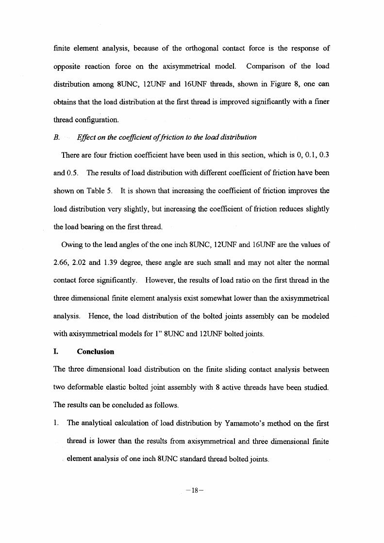
ftnite element analysis, because of the orthogonal contact force is the response of

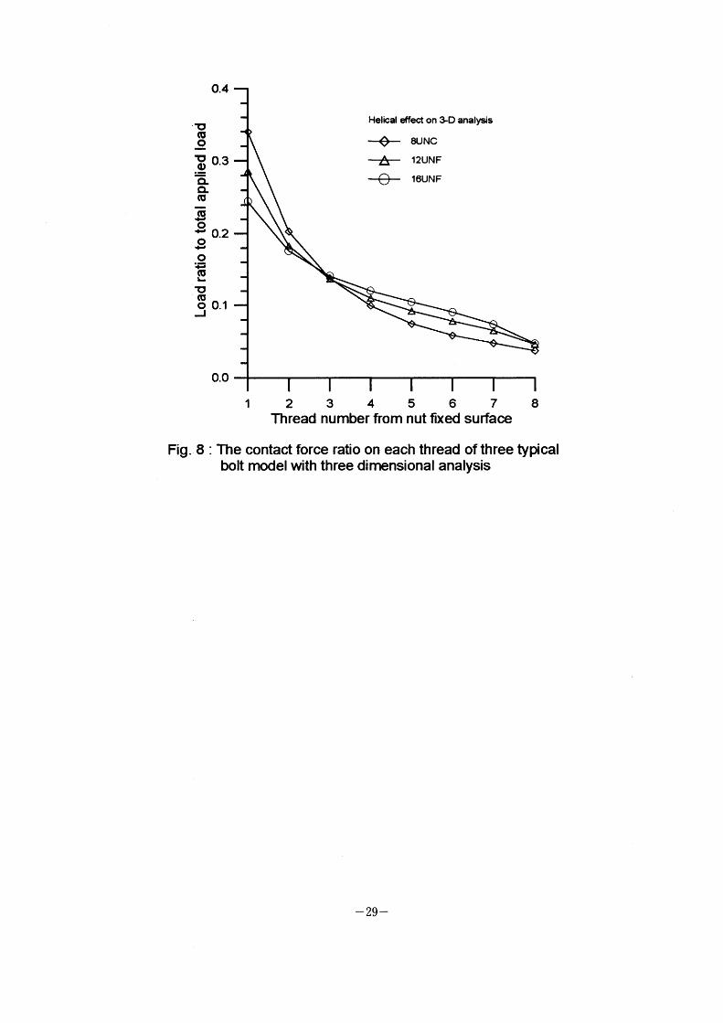
opposite reaction force on the axisymmetrical model. Comparison of the load

distribution among 8UNC, 1 2UNF and 16UNF threads, shown in Figure 8, one can

obtains that the load distribution at the flfst thread is improved significantly with a finer

thread configuration.

Effect on the coefficient offriction to the loed distribution B.

There are four friotion coefficient have been used in this section, which is O, O. I . 0.3

and 0.5. The results ofload distribution with different coefficient of friction have been

shown on Table 5. It is shown that increasing the coefficient of friction improves the

load distribution very slightly, but inereasing the coefficient of friction reduces slightly

the load bearing on the first thread,

Owing to the lead angles of the one inch 8UNC, 1 2UNF and 1 6UNF are the values of

2.66, 2.02 and I .39 degree, these angle are such small and may not alter the normal

contact force signifioantly. However, the results of load ratio on the frrst thread in the

three dimensional fmite element analysis exist somewhat lower than the axisymmetrical

analysis. Hence, the load distribution of the bolted joints assembly can be modeled

with axisymmetrical models for I " 8UNC and 1 2UNF bolted j oints.

I. Conclusion

The three dimensional load distribution on the finite sliding contact analysis between

two deformable elastic bolted joint assembly with 8 active threads have been studied.

The results oan be coneluded as follows.

l . The analytical calculation of load distribution by Yamamoto's method on the flfSt

thread is lower than the results from axisymmetrical and three dimensional finite

element analysis of one inch 8UNC standard thread bolted j oints .

-18-

2 The load distnbution of the first thread is improved more significantly by using

l 6UNF instead of 8UNC bolted joints for axisymmetrical and three dimensional

contact analysis.

3 . The effeGt of coefficient of friction on the load distribution of bolted joint assembly

is not evident, although increasing of friction will improve the load distribution

slightly.

4. The deviation of load ratio at the frrst thread are small for I " 8UNC and 1 2UNF,

but the error approaches to 1 20/0 for 1 6UNF bolted j oint.

Acknowledgnrents

This work is supported by Institute of Nuclear Energy Research. The authors wish

to aeknowledge the help from our colleagues at INER. The authors also wish to

express our appreciation to Dr. Kuen Ting encouragement .

Reference

Chaaban A., Jutras M., 1 992. Statie analysis of buttress threads using the fmite element

method" Joumal ofPressure Vessel Teohnology Vol. I 14, pp. 209-212.

Grosse I R Mitchell L. D., 1990 Nonlmear axral stifiness charactenstic of

axisymmetric bolted joint. Transaction of the ASME, Jounral of Mechanical Design,

Vol. I 12, pp. 442 449

Hibbitt , Karlsson, Sorenson 1 998. ABAQUS Finite Element Code version 5 .7.

Lehnhoff T. F., Wistehuff W. E., 1 996, Nonlinear effects on the stress and deformations

of bolted joints. Transaction of the ASME, Journal of Mechanical Design, Vol. I 1 8,

pp. 54-58.

Sopwith D. G., 1 948. The distribution of load in screw threads. Institute of Mechanieal

Engineering, Applied Mechanics Proceedings 1 59, pp. 373 383

-19-

Wileman J.. Choudhury M., Green I., 1 991. Computation of member stiffness in bolted

comeGtions. Transaction of the ASME, Journal ofMechanical Design, Vol. 1 1 3, pp.

432437.

Yamamoto A 1 980 The Theory and Computation of Thread ConneGtion Pressed

Yonkendo, Tokyo pp. 39-54.(in Japanese)

- 20 -

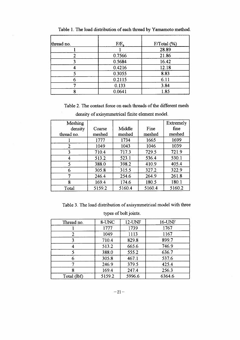
Table I . The load distribution of each thread by Yamamoto method.

Table 2. The oontact force on each threads of the different mesh

density of axisymmetrical finite element model.

Table 3 . The load distribution of axisymmetrical model with three

types of bolt joints.

-21-

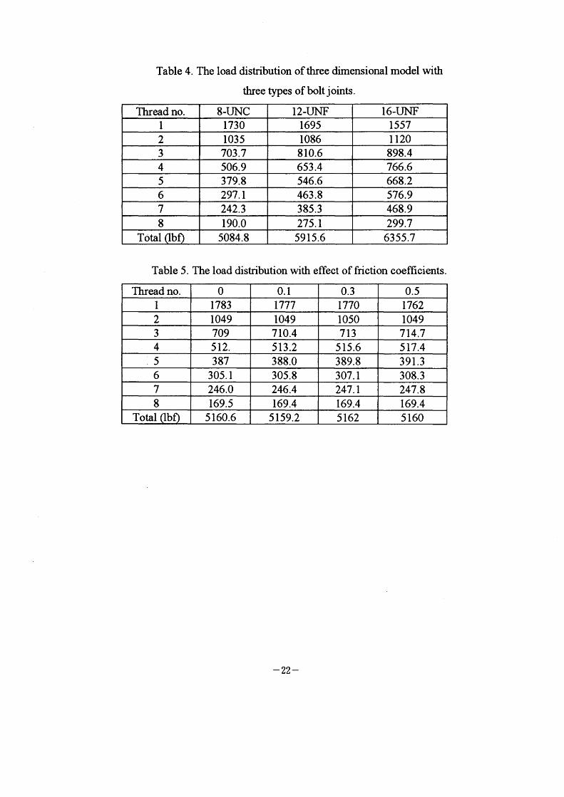
Table 4. The load distribution of three dimensional model with

three types of bolt joints.

Table 5 . The load disinbution with effect of frietion coefficients.

- 22 -

Coars e DenBe Mesh

Fig I (a) :Coarse meshed model

Middl e

Fig l(b)

High Dense

Fig l(C) :Fine meshed model

Dense Extremely High Dense Mesh

:Middle meshed model Fig I (a) :Extremely high meshed model

Fig I : Four types of the finite element axisymmetrical models.

-23-

~~~~)~~

~ ~~~ ~ ~

Fig 2 : The three dimensional model mesh of standard bolted j oints

assembly(upper) and bolt itself (Iower)

- 24 -

~~A~~~ ~l ~

Fig 3 : The three dimensional models of the I inch 1 2UNF and 1 6UNF bolted

joint assembly

- 25 -

2000

Q 1500 JD ~.

~ ~o 1000 ~S

8 500

O

=~ ~~ ~-

Meshing density

coarse meshed

middle meshed

flne meshed

extremely fine meshed

Fig .

7 4 5 6 1 2 3 Thread number from nut flxed surtace

4 : The contact force on each thread for different axisymmetrical flnite element model

8

- 26 -

0.4

~ c9 ~! ~o 0.3

li CL cs

c9 1. o t' 0.2 o d* o ~= c5L

U c:,o 0.1

J

0.0

-+, H~

Yamamoto's (1 9eo)

Axisymmetrical model

Three dimensional model

7 3 5 1 2 4 Thread number trom nut flxed surface

Fig. 5 : The load ratio on each thread for I " 8UNC bolted joints

0.4

1:I CU ~2

Uo 0.3

~QL CL cU.

-(U

'H o 4- 0.2 o d' o ~= ~ U CDO 0.1

J

0.0

-F =~ 12UNF, Axisymmetrical model

12UNF, 3-D model

Fig 6

4 5 6 7 8 1 2 3 Thread number from nut fixed surface

The load ratio on each thread of 1"-12UNF boit.

- 27 -

0.4

~ c9

o ~0 0.3

~ GL co

c9 .~ o '~ 0.2 o .~ o :,= c9

L U CDO 0.1

J

0.0

~--~ 16UNF Axisymmetrical model

16UNF 3-D model

7 8 1 2 3 4 5 6 Thread number from nut flxed surface

Fig. 7 : The load ratio oon each thread of I " -16UNF bolt.

- 28 -

o. 4

,~ c9 ~2 Uo 0,3

l~ ~ c9

J~ o t' 0,2 o 1. o :5:5 c9L

U g 0,1

J

0.0

Helical eFfect on 3-D analysis

-~ 8UNC ~~ 12UNF ~- 16UNF

Fig. 8

6 7 Thread number from nut fixed surface

The contact force ratio on each thread of three typical bolt model with three dimensional analysis

- 29 -

Session II

Structural Integrity and Life Prediction

II- l Probabilistic Fracture Mechanics of Nuclear Structural Components

Genki Yagawa, University of Tokyo, Japan

PROBABILISTIC FRACTURE MECHANICS OF NUCLEAR STRUCTURAL COMPONENTS = CONSIDERATION OF

TRANSITION FROM EMBEDDED CRACK TO SURFACE CRACK

Genki Yagawal), Yasuhrro Kant02) and Shinobu Yoshimural)

l ) School of Engineering, University of Tokyo,

7-3-1 Hongo, Bunkyo, Tokyo I 13-0033, Japan

2) Department of Mechanical Engineering, Toyohashi University of Science and Technology,

Tempaku, Toyohashi 441-8122, Japan

ABSTRACT

This paper describes a probabilistic fracture mechanics (PFM) analysis of

aged nuclear reactor pressure vessel (RPV) material. New interpolation formulas are first derived for both embedded elliptical surface cracks and

semi-elliptical surface cracks. To investigate effects of transition from

embedded crack to surface crack in PFM analyses, one of PFM round-robin problems set by JSME-RC111 commrttee I e "aged RPV under normal and upset operating conditions" is solved, employing the interpolation formulas .

1 . INTRODUCTION

In design and integrity evaluation processes for nuclear structural components, deterministic approaches have mainly been employed. All kinds of uncertainty related to operating history, material property change and damage mechanisms are taken into account in so-called safety factors. It is easily expected

that the results obtained are too conservative to perform a rational evaluation of

plant safety and to make judgement of life extension because of the accumulation

of conservatisms of all related factors.

Probabilistic Fracture Mechanics (PFM) has become an important tool [1, 2] .

The PFM approach is regarded as an appropriate method in rationally evaluating plant life and in risk-based decision making such as risk-informed inspection [3]

since it can consider various uncertainties such as sizes and distributions of cracks,

degradation of material strength due to aging effects, fluctuating loading histories,

accuracy and frequency of pre- and in-service inspections. Thus, various PFM

-31-

computer programs have been developed and applied in practical situations in the last two decades.

In Japan, one research activity on PFM approaches to the integrity studies of

nuclear pressure vessels and piping (PV&P) was initiated in 1 987 by the LE-PFM

subcommittee organized within the Japan Welding Engineering Society (JWES) under a subcontract of the Japan Atomic Energy Research Institute (JAERI), and continued for three years [4]. The activity was followed by the RC I I I research

committee organized in the Japan Society of Mechanical Engineers (JSME) in 1991, and fmished in March, 1995 [5]. Succeeding it, a new PFM subcommittee organized in JWES started again in May, 1996 [6], and is scheduled to continue until March, 1999. The purpose of the continuous activity is to establish standard

procedures for evaluating failure probabilities of Japanese nuclear structural components such as PV&P and stearn generator tube, combining the state-of-the art knowledge on structural integrity of nuclear structural components and modern computer technology such as parallel processing. Within the LE-PFM and JSME-RC I I I activities, we have set up the following three kinds of PFM

roud-robin problems on

(a) primary piping under normal operating conditions, (b) aged reactor pressure vessel (RPV) under normal & upset operating

conditions, and

(c) aged RPV under pressurized thennal shock (PTS) events.

The basic part of the last PTS problems is taken from some of US benchmark problems [7, 8]. For these round-robin problems, various sensitivity analyses were performed to quantify effects of uncertainty of data on failure probabilities.

Some of the detailed analysis results can be found in elsewhere [9-15].

In those analyses, we always assumed semi-elliptical surface cracks as initial

cracks for the purpose of convenience. However, as well known, embedded cracks seem more practical and probable as initial cracks. Thus as one of main

tasks in the JWES-PFM subcommittee, we are developing a new PFM model considering transition from embedded to surface cracks during crack growth. This paper describes its latest results. Here new interpolation forrnulas are frrst

derived for both embedded elliptical cracks and semi-elliptical surface cracks. To

investigate effects of transition from embedded to surface cracks in PFM analyses,

one of PFM round-robin problems set by JSME-RC111 committee, i.e. "aged RPV under normal and upset operating conditions" is solved employing the interpolation formulas.

- 32 -

2. OUTLINE OF PFM ANALYSIS

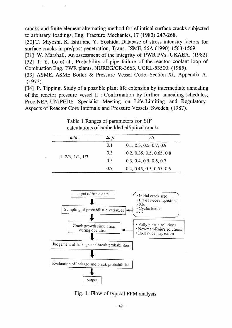
Figure I illustrates the flow of a typical PFM analysis. Firstly, some random variables are selected according to an analysis model employed. Random variables to be considered include initial crack sizes (crack depth and crack aspect

ratio) and location, accuracy and frequency of nondestructive tests, i.e. PSI and

ISI, material properties, cycles and amplitudes of applied loads. Next, crack

growth simulations are performed. Fracture mechanics models employed are based on the linear elastic fracture mechanics, i.e. Newman-Raju solutions [16], influence functions [ 1 7-20] and others [2l], and the nonlinear fracture mechanics,

i.e. fully plastic solutions [22, 23] or their combination [24, 25]. Besides, creep

crack growth can be simulated based on the nonlinear fracture mechanics [26, 27].

During the crack growth simulation, PSI and ISI are considered, and failure judgements of leakage and break are performed. Cumulative failure probabilities are calculated as functions of operation time in round-robin problems (a) and (b),

while failure probabilities for one PTS event are calculated in round-robin problem (c). To effectively calculate accurate failure probabilities, the Stratified

sampling Monte Carlo (SMC) algorithm is offen employed. Its parallel version is also very efficient [1 I].

3. INTERPOLATION FORMULAS OF STRESS INTENSITY FACTORS FOR EMBEDDED ELLIPTICAL CRACK & SEMI-ELLIPTICAL SURFACE CRACK

3.1 Stress Intensity Factors for Embedded Elliptical Cracks

Soneda and Fujioka calculated stress intensity factors (SIFs) of various elliptical cracks embedded in thick-wall cylinder subjected to arbitrarily distributed loadings, and constructed an influence function database [28]. They employed the finite element alternating method developed by Nishioka and Atluri

[29]. The analysis process is schematically illustrated in Figure 2 and summarized as follows :

l) Solve the uncracked fmite body under the given external loads by using

the finite element method. The uncracked body has the same geometry with the given problem except the crack.

2) Compute the stresses a.,.,k at the location of the original crack, using the

finite element solution.

3) Compare the residual stresses a.,,,k calculated in 2) with a permissible

stress magnitude. In the present study, 0.1 % of the initial a value .***k

was used for the permissible stress magnitude. 4) Calculate theoretically the SIF, KI(i)

i~fi~it* of the crack in infinite body,

- 33 -

applying the stresses a,,*,k Onto the crack surface.

5) Solve the cracked infmite body, applying the reversed stresses - a ****k

onto the crack surface.

6) Compute the stresses a*uf*** at the boundary of the original finite body,

using the finite element solution.

7) Solve the uncracked body under the 0=*ta,* onto its boundary by using the

finite element method.

Repeat 2)-7) steps in the iteration process until the residual stresses a**k On the

crack surface become negligible (Step 3). To obtain the final SIF solution KI ' add

the stress intensity factors of all iterations as :

( i)

i=0

where n is the number of iterations.

Here we consider only the axial elliptical crack embedded in cylinder as in

Figure 3. Following a typical influence function method, a stress distribution in

the thikness direction of the cylinder is first approximated by 4th-order polynomial in a normalized coordinate. Then the SIF values are expressed with the coefficients Ai Of the polynomial as follows :

l/ s Kl(e) S = (a~sin2e + a~cos2e '4~ A G i=0 l

(2)

where Gi is the influence function for the

square of elliptic integral of second kind

equatron :

j-th

and order stress distribution, Q is the

is approximated by the following

Q = I + 1.464 (a2 / al)1'65 (3)

where al and a2 are half lengths of the crack in the axial and thickness directions,

respectively. Gi Values are tabulated in Ref. [28]. In the present study, Gi Vaiues

are evaluated at the three points of elliptic angle 0=7c/2, O and -1c/2. In the three cases, (*)1/4 term in Eq. (2) reduces to (al)1/4, (a2)1/4 and (al)1/4, respectively.

When only tensile stress o:T and bending stress aB are considered, the coefficients Ai in Eq. (2) are simplified as follows :

Ao = OT ~ aB

Al = 20B Ak = O, for k ~: 2

(4)

- 34 -

Table I shows parameter ranges for which influence functions Gi are given in Ref. [28]. We then interpolate follOwing.

Gi = ~ ~ ~ ci=Pq,~Pnq~

p=0 q=0 '=0

those mfluence functron soluttons in the

(5)

where

~= _ ) + (ett) y [(

e/t ert ~~ ~'~ .2 e/t - l 12

0.90 - 2adt

( 6 a)

e/t e/t) j ( . ( -~" ~."

_ I (( I I y + (a /a ) - - ) 2 a'/a ao/a mm '2 max aa/a I - 2/3

n= - ) ( (2 ) 2 a /al max a /al mln 2/3 (6b)

~= . y [ ) + rL2a~t) ' 2 2adt - [2adt

~'" ~~* 2ajt - 0.4

. - [2a~t) ' (2a~ t)

~~ ~'" 0.6

(6c)

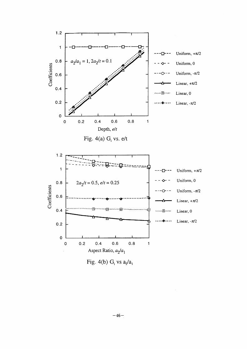
In the present study, only Gi Values of axial elliptical cracks for linear

components of stress distributions are interpolated, although more other solutions are given in Ref. [28]. The coefficients ci;pq' in Eq. (5) are tabulated in Table 2.

Figures 4(a) and 4(b) show some comparison of original and interpolated Gi values. These figures confirm that Eq. (5) provides accurate interpolation for all

the solutions. It should be also noted here that, as shown in Figure 4(b), Eq. (5)

exrapolates in the range of a2/al=0- 1/3. Its validity in the range is not proven yet.

3.2 Stress Intensity Factors for Semi-elliptical Surface Cracks

In PFM analyses considering the embedded elliptical cracks as described in 3.1, one can take into account uncracked ligament as small as 0.05t, where t is cylinder thickness. On the other hand, original finite element K solutions of

Newman-Raju [16], which have been employed in the PFM round-robin problems (a) and (b) are obtained till crack depth a =0.8t, i.e. uncracked ligament of 0.2t.

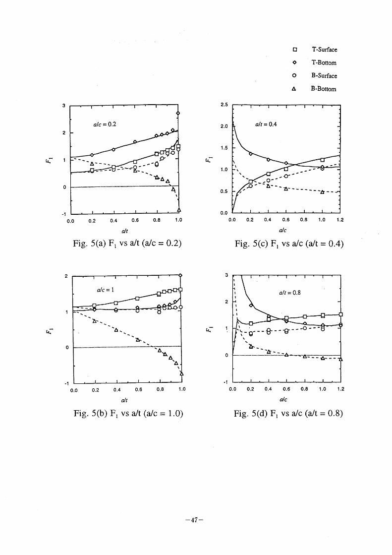
Miyoshi et al. performed precise finite element analyses for much deeper cracks than a=0.9t [30]. To make K solutions for surface cracks consistant with those for

embedded cracks, a new interpolation formula is also derived in this study using

both Newman-Raju's finite element solutions [16] and Miyoshi's [30].

Fundamental policy for this task is as follows :

1) Since K solutions increase rapidly over a/t > 0.95, the present interpolation certifies its validity until a/t=0.95.

- 35 -

3) The interpolation is performed only for K solutions at elliptic angle of

c =0 and lcl2.

The interpolation formula obtained is expressed as follows :

K =( ) I at + ab ~~~rFl (7)

where

Q - I o + 1 464 a/c 165 - . . ( J. Fl = ~ ~ G'j~i(~)j

i=0j=0

~=1-fr~~T

( 8 a)

(8b)

(8c)

where Gij are given in Table 3. The validity range of this interpolation is summarized in Table 4. Beyond the validity range in Table 4, Newman-Raju's equation is adopted except a/t > 0.95. Figures 4(a) and 4(b) show the comparison between finite element solutions and the interpolation of Eq. (7) for the purpose

of convenience.

4. ANALYSIS PROBLEM = AGED RPV UNDER NORMAL AND UPSET OPERATING CONDITION

A PFM model analyzed here is basically the same as the PFM round-robin problem for an aged RPV under normal and upset operating condition, which was given by JSME-RC 1 1 1 committee [5] except consideration of embedded cracks.

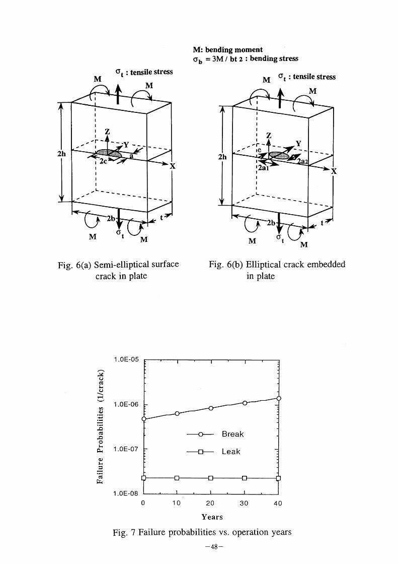
4.1 Analysis Models Two kinds of cracked models are assumed here. The one is a plate with a

semi-elliptical surface crack, while the other is a plate with an axial embedded

elliptical crack. These are illustrated in Figures 6(a) and 6(b). The embedded elliptical crack may be converted to the semi-elliptical surface crack, according to

a certain conversion criterion as described later. In both models, plate thickness

and width are taken to be t = 0.2m and 2b = 12.6m, considering the beltline portion of PWR pressure vessels. The plates are assumed to be subjected to various magnitudes of remote uniform tensile and bending stresses. For the purpose of simplicity, we ignore curvature effects of actual pressure vessels in

evaluating 3-dimensional SIFs. Cumulative failure probabilities of one existing crack, whose unit is l/crack, are calculated as functions of operation years.

- 36 -

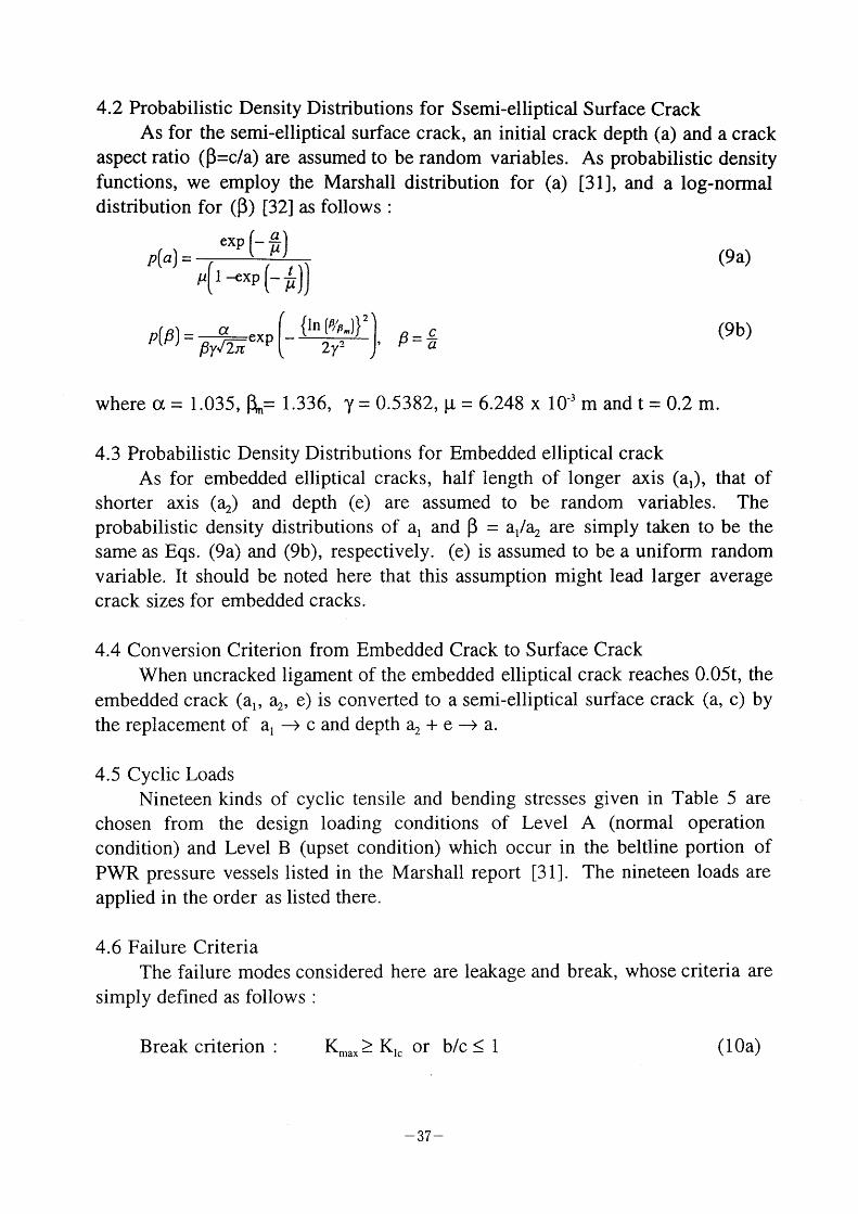
4.2 Probabilistic Density Distributions for Ssemi-elliptical Surface Crack

As for the semi-elliptical surface crack, an initial crack depth (a) and a crack

aspect ratio (P=c/a) are assumed to be random variables. As probabilistic density

functions, we employ the Marshall distribution for (a) [3l], and a log-normal distribution for (P) [32] as follows :

a exp --11

//[1~xp ( I/ _ ~jj

p(p) a {In [p,'fu~)} c (9b) p p yl~~ exp a 2Y

where oc = 1.035, ~= 1 336 Y O 5382 u 6 248 x 10 m and t O 2 m

4.3 Probabilistic Density Distributions for Embedded elliptical crack

As for embedded elliptical cracks, half length of longer axis (al)' that of

shorter axis (a2) and depth (e) are assumed to be random variables. The probabilistic density distributions of al and p = al/a2 are simply taken to be the

same as Eqs. (9a) and (9b), respectively. (e) is assumed to be a uniform random

variable. It should be noted here that this assumption might lead larger average

crack sizes for embedded cracks.

4.4 Conversion Criterion from Embedded Crack to Surface Crack When uncracked ligament of the embedded elliptical crack reaches 0.05t, the

embedded crack (al' a2, e) is converted to a semi-elliptical surface crack (a, c) by

the replacement of al ~ c and depth a2 + e ~> a.

4.5 Cyclic Loads Nineteen kinds of cyclic tensile and bending stresses given in Table 5 are

chosen from the design loading conditions of Level A (normal operation condition) and Level B (upset condition) which occur in the beltline portion of

PWR pressure vessels listed in the Marshall report [3l]. The nineteen loads are applied in the order as listed there.

4.6 Failure Criteria

The failure modes considered here are leakage and break, whose criteria are

simply defined as follows :

~***- tc -

- 37 -

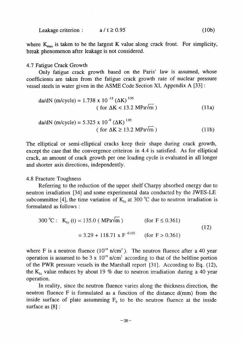
Leakage criterion : a / t ~ 0.95 ( I Ob)

where I(~*. is taken to be the largest K value along

break phenomenon after leakage is not considered.

crack front. For simplicity,

4.7 Fatigue Crack Growth Only fatigue crack growth based on the Paris' Iaw is assumed, whose

coefficients are taken from the fatigue crack growth rate of nuclear pressure vessel steels in water given in the ASME Code Section XI, Appendix A [33] :

da/dN (m/cycle) = 1.738 x 10 ~13 (AK) 5.95

( I I a)

da/dN (m/cycle) = 5.325 x 10~9 (AK) 1'95

( for AK ~ 13.2 MPa~~~: ) (1 Ib)

The elliptical or semi-elliptical cracks keep their shape during crack growth, except the case that the convergence criteiron in 4.4 is satisfied. As for elliptical

crack, an amount of crack growth per one loading cycle is evaluated in all longer

and shorter axis directions, independently.

4.8 Fracture Toughness Referring to the reduction of the upper shelf Charpy absorbed energy due to

neutron irradiation [34] and some experimental data conducted by the JWES-LE subcommittee [4], the time variation of KI* at 300 "C due to neutron irradiation is

formulated as follows :

300 'C : Ktc (t) = 135.0 ( MPa~fl ) (for F ~ 0.361) ( 1 2)

= 3.29 + l 18.71 x F ~o.l02 (for F > 0.361)

where F is a neutron fluence (l019 n/cm2 ). The neutron fluence after a 40 year operation is assumed to be 3 x I 019 n/cm2 according to that of the beltline portion

of the PWR pressure vessels in the Marshall report [3l]. According to Eq. (12), the Ktc value reduces by about 19 (~o due to neutron irradiation during a 40 year

operatron. In reality, since the neutron fluence varies along the thickness direction, the

neutron fluence F is formulated as a function of the distance d(mm) from the inside surface of plate assumming Fo to be the neutron fluence at the inside surface as [8] :

- 38 -

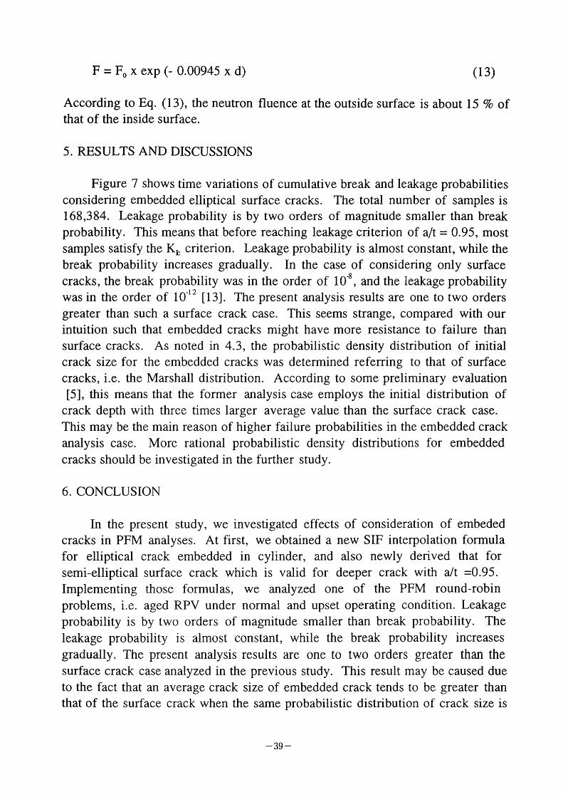
F = Fo x exp (- 0.00945 x d) (13)

According to Eq. (13), the neutron that of the inside surface.

fluence at the outside surface is about 1 5 % of

5. RESULTS AND DISCUSSIONS

Figure 7 shows time variations of cumulative break and leakage probabilities

considering embedded elliptical surface cracks. The total number of samples is 168,384. Leakage probability is by two orders of magnitude smaller than break probability. This means that before reaching leakage criterion of a/t = 0.95, most

samples satisfy the Kb criterion. Leakage probability is almost constant, while the

break probability increases gradually. In the case of considering only surface cracks, the break probability was in the order of 10~8 , and the leakage probability

12 was in the order of 10~ [13]. The present analysis results are one to two orders

greater than such a surface crack case. This seems strange, compared with our intuition such that embedded cracks might have more resistance to failure than surface cracks. As noted in 4.3, the probabilistic density distribution of initial

crack size for the embedded cracks was determined referring to that of surface cracks, i.e. the Marshall distribution. According to some preliminary evaluation [5], this means that the former analysis case employs the initial distribution of

crack depth with three times larger average value than the surface crack case.

This may be the main reason of higher failure probabilities in the embedded crack

analysis case. More rational probabilistic density distributions for embedded cracks should be investigated in the further study.

6. CONCLUSION

In the present study, we investigated effects of consideration of embeded cracks in PFM analyses. At first, we obtained a new SIF interpolation forrnula for elliptical crack embedded in cylinder, and also newly derived that for semi-elliptical surface crack which is valid for deeper crack with a/t =0.95.

Implementing those formulas, we analyzed one of the PFM round-robin problems, i.e. aged RPV under normal and upset operating condition. Leakage probability is by two orders of magnitude smaller than break probability. The leakage probability is almost constant, while the break probability increases gradually. The present analysis results are one to two orders greater than the

surface crack case analyzed in the previous study. This result may be caused due

to the fact that an average crack size of embedded crack tends to be greater than that of the surface crack when the same probabilistic distribution of crack size is

- 39 -

employed for both embedded crack and surface crack. More rational probabilistic density distributions for embedded cracks should be investigated in

the further study.

ACKNOWLEDGEMENTS

The authors wish to thank all the members of the PFM subcommittee in the Japan Welding Engineering Society (JWES) for their efforts to perform this work, and also thank the Japan Atomic Energy Research Institute (JAERI) for

financial support.

REFERENCES

[1] G. Yagawa, Structural integrity assessment of nuclear power plants using probabilistic fracture mechanics, Nuclear Eng., 34 (1988) 19-30 (in Japanese).

[2] D. O. Harris and K. R. Balkey, Probabilistic considerations in life extension

and aging, Technology for the '90s, ASME PVP Division, pp.243-269, (1993). [3] K.R. Balkey, N.B. Closky and M.K. Vermaut, Application of risk-based methods to inservice inspection and testing, Trans. 14th SMiRT, Lyon, M05/2, ( 1 997).

[4] JWES, Report of LE Subcommittee, Japan Welding Eng. Society (JWES), JWES-AE-9003, (1990) (in Japanese). [5] Final Report of RC111 Committee, Japan Society of Mechanical Engineers (JSME), (1995). [6] JWES Report of PFM Subcommittee, JWES, JWES-AE-9705, (1997) (in Japanese) .

[7] D. L. Selby et al., PTS evaluation of the H.B. Robinson Unit 2 nuclear power

plant, NUREG/CR-4183, Vols. l, 2, (1985). [8] B. A. Bishop, Benchmarking of PFM analyses of reactor vessels subjected to PTS Ioading, EPRI Research Project 2975-5, Final Report, (1993).

[9] S. Yoshimura, G. Yagawa et al., PFM analyses of LWR's pressure vessels and piping : Quantitative study on influences of distributions of initial crack sizes,

Proc. 20th MPA Seminar, Vol.2, pp.44.1-10, (1994). [10] G. Yagawa, S. Yoshimura, et al., Study on life extension of aged RPV material based on PFM -Japanese round robin, Trans. ASME, J. Pressure Vessel Technology, 1 17(1995) 7-13.

[1l] S. Yoshimura, M.-Y. Zhang and G. Yagawa, Life extension simulation of aged reactor pressure vessel material using PFM analysis on a massively parallel

computer, Nuclear Eng. & Design, 158 (1995) 341-350. [12] G. Yagawa, S. Yoshimura et al., PFM anaiyses of nuclear pressure vessels under PTS events, Nuclear Eng. & Design, 174 (1997) 91-lOO.

- 40 -

[13] G. Yagawa and S. Yoshimura, A study on PFM for nuclear pressure vessels and piping, Int. J. Pressure Vessels & Piping, 73 (1997) 97-l07.

[14] S. Yoshimura, G. Yagawa et al., PFM analysis for LBB evaluation of Light Water Reactor's piping, J. of Atomic Energy Society of Japan, 39 (1997) 777-787. [15] G. Yagawa and S. Yoshimura, Probabilistic fracture mechanics analyses of nuclear pressure vessels and piping : A review of Japanese activity, Trans. 14th

SMiRT, Lyon, GMW/1, pp.541-552, (1997). [16] J. C. Newman, Jr. and L. S. Raju, Stress intensity factor equations for cracks

in 3D finite bodies subjected to tension and bending loads, NASA -TM- 85793, 1984. [17] I. S. Raju and J. C. Newman, Stress intensity factors for internal and external surface cracks in cylindrical vessels, Trans. ASME, J. Pressure Vessel

Technology, 104 (1982) 293-298. [18] D. L. Stevens et al., VISA, NUREG/CR-3384, (1983). [19] F. A. Simonen et al.,VISA-II, NUREG/CR-4486, PNL-5775 RF, R5, (1986). [20] M. Shiratori, Analysis of stress intensity factors for surface cracks subjected

to arbitrarily distributed stresses, Bulletin of Faculty of Eng., Yokohama National

University, 35 (1986) 1-25.

[2l] S. Yoshimura, J.-S. Lee and G. Yagawa, Automated system for analyzing stress intensity factors of 3D cracks : Its applications to analyses of two dissimilar

semi-elliptical surface cracks in plate, Trans. ASME, J. Pressure Vessel Technology, 1 19 (1996) 18-26. [22] G. Yagawa, Y. Kitajima and H. Ueda, 3D fully plastic solutions for semi-elliptical surface cracks, Int. J. Pressure Vessels & Piping, 53 (1993)

457-510. [23] G. Yagawa, Y. Kitajima and H. Ueda, Erratum of [22], Int. J. Pressure Vessels & Piping, 74 (1997) 77-80.

[24] G.-W. Ye, G. Yagawa and S. Yoshimura, PFM analysis based on 3DJ-integral database, Eng. Fracture Mechanics, 44 (1993) 887-893.

[25] G. Yagawa and G.-W. Ye, A PFM analysis for cracked pipe using 3-D model, Reliability Eng. & System Safety, 41 (1993) 189-196.

[26] G. Yagawa, S. Yoshimura and H. Ueda, An estimation scheme for J- and C*- integrals of surface cracks, Proc. Int. Symp. Pressure Vessel Technology &

Nuclear Codes & Standards, Seoul, pp.8. 15-8.22, (1989).

[27] K. Hojo, G. Yagawa, S. Yoshimura et al., Applications of PFM to FBR components, Nuclear Eng. & Design, 42 (1993) 43-49. [28] N. Soneda and T. Fujioka, Stress intensity factor influence coefficients of

embedded cracks in cylinder, Komae Research Laboratory Report of Central Research Institute of Electric Power Industry (CRIEPI), No. T94037, (1995). [29] T. Nishioka and S.N. Atluri, Analytical solution for embedded elliptical

-41-

\

cracks and finite element alternating method for elliptical surface cracks subjected

to arbitrary loadings. Eng. Fracture Mechanics, 17 (1983) 247-268.

[30] T. Miyoshi, K. Ishii and Y. Yoshida, Database of stress intensity factors for

surface cracks in prelpost penetration, Trans. JSME, 56A (1990) 1563-1569.

[3l] W. Marshall, An assessment of the integrity of PWR PVs. UKAEA, (1982). [32] T. Y. Lo et al., Probability of pipe failure of the reactor coolant loop of

Combustion Eng. PWR plants, NUREG/CR-3663, UCRL-53500, (1985). [33] ASME, ASME Boiler & Pressure Vessel Code. Section XI, Appendix A, (1973).

[34] P. Tipping, Study of a possible plant life extension by intermediate annealing

of the reactor pressure vessel 11 : Confirmation by further annealing schedules,

Proc.NEA-UNIPEDE Specialist Meeting on Life-Limiting and Regulatory Aspects of Reactor Core Internals and Pressure Vessels, Sweden, ( 1 987).

Table I Ranges of parameters for SIF calculations of embedded elliptical cracks

a2/al 2a2/t e/ t

1, 2/3, 1/2, 1/3

O. 1

0.3

0.5

0.7

0.1, 0.3, 0.5, 0.7, 0.9

0.2, 0.35, 0.5, 0.65, 0.8

0.3, 0.4, 0.5, 0.6, 0.7

0.4, 0.45, 0.5, 0.55, 0.6

Input of basic data

~ Sampling of probabillstic variables

• Initial crack size • Pre-service inspection • Ktc • Cyclic loads ...

Crack growth simulation during operation

• Fully plastic so]utions • Newman-Raju's solutions • In-service inspection

Judgement of leakage and break probabilities

~ Evaluation of leakage and break probabi]itles

~ r~~~Tl output

Fig. 1 Flow of typical PFM analysis

- 42 -

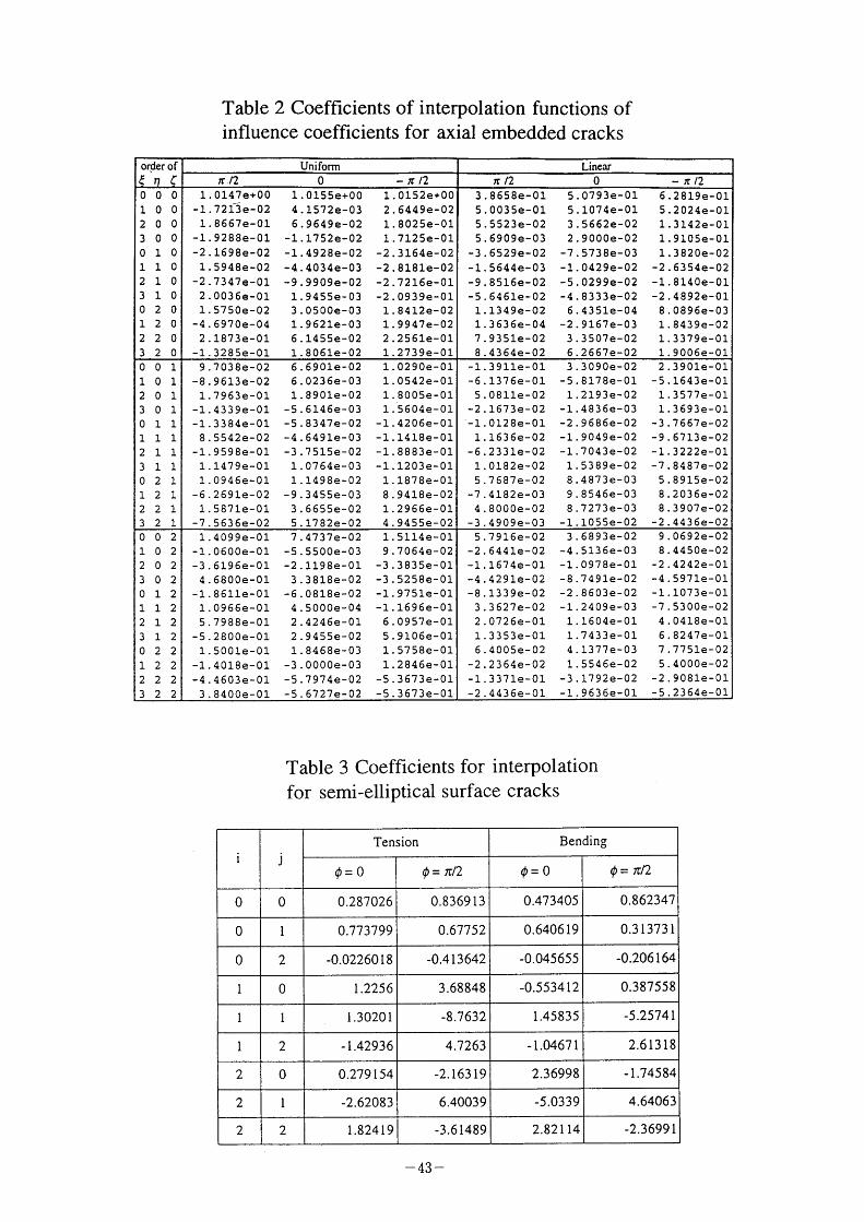
Table 2 Coefficients of interpolation functions of

influence coefficients for axial embedded cracks

Table 3 Coefficients for interpolation

for semi-elliptical surface cracks

- 43 -

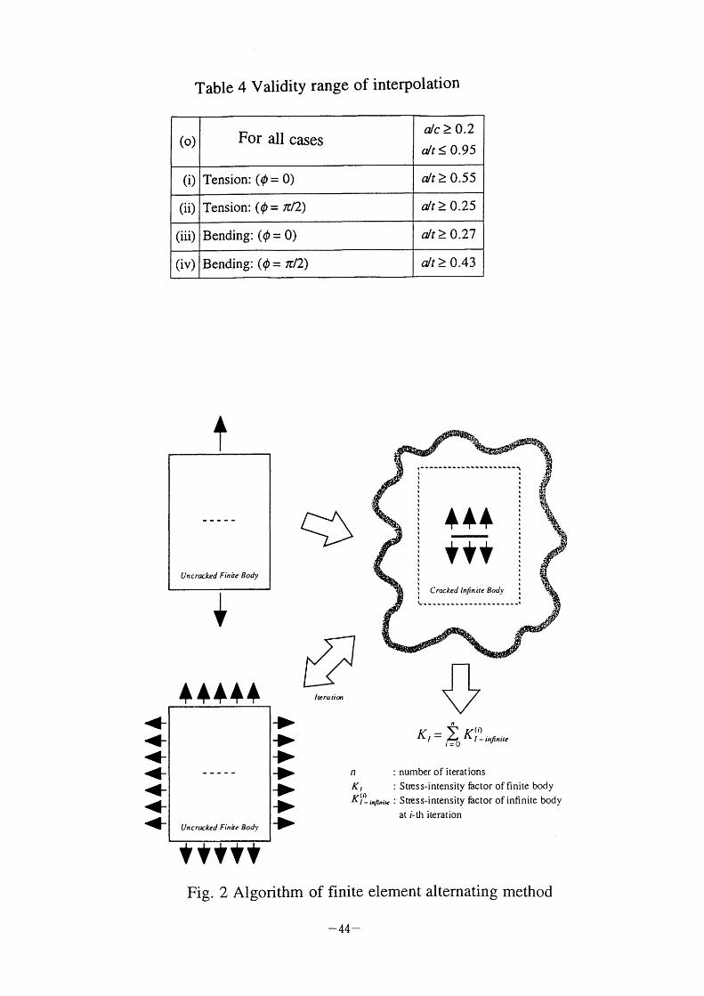
Table 4 Validity range of interpolation

t

Uncracked Finbe Body

~

~~~~~ i~ ~~

i~ i~

hera tio,'

Uncracked Finae Bod),

~!

t-- -*----**---------1~ 1 ,

t

N

N ,

l

b T~i~lf: , , t ~~ l ~ I ,

I ,

l

t

l Vtt ~ b

N

,

I

,

b 1 Cracked Infintte Body

t~.- -.'

n

K, . (f) KI-i,,fi,,ile :

~K K = (i) / i = o / ~ infinile

: number of iterations

Suess-intensity factor of finite body

Stress-intensity factor of infinite body

at i-th iteration

tVVVV Fig. 2 Algorithm of finite element alternating method

- 44 -

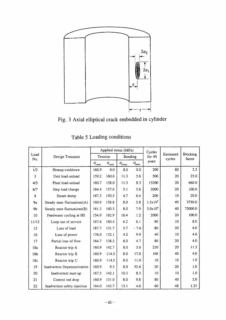
Fig.

2a2 i~--~ ~~ l

2a l

' l -~ e

t

3 Axial elliptical crack embedded in cylinder

Table 5 Loading conditions

- 45 -

C"

~ C: (L)

'C;

~ O O (J

1 .2

1

0.8

0.6

0.4

0.2

O

- CI--H:H--H:l

a2/al = 1 2a2/t O 1

a;••" . ~*

.S.:••"

J(. ~•/' ..*'

H:h- -H~: e•~" •t~i

, *,*~

' $'

(A::;••t' ,t4

,.

ldF .L

1,, t'

0.4 0.6 0.8 Depth, e/t

Fig. 4(a) Gi VS. e/t

1

1-11'd-Cha'l-

---O---

ll~l 'l 'f~3 tc l'] I Is'at

eP '1'1 I11'1

0.2

Uniform, +7T:/2

Unifonn, O

Uniform, -7t/2

Linear, +7c/2

Linear, O

Linear, -7cl2

c,D

~ c:::

o ~c-

~: oo

(J

1 .2

0.8

0.6

0.4

0.2

O

o

j I-_'i~_..;-._:_T; ~I:'~ 1lb 'I"_' :":

'~Lg: ='1'--"' 1-'

t ' e/t = O 25 2a2/t = O 5

.1 Idlll, Il e 'I' l ~ ldl 'l 11"I' l'N'I1'11"I'll lll,.

ft'lltl'f'~3at "t' tl'l I ~'t 'll B3'1 l' r yt~: d Idtflttttt'tl ('a ' ' "I I 'I'Itlll't"ttil"t'l a ll,II

0.2 0.4 0.6 0.8 Aspect Ratio, a2/a l

Fig. 4(b) Gj VS a2/al

1

-' ~ ~D- -"-

'I'-1C~-

--'1-0--'-'

~l-"t' " ~l 'I , I ,,1,I

I c l ll lllll

o

Uniform, +7d2

Uniform, O

Uniform, -7d2

Linear, +7~/2

Linear, O

Linear, -rd2

- 46 -

2.5

D

O

A

T-Surface

T-Bottom

B-Surface

B-Bottom

3

2

C

o

-1

a/c = 0.2

O pr

~A- - - -O , , ~-- --~--, ~ ~ ~ AAIA

,~

~ ~

0.2 0.4 0.6 0.8 1.0 dt

5(a) Fl vs a/t (a/c = 0.2)

C

2.0

1 .5

1 .o

0.5

o.o

Fig.

0.0

1 'L

a/t = 0.4

'L

,b

, ,O / /

.. _O ~ ,,.

"A "" 1'

o-~~

~i-- 11'A,•••-

o. o 0.2 0.4 0.6 0.8 1.0 1.2 dC

Fig. 5(c) Fl vs a/c (a/t = 0.4)

C

2

1

o

.1

a/c = 1

1'b

~;~~

~A ~ l~

~~~ ,, ••••Jlt ~ A1~ A

~ A 1

0.0 0.2 0.4 0.6 0.8 1 .o dt

5(b) Fl vs a/t (a/c = I .O)

~

3

2

1

o

-1

t

t

t a/t = 0.8 t

t

,

,

1 ' _ - -O - - -~\ - O~ ~ ~ ~ ~ t

,L

\ ~r-__

~ - :.::Ar~

Fig.

'ti:"'--rr N' _ -A~-

0.0

Fig

0.2 0.4 0.6 0.8 1.2 1 .o

dc

5(d) Fl vs a/c (a/t = 0.8)

- 47 -

M ot : tensile stress

M t

M

M: bending moment Gb = 3M / bt 2 : bending stress

M (;t : tensile stress

M t

M Fig. 6(a) Semi-elliptical surface

crack in plate

Fig. 6(b) Elliptical crack embedded in plate

'~, ,~ CJ CS L,

O .\ rl \J ~ ~J .--J:

C:l

~ O L, ~~

'L)

L, :l

~ .~ ~(

1 .OE-05

1 .OE-06

1 .OE-07

1 .OE-08

--~ -{l~-

Break

Leak

Fig.

o I o 20 Years

7 Failure probabilities vs.

- 48 -

30 40

operation years

II-2 Remaining Life Prediction Method Using Operating Data and

Knowledge on Mechanisms Bom Soon Lee, Materials and Corrosion Research Laboratory,

Korea Electric Power Research Institute, Korea Electric Power

Corporation, Korea

Remaining Life Ptediction Methods Using Operating Data

and Knowledge on Mechanisms*

Bom Soon Lee Han Sub Chung, and Ki-Tae l~m

Materials and Corrosion Research Labcratory

Korea Electric Power Research Institute

Korea Electric Power Corporation, Korea

ABSTRACT

It is very important to bc able to predict the remaining life of components and

structures in a power plant, both for nuclear and fossil units. The information needed

can be obtained from the controlled laboratory experiments and the plant operating data.

On materials degradation, we have accumulated a large amount of data from bcth sources. However, it is essential to formulate the best methodology to utilize these

information so that our needs can be met. In this paper, the methods currently used for

remaining life prediction are discussed with typical results. Also discussed are the

lirnitations and the benefits of different approaches along with suggestions for the future

R&D drections in this area.

INTRODUCTION

There are 478 nuclear power plants operating or being built in 32 countries

around the world supplying about 17% of the global need for electricity [Ref. I]. As the nuclear power plants get'~l~er, aging bccomes an issue, because aging degradation

can affect the structural soundness , of systems and components. All the nuclear plants

around the world should face this )issue sooner or later. For instance, United States

have the largest number of nuclear power plants in the world, and by the year 2014, 48

commercial nuclear power plants in the United States are projected to reach 40 years of

operation [Ref. 2] . The distribution by plant age for the operable USA plants is shown

in Figure I . In managing aging of these plants, good maintenance practices including

corrective and predictive ones are required. At the same time, it is very important and

necessary to be able to predict the remaining life of a component so that a right

decision can be made, in time, among the possible choices of taking no action, repair or

replacement. Also, the remaining life estimation will play an important role in the life

extension and license renewal processes for the existing nuclear plants.

* To be presented at the International Workshop on Integrity of Nuclear Components,

Tokyo, Japan (April, 1998)

- 49 -

When a new system or component is designed, the candidate materials are tested under simulated environments so that the right material is selected to assure that

the component will last the design life. In this process, the hrst step is identifying the

important parameters that affects the material's perforrnance. Usually, temperature,

stress levels, and other environmental parameters are identified in this process. The

next step is conducting accelerated tests varying only one parameter at a time while

keeping others constant. This experimental approach provides knowledge on the degradation mechanisms even though it is not always successful to understand them

with a high level of confidence. This is especially true when multiple parameters are

involved .

The predictions based on experimental mechanistic approaches have failed in

many cases with the most notable example of Alloy 600, which was believed to last

well past the 40 years of design life as a steam generator tube material. During actual

operation of nuclear plants, it was discovered that this material was showing several

different types of failures modes. The reason for this failure to predict the performance

of this material was the lack of knowledge on all the parameters involved in the

degradation. Also, the synergetic effects between different parameters are difficult to

test in the laboratory.

The operation of a nuclear plant can bc considered as a real time expenment

under realistic conditions. In fact, we should treat all the nuclear plant operating data

as real time (not accelerated) experimental data because we can pull out treasures of

failure infonnation from these operating data. If we use these data effectively, we can

get complementary information to the experimental results. In this paper, some examples of utilizing operating data are given, and the interrelation between the

operating data and experimental data are discussed in the case of steam generator for

pressurized water reactors (PWRs).

In utilizing the operating data, we encounter different limitations in predicting

remaining life depending on the type of a component, whether it is a component with

several subcomponents or rather a simple one. In this paper, to illustrate the differences, globe valves in the containment systems for the Westinghouse PWRs and a

steam generator are selected as examples. Globe valves have multi-subcomponents and

failure of each different subcomponents cause the failure of the valves. On the other

hand, a steam generator has many subeomponents as shown in Figure 2, but the degradation of the tubes is always the life limiting factor for a steam generator. The

methods we use to utilize the plant operating data to understand the failure causes and

mechanisms are discussed with these two different components.

- 50 -

AGlNG RESEARCH UTILIZlNG OPERATlNG DATA

The United States Nuclear Regulatory Comrnission (US NRO, Office of Nuclear

Regulatory Research has conducted the most extensive research on aging on systems,

structures and components (SSCs) of nuclear power plants. This prograrn, entitled

"Nuclear Plant Aging Research (NPAR), seeks to improve the operational readiness of

systems and components that are vital to nuclear power plants and their safety by

understanding and managing aging degradation. Since its inception, the NPAR program

has produced a wealth of knowledge on the aging of 19 systems and 29 components. The following were the technical objectives of the program [Ref. 3] :

O identify and characterize aging effects which, if unmitigated, could cause

degradation of SSCs and thereby impak safety,

O develop supporting data and information to facilitate management of age-related

degradation,

o identify methods of inspecting, surveillance, and monitoring of SSCs, or of

evaluating their remaining life to ensure the timely detection of signiflcant

effects before safety function is lost

o evaluate the effectiveness of storage, maintenance, repair, and replacement

practices in mitigating the effects of aging and dirninishing the rate and extent

of aging degradation,

o provide technical bases and support for the License Renewal Rule and the

license renewal process, and develop a regulatory guide on the format and

technical infonnation content for renewal applications .

Usually, for these aging studies, a detailed analysis was perfonned of the

following data bases summarizing the actual operating experience of SSCs:

Nuclear Plant Reliability Data System (NPRDS)

Licensee Event Reports (LERS)

Plant Specific Failure Data.

Analyzing these plant operating data provides information on degradation processes,

trend, failure modes, failure causes, and falure mechanisms. The main advantages of

using the plant operating data are the large number of data and the fact that these are

realistic data. However, since these data are not from the controlled environment, it is

not usually possible to identify the exact failure mechanisms. Also, extra caution should

- 51 -

be used in analyzing the data to obtain valid results. For instance, when analyzing

valve failure data, sirnilar types of valves should be grouped together.

Figure 3 shows the normalized aging-related failure frequency as a function of

age at failure for the globe valves in Westinghouse PWR Containment Isolation function

[Ref. 4] . This kind of plot provides information on trend of failure rate as a function of

age, but this information cannot be used to make decision on when to replace all the

valves. The analysis of faiilure data provides how and why the valves fail as shown in

Figure 4 and 5, respectively. Figure 5 shows that the failures caused by "worn

packing " and "worn gasket" mcreased during the later years, which explains the

mcrease of the failure mode "external leak" shown in Figure 4. Worn or out-of-adjustment packing and worn or damaged gasket result m external leak The failure

due to "aged seat/disk" also increased as the valves got older, which may explain the

increase of the failure mode "internal leak".

To obtain more detailed information on the effects of agmg on failure causes

the number of failures caused by three major causes were normalizod and plotted as a

function of age at failure (Figure 6). The frequency curve for the failures caused by

worn seats/discs has two peaks at 12 years and 21 years, which explains the peaks at

the same ages in the plot for globe valve failures (Figure 3). The failure caused by

corrosion product/dirt buildup has a high peak at 3 years, after which the frequency

stayed low until it began to increase at 13 years. At 16 to 18 years, many valve

failures were caused by worn packing, which explains the peak in the frequency of globe valve failure at 16 - 18 years (Figure 3).

As shown m this example rt rs not easy to predict the remaining life of a

component which has many subcomponents. However, this kind of operating data analysis provides an important information on when to conduct preventive maintenance

to prevent failures. In this example, it was shown that many reported failures were

caused by regular maintenance items, such as valve packings. These aging-related

failures can be, and should be, prevented by conducting proper scheduled maintenances,

which utilizes operating data.

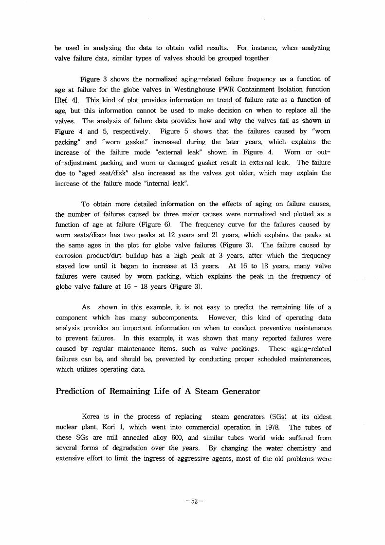
Prediction of Remaining Life of A Steam Generator

Korea is in the process of replacing steam generators (SGs) at its oldest

nuclear plant, Kori 1, which went into commerciai operation in 1978. The tubes of

these SGS are mill annealed alloy 600, and similar tubes world wide suffered from

several forms of degradation over the years. By changing the water chemistry and

extensive effort to limit the ingress of aggressive agents, most of the old problems were

- 52 -

solved except the intergranular attack/stress conosion cracking (IGA/SCO. Degradation of heat transfer tubes is the main issue for the nuclear steam generator life

prediction.

As discussed above, several different types of corrosion cause the degradation

and failures of steam generator tubes, and both statistical and mechanistic approaches

are required in order to predict rernaining life of a steam generator with a high level of

confidence. Which one is more useful depends on type of degradation, extent of experimental and operational data available, and the extent of mechanistic understanding

for the relevant degradation type.

Degradation of steam generator tubes can be considered as an ideal subj ect for

statistical evaluation. Thousands of identical tubes in a steam generator are exposed to

same operation condition so that degradation of each tube can be treated as random

variable in a statistical sense for a specific type of degradation. In service inspection

(ISD produces tube degradation data during each outage. It is not unusual that a significant amount of defected tubes are identfied at every inspection at the scheduled

outage.

Nevertheless, it should be noted that the extent of applicability of statistical

approach be limited and be reviewed with care. There have been series of steam generator design improvement by different vendors, and many different models are under

operation presently. Any steam generators of a model may not be identical to one another bccause details of operational conditions, especially water chemistry, vary from

plant to plant. Once a life threatening degradation form is identified, each plant start to

struggle to control and mitigate the degradation by corrective, preventive, and predictive

maintenance efforts, which include for example chemical cleaning, shot peening, corrosion

inhibitor, and sludge lancing . Even without the maintenance effort, a steam generator is

hardly operated under an identical condition throughout the whole life. Secondary side

corrosion of tubes attributed to occasional impurity intrusion into water chemistry is not

uncommon. There have bcen significant improvement of non destructive examination

(NDE) techniques for ISI. Improved ISI induces a transient of record by uncovering

defects not detected before. In a few instances, it was too late when significant amount

of tube degradation data enough to define a statistic trend were available because steam

generator replacement or a maj or sleeve campaign was needed already.

Even though factors listed above lirnit the applicability of statistical approach,

there are still cases where statistical analysis of the operating data plays a key roll in

steam generator life prediction. Primary water stress corrosion crack (PWSCO in roll

transition and secondary side inter granular attack / inter granular stress corrosion

crack (IGA/IGSCO in a steam generator with a well controlled water chemistry history

- 53 -

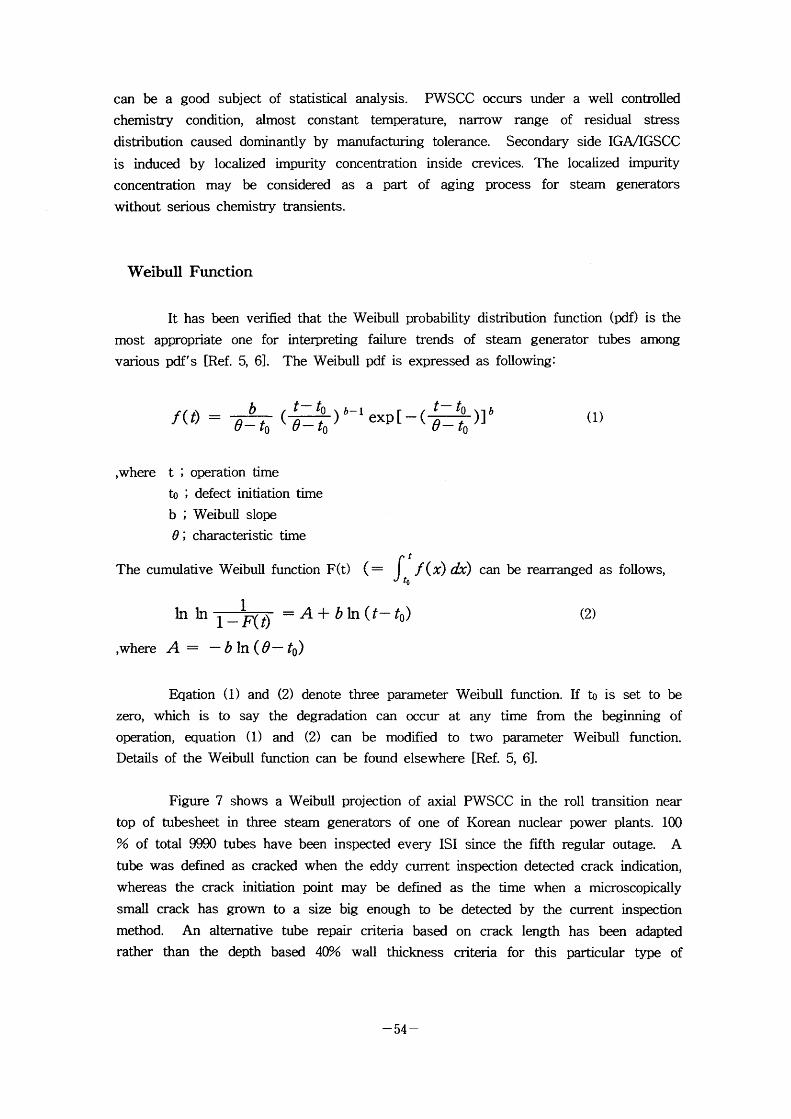
can be a good subject of statistical analysis. PWSCC occurs under a well controlled

chemistry condition, almost constant temperature, narrow range of residual stress

distribution caused dominantly by manufacturing tolerance. Secondary side IGA/IGSCC

is induced by localized impurity concentration inside crevices. The localized impurity

concentration may be considered as a part of aging process for steam generators without serious chemistry transients .

Weibull Function

It has bcen verified that the Weibull probability distribution function (Ixif) is the

most appropriate one for interpreting failure trends of steam generator tubes among

various pdf's [Ref. 5, 6]. The Weibull pdf is expressed as following:

b t- to b-l ) exp[-( t~to )]b f(t) = ( 6~ to e~ to 6~ to (1)

,where t ; operation time

to ; defect initiation time

b ; Weibull slope

6 ; characteristic time

f~ The cumulative Weibull function F(t) ( = f(x) dr) can be rearranged as follows,

1

In In = A + b In (t- t ) (2) ,where A = -bln(a-to)

Eqation (1) and (2) denote three parameter Weibull function. If to is set to be

zero, which is to say the degradation can occur at any time from the begiuning of operation, equation ( I ) and (2) can be modified to two parameter Weibull function.

Details of the Weibull function can be found elsewhere [Ref. 5, 6].

Figure 7 shows a Weibull proj ection of axial PWSCC in the roll transition near

top of tubesheet in three steam generators of one of Korean nuclear power plants. 100

% of total 99eo tubes have been inspected every ISI since the fifth regular outage. A

tube was defined as cracked when the eddy current inspection detected crack indication,

whereas the crack initiation point may be defined as the time when a microscopically

small crack has grown to a size big enough to be detected by the current inspection

method. An aiternative tube repair criteria based on crack length has been adapted

rather than the depth based 40%; wall thickness criteria for this particular type of

- 54 -

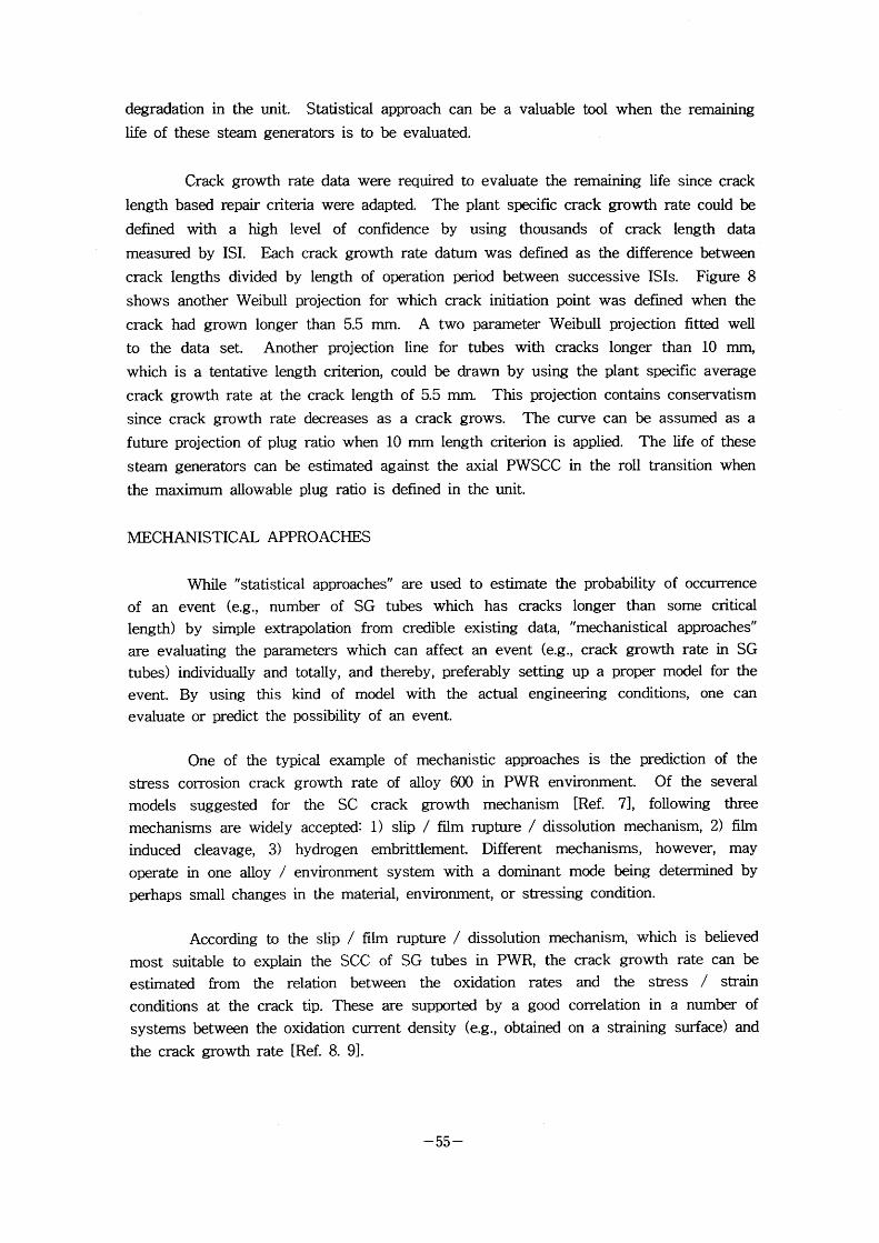
degradation in the unit. Statisticai approach can be a valuable tool when the remaining

life of these steam generators is to bc evaluated.

Crack growih rate data were required to evaluate the remaining life since crack

length based repair criteria were adapted. The plant specific crack growth rate could be

defined with a high level of confidence by using thousands of crack length data

measured by ISI. Each crack growih rate datum was defined as the difference between

crack lengths divided by length of operation period between successive ISls. Figure 8

shows another Weibull proj ection for which crack initiation point was defined when the

crack had grown longer than 5.5 mm. A two parameter Weibull proj ection fitted well

to the data set. Another projection line for tubes with cracks longer than 10 mm,

which is a tentative length criterion, could be drawn by using the plant specific average

crack growih rate at the crack length of 5.5 mm. This projection contains conservatism

since crack growih rate decreases as a crack grows. The curve can be assumed as a

future proj ection of plug ratio when 10 mm length criterion is applied. The life of these

steam generators can be estimated against the axial PWSCC in the roll transition when

the maximum allowable plug ratio is defined in the unit.

MECHANISTICAL APPROACHES

While "statistical approaches" are used to estimate the probability of occurrence

of an event (e,g., number of SG tubes which has cracks longer than some critical length) by simple extrapolation from credible existing data, "mechanistical approaches"

are evaluating the parameters which can affect an event (e.g., crack growih rate in SG

tubes) individually and totally, and thereby, preferably setting up a proper model for the

event. By using this kind of model with the actual engineering conditions, one can evaluate or predict the possibility of an event.

One of the typical example of mechanistic approaches is the prediction of the

stress corrosion crack growih rate of alloy 600 in PWR environment. Of the several

models suggested for the SC crack growih mechanism [Ref. 7], following three mechanisms are widely accepted: I ) slip / film rupture / dissolution mechanism, 2) film

induced cleavage, 3) hydrogen embrittlement. Different mechanisms , however, may operate in one alloy / environment system with a dominant mode bcing determined by perhaps small changes in the material, environment, or stressing condition.

According to the slip / film rupture / dissolution mechanism, which is believed

most suitable to explain the SCC of SG tubes in PWR, the crack growih rate can be estimated from the relation between the oxidation rates and the stress / strain

conditions at the crack tip. These are supported by a good correlation in a number of systems bctween the oxidation current density (e.g., obtained on a straining surface) and

the crack growth rate [Ref. 8. 9] .

- 55 -

For a given crack tip environment, corrosion potential, and material condition,

the crack growih will be controlled by the change in oxidation charge density with time

and the frequency of film rupture at the strained crack tip. As the crack grows, the

bare new surface becomes passivated (oxidized). The next crack growih can happen only when the passivated layer (oxide film) at the crack tip ruptures. Therefore, the

average crack growih rate, Vt, can be related to the oxidation charge density passed between film rupture events, Qf, and the strain rate at the crack tip, 8ct [Ref. 10]

V -t- M Qf 8ct (D

ZPF 8f

where: M, p = atomic weight and density of the crack tip metal

F = Faraday's constant z = electrical valence of a metal atom

8f = fracture strain of the film

The oxidation current transient generally shows an initially high bare surface dissolution

current density, io, for a short time, to, and thereafter decreases according to a power

law relationship as the following:

lt = io [t/to]~n (2)

where: it = oxidation current at time t

t=time n = constant

Because of this power law relationship, equation (1) can be reformulated as following

equation (3). This equation means that the crack growih rate behaviour can be evaluated by the repassivation response "n" value.

Vt = f(n) [8ct]~ (3)

The effect of n on predicted crack growih rate vs. stress intensity is ,, ,,

illustrated in Figure 9. There were much efforts to estimate or measure an appropnate n value under given temperature, environment, and alloy / microstructure conditions ,, ,,

[Ref. 11 - 14]. Figure 10 shows that the range in crack growih data in PWR environments are reasonably predicted by this modeling methodology.

- 56 -

Another example of mechanistic approaches is the evaluation of plugging criteria

of a SG tube to prevent tube burst. The plugging criteria of a tube can be fixed by a

maxirnum permissible crack length, ao, whic.h can be obtained according to the following

equation:

ao = ele Aa Aa (4)

where: ac = the minimal critical size which causes a fast burst of the tube

Details of ac assessment can be found elsewhere [Ref. 15].

Aal = the maximum uncertainty from the dimensioning of the

cracks of significant size by means of the inspection

technique used

Aa2 = crack growih between the two subsequent inspections

By using this criteria with the help of continuous in-service monitoring of primary to

secondary leak, a maximum permissible in-service leak criterion also can be set up.

As discussed above, the mechanistic approaches are very successful to formulate the working hypothesis and thereby quantify and validate against real observation for some corrosion problems. However, the diversity of working parameters

and yet unknown synergistic effects between them limits the validity of the mechanistic

a pproaches .

CONCLUSIONS

Experimental data and plant operating data are the two main sources of information that can be used to predict the remaining life of a component. However, only recently, it has been realized that plant operating data can bc treated as long terrn,

real time experimental data except that the experimental conditions vary a few times

during the real time experiments. In this paper, a few examples of utilizing the both

types of data to predict the remaining life of a component were shown and discussed,

and the following conclusions may be drawn.

o It is not easy to predict the remaining life of a component which has many subcomponents that fail independantly using the operaing data. However, the anaysis of

operating data can provide an irnportant infonnation on when and how to conduct preventive maintenance to prevent failures.

o Weibull statistics is an usuful tool in predicting the remaining life of a component utilizing the operating data as long as it can be assumed that the failure

mechanism stay the same.

o The mechanistic approaches are necessary in formulating the working hypothesis, which can be validated by experiments and in some c ases by utilizing the

- 57 -

operating data.

o More research should be focused on improving the methods to utilize the operating data to predict the remaining life of a nuclear component, since plenty of

operaing data are available, and are still being produced.

REFERENC E S

1. IAEA, International Atomic Energy Agency, IAEA-SM-353, 1998. 2. Blabnik. D.E., et al., "Insights Gained From Aging Research," NUREG/CR-5643,

BNL-NUREG 52323 March 1992 3. Vora, J.P., and Vagins, M., "Nuclear Plant Aging Research Program Plan,"

NUREG/CR-1144, Rev.2, 1991.

4. Lee B S et al "Agmg Assessment of Westinghouse PWR and General Electric Functions," NUREG/CR-63339, BWR Containment Isolation

BNL-NUREG-52462, Brookhaven National Laboratory, March 1996. 5. EPRI, NP 7493, "Statistical Analysis of Steam Generator Tube Degradation,"

1991.

6. EPRI TR 103566 "Statrstical Analysrs of Steam Generator Tube Degradation: Additional Topics," 1994.

7. Parkins, R., British Corr. J., 7, 15, 1972.

8. Ford, F.P., "Stress Corrosion Cracking", in Corrosion Processes, Ed. R.N. Parkins, Applied Science, 1982.

9. Parkins, R., '~nvironment Sensitive Fracture - Controlling Parameters", Proc., Third Int. Conf. on Mechanical Behaviour of Materials, Vol. 1,

p.139-164, 1980.

10. Ford, F.P. and Anderson, P.L., "Practical Application of Knowledge of

Mechanisms of EAC in LWRs", Proc., Int. Symp. on Steam Generator

Technology Update, KEPRI, Taejon, Korea, December 1997.

11. Thompson, C., et al, "Analysis of A600 and X-750 SCC Cracks", Proc., Alloy 600 Experts Meeting, Arlie, VA, EPRI, Palo Alto, April 6-9, 1993.

12. Thompson C et al, "Prediction of PWSCC in Nickel Base Alloys Using Crack Growih Models" Proc Seventh Int Symp. on Environmental Degradation of Materials in Nuclear Power Systems - Water Reactors,

NACE, p.867-880, 1995.

13. Carey D M et al, "Alloy 600 SCC Growih Measurements in Primary Coolant" Prod Workshop on PWSCC of Alloy 600 m PWRs, EPRI, November 1994.

14. Angeliu, T, et al, "Repassivation and Crack Propagation of Alloy 600 in

288C Water" Paper 96086 Corroslon/96, NACE, 1996.

15. Flesch, B., et al, 'Tailure Analysis Module for the EPM Code for PWR

Steam Generator Tube Mamtenance" Proc SMIRT 11 Tokyo 1991

- 58 -

Flgure 1

Figure 2

Figure 3

Figure 4

Figure 5

Flgure 6

Figure 7

Flgure 8

Figure 9

Figure 10

Age distribution of operable plants in the USA

Schematic diagram of a Westinghouse steam generator

Normalized failure frequency for globe valves in the Westinghouse CI

function

Failure modes for globe valves in Westinghouse PWR CI function during two periods

Failure causes for globe valves in Westinghouse PWR CI function

Frequency of globe valve failures caused by major failure causes

Weibull Projection, Fraction of Tubes Cracked vs. EFPY

Plug Ratio Projection Using Weibull Projection and Plant Speclfic Crack

Growih Rate Data

The effect of n on predicted crack growth rate for ductile austenitic ,, ,,

alloys (Fe and Ni-based) over the range of n values considered ,, ,,

applicable to 250-300C water. (after [10])

Compilation of Alloy 600 crack growih rate data vs. stress intensity in

high temperature deaerated pure water. Model predictions are shown for n values of 0.5 and 0.7. (after [10]) ,, ,,

- 59 -

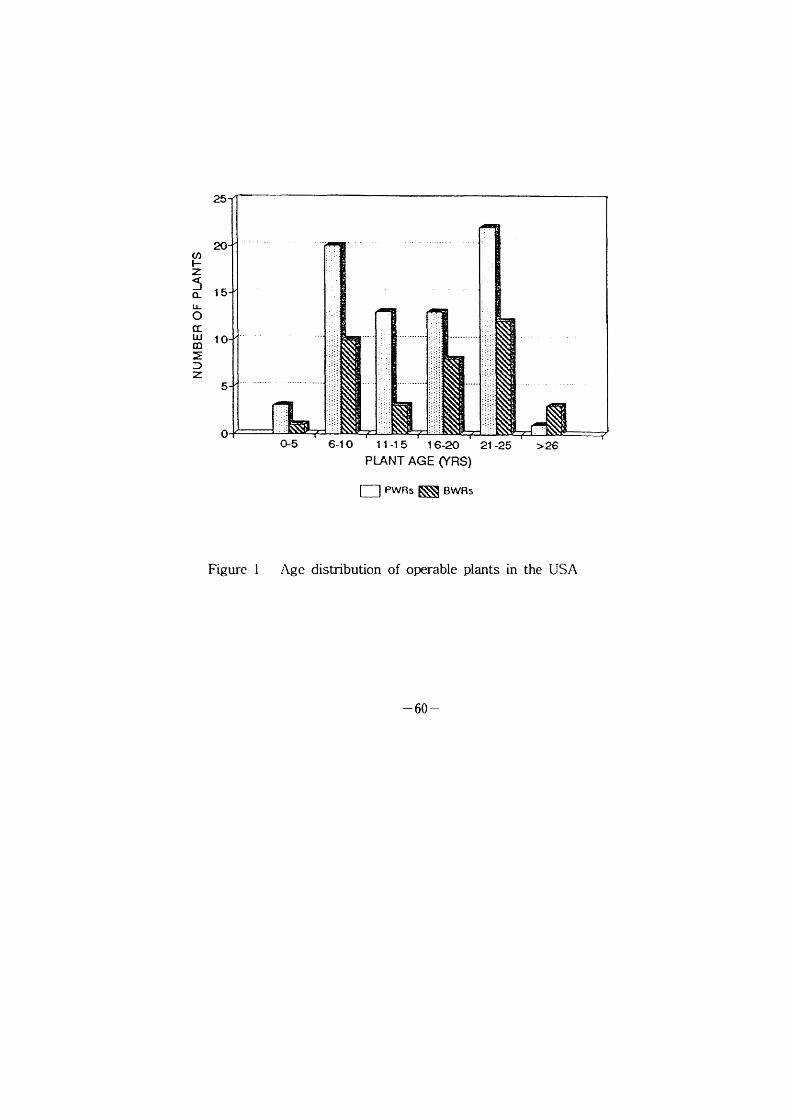
(1)

h z 5 ~ a: UJ cn

~ D z

25

20

15

10

5

O

Figure l

(~5 6-1 o 1 1 -1 5 1 e-20 21 -25 pU~NT AGE (YRS)

[] PWRS ~~ 8WRS

Age distribution of operable plants in

> 26

the USA

- 60 -

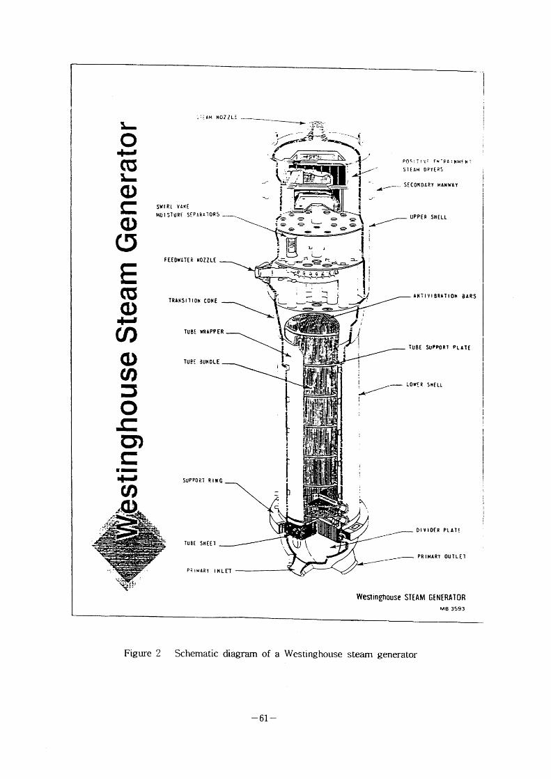
1~ cU

(D

CD

U'

~)

d~ Cl) _~'!1

.'iAH NOZZL~

SViRL VA~t HOI STURE S~P~PLIORS

F EE DVLTE R ~OZZLE

TRArsJTION CONE

~,~~'~

IJ

l/~ '~/

.,,11: -- d~ - ,~ --.-*.. ' 5i~l -\', ~/5f:a~~lL '

~' \~: .

1- G) ;_~ 1- II~ !

:LJ J

lv il :1r '1~F~ IE~ rt* :' '~r '~~~e~F~O-

~ ~~IC~~cG t G "e_Lat "-_h!~1-'~J:;1~-!

~ r', S tl

\~;! TUB! VRAPPER

TUeE 3UXDLE

SUPPORT RING

TU5[ SHECT

jl•~..

:~

. .l

,

J~ ll

PO1~' IY: T,(~pt: SIE*'N DPTtRS

SECOKDLRY

llr~ i

l

1

t

!l . l

UPPEP

I~:;'i I!I f

i

II

f!tl I

l

l

~1 ,

,

NHc N '

P.ANWAY

SHELL

f

f

,.

i

f

d

cf.

~

"' 'I' l'

'il= ti;{':: ' I=

, : "' " tt"I:f I II!

II

I"' !1 i' '

.t ' ' l't'l : : ' lll'

j il! I l

p :~~::~~

t'

\~ ~)\ \

\

~\,.

~~

l~

_/~

ANT I V 1 8RAT I ON

U8t SUPPOR1

*o~E R

.r

SM[LL

D, V I DER

PR tHARY

8ARS

PLATt

PLATE

OUTLE1

~;;~ ; 5; ~

'r'* 'r

P~ 1,1ARY IHLrT

l

l

i

WesTingtlouse STEAM GENERATOR

"8 3s93

Figure 2 Schematic diagram of a Westinghouse steam generator

-61-

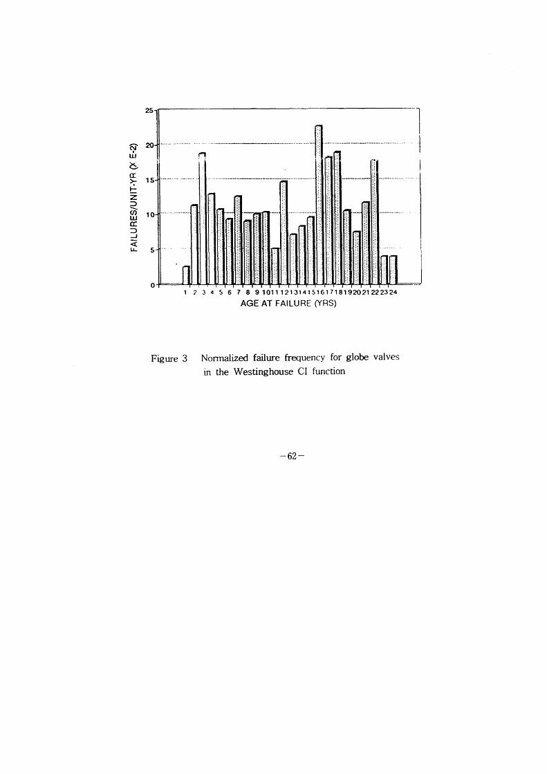
2s

-20 ti,

~~

~ IS H Z :)

~ (1) 10 UJ C: :)

J ~ LL 5

O

l

2 3 4 s 6 7 8 91011121314lsl61718192021222324 AGE AT FAILURE C(RS)

Figure 3 Nonnalized failure frequency for globe valves

in the Westinghouse CI function

- 62 -

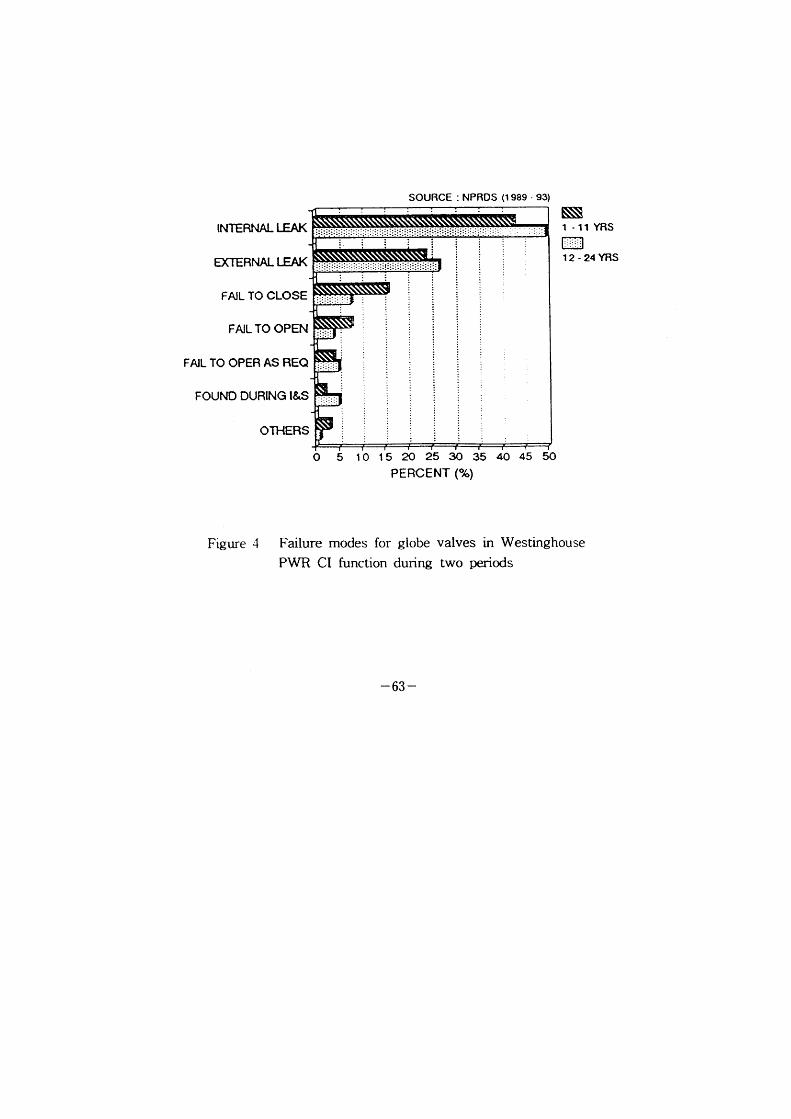
SOURCE : NPRDS (1989 . 93)

INTERNAL LEAK

~TERNAL LEAK

FAIL TO CLOSE

FAIL TO OPEN

FAIL TO OPER AS REQ

FOUND DURING I&S

OTHERS

~~~ 1 - 11 YRS

1 2 - 24 YRS

O 5 10 15 20 25 OO 35 40 45 50 PERCENT (%)

Figure 4 Pailure modes for globc valves in Westinghous~e

PWR CI function during two periods

- 63 -

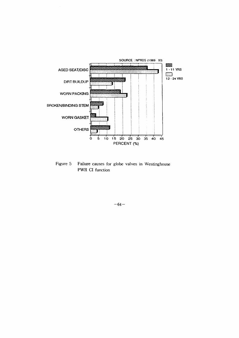
AGED SEATlDISC

DIRT BtJlti)tJP

WORN PACKING

BROKENIBINDING STEM

WORN GASKET

OTHERS

SOURCE : NPRDS (1 989 • 93) ~i~ 1 -11 YRS

1 2 - 24 YRS

Figure 5

o 5 Io 15 20 25 eo 35 40 45 PERCENT ('/.)

Failure causes for giobe valves in Westinghouse

PWR CI function

- 64 ~

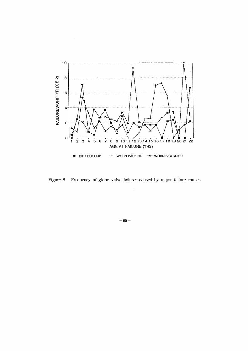
~ tiJ

~ a: > ~-- -

Z D ,~ (1)

UJ CC

D J

10

8 ..

6

4.

2

O

-~i-

T t

Figure 6

1 2 3 4 5 6 7 8 9 Ioll 12131415161718192021 22 AGE AT FAILURE (YRS)

-1- DIRT BUILDUP - WORN PACKING - WORN sEAT/olsc

Frequency of globe valve failures caused by major failure causes

- 65 -

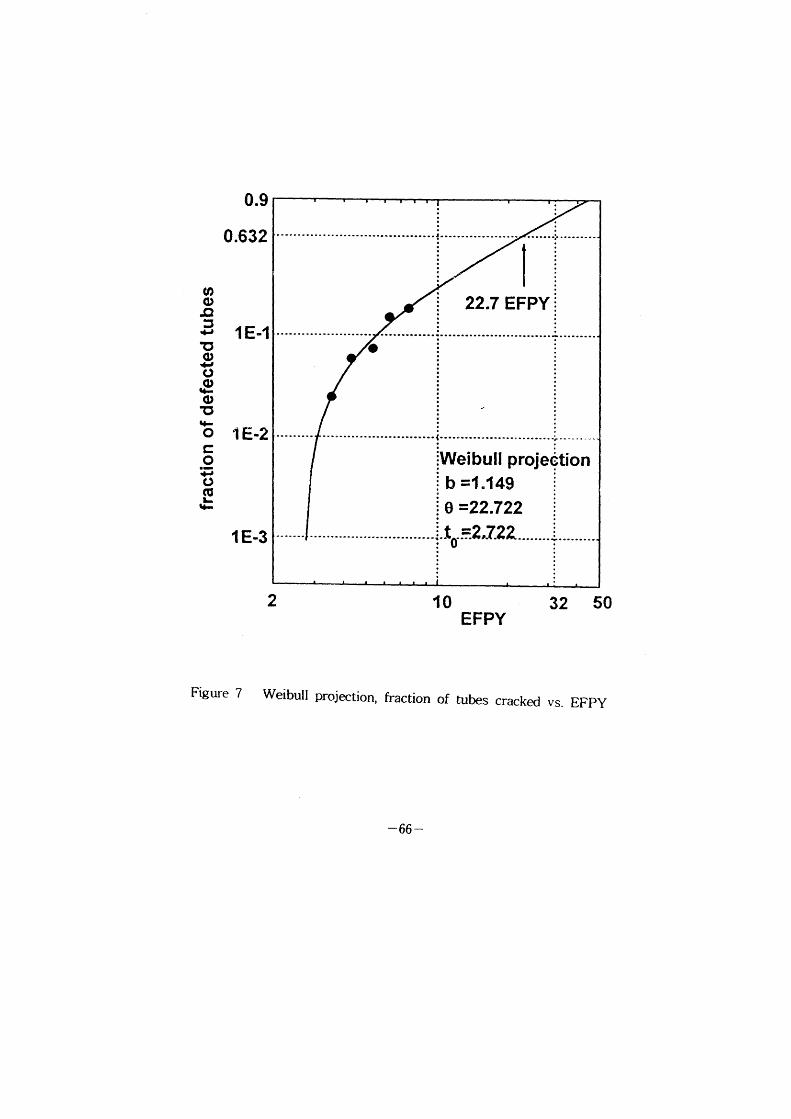
(o

O ~ 5 d'

~ (a,

1-o O ~-o 1: ~-o c o ~ o c~

'h

0.9

0.632

1 E-1

1 E-2

1 E-3

'..'... I

: 22,7 EFPY :

e

Welbull proJec~tion

j b - .149 ; 1 -i o -22.722 i -_i_ _ 2 -- 7-2a---.-- ~ '~~~~ to~ ' ~~-'--- , ,

2 10 32 50 EFPY

Pig ure 7 Weibull projection, fi-action of tubes cracked vs. EFPY

- 66 -

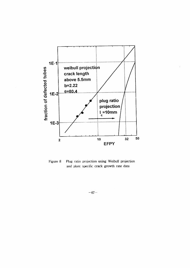
U)

o ~ :, ~,

~ o d~ o o ~-O 15 ~-o c o ~: o c:,

,~

1 E*1

1 E-2

1 E-3

weibull projectien

crack tength

above 5 5mm -2 22 b . --80^4___. ._.._Q.. -

: Iug ratlo .p : ro j ection j .p i I -10mm

-:c

2 10 32 50

E F PY

Flgure 8 Plug ratio

and plant

projection using Weibull projection

specific crack growth rate data

- 67 -

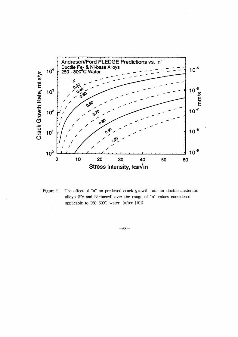
L 104 > '\ cl)

.~

o~ 103 ~ ca

r c ~0 102 t-

O ~, o caL 101

O 1 Oo

r~ Andresen/Ford PLEDGE Predictions vs. 'n' Ductile Fe- & Ni-base Alloys _ _ 250 - 3000c Water _ _ - - ~_ ~_ - -

~~ ~ -~ .(~ ~ ~ ~ ol~.((\ _ -

~ ~ ~ ~ ~ ~

ll ll

/

/ /

/

/ / / / ll

/

/

~b QI'

/

/

/ / O1:.O /

/ / o~P.

~9Pl / / l cP / \. /

/

/

/

/

/

/

/

/

/

/

/

,,

/

',

/

,,

/

11-

',

.l

11-

d~

*,

11-

(,

',

11-

1,

1~

1 0~5

1 O~(1)

.\ E E

1 0~7

1 O~

o 10 20 30 40 Stress Intensity, ks~/in

50 60

1 0~9

Figure q. The effect

alloys (Fe

applicable

,, ,, of n on prec]icted crack growth

and Ni-based) over the range of

to 250-300C water. (after [lO])

ra te

" u n

for' ductile austenitic

values considered

- 68 ~

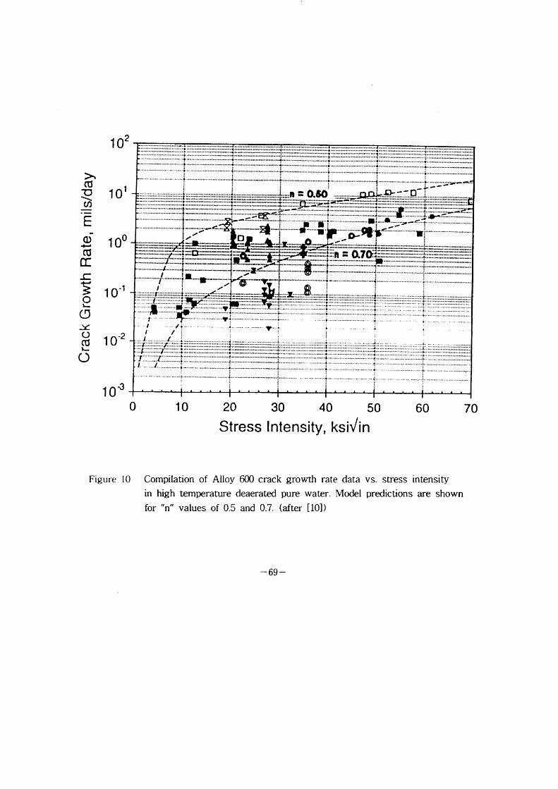
1 02

> CU ~ 101 u)

E Q) I OO ~ CU

~ l: ~ 10~1 o * (D

~ o (U 10~2 * O

1 O~

O 10 20 30 40 50 Stress Intensity, ksiVin

60 70

Figure lO Compilation of Alloy 600 crack growth rate data vs. stress [ntensity

in high temperature deaerated pure water. Model predictions are shown

for n values of 0.5 and 07 (after [10]) ,, ,,

- 69 -

II-3 Structural Integrity Assessment of the Reactor Pressure Vessel

under the External Cooling Condition

Jong Sung Kim, Yoon Snk Chang, Tae Eun Jin, Korea Power

Engineering Company, Inc., Korea

Structural Integrity Assessment of the Reactor Pressure Vessel

under the External Reactor Vessel Cooling Condition

Jong Sung Kim' and Tae Eun Jin

Key Words : In Vessel Retention, Extemal Reactor Vessel Cooling, Core Melting Accident, Transient State, Finite Element Method, Elastic-Perfect Plastic

Behavior, Larson-Miller Curve, Damage Rule

Ab stract

Since the suggestion of External Reactor Vessel Cooling(ERVO, the effects of

melting and cooling on the response of structural integrity of the Reactor Pressure

Vessel(RPV) under core melting accident conditions have been investigated. This paper

describes the vessel response according to the ERVC condition and analysis method.

The steady state and transient analysis for the temperature and stress field were

performed using ABAQUS. Especially, transient analyses were studied for the variable

boundary conditions. To obtain an analogy with real phenomena, the material properties

were determined by combining and modifying the existing results considering phase

transformation and temperature dependency. The results show that the vessel can be

melted if there is no external cooling. Finally, the potential for vessel damage is

discussed using the Larson-Miller curve and damage rule.

l . Introduction

ERVC(extemal reactor vessel cooling) has recently been studied and developed as the (4 5) management strategy for severe accidents(l-3). In previous studies ' for IVR(in-vessel

retention), the extrapolation method was used for the determination of material properties (6) beyond the temperature range presented in the ASME code or the material properties

of RPV material not to consider phase transformation and change are used.

But the real material properties are considered to be different from those found by the

extrapolation method because material properties, especially thermophysical material

properties, are abruptly changed with temperature due to phase transformation. Previous

studies(4,5) also utilized the steady state analysis to maintain a constant value of the

boundary condition variables for time. However, optimal ERVC time can not be determined

* KOPEC(Korea Power Engineering Company, Inc.)

- 71 -

using steady state analyses. Therefore, the ambiguous conjecture that the reactor cavity

would be completely submerged before molten debris reaches the RPV Iower head, is

presented by those studies.

In this study, however, the material properties for temperature are established like real

phenomenon, the boundary conditions are determined to consider the transient state that

boundary condition variables - the levels of molten debris/external vessel water, and the

temperatures/pressures of molten debris, external vessel water and gas in core - are

subjected to change over time. The database and the user subroutine program are

constructed in order to determine the material properties of molten debris and the

specification of boundary conditions according to transient state. The temperature and

the stress analysis are performed for the core melting accident due to large break LOCA by using ABAQUS(7). Finally, the damage and the stuctural integrity for RPV

are evaluated by using the Larson-Miller curve and damage rule(8). In addition, the

effects of analysis conditions on structural integrity - molten debris quantity, ERVC

condition, analysrs method and connection condition with RPV upper part - are

reviewed.

2 . Analysis model

2.1 Model configuration

The RPV configuration is shown for the case where molten debris and metallic layer

are located in the RPV Iower head in Fig. 1. The materials of RPV and cladding are

SA508 Gr.2 Cl.1(9) and SB166(ro) respectively. The thickness of cladding, t.lad, rs

3. 175mm.

2.2 Chemical composition and material properties

The chemical composition of SA508 Gr.2 Cl.1 is presented in Table 1(9). The liquidus

and solidus temperatures of SA508 Gr.2 Cl.1 are determined to be 1501.04iC and 1461.0 9~C respectively by substituting the chemical composition of Table I into Howe's(n) and

Kubachewski's(12) correlations. Density pRPV rs determined from the correlation by

(13) Jablonka et al. as shown in Fig. 2. The specific heat, c p. RPv and the thermal

conductivity, kRPv, for temperature are detemuned from ASME Code(6) and Thomas

- 72 -

(14) results as shown in Fig. 3 and 4, respectively. The elastic modulus, ERPV and the

yield strength, 6 ys. RPv, for temperature are determined from ASME Code(6) and Grill's

results(15) as shown in Fig. 5 and 6. Poisson's ratio vRPv rs determined to be 0.3. The

thermal expansion coefficient, aRPv, for temperature is determined from ASME Code(6)

(13) and Jablonka's results as shown in Fig. 7. (16) The Larson-Miller curve for SA508 Gr.2 Cl.1 is shown in Fig. 8. LM~ = O . OOIT

(20 + Iog t.)) is Larson-Miller parameter. t, is rupture time( hour).

( ro)

The chemical composition of SB166 is presented in Table 2 . The liquidus temperature of SB166 is determined to be 1427 iC (6). The thermal conductivity of SB166 for

temperature, h*/~, is detennined as shown in Fig. 9(6). The emissivities of SA508 Gr.2

Cl.1 and SB166, eRPv, are determined as shown in Fig. 10(17)

Molten debris is assumed to be composed of 72.25~(weight percentage) U02 and

27.75~6 Zt02. The solidus and liquidus temperatures of molten debris are 2536~C and 254

2~C(18) respectively. The density of molten debris, pl' versus temperature is determined

as shown in Fig. 1 1(18,19). The specific heat c p, i and the thermal conductivity k , J ,

(rs) versus temperature are shown in Fig. 12(18) and 13 , respectively. The volumetric

expansion coefficient, ~,, for temperature is determined as shown in Fig. 14(18,19). The

viscosity, p /' for temperature is as shown in Fig. 15(18,19)

The metallic layer is assumed to be composed of stainless steel. Therefore, emissivity

of metallic layer, et, is determined to be 0.43(17)

3 . Boundary condition

3.1 Accident scenario

The significant event stage and the time frame for a core melting accident occurs due to large break LOCA and SI(safety injection) failure are presented in Table 3(20)

3.2 Boundary condition variable

Boundary condition variables - the levels of molten debris/metallic layer/external

vessel water, the temperatures/pressures of molten debris, metallic layer, external vessel

water and gas in core, and the decay heat of molten debris - change over time.

- 73 -

Therefore, the applicable boundary condition region and the magnitude of heat transfer

coefficient also change according to time.

The levels of molten debris and metallic layer over time, H, and Ht, are shown

in Fig. 16(20). The temperatures of molten debris and metallic layer over time, T, and

(20) Tt, are shown in Fig. 17 . The temperature and the pressure of the gas in core

versus time, Tg" and Pg", are shown in Fig. 18 and 19(20) respectively. The level, the

temperature and the pressure of external vessel water versus time, H/' Tl and (20) Pt, are shown in Fig. 20, 21 and 22 , respectively. The decay heat of molten debris

for time, Q, is shown in Fig. 23(20). The Air temperature outside of RPV, T.i., is

supposed to be maintained at a constant 1271C.

3.3 Thermal boundary condition

In transient analysis, the thermal boundary condition of RPV is determined using the

following assumptions:

o The heat transfer is assumed to be the one for a quasi-static state.

o The therrnal conduction through debris crust and the gap between molten debris

and the inner wall of RPV Iower head are ignored.

o The temperature distributions of molten debris, metallic layer and extemal vessel

water are uniform over time.

o The heat convection on the RPV inner wall by the metallic layer is assumed to be

the one from molten debris. The heat transfer on the RPV inner wall during the

period when molten debris and metallic layer exist in the solid state is assumed to

be the heat convection from the molten debris.

o The water exists in RPV Iower head until 6528sec after the accident but the heat

convection is due to the gas in the core conservatively.

o The effect of insulation on the thermal behavior of RPV is not considered.

o The effect of cladding and gas in gap on the heat convection coefficients for

the inner wall of RPV Iower head are considered by using an equivalent film coef f icient(21)

The initial and the thermal boundary conditions for RPV are shown in Fig . 24. The

heat transfer mechanism change for time is presented in Table 4. In Table 5, the heat

transfer coefficients on the RPV inner and outer walls are presented for the heat

transfer except radiation. In Table 6, the radiation heat fluxes on the RPV inner wall

are presented according to the magnitudes of RPV inner wall temperature TRPV and

~ 74 -

Tmet during the transient state.

In steady state analysis, the thermal boundary condition of RPV is determined by

using the assumptions that the lower head is fully submerged in cavity water prior to

the deposition of molten debris on lower head and molten debris is located on lower

head from the accident initiation time. The boundary condition variables are fixed over

time in steady state analysis.

3.4 Mechanical boundary condition

The mechanical boundary condition for the RPV is deterrnined by considering the dead

weight effects of molten debris and external vessel water.

The mechanical boundary conditions for the RPV are shown in Fig. 25 where zl and

z2 are the depth from the metallic layer surface and water level, respectively. Unit for

pressure is MPa.

4 _ Analysis and Results

4.1 Analysis method

The analysis method for temperature and stress analysis is shown in Fig. 26. As shown in Fig. 26, the analysis system consists of a database, an ABAQUS Input File(7)

and an user subroutine program(7). The database presents the material properties of

molten debris with temperature. These material properties are presented in section 2.2.2.

The ABAQUS Input File(7) assigns the finite element model and configuration, material

properties of RPV, boundary conditions, analysis type and output data. The user subroutine prograrn(7) assigns the boundary conditions associated with the time variation

of boundary condition variables and links between the database and the ABAQUS Input

File.

4.2 Finite element model

The finite element for an analysis model is shown in Fig. 27. The numbers of an

element and a node are 157 and 5059, respectively. The element property is an 8-node

quadratic axis-symmetric element(7). The finite element model is simplified by the

deletion of nozzles because the effects of nozzles on the integrity of RPV Iower head

are minor. The model is an axis-symmetric model due to the axis-symmetric boundary

- 75 -

conditions and model configuration.

4.3 Temperature analysis

Temperature analysis is performed considering molten debris quantity, ERVC condition

and analysis method.

The conditions for temperature analysis are presented in Table 7.

The NLT(nondimensional ligament thickness) w at MTGP(maximum temperature generation part) versus time are shown for conditions @ and (~) in Fig. 28. The NLT

w means the nondimensional value calculated to divide ligament thickness w~ by

initial thickness w, at MTGP. As shown in Fig. 28, the value of NLT is zero and

molten debris penetrates through the thickness of RPV Iower head at 5.5xl03sec for the

case that ERVC is not applied and steady state analysis is performed. However, molten

debris does not penetrate in the case that ERVC is applied and steady state analysis is

performed .

In cases of condition (~) - @, the NLT w at MTGP are shown according to time in

Fig. 29. As shown in Fig. 29, the effects of molten debris quantity on NLT at MTGP

are minor in the case that ERVC is applied and steady state analysis is performed.

In cases of condition ~) and ~), the NLT w at MTGP are shown according to time

in Fig. 30. The time for transient analysis when the NLT is maintained with constant

value is later than the one for steady state analysis. When this steady state is reached,

the NLT by transient analysis is less than the one by steady state analysis.

The NLT w at MTGP versus time are shown for conditions ~) - O in Fig. 31. The

effect of ERVC completion time on NLT is minor for the case that the one is less than

10000sec and the NLT decreases with the increase of one.

4.4. Stress analysis

Stress analysis is performed considering the following variables : molten debris

quantity, ERVC condition, connection condition with RPV part and analysis method.

The conditions for stress analysis are presented in Table 8.

The hoop stresses at the internal points of MTGP versus time are shown for condition ~) in Fig. 32. The hoop stress at MTGP increases with the radial coordinate

- 76 -

r and the maximum value of hoop stress occurs on the outer wall surface of MTGP.

The hoop stresses at the outer wall of MTGP versus time are shown for conditions

~) - R in Fig. 33. The hoop stress at the outer wall of MTGP increases with molten

debris quantity in the case where ERVC is applied and steady state analysis is

performed .

The hoop stresses at the outer wall of MTGP versus time are shown for conditions

R and C in Fig. 34. The hoop stress at the outer wall of MTGP has almost a constant

value irrespective of the connection condition with RPV upper part.

The hoop stresses at the outer wall of MTGP versus time are shown for conditions

R and ~) in Fig. 35. The hoop stress at the outer wall of MTGP caused by the

transient analysis is smaller than the one by the steady state analysis.

The hoop stresses at the outer wall of MTGP versus time are shown for conditions

~) - ~) in Fig. 36. The hoop stress at the outer wall of MTGP versus time decre4ses

with an increase in ERVC completion times.

4.5 Damage and integrity evaluation

The conditions for damage evaluation are equal to the ones for stress analysis.

Damage factors are calculated by using the temperature and von-Mises effecpive

stress distributions of RPV, and the Larson-Miller parameter and curve for SA508 Gr.2

Cl.1.

To calculate the cumulative damage factor 1), the following life-fraction rule(8) is

used:

t'

D=~tl =1 (1)

where t, is the duration time for specific condition i and t~ is the rupture time for

specific condition i. The satisfaction of equation (1) means rupture.

The failure times when the average value of the cumulative damage factors of all

internal points in the maximum temperature generation part is equal to I are presented

for various conditions in Table 9. From Table 9, the failure time decreases with an

increase of molten debris quantity for the case where ERVC is applied and steady state

analysis is perfonned. The failure time by steady state analysis is smaller than the one

by transient analysis as shown in the comparison between the results of conditions ~)

- 77 -

and ~. The failure time decreases with an increase of ERVC completion time .

5 . Concluslons

The following conclusions are obtained from the structural integrity evaluation

performed for RPV subjected to a core melting accident due to large break LOCA:

(1) Molten debris penetrates through the thickness of RPV Iower head for the case

where ERVC is not applied and steady state analysis is performed.

(2) The failure time decreases with the increase quantity of molten debris for the case

where ERVC is applied and steady state analysis is performed.

(3) The failure time by steady state analysis is smaller than the one by transient

analy sis.

(4) The failure time decreases with an increase of ERVC completion time.

References

(1) O. Kymaelaeinen, H. Tuomisto and

accident management strategy for

WRSM, Bethesda, Maryland, 1996.

T.G.

the

Theofanous, In-vessel

Loviisa nuclear power

melt retention

plant, in the

as a 24th

(2) T.G. Theofanous et DOE/ID-104eo, Vol.1,

al.,

U.S.

In-vessel coolability

Department of Energy,

and retention

ldaho Operations

of a Of fice,

c ore

1995.

melt,

(3) R.E. Henry et al.,

Nuclear Technology,

Cooling

Vol.101 ,

of core debris within

1992, pp.385-399.

the reactor vessel lower head,

(4) J.L. Rempe

EGG-2618,

at al.

ldaho

, Light water reactor

National Engineering

lower

Lab.,

head

EG&G

f ailure

ldaho,

analysis, NUREG/CR-5642,

Inc., 1993.

(5) D. Azordi and P. Gruner,

penetration subjected to a

International Conference

France, 1997, pp.443-450.

Numerical simulation of

postulated core damage

on Structure Mechanics

a BWR vessel lower head with

accident, Transaction of the 14th

in Reactor Technology, Lyon,

(6) ASME bojler and pressure vessel code, Section 111, Division 1, Appendices, 1995.

- 78 -

(7) ABAQUS user's manual, Ver.5.6, HKS Inc., 1996.

(8) R. Viswanathan, Damage mechanisms and life assessment of high-temperature

components. ASM International, 1989.

(9) ASME boiler and pressure vessel code, Section II, Part A-Ferrous, 1995

(10) ASME boiler and pressure vessel code, Section 11 Part B Nonferrous 1995

(11) A.A. Howe, Estimation of liquidus temperatures for steels, Ironmaking and

Steelmaking, Vol.15, N0.3, 1988, pp.134-142.

(12) O. Kubachewski, Iron binary phase diagrams, Berlin Springer Verlag, 1982.

(13) A. Jablpnka, K. Harste and K. Schwerdtfeger, Thermomechanical properties of iron

and iron-carbon alloys: density and thermal contraction, Steel Research, Vol.62,

No.1, 1991, pp.24-33.

(14) B.G. Thomas, I.V. Samarasekera and J.K. Brimacombe, Mathematical model of the

thermal processing of steel ingots: part 1. heat flow model, Metallurgical

Transaction B, Vol.18B, 1987, pp.119-130.

(15) A. Grill, J.K. Brimacombe and F. Weinberg, Mathematical analysis of stresses in

continuous casting of steel, Ironmaking and Steelmaking, No.1, 1976, pp.38-47.

(16) G.L. Thinnes. G.E. Korth, S.A. Chavez and T.J. Walker, High-temperature creep

and tensile data for pressure vessel steels SA533B1 and SA508-C12, Nuclear

Engineering and Design, Vol.148, 1994, pp.343-350.

(17) T.G. Theofanous, G. Wang and X. Chen, The emissivity of the steel layer, T.G.

Theofanous et al., In-Vessel Coolability and Retention of a Core Melt, DOEl

ID-10460, Vol.1, 1995, 1-3-8.

(18) J.K. Hohorst et al., SCDAP/RELAP5/MOD2 code manual, volume 4: MATRO-a library of materials properties for light-water-reactor accident analysis, NUREG/

CR-5273, EGG-2555, Vol.4, R3, EG& G Idaho, Inc., 1990.

- 79 -

(19) C.C. Chu et al. Uncertainty analysis for therrnophysical properties used in in-vessel

retention analyses, T.G. Theofanous et al., In-Vessel Coolability and Retention of a

Core Melt, Appendix L, DOE/ID-10460, Vol.1, 1993, L.1-28.

(20) Korea Power Engineering Company, Inc., Severe accident evaluation report, 1996.

(21) J.P. Holman, Heat transfer Fourth edition Tower Press 1976

(22) R.J. Witt, Local creep rupture failure modes on a corium-loaded lower head,

Nuclear Engineering and Design, Vol.148, 1994, pp.385-411.

(23) M. Jahn and A.A. Emara, High Rayleigh number convection in enclosed fluid layers with internal heat sources, U.S. NRC, NUREG-75/065, 1975.

(24) M. Jahn and H.H. Reineke, Free convection heat transfer with internal heat sources:

calculations and measurements," Proc. 5th Int. Heat Transfer Conf., Tokyo, Vol.3,

NC-2.8, 1974.

(25) M.N. Ozisik. Heat transfer: a basic approach, McGraw-Hill, Inc., 1985.

- 80 -

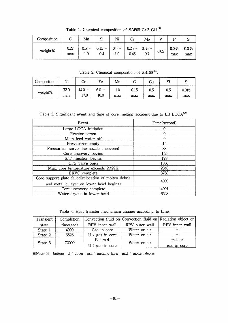
Table 1. Chemical composition of SA508 Gr.2 Cl.1(9)

Table 2. Chemical composition of SB166(ro)

Table 3. Significant event and time of core melting accident due to LB LOCA(20)

Table 4. Heat transf er mechanism change according to time.

~:Note) B bottom U : upper m.1. : metallic layer m.d. molten debri s

- 81 -

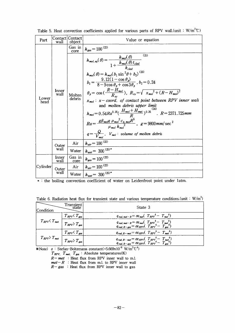
Table 5. Heat convection coefficients applied for various parts of RPV wall.(unit : W/m2 IC )

* : the boiling convection coefficient of water on Leidenfrost point under latm.

Table 6. Radiation heat flux for transient state and various temperature conditions.(unit : W/m2)

~ Note) o : Stefan-Boltzmann constant(=5.669xl0~8 w/m2ic4) TRPV. Tmet. Tg~~ : Absolute temperatures(K)

R-met : Heat flux from RPV inner wall to m.1. met-R : Heat flux from m.1. to RPV inner wall R-gas : Heat flux from RPV inner wall to gas

- 82 -

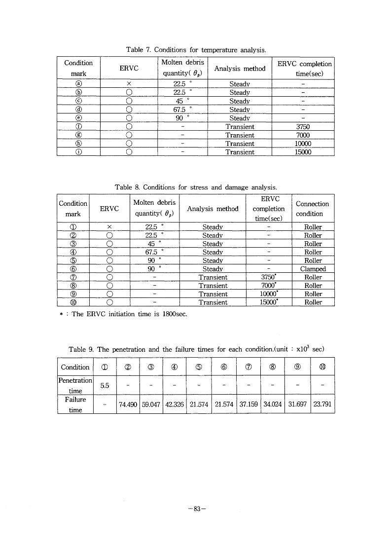
Table 7. Conditions for temperature analysis.

Table 8 Conditions for stress and damage analysis.

* The ERVC initiation time is 1800sec.

Table 9. The penetration and the failure times for each condition (umt xlO sec)

- 83 -

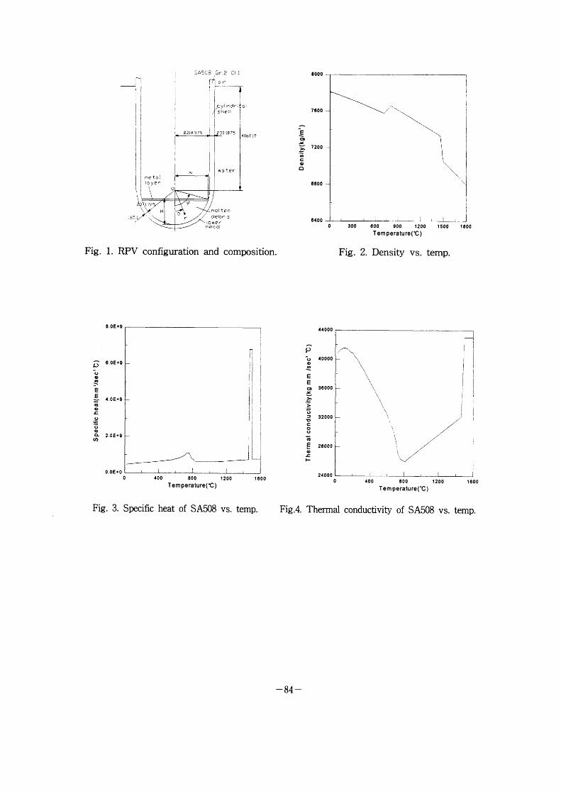
~* ~A~08 cr ~i~ Ci l

,'Llj"f olr f

l ~ /Cy!;nc~'*' cll

sheli

406n 19

l

~ ,,-••-,/:L~\; ,~

RPV configuration

8QOO

7eoo -

E OD , ~ 720O

O 680o

e40o

/ \

Fig. 1. and

l

, \

composition.

o 300

Fig .

600 900 1200 Tem peratu re( 'C )

2. Density vS.

15ao

tem p.

18OO

L)

Q o co

E~

E CD q, !:

o o a, CL

(,)

8.oEtg

6.0E•9

4 oE~g

2.oE~g

O.OE~O

rl

i'l

It

!

I

Specific

40o 8oo 120o T e m pe ra tu re ( tC )

heat Of SA508 vS.

16oo

temp .

O o o ,,,

~ E E o) x :~ :~

o ::

U c o o ,U

E a)

c h

Fig. 3.

4400o

400oo

360oo

32000

280ac

240oo

r-\ \ \ ,

\ ~

\ \

\\

\

\

* *~

/ \

*

!

f

i

j

Fig.4. Thermal

4oo 80o 1200 Temperature('c)

COnductiVity Of SA508 vs.

160o

temp .

- 84 -

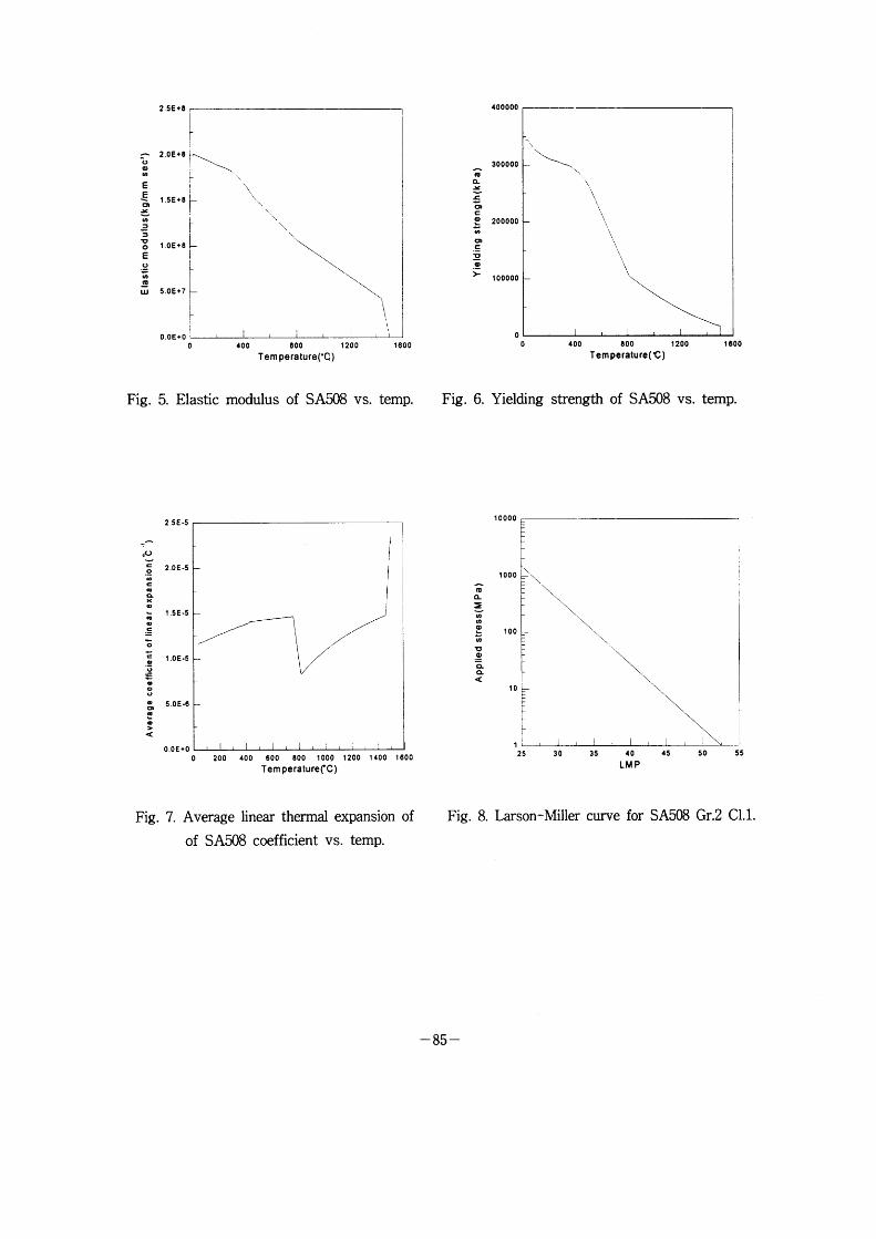
o o ,o

E E O, ~-o,

, l ~ O E o o c9

UJ

2'5Et8

~

2'oEt8 ' :\ 1'5E~8 ~

r

1 oE'8 L

l

5'oEt7 h

[

o oEto

\

\ \

\ \ \

\.

Elastic

,, i

_+_L] 4oo 80o 12oo Tem perature('O

modulus of SA508 vs.

,p ,L e-,: OD c o

O~

U o >

Fig. 5.

16oo

temp. Fig. 6.

400OOO

300OOO

20OOOO

100OOO

O

\

,, *\

\ \

\

\ \

\ \

\ \

\

Yielding

400 80o Tem perature(C)

strength of SA508

1200

VS.

1600

temp .

aO

c o ,o

c ,I

a X o c-

o ,:

O c:

O o o o o o O, c,

o :-

2 5E-5

2.OE-5

1 SE-5

1 OE-5

5 OE-6

O OE~O

7.

i

2oo 4oo 60o 80o looo 12oo 14oo Tem peraturecc)

Average linear thermal expansion

of SA508 coefficient vs. temp.

c9

~ =

O

1-o cL a

loooo

looo '\ ~ ,\\ [

\ r \\ ~ loo

f

10 L

IL=LJ-

Fig .

\ \ \.

\

16oo

of Flg 8

25 3o 35

Larson-Miller curve

40

LMP

fOr

'5

SA508

50

Gr.2

55

Cl.1.

- 85 -

~'

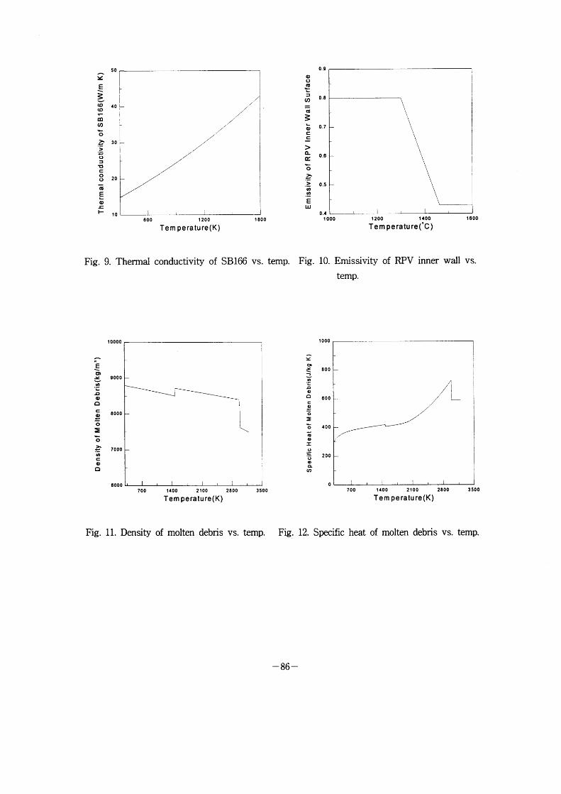
E ~ ~ ~ CO

O -a: U,

~ O > ~ > O

1:,

O O 15

E O J: h

5o

4o

3o

2o

10

/ /

'l ll

ll

600 12oo Tem peratu re (K) 1 800

o o CD

~ :: (O

co

~ o c c > o-a~ .* o > ~ :-

E UJ

o9

o.8

0.7

o .6

a .5

o .4

,

IOOO 1 200 140o Tem perature( C)

16OO

Fig . 9. Thermal conductivity of SB166 vs. tem p . Fig . 10. Emissivity of RPV inner wall vs.

tem p .

100oo

E O, ~ 90OO co

Q ,D

Q O 800O O = ~ O :~ 700O co

= O Q

60oo

L

210o 280o 140o Te m peratu re(K)

3500

1 ooo

X aD x 80O , e,

,, o Q 6OO

o = o 40O CD

o r o :; 2DO o o a co

o

700

./L

700 21OQ 280o 14oo T e m pe ratu re (K)

3soo

Fig . 11. Density of molten debris vs. temp. Fig. 12. Specific heat of molten debris vs. tem p .

- 86 -

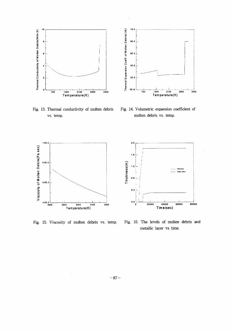
X E ~ ~ ~ J: o O o o :~

~ o :b

)

U o O 15

E o c h

10

l

'~ H

6

4

2

o

+\

f

700

X

,, o Q o o = o

o o O o co

c a, ,~

UJ

E ,p

c H

IE4 :

8E-5 '~

l

6E-5 Ih

r

4E-5 ~ L

2E-5

f

oE~o

~

14oo 2800 3500 21 oo

Tem perature(K) 7oo 14Qo 210o

Te m pe ratu re (K) 2800 350o

Fig . 13. Thermal conductivity of molten debris

vs. temp.

Fig . 14. Volumetric expansion coefficient of

molten debris vs. temp.

o o co

a,

~ co

G o o c o o = ~ o ~ ,o

o o ,o

>

1 OE*2

8.OE-3

6,0E-3

E ~ (D

~-o ,: H

2'o [

1.6 L

~

121_ l

:I o '8 j

0'4 L !

if L! I!

o'o L-i

'

!

M•t•1 ,•r•r md,•n (dPrt-

4 OE-3 2800

r~~~~~ 29oo 30oo 3100

Temperature(K) 3200 o 2ooOo 4OOOQ

T im e (sec) 60000 800oo

Fig . 15. Viscosity of molten debris vs. temp. Fig . 16. The levels of molten

metallic layer vs time.

debris and

- 87 -

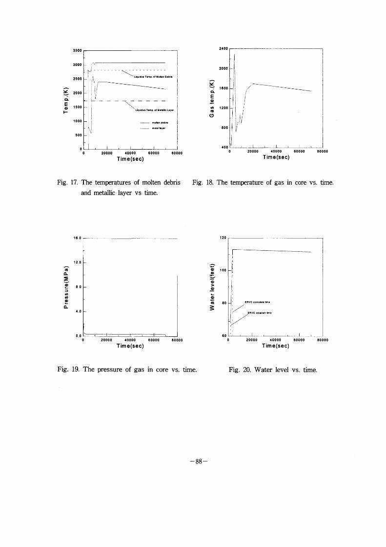
3soo

3000

25oO

~ ~e 20OO ~ ,L E O ISOO H

1 oOo

sOO

O

I

\----- 1 L~u~dut T,m ,. ef Me~'n D,bft l

~ - '1-\- ~ ~ I \ L~u~ut Tlmp of M'tlilic L'y'f

meft'ft d'trl'

m,ttl "y'r

2400

~~J

[

'i

/

ll ' li ll f 1' . 1' :1

l

2oooo 4oooo 6oooo 800oo Time(sec)

200o

~e

~ . 1 60O

a E O ~ co 1 2OO co

O 8oO

4oO

I / r

i

l*i

1

i

'*~-,'~'

.-J--O

~\~~

o 2oOoo 40ooo Time(sec)

6oooo 80ooo

Fig. 17. The and

temperatures of molten debris Fig 18

metallic layer vs time.

The temperature of gas in core vs. time .

~ ,~l

aL

~ ~ O

O CL

16 .o

12.o

8.o

40

o .O

o 200oo 4oooo 60ooo 80ooo Time(sec)

1 20

~ ~ o I OO a, .~ ~ O ) o LO

co 8o ;

6c

1 :

!:

i/ERvc "'pu't' s~'

ERVC i~it't'e~ ti*'

'l o 20oOO 4oooo

Time(sec) 6oooo 80ooO

Fig. 19. The pressure of gas in core vs. time. Fig. 20. Water level vs. time.

- 88 -

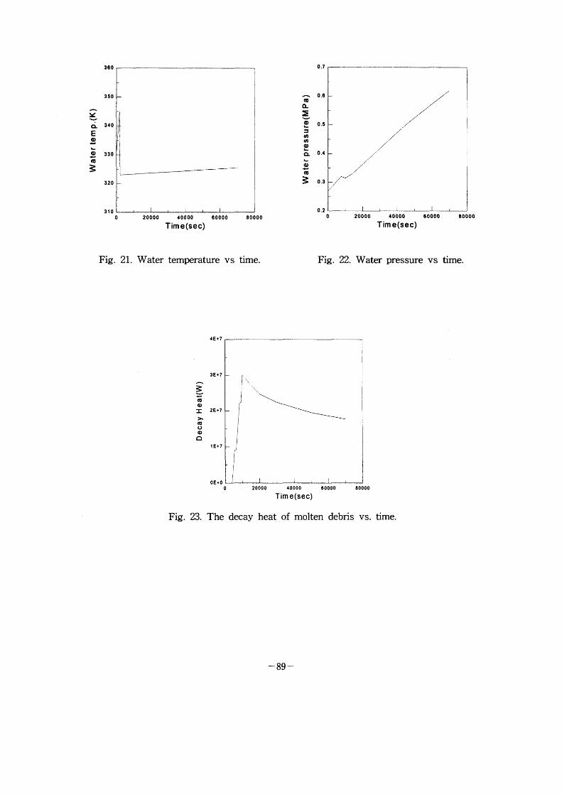
.~ X ,., 'L E O 1-

Q' 1* 'O ~:

36Q

35o

340

330

32o

310

J

!'

0.7

'~ 0'6 'L :~ ,~, O O'5

'OO

~ 0'4

(D ~J ~ O'3

o .2

o 20QOO 4oooo Time(sec)

6oooo 800oo

/ / /

.l /

o 20000 40000 80000 Tim e(sec)

8ooOo

Fig. 21. Water temperature vs time. Fig. 22. Water pressure vs time.

4E~7

3E~7

~ CO

O I 2E*7 :~ CO

O O O

IE*7

oEto

f' \

i

i

!

o 200oo 4oooo 60000 T im e (sec)

8oooo

Fig . 23. The decay heat of molten debris vs. time.

- 89 -

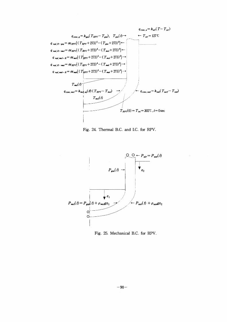
q.,a~h~r(T T~.)

. =hgas(TRPV- Tg"), Tg"(t)-) (- Tai'=127~~ qco~ g

4 (- j ~1 q nd.R-g,~= oeRP~( Trip +273) ( Tg"+273) } ~_

qradR- I= oieRP~(TRPV+273)4-(T,nol+273)4)~~ l

q .ed, mol-R= oe,,,o~ ( ~_ r""v+ 273)4~ ( Tmol+ 273)4}~~f

q nd.R-,~et= oeRP~ ( TJ~PV+ 273)4~ ( T,,,et+ 273)4}~F j f

qred"net T~p _R= oemet{ ( v+ 273)4~ ( T_t+ 273)4} -~I

Tmet( t) ,f ,l q._/= h,,,o eq(e) ( TRPV- Tmol) ~~ / . = hcoat( Tsarf~ Tt)

.l

TX t) ji "'

TRP~O) = Ti.i = eo21C , t= Osec

Fig. 24. Thermal. B.C. and I.C. fOr RPV

O O ~- Pair=P8oat(t) rlj [

I r~ Pgas(t) ~~ j z2

~ zl // /

O o

Fig. 25. Mechanical B.C. for RPV.

- 90 -

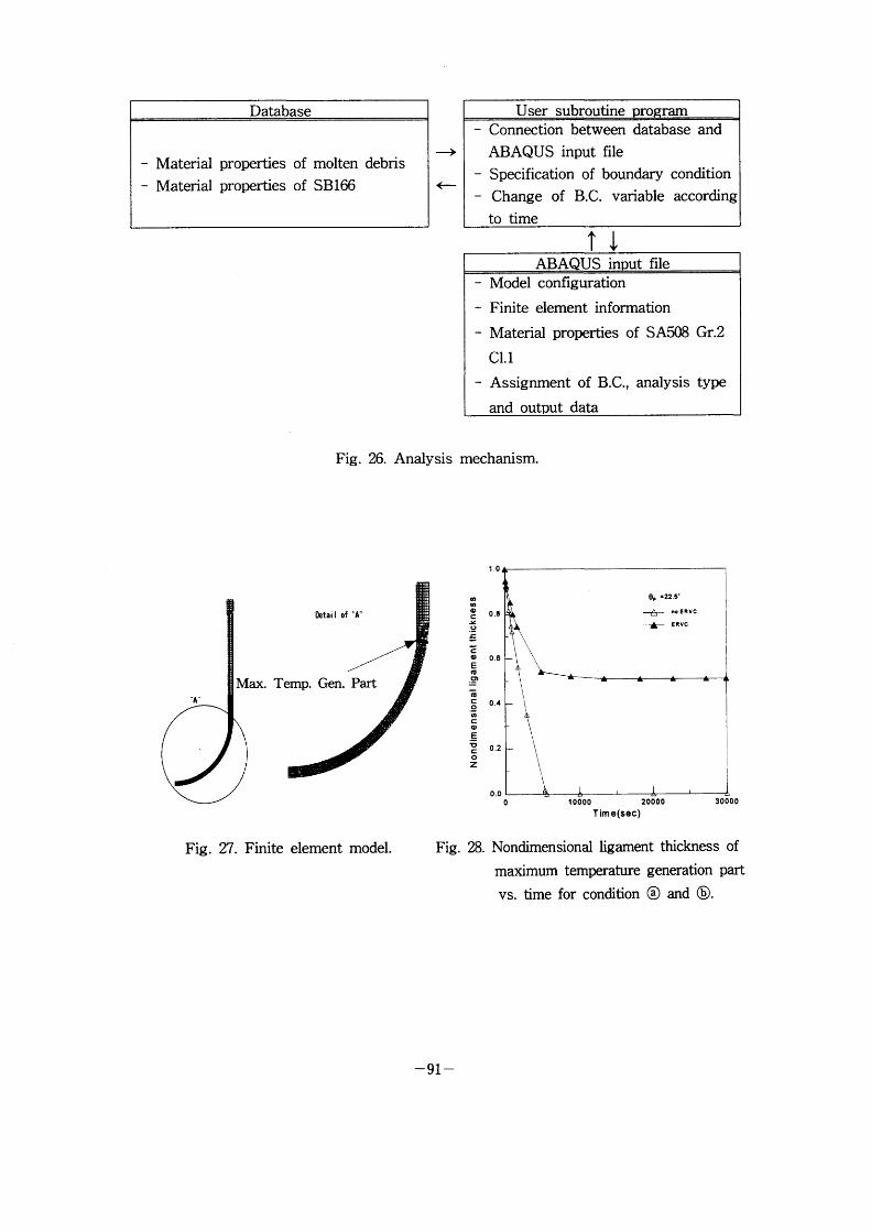
Database

Material

M ateri al

properties

properties

of

of

molten

SB166

debris ->

User subroutme ro ram Connection between database and

ABAQUS input file Specification of boundary condition

Change of B.C. variable according

to time

T~ ABAQUS input file

Model configuration

Finite element information

Material properties of SA508 Gr.2

Cl.1

Assignment of B.C., analysis type

and output data

Fig . 26. Analysis mechanism.

IIAI'

Fig .

Max. Temp .

Detail of

Gen. Part

27. Finite element model . Fig.

,,,

o c s' o J:

c o E (v o)

,D

c o c 1'

E ~ c o Z

28.

10

0.8

06

o.4

0.2

a.o

l

e, •22S' ~r noEIVC IF ERVC

t

loooa 2oooo 30000 Time(sec)

Nondimensional ligament thickness of

maximum temperature generation part

vs. time for condition @ and ~.

-91-

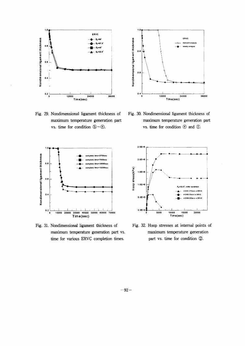
1.0

g, ,b lp c:

!~ 08 o c c o E c9

.9' O G

tD

c o ,o

c o E 0.4 ID c o Z

a.2

ERVC

-~ e,Ico'

~- O,•e7,5' 1- e,•4s' IF O,'22.5'

o 12aoo T im e(sec)

24000 36000

10

,e ,o

o = ~ o c O.8

= o E c9 OD

o c o co 06 = o e v c o Z

0.4

\ ~

ERVC -~~+. ,r,nti, pt I nl ~tit

-~ •t•tdy tn,ly,It

o 12000 Time(sec)

24000 36000

Fig . 29. Nondimensional ligament thickness of

maximum temperature generation part

vs. time for condition ~) - @.

Fig . 30. Nondimensional ligament thickness of

maximum temperature generation part

vs. time for condition ~ and R.

1 .o

o co

o ~ .o_ O . 8

= ~ ~ o E 1'

.a, O 6

cp

o co

c o E O4 lu c o Z

o. 2

~= 1--~ -h

com p,•te tim••37S0•le com pl•t• ~m ••1 OOO•ec comp,•t• tim•• 10000t•c cem prt• tim • • I SOOOt•c

o loooo 20000 3oooo 40000 Time(sec)

50000 600oo 70000

C9 O-

X c,,

cO

O 10

a O O I

2 5E*e

2,oEte

1.SEt6

1 OE~e

5.OEt5

Fig.

o OE*O

\ \

0,122 5', rop,r cond~ion

IF r•24S4 27Smm'nE•vc 4- r•2lesssmmi,IERVC Hr t•2S8,e2SmminERvc

31. Nondimensional ligament thickness of

maximum temperature generation part vs.

time for various ERVC completion times.

Fig.

o sooo 1000o Isooo T im e (sec)

2oOoo

32. Hoop stresses at internal points of

maximum temperature generation

part vs. time for condition ~).

- 92 -

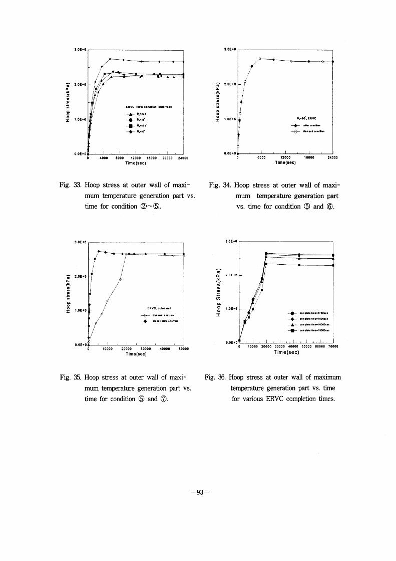
C-aL ,~

O tO

,L O O I

3.0Ete

2 OEt6

1 .OEt6

o. OE~O

l'

/ / r / E RVC , rol., coodabn

IF e,'22 s'

~- e,•as' Hr e,•,7 s' -~ 9,.,d

Out•f Wd

o 40OO 80QO 12000 Time(sec)

160OO 20OOO 24000

c-

t ~ to

s

,L o o I

3

2

1 .OEt6

O.OE~O

)e-~ ~~~~1

elpleo'. E RVC

-~ rod'r eoNe~'H

~- e"mp'd e'nd'i'l

O 80oo 12000 Time(sec)

leooo 240oo

Fig. 33. Hoo p

mum time

stress at outer wall of

temperature generation

for condition ~)-R.

maxi-

part vs.

Fig. 34. Hoop stress at outer wall of maxi-

mum temperature generation part

vs. time for condition R and C.

,,

~ ~ o

a o o :E

3 OE~6

2.oEte

1 .OE~6

o .OEtO

EAVC , out•r ,,1 Il

~ tr.nti•nt i•Ily.It

~- ,t••dy ttit• Ilaly,i$

200oo 3oooo Time(sec)

3.0E•e

co

~ 2 ~ ,o co

o u)

a o I oE*e o I

.oE+6

o.aE~o

o 10000

/ /

!

r

4oooo soooo

~- compbO,am••$7S0,1,c H~ cempl•t• dm••700O••c lr compl•t• ~ml'lOOOOt•c dF cof" p,,t• d,,•• I SOeo••e

O 10000 2000o 3000o 40000 T im e (sec)

50000 eoooo 7oooo

Fig. 35. Hoop

mum time

stress at outer wall of

temperature generation

for condition R and ~).

maxi -

part vs.

Fig. 36. Hoop stress

temperature

for various

at outer wall of maximurn

generation part vs. time

ERVC completion times.

- 93 -

Session 111

Plant Experiences

III- l The Evaluation of IGSCC Problems of Stainless Steel Piping

in Taiwan BWR-6 Nuclear Power Plant

Kuen Ting, Department of Nuclear Regulation Atomic Energy

Council,Taiwan, Republic of China

The Evaluation of IGSCC Problems of Stainless Steel Piping in Taiwan BWR-6 Nuclear Power Plant

Kuen Ting

Department of Nuclear Regulation Atomic Energy Council

Republic of China

ABSTRACT Taiwan BWR-6 Kuosheng Nuclear Power Plant Unit I implemented the inspeotion of the IGSCC-susoeptible wekhnents. of stainless steel piping in the reactor recirculation, reactor water clean-up, residual heat removal, core spray and feedwater systems. The purpose of this paper is to present the status of the fraoture problems in the weldments. The crack growth analysis due to IGSCC and the standard weld overlay design based on the ASME Code Section XI and NUREG-03 1 3 Rev. 2 for the fracture weldments are discussed in detail. Then, the contingent programs including the inspection program, fracture evaluation, the standard weld overlay are completely established to prevent the pipe

break during the reactor operation.

INTRODUCTION The objeetive of this paper is to present the intergranular stress corrosion cracking GGSCC) status

ofthe primary coolant system at BWR-6 Nuclear Power Station (NPS) unit I in Taiwan. This work was aehieved by identifying all the IGSCC-susceptible systems and the associated weldments. Following the procedures of inspeotion, evaluation and repair are based on the requirements of the United States Nuclear Regulatory Commission (USNRC) Report NUREG-0313. Rev. 2[l] and Generic Letter 88-O I [2] .

An inspections have been performed on the various IGSCC-susceptible weldments at BWR-6 NPS unit I in Taiwan since 1 983. The inspections, since 1 987 (EOC-4), have been performed to the requirements of NUREG-03 13, Rev.2. The total of 184 weldments which are contained in reactor recireulation, reaetor water clean-up, residual heat removal, core spray and feedwater systems are categorized as five groups. However, the inspection frequencies for the various weldment categories were more than the NUREG-03 1 3 requirements during the past I O years of operation in Taiwan. When a flawed weld is identified during inservice inspection, the flaw evaluation may be performed to meet the requirements of ASME Code Section XI in lieu of repair to justify continued operation for a specified evaluation period. This evaluation is based on the linear elastio fracture mechanics to Galculate

the IGSCC growih. If the crack growth exceeds the allowable critical length and depth, identified IGSCC in stainless steel may be used standard weld overlay for long-tenn repair. The design of the standard weld overlay is based on the net section collapse conoept. Significant field, and experimental

evidenGe has been assembled to meet ASME Code Case 504-1 [3] for the long term repairs of weld

- 95 ~

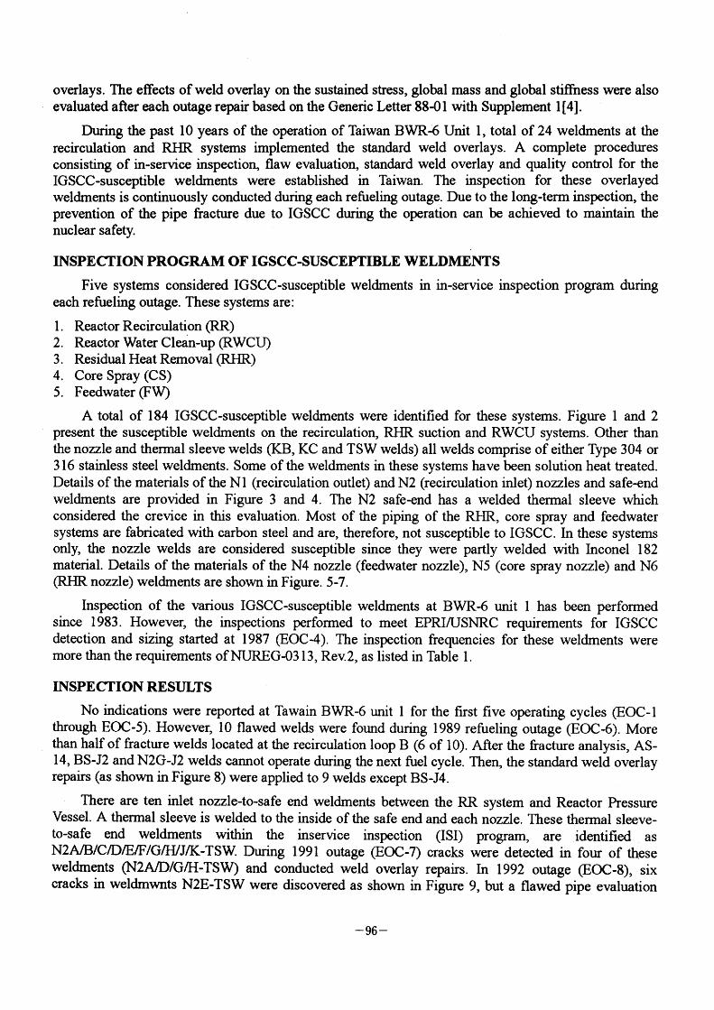
overlays. The effeGts of weld overlay on the sustained stress, global mass and global stiffness were also

evaluated after each outage repair based on the Generic Letter 88~)1 with Supplement I [4].

During the past I O years of the operation of Taiwan BWR~5 Unit I , total of 24 weldments at the

recirculation and RHR systems implemented the standard weld overlays. A Gomplete procedures consisting of in-service inspection, flaw evaluation, standard weld overlay and quality control for the

IGSCC-susceptible weldments were established in Taiwan. The inspection for these overlayed weldments is continuously conducted during each refueling outage. Due to the long-term inspection, the prevention of the pipe fracture due to IGSCC during the operation can be achieved to maintain the nuclear safety.

INSPECTION PROGRAM OF IGSCC-SUSCEPTIBLE WELDMENTS Five systems considered IGSCC-susceptible weldments in in-service inspection program during

each refueling outage. These systems are :

l . Reactor Recirculation (RR:)

2 . Reactor Water Clean-up (RWCU) 3 . Residual Heat Removal (RHR;) 4. Core Spray (CS) 5. Feedwater (FW)

A total of 1 84 IGSCC-susceptible weldments were identified for these systems. Figure I and 2 present the susGeptible weldments on the reoirculation, IuJR suction and RWCU systems. Other than the nozzle and thermal sleeve welds (KB, KC and TSW welds) all welds comprise of either Type 304 or 3 1 6 stamless steel weldments. Some of the weldments in these systems have been solution heat treated. Details of the materials of the Nl (recirculation outlet) and N2 (recirculation inlet) nozzles and safe-end

weldments are provided in Figure 3 and 4. The N2 safe-end has a welded thermal sleeve which considered the crevice in this evaluation. Most of the piping of the RHR, core spray and feedwater systems are fabricated with Garbon steel and are, therefore, not susceptible to IGSCC. In these systems only, the nozzle welds are considered susceptible since they were partly welded with Inconel 1 82 material. Details of the materials of the N4 nozzle (feedwater nozzle), N5 (core spray nozzle) and N6 (RHR nozzle) weldments are shown in Figure. 5-7.

Inspection of the various IGSCC-susceptible weldments at BWR-6 unit I has bcen performed since 1 983. However, the inspections performed to meet EPRI/USNRC requirements for IGSCC detection and sizing started at 1 987 (EOC-4). The inspection frequencies for these weldrnents were more than the requirements ofNUREG-03 1 3, Rev.2, as listed in Table I .

INSPEcrION RESIJIJTS No indications were reported at Tawain BWR-6 unit I for the flfst frve operating cycles (EOC-l

through EOC-5). However, 10 flawed welds were found during 1 989 refueling outage (EOC-6). More than half of fracture welds located at the recirculation loop B (6 of I O). After the fracture analysis, AS-

l 4, BS-J2 and N2G-J2 welds cannot operate during the next fuel cycle. Then, the standard weld overlay repairs (as shown in Figure 8) were applied to 9 welds except BS-J4.

There are ten mlet nozzle-to-safe end weldrnents between the RR system and Reactor Pressure Vessel. A thermal sleeve is welded to the inside of the safe end and each nozzle. These thermal sleeve-

to-safe end weldments within the inservice inspection (ISI) program, are identified as N2A/B/C/D/E/F/G/H/J/K-TSW. During 1 991 outage (EOC-7) cracks were detected in four of these weldments (N2A/D/G/H-TSW) and conducted weld overlay repairs. In 1 992 outage (EOC-8), six cracks in weldnwnts N2E-TSW were discovered as shown in Figure 9, but a flawed pipe evaluation

~ 96 -

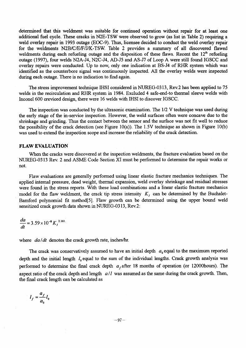
determined that this weldment was suitable for GOntinued operation without repair for at least one additional fuel Gycle. These Gracks in N2E-TSW were observed to grow (as list in Table 2) requinng a weld overlay repair in 1 993 outage (EOC-9). Thus, Iicensee decided to conduGt the weld overlay repair

for the weldments N2B/C/E/F/J/K-TSW. Table 2 provides a summary of all disGOVered flawed weldments during each refueling outage and the disposition of these flaws. ReGent the 1 2th refueling

outage (1997), four welds N2A-J4, N2C-J4. AD-J5 and AS-J7 of Loop A were still found IGSCC and overlay repairs were conducted. Up to now, only one indication at B S-J4 of RHR system which was identified as the GOunterbore signal was continuously inspected. All the overlay welds were inspected during each outage. There is no indication to find again.

The stress improvement technique IHSI considered in NUREG-03 1 3, Rev.2 has been applied to 75 welds in the reGirculation and RHR system in 1 984. Excluded 4 safe-end-to thennal sleeve welds with Inoonel 600 creviced design, there were 1 6 welds with IHSI to discover IGSCC.

The inspection was conduoted by the ultrasonic examination. The 1/2 V technique was used during the early stage of the in-service inspection. However, the weld surfaces often were concave due to the shrinkage and grinding. Thus the contact between the sensor and the surface was not fit well to reduce the possibility of the crack detection (see Figure I O(a)). The I .5V technique as shown in Figure lO(b) was used to extend the inspection scope and increase the reliability of the crack deteGtion.

FLAW EVALUATION When the cracks were discovered at the inspection weldments, the fracture evaluation based on the

NUREG-03 1 3 Rev. 2 and ASME Code Section XI must be performed to determine the repair works or not .

Flaw evaluations are generally performed using linear elastic fracture mechanios teohniques. The applied intemal pressure, dead weight, thermal expansion, weld overlay shrinkage and residual stresses were found in the stress reports. With these load combinations and a linear elastic fracture mechanics

model for the flaw weldment, the crack tip stress intensity KI can be detennined by the Buchalet-

Bamford polynomial fit method[5]. Flaw growth can be determined using the upper bound weld sensitized crack growih data shown in NUREG-03 1 3 . Rev.2:

da 2 161 dt = 3'59 x l0-8KI ' '

where da /dt denotes the craok growth rate, inches/br.

The crack was conservatively assumed to have an initial depth ao equal to the maximum reported

depth and the initial length lo equal to the sum of the individual lengths. Crack growth analysis was

performed to determine the final crack depth af after 1 8 months of operation (or 1 2000hours). The

aspect ratio of the crack depth and length a /1 was assumed as the same during the crack growth. Then,

the final crack length can be calculated as

If = af lo

ao

- 97 -

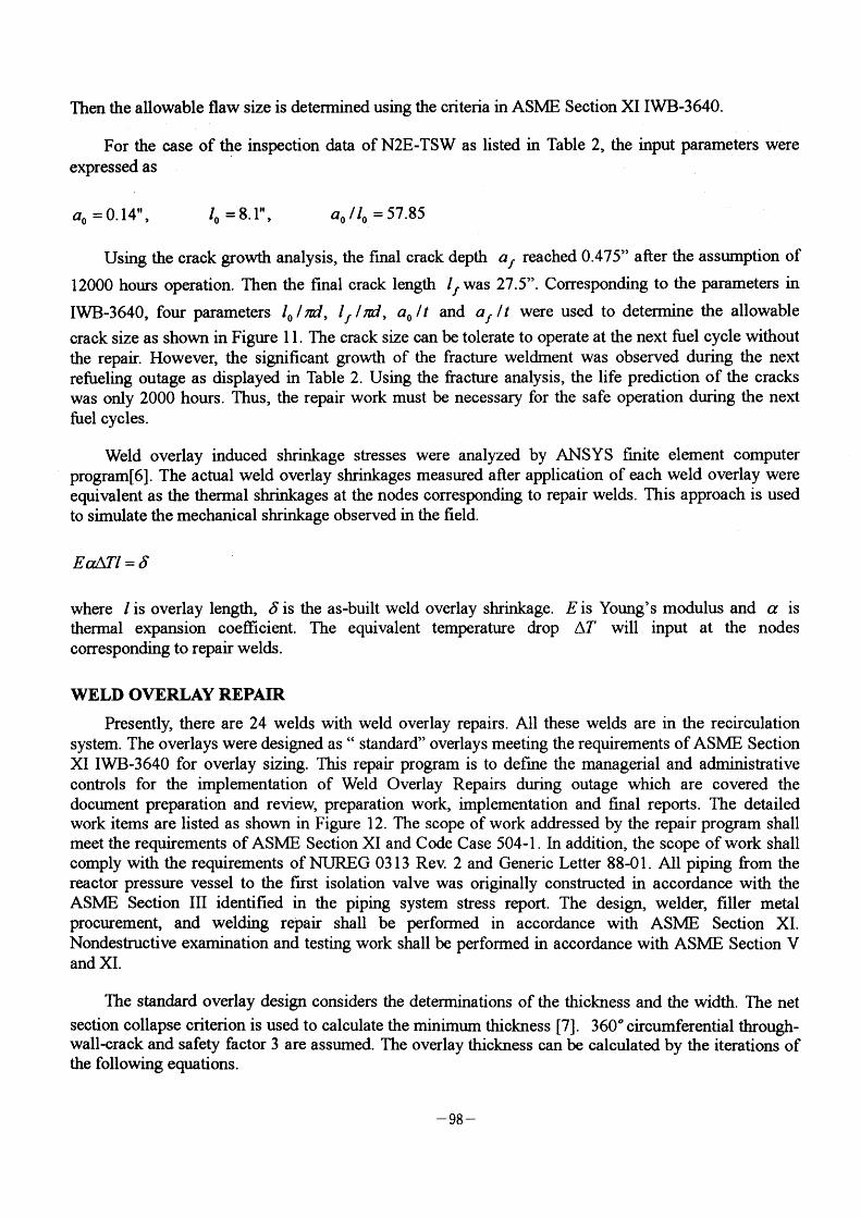
Then the allowable flaw size is determined using the criteria in ASME Section XI IWB-3640.

For the case of the inspection data of N2E-TSW as listed in Table 2, the input parameters were

expressed as

ao = 0.14", Io = 8. l" ao /lo = 57.85

Using the crack growih analysis, the fmal crack depth af reached 0.475" after the assumption of

l 2000 hours operation. Then the fmal crack length lf was 27.5". Corresponding to the parameters in

IWB-3640, four parameters lo /rd, If /rd, ao /t and af /t were used to determine the allowable

crack size as shown in Figure I I . The orack size can be tolerate to operate at the next fuel cycle without

the repair. However, the significant growth of the fraoture weldrnent was observed during the next refueling outage as displayed in Table 2. Using the fracture analysis, the life prediGtion of the cracks was only 2000 hours. Thus, the repair work must be neGessary for the safe operation during the next fuel cycles.

Weld overlay induced shrinkage stresses were analyzed by ANSYS finite element computer program[6] . The actual weld overlay shrinkages measured after application of each weld overlay were equivalent as the thermal shrinkages at the nodes corresponding to repair welds. This approach is used to simulate the mechanical shrinkage observed in the field.

Ea~TI = 5

where I is overlay length, 6 is the as-built weld overlay shrinkage. E is Young's modulus and a is thermal expansion coefficient. The equivalent temperature drop AT will input at the nodes corresponding to repair welds .

WELD OVERLAY REPAIR Presently, there are 24 welds with weld overlay repairs. All these welds are m the reclfculation

system. The overlays were designed as " standard" overlays meeting the requirements of ASME Section XI IWB-3640 for overlay sizing. This repair program is to define the managerial and administrative eontrols for the implementation of Weld Overlay Repairs during outage which are covered the document preparation and review, preparation work, implementation and final reports. The detailed work items are listed as shown in Figure 1 2. The scope of work addressed by the repair program shall meet the requirements of ASME Section XI and Code Case 504-1 , In addition, the scope of work shall comply with the requirements of NUREG 03 1 3 Rev. 2 and Generic Letter 88-0 1 . All piping from the reactor pressure vessel to the frrst isolation valve was originally constructed in aceordanGe with the ASME SeGtion 111 identified in the piping system stress report. The design, welder, filler metal procurement, and welding repair shall be performed in accordance with ASME SeGtion XI. Nondestructive examination and testing work shall be performed in aooordance with ASME Section V and XI.

The standard overlay design considers the determinations of the thickness and the width. The net

section GOllapse criterion is used to calculate the minimum thickness [7]. 360" circumferential tbrough-wall~rack and safety factor 3 are assumed. The overlay thickness oan be GalGulated by the iterations of the following equations.

- 98 -

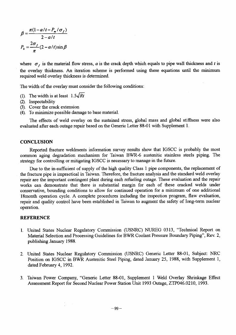
p = PT(1 -a/t - P~ Iaf )

2 - a/t

p = 2af (2 _a/t)sinp

;T

where af rs the material flow stress, a is the crack depth whioh equals to pipe wall thiGkness and t is

the overlay thickness. An iteration scheme is performed using these equations until the minimum required weld overlay thickness is determined.

The width of the overlay must consider the following conditions:

(1). The width is at least I .51!~

(2). InspeGtability

(3). Cover the crack extension (4). To minirnize possible damage to base material.

The effects of weld overlay on the sustained stress, global mass and global stiffaess were also evaluated after each outage repair based on the Generio Letter 88-0 1 with Supplement I .

CONCLUSION Reported fracture weldments information survey results show that IGSCC is probably the most

common aging degradation meehanism for Taiwan BWR-6 austenitie stainless steels piping. The strategy for controlling or mitigating IGSCC is necessary to manage in the future.

Due to the in-suffilcient of supply of the high quality Class I pipe components, the replacement of the fracture pipe is impractical in Taiwan. Therefore, the fracture analysis and the standard weld overlay

repair are the important contingent plant during each refueling outage. These evaluation and the repair

works can demonstrate that there is substantial margin for each of these cracked welds under conservative, bounding conditions to allow for continued operation for a minimum of one additional l 8month operation eycle. A complete procedures inoluding the inspeetion program, flaw evaluation, repair and quality control have been established in Taiwan to augrnent the safety of long-term nuclear

operation.

REFERENCE

l. United States Nuclear Regulatory Commission (USNRC) NUREG 0313, "Technical Report on Material Selection and Processing Guidelines for BWR Coolant Pressure Boundary Piping", Rev. 2,

publishing January 1 988.

2. United States Nuclear Regulatory Commission (USNRC) Generic Letter 88-0 1 , Subject: NRC Position on IGSCC in BWR Austenitic Steel Piping, dated January 25, 1 988, with Supplement I , dated February 4, 1992.

3. Taiwan Power Company, "Generic Letter 88-0 1 . Supplement I Weld Overlay Shrinkage Effect Assessment Report for Second Nuclear Power Station Unit 1 993 Outage, ZTP046 02 10 1 993

- 99 -

4. American Society of Mechanical Engineers (ASME) Boiler and Pressure Vessel Code Section XI, "Rules for Inservice Inspection ofNuclear Power Plant Components", 1 989 Edition.

5. Buchalet C.B. and Bamford W H "Stress Intensity Factor Solution for Contmuous Surface Flaws in Reactor Pressure Vessels", Mechonics ofCrack Growth, ASTM: STP 590, 1976.

6. Desalvo G. and Gormin, User Information Manual and Theoretica/ Manual. ANSYS Engineering System, 1 991 .

7. Smith E. ,"Theoretical Justification ofthe Association ofa Critical Net-Section Stress with Fracture Initiation at a Crack Tip", International Journal of Pressure Vessels and Piping, Vol. 8, 1 980, pp. 303-3 1 1 .

- 100 -

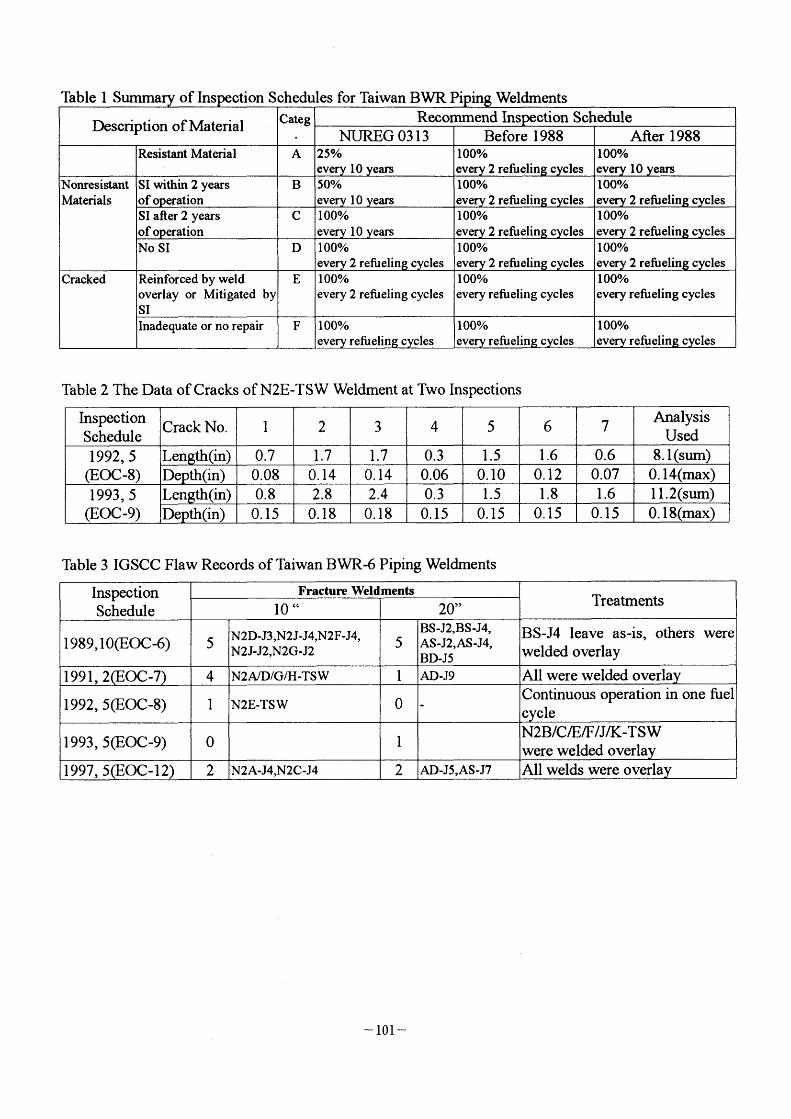
Table 2 The Data of Cracks of N2E-TSW Weldment at Two Inspections

Table 3 IGSCC Flaw Records of Taiwan BWR-6 Piping Weldments

- 101 -

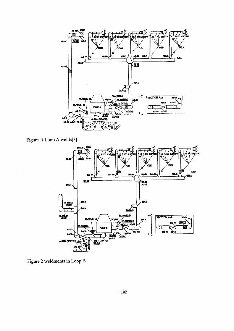
N18

A,n J~Ja~n

ALn

~ ~ '~"\\\~\~lll~

/ A ~'

a /(~:1 a~//

~L~~:~l~D

l' ,4

A,,J, \

~:~~/"

~

h~~('~i' /

~~f l' N28

~

Li~!

N ~a:r~t Jl ,?;/ I14

~'~(~;i/ 'L~tl2J:nttvl~;

~l

"~!!t

l

~~~ ./~~~ 'OdPA

A.n I '\bu2 AulO ~~

dhS2A (':~CU) l--;-/7rl~'~..~ ~_ _ _1/i7 \ .~- -:i'n

n~B~ J~ b\ ~'r

ANt ADn

a~B

AWll

n A~

A~'IO JL

JUhB

A•Ji ~!

S~~N ~A A~J-

ADJC

Ab.,,

I

ADd' ADn

Figure. I Loop A welds[3]

Figure 2 weldments in Loop B

- 102 -

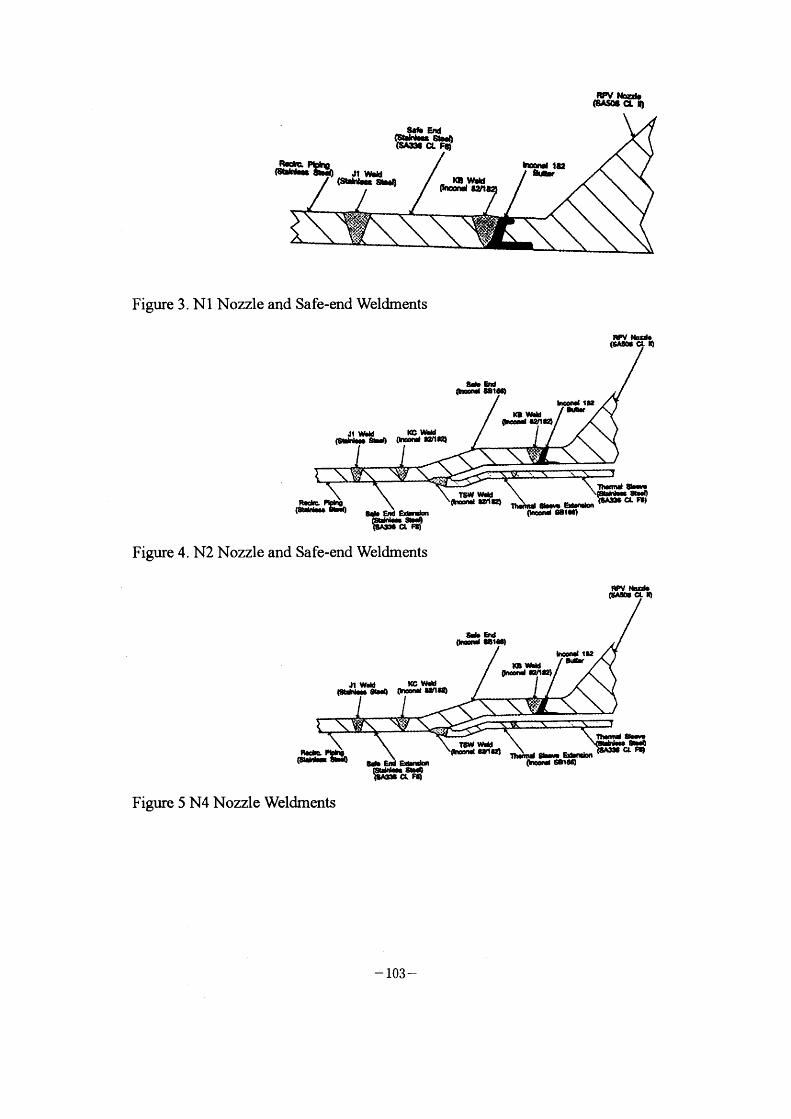
(~~GtND ,~r t~

SQ9b~d C~~ ~O ~8~CLFI~

W~ P~tll ~itda• ~O_ J1 V~U (~8N sbeO GWW 8U1 'QW~U

'~'ttl82

' ~;:

Figure 3 . Nl Nozzle and Safe-end Weldments

edb E,~' ~•"g~!9 ~~CL RI, o~•' a8t•e,

,~r Notd-(SASNGtlO

Figure 4. N2 Nozzle and Safe-end Weldrnents

~r NQd-

8db E,• ~•Q't ~~CL8bl)F~ Cb~,• G8lec,

,8~CLN,

Figure 5 N4 Nozzle Weldments

- 103 -

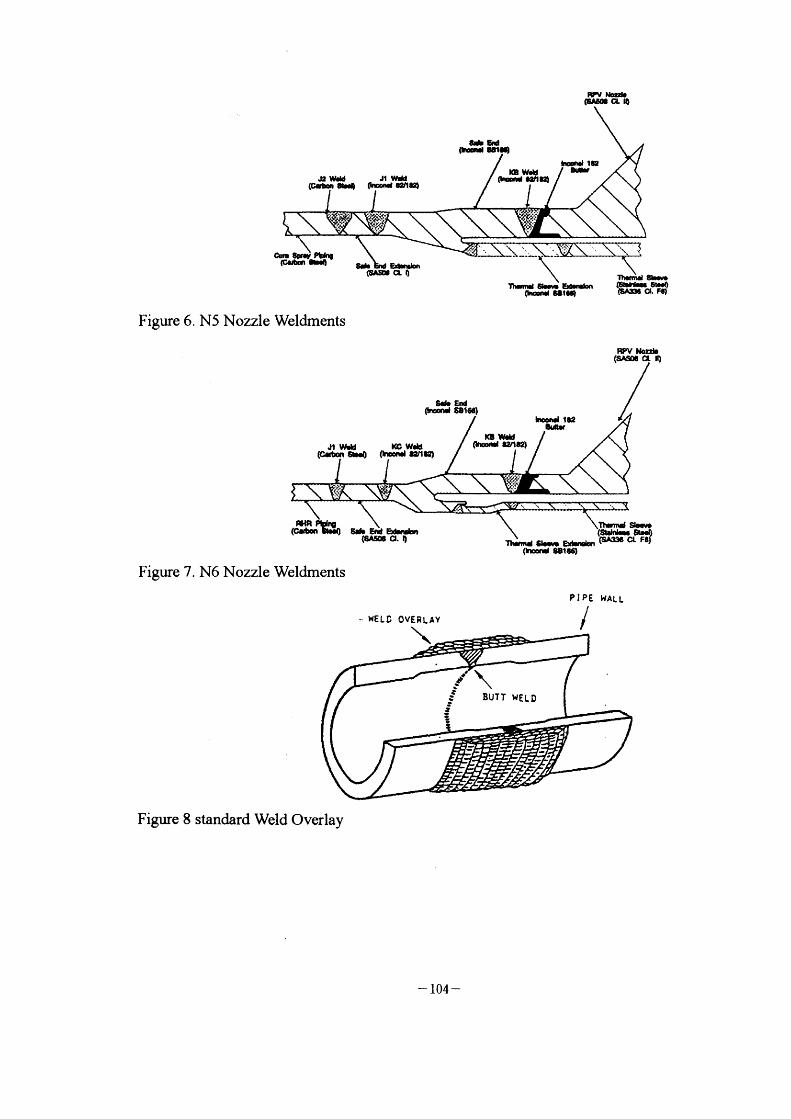
RPV b~ ,SA8NGL,O

Th~d a-- Ednbl aold 88leQ

T~~ef~i h-~,- ~,,~ ~A~a.Fe,

Figure 6. N5 Nozzle Weldrnents

8~ E~l a~•, 8ilee) bQ,.' Ie2

RPV Nordo (sA~eGtn)

8u.c

J1 W~ ,cCw•U (C•tn s,•eO OruJ ul~) ,aw~ a,u•' ~tn,

'~'ff;B'

~,,',, /\ \ (a'lc'taRrg~O 5d.E,eE'al~'

(~Go a. O 11•md Slw• ExD•ao (S~e ct Fa] T~~ S~-(StJd- ~!•D

(t~" 88le6,

Figure 7. N6 Nozzle Weldments

WELD OVERLAY

\ PIPE /

WAL L

f , ., i

~ ar S_

\ BUTT WELD

Figure 8 standard Weld Overlay

- 104 -

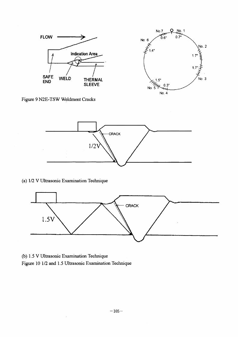
N0.7 No. 1

FLOW No 6 O 6" o. 7"

No. 2 1 .411

Indication Area 1 7,l

1 .711

SAFE WELD END THERMAL

SLEEVE No. 5

1 .5"

0.3,,

No 4

No. 3

Figure 9 N2E-TSW Weldment Cracks

CRACK

l 12

(a) I /2 V Ultrasonic Examination Technique

CRACK

l .5V

(b) I . 5 V Ultrasonic Examination Technique

Figure I O I /2 and I .5 Ultrasonic Examination Technique

- 105 -

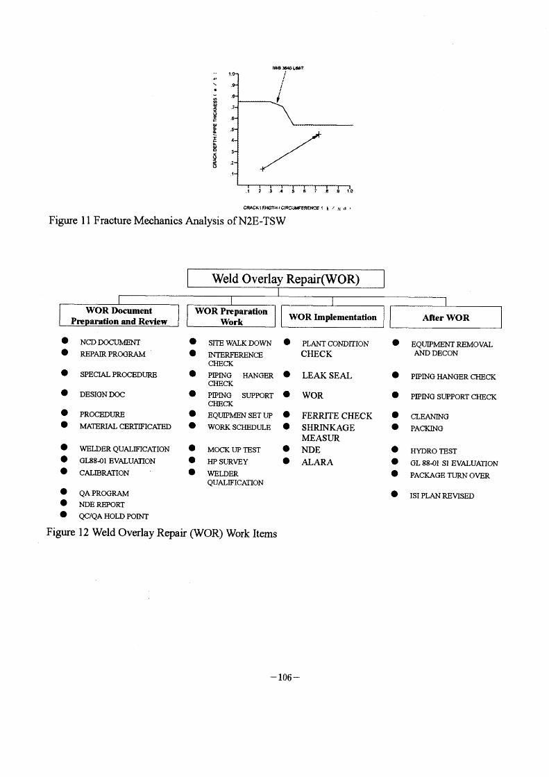
IO

\

(,) 6 IJ) $1i'

~

~ •6 ~ _5 ,}~r

!: 4 ,-a ~ e ~e " ~ 2

1 f

'wa eao Ldd'T

f

/

i '3 '4 s G P' 'e 1'c

cRAcF~lF'wcTHla"ciJ"FFRE'Nc'E t L "~' d '

Figure I I Fracture Mechanios Analysis ofN2E-TSW

e NCD DOCUMENT e SITE WALK DOWN O pLANT CONDrrloN O O REPAIR PROGRAM ' e INTERFERENCE CHECK

CHECK O SPECIAL PROCEDURE e plplNG HANGER e LEAK SEAL

CHECK e DESIGN Doc e plpING SUPPORT O WOR

CHECK e pROCEDUIU3 O EQUIPMEN SET UP O FERRJTE CHECK e MA113RIAL CERTIFICArl3D e WORK SCHEDULE O SHRINKAGE

MEASUR e waLDER QUALIFICATION e MOCK UP TE ST e N DE

e GL88~1 EVALUAIION e ALARA e HP SURVEY e CALn3RArION ' e WELDER

QUALIFICATION O QA PROORAM O NDE REPORT e QC/QA HOLD POn~T

Figure 1 2 Weld Overlay Repair (WOR) Work Items

e

o

o e

o e e

e

EQUD?MENT REMO VAL AND DECON

PIPlNG HANGER CHECK

PIPING SUPPORT CHECK

CLEANING PAClaNG

HYDRO TEST GL 88~)1 Sl EVALUAnoN

PACKAGE TUl~~1 OVER

ISI PLAN RBVISED

- 106 -

lll-2 ISI NDE in Korean Nuclear Power Plants Yi-Hwan (Peter) Jeong, Korea Electric Power Research

Institute, Korea

ISI NDE in KOrean NuClear POWer Plants

Yi-Hwan (Peter) Jeong

Hee-Jong Lee

Yong-Sik Kim Materials & Corrosion Laboratory

Korea Electric Power Research Institute

Taej on, Korea

Abstract

Structural integrity of nuclear components is important for a safe

operation of nuclear power plants. Therefore, the structural integrity

should always be maintained by reliable, periodic inservice inspections.

Korea Electric Power Company(KEPCO) operates the entire Korean nuclear power plants. Since the safe operation and the inservice inspection(ISD of the nuclear power plants are under the plant owner's

responsibility, Korea Electric Power Research Institute(KE;PRD, the R&D

division of KEPCO, has established an integrated ISI NDE support system(called, ISI NDE Total Support System: TSS), primarily focused on

the inservice inspection of nuclear power plants. And the KEPRI has

initiated a long -term plan for the development of key ISI NDE technology

that is necessary for an efficient on-site support. This paper describes

the KEPRI's TSS and the long-terrn plan for the key ISI NDE technology development.

Introduction

Since Kori Unit I , the first nuclear power plant in Korea, started

to generate electricity in 1978, Korea has built twelve nuclear power

plants and produces lOgigaWatts of electricity (25~ of the total electricity

- 107 -

in Korea, and 9th in the nuclear power generation worldwide). According

to the latest survey (Table I ), a total of 336 units at 81 power plants

nationwide (including hydraulic, f ossil and nuclear) generated over

4lgigaWatts of electricity in 1997(17th in the overall power generation

worldwide). Over the past years, Korean nuclear power plants showed

remarkable improvements in the perforrnance such as drop of unplanned

shutdowns and reduction of outages. The nuclear power generation is

now a wing of the main source of electricity in Korea. In a long-term,

the share of nuclear electricity production will increase to over 45%

nationally with the completion of additional nuclear power plants(23

nuclear power plants by the year 2006).

In addition to

important to supply

supply high-quality,

nuclear components inspections.

supplying a quantity of electricity to users, it is also

high-quality, stable(interruption-free) electricity. To

stable electricity, the structural integrity of the

should be maintained by reliable, periodic inservice

Tab le 1 . Electricity generated by Korean Power Plants

As of January of 1998 (Unit MW )

Notes: (1) 9th in the nuclear and 17th in the total power generations worldwide.

- 108 -

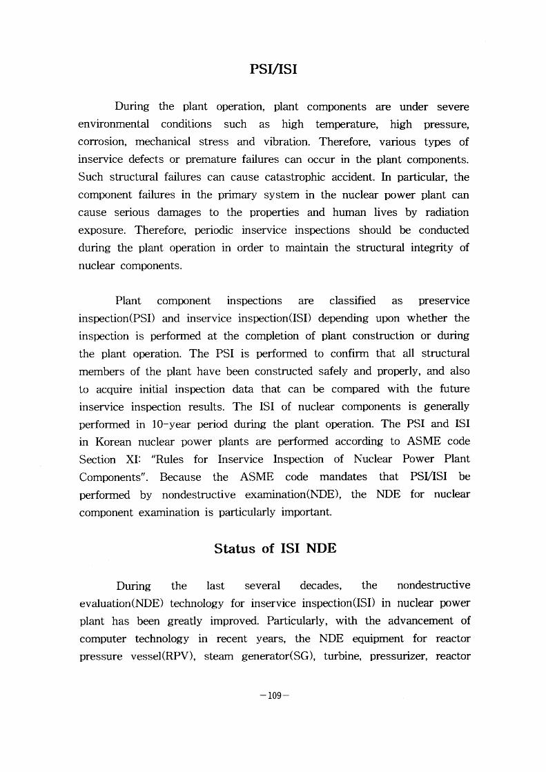
PSI/ISI

During the plant operation, plant components are under severe

environmental conditions such as high temperature, high pressure, corrosion, mechanical stress and vibration. Therefore, various types of

inservice defects or premature failures can occur in the plant components.

Such structural failures can cause catastrophic accident. In particular, the

component failures in the primary system in the nuclear power plant can

cause serious damages to the properties and human lives by radiation

exposure. Therefore, periodic inservice inspections should be conducted

during the plant operation in order to maintain the structural integrity of

nuclear components.

Plant component inspections are classified as preservice inspection(PSD and inservice inspection(ISD depending upon whether the

inspection is perforrned at the completion of plant construction or during

the plant operation. The PSI is perforrned to confinn that all structural

members of the plant have been constructed safely and properly, and also

to acquire initial inspection data that can be compared with the future

inservice inspection results. The ISI of nuclear components is generally

perfonned in 10-year period during the plant operation. The PSI and ISI

in Korean nuclear power plants are perforrned according to ASME code

Section XI: "Rules for Inservice Inspection of Nuclear Power Plant

Components" Because the ASME code mandates that PSVISI be perforrned by nondestructive exarnination(NDE), the NDE for nuclear

component examination is particularly important.

Status of ISI NDE

During the last several decades, the nondestructive evaluation(NDE) technology for inservice inspection(ISD in nuclear power

plant has been greatly improved. Particularly, with the advancement of

computer technology in recent years, the NDE equipment for reactor pressure vessel(RPV), steam generator(SG), turbine, pressurizer, reactor

- 109 -

coolant pump(RCP) and pipings were fully 2lutomated and sophisticated.

Consequently, the ilccuracy, the speed and the reliability of the ISl

perforrn~mce \vere impro\'ed accordingly.

Ilo\\'e\'er, the KEPCO has been he'avily relying on foreign

countries in conduc ting the inservice inspections of the nuclear components due to lack of key ISI NDE technology. Consequently, the ISl

operation costs KEPCO a great deal of financial burden. Furthermore, due

to lack of the key ISI NDE technology, the KEPCO has not been able to

respond to site problems in an efficient and timely manner. Such difficulties of Korean nuclear power plants provided the needed impetus

for KEPCO to develop a long-term plan for the ISI NDE technology development and to prepare for the independent operation of inservice

inspection of nuclear power plant components.

ISI NDE Long-Term Plan

The KE;PCO, as a utility, is primarily responsible for the safe and

reliable operation of the nuclear power plants. Therefore, the KEPCO

monitors the periodic inspections of nuclear components performed by

domestic and foreign companies. The mission of KEPRI, the R&D division of KEPCO, is to perform the research and development of ISI

N~DE technology as well as the associated technology transfer. To meet

such mission, the KEPRI has established an on-site support system,

called ISI NDE total support system(TSS), that can respond to various

plant ISI problems in an efficient and timely manner. Furthermore, in

order to successfully support the plant ISI operation, the KEPRI has

established a long-term plan for the development of key ISI NDE technology(Figure I ). The key ISI NDE technology areas were chosen

among the most important technical areas in conducting the on-site ISI

support tasks.

The TSS and the key IS'I NDE technology development programs contain the following three stages: preparation, independent operation, and

- I Io -

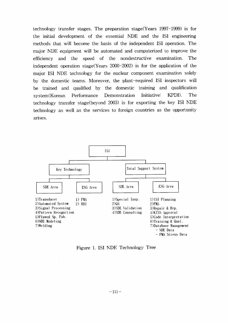
technology transfer stages. The preparation stage(Years 1997-1999) is for

the initial development of the essential NDE and the ISI engineering

methods that will become the basis of the independent ISI operation. The

major NDE equipment will be automated and computerized to improve the

efficiency and the speed of the nondestructive examination. The independent operation stage(Years 2000-2002) is for the application of the

major ISI NDE technology for the nuclear component examination solely

by the domestic teams. Moreover, the plant-required ISI inspectors will

be trained and qualified by the domestic training and qualification

system ( Korean Perforrnance Demonstration Initiative: KPDD. The technology transfer stage(beyond 2003) is for exporting the key ISI NDE

technology as well as the services to foreign countries as the opportunity

arises.

ISI

Kev. Techno I ogy

NDE Area

1)Transducer 2)Automated System 3)Signal Processing 4)Pat tern Recognit ion 5)Flawed Sp. Fab. ONDE Model ing 7 )We I d i ng

Tot a l Suppor t

EN 'G Area

1) FMA 2) RBI

S~. ,s t em

Figure

\.'DE Area

1)Special Insp. _9)QA

3)\'DE Val idat ion 4)NDE Consul t ing

1. ISI NDE Technology

E\G Area

1)ISI Plauning _? ) FMA

3)Repair & Rep. ~)KINS Appro\~a l 5)C.ode Interpretat ion 6)Training & Qual . 7)Dat abase \.fanagement

- \.'DE Data

- F~A Stress Data

Tree

-111-

ISI NDE Total Su pport System

The ISI of nuclear components typically include such tasks as ISI

planning, nondestructive testing(NDT), quality assurance(QA), fracture

mechanics analysis(FMA), and repair or replacement of defective components. And these tasks are being perfonned according to the rules

and the regulations of ASME Boiler And Pressure Vessel Code: e.g., the

NDE concepts and the criteria(Section XD, the NDE procedures(Section

V), the repair and replacement(Sections 111, IX, and XD, etc.. The ISI

planning is to plan the overall scope of the ISI operation, the sequence of

component examinations, and the associated time schedule. The NDT is

for the actual examination of nuclear components using various NDT

techniques such as ultrasonics, Eddy current, X-ray, dye penetrant, magnetic particle and visual examination. The quality assurance(QA) is to

confirm the accuracy and reliability of the NDT performed by other

inspection tearns. The FMA is to determine whether the detected flaws of

certain sizes could influence the component integrity during the operation.

If the flaws could indeed influence the component integrity, then, the

FMA determines how long the defective components could be safely operated without repair or replacement. The repair and replacement tasks

in TSS are to recommend the repair and replacement methodology for

defective components that can satisfy the relevant code requirements.

Since the component defects are being found during the ISI, the necessary repair or replacement tasks can not be incorporated into the ISI

planning. Therefore, it is necessary to make a prompt, sound judgement

at the site for whether the component should be either repaired or

replaced depending on the applicable code requirements. And if it has to

be repaired or replaced, then, it should be determined which repair or

replacement methods should be applied.

In fact,

on NDE tasks in

the tasks

the above ISI tasks require the knowledge and

technology and NDE code requirements in order

an accurate and proper way. Nevertheless, in the

were conducted by non-NDE personnel resulted

the experience

to perform the

past, some of

m unnecessary

- I12 -

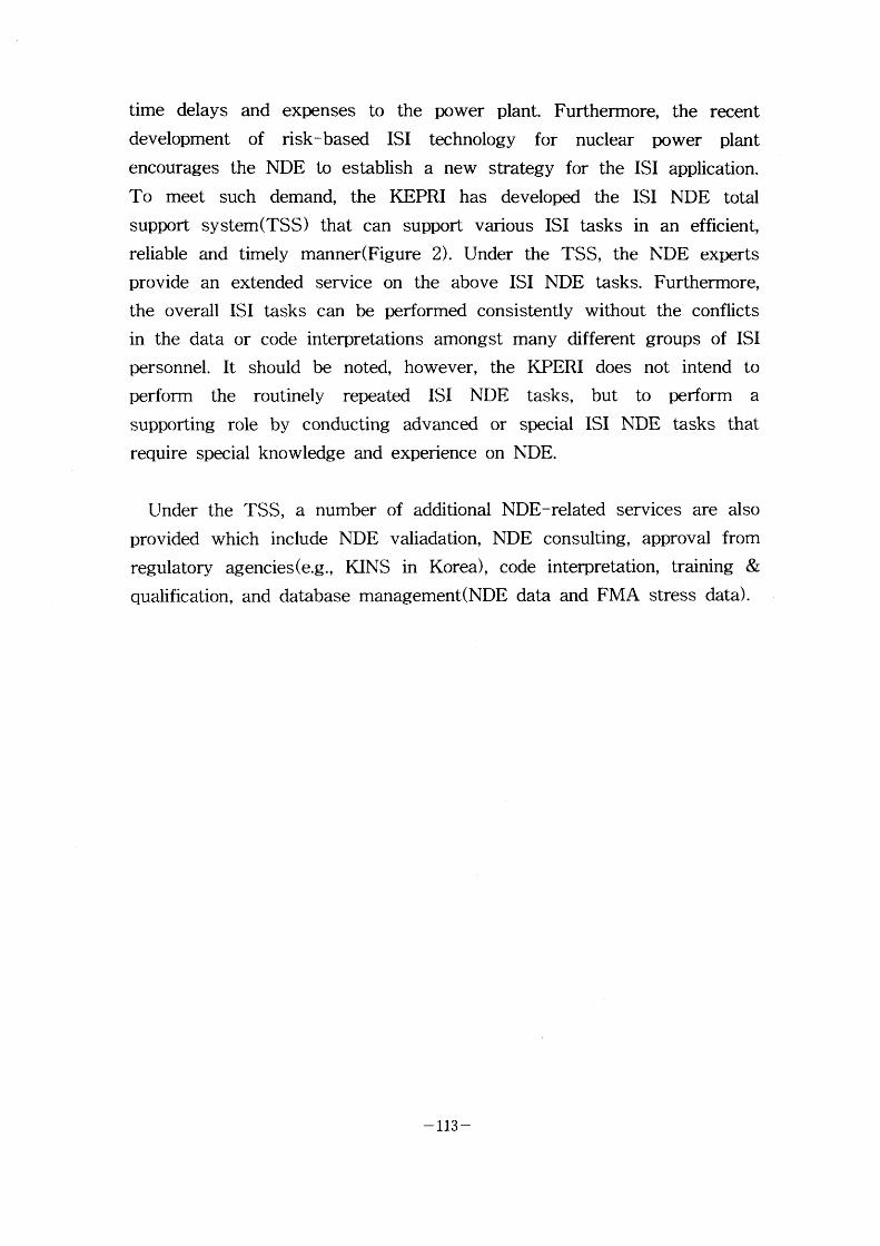
time delays and expenses to the power plant. Furtherrnore, the recent

development of risk-based ISI technology for nuclear power plant encourages the NDE to establish a new strategy for the ISI application.

To meet such demand, the KEPRI has developed the ISI NDE total support system(TSS) that can support various ISI tasks in an efficient,

reliable and timely manner(Figure 2). Under the TSS, the NDE experts

provide an extended service on the above ISI NDE tasks. Furthermore,

the overall ISI tasks can be performed consistently without the conflicts

in the data or code interpretations amongst many different groups of ISI

personnel. It should be noted, however, the KPERI does not intend to

perform the routinely repeated ISI NDE tasks, but to perform a supporting role by conducting advanced or special ISI NDE tasks that

require special knowledge and experience on NDE.

Under the TSS, a number of additional NDE-related services are also

provided which include NDE valiadation, NDE consulting, approval from

regulatory agencies(e.g., KINS in Korea), code interpretation, training &

qualification, and database management(NDE data and FMA stress data) .

-113-

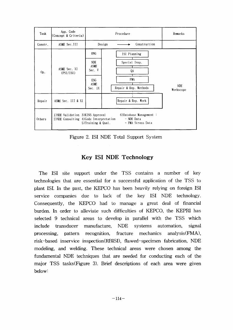
Figure 2. ISI NDE Total Support System

Key ISI NDE Technology

The ISI site support under the TSS contains a number of key technologies that are essential for a successful application of the TSS to

plant ISI. In the past, the KEPCO has been heavily relying on foreign ISI

service companies due to lack of the key ISI NDE technology. Consequently, the KEPCO had to manage a great deal of financial burden. In order to alleviate such difficulties of KEPCO, the KEPRI has

selected 9 technical areas to develop in parallel with the TSS which

include transducer manufacture, NDE systems automation, signal processing, pattern recognition, fracture mechanics analysis(FMA),

risk-based inservice inspection(RBISD, flawed-specimen fabrication, NDE

modeling, and welding. These technical areas were chosen among the

fundarnental NDE techniques that are needed for conducting each of the

major TSS tasks(Figure 3). Brief descriptions of each area were given

below :

-H4-

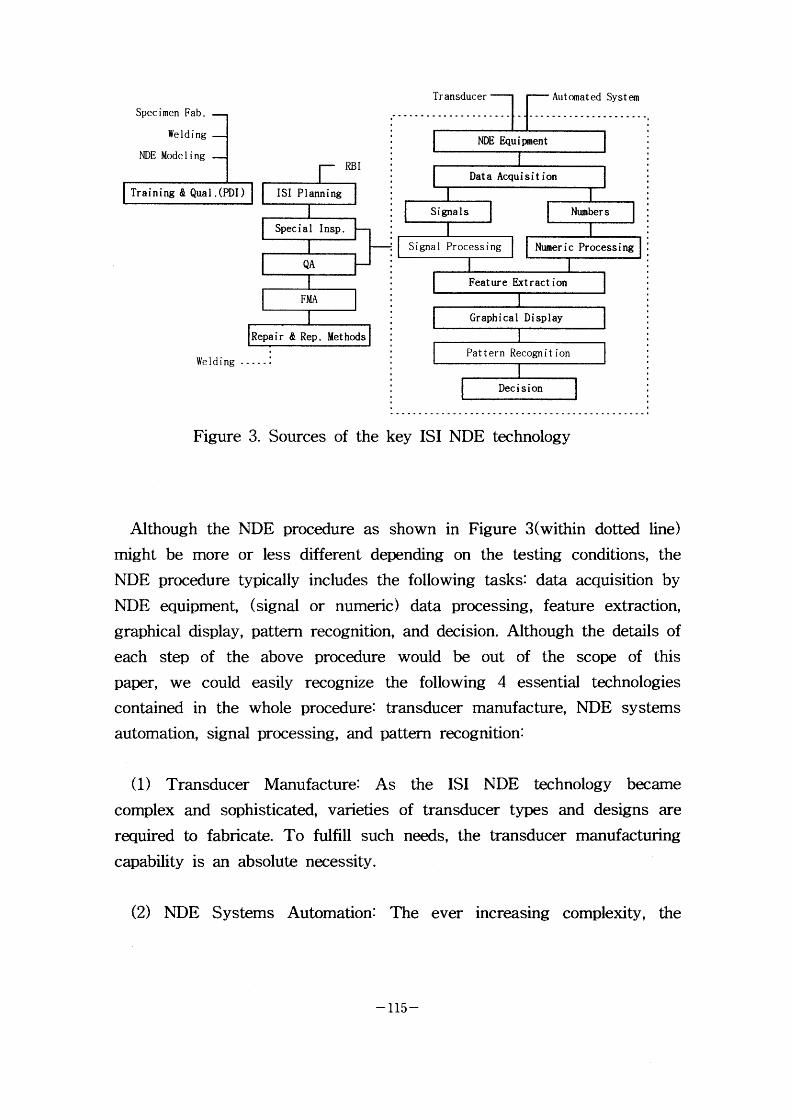
Specimen Fab.

Welding

NDE Model i ng

Training & Qual .(PDI)

Weldlng - - - -

Figure 3. Sources of the key IS I NDE technology

Although the NDE procedure as shown in Figure 3(within dotted line)

might be more or less different depending on the testing conditions, the

NDE procedure typically includes the following tasks: data acquisition by

NDE equipment, (signal or numeric) data processing, feature extraction,

graphical display, pattern recognition, and decision. Although the details of

each step of the above procedure would be out of the scope of this paper, we could easily recognize the following 4 essential technologies

contained in the whole procedure: transducer manufacture, NDE systems

automation, signal processing, and pattern recognition:

(1) Transducer Manufacture: As the ISI NDE technology became complex and sophisticated, varieties of transducer types and designs are

required to fabricate. To fulfill such needs, the transducer manufacturing

capability is an absolute necessity.

(2) NDE Systems Automation: The ever increasing complexlty the

- 115 -

volume and the number of testing components in recent years require the

speed, the accuracy, and the reliability. of nondestructive examination. To

meet such demand, and to keep pace with the fast growing modern NDE

technology, the NDE systems automation for the nuclear component examination should be seriously considered.

(3) Signal Processing: Answers for NDE problems are not always

contained in the raw data as acquired. For an example, some flaw characteristics are extractable not directly from the ultrasonic flaw signal,

but from some other modified data types such as frequency spectrum or

transfer function. Such signal processing techniques as FFT, correlation,

convolution, filtering, to name but a few, are essential for analyzing the

complicated data types.

(4) Pattern Recognition: When the signal processed NDE data is insufficient to extract a reliable answer, the data has to be further relied

upon the pattern recognition techniques. Pattern rec ognitions are

mathematical and statistical analysis methods that make decisions based

on multiple feature values extracted from the various data types

(e.g., Iinear or nonlinear regression. Bayes decision theory, discriminant

function, etc.). As the complexity of NDE data types grows, the need for

pattern recognition becomes more absolute.

(5) Fracture Mechanics Analysis(FMA): the nuclear components having

defects larger than the code-allowable sizes(in terms of length, depth,

width, etc.) should basically be either repaired or replaced. However, the

defective components may continuously be operated for an extended period of time only if the safe operation of the defective components is

theoretically(using FMA) demonstrated. The KE;PRI is in the development

process for the stress analysis and FMA programs, and for establishing

the stress database for major nuclear components that is necessary to

perforrn the FMA.

(6) Risk-Based Inservice Inspection(RBISD: The ASME Code-based ISI

-H6-

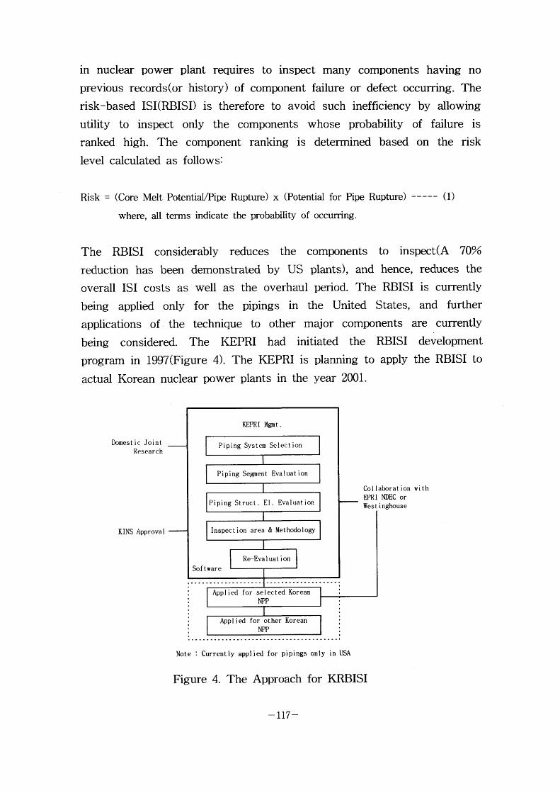
in nuclear power plant requires to inspect many components having no previous records(or history) of component failure or defect occurring. The

risk-based ISI(RBISD is therefore to avoid such inefficiency by allowing

utility to inspect only the components whose probability of failure is

ranked high. The component ranking is detennined based on the risk level calculated as follows:

Risk = (Core Melt PotentiaVPipe Rupture) x (Potential for Pipe Rupture) ----- (1)

where, all t.erms indicate the probability of occurring .

The RBISI considerably reduces the components to inspect(A 70~ reduction has been demonstrated by US plants), and hence, reduces the

overall ISI costs as well as the overhaul period. The RBISI is currently

being applied only for the piping s in the United States, and further

applications of the technique to other major components are currently

being considered. The KEPRI had initiated the RBISI development prograrn in 1997(Figure 4). The KEPRI is planning to apply the RBISI to

actual Korean nuclear power plants in the year 2001.

Domest ic Joint Research

KlNS Approval

Col laborat ion wi th

NDEC or Wes t i nghouse

Note : Currently applied for pipings only in USA

Figure 4. The ApprOach fOr KRBISI

-117-

The following 3 technical areas (flawed-specimen fabrication, NDE

modeling, and welding) are related to the KEPRI's Korean Performance

Demonstration Initiative(KPDD program initiated in 1997(Figure 5). In the

past, all ultrasonic inspectors were allowed to inspect nuclear components

if they have been qualified once in any certified training and qualification

institute. However, because detecting and sizing of flaws of complex

shapes(IGSCC, under-clad cracking, etc.) require special skills and

experience, the codes(ASME and CFR in the United States) mandated

that the performance demonstration of all ultrasonic inspectors be

conducted by an integrated qualification process combining the inspector,

the procedure, and the equipment, in order to improve the accuracy and

the reliability of NDE performance on specific ISI task. The KEPRI is

planning to apply the KPDI program to actual Korean nuclear power

plants in the year 2001. Brief descriptions of 3 additional technical areas

were provided next:

(7) Flawed-Specimen Fabrication: In order to evaluate the ultrasonic

inspector's performance, it is required to prepare test specimens

containing certain number of flaws of certain sizes as described in the

ASME Code Section XI, Appendix VIII. The fabrication of

flawed-specimen requires special techniques, and it involves technical

know-hows and therefore high fabrication cost. Considering the situation,

it would be beneficial to have the specimen fabrication capability in-house

to establish the training and qualification system for KPDI.

(8) NDE Modeling: For the application of performance demonstration

program(KPDD to ISI NDE inspectors, the test specimens that represent

all nuclear components should be prepared. To meet such requirement, a

great number of specimens of an extremely high cost has to be

fabricated. However, the use of NDE modeling can help reduce the

number of the specimens by theoretically(NDE modeling) demonstrating

the equivalency of similar inspection situations. The NDE modeling can

also help avoid unnecessary re-training and qualification for the similar

inspection situations. In addition, the NDE modeling can be utilized for an

- I18 -

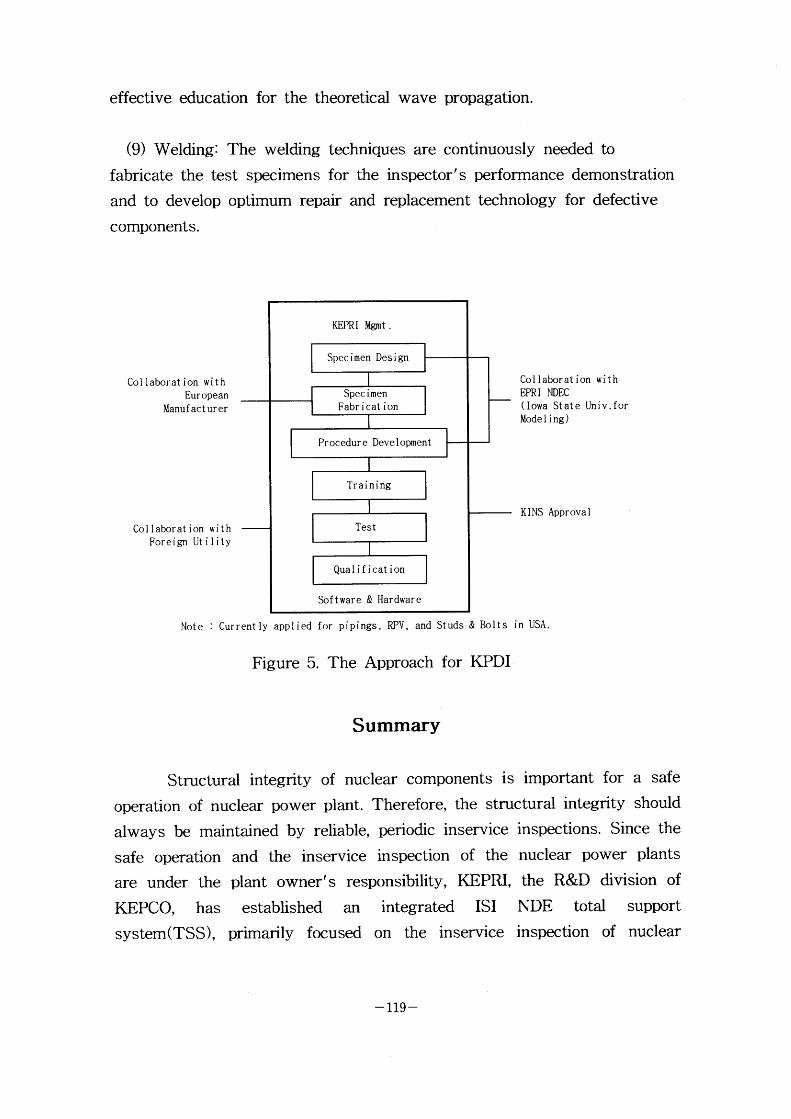
effective education for the theoretical wave propagation

(9) Welding: The welding techniques are continuously needed to

fabricate the test specimens for the inspector's performance demonstration

and to develop optimum repair and replacement technology for defective

com ponents.

col laborat lon wi th col laborat ion with European Spec imen EPRI NDEC Manutacturer Fabr i cat ion ( Iowa state Univ. for

Mode I i ng)

KINS Approval

col laborat ion with Foreign Ut i I ity

Note : currentfy applied for pipings, RPv, and studs & Bolts in USA.

Figure 5. The Approach for KPDI

Summary

Structural integrity of nuclear components is important for a safe

operation of nuclear power plant. Therefore, the structural integrity should

always be maintained by reliable, periodic inservice inspections. Since the

safe operation and the inservice inspection of the nuclear power plants

are under the plant owner's responsibility, KEPRI, the R&D division of

KE;PCO, has established an integrated ISI NDE total support system(TSS), primarily focused on the inservice inspection of nuclear

-119-

power plants. And the KEPRI has initiated a long-tenn plan for the

development of key ISI NDE technology that is necessary for an efficient

on-site support. Although KEPRI took the lead in this effort to establish

the TSS, the KEPRI intends to collaborate with industry, universities, and

research institutes throughout the development process in order to

promote the entire Korean ISI NDE technology.

Ref erences

1 . Plant Operatron Statistics Korea Electnc Power Company 1997

- 120 -

III-3 Core Shroud Replacement of Fukushima-Daiichi Unit #3

Jun Matsumoto, Nuclear Power Plant Management Dept.

Tokyo Electric Power Company, Japan

Core Shroud Replacement of Fnkushima-Daiichi Unit #3

J. MATSUMOTO Tokyo Electric Power Company

l - I -3 Uchisaiwai-cho, Chiyoda-ku Tokyo, Japan

Abstract

The core shroud replacement of a Boiling Water Reactor (B WR) is now

in progress at Fukushima-Daiichi Unit # 3(1F3) of the Tolyo Electric

Power Company (TEPCO) in Japan. The core shroud and other core

interna/ components made of type 304 stainless stee/ (SS) are replaced

with the ones made of low carbon ope 316L SS to improve Intergranular

Stress Corrosion Cracking (IGSCC) resistance. This project is the first

application of the replacement procedure developed for the welded core

shroud, and employs various advanced technologies. The outline of the

core shroud replacement project and applied technologies are discussed in

this paper.

1. Introduction

Since the core shroud cracking was found, the Japanese BWR owners and the plant

manufacturers have conducted several R&D programs to establish the countermeasures

for core shroud cracking. These countermeasures are repair and mitigation

technologies including replacement, bracket reinforcement, tie rod reinforcement,

hydrogen water chemistry (HWC), water jet peening, shot peening, and noble metal

technologies. When the crack was found in Fukushima-Daiichi Unit #2 ( IF2), the core

shroud was reinforced by the brackets which had been studied as one of the repair

concepts.

The countermeasures for the actual plants should be carefully selected considering

effect and applicability of the countermeasures, uncertainty of the developed

technologies, estimated cost (tool fabrication and implementation cost, inspection cost

through the plant life etc.), estimated schedule, possibility of cracking, political

- 121 -

environment, and so on. Based on the evaluation ofthese influential elements, TEPCO

decided to replace the core shrouds made of 304SS which has relatively higher potential

ofIGSCC. Among 1 7 BWR plants owned by TEPCO, four plants have the core

shrouds made of 304SS. In accordance with the long term outage schedule, I F3 was

selected as the first plant to replace the core shroud with the one made of 3 1 6L SS which

has much less potential of IGSCC.

In addition to the core shroud, the majority of the internal components made of 304SS

are replaced in the IF3 project. Those are (1) core shroud, (2) top guide, (3) core plate,

(4) core spray spargers, (5) feed water spargers, (6) jet pumps, (7) DP/LC pipe, (8) ICM

guide tubes, and internal pipes and nozzle safe ends connected to these components as

shown in Figure I . Prior to the application to IF3, integrity and reliability of the

replacement process were demonstrated by the full scale mock-up test, which was

conducted by the Nuclear Power Engineering Corporation (NUPEC).

2. Replacement Process

The replacement sequence is shown in Figure 2. Afier the removal of all fuels and

detachable components, inside of the pressure vessel and the remaining internal

components were chemically decontaminated. Subsequently, most ofthe removals are

conducted by means ofElectrical Discharge Machining (EDM) process under water.

Following the removal of all components to be replaced, the new components were

installed in reverse order ofthe removal. Most of the installation process including

welding was performed in a dry condition to acquire high quality of the weld. The

followings are the major technologies applied to the core shroud replacement process.

2.1 Chemical Decontamination

Prior to cutting the core shroud, the chemical decontamination was conducted. The

Chemical Oxidation Reduction Decontamination (CORD) process provides a high

Decontamination Factor (DF), and generates a small amount ofwaste in comparison to

other decontamination processes. Decontamination solution was circulated by the

Primary Loop Recirculation (PLR) pumps, and the dissolved active metal was captured

by ion exchange resins (Figure 3). In the core shroud replacement project for IF3, the

oxidation and reduction process was repeated three times in a week. The volume of

waste was approximately 5m3, and the DF measured under water was approximately 40

at the bottom of the RPV .

- 122 -

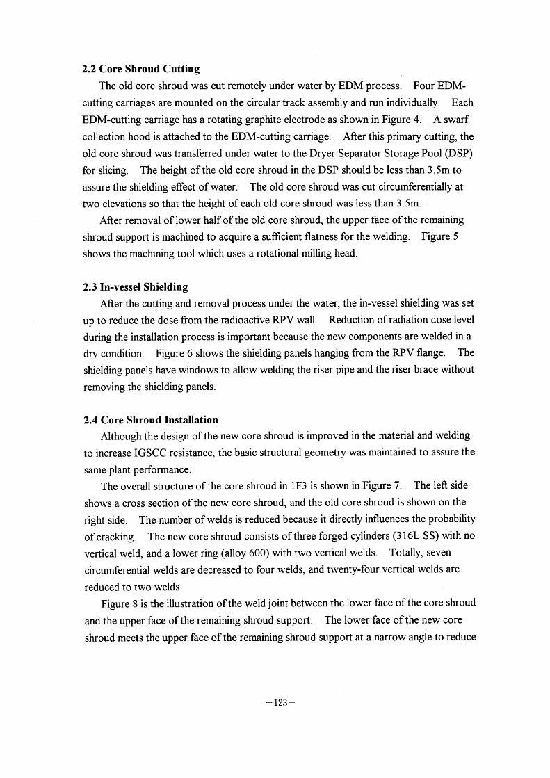
2.2 Core Shroud Cutting

The old core shroud was cut remotely under water by EDM process. Four EDM-

cutting carriages are mounted on the circular track assembly and run individually. Each

EDM-cutting carriage has a rotating graphite electrode as shown in Figure 4. A swarf

collection hood is attached to the EDM-cutting carriage. After this primary cutting, the

old core shroud was transferred under water to the Dryer Separator Storage Pool (DSP)

for slicing. The height ofthe old core shroud in the DSP should be less than 3.5m to

assure the shielding effect ofwater. The old core shroud was cut circunferentially at

two elevations so that the height of each old core shroud was less than 3 . 5m.

After removal of lower half of the old core shroud, the upper face of the remaining

shroud support is machined to acquire a sufficient flatness for the welding. Figure 5

shows the machining tool which uses a rotational milling head.

2.3 In-vessel Shielding

Afier the cutting and removal process under the water, the in-vessel shielding was set

up to reduce the dose from the radioactive RPV wall. Reduction of radiation dose level

during the installation process is important because the new components are welded in a

dry condition. Figure 6 shows the shielding panels hanging from the RPV flange. The

shielding panels have windows to allow welding the riser pipe and the riser brace without

removing the shielding panels.

2.4 Core Shroud Installation

Although the design of the new core shroud is improved in the material and welding

to increase IGSCC resistance, the basic structural geometry was maintained to assure the

same plant performance.

The overall structure of the core shroud in IF3 is shown in Figure 7. The left side

shows a cross section ofthe new core shroud, and the old core shroud is shown on the

right side. The number of welds is reduced because it directly influences the probability

of cracking. The new core shroud consists ofthree forged cylinders (3 1 6L SS) with no

vertical weld, and a lower ring (alloy 600) with two vertical welds. Totally, seven

circumferential welds are decreased to four welds, and twenty-four vertical welds are

reduced to two welds.

Figure 8 is the illustration ofthe weld joint between the lower face of the core shroud

and the upper face of the remaining shroud support. The lower face of the new core

shroud meets the upper face of the remaining shroud support at a narrow angle to reduce

- 123 -

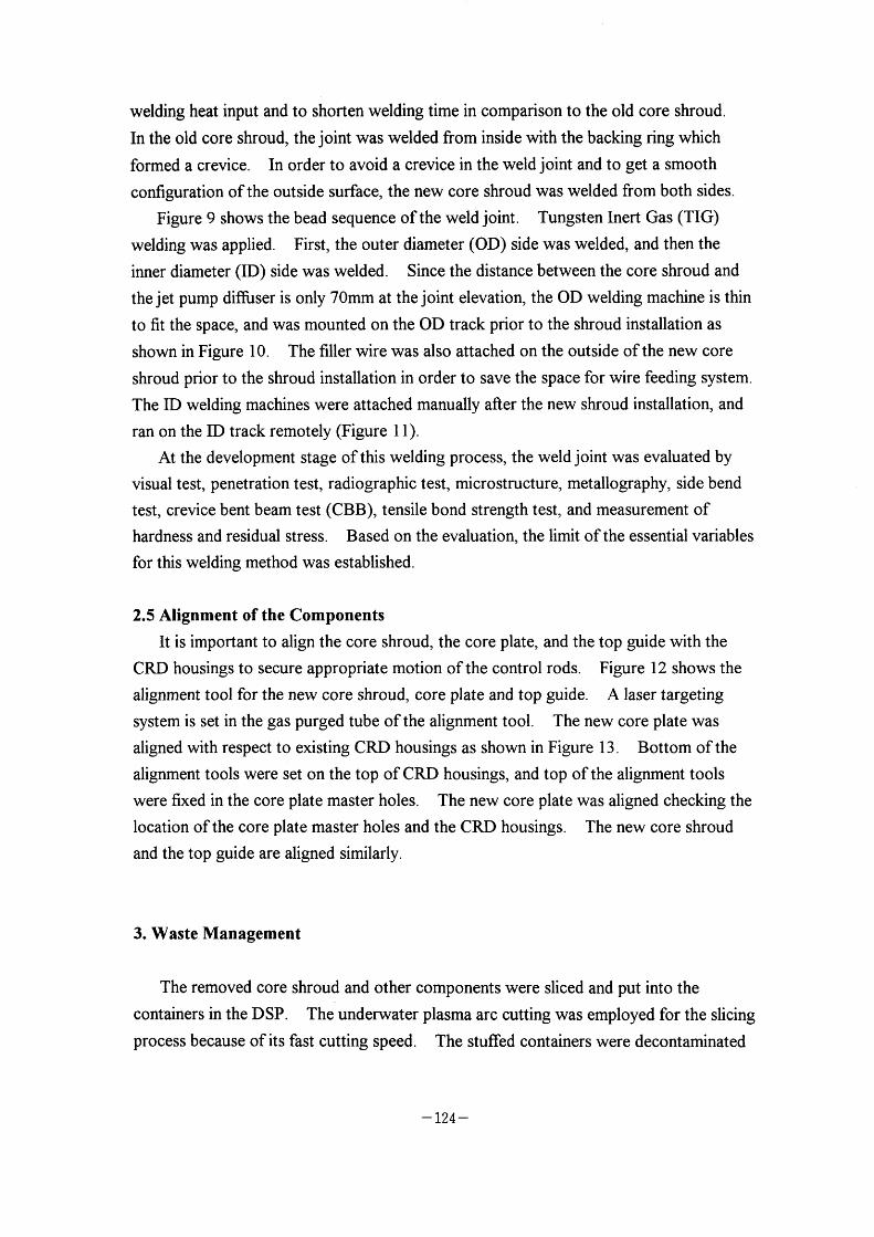
welding heat input and to shorten welding time in comparison to the old core shroud.

In the old core shroud, the joint was welded from inside with the backing ring which

formed a crevice. In order to avoid a crevice in the weld joint and to get a smooth

configuration ofthe outside surface, the new core shroud was welded from both sides.

Figure 9 shows the bead sequence ofthe weld joint. Tungsten Inert Gas (TIG)

welding was applied. First, the outer diameter (OD) side was welded, and then the

inner diameter (ID) side was welded. Since the distance between the core shroud and

the jet pump difftLser is only 70mm at the joint elevation, the OD welding machine is thin

to fit the space, and was mounted on the OD track prior to the shroud installation as

shown in Figure I O. The filler wire was also attached on the outside ofthe new core

shroud prior to the shroud installation in order to save the space for wire feeding system.

The ID welding machines were attached manually after the new shroud installation, and

ran on the ID track remotely (Figure 1 1 ).

At the development stage of this welding process, the weld joint was evaluated by

visual test, penetration test, radiographic test, microstructure, metallography, side bend

test, crevice bent beam test (CBB), tensile bond strength test, and measurement of

hardness and residual stress. Based on the evaluation, the limit ofthe essential variables

for this welding method was established.

2.5 Alignment of the Components

It is important to align the core shroud, the core plate, and the top guide with the

CRD housings to secure appropriate motion ofthe control rods. Figure 12 shows the

alignment tool for the new core shroud, core plate and top guide. A Iaser targeting

system is set in the gas purged tube of the alignment tool. The new core plate was

aligned with respect to existing CRD housings as shown in Figure 1 3 . Bottom of the

alignment tools were set on the top of CRD housings, and top ofthe alignment tools

were fixed in the core plate master holes. The new core plate was aligned checking the

location of the core plate master holes and the CRD housings. The new core shroud

and the top guide are aligned similarly.

3. Waste Management

The removed core shroud and other components were sliced and put into the

containers in the DSP. The underwater plasma arc cutting was employed for the slicing

process because of its fast cutting speed. The stuffed containers were decontaminated

- 124 -

and transferred to the site bunker pool and the dry storage facility in the site.

all of the waste is low level radioactive waste, the site bunker pool stores more

radioactive waste.

Although

4. Conclusion

TEPCO is replacing the core shroud of IF3 to improve IGSCC resistance. The

shroud replacement is considered to be one of the most comprehensive countermeasures

to improve IGSCC resistance for all the welds ofthe core shroud. As of April 1998,

the new core shroud has already been installed properly, and the project is under

restoration process of other internal components. Subsequently, the core shroud

replacement will be performed in several Japanese BWR plants.

- 125 -

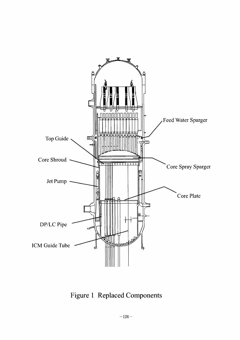
Top Guide

Core Shroud

Jet Pump

DP/LC Pipe

ICM Guide Tube

Figure 1 Replaced Components

- 126 -

Feed Water Sparger

Core Spray Sparger

Core Plate

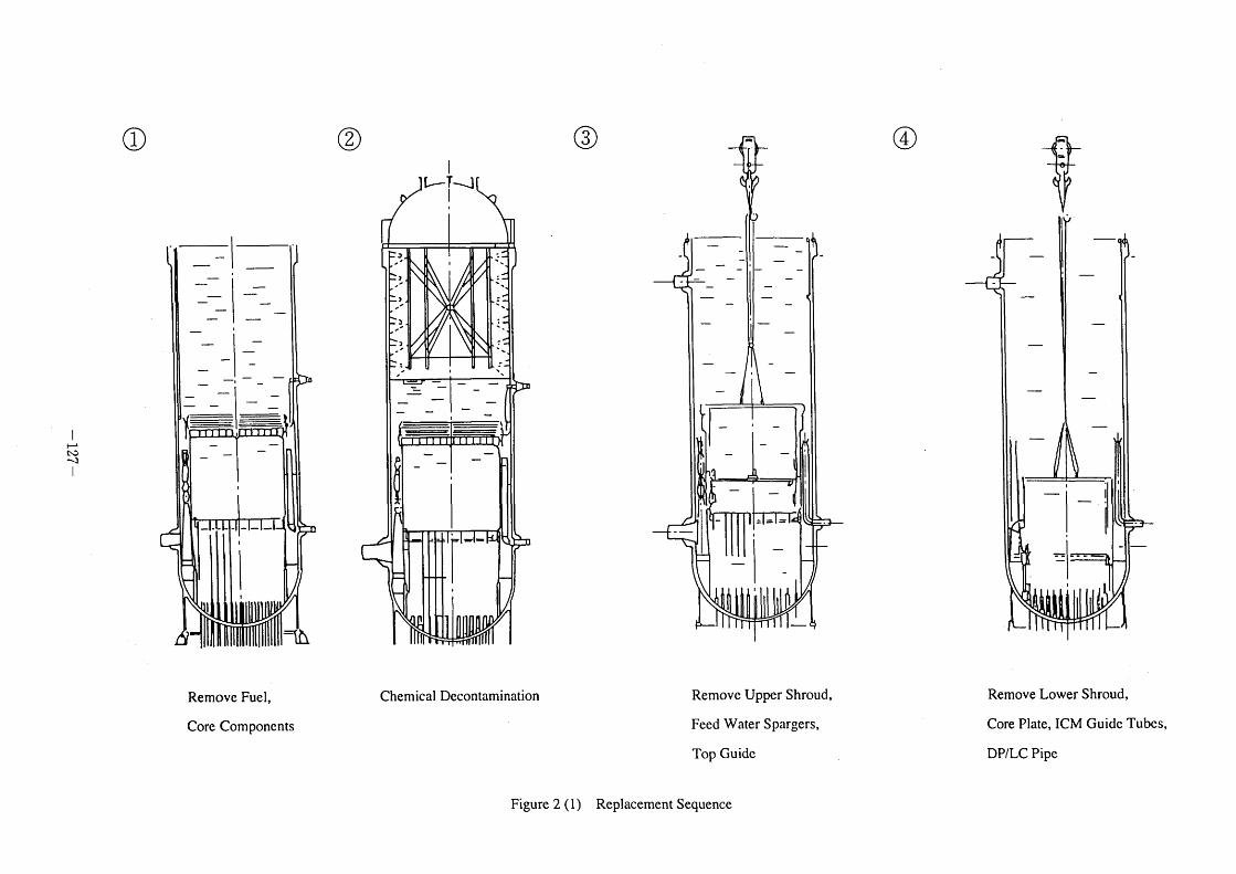
l

Ht~

~]

(D ~) i

,F' ~)

Remove Fuel,

Core Componcnts

Chemical Decontamination Remove Upper Shroud,

Feed Water Spargers,

Top Guide

Remove Lower Shroud,

Core Plate, ICM Guide Tubcs,

DP/LC Pipe

Figure 2 ( I ) Replacement Sequence

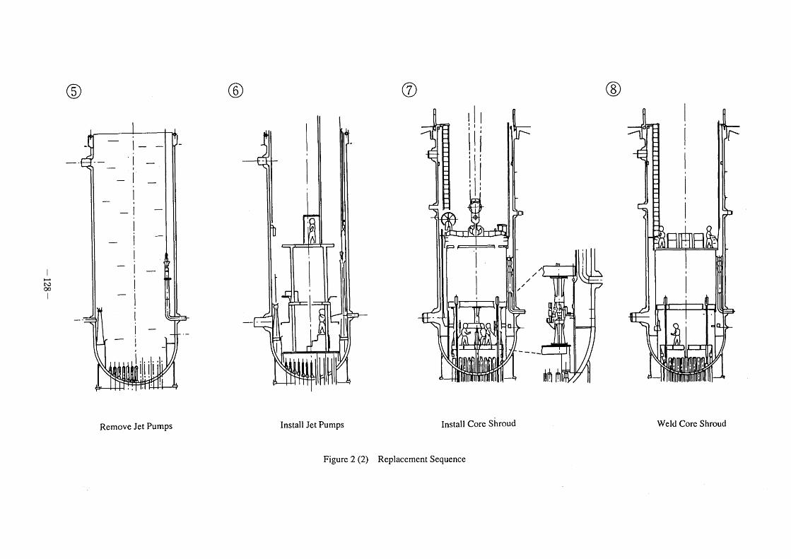
H' t~D co

l

R

Remove Jet Pumps

O

Install Jet Pumps

Figure 2 (2)

R

/ /

'!.

Install Core Shroud

Replacement Sequence

li~ h

l

R

Weld Corc Shroud

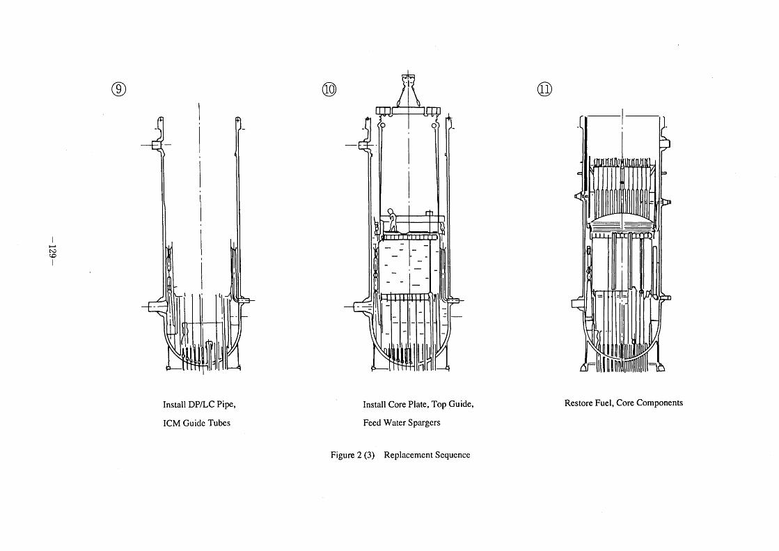
l

H' N) ~)

l

~)

t

R ~

l

Instal] DP/LC Pipe,

ICM Guidc Tubcs

Install Core Plate, Top Guide,

Feed Water Spargcrs

Restore Fuel, Core Components

Figure 2 (3) Replacement Scquence

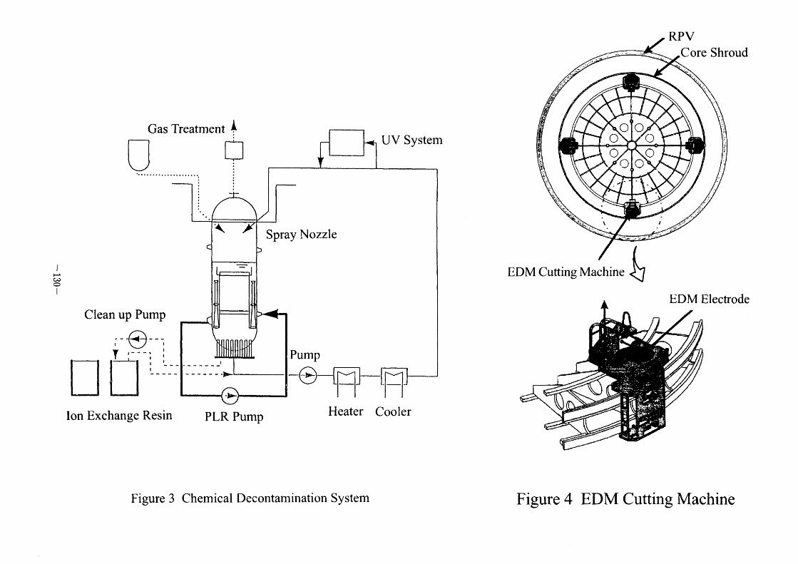
l

~'c'e

o

Gas Treatment L.

:.1.

Clean up Pump

r~e~~l YL_L'- ,

Ion Exchange Resin

UV System

~ Spray Nozzle

,

- - ->

'l>

PLR Pump

pump

-O ~I~ ~l~ Heater COOler

Figure 3 Chemical Decontamination System

RPV Core Shroud

OO O

OO

EDM Cutting Machine

o o

I

EDM Electrode

Figure 4 EDM Cutting Machine

' ~'~~/ .

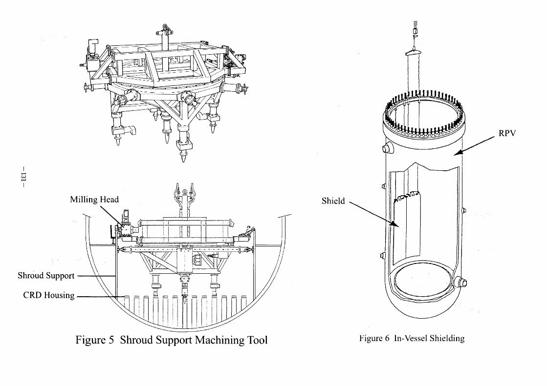
l:Al

C O

\

;~C=- i~ I~'

::1lr !~!~~ //=1/ ~~

Q e

-- ~~

~

L.'

l

~S

~

Milling Head

Shrbud Support

CRD Housing

lr

,l

Shield ,p

RPV

Figure 5 Shroud Support Machining Tool Figure 6 In-Vessel Shielding

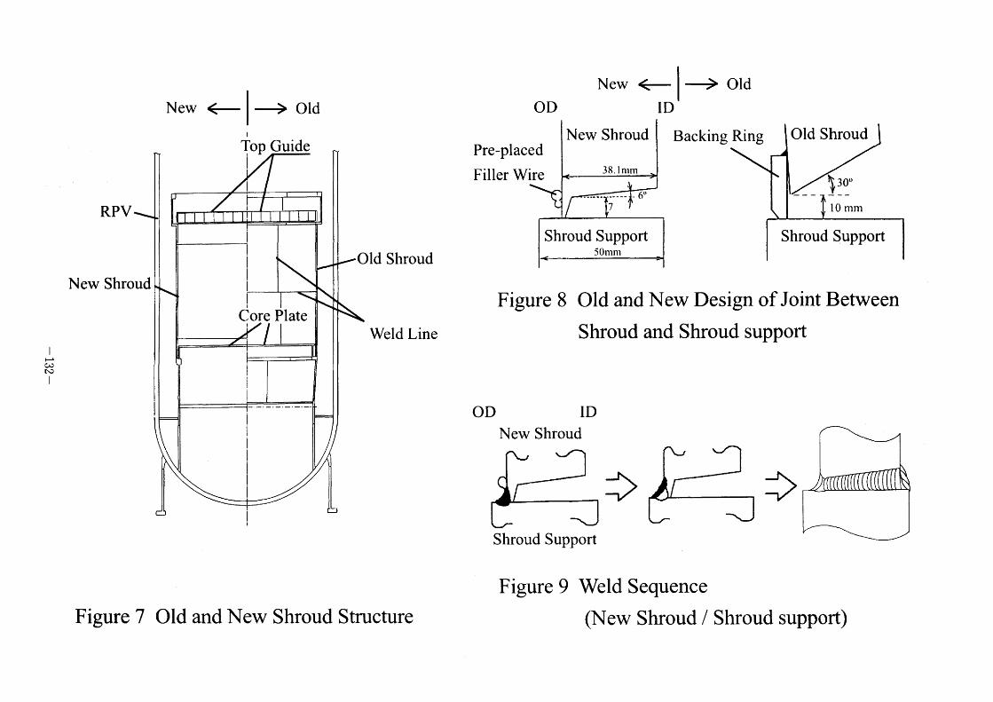
l

h' cJe t\D

RPV

N ew Shroud

Figure 7

-> Old +0p Guide

!

Old Shroud

Weld Line

Old and New Shroud Structure

New Old

Pre-placed New Shroud Backing Ring Old Shroud

38, I ~,,,,

' Io~~

Shroud Support Shroud Support 50~,~,

Figure 8 Old and New Design of Joint Between

Shroud and Shroud support

New Shroud

Shroud Support

Figure 9 Weld Sequence

(New Shroud / Shroud support)

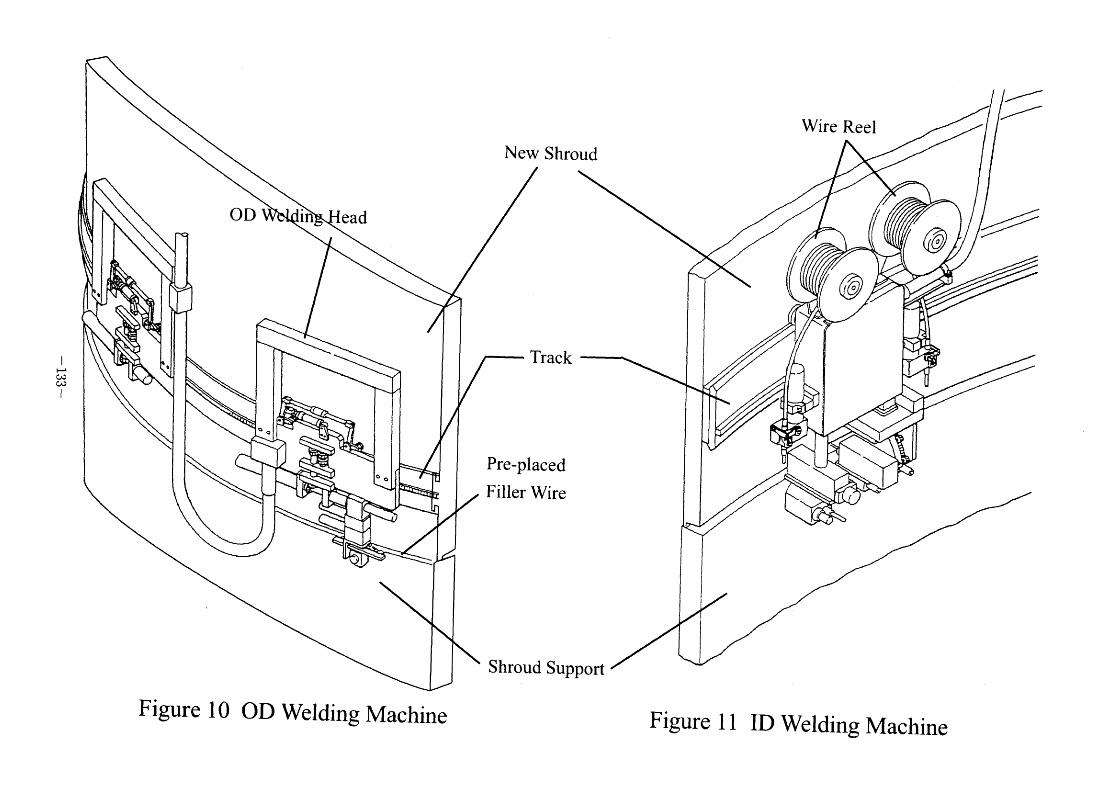
I

~; c~

l

New Shroud

Wire Reel

,

,

OD

.

Figure I O

e

in ead

eo

OD Welding Machine

Track

Pre- placed

Filler Wire

Shroud Support

Figure 1 1

~

r

,

ID Welding Machine

~1!l

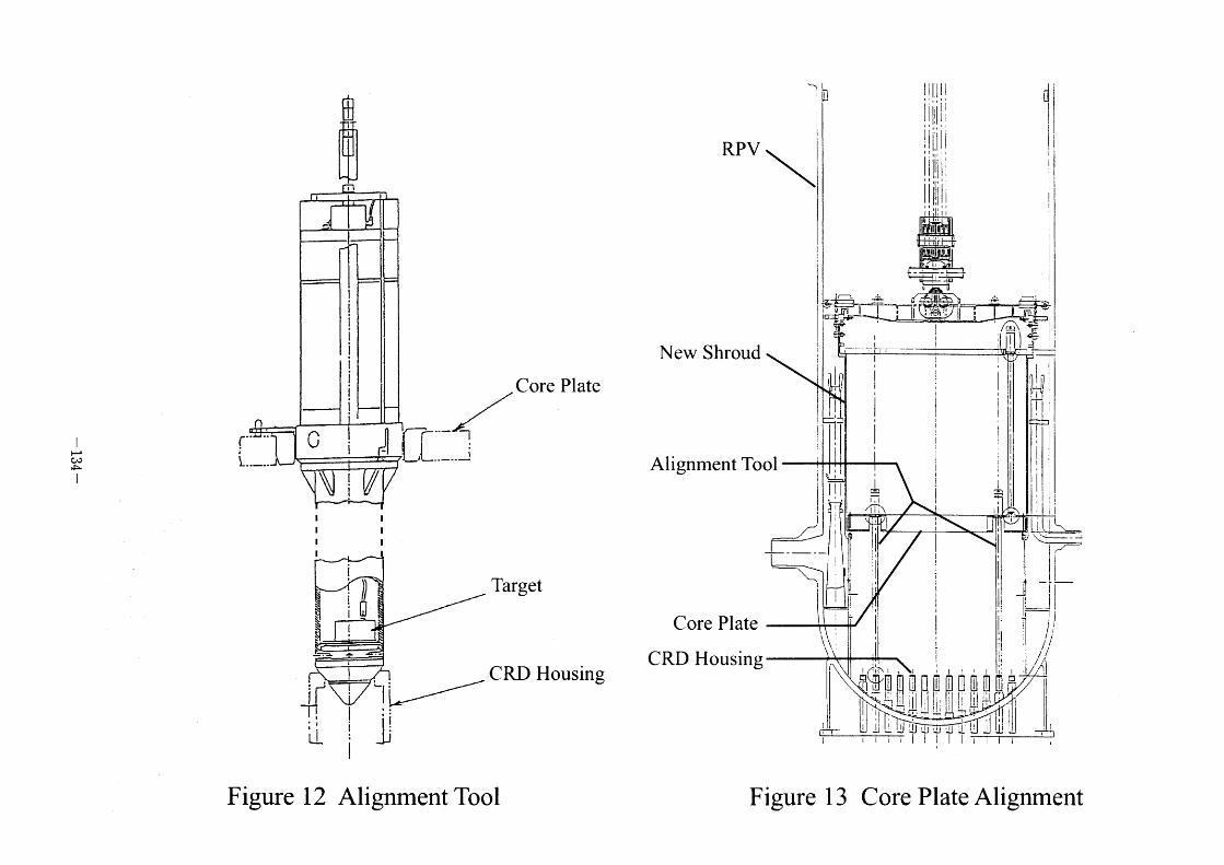
l

H ('o

~ I

~~-

rf_L I ///~ core ptate

~ i i Target ~~!

L/ CRD HOusmg ~i, I :=

~ :' ' L~I = I

Figure 1 2 Alignment TOOl

~1 = ~ Ill'll I d ':"ji l j I i !il ' ' l *,' [ :=' lllli

,

\ I i[ l!1 i : ,, ,',

,,'.' [ I Ill I ' j .l .. '' l...1= + : il li' ' ,,

"" I ~yll i * ,,, ~, l '- ' l! --~'~ ~:~i~ ~~ ~~~ ~ ~:+"__'~~:'1 ! l __ . '~~1[~711 : rL~~-*'

*t~i i'-*- Ij

New Shroud - ' ' '~' ' ,. . i, I~I!

l~li

c::~ l'

' 'l l

Alignment TOOI ! i ,I ~JL=' I i ii ~ ,

i, I ;..i = j l ll :~~ l ~ *l

"I 11' I 'll: . ,~ - .--. " I ~f~~!1( i [1 ~ ~JI I f' -.' l

' l l

l '\~f~ -\= H'i ' i jl.

L ( iii -fj___._.1[I ,*

I = "! ' ": =i = COre plate ; l: ! l' = !" ,

' ' ' 'l ll \\ 'I l t!

l i

*Il'l'l I~ '. , . : ' '1 '~1 '~f:~f'! ' ~ ' '~ I D'; ~ i ~'Oi'~~I~P// I ~Lli li !~"! =! ' l l i ~ = "II Il

~~~~~~~'~.-.LLI'J: Itl I ~' .=

Figure 1 3 Core Plate Alignment

III-4 The Evaluation of Erosion-Corrosion Problems of PWR Carbon

Steel Piping in Taiwan

Kuen Ting, Department of Nuclear Regulation Atomic Energy

Council, Taiwan, Republic of China

Yin Pang Ma, Institute of Nuclear Energy Research Atomic

Energy Council, Taiwan, Republic of China

THE EVALUATION OF EROSION/CORROSION PROBLEMS IN TAIWAN PWR CARBON STEEL PIPING

Kuen Ting Department of Nuclear Regulation

Atomic Energy Council Republic of China

Yin Pang Ma Institute of Nuclear Energy Research

Atomic Energy Council Republic of China

ABSTRACT Taiwan PWR Nuclear Power Plant Units I and 2 implemented the

measurements of the wall thinning of the carbon steel piping under the request of

regulation authority to prevent the events due to the erosion/corrosion since 1 989. At

the frrst, the licensee established the comprehensive inspection program by itself.

Over 2000 components were inspected per each unit and 300-500 pipe components

were examined by ultrasonio testing per soheduled outage. The simple predictive

methodology determined the operability of each individual piping oomponent in the

next fuel Gycle. Based on the inspection results, the susceptible pipe components

were established. The implementation of the effective correction management and

improved inspection program can improve the safety, as well as the efficiency, of

long-tenn reactor operations.

INTRODUCTION Erosion/corrosion is a piping degradation process that induces the pipe wall

thiming. The oxide layer on the carbon steel pipe is dissolved by single-phase or two-

phase flow in the nuclear power plant[1]. In 1 989, the regulatory authority requested

the licensee of Taiwan nuclear power plants to develop their own inspection program

to prevent the failure of piping due to erosion/corrosion damage. The licensee

established a full scope of pipe wall thickness database through "Pipe Wall Thiming

Measurement•Program"[2]. Over 2000 pipe components were selected per each unit and 300-500 pipe components were examined by ultrasonic testing per scheduled

outage. Based on the inspection results and the analytical method, the evaluation of

the susceptible pipe components in the licensee inspection program was established

during each scheduled outage. This paper will discuss the implementation of this

- 135 -

effeGtive management and the inspection program. The efforts can improve the safety,

as well as the efficiency, of long-term reactor operations.

INSPECTION PROGRAM In 1 989, after a severe piping rupture at Surry nuclear plant, the regulatory

authority requested the licensee to develop the plant specific-monitoring program to

prevent the failure of piping due to erosion-corrosion damage. The licensee, Taiwan

Power Company (TPC), established the comprehensive inspection program to

measure the thickness of most of the carbon steel piping components in the balance of

the plant. The inspeoted oomponents consist of straight pipes, elbows, tees and

expanders/reducers in the feedwater, condensate, extraction, heater drain and reheater

drain systems. The detailed configurations for measured points in each typical

component are displayed as Figure I .

The evaluation method of the inspection program is based on the measured data.

The thinning due to erosionfcorrosion wear T., oan be caloulated as

T,. = Tl ~ T,orT. - T. (ifno inspection data for reference)

T,. = (previous measured thickness)-(present measured thickness)

In which Tl and T. are the maxirnum and minimum measured thickness, respeotively. T~ is the nominal thickness. The wear rate can be defined as

W. = T.. IH

where H is the operating hours between two inspection intervals. The allowable

wear thickness T. is

T. =T. -T~ where T~ is the required thickness from the stress report or by analysis.

Thus, the remaining time of operation , L. ,can be estimated as

L. = T. /W.

The allowable number of remaining fuel cycles, I,al , can then be predieted as

lrd = L. l(KO.)

next fuel Gycle.

The tbtal number of the selected pipe components was greater than two

thousand per PWR unit. However, the oapacity ofrealistic ultrasonic testing was only

three to five hundred pipe components per outage. So, one PWR plant needs at least

seven outages to examine all selected oomponents and build up the complete database

of the wall thiming.

- 136 -

OBSERVATIONS OF THE INSPECTION The measured data from four outages have been studied according to the type of

the pipe components, such as 90" elbow, 45" elbow, reducer, tee and straight pipe.

Figure 2 displays the occurrences ofthe thinnest thickness versus measured points for

all inspeGted 90" elbows. The position B5 that is the outward bent of the elbow had

the majority of the occurrences of the thinnest thiGkness. Ahnost 700/0 of all inspected

elbows show that this region is easily erosive owing to the change of the flow

direction. This phenomenon is also found in the 45" elbow inspection as shown in

Figure 3 . The majority of the worst thinning occurs at the location B3 which is the

outward bent of the elbow.

For the erosion/corrosion of the reducer, the thinnest thickness locates at the two

ends Al, A4, Dl and D4 as shown in Figure 4. The fraction of these locations is

approximately 90010.

The distribution of the thiunest thickness is uniform for tee components in Figure

5. According to the experience, B and C sectors are not easily subjected to

erosion/corrosion. However, Figure 5 revealed that B and C sectors with 380/0 are the

positions of the thinnest thickness.

From Figure 6 presents the statistical distribution of the measured data for

straight pipe. The inlet position is the susceptible location for erosionfcorrosion as

antioipated.

THE EVALUATION OF THE POTENTIAL RISK OF THE CARBON STEEL PIPING UNDER EROSION/CORROSION

The ultrasonic inspection program of earbon steel piping due to erosionfcorrosion was

oomprehensive. An analytic method to evaluate the potential risk of the carbon steel

piping subjected to erosion/corrosion is necessary. Berge's model[3] assumed the

soluble iron species production and mass transfer effect on the erosion corrosion rate.

Thus, the total erosion/corrosion rate Vc is expressed as:

V KIK2 (C,q - C.) c ~ Kl +K2

where C~ is the soluble ferrous ion concentration at the bulk water; Kl is the

reaotion constant which depends on fluid velocity and water temperature; K2 is mass

transfer coeffilcient which depends on the Sherwood number Sh = al Re"' Sc"= , Re

and Sc are the Renolds number and Schmidt number, respectively; al ' a2 and a3

- 137 -

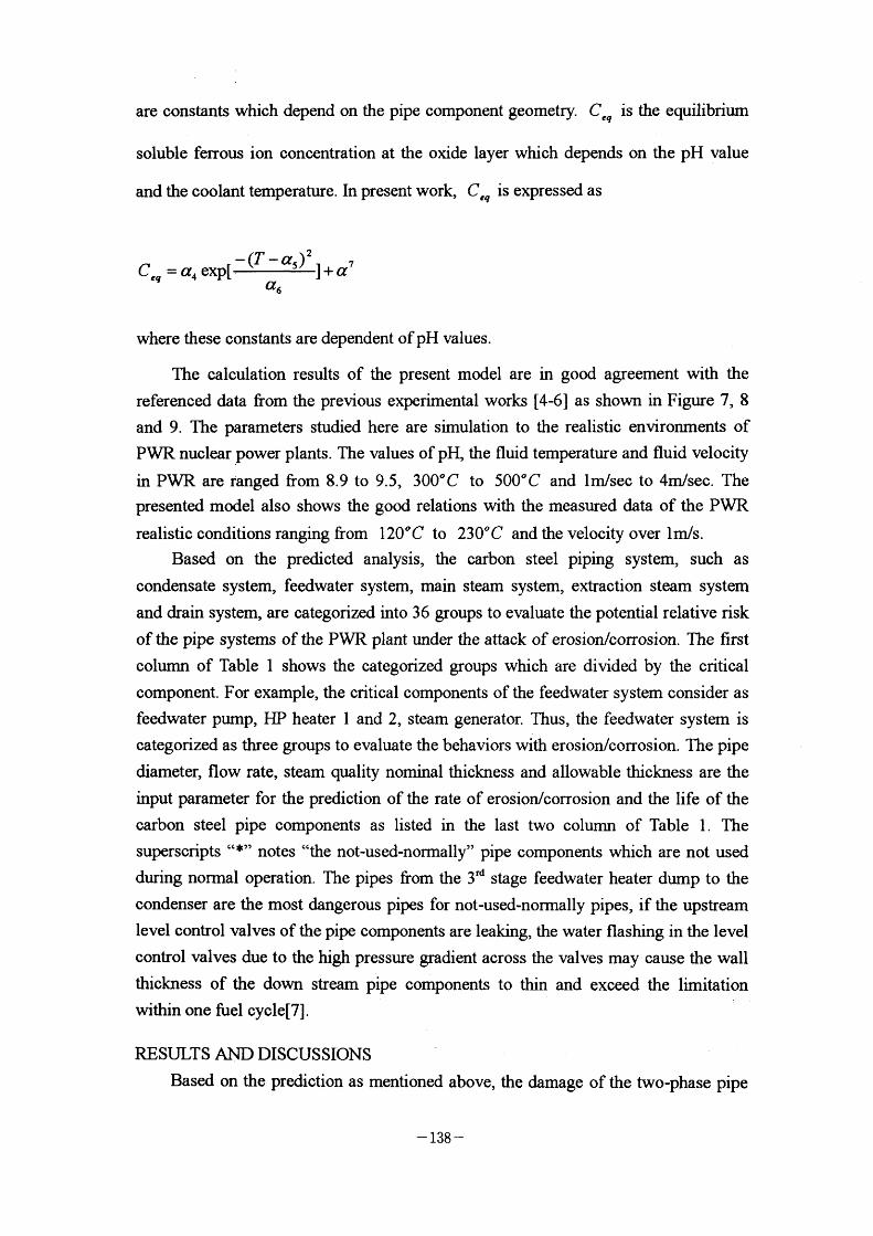
are constants which depend on the pipe component geometry. C,q is the equilibriurn

soluble ferrous ion conoentration at the oxide layer which depends on the pH value

and the coolant temperature. In present work, C,q is expressed as

C.q a exp[~(T -a5)2 J +a7

a6

where these constants are dependent of pH values.

The calculation results of the present model are in good agreement with the

referenced data from the previous experimental works [4-6] as shown in Figure 7, 8

and 9 . The parameters studied here are simulation to the realistic environments of

PWR nuolear power plants. The values of pH, the fluid temperature and fluid velocity

in PWR are fanged from 8.9 to 9.5, 300"C to 500"C and Im/sec to 4m/sec. The

presented model also shows the good relations with the measured data of the PWR

realistic oonditions ranging from 120"C to 230"C and the velocity over Im/s.

Based on the predicted analysis, the carbon steel piping system, such as

condensate system, feedwater system, main steam system, extraction steam system

and drain system, are oategorized into 36 groups to evaluate the potential relative risk

of the pipe systems of the PWR plant under the attack of erosion/corrosion. The frrst

column of Table I shows the categorized groups which are divided by the critical

component. For example, the critical components of the feedwater system consider as

feedwater pump, HP heater I and 2, steam generator. Thus, the feedwater system is

oategorized as three groups to evaluate the behaviors with erosion/oorrosion. The pipe

diameter, flow rate, steam quality nominal thickness and allowable thiekness are the

input parameter for the prediction of the rate of erosion/corrosion and the life of the

carbon steel pipe components as listed in the last two column of Table I . The

superscripts "*" notes "the not-used-normally" pipe components which are not used

during normal operation. The pipes from the 3'd stage feedwater heater dump to the

condenser are the most dangerous pipes for not-used-normally pipes, if the upstream

level oontrol valves of the pipe components are leaking, the water flashing in the level

control valves due to the high pressure gradient across the valves may cause the wall

thickness of the down stream pipe components to thin and exceed the limitation

within one fuel cycle[7].

RESULTS AND DISCUSSIONS Based on the prediction as mentioned above, the damage of the two-phase pipe

- 138 -

components is worse than the single-phase pipe components. The extraction lines

from the high pressure turbine to the frrst stage feedwater heaters in which the steam

quality is ranges from 880/0 to 950/0 were the high risk of the erosion/oorrosion. The

pipe components in the following pipes are also highly susceptible, suoh as:

(1). from the 4th stage feedwater heaters to the 3'd stage feedwater heaters ,

(2), from the '3'd stage feedwater heaters to feedwater pumps,

G). from the drain pumps to the feedwater pumps,

(4). from the 2~d stage feedwater heaters to the drain tank,

(~)• from the drain tank to the drain pumps, (~). from the 2~d reheater to the first feedwater heaters.

Table 2 desGribes the records of the replacements of the pipe components during

each outage. The extraction lines and the exhaust lines are the highly replacement rate

whieh are consistent with the predicted work as shown in Table I .

CONCLUSION The actual operating conditions in the nuclear power plants cannot be effectively

eontrolled as stringently as in the laboratory, and the analyiical predictions and

inspection program are not so reliable as anticipated. To avoid the erosion/eorrosion

damage, the current inspection program should be improved by a proper analyiical

method and engineering j udgment.

The present work provides a pipe erosion/corrosion inspeetion program and

analytical method to assist the relevant engineers in making engineering judgnlent and

to find out the susceptible pipe components and to evaluate the relative potential risk

of the pipe components . The results are helpful for the engineers to renew and audit

the monitoring prioritization of the pipe components.

REFERENCE l. U. S. Nuclear Regulatory Commission Bulletin 87-0 1 , "Thinning of pipe walls in

nuclear power plants," July 9, 1 987.

2. Taiwan Power Company, Nuclear power plant pipe wall monitoring program,

NED-NPS-OOOl, R2, TAIPOW, June, 1989. 3. J.P. Berge et al., Effect of chemistry on corrosion-erosion of steels in water and

wet steam, Proceeding of 2~d Conferenee on Water Chemistry, BNES, 1 980.

4. ASM Intemational Handbook Committee, Metals Handbook, 9th edition, Vol.13,

Corrosion.

5. J.P. Gof~m. Thickness measurements of pipes submitted to erosion and corrosion

problems in the steam, feedwater and condensate systems of the Doel I and 2

power plants, Intemational Atomic Energy Agency (IAEA) Specialist Meeting on

- 139 -

6.

7.

ErosionfCorrosion, September 1 2-14, Vienna, Austria, 1 988.

M. Bouchacourt, Flow assisted corrosion in power plants-part I : The EDF

research program, Intemational Atomic Energy Agency (IAEA) Specialist Meeting on Erosion/Corrosion. September 1 2-14, Vienna. Ausina, 1 988.

H.J. Chao and Y.P. Ma, User's manual for nuclear power plant pipe erosion/corrosion data base system, INER- 1 2 1 5, May, 1 994.

- 140 -

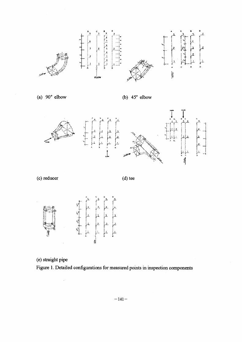
t I J~I>~T '(rt 1~.'5!-1":~

! r' : , l" ' ih //'~l' : ., . l.j'l! -~i l' t~~: ,• ' /'/ \~/\ I (\-~\*;:i4i//

"$!"I/ 5~:-~-'1~(" ,;.'

I~,

I1,

L1

It

A 5

il

:2

'L

e D 9 J t 8 f :"

: 2 :"' r~~ i-'--- t"' : _a_'

:'p

:2

; I :"' . t'- t.. .. 'f !; 9

rLOW

?/~ir~~:i ~' 'l

\ '/:~~~~~/ \ ,.1; '

(/~~{~ll,'!~. / //7/'

~~... : ( ~, '/;'

~•"/~~ -S;-~cl\

~'-' 7

A

,, r ~ /'~ i

It

, 2' i-- f

:'i l' : i ! _ '_

~i A

I" *:

~.

c ':' f-- ~' r l F* I

I '*, , . 1~ ! " f' v' i"i ' :~L*' ;~~~ ,

rl~ ? : 'Q: ; 't i + rc .t4 ~ .

~ .- i ~:

,,

d

i' ~~'

i

t~ t)

(a) 90" elbow (b) 45" elbow

,. , \ "I)i~ ;c-~ ~

'_/(~;" t' ' I.\ t ~K I(~ ~. /\/t~4. "~:L " ~__ ~] f~le~~:. /~' -'1:

/ " ~ ' '~~~ ~,

""I':

i

i

I

'h f

l~ -

4...

A t c rt /' *' -- " !L 4 r ' r ' I~'~ ? , , I I_ i i .. i-i L .1 { I')-.~ , . ' f . , :> . l I'~t ;~ ~L , r r~ I

: I l-i '~ ~ }-L A 9 a: o

.~

**.*~

" '~i' ' AI _ ::'~~ !~"'~f~~1'~~~, y?r\:..~ \

" /\fs-pr '\1- ' - \~* ~ l '~:'. !\.!

'lJ~ I

A A: ' ' :)~-' f i '

f } : : ' -- ' I

':{-- f, ~ ';•'-- ,~

~,: '~" ?J-~'L

~ At

)i'l~ J

eC rL J_~

i i

~= ; JL

i

if ~-. : - ;-

? l,.

~?i~il

:~

5i

r'~~~ -ir

f'-' ": 4 ;

r -~ .LJ3. :

~e I ' :- l }_lL _~

(c) reduoer (d) tee

~, ~L.. 85

I: '

l:: ' :1: l: : i I;

i: i : :!

;~,;~

,~L

lp - - rf-1$-

l' v! ; :1' ' : 's I'-- - -

Y. t~ ' " ; i " -L r-' v5~ r tl'~': : ;_1b

J_ i i

' r A

o o r ~ 'jL ' ~ ,L ,. J-; I' ~ 14 "a '~~' r~~~ t'~

f ! ;~ ! ::1 4 r JL .L Jh

lo' I~ f f" ' " "-(' rLi :5 t

;_i I ' ; i, - rL -L f

eL o ~Ji

~

(e) straight pipe

Figure I . Detailed configurations for measured points in inspection components

- 141 -

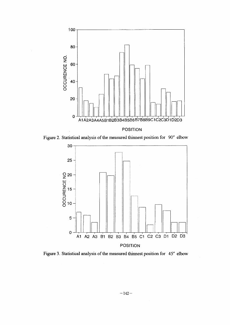
Figure 2.

Figure 3 .

o z UJ

~ ~ o o O

A1 A2A3A4A5 ~ I B2B3B'4B5B6 B7 B8B9d I C2C3D I D2D3

POSITION

Statistical analysis ofthe measured thinnest position for 90" elbow

i OO

80

60

40

20

o

A1 A2 A3 ~l B2 B3 B4 B5 C1 C2 C3 D1

•POSITION Statistical analysis of the measured thimest position for

30

25 ~

Oz 20 ~

Lu : O i zuJ15•~,~ cc = D : O : O = OIC1

O D2 D3

45" elbow

- 142 -

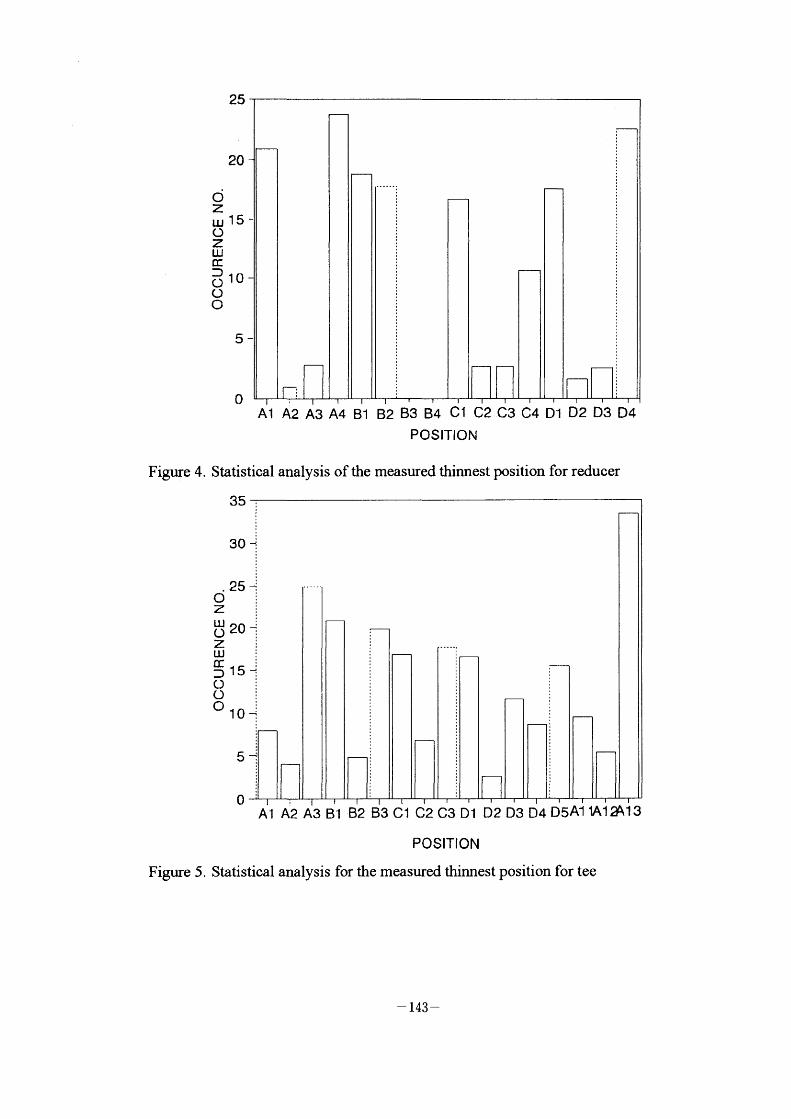
Figure 4.

Figure 5.

25

20

d z UJ 15 ~

o z UJ

~ D o 10 o O

5-

O A1 A2 A3 A4 B1 B2 B3 B4 C1 C2 C3 C4 D1 D2 D3 D4

POSITION

Statistioal analysis of the measured thinnest position for reducer

35 -:

A1 A2 A3 B1 B2 B3 C1 C2 C3 D1 D2 D3 D4 D5A1 IA12~l3

POSITION

Statistical analysis for the measured thimest position for tee

30 +

25 ~ c; ; z : LLl~ = O 'O ~

z i UJ : CCD 15 _•~

O i O : OIO~

5~

O

- 143 -

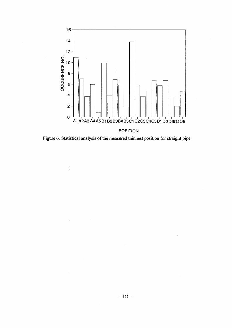
Figure 6.

16

14

12 C;

Z 10 LLJ' O ~8 GC :)

86 O

4

2

O A1 A2A3 A4 A5 ~l B2 B3B4 B5C1 C2d3C4C5D1 D2 D3D4D5

POSITION Statistical analysis of the measured thinnest position for straight pipe

- 144 -

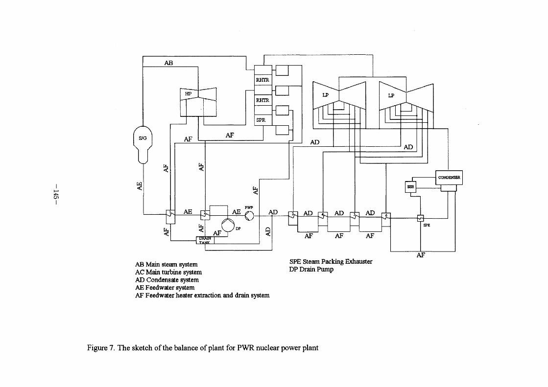
AB

I

~. J~ Ol

l

S/G

HP CJ

AF

RHTR

RE:lR

SPR

AF

Lp

~

~

1 AE

~

Fwr

~

~

~ AF

AE) DP

AD

~

LP

AD

3 AD AD

AD

AF

4

AF

5 AD 6

ssn

CONDENSER

AF sPE

AF AB Main steam system AC Main turbine system AD Condensate system AE Feedwater system AF Feedwater heater extraction and drairL system

SPE Steam Packing Exilauster DP Drain Pump

Figure 7. The sketch of the balance of plant for PWR nuclear power plant

,.

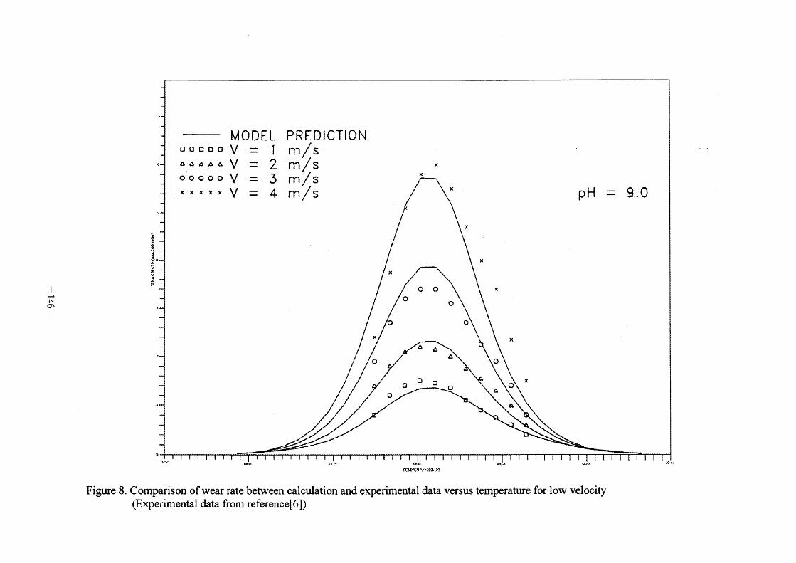
I

~' ~ cr)

~ ^ ^ ~

'i

,, *~'

*

1

,

MODEL OOODO V = 1 AAAAA oooooV = 3 x**x*V = 4

PREDICTION m/s m/s m/s m/s

x

x

X pH = 9.. o

x

x

X

,c

o

o oo

A A

o

d~

o

x

o

X

o

o o o o o

A o

A

X

IQI,,, .~::~ e.

fC,,,•',:~.1."~;ffh,1,) d'.,, ,•. .~II 'l.

Figure 8. Comparison of wear rate between calculation and experimental data versus temperature for low velocity

(Experimental data from reference[6])

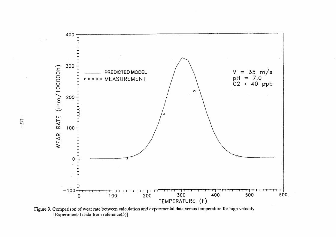
I

~' ~ ~]

I

400

- 300 ~:

O O O O O = \ 200 E E

~ LJ ~ O( I OO Q(

LU ~

o

- I OO

OODOD PREDICTED MODEL MEASUREMENT

D

o

V= pH = 35

7.

40

m/s pp b

Figure 9.

TEMPERATURE (F) Comparison of wear rate between calculation and experimental data versus temperature for high velocity

[Experimental dada from referenee(5)]

6Qo .

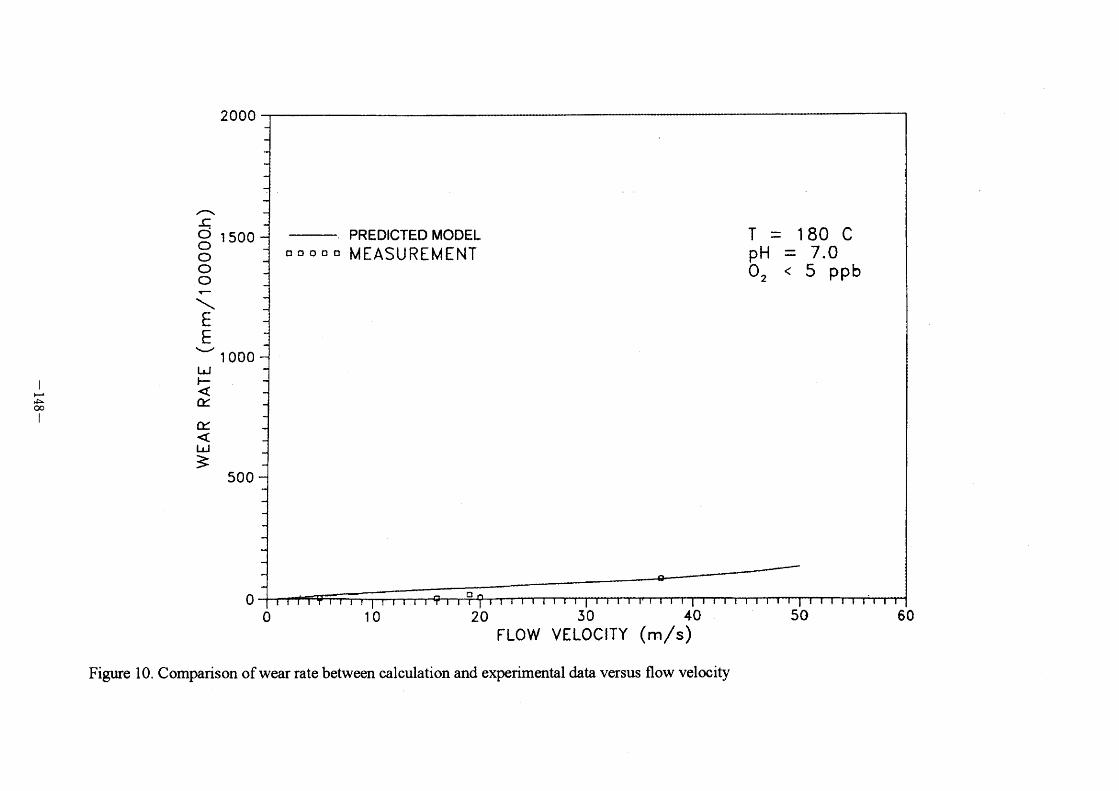
l

~. d~ oo

l

2000

~ ~. Oo 1500

O O O -\ E E

~ I OOO UJ H Q(

Q(

LJ ~

500

o

DOOOD PREDICTED MODEL MEASUREMENT

D

T pH 02

180 C 7.0 5 ppb

o 10 20 FLOW

30 VELOCITY

40 (m/s)

50 60

Figure lO. Comparison of wear rate between calculation and experimental data versus flow velocity

,-,

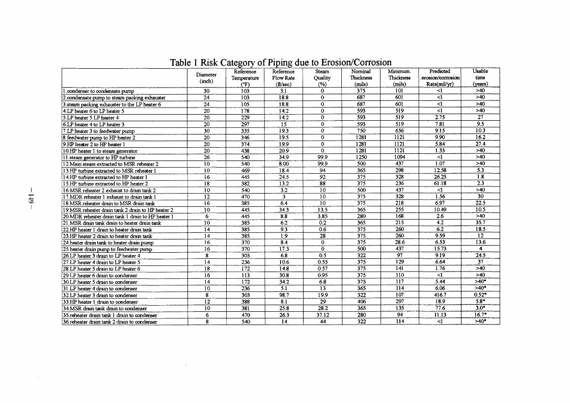
~ ~o

Table l Risk Category of Piping due to Erosion/Corrosion

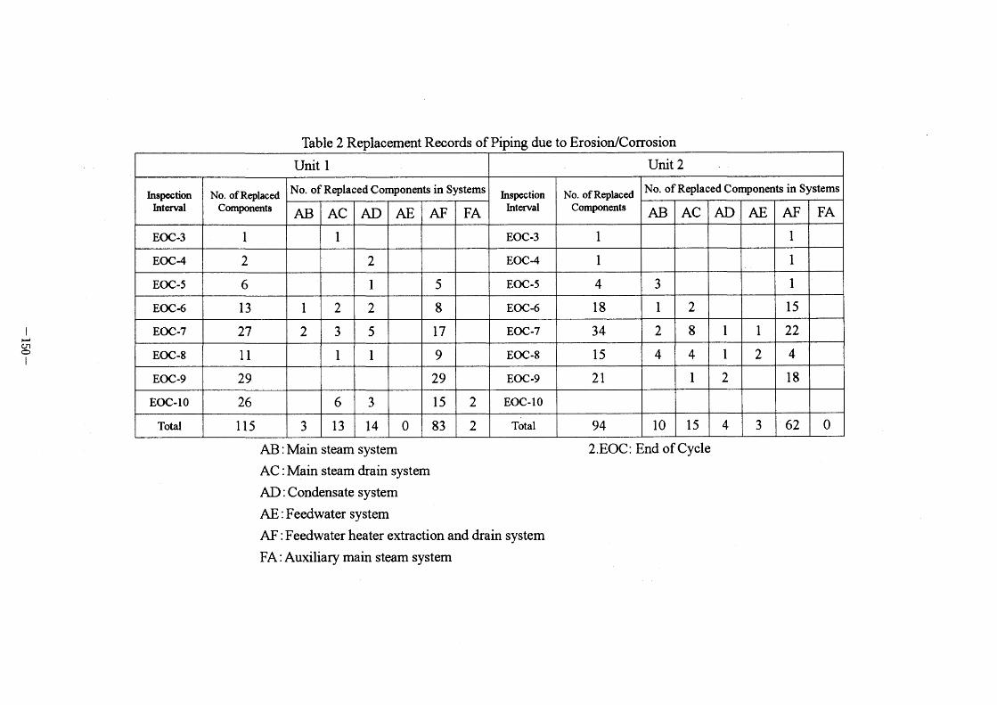
l

~:;

o I

Table 2 Replacement Records of Piping due to ErosionfCorrosion

AB : Main steam system

AC : Main steam drain system

AD : Condensate system

AE : Feedwater system

AF : Feedwater heater extraction and drain system

FA : Auxiliary main steam system

2 . EOC : End of Cycle

Session IV

Prpmg and LBB

IV- l Development of Modified Piping Evaluation Diagram for LBB

Ap plication

Y.J.Kim, Y.Z.Lee & N.S.Huh, Dept. of Mechanical

Engineering, Sung Kyun Kwan Univ., Suwon, Korea

C.R.Pyo, Dept.of Mechanical Engineering, Indnk college, Seoul, Korea

J.S.Yang, Korea Electric Power Research Institute, Daejon, Korea

Development of Modified Piping Evaluation Diagram for LBB Application to Korean Next Generation Reactor

Y J Kim', Y.Z. Lee', N.S. Huh', C.R Pyob J S Yang

'School of Mechanical Engineering, Sung Kyun Kwan Univ., Suwon, Korea bDept. of Mechanical Engineering, Induk Inst. of Technology, Seoul, Korea

'Korea Electric Power Research Institute, Daejon, Korea

Recently, the Piping Evaluation Diagram (PED) is accepted in nuclear industry for an efficient application of Leak-Before-Break (LBB) concept to piping system at an initial piping design stage. The objective of this paper is to develop the modified PED which can account for the variation of the material properties of the PED development stage and those

of the assembly stage. For this purpose, a parametric study was performed to investigate the

effect of stress-strain curve on the detectable leakage crack length and the effect of fracture

resistance curve on the LBB allowable load. Finite element analyses were also performed to

investigate the effect of stress-strain curve on the LBB allowable load. Finally a modified

PED was proposed as a function of crack length and the allowable safe shutdown earthquake load. The LBB analyses based on the modified PED are in good agreement with those based on the traditional PED. By adopting the modified PED, the variation of material properties can be considered in the LBB analysis and the computing times required for the application of LBB during the design process can be considerably reduced.

1. INTRODUCTION

The Leak-Before-Break (LBB) concept has been accepted as a justifiable approach for designing nuclear piping systems with the elimination of massive protective measures due to

the pipe rupture design requirement. If the LBB concept is applicable to nuclear piping design, the construction cost can be significantly reduced by eliminating unnecessary pipe

whip restraints and jet impingement devices. In order to apply the LBB concept to piping system, the nuclear piping design should meet all the criteria specified in NUFLEG 1061 , Vol.

3Ll] and Standard Review Plan 3.6.3[2]. Current LBB analyses on nuclear piping system are based on the plant-specific loads due to the geometry of the piping system and the operating

condition of concerned piping system. Therefore, if the analysis results do not meet the LBB

criteria, all the piping routing should be changed until the results are satisfactory. In performing LBB evaluation, highly specialized knowledge in fracture mechanics is required and lengthy period of time is required due to its complicated procedures and methods.

Recently, numerous studies have been reported on the applicability of LBB during the

initial piping design stage. The "Allowable Load Window" using the maximum and the

minimum moment of each piping was proposed by Nana and Yoon[3]• The "PED (Piping Evaluation Dragram)" usmg the Normal OPeratron (NOP) Ioad and the Safe Shutdown

Earthquake (SSE) Ioad was also proposed by Fabi et al.[4]• Swamy et al.[5] proposed the

- 151 --

"BAC (Boundary Analysis Curve)" using the stress at the normal operating condition and the

maximum stress. Y.J.Kim et al.[6] developed the "PEDs" using the NOP Ioad and the SSE load and applied for the safety injection and the shutdown cooling line in Korean Next Generation Reactor (KNGR). These diagrams were developed prior to the piping design and can be used for the evaluation of critical points for the LBB requirements in the piping system. Thus the iterative process of design to modification regarding the LBB applicability

can be eliminated.

According to the current LBB criteria, the final LBB evaluation should be performed using

the archival material properties. However, the PED may have to be modified to account for the difference between the material properties of the PED development stage and those of the

assembly stage. The objective of this paper is to develop a modified PED which can account for the variation of the material properties and apply them to the safety injection line and the

shutdown cooling line in KNGR.

2. DEVELOPMENT OF NUCLEAR PIPING MATERIAL DATABASE

NUclear Plping Material database (NUPIM database) was constructed prior to the development of the modified PED. The objective ofNUPIM database is to obtain the material properties such as stress-strain curves and fracture resistance curves required for the modified

PED. In designing nuclear piping systems, a plenty of material properties should be considered, and thus the development of NUPIM database which covers about 500 test data was essential.

Searching a material property in NUPIM database can be easily done owing to the hybrid

database which is connected to the DBMS (DataBase Management System). This DBMS searches the selected item from the stored material properties. The material properties stored

in database was obtained from domestic material test programs such as YGN 3&4[7], UCN 3&4[8] and the dynamic test for carbon steel[9]-

Search index of database consists of material name, welding method, yield stress, pipe thickness, temperature, pipe size et al. In order to provide various material properties, a

statistic calculation module with plenty of raw data has been attached to the database. Therefore, not only the material raw data but also pre-processed second hand material data can be easily obtained using NUPIM database.

3. PROCEDURE FOR DEVELOPING MODIFIED PED

3 . I General procedure

The general methodology and criteria used for developing the modified PED are based on NUREG I 061 , Vol. 3 and SRP 3.6.3. The material properties required for the development of

the modified PED were obtained from NUPIM database which consists of previous domestic LBB test results. Generally, the worst case material properties (worst stress-strain curve and

worst fracture toughness) are used in the analysis for ensuring the conservatism of the LBB

analysis. In this paper, an additional margin for the consideration of archival material properties, which are usually obtained at the fmal stage of the design process, was added by applying three different stress-strain curves in the LBB analysis. Different fracture resistance

curves considering archival material properties were also used in the analysis.

Fig. I illustrates the analysis procedure applied for the modified PED development. In the

- 152 -

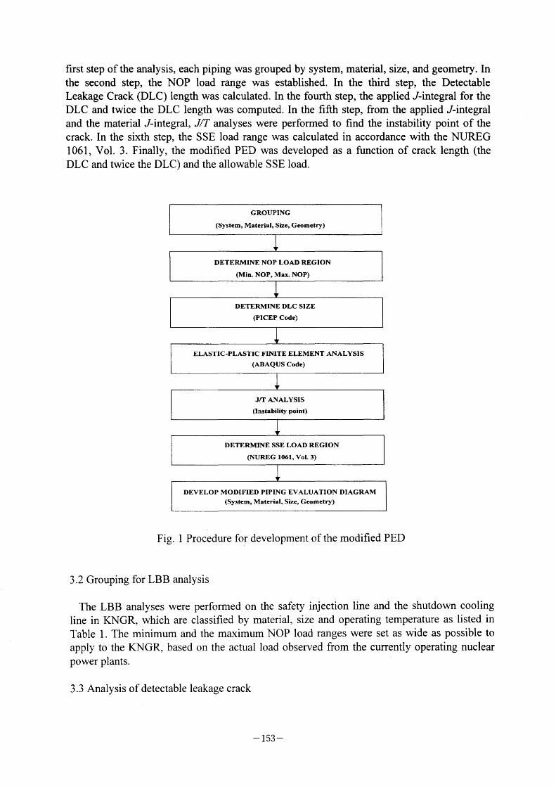
first step of the analysis, each piping was grouped by system, material, size, and geometry. In

the second step, the NOP Ioad range was established. In the third step, the Detectable Leakage Crack (DLC) Iength was calculated. In the fourth step, the applied J-integral for the

DLC and twice the DLC Iength was computed. In the fifih step, from the applied J-integral and the material J-integral, J/T analyses were performed to find the instability point of the

crack. In the sixth step, the SSE Ioad range was calculated in accordance with the NUREG l 061, Vol. 3. Finally, the modified PED was developed as a filnction of crack length (the

DLC and twice the DLC) and the allowable SSE Ioad.

Fig. I Procedure for development of the modified PED

3.2 Grouping for LBB analysis

The LBB analyses were performed on the safety injection line and the shutdown cooling line in KNGR, which are classified by material, size and operating temperature as listed in

Table I . The minimum and the maximum NOP Ioad ranges were set as wide as possible to apply to the KNGR, based on the actual load observed from the currently operating nuclear

power plants.

3.3 Analysis of detectable leakage crack

- 153 -

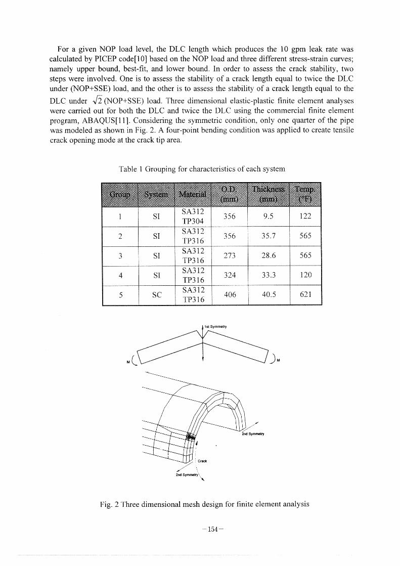
For a given NOP Ioad level, the DLC Iength which produces the I O gpm leak rate was calculated by PICEP code[1 O] based on the NOP Ioad and three different stress-strain curves;

namely upper bound, best-frt, and lower bound. In order to assess the crack stability, two steps were involved. One is to assess the stability of a crack length equal to twice the DLC

under (NOP+SSE) Ioad, and the other is to assess the stability of a crack length equal to the

DLC under ~/~ (NOP+SSE) Ioad. Three dimensional elastic=Plastic finite element analyses

were carried out for both the DLC and twice the DLC using the commercial fmite element program, ABAQUS[1 1]. Considering the symmetric condition, only one quarter of the pipe was modeled as shown in Fig. 2. A four-point bending condition was applied to create tensile

crack opening mode at the crack tip area.

Table l Grouping for characteristics of each system

~c

1 st Symmetry

)~

ll 2nc sym~ety

4

= C~aeX

./ \, 2~e Symmetry \\

Fig. 2 Three dimensional mesh design for finite element analysis

- 154 -

3 .4 Crack stability evaluation

For the crack stability evaluation, the J-integral / Tearing modulus (J/T) method was used.

For a stable crack growih, the material's tearing modulus (Tmat. ) must be greater than the

tearing modulus (Tapp. ) obtained from the applied load. The instability point may be found

by plotting Japp. versus Tapp, and Jmat. versus Tmat. on a single figure. The material J-R

curves can be obtained as following from the J-R data for weld metals.

C Aa C Jmat' = l( ) 2 (1)

And differentiating Eqn. ( I ) with the crack length, the material tearing modulus can be

obtained as follows:

dJ da

mat .

C2 -l = CIC2 (Aa) (2)

In this paper, various Cl and C2 Values were used for the development of the modified

PED. The J/T curves for applied load were obtained as follows. In the first step, from the

result of fmite element analysis, the applied J-integrals for crack lengths of a - 6 , a , and

a + 6 as well as 2a - 6 , 2a , and 2a + 6 were determined for the applied load. The crack length increment, 6 , was assumed as I Oo/o of crack length. In the second step, an equation for

() the J was postulated as a function of crack length a as following.

J = C a2 + c2a + c3 app. l

(3)

And also by differentiating Eqn. (3) with crack length, the applied tearing modulus was obtained as shown in the following equation.

dJ da

app.

2c a + c2 (4)

Finally, the J/T analyses were performed to find the instability point of the crack by applying

following equation.

dJapp dJmat (= Tmat ) (5)

Fig. 3 shows a typical J/T evaluation diagram.

3.5 SSE Ioad

The SSE Ioad for the modified PED was calculated in accordance with NUREG I 061 , Vol.

3[1]. For the DLC Iength, safety factor of J~ was applied on the load as following.

~/~[ Mtota/ = M + MSSE + Metc I ' NOP

- 155 -

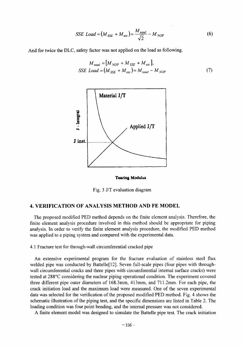
( Mtotal ) 1/~ ~MNOP SSE Load = MSSE + Metc = (6)

And for twice the DLC, safety factor was not applied on the load as following.

total ~ MNOP + MSSE + Metc]' M -[ SSE Load - MSSE + Metc)= Mtotal ~ MNOP -( (7)

~,

;1,

,

J inst.

Material J/T

Applied J/T

Tcaling Modutus

Fig. 3 J/T evaluation diagram

4. VERIFICATION OF ANALYSIS METHOD AND FE MODEL

The proposed modified PED method depends on the finite element analysis. Therefore, the finite element analysis procedure involved in this method should be appropriate for piping analysis. In order to verify the finite element analysis procedure, the modified PED method

was applied to a piping system and compared with the experimental data.

4. I Fracture test for through-wall circumferential cracked pipe

An extensive experimental program for the fracture evaluation of stainless steel flux welded pipe was conducted by BattelleL12]. Seven full-scale pipes (four pipes with through-wall circumferential cracks and three pipes with circumferential internal surface cracks) were

tested at 288'C considering the nuclear piping operational condition. The experiment covered

three different pipe outer diameters of 168.3mm, 413mm, and 71 1 .2mm. For each pipe, the

crack initiation load and the maximum load were measured. One of the seven experimental data was selected for the verification of the proposed modified PED method. Fig. 4 shows the

schematic illustration of the piping test, and the specific dimensions are listed in Table 2. The

loading condition was four point bending, and the internal pressure was not considered.

A finite element model was designed to simulate the Battelle pipe test. The crack initiation

- 156 -

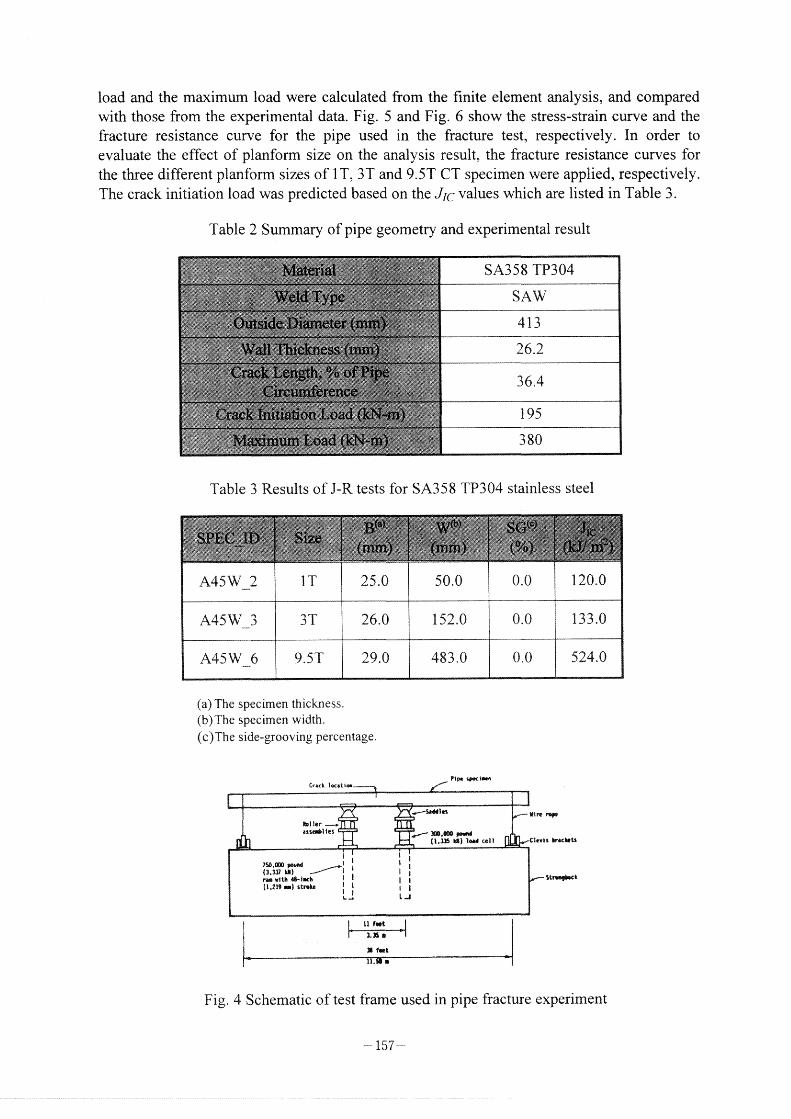
load and the maximum load were calculated from the fmite element analysis, and compared with those from the experimental data. Fig. 5 and Fig. 6 show the stress-strain curve and the

fracture resistance curve for the pipe used in the fracture test, respectively. In order to evaluate the effect of planform size on the analysis result, the fracture resistance curves for

the three different planform sizes of IT, 3T and 9.5T CT specimen were applied, respectively.

The crack initiation load was predicted based on the Jlc values which are listed in Table 3 .

Table 2 Summary of pipe geometry and experimental result

l 95

380

Table 3 Results of J-R tests for SA358 TP304 stainless steel

(a) The specimen thickness.

(b) The specimen width.

(c)The side-grooving percentage.

PiPe s~~~~~ef~

~~

s~~~tess

$t~~~et

i~~~Hlj S fQet

,

Fig. 4 Schematic of test frame used in pipe fracture experiment

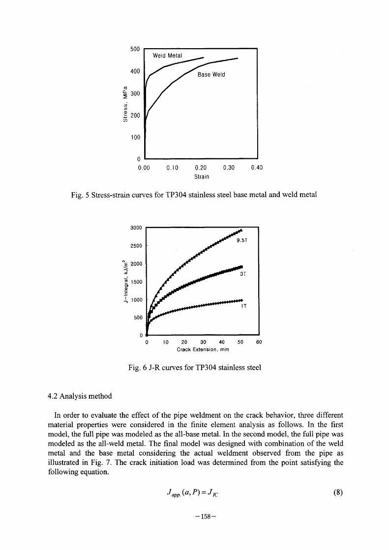
Fig.

cO CL

~

(D

~ Cl)

500

400

300

200

1 OO

O

O

Weld Metal

Base Weld

.OO 0.10 0.20 0.40 0.30

Strain

5 Stress-strain curves for TP304 stainless steel base metal and weld metal

3000

9.5T 2500

~E 2000

~ . ~ 1500 ~

~ Iooo IT

500

o I o 20 30 40 50 60 crack Extension, mm

Fig. 6 J-R curves for TP304 stainless steel

4.2 Analysis method

In order to evaluate the effect of the pipe weldment on the crack behavior, three different

material properties were considered in the finite element analysis as follows. In the first

model, the full pipe was modeled as the all-base metal. In the second model, the full pipe was

modeled as the all-weld metal. The final model was designed with combination of the weld

metal and the base metal considering the actual weldment observed from the pipe as illustrated in Fig. 7. The crack initiation load was deterrnined from the point satisfying the

following equation.

Japp (a P) = Jlc (8) - 158 -

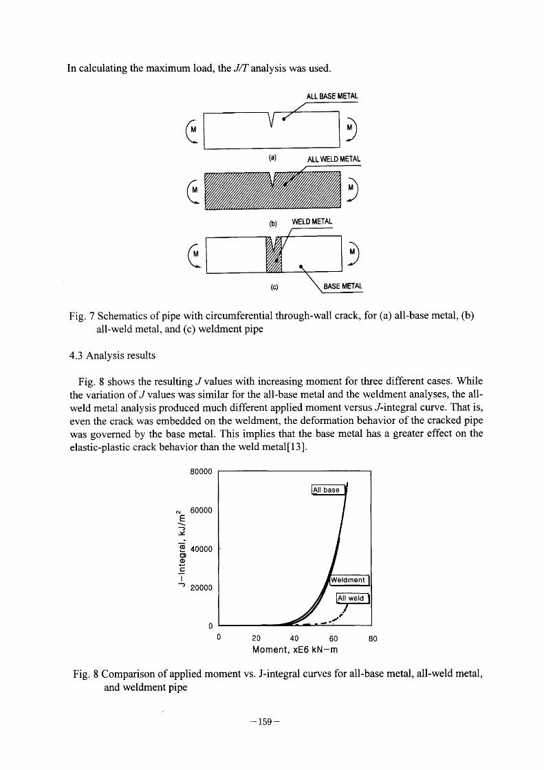
In calculating the maximum load, the J/T analysis was used.

ALL BASE METAL

~

~

~

(a ) ALL WELD METAL

(b) VVELD METAL

~ BASE METAL

Fig. 7 Schematics of pipe with circumferential through-wall crack, for (a) all base metal (b)

all-weld metal, and (c) weldment pipe

4.3 Analysis results

Fig. 8 shows the resulting J values with increasing moment for three different cases. While

the variation ofJ values was similar for the all-base metal and the weldment analyses, the all-

weld metal analysis produced much different applied moment versus J-integral curve. That is,

even the crack was embedded on the weldment, the deformation behavior of the cracked pipe was governed by the base metal. This implies that the base metal has a greater effect on the

elastic-plastic crack behavior than the weld metal[1 3] .

E ~_ 1 ~ ~CaL,

CD O d. E I

i)

80000

60000

40000

20000

O

All base

Weldment

~~~]All~Jld

. .l .'., ,

O 20 40 60 Moment, xE6 kN-m

80

Fig. 8 Comparison of applied moment vs. J-integral curves for all-base metal, all-weld metal,

and weldment pipe

- 159 -

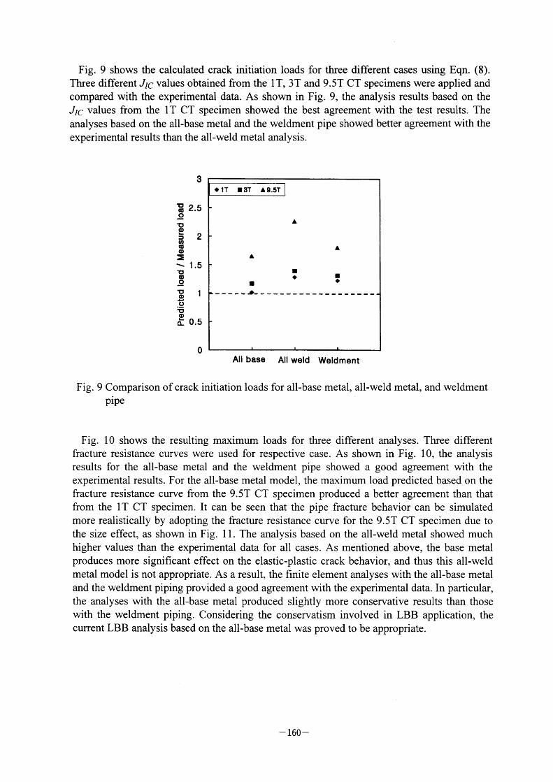
Fig. 9 shows the calculated crack initiation loads for three different cases using Eqn. (8).

Three different Jlc values obtained from the I T, 3T and 9.5T CT specimens were applied and

compared with the experimental data. As shown in Fig. 9, the analysis results based on the

Jlc values from the I T CT specimen showed the best agreement with the test results. The analyses based on the all-base metal and the weldment pipe showed better agreement with the experimental results than the all-weld metal analysis.

8

='25 a' ' ~ 1'

~ 2 coc"

o = '\ 1.5 ID CD

~ U 1 o ~ .S2

l9 o ~ Q- 0.5

O

• IT 1 3T L 9.5T

L

dL

A

l

--.---

AII base All weld Weldment

Fig. 9 Comparison of crack initiation loads for all-base metal, all-weld metal, and weldment

pipe

Fig. I O shows the resulting maximum loads for three different analyses. Three different fracture resistance curves were used for respective case. As shown in Fig. lO, the analysis

results for the all-base metal and the weldment pipe showed a good agreement with the experimental results. For the all-base metal model, the maximum load predicted based on the

fracture resistance curve from the 9.5T CT specimen produced a better agreement than that from the I T CT specimen. It can be seen that the pipe fracture behavior can be simulated more realistically by adopting the fracture resistance curve for the 9.5T CT specimen due to

the size effect, as shown in Fig. I I . The analysis based on the all-weld metal showed much

higher values than the experimental data for all cases. As mentioned above, the base metal produces more significant effect on the elastic-plastic crack behavior, and thus this all-weld

metal model is not appropriate. As a result, the finite element analyses with the all-base metal

and the weldment piping provided a good agreement with the experimental data. In particular,

the analyses with the all-base metal produced slightly more conservative results than those

with the weldment piping. Considering the conservatism involved in LBB application, the current LBB analysis based on the all-base metal was proved to be appropriate.

- 160 -

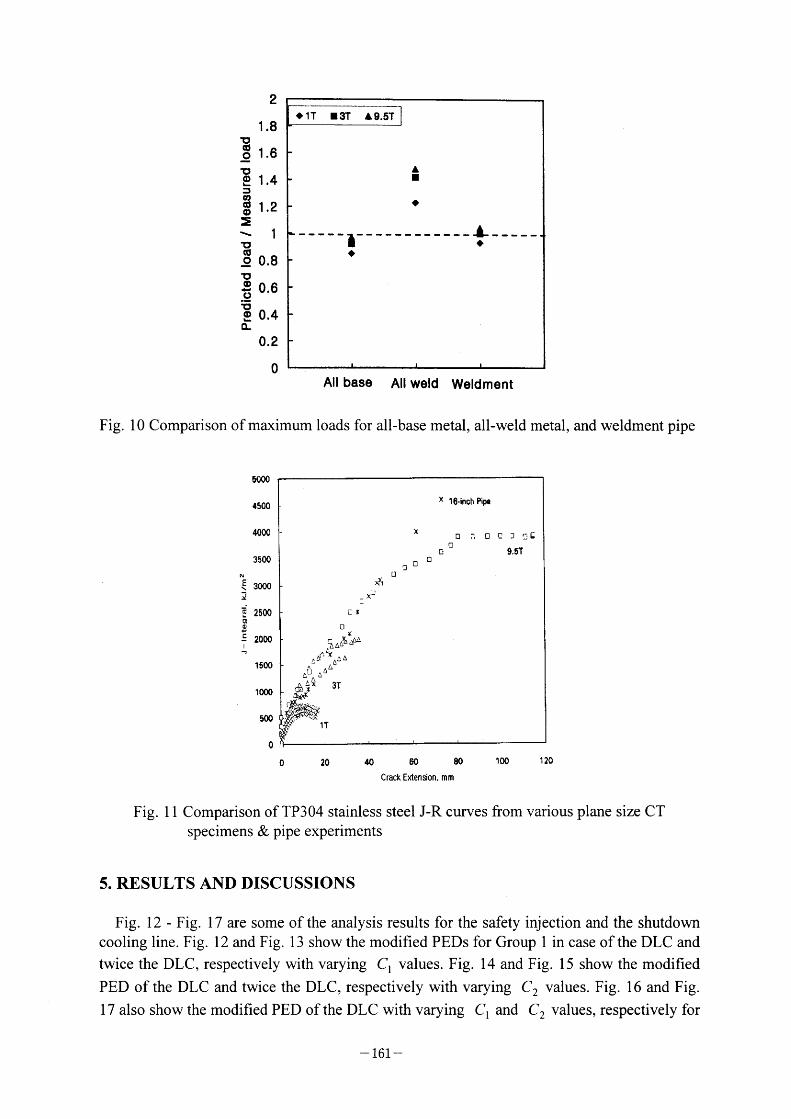
2

1 .8

1' c" o 1.6 ~o 2 1.4 = CQ c"o 1.2

:~

~ 1 ~ co o 0.8

1:,

006 ~ . o 1: 2 0.4 o_

0.2

O

• IT 1 3T JL9.5T

I ~ 1)

,

L

All base AII weld Weldment

Fig. l O Comparison of maximum loads for all-base metal, all-weld metal, and weldment pipe

5000

45co

400c

3500

E 300O , ~

~ 2500 ~ ~ E 2000

, 1 500

lOOO

eoo

r

~

[X C!

X r ~~' A i~*A~~ i~

. ~~ ~~~~ ~

L~] d!~ ~~ *~

C~ ~)(A 3T

(~~(

'',\

IT

>~l

X-

D :i

x

Cl C!

x 16•~lch Pip,I

C] r; D r_ J ,_~C

O D 9.5T

o

o 20 40 OO OO Crack Extension, mm

lOO 1 20

Fig. l I Comparison of TP304 stainless steel J-R curves from various plane size CT

specimens & pipe experiments

5. RESULTS AND DISCUSSIONS

Fig. 12 - Fig. 1 7 are some ofthe analysis results for the safety injection and the shutdown

cooling line. Fig. 12 and Fig. 1 3 show the modified PEDS for Group I in case ofthe DLC and

twice the DLC, respectively with varying Cl values. Fig. 14 and Fig. 1 5 show the modified

PED of the DLC and twice the DLC, respectively with varying C2 Values. Fig. 1 6 and Fig.

17 also show the modified PED ofthe DLC with varying Cl and C2 Values, respectively for

- 161 -

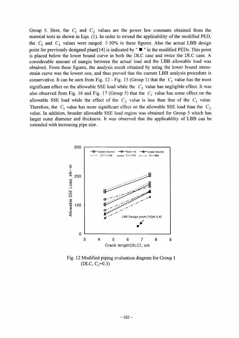
Group 5 . Here, the Cl and C2 Values are the power law constants obtained from the material tests as shown in Eqn. ( I ). In order to extend the applicability of the modified PED,

the Cl and C2 Values were ranged i 500/0 in these figures. Also the actual LBB design

point for previously designed plant[14] is indicated by " I " in the modified PEDs. This point

is placed below the lower bound curve in both the DLC case and twice the DLC case. A considerable amount of margin between the actual load and the LBB allowable load was obtained. From these figures, the analysis result obtained by using the lower bound stress-

strain curve was the lowest one, and thus proved that the current LBB analysis procedure is

conservative. It can be seen from Fig. 12 - Fig. 1 5 (Group 1) that the Cl value has the most

significant effect on the allowable SSE Ioad while the C2 Value has negligible effect. It was

also observed from Fig. 16 and Fig. 17 (Group 5) that the C2 Value has some effect on the

allowable SSE Ioad while the effect of the C2 Value is less than that of the Cl value.

Therefore, the Cl value has more significant effect on the allowable SSE Ioad than the C2

value. In addition, broader allowable SSE Ioad region was obtained for Group 5 which has larger outer diameter and thickness. It was observed that the applicability of LBB can be extended with increasing pipe size.

300

E l

z ~: 200 ~ca

~ LLJ cl) cl)

-JQ

co 100 ~

O

~hupper bound - C1 =1 1 55

~.1

er .'

~r

-~ Best-f't C I =770

I~ Lower bound - C1=385

,E] .,.

'/ : ~:. ' / 1; ,d:"

/'~/' , IA

/~ / / ' l' / " / / / / LBB Desi9n point (YGN 3,4)

/ l

3 4 5 6 7

Crack length(DLO, cm 8 9

Fig. 1 2 Modified piping evaluation diagram for Group l

(DLC, C2=0.3)

- 162 -

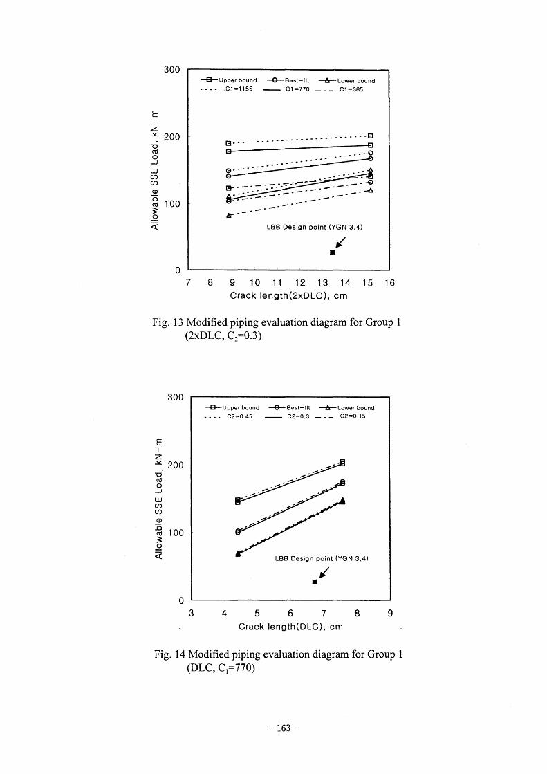
E I

Z x ~:) cV

J LJJ Cl) Cl)

~) cU

~

300

200

1 OO

O

-e-Upper bound - .CI =1 1 55

E!- - -

O- -

Er--

~r~

-~Best-fit C I =770

ihLower bound _ C1=385

- - -El

_--O

. -...-.--~ . - . ~ .~ .~. .~ .,.

.,..,.

LBB Design polnt (YGN 3,4)

/ I

Fig.

7 8 9 10 11 12 13 14 15 16 Crack length(2xDLC), cm

l 3 Modified piping evaluation diagram for Group l

(2XDLC, C2=0.3)

E I

Z ~:

~ ~ UJ Cl) Cl)

JO cUO~

300

200

1 OO

o

-B-Uppef bound - - - - C2=0.45

l:

d

-~ Best-fit C2=0.3

,,

.~l

,,

,~~

,,:

'!'

,:

.g::

~-Lower bound _ C2=0. 1 5

,, ,,

d d d

LBB Design point (YGN 3,4)

/ l

Fig.

3 4 5 7

Crack length(DLC), cm

l 4 Modified piping evaluation diagram for Group l

(DLC, Cl=770)

- 163 --

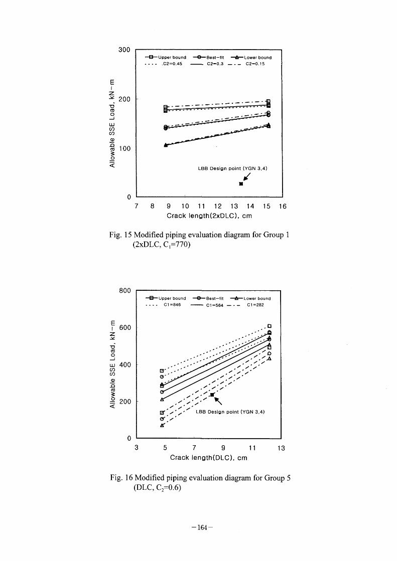
300

E I

z ~ _ 200 1)

~ UJ cl) cl)

~ ca 100 ~o

O

H~Upper bound - . C2 =0 . 45

-~ Best -fit C2=0.3

I~ Lower bound - - - C2=0.15

de d~ d~

LBB Desian point (YGN 3.4)

/ I

7 8 9 10 11 12 13 14 15 16 Crack length(2xDLC), cm

Fig. 1 5 Modified piping evaluation diagram for Group l

(2XDLC, Cl=770)

800

El 600

z !~

~ ~ UJ 400 cl:)

a:)

~ cu~o

- 200 ~

o

-E-Upper bound - C I =846

EI'

O'

~ of

g

/ / /

-~ Best-fit C I =564

IF LoweT bound - C1 =282

O

.lo l IA ' / ' / 'l

/// /// ./'/'/ / /'/' /'/'/'

/ ' / ;1" ./'/ / \ / / l'

ll ' LBB Desian point (YGN 3,4) /

5 9

Crack length(DLC), cm

Fig. 1 6 Modified piping evaluation diagram for Group 5

(DLC, C2=0.6)

- 164 -

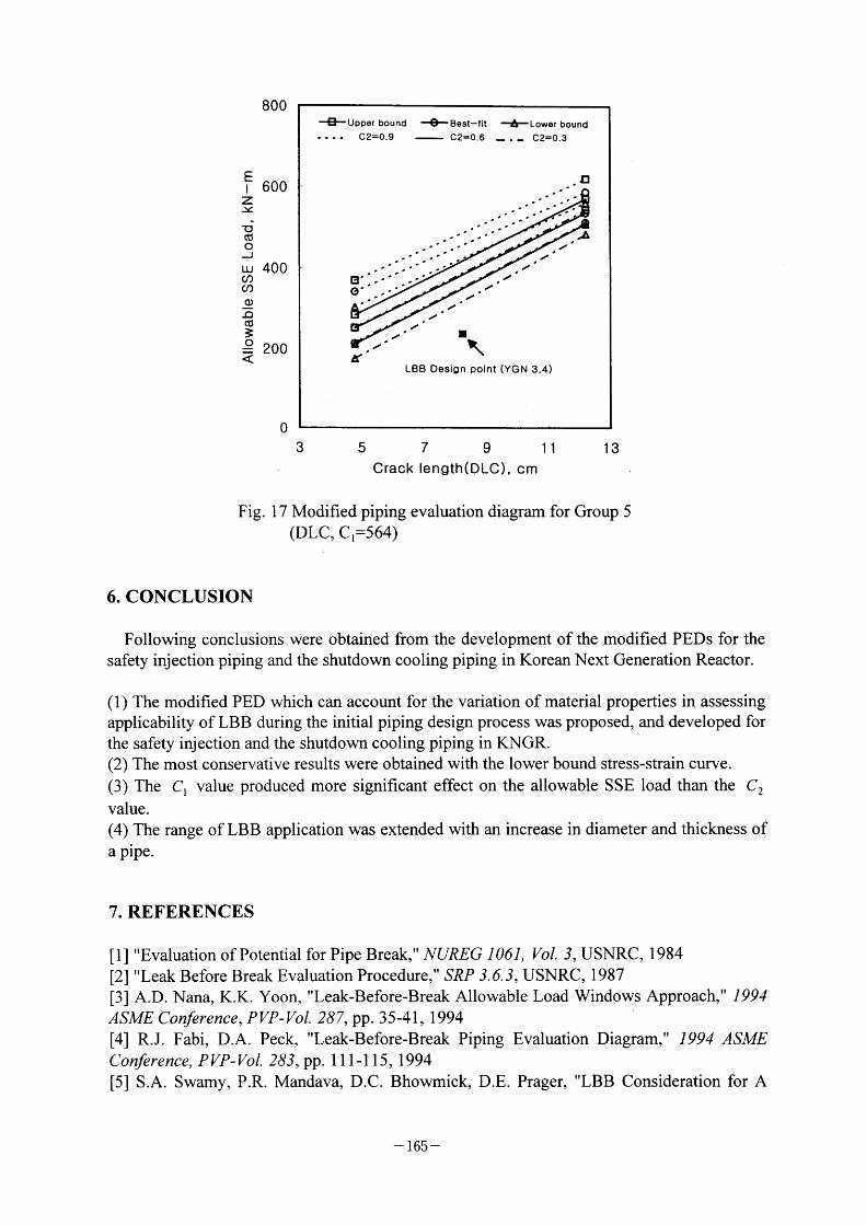
800

EI 600

z ~ ID cu

o J uJ 400 cl) cl)

o ~:) cv

~ ~ 200

O

HE-Upper bound - C2=0.9

E' . ' o' .

g /

-~ 8est-fit C2=0.6

~rLowor bound _ _ _ C2=0_3

/ /

/ /

/ /

/ / l l'

\ LBB Desion point (YGN 3,4)

/

o

A

3

Crack length(DLC), cm 13

Fig. 1 7 Modified piping evaluation diagram for Group 5

(DLC, Cl=564)

6. CONCLUSION

Following conclusions were obtained from the development of the modified PEDS for the safety injection piping and the shutdown cooling piping in Korean Next Generation Reactor.

(1) The modified PED which can account for the variation of material properties in assessing applicability of LBB during the initial piping design process was proposed, and developed for

the safety injection and the shutdown cooling piping in KNGR. (2) The most conservative results were obtained with the lower bound stress-strain curve.

(3) The Cl value produced more significant effect on the allowable SSE Ioad than the C2 value .

(4) The range of LBB application was extended with an increase in diameter and thickness of

a pipe.

7. REFERENCES

[l] "Evaluation of Potential for Pipe Break," NUREG 1061, Vol. 3, USNRC, 1 984

[2] "Leak Before Break Evaluation Procedure," SRP 3. 6.3, USNRC, 1 987 [3] A.D. Nana, K.K. Yoon, "Leak-Before-Break Allowable Load Windows Approach," 1994 ASME Conference, PVP-Vol. 287, pp. 35 41 1994 [4] R.J. Fabi, D.A. Peck, "Leak-Before-Break Piping Evaluation Diagram," 1994 ASME Conference, PVP-Vol. 283, pp. I 1 1 1 15 1994

[5] S A Swamy P R Mandava D C Bhowmrck D E Prager "LBB Consideration for A

- 165 -

New Plant Desrgn " NEA/CSNIIR(95)18 Vol 1, pp. 199-205, 1996 [6] N.S. Huh, J.H. Lee, Y.J. Kim, C.R. Pyo, S.D. Park, "Development of Piping Evaluation Diagram for LBB Application to Safety Injection and Shutdown Cooling Piping," Proc. of the Korean Nuclear Sociee/Autumn Meeting, Vol. II, pp. 697-702, 1996 [7] Y.J. Kim, C.S. Seok, "Stress-Strain and Fracture Resistance Characteristics of Primary

Piping Weld Materials for Younggwang 3/4 Nuclear Power Plants," S.K.K.U. Research Report, 1 992

[8] Y.J. Kim, C.S. Seok, "LBB Test Evaluation of Secondary Piping Materials for Ulchin 3/4

Nuclear Power Plants " S K K U Research Report, 1996 [9] Y.Y. Earmme et al., "Study of Effect of Dynamic Strain Aging on Fracture Toughness for

Main Steam Line Piping ofNuclear Power Plant," KAIST Research Report 1996 LIO] D M Noms B Chexal "PICEP : Plpe Crack Evaluation Program," EPRI Report NP 3596-SR, 1987 [1 I] ABAQUS User's manual, Hibbitt, Karlsson & Sorensen, Inc., 1 996

[12] G. Wilkowski et al., "Analysis of Experiments on Stainless Steel Flux Welds," NUREGICR-4878, 1987 [13] B.R. Ganta, D.J. Ayres "Analysrs of Cracked Prpe Weldment " Palo Alto CA EPRI NP-5057, 1987 [14] "Fmal Safety Analysrs Report (YGN 3/4) " Technrcal Report, KOPEC, 1993

- 166 -

IV-2 Fracture Mechanics Evaluation for The Cast Duplex

Stainless Steel after Thermal Aging

Shigeru Urata, Manager of Nuclear Safety Engineering

Section Kansai Electric Power Co. Inc., Japan

kIRACTURE MECHANICS EVNiUA nON roR THE CAST DUPLEX Sl:AINI.ESS STEEL AFIER

Tr{ERMAl. AGINIG

Shigeru Urata

The Kansal F.1ectric Po\~'er Company. Osaka. Japan.

Abstract

For the primary coolant piping of PWRS in Japan. cast duplex stainless steel \\'hich is excellent in terms of

strength, corrosion resistance. and v~~eldability has con\'entionally been used. The cast duple~c stainless steel

contains the ferrite phase in the austenite matrix and thermal aging after iong term service is knovb'n to

change its material characteristics.

It is considered appropriate to apply the methodology ofelastic plastic t~racture mechanlcs for an e\'aluation

oi' the inte_~rity of the primary coolant piping after thermal aglng. Therefore. \\e e\'aluated the integrity of

the primary coolant piping fbr an initial PWR plant in Japan by means of elastic plastic fracture mechanics.

The evaluation results sho\~~ that the crack \\ill not gro\\ into an unstable f~racture and the integrity ofthe

piping \\~ill be secured. even \~'hen such through \\-all crack length is assumed to equal the fatigue crack

gro\\th len_~th tbr a service period of~up to 60 years.

l . n~lTRODUCTION

For the primary coolant plping of PWRs in Japan. cast duple\ stainless steel (ASME SA_~5 1 Gr CF8M or

equivalent) has been applied. This cast duple\ stainless steel contains a ferrite phase of about 5 to 250 o in

the austenite matrix in order to impro\'e its characteristics ofcorrosion resistance. strength. \\-eldabillty. etc.

In the cast duple\ stainless steel. the f~errite phase is gradually separated \\'ithin the operatlng period at the

pWR operation temperature (at about _300 C). and that causes changes in its material characteristics.

An aging oflhe material tends to increase its tensile strength but reduces its fi-acture toughness. The dc_gree

ofthe toughness reduction becomes more si_gnificant \\'ith increasing ferrite contcnt and the rate of

- 167 -

tou_ghness reduction increases ',vith rising temperature. Both ofthese tendencies are mitigated vL~ith thc

aging progress.

The present paper summarizes evaluation results on integri~' oi~the primar) ' coolant piping afier thermal

aglng ibr initial PWR piant in Japan.

2. CRACK STABII_ITY ANAJ_YSIS

2 . I Evaluation Method

Fracture toughness of the primary coolant piping decreases due to thennal aging under long-term

plant operation. but this fracture type is considered to be a ductile fracture because ductile crack

gro\\th is recognized In the material test data after thermal aging. Therefbre. it is appropriate to apply

elastlc plastic fracture mechanics ibr an evaluation ofthe stabillty ofthe assumed crack.

The e\'aluation tlo\\~ is sho\\'n in Fi~:. I .

2.2 Selection ofEvaluatin Location

Material toughness. \\~hich represents fracture resistance. ~\~ill be reduced \vith increasing ferrlte

content and also \~~ith increasing operating temperature. In addltion. a high temperature causes a large

fi'acture force due to thermal bending moment. Thereibre. the hot leg piping at the reactor vessel

outlet nozzle \\as selected as the location to be evaluated since both temperature and imposed load are

se\'erer and ferrite content is relati\'ely high in the evaluating plant.

2 ,_3 Evaluation of Crack Gro\\th

The size ofthe fatigue crack is calculated under the condition that the assumed inltial defect on the

piping inside surface gro\\s duc to the stress cycles applied b~' thc plant operation.

( I ) F.\'aluation Conditions

(a) Size oflnitlal Defect

The size ofthe initial defect ~\'as conser\'ati\"ely assumed. v\'ith a sufi~rcient margin. to be about

tw~ice the size ofthe detectable single defect. Namely. the initial defect ~\'as assumed to be a

- 168 -

(b)

(c)

2)

seml-eiliptical. circumferential det~ect on the piping inside surface and its size to be 0.2t (depth)

l .Ot (surface length). \~'here "t" is the \\~all thickness.

Stress Cycle Used in Crack Gro\\th Analysis

The stress cycle \~'as produced on the basis of the transient conditions w~ith consideration of the

actual operating status of' the plant.

Fatigue Crack Growih I.avL~

The fatigue crack growth la\~' is represented by the follow~ing equations provided on the basis of

l, the test data under the PWR prlmary coolant envlronment :

da dN = CKefilTl . . . . ( I )

Kei~f = Kmax ( I -R)1) ) (2 ) ....

R == Kmm Kmax " " (_3)

Where.

da dN : Fatigue crack gro~\th rate Lmm cycle]

C : Constant = 7.0 l0~1()

m : Constant = 4.0 Keff : Effective stress intensity factor range [MPafm]

Kma~ Kmin : Ma)(imum. minimum stress intensity factors [MPafm]

R : Stress ratio

E_\'aluation Results

The results oi'the fatigue crack _gro\\th analysis are sho\\'n belo\\~. It re\'eals that the fatigue crack

gro\\th rate is lo\\~ and the crack does not penetrate the pipe vL~all (67.4mm thick) even after long-

term plant operation.

1 ) Assumed initial crack sizc

Depth : 1 3 .6 mm

I.ength : 67.4 mm

- 169 -

2) Crack size afier plant operation of60 years

Depth : 26.5 mm

Length : 108.8 mm

2.4 Crack Stabili ' Evaluation

( I ) Evaluation Method

Fracture toughness ofthe primary coolant pipe decreases after thermal aging. but this fracture

ty'pe can be considered to be a ductile fracture because a ductile crack growih is recognized in its

material tests. Therefore. elastlc plastic fracture mechanics are to be applied ibr an evaluation of

the stability ofthe assumed crack. Concretely, the crack stabillty is evaluated \\-ith the J jntegral

value (Japp). \\~hlch sho\\'s a fi'acture ibrce in comparison to the fracture toughness \'alue (Jmat).

\~'hich sho\\'s the fractttre resistance of the material after thermal aging.

(2) J Integral Value (Japp)

J jntegral \'alue is calculated \\-ith the stress analysis by using the f~mite element method on the

basis ofthe design load and the crack length tbr evaluation.

(a) Design Load

Loads imposed on the piping are those initiated under the normal operating condition and also

those caused by S I earthquake (maximum design earthquake).

(b) Analysis Model

For the analysis. the f~mite element model is applied to the elbo\~~ on the outlet side (high

temperature side) of the reactor \'essel \\-ith a circumt~erential crack on the inside surface.

Fig. 2 sho\\'s the fmite element model used fbr the analysis.

The crack gro\~th analysis \\'as conducted \~~ith the assumption ofan initial crack on the basis

ofthe number oftranslents durin_~ the operating period oi' 60 years. Then. the calculated

surface crack length \~~as conservatively con\'erted into the through \\'all crack ~\'hich length is

assumed I .6t as sho~\~n in Fig. I for the crack stability e\'aluation.

- 170 -

(c) Analysls ResLtlts

Fig. 3 shov\'s the analysis results fbr the Japp \'alue at the evaluating location.

(_~) The Fracture Toughness Value (Jmat)

The Jmat value w~as determined by the lo\\'er bound cur\'e oftoughness (-2 a lo\\er bound

curve) obtained \~lth the toughness prediction model (H3T Model : Hyperbollc-Time

Temperature Toughness) on the basis of the ferrite content at the evaluating location.

(a) The H_3T model

The H_3T model expresses the relation oi' Jlc and J6 to the aging time vL~ith the fbllov,'ing

hyperbolic i~unction as sho\\'n in Flg. 4.

M = A ~ B . . . . . (4) t -~ C

~\'here

M : Tou_g:hness ( Jlc or J6) kJ m~

t : Aging tirne. Hours

A : Fully aged toughness kJ m~

B : Constant relating to aging temperature

C : Constant relating to agin_g time

No\\ rt Is assumed that B exp (D I * Co) and D = Q R. \\-here T is the aglng temperature

(K). Co is a constant and R is gas constant. When T is Ti. B is Bi. When T = T_j. B is B_j.

Then.

Bi B_j-exp[D(1 Ti-1 'lli)] """"" """"""' (5)

Bi B_j-=e\p[Q R(1 Ti-1 1:i)1 -

The acti\'ation ener_gy Q (k-J mole) obtained l'rom temperature dependence of B is del~Ined to be

the embrittlement activation energy.

On the other hand. the initiation actl\'ation energy F is dei~med fi-om temperatLtre dependence of

initiation time of'tertiary embrittlement tF. namely

tFl tl'i ~ e\p [F R (1 'I'i - 1 1:i)1 " " " " " " " " " " " ' (7)

- 171 -

The Q and F values obtained from the J6 changes fbr the test materials aged at 290. 325, _350 and

400 C are about 100 to 1 80 kJ mol. From this. it Is considered that the result w~ill be

conservative \\'hen I OOkJ mol is used.

Fi_g. 5 sho\\~s the Flo\\' chart ofthe tou_ghness prediction model.

First. the data fbr the aging temperature of400 'C is fitted vL'ith the H3T model to obtain the

constant A (the i~ully aged toughness).

With this constant A fiY. ed. the data fbr agin_~: at 300 and 350 C are f~Itted \\'ith the H_3T model to

obtain the constants B and C at the agin_~ temperatures of_300 and _350'~'C.

By obtaining relation ofthe above-obtained constants I~ B. and C to chemical composition. the

predlction e\pression can be obtained.

Table I show's e)camples ofthe prediction ibrmulas obtained for Jlc and J6 at _~25 'C \\-hich are

constant A ibr the prediction model. We have been modifying these ibrmulas by Increaseing data

further.

Table I Predictlon lbrmulas oi'constant A for the toughness prediction model

(Temp.: -~25~C )

Fo o : Ferrite content (o o) by ASTM A800

In e\'aluating the integrity of duple\ stainless steel components after thermal aging. It is

important to predlct the J- A a curve. When the Jlc and J6 values at an optional aging condition

are obtained. the J- A a cur\'e can be obtained by the fbllo\ving expression \\'ith the above

prediction model by giving the flo\~~ stress :

c

- 172 -

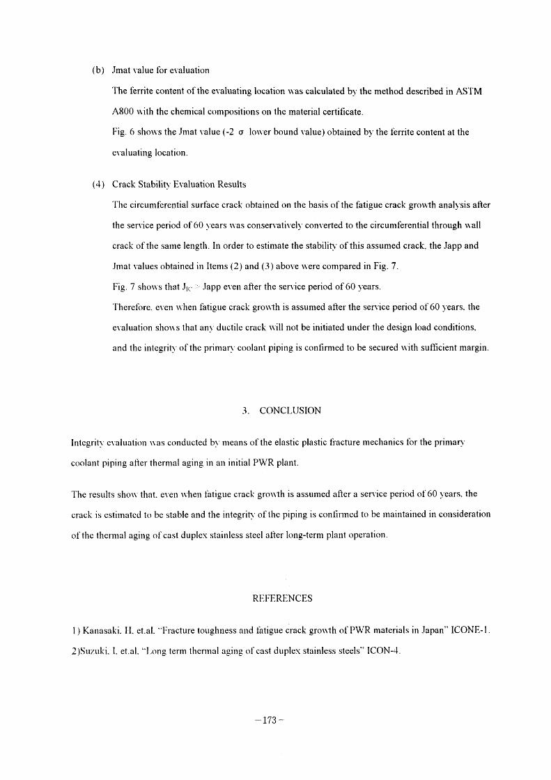
(b)

(4)

Jmat value for evaluation

The i'errite content of the evaluating location \~~as calculated b~_' the method described in ASTM

A800 \~~ith the chemical compositions on the material certificate.

Fig. 6 sho\\~s the Jmat value (-2 a lo\\'er bound value) obtained by the ferrlte content at the

e\'aluating location.

Crack Stabilit~' F_valuation Results

The circumferential surface crack obtained on the basis ofthe fatigue crack grovbth analysis after

the service period of 60 years \\~as conservatively converted to the circumferential through \~-all

crack ofthe same length. In order to estimate the stability ofthis assumed crack, the Japp and

Jmat values obtained in Items (2) and (3) above \~'ere compared in Fig. 7.

Fig. 7 sho\\~s that Jlc l" Japp even after the service period of60 ~_'ears.

Therefore. e\'en \\~hen fatigue crack gro\\th Is assumed afier the service period of60 years. the

evaluation sho\\'s that any ductile crack \\-ill not be initiated under the design load conditions.

and the integrity of the primary coolant piping is coni"rrmed to be secured \\'ith sufficient margin.

3 . CONC I_US ION

Inte_~rit~' e\'aluation \\~as conducted by means ofthe elastic plastic fracture mechanics fbr the primary

coolant pipin_~ after thermal agin_~ jn an initial PWR plant.

The results sho\\~ that. e\'en \\~hen fatl_~:ue crack gro\\th is assumed after a service period of 60 ~_ 'ears. the

crack is estimated to be stable and the inte_~ri~' ofthe piping is conf~Inned to be maintained in consideration

ofthe thermal agin_~ oi'cast duple\.' stainless steel after lon_~-term plant operation.

l ) Kanasaki

2)Su7uki. I.

RF.FF.RE.NCF_S

H. et.al. "Fracture toughness and fatigue crack gro\\ih of PWR materlals in Japan"

et.al. "I.on_~ term thernlal a_~in_~ oi~ cast duplex stainless steels" ICON-4.

ICONE- I .

- 173 -

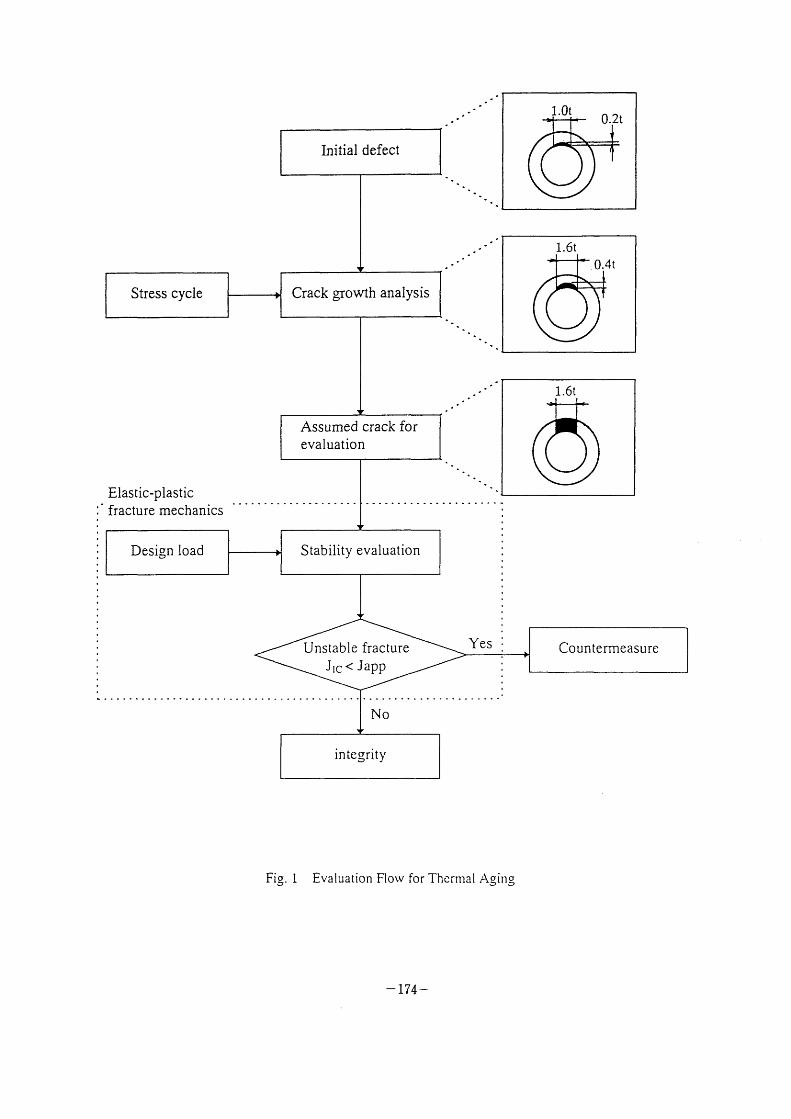
Initial defect

l.Ot 0.2t

Stress cycle Crack growth analysis

1.6t

0.4t

Elastic-plastic

fracture mechanics

Assumed crack for evaluation

Design load Stability evaluation

1.6t

Unstable fracture

No

Yes Countermeasure

integrity

Fig. l Evaluation Flo\v for Thcrmal Aging

- 174 -

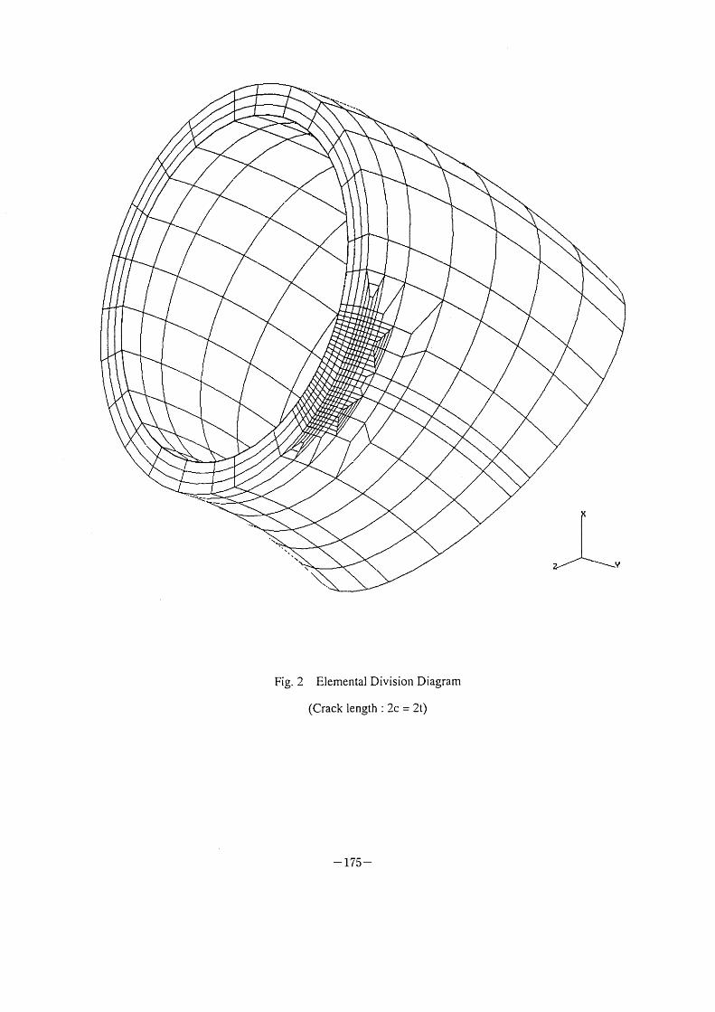
':tb

\,

~~

\ \ \ -~Y \ \1b

Fig. 2 Elemental Division Diagram

(Crack length : 2c = 2t)

- 175 -

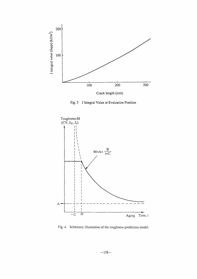
'f, ~a f::

~, *l !~:

~l 'F, ~ ~ {:3

'1 '~ ~) ::

> c:s

eJ) (:)

F,

200

lOO

Fig. 3

lOO '-OO Crack length (mm)

J Integral Value at Evaluation Position

300

Toughness:M (CV, Jlc, J6)

A~:F

ll

ll

ll

ll It\

lh IL I\ l \ l \ l \ l

l I [ l l l l l l I Il I ll l

I l l l l l 1-J I l

M=A+ B t+C

Fig. 4

-C tF Aging Time, t Schematic illustration of the toughness prediction model

- 176 -

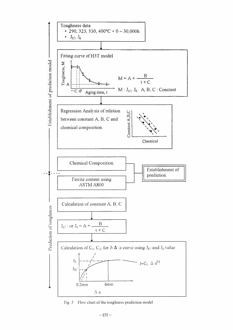
(L)

~:)

O fl r'

'-f,

O ,~ O ,~ *~,

O h, n~J1

~~, O

,-, ~:

O f, rl fl

,-, (1)

~ JD c~ '~ cl)

r7) cl)

fJ rl '-4 f,

'-, CU J O

O r' P~ '~_,

"~ -d O .'-1 '~* J .J

'-4

Colculation of constant A, B, C

T[ : or .T~= A + 13

t+c

calL;ulntlon ot Cl'

A / i

ll

'1~ r~~~~ /

/ T l ' ic~

C._ Ibr .T- A a cur\'c using .T[(] and .T6 \",lluc

~~~ J=CI L~ ac

O . 2 Tl~ rll

~~a

6 nl Tll

Fig. 5 FIO\\ Chal't Ol' IhC tOU~lllICSS pTCCllctiOll lllOdCl

- 177 -

800

700

rl

\ !4

l~ ,~ ::; fC::

~, ~J (L)

:3 ~-t

>

eJ) fJ

C ,,

600

5 oo

400

300

200

lOO

Fig. 6

4

J- A

8 12 16 20 Crack growth A a (mm)

a Curve (Hot Leg Pipe Material)

f~ Ql f'C:

.\ '1 .~'

'V

'l,

C~ C~~ C:5

'1

400

200

Jmat

JIC Japp

o l OO 2 O O

CTack length (mm)

30O

Crack length for

evaluation after service

period of 60 years

Fig. 7 Crack Stability Evaluation Diagram

- 178 -

IV-3 Fracture Behavior of Carbon Steel Pipe with Local Wall

Thinning Subjected to Bending Load

Katsumasa Miyazaki & Satoshi Kanno, Mechanical Engineering

Research Laboratory, Hitachi Ltd., Japan

Masayuki Ishiwata & Kunio Hasegawa, Hitachi Works, Hitachi Ltd ., Japan

Fracture Behavior of Carbon Steel Pipe with Local Wall Thinning

Subjected to Bending Load

Katsumasa Miyazaki, Satoshi Kanno, Mechanical Engineering Research Laboratory, Hitachi Ltd.

lbaraki, Japan

Masayuki Ishiwata and Kunio Hasegawa Hitachi Works, Hitachi Ltd.

lbaraki, Japan

1-1, Saiwal cho 3 chome Hrtachi shi lbarakl ken 317 Japan

ABSTRACT To evaluate the structural integrity of power plant piping, monotonic bending tests were

conducted on 4-inch diameter full-scale carbon steel pipe specimens with local wall thinning. The local wall thinning was simulated as a eroded part. Eroded part was subjected to tensile or compressive stress caused by applied bending load. The deformation or fracture behavior at maximum moments was classified into three types. When eroded part was subjected to tensile stress, ovalization and crack initiation was occurred. When eroded part was subjected to compressive stress, Iocal buckling occurred. When fracture behavior was ovalization or local buckling, the applied load decreased slightly form the maximum load. On the other hand,

in the case of crack initiation, the applied load was abruptly decreased from the maximum 10ad, because of circumferential crack propagation. The relationships between applied load and load line displacement for eroded pipes were compared with those for cracked pipes. The maximum loads and total displacement for the eroded pipes were higher than those for circunferentially cracked pipes. Maximum moments predicted using a net section stress approach gave overly conservative evaluation for pipe specimens with local wall thinning. Safety margin for locally thinned pipes was discussed compared with the design maximum load. The safety margin in this paper were roughly more than 2 times.

1. INTRODUCTION

Carbon steel is used extensively in piping systems in power plants. High temperature and high pressure water and steam flow at high velocities through these pipes. Erosion / corrosion

has caused wall thinning in high-energy carbon steel piping. It is important to evaluate the strength of piping with local wall thinning to maintain the integrity of the piping systems.

Burst and bending tests were performed on 6-inch diameter carbon steel pipes with local wall thinning by JAERI (Japan Atomic Energy Research Institute). From the experiment, it was found that fracture load was high, when locally thinned thickness of a pipe was the minimum required wall thickness defined in terms of design pressure (JAERI Report, 1993).

ASME (American Society of Mechanical Engineers) has considered the need to provide appropriate guidance to system engineers on the subject on erosion and erosion/corrosion in ferritic piping (Deardolff A. F., 1990). New criteria for acceptability of localized wall

- 179 -

thinning of piping components have been developed for inclusion in the ASME Boiler & Pressure Vessel Code, Section XI (ASME B&PV code, 1997a).

This study was undertaken in order to clarify the fracture behavior and strength of carbon steel pipes containing simulated local wall thinning to erosion/corrosion. Deformation

and fracture load for locally thinned pipes were compared with those for cracked pipes. The maximum moments were compared with the plastic collapse moments based on net section criteria. In addition, safety margins were discussed using design maximum load.

2. EXPERIMENTAL PROCEDURE

2.1 Material

The materials used in the experiments were carbon steel pipe called "Carbon steel pipe

for hrgh Pressure Servrce STS 410" m JIS (Japanese mdustnal Standards) , which are commonly used in coolant piping systems of nuclear power plants in Japan. The carbon steel, STS410 is similar to ASME A333 Gr.6. The yield strength and ultimate strength at ambient temperature were 326 MPa and 490 MPa, respectively for STS410.

2.2 Pipe Specimens

Full-scale experiments were performed on 4-inch diameter schedule 80 carbon steel pipes made of STS410 with local wall thinning. The pipe geometry and dimensions of local wall thinning are shown in Figure I and Table 2. The local wall thinning was machined on the inside of STS410 pipe. All local wall thinning to simulate erosion/corrosion thinning was

done by grinder machining. The eroded depth means metal loss depth in the thickness direction and the eroded angle was a circumferential wall thinning angle. The eroded length was an axial local wall thinning length which was roughly equal to the diameter of the 4-inch pipe .

2.3 Load Conditions

A static bending load without internal pressure was applied by four-point loading until maximum load appeared. The bending test apparatus was shown in Figure 2. The major span and minor span, respectively, were 960 mm and 300 mm. Displacement velocity at cross head was O. I mm/s. The total elapsed time from start of loading until fracture ranged from 10 to 20

minutes. The experiments were conducted at ambient temperature. The eroded area of the local wall thinning was located such that its center coincided

with the plane of maximum bending moment. There were two types of bending loads; for the majority of specimens, bending tensile stresses were applied to the locally eroded areas, bending were applied to the locally eroded areas of the other pipe specimens. Figure 2 showed an example of a pipe in which the tensile stress occurred at the eroded thinned area.

3. TEST RESULTS

3.1 Load - Displacement Curves

The maximum moments for all specimens are shown in Table 2. Eight pipe specimens applied tensile stress at locally eroded area, and two others applied compression stresses by four-point bending. In Table 2, the plastic collapse moment calculated based on net section

- 180 -

stress criteria and fracture behavior, described in detail later, were also listed.

The load-displacement curves for STS410 pipe specimens with local wall thinning subjected to tensile stress were shown in Figure 3. The fracture behavior was discussed later,

the eroded pipes subjected to tensile stress at eroded area showed two types of fracture behavior. One was ovalization, and the other was crack initiation with local necking at the eroded part. For Figure 3 (a), fracture behavior was ovalization (Specimens No. TP-5, TP-6 and TP-7). When fracture behavior was ovalization, the relationship between applied load and load line displacement remained the same in spite of difference of eroded area configuration. The maximum load was observed at about 80 mm in load line displacement.

For Figure 3 (b), fracture behavior was crack initiation (Specimens No. TP-3, TP-4 and TP-8). When the crack was initiated, the applied load dropped abruptly. In this case, the displacements of these specimens, after maximum load was applied, were very small, because crack propagated in the circumferential direction.

Load-displacement curves for pipe specimens (Specimens No. TP-9 and TP-ll) subjected to bending compressive stresses were shown in Figure 4, compared to the curves for the same local wall thinning geometry when tensile stress caused by bending moment was

applied. In Figure 4 (a), normalized eroded depth, d/t was 0.5 and eroded angle, 20 was 180" . On the other hand, normalized eroded depth, d/t was 0.8, erode angle, 2e was 180' ,

in Figure 4 (b). The maximum loads for TP-9 and TP-11, where compressive stress was applied to the eroded area, were less than those for the specimens subjected to tensile stress.

However, applied loads decreased slightly with increasing the displacement.

3.2 Fracture Behavior

When a local eroded area in a pipe was located on the tensile stress side, two types of fracture behaviors occurred at the maximum moments. When the eroded depth was shallow, ovalization occurred at the maximum moment. The fracture behavior of such an eroded pipe (specimen No. TP-6), occurring ovalization was shown in Figure 5. Crack initiation and growth at the eroded area were not observed at or after maximum moment. The load slowly decreased after maximum point accompanying deformation of ovalization. Total displacement was significantly large, when ovalization occurred.

When the eroded depth was deep, Iocal necking was observed first, then a crack initiated around the maximum load. The fracture behavior of the pipe (specimen No. TP-4) with deep eroded depth was shown in Figure 6. Local necking appeared in the local wall thinning area around the maximum load as shown in Figure 6 (a), and a crack initiated in the

local necking area and propagated circurnferentially as shown in Figure 6 (b). Total displacement after crack initiation was relatively small, and the load abruptly decreased. The crack initiation part after pipe fracture test was shown in Figure 7. The crack initiation point

agreed with the maximum eroded part. When the applied load increased, the maximum eroded part was necked. The crack initiation occurred, because of locally rupture at the

maximum eroded part. When the local eroded area was subjected compressive stress, Iocal buckling occurred

in the locally thinned area. Figure 8 is a photograph of local buckling (specimen No. TP-1 1),

which was taken after the un-loaded.

- 181 -

4. ANALYSIS OF EXPERIMENTS

4.1 Fracture Behavior at Maximum Load

Fracture behavior of pipes with local wall thinning can be classified into three types at

maximum load in case of receiving a monotonic bending moment; ovalization, Iocal necking-crack occurrence and local buckling .

When the eroded area in a pipe was subjected to tensile stress, ovalization or crack initiation occurred at the maximum load. The ovalization or crack initiation depended on the initial geometry of local wall thinning. The boundary between the ovalization and the crack initiation was illustrated in Figure 9. When eroded angle was large and depth was deep, Iocal

necking and crack initiation was observed. Crack was initiated at the maximum moment and propagated circumferentially after the maximum moment was reached. When the eroded area was short and thin, the pipe occurred ovalization at maximum moment, and showed a large degree of deformation.

Pipes containing a local erosion area with short angle and shallow depth showed high strength and a large degree of deformation. It seems reasonable to accept such eroded sizes below the straight line in Figure 9. It is conceivable that those were allowable local wall thinning sizes caused by erosion corrosion.

When the eroded area in a pipe was subjected to compressive stress, Iocal buckling occurred at and after the maximum moment, as shown in Figure 8. Although pipes subjected to compressive stress showed slightly less strength than with those subjected to tensile stress,

the degree of pipe deformation was large.

4.2 Counparison of Cracked Pipes

Four-point monotonic bending experiments were have been done on the same diameter carbon steel pipes with circunferential cracks at ambient temperature (Miyazaki, et al., 1996).

Testing machine and bending apparatus used for these experiments were the same as those shown in Figure 2. Also, the cracked pipes were made of the same material as the eroded pipe discussed in this paper.

The load-displacement curves for pipes with cracks, compared with the curves for pipes with local wall thinning, called eroded pipes, were shown in Figure 10. The cracks were through wall and part-through wall cracks. The crack angle and the eroded angle for both pipes were 2e = 60' . The maximum loads and total displacement for the eroded pipes were

higher than those for circumferentially cracked pipes.

4.3 Net Section Stress Approach

Fracture strength for a circumferentially cracked carbon steel pipes could be predicted by net-section stress approach (Kanno, et al., 1993). When the crack depth is d, and crack angle is 20, the plastic collapse moment Pc based on net section stress criteria is estimated by,

M 20 fR t(2sln P - d sinO) t

1 dO) P = ~(1C -t

pc = Mc 4(Lout ~ Lin )

(1)

(2)

(3)

- 182 -

where M* is the plastic collapse moment, t is the nominal vyall thickness, O is the eroded half

angle, R is the pipe mean radius, P is the neutral angle of the pipe, of rs the flow stress, Iout

was the major span and li~ was the minor span of the test apparatus. The flow stress was usually used as an average value of yield strength oy and ultimate strength o~. That is, the flow stress is defined as,

O Ov +0u

f 2 (4)

Maximum load Pwa* for circumferentially cracked carbon steel pipes can be accurately estimated from the plastic collapse moment calculated by Equations from (1) to (3).

Maximum moment, P~~* obtained in cracked pipe test and plastic collapse moment, P* calculated by Equations from (1) to (3) was compared in Figure 1 1 . The base material, STS410, used for cracked specimens was the same as that of the eroded pipes. The monotonic four-point bending tests using cracked pipe were performed at ambient temperature and at

265~C (Miyazaki, et al., 1996). The maximum load obtained from cracked pipe test was

slightly larger than plastic collapse load. It means that maximum load for a cracked pipe subjected to a bending moment can be predicted conservatively by Equations from ( 1) to (3).

The same technique was applied for locally eroded pipes, using Equations from (1) to (3). Plastic collapse load calculated from Equation from (1) to (3) was also listed in Table 2.

The relationship between maximum moment obtained from eroded pipe fracture tests and the plastic collapse moment was shown in Figure 12. When fracture behavior was ovalization, the ratio of maximum load to plastic collapse load, Pwa/P, was about 1.2. On the other hand, in case of crack initiation at eroded part subjected tension and local buckling at eroded part

subjected compression, P~~/P. was about from I .25 to I .85. The ratio of maximum load to plastic collapse load, P~*/P* , when occurring crack

initiation, was higher than that, when occurring ovalization. It means that maximum moments will be overly conservative, when applying the Equations from (1) to (3) for locally eroded

thinned pipes.

4.4 Safety Margin The primary stress for a pipe caused by a bending moment is designed to be less than

1 .5 S~ where S~ is the design stress given by ASME Boiler & Pressure Vessel Code Section III (ASME B&PV Code, 1997b) and MITI (Ministry of International Trade and Industry) Notification No. 501. The design stress S~ was 1 37N/mm2 for STS410. Then, I .5S~ = 206 N/mm2 for STS410 and 188 N/mm2 for STS370. The maximum design load, PD is given by,

MD = 1.5S~ X Z

PD = MD 4(Lout ~ Lin )

(5)

(6)

where MD is the design moment, Z is the section modules of the pipe. The maximum design load for 4-inch diameter carbon steel, STS410 were calculated using Equation from (5) to (7)

as,

PD = 88 kN for STS410 (4B, Schedule 80) (7)

- 183 -

The maximum moments in Table 2, the safety margins for eroded pipes tested in this paper were shown to be roughly more than 2 times.

5. CONCLUSIONS

Monotonic bending tests were conducted on 4-inch diameter full-scale carbon steel pipe specimens with local wall thinning at ambient temperature. It is concluded as follows;

1) Fracture behavior and sequence of fracture process for locally eroded pipes could be classified into three types; deformation of ovalization, Iocal necking - crack initiation -

propagation when tensile stress is applied to the eroded area, or local buckling during loading in case of compressive stress at the eroded area. It is conceivable that the locally

eroded sizes caused ovalization are allowable. 2) Fracture strength and total deformation of pipes with local wall thinning pipes

were higher than for the cracked pipes with the same depth and angle. 3) Net-section stress approach gives an overly conservative evaluation for pipes

containing locally wall thinning, as eroded area. The ratio of maximum load to plastic collapse load, P~~/P* , when occurring crack initiation, was higher than that, when occurring ovalization. It means that maximum moments will be overly conservative, when applying the Equations from (1) to (3) for locally eroded thinned pipes.

4) When comparing the maximum design moment, pipes with locally wall thinning have more than twice the safety margin compared with design load, even when eroded depth is 80 % of pipe wall thickness.

REFERENCES ASME 1997a "ASME Boiler & Pressure Vessel Code Sec. XI, Rules for Inservice

Inspection of Nuclear Power Plant Components". ASME, 1997b, " ASME Boiler & Pressure Vessel Code Sec. 111, Rules for Construction

of Nuclear Power Plant Components". Deardorff, A. F. and Bush, S. H., 1990, "Development of ASME Section XI Criteria for

Erosion-Corrosion Thinning of Carbon Steel Piping", ASME PVP PVP Vol 186 NDE Vol 7 pp.7 1 -75 .

Japan Atomic Energy Research Institute, 1993, "Technical Report on the Piping Reliability Tests at the Japan Atomic Energy Research Institute (Japanese)", JAERI-M, 93-076, pp, 104-1 15, May.

Kanno, K., Kimoto, H., Hayashi, M., Ishiwata M., Gotoh N Mrura N FuJroka T and Kahima K., 1993 "Low Cycle Fattgue Crack Growth and Ductile Fracture Under Dynamic /Cyclic Loadings for Japanese Carbon Steel Piping : Part I - Experimental Study", ASME PVP, PVP-Vol. 266, pp. 17 1-174.

Miyazaki, K., Kanno, S., Ishiwata, M., Gotoh, N., Miura, N., and Kashima K., 1996, "Fracture behavior under Monotonic and Low Cycle Loading in Carbon Steel Pipes and Welded Pipe Joints with a Defect" , ASME PVP, PVP-2 Fatigue and Fracture Vol. I , Book No. HO I 05 1 - 1 996.

- 184 -

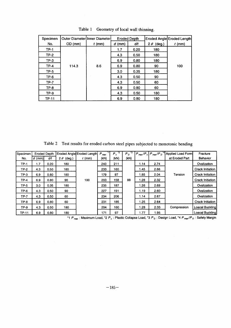
Table 1 Geometry of local wall thinning.

Table 2 Test results for eroded carbon steel pipes subjected to monotonic bending

tl Pmax ' Maximum Load, *2 Pc : Plastc Collapse Load, *3 PD : Design Load, *4 PmaxIPD : Safety Margin

- 185 -

.

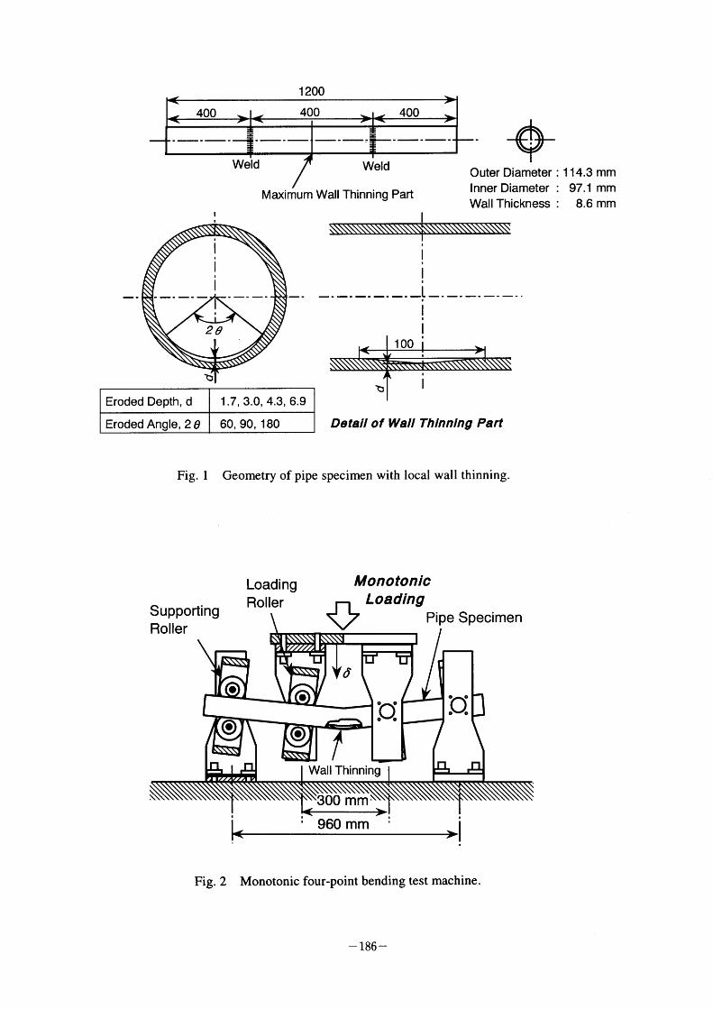
l

I

i

2e

~

1 200

Outer Diameter :

Maximum Wall Thinning Part Inner Diameter : Wall Thickness :

i

l

-. -[ -. -i

l

Fig. l

Detall of Wall Thlnnlng Part

Geometry of pipe specimen with local wall thinning.

1 14.3 mm 97.1 mm 8.6 mm

Supporting Roller

Loading Roller

Monotonic Load ing

~7 Pipe Specimen

e

@ e

@

(~

:O!

wau Thinning

ono oVo

~~~

l

300 mm~ 960 mm

Fig. 2 Monotonic four-point bending test machine.

- 186 -

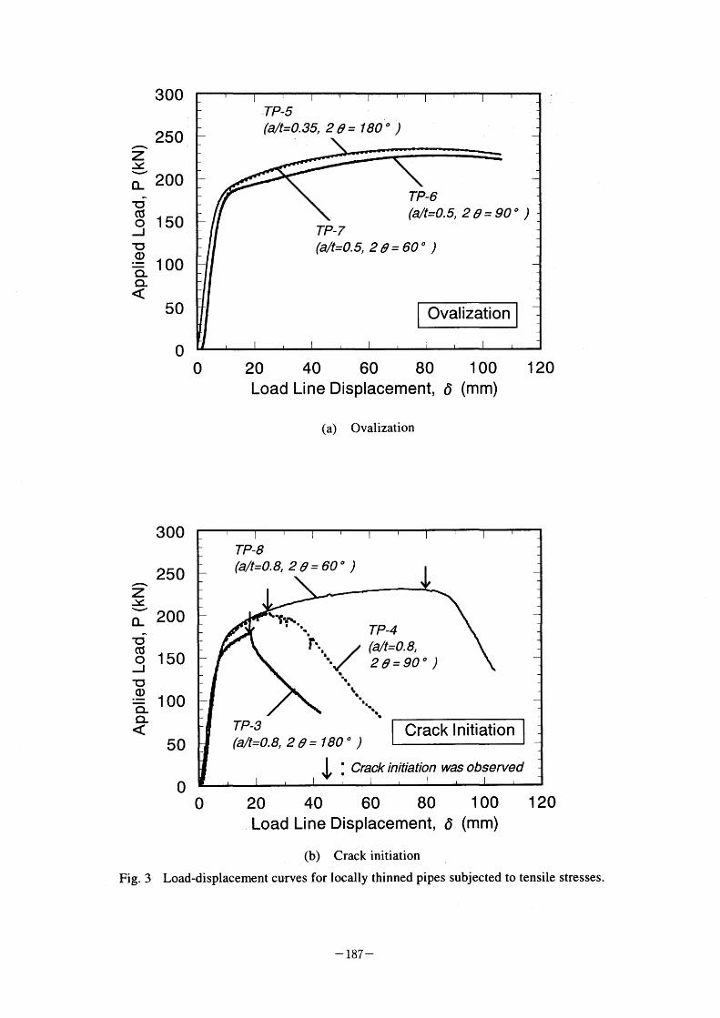
~ Z ~ O_ ~icc

o J ~1 o ,~ ~

300

250

200

1 50

1 OO

50

O

-TP-5 (alt=0.35, 2e= 180" )

TP-6 (alt=0.5, 2 e= 90 ' )

TP-7 (alt=0.5, 2e= 60 ' )

Ovalization

O 60 80 1 OO 20 40 Load Line Displacement, 6 (mm)

(a) 0+ah,ation

1 20

~ Z ~ ~ O_ 1:ca

o J ~ ~ CL

300

250

200

1 50

1 OO

50

O

(alt=0.8, 2 e= 180

~:

TP-8 (alt=0.8, 2 e= 60 ' )

~1'.,~. TP_4 ~ (alt=0. 8, f' '••••L/. 2 e = 90 " )

TP~3 crack Initiation .)

Crack initiation was observed

Fig. 3

O 20 40 60 80 1 OO 1 20 LOad Line Displacement, 6 (mm)

(b) Crack initiation

Load-displacement curves for locally thinned pipes subjected to tensile stresses.

- 187 -

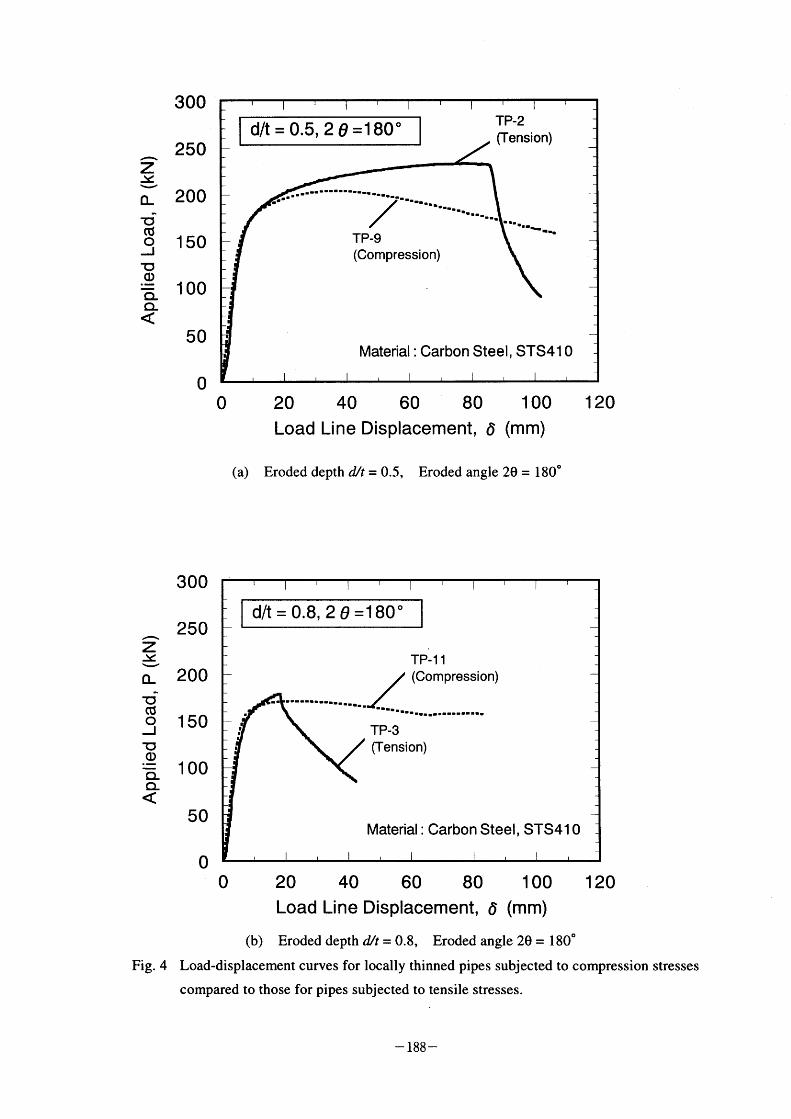
~ Z ~ ~ O_

~ c~l

o J 1:o

~ Q'

300

250

200

1 50

1 OO

50

O

d/t = 0.5, 2 O =1 80'

I

TP-2 CTension)

I'll 'IIIIIIII'llllllllllIIll"I'lllllIIIlll' I Il / I Ib' II' I 11 I

TP-9 (COmpresSlon)

Material : Carbon Steel, STS41 O

O 20 40 60 80 1 OO 1 20 Load Line Displacement, 6 (mm)

(a) Eroded depth d/It = 0.5. Eroded angle 20 = 180'

~ Z ~ O_

U CU

o J ~ o Q. Q.

300

250

200

1 50

1 OO

50

O

d/t = 0.8, 2 e =1 80-

TP-1 1

••_• •••_...... / (COmpresslon) ..

TP-3 (Tension)

Material : Carbon Steel, STS41 O

Fig. 4

80 1 OO Load Line Displacement, 6 (mm)

(b) Eroded depth d/It = 0.8. Eroded angle 20 = 180'

Load-displacement curves for locally thinned pipes subjected to compression stresses

compared to those for pipes subjected to tensile stresses.

- 188 -

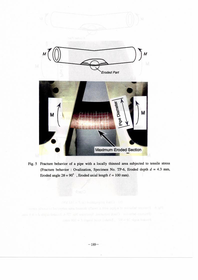
Eroded Part

~ S~:.~ t'~~-~ r~~: .:~~~ ~;f- ::T~ ~~=~ '

Maximum Eroded Section

Fig. 5 Fracture behavior of a pipe with a locally thinned area subjected to tensile stress

(Fracture behavior : Ovalization, Specimen No. TP-6, Eroded depth d = 4.3 mm,

Eroded angle 20 = 90' , Eroded axial length I = 100 mm).

- 189 -

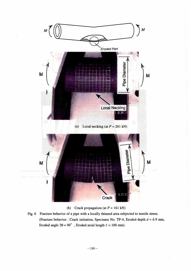
Eroded Part

M

Local Necking

~ 11~] ~*

d

M

(a) Local necking (at P = 20 1 kN)

M

',

)

o-

M

(b) Crack propagation (at P = 1 61 kN)

Fig. 6 Fracture behavior of a pipe with a locally thinned area subjected to tensile stress.

(Fracture behavior : Crack initiation, Specimen No. TP-4, Eroded depth d = 6.9 mm,

Eroded angle 20 = 90' , Eroded axial length I = 100 mm).

- 190 -

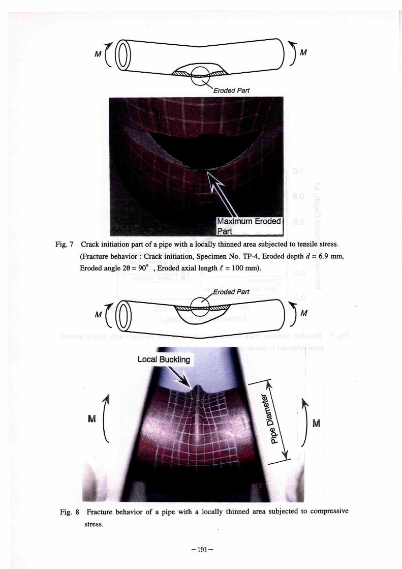
Eroded Part

Fig. 7 Crack initiation part of a pipe with a locally thinned area sbbjected to tensile stress.

(Fracture behavior : Crack initiation, Specimen No. TP-4, Eroded depth d = 6.9 mm,

Eroded angle 2e = 90' , Eroded axial length I = 100 mm).

Fig.

M

8 Fracture

stress'

l;: Local Buckling

Eroded Part

behavi or of a pipe with a locally thinned area

o~

~

subjected to

M

com pressive

- 191 -

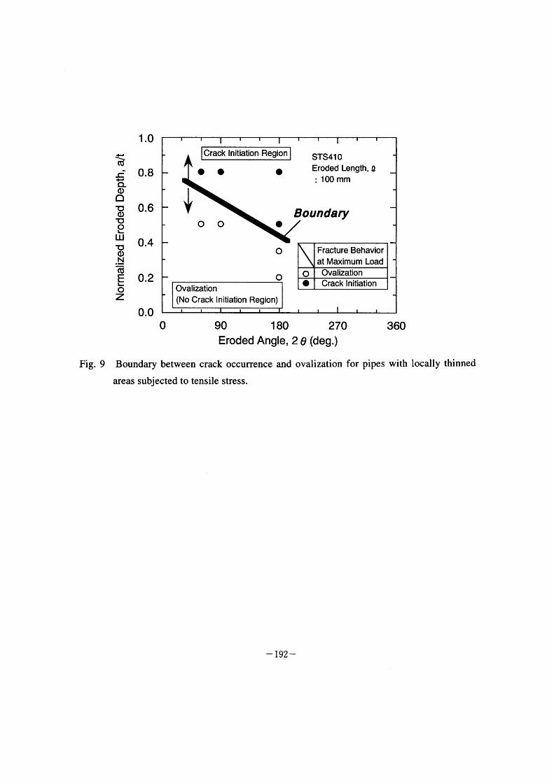
1 .O

~ ~~ E- 0.8 d~ 'l o O IDo 0.6 1~ o L LUU 0.4 ON

c~

EL 0.2 o Z

0.0

~

Crack Initiation Region

o o

o o

o

e

o

o

STS41 O Eroded Length, Q

1 OO mm

Bound ary

Ovalization

(NO Crack Initiation Region)

Fig. 9

1 80 270 360 Eroded Angle, 2 6 (deg.)

Boundary between crack occurrence and ovalization for pipes with locally thinned

areas subjected to tensile stress.

- 192 -

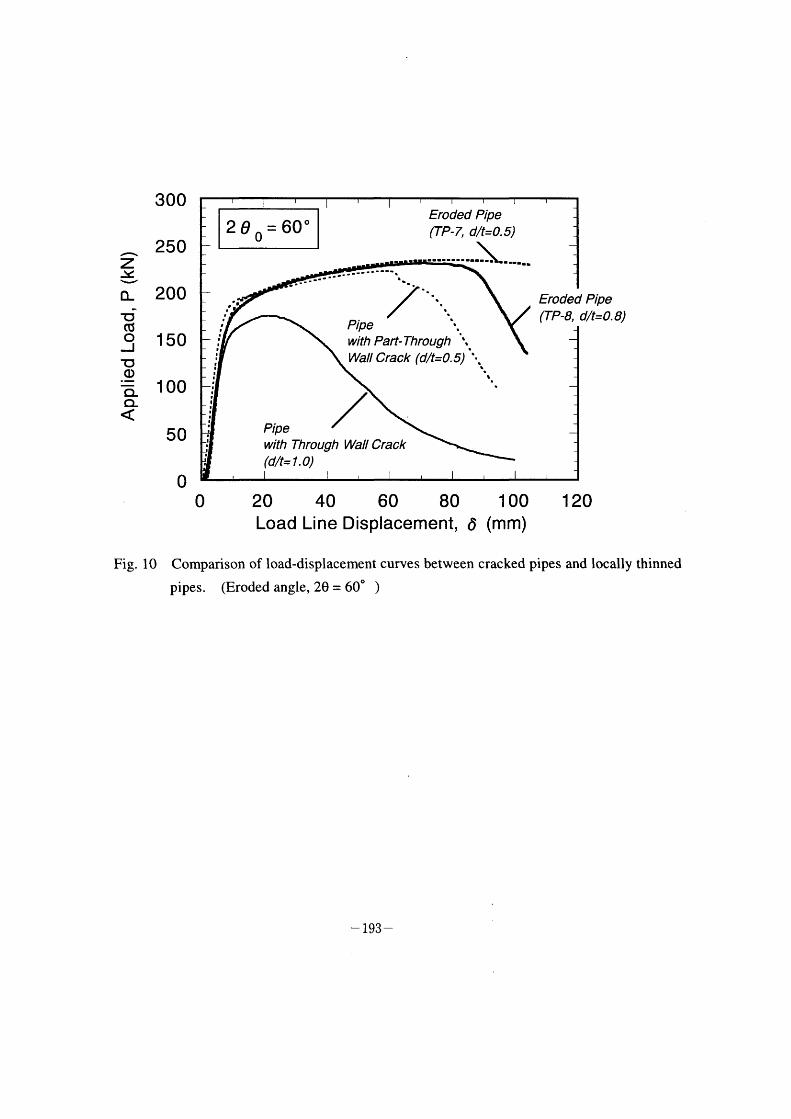
~ Z ~ CL ~lc:f

o J ~ o Q. ~

300

250

200

1 50

1 OO

50

O

2e O

l l

f l

, I

l l

I I

I

l , l

I

I I

I

I

lj f"

Eroded Pipe = 600 (TP-7, dlt=0.5)

Pipe ". with Part- Through ',

Wall Crack (dlt=0.5) '\

Pipe with Through Wall Cra ck (dlt-- I .O)

Eroded Pipe (TP-8, dlt=0. 8)

O 20 40 60 80 Load Line Displacement, 6

1 oo

(mm) 1 20

Fig. 10 Comparison of load-displacement curves between cracked pipes and locally thinned

pipes. (Eroded angle, 2e = 60' )

- 193 -

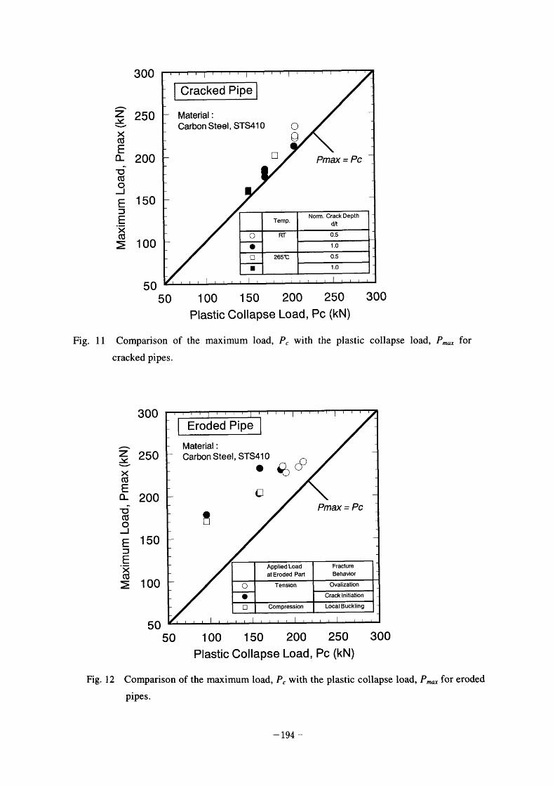
~ Z :~

~ as

E O_

~ c~f

S E

.=E_

~ ~

300

250

200

1 50

1 OO

50

Cracked Pipe

Material :

Carbon Steel , STS41 O

[l

o g

Pmax = Pc

o e

Temp.

RT

265lc

Norm. Crack Depth dlt

0.5

1 .o

0.5

1 .O

Fig. 1 1

50

Comparison

cracked pipes.

of

1 OO 1 50 200 250 Plastic Collapse Load, Pc (kN)

the maxrmum load, P, with the plastic

300

colla pse load, Pmax f or

~ Z ~ ~ ~ E O_

10 c~;

o J E

.E_

~ ~~

300

250

200

1 50

1 oO

50

Eroded Pipe

Material :

Carbon Steel, STS41 O

e C]

~

(~~

Pmax = Pc

O o []

Applied Load atEroded Part

Tension

Compression

Fracture

Behavior

Ovalization

Crack I nitiation

Local Buckling

Fig. 12

50 1 OO 1 50 200 250 300 Plastic Collapse LOad, Pc (kN)

Comparison of the maximum load. P. wrth the plastrc collapse load P. for eroded

pi pes.

- 194 --

I V-4 Leak-Before-Break Assessment of CANDU Pressure Tube

Consid~ring Leak Detection Capability

Youn-Won Park and Yeon-Ki Chung, Korea Institute of \_ ~uclear Safe~', Korea

Leak-Before-Break Assessment of CANDU Pressure Tube Considering Leak Detection Capability

Youn-Won Park and Yeon-Ki Chung Korea Institute of Nuclear Safety

19 Kusung-dong Yousung-ku Taejon, Korea, 305-338

Abstract

The LBB(Leak Before Break) concept is employed as defense in depth in CANDU reactors in order to avoid an unstable failure in pressure tubes. The LBB in pressure tubes can be satisfied when detection, confirmation, and loeation of the leak are canied out and the reactor

is placed in a depressurized condition before the crack exeeeds critical crack length. Leak

detection and location is provided by the Annulus Gas System. Therefore, the input parameters for LBB analysis, such as leak detection and leak location eapabilities, should be made available through AGS in-situ test. Recently, a simulated moisture inj ection test has

been performed in one of the CANDU reactors in Korea, and the LBB assessment was perfonned using the test results. Only leak detection eapability is considered for LBB analysis; the leak location is ruled out beeause of lack of information in the AGS response vis-a-vis leak location procedure. In this paper LBB assessment is presented using both the leak detection and leak location eapability,

1. Introduction

Since several ineidents of leaking in the pressure tubes in the CANDU reactors have been experienced, significant efforts have been made to improve the pressure tube integrity through design, material, and fabrieation upgrades during last deeade.

However, delayed hydride craeking (DHC) is still believed to be the major potential threat to pressure tube integrity. To cope with the likelihood of loss of pressure tube integrity due to

sueh DHC, Leak-Before-Break (LBB) is used as a defense-in-depth. The flaw acceptance eriteria for pressure tubes, provided by the Fitness For Service Guidelines, (FFSG)[1] requires demonstration that DHC will not oceur from flaws in pressure tubes when the hydrogen equivalent concentration exceeds the Terminal Solid Solubility (TSS) for dissolution at full power operating condition, and that if the flaw was propagated by DHC, unstable rupture of the pressure tube is avoided by LBB.

The LBB coneept requires timely detection, confirmation of leak, and appropriate operator aetion to shut the reactor down to a cold depressurized state before the growing craek exceeds

the critieal erack' Iength (CCL). Since the typical CANDU reaetor consists of 380 to 480 pressure tubes, even though a leak is detected in time and the reactor is cooled down, it is not

so easy to locate the tube eoncerned. This is beeause once the reaetor is in a depressurized condition, the crack closes and the leak is near impossible to fmd. Unless the leaking tube is identified, an entire core inspection is necessary at a cold state. This is very difficult, time

consuming, and expensive. Therefore, Ieak deteetion and leak location are important from an integrity viewpoint as well as eeonomical standpoint. Normally, only the leak detection is considered in the LBB analysis because there is not enough data for leak location tests[2]. During the pre-operational test of Wolsung unit 2, a complete set of tests for leak detection

- 195 -

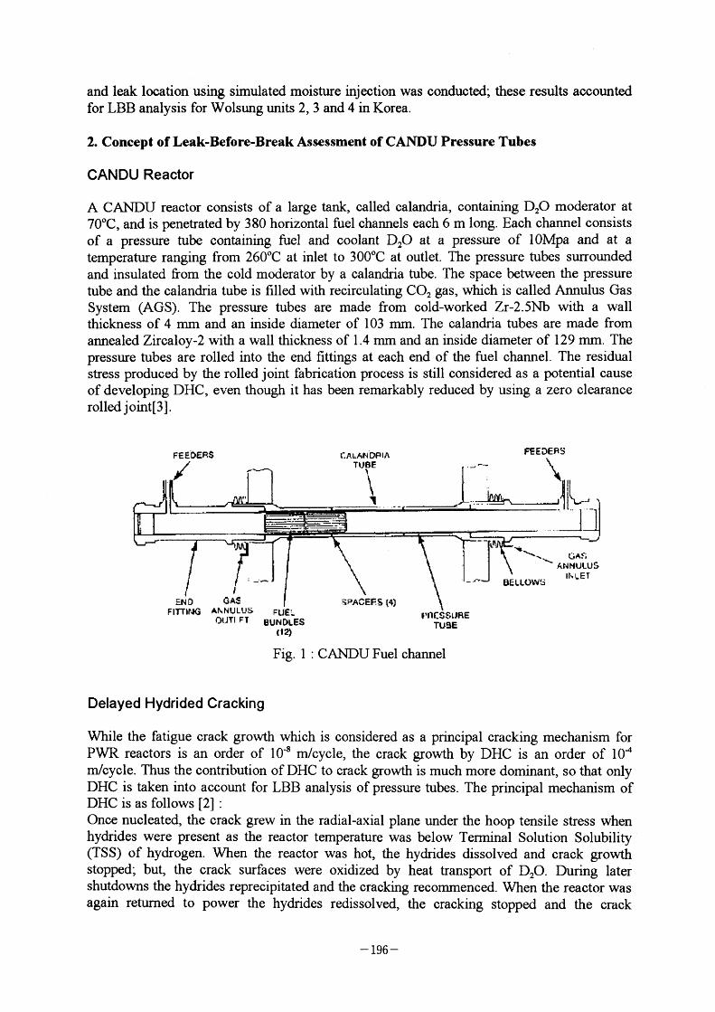
and leak location using simulated moisture inj ection was conducted; these results aGCOunted for LBB analysis for Wolsung units 2, 3 and 4 in Korea.

2. Concept of Leak-Before-Break Assesslnent of CANDU Pressure Tubes

CANDU Reactor

A CANDU reaetor consists of a large tank, called calandria, oontaining D20 moderator at 70"C, and is penetrated by 380 horizontal fuel channels each 6 m long. Each channel consists

of a pressure tube containing fuel and coolant D20 at a pressure of I OMpa and at a temperature ranging from 260~C at inlet to 300~C at outlet. The pressure tubes surrounded and insulated from the cold moderator by a ealandria tube. The spaee between the pressure tube and the calandria tube is filled with recirculating C02 gas, whieh is called Annulus Gas

System (AGS). The pressure tubes are made from cold-worked Zr-2.5Nb with a wall thickness of 4 mm and an inside diameter of I 03 mm. The calandria tubes are made from annealed Zircaloy-2 with a wall thickness of I .4 mm and an inside diameter of 1 29 nun. The pressure tubes are rolled into the end fittings at each end of the fuel ehannel. The residual stress produced by the rolled j oint fabrication process is still considered as a potential cause

of developing DHC, even though it has been remarkably reduced by using a zero elearance rolled j oint[3 1 -

FEEOERS CALA~l DP IA TVBE

FEEDEAS

FI~Ird(5 AhNULUS Ol.]TI FT

F UE L

EUNDLES C12)

Fig• 1

t'lICS.ct,L]RE

TUSE

CANDU Fuel channel

,,

J

Delayed Hydrided Cracking

While the fatigue crack growth which is considered as a principal cracking mechanism for PWR reactors is an order of I 0-8 m/cycle, the erack growth by DHC is an order of I 04 m/cyele. Thus the contribution of DHC to crack growih is mueh more dominant, so that only DHC is taken into account for LBB analysis of pressure tubes. The principal mechanism of DHC is as follows [2] :

Once nucleated, the crack grew in the radial-axial plane under the hoop tensile stress when hydrides were present as the reactor temperature was below Terminal Solution Solubility (TSS) of hydrogen. When the reactor was hot, the hydrides dissolved and crack growth stoppedj but, the crack surfaces were oxidized by heat transport of D20. During later shutdowns the hydrides reprecipitated and the cracking recommenced. When the reactor was again returned to power the hydndes redissolved, the eracking stopped and the crack

- 196 -

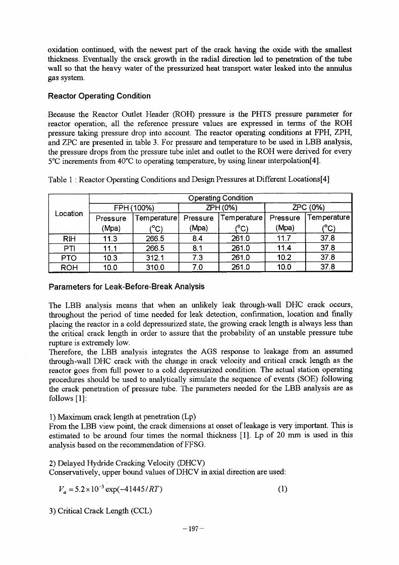
oxidation GOntinued, with the newest part of the crack having the oxide with the smallest thickness. Eventually the crack growth in the radial direction led to penetration of the tube wall so that the heavy water of the pressurized heat transport water leaked into the annulus

gas system.

Reactor Operating Condition

Because the Reactor Outlet Header (ROH) pressure is the PHTS pressure parameter for reactor operation, all the reference pressure values are expressed in terms of the ROH pressure taking pressure drop into account. The reactor operating conditions at FPH, ZPH, and ZPC are presented in table 3 . For pressure and temperature to be used in LBB analysis, the pressure drops from the pressure tube inlet and outlet to the ROH were derived for every 5'C increments from 40'C to operating temperature, by using linear interpolation[4]-

Table I : Reactor Operating Conditions and Design Pressures at Different Locations[4]

Parameters for Leak-Before-Break Analysis

The LBB analys'is means that when an unlikely leak through-wall DHC crack occurs, throughout the period of time needed for leak detection, eonfirmation, Iocation and finally plaeing the reactor in a cold depressurized state, the growing crack length is always less than the critical crack length in order to assure that the probability of an unstable pressure tube

rupture is extremely low. Therefore, the LBB analysis integrates the AGS response to leakage from an assumed through-wall DHC crack with the change in crack velocity and critical crack length as the reactor goes from full power to a cold depressurized condition. The actual station operating procedures should be used to analytieally simulate the sequence of events (SOE) following the crack penetration of pressure tube. The parameters needed for the LBB analysis are as follows [ I J :

l ) Maximum crack length at penetration (Lp) From the LBB view point, the crack dimensions at onset ofleakage is very important. This is estimated to be around four times the normal thickness [ I J . Lp of 20 mm is used in this

analysis based on the recommendation of FFSG.

2) Delayed Hydride Cracking Velocity (DHCV) Conservatively, upper bound values of DHCV in axial direction are used:

V 5 2xlO exp(-414451RT) (1) 3) Critical Crack Length (CCL)

- 197 -

The half-critical crack length (c), as a function of temperature, stress, fluence, and hydrogen

concentration, can be determined from the following equation:

K ~ f T

C - 2Ma 8af2 In[sec( h )] 2 cr f

ah = P(L + l)

w

(2)

(Ty + au

(Tf~ 2

M =[1+1.255(c2 /(r~w))-(0.0135(c /r~w) (O 0135(c /(r~w)2]1/2

4) Leak Rate A correlation of D20 Ieak rate (kg/hr) with eraek length (mm) is given:

Q = -1 1 .2 + 0.0014(2C)3 (3) where, 2C~~ = maximum axial crack length (mm)

This equation is based on PHTS operating conditions of 6MPa and 250~C. Thus, specific conditions other than 6MPa and 250~C, Ieak rates ean be determined using sealing coefficients.

5) Station Response to Moisture in AGS The time needed to detect, confirm, and loeate the leak should be provided. Following the first leak at penetration, the time necessary for initiating the rate of rise alarm is taken from

the AGS performance test carried out at Wolsung unit 2 in May 1 997. The AGS performanee test and its results will be described later on.

6) Pressure tube dimension For a conservative approach, pressure tube dimensions were taken from expected values after

l 5 years of operation [4]• Installed thickness is based on the minimum specified dimension of 4. 1 9 mm, subtraeting both the corrosion allowance of O. 1 40 mm and wear allowance of 0.064

mm. Dimensions after 1 5 years of operation are made by considering an additional wall thinning of O. 1 49 mm and a diametral creep strain of 2. I O/o. The wall thickness is also made

by considering a local wear of 0.028 mm due to the annulus spacer rolling. At the end of 1 5-

year serviee, the wall thickness is 3.83 mm, the maximum imer radius is 53.37 mm, and the mean radius is 57.20 mm.

Assumptions used for LBB analysis[5]

l ) The most likely area for DHC crack to oceur is inboard of the rolled j oint; because of relatively high residual stress. The crack growtll in one direction should be stopped due to restraint when the crack arrives at the rolled joint. However, to be conservative, the DHC craek growih is assumed in both directions throughout the event.

2) The crack is to propagate at the upper bound crack velocity 3) A Iower bound estimate of critical craek length and fracture toughness is used

4) The pressure tube leak oeeurs in the longest AGS ehaunel and the AGS is operated in very Iow recirculation flow. This leads to a longer moisture detection time.

5) There are sufficient hydrides at power for crack growth to oecur.

6) The pressure tube dimension of 1 5 years in operation is used for accounting for the wear and corrosion allowances, and the diametral creep and wall thinning.

- 198 -

3. Leak Detection and Location Capability Test

Leak detection in a pressure tube is provided by the Aunulus Gas System (AGS). The AGS circulates dry C02 gas in the aunular space between the calandria tubes and pressure tubes. The fuel channel annuli are connected in a series/parallel configuration to fonn a closed loop

as shown in Figure 2. There are 44 inlets conneeted, in parallel, to the recirculating gas supply system and 44 outlets connected, in parallel, to the drain and the suction side of the recirculating compressors.

A total of ten tests were completed[6]. Seven were moisture injection tests to determine system dew point versus time response with continuous injection until the dew point increased to - I O'C. Three of the ten tests were to measure the change in dew point response to leaking valve in and out proeess. The main purpose of the leak location test was to qualify the AGS abnormal operating proeedure to be used for identifying leak channels.

44 Inlet Tubes

Reactor 380 Channel

Annuli in SeTies/Parallel

3 to 11

1 1 Stnng

channel

4 Bank

O

O

Dew Point M ete r

O Compressor

Beetle

Fig. 2 : Aknnulus Gas System Configuration

Leak Detection Test

Of the seven moisture injection tests, three tests were conducted with the Primary Heat Transport System (PHTS) cold and four tests with PHTS Zero Power Hot (ZPH). Table l shows the test matrix for leak detection and leak location.

Test 1, 2, and 3

The first injection was carried out in the main circuit at the downstream of the compressors and upstream of the gas distribution manifolds. The injected D20 and C02 gas was therefore distributed to all the 44 strings. The purpose ofthese tests was to investigate dew point versus

- 199 -

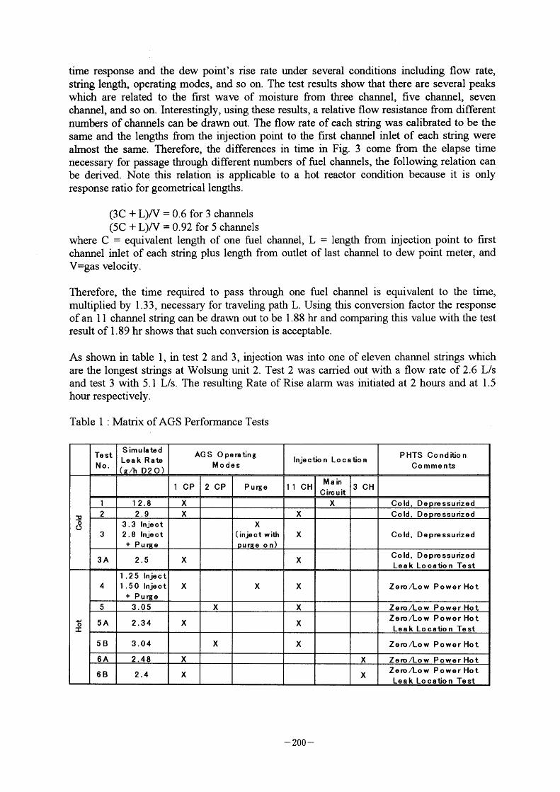
time response and the dew point's rise rate under several conditions including flow rate, string length, operating modes, and so on. The test results show that there are several peaks

which are related to the first wave of moisture from three channel, five channel, seven channel, and so on. Interestingly, using these results, a relative flow resistance from different

numbers of channels can be drawn out. The flow rate of each string was calibrated to be the same and the lengths from the inj ection point to the first channel inlet of each string were

almost the same. Therefore, the differences in time in Fig. 3 come from the elapse time neGessary for passage through different numbers of fuel channels, the following relation Gan be derived. Note this relation is applicable to a hot reactor condition because it is only response ratio for geometrical lengths.

(3C + L)N = 0.6 for 3 ehannels (5C + L)N = 0.92 for 5 chaunels

where C = equivalent length of one fuel channel. L = Iength from injection point to first channel inlet of each string plus length from outlet of last ehannel to dew point meter, and

V=gas velocity.

Therefore, the time required to pass through one fuel channel is equivalent to the time, multiplied by I . 3 3 , neeessary for traveling path L. Using this conversion factor the response

of an I I channel string can be drawn out to be I .88 hr and eomparing this value with the test result of I . 89 hr shows that such eonversion is acceptable.

As shown in table I , in test 2 and 3 , injection was into one of eleven channel strings which

are the longest strings at Wolsung unit 2. Test 2 was carried out with a flow rate of 2.6 L/s and test 3 with 5. I L/s. The resulting Rate of Rise alarm was initiated at 2 hours and at I . 5

hour respectively.

Table I : Mainx ofAGS Performance Tests

- 200 -

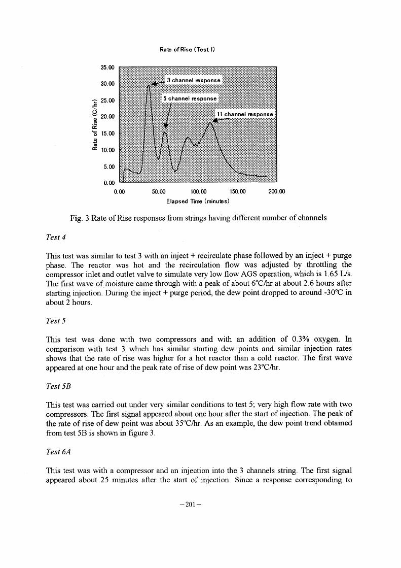
Rale of Rise (Test 1)

35. OO

30. OO

- 25.00 ~ \ o o 20.00 ~ i~

~ o 15.00 ~o

az 1000

5. OO

O. OO

O. OO

~; 5 channel response ;

11 channel response j

50. OO I OO. OO 1 50. OO Elapsed Time (minutes)

200. OO

Fig. 3 Rate of Rise responses from strings having different number of chaunels

Test 4

This test was similar to test 3 with an inject + recirculate phase followed by an inject + purge

phase. The reactor was hot and the recirculation flow was adjusted by throttling the compressor inlet and outlet valve to simulate very low flow AGS operation, which is I .65 L/s. The flrst wave of moisture came through with a peak of about 6'C/hr at about 2.6 hours after starting injection. During the inject + purge period, the dew point dropped to around -30'C in

about 2 hours .

Test 5

This test was done with two compressors and with an addition of 0.30/0 oxygen. In comparison with test 3 which has similar starting dew points and similar injection rates shows that the rate of rise was higher for a hot reactor than a cold reactor. The first wave appeared at one hour and the peak rate of rise of dew point was 23~C/hr.

Test 5B

This test was carried out under very similar conditions to test 5 ; very high flow rate with two

eompressors. The frrst signal appeared about one hour after the start of injection. The peak of

the rate of rise of dew point was about 3 5~C/hr. As an example, the dew point trend obtained

from test 5B is shown in figure 3 .

Test 6A

This test was with a compressor and an inj ection into the 3 channels string. The first signal

appeared about 25 minutes after the start of injection. Since a response corresponding to

- 201 -

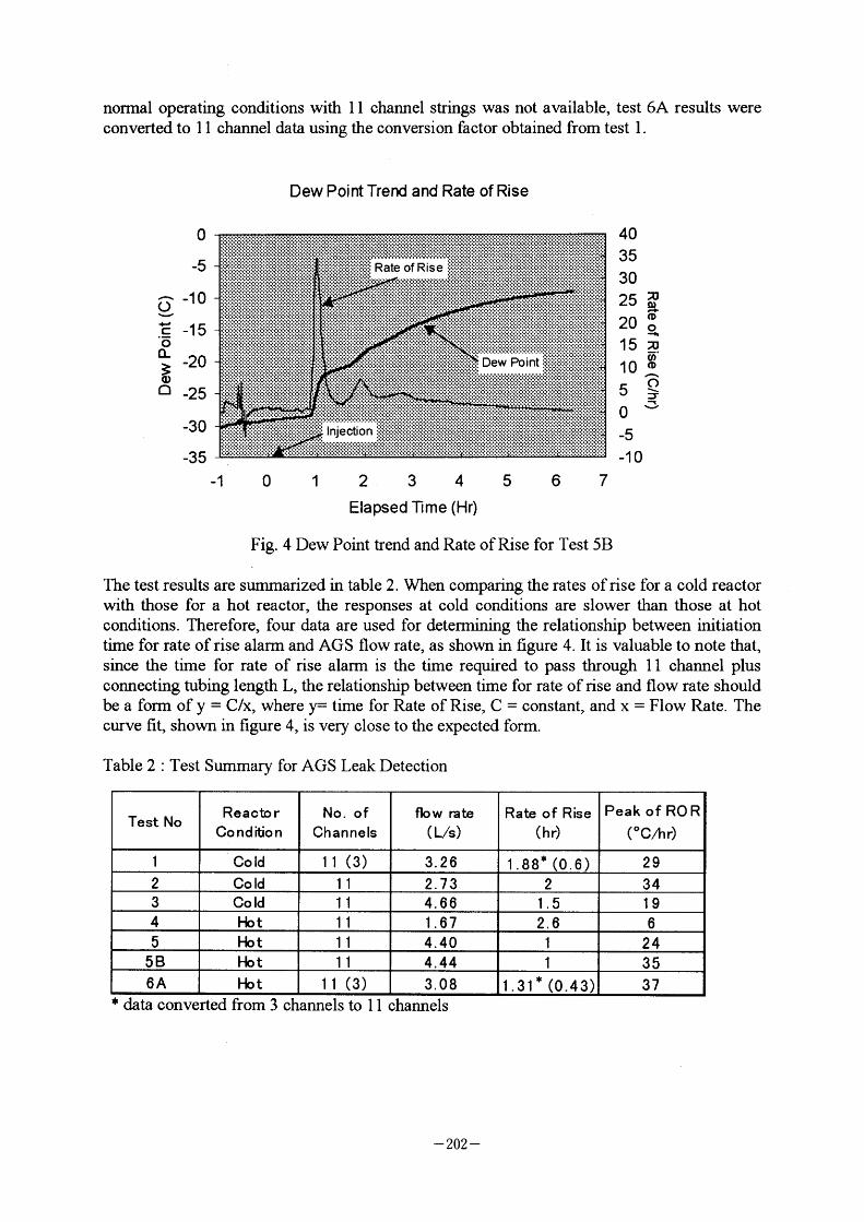
normal operating conditions with I I channel strings was not available, test 6A results were converted to I I channel data using the conversion factor obtained from test I .

Dew Point Trend and Rate of Rise

~ O ~ 4' .5

~ (D~

a

O

-5

-1 O

-1 5

-2 O

-2 5

-30

-35 -1 o

; Rate of Rise i

1 2 3 4 5 Elapsed Time (Hr)

6 7

40 35 30 25 ~ 20 (DO

~ 15 ;a ~5'

10 ;~

5~ * O~ -5

-1 O

Fig. 4 Dew Point trend and Rate of Rise for Test 5B

The test results are summarized in table 2. When eomparing the rates of rise for a cold reactor

with those for a hot reactor, the responses at cold eonditions are slower than those at hot conditions. Therefore, four data are used for determining the relationship between initiation time for rate of rise alarm and AGS fiow rate, as shown in figure 4. It is valuable to note that,

since the time for rate of rise alann is the time required to pass through I I channel plus conneoting tubing length L, the relationship between time for rate of rise and flow rate should

be a form of y = C/x, where r time for Rate of Rise, C = constant, and x = Flow Rate. The curve fit, shown in figure 4, is very close to the expected form.

Table 2 : Test Sununary for AGS Leak Deteetion

* data converted from 3 channels to I I channels

- 202 -

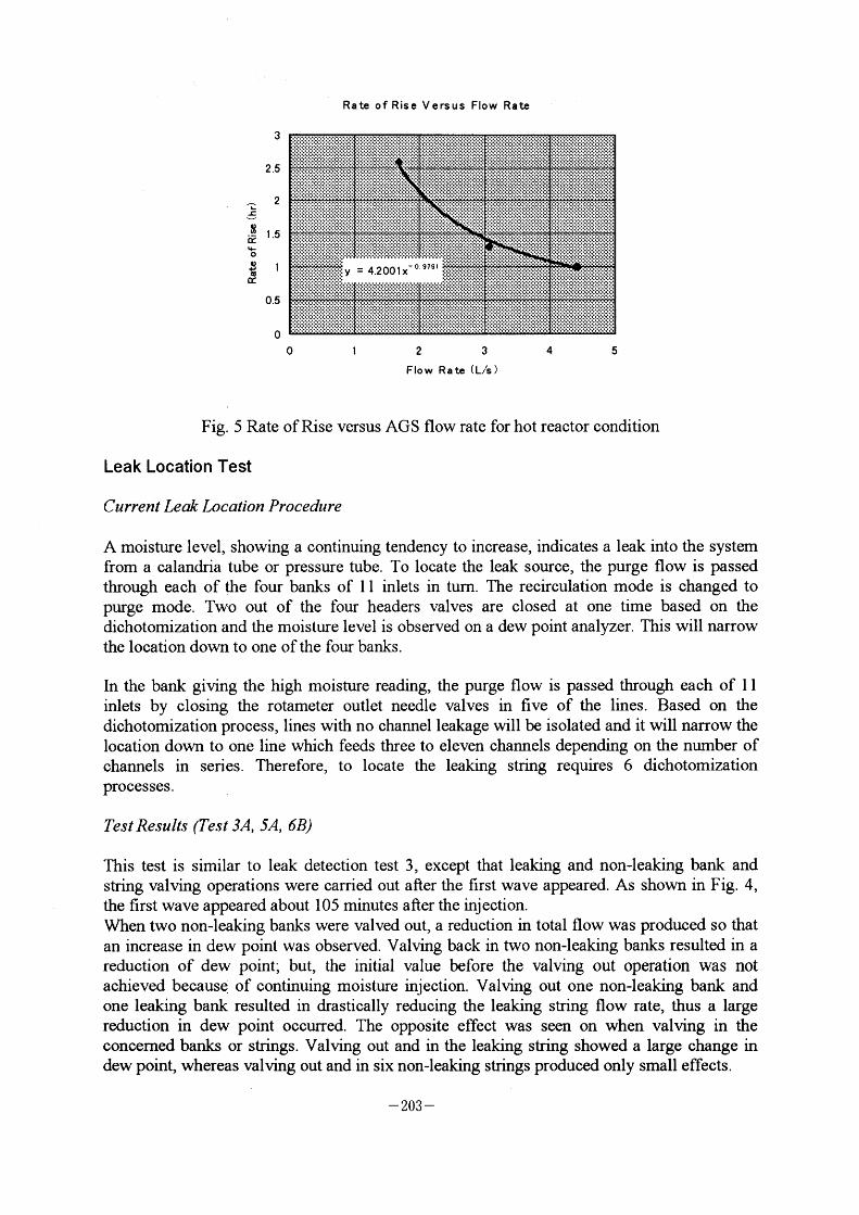
Rate of Rise Versus Flow Rate

J~

8 if

~ o ~ co

OC

3

2 .5

2

1 .5

O.5

O o 1 2 3

Flow Rate (L/s)

4 5

Fig. 5 Rate of Rise versus AGS flow rate for hot reactor eondition

Leak Location Test

Current Leak Location Procedure

A moisture level, showing a continuing tendency to increase, indicates a leak into the system from a calandria tube or pressure tube. To locate the leak source, the purge flow is passed through each of the four banks of I I inlets in turn. The recirculation mode is changed to purge mode. Two out of the four headers valves are closed at one time based on the dichotomization and the moisture level is observed on a dew point analyzer. This will narrow

the location down to one of the four banks.

In the bank giving the high moisture reading, the purge flow is passed through eaeh of I l inlets by closing the rotameter outlet needle valves in five of the lines. Based on the dichotomization process, Iines with no channel leakage will be isolated and it will narrow the

10cation down to one line which feeds three to eleven chaunels depending on the nuniber of channels in series. Therefore, to locate the leaking string requires 6 diehotomization

processes.

TestResults (Test 3A, 5A, 6B)

This test is similar to leak deteetion test 3 , except that leaking and non-leaking bank and string valving operations were carried out after the frrst wave appeared. As shown in Fig. 4, the first wave appeared about I 05 minutes after the inj ection.

When two non-leaking banks were valved out, a reduction in total flow was produced so that an increase in dew point was observed. Valving back in two non-leaking banks resulted in a reduction of dew point; but, the initial value before the valving out operation was not achieved beeaus~ of continuing moisture injection. Valving out one non-leaking bank and one leaking bank resulted in drastically reducing the leaking string flow rate, thus a large

reduction in dew point occurred. The opposite effect was seen on when valving in the concerned banks or strings. Valving out and in the leaking string showed a large change in dew point, whereas valving out and in six non-leaking strings produced only small effects.

- 203 -

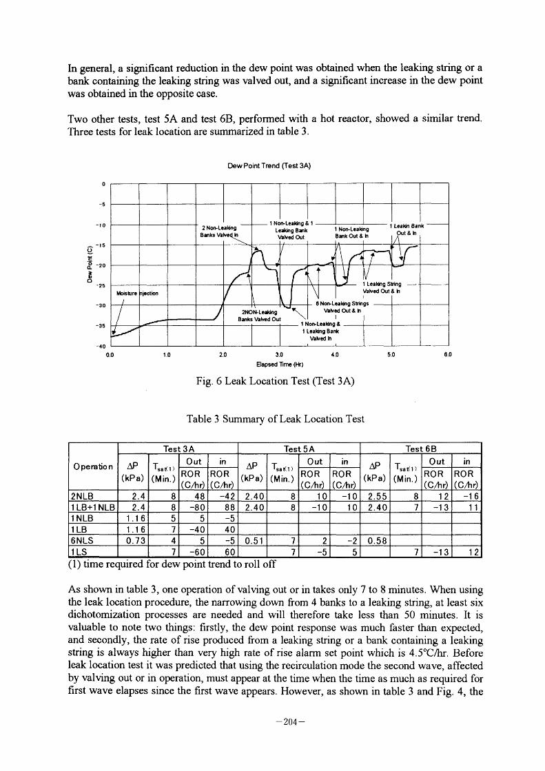
In general, a significant reduotion in the dew point was obtained when the leaking string or a bank containing the leaking string was valved out, and a significant increase in the dew point

was obtained in the opposite ease.

Two other tests, test 5A and test 6B, performed with a hot reactor, showed a similar trend. Three tests for leak location are summarized in table 3 .

Dew Point Trend Crest 3A)

o ~~

8 ~ o

O

-5

-10

-15

-20

-25

-30

-35

-40 0.0 1 .O 3.0

Elapsed Tlrne (Hr)

Fig. 6 Leak Location Test (Test 3A)

5.0 6.0

Table 3 Summary ofLeak Location Test

( I ) time required for dew point trend to roll off

As shown in table 3 , one operation of valving out or in takes only 7 to 8 minutes. When using the leak location proeedure, the narrowing down from 4 banks to a leaking string, at least six dichotomization processes are needed and will therefore take less than 50 minutes. It is valuable to note two things: firstly, the dew point response was much faster than expeeted, and secondly, the rate of rise produced from a leaking string or a bank containing a leaking string is always higher than very high rate of rise alarm set point which is 4.5'C/hr. Before leak location test it was predicted that using the recireulation mode the second wave, affected

by valving out or in operation, must appear at the time when the time as much as required for first wave elapses since the first wave appears. However, as shown in table 3 and Fig. 4, the

- 204 -

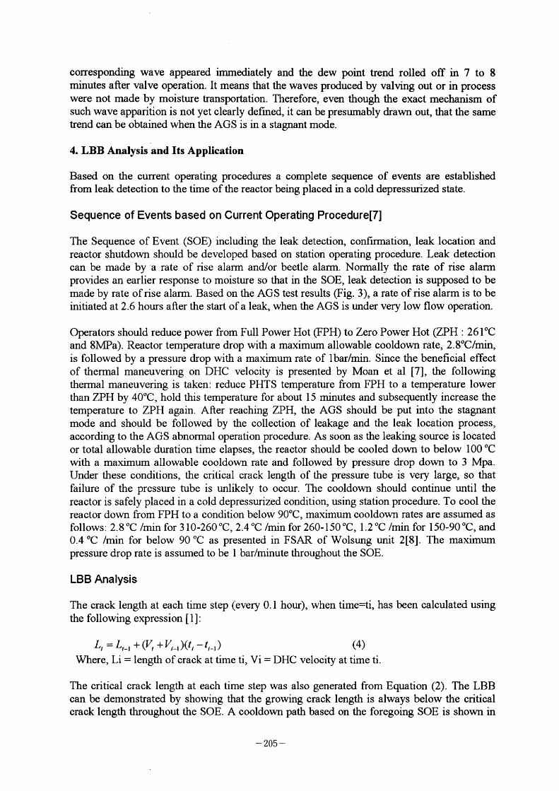
corresponding wave appeared immediately and the dew point trend rolled off in 7 to 8 minutes after valve operation. It means that the waves produced by valving out or in process

were not made by moisture transportation. Therefore, even though the exact mechanism of such wave apparition is not yet clearly defmed, it can be presumably drawn out, that the same trend can be obtained when the AGS is in a stagnant mode.

4. LBB Analysis and Its Application

Based on the current operating procedures a complete sequenoe of events are established from leak detection to the time of the reactor being placed in a oold depressurized state.

Sequence of Events based on Current Operating Procedure[7]

The Sequence of Event (SOE) including the leak detection, confrrmation, Ieak location and reactor shutdown should be developed based on station operating procedure. Leak detection can be made by 'a rate of rise alarm and/or beetle alarm. Normally the rate of rise alarm provides an earlier response to moisture so that in the SOE, Ieak detection is supposed to be made by rate of rise alarm. Based on the AGS test results (Fig. 3), a rate of rise alarm is to be

initiated at 2.6 hours after the start of a leak, when the AGS is under very low flow operation.

Operators should reduce power from Full Power Hot (FPH) to Zero Power Hot (ZPH : 26 1 'C and 8MPa). Reactor temperature drop with a maximum allowable cooldown rate, 2.8'C/min, is followed by a pressure drop with a maximum rate of I bar/min. Since the beneficial effect

of thermal maneuvering on DHC velocity is presented by Moan et al [7], the following thermal maneuvering is taken: reduce PHTS temperature from FPH to a temperature lower than ZPH by 40'C, hold this temperature for about 1 5 minutes and subsequently increase the temperature to ZPH again. After reaching ZPH, the AGS should be put into the stagnant mode and should be followed by the colleetion of leakage and the leak location process, according to the AGS abnormal operation procedure. As soon as the leaking source is located or total allowable duration time elapses, the reaotor should be cooled down to below I OO 'C

with a maximum allowable cooldown rate and followed by pressure drop down to 3 Mpa. Under these conditions, the critieal crack length of the pressure tube is very large, so that

failure of the pressure tube is unlikely to occur. The cooldown should continue until the reactor is safely placed in a cold depressurized eondition, using station proeedure. To cool the

reactor down from FPH to a condition below 90"C, maximum cooldown rates are assumed as follows: 2.8 "C /min for 3 l0-260 'C, 2.4 'C /min for 260-150 'C, I .2 ~C /min for 150-90 'C, and

0.4 ~C /min for below 90 'C as presented in FSAR of Wolsung unit 2[8]. The maximum pressure drop rate is assumed to be I bar/minute throughout the SOE.

LBB Analysis

The crack length at each time step (every O. I hour), when time=ti, has been calculated using the following expression [ I J :

Li = Li_1 + (Vi + Vi_1)(ti ~ ti-1 ) (4)

Where. Li = Iength of erack at time ti, Vi = DHC velocity at time ti.

The critical crack length at each time step was also generated from Equation (2). The LBB can be demonstrated by showing that the growing crack length is always below the critical crack length throughout the SOE. A cooldown path based on the foregoing SOE is shown in

- 205 -

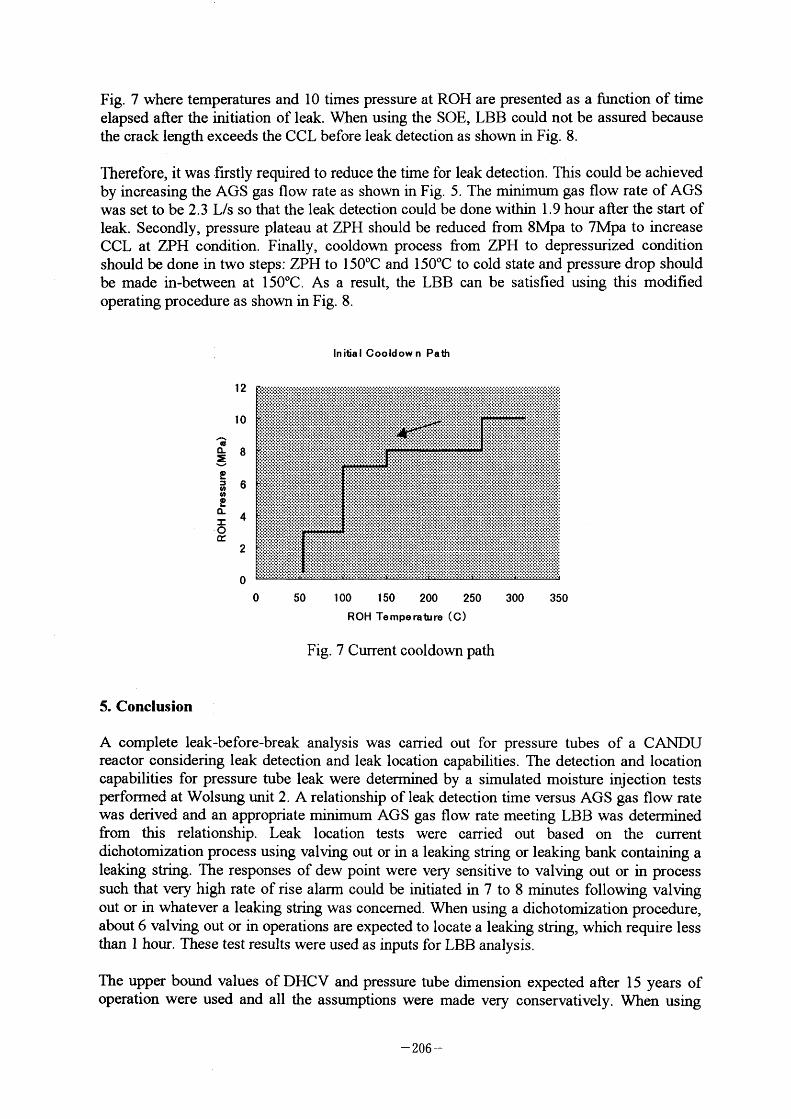
Fig. 7 where temperatures and I O times pressure at ROH are presented as a function of time elapsed after the initiation of leak. When using the SOE. LBB could not be assured because the crack length exceeds the CCL before leak deteetion as shown in Fig. 8.

Therefore, it was .hrstly required to reduce the time for leak detection. This could be achieved

by inoreasing the AGS gas flow rate as shown in Fig. 5. The minimum gas flow rate of AGS was set to be 2.3 L/s so that the leak detection could be done within I . 9 hour after the start of

leak. Secondly, pressure plateau at ZPH should be reduced from 8Mpa to 7Mpa to increase CCL at ZPH condition. Finally, cooldown process from ZPH to depressurized condition should be done in two steps: ZPH to 1 50~C and 1 50~C to cold state and pressure drop should be made in-between at 1 50'C. As a result, the LBB can be satisfied using this modified operating procedure as shown in Fig. 8.

Initial Cooldow n P8th

~ CL = ~ ~

c02

~ = O az

12

10

8

6

4

2

o

o 50 1 OO 1 50 200 250 350 300

ROH Tempemturo (O

Fig. 7 Current cooldown path

5. Conclusion

A oomplete leak-before-break analysis was carried out for pressure tubes of a CANDU reactor considering leak detection and leak location capabilities. The detection and location capabilities for pressure tube leak were determined by a simulated moisture inj ection tests perfonned at Wolsung unit 2. A relationship of leak detection time versus AGS gas flow rate was derived and an appropriate minimum AGS gas flow rate meeting LBB was determined from this relationship. Leak loeation tests were carried out based on the current dichotomization process using valving out or in a leaking string or leaking bank containing a

leaking string. The responses of dew point were very sensitive to valving out or in process such that very high rate of rise alarm eould be initiated in 7 to 8 minutes following valving

out or in whatever a leaking string was concerned. When using a dichotomization procedure, about 6 valving out or in operations are expected to loeate a leaking string, which require less than I hour. These test results were used as inputs for LBB analysis.

The upper bound values of DHCV and pressure tube dimension expected after 1 5 years of operation were used and all the assumptions were made very conservatively. When using

- 206 -

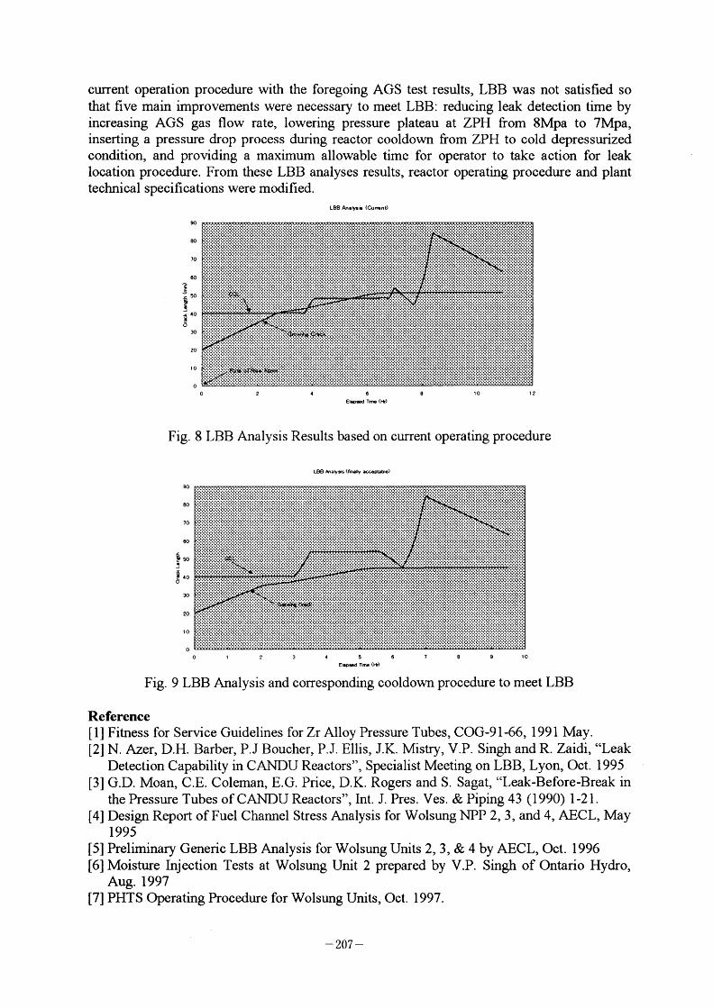
current operation procedure with the foregoing AGS test results, LBB was not satisfied so that five main improvements were neeessary to meet LBB: reducing leak detection time by increasing AGS gas flow rate. Iowering pressure plateau at ZPH from 8Mpa to 7Mpa, inserting a pressure drop process during reactor cooldown from ZPH to cold depressurized condition. and providing a maximum allowable time for operator to take action for leak location procedure. From these LBB analyses results. reactor operating procedure and plant teehnical specifieations were modified.

*"" ~.b** ''~-~"

'. '' =,."'' ~~.

Fig. 8 LBB Analysis Results based on eurrent operating proeedure

LBB Analysis (fln.hy alcceptabte)

Fig.

'. =.."'' '.~.

9 LBB Analysis and corresponding cooldown procedure to meet LBB

Reference [ I J Fitness for Serviee Guidelines for Zr Alloy Pressure Tubes, COG-91-66, 1 991 May. [2] N. Azer, D.H. Barber, P.J Boucher, P.J. Ellis, J.K. Mistry, V.P. Singh and R. Zaidi, "Leak

Detection Capability in CANDU Reactors", Speeialist Meeting on LBB, Lyon, Oct. 1 995 [3] G.D. Moan, C.E. Coleman, E.G. Price, D.K. Rogers and S. Sagat, "Leak-Before-Break in

the Pressure Tubes of CANDU Reactors", Int. J. Pres. Ves. & Piping 43 (1990) I -2 1 .

[4] Design Report of Fuel Channel Stress Analysis for Wolsung NPP 2, 3 , and 4, AECL. May l 995

[5] Preliminary Generic LBB Analysis for Wolsung Units 2, 3, & 4 by AECL, Oct. 1 996 [6] Moisture Injection Tests at Wolsung Unit 2 prepared by V.P. Singh of Ontario Hydro,

Aug. 1997 [7] PHTS Operating Procedure for Wolsung Units. Oct. 1 997.

- 207 -

IV-5 Approximate Evaluation Method for Ductile Fracture Analysis

of Circumferentially Through-Wall-Cracked Pipe Subjected

to Combined Bending and Tension

Naoki Miura (CRJEPD , Materials Science Department, Central

Research Institute of Electric Power Industiy, Japan

Approximate evaluation method for ductile fracture analysis of circumferentially through-wall-cracked pipe

subjected to combined bending and tension

N. Miura

Materials Science Department, Central Research Institute of Electric Power Industry 2- I I - I , Iwado Kita, Komae-shi, Tokyo 20 1 -85 1 1 JAPAN

Abstract

To estimate the structural integrity of the Light Water Reactor piping, combined loading consists of tensile load due to internal pressure and bending load under seismic condition should be considered as a basic loading mode. However, theoretical investigation on the methodology to evaluate ductile fracture behavior is not adequate to date. In this study, an approximate evaluation method for ductile fracture analysis of circumferentially through-wall-cracked pipe subjected to combined bending and tension was newly developed. This method can explicitly incorporate the contribution of both tension and bending. The effect of growing crack is also considered in the method. This method was then applied to the full-scale pipe fracture tests. Based on the comparison with experimental results as well as finite element calculations, it could be ascertained that the proposed method could well predict ductile fracture behavior under combined loading. The effect of combined loading on ductile fracture was sensitivity-studied using the proposed method. As a result, it was quantitatively found that the superposition of internal pressure reduced the maximum load of cracked pipe.

1. Introduction

To substantiate that pipe whip restraint and jet impingement shields can be eliminated, piping for nuclear power plant is required to satisfy Leak-Before-Break (LBB) analyses for postulated defects. One of the most important aspects in LBB analyses is to predict the ductile fracture behavior and the load-carrying capacity of a circumferentially through-wall-cracked pipe. Elastic-Plastic Fracture Mechanics (EPFM) methods can employ analytical approaches such as elaborate numerical simulations or some approximate evaluation methods. Numerical simulations are generally considered to give reliable predictions for a specific condition. However, approximate evaluation methods seem to be more useful to investigate the effect of various analytical situations systematically. Based on the J-Tearing theory, some methods have been proposed to evaluate the ductile fracture behavior of circumferentially through-wall-cracked pipe subjected to pure bending. When actual plant piping conditions are considered, however, the effect of the internal pressure acting as a tensile load also occurs. Theoretical investigation on the methodology to evaluate ductile fracture behavior under combined loading is not adequate to date. If combined loading effects are not properly considered, then the actual fracture resistance of the pipe could be in error.

In this study, an approximate evaluation method for ductile fracture analysis of circumferentially through-wall-cracked pipe subjected to combined bending and tension is newly developed. This method is intended to incorporate the contribution of both tension and bending. The method is then applied to the full-scale pipe fracture tests. The effect of combined loading on ductile fracture is sensitivity-studied using the proposed method.

- 209 -

2. Development of new evaluation method

2.1 Existing consideration on combined loading

Kumar and German ( 1988) have developed the GE/EPRI Estimation scheme for a circumferentially through-wall-cracked pipe subjected to combined bending and tension. Fully plastic solutions for power-law material were computed under proportional loading condition. Brust, et al. (1995) have presented more reliable solutions using elaborate three-dimensional finite element calculations under constant internal pressure condition. These solutions tabulated as functions of pipe dimension, crack dimension, strain hardening exponent, etc, are limited and discrete at this time. For example, the former solutions are given for only two radius/thickness ratios, two crack angles, and two or three hardening exponents. For the latter solutions, internal pressure is fixed to 15.5 MPa, which is equal to PWR operating condition, and cannot be a variable. Therefore, theses solutions are not always adequate to analyze ductile fracture behavior when analytical parameters such as crack angle or internal pressure significantly change during loading.

Paris/Tada method (Paris, 1983), LBB.NRC method (Klecker 1986), LBB.GE method (Brust, 1987), and LBB.ENG2 method (Brust, 1987 and Gilles, 1994) are other approximate evaluation methods which may have a potential to evaluate ductile fracture under combined loading. These methods were originally developed to apply to pure bending or pure tension. They are often applied to combined loading by substituting an internal pressure for an equivalent bending by some means. However, these approaches tend to give conservative prediction especially for the case with larger pressure (Brust, 1995). This might be because the interaction between tension and bending cannot be properly taken account in these cases. Attempts to evaluate J-integral under combined loading by adding J-integral due to pure tension and that due to pure bending were also seen in some instances, which have naturally no theoretical base since the principle of superposition 6annot be available in nonlinear region.

2.2 Evaluation of moment-rotation relation

Consider a circumferentially through-wall-cracked pipe subjected to combined four-point bending and tension due to internal pressure shown in Fig. I . Assume that the total load-

point rotation, c may be written as

c=cc+cNC (1)

where cc and cNC are c due to crack and c without crack, respectively. cNC can be easily obtained as

_ M Lin

where M is the applied moment, Lin is the inner span, E is the Young's modulus, and I is the

second moment of area for uncracked pipe. cc may be separated into its elastic and plastic

components.

cC=cEL+cpL (3)

The cEL and cpL under combined loading are evaluated as the following procedures.

When a pipe is subjected to bending moment, M and tensile load, T, bending stress, ab

and tensile stress, at are

o:b* M = T ,at 7cR2 t 2 7CR t (4)

- 210 -

where R is the mean radius and t is the pipe thickness. The stress intensity factor, Kl is represented as the sum of its bending and tensile components, Kb and Kt

K K + Kt = ab ~~~Fb (O) + at ~r~Ft (O) (5)

where e is the half crack angle, and the compliance functions, Fb and Ft are provided as

functions of 6/7T and R/t based on Sanders' solutions (Klecker 1986).

Fb (e) = I + Ab (~)1'5 + Bb (~)2.5 + Cb (~)3'5 (6)

1

Ab -3.26543 1.52784 -0.072698 0.0016011 R/t Bb = Il.36322 -3.91412 0.18619 -0.004099 (7) Cb -3 . 1 8609 3 . 84763 -O. 1 8304 0.00403 (Rlt)2

(R/t)3

2.5 F (6) I + At (~)1'5 + Bt (~) + Ct (~)3'5 (8)

A t -2.029 1 7 1 .67763 -0.07987 0.00 1 76 Rlt Bt = 7.09987 -4.42394 0.21036 -0.00463 (9) Ct 7 .7966 1 5 . 1 6676 -0.24577 0.0054 1 (R/t)2

(R/t)3

cEL are related with the strain energy due to crack, U using the Castigliano's theorem.

While the energy release rate, G may be written as

where A is the crack area. From Eqs. (10) and (1 1),

A

/dA aM o E

Since M and T are independent each other, substituting Eq. (5) into Eq. ( 1 2), then

cEL_ ab lb (O) + ~ I (6) (13) ~E w here

lb (e) = 4 OF~ (O) dO (14)

-211-

I, (6) = 4 OFb (6) F (O) dO ( 15)

Thus the cEL can be explicitly calculated.

As for the evaluation of cpL, the beam theory can be enforced to the pipe of nonlinear elastic material under the deformation theory of plasticity. This hypothesis is the same as the supposition used in the LBB.ENG2 method (Brust, 1987). Note that the LBB.ENG2 method considered the compatibility for pure bending or pure tension, while the new evaluation method attempts to take account of both bending and tension loading simultaneously.

The stress-strain relation is defined as the following power law.

ao

~o ao Based on the beam theory with the assumptions that plane sections remain plane, the deflection of the beam and the related strain and stress distributions are illustrated in Fig. 2. The stress distribution has to be in equilibrium with the applied tensile load and the bending moment. This follows

R T = MO h kTgT p

M = Mo h kM - [kT gT - K'~M gM] p2

(17)

(18)

where p identifies the location of the neutral axis shown in Fig. 2, Mo is the yield moment for uncracked pipe given as

M0= 4010R2t (19)

and the parameter, h is

h=( R )l Ce80p

(20)

~ ~ with p as the radius of curvature. Functions KM , KT , gM , and gT are introduced to approximate integral equations appeared in the process of the equilibrium calculations, which are given by

7c/2 F( I +1) l+1 _~ 2n kM= (sin e)~ d6- 2 r( I +~)

2n 2 kT= IT/2 _~~r(2ln +~) (sinO)~de- 2 F( I +1)

2n n+1 2 gM= n 7T

gT - I + ~

n7c

(2 1 )

(22)

(23)

(24)

The Gamma function, Fin Eqs. (21) and (22) can be approximated in the range of interest here by the Stirling's formula

- 212 -

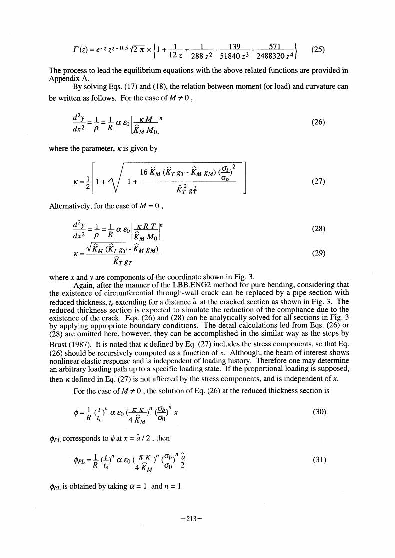
F(Z) = e~ z zz 0.5V~~xljl+ I + I _ _ 571 } l 39

12z 288z2 51840 z3 2488320 z4 (25)

The process to lead the equilibrium equations with the above related functions are provided in Appendix A.

By solving Eqs. ( 17) and ( 1 8), the relation between moment (or load) and curvature can

be written as follows. For the case of M ~ O ,

d2y _ I _ I _1CM In x ~~~~ [ oceo d 2 p R KM MOJ

(26)

where the parameter, Ic is given by

lc-i 1+ -2 l+

16 K"M (kT gT - K'~M gM) (o:~a:) 2

k~ g~ (27)

Alternatively, for the case of M = O ,

dx2 p R aeo -KRTJn =-=- [ KM Mo

~ ~ ~ ,c KM (KT gT - KM gM) (29) kT gT

where x and y are components of the coordinate shown in Fig. 3. Again, after the manner of the LBB.ENG2 method for pure bending, considering that

the existence of circumferential through-wall crack can be replaced by a pipe section with reduced thickness, te extending for a distance a at the cracked section .as shown in Fig. 3. The reduced thickness section is expected to simulate the reduction of the compliance due to the existence of the crack. Eqs. (26) and (28) can be analytically solved for all sections in Fig. 3 by applying appropriate boundary conditions. The detail calculations led from Eqs. (26) or (28) are omitted here, however, they can be accomplished in the similar way as the steps by

Brust (1987). It is noted that ,cdefined by Eq. (27) includes the stress components, so that Eq. (26) should be recursively computed as a function of x. Although, the beam of interest shows nonlinear elastic response and is independent of loading history. Therefore one may determine an arbitrary loading path up to a specific loading state. If the proportional loading is supposed,

then lc defined in Eq. (27) is not affected by the stress components, and is independent of x.

For the case of M ~ O , the solution of Eq. (26) at the reduced thickness section is

7CK " Cbn l (~)"acO( - ) ( ) x c=k te CO 4 KM (30)

cPL corresponds to c at x = a / 2 ,

then

cPL ~ i (L)n oc ejO ( 7C K )n (O:b)n ~

~R t ~ e /V O1 2 ~ AM O (31)

cEL is obtained by taking a = l and n = l

- 213 -

aba cEL_ ii 80 'cl olo ~ (32) ~R te

where

From Eqs. (31) and (32), cpL can be evaluated as

n I ,cn olbn-l cPL=(~) - ( ~ )na ( ) cEL (34) te 4KM Icl olo Similarly, for the case of M = O , the solution of Eq. (28) at the reduced thickness

section is

1 t 7c K )n (at)n x (35) cPL = - (-)" o~ co (

R t. 2~M ao cPL corresponds to c at x = a / 2 , then

cPL _ i (~)n a so ( 7c lc )n (ol~a;:)n ~ (36) ~R t ~ o e 2 KM

cEL is obtained by taking a = I and n = l

iL~02 Icl Rte ol02

From Eqs. (36) and (37), cpL can be evaluated as

cPL_(t) - ( lc )na 'cn (o:t)n-lcEL (39) _ _n I _ te 2KM 2 Icl ao

The equivalent reduced thickness in Eqs. (34) and (39) may be taken so that the Net-Section collapse moment of the cracked pipe under bending condition is identical to that of the reduced thickness section.

,1 2[ J

4 afR2 t[cos ~ ~ ~ ~ af (40) sin 6] = 4 o:fR te[cos

where af is the flow stress. The term in the bracket in right side indicates the effect of superposing tensile stress, and is equal to the ratio of the plastic collapse moment of cracked

~+~at _l pipe subjected to combined bending and tension, 4 afR2 te [cos ( ) ~ sin 6 to that 2 2af

2[ o I l subjected to pure bending, 4 cyR te [cos (~) ~ ~ sin e] at 6 = O . Since Eq. (40) is premised

on the rigid perfectly plastic behavior, it gives better results for small cracks. While it tends to

overpredict cpL for larger cracks (Gilles, 199 1 ). In the present evaluation method, the

correction factor of rd:4 deterrnined by Gilles ( 1 99 1 ) is used. That is,

-214-

t cos ~ a~o:IfJJ / [cos ~ ~ ~ sin 6J ' _ = ![ t el te cos ~ a_o:'JJ / [cos ~ - i Sin OJ 1[- - t lc

22 ' 4

6 tor0>~ !

4

(4 1 )

and are linearly interpolated between rd6 and 7d:4.

2.3 Evaluation of J-integral

When an experimental or an analytical relation between load and displacement is

known, the n-factor approach can be applied to evaluate the J-integral, J for a circumferentially through-wall-cracked pipe subjected to four-point bending (Zahoor, 198 l, Wilkowski, 1987). The existing evaluation methods mentioned above (i.e., Paris/Tada method, LBB.NRC method, LBB.GE method, and LBB.ENG2 method) that predict maximum load capability have

the n-factor analyses embedded in them. The earlier n-factor solutions have been developed for cracked pipes under either pure bending or pure tension. J is defined as the release rate of

potential energy of nonlinear elastic material, therefore, the n-factor solutions can be extended for combined loading if the energy release rate for cracked pipe subjected to multiple loads is generally described. Pan ( 1 984) has investigated the energy release rate for stationary cracked body under multiple loads, and has derived a generalized J evaluation equation. Further, Miura

and Wilkowski (1995) have developed the combined-load n-factor solution which was applicable to combined bending and tension taken account of growing crack. In this study, this

combined-load n-factor solution is expected to be included in the present evaluation method. When a circumferentially through-wall-cracked pipe shown in Fig. I is subjected to

combined four-point bending and tension due to internal pressure, J can be given as follows in spite of loading paths.

J aA aA Ic=0, TdT IT, M dM + (42)

where 6 is the axial displacement shown in Figure I . In the above equation, conditions that

Here J, c, and 6 are assumed to be divided into the elastic and plastic components,

J=JEL+JpL

where subscripts EL and pL denote elastic and plastic component, respectively. JEL is directly obtained from KI in Eq. (5).

(43)

The elastic J,

JEL=K12/E

And for the plastic J, JpL,

(44)

JPL = acpL IT, M dM + aa8A~~L Ic=0, TdT

aA (45)

- 215 -

The 6pL due to axial load is considered to be small, so that the second integration of the right side in Eq. (45) is negligible. By using the geometrical relations as,

A=2Rt6 cPL/2=ApL/Lz M=Lz/P

(46)

(47)

(48)

where ApL is the plastic load-point displacement, and P is the bending load shown in Fig. I ,

then Eq. (45) can become

JPL= acpL IT MdM= I aApL Is,PdP

aA ' R t ae (49)

Note that the non-dimensional tensile stress, s (defined as atlaf) is used instead of T.

Assuming that ApL is a function only of the ratio of P to the Net-Section collapse load, then 1lpL

can be expressed as

ApL = f (P / hp (O, s)) (50) e 7c l h (6 s) = cos (-+ - s) - - sin 6 (51) p ' 2 2 2

where hp rs equal to the ratio of the plastic collapse load of cracked pipe subjected to combined Ioading to that of uncracked pipe subjected to pure bending. Substituting Eq. (50) into Eq. (49), then gives

ApL

o

~2Rthp

This equation gives JpL for a stationary (non-growing) crack under bending and constant tension loading.

For a generalized case considered growing crack and tension changing, Eq. (50) is written in its inverse form,

P = hp F (ApL) (54)

In this equation, ApL, e, and s are assumed to be independent of each other, and since JpL is a

function of ApL, e, and s, the differential of JpL is

dJpL- aJpL de+

aO

aJpL

a ApL dApL +

a JpL

aS ds (55)

Substituting Eqs. (52) and (54) into Eq. (55), and are given by

-216-

JPL= 2 n P dApL + 2 Yp JPL d0+ 2 pp JPL ds oo

(56)

where,

yp- 2ahp/aO

pp = - a2hp / as a6 (58) 2 ahp I ae

The second term of the right side of Eq. (56) corresponds to the contribution of the crack

growth. The functions n and yin the original n-factor approach are replaced with functions np

and yp, respectively. The third term of the right side of Eq, (56) corresponds to the contribution of the tension changing. If an axial tension is constant, this term is equal to zero.

For the case of s = O , Eq. (56) is naturally identical to the original n-factor solution. Figs. 4 to

6 show the values of np, Yp, and /lp as a function of O, respectively. It can be seen that these

functions are affected by s as well as e.

2.4 Evaluation method for ductile fracture analysis

By integrating the moment-rotation evaluation in Section 2.2 and the J-integral evaluation in Section 2.3 together with the criterion of crack extension, an evaluation method for ductile fracture analysis taken account of both combined loading and growing crack was newly established. The developed evaluation method has an ability to consider an arbitrary combined loading history by nature, however, constant tensile load due to internal pressure followed by external monotonic bending load is supposed in this paper.

Fig. 7 shows the schematic of the developed evaluation method. As shown in this

figure, the unique relation between J and M is provided for a specific crack extension Aa. J

corresponding to the Aa is determined by the J-R curve, then M can be fixed at the point on the

J-M curve. The relation between M and c is also unique for the specific Aa, so c is given by

the point on the M-c curve. Repeating this process for a set of Aa, and taking an envelope of the points, then the prediction of the ductile fracture behavior with crack extension is accomplished. The flow of the evaluation procedure is sununarized in Fig. 8.

3. Application to pipe fracture tests

3.1 Analytical object and condition

The developed evaluation method was applied to analyze full-scale pipe fracture tests under combined bending and internal pressure. The predicted ductile fracture behavior was compared with experimental results as well as finite element calculations to validate the propriety of the method.

Table I shows the matrix of six pipe fracture tests analyzed. These tests were performed as a part of the NRC's Degraded Piping Program - Phase 11 (Wilkowski, 1989) and the IPIRG-2 Program (Scott, 1997). The materials used for the tests were AI06 Grade B and SA333 Grade 6 carbon steels, and Type 304 stainless steel. Tensile properties necessary to perform a fracture analysis are also listed in Table I . All tests were performed at 288"C. Four tests were conducted under tension loading due to internal pressure followed by bending, and two tests were conducted under pure bending condition for comparison. Experiments 413 1-7,

-217-

4 1 3 1-3, and Experiments 4 1 3 1 -5, 4 1 3 1 - I have almost the same dimensions and test conditions

except for the loading condition. Using these cases, the effect of combined loading can be evaluated. Experiment I .9 was performed under dynamic loading (time to crack initiation = 0.32 seconds). All the other experiments were conducted under quasi-static loading.

Two J-R curves were provided for the predictions for each material. One was the J-R curve obtained from compact tension (CT) specimen which had been cut from the test pipe.

The other was the J-R curve obtained from the pipe fracture test using the combined-load n-factor approach (Miura, 1 995). The use of the pipe J-R curve is desirable for the purpose of the validation of the proposed method, however, small specimen J-R data are typically applied because they are often the only data available, and because predicted results are generally considered to be lower bounds. The J-R curves used for the analysis are shown in Figs. 9(a) to (d). These J-R curves were extrapolated according to the equations shown in these figures.

A three-dimensional finite element analysis was carried out for Experiments 4 1 3 1 -7, 4 1 3 1-3, 4 1 3 1 -5, and 4 1 3 1 - I to confirm that the experimental results were appropriate.

The analysis was conducted using the computer code "MARC" with twenty-noded solid elements. Fig. 10 shows an example of the finite element mesh for the analytical model. Tensile properties in Table 2 were used for the analysis. In the analysis, the internal pressure was applied first, then the bending moment was applied with the constant internal pressure.

The experimental relation between A and 1la was numerically followed for the crack growth condition.

3.2 Results of analysis

Figs. I l(a) to (O show the predicted relations between bending load and load-point displacement compared with the experimental (and the analytical if available) relation(s).

Fig. I I (a) shows the load-displacement relations for Experiment I .9 (carbon steel 6-inch diameter pipe under bending and pressure). The proposed method using the CT J-R curve significantly underestimates the load-displacement relation. The prediction using the pipe J-R curve is still lower than the experimental result. The CT J-R curve for this material was obtained using sidegrooved specimens which lowered the toughness by constraining plasticity, and resulted in large difference. One reason of the poor predictability might be due to the complex crack growth aspects such as angled, asymmetric, and fast crack growth for this specific experiment.

Fig. I I (b) shows the load-displacement relations for Experiment I .8 (carbon steel 1 6-inch diameter pipe under bending and pressure). The drop of the displacement at about 275 mm in the experimental results just at maximum load is due to an unstable crack jump at this point. Although the proposed method using the both J-R curves gives slightly lower displacement than the experimental result, the predicted maximum moments are in good agreement with the experimental value .

Figs. I l(c) and (d) show the load-displacement predictions for Experiments 413 1-7 (carbon steel 10-inch diameter pipe under pure bending) and Experiment 4 1 3 1 -3 (carbon steel lO-inch diameter pipe under bending and pressure), respectively. It can be seen that the proposed method realizes fine predictions independent of the presence of pressure by comparing with experimental and FEM results. The relations from the CT J-R curve are lower than that from the pipe J-R curve. However, the differences are small for both experiments.

Figs. 1 1(e) and (D show the load-displacement predictions for Experiments 4131-5 (stainless steel 6-inch diameter pipe under pure bending) and Experiment 4 1 3 1 - I (stainless steel 6-inch diameter pipe under bending and pressure), respectively. The similar trends as the case of Figs. (c) and (d) can be observed, and the good predictability is secured both for combined loading and for pure bending. There seems to be a slight difference between the experimental and the FEM Ioad-displacement relation for Experiment 4 1 3 1 -5. The prediction based on the proposed method is closer to the FEM result rather than the experimental one.

Fig. 12 shows the predicted divided by the experimental maximum loads. The predictions by the proposed method using both the CT and pipe J-R curves and the prediction by FEM (if available) are provided for each experiment. The proposed method has an enough capability to predict maximum moment for various materials, pipe size and crack size. The use of the pipe J-R curves gives better predictions than the use of the CT J-R curves compared with

- 218 -

the experimental maximum loads. The predictions using the CT J-R curves are relatively conservative, however, the difference of the predicted maximum loads caused by the selection of the used J-R curve is not remarkable.

4. Sensitivity study on combined loading effect

4.1 Effect of internal pressure on ductile fracture

The effect of the superposing pressure on ductile fracture was investigated using the

proposed method. An analytical object was SA333 Grade 6 carbon steel 4B x Schedule 80 cracked pipe at 288'C. Dimensions of the pipe were 52.85 mm in mean radius and 8.60 mm in thickness. A crack with the total angle of 30' was supposed. The constant internal pressure preceding bending moment was considered to be a parameter, so that the ratio of the tensile

stress to the reference stress, atlolo was equal to 0.00, 0.05, 0,lO, 0.15, 0.20, and 0.25. The tensile properties listed in Table I and the pipe J-R curve presented in Fig. 9(c) were used for the analysis.

Fig. 13 shows the relations between moment and rotation for various atlob• The relations have similar configuration, and the maximum moment decreases with increasing tensile stress. For the case of at/ao = 0.25 , the maximum moment is about 12(~o lower than that without tensile stress. It can be also seen that the rotation at the maximum moment decreases with increasing tensile stress.

Fig. 14 shows the relations between J-integral and moment for various o;t/olo• Moment at the same J-integral decreases with increasing tensile stress, as is the case of Fig. 1 3 . While the value of J-integral at the maximum moment is not affected by tensile stress.

4.2 Dependence of dimensional parameters on maxrmum moment

Next, a sensitivity analysis was performed to study how the effect of the superposing pressure was affected by typical dimensional parameters represented by crack angle and pipe diameter. Again, an analytical object was SA333 Grade 6 carbon steel Schedule 80 (pipe thickness in 8.60 mm) cracked pipe at 288'C. The same tensile properties as well as J-R curve as the above-mentioned analysis were applied. Table 2 shows the matrix of the analytical condition. For the case that the dependence of crack angle was to be seen, nominal diameter was fixed to 4B (mean radius in 52. 85 nun) and total crack angle was varied from 30' to 1 80'. On the other hand, for the case that the dependence of pipe diameter was to be analyzed, crack angle was fixed to 30' and nominal diameter was varied from 4B (mean radius in 52.85 mm) to 24B (mean radius in 289.3 mm). The constant internal pressure preceding bending moment was considered to be a parameter, so that the ratio of the tensile stress to the reference stress,

atlolo was equal to 0.00, 0.05. 0.lO, 0.15, 0.20, and 0.25 for both cases.

Fig. 1 5 shows the dependence of crack angle on maximum moment. The maximum moment gradually decreases with increasing tensile stress, and this trend becomes significant as the crack angle increases.

Fig. 1 6 shows the dependence of pipe diameter on maximum moment. The maximum moment again decreases with increasing tensile stress, and this tendency is clear for the larger diameter pipe. Thus, it is numerically found that the reduction of the maximum moment with increasing internal pressure becomes notable for larger crack angle and for larger pipe diameter.

5. Conclusions

In this study, an approximate evaluation method for ductile fracture analysis of circumferentially through-wall-cracked pipe subjected to combined bending and tension was newly developed. Existing evaluation methods are limited and are inadequate for practical use to analyze the effect of combined loading, while the proposed method can explicitly incorporate the contribution of both tension and bending. The effect of growing crack is also considered in the method. The method was then applied to the full-scale pipe fracture tests. It could be ascertained that the proposed method could well predict ductile fracture behavior under

- 219 -

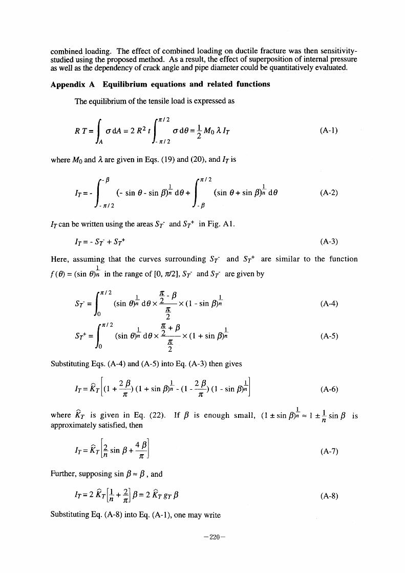
combined loading. The effect of combined loading on ductile fracture was then sensitivity-studied using the proposed method. As a result, the effect of superposition of internal pressure as well as the dependency of crack angle and pipe diameter could be quantitatively evaluated.

Appendix A Equilibrium equations and related functions

The equilibrium of the tensile load is expressed as

'cl 2

R T= adA = 2 R2 t ad0= ~MO ~lT

A - Icl2 (A- I )

where Mo and h are given in Eqs. (19) and (20), and IT is

IT= - (- sin 6 - sin p)n dO + (sm O + sm p)n dO

- ;T/ 2 - p (A-2)

IT Can be written using the areas ST~ and St+ in Fig. Al.

IT ST~ + ST+ (A-3)

Here, assuming that the curves surrounding ST~ f(6) = (sin 6)~ in the range of [O, 7z/2], ST- and ST~

and ST~ are

are given by

similar to the function

'c/2 ~_ p ST~= (sin 6)~dOx 27c x(1 -sinp)l

~ 'r/2 ~~ + p (sin 6)~ de x +_ 2~ x(1+sinp)i ST -

2

Substituting Eqs. (A-4) and (A-5) into Eq. (A-3) then gives

-J IT=KT[(1 + 7c ) (1 + sin p);T- (1 - 7c ) (1 - sin p)n

(A-4)

(A-5)

(A-6)

~ where KT is given in Eq. approximately satisfied, then

IT = kT [~ sin p + J

7c

(22). If p is enough small, l *1:!:'sinp is

(1 :!: sin p)n

(A-7)

Further, supposing sin p * p , and

IT 2KT[[~+2-7c]p=2kTgTp

Substituting Eq. (A-8) into Eq. (A- I ), one may write

(A-8)

- 220 -

~

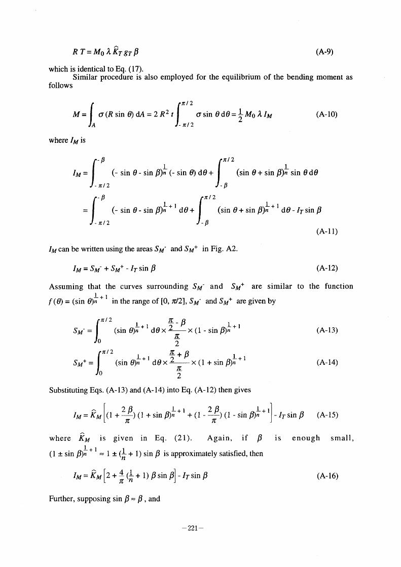
which is identical to Eq. ( 17).

Similar procedure is also employed for the equilibrium of the bending moment as follows

'T12

M = c(R sm 6) dA 2 R t asin 6d6= ~MO hlM (A-10)

where IM is

IM = (- sin O - sin p)~ (- sin 6) de + (sm O + sm p)n sm O dO

(- sin 6 - sin p)i+ I de + (sin e + sin p)1+ I de - IT sin p

- 'T/ 2 - p (A- I I )

IM can be written using the areas SM- and SM+ in Fig. A2.

IM = SM- + SM IT Sm p (A-12) Assuming that the curves surrounding SM- and SM+ are similar to the function f(6) = (sin e)~ + I in the range of [O, n/2], SM- and SM+ are given by

ITI 2 ~_p 27c x(1-sinp)l SM- = (sin e)~+ I d6 x (A-13) +1

~ 71:/2 ~ + p + l SM+ = (sin e)~+ I dO X 2 ~ x (1 + sin p)L (A-14)

2

Substituting Eqs. (A-13) and (A-14) into Eq. (A-12) then gives

J

2p 2p l +1 l+1 IM=KM (1 + 7c )(1 +sinp)~ +(1 - 7c )(1 -sinp)n

where kM is given in Eq. (21). Again, if p is enough small, (1 :!: sin p)~ + I = I :!: (~ + l) sin p is approximately satisfied, then

- -+ l) p sin plj ~ ITsin p

Further, supposing sin p * p , and

- 221 -

l ~ n ~ I ~ p2J - 2 kT[[1 + 2-JI p2 = 2 (K"M - [kT gT - kM gM] p2} [

IM=2KM[1+ nlc (A- 17)

Substituting Eq, (A- 17) into Eq. (A- lO), one may write

M = Mo ~ {K"M - [kT gT KM gMIJ p

which is identical to Eq. ( 1 8).

The above derivation is based on the assumption that the p is enough small. For

example, when p is less than 0.1lz:, it was numerically ascertained that the difference of IT computed by Eqs. (A-2) and (A-8), and the difference of IM computed by Eqs. (A-1 1 ) and (A-

1 7) are both less than 6(~o. p is a function of strain hardening exponent, n and the tensile to

bending load ratio, RT/M. n usually ranges between I to 10 for typical structural materials,

a significant ductile fracture behavior occurs at much higher value of RT/M than 0.4, the

assumption on p is considered to be appropriate for the loading mode of interest.

References

Brust, F. W. Approxnnate Methods for Fracture Analysrs of Through Wall Cracked Pipes, NUREG/CR-'4853, February 1987.

Brust, F. W., et al., Assessment of Short Through-Wall Circumferential Cracks in Pipes, NUREG/CR-6235, April 1995.

Gilles, P., Brust. F. W., 1994. Approximate Methods for Fracture Analysis of Tubular Members Subjected to Combined Tensile and Bending Loads, J. Offshore Mechanics and Arctic Engineering (OMAE), 1 1 6, 22 1 -227.

Gilles, P., Brust, F. W., 1991. Approximate Fracture Methods for Pipes - Part I: Theory, Nucl. Eng. Des., 127, 1-17.

Klecker, R., et al., NRC Leak-Before-Break (LBB.NRC) Analysis Method for Circumferentially Through-Wall Cracked Pipes Under Axial Plus Bending Loads, NUREG/CR-4572, May 1986.

Kumar, V., German, M. D., Elastic-Plastic Fracture Analysis of Through-Wall and Surface Flaws in Cylinders, EPRI NP-5596, Final Report, January 1 988.

Miura, N., Wilkowski, G., 1995. J-R Curves From Through-Wall-Cracked Pipe Tests - Combined Loading and Short Crack Considerations -, 1995 ASME Pressure Vessels and Piping Conf., 304, 171-179.

Pan, J., 1984. Some Considerations on Estimation of Energy Release Rates for ' Circumferentially Cracked Pipes, Trans. ASME J. Pressure Vessel Technol., 106, 391-398.

Paris, P. C.. Tada, H., The Application of Fracture Proof Design Method Using Tearing Instability Theory to Nuclear Piping Postulating Circumferential Through Wall Cracks, NUREG/CR-3464, September 1 983.

Scott, P., et al., IPIRG-2 Task I - Pipe System Experiments with Circumferential Cracks in Straight-Pipe Locations, NUREG/CR-6389, February 1 997.

Wilkowski, G., et al., Analysis of Experiments on Stainless Steel Flux Welds, NUREG/CR-4878, April 1987.

Wilkowski, G. M., et al., Summary of Technical Results and Their Significance to Leak-Before-Break and In-Service Flaw Acceptance Criteria, NUREG/CR-4082, 8, March 1989.

Zahoor, A., Kanninen, M. F., 1981. A Plastic Fracture Mechanics Prediction of Fracture Instability in a Circumferentially Cracked Pipe in Bending - Part I: J-Integral Analysis, Trans. ASME J. Pressure Vessel Technol., 103, 352-358.

- 222 -

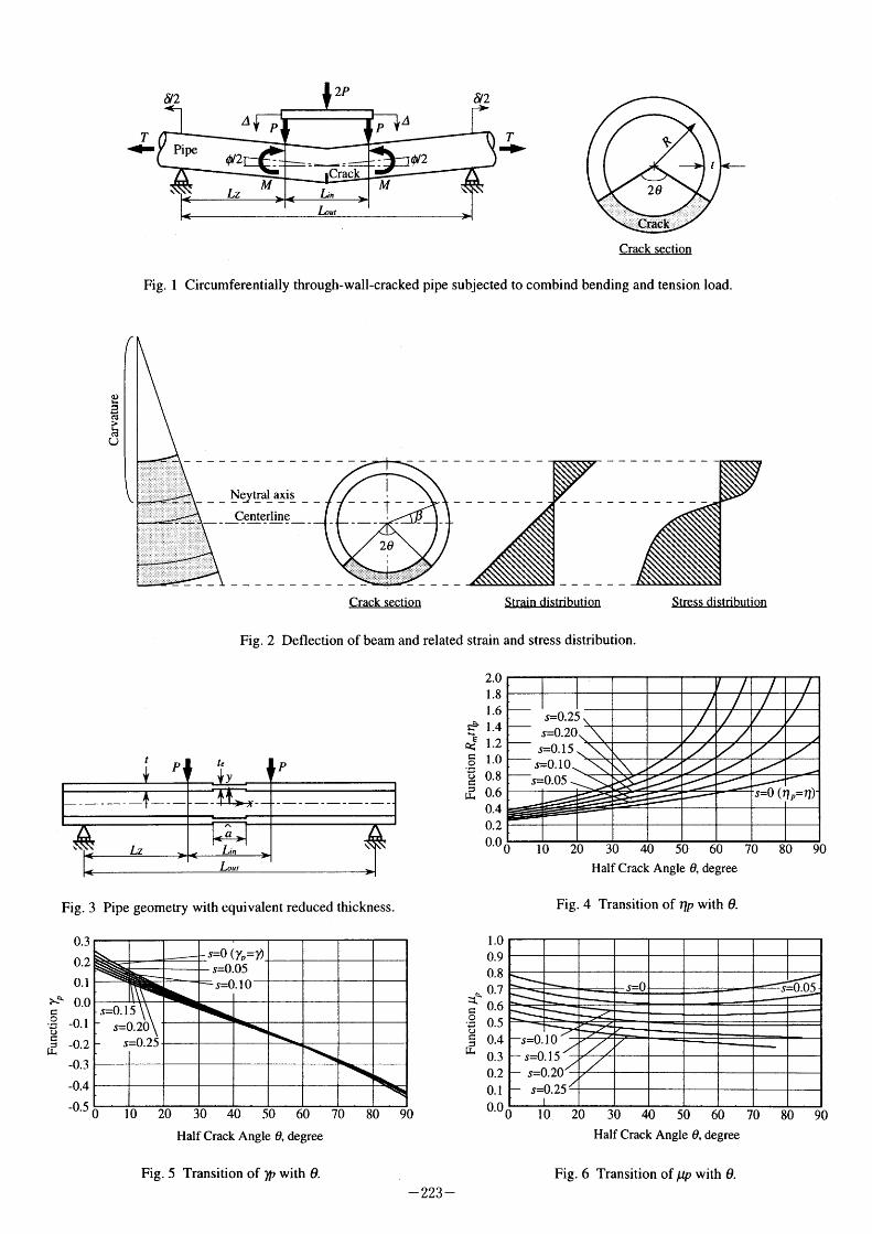
T ~-

Fig. 1

I~ t

26

Crack

Crack section

Circumferentially through-wall-cracked pipe subjected to combind bending and tension load.

(L)H

S ~, cs

> hc:$

(J

Neytral axis

Centerline

l

,

~~-T~~~ t

2e t

1

Fig. 3

0.3

0.2

O. l

>(~ 0.0 ~ •~ O l tS :::

~:' -0.2

-0.3

-0.4

-0.5 O

~l~~~~~~~~n Strai di tribution tress distribution

Fig. 2 Deflection of beam and related strain and stress distribution.

2.0 l .8

l.6

s~* 1.4

~ Q,:S 1.2

c::o 1.0

~ 0.8 :' 0.6 F~

0.4 O. 2

0.0 o I O 20 30 40 50 60 70 Half Crack Ang]e e, degree

Pipe geometry with equivalent reduced thickness. Fig. 4 Transition of np with O.

l .O

0.9

0.8

* 0.7 :tct 0.6

.~ 0.5 L) c:::s 0.4

p~ 0,3

0.2 O. 1

l O 20 30 40 50 60 70 80 90 0.0 O I O 20 30 40 50 60 70 Half Crack Angle e, degree Half Crack Angle O, degree

Fig. 5 Transition of w with O. Fig. 6 Transition of //P with O. - 223 -

80 90

80 90

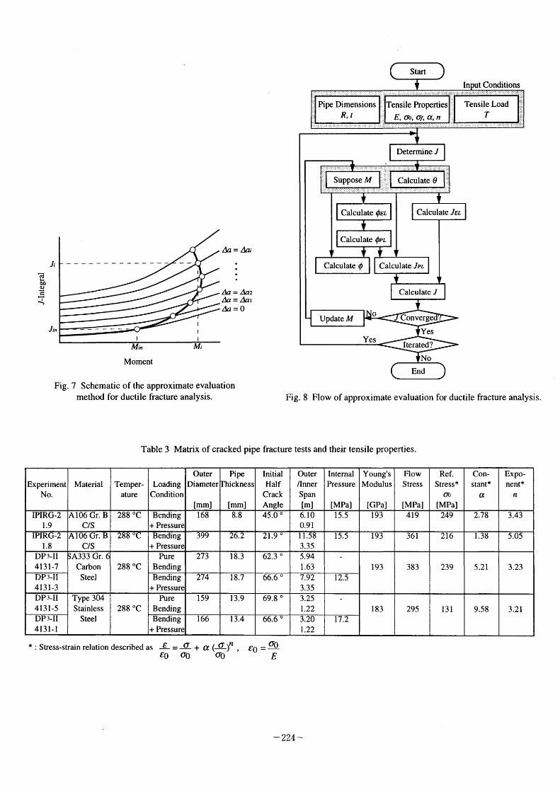
C:$ hbJb

Q) J, :::

I-' b,,l

Ji

Jin

l

I

l

I

I

Aa = Aa' l

~a = Aa2 Aa = Aal

Aa=0

Fig. 7

Min

Moment

Mi

Schematic of the approximate evaluation method for ductile fracture analysis. Fig. 8 Flow of approximate evaluation for ductile fracture analysis.

Table 3 Matrix of cracked pipe fracture tests and their tensile properties.

* : Stress-strain relation described as 8 80

= +a(a)n a olo ao

80 = Co

E

- 224 -

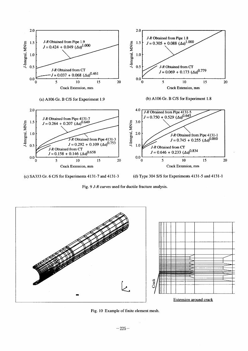
J-R Obtained from Pipe I .8

~ 1.5 J-R Obtained from Pipe 1.9 ~ 1.5 J = 0.305 + 0.088 (Aa)1.000 ~: J = 0.424 + 0.049 (Aa)1.000 ~: ~ Z

~' 0.5 ~, 0.5 J-R Obtained from CT J-R Obtained from CT J = 0.069 + 0.173 (Aa)0.779 0.46 l J = 0.037 + 0.068 (Aa)

15 5

Crack Extension, mm Crack Extension, mm (a) AI06 Gr. B C/S for Experiment I .9 (b) A 106 Gr. B C/S for Experiment I .8

2.0 4.0 J-R Obtained from Pipe 4131-5 J-R Obtained from Pipe 4131-7 J = 0.750 + 0.529 (Aa)0.645 J = 0.264 + 0.207 (lia)0.649

~

~ 1.0 ~ 2.0 J-R Obtained from Pipe 4131-l o o J = 0.745 + 0.255 (Aa)0.860 -R Obtained from Pipe 41 3 1-3 J = 0.292 + 0.109 (Aa)0.753

~' 0.5 ~' I .O J-R Obtained from CT J-R Obtained from CT J = 0.646 + 0.233 (Aa)0.834 J = 0.158 + 0.146 (Aa)0.658

O 5 20 15

Crack Extension, mm Crack Extension, mm (c) SA333 Gr. 6 C/S for Experiments 41 3 1-7 and 4131-3 (d) Type 304 S/S for Experiments 4131 -5 and 4131-l

Fig. 9 J-R curves used for ductile fracture analysis.

20

20

~~: Uc~$

~

Extensi on around crack

Fi g . lO Example of finite element mesh.

- 225 -

~ ~'

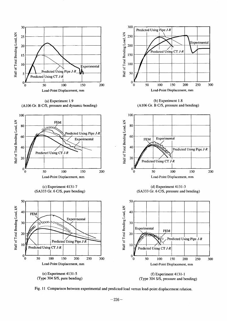
~ ed) F:

1:'

~ OCl

~ ~ ~O

~' ~c~l

~::

~ ~:'::'~

~ ~

~'s::

~ I~_

~ ~O

~ ~cE$

:~

~ 1::'C:'~

~ bO S

1:' '::Q)

CQ

~ ~ tHO

~~ ~c~S

::

Z =' ~ o

F::

~S

eQ ~~ ~ H * o ~ :1:

50 l 50 IOO

Load-Point Displacement, mm Load-Point Displacement, mm

(a) Experiment I .9 (b) Experiment I .8 (AI06 Gr. B C/S, pressure and dynamic bending) (AI06 Gr. B C/S, pressure and bending)

Z ~~

~ o ~ eJ)

;ej

s:

o eQ

~ o H * o ~~ :::

l 50 l OO

Load-Point Displacement, mm Load-Point Displacement, mm

(c) Experiment 41 3 1 -7 (d) Experiment 41 3 1-3 (SA333 Gr. 6 C/S, pure bcnding) (SA333 Gr 6 C/S, pressure and bending)

Z; ~:

~ o .1 bJ)

;5 F: (L)

a:l

~ 20 ~ o H * o ~~ :::

O I OO 1 50 200 250 300 O 50 1 OO 1 50 200 250 50

Load-Point Displacement, mm Load-Point Displacement, mm

(e) Exporiment 41 3 1 -5 (O Experiment 41 3 l- l (Type 304 S/S, pure bending) (Type 304 S/S, pressure and bending)

Fig. I I Comparison between experimental and predicted load versus load-point displacement relation.

~ 226 -

300

200

300

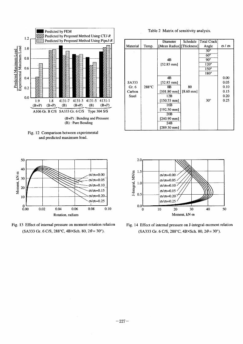
1' c~'

O ~I

~ ~ ~

.~

~: ~:'

o ~ u ;5~

~ ,~

l .2

~:' CQO 1.0

~l ~:'S 0.8

.~ ca

~: 0.6

~ c~

~ ~l (L)~ 0.4

'C:

o c~ ~ O.2

0.0

I Predicted by FEM ~ predicted by Proposed Method Using CTJ-R [] Predicted by Proposed Method Using PipeJ-R

l.9 1.8 (B+P) (B+P) AI06 Gr. B C/S

Fig.

4131-7 4131-3 4131-5 4131-l (B) (B+P) (B) (B+P)

SA333 Gr. 6 C/S Type 304 S/S

(B+P) : Bending and Pressure (B) : Pure Bending

12 Comparison between experimental and predicted maximum load.

Table 2 Matrix of sensitivity analysis.

50

40 ~ ~ 30

~ F::

o ~ 20 o ~:

lO

Fig.

O 0.00 0.02 0.04 0.06

Rotation, radians

0.08 O. I O

1 3 Effect of internal pressure on moment-rotation relation

(SA333 Gr. 6 C/S, 288'C, 4BXSch. 80, 2e = 30').

2.0

~ 1.5 .\ Z; ~:

~ 1.0 ~ c:$H

bo Q)

~ ~i

I~ 0.5 ~,

Fig.

0.0 o lO 20 30

Moment, kN-m 40 50

14 Effect of internal pressure on J-integral-moment relation

(SA333 Gr. 6 C/S, 288'C, 4BXSch. 80, 2e= 30').

- 227 -

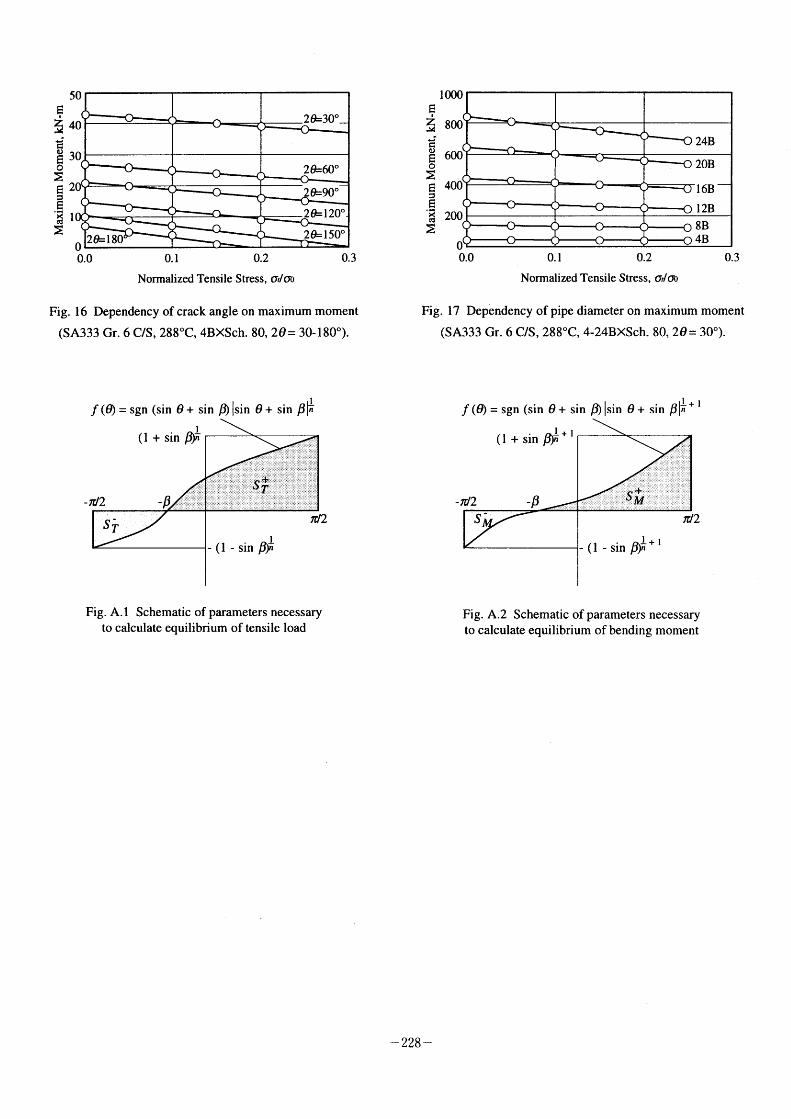
50 S,

~ 40

~ s:

~ 30 o ~:

~ 20 ~ ~ '~ l

:~

O

2e~30'

2e~180

2e~60-

e~90'

2 e~ 1 20-

2e~150-

0.2 0.3 0.0 O. 1 Normalized Tensile Stress, atloo

Fig. 16 Dependency of crack angle on maximum moment

(SA333 Gr. 6 C/S, 288'C, 4BXSch. 80, 20 = 30-1 80').

lOOO ~ ~ 800 ~i

~ " o ~:

~ 400 :'

~ '~ 200 ~:

O O. l 0.2

Normalized Tensile Stress, a,loo

Fig. 17 Dependency of pipe diameter on maximum moment

(SA333 Gr. 6 C/S, 288'C, 4-24BXSch. 80, 20= 30').

f (e) = sgn (Sin e + sin fi) Isin 6 + sin PI~

Fig. A.1 Schematic of parameters necessary to calculate equilibrium of tensile load

l ll l f (e) = sgn (sin 0+ sin p) sin O + sin p 71+

Fig. A.2 Schematic of parameters necessary to calculate equilibrium of bending moment

- 228 ~

IV-6 Low Alloy Steel Piping Test for Fracture Criteria of LBB

Koji Koyama, Nuclear Plant Component Designing

Section, Kobe Shipyard & Machinery Works, Mitsubishi

Heavy Industries, Ltd., Japan

LOW ALLOY STEEL PIPlNG TEST FOR FRACTURE CRrrERIA OF LBB

Koji Koyama and Itaru Muroya Mitsubishi Heavy lirdustries, Ltd.

Toshihiko Tanaka The Japan Atomic Power Company

Takao Nakamura The Kansai Electric Power Co., Inc.

Abstract

Seven pipe fracture tests were performed to provide the data for establishing fracture criteria of Leak Before Break for the low alloy steel pipe.

Test pipes were 6-inch and 8-inch diameter pipes made of SFVQIA or STPA24 Iow alloy steel. A circunferential through-wall crack was introduced at the center of a pipe, and four-point bending load was applied without internal pressure. Stable crack extensions were observed in all of the

experiments. To estimate the maximum applied load, the net-section criteria (NSC), R6 method Option 2 and

Option 3 were used. The predicted values by three kinds of evaluation methods were compared with the experimental loads. Most of all the predicted maximum loads agreed well with the experimental maximum loads within 20% difference. The NSC gave the most accurate prediction but also gave unconservative results in some test cases. The predicted maximum loads by R6 Op.2 were conservative in all of the test cases. From the view point of conservativeness R6 method can be used for evaluation of the low alloy steel pipe fracture. Therefore, the LBB concept would be applied to the protective design standard against pipe break for the material.

1. INTRODUCTION

The concept of leak before break (LBB) has been applied to the protective design standard against pipe break since 1992 in Japan. The LBB applicability evaluation flow is shown in Fig.1-1.

The current application of LBB concept is limited to the piping systems in the reactor cooling pressure boundary(RCPB) and of austenitic stainless steels. Nevertheless, this concept would also

be applicable to other piping systems and other materials, provided that plant shutdown can be achieved before fatal pipe break, taking account of fracture behavior the pipe material and the reliability of the performance of leak detection systems.

The recent study of fracture mechanics confirmed the adequacy of application of the LBB concept to the piping system of carbon steel piping/1/, consequently, the LBB concept would be applicable to the piping systems, as well, of low alloy steel, which is the same ferritic material as

carbon steel. Moreover, the existing leak detection system will be also effective to the application of LBB

concept for the PWR secondary piping systems inside the reactor containment vessel, such as main

feedwater system. This paper covers the experimental study performed on the fracture behavior of low alloy steel

pipes, which is expected to be applied to the reactor coolant piping and feedwater piping in

advanced PWRS in Japan.

- 229 -

2. TEST DESCRIPTION

2.1 IeSIMatdx

Seven pipe experiments were conducted to investigate the effects of the crack angle, material and pipe diameter on the fracture behavior. Table 2.1-1 shows the test matrix. In these tests, the 6-

inch and 8- inch diameter pipes were used.

2.2 I~sLEip~s

The pipes were made of srvQIA and STPA24 Iow alloy steel (Japanese Industrial Standard Specification equivalent to ASME SA508 Cl.3 and SA335 Gr. P22 respectively). The test sections were of base metal pipes or shop fabricated metal active gas (MAG) welds joining two pieces of the pipe. The pipe geometry is shown in Fig. 2.2-1.

A initial circunferential through-wall flaw was introduced into the center of the test section by

electric-discharge-machining(EDM) techniques, followed by cyclic loading until fatigue cracks extended to approximately 5 mm to sharpen the crack tip. Fig 2.2-2 shows the through-wall crack

geometry.

2.3 I~sLJ~rQ~~ure

The test system is shown in Fig.2.3-1. This test system has a capacity of 100 tonf (980 kN) per

ram and the maximum stroke is 500mm. The pipes was subjected four-point bending with the inner span of 800 mm and the moment arm length of 750mm. The experiments were conducted under displacement control with the displacement rate of 0.05 mm/sec.

The experiments of srvQIA pipes and the STPA24 pipes were conducted at 325~C and 310~C, respectively. To achieve these temperature, the hot air was ventilated into the test section

by the fan, and the heaters were used for the fine temperature adjustment of the center of the test

section. The temperature was monitored by five thermocouples to be maintained at the designated test temperature. After reaching the temperature, the test pipes were allowed to stabilize at the test

temperature at least 2 hours before applying bending moment load. No internal pressure was applied.

2.4

The following data were collected using the personal computers. The grid lines with 2 mm intervals were drawn near the crack tip of the pipe surface to observe crack extension behavior. Crack extension behavior was also recorded by video camera.

' Applied load (at each ram)

' Load-1ine displacement (at each ram)

' Pipe ovalization

' Crack opening displacements at three locations

• Strain ' Temperature near the crack tip

• Crack extension in both crack tips

- 230 -

2.5

The chemical compositions of the srvQIA and STPA24 steels are shown in Table 2.5-1. The stress-strain curves and J-resistance curves were obtained using the test specimens taken

from the pipes with the same sizes of the bending test pipes. For the fracture toughness test, the

1/2T CT specimens and IT planform size CT specimens which had the thickness of 1/2-inch were taken from 6-inch diameter pipes and 8-inch diameter pipes, respectively. The true stress-strain

curves of the base metals are shown m Frg 2 5 1-Frg 2.5-3. The J-resistance curves of the base

metals and the weld metals are shown in Fig. 2.5-4~Fig. 2.5-9. Also shown in those figures the fitting curves by Ramberg-Osgood's law for the stress-strain curves and the power law for the J-resistance curves are drawn in the same figures.

Table 2.5-2 shows the tensile properties and the Jlc Values of the test materials. The flow stress

is defined by the average of the 0.2% offset yield strength and the ultimate strength.

2.6

The experimental results are summarized in Table 2.6-1. The total applied load versus load -line displacement curves are shown in Fig. 2.6-1 and Fig. 2.6-2. At first from a fatigue crack tip,

two ductile cracks initiated and afterwards either of them propagated much longer than the other. All of the cracks propagated stably with the angle of about 45' to the pre-cracked cross sections.

According to the measured crack mouth opening displacement, the symmetrical opening behavior observed. The ovalization near the cracked section to the original diameter was within

2%.

3 . EVALUATION OF PIPE EXPERIMENT

In this study the net-section collapse criterion (NSC) and R6 method (Option 2 and Option 3)

were applied in order to estimate the maximum load. R6 Option 3 uses J-integral, which is calculated by the finite element analysis or the simplified equation as proposed by Zahoor /2/. In

this study, the simplified J-integral calculation was chosen for R6 method, because J-integral analysis by the finite element method would be time consuming to evaluate the pipe fracture behavior for each of the seven pipe tests. Therefore by the following three steps the validity of the

simplified J-integral is confirmed and the applicability of three evaluation method is investigated.

i. Validity of the modeling of the finite element analysis ii. Evaluation of the accuracy and conservativeness of the simplified J-integral comparing

with J-integral by the finite element analysis

iii. Evaluation of the accuracy of the predicted maximum applied load from each evaluation

method

3.1 a

(1) Description of the finite element(FE) models The analyzed case was Experiment SFB1. The analyses were made with the FE code MARC

(version K6-1). The FE model is shown in Fig.3.1-1. The model is one quarter of the test pipe

was modeled due to symmetry. The element type was 20 node solid element. The total number of elements and nodes was 1056 and 5727, respectively. The load-line displacement was applied at the outer support points.

- 231 -

For the crack extension analysis, two models were prepared. One was Model I which had the crack length corresponding to the initial crack length of half angle 45" . The other was Model 2

which had the extended crack length at the maximum applied load in the experiment. As mentioned previously the cracks extended diagonally to the pre-cracked cross section, Model 2 had the projected crack extension to the pre-cracked cross section at the maximum load. The experimental load-line displacement was applied to Model I until just before the ductile crack

initiation and the test load-line displacement at the maximum load was applied to Model 2.

(2) Global behavior of the test pipe

Fig. 3.1-2 shows the comparison of the calculated total applied load versus load-line displacement relation with the experimental result. Fig. 3.1-3 shows the similar comparison in the case of the crack mouth opening. In both comparisons, analytical results agree well with the

experimental results. These results gives the validity of the FE modeling including consideration

of the diagonal crack propagation.

3.2 d

(1) Accuracy and conservativeness of the simplified J-integral To calculate the simplified J-integral under the bending load, the stress-strain curve was fit

by Ramberg-Osgood's law expressed by the following equation.

E /E 0=(a/a )+a (a/a ) (3.2-1) The fitting curve is already shown in Fig.2.5-1. The parameters of Ramberg-Osgood's law are as follows;

a =1.47, a o = 413 MPa, E o =2.19 x 10~3, n = 7.91

Fig.3.2-1 shows the comparison of the simplified J-integral under the bending load with J-integral by the FE analysis. In these calculations the crack extension was ignored. At the bending stress of 392 MPa which is close to the maximum value in the experiment, the difference between both values is 10% and the simplified J gives conservative result.

(2) Comparison of Failure Assessment Curves (FAC) Fig. 3.2-2 shows the comparison of FAC of R6 method Option 3 using the simplified J with

that using J-integral by the FE analysis. Also from this figure the simplified J analysis method

gives the accurate and conservative FAC.

3.3 a t d a a at' t

(1) Analysis condition Material properties, the stress-strain curves and J-resistance curves shown in Table 2.5-2 and

Frg 2 5 1 -Frg 2 5 9 has been used for the analysis. Because the accuracy was confirmed, the

simplified J was used to obtain FAC in the case of R6 Option 3. To estimate the maximum load in the case of the pipes with the weld metal, the stress-strain curves of the base metal and J-

resistance curves of the weld metal were used for the conservative assumption.

(2) Results The maximum test loads normalized by the predicted maximum loads obtained from three

different kinds of evaluation methods are shown in Fig. 3.3-1-Fig. 3.3-3.

The average values of the normalized maximum loads of seven tests are I .05 from the NSC,

1.15 from R6 Op.2 and 1.09 from R6 Op.3. Most of all the predicted maximum loads agreed well with the experimental maximum loads within 20% difference. There are some cases that the normalized maximum load is below 1.0, two cases from the NSC, one case from R6 Op.3

- 232 -

and no case from R6 Op.2. Therefore, from the viewpoint of the accuracy, the NSC gives the most accurate prediction,

while from the viewpoint of the conservatism, the NSC may not always give conservative prediction and R6 Op.2 gives the most conservative results.

4. CONCLUSION

In order to provide the experimental data for establishing the leak before break criteria of the

low alloy steel pipe, seven pipe fracture experiments were performed. Test pipes were 6-inch and

8-inch diameter pipes of SFVQ IA or STPA24 Iow alloy steel. A circumferential through-wall crack was introduced at the center of a pipe, and four-point bending load was applied without internal pressure. Stable crack extensions were observed in all ofthe experiments.

To estimate the maximum applied load, the net-section criteria, R6 method Option 2 and Option 3 were used. The predicted values by three kinds of evaluation methods were compared with the experimental loads. Most of all the predicted maximum loads agreed well with the experimental maximum loads within 200/0 difference. In detail, the NSC gave the most accurate prediction but also gave two unconservative results. The predicted maximum loads by R6 Op.2 were conservative in all of the experiment cases. From the view point of conservativeness R6 method can be used for evaluation ofthe low alloy steel pipe fracture.

The further analyses on the pipe with the actual geometry is continuously followed to establish

the leak before break criteria of the low alloy steel pipe.

5. ACKNOWLEDGMENT This test was funded by five Japanese PWR utilities, and the results on this study were

discussed and reviewed in the committee under Thermal and Nuclear Power Engineering Society. The author acknowledges to the chairman Prof. Y. Asada, the committee members Prof. K. Miya, Dr. K. Shibata, Dr. K. Kashima and the other committee members including those from the utilities.

6. REFERENCES

/1/ Y. Asada, 'Development of Criteria for Protection Against Pipe Breaks in LWR Plants', pp.95-l I I , International Journal of Pressure Vessel & Piping, vol. 43, 1 990.

/2/ A. Zahoor, Ductile Fracture Handbook Volumel, NP-6301 -D N 1 4-1 Research Project 1 757-69,

June 1989. /3/ T. Tanaka, T. Nakamura, K. Koyama, I. Muroya, 'Four-Point Bending Tests of Low Alloy

Steel Pipes in Japan', presented at the 7th German Japanese Joint Seminar, Sept. 1 997.

- 233 -

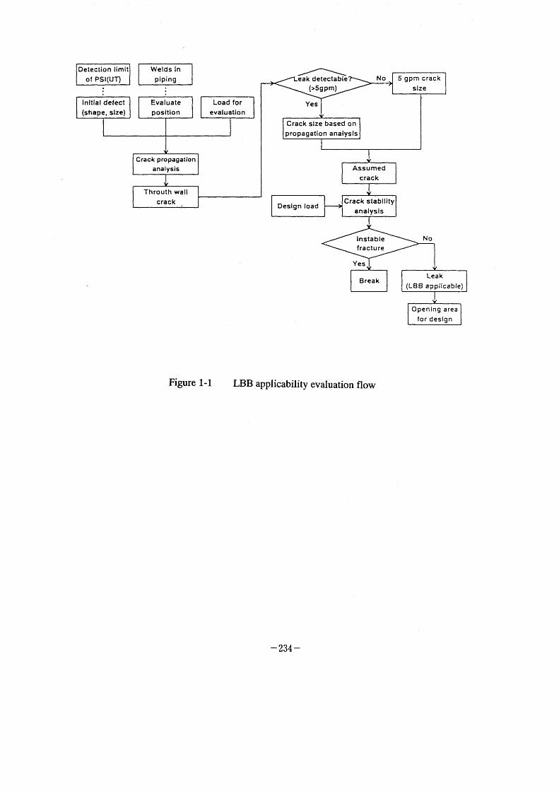
~~~~T~~T~T~l~~~I r~~rlL-J

ot Psl(uT) PiPing

Inltlal defect

(shape, slze) Evaluate position

Load for evaluatlon

Crack propagation analysis

Throuth wall crack

eak detectable (>5gpm)

Yes

No 5 gpm crack size

Crack size based on propagation analysls

Design load

Assumed crack

Crack stability

8nalysls

Instable f racture

No

Yes

Break Leak

(LB8 appllcable)

L~ ~~~~~ Jrl l9~e a

tor desi9n

Figure 1-1 LBB applicability evaluation flow

- 234 -

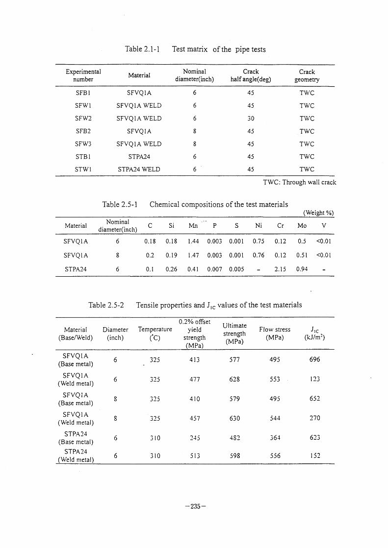
Table 2. I -1 Test matrix ofthe pipe tests

Experimental number

Material Nominal

diameter(inch) Crack

half angle(deg) Crack

geometry

SFB l

SFWl

SFW2

SFB2

SFW3

STB l

STW l

SFVQ I A

SFVQIA WELD

SFVQ I A WELD

SFVQ I A

SFVQ I A WELD

STPA24

STPA24 WELD

6

6

6

6

6

45

45

30

45

45

45

45

TWC TWC T\VC

TWC TWC TWC TWC

Table 2.5-1

TWC: Through wall crack

Chemical compositions of the test materials (weight '/.)

Materiai Nominal diameter(inch) C Si Mn P S Ni Cr Mo V

SFVQ I A

SFVQ I A

STPA24

6

8

6

O. 1 8

0.2

O. l

O. 1 8

O. 1 9

0.26

l .44

l .47

0.4 l

0.003

0.003

0.007

0.00 l

0.001

0.005

0.75

0.76

0.12

0.12

2.15

0.5

0.5 l

0.94

Table 2.5-2 Tensile properties and Jlc Values ofthe test materials

Material

(Base/~Veid) Diameter

(inch)

Temperature ('C)

0.2010 offset

yield

strength

(MPa)

Ultimate strength

(M:Pa)

Flow stress

(MPa) Jtc

(k J/m2)

SPVQ I A (Base metal)

SFVQ I A (Weld metal)

SFVQ I A (Base metal)

SFVQ I A (Weld metal)

STPA24 (Base metal)

STPA 24 (Weld metal)

6

6

8

6

6

325

3~~5

3,-5

3~~5

310

310

413

477

410

457

245

513

577

628

579

630

482

598

495

553

495

544

3 64

556

696

l 23

652

270

623

l 52

- 235 -

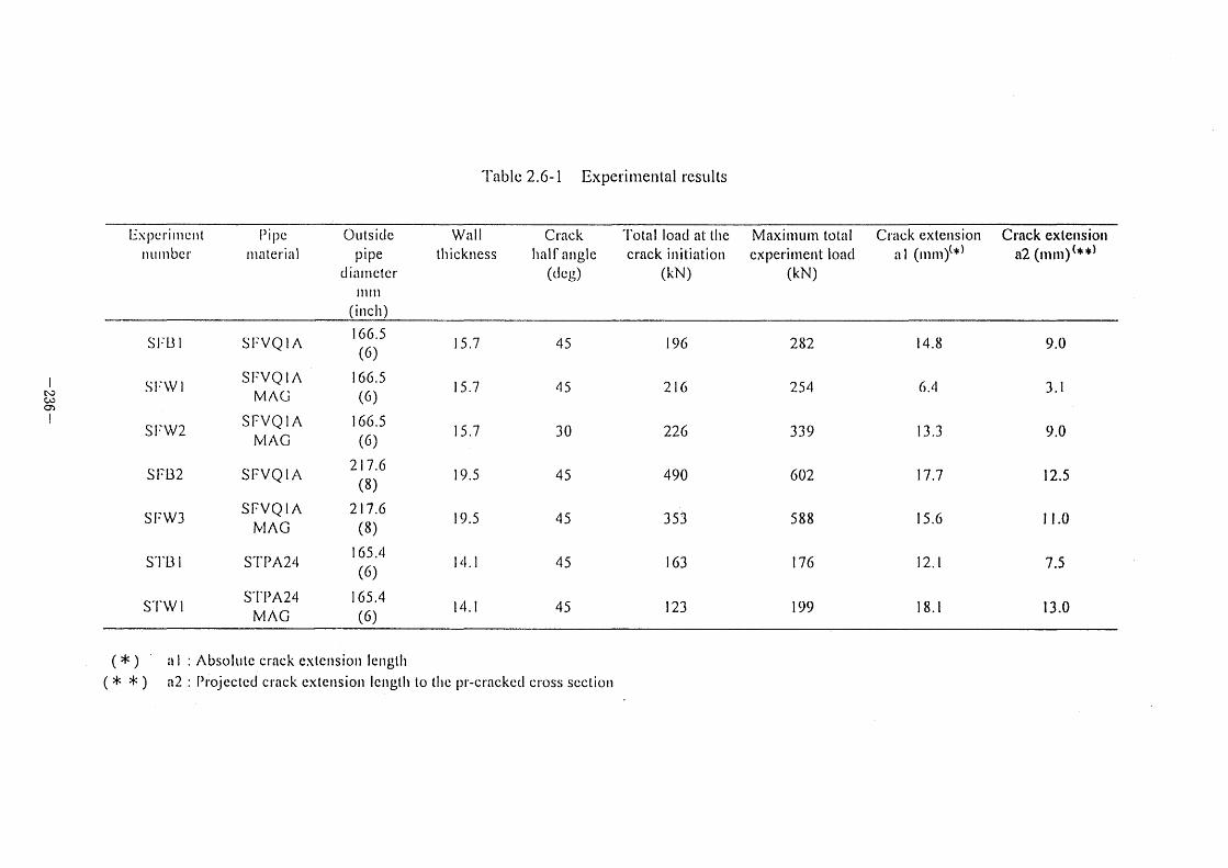
Tablc 2.6- l Experimental results

[3\pcrilncllt

tlulnbcr

I) i pc

lllllterial

Outside pipe

dlnnletcr

mln (inch)

Wa I l

thickness

C t-ack

ha I f' angle

(d cg)

'l'otal lo',Id at the

crack initi'ation

(kN)

Maximurn total experiment loacl

(kN)

Crack extension ai (mm)(*)

Ct'ack extcnsiot] (**] a2 (n]m)

l

~~ cb

I

SI'O i

SI'W l

SFW2

SFB2

sr'\v3

S'I'l3 l

S'I'W l

SI*VQ I A

SI*VQ I A

lvtAG

SFVQ I A M A G

Sl'VQ I A

SFVQ I A lvi A G

S'I' r) A 2 4

S'I'PA24

MAG

l 66.5

(6)

l 66.5

(6)

l 66.5

(6)

2 1 7.6

(8)

2 1 7.6

(8)

l 65.4

(6)

l 65.4

(6)

l 5.7

I 5.7

l 5.7

l 9.5

l 9.5

14.l

14.l

45

45

30

45

45

45

45

i 96

216

226

490

353

I 63

l 23

282

254

339

602

588

l 76

J 99

I 4.8

6 . 4

I 3.3

l 7.7

l 5.6

12. I

l 8. l

9.0

3.l

().O

12.5

l 1.0

7.5

13.0

(*) (* *)

il l

El 2

AbsolLttc crack extcnsion length

Projcctcd crack cxtcnsion lcngtll to tl]c pr-crirckcd cross section

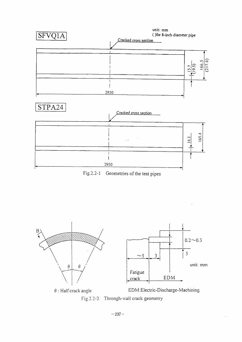
SFVQ I A unit: mm

( )for 8-inch diameter pipe

Cracked cross section

,,\

\J

STPA24

Fig.2.2- 1

Cracked cross section

Geometries of the test pipes

B ~i

l l

v

~5

Fatig ue

crack

l

v

3

A l

0.2-0.3

EDM

JL

5

unit: mm

e : Halfcrack angle

Fi~.2.2-2

EDM:Electnc-Dlscharge-Machirung

Throngh-\\'all crack geometry

- 237 -

!

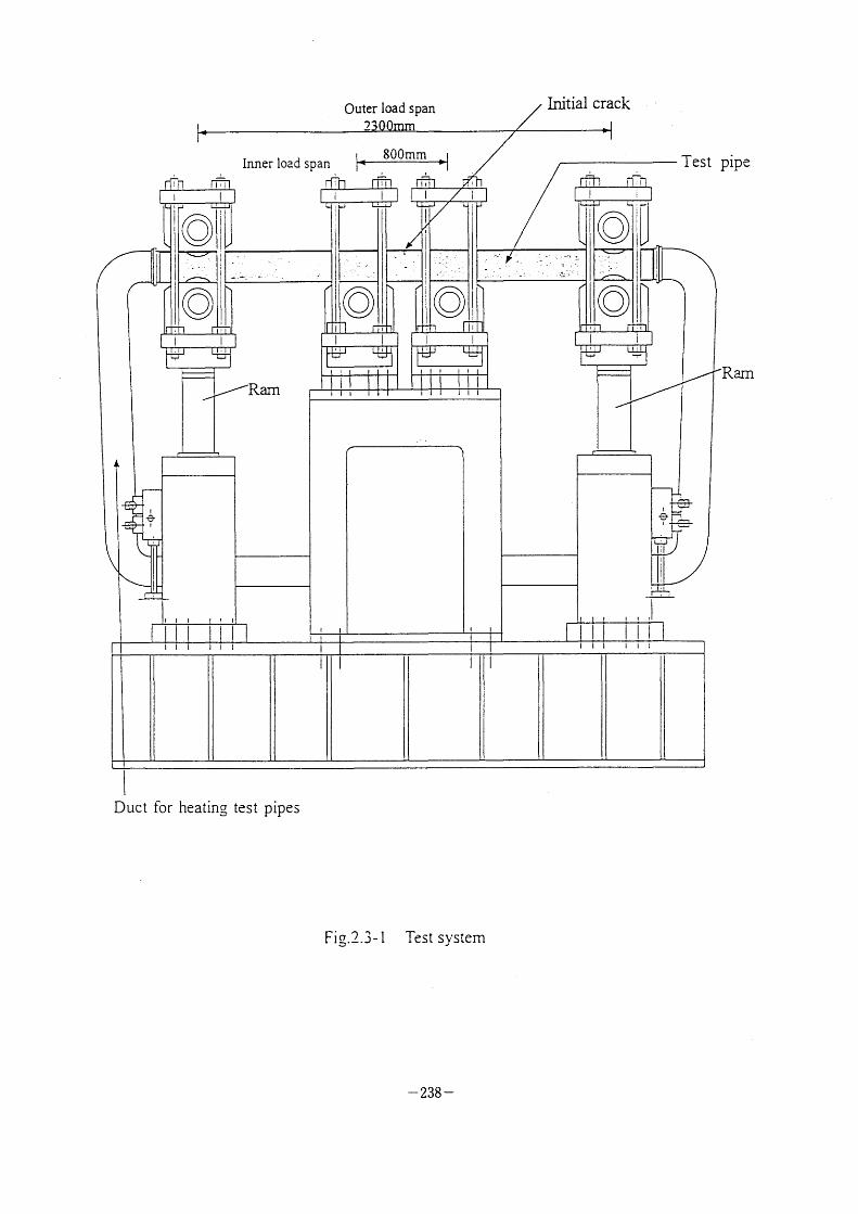
ll

l

lrtltial crack

A

!_ _1 I l

L~ t 1

Ram

l

~ t

'ft 'l l l

I l

l t

f ,

I

't~ ~~~__

~) I 'I

h~ I

''' 'l' 111

Ram

il 111 I III ll l

l I :

Duct for heating test pipes

Fig.2.3- I Test system

- 238 -

~:

:,,

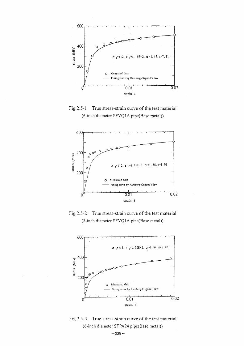
U, O ~ ;1,

600

400

200

o

o o

o

t I

a o 413, E Q=2. 19E-3, a=1.47,n=7.

Measured data

Firting cu~'$ by Rarnberg-Osgood's law

91

0.01 0.02 srrain a

Fig.2.5- I True stress-strain curve of the test material

(6-inch diameter SFVQ IA pipe(Base metal))

~ :1, :1,

:-

~ :/:

600

400

200

o

I ooo o

o

o

o

o

a 0=410. E 0=2.lSE 3 a 1 26 n 8 98

O Measured dala Firtin~_ curve by Ramberg-Osgood's law

0.01 0.02 strain e

Flg.2.5-2 True stress-strain curve ofthe test material

(8-inch diameter SFVQ I A pipe(Base metal))

4 :1,

t,

V:.

600

"+00

200

O

o

(90

o

a Q=24S, E 0=1. 30E-3, a =j. 64,n=5. 03

Mc,asurcd duta

Finins cur\c by R~mbcrs'Osgood's I;!Lv

0.0 1 0.02 strain e

Flg.2.5-3 True stress-strain cur\'e of the test material

(6-inch diameter STPA24 pipe(Base metal))

- 239 -

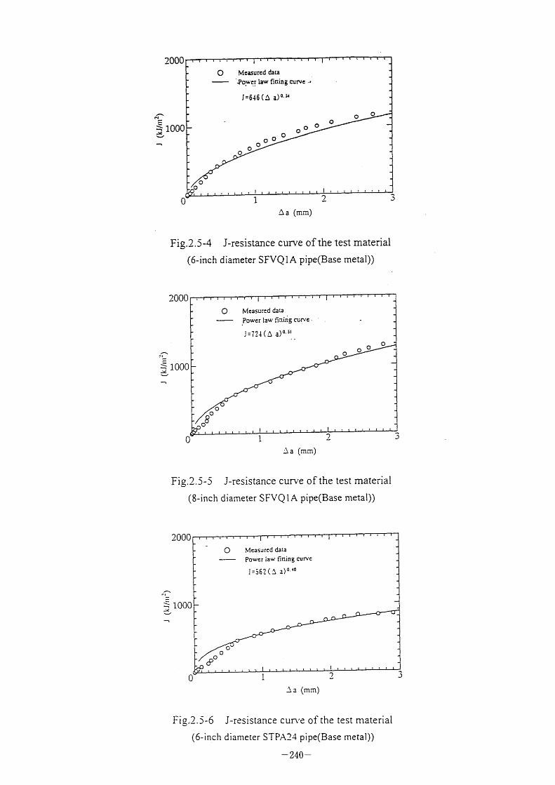
2000

'~ ,N

~ 1000 '\ -, ,, ~J -~

o

o o

i

Mcasured data '~)o,~~, Ia"v' fir,ing cul~lc .'

J=646 (A a)Q'54

o ooo

l

oo o o o o

o l ,)~ 3

A a (mm)

Fig.2.5-4 J-resistance curve ofthe test material

(6-inch diameter SFVQ IA pipe(Base metal))

•_ooo

'~ t]

~ 1000 '~, 'l ~ \J -,

O

080 o

Measured data

F•owcr law fining cl~~rc J= /~24 (A a)o.51

o oo o

o 1 ~- 3

:~ a (mm)

Frg ~-5-5 J-resistance curve ofthe test material

(8-inch diameter SFVQ I A pipe(Base metal))

2000

~ - 1000 --x

~ ~

O

cPo o

o

M:casurcd data

powcr isw fining curvc

l=56? (A a)a.4a

l

o 1 ,- 3

~~a (mm)

Fig.2.5-6 J-resistance cur~'e of the test material

(6-inch diameter STPA24 pipe(Base meta]))

- 240 -

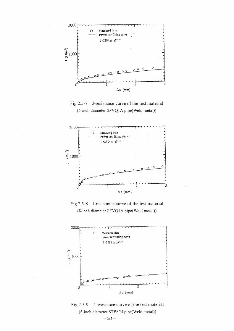
2000

l~ N ~: 1000 .~ ,-,

J'a ..,

-

O Measured data powet law fit:ing cu~!* e

J=250 (A a)a.19

o o oo o o o

I

oo o o

o l 2 3

~ a (mm)

Fig.2.5-7 J-resistance curve ofthe test material

(6-inch diameter SFVQIA pipe(Weld metal))

2000

'-~ ,N

~~ 1000 -;4 *~ ,~

o

O Measured data Po\iver I~w fitting F~r\'e-

J=3SS (~ a)Q'38

o o o

1 ,~ 3

Aa (mm)

Fig.2.5-8 J-resistance cun'e ofthe test material

(8-inch diameter SFVQ I A pipe(\Veid metal))

2000

r'

'\ 1000 -JJ:

,J '~

O

[

[

[

[

\L (c;IsuTcd data

Pol*'cr law nuing curve

i=2?9 (~ a)Q'Io

I

o l 1, 3

~a (mm)

Flg ~.5-9 J-reslstance cur\'e of the test material

(6-inch diameter STPA24 pipe(\Veld metai))

- 241 -

,~ ~ ~::

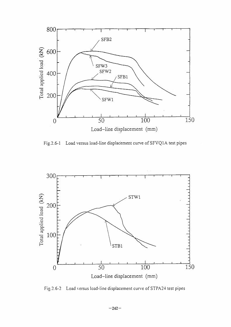
~l IS

c~;

O' ~ ~:;

O ~ n_

c:;

~ ~ O hl

800

600

400

~_oo

SFB2 ,l

\ SFW3

sFw2

~ ~\\ SFW1

o

I

/ SFB1

Fig.2.6-1

50 Load-line displacement (mm)

Load \'ersus load-line displac~ment curve of SFVQ IA test pipes

'f~ ~: ~: \J' i:D

c::;

O ~ ~ O ~ rl

-fl ~ ~ O rrl

300

~_oo

1 OO

/

STB 1

O

STW l

Fi~.2.6-~

l OO 50 Load-line displacement (mm)

Load \'ersus load-line displacement cur\"e of STPA24 test pipes

150

- 242 -

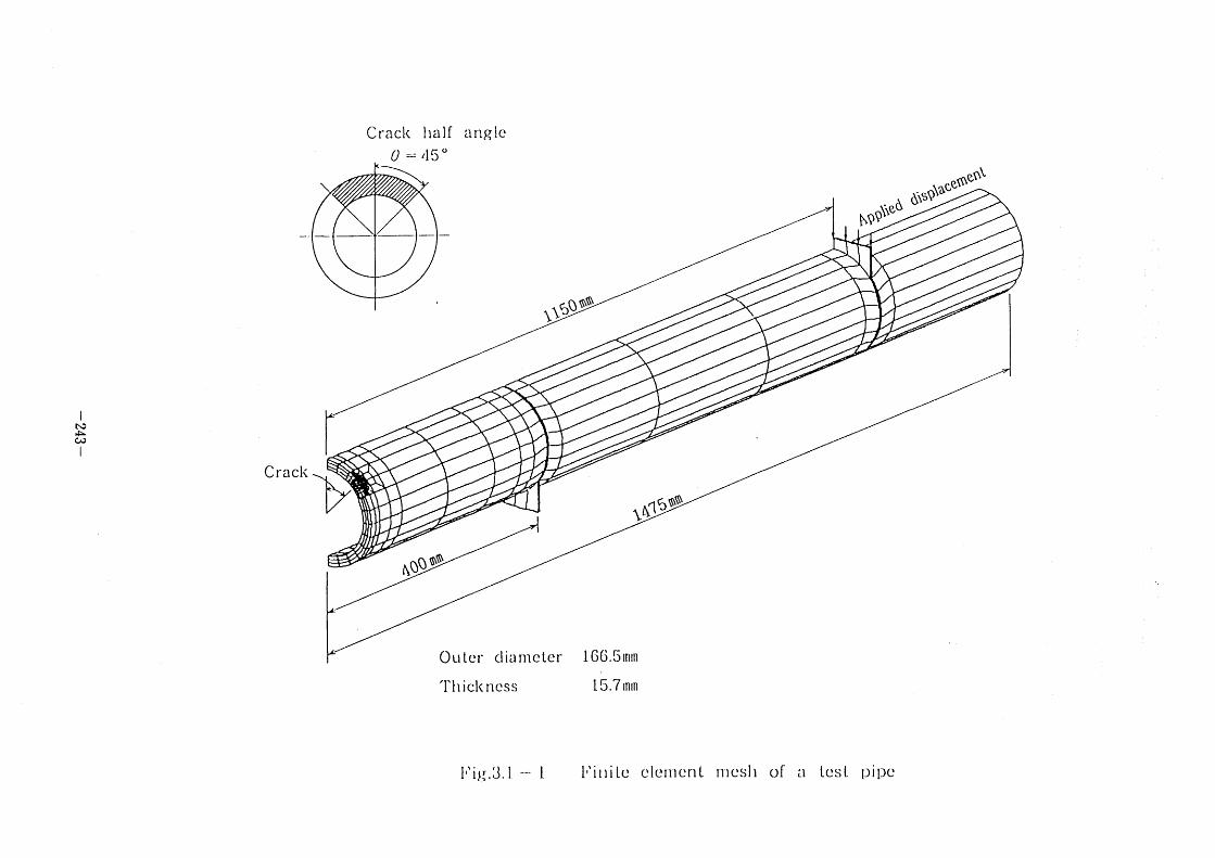
Cr'ack ll'.llf

O = 115*

'•1 Ilg I C

\\~~ I~~

(1\'~e~ ~\s~\~L:c;esc\:e~\~

~~y

I

t~ ~~ c~

I

Crack

\~~~I~~

Outcr diamctcr 16C.5mm 'l' I I i ck n cs s 1 ro .7 mm

1" ~ I --' l l . l ,t~ ' l,'il~llLc• C'ICll]CI~lL lllC'Sll Ol' tl LCSL p i pC

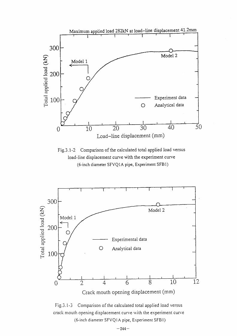
Maximum apphed load 28•_kN at load-line displacement 41.2mm

f\ Z; ~: '_/ 1'

c:;

O ~ vO

~ ~ n ~ ~ :j O H

300

2_OO

100

Model 1

O O

Model 2

O Experiment data

Analytical data

o Load-line displacement (mm)

50

Fig.3. I -2 Comparison ofthe calculated total applied load versus

load-line displacement curve with the experiment curve

(6-inch diameter SFVQI A pipe, Experiment SFB I )

r~ Z: ~: ~l 1:)

c:;

O ~ iO (L)

~ C~ h~ c:;

~ c::;

O H

300

~_oO

100

Model 1 ~~1

O Experimental data

Analytical data

Model 2

O

10 8 6 ~

Crack mouth openlng displacement mm) (

Fig.3. I -3 Comparison of the calculated total applied load versus

crack mouth openlng displacement cur\'e \\"ith the experiment cur\'e

(6-inch diameter SFVQI A pipe, E\periment SFB I )

- 244 -

12

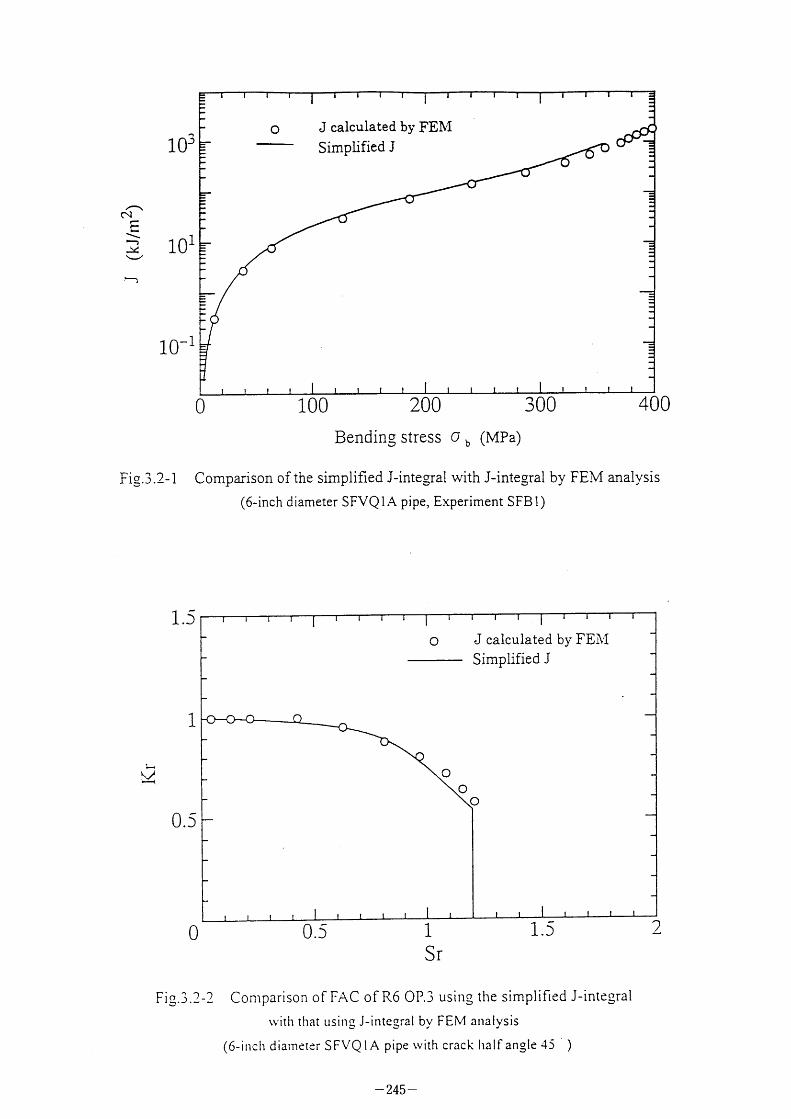
'~, c~'

~ '\ ~~ ,~'

~)

1 03

101

10-1

o J calculated by FEIVI

Simplified J

o l OO 200

Bending stress ab (MPa)

300 400

Fi~.3 .2- 1 Comparison ofthe simplified J-integral with J-integral by FEM analysis

(6-inch diameter SFVQ I A pipe, Experiment SFB 1)

~~{

1.5

l

0.5

O

O O

J calculated by FE~'l

Simplified J

O

o 0.5 1

Sr

1.5 ~~

Fl~.3.2-2 Comparison of FAC of P\6 OP.3 using the simplifled J-jntegral

\vith that usin_".. j-jnte_~._ral by FEM: analysis

(6-inch diameter SFVQ I A plpe \vith crack half angle 45 ' )

- 245 -

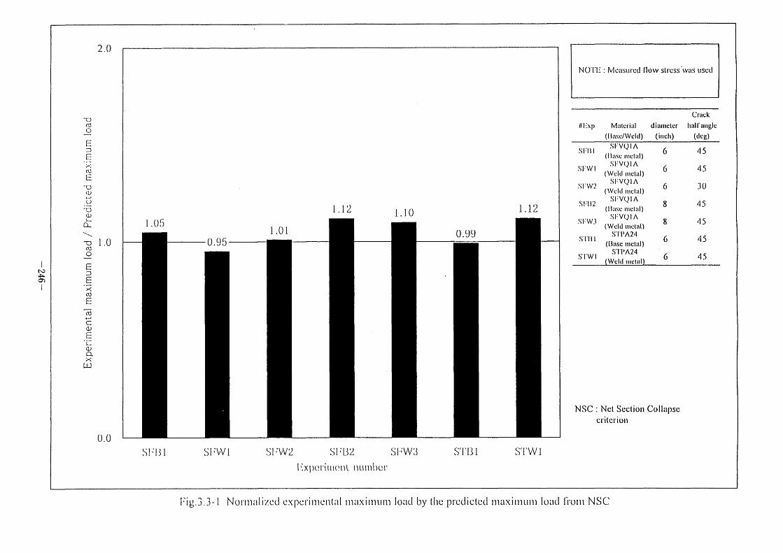
l

t\D ~~ (1)

l

l:jg.~) ,j- I Nol'Inilll7.cd c'xpcrlnlcntili inalximum lotlcl by tl]c prcdictcd nlalxlmunl loLld ll'oln NSC: ~'

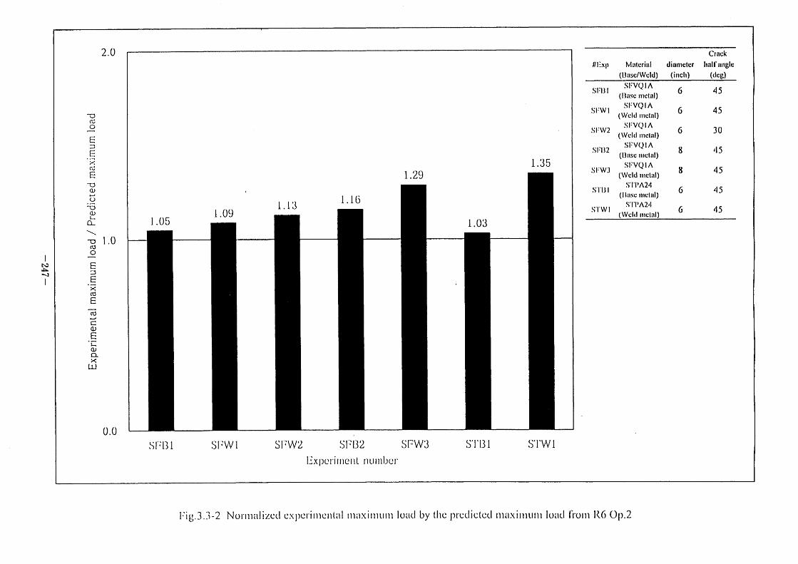
l

~e d~ ~ l

l:jg•3•],-2 Nol 111,llIZCCI C\pCI I111Cll[ Il i]1,1\lllILllll lO•1(1 by tllC pICCilctcd lll•lXlllILlill l0•lCI flOlll R6 Op 2

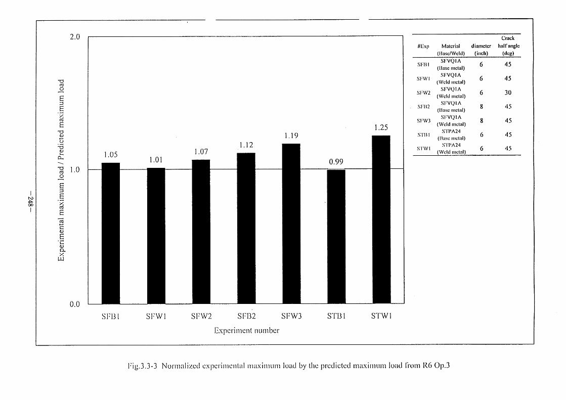
I

t\)

~ co I

I:jg•3•3 3 Nol'llltllil_CCI C'XpCl'illlC'I1[ill l]ItIXllllLllll lOil(1 by tl]C pl'C(lictccl lllalXll]Itllll lOilCl il•Olll R() Op•3

Session V

Material Characteristics

V- l Effect of Reverse Cyclic Loading on Fracture Resistance

Curves in CT Specimens

C. S. Seok, Sung Kyun Kwan University, Dept. of Mechanical

Engineering, Korea

Y. J. Kim, Sung Kyun Kwan University, Dept. of Mechanical

Design, Korea

J. I. Won, Sung Kyun Kwan University, Graduate School Dept. of

Mechanical Design, Koera

Effect of Reverse Cyclic Loading on the Fracture Resistance Curve in C(T) Specimen

C.S.Seoka, Y.J.Kima, J.1.Weona

'School of Mechanical Engineering, Sung Kyun Kwan Univ., Suwon, Korea

Fracture resistance (J-R) curves, which are used for elastic-plastic fracture mechanics analyses, are known to be dependent on the cyclic loading history. The objective of this paper is to investigate the effect of reverse cyclic loading on the J-R curves in C(T) specimens. Two

parameters were observed to be effective on the J-R curves during the reverse cyclic loading.

One was the minimum-to-maximum load ratio (R) and the other was the incremental plastic displacement ((5;.y.1/~:i), which is related to the amount of crack growth that occurs in a cycle.

Fracture resistance test on C(T) specimens with varying the load ratio and the incremental plastic displacement were performed, and the test results showed that the J-R curves were decreased with decreasing the load ratio and decreasing the incremental plastic displacement.

Direct Current Potential Drop (DCPD) method was used for the detection of crack initiation and crack growih in typical laboratory J-R tests. The values of J, and (5;, were also

obtained by using the DCPD method.

1. INTRODUCTION

This paper presents experimental results from cyclic displacement-controlled C(T) fracture tests. Seismic loading consists of dynamic loading and cyclic loading. According to a study by the International Piping Integrity Research Group (IPIRG) program[1], which pioneered the work on cyclic loading with C(T) and pipe specimens, the reverse cyclic loading was infiuenced by the parameters of load velocity, Ioad ratio, and incremental plastic displacement. The reverse cyclic loading could contribute to the reduction of material's fracture toughness, i.e., J-R curve. This work is applicable to flawed-structure evaluations

under seismic loading conditions, i.e. Leak-Before-Break (LBB) and in-service flaw evaluation criteria where seismic loading is addressed. In LBB and flaw evaluation criteria such as the ASME Section XI, the cyclic nature of the seismic loading is not implicitly accounted for on the potential effects on fracture toughness.

The objective of this paper is to study the effects of reverse cyclic loading on the nuclear

piping integrity. In order to assess the effect of cyclic loading on fracture behavior, the experiments considering two different parameters were performed. One parameter is load ratio (R) and the other is. incremental plastic displacement ((5i,y.11~;i), which can be just as

important as the load ratio parameter on the load-carrying capacity.

2. EXPERIMENTS

The test was performed at quasi-static loading rates. The detailed test procedure will be

followed.

- 249 -

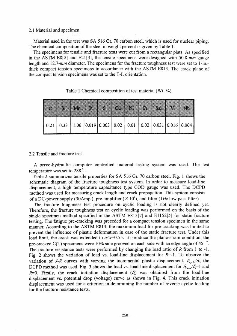
2. I Material and specimen.

Material used in the test was SA 5 1 6 Gr. 70 carbon steel, which is used for nuclear piping. The chemical composition of the steel in weight percent is given by Table I .

The specimens for tensile and fractwe tests were cut from a rectangular plats. As specified

in the ASTM E8[2] and E21L3], the tensile specimens were designed with 50.8-mm gauge length and 1 2.7-mm diameter. The specimens for the fracture toughness test were set to I -in.-

thick compact tension specimens in accordance with the ASTM E813. The crack plane of the compact tension specimens was set to the T-L orientation.

Table I Chemical composition oftest material (Wt. o/o)

2.2 Tensile and fracture test

A servo-hydraulic computer controlled material testing system was used. The test temperature was set to 288 ~ .

Table 2 summarizes tensile properties for SA 5 1 6 Gr. 70 carbon steel. Fig. I shows the schematic diagram of the fracture toughness test system. In order to measure load-line displacement, a high temperature capacitance type COD gauge was used. The DCPD method was used for measuring crack length and crack propagation. This system consists of a DC-power supply (30Amp.), pre-amplifier ( x l04), and filter (lHZ Iow pass filter).

The fracture toughness test procedure on cyclic loading is not clearly defined yet. Therefore, the fracture toughness test on cyclic loading was performed on the basis of the single specimen method specified in the ASTM E8 1 3 [4] and E I 1 52[5] for static fracture testing. The fatigue pre-cracking was preceded for a compact tension specimen in the same mauner. According to the ASTM E813, the maximum load for pre-cracking was limited to prevent the infiuence of plastic deformation in case of the static fracture test. Under this load limit, the crack was extended to a/w=0.55. To produce the plane-strain condition, the pre-cracked C(T) specimens were I Oo/o side grooved on each side with an edge angle of 45 '.

The fracture resistance tests were performed by changing the load ratio of R from I to - I .

Fig. 2 shows the variation of load vs. Ioad-line displacement for R=-1. To observe the variation of J-R eurves with varying the incremental plastic displacement, (5;.y.//6i, the

DCPD method was used. Fig. 3 shows the load vs. Ioad-Iine displacement for 6.y.//6,=1 and

R=0. Firstl)r; the crack initiation displacement ((5:i) was obtained from the load-line displacement vs. potential drop (voltage) curve as shown in Fig. 4. This crack initiation displacement was used for a criterion in determining the number of reverse cyclic loading for the fracture resistance tests.

- 250 -

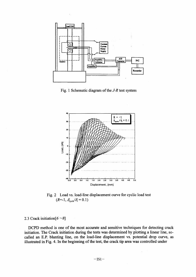
Fig. l Schematic diagram of the J-R test system

qo

3o

2o

10

Z :X - O 1:(!'

S -10

•20

•eo

•40

R = -l 5cvcle /~ = O' l

~: .5 o.o 0.6 1 o 1 5 2 o 2 6 Dis placement.,

3.0

(m m )

3 .5 4.0 4 5 5 .o

Fig. 2 Load vs. Ioad-line displacement curve for cyclic load test

(R=-1 (5; /~:..=01) ' .yct , '

2.3 Crack initiation[6 -8]

DCPD method is one of the most accurate and sensitive techniques for detecting crack initiation. The Crack initiation during the tests was determined by plotting a linear line, so-

called an E.P. blunting line, on the load-line displacement vs. potential drop curve, as illustrated in Fig. 4. In the beginning of the test, the crack tip area was controlled under

- 251 -

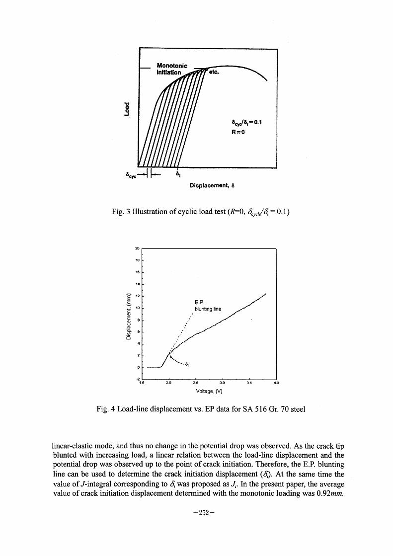
1'11'

s

Monotenic intt iaaon eta

8c~8i = 0.1

R=0

8=~ ~ 8i

Displacemen~ 8

Fig. 3 11lustration ofcyclic load test (R=0 (5; 1~:, = O I ) ' .yct i '

E E 4J c o E aJ

u (l9

a! (1)

b~

20

le

lo

14

12

10

e

8

4

2

o ~~

/

E.P. blunting line

.2 1,5 20 2.5 3.0

Voitage, (V)

3 .5 4.0

Fig. 4 Load-line displacement vs. EP data for SA 5 1 6 Gr. 70 steel

linear-elastic mode, and thus no change in the potential drop was observed. As the crack tip

blunted with increasing load, a linear relation between the load-Iine displacement and the potential drop was observed up to the point of crack initiation. Therefore, the E.P. blunting

line can be used to determine the crack initiation displacement ((5:i). At the same time the

value of J-integral corresponding to (5:, was proposed as J,. In the present paper, the average

value of crack initiation displacement determined with the monotonic loading was 0.92mm.

- 252 -

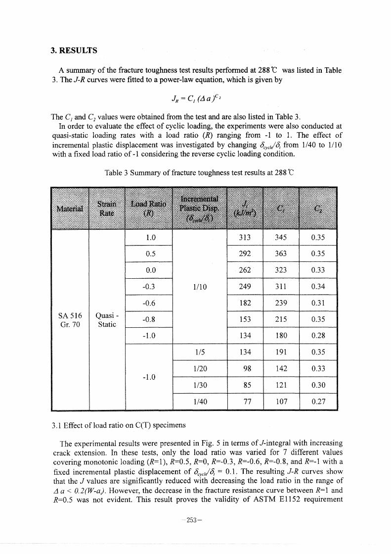
3. RESULTS

A summary ofthe fracture toughness test results performed at 288 ~ was listed in Table

3 . The J-R curves were fitted to a power-law equation, which is given by

JR = C] (A a)c2

The C1 and C2 Values were obtained from the test and are also listed in Table 3 .

In order to evaluate the effect of cyclic loading, the experiments were also conducted at

quasi-static loading rates with a load ratio (R) ranging from - I to I . The effect of incremental plastic displacement was investigated by changing 6,y,/1~;, from I /40 to I /10 with a fixed load ratio of - I considering the reverse cyclic loading condition.

Table 3 Summary of fracture toughness test results at 288 ~)

Mates.~

SA 516 Gr. 70

s.c~~ '

Ratc

Quasi -Static

f*•~ ~ t::ip;:::.~4~ip '

~~ .>' (s::•) , **=*

1 .O

o.5

o.o

-o.3

-O.6

-0.8

-1 .O

=1 .O

~~~~';~ ~; ' ~~ ' ';~l'~f~ ~ ~;~~;~;~~;;-'~~"~1/1"~~'~'i~~~/'~~~;~"~~i~://~' :;~~;:(~:~~~;": ~ '///:t:;:;i:i;~~...;;i=~;/~;~;/:~_=':~~':~ ~~;/;~;

!'~;t~ ~~'~':~~~~~"~~~~'~~~/~i~ ~ .. ,s;;'~~~~:""#~i!~ ~ ~~

~~' ~.*~~'f'~~'/~t~i.:"i'""~: '~i7~~;~(;; ;;,,/i~:"

1/10

1 15

l /20

l/30

l /40

313

292

262

249

l 82

153

134

134

98

85

77

+~:+

'~;~':~'~~*;." ~ +

"~ 'i':;~~~~t~"';.....~.j'~ ;:/,j.t;;~~ ~'"'?'~

345

363

323

311

239

215

180

191

1 42

121

l 07

_~ ~ ~~r

' ~1;c~

~~~ ~*/"'

~l "+~~= ~+ ~~ ;~~

o.35

o.35

o.33

0.34

O.3 l

o.35

o.28

o.35

o.33

o.30

o.27

3. I Eff_ect of load ratio on C(T) specimens

The experimental results were presented in Fig. 5 in terms ofJ-integral with increasing crack extension. In these tests, only the load ratio was varied for 7 different values covering monotonic loading (R=1), R=0.5, R=0, R=-O.3, R=-O.6, R=-O.8, and R=1 with a fixed incremental plastic displacement of (5i,y,/16:i = 0.1. The resulting J-R curves show that the J values are significantly reduced with decreasing the load ratio in the range of

R=0.5 was not evident. This result proves' the validity of ASTM E1152 requirement

~ 253 ~

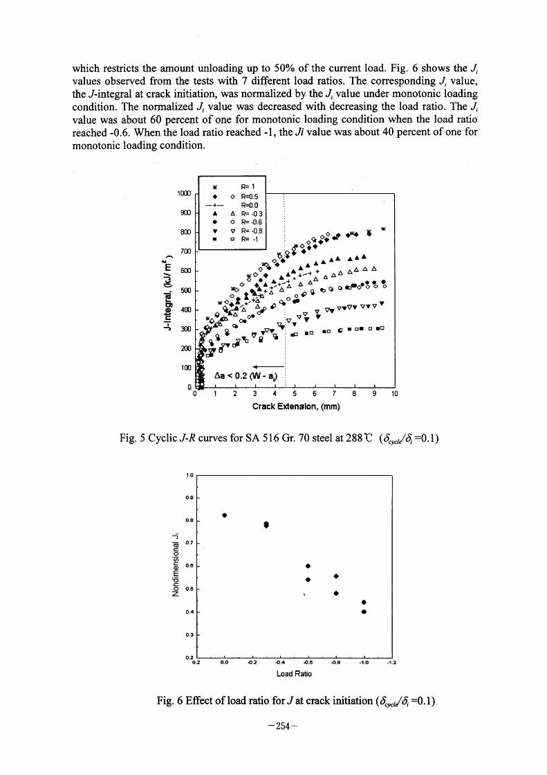
which restricts the amount unloading up to 500/0 of the current load. Fig. 6 shows the J, values observed from the tests with 7 different load ratios. The corresponding Ji Value, the J-integral at crack initiation, was nprmalized by the Ji,value under monotonic lpading

condition. The normalized Ji Value was decreased with decreasing the load ratio. The J, value was about 60 percent of one for monotonic loading condition when the load ratio reached -0.6. When the load ratio reached - I , the Ji value was about 40 percent of one for

monotonic loading condition.

f~ IE:

t~ ~ ~ '~ 15L*

O' O ~, =

J:b

10Cl]

900

8CID

7Cx)

5Cx]

500

400

300

200

ICx3

O

~K

1)

A e v

R= 1

c R=0.5 R=0.0

A R= -0.3 o R= -O.6 v R= -0.8 o R= -1

:~ (F.-

~$ ~~ AAAAA AJLA

A

~~(

O

le~

c~ A AA A A AA + C'(F. A4+ ~+~ A A ~ c (bLCiA$~AA+AA A A ee ()O ')q) QPe~eoeo c ~(~~~_t i +2~:A~a q,o ~

V Vy vvVv vvv ~~A/A ~,) IP :Vvvvy V oe ~((~^~~: o.

~r: -i~:q, ~~ 8dirlbVlv ~1 : IQ ID ID IE! IDI Dl ;Vv ;

~riV :

5 6 7 2

Crack Extension, (mm)

Fig. 5 Cyclic J-R curves for SA 5 16 Gr. 70 steel at 288 ~) (6.y.11~;, =0.1)

1 ,o

o.o

o .8

i) ~5 07 c: o '~5

c oo O ' E :~ c O o.6 Z

0.4

0.3

o .2

e ,

t

e e e

e e e

o .2 0.0 JD:2 .o.4 4.8 -0.8 . I .o - I .2 Load Ratio

Fig. 6 Effect of load ratio for J at crack initiation (6.yctl~:, =0. I )

- 254 ~

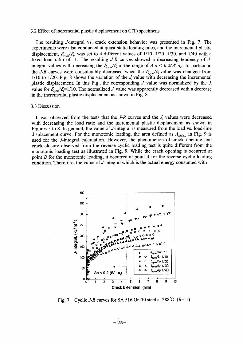
3 .2 Effect of incremental plastic displacement on C(T) specimens

The resulting J-integral vs. crack extension behavior was presented in Fig. 7. The experiments were also conducted at quasi-static loading rates, and the incremental plastic

displacement, (5:.y.//(5:i, was set to 4 different values of l/lO, l/20, l/30, and l/40 with a

fixed load ratio of - I . The resulting J-R curves showed a decreasing tendency of J-

the J-R curves were considerably decreased when the 6.y.1/6/ Value was changed from l/lO to 1/20. Fig. 8 shows the variation of the J, value with decreasing the incremental plastic displacement. In this Fig., the corresponding J, value was normalized by the J, value for (5;.y.1/~;,= I /lO. The normalized J, value was apparently decreased with a decrease

in the incremental plastic displacement as shown in Fig. 8.

3 .3 Discussion

It was observed from the tests that the J-R curves and the Ji Values were decreased with decreasing the load ratio and the incremental plastic displacement as shown in Figures 5 to 8. In general, the value ofJ-integral is measured from the load vs. Ioad-line displacement curve. For the monotonic loading, the area defined as A(BCD) m Fig. 9 is used for the J-integral calculation. However, the phenomenon of crack opening and crack closure observed from the reverse cyclic loading test is quite different from the monotonic loading test as illustrated in Fig. 9. While the crack opening is occurred at point B for the monotonic loading, it occurred at point A for the reverse cyclic loading condition. Therefore, the value ofJ-integral which is the actual energy consumed with

400

350

300

~ ~E 250

.~ 1 ~ ~ _s 200 Ca Lo,

_0= 150

!:,

100

50

o

e e e

: vV 7VVVV'V e , .V V:1~r V V' l I ll

I I olE]Ialal ala D o D D a ~y . cc c c c e~ Dolol i( 1~(CF~~ cA AAAJdL

_JF AAAJLAA VV aol I~IL~A~:A:AALA A AA~~AA;AA':L AA AJ2~AA A A ~~ A

~;Ii!~~l~Z~f.~ !

' ~I~:::~AAA : e 6cycJq= I / 5 : v v 60yde/q=1/10

I D ~ ce,lq=1120 11' c 6cyde/q=1/30

5 G 7 8 9 Io 1 2 3 4 Crack Exten8ion, (mm)

Fig. 7 Cyclic J-R curves for SA 5 16Gr. 70 steel at 288~C (R=-1)

- 255 -

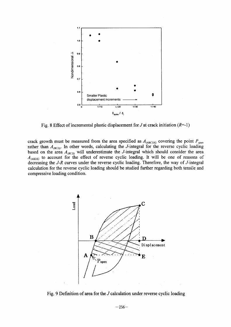
1 .1

1 .O

1 o .e CD

c o (1)

=a) o.e

E ~5 c o Z 0.7

o .e

o .5

e lp

(,

1)

Smaller Plastc displacement increments

e e

e

Fig.

1'10 1120 Il30 1/40 s / s. eyd. .

8 Effect of incremental plastic displacement for J at crack initiation (R=- I )

crack growih must be measured from the area specified as A(ABCDE) covering the point P "p'"

rather than A(BCD). In other words, calculating the J-integral for the reverse cyclic loading

based on the area A(BCD) will underestimate the J-integral which should consider the area A(ABDE) to account for the effect of reverse cyclic loading. It will be one of reasons of decreasing the J-R curves under the reverse cyclic loading. Therefore, the way of J-integral calculation for the reverse cyclic loading should be studied further regarding both tensile and

compressive loading condition.

l:,C:f

~

B .l /

l" ///

/ //' r/f/ ' ll.

' '/~ "' ll

ll /

ll

//'

/

/

/ *. t I

.* ,

I

..ll

J

$

) .'* I

C

A

'! "~* ~;' ' ;'~~ " / ' / ~~ *. ' '\\>~7'\' "

_~~/ ' Po pen

/

./i

F

t

D i sp I acemen t

E

Fig. 9 Definition of area for the J calculation under reverse cyclic loading

- 256 -

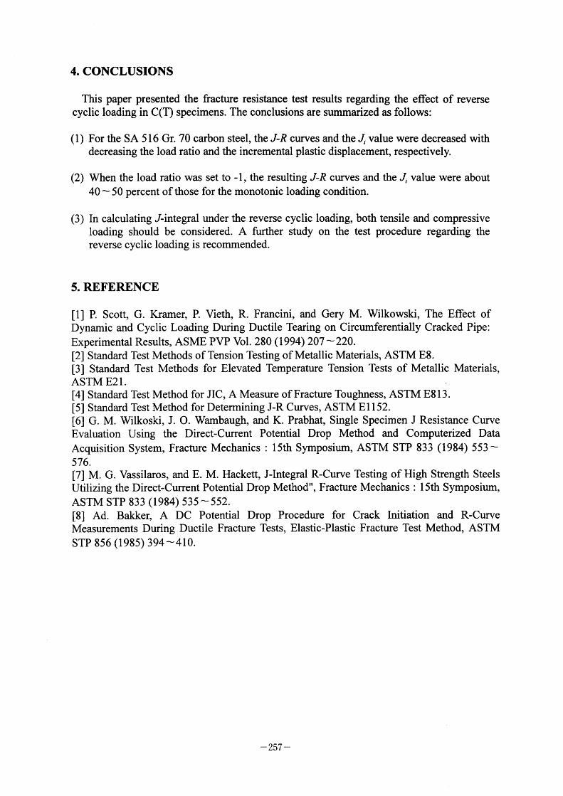
4. CONCLUSIONS

This paper presented the fracture resistance test results regarding the effect of reverse

cyclic loading in C(T) specimens. The conclusions are summarized as follows:

(1) For the SA 5 1 6 Gr. 70 carbon steel, the J-R curves and the Ji Value were decreased with

decreasing the load ratio and the incremental plastic displacement, respectively.

(2) When the load ratio was set to - I , the resulting J-R curves and the J, value were about

40 - 50 percent of those for the monotonic loading condition.

(3) In calculating J-integral under the reverse cyclic loading, both tensile and compressive

loading should be considered. A further study on the test procedure regarding the reverse cyclic loading is recommended.

5. REFERENCE

[ I J P. Scott, G. Kramer, P. Vieth, R. Francini, and Gery M. Wilkowski, The Effect of Dynamic and Cyclic Loading During Ductile Tearing on Circumferentially Cracked Pipe:

Experimental Results, ASME PVP Vol. 280 (1994) 207 - 220. [2] Standard Test Methods of Tension Testing of Metallic Materials, ASTM E8. [3] Standard Test Methods for Elevated Temperature Tension Tests of Metallic Materials, ASTM E2 1 . [4] Standard Test Method for JIC, A Measure of Fracture Toughness, ASTM E8 1 3 . [5] Standard Test Method for Determining J-R Curves, ASTM El 1 52. [6] G. M. Wilkoski, J. O. Wambaugh, and K. Prabhat, Single Specimen J Resistance Curve Evaluation Using the Direct-Current Potential Drop Method and Computerized Data Acquisition System, Fracture Mechanics : 1 5th Symposium, ASTM STP 833 (1984) 553 -576. [7] M. G. Vassilaros, and E. M. Hackett, J-Integral R-Curve Testing of High Strength Steels Utilizing the Direct-Current Potential Drop Method", Fracture Mechanics : 1 5th Symposium,

ASTM STP 833 (1984) 535 - 552. [8] Ad. Bakker, A DC Potential Drop Procedure for Crack Initiation and R-Curve Measurements During Ductile Fracture Tests, Elastic-Plastic Fracture Test Method, ASTM

STP 856 (1985) 394 -410.

- 257 -

V-2 The Frequency Effect on the Fatigue Crack Growth Rate of 304

Stainless Steel

Jien-Jong Chen & Yan-Shin Shih, Institute of Nuclear

Energy Research Atomic Energy Council, Taiwan, Republic of China

The frequency effect on the fatigue crack growth rate

of 304 stainless steel

Jien-Jong Chen"'b and Yan-Shin Shihb

"Nuclear Division of Institute of Nuclear Energy Research, Box 3-3, Lung-Tan,

Taoyuan Taiwan, Republic of China

b Mechanical Engineering , Chung-Yuan Christian University ,Chung-Li

32023,Taiwan,Republic of China

ABSTRACT Under cyclic loading condition, the fatigue crack growth (FCG) rate governed by

stress intensity factor and stress ratio is well known. Walker's equation, Forman's

equation and Elber's equation are the typical formulae of the FCG rate. However, the

loading frequency effect on the FCG rate is still need to explore. The behavior of

loading frequency effect has been studied on some of the visco-elastic material recently,

and gives a more clear aspect of the frequency effect on the FCG rate. In physical

sense, The knowledge is still lacking on for the loading frequency effect on the FCG

rate for the 304 stainless steel. James had provided a lot of experiments, through the

data analysis, he suggested an evaluation equation which is merely based upon the

experimental illustration. In this study, the alternation of physical properties of the

material under various loading frequency is used to illustrate the modification of FCG

rate, and a new formula based upon modified Forman's equation has been provided.

1. Introduction

The modified Forman's equation(Forman et. al. ., 1992) which accounts the stress

- 259 -

intensity factor range, the mean stress level and other important parameters is one of the

best formula for all the fatigue crack growth analysis. This equation is shown as

following:

da C~" [AK - ~~,h JP dN ~ [(1 -R)Kc ~~C]q (1)

where C, n, p, q are matenal constants R rs stress ratro ~~ rs the cntical stress

intensity factor, and AKth is threshold of stress intensity factor. Therefore, the modern

codes of FCG analysis, such as NASA/FLAGRO(EMT,1995), NASCRACK(F~~,

1994), etc., have already incorporated this model to evaluate FCG rate of structural

components. However, the FCG is a very complicated subject which can be affected

by material properties, Ioading history, global structure with local crack geometry and

environmental condition, etc. Hence, in the fatrgue llfe analysrs of machme

components, there are still somewhat difference between predictions and experimental

data. For experimental result, a great mount of these deviations may be caused by

different testing conditions. Hence. considering as many as the important parameters

into evaluation formula is sti]] as a major topic for fatigue life assessment. Many of

the modern structures may be operated for a wide range of loading frequency, and

fatigue failure occurs during their service life. Therefore, the effect of cyclic loading

frequency on the FCG rate is as an important research subject.

In the review by James(James, 1985), beside of the stress intensity factor, the FCG

rates are precisely affected by some other parameters, and the cyclic loading frequency

is a significant one of all the important parameters. However, due to the complicated

interaction between material and loading, the behavior of the loading frequency effects

on the FCG rate is still not clear.

- 260 -

In the analysis of FCG rate with loading frequency effect, there are two approaches

have been published in the literature. One constructs the model of FCG rate with the

frequency effect by analyzing experimental data, the other explains the underlying

reason of cyclic loading frequency. From experimental data, the increasing the

loading frequency generally decreases the FCG rate for various materials. In early

70's, a power law of loading frequency was added to the model by Muknerjee

(Mukherjee, 1971)

da

dN = Cof (~~) (2) wheref is loading frequency, Co ' ;L and n are constants for a given combination of the

material, temperature and environments. This model has also been adopted by

Solomon and Coffm ( Solomon et. al., 1973), James (James 1979), Plumtree and

Schafer (Plumtree et. al., 1984), and Yokobori and Sato (Yokobori et. al., 1976).

Alternatively, James (James 1985) performs a curve fitting of experimental data, and

suggested a formula as follow,

da dN = Co F(~C) (3)

log(F) = Bo + BIX + B2X2 + B3X3 (4)

where F is frequency correction factor, Bo ' Bl 'B2 and B* are fitting constants, and X is

logarithm of the frequency in cycle/min. This approach gives a closely frtting with

experimental data. Recently, some experimental datum show that a portion of FCG

rate curve is independent of cyclic loading frequency. Hence, a new concept on

critical frequency was presented by Makhlouf and Jones (Makhlouf, 1993) They

accomplished a series of experiments on 1 8010-Cr. ferritic stainless steel with various

- 261 -

frequency at elevated temperature, a step function of relationship was presented as

follows

[ da f da dN = C(AK) for f > f (6)

where f. (T) is a critical loading frequency on each temperature, such as f. (655 "C)

is closed to 60 cpm and f.(500 "C) is near by 3 cpm.

For the underlying reason of loading frequency effect can be speculated by

Yokobori and Kamei (Yokobori et. al., 1975) who use dislocation dynamic theory to

analyze the behavior of strain rate sensitivity of material and derive the relationship as

follow,

~+1 ~+1 da = Co f ~'2(~~)~'2 (7) dN

where m is the exponent in the dislocation velocity equationv=vo(T~ / T;)",T. is

applied shear stress, T; is a constant which represents the stress required to give v = l

cm/sec. This equation reaches the same form as eq.(2), and can be regarded as

physical basis of the power law equation, but the exponents of frequency and stress

intensity factor in Yokobori's formula have the same value with negative sign is hard to

confirm with experiments data.

The object of the present investigation is to study the effect of frequency on FCG

rate of 304 stainless steel. A new FCG rate model is developed based on Modified

Forman equation for better prescribing the loading frequency effect on FCG rate, it can

not only offer closer prediction on FCG rate but also with physical in sense.

- 262 -

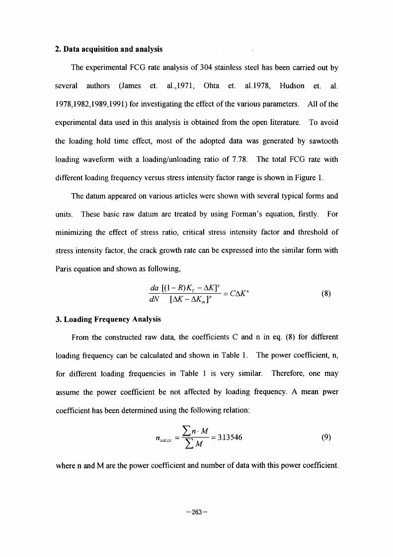
2. Data acquisition and analysis

The experimental FCG rate analysis of 304 stainless steel has been carried out by

several authors (James et al 1971, Ohta et. al. 1978, Hudson et. al.

1978,1982,1989,1991) for investigating the effect ofthe various parameters. All ofthe

experimental data used in this analysis is obtained from the open literature. To avoid

the loading hold time effect, most of the adopted data was generated by sawiooth

loading waveform with a loading/unloading ratio of 7.78. The total FCG rate with

different loading frequency versus stress intensity factor range is shown in Figure I .

The datum appeared on various articles were shown with several typical forms and

units. These basic raw datum are treated by using Forman's equation, firstly. For

minimizing the effect of stress ratio, critical stress intensity factor and threshold of

stress intensity factor, the crack growth rate can be expressed into the similar form with

Paris equation and shown as following,

da [(1 - R)Kc ~ ~~]* CAK (8) dN [AK - ~~,, J' ~

3. Loading Frequency Analysis

From the constructed raw data, the coefficients C and n in eq. (8) for different

loading frequency can be calculated and shown in Table I . The power coefficient, n,

for different loading frequencies in Table I is very similar. Therefore, one may

assume the power coefficient be not affected by loading frequency. A mean pwer

coefficient has been determined using the following relation:

n^,..~ - ~n ' M (9) = 3.13546

~M where n and M are the power coefficient and number of data with this power coefficient.

~* 263 -

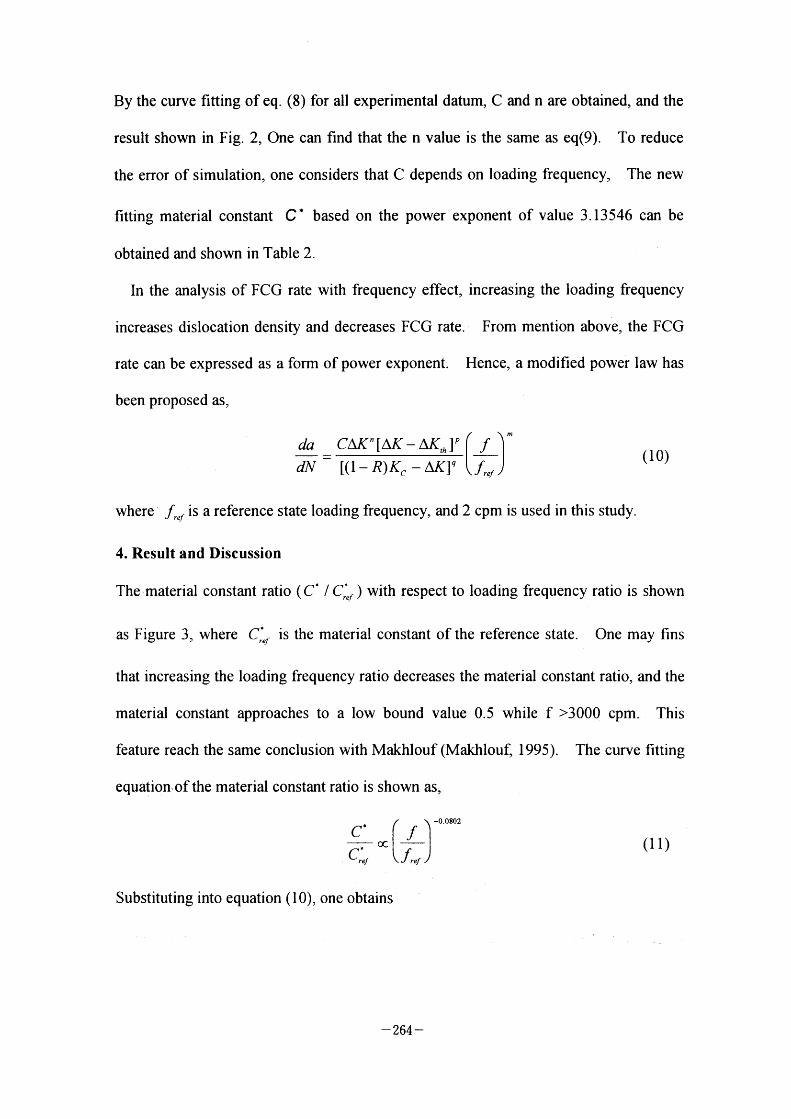
By the curve fitting of eq. (8) for all experimental datum, C and n are obtained, and the

result shown in Fig. 2, One can fmd that the n value is the same as eq(9). To reduce

the error of simulation, one considers that C depends on loading frequency, The new

frtting material constant C ' based on the power exponent of value 3.13546 can be

obtained and shown in Table 2.

In the analysis of FCG rate with frequency effect, increasing the loading frequency

increases dislocation density and decreases FCG rate. From mention above, the FCG

rate can be expressed as a form of power exponent. Hence, a modified power law has

been proposed as,

) r " da C~C"[AK- AK,h]P L f dN = [(1- R)Kc ~ ~K]q f..f (lO)

where fref is a reference state loading frequency, and 2 cpm is used in this study.

4. Result and Discussion

The material constant ratio ( C' / C~f ) with respect to loadmg frequency ratro rs shown

as Figure 3, where C:.f is the material constant of the reference state. One may fins

that increasing the loading frequency ratio decreases the material constant ratio, and the

material constant approaches to a low bound value 0.5 while f >3000 cpm. This

feature reach the same conclusion with Makhlouf (Makhlouf, 1995). The curve frtting

equation.ofthe material constant ratio is shown as,

o.0802 f )~ C' f f .,f

Substituting into equation (lO), one obtains

- 264 -

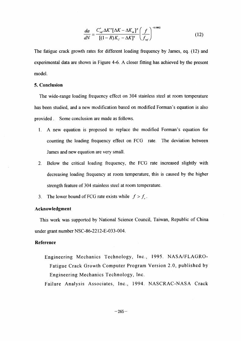
r ~o.oeo2 ) da C:,f~~"[AK- AK,h]P L f dN = [(1-R)Kc ~ AK]q f..f (12)

The fatigue crack growth rates for different loading frequency by James, eq. (12) and

experimental data are shown in Figure 4-6. A closer fitting has achieved by the present

model.

5. Conclusion

The wide-range loading frequency effect on 304 stainless steel at room temperature

has been studied, and a new modification based on modified Forman's equation is also

provided . Some conclusion are made as follows.

l . A new equation is proposed to replace the modified Forman's equation for

counting the loading frequency effect on FCG rate. The deviation between

James and new equation are very small.

2. Below the critical loading frequency, the FCG rate increased slightly with

decreasing loading frequency at room temperature, this is caused by the higher

strength feature of 304 stainless steel at room temperature.

3. The lower bound ofFCG rate exists while f > f. .

Acknowledgment

This work was supported by National Science Council, Taiwan, Republic of China

under grant number NSC-86-22 1 2-E-033 -004.

Reference

Engineering Mechanics Technology, Inc., 1995. NASA/FLAGRO-

Fatigue Crack Growth Computer Program Version 2.0, published by

Engineering Mechanics Technology, Inc.

Failure Analysis Associates, Inc., 1994. NASCRAC-NASA Crack

- 2,65 -

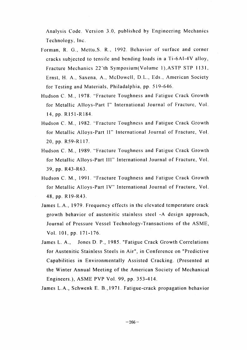
Analysis Code. Version 3.0, published by Engineering Mechanics

Technology. Inc.

Forman, R. G., Mettu.S. R., 1992. Behavior oi' Surface and corner

cracks subjected to tensile and bending loads in a Ti-6Al-4V alloy,

Fracture Mechanics 22'th Symposium(Volume l).ASTP STP I 131,

Ernst. H. A., Saxena, A.. McDowell, D.L., Eds.. American Society

for Testing and Materials, Philadalphia, pp. 5 19-646.

Hudson C. M., 1978. "Fracture Toughness and Fatigue Crack Growth

for Metallic Alloys-Part I" International Journal of Fracture, Vol.

14, pp. R15 l-R184.

Hudson C. M., 1982. "Fracture Toughness and Fatigue Crack Growth

for Metallic Alloys-Part ll" International Journal of Fracture, Vol.

20, pp. R59-RI 17.

Hudson C. M., 1989. "Fracture Toughness and Fatigue Crack Growth

for Metallic Alloys-Part lll" International Journal of Fracture, Vol.

39, pp. R43 R63

Hudson C. M., 1991. "Fracture Toughness and Fatigue Crack Growth

for Metallic Alloys-Part IV" International Journal of Fracture, Vol.

48, pp. R19-R43.

James L.A., 1979. Frequency effects in the elevated temperature crack

growth behavior of austenitic stainless steel -A design approach,

Journal of Pressure Vessel Technology-Transactions of the ASME,

Vol. 101, pp. 171-176.

James L A., Jones D. P., 1985. "Fatigue Crack Growth Correlations

for Austenitic Stainless Steels in Air", in Conference on "Predictive

Capabilities in Environmentally Assisted Cracking. (Presented at

the Winter Annual Meeting of the American Society of Mechanical

Engineers.), ASME PVP Vol. 99, pp. 353-414.

James L.A., Schwenk E. B.,1971. Fatigue-crack propagation behavior

- 266 -

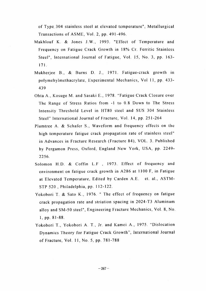
of Type_ 304 stainless steel at- elevated temperature"~ Metallurgical

Transactions of ASME, Vol. 2, pp. 491 496

Makhlouf K. & Jones J.W., 1993. "Effect of Temperature and

Frequency on Fatigue Crack Growth in 180/0 Cr. Ferritic Stain]ess

Steel" Internatlonal Journal of Fatlgue Vol 15 No 3 pp. 163-

171.

Mukherjee B., & Burns D. J., 1971. Fatigue-crack growth in

polymehylmethacrylate, Experimental Mechanics, Vol I l, pp. 433-

439

Ohta A., Kosuge M. and Sasaki E., 1978. "Fatigue Crack Closure over

The Range of Stress Ratios from -1 to 0.8 Down to The Stress

Intensity Threshold Level in HT80 steel and SUS 304 Stainless

Steel" Internatlonal Journal of Fracture Vol. 14, pp. 251-264

Plumtree A. & Schafer S., Waveform and frequency effects on the

high temperature fatigue crack propagation rate of stainless steel"

in Advances in Fracture Research (Fracture 84), VOL. 3. Pub]ished

by Pergamon Press, Oxford, England New York, USA, pp. 2249-

2256.

Solomon H.D. & Coffin L.F , 1973. Effect of frequency and environment on fatigue crack growth in A286 at I 100 F, in Fatigue

at Elevated Temperature, Edited by Carden A.E. et. al., ASTM-

STP 520 , Philadelphia, pp. I 12-122.

Yokobori T. & Sato K., 1976. " The effect of frequency on fatigue

crack propagation rate and striation spacing in 2024-T3 Aluminum

alloy and SM-50 stee]", Engineering Fracture Mechanics, Vol. 8, No.

l, pp. 81-88.

Yokobori T., Yokobori A. T., Jr. and Kamei A., 1975. "Dislocation

Dynamics Theory for Fatigue Crack Growth", International Journal

of Fracture, Vol. I l, No. 5, pp. 781-788

- 267 -

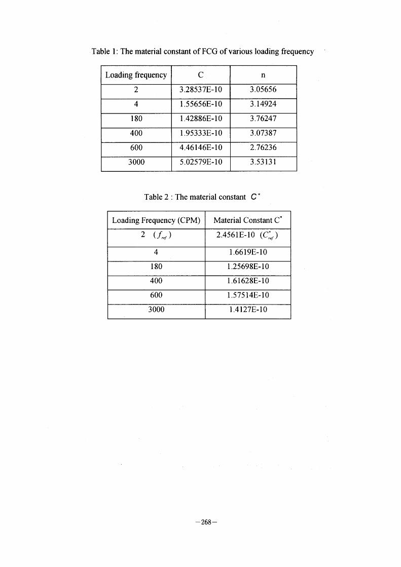
Table I : The material constant of FCG of various loading frequency

Table 2 The material constant C '

~ 268 -

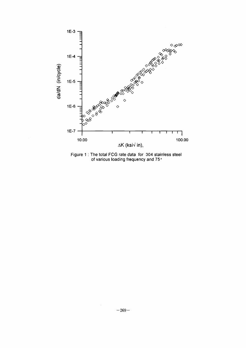
1 E-3

1 E-4

'~ o o > o .\ = _ I E-5 Z ~ .\ CU ~o

1 E-6

1 E-7

~~~~ ~; ~~~

~>~~~ ~~~

~~~~~; ~

l~~~~~ ~

~~ ~~

1 0.00 1 O0.00 AK (ksi~ in),

Figure I : The total FCG rate data for 304 stainless steel of various loading frequency and 75-

- 269 -

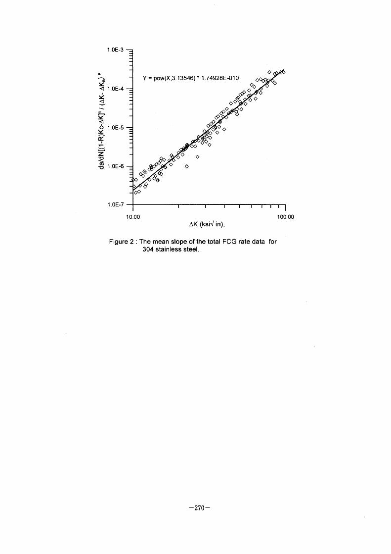
1 .OE-3

~ ~ ~~

~ '\ :L, ~e

d) 1.0E-5 ~e

~ OC

~-

~ -Z ~ ~. CU ~ 1.0E 6

1 .OE-7

Y = pow(X,3.13546) * I .74928E-OIO ~~ ~~~~~>

~ ~ ~:~x_

~;~~~~~ ~

~>~ ~~~;

~ ~~ ~> ~

~>

~

~

10,00 1 oO. OO

AK (ksi~ in),

Figure 2 : The mean slope of the total FCG rate data for 304 stainless steel.

- 270 -

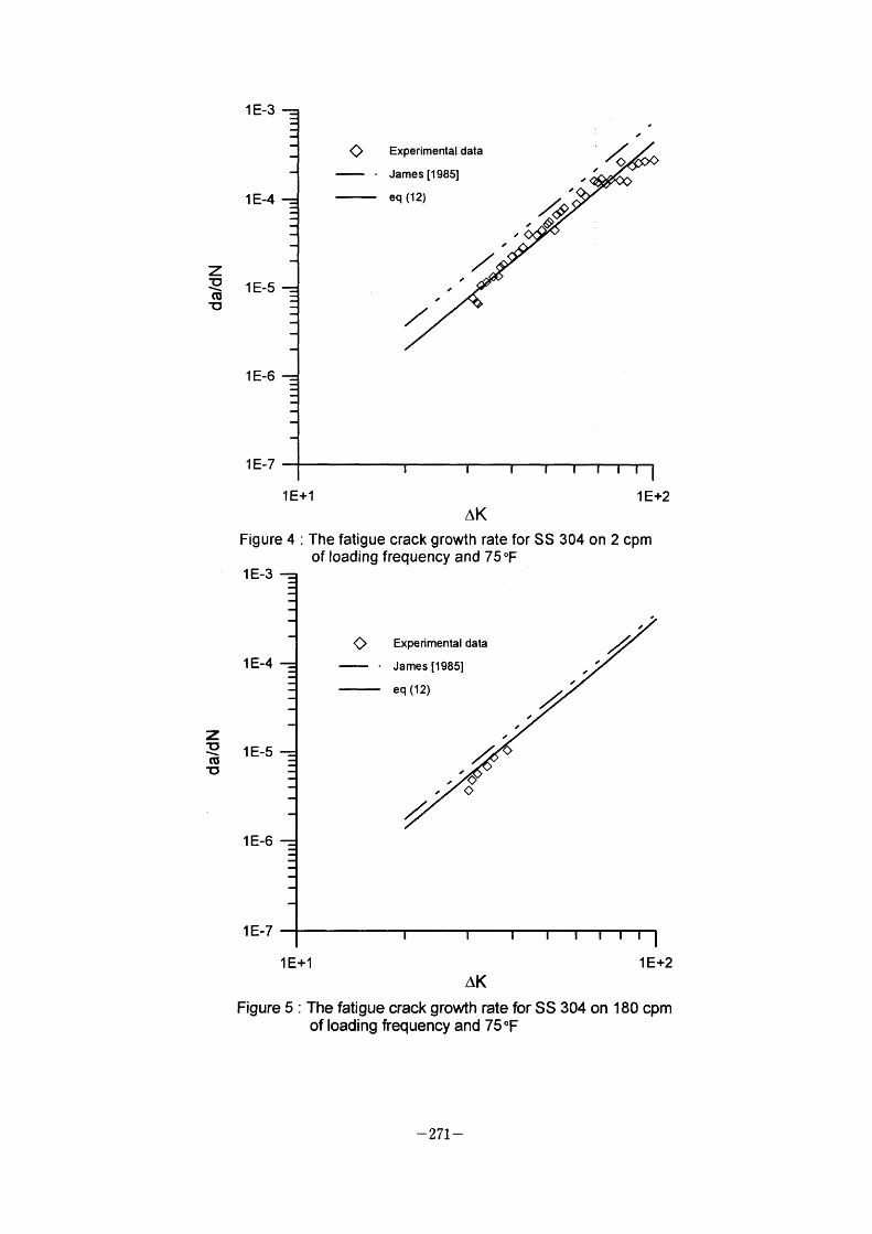
Z ._~

CU 1:

1 E-3

1 E-4

1 E-5

1 E-6

1 E-7

~ Experimental data

James [1985]

eq (12)

/ /

/ / /

/ /

.A~~~~ /

/ /

/~~ /

AK Figure 4 : The fatigue crack growth rate for SS 304 on 2 cpm

of loading frequency and 75 •F

Z ~ '\ cu

U

1 E-3

1 E-4

1 E-5

1 E-6

1 E-7

~ Experimental data

James [1 985]

eq (1 2)

~

/

/~~> • '~)

, ~

/ / ~

/ /

, ~ /

AK Figure 5 : The fatigue crack growl:h rate for SS 304 on 180 cpm

of loading frequency and 75•F

- 271 -

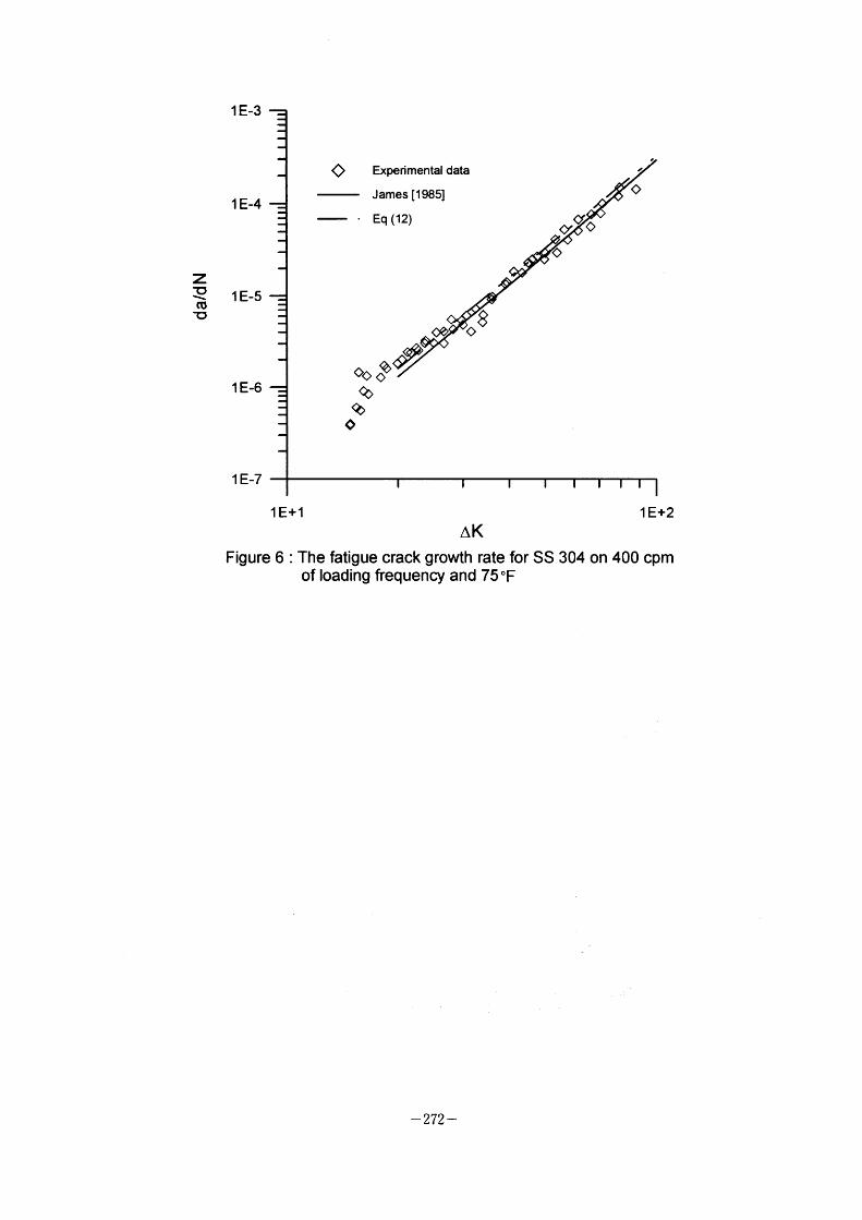
1 E-3

1 E-4

Z ~D •\ I E-5 CD

~

1 E-6

1 E-7

~ Experimental data

James [1 985]

• Eq(12)

~~ ~~l

~ ~ c

~~

~

d'

AK Figure 6 : The fatigue crack growth rate for SS 304 on 400 cpm

of loading frequency and 75•F

- 272 -

V-3 Investigation on Fracture Toughness Evaluation Method for

Reactor Pressure Vessel Surveillance

Kunio Onizawa, Tohru Tobitz & Masahide Suzuki,

Reactor Component Reliability Laboratory, Japan Atomic Energy

Research Institute, Japan

Investigation on Fracture Toughness Evaluation Method for Reactor Pressure Vessel Surveillance

Kunio ONIZAWA', Tohru TOBITA and Masahide SUZUKI Reactor Component Reliabilty Laboratory, Japan A tomic Energy Research Institute,

Tokai-mura, Naka-gun, Ibaraki-ken, 319- I 195, Japan

Abstract

To evaluate cleavage fracture toughness in the ductile-brittle transition range of RPV

steels, the applicability of precracked Charpy-v (PCCv) specimens has been investigated. An

approach based on the weakest link theory was applied to analyze the specimen size effect and

the scatter of fracture toughness values. Four kinds of ASTM A533B class I steels made by

Japanese steel makers were used.

The specimen size effect on cleavage fracture toughness was clearly seen among PCCv,

l T-CT and 4T-CT specimens. To obtain the equivalent data from PCCv specimens to I T-CT

specimens, the size correction scheme based on the weakest link theory was applied to the PCCv

data. The scatter of fracture toughness values was considered to have a Weibull type distribution.

lrradiation effect on the scatter was shown to be insignificant. The fracture toughness transition

curves were determined by PCCv data according to the drafi ASTM and the JEAC. The shifi of

the master curve by irradiation was somewhat greater than the Charpy 4 1 J shifi. The scheme for

the estimation of lower bound fracture toughness was also studied.

1. INTRODUCTION The brittle fracture of an RPV must be prevented, because it may lead to a catastrophic

fracture of the vessel followed by severe accident. Therefore, the RPV is operated at higher

temperature than the ductile-to-brittle transition temperature of the RPV steel . However, fast

neutrons from the reactor core during operation can cause the increase of the transition

temperature, i.e., the irradiation embrittlement. To assure the structural integrity of an RPV

throughout the operational life, the fracture toughness after neutron irradiation are needed. To do

this, the surveillance program for the RPV is performed according to a certain code and regulation. The results obtained from the Charpy impact tests according to the codes are used for

the estimation of fracture toughness after irradiation(1, 2). Most of the codes assume that the

degree of irradiation embrittlement obtained from Charpy impact tests are equivalent to that of

fracture toughness for the material concerned. Recent research, however, has indicated that the

correlation is not always conservative in predicting the degree of irradiation embrittlement in

terms of fracture toughness(3'4). Fracture mechanics methodology is, therefore, necessary for the

precise evaluation of irradiation embrittlement to assure the structural integrity of an RPV.

A methodology to evaluate fracture toughness of RPV steels has not been established

' Corresponding author. Tel: +81 29 282 5147; Fax: +81 29 282 5406; e-mail : konizawa@popsvr.tokai j aeri .go jp

- 273 -

completely, particularly in the transition range. As the fracture toughness values from test

specimens of the RPV steel show a large scatter in the ductile-to-brittle transition range, the

fracture toughness should be evaluated with the statistical nature. This means that a certain

statistical approach is necessary for the evaluation of the fracture toughness. Fracture toughness

values from small size specimens, such as surveillance specimens, also show large effects on

specimen size. Although intensive research("g' 5) has been conducted to establish the statistical

treatment and the evaluation method of size effects in the past, the methods need a large number

of specimens and/or relatively large size specimens(6). The number and the size of surveillance

specimens are limited by the small volume of a surveillance capsule. Therefore, further research

is desired to resolve the limitation and to establish an improved surveillance test method that is

applicable for the small nulnber and the small sizes of specimens.

This paper describes the results of fracture toughness tests using four kinds of pressure

vessel steels including an IAEA reference material JRQ. Based on the results of the fracture

toughness tests by precracked Charpy specimens and standard size I T-CT and 4T-CT specimens,

a statistical analysis was performed to evaluate the scatter and the lower bound of fracture

toughness in the transition temperature range . A part of this report was performed at JAERI in

the framework of the IAEA Coordinated Research Program Phase-3(7).

2. EXPERIMENTS

2.1 Materials

Materials used in this study were four kinds of pressure vessel steels of ASTM A533B

class I . The one is designated JRQ, which was used as a correlation monitor material in the

IAEA CRP-3(8). The another material w~s chosen to have a large number of database for

cleavage fracture toughness from small size specimens to large ones. The material is designated

as JSPS A533B-1 which was used in the round robin study organized by The Japan Society for Promoting of Science (JSPS)(9). The other materials were made as A533B-1 steels which were

called as Steel A and Steel B that corresponded to the old age RPV steel and the modem steel,

respectively. Chemical compositions of the materials are summarized in Table I . Mechanical

properties at room temperature for the materials are listed in Table 2.

2.2 Fracture Toughness Tests

Four types of specimens were used in this study, namely precracked Charpy (PCCv),

0.5T-DCT, I T-CT and 4T-CT. In some cases the specimens were side-grooved by I OO/o on each

side of the specimen after precracking. For JSPS A533B-1 steel, one of the authors performed

fracture toughness tests using PCCv specimens machined from halves of broken 2T-CT specimens at SCK/CEN(ro). The notch orientation of the specimens is T-L direction for all

specimens. All specimens were machined from the approximately quarter thickness position of

the material . Fracture toughness tests were performed at mainly lower transition temperature

range which a cleavage fracture was occurred before the limit load of the specimen. Some

specimens were also tested at an upper shelf temperature range to obtain J-R curves.

Testing and evaluation for fracture toughness were performed according to ASTM standards(ll,12) and JSME method(13). A valid plane-strain fracture toughness, Klc, could not be

- 274 -

obtained from the specimens except for 4T-CT specimens. The following method, therefore, was

applied to obtain elastic-plastic fracture toughness. Fracture toughness values at cleavage

fracture, Jc, were calculated based on the area under load-displacement curve up to the sudden

load drop and the cleavage fracture load (see eq. I ). Fracture toughness KJC Values were then

converted from Jc by the following equation (2). Elastic modulus E and Poisson's ratio v were

fixed to 206 GPa and 0.3 in this study, respectively.

J - Jcl + Jpl C~ K 2 nA - C + P! E' BN bo

(1)

where Kc: Stress intensity factor at the cleavage fracture,

n =2+0.522*(a~/W) for compact specimens,

n =2 for PCCv specimens, Apl: Plastic part of the area under load-displacement curve,

BN: Net thickness, bo: Initial ligament (=W-ao), ao: Initial crack length, W: Specimen width,

E'=E for ASTM, E'=E/(1- v 2) for JSME.

In the ASTM draft method(14), n factor has been changed from 2 O to 1 9 based on the

3-D detailed analysis for PCCv specimen(15). This makes the fracture toughness value lower by

maximum 50/0 in terms of J-integral. When some equations in the ASTM draft method are applied to the data, the new 7? factor is used.

At upper shelf temperature range, Jlc Values and J-R curves for the materials except for

the JSPS A533B-1 were obtained according to the JSME method. Ductile crack growih in a specimen during a test was measured by unloading elastic compliance method.

2.3 Irradiation

PCCv and 0.5T-DCT specimens of JRQ were irradiated in Japan Materials Testing Reactor (JMTR, thermal output 50MW). Fast neutron fluence for each specimen was calculated to be within the range from I .9 to 2.5 x I 019 n/cm2 (E> I MeV). The displacement per atom (dpa)

for iron by the irradiation to 2 x I 019 n/cm2 (E> I MeV) was about 3 x I 0-2. Fast neutron flux was

about I .2 x I 013 n/cm2s (E> I MeV). Temperature for the specimens during irradiation was

controlled in the range from 280 to 300 ~C . The shifts of Charpy transition temperatures and the

hardening by neutron irradiation are summarized in Table 3(7)

Many specimens of Steel A and Steel B were also irradiated at JMTR. Sixteen PCCv

specimens of the steels were encapsuled with ten Charpy-V specimens for the JMTR irradiation.

Post irradiation tests for those specimens are now underway.

3. RESULTS AND DISCUSSION

3.1 Fracture Toughness Database

Figures I to 5 show cleavage fracture toughness data

- 275 -

obtained in this studyl 1 6). The

validity limit for the PCCv data based on equation (3) is indicated. This criterion has been

stipulated in the JSPS method.

bo ' B > JcaY

25 (3)

The equation (3) used in the JSPS method is the same as the validity criterion on the

determination of a Jlc in the ASTM E813. For the PCCv specimen, the ligament size, bo, is

smaller than the specimen thickness, B. Therefore, bo is considered as a key parameter for the

validity of PCCv data.

Figure I shows KJC values of unirradiated JRQ specimens tested in the transition range.

At room temperature, cleavage fracture was not observed from any PCCv specimens, but from

all 0.5TDCT and ITCT specimens. When PCCv and IT-CT data are compared at -80 ~C, it is seen that I T-CT data are situated within the scatter range of PCCv data. The Jlc Value at I OO ~C

obtained from IT-CT and 0.5T-DCT specimens by means of the JSME method is also indicated

in the figure. Some data points of PCCv and compact specimens tested at upper transition

temperature range exceeded the Jlc Value.

Figure 2 shows all cleavage fracture toughness data of irradiated JRQ specimens. Test

temperatures for five PCCv and six 0.5TDCT specimens, performed in the frame work of IAEA CRP-3, were sparse from O to I OO ~C . We tested additional irradiated PCCv specimens; twelve

specimens around 1 7 ~C and ten at 35 ~C so that a statistical analysis could be done.

Figure 3 shows fracture toughness values from PCCv specimens of JSPS A533B-1 steel with a large number of database by means of compact specimens from 0.5T to 4T (13). The

database includes -25, O and 25 ~C data while PCCv were tested at O ~C. Obviously PCCv data

show higher fracture toughness values than the other compact specimen data.

The cleavage fracture toughness data of Steel A are shown in Figure 4. The data

include some valid Klc data from 4T-CT. The Klc data locates nearly the lowest bound of the

other data. The PCCv data show higher KJC Values than KJC Of I T-CT and Klc of 4T-CT data. The upper shelf fracture toughness, Jlc, obtained by I T-CT at 20 ~C is indicated in the figure.

More than halfofPCCv data at -50 ~C exceeded the Jlc Value.

Figure 5 indicates the results of fracture toughness tests by specimens of Steel B. Valid

Klc data points from 4T-CT are also shown in this figure. The Klc data lie nearly lowest bound of

the other data. Similarly to Steel A, PCCv data indicate higher toughness values than the other

CT data. The upper shelf fracture toughness, Jlc, obtained from I T-CT at 20 ~C is indicated in

the figure. Several PCCv data at -80 ~C exceeded the Jlc Value.

3.2 Specimen Size Effect on Cleavage Fracture Toughness

As is known well, a fracture toughness value from a small specimen can be higher than

that from a large specimen. In addition to this, in the transition range, a statistical effect on

cleavage fracture is apparent. This has been explained by the weakest link theoryll7,18) that is

based on the local inhomogeneity in the material. The theory treats the probability to find a

particle that is located randomly in the material and that leads to the fracture of the specimen.

Another reason is that the small specimen has insufficient length in thickness to keep small scale

yielding and maintain a certain level of constraint at a crack tip, as compared with a large size

specimen or a real heavy-section structure(19).

- 276 -

Figure 6 shows the effect of specimen thickness on fracture toughness value. Each

value was normalized by Klc Values for each testing condition. This figure clearly shows the size

dependence on the mean value. The highest PCCv data was larger than four times of Klc Value.

The mean values of PCCv data except for invalid data were I .5 to 2.2 compared to Klc Value. On

the other hand, the lowest value of PCCv data was approximately the same as the Klc Value.

To obtain a reliable fracture toughness value from a small size specimen, several correction schemes have been proposed. Wallin(20) has proposed the following equation for

correcting specimen size applicable to pressure vessel steels;

KJC y K~,~ )(B. / By)1/~ (4) + (KJC _' =K ~i*

where KJc_. ., y: KJC for specimens of thickness, B. ., y

K~j. = 20 MPal/~

m=4 Figure 6 includes the size effect correction curve based on the equation (4). The upper

curve is corresponding to Steel B, the lower curve is for Steel A. The correction curve for Steel

B overestimated 300/0 of Klc Value by 4T-CT specimen. Unfortunately Klc Value of JRQ was not

available. However, the size correction was compared between PCCv and I T-CT data. As a

result, the correction provided the I T-CT equivalent values from PCCv data. To verify the

correction equation, we need more database including sufficient number of PCCv data.

3.3 Scatter of Fracture Toughness

The equation (4) is based on the weakest link theory. The theory assumes that the

distribution of the fracture toughness values of a material can be described as a Weibull type

statistics. Using three parameters, K~i., m and Ko, the fracture probability based on Weibull statistics can be expressed by the following equation(20).

K KJc_rr ~20 " ~f =1-exp Jc_lT ~K~i~ ~ =1-exp

Ko ~ K~j. Ko ~ 20 (5) where Pf: Median ranking( = (i-0.3)/(N + 0.4) )

m, Ko: Fitting parameters

All data obtained by the same-type specimens at a certain temperature can be analyzed

by these equations (4) and (5). This equation (5) has also been incorporated into the ASTM draft

method to describe the statistics of cleavage fracture toughness.

Figures 7 to 9 compare Weibull plots of PCCv data and I T-CT data. PCCv data were

corrected by equation (4) to I T-CT thickness for comparison. These figures also include the

fitting curve by equation (5). Figure 7 indicates that the corrected PCCv data and I T-CT data of

unirradiated JRQ are in good agreement. The parameter m in equation (5) were 2.3 and 2.5 for

PCCv adjusted data and I T-CT data, respectively. These values were much less than the

theoretical value of four. Figure 8 shows the Weibull plots of PCCv data of irradiated JRQ. The

m values were 2.8 and 3 . I for the data tested at 1 7 ~C and 35 ~C, respectively. The slopes were

again smaller than the theoretical values. However, it is noted that the m value became a bit large

- 277 -

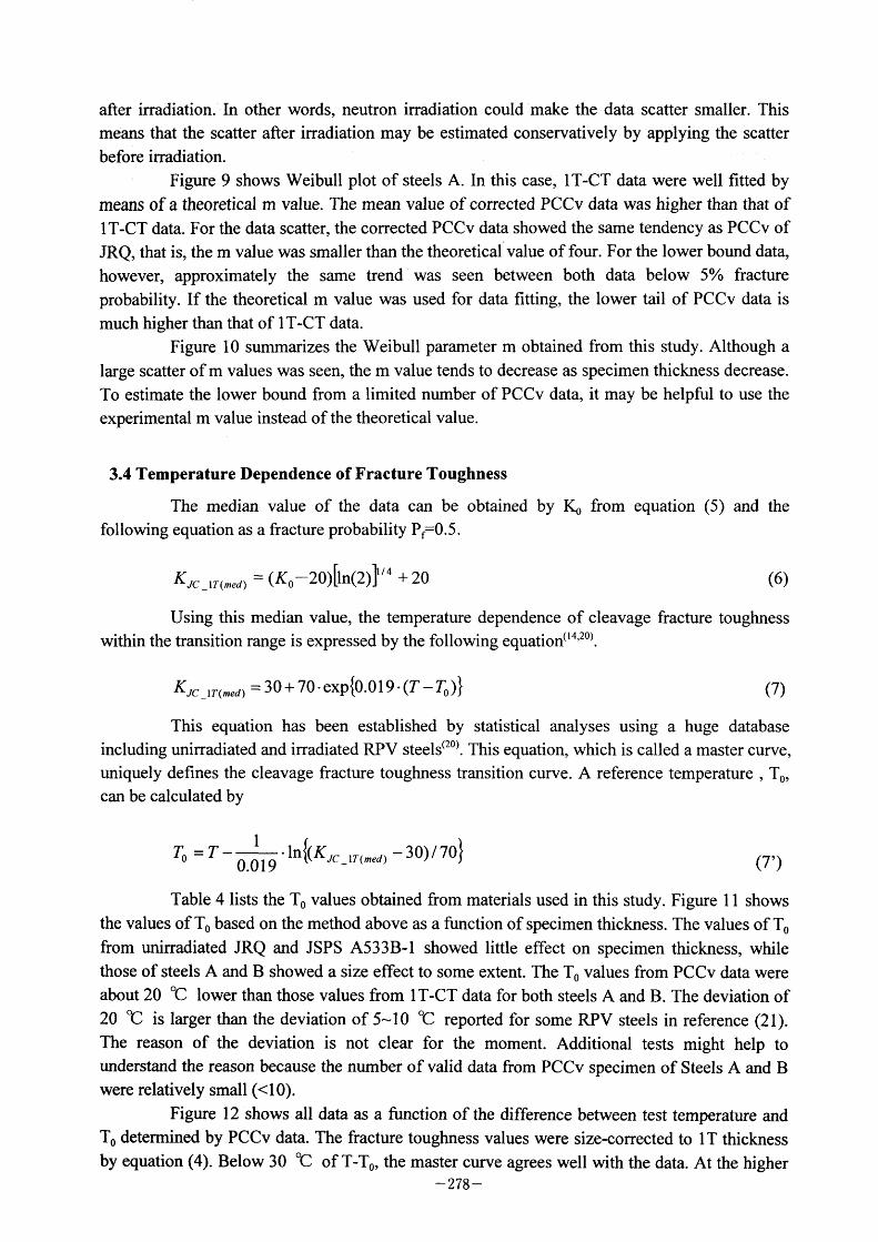
after irradiation.' In other words, neutron irradiation could 'make the data scatter smaller. This

means that the scatter after irradiation may be estimated conservatively by applying the scatter

before irradiation.

Figure 9 shows Weibull plot of steels A. In this case, I T-CT data were well fitted by

means of a theoretical m value. The mean value of corrected PCCv data was higher than that of

l T-CT data. For the data scatter, the corrected PCCv data showed the same tendency as PCCv of

JRQ, that is, the m value was smaller than the theoretical value of four. For the lower bound data,

however, approximately the same trend was seen between both data below 50/0 fracture probability. If the theoretical m value was used for data fitting, the lower tail of PCCv data is

much higher than that of I T-CT data.

Figure I O summarizes the Weibull parameter m obtained from this study. Although a

large scatter of m values was seen, the m value tends to decrease as specimen thickness decrease.

To estimate the lower bound from a limited number of PCCv data, it may be helpful to use the

experimental m value instead of the theoretical value .

3.4 Temperature Dependence of Fracture Toughness

The median value of the data can be obtained by Ko following equation as a fracture probability Pf=0.5.

from equation (5) and the

[ I KJC IT(med) = (K0~20) In(2) /4 + 20

Using this median value, the temperature dependence of cleavage within the transition range is expressed by the following equation(14.20).

(6)

fracture toughness

{ 30 + 70 • exp 0.019 • (T - To)} (7) Jc IT(med)

This equation has been established by statistical analyses using a huge database (20) including unirradiated and irradiated RPV steels . This equation, which is called a master curve,

uniquely defines the cleavage fracture toughness transition curve. A reference temperature , To'

can be calculated by

T = T I . In{(KJc IT(med) ~ 30)170}

Table 4 Iists the To Values obtained from materials used in this study. Figure I I shows

the values of To based on the method above as a function of specimen thickness. The values of To

from unirradiated JRQ and JSPS A533B-1 showed little effect on specimen thickness, while

those of steels A and B showed a size effect to some extent. The To Values from PCCv data were

about 20 ~C Iower than those values from I T-CT data for both steels A and B. The deviation of

20 ~C is larger than the deviation of 5-lO ~C reported for some RPV steels in reference (21).

The reason of the deviation is not clear for the moment. Additional tests might help to

understand the reason because the number of valid data from PCCv specimen of Steels A and B

Figure 1 2 shows all data as a function of the difference between test temperature and

To determined by PCCv data. The fracture toughness values were size-corrected to I T thickness

by equation (4). Below 30 ~C of T-To, the master curve agrees well with the data. At the higher

-278-

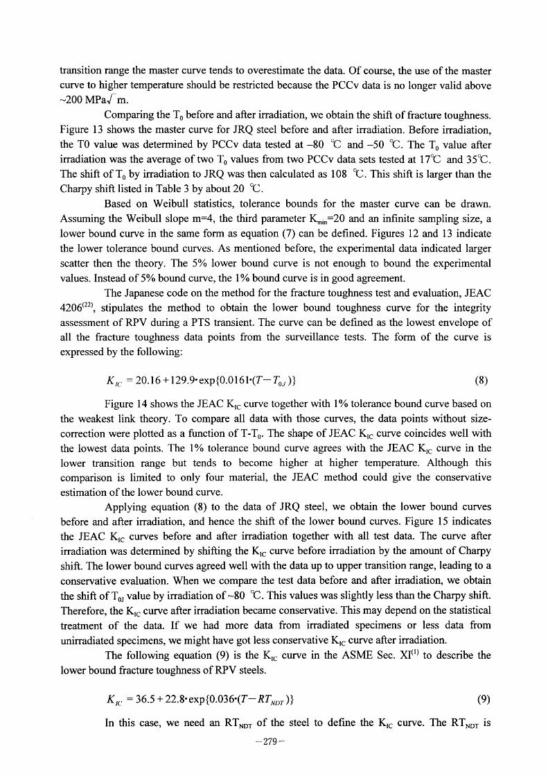
transition range the master curve tends to overestimate the data. Of course, the use of the master

curve to higher temperature should be restricted because the PCCv data is no longer valid above

-200 MPalrm. Comparing the To before and after irradiation, we obtain the shifi of fracture toughness.

Figure 1 3 shows the master curve for JRQ steel before and after irradiation. Before irradiation,

the TO value was determined by PCCv data tested at -80 ~C and -50 ~C . The To Value after

irradiation was the average oftwo To Values from two PCCv data sets tested at 1 7~C and 35~C.

The shift of To by irradiation to JRQ was then calculated as I 08 ~C. This shift is larger than the

Charpy shifi listed in Table 3 by about 20 ~C.

Based on Weibull statistics, tolerance bounds for the master curve can be drawn.

Assuming the Weibull slope m=4, the third parameter K~j.=20 and an mfinrte samplmg slze a

lower bound curve in the same form as equation (7) can be defined. Figures 1 2 and 1 3 indicate

the lower tolerance bound curves. As mentioned before, the experimental data indicated larger

scatter then the theory. The 50/0 Iower bound curve is not enough to bound the experimental

values. Instead of 50/0 bound curve, the I o/o bound curve is in good agreement.

The Japanese code on the method for the fracture toughness test and evaluation, JEAC

4206(22) stipulates the method to obtain the lower bound toughness curve for the integrity

assessment of RPV during a PTS transient. The curve can be defined as the lowest envelope of

all the fracture toughness data points from the surveillance tests. The form of the curve is

expressed by the following:

Figure 1 4 shows the JEAC Klc curve together with I o/o tolerance bound curve based on

the weakest link theory. To compare all data with those curves, the data points without size-

correction were plotted as a function of T-To' The shape of JEAC Klc curve coincides well with

the lowest data points. The I o/o tolerance bound curve agrees with the JEAC Klc curve in the

lower transition range but tends to become higher at higher temperature. Although this comparison is limited to only four material, the JEAC method could give the conservative

estimation of the lower bound curve.

Applying equation (8) to the data of JRQ steel, we obtain the lower bound curves

before and after irradiation, and hence the shift of the lower bound curves. Figure 1 5 indicates

the JEAC Klc curves before and after irradiation together with all test data. The curve after

irradiation was determined by shifting the Klc curve before irradiation by the amount of Charpy

shift. The lower bound curves agreed well with the data up to upper transition range, Ieading to a

conservative evaluation. When we compare the test data before and after irradiation, we obtain

the shift of ToJ value by irradiation of -80 ~C. This values was slightly less than the Charpy shift.

Therefore, the Klc curve after irradiation became conservative. This may depend on the statistical

treatment of the data. If we had more data from irradiated specimens or less data from unirradiated specimens, we might have got less conservative Klc curve after irradiation.

The following equation (9) is the Klc curve in the ASME Sec. XI(1) to describe the

lower bound fracture toughness of RPV steels.

RTN/)7' ) f

In this case, we need an RTNDT Of the steel to defme the Klc curve. The RTNDT is

- 279 -

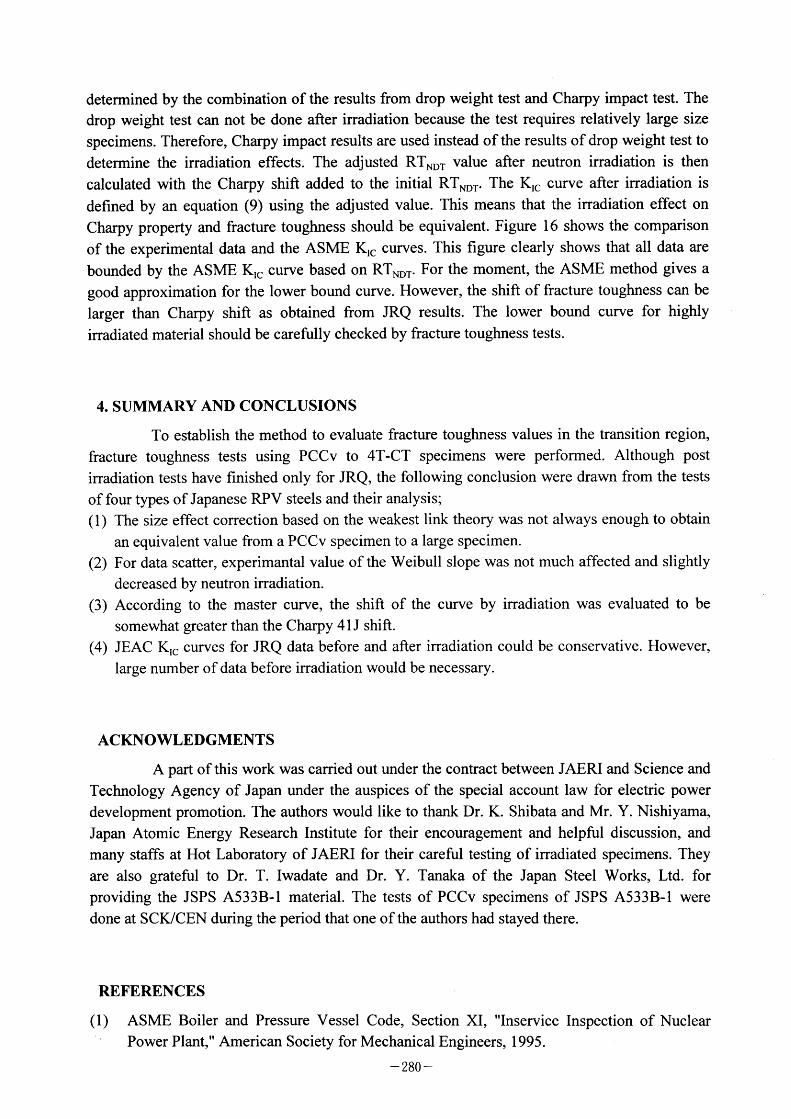
determined by the combination of the results from drop weight test and Charpy impact test. The

drop weight test can not be done afier irradiation because the test requires relatively large size

specimens. Therefore, Charpy impact results are used instead of the results of drop weight test to

determine the irradiation effects. The adjusted RTNDT Value after neutron irradiation is then

calculated with the Charpy shift added to the initial RTNDT. The Klc curve afier irradiation is

defined by an equation (9) using the adjusted value. This means that the irradiation effect on

Charpy property and fracture toughness should be equivalent. Figure 1 6 shows the comparison

of the experimental data and the ASME Klc curves. This figure clearly shows that all data are

bounded by the ASME Klc Curve based on RTNDT. For the moment, the ASME method gives a good approximation for the lower bound curve. However, the shift of fracture toughness can be

larger than Charpy shift as obtained from JRQ results. The lower bound curve for highly

irradiated material should be carefully checked by fracture toughness tests.

4. SUMMARY AND CONCLUSIONS To establish the method to evaluate fracture toughness values in the transition region,

fracture toughness tests using PCCv to 4T-CT specimens were perfonned. Although post irradiation tests have finished only for JRQ, the following conclusion were drawn from the tests

of four types of Japanese RPV steels and their analysis;

( I ) The size effect correction based on the weakest link theory was not always enough to obtain

an equivalent value from a PCCv specimen to a large specimen.

(2) For data scatter, experimantal value of the Weibull slope was not much affected and slightly

decreased by neutron irradiation.

(3) According to the master curve, the shift of the curve by irradiation was evaluated to be

somewhat greater than the Charpy 4 1 J shift.

(4) JEAC Klc curves for JRQ data before and after irradiation could be conservative. However,

large number of data before irradiation would be necessary.

ACKNOWLEDGMENTS A part of this work was carried out under the contract between JAERI and Science and

Technology Agency of Japan under the auspices of the special account law for electric power

development promotion. The authors would like to thank Dr. K. Shibata and Mr. Y. Nishiyama,

Japan Atomic Energy Research Institute for their encouragement and helpful discussion, and

many staffs at Hot Laboratory of JAERI for their careful testing of irradiated specimens. They

are also grateful to Dr. T. Iwadate and Dr. Y. Tanaka of the Japan Steel Works, Ltd. for

providing the JSPS A533B-1 material. The tests of PCCv specimens of JSPS A533B-1 were done at SCK/CEN during the period that one ofthe authors had stayed there.

REFERENCES (1) ASME Boiler and Pressure Vessel Code, Section XI, "Inservice Inspection

Power Plant," American Society for Mechanical Engineers, 1 995.

- 280 -

of Nuclear

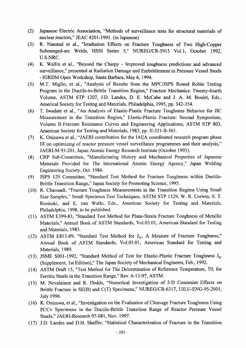
(2)

(3)

(4)

(5)

(6)

(7)

(8)

(9)

( I O)

(ll)

( 1 2)

(13)

( 1 4)

(15)

( 1 6)

( 1 7)

Japanese Electric Association, "Methods of surveillance tests for structural materials of

nuclear reactors," JEAC 4201 - 1 99 1 . (in Japanese)

R. Nanstad et al., "Irradiation Effects on Fracture Toughness of Two High-Copper

Submerged-arc Welds, HSSI Series 5," NUREG/CR-5913 Vol.1, October 1992, U.S.NRC .

K Wallm et al "Beyond the Charpy - Improved toughness predictions and advanced surveillance," presented at Radiation Damage and Embrittlement in Pressure Vessel Steels

- IGRDM Open Workshop. Santa Barbara. May 6, 1 994.

M.T. Miglin, et al., "Analysis of Results from the MPC/JSPS Round Robin Testing Program in the Ductile-to-Brittle Transition Region," Fracture Mechanics: Twenty-fourth

Volume, ASTM STP 1207, J.D. Landes, D. E. McCabe and J. A. M. Boulet, Eds., Americal Society for Testing and Materials, Philadelphia, 1995, pp. 342-354.

T. Iwadate et al., "An Analysis of Elastic-Plastic Fracture Toughness Behavior for JIC

Measurement in the Transition Region," Elastic-Plastic Fracture: Second Symposium,

Volume II-Fracture Resistance Curves and Engineering Applications, ASTM STP 803, American Society for Testing and Materials, 1 983, pp. II-53 1 -II-561 .

K. Onizawa et al., "JAERI contribution for the IAEA coordinated research program phase

III on optimizing of reactor pressure vessel surveillance programmes and their analysis,"

JAEFLl-M 93-201 , Japan Atomic Energy Research Institute (October 1 993).

CRP Sub-Committee, "Manufacturing History and Mechanical Properties of Japanese

Materials Provided for The International Atomic Energy Agency " Japan Weldmg Engineering Society, Oct. 1986.

JSPS 1 29 Committee, "Standard Test Method for Fracture Toughness within Ductile-Brittle Transition Range," Japan Society for Promoting Science, 1 995.

R. Chaouadi, "Fracture Toughness Measurements in the Transition Regime Using Small

Size Samples," Small Specimen Test Techniques, ASTM STP 1329, W. R. Corwin, S. T.

Rosinski, and E. van Walle, Eds., American Society for Testing and Materials, Philadelphia, 1 998, to be published.

ASTM E399-83, "Standard Test Method for Plane-Strain Fracture Toughness of Metallic

Materials," Annual Book of ASTM Standards, Vol.03.01, American Standard for Testing

and Materials, 1983.

ASTM E813 89 "Standard Test Method for Jlc, A Measure of Fracture Toughness " Annual Book of ASTM Standards, Vol.03.01, American Standard for Testing and Materials, 1989.

JSME SOOl-1992, "Standard Method of Test for Elastic-Plastic Fracture Toughness Jlc

(Supplement, I st Edition)," The Japan Society of Mechanical Engineers, Feb., 1992.

ASTM Draft 1 5, "Test Method for The Determination of Reference Temperature, TO, for

Ferritic Steels in the Transition Range," Rev. 6-13-97, ASTM.

M. Nevalainen and R Dodds "Numencal Investrgatron of 3 D Constramt Effects on Brittle Fracture in SE(B) and C(T) Specimens," NUREG/CR-63 17, UILU-ENG-95-2001,

July 1996.

K. Onizawa, et al., "Investigation on the Evaluation of Cleavage Fracture Toughness Using

PCCv Specimens in the Ductile-Brittle Transition Range of Reactor Pressure Vessel Steels," JAERI-Research 97-08 1 , Nov. 1 997.

J.D. Landes and D.H. Shaffer, "Statistical Characterization of Fracture in the Transition

- 281 -

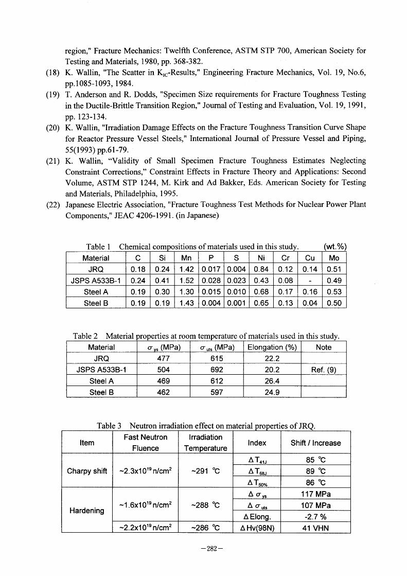
(18)

( 1 9)

(20)

(2 1 )

(22)

region," Fracture Mechanics: Twelfth Conference, ASTM STP 700, American Society for

Testing and Materials, 1980, pp. 368-382.

K. Wallin, "The Scatter in Klc~Results," Engineering Fracture Mechanics, Vol. 19, N0.6,

pp.l085-l093, 1984.

T. Anderson and R. Dodds, "Specimen Size requirements for Fracture Toughness Testing

in the Ductile-Brittle Transition Region," Joumal of Testing and Evaluation, Vol. 1 9, 1 991 ,

pp. 123-134.

K. Wallin, "Irradiation Damage Effects on the Fracture Toughness Transition Curve Shape

for Reactor Pressure Vessel Steels," Intemational Journal of Pressure Vessel and Piping,

55(1993) pp.61-79.

K Wallm "Validity of Small Specimen Fracture Toughness Estimates Neglecting Constraint Corrections," Constraint Effects in Fracture Theory and Applications: Second

Volume, ASTM STP 1 244, M. Kirk and Ad Bakker, Eds. American Society for Testing and Materials, Philadelphia, 1 995.

Japanese Electric Association, "Fracture Toughness Test Methods for Nuclear Power Plant

Components," JEAC 4206-1 991 . (in Japanese)

Table I Chemical compositions of materials used in this study. (Wt.olo)

Table 2 Material properties at room temperature ofmaterials used in this study.

Table 3 Neutron irradiation effect on material properties ofJRQ.

- 282 -

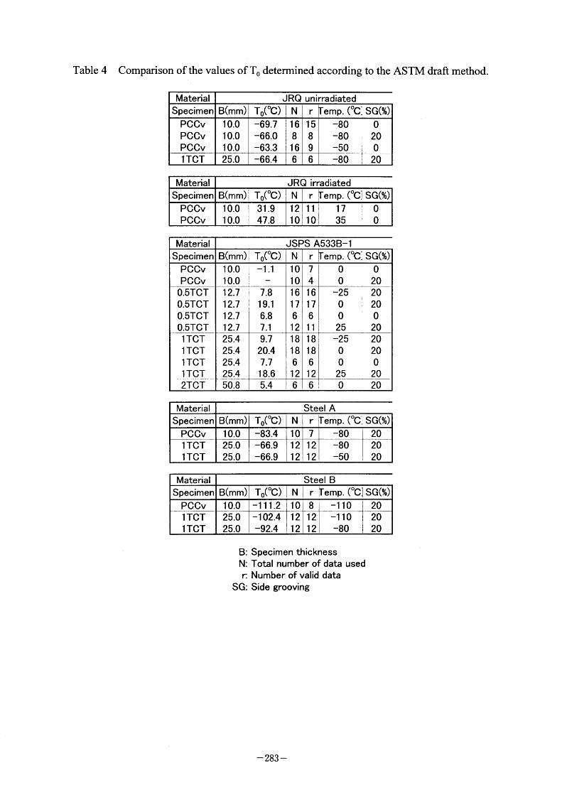
Table 4 Comparison of the values of To determined according to the ASTM drafi method.

B: Specimen thickness N: Total number of data used r Number of valid data

SG: Side grooving

- 283 -

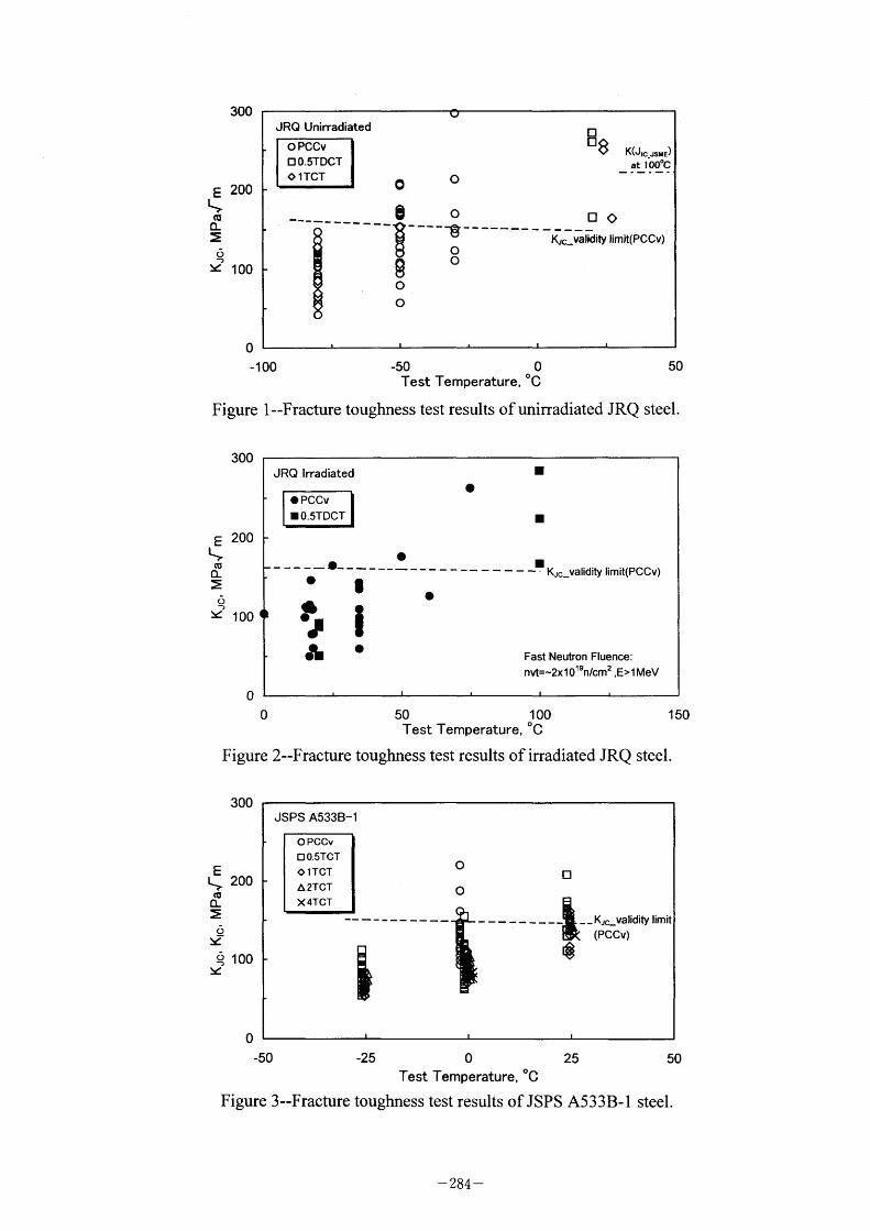
300

E 200 L. a CL

= ~~ 100

o

JRQ Unirradiated

O PCCv D 0.5TDCT O I TCT O o

e o ~~~ ~~ --~~ ~~ --o

g o o o

D D K(Jlc JSN'E) e at 100~C

D~ KJc_validity limit(PCCv)

o Test Temperature, 'C

Figure I --Fracture toughness test results of unirradiated JRQ steel.

300

E 200 L? ~ [~

:~

6 , :~ 100

O

JRQ Irradiated

~rl:~~~J~~CT

l 0'5TDCT

e - - e_ _ _

eC Jl i eRI o

e l

I

I KJc_validity limit(PCCv)

Fast Neutron Fluence: 19 nvi=-2xlO n/cm2,E>1MeV

1 oo Test Temperature, 'C

Figure 2--Fracture toughness test results of irradiated JRQ steel.

300

E L* 200 ~ ~ = l ~ 100

~e

o

JSPS A533B-1

O PCC+ D 0.5TCT e I TCT

A 2TCT X 4TCT

o

o Cl

- - - - - - - - -L- - KJcLvalidity limit

(PCCv)

~

Test Temperature, 'C

Figure 3--Fracture toughness test results of JSPS A533B- I steel.

- 284 -

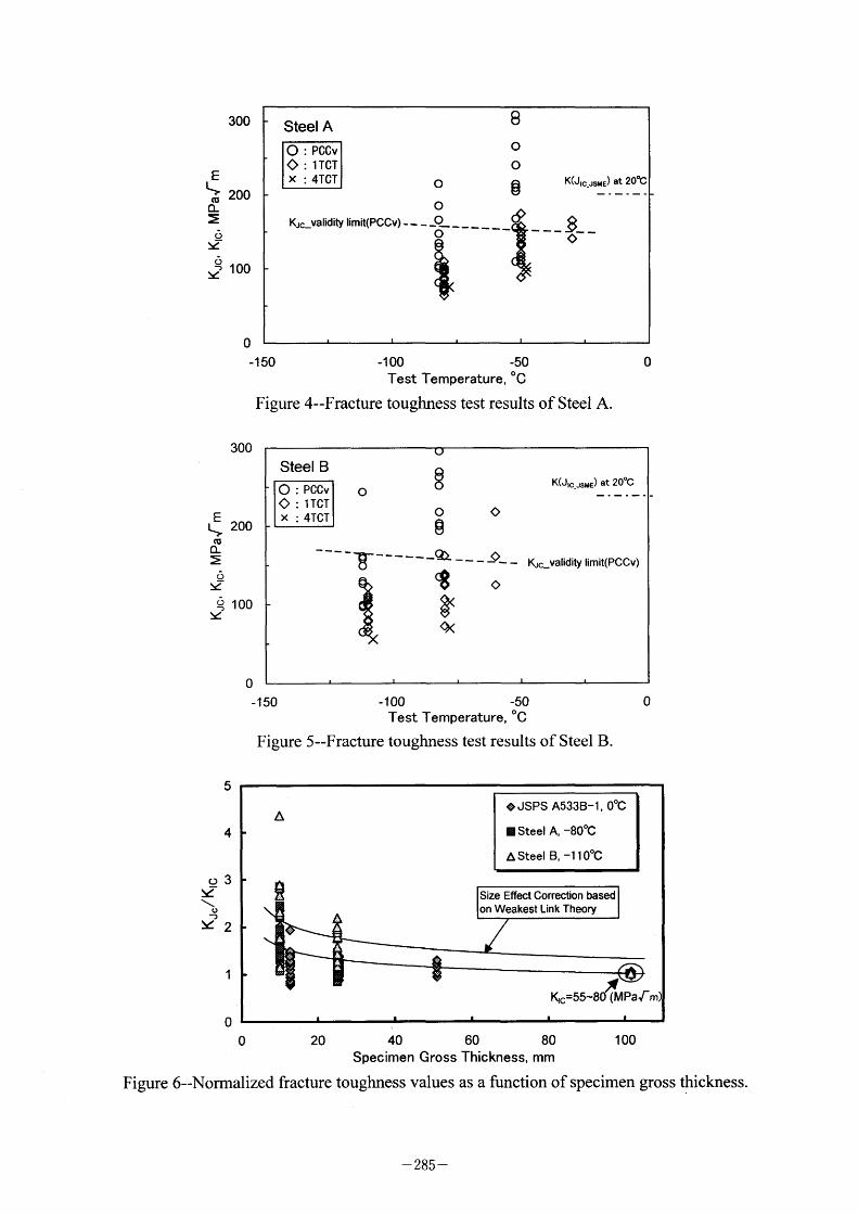
300

E ~ 200 ~ ~ :~

6 l ~e*~ 100

O

Steel A

~ : ITCT

x : 4TCT o O

KJc_validity nmit(Pccv) - - - O ~o~~~

8

~

~

K(J,c JSME) at 20cc

~__ (O~

-1 50 -1 OO -50 Test Temperature, 'C

Figure 4--Fracture toughness test results of Steel A.

300

O

E L? 200

c5

~ ~: o~_

~Z

~ 100 ~4

O

steel B ^o". : !ic""ci

= ITCT * = 4TCT ~

- _q~ __ _ ~_ ~-- --~ ~ ~

K(Jlc JsME) at 20'C

KJc_validity limit(PCCv)

5

4

3

2

1

O

- 1 50 - I OO -50 Test Temperature, 'C

Figure 5--Fracture toughness test results of Steel B.

O

~e~

\o ~41

A

~

~ JSPS A533B-1 , OPC

I Steel A, -80PC

ASteel B, -1 1 O~C

Size Effect Correction based

on Weakest Link Theory

1 ~c=55~80 (MPafm)

80 Specimen Gross Thickness, mm

Figure 6--Normalized fracture toughness values as a function of specimen gross thickness.

- 285 -

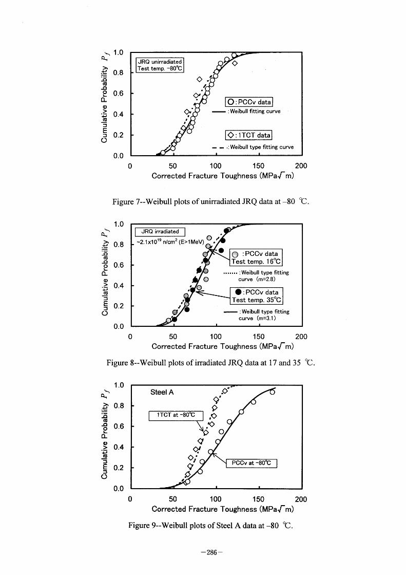
~~ 1.0 ~~

> ~' .- 0.8 ~: c9

JD OL 0.6

O_

o > ~' 0.4 cu

IS E:: 0.2

O 0.0

JRQ unirradiated Test temp. -80PC

l

~ .l Je

~

~, ,

l l

O : PCCv data : Weibull ftting curve

~ : I TCT data

- - ,:Weibull type fitting curve

O 50 1 OO 1 50

Corrected Fracture Toughness (MParm) 200

Figure 7--Weibull plots of unirradiated JRQ data at -80 ~C.

~ ~~

> :~:

JD CD

JD 9

ll

o > ~ CD

~

~

1 .O

0.8

0.6

0.4

0.2

0.0

JRQ irradiated

-2. I xl 019 n/cm2 (E>1 MeV)

l

al o ,

l

l

Ol e

o

: PCCv data Test temp. 1 6'C

•••.••• : Weibull type fitting curve (m=2.8)

O : PCCv data Test temp. 35~C

: Weibull type fitting

curve (m=3.1)

1 OO 1 50

Corrected Fracture Toughness (MParm)

Figure 8--Weibull plots ofirradiated JRQ data at 17 and 35 ~C.

1 .O

~ Q~

:E!_> 0.8

~ ,D

JD 06 9 O_

~ 0.4 ;5 ,g

E:':' 0.2

O 0.0

Steel A ~:

9 ,~

,~

~0

lll

1 TCT at -80~C

q ~,.

~>j

q ~:

PCCv at -80~C

l

1 OO 1 50

Corrected Fracture Toughness (MParm)

Frgure 9 Weibull plots of Steel A data at -80 ~C .

200

~ 286 -

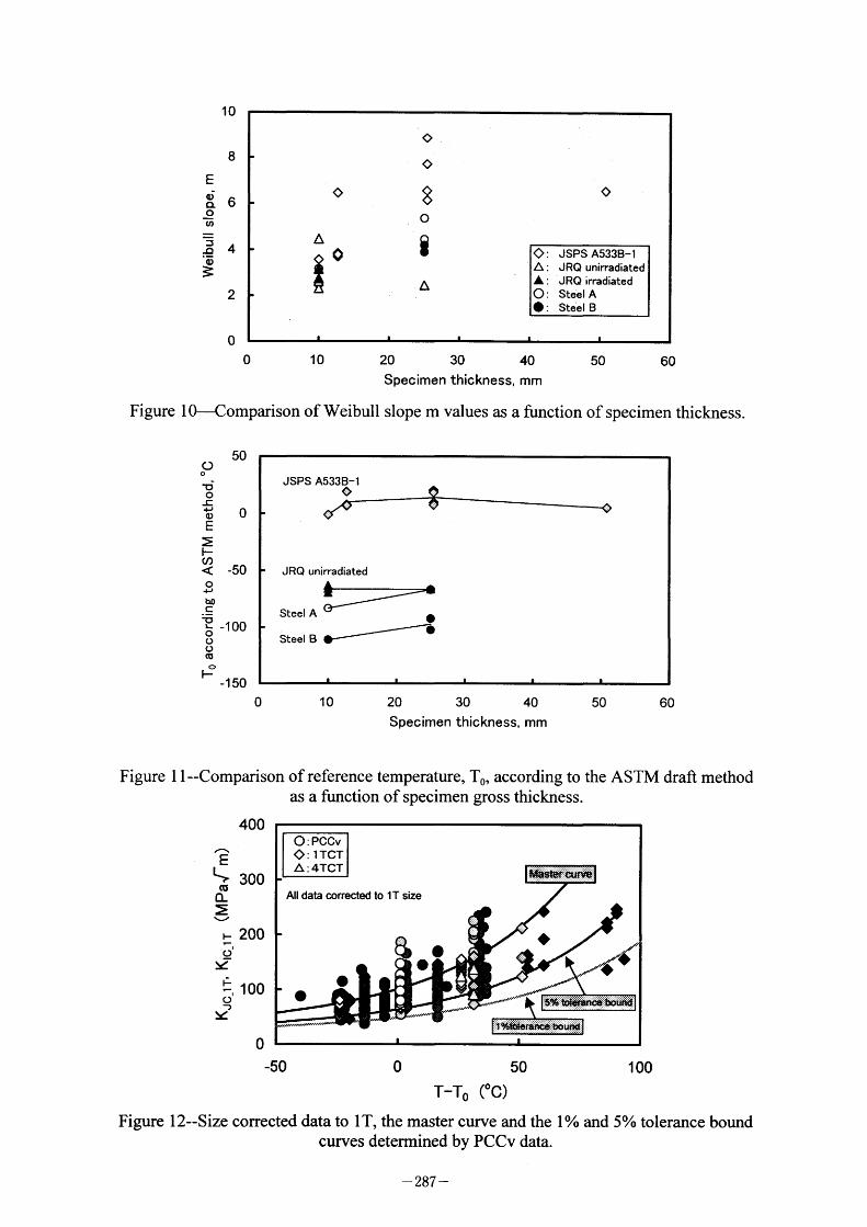
10

8

E

~6 o 1~;

~4 ~ 2

O

~

A ~0

~ ~

i

A

~)

: JSPS A533B-1 A: JRQ unirradiated JL : JRQ irradiated O: Stdel A e: Steel B

10 30 40 50 60 Specimen thickness, mm

Figure I O-Comparison of Weibull slope m values as a function of specimen thickness.

O ~F O = ~ o E

~:

H (1)

o ~ bo c

~L o o o ,U

Ho

50

O

-50

-1 OO

-1 50

JSPS A533B-1 c

JRQ unirradiated

Steel A

Steel B

O 10 20 30 40 Specimen thickness, mm

50 60

Figure I I --Comparison of reference temperature, To, according to the ASTM draft method as a function of specimen gross thickness.

400

~ E L?co 300

O_

= ~ ~ 200 o'

~~~

F: - 100 o'

, ~e

O

~ : I TCT A : 4TCT

Au data co~ected to I T size

e o

~)e e

Master curve

(,~

~p

Se5 ~efan# hound

1 ~efo~ra~e taurtd

T-To (oO

Figure 1 2--Size corrected data to I T, the master curve and the I o/o and 50/0 tolerance bound

curves detemrined by PCCv data.

- 287 -

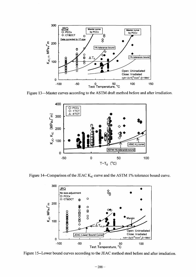
300

E 200 L?

cl'

CL :~

F:

o'

' 100 ~e

O

JRQ O: PCCv ~ : CT&DCT o

a orre edtolT '

Master curve by PCCv

~e

Master curve by PCCv

e

o 1 % tolerance bound

1~

~ ATO ~

~e o ,

o lolo tolerance bound

o o

e e

Open: Unirradiated Close: Irradiated nvt=-2xl 019nlcm2 , E>1 Mev

50 1 oO Test Temperature, 'C

Figure 1 3 Master curves according to the ASTM draft method before and after irradiation.

400

~ E 300 L? ~ = - 200 :~~

o 100 ~ o

~ : i;'•.~

o e

, ~F

e,

~~

JEAC Ktc curve

A.LS?t, {~~~ Icierance bcund

-50 O 50 1 OO

T-To ("O

Figure 1 4--Comparison of the JEAC Klc curve and the ASTM I o/o tolerance bound curve.

300

E 200 L? a ~ ~ ~Z 100

O

JRQ No size-adiustment

O: PCCv (~ : CT&DCT O

e

O ~ ~ O

o

o 9 o o

~

~ )1~1' A T41

o

o

e Margin

~

(,)

~

JEAC Lower Bound Curv

Open: Unirradiated Close: Irradiated

l9 nvt=-2 Io n/cm2 E>1Mev

- I oo -50 o 50 1 oo Test Temperature, 'C

Figure 1 5--Lower bound curves according to the JEAC method steel before and after irradiation.

- 288 -

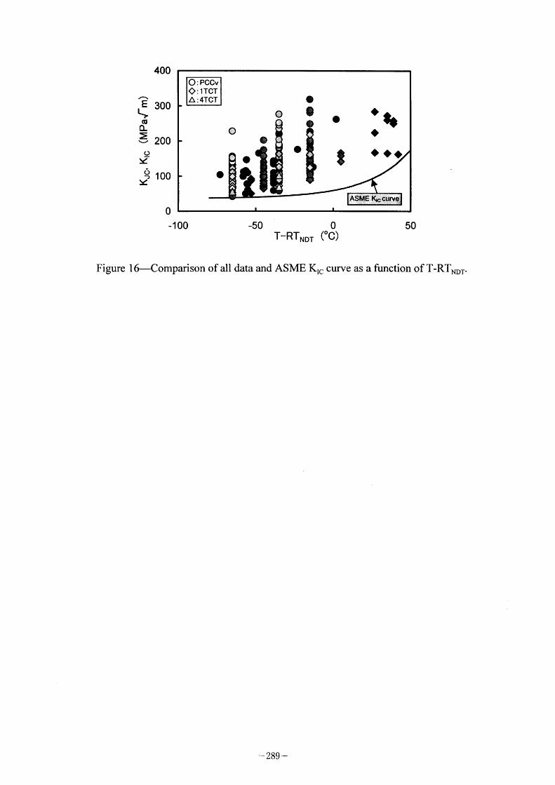
400

~ E 300 L? ~ = - 200 ~e~

~e*~ 100

O

^~OA : i ~:";~f

~=1TcT A = 4TCT

o

o

i

o

o

o O o e

$

~ .$,

ASME Xte cuwe

-1 OO

T-RTNDT ("O 50

Figure 1 6-Comparison of all data and ASME Klc curve as a function of T-RTNDT.

~ 289 -