Paper to be presented at the DRUID Summer Conference 2007

on

APPROPRIABILITY, PROXIMITY, ROUTINES AND INNOVATIONCopenhagen, CBS, Denmark, June 18 - 20, 2007

NOTHING'S GONNA STOP INNOVATORS NOW? AN EMPIRICAL INVESTIGATIONON THE 'SUCCESS BREEDS SUCCESS' HYPOTHESIS

Bettina PetersZEW

b.peters@zew.de

Abstract:Using an innovation panel data set on German manufacturing firms covering the period 1994-2005, this paperinvestigates whether innovation success breeds innovation success. The econometric results, based on a dynamicpooled and random effects tobit model and a new estimator recently proposed by Wooldrigde (2005), confirmthe hypothesis that past innovation success is an important key for subsequent success. First, successful productinnovators are more likely to introduce new products in the future and second, they achieve a higher share ofsales with these product novelties.

JEL - codes: O31, C23, L20

Nothing’s Gonna Stop Innovators Now?

An Empirical Investigation on the’Success Breeds Success’ Hypothesis

February 2006

Preliminary version.

Abstract: Using an innovation panel data set on German manufacturing firms cov-

ering the period 1994–2005, this paper investigates whether innovation success breeds

innovation success. The econometric results, based on a dynamic pooled and random

effects tobit model and a new estimator recently proposed by Wooldrigde (2005), confirm

the hypothesis that past innovation success is an important key for subsequent success.

First, successful product innovators are more likely to introduce new products in the

future and second, they achieve a higher share of sales with these product novelties.

Keywords: innovation, success breeds success, persistence, state dependence, dy-

namic random effects tobit model

JEL Classification: O31, C23, C25, L20

Any errors remain those of the author.

1 Introduction

Cases like Toyota in the automobile industry or Intel demonstrate that successful inno-

vators are able to sustain their market positions through permanent subsequent innova-

tions, and hence support a view that innovation success breeds innovation success. On

the other hand, there is also case evidence that successful innovators fail to keep pace

with the technological progress as time goes by1, that successful innovators can face great

difficulties when trying to do something radically different from their past experience or

that even failed innovation experience substantiates further success.

This paper analyses the dynamics in firms’ innovation success. In particular, it focuses

upon the following two research questions: First, are successful product innovators more

likely to introduce new products in the future? And second, given that they subsequently

innovate, are they more successful then previous non–innovators?

Large scale empirical evidence on the development of innovation success at the firm-

level is rare. There are a few patent–based studies which have mainly focused on the

question whether innovation persistence exists, irrespective of its origin. Malerba and

Orsenigo (1999), Cefis and Orsenigo (2001) and Cefis (2003) studied innovation per-

sistence using EPO patent application data of manufacturing firms from six countries

(France, Germany, Italy, Japan, USA and the UK). Their results showed that only a

small fraction of firms were able to patent permanently. Although these firms became

rather large innovators (in terms of the number of patents) over time, resulting in the

fact that persistent innovators, although small in absolute numbers, accounted for an

important part of all patents. The result that patent activities among patenting firms

exhibited only a little degree of persistence, was also confirmed by Geroski et al. (1997)

using data of UK manufacturing firms which had at least one patent granted in the US

between 1969 and 1988. It is well-known that patents are not a perfect indicator of

innovation success: Not all inventions are patentable and even if they are they do not

necessarily lead to patents. Instead of patents firms might choose other measures to

protect their inventions, like secrecy or complex designs. Furthermore, not all patents

lead to new products or processes, and the value of patents is highly skewed. In the

context of persistence analysis, patents have an additional drawback, because in this

kind of winner–takes–all contest, to be classified as permanent innovators firms have to

win the patent race continuously (Kamien and Schwartz 1975).

Due to the development of a common definition of innovation and several new inno-

vation indicators by the OECD and EUROSTAT (Oslo-manual, first published 1992) as

well as the release of European–wide harmonized innovation surveys (known as Commu-

nity Innovation Surveys CIS), researchers have recently started to analyze this question

1 See, for instance, Ford in the automobile industry or in recent times the development of Yahoo.

1

using innovation data. Most of the previous studies done so far measured innovation

success as the introduction of at least one (product and/or process) innovation, and

therefore investigated the persistence of innovation success by means of a simple binary

indicator (Flaig and Stadler 1994 and 1998, Duguet and Monjon 2004 or Peters 2005).

These studies confirm that previous innovators are more likely to innovate again. In

contrast to that, this paper applies a quantitative indicator to measure innovation suc-

cess. The firm’s success of offering innovative products to its customers is measured by

the share of sales due to these new or significantly improved products. This indicator

is recommended by the Oslo manual as product innovation output indicator (see OECD

and Eurostat 2005), and it can be interpreted as a sales weighted innovation count.

Hence, this study is similar in nature to the recent work of Raymond et al. (2006) who

first applied this quantitative innovation measure to investigate state dependence effects

for Dutch manufacturing firms. They set up an econometric framework in which the

decision to innovate in new products or processes depends on the preceding innovation

status which is a binary indicator. Condition on the introduction of a (product or pro-

cess) innovation, the product innovation outcome then depends on the lagged innovation

outcome. Surprisingly, Raymond et al. could not ascertain persistence in the occurrence

of innovations for Dutch manufacturing firms, but pointed out that among continuous

innovators the innovation success had a positive impact on future success. In addition to

the distinct data set, there are three main differences: First, this paper focuses solely on

product innovation decisions, since the innovation outcome relates only to product inno-

vations. Second, the framework I use in this paper takes into account that the decision

to innovate might not only depend on the previous innovation status (binary indicator),

but also on the level of the innovation success itself. That is, more successful innovators

might be more likely to develop and launch new products. Third, the econometric esti-

mation allows the unobserved firm-specific heterogeneity to correlate with the observed

firm characteristics.

The analysis is based on panel data from the German innovation survey covering

firms’ innovation activities during the period 1994–2005. The descriptive analysis reveals

that at the firm–level the introduction of product innovations show a high degree of

persistence over time. Likewise evident, but less pronounced is the perseverance in

innovation success. The question which factors drive this pattern – previous innovation

success, other observed firm characteristics or unobserved firm-specific heterogeneity (see

Heckman 1981a,b) – is then analysed and identified by means of a dynamic pooled and

random effects tobit model.

The outline of the paper is as follows. Section 2 explores the theoretical arguments

in favour of state dependence in innovation success. The construction of the panel data

set is described in Section 3 and Section 4 depicts some first descriptive results about

2

the persistence of product innovation occurrence and success. Section 5 presents the

econometric model and its empirical implementation. It further explores the estimation

method used and sets forth the econometric results. The final section contains some

concluding remarks.

2 Related Theoretical Literature

The view that ’innovation success breeds innovation success’ is actually based on dif-

ferent arguments in the literature. Economic theory provides at least three potential

explanations of why innovation success might demonstrate state dependence over time.

First, successful innovations positively affect the conditions for subsequent innovations

via an increasing permanent market power of prosperous innovators. In contrast to

Schumpeter, who assumed that the increasing market power is a temporary phenomenon

and is eroded by the entry of imitators or innovators, Phillips (1971) argued that success

favours growing barriers to entry that eventually allow a few increasingly successful firms

to permanently dominate an industry.

Second, successful innovations broaden the firm’s technological opportunities which

make subsequent innovation success more likely as was emphasised by Mansfield (1968) or

Stoneman (1983). Based on this idea of dynamic intra–firm spill–overs, Flaig and Stadler

(1994) developed a stochastic optimisation model in which firms maximise their expected

present value of profits over an infinite time horizon by simultaneously choosing optimal

sequences of both product and process innovations. Both were shown to be dynamically

interrelated in this model.

A third line of reasoning is the existence of constraints in financing innovation projects

(see Nelson and Winter 1982). Usually, information asymmetries about the risk and the

failure probability of an innovation project exist between the innovator and external

financial investors. This leads to adverse selection and moral hazard problems which

usually force firms to finance innovation projects by means of internal funds (Stiglitz

and Weiss 1981). Successful innovations provide firms with increased internal funding

and hence can be used to finance further innovation projects. The larger the previous

innovation success, the more likely it is, that the firm will carry out either (i) one larger

and more important innovation project or (ii) a larger number of smaller innovation

projects. Both strategies make the occurrence of future innovations not only more likely

but also increase the expected innovation success.

Another theory which is closely related to the ’success breeds success’ hypothesis is

the theory of ”dynamic competencies” (Winter 1987 and Teece and Pisano). The theory

states that firms’ technological capabilities are a decisive factor in explaining innovation.

3

Firms’ innovative capabilities in turn are primarily determined by human capital, i.e., by

the knowledge, skills and creativity of their employees. Experience in innovation is as-

sumed to be associated with dynamic increasing returns in the form of learning–by–doing

and learning–to–learn effects. That is, with innovation experience firms acquire techno-

logical competencies and accumulate technological capabilities which enhance knowledge

stocks and, therefore, the probability of future innovations. Learning can be related to a

better understanding of the pure technological context but also to improved knowledge of

how to commercialize new products. Since a firm’s absorptive capacity – i.e. its ability to

recognise and to assimilate the value of new external information – is likewise a function

of the level of knowledge, learning in one period will furthermore permit a more efficient

accumulation of external knowledge in subsequent periods (Cohen and Levinthal 1990).

The cumulative nature of knowledge should therefore induce state dependence in inno-

vation (see, e.g., Nelson and Winter 1982 and Malerba and Orsenigo 1993). Theories

which focus on how firms accumulate technological capabilities may also be considered

as ’success breeds success’ theories since technological capabilities might substantiate

sustained competitive advantages (Teece and Pisano 1994). On the other hand learning

can also occur as a result of unsuccessful innovations and the phenomenom that firms

learn from their mistakes or flops is called ’failure breeds success’. Furthermore, in con-

trast to their innovation input firms can not necessarily control their innovation outcome

because serendipity might play an important role in the innovation process (Kamien and

Schwartz 1982).

Common to all various ’success breeds success’ arguments is the notion that a firm

can gain some kind of locked–in advantage over other firms due to successful innovations

(Simons 1995). Based on these arguments, the following two hypotheses will be tested

in the empirical analysis:

H1: Do successful production innovations make a firm more likely for subsequent

product innovations?

H2: Do successful product innovations increase the firm’s subsequent innovation out-

come measured by the share of sales with new products?

3 Construction of the Data Set

The data set used is the Mannheim Innovation Panel (MIP), covering firms from manu-

facturing, mining, energy/water supply and construction. The MIP is based on inno-

vation surveys carried out by the ZEW on behalf of the German Federal Ministry of

Education and Research. The surveys are drawn as stratified random samples and are

representative of the corresponding target population. The target population spans all

4

legally independent enterprises with 5 or more employees and their headquarters located

in Germany.2 Firm size, industry and region serve as stratifying variables. The sur-

vey started in 1993.3 Every fourth year the survey is the German contribution to the

European–wide harmonized Community Innovation Surveys (CIS). While in most other

European countries innovation surveys take place every 4 years, they are conducted an-

nually in Germany. The survey methodology and definitions of innovation indicators

comply with the OSLO-Manual (OECD and Eurostat 1997), thereby yielding interna-

tionally comparable data. The MIP is designed as a panel. As in many other European

countries participation is voluntary in Germany. About 2000 to 2500 manufacturing

enterprises fill out the questionnaire each year, implying a response rate of between 20

to 25 %.4 A detailed description of the MIP is provided by Janz et al. (2002) or Peters

(2006).

Although we have a yearly and hence fairly long panel data set at hand, its full

exploitation is impeded by three facts: The first one is related to an important charac-

teristic of the CIS data. Since the time needed to develop an innovation is often more

than one year and innovation is therefore a multi–period activity, the indicator whether

a firm has introduced a product innovation is related to a 3–year period. As an example,

in the 2005 CIS survey a firm is defined as a product innovator if it has introduced at

least one new or significantly improved product in the period 2004–2002, in the 2004

survey this indicator is related to 2003–2001. The innovation success is measured by the

share of sales in a given year t due to product innovations introduced in the years t-2 to

t. Though this indicator is measured on a yearly base, admittedly it implies that a new

product introduced for example in 2002 counts for the share of sales with new products

in 2002, 2003 and 2004. Hence, it is likely that this measure show a high persistence on

a year-to-year basis and in the extreme case it might just reflect a stable market position

of the same new product.5 From a theoretical point of view, however, the ’success breeds

success’ hypothesis is related to the introduction of further innovations and the question

whether firms can sustain their innovation outcome with their subsequent innovations.

2An enterprise in the survey is defined as the smallest combination of legal units that is an organisa-tional unit producing goods or services. An enterprise carries out one or more activities at one or morelocations. An enterprise may be a sole legal unit. In the following, I will use the expressions enterpriseand firm interchangeable.

3Two years later the service sector was included. While in manufacturing the innovation outputindicator – share of sales due to new products – was included right at the start of the survey, it wasasked in the service sectors 1998 for the first time. Hence, I decided to focus on the industry sector.

4 The low response rates are in line with those of comparable voluntary surveys of German firms.In order to control for a response bias in the net sample, non-response analyses are carried out eachyear, covering a similar number of firms of the net sample and collecting information on product andprocess innovations by the means of telephone interviews. They come up with the result that the shareof innovators is only slightly underestimated in the net sample.

5 Due to data restrictions, the study of Raymond et al. (2006) in part suffer from this overlapping oftime periods problem.

5

To avoid embracing the same product innovations, the panel sample used only includes

every third wave.6

Table 1: Characteristics of the Panel

Panel A Panel B

Time Periods 1994–1996, 1994–1996,1997–1999, 1997–1999,2000–2002 2000–2002,

2003–2005

Number of observations 1401 972Number of firms 467 243Number of consecutive obs. per firm 3 4

The second difficulty is related to the fact that for analysing the firms’ innovation

success in a dynamic random effects tobit model, a balanced panel of only those firms

which have consecutively answered in at least three waves is required. Although the

survey is designed as a panel study, it has to be asserted that the main part of the firms

participated only once or twice.7 Furthermore, two major refreshment of the panel took

place in the 1995 and 2004 surveys. Balancing the need (i) to investigate the dynamics

in the innovation behaviour for a large number of enterprises, and (ii) to examine it

for a long time period – to ensure that we can observe firms’ innovation success over

different phases of the business cycle and over an observation period that is also longer

than the average product life cycle in an industry, lead me to the construction of two

different samples. Panel A comprises 467 German manufacturing firms which we observe

for three waves covering the time periods 1994–1996, 1997–1999 and 2000–2002. Panel

B consists of the smaller set of 231 firms for which innovation activities are available for

four waves spanning the period 1994–2005. Table 1 summarises the main characteristics

of both samples. For both balanced panels the distributional characteristics with respect

to firm size, region, industry and innovative activity have been compared with the ones

of the corresponding unbalanced panel. It turned out that both panels still reflect total–

sample distributional characteristics quite well, though the share of product innovators

are slightly lower in the balanced panels.

6 An alternative strategy is to use a panel with yearly observations and include a three-year-laggeddependent variable. The results are nearly unaltered and not reported here, but available upon requestfrom the author.

7 Peters (2005) provides more information on the individual participation behaviour of the sampledfirms.

6

4 Descriptive Analysis

Before turning to the econometric results, I first provide a brief descriptive analysis of

the data. Though evidence is provided for both panels, the interpretation of the results

will be mainly based on panel A. In total, the share of product innovators is about 48%

in the panel A and 45 % in panel B. A more interesting question though is that of ”How

persistently do firms innovate?”. Table 2 and Table 3 report the transition probabilities

for the introduction of new products for the whole period and differentiated by periods.

Note that in the following t is used as an index for the period, k indicates a year.

Table 2: Transition Probabilities in Product Innovation (0/1), Whole Period

Innovation status in t + 1

Panel A Panel B

Innovation status in t Non–Inno Inno Total Non–Inno Inno Total

Non–Inno 85.3 14.7 100.0 84.9 15.1 100.0Inno 21.4 78.6 100.0 23.3 76.7 100.0

Table 3: Transition Probabilities in Product Innovation (0/1), by Period

Innovation Status Period

Period t Period t + 1 94–96/97–99 97–99/00-02 00–02/03–05

Panel A

Non–Inno Non–Inno 79.5 91.7 −

Inno 20.5 8.3 −

Inno Non–Inno 12.3 29.7 −

Inno 87.7 70.3 −

Panel B

Non–Inno Non–Inno 76.2 91.2 87.7

Inno 23.8 8.9 12.3

Inno Non–Inno 14.5 33.1 20.6

Inno 85.5 66.9 79.4

Table 2 indicates that innovation is permanent at the firm-level to a very large extent.

Nearly 79% of product innovators in manufacturing in one period persisted in product

innovation activities in the subsequent period while 21% did not succeed in introducing

at least one new product. The persistence is even higher among non–product innovators,

with a share of about 85% of them remaining non– product innovators in the following

period.8 Only 15% of previous non-product innovators offered new products in the

8 Of course, this figure does not allow to distinguish whether previous non–product innovators didn’tstart to innovate at all or whether they didn’t succeed in introducing new products.

7

subsequent period. The probability of introducing a new product in period t + 1 was

about 64 percentage points (hereafter: PP) higher for innovators than for non-innovators

in t which can be interpreted as a measure of state dependence.

Table 3 shows that these transition probabilities vary over time. The drop out of

as well as entry into product innovation activities was particularly high for the period

1998–2000. This period marked a boom phase in the the German economy. This result

is astonishing since it contradicts the demand-pull theory which predicts pro–cyclical

effects to occur because the cash–flow as an important source of financing innovations

is positively correlated with economic activity, see Himmelberg and Petersen (1994).

Moreover, Judd (1985) argued that markets have a limited capacity for absorbing new

products and thus firms are more likely to introduce new products in prosperous market

conditions.

Table 4: Number of Entries into and Exits from Product Innovation

Panel A Panel B

Number of Total Non–Inno Inno Total Non–Inno Innochanges in t = 0 in t = 0 in t = 0 in t = 0

0 72.8 74.0 70.6 61.3 65.1 57.31 18.2 10.5 26.3 21.8 11.9 32.52 9.0 14.6 3.1 15.6 21.4 9.43 – – – 1.2 1.6 0.9

Total 100 100 100 100 100 100

Notes: Figures are calculated as share of total firms, initial non–product innovators and product inno-vators, respectively. Sample: Balanced Panel.

Looking at the innovative history of firms, Table 4 reports the number of (re–)entry

into and (re–)exit from product innovation activities. 71% of the initial (t = 0) product

innovators were continuously engaged in introducing new products throughout all three

periods in panel A. This implies that 34.5% of all firms can be classified as permanent

product innovators during the period 1994-2002. In panel B the share is somewhat

lower, but still 57% of the initial product innovators kept in introducing new products

in all following three periods. On the other hand, in panel A about 74% of the initial

non–product innovators kept out of introducing new products in all following periods.

This implies that 38% of all firms didn’t launch any new products during the period

1994-2002.

Table 5 and 6 shed light into the dynamics of the innovation success with new products.

Table 5 depict the innovation success in period t by its preceding product innovation

status. The innovation success of firm i in period t is measured as the share of sales with

new products in year k with products introduced in the period (i.e. the three years k,,

k − 1 and k − 2). On average, product innovators earn 42% of their sales in year k with

new products launched in the period t. Differentiating by their preceding innovation

8

status, it turns out that product innovators which have also introduced new products in

the period t − 1 achieve a share of sales with new products that is about 8 percentage

points higher than that of prior non-product innovators. A mean difference test show

that this difference is significant at the 5 percent level.

Table 5: Innovation Success by Preceding Product Innovation Status, Panel A

Group Mean St.dev. Min Max Obs n ttestOverall Between Within

PDt = 1 0.420 0.293 0.252 0.172 0 1 670 288

PDt = 1 &PDt−1 = 0 0.311 0.300 0 1 67 67

PDt = 1 &PDt−1 = 0 0.393 0.283 0 1 375 214 0.016

Notes: t is an index for the period. Obs denotes the number of observations, n the number of firms.ttest is the p–value of a one–tailed t–test on equal means in both groups (the variances are allowed tobe unequal between both groups). Note, the fact that the overall mean for PDt = 1 is larger than forthe subsamples is due to the fact that differentiating by prior innovation status reduces the number ofperiods by one.

Table 6: Transition Probabilities in Product Innovation Success, Panel A

Innovation success category in t + 1

Innovation success category in t 0 1 2 3 4

0 85.4 4.5 5.2 1.7 3.2

1 22.7 34.0 27.8 12.4 3.1

2 21.7 11.7 30.8 26.7 9.2

3 21.0 6.5 18.6 31.5 22.6

4 19.7 3.9 8.7 18.9 48.8

Finally, the innovation success in each period was divided into 5 categories and Table 6

shows the one-period-movements between the different categories. To take into account

that the share of sales with new products varies over time, the success categories are

defined not in absolute terms but on a relative base. That is, the categorial variable in a

period t takes on the value 0 if the firm has not introduced any product innovations in t.

It equals 1 if the share of sales with new products is positive and is lower than the first

quartile of the distribution (calculated for all firms with product innovations in period

t). The values 2, 3 and 4 means the innovation success lies between the first quartile

and the median, the median and the second quartile, and above the second quartile.

Bases on the ’success breeds success’ hypothesis we would expect firms a movement to

higher innovation success classes. For each category the highest value can be found on

the diagonal and the second highest value for the categories directly above the diagonal.

That is, firms have the highest probability of sustaining their innovation success or even

9

slightly improving their position. Interestingly enough nearly every second firm which

belongs to the most successful innovators in period t, can sustain its outstanding position

in the following period.

5 Econometric Analysis

5.1 Econometric Model and Estimation Method

Though interesting, transition rates only depict the degree of persistence in the innova-

tion success, but don’t offer a clue to the causes of this phenomenon since we do not

control for observed and unobserved individual characteristics. This is taken into account

in the following econometric analysis.

We start on the assumption that the innovation success yit of firm i in period t de-

pends on its previous innovation success yi,t−1, on some observable explanatory variables

summarised in the l–dimensional row vector xit and on unobservable factors uit. The

innovation success, however, is only observed if the firm introduces a new product and

is 0 otherwise (corner solution problem). We therefore model the innovation success by

the following equation:

yit = max[0, γ yi,t−1 + xit β + uit] i = 1, . . . , N, t = 1, . . . , T (1)

The ’success breed success’ hypothesis implies that γ > 0. For the unobservable

factors uit I allow for two different assumptions. Assumption 1 is that of a pooled tobit

model: uit|xit ∼ N(0, σ2

u). This implies that uit is independent of xit, but that the

relationship between uit and xis is unspecified for s 6= t. Hence it does not impose a

strict exogeneity assumption of the xit (see Wooldridge 2002). On the other hand, if

the innovation success is influenced by firm–specific unobserved factors, a pooled tobit

estimation leads to biased results. The second estimation strategy therefore allows for

unobserved individual heterogeneity by assuming that

uit = µi + εit (2)

µi captures time-constant firm-specific effects. The effect of other time–varying un-

observable determinants is summarized in the idiosyncratic error εit. It is assumed

that εit|yi0, . . . , yi,t−1, xi, µi is i.i.d. as N(0, σ2

ε) and that εit ⊥ (yi0, xi, µi) where xi =

(xi1, . . . , xiT ).

One important problem in parametric estimation of dynamic non–linear models refers

to the handling of the initial condition yi0. I follow the conditional ML approach recently

10

proposed by Wooldridge (2005). The idea is to assume that the individual heterogeneity

depends on the initial innovation success and the strictly exogenous variables in the

following way:

µi = α0 + α1 yi0 + xi α2 + ai, (3)

where xi = T−1∑T

t=1xit denotes the time–averages of xit.

9 Adding the means of the

explanatory variables as a set of controls for unobserved heterogeneity is intuitive in

the sense that we are estimating the effect of changing xit but holding the time average

fixed. For the error term ai we assume that ai ∼ i.i.d.N(0, σ2

a) and ai ⊥ (yi0, xi) and thus

µi|yi0, xi follows a N(α0+α1yi0+xi α2, σ2

a) distribution. Having specified the distribution

of µi in this way, Wooldridge (2005) showed that the likelihood of this dynamic random

effects tobit model is the same as in the standard random tobit model, except that the

explanatory variables are given by xit, yi,t−1, yi0 and xi. Identification of the β′s requires

that the exogenous variables vary across time. If the structural model contains time–

invariant regressors like industry dummies, one can include them in the regression to

increase explanatory power. However, it is not possible to separate out the direct effect

and the indirect effect via the heterogeneity equation. Time dummies which are the

same for all i are excluded from xi.

5.2 Empirical Model Specification

As already explained the dependent variable, i.e. the innovation success of firm i in period

t is measured as the share of sales with new products in year k with products introduced

in the last three years k,, k−1 and k−2 (SUCCESS), see Table 7 for more details on the

variable definitions. Besides own previous innovation success, the theoretical literature

has identified a bunch of other potential success factors and most of them have been

confirmed to have a positive impact on the success of product innovations in previous

cross–sectional studies, among others: R&D and innovation input (see, for instance,

Crepon et al. 1998, Loof and Heshmati 2001, Love and Roper 2001 or Janz et al. 2004),

technological opportunities (see Cohen and Levinthal 1989), technological capabilities

(see, e.g., Dosi 1997 or Konig and Felder 1994, Love and Roper 2001), absorptive capacity

(see, e.g., Becker and Peters 2000, Raymond et al. 2006), appropriability conditions,

market demand (see, e.g., Crepon et al. 1998), degree of international competition,

network relationships, especially with customers (see, e.g., Hippel 1988) or corporate

governance structure (see, e.g., Czarnitzki and Kraft 2004).

9 Instead of xi the original estimator used xi = (xi1, . . . , xiT ) in equation (3), but time–averages areallowed to reduce the number of explanatory variables (see Wooldridge 2005).

11

The following econometric analysis accounts for most of these factors. The innovation

input (INPUT) is measured by the innovation intensity, that is the ratio of the innova-

tion expenditure to sales. The innovation output equation is also specified as a function

of technological capabilities. In addition to innovation experience, technological capa-

bilities are mainly determined by the skills of employees. Hence, I operationalise this

construct by means of three variables: the share of employees with a university degree

(HIGH), a dummy variable equaling 1 if a firm has not invested in training its employees

in the previous period (NOTRAIN) and the amount of training expenditure per em-

ployee (TRAINEXP). As in many previous studies, absorptive capacities are proxied by

a dummy variable indicating whether the firm carries out R&D activities (R&D). The

degree of international competition is measured by the export intensity (EXPORT). All

these explanatory variables are measured by their value at the end of the period prior

to the introduction of the new products accounted for by the dependent variable, that

is in year k − 3, to reduce potential endogeneity problems. The estimation also con-

trols for ownership structure by distinguishing between public limited companies (PLC),

private limited liability companies (LTD) and private partnerships (PRIVPART). One

argument stressed by the principal agency theory is that managers prefer to carry out

less risky investment and innovation projects than owners because managers are more

closely related to the company and they will be threatened with the loss of their job if the

investment fails while owners can spread their risk by diversification strategies (Jensen

and Meckling 1976).

The regression further controls for firm size, ex ante market structure and availability

of financial resources. Firm size is measured by the log number of employees (SIZE)

and the market structure is captured by the Herschmann–Herfindahl index (HHI). The

availability of financial resources is proxied by an index of creditworthiness (RATING).

Note that we expect a negative coefficient of this variable, since the index ranges from

1 (best rating) to 6 (worst rating) and thus a higher value of RATING implies that

less external funding is available and that it is more costly due to higher interest rates,

making fewer innovation projects profitable and feasible. Again, all variables refer to the

end of the period t − 1, i.e. the year k − 3.

In addition, firm–specific variables reflecting whether a firm has received public fund-

ing in the previous period (PUBLIC), firm age (AGE), location (EAST), whether the

firm is part of an enterprise group (GROUP) and whether the group’s headquarter is

located abroad (FOREIGN) are included.

Industry characteristics – alone or in combination with firm–specific features – may

also breed firms’ innovation success. In particular, technological opportunities and ef-

fective appropriability conditions are expected to play a significant role. The concept

of technological opportunities can be summarised by the fact that the prevailing tech-

12

nological dynamics (basic inventions, spillover potentials of new technologies) in some

industries spur innovation stronger than in other industries. Effective appropriability

conditions are important in that they allow innovators to receive the returns on their

innovation activities. Due to the lack of a good measurement for both concepts, industry

dummies are intended to account for them.

Finally, time dummies are included in the regression.

Table 7: Variable Definition

Variable Type Definition

Endogenous variable

SUCCESS 0-1 Innovation success in period t measured as share of sales in year k with

new products introduced in the years k − 2 to k. A product innova-

tion is a good or service which is new or significantly improved with

respect to its fundamental characteristics, technical specifications, in-

corporated software or other immaterial components, intended uses,

or user friendliness. The innovation should be new to the enterprise;

it has not necessarily to be new to the market.

Explanatory variables varying across individuals and time

SIZE c Number of employees at the end of period t− 1, i.e. in year k − 3 (in

log).

RATING c Credit rating index at the end of period t − 1, i.e. in year k − 3,

ranging between 1 (highest) and 6 (worst creditworthiness).

AGE c Age at the end of period t (in log).

GROUP 0/1 1 if firm i belongs to a group at the end of period t.

NOTRAIN 0/1 1 if firm i has no training expenditure in period t − 1, i.e. in year

k − 3.

TRAINEXP c Training expenditure per employee at the end of period t − 1, i.e. in

year k − 3 if NOTRAIN=0 (in log), otherwise 0.

HIGH c Share of employees with a university or college degree at the end of

period t − 1, i.e. in year k − 3.

EXPORT c Export intensity defined as exports/sales at the end of period t − 1,

i.e. in year k − 3.

PUBLIC 0/1 1 if firm i received public funding for innovation at the end of period

t − 1, i.e. in year k − 3.

INPUT c Innovation intensity which is defined as the ratio of innovation ex-

penditure to sales at the end of period t − 1, i.e. in year k − 3.

Innovation expenditure includes expenditure for intra– and extramu-

ral R&D, acquisition of external knowledge, machines and equipment,

training, market introduction, design and other preparations for prod-

uct and/or process innovations.

R&D 0/1 1 if firm i carries out R&D in year k − 3.

Continued on next page.

13

Table 7 – continued from previous page

Variable Type Definition

Explanatory variables varying across industries and time

HERFIN c Hirschman–Herfindahl Index in year k − 3, on a 3–digit NACE level,

divided by 100.

Time–constant individual–specific explanatory variables

FOREIGN 0/1 1 if firm i is a subsidiary of a foreign company.

EAST 0/1 1 if firm i is located in Eastern Germany.

PLC 0/1 1 if firm i is a public limited company.

LTD 0/1 1 if firm i is a private limited liability company.

PRIVPART 0/1 1 if firm i is a private partnership.

IND 0/1 System of 15 industry dummies, see Table 10.

Time–varying individual–constant explanatory variables

TIME 0/1 System of time dummies for each period.

Notes: c denotes a continuous variable.

5.3 Econometric Results

Table 8 and Table 9 show the estimation results of the pooled tobit model and of the RE

effects tobit model for Panel A, respectively. Estimation results for Panel B, though not

shown here, overwhelmingly supports the results found for Panel A and are available upon

request. In both tables, the first column of each regression reports the marginal effects

for the probability of having product innovations10. The second columns contain the

marginal effect for the expected value of the innovation success conditional on introducing

new products. Both marginal effects are calculated at the sample means of the observable

variables and in the RE model additionally at the average value of the unobserved

heterogeneity. One limitation of the RE estimator is the fact it assumes strict exogeneity

of the explanatory variables. Hence, feedback effects from the innovation success on

future values of the explanatory variables are ruled out. This strong assumption in the

RE effects model seems to be contestable at least for some of the explanatory variables.

It is particularly crucial for the innovation input or the R&D variable, since it likely that

shocks in the innovation outcome equation will have an impact on firms’ subsequent

innovation input behaviour. To assess the impact on the estimated state dependence

effect by including variables, which potentially fail the strict exogeneity assumption,

I apply a stepwise procedure. That is, I start estimating an extremely parsimonious

10 Strictly speaking, it is the probability of observing a positive innovation success. Since nearly allproduct innovators demonstrate a positive share of sales with new product, I use the expression ”havingproduct innovations” interchangeably.

14

specification including only industry and time dummies as strictly exogenous variables.

Then additional explanatory variables are included which might fail this assumption.

Estimates of the pooled tobit model show a highly significant impact of previous

innovation success on the actual innovation success. This result is seen in the very

parsimonious specification and is robust to including additional explanatory variables.

Remember that strict exogeneity is not required for the pooled model. These results

would corroborate the ’success breeds hypothesis’. However, the pooled model does not

control for unobserved heterogeneity. It might be the case that the lagged dependent

variable just picks up the effect of time–constant firm specific characteristics not con-

trolled for in the regression. The estimates of the dynamic RE tobit model, however,

indicate that even after controlling for individual effects, the lagged dependent variable

is still significant at the 5% level. The marginal effects though are much smaller than

in the pooled model. Based on the estimates in specification (2) an increase in prior

innovation success by 10%, for instance from the average value of 24.6% to 27.1%, lead

to increase of the probability of introducing new products in the subsequent period by

3 percentage points. And given the firm introduces new products, the firms achieve a

share of sales with these new products that is about 1 percentage point higher (0.86).

The effects still hold and are nearly unaltered after controlling for innovation input and

absorptive capacities which themselves enter significantly.11 All in all, the estimates

provide convincing evidence that innovation success breeds innovation success.

In addition to prior innovation success, innovation input and absorptive capacity,

skills, age, foreign ownership and unobserved heterogeneity are crucial to the innovation

success. The results found for age, for instance, indicate that firms with a lower average

age in the period under consideration demonstrate a smaller innovation success, but with

increasing age their innovation success steps up. Foreign owned enterprises show a sig-

nificantly worse innovation performance that domestic enterprises. This is line with the

’liabilities of foreignness’ hypothesis (see Zaheer 1995). The importance of unobserved

heterogeneity can be gauged from ρ = σ2

a/(σ2

ε + σ2

a). Unobserved heterogeneity still ex-

plains between 25 and 18% of the variation in the dependent variable in manufacturing

depending on the specification of µi

11 Since the R&D indicator variable shows only little variation over time, only the firm-specific time-averaged value was included.

15

Table 8: Dynamic Pooled Tobit Estimations, Panel A

Regression 1 2 3

P (y = 1) E(y|y > 0) P (y = 1) E(y|y > 0) P (y = 1) E(y|y > 0)

SUCCESS−1 0.934∗∗∗ 0.280∗∗∗ 0.836∗∗∗ 0.234∗∗∗ 0.589∗∗∗ 0.146∗∗∗

(0.053) (0.015) (0.057) (0.015) (0.061) (0.015)

SIZE — — 0.053∗∗∗ 0.015∗∗∗ 0.024∗ 0.006∗

(0.014) (0.004) (0.015) (0.004)

HERFIN — — 0.058∗ 0.016∗ 0.055∗ 0.014∗

(0.032) (0.009) (0.033) (0.008)

RATING — — 0.011 0.003 0.009 0.002(0.028) (0.008) (0.028) (0.007)

AGE — — 0.002 0.0004 -0.001 -0.0002(0.026) (0.007) (0.026) (0.007)

GROUP — — 0.068∗ 0.019 0.033 0.008(0.036) (0.010) (0.037) (0.009)

EXPORT — — 0.116 0.032 -0.023 -0.006(0.079) (0.022) (0.083) (0.021)

HIGH — — 0.360∗∗ 0.101∗∗ 0.152 0.038(0.147) (0.041) (0.155) (0.038)

NOTRAIN — — -0.334∗∗∗ -0.088∗∗∗ -0.193∗ -0.045∗

(0.090) (0.024) (0.110) (0.025)

TRAINEXP — — 0.016 0.004 0.001 0.0003(0.014) (0.003) (0.014) (0.004)

PUBLIC — — — — 0.072∗ 0.018∗

(0.043) (0.011)FOREIGN — — -0.172∗∗∗ -0.045∗∗∗ -0.082 -0.020

(0.056) (0.014) (0.063) (0.015)

EAST — — 0.005 0.001 -0.030 -0.007(0.042) (0.012) (0.045) (0.011)

PLC — — -0.058 -0.017 0.032 0.008(0.088) (0.023) (0.094) (0.024)

PRIVPART — — -0.010 -0.003 0.031 0.008(0.062) (0.017) (0.065) (0.017)

INPUT — — — — 1.302∗∗∗ 0.322∗∗∗

(0.252) (0.062)R&D — — — — 0.454∗∗∗ 0.128∗∗∗

(0.036) ( 0.012)

σu 0.338 0.323 .2900.012 0.012 .010

ln L -391.5 -349.8 -249.2ln LR 0.000 0.000 0.000R2

MF0.389 0.454 0.611

WTIME 0.000 0.000 0.000WIND 0.003 0.004 0.028

Obs 934 934 934Cens 497 497 497Uncen 437 437 437

Notes: ∗ ∗ ∗, ∗∗ and ∗ indicate significance on a 1%, 5% and 10% level, respectively. Marginal

effects are reported. Time and industry dummies are included in each regression. WIND and WTIME

test for the null hypothesis that the industry and time dummies are jointly equal to zero.

16

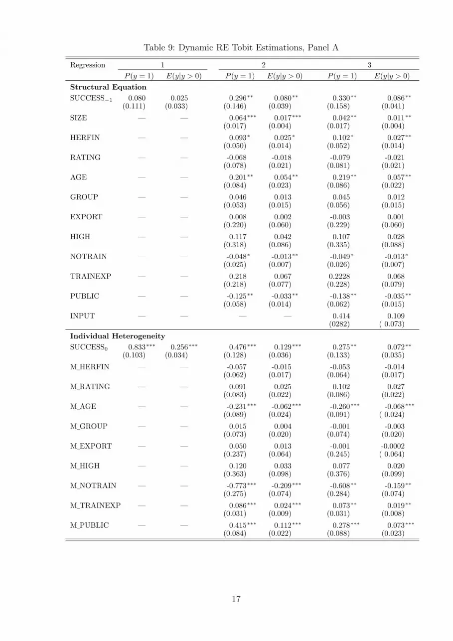
Table 9: Dynamic RE Tobit Estimations, Panel A

Regression 1 2 3

P (y = 1) E(y|y > 0) P (y = 1) E(y|y > 0) P (y = 1) E(y|y > 0)

Structural Equation

SUCCESS−1 0.080 0.025 0.296∗∗ 0.080∗∗ 0.330∗∗ 0.086∗∗

(0.111) (0.033) (0.146) (0.039) (0.158) (0.041)

SIZE — — 0.064∗∗∗ 0.017∗∗∗ 0.042∗∗ 0.011∗∗

(0.017) (0.004) (0.017) (0.004)

HERFIN — — 0.093∗ 0.025∗ 0.102∗ 0.027∗∗

(0.050) (0.014) (0.052) (0.014)

RATING — — -0.068 -0.018 -0.079 -0.021(0.078) (0.021) (0.081) (0.021)

AGE — — 0.201∗∗ 0.054∗∗ 0.219∗∗ 0.057∗∗

(0.084) (0.023) (0.086) (0.022)

GROUP — — 0.046 0.013 0.045 0.012(0.053) (0.015) (0.056) (0.015)

EXPORT — — 0.008 0.002 -0.003 0.001(0.220) (0.060) (0.229) (0.060)

HIGH — — 0.117 0.042 0.107 0.028(0.318) (0.086) (0.335) (0.088)

NOTRAIN — — -0.048∗ -0.013∗∗ -0.049∗ -0.013∗

(0.025) (0.007) (0.026) (0.007)

TRAINEXP — — 0.218 0.067 0.2228 0.068(0.218) (0.077) (0.228) (0.079)

PUBLIC — — -0.125∗∗ -0.033∗∗ -0.138∗∗ -0.035∗∗

(0.058) (0.014) (0.062) (0.015)

INPUT — — — — 0.414 0.109(0282) ( 0.073)

Individual Heterogeneity

SUCCESS0 0.833∗∗∗ 0.256∗∗∗ 0.476∗∗∗ 0.129∗∗∗ 0.275∗∗ 0.072∗∗

(0.103) (0.034) (0.128) (0.036) (0.133) (0.035)

M¯HERFIN — — -0.057 -0.015 -0.053 -0.014

(0.062) (0.017) (0.064) (0.017)

M¯RATING — — 0.091 0.025 0.102 0.027

(0.083) (0.022) (0.086) (0.022)

M¯AGE — — -0.231∗∗∗ -0.062∗∗∗ -0.260∗∗∗ -0.068∗∗∗

(0.089) (0.024) (0.091) ( 0.024)

M¯GROUP — — 0.015 0.004 -0.001 -0.003

(0.073) (0.020) (0.074) (0.020)

M¯EXPORT — — 0.050 0.013 -0.001 -0.0002

(0.237) (0.064) (0.245) ( 0.064)

M¯HIGH — — 0.120 0.033 0.077 0.020

(0.363) (0.098) (0.376) (0.099)

M¯NOTRAIN — — -0.773∗∗∗ -0.209∗∗∗ -0.608∗∗ -0.159∗∗

(0.275) (0.074) (0.284) (0.074)

M¯TRAINEXP — — 0.086∗∗∗ 0.024∗∗∗ 0.073∗∗ 0.019∗∗

(0.031) (0.009) (0.031) (0.008)

M¯PUBLIC — — 0.415∗∗∗ 0.112∗∗∗ 0.278∗∗∗ 0.073∗∗∗

(0.084) (0.022) (0.088) (0.023)

17

Table 9 – continued from previous page

Regression 1 2 3

P (S = 1) E(S|S > 0) P (S = 1) E(S|S > 0) P (S = 1) E(S|S > 0)

FOREIGN — — -0.165∗∗∗ -0.042∗∗∗ -0.151∗∗ -0.037∗∗∗

(0.060) (0.015) (0.061) (0.015)

EAST — — -0.101∗∗ -0.027∗∗ -0.081 -0.021(0.050) ( 0.014) (0.051) (0.013)

PLC — — -0.064 -0.017 0.010 0.003(0.097) (0.025) ( 0.099) (0.026)

PRIVPART — — 0.027 0.007 0.062 0.017(0.068) (0.019) (0.068 ) (0.019)

M¯R&D — — — — 0.370∗∗∗ 0.097∗∗∗

(0.060) (0.016)

σa 0.239 0.159 0.1330.028 0.037 0.044

ρ 0.454 0.254 0.1870.080 0.108 0.118

ln L -371.0 -313.2 -291.0ln LR 0.000 0.000 0.000R2

MF0.350 0.451 0.490

WTIME 0.000 0.000 0.000WIND 0.011 0.033 0.071

Notes: ∗ ∗ ∗, ∗∗ and ∗ indicate significance on a 1%, 5% and 10% level, respectively. Marginal

effects are reported. Time and industry dummies are included in each regression. WIND and WTIME

test for the null hypothesis that the industry and time dummies are jointly equal to zero.

6 Conclusion

This paper has investigated the persistence of innovation success at the firm level and

whether preceding innovation performance substantiates further innovation success. Ev-

idence is based on data form German manufacturing firms during the period 1994-2005.

The econometric results confirm the ’success breeds success’ hypothesis. First, suc-

cessful product innovators are more likely to introduce new products in the future and

second, they achieve a higher share of sales with these product novelties. These results

hold even after controlling for unobserved heterogeneity across firms.

An essential element of the ”dynamic competence” approach to the theory of the

firm concerns the cumulative nature of firms’ competencies implying that firms tend to

improve gradually following rather rigid directions. As a consequence, they can face great

difficulties when trying to do something radically different from their past experience

Malerba et al. (2001). In this study innovation success is measured by means of products

that are new to the firm, not necessarily new to the market. One obvious question for

further research is whether the success breeds success hypothesis applies equally to both

kinds of innovation.

18

References

Becker, W. and Peters, J. (2000). Technological Opportunities, Absorptive Capacities

and Innovation, Volkswirtschaftliche Diskussionsreihe 195, Universitat Augsburg,

Augsburg.

Cefis, E. (2003). Is there Persistence in Innovative Activities?, International Journal of

Industrial Organization 21, 489–515.

Cefis, E. and Orsenigo, L. (2001). The Persistence of Innovative Activities. A Cross–

Countries and Cross–Sectors Comparative Analysis, Research Policy 30(7), 1139–

1158.

Cohen, W. M. and Levinthal, D. A. (1989). Innovation and Learning: The Two Faces

of R&D, The Economic Journal 99(397), 569–596.

Cohen, W. M. and Levinthal, D. A. (1990). Absorptive Capacity: A New Perspective

on Learning and Innovation, Administrative Science Quarterly 35, 128–158.

Crepon, B., Duguet, E. and Mairesse, J. (1998). Research Innovation and Productivity:

An Econometric Analysis at the Firm Level, Economics of Innovation and New

Technology 7, 115–158.

Czarnitzki, D. and Kraft, K. (2004). Firm Leadership and Innovative Performance:

Evidence from Seven EU Countries, Small Business Economics 22(5), 325–332.

Dosi, G. (1997). Opportunities, Incentives and the Collective Patterns of Technological

Change, The Economic Journal 107(444), 1530–1547.

Duguet, E. and Monjon, S. (2004). Is Innovation Persistent at the Firm Level? An

Econometric Examination Comparing the Propensity Score and Regression Meth-

ods, Cahiers de la Maison des Sciences Economiques v04075, Paris.

Flaig, G. and Stadler, M. (1994). Success Breeds Success. The Dynamics of the Innova-

tion Process, Empirical Economics 19, 55–68.

Flaig, G. and Stadler, M. (1998). On the Dynamics of Product and Process Innovations.

A Bivariate Random Effects Probit Model, Jahrbucher fur Nationalokonomie und

Statistik 217, 401–417.

Geroski, P. A., Van Reenen, J. and Walters, C. F. (1997). How Persistently Do Firms

Innovate?, Research Policy 26(1), 33–48.

Heckman, J. J. (1981a). Heterogeneity and State Dependence, in: Rosen, S. (ed.),

Studies in Labour Markets, Chicago, 91–139.

19

Heckman, J. J. (1981b). Statistical Models for Discrete Panel Data, in: Manski, C.

and McFadden, D. (eds), Structural Analysis of Discrete Data with Econometric

Applications, Cambridge, Mass., 114–178.

Himmelberg, C. P. and Petersen, B. C. (1994). R&D and Internal Finance: A Panel

Study of Small Firms in High–Tech Industries, Review of Economics and Statistics

38–51.

Hippel, E. v. (1988). The Sources of Innovation, New York.

Janz, N., Ebling, G., Gottschalk, S. and Peters, B. (2002). Die Mannheimer Innova-

tionspanels, Allgemeines Statistisches Archiv 86, 189–201.

Janz, N., Loof, H. and Peters, B. (2004). Firm Level Innovation and Productivity - Is

There a Common Story Across Countries?, Problems and Perspectives in Manage-

ment 2, 184–204.

Jensen, M. C. and Meckling, W. H. (1976). Theory of the Firm: Managerial Behavior,

Agency Costs and Ownership Structure, Journal of Financial Economics 3, 305–

360.

Judd, K. L. (1985). On the Performance of Patents, Econometrica 53, 567–585.

Kamien, M. I. and Schwartz, N. L. (1975). Market Structure and Innovation: A Survey,

Journal of Economic Literature 13, 1–37.

Kamien, M. I. and Schwartz, N. L. (1982). Market Structure and Innovation, Cambridge,

Mass.

Konig, H. and Felder, J. (1994). Innovationsverhalten der deutschen Wirtschaft, in:

Zoche, P. and Harmsen, D.-M. (eds), Innovation in der Informationstechnik fur die

nachste Dekade, Bedarfsfelder und Chancen fur den Technologiestandort Deutsch-

land, Karlsruhe, 35–64.

Loof, H. and Heshmati, A. (2001). Knowledge Capital and Performance Heterogeneity:

A Firm Level Innovation Study, International Journal of Production Economics

0, 1–25.

Love, J. H. and Roper, S. (2001). Location and Network Effects on Innovation Success:

Evidence for UK, German and Irish Manufacturing Plants, Research Policy 30, 643–

661.

Malerba, F., Nelson, R., Orsenigo, L. and Winter, S. (2001). History-Friendly Models:

An Overview of the Case of the Computer Industry, Journal of Artificial Societies

and Social Simulation 4(3).

20

Malerba, F. and Orsenigo, L. (1993). Technological Regimes and Firm Behaviour, In-

dustrial Corporate Change 2(1), 45–71.

Malerba, F. and Orsenigo, L. (1999). Technological Entry, Exit and Survival: An Em-

pirical Analysis of Patent Data, Research Policy 28, 643–660.

Mansfield, E. (1968). Industrial Research and Technological Innovation: An Econometric

Analysis, New York.

Nelson, R. R. and Winter, S. (1982). An Evolutionary Theory of Economic Change,

Cambridge, Mass.

OECD and Eurostat (1997). Oslo Manual, Proposed Guidelines for Collecting and In-

terpreting Technological Innovation Data, 2. edn, Paris.

OECD and Eurostat (2005). Oslo Manual, Proposed Guidelines for Collecting and In-

terpreting Technological Innovation Data, 3. edn, Paris.

Peters, B. (2005). Persistence of Innovation: Stylised Facts and Panel Data Evidence,

ZEW Discussion Paper 05–81, Mannheim.

Peters, B. (2006). Innovation and Firm Performance. An Empirical Investigation for

German Firms, PhD thesis, University of Wurzburg, Wurzburg.

Phillips, A. (1971). Technology and Market Structure: A Study of the Aircraft Industry,

Lexington.

Raymond, W., Mohnen, P., Palm, F. and Schim van der Loeff, S. (2006). Persistence

of Innovation in Dutch Manufacturing: Is it Spurious?, UNU–Merit Working Paper

2006–011, Maastricht.

Simons, K. (1995). Shakeouts: Firm Survival and Technological Change in New Manu-

facturing Industries, PhD thesis, Carnegie Mellon University.

Stiglitz, J. E. and Weiss, A. (1981). Credit Rationing in Markets with Imperfect Infor-

mation, American Economic Review 71, 393—410.

Stoneman, P. (1983). The Economic Analysis of Technological Change, New York.

Teece, D. and Pisano, G. (1994). The Dynamic Capabilities of Firms: An Introduction,

Industrial and Corporate Change 3(3), 537–555.

Winter, S. (1987). Knowledge and Competence as Strategic Assets, The Competitive

Challenge, Teece, D.J., Cambridge (Mass), 159–184.

21

Wooldridge, J. (2005). Simple Solutions to the Initial Conditions Problem in Dynamic

Nonlinear Panel Data Models with Unobserved Heterogeneity, Journal of Applied

Econometrics 20(1), 39–54.

Wooldridge, J. M. (2002). Econometric Analysis of Cross Section and Panel Data,

Cambridge, Mass.

Zaheer, S. (1995). Overcoming the Liability of Foreignness, Academy of Management

Journal 38(2).

22

Appendix: Tables

Table 10: Branches of Industry

Branches of Industry NACE

Mining 10 − 14Manufacturing

Food 15 − 16Textile 17 − 19Wood/paper/printing 20 − 22Chemicals 23 − 24Plastic/rubber 25Glass/ceramics 26Metals 27 − 28Machinery 29Electrical engineering 30 − 32MPO instruments 33Vehicles 34 − 35Furniture/recycling 36 − 37

Energy/water 40 − 41Construction 45

Notes: The industry definition is based on the classification system NACE Rev.1, using 2–digit or 3–digitlevels. MPO: Medical, precision and optical instruments.

23