00051098(94)OOl50-2 Aukma~rca, Vol. 31, No. 5, pp. 697-714, 1995

Copyright 0 1995 Elsevier Science Ltd Printed in Great Britain. All rights reserved

ooo5-1098/95 $9.50 + 0.00

Nonlinear Model-based Control Using Second-order Volterra Models*

FRANCIS J. DOYLE III,tS BABATUNDE A. OGUNNAIKEt and RONALD K. PEARSON?

Analysis, synthesis and design procedures are presented for nonlinear model-based control employing a Volterra model+ nonlinear extension of the linear convolution model used in conventional model predictive control.

Key Words-Nonlinear control systems; process control; process models; predictive control; inverse systems.

Abstract-A nonlinear controller synthesis scheme is presented that retains the original spirit and characteristics of conventional (linear) model predictive control (MPC) while extending its capabilities to nonlinear systems. The scheme employs a Volterra model-a simple and convenient nonlinear extension of the linear convolution model employed by conventional MPC-and gives rise to a controller composed of a conventional linear controller augmented by an auxiliary loop of nonlinear ‘corrections’. Simulation case studies involving two different examples representative of the typical spectrum of nonlinear behavior in real chemical processes-an industrial polymerization reactor and an isothermal reactor exhibiting inverse response-are used to demonstrate the practical utility of the control scheme and to evaluate its performance.

1. INTRODUCTION

Linear controller design techniques are widely employed in the chemical/petrochemical in- dustries. In particular, conventional model predictive control (MPC) has enjoyed wide- spread acceptance and success as an effective technique for dealing with difficult control problems of industrial importance. The appeal of MPC (and other linear techniques) is partly due to the simplicity arising from the linear models used to approximate process behavior. However, this also constitutes a potential deficiency, because such simple linear models are often inadequate if a more realistic approximation of the usually complex, nonlinear processes is desired. On the other hand, the nonlinear control schemes that employ more realistic-and often more complex-nonlinear process descrip- tions typically sacrifice the simplicity associated

*Received 15 September 1993; received in final form 2 August 1994. This paper was not presented at any IFAC meeting. This paper was recommended for publication in revised form by Associate Editor J. C. Kantor under the direction of Editor Yaman Arkun. Corresponding author Dr Babatunde A. Ogunnaike. Tel. +l 302 695 2535; Fax +l 302 695 2645; E-mail-ogunnaike@essptd. dnet. dupont.com.

t E. I. DuPont deNemours & Co.. Inc.. Experimental Station El, Wilmington, DE 19880-0101; U.S.A. .

$ Present address: School of Chemical Engineering, Purdue University, West Lafayette, IN 47907-1283, U.S.A.

with linear techniques in order to achieve improved performance (cf. Eaton and Rawlings, 1990; Zafiriou and Marchal, 1991; Beigler and Rawlings, 1991). More importantly, these non- linear techniques require nonlinear differential equation process models. This limits industrial application, since such first principles models are not readily available in industrial practice (because of a chronic lack of detailed and extensive process knowledge required for their development).

In this paper we present a direct synthesis scheme for nonlinear model-based control that employs a Volterra model: a nonlinear process representation obtainable from input/output data and similar in form to the conventional MPC model. Furthermore, the scheme gives rise to a controller that clearly decomposes into a conventional linear model-based controller plus a sequence of analytical nonlinear ‘perturbation’ or correction terms. In particular, when the process representation is a second-order Vol- terra model, the control structure is decomposed into two elements: (i) an optimal linear controller;

(ii) a loop with a second-order Volterra term to account for the process nonlinearity.

The first step involves the typical linear model inversion that characterizes conventional model- based control. The notion of ‘inversion’ that is used here is fairly general and can be relaxed to incorporate penalties on manipulated variables and receding horizon performance criteria (see e.g. Richalet et al., 1978; Garcia, 1984). The control engineer is at liberty to select the linear strategy for implementing this step; the correction obtained in the second step involves only the second-order Volterra plant model. Thus, only the linear inversion involved in obtaining the linear controller is required to synthesize the compensator for the full second-

697

698 F. J. Doyle et al.

order Volterra model. For higher-order Volterra models, the successively higher-order correction terms (third, fourth etc.) required in addition to the linear controller are implemented in a similarly straightforward manner.

The idea of employing second-order and bilinear models for model-based control has been explored by a number of investigators. Yeo and co-workers (Yeo and Williams, 1987; Lo ef al., 1992) have formulated a nonlinear MPC algorithm for bilinear process model descrip- tions. No formal approach for the identification of their model is presented, and the solution of the resulting optimization problem still requires nonlinear programming techniques. Recently, Bartee and Georgakis (1992) have investigated Volterra modeling for process control employing a reference system synthesis technique for controller design, and an identification proce- dure that utilizes PRBS signals to generate a bilinear model from which the equivalent Volterra model is then generated. The idea of using Volterra series to calculate analytically the control law required to eliminate successively higher-order effects in the closed-loop is originally due to Sain and Al-Baiyat (Al-Baiyat. 1986; Al-Baiyat and Sain, 1986). Explicit expressions for the time-domain realizations of the Laplace-domain controller are determined from bilinear approximation of a first-principles model, and explicit expressions for its time- domain realization are presented; the limitations imposed by non-invertible plants are not addressed, however.

The nonlinear model-based scheme we pro- pose essentially relies on an arbitrary linear model-based controller for a foundation and augments the linear control solution with analytical, second- and higher-order correction terms, which are implemented in the form of an auxiliary loop around the linear controller. Such a scheme has the advantage of providing an extra level in the hierarchical structure available to the control room operator: instead of having ‘manual’ and ‘automatic’ as the only options, the operator now has the additional option of switching off only the auxiliary nonlinear loop, and downgrade, if necessary, not all the way to manual, but first to the basic linear scheme. In contrast to the extended DMC approach (Simminger et al., 1991, Peterson et al., 1992), which also employs a perturbation approach to nonlinear model predictive control, the approach we present here requires no iterations for obtaining the correction term.

The fact that only a linear inversion is required in the synthesis of this controller is a most attractive characteristic of the scheme: it also underscores the well-known performance

limitation imposed on all control strategies (linear and nonlinear), namely the invertibility of the underlying process model. Thus the issue of how to handle, within this framework, nonlinear systems that suffer from invertibility problems, is also discussed. Not surprisingly, the resulting controller has the exact model inverse replaced by an appropriate pseudo-inverse. We address in a different paper the important and closely related issue of how the Volterra models upon which this scheme is based may be identified from plant input/output data (cf. Pearson et al., 1992).

The paper is organized as follows. In Section 2 a partition model structure-of which the Volterra model is a specific example-is introduced as the basis of the direct synthesis scheme for nonlinear control. In Section 3 a brief review of Volterra series is presented along with strategies for obtaining Volterra series models. In Section 4 a control synthesis strategy that utilizes a Volterra series model is discussed in detail. In Section 5 this control approach is applied to two different chemical reactors that are representative of the range of practical nonlinear process control problems. Conclusions and a summary follow in Section 6.

1. NONLINEAR CONTROLLER SYNTHESIS

2.1. General concepts Consider a process whose dynamic behavior is

represented by the nonlinear input/output correlation implied by the model:

y^ = P[ul, (1)

where P is a general nonlinear operator that maps the input u into the output, or response, 9. If y represents the actual measurement of the plant output then the model error obtained as

e=y-y^ (2)

enables us to write

y = P[u] + e (3)

as the relationship between the plant input and the actual plant output.

Given y* as the desired trajectory for the actual plant output y to follow, the control action U, that satisfies the objective

mm+= NY*-YII (4) I‘

is easily obtained as

11 = P-‘[y* - e]

provided the inverse of the operator P exists. If y* is chosen as yd, the set-point for y, then

u = P-‘[yd - e]. (5)

Volterra model-based control 699

Note here that nominal stability is concerned with the case e = 0, for which (5) implies an open-loop control policy; feedback appears only in the presence of modeling error and un- measured disturbances (e # 0).

There are several theoretical issues raised by such a synthesis technique, which are better confronted later when we consider a specific form for the nonlinear operator P; in the meantime we note that, in general,

(0

(ii)

(iii)

P-’ may not exist; ‘and-when it does, it may not be realizable; even when P-’ exists (and is realizable), it is clear that (5) results in so-called ‘perfect control’, with all the attendant robustness and implementation problems; the model error e is composed of an essentially inseparable combination of un- modelled dynamics, unmeasured distur- bances and noise components; responding to this signal directly as implied in (5) will result in serious robustness problems.

The standard approach to this problem is the introduction of a set-point ‘filter’ defined by

Y * = F]Y~I

and a systematic ‘error estimator’ E, which produces Z (given y, P and u), and a resulting 9, according to

e’ = WY, P, ~1,

jj = P[U] + t?.

Then, by modifying the objective in (4) using jj in place of y, the result in (5) is modified to read

u = P-‘[F[y‘,] -e-l. (6)

In principle, the two operators E and F may be chosen appropriately to address the problem of realizability, robustness and implementation raised by the requirement of the operator inverse in (5).

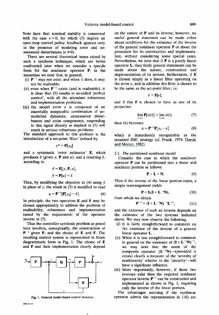
Thus the controller synthesis problem as posed here involves, conceptually, the construction of P-’ given P, and the choice of E and F. The resulting control system is represented in block diagrammatic form in Fig. 1. The choice of E and F and their implementation clearly depend

I * I

Fig. 1. General model-based control structure.

on the nature of P and its inverse; however, no useful general statement can be made either about conditions for the existence of the inverse of the general nonlinear operator P or about the procedure for its construction and implementa- tion, without considering some special cases. Nevertheless, we note that if P is a purely linear operator L, then fairly general statements can be made about the nature, construction and implementation of its inverse; furthermore, if E is chosen simply as a linear filter operating on the error e, and in addition this filter is chosen to be the same as the set-point filter, i.e.

I? = F[e],

and if this F is chosen to have as one of its properties

lim F[x(t)] = lim x(t), (7) *+m 1-m

then (6) becomes

u = P-‘F[yd - e] (8)

which is immediately recognizable as the standard IMC strategy (cf. Frank, 1974; Garcia and Morari, 1982).

2.2. The partitioned nonlinear model Consider the case in which the nonlinear

operator P can be partitioned into a linear and nonlinear portion as follows:

P=L+N. (9)

Then if the inverse of the linear portion exists, a simple rearrangement yields

P = L(I+ L-‘N), (10) from which we obtain

P-’ = (I + L-‘N)-‘L-l, (11)

and the existence of such an inverse depends on the existence of the two inverses indicated above. We may now observe the following.

(i)

(ii)

(iii)

It is fairly straightforward to comment on the existence of the inverse of a general linear operator L. While it is less straightforward to comment in general on the existence of (I + L-%-l, we may note that the norm of the composite operator [IL-‘Nil-(provided it exists) clearly a measure of the ‘severity of nonlinearity’ relative to the ‘linearity’-will have a significant influence. More importantly, however, if these two inverses exist then the required nonlinear operator inverse P-’ can be constructed and implemented as shown in Fig. 2, requiring only the inverse of the linear portion.

The advantages accruing if the nonlinear operator admits the representation in (10) are

700 F. J. Doyle et al.

L-l -v---h 4---G N

Fig. 2. Realization of partitioned nonlinear model inverse.

now clear: the nature of the operator inverse and the conditions for its existence are easier to determine; its construction and its implementa- tion depend in a remarkably straightforward manner only on the linear subsystem inverse. We now note that the Volterra model not only naturally occurs in the partitioned form in (9), but its linear portion is precisely what conven- tional MPC is based upon. The rest of the paper is devoted to exploiting these facts for the development of a scheme to extend conventional linear model-based control schemes to nonlinear systems.

3. NONLINEAR SYSTEM DYNAMICS VIA VOLTERRA SERIES APPROXIMATIONS

3.1. Input/output representations in the time domain

For linear systems, the linear convolution integral

y(t) = 1; h,(c+)u(t - a) dc 0

( 12)

(a functional that maps the entire past input to the value of the output at the present time) is well known as a useful model for representing arbitrary system dynamic behavior. Here h,(a). the ‘kernel’ of the transformation, is the system’s impulse response function. For nonlinear sys- tems, Volterra generalized this functional rep- resentation in the form of a power series:

y(t) = y,(t) + Yz(t) + y3(t) + . . . 9 (13)

where y,(t), the first-order term, is defined as in

(12)Y and the other terms in the series are defined as follows:

y*(t) = = II

=h,(v,, cr,)u(t - a,)u(t - v2) du, daz 0 0

(14)

y&) = L= j-y 1; h,(a, 7 ~2, a,)u(t - ~1)

x u(t - a&(t - a3) da, daz da, (1%

7.

I I x

y,(t) = . . . hi(u I,.... a,b(t - Cl) 0 0

. . . u(t - vi) da, . . . dc,,. (16)

A discrete-time representation in the same spirit takes the form of the discrete power series

Y(k) = Y,(k) + YG) + Y,(k) + . . . 9 (17)

where the first term, given by

y,(k) = 2 h,(i)u(k -i), I_ I

(18)

is recognizable as a variation of the linear convolution model employed in traditional MPC: higher-order terms are given by

X x

y,(k) = 2 2 &(L j)u(k - i)u(k - j), t=l j=l

(19)

zc r r

y,(k) = g, ,;, z, h&j, 00 - i)u(k -j)+ - 0.

(20)

The Volterra series representation is a temporal extension of the Taylor series expan- sion: it is thus limited to approximating systems with fading memory (Boyd and Chua 1985). Nevertheless, for a wide variety of nonlinear chemical processes that cannot be approximated adequately by the linear convolution model in (18) (e.g. exothermic chemical reactors or high-purity distillation columns), the Volterra series model, as a logical nonlinear extension of (12) or (18), often provides improved process representation.

These models may be represented compactly as

y = P]ul, (21)

where P is the nonlinear plant model operator that maps the input space to the output space. Observe from the model form that P may be represented as

p=p,+p,+p,+..., (22)

where, in the discrete case, the degree-l (linear), degree-2 (quadratic) and degree-3 (cubic) operators are given respectively by

P,[u] = 2 h,(i)u(k - i), ,-I

P2[u] = c c h2(ir j)W - i)u(k -i), ,=I j-l

P3[u] = % c 5 h3(i, j, f)u(k - i) r=l j=l /=I

X u(k - j)u(k - I),

with the summations replaced by the appropriate

Volterra model-based control 701

integral in the continuous case. In the following we shall make no distinction between operators representing discrete models and operators representing continuous models. The issue regarding the specific mathematical properties of the continuous, as compared with the discrete, versions of Volterra operators, and the implica- tions they have for dynamic analysis in the continuous as compared with the discrete, time domain, have been carefully discussed by Schetzen (1980) and Rugh (1981). It is sufficient to note that in (21) and (22), as in the subsequent discussion, the operators are genera- lized and could be either continuous or discrete.

Observe now that, by separating the linear P1 from the rest of the higher-degree operators, referring to this residual sum collectively as N, the Volterra model is clearly of the partition form in (9).

3.2. Obtaining Volterra series models Volterra models may be obtained as follows.

(9

(ii)

(iii)

(iv)

From a nonlinear first principles model, by obtaining the Carleman linearization (ap- proximation) (Schetzen, 1980; Rugh 1981) of the original system. The pertinent details of this procedure (which was actually employed in the example problems dis- cussed in Section 5) can be found in the two cited references. From a polynomial NARMAX model, using a procedure due to Diaz and Desrochers (1988); the interested reader is referred to the cited reference for the details. From an artificial neural network. It has been shown recently (cf. Wray et al., 1992) that for every artificial neural network that employs the usual sigmoidal squashing function, there is an exact-not approximate--equivalent infinite Volterra series representation. By using the infinite series representation of these sigmoidal functions, it is possible, through straightfor- ward (but quite tedious) algebraic man- ipulations, to compute precisely the equiv- alent Volterra kernels from the synaptic weights. The interested reader is referred to Wray et al. (1992) for the complete details. From input/output data. A number of techniques have been proposed for comput- ing the Volterra kernels strictly from input/output data gathered directly from the process. In each case the choice of input signals and the optimization criteria employed in computing parameter estimates are very critical elements of the identifica- tion procedure. New results and a detailed discussion of these and other related issues

are given by Pearson et al. (1992), to which the interested reader is referred. (cf. Seinfeld and Lapidus 1974; Schetzen, 1980; Rugh, 1981; Koh and Powers, 1985; Bendat, 1990; Pearson et al., 1992).

4. CONTROLLER SYNTHESIS BASED ON VOLTERRA MODELS

4.1. Controller synthesis results 4.1.1. Linear systems. From Section 2, for the

linear system modeled by

Y = P&l, the basic controller synthesis result is

(23)

c4 = P;‘[y, - e]. (24)

Even though, as previously noted, this may be modified as needed using the ‘estimator’ E and the ‘filter’ F, this controller is primarily based on

P;‘, the linear model inverse. 4.1.2. Nonlinear systems. Of the class of

Volterra models, the simplest nonlinear exten- sion of the linear convolution model in (23) is

y = (P, + PJbl, (25)

the second-order Volterra model. From the result in Section 2, therefore, the controller synthesis procedure yields in this case

U = (I + P;lP$‘P;‘[s], (26) where

5 = y, - e. (27)

The important point to note here is that such a controller can in fact be implemented as shown in Fig. 2: the ‘main controller’ still remains the linear model inverse; but it is now augmented with the auxiliary loop incorporating the quadratic nonlinear operator P2.

It is now a straightforward exercise to show that in the general case, with

P = P* + P2 + Pj + . . * ) (28)

the corresponding controller expression is

Q = P-’ = (I + P;‘P* + P;‘P3 + - * .)-‘P;‘, (29)

and the corresponding block diagram will now have the residual nonlinear operators (Pz + P3 + * * *) in the auxiliary loop.

In the following subsection we derive the result that is presented in (26) using expansions of Volterra series operators (and their inverses). Once the equivalence has been established between the two approaches, we shall use the Volterra series expansion approach to derive controllers for broad classes of dynamical systems using generalized inverses.

702 F. J. Doyle er al.

4.2. The ‘standard’ approach An alternative approach to the derivation of

the controller in (26) is outlined below. Consider a controller operator Q (to be determined) represented by

ld = QLCI, (30) with 5 as previously defined in (27). Substituting these expressions for Q and 5 into (4) yields the control problem

mt 4 = 115 - P[Q[~lllI. (31)

This objective will clearly be minimized if the following relationship holds:

P[QH= 6 (32) The discussions that follow will be very much concerned with the computation of the nonlinear operators P and Q appearing in (31) and (32). To simplify these discussions, define the nonlinear operator H as this composition, i.e.

H=P*Q, (33)

where * denotes composition of operators. As mentioned earlier, the resulting Q will cleary be the inverse of P (provided that it exists).

In following such a procedure, as noted in Chapter 7 of Schetzen (1980) it should be kept in mind that not all nonlinear systems possess such an inverse; also many possess an inverse only for a restricted range of input amplitude. One must therefore be careful to ensure that the range of the operator Q is contained in the domain of the operator P. This will be assumed throughout the following discussion. For further discussion of the various implications of this statement, see, for example, Chapter 7 of Schetzen (1980).

To obtain an explicit expression for Q, using the operator notation defined above, with the plant represented by the operator

P = P, + P, + P, i- . . . . (34)

the controller operator Q is also set up as an infinite sequence of operators:

with Q=Q, +Qz+Q3+.... (35)

,v

Q,[tl = 2 4Mk - 4, (36) l=l

Q,[E] = 2 2 w(i, j)5(k - i)5(k -i), (37) ,=I j-1

NNN

Q&l= c c c $Gj, M(k - iM(k -Mk - 0 ,=l,=l/=l (38)

in the discrete case, with the corresponding integral expressions in the continuous case.

Thus the controller synthesis problem requires solution of the equation

I=P*Q=(P,+P,+P,i-...)

*(Q,+Qz+Q3+...) (39)

for the controller Q. By expanding the composition of the operators indicated in (39) and rearranging and grouping the results according to operator order and equating like terms. it has been shown (Schetzen, 1980) that the controller operator will be given explicitly by

Q, = Pi ‘. (40)

Q2= -Pi’*P,*Q,, (41)

Q,=-P11*(P?*(Q,+Q2)-P2*Q, -Pz*Q~+P~*Q,). (42)

(43)

Note that this controller is an infinite sequence of operators, that the first term in the sequence is the linear model inverse, and that this is the only inverse operator present in the subsequent terms.

A key property of the expressions for the controller Q as the Volterra operator inverse is the fact that the calculation of successive terms are completely decoupled. In other words, a linear operator inversion is all that is required initially, and subsequent terms depend only upon the same linear inverse, previous terms in the inverse operator series, and terms from the original plant operator series. However, there are three important issues that this approach does not address. (i)

(ii)

(iii)

Since Q is obtained by this technique as an infinite sequence of operators, it is pertinent to contemplate the issue of convergence. Under what conditions will the sequence in (35) converge? Even when the sequence can be shown to converge, how is the controller to be implemented in practice, particularly when the rate of convergence is slow? What happens when the inverse of P, either does not exist or is unrealizable? procedure we have introduced in Section

4.1 resolves the first two issues, because The

(i) it provides an exact, analytical expression for the controller Q represented as an infinite sequence using the alternative approach;

(ii) as shown previously, it results in a controller that can be implemented as shown in the block diagram in Fig. 2.

This analytical representation for the controller

Volterra model-based control 703

therefore has the dual advantage that it does not depend on the properties of an infinite series, and its implementation is straightforward and intuitive.

The third issue is resolved using generalized inverses, as we now discuss.

4.3. Controller synthesis using generalized inverses

In recognition of the fact that there will be situations in which Pi, the linear (degree-l) operator, either has no inverse or its inverse is undesirable for any number of reasons, we now proceed to develop explicit expressions for the controller in terms of appropriate generalized inverses.

4.3.1. Problem formulation and solution. In finding the exact inverse of P and using it as the controller Q, the strategy as presented in Section 4.2 has been to solve the series of equations resulting from (39). For our current purposes, we now reformulate the problem as follows. Since model prediction using P and control action using Q are respectively determined according to

y = WI, (44 u = Q[tl, (45)

from the definition of each operator, we have first that

y = yU) + y(2) + y(3) + . . . 9 (46)

where yci) is the degree-i contribution to the overall signal y, arising from

Y Ci) = P,[U].

Similarly, we also have

u = u(l) + @) + U(3) + . . . ,

(47)

(48)

where u(j) is the degree-i contribution to the overall control action signal u, arising from

uci) = Qi[s]. (49)

Finally, observe from (46) and (47) that

y = PJU] + PJU] + P3[u] + * * * ) (50)

but, from (48), u itself is the indicated infinite sequence. We now introduce the notation

sy(N = pi[uG)], (51)

with the first index denoting the degree of the operator and the second index the contributing degree of the component of the signal being operated upon. Thus, for example, Syo2) is that portion of y (I), the degree-l contribution to y, due to the u(‘), degree-2, component of the input signal u: it is obtained by operating on uc2) by P,.

Let r be the residual signal, the difference

between the plant/controller operator composi- tion H acting on 5 and the desired value of this composition (i.e. 5 itself):

r = H[t] - 5. (52)

Now let r be defined in the same manner as y and u in (46) and (48), so that

r = #l) + r(2) + #3) + . . . .

That is, r(‘) is given by

(53)

r(l) = H,[[] - 5, (54)

r”‘) = Hj[t] for j = 2, 3, . . . , (55)

where Hi is the jth-order term in the expansion of the composition H defined in (39). Observe now that obtaining the exact inverse of P (demanding that H = I) is equivalent to requiring

r(‘) = 0 for all i = 1, 2, 3, . . . . (56)

As shown previously, this requires the existence of p;‘. It is possible to relax this requirement and, instead of (56), require only that the norm 11 rci) 11 be minimized.

It is important to note that the required minimization is on each individual degree-i contributor to the residual signal, not the composite residual signal itself. What is required here is equivalent to minimizing the operator norm of the difference between corresponding degree-i operators, Ii and Hi, for each i. This clearly gives rise to a much stronger result, since it guarantees that each degree-i operator is as ‘close’ as possible to the ideal operator of corresponding degree, and not merely that the overall operator H is as ‘close’ to I as possible.

Remarks. There are some subtle issues of mathematical rigor associated with the solution of the minimization problems we have posed.

(i) First, there is the issue of the precise

(ii)

definition of the domain and range of the yet-undetermined, obviously nonlinear, operator Q that we seek to derive via optimization. Discussions of this kind for the Volterra operator P employed for the plant model may be found, for example in Section 1.5 of Rugh (1981). The converse discussion, in which it is recognized that in determining Q as the inverse of P, the domain of the latter is the range of the former, and vice versa, may be found in Chapter 7 of Schetzen (1980). It is relatively easy to show that the same arguments hold in this case, since what we are deriving is, in fact, a less stringent inverse of P. A more serious issue has to do with the convergence of Q. It is clear from the

704 F. J. Doyle er al.

(iii)

(iv)

earlier discussion that, in general, a stable, causal Q does not exist as an exact inverse of P if PC’ is not stable or causal. However, as we shall soon show. a stable, causal Q, which will depend on a generalized inverse for P,, may be obtained under these circumstances. Such a Q will of course be a pseudo-inverse of P, but by choosing the criteria for pseudo-inverse carefully (see e.g. Ben-Israel and Greville. 1974), we can guarantee stability and cuasality for Q. Nevertheless, even in this case, the resulting operator Q, expressed as the Volterra series in (3.5) may converge only under a limited range of the amplitude of its input 5. Further, as indicated in Section 7.5 of Schetzen (1980) this range is not easy to determine in general. These facts not- withstanding, we may make an appeal to the earlier discussion and employ the ‘filter’ F and the estimator E in the feedback loop as a means of ensuring that the amplitude of the feedback signal 5 is sufficiently modified for the purpose of achieving convergence for Q. The notion of ‘inversion’ that is used here is fairly general, and can be relaxed, from a numerical perspective (Economou, 1985) or from a performance perspective, to yield robust controlled behavior. For instance. the analytical solution to the standard unconstrained model predictive control problem contains an explicit weighting term that relaxes the explicit model inversion as a direct consequence of incorporating a penalty on the manipulated variable. For a nice summary of this notion of relaxed model inversion, see Hernandez (1992). Finally, even though we shall soon show that the solution of the specific optimization problem posed above technically involves only the linear operator P, explicitly, it is nevertheless also clear from (52) that at the foundation of the entire exercise is the notion of the norm of nonlinear operators (for i > 1). While the notion of the norm of a linear operator is straightforward and well known, it is not as obvious or as straightforward with nonlinear operators. It is clearly outside the intended scope of this paper to provide even a cursory discussion of the precise mathematical foundations underlying the operations indicated in (52) and which make it possible to derive from it the results we shall soon present. It is sufficient to note that most of the pertinent issues are taken up with enough detail for example in Chapter 2 of Berger (1977). The

specific issues regarding the spaces of nonlinear operators. as well as those regarding the existence of solutions to nonlinear operator equations in Banach spaces (such as the kind we have posed in (52)) are considered in detail in Chapters 3 and 4 of Martin 1976. The interested reader is encouraged to consult these references.

We now proceed to obtain the solution to the optimization problem. Degwr 1. In this case. since

H,El = P, * Q,[Sl, (57)

and I,[ [] = 5, we have

r(” = P, * a,[.$] ~ 5. (58)

but. by detinition, Q,[[] = u”). so that the optimization problem becomes

Ilr(“ll = IIP,bJ”l - 511. (59)

If in particular (I.11 refers to the L, norm then (59) has the well-known solution

I4(‘) = Pi[‘$], (60)

where the operator P: is the left inverse of P, defined by

PTP, = I,. (61)

Of course, since, by definition, u(‘) = a,[[], it follows from (60) that the linear portion of the Q operator is given by

QI = Pi (62) (compare with Q, = Pi-’ for the exact inverse controller). Degree 2. In this case

K]tl= P, *Q&l + PI * Q,k% or. equivalently.

(63)

H&] = P,[u’*‘] + P,[u”‘]. (64)

If we keep in mind that, from (60), 14~‘) is now a

known quantity, and recall the definition of 6v”“, we observe immediately that the expres- sion in (64) becomes

Hz[t] = P,[u’~‘] + Sy (21). , (65)

and finally, since 12[5] = 0, we then have the second-degree optimization problem as

/lr(2)/1 = llP,[U’2’] + 6y’21’/1, (66)

a problem entirely similar in structure to (59). and involving only the linear operator P,, even though the input signal in question, uc2), is a second-degree contribution. The solution is

U(2) = -p~[~y’21’], (67)

with the same P: as in (60).

Volterra model-based control 705

Degree 3. Here the problem is somewhat more complicated, but the principles are essentially the same. In this case

H&l = PI * Q&F1 + P3 * QJtl - Pz * Q1[61 - Pz * Q&I + Pz * [QJtl + Q&II, (68)

or, equivalently,

H3[4 = P&L(~)] + P3[uC1)] - P&L(~)]

- P&Q)] + P2[G + U(2)]. (69)

Since, by now, both u(l) and uC2) are known quantities, we may simplify (69) by defining

Q?(3) = QY(31) - (pu - Qp) + ~p2)) (70)

with S_y (2S12) defined as

@W’Z) = p2[u(1) + u(2)] (71)

and the others as previously defined; the result is that (69) becomes- -

H3[5] = P,[u’~‘] + QC3’,

and again, since I,[s] = 0, we third-degree optimization problem as

]lr@l) = ]lPJU(3)] + &!j’3’]1.

(72)

have the

(73)

Observe again that this is a problem entirely similar in structure to (59), involving again only the linear operator P1. (The input signal in question, uc3), of course, is a third-degree contribution). The solution again is

(74)

with the same P: as in the degree-l and -2 problems.

It is now possible to generalize: the degree-i problem will always have the form

Ilr(‘)J( = ]lP&(‘)] + 6@“]l, (75)

where St(‘) consists only of known quantities dependent on r&l), and other components of lower degree up to and including u(i).

We now observe, once again, that, as previously obtained under the assumption that P;’ exists, the controller implied above is an

infinite sequence, with each term involving only Pi this time. It can be shown that the corresponding analytical expression for this infinite sequence controller is precisely as in (26) and (29), but now with P;’ replaced with PI.

;

Fig. 3. Structure for second-order Volterra controller.

4.3.2. Implications for constrained discrete MPC. The fact that the problem of generating the controller Q can be thus posed as an optimization problem has some significant implications for controller implementation within the explicit MPC framework. Observe that the norms to be minimized could be weighted, and the weights could in fact be made dependent on the operator degree; constraints could also be introduced (in the multivariable case) if needed. Furthermore, the entire controller could be implemented as in Fig. 3, with P;’ replaced by the linear MPC controller, noting the crucial point that the auxiliary loop endows the otherwise well-known linear MPC controller with nonlinear characteristics by providing a form of ‘correction’ for the effect of nonlinearities.

These and other related issues are significant enough in their own right that they warrant a full-scale discussion, which we shall defer to a subsequent paper.

5. CASE STUDY

5.1. Continuous polymerization reactor example In this section we consider the application of

the proposed controller design strategy to a polymerization reaction taking place in a jacketed CSTR. The reaction under considera- tion is the free-radical polymerization of methyl methacrylate (MMA) with azo-bis-isobutyro- nitrile (AIBN) as initiator and toluene as solvent. Details of the rate laws for free-radical polymerization were obtained from Congalidis et al. (1989), Daoutidis et al. (1990) and Ray (1972). For this particular case study, we make the following simplifying assumptions:

isothermal operation; perfect mixing; constant heat capacity; no polymer in the inlet stream; no gel effect; constant reactor volume; negligible initiator flow rate (in comparison with monomer flow rate);

Volterra model-based control

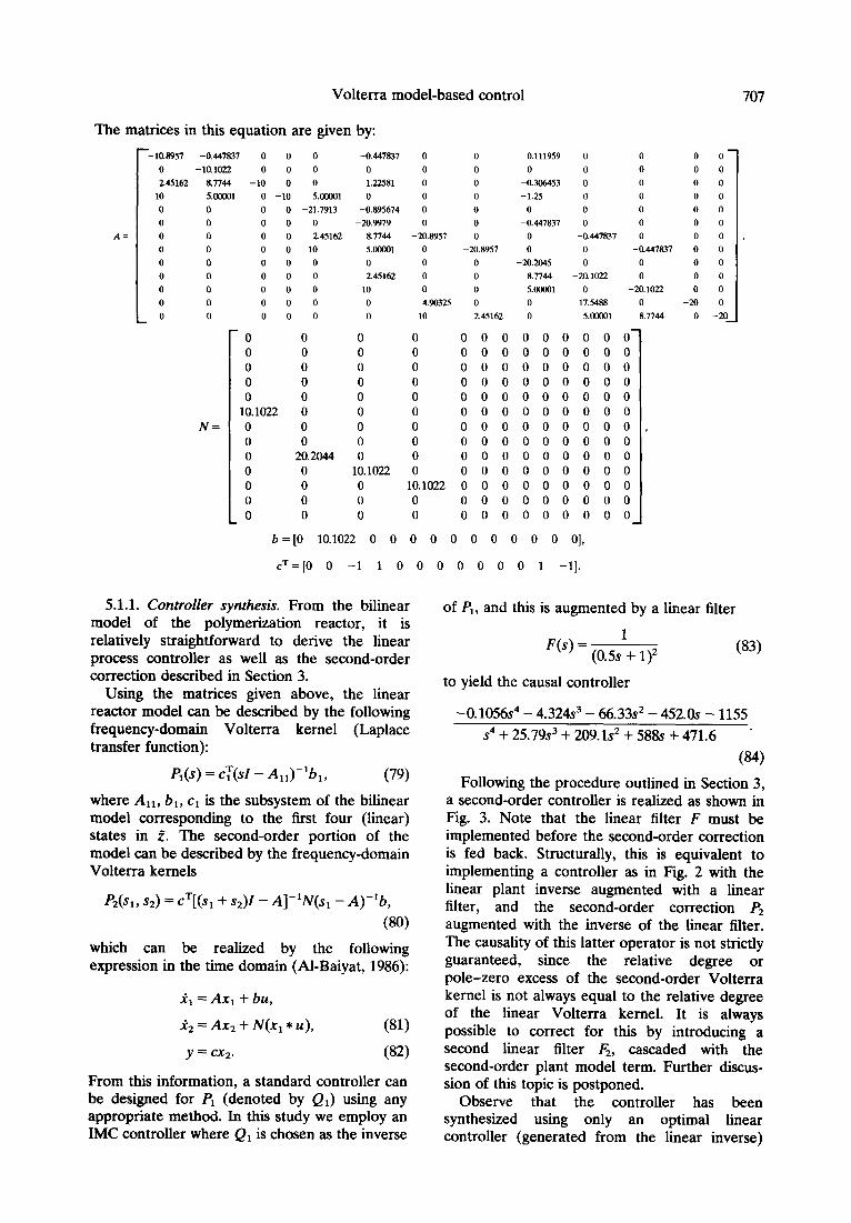
The matrices in this equation are given by:

A=

--10.6957 -0.447837 0 0

0 -10.1022 0 0

245162 a7744 -10 0

10 5.DlOO1 0 -10

0 0 0 0

0 0 0 0

0 0 0 0

0 0 0 0

0 0 0 0

0 0 0 0

0 0 0 0

0 0 0 0

0 0 0 0

N=

0 0 0 0 0 10.1022 0 0 0 0 0 0 0

0 0 0 0 0 0 0 0 20.2044 0 0 0 0

0

0

0

5.cQOO1

-21.7913

0

245162

10

0

0

0

0

0

-0.447837

1.22581

0

-0.695674

-20.9979

a7744

5.m1

0

2.45162

10

0

0

0

0

0

0

0

-20.6957

0

0

0

0

4.90325

10

0

0

0

0

0

0

-20.6957

0

0

0

0

245162

0.111959 0

0 0

-0.306453 0

-1.25 0

0 0

-0.447837 0

0 -0.447837

0 0

-20.2045 0

8.7744 -20.1022

5.cKmOl 0

0 17.5488

0 5.cMQl

0 0 0 0 0 0 0 0 0 10.1022 0 0 0

b =[0 10.1022 0 0 0 0 0 0 0 0 0 0 01,

0 000000000 0 000000000

0 000000000

0 000000000

0 000000000 0 000000000

0 000000000 0 000000000 0 000000000

0 000000000

10.1022 0 0 0 0 0 0 0 0 0 0 000000000 0 000000000

cT=[O 0 -1 1 0

5.1 .l. Controller synthesis. From the bilinear model of the polymerization reactor, it is relatively straightforward to derive the linear process controller as well as the second-order correction described in Section 3.

Using the matrices given above, the linear reactor model can be described by the following frequency-domain Volterra kernel (Laplace transfer function):

P,(s) = c:(sZ - AIJ1bl, (79)

where AlI, bl, cl is the subsystem of the bilinear model corresponding to the first four (linear) states in z’. The second-order portion of the model can be described by the frequency-domain Volterra kernels

Pz(s,, s2) = c=[(sr + s2)Z - A]-lN(.s, - A)-%,

(W

which can be realized by the following expression in the time domain (Al-Baiyat, 1986):

& = AxI + bu,

Y2 = Ax2 + N(x, * u), (81)

y = cx2. (82)

From this information, a standard controller can be designed for P1 (denoted by Qr) using any appropriate method. In this study we employ an IMC controller where Qr is chosen as the inverse

0 0 0 0 0 0 1 -11.

of Pi, and this is augmented by a

1

P@) = (0.5s + 1)2

to yield the causal controller

linear filter

(83)

-0.1056.~~ - 4.324~~ - 66.33~~ - 452.0s - 1155

s4 + 25.79~~ + 209.1~~ + 588s f 471.6 ’

w

Following the procedure outlined in Section 3, a second-order controller is realized as shown in Fig. 3. Note that the linear filter F must be implemented before the second-order correction is fed back. Structurally, this is equivalent to implementing a controller as in Fig. 2 with the linear plant inverse augmented with a linear filter, and the second-order correction P2 augmented with the inverse of the linear filter. The causality of this latter operator is not strictly guaranteed, since the relative degree or pole-zero excess of the second-order Volterra kernel is not always equal to the relative degree of the linear Volterra kernel. It is always possible to correct for this by introducing a second linear filter F2, cascaded with the second-order plant model term. Further discus- sion of this topic is postponed.

Observe that the controller has been synthesized using only an optimal linear controller (generated from the linear inverse)

708 F. J. Doyle et al.

0 2 4 6 a 10 12 14 16

E Time(hour) .g

H 01,

Fig. 4. Open-loop simulattons of polymerizer reactor for step inputs of small magnitude.

-1’ 0 2 4 6 6 10 12 14 16

i

:

Time (hour)

0.6,

Fig. 5. Open-loop simulations of polymcrizer reactor for step inputs of large magnitude.

and the second-order Volterra kernel for the reactor model.

5.1.2. Simulation results. The nonlinear nature of the polymerization reactor under investigation is revealed in the open-loop simulations in Figs 4 and 5. Figure 4 shows the response of the full nonlinear model (solid line, (77)) the second-order bilinear (Volterra) approximation (dotted line. (78)) and the linear approximation (dashed line, (79)), to step changes in the initiator flow rate that range ~~20%. As can be seen in the figure, all three curves overlap for small input changes. but as the magnitude of the change increases, the nonlinear curve separates from the other two. However, the second-order Volterra model tracks the true nonlinear response more accurately than the linear model.

Results from a similar simulation are displayed in Fig. 5. where now the magnitude of the input step change has been increased to *90%. While these may appear to be unrealistic changes, they do highlight the relative accuracy of the linear and second-order model approximations. In this case there is a significantly larger difference between the true nonlinear response and both the linear and second-order models. And, as before. the second-order response tracks the full nonlinear response more closely than the linear response.

Figure 6 shows the response of the closed-loop system to a - 10% step change in the set-point:

(i) closed-loop with linear controller (dashed line):

(ii) Closed-loop with linear controller plus second-order correction (Volterra con- troller) (dotted line):

-0.12' 0 5 10

Time(hour)

Fig. 6. Closed-loop simulation of polymerizer reactor for a - 10% step in the set-point.

Volterra model-based control 709

_J

5 10 15 Time (hour)

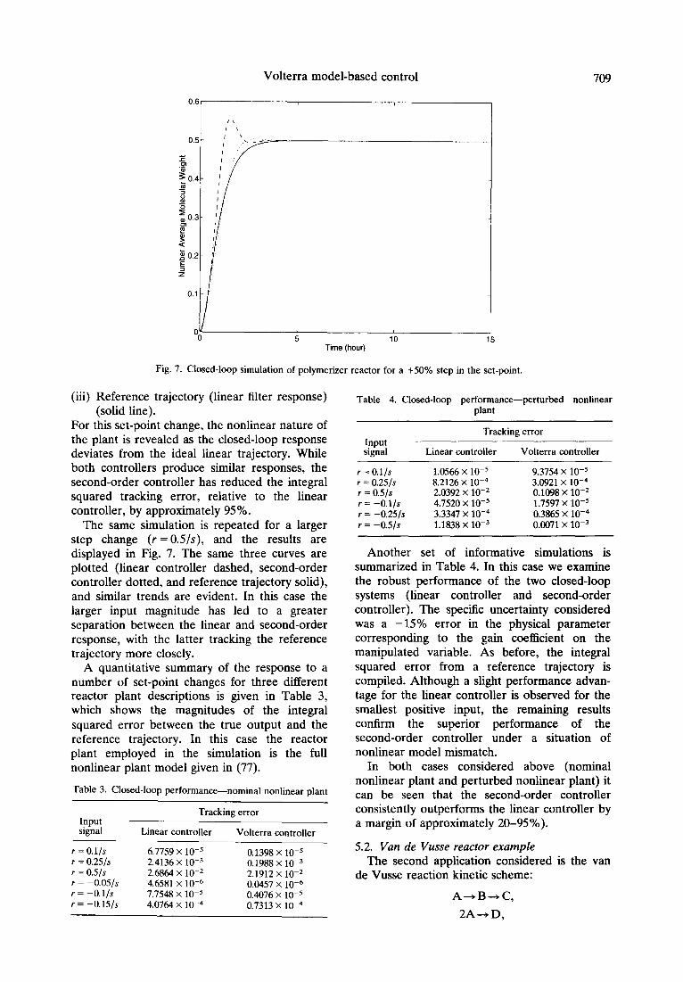
Fig. 7. Closed-loop simulation of polymerizer reactor for a +50% step in the set-point.

(iii) Reference trajectory (linear filter response) (solid line).

For this set-point change, the nonlinear nature of the plant is revealed as the closed-loop response deviates from the ideal linear trajectory. While both controllers produce similar responses, the second-order controller has reduced the integral squared tracking error, relative to the linear controller, by approximately 95 % .

The same simulation is repeated for a larger step change (r = OS/s), and the results are displayed in Fig. 7. The same three curves are plotted (linear controller dashed, second-order controller dotted, and reference trajectory solid), and similar trends are evident. In this case the larger input magnitude has led to a greater separation between the linear and second-order response, with the latter tracking the reference trajectory more closely.

A quantitative summary of the response to a number of set-point changes for three different reactor plant descriptions is given in Table 3, which shows the magnitudes of the integral squared error between the true output and the reference trajectory. In this case the reactor plant employed in the simulation is the full nonlinear plant model given in (77).

Table 3. Closed-loop performance-nominal nordinear plant

Input signal

f =0.1/s r = 0.25/s r = 0.5 Js r = -0.05/s r = -0.1/s r = -0.15/s

Tracking error

Linear controller Volterra controller

6.7759 x 1O-5 0.1398 x 1O-5 2.4136 x 1O-3 0.1988 x 10m3 2.6864 x lo-* 2.1912 x lo-* 4.6581 x 1O-6 0.0457 x 10-e 7.7548 x 10-S 0.4076 x 10m5 4.0764 x 10-d 0.7313 x 10-d

Table 4. Closed-loop performance-perturbed nonlinear plant

Input signal

r =0.1/s r = 0.25/s r = 0.5/s r = -0.1/s r = -0.25/s 1 = -0.5/s

Tracking error

Linear controller Volterra controller

1.0566 x 10-s 9.3754 x 1o-5 8.2126 x 1O-4 3.0921 x 1o-4 2.0392 x lo-’ 0.1098 x lo-* 4.7520 x lo-’ 1.7597 x 10-5 3.3347 x 1o-4 0.3865 x 1o-4 1.1838 x 1O-3 0.0071 x 1o-3

Another set of informative simulations is summarized in Table 4. In this case we examine the robust performance of the two closed-loop systems (linear controller and second-order controller). The specific uncertainty considered was a -15% error in the physical parameter corresponding to the gain coefficient on the manipulated variable. As before, the integral squared error from a reference trajectory is compiled. Although a slight performance advan- tage for the linear controller is observed for the smallest positive input, the remaining results confirm the superior performance of the second-order controller under a situation of nonlinear model mismatch.

In both cases considered above (nominal nonlinear plant and perturbed nonlinear plant) it can be seen that the second-order controller consistently outperforms the linear controller by a margin of approximately 20-95%).

5.2. Van de Vusse reactor example The second application considered is the van

de Vusse reaction kinetic scheme:

A+B-,C,

2A+D,

710 F. J. Doyle et al.

0 50 100 150 Inlet Flow Rate

200 250

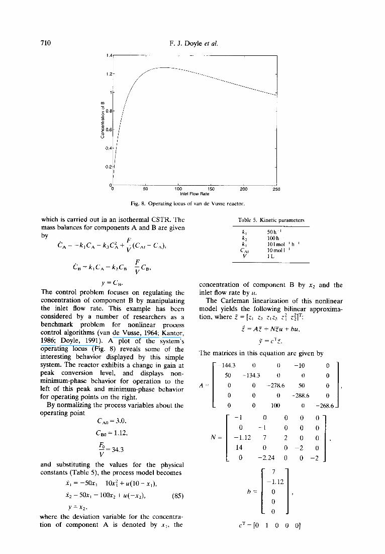
Fig. 8. Operating locus of van de Vusse reactor.

which is carried out in an isothermal CSTR. The mass balances for components A and B are given

by c, = -k,C,c, - k3C: + ;(C,, - C,),

&=k,C,-k,C.-;C,,

y = cg.

The control problem focuses on regulating the concentration of component B by manipulating the inlet flow rate. This example has been considered by a number of researchers as a benchmark problem for nonlinear process control algorithms (van de Vusse, 1964; Kantor, 1986; Doyle, 1991). A plot of the system’s operating locus (Fig. 8) reveals some of the interesting behavior displayed by this simple system. The reactor exhibits a change in gain at peak conversion level, and displays non- minimum-phase behavior for operation to the left of this peak and minimum-phase behavior for operating points on the right.

By normalizing the process variables about the operating point

c,, = 3.0,

csO = 1.12,

6 v = 34.3

and substituting the values for the physical constants (Table 5) the process model becomes

i’1 = -50x, - 10x: + u(10 - x,),

.& = 50X, - 100x2 + U( -x2), (85)

y=xz,

where the deviation variable for the concentra- tion of component A is denoted by xl, the

Table 5. Kinetic parameters

k, 50h~’

kz lOOh ’ k, 101 mol-’ h&’

c AI 10moll~~’ V 1L

concentration of component B by x2 and the inlet flow rate by K.

The Carleman linearization of this nonlinear model yields the following bilinear approxima- tion, where z” = [z, z2 z1z2 z: z:lT:

i=AZ+NZu+bu,

p = C7.B.

The matrices in this equation are given by

- 144.3 0 0 -10 0

50 -134.3 0 0 0

A= 0 0 -278.6 50

0 0 0 -288.6 0

0 0 100 0 0, I -268.6

N=

-1 0 000

0 -1 0 0 0

-1.12 7 -2 0 0

14 0 0 -2 0

0 -2.24 0 0 -2

,

CT = [O 1 0 0 O]

Volterra model-based control 711

0.16

.--------- - - -_ --------__----_____

0.14- ,

I

0.12- :I I

-0.04 0 0.05 0.1 0.15 0.2 0.25

Time (hour)

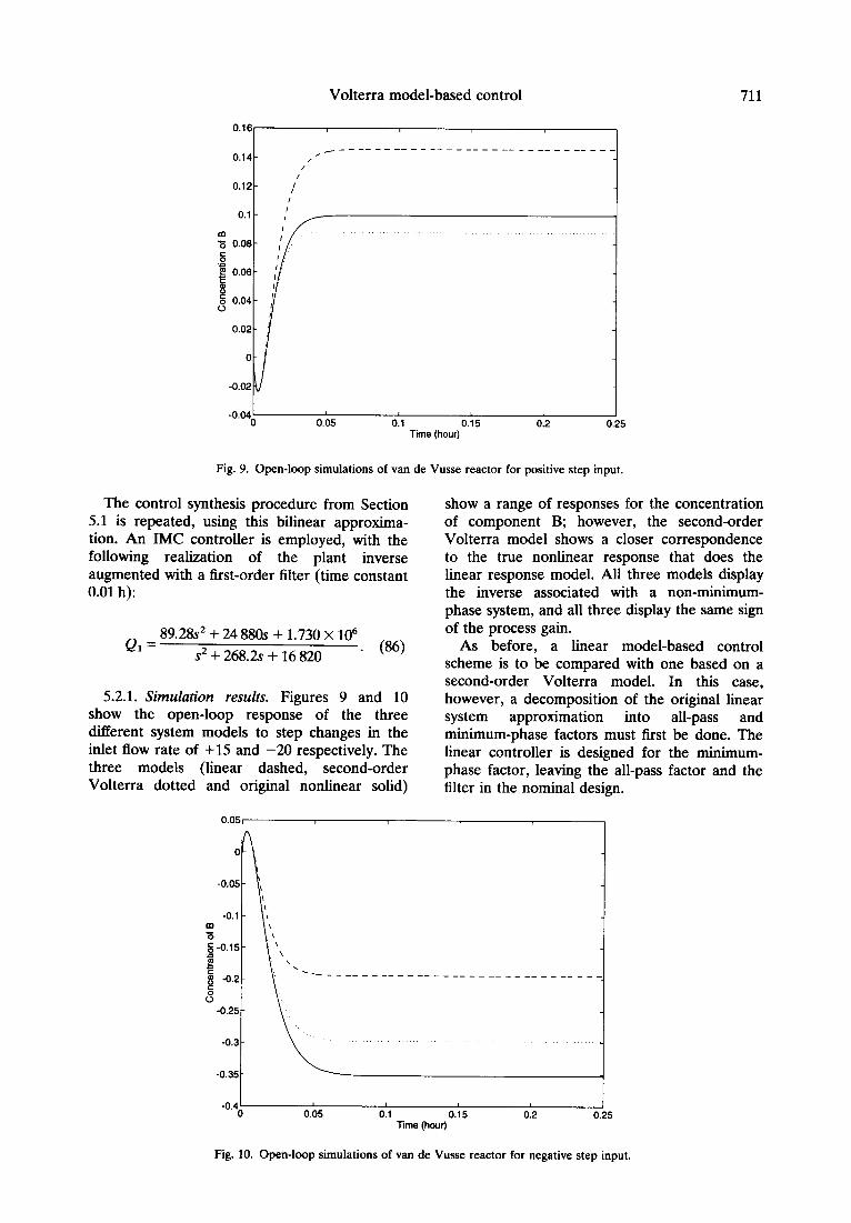
Fig. 9. Open-loop simulations of van de Vusse reactor for positive step input.

The control synthesis procedure from Section 5.1 is repeated, using this bilinear approxima- tion. An IMC controller is employed, with the following realization of the plant inverse augmented with a first-order filter (time constant 0.01 h):

52.1. Simulation results. Figures 9 and 10 show the open-loop response of the three different system models to step changes in the inlet flow rate of +15 and -20 respectively. The three models (linear dashed, second-order Volterra dotted and original nonlinear solid)

show a range of responses for the concentration of component B; however, the second-order Volterra model shows a closer correspondence to the true nonlinear response that does the linear response model. All three models display the inverse associated with a non-minimum- phase system, and all three display the same sign of the process gain.

As before, a linear model-based control scheme is to be compared with one based on a second-order Volterra model. In this case, however, a decomposition of the original linear system approximation into all-pass and minimum-phase factors must first be done. The linear controller is designed for the minimum- phase factor, leaving the all-pass factor and the filter in the nominal design.

I 0.1 0.15 0.2 0.25

Time (hour)

Fig. 10. Open-loop simulations of van de Vusse reactor for negative step input.

712 F. J. Doyle et al.

0.1 _____--.

0.06 0.08 Time(hour)

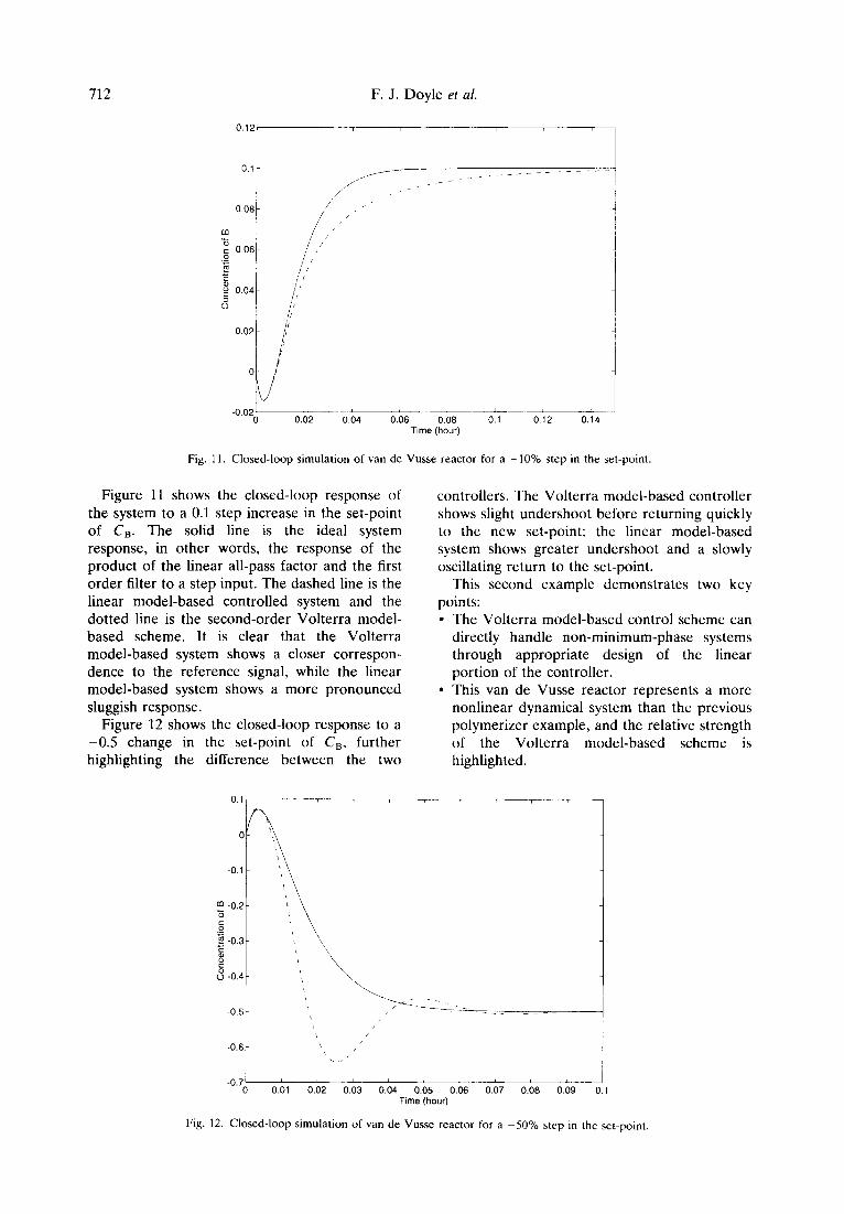
Fig. 11. Closed-loop simulation of van de Vusse reactor for a +lO% step in the set-point.

Figure 11 shows the closed-loop response of the system to a 0.1 step increase in the set-point of c,. The solid line is the ideal system response, in other words, the response of the product of the linear all-pass factor and the first order filter to a step input. The dashed line is the linear model-based controlled system and the dotted line is the second-order Volterra model- based scheme. It is clear that the Volterra model-based system shows a closer correspon- dence to the reference signal, while the linear model-based system shows a more pronounced sluggish response.

Figure 12 shows the closed-loop response to a -0.5 change in the set-point of C,, further highlighting the difference between the two

0.1 h

-0.1 ’ \

m -0.2 ! I\

i ‘i5

controllers. The Volterra model-based controller shows slight undershoot before returning quickly to the new set-point; the linear model-based system shows greater undershoot and a slowly oscillating return to the set-point.

This second example demonstrates two key points:

The Volterra model-based control scheme can directly handle non-minimum-phase systems through appropriate design of the linear portion of the controller. This van de Vusse reactor represents a more nonlinear dynamical system than the previous polymerizer example, and the relative strength of the Volterra model-based scheme is highlighted.

1

t

1 I

-0.6 \ / ’ ,’

-0.7 0

I 0.01 0.02 0.03 0.04 0.05 0.06 0.07 0.08 0.09 0.1

Time (hour)

Fig. 12. Closed-loop simulation of van de Vusse reactor for a -50% step in the set-point.

Volterra model-based control 713

6. SUMMARY

In this paper we have presented a systematic procedure for nonlinear model-based controller design using Volterra models. These models are similar in structure to the conventional MPC models, and can be obtained from input/output data; they therefore provide a means for preserving the original spirit of conventional MPC in tackling nonlinear problems. The controller can be implemented as a linear controller augmented with an auxiliary loop incorporating corrections for the effect of nonlinearities. Thus, the computational require- ments for this procedure are minimal: (i) a second-order Volterra model and (ii) a linear controller derived from the inverse (or pseudo- inverse) of the linear portion of the process model.

The performance of the nonlinear model- based controller was evaluated using two examples.

For a moderately nonlinear, but practical, polymerization reactor, it was shown that the second-order correction provided significant performance improvement over a wide range of conditions. For a highly nonlinear benchmark problem, the van de Vusse reaction scheme, it was demonstrated that the performance of the Volterra model-based controller was sig- nificantly better than that of a linear controller. This example also demonstrated the ability of this approach to handle non-minimum-phase systems. Current efforts in this area involve explicit

MPC implementation of this Volterra model- based controller, particularly for multivariable systems with constraints. Another direction currently under investigation is the integration of the identification results described by Pearson et al. (1992) with the controller synthesis tech- niques described in this paper to yield a unified approach to nonlinear process identification and control. These results will be discussed in subsequent papers.

REFERENCES

Al-Baiyat, S. (1986). Nonlinear feedback synthesis: a Volterra approach. PhD thesis, Electrical and Computer Engineering Department, University of Notre Dame.

Al-Baiyat, S. and Sain, M. (1986). Control design with transfer functions associated to higher order volterra kernels. In Proc. 25th IEEE Conf on Decision and Control, pp. 1306-1311.

Bartee, J. and Georgakis, C. (1992). Identification and control of bilinear systems. In Proc. American Control Conf

Ben-Israel, A. and T. Greville (1974). Generalized Inverses: Theory and Applications. Krieger, New York.

Bendat, J. (1990). Nonlinear System Analysis and Identijica- tion from Random Data. Wiley, New York.

Berger, M. (1977). Nonlinearity and Functional Analysis. Academic Press, New York.

Biegler, L. and J. Rawlings (1991). Optimization approaches to nonlinear model predictive control. In Proc. 4th International Conf. of Chemical Process Control.

Boyd, S. and L. Chua (1985). Fading memory and the problem of approximating nonlinear operators with Volterra series. IEEE Trans. Circuits Syst., CAS-32, 1150-1161.

Congalidis, J., J. Richards and W. Ray (1989). Feedforward and feedback control of a copolymerization reactor. AIChE J., 35,891~907.

Daoutidis, P., M. Sorousch and C. Kravaris (1990). Feedforward/feedback control of multivariable nonlinear processes. AIChE J., 36,1471-1484.

Diaz, H. and A. Desrochers (1988). Modeling of nonlinear discrete-time systems from input-output data. Automatica, 24,629~641.

Doyle III, F. (1991). Robustness properties of nonlinear process control and implications for the design and control of a packed bed reactor. PhD thesis, Chemical Engineering Department, California Institute of Technology.

Eaton, J. and J. Rawlings (1990). Feedback control of chemical processes using on-line optimization techniques. Comput. Chem. Engng, 14,469-479.

Economou, C. (1985).-An operator theory approach to nonlinear controller desien. PhD thesis. Chemical Enai- neering, Department, Calyfornia Institute’of Technologyr

Frank, P. (1974). Entwurf van Regelkreisen mit uorgeschriebenem Verhalten. G. Braun, Karlsruhe.

Garcia, C. (1984). Quadratic dynamic matrix control of nonlinear processes. In Proc. AIChE Annual Meeting.

Garcia, C. and Morari, M. (1982). Internal model control: l-a unifying review and some new results. 2nd. Engng Chem. Process Res. Dev., 21,308.

Hemandez, E. (1992). Control of nonlinear systems using input-output information. PhD thesis, Chemical Engi- neering, Department, Georgia Institute of Technology.

Kantor, J. (1986). Stability of state feedback transformations for nonlinear systems-some practical considerations. In Proc. American Control Conf, pp. 1014-1016.

Koh, T. and E. Powers (1985). Second-order Volterra filtering and its application to nonlinear system identifica- tion. IEEE Trans. Acoust. Speech Sig. Process., ASSP-33, 1445-1455.

Lo, K., Y.-K. Yeo, H.-K. Song and E. Yoon (1992). Application of a bilinear long-range predictive control method in a distillation process. In Proc. DYCORD+ ‘92’, IFAC, pp. 363-368.

Martin, R. (1976). Nonlinear Operators and Differential Equations in Banach Spaces. Wiley, New York.

Pearson, R., B. Ogunnaike and F. Doyle III (1992). Identification of discrete convolution models for nonlinear processes. In Proc. AlChE Annual Meeting.

Peterson, T., E. Hernandez, Y. Arkun and F. Schork (1992). Nonlinear dmc algorithm and its application to a semi batch polymerization reactor. Chem. Engng Sci., 47, 737-753.

Ray, W. (1972). On the mathematical modeling of polymerization reactors. J. Macromol. Sci.-Rev. Mac- romol. Chem., C8, l-56.

Richalet, J., A. Rault, J. Testud and J. Papon (1978). Model predictive heuristic control; application to industrial processes. Automatica, 14,413-428.

Rugh, W. (1981). Nonlinear System Theory-The Volterral Wiener Approach. The Johns Hopkins University Press, Baltimore.

Schetzen, M. (1980). The Volterra and Wiener Theories of Nonlinear Systems. Wiley, New York.

Seinfeld, J. & L. Lapidus (1974). Mathematical Methods in Chemical Engineering, Vol. 3: Process Modeling, Estimation, and Identification. Prentice-Hall, Englewood Cliffs, NJ.

Simminger, J., E. Hernandez, Y. Arkun and F. Schork

714 F. J. Doyle et al.

(1991). A constrained multivariable nonlinear model predictive controller based on iterative QDMC. In proc. IFAC ADCHEM Conf

van de Vusse, J. (1964). Plug-Row type reactor versus tank reactor. Chem. Engng Sci., 19,994~997.

Wray, J., D. Sanders and G. Green (1992). Neural networks

and nonlinear prediction. In Proc. American Conrrol Con5 Yeo, Y. and C. Williams (1987). Bilinear model predictive

control. Indust. Engng Chem. Res., 26,2267-2274. Zafiriou, E. and A. Marchal (1991). Stability of SISO

quadratic dynamic matrix control with hard output constraints. AIChE J. 37, 1550-1560.